Download Embedded system

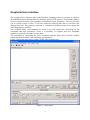
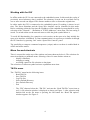
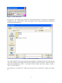
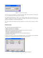
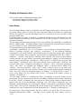
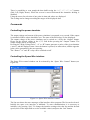
MAG EGSE
User Manual
The MAG EGSE consists of two parts: the embedded Linux system and the Graphical User
Interface.
The embedded Linux system controls the Space Wire Interface and the Power Simulator. It
communicates with the Graphical User Interface (GUI) through Ethernet using TCP/IP
protocol. It accepts command from only one GUI program, but it can send data to six different
GUI the same time.
The Graphical User Interface is implemented under Windows operating system. Its task is:
- connect to the embedded system,
- send telecommand to the MAG device,
- display and store the MAG telemetry,
- control the space wire interface,
- control the Power Simulator
Embedded system
The embedded system is based on a PC 104 computer. A real-time Linux operating system
(RT-Linux) is running on it. The interface drivers are realized as real-time kernel modules.
The user programs exchange data with them through real-time fifos. The user programs
receive and send data through the Ethernet interface, interprets the control commands,
forwards the telecommands through the Space Wire interface and receives telemetry from it.
The embedded system contains an own developed Space Wire (SPW) interface card. It can
drive two lines (main or redundant), and realizes all requirements described in SIIS
Requirements_SOL.S.ASTR.RS.00080_02_00-1[2].pdf including the error generation
features.
The galvanic isolated Power Simulator unit is controlled via serial line. The settings are:
speed = 9600 Baud, no parity, 1 stop bit, 8 data bits.
The embedded system communicates with the GUI through the Ethernet interface using
TCP/IP protocol. Two ports are used: 8040 for input (commands) and 8050 for output
(telemetry). The embedded system acts as server on both ports.
The data structures are described in SOL-MAG-TMTCICD_Issue1_Rev1_19Mar13.pdf.
There are three types of commands:
- MAG telecommands are marked in field “apid” with value equal 63,
- Space wire control commands are marked with other apid and in field “service” with
value greater then 1,
- Power Supply commands.
Four bytes are inserted before the MAG telecommand – they have value 1,2,0,0. The MAG
telecommands are forwarded to the Space Wire (SPW) interface.
The SPW control enables the switchover the main and redundant interfaces and to set the
communication speed furthermore to generate different errors.
1
The Power Supply (PWS) control enables to switch the unit on/off, to set the output voltage
and to switch on/off signals for high voltage and heather relays.
There are tree types of telemetry data:
- MAG telemetry marked in field “apid” with value equal 63,64,65,66,
- SPW interface status messages with other apid values and marked in field
“destination” with value equal 1,
- PWS messages marked in field “destination” with value equal 0.
In the MAG telemetry the leading 4 bytes are cut from the received data block. The first byte
must have value x23 or x33, the second 2 and the third 0. The last can have any value.
After powering the embedded system all programs are started automatically. To avoid fail
functionality (for example to receive noises on the space wire line) initially the space wire
interface is inhibited. To start communication it is necessary to initialize it through the GUI
interface by pressing “Init” on the “SpaceWire Controll” panel.
2
Graphical User Interface
The Graphical User Interface runs under Windows operating system. It connects as client to
the embedded system through Ethernet interface using TCP/IP protocol. Port number 8040 is
used for output direction (telecommands) and 8050 for input (telemetry). The received data
can be stored on disk in files. In off line mode the archived data can be read back and
displayed as well. The telemetry data can be visualized in different forms: hexa dump and
chart diagrams are available.
The available MAG telecommands are stored in an xml control file describing all the
commands and their parameters. There is a possibility to compose and store command
sequences (script file) and later execute them.
The possibility of controlling the Power Simulator and the Space Wire interface enables
testing the MAG hardware under different circumstances.
Figure 1 shows the main panel of MAG EGSE after program start.
Figure 1 – main panel
3
Working with the GUI
In offline mode the GUI is not connected to the embedded system. In this mode the replay of
previously stored telemetry data is enabled. The telemetry records can be read back one by
one or some records can skipped. This feature enables to slow or fasten the original time.
In online mode the GUI is connected to the embedded system. Everything is shown in real
time. The Power Simulator and the Space Wire interface can be controlled in this mode.
Before switching online the first time the IP address of the embedded system should be set by
selection of the “Network” - “Definition of TCP/IP Addresses” menu item. The last setting is
stored. To switch online use the network menu or click the globe symbol below it.
To avoid fail functionality (for example to receive noises on the space wire line) initially the
space wire interface is inhibited. To start communication it is necessary to initialize it through
the GUI interface by pressing “Init” on the “SpaceWire Controll” panel.
The possibility to compose command sequences (scripts) and to test them is enabled both in
offline and online modes.
Menu line and shortcuts
There is a menu line on the top of the window and some shortcuts below it. The selection of a
menu item displays a pulldown menu. Selecting a line of it starts further actions as
- display a submenu,
- changing a setting,
- activating a panel for file selection or data input.
The selection of a shortcut symbol activates a pulldown menu item.
TM File menu
The “TM File” menu has the following items:
- Read TM File
- Save TM File
- Log File Size
- Select Default Directory
- Save Default Directory
- Exit
-
The “TM” shortcut below the “TM File” activates the “Read TM File” menu item as
well. A file selection window is displayed as shown on Figure 3. After selection with
double-click on the file name or pressing the OK button the “Read TM options”
window appears. See Figure 2.
4
Figure 2 – Read TM options
Pressing the “All” button the records are read without break. To break the continuously
readings press the “read TM File” again. Pressing the “Next” button only the given number of
record is read continuously.
Figure 3 – file selection display
The “Save TM File” menu item activates the recording of telemetry data in file. Pressing the
“Save TM” button on left side below the white display area does the same. The file name is
generated automatically (“SIIS” + two digit of year, month, day, hour, minute, second +
“.dat”). See also Figure 3.
The selection of “Log File Size” menu item activates the “Log File Size” window (see Figure
4).
5
Figure 4 – Log File Size window
The size of the saved TM files is controlled with this value. When the data file reaches this
size it is automatically closed and a new file is opened.
The “Select Default Directory” shows a file selection window (title “Select Directory”). It
enables to change the directory for telemetry recording. The next menu item stores this
directory recognizing it even after program restart.
The “Exit” menu item terminates the GUI program as well as the “Stop” shortcut or Alt/F4
does it.
Network menu
The “Network” menu has the following items:
- Register to the Device for Telemetry,
- Register to the Device for Commands,
- Register TM & Command Direction or the globe shortcut below “Network”,
- Disconnect Telemetry Direction from Device,
- Disconnect Command Direction from Device,
- Disconnect TM & Command Direction or the crossed globe shortcut,
- Definition of TP addresses.
Use this menu items to connect to the embedded system. The IP address of the embedded
system can be set using the last menu item. Figure 5 shows how to do it.
Figure 5 – Setting the TCP/IP address and port numbers
6
HX Dump Option menu
This menu controls the decoding of telemetry data. The byte order of header and data part can
be controlled separately. The detailed printout of header and data part can be disabled. The
xml driven decoding of TM messages can be enabled or disabled too.
Script menu
The menu contains the following items:
- Record > Save or “Recording” button on left side on underside
- Select > Run or “Execute” button in the same line to the right
- Select Script Directory
- Save Script Directory
The first item starts recording of the commands. The first question is shown on Figure 6. If
the answer is no, the commands are not sent to the embedded system i.e. the network output
direction is temporally disabled. After it select a file name. An existing file will be
overwritten. Before starting the recording fill the “Script comment” window (Figure 7) and
press start saving.
Figure 6 – Control during recording
To execute an existing script file use the second menu item. Select a file in the file selection
window. Use the “Run” or “Step” button to execute the script.
The default directory of script file can be changed using the “Select Script Directory” menu
item and can the setting can be saved with the next menu item.
7
Figure 7 – Script comments
Ranges menu
The science data have measured value and range pairs. The row measured values (signed 16
bit long integer) are multiplied with the corresponding values defined in the table shown on
Figure 8 whenever the science data are displayed on a flip chart. The values of the table are
saved under the configuration data at program exit and restored at program start. The changes
take effect when the “OK” button is pressed.
Figure 8 – Set Ranges
About menu
Selection of this menu displays information about the GUI program generation.
8
Display of telemetry data
There is three mode of displaying telemetry data:
- hexadecimal dump for all type of data,
- the timeline diagram for science data.
Hexa Dump
The hexa dump display mode is controlled by the HX Dump Option menu. At least one line
per packet always appears. It shows the most important fields of the header: the application
(MAG), the sequence count, the data length, the service and subservice type, the source of the
message and the time.
If the hexa dump of header is enabled, it is displayed before the decoded header line. The
detailed display of the data part can be enabled for science data (category= 12) and for service
responses separately.
The decoding of housekeeping messages can be also enabled. The decoding is controlled by
the file “tmdata.config”. It contains display control information for different packet categories
or service-subservice types. Each field is printed in a new line.
GUI program interprets the following keywords:
”packettype”, identified by “cat=” or “servicetype= service subtype= (and optionally apid=)”
selects a telemetry category type called by “description=”. If the telemetry identifier
corresponds to the given value(s), the following lines describe the display rules between
“context” line limiters. Each “parameter” line describes one interpretation rule. The “offset=”,
“numbits=’, “startbit=” and optional “endianity=little” identify a bit stream of the telemetry
records data part. Its value will be converted corresponding the “display” rule and displayed
after the string of defined by “description=”. When “value=” is defined, the text given after
“Description=” is displayed only if the selected fields value is equal with it. Otherwise the
selected fields value is displayed according the “display=” rules. Conversion parameters
“mul=” and “add=” are optional, the displayed value is converted when defined. The
“display=” rule can be “float32”, “float”, “hex” (“map” is same as “hex”) or any other value
interpreted as decimal. The value “float32” defines a 32 bit long floating number starting on
offset. Any other values are unsigned integers. If “display=” is missing and no “value=” is
given, a hex dump of a byte stream from “offset=” is displayed, the number of bytes is
“numbit=” divided by 8 .
The Hex Dump window is a scrolling list. There is possibility to stop the display process
pressing the “Frozen” button. In this case the refreshing is inhibited; the new data is not listed.
If only the “Scroll” is inhibited, the new packets are listed, but the display window doesn’t
jump to the end of list automatically. Using the “Up” and “Down” button the user can
manually control the display area. Pressing the “Where?” button there is possibility to define a
search string. The first line containing the search string will be displayed on the top. The
search process can be continued in forward direction by the “>” button, or backwards by “<”.
By pressing the “Save Dump” button the list is saved in an ASCII file. The file name is
generated automatically (“SIIS” + two digit of year, month, day, hour, minute, second +
“.txt”).
9
Timeline of science data
Figure 9 shows the timeline chart diagram. Only normal and burst mode science data (PID =
65 or 66) are displayed on this chart. The MAG device has a primary and a secondary sensor,
both of them are measuring the three dimensional magnetic field. Therefore there are 6
diagrams on the chart. When a new data packet arrives, the diagrams are shifted to the left.
There is a possibility to hide or show each diagram separately.
The row data is multiplied by the values defined in the Range table. See Ranges menu! This
feature enables to convert the row data of the analog/digital converter to engineering units as
milivolts or Tesla.
Figure 9 – Timeline of science data
The data buffering can be suspended by the Frozen button. The Clear button deletes the data
buffer and the screen.
10
There is possibility to scan trough the data buffer using the “<<”, “<”, “>”, “>>” buttons
(End, Left, Right, Home). When the screen is moved backwards the automatic shifting is
disabled.
Using the cursor for selection of one point its time and values are displayed.
The scaling can be change according the ranges of the displayed data.
Commands
Controlling the power simulator
The output voltage and current of the power simulator is measured every second. If the output
is switched off these values should be zero. The state of the RSA relays is also displayed.
The output voltage of the power simulator can be switch on / off by the “Output” button.
Please set the desired voltage in the “(V)” field before pressing the “Output” button. The
output voltage can be set any time.
Pressing the “High Voltage Pulse” “A” or “B” button generates a pulse of the given duration
(“msec”) and the displayed state. Once the button is pressed, its states alters, and the opposite
pulse can be generated by the next pressing.
The “Heater” “A” and “B” relay can be switched on/off.
Controlling the Space Wire interface
The Space Wire control window can be activated by the “Space Wire Control” button (see
Figure 10).
Figure 10– Space Wire interface control
The list area shows the trace messages of the interface driver program. The list can be cleared.
Initially the space wire interface is inhibited. To start communication it is necessary to
initialize it by pressing “Init”. To change the interface settings select the line and the desired
speed (click on the input field to see the available values) and press the “Init” button.
11
For error generation at first set the error position. For example parity error can’t be placed on
position 0. After it select the desired error type from the list appearing by selection of the
error field. Send MAG telecommand(s). The error takes usually effect when the given amount
of bytes (“Position”) has been transferred. The “Address Error” takes effect by the first
telecommand - in this case the “Position” field defines the 4 byte SPW address.
SIIS commands
The Command window is activated by the “SIIS command” button (see figure 11). The
available commands and their parameters are described in the file “command.config”. Choose
the desired command and double-click on it. To change a parameter value select it by pressing
double-clicks and type in the new value in the bottom line. Select the acknowledgement fields
and the source and press “Send” to send the command.
Figure 11 – Generate SIIS command
12
Scripts
A set of commands can be stored in script files and later executed as described in chapter
“Srcipt menu”. The script files are xml files, and can be edited with any text editor too.
Script generation
The script generation is started from the script menu or by pressing the “recording” button.
The script generation is finished by pressing the same button or it can be aborted by the
“Abort Record” button. Delay instructions can be inserted between the issued commands
using the “Ins. Del.” button. The delay value can be set in range from 1 sec to several days.
Even embedded command loops can be defined with fixed repeat count. There is also
possibility to include another already existing script file. Using the “Comment” button
comments are inserted into the script file.
Script execution
The script execution is started by the “Execute” button. After the file selection the automatic
execution is started by the “Run” button. The color of the “Execute” button changes on green
showing that the script is running. The time fields below the Execute buttons show the
elapsed time. The time fields above “Ins.Del.” button show the remaining time of a delay
instruction.
The execution can be aborted by the “Abort” button or suspended by the “Pause” button. If
the execution is suspended, continue the execution with the “Run” button.
There is a possibility to execute a script file step by step using the “Step” button instead of the
“Run” button. In this case the delay instruction is skipped.
13