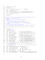
1
AN UHF FMCW
WIND PROFILER
DEVELOPMENT AND RESULTS
A Thesis Presented By
Carolina Asturiano Gómez
Projecte Final de Carrera
Enginyeria de Telecomunicació
Submitted to Universitat Politècnica de Catalunya
(Escola Tècnica Superior d’Enginyeria de Telecomunicació de Barcelona)
in fulfillment of the requirements for:
Projecte Final de Carrera
Enginyeria de Telecomunicació
Approved as to style and content by:
Stephen J. Frasier, Advisor
Amherst, Massachusetts
May 2010
ii
In any situation,
the best thing you can do is the right thing;
the next best thing you can do is the wrong thing;
the worst thing you can do is nothing.
Theodore Roosevelt
iii
ABSTRACT
Radars based on the Frequency-Modulated Continuous-Wave (FMCW) technique
have proven to be an excellent tool for the Atmospheric Boundary Layer (ABL) studies. This layer of the atmosphere is of vital importance for the understanding of
weather and climate. FMCW radars provide high sensitivity and high range resolution needed for observation of small scale turbulence.
This thesis describes the FMCW Wind Profiler operating at UHF band as of
Spring 2010. At a later stage it will utilize the spaced antenna (SA) technique for
achieving three-dimensional wind fields. This work describes its principles of operation, the current status of the radar hardware, and comments the new programs
developed for its proper operation. It discusses the sensitivity of the Wind Profiler
derived from laboratory tests and the results of the field deployments. The current
design uses four antennas, one for transmission and three for reception. The major
drawback of the Wind Profiler is the isolation required between the transmitter and
the receiver. A new scheme is proposed to overcome this problem by using Interrupted FMCW. Recommendations for the future hardware development of the radar
and conclusions are provided.
iv
TABLE OF CONTENTS
ABSTRACT . . . . . . . . . . . . . . . . . . . . . . . . . . . . . . . . . . . . . iv
LIST OF FIGURES AND TABLES . . . . . . . . . . . . . . . . . . . . . . . . . viii
LIST OF SYMBOLS . . . . . . . . . . . . . . . . . . . . . . . . . . . . . . . . . xi
ACKNOWLEDGEMENTS . . . . . . . . . . . . . . . . . . . . . . . . . . . . . xii
CHAPTER 1 INTRODUCTION . . . . . . . . . . . . . . . . . . . . . . . . . . . 1
1.1
Motivation . . . . . . . . . . . . . . . . . . . . . . . . . . . . . . . . . . . 1
1.2
Summary of Chapters
. . . . . . . . . . . . . . . . . . . . . . . . . . . .3
CHAPTER 2 WIND PROFILER RADAR BACKGROUND . . . . . . . . . . . . 5
2.1
Atmospheric boundary layer . . . . . . . . . . . . . . . . . . . . . . . . . 5
2.2
Clear air back scattering Theory . . . . . . . . . . . . . . . . . . . . . . . 6
2.3
FMCW Principles . . . . . . . . . . . . . . . . . . . . . . . . . . . . . . . 7
2.4
Interrupted FMCW . . . . . . . . . . . . . . . . . . . . . . . . . . . . . 12
CHAPTER 3 SYSTEM DESCRIPTION . . . . . . . . . . . . . . . . . . . . . . 15
3.1
Current Hardware Configuration . . . . . . . . . . . . . . . . . . . . . . 15
3.2
Windprofiler Subsystems . . . . . . . . . . . . . . . . . . . . . . . . . . 18
3.2.1
Control and Transmit Subsystem . . . . . . . . . . . . . . . . . 18
3.2.2
Calibration Loop . . . . . . . . . . . . . . . . . . . . . . . . . . 19
3.2.3
Receiver Subsystem . . . . . . . . . . . . . . . . . . . . . . . . . 19
CHAPTER 4 DATA ACQUISITION . . . . . . . . . . . . . . . . . . . . . . . . 21
4.1
Acquisition Board . . . . . . . . . . . . . . . . . . . . . . . . . . . . . . 21
4.2
Data acquisition program
. . . . . . . . . . . . . . . . . . . . . . . . . 24
v
CHAPTER 5 SIGNAL PROCESSING . . . . . . . . . . . . . . . . . . . . . . . 27
5.1
Signal processing programs . . . . . . . . . . . . . . . . . . . . . . . . . 27
5.2
GUI . . . . . . . . . . . . . . . . . . . . . . . . . . . . . . . . . . . . . 29
CHAPTER 6 RADAR TESTS . . . . . . . . . . . . . . . . . . . . . . . . . . . 31
6.1
Synchronization . . . . . . . . . . . . . . . . . . . . . . . . . . . . . . . 31
6.2
Minimum detectable Signal . . . . . . . . . . . . . . . . . . . . . . . . 33
CHAPTER 7 FIELD DEPLOYMENTS . . . . . . . . . . . . . . . . . . . . . . 41
7.1
Antenna Isolation . . . . . . . . . . . . . . . . . . . . . . . . . . . . . . 41
7.2
Deployment results . . . . . . . . . . . . . . . . . . . . . . . . . . . . . 42
CHAPTER 8 FUTURE WORK . . . . . . . . . . . . . . . . . . . . . . . . . . . 51
8.1
FMICW configuration . . . . . . . . . . . . . . . . . . . . . . . . . . . 51
8.2
Spaced Antenna . . . . . . . . . . . . . . . . . . . . . . . . . . . . . . . 54
CHAPTER 9 CONCLUSIONS . . . . . . . . . . . . . . . . . . . . . . . . . . . 57
BIBLIOGRAPHY . . . . . . . . . . . . . . . . . . . . . . . . . . . . . . . . . . 59
APPENDIX A - ACQUISITION SOURCE CODE . . . . . . . . . . . . . . . . 61
A.1 Savedata Windprof . . . . . . . . . . . . . . . . . . . . . . . . . . . . . 61
A.1.1 main.c . . . . . . . . . . . . . . . . . . . . . . . . . . . . . . . . 61
A.1.2 savedata.c . . . . . . . . . . . . . . . . . . . . . . . . . . . . . . 65
A.1.3 fmcw conf.c . . . . . . . . . . . . . . . . . . . . . . . . . . . . . 69
APPENDIX B - SIGNAL PROCESSING PROGRAMS . . . . . . . . . . . . . . 73
B.1 Windprofiler2010 . . . . . . . . . . . . . . . . . . . . . . . . . . . . . . 73
B.1.1 Windprof process.pro . . . . . . . . . . . . . . . . . . . . . . . . 74
B.1.2 Windprof process2.pro . . . . . . . . . . . . . . . . . . . . . . . 77
vi
B.1.3 Windprof display.pro . . . . . . . . . . . . . . . . . . . . . . . . 77
B.1.4 Windprof process realtime.pro . . . . . . . . . . . . . . . . . . . 79
B.1.5 Windprof display realtime.pro . . . . . . . . . . . . . . . . . . . 82
B.1.6 GUI . . . . . . . . . . . . . . . . . . . . . . . . . . . . . . . . . 86
B.1.7 wgui create.pro . . . . . . . . . . . . . . . . . . . . . . . . . . . 86
B.1.8 wgui event.pro . . . . . . . . . . . . . . . . . . . . . . . . . . . 88
APPENDIX C - RADAR BOXES . . . . . . . . . . . . . . . . . . . . . . . . . . 93
C.1 Boxes . . . . . . . . . . . . . . . . . . . . . . . . . . . . . . . . . . . . 93
C.2 Connections . . . . . . . . . . . . . . . . . . . . . . . . . . . . . . . . . 94
vii
LIST OF FIGURES AND TABLES
Figure 2.1 The diurnal evolution of the atmospheric boundary layer over land
(from Wyngaard, 1992) . . . . . . . . . . . . . . . . . . . . . . . . . . 5
Figure 2.2 Waveform of sent signal . . . . . . . . . . . . . . . . . . . . . . . . . . 8
Figure 2.3 FMCW Radar Sweep (left) and Frequency diagram (right) . . . . . . 9
Figure 2.4 FMICW principles . . . . . . . . . . . . . . . . . . . . . . . . . . . 12
Figure 2.5 FMICW Sensitivity function . . . . . . . . . . . . . . . . . . . . . . 13
Figure 3.1 Current FMCW Wind Profiler block diagram . . . . . . . . . . . . . 17
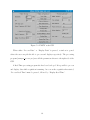
Figure 3.2 FPGA Control signals generation . . . . . . . . . . . . . . . . . . . 19
Figure 3.3 Audio module filter response . . . . . . . . . . . . . . . . . . . . . . 20
Figure 4.1 24DSI6LN Data Acquisition Card . . . . . . . . . . . . . . . . . . . 21
Figure 4.2 DAQ Connector . . . . . . . . . . . . . . . . . . . . . . . . . . . . . 23
Figure 5.1 Amplitude of a chirp and Power Spectrum . . . . . . . . . . . . . . 28
Figure 5.2 FMCW radar GUI . . . . . . . . . . . . . . . . . . . . . . . . . . . 30
Figure 6.1 Power spectrum (left) and Phase of the 300m bin and 400m bin (right)31
Figure 6.2 Power spectrum (left) and Phase of the 300m bin (right) with phase
correction . . . . . . . . . . . . . . . . . . . . . . . . . . . . . . . . 32
Figure 6.3 Minimum detectable with default configuration . . . . . . . . . . . . 34
Figure 6.4 Lab Setup . . . . . . . . . . . . . . . . . . . . . . . . . . . . . . . . 35
Figure 6.5 Noise floor with and without 17dB amplifier . . . . . . . . . . . . . 35
Figure 6.6 Noise floor with averaging of 1000 profiles . . . . . . . . . . . . . . . 36
Figure 6.7 Noise floor adding 2 profiles . . . . . . . . . . . . . . . . . . . . . . 36
Figure 6.8 Minimum detectable Cn2 when received power is -160dBm . . . . . . 37
viii
Figure 6.9 Noise floor with different configurations (Averaging of 1000 profiles) 39
Figure 6.10 Noise floor Pleak = −40.5dBm . . . . . . . . . . . . . . . . . . . . . 40
Figure 7.1 Antennas in Tillson farm . . . . . . . . . . . . . . . . . . . . . . . . 41
Figure 7.2 Received leakage
. . . . . . . . . . . . . . . . . . . . . . . . . . . . 42
Figure 7.3 Minimum detectable Cn2 when received power is -140dBm . . . . . . 43
Figure 7.4 Returned power and Doppler velocity during deployment on April
14th (Default configuration) . . . . . . . . . . . . . . . . . . . . . . 45
Figure 7.5 Returned power and Doppler velocity during deployment on April
14th (B=12.5MHz) . . . . . . . . . . . . . . . . . . . . . . . . . . . 45
Figure 7.6 Returned power and Doppler velocity during deployment on May 5th 46
Figure 7.7 Data Power Spectrum (April 14th) . . . . . . . . . . . . . . . . . . 46
Figure 7.8 Returned power and Doppler velocity on April 22nd . . . . . . . . . 47
Figure 7.9 Audio module output . . . . . . . . . . . . . . . . . . . . . . . . . . . . 47
Figure 7.10 Antennas with additional shrouds . . . . . . . . . . . . . . . . . . . 48
Figure 7.11 Returned power and Doppler velocity during deployment on May 12th49
Figure 8.1 FMICW Block Diagram . . . . . . . . . . . . . . . . . . . . . . . . 51
Figure 8.2 3-antenna SA-FMICW . . . . . . . . . . . . . . . . . . . . . . . . . 54
Figure C.1 Wind Profiler Boxes . . . . . . . . . . . . . . . . . . . . . . . . . . . 93
Figure C.2 Radar connections . . . . . . . . . . . . . . . . . . . . . . . . . . . . 94
Table 3.1
System specifications . . . . . . . . . . . . . . . . . . . . . . . . . . 16
Table 4.1
Input Data Buffer Organization . . . . . . . . . . . . . . . . . . . . 22
Table 4.3
Files in savedata windprof/ . . . . . . . . . . . . . . . . . . . . . 24
Table 5.1
FMCW Radar collection&display data procedure . . . . . . . . . . 29
Table 6.1
FMCW parameters . . . . . . . . . . . . . . . . . . . . . . . . . . . 38
ix
Table 8.1
High Power Switch SPDT (Ref. ES0309-50) . . . . . . . . . . . . . 52
Table 8.2
Low Power Switch SPST (Ref. ZFSWHA-1-20+)
Table 8.3
FMICW parameters . . . . . . . . . . . . . . . . . . . . . . . . . . . 54
Table B.1
Windprofiler2010 files . . . . . . . . . . . . . . . . . . . . . . . . . . 73
x
. . . . . . . . . . 53
LIST OF SYMBOLS
Structure Constant . . . . . . . . . . . . . . . . . . . . . . . . . . . . . . . . . . Cn2
Sweep Time . . . . . . . . . . . . . . . . . . . . . . . . . . . . . . . . . . . . . . TP
Bandwidth . . . . . . . . . . . . . . . . . . . . . . . . . . . . . . . . . . . . . . B
Range . . . . . . . . . . . . . . . . . . . . . . . . . . . . . . . . . . . . . . . . . R
Beat frequency . . . . . . . . . . . . . . . . . . . . . . . . . . . . . . . . . . . . fb
Sampling frequency . . . . . . . . . . . . . . . . . . . . . . . . . . . . . . . . fSample
Switch frequency . . . . . . . . . . . . . . . . . . . . . . . . . . . . . . . . . . . fS
Range resolution . . . . . . . . . . . . . . . . . . . . . . . . . . . . . . . . . . 4R
Compression gain . . . . . . . . . . . . . . . . . . . . . . . . . . . . . . . . . . . GC
Transmit power . . . . . . . . . . . . . . . . . . . . . . . . . . . . . . . . . . . . Pt
Receive power . . . . . . . . . . . . . . . . . . . . . . . . . . . . . . . . . . . . . Pr
Transmit antenna gain . . . . . . . . . . . . . . . . . . . . . . . . . . . . . . . . Gt
Receive antenna gain . . . . . . . . . . . . . . . . . . . . . . . . . . . . . . . . . Gr
Radar wavelength . . . . . . . . . . . . . . . . . . . . . . . . . . . . . . . . . . . . λ
Half power beamwidth . . . . . . . . . . . . . . . . . . . . . . . . . . . . . . . . . θ
Volume reflectivity . . . . . . . . . . . . . . . . . . . . . . . . . . . . . . . . . . . η
Antenna correction term . . . . . . . . . . . . . . . . . . . . . . . . . . . . . . . Ca
xi
ACKNOWLEDGEMENTS
Firstly, I would like to thank the supervisor of this thesis, Dr. Stephen Frasier
for his assistance and supervision during the whole process of this work, and also
for giving me the opportunity to be at MIRSL. It has been an excellent experience
that really helped me to expand my knowledge a lot, and to grow as an engineer. I
would like to thank to all the people working here at MIRSL who were always willing
to answer my questions and whenever I needed, they helped me, even in the field
deployments. I would especially give thanks to David Garrido, who initially walked
me through the radar project. Without his help this work would have been harder.
Also thanks to him for being a good friend, making me feel comfortable since my first
day in Amherst.
I am also grateful to the friends with whom I have been sharing all these time as an
exchange student here in Amherst. Thanks to them, these months are unforgettable.
Finally, my warmest thanks to my friends from back home, my boyfriend and my
family for supporting me from a great distance.
xii
CHAPTER 1
INTRODUCTION
1.1
Motivation
The Atmospheric Boundary Layer (ABL) is the lowest few hundred meters of the
atmosphere, where the Earth’s surface most directly influences atmospheric processes.
The structure and dynamics of the ABL are of vital importance for the understanding of weather and climate, the dispersion of pollutants, and the exchange of heat,
water vapor, and momentum with the underlying surface. The knowledge of this it
allows more refined and reliable numerical models for daily weather forecasts, dispersion events, and future global climate on Earth. The effect of the troposphere on
wave propagation has also been studied extensively for improving radio communications. Radio signals are altered by slight changes in the refractive index in the lower
atmosphere caused by air turbulence, and small changes in temperature, humidity
and barometric pressure. This makes it very important to have a full and detailed
description of the refractive index structure.
Frequency modulated continuous wave (FMCW) radars are able to provide information on the ranges and Doppler shifts of multiple targets. This information
is essentially equivalent to that provided by coherent pulsed radars. However, as
the signal to noise performance of a radar depends on average, rather than peak
transmitted power, the high duty cycle of the FMCW waveform can provide good
performance from a relatively compact and inexpensive radar system. Additional
advantages come from the fact that the range resolution of an FMCW radar is determined principally by the bandwidth of the linear frequency sweep. Consequently,
high range resolutions can be obtained without the attendant problems of generating
very short pulses. Further, the FMCW waveform provides good performance at close
ranges and low interference to other systems when compared with conventional pulsed
1
radars. A major disadvantage of FMCW systems is the need to use two separate,
well shielded antennas for transmission and reception.
There exists an S-band FMCW radar for atmospheric boundary layer studies
which was developed in The Microwave Remote Sensing Laboratory (at University
of Massachusetts, Amherst) [1]. This radar is sensitive to Rayleigh scattering from
insects which can be much greater than the weak Bragg scattering from refractive
index irregularities. Therefore it was proposed to change the frequency from S-band
(3GHz) to UHF (915MHz). Vertically pointed radars can measure vertical wind
velocities. In order to retrieve horizontal winds, the proposed profiler uses a spaced
antenna (SA).
A low-power, cost effective and mobile UHF FMCW-SA Wind profiler Radar is
being developed at MIRSL. It will allow to observe and retrieve information about
the structure and processes in the ABL with high resolution. The Wind Profiler
design and development was initiated in the summer of 2006 by Prof. Frasier and the
former students Albert Genis during 2008, Iva Kostadinova on 2008-2009 and David
Garrido on 2009. Many changes have been introduced to the radar, after upgrading
and overcoming the different problems that were affecting it.
The primary objective of this thesis is to continue with the work achieved by David
Garrido [2, 3], first of all focusing on data acquisition and synchronization issues, and
secondly developing the required signal processing programs. The current hardware
configuration of the UHF Wind Profiler, as well as the obtained outcomes, will be
described in detail in the laboratory and the field deployment. Finally, recommendations for future work are discussed.
2
1.2
Summary of Chapters
This thesis documents the FMCW Wind Profiler radar as of Spring 2010. Chapter
2 provides a brief description of the atmospheric boundary layer, discusses the principles of operation of FMCW radars as well as Interrupted FMCW radars. Chapter
3 provides an overview of the current status of the Wind Profiler hardware.
The main part of this thesis begins with the development of the new data acquisition programs, and subsequently, the development of the signal processing programs
required for the proper operation of the radar. These are described in Chapters 4 and
5 respectively. A series of tests are performed in the laboratory for the evaluation
of the Wind Profiler. The adopted solution for the synchronization issues, and the
minimum detectable signal for the Wind Profiler are discussed in Chapter 6. In the
next chapter, the results of the field deployment are presented. Chapter 8 comments
some future work that can be done in the system, a new scheme is proposed to enable
the radar to operate with a single antenna for transmission and reception. Finally,
Chapter 9 concludes this thesis.
3
CHAPTER 2
WIND PROFILER RADAR BACKGROUND
2.1
Atmospheric boundary layer
The atmospheric boundary layer is the lower part of the atmosphere that is di-
rectly influenced by the surface of the Earth. The diurnal heat, moisture or momentum transfer to or from the surface create strong mixing and turbulent processes with
a time scales of about an hour or less. The structure of ABL turbulence is strongly
affected by the diurnal cycle of surface heating and cooling, and by presence of clouds.
Basically there are two types of boundary layer based on buoyancy effects: (i) Convective boundary layer, where heat from the surface of the Earth creates positive
buoyancy flux and instabilities that lead to turbulence and (ii) Nocturnal boundary
layer, where negative buoyancy flux decreases the turbulence and stable stratified
conditions prevail.
Figure 2.1: The diurnal evolution of the atmospheric boundary layer over land (from
Wyngaard, 1992)
The nocturnal boundary layer may also be convective when cold air advects over a
5
warm surface. Typical boundary layer structure is depicted in figure Figure 2.1. The
depth of the ABL can range from only a few meters in strongly stable stratification
to several kilometers in highly convective conditions.
2.2
Clear air back scattering Theory
In 1966 Hardy and Atlas were the first to attribute the detected backscattered
signals from clear air due to Bragg scattering from random fluctuations in the refractive index [4]. Radar backscattering from refractive index variation is able to provide
helpful information about the atmospheric structure.
The radar backscattering from the clear air atmosphere, is caused by irregular
small-scale fluctuations in the radio refractive index produced by turbulent mixing
and is dependent on the atmospheric water vapor, temperature, and pressure.
The parameter Cn2 is called the structure constant and is a major characteristic
describing the intensity of atmospheric turbulence. In 1969 Ottersen [5] was the first
to derive the relationship between the radar volume reflectivity and refractive index
structure as
1
η(λ) ≈ 0.38Cn2 λ− 3
(2.1)
For a given radar , the radar reflectivity of a region of refractive index fluctuations
is directly proportional to Cn2 when the length scale of one-half of the radar wavelength
falls within the inertial subrange. The more violent the turbulent mixing the larger
the displacements, and the stronger the inhomogeneities will be. Consequently, strong
turbulence and sharp mean gradients contribute to high Cn2 values. Typical values
of the structure constant for the convective boundary layer lie in the range between
10=15 to 10=13 m
=2
3
. Radar backscatter can also be due to Rayleigh scattering from
birds, insects, and hydrometeors where the size of the scatterers is much smaller than
the radar wavelength.
6
2.3
FMCW Principles
FMCW is a common technique used in radar technology, that is not limited by the
constraints of pulsed radars. FMCW consists of the transmission of a sinusoid whose
frequency changes over time. FMCW Radar transmits a frequency sweep, commonly
called a chirp. The signal is reflected from distant targets and detected by the receiver
where the returned signal is mixed with a copy of the transmitted signal to determine
the range of the target. The transmitted waveform has a time varying frequency f (t)
given by:
f (t) = F1 + α · t ∀t < TP
(2.2)
where F1 is the initial frequency, α the rate of change of frequency and TP the
Sweep time. This is a linearly increasing frequency sweep as shown in Figure 2.2.
Ideally the instantaneous frequency should augment indefinitely with time, but in
order to have a realistic system the frequency will increase until a maximum value,
and will start from the initial frequency once that point is reached. The frequency
increases from F1 at the start of the sweep to F2 at the end of the sweep after a time
TP . The bandwidth B is the difference between F2 and F1 . The rate of change of
frequency is then defined as α =
B
TP
.
The transmitted waveform travels to the target at distance R and the back scattered signal from an atmospheric target, usually referred to as an echo, will be delayed
by τ =
2R
c
(where c is the speed of light). The back scattered signal will also be atten-
uated and possibly Doppler-shifted in case the target is not stationary. The process
of generating the beat frequency from the return signal can be visualized as shown in
Figure 2.3.
Given that the transmitted signal frequency fT (t) = F1 + αt ∀0<t < TP and
assuming an ideal point target, the received signal frequency fR is given by fR (t) =
F1 + α(t − τ ) ∀τ <t < TP . Mixing these two signals produces sum and difference
7
Figure 2.2: Waveform of sent signal
frequencies, fT + fR and fT − fR . The resulting signal is then low pass filtered to
remove the fT + fR term. The term that remains is the beat frequency fb =
beat frequency term is directly related to the range by fb = fT − fR =
B
TP
2RB
,
cTP
t. The
i.e. for
stationary targets the range R can be expressed as:
R=
cTP
fb
2B
(2.3)
The sampling frequency (fSample ) of the A/D conversion determines the maximum
beat frequency that can be detected without aliasing. Using 2.3 the maximum beat
frequency determines the maximum range for FMCW radars as:
Rmax =
cTP
cTP fSample
fbM AX =
2B
2B
2
(2.4)
With the beat frequency and the radar parameters B and TP known, we can
retrieve range information from the return signal. The Fast Fourier Transform (FFT)
is the mathematical tool used to interpret the spectrum of the beat frequency signal
in terms of radar range. The point target scenario can be extended to multiple targets
8
Figure 2.3: FMCW Radar Sweep (left) and Frequency diagram (right)
as well. Each target will produce a return signal with a frequency corresponding to
the distance. In addition, this return signal will have an amplitude corresponding to
the round trip attenuation to its specific target. These can be seen as peaks in the
frequency domain.
In an FMCW radar, range resolution means the ability to separate adjacent spectra. The frequency resolution in this case is defined as 4f =
1
TP
. The range resolution
of an FMCW system is only dependent on the bandwidth of the transmitted signal.
Using 2.3 the range resolution 4R is derived as:
4R =
c
2B
(2.5)
Parameters such as B and TP are configurable in an FMCW radar thus providing
flexibility to adapt to the most suitable mode. For example, in order to improve
range resolution the chirp bandwidth B should be increased. Keeping all other parameters constant, this will reduce the maximum range. One of the advantages of
FMCW radars is that they allow for change in range resolution without change in
the peak transmit power for a given sensitivity. To maximize range resolution and
sensitivity, both B and TP should be as large as possible. TP , however, is constrained
9
by the coherence time of the atmospheric echo as the presented theory is based on
the assumption that the target remains coherent during the sweep interval.
FMCW radars are a type of pulse-compression radar that provide exceptional
range resolution when compared to pulsed radars. They operate by transmitting a
long, coded waveform of duration TP , and bandwidth B. The improvement factor
they gain over pulsed radars of equivalent range resolution is given by the compression
gain:
GC = BTP
(2.6)
It is possible to determine Doppler velocities by comparing the phase changes
of two consecutive received pulses. In this case, the Nyquist Doppler frequency is
1
2TP
=
P RF
2
and the unambiguous velocity interval is given by
|vr | ≤
λ
P RF
4
(2.7)
where λ is the radar wavelength, P RF is the Pulse Repetition Frequency and equals
the inverse of TP when the radar has a duty cycle of 100%. It can be shown that
the response of the FMCW radar to a point target at range R0 , moving at a radial
velocity vr , can be expressed as [1]:
y(R) =
where fd =
2vr
λ
sinπ(fd TP + (R − R0 )/4R)
π(fd TP + (R − R0 )/4R)
(2.8)
is the Doppler frequency. The presence of both range and Doppler
terms in the argument of the sinc function illustrates the effect of target motion on
the radar’s ability to locate. By rearranging the terms in the argument in 2.8, the
apparent range of the target Rapp can be expressed as:
10
Rapp = R0 − fd TP 4R
(2.9)
where it is obvious that misregistration by one resolution cell occurs when the product
fd TP equals unity, or when vr = ± λ2 T1P = ± λ2 P RF . Thus, targets with unambiguously measured velocities are misregistered by no more than one half a resolution cell.
Averaging is a powerful tool for increasing radar sensitivity. The minimum detectable Cn2 can be increased by coherent and non-coherent averaging over a period
of time. The number of pulses available for coherent integration is closely related to
the coherence time of the observed target. It is assumed that during this coherence
time, the phase of the target changes much less than a wavelength. If NCOH is the
number of pulses available for coherent integration, the improvement in SNR due to
coherent averaging is:
I [dB] = 10log(NCOH )
(2.10)
The choice for non-coherently averaged pulses is dictated by the amount of spatial
and temporal detail needed in the observed phenomena and the time over which these
phenomena don’t change significantly over the spatial extent of the resolution volume.
The improvement in SNR for non-coherent averaging is:
q
I [dB] = 10log( NN COH )
where NN COH is the number of non-coherently averaged pulses.
11
(2.11)
2.4
Interrupted FMCW
A major disadvantage of FMCW systems is the need to use two separate, well
shielded antennas for transmission and reception to prevent direct leakage of transmitted energy from overloading the receiver. Several schemes have been devised to
enable FMCW radars to operate with a single antenna. In one such scheme the
transmitter, antenna and receiver are connected by means of a circulator which allows energy to pass from the transmitter to the antenna and from the antenna to
the receiver but isolates the receiver from direct leakage from the transmitter. Alternatively a transmit/receive (T/R) switch can be used to switch a single antenna
between the transmitter and receiver. The requirement in this case is good isolation
between the transmit and receiveports of the T/R switch.
Even though this system is no longer a true continuous wave radar, the essential
properties of the FMCW waveform are preserved with little degradation in performance, provided suitable constraints on the switching waveform are met. This system
is referred to as a frequency modulated interrupted continuous wave (FMICW) radar.
FMICW systems have the advantage of increasing the portability of the radar system, simpler antenna alignment geometry, and relaxing the isolation requirements
between transmitter and receiver, but have the disadvantage of limited range due to
the switching constraints.
Figure 2.4: FMICW principles
12
A scheme is possible in which a 50% duty cycle square wave is used as the T/R
switching waveform [6]. The transmitter and receiver may be connected to a single
antenna by a T/R switch. This scheme has the advantage of maximising average
transmitted power. The effect of switching with a 50% duty cycle is depicted in
Figure 2.4.
Figure 2.5: FMICW Sensitivity function
The FMICW receiver output signal is the unswitched FMCW beat signal multiplied by a pulse train with switch frequency fS , and duty cycle which depends on
target range as shown in Figure 2.5. It can be seen that when the duty cycle is 50%
the echo delay equals half the switch period. The switch frequency fS is chosen to
give the maximum sensitivity at maximum range (RM AX ), thus:
fS =
c
4RM AX
(2.12)
As it is shown in Figure 2.5, there exist some ranges whose associated sensitivity
is null. These ranges are called blind ranges:
RB =
c
n n = 0, 1, 2...
2fS
(2.13)
The received signal is an echo from the target modulated with a rectangular
wave. This modulation produces copies of the spectrum shifted +nfS Hz, where n is
an integer. This introduces the condition that the switching frequency must be larger
13
than twice the highest beat frequency fb,M AX to avoid spectral aliasing.
fS >2fb,M AX = fSample
(2.14)
Then, using that and equations 2.4 and 2.12, it follows that:
s
RM AX <
14
c2 TP
16B
(2.15)
CHAPTER 3
SYSTEM DESCRIPTION
The current FMCW radar project started as an analog of the S-Band FMCW
boundary layer profiler developed in 2003 at the University of Massachusetts at
Amherst [1]. The change from S-Band to UHF was proposed in order to reduce
the Rayleigh scattering from insects and birds which appeared to dominate the observed vertical profile of the mean reflectivity at S-Band. The current FMCW Wind
Profiler was started in the summer 2006 by the former students Albert Genis during
2008 [7], Iva Kostadinova in 2008-2009 [8], and David Garrido [2, 3] in 2009. This
chapter reviews the current design of the Wind Profiler system.
3.1
Current Hardware Configuration
The Wind Profiler is an FMCW radar that operates in the 900 MHz ISM frequency
band (902-928MHz) with a center frequency of 915MHz. The chirp is generated by
a Direct Digital Synthesizer (DDS) with a bandwidth up to 25MHz and linear FM
modulation. It is able to achieve a maximum range resolution of 6m. Table 3.1 lists
the basic system specifications and Figure 3.1 depicts the major blocks of the current
Wind Profiler design.
The default mode of operation had a P RF of 100Hz, and a duty cycle of 100%
(TP =10ms). Using Equation 2.7 it is possible to calculate the vertical unambiguous
velocity up to 8.2 m/s which exceeds the range of usual turbulent velocities on the
boundary layer (3-5m/s). All the signals needed to start the radar, such as those
used to start and set up the DDS are generated by a Field Programmable Gate Array
Board (FPGA). The parameters of the radar such as bandwidth, P RF and TP are
configurable. This allows for adaptation to the resolution and scenario as necessary.
The antennas are 4ft diameter parabolic dish antennas with dipole antenna feeds,
15
Transmitter
Center Frequency
Peak transmit power
Transmitter type
Bandwidth
PRF (100% duty cycle)
Antennas
Type
Gain
Polarization
Front to Back Ratio
915 MHz
30 W (44.77 dBm)
Solid State RF
≤25 MHz
100 Hz
Four Parabolish dish
18 dB
Linear
22 dB
Table 3.1: System specifications
19º beamwidth and 18dB of gain. The antennas have a broad beam, in order to
employ a SA technique for estimating horizontal winds.
16
Figure 3.1: Current FMCW Wind Profiler block diagram
17
FPGA
DDS
24
x2
fc = 915 MHz
BW = 25 MHz
CH0
CH3
CH2
CH1
DAQ
SYNC
G = 20 dB
SPLITTER
G = 70 dB 1.5 kHz- 40 kHz
Audio Module
Signal Generator
fo = 10 MHz
Signal Generator
fo = 200 MHz
SINE /
TTL
x2
LNA
G = 23 dB
IF
RF
LO
IF
RF
LO
IF
RF
LO
-20 dB
SSPA
G = 50 dB
G =17 dB
-40dB
SPLITTER
2 µs
DELAY
LINE
-20 dB
-20 dB
LNA
-20 dB
G = 23 dB
-10 dB
fc = 915 MHz
BW = 25 MHz
-30 dB
3.2
Windprofiler Subsystems
Figure 3.1 shows a simplified block diagram of the FMCW Wind Profiler. Cur-
rently all the hardware, apart from the computer which contains the Data Acquisition
Card (DAQ) and the audio module with its power supply, is in 4 boxes (FPGA Box,
Big Amplifier Box, RF Box and Power Supply Box). The current state of the boxes
as well as the connections between them can be found in Appendix C.
3.2.1
Control and Transmit Subsystem
The FPGA (Altera Cyclone II EP2C20) generates all the radar signals required
for the proper operation of the Wind Profiler . It uses a clock at 10MHz. The design is
characterized by the generation of all signals in total synchronization, giving no room
for timing skews that can lead to phase wrapping in the received data. Besides, the
duty cycle of the Wind Profiler is set up to 100%. The operator stores the necessary
parameters to configure the radar in a file which will be sent via serial interface to the
FPGA. That file and its parameters can be modified at any time, making the radar
flexible to operate in different contexts (see Figure 3.2).
The transmitted chirp is generated by a 10-bit Digital Signal Synthesizer from
Analog Devices (AD9858 DDS). The DDS receives the needed parameters for frequency sweep generation from the FPGA. The DDS board uses an external 800MHz
clock signal that comes from a 200MHz oscillator and two doublers. The analog
mixer mixes the clock signal with the chirp centered at 115 MHz to produce the desired product at 915 MHz. The undesired mixing products are filtered and the signal
is amplified. A 4-way splitter splits the transmitted signal to the three LO inputs of
the receiver mixers and to the RF high power amplifier. The high power amplifier is
a linear power solid state RF amplifier from OPHIRRF with a gain of 50dB providing
a 30W (44.8 dBm) output. A 20dB directional coupler delivers the output of the
amplifier to the antenna and couples part of it to the calibration loop.
18
DDS
·
·
·
·
Center Frequency
Bandwidth
Chirp length (Tp)
100% duty cycle
Reset
Configuration file (.conf)
Center Frequency (MHz): 114.5
Bandwidth (MHz)
: 25
Chirp Length(ms)
: 10
PRF (Hz)
: 100
Sample Frequency (KHz) : 60
Total Profiles : 1000
Number of Channels: 3
DAQ Board
FPGA
·
·
·
·
SYNC channel
Sample Frequency
Chirp length (Tp)
#Total profiles
Figure 3.2: FPGA Control signals generation
3.2.2
Calibration Loop
The calibration loop allows continuous monitoring of the system performance and
gives a reference point for the evaluation of the radar sensitivity. The Wind Profiler
uses a bulk acoustic wave (BAW) delay line, with an effective delay of 2ms from
Teledyne Electronic Devices. An attenuated replica of the transmitted signal serves
as its input. This delay will produce an echo corresponding to a fixed range of 300m.
The output obtained is coupled into the receiver chain through a 20dB coupler. The
delayed chirp produces a signal of a fixed fb at the mixer’s IF port. Using the default
configuration (TP =10ms, B=25MHz) the beat frequency is 5kHz (see equation 2.3).
Other fixed beat frequencies will appear at 3fb and 5fb (corresponding to 900m and
1500m) due to the triple and quintuple travel signal in the delay line.
3.2.3
Receiver Subsystem
The receiver chain consists of three channels for the three receiving antennas which
would allow the SA technique to retrieve horizontal winds. The calibration signal is
coupled to the received signal in the front end. The coupler is a 20dB coupler from
Narda Microwave East. To ensure a good noise figure, the first component in the
receiver is a 23dB low noise amplifier. The next components in the chain are a
19
ceramic band pass filter from Lark Engineering and a 17dB amplifier.
Figure 3.3: Audio module filter response
The output of the amplifier is passed on to the RF port of the mixer. Then the
return signal is mixed with an attenuated copy of the transmitted signal through a
high power mixer from Mini Circuits (ZEM-4300MH+). The IF signal at the mixer
output is fed into the audio module [2] designed with low noise components. The
audio module filter response can be seen in Figure 3.3. Finally, the amplified base
band signal is digitalized by a four channel Analog-Digital Converter (ADC) and
stored on a local computer.
20
CHAPTER 4
DATA ACQUISITION
A new Data Acquisition Board was integrated in the radar. The board is a
four-channel low-noise 24-bit delta sigma PC104-Plus from General Standards. Data
acquisition programs were developed for it, but there were synchronization issues that
should be corrected. The adopted solution and all relevant information will be showed
in the following sections.
4.1
Acquisition Board
Figure 4.1: 24DSI6LN Data Acquisition Card
The Data Acquisition Card in the current Wind Profiler is a 24-bit 24DSI6LN from
General Standards. The board has 4 input channels and it allows sample rates from
2 KSPS to 200 KSPS per channel with an accuracy of 25 PPM. Each of four analog
input channels contains a low-pass image filter and a delta-sigma A/D converter that
21
provides digital antialias filtering. A linear-phase digital antialiasing filter rejects outof-band signals, and a low-pass analog filter reject those interference signals that fall
within the harmonic images of the digital filter.
The configured voltage range is
±10V corresponding to a maximum input power
of 30dBm for a single tone and the dynamic range of the board is 110dB. All the
specifications can be found in [9]. All data transfers are long-word D32 (32 bits).
The width of the data field is adjustable from 16 bits to 24 bits, in this case it is set
to 24 bits. Each value in the data buffer consists of a 5-bit channel tag field and a
data field, as shown in Table 4.1 [10].
DATA WIDTH
RESERVED (Zero)
CHANNEL TAG
CHANNEL DATA VALUE
24 bits
D[31..29]
D[28..24]
D[23..0]
Table 4.1: Input Data Buffer Organization
Input data values are configured to be represented in offset binary format instead
of two’s complement format. The Full-scale Range (FSR) is 20V (±10V). One LSB
equals the full-scale range divided by 224 :
1LSB =
20
(1.192µV )2
=
1.192µV
=
10
log
+ 30 = −105dBm
224
50
(4.1)
The Delta Sigma architecture is based on the technique of oversampling to reduce
the noise in the band of interest, which also avoids the use of high-precision circuits
for the antialiasing filter. In Delta Sigma converters, noise is further reduced at low
frequencies, which is the band where the signal of interest is, and it is increased at
the higher frequencies, where it can be altered. Due to the oversampling the external
input clock needs to be very fast (25.6-51.2 MHz [9]). With the old DAQ board it
was possible to use a clock provided by the FPGA, achieving a totally synchronized
system. At the moment, this is not possible because the fastest clock speed the FPGA
can provide is 10MHz.
For the signal processing, it is necessary to determine both the beginning and
22
the end of each profile. Therefore, some kind of synchronization is needed between
the DAQ and the FPGA. One possible solution could be to use an external sync
signal with a period of TP , and then, to acquire certain amount of data (which would
correspond to a profile) at every positive edge of the sync signal. This type operation
is known as bursting (capturing a fixed number of samples at a time). In this case,
it is not possible because this board doesn’t support any type of bursting feature.
The chosen solution consists of using the signal at frequency of
1
TP
provided by the
FPGA as input for the analog channel 3 (because the board has 4 channels and only
3 are needed for the 3 receiver antennas), and adapting the acquisition program to
store the corresponding number of samples at each positive edge of the sync signal.
System cable signal pin assignments are described below (for further information refer
to [10]).
Figure 4.2: DAQ Connector
23
4.2
Data acquisition program
A new program has been developed to collect data. It can be found in /usr/src/kernels/
.../drivers/24dsi/savedata windprof.
Table 4.3 lists all the files contained in this folder
and describes them briefly. This program is initially based on the “Save Acquired Data
sample” application provided by General Standards Corporation [11]. The source files
are provided and explained in Appendix A. The main program configures the board
according to the desired parameters, and acquires the data from channels 0-2. As
explained before, it is necessary to synchronize the collected data to determine when
a profile starts and ends. For this purpose, the program also acquires channel 3 which
corresponds to the synchronization signal at 100Hz ( T1P ).
File name
main.c
savedata.c
fmcw conf.c
Description
The main program. Contains all the procedures needed to configure
the board and collect the data.
Contains some useful functions. Currently only it is used by the main
application the functions channels profiler, save data
and dsi config board profiler.
Contains read fmcw conf and fwrite fmcw conf functions to
read and write the .conf file which is also used by the FPGA.
Table 4.3: Files in savedata windprof/
Before executing the program it is necessary to start the driver manually. Log
in as root user, change to the directory where the drivers are installed, which may
be /usr/src/kernels/.../drivers/24dsi/driver. Then, install the driver module and
create the device nodes by executing the command ./start. It is possible to verify that the device driver module has been loaded by issuing the command lsmod
and examining the output (the module name 24dsi should be included in the output) . To collect data, the program needs to run while the radar is operating, i.e.
the programs that start the radar have to be executed beforehand. To execute the
acquisition program, change to the directory where the acquisition application is
installed (/usr/src/kernels/... /drivers/24dsi/savedata windprof), build the applica24
tion by issuing the command make all, and start the application issuing the command
./savedata -m, where the parameter m is optional, which represents the maximum duration in minutes of the data acquisition.
The main program works as follows. First the board is identified and selected, the
device is opened, and the board is configured using FMCW defaults. The file in which
the data will be stored is created, has this name format: ‘‘#month#day#hour#minute.dat’’
and it will be stored in windprofiler2010/data/. The .conf file is read and the appropriate header is written. There are some necessary parameters defined in the .conf
file: the sample frequency fSample , the total number of profiles and the chirp length
TP . The acquisition starts. First of all it reads only channel 3, which contains the
sync signal, looking for its first positive edge. To find the edge a value for the threshold is set approximately to 1.65V because the sync signal generated by the FPGA is
a square wave with 3.3V of amplitude. The Block Size is the number of scans per
profile. When a positive edge is found, Block Size samples of the data channels are
saved. The Block Size is calculated as fSample · TP − 5 instead of fSample · TP so there
is enough time to look for the next edge. The program will be looking for the next
positive edge of the sync signal, and will save the next block until the number of
profiles read in the .conf file is reached or a timeout occurs.
25
CHAPTER 5
SIGNAL PROCESSING
New signal processing programs have been developed. The previously programs
were too slow and they needed to be improved as well since they used some kind of
preprocessing so as to find out the beginning and the end of the profiles. This it is
not needed anymore thanks to the new acquisition program. Signal real processing
program has also been implemented. All these programs will allow the radar to be
tested in an easier way both in the laboratory, and later, in the field deployment.
5.1
Signal processing programs
After the data acquisition, it is necessary to process it properly to extract the
required information. In the Wind Profiler, two different kinds of information can be
extracted from the data: range and doppler velocity. To perform the data processing, programs in IDL [12] have been developed. In this section these programs are
described and all the source code is provided in Appendix B.
The program called windprof process reads the raw data from the file created by
the acquisition program with a .dat extension, and it will create another file with
the same name, but with a .fig extension. This file will contain the averaged power,
the Doppler velocity, the matrix mean and correlation coefficient for each set of the
averaged profiles.
The program requires the name of the raw data file with the .dat extension, the
time for noncoherent integration and the number of the channel are required as input
of the program. Apart from this, there are other options which serve as input:
mr: If mr=1, means removal is performed, and ground clutter rejection and
rejection of stationary targets is achieved. mr=0 will be useful for testing when
it is required that a calibration signal appears.
27
pc: If pc=1 a phase correction is carried out.
delete samples: The number of samples to delete at the beginning of each
chirp. As shown in Figure 5.1 the chirp has a transient which contains no
information and these samples can be deleted.
png: If png=1 the plot is saved in a .png file (it can be found in windprofiler2010/data/).
Figure 5.1: Amplitude of a chirp and Power Spectrum
The program’s structure is as follows. It reads the header of the raw data file and
writes the corresponding header to the output file. It reads the number of profiles
available for noncoherent integration (prof avg) and stores it in a matrix (f frame).
The first 8 bits of each sample are discarded because they indicate the channel number,
and by using 4.1 the sample’s value is transformed to real voltage value. A Fast Fourier
Transform is done on the matrix. A phase correction is needed at this stage, which will
be explained in section 6.1 Synchronization. The mean of the FFT from each sweep
is calculated, if rm=1 the mean from the FFT is removed. The matrix is multiplied
by its conjugate to compute the average power. The pulse-pair technique described
in Section 2.3 is used to estimate the mean Doppler velocity. Then, it calculates the
28
autocorrelation of the matrix with lag of one sweep and computes Doppler velocity
from the phase of the autocorrelation. The correlation coefficient is also calculated.
All this process is repeated until the end of file is reached. Finally all this information
for each set of averaged profiles is stored in the output file with the .fig extension.
The IDL procedure called windprof display reads the .fig file and after some range
correction, it creates 2D images of the radar reflectivity and Doppler velocity.
5.2
GUI
The procedure to use the FMCW Radar and the main programs used are sum-
marized below (for further details see Appendix B):
1.
2.
3.
4.
5.
Start DAQ drivers
Start Radar
Start acquisition
Processing of raw data
Display data
.../24dsi/driver/start.c
fmcw current.conf, windprofiler 0409.c
.../savedata windprof/savedata.c
windprof process.pro
windprof display.pro
Table 5.1: FMCW Radar collection&display data procedure
A graphical user interface (GUI) has been created with the purpose of managing
all the operations and making the operation of the Wind Profiler easier. To start the
FMCW Radar GUI, go to the windprofiler2010/ directory and execute the command
idl wgui.
The GUI interface is shown in Figure 5.2.
When the button “Start Radar” is pressed the parameters introduced in Radar and
Acquisition Settings are stored in the fmcw current.conf. Then, the windprofiler 0409.c
is executed, and it sends the parameters to the FPGA through the serial port, and
initiates the Radar. If “radar reset” button is pressed the FPGA is reset and the
Wind Profiler stops. It is important to bear in mind that the acquisition program
also uses the .conf file, so these parameters must not change between radar initialization and data acquisition. The “Start Acquisition” and “Stop Acquisition” buttons
execute and kill the data collection program respectively.
29
Figure 5.2: FMCW radar GUI
When either “Process Data” or “Display Data” is pressed, a window is opened
where the user can pick the file to process and display respectively. The processing
program (windprof process.pro) uses all the parameters shown to the right side of the
GUI.
A Real Time processing program also has been developed. It is possible to process
and display data while acquisition is running. As soon as the acquisition has started,
“Process Real Time” must be pressed, followed by “Display Real Time”.
30
CHAPTER 6
RADAR TESTS
Following the changes to the acquisition program and the implementation of the
new signal processing programs outlined in the previous chapter, a series of laboratory
tests was done to evaluate the system performance. In these preliminary tests, the
radar operates with only one receiving antenna and it is able to analyze scattering in
the vertical direction. Their setup and the results are described here.
6.1
Synchronization
Once the new data acquisition program finishes, it then proceeds to check the
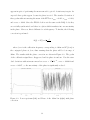
timing, a correct synchronization will allow the computation of the doppler information. The results are shown on Figure 6.1. This figure corresponds to when the FFT
of the averaging of 100 profiles and mean removal is carried out. It shows the power
spectrum of the averaged profiles (left) and the phase of the bin which is equivalent to 300m (right). The phase of the 400m bin also is plotted with the purpose of
comparing it with the 300m bin.
Figure 6.1: Power spectrum (left) and Phase of the 300m bin and 400m bin (right)
It is seen that the peaks corresponding to the calibration (300m, 900m and 1500m)
31
appears in spite of performing the mean removal to get rid of stationary targets. As
expected these peaks appear because its phase is not 0. The standard deviation of
these peaks without removing the mean of the FFT are σ300m = 0.061, σ900m = 0.039,
and σ1500m = 0.040. Since the FPGA clock is not the same as the DAQ clock, they
are not fully synchronized and there is a jitter which translates into an uncertainty
in the phase. Moreover, this is different for each frequency. To fix this, the following
correction is performed:
Φ(f ) = Φ∗ (fCAL )·
f
fCAL
where fCAL is the calibration frequency corresponding to 300m and Φ∗ (fCAL ) is
the conjugated phase at fCAL , thus ensuring that the phase will be 0 at range of
300m. The results with the phase correction are shown in Figure 6.2. The peaks
of the calibration signal have disappeared and its phase is random. Now the standard deviations without mean removal are σ300m = 1.76·10−18 , σ900m = 0.00024 and
σ1500m = 0.0027 , so the uncertainty of the phase is significantly reduced.
Figure 6.2: Power spectrum (left) and Phase of the 300m bin (right) with phase
correction
32
6.2
Minimum detectable Signal
For bistatic weather radar with Gaussian shaped beams, the received mean power
at the antenna port from a scattering volume in the far field is [13]:
Pr =
Pt Gt Gr λ2 θ2 4R η
Ca
512 ln 2π 2 R2
The parameter Ca accounts for the antenna parallax existing in every bistatic radar
and is given by Ca = exp(=2 ln 2 θ2dR2 ) where d is the distance between the centers of
2
the antennas in meters. Using (2.1), the structure constant can be expressed in terms
of the received power as :
Cn2 =
Pr 512 ln 2π 2 R2
Pt Gt Gr 0.38λ5/3 θ2 ∆R Ca
Typical values for the structure constant Cn2 vary from 10=15 m
bulence to 10=13 m
=2
3
(6.1)
=2
3
for weak tur-
for intensive turbulence within the convective boundary layer.
Besides, the parameter Cn2 depends on the season and the weather. Going from
10=17 m
=2
3
in a cold, dry day in winter, to 10=12 m
=2
3
in a hot, and humid day. The
range of the convective boundary layer is below 3Km, typically 2Km in New England.
And the usual turbulent velocities can reach 3-5 m/s. Knowing the minimum received
power and using equation 6.1 it is possible to find what the minimum structure constant Cn2 is. These values are plotted in Figure 6.3 for different values of received
power (Pr ).
The set up to measure the noise floor is depicted in Figure 6.4. To simulate the
leakage, a high power load, cable and attenuators are used. The frequency of the
simulated leakage is fleak ' 210Hz (B = 25M Hz, Tp = 10ms) which corresponds at
range of Rleak = 12.6m and is in good agreement with the previously obtained one in
the field deployment [8].
The expected performance of the delay line was experimentally validated, and this
33
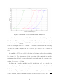
Figure 6.3: Minimum detectable with default configuration
was used to determine the true available SNR and minimum detectable signal in the
Wind Profiler. The transmitted power is 44.8dBm. The total attenuation calculated
in calibration path is LCAL P ath ' 135dB. Therefore, the level of the calibration signal
in the receiver input is PCAL ' −90dBm. If not stated otherwise in the following
outcomes the default configuration (B = 25M Hz, Tp = 10ms, P RF = 100Hz) is
used.
An amplifier of 17dB was added in the front end to improve the radar sensitivity
(see Figure 6.5). The disadvantage of this increasing of the sensitivity is that the
maximum leakage allowed decreases. As stated previously, using the current configuration: Pleak M AX ' −50 dBm.
At this point if another amplifier is added in the front end, the noise floor is
increased by its gain. Thereby the noise figure in a receiver is primarily determined
by the first components in the receiver chain.
As shown in Figure 6.5 the noise floor when the 17dB amplification is added is
around -140dBm, thus the minimum detectable Cn2 in that case is between 10−12.5 m
34
−2
3
FPGA
BOX
CAL IN
RF2 IN RF1 IN RF0 IN
RF
BOX
RF OUT
POWER
SUPPLY
BOX
BIG AMP
BOX
CAL OUT
Ptx=44,8dBm
Attenuators
-20dB
High Power
20dB Coupler
High
Power
Load
Figure 6.4: Lab Setup
Figure 6.5: Noise floor with and without 17dB amplifier
and 10−10.5 m
−2
3
. It is seen that the radar can only detect very high values of the
structure constant which correspond to high intensity refractive index fluctuations
due to very strong turbulence. There are some options to improve the sensitivity in
the signal processing. The non-coherent averaging will improve the SNR and smaller
structure constant values will be able to be detected, reducing the temporal resolution
of the Wind Profiler. It is possible to have an improvement of 15dB (see Equation
2.11) with averaging of 1000 profiles, i.e. 10sec. The result is plotted in the next
figure (Figure 6.6).
35
Figure 6.6: Noise floor with averaging of 1000 profiles
In the same way, it is possible to improve 6dB more by adding 2 consecutive
chirps. This will reduce the effective P RF and therefore the maximum unambiguous
velocity (see Equation 2.7).
Figure 6.7: Noise floor adding 2 profiles
If the noise floor is below -160dBm it is possible to measure values of the structure
constant Cn2 up to 10−14 m
−2
3
depending on the bandwidth and the height. This is
depicted in Figure 6.8.
36
Figure 6.8: Minimum detectable Cn2 when received power is -160dBm
By varying the sweep time (Tp ) and the bandwidth (B), the radar can be operated
in a mode suitable for particular atmospheric conditions. For example, to improve
range resolution the chirp bandwidth B should be increased. Keeping all other parameters the same, this will reduce the Rmax . The maximum unambiguous Doppler
velocity (vr, max ) in this case will remain the same. If higher unambiguous velocities
are desired, Tp should be decreased keeping B the same. This will not affect the range
resolution but it will again decrease the maximum range. One of the advantages of
FMCW radars is that they allow for change in range resolution without change in
the peak transmit power for a given sensitivity.
A trade-off exists between the parameters of the windprofiler, mainly ∆R, Rmax
and vr, max . The minimum Range (RM IN ) must also be included due to the cut
frequency of the audio module at 2.17kHz. In the following table (Table 6.1) these
parameters are calculated for different configurations (values of TP , B and fSample )
and in Figure 6.9 some results are plotted.
37
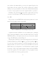
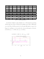
TP
B
fSample
∆R
Rmax
vr, max
fb,CAL
Rmin
fLeak
10 ms
25 MHz
60 kHz
6m
1800 m
8.2 m/s
5 kHz
150 m
210 Hz
10 ms
12.5 MHz
60 kHz
12 m
3600 m
8.2 m/s
10 ms
5 MHz
60 kHz
30 m
9000 m
8.2 m/s
5 ms
25 MHz
60 kHz
6m
900 m
16.4 m/s
5 ms
25 MHz
120 kHz
6m
1800 m
16.4 m/s
5 ms
12.5 MHz
60 kHz
12 m
1800 m
16.4 m/s
20 ms
25 MHz
60 kHz
6m
3600 m
4.1 m/s
2.5 kHz
RCAL = 300m
1 kHz
10 kHz
10 kHz
5 kHz
2.5 kHz
300 m
fc,f ilter ' 2.5kHz
750 m
75 m
75 m
150 m
300 m
105 Hz
Rleak,lab = 12.6m
42 Hz
420 Hz
420 Hz
210 Hz
105 Hz
Table 6.1: FMCW parameters
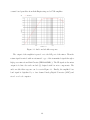
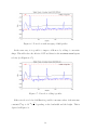
As it is shown on Figure 6.9.a the dominant fb,CAL = 5kHz frequency is seen along
with the triple travel chirp at 15 kHz and the quintuple travel chirp at 25kHz which
are about 15dB and 30dB respectively below the main 5kHz signal, as expected. In
Figure 6.9.b and Figure 6.9.c it is seen the effect of the cut-off frequencies of the audio
module filter (fc,low = 2.17kHz and fc,high = 29.3kHz).
(a) Default:B = 25M Hz, TP = 10ms, fSample = 60kHz
38
(b) B = 5M Hz, TP = 10ms, fSample = 60kHz
(c) B = 25M Hz, TP = 5ms, fSample = 120kHz
(d) B = 25M Hz, TP = 20ms, fSample = 60kHz
Figure 6.9: Noise floor with different configurations (Averaging of 1000 profiles)
39
The detectable minimum also is calculated with a simulated leakage of -40.5dBm.
To prevent saturating the audio module an attenuator of 10dB is added in its input.
The result is plotted in the next figure (Figure 6.10), using default configuration,
10sec of averaging and adding 2 chirps. It is seen with these conditions the noise
floor is around -150dBm, thus strong turbulence could be measured with values of
the structure constant Cn2 between 10=13 m
=2
3
and 10=12 m
=2
3
, and velocities up to 4.1
m/s.
Figure 6.10: Noise floor Pleak = −40.5dBm
40
CHAPTER 7
FIELD DEPLOYMENTS
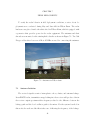
To verify the radar behavior in field deployment conditions, a series of test deployments were conducted during May and June 2010 in Tillson Farm. The radar
hardware was placed inside the white shed in Tillson Farm, which is quipped with
a generator that provides power for the radar equipment. The antennas and their
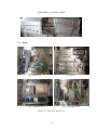
shrouds were mounted on the existing flatbed trailer as shown in Figure 7.1. Two 50ft
N-type cables whose losses are 2dB at 915MHz are used for connecting the antennas.
Figure 7.1: Antennas in Tillson farm
7.1
Antenna Isolation
The received signal is a mix of atmospheric echoes, clutter, and antenna leakage.
In an FMCW radar, transmitter energy leaking into the receiver will produce a line in
the receiver output spectrum with a frequency related to the difference between the
leakage path and the local oscillator path to the mixer. For the system described in
this work, the audio module filter takes care of filtering the frequency of the leakage.
41
However, it must be ensured that the leakage signal does not overload any part of the
receiver. It is also necessary to ensure that transmitter leakage does not exceed the
recommended maximum input level of the mixer, thus generating distortion products
that can contaminate the entire receiver spectrum. In this case the maximum leakage
is primarily determined by the audimodule. It must ensured that the amplifiers of
the audio module filter are just below saturation. With the default configuration
(P RF =100Hz, TP =10ms and B=25Hz) the maximum acceptable leakage is around
−50dBm. The transmit power is 44.8dBm, hence an isolation of 95dB would be
needed. If attenuators are added to the input of the audiomodule, the maximum
leakage can be increased but consequently the sensitivity of the wind profiler will
decrease.
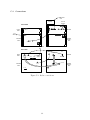
With the new shrouds, which are
based on a NOAA design [14], it is possible to improve the isolation about 15dB
[3]. The antenna isolation was measured
using the shrouds. There was 1m of separation between the edges of the antennas.
The result of the first test was a leakFigure 7.2: Received leakage
age of -35.6dBm in the front end (Fig-
ure 7.2), which translates into a isolation of about 80dB. Therefore, 15dB of attenuation had to be added before the audio module.
7.2
Deployment results
The atmospheric refractive index fluctuations represent a very weak target, being
orders of magnitude smaller than the ground clutter. Returns from trees, buildings
and other objects on the ground give rise to ground clutter and are dependent on
the site. This ground clutter enters the receiver through the antenna side lobes and
42
decreases with the third power of range. Preferably, the Wind Profiler should be
deployed in an environment as clutter free as possible.
As mentioned before, 15dB of attenuation were added, resulting in a theoretical
noise floor of about -140dBm and a radar sensitivity which is too low to measure the
typical values of turbulences (see Figure 7.3) .
Figure 7.3: Minimum detectable Cn2 when received power is -140dBm
Only turbulences with values of Cn2 higher than 10−12 m
−2
3
can be detected. In
order to test the radar sensitivity, rain can be used as a target with higher reflectivity.
The received power from a volume filled with rain drop scatterers and antennas with
Gaussian-shaped beams is given by Equation 7.1. This expression illustrates that the
received power is solely dependent upon radar system parameters, is proportional to
the radar reflectivity factor Z, and is inversely proportional to R2 [15].
Pt G2 θ2 4R π 3 |K|2 Z
Pr =
512(4 ln 2) R2 λ2
(7.1)
where |K|2 ' 0.93 at centimeter wavelengths. The calculation of Z from Equation
7.1 will have dimensions of
m6
m3
. Conversion to the more commonly used units of
43
mm6
m3
requires that the result be multiplied by a factor 1018 . Because the Z values of
interest can range over several orders of magnitude, a logarithmic scale is often used,
where dBZ = 10log Z
h
mm6
m3
i
.
Using Equation 6.1 and Equation 7.1, the relationship between Z and Cn2 is derived
as
Cn2 =
π 5 |K|2 Z
h
mm6
m3
i
1018
4·0.38·λ 3
11
(7.2)
In the optically clear boundary layer, Z values of the order -20dBZ to 10dBZ
(Cn2 ∈ [10−16 , 10−13 ]) are of interest. In rainy conditions, Z may range from about
20dBZ to as much as 60dBZ (Cn2 ∈ [10−12 , 10−8 ]).
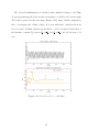
During the months of April and May series of field deployments were carried out
using different configurations under different weather conditions.
In the deployment of April 14th, 30 minutes of data were acquired. The sky was
clear, the temperature was around 60°F with a humidity of 28%. The following images
show the obtained results performing noncoherent averaging of 1sec and adding 2
consecutive chirps. Figure 7.4 using default configuration (TP =10ms and B=25Hz)
and Figure 7.5 using half bandwidth (TP =10ms and B=12.5Hz).
The radar image shown in Figure 7.6, corresponds to 14min collected data on May
5th. For the processing, averaging of 10sec and adding 2 consecutive chirps were used
to improve the sensitivity. The sky was clear with a humidity of about 40% and 70°F
of temperature.
44
Figure 7.4: Returned power and Doppler velocity during deployment on April 14th
(Default configuration)
Figure 7.5: Returned power and Doppler velocity during deployment on April 14th
(B=12.5MHz)
45
Figure 7.6: Returned power and Doppler velocity during deployment on May 5th
No discernible boundary layer features were observed in the reflectivity image.
The clutter is observed in the previous images below 500m. The power spectrum of
the averaging of 10,000 profiles is plotted in Figure 7.7. Knowing that the strength
of radar returns from ground clutter varies with the third power of range, it can be
concluded that it corresponds to ground clutter.
Figure 7.7: Data Power Spectrum (April 14th)
46
Figure 7.8: Returned power and Doppler velocity on April 22nd
The main problem of the field deployments was the instability of the audio
module filter.
This is an active filter
and becomes saturated due to its dependence on the leakage. In the deployment
of April 22nd, 50min data was acquired
using TP =10ms and fSample = 30kHz.
At the time of the data collection the
sky was partly cloudy and the temperature around 65°F. Unfortunately, when
Figure 7.9: Audio module output
it started drizzling, the filter saturated
47
(see Figure 7.8). The chirp at the output of the audio module is shown on Figure 7.9.
The same situation occurred using different configurations in several deployments
when it was trying to acquire data while it was raining. More attenuation was added
not to saturate the filter, resulting in a noise floor which was not good enough to
detect the atmospheric turbulences.
Figure 7.10: Antennas with additional shrouds
To improve the isolation between transmitting and receiving antennas for the
wind profiler, additional shrouds were added to the current antennas as shown in
Figure 7.10. Using these shrouds, the antenna isolation improved by 5dB. Thus only
10dB of attenuation were necessary at the audio module input. With this configuration data was acquired on May 12th. The sky was cloudy with a humidity of
80% and temperature of 44°F. The result is shown on Figure 7.11, using the default
configuration, adding 2 consecutive chirps and averaging of 10sec. A cloud can be
observed in the radar image between 600-800m of height.
48
Figure 7.11: Returned power and Doppler velocity during deployment on May 12th
49
CHAPTER 8
FUTURE WORK
FMCW radars offer many advantages such as low peak power, low probability of
interception, low interference with other systems, and high-range resolution. However,
their major drawback is the isolation required between the transmitter and receiver.
A scheme has been proposed to enable FMCW radar to operate with a single antenna
using frequency-modulated interrupted continuous-wave (FMICW) technology. The
wind profiler at later stage will utilize spaced antenna (SA) technique for achieving
three-dimensional wind field.
8.1
FMICW configuration
As commented before, high transmit/receive isolation requirements are difficult
to achieve. For this reason a FMICW design has been proposed. In this section
it is described the configuration of the UHF FMCW radar that has been adapted
for single antenna operation by alternately switching the single antenna between the
transmitter and the receiver. A simplified scheme of the system is given in Figure 8.1.
Isolator
SPLITTER
High Power
Switch
SSPA
G = 50 dB
CAL
Path
DDS
FPGA
TTL
SYNC
DAQ
Audio Module
Low Power
Switch
Figure 8.1: FMICW Block Diagram
51
This scheme works with two PIN diodes switches, a high power switch and a low
power switch. Considering isolation constraints and the performance of the wind
profiler, both have been chosen from available commercial PIN diode switches. The
high power switch from Micronetics, Inc. is a Single Pole Double Throw (SPDT)
for T/R. It is reflective, which means that power presented at any OFF port will
be reflected. For this reason an isolator is located in the system. It is designed for
reliable operation at power levels of 50W averages, thus it is good enough for the
requirement of the transmitted power (30W). It offers high isolation, fast switching
speed and low loss. Table 8.1 lists the basic specifications.
Frequency Range
Power, CW (Maximum)
Isolation (Minimum)
Insertion Loss (Maximum)
RF Switching Speed (Maximum)
Control Switching Freq. (Maximum)
0.1 to 1 GHz
50 Watts
50 dB
0.75 dB
200 ns
100 KHz
DC Power Requirements
Positive Supply
+5 +/-2% Vdc
Positive Supply Current (Max)
150 mA
Negative Supply Voltage
-70 +/-2% Vdc
Negative Supply Current (Max)
150 mA
Table 8.1: High Power Switch SPDT (Ref. ES0309-50)
The Low Power SPST Diode switch is from Mini-Circuits. It is absorptive, and it
provides high isolation and very high switching speed. Its specifications are given in
Table 8.2.
In both cases the necessary switching voltages are derived from TTL signals (without built-in drivers), these signals have to be generated by the FPGA. In order to
allow for the switching time and to achieve the required isolation, a dead time of the
order of nanoseconds must be provided between transmit and receive phases of the
switching. This ensures that the transmitter is turned fully off before the receiver
starts to turn on. The required power supplies for these switches will have to be
52
Frequency Range
DC to 2000 MHz
RF Power Input Max.
+33 dBm
Isolation (Minimum)
58 dB
Insertion Loss (Typical)
1.3 dB
Rise/Fall Time (10%-90%) (Max.)
5 ns
Switching Time (Typical)
50% of control to 90% RF (Turn-on)
7 ns
50% of control to 10% RF (Turn-off )
3 ns
Control Voltage
Low State
-0.2 to 0 V
High State (negative)
-5 to -8 V
Control Current
0.2mA Max. to -8V
0.5mA Max. at -9V to -12V Typ.
Table 8.2: Low Power Switch SPST (Ref. ZFSWHA-1-20+)
included in the radar hardware.
The switching induces a constraint on RM AX , given by Equation 2.15. As commented in Section 2.3 the rectangular wave which finally modulates an echo depends
on the target range. The limit on the maximum range can be increased by reducing
the duty cycle of the T/R waveform, at the expense of reduced signal to noise ratio.
However, this scheme has the additional advantage of introducing a desirable range
sensitivity characteristic. The system has its best performance when the choice of the
switching frequency is given by Equation 2.12. By this way, the power of the closest
ranges will be significantly reduced, but the farthest targets, more attenuated due to
propagation losses, have the highest sensitivity. In this case the achieved isolation is
good enough for the wind profiler. On Table 6.1 FMICW parameters are calculated
for different configurations.
Unlike FMCW it is not possible to choose any value for the sampling rate as it
is determined by Equation 2.14. An antialiasing filter is still necessary to prevent
aliasing when the received signal is sampled by the ADC but the filter must also
remove the higher order copies of the echo spectrum produced by the switching. That
53
TP
B
∆R
Rmax,F M ICW
fS (>fSample )
vr, max
fb,CAL
Rmin
fLeak
10 ms
25 MHz
6m
1500 m
50 kHz
8.2 m/s
5 kHz
10 ms
12.5 MHz
12 m
2121 m
35.36 kHz
8.2 m/s
10 ms
5 MHz
30 m
3354 m
22.36 kHz
8.2 m/s
RCAL = 300m
2.5 kHz
1 kHz
5 ms
25 MHz
6m
1061 m
70.71 kHz
16.4 m/s
5 ms
12.5 MHz
12 m
1500 m
50 kHz
16.4 m/s
20 ms
25 MHz
6m
2121 m
35.36 kHz
4.1 m/s
10 kHz
5 kHz
2.5 kHz
75 m
150 m
300 m
210 Hz
105 Hz
150 m
fc,f ilter ' 2.5kHz
300 m
750 m
210 Hz
Rleak,lab = 12.6m
105 Hz
42 Hz
420 Hz
Table 8.3: FMICW parameters
is not a big issue since the ADC provides the antialiasign filter, only it is necessary
to set the appropriate sample frequency fSample .
8.2
Spaced Antenna
Figure 8.2: 3-antenna SA-FMICW
As commented before the radar now operates with one receiving antenna, but the
final design will utilize spaced-antenna technique to measure horizontal winds, hence
providing information about 3D wind fields. This technique can obtain more rapid
wind estimates compared to Doppler beam swinging systems [16]. It is planned to
use three antennas: one transmit/receive antenna and two receive antennas arranged
in a triangle, as shown in Figure 8.2. Solid circles denote physical apertures, while
54
dashed lines denote virtual apertures. They would form an effective antenna whose
phase center is between the physical antennas.
55
CHAPTER 9
CONCLUSIONS
The work presented in this thesis is a description of the the FMCW Wind Profiler
as of Spring 2010. A new Data Acquisition Card was integrated to increase the dynamic range of the radar. New data collection programs were developed for it, solving
the synchronization issues. Signal processing programs have also been developed to
retrieve and display the reflectivity power and the Doppler velocity of the wind profiler. Since all the required operations to manage the radar, e.g. initialization of the
acquisition card and data processing, are quite complex, a graphical user interface has
been created to make the operator tasks easier. Moreover, to avoid waits to acquire
all the data to start the processing, real time programs were developed too, which
allow displaying the reflectivity power while data is being acquired.
A series of tests were carried out in the laboratory. The maximum sensitivity the
radar can reach was determined. For this purpose the noise floor was measured using
the calibration signal as a reference. A needed extra amplifier was added in the front
end. This way, the noise floor is primarily determined by the front end instead of
the audio module. As a consequence of adding this amplifier, the maximum leakage
acceptable was decreased, which translates into a high value of the necessary isolation.
Following this, the isolation was measured in the first field deployment using the
shrouds. To do the field measurements, attenuators had to be added before the
audio module, because this is the first component to become saturated. Thereby, the
sensitivity of the radar was reduced. The results of the field deployments have been
discussed. The audio module could be modified in the future since it was designed
for the old DAQ, and currently the antialiasing filter is already provided by the ADC.
To improve the isolation it could use larger antennas and therefore, greater gain. But
this would make the use of spaced antenna technique difficult.
57
The isolation requirements are difficult to achieve. To solve that, the use of
frequency-modulated interrupted continuous-wave is planned, as well as reducing the
number of antennas from four to three. The new scheme has been described and the
new parameters of the wind profiler have been calculated. Finally, the use of a spaced
antenna technique is also planned to add the ability to analyze horizontal winds.
58
BIBLIOGRAPHY
[1] Muschinski A., Turker I., Frasier S. and Pazmany A. An S-band FMCW boundary layer profiler: Description and initial results. Radio Science 38, 2003.
[2] David Garrido Lopez. An UHF Frequency-Modulated Continous Wave WindProfiler - Receiver and Audio Module Development. Master’s Thesis at UMASS
Amherst, 2009.
[3] David Garrido Lopez. An UHF Frequency-Modulated Continous Wave WindProfiler - Developement and Initial Results. Master’s Thesis at UMASS Amherst,
2009.
[4] David Atlas. Radar in Meteorology. American Meteorological Society, Boston,
1990.
[5] Ottersen H. Atmospheric structure and radar backscattering in clear air. Radio
Science 4, 12:1179–1193, 1969.
[6] J.A. McGregor, E.M. Poulter, M.J. Smith. Switching system for single antenna
operation of an S-band FMCW Radar. IEE Proceedings- Radar, Sonar and
Navigation, 141(4):241–248, 1994.
[7] Albert Genis. Implementation and test of an FMCW Wind Profiler Transceiver.
Master’s Thesis at UMASS Amherst, 2008.
[8] Iva Kostadinova. An UHF Frequency-Modulated Continous Wave WindProfiler
- Developement and Initial Results. Master’s Thesis at UMASS Amherst, 2009.
[9] General Standards Corporation. PC104P-24DSI6LN Specifications.
[10] General Standards Corporation. PC104P-24DSI6LN Reference Manual.
[11] General Standards Corporation. 24DSI Linux Device Driver User Manual. 2009.
[12] ITT Visual Information Solutions. Programming in IDL.
[13] Richard J. Doviak and Dusan S. Zrnic. Doppler Radar and Weather Observations. Dover Publications, Inc. Mineola New York, 1984.
59
[14] Paul E. Johnston, David A. Carter, James R. Jordan, Allen B. White. A New
Snow-Level Detection Radar. NOAA, 2009.
[15] Merrill Skolnik. Radar handbook. McGraw Hill, Boston, 1990.
[16] Muschinski A., S.J. Frasier. Supplement to ’Investigation of Turbulence and
Intermittency in the Convective Boundary Layer Using a 915MHz Volume Wind
Profiler’: Profiler Fabrication. 2006.
60
APPENDIX A - ACQUISITION SOURCE CODE
Savedata Windprof
A.1
The source code used to collect data can be found in savedata windprof folder
and it is detailed below.
A.1.1
main.c
C u r r e n t l y t h e program o n l y a c q u i r e s data from c h a n n e l 0 , t o a c q u i r e a l s o
c h a n n e l 1 and 2 , i t i s r e q u i r e d t o comment t h e f o l l o w i n g l i n e :
”251 i f ( ( l %4==0) | ( l ==0)) {//Now o n l y we want chan 0”
Don ’ t f o r g e t i n w i n d p r o f p r o c e s s . pro change t h e v a r i a b l e which i n d i c a t e s
t h e number o f c h a n n e l s i n raw f i l e ( number channels=1 −> 4 ) .
1
2
3
4
5
6
7
8
9
10
11
12
13
14
15
16
17
18
19
20
21
22
23
24
25
26
27
28
29
30
31
32
33
34
35
36
37
# include < ctype .h >
# include < stdio .h >
# include < stdlib .h >
# include < string .h >
# include < time .h >
# include " main . h "
# include " fmcw_conf . c "
# define BLOC K_SIZE_ MAX 2000 L
# define CHANS_ENABLED
4
# define THRESHOLD 60063000
// variables * * * * * * * * * * * * * * * * * * * * * * * * * * * * * * * * * * * * * * * * * * * * * * * * * * *
static
int
_continuous
= 0;
static
int
_ignore _errors = 0;
static
int
_index
= 0;
static
long _minute_limit = 0;
static
__s32 _buffer1 [1 L ];
static
__s32 _buffer_data [ BL OCK_SIZE _MAX ];
/* * * * * * * * * * * * * * * * * * * * * * * * * * * * * * * * * * * * * * * * * * * * * * * * * * * * * * * * * * * * * * * *
* Function :
_parse_args
* Purpose : Parse the command line arguments .
* Arguments :
*
argc The number of command line arguments given .
*
argv The list of command line arguments given .
* Returned :
>= 0 The number of errors encounterred .
* * * * * * * * * * * * * * * * * * * * * * * * * * * * * * * * * * * * * * * * * * * * * * * * * * * * * * * * * * * * * * * * */
static int _parse_args ( int argc , char ** argv )
{
char c ;
int
errs = 0;
int
i;
int
j;
int
k;
printf ( " USAGE : savedata <-c > <-C > <-m # > <-n # > < index >\ n " ) ;
printf ( "
-c
Continue testing until an error occurs .\ n " ) ;
printf ( "
-C
Continue testing even if errors occur .\ n " ) ;
61
38
39
40
41
42
43
44
45
46
47
48
49
50
51
52
53
54
55
56
57
58
59
60
61
62
63
64
65
66
67
68
69
70
71
72
73
74
75
76
77
78
79
80
81
82
83
84
85
86
87
88
89
90
91
92
93
94
95
96
97
98
99
100
101
102
103
104
105
printf ( "
-m #
Run for at most # minutes ( a decimal number ) .\ n " ) ;
printf ( "
index The index of the board to access .\ n " ) ;
printf ( " NOTE : Hit Ctrl - C to abort continuous testing .\ n " ) ;
for ( i = 1; i < argc ; i ++)
{
if ( strcmp ( argv [ i ] , " -c " ) == 0)
{
_continuous
= 1;
_ign ore_erro rs = 0;
continue ;
}
if ( strcmp ( argv [ i ] , " -C " ) == 0)
{
_continuous
= 1;
_ign ore_erro rs = 1;
continue ;
}
if (( argv [ i ][0] == ’ - ’) && ( argv [ i ][1] == ’m ’) && ( argv [ i ][2]) )
{
j = sscanf (& argv [ i ][2] , " % d % c " , &k , & c ) ;
if (( j == 1) && ( k > 0) )
{
_minute_limit = k ;
continue ;
}
errs = 1;
printf ( " ERROR : invalid argument : % s \ n " , argv [ i ]) ;
break ;
}
j = sscanf ( argv [ i ] , " % d % c " , &k , & c ) ;
if (( j == 1) && ( k >= 0) )
{
_index
= k;
continue ;
}
else
{
errs = 1;
printf ( " ERROR : invalid board selection : % s \ n " , argv [ i ]) ;
break ;
}
}
return ( errs ) ;
}
/* * * * * * * * * * * * * * * * * * * * * * * * * * * * * * * * * * * * * * * * * * * * * * * * * * * * * * * * * * * * * * * *
* Function :
_perfo rm_test s
* Purpose : Perform the appropriate testing .
* Arguments : fd The handle for the board to access .
* Returned :
>= 0 The number of errors encounterred .
* * * * * * * * * * * * * * * * * * * * * * * * * * * * * * * * * * * * * * * * * * * * * * * * * * * * * * * * * * * * * * * * */
static int _per form_tes ts ( int fd )
{
int
errs = 0;
const char * psz ;
struct tm * stm ;
time_t
tt ;
time (& tt ) ;
stm
= localtime (& tt ) ;
psz
= asctime ( stm ) ;
gsc_label ( " Performing Operation " ) ;
printf ( " % s " , psz ) ;
errs += gsc_id_driver ( fd , DSI_BASE_NAME ) ; // Identify the driver
errs += dsi_id_board ( fd , -1 , NULL ) ; // Identify the board
errs += save_data ( fd ) ;
62
106
107
108
109
110
111
112
113
114
115
116
117
118
119
120
121
122
123
124
125
126
127
128
129
130
131
132
133
134
135
136
137
138
139
140
141
142
143
144
145
146
147
148
149
150
151
152
153
154
155
156
157
158
159
160
161
162
163
164
165
166
167
168
169
170
171
172
return ( errs ) ;
}
/* * * * * * * * * * * * * * * * * * * * * * * * * * * * * * * * * * * * * * * * * * * * * * * * * * * * * * * * * * * * * * * *
*
Function :
findedge
* Purpose : find positive or negative edge
* Arguments : aux
( previous state sample ’0 ’ or ’1 ’)
*
c urrent_s ample
* Returned :
1 positive edge , 2 negative edge
*
0 no edge
* * * * * * * * * * * * * * * * * * * * * * * * * * * * * * * * * * * * * * * * * * * * * * * * * * * * * * * * * * * * * * * * */
int findedge ( int aux , long c urrent_ sample )
{
if ( aux ==0) // Currently low level , start looking for a positive edge
{
if ( current_sample > THRESHOLD )
{
return (1) ; // Positive edge found
}
}
else // ( aux ==1) continue looking for low level
{
if ( current_sample < THRESHOLD )
{ return (2) ; // Negative edge found
}
}
return (0) ;
}
/* * * * * * * * * * * * * * * * * * * * * * * * * * * * * * * * * * * * * * * * * * * * * * * * * * * * * * * * * * * * * * * *
* Function :
main
* Purpose : Control the overall flow of the application .
* Arguments : argc The number of command line arguments .
*
argv The list of command line arguments .
* Returned :
EXIT_SUCCESS
We tested a device .
*
EXIT_FAILURE
We didn ’t test a device .
* * * * * * * * * * * * * * * * * * * * * * * * * * * * * * * * * * * * * * * * * * * * * * * * * * * * * * * * * * * * * * * * */
int main ( int argc , char * argv [])
{
int
errs ;
int
fd = 0;
FILE * fd_file ;
time_t
exec = time ( NULL ) ;
long hours , mins , secs ;
time_t
starttime , now , t_limit , test ;
struct tm * today ;
__s32 chans = 32;
int
qty ;
int
ret = EXIT_FAILURE ;
char datebuf [128];
char filename [128];
int got ;
int start =0;
int cont_profiles =0;
int aux ;
int flag_edge =0;
int cont =0;
int cont_writing =0;
int l , i ;
gsc_l abel_in it (26) ;
int n u m b e r _ t o t a l _ p r o f i l e s ;
test = time ( NULL ) ;
printf ( " savedata - Capture and Save Data to Disk by Carol ( Version % s ) \ n " , VERSION
);
errs = _parse_args ( argc , argv ) ;
long sample_rate ;
long Block_Size ;
63
173
174
175
176
177
178
179
180
181
182
183
184
185
186
187
188
189
190
191
192
193
194
195
196
197
198
199
200
201
202
203
204
205
206
207
208
209
210
211
212
213
214
215
216
217
218
219
220
221
222
223
224
225
226
227
228
229
230
231
232
233
234
235
long TamBuffer ;
// reading header
struct fm c w _ c on f _ s t r u c t fmcw_conf ;
printf ( " fmcw : reading configuration file \ n " ) ; // Read FMCW configuration file
if ( r ead_fmc w_conf ( " / home / profiler / Desktop / w i n d p ro f i l e r 2 0 1 0 / fmcw_current . conf " , &
fmcw_conf ) ) {
fprintf ( stderr , " fmcw : configuration file error \ n " ) ;
}
n u m b e r _ t o t a l _ p r o f i l e s = fmcw_conf . n u m b e r _ o f _ p r o f i l e s ;
sample_rate = fmcw_conf . s a m p l e _ f r e q u e n c y *1000 L ;
Block_Size =( fmcw_conf . chirp_length * fmcw_conf . sample_frequency -5) ;
TamBuffer = Block_Size *4;
// printf (" TamBuffer % ld and sizeof ( _buffer_data ) =% ld \ n " , TamBuffer , sizeof (
_buffer_data ) ) ;
gsc_id_host () ; // Identify the host os and machine
t_limit = exec + ( _minute_limit * 60) ;
qty
= g s c _ c o u n t _ b o a r d s ( DSI_BASE_NAME ) ; // Count the number of installed SI04
errs = g s c _ s e l e c t _ 1 _ b o a r d ( qty , & _index ) ; // Select the board to utilize when more
than one is present
if (( qty <= 0) )
errs ++;
gsc_label ( " Accessing Board Index " ) ;
printf ( " % d \ n " , _index ) ;
fd = gsc_dev_open ( _index , DSI_BASE_NAME ) ; // Perform an open on the device with
the specified index .
if ( fd == -1) // finish testing and start acquiring data
if (! errs || ( _ignor e_errors == 0) )
{
fd = gsc_dev_open ( _index , DSI_BASE_NAME ) ;
d s i _ c o n f i g _ b o ar d ( fd , -1 , -1 , sample_rate ) ;
errs += _ c h a n n e l s _ p r o f i l e r ( fd , & chans ) ;
// Creating the file
printf ( " Creating the file where the data will be stored \ n " ) ;
time (& starttime ) ; today = localtime (& starttime ) ;
strftime ( datebuf , 128 , " % m % d % H % M " , today ) ;
sprintf ( filename , " / home / profiler / Desktop / w i n d p r o f i l e r 2 0 1 0 / data /% s . dat " ,
datebuf ) ;
fd_file = fopen ( filename , " w + b " ) ;
if ( fd_file == -1)
errs = 1;
else printf ( " file created : % s \ n " , filename ) ;
f w r i t e _ f m c w _ c on f ( fmcw_conf , fd_file ) ; // write header to file
printf ( " Starting acquisition ! ! ! ! ! ! ! ! ! ! ! ! ! ! ! ! \ n Wait ...\ n " ) ;
for (;;)
{
now = time ( NULL ) ;
errs = 0;
if ( start ==0) // to figure out which is the 1 st state ( aux = 0 or 1?)
{
got = dsi_dsl_read ( fd , _buffer1 , sizeof ( _buffer1 ) ) ; // Read first sample
if ( got < 0)
errs = 1;
else
errs = 0;
if ( _buffer1 [0]==8388608) start =0; // no count 1 st samples 0 ...
else {
start =1;
/* Notes :
_buffer1 [0] corresponds to chan 0 -- DATA
_buffer1 [3] corresponds to chan 3 -- SYNC
*/
if ( _buffer1 [3] < THRESHOLD ) aux =0;
else if ( _buffer1 [3] > THRESHOLD )
aux =1;
}
} else { // if ( start ==0)
got = dsi_dsl_read ( fd , _buffer1 , sizeof ( _buffer1 ) ) ; // Read next sample
if ( got < 0)
errs = 1;
else
errs = 0;
flag_edge = findedge ( aux , _buffer1 [3]) ;
if ( flag_edge ==1) {
aux =1;
64
236
237
238
239
240
241
242
243
244
245
246
247
248
249
250
251
252
253
254
255
256
257
258
259
260
261
262
263
264
265
266
267
268
269
270
271
272
273
274
275
276
277
278
cont_writing =1;
cont =0;}
if ( flag_edge ==2) { aux =0;
}
if ( cont_writing ==1) // Save Block_Size samples
{
// Read next Blocksize & Writing block
for ( l =0; l < TamBuffer ; l ++) _buffer_data [ l ]=0;
got = dsi_dsl_read ( fd , _buffer_data , TamBuffer ) ;
if ( got < 0) errs = 1;
else if ( got != TamBuffer )
{ printf ( " There aren ’t a full block \ n " ) ;
}
else {
for ( l =0; l < TamBuffer ; l ++)
{ if (( l %4==0) |( l ==0) ) { // Now only we want chan 0
// printf (" got = %d , sample read buffer1 =%08 lX \ n " , got , _buffer_data [ l ]) ;
i = fwrite ( & _buffer_data [ l ] ,1 , 4 , fd_file ) ;
cont ++;
}
}
// printf (" Block read :% d samples \ n " , cont ) ;
cont_writing =0;
cont_profiles ++;
}
} // if ( cont_writing ==1)
} // if ( start ==0)
if (( _minute_limit ) && ( now >= t_limit ) ) break ;
if (( _ignor e_errors == 0) && ( errs ) )
break ;
if ( cont_profiles == n u m b e r _ t o t a l _ p r o f i l e s ) break ;
} // for (;;)
if ( cont_profiles < n u m b e r _ t o t a l _ p r o f i l e s ) n u m b e r _ t o t a l _ p r o f i l e s = cont_profiles ;
printf ( " Total number of profiles :% d \ n " , n u m b e r _ t o t a l _ p r o f i l e s ) ;
if ( errs ==0) printf ( " the end OK :) \ n " ) ;
else printf ( " the end with some error :( \ n " ) ;
gsc_dev_close ( _index , fd ) ;
fclose ( fd_file ) ;
}
return ( ret ) ;
}
A.1.2
1
2
3
4
5
6
7
8
9
10
11
12
13
14
15
16
savedata.c
# include < ctype .h >
# include < stdio .h >
# include < stdlib .h >
# include < string .h >
# include < time .h >
# include " main . h "
// # defines * * * * * * * * * * * * * * * * * * * * * * * * * * * * * * * * * * * * * * * * * * * * * * * * * * * * * * * * * * * * * * * * * * *
# define _1M
(1024 L * 1024 L )
# define TRIGGER_RATE
100
# define SAMPLE_RATE
60000 L
# define CHANS_ENABLED
4
// variables
***************************************************************
static
__u32 _buffer [( SAMPLE_RATE * CHANS_ENABLED ) / TRIGGER_RATE ];
/* * * * * * * * * * * * * * * * * * * * * * * * * * * * * * * * * * * * * * * * * * * * * * * * * * * * * * * * * * * * * * * * * * * * * * * * * * * * * *
*
* Function :
_channels
65
17
18
19
20
21
22
23
24
25
26
27
28
29
30
31
32
33
34
35
36
37
38
39
40
41
42
43
44
45
46
47
48
49
50
51
52
53
54
55
56
57
58
59
60
61
62
63
64
65
66
67
68
69
70
71
72
73
74
75
76
77
78
79
80
81
82
83
84
* Purpose :
*
Check to see how many channels the board has .
* Arguments :
*
fd
The handle for the board to access .
*
chan Report the number of channels here .
* Returned :
*
>= 0 The number of errors encounterred .
* * * * * * * * * * * * * * * * * * * * * * * * * * * * * * * * * * * * * * * * * * * * * * * * * * * * * * * * * * * * * * * * * * * * * * * * * * * * * */
static int _channels ( int fd , __s32 * chans )
{
int
errs ;
gsc_label ( " Input Channels " ) ;
errs = dsi_query ( fd , DSI_QUERY_CHANNEL_QTY , chans ) ;
if ( errs == 0)
printf ( " % ld Channels \ n " , ( long ) chans [0]) ;
return ( errs ) ;
}
/* * * * * * * * * * * * * * * * * * * * * * * * * * * * * * * * * * * * * * * * * * * * * * * * * * * * * * * * * * * * * * * * * * * * * * * * * * * * * *
* Function :
_read_data
* Purpose :
*
Read data into the buffer .
* Arguments :
*
fd
The handle for the board to access .
* Returned :
*
>= 0 The number of errors encounterred .
* * * * * * * * * * * * * * * * * * * * * * * * * * * * * * * * * * * * * * * * * * * * * * * * * * * * * * * * * * * * * * * * * * * * * * * * * * * * * */
static int _read_data ( int fd )
{
int
errs ;
long get
= sizeof ( _buffer ) / CHANS_ENABLED ;
int
got ;
gsc_label ( " Reading " ) ;
got
= dsi_dsl_read ( fd , _buffer , get ) ;
if ( got < 0)
{
errs = 1;
}
else if ( got != get )
{
errs = 1;
printf ( " FAIL <--- ( got % ld samples , requested % ld ) \ n " ,
( long ) got ,
( long ) get ) ;
}
else
{
errs = 0;
printf ( " PASS (% ld samples ) \ n " ,
( long ) get ) ;
}
return ( errs ) ;
}
/* * * * * * * * * * * * * * * * * * * * * * * * * * * * * * * * * * * * * * * * * * * * * * * * * * * * * * * * * * * * * * * * * * * * * * * * * * * * * *
* Function :
_save_data
* Purpose :
*
Save the read data to a text file .
* Arguments :
*
fd
The handle for the board to access .
*
chan The number of channels .
*
errs have there been any errors so far ?
* Returned :
*
>= 0 The number of errors encounterred .
* * * * * * * * * * * * * * * * * * * * * * * * * * * * * * * * * * * * * * * * * * * * * * * * * * * * * * * * * * * * * * * * * * * * * * * * * * * * * */
66
85
86
87
88
89
90
91
92
93
94
95
96
97
98
99
100
101
102
103
104
105
106
107
108
109
110
111
112
113
114
115
116
117
118
119
120
121
122
123
124
125
126
127
128
129
130
131
132
133
134
135
136
137
138
139
140
141
142
143
144
145
146
147
148
149
150
151
152
static int _save_data ( int fd , int chan , int errs )
{
FILE *
file ;
int
i;
long
l;
const char * name = " data . txt " ;
long
samples = sizeof ( _buffer ) / CHANS_ENABLED ;
gsc_label ( " Saving " ) ;
for (;;)
{
if ( errs )
{
printf ( " SKIPPED ( errors ) \ n " ) ;
errs = 0;
break ;
}
file = fopen ( name , " w + b " ) ;
if ( file == NULL )
{
printf ( " FAIL <--- ( unable to create % s ) \ n " , name ) ;
errs = 1;
break ;
}
for ( l = 0; l < samples ; l ++)
{
i = fprintf ( file , " %08 lX " , ( long ) _buffer [ l ]) ;
if ( i != 10)
{
printf ( " FAIL <--- ( fprintf () failure to % s ) \ n " , name ) ;
errs = 1;
break ;
}
if (( l % chan ) == ( chan - 1) )
{ i = fprintf ( file , " \ r \ n " ) ;
if ( i != 2)
{
printf ( " FAIL <--- ( fprintf () failure to % s ) \ n " , name ) ;;
errs = 1;
break ;
}
}
}
fclose ( file ) ;
if ( errs == 0)
printf ( " PASS (% s ) \ n " , name ) ;
break ;
}
return ( errs ) ;
}
/* * * * * * * * * * * * * * * * * * * * * * * * * * * * * * * * * * * * * * * * * * * * * * * * * * * * * * * * * * * * * * * * * * * * * * * * * * * * * *
* Function :
save_data
* Purpose :
*
Configure the board , then capture data to a file .
* Arguments :
*
fd
The handle for the board to access .
* Returned :
*
>= 0 The number of errors encounterred .
* * * * * * * * * * * * * * * * * * * * * * * * * * * * * * * * * * * * * * * * * * * * * * * * * * * * * * * * * * * * * * * * * * * * * * * * * * * * * */
int save_data ( int fd )
{
__s32 chans = 32;
int
errs = 0;
67
153
154
155
156
157
158
159
160
161
162
163
164
165
166
167
168
169
170
171
172
173
174
175
176
177
178
179
180
181
182
183
184
185
186
187
188
189
190
191
192
193
194
195
196
197
198
199
200
201
202
203
204
205
206
207
208
209
210
211
212
213
214
215
216
gsc_label ( " Capture & Save " ) ;
printf ( " \ n " ) ;
g s c _ l a b e l _ l e v e l _ i n c () ;
errs
errs
errs
errs
errs
errs
+=
+=
+=
+=
+=
+=
d s i _ c o n f i g _ b o a r d _ p r o f i l e r ( fd , -1 , -1 , SAMPLE_RATE ) ;
_channels ( fd , & chans ) ;
_read_data ( fd ) ;
d s i _ a i n _ b u f _ o v e r f l o w ( fd , -1 , DSI_AIN_BUF_OVERFLOW_TEST , NULL ) ;
d s i _ a i n _ b u f _ u n d e r f l o w ( fd , -1 , DSI_AIN_BUF_UNDERFLOW_TEST , NULL ) ;
_save_data ( fd , chans , errs ) ;
g s c _ l a b e l _ l e v e l _ d e c () ;
return ( errs ) ;
}
/* * * * * * * * * * * * * * * * * * * * * * * * * * * * * * * * * * * * * * * * * * * * * * * * * * * * * * * * * * * * * * * * * * * * * * * * * * * * * *
* Function :
dsi_config_board_profiler
* Purpose :
* Configure the given board using common FMCW defaults .
* Arguments :
*
fd
The handle to use to access the driver .
*
index The index of the board to access . Ignore if < 0.
*
fref This is the PLL Fref value , or -1 to use the default .
*
fsamp This is the desired Fsamp rate , of -1 to use the default .
* Returned :
*
>= 0 The number of errors encountered here .
* * * * * * * * * * * * * * * * * * * * * * * * * * * * * * * * * * * * * * * * * * * * * * * * * * * * * * * * * * * * * * * * * * * * * * * * * * * * * */
int
{
d s i _ c o n f i g _ b o a r d _ p r o f i l e r ( int fd , int index , __s32 fref , __s32 fsamp )
int
errs = 0;
__s32 ndiv ;
__s32 nrate ;
// Legacy
__s32 nref ; // PLL
__s32 nvco ; // PLL
errs += dsi_ rx_io_mo de
( fd , index , GSC_IO_MODE_DMA , NULL ) ;
errs += d s i _ r x _ i o _ o v e r f l o w
( fd , index , DSI_IO_OVERFLOW_CHECK , NULL ) ;
errs += d s i _ r x _ i o _ t i m e o u t
( fd , index , 30 , NULL ) ;
errs += d s i _ r x _ i o _ u n d e r f l o w
( fd , index , DSI_IO_UNDERFLOW_CHECK , NULL ) ;
errs += dsi_ initiali ze
( fd , index ) ;
errs += dsi_ain_mode
( fd , index , DSI_AIN_MODE_DIFF , NULL ) ;
errs += dsi_ain_range
( fd , index , DSI_AIN_RANGE_10V , NULL ) ;
errs += d s i _ a i n _ b u f _ i n p u t
( fd , index , DSI_AIN_BUF_INPUT_ENABLE , NULL ) ;
errs += d s i _ a i n _ b u f _ t h r e s h o l d
( fd , index , 128 L * 1024 , NULL ) ;
errs += d s i _ s w _ s y nc _ m o d e
( fd , index , DSI_SW_SYNC_MODE_CLR_BUF , NULL ) ;
errs += d s i _ c h a n n e l _ o r d e r
( fd , index , DSI_CHANNEL_ORDER_SYNC , NULL ) ;
errs += d s i_ da ta _ fo rm at
( fd , index , DSI_DATA_FORMAT_OFF_BIN , NULL ) ;
errs += dsi_ data_wid th
( fd , index , DSI_DATA_WIDTH_24 , NULL ) ;
errs += dsi_init_mode
( fd , index , DSI_INIT_MODE_INITIATOR , NULL ) ;
errs += d s i _ e x t e r n a l _ c l o c k _ s o u r c e ( fd , index , DSI_EXT_CLK_SRC_GRP_0 , NULL ) ;
errs += d s i _ f r e f _ co m p u t e
( fd , index , 0 , & fref ) ;
errs += d s i _ c h a n n e l _ g r o u p _ s o u r c e _ a l l ( fd , index , DSI_CH_GRP_SRC_GEN_A , 1) ; //
DSI_CH_GRP_SRC_GEN_A
errs += d s i _ f s a m p _ c o m p u t e
( fd , index , 0 , 0 , fref , & fsamp , & nvco , & nref , &
nrate , & ndiv ) ;
errs += d s i _ r a t e _ g e n _ x _ n v c o _ a l l
( fd , index , nvco , 1) ;
errs += d s i _ r a t e _ g e n _ x _ n r e f _ a l l
( fd , index , nref , 1) ;
errs += d s i _ r a t e _ g e n _ x _ n r a t e _ a l l
( fd , index , nrate , 1) ;
errs += d s i _ r a t e _ g e n _ x _ n d i v _ a l l
( fd , index , ndiv , 1) ;
errs += d s i _ f s a m p _ r e p o r t _ a l l
( fd , index , 1 , & fref ) ;
errs += dsi_xcvr_type
( fd , index , DSI_XCVR_TYPE_LVDS , NULL ) ;
errs += d s i _ a u t o _ c a l i b r a t e
( fd , index ) ;
errs += d s i _ a i n _ b u f _ c l e a r _ a t _ b o u n d a r y ( fd , index ) ;
errs += d s i _ a i n _ b u f _ o v e r f l o w
( fd , index , DSI_AIN_BUF_OVERFLOW_CLEAR , NULL ) ;
errs += d s i _ a i n _ b u f _ u n d e r f l o w
( fd , index , DSI_AIN_BUF_UNDERFLOW_CLEAR , NULL )
;
217
68
218
219
220
221
222
223
224
225
226
227
228
229
230
231
232
233
234
235
236
237
238
239
240
241
242
243
244
245
246
247
248
249
250
251
252
253
254
255
256
257
258
259
260
261
262
263
264
265
266
267
268
1
2
3
4
5
6
7
8
9
10
11
return ( errs ) ;
}
/* * * * * * * * * * * * * * * * * * * * * * * * * * * * * * * * * * * * * * * * * * * * * * * * * * * * * * * * * * * * * * * * * * * * * * * * * * * * * *
* Function :
_save_data_profiler
* Purpose :
*
Save the read data to a file , customized for te FMCW radar
* Arguments :
*
Buffer
The data to store
*
chan
The number of channels
*
fd_file
Th handle of the file where to store the data
* Returned :
*
>= 0 The number of errors encountered here .
* * * * * * * * * * * * * * * * * * * * * * * * * * * * * * * * * * * * * * * * * * * * * * * * * * * * * * * * * * * * * * * * * * * * * * * * * * * * * */
int _ s a v e _ d a t a _ p r o f i l e r ( FILE * fd_file , int chan , __s32 * buffer , long samples )
{
int i ;
long l ;
// long samples = sizeof ( buffer ) / CHANS_ENABLED ;
int errs = 0;
// gsc_label (" Saving data profiler \ n ") ;
for ( l =0; l < samples ; l ++)
{
i = fprintf ( fd_file , " %08 lX " , ( long ) buffer [ l ]) ;
// i = fwrite ( & buffer [ l ] ,1 , sizeof ( buffer [ l ]) , fd_file ) ;
// printf (" Sample % i % ld \ n " , i ,( long ) buffer [ l ]) ;
}
return ( errs ) ;
}
/* * * * * * * * * * * * * * * * * * * * * * * * * * * * * * * * * * * * * * * * * * * * * * * * * * * * * * * * * * * * * * * * * * * * * * * * * * * * * *
* Function :
_channels_profiler
* Purpose :
*
Check to see how many channels the board has .
* Arguments :
*
fd
The handle for the board to access .
*
chan Report the number of channels here .
* Returned :
*
>= 0 The number of errors encounterred .
* * * * * * * * * * * * * * * * * * * * * * * * * * * * * * * * * * * * * * * * * * * * * * * * * * * * * * * * * * * * * * * * * * * * * * * * * * * * * */
int _ c h a n n e l s _ p r o f i l e r ( int fd , __s32 * chans )
{
int
errs ;
gsc_label ( " Input Channels " ) ;
errs = dsi_query ( fd , DSI_QUERY_CHANNEL_QTY , chans ) ;
if ( errs == 0)
printf ( " % ld Channels \ n " , ( long ) chans [0]) ;
return ( errs ) ;
}
A.1.3
fmcw conf.c
# include
# include
# include
# include
# include
# include
# include
# include
# include
# include
# include
< stdlib .h >
< stdio .h >
< fcntl .h >
< unistd .h >
< string .h >
< sys / time .h >
< ctype .h >
< math .h >
< errno .h >
< signal .h >
< stdint .h >
69
12
13
14
15
16
17
18
19
20
21
22
23
24
25
26
27
28
29
30
31
32
33
34
35
36
37
38
39
40
41
42
# include " fmcw_conf . h "
int read_fm cw_conf ( const char cf_filename [] , struct f m c w _ c o n f _ s t r uc t * conf ) {
/* Open FMCW config file */
FILE * fp ;
int line_ctr ;
char current_line [256];
char * token_ptr ;
char data_dir [256];
char desc [80];
float params [ F M C W _ C O N F _ N U M _ P A R A M S ];
size_t param_check ;
if (( fp = fopen ( cf_filename , " r " ) ) == NULL ) {
fprintf ( stderr , " fmcw : unable to open % s \ n " , cf_filename ) ;
return F M C W _ C O N F _ R E A D _ E R R O R ;
}
for ( line_ctr = 0; line_ctr < 10 /* F M C W _ C O N F _ N U M _ P A R A M S */ ; line_ctr ++) {
/* Read configuation file line */
if ( fgets ( current_line , sizeof current_line , fp ) == NULL ) {
fprintf ( stderr , " fmcw : error reading from % s \ n " , cf_filename ) ;
fclose ( fp ) ;
return F M C W _ C O N F _ R E A D _ E R R O R ;
}
// printf ("% s :% d % s " , cf_filename , line_ctr , current_line ) ;
/* Search line for separator token ’: ’ */
if (( token_ptr = strchr ( current_line , ’: ’) ) == NULL ) {
fprintf ( stderr , " fmcw : separator token missing in % s :% d \ n " , cf_filename ,
line_ctr ) ;
fclose ( fp ) ;
return F M C W _ C O N F _ R E A D _ E R R O R ;
}
/* Read the parameters */
/* switch ( line_ctr ) {
case DATA_DIR :
param_check = sscanf ( token_ptr + sizeof ( char ) , "% s " , data_dir ) ;
printf (" fmcw : % s \ n " , data_dir ) ;
if ( param_check <= 0) {
fprintf ( stderr , " fmcw : parameter incorrectly set in % s :% d \ n " , cf_filename ,
line_ctr ) ;
fclose ( fp ) ;
return F M C W _ C O N F _ R E A D _ E R R O R ;
}
break ;
default : */
param_check = sscanf ( token_ptr +1 , " % f " , &( params [ line_ctr ]) ) ;
if ( param_check <= 0) {
fprintf ( stderr , " fmcw : parameter incorrectly set in % s :% d \ n " , cf_filename ,
line_ctr ) ;
fclose ( fp ) ;
return F M C W _ C O N F _ R E A D _ E R R O R ;
}
// printf (" Params read % d % f \ n " , line_ctr , params [ line_ctr ]) ;
// break ;
// }
43
44
45
46
47
48
49
50
51
52
53
54
55
56
57
58
59
60
61
62
63
64
65
66
67
68
69
70
71
72
73
74
75
76
}
fclose ( fp ) ;
/* Update configuration structure */
// strcpy ( conf - > data_dir , data_dir ) ;
// printf (" fmcw : data directory is % s \ n " , conf - > data_dir ) ;
// strcpy ( conf - > desc , desc ) ;
// printf (" Description : % s \ n " , conf - > data_dir ) ;
// conf - > num_ data_fil es = ( int ) ( params [ NUM_ DATA_FIL ES ]) ;
70
77
78
79
80
81
82
83
84
85
86
87
88
89
90
91
92
93
94
95
96
97
98
99
100
101
102
103
104
105
106
107
108
109
110
conf - > a in _f ra m e_ sc an s = ( int ) ( params [8]) ;
conf - > bandwidth = ( float ) ( params [1]) ;
printf ( " bandwidth =% f \ n " , conf - > bandwidth ) ;
conf - > chirp_length = ( float ) ( params [2]) ;
printf ( " Tp =% f \ n " , conf - > chirp_length ) ;
conf - > s a m p l e _ f r e q u e n c y = ( long int ) ( params [4]) ;
printf ( " sample freq =% ld \ n " , conf - > s a m p l e _ f r eq u e n c y ) ;
conf - > prf = ( int ) ( params [3]) ; // IGNORE
// printf (" PRF =% d \ n " , conf - > prf ) ;
conf - > s am pl es _ in _p ro f = ( int ) ( conf - > s a m p l e _ f r e q u en c y * conf - > chirp_length -5) ;
printf ( " samples in prof =% d \ n " , conf - > s a mp le s_ i n_ pr of ) ;
conf - > n u m b e r _ o f _ p r o f i l e s = ( int ) ( params [9]) ;
printf ( " Total Number of profiles =% d \ n " , conf - > n u m b e r _ o f _ p r o f i l e s ) ;
return FMCW_NO_ERROR ;
}
void f w r i t e _ f m c w _ c o n f ( struct f m c w _ c o nf _ s t r u c t fmcw_conf , FILE * file )
{
int header_ version =1;
fwrite (& header_version , sizeof ( int ) ,1 , file ) ;
int a in _f r am e_ sc a ns =10; // no matter
fwrite (&( a i n_ fr am e _s ca ns ) , sizeof ( int ) ,1 , file ) ;
int num_channels =3;
fwrite (&( num_channels ) , sizeof ( int ) ,1 , file ) ;
fwrite (&( fmcw_conf . bandwidth ) , sizeof ( float ) ,1 , file ) ;
fwrite (&( fmcw_conf . chirp_length ) , sizeof ( float ) ,1 , file ) ;
int c e n t e r _ f r e q u e n c y =114.5;
fwrite (&( c e n t e r _ f r e qu e n c y ) , sizeof ( int ) ,1 , file ) ;
fwrite (&( fmcw_conf . s a m p l e _ f r e q u e n cy ) , sizeof ( long int ) ,1 , file ) ;
fwrite (&( fmcw_conf . prf ) , sizeof ( int ) ,1 , file ) ;
fwrite (&( fmcw_conf . sa mp le s _i n_ pr o f ) , sizeof ( int ) ,1 , file ) ;
fwrite (&( fmcw_conf . n u m b e r _ o f _ p r o f i l e s ) , sizeof ( int ) ,1 , file ) ;
}
For historical reasons the format of the configuration file ’fmcw2010.conf’ is the
following:
Center Frequency (MHz) :114.5
Bandwidth (MHz) :25
Chirp Length(ms) :10
PRF (Hz) :100
Sample Frequency (KHz) :60
AO Sampling Frequency(kHz):40
Daq trigger param :40000
Scans per Profile :595
Scans Per Frame :29750
Total Profiles :5000
Number of Channels :3
But there there are some parameters which currently are not used: Daq trigger
param, Scans per frame and AO Sampling Frequency.
71
APPENDIX B - SIGNAL PROCESSING PROGRAMS
B.1
Windprofiler2010
This folder contains all the required files for the signal processing and for the
configuration of the FPGA. The files are briefly described below.
FPGA
windprofiler 0409.c/exe
reset.c/exe
fmcw2010.conf
fmcw current.conf
Processing & Display
Data/
windprof
windprof
windprof
windprof
windprof
process.pro
process2.pro
process realtime.pro
display.pro
display realtime.pro
windprof par2.pro
windprof par out.pro
load ct rb.pro
imgunder.pro
GUI
wgui.pro
wgui create.pro
wgui event.pro
run windprof.pro
reset windprof.pro
run daq.pro
create conf.pro
run process realtime.pro
windprof.conf
run display.pro
run display realtime.pro
Initializes the FPGA sending the parameters of the
.conf file through the serial port.
Resets the FPGA.
Contains the parameters to configure the wind profiler.
This folder contains all acquired data files from DAQ
(.dat) and all processed files (.fig) .
Processes acquired data from savedata windprof.
It is already explained in Chapter 5.
Processes acquired data in real time.
Display processed data from windprof process.pro.
Display processed data from windprof process realtime.pro in real time.
Defines the header written by acquisition program to be
read by windprof process.pro.
Defines the header written by windprof process.pro
to be read by windprof display.pro.
Functions required by windprof display.pro and
windprof display realtime.pro.
Starts FMCW Profiler GUI.
Defines the graphical interface and buttons of the GUI.
Defines the functions of the buttons.
Executes windprofiler 0409. It loads drivers for
DAQ and compiles savedata.
Executes reset.exe.
Executes savedata.
Creates the .conf file.
Starts windprof process realtime.pro with the input
parameters that are contained in windprof.conf.
Starts windprof display.pro.
Starts windprof display realtime.pro.
Table B.1: Windprofiler2010 files
73
B.1.1
1
2
3
4
5
6
7
8
9
10
11
12
13
14
15
16
17
18
19
20
21
22
23
24
25
26
27
28
29
30
31
32
33
34
35
36
37
38
39
40
41
42
43
44
45
46
47
48
49
50
51
52
53
54
55
56
57
58
59
60
61
62
63
64
;
;
;
;
;
;
;
;
;
;
;
;
;
;
;
Windprof process.pro
Carol Asturiano
MIRSL Lab @ UMass Amherst
Process acquired data from s a v e d a t a _ w i n d p r o f
Steps for FMCW Processing
1.
2.
3.
4.
read header , creating a structure
read profile and convert data to time domain using fft
( pc =1) remove constant phase that appears in calibration signal
( mr =1) remove temporal mean to get rid of stationary targets such as
buildings and trees ...
5. get power and average in time
6. get doppler using pulse - pair
To execute : windprof_process , ’02221042. dat ’ ,1 ,0 ,1 ,1 ,0
pro windprof_process , infile , time_avg , number_channel , mr , pc , delete_samples , png = png
lun = 1
lun_out = 2
close , / all
on_ioerror , at_eof
; our input file
; our output file
; jump to at_eof in case of ioerror
if ( not keyword_set ( del ete_samp les ) ) then delete_s amples =0
print , ’ mr = ’ ,mr , ’ pc = ’ ,pc , ’ delete_ samples = ’ , de lete_sam ples
lambda =3 e8 /915 e6
n um be r_ c ha nn el s =1 ; 4 number of channels on the file to process
ch = numbe r_chann el
infile = ’/ home / profiler / Desktop / w i n dp r o f i l e r 2 0 1 0 / data / ’ + infile
outfile = infile + ’. fig ’ ; that should be modified later for ordinary data
print , " created file " , outfile
; ;;;;;;;;;;;;;;;;;;;;;;;;;;;;;;;;;;;;;;;;;;;;;;;;;;;;;;;;;;
;
; Read header , creating a structure
;
print , " Reading header ... "
openr , lun , infile
openw , lun_out , outfile
heade r_versi on =1 L
readu , lun , h eader_ve rsion
if he ader_ver sion ne 1 then begin
print , " Wrong header version "
;
return
endif
print , " header version : " , he ader_ver sion
par = windprof_par2 ()
readu , lun , par
print , " a in _ fr am e_ s ca ns " , par . ai n_ f ra me _ sc an s
print , " a i n _ nu m _ c h a n n e l s " , par . a i n _ n u m _ c h a n n e l s
print , " bandwidth " , par . bandwidth
print , " chirp_length " , par . chirp_length
print , " c e n t e r_ f r e q u e n c y " , par . c e n t e r _ f r e q u e n c y
print , " sample_freq " , par . sample_freq
print , " prf " , par . prf
print , " scans_in_prof " , par . scans_in_prof
print , " total number profiles " , par . t o t a l _ n u m b e r _ p r o f i l e s
Block_size = par . scans_in_prof
prf = par . prf
74
65
66
67
68
69
70
71
72
73
74
75
76
77
78
79
80
81
82
83
84
85
86
87
88
89
90
91
92
93
94
95
96
97
98
99
100
101
102
103
104
105
106
107
108
109
110
111
112
113
114
115
116
117
118
119
120
121
122
123
124
125
126
127
128
129
130
info = fstat ( lun )
tam = info . size
tamheader =10
print , " File size : " , tam , " bytes "
numbe r_sampl es = tam /4 - tamheader ; Total samples , (4 bytes / sample )
n um be r_ p ro fi le s = numb er_sampl es / Block_size
print , " Calculated Number of profiles : " , nu mb er _ pr of il e s
n um be r_ p ro fi le s = par . t o t a l _ n u m b e r _ p r o f i l e s
; Create output header ...
par_out = w i n d p r o f _p a r _ o u t ()
par_out . bandwidth = par . bandwidth
par_out . chirp_length = par . chirp_length
par_out . c e n t e r _ fr e q u e n c y = par . c e n t e r _ f r e q u e n c y
par_out . s a m p l e _ fr e q u e n c y = par . sample_freq
par_out . prf = par . prf
par_out . scans_in_prof =( Block_size - d elete_s amples ) /2
par_out . time_avg = time_avg
prof_avg = time_avg * par . prf
par_out . n u m b e r _ o f _ p r o f i l e s = n u mb er _p r of il es / prof_avg
print , " par out : scans in prof " , par_out . scans_in_prof
; print ," par out " , par_out
; write it to the file
writeu , lun_out , par_out
; Data should be transformed to real Voltage values .
; 1 LSB equals the full escale (20 V ) divided by 1.1921 uV (24 bits )
LSB = 20 D /(2 D ^24 D )
; the first 8 bits are discarded , they indicated the channel only
mask =16777215 ; 4278190080 = FF000000 and 16777215=00 FFFFFF
; ;;;;;;;;;;;;;;;;;;;;;;;;;;;;;;;;;;;;;;;;;;;;;;;;;;;;;;;;;;;;;;;;;;;;;;;;
print , ’ Processing ...
Prof . avg = ’ , prof_avg
f_frame = dblarr ( Block_size - delete_samples , prof_avg )
raw_data = lonarr ( number_channels , Block_size )
ch_info = dblarr ( number_channels , Block_size )
wsamples = Block_size - dele te_sampl es
windw = rebin ( hanning ( wsamples ) , wsamples , prof_avg )
winfunc = dblarr ( Block_size - delete_samples , prof_avg )
winfunc [0: wsamples -1 ,*]= windw
for a vg _f r am e_ in d ex =0 L , nu mb e r_ pr of i le s / prof_avg -1
do begin ; big loop
for frame_index = 0L , prof_avg -1 do begin
readu , lun , raw_data
raw_data = mask AND raw_data ; the first 8 bits are discarded , they indicated the
channel only
ch_info = raw_data * LSB -10 ; transforming integer to real voltage value
f_frame [* , frame_index ] = ch_info ( ch , delete_s amples : Block_size -1)
; print , ’ f_frame_index ’, frame_index
endfor
f_frame = f_frame * winfunc
c_frame =( fft ( f_frame , dimension =1) ) [0:( Block_size - delete _samples ) /2 -1 ,*] ;
if ( pc eq 1) then begin
; Do phase correction
j = complex (0 ,1)
fb =2.0* par . bandwidth / par . chirp_length
fs = par . sample_freq
i_ref = round ( fb *( Block_size +5 - delet e_sample s ) / fs ) ; it corresponds to fb (=5 kHz )
when delete_s amples =0 and default config ;
fi_ref = atan ( conj ( c_frame [ i_ref ,*]) ,/ phase )
for i = 0 , ( Block_size - dele te_sampl es ) /2 -1 do begin
75
131
132
133
134
135
136
137
138
139
140
141
142
143
144
145
146
147
148
149
150
151
152
153
154
155
156
157
158
159
160
161
162
163
164
165
166
167
168
169
170
171
172
173
174
175
176
177
178
179
180
181
182
183
184
185
186
187
188
189
190
191
192
193
194
195
c_cor = exp ( j * fi_ref * i / i_ref )
c_frame [i ,*]= c_frame [i ,*]* c_cor
endfor
; print , ’ Block ’, Block_size , ’ fs ’,fs , ’ fb cal ’,fb , ’ i ref ’, i_ref
endif
c_mean = total ( c_frame ,2) / prof_avg
if ( mr eq 1) then begin
c_frame1 = c_frame - complex ( rebin ( real_part ( c_mean ) ,( Block_size - delete _sample s ) /2 ,
prof_avg ) , rebin ( imaginary ( c_mean ) ,( Block_size - delete_ samples ) /2 , prof_avg ) )
endif else begin
c_frame1 = c_frame
endelse
pow = total ( double ( c_frame * conj ( c_frame ) ) , 2) / prof_avg
pow1 =( total ( double ( c_frame1 * conj ( c_frame1 ) ) , 2) / prof_avg )
autocorr = total ( c_frame [* ,1: prof_avg -1]* $
conj ( c_frame [* ,0: prof_avg -2]) ,2) / ( prof_avg -1)
autoc orr_pha se = atan ( autocorr ,/ phase )
autocorr1 = total ( c_frame1 [* ,1: prof_avg -1]* $
conj ( c_frame1 [* ,0: prof_avg -2]) ,2) / ( prof_avg -1)
a ut oc orr _p ha se 1 = atan ( autocorr1 ,/ phase )
; Get velocity
; vel = auto corr_ph ase *( prf * lambda ) /(4*! pi )
vel1 = au to c or r_ ph a se 1 *( prf * lambda ) /(4*! pi )
; Get coherence
; rho = abs ( autocorr ) / pow
rho = abs ( autocorr1 )
rho1 = abs ( autocorr1 ) / pow1
; powdb =10* alog10 ( pow )
; powdb1 =10* alog10 ( pow1 )
; writeu , lun_out , pow , vel , rho , c_mean
writeu , lun_out , pow1 , vel1 , rho1 , c_mean
endfor
print , ’ Amplitude max ch_info ’ , max ( ch_info [ ch ,*]) , ’V
min ch_info ’ , min ( ch_info [ ch ,*])
, ’V ’
; print , ’ Pw max ’, max ( pow1 ) ,’W = ’ ,10* alog10 ( max ( pow1 ) ) +30 , ’ dBm
min ’, min ( pow1 ) ,’W ’
titlestr1 = ’ Chirp Amplitude ’ + strmid ( infile , 45 , 13)
titlestr2 = ’ Signal Power at receiver input ’ + strmid ( infile , 45 , 13)
window , XSize =600 , YSize =600
! p . multi =[0 ,1 ,2]
plot , ch_info ( ch , de lete_sam ples : Block_size -1) , title = titlestr1 , xtitle = ’ samples ’
if ( d elete_s amples ne 0) then begin
str = ’ Delete samples : ’+ strtrim ( delete_samples ,2)
xyouts ,450 ,8 , str
endif
; oplot , ch_info , COLOR = ’ FF00FF ’x
Grec = -114.5+10
plot , 10* alog10 ( pow1 ) +30+ Grec , title = titlestr2 , xtitle = ’ samples ’ , ytitle = ’ dBm ’ , YRANGE
=[ -200 , -80]
; Pmax =10* alog10 ( max ( pow1 ) ) +30+ Grec
str = ’ Profiles average : ’+ strtrim ( prof_avg ,2)
xyouts ,( Block_size - delete_ samples ) /2 -75 , -90 , str
76
196
197
198
199
200
201
202
203
204
205
206
207
208
209
210
211
212
; noise - floor
oplot , 10* alog10 ( rho ) +30+ Grec , COLOR = ’ 00 FF00 ’x
at_eof :
close , lun
close , lun_out
print , ’ File created . ’
; Save plot in a . png file if option is set
if keyword_set ( png ) then begin
a = tvrd (/ true )
write_png , infile + ’. png ’ ,a
endif
end
B.1.2
Windprof process2.pro
The only difference with the previous one, is that after the phase correction makes
the sum of two consecutive chirps.
1
2
3
4
5
; add 2 consecutive chirps
k =0 U
for j = 0 ,( prof_avg /2 -1) do begin
c_frame2 [* , j ]= c_frame [* , k ]+ c_frame [* , k +1]
k = k +2
B.1.3
1
2
3
4
5
6
7
8
9
10
11
12
13
14
15
16
17
18
19
20
21
22
23
24
25
26
27
28
Windprof display.pro
; Carol Asturiano
; MIRSL Lab @ UMass Amherst
;
; Display the processed data file
;
; windprof_display , ’02011520. dat . fig ’, pixmap = pixmap , png =1
pro windprof_display , file , pixmap = pixmap , png = png
device , decomposed =0
; Physical constants
c = 299792458.0 ; m / s
par_out = w i n d p r o f _p a r _ o u t ()
lun_out = 2
close , lun_out
file = ’/ home / profiler / Desktop / w i n d p r o f i l e r 2 0 1 0 / data / ’ + file
openr , lun_out , file
readu , lun_out , par_out
print , par_out
range_bins = par_out . scans_in_prof
print , " range bins " , par_out . scans_in_prof
;
; calculate display range resolution
;
deltaR = c /(2 e6 * par_out . bandwidth )
print , " deltaR " , deltaR
77
29
30
31
32
33
34
35
36
37
38
39
40
41
42
43
44
45
46
47
48
49
50
51
52
53
54
55
56
57
58
59
60
61
62
63
64
65
66
67
68
69
70
71
72
73
74
75
76
77
78
79
80
81
82
83
84
85
86
87
88
89
90
91
92
93
94
; r = deltaR * findgen ( range_bins ) * par_out . prf * par_out . chirp_length
; To accound for the delay that we put in the LO of the mixer ( reference chirp ) we
need to add 15 m to each range bin
r = deltaR * findgen ( range_bins ) * par_out . prf * par_out . chirp_length *1 e -3
; r (0) = 1.0 ; Don ’t multiply the first range gate by zero
; Variables
profs = par_out . n u m b e r _ o f _ p r o f i l e s
print , " number of profs " , profs
;
; declare processed data records in . img file
;
pwr = dblarr ( range_bins ) ; Single profile
velocity = dblarr ( range_bins )
rho = dblarr ( range_bins )
avg = dcomplexarr ( range_bins )
;
; declare
;
rti =
rtv =
rtrho
rtc =
;
;
;
2 D ( range - time image ) for power , vel , rho , etc .
dblarr ( profs , range_bins )
dblarr ( profs , range_bins )
= dblarr ( profs , range_bins )
dblarr ( profs , range_bins )
jump to at_eof : if we hit end - of - file
on_ioerror , at_eof
for i = 0L , profs -1 do begin
readu , lun_out , pwr , velocity , rho , avg
rti [i ,*] = pwr
rtv (i ,*) = velocity
rtrho (i ,*) = rho
rtc (i ,*) = double ( avg * conj ( avg ) )
endfor
at_eof :
if ( i lt profs -1) then begin
profs = i -1
rti = rti (0: profs -1 ,*)
rtv = rtv (0: profs -1 ,*)
rtrho = rtrho (0: profs -1 ,*)
rtc = rtc (0: profs -1 ,*)
endif
close , lun_out
free_lun , lun_out
;
; create time vector ( time in minutes starting at zero )
;
time_avg = par_out . time_avg
t = findgen ( profs )
t = t * time_avg /60
;
; R ^2 range correction . Note : Here the filter freq response should also be take into
account later !!!
;
r2 = rebin ( transpose ( r ^2) /1 e6 , profs , range_bins )
rti = rti * r2
; rti = rti * rtrho ; rti * r2 * rtrho
; mask = rtrho
; mask (*) = 1
; idx = where ( rtrho lt 0.3)
; mask ( idx ) = 0
78
95
96
97
98
99
100
101
102
103
; rtv = rtv * mask
window , 0 , xsize =810 , ysize =600 ; , pixmap = pixmap
! p . multi =[0 ,1 ,2]
print , ’ Pw max ’ , max ( rti ) , ’W
min ’ , min ( rti ) , ’W ’
loadct , 5
titlestr = ’ UMass FMCW : ’ + strmid ( file , 45 , 16)
contour , rti , t , r , / nodata , / xs , / ys , title = titlestr , xtitle = ’ time ( min ) ’ ,
ytitle = ’ height ( m ) ’; Color =! P . Background , Background =! P . Color
imgunder , bytscl (10* alog10 ( rti ) +30 , min = -40 , max =0)
contour , rti , t , r , / nodata , / xs , / ys , / noerase , title = titlestr , xtitle = ’ time (
min ) ’ , ytitle = ’ height ( m ) ’; Color =! P . Background , Background =! P . Color
104
105
106
107
108
109
110
111
112
113
114
115
116
117
118
119
loadct_rb
contour , rtv , t , r , / nodata , / xs , / ys
imgunder , bytscl ( rtv ) ; , min = -1 , max =1)
contour , rtv , t , r , / nodata , / xs , / ys , / noerase
! p . multi =0
if keyword_set ( png ) then begin
a = tvrd (/ true )
write_png , file + ’. png ’ , a
endif
stop
end
B.1.4
1
2
3
4
5
6
7
8
9
10
11
12
13
14
15
16
17
18
19
20
21
22
23
24
25
26
27
28
29
30
31
32
33
34
35
;
;
;
;
;
;
;
;
;
;
;
;
;
;
Windprof process realtime.pro
Carol Asturiano
MIRSL Lab @ UMass Amherst
Process acquired data from s a v e d a t a _ w i n d p r o f
1.
2.
3.
4.
read header , creating a structure
read profile and convert data to time domain using fft
perform phase correction
remove temporal mean to get rid of stationary targets such as
buildings and trees ..
5. get power and average in time
6. get doppler using pulse - pair
windprof_process_realtime , ’02091045. dat ’ ,1 ,0
pro windprof_process_realtime , infile , time_avg , number_ channel
lun = 1
lun_out = 2
close , / all
on_ioerror , at_eof
; our input file
; our output file
; jump to at_eof in case of ioerror
lambda =3 e8 /915 e6
n um be r_ c ha nn el s =1 ; 4 number of channels on the file to process
ch = numbe r_chann el
infile = ’/ home / profiler / Desktop / w i nd p r o f i l e r 2 0 1 0 / data / ’ + infile
outfile = infile + ’. fig ’ ; that should be modified later for ordinary data
print , " created file " , outfile
; ;;;;;;;;;;;;;;;;;;;;;;;;;;;;;;;;;;;;;;;;;;;;;;;;;;;;;;;;;;
;
; Read header , creating a structure
;
79
36
37
38
39
40
41
42
43
44
45
46
47
48
49
50
51
52
53
54
55
56
57
58
59
60
61
62
63
64
65
66
67
68
69
70
71
72
73
74
75
76
77
78
79
80
81
82
83
84
85
86
87
88
89
90
91
92
93
94
95
96
97
98
99
100
101
102
103
print , " Reading header ... "
openr , lun , infile
openw , lun_out , outfile
heade r_versi on =1 L
;
;
; wait for header to be written to file
;
;
header_size =11
fs = fstat ( lun )
while ( fs . size le header_size ) do begin ; specify header lenght ! ! ! ! ! ! ! ! ! ! ! ! ! ! ! ! ! !
wait , 1
fs = fstat ( lun )
endwhile
readu , lun , header_ve rsion
print , ’ header read ’
if hea der_ver sion ne 1 then begin
print , " Wrong header version "
return
endif
print , " header version : " , he ader_ver sion
par = windprof_par2 ()
readu , lun , par
print , " a in _ fr am e_ s ca ns " , par . ai n_ f ra me _ sc an s
print , " a i n _ nu m _ c h a n n e l s " , par . a i n _ n u m _ c h a n n e l s
print , " bandwidth " , par . bandwidth
print , " chirp_length " , par . chirp_length
print , " c e n t e r _ f r e q u e n c y " , par . c e n t e r _ f r e q ue n c y
print , " sample_freq " , par . sample_freq
print , " prf " , par . prf
print , " scans_in_prof " , par . scans_in_prof
print , " total number profiles " , par . t o t a l _ n u m b e r _ p r o f i l e s
Block_size = par . scans_in_prof
prf = par . prf
info = fstat ( lun )
tam = info . size
tamheader =10
print , " File size : " , tam , " bytes "
numbe r_sampl es = tam /4 - tamheader ; Total samples , (4 bytes / sample )
n umbe r_ p ro fi l es = par . t o t a l _ n u m b e r _ p r o f i l e s
n u m b e r _ pr o f i l e s 2 = numbe r_sample s / Block_size
print , " Calculated Number of profiles : " , n u m b e r _ p r o f il e s 2
; stop
; Create output header ...
par_out = w i n d p r o f _p a r _ o u t ()
par_out . bandwidth = par . bandwidth
par_out . chirp_length = par . chirp_length
par_out . c e n t e r _ fr e q u e n c y = par . c e n t e r _ f r e q u e n c y
par_out . s a m p l e _ fr e q u e n c y = par . sample_freq
par_out . prf = par . prf
par_out . scans_in_prof =( Block_size ) /2
par_out . time_avg = time_avg
prof_avg = time_avg * par . prf
print , ’ prof avg ’ , prof_avg
par_out . n u m b e r _ o f _ p r o f i l e s = n u mb er _p r of il es / prof_avg
; print ," par out " , par_out
; write it to the file
80
104
105
106
107
108
109
110
111
112
113
114
115
116
117
118
119
120
121
122
123
124
125
126
127
128
129
130
131
132
133
134
135
136
137
138
139
140
141
142
143
144
145
146
147
148
149
150
151
152
153
154
155
156
157
158
159
160
161
162
163
164
165
166
writeu , lun_out , par_out
; Data should be transformed to real Voltage values .
; 1 LSB equals the full escale (20 V ) divided by 1.1921 uV (24 bits )
LSB = 20 D /(2 D ^24 D )
; the first 8 bits are discarded , they indicated the channel only
mask =16777215 ; 4278190080 = FF000000 and 16777215=00 FFFFFF
; ;;;;;;;;;;;;;;;;;;;;;;;;;;;;;;;;;;;;;;;;;;;;;;;;;;;;;;;;;;;;;;;;;;;;;;;;
print , ’ Processing ...
Prof . avg = ’ , prof_avg
f_frame = dblarr ( Block_size , prof_avg )
raw_data = lonarr ( number_channels , Block_size )
ch_info = dblarr ( number_channels , Block_size )
wsamples = Block_size
windw = rebin ( hanning ( wsamples ) , wsamples , prof_avg )
winfunc = dblarr ( Block_size , prof_avg )
winfunc [0: wsamples -1 ,*]= windw
;
;
read_ok =0 ; variable that helps to read on real time
size_profile =4* par . scans_in_prof
; * number_chans
print , ’ size_profile ’ , size_profile
;
;
for a vg _f r am e_ in d ex =0 L , nu mb e r_ pr of i le s / prof_avg -1 do begin ; big loop
for frame_index = 0L , prof_avg -1 do begin ; insert here the wait loop ( per profile
[ Beta ])
;
;
;
while ( read_ok eq 0) do begin ; we ’ ll wait till there ’s a new profile
available to read
info = fstat ( lun ) ; get the read file status
current = info . cur_ptr
fsize = info . size
pos_to_eof = fsize - current ; calculate the diference between eof and the
pointer
; print , ’ size : ’, fsize , ’ pointer : ’, current , ’ pos_to_eof : ’, pos_to_eof , ’
size_profile : ’, size_profile
if ( pos_to_eof ge size_profile ) then begin
read_ok =1
endif else begin
read_ok =0
wait , 0.1 ; we wait for the data to be ready
endelse
; if ( pos_to_eof eq 0) then begin ; if the file is finished go to end
; goto , at_eof
; endif
endwhile
;
;
;
readu , lun , raw_data
raw_data = mask AND raw_data ; the first 8 bits are discarded , they indicated the
channel only
ch_info = raw_data * LSB -10 ; transforming integer to real voltage value
f_frame [* , frame_index ] = ch_info ( ch ,*)
read_ok =0 ; to check if the next profile will be ready to read
endfor
f_frame = f_frame * winfunc
c_frame =( fft ( f_frame , dimension =1) ) [0: Block_size /2 -1 ,*] ;
; Do phase correction
j = complex (0 ,1)
81
167
168
169
170
171
172
173
174
175
176
177
178
179
180
181
182
183
184
185
186
187
188
189
190
191
192
193
194
195
196
197
198
199
200
201
202
203
204
205
206
207
208
209
fb =2.0* par . bandwidth / par . chirp_length
fs = par . sample_freq
i_ref = round ( fb *( Block_size +5) / fs ) ; it corresponds to fb (=5 kHz , Default conf .) ;
fi_ref = atan ( conj ( c_frame [ i_ref ,*]) ,/ phase )
for i = 0 , ( Block_size ) /2 -1 do begin
c_cor = exp ( j * fi_ref * i / i_ref )
c_frame [i ,*]= c_frame [i ,*]* c_cor
endfor
c_mean = total ( c_frame ,2) / prof_avg
c_frame1 = c_frame - complex ( rebin ( real_part ( c_mean ) , Block_size /2 , prof_avg ) , rebin (
imaginary ( c_mean ) , Block_size /2 , prof_avg ) )
pow = total ( double ( c_frame * conj ( c_frame ) ) , 2) / prof_avg
pow1 =( total ( double ( c_frame1 * conj ( c_frame1 ) ) , 2) / prof_avg )
autocorr = total ( c_frame [* ,1: prof_avg -1]* $
conj ( c_frame [* ,0: prof_avg -2]) ,2) / ( prof_avg -1)
autoc orr_pha se = atan ( autocorr ,/ phase )
autocorr1 = total ( c_frame1 [* ,1: prof_avg -1]* $
conj ( c_frame1 [* ,0: prof_avg -2]) ,2) / ( prof_avg -1)
a ut oc orr _p ha se 1 = atan ( autocorr1 ,/ phase )
; Get velocity
vel = au tocorr_p hase *( prf * lambda ) /(4*! pi )
vel1 = auto c or r_ ph a se 1 *( prf * lambda ) /(4*! pi )
; Get coherence
rho = abs ( autocorr ) / pow
rho1 = abs ( autocorr1 ) / pow1
; powdb =10* alog10 ( pow )
; powdb1 =10* alog10 ( pow1 )
; writeu , lun_out , pow , vel , rho , c_mean
writeu , lun_out , pow1 , vel1 , rho1 , c_mean
endfor
at_eof :
close , lun
close , lun_out
print , ’ File created . ’
end
B.1.5
1
2
3
4
5
6
7
8
9
10
11
12
13
14
15
16
17
18
Windprof display realtime.pro
; Carol Asturiano
; MIRSL Lab @ UMass Amherst
;
; Display the processed data file in real time
;
; windprof_display_realtime , ’02091310. dat . fig ’, pixmap = pixmap , png = png
pro windprof_display_realtime , file , pixmap = pixmap , png = png
if ( not keyword_set ( pixmap ) ) then pixmap =0
; Physical constants
c = 299792458.0
profile_size = 297*5*8
; m/s
; define the size of a pow1 , vel , rho , c_mean block
;
; create plotting window on the screen
;
82
19
20
21
22
23
24
25
26
27
28
29
30
31
32
33
34
35
36
37
38
39
40
41
42
43
44
45
46
47
48
49
50
51
52
53
54
55
56
57
58
59
60
61
62
63
64
65
66
67
68
69
70
71
72
73
74
75
76
77
78
79
80
81
82
83
wid =10
window , wid , title = ’ UMass FMCW : ( Right click to Stop or Left click to freeze ) ’ ,
xsize =800 , ysize =600 , pixmap = pixmap
;
; Create plotting window on memory ( pixmap ) , we ’ ll draw on this one
;
pix =11
window , pix , xsize =800 , ysize =600 , / pixmap
par_out = w i n d p r o f _p a r _ o u t ()
lun_out = 2
close , lun_out
file = ’/ home / profiler / Desktop / w i n d p r o f i l e r 2 0 1 0 / data / ’ + file
openr , lun_out , file
readu , lun_out , par_out
print , par_out
range_bins = par_out . scans_in_prof
print , " range bins " , par_out . scans_in_prof
;
; calculate display range resolution
;
deltaR = c /(2 e6 * par_out . bandwidth )
print , " deltaR " , deltaR
r = deltaR * findgen ( range_bins ) * par_out . prf * par_out . chirp_length *1 e -3
; Variables
;
profiles = par_out . n u m b e r _ o f _ p r o f i l e s
time_index = indgen ( par_out . n u m b e r _ o f _ p r o f i l e s )
profs = profiles
print , " number of profs " , profs
;
; declare processed data records in . img file
;
pwr = dblarr ( range_bins ) ; Single profile
velocity = dblarr ( range_bins )
rho = dblarr ( range_bins )
avg = dcomplexarr ( range_bins )
;
; declare
;
rti =
rtv =
rtrho
rtc =
;
;
;
2 D ( range - time image ) for power , velocity , rho , etc .
dblarr ( profs , range_bins )
dblarr ( profs , range_bins )
= dblarr ( profs , range_bins )
dblarr ( profs , range_bins )
jump to at_eof : if we hit end - of - file
on_ioerror , at_eof
read_ok =0 ; create the var read_ok to make sure in every loop that there ’s data
available
prof =0 ; count the number of read profiles so far
change =0 ; variable that says if we ’ ve read new data , so we ’ ve to refresh the
window
83
84
85
86
87
88
89
90
91
92
93
94
95
96
97
98
99
100
101
102
103
104
105
106
107
108
109
110
111
112
113
114
115
116
117
118
119
120
121
122
123
124
125
126
127
128
129
130
131
132
133
134
135
136
137
138
139
140
141
142
143
144
145
146
147
148
for i = 0L , profiles -1 do begin ; insert here the wait loop
read_profiles :
; print , ’ read profiles , readok ’, read_ok , ’ change ’, change , ’ i ’, i , ’ prof ’,
profiles -1
wset , pix ; current window equal pixmap !!!
;
;
while ( read_ok eq 0) do begin ; we ’ ll wait till there ’s a new profile
available to read
info = fstat ( lun_out ) ; get the read file status
current = info . cur_ptr
fsize = info . size
pos_to_eof = fsize - current
; print , ’ pointer : ’, current , ’ pos_to_eof : ’, pos_to_eof
if ( pos_to_eof gt profile_size ) then begin
read_ok =1 ; we have enough data to read
change =1 ; we ’ re goin ’ to read more data , so we ’ ll need to refresh the
window
endif else begin
read_ok =0
wait , 0.2 ; we wait for the data to be ready
if ( change eq 1) then begin
goto , display ; we display data while the data is not ready
endif
endelse
wset , wid
cursor , ix , iy , / nowait
if (! mouse . button eq 4) then goto , at_eof2 $ ; right click , exit
else if (! mouse . button eq 1) then $
cursor , ix , iy , / up ; left button , freeze
wset , pix
endwhile
;
;
;
; info = fstat ( lun_out )
; print , ’ curent pointer before read :
’, info . cur_ptr
readu , lun_out , pwr , velocity , rho , avg
rti [i ,*] =
rtv (i ,*) =
rtrho (i ,*)
rtc (i ,*) =
pwr
velocity
= rho
double ( avg * conj ( avg ) )
; info = fstat ( lun_out )
; print , ’ curent pointer after read :
’, info . cur_ptr
prof = prof +1 ; we ’ ve read one more profile
; print , ’ prof # ’ , prof
read_ok =0
endfor
; stop
at_eof :
if ( i lt
profs
rti =
rtv =
rtrho
rtc =
endif
profs -1) then begin ; if ioerror
= i -1
rti (0: profs -1 ,*)
rtv (0: profs -1 ,*)
= rtrho (0: profs -1 ,*)
rtc (0: profs -1 ,*)
84
149
150
151
152
153
154
155
156
157
158
159
160
161
162
163
164
165
166
167
168
169
170
171
172
173
174
175
176
177
178
179
180
181
182
183
184
185
186
187
188
189
190
191
192
193
194
195
196
197
198
199
200
201
202
203
204
205
206
207
208
209
210
211
212
213
close , lun_out
free_lun , lun_out
display : ; if there ’s no data available we ’ ll display the data we have in the
meantime
; print , ’ display .. ’
;
; create time vector ( time in minutes starting at zero )
;
time_avg = par_out . time_avg
t = findgen ( profs )
t = t * time_avg /60
;
; R ^2 range correction
;
r2 = rebin ( transpose ( r ^2) /1 e6 , profs , range_bins )
; rti = rti * r2
; rti = rti * rtrho ; rti * r2 * rtrho
; mask = rtrho
; mask (*) = 1
; idx = where ( rtrho lt 0.3)
; mask ( idx ) = 0
; rtv = rtv * mask
; pfact = profs /900
; rti_disp = rebin ( rti , profs / pfact , range_bins )
; rtv_disp = rebin ( rtv , profs / pfact , range_bins )
; rtc_disp = rebin ( rtc , profs / pfact , range_bins )
; t = rebin (t , profs / pfact )
; stop
! p . multi =[0 ,1 ,2]
loadct , 5
titlestr = ’ UMass FMCW : ’ + strmid ( file , 45 , 16)
contour , rti , t , r , / nodata , / xs , / ys , title = titlestr , xtitle = ’ time ( min ) ’ ,
ytitle = ’ height ( m ) ’; Color =! P . Background , Background =! P . Color
imgunder , bytscl (10* alog10 ( rti ) +30 , min = -40 , max = -10)
contour , rti , t , r , / nodata , / xs , / ys , / noerase , title = titlestr , xtitle = ’ time (
min ) ’ , ytitle = ’ height ( m ) ’; Color =! P . Background , Background =! P . Color
loadct_rb
contour , rtv , t , r , / nodata , / xs , / ys
imgunder , bytscl ( rtv ) ; , min = -1 , max =1)
contour , rtv , t , r , / nodata , / xs , / ys , / noerase
! p . multi =0
;
; Now copy the pixmap to the display window
;
wset , wid
if ( change eq 1) then begin
device , copy =[0 , 0 , ! d . x_vsize , ! d . y_vsize ,0 ,0 , pix ]
endif
change =0 ; we ’ ve refresh the window so we wait to the next read data
if keyword_set ( png ) then begin
a = tvrd (/ true )
write_png , strmid ( file , 0 , 14) + ’. png ’ , a
endif
85
214
215
216
217
218
219
220
221
222
223
224
225
226
227
228
229
230
231
232
233
234
235
236
237
1
2
3
4
5
6
7
8
9
10
11
12
13
14
15
16
17
18
19
20
21
22
23
24
25
26
27
28
29
30
31
32
33
34
35
;
; Check to see if a mouse button has been pressed
;
cursor , ix , iy , / nowait
if (! mouse . button eq 4) then goto , at_eof2 $ ; right click , exit
else if (! mouse . button eq 1) then $
cursor , ix , iy , / up ; left button , freeze
;
; If we have more profiles to read let ’s go and try to read them !
;
if ( prof lt par_out . n u m b e r _ o f _ p r o f i l e s ) then begin
goto , read_profiles
endif
; stop
at_eof2 :
close , lun_out
free_lun , lun_out
wdelete , pix
wdelete , wid
return
end
B.1.6
GUI
B.1.7
wgui create.pro
; Carol Asturiano
; MIRSL Lab @ UMass Amherst
;
; for UHF - FMCW Radar
;
PRO wgui_create
COMMON SHARE1 , hdr , display , datafile , lun
display =1
datafile = ’ test . dat ’
; hdr = header_w ()
base = widget_base ( title = ’ UMass FMCW Radar GUI v2 .0 ’ , / row )
;
; Positioner settings
;
b0 = widget_base ( base , / frame , / column )
t0 = widget_label ( b0 , value = " -- Radar Settings --" )
b1
t2
t2
t2
=
=
=
=
widget_base ( b0 , / row )
widget_label ( b1 , value = ’
Bandwidth :
’)
widget_text ( b1 , / editable , xsize =8 , uname = ’ bandwidth ’ , value = ’ 25 ’)
widget_label ( b1 , value = ’[ MHz ] ’)
b1
t2
t2
t2
=
=
=
=
widget_base ( b0 , / row )
widget_label ( b1 , value = ’
Tp :
’)
widget_text ( b1 , / editable , xsize =8 , uname = ’ Tp ’ , value = ’ 10 ’)
widget_label ( b1 , value = ’[ ms ] ’)
b1
t2
b1
t2
=
=
=
=
widget_base ( b0 , / row )
widget_label ( b1 , value = ’
widget_base ( b0 , / row )
widget_label ( b1 , value = ’
100% duty cycle ’)
Center Frequency : 915
86
[ MHz ] ’)
36
37
38
39
40
41
42
43
44
45
46
47
48
49
50
51
52
53
54
55
56
57
58
59
60
61
62
63
64
65
66
67
68
69
70
71
72
73
74
75
76
77
78
79
80
81
82
83
84
85
86
87
88
89
90
91
92
93
94
95
b1 = widget_base ( b0 , / row )
t2 = widget_label ( b1 , value = ’
’)
b1 = widget_base ( b0 , / row )
t0 = widget_label ( b0 , value = " -- Acquisition Settings --" )
b1
t2
t2
t2
=
=
=
=
widget_base ( b0 , / row )
widget_label ( b1 , value = ’
Sample Frequency : ’)
widget_text ( b1 , / editable , xsize =8 , uname = ’ sample_freq ’ , value = ’ 60 ’)
widget_label ( b1 , value = ’[ kHz ] ’)
b1 = widget_base ( b0 , / row )
t2 = widget_label ( b1 , value = ’
Number of profiles : ’)
t2 = widget_text ( b1 , / editable , xsize =8 , uname = ’ nu mb er _ pr of il e s ’ , value = ’ 1000 ’)
b1 = widget_base ( b0 , / row )
;
;
;
Radar buttons
b1 = widget_base ( base , / frame , / column )
t0 = widget_label ( b1 , value = ’ -- Radar configuration -- ’)
b2 = widget_button ( b1 , value = ’ Start Radar ’ , uname = " start_radar " , uvalue = " start_radar " )
b2 = widget_button ( b1 , value = ’ Reset Radar ’ , uname = " reset_radar " , uvalue = " reset_radar " )
; b2 = widget_base ( b1 , / row )
; t2 = widget_label ( b2 , value = ’
’)
t2 = widget_label ( b1 , value = " -- Data collection --" )
b2 = widget_button ( b1 , value = ’ Start Acquisition ’ , uname = " data_start " , uvalue = "
data_start " )
b2 = widget_button ( b1 , value = ’ Stop Acquisition ’ , uname = " data_stop " , uvalue = " data_stop
")
t2 = widget_label ( b1 , value = " -- Display Data --" )
b2 = widget_button ( b1 , value = ’ Process Data ’ , uname = " process_data " , uvalue = "
process_data " )
b2 = widget_button ( b1 , value = ’ Process - Adding 2 chirps ’ , uname = " process_data2 " , uvalue
= " process_data2 " )
b2 = widget_button ( b1 , value = ’ Display Data ’ , uname = " display_data " , uvalue = "
display_data " )
b2 = widget_base ( b1 , / row )
; t0 = widget_label ( b2 , value =" Current file :")
; b2 = widget_base ( b1 , / row )
; t2 = widget_text ( b2 , xsize =24 , uname = ’ data_file ’, value = ’ data . dat ’)
b2 = widget_button ( b1 , value = ’ Process Real Time ’ , uname = " p r o c e s s _ r e a l t i m e " , uvalue = "
process_realtime ")
b2 = widget_button ( b1 , value = ’ Display Real Time ’ , uname = " d i s p l a y _ r e a l t i m e " , uvalue = "
display_realtime ")
b3 = widget_base ( base , / frame , / column )
t0 = widget_label ( b3 , value = ’ -- Processing Options - - ’)
b4 = widget_base ( b3 , / row )
t2 = widget_label ( b4 , value = ’ Number channel : ’)
t2 = w i dg et _c o mb ob ox ( b4 , uname = ’ number_chan ’ , value =[ ’0 ’ , ’1 ’ , ’2 ’] , uvalue = ’
number_chan ’)
b4 = widget_base ( b3 , / row )
87
96
97
98
99
100
101
102
103
104
105
106
107
108
109
110
111
112
113
114
115
116
117
118
119
120
121
122
123
t2 = widget_label ( b4 , value = ’ Time average :
’)
t2 = widget_text ( b4 , / editable , xsize =8 , uname = ’ time_average ’ , value = ’1 ’)
t2 = widget_label ( b4 , value = ’[ s ] ’)
b4 = widget_base ( b3 , / row )
t2 = widget_label ( b4 , value = ’ Mean Removal :
’)
t2 = w i dg et_c o mb ob ox ( b4 , uname = ’ mean_removal ’ , value =[ ’ Yes ’ , ’ No ’] , uvalue = ’
mean_removal ’)
b4 = widget_base ( b3 , / row )
t2 = widget_label ( b4 , value = ’ Phase Correction : ’)
t2 = w i dg et_c o mb ob ox ( b4 , uname = ’ p h a s e _ c o r r e ct i o n ’ , value =[ ’ Yes ’ , ’ No ’] , uvalue = ’
p h a s e _ c o r r e c t i o n ’)
b4
t2
t2
b4
t2
=
=
=
=
=
widget_base ( b3 , / row )
widget_label ( b4 , value = ’ Delete Samples :
’)
widget_text ( b4 , / editable , xsize =8 , uname = ’ dele te_samp les ’ , value = ’0 ’)
widget_base ( b3 , / row )
widget_label ( b4 , value = ’
( usually 80) ’)
b4 = widget_base ( b3 , / row )
t2 = widget_label ( b4 , value = ’ Save . png ?
’)
t2 = w i dg et _c o mb ob ox ( b4 , uname = ’ save_png ’ , value =[ ’ No ’ , ’ Yes ’] , uvalue = ’ save_png ’)
setenv , ’ INIT =1 ’
widget_control , base , / realize
xmanager , ’ wgui ’ , base
END
B.1.8
1
2
3
4
5
6
7
8
9
10
11
12
13
14
15
16
17
18
19
20
21
22
23
24
25
26
27
28
29
30
31
32
wgui event.pro
; Carol Asturiano
; MIRSL Lab @ UMass Amherst
;
; for UHF - FMCW Radar
;
PRO wgui_event , ev
COMMON SHARE1 , hdr , display , datafile , lun
widget_control , ev . id , get_uvalue = value
case ( value ) of
" reset_radar " : begin
reset _windpr of
print , " . . . . . . . . . . . . . . . . . radar reset done "
return
end
" start_radar " : begin
print , ’ radar start ’
create_conf , ev ; create the . conf file
run_windprof
print , " . . . . . . . . . . . . . . . . . radar start done "
return
end
" data_start " : begin
print , ’ data acquisition start ’
create_conf , ev ; create the . conf file
run_daq ; inits data acquisition
88
33
34
35
36
37
38
39
40
41
42
43
44
45
46
47
48
49
50
51
52
53
54
55
56
57
58
59
60
61
62
63
64
65
66
67
68
69
70
71
72
73
74
75
76
77
78
79
80
81
82
83
84
85
86
87
88
89
90
91
92
93
94
95
96
97
98
99
return
end
" data_stop " : begin
print , ’ data acquisition stop ! ’
spawn , ’ sudo killall -s TERM savedata ’
return
end
" process_data " : begin
print , ’ . . . . . . . . . . . . . . . . . start processing data ’
id = widget_info ( ev . top , find_by_uname = ’ number_chan ’)
num = widget_info ( id , / c o m b o b o x _ g e t t e x t )
numbe r_chann el = fix ( num )
id = widget_info ( ev . top , find_by_uname = ’ time_average ’)
widget_control , id , get_value = time_average
time_avg = fix ( time_average [0])
id = widget_info ( ev . top , find_by_uname = ’ delete _samples ’)
widget_control , id , get_value = de lete_sam ples
delet e_sampl es = fix ( dele te_sampl es [0])
id = widget_info ( ev . top , find_by_uname = ’ mean_removal ’)
mr1 = widget_info ( id , / c o m b o b o x _ g e t t e x t )
mr = strcmp ( mr1 , ’ Yes ’)
print , ’ mean removal = ’ , mr1
id = widget_info ( ev . top , find_by_uname = ’ p h a s e _ c o r r e c t i o n ’)
pc1 = widget_info ( id , / c o m b o b o x _ g e t t e x t )
pc = strcmp ( pc1 , ’ Yes ’)
print , ’ phase correction = ’ , pc1
id = widget_info ( ev . top , find_by_uname = ’ save_png ’)
pn1 = widget_info ( id , / c o m b o b o x _ g e t t e x t )
png1 = strcmp ( pn1 , ’ Yes ’)
print , ’ save png = ’ , png1
print , ’o Time average : ’ , time_average
print , ’o Number channel : ’ , n umber_c hannel
print , ’o Delete samples : ’ , d elete_s amples
file = pickfile (/ READ , PATH = ’/ home / profiler / Desktop / w i n d p r o f i l e r 2 0 10 / data ’ , FILTER = ’
*. dat ’)
infile = strmid ( file , 45 , 13)
print , " file name : " , infile
windprof_process , infile , time_avg , number_channel , mr , pc , delete_samples , png = png1
print , ’ . . . . . . . . . . . . . . . . . processing done ’
return
end
" process_data2 " : begin
print , ’ . . . . . . . . . . . . . . . . . start processing data ’
id = widget_info ( ev . top , find_by_uname = ’ number_chan ’)
num = widget_info ( id , / c o m b o b o x _ g e t t e x t )
numbe r_chann el = fix ( num )
id = widget_info ( ev . top , find_by_uname = ’ time_average ’)
widget_control , id , get_value = time_average
time_avg = fix ( time_average [0])
id = widget_info ( ev . top , find_by_uname = ’ delete _samples ’)
widget_control , id , get_value = de lete_sam ples
delet e_sampl es = fix ( dele te_sampl es [0])
id = widget_info ( ev . top , find_by_uname = ’ mean_removal ’)
mr1 = widget_info ( id , / c o m b o b o x _ g e t t e x t )
mr = strcmp ( mr1 , ’ Yes ’)
89
100
101
102
103
104
105
106
107
108
109
110
111
112
113
114
115
116
117
118
119
120
121
122
123
124
125
126
127
128
129
130
131
132
133
134
135
136
137
138
139
140
141
142
143
144
145
146
147
148
149
150
151
152
153
154
155
156
157
158
159
160
161
162
163
print , ’ mean removal = ’ , mr1
id = widget_info ( ev . top , find_by_uname = ’ p h a s e _ c o r r e c t i o n ’)
pc1 = widget_info ( id , / c o m b o b o x _ g e t t e x t )
pc = strcmp ( pc1 , ’ Yes ’)
print , ’ phase correction = ’ , pc1
id = widget_info ( ev . top , find_by_uname = ’ save_png ’)
pn1 = widget_info ( id , / c o m b o b o x _ g e t t e x t )
png1 = strcmp ( pn1 , ’ Yes ’)
print , ’ save png = ’ , png1
print , ’o Time average : ’ , time_average
print , ’o Number channel : ’ , n umber_c hannel
print , ’o Delete samples : ’ , d elete_s amples
file = pickfile (/ READ , PATH = ’/ home / profiler / Desktop / w i n d p r o f i l e r 2 0 10 / data ’ , FILTER = ’
*. dat ’)
infile = strmid ( file , 45 , 13)
print , " file name : " , infile
windprof_process2 , infile , time_avg , number_channel , mr , pc , delete_samples , png =
png1
print , ’ . . . . . . . . . . . . . . . . . processing done ’
return
end
" p r o c e s s _ r e a l t i m e " : begin
print , ’ . . . . . . . . . . . . . . . . . start processing real time ’
id = widget_info ( ev . top , find_by_uname = ’ number_chan ’)
num = widget_info ( id , / c o m b o b o x _ g e t t e x t )
numbe r_chann el = fix ( num )
id = widget_info ( ev . top , find_by_uname = ’ time_average ’)
widget_control , id , get_value = time_average
time_avg = fix ( time_average [0])
print , ’o Time average : ’ , time_average
print , ’o Number channel : ’ , n umber_c hannel
ls = file_search ( ’ data /*. dat ’) ; we search all the . fig files on a folder , and store
the result on an array
x = size ( ls ) ; we figure out the size of the array
x = x (1) -1 ; find the number of elements in ls , and then we adquire the last one
file_name = ls ( x )
file_name = strmid ( file_name , 5 , 19)
; id = widget_info ( ev . top , find_by_uname = ’ data_file ’)
; widget_control , id , set_value = file_name
print , ’ the name of the last . dat file is : ’ , file_name
lun_proc =13
close , lun_proc
close , 14
openw , 14 , ’ windprof . conf ’
printf , 14 , file_name
printf , 14 , time_avg
printf , 14 , number_ channel
close , 14
spawn , " idl r u n _ p r o c e s s _ r e a l t i m e " , unit = lun_proc
return
end
" display_data " : begin
lun_disp =12
close , lun_disp
spawn , " idl run_display " , unit = lun_disp
end
" d i s p l a y_ r e a l t i m e " : begin
ls = file_search ( ’ data /*. fig ’) ; we search all the . fig files on a folder , and store
the result on an array
x = size ( ls ) ; we figure out the size of the array
90
164
165
166
167
168
169
170
171
172
173
174
175
176
177
178
179
180
x = x (1) -1 ; find the number of elements in ls , and then we adquire the last one
file_name = ls ( x )
file_name = strmid ( file_name , 5 , 21)
print , ’ the name of the last . fig file is : ’ , file_name
lun_disp =12
close , lun_disp
spawn , " idl r u n _ d i s p l a y _ r e a l t i m e " , unit = lun_disp
end
else : return
endcase
return
END
91
APPENDIX C - RADAR BOXES
C.1
Boxes
(a) FPGA Box
(b) RF Box
(c) Big Amplifier Box
(d) Power supply Box
Figure C.1: Wind Profiler Boxes
93
C.2
Connections
To DAQ Board
CH0
Audio
module
from Rx
antenna
FRONT VIEW:
FPGA
BOX
CAL IN
RF2 IN RF1 IN RF0 IN
RF BOX
to Tx
antenna
RF OUT
POWER
SUPPLY
BOX
BIG AMP
BOX
CAL OUT
To DAQ Board
CH3
BACK VIEW:
RF OUT
RF IN
POWER IN
POWER IN
RF BOX
FPGA
BOX
RF OUT
serial
USB
SYNC
TO RF
RF IN
BIG AMP
BOX
AC
AC IN
Figure C.2: Radar connections
94
TO FPGA
POWER
SUPPLY
BOX