Download think forward - UC Davis Nuclear Magnetic Resonance Facility

Bruker BioSpin
Processing
Commands and References
TopSpin 2.1
Version 2.1.2
NMR Spectroscopy
think forward
Copyright (C) by Bruker BiosSpin GmbH
All rights reserved. No part of this publication may be reproduced, stored in
a retrieval system, or transmitted, in any form, or by any means without
prior consent of the publisher. Product names used are trademarks or registeresd trademarks of their respective holders.
This document was written by
NMR
(C); Bruker BioSpin GmbH
printed in Federal Republic
of Germany 03-07-2008
Part No./Variant: H9776SA2/10
Document No: SM/Proc2.1.2
Document Part No: /02
Contents
Chapter 1
Introduction . . . . . . . . . . . . . . . . . . . . . . . . . . . . . . . . . . . . . . . . . . . . P-3
1.1
1.2
1.3
1.4
1.5
1.6
1.7
1.8
1.9
Chapter 2
P-3
P-3
P-4
P-5
P-6
P-8
P-8
P-9
P-9
TOPSPIN parameters . . . . . . . . . . . . . . . . . . . . . . . . . . . . . . . . . . . . P-15
2.1
2.2
2.3
2.4
2.5
2.6
Chapter 3
Chapter 4
Chapter 5
Chapter 6
Chapter 7
Chapter 8
Chapter 9
Chapter 10
Chapter 11
Chapter 12
Chapter 13
Chapter 14
About this manual. . . . . . . . . . . . . . . . . . . . . . . . . . . . . . . . . . . . . . . . . .
Conventions . . . . . . . . . . . . . . . . . . . . . . . . . . . . . . . . . . . . . . . . . . . . . .
About directions . . . . . . . . . . . . . . . . . . . . . . . . . . . . . . . . . . . . . . . . . . .
About time and frequency domain data . . . . . . . . . . . . . . . . . . . . . . . . .
About raw and processed data. . . . . . . . . . . . . . . . . . . . . . . . . . . . . . . .
About digitally filtered Avance data. . . . . . . . . . . . . . . . . . . . . . . . . . . . .
Usage of processing commands in AU programs . . . . . . . . . . . . . . . . .
Clicking commands from the TOPSPIN menu. . . . . . . . . . . . . . . . . . . . . .
Userspecific handling of Source Directories. . . . . . . . . . . . . . . . . . . . . .
About TOPSPIN parameters . . . . . . . . . . . . . . . . . . . . . . . . . . . . . . . . . .
Parameter values . . . . . . . . . . . . . . . . . . . . . . . . . . . . . . . . . . . . . . . . .
Parameter files . . . . . . . . . . . . . . . . . . . . . . . . . . . . . . . . . . . . . . . . . . .
List of processing parameters . . . . . . . . . . . . . . . . . . . . . . . . . . . . . . .
Processing status parameters . . . . . . . . . . . . . . . . . . . . . . . . . . . . . . .
Relaxation parameters . . . . . . . . . . . . . . . . . . . . . . . . . . . . . . . . . . . .
P-15
P-17
P-18
P-19
P-40
P-47
1D Processing commands . . . . . . . . . . . . . . . . . . . . . . . . . . . . . . . P-51
2D processing commands . . . . . . . . . . . . . . . . . . . . . . . . . . . . . . P-143
3D processing commands . . . . . . . . . . . . . . . . . . . . . . . . . . . . . . P-265
nD processing commands . . . . . . . . . . . . . . . . . . . . . . . . . . . . . . P-311
Print/Export commands . . . . . . . . . . . . . . . . . . . . . . . . . . . . . . . . P-347
Analysis commands . . . . . . . . . . . . . . . . . . . . . . . . . . . . . . . . . . . P-371
Dataset handling . . . . . . . . . . . . . . . . . . . . . . . . . . . . . . . . . . . . . . P-415
Parameters, lists, AU programs . . . . . . . . . . . . . . . . . . . . . . . . . P-461
Automation . . . . . . . . . . . . . . . . . . . . . . . . . . . . . . . . . . . . . . . . . . P-501
Conversion commands . . . . . . . . . . . . . . . . . . . . . . . . . . . . . . . . P-533
TOPSPIN Interface/Processes . . . . . . . . . . . . . . . . . . . . . . . . . . . . P-567
TOPSPIN User Management . . . . . . . . . . . . . . . . . . . . . . . . . . . . . . P-597
Index
1
Chapter 1
Introduction
1.1 About this manual
This manual is a reference to TOPSPIN processing commands and parameters. Every command is described on a separate page with its syntax and
function as well and its main input/output files and input/output parameters.
Most of them are processing commands in the sense that they manipulate
the data. The manual, however, also includes several commands that analyse data or send information to the screen or printer.
1.2 Conventions
Font conventions
abs - commands to be entered on the command line are in courier bold
italic
ProcPars - commands to be clicked are in times bold italic
fid - filenames are in courier
name - any name which is not a filename is in times italic
Introduction
File/directory conventions
<tshome> - the TOPSPIN home directory (default C\:Bruker\topspin1 under
Windows and /opt/topspin under LINUX) INDEX
<userhome> - the user home
directory
DONE
INDEX
Header conventions
SYNTAX - only included if the command described requires arguments.
USED IN AU PROGRAMS - only included if an AU macro exist for the
command described
1.3 About directions
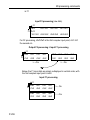
TOPSPIN can process data up to 8-dimension. TOPSPIN 2.1 has been tested
for data up to dimension 6. The directions of a dataset are indicated with
the terms F6, F5, F4, F3, F2 and F1 which are used as follows:
1D data
F1 - first and only direction
2D data
F2 - first direction (acquisition or direct direction)
F1 - second direction (indirect direction)
Commands like xf2 and abs2 work in the F2 direction. xf1, abs1 etc.
work in F1. xfb, xtrf etc. work in both F2 and F1.
3D data
F3 - first direction (acquisition or direct direction)
F2 - second direction (indirect direction)
F1 - third direction (indirect direction)
4D data
F4 - first direction (acquisition or direct direction)
F3 - second direction (indirect direction)
F2 - third direction (indirect direction)
1. If C if the default drive.
P-4
Introduction
F1 - fourth direction (indirect direction)
Commands like tf3 and tabs3 work in F3. tf2, tabs2 etc. work in F2.
INDEX
tf1, tabs1 etc.
work in F1.
INDEX> 3, canDONE
Data with dimension
be processed with the command ftnd.
1.4 About time and frequency domain data
The result of an acquisition is a representation of intensity values versus
acquisition time (seconds); the data are in the time domain. The result of a
Fourier transform is a representation of intensity values versus frequency
(Hz or ppm); the data are in the frequency domain.
Examples of time domain data are:
• raw data (1D, 2D, and 3D)
• 1D data processed with bc, em or gm
• 2D data processed with xf2 (time domain in F1)
• 3D data processed with tf3 (time domain in F2 and F1)
Examples of frequency domain data are:
• 1D data processed with ft, ef, gf, efp, gfp, trf*
• 2D data processed with xfb, xf2, xf1, xtrf*
• 3D data processed tf3, tf2, tf1
Be aware: the commands trf* and xtrf* only perform a Fourier transform if the processing parameter FT_mod (type edp) is set (see trf).
Time and frequency domain data can usually be distinguished by the data
type (FID versus spectrum) and axis labelling (Hz or ppm versus sec). The
only unequivocal way to distinguish them, however, is the processing
parameter FT_mod (type dpp):
• FT_mod = no : no FT was done and the data are still in the time
domain
• FT_mod = f* : FT was done and the data are in the frequency domain
• FT_mod = i* : FT and IFT was done and the data are again in the
time domain
P-5
Introduction
1.5 About raw and processed data
INDEX
The result of an acquisition are raw data. Raw
data are data which have
not been processed in any way. They are stored in:
DONE
INDEX
<dir>/data/<user>/nmr/<name>/<expno>/
fid - 1D raw data
ser - 2D or 3D raw data
The result of processing are processed data. They are stored in:
<dir>/data/<user>/nmr/<name>/<expno>/pdata/<procno>/
1r, 1i - 1D processed data
2rr, 2ir, 2ri, 2ii - 2D processed data
3rrr, 3irr, 3rir, 3rri - 3D processed data
Concerning their input data, processing commands can be divided into:
• commands which only work on raw data
• commands which only work on processed data
• commands which work on raw or processed data
1.5.1 Commands that only work on raw data
The following commands only work on raw data. If no raw data exist, they
stop with an error message.
• 1D commands bc, trf, addfid, convdta
• 2D commands xtrf, xtrf2, addser, convdta
• 3D commands tf3, convdta
1.5.2 Commands that work on raw data or processed data
The following processing commands work on raw or processed 1D data:
em, gm, sinm, qsin, sinc, qsinc, tm, traf, trafs,
ft, ef, gf, efp, gfp
They work on raw data if one of the following is true:
• no processed data exist (file 1r and/or 1i do not exist)
• processed data exist but they are already Fourier transformed
P-6
Introduction
They work on processed data if the following is true:
• processed data exist but they are not Fourier transformed
INDEX
add, addc, and, div, filt, ls, mul, mulc, or, rs, rv, xor, zf, zp
INDEX
They work
on raw dataDONE
if the parameter DATMOD = raw
They work on processed data if the parameter DATMOD = processed
The following processing commands work on raw or processed 2D data:
xfb, xf2, xf1
They work on raw data if one of the following is true:
• the option raw is added, e.g. xfb raw
• no processed data (i.e. the file 2rr) exist
• the processing status parameter files procs or proc2s do not
exist or are not readable
• for xf2: data are already Fourier transformed in F2
• for xf1: data are already Fourier transformed in F1
• for xfb: data are already Fourier transformed in both F2 and
F1
• the processing status parameter PH_mod is set to ps (power
spectrum) or mc (magnitude spectrum) in F2 and/or F1
They work on processed data if one of the following is true:
• the option proc is used, e.g. xfb proc
• none of the conditions for using raw data is fulfilled
1.5.3 Commands that always work on processed data
Several processing commands can, by definition, only work on processed
data. If no processed data exist, they stop with an error message.
On 1D data:
abs, absf, absd, apk, apk0, apk1, apks, bcm, sab, trfp, ift, ht,
genfid, filt
On 2D data:
P-7
Introduction
abs2, abs1, abst2, abst1, sub2, sub1, sub1d2, sub1d1, bcm2,
bcm1, xf2p, xf1p, xfbp, xf2m, xf1m, xfbm, xf2ps, xf1ps, xfbps,
sym, syma, symj, tilt, ptilt, ptilt1,INDEX
rev2, rev1, xif2, xif1,
xht2, xht1, xtrfp, xtrfp2, xtrfp1, add2d, genser
On 3D data:
DONE
INDEX
tf2, tf1, tht3, tht2, tht1,tf3p, tf2p, tf1p,tabs3, tabs2, tabs1
1.6 About digitally filtered Avance data
The first points of the raw data measured on an Avance spectrometer are
called group delay. These points represent the delay caused by the digital
filter and do not contain spectral information. The first points of the group
delay are always zero. The group delay only exists if digital filtering is actually used, i.e. if the acquisition parameter DIGMOD is set to digital.
1.7 Usage of processing commands in AU programs
Many processing commands described in this manual can also be used in
AU programs. The description of these commands contains an entry
USAGE IN AU PROGRAMS. This means an AU macro is available which
is usually the name of the command in capitalized letters. If the entry
USAGE IN AU PROGRAMS is missing, no AU macro is available. Usually,
such a command requires user interaction and it would not make sense to
put it in an AU program. However, if you still want to use such a command
in AU, you can use the XCMD macro which takes a TOPSPIN command as
argument. Examples are:
XCMD("edp")
XCMD("setdef ackn no")
AU programs can be set up with the command edau.
Most TOPSPIN commands can also be used in a TOPSPIN macro (see
edmac) or Python program (see edpy).
P-8
Introduction
1.8 Clicking commands from the TOPSPIN menu
This manuals INDEX
describes all processing commands as they can be entered
on the command line. However, they can also be clicked from the TOPSPIN
INDEX
DONE
popup menus. Most commands can be found under the Processing or Analysis menu. The corresponding command line commands are specified in
square brackets or appear on right-clicking the menu item.
1.9 Userspecific handling of Source Directories
1.9.1 Source Directory Handling - Introduction
The following paragraphe describes the fundamental handling how TopSpin 2.1 and newer is searching for information like pulse programs, parameter sets, AU programs, lists like VD-list and files like intrng-files (see
listing below, paragraphe 1.9.3). The information where to find these files
is stored in the definition of Source Directories in TopSpin. There each
TopSpin user can add/remove directories and change the order of directories. The order of the directories defines the priority for TopSpin when
searching for a file.
This function is complemented now with the function called Manage
Source Directories. There all user preferences regarding Directory Handling can be defined and are keeped.
TopSpin 2.1 does not use the database anymore, which has been used
in TopSpin 2.0.
1.9.2 Examples of use
In order to describe the new userspecific handling of Source Directories
in TopSpin 2.1 more considerable you can find two examples of use in
the following:
1. Protection of user defined files
With the new userspecific handling of Source Directories all userspecific files can be protected. If e.g. all user-files are stored in the own
"Home"-Directory nobody else than the actual user can read or modifiy any file, because this directory is read- and write protected.This
P-9
Introduction
protection for example can be important for pulse program development.
INDEX
2. Simple and secure working in laboratories
with various spectrometers
DONE
INDEX
All TopSpin installations that provide the basis for spectormeter control, can be configured in TopSpin 2.1 to be got from the same directories. With this use of Manage Source Directories for example Pulse
Programs can be taken from one common directory so that all modifications and improvements can be used from all spectrometer in the
laboratory immediately. Along this way Source directory handling
becomes much more comfortable and much fewer failures will arrive.
1.9.3 Source Directories
In TopSpin 2.1 users can specify individual directories for:
• Pulse Programs
• CPD Programs
• Shape Files
• Gradient Files
• Parameter Sets
• Macros
• Python Programs
• AU Programs
• VD Delay lists
• VP Loup Cont lists
• VC lists
• VA Amplitude lists
• VT Temperature lists
• F1 Frequency lists
• SP Shape lists
• DS Data Set lists
• Solvent Region Files
• Phase Program lists
P-10
Introduction
• ’intrng’ files
• ’peakrng’ files
INDEX
• ’baslpnts’ files
INDEX
• ’base_info’
files
DONE
• ’peaklist’ files
• ’clevels’ files
• ’reg’ files
• ’int2drng’ files
• Structure files
1.9.4 Default directories
The default paths for directories, e.g. Pulse Programs, are:
Bruker files in: .../exp/stan/nmr/lists/pp
User files in: .../exp/stan/nmr/lists/pp/user
The default path for lists, e.g. VD lists, is
Bruker/User files in:.../exp/stan/nmr/lists/vd
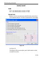
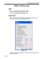
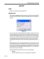
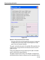
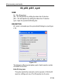
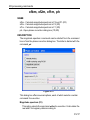
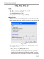
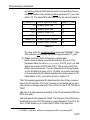
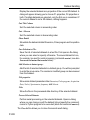
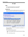
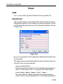
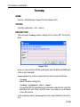
1.9.5 How to define userspecific directories
With TopSpin 2.1 and newer the directory/file structure enables all users
to define individual directories. The userspecific path definition of Source
Directories can be reached from the menu bar by
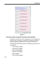
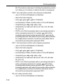
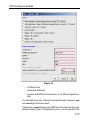
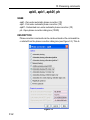
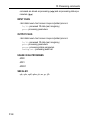
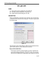
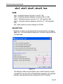
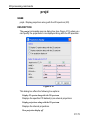
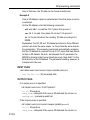
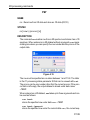
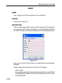
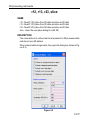
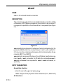
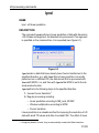
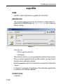
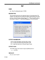
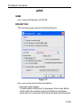
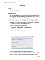
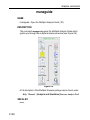
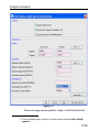
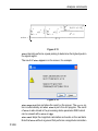
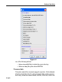
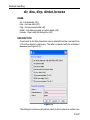
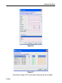
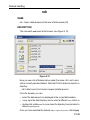
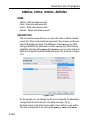
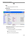
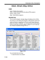
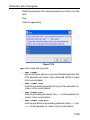
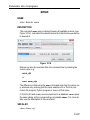
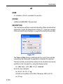
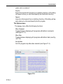
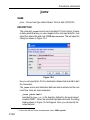
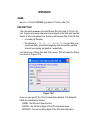
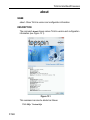
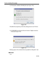
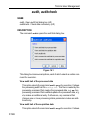
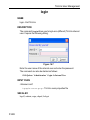
Options ’ Preferences ’ Directories ’ Manage Source Directories ’ Change.
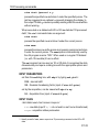
This way leads to a list of all Source Directories, where the userspecific
paths can be specified (see Figure 1.1). With this structure each user can
define his own directories in an unlimited number.
This window enables the user to define the individual directories for all
files as Pulse Programs, AU Programs etc. (for the complete list of
Source Directories see paragraphe 1.9.3).
The order of the directories defines the priority for TopSpin when searching for a file.
Please note that changes will not become effective before TopSpin restart.
P-11
Introduction
INDEX
DONE
INDEX
Figure 1.1
1.9.6 How to define userspecific directories with commands
Userspecific directories can also be configured from the corresponding
reading-/writing- and editing-commands for the respective information
like pulse programs, parameter sets, AU programs, lists and files.
For defining special lists please enter the corresponding command in the
command line:
• Pulse Programs (edpul)
• CPD Programs (edcpd)
• Shape Files (edshape)
• Parameter Sets (edpar)
• Macros (edmac)
• Python programs (edpy)
P-12
Introduction
• AU Prgrams (edau)
• VD, VP, VC, VA, VT, F1, DS, Solvent Region Files, Phases
INDEX
(edlist)
• ’intrng’
Files, ’peakrng’
Files etc. (edmisc)
INDEX
DONE
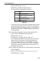
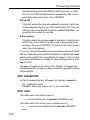
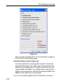
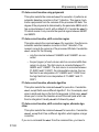
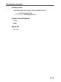
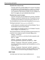
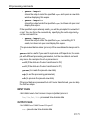
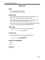
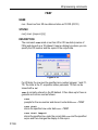
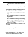
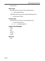
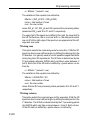
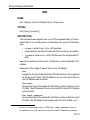
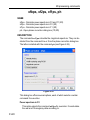
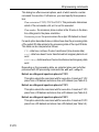
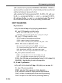
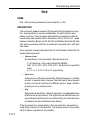
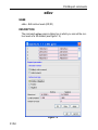
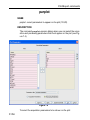
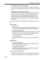
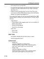
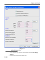
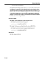
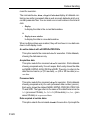
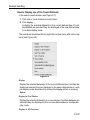
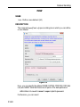
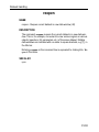
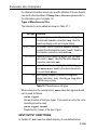
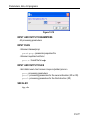
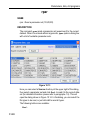
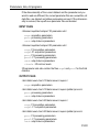
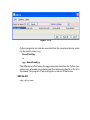
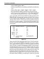
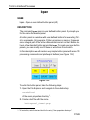
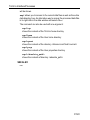
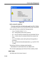
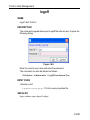
After entering the respective command in the command line, TopSpin will
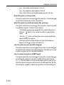
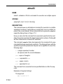
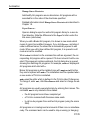
open the corresponding window in appearance like the following window.
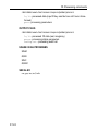
Here the example for the command edlist (see Figure 1.2).
Figure 1.2
On the topright of this window the sources are listed in the pull-down
menu and below the file types are shown also in a pull-down menu.
All shown items can be edited, read, written or written new depending on
user wishes.
By clicking Options ’ Manage Source Directories the window for defining
user-specific directories for Source Directories as described below will
appear (see Figure 1.1).
Please note that in the following chapters where the respective commands for pulse programs, parameter sets, AU programs, lists and files
are described, we will always refer to this chapter and the function Options ’ Manage Source Directories.
P-13
Chapter 2
TOPSPIN parameters
2.1 About TOPSPIN parameters
TOPSPIN parameters are divided in acquisition and processing parameters.
In this manual, we will mainly concern ourselves with processing parameters.
The following terms are used:
processing parameters
Parameters which must be set, for example by entering edp or clicking
the Procpars tab, and are interpreted by processing commands.
acquisition status parameters
Parameters which are set by acquisition commands like zg. They represent the acquisition status of a dataset and can be viewed, for example,
by entering dpa or clicking the Acqupars tab. Some acquisition status parameters are used as input by processing commands.
processing status parameters
Parameters which are set by processing commands. They represent the
processing status of a dataset and can be viewed, for example, by dpp
TOPSPIN parameters
or by clicking the Procpars tab. Most processing status parameters get
the value of the corresponding processing parameter as it was set by the
user (edp). Some parameters, however, are
explicitly set or modified by
INDEX
the processing command.
DONE
INDEX
input parameters
Parameters which are interpreted by processing commands. These can
be:
• processing parameters (set by the user). Most input parameters
are processing parameters.
• acquisition status parameters (set by an acquisition command).
An example is parameter AQ_mod.
• processing status parameters (set by the previous processing
command). An example is the parameter SI set by ft and then
interpreted by abs. This means you cannot change the size
between ft and abs.
output parameters
Parameters which are set or modified by processing commands. These
can be:
• processing status parameters. Examples are FT_mod and
YMAX_p, set by ft. Most output parameters are processing status parameters.
• processing parameters. Examples are PHC0 and PHC1, set by
apk and SR and OFFSET, set by sref.
Processing parameters can be set with the parameter editor edp and
processing status parameters can be viewed with dpp. Alternatively, each
parameter can be set or viewed by entering its name in lowercase letters
on the command line. For example, the parameter SI:
• si - set the parameter SI
• s si - view the status parameter SI
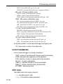
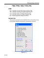
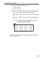
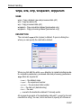
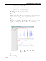
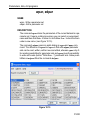
The dimensionality of the dataset is automatically recognized. For example, for a 2D dataset the following dialog box is offered:
Although status parameters are normally not changed by the user, a com-
P-16
TOPSPIN parameters
INDEX
INDEX
DONE
mand like s si allows you to do that. This, however, could make the dataset inconsistent which can be checked with the command auditcheck.
Before any processing has been done, the processing status parameters of
a dataset do not contain significant values. After the first processing command, they represent the current processing status of the data. Any further
processing command will update the processing status parameters.
After processing, the relevant processing status parameters are usually set
to the same values as the corresponding processing parameters. In other
words, the command has done what you told it to do. There are, however,
some exceptions:
• when a processing command was interrupted, the processing status
parameters might not have been updated yet.
• some processing parameters are modified by the processing command, e.g. STSI is rounded to the next higher multiple of 16 by xfb.
The rounded value is stored as the processing status parameter.
• the values of some parameters are a result of processing. They cannot be set by the user (they do not appear as processing parameters)
but they are stored as processing status parameters. Examples are
NC_proc, S_DEV and TILT.
2.2 Parameter values
With respect to the type of values they take, parameters can be divided into
three groups:
• parameters taking integer values, e.g. SI, TDeff, ABSG, NSP
• parameters taking float or double values, e.g. LB, PHC0, ABSF1
P-17
TOPSPIN parameters
• parameters using a predefined list of values, e.g. BC_mod, WDW,
PSCAL
INDEX
You can easily see to which group a parameter
belongs from the parameter
editor opened by entering edpDONE
or clicking Procpars.
INDEXNote that the values of
parameters which use a predefined list are actually stored as integers. The
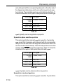
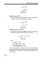
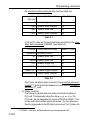
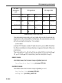
first value of the list is always stored as 0, the second value as 1 etc. Table
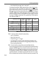
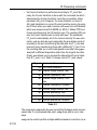
2.1 shows the values of the parameter PH_mod as an example:
Parameter
value
Integer stored in the proc(s)
file
no
0
pk
1
mc
2
ps
3
Table 2.1
2.3 Parameter files
TOPSPIN parameters are stored in various files in the dataset directory tree.
In a 1D dataset:
<dir>/data/<user>/nmr/<name>/<expno>/
acqu - acquisition parameters
acqus - acquisition status parameters
<dir>/data/<user>/nmr/<name>/<expno>/pdata/<procno>/
proc - processing parameters
procs - processing status parameters
In a 2D dataset:
<dir>/data/<user>/nmr/<name>/<expno>/
acqu - F2 acquisition parameters
acqu2 - F1 acquisition parameters
acqus - F2 acquisition status parameters
acqu2s - F1 acquisition status parameters
P-18
TOPSPIN parameters
<dir>/data/<user>/nmr/<name>/<expno>/pdata/<procno>/
proc - F2 processing parameters
proc2 -INDEX
F1 processing parameters
procs -INDEX
F2 processingDONE
status parameters
proc2s - F1 processing status parameters
In a 3D dataset:
<dir>/data/<user>/nmr/<name>/<expno>/
acqu - F3 acquisition parameters
acqu2 - F2 acquisition parameters
acqu3 - F1 acquisition parameters
acqus - F3 acquisition status parameters
acqu2s - F2 acquisition status parameters
acqu3s - F1 acquisition status parameters
<dir>/data/<user>/nmr/<name>/<expno>/pdata/<procno>/
proc - F3 processing parameters
proc2 - F2 processing parameters
proc3 - F1 processing parameters
procs - F3 processing status parameters
proc2s - F2 processing status parameters
proc3s - F1 processing status parameters
2.4 List of processing parameters
This paragraph contains a list of all processing parameters with a description of their function and the commands they are interpreted by. Please
note that composite processing commands like efp (which combines em,
ft and pk) are not mentioned here. Nevertheless, they interpret all parameters which are interpreted by the single commands they combine.
Processing parameters can be set from the parameter editor, which can be
opened by entering edp or clicking Procpars. Alternatively, you can set
parameters by entering their names in lowercase letters on the command
line.
ABSF1 - low field limit of the region which is baseline corrected
• used in 1D, 2D and 3D datasets in all directions
P-19
TOPSPIN parameters
• takes a float value (ppm) and must be greater than ABSF2
• interpreted by absf, apkf, abs1, abs2, abst*, absot*, zert*,
INDEX
tabs*
• The 1D commands abs and
absd do not
interpret ABSF1 because
DONE
INDEX
they work on the entire spectrum. The command apkf, for automatic
phase correction, uses ABSF1 as the left limit of the region on which
it calculates the phase values.
ABSF2 - high field limit of the region which is baseline corrected
• used in 1D, 2D and 3D datasets in all directions
• takes a float value (ppm), must be smaller than ABSF1
• interpreted by absf, apkf, abs2, abs1, abst*, absot*, zert*,
tabs*
• The 1D commands abs and absd do not interpret ABSF2 because
they work on the entire spectrum. The command apkf, for automatic
phase correction, uses ABSF2 as the right limit of the region on
which it calculates the phase values.
ABSG - degree of the polynomial which is subtracted in baseline correction
• used in 1D, 2D and 3D datasets in all directions
• takes an integer value between 0 and 5 (default is 5)
• interpreted by abs, absd, absf, abs2, abs1, abst*, absot*,
tabs*
• A polynomial of degree ABSG is calculated by the baseline correction commands and then subtracted from the spectrum.
ABSL - integral sensitivity factor with reference to the noise
• used in 1D datasets
• takes a float value between 0 and 100 (default is 3)
• interpreted by abs, absd, absf
• Data points greater than ABSL*(standard deviation) are considered
spectral information, all other points are considered noise.
ALPHA - correction factor
• used in 2D datasets in F2 and F1
P-20
TOPSPIN parameters
• takes a float value
• interpreted by ptilt, ptilt1 and add2d
INDEX
• For ptilt, F2 ALPHA is the tilt factor. For ptilt1, F1 ALPHA is the
tilt factor.INDEX
They must have
a value between -2.0 and 2.0. For add2d,
DONE
F2 ALPHA is the multiplication factor for the current dataset (see also
parameter GAMMA).
AQORDER - Acquisition order
• used in datasets with dimensionality ≥ 3
• takes one of the values 321, 312 for 3D data
• takes one of the values 4321, 4312, 4231, etc. for 4D data
• takes ..... etc.
• only interpreted if AQSEQ is not set, by the processing commands
ftnd and tf3
• AQORDER describes the order in which the indirect directions have
been acquired. For example, a 3D pulse program usually contains a
double nested loop with loop counters td1 and td2. If td1 is used in
the inner loop and td2 in the outer loop, the acquisition order is 312.
Otherwise it is 321.
Caution: the acquisition order is normally evaluated from the acquisition status parameter AQSEQ. Only if this parameter is not set,
AQORDER is used.
ASSFAC - assign the highest or second highest peak as reference for scaling
• used in 1D datasets
• takes a float value (default is 0.0)
• interpreted by pp*, lipp*
• This parameter is interpreted as follows:
If ASSFAC > 1, the second highest peak is used as reference for scaling, if the following is true: h2 < hmax/ASSFAC, where h2 is the intensity
of the second highest peak and hmax the intensity of the highest peak.
If this condition is false, the highest peak is used as reference.
Other values of ASSFAC have no effect on the plot scaling.
P-21
TOPSPIN parameters
ASSWID - region excluded from second highest peak search
• used in 1D datasets
• takes a float value (Hz, default is 0)
DONE
• interpreted by pp*, lipp*
INDEX
INDEX
• ASSWID is interpreted as follows:
If abs(ASSFAC) > 1, a region of width ASSWID around the highest
peak is excluded from the search for the second highest peak
AUNMP - processing AU program name
• used in 1D, 2D and 3D datasets in the first direction
• takes a character string value
• interpreted by xaup
• In all Bruker standard parameter sets, the parameter AUNMP is set
to a suitable processing AU program.
AZFE - integral extension factor
• used in 1D datasets
• takes a float value (ppm, default 0.1)
• interpreted by abs
• Integral regions are extended at both sides by AZFE ppm. If this
extension causes adjacent regions to overlap, the centre of the overlap is used as the limit of the two regions.
AZFW - minimum distance between peaks for independent integration
• used in 1D datasets
• takes a float value (ppm)
• interpreted by abs, ldcon, gdcon, mdcon
• If peaks are more than AZFW apart, they are treated independently.
If peaks are less than AZFW ppm apart, they are considered to be
overlapping.
BCFW - filter width for FID baseline correction.
• used in 1D datasets
• takes a float value (ppm)
P-22
TOPSPIN parameters
• interpreted by bc when BC_mod = sfil or qfil
• sfil/qfil is used to suppress signals in the center of the spectrum.
INDEX the width of the region, around the center of the
BCFW determines
spectrum, which is affected by bc.
INDEX
DONE
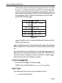
BC_mod - FID baseline correction mode
• used for 1D, 2D, and 3D dataset in all directions
(only useful in the acquisition direction)
• takes one of the values no, single, quad, spol, qpol, sfil, qfil
• interpreted by bc, em, gm, ft, trf, xfb, xf2, xf1, xtrf*, tf*
• The values of BC_mod and the corresponding functions are shown in
table 2.2. Most commands evaluate BC_mod for the function to be
subtracted but not for the detection mode. The latter is then evaluated from the acquisition status parameter AQ_mod. This means, for
example, it does not matter if you set BC_mod to single or quad. Only
trf and xtrf* evaluate the detection mode from BC_mod and distinguish between BC_mod = single and BC_mod = quad. The same
counts for the values spol/qpol and sfil/qfil.
BC_mo
d
no
Function subtracted from the FID
Detection
mode
no function
single
average intensity of the last quarter of the
FID
single channel
quad
average intensity of the last quarter of the
FID
quadrature
spol
polynomial of degree 5 (least square fit)
single channel
qpol
polynomial of degree 5 (least square fit)
quadrature
sfil
Gaussian function of width BCFW a
single channel
qfil
Gaussian function of width BCFW a
quadrature
Table 2.2
a. Marion, Ikura, Bax, J. Magn. Res. 84, 425-420 (1989)
COROFFS - correction offset for FID baseline correction
P-23
TOPSPIN parameters
• used in 1D, 2D and 3D datasets in all directions
• takes a double value (Hz, default is 0.0)
INDEX
• interpreted by bc, em, gm, trf, xfb, xf2, xf1, xtrf*, tf3, tf2,
tf1
DONE
INDEX
• COROFFS is only interpreted for BC_mod = qpol or qfil. The center
of the baseline correction is shifted by COROFFS Hz.
CURPLOT - Default plotter for Plot Editor
• used in 1D and 2D datasets
• interpreted by plot and autoplot
• The plotter set by CURPLOT overrides the plotter specified in the
Plot Editor Layout. It allows you to use the same plotter for all layouts.
DATMOD - data mode: work on ’raw’ or ’proc’essed data
• used in 1D datasets
• takes the value raw or proc
• interpreted by add, addc, and, div, filt, mul, mulc, ls, or, rs,
rv, xor, zf, zp
DC - multiplication factor or addition constant
• used in 1D datasets
• takes a float value
• interpreted by add, addc, addfid and mulc
• For addc, DC is an addition constant. For add, addfid and mulc,
DC is a multiplication factor.
DFILT - Digital filter filename
• used in 1D datasets
• takes a character string value
• interpreted by filt
• The file specified by DFILT must reside in the directory:
<tshome>/exp/stan/nmr/filt/1d
and must be set up from a command shell. One standard file called
threepoint is delivered with TOPSPIN.
P-24
TOPSPIN parameters
FCOR - first (FID) data point multiplication factor
• used in 1D, 2D and 3D datasets in all directions
INDEX
• takes a float value between 0.0 and 2.0
INDEX
• interpreted
by ft, trf,DONE
xfb, xf2, xf1, xtrf, xtrfp, tf3, tf2, tf1
• For 1D digitally filtered Avance data (DIGMOD = digital), FCOR does
not play a role because the first raw data point is always zero. FCOR,
however, allows you to control the DC offset of the spectrum in the
following cases:
- on A*X data
- on Avance data measured in analog mode (DIGMOD = analog)
- on 2D/3D Avance data in the second/second+third direction
FT_mod - Fourier transform mode
• used in 1D, 2D and 3D in all directions
• takes one of the values no, fsr, fqr, fsc, fqc, isr, iqr, iqc, isc
• interpreted by trf, xtrf*, xtrfp*
• the Fourier transform commands ft (1D), xfb, xf2, xf1 (2D) and
tf* (3D) do not interpret FT_mod because they evaluate the Fourier
transform mode from the acquisition status parameter AQ_mod.
They do, however, set the processing status parameter FT_mod.
P-25
TOPSPIN parameters
• The values of FT_mod have the following meaning:
FT_mod
Fourier transformINDEX
mode
no
no Fourier transform
fsr
forward, single channel, real
fqr
forward, quadrature, real
fsc
forward, single channel, complex
fqc
forward, quadrature, complex
isr
inverse, single channel, real
iqr
inverse, quadrature, real
isc
inverse, single channel, complex
iqc
inverse, quadrature, complex
DONE
INDEX
Table 2.3
GAMMA - multiplication factor
• used in 2D datasets in F2
• takes a float value
• interpreted by add2d
• GAMMA is the multiplication factor for the second dataset (see also
parameter ALPHA).
GB - Gaussian broadening factor for Gaussian window multiplication
• used in 1D, 2D and 3D datasets in all directions
• takes a float value between 0.0 and 1.0
• interpreted by gm
• interpreted by trf, xfb, xf2, xf1, xtrf*, tf* if WDW = EM or GM
INTBC - automatic baseline correction of integrals created by abs
• used in 1D datasets
• takes the value yes or no
• interpreted by li, lipp, lippf
P-26
TOPSPIN parameters
• INTBC has no effect on integrals which were created interactively in
the Integration mode.
INDEX
INTSCL - scale
1D integrals relative to a reference dataset
• used in 1D
datasets
INDEX
DONE
• takes an integer value
• interpreted by li, lipp, lippf
• INTSCL is used as follows:
For INTSCL > 0, the integral values are scaled individually for each
spectrum.
For INTSCL = 0, the integrals on the plot will obtain the same numeric
values as defined interactively in the integration mode.
For INTSCL = -1, scaling is performed relatively to the last spectrum
plotted.
ISEN - integral sensitivity factor with reference to the largest integral
• used in 1D datasets
• takes a positive float value (default 128)
• interpreted by abs, absd, absf
• Only the regions of integrals which are larger (area) than the largest
integral divided by ISEN are stored.
LB - Lorentzian broadening factor for exponential window multiplication
• used in 1D, 2D and 3D datasets in all directions
• takes a float value
• interpreted by em, gm
• interpreted by trf, xfb, xf2, xf1, xtrf*, tf* if WDW = EM or GM
• LB must be positive for an exponential and negative for Gaussian
window multiplication.
LPBIN - number of points for linear prediction
• used in 1D, 2D and 3D datasets in all directions
• takes a positive integer value
• interpreted by ft, trf, xfb, xf2, xf1, xtrf*, tf*
P-27
TOPSPIN parameters
• also interpreted by em, gm, *sin*, tm, traf*
For backward prediction, LPBIN represents the number of input points
INDEXvalue of LPBIN is zero,
with a maximum of TD - abs(TDoff). The default
which means all data pointsDONE
are used as input.
The status parameter LPINDEX
BIN (dpp) shows how many input points were actually used. For forward
prediction, LPBIN can be used to reduce the number of prediction output
points as specified in table 2.4. Note LPBIN only has an effect in the last
two cases. If LPBIN is smaller than TD or greater than 2*SI this has the
same effect as LPBIN = 0.
parameter values
normal
points
predicted
points
zeroes
LPBIN = 0, 2*SI < TD
2*SI
-
-
LPBIN = 0, TD < 2*SI <
2*TD
TD
2*SI - TD
-
LPBIN = 0, 2*TD < 2*SI
TD
TD
2*SI - 2*TD
TD < LPBIN < 2*SI< 2*TD
TD
LPBIN - TD
2*SI - LPBIN
TD < LPBIN < 2*TD < 2*SI
TD
LPBIN - TD
2*SI - LPBIN
Table 2.4 Linear forward prediction
MAXI - maximum relative intensity for peak picking
• used in 1D datasets
• takes a float value (cm)
• interpreted by pp*, li, lipp*
• only peaks with an intensity smaller than MAXI will appear in the
peak list. MAXI can also be set from the pp dialog box and, interactively, in peak picking mode.
MC2 - Fourier transform mode of the second (and third) direction
the processing parameter MC2 is only interpreted if the acquisition status
parameter FnMODE (dpa) does not exist or has the value undefined. FnMODE must be set (with eda) according to the experiment type before
the acquisition is started. As MC2, FnMODE only exists in the second
(and third) direction. On datasets acquired with XWIN-NMR 2.6 or earlier,
MC2 is interpreted and must be set before the data are processed. The
P-28
TOPSPIN parameters
parameter MC2:
• is used in 2D datasets in the second direction (F1)
INDEX
• is used in 3D datasets in the second and third direction (F2 and F1)
INDEX
• takes one
of the valuesDONE
QF, QSEQ, TPPI, States, States-TPPI, echoantiecho
• is interpreted by xfb, xf2, xf1, xtrf*, tf*
ME_mod - FID linear prediction mode
• used in 1D, 2D and 3D datasets in all directions
• takes one of the values no, LPfr, LPfc, LPbr, LPbc, LPmifr, LPmifc
• interpreted by ft, trf, xfb, xf2, xf1, xtrf*, tf*
• also interpreted by em, gm, *sin*, tm, traf*
• The values of ME_mod have the following meaning:
LPfr
forward LP on real data
LPfc
forward LP on complex data
LPbr
backward LP on real data
LPbc
backward LP on complex data
LPmifr
mirror image forward LP on real data
LPmifc
mirror image forward LP on complex data
Table 2.5
Linear prediction is only performed for NCOEF > 0. Furthermore, LPBIN and, for backward prediction, TDoff play a role. The commands
ft, xfb, xf2 and xf1 evaluate ME_mod but do not distinguish between LPfr and LPfc nor do they distinguish between LPbr and LPbc.
The reason is that the detection mode (real or complex) is evaluated
from the acquisition status parameter AQ_mod. However, trf, xtrf
and xtrf2 evaluate the detection mode from ME_mod. In 1D, a combination of forward and backward prediction can be done by running
trf with ME_mod = LPfc and trfp (or ft) with ME_mod = LPbc. In
2D, this would be the sequence xtrf - xtrfp (or xfb). Note that not
only Fourier transform but also window multiplication commands perform linear prediction when ME_mod is set. This allows you to easily
P-29
TOPSPIN parameters
see the effect of linear prediction on the FID, for example by executing
em with LB = 0.
INDEX
MI - minimum relative intensity for peak picking
• used in 1D datasets
DONE
INDEX
• takes a float value (cm)
• interpreted by pp*, li, lipp*
• only peaks with an intensity greater than MI will appear in the peak
list. MI can also be set from the pp dialog box and, interactively, in
peak picking mode.
NCOEF - number of linear prediction coefficients
• used in on 1D, 2D and 3D datasets in all directions
• takes a positive integer value (default is 0)
• interpreted by ft, trf, xfb, xf2, xf1, xtrf*, tf*
• also interpreted by em, gm, *sin*, tm, traf*
• NCOEF is typically set to 2-3 times the number of expected peaks.
For NCOEF = 0, no prediction is done. Linear prediction also
depends on the parameters ME_mod, LPBIN and TDoff.
NOISF1 - low field (left) limit of the noise region
• used in 1D datasets
• takes a float value (ppm)
• interpreted by sino
• The noise in the region between NOISF1 and NOISF2 is calculated
according to the algorithm described for the command sino.
NOISF2 - high field (right) limit of the noise region
• used in 1D datasets
• takes a float value (ppm)
• interpreted by sino
• The noise in the region between NOISF1 and NOISF2 is calculated
according to the algorithm described for the command sino.
NSP - number of data points shifted during right shift or left shift
P-30
TOPSPIN parameters
• used in 1D datasets
• takes a positive integer value (default is 1)
INDEX
• interpreted by ls and rs
INDEX
DONE
• NSP points
are discarded
from one end and NSP zeroes are added
to the other end of the spectrum.
NZP - number of data points set to zero intensity
• used in 1D datasets
• takes a positive integer value (default is 0)
• interpreted by zp
• zp sets the intensity of the first NZP points of the dataset to zero.
OFFSET - the ppm value of the first data point of the spectrum
• used in 1D, 2D and 3D datasets in all directions
• takes a float value (ppm)
• set by sref or interactive calibration
• also set by accumulate
• The value is calculated according to the relation:
OFFSET = (SFO1/SF-1) * 1.0e6 + 0.5 * SW * SFO1/SF
where SW and SFO1 are acquisition status parameters. In fact, the relation for OFFSET depends on the acquisition mode. When the acquisition status parameter AQ_mod is qsim, qseq or DQD, which is usually
the case, the above relation counts. When AQ_mod is qf, the equation:
OFFSET = (SFO1/SF-1) * 1.0e6
is used.
PC - peak picking sensitivity
• used in 1D datasets
• takes a float value
• interpreted by pp*, li, lipp*
• a spectral point is only a considered peak if it is a maximum which is
greater than the previous minimum plus 4*PC*noise. In addition to
P-31
TOPSPIN parameters
MI, PC provides an extra way of controlling the peak picking sensitivity. It allows you, for instance, to detect a shoulder on a large peak.
INDEX independent)
PHC0 - zero order phase correction value (frequency
• used in 1D, 2D and 3D datasets
DONE in all directions
INDEX
• takes a float value (degrees)
• set by apk, apks, apkf, apk0 on 1D datasets
• set interactively in Phase correction mode on 1D and 2D datasets
• interpreted by pk, xfbp, xf2p, xf1p, tf*p
• interpreted by trf, xfb, xf2, xf1, xtrf*, tf3, tf2, tf1 when
PH_mod = pk
• PHC0 is one of the few examples where a processing parameter is
set by a processing command. For example, apk sets both the
processing and processing status parameter PHC0. pk reads the
processing parameter and updates the processing status parameter.
For multiple phase corrections, the total zero order phase value is
stored as the processing status parameter PHC0.
PHC1 - first order phase correction value (frequency dependent)
• used in 1D, 2D and 3D datasets in all directions
• takes a float value (degrees)
• set by apk, apks, apkf, apk1 on 1D datasets
• set interactively in Phase correction mode on 1D and 2D datasets
• interpreted by pk, xfbp, xf2p, xf1p, tf*p
• interpreted by trf, xfb, xf2, xf1, xtrf*, tf3, tf2, tf1 when
PH_mod = pk
• PHC1 is one of the few examples where a processing parameter is
set by a processing command. For example, apk sets both the
processing and processing status parameter PHC1. pk reads the
processing parameter and updates the processing status parameter.
For multiple phase corrections the total first order phase value is
stored as the processing status parameter PHC1.
PH_mod - phase correction mode
• used in 1D, 2D and 3D datasets in all directions
P-32
TOPSPIN parameters
• takes one of the value no, pk, mc, ps
• interpreted by trf, xfb, xf2, xf1, xtrf*, tf*
INDEX
• The values of PH_mod are described in table 2.6.
INDEX
PH_mod
DONE
mode
no
no phase correction
pk
phase correction according to
PHC0 and PHC1
mc
magnitude calculation
ps
power spectrum
Table 2.6
• The value PH_mod = pk is only useful if the phase values are known
and the parameters PHC0 and PHC1 have been set accordingly. In
1D, they can be determined with apk or apks, or, interactively, from
the Phase correction mode. In 2D and 3D, they can only be determined interactively.
PKNL - group delay compensation (Avance) or filter correction (A*X)
• used in 1D, 2D and 3D datasets in the first direction
• takes the value true or false
• interpreted by ft, trf, xfb, xf2, xf1, xtrf*, tf*
• On A*X spectrometers, PKNL = true causes a non linear 5th order
phase correction of the raw data. This corrects possible errors
caused by non linear behaviour of the analog filters. On Avance
spectrometers, PKNL must always be set to TRUE. For digitally filtered data, it causes ft to handle the group delay of the FID. For
analog data it has no effect.
PSCAL - determines the region with the reference peak for vertical scaling
• used in 1D datasets
• takes one of the values global, preg, ireg, pireg, sreg, psreg, noise
• interpreted by pp*, li, lipp*
P-33
TOPSPIN parameters
• the values of PSCAL have the following meaning:.
PSCAL
global
Peak used as reference for vertical
scaling
INDEX
The highest peak of the entire spectrum.
DONE
INDEX
preg
The highest peak within the plot region.
ireg
The highest peak within the regions specified in the reg
file. If the reg file does not exist, global is used.
pireg
as ireg, but the peak must also lie within the plot region.
sreg
The highest peak in the regions specified in scaling
region file. This file is specified by the parameter
SREGLST. If SREGLST is not set or specifies a file
which does not exist, global is used.
psreg
as sreg but the peak must also lie within the plot region.
noise
The intensity of the noise.
Table 2.7
• For PSCAL = ireg or pireg, the reg file is interpreted. The reg file
can be created in interactive integration mode and can be viewed or
edited with the command edmisc reg.
• For PSCAL = sreg or psreg, the scaling region file is interpreted. This
feature is used to exclude the region in which the solvent peak is
expected. The name of a scaling region file is typically of the form
NUCLEUS.SOLVENT, e.g. 1H.CDCl3. For all common nucleus/solvent combinations, a scaling region file is delivered with TOPSPIN.
These can be viewed or edited with the command edlist scl. In
several 1D standard parameter sets which are used during automation, PSCAL is set to sreg and SREGLIST to NUCLEUS.SOLVENT as
defined by the parameters NUCLEUS and SOLVENT.
PSIGN - peak sign for peak picking
• used in 1D datasets
• takes the value pos, neg or both (default is pos)
• interpreted by pp*, lipp*
• in most 1D standard parameter sets PSIGN is set to pos which means
only positive peaks are picked
P-34
TOPSPIN parameters
REVERSE - flag indicating to reverse the spectrum during Fourier transform
INDEX
• used in 1D,
2D and 3D datasets in all directions
• takes theINDEX
value true or DONE
false (default is false)
• interpreted by ft, trf, xfb, xf2, xf1, xtrf*, tf*
• Reversing the spectrum can also be done after Fourier transform with
the commands rv (1D) or rev2, rev1 (2D).
SF - spectral reference frequency
• used in 1D, 2D and 3D datasets in the first direction
• takes a positive float value
• set by sref or interactive calibration
• sref calculates SF according to the relation:
SF=BF1/(1.0+RShift * 1e-6)
where RShift is taken from the edlock table and BF1 is an acquisition
status parameter. SF is interpreted by display and plot routines for
generating the axis (scale) calibration.
SI - size of the processed data
• used in 1D, 2D and 3D datasets in all directions
• takes an integer value
• interpreted by processing commands which work on the raw data
(commands working on processed interpret the processing status
parameter SI)
• The total size of the processed data (real+imaginary) is 2*SI. In
Bruker standard parameter sets (see rpar), SI is set to TD/2, where
TD is an acquisition status parameter specifying the number of raw
data points.
SIGF1 - low field (left) limit of the signal region
• used in 1D and 2D datasets
• takes a float value (ppm), must be greater than SIGF2
• interpreted by sino
P-35
TOPSPIN parameters
•
If SIGF1 = SIGF2, the signal region is defined by the entire spectrum
minus the first 16th part or, if the scaling region file exists, by the
regions in this file. The name of the scaling
region file is NUC1.SOLINDEX
VENT where NUC1 and SOLVENT are acquisition status parameDONE
INDEX
ters.
• SIGF1 is also used in 2D datasets as the low field limit for 2D baseline correction by abst2, abst1, absot2, absot1, zert1, and
zert2.
SIGF2 - high field (right) limit of the signal region
• used in 1D and 2D datasets
• takes a float value (ppm), must be smaller than SIGF1
• interpreted by sino
• If SIGF1 = SIGF2, the signal region is defined by the entire spectrum
minus the first 16th part or, if the scaling region file exists, by the
regions in this file. The scaling region file is defined as NUC1.SOLVENT where NUC1 and SOLVENT are acquisition status parameters.
• SIGF2 is also used in 2D datasets as the high field limit for 2D baseline correction by abst2, abst1, absot2, absot1, zert1, and
zert2.
SINO - signal to noise ratio
• used in 1D datasets
• takes a float value
• used in AU as an acquisition criterion (not used by processing commands)
• the processing parameter SINO (set with edp) can be used in an AU
program to specify a signal/noise ratio which must be reached in an
acquisition. The acquisition runs until the value of SINO is reached
and then it stops. An example of such an AU program is au_zgsino.
SINO can be set with edp but not from the command line. The reason is that entering sino on the command line would execute the
command sino. Note that the processing parameter SINO (edp) has
a different purpose than the processing status parameter SINO
P-36
TOPSPIN parameters
(dpp). The latter represents the signal to noise ratio calculated by the
processing command sino.
INDEX
SREGLST - name
of the scaling region file
• used in 1D
datasets
INDEX
DONE
• takes a character string value
• interpreted by li, lipp* if PSCAL = sreg or psreg
• interpreted by sino
• scaling region files contain the regions in which the reference peak is
searched. They are used to exclude the region in which the solvent
peak is expected. Because this region is nucleus and solvent specific
the name of a scaling region file is of the form NUCLEUS.SOLVENT,
e.g. 1H.CDCl3. For all common nucleus/solvent combinations, a
scaling region file is delivered with TOPSPIN. They can be viewed or
edited with edlist scl.
SSB - sine bell shift
• used in 1D, 2D and 3D datasets in all directions
• takes a positive float value
• interpreted by sinm, qsin, sinc, qsinc
• interpreted by trf, xfb, xf2, xf1, xtrf*, tf* if WDW = sine,
qsine, sinc or qsinc
SR - spectral reference
• used in 1D, 2D and 3D datasets in all directions
• takes a float value (Hz)
• set by sref or interactive calibration
• The spectral reference is calculated according to the relation:
SR = SF - BF1
STSI - strip size: number of output points of strip transform
• used in 1D, 2D and 3D datasets in all directions
• takes an integer value between 0 and SI (default 0)
• interpreted ft, trf, xfb, xf2, xf1, xtrf, xtrf2, tf3, tf2, tf1
P-37
TOPSPIN parameters
• During strip transform, only the region determined by STSI and
STSR is stored. For STSI = 0, a normal (full) transform is done. STSI
is always rounded; in 1D to the next lower
multiple of 4, in 2D and 3D
INDEX
to the next higher multiple of 16. Furthermore, when the 2D (3D) data
DONE format,
INDEX
are stored in submatrix (subcube)
STSI is rounded to the next
multiple of the submatrix (subcube) size.
STSR - strip start: first output point of a strip transform
• used in 1D, 2D and 3D datasets in all directions
• takes an integer value between 0 and SI (default 0)
• interpreted ft, xfb, xf2, xf1, xtrf, xtrf2, tf3, tf2, tf1
• During strip transform, only the region determined by STSI and
STSR is stored.
TDeff - number of raw data points to be used for processing
• used in 1D, 2D and 3D datasets in all directions
• takes an integer value between 0 and TD (default is 0 which means
all)
• interpreted by processing commands which work on the raw data
• The first TDeff raw data points are used for processing. For TDeff =
0, all points are used, with a maximum of 2*SI.
TDoff - number of raw data points ignored or predicted
• used in 1D, 2D and 3D datasets in all directions
• integer value between 0 and TD (default is 0)
• interpreted by 2D and 3D processing commands which work on raw
data
The first raw data point that contributes to processing is shifted by
TDoff points. For 0 < TDoff < TD the first TDoff raw data points are
cut off at the beginning and TDoff zeroes are appended at the end
(corresponds to left shift). For TDoff < 0, -TDoff zeroes are prepended at the beginning and:
• for SI < (TD-TDoff)/2 raw data are cut off at the end
• for DIGMOD=digital, the zeroes would be prepended to the
group delay which does not make sense. You can avoid that by
P-38
TOPSPIN parameters
converting the raw data with convdta before you process
them.
INDEX by 1D, 2D and 3D processing commands which do
• also interpreted
linear backward prediction, i.e. ft, xfb of tf3 when ME_mod is lpbr
INDEX
DONE
or lpbc.
For TDoff > 0, the first TDoff points are replaced by predicted points.
For TDoff < 0, abs(TDoff) predicted points are added to the beginning
and cut off at the end of the raw data. If zero filling occurs (2*SI >
TD), then only zeroes are cut off at the end as long as abs(TDoff) <
2*SI - TD. Note that digitally filtered Avance data start with a group
delay. This means that a backward prediction does not make sense
unless the data are first converted AMX format with convdta.
TM1 - the end of the rising edge of a trapezoidal window
• used in 1D, 2D and 3D datasets in all directions
• takes a float value between 0.0 and 1.0
• interpreted by tm
• TM1 represents a fraction of the acquisition time and must be smaller
than TM2
TM2 - the start of the falling edge of a trapezoidal window
• used in 1D, 2D and 3D datasets in all directions
• takes a float value between 0.0 and 1.0
• interpreted by tm
• TM2 represents a fraction of the acquisition time and must be greater
than TM1.
WDW - FID window multiplication mode
• used in 1D, 2D and 3D datasets in all directions
• takes one of the values no, em, gm, sine, qsine, trap, user, sinc, qsinc,
traf, trafs
• interpreted by trf, xfb, xf2, xf1, xtrf*, tf*
• On 1D data, window multiplication is usually done with commands
like em, gm, sinm etc. which do not interpret WDW. These com-
P-39
TOPSPIN parameters
mands are already specific for one type of window multiplication. The
values of WDW have the following meaning:
WDW
value
Function
INDEX
DONE
Depend-
INDEX
ent
Specific 1D
command
parameters
em
Exponential
LB
em
gm
Gaussian
GB, LB
gm
Sine
SSB
sinm
Sine squared
SSB
qsin
trap
Trapezoidal
TM2, TM1
tm
sinc
Sine
SSB, GB
sinc
Sine squared
SSB, GB
qsinc
sine
qsine
qsinc
traf
Traficante (JMR, 71, 1987,
237)
traf
trafs
Traficante (JMR, 71, 1987,
237)
trafs
Table 2.8
2.5 Processing status parameters
After processing, most processing status parameters have been set to the
same value as the corresponding processing parameter. For some
processing status parameters, however, this is different. The reason can be
that:
• the corresponding processing parameter does not exist, e.g.
NC_proc
• the corresponding processing parameter is not interpreted, e.g.
FT_mod
• the value of the corresponding processing parameter is adjusted, e.g.
STSI
These type of processing status parameters are listed below and described
P-40
TOPSPIN parameters
as output parameters for each processing command. They can be viewed
with dpp (see also chapter 2.1).
INDEX
BYTORDP - byte
order of the processed data
• used in 1D,
2D and 3DDONE
datasets in the first direction
INDEX
• takes the value little or big
• set by the first processing command
• interpreted by various processing commands
• Big endian and little endian are terms that describe the order in which
a sequence of bytes are stored in a 4-byte integer. Big endian means
the most significant byte is stored first, i.e. at the lowest storage
address. Little-endian means the least significant byte is stored first.
TOPSPIN only runs on computers with byte order little endian. However, TOPSPIN’s predecessor XWIN-NMR also runs on SGI workstations
which are big endian. The byte order of the raw data is determined by
the computer which controls the spectrometer and is stored in the
acquisition status parameter BYTORDA (type s bytorda). This
allows raw data to be processed on computers of the same or different storage types. The first processing command interprets
BYTORDA, stores the processed data in the byte order of the computer on which it runs and sets the processing status parameter
BYTORDP accordingly (type s bytordp). All further processing
commands interpret this status parameter and store the data accordingly. As such, the byte order of the computer is handled automatically and is user transparent. 2D and 3D processing commands,
however, allow you to store the processed data with a byte order different from the computer on which they run. For example, the commands xfb big and tf3 big on a Windows or Linux PC store the
data in big endian although the computer is little endian. The
processing status parameter BYTORDP is set accordingly.
FT_mod - Fourier transform mode
• used in 1D, 2D and 3D datasets in all directions
• takes one of the values no, fsr, fqr, fsc, fqc, isr, iqr, iqc, isc
• set by all Fourier transform commands, e.g. ft, trf, xfb, xf2, xf1,
trf*, xtrf*, tf3, tf2, tf1
• interpreted by trf and xtrf*.
P-41
TOPSPIN parameters
• also exists as processing (edp) parameter (interpreted by trf and
xtrf*)
• The values of FT_mod are described inINDEX
chapter 2.4.
MC2 - Fourier transform modeDONE
of the secondINDEX
(and third) direction
• is used in 2D datasets in the second direction (F1)
• is used in 3D datasets in the second and third direction (F2 and F1)
• takes one of the values QF, QSEQ, TPPI, States, States-TPPI, echoantiecho
• is set by xfb, xf2, xf1, xtrf*, tf*
• is interpreted by xf1, xtrf1, tf2, tf1
• The processing status parameter MC2 is set according to the acquisition status parameter FnMODE. If, however, FnMODE = undefined,
the processing status parameter MC2 is set according to the
processing parameter MC2. Furthermore, status MC2 is interpreted
during 2D processing in F1, on processed data, for example by xf1
on data which have already been processed with xf2.
NC_proc - intensity scaling factor
• used in 1D, 2D and 3D datasets in the first direction
• takes an integer value
• set by all processing commands
• only exists as processing status parameter
• Processing in TOPSPIN performs calculations in double precision floating point but stores the result in 32-bit integer values. During double
to integer conversion, the data are scaled up or down such that the
highest intensity of the spectrum lies between 2 28 and 2 29 . This
means the 32 bit resolution is not entirely used. This allows for the
highest intensity to be increased, for example during phase correction, without causing data overflow. NC_proc shows the amount of
scaling that was done, for example:
NC_proc = -3 : data were scaled up (multiplied by 2) three times
NC_proc = 4 : the data were scaled down (divided by 2) four times
P-42
TOPSPIN parameters
• Although NC_proc is normally calculated by processing commands,
2D processing also allows you to predefine the scaling factor with the
argument
nc_proc, for example:
INDEX
xfb nc_proc 2
INDEX
DONE
scales down the data twice. However, you can only scale the data
more down (or less up) than the command would have done without
the argument nc_proc. The latter is shown by the processing status
parameter NC_proc (type dpp). Smaller (more negative) values of
nc_proc are ignored to avoid data overflow. The command:
xfb nc_proc last
takes the current value of the processing status parameter NC_proc
(type dpp) as input value.
PPARMOD - dimensionality of the processed data
• takes one of the values 1D, 2D,..., 8D
• interpreted by TOPSPIN display, parameter editor edp and processing
commands that access processed data like abs and apk.
• can be set by changing the dimension from the parameter editor
(edp) toolbar.
• The status parameter PPARMOD defines the dimensionality of the
processed data. Note the following restriction: PPARMOD <= PARMODE.
PHC0 - zero order phase correction value (frequency independent)
• used in 1D, 2D and 3D datasets in all directions
• takes a float value (degrees)
• set by apk, apks, apkf, apk0, apk0f, apkm in 1D datasets
• set interactively in Phase correction mode in 1D and 2D datasets
• also exists as processing parameter (edp)
• PHC0 is one of the few examples where a processing parameter is
set by a processing command. For example, apk sets both the
processing and processing status parameter PHC0. pk reads the
processing parameter and updates the processing status parameter.
After multiple phase corrections, the processing status parameter
PHC0 shows the total zero order phase correction.
P-43
TOPSPIN parameters
PHC1 - first order phase correction value (frequency dependent)
• used in 1D, 2D and 3D datasets in all directions
• takes a float value (degrees)
INDEX
• set by apk, apks, apkf,DONE
apk1, apkmINDEX
in 1D datasets
• set interactively in Phase correction mode in 1D and 2D datasets
• also exists as processing parameter (edp)
• PHC1 is one of the few examples where a processing parameter is
set by a processing command. For example, apk sets both the
processing and processing status parameter PHC1. pk reads the
processing parameter and updates the processing status parameter.
For multiple phase corrections, the processing status parameter
PHC1 shows the total first order phase correction.
SINO - signal to noise ratio
• used in 1D datasets
• takes a float value
• set by sino
• also exists as processing parameter
• The signal is determined in the region between SIGF2 and SIGF1.
The noise is determined in the region between NOISF2 and NOISF1.
Note that SINO also exists as a processing parameter (edp) which
has a different purpose (see chapter 2.4)
SW_p - spectral width of the processed data
• used in 1D, 2D and 3D datasets in all directions
• takes a double value
• set by all processing commands
• only exists as processing status parameter
• Normally, SW_p will be the same as the acquisition status parameter
SW. However, in case of stripped data (see processing commands
STSR and STSI), the processing spectral width differs from the
acquired spectral width.
SYMM - 2D symmetrization type done
• used in 2D datasets in the F2 direction
P-44
TOPSPIN parameters
• takes the value no, sym, syma or symj
• set by sym, syma and symj
INDEX
• only exists as processing status parameter (dpp)
INDEX
• SYMM shows
the (last)DONE
kind of symmetrization that was done.
STSI - strip size; the number of output points of a strip transform
• used in 1D, 2D and 3D datasets in all directions
• takes an integer value between 0 and SI (default 0)
• also exists as processing parameter (edp)
• rounded by ft, trf, xfb, xf2, xf1, xtrf, xtrf2, tf3, tf2, tf1
• During strip transform, only the region determined by STSI and
STSR is stored. Processing commands round the value of the
processing parameter STSI; in 1D to the next lower multiple of 4, in
2D and 3D to the next higher multiple of 16 (see processing command STSI). Furthermore, when the 2D (3D) data are stored in submatrix (subcube) format, STSI is rounded to the next multiple of the
submatrix (subcube) size. The rounded value is stored as the
processing status parameter STSI. If no strip transform is done (STSI
= 0), the status STSI is set to the value of SI.
TDeff - number of raw data points that were used for processing
• used in 1D, 2D and 3D datasets in all directions
• set by ft, xfb, xf2, xf1, trf*, xtrf*
• also exists as processing parameter (edp)
• Normally, all raw data points are used as input. However, the number
of input points can be decreased with the processing parameter
TDeff or increased by doing linear forward or backward prediction
with TDoff < 0. The number of raw data points that were actually used
is stored in the processing status parameter TDeff.
TILT - flag indicating whether a tilt command has been performed
• used in 2D datasets in the F2 direction
• takes the value TRUE or FALSE
• set by ptilt, ptilt1 or tilt
• only exists as processing status parameter (dpp)
P-45
TOPSPIN parameters
XDIM - submatrix or subcube size
• used in 2D and 3D datasets in all directions
• takes an integer value
INDEX
DONE
INDEX
• set by xfb, xf2, xf1, xtrf,
xtrf2, tf3
• also exists as processing parameter
• Although XDIM is normally calculated by processing commands, 2D
and 3D processing also allow you to predefine the submatrix sizes,
using the argument xdim:
On a 2D dataset, the command:
xfb xdim
interprets the processing parameter XDIM in both F2 and F1.
On a 3D dataset, the command:
tf3 xdim
interprets the processing parameter XDIM in F3, F2 and F1.
FTSIZE - Fourier transform size
• used in 1D, 2D and 3D datasets in all directions
• takes an integer value
• set by all processing command that perform Fourier transform
• Normally, the status parameter FSIZE has the same value as the status parameter SI. Only in case of strip transform (STSR > 0 and/or
STSI > 0), they are different. FTSIZE then represents the size with
which the raw data were Fourier transformed whereas SI represents
the size with which the processed data are stored.
YMAX_p - maximum intensity of the processed data
• used in 1D, 2D and 3D datasets in the first direction
• takes a float value
• set by all processing commands
• only exists as processing status parameter (dpp)
YMIN_p - minimum intensity of the processed data
• used in 1D, 2D and 3D datasets in the first direction
P-46
TOPSPIN parameters
• takes a float value
• set by all processing commands
INDEX
• only exists as processing status parameter (dpp)
INDEX
DONE
2.6 Relaxation parameters
Relaxation parameters can be set with the command edt1 which can be
entered from the Relaxation menu.
COMPNO - number of components contributing to the relaxation curve
• used in pseudo 2D relaxation datasets
• takes an integer value (default is 1)
• interpreted by simfit
• Peak positions are determined on a row which is specified by the
parameter START (usually the first row). These positions are then
used by pd for each row of the 2D data. However, peak positions
sometimes drifts in the course of the experiment, i.e. they might shift
one or more points in successive rows. Therefore, pd searches for
the maximum intensity at the predefined peak position plus or minus
DRIFT.
DRIFT - drift of the peak positions in the course of the experiment
• used in pseudo 2D relaxation datasets
• takes an integer value (must be 1 or greater, default is 5)
• interpreted by pd
• Relaxation analysis is usually done with a series of relaxation curves,
one for each peak in the spectrum. One curve shows the intensity
distribution of one peak over a series of experiments, i.e. a series of
rows in a pseudo 2D dataset. First the peak positions are determined
on one row, for example with ppt1. Then the command pd determines the intensity at these positions in each row. However, peak
positions sometimes drifts in the course of the experiment, i.e. they
can be slightly different in different rows. Therefore, pd searches for
the maximum intensity in a range around a each peak position. This
range is determined by the parameter DRIFT.
P-47
TOPSPIN parameters
EDGUESS - table of initial values and step rates of the function variables
• used in pseudo 2D relaxation datasets
• interpreted by simfit
INDEX
DONE
INDEX
• The EDGUESS table shows
all variables
of the function specified by
FCTTYPE. For each variable, the initial guess (G) and step rate (S)
can be set for each component (C). Table 2.9 shows the EDGUESS
table for an inversion recovery experiment, with 2 components. The
initial guess for I[0] must be such that the total value of all components
GC1I0
0.5
SC1I0
0.05
GC1A
1.0
SC1A
0.1
GC1T1
2.0
SC1T1
0.2
GC2I0
0.5
SC2I0
0.05
GC2A
1.0
SC2A
0.1
GC2T1
2.0
SC2T1
0.2
Table 2.9
does not exceed 1. If there is only one component, I[0] is usually set
to 1. The step rate is usually set to about one tenth or the initial guess.
If the step rate of a variable is set to zero, then this variable is not
changed during the iterations. Note that the commands ct1, ct2,
dat1 or dat2 do not use the EDGUESS table. They calculate the initial values and step rates of the T1/T2 function variables I[0], P and
T1.
FCTTYPE - function type used for fitting the relaxation curve
• used in pseudo 2D relaxation datasets
• takes one of the values listed in Table 2.10
• interpreted by simfit
• Table 2.10 shows the experiment types which simfit can handle
and the corresponding fit functions. Note that ct1, ct2, dat1 and
dat2 do not evaluate FCTTYPE because they can only handle
T1/T2 experiments. They do, however, set FTCTYPE to the value
t1/t2.
P-48
TOPSPIN parameters
Exp. type
uxnmrt1t
2
Com
p
Fit function
INDEXI[t] = I[0]+P*exp(t/T1)
1
INDEX
DONE
invrec
1-4
I[t] = I[0]*(1-2A*exp(-t/T1))
satrec
1-6
I[t] = I[0]*(1-exp(-t/T1))
cpt1rho
1-4
I[t] = I[0]/(1-TIS/T1rho)*(exp(-t/T1rho)-exp(t/TIS))
expdec
1-6
I[t] = I[0]*exp(-t/T)
gaussdec
1-6
I[t] = I[0]*exp(-SQR(t/T))
lorgauss
1-3
I[t] = IL*exp(-t/TL)+IG*exp(-SQR(t/TG))
linear
1-6
I[t] = A+B*t
varbigdel
1-6
I = I[0]*exp(-D*SQR(2*PI*gamma*G*LD)*(BD-LD/3)*1e4)
varlitdel
1-6
I = I[0]*exp(-D*SQR(2*PI*gamma*G*LD)*(BD-LD/3)*1e4)
vargrad
1-6
I = I[0]*exp(-D*SQR(2*PI*gamma*G*LD)*(BD-LD/3)*1e4)
raddamp
1-6
MZ[t]=A0+MZ[0]*tanh((t-T0)/TRD)
Table 2.10
• used in pseudo 2D relaxation datasets
• takes the value area or intensity (default is intensity)
• interpreted by pd, ct1, dat1 and simfit
• Before you run pd, both the integral ranges and peak positions
should be determined (see rspc and ppt1). pd then picks the points
storing both their integrals and intensities but it only displays one
curve; the one defined by FITTYP. ct1 or simfit then calculate the
relaxation value for one peak according to FITTYPE. You can change
FITTYP and recalculate the relaxation value without running pd
again. The same counts for the commands dat1 and simfit all
which fit all peaks.
INC - point (1D) or row (2D) increment
• used in 1D and pseudo 2D relaxation datasets
• takes an integer value (default is 1)
• interpreted by pft2 (1D data)
P-49
TOPSPIN parameters
• interpreted by pd (pseudo 2D data)
• Starting with START, every INC point (1D) or row (pseudo 2D) is used
INDEX
for relaxation analysis.
NUMPNTS - number of data points
used for INDEX
relaxation analysis
DONE
• used in 1D and pseudo 2D relaxation datasets
• takes an integer value (default is TD)
• interpreted by pft2 (1D)
• interpreted by pd (pseudo 2D)
• The default value of NUMPNTS is the number of available points, i.e.
TD (1D) or F1 TD (pseudo 2D). TD is the acquisition status parameter which can be viewed with dpa or s td. Note that if you increase
INC, you must reduce NUMPNTS such that INC*NUMPNTS does not
exceed TD.
START - first point (1D) or row (2D) used for relaxation analysis
• used in 1D and pseudo 2D relaxation datasets
• takes an integer value (default is 1)
• interpreted by pft2 (1D data)
• interpreted by pd (pseudo 2D data)
• Note that the default value (1) is not the first but the second point of a
1D dataset. It is, however, the first row of a pseudo 2D dataset. The
point or row used is START + n*INC.
P-50
Chapter 3
1D Processing commands
This chapter describes all TOPSPIN 1D processing commands. Several of
them can also be used to process one row of 2D or 3D data. They store
their output in processed data files and do not change the raw data.
For each command, the relevant input and output parameters are mentioned. Furthermore, the relevant input and output files and their location
are mentioned. Although file handling is completely transparent, it is sometimes useful to know which files are involved and where they reside. For
example, if you have permission problems or if you want to process or
interpret your data with third party software.
1D Processing commands
abs, absf, absd, bas
INDEX
NAME
DONE (1D) INDEX
abs - Automatic baseline correction
absf - Automatic baseline correction of the plot region (1D)
absd - Automatic baseline correction, special algorithm (1D)
bas - Open baseline correction dialog box (1D)
DESCRIPTION
Baseline correction commands can be started on the command line or
from the baseline correction dialog box. The latter is opened with the
Figure 3.1
P-52
1D Processing commands
command bas.
This dialog box offers several options, each of which selects a certain
INDEX
command for
execution.
INDEX
DONE
Auto-correct
baseline using
polynomial
This option selects the command abs for execution. It performs an automatic baseline correction of the spectrum by subtracting a polynomial. The degree of the polynomial is determined by the parameter
ABSG which has a value between 0 and 5, with a default of 5. abs first
determines which parts of the spectrum contain spectral information
and stores the result in the file intrng (integral regions). The remaining part of the spectrum is considered baseline and used to fit the polynomial function.
abs also interprets the parameters ABSL, AZFW, AZFE and ISEN.
Since these parameters apply to integration rather than baseline correction, they do not appear in the bas dialog box. They do appear in
the integration dialog box (command int). Data points greater than
ABSL*(standard deviation) are considered spectral information, all
other points are considered noise. If two peaks are more than AZFW
apart, they are treated independently. If they are less than AZFW ppm
apart, they are considered to be overlapping. Integral regions are extended at both sides by AZFE ppm. If this extension causes adjacent
regions to overlap, the centre of the overlap is used as the limit of the
two regions. Only regions whose integrals are larger (area) than the
largest integral divided by ISEN are considered.
abs n does not store the integral ranges. It is, for example, used in the
command sequence ef, mc, abs, efp, abs n to store the integral regions of both positive and negative peaks. The command abs only
stores the regions of positive peaks.
Auto-correct spectral range ABSF1 .. ABSF2 only
This option selects the command absf for execution. It works like
abs, except that it only corrects the spectral region which is determined by the processing parameters ABSF1 and ABSF2.
Auto-correct baseline, alternate algorithm
This option selects the command absd for execution. It works like
P-53
1D Processing commands
abs, except that it uses a different algorithm1. It is, for example, used
when a small peak lies on the foot of a large peak. In that case, absd
allows you to correct the baseline around
the small peak which can
INDEX
then be integrated. Usually absd is followed by abs.
DONE
INDEX
To display the integral regions determined by one of the above commands:
1. Right-click inside the data window and select Display Properties
2. Check the entry Integrals and click OK
The integral regions are also used by various commands which calculate
spectral integrals like li, lipp and plot.
If you run a command like abs from the command line, you have to make
sure that the required parameters are already set. Click the Procpars tab
or enter edp to do that.
If automatic baseline correction does not give satisfactory results, you
can apply an interactively determined polynomial, exponential, sine or
spline baseline correction. This can be started with the first entry of the
bas dialog box, by clicking the
button in the toolbar or by entering
.basl on the command line.
The bas command can be used on 1D or 2D data. It recognizes the data
dimensionality and opens a dialog box with the appropriate options and
parameters.
INPUT PARAMETERS
set from the bas dialog box, with edp or by typing absg, absf1 etc.:
ABSG - degree of the polynomial (input of abs, absf, absd)
ABSF1 - low field (left) limit of the region corrected by absf
ABSF2 - high field (right) limit of the region corrected by absf
set from the int dialog box, with edp or by typing absl, azfw etc.:
ABSL - integral sensitivity factor with reference to the noise
AZFW - minimum distance between peaks for independent integration
AZFE - integral extension factor
ISEN - integral sensitivity factor with reference to the largest integral
1. It uses the same algorithm as the command abs in DISNMR
P-54
1D Processing commands
INPUT FILES
<dir>/data/<user>/nmr/<name>/<expno>/pdata/<procno>/
INDEX
1r - real processed 1D data
proc - processing
INDEX parameters
DONE
OUTPUT FILES
<dir>/data/<user>/nmr/<name>/<expno>/pdata/<procno>/
1r - real processed 1D data
procs - processing status parameters
intrng - integral regions (output of abs, absf , absd)
auditp.txt - processing audit trail
USAGE IN AU PROGRAMS
ABS
ABSD
ABSF
SEE ALSO
bcm, sab, bc, .basl
P-55
1D Processing commands
add, duadd, addfid, addc, adsu
NAME
INDEX
DONE multiply
INDEX
add - Add two datasets point-wise,
2nd with DC (1D)
duadd - Add two datasets ppm/Hz-wise, mult. 2nd with DC (1D)
addfid - Add two FIDs, multiply 2nd with DC (1D)
addc - Add the constant DC to the current dataset
adsu - Open add/subtract/multiply dialog box (1D, 2D)
DESCRIPTION
Addition commands can be entered on the command line or started from
the add/subtract/multiply dialog box. The latter is opened with the command adsu.
This dialog box offers several options, each of which selects a certain
command for execution.
Add a 1D spectrum point-wise
This option selects the command add for execution. It adds the second dataset, multiplied with the constant DC, to the current dataset.
add performs a point to point addition which is independent of the
spectrum calibration.The result is stored in the current dataset. DC
can be set by entering dc on the command line or in the Procpars
pane. If the second dataset has not been defined yet, the add/subtract
dialog box is opened. Here you can define the second dataset and
start the add command. add works on raw or on processed data, depending on the value of DATMOD. For DATMOD = raw, add adds the
raw data of the current and second dataset but stores the result as
processed data in the current dataset. As such, the raw data of the
current dataset are not overwritten.
Add a 1D spectrum ppm/Hz-wise
This option selects the command duadd for execution. It works like
add, except that it adds two datasets according to their chemical shift
values. Each ppm value of one dataset is added to the same ppm value of a second dataset.
duadd is useful when the two input spectra are:
P-56
1D Processing commands
INDEX
INDEX
DONE
Figure 3.2
• of different size
• referenced differently
• acquired with different frequencies (i.e. on different spectrometers)
For data with equal size, reference and spectrometer frequency, add
and duadd give the same result.
Furthermore, duadd allows you to shift the second spectrum by a user
defined number of ppm. The parameter ppm or hz is only relevant if the
P-57
1D Processing commands
input data were acquired with different basic frequencies, i.e. when
they come from different spectrometers. duadd only works on processed data, independent of the value of
DATMOD.
INDEX
Add an FID
DONE
INDEX
This option selects the command addfid for execution. It adds two
1D raw datasets multiplying one of them with the factor DC. The result
is stored in the current dataset. It works like add with DATMOD = raw,
except that it overwrites the raw data.
Add a constant
This option selects the command addc for execution. It adds the value
of DC to the current dataset. It works on raw or processed data, depending on the value of DATMOD. The result is stored as processed
data in the current dataset.
If you run a command like add from the command line, it behaves slightly
different. It adds the second and the third dataset, as specified with edc2
and stores the result in the current dataset. You have to make sure that
the required parameters are already set. Click the Procpars tab or enter
edp to do that.
The adsu command can be used on 1D or 2D data. It recognizes the
data dimensionality and opens a dialog box with the appropriate options
and parameters.
INPUT PARAMETERS
set from the adsu dialog box, with edp or by typing dc, datmod etc.:
DC - multiplication factor
DATMOD - data mode: work on ’raw’ or ’proc’essed data
INPUT FILES
<dir>/data/<user>/nmr/<name>/<expno>/
fid - current raw data (input of add/addc if DATMOD = raw)
<dir>/data/<user>/nmr/<name>/<expno>/pdata/<procno>/
1r, 1i - current processed data (input of add/addc if DATMOD =
proc)
P-58
1D Processing commands
proc - processing parameters
curdat2 - definition of the second dataset
INDEX
<dir2>/data/<user2>/nmr/<name2>/<expno2>/
INDEX
fid - second
raw dataDONE
(input of add if DATMOD = raw, addfid)
<dir2>/data/<user2>/nmr/<name2>/<expno2>/pdata/<procno2>/
1r, 1i - second processed data (input of add if DATMOD = proc)
OUTPUT FILES
<dir>/data/<user>/nmr/<name>/<expno>/
fid - current raw data (output of addfid)
audita.txt - acquisition audit trail (output of addfid)
<dir>/data/<user>/nmr/<name>/<expno>/pdata/<procno>/
1r, 1i - current processed data (output of add and addc)
procs - processing status parameters
auditp.txt - processing audit trail (output of add and addc)
USAGE IN AU PROGRAMS
ADD
ADDFID
ADDC
SEE ALSO
mul, mulc, div, add2d
P-59
1D Processing commands
accumulate
INDEX
NAME
DONE
INDEX (1D)
accumulate - Accumulate 1D
datasets ppm/Hz-wise
SYNTAX
accumulate [start] offset scale Hz|ppm procno [expno [name [user [dir]]]]
DESCRIPTION
The command accumulate accumulates 1D datasets. It adds a specified processed dataset to the current dataset. accumulate has the following features:
• the specified data can be shifted and scaled with respect to the
current data.
• addition can be performed ppm-wise or hz-wise
• the specified data can overwrite the current data or can be added
to the current data
All required information must be specified by command line arguments.
As such, accumulate takes 4 to 9 arguments. Here are some examples
of its usage:
accumulate <offset> <scale> ppm |hz <procno>
Add the processed data of the specified procno to the current procno
as follows:
• shift the added data by <offset> ppm
• scale added data by the value <scale>
• perform the addition ppm-wise or hz-wise as specified
Example: accumulate 0.0 1.0 ppm 3
accumulate start <offset> <scale> ppm |hz <procno>
Same as above, except that the processed data of the specified procno are copied to the current procno, overwriting possibly existing data.
Example: accumulate start 0.0 1.0 ppm 3
P-60
1D Processing commands
Note that here, the arguments offset and ppm |hz do not affect the
data but do affect the status parameter OFFSET.
In the examples
INDEX above, the accumulated dataset has the same datapath as the original data except for the procno. To accumulate data
INDEXdatapath,
DONE
with a different
you can specify other parts of the datapath
as arguments. Parts that are not specified are taken from the current
dataset.
Examples:
accumulate <offset> <scale> ppm |hz <procno> <expno>
accumulate start <offset> <scale> ppm |hz <procno>
<expno> <user> <dir>
accumulate works like the command duadd, except that all information
is specified on the command line. accumulate is typically used repeatedly to accumulate a series of 1D processed data. The first instance of
accumulate overwrites the current data with the specified data, defining
the accumulation start. All further instances add the specified data to the
current data.
OUTPUT PARAMETERS
OFFSET - the ppm value of the first data point of the spectrum
INPUT FILES
<dir>/data/<user>/nmr/<name>/<expno>/pdata/<procno>/
1r, 1i - current processed data
proc - processing parameters
<dir2>/data/<user2>/nmr/<name2>/<expno2>/pdata/<procno2>/
1r, 1i - second processed data
OUTPUT FILES
<dir>/data/<user>/nmr/<name>/<expno>/pdata/<procno>/
1r, 1i - current processed data
procs - processing status parameters
auditp.txt - processing audit trail
SEE ALSO
duadd
P-61
1D Processing commands
apk0, apk1, apk0f, ph
INDEX
NAME
INDEX
apk0 - Zero-order automaticDONE
phase correction
(1D)
apk1 - First-order automatic phase correction (1D)
apk0f - Customized zero-order automatic phase correction (1D)
ph - Open phase correction dialog box (1D/2D)
DESCRIPTION
Phase correction commands can be can be entered on the command line
or started from the phase correction dialog box (see Figure 3.3). This di-
Figure 3.3
P-62
1D Processing commands
alog is opened with the command ph. It offers several options, each of
which selects a certain command for execution.
AutomaticINDEX
phasing, 0th order only
INDEX
This option
selects the DONE
command apk0 for execution. It works like
apk, except that it only performs the zero order phase correction.
Automatic phasing, 1st order only
This option selects the command apk1 for execution. It works like
apk, except that it only performs the first order phase correction.
Automatic zero order phasing, selected region order only
This option selects the command apk0f for execution. It works like
apkf, except that it only performs the zero order phase correction.
If you run a command like apk0f from the command line, you have to
make sure that the required parameters are already set. Click the
Procpars tab or enter edp to do that.
If automatic phase correction does not give satisfactory results, you can
perform interactive phase correction. This can be started with the entry
Manual phasing in the ph dialog box, by clicking the
button in the
toolbar or by entering .ph on the command line.
The ph command can be used on 1D, 2D or 3D data. It recognizes the
data dimensionality and opens a dialog box with the appropriate options
and parameters.
INPUT PARAMETERS
set from the ph dialog box, with edp or by typing absf1, absf2 etc.:
ABSF1 - low field (left) limit of the region used by apk0f
ABSF2 - high field (right) limit of the region used by apk0f
OUTPUT PARAMETERS
can be viewed with edp, dpp or by typing phc0, s phc0 etc.:
PHC0 - zero order phase correction value (output of apk0 and apk0f)
PHC1 - first order phase correction value (output of apk1)
Note that this is one of the rare cases where the output parameters of a
P-63
1D Processing commands
command are stored as processing (edp) and as processing status parameters (dpp).
INPUT FILES
INDEX
DONE
INDEX
<dir>/data/<user>/nmr/<name>/<expno>/pdata/<procno>/
1r, 1i - processed 1D data (real, imaginary)
proc - processing parameters
OUTPUT FILES
<dir>/data/<user>/nmr/<name>/<expno>/pdata/<procno>/
1r, 1i - processed 1D data (real, imaginary)
proc - processing parameters
procs - processing status parameters
auditp.txt - processing audit trail
USAGE IN AU PROGRAMS
APK0
APK1
APK0F
SEE ALSO
apk, apks, apkf, apkm, pk, mc, ps, .ph
P-64
1D Processing commands
apk, apks, apkm, apkf, ph
NAME
INDEX
INDEX
DONE (1D)
apk - Automatic
phase correction
apks - Automatic phase correction with a different algorithm (1D)
apkm - Automatic phase correction with a different algorithm 2 (1D)
apkf - Customized automatic phase correction (1D)
ph - Open phase correction dialog box (1D/2D)
DESCRIPTION
Phase correction commands can be can be entered on the command line
or started from the phase correction dialog box (see Figure 3.4). This dialog is opened with the command ph. It offers several options, each of
which selects a certain command for execution.
Automatic phasing
This option selects the command apk for execution. It calculates the
zero and first order phase values and then corrects the spectrum according to these values. The phase values are stored in the parameters PHC0 and PHC1, respectively. Note that apk stores the
calculated phase values both as processing parameters (edp) and as
processing status parameters (dpp).
Automatic phasing, alternate algorithm
This option selects the command apks for execution. It works like
apk, except that it uses a different algorithm which gives better results
on certain spectra.
Automatic phasing, alternate algorithm 2
This option selects the command apkm for execution. It uses symmetric isolated peaks, regions with positive/negative signals and regions
of flat baseline for automated phase correction of 1D NMR spectra.
The automated phasing is performed by means of minimization of certain penalty function with four terms. The first term is responsible for
phases of symmetric isolated peaks, the second accounts for regions
with positive/negative signals, the third accounts for baseline regions,
and the fourth gives additional penalty for large values of first-order
P-65
1D Processing commands
INDEX
DONE
INDEX
Figure 3.4
phase correction parameter PHC1. For a full description of apkm, enter the TOPSPIN command help apkm.
Automatic phasing, selected region only
This option selects the command apkf for execution. It works like
apk, except that it uses only a certain region of the spectrum for the
calculation of the phase values. This region is determined by the parameters ABSF1 and ABSF2. The calculated phase values are then
applied to the entire spectrum. Note that the parameters ABSF1 and
ABSF2 are also used by the command absf.
If you run a command like apkf from the command line, you have to
P-66
1D Processing commands
make sure that the required parameters are already set. Click the
Procpars tab or enter edp to do that.
If automaticINDEX
phase correction does not give satisfactory results, you can
perform interactive
correction. This can be started with the entry
INDEX phaseDONE
Manual phasing in the ph dialog box, by clicking the
button in the
toolbar or by entering .ph on the command line.
The ph command can be used on 1D or 2D data. It recognizes the data
dimensionality and opens a dialog box with the appropriate options and
parameters.
INPUT PARAMETERS
set from the ph dialog box, with edp or by typing absf1, absf2 etc.:
ABSF1 - low field (left) limit of the region used by apkf
ABSF2 - high field (right) limit of the region used by apkf
OUTPUT PARAMETERS
can be viewed with edp, dpp or by typing phc0, s phc0 etc.:
PHC0 - zero order phase correction value (frequency independent)
PHC1 - first order phase correction value (frequency dependent)
Note that this is one of the rare cases where the output parameters of a
command are stored as processing (edp) and as processing status parameters (dpp).
INPUT FILES
<dir>/data/<user>/nmr/<name>/<expno>/pdata/<procno>/
1r, 1i - processed 1D data (real, imaginary)
proc - processing parameters
OUTPUT FILES
<dir>/data/<user>/nmr/<name>/<expno>/pdata/<procno>/
1r, 1i - processed 1D data (real, imaginary)
proc - processing parameters
procs - processing status parameters
auditp.txt - processing audit trail
P-67
1D Processing commands
USAGE IN AU PROGRAMS
APK
INDEX
APKF
APKS
SEE ALSO
apk0, apk1, apk0f
P-68
DONE
INDEX
1D Processing commands
bc
INDEX
NAME
INDEX
bc - Baseline
correction ofDONE
the FID (1D)
DESCRIPTION
The command bc performs a baseline correction of raw 1D data. The
type of correction is determined by the processing parameter BC_mod as
shown in table 3.1.
BC_mod
no
Function subtracted from the FID
Detection
mode
no function
single
average intensity of the last quarter of the
FID
single channel
quad
average intensity of the last quarter of the
FID
quadrature
spol
polynomial of degree 5 (least square fit)
single channel
qpol
polynomial of degree 5 (least square fit)
quadrature
sfil
Gaussian function of width BCFW a
single channel
qfil
Gaussian function of width BCFW
quadrature
Table 3.1
a. Marion, Ikura, Bax, J. Magn. Res. 84, 425-420 (1989)
spol/qpol and sfil/qfil are especially used to subtract strong signals, e.g. a
water signal at the centre of the spectrum. Note that sfil/qfil perform a better reduction at the risk of losing valuable signal. For reducing off-centre
signal, you can set the parameter COROFFS to the offset frequency.
In this table, s(ingle) stands for single detection mode and q(uad) for quadrature detection mode. bc evaluates BC_mod for the function to be subtracted but not for the detection mode. The latter is evaluated from the
acquisition status parameter AQ_mod. This means, for example, it does
not matter if you set BC_mod to single or quad. The same counts for the
P-69
1D Processing commands
values spol/qpol and sfil/qfil. Furthermore, for AQ_mod = DQD, no baseline correction is performed for BC_mod = single or quad. Note that the
commands trf and xtrf* do evaluate the
detection mode from
INDEX
BC_mod and perform the baseline correction for BC_mod = single/quad
DONE
INDEX
when AQ_mod = DQD.
The command bc is automatically executed as a part of the commands
em, gm, ft, or any of the composite Fourier transform commands.
When executed on a 2D or 3D dataset, bc prompts you for the row and
output procno. Alternatively, it can be entered with up to four arguments:
bc <row> <procno> n y
process the specified row and store it under the specified procno. The
last two arguments are optional: n prevents changing the display to
the output 1D data, y causes a possibly existing data to be overwritten
without warning.
When executed on a dataset with 2D or 3D raw data but 1D processed
data1, bc takes one argument:
bc <row>
process the specified row and store it under the current procno.
bc same
process the same row as the previous processing command and store
it under the current procno. The same option is automatically used by
the AU program macro BC. When used on a regular 1D dataset (i.e.
with 1D raw data) it has no effect.
bc can also be started from the baseline dialog box which is opened with
the command bas.
INPUT PARAMETERS
set from the bas dialog box, with edp or by typing bc_mod, bcfw etc.:
BC_mod - FID baseline correction mode
BCFW - filter width for BC_mod = sfil or qfil
COROFFS - correction offset in Hz, for BC_mod = spol or qpol and
1. Usually a result of rsr, rsc or a 1D processing command on that 2D or 3D dataset.
P-70
1D Processing commands
sfil/qfil
INPUT FILESINDEX
<dir>/data/<user>/nmr/<name>/<expno>/
INDEX
DONE
fid - raw data (time domain)
<dir>/data/<user>/nmr/<name>/<expno>/pdata/<procno>/
proc - processing parameters
OUTPUT FILES
<dir>/data/<user>/nmr/<name>/<expno>/pdata/<procno>/
1r, 1i - processed data (time domain)
procs - processing status parameters
auditp.txt - processing audit trail
USAGE IN AU PROGRAMS
BC
SEE ALSO
bas
P-71
1D Processing commands
bcm
INDEX
NAME
DONE
INDEX (1D)
bcm - User defined spectrum
baseline correction
DESCRIPTION
The command bcm performs a spectrum baseline correction by subtracting a polynomial, sine or exponential function.
This involves the following steps:
1. Click
or enter.basl to change to baseline correction mode.
2. Fit the baseline of the spectrum with a polynomial, exponential or
sine function. Click-hold the button A and move the mouse to
determine the zero order correction. Do the same with the buttons
B, C etc. for higher order corrections until the line matches the
baseline of the spectrum.
3. Click
to return. The command bcm is automatically executed.
The interactively determined baseline function is stored in the file
base_info. This file can be stored for general usage with the command
wmisc. After that, you can read it with rmisc on another dataset and run
bcm to perform the same baseline correction.In this case, bcm can be
started from the command line or from the baseline dialog box which is
opened with the command bas.
INPUT FILES
<dir>/data/<user>/nmr/<name>/<expno>/pdata/<procno>/
1r - real processed 1D data
proc - processing parameters
base_info - baseline correction coefficients
OUTPUT FILES
<dir>/data/<user>/nmr/<name>/<expno>/pdata/<procno>/
1r - real processed 1D data
procs - processing status parameters
P-72
1D Processing commands
auditp.txt - processing audit trail
USAGE IN AU
PROGRAMS
INDEX
BCM
INDEX
DONE
SEE ALSO
bas, sab, .basl
P-73
1D Processing commands
dt
NAME
INDEX
DONE
INDEX
dt - Calculate the first derivative
of the data
(1D)
DESCRIPTION
The command dt calculates the first derivative of the current dataset.
Depending on the value of DATMOD, dt works on the raw or on the processed data.
INPUT PARAMETERS
set by the user with edp or by typing datmod :
DATMOD - data mode: work on ’raw’ or ’proc’essed data
INPUT FILES
<dir>/data/<user>/nmr/<name>/<expno>/
fid - raw data (input if DATMOD = raw)
<dir>/data/<user>/nmr/<name>/<expno>/pdata/<procno>/
1r, 1i - processed 1D data (input if DATMOD = proc)
proc - processing parameters
OUTPUT FILES
<dir>/data/<user>/nmr/<name>/<expno>/pdata/<procno>/
1r, 1i - processed 1D data (real, imaginary)
procs - processing status parameters
auditp.txt - processing audit trail
USAGE IN AU PROGRAMS
DT
P-74
1D Processing commands
ef, efp
NAME
INDEX
INDEX
DONE
ef - Exponential
window multiplication
+ Fourier transform (1D)
efp - Exponential window multiplication + FT + phase correction (1D)
DESCRIPTION
The composite processing command ef is a combination of em and ft,
i.e. it performs an exponential window multiplication and a Fourier transform.
efp is a combination of em, ft and pk, i.e. it does the same as ef but,
in addition, performs a phase correction.
ef and efp automatically perform an FID baseline correction according
to BC_mod.
All composite processing commands can be found under the menu:
Processing ’ More Transforms ’ Shortcuts
INPUT FILES
<dir>/data/<user>/nmr/<name>/<expno>/
fid - raw data (input if 1r, 1i do not exist or are Fourier transformed)
acqus - acquisition status parameters
<dir>/data/<user>/nmr/<name>/<expno>/pdata/<procno>/
1r, 1i - processed data (input if they exist but are not Fourier transformed)
proc - processing parameters
OUTPUT FILES
<dir>/data/<user>/nmr/<name>/<expno>/pdata/<procno>/
1r, 1i - processed 1D data (real, imaginary)
procs - processing status parameters
auditp.txt - processing audit trail
P-75
1D Processing commands
USAGE IN AU PROGRAMS
EF
INDEX
EFP
SEE ALSO
gf, gfp, fp, fmc
P-76
DONE
INDEX
1D Processing commands
em, gm, wm
NAME
INDEX
INDEX
em - Exponential
window DONE
multiplication of the FID (1D)
gm - Gaussian window multiplication of the FID (1D)
wm - Open window function dialog box (1D, 2D)
DESCRIPTION
Window multiplication commands can be entered on the command line
or started from the window function dialog box. The latter is opened with
the command wm.
Figure 3.5
The parameter section of this dialog box offers several window functions,
each of which selects a certain command for execution.
Exponential multiplication
This function selects the command em for execution. It performs an
exponential window multiplication of the FID. It is the most used window function for NMR spectra. em multiplies each data point i with the
P-77
1D Processing commands
factor:
( i – 1 ) ⋅ LB ⋅ π
exp ⎛ – -----------------------------------⎞
⎝
2 ⋅ SWH ⎠
INDEX
DONE
INDEX
where LB (the line broadening factor) is a processing parameter and
SWH (the spectral width) an acquisition status parameter.
Gaussian multiplication
This function selects the command gm for execution. It performs a
Gaussian window multiplication of the FID. The result is a Gaussian
lineshape after Fourier transform. This lineshape has sharper edges
than the lineshape caused by em. gm multiplies the FID with the function:
2
exp ( ( ( – at ) ) – ( – bt ) )
where t is the acquisition time in seconds and a and b are defined by:
a
a = π ⋅ LB and b = – -----------------------2GB ⋅ AQ
In this equation, LB and GB are processing parameters which represent the exponential broadening factor and the Gaussian broadening
factor, respectively. AQ is an acquisition status parameter which represents the acquisition time.
gm allows you to separate overlapping peaks. The quality of the separation depends on the choice of the parameters LB and GB. Suitable
values can be determined with Manual window adjustment. The value
of LB must be negative, typically the half line width of the spectral
peaks. Note that for exponential window multiplication (em), LB must
be positive. The value of GB must lie between 0 and 1. It determines
the position of the top of the Gaussian function. For example, for GB
= 0.5 the top lies in the middle of the FID. Note that for large values of
GB (close to 1), peaks can become negative at the edges which can
impair quantitative analysis of the spectrum.
em and gm implicitly perform a baseline correction of the FID, according
to the processing parameter BC_mod. Furthermore, they perform linear
prediction according to the parameters ME_mod, NCOEF and LPBIN.
P-78
1D Processing commands
When executed on 2D or 3D data, em and gm take up to four arguments,
e.g.:
INDEX
em <row>
<procno> n y
DONE
process INDEX
the specified row
and store it under the specified procno. The
last two arguments are optional: n prevents changing the display to
the output 1D data, y causes a possibly existing data to be overwritten
without warning.
When executed on a dataset with 2D or 3D raw data but 1D processed
data1, em and gm take one argument, e.g.:
em <row>
process the specified row and store it under the current procno.
em same
process the same row as the previous processing command and store
it under the current procno. The same option is automatically used by
the AU program macros EM and GM. When used on a regular 1D dataset (i.e. with 1D raw data) it has no effect.
If you run a command like em from the command line, you have to make
sure that the required parameters are already set. Click the Procpars tab
or enter edp to do that.
The wm command can be used on 1D or 2D data. It recognizes the data
dimensionality and opens a dialog box with the appropriate options and
parameters.
INPUT PARAMETERS
set from the wm dialog box, with edp or by typing lb, bc_mod etc.:
LB - Lorentzian broadening factor
GB - Gaussian broadening factor
BC_mod - FID baseline correction mode
set by the acquisition, can be viewed with dpa or s swh:
SWH - spectral width
1. Usually a result of rsr, rsc or a previous 1D processing command on that 2D or 3D
data.
P-79
1D Processing commands
INPUT FILES
<dir>/data/<user>/nmr/<name>/<expno>/
INDEX
fid - raw data (input if 1r, 1i do not exist or are Fourier transformed)
acqus - acquisition status
parametersINDEX
DONE
<dir>/data/<user>/nmr/<name>/<expno>/pdata/<procno>/
1r, 1i - processed data (input if they exist but are not Fourier transformed)
proc - processing parameters
OUTPUT FILES
<dir>/data/<user>/nmr/<name>/<expno>/pdata/<procno>/
1r, 1i - processed 1D data (real, imaginary)
procs - processing status parameters
auditp.txt - processing audit trail
USAGE IN AU PROGRAMS
EM
GM
SEE ALSO
sinm, qsin, sinc, qsinc, tm, traf, trafs
P-80
1D Processing commands
filt
NAME
INDEX
DONE
filt - Digital INDEX
filtering of the data
(1D)
DESCRIPTION
The command filt smoothes the data by replacing each point with a
weighted average of its surrounding points. By default, filt uses the
weighting coefficients 1-2-1 which means that the intensity p(i) of data
point i is replaced by:
1 ⋅ p ( i – 1 ) + 2 ⋅ p ( i ) + 1 ⋅ p ( i + 1 ).
Figure 3.6
Different weighting algorithms can be set up by creating a new file in the
directory:
<tshome>/exp/stan/nmr/filt/1d
Just copy the default file threepoint to a different name and modify it
with a text editor. The file must look like:
3,1,2,1
or
5,1,2,3,2,1
where the first number represents the number of points used for smoothing and must be odd. The other numbers are the weighting coefficients
for the data points. The processing parameter DFILT determines which
file is used by filt.
This is one of the few cases where file handling cannot be done from TOPand needs to done on operating system level.
SPIN
P-81
1D Processing commands
INPUT PARAMETERS
set by the user with edp or by typing dfilt, datmod etc. :
INDEX
DFILT - digital filter filename
DATMOD - data mode: work
on ’raw’ or
’proc’essed data
DONE
INDEX
INPUT FILES
<dir>/data/<user>/nmr/<name>/<expno>/pdata/<procno>/
1r, 1i - processed 1D data (real, imaginary)
proc - processing parameters
<tshome>/exp/stan/nmr/filt/1d/*
digital filtering file(s)
OUTPUT FILES
<dir>/data/<user>/nmr/<name>/<expno>/pdata/<procno>/
1r, 1i - processed 1D data (real, imaginary)
procs - processing status parameters
auditp.txt - processing audit trail
USAGE IN AU PROGRAMS
FILT
P-82
1D Processing commands
fp, fmc
NAME
INDEX
DONE
fp - FourierINDEX
transform +phase
correction (1D)
fmc - Fourier transform + magnitude calculation (1D)
DESCRIPTION
The composite processing command fp is a combination of ft and pk,
i.e. it performs a 1D Fourier transform and a phase correction.
fmc is a combination of ft and mc, i.e. it performs a 1D Fourier transform
and a magnitude calculation.
fp and fmc automatically perform an FID baseline correction according
to BC_mod.
All composite processing commands can be found under the menu:
Processing ’ More Transforms ’ Shortcuts
INPUT AND OUTPUT PARAMETERS
see the commands ft, pk and mc.
INPUT FILES
<dir>/data/<user>/nmr/<name>/<expno>/
fid - raw data (input if 1r, 1i do not exist or are Fourier transformed)
acqus - acquisition status parameters
<dir>/data/<user>/nmr/<name>/<expno>/pdata/<procno>/
1r, 1i - processed data (input if they exist but are not Fourier transformed)
proc - processing parameters
OUTPUT FILES
<dir>/data/<user>/nmr/<name>/<expno>/pdata/<procno>/
1r, 1i - processed 1D data (real, imaginary)
procs - processing status parameters
P-83
1D Processing commands
auditp.txt - processing audit trail
USAGE IN AU PROGRAMS
FP
FMC
SEE ALSO
ef, efp, gf, gfp
P-84
DONE
INDEX
INDEX
1D Processing commands
ft, ftf
NAME
INDEX
INDEX (1D)DONE
ft - Fourier transform
ftf - Open the Fourier transform dialog box (1D, 2D)
DESCRIPTION
The command ft Fourier transforms a 1D dataset or a row of a dataset
with dimension ≥ 2. It can be started from the command line or from the
Fourier transform dialog box. The latter is opened with the command ftf
Figure 3.7
This dialog box offers two options both of which select the ft command
P-85
1D Processing commands
for execution.
Standard Fourier transform
INDEX
This option only allows you to set the parameter SI, the size of the real
DONE
INDEX
spectrum.
Advanced Fourier transform
This option allows you to set all FT related parameters.
Fourier transform is the main step in processing NMR data. The time domain data (FID) which are created by acquisition are transformed into frequency domain data (spectrum). Usually, Fourier transform is preceded
by other processing steps like FID baseline correction (bc) and window
multiplication (em, gm, etc.) and followed by steps like phase correction
(apk) and spectrum baseline correction (abs).
The size of the resulting spectrum is determined by the parameter SI. An
FID of TD time domain points is transformed to a spectrum of SI real and
SI imaginary data points. A typical value for SI is TD/2. In that case, all
points of the FID are used by the Fourier transform and no zero filling is
done.
The size of the spectrum and the number of FID points which are used
can be determined in the following ways:
•
SI > TD/2: the FID is zero filled
•
SI < TD/2: only the first 2*SI points of the FID are used
•
0 < TDeff < TD: only the first TDeff points of the FID are used
In the latter two cases, the spectrum will contain less information then the
FID. Note that the parameter TDoff only plays a role for linear prediction
and in 2D and 3D Fourier transform.
You can also perform a so-called strip transform which means that only
a certain region of the spectrum is stored. This can be done by setting the
parameters STSR and STSI which represent the strip start and strip size,
respectively. They can take values between 0 and SI. The processing
status parameters STSI and SI are both set to this value. You can check
this by entering dpp or clicking the Procpars tab.
The Fourier transform mode depends on the acquisition mode; single, sequential or simultaneous. For this purpose, ft evaluates the acquisition
P-86
1D Processing commands
status parameter AQ_mod as shown in table 3.2 . Note that ft does not
AQ_mod
INDEX
FT_mod
Fourier transform mode
qf
fsr
forward, single channel, real
qsim
fqc
forward, quadrature, complex
qseq
fqr
forward, quadrature, real
DQD
fqc
forward, quadrature, complex
INDEX
DONE
Table 3.2
evaluate the processing parameter FT_mod but it does store the Fourier
transform mode, as evaluated from the acquisition mode, in the processing status parameter FT_mod. However, the command trf determines
the Fourier transform mode from the processing parameter FT_mod and
not from the acquisition mode (see trf).
ft evaluates the parameter FCOR. The first point of the FID is multiplied
with FCOR which is a value between 0.0 and 2.0. However, on Avance
spectrometers, the FID of digitally filtered data starts with a group delay
of which the first points are zero so that the value of FCOR is irrelevant.
On A*X data, FCOR allows you to control the DC offset of the spectrum.
ft evaluates the parameter PKNL. On A*X spectrometers, PKNL = true
causes a non linear 5th order phase correction of the raw data. This corrects possible errors caused by non linear behaviour of the analog filters.
On Avance spectrometers, PKNL must always be set to TRUE. For digitally filtered data, it causes ft to handle the group delay of the FID. For
analog data it has no effect.
ft evaluates the parameter REVERSE. If REVERSE = TRUE, the spectrum will be reversed, i.e. the first output data point becomes the last and
the last point becomes the first. The same effect is attained by using the
command rv after ft.
ft automatically performs an FID baseline correction according to
BC_mod.
ft performs linear prediction according to ME_mod. This parameter can
take the following values:
no : no linear prediction
P-87
1D Processing commands
LPfr : forward LP on real data
LPfc : forward LP on complex data
LPbr : backward LP on real data INDEX
LPbc : backward LP on complex data
LPmifr : mirror image DONE
forward LP onINDEX
real data
LPmifc : mirror image forward LP on complex data
Forward prediction can, for example, be used to extend truncated FIDs.
Backward prediction can be used to improve the initial data points of the
FID. ft determines the detection mode (real or complex) from the acquisition status parameter AQ_mod, not from ME_mod. As such, ft does
not distinguish between ME_mod = LPfr and ME_mod = LPfc. The same
counts for backward prediction. Note that the command trf does determine the detection mode from ME_mod. Linear prediction is only performed for NCOEF > 0. Furthermore, LPBIN and, for backward
prediction, TDoff play a role (see these parameters in chapter 2.4). By
default, ME_mod is set to no which means no linear prediction is done.
When executed on a 2D or 3D dataset, ft takes up to four arguments,
e.g.:
ft <row> <procno> y n
process the specified row and store it under the specified procno. The
last two arguments are optional: y causes a possibly existing data to
be overwritten without warning, n prevents TOPSPIN from changing to
the destination dataset. Note that the oder of the last two arguments,
y and n, is irrelevant.
If you run a command like ft from the command line, you have to make
sure that the required parameters are already set. Click the Procpars tab
or enter edp to do that.
The ft command can be used on multidimensional data. In that case it
automatically recognizes the dimensionality of the data and prompt you
for the row to be processed and the output procno. It only applies to the
acquisition direction.
The ftf command can be used on 1D and 2D data. It recognizes the
data dimensionality and opens a dialog box with the appropriate options
and parameters.
P-88
1D Processing commands
INPUT PARAMETERS
set from the ftf dialog box, with edp or by typing si, stsr etc.:
INDEX
SI - size of the processed data
STSR - strip
start: first DONE
output point of strip transform
INDEX
STSI - strip size: number of output points of strip transform
TDeff - number of raw data points to be used for processing
FCOR - first (FID) data point multiplication factor (0.0-2.0, default 0.5)
REVERSE - flag indicating to reverse the spectrum
PKNL - group delay compensation (Avance) or filter correction (A*X)
ME_mod - FID linear prediction mode
NCOEF - number of linear prediction coefficients
LPBIN - number of points for linear prediction
TDoff - number of raw data points predicted for ME_mod = LPb*
set by the acquisition, can be viewed with dpa or by typing s aq_mod
etc.:
AQ_mod - acquisition mode (determines the Fourier transform mode)
TD - time domain; number of raw data points
BYTORDA - byteorder or the raw data
NC - normalization constant
OUTPUT PARAMETERS
can be viewed with dpp or by typing s ft_mod, s tdeff etc.:
FT_mod - Fourier transform mode
TDeff - number of raw data points that were used for processing
STSR - strip start: first output point of strip transform
STSI - strip size: number of output points of strip transform
NC_proc - intensity scaling factor
YMAX_p - maximum intensity of the processed data
YMIN_p - minimum intensity of the processed data
BYTORDP - data storage order
INPUT FILES
<dir>/data/<user>/nmr/<name>/<expno>/
fid - raw data (input if 1r, 1i do not exist or are Fourier transformed)
acqus - acquisition status parameters
P-89
1D Processing commands
<dir>/data/<user>/nmr/<name>/<expno>/pdata/<procno>/
1r, 1i - processed data (input if they exist but are not Fourier transINDEX
formed)
proc - processing parameters
DONE
INDEX
OUTPUT FILES
1r, 1i - processed 1D data (real, imaginary)
procs - processing status parameters
auditp.txt - processing audit trail
USAGE IN AU PROGRAMS
FT
SEE ALSO
trf, trfp, ift, ht
P-90
1D Processing commands
gdcon, ldcon, mdcon, ppp, dconpl, dcon
NAME
INDEX
INDEXdeconvolution
DONE (1D)
gdcon - Gaussian
ldcon - Lorentzian deconvolution (1D)
mdcon - Mixed Gaussian/Lorentzian deconvolution (1D)
ppp - Generate peak list for deconvolution (1D)
dconpl - Show result of last deconvolution (1D)
dcon - Open deconvolution dialog box (1D,2D)
DESCRIPTION
Deconvolution commands can be entered on the command line or started from the deconvolution dialog box (see Figure 3.8). The latter is
opened with the command dcon.
This offers several options, each of which selects a certain command for
execution.
Use Lorentzian shape
This option selects the command ldcon for execution. It deconvolves
the spectrum fitting a Lorentzian function to the peaks. It is typically
used for overlapping peaks with a Lorentzian lineshape to determine
the ratio of each individual peak.
Use Gaussian shape
This option selects the command gdcon for execution. It deconvolves
the spectrum by fitting a Gaussian function to the peaks. It is typically
used for overlapping peaks with a Gaussian lineshape to determine
the ratio of each individual peak.
Use mixed shape, auto peak pick into file ’peaklist’
This option selects the command mdcon auto for execution. It first
picks the peaks for deconvolution and stores them in the peaklist
file. Then it deconvolves the spectrum by fitting a mixed Lorentzian/Gaussian function to these peaks. This command is typically used
to deconvolve spectra which cannot be approximated by a pure
Lorentzian or a pure Gaussian lineshape.
P-91
1D Processing commands
INDEX
DONE
INDEX
Figure 3.8
Use mixed shape, use peaks from file ’peaklist’
This option selects the command mdcon for execution. It works like
mdcon auto, except that it uses an existing peaklist file. This file
must have been created:
by executing mdcon auto
by executing ppp
by executing pps and exporting the peak table (Peaks tab in data
window) to the file peaklist.
Generate peaklist, no deconvolution
This option selects the command ppp for execution. It picks the peaks
P-92
1D Processing commands
for deconvolution and stores the result in the file peaklist. ppp is
implicitly executed by mdcon auto.
Re-DisplayINDEX
peaklist from last deconvolution
INDEX
This option
selects the DONE
command dconpl for execution. It shows the
peaklist (file dconpeaks.txt) which was created with the last deconvolution on the current dataset.
Display the Lorentz/Gauss curves of the last deconvolution
This option selects the command dconpl v for execution. It shows
the individually fitted peaks and their sum.
The deconvolution commands only work on the displayed region, as expressed by the parameters F1P and F2P. Furthermore, they select peaks
according to the peak picking parameters MI, MAXI and PC. They also
evaluate the parameter AZFW, which determines the minimum distance
between two peaks for them to be fitted independently. Peaks which are
less than AZFW ppm apart, are considered to be overlapping. As a rule
of the thumb, you can set AZFW to ten times the width at half height of
the signal.
The result of deconvolution is:
• the quality of the fit expressed by the minimized chi-square value
• a list of peaks within the plot region, and for each peak its frequency, width, intensity and area. This list is displayed on the
screen.
• the fitted lineshape which is shown together with the original spectrum in multi-display mode.
• individually fitted peaks and their sum, as shown by dconpl v
All deconvolution commands can be started from the command line. In
this case, they use the current values of the required parameters.
Tailor Mixed Shape Deconvolution
Use peak list created by regular peak picking
Mixed deconvolution creates and uses its own peaklist. You can, however, force it use the peaklist created with regular peak picking with
the command convertpeaklist. To do that:
P-93
1D Processing commands
1. Perform peak picking, e.g. with pps.
2. Enter convertpeaklist peaklist
INDEX
3. Enter mdcon.
DONE
INDEX
Select fit parameters for each
individual
peaks
The deconvolution fit parameters can be enabled/disabled for each individual peak.To do that:
Edit the file peaklist in the PROCNO directory of the dataset. At the
end of a peak entry, you can specify three flags for the three parameters to be optimized; chemical shift, half width and amplitude:
0 = optimize this parameter
1 = do not optimize this parameter
Here is an example of a peaklist:
H
#frequency half width %gauss/100.
3304.390
3289.368
3262.410
3216.022
4.52
2.26
7.91
4.52
0.0
0.0
0.0
0.0
0
1
0
0
0
1
1
0
0
1
0
1
Signal 1: All 3 Parameters are optimized (default)
Signal 2: All three Parameters are not optimized
Signal 3:chemical shift and amplitude are optimized, half width is not
Signal 4: chemical shift and half width are optimized, amplitude is not
INPUT PARAMETERS
set from the dcon dialog box, with edp or by typing azfw, f1p etc.:
AZFW - minimum distance in ppm for peaks to be fitted independently
F1P - low field (left) limit of the deconvolution region (= plot region)
F2P - high field (right) limit of the deconvolution region (= plot region)
MI - minimum relative intensity (cm) for peak picking
MAXI - maximum relative intensity (cm) for peak picking
PC - peak picking sensitivity
P-94
1D Processing commands
INPUT FILES
<dir>/data/<user>/nmr/<name>/<expno>/pdata/<procno>/
INDEX
1r - real processed 1D data
dconpeaks.txt
list (input of dconpl)
INDEX - peak
DONE
peaklist - peak list (input of mdcon)
proc - processing parameters
OUTPUT FILES
<dir>/data/<user>/nmr/<name>/<expno>/pdata/<procno>/
1r - real processed 1D data
dconpeaks.txt - peak list (output of ldcon, gdcon, mdcon)
peaklist - peak list (output of ppp and mdcon auto)
procs - processing status parameters
USAGE IN AU PROGRAMS
LDCON
GDCON
MDCON
PPP
USAGE IN AU PROGRAMS
dcon2d
For further information about deconvolution please look up the User
Manual.
P-95
1D Processing commands
genfid
INDEX
NAME
DONE
genfid - Generate pseudo-raw
data (1D) INDEX
DESCRIPTION
The command genfid generates pseudo-raw data from processed data. When entered without arguments, it opens a dialog box where you
can specify the destination dataset.
Figure 3.9
genfid is normally used in combination with the command ift which
performs an inverse Fourier transform, converting a spectrum into an
FID. Actually, ift transforms processed frequency domain data into
processed time domain data. genfid converts these processed time domain data into pseudo-raw time domain data and stores them under a
new name or experiment number (expno).
Note that genfid does not modify the data, but only stores them in a different format. The number of data points of the pseudo-raw data, is twice
the size (SI) of the processed data they are created from. The acquisition
status parameter TD (types s td or dpa) is set accordingly; TD = 2*SI.
genfid takes arguments and can be used as follows:
1. genfid <expno>
The FID will be stored under the specified expno.
2. genfid <expno> <name> y
P-96
1D Processing commands
The FID will be stored under the specified name and expno. The
last argument (y) causes genfid to overwrite possibly existing
data. INDEX
You can use
any other combination
INDEX
DONE of arguments as long they are entered in the correct order. The processed data number (procno) of the output dataset is always set to 1.
genfid can be used if you want to reprocess a 1D spectrum, for example with different processing parameters, but the raw data do not exist
any more. An example of such a procedure is:
ift (if the data are Fourier transformed)
genfid (to create the pseudo-raw data)
edp (to set the processing parameters)
ef (to process the pseudo-raw data)
If the input data are processed but not Fourier transformed, you can skip
the first step.
INPUT FILES
<dir>/data/<user>/nmr/<name>/<expno>/pdata/<procno>/
1r, 1i - processed time domain data (real, imaginary)
OUTPUT FILES
<dir>/data/<user>/nmr/<name>/<expno>/
fid - pseudo-raw data
audita.txt - acquisition audit trail
USAGE IN AU PROGRAMS
GENFID(expno)
overwrites possibly existing raw data in the specified expno
SEE ALSO
ift, genser
P-97
1D Processing commands
gf, gfp
NAME
INDEX
DONE + Fourier
INDEX
gf - Gaussian window multiplication
transform (1D)
gfp - Gaussian window multiplication + FT + phase correction (1D)
DESCRIPTION
The composite processing command gf is a combination of gm and ft,
i.e. it performs a Gaussian window multiplication and a Fourier transform.
gfp is a combination of gm, ft and pk, i.e. it does the same as gf but,
in addition, performs a phase correction.
gf and gfp automatically perform an FID baseline correction according
to BC_mod.
All composite processing commands can be found under the menu:
Processing ’ More Transforms ’ Shortcuts
INPUT AND OUTPUT PARAMETERS
see gm, ft and pk
INPUT FILES
<dir>/data/<user>/nmr/<name>/<expno>/
fid - raw data (input if 1r, 1i do not exist or are Fourier transformed)
acqus - acquisition status parameters
<dir>/data/<user>/nmr/<name>/<expno>/pdata/<procno>/
1r, 1i - processed data (input if they exist but are not Fourier transformed)
proc - processing parameters
OUTPUT FILES
<dir>/data/<user>/nmr/<name>/<expno>/pdata/<procno>/
1r, 1i - processed 1D data (real, imaginary)
procs - processing status parameters
P-98
1D Processing commands
auditp.txt - processing audit trail
USAGE IN AU
PROGRAMS
INDEX
GF
GFP
INDEX
DONE
SEE ALSO
ef, efp, fp, fmc
P-99
1D Processing commands
ht
NAME
ht - Hilbert transform (1D) DONE
INDEX
INDEX
DESCRIPTION
The command ht performs a Hilbert transform which means the imaginary part of a spectrum is calculated from the real part. This is only useful
when the real data have been created from zero filled raw data, with SI ≥
TD. Only then, will they contain the entire spectral information.
Imaginary data are required for phase correction. They are normally created together with the real data by Fourier transform. Directly after the
Fourier transform, real and imaginary data are consistent and can be
used for phase correction. If, however, the real data are manipulated, e.g.
by abs, they are no longer consistent with the imaginary data. In that
case, or when the imaginary data have been deleted, ht can be used to
create new imaginary data.
Hilbert transform is based on the so called dispersion relations or Kramers-Kronig relations (see, for example, R. R. Ernst, G. Bodenhausen and
A. Wokaun, Principles of nuclear magnetic resonance in one and two dimensions, Clarendon Press, Oxford, 1987).
INPUT FILES
<dir>/data/<user>/nmr/<name>/<expno>/pdata/<procno>
1r - real processed 1D data
OUTPUT FILES
<dir>/data/<user>/nmr/<name>/<expno>/pdata/<procno>/
1i - imaginary processed data
auditp.txt - processing audit trail
USAGE IN AU PROGRAMS
HT
SEE ALSO
ft, ift, trf, trfp
P-100
1D Processing commands
ift
NAME
INDEX
DONE
ift - InverseINDEX
Fourier transform
(1D)
DESCRIPTION
The command ift performs an inverse Fourier transform of a 1D spectrum, thus creating an artificial FID. Normally, ift is done when the raw
data do not exist any more. If, however, raw data do exist, they are not
overwritten. ift stores the resulting FID as processed data, i.e. it overwrites the current spectrum.
After ift, you can create pseudo-raw data with the command genfid
which creates a new dataset. Note that the number of data points of the
pseudo-raw data, is twice the size of the processed data they are created
from. The acquisition status parameter TD (dpa) is set accordingly; TD =
2*SI.
INPUT FILES
<dir>/data/<user>/nmr/<name>/<expno>/pdata/<procno>/
1r, 1i - processed 1D data (frequency domain)
OUTPUT FILES
<dir>/data/<user>/nmr/<name>/<expno>/pdata/<procno>/
1r, 1i - processed 1D data (time domain)
auditp.txt - processing audit trail
USAGE IN AU PROGRAMS
IFT
SEE ALSO
genfid, ft, trf, trfp
P-101
1D Processing commands
ls, rs
INDEX
NAME
DONE
ls - Left shift data NSP points
(1D)
rs - Right shift data NSP points (1D)
INDEX
DESCRIPTION
The command ls shifts 1D data to the left. The number of points shifted
is determined by the parameter NSP. The right end of the data is filled
with NSP zeroes.
rs shifts 1D data to the right. The number of points shifted is determined
by the parameter NSP. The left end of the data is filled with NSP zeroes.
Depending on the parameter DATMOD, rs and ls work on raw or processed data.
The value of NSP is the number of the real plus imaginary data points
that are shifted. As such, the real data are shifted NSP/2 points and the
imaginary data are shifted NSP/2 points. For odd values of NSP the real
and imaginary data points are interchanged. As such the displayed spectrum is not only shifted but also changes from real (absorption) to imaginary (dispersion) or vice versa. Note that his only plays a role for
DATMOD = proc.
INPUT PARAMETERS
set by the user with edp or by typing nsp, datmod etc.:
NSP - number of points to be shifted
DATMOD - data mode: work on ’raw’ or ’proc’essed data
INPUT FILES
<dir>/data/<user>/nmr/<name>/<expno>/
fid - raw data (input if DATMOD = raw)
<dir>/data/<user>/nmr/<name>/<expno>/pdata/<procno>/
1r, 1i - processed 1D data (input if DATMOD = proc)
proc - processing parameters
P-102
1D Processing commands
OUTPUT FILES
<dir>/data/<user>/nmr/<name>/<expno>/pdata/<procno>/
INDEX
1r, 1i - processed 1D data (real, imaginary)
procs -INDEX
processing status
parameters
DONE
auditp.txt - processing audit trail
USAGE IN AU PROGRAMS
LS
RS
SEE ALSO
pk
P-103
1D Processing commands
mc
INDEX
NAME
mc - Magnitude calculation DONE
(1D)
INDEX
DESCRIPTION
The command mc calculates the magnitude spectrum of a 1D dataset.
The intensity of each point i is replaced by its absolute value according
to the formula:
ABS ( i ) =
2
2
(R(i) + I(i) )
Figure 3.10
where R and I are the real and imaginary part of the spectrum, respectively. If no processed input data exist, mc works on the raw data.
mc can also be started from the phase correction dialog box which is
opened with ph.
INPUT FILES
<dir>/data/<user>/nmr/<name>/<expno>/
fid - raw 1D data (input if 1r, 1i do not exist)
<dir>/data/<user>/nmr/<name>/<expno>/pdata/<procno>/
1r, 1i - processed 1D data (input if they exist)
OUTPUT FILES
<dir>/data/<user>/nmr/<name>/<expno>/pdata/<procno>/
1r, 1i - processed 1D data (real, imaginary)
auditp.txt - processing audit trail
P-104
1D Processing commands
USAGE IN AU PROGRAMS
MC
SEE ALSO
INDEX
INDEX
ps, pk, apk, trf, trfp
DONE
P-105
1D Processing commands
mul, mulc, nm, div, adsu
NAME
INDEX
DONE
INDEX
mul - Multiply two datasets (1D)
mulc - Multiply data with a constant (1D)
nm - Negate data (1D)
div - Divide two datasets (1D)
adsu - Open add/subtract/multiply dialog box (1D, 2D)
DESCRIPTION
Multiplication commands can be entered on the command line or started
from the add/subtract/multiply dialog box. The latter is opened with adsu.
This dialog box offers several options, each of which selects a certain
command for execution.
Multiply with 1D spectrum/fid
This option selects the command mul for execution. It multiplies the
second dataset with the third dataset. The result is stored in the current dataset.
Multiply with constant
This option selects the command mulc for execution. It multiplies the
current data with the value of DC.
Multiply with -1
This option selects the command nm for execution. It negates the current data which means all data points are multiplied by -1.
Divide by 1D spectrum/fid
This option selects the command div for execution. It divides the second dataset by the third dataset. The result is stored in the current dataset.
mul/div perform a complex multiplication/division on complex spectra.
This requires that for both the second and third dataset:
• the status parameter FT_mod = fqc or fsc
• real (file 1r) and imaginary (file 1i) data exist
P-106
1D Processing commands
INDEX
INDEX
DONE
Figure 3.11
This is the case for most data that have been acquired in Avance spectrometers. If the above requirements are not fulfilled, real and imaginary
data are multiplied/divided pointwise. When a complex operation has
been performed, this is reported in the audit trail output file.
Please note in addition that deleting the imaginary data enforces a pointwise multiplication for the command mul instead of a complex multiplication.
mul, div, mulc and nm work on raw or on processed data, depending on
the value of DATMOD. The result is always stored as processed data in
P-107
1D Processing commands
the current dataset. The raw data are not overwritten.
When mul and div are started from the command line, they will run withINDEX
out user interaction if the second dataset is
already defined (file
curdat2). If this is not defined,
the adsuINDEX
dialog box will be opened.
DONE
When you run a multiplication or division command from the command
line, make sure that the required parameters are set. Click the Procpars
tab or enter edp to do that.
The adsu command can be used on 1D or 2D data. It recognizes the
data dimensionality and opens a dialog box with the appropriate options
and parameters.
INPUT PARAMETERS
set from the adsu dialog box, with edp or by typing dc, datmod etc.:
DC - multiplication factor (input of mulc)
DATMOD - data mode: work on ’raw’ or ’proc’essed data
INPUT FILES
<dir>/data/<user>/nmr/<name>/<expno>/
fid - raw data (input if DATMOD = raw)
<dir>/data/<user>/nmr/<name>/<expno>/pdata/<procno>/
1r, 1i - processed 1D data (input if DATMOD = proc)
proc - processing parameters
curdat2 - definition of the second dataset
<dir2>/data/<user2>/nmr/<name2>/<expno2>/
fid - second raw data (input if DATMOD = raw)
<dir2>/data/<user2>/nmr/<name2>/<expno2>/pdata/<procno2>/
1r, 1i - processed 1D data (input if DATMOD = proc)
OUTPUT FILES
<dir>/data/<user>/nmr/<name>/<expno>/pdata/<procno>/
1r, 1i - processed 1D data (real, imaginary)
procs - processing status parameters
P-108
1D Processing commands
auditp.txt - processing audit trail
USAGE IN AU
PROGRAMS
INDEX
MUL
MULC
INDEX
DONE
NM
DIV
SEE ALSO
add, addc, addfid
P-109
1D Processing commands
pk
INDEX
NAME
DONE
INDEX(1D)
pk - Phase correction according
to PHC0/PHC1
DESCRIPTION
The command pk performs a zero and first order phase correction according to user defined phase values. These phase values are read from
the processing parameters PHC0 and PHC1.
The data, consisting of real points R(i) and imaginary points I(i) are phase
corrected according to the formula:
R0 ( i ) = R ( i ) cos a ( i ) – I ( i ) sin a ( i )
I0 ( i ) = I ( i ) cos a ( i ) + R ( i ) sin a ( i )
Figure 3.12
where:
a ( i ) = PHC0 + ( i – 1 )PHC1
Figure 3.13
where i > 0, R0 and I0 represent the corrected values and PHC0 and
PHC1 are processing parameters.
pk does not calculate the phase values but uses the preset values.
Therefore, pk is only useful when these values are known. They can be
determined, interactively, in Phase correction mode or, automatically,
with apk or apks.
P-110
1D Processing commands
pk is typically used in a series of experiments where the first spectrum is
corrected with apk and each successive spectrum with pk, using the
same values
(see for example AU program proc_noe).
INDEX
pk applies INDEX
but does not change
DONEthe processing parameters PHC0 and
PHC1 (edp). It does, however, change the corresponding processing
status parameters PHC0 and PHC1 (dpp), by adding the applied phase
values.
pk is a part of the composite processing commands efp, fp and gfp.
pk can also be used to perform a phase correction on an FID rather than
a spectrum. This is automatically done if you enter pk on a dataset which
does not contain processed data. Phase correction on an FID is used prior to Fourier transform to induce a shift in the resulting spectrum. The
spectrum is shifted according to the value of PHC1; one real data point
to the left for each 360°. A negative value of PHC1 causes a right shift.
The points which are cut off on one side of the spectrum are appended
on the other side. Note the difference with performing a left shift (ls) or
right shift (rs) after Fourier transform. This appends zeroes at the opposite side. If processed data do exist and you still want to do a phase correction on the FID, you can do this with the command trf.
The command pk can also be started from the phase correction dialog
box which is opened with ph.
INPUT PARAMETERS
set from the ph dialog box, with edp or by typing phc0, phc1 etc.:
PHC0 - zero order phase correction value (frequency independent)
PHC1 - first order phase correction value (frequency dependent)
OUTPUT PARAMETERS
can be viewed with dpp or by typing s phc0, s phc1 etc.:
PHC0 - zero order phase correction value (frequency independent)
PHC1 - first order phase correction value (frequency dependent)
INPUT FILES
<dir>/data/<user>/nmr/<name>/<expno>/
P-111
1D Processing commands
fid - raw data (input if no processed data exist)
<dir>/data/<user>/nmr/<name>/<expno>/pdata/<procno>/
INDEX
1r, 1i - processed 1D data (input if they exist)
DONE
INDEX
proc - processing parameters
OUTPUT FILES
<dir>/data/<user>/nmr/<name>/<expno>/pdata/<procno>/
1r, 1i - processed 1D data (real, imaginary)
procs - processing status parameters
auditp.txt - processing audit trail
USAGE IN AU PROGRAMS
PK
SEE ALSO
mc, ps, apk, trf, trfp
P-112
1D Processing commands
prguide
NAME
INDEX
INDEX
DONE
prguide - Open
the Processing
Guide (1D,2D)
DESCRIPTION
The command prguide opens the TOPSPIN Processing Guide (see Figure 3.14). This contains a workflow for processing data, especially suited
for new or occasional users. In Automatic mode, the Processing Guide will
simply execute a processing command when you click the corresponding
button. This requires the processing parameters to be set correctly. In interactive mode (Automatic mode unchecked), the Processing Guide will,
at each step, open a dialog box offering you the available options and required parameters. For example, the phase correction button offers various automatic algorithms as well as an option to switch to interactive
phasing mode.
Experienced users normally enter the individual processing commands
from the command line. This requires that, for each command, the
processing parameters are set correctly.
The Processing Guide can be used for 1D and 2D processing.
SEE ALSO
aqguide, t1guide, managuide, solaguide
P-113
1D Processing commands
INDEX
DONE
Figure 3.14
P-114
INDEX
1D Processing commands
proc1d
NAME
INDEX
INDEX
DONE
proc1d - Open
1D Processing
dialog
DESCRIPTION
The command proc1d opens a 1D processing dialog (see Figure 3.15).
Figure 3.15
This dialog can be used for standard 1D processing, including exponential multiplication, Fourier transform, phase correction, referencing,
baseline correction and plotting. Processing steps can be switched on or
off and two parameters, line broadening and plot layout, can be set.
The command takes one argument:
proc1d y
will process the current dataset without opening the dialog, using the last
settings.
SEE ALSO
prguide
P-115
1D Processing commands
ps
INDEX
NAME
DONE
ps - Calculate power spectrum
(1D)
INDEX
DESCRIPTION
The command ps calculates the power spectrum of the 1D current dataset, replacing the intensity of each data point i according to the formula:
2
PS ( i ) = R ( i ) + I ( i )
2
Figure 3.16
where R and I are the real and imaginary part of the spectrum, respectively. If no processed input data exist, ps works on the raw data. The result is always stored as the real processed data.
ps can also be started from the phase correction dialog box which is
opened with ph.
INPUT FILES
<dir>/data/<user>/nmr/<name>/<expno>/
fid - raw data (input if no processed data exist)
<dir>/data/<user>/nmr/<name>/<expno>/pdata/<procno>/
1r, 1i - processed 1D data (real, imaginary)
OUTPUT FILES
<dir>/data/<user>/nmr/<name>/<expno>/pdata/<procno>/
1r, 1i - processed 1D data (real, imaginary)
auditp.txt - processing audit trail
P-116
1D Processing commands
USAGE IN AU PROGRAMS
PS
SEE ALSO
INDEX
INDEX
mc, pk, apk, trf, trfp
DONE
P-117
1D Processing commands
peakw
INDEX
NAME
DONE peak inINDEX
peakw - Calculate width of highest
displayed region (1D)
DESCRIPTION
The command peakw calculates the peak width at half height of the highest peak in the displayed region. The result is stored in the notebook and
displayed on the screen:
Figure 3.17
The command can also be used with one argument, the height at which
the width must be calculated:
peakw <height>
For example, peakw 0.66 calculates the width of the highest peak in the
displayed region at 66% of the height.
OUTPUT FILES
<userprop>/notebook.txt - notebook text file
SEE ALSO
nbook
P-118
1D Processing commands
sinm, qsin, sinc, qsinc, wm
NAME
INDEX
DONE of the FID (1D)
sinm - SineINDEX
window multiplication
qsin - Sine squared window multiplication of the FID (1D)
sinc - Sinc window multiplication of the FID (1D)
qsinc - Sinc squared window multiplication of the FID (1D)
wm - Open window multiplication dialog box (1D,2D)
DESCRIPTION
Window multiplication commands can be started from the command line
or from the window function dialog box. The latter is opened with the
command wm (see Figure 3.18).
Figure 3.18
This dialog box offers several window functions, each of which selects a
certain command for execution.
Sine bell
This window function selects the command sinm for execution. It per-
P-119
1D Processing commands
forms a sine window multiplication, according to the function:
INDEX
SINM ( t ) = sinDONE
( ( π – PHI ) ⋅ ( tINDEX
⁄ AQ ) + PHI )
Figure 3.19
where
0 < t < AQ and PHI = π ⁄ SBB
Figure 3.20
where AQ is an acquisition status parameter and SSB a processing
parameter.
Typical values are SSB = 1 for a pure sine function and SSB = 2 for a
pure cosine function. Values greater than 2 give a mixed sine/cosine
function. Note that all values smaller than 2, for example 0, have the
same effect as SSB = 1, namely a pure sine function.
Squared sine bell
This window function selects the command qsin for execution. It performs a sine squared window multiplication, according to the function:
QSIN ( t ) = sin ( ( π – PHI ) ⋅ ( t ⁄ AQ ) + PHI )
Figure 3.21
P-120
2
1D Processing commands
where
INDEX
INDEX 0 < t <DONE
AQ and PHI = π ⁄ SBB
Figure 3.22
where AQ is an acquisition status parameter and SSB a processing
parameter.
Typical values are SSB = 1 for a pure sine function and SSB = 2 for a
pure cosine function. Values greater than 2 give mixed sine/cosine
functions. Note that all values smaller than 2 have the same effect as
SSB = 1, namely a pure sine function.
Sinc
This window function selects the command sinc for execution. It performs a sinc window multiplication, according to the function:
sin t
SINC ( t ) = --------t
Figure 3.23
where
– 2π ⋅ SBB ⋅ GB < t < 2π ⋅ SSB ⋅ ( 1 – GB )
Figure 3.24
P-121
1D Processing commands
and SSB and GB are processing parameters.
Squared sinc
INDEX
This window function selects the command qsinc for execution. It
INDEX according to the funcperforms a sinc squared DONE
window multiplication,
tion:
sin t 2
QSINC ( t ) = ⎛ ---------⎞
⎝ t ⎠
Figure 3.25
where
– 2π ⋅ SBB ⋅ GB < t < 2π ⋅ SSB ⋅ ( 1 – GB )
Figure 3.26
and SSB and GB are processing parameters.
The *sin* commands implicitly perform a baseline correction of the FID,
according to the processing parameter BC_mod. Furthermore, they perform linear prediction according to the parameters ME_mod, NCOEF and
LPBIN.
If you run a command like sinm from the command line, you have to
make sure that the required parameters are already set. Click the
Procpars tab or enter edp to do that.
When executed on 2D or 3D data, the *sin* commands take up to four
arguments, e.g.:
P-122
1D Processing commands
sinm <row> <procno> n y
process the specified row and store it under the specified procno. The
last two INDEX
arguments are optional: n prevents changing the display to
the output
1D data, y causes
INDEX
DONEa possibly existing data to be overwritten
without warning.
When executed on a dataset with 2D or 3D raw data but 1D processed
data1, the sin* commands take one argument:
sinm <row>
process the specified row and store it under the current procno.
sinm same
process the same row as the previous processing command and store
it under the current procno. The same option is automatically used by
the AU program macros *SIN*. When used on a regular 1D dataset
(i.e. with 1D raw data) it has no effect.
The wm command can be used on 1D or 2D data. It recognizes the data
dimensionality and opens a dialog box with the appropriate options and
parameters.
INPUT PARAMETERS
set from the wm dialog box, with edp or by typing ssb, gb etc.:
SSB - sine bell shift
GB - Gaussian broadening factor (input of sinc and qsinc)
set by the acquisition, can be viewed with dpa or s aq:
AQ - Acquisition time (input of sinm and qsin)
INPUT FILES
<dir>/data/<user>/nmr/<name>/<expno>/
fid - raw data (input if 1r, 1i do not exist or are Fourier transformed)
acqus - acquisition status parameters
1. Usually a result of rsr, rsc or a previous 1D processing command on that 2D or 3D
data.
P-123
1D Processing commands
<dir>/data/<user>/nmr/<name>/<expno>/pdata/<procno>/
1r, 1i - processed data (input if they exist but are not Fourier transINDEX
formed)
proc - processing parameters
DONE
INDEX
OUTPUT FILES
<dir>/data/<user>/nmr/<name>/<expno>/pdata/<procno>/
1r, 1i - processed 1D data (real, imaginary)
procs - processing status parameters
auditp.txt - processing audit trail
USAGE IN AU PROGRAMS
SINM
QSIN
SINC
QSINC
SEE ALSO
em, gm, tm, traf, trafs
P-124
1D Processing commands
rv
NAME
INDEX
INDEX
DONE
rv - Reverse
spectrum or FID
(1D)
DESCRIPTION
The command rv reverses the data with respect to the middle data point,
i.e. the leftmost data point becomes the rightmost point and vice versa.
The real and imaginary parts of the spectrum are thereby interchanged.
Depending on the value of DATMOD, rv works on the raw or on the processed data. The result is always store as processed data.
A spectrum can also be reversed as a part of the Fourier transform by
setting the processing parameter REVERSE to TRUE.
INPUT PARAMETERS
set by the user with edp or by typing datmod :
DATMOD - data mode: work on ’raw’ or ’proc’essed data
INPUT FILES
<dir>/data/<user>/nmr/<name>/<expno>/
fid - raw data (input if DATMOD = raw)
<dir>/data/<user>/nmr/<name>/<expno>/pdata/<procno>/
1r, 1i - processed 1D data (input if DATMOD = proc)
proc - processing parameters
OUTPUT FILES
<dir>/data/<user>/nmr/<name>/<expno>/pdata/<procno>/
1r, 1i - processed 1D data
procs - processing status parameters
auditp.txt - processing audit trail
P-125
1D Processing commands
USAGE IN AU PROGRAMS
RV
SEE ALSO
ft, trf
P-126
INDEX
DONE
INDEX
1D Processing commands
sab
INDEX
NAME
DONE(1D)
sab - SplineINDEX
baseline correction
DESCRIPTION
The command sab performs a spline baseline correction. This is based
on a predefined set of data points which are considered to be a part of
the baseline. The regions between these points are individually fitted. In
order to execute sab, the baseline points must have been determined.
You can do this as follows:
1. Click
or enter.basl to change to baseline correction mode.
2. Click
to switch to Define baseline points mode
(if the baseline points have been defined before, you are first
prompted to append to (a) or overwrite (o) the existing list of
points)
3. Move the cursor along the spectrum and click the left mouse button at several positions which are part of the baseline.
4. Click
to return. The command sab is automatically executed.
The set of baseline points is saved in the file baslpnts. This file can be
stored for general usage with the command wmisc. After that, you can
read it with rmisc on another dataset and run sab to perform the same
baseline correction.
sab can be started from the command line or from the baseline dialog
box which is opened with the command bas.
INPUT FILES
<dir>/data/<user>/nmr/<name>/<expno>/pdata/<procno>/
1r - real processed 1D data
baslpnts - baseline points (points and ppm values)
OUTPUT FILES
<dir>/data/<user>/nmr/<name>/<expno>/pdata/<procno>/
P-127
1D Processing commands
1r - real processed 1D data
auditp.txt - processing audit trail
USAGE IN AU PROGRAMS
DONE
SAB
SEE ALSO
bas, bcm, .basl
P-128
INDEX
INDEX
1D Processing commands
tm, traf, trafs, wm
NAME
INDEX
INDEX
DONE
tm - Trapezoidal
window multiplication
of the FID (1D)
traf - Traficante window multiplication of the FID (1D)
trafs - Traficante window multiplication of the FID (1D)
wm - Open window function dialog box (1D,2D)
DESCRIPTION
Window multiplication can be executed from the command line or from
the window function dialog box. The latter is opened with the command
wm (see Figure 3.27).
Figure 3.27
This dialog box offers several window functions, each of which selects a
certain command for execution.
Trapezoid
This function selects the command tm for execution. It performs a
trapezoidal window multiplication of the FID. The rising and falling
P-129
1D Processing commands
edge of this function are defined by the processing parameters TM1
and TM2. These represent a fraction of the acquisition time as displayed below.
INDEX
DONE
Factor
INDEX
1
0
t/AQ
0
TM1
TM2
1
Figure 3.28
Traficante and trafic.s/n
This function selects the commands traf and trafs , respectively,
for execution. The algorithms used by these commands are described
by D. D. Traficante and G. A. Nemeth in J. Magn. Res., 71, 237 (1987).
tm, traf and trafs implicitly perform a baseline correction of the FID,
according to the processing parameter BC_mod. Furthermore, they perform linear prediction according to the parameters ME_mod, NCOEF and
LPBIN.
When executed on 2D or 3D data, tm and traf* take up to four arguments, e.g.:
tm <row> <procno> n y
process the specified row and store it under the specified procno. The
last two arguments are optional: n prevents changing the display to
the output 1D data, y causes a possibly existing data to be overwritten
without warning.
If you run a command like tm from the command line, you have to make
sure that the required parameters are already set. Click the Procpars tab
P-130
1D Processing commands
or enter edp to do that.
When executed on a dataset with 2D or 3D raw data but 1D processed
INDEX
traf* take one argument, e.g.:
data1, tm and
INDEX
tm <row>
DONE
process the specified row and store it under the current procno.
tm same
process the same row as the previous processing command and store
it under the current procno. The same option is automatically used by
the AU program macro TM. When used on a regular 1D dataset (i.e.
with 1D raw data) it has no effect.
The wm command can be used on 1D or 2D data. It recognizes the data
dimensionality and opens a dialog box with the appropriate options and
parameters.
INPUT PARAMETERS
set from the wm dialog box, with edp or by typing tm1, lb etc.:
TM1 - the end of the rising edge of a trapeziodal window (input of tm)
TM2 - the start of the falling edge of a trapezoidal window (input of tm)
LB - Lorentzian broadening factor (input of traf*)
set by the acquisition, can be viewed with dpa or s aq:
AQ - acquisition time (input of tm)
INPUT FILES
<dir>/data/<user>/nmr/<name>/<expno>/
fid - raw data (input if 1r, 1i do not exist or are Fourier transformed)
acqus - acquisition status parameters
<dir>/data/<user>/nmr/<name>/<expno>/pdata/<procno>/
1r, 1i - processed data (input if they exist but are not Fourier transformed)
1. Usually a result of rsr, rsc or a previous 1D processing command on that 2D or 3D
data.
P-131
1D Processing commands
proc - processing parameters
OUTPUT FILES
INDEX
<dir>/data/<user>/nmr/<name>/<expno>/pdata/<procno>/
DONE
INDEX
1r, 1i - processed 1D data (real, imaginary)
procs - processing status parameters
auditp.txt - processing audit trail
USAGE IN AU PROGRAMS
TM
SEE ALSO
em, gm, sinm, qsin, sinc, qsinc
P-132
1D Processing commands
trf, trfp
NAME
INDEX
INDEX
DONE
trf - User defined
processing
of raw data (1D)
trfp - User defined processing of processed data (1D)
DESCRIPTION
The command trf processes the raw data performing the following
steps:
• baseline correction according to BC_mod
• linear prediction according to ME_mod
• window multiplication according to WDW
• Fourier transform according to FT_mod
• phase correction according to PH_mod
trf offers the following features:
• when all parameters mentioned above are set to no, the raw data
(file fid) are simply stored as processed data (files 1r, 1i). The
even points are stored as real data (file 1r) and the odd points as
imaginary data (file 1i). The size of these processed data and the
number of input FID points are determined by the parameters SI
and TDeff, as described for the command ft. For example, if 0 <
TDeff < TD, the processed data are truncated. This allows you to
create an FID with a smaller size than the original one (see also
the command genfid).
• trf evaluates BC_mod for the baseline correction mode (e.g.
quad, qpol or qfil) and detection mode (e.g. single or quad, spol or
qpol, sfil or qfil). Note that the command bc evaluates the acquisition status parameter AQ_mod for the detection mode and ignores
the BC_mod detection mode (see parameter BC_mod).
• trf evaluates WDW for the window multiplication mode (em, gm,
sine, qsine, trap, user, sinc, qsinc, traf or trafs). This allows you to
vary the window multiplication by varying the value of WDW rather
than the window multiplication command. This can be useful in AU
programs.
P-133
1D Processing commands
• the Fourier transform is performed according to FT_mod. Normally, the Fourier transform is done with the command ft which
determines the Fourier transform mode
from acquisition status
INDEX
parameter AQ_mod. However, for some datasets, no value of
INDEX
AQ_mod translates toDONE
a correct Fourier
transform mode. An example of this is when you read a column (with rsc) from a 2D dataset
which was measured with FnMODE (or MC2) = States-TPPI and
Fourier transformed in the F2 direction only. The resulting FID can
only be Fourier transformed correctly with trf. The parameter
FT_mod is automatically set to the correct value by the rsc command. trf can also be used manipulate the acquisition mode of
raw data by Fourier transforming the data with one FT_mod and
inverse Fourier transforming them with a different FT_mod. From
the resulting data you could create pseudo-raw data (using genfid) with a different acquisition mode than the original raw data.
Finally, trf allows you to process the data without Fourier transform (FT_mod = no). Table 3.3 shows a list of FT_mod values:
FT_mod
Fourier transform mode
no
no Fourier transform
fsr
forward, single channel, real
fqr
forward, quadrature, real
fsc
forward, single channel, complex
fqc
forward, quadrature, complex
isr
inverse, single channel, real
iqr
inverse, quadrature, real
isc
inverse, single channel, complex
iqc
inverse, quadrature, complex
Table 3.3
The command trfp works like trf, except that it always works on processed data. If no processed data exist, trfp stops with an error message.
trfp can be used to perform multiple additive baseline corrections, to re-
P-134
1D Processing commands
move multiple frequency baseline distortions. This cannot be done with
bc or trf because these commands always work on the raw data, i.e.
they are notINDEX
additive. Note that the window multiplication commands (e.g.
em, gm, sine etc.) are additive. The same counts for linear prediction
DONE (pk).
(part of ft)INDEX
and phase correction
trf can be used to do a combination of forward and backward prediction. Just run trf with ME_mod = LPfc and then trfp (or ft) with
ME_mod = LPbc.
When executed on a 2D or 3D dataset, trf takes up to four arguments:
trf <row> <procno> n y
process the specified row and store it under the specified procno. The
last two arguments are optional: n prevents changing the display to
the output 1D data, y causes a possibly existing data to be overwritten
without warning.
When executed on a dataset with 2D or 3D raw data but 1D processed
data1, trf takes one argument:
trf <row>
process the specified row and store it under the current procno.
trf same
process the same row as the previous processing command and store
it under the current procno. The same option is automatically used by
the AU program macro TRF. When used on a regular 1D dataset (i.e.
with 1D raw data), it has no effect.
INPUT PARAMETERS
set by the user with edp or by typing si, tdeff etc.:
SI - size of the processed data
TDeff - number of raw data points to be used for processing
FCOR - first (FID) data point multiplication factor (0.0-2.0, default 0.5)
BC_mod - FID baseline correction mode
1. Usually a result of rsr, rsc or a previous 1D processing command on that 2D or 3D
data.
P-135
1D Processing commands
BCFW - filter width for BC_mod = sfil or qfil
COROFFS - correction offset for BC_mod = spol/qpol or sfil/qfil
ME_mod - FID linear prediction mode INDEX
NCOEF - number of linear prediction coefficients
INDEX
LPBIN - number of points DONE
for linear prediction
TDoff - number of raw data points predicted for ME_mod = LPb*
WDW - FID window multiplication mode
LB - Lorentzian broadening factor for WDW = em or gm
GB - Gaussian broadening factor for WDW = gm, sinc or qsinc
SSB - Sine bell shift for WDW = sine, qsine, sinc or qsinc
TM1, TM2 - limits of the trapezoidal window for WDW = trap
FT_mod - Fourier transform mode
REVERSE - flag indicating to reverse the spectrum
PKNL - group delay compensation (Avance) or filter correction (A*X)
STSR - strip start: first output point of strip transform
STSI - strip size: number of output points of strip transform
PH_mod - phase correction mode
PHC0 - zero order phase correction value for PH_mod = pk
PHC1 - first order phase correction value for PH_mod = pk
set by the acquisition, can be viewed with dpa or by typing s td :
TD - time domain; number of raw data points
OUTPUT PARAMETERS
can be viewed with dpp or by typing s tdeff etc.:
TDeff - number of raw data points that were used for processing
STSR - strip start: first output point of strip transform
STSI - strip size: number of output points of strip transform
NC_proc - intensity scaling factor
YMAX_p - maximum intensity of the processed data
YMIN_p - minimum intensity of the processed data
BYTORDP - data storage order
INPUT FILES
<dir>/data/<user>/nmr/<name>/<expno>/
fid - raw data (input of trf)
acqus - F2 acquisition status parameters
P-136
1D Processing commands
<dir>/data/<user>/nmr/<name>/<expno>/pdata/<procno>/
1r, 1i - processed 1D data (input of trfp)
INDEX parameters
proc - processing
INDEX
OUTPUT FILES
DONE
<dir>/data/<user>/nmr/<name>/<expno>/pdata/<procno>/
1r, 1i - processed 1D data
procs - processing status parameters
auditp.txt - processing audit trail
USAGE IN AU PROGRAMS
TRF
TRFP
SEE ALSO
ftf, ft, bc, em, pk
P-137
1D Processing commands
zf
INDEX
NAME
zf - Zero all data points (1D)DONE
INDEX
DESCRIPTION
The command zf sets the intensity of all data points to zero. Depending
on the value of the parameter DATMOD, zf works on raw or processed
data. The result is always stored as processed data, the raw data are
never overwritten.
The output of zf is usually the same for DATMOD = raw or processed,
namely SI processed data points with zero intensity. However, for DATMOD = proc, the existing processed data are set to zero whereas for
DATMOD = raw, new processed data are created according to the current processing parameters. The result is different when the data have
been Fourier transformed with STSI < SI. zf with DATMOD = proc creates STSI zeroes whereas zf with DATMOD = raw creates SI zeroes.
The reason is that zf with DATMOD = raw reprocesses the raw data but
does not interpret STSI since no Fourier transform is done.
INPUT PARAMETERS
set by the user with edp or by typing datmod, si etc.:
DATMOD - data mode: work on ’raw’ or ’proc’essed data
SI - size of the processed data
STSI - strip size (input if DATMOD = proc)
INPUT FILES
<dir>/data/<user>/nmr/<name>/<expno>/
fid - raw data (input if DATMOD = raw)
<dir>/data/<user>/nmr/<name>/<expno>/pdata/<procno>/
1r, 1i - processed 1D data (input if DATMOD = proc)
proc - processing parameters
P-138
1D Processing commands
OUTPUT FILES
<dir>/data/<user>/nmr/<name>/<expno>/pdata/<procno>/
INDEX
1r, 1i - processed 1D data
procs -INDEX
processing status
parameters
DONE
auditp.txt - processing audit trail
USAGE IN AU PROGRAMS
ZF
SEE ALSO
zp
P-139
1D Processing commands
zp
NAME
INDEX
zp - Zero the first NZP data DONE
points (1D) INDEX
DESCRIPTION
The command zp sets the intensity of the first NZP points of the dataset
to zero. It works on raw or processed data depending on the value of the
parameter DATMOD. The parameter NZP can take a value between 0
and the size of the FID or spectrum.
The value of NZP is the number of the real plus imaginary data points that
are zeroed. As such, the first (NZP+1)/2 real points and the first NSP/2
imaginary data points are zeroed.
INPUT PARAMETERS
set by the user with edp or by typing nzp, datmod etc.:
NZP - number of data points set to zero intensity
DATMOD - data mode: work on ’raw’ or ’proc’essed data
INPUT FILES
<dir>/data/<user>/nmr/<name>/<expno>/
fid - raw data (input if DATMOD = raw)
<dir>/data/<user>/nmr/<name>/<expno>/pdata/<procno>/
1r, 1i - processed 1D data (input if DATMOD = proc)
proc - processing parameters
OUTPUT FILES
<dir>/data/<user>/nmr/<name>/<expno>/pdata/<procno>/
1r, 1i - processed 1D data (real, imaginary)
procs - processing status parameters
auditp.txt - processing audit trail
P-140
1D Processing commands
USAGE IN AU PROGRAMS
ZP
SEE ALSO
zf
INDEX
INDEX
DONE
P-141
Chapter 4
2D processing commands
This chapter describes all TOPSPIN 2D processing commands. Most of them
only work on 2D data but some, e.g. xfb, can also be used to process a
plane of 3D data. They store their output in processed data files and do not
change the raw data.
We will often refer to the two directions of a 2D dataset as the F2 and F1
direction. F2 is the acquisition direction which is displayed horizontally and
F1 the orthogonal direction which is displayed vertically. The names of
most 2D processing commands express the direction in which they work,
e.g. xf2 works in F2, xf1 in F1 and xfb in both directions. F2 traces are
usually referred to as rows, F1 traces as columns. Some commands
express this terminology, e.g. rsr reads and stores rows and rsc reads
and stores columns of a 2D spectrum.
For each command, the relevant input and output parameters are mentioned. Furthermore, the relevant input and output files and their location
are mentioned. Although file handling is completely transparent, it is sometimes useful to know which files are involved and where they reside. For
example, if you have permission problems or if you want to process or
interpret your data with third party software.
2D processing commands
abs2, abst2, absd2, absot2, bas
INDEX
NAME
DONE in F2INDEX
abs2 - Automatic baseline correction
(2D)
abst2 - Automatic selective baseline correction in F2 (2D)
absd2 - Automatic baseline correction in F2, diff. algorithm (2D)
absot2 - Automatic selective baseline correction in F2, diff. algorithm
(2D)
bas - Open baseline correction dialog box (1D,2D)
DESCRIPTION
Baseline correction commands can be started from the command line, by
entering abs2, abst2 etc. or from the baseline dialog box. The latter is
opened with the command bas:
Figure 4.1
This dialog box offers several options, each of which selects a certain
command for execution. The command further depends on the selected
P-144
2D processing commands
direction. Here we describe the commands for the F2 direction.
F2 Auto-correct baseline using polynomial
INDEX
This option selects the command abs2 for execution. It performs an
INDEX
DONE in the F2 direction. This means it subautomatic
baseline correction
tracts a polynomial from the rows of the processed 2D data. The degree of the polynomial is determined by the parameter ABSG which
has a value between 0 and 5, with a default of 5. It works like absf in
1D which means it only corrects the spectral region between ABSF1
and ABSF2.
F2 Auto-correct baseline, shift correction region
This option selects the command abst2 for execution. It performs an
automatic selective baseline correction in the F2 direction. This
means it corrects the rows of the processed 2D data. It works like
abs2, except for the following:
• only the rows between F1-ABSF2 and F1-ABSF1 are corrected
• the part (region) of each row which is corrected shifts from row
to row. The first row is corrected between F2-ABSF2 and F2ABSF1. The last row is corrected between F2-SIGF2 and F2SIGF1. For intermediate rows, the low field limit is an interpolation of F2-ABSF2 and F2-SIGF2 and the high field limit is an
interpolation of F2-ABSF1 and F2-SIGF1.
F2 Auto-correct baseline, alternate algorithm
This option selects the command absd2 for execution. It works like
abs2, except that it uses a different algorithm1. It is, for example, used
when a small peak lies on the foot of a large peak. In that case, absd2
allows you to correct the baseline around the small peak which can
then be integrated. Usually absd2 is followed by abs2.
F2 Auto-correct baseline, shift correction region, alternate algorithm
This option selects the command absot2 for execution. It works like
abst2, except that it has a different algorithm which applies a larger
correction.
1. It uses the same algorithm as the command abs in DISNMR
P-145
2D processing commands
If you run a command like abs2 from the command line, you have to
make sure that the required parameters are already set. Click the
Procpars tab or enter edp to do that.
INDEX
The bas command can be used on 1D, 2D or 3D data. It recognizes the
DONE
INDEX
data dimensionality and opens
a dialog box
with the appropriate options
and parameters.
INPUT PARAMETERS
set from the bas dialog box, with edp or by typing absg, absf1 etc.:
ABSG - degree of the polynomial to be subtracted (0 to 5, default is 5)
ABSF1 - low field limit of the region which is baseline corrected
ABSF2 - high field limit of the region which is baseline corrected
SIGF1 - low field limit of the correction region in the last row
SIGF2 - high field limit of the correction region in the last row
INPUT FILES
<dir>/data/<user>/nmr/<name>/<expno>/pdata/<procno>/
2rr - real processed 2D data
proc - F2 processing parameters
OUTPUT FILES
<dir>/data/<user>/nmr/<name>/<expno>/pdata/<procno>/
2rr - real processed 2D data
procs - F2 processing status parameters
auditp.txt - processing audit trail
USAGE IN AU PROGRAMS
ABS2
ABST2
ABSD2
ABSOT2
SEE ALSO
abs1, abst1, absd1, absot1
P-146
2D processing commands
abs1, abst1, absd1, absot1, bas
NAME
INDEX
INDEX
abs1 - Automatic
baselineDONE
correction in the F1 (2D)
abst1 - Automatic selective baseline correction in the F1 (2D)
absd1 - Automatic baseline correction in F1, diff. algorithm (2D)
absot1 - Automatic selective baseline correction in F1, diff. algorithm
(2D)
bas - Open baseline correction dialog box (1D,2D)
DESCRIPTION
Baseline correction can be started from the command line, with abs1,
abst1 etc., or from the baseline dialog box. The latter is opened with the
command bas
Figure 4.2
This dialog box offers several options, each of which selects a certain
command for execution.The command further depends on the selected
direction. Here we describe the commands for the F1 direction.
P-147
2D processing commands
F1 Auto-correct baseline using polynomial
This option selects the command abs1 for execution. It performs an
automatic baseline correction in the F1INDEX
direction. This means it subtracts a polynomial from DONE
the columns of
the processed 2D data. The
INDEX
degree of the polynomial is determined by the parameter ABSG which
has a value between 0 and 5, with a default of 5. It works like absf in
1D which means it only corrects the spectral region between ABSF1
and ABSF2.
F1 Auto-correct baseline, shift correction region
This option selects the command abst1 for execution. It performs an
automatic selective baseline correction in the F1 direction. This
means it corrects the columns of the processed 2D data. It works like
abs1, except for the following:
• only the columns between F2-ABSF2 and F2-ABSF1 are corrected
• the part (region) of each column which is corrected shifts from
column to column. The first column is corrected between F1ABSF2 and F1-ABSF1. The last column is corrected between
F1-SIGF2 and F1-SIGF1. For intermediate columns, the low
field limit is an interpolation of F1-ABSF2 and F1-SIGF2 and
the high field limit is an interpolation of F1-ABSF1 and F1SIGF1.
F1 Auto-correct baseline, alternate algorithm
This option selects the command absd1 for execution. It works like
abs1, except that it uses a different algorithm1. It is, for example, used
when a small peak lies on the foot of a large peak. In that case, absd1
allows you to correct the baseline around the small peak which can
then be integrated. Usually absd1 is followed by abs1.
F1 Auto-correct baseline, shift correction region, alternate algorithm
This option selects the command absot1 for execution. It works like
abst1, except that it has a different algorithm which applies a larger
correction.
If you run a command like abs1 from the command line, you have to
P-148
2D processing commands
make sure that the required parameters are already set. Click the
Procpars tab or enter edp to do that.
INDEX can be used on 1D or 2D data. It recognizes the data
The bas command
dimensionality
and opensDONE
a dialog box with the appropriate options and
INDEX
parameters.
INPUT PARAMETERS
set from the bas dialog box, with edp or by typing absf1, absf2 etc.:
ABSG - degree of the polynomial to be subtracted (0 to 5, default is 5)
ABSF1 - low field limit of the correction region in the first row
ABSF2 - high field limit of the correction region in the first row
SIGF1 - low field limit of the correction region in the last row
SIGF2 - high field limit of the correction region in the last row
INPUT FILES
<dir>/data/<user>/nmr/<name>/<expno>/pdata/<procno>/
2rr - real processed 2D data
proc2 - F1 processing parameters
OUTPUT FILES
<dir>/data/<user>/nmr/<name>/<expno>/pdata/<procno>/
2rr - real processed 2D data
proc2s - F1 processing status parameters
auditp.txt - processing audit trail
USAGE IN AU PROGRAMS
ABS1
ABST1
ABSD1
ABSOT1
SEE ALSO
abs2, abst2, absd2, absot2
P-149
2D processing commands
add2d, mul2d, addser, adsu
INDEX
NAME
add2d - Add or subtract twoDONE
datasets (2D)INDEX
mul2d -Multiply two datasets (2D)
addser - Add two raw datasets (2D, 3D)
adsu - Open add/subtract/multiply dialog box (1D, 2D)
DESCRIPTION
Addition commands can be started from the command line or from the
add/subtract dialog box. The latter is opened with the command adsu
Figure 4.3
P-150
2D processing commands
(see Figure 4.3).
This dialog box offers several options, each of which selects a certain
INDEX
command for
execution.
INDEX
Add a 2D spectrum
DONE
This option selects the command add2d for execution. It adds the
processed data of the second dataset to those of the current 2D dataset, according to the following formula:
current = ALPHA*current + GAMMA*second
where ALPHA and GAMMA are processing parameters. Both real and
imaginary data are added. The result overwrites the current processed data. For APLHA = 1 and GAMMA = -1, the spectra are subtracted.
Multiply with another 2D spectrum
This option selects the command mul2d for execution. It multiplies the
processed data of the second dataset with those of the current 2D dataset. Both real and imaginary data are multipied.The result overwrites
the current processed data.
Add 2D fid (ser)
This option selects the command addser for execution. It adds the
raw data of the second dataset to those of the current 2D dataset. The
result overwrites the current raw data. Note that addser also works
on 3D data.
Caution: the two 2D datasets to be added or multiplied must have equal
sizes.
If you run a command like add2d from the command line, you have to
make sure that the required parameters are already set. Click the
Procpars tab or enter edp to do that. If the second dataset has not been
defined yet, add2d opens the add/subtract (adsu) dialog box.
The adsu command can be used on 1D or 2D data. It recognizes the
data dimensionality and opens a dialog box with the appropriate options
and parameters.
P-151
2D processing commands
INPUT PARAMETERS
set from the adsu dialog box, with edp or by typing alpha, gamma etc.:
INDEX
ALPHA - multiplication factor of the current spectrum
GAMMA - multiplication factor
spectrum
DONEof the second
INDEX
INPUT FILES
<dir>/data/<user>/nmr/<name>/<expno>/pdata/<procno>/
2rr, 2ir, 2ri, 2ii - processed data of the current dataset
proc - F2 processing parameters
<dir2>/data/<user2>/nmr/<name2>/<expno2>/pdata/<procno2>/
2rr, 2ir, 2ri, 2ii - processed data of the second dataset
OUTPUT FILES
<dir>/data/<user>/nmr/<name>/<expno>/pdata/<procno>/
2rr, 2ir, 2ri, 2ii - processed data
procs - F2 processing status parameters
auditp.txt - processing audit trail
USAGE IN AU PROGRAMS
ADD2D
ADDSER
MUL2D
SEE ALSO
add, duadd, mul
P-152
2D processing commands
bcm2, bcm1
NAME
INDEX
INDEX
DONE
bcm2 - User
defined baseline
correction in F2 (2D)
bcm1 - User defined baseline correction in F1 (2D)
DESCRIPTION
Baseline correction commands can be started from the command line or
from the baseline dialog box. The latter is opened with the command bas
Figure 4.4
(see Figure 4.4)
This dialog box offers several options, each of which selects a certain
command for execution.
P-153
2D processing commands
Correct baseline, using correction result from 1D row/column (F2)
This option selects the command bcm2 for execution. It performs a
INDEX
baseline correction in the F2 direction by
subtracting a polynomial,
sine or exponential function.
Before you
can use bcm2, you must first
DONE
INDEX
do the following:
1. Read a row with rsr (TOPSPIN will switch to the 1D data window)
2. Click
3. Click
or enter .basl to switch to baseline mode.
,
or
to select the baseline correction func-
tion.
4. Fit the baseline of the spectrum with the function you selected in
step 2 (initially represented by a straight horizontal line). Click-hold
button A and move the mouse to determine the zero order correction. Do the same with the buttons B, C for higher order corrections until the line matches the baseline of the spectrum.
5. Click
to save the baseline correction to the 2D dataset and
leave baseline mode.
6. Select the 2D data window.
Then you can enter bcm2 to perform the baseline correction.
Correct baseline, using correction result from 1D row/column (F1)
This option selects the command bcm1 for execution. It works like
bcm2, except that it performs a baseline correction in the F1 direction
(columns). Before you can use bcm1, you must read a column with
rsc and define the baseline on it (see above).
bcm* commands only works on the real data. After applying them, the imaginary data no longer match the real data and cannot be used for phase
correction.
INPUT FILES
<dir>/data/<user>/nmr/<name>/<expno>/pdata/<procno>/
2rr - real processed 2D data
base_info - baseline correction coefficients
P-154
2D processing commands
OUTPUT FILES
<dir>/data/<user>/nmr/<name>/<expno>/pdata/<procno>/
INDEX
2rr - real processed 2D data
auditp.txt
- processing
audit trail
INDEX
DONE
USAGE IN AU PROGRAMS
BCM2
BCM1
SEE ALSO
abs2, abs1
P-155
2D processing commands
dcon2d, dcon
INDEX
NAME
DONE
INDEX
dcon2d - Gaussian, Lorentzian
or mixed deconvolution
(2D)
dcon - Open deconvolution dialog box (1D,2D)
DESCRIPTION
The command dcon2d performs deconvolution, fitting a Gaussian,
Lorentzian or mixed function to the peaks in the displayed region. Before
you start this command, you must select the desired region and perform
peak picking (command pp). Then enter the command dcon or dcon2d
to open the dialog box (see Figure 4.5).
Figure 4.5
P-156
2D processing commands
This offers several options, each of which selects a certain command for
execution.
INDEX
Use Lorentzian
shape
INDEX
DONE
This option
deconvolves
the spectrum by fitting a Lorentzian function
to the peaks. It is typically used for overlapping peaks with a Lorentzian lineshape to determine the ratio of each individual peak.
Use Gaussian shape
This option deconvolves the spectrum by fitting a Gaussian function
to the peaks. It is typically used for overlapping peaks with a Gaussian
lineshape to determine the ratio of each individual peak.
Use mixed shape
This option deconvolves the spectrum by fitting a mixed Lorentzian/Gaussian function to the peaks. It requires the parameter Gaussian percentage for mixed shape to be set. A mixed shape
deconvolution is typically used for spectra which cannot be approximated by a pure Lorentzian or a pure Gaussian lineshape.
View fitted parameters of the last deconvolution
This option shows the fitted parameters and peaks of the last performed deconvolution on the current dataset.
View calculated spectrum of the last deconvolution
This option shows the graphical result of the last deconvolution; the
original and the deconvolved spectrum in multi-display mode.
The result of deconvolution is:
• The quality of the fit expressed by the minimized chi-square value.
• a list of peaks within the selected region, and for each peak its frequency, width, intensity and integral. This list is displayed on the
screen.
• the fitted lineshape, which is shown together with the original
spectrum in multi-display mode.
Note that the deconvolution can be optimized for memory usage or
speed. Furthermore, you can check the option Save individual peak lineshapes to store the deconvolution result for each peak in a separate proc-
P-157
2D processing commands
no. All resulting procnos are shown superimposed in multi-display mode.
As such, each deconvolved peak can be separately scaled and shifted.
INPUT FILES
INDEX
DONE
INDEX
<dir>/data/<user>/nmr/<name>/<expno>/pdata/<procno>/
2rr - real processed 2D data
peaklist.xml - peak list
proc - processing parameters
OUTPUT FILES
<dir>/data/<user>/nmr/<name>/<expno>/pdata/1000/
2rr - deconvolved processed 2D data (first individual peak)
dcon2dpeaks.txt - deconvolution parameters and peaks
procs - processing status parameters
<dir>/data/<user>/nmr/<name>/<expno>/pdata/1001/
2rr - deconvolved processed 2D data (second individual peak)
dcon2dpeaks.txt - deconvolution parameters and peaks
procs - processing status parameters
etc.
SEE ALSO
ldcon, gdcon, mdcon
P-158
2D processing commands
dosy2d
NAME
INDEX
INDEXDOSY dataset
DONE (2D)
dosy2d - Process
DESCRIPTION
The command dosy2d processes a 2D DOSY dataset.
DOSY is a special representation of diffusion measurements. Instead of
generating just numbers using the T1/T2 fitting package (i.e. diffusion coefficients and error values), the DOSY processing gives pseudo 2D data
where the F1 axis displays diffusion constants rather than NMR frequencies.
For more information on dosy :
click Help ’ Manuals ’ [Acquisition Application Manuals] Dosy
INPUT FILES
<dir>/data/<user>/nmr/<name>/<expno>/
difflist - list of gradient amplitudes in Gauss/cm
<dir>/data/<user>/nmr/<name>/<expno>/pdata/<procno>/
2rr - 2D data processed in F2 only
dosy - DOSY processing parameters
OUTPUT FILES
<dir>/data/<user>/nmr/<name>/<expno>/pdata/<procno>/
2rr - 2D processed data
auditp.txt - processing audit trail
SEE ALSO
eddosy, dosy3d
P-159
2D processing commands
f2disco, f1disco, proj
INDEX
NAME
DONE in F2 INDEX
f2disco - Calculate disco projection
(2D)
f1disco - Calculate disco projection in F1 (2D)
proj - Open projections dialog box (2D,3D)
DESCRIPTION
The disco projection commands open the projections dialog box (see
Figure 4.6) selecting the corresponding command.
Figure 4.6
This dialog box has several options, each of which selects a certain command for execution.
P-160
2D processing commands
Calculate disco sum (of rows)
This option selects the command f2disco for execution. Like f2sum,
INDEX
it calculates
the sum of all rows between firstrow and lastrow. However,
for eachINDEX
row, the intensity
at the intersection with the reference colDONE
umn is determined. If this intensity is positive, the row is added to the
total. If it is negative, the row is subtracted from the total.
Calculate disco sum (of columns)
This option selects the command f1disco for execution. It works like
f2disco, except that it calculates the sum of the specified columns
considering the intensities at the intersections with a reference row.
The calculated disco sum is stored under the specified Destination procno.
The Required parameter Display projection can be set to:
on 2D to display the calculated projection with the 2D dataset. The current 2D dataset remains the active dataset.
as 1D to display the calculated projection as a 1D dataset. The active
dataset changes to the destination procno.
The required parameters can also be specified as arguments on the command line. As an example we use the command f2disco here.
f2disco <firstrow>
prompts for lastrow and refrow and stores the disco projection under
data name ~TEMP
f2disco <firstrow> <lastrow> <refrow>
stores the specified disco projection under data name ~TEMP
f2disco <firstrow> <lastrow> <refrow> <procno>
stores the specified disco projection under the specified procno of the
current data name
f2disco <firstrow> <lastrow> <refcol> <procno> n
stores the specified disco projection under the specified procno of the
current data name but does not change the display to this procno
INPUT FILES
<dir>/data/<user>/nmr/<name>/<expno>/pdata/<procno>/
P-161
2D processing commands
2rr, 2ir, 2ri, 2ii - processed data
OUTPUT FILES
INDEX
<dir>/data/<user>/nmr/<name>/<expno>/pdata/<procno>/
DONE
INDEX
1r, 1i- 1D spectrum containing the F1 disco projection
auditp.txt - processing audit trail
USAGE IN AU PROGRAMS
F2DISCO(firstrow, lastrow, refcol, procno)
F1DISCO(firstcol, lastcol, refrow, procno)
for procno = -1, the disco projection is written to the dataset ~TEMP
SEE ALSO
f2projn, f2sum, rhpp
P-162
2D processing commands
f2projn, f2projp, f1projn, f1projp, proj
NAME
INDEX
INDEXnegative
DONE
f2projn - Calculate
partial projection in F2 (2D)
f2projp - Calculate positive partial projection in F2 (2D)
f1projn - Calculate negative partial projection in F1 (2D)
f1projp - Calculate positive partial projection in F1 (2D)
proj - Open projections dialog box
DESCRIPTION
The projection commands open the projections dialog box (see Figure
4.7) selecting the corresponding command.
Figure 4.7
P-163
2D processing commands
This dialog box has several options, each of which selects a certain command for execution.
Calculate positive projection (of rows) INDEX
DONE f2projp
INDEX
This option selects the command
for execution. It calculates
the positive partial 1D projection of the 2D dataset in the F2 direction
Calculate positive projection (of columns)
This option selects the command f1projp for execution. It calculates
the positive partial 1D projection of the 2D dataset in the F1 direction
Calculate negative projection (of rows)
This option selects the command f2projn for execution. It calculates
the negative partial 1D projection of the 2D dataset in the F2 direction
Calculate negative projection (of columns)
This option selects the command f1projn for execution. It calculates
the negative partial 1D projection of the 2D dataset in the F1 direction
The calculated projection is stored under the specified Destination procno.
The Required parameter Display projection can be set to:
on 2D to display the calculated projection with the 2D dataset. The current 2D dataset remains the active dataset.
as 1D to display the calculated projection as a 1D dataset. The active
dataset changes to the destination PRONCNO.
The required parameters can also be specified as arguments on the command line. As an example we use the command f2projn here.
f2projn <firstrow>
prompts for lastrow and stores the projection under data name ~TEMP
f2projn <firstrow> <lastrow>
stores the specified projection under data name ~TEMP
f2projn <firstrow> <lastrow> <procno>
stores the specified projection under the specified procno of the current data name
f2projn <firstrow> <lastrow> <procno> n
P-164
2D processing commands
stores the specified projection under the specified procno of the current data name but does not change the display to this procno
A projectionINDEX
is a 1D trace where every point has the highest intensity of
all points ofINDEX
the corresponding
orthogonal trace in the 2D spectrum. ParDONE
tial means that only a specified range of rows (or columns) is are evaluated, i.e. only a part of the orthogonal trace is scanned for the highest
intensity. Negative projections contain only negative intensities, positive
projections contain only positive intensities.
A special case is the command f1projp or f1projn on a hypercomplex 2D dataset (MC2 ≠ QF) that has been processed in F2 only. Suppose you would perform the following command sequence:
xf2 - to process the data in F2 only
s si - to check the F1 size of the 2D data ’ click Cancel
s mc2 - to check status MC2 (≠ QF) ’ click Cancel
f1projp - to store the F1 projection in ~TEMP and change to that dataset
s si - to check the size of the resulting 1D dataset ’ click Cancel
You will see that the size of the 1D data is only half the F1 size of the 2D
data. The reason is that f1projp unshuffles the input data (file 2rr). As
such, f1projp behaves like the command rsc. If you want to prevent
the unshuffling of the input data (file 2rr), you can use the following trick.
Set the status parameter MC2 to QF before you run f1projp :
s mc2 ’ click QF
Then, the size of the 1D data will be the same as the F1 size of the 2D
data.
INPUT FILES
<dir>/data/<user>/nmr/<name>/<expno>/pdata/<procno>/
2rr - processed data
OUTPUT FILES
<dir>/data/<user>/nmr/<name>/<expno>/pdata/<procno>/
P-165
2D processing commands
f2projn - ascii file specifying the range of rows and the 1D data path
f2projp - ascii file specifying the range of rows and the 1D data path
f1projn - ascii file specifying the range
of columns and the 1D data
INDEX
path
DONEthe range
INDEX
f1projp - ascii file specifying
of columns and the 1D data
path
<dir>/data/<user>/nmr/<name>/<expno>/pdata/<procno>/
1r - 1D spectrum containing the projection
auditp.txt - processing audit trail
If the commands are used with less than three arguments, the files are
stored in:
<dir>/data/<user>/nmr/~TEMP/1/pdata/1/
USAGE IN AU PROGRAMS
F2PROJN(firstrow, lastrow, procno)
F2PROJP(firstrow, lastrow, procno)
F1PROJN(firstcol, lastcol, procno)
F1PROJP(firstcol, lastcol, procno)
For all these macros counts that if procno = -1, the projection is written to
the dataset ~TEMP
SEE ALSO
f2disco, f2sum, rhpp
P-166
2D processing commands
f2sum, f1sum, proj
NAME
INDEX
INDEXpartial sum
DONE
f2sum - Calculate
in F2 (2D)
f1sum - Calculate partial sum in F1 (2D)
proj - Open the projections dialog box (2D,3D)
DESCRIPTION
The projection sum commands open the projections dialog box selecting
the corresponding command.
Figure 4.8
This dialog box has several options, each of which selects a certain command for execution.
P-167
2D processing commands
Calculate sum (of rows)
This option selects the command f2sum for execution. It calculates the
INDEX
sum of all rows within a region specified by
the parameters.
DONE
Calculate sum (of columns)
INDEX
This option selects the command f1sum for execution. It calculates the
sum of all columns within a region specified by the parameters.
The calculated sum is stored under the specified Destination procno.
The Required parameter Display projection can be set to:
on 2D to display the calculated projection with the 2D dataset. The current 2D dataset remains the active dataset.
as 1D to display the calculated projection as a 1D dataset. The active
dataset changes to the destination procno.
The required parameters can also be specified as arguments on the command line. As an example we use the command f2sum here.
f2sum <firstrow>
prompts for lastrow and stores the sum under data name ~TEMP
f2sum <firstrow> <lastrow>
stores the specified sum under data name ~TEMP
f2sum <firstrow> <lastrow> <procno>
stores the specified sum under the specified procno of the current
data name
f2sum <firstrow> <lastrow> <procno> n
stores the specified sum under the specified procno of the current
data name but does not change the display to this procno
INPUT FILES
<dir>/data/<user>/nmr/<name>/<expno>/pdata/<procno>/
2rr, 2ir, 2ri, 2ii - processed data
OUTPUT FILES
<dir>/data/<user>/nmr/<name>/<expno>/pdata/<procno>/
P-168
2D processing commands
1r, 1i- 1D spectrum containing the sum
auditp.txt - processing audit trail
INDEX
USAGE IN AU PROGRAMS
INDEX
DONE
F2SUM(firstrow, lastrow, procno)
F1SUM(firstcol, lastcol, procno)
For both macros counts that if procno = -1, the sum is written to the dataset ~TEMP
SEE ALSO
f2projn, f2disco, rhpp
P-169
2D processing commands
genser
INDEX
NAME
DONE
genser - Generate pseudo-raw
data (2D) INDEX
DESCRIPTION
The command genser generates pseudo-raw data from processed 2D
data. When entered without arguments, genser opens the following dialog box:
Figure 4.9
Here, you specify the output dataset and click OK to actually execute the
command. genser is normally used in combination with xif2 and xif1.
These commands perform an inverse Fourier transform, converting processed frequency domain data into processed time domain data. genser
converts these processed time domain data into pseudo-raw time domain data and stores them under a new name or experiment number (expno).
Note that genser does not modify the data, but only stores them in a different format. The number of data points of the pseudo-raw data, is twice
the size (SI) of the processed data they are created from. The acquisition
status parameter TD (type dpa) is set accordingly; TD = 2*SI. This count
for both the F2 and F1 direction.
genser takes three arguments and can be used as follows:
• genser
opens a dialog box where you can specify the output data.
P-170
2D processing commands
• genser <expno>
stores the output under the specified expno and opens a new data
window
displaying this expno.
INDEX
• genser <expno> n
INDEX
DONE
stores the output under the specified expno, but does not open and
display this expno.
If the specified expno already exists, you will be prompted to overwrite it
or not. You can force the overwrite by specifying the extra argument y
on the command line:
• genser <expno> y n
stores the output under the specified expno, overwriting it if it
exists, but does not open and display this expno.
The processed data number (procno) of the new dataset is always set to
1.
genser can be useful if you want to reprocess a 2D spectrum, for example with different processing parameters, but the raw data do not exist
any more. An example of such a procedure is:
xif2 (if the data are Fourier transformed in F2)
xif1 (if the data are Fourier transformed in F1)
genser (to create the pseudo-raw data)
edp (to set the processing parameters)
xfb (to process the pseudo-raw data)
If the input data are processed but not Fourier transformed, you can skip
the first two steps.
INPUT FILES
<dir>/data/<user>/nmr/<name>/<expno>/pdata/<procno>/
2rr, 2ir, 2ri, 2ii - processed time domain data
OUTPUT FILES
<dir>/data/<user>/nmr/<name>/<expno>/
ser - pseudo-raw time domain data
P-171
2D processing commands
audita.txt - acquisition audit trail
USAGE IN AU PROGRAMS
GENSER(expno)
SEE ALSO
xif2, xif1, genfid
P-172
DONE
INDEX
INDEX
2D processing commands
projd
NAME
INDEX
INDEX
projd - Display
projectionsDONE
along with the 2D spectrum (2D)
DESCRIPTION
The projd commands opens a dialog box (see Figure 4.10) where you
can specify the projections to be displayed along with the 2D spectrum.
Figure 4.10
This dialog box offers the following tree options:
Display 1D spectra along with the 2D spectrum
Displays the specified 1D dataset(s) as external projections
Display projections along with the 2D spectrum
Displays the internal projections.
Turn projection display off
P-173
2D processing commands
Turns off the projection display.
In the lower part of the dialog you can specify the 1D datasets to be used
for the first option. The checkboxes allow INDEX
you to display the F2-projection, F1-projection or both. Clicking
show the projections accordDONE OK will
INDEX
ing to the chosen option and close the dialog.
Note that the effect of the second and third option can also be reached
by clicking the
button of the toolbar or entering .pr on the command
line.
INPUT FILES
<dir>/data/<user>/nmr/<name>/<expno>/pdata/<procno>/
1r - 1D processed data (input for 1st option)
OUTPUT FILES
<dir>/data/<user>/nmr/<name>/<expno>/pdata/<procno>/
curdat2 - definition of the second and third dataset
SEE ALSO
f2projn, f2sum, rhpp
P-174
2D processing commands
rev2, rev1
NAME
INDEX
INDEX
DONE
rev2 - Reverse
spectrum in
F2 (2D)
rev1 - Reverse spectrum in F1 (2D)
DESCRIPTION
The command rev2 reverses the spectrum in the F2 direction. This
means, each row is mirrored about the central column.
The command rev1 reverses the spectrum in the F1 direction. This
means, each column is mirrored about the central row.
Note that the spectrum can also be reversed by during xfb by setting the
F2 and/or F1 processing parameter REVERSE to TRUE.
INPUT FILES
<dir>/data/<user>/nmr/<name>/<expno>/pdata/<procno>/
2rr, 2ir, 2ri, 2ii - processed data
OUTPUT FILES
<dir>/data/<user>/nmr/<name>/<expno>/pdata/<procno>/
2rr, 2ir, 2ri, 2ii - processed data
auditp.txt - processing audit trail
USAGE IN AU PROGRAMS
REV2
REV1
SEE ALSO
rv
P-175
2D processing commands
rhpp, rhnp, rvpp, rvnp, proj
INDEX
NAME
DONE
INDEX (2D)
rhpp - Calculate horizontal (F2)
positive projection
rhnp - Calculate horizontal (F2) negative projection (2D)
rvpp - Calculate vertical (F1) positive projection (2D)
rvnp - Calculate vertical (F1) negative projection (2D)
proj - Open the projections dialog box (2D,3D)
DESCRIPTION
The projection commands can be started from the command line or from
the projection dialog box selecting the corresponding command.
Figure 4.11
P-176
2D processing commands
This dialog box has several options, each of which selects a certain command for execution.
INDEX
Read positive
projection (on rows)
INDEX
DONE rhpp for execution. It calculates the
This option
selects the command
full positive projection of a 2D spectrum in the F2 direction and stores
it as a 1D dataset.
Read positive projection (on columns)
This option selects the command rvpp for execution. It calculates the
full positive projection of a 2D spectrum in the F1 direction and stores
it as a 1D dataset.
Read negative projection (on rows)
This option selects the command rhnp for execution. It calculates the
full negative projection of a 2D spectrum in the F2 direction and stores
it as a 1D dataset.
Read negative projection (on columns)
This option selects the command rvnp for execution. It calculates the
full negative projection of a 2D spectrum in the F1 direction and stores
it as a 1D dataset.
A projection is a 1D trace where every point has the highest intensity of
all points of the corresponding orthogonal trace in the 2D spectrum.
r*p commands only take the projection of the first quadrant data (file
2rr) and store it as real 1D data (file 1r)
r*p commands can be started from the command line. When entered
without arguments, they open a dialog box as shown in Figure 4.12.
Figure 4.12
P-177
2D processing commands
The required arguments can also be specified on the command line.
rhpp <procno>
INDEX
stores the projection under the specified
procno of the current data
name
DONE
INDEX
rhpp <procno> n
stores the projection under the specified procno but does not change
the display to that procno
The three other r*p command have the same syntax.
A special case is the command rvpp or rvnp on a hypercomplex 2D dataset (MC2 ≠ QF) that has been processed in F2 only. Suppose you
would perform the following command sequence:
xf2 - to process the data in F2 only
s si - to check the F1 size of the 2D data ’ click Cancel
s mc2 - to check status MC2 (≠ QF) ’ click Cancel
rvpp - to store the F1 projection in ~TEMP and change to that dataset
s si - to check the size of the resulting 1D dataset ’ click Cancel
You will see that the size of the 1D data is only half the F1 size of the 2D
data. The reason is that rvpp unshuffles the input data (file 2rr). As
such, rvpp behaves like the command rsc. If you want to prevent the
unshuffling of the input data (file 2rr), you can use the following trick. Set
the status parameter MC2 to QF before you run rvpp :
s mc2 ’ click QF
Then, the size of the 1D data will be the same as the F1 size of the 2D
data.
INPUT FILES
<dir>/data/<user>/nmr/<name>/<expno>/pdata/<procno>/
2rr - real processed 2D data
OUTPUT FILES
<dir>/data/<user>/nmr/<name>/<expno>/pdata/<procno>/
P-178
2D processing commands
1r - 1D spectrum containing the projection
auditp.txt - processing audit trail
INDEX
If the commands
are used without arguments, the files are stored in:
INDEX
DONE
<dir>/data/<user>/nmr/~TEMP/1/pdata/1/
USAGE IN AU PROGRAMS
RHPP(procno)
RHNP(procno)
RVPP(procno)
RVNP(procno)
For all these macros counts that if procno = -1, the projection is written to
the dataset ~TEMP
SEE ALSO
f2projn, f2sum, f2disco
P-179
2D processing commands
rsc
INDEX
NAME
rsc - Read column from 2D DONE
data and storeINDEX
as 1D data
SYNTAX
rsc [<column> [<procno>] [n]]
DESCRIPTION
The command rsc reads a column from a 2D spectrum and stores it as
a 1D spectrum. When entered on a 2D dataset without arguments, rsc
opens a dialog box where you can specify the column number and the
procno of the output data.
Figure 4.13
The column must be specified as a number between 1 and F2-SI. The
latter is the F2 processing status parameter SI that can be viewed with s
si. The procno can be any number other that the current procno. If the
procno field is left empty, the output dataset is stored under data name
~TEMP.
When entered on a 2D dataset, rsc takes up to three arguments and can
be used as follows:
rsc
opens the above dialog box
rsc <column>
stores the specified column under data name ~TEMP
P-180
2D processing commands
rsc <column> <procno>
stores the specified column under the current data name, the current
expno and
the specified procno. It changes the display to the output
INDEX
1D data.
INDEX
DONE
rsc <column> <procno> n
stores the specified column under the current data name, the current
expno and the specified procno. It does not change the display to the
output 1D data.
After rsc has read a column and the display has changed to the destination 1D dataset, a subsequent rsc command can be entered on this
1D dataset. This takes two arguments and can be used as follows:
rsc
opens the above dialog box
rsc <column>
reads the specified column from the 2D dataset from which the current
1D dataset was extracted
rsc <column> <procno>
reads the specified column from the 2D dataset that resides under the
current data name 1, the current expno and the specified procno. Specifying the procno allows you to read a column from a 2D dataset other
than the one from which the current 1D dataset was extracted. Furthermore, the AU macro RSC requires two arguments, no matter if it
is used on a 1D or on a 2D dataset.
rsr can also be started from the dialog box that is opened with the command slice.
A special case is a 2D dataset that has been Fourier transformed in F2
but not in F1. rsc then stores 1D processed data that are in the time domain rather than the frequency domain. Below are five different examples of this case.
Example 1
1. However, if the current data name is ~TEMP, rsc <column> <procno> reads
from the specified procno in the dataset from which the current 1D dataset was
extracted.
P-181
2D processing commands
A 2D dataset is Fourier transformed in F2, column 17 (time domain) is
extracted and stored under the same name and expno, in procno 2.
The resulting 1D dataset is Fourier transformed.
INDEX
On the 2D dataset, enterDONE
the following INDEX
commands:
xf2 - to Fourier transform in F2 only
rsc 17 2 - to read column 17 to procno 2 and switch to that dataset
ft - to Fourier transform the resulting 1D data according to FnMODE
Explanation: the 1D data shares the expno, and the acquisition parameters in it, with the source 2D dataset. 1D processing commands
automatically recognize that this 1D dataset is a column from a 2D dataset. The command ft interprets the F1 acquisition parameter FnMODE to determine the Fourier transform mode.
Example 2
A 2D dataset with F1 acquisition mode States is Fourier transformed in
F2. Column 17 (time domain) is extracted and stored under data name
~TEMP. The resulting 1D dataset is Fourier transformed.
On the 2D dataset, enter the following commands:
s fnmode - check the FnMODE value (States) ’ click Cancel
xf2 - to Fourier transform in F2 only
s mc2 - check the MC2 value (States) ’ click Cancel
rsc 17 - read column 17 to ~TEMP and switch to that dataset
s aq_mod - check the AQ_mod value (qsim) ’ click Cancel
ft - Fourier transform the resulting 1D data according to AQ_mod
Explanation: the source 2D and the destination 1D have a separate a
set of acquisition parameters. rsc reads the F1 status parameter
MC2 of the 2D data and translates that to the corresponding AQ_mod
of the 1D data. 1D processing commands recognizes this 1D dataset
as regular 1D data. This means, for example, that ft interprets the
AQ_mod to determine the Fourier transform mode.
Example 3
P-182
2D processing commands
A 2D dataset with an F1 acquisition mode States-TPPI is Fourier
transformed in F2. Column 17 (time domain) is extracted and stored
under data
name ~TEMP. The resulting 1D dataset is Fourier transINDEX
formed.
INDEX
DONE
On the 2D dataset, enter the following commands:
s fnmode - check the FnMODE value (States-TPPI) ’ click Cancel
xf2 - to Fourier transform in F2 only
s mc2 - check the MC2 value (States-TPPI) ’ click Cancel
rsc 17 - to read column 17 to ~TEMP and switch to that dataset
ft_mod - check the FT_mod value (fsc) ’ click Cancel
trfp - to Fourier transform the resulting 1D data according to
FT_mod
Explanation: the source 2D and the destination 1D have a separate a
set of acquisition parameters. Since there is no value for AQ_mod that
corresponds to States-TPPI, rsc sets the processing parameter
FT_mod instead of the acquisition status parameter AQ_mod. As
such, the resulting 1D dataset can only be Fourier transformed correctly with trfp.
Example 4
A 2D dataset with an F1 acquisition mode QF is Fourier transformed
in F2. Column 17 (time domain) is extracted and stored under data
name ~TEMP. From the 2D dataset, enter the following commands:
s fnmode - check the FnMODE value (QF) ’ click Cancel
xf2 - to Fourier transform in F2 only
s mc2 - check the MC2 value (QF) ’ click Cancel
rsc 17 - to read column 17 to ~TEMP and switch to that dataset
s si - check the size of the 1D dataset ’ click Cancel
Explanation: for FnMODE = QF the 2D storage mode is different than
for other values (see the description of xfb). As such, the size of the
resulting 1D data is twice as large as for other values of FnMODE. If
2D imaginary data (file 2ii) exist, 1D imaginary (file 1i) are created.
P-183
2D processing commands
Only in that case, the 1D data can be Fourier transformed.
Example 5
INDEX
From a 3D dataset, a plane is extracted and, from this plane a column
DONE
INDEX
is extracted.
On the 3D dataset, enter the following commands:
xf2 s13 48 2 - to read the F3-F1 plane 48 to procno 2
rsc 19 3 - to read, from plane 48, column 19 to procno 3
ft : to Fourier transform the resulting 1D data according to FnMODE
Explanation: the 3D, 2D and 1D dataset are stored in three different
procno’s all under the same expno, i.e. they share the same acquisition parameters. 1D processing commands automatically recognize
that the 1D dataset is a column from an F3-F1 plane that was extracted from a 3D dataset. As such, ft interprets the F1 parameter FnMODE to determine the Fourier transform mode. Note that F1 is the
third direction of the 3D dataset. The parameter handling, however, is
transparent to the user.
INPUT FILES
<dir>/data/<user>/nmr/<name>/<expno>/pdata/<procno>/
2rr, 2ir, 2ri, 2ii - 2D processed data
OUTPUT FILES
If no output procno is specified:
<dir>/data/<user>/nmr/~TEMP/1/pdata/1/
1r, 1i - 1D spectrum
used_from - data path of the source 2D data and the column no.
auditp.txt - processing audit trail
If the output procno is specified:
<dir>/data/<user>/nmr/<name>/<expno>/pdata/<procno>/
1r, 1i - 1D spectrum
used_from - data path of the source 2D data and the column no.
P-184
2D processing commands
auditp.txt - processing audit trail
USAGE IN AU
PROGRAMS
INDEX
RSC(column, procno)
INDEX
DONE
If procno = -1, the column is written to the dataset ~TEMP
SEE ALSO
rtr, rsr, wsr, wsc, rser, rser2d, wser, wserp, slice
P-185
2D processing commands
rser
INDEX
NAME
INDEX
rser - Read row from 2D rawDONE
data and store
as 1D FID (2D,1D)
SYNTAX
rser [<row> [<expno>] [n]]
DESCRIPTION
The command rser reads a row from 2D or 3D raw data (a series of
FIDs) and stores it as a 1D dataset. It opens a dialog box where you can
specify the FID number and the expno of the output data.
Figure 4.14
For 2D data, the row must be specified as a number between 1 and F1TD. The latter is the F1 acquisition status parameter TD that can be
viewed with s td.
rser is normally entered on the 2D dataset. It then takes up to three arguments and can be used as follows:
rser
prompts for the row number and stores it under data name ~TEMP
rser <row>
stores the specified row under data name ~TEMP
rser <row> <expno>
stores the specified row under the current data name and the specified
expno and then changes the display to this expno
P-186
2D processing commands
rser <row> <expno> n
stores the specified row under the current data name and the specified
expno but
does not change the display to this expno
INDEX
After rser has
read a rowDONE
and the display has changed to the destination
INDEX
1D dataset, a subsequent rser command can be entered on this 1D dataset. This takes two arguments and can be used as follows:
rser
opens the above dialog box where you can specify the row number
and the procno of the 2D dataset from which the current 1D dataset
was extracted
rser <row>
reads the specified row from the 2D dataset from which the current 1D
dataset was extracted
rser <row> <expno>
reads the specified row from the 2D dataset that resides under the current data name 1, the specified expno and procno 1.
Note that on 3D data, rser does not distinguish between the F2 and F1
direction and treats the 3D dataset as a large 2D dataset. This implies
that the row number must lie between 1 and (F2-TD) * (F1-TD).
rser can also be started from the dialog box that is opened with the command slice.
INPUT FILES
<dir>/data/<user>/nmr/<name>/<expno>/
ser - 2D or 3D raw data
OUTPUT FILES
If the output expno is specified:
<dir>/data/<user>/nmr/<name>/<expno>/
fid - 1D FID
audita.txt - acquisition audit trail
1. However, if the current data name is ~TEMP, the input dataset is the one from which
the current 1D dataset was extracted, except for the specified expno (procno).
P-187
2D processing commands
<dir>/data/<user>/nmr/<name>/<expno>/pdata/1/
used_from - data path of the source 2D data and the row no.
If no output expno is specified:
DONE
<dir>/data/<user>/nmr/~TEMP/1/
INDEX
INDEX
fid - 1D FID
<dir>/data/<user>/nmr/~TEMP/1/pdata/1
used_from - data path of the source 2D data and the row no.
USAGE IN AU PROGRAMS
RSER(row, expno, procno)
If expno = -1, the row is written to the dataset ~TEMP
SEE ALSO
wser, wserp, rser2d, rsr, rsc, wsr, wsc, slice
P-188
2D processing commands
rsr
NAME
INDEX
INDEX
DONE
rsr - Read row
from 2D data
and store as 1D data (2D,1D)
SYNTAX
rsr [<row> [<procno>] [n]]
DESCRIPTION
The command rsr reads a row from a 2D spectrum and stores it as a 1D
spectrum. When entered on a 2D dataset without arguments, rsr opens
a dialog box where you can specify the row number and the procno of the
output data.
Figure 4.15
The row must be specified as a number between 1 and F1-SI. The latter
is the F1 processing status parameter SI that can be viewed with s si.
The procno can be any number other that the current procno. If the procno field is left empty, the output dataset is stored under data name
~TEMP.
When entered on a 2D dataset, rsr takes up to three arguments and can
be used as follows:
rsr <row>
stores the specified row under data name ~TEMP
rsr <row> <procno>
stores the specified row under the current data name, the current exp-
P-189
2D processing commands
no and the specified procno. It changes the display to the output 1D
data.
INDEX
rsr <row> <procno> n
stores the specified row under
data name, the current expDONEthe current
INDEX
no and the specified procno. It does not change the display to the output 1D data.
After rsr has read a row and the display has changed to the destination
1D dataset, a subsequent rsr command can be entered on this 1D dataset. This takes two arguments and can be used as follows:
rsr
opens the dialog box where you can specify the row and procno of the
2D data
rsr <row>
reads the specified row from the 2D dataset from which the current 1D
dataset was extracted
rsr <row> <procno>
reads the specified row from the 2D dataset that resides under the current data name 1, the current expno and the specified procno. Specifying the procno allows you to read a row from a 2D dataset other than
the one from which the current 1D dataset was extracted. Furthermore, the AU macro RSR requires two arguments, no matter if it is
used on a 1D or on a 2D dataset.
rsr can also be started from the dialog box that is opened with the command slice.
INPUT FILES
<dir>/data/<user>/nmr/<name>/<expno>/pdata/<procno>/
2rr, 2ir, 2ri, 2ii - 2D processed data
1. However, if the current data name is ~TEMP, rsr <row> <procno> reads from
the specified procno in the dataset from which the current 1D dataset was
extracted.
P-190
2D processing commands
OUTPUT FILES
If no procno is specified:
INDEX
<dir>/data/<user>/nmr/~TEMP/1/pdata/1/
INDEX
DONE
1r, 1i - 1D spectrum
used_from - data path of the source 2D data and the row no.
auditp.txt - processing audit trail
If the output procno is specified:
<dir>/data/<user>/nmr/<name>/<expno>/pdata/<procno>/
1r, 1i - 1D spectrum
used_from - data path of the source 2D data and the row no.
auditp.txt - processing audit trail
USAGE IN AU PROGRAMS
RSR(row, procno)
If procno = -1, the row is written to the dataset ~TEMP
SEE ALSO
rtr, rsc, wsr, wsc, rser, rser2d, wser, wserp, slice
P-191
2D processing commands
sub2, sub1, sub1d12, sub1d1, adsu
NAME
INDEX
DONE
INDEX
sub2 - Subtract 1D data from
2D data rows,
keep sign (2D)
sub1 - Subtract 1D data from 2D data columns, keep sign (2D)
sub1d2 - Subtract 1D data from 2D data rows (2D)
sub1d1 - Subtract 1D data from 2D data columns (2D)
adsu - Open add/subtract/multiply dialog box (1D, 2D)
DESCRIPTION
Subtracting a 1D data from a 2D data can be started from the command
line or from the add/subtract dialog box. The latter is opened with the
command adsu.
This dialog box offers several options, each of which selects a certain
command for execution.
Subtract a 1D spectrum from each row, retain sign
This option selects the command sub2 for execution. It subtracts a 1D
dataset from each row of the current 2D spectrum. It first compares
the intensity of each data point of the 1D spectrum with the intensity
of the corresponding data point in the 2D spectrum. If they have opposite signs, no subtraction is done and the 2D data point remains unchanged. If they have the same sign and the 1D data point is smaller
than the 2D data point, the subtraction is done. If the 1D data point is
greater than the 2D data point, the latter is set to zero. As such, the
sign of the 2D data points always remains the same.
Subtract a 1D spectrum from each column, retain sign
This option selects the command sub1 for execution. It works like
sub2, except that it subtracts the 1D second dataset from each column of the current 2D spectrum.
Subtract a 1D spectrum from each row
This option selects the command sub1d2 for execution. It subtracts a
1D dataset from each row of the current 2D spectrum. Unlike sub2, it
does not compare intensities.
P-192
2D processing commands
INDEX
INDEX
DONE
Figure 4.16
Subtract a 1D spectrum from each column
This option selects the command sub1d1 for execution. It subtracts a
1D dataset from each column of the current 2D spectrum. Unlike
sub1, it does not compare intensities.
The sub* commands only work on the real data. After using them, the
imaginary data no longer match the real data and cannot be used for
phase correction.
If the second dataset has not been defined yet, the sub* commands
open the add/subtract (adsu) dialog box.
The adsu command can be used on 1D or 2D data. It recognizes the
data dimensionality and opens a dialog box with the appropriate options
P-193
2D processing commands
and parameters.
INPUT FILES
INDEX
<dir>/data/<user>/nmr/<name>/<expno>/pdata/<procno>/
DONE
2rr - real processed 2D data
INDEX
<dir2>/data/<user2>/nmr/<name2>/<expno2>/pdata/<procno2>/
1r - real processed 1D data
OUTPUT FILES
<dir>/data/<user>/nmr/<name>/<expno>/pdata/<procno>/
2rr - real processed 2D data
auditp.txt - processing audit trail
USAGE IN AU PROGRAMS
SUB2
SUB1
SUB1D2
SUB1D1
SEE ALSO
add2d
P-194
2D processing commands
sym, syma, symj, symt
NAME
INDEX
INDEXspectrum
DONE
sym - Symmetrize
about the diagonal (2D)
syma - Symmetrize spectrum about the diagonal, keep sign (2D)
symj - Symmetrize spectrum about central horizontal line (2D)
symt - Open symmetrization and tilt dialog box (2D)
DESCRIPTION
All sym* commands open the symmetrize/tilt dialog box:
Figure 4.17
This dialog box offers several options, each of which selects a certain
command for execution.
Symmetrize COSY type spectrum
This option selects the command sym for execution. It symmetrizes a
2D spectrum about a diagonal from the lower left corner (data point
1,1) to the upper right corner (data point F2-SI, F1-SI). It compares
P-195
2D processing commands
each data point with the corresponding data point on the other side of
the diagonal and determines which one has the lowest (most negative) intensity. Then both data points are
set to that intensity.Table 4.1
INDEX
shows the intensities of four pairs of data points before and after sym:
DONE
before sym
-370000,
12000
1000, -700
18000, 6000
-13000, -8000
INDEX
after sym
-370000, -370000
-700, -700
6000, 6000
-13000, -13000
Table 4.1
sym is typically used on magnitude cosy spectra.
Symmetrize phase sensitive spectrum
This option selects the command syma for execution. It works like
sym, except that it compares each data point with the corresponding
data point on the other side of the diagonal and determines which one
has the lowest absolute intensity. Then both data points are set to that
intensity while each point keeps its original sign. Table 4.2 shows the
intensities of four pairs of data points before and after syma:
before syma
-370000,
12000
1000, -700
18000, 6000
-13000, -8000
after syma
-12000, 12000
700, -700
6000, 6000
-8000, -8000
Table 4.2
syma is typically used on phase sensitive cosy spectra.
Symmetrize J-resolved spectrum
This option selects the command symj for execution. It symmetrizes
P-196
2D processing commands
a 2D spectrum about a horizontal line through the middle. It is similar
to sym, i.e. it compares each data point with the corresponding data
point on INDEX
the other side of the horizontal line and determines which one
has the lowest (most negative) intensity. Then both data points are set
INDEX Table 4.3
DONE
to that intensity.
shows the intensities of 5 pairs of data
points before and after symj:
before symj
-370000,
12000
1000, -700
18000, 6000
after symj
-370000, -370000
-700, -700
6000, 6000
-13000, -8000
-13000, -13000
-8000, -25000
-25000, -25000
Table 4.3
symj is typically used on J-resolved spectra which have been tilted
with the command tilt.
sym* commands only work on the real data. After using it, the imaginary
data no longer match the real data and cannot be used for phase correction.
When executed from the command line, the command sym, syma and
symj select the corresponding option in the dialog box. This means, you
can just click OK or hit Enter to start the command. In contrast, symt
selects the last used symmetrization command.
OUTPUT PARAMETERS
can be viewed with dpp or by typing s symm :
SYMM - type of symmetrization (no, sym, syma or symj) done
INPUT FILES
<dir>/data/<user>/nmr/<name>/<expno>/pdata/<procno>/
2rr - real processed 2D data
P-197
2D processing commands
OUTPUT FILES
<dir>/data/<user>/nmr/<name>/<expno>/pdata/<procno>/
INDEX
2rr - real processed 2D data
auditp.txt - processing
audit trail INDEX
DONE
USAGE IN AU PROGRAMS
SYM
SYMA
SYMJ
SEE ALSO
tilt, ptilt, ptilt1
P-198
2D processing commands
tilt, ptilt, ptilt1, symt
NAME
INDEX
INDEX
tilt - Tilt a 2D
spectrum DONE
ptilt - Tilt a 2D spectrum by shifting the data in the F2 direction
ptilt1 - Tilt a 2D spectrum by shifting the data in the F1 direction
symt - Open the symmetrize/tilt dialog box
DESCRIPTION
All *tilt* commands open the symmetrize/tilt dialog box (see Figure
4.18)
Figure 4.18
This dialog box offers several options, each of which selects a certain
command for execution.
Auto-tilt along rows
This option selects the command tilt for execution. It tilts the 2D
spectrum, shifting each row of the 2D spectrum by the value:
P-199
2D processing commands
n = tiltfactor * (nsrow/2 - row)
The variables in this equation are defined as:
INDEX
tiltfactor = (SW_p1/SI1) / (SW_p2/SI2)
INDEX
nsrow = total number DONE
of rows
row = the row number
where SW_p1, SI1, SW_p2 and SI2 represent the processing status
parameters SW_p and SI in F1 and F2, respectively.
The upper half of the spectrum is shifted to the right, the lower half to
the left. Furthermore, this is a circular shift, i.e. the data points which
are cut off at the right edge of the spectrum are appended at the left
edge and vice versa.
Tilt along rows
This option selects the command ptilt for execution. It tilts the 2D
spectrum about a user defined angle, by shifting the data points in the
F2 direction. It is typically used to correct possible magnet field drifts
during long term 2D experiments. The tilt factor is determined by the
F2 processing parameter ALPHA which can take a value between -2
and 2. Each row of the 2D matrix is shifted by n points where n is defined by:
n = tiltfactor * (nsrow/2 - row)
The variables in this equation are defined by:
tiltfactor = ALPHA*SI2 / SI1
nsrow = total number of rows
row = the row number
where SI2 and SI1 are processing status parameter SI in F2 and F1,
respectively.
Tilt along columns
This option selects the command ptilt1 for execution. It tilts the 2D
spectrum about a user defined angle, by shifting the data points in the
F1 direction. The tilt factor is determined by the F1 processing parameter ALPHA which can take a value between -2 and 2. Each column
of the 2D matrix is shifted by n points where n is defined by:
P-200
2D processing commands
n = tiltfactor * (nscol/2 - col)
The variables in this equation are defined by:
INDEX
tiltfactor = ALPHA*SI1/ SI2
nscolINDEX
= total numberDONE
of columns
col = the column number
where SI2 and SI1 are processing status parameter SI in F2 and F1,
respectively.
For F2-ALPHA = 1 and F1-ALPHA = 1:
• the sequence ptilt - ptilt1 rotates the spectrum by 90°
• the sequence ptilt1 - ptilt rotates the spectrum by -90°.
The command ptilt1 is used in the AU program shear which can be
viewed with the command edau shear.
When executed from the command line, the command tilt, ptilt and
ptilt1 select the corresponding option in the dialog box. This means,
you can just click OK or hit Enter to start the command. In contrast,
symt selects the last used tilt command.
INPUT PARAMETERS
set from the symt dialog box, with edp or by typing alpha :
ALPHA - tilt factor (used by ptilt and ptilt1)
set by initial processing command, e.g. xfb, can be viewed with dpp:
SW_p - spectral width of the processed data (used by tilt)
SI - size of the processed data
OUTPUT PARAMETERS
can be viewed with dpp:
TILT - shows whether tilt, ptilt or ptilt1 was done (true or
false)
INPUT FILES
<dir>/data/<user>/nmr/<name>/<expno>/pdata/<procno>/
2rr - real processed 2D data
P-201
2D processing commands
OUTPUT FILES
<dir>/data/<user>/nmr/<name>/<expno>/pdata/<procno>/
INDEX
2rr - real processed 2D data
auditp.txt - processing
audit trail INDEX
DONE
USAGE IN AU PROGRAMS
TILT
PTILT
PTILT1
SEE ALSO
sym, syma, symj
P-202
2D processing commands
wsc
NAME
INDEX
INDEX
DONE
wsc - Replace
column of 2D
spectrum by 1D spectrum
SYNTAX
wsc [<row> [<procno> ]]
DESCRIPTION
The command wsc replaces one column of 2D processed data by 1D
processed data. It is normally used in combination with rsc in the following way:
1. Run rsc to extract column x from a 2D spectrum
2. Manipulate the resulting 1D data with 1D processing commands
3. Run wsc to replace column x of the 2D data with the manipulated
1D data
wsc can be entered on the source 1D dataset or on the destination 2D
dataset.
Examples of the usage of wsc on the source 1D dataset:
wsc
prompts for the column of the destination 2D data which must be replaced by the current 1D data. The 2D dataset is the one from which
the 1D dataset was extracted.
wsc <column>
the specified column of the destination 2D data is replaced by the current 1D data. The 2D dataset is the one from which the current 1D dataset was extracted.
wsc <column> <procno>
the specified column of the destination 2D data is replaced by the current 1D data. The 2D dataset must reside under the current data name
1, the current expno and the specified procno.
Examples of usage of wsc on the destination 2D dataset:
P-203
2D processing commands
wsc <column>
the specified column of the current 2D processed data is replaced.
The source 1D data must reside underINDEX
the data name ~TEMP
wsc <column> <procno>
DONE
INDEX
the specified column of the current 2D processed data is replaced.
The source 1D data must reside under the current data name, the current expno and the specified procno.
Although wsc is normally used as described above, it allows you to specify a full dataset path in the following way:
wsc <column> <procno> <expno> <name> <user> <dir>
When entered on a 1D dataset, the arguments specify the destination 2D
dataset. When entered on a 2D dataset, the arguments specify the
source 1D dataset. If only certain parts of the destination 2D data path
are specified, e.g. the expno and name, the remaining parts are the same
as in the current 1D data path. In AU programs, wsc must always have 6
arguments (see USAGE IN AU PROGAMS below).
wsc can also be started from the dialog box that is opened with the command slice.
INPUT FILES
<dir>/data/<user>/nmr/~TEMP/1/pdata/1
1r, 1i - 1D processed data
used_from - data path of the 2D data (input of wsc on a 1D dataset)
or
<dir>/data/<user>/nmr/<name>/<expno>/pdata/<procno>
1r, 1i - 1D processed data
used_from - data path of the 2D data (input of wsc on a 1D dataset)
OUTPUT FILES
<dir>/data/<user>/nmr/<name>/<expno>/pdata/<procno>
1. However, if the current data name is ~TEMP, wsc <column> <procno> writes
to the specified procno in the dataset from which the current 1D dataset was
extracted.
P-204
2D processing commands
2rr, 2ri - processed 2D data
auditp.txt - processing audit trail
INDEX
USAGE IN AU PROGRAMS
INDEX
DONE
WSC(column, procno, expno, name, user, dir)
SEE ALSO
rsc, wsr, rsr, wser, wserp, rser, rser2d, slice
P-205
2D processing commands
wser
INDEX
NAME
DONE
wser - Replace row of 2D raw
data by 1DINDEX
raw data (2D)
SYNTAX
wser [<row> [<expno> ]]
DESCRIPTION
The command wser replaces one row of 2D raw data by 1D raw data. It
can be entered on the source 1D dataset or on the destination 2D dataset. When entered on a 1D dataset, wser opens the following dialog box:
Figure 4.19
Here, you can enter the FID number to be replaced and the destination
data path.
Usage of wser with arguments on the source 1D dataset:
wser <row>
the specified row of the 2D raw data is replaced by the current 1D FID.
The destination 2D dataset is the one from which the current 1D dataset was extracted.
P-206
2D processing commands
wser <row> <expno>
the specified row of the 2D raw data is replaced by the current 1D FID.
INDEXmust reside under the current data name, the specified
The 2D dataset
expno and
procno 1. DONE
INDEX
Usage of wser with arguments on the destination 2D dataset:
wser <row> <expno>
the specified row of the current 2D raw data is replaced. The source
1D dataset must reside under the current data name, specified expno
and procno 1.
INPUT FILES
<dir>/data/<user>/nmr/~TEMP/1/
fid - 1D raw data
<dir>/data/<user>/nmr/~TEMP/1/pdata/1
used_from - data path of the 2D data (input of wser on a 1D dataset)
or
<dir>/data/<user>/nmr/<name>/<expno>/
fid - 1D raw data
<dir>/data/<user>/nmr/<name>/<expno>/pdata/<procno>/
used_from - data path of the 2D data (input of wser on a 1D dataset)
wser can also be started from the dialog box that is opened with the command slice.
OUTPUT FILES
<dir>/data/<user>/nmr/<name>/<expno>/
ser - raw 2D data
audita.txt - acquisition audit trail
USAGE IN AU PROGRAMS
WSER(row, name, expno, procno, dir, user)
Note that the order of the arguments in AU programs is different from the
P-207
2D processing commands
order on the command line.
SEE ALSO
INDEX
wserp, rser, rser2d, wsr, wsc, rsr, rsc, slice
DONE
P-208
INDEX
2D processing commands
wserp
NAME
INDEX
INDEX
wserp - Replace
row of 2DDONE
raw data by 1D processed data
SYNTAX
wserp [<row> [<expno> ]]
DESCRIPTION
The command wserp replaces one row of 2D raw data by processed 1D
data. It can be entered on the source 1D dataset or on the destination 2D
dataset. When entered on a 1D dataset, wserp opens the following dialog box:
Figure 4.20
Here, you can enter the FID number to be replaced and the destination
data path.
Usage of wserp with arguments on the source 1D dataset:
wserp <row>
the specified row of the 2D raw data is replaced by the current 1D
processed data. The 2D dataset is the one from which the current 1D
dataset was extracted.
wserp <row> <expno>
P-209
2D processing commands
the specified row of the 2D raw data under the specified expno is replaced by the current 1D processed data. The 2D dataset name, user
and dir are the same as in the dataset as
the current 1D data were exINDEX
tracted from.
DONE
INDEX
Usage of wserp with arguments on the destination 2D dataset:
wserp <row> <expno>
the specified row of the current 2D raw data is replaced. The source
1D dataset must reside under the current data name, specified expno
and procno 1.
wserp can also be started from the dialog box that is opened with the
command slice.
INPUT FILES
<dir>/data/<user>/nmr/~TEMP/1/pdata/1/
1r, 1i - 1D processed data (real, imaginary)
used_from - data path of the 2D data (input of wserp on a 1D dataset)
or
<dir>/data/<user>/nmr/<name>/<expno>/pdata/<procno>/
1r, 1i - 1D processed data (real, imaginary)
used_from - data path of the 2D data (input of wserp on a 1D dataset)
OUTPUT FILES
<dir>/data/<user>/nmr/<name>/<expno>/
ser - raw 2D data
audita.txt - acquisition audit trail
USAGE IN AU PROGRAMS
WSERP(row, name, expno, procno, dir, user)
Note that the order of the arguments in AU programs is different from the
order on the command line.
SEE ALSO
wser, rser, rser2d, wsr, wsc, rsr, rsc, slice
P-210
2D processing commands
wsr
INDEX
NAME
INDEX
wsr - Replace
row of a 2DDONE
spectrum by 1D spectrum
SYNTAX
wsr [<row> [<procno> ]]
DESCRIPTION
The command wsr replaces one row of 2D processed data by 1D processed data. It is normally used in combination with rsr in the following
way:
• run rsr to extract row x from a 2D spectrum
• manipulate the resulting 1D data with 1D processing commands
•
run wsr to replace row x of the 2D data with the manipulated 1D
data
wsr can be entered on the source 1D dataset or on the destination 2D
dataset.
Examples of the usage of wsr on the source 1D dataset:
wsr
prompts for the row of the destination 2D data which must be replaced
by the current 1D data. The 2D dataset is the one from which the current 1D dataset was extracted.
wsr <row>
the specified row of the destination 2D data is replaced by the current
1D data. The 2D dataset is the one from which the current 1D dataset
was extracted.
wsr <row> <procno>
the specified row of the destination 2D data is replaced by the current
1D data. The 2D dataset must reside under the current data name 1,
1. However, if the current data name is ~TEMP, wsr <row> <procno> writes to
the specified procno in the dataset from which the current 1D dataset was extracted.
P-211
2D processing commands
the current expno and the specified procno.
Examples of usage of wsr on the destination 2D dataset:
INDEX
wsr <row>
DONE2D processed
INDEXdata is replaced. The
the specified row of the current
source 1D data must reside under the data name ~TEMP.
wsr <row> <procno>
the specified row of the current 2D processed data is replaced. The
source 1D data must reside under the current data name, the current
expno and the specified procno.
wsr can also be started from the dialog box that is opened with the command slice.
INPUT FILES
<dir>/data/<user>/nmr/~TEMP/1/pdata/1
1r, 1i - 1D processed data
used_from - data path of the 2D data (input of wsr on a 1D dataset)
or
<dir>/data/<user>/nmr/<name>/<expno>/pdata/<procno>
1r, 1i - 1D processed data
used_from - data path of the 2D data (input of wsr on a 1D dataset)
OUTPUT FILES
<dir>/data/<user>/nmr/<name>/<expno>/pdata/<procno>
2rr, 2ir - processed 2D data
auditp.txt - processing audit trail
USAGE IN AU PROGRAMS
WSR(row, procno, expno, name, user, dir)
SEE ALSO
wsc, rsr, rsc, wser, wserp, rser, rser2d, slice
P-212
2D processing commands
xf1
NAME
INDEX
INDEX
DONE
xf1 - Process
data, including
FT, in F1 (2D)
DESCRIPTION
The command xf1 processes a 2D dataset in the F1 direction. It can be
started from the command line or from the Fourier transform dialog box.
The latter is opened with the command ftf.
xf1 Fourier transforms time domain data (FID) into frequency domain
data (spectrum). Depending on the F1 processing parameters BC_mod,
WDW, ME_mod and PH_mod, xf1 also performs baseline correction,
window multiplication, linear prediction and phase correction, respectively. These steps are described in detail for the command xfb.
Normally, 2D data are processed with the command xfb which performs
a Fourier transform in both directions, F2 and F1. In some cases, however, it is useful to process the data in two separate steps using the sequence xf2 - xf1, for example to view the data after processing them in
F2 only.
If you run xf1 without running xf2 first, a warning that the F2 transform
has not been done will appear. When the command has finished the data
are in the time domain in F2 and in the frequency domain in F1. The opposite case, however, is more usual, i.e. data which have only been processed with xf2.
xf1 takes the same options as xfb.
The F1 Fourier transform mode and data storage mode depends on the
F1 acquisition mode (see INPUT PARAMETERS below and the description of xfb).
INPUT PARAMETERS
F2 and F1 parameters
set by xf2, can be viewed with dpp or by typing s si, s stsr etc.:
SI - size of the processed data
P-213
2D processing commands
STSR - strip start: first output point of strip transform
STSI - strip size: number of output points of strip transform
TDeff - number of raw data points to beINDEX
used for processing
TDoff - first point of the FID used for processing (default 0)
DONE
INDEX
If xf2 has not been done, xf1 uses the edp parameters set by the user.
F1 parameters
set from the ftf dialog box, with edp or by typing bc_mod etc.
BC_mod - FID baseline correction mode
BCFW - filter width for BC_mod = sfil or qfil
COROFFS - correction offset for BC_mod = spol/qpol or sfil/qfil
ME_mod - FID linear prediction mode
NCOEF - number of linear prediction coefficients
LPBIN - number of points for linear prediction
TDoff - number of raw data points predicted for ME_mod = LPb*
WDW - FID window multiplication mode
LB - Lorentzian broadening factor for WDW = em or gm
GB - Gaussian broadening factor for WDW = gm, sinc or qsinc
SSB - Sine bell shift for WDW = sine, qsine, sinc or qsinc
TM1, TM2 - limits of the trapezoidal window for WDW = trap
PH_mod - phase correction mode
PHC0 - zero order phase correction value for PH_mod = pk
PHC1 - first order phase correction value for PH_mod = pk
FCOR - first (FID) data point multiplication factor (0.0-2.0, default 0.5)
REVERSE - flag indicating to reverse the spectrum
set by the xf2, can be viewed with dpp or by typing s mc2 :
MC2 - Fourier transform mode (input of xf1 on processed data)
set by the acquisition, can be viewed with dpa or by typing s fnmode:
FnMODE - Acquisition mode (input of xf1 on raw data)
OUTPUT PARAMETERS
F1 parameters
can be viewed with dpp or by typing s ft_mod etc.:
P-214
2D processing commands
FT_mod - Fourier transform mode
FTSIZE - Fourier transform size
INDEX
F2 parameters
INDEX
can be viewed
with dppDONE
or by typing s ymax_p, s ymin_p etc.:
YMAX_p - maximum intensity of the processed data
YMIN_p - minimum intensity of the processed data
S_DEV - standard deviation of the processed data
NC_proc - intensity scaling factor
INPUT FILES
<dir>/data/<user>/nmr/<name>/<expno>/
ser - raw data (input if 2rr does not exist or is Fourier transformed in
F1)
acqu2s - F1 acquisition status parameters
<dir>/data/<user>/nmr/<name>/<expno>/pdata/<procno>/
2rr - real processed data (input if it exists but is not processed in F1)
2ir - second quadrant imaginary processed data (input if FnMODE ≠
QF)
2ii - second quadrant imaginary processed data (input if FnMODE =
QF)
proc - F2 processing parameters
proc2 - F1 processing parameters
OUTPUT FILES
<dir>/data/<user>/nmr/<name>/<expno>/pdata/<procno>/
2rr - real processed data
2ir - third quadrant imaginary processed data (output if FnMODE ≠
QF)
2ii - fourth quadrant imaginary processed data (output if FnMODE ≠
QF)
2ii - second quadrant imaginary processed data (output if FnMODE
= QF)
procs - F2 processing status parameters
proc2s - F1 processing status parameters
P-215
2D processing commands
auditp.txt - processing audit trail
USAGE IN AU PROGRAMS
XF1
SEE ALSO
xf2, xfb, xtrf, xtrfp1
P-216
DONE
INDEX
INDEX
2D processing commands
xfbm, xf2m, xf1m, ph
NAME
INDEX
INDEX
DONE
xfbm - Calculate
magnitude
spectrum in F2 and F1 (2D)
xf2m - Calculate magnitude spectrum in F2 (2D)
xf1m - Calculate magnitude spectrum in F1 (2D)
ph - Open phase correction dialog box (1D,2D)
DESCRIPTION
The magnitude spectrum commands can be started from the command
line or from the phase correction dialog box. The latter is started with the
command ph:
Figure 4.21
This dialog box offers several options, each of which selects a certain
command for execution.
Magnitude spectrum (F2)
This option selects the command xf2m for execution. It calculates the
real and F2-imaginary data according to:
P-217
2D processing commands
rr =
2
rr + ir
2
INDEX
2
2
DONE
ri = ri + ii INDEX
Figure 4.22
Magnitude spectrum (F1)
This option selects the command xf1m for execution. It calculates the
real and F1-imaginary data according to according to:
2
2
2
2
rr =
rr + ri
ir =
ir + ii
Figure 4.23
Magnitude spectrum (F12 and F1)
This option selects the command xfbm for execution. It calculates the
real andF1/F2-imaginary data according to according to:
rr =
2
2
2
rr + ir + ri + ii
2
Figure 4.24
where:
rr = real data (2rr file)
ir = F2-imaginary data (2ir file)
ri = F1- imaginary data (2ri file)
ii = F2/F1-imaginary data (2ii file)
The commands xf*m are, for example, used to convert a phase sensitive
spectrum to magnitude spectrum. This is useful for data which cannot be
phased properly or data which are not phase sensitive but have been acquired as such.
P-218
2D processing commands
The ph command can be used on 1D or 2D data. It recognizes the data
dimensionality and opens a dialog box with the appropriate options and
parameters.INDEX
INPUT FILESINDEX
DONE
<dir>/data/<user>/nmr/<name>/<expno>/pdata/<procno>/
2rr, 2ir, 2ri, 2ii - processed 2D data
OUTPUT FILES
<dir>/data/<user>/nmr/<name>/<expno>/pdata/<procno>/
2rr, 2ir, 2ri, 2ii - processed 2D data
auditp.txt - processing audit trail
USAGE IN AU PROGRAMS
XFBM
XF2M
XF1M
SEE ALSO
xf2ps, xf1ps, xfbps
P-219
2D processing commands
xfbps, xf2ps, xf1ps, ph
INDEX
NAME
DONEin F2 and
INDEX
xfbps - Calculate power spectrum
F1 (2D)
xf2ps - Calculate power spectrum in F2 (2D)
xf1ps - Calculate power spectrum in F1 (2D)
ph - Open phase correction dialog box (1D,2D)
DESCRIPTION
The commands xf*ps calculate the magnitude spectrum. They can be
started from the command line or from the phase correction dialog box.
The latter is started with the command ph (see Figure 4.25).
Figure 4.25
This dialog box offers several options, each of which selects a certain
command for execution.
Power spectrum in F2
This option selects the command xf2ps for execution. It recalculates
the real and F2-imaginary data according to:
P-220
2D processing commands
2
2
rr = rr + ir
INDEX
INDEX
2
ri = ri + ii
2
DONE
Figure 4.26
Power spectrum (F1)
This option selects the command xf1ps for execution. It recalculates
the real and F1-imaginary data according to:
2
rr = rr + ri
2
ir = ir + ii
2
2
Figure 4.27
Power spectrum (F2 and F1)
This option selects the command xfbps for execution. It recalculates
the real according to:
2
2
2
rr = rr + ir + ri + ii
Figure 4.28
2
where:
rr = real data (2rr file)
ir = F2-imaginary data (2ir file)
ri = F1- imaginary data (2ri file)
ii = F2/F1-imaginary data (2ii file)
The commands xf*ps is, for example, used in special cases to convert
a phase sensitive spectrum to a power spectrum. This is useful for data
which cannot be phased properly or data which are not phase sensitive
but have been acquired as such.
The ph command can be used on 1D or 2D data. It recognizes the data
dimensionality and opens a dialog box with the appropriate options and
parameters.
P-221
2D processing commands
INPUT FILES
<dir>/data/<user>/nmr/<name>/<expno>/pdata/<procno>/
INDEX
2rr, 2ir, 2ri, 2ii - processed 2D data
OUTPUT FILES
DONE
INDEX
<dir>/data/<user>/nmr/<name>/<expno>/pdata/<procno>/
2rr, 2ir, 2ri, 2ii - processed 2D data
auditp.txt - processing audit trail
USAGE IN AU PROGRAMS
XFBPS
XF2PS
XF1PS
SEE ALSO
xfbm, xf2m, xf1m
P-222
2D processing commands
xf2
NAME
INDEX
INDEX
DONE
xf2 - Process
data, including
FT, in F2 (2D)
DESCRIPTION
The command xf2 processes a 2D dataset in the F2 direction. It can be
started from the command line or from the Fourier transform dialog box.
The latter is opened with the command ftf.
xf2 Fourier transforms time domain data (FID) into frequency domain
data (spectrum). Depending on the F2 processing parameters BC_mod,
WDW, ME_mod and PH_mod, xf2 also performs baseline correction,
window multiplication, linear prediction and phase correction, respectively. These steps are described in detail for the command xfb.
Normally, 2D data are processed with the command xfb which performs
a Fourier transform in both directions, F2 and F1. In some cases, however, 2D data must only be processed in the F2 direction. Examples are T1,
T2 or Dosy data, or a 2D dataset which has been created from a series
on 1D datasets.
Even if a 2D dataset must be processed in both directions, it is sometimes useful to do that in two separate steps using the sequence xf2 xf1. The result is exactly the same as with xfb with one exception; xfb
performs a quad spike correction (see xfb) and the sequence xf2 - xf1
does not.
xf2 takes the same options as xfb. Furthermore, xf2 takes the special
option nd2d converting an nD dataset (n>2) to a 2D dataset processing
it in the acquisition direction. The size in the orthogonal direction (F1-SI)
of the destination 2D dataset, is the product of the TD values of the
source nD dataset.
xf2 can also be used to process one 2D plane of a 3D spectrum (see
xfb).
INPUT PARAMETERS
F2 and F1 parameters
P-223
2D processing commands
set from the ftf dialog box, with edp or by typing si, stsr etc.:
SI - size of the processed data
INDEX
STSR - strip start: first output point of strip
transform
STSI - strip size: numberDONE
of output points
of strip transform
INDEX
TDeff - number of raw data points to be used for processing
TDoff - first point of the FID used for processing (default 0)
XDIM - submatrix size (only used for the command xf2 xdim)
set by the acquisition, can be viewed with dpa or by typing s td:
TD - time domain; number of raw data points
F2 parameters
set from the ftf dialog box, with edp or by typing bc_mod etc.
BC_mod - FID baseline correction mode
BCFW - filter width for BC_mod = sfil or qfil
COROFFS - correction offset for BC_mod = spol/qpol or sfil/qfil
ME_mod - FID linear prediction mode
NCOEF - number of linear prediction coefficients
LPBIN - number of points for linear prediction
TDoff - number of raw data points predicted for ME_mod = LPb*
WDW - FID window multiplication mode
LB - Lorentzian broadening factor for WDW = em or gm
GB - Gaussian broadening factor for WDW = gm, sinc or qsinc
SSB - Sine bell shift for WDW = sine, qsine, sinc or qsinc
TM1, TM2 - limits of the trapezoidal window for WDW = trap
PH_mod - phase correction mode
PHC0 - zero order phase correction value for PH_mod = pk
PHC1 - first order phase correction value for PH_mod = pk
FCOR - first (FID) data point multiplication factor (0.0-2.0, default 0.5)
REVERSE - flag indicating to reverse the spectrum
set by the acquisition, can be viewed with dpa or by typing s aq_mod:
AQ_mod - acquisition mode (determines the Fourier transform mode)
BYTORDA - byteorder or the raw data
NC - normalization constant
F1 parameters
set by the acquisition, can be viewed with dpa or by typing s fnmode :
P-224
2D processing commands
FnMODE - Fourier transform mode
OUTPUT PARAMETERS
INDEX
F2 and F1 parameters
INDEX
DONE
can be viewed with dpp or by typing s si, s tdeff etc.:
SI - size of the processed data
TDeff - number of raw data points that were used for processing
STSR - strip start: first output point of strip transform
STSI - strip size: number of output points of strip transform
FTSIZE - Fourier transform size
XDIM - submatrix size
F2 parameters
can be viewed with dpp or by typing s ft_mod, s ymax_p etc.:
FT_mod - Fourier transform mode
YMAX_p - maximum intensity of the processed data
YMIN_p - minimum intensity of the processed data
S_DEV - standard deviation of the processed data
NC_proc - intensity scaling factor
BYTORDP - byte order of the processed data
F1 parameters
set by the acquisition, can be viewed with dpp or by typing s mc2 :
MC2 - Fourier transform mode
INPUT FILES
<dir>/data/<user>/nmr/<name>/<expno>/
ser - raw data (input if 2rr does not exist or is Fourier transformed in
F2)
acqus - F2 acquisition status parameters
acqu2s - F1 acquisition parameters
<dir>/data/<user>/nmr/<name>/<expno>/pdata/<procno>/
2rr - processed data (input if it exists but is not Fourier transformed
in F2)
proc - F2 processing parameters
P-225
2D processing commands
proc2 - F1 processing parameters
Note that if 2rr is input, 2ri is also input if xf1 has been done.
INDEX
OUTPUT FILES
DONE
INDEX
<dir>/data/<user>/nmr/<name>/<expno>/pdata/<procno>/
2rr - first quadrant real processed data
2ir - second quadrant imaginary processed data (output if FnMODE
≠ QF)
2ii - second quadrant imaginary processed data (output if FnMODE
= QF)
procs - F2 processing status parameters
auditp.txt - processing audit trail
USAGE IN AU PROGRAMS
XF2
SEE ALSO
xf1, xfb, xtrf, xtrf2
P-226
2D processing commands
xfb, ftf
NAME
INDEX
INDEX
DONE
xfb - Process
data, including
FT, in F2 and F1 (2D)
ftf - Open Fourier transform dialog box (1D,2D)
DESCRIPTION
The command xfb processes a 2D dataset or a plane of a dataset with
dimension ≥ 3. It can be started from the command line or from the Fourier transform dialog box (see Figure 4.29). The latter is opened with the
command ftf.
The ftf command recognizes the data dimensionality and opens a dialog box with the appropriate options and parameters. For 2D data, two
options appear, both of which select the xfb command for execution,
provided the F2 and F1 direction are both enabled.
Standard Fourier transform
This option only allows you to set the parameter SI, the size of the real
spectrum.
Advanced Fourier transform
This option allows you to set all Fourier transform related parameters.
xfb Fourier transforms time domain data into frequency domain data.
Depending on the processing parameters BC_mod, WDW, ME_mod and
PH_mod, xfb also performs baseline correction, window multiplication,
linear prediction and spectrum phase correction.
The processing steps done by xfb can be described as follows:
1. Baseline correction of the 2D time domain data
Each row and/or column is baseline corrected according to
BC_mod. This parameter takes the value no, single, quad, spol,
qpol sfil or qfil. More details on BC_mod can be found in chapter
2.4.
2. Linear prediction of the 2D time domain data
Linear prediction is done according to ME_mod. This parameter
takes the value no, LPfr, LPfc, LPbr, LPbc, LPmifr or LPmifc. Usu-
P-227
2D processing commands
INDEX
DONE
INDEX
Figure 4.29
ally, ME_mod = no, which means no prediction is done. Forward
prediction (LPfr, LPfc, LPmifr or LPmifc) can, for example, be used
to extend truncated FIDs. Backward prediction (LPbr or LPbc) can
be used to improve the initial data points of the FID. Linear prediction is only performed for NCOEF > 0. Furthermore, LPBIN and,
for backward prediction, TDoff play a role (see these parameters
in chapter 2.4).
3. Window multiplication of the 2D time domain data
P-228
2D processing commands
Each row and/or column is multiplied with a window function
according to WDW. This parameter takes the value em, gm, sine,
qsine,INDEX
trap, user, sinc, qsinc, traf or trafs. More details on WDW can
be found in chapter 2.4.
INDEX
DONE
4. Fourier transform of the 2D time domain data
Each row is Fourier transformed according to the acquisition status parameter AQ_mod as shown in table 4.4. Each column (F1)
F2
AQ_mod
Fourier transform mode
F2 status FT_mod
forward, single, real
fsr
qsim
forward, quad, complex
fqc
qseq
forward, quad, real
fqr
DQD
forward, quad, complex
fqc
qf
Table 4.4
F1 FnMODE
Fourier transform mode
F1 status FT_mod
QF
forward, quad, complex
fqc
forward, quad, real
fqr
forward, single, real
fsr
forward, quad, complex
fqc
forward, single, complex
fsc
forward, quad, complex
fqc
QSEQ
TPPI
States
States-TPPI
Echo-AntiEcho
Table 4.5
is Fourier transformed according to the acquisition status parameter FnMODE as shown in table 4.5. xfb does not evaluate the
processing parameter FT_mod! However, it stores the Fourier
transform mode as it was evaluated from AQ_mod (F2) or
FnMODE (F1) in the processing status parameter FT_mod. If, for
some reason, you want to Fourier transform a spectrum with a different mode, you can set the processing parameter FT_mod (with
edp) and use the command xtrf (see xtrf). More details on
FT_mod can be found in chapter 2.4.
P-229
2D processing commands
5. Phase correction of the 2D spectrum according to PH_mod. This
parameter takes the value no, pk, mc or ps. For PH_mod = pk, xfb
applies the values of PHC0 and PHC1.
This is only useful if the
INDEX
phase values are known. If they are not, you can do an interactive
DONE
INDEX
phase correction in Phase
correction
mode after xfb has finished.
More details on PH_mod can be found in chapter 2.4.
The size of the processed data is determined by the processing parameter SI; SI real and SI imaginary points are created. A typical value for SI
is TD/2 in which case, all raw data points are used and no zero filling is
done. In fact, several parameters control the number of input and output
data points, for example:
1. SI > TD/2: the raw data are zero filled before the Fourier transform
2. SI < TD/2: only the first 2*SI raw data points are used
3. 0 < TDeff < TD: only the first TDeff raw data points are used
4. 0 < TDoff < TD: the first TDoff raw data points are cut off at the
beginning and TDoff zeroes are appended at the end (corresponds to left shift).
5. TDoff < 0: -TDoff zeroes are prepended at the beginning. Note
that:
• for SI < (TD-TDoff)/2 raw data are cut off at the end
• for DIGMOD=digital, the zeroes would be prepended to the
group delay which does not make sense. You can avoid that by
converting the raw data with convdta before you process
them.
6. 0 < STSR < SI: only the processed data between STSR and
STSR+STSI are stored (if STSI = 0, STSR is ignored and SI
points are stored)
7. 0 < STSI < SI: only the processed data between STSR and
STSR+STSI are stored.
Note that only in the first case the processed data contain the total information of the raw data. In all other cases, information is lost.
xfb performs a quad spike correction which means that the central data
point of the spectrum is replaced by the average of the neighbouring data
points in the F1 direction. Note that the quad spike correction is skipped
P-230
2D processing commands
if you process the data with the sequence xf2 - xf1.
xfb evaluates the parameter FCOR. The first point of the FIDs is multiINDEX
plied with the
value of FCOR which lies between 0.0 and 2.0. For digitally
filtered Avance
data, FCOR
is only used in the F1 direction. In F2, it has
INDEX
DONE
no effect because the first point is part of the group delay and, as such,
is zero. However, A*X data or Avance data measured with DIGMOD =
analog, FCOR is used in F1 and F2.
xfb evaluates the F2 parameter PKNL. On A*X spectrometers, PKNL =
true causes a non linear 5th order phase correction of the raw data. This
corrects possible errors caused by non linear behaviour of the analog filters. On Avance spectrometers, PKNL must always be set to TRUE. For
digitally filtered data, it causes xfb to handle the group delay of the FID.
For analog data it has no effect.
xfb evaluates the F2 and F1 parameter REVERSE. If REVERSE =
TRUE, the spectrum will be reversed in the corresponding direction, i.e.
the first data point becomes the last and the last data point becomes the
first. The same effect can be obtained with the commands rev2 and/or
rev1 after xfb.
xfb is normally used without options. There are, however, several options available:
n
xfb normally stores real and imaginary processed data. However, the
imaginary data are only needed for phase correction. If the parameters PHC0 and PHC1 are set correctly, then you don’t need to store
the imaginary data. The option n allows you to do that. This will save
processing time and disk space. If you still want to do a phase correction, you can create imaginary data from the real data with a Hilbert
transform (see xht2 and xht1).
nc_proc value
xfb scales the data such that, i.e. the highest intensity of the spectrum lies between 228 and 229. The intensity scaling factor is stored in
the processing status parameter NC_proc and can be viewed with
dpp. The option nc_proc causes xfb to use a specific scaling factor.
However, you can only scale down the data by entering a greater
(more positive) value than the one xfb would use without this option.
P-231
2D processing commands
If you enter a smaller (more negative) value, the option will be ignored
to prevent data overflow. The option nc_proc last causes xfb to
use the current value of the status processing
parameter NC_proc, i.e.
INDEX
the value set by the previous processing step on this dataset.
raw/proc
DONE
INDEX
xfb works on raw data if no processed data exist or if processed data
exist and have been Fourier transformed in F2 and/or F1. One of them
is usually true, i.e. the data have not been processed yet or they have
been processed, for example with xfb. If, however, the data have
been processed with xtrf with FT_mod = no, they are not Fourier
transformed and a subsequent xfb will work on the processed data.
The raw option causes xfb to work on the raw data, no matter what.
The proc option causes xfb to work on the processed data. If these
do not exist or are Fourier transformed, the command stops and displays an error message. In other words, the option proc prevents xfb
to work on raw data.
big/little
xfb stores the data in the data byte order (big or little endian) of the
computer it runs on e.g. little endian on Windows PCs. Note that TOPSPIN’s predecessor XWIN-NMR on SGI UNIX workstations stores data
in big endian. The byte order is stored in the processing status parameter BYTORDP which can be viewed with s bytordp. The option big
or little allows you to predefine the byte order. This, for example,
is used to read processed data with third party software which can not
interpret BYTORDP. This option is only evaluated when xfb works on
the raw data.
xdim
Large 2D spectra are stored in the so-called submatrix format. The
size of the submatrices are calculated by xfb and depend on the size
of the spectrum and the available memory. The option xdim allows
you to use predefined submatrix sizes. It causes xfb to interpret the
F2 and F1 processing parameter XDIM which can be set by entering
xdim on the command line. The actually used submatrix sizes, whether predefined or calculated, are stored as the F2 and F1 processing
status parameter XDIM and can be viewed with dpp. Predefining sub-
P-232
2D processing commands
matrix sizes is, for example, used to read the processed data with third
party software which can not interpret the processing status parameter XDIM.
This option is only evaluated when xfb works on the raw
INDEX
data.
INDEX
DONE
Normally, xfb stores the entire spectral region as determined by the
spectral width. You can, however, do a so-called strip transform which
means that only a certain region of the spectrum is stored. This can be
done by setting the parameters STSR and STSI which represent the strip
start and strip size, respectively. They both can take a value between 0
and SI. The values which are actually used can be a little different. STSI
is always rounded to the next multiple of 16. Furthermore, when the data
are stored in submatrix format (see below), STSI is rounded to the next
higher multiple of the submatrix size. Type dpp to check this; if XDIM is
smaller than SI, then the data are stored in submatrix format and STSI is
a multiple of XDIM.
Depending on size of the processed data and the available computer
memory, xfb stores the data in sequential or submatrix format. Sequential format is used when the entire dataset fits in memory, otherwise submatrix format is used. xfb automatically calculates the submatrix sizes
such that one row (F2) of submatrices fits in the available memory. The
calculated submatrix sizes are stored in the processing status parameter
XDIM (type dpp). Table 4.6 and 4.8 show the alignment of the data points
for sequential and submatrix format, respectively. This example shows a
dataset with the following sizes: F2 SI = 16, F1 SI = 16, F2 XDIM = 8, F1
XDIM = 4. The storage handling is completely transparent to the user and
is only of interest when the data are interpreted by third party software.
P-233
2D processing commands
F2
0
1
2
3
4
5
6
7
8
9INDEX
10 11
12 13 14 15
F1 16 17 18 19 20 21 22 23 24 25 26 27 28 29 30 31
32
48
64
80
96
112
128
144
160
176
192
208
224
240
33
49
65
81
97
113
129
145
161
177
193
209
225
241
34
50
66
82
98
114
130
146
162
178
194
210
226
242
35
51
67
83
99
115
131
147
163
179
195
211
227
243
36
52
68
84
100
116
132
148
164
180
196
212
228
244
38
53
69
85
101
117
133
149
165
181
197
213
229
245
DONE
38 39 40 41INDEX
42 43 44 45 46 47
54
70
86
102
118
134
150
166
182
198
214
230
246
55
71
87
103
119
135
151
167
183
199
215
231
247
56
72
88
104
120
136
152
168
184
200
216
232
248
57
73
89
105
121
137
153
169
185
201
217
233
249
58
74
90
106
122
138
154
170
186
202
218
234
250
59
75
91
107
123
139
155
171
187
203
219
235
251
60
76
92
108
124
140
156
172
188
204
220
236
252
61
77
93
109
125
141
157
173
189
205
221
237
253
Table 4.6 2D data in sequential storage format
P-234
62
78
94
110
126
142
158
174
190
206
222
238
254
63
79
95
111
127
143
159
175
191
207
223
239
255
2D processing commands
F2
0
F1 8
16
24
64
72
80
88
128
136
144
152
192
200
208
216
1
9
17
25
65
73
81
89
129
137
145
153
193
201
209
217
INDEX
2 3 4
INDEX
10
11 12
18 19 20
26 27 28
66 67 68
74 75 76
82 83 84
90 91 92
130 131 132
138 139 140
146 147 148
154 155 156
194 195 196
202 203 204
210 211 212
218 219 220
5 6 7
13 DONE
14 15
21 22 23
29 30 31
69 70 71
77 78 79
85 86 87
93 94 95
133 134 135
141 142 143
149 150 151
157 158 159
197 198 199
205 206 207
213 214 215
221 222 223
32
40
48
56
96
104
112
120
160
168
176
184
224
232
240
248
33
41
49
57
97
105
113
121
161
169
177
185
225
233
241
249
34
42
50
58
98
106
114
122
162
170
178
186
226
234
242
250
35
43
51
59
99
107
115
123
163
171
179
187
227
235
243
251
36
44
52
60
100
108
116
124
164
172
180
188
228
236
244
252
37
45
53
61
101
109
117
125
165
173
181
189
229
237
245
253
38
46
54
62
102
110
118
126
166
174
182
190
230
238
246
254
39
47
55
63
103
111
119
127
167
175
183
191
231
239
247
255
Table 4.7 2D data in 8*4 submatrix storage format
As can be seen in table 4.5, the acquisition mode in F1 (FnMODE) determines the Fourier transform mode. Furthermore, FnMODE determines
the data storage mode. The description below demonstrates the difference in data storage between a data set with FnMODE = QF and one
with FnMODE ≠ QF.
FnMODE = QF
xfb performs complex (two-quadrant) processing. In F2 the data are
acquired phase sensitive, in F1 non-phase sensitive. In the example
below, the following parameter settings are used:
In F2: TD = 8, SI is 4
In F1: TD = 2, SI = 2
Furthermore, the following notation is used for individual data points:
rncm : point n of FID m. This point is real in F2 and complex in F1
incm : point n of FID m. This point is imaginary in F2 and complex
P-235
2D processing commands
in F1
INDEX
Input F2 DONE
processing (raw
data)
INDEX
F2
r1c1
F1 i1c1
r1c2 i1c2
r2c1 i2c1
r3c1 i3c1
r4c1 i4c1
r2c2 i2c2
r3c2 i3c2
r4c2 i4c2
For F2 processing, r1c1 i1c1 is the first complex input point, r2c1 i2c1
the second etc.
Output F2 processing = Input F1 processing
F2
r1c1
r2c1
r3c1
r4c1
F1 r1c2
i1c1
i2c1
i3c1
i4c1
r2c2
r3c2
r4c2
i1c2
i2c2
i3c2
i4c2
2rr file
2ii file
Below, the F1 input data are simply redisplayed in vertical order, with
the first complex input point in bold.
Input F1 processing
P-236
F2
r1c1
r2c1
r3c1
r4c1
F1 r1c2
r2c2
r3c2
r4c2
i1c1
i2c1
i3c1
i4c1
i1c2
i2c2
i3c2
i4c2
2rr file
2ii file
2D processing commands
Output F1 processing
F2
r1c1
INDEX
r2c1
r3c1
r4c1
F1INDEX
r1c2 r2c2 DONE
r3c2 r4c2
i1c1
i2c1
i3c1
i4c1
i1c2
i2c2
i3c2
i4c2
2rr file
2ii file
FnMODE ≠ QF
xfb performs hypercomplex (four-quadrant) processing. Both in F2
and F1, the data are acquired phase sensitive. In the example below,
the following parameters settings are used:
In F2: TD = 8, SI is 4
In F1: TD = 4, SI = 2
Furthermore, the following notation is used for individual data points:
• rnrm : point n of FID m. This point is real in F2 and F1
• inrm : point n of FID m. This point is imaginary in F2 and real in
F1
• rnim: point n of FID m. This point is real in F2 and imaginary in
F1
• inim : point n of FID m. This point is imaginary in F2 and F1
Input F2 processing (raw data)
F2
r2r1 i2r1
r3r1 i3r1
r4r1 i4r1
F1 r1i1 i1i1
r1r1 i1r1
r2i1 i2i1
r3i1 i3i1
r4i1 i4i1
r1r2 i1r2
r2r2 i2r2
r3r2 i3r2
r4r2 i4r2
r1i2 i1i2
r2i2 i2i2
r3i2 i3i2
r4i2 i4i2
ser file
For F2 processing, r1r1 i1r1 is the first hypercomplex input data point,
r2r1 i2r1 the second etc.
P-237
2D processing commands
Output F2 processing = Input F1 processing
F2
r1r1
r2r1
r3r1
F1 r1i1
r2i1
r3i1
DONE
r4i1
r1r2
r2r2
r3r2
r1i2
r2i2
r3i2
r4r1
INDEX
i1r1
i2r1
i3r1
i4r1
i1i1
i2i1
i3i1
i4i1
r4r2
i1r2
i2r2
i3r2
i4r2
r4i2
i1i2
i2i2
i3i2
i4i2
INDEX
2rr file
2ir file
Below, the F1 input data are simply redisplayed, with the first F1 complex input points in bold.
Input F1 processing
F2
r1r1
r2r1
r3r1
r4r1
F1 r1i1
i1r1
i2r1
i3r1
i4r1
r2i1
r3i1
r4i1
i1i1
i2i1
i3i1
i4i1
r1r2
r2r2
r3r2
r4r2
i1r2
i2r2
i3r2
i4r2
r1i2
r2i2
r3i2
r4i2
i1i2
i2i2
i3i2
i4i2
2rr file
2ir file
Output F1 processing
F2
r1r1
r2r1
r3r1
r4r1
F1 r1r2
i1r1
i2r1
i3r1
i4r1
r2r2
r3r2
r4r2
i1r2
i2r2
i3r2
i4r2
2rr file
2ir file
r1i1
r2i1
r3i1
r4i1
i1i1
i2i1
i3i1
i4i1
r1i2
r2i2
r3i2
r4i2
i1i2
i2i2
i3i2
i4i2
2ri file
2ii file
FnMODE = Echo-Antiecho
xfb performs hypercomplex (four-quadrant) processing. Both in F2
and F1, the data are acquired phase sensitive. In the example below,
P-238
2D processing commands
the following parameters settings are used:
In F2: TD = 8, SI is 4
In F1:INDEX
TD = 4, SI = 2
INDEX
DONE
Furthermore,
the following
notation is used for individual data points:
• rnrm : point n of FID m. This point is real in F2 and F1
• inrm : point n of FID m. This point is imaginary in F2 and real in
F1
• rnim: point n of FID m. This point is real in F2 and imaginary in
F1
• inim : point n of FID m. This point is imaginary in F2 and F1
Input F2 processing (raw data)
F2
F1
r1r1 i1r1
r2r1 i2r1
r3r1 i3r1
r4r1 i4r1
r1i1 i1i1
r2i1 i2i1
r3i1 i3i1
r4i1 i4i1
r1r2 i1r2
r2r2 i2r2
r3r2 i3r2
r4r2 i4r2
r1i2 i1i2
r2i2 i2i2
r3i2 i3i2
r4i2 i4i2
ser file
For F2 processing, r1r1 i1r1 is the first hypercomplex input data point,
r2r1 i2r1 the second etc.
P-239
2D processing commands
Output F2 processing = Input F1 processing
F2
-i1r1-i1i1
INDEX
-i2r1-i2i1
-i3r1-i3i1
-i4r1-i4i1
-r2r1+r2i1
-r3r1+r3i1
-r4r1+r4i1
-i1r2-i1i2
-i2r2-i2i2
-i3r2-i3i2
-i4r2-i4i2
-r1r2+r1i2
-r2r2+r2i2
-r3r2+r3i2
-r4r2+r4i2
F1 -r1r1+r1i1
DONE
INDEX
2rr file
r1r1+r1i1
r2r1+r2i1
r3r1+r3i1
r4r1+r4i1
-i1r1+i1i1
-i2r1+i2i1
-i3r1+i3i1
-i4r1+i4i1
r1r2+r1i2
r2r2+r2i2
r3r2+r3i2
r4r2+r4i2
-i1r2+i1i2
-i2r2+i2i2
-i3r2+i3i2
-i4r2+i4i2
2ir file
Below, the F1 input data are simply redisplayed, with the first F1 complex
input points in bold.
Input F1 processing
F2
-i1r1-i1i1
-i2r1-i2i1
-i3r1-i3i1
-i4r1-i4i1
-r2r1+r2i1
-r3r1+r3i1
-r4r1+r4i1
-i1r2-i1i2
-i2r2-i2i2
-i3r2-i3i2
-i4r2-i4i2
-r1r2+r1i2
-r2r2+r2i2
-r3r2+r3i2
-r4r2+r4i2
r1r1+r1i1
r2r1+r2i1
r3r1+r3i1
r4r1+r4i1
-i1r1+i1i1
-i2r1+i2i1
-i3r1+i3i1
-i4r1+i4i1
r1r2+r1i2
r2r2+r2i2
r3r2+r3i2
r4r2+r4i2
-i1r2+i1i2
-i2r2+i2i2
-i3r2+i3i2
-i4r2+i4i2
F1 r1r1+r1i1
2ir file
P-240
2D processing commands
Output F1 processing
F2
INDEX
-i1r1-i1i1
INDEX
F1 -i1r2-i1i2
-i2r1-i2i1
-i3r1-i3i1
-i4r1-i4i1
-i2r2-i2i2
-i3r2-i3i2
-i4r2-i4i2
DONE
2rr file
r1r1+r1i1
r2r1+r2i1
r3r1+r3i1
r4r1+r4i1
r1r2+r1i2
r2r2+r2i2
r3r2+r3i2
r4r2+r4i2
2ir file
r1r1+r1i1
-r2r1+r2i1
-r3r1+r3i1
-r4r1+r4i1
-r1r2+r1i2
-r2r2+r2i2
-r3r2+r3i2
-r4r2+r4i2
-i1r1+i1i1
-i2r1+i2i1
-i3r1+i3i1
-i4r1+i4i1
-i1r2+i1i2
-i2r2+i2i2
-i3r2+i3i2
-i4r2+i4i2
2ii file
Note that:
• for FnMODE ≠ QF, zero filling once in F1 is done when SI = TD.
For FnMODE = QF, zero filling once in F1 is done when SI = 2*TD.
• FnMODE = QF is normally used on magnitude or power data. For
this purpose, the F1 processing parameter PH_mod must be set
to MC or PS, respectively. Note that in these cases, no imaginary
data are stored after F1 processing.
• FnMODE = Echo-Antiecho is equivalent to FnMODE = States,
except that two consecutive FIDs (rows of the 2D raw data) are
linearly combined according to the following rules:
re0 = -im1 - im0
im0 = re1 + re0
re1 = re1 - re0
im1 = im1 - im0
P-241
2D processing commands
• the command xfb n does not store imaginary data after F1
processing.
2D PROCESSING OF 3D DATA
INDEX
DONE one 2D
INDEX
xfb can also be used to process
plane of a 3D spectrum. This
can be a plane in the F3-F2 or in the F3-F1 direction. The output 2D
data are stored in a separate procno. When the current dataset is a
3D, xfb will prompt you for the plane axis direction, the plane number,
the output procno and, if applicable, for the permission to overwrite existing data. Alternatively, you can enter this information as arguments
on the command line, for example:
xfb s23 17 2 y
will read the F3-F2 plane number 17 and store it under procno 2, overwriting possibly existing data. Furthermore, you can use the nodisp
argument to prevent opening/displaying the destination dataset, e.g.:
xfb s23 17 2 y nodisp
For 2D processing of 3D echo-antiecho (EA) data the option eao is
available. This option ensures EA calculation when:
• the 3D raw data are EA in either F2 or F1 (the acquisition status
parameter FnMODE = Echo-Antiecho in F2 or F1, respectively)
• the processed plane does not include the EA direction
For example, to process F2-F3 plane 17 of a 3D dataset which is EA
in F1, enter:
xfb eao s23 17 2 y
If you omit the eao option, the plane is still processed but no EA calculation is done. Using the eao option allows you to determine the correct phase values for EA data or compare the processed plane with a
plane extracted from a 3D processed data. Note that if the processed
plane includes the EA direction, or if the 3D data are not EA in any direction, the option eao has no effect.
When executed on a dataset with 3D raw data but 2D processed data1, xfb takes one argument:
1. Usually a result of a previous 2D processing command on that 3D dataset.
P-242
2D processing commands
xfb <plane>
process the specified plane and store it under the current procno.
INDEX
xfb same
INDEX
DONE
process the same plane as the previous processing command and
store it under the current procno. The same option is automatically
used by the AU program macro XFB. When used on a regular 2D dataset (i.e. with 2D raw data), it has no effect.
INPUT PARAMETERS
F2 and F1 parameters
set from the ftf dialog box, with edp or by typing bc_mod, bcfw etc.
BC_mod - FID baseline correction mode
BCFW - filter width for BC_mod = sfil or qfil
COROFFS - correction offset for BC_mod = spol/qpol or sfil/qfil
ME_mod - FID linear prediction mode
NCOEF - number of linear prediction coefficients
LPBIN - number of points for linear prediction
TDoff - number of raw data points predicted for ME_mod = LPb*
WDW - FID window multiplication mode
LB - Lorentzian broadening factor for WDW = em or gm
GB - Gaussian broadening factor for WDW = gm, sinc or qsinc
SSB - Sine bell shift for WDW = sine, qsine, sinc or qsinc
TM1, TM2 - limits of the trapezoidal window for WDW = trap
PH_mod - phase correction mode
PHC0 - zero order phase correction value for PH_mod = pk
PHC1 - first order phase correction value for PH_mod = pk
SI - size of the processed data
STSR - strip start: first output point of strip transform
STSI - strip size: number of output points of strip transform
TDeff - number of raw data points to be used for processing
TDoff - first point of the FID used for processing (default 0)
FCOR - first (FID) data point multiplication factor (0.0-2.0, default 0.5)
REVERSE - flag indicating to reverse the spectrum
XDIM - submatrix size (only used for the command xfb xdim)
set by the acquisition, can be viewed with dpa or by typing s td :
P-243
2D processing commands
TD - time domain; number of raw data points
F2 parameters
INDEX
set from the ftf dialog box, with edp or by typing pknl :
DONE
INDEX
PKNL - group delay compensation (Avance) or filter correction (A*X)
set by the acquisition, can be viewed with dpa or by typing s aq_mod.:
AQ_mod - acquisition mode (determines the Fourier transform mode)
BYTORDA - byteorder or the raw data
NC - normalization constant
F1 parameters
set by the acquisition, can be viewed with dpa or by typing s fnmode :
FnMODE - F1 Acquisition transform mode
set by the user with edp or by typing mc2 :
MC2 - FT mode in F1 (only used if F1-FnMODE = undefined)
OUTPUT PARAMETERS
F2 and F1 parameters
can be viewed with dpp or by typing s si, s tdeff etc.:
SI - size of the processed data
TDeff - number of raw data points that were used for processing
FTSIZE - Fourier transform size
STSR - strip start: first output point of strip transform
STSI - strip size: number of output points of strip transform
XDIM - submatrix size
FT_mod - Fourier transform mode
F2 parameters
can be viewed with dpp or by typing s ymax_p, s ymin_p etc.:
YMAX_p - maximum intensity of the processed data
YMIN_p - minimum intensity of the processed data
S_DEV - standard deviation of the processed data
NC_proc - intensity scaling factor
BYTORDP - byte order of the processed data
P-244
2D processing commands
INPUT FILES
<dir>/data/<user>/nmr/<name>/<expno>/
INDEX
ser - raw data (input if 2rr does not exit or is Fourier transformed)
INDEX
DONE
<dir>/data/<user>/nmr/<name>/<expno>/pdata/<procno>/
2rr - real processed 2D data (input if it exists but is not Fourier transformed)
proc - F2 processing parameters
proc2 - F1 processing parameters
acqus - F2 acquisition status parameters
acqu2s - F1 acquisition status parameters
Note that if 2rr is input, then 2ir and 2ri can also be input, depending
on the processing status of the data.
OUTPUT FILES
<dir>/data/<user>/nmr/<name>/<expno>/pdata/<procno>/
For FnMODE ≠ QF:
2rr - real processed 2D data
2ir - second quadrant imaginary processed data
2ri - third quadrant imaginary processed data
2ii - fourth quadrant imaginary processed data
For FnMODE = QF:
2rr - real processed 2D data
2ii - second quadrant imaginary processed data
For all values of FnMODE:
procs - F2 processing status parameters
proc2s - F1 processing status parameters
auditp.txt - processing audit trail
USAGE IN AU PROGRAMS
XFB
If you want to use XFB with an option, you can do that with XCMD, e.g.
XCMD("xfb raw")
P-245
2D processing commands
SEE ALSO
xf2, xf1, xfbp, xfbm, xfbps, xtrf
DONE
P-246
INDEX
INDEX
2D processing commands
xfbp, xf2p, xf1p, ph
NAME
INDEX
INDEX
xfbp - Phase
correction inDONE
F2 and F1 direction (2D)
xf2p - Phase correction in F2 (2D)
xf1p - Phase correction in F1 (2D)
ph - Open phase correction dialog box (1D,2D)
DESCRIPTION
2D phase correction can be started from the command line or from the
phase correction dialog box. The latter is opened with the command ph:
Figure 4.30
This dialog box offers several options, each of which selects a certain
command for execution.
Additive phasing using PHC0/1 (F2 and F1)
This option selects the command xfbp for execution. It performs a
zero and first order 2D phase correction in the F2 and F1 direction.
xfbp works like the 1D command pk. This means it does not calculate
P-247
2D processing commands
the phase values, it simply applies the current values of PHC0 and
PHC1.
Additive phasing using PHC0/1 (F2)
INDEX
DONE xf2pINDEX
This option selects the command
for execution. It works like
xfbp, except that it only corrects the phase in the F2 direction.
Additive phasing using PHC0/1 (F1)
This option selects the command xf1p for execution. It works like
xfbp, except that it only corrects the phase in the F1 direction.
xf*p are only useful when the PHC0 and PHC1 values are known. If
they are not, you can perform 2D interactive phase correction. To do that
select the option Manual Phasing in the ph dialog box or click
in the
toolbar. The interactive phase correction procedure is described in the
TOPSPIN Users Guide.
The phase values can also be determined by the 1D interactive phase
correction of a row or column. To do that, read a row (rsr) and/or column
(rsc) and click
in the toolbar (see TOPSPIN Users Guide). Alternatively, you can phase correct a row or column with apk and view the calculated phase values with dpp. Then you can go back to the 2D dataset,
set the determined phase values with edp and run xfbp to apply them.
xfbp uses but does not change the processing parameters PHC0 and
PHC1 (edp). It does, however, change the corresponding processing
status parameters (dpp), by adding the applied phase values.
The ph command can be used on 1D or 2D data. It recognizes the data
dimensionality and opens a dialog box with the appropriate options and
parameters.
INPUT PARAMETERS
set from the ph dialog box, with edp or by typing phc0, phc1:
PHC0 - zero order phase correction value (frequency independent)
PHC1 - first order phase correction value (frequency dependent)
OUTPUT PARAMETERS
can be viewed with dpp or by typing s phc0, s phc1:
P-248
2D processing commands
PHC0 - zero order phase correction value (frequency independent)
PHC1 - first order phase correction value (frequency dependent)
INDEX
INPUT FILES
INDEX
DONE
<dir>/data/<user>/nmr/<name>/<expno>/pdata/<procno>/
2rr, ir, 2ri, 2ii - processed 2D data
procs - F2 processing status parameters
proc2s - F1 processing status parameters
OUTPUT FILES
<dir>/data/<user>/nmr/<name>/<expno>/pdata/<procno>/
2rr, ir, 2ri, 2ii - processed 2D data
procs - F2 processing status parameters
proc2s - F1 processing status parameters
auditp.txt - processing audit trail
USAGE IN AU PROGRAMS
XFBP
XF2P
XF1P
SEE ALSO
xfb, xf2, xf1, xtrf, xtrfp, xtrfp2, xtrfp1
P-249
2D processing commands
xht2, xht1
NAME
DONE
xht2 - Hilbert transform in F2
(2D)
xht1 - Hilbert transform in F1 (2D)
INDEX
INDEX
DESCRIPTION
The command xht2 performs a Hilbert transform of 2D data in the F2 direction.
The command xht1 performs a Hilbert transform of 2D data in the F1 direction.
Hilbert transform creates imaginary data from the real data. Imaginary
data are required for phase correction. They are normally created during
Fourier transform with xfb, xf2 or xf1. If, however, if the imaginary data
were not stored (xfb n) or have been deleted (deli), you can (re)create
them with xht2 or xht1.
Note that Hilbert Transform is only useful when the real data have been
created from zero filled raw data, with SI ≥ TD.
Hilbert transform can also be used if the imaginary data exist but do not
match the real data. This is the case when the latter have been manipulated after Fourier transform, for example by abs1, abs2, sub*, sym or
third party software.
INPUT FILES
<dir>/data/<user>/nmr/<name>/<expno>/pdata/<procno>/
2rr - real processed 2D data
2ir - second quadrant imaginary data (if existing, input of xht1)
2ri - third quadrant imaginary data (if existing, input of xht2)
OUTPUT FILES
<dir>/data/<user>/nmr/<name>/<expno>/pdata/<procno>/
2rr - real processed 2D data
2ir - second quadrant imaginary data (output of xht2, created from
2rr)
P-250
2D processing commands
2ri - third quadrant imaginary data (output of xht1, created from
2rr)
2ii - fourth
quadrant imaginary data
INDEX
auditp.txt - processing audit trail
INDEX
DONE
USAGE IN AU PROGRAMS
XHT2
XHT1
SEE ALSO
xfb, xf2, xf1
P-251
2D processing commands
xif2, xif1
NAME
INDEX
DONE
xif2 - Inverse Fourier transform
in F2 (2D)INDEX
xif1 - Inverse Fourier transform in F1 (2D)
DESCRIPTION
The command xif2 performs an inverse Fourier transform in the F2 direction. This means frequency domain data (spectrum) are transformed
into time domain data (FID).
xif1 performs an inverse Fourier transform in the F1 direction.
Note that after xif2 or xif1 (or both), the data are still stored as processed data, i.e. the raw data are not overwritten. You can, however, create pseudo-raw data with the command genser which creates a new
dataset.
Inverse Fourier transform can also be done with the commands xtrfp,
xtrfp2 and xtrfp1. To do that:
1. Type dpp and check the status FT_mod.
2. Type edp to set the processing parameters; set BC_mod, WDW,
ME_mod and PH_mod to no and FT_mod to the inverse equivalent of the status FT_mod.
3. Perform xtrfp, xtrfp2 or xtrfp1.
INPUT FILES
<dir>/data/<user>/nmr/<name>/<expno>/pdata/<procno>/
2rr, ir, 2ri, 2ii - processed 2D data
OUTPUT FILES
<dir>/data/<user>/nmr/<name>/<expno>/pdata/<procno>/
2rr, ir, 2ri, 2ii - processed 2D data
auditp.txt - processing audit trail
P-252
2D processing commands
USAGE IN AU PROGRAMS
XIF2
XIF1
SEE ALSO
INDEX
INDEX
DONE
genser, xtrfp, xtrfp2, xtrfp1
P-253
2D processing commands
xtrf, xtrf2
NAME
INDEX
xtrf - Custom processing of DONE
raw data in F2INDEX
and F1 (2D)
xtrf2 - Custom processing of raw data in F2 (2D)
DESCRIPTION
The command xtrf performs customized processing of the raw data in
both the F2 and F1 direction. It processes data according to the processing parameters BC_mod, WDW, ME_mod, FT_mod and PH_mod. xtrf
works like xfb, except for the following differences:
• the Fourier transform is performed according to the processing
parameter FT_mod, whereas the acquisition status parameter
AQ_mod is ignored. This, for example, allows you to process the
data without Fourier transform (FT_mod = no). Furthermore, you
can choose a Fourier transform mode different from the one that
would be evaluated from the acquisition mode. This feature is not
used very often because the Fourier transform as evaluated from
the acquisition mode is usually the correct one. If, however, you
want to manipulate the acquisition mode of the raw data, you can
Fourier transform the data with one FT_mod, inverse Fourier
transform them with a different FT_mod. Then you can use
genser to create pseudo-raw data with a different acquisition
P-254
2D processing commands
mode than the original raw data. Table 4.8 shows a list of values of
FT_mod:
INDEX
FT_mod
Fourier transform mode
INDEXno noDONE
Fourier transform
fsr
forward, single channel, real
fqr
forward, quadrature, real
fsc
forward, single channel, complex
fqc
forward, quadrature, complex
isr
inverse, single channel, real
iqr
inverse, quadrature, real
isc
inverse, single channel, complex
iqc
inverse, quadrature, complex
Table 4.8
• a baseline correction is performed according to BC_mod. This
parameter can take the value no, single, quad, spol, qpol, sfil or qfil.
xtrf evaluates BC_mod for the baseline correction mode (e.g.
quad, qpol or qfil) and for the detection mode (e.g. single or quad,
spol or qpol, sfil or qfil). Note that xfb evaluates the acquisition
status parameter AQ_mod for the detection mode. More details on
BC_mod can be found in chapter 2.4.
• when all parameters mentioned above are set to no, no processing is done but the raw data are still stored as processed data and
displayed on the screen. This means the raw data are converted
to submatrix format (files 2rr, 2ir, 2ri and 2ii) and scaled
according to the vertical resolution. The intensity scaling factor is
stored in the processing status parameter NC_proc and can be
viewed with dpp. The size of these processed data and the
number of raw data points which are used are determined by the
parameters SI, TDeff and TDoff, as described for the command
xfb. For example, if 0 < TDeff < TD, the processed data are truncated. This allows you to create pseudo-raw data with a smaller
size than the original raw data (see also genser).
P-255
2D processing commands
The F1 Fourier transform mode and data storage mode depends on the
F1 acquisition mode (see INPUT PARAMETERS below and the description of xfb).
INDEX
xtrf2 works like xtrf, except
that it only
works in the F2 direction.
DONE
INDEX
xtrf and xtrf2 take the same options as xfb.
xtrf can be used to do a combination of forward and backward prediction. Just run xtrf with ME_mod = LPfc and xtrfp (or xfb) with
ME_mod = LPbc.
INPUT PARAMETERS
F2 and F1 direction
set by the user with edp or by typing si, bc_mod, bcfw etc.:
SI - size of the processed data
TDeff - number of raw data points to be used for processing
TDoff - first point of the FID used for processing (default 0)
FCOR - first (FID) data point multiplication factor (0.0-2.0, default 0.5)
BC_mod - FID baseline correction mode
BCFW - filter width for BC_mod = sfil or qfil
COROFFS - correction offset for BC_mod = spol/qpol or sfil/qfil
ME_mod - FID linear prediction mode
NCOEF - number of linear prediction coefficients
LPBIN - number of points for linear prediction
TDoff - number of raw data points predicted for ME_mod = LPb*
WDW - FID window multiplication mode
LB - Lorentzian broadening factor for WDW = em or gm
GB - Gaussian broadening factor for WDW = gm, sinc or qsinc
SSB - Sine bell shift for WDW = sine, qsine, sinc or qsinc
TM1, TM2 - limits of the trapezoidal window for WDW = trap
FT_mod - Fourier transform mode
STSR - strip start: first output point of strip transform
STSI - strip size: number of output points of strip transform
REVERSE - flag indicating to reverse the spectrum
PKNL - group delay compensation (Avance) or filter correction
(A*X)
PH_mod - phase correction mode
PHC0 - zero order phase correction value for PH_mod = pk
P-256
2D processing commands
PHC1 - first order phase correction value for PH_mod = pk
set by the acquisition, can be viewed with dpa or by typing s td :
INDEX
TD - time domain; number of raw data points
INDEX
F2 direction
DONE
set by the acquisition, can be viewed with dpa or by typing s bytorda:
BYTORDA - byteorder or the raw data
NC - normalization constant
F1 direction
set by the acquisition, can be viewed with dpa or by typing s fnmode:
FnMODE - Acquisition mode
OUTPUT PARAMETERS
F2 and F1 parameters
can be viewed with dpp or by typing s si etc.:
SI - size of the processed data
TDeff - number of raw data points that were used for processing
STSR - strip start: first output point of strip transform
STSI - strip size: number of output points of strip transform
XDIM - submatrix size
F2 parameters
can be viewed with dpp or by typing s ymax_p, s ymin_p etc.:
YMAX_p - maximum intensity of the processed data
YMIN_p - minimum intensity of the processed data
S_DEV - standard deviation of the processed data
NC_proc - intensity scaling factor
BYTORDP - byte order of the processed data
INPUT FILES
<dir>/data/<user>/nmr/<name>/<expno>/
ser - raw data
acqus - F2 acquisition status parameters
P-257
2D processing commands
acqu2s - F1 acquisition status parameters
<dir>/data/<user>/nmr/<name>/<expno>/pdata/<procno>/
proc - F2 processing parameters
DONE
proc2 - F1 processing parameters
INDEX
INDEX
OUTPUT FILES
<dir>/data/<user>/nmr/<name>/<expno>/pdata/<procno>/
2rr, 2ir, 2ri, 2ii - processed 2D data
procs - processing status parameters
proc2s - processing status parameters
auditp.txt - processing audit trail
USAGE IN AU PROGRAMS
XTRF
XTRF2
SEE ALSO
xtrfp, xtrfp2, xtrfp1, xfb, xf2, xf1
P-258
2D processing commands
xtrfp, xtrfp2, xtrfp1
NAME
INDEX
INDEX
xtrfp - Custom
processingDONE
of processed data in F2 and F1 (2D)
xtrfp2 - Custom processing of processed data in F2 (2D)
xtrfp1 - Custom processing of processed data in F1 (2D)
DESCRIPTION
The command xtrfp performs customized processing of processed
data both the F2 and F1 direction. It works like xtrf, except that it only
works on processed data. If processed data do not exist, an error message is displayed. If processed data do exist, they are further processed
according to the parameters BC_mod, WDW, ME_mod, FT_mod and
PH_mod as described for xtrf.
xtrfp2 works like xtrfp, except that it only works in the F2 direction.
xtrfp1 works like xtrfp, except that it only works in the F1 direction.
The xtrfp* commands can, for example, be used to perform multiple
additive baseline corrections. This can be necessary if the raw data contain multiple frequency baseline distortions. You cannot do this with xfb
or xtrf because these commands always work on the raw data, i.e. they
are not additive.
xtrfp, xtrfp2 and xtrfp1 can also be used for inverse Fourier transform. To do that:
1. Type dpp to check the status FT_mod
2. Type edp to set the processing parameters; set BC_mod, WDW,
ME_mod and PH_mod to no and FT_mod to the inverse equivalent of the status FT_mod
3. Perform xtrfp, xtrfp2 or xtrfp1
An alternative way to do an inverse Fourier transform is the usages of the
commands xif2 and xif1.
INPUT PARAMETERS
F2 and F1 parameters
P-259
2D processing commands
set by the user with edp or by typing bc_mod, bcfw etc.:
BC_mod - FID baseline correction mode
INDEX
BCFW - filter width for BC_mod = sfil or qfil
COROFFS - correction offset for BC_mod = spol/qpol or sfil/qfil
DONE
ME_mod - FID linear prediction mode
INDEX
NCOEF - number of linear prediction coefficients
LPBIN - number of points for linear prediction
TDoff - number of raw data points predicted for ME_mod = LPb*
WDW - FID window multiplication mode
LB - Lorentzian broadening factor for WDW = em or gm
GB - Gaussian broadening factor for WDW = gm, sinc or qsinc
SSB - Sine bell shift for WDW = sine, qsine, sinc or qsinc
TM1, TM2 - limits of the trapezoidal window for WDW = trap
FT_mod - Fourier transform mode
PH_mod - phase correction mode
PHC0 - zero order phase correction value for PH_mod = pk
PHC1 - first order phase correction value for PH_mod = pk
FCOR - first (FID) data point multiplication factor (0.0-2.0, default 0.5)
REVERSE - flag indicating to reverse the spectrum
set by a previous processing command, e.g. xtrf, can be viewed with
dpp :
SI - size of the processed data
STSR - strip start: first output point of strip transform
STSI - strip size: number of output points of strip transform
TDeff - number of raw data points to be used for processing
TDoff - first point of the FID used for processing (default 0)
F1 parameters
set by a previous processing command, e.g. xtrf, can be viewed with
dpp :
MC2 - Fourier transform mode
OUTPUT PARAMETERS
F2 parameters
can be viewed with dpp or by typing s ymax_p, s ymin_p etc.:
P-260
2D processing commands
YMAX_p - maximum intensity of the processed data
YMIN_p - minimum intensity of the processed data
S_DEV -INDEX
standard deviation of the processed data
NC_proc - intensity scaling factor
INDEX
BYTORDP
- byte orderDONE
of the processed data
INPUT FILES
<dir>/data/<user>/nmr/<name>/<expno>/pdata/<procno>/
2rr, 2ir, 2ri, 2ii - processed 2D data
proc - F2 processing parameters
proc2 - F1 processing parameters
OUTPUT FILES
<dir>/data/<user>/nmr/<name>/<expno>/pdata/<procno>/
2rr, 2ir, 2ri, 2ii - processed 2D data
procs - F2 processing status parameters
proc2s - F1 processing status parameters
auditp.txt - processing audit trail
USAGE IN AU PROGRAMS
XTRFP
XTRFP2
XTRFP1
SEE ALSO
xtrf, xtrf2, xfb, xf2, xf1
P-261
2D processing commands
zert2, zert1, zert
INDEX
NAME
DONE
INDEX
zert2 - Zero a trapezoidal region
of each row
(2D)
zert1 - Zero a trapezoidal region of each column (2D)
zert - Open zero region dialog box (2D)
DESCRIPTION
The zero region commands can be started from the command line or
from the zero region dialog box. The latter is opened with the command
zert.
Figure 4.31
This dialog box offers only one option which can be used in the F2 or F1
direction.
Zero trapezoidal region in F2
This option selects the command zert2 for execution. The trapezoidal region to be zeroed is defined as follows:
• only the rows between F1-ABSF2 and F1-ABSF1 are zeroed
P-262
2D processing commands
• the part (region) of each row which is zeroed shifts from row to
row. The first row is zeroed between F2-ABSF2 and F2ABSF1.
The last row is zeroed between F2-SIGF2 and F2INDEX
SIGF1. For intermediate rows, the low field limit is an interpolaINDEX
tion
of F2-ABSF2DONE
and F2-SIGF2 and the high field limit is an
interpolation of F2-ABSF1 and F2-SIGF1.
zert2 works exactly like abst2, except that the data points are zeroed instead of baseline corrected.
Zero trapezoidal region in F1
This option selects the command zert1 for execution. The trapezoidal region to be zeroed is defined as follows:
• only the columns between F2-ABSF2 and F2-ABSF1 are
zeroed
• the part (region) of each column which is zeroed shifts from column to column. The first column is zeroed between F1-ABSF2
and F1-ABSF1. The last column is zeroed between F1-SIGF2
and F1-SIGF1. For intermediate columns, the low field limit is
an interpolation of F1-ABSF2 and F1-SIGF2 and the high field
limit is an interpolation of F1-ABSF1 and F1-SIGF1.
zert1 works exactly like abst1, except that the data points are zeroed instead of baseline corrected.
INPUT PARAMETERS
set from the zert dialog box, with edp or by typing absf1, absf2 etc.:
ABSF1 - low field limit of the zero region in the first row
ABSF2 - high field limit of the zero region in the first row
SIGF1 - low field limit of the zero region in the last row
SIGF2 - high field limit of the zero region in the last row
INPUT FILES
<dir>/data/<user>/nmr/<name>/<expno>/pdata/<procno>/
2rr - real processed 2D data
proc2 - F1 processing parameters
P-263
2D processing commands
OUTPUT FILES
<dir>/data/<user>/nmr/<name>/<expno>/pdata/<procno>/
INDEX
2rr - real processed 2D data
proc2s - F1 processing DONE
status parameters
INDEX
auditp.txt - processing audit trail
USAGE IN AU PROGRAMS
ZERT2
ZERT1
SEE ALSO
abst2, abst1
P-264
Chapter 5
3D processing commands
This chapter describes all TOPSPIN 3D processing commands. They only
work on 3D data and store their output in processed data files. 3D raw data
are never overwritten.
We will often refer to the three directions of a 3D dataset as the F3, F2 and
F1 direction. F3 is always the acquisition direction. For processed data, F2
and F1 are always the second and third direction, respectively. For raw
data, this order can be the same or reversed as expressed by the acquisition status parameter AQSEQ. 3D processing commands which work on
raw data automatically determine their storage order from AQSEQ.
The name of a 3D processing command expresses the direction in which it
works, e.g. tf3 works in F3, tf2 in F2 and tf1 in the F1 direction. The
command r12 reads an F1-F2 plane, r13 reads an F1-F3 plane etc.
For each command, the relevant input and output parameters are mentioned.
Furthermore, the relevant input and output files and their location are mentioned. Although file handling is completely transparent, it is sometimes
useful to know which files are involved and where they reside. For example, if you have permission problems or if you want to process or interpret
your data with third party software.
3D processing commands
dosy3d
INDEX
NAME
DONE
dosy3d - Process DOSY dataset
(3D)
INDEX
DESCRIPTION
The command dosy3d processes a 3D DOSY dataset.
DOSY is a special representation of diffusion measurements. Instead of
generating just numbers using the T1/T2 fitting package (i.e. diffusion coefficients and error values), the DOSY processing gives pseudo 3D data
where the F2 or F1 axis displays diffusion constants rather than NMR frequencies.
For more information on dosy3d :
click Help ’ Manuals ’ [Acquisition Application Manuals] Dosy
INPUT FILES
<dir>/data/<user>/nmr/<name>/<expno>/
difflist - list of gradient amplitudes in Gauss/cm
<dir>/data/<user>/nmr/<name>/<expno>/pdata/<procno>/
3rrr - 3D data which are processed in F3 and F2 or in F3 and F1
dosy - DOSY processing parameters
OUTPUT FILES
<dir>/data/<user>/nmr/<name>/<expno>/pdata/<procno>/
3rrr - 3D processed data
auditp.txt - processing audit trail
SEE ALSO
eddosy, dosy2d
P-266
3D processing commands
ft3d
NAME
INDEX
INDEX
DONE
ft3d - Process
data, including
FT, in the F3, F2 and F1 direction (3D)
DESCRIPTION
The command ft3d processes a 3D dataset in all three directions F3, F2
and F1. It is equivalent to the command sequence tf3-tf2-tf1 or tf3tf1-tf2 (see below).
ft3d performs a Fourier transform which transforms time domain data
(FID) into frequency domain data (spectrum). Depending on the processing parameters BC_mod, WDW, ME_mod and PH_mod, it also performs
baseline correction, window multiplication, linear prediction and spectrum phase correction.
ft3d executes the following processing steps:
1. Baseline correction
The time domain data are baseline corrected according to
BC_mod. This parameter takes the value no, single, quad, spol,
qpol sfil or qfil.
2. Linear prediction
Linear prediction is done according to ME_mod. This parameter
takes the value no, LPfr, LPfc, LPbr, LPbc, LPmifr or LPmifc. Usually, ME_mod = no, which means no prediction is done. Forward
prediction (LPfr, LPfc, LPmifr or LPmifc) can, for example, be used
to extend truncated FIDs. Backward prediction (LPbr or LPbc) is
usually only done in F3, e.g. improve the initial data points of the
FID. Linear prediction is only performed if NCOEF > 0. Furthermore, the parameters LPBIN and, for backward prediction, TDoff
are evaluated.
3. Window multiplication
The time domain data are multiplied with a window function
according to WDW. This parameter takes the value em, gm, sine,
qsine, trap, user, sinc, qsinc, traf or trafs.
4. Fourier transform
The time domain data are Fourier transformed in F3 according to
P-267
3D processing commands
the acquisition status parameter AQ_mod (see table 5.6).
status
AQ_mod
qf
Fourier transform mode
INDEX status FT_mod
DONE
forward,
single, real INDEX fsr
qsim
forward, quad, complex
fqc
qseq
forward, quad, real
fqr
DQD
forward, quad, complex
fqc
Table 5.1
In F2 and F1, they are Fourier transformed according to the acquisition status parameter FnMODE 1(see table 5.2).
FnMODE
Fourier transform mode
undefined
according to MC2
status FT_mod
QF
forward, quad, real
fqc
QSEQ
forward, quad, real
fqr
forward, single, real
fsr
forward, quad, complex
fqc
forward, single, complex
fsc
forward, quad, complex
fqc
TPPI
States
States-TPPI
Echo-AntiEcho
Table 5.2
The Fourier transform mode is stored in the processing status parameter FT_mod. Note that ft3d does not evaluate the processing
parameter FT_mod!
5. Phase correction
The frequency domain data are phase corrected according to
PH_mod. This parameter takes the value no, pk, mc or ps. For
PH_mod = pk, ft3d applies the values of PHC0 and PHC1. This
is only useful if the phase values are known. You can determine
them by typing xfb on the 3D data to process a 23 or 13 plane, do
1. If FnMODE = undefined, ft3d evaluates the processing parameter MC2.
P-268
3D processing commands
a phase correction on the resulting the 2D dataset and store the
phase values to 3D.
The size ofINDEX
the processed data is determined by the processing parameter SI; SI real
and SI imaginary
INDEX
DONEpoints are created. A typical value for SI
is TD/2 in which case, all raw data points are used and no zero filling is
done. In fact, several parameters control the number of input and output
data points, for example:
1. SI > TD/2: the raw data are zero filled before the Fourier transform
2. SI < TD/2: only the first 2*SI raw data points are used
3. 0 < TDeff < TD: only the first TDeff raw data points are used
4. 0 < TDoff < TD: the first TDoff raw data points are cut off and TDoff
zeroes are appended at the end
5. TDoff < 0: -TDoff zeroes are prepended at the beginning. Note
that:
• for SI < (TD-TDoff)/2 raw data are cut off at the end
• for DIGMOD=digital, the zeroes would be prepended to the
group delay which does not make sense. You can avoid that by
converting the raw data with convdta before you process
them.
6. 0 < STSR < SI: only the processed data between STSR and
STSR+STSI are stored (if STSI = 0, STSR is ignored and SI
points are stored)
7. 0 < STSI < SI: only the processed data between STSR and
STSR+STSI are stored.
Note that only in the first case the processed data contain the total information of the raw data. In all other cases, information is lost. Before you
run ft3d, you must set the processing parameter SI in all three directions F3, F2 and F1.
ft3d evaluates the acquisition status parameter AQSEQ, which defines
the storage order of the raw data. Raw data can be stored in the order 32-1 or 3-1-2. Processed data, however, are always stored in the order 32-1. For AQSEQ=321, ft3d is equivalent to the command sequence
tf3-tf2-tf1. For AQSEQ=312, it is equivalent to tf3-tf1-tf2. Note,
however, that for magnitude or power data, the processing order is inde-
P-269
3D processing commands
pendent of AQSEQ. ft3d then behave as follows:
• for F1-PH_mod = mc / ps, tf3-tf2-tf1 is executed
INDEX
• for F2-PH_mod = mc / ps, tf3-tf1-tf2 is executed
Note that PH_mod = mc/ps DONE
is only allowedINDEX
in either F2 or F1, not in both
and also not in F3.
ft3d evaluates the processing parameter FCOR. The first point of the
FIDs is multiplied with the value of FCOR which lies between 0.0 and 2.0.
For digitally filtered Avance data, FCOR has no effect in F3 because the
first point is part of the group delay and, as such, is zero. In that case, it
only plays a role in the F2 and F1 direction. However, on A*X data or
Avance data measured with DIGMOD = analog, there is no group delay
and FCOR also plays a role in F3.
ft3d evaluates the processing parameter PKNL. On A*X spectrometers,
PKNL = true causes a non linear 5th order phase correction of the raw
data. This corrects possible errors caused by non linear behaviour of the
analog filters. On Avance spectrometers, PKNL must always be set to
TRUE. For digitally filtered data, it causes ft3d to handle the group delay of the FID. For analog data it has no effect.
ft3d evaluates the processing parameter REVERSE. If REVERSE =
TRUE, the spectrum will be reversed, i.e. the first data point becomes the
last and the last data point becomes the first.
ft3d can be used with the following command line arguments:
n
ft3d will not store the imaginary data. Imaginary data are only needed for phase correction in last processed direction. If the phase values
are already known and PHC0 and PHC1 have been set accordingly,
ft3d will perform phase correction and there is no need to store the
imaginary data. This will save processing time and disk space. If you
still need to do a phase correction after ft3d, you can create imaginary data from the real data with a Hilbert transform (see tht1). Note
that if the n option is omitted, imaginary data are only stored in the last
processed direction.
21 or 12
P-270
3D processing commands
ft3d 21 is equivalent to the command sequence tf3-tf2-tf1,
whereas ft3d 12 is equivalent to tf3-tf1-tf2.
xdim
INDEX
INDEX
3D spectra
are stored inDONE
the so-called subcube format. The size of the
subcubes is calculated by ft3d and depends on the size of the spectrum and the available memory. The option xdim allows you to use
predefined subcube sizes. It causes ft3d to interpret the F3, F2 and
F1 processing parameter XDIM which can be set by entering xdim.on
the command line. Note that XDIM = 0, is evaluated as XDIM = SI. The
actually used subcube sizes, whether predefined or calculated, are
stored as the F3, F2 and F1 processing status parameter XDIM and
can be viewed with dpp. Predefining subcube sizes is, for example,
used to read the processed data with third party software which can
not interpret the processing status parameter XDIM.
big/little
ft3d stores the data in the data storage order of the computer it runs
on, e.g. little endian on Windows PCs. Note that TOPSPIN’s predecessor XWIN-NMR on SGI UNIX workstations stores data in big endian.The
storage order is stored in the processing status parameter BYTORDP
(type s bytordp). If, however, you want to read the processed data
with third party software which can not interpret this parameter, you
can use the big/little option to predefine the storage order.
p<du>
the option p allows you to store the processed data on a different top
level data directory, typically a different disk. The rest of the data directory path is the same as that of the raw data. If the specified top
level directory does not exist, it will be created.
Normally, ft3d stores the entire spectral region as determined by the
spectral width. However, you can do a so-called strip transform which
means that only a certain region of the spectrum is stored. This can be
done by setting the parameters STSR and STSI which represent the strip
start and strip size, respectively. They both can take a value between 0
and SI. The values which are actually used can be a little different. STSI
is always rounded to the next higher multiple of 16. Furthermore, when
the data are stored in subcube format (see below), STSI is rounded to the
P-271
3D processing commands
next multiple of the subcube size. Type dpp to check this; if XDIM is
smaller than SI, then the data are stored in subcube format and STSI is
a multiple of XDIM.
INDEX
ft3d stores the data in subcube
format. ItINDEX
automatically calculates the
DONE
subcube sizes such that one row (F3) of subcubes fits in the available
memory. Furthermore, one column (F2) and one tube (F1) of subcubes
must fit in the available memory. The calculated subcube sizes are stored
in the processing status parameter XDIM (type dpp). The alignment of
the data points subcube format is the extension of the alignment in a 2D
dataset as it is shown in table 4.7. The storage handling is completely
transparent to the user and is only of interest when the data are interpreted by third party software.
INPUT PARAMETERS
F3, F2 and F1 parameters
set by the acquisition, can be viewed with dpa or s td :
TD - time domain; number of raw data points
set by the user with edp or by typing si, stsr etc.:
SI - size of the processed data
STSR - strip start: first output point of strip transform
STSI - number of output points of strip transform
TDeff - number of raw data points to be used for processing
TDoff - first point of the FID used for processing (default 0)
BC_mod - FID baseline correction mode
BCFW - filter width for BC_mod = sfil or qfil
COROFFS - correction offset for BC_mod = spol/qpol or sfil/qfil
ME_mod - FID linear prediction mode
NCOEF - number of linear prediction coefficients
LPBIN - number of points for linear prediction
TDoff - number of raw data points predicted for ME_mod = LPb*
WDW - FID window multiplication mode
LB - Lorentzian broadening factor for WDW = em or gm
GB - Gaussian broadening factor for WDW = gm, sinc or qsinc
SSB - Sine bell shift for WDW = sine, qsine, sinc or qsinc
TM1, TM2 - limits of the trapezoidal window for WDW = trap
PH_mod - phase correction mode
P-272
3D processing commands
PHC0 - zero order phase correction value for PH_mod = pk
PHC1 - first order phase correction value for PH_mod = pk
FCOR - INDEX
first (FID) data point multiplication factor (0.0-2.0, default 0.5)
REVERSE - flag indicating to reverse the spectrum
INDEX
F3 parameters
DONE
set by the acquisition, can be viewed with dpa or s aq_mod etc.:
AQ_mod - acquisition mode (determines the status FT_mod)
AQSEQ - acquisition sequence (3-2-1 or 3-1-2)
BYTORDA - byteorder or the raw data
NC - normalization constant
F2 and F1 parameters
set by the acquisition, can be viewed with dpa or by typing s fnmode:
FnMODE - Fourier transform mode
OUTPUT PARAMETERS
F3, F2 and F1 parameters
can be viewed with dpp or by typing s si, s stsr etc.:
SI - size of the processed data
STSR - strip start: first output point of strip transform
STSI - strip size: number of output points of strip transform
FTSIZE - Fourier transform size
TDeff - number of raw data points that were used for processing
TDoff - first point of the FID used for processing (default 0)
XDIM - subcube size
FT_mod - Fourier transform mode
F3 parameters
can be viewed with dpp or by typing s ymax_p etc.:
YMAX_p - maximum intensity of the processed data
YMIN_p - minimum intensity of the processed data
S_DEV - standard deviation of the processed data
NC_proc - intensity scaling factor
BYTORDP - byte order of the processed data
P-273
3D processing commands
F2 and F1 parameters
can be viewed with dpp or by typing s mc2:
MC2 - Fourier transform mode
DONE
INDEX
INDEX
INPUT FILES
<dir>/data/<user>/nmr/<name>/<expno>/
ser - raw data
acqus - F3 acquisition status parameters
acqu2s - F2 acquisition status parameters
acqu3s - F1 acquisition status parameters
<dir>/data/<user>/nmr/<name>/<expno>/pdata/<procno>/
proc - F3 processing parameters
proc2 - F2 processing parameters
proc3 - F1 processing parameters
OUTPUT FILES
<dir>/data/<user>/nmr/<name>/<expno>/pdata/<procno>/
3rrr - real processed 3D data
3rri - real/imaginary processed data (for AQSEQ =321, FnMODE ≠
QF)
3rir - real/imaginary processed data (for AQSEQ =312, FnMODE ≠
QF)
3iii - imaginary processed data (for FnMODE = QF)
procs - F3 processing status parameters
proc2s - F2 processing status parameters
proc3s - F1 processing status parameters
auditp.txt - processing audit trail
USAGE IN AU PROGRAMS
FT3D
SEE ALSO
tf3, tf2, tf1
P-274
3D processing commands
projplp, projpln, sumpl
NAME
INDEX
INDEXpositiveDONE
projplp - Calculate
projection (nD)
projpln - Calculate negative projection (nD)
sumpl - Calculate sum projection (nD)
DESCRIPTION
The commands projplp, projpln and sumpl calculate the 2D positive, negative and sum projection, respectively. When entered without arguments, they all open the same dialog (see Figure 5.1).
Figure 5.1
Here you can select the desired command in the Options section and
specify the plane orientation, first and last row/column and output PROCNO in the Parameter section.
The parameters can also be specified as arguments. Up to 5 arguments
can be used:
<plane orientation>
23, 13, 12 (3D data)
34, 24, 14, 23, 13, 12, 43, ..., 21 (4D data)
P-275
3D processing commands
<first plane>
the plane included in the calculation
INDEX
<last plane>
the last plane included inDONE
the calculation
INDEX
<dest. procno>
the procno where the 2D output data are stored
n
prevents the destination dataset from being displayed/activated (optional)
Here is an example:
projplp 13 10 128 998 n
calculates the positive F1-F3 projection of the planes 10 to 128 along
F2 and stores it under PROCNO 998.
Instead of specifying the first and last plane, you can also use the argument all for all cubes. For example:
projplp 23 all 10
calculates the positive F2-F3 projection of all planes along F1 and
stores it under PROCNO 10.
projplp, projpln and sumpl work on data of dimension ≥3D. On 4D
and 5D data, the dialog shown in Figure 5.1 does not appear. Instead, the
arguments are prompted for one at a time, if they are not specified on the
command line.
INPUT FILES
<dir>/data/<user>/nmr/<name>/<expno>/pdata/<procno>/
3rrr - real processed 3D data
OUTPUT FILES
<dir>/data/<user>/nmr/<name>/<expno>/pdata/<procno>/
2rr - real processed 2D data
SEE ALSO
rpl, wpl, rser2d
P-276
3D processing commands
r12, r13, r23, slice
NAME
INDEX
DONE
r12 - Read INDEX
F1-F2 plane from
3D data and store as 2D data
r13 - Read F1-F3 plane from 3D data and store as 2D data
r23 - Read F2-F3 plane from 3D data and store as 2D data
slice - Open the read plane dialog box (2D,3D)
DESCRIPTION
The commands r12, r13 and r23 read a plane from 3D processed data
and store it as a 2D dataset.
When entered without arguments, they open the dialog box shown in Figure 5.2).
Figure 5.2
P-277
3D processing commands
This dialog box offers several options, each of which selects a certain
command for execution. Furthermore, you must specify three parameters:
INDEX
Plane orientation: F1-F2, F1-F3
This parameter determines
DONEor F2-F3.
INDEX
which of the commands r12, r13 or r23 is executed.
Plane number: the maximum plane number is the SI value in the direction orthogonal to the plane orientation.
Destination procno: the procno where the output 2D dataset is stored
For each option described below, a table shows how the processing state
of the output 2D data relates to the processing state of the input 3D data.
This table can be interpreted as follows:
FID - data have not been Fourier transformed (time domain data)
real - data have been Fourier transformed but imaginary data do not
exist
real+imag - data have been Fourier transformed and imaginary data
exist
Depending on the processing state, an extracted plane can be further
processed with 2D processing commands like xf2, xf1, xf2p etc.
Extract an orthogonal spectrum plane in F1-F2
This option selects the command r12 for execution. It reads an F1-F2
plane from a 3D dataset and stores it as a 2D dataset (see Table 5.3).
Extract an orthogonal spectrum plane in F1-F3
This option selects the command r13 for execution. It reads an F1-F3
plane from a 3D dataset and stores it as a 2D dataset (see Table 5.4).
Extract an orthogonal spectrum plane in F2-F3
This option selects the command r23 for execution. It reads an F2-F3
plane from a 3D dataset and stores it as a 2D dataset (see Table 5.5).
P-278
3D processing commands
3D data
processed INDEX
with
INDEX
3D input data
DONE
2D output data
F3
F2
F3
F2
F1
real+ima
g
FID
FID
FID
FID
tf3, tf2
real
real+ima
g
FID
real+ima
g
FID
tf3, tf2, tf1
real
real
real+ima
g
real
real+ima
g
tf3, tf1, tf2
real
real+ima
g
real
real+ima
g
real
tf3
Table 5.3 r12 input/output data
3D data
processed
with
3D input data
2D output data
F3
F2
F1
F2
F1
real+ima
g
FID
FID
real+ima
g
FID
tf3, tf2
real
real+ima
g
FID
real
FID
tf3, tf2, tf1
real
real
real+ima
g
real
real+ima
g
tf3, tf1, tf2
real
real+ima
g
real
real
real
tf3
Table 5.4 r13 input/output data
P-279
3D processing commands
3D data
processed
with
3D input data
2D output data
INDEX
F3
F2DONE
real+ima
g
FID
tf3, tf2
real
real+ima
g
FID
real
real+ima
g
tf3, tf2, tf1
real
real
real+ima
g
real
real
tf3, tf1, tf2
real
real+ima
g
real
real
real+ima
g
tf3
F1 INDEX F2
FID
real+ima
g
F1
FID
Table 5.5 r23 input/output data
The parameters required by r12, r13 and r23 can also be entered as
arguments on the command line. In that case, the command is executed
without opening the dialog box. For example:
r12 10 999
reads an F1-F2 plane number 10 and stores it in procno 999. Note that
the Plane orientation is not specified as an argument but part of the command name.
The commands r12, r13 and r23 are equivalent to the commands rpl
12, rpl 13 and rpl 23, respectively (see the description of rpl).
INPUT FILES
<dir>/data/<user>/nmr/<name>/<expno>/pdata/<procno>/
3rrr, 3irr, 3rir, 3rri, 3iii - processed 3D data
OUTPUT FILES
<dir>/data/<user>/nmr/<name>/<expno>/pdata/<procno>/
2rr, 2ir, 2ri, 2ii - processed 2D data
auditp.txt - processing audit trail
P-280
3D processing commands
USAGE IN AU PROGRAMS
R12(plane, procno)
INDEX
for example
R12(64, 1)
DONE
R13(plane,INDEX
procno)
for example R13(64, 1)
R23(plane, procno)
for example R23(64, 1)
SEE ALSO
r12d, r13d, r23d, rpl, wpl
P-281
3D processing commands
r12d, r13d, r23d
INDEX
NAME
INDEX
r12d - Read diagonal F1=F2DONE
plane and store
as 2D data (3D)
r13d - Read diagonal F1=F3 plane and store as 2D data (3D)
r23d - Read diagonal F2=F3 plane and store as 2D data (3D)
DESCRIPTION
Read plane commands can be started from the command line or from the
read plane dialog box. The latter is opened with the command slice
Figure 5.3
This dialog box offers several options, each of which selects a certain
command for execution.
P-282
3D processing commands
Extract a diagonal spectrum plane in F1-F2
This option selects the command r12d for execution. It reads the diINDEX
agonal F1=F2
plane from a 3D dataset and stores it as a 2D dataset.
INDEX spectrum
DONE
Extract a diagonal
plane in F1-F3
This option selects the command r13d for execution. It reads the diagonal F1=F3 plane from a 3D dataset and stores it as a 2D dataset.
Extract a diagonal spectrum plane in F2-F3
This option selects the command r23d for execution. It reads the diagonal F2=F3 plane from a 3D dataset and stores it as a 2D dataset.
For each option, you must specify the destination procno.
r12d, r13d and r23d only store the real data.
INPUT FILES
<dir>/data/<user>/nmr/<name>/<expno>/pdata/<procno>/
3rrr - real processed 3D data
OUTPUT FILES
<dir>/data/<user>/nmr/<name>/<expno>/pdata/<procno>/
2rr - real processed 2D data
SEE ALSO
r12, r13, r23, rpl, wpl
P-283
3D processing commands
rser2d
INDEX
NAME
DONE
INDEX
rser2d - Read plane from raw
3D data and
store as a 2D (3D)
DESCRIPTION
The command rser2d reads a plane from 3D raw data (a series of FIDs)
and stores it as a pseudo raw 2D dataset. When entered without arguments, it opens the following dialog box:
Figure 5.4
Here you can specify three required parameters:
Plane orientation: F1-F3 or F2-F3 (must contain acquisition (F3) direction)
P-284
3D processing commands
Plane number: the maximum plane number is the TD value in the direction orthogonal to the plane orientation
INDEX
Destination
EXPNO: the expno where the output 2D dataset is stored
INDEX
DONE
The parameters
can also be
entered as arguments on the command line.
In that case, the command is executed without opening the dialog box.
For example:
rser2d s23 10 999
reads an F3-F2 plane number 10 and stores it in expno 999
In contrast to rser, rser2d can only be entered on the source dataset,
not on the destination dataset.
INPUT FILES
<dir>/data/<user>/nmr/<name>/<expno>/
ser - 3D raw data
OUTPUT FILES
<dir>/data/<user>/nmr/<name>/<expno>/
ser - 2D pseudo raw data
audita.txt - acquisition audit trail
<dir>/data/<user>/nmr/<name>/<expno2>/pdata/1/
used_from - data path of the source 3D data and the plane number
USAGE IN AU PROGRAMS
RSER2D (direction, plane, expno)
SEE ALSO
rser, wser, wserp, rpl, wpl
P-285
3D processing commands
tabs3, tabs2, tabs1
NAME
INDEX
DONE in F3
INDEX
tabs3 - Automatic baseline correction
(3D)
tabs2 - Automatic baseline correction in F2 (3D)
tabs1 - Automatic baseline correction in F1 (3D)
DESCRIPTION
tabs3 performs an automatic baseline correction in the F3 direction, by
subtracting a polynomial. The degree of the polynomial is determined by
the F3 parameter ABSG which has a value between 0 and 5, with a default of 5. tabs3 works like absf in 1D and abs2 in 2D. This means that
it only corrects a certain spectral region which is determined by the parameters ABSF1 and ABSF2.
tabs2 works like tabs3, except that corrects data in the F2 direction using the F2 parameters ABSG, ABSF2 and ABSF1.
tabs1 works like tabs3, except that corrects data in the F1 direction using the F1 parameters ABSG, ABSF2 and ABSF1.
INPUT PARAMETERS
F3 parameters
set by the user with edp or by typing absg:
ABSG - degree of the polynomial to be subtracted (0 to 5, default of 5)
F3, F2 and F1 parameters
set by the user with edp or by typing absf1, absf2:
ABSF1- low field limit of the correction region
ABSF2 - high field limit of the correction region
INPUT FILES
<dir>/data/<user>/nmr/<name>/<expno>/pdata/<procno>/
3rrr - real processed 3D data
proc - F3 processing parameters
proc2 - F2 processing parameters
P-286
3D processing commands
proc3 - F1 processing parameters
OUTPUT FILES
INDEX
<dir>/data/<user>/nmr/<name>/<expno>/pdata/<procno>/
INDEX
DONE
3rrr - real processed 3D data
procs - F3 processing status parameters
proc2s - F2 processing status parameters
proc3s - F1 processing status parameters
auditp.txt - processing audit trail
USAGE IN AU PROGRAMS
TABS3
TABS2
TABS1
SEE ALSO
abs2, abs1, absf
P-287
3D processing commands
tf3
NAME
INDEX
INDEX
tf3 - Process data, includingDONE
FT, in F3 (3D)
DESCRIPTION
The command tf3 processes a 3D dataset in the F3 direction. F3 is the
first direction of a 3D dataset, i.e. the acquisition direction. tf3 always
performs a Fourier transform which transforms time domain data (FID)
into frequency domain data (spectrum). Depending on the processing
parameters BC_mod, WDW, ME_mod and PH_mod, it also performs
baseline correction, window multiplication, linear prediction and spectrum phase correction.
The processing steps done by tf3 can be described as follows:
1. Baseline correction of the F3 time domain data
Each row is baseline corrected according to BC_mod. This parameter takes the value no, single, quad, spol, qpol sfil or qfil. More
details on BC_mod can be found in chapter 2.4.
2. Linear prediction of the F3 time domain data
Linear prediction is done according to ME_mod. This parameter
takes the value no, LPfr, LPfc, LPbr, LPbc, LPmifr or LPmifc. Usually, ME_mod = no, which means no prediction is done. Forward
prediction (LPfr, LPfc, LPmifr or LPmifc) can, for example, be used
to extend truncated FIDs. Backward prediction (LPbr or LPbc) can
be used to improve the initial data points of the FID. Linear prediction is only performed if NCOEF > 0. Furthermore, the parameters
LPBIN and, for backward prediction, TDoff play a role (see these
parameters in chapter 2.4).
3. Window multiplication of the F3 time domain data
Each row is multiplied with a window function according to WDW.
This parameter takes the value em, gm, sine, qsine, trap, user, sinc,
qsinc, traf or trafs. More details on WDW can be found in chapter
2.4.
4. Fourier transform of the F3 time domain data
Each row is Fourier transformed according to the acquisition sta-
P-288
3D processing commands
tus parameter AQ_mod as shown in table 5.6. tf3 does not evalAQ_mod
INDEX Fourier transform mode
qf
status FT_mod
forward, single, real
fsr
qsim
forward, quad, complex
fqc
qseq
forward, quad, real
fqr
DQD
forward, quad, complex
fqc
INDEX
DONE
Table 5.6
uate the processing parameter FT_mod! However, it stores the
Fourier transform mode in the processing status parameter
FT_mod.
5. Phase correction of the F3 frequency domain data
Each row is phase corrected according to PH_mod. This parameter takes the value no, pk, mc or ps. For PH_mod = pk, tf3 applies
the values of PHC0 and PHC1. This is only useful if the phase values are known. You can determine them by typing xfb on the 3D
data to process a 23 or 13 plane, do a phase correction on the
resulting the 2D dataset and store the phase values to 3D. More
details on PH_mod can be found in chapter 2.4.
The size of the processed data is determined by the processing parameter SI; SI real and SI imaginary points are created. A typical value for SI
is TD/2 in which case, all raw data points are used and no zero filling is
done. In fact, several parameters control the number of input and output
data points, for example:
1. SI > TD/2: the raw data are zero filled before the Fourier transform
2. SI < TD/2: only the first 2*SI raw data points are used
3. 0 < TDeff < TD: only the first TDeff raw data points are used
4. 0 < TDoff < TD: the first TDoff raw data points are cut off and TDoff
zeroes are appended at the end
5. TDoff < 0: -TDoff zeroes are prepended at the beginning. Note
that:
• for SI < (TD-TDoff)/2 raw data are cut off at the end
P-289
3D processing commands
• for DIGMOD=digital, the zeroes would be prepended to the
group delay which does not make sense. You can avoid that by
converting the raw data with convdta
before you process
INDEX
them.
DONE
INDEX
6. 0 < STSR < SI: only the processed data between STSR and
STSR+STSI are stored (if STSI = 0, STSR is ignored and SI
points are stored)
7. 0 < STSI < SI: only the processed data between STSR and
STSR+STSI are stored.
Note that only in the first case the processed data contain the total information of the raw data. In all other cases, information is lost.
Before you run tf3, you must set the processing parameter SI in all three
directions F3, F2 and F1. The commandtf2 does not evaluate the F2
processing parameter SI, it evaluates the processing status parameter SI
as it was set by tf3.
tf3 evaluates the acquisition status parameter AQSEQ. This parameter
defines the storage order of the raw data 3-2-1 or 3-1-2. For processed
data, F2 and F1 are always the second and third direction, respectively.
For raw data, this order can be the same or reversed as expressed by
AQSEQ.
tf3 evaluates the processing parameter FCOR. The first point of the
FIDs is multiplied with the value of FCOR which lies between 0.0 and 2.0.
For digitally filtered Avance data, FCOR has no effect in F3 because the
first point is part of the group delay and, as such, is zero. In that case, it
only plays a role in the F2 and F1 direction (see tf2 and tf1). However,
on A*X data or Avance data measured with DIGMOD = analog, there is
no group delay and FCOR also plays a role in F3.
tf3 evaluates the processing parameter PKNL. On A*X spectrometers,
PKNL = true causes a non linear 5th order phase correction of the raw
data. This corrects possible errors caused by non linear behaviour of the
analog filters. On Avance spectrometers, PKNL must always be set to
TRUE. For digitally filtered data, it causes tf3 to handle the group delay
of the FID. For analog data it has no effect.
tf3 evaluates the processing parameter REVERSE. If REVERSE =
TRUE, the spectrum will be reversed in F3, i.e. the first data point be-
P-290
3D processing commands
comes the last and the last data point becomes the first.
tf3 can be used with the following command line options:
INDEX
n
INDEX
DONE
tf3 will not store the imaginary data. Imaginary data are only needed
for phase correction. If the phase values are already known and PHC0
and PHC1 have been set accordingly, tf3 will perform phase correction and there is no need to store the imaginary data. This will save
processing time and disk space. If you still need to do a phase correction after tf3, you can create imaginary data from the real data with
a Hilbert transform (see tht3).
xdim
3D spectra are stored in the so-called subcube format. The size of the
subcubes is calculated by tf3 and depends on the size of the spectrum and the available memory. The option xdim allows you to use
predefined subcube sizes. It causes tf3 to interpret the F3, F2 and
F1 processing parameter XDIM which can be set with the command
xdim. The actually used subcube sizes, whether predefined or calculated, are stored as the F3, F2 and F1 processing status parameter
XDIM and can be viewed with dpp. Predefining subcube sizes is, for
example, used to read the processed data with third party software
which can not interpret the processing status parameter XDIM.
big/little
tf3 stores the data in the data storage order of the computer it runs
on, e.g. little endian on Windows PCs. Note that TOPSPIN’s predecessor XWIN-NMR on SGI UNIX workstations stores data in big endian.The
storage order is stored in the processing status parameter BYTORDP
(type s bytordp). If, however, you want to read the processed data
with third party software which can not interpret this parameter, you
can use the big/little option to predefine the storage order.
p<du>
the option p allows you to store the processed data on a different top
level data directory, typically a different disk. The rest of the data directory path is the same as that of the raw data. If the specified top
level directory does not exist, it will be created.
P-291
3D processing commands
Normally, tf3 stores the entire spectral region as determined by the
spectral width. However, you can do a so-called strip transform which
means that only a certain region of the spectrum
INDEXis stored. This can be
done by setting the parameters STSR and STSI which represent the strip
DONE
INDEX
start and strip size, respectively.
They both
can take a value between 0
and SI. The values which are actually used can be a little different. STSI
is always rounded to the next higher multiple of 16. Furthermore, when
the data are stored in subcube format (see below), STSI is rounded to the
next multiple of the subcube size. Type dpp to check this; if XDIM is
smaller than SI, then the data are stored in subcube format and STSI is
a multiple of XDIM.
tf3 stores the data in subcube format. It automatically calculates the
subcube sizes such that one row (F3) of subcubes fits in the available
memory. Furthermore, one column (F2) and one tube (F1) of subcubes
must fit in the available memory. The calculated subcube sizes are stored
in the processing status parameter XDIM (type dpp). The alignment of
the data points for sequential and subcube format is the extension of the
alignment in a 2D dataset as it is shown in table 4.6 and 4.7. The storage
handling is completely transparent to the user and is only of interest when
the data are interpreted by third party software.
INPUT PARAMETERS
F3, F2 and F1 parameters
set by the user with edp or by typing si, stsr etc.:
SI - size of the processed data
STSR - strip start: first output point of strip transform
STSI - number of output points of strip transform
TDeff - number of raw data points to be used for processing
TDoff - first point of the FID used for processing (default 0)
F3 parameters
set by the user with edp or by typing bc_mod, bcfw etc.:
BC_mod - FID baseline correction mode
BCFW - filter width for BC_mod = sfil or qfil
COROFFS - correction offset for BC_mod = spol/qpol or sfil/qfil
ME_mod - FID linear prediction mode
P-292
3D processing commands
NCOEF - number of linear prediction coefficients
LPBIN - number of points for linear prediction
TDoff -INDEX
number of raw data points predicted for ME_mod = LPb*
WDW - FID window multiplication mode
INDEXbroadening
DONE
LB - Lorentzian
factor for WDW = em or gm
GB - Gaussian broadening factor for WDW = gm, sinc or qsinc
SSB - Sine bell shift for WDW = sine, qsine, sinc or qsinc
TM1, TM2 - limits of the trapezoidal window for WDW = trap
PH_mod - phase correction mode
PHC0 - zero order phase correction value for PH_mod = pk
PHC1 - first order phase correction value for PH_mod = pk
FCOR - first (FID) data point multiplication factor (0.0-2.0, default 0.5)
REVERSE - flag indicating to reverse the spectrum
PKNL - group delay compensation (Avance) or filter correction (A*X)
set by the acquisition, can be viewed with dpa or s aq_mod etc.:
AQ_mod - acquisition mode (determines the status FT_mod)
AQSEQ - acquisition sequence (3-2-1 or 3-1-2)
TD - time domain; number of raw data points
BYTORDA - byteorder or the raw data
NC - normalization constant
F2 and F1 parameters
set by the acquisition, can be viewed with dpa or by typing s fnmode
etc.:
FnMODE - Fourier transform mode
OUTPUT PARAMETERS
F3, F2 and F1
can be viewed with dpp or by typing s si, s stsi etc.:
SI - size of the processed data
STSR - strip start: first output point of strip transform
STSI - strip size: number of output points of strip transform
TDeff - number of raw data points that were used for processing
TDoff - first point of the FID used for processing (default 0)
XDIM - subcube size
P-293
3D processing commands
F3 parameters
can be viewed with dpp or by typing s si, s tdeff etc.:
INDEX
FTSIZE - Fourier transform size
DONE
INDEX
FT_mod - Fourier transform
mode
YMAX_p - maximum intensity of the processed data
YMIN_p - minimum intensity of the processed data
S_DEV - standard deviation of the processed data
NC_proc - intensity scaling factor
BYTORDP - byte order of the processed data
F2 and F1 parameters
can be viewed with dpp or by typing s mc2 etc.:
MC2 - Fourier transform mode
INPUT FILES
<dir>/data/<user>/nmr/<name>/<expno>/
ser - raw data
acqus - F3 acquisition status parameters
acqu2s - F2 acquisition status parameters
acqu3s - F1 acquisition status parameters
<dir>/data/<user>/nmr/<name>/<expno>/pdata/<procno>/
proc - F3 processing parameters
proc2 - F2 processing parameters
proc3 - F1 processing parameters
OUTPUT FILES
<dir>/data/<user>/nmr/<name>/<expno>/pdata/<procno>/
3rrr - real processed 3D data
3irr - real/imaginary processed data (for FnMODE ≠ QF)
3iii - real/imaginary processed data (for FnMODE = QF)
procs - F3 processing status parameters
proc2s - F2 processing status parameters
proc3s - F1 processing status parameters
auditp.txt - processing audit trail
P-294
3D processing commands
USAGE IN AU PROGRAMS
TF3(store_imag, partition)
INDEX
where store_image can be y or n and partition is the top level data directory
SEE ALSO
INDEX
DONE
tf2, tf1, ft3d
P-295
3D processing commands
tf2
NAME
INDEX
INDEX
tf2 - Process data, includingDONE
FT, in F2 (3D)
DESCRIPTION
The command tf2 processes a 3D dataset in the F2 direction. This involves a Fourier transform which transforms time domain data (FID) into
frequency domain data (spectrum). Depending on the processing parameters BC_mod, WDW, ME_mod and PH_mod, tf2 also performs baseline correction, window multiplication, linear prediction and spectrum
phase correction.
The processing steps done by tf2 can be described as follows:
tf2 only works on data which have already been processed with tf3. It
performs the following processing steps in the F2 direction:
1. Baseline correction of the F2 time domain data
Each column is baseline corrected according to BC_mod. This
parameter takes the value no, single, quad, spol, qpol sfil or qfil.
More details on BC_mod can be found in chapter 2.4.
2. Linear prediction of the F2 time domain data
Linear prediction is done according to ME_mod. This parameter
takes the value no, LPfr, LPfc, LPbr, LPbc, LPmifr or LPmifc. Usually, ME_mod = no, which means no prediction is done. Forward
prediction in F2 (LPfr, LPfc, LPmifr or LPmifc) can, for example, be
used to extend truncated FIDs. Backward prediction (LPbr or
LPbc) is not used very often in F2. Linear prediction is only performed for NCOEF > 0. Furthermore, LPBIN and, for backward
prediction, TDoff play a role (see these parameters in chapter 2.4).
3. Window multiplication of the F2 time domain data
Each column is multiplied with a window function according to
WDW. This parameter takes the value em, gm, sine, qsine, trap,
user, sinc, qsinc, traf or trafs. More details on WDW can be found in
chapter 2.4.
4. Fourier transform of the F2 time domain data
tf2 Fourier transforms each column according to the F2 process-
P-296
3D processing commands
ing status parameter MC2 and stores the corresponding Fourier
transform mode in the processing status parameter FT_mod (see
table INDEX
5.7t). The status MC2 has been set by the tf3 command to
INDEX
DONE
F2 status
MC2 Fourier
transform mode
status FT_mod
QF
forward, quad, real
fqc
QSEQ
forward, quad, real
fqr
forward, single, real
fsr
forward, quad, complex
fqc
forward, single, complex
fsc
forward, quad, complex
fqc
TPPI
States
States-TPPI
Echo-AntiEcho
Table 5.7
the value of the F2 acquisition status parameter FnMODE 1. Note
that tf2 does not evaluate the processing parameter FT_mod!
5. Phase correction of the F2 frequency domain data.
Each column is phase corrected according to PH_mod. This
parameter takes the value no, pk, mc or ps. For PH_mod = pk, tf2
applies the values of PHC0 and PHC1. This is only useful if the
phase values are known. You can determine them by typing xfb
on the 3D data to process a 23 or 12 plane, do a phase correction
on the resulting the 2D dataset and store the phase values to 3D.
More details on PH_mod can be found in chapter 2.4.
The F2 processing parameter SI determines the size of the processed
data in the F2 direction. This must, however, be set before tf3 is done
and cannot be changed after tf3. See tf3 for the role of TD, TDeff and
TDoff.
tf2 can do a strip transform according to the F2 parameters STSR and
STSI (see tf3).
tf2 evaluates the F2 parameter FCOR. The first point of the FIDs is multiplied with the value of FCOR which is a value between 0.0 and 2.0. As
such, FCOR allows you to control the DC offset of the spectrum.
1. If FnMODE = undefined, tf3 sets processing status MC2 to processing MC2.
P-297
3D processing commands
tf2 evaluates the F2 parameter REVERSE. If REVERSE = TRUE, the
spectrum will be reversed in F2, i.e. the first data point becomes the last
and the last data point becomes the first. INDEX
tf2 evaluates the F2 statusDONE
parameter MC2.
For MC2 ≠ QF, tf2 uses
INDEX
the file 3rrr as input and the files 3rrr and 3rir as output. For MC2 =
QF, tf2 uses the files 3rrr and 3iii as input and output. The role of
MC2 is described in detail for the 2D processing command xfb.
INPUT PARAMETERS
F2 parameters
set by the user with edp or by typing bc_mod, bcfw etc.:
BC_mod - FID baseline correction mode
BCFW - filter width for BC_mod = sfil or qfil
COROFFS - correction offset for BC_mod = spol/qpol or sfil/qfil
ME_mod - FID linear prediction mode
NCOEF - number of linear prediction coefficients
LPBIN - number of points for linear prediction
TDoff - number of raw data points predicted for ME_mod = LPb*
WDW - FID window multiplication mode
LB - Lorentzian broadening factor for WDW = em or gm
GB - Gaussian broadening factor for WDW = gm, sinc or qsinc
SSB - Sine bell shift for WDW = sine, qsine, sinc or qsinc
TM1, TM2 - limits of the trapezoidal window for WDW = trap
PH_mod - phase correction mode
PHC0 - zero order phase correction value for PH_mod = pk
PHC1 - first order phase correction value for PH_mod = pk
FCOR - first (FID) data point multiplication factor (0.0-2.0, default 0.5)
REVERSE - flag indicating to reverse the spectrum
F3, F2 and F1 parameters
set by tf3, can be viewed with dpp or by typing s si, s stsi etc.:
SI - size of the processed data
STSR - strip start: first output point of strip transform
STSI - strip size: number of output points of strip transform
TDeff - number of raw data points to be used for processing
TDoff - first point of the FID used for processing (default 0)
P-298
3D processing commands
F2 parameters
set by the tf3, can be viewed with dpp or by typing s mc2 :
INDEX
MC2 - Fourier transform mode
INDEX
F1 parameters
DONE
set by the acquisition, can be viewed with dpa or by typing s td etc.:
TD - time domain; number of raw data points
OUTPUT PARAMETERS
F2 parameters
can be viewed with dpp or by typing s ft_mod :
FT_mod - Fourier transform mode
FTSIZE - Fourier transform size
F3 parameters
can be viewed with dpp or by typing s ymax_p, s ymin_p etc.:
YMAX_p - maximum intensity of the processed data
YMIN_p - minimum intensity of the processed data
S_DEV - standard deviation of the processed data
NC_proc - intensity scaling factor
INPUT FILES
<dir>/data/<user>/nmr/<name>/<expno>/
acqu2s - F2 acquisition status parameters
<dir>/data/<user>/nmr/<name>/<expno>/pdata/<procno>/
3rrr - processed 3D data (Fourier transformed in F3)
3iii - real/imaginary processed data (if MC2 = QF)
proc2 - F2 processing parameters
procs, proc2s, proc3s - F3, F2, F1 processing status parameters
OUTPUT FILES
<dir>/data/<user>/nmr/<name>/<expno>/pdata/<procno>/
3rrr - real processed 3D data
P-299
3D processing commands
3rir - real/imaginary data (if MC2 ≠ QF)
3iii - real/imaginary processed data (if MC2 = QF)
procs - F3 processing status parameters
INDEX
proc2s - F2 processing status parameters
DONE
auditp.txt - processing
audit trail INDEX
USAGE IN AU PROGRAMS
TF2(store_imag)
where store_image can be y or n
SEE ALSO
tf3, tf1, ft3d
P-300
3D processing commands
tf1
NAME
INDEX
INDEX
DONE
tf1 - Process
data, including
FT, in F2 (3D)
DESCRIPTION
The command tf1 processes a 3D dataset in the F1 direction. This involves a Fourier transform which transforms time domain data (FID) into
frequency domain data (spectrum). Depending on the processing parameters BC_mod, WDW, ME_mod and PH_mod, tf1 also performs baseline correction, window multiplication, linear prediction and spectrum
phase correction.
The processing steps done by tf1 can be described as follows:
tf1 only works on data which have already been processed with tf3
and possibly with tf2. It performs the following processing steps:
1. Baseline correction of the F1 time domain data
Each tube is baseline corrected according to BC_mod. This
parameter takes the value no, single, quad, spol, qpol sfil or qfil.
More details on BC_mod can be found in chapter 2.4.
2. Linear prediction of the F1 time domain data
Linear prediction is done according to ME_mod. This parameter
takes the value no, LPfr, LPfc, LPbr, LPbc, LPmifr, LPmifc. Usually,
ME_mod = no, which means no prediction is done. Forward prediction in F1 (LPfr, LPfc, LPmifr or LPmifc) can, for example, be
used to extend truncated FIDs. Backward prediction (LPbr or
LPbc) is not used very often in F1. Linear prediction is only performed for NCOEF > 0. Furthermore, LPBIN and, for backward
prediction, TDoff play a role (see these parameters in chapter 2.4).
3. Window multiplication of the F1 time domain data
Each tube is multiplied with a window function according to WDW.
This parameter takes the value em, gm, sine, qsine, trap, user, sinc,
qsinc, traf or trafs. More details on WDW can be found in chapter
2.4.
4. Fourier transform of the F1 time domain data
P-301
3D processing commands
Each tube is Fourier transformed according to the F1 processing
F1 MC2
Fourier transform mode
INDEX status FT_mod
QF
forward, quad, real
QSEQ
forward, quad, real
TPPI
States
States-TPPI
Echo-AntiEcho
DONE
INDEX
fqc
fqr
forward, single, real
fsr
forward, quad, complex
fqc
forward, single, complex
fsc
forward, quad, complex
fqc
Table 5.8
status parameter MC2 as shown in table 5.7. tf1 does not evaluate the processing parameter FT_mod! Instead, it evaluates the
F1 processing status parameter MC2, which was set by tf3 to the
value of the F1 acquisition status parameter FnMODE 1. tf1
stores the corresponding Fourier transform mode as the processing status parameter FT_mod (type dpp).
5. Phase correction of the F1 frequency domain data.
Each column is phase corrected according to PH_mod. This
parameter takes the value no, pk, mc or ps. For PH_mod = pk, tf1
applies the values of PHC0 and PHC1. This is only useful if the
phase values are known. You can determine them by typing xfb
on the 3D data to process a 13 or 12 plane, do a phase correction
on the resulting the 2D dataset and store the phase values to 3D.
More details on PH_mod can be found in chapter 2.4.
The F1 processing parameter SI determines the size of the processed
data in the F1 direction. This must, however, be set before tf3 is done
and cannot be changed after tf3. See tf3 for the role of TD, TDeff and
TDoff.
tf1 can do a strip transform according to the F1 parameters STSR and
STSI (see tf3).
tf1 evaluates the F1 parameter FCOR. The first point of the FIDs is mul1. If FnMODE = undefined, tf3 sets processing status MC2 to processing MC2.
P-302
3D processing commands
tiplied with the value of FCOR which is a value between 0.0 and 2.0. As
such, FCOR allows you to control the DC offset of the spectrum.
INDEX
tf1 evaluates
the F1 parameter REVERSE. If REVERSE=TRUE, the
spectrum will
be reversedDONE
in F1, i.e. the first data point becomes the last
INDEX
and the last data point becomes the first.
tf1 evaluates the F1 status parameter MC2. For MC2 ≠ QF, tf1 uses
the file 3rrr as input and the files 3rrr and 3rri as output. For MC2 =
QF, tf1 uses the files 3rrr and 3iii as input and output. The role of
MC2 is described in detail for the 2D processing command xfb.
INPUT PARAMETERS
F1 parameters
set by the user with edp or by typing bc_mod, bcfw etc.:
BC_mod - FID baseline correction mode
BCFW - filter width for BC_mod = sfil or qfil
COROFFS - correction offset for BC_mod = spol/qpol or sfil/qfil
ME_mod - FID linear prediction mode
NCOEF - number of linear prediction coefficients
LPBIN - number of points for linear prediction
TDoff - number of raw data points predicted for ME_mod = LPb*
WDW - FID window multiplication mode
LB - Lorentzian broadening factor for WDW = em or gm
GB - Gaussian broadening factor for WDW = gm, sinc or qsinc
SSB - Sine bell shift for WDW = sine, qsine, sinc or qsinc
TM1, TM2 - limits of the trapezoidal window for WDW = trap
PH_mod - phase correction mode
PHC0 - zero order phase correction value for PH_mod = pk
PHC1 - first order phase correction value for PH_mod = pk
FCOR - first (FID) data point multiplication factor (0.0-2.0, default 0.5)
REVERSE - flag indicating to reverse the spectrum
F3, F2 and F1 parameters
set by tf3, can be viewed with dpp or by typing s si, s stsi etc.:
SI - size of the processed data
STSR - strip start: first output point of strip transform
STSI - strip size: number of output points of strip transform
P-303
3D processing commands
TDeff - number of raw data points to be used for processing
TDoff - first point of the FID used for processing (default 0)
F1 parameters
INDEX
DONE
set by the tf3, can be viewed
with dppINDEX
or by typing s mc2 :
MC2 - Fourier transform mode
OUTPUT PARAMETERS
F1 parameters
can be viewed with dpp or by typing s ft_mod :
FT_mod - Fourier transform mode
FTSIZE - Fourier transform size
F3 parameters
can be viewed with dpp or by typing s ymax_p etc.:
YMAX_p - maximum intensity of the processed data
YMIN_p - minimum intensity of the processed data
S_DEV - standard deviation of the processed data
NC_proc - intensity scaling factor
INPUT FILES
<dir>/data/<user>/nmr/<name>/<expno>/
acqu3s - F1 acquisition status parameters
<dir>/data/<user>/nmr/<name>/<expno>/pdata/<procno>/
3rrr - processed 3D data (Fourier transformed in F1)
3iii - real/imaginary processed data (if MC2 = QF)
proc3 - F1 processing parameters
OUTPUT FILES
<dir>/data/<user>/nmr/<name>/<expno>/pdata/<procno>/
3rrr - real processed 3D data
3rir - real/imaginary data (if MC2 ≠ QF)
3iii - real/imaginary processed data (if MC2 = QF)
proc3s - F1 processing status parameters
P-304
3D processing commands
auditp.txt - processing audit trail
USAGE IN AU
PROGRAMS
INDEX
TF1(store_imag)
INDEX
DONE
where store_image can be y or n
SEE ALSO
tf3, tf2, ft3d
P-305
3D processing commands
tf3p, tf2p, tf1p
NAME
tf3p - Phase correction in F3DONE
(3D)
tf2p - Phase correction in F2 (3D)
tf1p - Phase correction in F1 (3D)
INDEX
INDEX
DESCRIPTION
tf3p performs a phase correction in the F3 direction applying the values
of PHC0 and PHC1. These values must first be determined, for example
on a 2D plane. You can do that by typing xfb on the 3D data to process
a 23 or 13 plane, do a phase correction on the resulting the 2D dataset
and store the phase values to 3D.
tf2p works like tf3p, except that it works in the F2 direction applying
the F2 parameters PHC0 and PHC1. These can be determined on a 2D
plane extracted with r23 or r12.
tf1p works like tf3p, except that it works in the F1 direction applying
the F1 parameters PHC0 and PHC1. These can be determined on a 2D
plane extracted with r13 or r12.
tf3p can only be done:
• directly after tf3 (not after tf2 or tf1)
• if the F3 imaginary data exist
Note that the command tf3 n does not store the imaginary data. You
can, however, create them data from the real data with a Hilbert transform (command tht3).
Phase correction is already done as a part of the commands tf3, tf2
and tf1, if PH_mod = pk and PHC0 and PHC1 are set.
INPUT PARAMETERS
set by the user with edp or by typing phc0, phc1 etc.
PHC0 - zero order phase correction value (frequency independent)
PHC1 - first order phase correction value (frequency dependent)
P-306
3D processing commands
OUTPUT PARAMETERS
can be viewed with dpp or by typing s phc0, s phc1 etc.:
INDEX
PHC0 - zero order phase correction value (frequency independent)
PHC1 - first
order phase
correction value (frequency dependent)
INDEX
DONE
INPUT FILES
<dir>/data/<user>/nmr/<name>/<expno>/pdata/<procno>/
3rrr - real processed 3D data
3irr - F3 imaginary processed data (input of tf3p)
3rir - F2 imaginary processed data (input of tf2p)
3rri - F1-imaginary processed data (input of tf1p)
OUTPUT FILES
<dir>/data/<user>/nmr/<name>/<expno>/pdata/<procno>/
3rrr - real processed 3D data
3irr - F3 imaginary processed data (output of tf3p)
3rir - F2 imaginary processed data (output of tf2p)
3rri - F1-imaginary processed data (output of tf1p)
auditp.txt - processing audit trail
USAGE IN AU PROGRAMS
TF3P(store_imag)
where store_image can be y or n
TF2P(store_imag)
where store_image can be y or n
TF1P(store_imag)
where store_image can be y or n
SEE ALSO
tf3, tf2, tf1, xf2p, xf1p, pk
P-307
3D processing commands
tht3, tht2, tht1
NAME
tht3 - Hilbert transform in F3DONE
(3D)
tht2 - Hilbert transform in F2 (3D)
tht1 - Hilbert transform in F1 (3D)
INDEX
INDEX
DESCRIPTION
tht3 performs a Hilbert transform in the F3 direction creating imaginary
data from the real data. The resulting imaginary data can then be used
for phase correction with tf3p.
tht2 performs a Hilbert transform in the F2 direction creating imaginary
data from the real data. The resulting imaginary data can then be used
for phase correction with tf2p.
tht1 performs a Hilbert transform in the F1 direction creating imaginary
data from the real data. The resulting imaginary data can then be used
for phase correction with tf1p.
Note that Hilbert Transform is only useful when the real data have been
created from zero filled raw data, with SI ≥ TD.
Normally, the imaginary data are created during Fourier transform. If,
however, the imaginary data are missing or do not match the real data
and you want to do a phase correction, you can (re)create them with
Hilbert transform. Imaginary data do not match the real data if the latter
have been manipulated after the Fourier transform, for example by baseline correction or third party software.
INPUT FILES
<dir>/data/<user>/nmr/<name>/<expno>/pdata/<procno>/
3rrr - real processed 3D data
OUTPUT FILES
<dir>/data/<user>/nmr/<name>/<expno>/pdata/<procno>/
3irr - F3 imaginary processed data (output of tht3)
3rir - F2 imaginary processed data (output of tht2)
P-308
3D processing commands
3rri - F1-imaginary processed data (output of tht1)
auditp.txt - processing audit trail
SEE ALSO
tf3, tf2, tf1
INDEX
INDEX
DONE
P-309
Chapter 6
nD processing commands
TOPSPIN 2.0 and newer offers nD processing. Datasets up to 5D have been
tested by Bruker. nD data can be displayed by reading cubes, planes or
traces.
nD processing commands
absnd
INDEX
NAME
DONE
absnd - nD automatic baseline
correctionINDEX
DESCRIPTION
The command absnd performs an automatic baseline correction of data
of dimension ≥3D. It takes one argument, the direction to be corrected. If
no argument is specified on the command line, it is requested (see Figure
6.1).
Figure 6.1
absnd subtracts a polynomial, the degree of which is determined by the
parameter ABSG, which has a value between 0 and 5, with a default of
5. It only corrects a certain spectral region which is determined by the parameters ABSF1 and ABSF2.
absnd actually processes 2D planes of an nD dataset, performing a series of abs2 or abs1 commands. On 3D data, the commands absnd 3,
absnd 2 and absnd 1 are equivalent to tabs3, tabs2 and tabs1, respectively.
INPUT PARAMETERS
Acquisition direction:
set by the user with edp or by typing absg.:
ABSG - degree of the polynomial to be subtracted (0 to 5, default of 5)
All directions:
P-312
nD processing commands
set by the user with edp or by typing absf1, absf2:
ABSF1- low field limit of the correction region
ABSF2 -INDEX
high field limit of the correction region
INDEX
INPUT FILES
DONE
For 4D data:
<dir>/data/<user>/nmr/<name>/<expno>/pdata/<procno>/
4rrrr - processed 4D data
proc - F4 processing parameters
proc2 - F3 processing parameters
proc3 - F2 processing parameters
proc4 - F1 processing parameters
For 3D data, the input data file is 3rrr whereas the proc4 does not exist. For data of dimension n where n ≥ 5, input data files are named nr
and ni, e.g. 5r, 5i, 6r, 6i etc.
OUTPUT FILES
For 4D data:
<dir>/data/<user>/nmr/<name>/<expno>/pdata/<procno>/
4rrrr - processed 4D data
procs - F4 processing status parameters
proc2s - F3 processing status parameters
proc3s - F2 processing status parameters
proc4s - F1 processing status parameters
For 3D data, the output data file is 3rrr whereas proc4s does not exist.
For data of dimension n where n ≥ 5, output data files are named nr and
ni, e.g. 5r, 5i, 6r, 6i etc.
SEE ALSO
abs2, abs1, tabs3, tabs2, tabs1
P-313
nD processing commands
ftnd
INDEX
NAME
DONE
INDEX(≥ 3D)
ftnd - nD processing including
Fourier transform
DESCRIPTION
The command ftnd processes nD data performing fid baseline correction, linear prediction, window multiplication, Fourier transform and
phase correction. The command automatically recognizes the data dimensionality and handles data of dimension ≥3D. In TOPSPIN 2.1, ftnd
has been tested by Bruker on 3D, 4D, 5D and 6Ddata. Note that 3D data
can also be processed with the conventional commands tf3, tf2, tf1
and ft3d.
As an example, ftnd is described here for a 4D dataset. It takes the following three arguments:
• <direction>
the direction(s) to be processed. Allowed values are:
0 : all directions, in the order defined by AQSEQ
4321, 4312, 4231, 4213, 4132, 4123 : all directions in specified
order
4, 3, 2, or 1 : F4, F3, F2 or F1, respectively.
• <procno>
Output procno of the processed data. Optional argument, normally
unused. In special cases, however, the data cannot be processed
in-place, and must be stored in a different procno. ftnd will then
prompt you for an output procno.
• dlp
Delayed linear prediction. Optional argument, only applicable when
all directions are processed. This argument ensures that when linear prediction is performed in a certain direction, all other directions
are already Fourier transformed (see below).
If the arguments are not specified on the command line, ftnd will normally only prompt you for the direction. The output procno is only prompted for if inplace operation is not possible.
P-314
nD processing commands
Here are some example of specifying arguments on the command line:
ftnd 0
ProcessINDEX
the data in all directions in the order defined by the acquisition
status parameter
INDEX AQSEQ
DONE
ftnd 4
Process data in direction F4
ftnd 4312 999
Process the data in all directions, in the order F4-F3-F1-F2 and store
the result in procno 999
ftnd 0 dlp
Process the data in all directions, in the order defined by AQSEQ, performing delayed linear prediction according to ME_MOD and NCOEF.
Missing arguments are prompted for, except for the dlp argument. Note
that for the first argument, the direction, only the allowed directions are
displayed and the next logical direction is suggested. Figure 6.2 shows
the dialog opened by ftnd on a 4D dataset that has already been processed in F4 and F3.
Figure 6.2
Extract 1D, 2D or 3D data from 4D, 5D,... processed data.
To view the result of 4D processing, open the dataset (procno) where the
processed data are stored and read a 3D-cube, 2D-plane or 1D trace.
This can be done with the commands rcb, rpl and rtr, respectively.
These commands automatically switch to the destination dataset showing the 3D, 2D or 1D dataset, respectively (see the description of these
P-315
nD processing commands
commands for more information). Furthermore, you can extract positive,
negative or sum cube projections with the commands projcbp, projcbn and sumcb, respectively. Similarly, you
can extract plane projecINDEX
tions with the commands projplp, projpln and sumpl, respectively.
DONE
INDEX
Instead of processing the entire 4D dataset and reading a certain plane
or trace, you can also process single 2D-planes or 1D fids of the 4D raw
data. To process a plane, just enter xfb, xf2 or xtrf and specify the
requested plane axis orientation, plane number and output procno. To
process a trace, just enter a 1D processing command like ft or trf and
specify the requested fid number and output procno. Obviously, 1D/2D
processing commands can also be used to further process or reprocess
traces/planes or processed 4D data. For example:
1. Open a 4D dataset
2. ftnd 4
Perform 4D processing in the F4 direction
3. rpl 34 1 999
Read F3-F4 plane 1 and store it in procno 999. Note that the plane
is stored as a F2-processed 2D dataset.
4. xf1
Perform 2D processing in the F1-direction.
Processing the four directions in separate steps
Normally, ftnd with the argument 0 or one of the arguments 4321, 4312,
.. etc. to process all directions. In some cases, you may want to process
the different directions in individual steps and perform the sequence
ftnd 4, ftnd 3, .. etc. The first direction to be processed must be F4,
the other three directions can be processed in any order. Note that every
order in which the data are processed in F3, F2 an and F1 gives the same
result, unless linear prediction is done (ME_mod and NCOEF ≠ 0)
Delayed linear prediction
Linear prediction is a valuable method for improving the resolution of nD
data with small TD values and often truncated FIDs. The effect of linear
prediction in one direction can, however, be distorted by modulations introduced by other, untransformed, directions. The dlp argument allows
you to perform linear prediction in a certain direction while all other directions have already been Fourier transformed. Let’s take an example to
P-316
nD processing commands
see how this works. Suppose you have a 4D dataset with acquisition order 4321 (parameter AQSEQ), which you want to processed in all 4 directions including
INDEXWindow Multiplication (WM) and Fourier transform
(FT). Furthermore, you want to increase the resolution with linear predicDONE
tion (LP) in INDEX
the third (F2) and
fourth (F1) direction. As such, you have set
the parameters WDW, and, in F2 and F1, ME_mod and NCOEF, to appropriate values. If you use the command ftnd 0 the following happens:
1. Processing in F4 (WM - FT)
2. Processing in F3 (WM - FT
3. Processing in F2 (LP - WM - FT
4. Processing in F1 (LP - WM - FT
So when linear prediction is done in F2, data have not been Fourier transformed yet in F1, which can cause distortions.
If, however, you use the command ftnd 0 dlp for delayed linear prediction, the following happens:
1. Processing in F4 (WM - FT)
2. Processing in F3 (WM - FT)
3. Processing in F2 (FT)
4. Processing in F1 (LP - WM - FT)
5. Processing in F2 (IFT 1)
6. Processing in F2 (LP - WM - FT)
Now when linear prediction is done in F2, the data are Fourier transformed in F1 (and all other directions). For the F1 direction, linear prediction does not have to be delayed because F1 is the last direction being
processed. Note that ftnd also performs fid baseline correction and
spectrum phase correction if the parameters BC_mod and PH_mod, respectively, are set.
Delayed linear prediction can also be performed in two steps. The command:
ftnd 0 dlp (with F2-ME_mod ≠ 0 and NCOEF ≠0)
1. Inverse Fourier transform, including Hilbert Transform to create temporary imaginary
data.
P-317
nD processing commands
is equivalent with the command sequence:
1. ftnd 0 (with F2-ME_mod = 0) and WDW = 0
INDEX
2. lpnd 2 (with F2-ME_mod ≠ 0, NCOEF ≠ 0 and WDW ≠ 0)
In-place operation
DONE
INDEX
Normally, ftnd can perform an in-place operation, which means the
processed data are stored in the current procno. In special cases, however, in-place operation is not possible and the processed data must be
stored in a different procno. ftnd will prompt the user for the output procno. When processing is finished, the display will automatically change to
the destination PROCNO.
Whether or not in-place operation is possible depends on the direction
being processed and the zero-filling conditions. In-place operation is
done:
• In the first direction: always
• In the second direction: always as long as all directions are processed with one command, e.g. with ftnd 0.
• In the third, fourth etc. directions: if at least single zero filling (SI ≥
TD and (STSI = 0 or STSI ≥ TD)).
Note that if a procno is specified on the command line, it is used, i.e. the
processed data of the last two directions are stored there.
Restrictions nD processing
The command ftnd has the following two restrictions:
• Raw and processed data have the same dimensionality, i.e. the
values of the status parameters PARMODE and PPARMOD must
be the same. Note that 2D processing commands like xfb also
work on datasets with different raw and processed data dimensionality, e.g. 3D raw and 2D processed data.
• If the acquisition mode (acquisition status parameter FnMODE) is
QF in one direction, it must be QF in all directions. In other words,
you can not process mixed single detection/hypercomplex data.
• For data of dimension ≥ 5D, only the natural acquisition order
(AQSEQ = 0) is supported.
P-318
nD processing commands
• Simultaneous echo-antiecho not supported; the acquisition
status parameter FnMODE must not be echo-antiecho in
moreINDEX
than 1 direction.
Note that the
values of parameters
INDEX
DONE which use a predefined list are stored
as integers. The first value of the list is always stored as 0, the second
value as 1 etc. Table 6.1 shows the values of the parameter PH_mod as
an example:
Parameter
value
Integer stored in the proc(s)
file
no
0
pk
1
mc
2
ps
3
Table 6.1
INPUT PARAMETERS
F4, F3, F2 and F1 parameters
set by the user with edp or by typing si, stsr etc.:
SI - size of the processed data
STSR - strip start: first output point of strip transform
STSI - number of output points of strip transform
TDeff - number of raw data points to be used for processing
TDoff - first point of the FID used for processing (default 0)
FCOR - first (FID) data point multiplication factor (0.0-2.0, default 0.5)
REVERSE - flag indicating to reverse the spectrum
BC_mod - FID baseline correction mode
BCFW - filter width for BC_mod = sfil or qfil
COROFFS - correction offset for BC_mod = spol/qpol or sfil/qfil
ME_mod - FID linear prediction mode
NCOEF - number of linear prediction coefficients
LPBIN - number of points for linear prediction
TDoff - number of raw data points predicted for ME_mod = LPb*
WDW - FID window multiplication mode
LB - Lorentzian broadening factor for WDW = em or gm
P-319
nD processing commands
GB - Gaussian broadening factor for WDW = gm, sinc or qsinc
SSB - Sine bell shift for WDW = sine, qsine, sinc or qsinc
TM1, TM2 - limits of the trapezoidal window
for WDW = trap
INDEX
PH_mod - phase correction mode
DONE value for
INDEX
PHC0 - zero order phase correction
PH_mod = pk
PHC1 - first order phase correction value for PH_mod = pk
set by the acquisition, can be viewed with dpa or s aq_mod etc.:
TD - time domain; number of raw data points
F4 parameters
set by the user with edp or by typing aqorder, pknl etc.:
AQORDER - Acquisition order
PKNL - group delay compensation (Avance) or filter correction (A*X)
set by the acquisition, can be viewed with dpa or s aq_mod etc.:
AQ_mod - acquisition mode (determines the status FT_mod)
AQSEQ - acquisition sequence (3-2-1 or 3-1-2)
BYTORDA - byteorder or the raw data
NC - normalization constant
F3, F2 and F1 parameters
set by the acquisition, can be viewed with dpa or by typing s fnmode
etc.:
FnMODE - Fourier transform mode
OUTPUT PARAMETERS
F4, F3, F2 and F1
can be viewed with dpp or by typing s si, s stsi etc.:
SI - size of the processed data
STSR - strip start: first output point of strip transform
STSI - strip size: number of output points of strip transform
TDeff - number of raw data points that were used for processing
TDoff - first point of the FID used for processing (default 0)
XDIM - subcube size
FT_mod - Fourier transform mode
P-320
nD processing commands
FTSIZE - Fourier transform size
F4 parameters
INDEX
can be viewed with dpp or by typing s si, s tdeff etc.:
INDEX
DONE
AQORDER - Acquisition order
YMAX_p - maximum intensity of the processed data
YMIN_p - minimum intensity of the processed data
S_DEV - standard deviation of the processed data
NC_proc - intensity scaling factor
BYTORDP - byte order of the processed data
F3, F2 and F1 parameters
can be viewed with dpp or by typing s mc2 etc.:
MC2 - Fourier transform mode
INPUT FILES
For 4D data:
<dir>/data/<user>/nmr/<name>/<expno>/
ser - raw data
acqus - F4 acquisition status parameters
acqu2s - F3 acquisition status parameters
acqu3s - F2 acquisition status parameters
acqu4s - F1 acquisition status parameters
<dir>/data/<user>/nmr/<name>/<expno>/pdata/<procno>/
proc - F4 processing parameters
proc2 - F3 processing parameters
proc3 - F2 processing parameters
proc4 - F1 processing parameters
For 3D data proc4s does not exist. For data of dimension n where n ≥ 5
the additional files proc5,...,etc. exist.
OUTPUT FILES
For 4D data:
<dir>/data/<user>/nmr/<name>/<expno>/pdata/<procno>/
P-321
nD processing commands
4rrrr - processed 4D data
procs - F4 processing status parameters
proc2s - F3 processing status parameters
INDEX
proc3s - F2 processing status parameters
INDEX
proc4s - F1 processing DONE
status parameters
For 3D data, the output data file is 3rrr whereas proc4s does not exist.
For data of dimension n where n ≥ 5, processed data files are named nr
and ni, e.g. 5r, 5i, 6r, 6i etc. and the additional files proc5s,..., etc. exist.
SEE ALSO
absnd, pknd, lpnd, projcbp, projcbn, sumcb, projplp, projpln, sumpl
P-322
nD processing commands
lpnd
NAME
INDEX
INDEX
lpnd - nD linear
predictionDONE
DESCRIPTION
The command lpnd performs a linear prediction of data with dimension
≥3D. It takes one argument, the direction to be processed. If no argument
is specified on the command line, it is requested (see Figure 6.1).
Figure 6.3
lpnd works on data that have already been Fourier transformed in the
specified direction, e.g. with ftnd. Since linear prediction is normally
performed on a unfiltered FID, the data should first be processed with
ftnd with WDW = no, and then with lpnd while WDW is set to the desired window function.
lpnd performs the following steps in the specified direction:
1. Inverse Fourier transform1
2. Regular processing including:
• Linear prediction according to ME_mod, NCOEF
• Window multiplication according to WDW
• Fourier transform
Linear prediction is a valuable method for improving the resolution of nD
data with small TD values and often truncated FIDs. The effect of linear
1. If imaginary data do not exist, they are automatically created with Hilbert transform.
P-323
nD processing commands
prediction in one direction can, however, be distorted by modulations introduced by other, untransformed, directions. Therefore, it is a good idea
to first process the data in all directions and
then perform lpnd. This enINDEX
tire procedure, including the correct window handling, is automatically
INDEXlinear prediction). Howperformed by the commandDONE
ftnd dlp (delayed
ever, if you want both backward and forward prediction, the latter must
be done with lpnd. In this case, you have to perform the following steps:
1. Backward prediction with ftnd while ME_mod=LPbr or LPbc and
WDW=no.
2. Forward prediction with lpnd while ME_mod=LPfr or LPfc and
WDW set to the desired window function.
For more information, see the description of ftnd.
INPUT AND OUTPUT PARAMETERS
see ftnd
INPUT FILES
For 4D data:
<dir>/data/<user>/nmr/<name>/<expno>/pdata/<procno>/
4rrrr - processed 4D data
proc - F4 processing parameters
proc2 - F3 processing parameters
proc3 - F2 processing parameters
proc4 - F1 processing parameters
For 3D data, the input data file is 3rrr whereas the proc4 does not exist. For data of dimension n where n ≥ 5, input data files are named nr
and ni, e.g. 5r, 5i, 6r, 6i etc.
OUTPUT FILES
For 4D data:
<dir>/data/<user>/nmr/<name>/<expno>/pdata/<procno>/
4rrrr - processed 4D data
procs - F4 processing status parameters
proc2s - F3 processing status parameters
P-324
nD processing commands
proc3s - F2 processing status parameters
proc4s - F1 processing status parameters
INDEX
For 3D data,
the output data file is 3rrr whereas proc4s does not exist.
For data of INDEX
dimension n where
n ≥ 5, output data files are named nr and
DONE
ni, e.g. 5r, 5i, 6r, 6i etc.
SEE ALSO
ftnd
P-325
nD processing commands
pknd
INDEX
NAME
pknd - nD phase correction DONE
INDEX
DESCRIPTION
The command pknd performs a phase correction of data of dimension
≥3D, applying the values of PHC0 and PHC1. It takes one argument, the
direction to be corrected. If no argument is specified on the command
line, it is requested (see Figure 6.4).
Figure 6.4
Before you execute pknd, the phase values must first be determined, for
example on a 2D plane. You can do that by typing xfb on the nD data to
process a plane, do a phase correction on the resulting the 2D dataset
and store the phase values in the nD dataset.
Note that phase correction normally requires the existence of imaginary
data. Usually, however these do not exist for data of dimension ≥ 4.
Therefore, pknd automatically creates temporary imaginary data using
Hilbert transform. Actually the command processes 2D planes of an nD
dataset, performing a series of xht2 - xf2p or xht1 - xf1 commands.
On 3D data, the commands pknd 3, pknd 2 and pknd 1 are equivalent
to tf3p, tf2p and tf1p, respectively.
INPUT PARAMETERS
set by the user with edp or by typing phc0, phc1 etc.
PHC0 - zero order phase correction value (frequency independent)
P-326
nD processing commands
PHC1 - first order phase correction value (frequency dependent)
OUTPUT PARAMETERS
INDEX
can be viewed with dpp or by typing s phc0, s phc1 etc.:
INDEX
DONE
PHC0 - zero order phase correction value (frequency independent)
PHC1 - first order phase correction value (frequency dependent)
INPUT FILES
For 4D data:
<dir>/data/<user>/nmr/<name>/<expno>/pdata/<procno>/
4rrrr - processed 4D data
proc - F4 processing parameters
proc2 - F3 processing parameters
proc3 - F2 processing parameters
proc4 - F1 processing parameters
For 3D data, the input data file is 3rrr whereas the proc4 does not exist. For data of dimension n where n ≥ 5, input data files are named nr
and ni, e.g. 5r, 5i, 6r, 6i etc.
OUTPUT FILES
For 4D data:
<dir>/data/<user>/nmr/<name>/<expno>/pdata/<procno>/
4rrrr - processed 4D data
procs - F4 processing status parameters
proc2s - F3 processing status parameters
proc3s - F2 processing status parameters
proc4s - F1 processing status parameters
For 3D data, the output data file is 3rrr whereas proc4s does not exist.
For data of dimension n where n ≥ 5, output data files are named nr and
ni, e.g. 5r, 5i, 6r, 6i etc.
SEE ALSO
ftnd, tf3p, tf2p, tf1p, xf2p, xf1p, xht2, xht1
P-327
nD processing commands
projcbp, projcbn, sumcb
NAME
INDEX
projcbp - Calculate positive DONE
3D projectionINDEX
projcbn - Calculate negative 3D projection
sumcb - Calculate sum 3D projection
DESCRIPTION
The commands projcbp, projcbn and sumcb calculate the positive,
negative and sum 3D projection, respectively, from a dataset of dimension ≥ 4.
They require take up to 5 arguments:
<cube orientation> : 234, 134, 124, ..., 432, 321 etc.
<first cube> : the first cube included in the calculation
<last cube> : the last cube included in the calculation
<dest. procno> : the procno where the 3D output data are stored
xdim : sets the subcube sizes according to XDIM (optional)
n : prevents the destination dataset from being displayed/activated
(optional)
Here is an example of the usage of a 3D projection command:
projcbp 234 1 32 999 n
calculates the positive F2-F3-F4 3D projection of cube 1 to 32 along
the F1 direction, stores it under PROCNO 999 but does not change
the display to the output data.
Instead of specifying the first and last cube, you can also use the argument all for all cubes. For example:
projcbp 234 all 10
calculates the positive F2-F3-F4 3D projection of all cubes along F1
and stores it under PROCNO 10.
Missing arguments (except for the optional ones) will be prompted for.
For example, if you enter projcbp without any arguments, it will start
with the dialog shown in Figure 6.5:
P-328
nD processing commands
INDEX
INDEX
DONE
Figure 6.5
Note the following aspects:
• the maximum first and last cube is determined by the size of the
data in the direction not included cube orientation; i.e. the direction
along which the projection is calculated.
• XDIM is a processing parameter which must be set in each direction included cube orientation when with the xdim argument is
used.
• the numerical arguments must be specified in the above order,
whereas the arguments all, xdim and n can be specified at any
position.
INPUT FILES
For a 4D dataset:
<dir>/data/<user>/nmr/<name>/<expno>/pdata/<procno>/
4rrrr - real processed 4D data
OUTPUT FILES
<dir>/data/<user>/nmr/<name>/<expno>/pdata/<procno>/
3rrr - real processed 3D data
procs - F3 processing status parameters
proc2s - F2 processing status parameters
proc3s - F1 processing status parameters
auditp.txt - processing audit trail
SEE ALSO
projplp, projpln, sumpl
P-329
nD processing commands
rcb
INDEX
NAME
rcb - Read cube from data ≥DONE
4D and storeINDEX
as 3D data
DESCRIPTION
The command rcb reads a cube from processed data of dimension ≥ 4.
It stores the extracted cube in a different procno as a 3D dataset.
rcb takes up to five arguments:
<cube axis orientation> : 234, 134, 124, ..., 432, 321 etc.
The digits refer to the F4, F3, F2 and F1 axes of the 4D data. Note
that the order of the three digits is relevant:
• the first digit is the 4D axis that corresponds to the 3D-F1 axis
• the second digit is the 4D axis that corresponds to the 3D-F2
axis
• the last digit is the 4D axis that corresponds to the 3D-F3-axis
This means that for values like 234, 134, 124 etc. the axis order or
the 3D cube and the 4D dataset are the same. For values like 432,
423, 143 etc., they are different.
<cube number> : 1 - SI
SI is the 4D size in the direction orthogonal to the cube orientation
<procno> :
destination 3D procno (source 4D procno if rcb is entered on the
destination 3D dataset)
xdim : optional argument
sets the subcube sizes according to the processing parameter
XDIM in the respective directions. This parameter must be set in
the source 4D dataset before rcb is executed.
n : optional argument
prevents the destination dataset from being displayed/activated
P-330
nD processing commands
Arguments which are not specified on the command line will be prompted
for, except for xdim and n argument.
rcb can beINDEX
entered on the source 4D dataset or, if this already exists, on
the destination 3D dataset. The number of required arguments is differINDEX
DONE
ent (see below).
rcb entered on a source 4D dataset
In this case, rcb prompts the user for three arguments. Alternatively,
these can be entered on the command line.
Here are some examples:
rcb
Prompt the user for the cube axis orientation, the cube number and
destination 3D procno and read the cube accordingly.
rcb 234 10 999
Read F2-F3-F4 cube 10 and store it in procno 999.
rcb 324 10 999
Read F2-F3-F4 plane 10 and store it in procno 999, exchanging the
F2 and F3 axes
rcb 124 64 101 xdim
Read F1-F2-F4 plane 64 with subcube sizes according to the respective XDIM values and store it in procno 101.
rcb 124 64
Read F1-F2-F4 plane 64, prompt the user for the destination procno
rcb 214 1 10 n
Read an F1-F2-F4 plane number 1 and store it in procno 10, exchanging the F2 and F1 axes. Do not display/activate the destination dataset.
rcb entered on a destination 3D dataset
This is typically done on a 3D dataset which is a cube extracted by a
previous rcb command, which was entered on the source 4D dataset.
In that case, rcb requires only one argument; the cube number. By de-
P-331
nD processing commands
fault, the same cube axis orientation and source 4D dataset (procno) are
used as with the previous rcb command (as defined in the used_from
file of the 3D dataset). You can, however,
use two or three arguments
INDEX
to specify a different cube axis orientation and/or 4D source procno. On a
DONEfrom a 3D),
INDEX
regular 3D dataset (not a plane
rcb requires three arguments.
Here are some examples of rcb executed on a 3D dataset, where the
3D dataset is a cube from a 4D dataset:
rcb
Prompt the user for the cube number. Use the cube axis orientation
and source 4D procno as defined in the current 3D dataset.
rcb 11
Read cube 11. Use the cube axis orientation and Source 4D procno as
defined in current 3D dataset.
rcb 123 11
Read F1-F2-F3 plane 11. Use the source 4D procno as defined in
current 3D dataset.
rcb 123 11 2
Read F1-F2-F3 plane 11 from the 4D dataset under procno 2
As described above, the rcb argument cube axis orientation determines
whether the axes are exchanged. Axes exchange is sometimes required
to match nuclei when you compare a 4D cube with a 3D dataset.
INPUT FILES
<dir>/data/<user>/nmr/<name>/<expno>/pdata/<procno>/
4rrrr, 4iiii - processed 4D data
OUTPUT FILES
<dir>/data/<user>/nmr/<name>/<expno>/pdata/<procno>/
3rrr, 3iii - processed 3D data
auditp.txt - processing audit trail
P-332
nD processing commands
used_from - data path of the source 4D data and the cube axis orientation
SEE ALSO
INDEX
INDEX
rpl, wpl, rtr, wtr
DONE
P-333
nD processing commands
rpl
INDEX
NAME
rpl - Read plane from data ≥DONE
3D and storeINDEX
as 2D data
DESCRIPTION
The command rpl reads a plane from processed data with dimension ≥
3D and stores it as a 2D dataset in a different procno.
rpl takes up to five arguments. As an example we take a plane read
from a 3D dataset:
<plane axis orientation> : 23, 13, 12, 32, 31 or 21
The digits refer to the F3, F2 and F1 axes of the 3D data. Note that
the order of the two digits is relevant:
• the first digit is the 3D axis that corresponds to the 2D-F1 axis
• the last digit is the 3D axis that corresponds to the 2D-F2-axis
This means that for the values 21, 31 and 32, the axes are exchanged, storing rows as columns and vice versa (see below).
<plane number> : 1 - SI
SI is the 3D size in the direction orthogonal to the plane orientation
<procno> :
destination 2D procno (source 3D procno if rpl is entered on the
destination 2D dataset)
<inmem> : optional argument for usage in AU programs only
improves performance by data caching. Caution: nD data must
not be modified by any command other than wpl between two consecutive rpl inmem or wpl inmem commands.
n : optional argument
prevents the destination dataset from being displayed/activated
Obligatory arguments which are not specified on the command line will
be prompted for.
P-334
nD processing commands
rpl can be entered on the source 3D dataset or, if it already exists, on
the destination 2D dataset. The number of required arguments is different (see below).
INDEX
rpl entered
on a sourceDONE
3D dataset
INDEX
In this case, rpl prompts the user for three arguments. Alternatively,
these can be entered on the command line.
Here are some examples:
rpl
Prompt the user for the plane axis orientation, the plane number and
source 3D procno and read the plane accordingly.
rpl 23 10 999
Read F2-F3 plane 10 and store it in procno 999.
rpl 32 10 999
Read F2-F3 plane 10 and store it in procno 999, exchanging the F2
and F3 axes.
rpl 12 64 101
Read F1-F2 plane 64 and store it in procno 101.
rpl 12 64
Read F1-F2 plane 64, prompt the user for the destination procno
rpl 31 1 10 n
Read an F1-F3 plane number 1 and store it in procno 10, exchanging the F1 and F3 axes. Do not display/activate the destination dataset.
rpl entered on a destination 2D dataset
This is typically done on a 2D dataset which is a plane extracted by a
previous rpl command, which was entered on the source 3D dataset.
In that case, rpl requires only one argument; the plane number. By default, the same plane axis orientation and source 3D dataset (procno) are
used as with the previous rpl command (as defined in the used_from
file of the 2D dataset). You can, however, use two or three arguments
to specify a different plane axis orientation and/or 3D source procno. On a
regular 2D dataset (not a plane from a 3D), rpl requires three arguments.
P-335
nD processing commands
Here are some examples of rpl executed on a 2D dataset, where the
2D dataset is a plane from a 3D dataset:
rpl
INDEX
INDEX
Prompt the user for theDONE
plane number,
use the plane axis orientation
and source 3D procno as defined in the current 2D dataset and read
the plane accordingly.
rpl 11
Read plane 11. Use the plane axis orientation and source 3D procno
as defined in current 2D dataset.
rpl 31 11
Read F1-F3 plane 11, exchanging the F1 and F3 axes. Use the
source 3D procno as defined in current 2D dataset.
rpl 13 11 2
read F1-F3 plane 11 from the 3D dataset under procno 2
As described above, the rpl argument plane axis orientation determines
whether the axes are exchanged. This is sometimes required to match
nuclei when you compare a 3D plane with a 2D dataset. Example: you
have a 3D NOESYHSQC (F3-1H, F2-13C, F1-1H) and want to compare
an F2-F1 plane with a 2D HSQC (F2-1H, F1-13C). Now compare the following actions:
rpl 12: The plane is stored as a 2D dataset with F2-13C, F1-1H
which cannot be directly compared with the a HSQC.
rpl 21: The plane is stored as a 2D dataset with F2-1H, F1-13C
which can be directly compared with the a HSQC.
In special cases, rpl results in a 2D dataset which is not Fourier transformed in F2. This occurs, for example, if you run rpl 12 on a 3D dataset
which has only been transformed in F3. rpl unshuffles the output data,
storing the odd and even points in separate data files (2rr and 2ir). As
a result the size in F2 (parameter SI) is only half the size of the corresponding direction in the 3D dataset. If, for some reason, you want keep
the same size, you can use rpl with the option keepsize. The output
data are then zero filled once in F2. Here is an example:
P-336
nD processing commands
rpl 12 1 10 keepsize
Note that a plane read with keepsize cannot be written back to the
INDEX
source dataset
because the sizes do not match.
INDEX
DONE
Note that the
command rpl
replaces the old commands r12, r13 and
r23 which do not allow axes exchange. For compatibility reasons, these
commands are still available. Note however, their usage in AU programs
has changed compared to TOPSPIN 1.1 and XWIN-NMR (see the description of r12).
The behaviour of the command rpl is similar to the commands rsr and
rsc, in the sense that it can be entered from the source and destination
dataset.
On a data with dimension > 3, rpl works the same as on a 3D dataset,
except that there are more plane axis orientations. For example on 4D
dataset, possible orientations are 34, 24, 14, 23, 13, 12, 43, 42, 41, 32, 31
and 21.
For an example if the inmem option, see the AU program ift3d.
INPUT FILES
<dir>/data/<user>/nmr/<name>/<expno>/pdata/<procno>/
3rrr, 3irr, 3rir, 3rri, 3iii - processed data (rpl on 3D data)
4rrrr, 4iiii - processed data (rpl on 4D data)
OUTPUT FILES
<dir>/data/<user>/nmr/<name>/<expno>/pdata/<procno>/
2rr, 2ir, 2ri, 2ii - processed 2D data
auditp.txt - processing audit trail
used_from - data path of the source 3D data and the plane number
SEE ALSO
wpl, rtr, wtr, rcb, rser, wser, wserp, rser2d
P-337
nD processing commands
rtr
INDEX
NAME
rtr - Read trace from data ≥ DONE
2D and store INDEX
as 1D data
DESCRIPTION
The command rtr reads a trace from processed data with dimension ≥
2D and stores it as a 1D dataset.
rtr takes up to four arguments. As an example we take a trace read
from a 3D dataset:
<axis orientation> : 1, 2 or 3
The digit refers to the F3, F2 and F1 axis of the 3D data.
<trace number> : 1 - MAX
where MAX is the product of the SI value in the directions orthogonal to the trace orientation.
<procno> :
destination 1D procno (source 3D procno if rtr is entered on the
destination 1D dataset)
n : optional argument.
prevents the destination dataset from being displayed/activated
Obligatory arguments that are not specified on the command line will be
prompted for.
rtr can be entered on the source 3D dataset or, if this already exists, on
the destination 1D dataset. The number of required arguments is different (see below).
rtr entered on a source 3D dataset
In this case, rtr prompts the user for three arguments. Alternatively,
these can be entered on the command line.
rtr
Prompt the user for the axis orientation, trace number and destination
P-338
nD processing commands
procno and read the trace accordingly.
rtr 3 10 999
INDEX
Read F3 trace 10 and store it in procno 999.
INDEX
rtr 1 1 10 n
DONE
Read F1 trace 1 and store it in procno 10. Do not display/activate
the destination dataset.
rtr entered on a destination 1D dataset
This is typically done on a 1D dataset which is a trace extracted by a
previous rtr command, which was entered on the source 3D dataset.
In that case, rtr requires only one argument; the trace number. By default, the same axis orientation and source 3D dataset (procno) are used
as with the previous rtr command (as defined in the used_from file
of the 1D dataset). You can, however, use two or three arguments to
specify a different axis orientation and/or 3D source procno. On a regular
1D dataset (not a trace from a 3D), rtr requires three arguments.
Here are some examples of rtr executed on a 1D dataset which is a
trace from a 3D dataset:
rtr
Prompt the user for the trace number, use the axis orientation and
source 3D procno as defined in the current 1D dataset and read the
trace accordingly.
rtr 11
Read trace 11. Use the axis orientation and source 3D procno as defined in current 1D dataset.
rtr 3 11 2
Read F3 trace 11 from the 3D dataset under procno 2
Note that on 2D data the command rtr works like rsr and rsc, except
that the trace direction can be freely chosen. Furthermore, rtr always
stores the 1D output data in a different procno of the same dataset
whereas rsr and rsc can store data in the dataset ~TEMP.
On 4D or higher dimensional datasets, rtr works the same as on a 3D
P-339
nD processing commands
dataset, except that there are more axis orientations.
INPUT FILES
INDEX
<dir>/data/<user>/nmr/<name>/<expno>/pdata/<procno>/
DONE
INDEX
2rr, 2ir, 2ri, 2ii - processed data (rtr on 2D data)
3rrr, 3irr, 3rir, 3rri, 3iii - processed data (rtr on 3D data)
4rrrr, 4iiii - processed data (rtr on 4D data)
OUTPUT FILES
<dir>/data/<user>/nmr/<name>/<expno>/pdata/<procno>/
1r, 1i - processed 1D data
auditp.txt - processing audit trail
used_from - data path of the source data and the trace number
SEE ALSO
wtr, rpl, wpl, rcb, rser, wser, wserp
P-340
nD processing commands
wpl
NAME
INDEX
DONE
wpl - Write INDEX
2D data to a plane
of data ≥ 3D
DESCRIPTION
The command wpl replaces a plane of processed data with dimension ≥
3D with a 2D processed dataset. It is usually, but not necessarily, used to
write back a plane that was extracted with rpl. This plane can be modified and/or written back to a different plane number.
wpl takes up to four arguments. As an example we take a plane written
to a 3D dataset:
<plane axis orientation> : 12, 13, 23, 21, 31 or 32
The digits refer to the F3, F2 and F1 axes of the 3D data. Note that
the order of the two digits is relevant:
• the first digit is the 3D axis that corresponds to the 2D-F1 axis
• the last digit is the 3D axis that corresponds to the 2D-F2-axis
This means that for the values 21, 31 and 32, the axes are exchanged, i.e. rows are stored as columns and vice versa (see below).
<plane number> : 1 - SI
SI is the 3D size in the direction orthogonal to the plane axis orientation
<procno>
destination 3D procno (source 3D procno if wpl is entered on the
destination 2D dataset)
<inmem> : optional argument for usage in AU programs only
improves performance by data caching. Caution: nD data must not
be modified by any command other than wpl between two consecutive rpl inmem or wpl inmem commands.
n
P-341
nD processing commands
do not write imaginary data. Only the real data plane is written
to the real destination data. This option prevents wpl to abort
INDEX
when nD destination data exist, but
2D source data do not.
Caution: this options makes the nD imaginary data inconsisDONE
INDEX
tent.
wpl can be entered on the 2D source dataset or on the destination 3D
dataset. The number of required arguments is different (see below).
wpl entered on the source 2D dataset
In this case, wpl prompts the user for two arguments only, the plane
number and the 3D destination procno. The plane axis orientation is taken
from the 2D dataset (used_from file). The two arguments can also be
specified on the command line. If, however, you specify three arguments, the plane axis orientation is taken from the first argument rather
than from the 2D dataset.
Examples:
wpl
prompt the user for the plane number and destination 3D procno, take
the plane axis orientation from the current 2D dataset and write the
plane accordingly.
wpl 11 1
write the current 2D data to plane 11 of the 3D dataset in procno 1.
Take the plane axis orientation from the current 2D dataset.
wpl 31 11 2
write the current 2D data to F1-F3 plane number 11 of the 3D data
in procno 2, exchanging the F1 and F3 axes.
Note that if the source 2D dataset does not contain a used_from file,
for example because it is not an extracted plane, wpl will prompt the
user for the plane axis orientation.
Entering wpl on the destination 3D dataset
In this case, wpl prompts the user for three arguments. Alternatively,
these can be entered on the command line.
P-342
nD processing commands
Examples:
wpl 23 10 999
INDEX
Write the 2D data in procno 999 to F2-F3 plane 10 of the current
INDEX
DONE
3D data.
wpl 12 32 101
Write the 2D data in procno 101, to the F1-F2 plane 32 of the current 3D data
wpl 12
Prompt the user for the procno of the source 2D dataset and the
plane number. Write the 2D dataset to the specified F1-F2 plane
accordingly.
Entering wpl on a 4D dataset
On a data with dimension > 3, wpl works the same as on a 3D dataset,
except that there are more plane axis orientations. For example on 4D
dataset, possible orientations are 12, 13, 14, 23, 24, 34, 21, 31, 32, 41,
42 and 43.
INPUT FILES
<dir>/data/<user>/nmr/<name>/<expno>/pdata/<procno>/
2rr, 2ir, 2ri, 2ii - processed 2D data
used_from - data path of the source 3D data and the plane number
OUTPUT FILES
<dir>/data/<user>/nmr/<name>/<expno>/pdata/<procno>/
3rrr, 3irr, 3rir, 3rri, 3iii - processed data (wpl on 3D data)
4rrrr, 4iiii - processed data (wpl on 4D data)
auditp.txt - processing audit trail
SEE ALSO
rpl, rtr, wtr, rcb, rser, wser, wserp
P-343
nD processing commands
wtr
INDEX
NAME
DONE
wtr - Write 1D data to a trace
of data ≥ 2DINDEX
DESCRIPTION
The command wtr replaces a trace of processed data with dimension ≥
2D with a 1D processed dataset. It is usually, but not necessarily, used to
write back a trace that was extracted with rtr. This trace can be modified
and/or written back to a different trace number.
wtr takes up to three arguments. As an example we take a trace written
to a 3D dataset:
<axis orientation> : 1, 2 or 3
The digit refer to the F3, F2 and F1 axes of the 3D data.
<trace number> : 1 - MAX
where MAX is the product of the SI value in the directions orthogonal to the trace orientation
<procno>
destination 3D procno (source 1D procno if wtr is entered on the
destination 3D dataset)
wtr can be entered on the 1D source dataset or on the destination 3D
dataset. The number of required arguments is different (see below).
wtr entered on the source 1D dataset
In this case, wtr prompts the user for two arguments only, the trace
number and the 1D destination procno. The axis orientation is taken from
the 3D dataset (used_from file). The two arguments can also be specified on the command line. If, however, you specify three arguments,
the axis orientation is taken from the first argument rather than from the
3D dataset.
Examples:
wtr
P-344
nD processing commands
prompt the user for the trace number and destination 3D procno, take
the axis orientation from the current 1D dataset and write the trace
accordingly.
INDEX
wtr INDEX
11 1
DONE
write the current 1D data to trace 11 of the 3D dataset in procno 1.
Take the axis orientation from the current 1D dataset.
wtr 3 11 2
write the current 1D data to F3 trace number 11 of the 3D data in
procno 2.
Note that if the source 1D dataset does not contain a used_from file,
for example because it is not an extracted trace, wtr will prompt the
user for the axis orientation.
Entering wtr on the destination 3D dataset
In this case, wtr prompts the user for three arguments. Alternatively,
these can be entered on the command line.
Examples:
wtr 2 10 999
Write the 1D data in procno 999 to F2 trace 10 of the current 3D
data.
wtr 1 32 101
Write the 1D data in procno 101, to the F1 trace 32 of the current
3D data.
wtr 1
Prompt the user for the trace number and the procno of the source
1D dataset. Write the 1D dataset to the specified F1 trace accordingly.
Entering wtr on a 4D dataset
On a data with dimension > 3, wtr works the same as on a 3D dataset,
except that there are more axis orientations. For example on 4D dataset, possible orientations are 1, 2, 3 and 4.
P-345
nD processing commands
INPUT FILES
<dir>/data/<user>/nmr/<name>/<expno>/pdata/<procno>/
INDEX
1r, 1i - processed 1D data
used_from - data path of
the source nD
data and the trace number
DONE
INDEX
OUTPUT FILES
<dir>/data/<user>/nmr/<name>/<expno>/pdata/<procno>/
2rr, 2ir, 2ri, 2ii - processed data (wtr on 2D data)
3rrr, 3irr, 3rir, 3rri, 3iii - processed data (wtr on 3D data)
4rrrr, 4iiii - processed data (wtr on 4D data)
auditp.txt - processing audit trail
SEE ALSO
rtr, rpl, wpl, rcb, rser, wser, wserp
P-346
Chapter 7
Print/Export commands
This chapter describes TOPSPIN print, plot and export commands. Printing
can be done directly from the TOPSPIN interface or from the Plot Editor. The
data window can be exported into a graphics file. Commands are available
for setting the plot title and, for 2D and 3D data, the contour levels.
Print/Export commands
autoplot
NAME
INDEX
DONE
INDEX
autoplot - Plot data according
to Plot Editor
layout (1D,2D)
DESCRIPTION
The command autoplot plots the current dataset according to a Plot
Editor layout. The layout must be specified with the processing parameter LAYOUT. This layout can be a standard Plot Editor layout which is delivered with TOPSPIN or a user defined layout which has been set up from
the Plot Editor.
autoplot can take the following arguments:
-s setup.prt
Use printer setup file setup.prt instead of the printer setup that was
saved with the layout (not available in Windows version).
-l N
Remove N data sets from the portfolio and print again.
-n
Don‘t reset before printing.
-f
Force all 1D and/or 2D objects in the layout to use axis limits as used
in TOPSPIN (uses the F1P/F2P parameter for each direction).
-e output.ps
Create e.g. a Postscript file instead of printer output. Use the -? option
to see a complete list of supported file formats.
-v
Show autoplot version number.
-h
Show help text.
-?
Same as -h.
For a extended description of autoplot please refer to the Plot Editor
P-348
Print/Export commands
online help.
INPUT PARAMETERS
INDEX
set with edp or by typing layout etc.:
INDEX
DONE
LAYOUT - Plot Editor layout
CURPLOT - Default plotter for Plot Editor
INPUT FILES
<tshome>/plot/layouts/*.xwp - Bruker library Plot Editor layouts
<dir>/data/<user>/nmr/<name>/<expno>/pdata/<procno>/
1r - real processed 1D data
procs - processing status parameters
intrng - integral regions
parm.txt - ascii file containing parameters which appear on the plot
title - default title file
outd - output device parameters
portfolio.por - Plot Editor portfolio (input file is it exists)
For a 2D dataset, the files 2rr, proc2s and clevels are also input.
USAGE IN AU PROGRAMS
AUTOPLOT
AUTOPLOT_WITH_PORTFOLIO
AUTOPLOT_TO_FILE(outputfile)
AUTOPLOT_WITH_PORTFOLIO_TO_FILE(outputfile)
SEE ALSO
plot, print, prnt
P-349
Print/Export commands
exportfile
INDEX
NAME
DONE
INDEX
exportfile - Export data window
to graphics
file (1D,2D,3D)
DESCRIPTION
The command exportfile saves the contents of a data window in a
graphics file of selectable type, e.g. .png, .tif, .wmf etc. It opens an
Explorer window.
Figure 7.1
Here you can:
• Click or type the output file
• Click Export
The resolution of such a screen dump equals the resolution of your screen.
When you import a graphics file into an other program, you may loose information when resizing the graphics.
Entering exportfile on the command line is equivalent to clicking File
’ Export....
In TOPSPIN 2.1 and newer, the pathname of the destination graphics file
is available in the Windows clipboard.
OUTPUT FILES
<outputdir>
P-350
outputfile[.png, .jpg, .jpeg, .bmp, .emf, .wmf] - graphics file
SEE ALSO
plot, autoplot, prnt, print
Print/Export commands
edlev
INDEX
NAME
DONE
edlev - Edit contour levels (2D,3D)
INDEX
DESCRIPTION
The command edlev opens a dialog box in which you can set the contour levels of a 2D dataset (see Figure 7.2).
Figure 7.2
P-352
Print/Export commands
Manual setup
This allows you to create an arbitrary sequence of levels
INDEX
1. Enter the level values in the fields 1, 2, ... at the top of the dialog
box. INDEX
DONE
2. Click Apply to update the display or OK to store the levels, update
the display and close the dialog box.
Calculation
This allows you to easily create a geometric or equidistant sequence of
levels.
1. Click one of the following items:
•
Multiply with increment
to create a geometric sequence of levels.
•
Add increment
to create a equidistant sequence of levels.
2. Enter the desired Base level, Level increment and Number of levels.
3. Click Fill to display and activate the sequence.
4. Click Apply to update the display or OK to store the levels, update
the display and close the dialog box.
The Contour level sign allows you to select positive or negative levels, or
both.
Note that if you change the intensity interactively, for example with the
buttons
,
or
, the contour levels are automatically adjusted.
Entering edlev will show the adjusted levels and clicking
will save
them to disk.
INPUT AND OUTPUT FILES
<dir>/data/<user>/nmr/<name>/<expno>/pdata/<procno>/
clevels - Contour levels
SEE ALSO
.ls, .lt
P-353
Print/Export commands
dpl
INDEX
NAME
DONE
dpl - Save the displayed region
(1D,2D) INDEX
DESCRIPTION
The command dpl saves the displayed region in the parameters F1P
and F2P. The command can also be executed by right-clicking in the data
window and selecting Save Display Region To... This will open the dialog
box shown in Figure 7.3. Here select Parameters F1/2 and click OK.
Figure 7.3
OUTPUT PARAMETERS
can be viewed with edp or by typing f1p or f2p :
F1P - low field (left) limit of the plot region in ppm
F2P - high field (right) limit of the plot region in ppm
OUTPUT FILES
<dir>/data/<user>/nmr/<name>/<expno>/pdata/<procno>/
proc - plot title
SEE ALSO
plot, prnt, print, autoplot
P-354
Print/Export commands
.md, .md no_load, .md write
NAME
INDEX
INDEX
DONE display
.md - displays
spectra in multiple
.md no_load - entering multiple display by ignoring other sessions
.md write - writes the assoc file containing the data set list for multiple
display
DESCRIPTION
The following arguments of .md for controlling data sets from command
line, AU-programs or Python programs are available:
1. Specified data set names can be shown in the display by command
.md:
Enter command and full pathname for a specified dataset in the TopSpin command line:
md <PathToDataset1>\<expno1>\pdata\<procno> <PathToDataset2>
\<expno2>\pdata\<procno>
2. The command .md no_load ignores the datasets stored in the last
multiple display session and enters the multiple display
3. The command .md write writes only the assoc file containing the
data set list for multiple display. Please note that the multiple display
module is not started with this command.
Enter command and full pathname of specified dataset in the TopSpin
command line:
.md write <PathToDataset1>\<expno1>\pdata\
<procno> <PathToDataset2>\<expno2>\pdata\<procno>
Multiple display mode is supported for 1D and 2D spectra. For spectra
with a dimension > 2 the selected slice (subplane) is shown.
P-355
Print/Export commands
parplot
INDEX
NAME
INDEX
parplot - select parameters DONE
to appear on the
plot (1D,2D)
DESCRIPTION
The command parplot opens a dialog where you can select the acquisition and processing parameters that must appear on the plot (see Figure 7.4).
Figure 7.4
To select the acquisition parameters to be shown on the plot:
P-356
Print/Export commands
1. Enable the radio button Acquisition Parameters
By default, all acquisition parameters are shown and the Hide colINDEX
umn is
empty.
2. In theINDEX
Show column:DONE
select the parameters to be hidden.
3. Click the < button in the center of the dialog.
4. If desired, you can also select experiment specific (ased) parameters by selecting the respective Parameter filter and repeating step
2 and 3.
To select the processing parameters to be shown on the plot:
5. Enable the radio button Processing Parameters
By default, some processing parameters are shown while most are
hidden.
6. In the Show column: select the parameters to be hidden.
7. Click the < button in the center of the dialog.
8. In the Hide column: select the parameters to be shown.
9. Click the > button in the center of the dialog.
After selecting the acquisition and/or processing parameters:
10.Click OK to save the selection
The dialog offers the following buttons:
Save as... : save the current selection under a user defined name
Open... : open a user defined selection
Restore Defaults : restore the TOPSPIN default selection
OK : save the current selection
Cancel : Close the dialog
The Save as... and Open button allow you to store several selections. Note
that these can only be activated from the parplot dialog by using the
Open and OK buttons, respectively and then count for all dataset.
Only parameters selected with parplot will appear on the plot. 1This
counts for both interactive plotting (command plot) and automated plotting (command autoplot).
P-357
Print/Export commands
INPUT AND OUTPUT FILES
<tshome>/exp/stan/nmr/form/acqu.l
INDEX
normpl - acquisition parameters that appear on the plot
DONE
<tshome>/exp/stan/nmr/form/proc.l
INDEX
normpl - processing parameters that appear on the plot
<tshome>/exp/stan/nmr/form/
<name> - user defined selection of acquisition/processing parameters
INPUT AND OUTPUT FILES
plot, autoplot
1. On datasets created with TOPSPIN 1.3 or older, first remove the files format.temp in
the dataset EXPNO and parm.txt in the dataset PROCNO.
P-358
Print/Export commands
edti
NAME
INDEX
INDEX
edti - Set the
dataset title DONE
(1D,2D,3D)
DESCRIPTION
The command edti allows you to define the dataset title. Entering this
command is equivalent to clicking the Title tab. Changes in the title will
automatically appear in the data window after clicking the Spectrum or Fid
tab.
The title defined with edti will also appear on plots created with prnt or
autoplot.
The command edti replaces the formerly used command setti which
is still available.
INPUT FILES
<dir>/data/<user>/nmr/<name>/<expno>/pdata/<procno>/
title - plot title
OUTPUT FILES
<dir>/data/<user>/nmr/<name>/<expno>/pdata/<procno>/
title - plot title
SEE ALSO
edtix, plot, prnt, print, autoplot
P-359
Print/Export commands
edtix
NAME
DONE
edtix - Set the dataset title (1D,2D,3D)
INDEX
INDEX
DESCRIPTION
The command edtix allows you to define the dataset title with an external editor. It uses the editor that is defined in the User Preferences. To set
this editor:
1. Click Options ’ Preferences [set ]
2. Click Miscellaneous in the left part of the dialog box.
3. Select the Preferred text editor or click the respective Change button
to add a new editor.
The title will appear in the data window and on plots created with prnt
or autoplot.
INPUT FILES
<dir>/data/<user>/nmr/<name>/<expno>/pdata/<procno>/
title - plot title
OUTPUT FILES
<dir>/data/<user>/nmr/<name>/<expno>/pdata/<procno>/
title - plot title
SEE ALSO
edti, plot, prnt, print, autoplot
P-360
Print/Export commands
plot
NAME
INDEX
plot - OpenINDEX
the Plot EditorDONE
(1D,2D)
DESCRIPTION
The command plot starts the Plot Editor with the current dataset and the
layout defined by the processing parameter LAYOUT. The plot limits of all data
objects will be the same as in TOPSPIN. The command plot can take various arguments and can be used as follows:
The command plot can be used with the following arguments:
(no option) Force all data objects to use limits from TOPSPIN
-r Apply Reset Actions on all objects after loading the layout
-n Do not change anything after loading the layout
-p myfile.por Load the portfolio file myfile.por
-i Ignore a portfolio.por file found in the data set
The main window of the Plot Editor consists of a drawing area, a menu
bar and a toolbar which offers various graphical objects. Here you can
display objects like FIDs, one- or two-dimensional NMR spectra, Stacked
Plots, parameter lists and titles. You can add integral curves and peak
lists to a spectrum, combine several spectra to a stacked plot draw projections around a 2D spectrum.
Furthermore, the Plot Editor offers a set of so-called graphic primitives
like lines, text, rectangles and bezier curves. You can place these objects
anywhere on the screen and change their appearance . They can be superimposed on NMR-related graphics. All objects can be moved and resized interactively and for each object a range of editing modes is
available.
The TOPSPIN command autoplot allows you to plot a spectrum using a
Plot Editor layout.
For a full description, please click:
click Help ’ Manuals ’ [Automation and Plotting] TopSpin Plotting
P-361
Print/Export commands
INPUT PARAMETERS
set with edp or by typing layout etc.:
INDEX
LAYOUT - Plot Editor layout
CURPLOT - Default plotter
for Plot Editor
DONE
INDEX
INPUT AND OUTPUT FILES
<tshome>/plot/layouts/*.xwp - Bruker library Plot Editor layouts
portfolio.por - Plot Editor portfolio (input file is it exists)
<dir>/data/<user>/nmr/<name>/<expno>/pdata/<procno>/
layout.xwp - Plot Editor layout
last_plot.xwp - Last stored Plot Editor layout
portfolio.por - Plot Editor portfolio
INPUT FILES
<dir>/data/<user>/nmr/<name>/<expno>/pdata/<procno>/
1r - real processed 1D data
procs - processing status parameters
intrng - integral regions
parm.txt - ascii file containing parameters which appear on the plot
title - default title file
outd - output device parameters
For a 2D dataset, the files 2rr, proc2s and clevels are also input.
SEE ALSO
print, prnt, autoplot
P-362
Print/Export commands
print
NAME
INDEX
DONE
print - OpenINDEX
print dialog box
(1D,2D,3D)
DESCRIPTION
The command print opens the following dialog box
Figure 7.5
Here, you can choose from three print options:
• Print active window [prnt]
The data window is printed as it is displayed on the screen. Before
printing starts, the operating system print dialog box will appear
where you can, for example, select the printer and printer properties.
P-363
Print/Export commands
• Print with layout - start Plot Editor [plot]
If you select this option and click OK, the Plot Editor will be started.
This option is equivalent to entering plot
on the TOPSPIN command
INDEX
line.
DONE
INDEX
• Print with layout - plot directly [autoplot]
Selecting this option activates the Plot Editor layout list box. Select
the desired layout and click OK to print. Standard layouts are delivered with TOPSPIN. They use the Windows default printer. User
defined layouts use the printer defined in the Plot Editor. On a 1D
dataset, only 1D layouts are listed, on a 2D dataset only 2D layouts
are listed etc.
For the last two options, the following Required Parameters are available:
Use plot limits
• from screen/ CY
the plot limits and maximum intensity are used as they are on the
screen (processing parameter F1P, F2P and CY, respectively)
• from Plot Editor Reset Actions
the plot limits and maximum intensity are set according to the Plot
Editor Reset Actions (right-click inside the Plot Editor data field
and choose Automation to set the Reset Actions).
• as saved in Plot Editor
the plot limits and maximum intensity are set in the specified layout
Fill dataset list
• from your default portfolio
the portfolio contains the current TOPSPIN dataset plus the data
from the default Plot Editor portfolio
• from port folio saved in dataset
the portfolio contains the current TOPSPIN dataset plus the data
from the portfolio stored in this dataset
Override Plotter saved in Plot Editor
If enabled, the plotter defined in the Plot Editor layout will be overridden by the plotter defined by the processing parameter CURPLOT.
P-364
Print/Export commands
For each Option/Required Parameter combination, the corresponding
command line command is shown in the title bar of the dialog box. In the
example above
this is the command plot -f.
INDEX
INPUT FILESINDEX
DONE
see the description of prnt, plot and autoplot
SEE ALSO
prnt, plot, autoplot
P-365
Print/Export commands
prnt
NAME
INDEX
DONE
prnt - Print the current dataset
(1D,2D,3D)INDEX
DESCRIPTION
The command prnt prints the current dataset as it is shown on the
screen. Before printing starts, the operating system print dialog box will
appear. Here you can, for example, select the printer and printer properties.
SEE ALSO
print, plot, autoplot
P-366
Print/Export commands
savelogs
NAME
INDEX
INDEX
savelogs - Save
logfiles DONE
DESCRIPTION
The command savelogs collects important support information about
the userspecific TopSpin installation and saves them on user-pc or on the
Bruker FTP-server in a zipped tar-file (.tar.gz).
Please note only to use the automatic ftp-upload function if you have
been instructed by Bruker to do so.If it is insturcted by Bruker NMR Software Support the logfiles can be loaded up automatically to the Bruker
FTP-server, but only if the user assertively affirms.
This tool is also available in the menu bar:
• Click Options ’ Administration ’ Execution protocols
• Click Execute savelogs
• The following window will appear:
Figure 7.6
The recommended token will be told by Bruker support.
If the possibility "Send the result of "savelogs" command to Bruker FTP
server is not chosen, the collected logfiles will be saved on user-PC.
P-367
Print/Export commands
• Click execute to save the output files.
• The output files and information about the ftp-upload (if selected) will
INDEX
be shown in the same window below the
line "Output of savelogs".
(See Figure 7.6)
DONE
INDEX
• Please note that if ftp-upload doesn’t work the "tar.gz"-file can be
send manually to Bruker NMR Software Support under the following
address: [email protected]
If you cannot start TopSpin, but want and are instructed by Bruker NMR
Software Support to transfer your log-data to Bruker FTP server, do the
following:
Under Windows:
• Click the Bruker Utilities<topspin version> icon on your desktop. An
Explorer will be opened.
• Double-click Miscellaneous
• Execute the script savelogs
Under Linux:
• Open a shell.
• Type savelogs
INPUT FILES
User-specific installation files like history files etc. named:
<tshome>/prog/curdir/<user>/*
OUTPUT FILES
• Windows XP:
<userhome>\AppData\Local Settings\Temp\
TopSpinSupportFiles_<Support-Token><operating-systemuser><year><month><day><hour><minute>.tar.gz
• Windows Vista:
<userhome>\AppData\Local\Temp\
TopSpinSupportFiles_<Support-Token><operating-systemuser><year><month><day><hour><minute>.tar.gz
P-368
• Linux:
tmp\TopSpinSupportFiles_<Support-Token>_<operating-systemuser><year><month><day><hour><minute>\.tar.gz
SEE ALSO
hist
Print/Export commands
INDEX
DONE
P-370
INDEX
Analysis commands
Chapter 8
INDEX
INDEX
DONE
Analysis
commands
This chapter describes TOPSPIN analysis commands for 1D, 2D and 3D
data. Although they do not really process (manipulate) the data, they are
part of the processing part of TOPSPIN. Some of them merely interpret the
data and display their output, i.e. they do not change the dataset in any
way. Others change parameters (like sref and sino) or create new files
(like edti and pps). None of them, however change the processed data.
P-371
Analysis commands
autolink
NAME
INDEX
DONE
INDEX
autolink - Automatic backbone
assignment
DESCRIPTION
The command autolink analyses the peak information available on a
given set of protein spectra and calculates a backbone assignment. For
a step-by-step description of Autolink:
Click Help ’ Manuals ’ [Analysis and Simulation] Protein resonance
Assignment
Autolink can be started as follows:
Click Analysis ’ Proteins ’ Automatic Backbone Assignment
SEE ALSO
ft3d
P-372
auremol
NAME
auremol - automated protein structure determination
DESCRIPTION
The command auremol allows automated spectrum evaluation and
protein structure determination.
Auremol can be started as follows:
Click Analysis ’ Proteins ’ Structure determination with AUREMOL
For a full description of AUREMOL:
Click Help ’ AUREMOL manual from the AUREMOL interface.
Analysis commands
daisy
INDEX
NAME
DONE
daisy - 1D simulation program
INDEX
DESCRIPTION
TOPSPIN 2.1 and newer offers the Daisy package for simulating spectra
based on chemical shifts and coupling constants. Daisy supports the following input data:
• TOPSPIN multiplet analysis package
• Windaisy
• HAM
• ACD
• Perch
Daisy can be started as follows:
Click Analysis ’ Structure Analysis ’ 1D spectrum Simulation [daisy ]
Figure 8.1
For more information on daisy :
click Help ’ Manuals ’ [Analysis and Simulation] Daisy
SEE ALSO
daisyguide
P-374
Analysis commands
daisyguide
NAME
INDEX
daisyguide INDEX
- Daisy tutorialDONE
DESCRIPTION
The command daisyguide opens the Daisy tutorial (see Figure 8.2).
This guides you through the Daisy program.
Note that this can also be started with the command daisy.
Figure 8.2
For more information on daisyguide :
click Help ’ Manuals ’ [Analysis and Simulation] Daisy
SEE ALSO
daisy
P-375
Analysis commands
edstruc
INDEX
NAME
DONE
edstruc - Open the 2D Molecule
StructureINDEX
Editor
DESCRIPTION
The command edstruc opens the 2D Molecule Structure Editor. Entering this command is equivalent to clicking the Structure tab in the 2D data
window and the clicking the button 2D Editor.
Figure 8.3
A full description of the 2D Structure Editor package can be found under:
Help ’ Manuals ’ [Analysis and Simulation] Structure Analysis Tools
SEE ALSO
jmol
P-376
Analysis commands
int2d, int3d, int
NAME
INDEX
INDEX
int2d - Calculate
integralsDONE
(2D)
int3d - Calculate integrals (2D)
int - Open integral dialog box (1D,2D,3D)
DESCRIPTION
The command int2d calculates 2D integrals. It opens the following dialog box:
Figure 8.4
Here you can set the minimum threshold for integration. You can enter:
• Enter the relative intensity: value between 0.0 and 1.0
• Enter the absolute intensity: value between 0.0 and YMax_p
(processing status parameter).
• Click the Set to... button and choose from one of the following
options:
lowest contour level - value of the lowest contour level (see edlev)
value stored in MI - value of the processing parameter MI (see edp)
most recent MI used - value used by last int2d command on any
dataset
If you enter a relative value, the absolute value is automatically adjusted
and vice versa. Setting the most recent MI used, allows you to compare
P-377
Analysis commands
integral value, e.g. of the NOE peak of a series of 2D spectra. Obviously,
this only makes sense for spectra that are measured and processing under similar conditions.
INDEX
The calculated integrals will DONE
be marked in INDEX
the data field and can be listed
by clicking the Integrals tab.
int3d is the same as int2d, except that it works on 3D data.
The int command can be used on 1D, 2D or 3D data. It recognizes the
data dimensionality and opens a dialog box with the appropriate options
and parameters.
Figure 8.5 shows a region of peaks after peak picking. Figure 8.6 shows
the same region after 2D integration. Here you can see the integral labels
and areas. The area color can be set in the user preferences (command
set) as Color of 3rd 1D spectrum.
Figure 8.5
P-378
Analysis commands
INDEX
INDEX
DONE
Figure 8.6
INPUT FILES
<dir>/data/<user>/nmr/<name>/<expno>/pdata/<procno>/
2rr - real processed 2D data (input of int2d)
3rrr - real processed 3D data (input of int3d)
OUTPUT FILES
<dir>/data/<user>/nmr/<name>/<expno>/pdata/<procno>/
integ_points.txt - data points of integral regions
integrals.txt - peaks, integral regions and integral values
SEE ALSO
li
P-379
Analysis commands
jmol
NAME
INDEX
DONE
INDEX
jmol - Open the Jmol molecule
structure viewer
DESCRIPTION
The command jmol opens the Jmol molecule structure editor. TOPSPIN
1.3 and newer contains Jmol version 10.
A description of the Jmol Molecule Viewer can be found under the Jmol
Help menu, submenu User Guide.
INPUT PARAMETERS
set by the user with eda or by typing chemstr :
CHEMSTR - molecule structure filename
INPUT FILES
<dir>/data/<user>/nmr/<name>/<expno>/
<name> - molecule structure file
acqu - TOPSPIN acquisition parameters
<tshome>/classes/prop/StructureSamples/* - molecule structure files
SEE ALSO
edstruc
P-380
Analysis commands
li, lipp, lippf, int
NAME
INDEX
INDEX
DONE
li - List integrals
(1D)
lipp - List integrals and peaks within F1P-F2P (1D)
lippf - List integrals and peaks of the full spectrum (1D)
int - Open integral dialog box (1D,2D,3D)
DESCRIPTION
Integral commands can be started from the command line or from the integration dialog box (see Figure 8.7). The later is opened with the com-
Figure 8.7
P-381
Analysis commands
mand int
This dialog box has several options, each of which selects a certain comINDEX
mand for execution.
DONE
INDEX
Auto-find regions, integrate
& display results
This option executes the command sequence abs - li. The command abs determines the integral regions creating the ’intrng’ file.
The command li calculates the integral value for each integral region
and shows the result in on the screen.
Integrate existing regions and display results
This option executes the command li. This command calculates the
integral value for each integral region and shows the result in on the
screen.
List peaks and integrals within the displayed region
This option executes the command lipp. It works like li, except that
it also performs peak picking and shows a list of integral regions and
peaks within the region F1P - F2P.
List peaks and integrals of the entire spectrum
This option executes the command lippf. It works like lipp, except
that it only determines the integrals and peaks over the entire spectrum.
The li* commands evaluates the parameter INTSCL if the regions have
been determined interactively. For INTSCL ≠ – 1 , the current dataset is
defined as reference dataset for integral scaling. For INTSCL = – 1 , the
integrals of the current dataset are scaled relative to the reference dataset. As such, you can compare the areas of peaks in a series of experiments. Furthermore, the parameter INTBC is evaluated. For INTBC =
yes, an automatic baseline correction (slope and bias) of the integrals is
performed. This, however, is only done when the integral regions were
determined with abs, not if they were determined interactively.
The int command can be used on 1D, 2D or 3D data. It recognizes the
data dimensionality and opens a dialog box with the appropriate options
and parameters.
P-382
Analysis commands
INPUT PARAMETERS
set with edp, from the int dialog box or by typing intscl, intbc etc.:
INDEX
INTSCL - scale 1D integrals relative to a reference dataset
INTBC -INDEX
automatic baseline
correction of integrals created by abs
DONE
F1P - low field (left) limit of the plot region in ppm (input for lipp)
F2P - high field (right) limit of the plot region in ppm (input for lipp)
INPUT FILES
<dir>/data/<user>/nmr/<name>/<expno>/pdata/<procno>/
1r - real processed 1D data
intrng - 1D integral regions (created by abs or interactive integration)
OUTPUT FILES
<dir>/data/<user>/nmr/<name>/<expno>/pdata/<procno>/
integrals.txt - ascii file containing the output of li
integrals_lipp.txt - ascii file containing the output of lipp
integrals_lippf.txt - ascii file containing the output of lippf
USAGE IN AU PROGRAMS
LI
LIPP
LIPPF
SEE ALSO
int2d
P-383
Analysis commands
mana
INDEX
NAME
DONE mode INDEX
mana - Switch to multiplet analysis
(1D)
DESCRIPTION
The command mana switches to multiple analysis mode (see Figure 8.8).
Figure 8.8
It can be started as follows:
Click Analysis ’ Structure Analysis ’ Multiplet Definition.
P-384
Analysis commands
or from the command line or opened from the Multiplet Analysis Guide
(command managuide):
INDEX
A full description
of the Multiplet Analysis package can be found under:
INDEX’ [Analysis
DONE
Help ’ Manuals
and Simulation] Structure Analysis Tools
SEE ALSO
managuide
P-385
Analysis commands
managuide
INDEX
NAME
DONE
managuide - Open the Multiplet
Analysis INDEX
Guide (1D)
DESCRIPTION
The command managuide opens the Multiplet Analysis Guide which
guides you through the multiplet analysis procedure (see Figure 8.9).
Figure 8.9
A full description of the Multiplet Analysis package can be found under:
Help ’ Manuals ’ [Analysis and Simulation] Structure Analysis Tools
SEE ALSO
mana
P-386
Analysis commands
pps, ppf, ppl, pph, ppj, pp
NAME
INDEX
INDEX
DONE
pps - Perform
peak picking
on displayed region
ppf - Perform peak picking on full spectrum
ppl - Perform peak picking in predefined regions
pph - Perform peak picking and also show an intensity histogram
ppj - Perform peak picking and store peaks in JCAMP-DX format
pp - Open the peak picking dialog box
DESCRIPTION
Peak picking commands can be started from the command line or from
the peak picking dialog box (see Figure 8.10).
All peak picking commands open the dialog box with the corresponding
option selected. The command pp, however, selects the last used option.
Auto-Pick peaks on displayed spectrum region
This option selects the command pps for execution. It determines all
peaks within the displayed region. Table 8.1 shows an example of its
output.
#
ADDRES
S
FREQUENCY
[Hz]
[PPM]
INTENSITY
1
648.7
3698.825
7.3995
0.17
2
658.4
3687.649
7.3771
0.21
Table 8.1
The peak list is created according to several criteria which are determined by various parameters. A data point is added to the peak list if:
• its intensity is higher than its two neighbouring points
• its relative intensity is smaller than MAXI
• its relative intensity is larger than MI
P-387
Analysis commands
INDEX
DONE
INDEX
Figure 8.10
• its absolute intensity is larger than PC*noise
• it lies within the displayed region as expressed by F2P and F1P
where MAXI, MI and PC are processing parameters and noise is calculated from the first 32th part of the spectrum.
The values of MI and MAXI must be chosen in relation to the plot parameter CY; the intensity (in cm) of the reference peak. The reference
peak is the highest peak in the spectrum or in a certain part of it. The
spectral region which contains reference peak, is determined by the
P-388
Analysis commands
parameter PSCAL. For PSCAL = global, this is entire spectrum. Table
8.2 shows all possible values of PSCAL and the corresponding regions. For
PSCAL = ireg or pireg, the reg file is interpreted. To create
INDEX
PSCALINDEX
Peak used DONE
as reference for vertical scaling
global
The highest peak of the entire spectrum.
preg
The highest peak within the plot region.
ireg
The highest peak within the regions specified in
the reg file. If it does not exist, global is used.
pireg
as ireg, but the peak must also lie within the plot
region.
sreg
The highest peak in the regions specified in scaling region file. This file is specified by the parameter SREGLST. If SREGLST is not set or it
specifies a file which does not exist, global is
used.
psreg
as sreg but the peak must also lie within the plot
region.
noise
The intensity height of the noise of the spectrum.
Table 8.2
a reg file click
to switch to integration mode, click
and select
Save regions to ’reg’. The reg file can be viewed or edited with the
command edmisc reg.
For PSCAL = sreg or psreg, the scaling region file is interpreted. This
is used to make sure the solvent peak is not used as reference. The
name of a scaling region file is typically of the form NUCLEUS.SOLVENT, e.g. 1H.CDCl3. For most common nucleus/solvent combinations, a scaling region file is delivered with TOPSPIN. They can be
viewed or edited with edlist scl. In several 1D standard parameter
sets which are used during automation, PSCAL is set to sreg and
SREGLIST to NUCLEUS.SOLVENT as defined by the parameters
NUCLEUS and SOLVENT.
pps evaluates the parameter PSIGN which can take three possible
value:
P-389
Analysis commands
• pos - only positive peaks appear in the list
• neg - only negative peaks appear in the list
INDEX
• both - both positive and negative peaks appear in the list
DONE
Auto-Pick peaks on full spectrum
INDEX
This option selects the command ppf for execution. It works like pps
except that it picks peaks on the full spectrum.
Auto-Pick peaks in predefined regions (file ’peakrng’)
This option selects the command ppl for execution. It pick the peaks
in predefined regions. To define those regions:
•
click Define regions/peaks manually in the peaks dialog box or
click the
button in the toolbar to switch to peak picking
mode
•
click the
button and drag the cursor inside the data window to defined the regions
• right-click inside the data window and select Pick Peaks on
ranges or enter ppl on the command line
Like 1st option but peak list with histogram
This option selects the command pph for execution. It works like pps,
except that it also shows an intensity histogram. This allows you to get
a quick overview over the intensity distribution.
Like 1st option but peak in JCAMP format
This option selects the command ppj for execution. It works like pps,
except that the peak list is stored in JCAMP-DX format in the file
pp.dx. This file resides in the processed data directory and can be
used for external programs which require JCAMP peak lists. As the
file created by tojdx it contains the acquisition and processing pa-
P-390
Analysis commands
rameters but instead of data points it contains a list of peaks. The
INDEX##NPOINTS= 4
##PEAK TABLE= (XY..XY)
INDEX
2.3241
DONE
1.58
2.2962
1.18
1.9943
10.00
1.8725
1.36
Table 8.3
last part of the file pp.dx looks like:
The pp command can be used on 1D, 2D or 3D data. It recognizes the
data dimensionality and opens a dialog box with the appropriate options
and parameters.
For compatibility reasons,
INPUT PARAMETERS
set by the user with edp or by typing mi, maxi etc.:
MI - minimum relative intensity (cm)
MAXI - maximum relative intensity (cm)
PC - peak picking sensitivity
PSIGN - peak sign (pos, neg, or both)
PSCAL - determines the region with the reference peak for vertical
scaling
SREGLST - name of the scaling region file used for PSCAL =
sreg/psreg
ASSFAC - assign the highest or second highest peak as reference for
scaling
ASSWID - region excluded from second highest peak search
set by the user with edp or by typing f1p, f2p etc.:
F1P - low field (left) limit of the plot region in ppm
F2P - high field (right) limit of the plot region in ppm
P-391
Analysis commands
INPUT FILES
<dir>/data/<user>/nmr/<name>/<expno>/pdata/<procno>/
INDEX
1r - real processed 1D data
proc - processing parameters
DONE
INDEX
reg - region with the reference peak for PSCAL = ireg or pireg
<tshome>/exp/stan/nmr/lists/scl/
<SREGLST> - regions containing the reference peak if PSCAL =
sreg/psreg
OUTPUT FILES
<dir>/data/<user>/nmr/<name>/<expno>/pdata/<procno>/
peaks - peak list containing all peaks in the entire spectrum
peaklist.xml - peak list created by pp and pps for the Plot Editor
(TOPSPIN 2.1 and newer)
peak.txt - peak list created by pp and pps (TOPSPIN 2.0 and older)
or by convertpeaklist (TOPSPIN 2.1 and newer)
peakhist.txt - peak list with histogram, created by pph
pp.dx - peak list in JCAMP-DX format created by ppj
USAGE IN AU PROGRAMS
PP
PPL
PPH
PPJ
SEE ALSO
peakw, ppp, lipp, lippf
P-392
Analysis commands
ppd
NAME
INDEX
INDEX
DONE
ppd - Perform
peak picking
with derivative-based algorithm
DESCRIPTION
The command ppd performs.It can be usefull to pick peak shoulders
which are not found by other peak picking commands.
INPUT FILES
<dir>/data/<user>/nmr/<name>/<expno>/pdata/<procno>/
1r - real processed 1D data
proc - processing parameters
OUTPUT FILES
<dir>/data/<user>/nmr/<name>/<expno>/pdata/<procno>/
peaklist.xml - peak list created for the Plot Editor
SEE ALSO
pps, ppf, ppl, pph, ppj, pp
P-393
Analysis commands
pp2d, pp
NAME
INDEX
INDEX
pp2d - Perform peak pickingDONE
(2D)
pp - Open peak picking control dialog (1D,2D,3D)
DESCRIPTION
2D peak picking can be started from the command line or from the peak
picking dialog box. The latter can be opened with the command pp (see
Figure 8.11).
In this dialog window, you can set the following options:
• Append peaks to list
When it is checked, the found peaks are appended to a possibly
existing list. When it is unchecked, a new list is created [ pp2d
append ]
• Discard new peak(s) if already in list
Check this option to avoid duplicate peaks [ pp2d noduplicates
]
• Export results as XwinNmr peak list
In addition to TOPSPIN XML format, the result is also stored in
XWIN-NMR format (file peak.txt) [ pp2d txt]. This file is typically
used with XWIN-NMR AU programs.
Furthermore, you can set the following peak picking parameters:
Region parameters
Here you can set the region limits for both the F2 and F1 direction. Only
peaks within this region will be picked. Note that the limits can be specified in the text fields or set with the button Set to. The latter allows you to
select from:
Full range - full spectrum
Displayed range - range displayed in the data window
Range defined by stored parameters - range stored in parameters
F1P/F2P 1
P-394
Analysis commands
INDEX
INDEX
DONE
Figure 8.11
Most recent range stored in peak list - range on which last automatic
1. To store displayed region: right-click in the data window and select Save display
region to
P-395
Analysis commands
peak picking was done 1.
Sensitivity parameters
INDEX
Here you can set the peak picking parameters MI and MAXI which are
DONE
INDEX
also used for 1D peak picking.
Note that MI
can also be set interactively
with the button Set to, to the lowest contour level, the current value of MI or
the most recent value stored in the peak list. Furthermore, you can set the parameters:
PPDIAG - diagonal gap; minimum distance between picked peaks
and diagonal signals. Mainly used for homonuclear spectra.
PPRESOL - peak picking resolution
Miscellaneous parameters
Here you can set the following parameters:
PPMPNUM - Maximum number of picked peaks. Note that 0 or no
value specified means unlimited.
PPIPTYP - Peak picking interpolation type (parabolic or none).
PSIGN - The sign of the picked peaks (positive, negative or both).
To start peak picking:
Click OK
The peak picking progress will be shown in the TOPSPIN status line. When
the peak picking process has finished:
• The number of found peaks is displayed in the status line. Note
that if the option Append peaks to list is checked, only additional
peaks are reported as found.
• The peaks and parameters are stored in the processing directory.
To view the peak list, click the Peaks tab of the data window toolbar.
The peak picking dialog window has two extra buttons:
Reset all to
allows you to reset all parameters to the stored parameters or to the
1. Only active when peak picking was already done.
P-396
Analysis commands
most recent values stored in the peak list. Note that the stored parameters and the parameters in the peak list can be different since parameters canINDEX
also be set with edp or from the command line. However,
right after peak picking they are the same.
INDEX
Start manual picker
DONE
To switch to interactive peak picking mode (equivalent to clicking the
button in the TOPSPIN upper toolbar).
The options specified in square brackets in the dialog window and further
options can also be specified on the command line. For example:
pp append
open peak picking dialog with the Append.. option checked.
pp noduplicates
open peak picking dialog with the Discard new peaks.. option
checked.
pp silent
perform peak picking on the displayed region with the last stored options (no dialog). Equivalent to the command pps.
pp nodia
perform peak picking on the last stored region with the last stored options (no dialog).
pp append noduplicates nodia
perform peak picking on the last stored region with the specified options.
The pp command can be used on 1D, 2D or 3D data. It recognizes the
data dimensionality and opens a dialog box with the appropriate options
and parameters.
INPUT PARAMETERS
set from the pp dialog box, with edp or by typing f1p, mi etc.:
F1P - low field (left) limit of the peak picking region in F2 and F1
F2P - high field (left) limit of the deconvolution region F2 and F1
MI - minimum relative intensity (cm)
MAXI - maximum relative intensity (cm)
P-397
Analysis commands
PC - peak picking sensitivity
PPDIAG - diagonal gap; minimum distance to spectrum diagonal
PPRESOL - peak picking resolution INDEX
PPMPNUM - maximum number of picked peaks
INDEX
PPIPTYP - interpolation DONE
type
PSIGN - peak sign (pos, neg, or both)
INPUT FILES
<dir>/data/<user>/nmr/<name>/<expno>/pdata/<procno>/
2rr - real processed 2D data
proc - F2 processing parameters, including peak picking parameters
OUTPUT FILES
<dir>/data/<user>/nmr/<name>/<expno>/pdata/<procno>/
procs - F2 processing parameters, including peak picking parameters
peaklist.xml - 2D peak list in XML format
peak.txt - 2D peak list in TXT format
<userhome>/<.topspin-hostname/prop/
globals.prop - peak picking setup
USAGE IN AU PROGRAMS
PP2D
SEE ALSO
pp3d, pps, ppl, pph, ppj
P-398
Analysis commands
pp3d, pp
NAME
INDEX
INDEX
DONE
pp3d - Perform
peak picking
(3D)
pp - Open peak picking control dialog (1D,2D,3D)
DESCRIPTION
3D peak picking can be started from the command line or from the peak
picking dialog box. The latter can be opened with the command pp (see
Figure 8.12).
In this dialog window, you can set the following options:
• Append peaks to list
When it is checked, the found peaks are appended to a possibly
existing list. When it is unchecked, a new list is created [ pp3d
append ]
• Discard new peak(s) if already in list
Check this option to avoid duplicate peaks [ pp3d noduplicates ]
• Export results as XwinNmr peak list
In addition to TOPSPIN XML format, the result is also stored in
XWIN-NMR format (file peak.txt) [ pp3d txt]. This file is typically used with XWIN-NMR AU programs.
Furthermore, you can set the following peak picking parameters:
Region parameters
Here you can set the region limits for the F3, F2 and F1 direction. Only
peaks within this region will be picked. Note that the limits can be
specified in the text fields or set with the button Set to to:
Full range - full spectrum
Displayed range - range displayed in the data window
Range defined by stored parameters - range stored in parameters
F1P/F2P 1
Most recent range stored in peak list - range on which last automatic
P-399
Analysis commands
INDEX
DONE
INDEX
Figure 8.12
peak picking was done 1.
1. To store displayed region: right-click in the data window and select Save display
region to
1. Only active when peak picking was already done.
P-400
Analysis commands
Sensitivity parameters
Here you can set the peak picking parameters MI and MAXI, which are
INDEX
also used for
1D peak picking. Note that MI can also be set interactively
with the button
Set to, to the
current value of MI or the lowest contour levINDEX
DONE
el. Furthermore, the parameter PPRESOL for peak picking resolution
can be set.
Miscellaneous parameters
Here you can set the following parameters:
PPMPNUM - Maximum number of picked peaks. Note that 0 or no
value specified means unlimited.
PPIPTYP - Peak picking interpolation type (parabolic or none).
PSIGN - The sign of the picked peaks (positive, negative or both).
To start peak picking:
Click OK
The peak picking progress will be shown in the TOPSPIN status line. When
the peak picking process has finished:
• The number of found peaks is displayed in the status line. Note
that if the option Append peaks to list is checked, only additional
peaks are reported as found.
• The peaks and parameters are stored in the processing directory.
To view the peak list, click the Peaks tab of the data window toolbar.
The peak picking dialog window has two extra buttons:
Reset all to
allows you to reset all parameters to the stored parameters or to the
most recent values stored in the peak list. Note that the stored parameters and the parameters in the peak list can be different since parameters can also be set with edp or from the command line. However,
right after peak picking they are the same.
Start manual picker
To switch to interactive peak [picking mode (equivalent to clicking the
button in the TOPSPIN upper toolbar).
P-401
Analysis commands
The options specified in square brackets in the dialog window and further
options can also be specified on the command line. For example:
INDEX
pp append
open peak picking dialogDONE
with the Append..
option checked.
INDEX
pp noduplicates
open peak picking dialog with the Discard new peaks.. option
checked.
pp silent
perform peak picking on the displayed region with the last stored options (no dialog). Equivalent to the command pps.
pp nodia
perform peak picking on the last stored region with the last stored options (no dialog).
pp append noduplicates nodia
perform peak picking on the last stored region with the specified options.
The pp command can be used on 1D, 2D or 3D data. It recognizes the
data dimensionality and opens a dialog box with the appropriate options
and parameters.
INPUT PARAMETERS
set from the pp dialog box, with edp or by typing f1p, mi etc.:
F1P - low field (left) limit of the peak picking region in F3, F2 and F1
F2P - high field (left) limit of the deconvolution region F3, F2 and F1
MI - minimum relative intensity (cm)
MAXI - maximum relative intensity (cm)
PC - peak picking sensitivity
PPRESOL - peak picking resolution
PPMPNUM - maximum number of picked peaks
PPIPTYP - Interpolation type
PSIGN - peak sign (pos, neg, or both)
INPUT FILES
<dir>/data/<user>/nmr/<name>/<expno>/pdata/<procno>/
P-402
Analysis commands
3rrr - real processed 3D data
proc - F3 processing parameters, including peak picking parameters
INDEX
OUTPUT FILES
INDEX
DONE
<dir>/data/<user>/nmr/<name>/<expno>/pdata/<procno>/
procs - F3 processing parameters, including peak picking parameters
peaklist.xml - 3D peak list in XML format
peak.txt - 3D peak list in TXT format
<userhome>/<.topspin-hostname/prop/
globals.prop - peak picking setup
SEE ALSO
pp2d, pps, ppl, pph, ppj
P-403
Analysis commands
solaguide
NAME
INDEX
INDEX
solaguide - Open the solidsDONE
analysis guide
(1D)
DESCRIPTION
The command solaguide opens a dialog box with a workflow for Solids
Line Shape Analysis. This procedure is completely described in the TOPSPIN Users Guide. To open this:
click Help ’ Manuals ’ [Analysis and Simulation] Structure Analysis
Tools
SEE ALSO
sola
P-404
Analysis commands
sino
NAME
INDEX
INDEX
DONE
sino - Calculate
signal to noise
ratio (1D)
SYNTAX
sino [real] [noprint]
DESCRIPTION
The command sino calculates the signal to noise ratio of a 1D spectrum
according to the formula:
maxval
SINO = --------------------2 ⋅ noise
where maxval is highest intensity in the signal region. The signal region is
determined by the processing parameters SIGF1 and SIGF2. If SIGF1 =
SIGF2, the signal region is defined by:
• the entire spectrum minus the first 16th part (if the scaling region
file is not defined)
• the regions defined in the scaling region file NUC1.SOLVENT
where NUC1 and SOLVENT are acquisition status parameters.
Standard scaling region files can be installed with expinstall and can
be edited with edlist scl.
The factor noise is calculated according to the algorithm shown in Figure
8.13.
where N is the total number of points in the noise region, n = (N-1)/2, and
y(i) is the nth point in the noise region. The limits of the noise region is
determined by the processing parameters NOISF1 and NOISF2. If they
are equal, the first 1/16th of the spectrum is used as the noise region.
The parameters SIGF1, SIGF2, NOISF1 and NOISF2 can be set from the
command line, from the Procpars tab (command edp) or, interactively, in
Signal/Noise display mode. The latter can be entered by clicking Analysis
’ Signal/Noise Calculation or by entering .sino on the command line.
P-405
Analysis commands
INDEX
DONE
n
2
⎛
3⋅⎛
i ( y ( i ) – y ( – i ) )⎞ ⎞
2
n
⎝ i=1
⎠ ⎟
1 ⎜⎛ n
2
-⎟
y ( i )⎞ + -----------------------------------------------------------------y ( i ) – ---- ⎜
2
⎠
N ⎜ ⎝ i = –n
⎟
i = –n
N –1
⎝
⎠
------------------------------------------------------------------------------------------------------------------------------------------------------------N–1
∑
noise =
INDEX
∑
∑
Figure 8.13
sino internally performs a peak picking to determine the highest peak in
the signal region.
The result of sino appears on the screen, for example:
Figure 8.14
sino noprint does not show the result on the screen. The noprint option is automatically set when sino is part of an AU program. The result
of sino is also stored in the processing status parameter SINO which
can be viewed with s sino or dpp.
sino real skips the magnitude calculation and works on the real data.
Note that sino without argument first performs a magnitude calculation
P-406
Analysis commands
and then calculates the signal to noise ratio on the magnitude data.
The parameter SINO exists as processing parameter (edp) and as
processing INDEX
status parameter (dpp) and they have different functions. The
latter is used
to store the result
INDEX
DONEof the command sino as discussed
above. The former can be used to specify a signal to noise ratio which
must be reached in an acquisition (see the parameter SINO in chapter
2.4 and the AU program au_zgsino).
INPUT PARAMETERS
set in .sino display mode, with edp or by typing noisf1, noisef2
etc.:
NOISF1 - low field (left) limit of the noise region
NOISF2 - high field (right) limit of the noise region
SIGF1 - low field (left) limit of the signal region
SIGF2 - high field (right) limit of the signal region
set by the acquisition, can be viewed with dpa or by typing s nuc1 etc.:
NUC1 - observe nucleus
SOLVENT - sample solvent
OUTPUT PARAMETERS
can be viewed with dpp or by typing s sino :
SINO - signal to noise ratio
INPUT FILES
<dir>/data/<user>/nmr/<name>/<expno>/pdata/<procno>/
1r - real processed 1D data
1i - imaginary processed data (not used for sino real)
proc - processing parameters
<tshome>/exp/stan/nmr/lists/scl/
<NUC1.SOLVENT> - scaling region file
OUPUT FILES
<dir>/data/<user>/nmr/<name>/<expno>/pdata/<procno>/
P-407
Analysis commands
procs - processing status parameters
USAGE IN AU PROGRAMS
SINO
SEE ALSO
mc, abs
P-408
DONE
INDEX
INDEX
Analysis commands
sola
NAME
INDEX
INDEX
DONEanalysis mode
sola - Switch
to solids lineshape
DESCRIPTION
The command sola switches to solids lineshape analysis mode. This
procedure is completely described in the TOPSPIN Users Guide. To open
this:
click Help ’ Manuals ’ [Analysis and Simulation] Structure Analysis
Tools
SEE ALSO
solaguide
P-409
Analysis commands
sref, cal
INDEX
NAME
DONE
sref - Calibrate the spectrum;
set the TMSINDEX
signal to 0 ppm (1D,2D)
cal - Open calibration dialog box (1D,2D)
DESCRIPTION
Spectrum calibration can be started from the command line with sref or
from the calibration dialog box which is opened with the cal command.
Figure 8.15
This dialog box offers two options, one for manual and one for automatic
calibration.
Manual calibration
This option selects the .cal command for execution. This is equivalent to clicking the
button in the toolbar and switches to interactive
calibration mode. Click inside the data window at the reference peak,
enter the frequency value in the appearing dialog box and click OK.
Automatic calibration
This option selects the sref command for execution. It calibrates the
spectrum by setting the TMS signal of a spectrum to exactly 0 ppm. It
works on 1D and 2D spectra.
sref makes use of the lock table. This must be set up once after installing TOPSPIN with the command edlock.
On 1D spectra, sref involves three steps which are discussed below.
P-410
Analysis commands
During the first step sref sets the value of the processing parameter SF
according to the formula:
INDEX
SF=BF1/(1.0+RShift
* 1e-6)
INDEX
where RShift
is taken fromDONE
the edlock table and BF1 is an acquisition
status parameter. Changing SF automatically changes the processing
parameters SR, the spectral reference, and OFFSET, the ppm value of
the first data point, according to the following relations:
SR = SF - BF1
where BF1 is an acquisition status parameter
OFFSET = (SFO1/SF-1) * 1.0e6 + 0.5 * SW * SFO1/SF
where SW and SFO1 are acquisition status parameters
Actually, the relation for OFFSET depends on the acquisition mode.
When the acquisition status parameter AQ_mod is qsim, qseq or DQD,
which is usually the case, the above relation count. When AQ_mod is qf,
the relation OFFSET = (SFO1/SF-1) * 1.0e6 is used.
sref then calculates which data point (between 0 and SI) in your spectrum corresponds to the ppm value Ref. from the edlock table. This data
point will be used in the second step. The first step is independent of a
reference substance.
During the second step, sref scans a region around the data point found
in the first step for a peak. It will normally find the signal of the reference
substance. The width of the scanned region is defined by the parameter
Width in edlock table, so this region is Ref. +/- 0.5*Width ppm. This step
is necessary because the lock substance (solvent) will not always resonate at exactly the same position relative to the reference shift. The absolute chemical shift of the lock substance (solvent) differs because of
differences in susceptibility, temperature, concentration or pH, for instance.
The third step depends on whether or not a peak was found in the second
step. If a peak was found, sref determines the interpolated peak top and
shifts its ppm value to the ref. value from the edlock table. The processing parameters OFFSET, SF and SR are changed accordingly. As such,
the result of the default (step 1) is slightly corrected in order to set the
peak of the reference substance exactly to 0. You can check this by
P-411
Analysis commands
putting the cursor on this peak. If no peak was found, you will get the
message: 'sref: no peak found default calibration done'. The result of the
default calibration (step 1) is stored without
any further correction.
INDEX
The three cases below show
the calibration
of a 1H, 13C and 31P specDONE
INDEX
trum with C6D6 as a solvent. Table 8.4 shows the corresponding entry in
the edlock table:
Solvent
Field
Lock
powe
r
C6D6
-150
-15.0
Nucleu
s
Distance
[ppm]
Ref.
[ppm]
Width
[ppm]
RShift
[ppm]
1H
7.28
0.0
0.5
0.000
2H
7.28
0.0
0.5
0.000
13C
128.0
0.0
5.0
0.220
31P
0.00
10.5
5.0
13.356
Table 8.4
case #1 - calibration of a 1H spectrum: A spectrum was acquired while
being locked on C6D6. sref will do a default calibration and look for a
signal at 0.0 ppm (Ref.) in a window of +/- 0.25 ppm. If a peak is found,
its chemical shift will be set to 0 ppm.
case #2 - calibration of a 13C spectrum: A spectrum was acquired while
being locked on C6D6. sref will do a default calibration and look for a
signal at 0.0 ppm (Ref.) in a window of +/- 2.5 ppm. If a peak is found, its
chemical shift will be set to 0 ppm.
case #3 - calibration of a 31P spectrum: A spectrum was acquired while
being locked on C6D6. sref will do a default calibration and look for a
signal at 10.5 ppm (Ref.) in a window of +/- 2.5 ppm. If a peak is found,
its chemical shift will be set to exactly 10.5 ppm.
On 2D spectra, sref calibrates the F2 and F1 direction and this involves
the same steps as described above for 1D spectra.
INPUT PARAMETERS
set by the acquisition, can be viewed with dpa or by typing s solvent
P-412
etc.:
SOLVENT - the solvent of the sample
INSTRUM - configuration name (entered during cf) of the spectrometer
LOCNUC - lock nucleus
SFO1 - spectral frequency
NUC1 - measured nucleus
SW - sweep width
OUTPUT PARAMETERS
processing parameters which can be viewed with edp:
processing status parameters which can be viewed with dpp :
SF - spectral reference frequency
OFFSET - the ppm value of the first data point of the spectrum
SR - spectral reference
INPUT FILES
<tshome>/conf/instr/<instrum>/
2Hlock - edlock table for 2H locked samples
19Flock - edlock table for 19F locked samples
OUTPUT FILES
<dir>/data/<user>/nmr/<name>/<expno>/pdata/<procno>/
proc - processing parameters
procs - processing status parameters
USAGE IN AU PROGRAMS
SREF
Analysis commands
t1guide
NAME
INDEX
DONE
INDEX
t1guide - Open the relaxation
analysis guide
(2D)
DESCRIPTION
The command t1guide opens a dialog box with a workflow for relaxation analysis including T1/T2. This procedure is completely described in
the TOPSPIN Users Guide. To open this:
click Help ’ Manuals ’ [General] User Manual
P-414
Dataset handling
Chapter 9
INDEX
INDEX
DONE
Dataset
handling
This chapter describes all TOPSPIN commands which can be used to read
or write or delete datasets.
P-415
Dataset handling
copy
NAME
INDEX
DONE
INDEX
copy - Copy the contents of the
current data
window to the Clipboard (nD)
DESCRIPTION
Under Windows, the command copy copies the contents of the current
data window to the clipboard. The data are copied as a bitmap 1. To copy
the data as a windows metafile, use the command copy wmf.
On Linux is the screen dump (png format) copied to a temporary file, the
pathname of this file is copied to clipboard.
Entering copy on the command line is equivalent to clicking File ’ Copy
in the menu.
SEE ALSO
paste
1. In Topspin 2.0 and older, data were copied in WMF format.
P-416
Dataset handling
dalias
NAME
INDEX
INDEX
DONE
dalias - Create
an alias name
for a dataset (nD)
DESCRIPTION
The command dalias creates or interprets alias names for TOPSPIN data. The command requires various arguments and can be used as follows:
Create alias names
dalias add <alias> <name> <eno> <pno> <dir> <usr>
create the alias name <alias> for the specified dataset, e.g.:
dalias add e1h exam1d_1H 1 1 C:/bio joe
dalias add <alias> <pathname>
create the alias name <alias> for the specified dataset, e.g.:
dalias add e1h C:/bio/data/guest/nmr/exam1d_1H/1/pdata/1
Show full names on the screen
dalias pr <alias>
print the name, expno, procno, dir and user of the specified alias name
dalias prgen <alias>
print the full pathname of the specified alias name
dalias prall
print the name, expno, procno, dir and user of all alias names
dalias prallgen
print the full datapath of all alias names
Remove alias names
dalias rm <alias>
remove the specified alias name
dalias rmall
remove all alias names
Note that removing alias names does not remove the corresponding da-
P-417
Dataset handling
ta.
Entering the command dalias without arguments shows a help mesINDEX
sage with a summary of the above information.
SEE ALSO
re
P-418
DONE
INDEX
Dataset handling
del, dela, delp, deldat, delete
NAME
INDEX
DONE
del - DeleteINDEX
data (nD)
dela - Delete raw data (nD)
delp - Delete processed data (nD)
deldat - Delete data acquired at certain dates (nD)
delete - Open the delete dialog box (nD)
SYNTAX
del* [<name>]
DESCRIPTION
Delete commands can be started from the command line or from the delete dialog box. The latter is opened with the command delete (see Figure 9.1).
This dialog box has several options, each of which selects a certain command for execution.
The commands del, dela, delp and deldat allow you to display a list
of datasets. Such a list includes datasets containing raw and/or processed data as well as empty datasets which only contain parameter files.
You can click one or more datasets in the list to mark them for deletion
and then click Delete... to actually delete them.
An entire dataset with all expnos/procnos
This option selects the command del for execution. It lists datasets,
only showing the dataset name. To delete data, mark one or more datasets and click Delete. The marked datasets are entirely deleted, including data files, parameter files and the data name directory.
Acquisition data
This option selects the command dela for execution. It. It lists datasets showing a separate entry for each experiment number (expno).
Each entry shows the dataset NAME, EXPNO, ACQU.DATA and
SIZE. Datasets which do not contain raw data are displayed with ACQU.DATA none. To delete data, mark one or more datasets and click
P-419
Dataset handling
INDEX
DONE
INDEX
Figure 9.1
one of the following buttons:
• Delete selected EXPNOs to delete the expno directory
• Delete raw data files of the selected EXPNOs
Processed data
This option selects the command delp for execution. It lists datasets
showing a separate entry for each processed data number (procno).
Each entry shows the dataset NAME, EXPNO, PROCNO, PROC.DA-
P-420
Dataset handling
TA and SIZE. Datasets which do not contain processed data are displayed with PROC.DATA none. To delete data, mark one or more
datasetsINDEX
and click one of the following buttons:
• Delete selected PROCNOs to delete the procno directories
INDEX
DONE
• Delete processed data files of the selected PROCNOs
Data acquired at certain dates
This option selects the command deldat for execution. It prompts the
user for a time range as specified in table 9.1. Depending on the time
all
between
day
earlier
later
all data acquired by the current user
data acquired between two specified dates
data acquired on the specified date
data acquired before the specified date
data acquired later than the specified date
Table 9.1
range you select, you are further prompted for one or two specific
dates. A list of datasets that were measured within the specified time
range is displayed with a separate entry for each experiment number
(expno).
When started from the command line, del* commands can take one argument which may contain wild cards. Examples:
dela exam1d*
list all datasets whose name starts with exam1d
dela exam1d???
list all datasets whose name is exam1d plus three extra characters
del* commands only list and delete the datasets of current user. The
current user here refers to the user part of the data path of the currently
selected dataset.
Please distinguish:
• the user part of the data path
• the owner of the dataset
P-421
Dataset handling
• the user who runs TOPSPIN
Usually these three things are the same, i.e. a user works on his own data. However, the user part of the data pathINDEX
can be any character string
and does not have to correspond
to a userINDEX
account on the computer. FurDONE
thermore, the user who runs TOPSPIN might work on someone else’s data.
In this case, he/she may or may not have the permission to delete this
dataset. In the latter case, the del* commands will not delete the dataset
but show an error message instead.
OUTPUT FILES
For dela ’ Delete raw data files of the selected EXPNOs:
<dir>/data/<user>/nmr/<name>/<expno>/
audita.txt - acquisition audit trail
For delp ’ Delete processed data files of the selected PROCNOs:
<dir>/data/<user>/nmr/<name>/<expno>/pdata/<procno>/
auditp.txt - processing audit trail
SEE ALSO
delf, dels, delser, del2d, deli
P-422
Dataset handling
delf, dels, delser, del2d, deli, delete
INDEX
NAME
delf - DeleteINDEX
raw data (1D)DONE
dels - Delete processed data (1D)
delser - Delete raw data (2D,3D)
del2d - Delete processed data (2D,3D)
deli - Delete imaginary processed (nD)
delete - Open delete dialog box (nD)
SYNTAX
del* [<name>]
DESCRIPTION
Delete commands can be started from the command line or from the delete dialog box. The latter is opened with the command delete (see Figure 9.2).
This dialog box has several options, each of which selects a certain command for execution.
The commands delf, dels, delser, del2d and deli display a list of
datasets. Such a list only includes datasets which contain data files. As
opposed to commands like del and dela, they do not show empty datasets. You can click one or more datasets to mark them for deletion and
then click Delete.. to actually delete them.
1D raw data
This option selects the command delf for execution. It lists 1D datasets which contain raw data showing a separate entry for each experiment number (expno). Each entry shows the dataset NAME, EXPNO,
ACQU.DATA and SIZE. To delete data, mark one or more datasets
and click one of the following buttons:
• Delete selected EXPNOs to delete the expno directory
• Delete raw data files of the selected EXPNOs
1D processed data
P-423
Dataset handling
INDEX
DONE
INDEX
Figure 9.2
This option selects the command dels for execution. It lists 1D datasets which contain processed data showing a separate entry for each
processed data number (procno). Each entry contains the dataset
NAME, EXPNO, PROCNO, PROC.DATA and SIZE. To delete data,
mark one or more datasets and click one of the following buttons:
• Delete selected PROCNOs to delete the procno directories
• Delete processed data files of the selected PROCNOs
P-424
Dataset handling
2D/3D raw data
This option selects the command delser for execution. It lists 2D and
INDEX
3D datasets
which contain raw data showing a separate entry for each
experiment
number (expno).
Each entry shows the dataset NAME, EXINDEX
DONE
PNO, ACQU.DATA and SIZE.To delete data, mark one or more datasets and click one of the following buttons:
• Delete selected EXPNOs to delete the expno directory
• Delete raw data files of the selected EXPNOs
2D processed data
This option selects the command del2d for execution. It lists 2D datasets which contain processed data showing a separate entry for
each processed data number (procno). Each entry shows the dataset
NAME, EXPNO, PROCNO, PROC.DATA and SIZE. To delete data,
mark one or more datasets and click one of the following buttons:
• Delete selected PROCNOs to delete the procno directories
• Delete processed data files of the selected PROCNOs
Imaginary processed data
This option selects the command deli for execution. It lists datasets
which contain 1D, 2D or 3D imaginary data showing a separate entry
for each processed data number (procno). Each entry shows the dataset NAME, EXPNO, PROCNO, PROC.DATA and SIZE. Only the imaginary processed data files are deleted. Raw data, processed data
and parameter files are kept. To delete data, mark one or more datasets and click the button:
• Delete imaginary processed data of the selected PROCNOs
When started from the command line, del* commands can take one argument which may contain wild cards. Examples:
delf exam1d*
list all datasets whose name starts with exam1d
delf exam1d???
list all datasets whose name is exam1d plus three extra characters
del* commands only list and delete the datasets of current user. The
current user here refers to the user part of the data path of the currently
P-425
Dataset handling
selected dataset. Please distinguish:
• the user part of the data path
• the owner of the dataset
DONE
• the user who runs TOPSPIN
INDEX
INDEX
Usually these three things are the same, i.e. a user works on his own data. However, the user part of the data path can be any character string
and does not have to correspond to a user account on the computer. Furthermore, the user who runs TOPSPIN might work on someone else’s data.
In this case, he/she may or may not have the permission to delete this
dataset. In the latter case, the del* commands will not delete the dataset
but show an error message instead.
OUTPUT FILES
For delf/delser ’ Delete raw data files of the selected EXPNOs:
<dir>/data/<user>/nmr/<name>/<expno>/
audita.txt - acquisition audit trail
For dels/del2d/deli ’ Delete processed data files of the selected PROCNOs:
<dir>/data/<user>/nmr/<name>/<expno>/pdata/<procno>/
auditp.txt - processing audit trail
SEE ALSO
del, dela, delp, deldat
P-426
Dataset handling
dir, dira, dirp, dirdat, browse
NAME
INDEX
INDEX
dir - List datasets
(nD) DONE
dira - List raw data (nD)
dirp - List processed data (nD)
dirdat - List data acquired at certain dates (nD)
browse - Open data list dialog box (nD)
DESCRIPTION
Commands to list data directories can be started from the command line
or from the directory dialog box. The latter is opened with the command
browse (see Figure 9.3).
Figure 9.3
This dialog box has several options, each of which selects a certain com-
P-427
Dataset handling
mand for execution.
The commands dir, dira, dirp and dirdat display all datasets containing raw and/or processed data as wellINDEX
as empty datasets which only
contain parameter files. YouDONE
can mark oneINDEX
or more entries in the list and
click:
• Display
to display the data in the current data window
or
• Display in new window
to display the data in a new data window
When multiple entries were marked, they will be shown in one data window in multi-display mode.
An entire dataset with all EXPNOs/PROCNOs
This option selects the command dir for execution. It lists datasets,
showing the data names only.
Acquisition data
This option selects the command dira for execution. It lists datasets
showing a separate entry for each expno. Each entry shows the dataset NAME, EXPNO, ACQU.DATA and SIZE. The entry file refers to the
data files and can be fid (1D raw data), ser (2D or 3D raw data) or no
raw data.
Processed data
This option selects the command dirp for execution. It lists datasets
showing a separate entry for each processed data number (procno).
Each entry shows the dataset NAME, EXPNO, PROCNO, PROC.DATA and SIZE. The type refers to the name of the data files and can be
1r 1i (processed 1D data), 2rr 2ir 2ri 2ii (2D raw data), 3rrr, 3rri, ..(processed 3D data) or no processed data.
Data acquired at certain dates
This option selects the command dirdat for execution. It prompts the
P-428
Dataset handling
user for a time range as specified in table 9.2. Depending on the time
all all data acquired by the current user
INDEX
between
INDEX
day
earlier
later
data acquired between two specified dates
DONE
data acquired on the specified date
data acquired before the specified date
data acquired later than the specified date
Table 9.2
range you select, you are further prompted for one or two specific
dates. A list of datasets which were measured within the specified time
range is displayed with a separate entry for each expno.
When started from the command line, dir* commands can take one argument which may contain wild cards. Examples:
dir exam1d*
list all datasets whose name starts with exam1d
dir exam1d???
list all datasets whose name is exam1d plus three extra characters
INPUT FILES
<dir>/data/<user>/nmr/<name>/<expno>/
fid - 1D raw data
ser - 2D or 3D raw data
<dir>/data/<user>/nmr/<name>/<expno>/pdata/<procno>/
1r, 1i - processed 1D data
2rr, 2ir, 2ri, 2ii - processed 2D data
3rrr, 3irr, 3rir, 3iir - processed 3D data
SEE ALSO
dirf, dirs, dirser, dir2d, open, find, re, rep, rew, repw, reb
P-429
Dataset handling
dirf, dirs, dirser, dir2d, browse
NAME
INDEX
DONE
INDEX
dirf - List raw data (1D)
dirs - List processed data (1D)
dirser - List raw data (2D,3D)
dir2d - List processed data (2D,3D)
browse - Open the list data dialog box (nD)
SYNTAX
dir* [<name>]
DESCRIPTION
The dir* commands display a list of datasets according to certain criteria. They can be started from the command line or from the browse dialog box (see Figure 9.4).
The commands dirf, dirs, dirser and dir2d display a list of datasets. This list only includes datasets which contain certain data files. As
opposed to commands like dir and dira, they do not show empty datasets. You can mark one or more datasets in the list and click:
• Display
to display the data in the current data window
or
• Display in new window
to display the data in a new data window
When multiple entries were marked, the will be shown in one data window in multi-display mode.
1D raw data
This option selects the command dirf for execution. It lists 1D datasets which contain raw data showing a separate entry for each experiment number (expno). Each entry shows the dataset NAME, EXPNO,
ACQU.DATA and SIZE.
1D processed data
P-430
Dataset handling
INDEX
INDEX
DONE
Figure 9.4
This option selects the command dirs for execution. It lists 1D datasets which contain processed data showing a separate entry for each
processed data number (procno). Each entry shows the dataset
NAME, EXPNO, PROCNO, PROC.DATA and SIZE.
2D/3D raw data
This option selects the command dirser for execution. It lists 2D and
3D datasets which contain raw data showing a separate entry for each
experiment number (expno). Each entry shows the dataset NAME, EXPNO, ACQU.DATA and SIZE.
2D processed data
This option selects the command dir2d for execution. It lists 2D datasets which contain processed data showing a separate entry for
each processed data number (procno). Each entry shows the dataset
NAME, EXPNO, PROCNO, PROC.DATA and SIZE.
P-431
Dataset handling
INPUT FILES
<dir>/data/<user>/nmr/<name>/<expno>/
fid - 1D raw data
ser - 2D or 3D raw data DONE
INDEX
INDEX
<dir>/data/<user>/nmr/<name>/<expno>/pdata/<procno>/
1r, 1i - processed 1D data
2rr, 2ir, 2ri, 2ii - processed 2D data
3rrr, 3irr, 3rir, 3iir - processed 3D data
SEE ALSO
dir, dira, dirp, dirdat, browse, find, re, rep, rew, repw, reb
P-432
Dataset handling
edc2
NAME
INDEX
INDEX
edc2 - Define
second andDONE
third dataset
DESCRIPTION
The command edc2 opens a dialog box in which you can define the second and third dataset (see Figure 9.5).
Figure 9.5
You can define the NAME, EXPNO, PROCNO, DIR (disk unit) and USER. Note that these are all parts of the data pathname:
<dir>\data\nmr\<user>\<name>\<expno>\pdata\<procno>
The second dataset is used by 1D commands like add, duadd, mul, div
and addfid and by 2D commands like add2d, mul2d and addser. The
second dataset is, however, usually set from the add/multiply dialog box
(command adsu).
The third dataset is used by the 1D command add when entered from the
command line and in various AU programs (macro DATASET3).
INPUT AND OUTPUT FILES
<dir>/data/<user>/nmr/<name>/<expno>/pdata/<procno>/
P-433
Dataset handling
curdat2 - definition of the second dataset
SEE ALSO
INDEX
add, duadd, mul, div, addfid, add2d, mul2d, addser
DONE
P-434
INDEX
Dataset handling
find, search
NAME
INDEX
INDEX
find - Find data
accordingDONE
to specified criteria (nD)
DESCRIPTION
The command find allows you to find TOPSPIN data according to various
criteria. To start searching, do the following:
1. Click Edit ’ Find data [Ctrl+f | find ]
to open the Find data window (see Figure 9.6).
2. Enter the search items in the upper part of the dialog. Note that:
• There will be searched for items containing the specified string
• Exact matching is performed for dataset variables, NAME,
EXPNO, PROCNO and USER, if the checkboxes at the right are
enabled.
• The search is restricted to data created between the specified
dates. Note that this refers to the acquisition date.
• The Reset mask button allows you to reset the default criteria.
3. Select the Data directories to be searched in the lower part of the
dialog. If no directories are selected, all will be searched.
4. Click OK
to start the search. A list of data that fulfil the defined criteria will
appear (see Figure 9.7).
P-435
Dataset handling
INDEX
DONE
INDEX
Figure 9.6
Figure 9.7
Note that on exiting TOPSPIN, the search criteria will be rest to default.
P-436
Dataset handling
How to Display one of the Found Datasets
In the search result window (see Figure 9.7):
INDEX
1. Click one or more datasets to select them.
INDEX
DONE
2. Click Display
to display the selected dataset(s) in the current data window. If multiple datasets are selected they are displayed in the new data window
in multiple display mode.
The search result window offers a right-click context menu with various options (see Figure 9.8).
Figure 9.8
Display
Display the selected dataset(s) in the current data window. If multiple datasets are selected they are displayed in the same data window in multiple display mode. Equivalent to clicking the Display button or pressing
Enter.
Display In New Window
Display the selected dataset(s) in a new window. If multiple datasets are
selected they are displayed in the one new data window in multiple display mode.
Display As 2D Projection
P-437
Dataset handling
Display the selected dataset as a projection of the current 2D dataset. A
dialog will appear allowing you to choose F1-projection, F2-projection or
both. If multiple datasets are selected, only
the first one is considered. If
INDEX
the current dataset is not a 2D dataset, nothing happens.
Sort This Column
DONE
INDEX
Sort the selected column in ascending order.
Sort + Reverse
Sort the selected column in descending order.
Show Details
Show/hide the dataset details Dimension, Pulse program and Acquisition
date.
Save Selection to File..
Save the list of selected datasets in a text file. First opens a file dialog
where you can select or specify a filename. The saved dataset list can,
for example, be used for serial processing (command serial, see also
Process Selected Datasets below).
Add Selection to dataset group..
Add the list of selected datasets to a dataset group. You will be prompted
to enter the group name. The created or modified group can be accessed
from the browser.
File properties
Show main dataset parameters like Dimension, Pulse program, Acquisition
Date, Nuclei, Spectrometer frequency and Solvent.
Files
Show the files in the processed data directory of the selected dataset.
Process Selected Datasets
Perform serial processing on the selected datasets. Opens a dialog
where you can change or edit the dataset list and specify the command,
macro or Python program to be executed (starts the command serial).
The Close button allows you to close the search result dialog.
P-438
Dataset handling
INPUT FILES
<dir>/data/<user>/nmr/<name>/<expno>/
INDEX
fid - 1D raw data
acqu - acquisition
INDEX parameters
DONE
acqus - acquisition status parameters
<dir>/data/<user>/nmr/<name>/<expno>/pdata/<procno>/
1r, 1i - processed 1D data
proc - processing parameters
procs - processing status parameters
Note that these are only the main 1D data files.
SEE ALSO
open, new, re, rep, rew, repw, reb, dir*
P-439
Dataset handling
new
INDEX
NAME
new - Define a new datasetDONE
(nD)
INDEX
DESCRIPTION
The command new [Ctrl-n] opens a dialog box in which you can define
a new dataset.
Figure 9.9
Here, you can specify the dataset NAME, EXPNO, PROCNO, DIR (disk
unit) and USER. Note that these are all parts of the data pathname:
<dir>\data\nmr\<user>\<name>\<expno>\pdata\<procno>
Furthermore, you can select:
P-440
Dataset handling
• Solvent
sets the acquisition parameter SOLVENT. Default is the solvent of
the current
dataset.
INDEX
• Experiment (=parameter set)
INDEX
DONE
copies the acquisition and processing parameters. Default is "Use
current parameters".
When you click OK, the dataset is created and made the current data window. If the specified dataset already exists, you will be prompted to overwrite this or not. Note that this will only overwrite the parameters, not the
data files.
new is equivalent to the command edc.
INPUT FILES
<tshome>/prog/curdir/<user>/
curdat - current dataset definition
If Experiment = Use current params:
<dir>/data/<user>/nmr/<name>/<expno>/
acqu - acquisition parameters
acqus - acquisition status parameters
<dir>/data/<user>/nmr/<name>/<expno>/pdata/<procno>/
proc - processing parameters
procs - processing status parameters
If Experiment ≠ Use current params.:
<tshome>/exp/stan/nmr/par/<experiment>/
acqu - acquisition parameters
proc - processing parameters
OUTPUT FILES
<tshome>/prog/curdir/<user>/
curdat - current dataset definition
If the dataset specified with new does not exist yet, the current dataset is
P-441
Dataset handling
copied:
<dir>/data/<user>/nmr/<name>/<expno>/
INDEX
acqu - acquisition parameters
DONE
acqus - acquisition status
parametersINDEX
<dir>/data/<user>/nmr/<name>/<expno>/pdata/<procno>/
proc - processing parameters
procs - processing status parameters
For 2D and 3D data the files acqu2, acqu2s etc. are also output.
SEE ALSO
open, find, re, rep, rew, repw, reb, dir*
P-442
Dataset handling
open
NAME
INDEX
INDEX
DONE
open - Open
a dataset, pulse
program, AU program etc. (nD)
DESCRIPTION
Opening data, parameters, lists and various other files can be started
from the command line or from the open dialog box. The latter is opened
with the command open [Ctrl-o] (see Figure 9.10).
Figure 9.10
This dialog box has three options each with several file types. Each file
type selects a certain command for execution.
Open NMR data stored in standard Bruker format
This option allows you to open Bruker format data in the following
ways:
• File chooser [reb]
• RE dialog [re]
• PROCNO dialog [rep]
Open NMR data stored in special formats
This option allows you to open the following NMR data types (for-
P-443
Dataset handling
mats):
• JCAMP-DX [fromjdx]
• Zipped TOPSPIN [fromzip]
DONE
• WIN-NMR [winconv]
INDEX
INDEX
• A3000 [conv]
• VNMR [vconv]
• JNMR [jconv]
• Felix [fconv]
Open other file:
This option allows you to open the following lists and programs:
• Pulse programs [edpul]
• Au programs [edau]
• Gradient programs [edgp]
• CPD programs [edcpd]
• Miscellaneous files [edmisc]
• Parameter lists [edlist]
• Python program [edpy]
The corresponding command line commands are specified in square
brackets.
After clicking OK, a new dialog box will appear according to the selected
option and file type.
SEE ALSO
re, rep, rew, repw, reb, fromjdx, fromzip, winconv, conv, vconv, jconv, fconv,
edpul, edau, edgp, edcpd, edmisc, edlist, edmac
P-444
Dataset handling
paste
INDEX
NAME
INDEX
DONE
paste - Open
the dataset that
was last copied (nD)
DESCRIPTION
The command paste opens the dataset which was previously copied
from the a TOPSPIN data window or from the File Explorer. This involves
two steps:
1. Copy
In the File Explorer:
• Go to a dataset
• Right-click a dataset folder or file, e.g. the data name, expno or
procno folder or any file in it and click Copy
2. Paste
In TOPSPIN:
• Click File ’ Paste or type paste
Note that if you select and copy a the dataset in the File Explorer, its data
path is copied to the Clipboard. The command Paste reads this path from
the Clipboard. If you run Paste without first copying a dataset from the Explorer, TOPSPIN tries to read whatever is currently stored in the Clipboard.
If that is a data path, TOPSPIN will read it, otherwise you will get an error
message.
OUTPUT FILES
<tshome>/prog/curdir/<user>/
curdat - current data definition
SEE ALSO
copy
P-445
Dataset handling
re, rep, rew, repw
INDEX
NAME
DONE
re - Read data of specified name
or expnoINDEX
(nD)
rep - Read data of specified procno (nD)
rew - Read data of specified name/expno in new window (nD)
repw - Read data of specified procno in new window (nD)
DESCRIPTION
The commands re and rew allow you to read and display a new dataset.
They open a dialog box with the corresponding option selected (see Figure 9.11). These options are:
Figure 9.11
Display data in same window
Selects the command re for execution. It reads the specified dataset
in the current data window.
Display data in new window
Selects the command rew for execution. It reads the specified dataset
P-446
Dataset handling
in a new data window.
specify the data path variables. A full data path is:
INDEX
<dir>/data/<user>/nmr/<name>/<expno>/pdata/<procno>
INDEX
DONE
re replaces the dataset in the current data window (if it exists).
The data path variables can also be specified on the command line. In
this case, the dialog box is not opened and the missing data path variables are taken from the current dataset. Examples:
re
re
re
re
re
re
<name>
<expno>
<name> <expno>
<expno> <procno>
<name> <expno> <procno>
<name> <expno> <procno> <dir> <user>
Alternatively, re and rew can be entered with an alias name as argument, i.e.:
re <aliasname>
Note that the first alphanumeric argument is always interpreted as the
name (or alias name) and the first numeric argument as experiment
number.
The commands rep and repw allow you to read and display a new processed data number (procno) of the current dataset. They open a dialog
box with the corresponding option selected (see Figure 9.12).
Figure 9.12
These options are:
P-447
Dataset handling
Display data in same window
Selects the command rep for execution. It reads the specified PROCINDEX
NO in the current data window.
DONE
Display data in new window
INDEX
Selects the command repw for execution. It reads the specified
PROCNO in a new data window.
The destination procno can also be specified on the command line, e.g.:
rep 77
INPUT FILES
For re and rew:
<dir>/data/<user>/nmr/<name1D>/<expno>/
fid - 1D raw data
acqu - acquisition parameters
acqus - acquisition status parameters
For re, rew, rep and repw:
<dir>/data/<user>/nmr/<name1D>/<expno>/pdata/<procno>/
1r, 1i - processed 1D data
proc - processing parameters
procs - processing status parameters
Note that these are only the main files of a 1D dataset.
OUTPUT FILES
<tshome>/prog/curdir/<user>/
curdat - current data definition
USAGE IN AU PROGRAMS
RE(name)
SEE ALSO
reb, open, new, find, dir*
P-448
Dataset handling
reb
NAME
INDEX
reb - Open INDEX
a data browserDONE
at the level of data names (nD)
DESCRIPTION
The command reb opens a file browser (see Figure 9.13).
Figure 9.13
Here you see a list of dataset names under the same <dir> and <user>
as the currently selected dataset. Note that TOPSPIN data are stored in a
directory:
<dir>/data/<user>/nmr/<name>/<expno>/pdata/<procno>
From the browser, you can:
• select the data name to be displayed in the current data window
•
move up in the data directory tree to select a different user and/or dir
• double-click a data name to move down the directory tree and select a
desired expno/procno.
Once you have selected the desired name, expno or procno, click Display
P-449
Dataset handling
or hit Enter to display the dataset in the current data window.
In Topspin 2.0 and newer, reb allows opening datasets stored in the folINDEX
lowing directories structures:
DONE
INDEX
<mydata>/<dataname>/<expno>/pdata/<procno>
Note that this will create a copy the dataset in the standard Topspin datapath:
<tshome>/data/<user>/nmr/<dataname>/<expno>/pdata/<procno>
where <user> is the current internal Topspin user. This copy can be processed, delete or overwritten, even if the original dataset is write protected. The original data set is left unchanged.
SEE ALSO
open, re, rep, rew, repw, new, find
P-450
Dataset handling
rel, repl
NAME
INDEX
DONE in current dataset
rel - Open aINDEX
list of expnos/procnos
repl - Open a list of procnos in the current expno
DESCRIPTION
The command rel lists the available expnos/procnos under the current
dataset and allows you to select and open one (see Figure 9.14).
Figure 9.14
If the current dataset contains only one expno/procno combination, it is
automatically opened.
The dialog offers the following buttons:
Open : open the highlighted dataset (equivalent to pressing the Enter
key)
Print : print the dialog contents
P-451
Dataset handling
Save : print the dialog contents to a text file
Cancel : Close the dialog
INDEX
The command repl works like rel, except that it lists the available procDONE
INDEX
nos under the current expno.
If no dataset is open, rel refers to the last active dataset. If no dataset
has been open yet during the current TOPSPIN session, it shows an error
message.
SEE ALSO
repl, re, rep, rew, repw, new
P-452
Dataset handling
reopen
NAME
INDEX
INDEX
DONE in new data window (nD)
reopen - Reopen
current dataset
DESCRIPTION
The command reopen reopens the current dataset in a new data window. This is, for example, convenient to view various regions or various
objects (spectrum, fid, parameters etc.) of the same dataset. Multiple
data windows are indicated with a number in square brackets, e.g. [1], in
the title bar.
Entering reopen on the command line is equivalent to clicking File ’ Reopen in the menu.
SEE ALSO
open
P-453
Dataset handling
smail
INDEX
NAME
DONE
smail - Send the current dataset
by EmailINDEX
(1D,2D,3D)
DESCRIPTION
The command smail sends the current dataset by Email. It opens a dialog box where you can specify the required information or accept the
default values.
Figure 9.15
In the dialog box, you can select the:
• Archive type: ZIP or JCAMP
•
P-454
Data type(s) included: FID, Spectrum and/or Parameters
Dataset handling
For ZIP format data you can choose between compression and no compression.
For JCAMPINDEX
format, you can choose between the following compression
modes:
INDEX
DONE
• FIX (=0) : table format
• PACKED (=1) : no spaces between the intensity values
• SQUEEZED (=2) : the sign of the intensity values is encoded in the
first digit
• DIFF/DUP (=3) : the difference between successive values is
encoded, suppressing repetition of successive equal values
(default = DIFF/DUP)
For the included data types, you have the following choices:
• FID+RSPEC+ISPEC: raw + real and imaginary processed data
• FID+RSPEC: raw + real processed data
• FID: raw data
• RSPEC+ISPEC: real and imaginary processed data
• RSPEC: real processed data
• PARAMS: parameter files
Before you can send the data you must fill in the fields:
• To: the email address of the recipient
• From: your own email address
• SMTP mail server:
• Subject:
• Text:
INPUT FILES
<tshome>/prog/curdir/<user>/
curdat - current data definition
If data type includes FID :
<dir>/data/<user>/nmr/<name>/<expno>/
P-455
Dataset handling
fid - 1D raw data
ser - 2D raw data
If data type includes RSPEC :
INDEX
DONE
INDEX
<dir>/data/<user>/nmr/<name>/<expno>/pdata/<procno>
1r - real processed 1D data
2rr - real processed 2D data
If data type includes ISPEC :
<dir>/data/<user>/nmr/<name>/<expno>/pdata/<procno>
1i - imaginary processed 1D data
2ir - F2-imaginary processed 2D data
2ri - F1-imaginary processed 2D data
2ii - F2/F1-imaginary processed 2D data
All other files which are part of a dataset like parameter files, audit trails
files etc. are sent for all data types.
OUTPUT FILES
<userhome>/<mydata.dx> - TOPSPIN data in JCAMP-DX format
<userhome>/<mydata.bnmr.zip> - TOPSPIN data in ZIP format
SEE ALSO
tojdx, tozip
P-456
Dataset handling
wrpa, wra, wrp, wraparam, wrpparam
NAME
INDEX
DONE
wrpa - CopyINDEX
a dataset, raw
and processed data (nD)
wra - Copy raw data (nD)
wrp - Copy processed data (nD)
wraparam - Copy acquisition dataset (parameters only)
wrpparam - Copy processing dataset (parameters only)
DESCRIPTION
The command wrpa writes (copies) a dataset. It opens a dialog box
where you can specify the destination dataset:
Figure 9.16
When you click OK, the entire expno directory is copied including raw data, acquisition parameters, processed data and processing parameters.
wrpa takes six arguments:
<name> - the dataset name
<expno> - the experiment number
<procno> - the processed data number
<dir> - the disk unit (data directory)
<user> - the user
y - overwrite the destination dataset if it already exists
All arguments are parts of the destination data path1, except for the last
one which is a flag. You can, but do not have to, specify all of these ar-
P-457
guments. If the first argument is a character string, it is interpreted as the
destination data name. If the first argument is an integer value, it is interpreted as the destination experiment number. Examples of using wrpa
are:
wrpa
wrpa
wrpa
wrpa
wrpa
<name>
<expno>
<name> <expno>
<name> <expno> <procno>
<name> <expno> <procno> <dir> <user> y
wra makes a copy of the current expno directory, including raw data, acquisition parameters, and processing parameters. The command takes
two arguments and can be used as follows:
wra - prompts you for the destination experiment number
wra <expno> - copies the raw data to <expno>
wra <expno> y - overwrites existing raw data in <expno>
wrp makes a copy of the current procno directory, including the processed data and processing parameters. The command takes two arguments and can be used as follows:
wrp - prompts you for the destination processed data number
wrp <procno> - copies processed data to <procno>
wrp <procno> y - overwrites existing processed data in <procno>
wrpparam works like wrp, except that it does not copy the processed
data files and auditp.txt file.
wraparam works like wra, except that it does not copy the raw data files
and audita.txt file.
Note that the wr* commands only work if user who started TOPSPIN has
the permission to create the destination dataset.
INPUT AND OUTPUT FILES
For wrpa, wra and wraparam:
<dir>/data/<user>/nmr/<name>/<expno>/
fid - 1D raw data
1. The data path of the foreground dataset is displayed above the TOPSPIN data field
ser - 2D or 3D raw data
acqu - acquisition parameters
acqus - acquisition status parameters
For wrpa and wra :
<dir>/data/<user>/nmr/<name>/<expno>/
fid - raw data (1D)
ser - raw data (nD)
audita.txt - acquisition audit trail
For wrpa, wra, wrp and wrpparam:
<dir>/data/<user>/nmr/<name>/<expno>/pdata/<procno>/
proc - processing parameters
procs - processing status parameters
For wrpa, wra and wrp:
<dir>/data/<user>/nmr/<name>/<expno>/pdata/<procno>/
1r, 1i - processed data (1D)
2rr, 2ir, 2ri, 2ii - processed data (2D)
3rrr, 3irr, 3rir, 3rri, 3iii - processed data (3D)
4rrrr, 4iiii - processed 4D data
auditp.txt - processing audit trail
For 2D data, the additional parameter files acqu2, acqu2s, proc2 and
proc2s will be created. For 3D, 4D etc. data, the respective additional
parameter files will be created.
Note that apart from data and parameters several other files are copied.
USAGE IN AU PROGRAMS
WRPA(name, expno, procno, diskunit, user)
WRA(expno)
WRP(procno)
Note that these macros overwrite possibly existing data.
SEE ALSO
new, open, re, rep, rew, repw, reb, dir*
Dataset handling
INDEX
DONE
P-460
INDEX
Parameters, lists, AU programs
Chapter 10
INDEX
INDEX
DONE
Parameters,
lists, AU
programs
This chapter describes all TOPSPIN commands which handle parameters
and parameter sets. Furthermore, you will find commands that are used to
read or edit lists like pulse programs, gradient programs, frequency lists
etc. Note that several commands in this chapter are acquisition related
rather than processing related. Nevertheless they play a role in the
processing part of TOPSPIN.
P-461
Parameters, lists, AU programs
dpp
INDEX
NAME
DONE
INDEX
dpp - Display processing status
parameters
(1D,2D,3D)
DESCRIPTION
The command dpp displays the processing status parameters. Entering
dpp is equivalent to clicking the ProcPars tab in the data window and
clicking the
button.
Figure 10.1
The processing status parameters are set by processing commands and
represent the status of the processed data. As such, they can only be
viewed in the dpp window.
The following buttons are available:
P-462
Parameters, lists, AU programs
Undo the last modification (unused for status parameters)
Switch
between processing and processing status parameters
INDEX
INDEX
DONE specified in the search field
Search
for the parameter
Processing status parameters can also be viewed by entering their
names on the command line. For example:
s ft_mod
display the processing status parameter FT_mod
s nc_proc
display the processing status parameter NC_proc
INPUT FILES
<tshome>/classes/prop/
pared.prop - parameter properties file
<tshome>/exp/stan/nmr/form/
proc.e - processing parameter format file
<dir>/data/<user>/nmr/<name>/<expno>/pdata/<procno>/
procs - processing status parameters
On 2D and 3D data the files proc2s and proc3s are used for the second and third direction, respectively (see also chapter 2.3).
SEE ALSO
edp, dpa
P-463
Parameters, lists, AU programs
eddosy
INDEX
NAME
DONE
INDEX
eddosy - Edit DOSY processing
parameters
(2D,3D)
DESCRIPTION
The command eddosy opens a dialog box in which you can set DOSY
processing parameters.
Figure 10.2
These parameters are used by the command dosy2d and dosy3d on
2D and 3D data, respectively.
The following buttons are available:
Undo the last modification. Can be used repeatedly.
P-464
Parameters, lists, AU programs
Switch to processing parameters
Switch
to Gifa parameters
INDEX
INDEX
Copy
parameters DONE
from experiment (AU program setdiffparm)
Get display limits from dataset
Execute Fourier Transform (command xf2)
Start fitting
Search for the parameter specified in the search field
For more information on eddosy:
click Help ’ Manuals ’ [Acquisition Application Manuals] Dosy
INPUT FILES
<tshome>/exp/stan/nmr/form/
dosy.e - format file for eddosy
INPUT AND OUTPUT FILES
<dir>/data/<user>/nmr/<name>/<expno>/pdata/<procno>
dosy - DOSY processing parameters
SEE ALSO
dosy2d, dosy3d
P-465
Parameters, lists, AU programs
edlist, dellist
INDEX
NAME
edlist - Edit Parameter lists DONE
dellist - Deleter Parameter lists
INDEX
DESCRIPTION
The command edlist allows you to edit parameter lists like VD Delay
lists, VP Pulse lists, VC Loop Counts lists, VA Amplitude lists, VT Temperature lists, F1 Frequency lists, SP Shape lists, DS Data Set lists, SCL
Solvent Region lists and PHASE Phases lists.
The command edlist opens the following window (see Figure 10.3).
Figure 10.3
On the topright you can change the Source and specifiy the List type with
the pull-down menus that should be shown in the table (see figure 10.4).
All items shown in the table can be edited in the upcoming text editor.
For detailed information user-specific definition of Source Directories and
the functionalities of Manage Source Directories please refer to the
information given in Chapter 1.9.
The dialog (Figure 10.3) offers the following buttons:
P-466
Parameters, lists, AU programs
Edit
After selecting a list by mouseclick the button "edit" opens a text window
INDEX
in which you
can edit the chosen list. Same functionality is available by
double-click.
Saving the modifications
will overwrite the existing list.
INDEX
DONE
Close
Closes the dialog.
dellist opens the same dialog box as edlist expect that the Delete
option is selected. When you select a List Type, and click OK, the available files of that type appear. You can click one or more entries to mark
them for deletion. Clicking the Delete button deletes all marked entries.
INPUT/OUTPUT DIRECTORIES
In TopSpin 2.1 and newer the default directory for user-defined lists is:
<tshome>/exp/stan/nmr/lists/<listname>
SEE ALSO
edmisc
P-467
Parameters, lists, AU programs
edmisc, rmisc, wmisc, delmisc
INDEX
NAME
edmisc - Edit miscellaneousDONE
lists
rmisc - Read miscellaneous lists
wmisc - Write miscellaneous lists
delmisc - Delete miscellaneous lists
INDEX
DESCRIPTION
The commands *misc allow you to read, edit, write or delete miscellaneous lists. When entered without arguments, they all open an akin window for Miscellaneous Files. The difference is that wmisc only offers
writing possibilities for Miscellaneous Files, rmisc only offers reading
possibility, whereas with edmisc and delmisc you can read, write and
edit the correesponding/selected Miscellaneous File, as shown in Figure
10.4.
Figure 10.4
On the topright you can change the Source and specifiy the Miscellaneous type that should be shown in the table (see figure 10.4).
All items shown in the table can be edited, read, written or new written.
This also corresponds to the commands edmisc, rmisc and wmisc.
P-468
Parameters, lists, AU programs
For detailed information about user-specific definition of Source Directories and the functionalities of Manage Source Directories please refer to
the information
given in chapter 1.9.
INDEX
Types of Miscellaneous
Files
INDEX
DONE
The lists which can be edited are shown in Table 10.1
.
list type
contains
intrng
integral regions, created by interactive integration
or automatic baseline correction (abs). Used for
spectrum display, print and integral listing.
base_info
polynomial, sine or exponential baseline function,
created from the baseline mode (.basl). Used by
the baseline correction command bcm..
baslpnts
baseline points created by def-pts from the baseline mode (.basl). Used by the spline baseline
correction command sab.
peaklist
peak information, created by the command ppp
and mdcon auto. Used by the mixed deconvolution command mdcon.
reg
plot regions, created in interactive integration
mode (command .int). Used by pp, lipp when
PSCAL=ireg or pireg.
Table 10.1 Miscellaneous list types
When entered on the command line, rmisc takes two arguments and
can be used as follows:
rmisc <type>
Shows all entries of the type <type>. If you select an entry, the corresponding list will be read.
rmisc <type> <name>
Reads the list <name> of the type <type> .
INPUT/OUTPUT DIRECTORIES
In TopSpin 2.1 and newer the default directory of user-defined lists is:
P-469
Parameters, lists, AU programs
<tshome>/exp/stan/nmr/lists
intrng - integral range files
baslpnts - spline baseline points file INDEX
base_info - pol. exp. or sine
baseline function
DONE
INDEXfiles
peaklist - peak information files
reg - plot region files
USGAE IN AU PROGRAMS
RMISC(type, file)
WMISC(type, file)
SEE ALSO
edlist
P-470
Parameters, lists, AU programs
edshape
NAME
INDEX
INDEX
DONE
edshape - Edit
Shape Files
delshape - Delete Shape Files
DESCRIPTION
When entered without arguments, the Shape File commands edshape
and delshape all open the AU program dialog box (see Figure 10.5).
Figure 10.5
On the topright of the upcoming window you can find the Sources where
the listed Shape Files are stored. With pull-down menu and click on the
respective Source you can change the Shape File Source to let them be
listed in this dialog.
The AU programs are selected from the Source directory as selected at
the upper right of the dialog. Note that:
<tshome>\exp\stan\nmr\lists\wave
P-471
Parameters, lists, AU programs
contains all Bruker Shape Files.
<tshome>\exp\stan\nmr\lists\wave\user
INDEX
contains all user defined Shape Files.
DONE
INDEX
The dialog offers the following buttons:
Edit
Edit the selected Shape File. Equivalent to double-clicking the Shape File
name or entering edshape <name> on the command line.
Display
Display the selected Shape File. The Shape Tool will be opened for display the current Shape File (The result can be seen in 10.6).
Figure 10.6
Close
Close the dialog.
P-472
Parameters, lists, AU programs
The File menu
The File menu offers the following functions:
New...
INDEX
INDEX
DONE
Create a new Shape File. Note that new Shape Files can only be
stored in user defined directories.
Save as...
Save the selected Shape Files under a new name. A dialog will appear where you can specify the Shape File name and destination directory.
Delete...
Delete the selected Shape File.
Rename...
Rename the selected Shape file. Note that only user defined Shape
Files can be renamed.
Export...
Export the selected Shape File to an arbitrary directory. A file dialog
will appear where you can select/specify the destination directory.
Import...
Import a Shape File from an arbitrary directory. A file dialog will appear
where you can select/specify the Shape File.
Close
Close the Shape File lists.
The Options menu
The Options menu offers the following functions:
Show Comment
Toggles between displaying Shape File with/without comments (see
Figure 10.7)
Show Date
Toggles between displaying Shape File with/without date (see Figure
P-473
Parameters, lists, AU programs
10.7).
Sort by Date
INDEX
Sort Shape Files by date when selected (see Figure 10.7).
DONE
INDEX
Figure 10.7
Manage Source Directories
Add/modify Shape Files source directories. Shape Files will be
searched for in the order of the directories specified.
Detailed information about Manage Source Directories are described in
Chapter 1.9.
INPUT/OUTPUT FILES
In TopSpin 2.1 and newer the default directory for user-defined files is:
<tshome>/exp/stan/nmr/lists/files/*
SEE ALSO
edlist
P-474
Parameters, lists, AU programs
edp
NAME
INDEX
INDEX parameters
DONE (1D,2D,3D)
edp - Edit processing
DESCRIPTION
The command edp opens a dialog box in which you can set all processing parameters.
Figure 10.8
Entering edp on the command line is equivalent to clicking ProcPars in
the tab bar of the data window.
The following buttons are available:
Undo the last modification. Can be used repeatedly.
Switch to Maxent parameters
Switch to processing status parameters
P-475
Parameters, lists, AU programs
Change raw dataset dimensionality (parameter PPARMOD)
Search for the parameter specified
in the search field
INDEX
Inside the parameter editor,DONE
you can do the
following actions:
INDEX
• click a processing step, e.g. Window at the left of the dialog box.
The step becomes highlighted and the corresponding parameters
will appear in the right part of the dialog box.
• click in a parameter field, e.g. SI to set the parameter value. It is
automatically stored.
• hit the Tab key to jump to the next parameter field
• hit Shift-Tab to jump to the previous parameter field
• use the scroll bar at the right of the dialog box to move to parameters further up or down in the dialog box.
Note that you can also set parameters by entering there names on the
command line. A dialog window will appear where you can enter the parameter value(s). For example:
si
on a 1D dataset.
Figure 10.9
or on a 2D dataset:
Alternatively, you can specify the parameter value as an argument on
the command line, For example;
si 4k
The size will be set to 4k
P-476
Parameters, lists, AU programs
INDEX
INDEX
DONE
Figure 10.10
INPUT AND OUTPUT PARAMETERS
All processing parameters.
INPUT FILES
<tshome>/classes/prop/
pared.prop - parameter properties file
<tshome>/exp/stan/nmr/form/
proc.e - format file for edp
INPUT AND OUTPUT FILES
<dir>/data/<user>/nmr/<name>/<expno>/pdata/<procno>
proc - processing parameters
proc2 - processing parameters for the second direction (2D or 3D)
proc3 - processing parameters for the third direction (3D)
SEE ALSO
dpp, eda
P-477
Parameters, lists, AU programs
edpul, edcpd, edpy, edmac
INDEX
NAME
INDEX
edpul - Edit pulse programsDONE
edcpd - Edit composite pulse decoupling (CPD) programs
edpy - Edit Python programs
edmac - Edit macros
DESCRIPTION
The commands edpul, edcpd, edpy and edmac open a dialog that lists
pulse programs, CPD programs, Python programs and macros, respectively. The dialog offers various functions like edit, create, search, delete,
import and export. In TOPSPIN 2.1 and newer, these programs are stored
in a database.
The dialog for the command edpul is shown in Figure 10.11. The dialogs
for edcpd, edpy and edmac have the same menu but can offer different
buttons.
Search List Box
Database items can be searched in two possible ways, as can be
chosen from the list box at the upper left of the dialog:
• Search in names
to search for a string in the item names.
• Search in text
to search for a string in item text contents.
Search Text Field
Here you can enter one or more characters of the item name or contents. The following wildcards can be used=:
* : for zero or more occurrences of any character
? : for a single occurrence of any character
Here are some examples:
• *xxx* finds all occurrences of xxx.
P-478
Parameters, lists, AU programs
Avance.inclAvance.incl
INDEX
INDEX
DONE
Figure 10.11
• ??xxx* finds all occurrences of xxx preceded by two arbitrary
characters.
A search mask for item names can also be specified on the command
line, e.g. edpul ??cos*
Conditional List boxes
These list boxes are only offered if the selected item has the corresponding item defined. For example, most high resolution pulse programs have a Class and Dim definition but not Type or SubType
definition.
Class
Allows you to show a particular class of items or all items (any).
Dim
Allows you to show items of a particular dataset dimension or all items
(any).
P-479
Parameters, lists, AU programs
Type
Allows you to show a particular type of items or all items (any).
SubType
INDEX
DONE
INDEX
Allows you to show items of a particular subtype of items or all items
(any).
Available Buttons
All
Show items of all classes, dimensions, types and subtypes.
Edit
Opens the selected item (pulse program, CPD program, ...) in the TOPtext editor or viewer, depending on whether the selected item is
writable for the current user or not (see below). Writable items can be
modified in the editor. They can be saved from the editor as follows:
SPIN
Click File ’ Save [Ctrl-s]
Write-protected items can be saved under a different name as follows:
Click File ’ Save as..
The new item is owned by and writable for the current TOPSPIN user.
Items can also be created /modified with an external (non-TOPSPIN) editor. They can then be imported in the database as described below.
Graphical Edit (for pulse programs only)
Opens a symbolic graphical display of the selected pulse program,
with the possibility of graphical editing.
Set PULPROG (for pulse programs only)
Sets the acquisition parameter PULPPROG to the name of the selected pulse program.
The Options menu
The Options menu offers the following functions:
Show Comment
Toggles between displaying items with/without comments.
P-480
Parameters, lists, AU programs
Show Date
Toggles between displaying items with/without date.
INDEX
Sort by Date
INDEX
DONE
Sort items by date when selected.
Manage Source Directories
Add/modify item source directories. Items will be searched for in the
order of the directories specified.
For detailed information about Source Directory Handling and Manage
Source Directories please refer to Chapter 1.9.
Export Sources...
Opens a dialog to export an entire item library to a user defined directory. Note the difference to the Export function under the File menu
(see below).
The File menu
The File menu offers the following functions:
New
Opens an empty editor for creating a new item, e.g. a pulse program.
Saving the text will prompt you for the item name, and will store it in
the database. The owner of the item will be the current TOPSPIN user.
Save As...
Saves the selected item under a new name. Opens a dialog where
you can selected a source directory and specify a filename.
Delete...
Deletes all selected items from the database (if not write protected).
You will be prompted to confirm deletion.
Rename...
Allows you to rename the selected item in the database (if not write
protected).
Export...
P-481
Parameters, lists, AU programs
Exports one or more items to text files. To do that:
1. Mark one or more items in the dialog.
2. Click File ’ Export...
INDEX
INDEX
3. Select or enter the DONE
storage directory
and click Export...
The selected item(s) will be stored under their original names, provided there is write permission.
Import...
Imports external item (e.g. pulse program) files into the database and lists it
in the dialog. First, it opens a file browser where you can navigate to a directory containing your text files (which may have been created outside of TOPSPIN). Select or enter the desired files in the browser and click the Import
button. The dialog will be updated showing the imported item. Please note
that:
• The owner of imported items is the current TOPSPIN user.
• Write-protected items in the database cannot be overwritten by
importing items with the same name.
• Writable items with the same name are only overwritten by
import, after user confirmation.
Close
Close the dialog
Current TopSpin User
The current TOPSPIN user can be one of the following users:
•
the system login user, i.e. the user who started TOPSPIN. This is
the case if ’TOPSPIN internal login/logoff’is disabled.
•
the current internal TOPSPIN user. This is the case if ’TOPSPIN
internal login/logoff’ is enabled.
To enable/disable ’TOPSPIN internal login/logoff’, enter set and click
the Change button to the right of the item Setup users for internal....
Write Protection
An item (e.g. pulse program) in the database is write-protected (cannot be modified or deleted), if its owner is Bruker or if its owner is not
P-482
Parameters, lists, AU programs
the current TOPSPIN user.
Owner
INDEX
Each item (e.g. pulse program) in the database has an assigned ownINDEX
DONEaspects:
er. Please
note the following
• For all items (e.g. pulse programs) delivered by Bruker, the owner
is Bruker
• The description of the Edit, New and Import functions above shows how
an owner is assigned to an item.
• Bruker-owned items are write protected (cannot be changed/deleted).
They may, however, be copied to a new name (see Edit above).
• Pulse programs names MUST be unique across all owners! The
database cannot contain two pulse programs with same name,
even if their assigned owners are different.
Using Pulse/CPD Programs from a User-defined Directory
When you run an acquisition, using commands like zg, gs, .., the required pulse or CPD program is normally taken from the database. You
might, however, want to use pulse programs from an arbitrary, user-defined directory, e.g. for development purposes. You can do this by setting
the operating system environment variables PULPPROG_DIR and
CPDPROG_DIR. They can be set in two different ways, with or without a
minus sign, determining the item search order.
Examples:
• PULPPROG_DIR=c:\mydir
will cause zg, gs... to search for the pulse program in the database and then, if it did not find it there, in c:\mydir. So the database is searched first, then the defined directory.
• PULPPROG_DIR=-c:\mydir
will cause zg, gs... to search for the pulse program in c:\mydir,
and then, if it did not find it there, in the database. So the directory
is searched first, then the database.
Each time a pulse or CPD program is taken from a directory (rather
than from the database), a message is written into the history file (to
be viewed with command hist).
P-483
Parameters, lists, AU programs
Please note:
• the commands edpul and edcpd do not evaluate the above enviINDEX
ronment variables.
• When TOPSPIN is running
that controls a remote
DONEas a client
INDEX
spectrometer, the remote environment variables are evaluated.
About Macros
Macros are text files which contain a sequence of TOPSPIN commands
and/or Python commands. A simple macro for processing and plotting
the current dataset is:
# 1D processing macro
em
ft
apk
sref
autoplot # plot according to Plot Editor layout
TOPSPIN commands can be inserted in lower or uppercase letters. Python
commands must be entered as follows:
xpy <name>
All text behind a # character is treated as comment.
About Python programs
Python programming is extensively described in a separate document
available under:
click Help ’ Manuals ’ [Programming Manuals] Python programming
INPUT AND OUTPUT FILES
In TopSpin 2.1 and newer the default directories for pulse programs, CPD
programs, Macros and Python programs are listed below, just like Bruker
default directories:
<tshome>/exp/stan/nmr/lists/pp/* - Bruker pulse programs
<tshome>/exp/stan/nmr/lists/pp/user/* - User defined pulse programs
<tshome>/exp/stan/nmr/lists/cpd/* - Bruker/CPD programs
P-484
Parameters, lists, AU programs
<tshome>/exp/stan/nmr/lists/cpd/user/* - User CPD programs
<tshome>/exp/stan/nmr/lists/mac/* - Bruker TOPSPIN macros
INDEX
<tshome>/exp/stan/nmr/lists/mac/user/* - User TOPSPIN macros
INDEX
DONE
<tshome>/exp/stan/nmr/py/* - Bruker Python programs
<tshome>/exp/stan/nmr/py/user/* - User Python programs
SEE ALSO
edlist, delpul, delcpd, delpy, delmac, xmac, xpy
P-485
Parameters, lists, AU programs
delpul, delcpd, delpy, delmac
INDEX
NAME
DONE
INDEX
delpul - Delete pulse programs
delcpd - Delete composite pulse decoupling (CPD) programs
delmac - Delete macros
delpy - Delete Python programs
DESCRIPTION
The commands delpul, delcpd, delpy and delmac open a dialog
from which you can delete pulse programs, CPD programs, Python programs and macros, respectively. In TOPSPIN 2.0 and newer, these programs are stored in a database. The commands open the same dialog
as the corresponding commands edpul, edcpd, etc. (see the description of these commands and Figure 10.12).
Figure 10.12
You can delete items as follows:
1. Select the items to be deleted
P-486
Parameters, lists, AU programs
2. Click More ... ’ Delete...
3. Confirm the appearing warning by clicking OK.
INDEX
INPUT FILES
INDEX
DONE
<tshome>/exp/stan/nmr/lists/pp/* - pulse programs
<tshome>/exp/stan/nmr/lists/cpd/* - CPD programs
<tshome>/exp/stan/nmr/lists/mac/* - TOPSPIN macros
<tshome>/exp/stan/nmr/py/* - Python programs
SEE ALSO
edpul, edcpd, edpy, xpy, edmac, xmac
P-487
Parameters, lists, AU programs
rpar
INDEX
NAME
rpar - Read a parameter setDONE
(1D,2D,3D) INDEX
DESCRIPTION
The command rpar reads a parameter set (experiment) to the current
dataset. When it is entered without arguments, rpar opens a dialog box
with a list of available parameter sets.
Figure 10.13
Here you can select a Source directory at the upper right of the dialog,
then select a parameter set and click Read.. to read it to the current dataset (for detailed information please refer to paragraphe 1.9). This will
open the dialog shown in Figure 10.14. In this dialog, you can select the
file types to be read, or just click OK to read all types.
The following buttons are available:
Read...
P-488
Parameters, lists, AU programs
Read the parameters of the selected parameter set to the current dataset.
Close
INDEX
INDEX
Close the
rpar dialog.DONE
Figure 10.14
rpar can be used with arguments
• rpar <name>
opens a dialog box where you can select individual parameter files
of the parameter set <name>. Upon clicking OK, this file is copied
to the current dataset.
• rpar <name> acqu
reads the acquisition parameters (file acqu) of the parameter set
<name> to the current dataset.
• rpar <name> proc
reads the processing parameters (file proc) of the parameter set
<name> to the current dataset.
• rpar <name> acqu proc
reads the acquisition and processing parameters (files acqu and
proc) of the parameter set <name> to the current dataset.
P-489
Parameters, lists, AU programs
• rpar <name> all
reads all parameter files of the parameter set <name> to the current dataset.
INDEX
• rpar <name> all remove=yes
DONE
INDEX
reads all parameter files of the parameter set <name> to the current dataset, deleting all data files and all status parameters
The first argument may contain wildcards, e.g.:
rpar C* shows all parameter sets beginning with the letter C
The remove=yes argument can be used together with any other argument.
After reading a parameter set with rpar, you can modify parameters of
the various types with the commands:
• eda - acqu parameters
• edp - processing parameters
Note that Bruker parameter sets contain all parameter types, but user defined parameter sets contain only those parameter types that were stored
when the parameter set was created (see wpar). Usually, however, user
defined parameter sets are also stored with all parameter types.
Bruker parameter sets are delivered with TOPSPIN and installed with the
command expinstall.
User defined parameter sets are created with wpar, which stores the parameters of the current dataset under a new or existing parameter set
name.
rpar allows you to read parameters sets of various dimensionalities, 1D,
2D, etc. If the dimensionality of the current dataset and the parameter set
you want to read are the same, e.g. both 1D, the current parameter files
are overwritten. If the current dataset contains data (raw and/or processed data), these are kept. Furthermore, the status parameters are kept
so you still have a consistent dataset. However, as soon as you process
the data, the new processing parameters are used, the processed data
files are overwritten and the processing status parameters are updated.
When you start an acquisition, the new acquisition parameters are used,
the raw data are overwritten and the acquisition status parameters are
updated.
P-490
Parameters, lists, AU programs
If the dimensionality of the current dataset and the parameter set you
want to read are different, the current parameter files are overwritten, all
data files are
deleted and status parameters are kept. If the dimensionINDEX
ality is reduced, the superfluous parameter files are deleted.
INDEX
INPUT FILES
DONE
<tshome>/exp/stan/nmr/par/<1D parameter set>/
acqu - acquisition parameters
proc - processing parameters
outd - output device parameters
<tshome>/exp/stan/nmr/par/<2D parameter set>/
acqu - F2 acquisition parameters
acqu2- F1 acquisition parameters
proc - F2 processing parameters
proc2 - F1 processing parameters
outd - output device parameters
clevels - 2D contour levels
3D parameter sets also contain the files acqu3 and proc3 for the third
direction.
OUTPUT FILES
<dir>/data/<user>/nmr/<1D data name>/<expno>/
acqu - acquisition parameters
<dir>/data/<user>/nmr/<1D data name>/<expno>/pdata/<procno>/
proc - processing parameters
outd - output device parameters
<dir>/data/<user>/nmr/<2D data name>/<expno>/
acqu - F2 acquisition parameters
acqu2 - F1 acquisition parameters
<dir>/data/<user>/nmr/<2D data name>/<expno>/pdata/<procno>/
proc - F2 processing parameters
proc2 - F1 processing parameters
outd - output device parameters
P-491
Parameters, lists, AU programs
clevels - 2D contour levels
In TOPSPIN 2.1 and newer, the default directory for user defined parameINDEX
ter sets is:
DONE
<tshome>/exp/stan/nmr/par/user
USAGE IN AU PROGRAMS
RPAR(name, type)
SEE ALSO
wpar, delpar, expinstall
P-492
INDEX
Parameters, lists, AU programs
wpar, edpar
NAME
INDEX
DONE
wpar - WriteINDEX
a parameter set
edpar - Edit a parameter set
DESCRIPTION
The command wpar stores the parameters of the current dataset in a parameter set. It opens a dialog box where you can select an experiment
name and then click Write.. to store it or click Write New... to store the them
under a new name. (see Figure 10.15).
The command edpar opens an ankin dialog as rpar and wpar command. The difference to wpar and rpar is that with edpar parameter
sets can be read, written, written new and edited, whereas rpar only offer reading possibilities for parameter sets and wpar gives the possibility
to write and create (button "Write New ...") parameter sets. Same possibilities as edpar offers the command delpar.
Figure 10.15
P-493
Parameters, lists, AU programs
The following buttons are available:
Write...
INDEX
Write the parameters of the current dataset to the selected parameter
DONE
INDEX
set.
Write New...
Write the parameters of the current dataset to a new experiment
name. You will be prompted to enter this name.
Close
Close the wpar dialog.
The parameters are written to the Source directory as selected at the upper right of the dialog.
wpar can be used with arguments
• wpar <name>
opens a dialog box where you can select individual parameter files
of the parameter set <name>. Upon clicking OK, this file is copied
to the current dataset.
• wpar <name> acqu
reads the acquisition parameters (file acqu) of the parameter set
<name> to the current dataset.
• wpar <name> proc
reads the processing parameters (file proc) of the parameter set
<name> to the current dataset.
• wpar <name> acqu proc
reads the acquisition and processing parameters (files acqu and
proc) of the parameter set <name> to the current dataset.
• wpar <name> all
reads all parameter files of the parameter set <name> to the current dataset.
The first argument may contain wildcards, e.g.:
wpar C* shows all parameter sets beginning with the letter C
Bruker standard experiment names should not be used when storing
your own experiments with wpar. The reason is that they are overwritten
P-494
Parameters, lists, AU programs
when a new version of TOPSPIN is installed.
wpar is often used in the following way:
INDEX
1. Define a new dataset with the command new.
2. EnterINDEX
rpar to read DONE
a Bruker parameter set which defines the
experiment you want to do.
3. Modify the acquisition parameters (with eda) to your preference
and run the acquisition.
4. Modify processing parameters (with edp) to your preference and
process the data.
5. Store the parameters with wpar under a new experiment name for
general usage.
son is that is that rpar with two arguments is used in automation.
INPUT FILES
<dir>/data/<user>/nmr/<1D data name>/<expno>/
acqu - acquisition parameters
<dir>/data/<user>/nmr/<1D data name>/<expno>/pdata/<procno>/
proc - processing parameters
outd - output device parameters
<dir>/data/<user>/nmr/<2D data name>/<expno>/
acqu - F2 acquisition parameters
acqu2 - F1 acquisition parameters
<dir>/data/<user>/nmr/<2D data name>/<expno>/pdata/<procno>/
proc - F2 processing parameters
proc2 - F1 processing parameters
outd - output device parameters
clevels - 2D contour levels
OUTPUT FILES
<tshome>/exp/stan/nmr/par/user/<1D parameter set>
acqu - acquisition parameters
P-495
Parameters, lists, AU programs
proc - processing parameters
outd - output device parameters
INDEXset>
<tshome>/exp/stan/nmr/par/user/<2D parameter
DONE
acqu - F2 acquisition parameters
acqu2- F1 acquisition parameters
proc - F2 processing parameters
proc2 - F1 processing parameters
outd - output device parameters
clevels - 2D contour levels
INDEX
3D parameter sets also contain the files acqu3 and proc3 for the third
direction.
Note that in TOPSPIN 2.0 and older, the user subdirectory does not exist
and user defined parameter sets are stored in:
<tshome>/exp/stan/nmr/par
the same location as Bruker parameter sets.
USAGE IN AU PROGRAMS
WPAR(name, type)
SEE ALSO
rpar, expinstall
P-496
Parameters, lists, AU programs
xmac
NAME
INDEX
INDEX
xmac - Execute
macro
DONE
DESCRIPTION
The command xmac opens a dialog showing all available macros (see
Figure 10.16). Just select the desired macro and click the Execute button
to execute it.
Figure 10.16
Macros can also be executed from the command line by entering the
macro name, e.g.:
exam_efp
or
xmac exam_efp
The difference is that using the xmac command searches for macros only, whereas only entering just the name searches for a TOPSPIN command, AU program, Python program or macro of that name.
In TOPSPIN 2.0 and newer, macros are stored in a database. xmac opens
the same dialog as the corresponding commands edmac. For more details, see the description of this command.
SEE ALSO
edmac, delmac, xpy
P-497
xpy
NAME
xpy - Execute Python program
DESCRIPTION
The command xpy opens a dialog where you can select the desired Python Program (see Figure 10.17).
Figure 10.17
This dialog offer the following functions:
Path
Field where you can enter the full pathname of the Python program.
Click Execute to run it.
Browse
Button to open a file browser where you can enter or select the Python
program. Click Execute to run it.
Browse in data base
Button to open a dialog showing the available Python programs in the
database (see Figure 10.1).Just select the desired macro and click the
Execute button to run it. In TOPSPIN 2.0 and newer, Python programs
can be stored in a database. xpy opens the same dialog as the corresponding commands edpy. For more details, see the description of
this command.
Figure 10.18
Python programs can also be executed from the command line by entering the macro name, e.g.:
ExamCmd4.py
or
xpy ExamCmd4.py
The difference is that using the xpy command searches for Python programs only, whereas only entering just the name searches for a TOPSPIN
command, AU program, Python program or macro of that name.
SEE ALSO
edpy, delpy, xmac
Parameters, lists, AU programs
INDEX
DONE
P-500
INDEX
Automation
Chapter 11
INDEX
INDEX
DONE
Automation
This chapter describes all TOPSPIN commands which handle parameters
and parameter sets. Furthermore, you will find commands that are used to
read or edit lists like pulse programs, gradient programs, frequency lists
etc. and, finally, commands which are used to read, edit or run AU programs. Note that several commands in this chapter are acquisition related
rather than processing related. Nevertheless they play a role in the
processing part of TOPSPIN.
P-501
Automation
at
INDEX
NAME
DONEfor execution
INDEX
at - schedule a TOPSPIN command
SYNTAX
at [HH[:mm]] [DD[.MM[.YY]]] command
DESCRIPTION
The command at performs command scheduling. When entered without
arguments, it opens the dialog shown in Figure 11.1. Here you can specify the command to be scheduled, e.g. zg, and the starting time and date
Figure 11.1
The Time and Date fields are initialized with the current time and date,
respectively. By clicking OK, the specified is scheduled for execution.
The time and date, as well as the command to be scheduled can also be
specified on the command line, using the following syntax:
at [HH[:mm]] [DD[.MM[.YY]]] command
Here are some examples:
at 23:30 25.12.07 zg
will start an acquisition on the 25th of December 2007 at 23.30.
at 13 zg
P-502
Automation
will start an acquisition today at 13:00.
The command at works user specific, i.e. the scheduled command is
INDEX
only executed
if TOPSPIN runs at the specified time and the TOPSPIN internal user is the
user who scheduled
INDEX
DONE the command. For more flexible time
definition and user independent scheduling, you can use the command .
Scheduled commands can be viewed in the command spooler, which
can be started with the command spooler and is available in the spectrometer status bar.
SEE ALSO
cron, qu, qumulti, atmulti, spooler
P-503
Automation
atmulti
INDEX
NAME
atmulti - schedule a TOPSPINDONE
command forINDEX
execution on multiple expnos
SYNTAX
atmulti [{*|1,2,3|1..7|1-7|1-7,20,21}}]
DESCRIPTION
The command atmulti schedules a command for execution on multiple
experiment numbers. It works like at, except that it runs on multiple expnos of the current dataset. When entered without arguments, atmulti
opens the dialog shown in Figure 11.2.
Here you can enter the command to be executed, specify the time and
date of execution and select the target experiments numbers. Clicking OK
will then schedule the command for execution.
The command atmulti takes two arguments, the command to be executed and the target experiment number(s). The dialog will open with the
specified arguments preselected. Expnos can be specified in one of the
following ways:
n : a single experiment number
* : all expnos under the current dataname
n-m : expno n through m
n..m : equivalent to n-m
n,m : expno n and m
n m : equivalent to n,m
The command to be executed can be specified before or after the expno(s).
Examples of argument strings:
The argument:
efp 1,3,4-6 8 11
P-504
Automation
INDEX
INDEX
DONE
Figure 11.2
will preselect the command efp and the expnos:
1, 3, 4, 5, 6, 8 and 11
The argument:
1..8,10 15-20
will preselect the expnos:
1, 2, 3, 4, 5, 6, 7, 8, 10, 15, 16, 17, 18, 19 and 20
and leave the command field empty.
Specified expnos which do not exist are ignored. The preselected command and expnos can be modified/extended in the dialog.
P-505
Automation
To select or deselect all expnos in the opened dialog:
Right-click in the dialog and choose Select all or Deselect all, respecINDEX
tively.
On clicking OK, a delay job DONE
is created for INDEX
each selected expno, starting
with the lowest expno, and sent to the queue.
Scheduled commands can be viewed in the command spooler, which
can be started with the command spooler and is available in the spectrometer status bar.
Note that if you try to exit TOPSPIN while a priority job is still active, you
will be warned about this and requested to confirm exiting.
SEE ALSO
at, qu, qumulti, cron, spooler
P-506
Automation
compileall
NAME
INDEX
DONE
compileall -INDEX
Compile all Bruker
and User AU programs
DESCRIPTION
The command compileall compiles all Bruker and User AU programs.
In order to compile Bruker AU programs, these must have been installed.
This can be done with the command expinstall, with the option "Install Bruker library AU programs" enabled.
For more information on AU programs please refer to the AU reference
manual.
INPUT FILES
<tshome>/exp/stan/nmr/au/src/*
AU programs (source files)
OUTPUT FILES
<tshome>/prog/au/bin/*
AU programs (executable files)
SEE ALSO
expinstall, cplbruk, cpluser, edau, xau, xaua, xaup, delau
P-507
Automation
cplbruk, cpluser
NAME
INDEX
DONE
cplbruk - Compile Bruker AU
programs INDEX
cpluser - Compile user defined AU programs
SYNTAX
cplbruk [<name> | all ]
cpluser [<name> | all ]
DESCRIPTION
The command cplbruk allows you to compile one or more Bruker AU
programs. Before you can use it, the command expinstall must have
been executed once, with the option "Install Bruker library AU programs"
enabled. Then you can use cplbruk in three different ways:
cplbruk <name> - compile the Bruker AU program <name>
cplbruk all - compile all Bruker AU programs
cplbruk - lists Bruker AU programs; double-click one to compile it
If you specify an argument, then it may contain wildcards; for example
cplbruk a* compiles all Bruker AU programs which start with a.
cpluser works like cplbruk, except that it compiles user defined AU
programs.
For more information on AU programs please refer to the AU reference
manual.
INPUT FILES
<tshome>/exp/stan/nmr/au/src/*
AU programs (source files)
OUTPUT FILES
<tshome>/prog/au/bin/*
AU programs (executable files)
SEE ALSO
expinstall, compileall, edau, xau, xaua, xaup, delau
P-508
Automation
cron
NAME
INDEX
INDEX
cron - schedule
a TOPSPINDONE
command for execution
DESCRIPTION
The command cron performs command scheduling. It allows you to executed commands periodically at predefined times. It is more versatile
then the commands at and atmulti offering full flexibility in time definition, off-schedule execution and user control. When entered without arguments, it opens the dialog shown in Figure 11.3. Here you can specify
the command to be scheduled, some scheduling options and the starting
time and date. The following fields are available:
Command
The command to be executed.
Description
A description of the command.
Execution Scope
The scope of the command execution, User or Topspin. For scope User,
the scheduled command will only be executed if TOPSPIN is run by the
same (internal) user that is active during cron definition. If the scope
is TOPSPIN, the scheduled command will be executed for any (internal)
user. Scheduled commands with TOPSPIN execution scope can only
be defined, cancelled or modified after entering the NMR-Administration password.
Off-schedule execution
This flag allows you to execute commands that were scheduled to run
at the time when TOPSPIN was not running. These commands are executed after TOPSPIN startup. Note that commands that were scheduled to run multiple times during TOPSPIN downtime are only executed
once.
Direct execution
P-509
Automation
The option direct execution allows you to run commands directly, i. e.
by passing the default queue mechanism. Usually an expired cron job
is moved into the priority queue, i. e. the
job would wait for any other
INDEX
queued jobs to finish. Setting this flag by passes this mechanism i. e.
DONE
INDEX
the job is executed directly
when its shedule
is due. Please note that
however processing commands can be ran in parallel. This is a useful
tool to execute for example nmr_save and another processing command at the same time.
Figure 11.3
P-510
Automation
The following time scheduling rules exist:
Minute of the hour: 00 through 59
INDEX
Hour of the day: 00 through 23
INDEX
DONE
Day of the month: 00 through 31
Month of the year: January through december
Day of the week: Sunday through Saturday
For each of these fields, you can define an interval by selecting a value
in the From and a value in the To field. Setting the To field to Ignore,
schedules the command for execution only at the time/date selected in
the From field. An asterix (*) in the From field indicated all possible
times. Clicking the + button to the right of a field, adds an extra field of
the same type, allowing multiple interval definition. Clicking the - button
removes the extra field.
The cron dialog also offers a right-click menu which allows following options:
• Add new rule - adding new scheduling rules
• Remove rule - removing scheduling rules
• Favorites - define favorites for scheduling rules
SEE ALSO
at, atmulti, qu, qumulti, spooler
P-511
Automation
edau, xau, delau
INDEX
NAME
edau - Edit an AU program DONE
xau - Execute an AU program
delau - Delete an AU program
INDEX
SYNTAX
edau [<name>]
xau [<name>]
delau [<name>]
DESCRIPTION
When entered without arguments, the AU program commands edau,
xau and delau all open the AU program dialog box (see Figure 11.4).
Figure 11.4
The dialog offers the following buttons:
P-512
Automation
Edit
Edit the selected AU program. Equivalent to double-clicking the AU program nameINDEX
or entering edau <name> on the command line.
Compile INDEX
DONE
Compile the selected AU program. Equivalent to entering cplbruk
<name> on the command line.
Execute
Execute the selected AU program. Equivalent to entering <name> or
xau <name> on the command line.
Close
Close the dialog.
The AU programs are selected from the Source directory as selected at
the upper right of the dialog. Note that:
<tshome>\exp\stan\nmr\au\src
contains all Bruker AU programs
<tshome>\exp\stan\nmr\au\src\user
contains all user defined AU programs
The File menu
The File menu offers the following functions:
New...
Create a new AU program. Note that new AU programs can only be
stored in user defined directories.
Save as...
Save the selected AU program under a new name. A dialog will appear where you can specify the AU program name and destination directory.
Delete...
Delete the selected AU program. Note that both the source and binary
AU program are deleted.
Rename...
Rename the selected AU program. Note that both the source and binary AU program are deleted.Note that only user defined AU pro-
P-513
Automation
grams can be renamed.
Export...
INDEX directory. A file dialog
Export the selected AU program to an arbitrary
will appear where you can
select/specify
the destination directory.
DONE
INDEX
Import...
Import an AU program from an arbitrary directory. A file dialog will appear where you can select/specify the AU program.
The Options menu
The Options menu offers the following functions:
Show Comment
Toggles between displaying AU programs with/without comments
(see Figure 11.5)
Show Date
Toggles between displaying AU programs with/without date (see Figure 11.5).
Sort by Date
Sort AU programs by date when selected (see Figure 11.5).
Figure 11.5
P-514
Automation
Manage Source Directories
Add/modify AU programs source directories. AU programs will be
searchedINDEX
for in the order of the directories specified.
DONE
DetailedINDEX
information about
Manage Source Directories are described in
Chapter 1.9.
Export Sources...
Opens a dialog to export an entire AU program library to a user defined directory. Note the difference to the Export function under the
File menu (see below).
When you edit a Bruker AU program, it is shown in view mode which
means it cannot be modified. However, if you click Save as.. and store it
under a different name, the stored file is automatically opened in edit
mode. When you edit a User defined AU program, it is opened in edit
mode and can be modified.
When edau is entered on the command line with an argument, the corresponding AU program will be opened. If it does not exist it will be created. If the argument contains wildcards, the AU dialog box is opened
showing the matching AU programs. For example, edau a* displays all
AU programs which start with a.
Bruker AU programs must be installed once with expinstall before
they can be opened with edau. The installation must be repeated when
a new version of TOPSPIN is installed.
edau uses the editor which is defined in the TOPSPIN User Preferences.
To change it, enter set, click Miscellaneous and select or change the editor.
AU programs are usually executed simply by entering their names. The
command xau is only needed in three cases:
• the AU program has not been compiled yet
• a TOPSPIN command with the same name exists
• to call an Au program from another AU program (using the macro
XAU)
AU programs run in background and several of them can run simultaneously. The command kill can be used to stop a running (or hanging)
P-515
Automation
AU program.
For details on writing, compiling, and executing AU programs please reINDEX
fer to the AU reference manual:
DONE
INDEX
click Help ’ Manuals ’ [Programming
Manuals] AU programming
INPUT/OUTPUT FILES
<tshome>/exp/stan/nmr/au/src/*
AU program source files
<tshome>/prog/au/bin/*
AU program executable binary files
SEE ALSO
expinstall, compileall, cpluser
P-516
Automation
intser
NAME
INDEX
INDEX
DONE (1D, 2D)
intser - integrate
a list of spectra
DESCRIPTION
The command intser integrates a series of 1D or 2D data. It starts by
opening opens the dialog window shown in Figure 11.6.
Figure 11.6
Here you can specify, find or edit the list of datasets to be processed. The
functions of the buttons are described in the dialog.
A dataset list is a list of full pathnames, e.g.:
C:\bio\data\guest\nmr\exam1d_13C\1\pdata\1
C:\bio\data\guest\nmr\exam1d_13C\2\pdata\1
C:\bio\data\guest\nmr\exam1d_13C\3\pdata\1
The first dataset in the list serves as reference dataset. Its PROCNO directory must contain an intrng file with the spectral regions to be integrated.
This file is created by automatic integration (command abs) or by interactive integration (command .int).
The Next button in the dialog allows you to go to the next dialog (see Figure
11.7)
P-517
Automation
INDEX
DONE
INDEX
Figure 11.7
In this dialog you have to specify the following information:
Number of region to be normalized
An integer 0, 1, 2, ... .
Value of normalization region
An arbitrary floating number.
The intrng file contains the integral regions in the order the integrals
are displayed on screen from left to right. We number them from 0 on.
For example, if you specify:
Number of region to be normalized=1
Value of normalization region=37.5
then region 1 of the reference spectrum gets assigned the value 37.5.
Global scaling
Takes the value yes or no. For yes, all integrals of all spectra in the list
will be scaled relative to the normalization region of the reference
spectrum.
For no, all integrals of one spectrum will be scaled relative to the normalization region of the same spectrum. The normalization region
number and value are same for each spectrum (the specified values).
Clicking the button Process specified data set list will integrate the data in
P-518
Automation
the specified dataset list.
The integration result is stored in a text file whose contents is shown
INDEXIts format is demonstrated by the following example.
on the screen.
Lines beginning
# are comment lines. The format is suitable to
INDEX with a DONE
be imported into a spreadsheet program such as Excel for further
processing. The example is the result of integrating the 3 defined regions of 3 datasets.
# Intser Processing Finished
# Data set list (full path) = c:\intser-list1.txt
# Result file (full path) = c:\res1.txt
# --- Integral info --# A 1.0 #regions in PPM
# # low field high field bias slope
# 8.44574704397792 8.322631197855793 -0.0 -0.0 # for region 1
# 7.821960090292476 7.485443444225329 -0.0 -0.0 # for region 2
# 7.345912151953584 7.206380859681841 -0.0 -0.0 # for region 3
# Spectrum number; Integral range 0; Integral range 1; Integral
range 2;
0;0.307;0.587;1;
1;0.615;1.174;2;
2;1.229;2.348;4;
The command intser can also be used to integrate a series of 2D data.
Note that in this case the file containing the integral regions is int2drng.
SEE ALSO
serial
P-519
Automation
qu
NAME
INDEX
DONE
INDEX
qu - queue a TOPSPIN command
for execution
DESCRIPTION
The command qu queues a command for execution. It requires one argument, the command to be queued. For example, the command:
qu xfb
queues the command xfb for execution. This means that xfb is executed as soon as the currently running command and previously queued
commands have finished.
Command queuing can, for example be used, to process a 2D dataset
immediately after acquisition. This is done with the command sequence:
zg
qu xfb
Note that in TOPSPIN 2.0 and newer, acquisition command like zg, go,
rga and atma are automatically queued, if auto-spooling is enabled in the
User Preferences (command set).
Queued commands can be viewed in the command spooler, which can
be started with the command spooler and is available in the spectrometer status bar.
SEE ALSO
cron, at, qumulti, atmulti, spooler
P-520
Automation
qumulti
NAME
INDEX
INDEX
qumulti - queue
a TOPSPINDONE
command for execution on multiple expnos
SYNTAX
qumulti [{*|1,2,3|1..7|1-7|1-7,20,21}}]
DESCRIPTION
The command qumulti queues a command for execution on multiple expnos of the current dataset. When entered without arguments, qumulti
opens the dialog shown in Figure 11.8.
Figure 11.8
Here you can enter the command to be executed and select the experi-
P-521
Automation
ments numbers on which the specified command should work. The dialog shows all available expnos, with the active dataset selected.
INDEX
Clicking OK queues the command for execution.
DONE
INDEX
The command qumulti takes
two arguments,
the command to be executed and the target experiment number(s). The dialog will open with the
specified arguments pselected. Expnos can be specified in one of the following ways:
n : a single experiment number
* : all expnos under the current dataname
n-m : expno n through m
n..m : equivalent to n-m
n,m : expno n and m
n m : equivalent to n,m
The command to be executed can be specified before or after the expno(s).
Examples of argument strings:
The argument:
efp 1,3,4-6 8 11
will preselect the command efp and the expnos:
1, 3, 4, 5, 6, 8 and 11
The argument:
1..8,10 15-20
will preselect the expnos:
1, 2, 3, 4, 5, 6, 7, 8, 10, 15, 16, 17, 18, 19 and 20
and leave the command field empty.
Specified expnos which do not exist are ignored. The preselected command and expnos can be modified/extended in the dialog.
To select or deselect all expnos in the opened dialog:
P-522
Automation
Right-click in the dialog and choose Select all or Deselect all, respectively.
If qumultiINDEX
is entered without argument, only the current expno is preselected.
INDEX
DONE
On clicking OK, a priority job is created for each selected expno, starting
with the lowest expno, and sent to the queue.
Queued commands can be viewed in the command spooler, which can
be started with the command spooler and is available in the spectrometer status bar.
Note that if you try to exit TOPSPIN while a priority job is still active, you
will be warned about this and requested to confirm exiting.
SEE ALSO
cron, qu, at, atmulti, spooler
P-523
Automation
run
INDEX
NAME
DONE
run - Open dialog for starting
macro, AU, INDEX
Python or serial
DESCRIPTION
The command run opens the run dialog window:
Figure 11.9
This dialog box has various options, each of which selects a certain command for execution.
Open the file explorer
This option selects the command expl for execution. It opens the File
Explorer showing the processed data files (the files in the procno directory) of the active dataset. Under Linux the KDE konqueror will be
opened. If no dataset is open in the TOPSPIN data area, the Explorer
will show the users home directory. expl allows you access to the
current data files as well as the entire data directory tree.
An alternative way to access data files is to right-click inside the data
window and select Files in the appearing popup menu.
P-524
Automation
Open Command Prompt/Shell
This option selects the command shell for execution. It opens a WinINDEX Prompt or Linux Shell, depending on your operating
dows COmmand
system. INDEX
DONE
Serial Processing
This option selects the command serial for execution. It opens a dialog window where you can set up and start data processing of a series of datasets using TOPSPIN commands, macros or Python
programs.
Execute an AU program
This option selects the command xau for execution. It opens the AU
dialog box showing a list of available AU program. Here you can select
an AU program and click Execute to execute it. xau can also be entered on the command line in which case you can specify the AU program as an argument.
Execute a Python program
This option selects the command xpy for execution. It prompts you for
the pathname of a Python program. Just enter this pathname and click
OK to execute the Python program.
Execute a Macro
This option selects the command xmac for execution. It opens the
Macro dialog box showing a list of available macros. Here you can select macro and click Execute to execute it. xmac can also be entered
on the command line in which case you can specify the macro as an
argument.
Open a text editor
This option selects the command edtext for execution. It opens an
empty text file with the TOPSPIN editor. The file can be stored in any directory.
SEE ALSO
expl, shell, xau, xpy, xmac, edtext
P-525
Automation
serial
INDEX
NAME
DONE
INDEX
serial - Serial processing with
macro or Python
script
DESCRIPTION
The command serial opens the dialog window shown in Figure 11.10.
Figure 11.10
Here you can specify, find or edit the list of datasets to be processed. The
functions of the buttons are described in the dialog.
A dataset list is a list of full pathnames, e.g.:
C:\bio\data\guest\nmr\exam1d_13C\1\pdata\1
C:\bio\data\guest\nmr\exam1d_13C\2\pdata\1
C:\bio\data\guest\nmr\exam1d_13C\3\pdata\1
The Next button in the dialog allows you to go to the next dialog (see Figure
11.11) where you can specify the command(s), macro or Python program
to be executed. The functions of the buttons are described in the dialog.
The Browse button not only allow you to browse for macros/Python programs but also to create new ones.
Clicking the Execute button will actually start the execution.
P-526
Automation
INDEX
INDEX
DONE
Figure 11.11
An example of a simple processing sequence is exponential window multiplication, Fourier transform and automatic phase correction of a 1D dataset. A TOPSPIN macro performing this task would be:
ef
apk
A Python programs performing the same task would be:
EF()
APK()
Note that Python programs are much more versatile than macros. Details
on Python programming can be found under:
Help ’ Manuals ’ [Programming Manuals] Python programming
Note that serial processing also be started as follows:
• click Processing ’ Serial Processing...
or
P-527
Automation
• click File ’ Run, choose Execute Serial script on Data set list and click
OK.
INPUT/OUTPUT FILES
INDEX
DONE
<tshome>/exp/stan/nmr/py
INDEX
<tshome>/exp/stan/nmr/py/user
ser_*.py - Python programs for serial processing
<tshome>/exp/stan/nmr/lists/mac/
<tshome>/exp/stan/nmr/lists/mac/user
ser_* - Macros for serial processing
SEE ALSO
edpy, edmac, intser
P-528
Automation
spooler
NAME
INDEX
INDEX
spooler - display
queued, DONE
scheduled and cron jobs
DESCRIPTION
The command spooler displays the spooler jobs. It opens a dialog
showing:
• Queued jobs (jobs started with the command qu or qumulti)
• Scheduled jobs (jobs started with the command at or atmulti)
• Cron jobs (jobs started with the command cron)
For each job the dialog shows the command to be executed, the target
data object, the owner and, depending on the job various other information.
The Spooler dialog offer the following menus:
Spooler
Allows you to suspend or remove all queued, scheduled or cron jobs.
Queue
Allows you to:
• Create new jobs
• Suspend all jobs.
• Remove all jobs.
for priority, delayed and cron jobs, separately.
Job
Allows you to:
• Create new jobs
• Stop, restart or delete selected jobs.
• Open the job properties dialog from here (also available by double
click on the job entry).
for the selected job type.
P-529
Tools
Allows you show the spooler log file and spooler report.
Figure 11.12
•
Figure 11.13
Spooler Report
To show the spooler report:
Click Tools ’ Show spooler report
To delete entries from the spooler report:
1. Mark the entries to be deleted
2. Right-click in the dialog and choose Delete.
To open datasets from the spooler report:
Double-click the respective entry
or
Right-click the respective entry and choose Display
Figure 11.14
Note that the spooler report can also be opened from Spooler field (if enabled) in the Acquisition Status Bar by right-clicking the word Spooler
and choosing Show spooler report.
INPUT/OUTPUT FILES
<tshome>/conf/globals
spoolerprotocol.xml - system spooler report
<userhome>/.topspin-<hostname>/prop/
spoolerprotocol.xml - user spooler report
SEE ALSO
cron, qu, qumulti, at, atmulti
Automation
INDEX
DONE
P-532
INDEX
Conversion commands
Chapter 12
INDEX
INDEX
DONE
Conversion
commands
This chapter describes all TOPSPIN conversion commands. These are commands which convert one data format to another. Described are the conversion of Bruker Aspect 2000/3000, WINNMR, Varian, Jeol and Felix data
to TOPSPIN. Furthermore, the conversion to and from JCAMP-DX, ZIP and
TXT format.
P-533
Conversion commands
conv
INDEX
NAME
DONEdata toINDEX
conv - Convert Aspect 2000/3000
TOPSPIN format (1D,2D,3D)
DESCRIPTION
The command conv converts DISNMR/DISMSL data (data from an Aspect 2000/3000) to the TOPSPIN format. It opens a file browser where you
can:
1. Navigate to the input directory where the DISNMR/DISMSL data
reside.
2. Select the datafile to be converted and click convert
3. In the appearing dialog box (see Figure 12.1)
Specify the output TOPSPIN dataset. Note that the datapath variables are initialized as follows:
• NAME is the filename of the DISNMR input data
• EXPNO is the extension of the DISNMR input dataset. If the
extension is not numeric or if it is missing, EXPNO is initialized
with 1.
• PROCNO is set to 1 and cannot be changed
• DIR is the <DIR> value of the current TOPSPIN datapath
• USER is the <USER> value of the current TOPSPIN datapath
Figure 12.1
P-534
Conversion commands
The command conv executes the AU program disconv. This means
the command expinstall must have been executed once, installing
the Bruker AU
programs, before you can use conv.
INDEX
The dialog INDEX
box in Figure 12.1
shows the button xau disinfo. Clicking this
DONE
button executes the corresponding AU program showing the relevant dataset parameters.
Please note that the TOPSPIN command conv does not need the disnmr.conf or dismsl.conf files which were needed by TOPSPIN’s predecessor XWIN-NMR. Therefore, the XWIN-NMR command convsys does
not exist in TOPSPIN.
INPUT FILES
<input directory>/* - A2000/3000 data
OUTPUT FILES
<dir>/data/<user>/nmr/<name>/<expno>/
fid - Avance type 1D raw data
ser - Avance type 2D or 3D raw data
acqu - acquisition parameters
acqus - acquisition status parameters
<dir>/data/<user>/nmr/<name>/<expno>/pdata/<procno>
1r, 1i - converted processed 1D data
2rr, 2ir, 2ri, 2ii - converted processed 2D data
proc - processing parameters
procs - processing status parameters
For 2D data, the additional parameter files acqu2, acqu2s, proc2 and
proc2s will be created. For 3D data, the additional parameter files
acqu2, acqu2s, proc2 and proc2s and acqu3, acqu3s, proc3 and
proc3s will be created.
SEE ALSO
winconv, convdta, vconv, jconv, fconv
P-535
Conversion commands
convdta
NAME
INDEX
DONE
INDEX
convdta - Convert Avance type
raw data to
AMX type (1D,2D,3D)
DESCRIPTION
The command convdta converts Avance type raw data to AMX type raw
data. It can handle 1D, 2D and 3D data. This is useful if you want to process data that have been acquired on an Avance spectrometer on an AMX
or ARX spectrometer.
convdta takes up to six arguments and can be used as follows:
1. convdta
You will be prompted for an expno under which the raw data must
be stored
2. convdta <expno>
The raw data will be stored under the specified expno.
3. convdta <expno> <name> y
The output will be stored under the specified name and expno. The
last argument (y) causes convdta to overwrite existing data without a warning.
4. convdta <expno> <name> <user> <dir> y n
The output will be stored under the specified expno, name, user and
dir. The second last argument (y) causes convdta to overwrite
existing data without a warning. The last argument (n) causes the
display to remain on the current dataset rather than change to the
output dataset.
You can use any other combination of arguments as long they are entered in the correct order. The processed data number (procno) of the
new dataset cannot be chosen, it is always set to 1.
INPUT FILES
<dir>/data/<user>/nmr/<name>/<expno>/
fid - Avance type 1D raw data
ser - Avance type 2D or 3D raw data
P-536
Conversion commands
acqu - acquisition parameters
acqus - acquisition status parameters
INDEX
<dir>/data/<user>/nmr/<name>/<expno>/pdata/<procno>
INDEX parameters
DONE
proc - processing
procs - processing status parameters
OUTPUT FILES
<dir>/data/<user>/nmr/<name>/<expno>/
fid - AMX type 1D raw data
ser - AMX type 2D or 3D raw data
acqu - acquisition parameters
acqus - acquisition status parameters
audita.txt - acquisition audit trail
<dir>/data/<user>/nmr/<name>/<expno>/pdata/<procno>
proc - processing parameters
procs - processing status parameters
For 2D data, the additional parameter files acqu2, acqu2s, proc2 and
proc2s will be used. For 3D data, the additional parameter files acqu2,
acqu2s, proc2 and proc2s and acqu3, acqu3s, proc3 and proc3s
will be used.
USAGE IN AU PROGRAMS
CONVDTA(expno)
SEE ALSO
conv, vconv, jconv, fconv
P-537
Conversion commands
convertpeaklist
NAME
INDEX
DONE peaklist
INDEX
convertpeaklist - Convert XML-format
to TXT-format peaklist
DESCRIPTION
The command convertpeaklist converts an XML-format peaklist to
various other formats. The output format can be controlled with the argument:
txt - text format (TOPSPIN 2.0 and older and XWIN-NMR), file
peak.txt
peaklist - Mixed Shape Deconvolution format, file peaklist
ml - AUREMOL format, file 1r.ml (1D), masterlist.ml (2D)
peaks - XEASY format, file xeasy.peaks)
INPUT FILES
<dir>/data/<user>/nmr/<name>/<expno>/pdata/<procno>/
peaklist.xml - peak list for the Plot Editor in XML format
OUTPUT FILES
<dir>/data/<user>/nmr/<name>/<expno>/pdata/<procno>/
peak.txt - peak list for the Plot Editor in TXT format
SEE ALSO
pps, pp, mdcon
P-538
Conversion commands
fconv
NAME
INDEX
INDEX
fconv - Convert
Felix typeDONE
data to Bruker TOPSPIN type data (1D)
DESCRIPTION
The command fconv converts Felix data to TOPSPIN format. It opens a
dialog window where you can navigate to the Felix input data file. Just select the desired file and click convert. This will open the dialog box shown
in Figure 12.2.
Figure 12.2
Her you can specify the TOPSPIN destination dataset and click OK to start
the conversion.
The fconv source and destination data can also be entered on the command line. Here are some examples:
fconv <path>/fdata
When the specified input data are found, the dialog window shown in
Figure 12.2 will appear. Here, you can specify the output dataset.
vconv fdata <name> <expno> <dir> <user>
Here, the destination dataset is specified as command line arguments. The procno is automatically set to 1. If the dataset specification
P-539
Conversion commands
is incomplete, the dialog window shown in Figure 12.2 will appear.
fconv can convert raw and processed Felix data.
Note that fconv converts 1D data only.
DONE
INDEX
INDEX
INPUT FILES
<fdata_name> - Felix data file
OUTPUT FILES
<dir>/data/<user>/nmr/<name>/<expno>/
fid - TOPSPIN 1D raw data
acqu - TOPSPIN acquisition parameters
acqus - TOPSPIN acquisition status parameters
audita.txt - acquisition audit trail
<dir>/data/<user>/nmr/<name>/<expno>/pdata/1/
proc - TOPSPIN processing parameters
procs - TOPSPIN processing status parameters
SEE ALSO
vconv, jconv, conv, winconv, convdta
P-540
Conversion commands
fromjdx
NAME
INDEX
INDEXa JCAMP-DX
DONEdatafile to TOPSPIN format (1D,2D)
fromjdx - Convert
SYNTAX
fromjdx [<pathname> [<path-variable>] [y]]
DESCRIPTION
The command fromdjx converts a JCAMP-DX data file to a TOPSPIN dataset. JCAMP-DX is a standard ascii exchange format for spectroscopic
data.
fromdjx supports the conversion of 1D data (raw or processed) and 2D
data (raw or processed-real).
fromjdx takes up to three arguments and can be used as follows:
fromjdx
prompts for the pathname of the JCAMP-DX input file, converts it and
stores it under the lowest empty expno and procno 1.
fromjdx <pathname>
converts the JCAMP-DX file specified by the pathname and stores it
under the lowest empty expno and procno 1
fromjdx <pathname> y
converts the JCAMP-DX file specified by the pathname and stores it
under expno 1 and procno 1. Possibly existing data are overwritten
(y).
In the examples above, fromjdx stores the output dataset in the directory:
<dir>/data/<user>/nmr/<name>/<expno>/pdata/<procno>
where
<dir> - the data directory of the current dataset
<user> - the user of the currently current dataset
<name> - the name of the JCAMP-DX file but without the extension
P-541
Conversion commands
.dx
Further examples:
INDEX
fromjdx <pathname> du
converts the JCAMP-DXDONE
file specified INDEX
by the pathname and stores it
under the dir (=du), user, name, expno and procno as specified in the
input JCAMP-DX file.
fromjdx <pathname> user
converts the JCAMP-DX file specified by the pathname and stores it
under the dir of the current dataset and the user, name, expno and
procno as specified in the input JCAMP-DX file.
fromjdx <pathname> name
converts the JCAMP-DX file specified by the pathname and stores it
under the dir and user of the active dataset and the name, expno and
procno as specified in the input JCAMP-DX file.
fromjdx <pathname> expno
converts the JCAMP-DX file specified by the pathname and stores it
under the dir, user and name of the active dataset and the expno and
procno as specified in the input JCAMP-DX file.
fromjdx <pathname> procno
converts the JCAMP-DX file specified by the pathname and stores it
under the dir, user and name of the active dataset, expno 1 and the
procno as specified in the input JCAMP-DX file.
All the above examples can be used with the y option to overwrite possibly existing data.
INPUT FILES
<pathname>/<mydata.dx> - TOPSPIN data in JCAMP-DX format
OUTPUT FILES
For 1D and 2D data:
<tshome>/prog/curdir/<user>/
curdat - current data definition
<dir>/data/<user>/nmr/<name>/<expno>/
P-542
Conversion commands
audita.txt - acquisition audit trail (if input file contains raw data)
<dir>/data/<user>/nmr/<name>/<expno>/pdata/<procno>
INDEX
auditp.txt - processing audit trail (if input file contains processed
DONE
data) INDEX
outd - output device parameters
title - title file (see edti)
For 1D data:
<dir>/data/<user>/nmr/<name>/<expno>/
fid - 1D raw data (if input file contains 1D raw data)
acqu - acquisition parameters
acqus - acquisition status parameters
<dir>/data/<user>/nmr/<name>/<expno>/pdata/<procno>
1r - real processed 1D data (if input file contains 1D real processed
data)
1i - imaginary processed 1D data (if input file contains 1D imaginary
data)
proc - processing parameters
procs - processing status parameters
For 2D data:
<dir>/data/<user>/nmr/<name>/<expno>/
ser - 2D raw data (input if Output Data = raw)
acqu - F2 acquisition parameters
acqu2 - F1 acquisition parameters
acqus - F2 acquisition status parameters
acqu2s - F1 acquisition status parameters
<dir>/data/<user>/nmr/<name>/<expno>/pdata/<procno>
2rr - real processed 2D data (if input file contains 2D real processed
data)
proc - F2 processing parameters
proc2 - F1 processing parameters
procs - F2 processing status parameters
proc2s - F1 processing status parameters
clevels - 2D contour levels
P-543
Conversion commands
USAGE IN AU PROGRAMS
FROMJDX(name)
INDEX
for example FROMJDX("/tmp/mydata.dx")
SEE ALSO
tojdx, totxt, tozip, fromzip
P-544
DONE
INDEX
Conversion commands
fromzip
NAME
INDEX
INDEX
DONETOPSPIN dataset (nD)
fromzip - Unzip/display
a zipped
SYNTAX
fromzip [<pathname> <dir> <user> ]
DESCRIPTION
The command fromzip opens a dialog box to unzip a ZIP TOPSPIN dataset.
Figure 12.3
Here you can enter the ZIP file (pathname) and the DIR and USER part
of the output data path.
fromzip takes up to three arguments and can be used as follows:
fromzip
opens the above dialog box.
fromzip <pathname> <dir> <user>
converts the ZIP file specified by the pathname and stores it under the
specified <dir> and <user> and the name, expno and procno as stored
in the ZIP archive.
In the examples above, fromzip stores the output dataset in the directory:
P-545
Conversion commands
<dir>/data/<user>/nmr/<name>/<expno>/pdata/<procno>
The TOPSPIN dataset created by fromzip becomes the active dataset.
INDEX
INPUT FILES
DONE
INDEX
<pathname>/<mydata.bnmr.zip> - TOPSPIN data as stored by tozip
OUTPUT FILES
For 1D and 2D data:
<tshome>/prog/curdir/<user>/
curdat - current data definition
<dir>/data/<user>/nmr/<name>/<expno>/
audita.txt - acquisition audit trail (if input file contains raw data)
<dir>/data/<user>/nmr/<name>/<expno>/pdata/<procno>
auditp.txt - processing audit trail (if input file contains processed
data)
outd - output device parameters
title - title file (see edti)
For 1D data:
<dir>/data/<user>/nmr/<name>/<expno>/
fid - 1D raw data (if input file contains 1D raw data)
acqu - acquisition parameters
acqus - acquisition status parameters
<dir>/data/<user>/nmr/<name>/<expno>/pdata/<procno>
1r - real processed 1D data (if input file contains 1D real processed
data)
1i - imaginary processed 1D data (if input file contains 1D imaginary
data)
proc - processing parameters
procs - processing status parameters
For 2D data:
<dir>/data/<user>/nmr/<name>/<expno>/
P-546
Conversion commands
ser - 2D raw data (input if Output Data = raw)
acqu - F2 acquisition parameters
acqu2 -INDEX
F1 acquisition parameters
acqus - F2 acquisition status parameters
DONE
acqu2sINDEX
- F1 acquisition
status parameters
<dir>/data/<user>/nmr/<name>/<expno>/pdata/<procno>
2rr - real processed 2D data (if input file contains 2D real processed
data)
proc - F2 processing parameters
proc2 - F1 processing parameters
procs - F2 processing status parameters
proc2s - F1 processing status parameters
clevels - 2D contour levels
For 3D data, the additional parameter files acqu3, acqu3s, proc3 and
proc3s will be created.
SEE ALSO
tozip, tojdx, totxt, fromjdx
P-547
Conversion commands
jconv
INDEX
NAME
DONE
jconv - Convert Jeol type data
to Bruker TINDEX
OPSPIN data (1D,2D,3D)
DESCRIPTION
The command jconv converts Jeol raw data to TOPSPIN format. It opens
a dialog window where you can navigate to the Jeol input data file. Just
select the desired file and click JNMR data conversion. This will open the
dialog box shown in Figure 12.4.
Figure 12.4
Her you can specify the TOPSPIN destination dataset and click OK to start
the conversion.
The jconv source and destination data can also be entered on the command line. Here are some examples:
jconv jdata.<ext>
searches for jdata.<ext> in the directory defined by the environment
variable JNMR 1. When the specified input data are found, the dialog
window shown in Figure 12.4 will appear. Here, you can specify the
output dataset.
1. Can be set with the TOPSPIN command env set JNMR=<path>
P-548
Conversion commands
vconv <path>/jdata.<ext>
as above, except that the source data are searched for in the directory
<path> INDEX
vconv jdata.<ext>
<name> <expno> <dir> <user>
INDEX
DONE
Here, the destination dataset is specified as command line arguments. The procno is automatically set to 1. If the dataset specification
is incomplete, the dialog window shown in Figure 12.4 will appear.
jconv can handle Jeol EX, GX and ALPHA raw data and works on 1D,
2D and 3D data. Processed data cannot be converted. The conversion
of FX FID data has been implemented. FX data must have a numerical
extension (like in proton.1) and the name must be specified on the command line, e.g. jconv proton.1. No parameter file is needed for the
conversion, the most relevant parameters are extracted from the header
of the data file.
Data
type
extension of data file
extension of parameter
file
EX
.gxd
.gxp
GX
.gxd
.gxp
ALPHA
.nmf
.txt
DELTA
.bin
.hdr
.num (an integer
number)
no parameter file
FX
Table 12.1
jconv converts all JNMR parameters which have a TOPSPIN equivalent.
First, the JNMR parameter EXMOD is interpreted. If it is set to a certain
name, jconv checks the existence of a TOPSPIN parameter set with that
name. If it exists, it is copied to the destination dataset. If it does not exist,
a standard parameter set (standard1D for 1D data) is copied. Then jconv
converts all JNMR parameters which have a TOPSPIN equivalent and overwrites the values of the parameter set which was previously copied. The
parameters of the TOPSPIN parameter set which do not have a JNMR
equivalent keep their original values. If you frequently convert Jnmr data,
with typical values of EXMOD, you might want to create the TOPSPIN pa-
P-549
Conversion commands
rameter sets with the corresponding names. This can be done by reading
a standard parameter set with rpar, modify it with eda and edp and then
store it with wpar.
INDEX
INPUT FILES
DONE
INDEX
<jdata.ext> - Jeol raw data
OUTPUT FILES
<dir>/data/<user>/nmr/<name>/<expno>/
fid - TOPSPIN 1D raw data
acqu - TOPSPIN acquisition parameters
acqus - TOPSPIN acquisition status parameters
audita.txt - acquisition audit trail
<dir>/data/<user>/nmr/<name>/<expno>/pdata/1/
proc - TOPSPIN processing parameters
procs - TOPSPIN processing status parameters
jnm original Jeol parameter file
For 2D and 3D data, the raw data are stored in the file ser and the additional parameter files acqu2(s), acqu3(s), proc2(s) and
proc3(s)are created.
USAGE IN AU PROGRAMS
JCONV(jname,uxname,uxexp,uxdisk,uxuser)
SEE ALSO
vconv, fconv, conv, winconv, convdta
P-550
Conversion commands
tojdx
NAME
INDEX
INDEX
tojdx - Convert
dataset to DONE
JCAMP-DX format (1D,2D)
DESCRIPTION
The command todjx converts a TOPSPIN dataset to JCAMP-DX format.
JCAMP-DX is a standard ascii exchange format for spectroscopic data.
When tojdx is entered without argument, it will open a dialog box.
Figure 12.5
in which you can enter the required information. This includes:
Name of the archive file
The filename should have the extension .dx. This allows you to open
it in TOPSPIN with drop & drag. Default is the dataset name with the extension .dx.
Directory of the archive file
Any directory. Default is the users home directory.
Type of archive file
For JCAMP format, you can choose between the following archive
P-551
Conversion commands
types:
• FIX (=0) : table format
INDEX
• PACKED (=1) : no spaces between the intensity values
DONE
• SQUEEZED (=2) : the
sign of the INDEX
intensity values is encoded in
the first digit
• DIFF/DUP (=3) : the difference between successive values is
encoded, suppressing repetition of successive equal values
The default value is DIFF/DUP.
Include these data types
For the included data types, you have the following choices:
• FID (=0)
raw data
• RSPEC (=1)
real processed data
• RSPEC+ISPEC (=2)
real and imaginary processed data
• PARAMS (=3)
parameter files
• FID+RSPEC+ISPEC (=4)
raw data + real and imaginary processed data
• FID+ALL_PROCNOS (=5)
Raw data +real and imaginary processed data of all
PROCNO’s under the current EXPNO
• ALL_EXPNOS_DIM_1_2 (=6)
Raw data +real and imaginary processed data of all EXPNO’s
under the current NAME
The default value is RSPEC+ISPEC (=2)
The above information can be entered as arguments of tojdx as follows:
tojdx <path> <data> <file> <title> <origin> <owner>
Note that in this case three extra arguments are required. The arguments
have the following meaning:
P-552
Conversion commands
• <path>: name and directory of the archive file
• <data>: data types included
INDEX
• <file>: type of archive file
INDEX
• <title>:
the title as it DONE
appears in the output file: enter a character
string
• <origin>: the origin as it appears in the output file: enter a character string
• <owner>: the owner as it appears in the output file: enter a character string
The default title is the plot title as defined with edti. If no plot title is defined the data name is taken as default. The default origin and owner are
taken from the acquisition status parameter files (acqus). If you enter an
* character as argument, the default value will be used.
Here are some examples are:
tojdx C:\temp\mydata.dx 0 2 mytitle BRUKER guest
tojdx D:\nmr\mydata.dx 0 2 mytitle * *
tojdx * 1 * mytitle MYORIGIN joe
tojdx F:\users\guest\mydata.dx * * * * *
INPUT FILES
For 1D and 2D data:
<tshome>/prog/curdir/<user>/
curdat - current data definition
For 1D data:
<dir>/data/<user>/nmr/<name>/<expno>/
fid - 1D raw data
acqus - acquisition status parameters
<dir>/data/<user>/nmr/<name>/<expno>/pdata/<procno>
1r - real processed 1D data
1i - imaginary processed 1D data
proc - processing status parameters
P-553
Conversion commands
procs - processing status parameters
For 2D data:
INDEX
<dir>/data/<user>/nmr/<name>/<expno>/
DONE
INDEX
ser - 2D raw data
acqus - F2 acquisition status parameters
acqu2s - F1 acquisition status parameters
<dir>/data/<user>/nmr/<name>/<expno>/pdata/<procno>
2rr - real processed 2D data
proc - F2 processing parameters
proc2 - F1 processing parameters
procs - F2 processing status parameters
proc2s - F1 processing status parameters
OUTPUT FILES
<pathname>/<mydata.dx> - TOPSPIN data in JCAMP-DX format
USAGE IN AU PROGRAMS
TOJDX(name, data, mode, title, origin, owner)
for example TOJDX("/tmp/mydata.dx", 0, 2, "mytitle", "BRUKER",
"joe")
SEE ALSO
fromjdx, tozip, totxt
P-554
Conversion commands
totxt
NAME
INDEX
DONE region as a text file (1D,2D)
totxt - SaveINDEX
the currently displayed
DESCRIPTION
The command totxt saves the currently displayed spectral region as
text file. It will open the following dialog box.
in which you can enter the text filename and directory.
totxt works on 1D and 2D datasets and only stores the real processed
data. The 1D file format is:
# File created = Wednesday, March 3, 2004 11:52:01 AM CET
# Data set = exam1d_13C 1 1 C:\bio guest
# Spectral Region:
# LEFT = 145.2549493926 ppm. RIGHT = 116.58206350384 ppm.
# SIZE = 3940 ( = number of points)
# In the following ordering is from the 'left' to the
'right' limits!
# Lines beginning with '#' must be considered as comment..
#
1.4612096E7
3084512.0
4615664.0
1.6594048E7
4898192.0
-4555792.0
...
P-555
Conversion commands
INPUT FILES
For 1D data:
INDEX
<dir>/data/<user>/nmr/<name>/<expno>/pdata/<procno>
DONE
1r - real processed 1D data
INDEX
For 2D data:
<dir>/data/<user>/nmr/<name>/<expno>/pdata/<procno>
2rr - real processed 2D data
OUTPUT FILES
<pathname>/<mydata.txt> - text file containing displayed region
SEE ALSO
tojdx, tozip
P-556
Conversion commands
tozip
NAME
INDEX
DONE
tozip - StoreINDEX
current dataset
in ZIP file (nD)
DESCRIPTION
The command tozip converts a TOPSPIN dataset to ZIP format.
It opens a dialog box where you can enter the required information
Figure 12.6
This information includes:
Name of archive file: output file name and extension
(<datasetname> .topspin.zip)
Directory of archive file: directory where output file is stored
Type of archive:
• ZIP-compress - compressed nmr data in zip format
• ZIP-no compress - uncompressed nmr data in zip format
Data types included:
• FID+RSPEC+ISPEC: raw, real and imaginary processed data
• FID+RSPEC: raw + real processed data
P-557
Conversion commands
• FID: raw data
• RSPEC+ISPEC: real and imaginary processed data
• RSPEC: real processed data
INDEX
DONEonly, or
INDEX
Zip current EXPNO/PROCNO
all of ...: archive current expno/procno or all expnos/procnos in current dataset.
Options for tozip dialog window:
Without argument, tozip will open it’s dialog showing the default destination file <dataname>.topspin.zip. You can change this default as follows:
1. Enter expl prop in TopSpin command line
to open the file explorer in the user properties directory.
2. Edit the file globals.prop
3. Add the line:
TOZIP_CONFIG=option1|option2
where the options must be separated by the character "|" and
option1= N, NE or NEP, for name, name-expno or name-expno-procno, respectively.
option2 = any string, e.g. “-mycompany.zip“
Example:
Dataset: "exam1d_13C 102 1 c:\bruker\topspin guest"
option2=.bruker.zip
If option1=N:
the default name is: exam1d_13C.bruker.zip.
If option1= NE:
the default name is exam1d_13C-102.bruker.zip
If option1 was NEP:
the default name is exam1d_13C-102-1.bruker.zip
Options for the command tozip
• Arguments for the command tozip:
P-558
Conversion commands
In TOPSPIN 2.1 and newer, the command tozip takes four arguments,
"tozip optionA, optionB, optionC, optionD":
optionA INDEX
= nmr-data which should be transferred to zipfile
DONE of archive data
optionB INDEX
= name and directory
optionC = FID_RE_IM, FID_RE, FID, RE_IM, RE, PARAMS
optionD = COMPRESS, NO_COMPRESS
• Zipfile from command line:
The command tozip can be executed on the command line with the
option ’- d’ and only the pathname of the new zipfile:
tozip -d <path>/<filename>.zip
This command transfers the raw and processesd data in uncompressed zip-format.
If the graphical user interface should be used, simply enter the command tozip as described above.
Zipfile from within an AU Program:
In AU Programs both commands tozip and tozip -d can be used
with the command sendgui.
The following two examples show the entering-procedure:
• XCMD("sendgui tozip -d C:/mydata.zip")
QUIT
• XCMD("sendgui tozip
C:/Bruker/ts21pl1/data/guest/nmr/exam1d_1H/1/pdata/1,
C:/testdata.zip, FID_RE_IM, NO_COMPRESS")
QUIT
INPUT FILES
If Data type includes FID
<dir>/data/<user>/nmr/<name>/<expno>/
fid - 1D raw data
ser - 2D or 3D raw data
P-559
Conversion commands
If Data type includes RSPEC
<dir>/data/<user>/nmr/<name>/<expno>/pdata/<procno>
1r - real processed 1D data
2rr - real processed 2D DONE
data
3rrr - real processed 3D data
INDEX
INDEX
If Data type includes ISPEC
<dir>/data/<user>/nmr/<name>/<expno>/pdata/<procno>
1i - imaginary processed 1D data
2ir, 2ri, 2ii - imaginary processed 2D data
3irr, 3rir, 3iii - imaginary processed 3D data
The parameter files acqu* and proc* are stored for all data types.
OUTPUT FILES
<pathname>/<mydata.topspin.zip> - TOPSPIN data in ZIP format
SEE ALSO
fromzip, tojdx, totxt
P-560
Conversion commands
vconv
NAME
INDEX
INDEX
DONE
vconv - Convert
Varian type
data to TOPSPIN data (1D,2D,3D)
DESCRIPTION
The command vconv converts Varian data, which were measured with
the VNMR program, to TOPSPIN format. It opens a browser where you can
navigate to the Varian input data file. Just select the desired file and click
VNMR data conversion. This will open the dialog box shown in Figure
12.7.
Figure 12.7
Here you can specify the TOPSPIN destination dataset and click OK to
start the conversion.
The vconv source and destination data can also be entered on the command line. Here are some examples:
vconv vdata.fid
searches for vdata.fid in the directory defined by the environment variable VNMR 1. When the specified input data are found, the dialog window shown in Figure 12.7 will appear. Here, you can specify the
1. Can be set with the TOPSPIN command env set VNMR=<path>
P-561
Conversion commands
output dataset.
vconv <path>/vdata.fid
INDEX
as above, except that the source data are
searched for in the directory
<path>
DONE
INDEX
vconv vdata.fid <name> <expno> <dir> <user>
Here, the destination dataset is specified as command line arguments. The procno is automatically set to 1. If the dataset specification
is incomplete, the dialog window shown in Figure 12.7 will appear.
Note that the extension .fid of the Vnmr dataset is not obligatory.
vconv converts all VNMR parameters which have a TOPSPIN equivalent.
First, the VNMR parameter SEQFIL is interpreted. If it is set to a certain
name, vconv checks the existence of a TOPSPIN parameter set with that
name. If it exists, it is copied to the destination dataset. If it does not exist,
a standard parameter set (standard1D for 1D data) is copied. Then vconv
converts all VNMR parameters which have a TOPSPIN equivalent and overwrites the values of the parameter set which was previously copied. The
parameters of the TOPSPIN parameter set which do not have a VNMR
equivalent keep their original values. If you frequently convert Vnmr data,
with typical values of SEQFIL, you might want to create the TOPSPIN parameter sets with the corresponding names. This can be done by reading
a standard parameter set with rpar, modify it with eda and edp and then
store it with wpar.
P-562
Conversion commands
XWIN-NMR
VNMR INDEX
ct
NS(status)
d1
INDEX
D1
DONE
VNMR
XWIN-NMR
rfl/rfp
OFFSET
rfl1/rfp1
OFFSET(2D)
date
DATE
rfl2/rfp2
OFFSET(3D)
dfrq
BF2
rp
PHC0
dfrq2
BF3
rp/lp
PHC0/PHC1
dmf
P31
rp1/lp1
PHC0/PHC1(2D)
dn
DECNUC
rp2/lp2
PHC0/PHC1(3D)
dn2
DECBNUC
seqfil
PULPROG
dof
O2
sfrq
BF1
dof2
O3
solvent
SOLVENT
fb
FW
spin
RO
fn
SI
ss
DS
lp
PHC1
sw
SW_h
np
TD
sw1
SW_h(2D)
nt
NS(foreground)
sw2
SW_h(3D)
pp
P3
temp
TE
pslabel
AUNM
tn
NUCLEUS
pw
P0
tof
O1
pw90
P1
Table 12.2
The original VNMR parameter file procpar is stored in the TOPSPIN processed data directory. You can check this ascii file for possible parameters
which could not be converted.
Table 12.2 shows the Varian parameters and there TOPSPIN equivalent.
vconv can handle Unity and Gemini data acquired with VNMR 4.1 or newer. Data from older Varian spectrometers or acquired with older software
P-563
versions might also work, but have not been tested by Bruker.
INPUT FILES
<dir>/data/<user>/nmr/<vdata>.fid
or
<VNMR>/<vdata>.fid/
fid - the VNMR raw data
procpar - the parameters
text - title file
OUTPUT FILES
<dir>/data/<user>/nmr/<name>/<expno>/
fid - TOPSPIN 1D raw data
acqu - TOPSPIN acquisition parameters
acqus - TOPSPIN acquisition status parameters
audita.txt - acquisition audit trail
<dir>/data/<user>/nmr/<name>/<expno>/pdata/1
proc - TOPSPIN processing parameters
procs - TOPSPIN processing status parameters
procpar - VNMR parameter file
For 2D and 3D data, the raw data are stored in the file ser and the additional parameter files acqu2(s), acqu3(s), proc2(s) and
proc3(s)are created.
USAGE IN AU PROGRAMS
VCONV(vname, xwname, xwexpno, xwdisk, xwuser)
SEE ALSO
jconv, fconv, conv
winconv
NAME
winconv - Convert WINNMR type data to TOPSPIN data (1D)
DESCRIPTION
The command winconv converts Bruker WIN-NMR data to TOPSPIN format. It opens a browser where you can navigate to the WIN-NMR input datasets. A WIN-NMR dataset is a directory with several files. Each file has:
• a number as filename
• the extension .FID, .1R, .1I, .AQS or .FQS for raw data, processed real data, processed imaginary data, acquisition parameters and processing parameters, respectively.
Just select any of these files and click convert. This will open the dialog
box shown in Figure 12.8.
A
Figure 12.8
Here you can specify the TOPSPIN destination dataset. The datapath
fields are initialized as follows:
NAME - the WIN-NMR data directory
EXPNO - the first three digits of the WIN-NMR data name
PROCNO - the second three digits of the WIN-NMR data name
Conversion commands
DIR - DIR of the active TOPSPIN dataset
USER - USER of the active TOPSPIN dataset
INDEXand click OK to start the
Specify a the datapath or accept the initial values
conversion. To display the dataset,
it from the TOPSPIN browser
DONE just open
INDEX
or use the command re.
INPUT FILES
<name>/
num.FID - WIN-NMR raw data
num.1R - WIN-NMR real processed data
num.1I - WIN-NMR imaginary processed data
num.1I - WIN-NMR imaginary processed data
num.AQS - WIN-NMR acquisition parameters
num.FQS - WIN-NMR processing parameters
num.TIT - WIN-NMR title
OUTPUT FILES
<dir>/data/<user>/nmr/<name>/<expno>/
fid - TOPSPIN 1D raw data
acqu - TOPSPIN acquisition parameters
acqus - TOPSPIN acquisition status parameters
<dir>/data/<user>/nmr/<name>/<expno>/pdata/1
1r - real processed data
1i - imaginary processed data
proc - TOPSPIN processing parameters
procs - TOPSPIN processing status parameters
SEE ALSO
conv, fconv, jconv, vconv, convdta
P-566
TOPSPIN Interface/Processes
Chapter 13
INDEX
INDEX
DONE
TOPSPIN
Interface/Processes
This chapter describes commands which are related to the User interface
and TOPSPIN processes. Each user can set up his/her own interface including the TOPSPIN menu, colours, printer usage etc. Commands are
described for following processes on the screen, storing them in the history
file or killing them. Online help is described as far as it can be started from
the command line.
P-567
TOPSPIN Interface/Processes
about
INDEX
NAME
DONE
INDEXinformation.
about - Show TOPSPIN version
and configuration
DESCRIPTION
The command about shows various TOPSPIN version and configuration
information (see Figure 13.1).
Figure 13.1
This command can also be started as follows:
Click Help ’ Version Info
P-568
TOPSPIN Interface/Processes
bpan
NAME
INDEX
INDEX
DONE
bpan - Open
a user defined
button panel (nD)
DESCRIPTION
The command bpan opens a user defined button panel. It prompts you
for the name the desired panel.
A button panel is a window with user-defined buttons for executing TOPSPIN commands, AU programs, Python programs or macros. It appears
as an integral part of the active data window and act on that. Bruker delivers a few standard button panels like bnmr. To create your own button
panels, you can modify one of these or write them from scratch.
In this description we will create a very simple button panel with some 1D
processing commands and print/export buttons (see Figure 13.2)
Figure 13.2
To write this button panel, take the following steps:
1. Open the File Explorer and navigate to the subdirectory:
userdefined
of the users properties directory 1.
2. Create a text file with the name
buttonpanel_<name>.prop
1. To locate this, enter hist and look for the entry "User properties directory=".
P-569
TOPSPIN Interface/Processes
where <name> is the name of the button panel.
3. Enter the button definitions including Panel title, Colors, Toggle buttons,
INDEX
Top buttons, Panel layout, Panel buttons and
Tooltips.
4. Save the file. Make sure DONE
the extensionINDEX
of the file is .prop and not
.txt, .prop.txt or anything else.
5. Enter bpan <name> on the command line to open the button panel.
Here is the contents of the properties file for the button panel above:
# Color definitions used in this file (RGB)
BLUE1=51$ 204$ 255
YELLOW1=255$ 255$ 0
GREEN1=84$ 196$ 20
# Title definition
TITLE=1D Processing Panel
TITLE_COLOR=0$ 0$ 255
# Toggle button definition
TOGGLE_BUTTON=To 2D
TOGGLE_CMD=bpan bproc2d
TOGGLE_TIP=Switch to 2D processing
# Top row button definition
TOP_BUTTONS=EM$ $FT$ $PK$ $
TOP_COLORS=YELLOW1$ YELLOW1$ YELLOW1
TOP_CMDS=em$ ft$ pk
TOP_TIPS=Exponential multiplication $\
Fourier transform$\
Phase correction
# Panel button definitions
# LAYOUT format: rows columns hgap vgap
PAN_LAYOUT=1$ 3$ 8$ 8
PAN_BUTTONS=Print$ $ EXPORT$ $SEND TO$ $
PAN_COLORS=BLUE1$ BLUE1$ BLUE1
PAN_CMDS=prnt$ exportfile$ smail
PAN_TIPS=Print the spectrum<br>\
as it appears on the screen$\
Export the dataset<br>\
to png, jpg, bmp etc.$\
P-570
TOPSPIN Interface/Processes
Send the dataset by email
Note that:
INDEX
• the Close button and Tips switch are automatically created. You
don’t INDEX
need to specifyDONE
them.
• The TOGGLE button is typically, but not necessarily, used to call
another button panel. In this example it calls the panel bproc2d.
• items must be separated with the "$" character, button items with
"$ $"
• a "\" followed by "end of line" continues an item on the next line
• tooltips may use html tags for text formatting
• commands may be specified as single commands like "em" or as
composite commands like "em\nft\npk". Note that in the latter
case, the commands must be separated by "\n".
INPUT FILES
<userhome>/<.topspin-hostname>/prop/userdefined/cmdpanel_<name>.prop
SEE ALSO
bnmr
P-571
TOPSPIN Interface/Processes
cmdindex
INDEX
NAME
DONE
cmdindex - Open the command
index
INDEX
DESCRIPTION
The command cmdindex opens a command index dialog box (see Figure 13.3).
Figure 13.3
It shows all TOPSPIN commands which can be entered from the command
line with a one-line description for each command. You can select one or
more commands for further actions. The following actions are available:
Help
Open the HTML Help page of the selected command. This is equivalent
P-572
TOPSPIN Interface/Processes
to double-clicking the command.
Execute
INDEX
Execute the selected command or commands.
Append
INDEX
DONE
Append the (first) selected command to the command line. The appended command can be edited and executed. Useful for commands with many arguments such as re.
Save as..
The selected command(s) are stored as a macro. You will be prompted
for the macro name. To edit this macro, enter edmac <macro-name>.
To execute it, just enter the name on the command line.
Find
Find a character string in the command index.
INPUT FILES
<tshome>/classes/prop
cmdindex_main.prop - command index properties file
<tshome>/prog/docu>/english/xwinproc/html
*.html - TOPSPIN command help files
OUTPUT FILES
<tshome>/exp/stan/nmr/lists/mac/
* - Macros (created by cmdhist ’ Save as..)
SEE ALSO
cmdhist
P-573
TOPSPIN Interface/Processes
cmdhist
INDEX
NAME
DONE
cmdhist - Open command history
INDEX
DESCRIPTION
The command cmdhist opens a command history control window (see
Figure 13.4).
Figure 13.4
It shows all commands that have been entered from the command line
since TOPSPIN was started. You can select one or more commands. Furthermore, the following buttons are available:
Execute
Execute the selected command or commands.
Append
Append the (first) selected command to the command line. The appended command can be edited and executed. Useful for commands with many arguments such as re.
Save Macro...
P-574
TOPSPIN Interface/Processes
The selected command(s) are stored as a macro. You will be prompted
for the macro name. To edit this macro, enter edmac <macro-name>.
To execute INDEX
it, just enter the name on the command line.
The command
history control
window can also be started as follows:
INDEX
DONE
• Click View ’ Command Line History
or
• Right-click in the command line and select Command Line History
OUTPUT FILES
<tshome>/exp/stan/nmr/lists/mac/
* - Macros (created by cmdhist ’ Save as..)
SEE ALSO
hist, edmac
P-575
TOPSPIN Interface/Processes
docs
INDEX
NAME
docs - Open Manual list
DONE
INDEX
DESCRIPTION
The command docs opens a list of available documents. This list shows
all Bruker manuals delivered on the TOPSPIN DVD (Figure 13.5).
Figure 13.5
The manuals are divided in the topics TopSpin, Beginners Guides, etc....
Just click the manual name to open it. Furthermore, the Manual dialog offer the following buttons:
• Close this dialog when a manual is opened
• Books - list available hardcopy (printed) manuals
• Close - close the Manuals dialog
SEE ALSO
help
P-576
TOPSPIN Interface/Processes
edtext
NAME
INDEX
INDEX
DONE
edtext - Open
an empty text
file with an editor
DESCRIPTION
The command edtext open an empty text file with the TOPSPIN editor.
The file can be stored in any directory.
SEE ALSO
nbook
P-577
TOPSPIN Interface/Processes
exit
INDEX
NAME
exit - Exit TOPSPIN
DONE
INDEX
DESCRIPTION
The command exit exits TOPSPIN and terminates all running processes.
Before this happens, the following warning is displayed.
Figure 13.6
Furthermore TopSpin 2.1 and newer displays different warnings and error
messages, depending on the actual TopSpin use, before exiting the programm:
1.) If Acquisition is running (see Figure 13.7)..
Figure 13.7
P-578
TOPSPIN Interface/Processes
2.) If the spooler contains unfinished jobs (see Figure 13.8).
INDEX
INDEX
DONE
Figure 13.8
Click OK in the respectively of the three dialogs above to exit TOPSPIN.
3.) If ICON-NMR runs actively at the exit-moment, TopSpin cannot be
closed (see Figure 13.9).
.
Figure 13.9
Entering exit on the command line is equivalent to clicking File ’ Exit.
SEE ALSO
close
P-579
TOPSPIN Interface/Processes
expl
INDEX
NAME
DONE
INDEX folder
expl - Open File Explorer, show
current processing
DESCRIPTION
The command expl opens the Explorer (Windows) or Konqueror/Nautilus (Linux) showing the processed data files (the files in the procno directory) of the active dataset (see Figure 13.10).
Figure 13.10
If no dataset is open in the TOPSPIN data area, the users home directory
P-580
TOPSPIN Interface/Processes
will be shown.
expl allows you to access to the current data files as well as the entire
INDEX
data directory
tree. An alternative way to access the processed data files
is to right-click
in the dataDONE
window and select Files...
INDEX
The command can also be used with one argument:
expl top
shows the contents of the TOPSPIN home directory
expl home
shows the contents of the User home directory
expl spect
shows the contents of the directory <tshome>/conf/instr/<curinst<
expl prop
shows the contents of the User properties directory
expl <absolute_path>
shows the contents of directory <absolute_path>
SEE ALSO
run
P-581
TOPSPIN Interface/Processes
hist
NAME
INDEX
DONE
INDEX
hist - Show the TOPSPIN history
and protocol
DESCRIPTION
The command hist shows the TOPSPIN protocol and history files. These
files only contain information if the protocol function is active. You can
switch on this function as follows:
1. Click Options ’ Preferences [set ]
2. Click Miscellaneous in the left part of the dialog box.
3. Check the item Record commands in protocol file
The protocol file contains TOPSPIN startup information and command information on interface level. The history file contains command information on the level of the command interpreter and application modules. It
also contains error messages.
Note that the files history and protocol are emptied when you restart
TOPSPIN which means the history of the previous TOPSPIN session is lost.
In case of problems, you should first make a copy of these files before
you restart TOPSPIN. Note that a long TOPSPIN session, especially with automation can create very large history and protocol files. Therefore, it
is useful to regularly check the size of the files or simply restart TOPSPIN
after each (automation) session.
OUTPUT FILES
<tshome>/prog/curdir/<user>/
history - TOPSPIN history file
history_i.txt - TOPSPIN protocol file
SEE ALSO
ptrace
P-582
TOPSPIN Interface/Processes
help, ghelp
NAME
INDEX
INDEX
DONE
help - Search
for keywords
in command help
ghelp - Search for keywords in command in NMR Guide
DESCRIPTION
The command help opens a search dialog (see Figure 13.11).
Figure 13.11
This dialog box has several options, each of which selects a certain command for execution.
Search in command documentation
This option activates the command help. It allows you to search for the
specified item in the command help documents.
Search in NMR Guide knowledge base
This option activaytes the command ghelp. It allows you to search for
the specified item in the NMR Guide knowledge base.
Search in NMR Guide knowledge base
This option activaytes the command cmdindex. It opens the command
index dialog, irrespective of the specified command.
P-583
TOPSPIN Interface/Processes
Entering help on the command line is equivalent to clicking Help ’ Advanced Search or hitting the F1 key.
INPUT FILES
INDEX
DONE
INDEX
<tshome>/prog/docu>/english/xwinproc/html
*.html - TOPSPIN command help files
<tshome>/guide/
* - NMR Guide files and directories
SEE ALSO
docs
P-584
TOPSPIN Interface/Processes
kill, show
NAME
INDEX
DONEcommands and allow to kill them
kill, show - INDEX
Show active TOPSPIN
DESCRIPTION
The command kill displays a list of all active TOPSPIN commands. To
kill a command:
• click a command entry
• click the button Kill...
The command show is equivalent to kill.
A running acquisition should not be stopped with kill because this
would leave an inconsistent dataset. Instead, the commands halt or
stop should be used for this purpose.
P-585
TOPSPIN Interface/Processes
nbook
NAME
DONE
nbook - Open the user notebook
INDEX
INDEX
DESCRIPTION
The command nbook opens a user specific notebook. Each user can
create and keep his/her own notebook for individual notes, information,
settings etc.
INPUT AND OUTPUT FILES
<userhome>/<.topspin-hostname/prop/
notebook.txt - notebook text file
SEE ALSO
peakw
P-586
TOPSPIN Interface/Processes
newtop
NAME
INDEX
INDEX
DONE
newtop - Open
a new Topspin
interface
DESCRIPTION
The command newtop opens a new additional TOPSPIN interface. The
additional interface is completely equivalent to the one it was started
from. Entering newtop in the second or in the initial TOPSPIN interface
opens another interface etc. The number of TOPSPIN interfaces is only
limited by the available computer memory.
When single dataset is displayed in multiple TOPSPIN interfaces, the display in each interface is completely independent from the others. As
such, you can display different regions, scalings and data objects. When
the dataset is (re)processed from one interface, its display is automatically updated in all TOPSPIN interfaces.
The command exit closes the current Topspin interface. Interfaces that
were opened from that interface remain open. Entering exit in the last
open TOPSPIN interface, finishes the entire TOPSPIN session.
The position and geometry of each TOPSPIN interface is saved and restored after restart.
SEE ALSO
exit, newwin, hist
P-587
TOPSPIN Interface/Processes
newwin, nextwin, close, closeall
NAME
INDEX
DONE
INDEX
newwin - Open a new (empty)
data window
nextwin - Select the next data window
close - Close the current data window
closeall - Close all data windows
DESCRIPTION
The command newwin opens a new empty data window. It is equivalent
to clicking Window ’ New Window
The command nextwin activates the next open data window. It is equivalent to clicking Window ’ Next Window or hitting the F6 key
The command close closes the current data window. It is equivalent to
clicking File ’ Close or hitting Ctrl-w.
The command closeall closes the current data window. It is equivalent
to clicking File ’ Closeall.
SEE ALSO
newtop
P-588
TOPSPIN Interface/Processes
ptrace
NAME
INDEX
INDEX
ptrace - Display
messagesDONE
from various log files time sorted
DESCRIPTION
The command ptrace shows the TOPSPIN protocol and history files time
sorted (see Figure 13.12). These files only contain valuable information
if the protocol function is active. You can switch on this function as follows:
1. Click Options ’ Preferences [set ]
2. Click Miscellaneous in the left part of the dialog box.
3. Check the item Record commands in protocol file
The protocol file contains TOPSPIN startup information and command information on interface level. The history file contains command information on the level of the command interpreter and application modules. It
also contains error messages.
Note that the files history and protocol are emptied when you restart
TOPSPIN which means the history of the previous TOPSPIN session is lost.
In case of problems, you should first make a copy of these files before
you restart TOPSPIN. Note that a long TOPSPIN session, especially with automation can create very large history and protocol files. Therefore, it
is useful to regularly check the size of the files or simply restart TOPSPIN
after each (automation) session.
OUTPUT FILES
<tshome>/prog/curdir/<user>/
history - TOPSPIN history file
history_i.txt - TOPSPIN protocol file
history.traffic.txt - network traffic log
stdout.dataserver.<number>.txt - dataserver output file
<userhome>/<.topspin-hostname>/prop/
protocol.txt - TOPSPIN protocol file (if TOPSPIN was started as
P-589
TOPSPIN Interface/Processes
topspin -client)
INDEX
DONE
Figure 13.12
P-590
INDEX
TOPSPIN Interface/Processes
SEE ALSO
hist
INDEX
INDEX
DONE
P-591
TOPSPIN Interface/Processes
set
INDEX
NAME
DONE
set - Open the user preferences
window INDEX
DESCRIPTION
The command set allows you to set user preferences. It opens the dialog box shown in Figure 13.13.
Figure 13.13
In the left part of the dialog window, you find various cathegories of objects. Click the cathegory of which you want to view/change certain objects. It will become highlighted and the corresponding objects will be
displayed at the right part of the dialog box. Some objects can be
changed by entering a value, others can be changed by clicking the
Change button to the right of the object entry.
INPUT AND OUTPUT FILE
<home>/.topspin-<hostname>/prop
P-592
TOPSPIN Interface/Processes
globals.prop - ascii file containing User Interface settings
view.prop - colors fonts etc.
where
INDEX
INDEX
DONE
<home> is the users home directory
<hostname> is the hostname of the computer
P-593
TOPSPIN Interface/Processes
setdef
NAME
INDEX
DONE
INDEXon/off
setdef - Switch error message
acknowledgment
DESCRIPTION
The command setdef is mainly used to switch the error message acknowledgement function on or off. It takes two arguments and can be
used as follows:
setdef ackn no - commands continue without acknowledgment
setdef ackn ok - commands require acknowledgment before continuing
Note that (re)starting TOPSPIN always sets setdef ackn to its default value which is ok.
setdef can also be used to switch the storage of standard output and
standard error message off or on. In this case it must be entered in the
form:
setdef stdout on - store standard output message
setdef stdout off - do not store standard output messages
The equivalent for standard error messages is setdef stderr ok/no.
OUTPUT FILES
<tshome>/prog/curdir/<user>
stdout.num - standard TOPSPIN output file for setdef stdout ok
stderr.num - standard TOPSPIN error file for setdef stderr ok
P-594
TOPSPIN Interface/Processes
shell
NAME
INDEX
DONE Prompt or Linux Shell
shell - OpenINDEX
a Windows Command
DESCRIPTION
The command shell opens a Command Prompt (under Windows) or a
shell (under Linux).
P-595
swin
NAME
swin - Swap the position and geometry of two data windows
DESCRIPTION
The command swin swaps the position of two data windows. If the layout
contains exactly two data windows, swin simple swaps their position and
geometry. If the layout contains more than two data windows, swin allows you to swap the currently selected (active) data window with any of
the other data windows. The latter can be selected from a list.
swin is typically used after reading a window layout with more than one
data window.
SEE ALSO
close, newwin, nextwin
Chapter 14
TOPSPIN User Management
This chapter describes commands which are related to TOPSPIN audit trail
and user management. The audit trail contains a record of all acquisition
and processing activities, data checksums and electronic signatures. The
can be included by TOPSPIN internal users, which can be set up by the NMR
administrator. Internal users are required to log in to TOPSPIN before they
can use it or exit it.
TOPSPIN User Management
audit, auditcheck
INDEX
NAME
DONE
audit - Open audit trail dialog
box (nD) INDEX
auditcheck - Check data consistency (nD)
DESCRIPTION
The command audit opens the audit trail dialog box.
Figure 14.1
This dialog box has several options, each of which selects a certain command for execution.
View audit trail of the processed data
This option selects the command audit proc for execution. It shows
the processing audit trail file auditp.txt. This file is created by the
processing command that creates the processed data, e.g. em. Any
processing command that modifies/updates the processed data, e.g.
ft, makes an additional entry. Furthermore, any command that
changes one or more processing status parameters makes an additional entry.
View audit trail of the acquisition data
This option selects the command audit acqu for execution. It shows
P-598
TOPSPIN User Management
the acquisition audit trail file audita.txt. This file is created by the
acquisition command that creates the raw data, e.g. zg. Any acquisition command
INDEXthat modifies/updates the raw data, e.g. go, makes an
additional entry. Furthermore, any command that changes one or
INDEX statusDONE
more acquisition
parameters makes an additional entry.
Verify audit trails
This option selects the command audit check for execution. It performs an audit trail check, i.e. a data consistency check. If both raw
and processed data are consistent, you will get the following message:
Figure 14.2
If the data have been manipulated, e.g. with third party software or by
changing certain status parameters (e.g. SI), the checksum will be inconsistent. Figure 14.3 shows the message for inconsistent processed data.
P-599
TOPSPIN User Management
INDEX
DONE
INDEX
Figure 14.3
Add a comment to audit trail
This option selects the command audit com for execution. It allows
you to add a comment to one of the audit trail files (raw or processed).
Each audit trail file entry contains the following elements:
• Number: the entry number (1, 2, 3,...)
• When : starting date and time of the command
• Who : user who starts the command (the user that started TOPSPIN)
• Where : location where the command started (the computer host
name)
• Version: the TopSpin version which performed the acquisition or
processing.
• What : command and associated parameters, e.g. <em LB = 0.3 SI
= 16384>
The last line of the file is a checksum which looks like:
$$ 24 EB 5D 82 76 AD F2 2B 7E D2 A1 35 7B B5 C4 D5
The command auditcheck uses this line for the consistency check.
INPUT FILES
<dir>/data/<user>/nmr/<name>/<expno>/
P-600
TOPSPIN User Management
audita.txt - acquisition audit trail
<dir>/data/<user>/nmr/<name>/<expno>/pdata/<procno>/
INDEX
auditp.txt - processing audit trail
INDEX
DONE
Note that these are also the output files for audit com.
SEE ALSO
gdcheck
P-601
TOPSPIN User Management
chpwd
INDEX
NAME
chpwd - Exit TOPSPIN
DONE
INDEX
DESCRIPTION
The command chpwd allows you to change the password of the internal
user. It opens the following dialog:
Figure 14.4
Enter the new password twice and click OK
The command can also be started as follows:
click Options ’ Administration ’ Change internal user password
SEE ALSO
uadmin, esign, logoff
P-602
TOPSPIN User Management
esign
NAME
INDEX
esign - ExitINDEX
TOPSPIN
DONE
DESCRIPTION
The command esign adds an electronic signature to the raw data and/or
to the processed data of a dataset. It opens the following dialog:
Graphi
Figure 14.5
Just select the data component to be signed, the signature meaning and,
optionally, add a comment.Then click Sign now.
The signature will appear with the parameters on the plot (commands
plot, autoplot) and in the Audit file (command audit proc). It consists of four lines, e.g.:
USER ID
larry
USER NAME Larry Hill
MEANING
approval
COMMENT
Spectrum quality is OK.
The command esign can also be started as follows:
Click Options ’ Administration ’ E-Sign Data Set
P-603
TOPSPIN User Management
esign requires that the NMR administrator has set up a list of users who
are allowed to sign a data set, along with definitions of signature meanings (e.g. review, approval).
INDEX
INPUT FILES
DONE
INDEX
<tshome>/conf/
topspin-users.prop - TOPSPIN users properties file
OUTPUT FILES
<dir>/data/<user>/nmr/<name>/<expno>/pdata/<procno>/
auditp.txt - processing audit trail
SEE ALSO
uadmin, chpwd, logoff, lockgui
P-604
TOPSPIN User Management
gdcheck
NAME
INDEX
INDEX data checksum
DONE
gdcheck - Generate
DESCRIPTION
The command gdcheck generates a data checksum. It updates the audit trail files. It takes one argument and can be used as follows:
gdcheck
make the processing audit trail consistent
gdcheck raw
make the acquisition audit trail consistent
gdcheck is, for example, required if a dataset has been manipulated
with third party software. In that case the audit trail would be inconsistent,
i.e. the command auditcheck would report an inconsistency error. gdcheck updates the audit trail file with a new data checksum and adds the
entry:
Unknown data manipulation detected
After this, auditcheck would report:
Unknown data manipulation
For 2D and 3D data, gdcheck adds a data checksum. For 1D data, a
data checksum is automatically created by processing commands. In 2D
and 3D, however, processing commands do not create a data checksum
because this would be too time consuming. If it is required gdcheck allows you to create it.
INPUT AND OUTPUT FILES
<dir>/data/<user>/nmr/<name>/<expno>/
audita.txt - acquisition audit trail
<dir>/data/<user>/nmr/<name>/<expno>/pdata/<procno>/
auditp.txt - processing audit trail
P-605
TOPSPIN User Management
USAGE IN AU PROGRAMS
GDCHECK
INDEX
GDCHECK_RAW
DONE
INDEX
executes the command gdcheck raw
AUDITCOMMENTA("user comment")
adds a user comment to the audita.txt file.
AUDITCOMMENTP("user comment")
adds a user comment to the auditp.txt file.
SEE ALSO
audit, auditcheck
P-606
TOPSPIN User Management
lockgui
NAME
INDEX
INDEX
lockgui - Lock
the TOPSPINDONE
interface
DESCRIPTION
The command lockgui allows you to logoff the internal user. It opens
the dialog shown in Figure 14.6.
Figure 14.6
This indicates the locked status and offers buttons to unlock. Note that
only the current internal user and the NMR Administrator can unlock the
interface
The command can also be started as follows:
click Options ’ Administration ’ Lock TopSpin user interface
INPUT FILES
<tshome>/conf/
topspin-users.prop - TOPSPIN users properties file
SEE ALSO
uadmin, esign, chpwd, login, logoff
P-607
TOPSPIN User Management
login
INDEX
NAME
login - Exit TOPSPIN
DONE
INDEX
DESCRIPTION
The command login allows you to login as a (different) TOPSPIN internal
user. It opens the following dialog:
Figure 14.7
Enter the user name of the internal user and enter the password.
The command can also be started as follows:
click Options ’ Administration ’ Login As Internal User
INPUT FILES
<tshome>/conf/
topspin-users.prop - TOPSPIN users properties file
SEE ALSO
logoff, uadmin, esign, chpwd, lockgui
P-608
TOPSPIN User Management
logoff
NAME
INDEX
logoff - ExitINDEX
TOPSPIN
DONE
DESCRIPTION
The command logoff allows you to logoff the internal user. It opens the
following dialog:
Figure 14.8
Enter the current user name and enter the password.
The command can also be started as follows:
click Options ’ Administration ’ Log Off From Internal User
INPUT FILES
<tshome>/conf/
topspin-users.prop - TOPSPIN users properties file
SEE ALSO
login, uadmin, esign, chpwd, lockgui
P-609
uadmin
NAME
uadmin - TOPSPIN internal user administration
DESCRIPTION
The command uadmin allows you to administer TOPSPIN internal users.
It opens the dialog shown in Figure 14.9.
Figure 14.9
To add a new user, click the button Add User, which will open the following
dialog: shown in Figure 14.10. Here you can enter the User-Id, full user
name and Signature meaning.
The Signature meaning can be chosen userspecifically. This freedom is
offered by Bruker TopSpin Software because normally the Signature
meaning is acted in accordance to the guidelines of your concern (e. g.
ISO 9001).
TOPSPIN User Management
INDEX
INDEX
DONE
Figure 14.10
The uadmin dialog also offer the following buttons:
• Change Meaning - change the signature meaning of the marked
user
• Remove User - remove the marked user entry
• Passwd Length - change the minimum password length
• Save - save the user administration
• Save+Close - save the user administration and close the dialog
• Cancel - Close the dialog discarding any changes
The command can also be started as follows:
click Options ’ Administration ’ Change internal user password
INPUT/OUTPUT FILES
<tshome>/conf/
topspin-users.prop - TOPSPIN users properties file
SEE ALSO
esign, logoff, chpwd, lockgui
P-611
TOPSPIN User Management
INDEX
DONE
P-612
INDEX
Index
Symbols
.basl command 469
.md command 355
.png files 350
.tif files 350
.wmf files 350
A
about 568
abs command 52, 86, 469
abs1 command 147
abs2 command 144
absd command 52
absd1 command 147
absd2 command 144
absf command 52
absnd command 312
absot1 command 147
absot2 command 144
abst1 command 147
abst2 command 144
accumulate command 60
acquisition
dimension 4, 23, 143, 265, 288
mode 31, 86, 87, 134, 254, 411
parameters 15, 18, 457, 458, 490, 495
status parameters 15, 16, 18, 19, 31, 36,
405, 411, 490
time 5, 39, 78, 130
add
two 1D datasets 56
two 1D fids 56
two 2D datasets 150
two 2D raw datasets 150
add command 56
add increment in 2D levels 353
add2d command 150
addc command 56
addfid command 56
addition factor 24
addser 150
adsu command 56, 106, 150, 192
AMX
format 39, 536
spectrometer 33, 536
apk command 65, 86
apk0 command 62
apk0f command 62
apk1 command 62
apkf command 65
apkm command 65
apks command 65
at command 502
atmulti command 504
AU program
binaries 507, 508, 516
compile 507, 508
install 515
kill 516
macros 8
processing 22
setup 512
sources 507, 508
AU reference manual 516
audit command 598
audit trail 605
auditcheck command 598, 605
auremol command 373
autolink command 372
automatic baseline correction 1D 52
automatic baseline correction 2D 144, 147
automatic mode of the Processing Guide 113
automatic shifting baseline correction 2D 144,
147
autoplot command 348, 359, 360, 364
Avance
data 25, 39, 231, 270, 290, 535, 536
spectrometer 8, 33, 87, 231
I-1
B
cmdhist 574
cmdindex 572
bas command 52, 144, 147
compileall command 507
base_info file 469
INDEX
compiling AU programs 508, 515
baseline correction
composite processing command 19, 75, 83, 98,
1D automatic 20, 52, 54, INDEX
86, 469
DONE
111
1D fid 22, 69, 75, 86, 133, 134
composite pulse decoupling 478, 486
1D spline 127, 469
contour levels 352
1D user defined 72, 469
conv command 444, 534
2D automatic 36, 144, 145, 148, 213, 223
convdta command 536
2D automatic shifting 145, 148
conversion commands 533
2D FID 227, 255
convertpeaklist command 538
2D user defined 153
copy command 416
3D automatic 286
correction offset 23
3D FID 267, 288, 296, 301
cosine window multiplication 120, 121
frequency offset 23
CPD
mode 23
programs 478, 486
multiple additive 259
cplbruk command 508
of integrals 26, 382
cpluser command 508
of the FID 24
cron command 509
basl command 154
current 441
baslpnts file 469
bc command 69, 86, 133
D
bcm command 72, 469
daisy command 374
bcm1 command 153
daisyguide command 375
bcm2 command 153
dalias command 417
bias correction 382
data
big endian 41, 232, 271, 291
mode 24
bnmr command 569
overflow 42, 232
bpan command 569, 570
data
window
browse command 427, 430
close
588
byte order 41, 232
current 428, 430, 441
geometry 596
C
new 428, 430, 588
cal command 410
next 588
calibration
position 596
automatic 410
reopen 453
default 411
swap 596
interactive 31, 35, 37
dataset
checksum 605
dimensionality 16
chemical shift 411, 412
directory tree 18
chpwd command 602
dosy 3D 266
circular shift 200
hypercomplex 2D 178
Clipboard 416, 445
inconsistent 585
close command 588
status 15
closeall command 588
I-2
dcon command 91, 156
processing 81
dcon2d command 156
digitally filtered data 8, 25, 33, 87, 231, 270, 290
dconpl command 91
dimensionality 490, 491
INDEX
deconvolution
dimensionality of data 43
Gaussian 91
dir command 427
INDEX
DONEdir2d command 430
Lorentzian 91
mixed Gaussian/Lorentzian 91, 469
dira command 427
deconvolution 2D 156
dirdat command 427
default
dirf command 430
calibration 411
dirp command 427
find criteria 435
dirs command 430
printer 364
dirser command 430
degree of the polynomial 20, 53, 145, 148, 286,
disco projection 160, 161
312
disk space 231, 270, 291
del command 419
disk unit 457
del2d command 423
Display
dela command 419
button 437
delau command 512
display
delcpd 486
found dataset 437
deldat command 419
div command 106
delete
docs 576
1D processed data 423
dosy2d command 159
1D raw data 423
dosy3d command 266
2D processed data 423
dpl command 354
2D raw data 423
dpp command 462
imaginary data 423
dt command 74
integral lists 468
duadd command 56
processed data 419
E
raw data 419
delete command 419, 423
edau command 8, 444, 512
delf command 423
edc2 command 433
deli command 250, 423
edcpd 478
delmac 486
edcpd command 444
delmisc command 468
eddosy command 464
delp command 419
edgp command 444
delpul 486
edlev command 352
delpy 486
edlist command 444, 466
dels command 423
edmac 478
delser command 423
edmisc command 444, 468
detection mode 23, 29, 69, 88, 133, 255
edp command 475
diagonal
edpar command 493
line in 2D 195
edpul command 444, 478
plane in 3D 282
edpy 478
digital filtering 24
edpy command 444
acquisition 8
edshape command 471
I-3
edstruc command 376
edtext command 577
edti command 359
INDEX
edtix command 360
ef command 75
INDEX
efp command 75
em command 75, 77, 86, 135
equidistant sequence of levels 353
esign command 603
exit command 578
expinstall command 405, 490, 507, 508, 515
expl command 580
exponential
baseline correction 1D 54, 72, 469
baseline correction 2D 154
broadening factor 78
window multiplication 27, 40, 75, 77, 78
exportfile command 350
227, 252, 267, 288, 289, 296, 301
fromjdx command 444, 541, 545
fromzip command 444
ft command 75, 83, 85, 98
ft3d command 267
DONEftf command 85, 227
ftnd 314
F
f1disco command 160
f1projn command 163
f1projp command 163
f1sum command 167
f2disco command 160
f2projn command 163
f2projp command 163
f2sum command 167
fconv command 444, 539
files of a dataset 524, 580
filt command 81
filter width 22
find command 435
first order phase correction 32, 44, 62, 110
first point correction 25
fit function 49
fmc command 83
Fourier transform 5, 25, 41
1D 75, 83, 85, 86, 87, 98, 100, 125, 133, 134
2D 213, 223, 227, 229, 250, 254
3D 230, 267, 269, 288, 289, 296, 301, 308
Fourier transform mode 25, 28, 41, 42, 87, 134,
229
fp command 83
frequency domain data 5, 86, 96, 170, 213, 223,
I-4
G
Gaussian
baseline function 23, 69
broadening factor 78, 123
deconvolution 91, 156
lineshape 91, 157
window multiplication 26, 27, 40, 77, 98
gdcheck command 605
gdcon command 91
genfid command 96, 101, 133
genser command 170, 252, 254, 255
geometric sequence of levels 353
gf command 98
gfp command 98
ghelp 583
gm command 77, 86, 98, 135
graphics file 350
group delay 8, 33, 39, 87, 231, 270, 290
H
help command 583
Hilbert transform
1D 100
2D 231, 250
3D 270, 291, 306, 308
hist command 582
history
function 582
ht command 100
I
ift command 96, 101
imaginary data
1D 86, 100, 104, 110, 116, 133
2D 218, 221, 231, 250
3D 270, 291, 306, 308
deleting 425
input parameters 16
int command 377, 381
int2d command 377
INDEX
int3d command 377
integral
INDEX
extension factor 22
regions 1D 22, 53, 469
scaling 1D 382
sensitivity 27
sensitivity factor 20
values 1D 27
integration
interactive 469
menu 469
intensity
histogram 387, 390
scaling factor 42, 231, 255
value 5
intrng file 53, 469
intser command 517
inverse Fourier transform
1D 96, 101, 134
2D 170, 252, 254, 259
J
JCAMP-DX format 387, 390, 541, 551
jconv command 444, 548
Jeol data 533
jmol command 380
K
KDE konqueror 524
kill command 515, 585
L
layout Plot Editor 348
ldcon command 91
least significant byte 41
least square fit 23, 69
left shift 30, 102, 111
li command 54, 381
line broadening factor 78
linear prediction
1D 87, 88, 133, 135
2D 213, 223, 227, 256
3D 267, 288, 296, 301
number of coefficients 30
number of points 27
lipp command 54, 381
lippf command 381
DONElist
found data 435
of active commands 585
of AU programs 525
of datasets 419, 421, 423, 427, 430
of integrals 381
of miscellaneous files 469
of parameter sets 488
of processing parameters 19
plot layouts 364
little endian 41, 232, 271, 291
lock substance 411
lock table 410
lockgui command 607
logoff command 609
Lorentzian
broadening factor 27
deconvolution 91, 156
lineshape 91, 157
lpnd command 323
ls command 102, 111
M
macros
in AU programs 8
in TOPSPIN 8, 478, 486, 497, 498
magnet field drifts 200
magnitude calculation
1D 33, 83, 104, 407
magnitude spectrum
1D 104
2D 7, 196, 217, 218, 220
mana command 384
managuide command 386
maximum intensity
in 1D peak picking 94, 391
of a spectrum 46
mc command 83, 104
mdcon command 91, 469
minimum intensity
I-5
in 1D peak picking 94, 391
sign 34, 390, 391
of a spectrum 46
peak picking
miscellaneous lists 468
1D 406
mixed Gaussian/Lorentzian INDEX
deconvolution 91,
2D 394
469
3D 399
INDEX 156 DONE maximum intensity 28
Mixed Lorentzian/Gaussian deconvolution
mixed sine/cosine function 120, 121
minimum intensity 30
most significant byte 41
parameters 93
mul command 106
sensitivity 31, 94, 391
mul2d command 150
peak.txt file 392, 538
mulc command 106
peaklist file 469
multiplication factor
peaklist.xml file 392, 393, 538
1D 24
peaks file 392
2D 21, 26
peakw command 118
first point acquisition 25
ph command 62, 65, 217, 220, 247
multiply two datasets 106
phase correction
multiply with increment in 2D levels 353
1D 75, 83, 98, 100, 110, 133, 135
1D automatic 65, 86
N
2D 213, 223, 227, 231, 247, 250
3D 267, 270, 288, 291, 296, 301, 306, 308,
nbook 586
326
negate a dataset 106
automatic 20
new command 440
first order 32, 44, 62, 63
new dataset 101, 252, 440, 495, 536
interactive 2D 230
newtop command 587
mode 32
newwin command 588
multiple 32, 43, 44
nextwin command 588
of 1D raw data 111
nm command 106
of raw AMX data 270, 290
noise region 30, 405
of raw data 33, 87
O
zero order 32, 43, 62, 63
phase sensitive spectrum
objects
2D 196, 218, 221
of a dataset 453
phase
values
open command 443
1D 20, 65, 110
orthogonal trace 165, 177
2D 230
output parameters 16
3D 268, 270, 289, 291, 297, 302
overlapping peaks 53, 78, 91, 157
pk command 75, 83, 98, 110
P
pknd command 326
plane from 3D data 242, 277, 282, 284, 306, 326,
parameter sets 461, 490, 501, 549, 561
334, 341
parplot command 356
plot
paste command 445
editor 361
peak
layouts 348
highest 34, 389
region 1D 34, 52, 388, 389, 469
second highest 21, 22, 391
title 359, 360, 553
seperation 22
I-6
plot command 54, 361, 364
Plot Editor 348, 364
polynomial baseline correction
1D spectrum 53, 54, 72, INDEX
469
2D spectrum 145, 148, 154
3D spectrum 286, 312 INDEX
fid 23, 69
Postscript 348
power spectrum
1D 116
2D 7, 220
mode 33
pp command 28, 387, 394, 399, 469
pp2d command 394
pp3d command 399
ppd command 393
ppf command 387
pph command 387
ppj command 387
ppl command 387
ppp command 91, 469
pps command 387
prguide command 113
print
the active window 363
print command 363
prnt command 359, 360, 363, 366
proc1d command 115
processed data 6, 7, 24
processing
commands 21, 43
Processing Guide 113
processing parameters 15, 18
processing status parameters 15, 18, 462
PROCNO 524, 580
proj command 160, 163, 167, 176
projcbn command 328
projcbp command 328
projd command 173
projection
disco 2D 160
negative full 2D 176
negative partial 2D 163
positive 3D 275, 328
positive full 2D 176
positive partial 2D 163
projpln command 275
projplp command 275
properties
of a printer 363
DONEps command 116
pseudo-raw data 96, 101, 170, 252
ptilt command 199
ptilt1 command 199
ptrace 589
pulse program
edit 478, 486
Q
qsin command 119
qsinc command 119
qu command 520
quad spike correction 223, 230
quadrature detection mode 26, 69, 134, 255
qumulti command 521
R
r12 command 277, 306
r12d command 282
r13 command 277, 306
r13d command 282
r23 command 277, 306
r23d command 282
raw data 5, 6, 8, 24, 41, 58
rcb command 330
re command 443, 446
reb command 443, 449
reference
column for disco projections 161
data for integral scaling 27, 382
frequency 35, 37, 411
peak for frequency calibration 410
peak for scaling 21, 33, 37, 388, 391
row for disco projections 161
shift 411
substance 411
reg file 34, 389, 392, 469
rel 451
reopen command 453
rep command 443, 446
I-7
repl command 451
repw command 446
reset
INDEX
search mask 435
resolution of a screen dump 350
INDEX
rev1 command 175, 231
rev2 command 175, 231
reverse
1D spectrum 87, 125
2D spectrum 175, 231
3D spectrum 270, 290, 298, 303
flag 35
rew command 446
rhnp command 176
rhpp command 176
right shift 30, 102, 111
rmisc command 468
rpar command 488, 495, 550, 561
rpl command 334
rs command 102, 111
rsc command 134, 154, 180, 203, 248
rser command 186
rser2d command 284
rsr command 154, 189, 211, 248
rtr command 338
run command 524
rv command 87, 125
rvnp command 176
rvpp command 176
S
sab command 127, 469
save
a data window to a graphics file 350
savelogs command 367
scaling region file 34, 37, 389, 391, 405, 407
screen dump 350
search
criteria 435
result window 437
search command 435
second dataset 26
select
a plot layout 364
a printer 363
I-8
sequential
data format 233
detection mode 86
serial command 526
set command 592
DONEsetdef command 8, 594
SGI workstation 41, 232, 271, 291
shear AU program 201
shell command 595
show command 585
signal region 35, 36, 405, 406
signal to noise ratio 36, 44, 405
simultaneous detection mode 86
sinc
squared window multiplication 119
window multiplication 121
sinc command 119
sine
baseline correction 1D 54, 72
baseline correction 2D 154
squared window multiplication 40, 119
window multiplication 40, 119
sine bell shift 37, 123
sine command 135
single detection mode 23, 26, 69, 86
sinm command 119
sino command 405
slice command 277
slope correction 382
smail command 454
sola command 409
solaguide 404
solvent peak 34, 37, 389
spline baseline correction 54, 127, 469
spooler command 529
square brackets 453
sref command 410
standard deviation 20, 53, 215
status parameter
display 476
storage order 3D data 265
strip
size 37, 45, 86, 233, 271, 292
start 38, 86, 233, 271, 292
transform 37, 38, 45
transform 1D 86
transform 2D 233
transform 3D 271, 292, 297, 302
INDEX
sub1 command 192
sub1d1 command 192
INDEX
sub1d2 command 192
sub2 command 192
subcube format 38, 45, 271, 272, 291, 292
subcube size 46, 272, 292
submatrix format 38, 45, 232, 255
submatrix size 46, 224, 225, 233, 243
subtract a 1D from a 2D 192
subtract two 2D datasets 150
sumcb command 328
sumpl command 275
susceptibility 411
swin command 596
sym command 195, 197
syma command 195
symj command 195
symmetrize a 2D spectrum 44, 195
symt command 195, 199
tojdx command 390, 551
totxt command 555
tozip command 557
trace 143, 165, 177
traf command 129
DONETraficante window multiplication 40, 129
trafs command 129
trapezoidal window multiplication 39, 40, 129
trf command 87, 88, 111, 133
trfp command 133, 183
truncated fid 88, 228, 267, 288, 296, 301
tube of 3D data 272, 292, 301
T
t1guide command 414
tabs1 command 286
tabs2 command 286
tabs3 command 286
tf1 command 41, 301, 306
tf1p command 306, 308
tf2 command 296, 306
tf2p command 306, 308
tf3 command 21, 288, 296, 297, 301, 306
tf3p command 306, 308
third party software 232, 233, 250, 265, 271,
272, 291, 292, 308
tht1 command 308
tht2 command 308
tht3 command 270, 291, 306, 308
tilt a 2D spectrum 199
tilt command 199
tilt factor 21, 200
time domain data 5, 86, 96, 170, 227, 252, 278
title bar 453
tm command 129
U
uadmin command 610
user defined
AU programs 508
baseline correction 72, 153
parameter sets 490
plot layouts 364
processing 133
tilt angle 200
User Interface 593
V
Varian data 533, 560
vconv command 444, 560
W
weighting coefficients 81
winconv command 444, 564
window multiplication
1D 86, 133, 135
1D exponential 75, 77, 78
1D Gaussian 77, 98
1D sinc squared 119
1D sine 119
1D square sine 119
1D Traficante 129
1D trapezoidal 129
2D 213, 223, 227, 228
3D 267, 288, 296, 301
exponential 27
Gaussian 26
mode 39, 133
I-9
wm command 77, 119, 129
wmisc command 468
wpar command 490, 493, 550, 561
INDEX
wpl command 341
wra command 457
INDEX
wraparam command 457
wrp command 457
wrpa command 457
wrpparam command 457
wsc command 203
wser command 206
wserp command 209
wsr command 211
wtr command 344
zero intensity 31, 138
zero order
baseline correction 72, 154
phase correction 32, 43, 62, 110
zert command 262
DONEzert1 command 262
zert2 command 262
zf command 138
zp command 140
X
xau command 512
XCMD 8, 246
xf1 command 213, 223, 231, 250, 278
xf1m command 217
xf1p command 247
xf1ps command 220
xf2 command 213, 223, 231, 250, 278
xf2m command 217
xf2p command 247, 278
xf2ps command 220
xfb command 213, 227, 254
xfbm command 217
xfbp command 247
xfbps command 220
xht1 command 250
xht2 command 250
xif1 command 170, 171, 252
xif2 command 170, 171, 252
xmac 497
xpy 498
xtrf command 232, 254, 259
xtrf2 command 254
xtrfp command 252, 256, 259
xtrfp1 command 252, 259
xtrfp2 command 252, 259
Z
zero data 138
zero filling 39, 86, 230, 269, 289
I-10