Download File - Dr. Hussein S Abdul

Multi-Robot Behavioural
Algorithms Implementation in
Khepera III Robots
FINAL PROJECT DEGREE IN INDUSTRIAL ENGINEERING
AUTHOR:
David Arán Bernabeu
SUPERVISOR:
Dr. Lyuba Alboul
Sheffield, 2010
Preface
This report describes the project work carried out at the Faculty of Arts, Computing,
Engineering and Sciences (ACES) at Sheffield Hallam University during the period
between February 2010 and July 2010.
The contents of the report are in accordance with the requirements for the award of the
degree of Industrial Engineering in the Universitat Politècnica de València.
I
Acknowledgements
It is my desire to express my gratitude to those people and institutions who made
possible the realization of this project, like Sheffield Hallam University for its support
and teachings and Universitat Politècnica de València, for all this years of study and
education.
Specially, I would like to say thanks to these people for their valuable contributions to
my project:
My Supervisor Dr. Lyuba Alboul, for her warming welcome to the university and for
being always thoughtful and kind. She helped when some trouble appeared and always
was really interested about the developing of the project, encouraging me with some ideas
and guidelines. Thank her for all the inestimable support.
Mr. Hussein Abdul-Rachman, who helped me in the understanding of Player/Stage and
Linux environment. Without his rewarding ideas and advices and his help in the mental
block moments I would not be able of carry on with my thesis.
Mr. Georgios Chliveros for helping me with the installation and set up of Linux.
My laboratory friends Jorge, Morgan and Nicola, for become a source of inspiration and
motivation.
My family and my girlfriend, for their endless love and support in my months in the
United Kingdom.
II
Abstract
The purpose of this study is to develop non-communicative behavioural algorithms for
being implemented in a team of two Khepera III robots. One robot is the leader, and
realize tasks such as wall following and obstacle avoidance, and the other robot is the
follower, which recognizes the leader differentiating it from the rest of the environment
and follows it. The aim is that robots are able to do the requested actions only using a
laser ranger as a sensor and its own motors and odometry measures.
With that purpose, simulations in the Player/Stage simulation software have been made
for test the developed code that lately has been run in the real robots. For the follower
robot, a movement detection system by comparing laser scans in two consecutive instants
of time has been developed to obtain the direction of the leader.
III
Contents
1 Introduction
1.1 Introduction . . . . . . . .
1.2 Background . . . . . . . .
1.3 Motivation . . . . . . . . .
1.4 Objectives/deliverables . .
1.5 Project flow diagram . . .
1.6 Thesis guideline/structure
.
.
.
.
.
.
.
.
.
.
.
.
.
.
.
.
.
.
.
.
.
.
.
.
.
.
.
.
.
.
.
.
.
.
.
.
2 Player/Stage
2.1 Introduction . . . . . . . . . . . . . .
2.1.1 Features . . . . . . . . . . . .
2.2 Player, network server . . . . . . . .
2.3 Stage, robot platform simulator . . .
2.4 Gazebo, three dimensional simulator
2.5 Player/Stage tools . . . . . . . . . .
2.5.1 Sensor visualization: playerv .
2.5.2 Client libraries . . . . . . . .
2.5.3 Proxies . . . . . . . . . . . . .
2.5.3.1 Position2d proxy . .
2.5.3.2 Laser proxy . . . . .
2.5.4 Stage tools . . . . . . . . . . .
2.6 Programming in Player . . . . . . . .
2.6.1 World file . . . . . . . . . . .
2.6.2 Configuration file . . . . . . .
2.6.3 Makefile . . . . . . . . . . . .
2.6.4 Main program file . . . . . . .
2.7 Running program . . . . . . . . . . .
.
.
.
.
.
.
.
.
.
.
.
.
.
.
.
.
.
.
.
.
.
.
.
.
.
.
.
.
.
.
.
.
.
.
.
.
.
.
.
.
.
.
.
.
.
.
.
.
.
.
.
.
.
.
.
.
.
.
.
.
.
.
.
.
.
.
.
.
.
.
.
.
.
.
.
.
.
.
.
.
.
.
.
.
.
.
.
.
.
.
.
.
.
.
.
.
.
.
.
.
.
.
.
.
.
.
.
.
.
.
.
.
.
.
.
.
.
.
.
.
.
.
.
.
.
.
.
.
.
.
.
.
.
.
.
.
.
.
.
.
.
.
.
.
.
.
.
.
.
.
.
.
.
.
.
.
.
.
.
.
.
.
.
.
.
.
.
.
.
.
.
.
.
.
.
.
.
.
.
.
.
.
.
.
.
.
.
.
.
.
.
.
.
.
.
.
.
.
.
.
.
.
.
.
.
.
.
.
.
.
.
.
.
.
.
.
.
.
.
.
.
.
.
.
.
.
.
.
.
.
.
.
.
.
.
.
.
.
.
.
.
.
.
.
.
.
.
.
.
.
.
.
.
.
.
.
.
.
.
.
.
.
.
.
.
.
.
.
.
.
.
.
.
.
.
.
.
.
.
.
.
.
.
.
.
.
.
.
.
.
.
.
.
.
.
.
.
.
.
.
.
.
.
.
.
.
.
.
.
.
.
.
.
.
.
.
.
.
.
.
.
.
.
.
.
.
.
.
.
.
.
.
.
.
.
.
.
.
.
.
.
.
.
.
.
.
.
.
.
.
.
.
.
.
.
.
.
.
.
.
.
.
.
.
.
.
.
.
.
.
.
.
.
.
.
.
.
.
.
.
.
.
.
.
.
.
.
.
.
.
.
.
.
.
.
.
.
.
.
.
.
.
.
.
.
.
.
.
.
.
.
.
.
.
.
.
.
.
.
.
.
.
.
.
.
.
.
.
.
.
.
.
.
.
.
.
.
.
.
.
.
.
.
.
.
.
.
.
.
.
.
.
.
.
.
.
.
.
.
.
.
.
.
.
.
.
.
.
.
.
.
.
.
.
.
.
.
.
.
.
.
.
.
.
.
.
1
1
2
2
3
3
3
.
.
.
.
.
.
.
.
.
.
.
.
.
.
.
.
.
.
5
5
5
6
8
8
9
10
11
11
12
13
13
14
15
15
15
16
17
3 Robot and laser characteristics
19
3.1 Introduction . . . . . . . . . . . . . . . . . . . . . . . . . . . . . . . . . . . 19
IV
3.2 Khepera III . . . . . . . .
3.2.1 Characteristics . .
3.3 Hokuyo URG-04LX Laser
3.3.1 Characteristics . .
3.4 Robot with laser . . . . .
.
.
.
.
.
.
.
.
.
.
.
.
.
.
.
.
.
.
.
.
4 Literature and review
4.1 Introduction . . . . . . . . . . . .
4.2 Wall following . . . . . . . . . . .
4.2.1 Artificial vision . . . . . .
4.2.2 Neuro-fuzzy controllers . .
4.2.3 Emitting signal sensor . .
4.2.4 Autonomous robots . . . .
4.2.5 3D Laser Rangefinder . . .
4.2.6 Odometry and range data
4.3 Obstacle avoidance . . . . . . . .
4.3.1 Fuzzy control . . . . . . .
4.3.2 Probabilistic approach . .
4.3.3 Camera . . . . . . . . . .
4.4 Robot following . . . . . . . . . .
4.4.1 Attraction-repulsion forces
4.4.2 Selfmade follower . . . . .
4.5 Localization problem . . . . . . .
4.5.1 Odometry Sensors . . . .
4.5.2 Laser range finders . . . .
.
.
.
.
.
.
.
.
.
.
.
.
.
.
.
.
.
.
.
.
.
.
.
.
.
.
.
.
.
.
.
.
.
.
.
.
.
.
.
.
.
.
.
.
.
.
.
.
.
.
.
.
.
.
.
.
.
.
.
.
.
.
.
.
.
.
.
.
.
.
.
.
.
.
.
.
.
.
.
.
.
.
.
.
.
.
.
.
.
.
.
.
.
.
.
.
.
.
.
.
.
.
.
.
.
.
.
.
.
.
.
.
.
.
.
.
.
.
.
.
.
.
.
.
.
.
.
.
.
.
.
.
.
.
.
.
.
.
5 Robot behaviour algorithms and theory
5.1 Introduction . . . . . . . . . . . . . . . . . .
5.2 Leader robot . . . . . . . . . . . . . . . . . .
5.2.1 Obstacle avoidance . . . . . . . . . .
5.2.2 Wall following . . . . . . . . . . . . .
5.2.2.1 Calculate the turn to keep a
5.2.3 Simulation . . . . . . . . . . . . . . .
5.3 Follower robot . . . . . . . . . . . . . . . . .
5.3.1 Robot following . . . . . . . . . . . .
5.3.1.1 Non-obstacles environment
5.3.1.2 Environment with obstacles
5.3.2 Obstacle avoidance . . . . . . . . . .
V
.
.
.
.
.
.
.
.
.
.
.
.
.
.
.
.
.
.
.
.
.
.
.
.
.
.
.
.
.
.
.
.
.
.
.
.
.
.
.
.
.
.
.
.
.
.
.
.
.
.
.
.
.
.
.
.
.
.
.
.
.
.
.
.
.
.
.
.
.
.
.
.
.
.
.
.
.
.
.
.
.
.
.
.
.
.
.
.
.
.
.
.
.
.
.
.
.
.
.
.
.
.
.
.
.
.
.
.
.
.
.
.
.
.
.
. . . . .
. . . . .
. . . . .
. . . . .
constant
. . . . .
. . . . .
. . . . .
. . . . .
. . . . .
. . . . .
.
.
.
.
.
.
.
.
.
.
.
.
.
.
.
.
.
.
.
.
.
.
.
.
.
.
.
.
.
.
.
.
.
.
.
.
.
.
.
.
.
.
.
.
.
.
.
.
.
.
.
.
.
.
.
.
.
.
.
.
.
.
.
.
.
.
.
.
.
.
.
.
.
.
.
.
.
.
.
.
.
.
.
.
.
.
.
.
.
.
.
.
.
.
.
.
.
.
.
.
.
.
.
.
.
.
.
.
.
.
.
.
.
.
.
. . . . .
. . . . .
. . . . .
. . . . .
distance
. . . . .
. . . . .
. . . . .
. . . . .
. . . . .
. . . . .
.
.
.
.
.
.
.
.
.
.
.
.
.
.
.
.
.
.
.
.
.
.
.
.
.
.
.
.
.
.
.
.
.
.
.
.
.
.
.
.
.
.
.
.
.
.
.
.
.
.
.
.
.
.
.
.
.
.
.
.
.
.
.
.
.
.
.
.
.
.
.
.
.
.
.
.
.
.
.
.
.
.
.
.
.
.
.
.
.
.
.
.
.
.
.
.
.
.
.
.
.
.
.
.
.
.
.
.
.
.
.
.
.
.
.
.
.
.
.
.
.
.
.
.
.
.
.
.
.
.
.
.
.
.
.
.
.
.
.
.
.
.
.
.
.
.
.
.
.
.
.
.
.
.
.
.
.
.
.
.
.
.
.
.
.
.
.
.
.
.
.
.
.
.
.
.
.
.
.
.
.
.
.
.
.
.
.
.
.
.
.
.
.
.
.
.
.
.
.
.
.
.
.
.
.
.
.
.
.
19
21
22
22
23
.
.
.
.
.
.
.
.
.
.
.
.
.
.
.
.
.
.
25
25
25
25
26
26
26
27
27
28
28
28
29
29
29
30
30
30
31
.
.
.
.
.
.
.
.
.
.
.
32
32
33
33
35
36
38
38
40
40
42
45
5.3.3 Code for Khepera III . . . . . . . . . . . . . . . . . . . . . . . . . . 47
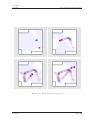
5.4 Implementation in Khepera III . . . . . . . . . . . . . . . . . . . . . . . . 49
5.4.1 Results . . . . . . . . . . . . . . . . . . . . . . . . . . . . . . . . . . 49
6 Conclusion and further work
6.1 Conclusion . . . . . . . . . . . . . . . . . . . .
6.2 Further work . . . . . . . . . . . . . . . . . .
6.2.1 Addition of more follower robots to the
6.2.2 Accumulative errors . . . . . . . . . .
6.2.3 Loss of the leader . . . . . . . . . . . .
. . . .
. . . .
system
. . . .
. . . .
.
.
.
.
.
.
.
.
.
.
.
.
.
.
.
.
.
.
.
.
.
.
.
.
.
.
.
.
.
.
.
.
.
.
.
.
.
.
.
.
.
.
.
.
.
.
.
.
.
.
.
.
.
.
.
.
.
.
.
.
51
51
52
52
52
53
Bibliography
54
Appendices
57
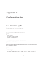
A Configuration files
58
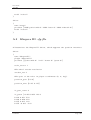
A.1 Simulation .cfg file . . . . . . . . . . . . . . . . . . . . . . . . . . . . . . . 58
A.2 Khepera III .cfg file . . . . . . . . . . . . . . . . . . . . . . . . . . . . . . . 59
B World file
61
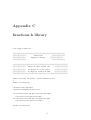
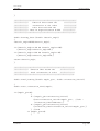
C functions.h library
65
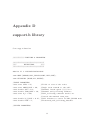
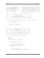
D support.h library
68
VI
List of Figures
1.1 Project flow diagram . . . . . . . . . . . . . . . . . . . . . . . . . . . . . .
4
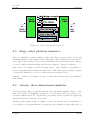
2.1 The server/client control structure of Player/Stage . . . . . . . . . . . . .
7
2.2 Player communication protocol
. . . . . . . . . . . . . . . . . . . . . . . .
8
2.3 Snapshot of a Stage simulation
. . . . . . . . . . . . . . . . . . . . . . . .
9
. . . . . . . . . . . . . . . . . . . . . . .
9
2.4 Snapshot of a Gazebo simulation
2.5 Player viewer visualization tool . . . . . . . . . . . . . . . . . . . . . . . . 10
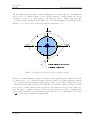
2.6 Odmetry coordinate system . . . . . . . . . . . . . . . . . . . . . . . . . . . 12
3.1 Khepera III robot . . . . . . . . . . . . . . . . . . . . . . . . . . . . . . . . 20
3.2 Ranger sensor of the Khepera III robots . . . . . . . . . . . . . . . . . . . . 20
3.3 Laser characteristics . . . . . . . . . . . . . . . . . . . . . . . . . . . . . . 22
3.4 Field of view of the laser . . . . . . . . . . . . . . . . . . . . . . . . . . . . 23
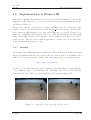
3.5 Khepera III robot with laser range finder . . . . . . . . . . . . . . . . . . . 24
5.1 Division of laser sensor
. . . . . . . . . . . . . . . . . . . . . . . . . . . . 33
5.2 Obstacle avoidance behaviour
. . . . . . . . . . . . . . . . . . . . . . . . . 35
5.3 Robot modes flow diagram . . . . . . . . . . . . . . . . . . . . . . . . . . . 36
5.4 Calculate the slope of a straight line . . . . . . . . . . . . . . . . . . . . . . 37
5.5 Wall following simulation . . . . . . . . . . . . . . . . . . . . . . . . . . . 39
5.6 Important global and local angles
. . . . . . . . . . . . . . . . . . . . . . . 41
VII
5.7 Simulation of the first approach . . . . . . . . . . . . . . . . . . . . . . . . 42
5.8 Follower robot detecting the position of the leader . . . . . . . . . . . . . . 44
5.9 Angle ranges
. . . . . . . . . . . . . . . . . . . . . . . . . . . . . . . . . . 45
5.10 Robot following simulation . . . . . . . . . . . . . . . . . . . . . . . . . . . 46
5.11 Khepera GetYaw function coordinate system . . . . . . . . . . . . . . . . . 48
5.12 Snapshots of the test made with the robots . . . . . . . . . . . . . . . . . . 49
VIII
List of Tables
2.1 Player/Stage main features
. . . . . . . . . . . . . . . . . . . . . . . . . .
5
3.1 Khepera III characteristics . . . . . . . . . . . . . . . . . . . . . . . . . . . 21
5.1 Wall following modes . . . . . . . . . . . . . . . . . . . . . . . . . . . . . . 35
IX
Chapter 1
Introduction
1.1
Introduction
The purpose of this thesis is to develop behavioural algorithms for being implemented in
real mobile robots, in this case Khepera III robots. The project has been made for being
implemented in two robots: one takes the role of the leader robot and the other one is
denominated as the follower robot. Therefore, we can consider algorithms for the real
robot like obstacle avoidance and wall following and algorithms for the follower robot,
like obstacle avoidance and robot following.
Some of this approaches in multi-robot systems include the use of fiducials makers as point
of reference or measure [JSPP08] [KLM06]. This can be very helpful when detecting the
position of the robot on the group, as one robot can automatically know the position of the
others, and therefore, if initial positions are known, its global position in the environment.
Unfortunately, this fiducial tool is only available for simulation, as it is not existing for real
robots. In addition, any similar solution in real robots implies any kind of communication
between them, which we are trying to avoid in this thesis.
The tools that use the robots are a laser range finder and the odometry. The laser range
finder is used to measure the distance to the objects in the environment. This allow the
robot, for example, to know the distance to the closest wall to follow or to the closest
object to avoid. It can also be used to detect the approximate position of the other
robot. It can be said that the laser range finder is the only way to receive data from the
environment. The odometry part is used for sending motion orders to the robot motors
and also for calculate the current orientation of the robot.
1
Final Thesis
July 2010
Introduction
Another important factor to consider is that results in simulation will vary from real
results, as there are more factors to take in account when working with physical robots.
These factors include inaccuracy of the laser and the position proxy measures, nonexact response of the motors, wheel slipping, accumulative errors in sensors . . . Moreover,
there are a few functions from the odometry system that works with no problems in the
simulation environment but that are not available when implemented in Khepera robots.
That reduces the range of options available when looking for a solution, and makes the
simulation code being made from the functions available for the real robots.
1.2
Background
The use of multi-robot teams working together have lots of advantages in front of singlerobot systems. They can be used for environment exploration and mapping, with one
ore more robots taking data from the scenario. One of the advantages of this systems is
that they are more robust, because if one robot fails, the rest of then can keep doing the
assigned task.
The above-mentioned tasks has been implemented, for example, in the GUARDIANS and
View-Finder projects, both developed at Sheffield Hallam University in collaboration with
several European partners, including South Yorkshire Fire and Rescue Services [GUA]
[Vie]. These robots will assist in the search and rescue in dangerous circumstances by
ensuring the communication link and helping the human team to estimate the safety of
the path they are taking and the best direction to follow.
Non-communicative approaches are also wide used in robotics. The groups of robots
can operate together for accomplish a goal, but without sharing any data or sending
information [JRK04]. This concept has also the advantage of the high reliability, as if
one robot fail the others will keep working as they are not using the data from the failed
robot to do its task.
Taking in account all this information, I have tried to create two separate algorithms
using minimum physical resources (taking data only a laser sensor and the odometry) to
realize wall following, obstacle avoidance and robot following algorithms.
1.3
Motivation
The main motivation for develop this thesis is to create the aforementioned algorithms for
their implementation in real robots. There are lots of thesis and projects that rely only
in simulation codes, assuming that all the data they use is ideal, without considering the
David Arán
Page 2
Final Thesis
July 2010
Introduction
non-linearities of the real systems. Likewise, they use some functions and features that
don’t exist or are very difficult to implement in physical systems.
Also, the Department had the desire of the implementation of this algorithms in the
Khepera III robots and the URG-04LX UG01 laser range finders that they own, so all the
efforts were focused to develop the best possible code with the features and characteristics
of the available hardware .
1.4
Objectives/deliverables
The main objectives of this dissertation are the followings:
• Introduction and comprehension of Linux and Player/Stage software.
• Research of information for the correct development of the thesis.
• Develop of navigation algorithms (wall following and obstacle avoidance) for the
leader robot, using laser and odometry in Player/Stage.
• Develop of following algorithms (robot following and obstacle avoidance) for the
follower robot, using laser and odometry in Player/Stage.
• Field tests of the final codes in physical Khepera III robots.
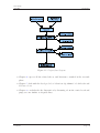
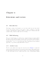
1.5
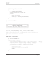
Project flow diagram
This flow diagram of the activities made in this thesis can be seen in the figure 1.1
1.6
Thesis guideline/structure
This thesis is organized as follows:
• Chapter 2 introduces and explains all the characteristics and peculiarities of the
Player/Stage software used for run programs in the robots and for make simulation
test.
• Chapter 3 shows the hardware devices used in the implementation of the code and
its characteristics.
David Arán
Page 3
Final Thesis
July 2010
Introduction
Figure 1.1: Project flow diagram
• Chapter 4 exposes all the related theory and literature consulted in the research
phase.
• Chapter 5 deals with the developed robot behaviour algorithms for both leader and
follower robots.
• Chapter 6 concludes the the dissertation by discussing about the carried work and
purposes some further work guide-lines.
David Arán
Page 4
Chapter 2
Player/Stage
2.1
Introduction
The Player/Stage software is a project to provide free software for research into robotics
and sensor systems. Its components include the Player network server and Stage and
Gazebo robot platform simulators. The project was founded in 2000 by Brian Gerkey,
Richard Vaughan and Andrew Howard at the University of Southern California at Los
Angeles [Vau00], and is widely used in robotics research and education. It releases its
software under the GNU General Public License with documentation under the GNU
Free Documentation License. Also, the software aims for POSIX compilance [sou].
2.1.1
Features
These are some features of the Player/Stage software (table 2.1)
Developers
Latest release
Operating systems
Languages supported
License
Website
Brian Gerkey, Richard Vaughan and Andrew Howard
Player 3.0.2, June 28, 2010
Linux, Mac OS X, Solaris, BSD
C, C++, Java, Tcl, Python
GNU General Public Licence
http://www.player.sourceforge.net
Table 2.1: Player/Stage main features
5
Final Thesis
July 2010
Player/Stage
The software is designed to be language and platform independent, if the language support
TCP sockets and the platform has a network connection to the robot, respectively. This
gives the user freedom to use the most suitable tools for each project. It also allows
support of multiple devices in the same interface, providing high flexibility.
The code made for Player can be simulated in a virtual environment thanks to the Stage
simulation tool, in which the robot and the rest of the environment are simulated in a 2D
representation. There are several advantages simulating the code before implement it on
physical systems. Here are some of them:
• Evaluating, predicting and monitoring the behavior of robot.
• Fastening error finding the implemented control algorithm.
• Reducing testing and development time.
• Avoiding robot damage and operator injures due to control algorithm failure, which
indirectly reducing robot repair cost and medical cost.
• Offering data access that is hard to be measured on real mobile robot.
• Allowing testing on several kinds of mobile robots without need of significant
adaptation of the implemented algorithm.
• Easy switching between a simulated robot and a real one.
• Providing high probability of getting success when implemented on real robot if the
algorithm tested in simulation is proved to be successful.
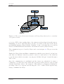
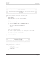
The communication protocol between the parts of the system is made via TCP protocol,
as shown in figure 2.1
Player uses a Server/Client structure in order to pass data and instructions the user’s
code the robot’s hardware or the simulated robots. Player is a server, and a device on the
robot (real or simulated) is subscribed as a client to the server via a thing called a proxy.
This concepts will be explained in depth in the next sections.
2.2
Player, network server
Player is a Hardware Abstraction Layer. It communicates with the devices of the robot,
such as ranger sensors, motors or camera via an IP network, and allows the user’s code
to control them, saving the user all the robot’s work. The code communicates with the
David Arán
Page 6
Final Thesis
July 2010
Player/Stage
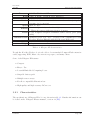
Figure 2.1: The server/client control structure of Player/Stage when used as a simulator
or in physical robots
robot via a TCP socket, sending data to the actuators and receiving it from the sensors.
Simplifying, it can be said that Player gets the code made by the user in the chosen
programming language (Player Client), “translate” it into orders that the robot and its
devices can understand and send them to the mentioned devices (Player Server).
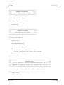
The communication protocol used by Player can be seen in figure 2.2. The process works
as follows.
Firstly, the Player client establishes communication with the server (step 1). As has been
said, there are different connection points for each robot and devices, so the client has
to say the server which ones want to use (step 2). All this “dialogue” is made through a
TCP socket.
Once the communication is established and the devices are subscribed, it starts a
continuous loop, where the server sends data received from the sensors to the program
and the client sends orders to the actuators. This endless loop happens at high speed,
providing a fast robot response and allowing the code to behave in the expected way,
trying to minimize the delays.
David Arán
Page 7
Final Thesis
July 2010
Player/Stage
Figure 2.2: Player communication protocol
2.3
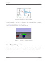
Stage, robot platform simulator
Stage is a simulation software, which together with Player recreates mobile robots and
determined physical environments in two dimensions. Various physics-based models for
robot sensors and actuators are provided, including sonar, laser range finder, camera,
colour blob finder, fiducial tracking and detection, grippers, odometry localization . . .
Stage devices are usually controlled through Player. Stage simulates a population of
devices and makes them available through Player. Thus, Stage allows rapid prototyping
of controllers destined for a real robot without having a physical device.
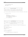
In figure 2.3 there is an example of some robots moving and interacting in a simulated
environment.
2.4
Gazebo, three dimensional simulator
The Player/Stage suite is completed with the 3D environment simulator Gazebo. Like
Stage, it is capable of simulating a population of robots, sensors and objects, but does so
in a three-dimensional world. It generates both realistic sensor feedback and physically
plausible interactions between objects [Gaz].
Client programs written using one simulator can be used in the other one with little or
no modification. The main difference between these two simulators is that while Stage is
David Arán
Page 8
Final Thesis
July 2010
Player/Stage
Figure 2.3: Snapshot of a Stage simulation
designed to simulate a very large robot population with low fidelity, Gazebo is designed
to simulate a small population with high fidelity.
Figure 2.4 shows how a Gazebo environment looks like.
Figure 2.4: Snapshot of a Gazebo simulation
2.5
Player/Stage tools
In this section, the main features and tools provided by Player/Stage will be explained,
like the playerv sensor visualization tool, client libraries, proxies and some Stage tools.
David Arán
Page 9
Final Thesis
July 2010
2.5.1
Player/Stage
Sensor visualization: playerv
Player provides a sensor visualization tool called player viewer (playerv ), which gives the
possibility of visualization of the robot sensors, both in simulation and in real robots.
Let’s explain how playerv works with a simulated robot. Once Player opens the
configuration file (explained in 2.6), the application is “listening” for any program or
code. After that, the program can be opened typing in shell (if working in Linux) the
next command:
-$ playerv
Then, a window is opened, where all the available devices can be shown, and even the
robot can be moved through the environment if the position device is subscribed. For
instance, figure 2.5 shows a robot in which the sonar device is subscribed. In this case,
only one robot is used, calling then playerv the default port 6665. If there were more
robots, the ports wanted to call each robot should be specified in the configuration file,
as shown in the next example.
Figure 2.5: Player viewer visualization tool
driver
(
name "stage"
provides ["6665:position2d:0" "6665:laser:0" "6665:sonar:0"]
model "robot"
)
The driver is called “stage” because it is calling a simulated robot using the 6665 port,
which has position control, laser and sonar sensors. The name of the model is “robot”.
Now, if one wants to visualize this specific robot, the line to type in shell is:
David Arán
Page 10
Final Thesis
July 2010
Player/Stage
-$ playerv -p 6665
With “-p 6665 ”, we are telling player that the device to use is the one defined in the
configuration file in the port 6665. Therefore, if more robots are needed, they can be
defined with the successive port numbers 6666, 6667 . . .
The above mentioned shell commands are used in simulated environments. For using
playerv in real robots, slightly different changes should being made. The configuration
file should be adequate for its use in physical systems and have to be run in the robot.
The shell line to type while Player is “listening” presents this aspect:
-$ playerv -h robotIP
With this command playerv is run in a host (hence -h) which IP number is robotIP. Hence,
the robot devices actions and measurements can be monitored in the same way than in
the simulation, presenting a similar presentation as in figure 2.5.
2.5.2
Client libraries
When using the Player server (whether with hardware or simulation), client libraries can
be used to develop the robot control program. Libraries are available in various languages
to facilitate the development of TCP client programs.
There are three available libraries, although more third-party contributed libraries can be
found at [lib].
• libplayerc, library for C language
• libplayerc py , library for Python
• libplayerc++, library for C++
As the code use for develop the algorithms is c++, the library used was libplayerc++.
2.5.3
Proxies
The C++ library is built on a ”service proxy” model in which the client maintains local
objects that are proxies for remote services. There are two kinds of proxies: the special
David Arán
Page 11
Final Thesis
July 2010
Player/Stage
server proxy PlayerClient and the various device-specific proxies. Each kind of proxy
is implemented separately. The user first creates a PlayerClient proxy and uses it to
establish a connection to a Player server. Next, the proxies of the appropriate devicespecific types are created and initialized using the existing PlayerClient proxy. There are
thirty-three different proxies in the version used for this dissertation (2.1.2), but it have
been used only three of them: PlayerClient proxy, Position2d proxy and Laser proxy.
PlayerClient proxy is the base class for all proxy devices. Access to a device is provided
by a device-specific proxy class. These classes all inherit from the Client proxy class which
defines an interface for device proxies.
2.5.3.1
Position2d proxy
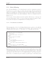
The class Position2dProxy is the C++ proxy in Player which handles robots position
and motion. It calculates the X, Y positions and angle coordinates of the robot and
returns position information according to the client programs demands. The odometry
system takes negative angles clockwise and positive counter-clockwise, as can be seen in
the odometry coordinate system in fig 2.6.
Figure 2.6: Odmetry coordinate system
Hereafter some of the main commands available in the proxy are shown.
ResetOdometry() Reset odometry to (0,0,0) Although this command could be very
useful when working with global/local coordinates, it has been proved not to work
properly, specially in physical robots.
David Arán
Page 12
Final Thesis
July 2010
Player/Stage
SetOdometry (double aX, double aY, double aYaw) . Sets the odometry to the
pose (x, y, yaw). In the same way as ResetOdometry, this function does not work
in a good way, being then usefulness.
GetXPos Get current X position.
GetYPos Get current Y position.
GetYaw Get current angular position.
SetSpeed(Xspeed, YawSpeed) Send commands to motor with linear and angular
speed.
As it will be seen in the chapter 5.3, GetYaw function will be a key function for the success
of the algorithm.
2.5.3.2
Laser proxy
One of the most important proxies used to develop this thesis algorithms is the LaserProxy
provided by Player. In fact, is the only way the robot has to interact with the environment.
It plays major role in wall following and collision avoiding processes, as well as in robot
following algorithm. Player provides standard set of commands to control LaserProxy
data such as:
GetCount() Get the number of points scanned.
GetMaxRange() Maximum range of the latest set of data, in meters.
GetRange(Index) Get the range of the beam situated in the “Index” position.
GetBearing(Index) Get the angle of the beam situated in the “Index” position.
The main properties of the laser device will be explained in chapter 3.
2.5.4
Stage tools
Stage provides a graphical interface with the user (GUI) for watching the proper working
of the simulation developed in Player. To simplify this work, Stage provides some tools.
The environment where the robots are operating in Stage is called “world”, these “worlds”
are bitmap files. So, these files can be created and changed with any drawing software.
David Arán
Page 13
Final Thesis
July 2010
Player/Stage
All the white spaces will be considered as open spaces while different colors are considered
as obstacles or walls.
It is possible to zoom by clicking the right mouse button and moving in any part of the
map. A circumference in the middle of the map will appear. By dragging the mouse
towards the centre “zoom in” will be achieved and, by reversing this operation, “zoom
out” will be performed. With the left-click in any part of the map it is possible to move
the map “Up-Down-Right-Left” accordingly.
Also it is possible to change the robot position by dragging the robot with the
left mouse button; and changing its orientation with the right button. Besides the
aforementioned, it is possible to save an image of the current display of the map. Select
File→Screenshot→Single Frame. To save an image sequence with a fixed interval, use
the option File→Screenshot→Multiple Frames selecting previously the interval duration
in the same menu. The image is saved in the current working directory.
Other useful menu options can be found in the tab “view”, for example, it is possible to
represent the grid, view the path taken by the robot with the option Show trails (useful
to identify where the robot has been before), view the robot position lines projected on
the global frame of reference, view velocity vectors, display laser data and so on.
2.6
Programming in Player
This section is an overview about the different files present on a Player/Stage project.
These are:
• World files (.world )
• Configuration files (.cfg)
• Make files
• Include files (.inc)
• .h files
• Main program file
• Bitmaps
Some of this files will be explained in the next sub-sections.
David Arán
Page 14
Final Thesis
July 2010
2.6.1
Player/Stage
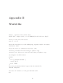
World file
The .world file tells Player/Stage what things are available to put in the simulated world.
In this file the user describes the robots, any items which populate the world and the
layout of the world. Parameters such as resolution and time step size are also defined.
The .inc file follows the same syntax and format of a .world file but it can be included.
So if there is an object in the world wanted to be used in other worlds, such as a model
of a robot, putting the robot description in a .inc file just makes it easier to copy over,
it also means that if a robot description is wanted to be changed, then the only thing
needed to do is to change it in one place and your multiple simulations are changed too.
2.6.2
Configuration file
The .cfg file is what Player reads to get all the information about the robot. This file
tells Player which drivers it needs to use in order to interact with the robot, if the user
is using a real robot these drivers are built in to Player , alternatively, if the user wants
to make a simulation, the driver is always Stage. The .cfg file tells Player how to talk to
the driver, and how to interpret any data from the driver so that it can be presented into
the user code.
Items described in the .world file should be described in the .cfg file if the user wants the
code to be able to interact with those item (such as a robot), if the code is not needed to
interact with the item then this is not necessary. The .cfg file does all this specification
using interfaces and drivers.
For each driver we can specify the following options:
name: The name of a driver to instantiate, (required).
plugin: The name of a shared library that contains the driver, (optional).
provides: The device address or addresses through which the driver can be accessed. It
can be combination of strings (required).
requires: The device address or addresses to which the driver will subscribe. It can be
a combination of strings, (optional).
An simple example of this is shown below:
2.6.3
David Arán
Makefile
Page 15
Final Thesis
July 2010
Player/Stage
driver
(
name ‘‘stage’’
provides [‘‘6665:position:0’’
‘‘6665:sonar:0’’
‘‘6665:blobfinder:0’’
‘‘6665:laser:0’’]
)
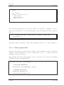
Once the Player/Stage files are ready, the client code should be compiled in order to
create the executable file to run. For that purpose, the following line should be typed in
shell:
g++ -o example ‘pkg-config --cflags playerc++‘ example.cc ‘pkg-config
--libs playerc++‘
That will compile a program to a file called example from the C++ code file example.cc.
2.6.4
Main program file
This file is the main code that the user wants to run through Player into the physical
systems or in the simulation. It can be written into C, C++, or Python, as it was
explained in the above sections.
All programs follows the same structure, as the one shown below. It’s also the similar
than in the behaviour explained in 2.1.
int main (int argc, char **argv)
{
// ESTABLISH CONNECTION
PlayerClient robot(gHostname, gPort);
// INSTANTIATE DEVICE
LaserProxy lp(&robot,0);
PositionProxy pp(&robot,0);
David Arán
Page 16
Final Thesis
July 2010
Player/Stage
While(1)
{
// DATA ACQUISITION
robot.Read();
// PROCESS DATA
// send command
}
}
In first place, the PlayerClient subscribes a device called robot, with gHostaname adress
and situated in the port gPort. Secondly, the sensors and devices of the robot are
subscribed as well, in this case Laser and Position proxies. Then starts the think-actloop, where the code interacts with the different devices. With the robot.Read command,
the data from the robot is acquired, and after being processed the orders to the actuators
are sent.
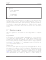
2.7
Running program
This section explains how to run the client code into the Stage simulation or in physical
robot.
Stage simulation
For run the client code into a Stage simulation, the first thing is to open the configuration
file on a shell. This file should be linked to the .world file, where the simulation objects
are defined. Once this is done, Player is listening for any binary file to be executed. This
file is generated from the main client file (in this this case, from a .cc file) as explained in
the section 2.6.3. The only thing to is do is run it using the syntax ./file. After that, the
code would be run in the simulated world.
Physical robot
Te process for run the client code into physical systems is slightly different. The way
here explained is for the Khepera robots used in this project. The first thing that should
be done is connect the computer with the robot or robots via wireless. Once the link
is established, a secure connection is made from the computer to the robot via SSH
[BSB05]. Once inside the robot, the configuration file should be run (notice that this file
will be different than the ones for simulations). Then, the robot will be “listening” for
David Arán
Page 17
Final Thesis
July 2010
Player/Stage
any program do be run. So, the user should run it from a shell window in its computer,
specifying the IP of the robot, as said in the previous sections.
David Arán
Page 18
Chapter 3
Robot and laser characteristics
3.1
Introduction
This chapter explains the main features and characteristics of the robot utilized for
accomplish this project. The robots are Khepera III, from the Swiss company K-Team
[kte] and the laser used is the Hokuyo URG-04LX Laser, from the Japanese company
Hokuyo Automatic Co.,LTD [Hok].
3.2
Khepera III
The Khepera III is a small differential wheeled mobile robot( 3.1). Features available
on the platform can match the performances of much bigger robots, with a upgradable
embedded computing power using the KoreBot system, multiple sensor arrays for both
long range and short range object detection, swappable battery pack system for optimal
autonomy, and differential drive odometry. The Khepera III architecture provides
exceptional modularity, using an extension bus system for a wide range of configurations.
The robot base can be used with or without a KoreBot II board. Using the KoreBot II,
it features a standard embedded Linux Operating System for quick and easy autonomous
application development. Without the KoreBot II, the robot can be remotely operated,
and it is easily interfaced with any Personal Computer. Remote operation programs can
be written with Matlab, LabView, or with any programming language supporting serial
19
Final Thesis
July 2010
Robot and laser characteristics
Figure 3.1: Khepera III robot
port communication. In this project, the robot was used with the KoreBot board, so that
the configuration files were run on it, thanks to its embedded Linux.
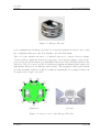
The robot base includes an array of 9 infrared Sensors for obstacle detection (figure
3.2,a) as well as 5 ultrasonic Sensors for long range object detection (figure 3.2,b). It also
proposes an optional front pair of ground Infrared Sensors for line following and table edge
detection. The robot motor blocks are Swiss made quality mechanical parts, using very
high quality DC motors for efficiency and accuracy. The swappable battery pack system
provides an unique solution for almost continuous experiments, as an empty battery can
be replaced in a couple of seconds.
a) Infrared
b) Sonar
Figure 3.2: Ranger sensor of the Khepera III robots
David Arán
Page 20
Final Thesis
July 2010
Robot and laser characteristics
Processor
RAM
Flash
Motion
DsPIC 30F5011 at 60MHz
4 KB on DsPIC, 64 MB KoreBot Extension
66 KB on DsPIC, 32MB KoreBot Extension
2 DC brushed servo motors with incremental encoders (∼22 pulses
per mm of robot motion)
Speed Max: 0.5 m/s
11 infrared proximity and ambient light sensors
Sensors
5 Ultrasonic sensors with range 20cm to 4 meters
Power Power Adapater Swapable Lithium-Polymer battery pack (1400
mAh)
Communication Standard Serial Port, up to 115kbps USB communication with
KoreBot Wireless Ethernet with KoreBot and WiFi card
Size Diameter: 130 mm Height: 70 mm
Weight 690 g
Table 3.1: Khepera III characteristics
Trough the KoreBot II, the robot is also able to host standard Compact Flash extension
cards, supporting WiFi, Bluetooth, extra storage space, and many others.
Some of the Khepera III features:
• Compact
• Easy to Use
• Powerful Embedded Computing Power
• Swapable battery pack
• Multiple sensor arrays
• KoreBot compatbible Extension bus
• High quality and high accuracy DC motors
3.2.1
Characteristics
The specifications of Khepera III robot are shown in table 3.1. Further information can
be found on the “Khepera III user manual”, version 2.2 [FG].
David Arán
Page 21
Final Thesis
July 2010
3.3
Robot and laser characteristics
Hokuyo URG-04LX Laser
A laser ranger is an optional component which can be added to the Khepera robot, and
gives reliable and precise length measurements. This device mechanically scans a laser
beam, producing a distance map to nearby objects, and is suitable for next generation
intelligent robots with an autonomous system and privacy security. The URG-04LX is a
lightweight, low-power laser rangefinder.
3.3.1
Characteristics
This sensor offers both serial (RS-232) and USB interfaces to provide extremely accurate
laser scans. The field-of-view for this detector is 240 degrees and the angular resolution
is 0.36 degrees with a scanning refresh rate of up to 10Hz. Distances are reported from
20mm to 4 meters. Power is a very reasonable 500mA at 5V. Some of its characteristics,
features and its physical dimensions scheme are shown in figure 3.3.
Figure 3.3: Laser characteristics
David Arán
Page 22
Final Thesis
July 2010
Robot and laser characteristics
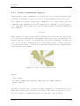
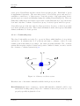
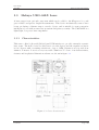
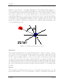
More info can be found in [Hok08], [Hl].The Laser range finder covers a range of 240
degrees. Note that the angles are measured positive counter clockwise and negative in
clockwise. The 120 degrees of area covering back side of the robot is considered as the
blind area as the laser does not operate in that area. Figure 3.4 shows the scheme of the
laser range.
Figure 3.4: Field of view of the laser
3.4
Robot with laser
The Hokuyo URG-04LX laser is connected to the Khepera III robot via USB. In the
configuration file that should be open in the Khepera, there is an instantiation of the
laser driver, as shown below:
driver
(
name "urglaser"
provides ["laser:0"]
port "/dev/ttyACM0"
)
It accesses a device called urglaser, which provides a laser ranger connected in the route
/dev/ttyACM0. The whole configuration file is shown in the appendix A.
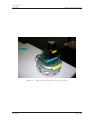
The resultant robot-laser system can be seen in figure 3.5.
David Arán
Page 23
Final Thesis
July 2010
Robot and laser characteristics
Figure 3.5: Khepera III robot with laser range finder
David Arán
Page 24
Chapter 4
Literature and review
4.1
Introduction
This chapter contains a brief discussion over some basic technologies and other related
projects and researches worked by other parties to make a foundation of the main
objectives of this dissertation, which are multi-robot behaviours for different tasks such
as wall following, obstacle avoidance and robot following.
4.2
Wall following
The goal of wall following robot behaviour is to navigate through open spaces until it
encounters a wall, and then navigate along the wall at some fairly constant distance.
The successful wall follower should traverse the entire environment at least once without
straying either too close, or too far from the walls. The following subsections show different
approaches to de problem by using different kind of sensors.
4.2.1
Artificial vision
The idea of the artificial vision approach comes from source [DRGQ07]. A visual and
reactive wall following behaviour can be learned by reinforcement. With artificial vision
the environment is perceived in 3D, and it is possible to avoid obstacles that are invisible
to other sensors that are more common in mobile robotics. Reinforcement learning
25
Final Thesis
July 2010
Literature and review
reduces the need for intervention in behaviour design, and simplifies its adjustment to
the environment, the robot and the task. In order to facilitate its generalization to
other behaviours and to reduce the role of the designer, it can be used a regular imagebased codification of states. Even though this is much more difficult, its implementation
converges and is robust.
4.2.2
Neuro-fuzzy controllers
Neuro-fuzzy refers to combinations of artificial neural networks and fuzzy logic. In
[SKMM10], an intelligent wall following system that allows an autonomous car-like mobile
robot to perform wall following tasks is used. Soft computing techniques were used to
overcome the need of complex mathematical models that are traditionally used to solve
autonomous vehicle related problems. A neuro-fuzzy controller is implemented for this
purpose, which is designed for steering angle control, and is implemented with the use
of two side sensors that estimate the distance between the vehicle front side and the
wall, and the distance between the vehicle back side and the wall. These distances get
then inputted to a steering angle controller, which as a result outputs the appropriate
real steering angle. A neuro fuzzy controller overcomes the performance of the previously
implemented fuzzy logic based controller, and significantly reduces the trajectory tracking
error, but at the expense of using more DSP resources causing a slower throughput time.
This autonomous system can be realized on an FPGA platform, which has the advantage
of making the system response time much faster than software-based systems.
4.2.3
Emitting signal sensor
In [Jon] is presented a set consisting of a robot obstacle detection system which navigates
with respect to a surface and a sensor subsystem aimed at the surface for detecting the
surface. The sensor subsystem includes an emitter which sends out a signal having a field
of emission and a photon detector having a field of view which intersects with that field of
emission at a region. The subsystem detects the presence of an object proximate to the
mobile robot and determines a value of a signal corresponding to the object. It compares
the obtained value to a predetermined value, moves the mobile robot in response to the
comparison, and updates the predetermined value upon the occurrence of an event.
4.2.4
Autonomous robots
Autonomous robots are electromechanical devices that are programmed to achieve several
goals. They are involved in a few tasks such as moving and lifting objects, gathering
David Arán
Page 26
Final Thesis
July 2010
Literature and review
information related to temperature and humidity, and follow walls. From a system’s
engineering point of view, a well designed autonomous robot has to be adaptable enough
to control its actions. In addition, it needs to perform desired tasks precisely and
accurately. The source of this idea is in the paper [Meh08]. The robot follows a wall
using a PIC 18F4520 microcontroller as its brain. PIC 18F4520 receives input from
Ultrasonic Distance Meter (UDM). Some computations are performed on this input and
a control signal is generated to control the robot’s position. This control signal is generated
through a PD (Proportional and Derivative) controller, which is implemented in the
microcontroller. Afterwards, microcontroller is programmed in C language using a CCS
(A Calculus of Communicating Systems) compiler.
4.2.5
3D Laser Rangefinder
The technical report [MA02] shows a technique for real-time robot navigation. Offline planned trajectories and motions can be modified in real-time to avoid obstacles,
using a reactive behaviour. The information about the environment is provided to the
control system of the robot by a rotating 3D laser sensor which have two degrees of
freedom. Using this sensor, three dimensional information can be obtained, and can be
used simultaneously for obstacle avoidance, robot self-localization and for 3D local map
building. Obstacle avoidance problem can also be solved with this kind of sensor. This
technique presents a great versatility to carry out typical tasks such as wall following,
door crossing and motion in a room with several obstacles.
4.2.6
Odometry and range data
In [BPC02], an enhanced odometry technique based on the heading sensor called “clinogyro” that fuses the data from a fibre optic gyro and a simple inclinometer is proposed.
In the proposed scheme, inclinometer data are used to compensate for the gyro drift due
to rollpitch perturbation of the vehicle while moving on the rough terrain. Providing
independent information about the rotation (yaw) of the vehicle, clino-gyro is used to
correct differential odometry adversely affected by the wheel slippage. Position estimation
using this technique can be improved significantly, however for the long term applications
it still suffers from the drifts of the gyro and translational components of wheel skidding.
Fusing this enhanced odometry with the data from environmental sensors (sonars, laser
range finder) through Kalman filter-type procedure a reliable positioning can be obtained.
Obtained precision is sufficient for navigation in underground mining drifts. For open-pit
mining applications further improvements can be obtained by fusing proposed localization
algorithm with GPS data
David Arán
Page 27
Final Thesis
July 2010
4.3
Literature and review
Obstacle avoidance
The obstacle avoidance algorithm is one of the basic and common behaviour for almost
every autonomous robot systems. Here are shown some approaches to this problem.
4.3.1
Fuzzy control
Fuzzy control algorithms are used sometimes for obstacle avoidance behaviour [JXZQ09].
Autonomous obstacle avoidance technology is a good way to embody the feature of
robot strong intelligence in intelligent robot navigation system. In order to solve the
problem of autonomous obstacle avoidance of mobile robot, an intelligent model is used.
Adopting multisensor data fusion technology and obstacle avoidance algorithm based on
fuzzy control, a design of intelligent mobile robot obstacle avoidance system is obtained.
The perceptual system can be composed of a group of ultrasonic sensors to detect the
surrounding environment from different angles, enhancing the reliability of the system on
the based of redundant data between sensors, and expanding the performance of individual
sensors with its complementary data. The processor receives information from perceptual
system to calculate the exact location of obstructions to plan a better obstacle avoidance
path by rational fuzzy control reasoning and defuzzification method.
4.3.2
Probabilistic approach
In this approach, emerged after consult [BLW06], autonomous vehicles need to plan
trajectories to a specified goal that avoid obstacles. Previous approaches that used a
constrained optimization approach to solve for finite sequences of optimal control inputs
have been highly effective. For robust execution, it is essential to take into account the
inherent uncertainty in the problem, which arises due to uncertain localization, modelling
errors, and disturbances.
Prior work has handled the case of deterministically bounded uncertainty. This is an
alternative approach that uses a probabilistic representation of uncertainty, and plans the
future probabilistic distribution of the vehicle state so that the probability of collision
with obstacles is below a specified threshold. This approach has two main advantages;
first, uncertainty is often modelled more naturally using a probabilistic representation
(for example in the case of uncertain localization); second, by specifying the probability
of successful execution, the desired level of conservatism in the plan can be specified in a
meaningful manner.
David Arán
Page 28
Final Thesis
July 2010
Literature and review
The key idea behind the approach is that the probabilistic obstacle avoidance problem
can be expressed as a Disjunctive Linear Program using linear chance constraints. The
resulting Disjunctive Linear Program has the same complexity as that corresponding to
the deterministic path planning problem with no representation of uncertainty. Hence the
resulting problem can be solved using existing, efficient techniques, such that planning
with uncertainty requires minimal additional computation.
4.3.3
Camera
Other interesting approach for obstacle avoidance is the use of a a vision based system
using a camera [WKPA08]. The technique is based on a single camera and no further
sensors or encoders are required. The algorithm is independent of geometry and even
moving objects can be detected. The system provides a top view map of the robot’s field of
view in realtime. First, the images are segmented reasonably. Ground motion estimation
and stereo matching is used to classify each segment either belonging to the ground plane
or belonging to an obstacle. The resulting map is used for further navigational processing
like obstacle avoidance routines, path planning or static map creation.
4.4
Robot following
Here are some ideas and theories found about robot following formation.
4.4.1
Attraction-repulsion forces
The background of this section comes from the source [BH00], where the main idea of
applying the potential functions is developed.
A potential function is a differentiable real-valued function U : ℜm → ℜ, in our case
m will be equal to 1. The value of a potential function can be viewed as energy and
therefore the gradient of the potential is force. The gradient is a vector which points in
the direction that locally maximally increases U.
There is a relationship between work and kinetic energy. Work is defined in physics as
the result of a force moving an object a distance (W = F d). But the result of the force
being applied on the object also means that the object is moving with some given velocity
(F = ma). From those two equations, it can be shown that work is equivalent to kinetic
energy: UKE = 21 mv 2 . When U is energy, the gradient vector field has the property that
work done along any closed path is zero.
David Arán
Page 29
Final Thesis
July 2010
4.4.2
Literature and review
Selfmade follower
This idea come from [FFB05]. In this approach, the control law of the follower robot
includes the states of the leader robot. This is a drawback for implementing the control
laws on real mobile robots. To overcome this drawback, a new follower’s control law
is purposed, called the self-made follower input, in which the state of the leader robot
is estimated by the relative equation between the leader and the follower robots in the
discrete-time domain. On the other hand, a control law of the leader robot is designed
with a chained system to track a given reference path.
4.5
Localization problem
For numerous tasks a mobile robot needs to know “where it is” either at the time of
its current operation or when specific events occur. The Localization problem can be
divided mainly in to two sub sections, Strong Localization and Weak Localization [GM00].
Estimating the robots position with respect to some global representation of space is
called Strong Localization. The Weak Localization is mainly based on the correspondence
problem, and in this case complete qualitative maps can be constructed using Weak
Localization.
There are many approaches to solve localization problem such as dead reckoning, simple
landmark measurements, landmark classes, Triangulation, and Kalman filtering [GM00].
There are many researches dedicated to investigate on robot localization such as Monte
Carlo, the bounded uncertainty approach, and by using Bayesian statistic. Basically
the Bayesian approach is the widely used robot localization method. Not only for the
localization, but also for building maps the Bayesian rule is widely used.
4.5.1
Odometry Sensors
Mobile robots often have odometry sensors; them calculate how far the robot has traveled
based on how many wheel rotations took place. These measurements may be inaccurate
due to many reasons such as wheel slipping, surface imperfections, and small modeling
errors. For example, suppose a bicycle wheel of a 2 meter circumference has turned 10
revolutions, then the odometry reading is 10 and the calculated answer would be 20m.
Some of the problems of the odometry sensors can be listed as below:
• Weak supposition (Slide errors, accuracy, etc)
David Arán
Page 30
Final Thesis
July 2010
Literature and review
• Methodical errors
· Different wheel diameter problems
· Wheel alignment problems
· Encoders resolution and sampling problems
• Non-Systematic errors
· Wheel Slides problems
· Floor Roughness problems
· Floor Object problems
4.5.2
Laser range finders
Laser scanners mounted on mobile robots have recently become very popular for various
indoor robot navigation tasks. Their main advantage over vision sensors is that they are
capable of providing accurate range measurements of the environment in large angular
fields and at very fast rates [BAT03]. Laser range finders are playing a great role not
only in 2D map building but in 3D map building too. The laser range finder sensor data
can be also used for variety of tasks such as wall following and collision avoiding. There
are many projects and research work have used laser range finders. The efficiency and
the accuracy of the laser range finder depends on many factors such as: transmitted laser
power, carrier modulation depth, beam modulation frequency, distance from the target,
atmospherics absorption coefficient, target average reflectivity, collecting efficiency of the
receiver, and pixel sampling time [BBF+ 00].
ToDo: revisar los = en la bibliografia
David Arán
Page 31
Chapter 5
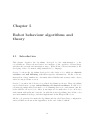
Robot behaviour algorithms and
theory
5.1
Introduction
This chapter describes the algorithms developed for the implementation of the
robotb́ehaviour. This work was carried once understood the operation of Player/Stage
and after the research and investigation stage. With all the collected information, the
developing of the code started, using structured C++ language.
Section 5.2 shows the algorithms developed for the leader robot, which are obstacle
avoidance and wall following, with their respective sub-functions. All the codes are
first tried in a Stage simulation to determine their reliability and accuracy and to detect
and solve any problems or errors.
Section 5.3 is where the follower robot related algorithms are shown. These algorithms
can be divided in two groups: robot following and obstacle avoidance. For the robot
following algorithm, first it was made a code assuming there is no environment, just the
leader and the follower robots. After, it was improved for make the robot to move in a
environment with walls and obstacles. As with the leader algorithms, here all the codes
were first simulated in Stage, and after implemented in the Khepera III robots.
All the code generated for make the algorithms and also the Player/Stage configuration
and world files are shown in the appendixes, at the end of this document.
32
Final Thesis
July 2010
5.2
Robot behaviour algorithms and theory
Leader robot
This section explains the main solutions taken for implement the leader robot algorithms.
They can be divided into obstacle avoidance algorithms and wall following algorithms.
The only proxies used for these task are Position2dProxy and LaserProxy.
5.2.1
Obstacle avoidance
This part of the program is maybe the basic behaviour of the robot, because if it fails,
the robot can crash and suffer important damages. Then, it is important its correct
performance for the development of further algorithms.
The main idea of this algorithm is based in the measures taken by the laser ranger. It
is constantly scanning and taking samples of the environment, detecting the obstacles
around them and their distance to the robot. If this distances are smaller than a
determined value (set by the user), then the robot is too close to an obstacle and it
has to stop or change its direction.
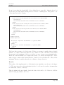
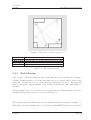
For accomplish that, the field of view of the robot was divided in three part, as seen in
the figure 5.1.
Figure 5.1: Division of laser sensor
David Arán
Page 33
Final Thesis
July 2010
Robot behaviour algorithms and theory
It can be seen that the frontal field of view defined is not very wide, otherwise the robot
would have problems when entering narrow corridors or small spaces. The pseudo code
of the function is the following.
for all laser scans do
if the obstacle is in the right part and closer than detection distance then
sum right part;
if new measure is smaller than the minimum, save new minimum;
end if
if the obstacle is in the central part and closer than detection distance then
sum central part
if new measure is smaller than the minimum, save new minimum;
end if
if the obstacle is in the left part and closer than detection distance then
sum right part
if new measure is smaller than the minimum, save new minimum;
end if
end for
calculate left mean;
calculate right mean;
if left mean < right mean and minimum < stop distance then
turn right
end if
if right mean < left mean and minimum < stop distance then
turn left
end if
The laser take measures of all the scans. When one measure is smaller than a defined
distance, a counter is increased (there is one counter for each of the three areas) and if
the measure is the minimum of those recorded in one area, it saves a new minimum value.
When the scan has finished, it compares the values of both left and right sides. Those
with a bigger counter value means that the obstacle is closer in that side. Then, if the
minimum distance is smaller than the stop distance, change direction.
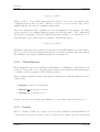
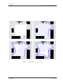
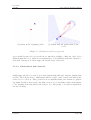
Results
The results of the implementation of this functions in simulation are shown in the figure
5.2. The grey traces show the path taken by the robot. It can be seen how it turns when
it founds and obstacle on its way.
This algorithm is the most simple, but is the basis of the whole code. Next is to add the
wall following algorithm to the code.
David Arán
Page 34
Final Thesis
July 2010
Robot behaviour algorithms and theory
Figure 5.2: Obstacle avoidance behaviour
Search
Wall follow
Left
Right
The robot goes straight looking for a wall
Transit state. It decides which direction to turn
The robot follows a wall on its left
The robot follows a wall on its right
Table 5.1: Wall following modes
5.2.2
Wall following
The objective of this algorithm is to find a wall and follow it in a parallel way, keeping a
certain constant distance to it. At the same time, the avoid obstacle will be active at the
same time, avoiding the robot to crash when the wall changes its slope. The approach
made for keep the constant distance to the wall is calculating the angle with respect to
the wall.
The movement of the robot is based in four behaviour modes, which depends of the laser
measures and the previous mode, as seen in the table 5.1
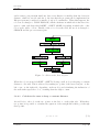
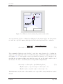
The transit between the different modes are explained in the flow diagram on figure 5.3.
When the code starts running, the robot is in mode SEARCH. The motors are enabled
David Arán
Page 35
Final Thesis
July 2010
Robot behaviour algorithms and theory
and it starts going straight until any laser scan distance is smaller than the detection
distance, which in our case and due to the fact that the program will be implemented in
Khepera systems (considered as small robots) is 25 centimetres. When this happens, the
robot mode changes to WALL FOLLOW, which calculates in which side it has more free
space to turn, and then takes RIGHT or LEFT MODE, depending in which side of the
robot is the wall to follow. Finally, if the robot loses the wall, the mode is changed to
SEARCH and the process starts again.
Figure 5.3: Robot modes flow diagram
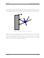
When the robot is in mode RIGHT or LEFT following a wall, it does it keeping a constant
distance to the wall. This is achieved by tanking two points of the laser scan (two on the
left or two on the right side, depending on the mode), and calculating the inclination of
the wall with respect the robot, obtaining then the angle to turn.
5.2.2.1
Calculate the turn to keep a constant distance
As said before, the robot take two points on the left or on the right side. With these
two points, it is possible to calculate the equation of the straight line which goes through
these points:
y =m·x+n
David Arán
(5.1)
Page 36
Final Thesis
July 2010
Robot behaviour algorithms and theory
Once obtained the slope of the line (m), the orientation of the wall with respect to the
robot is known, being possible to calculate the angle to turn in order to keep parallel to
the wall, making m tends to 0. The scheme of figure 5.4 illustrates how the process works.
Figure 5.4: Calculate the slope of a straight line
When the wall is on the right side, the scans situated in the angles 35 and 75 degrees
take the points, while when the wall is in the left, the scans are the ones in 165 and 205
degrees. Using simple trigonometrical relations, and using the equation of the straight
line, the slope of the wall is obtained, knowing then the necessary angle to turn. The
pseudo code of the whole program is the following.
David Arán
Page 37
Final Thesis
July 2010
Robot behaviour algorithms and theory
if mode = Search then
go straight
else
calculate turn rate left/right
if left mean < right mean and mode = Wall follow
mode = Left
calculate the slope of the straight line → turnrate
if right mean < left mean and mode = Wall follow
mode = Right
calculate the slope of the straight line → turnrate
avoid obstacles();
if robot loses the wall
mode = Search
end if
if the obstacle is closer than 25cm and mode = Search then
mode = Wall follow
end if
5.2.3
Simulation
This section shows the result of the simulation of the code in an simulated environment.
The results can be found in figure 5.5. On it, there are four snapshots in of the simulation
in four different times.
Due to simulation results, we can conclude that the robot has a good response. First it
searches for a wall, and when it finds it, it keeps following it without losing it. Therefore,
the simplicity of the approach allows easily its use in other algorithms.
5.3
Follower robot
The next section explains the solutions adopted for the follower robot. The idea is that it
detects the leader robot and follows it. The main behaviour modes of the robot are robot
following and obstacle avoidance. In the same way than in chapter 5.2, this functions
are implemented using the Position2dProxie and the LaserProxie, avoiding the use of any
kind of communication between the robots, having then two independent systems.
David Arán
Page 38
Final Thesis
July 2010
Robot behaviour algorithms and theory
Figure 5.5: Wall following simulation
David Arán
Page 39
Final Thesis
July 2010
5.3.1
Robot behaviour algorithms and theory
Robot following
One of the main difficulties to solve in this dissertation was how to implement a system for
the follower robot to detect other robot using only a laser ranger. The idea was that they
could not use any kind of communication between them, which includes FiducialProxie.
This proxy would make the code easier and the robot response would be more accurate,
but the problem is that it only exists in simulations. there are no fiducials devices for
Khepera robots.
The developing of this algorithm was made through three different stages: a first approach
in an environment with no walls, a second in a regular environment and a third one where
the program was adapted for its implementation in a Khepera III robot.
5.3.1.1
Non-obstacles environment
The fist approach to the robot following behaviour was to create a code with the
supposition that there are not obstacles in the environment. This is, if the laser detects
something, that is the leader robot. The pseudo-code of this approach is the next:
take all laser scans
if any laser beam detects something then
leader detected
calculate relative angle to the leader robot
end if
if follower is facing the leader then
turn rate = 0
else
if robot on the right
turn clockwise until angle difference ≃ 0
if robot on the left
turn counter clockwise until angle difference ≃ 0
end if
if distance to the robot > stop distance then
go forward until distance to the robot < stop distance
end if
Firstly the robot scans all its laser range. If any measure is smaller than 5 meters, which
is the maximum range of the robot, then the robot is detecting the leader. An average
of all the scans detecting the leader is made, and then the relative angle α of the leader
with respect to the front of the robot is calculated with the order GetBearing(index).
After it, the robot calculates its global orientation (β) with respect of the initial position
David Arán
Page 40
Final Thesis
July 2010
Robot behaviour algorithms and theory
using the order GetYaw(). A graphic explanation of both angles is made in figure 5.6.
Once both angles are know, it calculates the difference between them. If the difference is
≃ 0, then the follower is facing the leader and the robot does not turn. On the contrary,
if the angle is different, the robot starts turning right or left (depends where the robot
are) until the difference is ≃ 0. Once the follower faces the leader, it checks the distance
between them. If it is bigger than a parameter called stop distance, then the follower will
go straight to the leader until their distance is equal or smaller than stop distance. All
this process is inside an endless loop, being the robot taking points and measures each
loop and updating the data.
Figure 5.6: Important global and local angles
Simulation
The system was simulated in a world file which map has no wall nor obstacles, only two
robots. The leader is moved in the scenario using playerv and the follower tries to find
it and move to it, as seen in figure 5.7. The blue robot is the leader, while the red is the
follower. At the beginning (image a) both robots are static, because the program is still
not run. When it is run, as the leader is further than the stop distance (in this case 40
centimetres), it turns and moves until its laser measure is smaller than that value (figure
b). As the trails made by the robots shown, when the leader is moving in the environment,
the follower turns facing it and starts following it when the distance to it is smaller than
the limit.
Results
The algorithm is working properly, as the robot follows the leader wherever it goes and
keeps a limit distance to it for avoid any kind of collision. Nevertheless, this approach
David Arán
Page 41
Final Thesis
July 2010
Robot behaviour algorithms and theory
a) System at the beginning, static
b) System with the paths taken by the
robots
Figure 5.7: Simulation of the first approach
is not useful because it does not take in account the possibility of find any other object
different than the robot, while in real systems the robots will finds walls and obstacles to
deal with. Anyway, it is a first approach and the basis of the next.
5.3.1.2
Environment with obstacles
In this approach, the robots move in a environment with walls and obstacles, similar than
real life. The follower have to differentiate what is a wall or and obstacle and what is the
leader robot to follow it. This goal has been accomplished using a movement recognition
algorithm. It will work properly only with one more robot and with a static environment,
so if something is moving, that is the leader robot. The pseudo code and its explanation
are the following.
David Arán
Page 42
Final Thesis
July 2010
Robot behaviour algorithms and theory
stop robot. Laser scan → save in a vector
wait one cycle
scan again → save in a different vector
compare both vectors index by index → substraction
calculate relative angle to the robot
if in any index, any subtraction 6= 0 then
something has moved → it is the leader robot
get laser scans where the leader is → calculate average beam
end if
if any laser beam detects something then
leader detected
calculate relative angle to the leader robot
end if
if follower is facing the leader then
turn rate = 0
else
if robot on the right
turn clockwise until angle difference ≃ 0
if robot on the left
turn counter clockwise until angle difference ≃ 0
end if
if distance to the robot > stop distance then
go forward until distance to the robot < stop distance
end if
Before take any scan, the robot should be still, otherwise it will think all the environment
is moving and will behave in a inappropriate way. The robot takes a scan and store it in a
vector, then waits one cycle and takes another scan, saving it in a different vector. While
the program is working normally, this process is continuous, and while two vectors and
being compared, the current measure is stored for compare it with the following one in
the next cycle. Then, both vectors (former and current measures) are subtracted element
by element, storing it in a new vector called diff vectors. If the values of the different
indexes of the vectors are equal to zero, then nothing has moved in the system during the
time between those two scans, and consequently the follower robot keeps still, waiting and
scanning to find any movement. If any of the values of the vector diff vectors is different
than 0, then the leader has moved on the environment during the instant between the two
scans. The follower acquires the laser scans indexes where the movement was registered
and calculate the average index of them. With it, it obtains the direction the follower has
to turn to face the leader. A graphic explanation is shown in figure 5.8.
Once the direction to the leader is obtained, the algorithm is the same that the developed
in the first approach, explained in 5.3.1.1. The follower uses the order GetBearing(index)
for finding its relative position with respect to the leader and also the command GetYaw()
for calculate its angular orientation in global coordinates. For operate with them, both
have to stay in the same coordinate system. Thus, the local position of the leader robot
David Arán
Page 43
Final Thesis
July 2010
Robot behaviour algorithms and theory
Figure 5.8: Follower robot detecting the position of the leader
was converted into global coordinates by adding the local position angle to the last position
recorded into a global counter, which provide the leader angle in global coordinates.
last global position
relative leader orientation
}|
{
z
}|
{
z
robot angle = robot angle + lp1.GetBearing(index)
(5.2)
The commands GetBearing and GetYaw() work in a range between [0, −π] when the
angles are in the right side of the robot and between [0, π] when the angles are in the left
side (figure 5.9). So, the variable robot angle should be between [−π, π], but due to the
fact that the program is adding every time the new positions, the value could be out of
the interval. In order to avoid that, the next algorithm is implemented:
robot angle = robot angle + lp1.GetBearing(index)
(5.3)
if(robot angle < −π) robot angle = robot angle + 2π;
if(robot angle > π) robot angle = robot angle − 2π;
With this function, the value of the variable robot angle will be always inside the desired
interval.
David Arán
Page 44
Final Thesis
July 2010
Robot behaviour algorithms and theory
Figure 5.9: Angle ranges
Simulation
The program has been tried in a Stage simulation, in a bounded environment with walls.
As the obstacle avoidance algorithm has not already been described, in this simulation
the follower is far enough to the wall for have any problem. The leader robot is again
moved using playerv, shown in figure 5.10.
Results
As results shown in 5.10, the follower robot follows the leader with no problem. When
the leader is closer than the stop distance, the follower just turns facing the other one,
without moving straight. When the leader is further, the code makes the follower walk
into leader’s direction.
When this code was implemented in the real Khepera robot, some functions did not work
in the same way than in simulation. Then, some functions were adapted for its correct
work into the physical robot, but this will be shown in section 5.3.3.
5.3.2
Obstacle avoidance
This section explains how the robot detects the walls and avoid to crash against them.
The algorithm used to achieve this is very simple. As the robot will always be following
the leader, in theory it will stop when the follower finds it. However, sometimes the
follower can lose the leader. This could happen for some reasons. One of them is because
the leader has a excessive speed and the follower is way further than the stop distance.
As we said, the follower does not take new scans while it is moving, and goes straight just
David Arán
Page 45
Final Thesis
July 2010
Robot behaviour algorithms and theory
Figure 5.10: Robot following simulation
David Arán
Page 46
Final Thesis
July 2010
Robot behaviour algorithms and theory
to the last calculated direction until it finds the other robot. So maybe, if the leader is
moving too fast, when the follower arrives where the leader was supposed to stay it finds
nothing and keeps going straight until it finds a wall to stop and scan the environment
again looking for the leader. This problem is solved in section 5.3.3. It can also happen
because of imprecisions of the robot or delays when running the code in the real Khepera
III robot.
For detecting the minimum distance of the objects in front of the robot, the same function
DivideLaser utilized for the obstacle avoidance behaviour of the leader robot is used. So
basically, the robot follow this pattern:
once the robot direction is computed, go to it following this vector
if front minimum < stop distance then
stop
scan again to find the robot
else
keep going straight until minimum distance < stop distance
end if
5.3.3
Code for Khepera III
As was explained in the previous section, the robot answers in a different way that it does
in simulation. This happens because of the delays that appears when running the code
on it, because the response time is not as ideal as in simulation. Therefore, sometimes
the robot could lose the leader because it moves too fast, and then the follower would go
following an erroneous path. In order to avoid that, there have been added a new series
of commands, presented in the pseudo-code behind.
when follower is moving through last computed direction
if minimum distance > alone distance then
keep moving 2 seconds
stop moving
scan again to find the robot
end if
The robot moves following the last computed direction. If its minimum distance is bigger
than a variable called alone distance the robot stops and scans again. The mission of alone
distance is to detect if the leader is in front of the follower or if it has got lost. This variable
should not be small enough to be confused with stop distance nor big enough so that the
follower detects a wall and thought it is the leader robot. In this dissertation, as the
available arena in the laboratory is about one squared meter, its value is 45 centimetres.
David Arán
Page 47
Final Thesis
July 2010
Robot behaviour algorithms and theory
Another different characteristic of the real Khepera robot with respect to its simulation
model is the coordinate system of the GetWay function, which returns the global
orientation of the robot with respect of the initial position. While Stage uses the
coordinate system explained in the figure 5.9, whose measurements are included in the
interval [−π, π], the real robot uses the system of the figure 5.11.
Figure 5.11: Khepera GetYaw function coordinate system
If the robot starts turning clockwise, the function will return negative values, and it will
no change from −π to π when it changes from the fourth to the third quadrant. Instead
of it, it will be keep incrementing with negative values, and it will decrement the global
counter and start return positive values when the robot turns counter clockwise. For that
reason and to ensure that the data provided by the functions GetYaw and GetBearing
is in the same coordinate systems, a function was developed in order to maintain the
data obtained from the GetYaw function in the interval [−π, π]. This function is called
calc yaw and can be consulted in appendix D.
David Arán
Page 48
Final Thesis
July 2010
5.4
Robot behaviour algorithms and theory
Implementation in Khepera III
Once all the explained algorithms have been tested and work in simulation, and after the
adaptation of the follower robot’s code, the system is ready for being implemented in the
real Khepera III robots.
The process to run the code into the robots was explained at the end of chapter 2. After
connect to the robot’s wireless network called Khepera Network, the user opens a secure
shell connection (SSH) in the robot, one for the leader and one for the follower robot.
Then, the configuration file is run in each robot. This file instantiates the KheperaIII
driver, which supports the position interface. It also defines a laser driver for a device
called urglaser. This file can be found in appendix A. Finally, the follower and leader
codes are run in their respective hosts.
5.4.1
Results
The results of the implementation are satisfactory. The test was made in the arena that
has the department in the laboratory, whose size is about 1x1 meter. A one minute video
with the robots interacting and moving in the environment can be seen in the next url:
http://vimeo.com/13212126
It can be seen how the leader is moving following a wall, maintaining a constant distance
of 20 centimetres more or less with the wall. Meanwhile, the follower scans, finds the
leader and follows it. There are some snapshots of the exercise in figure 5.12.
Figure 5.12: Snapshots of the test made with the robots
David Arán
Page 49
Final Thesis
July 2010
Robot behaviour algorithms and theory
Although the response is good, the computational time of the robots is elevated, and
consequently it takes sometime until the response is executed. Eventually, the follower
can loose the leader and get stuck “staring” at a wall because the leader is out of the laser
field of view. However, when the leader enters the laser field of view again, the follower
will work properly again. Some principles of solution for this problem are purposed in
section 6.2.
David Arán
Page 50
Chapter 6
Conclusion and further work
This chapter shows the conclusions reached after the accomplishment of the project. It
should be kept in mind that the present code has been developed for its simulation in
Player/Stage software, and subsequently for its implementation in Khepera III robots with
the Hokuyo URG-04LX Laser. Therefore, if the user wants to use the code in different
software and hardware devices, it is necessary to bear in mind that the final behaviour
may be not the expected.
In addition, the use of the code in a specific Khepera system may differ from its use in
a different Khepera robot. This may be due to the difference of the odometry and laser
measures, an unbalanced pair of motors, ageing and deterioration of components, different
computational times . . .
6.1
Conclusion
In this thesis a two-robot non-communicative system has been developed, where the first
one (know as the leader) tries to find a wall and follows it maintaining a certain distance
to it while avoids obstacles and the second one (know as the follower) tries to detect the
leader using the laser ranger and follows it. For accomplish this, each code program has
been tested first in a computer simulation to prove its correct behaviour and ensure the
reliability of the system. After it, each system has been tried individually in the physical
robots, and finally both have been tested in the same arena successfully.
The leader robot behaviour has been proved of being reliable, accurate and precise. Due
to each cycle takes some time for the robot to compute, the program works properly for
51
Final Thesis
July 2010
Conclusion and further work
speeds smaller than 0.2 meters per second, otherwise the robot is going very fast and the
processor has no time for compute and send all the information required.
The code developed for the follower robot provides a simple and easy implementation of
the robot following algorithm using laser. Its accuracy is not very high because of the
high computational time that the robot needs for each cycle and for the small size of the
laser, which makes the detection of the leader complicated. However, it provides a first
and simple approach to robot following using laser that can be the basis of further and
more sophisticated algorithms.
6.2
6.2.1
Further work
Addition of more follower robots to the system
This code is made for a team composed by two robots: the leader and the follower. This
is because of the supposition that any movement that the follower detects, is made by the
leader. However, maybe a team with more follower robots is needed for a specific task.
Then, instead of a change in a small region in the comparison vector (explained in 5.3,
there would be changes in two different areas of the scan, and the robot should act in
consequence. Even in this case, another algorithms should be developed to determine in
which of these two directions is the leader and in which one is the other follower.
6.2.2
Accumulative errors
As was said in section 5.3.3, the order GetWay returns the robot global orientation in
a different way than in the Stage simulation, hence the function created to keep it in a
[−π, π] range. Despite this feature, if the robot turns lots of time in a row in the same
direction, the global counter will keep rising, accumulating consequently all the position
errors, and maybe at one point, the measurements and direction vectors obtained would
be wrong.
As there is a reset function in the Position proxy for this task called ResetOdometry but
it does not work does not properly, and interesting idea could be the implementation of
any kind of reset for the odometry counter. With that, each time the robot turns more
than a certain value that can provide wrong measures, the orientation counter will restart
again, getting rid of all the accumulate position errors.
David Arán
Page 52
Final Thesis
July 2010
6.2.3
Conclusion and further work
Loss of the leader
In the follower robot algorithm, if the leader is further than the detection distance, the
robot will stop and scan to find it again. This will work if the leader is in the field of
view of the laser. However, it is possible that eventually the follower loses the leader and
this was behind the field of view of the robot. In this case, the follower will keep going
straight, stopping each certain period of time for make a scan again until it arrives in
front of a wall and stops. The robot would not move until the leader arrives close to it
again.
A possibility for avoid it could be to make any kind of counter that activates when the
robot is closer than the variable stop distance to something (could be a wall or a robot)
and the environment does not change in a period of time (then, it could only be a wall).
If this happens, the robot could rotate on its own axis and making scans each 90 degrees.
Thus, the follower can detect the leader again move to it.
David Arán
Page 53
Bibliography
[BAT03]
H. Baltzakis, A. Argyros, and P. Trahanias, Fusion of laser and visual data
for robot motion planning and collision avoidance, Tech. report, Institute of
Computer Science, Foundation for Research and Technology, 2003. 4.5.2
[BBF+ 00] L. Bartolini, A. Bordone, R. Fantoni, M. Ferri de Collibus, G. Fornetti,
C. Moriconi, and C. Poggi, Development of a laser range finder for the
Antartic Plateau, Tech. report, Division of Applied Physics, ENEA, 2000.
4.5.2
[BH00]
T. Balch and M. Hybinette, Social potentials for scalable multi-robots
formation, Tech. report, The Robotics Institute, Carnegie Mellon University,
Pittsburgh PA, USA, 2000. 4.4.1
[BLW06]
L. Blackmore, H. Li, and B. Williams, A Probabilistic Approach to Optimal
Robust Path Planning with Obstacles, Tech. report, 2006. 4.3.2
[BPC02]
J. Nsasi Bakambu, V. Polotski, and P. Cohen, Heading-aided odometry
and range-data integration for positioning of autonomous mining vehicles,
Tech. report, Perception and Robotics Laboratory, Ecole Polytechnique de
Montreal, Canada, 2002. 4.2.6
[BSB05]
Daniel J. Barrett, Richard E. Silverman, and Robert G. Byrnes, SSH, the
secure shell: The definitive guide, O’Reilly Media, Inc., 2005. 2.7
[DRGQ07] Jose E. Domenech, Carlos V. Regueiro, C. Gamallo, and Pablo Quintia,
Learning Wall Following Behaviour in Robotics through Reinforcement and
Image-based States, Tech. report, Facultad de Informatica”, address =, 2007.
4.2.1
[FFB05]
A. Fujimori, T. Fujimoto, and G. Bohatcs, Distributed Leader-Follower
Navigation of Mobile robots, Tech. report, 2005. 4.4.2
54
Final Thesis
July 2010
Conclusion and further work
[FG]
F.Lambercy and G.Caprari, Khepera III robot user manual, K-Team. 3.2.1
[Gaz]
Gazebo user / reference manual,
http://playerstage.sourceforge.net/doc/Gazebo-manual-0.8.0-pre1-html/
last accessed 15 March. 2.4
[GM00]
Dudek. G and Jenkin. M, Computational principles of mobile robotics, 1 ed.,
Cambridge University Press, 2000. 4.5
[GUA]
The GUARDIANS Project, http://www.guardians-project.eu/
last accessed 11 March. 1.2
[Hl]
Hokuyo URG-04LX Laser,
http://www.hokuyo-aut.jp/02sensor/07scanner/urg_04lx.html
last accessed 14 April. 3.3.1
[Hok]
Hokuyo Automatic Co. LTD,
http://www.hokuyo-aut.jp/
last accessed 14 April. 3.1
[Hok08]
Hokuyo, Scanning laser range finder URG-04LX specifications, Hokuyo
Automatics Co, LTD, 2008. 3.3.1
[Jon]
Joseph L. Jones, Robot obstacle detection system,
Patent in http://www.eipa-patents.org/
last accessed 20 April. 4.2.3
[JRK04]
N. Vlassis Jelle R. Kok, Matthijs T.J. Spaan, Non-communicative multi-robot
coordination in dynamic environments, Tech. report, Informatics Institute,
Faculty of Science, University of Amsterdam, The Netherlands, 2004. 1.2
[JSPP08]
V. Gazi J. Saez-Pons, L. Alboul and J. Penders, Non-communicative robot
swarming in the guardians project, Tech. report, Materials and Engineerig
Research Institute, Sheffield Hallam University, UK, 2008. 1.1
[JXZQ09] Y. Jincong, Z. Xiuping, N. Zhengyuan, and H. Quanzhen, Intelligent Robot
Obstacle Avoidance System Based on Fuzzy Control, Tech. report, College
of Computer and Information Science, Fujian Agriculture and Forestry
University, Fuzhou, China, 2009. 4.3.1
[KLM06]
David Arán
A. Galstyan K. Lerman, C. Jones and Maja J Mataric, Analysis of dynamic
task allocation in multi-robot systems, The International Journal of Robotics
Research (2006). 1.1
Page 55
Final Thesis
July 2010
Conclusion and further work
[kte]
K-Team,
http://www.k-team.com/
last accessed 14 April. 3.1
[lib]
Player client libraries,
http://playerstage.sourceforge.net/wiki/PlayerClientLibraries
last accessed 6 April. 2.5.2
[MA02]
L. Montano and Jose R. Asensio, Real-Time Robot Navigation in Unstructured
Environments Using a 3D Laser Rangefinder, Tech. report, Dpto. de
Informatica e Ingenieria de Sistemas, Centro Politenico Superior, Universidad
de Zaragoza, Spain, 2002. 4.2.5
[Meh08]
S. Mehta, Robo 3.1. An Autonomous Wall Following Robot, Tech. report,
Department of Electrical and Computer Engineering, Cleveland State
University, USA, 2008. 4.2.4
[SKMM10] J. Abou Saleh, F. Karray, M. Slim Masmoudi, and M. Masmoudi, Soft
Computing Techniques in Intelligent Wall Following Control for a Carlike Mobile Robot, Tech. report, Electrical and Computer Engineering
Department, University of Waterloo, Canada, 2010. 4.2.2
[sou]
Player/Stage on SourceForge,
http://sourceforge.net/projects/playerstage/
last accessed 15 March. 2.1
[Vau00]
Richard T. Vaughan, Stage: A multiple robot simulator, Tech. Report IRIS00-394, Institute for Robotics and Intelligent Systems, School of Engineering,
University of Southern California, USA, 2000. 2.1
[Vie]
The View-Finder Project,
http://www.shu.ac.uk/mmvl/research/viewfinder/
last accessed 11 March. 1.2
[WKPA08] T. Wekel, O. Kroll-Peters, and S. Albayrak, Vision Based Obstacle Detection
for Wheeled Robots, Tech. report, Electrical Engineering and Computer
Science, Technische Universitat Berlin, Germany, 2008. 4.3.3
David Arán
Page 56
Appendices
Appendix A
Configuration files
A.1
Simulation .cfg file
Used in simulations for the second approach.
# load the Stage plugin simulation driver
driver
(
name "stage"
provides ["simulation:0" ]
plugin "libstageplugin"
# load the named file into the simulator
worldfile "first.world"
)
# Create a Stage driver and attach position2d and laser interfaces
# to the model "robot1"
driver
(
name "stage"
provides ["6665:position2d:0" "6665:laser:0" "6665:fiducial:0"]
58
Final Thesis
July 2010
Configuration files
model "robot1"
)
driver
(
name "stage"
provides ["6666:position2d:0" "6666:laser:0" "6666:fiducial:0"]
model "robot2"
)
A.2
Khepera III .cfg file
# Instantiate the KheperaIII driver, which supports the position interface
driver
(
name "KheperaIII"
plugin "KheperaIII"
provides ["position2d:0" "ir:0" "sonar:0" "power:0"]
scale_factor 1
#The wheel encoder resolution
encoder_res 4
#The pose of the robot in player coordinates (m, m, deg).
position_pose [0 0 0]
position_size [0.127 0.127]
ir_pose_count 9
ir_poses [-0.043 0.054 128 0
0.019 0.071 75 0
0.056 0.050 42 0
0.075 0.017 13 0
0.075 -0.017 -13 0
David Arán
Page 59
Final Thesis
July 2010
Configuration files
0.056 -0.050 -42 0
0.019 -0.071 -75 0
-0.043 -0.054 -142 0
-0.061 0 180 0
]
sonar_count 5
sonar_poses [
0.0005 0.075 90
0.046 0.044 45
0.061 0 0
0.046 -0.044 -45
0.0005 -0.075 -90
]
)
driver
(
name "urglaser"
provides ["laser:0"]
port "/dev/ttyACM0"
)
David Arán
Page 60
Appendix B
World file
# Desc: 1 pioneer robot with laser
# CVS: $Id: simple.world,v 1.63 2006/03/22 00:22:44 rtv Exp $
# size of the world in meters
size [1.5 1.6]
# set the resolution of the underlying raytrace model in meters
resolution 0.02
# set the ratio of simulation and real time
interval_sim 100 # milliseconds per update step
interval_real 100 # real-time milliseconds per update step
# configure the GUI window
window
(
size [ 680.000 700.000 ]
center [0 0]
scale 0.003
)
# load a pre-defined model type from the named file
include "map.inc"
# create an instance of the pre-defined model
map
61
Final Thesis
July 2010
World file
(
color "black" #Colour of the map’s frame
polygons 4
polygon[0].points 4
polygon[0].point[0]
polygon[0].point[1]
polygon[0].point[2]
polygon[0].point[3]
[0
[1
[1
[0
0]
0]
0.01]
0.01]
polygon[1].points 4
polygon[1].point[0]
polygon[1].point[1]
polygon[1].point[2]
polygon[1].point[3]
[0
[1
[1
[0
1]
1]
0.99]
0.99]
polygon[2].points 4
polygon[2].point[0]
polygon[2].point[1]
polygon[2].point[2]
polygon[2].point[3]
[0 0]
[0 1]
[0.01 1]
[0.01 0]
polygon[3].points 4
polygon[3].point[0]
polygon[3].point[1]
polygon[3].point[2]
polygon[3].point[3]
[1 0]
[1 1]
[0.99 1]
[0.99 0]
size [15 15]
)
##### uncomment this section to load some obstacles from the bitmap
map
(
bitmap "./bitmaps/arena.png"
name "map"
size [1.5 1.6]
border 0
)
# define a URG1-like laser scanner model, based on the built-in "laser" model
define urg_laser laser
David Arán
Page 62
Final Thesis
July 2010
World file
(
range_min 0.0
range_max 5.0
fov 240
samples 685
color "black"
size [ 0.02 0.02 ]
)
# define an khepera-like robot model, based on the built-in "position" model
define khepera position
(
# actual size
size [0.08 0.1]
# the center of rotation is offset from its center of area
origin [0.01 0 0]
# draw a nose on the robot so we can see which way it points
gui_nose 1
# estimated mass in KG
mass 0.7
# this polygon approximates the shape of a Khepera III
polygons 1
polygon[0].points 9
polygon[0].point[0] [ -0.04
0.05 ]
polygon[0].point[1] [ -0.01
0.055 ]
polygon[0].point[2] [ 0.02
0.05 ]
polygon[0].point[3] [ 0.035 0.025 ]
polygon[0].point[4] [ 0.04
0
]
polygon[0].point[5] [ 0.035 -0.025 ]
polygon[0].point[6] [ 0.02 -0.05 ]
polygon[0].point[7] [ -0.01 -0.055 ]
polygon[0].point[8] [ -0.04 -0.05 ]
# create an instance of our "urg_laser" model
urg_laser
(
# speed hack: raytrace only every 5th laser sample, interpolate the rest
David Arán
Page 63
Final Thesis
July 2010
World file
laser_sample_skip 5
fiducialfinder( range_max 5 range_max_id 10 fov 360)
)
)
# create some instances of our khepera robot model
khepera
(
name "robot1"
color "blue"
pose [0.5 0.5 90]
fiducial_return 1
)
khepera
(
name "robot2"
color "red"
pose [0 0 90]
fiducial_return 2
)
David Arán
Page 64
Appendix C
functions.h library
Some support functions
////////////////////////////////////////////////////////
//////////////
Functions
//////////////
//////////////
Support Library
//////////////
//////////////
//////////////
///////////////////////////////////////////////////////////
////////////// Function that return the
//////////////
////////////// orientation of the robot
//////////////
o
////////////// in degrees between 0-360
//////////////
///////////////////////////////////////////////////////////
double bearing (PlayerCc::Position2dProxy &P)
{
double orientacion;
orientacion=P.GetYaw();
orientacion=RTOD(orientacion);
if (orientacion>=-90 && orientacion<=180)
{orientacion=orientacion+90;}
if (orientacion>-180 && orientacion<-90)
{orientacion=orientacion+450;}
return orientacion;
65
Final Thesis
July 2010
functions.h library
}
/////////////////////////////////////////////////////////////
//////////////
Function that return the
////////////
//////////////
orientation of the other
////////////
//////////////
robot detected with the
////////////
o
////////////// laser in degrees between 0-360 ////////////
/////////////////////////////////////////////////////////////
double bearing_laser (double obstacle_angle)
{
obstacle_angle=RTOD(obstacle_angle);
if (obstacle_angle>=-90 && obstacle_angle<=180)
{obstacle_angle=obstacle_angle+90;}
if (obstacle_angle>-180 && obstacle_angle<-90)
{obstacle_angle=obstacle_angle+450;}
return obstacle_angle;
}
///////////////////////////////////////////////////////////
////////////// Function that return the
//////////////
////////////// final orientation of robot
//////////////
///////////////////////////////////////////////////////////
double final_bearing (double angulo_giro, double orientacion_inicial)
{
double resto,orientacion_final,angulo;
if (angulo_giro<0)
{
if (-angulo_giro>orientacion_inicial)
{resto=orientacion_inicial+angulo_giro; //sale orientacion_final=360+resto;}
if (-angulo_giro<orientacion_inicial)
{orientacion_final=orientacion_inicial+angulo_giro;}
} //if<0
if (angulo_giro>0)
{
David Arán
Page 66
Final Thesis
July 2010
functions.h library
angulo=angulo_giro+orientacion_inicial;
if (angulo>360)
{resto=orientacion_inicial+angulo_giro;
orientacion_final=resto-360;}
if (angulo<360)
{orientacion_final=angulo_giro+orientacion_inicial;}
}
//if >0
std::cout<<"Angulo Giro: "<<angulo_giro<<std::endl;
std::cout<<"Orientacion Inicial: "<<orientacion_inicial<<std::endl;
std::cout<<"Orientacion Final: "<<orientacion_final<<std::endl;
return orientacion_final;
}
David Arán
Page 67
Appendix D
support.h library
Some support functions
//////////// FUNCTIONS & PARAMATERS
//////////////////////////////////
////
DEFINITIONS
////
//////////////////////////////////
#define PI 3.14159265358979323846
enum MODE {SEARCH,WALL_FOLLOW,RIGHT,LEFT,STOP};
enum SITUACION {ALONE,ALL,VECTOR};
//ROBOT PARAMETERS
const uint VIEW = 25;
const uint ANGLE_DIST = 60;
const double VEL = 0.2;
const double TURN_RATE = 30;
const uint K_P = 100;
//Field of view of the robot
//Angle from towards to the wall
//Maximal linear speed ////// 0.2
//Maximal wall_following turnrate
//Wall_following constant used to no
//exceed the maximal turn_rate
const double W_F_DIST = 0.25; //Wall distance to enter in WALL_FOLLOW mode
const double DIST = 1;
//Preferred_wall_following_distance
//STATES PARAMETERS
68
Final Thesis
July 2010
const
const
const
const
const
double
double
double
double
double
support.h library
WALL_DIST = 0.25;
STOP_DIST = 0.15;
STOP_ROT = 25;
ALONE_DIST = 0.35;
CLST_ROB = 1.5;
//Distance to find the wall or obstacle
//Stop distance to avoid wall collision
//Rotation speed to avoid wall collision
//Distance to return SEARCH mode (was 2)
//If the closest robot is nearer than that
//distance, it stops.
///////////////////////////////////////////////////////
////
CALCULATE RANGES
////
////
Calculate ranges of the laser
////
///////////////////////////////////////////////////////
void calc_range(PlayerCc::LaserProxy &L, double range[], int scans)
{
for (int j=1;j<scans;j++)
{
range[j] = L.GetRange(j);
}
}
////////////////////////////////////////////////////
////
CALCULATE YAW
////
////
Changes the value of the robot angle
////
////
into a [0,-pi] or [0,pi] interval
////
////////////////////////////////////////////////////
double calc_yaw(PlayerCc::Position2dProxy &P)
{
double n;
int turns;
double current_yaw = P.GetYaw();
if (current_yaw<0) // right side
{
n = (-PI-current_yaw)/(2*PI);
if (n<0) current_yaw = current_yaw;
if (n>0)
{
turns = floor(n)+1;
current_yaw = current_yaw+(turns*2*PI);
}
David Arán
Page 69
Final Thesis
July 2010
support.h library
}
if (current_yaw>0) // left side
{
n = (current_yaw-PI)/(2*PI);
if (n<0) current_yaw = current_yaw;
if (n>0)
{
turns = floor(n)+1;
current_yaw = current_yaw-(turns*2*PI);
}
}
return current_yaw;
}
//////////////////////////////////////////////////
////
CALCULATE FORMER RANGE
////
//// Calculate the former ranges of the laser ////
//////////////////////////////////////////////////
void calc_former_range(double former_vector[], double range[],
double other_former_vector[], double& sum_scans, double& sum_distances,
int& count, int scans, bool detected)
{
double diff_vectors[scans];
for (int j=1;j<scans;j++)
{
former_vector[j] = range[j];
if (detected==false) diff_vectors[j] = other_former_vector[j] - range[j];
if (detected==true) diff_vectors[j] = range[j] - range[j];
if ((fabs(diff_vectors[j])>0.05)&&(detected==false))
{
sum_scans=sum_scans+j;
sum_distances=sum_distances+range[j];
count++;
}
}
David Arán
Page 70
Final Thesis
July 2010
support.h library
}
////////////////////////////////////////////////////////////////////
////
FRONT DISTANCE
////
//// Calculates the average distance to the front of the robot ////
////
100 scans
////
////////////////////////////////////////////////////////////////////
double front_distance (PlayerCc::LaserProxy &L)
{
double SCANS;
double sum_dist = 0, cont = 0,front_dist;
// Loop
SCANS = L.GetCount();
for (int j= (SCANS/2)-100;j< (SCANS/2)+100;j++)
{
sum_dist = sum_dist+L.GetRange(j);
cont++;
}
front_dist = sum_dist/cont;
std::cout << "Front distance: " << front_dist << std::endl;
std::cout << "I’m in" << std::endl;
return front_dist;
}
/////////////////////////////////////////////////////
////
EUCLIDEAN DISTANCE
////
//// Calculate the euclidian distance to a point ////
/////////////////////////////////////////////////////
double hip (double x, double y)
{
double res;
res=sqrt(x*x + y*y);
return res;
}
David Arán
Page 71
Final Thesis
July 2010
support.h library
/////////////////////////////////////////
////
DEGREES TO RADIANS
////
////
Turn degrees into radians
////
/////////////////////////////////////////
double D2R (double degree)
{
double rad;
rad=degree*(PI/180);
return rad;
}
//////////////////////////////////////////
////
DEGREES TO SCANS
////
////
Turn degrees into scans
////
//////////////////////////////////////////
int DtoS (int degree)
{
double scan;
int res;
scan=degree*685/240;
for (uint d=1;d<685;++d)
{
if ((scan<=d+0.5)&&(scan>d-0.5))
res=d; //calculate the entire part rounded
}
return res;
}
////////////////////////////////////////////////////////////////
////
MAXIMUM TURN
////
//// Is not allowed to exceed a maximum turn given. If it ////
//// happens the turn is fixed to the maximum value allowed ////
////////////////////////////////////////////////////////////////
double turn_max (double turn_lat, double turn_rate_max)
{
double turn;
turn = turn_lat;
David Arán
Page 72
Final Thesis
July 2010
support.h library
if (turn_lat>turn_rate_max)
turn = turn_rate_max;
return turn;
}
/////////////////////////////////////////////////////////////////
////
COLLISION AVOIDANCE
////
////If the obstacle in front of the robot is nearer than 0.15////
////then it turn left or right depending on the previous mode////
/////////////////////////////////////////////////////////////////
void collision_avoidance( double min_dist, uint mode, double &speed, double &turn)
{
if (min_dist < 0.15)
{
speed = 0;
if (mode==LEFT) // right turn
turn = D2R(-STOP_ROT); //STOP_ROT=30;
if (mode==RIGHT) // left turn
turn = D2R(STOP_ROT);
}
}
////////////////////////////////////////////////////////////////////
////
AVOID OBSTACLES
////
//// When there is an obstacle in the robot’s way, it avoids it ////
//// turning 45o left or right depending if the obstacle is on ////
////
the right or on the left
////
////////////////////////////////////////////////////////////////////
void avoid_obstacles (PlayerCc::LaserProxy &L, PlayerCc::Position2dProxy &P)
//pass by reference
{
double NumScan=L.GetCount();
double minDist=1.0;
int abs;
// Loop for avoid obstacles;
for(int i=0;i<NumScan;i++)
{
if (L.GetRange(i)<minDist && L.GetRange(i)!=0
David Arán
Page 73
Final Thesis
July 2010
support.h library
{
minDist=L.GetRange(i);
abs=i; //Save the minimum distance to the obstacle
}
if(minDist<0.8)
//If is closer than 0.8m it stops and turn
{
if (L.GetBearing(abs)<0) //If the obstacle is on its right
P.SetCarlike(0.0, DTOR(45)); //Turn left
else //else, the obstacle is on its left
P.SetCarlike(0.0, DTOR(-45)); //Turn right
}
}
}
////////////////////////////////////////////////////////////////////
////
AVOID OBSTACLES 2
////
//// When there is an obstacle in the robot’s way, it avoids it ////
//// turning 45o left or right depending if the obstacle is on ////
////
the right or on the left (smaller distance)
////
////////////////////////////////////////////////////////////////////
void avoid_obstacles2 (PlayerCc::LaserProxy &L, PlayerCc::Position2dProxy &P)
{
double NumScan=L.GetCount();
double minDist=1.0;
int abs;
// Loop for avoid obstacles;
for(int i=0;i<NumScan;i++)
{
if (L.GetRange(i)<minDist && L.GetRange(i)!=0)
{
minDist=L.GetRange(i);
abs=i; //Save the minimum distance to the obstacle
}
if(minDist<0.2) //If is nearer than 0.8m it stops and turn
{
David Arán
Page 74
Final Thesis
July 2010
support.h library
if (L.GetBearing(abs)<0) //If the obstacle is on its right
P.SetCarlike(0.0, DTOR(45)); //Turn left
else //else, the obstacle is on its left
P.SetCarlike(0.0, DTOR(-45)); //Turn right
}
}
}
////////////////////////////////////////////////////////////////////
////
DIVIDE LASER
////
//// Separates the laser’s FOV in tree parts (right, center and ////
////
left) and gives in what of those parts is the closest
////
////
obstacle calculating different means
////
////////////////////////////////////////////////////////////////////
void divide_laser(PlayerCc::LaserProxy &L, double &left_mean, double &right_mean,
double &min_right, double &min_left, double &min_dist)
{
double NumScan=L.GetCount();
uint right_view=DtoS(120-VIEW), left_view=DtoS(120+VIEW); //VIEW=25;
double right_sum=0, left_sum=0;
uint i, right_count=0, left_count=0;
min_right=1; //10
min_left=1; //10
min_dist=1; //10
left_mean=0;
right_mean=0;
for (i = 0; i <NumScan ; ++i)
{
if (L.GetRange(i)!=0)
{
if (i<right_view)
{
right_sum += L.GetRange(i);
++right_count;
if (L.GetRange(i)<min_right)
min_right = L.GetRange(i);
}
if ((i>right_view)&&(i<left_view)&&(L.GetRange(i)<min_dist))
David Arán
Page 75
Final Thesis
July 2010
support.h library
min_dist = L.GetRange(i);
if (i>left_view)
{
left_sum += L.GetRange(i);
++left_count;
if (L.GetRange(i)<min_left)
min_left = L.GetRange(i);
}
}
}
left_mean = left_sum/left_count;
right_mean = right_sum/right_count;
}
/////////////////////////////////////////////////////////////////////
////
CALCULATE straight line SLOPE
////
//// Takes two points from an obstacle then obtains the straight ////
//// line between them and calculate it slope. With this we have ////
////
the robot’s orientation
////
/////////////////////////////////////////////////////////////////////
void calculate_slope (double &turn, uint mode, PlayerCc::LaserProxy &L)
{
double m, b, heading;
double x1_right, x2_right, y1_right, y2_right;
double x1_left, x2_left, y1_left, y2_left;
if(mode==RIGHT)
{
x1_right=L.GetRange(DtoS(35))*cos(L.GetBearing(DtoS(35)));//+W)+X;
y1_right=L.GetRange(DtoS(35))*sin(L.GetBearing(DtoS(35)));//+W)+Y;
x2_right=L.GetRange(DtoS(75))*cos(L.GetBearing(DtoS(75)));//+W)+X;
y2_right=L.GetRange(DtoS(75))*sin(L.GetBearing(DtoS(75)));//+W)+Y;
m=(y1_right-y2_right)/(x1_right-x2_right);
b=y1_right-m*x1_right;
std::cout << "(" << x1_right << "," << y1_right << ")" << std::endl;
std::cout << "(" << x2_right << "," << y2_right << ")" << std::endl;
heading=atan(m);
David Arán
Page 76
Final Thesis
July 2010
support.h library
turn=heading;
}
if(mode==LEFT) // el modo LEFT ya va bien
{
x1_left=L.GetRange(DtoS(205))*cos(L.GetBearing(DtoS(205)));//+W)+X;
//1er punto: x1,y1
y1_left=L.GetRange(DtoS(205))*sin(L.GetBearing(DtoS(205)));//+W)+Y;
x2_left=L.GetRange(DtoS(165))*cos(L.GetBearing(DtoS(165)));//+W)+X;
//2n punto: x2,y2
y2_left=L.GetRange(DtoS(165))*sin(L.GetBearing(DtoS(165)));//+W)+Y;
m=(y1_left-y2_left)/(x1_left-x2_left);
b=y1_left-m*x1_left;
std::cout << "(" << x1_left << "," << y1_left << ")" << std::endl;
std::cout << "(" << x2_left << "," << y2_left << ")" << std::endl;
heading=atan(m);
turn=heading;
}
}
////////////////////////////////////////////////////////////////////
////
KEEP DISTANCE TO THE WALL
////
//// These expresions are useful for calculate the distance to ////
////
keep the robot and the wall
////
////////////////////////////////////////////////////////////////////
void keep_wall_distance (double &turn_left, double &turn_right,
PlayerCc::LaserProxy &L)
{
uint on_the_right=DtoS(120-ANGLE_DIST), on_the_left=DtoS(120+ANGLE_DIST);
turn_left = D2R(K_P*(L.GetRange(on_the_left)-WALL_DIST));
turn_right = D2R(K_P*(L.GetRange(on_the_right)-WALL_DIST));
}
/////////////////////////////////////////////////////////////////
////
TAKE MODE (Straight line)
////
//// Selects the working mode calculating the slope of a
////
David Arán
Page 77
Final Thesis
July 2010
support.h library
////
straight line formed by two points
////
/////////////////////////////////////////////////////////////////
void take_linear_mode(double &turn, double &speed, uint &mode,
PlayerCc::LaserProxy &L, double left_mean, double right_mean,
double min_right, double min_left, double min_dist)
{
double turn_left, turn_right;
if (mode == SEARCH)
{
turn=0;
}
else
{
keep_wall_distance (turn_left, turn_right, L);
if ((right_mean<left_mean)&&(mode==WALL_FOLLOW))
mode=RIGHT;
if ((left_mean<right_mean)&&(mode==WALL_FOLLOW))
mode=LEFT;
calculate_slope (turn, mode, L);
if ((mode == RIGHT)&&(L.GetRange(DtoS(60))<WALL_DIST))
{
turn = -turn_max (turn_right,D2R(TURN_RATE));//turn = -turn_right;
}
if ((mode == LEFT)&&(L.GetRange(DtoS(180))<WALL_DIST))
{
turn = turn_max (turn_left,D2R(TURN_RATE));//turn = turn_left;
}
collision_avoidance (min_dist, mode, speed, turn);
if ((min_left>ALONE_DIST) && (min_right>ALONE_DIST) && (min_dist>ALONE_DIST))
mode = SEARCH;
David Arán
Page 78
Final Thesis
July 2010
support.h library
if (mode == STOP)
{
speed=0;
turn=0;
}
} /////////// close else
if (((L.GetRange(DtoS(210)) < W_F_DIST) || (L.GetRange(DtoS(30)) < W_F_DIST)
|| (min_dist < W_F_DIST)) && (mode==SEARCH) && (min_dist!=0))
mode=WALL_FOLLOW;
}
////////////////////////////////////////////////////////////////////
////
TAKE MODE (Wall following)
////
//// Selects the working mode with the wall following formule ////
////////////////////////////////////////////////////////////////////
//The robot go forward and try to search some obstacle or wall
void take_wall_follow_mode(double &turn, double &speed, uint &mode,
PlayerCc::LaserProxy &L, double left_mean, double right_mean,
double min_right, double min_left, double min_dist)
{
double turn_left, turn_right;
if (mode == SEARCH)
turn=0;
else
{
keep_wall_distance (turn_left, turn_right, L);
if ((left_mean<right_mean)&&(mode==WALL_FOLLOW))
mode = LEFT;
if ((left_mean>right_mean)&&(mode==WALL_FOLLOW))
mode = RIGHT;
if (mode==LEFT)
turn = turn_max (turn_left,D2R(TURN_RATE));//turn = turn_left;
David Arán
Page 79
Final Thesis
July 2010
support.h library
if (mode==RIGHT)
turn = -turn_max (turn_right,D2R(TURN_RATE));//turn = -turn_right;
if (min_dist < STOP_DIST)
{
speed = 0;
if (left_mean<right_mean)
turn = D2R(-STOP_ROT);
if (left_mean>right_mean)
turn = D2R(STOP_ROT);
}
if ((min_left>ALONE_DIST) && (min_right>ALONE_DIST) &&
(min_dist>ALONE_DIST))
mode = SEARCH;
if (mode == STOP)
{
speed=0;
turn=0;
}
} //close else
if ((min_dist<1)&&(mode == SEARCH)&&(min_dist!=0)&&(mode!=STOP))
mode = WALL_FOLLOW;
}
David Arán
Page 80