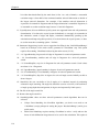
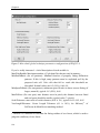
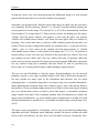
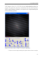
1
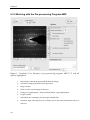
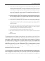
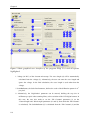
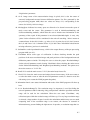
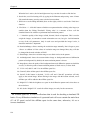
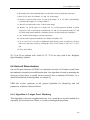
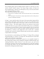
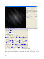
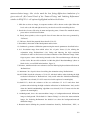
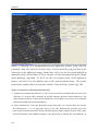
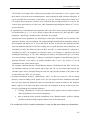
Chapter 6
User manual of EDiff: A unit-cell determination
and indexing software
EDiff® is a scientific software package to determine the unit cell of nano-crystals
from the randomly oriented electron diffraction data. EDiff is used to index the
reflections in the electron diffraction images, and is the first step in reconstructing
the 3D atomic structure of organic and inorganic molecules and proteins.
EDiff includes the data pre-processing program AMP*, which cleans up diffraction
patterns and calculates their autocorrelation patterns, which serve as input for
EDiff.
EDiff: Copyright 2007-2008. BFSC, Leiden Univ., the Netherlands.
* A paper about the pre-processing program AMP was accepted and will be published in the
proceeding of the 2009 IEEE International Conference on Image and Signal Processing (CISP’09):
Jiang, L., Georgieva, D., IJspeert, K., Abrahams, J.P., 2009. An Intelligent Peak Search Program for
Digital Electron Diffraction Images of 3D Nano-crystals.
Chapter 6
6.1. The Electron-Diffraction-Software (EDiff) Package for
Windows® Users
The package includes the following executable files:
x
x
x
x
EDiff.exe;
Patternson_dir_gui.exe;
FirstInstall.bat
MCRInstaller.msi and other supporting archives.
6.2. Configuring and running EDiff on Windows Platforms
1 Open/Unpack the package in a new directory.
2 Run FirstInstall.bat once on the machine where you want to use the software.
MATLAB Component Runtime (MCR) Libraries will install automatically, 300M
space on the C: disk is needed. Note: if installation fails, double click the file
MCRInstaller.msi to install it.
3 Run Patternson_dir_gui.exe to start working with electron diffraction (EM) images.
The fist time this program is started, it will unpack the supporting archives, taking
several minutes. This software will generate four output files for each EM image:
<image-name>.atc.plt, <image-name>.atc.jpg, <image-name>.ctr.pks, and
<image-name>.ctr.png. Put these outputs in a separate directory for the next step.
4 Run EDiff.exe to determine the Unit-Cell parameters and index individual EM
image.
6.3. AMP: Pre-processing diffraction data
The pre-processing program AMP (Autocorrelation Mapping Program) – with the
executable file name Patternson_dir_gui.exe – has a Graphical User Interface (GUI).
110
User manual of EDiff
This program is used to remove the background and for picking reflection spots from
diffraction images. A snapshot of the user interface is shown in figure 1.
This program creates an autocorrelation pattern of the electron diffraction pattern
which fills up gaps or absences in the data, enhances the signal to noise ratio, and
centers the diffraction pattern. The autocorrelation map and peak coordinates serve as
input files for EDiff, the main program that determines the unit cell of a crystal. The
autocorrelation patterns are essential for finding the unit cell, but cannot be used for
further steps in the structure determination.
6.3.1 Preparing the Input Data for the Pre-processing Program
AMP
AMP expects electron diffraction images of about 1024 by 1024 pixels (though they
needn’t to be exactly this size). Furthermore, diffracted intensity should be positive
(‘white’ on most display programs; if the spots are black on a white background, you
have to invert the image). The beam center of the diffraction pattern should be more or
less in the centered. Make sure that all the images that you want to process are in the
same directory. It is good practice to store all the data of one EM session in a single
directory, ensuring that all diffraction patterns were collected with the same voltage,
camera length and digitization parameters. If these microscopy parameters are changed
during a session, then separate the data set into different directories for proper
processing.
111
Chapter 6
6.3.2 Working with the Pre-processing Program AMP
Figure 1 Graphical User Interface of pre-processing program AMP V1.2 with all
options highlighted.
1.
Run button to start the program with the desired settings
2.
Selection of images types that will be processed
3.
Image window
4.
Slider to select current image in directory
5.
Change to original pattern / Autocorrelation pattern / png-output pattern
6.
Progress tracker
7.
Information box containing error messages and help files
8.
Parameter input, allowing the user to change area of the center beam that needs to be
removed
112
User manual of EDiff
9.
Allows the user to make the program more or less flexible in finding the center of the
diffraction pattern automatically. The number indicates the allowed error that is based
on the difference in length between two different, independent calculations of the beam
center. Setting it to a higher value allows the program to accept more elliptic or irregular
shapes of the central beam, whereas setting it to 0 automatically redirects the user to a
window for interactively setting the center.
10. Instead of setting the value to 0 one can also chose to use the beam stop removal tool for
any given shape of beam stop. This comes in handy when the user suspects that the
center is found far from its actual position.
11. Allows the user to smooth the image. This option is only advised when salt and pepper
noise is present, because this type of noise is not removed well with the standard
background removal tools. The user is notified that using this option might result in a
minor loss of data.
12. Allows the user to decide which intermediate output images are shown while running
the program. This output consumes large amounts of memory, so when you process
more than ten images, you would better not choose this option.
13. Selects the directory that contains the original images (*.jpeg, *.tiff)
14. &15. Selects the directory that will be used to store the plt-files and autocorrelation
images.
16. Quits the program
The program processes all images in one directory. One can chose to work with *.jpeg,
*.tiff or both file types simultaneously. The program takes about 2 minutes to process a
single image. In the current version, we strongly advise against dragging or changing
any windows that are related to the GUI during image processing, or you might crash
the program. Currently, AMP is a single thread program, which means that it can’t
handle more than one job at a time. Furthermore, there is a limited amount of virtual
memory available, which allows a maximum of ~50 figure windows to be open
simultaneously. If you have a lot of images in one directory, make sure you have
disabled the option of ‘figure output’.
To work efficiently, it is advised to work with electron diffraction data sets that all have
been recorded in the same session. For a quick test, do not save any autocorrelation
maps or plt-files just yet, because this option extends the running time by roughly one
113
Chapter 6
minute. Removing the background can still go wrong, so a user should only enable the
option ‘Removed beamstop’ to see the results of one single image. If one is satisfied,
the user can proceed by enabling the ‘autocorrelation map’ and ‘show plt output’.
When this output is reasonable as well, the user can disable all ‘figure outputs’ and
process all images of the data set in a single run.
6.3.3 Output Data of the Pre-processing Program AMP
This program calculates autocorrelation images and extracts peak positions from
diffraction patterns and their corresponding autocorrelation images. Four output files of
each EM image are generated:
x <image-name>.atc.plt: the peaks positions of autocorrelation map;
x <image-name>.atc.jpg: the autocorrelation map
x <image-name>.ctr.pks: the peak positions of centered background-removed
diffraction image,
x <image-name>.ctr.png: the centered background-removed diffraction image.
It is good practice to save these output files in another directory to avoid mixing with
the original diffraction data.
6.4. EDiff: Finding Units Cells
EDiff.exe is the main program of the electron-diffraction (EDiff) software package. It
finds and optimizes unit cell parameters and fits and indexes diffraction patterns. The
input data for EDiff are not the original electron diffraction images, but the
pre-processed output data from AMP (see above). Please read the part of manual on
the pre-processing program AMP for more details. All the input data should be in one
directory, typically 4 files for each electron diffraction image: <image-name>.atc.plt,
<image-name>.atc.jpg, <image-name>.ctr.pks, <image-name>.ctr.png. All the data in
one directory are assumed to be generated from one EM session, that is, with the same
voltage, camera length of microscopy and digitization parameter. If not, the data have
to be separated into different directories.
114
User manual of EDiff
For unit-cell determination only, <image-name>.atc.plt and <image-name>.atc.jpg
files are required. For indexing, <image-name>.ctr.pks and <image-name>.ctr.png files
are required (please see the part of Indexing an Electron Diffraction Image with
Known Unit-cell Parameters).
Click the ‘SetDataDir’ button to set the directory with the data that need to be
processed. The selected directory will be shown in a line above the button.
Some definitions of electron diffraction images that are used in this document:
x A reflection is a spot corresponding to a vector from beam- or image center to this
spot.
x Two reflection spots together with the beam- or image center point form a triangle;
we call this a ‘facet’.
x The facet defined by the two shortest vectors (corresponding to two reflection
spots closest to the center) is called a ‘main facet’.
In short, every reflection pair defines a facet. The main facet defines the smallest
repeating unit of the 2D lattice defined by the low resolution spacings (but not any
higher-order Laue zone (HOLZ) that may be visible at high resolution).
EDiff.exe also has a Graphical User Interface (GUI); a snapshot is shown in figure 2.
115
Chapter 6
Figure 2 Main graphical user interface of the program EDiff V1.0 with all options
highlighted.
1. Voltage (in KeV) of the electron microscope. The wave length (4) will be automatically
calculated from the voltage (2). Alternatively, the user can enter the wave length and
ignore the voltage. In the final calculation, the wave length is used rather than the
voltage.
5. ScaleBarParam, the Scale Bar Parameter, defines the scale of the diffraction pattern in A-1
per pixel.
8. Alternatively, the ‘Digitization’ parameter can be entered, defining the step size in
millimeter per pixel when scanning films, or the resolution of the CCD digital camera. In
this case, the user also needs to set the ‘ED Constant’ parameter (9) (or the
‘CameraLength’ and ‘WaveLength’ parameters (11 and 4), from which the ‘ED Constant’
is calculated). The ScaleBarParam (5) is calculated from the ‘ED Constant’ (9) and the
116
User manual of EDiff
“Digitization’ parameter.
42. & 43. Image center of the autocorrelation image in pixels; this is also the center of
centered, background-corrected electron diffraction pattern. For files generated by the
pre-processing program AMP, these two values are always 513, corresponding to the
center of a 1024 by 1024 size image.
44. MissingSpots indicates how many spots are allowed to be absent between the spots of
main vector and the center. This parameter is used in MainVectorMatching and
FullVectorMatching methods, which allow the user to include extra information on the
symmetry of the crystal. If this parameter is not selected (MaxMissingNo. is zero), only
‘prime’ index reflections will be considered in the unit-cell searching. ‘Prime’ means no
common factor for the (h,k.l) index, e.g. index (5,4,3) is prime, but (6,4,2) isn’t, because
the h, k and l have 2 as a common divisor. If you don’t have information about known
missing reflections, just leave it unchecked.
27. SetDataDir: set the input data directory, which is the output directory of the pre-processing
program AMP (see 6.3).
28. CheckData allows some types of verification. It allows checking whether the peak
positions of the auto-correlation images and peak positions of the background-removed
diffraction pattern coincide. This helps the user to select the proper ‘ResolutionRange’
for the unit-cell parameter search. Setting ‘CheckData’ allows checking the main vectors
for the ‘MainVectorMatching’ and ‘Brightest Spots Matching’ methods. The option saves
the main vectors to a ‘V1V2’ file.
40. ReadV1V2: reads the main vectors ‘V1V2’ (the main facet) from a file.
41. ClearV1V2: clears the main vectors and unique facets from memory. If the user wants to
re-select the main vectors or redo the unit-cell parameters search, it’s better to erase the
old settings (or to restart the EDiff program altogether).
32 Information Panel: some status information and results of the EDiff program will show up
here.
13. & 14. ResolutionRange(Å): The resolution range, in Angstrom, is used for finding the
unit-cell parameters and for indexing. Only peak positions within the specified resolution
range will be used for the calculation. When the user starts ‘CheckData’, only
reflections/spots within the resolution range will show up. If a very large resolution range
is selected, a large number of spots is used in the calculation and this may cost too much
computing time. If the resolution range is too narrow, the absence of essential of
information may prevent finding the right answer. In practice, a resolution range that is a
117
Chapter 6
bit wider than that defined by the main facet is fine. As a rule of thumb, a reasonable
resolution range is from half of the estimated smallest unit-cell dimension to double of
the largest unit-cell dimension. For example, if the smallest unit-cell dimension is
expected to be around 30 Ångstrom and the largest dimension is around 80 Ångstrom, it
is reasonable to set the resolution range between 15 and 160 Ångstrom.
15. CrystalSystem; all seven different crystal systems are supported in the unit-cell parameters
determination. If we know the crystal system beforehand, we can apply its constraints in
the exhaustive search of edges and angles, sometimes dramatically speeding up the
calculations and improving their precision. If we don’t know the crystal system, we have
to use the most time consuming option – Triclinic.
66. Parameter Suggestion gives the user a suggestion for filling in the ‘UnitCellSearchRange’
based on an analysis of the main vectors generated in ‘CheckData’ step. This option
requires first running ‘CheckData’ and saving the main vectors (V1V2).
17. – 19. UpperBoundary, largest unit cell edge in Ångstrom for a unit-cell parameter search.
20. – 22. LowerBoundary, smallest unit cell edge in Ångstrom for a unit-cell parameter
search.
23. – 25. SearchStepSize, step size in Ångstrom for unit cell parameter search. Usual values
are about 0.5 or 1 Ångstrom.
60. – 62. UpperBoundary, upper boundary in degrees for unit cell parameters search.
57. – 59. LowerBoundary, Lower Boundary in degrees for unit cell parameters search.
54. – 56. SearchStepSize, Step Size in degrees for unit cell angle search. Initially set this to
about 1 degree.
63. SearchList, the user can define a list of angles to be checked, instead of performing
exhaustive angle searching. The angle list should be saved as a text file, with each line a
tri-angle group (alpha beta and gamma, in degrees and separated by blank space).
64. The file of the angle search list
65. Remove the angle search list
26. SearchAlgorithm: there are three unit-cell parameters search algorithms that can be
selected:
x
Unique Facet Matching: the friendliest algorithm, you don’t even need to run
‘CheckData’ (except perhaps for setting the proper ‘ResolutionRange’) and it gives
quick results.
x
Main Vector Matching: requires running ‘CheckData’ to select / verify and save the
facets of each diffraction image that are to be used in the calculation. This option is
118
User manual of EDiff
useful for very noisy and/or marginal data
x
Full Vector Matching: does not require running ‘CheckData’ as it uses all vectors
within the resolution range. It can be rather slow, but it is useful for refinement and
comparison.
x
Brightest Spots Matching: a variation of ‘Main Vector Matching’, especially useful
for thin nano-crystals with a large unit-cells.
For more details, please see the chapter on ‘Unit-cell Parameters Determination’.
29. SaveParms, save all the parameters in a file, so that the parameters can be loaded next
time by select ‘File-Open’ menu.
30. DoSearch to start unit-cell parameter determination. The result will show on the console
window and the ‘BestFit UnitCell’ column.
31. DoRefine, refine the unit-cell parameters refinement edge parameters: steepest descend
refinement (with decreasing step size) starting from the ‘BestFit UnitCell’ and reporting
the result in ‘Refined UnitCell’.
33. BestFit UnitCell reports the best fitting unit cell parameters found by ‘DoSearch’
procedure.
36. Refined UnitCell reports the refined unit cell parameters generated by ‘DoRefine’
procedure.
39. Show Fitting: fit each auto-correlation image with the ‘Refined UnitCell’ model (if there is
no refined unit cell, it uses the ‘BestFit UnitCell’ instead). Used for indexing an
auto-correlation pattern and verifying the search result of the unit-cell parameters.
53. Indexing: index the centered background-removed diffraction image.
52. EDMosaic: simulating a diffraction pattern for testing.
By selecting the ‘Tool’-‘Config’ menu, a window opens that allows detailed
configuration of some global parameters, see Figure 3. The default parameters are
empirical settings, they work well with most of the data used for testing. Don’t change
them, unless you do really know the meaning of each parameter (and know what
you’re doing)!
119
Chapter 6
Figure 3 More detail global technique parameters configuration of EDiff V1.0
If you’re really interested – a brief description of each variable is:
MaxFilesReadIn: Maximum number of *.plt data files that are read in memory.
MinPattFitRatio (for all patterns): Minimal fraction of properly fitting diffraction
patterns. If this is high, many patterns must be explained well by the
proposed unit cell. Unit cells that fail to reach this threshold are
discarded. Normal values are 0.5 (50%), 0.66, 0.8
MinSpotsFitRatio (For one pattern): minimum spots fit ratio to detect correct fitting (if
larger, mean fit), typical: 0.5 (50%), 0.66
MaxFitError (For one spot): max distance error in pixels, the distance between fitted
and real spots should be smaller, typical value: 7 (pixels)
ScaleTolerance: max value of scale tolerance (0.01 is 1%), typical: 0.01, 0.03, 0.05
VectLengthTolerance: Vector Length Tolerance (0.1 is 10%), for fitFacet() 4 of
FullVector & MainVector matching method
4
‘fitFacet’ is a function to calculate the fitting residue of two facets, which is used to
judge the similarity of two facets.
120
User manual of EDiff
VectAngleTolerance: Vector Angle Tolerance (in degrees), for fitFacet()
FullVector&MainVector Matching Method
AngleLowerBoundary: Angular Lower Boundary (in degrees), for UniqFacet
lattice.Lattice2MainFacet_BEval()5
AngleUpperBoundary: Angular Upper Boundary (in degrees), for UniqFacet
lattice.Lattice2MainFacet_BEval().
AngleLowerBoundary: Angular Lower Boundary, for MainVectorPair
lattice.Lattice2FacetTri_BEval()6
AngleUpperBoundary: Angular Upper Boundary, for MainVectorPair
lattice.Lattice2FacetTri_BEval()
of
in
in
in
in
6.5 Checking the Data
After having run AMP to prepare the data for EDiff, the data can be ‘checked’ by
entering the data directory in EDiff (SetDataDir, button 27) and clicking the
‘CheckData’ button (28). This opens the window shown in Figure 4.
The purpose of checking the data is to allow the user to verify that the peak positions
of the auto-correlation images and peaks positions of the background-removed
diffraction patterns coincide. It also automatically finds the main facet (also called
main vectors, V1V2) for each autocorrelation image. Here, the peaks of the spots
within the resolution range are visualized as crosses; the points of simulated lattice
generated from this main facet are indicated by small circles. Normally, if the crosses
5
Lattice2MainFacet_BEval is a function to generate main facets from electron
diffraction images for the Unique Facet Matching algorithm calculation. The angle of
the facet is limited in between ‘AngleLowerBoundary’ and ‘AngleUpperBoundary’ of
‘Find UniqFacet in Pattern’.
6
Lattice2FacetTri_BEval is a function to generate main facets from electron
diffraction images for the Main Vector Matching algorithm calculation. The angle of
the facet is limited in between ‘AngleLowerBoundary’ and ‘AngleUpperBoundary’ of
‘Find MainVectorPair in Pattern’.
121
Chapter 6
overlap the circles very well, then that means the diffraction image is a well oriented
pattern and the main facet was correctly found by the program.
Sometimes, the program can’t find the correct main facet, in which case the user has to
set it manually by first choosing ‘ResetV1’ or ‘ResetV2’ and then double clicking the
correct peak/cross in the image. The selected V1 or V2 will be automatically switched
if the length of V1 is larger than V2. There are lots of tricks for making your life easier:
<double click left mouse button> will capture a cross near the place you clicked.
<double click middle mouse button> will locate the exact place that you clicked; by
pressing <Ctrl> at the same time, it will try to find a intensity peak near the place you
clicked. There are more complicated options for advanced users: if you press the key
<Shift>, <Alt> or <Ctrl> when you do <double click left mouse button> or <double
click middle mouse button> on the peaks of the image, the 1/2, 1/3 or 1/4 position is
located relative to the cross that you selected or the point that you clicked. You even
can combine use the <Shift> and <Alt> key, which will locate 1/6 position. When the
peaks are not correctly generated by the pre-processing program AMP, these operations
are very useful to help you to manually reset the correct V1 and V2, provided you
know what you’re doing (which requires understanding reciprocal space).
The user can run CheckData to find the proper ‘ResolutionRange’ for the unit-cell
parameter search. A very large resolution range is fine from a theoretical perspective,
but may include too many spots in the calculation and therefore cost too much
computing time. A resolution range that is too narrow may lose essential information.
When adjusting the resolution range, don’t forget to press ‘enter’ after having filled in
the numbers. Let the resolution range (shown as two black circles in the image window)
just cover all the main vectors (or make it just a little larger). A reasonable resolution
range extends from half of the estimated smallest unit-cell dimension to double the
largest unit-cell dimension, e.g. if the smallest unit-cell dimension is around 30 Å and
the largest dimension is around 80 Å, a reasonable resolution range extends from 15 to
160 Å.
The main vectors generated in ‘CheckData’ will be used in the MainVectorMatching
algorithm and in the ‘Brightest Spots Matching’ method. In order to validate the main
facets/vectors selected here, the user has to save the main vectors by clicking the ‘Save
122
User manual of EDiff
V1V2’ button or ‘Save As’ a ‘V1V2’ file. For the UniqFacetMatching method, the
program will generate the main facets automatically when the unit-cell parameter
search is started. Running ‘CheckData’ is not required for the UniqFacetMatching and
FullVectorMatching algorithms.
Figure 4 Check-data window in EDiff V1.0, all options highlighted.
1. Slide bar to select an image for checking, the sequence number will show on the right.
123
Chapter 6
When the bar is active, the left and right arrow keys can also be used to slide the bar.
2. Search box, used for locating a file by typing in the filename and pressing ‘enter. If more
files match the name, pressing enter switches between them.
3. Slide bar to set the fitting threshold (show on the right), which is used in the ‘Find Next’
function.
4. ‘Find Next >>’: click this button to find the next pattern that has a fitting value larger (or
smaller) than the Fitting Threshold. ‘Fitting value’ is a measure of how well the
simulated lattice fits with the experimental autocorrelation pattern.
5. – 7. Mark the quality of the image as Bad, Normal, Good or Important. This is used to
weigh the images, as sometimes certain orientations are rare, but give vital information
on one of the cell parameters. Only in such cases and provided the image is nice, it
should be marked as ‘Important’.
16. ResolutionRange: allows entering the resolution range manually. Don’t forget to press
<Enter> to validate it. If the values of resolution range are changed here, they will also
be changed in the main window of EDiff.
17. ShowRange: shows the resolution range as two black circles in the pattern.
25. AtcBackground: shows the autocorrelation image or background-removed diffraction
pattern as background. By default, the autocorrelation pattern is shown.
26. ImageSpots, show the peaks of the background-removed diffraction pattern as dark blue
crosses, or show the peaks of autocorrelation pattern as black crosses, or show both.
27. V1V2->Aff, add V1 and V2 to An affiliate spots list7.
28. ClearAff, delete all the spots in the affiliate spots list.
29. SetAff: if this button is checked, ‘V1V2->Aff’ and ‘ClearAff’ operations will only
apply to the current image. When clicking in the image with this button selected, a new
affiliate spot will be added to the affiliate spots list.
23. BrightV1V2: find the brightest two spots in the diffraction pattern and select these as
the main facet.
22. All: do the ‘BrightV1V2’ search for all the images, not only for the current one.
7
An ‘affiliate spots list’ is a list of reflections that is used for checking a simulated 2D
lattice. Every diffraction simulation of a potential unit cell must contain the main facet
(V1 & V2 spots) and all the affiliate spots in the same time; otherwise, it’s not a
correct simulation.
124
User manual of EDiff
8. ShowSimu, show the simulated lattice as small blue circles by tiling the main facet.
9. ShowV1V2, show in red labels ‘V1’ and ‘V2’ in the image.
10. ResetV1, reset the main vector V1 spot in the image. V1 or V2 will be automatically
switched if the length of V1 is larger than V2
11. ResetV2, reset the main vector V2 spot in the image.
20. Refine, use all the spots on a single line (or a multi-regression method if option
‘regression’ (24) is selected) to recalculate the V1 and V2, the operation makes V1 and
V2 fit the image better and their coordinates can now be non-integer pixel multiples.
21. All, ‘Refine’ all the images, not only current one.
24. Use the multi-regression method to for ‘Refine’ and refine ‘All’.
12. & 13. Save V1V2: In order to validate the main facets/vectors selected here, the user
has to save the main vectors by clicking the ‘Save V1V2’ button or ‘Save As’ a ‘V1V2’
file.
14. Close this window
20, 21 & 24 are optional tools, while 22, 23, 27-29 are only used in the ‘Brightest
Spots Matching’ method.
6.6 Unit-cell Determination
One of the main functions of EDiff is to determine the unit cell of nano-crystals from
the randomly oriented electron diffraction data. Our algorithm is based on matching the
observed crystal facets to model facets extracted from a simulated 3D lattice (or a
detailed description of the algorithm, see chapter 5).
EDiff has several variations of the general algorithm for identifying unit cell
parameters, which are discussed below.
6.6.1 Algorithm 1: Unique Facet Matching
This algorithm is the most straightforward one. It is a good idea to try this method first,
especially for first-time users. Below, we walk you through the procedure.
125
Chapter 6
Main steps:
1.
Set the basic microscope and diffraction parameters in the graphic interface (figure 2).
Choose a data directory with ‘SetDataDir’. If you know the crystal system or want to test
out whether your assumption of the crystal system is reasonable, select it, otherwise select
‘Triclinic’. Set the search range of edges and angles. Set the ‘SearchAlgorithm’ to
‘UniqFacetMatching’.
2.
Find the proper ‘ResolutionRange’: click ‘CheckData’ and adjust the resolution range to
cover all the main vectors in different images. Close the window of ‘CheckData’. ‘Save
V1V2’ is NOT necessary.
3.
Click the ‘DoSearch’ button to perform unit-cell parameters search. The console window
running in the background will indicate progress.
4.
The best fitting unit-cell parameters will be displayed in the ‘BestFit UnitCell’ column and
the best five results will be shown in the console window. Use ‘Show Fitting’ to check
whether the result is reasonable or not.
This algorithm is the most automated one. After the user has clicked the ‘DoSearch’
button, the program first generates a main facet for each autocorrelation pattern and
accumulates all the facets in List1, then analyses List1 to remove any congruent facets,
shrinking List1 to contain only unique facets. The matching procedure is described in
fig. 5.
6.6.2 Algorithm 2: Main Vector Matching
This algorithm requires more user interaction compared to the Unique Facet Matching
algorithm. The most important difference is that the main facets (V1 & V2) have to be
examined (and possibly reset) by the user using the ‘CheckData’ tool. The main facets
in List1 are checked by hand and a quality remark (Bad, Normal, Good, or Important)
can be given to each individual image. Congruent facets extracted from different
diffraction pattern are not removed from List1. When the experimental data are very
noisy and lots of mis-tilted diffractions were collected, this solution is more reliable in
the hands of an experienced user. The user is encouraged to run ‘CheckData’ and try
this method for more accurate results.
Main steps:
126
User manual of EDiff
1.
Set the basic microscope and diffraction parameters in the graphic interface (figure 2).
Choose a data directory with ‘SetDataDir’. If you know the crystal system or want to test
out whether your assumption of the crystal system is reasonable, select it, otherwise select
‘Triclinic’. Set the search range of edges and angles. Set the ‘SearchAlgorithm’ to
‘MainVectorMatching’.
2.
Find the proper ‘ResolutionRange’: click ‘CheckData’ and adjust the resolution range to
cover all the main vectors in different images.
3.
In the window of ‘CheckData’, verify that the V1 and V2 spots (auto-selected by the
program) are the closest two spots near the center. If there are any other spots closer to the
center, reset the V1 or V2 to these spots. Normally a correct choice for V1 & V2 result in a
high ‘fitting value’ between the image peaks and a lattice using V1&V2 as a basis. Please
read the section 6.5 on Checking the Data for more details.
4.
‘Save V1V2’ or ‘Save As’ a V1&V2 file before closing the window of ‘CheckData’.
5.
Click the ‘DoSearch’ button to perform unit-cell parameters search. The console window
running in the background will indicate progress.
6.
The best fitting unit-cell parameters will be displayed in the ‘BestFit UnitCell’ column and
the best five results will be shown in the console window. Use ‘Show Fitting’ to check
whether the result is reasonable or not.
When the user clicks the ‘DoSearch’ button, the program will use the main facets saved
in the ‘CheckData’ step in List1. For the Main Vector Matching algorithm, this List1 is
filled interactively using the ‘CheckData’ tool. In testing out potential unit cells,
unit-cells are skipped if none of its facets can be matched to the measured patterns
marked as ‘Important’.
6.6.3 Algorithm 3: Full Vector Matching
To the user, the Full Vector Matching algorithm appears very similar to the Unique
Facet Matching algorithm, but its inner workings are different. Normally, it’s rather
slow and we advise you to only use it for comparison and verification. On the other
hand, as it uses more data, it can be more accurate.
Main steps:
1.
Set the basic microscope and diffraction parameters in the graphic interface (figure 2).
127
Chapter 6
Choose a data directory with ‘SetDataDir’. If you know the crystal system or want to test
out whether your assumption of the crystal system is reasonable, select it, otherwise select
‘Triclinic’. Set the search range of edges and angles. Set the ‘SearchAlgorithm’ to
‘FullVectorMatching’.
2.
Find the proper ‘ResolutionRange’: click ‘CheckData’ and adjust the resolution range to
cover all the main vectors in different images. It is important to set the resolution range as
narrow as possible, as this solution is very time consuming since it uses all the vectors in
the resolution range in its calculations. Close the window of ‘CheckData’. ‘Save V1V2’ is
NOT necessary.
3.
Click the ‘DoSearch’ button to perform unit-cell parameters search. The console window
running in the background will indicate progress.
4.
The best fitting unit-cell parameters will be displayed in the ‘BestFit UnitCell’ column and
the best five results will be shown in the console window. Use ‘Show Fitting’ to check
whether the result is reasonable.
When the user clicks the ‘DoSearch’ button, the program will use all the possible
vectors pairs (not only the main facet) in each autocorrelation image for its calculations.
For matching an observed vector pair (a facet in List1) to a simulated facet in List2, a
2D lattice is generated from the simulated facet and compared with the observed
diffraction pattern to get a fitting value. The fitting value is used as the accumulated
residual, which is different from the residual of two fitted facets in the other solutions.
By using all the vector pairs and simulating 2D diffraction patterns, this algorithm
requires heavy computing and is therefore slow.
6.6.4 Algorithm 4: Brightest Spots Matching (especially suited for large
unit cells)
The ‘Brightest Spots Matching’ algorithm is a variation of the ‘Main Vector Matching’
algorithm. It’s the most accurate algorithm and is especially useful for thin
nano-crystals with large unit-cell. However, it does require some expertise and you
need to know what you’re doing. Try it out if you have plate-like nano-crystals that lie
in preferred orientations on the grid. If this is the case, the information of the unit cell
dimension in the direction of the beam is not (well) determined. If this is the case,
128
User manual of EDiff
make sure to tilt the samples away from the main zones before diffracting them by as
high an angle as the microscope allows. Moreover, if the unit-cell is large, the
reflection spots will often be elongated in the direction normal to the plane of the
crystal due to the wide ‘spike function’ (or ‘rocking curve’ in X-ray terms) in this
particular direction. This can be caused by the limited number of unit cells in this
direction. As a result of this elongation, the positions of the reflections present on the
diffraction patterns may not represent the centroid of the reflection. As this is an
implicit assumption of the algoritms discussed previously, they may not be reliable any
more for thin, plate-like nano-crystals with a large unit-cell. This may be compounded
by missing information on the unit cell dimension normal to the plane (a few ultra-high
tilted diffraction images may still have some useful information, but may have a very
poor quality due to the high tilt).
This algorithm abandons the idea of using the main facets, and instead uses the two
brightest spots in the diffraction image (not the autocorrelation image). The brightest
spots are most likely to have their centroids closest to the Ewald sphere and can be
further from the center, thus containing higher index information, also in the direction
normal to the plane of the crystal.
The main practical difference from the users perspective is that the two brightest spots
are set as the new main facet (V1 & V2) in ‘CheckData’ tool. It is strongly advised to
set the original main facet (old V1 & V2) as affiliate spots. Buttons 22, 23, 27-29 of the
‘CheckData’ window (see figure 4) allow these actions. Button 27 ‘V1V2->Aff’ must
be used to add V1 and V2 to the affiliate spots list. Button 23 ‘BrightV1V2’ will find
the brightest two spots in the diffraction image and reset V1&V2 to them. The user can
switch the background from the autocorrelation pattern to centered diffraction pattern
for verification (by turning off the radio button 25 ‘AtcBackground’).
This solution proved also valid and reliable in various test cases in which the
experimental data were very noisy and lots of miss-tilted diffractions were collected.
We encourage all experienced users to try this method at least once!
Main steps:
1.
Set the basic microscope and diffraction parameters in the graphic interface (figure 2).
Choose a data directory with ‘SetDataDir’. If you know the crystal system or want to test
129
Chapter 6
out whether your assumption of the crystal system is reasonable, select it, otherwise select
‘Triclinic’. Set the search range of edges and angles. Set the ‘SearchAlgorithm’ to
‘BrightestSpotsMatching’.
2.
Click ‘CheckData’ and set a large resolution range to cover most of the brightest spots in
different images.
3.
In the window of ‘CheckData’, visually check the main facet V1&V2. Button 20 ‘Refine’
(in figure 4) can be used to refine the position of V1&V2. Button 27 ‘V1V2->Aff’ (in
figure 4) is used to add V1&V2 to an affiliate spots list. Button 23 ‘BrightV1V2’ will find
the brightest two spots in the diffraction image and reset V1&V2 to them. The user can
switch the background from the autocorrelation pattern to centered diffraction pattern for a
better visualisation (by turning off the radio button 25 ‘AtcBackground’). Be careful of
Button 22 and 29 as their operation will affect all the images, not just current one.
4.
Find the proper ‘ResolutionRange’. In the window of ‘CheckData’, adjust the resolution
range to cover all the brightest spots and affiliate spots in all images that must be used in
the calculation. ‘Save V1V2’ or ‘Save As’ a V1&V2 file, and then close the window of
‘CheckData’.
5.
Click the ‘DoSearch’ button to perform unit cell search. The console window running in the
background will indicate progress.
6.
The best fitting unit-cell parameters will be displayed in the ‘BestFit UnitCell’ column and
the best five results will be shown in the console window. Use ‘Show Fitting’ to check
whether the result is reasonable or not.
When the user clicks the ‘DoSearch’ button, the program will use both the V1&V2 and
main facets (as affiliate spots) saved in ‘CheckData’ step. In the searching, every
diffraction simulation of a potential unit-cell has to match the V1&V2 spots and all the
affiliate spots at the same time. Because this method needs to check the additional
affiliate spots, it’s a bit slower than the normal ‘Main Vector Matching’ method.
6.7 Pattern Fitting of the Autocorrelation pattern: Verifying the
Unit-cell Parameters
After unit cell parameters have been found, ‘Show Fitting’ (39, in figure 2) can open a
pattern fitting window for verification. The ‘Pattern Fitting’ window will fit each
130
User manual of EDiff
auto-correlation pattern with the ‘Refined UnitCell’ model (or, if this does not exist,
with the ‘BestFit UnitCell’ instead). The ‘Pattern Fitting’ window will index the
auto-correlation image. Therefore, the control panel (see fig. 5) has the same interface
as the ‘Indexing Refinement’ window.
This ‘Pattern Fitting’ algorithm works as follows:
1.
find the facet in a simulated 3D lattice that best fits the main facet of an autocorrelation
pattern;
2.
then cut through the 3D model lattice using the plane defined by the best fitting facet to
generate a 2D diffraction simulation.
In figure 5, crosses mark the peaks of the spots of the autocorrelation image and blue
circles mark the model lattice. If the unit-cell is correct, the crosses and the blue circles
should overlap well. When almost of the images (>90%) fit well, the unit cell most
probably is correct. The outliers might be caused by the inclusion of some deviant
crystals in the data set, by poor crystals with streaked rocking curves, by unfortunate
orientations or unexpected failures to index the pattern properly. Only an experienced
eye can tell. However, don’t be fooled into certainty when the information of one unit
cell dimension is missing in the original data (some crystals have a preferred
orientation, and if you haven’t tilted the diffraction grid, you may not have sampled the
reciprocal lattice well enough).
If you don’t believe a certain indexing, click ‘FitFacets’ (17 in figure 5B) to go through
all potential fittings in a spin-box (16 in figure 5B). The fitted facets are sorted and a
smaller number should give a better fitting.
The buttons and options in ‘RefineOrient’ group box are not originally designed for
this ‘Pattern Fitting’ window, but for refining the orientation of diffraction image in the
‘Indexing Refinement’ window. However, if you really want to, you can use this
‘RefineOrient’ operation to index the autocorrelation pattern for testing and comparing,
even though some buttons to do with refining diffraction patterns may be not fully
functional for refining autocorrelation images.
131
Chapter 6
(A)
(B)
Figure 5 (A) Pattern fitting of the main facet and the peaks of the autocorrelation
image to unit-cell parameters. Crosses mark the peaks of the spots of the
132
User manual of EDiff
autocorrelation image, blue circles mark the best fitting diffraction simulation of a
given unit-cell. (B) Control Panel of the ‘Pattern Fitting’ and ‘Indexing Refinement’
window in EDiff V1.0 – all options highlighted and described below.
1. Slide bar to select an image, its sequence number will be shown on the right. When the
bar is active, the left and right arrow key can also be used for controlling the bar.
2. Search box, locate a file using its name and pressing enter, if more files match the name,
press enter to switch between them.
16. Fitted_facets spinbox, select a specific facet if more than one facet was generated by
‘FitFacets’.
17. FitFacets, find all the potential facets that fit V1 & V2.
3. ShowIndex, show/turn off the fitted pattern and its index.
15. GenMosaic, generate a diffraction pattern using the mosaic parameters described below
4. & 5. Resolution range from which select ‘No. of pairs’ facets (11) for refining the
orientation using ‘RefineOrient’ (10): fitting and indexing the high resolution
reflections in order to find a more accurate orientation of the diffraction image. Don’t
forget to press <enter> after having inserted a value. The resolution range will show up
as blue circles. Be sure this resolution is within the global ‘ResolutionRange’ (show as
black circles, set on EDiff main interface, figure 2).
7.Tolerance, maximum index error tolerance used for indexing high resolution reflections in
‘RefineOrient’.
11. Maximum ‘No. of pairs’ facets for refining the orientation using ‘RefineOrient’.
20.ckV1V2hkl, check the existence of V1 & V2 with their indices when indexing the high
resolution reflections in ‘RefineOrient’. Only useful when the ‘MainVectorMatching’
algorithm was selected (V1 & V2 must exist for this option to be meaningful).
21.checkV1V2, check the existence of the two reflections V1 & V2 and show their
positions when indexing the high resolution reflections in ‘RefineOrient’. Only useful
when the ‘MainVectorMatching’ algorithm was selected (V1 & V2 must exist for this
option to be meaningful).
8. AtcBackground, show the autocorrelation image or background-removed diffraction
image as background. The default for ‘Pattern Fitting’ is to show the autocorrelation
image; for ‘Indexing Refinement’ the default is to show the background-removed
diffraction image.
6. Rotation matrix defining the potential orientations found by ‘RefineOrient’, ‘RF2’, or
133
Chapter 6
‘RF3’. The matrices are sorted by quality: the top matrices fit best.
10. RefineOrient, finds a more accurate orientation of a diffraction image using known
and/or found unit cell parameters by selecting pairs of high resolution reflections, and
fitting and indexing these pairs.
19. RF2 provides a different method for orientation refinement, sampling all different tilt
orientations based on the orientation of V1 &V2 (and their indices) to find the best
fitting.
18. RF3 provides yet another method for orientation refinement, sampling all different tilt
orientations based on the orientation of V1 &V2 to find the best fitting. The spike
function of the reflection is considered, that is, the elongation of the reflection is
simulated. The ‘MosaicType’ must be 3 (side elongation, threshold default value 0.05).
9. ShowRF, show/turn off the simulated refined pattern and its indices; for indexing an
autocorrelation image, ‘ShowMosaic’ may be a better choice.
12. ShowMosaic, show/turn off the simulated pattern with increased mosaicity, together
with its indices.
13. Threshold for the simulation an increased mosaicity. For mosaic type 1 the default is
0.03, for mosaic type 2 it is 0.004, for mosaic type 3 the default is 0.05,
14. MosaicType encodes different models for simulating the mosaic spread of the
diffraction pattern. It defines whether an off-Ewald sphere reflection should be shown
on the simulated diffraction or not. 1: Angular mosaic, the angular error of a reflection.
2: Absolute distance, the reciprocal distance between a reflection and the Ewald sphere.
3: side elongation, simulate the spot elongation along the main direction of the unit
cell that lies most closely to the direction of the electron beam and calculate the
reciprocal distance to the Ewald sphere (useful for very thin, plate-like crystals that
have characteristics of 2D crystals). .
6.8 Indexing an Electron Diffraction Image with Known Unit-cell
Parameters
Once unit cell parameters have been inferred, clicking the ‘Indexing’ (53, in figure 2)
button opens the ‘Indexing Refinement’ window (figure 6). This window is used for
indexing centered, background-corrected diffraction images. The main difference
between ‘Indexing Refinement’ (figure 6) and ‘Pattern Fitting’ (figure 5) is that in the
134
User manual of EDiff
former a diffraction pattern is indexed and in the latter an autocorrelation image is
indexed . The default background of ‘Indexing Refinement’ window is the diffraction
image, while the default background for ‘Pattern Fitting’ is the autocorrelation image.
After having found unit cell parameters, the global ‘Resolution Range’ (set in the EDiff
main window) can be increased for ‘Indexing Refinement’. The ‘Search Algorithm’
should be changed to ‘MainVectorMatching’, no matter what algorithm was used for
getting the unit-cell parameters. It is necessary to run ‘Check Data’ in order to select a
main facet on which the indexing refinement will be based.
When the window opens, a rough fitting is showing. It’s the same as in the ‘Pattern
Fitting’ window: the program finds the best fitting facet in a simulated 3D unit-cell
model for the main facet (V1 & V2), then cuts through the 3D model lattice along the
plane defined by the selected facet in order to generate a simulated 2D diffraction
pattern (show as small blue circles). If the diffraction image is taken right from the
main zone, this provides an accurate indexing. However, in more usual cases, the
experimental diffraction pattern is tilted away from the main zone. In order to find the
exact orientation of an individual diffraction image (so as to index the reflections
correctly), we need to select ‘Refine Orient’, which opens a new window (fig. 6).
The ‘RefineOrient’ is based on the index of the main facet (V1&V2). Hence the
‘MainVectorMatching’ or ‘BrightestSpots’ algorithms are strongly suggested for
indexing refinement.
135
Chapter 6
Figure 6 Indexing of a background-corrected diffraction pattern using unit-cell
parameters that were inferred in earlier steps. Crosses mark the peak positions of the
reflections of the diffraction image; Small blue circles are the best fitted diffraction
simulation of the selected unit cell. Here, the unit cell was determined using the ‘Bright
Spots Matching’ algorithm; V1 & V2 are the two brightest spots of the diffraction
pattern; A0 and A1 are the affiliate spots of the autocorrelation image. The control
panel of this window shares its interface with the ‘Pattern Fitting’ window (fig. 5B)
Steps of orientation refinement and indexing:
1. Visually check whether the main facet (V1 & V2) fits well and is reasonable indexed. If not, click
‘FitFacets’ (17 in figure 5B) to generate all possible solutions and pick a better fitting facet. The
‘RefineOrient’ procedure is based on this fitted facet. If this fitting is not correct, the orientation
refinement and indexing will be meaningless.
2a. Select ‘RefineOrient’. Select the ‘Resolution’ range from which ‘No. of pairs’ facets are used for
the refinement (4, 5, 7, 11 in figure 5B need to be set). The ‘RefineOrient’ procedure will select
pairs of high resolution reflections, fitting and indexing these high resolution facets to find a more
accurate orientation of the diffraction pattern, using the known or inferred unit cell parameters. If
136
User manual of EDiff
‘ckV1V2hkl’ (20 in figure 5B) is checked, the procedure will ensure that V1 & V2 together with
their indices are present in the simulated pattern, when indexing the high resolution reflections. If
you’re uncertain of the correctness of the indices of V1 & V2, click the radio button ‘checkV1V2’
(21 in figure 5B) to ensure the existence of two reflections shown on the positions of V1 & V2, but
without fixing their indices (so in this case, other orientations that change the indices of V1 & V2
are also allowed).
2b. Alternatively to ‘RefineOrient’, the algorithms ‘RF2’ and ‘RF3’ can be selected. Some parameters
for ‘RefineOrient’ (4, 5, 7, 11, 20, 21 options in figure 5B) are not used by ‘RF2’ and ‘RF3’. Other
parameters: ‘MosaicType’ and the mosaic ‘Threshold’, are required.
Selecting the correct parameters for ‘MosaicType’ and mosaic ‘Threshold’ can be critical for the
program to find the correct orientation. The program samples all different tilt orientations based on
the orientation and indices of V1 &V2, and selects the best fit (between the simulated and the
observed diffraction pattern). In ‘RF2’ the rocking curve (or spike function) of the reflections is not
considered. In ‘RF3’ The difference between ‘RF2’ and ‘RF3’ is, spike function of a reflection is
considered in ‘RF3’, an elongation in reciprocal space of a reflection is simulated. The most
meaningful ‘MosaicType’ is 3 for ‘RF3’, although you could try selecting mosaic type 1 or 2: there
is no error message. ‘MosaicType’ 3 indicates a lengthwise elongation of the diffraction spot in a
principal direction of the lattice; its default threshold value is 0.05. See section 6.7 for an
explanation of the various mosaic types.
For inorganic materials that have crisp diffraction patterns, ‘RefineOrient’ and ‘RF2’ will be fine
for reasonable indexing. For the crystals with a large unit cell, e.g. the protein nano-crystals, the
reflection spots can be elongated along the unit-cell edge direction normal to the plane of the
crystal. In this case ‘RF3’ is a wise choice.
3. Potential orientations found by ‘RefineOrient’, ‘RF2’, or ‘RF3’ are stored in a list of rotation
matrices, sorted according to their quality of fit. You can inspect all these orientations and check
how well they match the diffraction pattern by selecting their sequence number in the ‘Rotation
Matrix’ spin-box (6 in figure 5B). Most of the time, the orientation at the top of the list fits best.
One way of picking the best indexing solution is:
x
Clicking ‘ShowMosaic’ to show the indexed mosaic pattern (all the model reciprocal
lattice spots that are close to the Ewald sphere);
x
then go through all the possible orientations in the ‘Rotation Matrix’ spin box (starting
from the most likely fitting sequence number zero) to find the best fit.
For certain unit cells in certain orientations, it may be that more than one orientations /
137
Chapter 6
indexing solution fits well. This depends on the unit cell parameters and unfortunate
combinations can exist in which it is not possible to distinguish on the basis of the
positions of the diffraction spots alone. In this case you would also need to include
intensity information and 3D merging of the diffraction data. This is beyond the current
scope of EDiff. In these (rare) cases, you have to judge for yourself which is the most
reasonable indexing.
6.9 Conclusion
The program EDiff will allow you to determine the unit cell of a crystal type, even if
you can only collect single shots from randomly oriented crystals. It will index the
diffraction images and allows considerable user interaction in determining, verifying
and assessing the results. This is required as every crystal may have its own
peculiarities and only by understanding the way in which the program its results can
you truly appreciate the relevance of the suggested solution. Next steps include
integration of the data (determining the intensities of the diffraction spots) and phasing.
These are currently beyond the capacities of EDiff, and I am working towards these
additional options.
138