Download A Tool for Astrophysical Data Analysis user manual

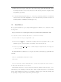
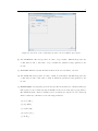
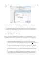
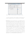
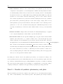
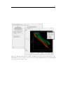
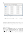
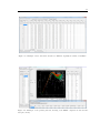
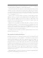
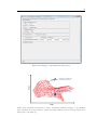
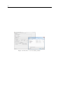
TA-DA
A Tool for Astrophysical Data Analysis
version 0.98
user manual
Nicola Da Rio
[email protected]
August 8, 2012
TA-DA was developed thanks to funding from the NASA Award Number NNX07AT37G
Chapter 1
Introduction
1.1
What is TA-DA
TA-DA is a powerful, integrated tool for the analysis of stellar photometric data, aimed to
significantly simplify the process of comparing stellar photometric data with theoretical models.
In the released version TA-DA allows to easily and reliably operate on synthetic photometry, creating theoretical spectral energy distributions (SEDs). The tool also supports analysis
of photometry from different archives, SED model fitting, self-consistent prediction of stellar
parameters based on multi-band photometry. TA-DA includes a comprehensive and updatable
repository of throughputs of astronomical instruments and filters, stellar and synthetic spectra,
and evolutionary models. Photometric and spectroscopic data can easily be imported from the
Virtual Observatory as well as from user’s own tables and models. Results are produced in
tabular or graphic format, readily usable for publication.
TA-DA runs as an IDL widget application publicly available for download.
1.2
TA-DA functionalities
We summarize here the main functionalities of TA-DA:
1. Computation synthetic photometry of complete grids of evolutionary models, or part of
them, or any arbitrary set of stellar parameters. Observed fluxes or magnitudes and colors
are computed in a number of units. Dust extinction can be considered in the computation.
2. The results of synthetic photometry are plotted for visual inspection, and can be saved to
file.
1
2
3. Tables with observed photometry can be imported in the program. The individual entries
in the imported table can be sorted and selected. The data are plotted in comparison with
the synthetic photometry.
4. A universal fitting algorithm is used to derive the best stellar parameters of individual
sources, based on the their magnitudes or colors, and associated photometric errors, in an
arbitrary number of simultaneous bands (up to 16).
1.3
Installation
The program is available as a pre-compiled IDL application. TA-DA can be obtained from the
following URL:
http://www.rssd.esa.int/SA-general/Projects/Staff/ndario/TADA/index.html
as a compressed archive tada.zip. The archive content is the following:
• the file tada.sav: the pre-compiled IDL code.
• the directory tada data/: contains the necessary data for the program to run; e.g., the
synthetic spectra, the filter profiles, some family of theoretical isochrones.
• the directory example input files/: contains examples of input files that can be imported
to data for testing.
To install TA-DA it is sufficient to decompress the archive, and run the program tada.sav
from IDL:
IDL> cd,’/path/where/tada/is/located/’
IDL> tada
Note: the user may consider adding the directory where the program is located is added to
the IDL path, although this is not necessary.
When TA-DA is started, it creates a widget-based interface. This is divided in 4 tabs, one for
each main step of the analysis performed by the software: 1) The interpolation of evolutionary
models; 2) the synthetic photometry, 3) the results of synthetic photometry, the plotting, and
the uploading of the photometric data, and 4) the fitter engine.
3
1.4
Compatibility
TA-DA has been developed to work under IDL version 7.0 or higher, on all Windows, Linux, or
Mac OS platforms. The widget-based graphical user interface, however, looks and behaves best
under Windows systems. This is because IDL widgets allow more strict positioning and sizes
under Windows.
4
Chapter 2
Using TA-DA
2.1
Panel 1 - Physical stellar parameters for the model
The first panel is dedicated to the preparation of the model stellar parameters for synthetic
photometry. TA-DA allows two general approaches for this step, which can be switched from
the top row of Panel 1 (see also Figure 2.1):
1. Evolutionary models: this approach considers evolutionary models (evolutionary tracks
and isochrones). In this way the stellar parameters include, besides the effective temperature Teff , the stellar radius R, and the surface gravity log g (parameters necessary for
synthetic photometry), also stellar masses M and stellar ages.
2. Arbitrary: this approach considers only the minimum parameters to perform synthetic
photometry, i.e., Teff , R and log g. Stellar masses and ages, which are model dependent
quantities, will be undefined.
2.1.1
Evolutionary models
When selecting the evolutionary model approach, the panel shows additional widgets (see, e.g.,
Figures 2.1 and 2.2) where the parameters must be specified. Specifically, the user selects the
family of evolutionary models; the available models are loaded automatically by TA-DA at
startup, and additional families can be added (see the appendix for details). The user can then
select among 5 options:
(a) all isochrones: TA-DA considers all isochrones from the selected family of models.
5
6
Figure 2.1: Selection of the evolutionary models to use for synthetic photometry.
(b) one isochrones: The user specifies one value of age, in Myr. TA-DA interpolates the
evolutionary models to that value of age, if within the parameter range spanned by the
models.
(c) all tracks: TA-DA considers all mass tracks from the selected family of models.
(d) one track: The user specifies one value of mass, in solar masses. TA-DA interpolates the
evolutionary models to that value of mass, if within the parameter range spanned by the
models.
(e) manual input: Selecting this option the user specifies an arbitrary set of stellar parameters;
this is passed to the software through an ASCII text file, selected through a popup window.
The ASCII file must contain 2 columns (or more, in which case only the two are considered)
which contain any combination of the following parameters:
(a) mass (M )
(b) age (Myr)
(c) log Teff (K)
(d) log Lbol (L )
(e) R (R )
7
The type of parameter described in each column must be manually specified through 2
drop lists in the widget GUI. The remaining 3 parameters (as well as the surface gravity
log g) are interpolated by the TA-DA from the considered evolutionary models. TA-DA also
checks that the user provided parameter grid lies inside the parameter space covered by
the evolutionary models. If this condition is not matched for a fraction of the points, an
warning message is generated, and the software neglects these points. If all the specified
points lie outside the evolutionary model grid, an error is generated and the user is asked to
modify the input parameters. Finally, the user must specify wether the parameters provided
through the ASCII file represent a 1-dimensional curve, or a 2-dimensional grid. In the latter
case, the grid must be rectilinear in the 2 parameters listed in the ASCII table, i.e.
a “cartesian grid” with arbitrary spacing between lines and columns, no “holes”, and not
necessarily complete at the edges. In Figure 2.3 some examples of allowed and not allowed
configurations are shown for clarity. The distinction between a 1 or 2-dimensional inputs is
relevant only when one runs the fitter within TA-DA, and is irrelevant for the computation
of the synthetic photometry. In particular, if the parameters represent a 2D grid, the fitter
will interpolate over the grid until the solution is found.
The options a) and c) are very similar, since they both load the entire parameter space covered
by the models. Nevertheless, there are two main differences between them: First, the option “all
isochrones” has a finer sampling in masses, whereas “all tracks” has a finer sampling in ages.
Therefore, if the ultimate goal of the user is a precise estimate of stellar masses, selecting “all
isochrones” is more appropriate, and viceversa. Second, when plotting the result of synthetic
photometry, TA-DA will plot individual isochrones or tracks according to the choice done here.
2.1.2
No evolutionary models, defining only Teff , log g, R
TA-DA also allows to specify a more general set of stellar parameters which is independent on
stellar evolutionary models. This method is activated selecting ”Arbitrary” option on the upperright part of the first panel. In this case (see Figure 2.4), the user must provide a 3-column ASCII
table containing (in this order), values of Teff (in K), log g (in cgs units) and stellar radii R (in
units of R ). These 3 parameters are sufficient to perform synthetic photometry (see Section
2) and compute absolute magnitudes (or fluxes); however, stellar masses and ages will not be
defined.
Note: unlike magnitudes, stellar colors are independent on luminosity, therefore on stellar
radius. If user aims only at the analysis of stellar colors, the values of stellar radii specified in
8
Figure 2.2: Importing an arbitrary table of 2 stellar parameters.
OK
parameter 1
parameter 1
parameter 1
NO
parameter 2
NO
parameter 2
parameter 2
NO
parameter 1
OK
parameter 2
parameter 2
parameter 2
OK
parameter 1
parameter 1
Figure 2.3: Examples of allowed (top row ) and not allowed (bottom row ) configurations for a
user supplied 2-dimensional grid of stellar parameters.
9
Figure 2.4: Importing a set of values of Teff , gravity and stellar radius.
the 3rd column of the ASCII file can be arbitrary, for example 1 R for every model point.
In the first panel, clicking on the ”Submit” button will lock in the input parameters. TA-DA
organizes the set of stellar parameters, perform any interpolation if needed, checks the validity
of the model points, and moves to the next panel.
Panel 2 - Synthetic Photometry
In the second panel of TA-DA the user can define all the necessary ingredients to perform
synthetic photometry on the previously defined grid of grid of stellar models. An example of the
layout of this panel is shown in Figure 2.5.
• Selection of the synthetic model grid: a drop-down menu lists the available grids of
synthetic spectra. These are contained as fits table files in the subdirectory tada data/spectra/
within the TA-DA installation directory. When TA-DA is launched, the content of this directory is explored and the information on each data-cube of spectra is read. Thus, the
user can add additional grids of atmosphere models, besides the defauld ones, provided
that they are saved in the proper format and copied in the appropriate directory. Each
grid can contain stellar spectra as a function of 3 parameters. The first two are Teff and
log g; the third can be an arbitrary additional quantity, such as metallicity or any arbitrary
parameter. The information on this parameter, as well as its range, are stored in the header
10
Figure 2.5: TA-DA second panel: input parameters for the synthetic photometry.
of the fits table and automatically considered by TA-DA. For additional instructions on
the format of the synthetic spectra cubes, see the appendix at the end of this manual.
• Extrapolation of log g: this option allows the user to choose how TA-DA should consider
model points with a surface gravity log g outside the parameter range convered by the
selected grid of atmosphere models. If the option is deactivated, any point of the stellar
parameters defined in panel 1 with a log g value outside the range spanned by the spectra
(for the Teff of that point) is neglected in the computation of the synthetic photometry.
If the option is activated, magnitudes and colors of parameter points with a log g out of
range are extrapolated from synthetic photometry within the covered log g range. This
extrapolation is useful when some model points correspond to log g values located just
outside the grid. An example of such scenario is when the spectra from the AMES grid
of Allard et al. (2000), defined for log g > 3.5, is selected together with PMS evolutionary
models, which predict log g > 3.2 for the youngest ages in the very-low mass range. Since
in general the computed magnitudes and colors depend only weakly on log g, extrapolating
the results to a small extent outside of the grid, still provides acceptable results. The
users should however be careful in selecting this option, making sure they are aware of the
parameter space covered by their stellar parameters and the grid of spectra.
11
• Dust extinction: extinction can be added directly to the synthetic spectra before the
computation of the synthetic colors and magnitudes. TA-DA currently includes the Galactic Cardelli (1989) extinction law, as well as the the reddening curves for the Magellanic
Clouds from Gordon et al. (2003, LMC average, LMC2 supershell, SMC bar). The user
specifies one or more values of V-band extinctions AV , and one or more values of the relative extinction parameter RV (only if the Cardelli reddening law is selected). Synthetic
photometry will be performed separately for each of these n(AV ) × n(RV ) values on every
stellar parameter point provided in Panel 1. If the user wants to leave reddening as a free
parameter to be fit to the observational data (last panel of TA-DA widget GUI, see next
sections), it is mandatory to indicate at least 2 distinct values of AV (e.g., 0 and 1) in this
field.
• Distance modulus: a unique value for the distance modulus (in magnitudes) to be applied
to the computed magnitudes or fluxes must be specified in this field.
• Photometric bands: the user specifies multiple (up to 16) photometric bands in which
synthetic photometry has to be computed. These can be selected through drop-down
menus, separately for the instrument (or photometric system) and the filter. The filter
throughputs are stored as individual files in a TA-DA installation subdirectory ’/tada data/throughputs/’.
The convention for the filenames is instrument filter.dat, and they contain a 2-column
ascii indicating wavelength (in Å) and throughput (arbitrary relative units). TA-DA scans
the content of this directory at start, so additional photometric systems or bands can be
added by simply placing the relative files describing the filters profile in the appropriate
directory. See the appendix for further details.
By clicking the ”submit” button, the synthetic photometry code is started according to the
selected parameters and options. Particularly large sets of model points may require some time
(e.g. a full set of stellar masses and ages counting 100,000 model points, for 6 values of reddening
and 6 photometric bands requires about 15 minutes of computing time on an average desktop
computer). During the computation, the approximate progress (in percentage) is shown.
Panel 3 - Results of synthetic photometry and plots
After the synthetic photometry is computed, the software moves to the third panel (see Figure
2.6). Here a brief summary of the results is present. The synthetic photometry is natively
12
Figure 2.6: TA-DA panel with the results of synthetic photometry and plotting window. The
small window on the top right corner is the model point information generated by right-clicking
on a point of the plot (see below)
13
computed in units of VegaMag magnitudes, calibrated using a flux-calibrated spectrum of Vega
(Bohlin et al 2007). However, the program derives all the conversions to express the results in
units of ABmag or STmag magnitudes, as well as flux (either Jansky or erg/s/cm2 /Å). In the
third panel it is possible to switch from one to another units. The results of synthetic photometry,
in the chosen units, can be saved to a file through an apposite button. This will be an ASCII
table, in which every row represents one model point. The columns report all the stellar physical
parameters, as well as AV and the magnitudes (or fluxes).
From panel 3 (with the button “Save filters information to file”)the saves a file with the
information about the selected photometric bands. This includes effective wavelength, central
wavelength, equivalent width, and the zero points in Jansky and erg/s/cm2 /Å. Such information
may be useful when new filters are added providing solely the filter throughputs.
At the completion of the synthetic photometry computation, TA-DA also creates a plotting
window showing the results (see Figure 2.6). One can select the quantities shown in the two
axes, choosing either colors or magnitudes, and arbitrary ranges for each axis. The units for each
axis in the plot are automatically updated when the user changes the defaults units in Panel 3.
If the selected units represent a flux (i.e., Jansky or rg/s/cm2 /Å), the color terms will be the
ratio (instead of the difference) between the fluxes in the 2 selected filters.
Panel 3 - Attaching photometric data
From the right hand part of panel 3, the user can attach a table containing observational data
to TA-DA. This is expected to contain multiple rows, one for each star, and multiple columns,
providing photometry or additional data relative to each source. This generates a new widget
window, showing the content of the table as well as a number of widgets to explore and organize
its content, select individual sources, etc. Supported formats are either ASCII table or XML
VOtable. The format, as well as the number columns and rows of the attached table are automatically detected by TA-DA. Figure 2.7 and 2.8 show two examples of the result, respectively
for an ASCII and a VOTable.
If the attached table is a VOtable, the original names of the fields (columns) are shown. In
any case, the user must specify manually, through a drop-down menu for individual columns, if
a particular column reports the observed photometry (or the associated photometric errors) in
one of the bands for which synthetic photometry is computed. The software assumes the units
are the same selected in Panel 3 of the main TA-DA window. The user table window also allows
one to navigate through the table, sort columns and select individual rows (stars) for further
14
analysis. The selection can be performed manually, by clicking to the left side of each row, or
automatically, by selecting all the rows, or the first n-rows in a given page or the entire table, or
through and IDL logical expression. En example of such expression could be the following:
johnson v ge 10 and err cousins i lt 1 and col9 ne ’new’
meaning that the software will select all the rows for which the Johnson V magnitude is greater
or equal than 10 mag, the photometric error associated to the Cousins I photometry is less than 1
mag and the 9th column, not associated any photometric band, is not equal to the string ”new”.
Note: the automatic selections at the bottom of the table window (selection by rows and
by logical expression) are additive: stars that satisfy the input conditions are added to those
previously selected. If you want to select only the stars that satisfy the last condition, you must
deselect all the stars first, using the apposite button.
Note: unlike magnitudes, stellar colors are independent on luminosity, therefore on stellar
radius. If user aims only at the analysis of stellar colors, the values of stellar radii specified in
the 3rd column of the ASCII file can be arbitrary, for example 1 R for every model point.
When the user defines which column is associated to any photometric band previously used
for performing synthetic photometry, and some stars (rows) are selected in the table window, the
plot window is automatically updated showing, together with the computed models, the observed
photometry of the selected stars. An example of this is shown in Figure 8: in this example the
plot window shows a 2 color diagram computed in the bands (WFI V, WFI I and WFI Ti620),
and the attached table provides photometry in these (and other) bands obtained in the Orion
Nebula Cluster (Da Rio et al 2009). The models, indicate with different colors, represent the
synthetic photometry in these bands for different Palla & Stahler isochrones.
When at least 2 photometric bands are specified in the table window, and at least one star is
selected, in the TA-DA main window the button ”go to the fitter” is activated. Clicking on this
button produces a fourth panel in the TA-DA main window, with a list of options to perform
the fit of the models on the attached data.
Clicking on the plot window
A mouse click on the plot window provides information on both stars and model points located
in that point of the plot.
• A left click is for the closest selected star to the clicked point: a popup windows is created
showing the stars’ photometry, and the location of this star in the uploaded table.
15
Figure 2.7: Example of ASCII table imported to the TADA.
• A right click is for the closest model point to the clicked point: a popup windows is
created showing the parameters associated to that point (e.g., mass, age, log Teff , log L,
stellar radius, log g, as well as the value of the quantities plotted in the two axes (e.g., color
and magnitude).
Clearly, whereas the right click will in general always work (results of synthetic photometry
always appear in the plot), the left click will work only if a table with the observed photometry
is attached, the two quantities plotted are specified, and at least one star is selected from the
table panel.
Adding labels to the plot
By default, the plot window shows a label, located in the top left corner, reporting the name
of the used evolutionary models and synthetic spectra. It is possible to customize the label,
remove it, displace it, or change the information reported. This can be done by editing the file
tada data/tadaplot additional instructions.dat within the TA-DA installation directory,
where the actual IDL code lines which produce the label are declared. Further explanations on
how to do this, as well as additional examples, are present in the file itself.
16
Figure 2.8: Example of user data table attached to TA-DA, originally in format of VOTable.
Figure 2.9: Example of the plotting window, showing both TADA computed models and the
user photometry.
17
Panel 4 - The stellar parameter fitter
The photometry fitter included in TA-DA allows one to derive the stellar parameters of the
individual stars selected in the attached table. This is a universal fitter and can be used in
different scenarios, based on the type of models on which synthetic photometry is performed,
the number of photometric bands of the measured photometry, and the options declared in the
fitter panel. In general, we distinguish two cases:
1. Interpolation of evolutionary models (and extinction): if the number of free parameters is equal to the dimension of the measured photometry space, an exact solution
can be obtained (potentially) of each source. Some examples are:
(a) Interpolation in the CMD: the synthetic photometry is computed for a number of
isochrones or tracks, the data include 2 photometric bands, and the extinction is a
fixed parameter: the software will assign age and mass to the individual sources.
(b) Dereddening onto one isochrone: the synthetic photometry is computed for a single
isochrones, 2 observed magnitudes or colors are provided, the extinction is a free
parameter: the software will determine the amount of reddening and the de-reddened
position along the isochrone for each star.
(c) Determination of 2 stellar parameters (e.g., mass and age, or Teff and log L) as well
as extinction, for each star, based on 3 magnitudes or 3 colors.
2. Probabilistic (SED) fitting: if the number of measured magnitudes or colors exceeds
that of the free parameters, the best fit solution for the parameters of each star is provided.
This approach is analogous to a general spectral energy distribution (SED) fitting procedure, in which extinction can be either constrained of left as a free parameter, and the user
can decide whether to consider only the shape of the SED, or also the actual luminosity
(fitting photometric colors or photometric magnitudes).
Figure 9 shows an example of the fitter panel. From the top of the panel, the user selects
which photometric bands to use for estimating the stellar parameters. The available bands are
those for which synthetic photometry was previously computed. The user should keep in mind
to select only bands for which the observed magnitudes or fluxes are provided, and declated in
the table window. Clearly, at least 2 bands must be selected.
Next, the user can specify if the fit should be performed on the magnitudes (in a n-dimensional
magnitude space) or on the colors (in a n-1 dimensional color space). The latter option is useful
18
when the particular astrophysical problem the user is interested to solve requires the assessment
of the stellar parameters in a luminosity (or distance) independent way.
If the uploaded photometry table includes also columns reporting the photometric errors in
each band, it is possible to select weather the software should consider these errors in the fit
or to neglect photometric errors and treat the photometry as a individual points for each star.
Practically, not considering the photometric errors corresponds to assigning a constant identical
error to every magnitude or color.
If the photometric errors are used, a further options allows to activated a Monte Carlo (MC)
simulation to derive the errors in each derived stellar parameter for the individual sources.
This step is quite time consuming; however it is needed to allow for a reliable estimate of the
uncertainties, since, in general, the measured photometric errors lead to highly correlated and
non-linear errors in the model parameter space.
Finally the user can select whether to fix a single value of AV for every star, or to leave the
reddening as a free parameter, to be derived by the fitter star by star. In this latter case, a range
of extinction values and a first order resolution is specified. Important note: in order to leave
reddening as a free parameters, at least 2 distinct values of AV must have been specified earlier
when the synthetic photometry was performed (Panel 2).
By clicking on the button ”run fitter”, the parameter fitting algorithm processes each selected star of the user data table.
Data outside the model predicted space
In both the cases introduced above (interpolation and exact solution, or probabilistic approach),
it is possible that stars show observed magnitude or colors which are incompatible with the
predictions from the synthetic photometry on the evolutionary models. As an example, one
could consider a star located just below the main sequence on a CMD. In these cases, TADA still provides the most probable solution, which is the closest point to the observed fluxes
and within the theoretical magnitude space in the direction of the photometric errors. This is
illustrated in Figure 2.11. Along with the estimated parameters for each source, the results of
the fitter provide the distance, in units of photometric error sigma, from the observed fluxes to
the those of the most probable solution. The user can then use these values to discern among
solutions to be kept or rejected.
Although this applies to both the case of interpolation of parameters and SED fitting, there
is a significant conceptual difference between these two cases:
19
• in the interpolation case (number of free parameters = number of fitted observed quantities), if a star is located within the modeled grid, an exact solution is always found (χ2 = 0).
Thus the fitter precisely distinguish between points inside or outside the grid, flags sources
accordingly, and use the correct method to provide the best-fit parameters. Figure 10
schematizes the process for the two sub-cases a) and b), for a 2 dimensional magnitude
space.
• in the actual SED fitting case (number of free parameters ¡ number of fitted observed
quantities) an exact solution (χ2 = 0) is generally never found. Thus, TA-DA arbitrarily
considers stars to be incompatible with the model grid when they lie at > 3σ from the edge
of the grid.
In any case, the results of the fitter include, for every star, two parameters that are useful to
understand the goodness of the fit:
1. “exact”: is 1 if the observed star lies inside the parameter space covered by the model, 0
otherwise (see above)
2. “distance in sigma”: reports the distance, in units of the overall photometric error, from
the observed magnitude, colors, or fluxes of the star to the closest (best-fit) point of the
model grid.
The results of the fit can be saved to an ASCII table, either preserving the same row to row
correspondence of the imported data table, or just limited to the selected source.
20
Figure 2.10: Example of the Parameters Fitter panel
data point outside grid:
most likely solution
mag2
a
b
data point inside grid:
exact solution + error range
model
mag1
Figure 2.11: Schematic representation of the best-parameter fitting technique: a probabilistic
approach when the observed data are outside the range spanned by the models (a) and an exact
interpolation otherwise (b)
21
Figure 2.12: Interface to save the fitting results.
22
Appendix
Filter profiles
The current version of TA-DA includes the following filter profiles, located in the folder tada data/throughputs/:
2MASS H
2MASS J
2MASS KS
ACSHRC F220W
ACSHRC F250W
ACSHRC F330W
ACSHRC F344N
ACSHRC F435W
ACSHRC F475W
ACSHRC F502N
ACSHRC F550M
ACSHRC F555W
ACSHRC F606W
ACSHRC F625W
ACSHRC F658N
ACSHRC F660N
ACSHRC F775W
ACSHRC F814W
ACSHRC F850LP
ACSHRC F892N
ACSSBC F115LP
ACSSBC F122M
ACSSBC F125LP
ACSSBC F140LP
ACSSBC F150LP
ACSSBC F165LP
ACSWFC F435W
ACSWFC F475W
ACSWFC F502N
ACSWFC F550M
ACSWFC F555W
ACSWFC F606W
ACSWFC F625W
ACSWFC F658N
ACSWFC F660N
ACSWFC F775W
ACSWFC F814W
ACSWFC F850LP
BESSELL B
BESSELL BW
BESSELL I
BESSELL R
BESSELL U
BESSELL V
CFHT H
CFHT I
CFHT J
CFHT KS
CFHT Y
COUSINS I
COUSINS R
GALEX FUV
GALEX NUV
IRAC I1
IRAC I2
IRAC I3
IRAC I4
ISAAC F1215
ISAAC F1710
ISAAC F2090
ISAAC F3280
ISAAC FL BB
JOHNSON B
JOHNSON U
JOHNSON V
LANDOLT B2
LANDOLT B3
LANDOLT U
LANDOLT V
NICMOS F110W
NICMOS F160W
NICMOS F165M
NICMOS F187W
NICMOS F190N
NICMOS F205W
NICMOS F207M
NICMOS F222M
NIRCAM F070W
NIRCAM F090W
NIRCAM F115W
NIRCAM F140M
NIRCAM F150W
NIRCAM F150W2
NIRCAM F162M
NIRCAM F164N
NIRCAM F182M
NIRCAM F187N
NIRCAM F200W
NIRCAM F210M
NIRCAM F212N
NIRCAM F225N
NIRCAM F250M
NIRCAM F277W
NIRCAM F300M
NIRCAM F322W2
NIRCAM F323N
NIRCAM F335M
NIRCAM F356W
NIRCAM F360M
NIRCAM F405N
NIRCAM F410M
NIRCAM F418N
NIRCAM F430M
NIRCAM F444W
NIRCAM F460M
NIRCAM F466N
NIRCAM F470N
NIRCAM F480M
SDSS G
SDSS I
SDSS R
SDSS U
SDSS Z
STISCCD 50CCD
STISCCD F28X50LP
STISFUV 25MAMA
STISFUV F25LYA
STISFUV F25QTZ
STISFUV F25SRF2
STISNUV 25MAMA
STISNUV F25CIII
STISNUV F25CN182
STISNUV F25CN270
STISNUV F25MGII
STISNUV F25QTZ
STISNUV F25SRF2
STROMGREN B
STROMGREN OLD U
STROMGREN U
STROMGREN V
STROMGREN Y
TYCHO B
TYCHO V
WFC3IR F098M
WFC3IR F105W
WFC3IR F110W
WFC3IR F125W
WFC3IR F126N
WFC3IR F127M
WFC3IR F128N
WFC3IR F130N
WFC3IR F132N
WFC3IR F139M
WFC3IR F140W
WFC3IR F153M
WFC3IR F160W
WFC3IR F164N
WFC3IR F167N
WFC3UVIS F200LP
WFC3UVIS F218W
WFC3UVIS
WFC3UVIS
WFC3UVIS
WFC3UVIS
WFC3UVIS
WFC3UVIS
WFC3UVIS
WFC3UVIS
WFC3UVIS
WFC3UVIS
WFC3UVIS
WFC3UVIS
WFC3UVIS
WFC3UVIS
WFC3UVIS
WFC3UVIS
WFC3UVIS
WFC3UVIS
WFC3UVIS
WFC3UVIS
WFC3UVIS
WFC3UVIS
WFC3UVIS
WFC3UVIS
WFC3UVIS
WFC3UVIS
WFC3UVIS
WFC3UVIS
WFC3UVIS
WFC3UVIS
WFC3UVIS
WFC3UVIS
WFC3UVIS
WFC3UVIS
WFC3UVIS
WFC3UVIS
WFC3UVIS
WFC3UVIS
WFC3UVIS
WFC3UVIS
WFC3UVIS
WFC3UVIS
WFC3UVIS
WFC3UVIS
WFC3UVIS
WFC3UVIS
WFC3UVIS
WFC3UVIS
WFC3UVIS
WFC3UVIS
F225W
F275W
F280N
F300X
F336W
F343N
F350LP
F373N
F390M
F390W
F395N
F410M
F438W
F467M
F469N
F475W
F475X
F487N
F502N
F547M
F555W
F600LP
F606W
F621M
F625W
F631N
F645N
F656N
F657N
F658N
F665N
F673N
F680N
F689M
F763M
F775W
F814W
F845M
F850LP
F953N
FQ232N
FQ243N
FQ378N
FQ387N
FQ422M
FQ436N
FQ437N
FQ492N
FQ508N
FQ575N
WFC3UVIS FQ619N
WFC3UVIS FQ634N
WFC3UVIS FQ672N
WFC3UVIS FQ674N
WFC3UVIS FQ727N
WFC3UVIS FQ750N
WFC3UVIS FQ889N
WFC3UVIS FQ906N
WFC3UVIS FQ924N
WFC3UVIS FQ937N
WFI 571
WFI 753
WFI 770
WFI 851
WFI 852
WFI 853
WFI 870
WFI B
WFI B842
WFI FLAT
WFI HA
WFI I
WFI I879
WFI TI620
WFI U
WFI U841
WFI V
WFPC2 F170W
WFPC2 F255W
WFPC2 F300W
WFPC2 F336W
WFPC2 F380W
WFPC2 F439W
WFPC2 F450W
WFPC2 F467M
WFPC2 F502N
WFPC2 F547M
WFPC2 F555W
WFPC2 F569W
WFPC2 F606W
WFPC2 F631N
WFPC2 F656N
WFPC2 F673N
WFPC2 F675W
WFPC2 F702W
WFPC2 F785LP
WFPC2 F791W
WFPC2 F814W
WFPC2 F850LP
WHITE WHITE
To add new filters, it is sufficient to put a file containing its profile in the same directory. This
23
24
must be a 2-column ASCII file, with a name instrumentname bandname.dat. The first column
is the wavelength in Angstrom, the second is the associated filter throughput. The scaling units
of the throughputs are absolutely irrelevant (e.g., the peak could be 1 or not).
In case of broad band filters, make sure that the profile you have includes also the other
instrumental efficiencies, e.g., the transparency of the optics and most importantly the detector
efficiency as a function of wavelength.
If your filter has a VegaMag zeropoint (which is the magnitude of Vega in that filter) different
than zero (which is the case for some old photometric systems), this value should be added in
the file tada data/zeropoints.dat, following the format of the entries in the same file.
Evolutionary models
The present version of TA-DA includes already a number of evolutionary models namely:
• for evolved population (e.g, globular clusters):
– Marigo et al. (2008) models
• for pre-main sequence populations:
– Palla & Stahler (1999) models
– Siess et al. (2000) models
– Baraffe et al. (1998) models
– D’Antona & Mazzitelli (1998) models
– PISA/Franec models from Tognelli et al. (2011)
These are located, as fits table files, in the directory tada data/isochrones/. The PISA/Franec
grids include a large number of isochrones for several metallicities, mixing length parameter, helium abundance and deuterium abundance. For this reason, the original installation package
of TA-DA (tada.zip, downloadable from the website) includes only the most used models for
solar metalliticy. The rest of the grid can be downloaded, if needed, separately from the TA-DA
website.
To add new family of models, one must put a properly formatted file containing them in this
directory. Specifically, this must be a fits table must contain 4 columns, in this order:
1. mass (in units of M )
2. log age (in logarithm of years)
25
3. log Teff (in logarithm of K)
4. log Lbol (in L )
The header of the fits table must also include the following additional keywords:
• NAME - the name of the family of models, e.g., “Siess (2000) oversh.”
• SHORTNAM - a shorter (with no spaces) name, e.g., “siessover”
• M/H - the metallicity [M/H], e.g, ’0.0’ (float)
• MTYPE - the type of models, e.g, “PMS” (not used by TA-DA)
• col1 - mass (content of the first column, not actually used by TA-DA, so please do not
change the order of the four)
• col2 - logage (content of the second column)
• col3 - logt (content of the third column)
• col4 - logl (content of the fourth column)
Here we have an example of how to produce a valid format fits table from IDL. I will assume
you have already 4 IDL variables named "mass", "logage", "logt", "logl" as one dimensional
arrays of floating-point numbers containing this quantities.
;;;;;;;;;;;;;;;;;;;;;;;;;;;;;;;;;;;;;;;;;;;;;;;;
fileout=’/your/path/girardi_models.fits’
FXHMAKE,hdr,/EXTEND
FXWRITE,fileout,hdr
FXBHMAKE,newhdr,1
FXBADDCOL,c1,newhdr,[[mass]]
FXBADDCOL,c2,newhdr,[[logage]]
FXBADDCOL,c3,newhdr,[[logt]]
FXBADDCOL,c4,newhdr,[[logl]]
FXADDPAR,newhdr,’NAME’,’Girardi et al. (2000)’
FXADDPAR,newhdr,’SHORTNAM’,’girardi’
FXADDPAR,newhdr,’MTYPE’,’postMS’
FXADDPAR,newhdr,’M/H’,0.0
FXADDPAR,newhdr,’col1’,’mass’
FXADDPAR,newhdr,’col2’,’logage’
FXADDPAR,newhdr,’col3’,’logt’
FXADDPAR,newhdr,’col4’,’logl’
FXBCREATE,unit,fileout,newhdr
FXBWRITE,unit,mass,c1,1
26
FXBWRITE,unit,logage,c2,1
FXBWRITE,unit,logt,c3,1
FXBWRITE,unit,logl,c4,1
FXBFINISH,unit
;;;;;;;;;;;;;;;;;;;;;;;;;;;;;;;;;;;;;;;;;;;;;;;;
Important note: the grid of evolutionary models must be already densely interpolated (with
a resolution in the parameter space not much worse than the precision you aim to achieve in
fitting your data with TA-DA), and rectilinear in mass and log age (see Figure 2.3 for what this
means).
Synthetic spectra
The current version of TA-DA includes a number of grids of synthetic spectra, used to perform
synthetic photometry. These are:
• The BT-Settle grid of Allard et al. (2010), defined for 2000 K< Teff <70,000 K, -0.5<
log g <5.5, -1< [M/H] <0.3
• The NextGen grid of Hauschildt et al. (1997), defined for 2500 K< Teff <50,000 K,
2< log g <5.5, -1.5< [M/H] <0
• The NextGen grid of Hauschildt et al. (1997) complemented with the AMES-MT grid of
Allard et al. (2001) for the low Teff , defined for 2000 K< Teff <50,000 K, 3< log g <5.5,
[M/H] = 0
• The AMES-Settle grid of Allard et al. (2002), defined for 1100 K< Teff <2300 K, 4.5<
log g <5.5, -1< [M/H] <0
One can add additional grids, by placing them in a proper format in the same directory. The
grid of spectra must include a spectrum as a function of 3 parameters: the first 2 must be Teff (in
Kelvin) and log g (in logarithm of cm s−2 ); the third parameter is typically metallicity [M/H],
but can be any other arbitrary quantity.
The grids of spectra must be stored as a 5-column fits table, where the columns are:
1. wavelength - in Angstrom (1-dimensional, nlambda elements)
2. Tef f - in Kelvin (1-dimensional, nmodels elements)
3. log g - in log of cm s−2 (1-dimensional, nmodels elements)
27
4. third parameter - whatever units, e.g., metalliticy in [M/H] (1-dimensional, nmodels
elements)
5. the actual spectra - in erg s−1 cm−2 Å−1 (2-dimensional, nmodels×nlambda elements)
The fits tables must also include these additional keywords in their headers:
NAME
= ’Ames Settle 2002’
PARN
=
WAVN
=
/name of the grid
3 /number of model parameters
1221 /number of wavelength points
WAVUNIT = ’Angstrom’
/units of wavelength scale
PARNAME1=
T /name of first parameter
PARNAML1= ’Temperature’
/name of first parameter (long)
PARUNIT1= ’K
/units of first parameter
’
PARMIN1 =
1100.00 /minimum value of first parameter
PARMAX1 =
2300.00 /maximum value of first parameter
PARNAME2= ’logg
’
/name of second parameter
PARNAML2= ’Surface gravity’
/name of second parameter (long)
PARUNIT2= ’log(cgs)’
/units of second parameter
PARMIN2 =
4.50000 /minimum value of second parameter
PARMAX2 =
PARNAME3= ’[M/H]
5.50000 /maximum value of second parameter
’
/name of third parameter
PARNAML3= ’Metallicity’
/name of third parameter (long)
PARUNIT3= ’log(ratio)’
/units of third parameter
PARMIN3 =
-1.00000 /minimum value of third parameter
PARMAX3 =
0.000000 /maximum value of third parameter
MODN
=
52 /number of model spectra
Here I present an example of IDL code to produce a model grid. It is assumed that the 5
variables lambda, teff, logg, metallicity and spectra are already stored in IDL as arrays:
filename=’/your/path/synthetic_grid.fits’
FXHMAKE,hdr,/EXTEND
FXWRITE,filename,hdr
FXBHMAKE,newhdr,1
FXBADDCOL,c1,newhdr,[[lambda]]
FXBADDCOL,c2,newhdr,[[teff]]
FXBADDCOL,c3,newhdr,[[logg]]
FXBADDCOL,c4,newhdr,[[metallicity]]
FXBADDCOL,c5,newhdr,[[spectra]]
FXADDPAR,newhdr,’NAME’,’The name of my grid’
FXADDPAR,newhdr,’MODTYPE’,’Star’
FXADDPAR,newhdr,’PARN’,3
FXADDPAR,newhdr,’WAVN’,(size(lambda))[1]
FXADDPAR,newhdr,’WAVUNIT’,’Angstrom’
FXADDPAR,newhdr,’PARNAME1’,’T’
FXADDPAR,newhdr,’PARNAML1’,’Temperature’
FXADDPAR,newhdr,’PARUNIT1’,’K’
FXADDPAR,newhdr,’PARLOG1’,0
28
FXADDPAR,newhdr,’PARMIN1’,min(teff)
FXADDPAR,newhdr,’PARMAX1’,max(teff)
FXADDPAR,newhdr,’PARNAME2’,’logg’
FXADDPAR,newhdr,’PARNAML2’,’Surface gravity’
FXADDPAR,newhdr,’PARUNIT2’,’log(cgs)’
FXADDPAR,newhdr,’PARLOG2’,1
FXADDPAR,newhdr,’PARMIN2’,min(logg)
FXADDPAR,newhdr,’PARMAX2’,max(logg)
FXADDPAR,newhdr,’PARNAME3’,’[M/H]’
FXADDPAR,newhdr,’PARNAML3’,’Metallicity’
FXADDPAR,newhdr,’PARUNIT3’,’log(ratio)’
FXADDPAR,newhdr,’PARLOG3’,1
FXADDPAR,newhdr,’PARMIN3’,min(metallicity)
FXADDPAR,newhdr,’PARMAX3’,max(metallicity)
FXADDPAR,newhdr,’MODN’,(n_elements(teff))
FXBCREATE,unit,’filename,newhdr
FXBWRITE,unit,lambda,c1,1
FXBWRITE,unit,teff,c2,1
FXBWRITE,unit,logg,c3,1
FXBWRITE,unit,metallicity,c4,1
FXBWRITE,unit,spectra,c5,1
FXBFINISH,unit
Contents
1 Introduction . . . . . . . . . . . . . . . . . . . . . . . . . . . . . . . . . . . . . . .
1
1.1
What is TA-DA . . . . . . . . . . . . . . . . . . . . . . . . . . . . . . . . . . . . .
1
1.2
TA-DA functionalities . . . . . . . . . . . . . . . . . . . . . . . . . . . . . . . . .
1
1.3
Installation . . . . . . . . . . . . . . . . . . . . . . . . . . . . . . . . . . . . . . .
2
1.4
Compatibility . . . . . . . . . . . . . . . . . . . . . . . . . . . . . . . . . . . . . .
3
2 Using TA-DA . . . . . . . . . . . . . . . . . . . . . . . . . . . . . . . . . . . . . .
2.1
5
Panel 1 - Physical stellar parameters for the model . . . . . . . . . . . . . . . . .
5
2.1.1
Evolutionary models . . . . . . . . . . . . . . . . . . . . . . . . . . . . . .
5
2.1.2
No evolutionary models, defining only Teff , log g, R . . . . . . . . . . . . .
7
Panel 2 - Synthetic Photometry . . . . . . . . . . . . . . . . . . . . . . . . . . . . . . .
9
Panel 3 - Results of synthetic photometry and plots . . . . . . . . . . . . . . . . . . .
11
Panel 3 - Uploading photometric data . . . . . . . . . . . . . . . . . . . . . . . . . . .
13
Clicking on the plot window . . . . . . . . . . . . . . . . . . . . . . . . . . . . . .
14
Adding labels to the plot
. . . . . . . . . . . . . . . . . . . . . . . . . . . . . . .
15
Panel 4 - The stellar parameter fitter . . . . . . . . . . . . . . . . . . . . . . . . . . . .
17
Models and Filters . . . . . . . . . . . . . . . . . . . . . . . . . . . . . . . . . . . . . 23
Filter profiles . . . . . . . . . . . . . . . . . . . . . . . . . . . . . . . . . . . . . . . . .
23
Evolutionary models . . . . . . . . . . . . . . . . . . . . . . . . . . . . . . . . . . . . .
24
Synthetic spectra . . . . . . . . . . . . . . . . . . . . . . . . . . . . . . . . . . . . . . .
26
29