Download Linkage Designer User Manual

ImsinahceM$
redilSknarC
redilSknarC
redilSknarC
D
selbairaVgnivirD$
Crank
Workbench
retemaraPelpmiS$
ConnectingRodCrankSlider
$MechanismI D
$DrivingVariables
Crank
ConnectingRod
Workbench
$SimpleParameter s
Crank
ConnectingRod
Workbench
$Structure
WorkbeCnrcahnk
Slider
Slider
$LowOrderJoint
$LinkGeometry
Crank
z
$DerivedParametersB
x x
z
y
Slider
1p
1l
2l
0l
sffol
0
0
5
01
51
dnuorG
hcnebkroW
0
y
redilSknarC
Ground
Workbench
erutcurtS$
esaB
redilSknarC
tnioJlanoitatoR
redilSknarC
tnioJlanoitatoR
redilSknarC
tnioJlanoitatoR
redilSknarC tnioJlanoitalsnarT
tnioJredrOwoL$
emoeGkniL$
CrankSlider
ConnectingRod
Workbench
CrankSlider
Slider
CrankSlider
1 0
p1 0
l1 5
l2 10
l0 15
loffs
0
s
1
Base
BsretemaraPdevireD$
yrt
0
CrankSlider
RotationalJoint
CrankSlider
RotationalJoint
CrankSlider
RotationalJoint
CrankSlider
TranslationalJoin
CrankSlider
RotationalJoint
CrankSlider
RotationalJoint
CrankSlider
RotationalJoint
CrankSlider
CrankSlider
Conz
nectingRodCrankSlider
CrankSlider
Slidz
er
CrankSlider
y
y
y
Workbench
Crank
ConnectingRod
Slider
TranslationalJoin
redilSknarC
tnioJlanoitatoR
redilSknarC
tnioJlanoitatoR
redilSknarC
tnioJlanoitatoR
redilSknarC
redilSknarC
redilSknarC
redilSknarC
hcnebkroW
knarC
doRgnitcennoC
redilS
x
z
0
redilSknarC
dnuorG
kn,arC
S
,1 ,0 ,0 0 , ,0 ,1 ,0 0 ,
r
e
d
i
l
S
k
n
a
r
C
h
c
n
e
b
k
r
o
W
,C
r
1
1 , iS n 1p
1
soC 1p
knarC
,C
Sknar
l
2redilSknarsCoC
2 , iS n 2 ,0 ,l 1
nitcennoC
doRg
3redilSknarsCoC
3 , iS n 3 ,0 ,l 2
redi4lSknarC
hcnebkroW
,C r
pooL$
,
redi1lSknarC
hcnebkroW
, ,1
redilSknarC
knarC
, ,1 ,0 0,
redi2lSknarC
knarC
, ,1 ,0 0,
redilSknarC
nitcennoC
doRg
,
redilSknarC
nitcennoC
doRg
,
redilS
, ,1 ,0 0
redi3lSknarC
D3scihparG
D3scihparG
D3scihparG
D3scihparG
0l iS n p
4 856238000.00
soC 1p
z
CrankSlider
Ground , Crank S
1, 0, 0, 0 , 0, 1, 0, 0 ,
y CrankSlider
Workbench
, Cr
1
Cos p1
1 , Sin p1
1
CrankSlider
Crank
,
CrankS
l
2
Cos 2 , Sin 2 , 0, l1
CrankSlider
ConnectingRod
3
Cos 3 , Sin 3 , 0, l2
CrankSlider
Workbench
, Cr
t 4
$Loop ,
CrankSlider
Workbench
, 1,
1
CrankSlider
Crank , 1, 0, 0,
CrankSlider
Crank , 1, 0, 0,
2
CrankSlider
ConnectingRod
,
CrankSlider
ConnectingRod
,
3
CrankSlider
Slider , 1, 0, 0
Graphics3D
Graphics3D
Graphics3D
Graphics3D
2 0
l0 Sin p
t 4
3 0.0008658
Cos p1
x
redilSknarC tnioJlanoitalsnarT
x
x
Mathematica
LinkageDesigner
Copyright
Linkage Designer is a trademark of Bit-Plié 2003 BT.
Aug 2005
First edition
Intended for use with Mathematica Versions 5.0, 5.1 or 5.2
Software and manual written by: Dr Gábor Erd!s
Copyright © 2005 byDr Gábor Erd!s
All rights reserved. No part of this document may be reproduced, stored in a retrieval system, or transmitted in any form
or by any means, electronic, mechanical, photocopying, recording or otherwise, without prior written permission of the
author, Dr Gábor Erd!s;Bit-Plié 2003 BT; and Wolfram Research,Inc.
Dr Gábor Erd!s is the holder of the copyright to the Linkage Designer software and documentation ("Product")
described in this document, including without limitation such aspects of the Product as its code, structure, sequence,
organization, "look and feel", programming language and compilation of command names. Use of the Product, unless
pursuant to the terms of a license granted by Wolfram Research, Inc. or as otherwise authorized by law, is an
infringement of the copyright.
The author, Dr Gábor Erd!s;Bit-Plié 2003 BT.; and Wolfram Research, Inc., make no representations, express or
implied, with respect to this Product, including without limitations, any implied warranties of merchantability or fitness for
a particular purpose, all of which are expressly disclaimed. Users should be aware that included in the terms and
conditions under which Wolfram Research is willing to license the Product is a provision that the author, Dr Gábor
Erd!s;Bit-Plié 2003 BT.; and Wolfram Research, Inc., and distribution licensees, distributors and dealers shall in no
event be liable for any indirect, incidental or consequential damages, and that liability for direct damages shall be
limited to the amount of the purchase price paid for the Product.
In addition to the foregoing, users should recognize that all complex software systems and their documentation contain
errors and omissions. The author, Dr Gábor Erd!s;Bit-Plié 2003 BT.; and Wolfram Research, Inc., shall not be
responsible under any circumstances for providing information on or corrections to errors and omissions discovered at
any time in this document or the package software it describes, whether or not they are aware of the errors or
omissions. The author, Dr Gábor Erd!s;Bit-Plié 2003 BT; and Wolfram Research, Inc., do not recommend the use of
the software described in this document for applications in which errors or omissions could threaten life, injury or
significant loss.
Linkage Designer
Table of Contents
Introduction ......................................................................................................................
Feature List ...............................................................................................................
1
4
Quick Tour ........................................................................................................................
Define linkage ...........................................................................................................
Define the "open" kinematic pairs ..................................................................
Define the loop closing kinematic pair ...........................................................
Place the linkage ..............................................................................................
Define the geometry ........................................................................................
Template based solver ..............................................................................................
Solve the loop-closure constraint equation .....................................................
Define two resolved linkage ............................................................................
Save linkage ..............................................................................................................
Animate Linkage .......................................................................................................
5
6
8
14
16
17
20
21
24
25
26
Principles of linkage definition ........................................................................................
1.1 Rigid body representation ...................................................................................
1.2 Homogenous matrixes ........................................................................................
1.3 Kinematic graph ..................................................................................................
1.4 How to define kinematic pair ..............................................................................
1.4.1 "Out-Of-Place" kinematic pair definition ..............................................
1.4.2 "In-Place" kinematic pair definition .......................................................
1.4.3 Kinematic pair definition with Denavith-Hartenberg variables .............
31
31
33
35
39
40
45
49
LinkageData: A new datatype .........................................................................................
2.1 Predefined records ..............................................................................................
2.2 Structural information of the linkage ..................................................................
2.3 Independent variables of the linkage ..................................................................
2.4 Dependent variables of the linkage .....................................................................
2.4.1 Implicitly defined dependent variables ..................................................
2.4.2 Explicitly defined dependent variables ..................................................
2.5 Auxiliary records ................................................................................................
2.6 Records of the time dependent linkage ...............................................................
53
54
55
59
62
63
65
67
72
Render linkages ................................................................................................................ 75
3.1 Render linkage in Mathematica notebook .......................................................... 75
3.2 Render linkage in Dynamic Visualizer ............................................................... 80
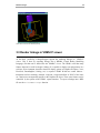
3.3 Render linkage in VRML97 viewer .................................................................... 85
3.4 Animate Linkage ................................................................................................. 88
Join linkages ...................................................................................................................... 97
4.1 Create one piston ................................................................................................ 98
4.2 Assembly the pistons .......................................................................................... 103
4.3 Finalize the V-Engine definition ........................................................................ 109
Advanced linkage definition ............................................................................................ 113
5.1 Open kinematic pair definitions .......................................................................... 114
5.1.1 Define the rotational joints ..................................................................... 115
5.1.2 Define the spherical joints ...................................................................... 118
5.2 Loop closing kinematic pair definitions ............................................................. 125
5.2.1 Automatic loop variables selection ........................................................ 127
5.2.2 Manual loop variables selection ............................................................ 130
5.2.3 Finalizing the linkage definition ............................................................ 138
Template based solver ...................................................................................................... 143
6.1 Define the PUMA 560 robot ............................................................................... 144
6.1.1 Add geometry ........................................................................................ 146
6.2 Solve the inverse kinematics problem ................................................................ 148
6.2.1 TemplateEquation data type ................................................................... 150
6.2.2 Generate starting equation ...................................................................... 153
6.2.3 Search for matching equations ............................................................... 155
First Iteration ........................................................................................ 156
Second Iteration .................................................................................... 158
Third Iteration ........................................................................................ 160
Fourth Iteration ...................................................................................... 164
Fith Iteration ......................................................................................... 166
6.3 Define the inverse linkages ................................................................................. 168
References ................................................................................................................. 172
Kinematics of linkages ..................................................................................................... 173
7.1 Define the cardan shaft linkage .......................................................................... 174
7.2 Kinematics of the cardan shaft ............................................................................ 182
7.2.1 Create time dependent linkage ............................................................... 183
7.2.2 Calculate the velocity of the motion ...................................................... 190
7.2.3 Plot velocity and acceleration diagrams ................................................. 193
Index .................................................................................................................................. 201
Introduction
LinkageDesigner is an application package for virtual prototyping linkages. It is designed to
analyse, synthesize and simulate linkages with serial chain, tree and graph structure. Using
the symbolic calculation capabilities of Mathematica LinkageDesigner support fully
parametrized linkage definition and analysis too.
Linkages are described in LinkageDesigner as a set of kinematic pairs. Kinematic pair
definitions are stored in LinkageData object, which is the base data model of the package.
Kinematic pairs are defined with DefineKinematicPair function. Principally there
are two different types of kinematic pairs handeld by this function; i.) kinematic pair, that
does not create loop in the kinematic graph of the linkage (open kinematic pair) ii.) loop
creating kinematic pair (loop closing kinematic pair). In the first case the mobility of the
linkages is increased by the number of joint variables of the open kinematic pair. In the
second case the mobility of the linkages is decreased by the number of non-redundant
constraint equations imposed.
2
Linkage Designer:Getting Started
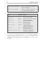
RotationalJoint
allows relative rotation of the two links
of the kinematic pair around a common axis.
TranslationalJoi
nt
allows relative translation of the two links of the kinematic pair
along a common axis, but no relative rotation of the links.
UniversalJoint
allows relative rotation of the two links of
the kinematic pair around two perpendicular axis.
PlanarJoint
allows relative translation of the two links of
the kinematic pair in a common plane and relative
rotation around an axis perpendicular to the plane.
CylindricalJoint
allows relative translation and rotation of the
two links of the kinematic pair along a common axis.
SphericalJoint
allows relative rotation of the two links
of the kinematic pair around a common point.
FixedJoint
connects the two links of the kinematic pair rigidly.
Possible kinematic pair definition with DefineKinematicPair function
The mobility of the linkage is the Degree Of Freedom (DOF) of the linkage. In
LinkageDesigner the mobility of the linkage is always equal to the number of driving
variables ( stored in the $DrivingVariables record ) of the LinkageData object.
Unique feature of DefineKinematicPair function, that it calculates the non-redundant
constraint equations in case of loop closing kinematic pair definition. It removes as as many
driving variables from the
$DrivingVariables record
as
the number of
non-redundant constraint equations. This feature has two important implications. It is
possible to detect the "lock up" ( having 0 mobility) and not feasible mechanism ( having
"negative" mobility ) definition, at the time the closing kinematic pair is defined.
LinkageDesigner can calculate the velocity, angular velocity, acceleration, angular
acceleration or even higher order derivatives of any links in closed form. This feature is valid
for any type ( serial, tree, graph structure) linkages.
Even if every transformation matrix, constraint equations or any other informations stored in
LinkageData is accessible to the user, most often animations or visualizations of the linkages
give more information, than the expressions. LinkageDesigner package has an extensive
support for visualizing and animating linkages. Linkages can be displayed or animated in
Linkage Designer:Getting Started
3
Mathematica notebook, in Dynamic Visualizer or can be exported to a VRM97 world.
LinkageDesigner supports parameterized linkage definition. This way different dimensions
of the links ( e.g. length of a link ) can be represented by a parameter and the kinematic pair
definitions are generated with parameters. If the user would like to change the numerical
value of the parameters, it can be done by simply re-setting it without redefining the whole
linkage.
LinkageData currently supports three type of parameter definitions :
$SimpleParameters
record stores parameters together with
their substitution values. e.g. toolLengthØ10
$DerivedParametersA
record stores parameters,
that are expressed as the explicit functions of simple
parameters andêor driving variables. e.g. q1Ø ArcTan@x,yD
$DerivedParametersB
record stores parameters,
that are defined implicitly as a set of equation
of parameters andêor driving variables of
the linkage. e.g. q1Ø Sin@q1D+Cos@xD==d
Parameters in LinkageData
4
Linkage Designer:Getting Started
Feature List
1. Kinematic graph based modeling.
2. Unified handling of 2D and 3D linkages with serial chain, tree and graph structure.
3. Support for parametrized linkage definition.
4. Constraint equations are generated only in case of loop closing kinematic pair
definition. Only non-redundant constraint equation are generated.
5. Exact mobility of the linkage calculation even for parametrically defined linkages.
6. Support for solving inverse kinematic problem of linkages using pattern equation
based solver.
7. Calculation of translational velocity and angular velocity and higher order
derivatives of any links in the linkage in closed form.
8. Exchange linkage models with other users.
9. Visualize and animate linkage in Mathematica notebook or in Dynamic Visualizer.
10. Export linkage or animation of the linkage into VRML97 world.
1500
1000
500
0
2000
20
10
0 y
0
-10
-10
0
x
10
1500
1000
500
0
20 -20
-1000
-500
0
500
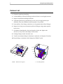
Abdank - Abakanowicz integrator
5 - axis milling machine
Linkage Designer:Getting Started
5
Quick Tour
The first step in getting started with LinkageDesigner is to load the package.
† Load LinkageDesigner package
In[1]:=
<< LinkageDesigner`
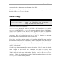
In this quick tour you will build one of the simplest closed-loop linkage, the four-bar
mechanism. The schematic figure of this linkage is shown below. You will define the
parametrized model of this linkage using the parameters of Figure 1.
Figure 1: Fourbar mechanism
The linkage definition in LinkageDesigner is nothing else but filling up a LinkageData
object. LinkageData is new datatype introduced by LinkageDesigner, that wraps all
relevant information of linkages. Besides other informations LinkageData stores the
kinematic graph of the linkage. The edges of this graph represent the kinematic pairs, while
the vertexes correspond to the rigid bodies, or as we will further refer to the links of the
linkage. From kinematic point of view the links are specified with body attached frames,
called Local Link Reference Frames (LLRF). The kinematic pairs on the other hand are
6
Linkage Designer:Getting Started
represented with the homogenous transformation of the LLRFs.
The first step in defining the four-bar mechanism is to create a LinkageData object with
the help of the CreateLinkage function.
Define linkage
CreateLinkage@nameD
returns the LinkageData object of an empty
linkage. The name of the linkage is name
Create an empty LinKageData object in LinkageDesigner
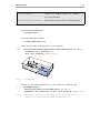
CreateLinkage automatically adds two rigid body to the linkage, the Ground and the
Workbench link. The LLRF of Ground link represent the global reference of the linkage.
The Workbench link is the base link, or the local ground of the linkage. By default the
LLRF of these links are superpositioned. One can imagine that the linkage is built on a
workbench, which can be placed anywhere in the "world" by changing the placement
transformation between the Workbench and the Ground links.
Every links should have a unique name in the LinkageData database.The string identifiers
therefore stored in their full name. A full name is made up of the name of the linkage (this is
the "surname") and the entity name ( this the "given name"). For example the name of the
linkage is "fourBar" and the entity name of the link is "link0" then the full name of this link
will be "fourBar@link0".
CreateLinkage defines automatically a name to the two base links. To change the default
name assigned to the Ground and Workbench links the GroundName and
WorkbenchName options of CreateLinkage function should be used. On Figure 1
"link0" notifies the local ground of the linkage, therefore specify the WorkbenchName
options to "link0". Also add the angle (f) of the "link0" link and the reference x-axis to the
LinkageData record as a simple parameter.
Linkage Designer:Getting Started
7
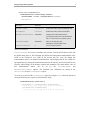
† This create a LinkageData object
fourBarMechanism = CreateLinkage@"FourBar",
WorkbenchName → "link0", SimpleParameters → 8φ → 0<D
−LinkageData,6−
option name
default value
WorkbenchName
'' Workbench''
defines the name of the Workbench link
GroundName
'' Ground''
defines the name of the Ground link
WorkbenchPlacement Automatic
PlacementName
Automatic
SimpleParameters
8<
Homogenous transformation matrix
specifying the placement of the Workbench
link w.r.t. the reference coordinate system
Name of the kinematic pair
defining the Workbech placement
List of simple parameters
Options of the CreateLinkage
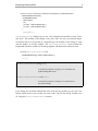
CreateLinkage also create a kinematic pair between Ground and Workbench link with
the default name Base-0. This kinematic pair defines the homogenous transformation of the
LLRF of the Workbench w.r.t LLRF of the Ground and vice versa. By default this
transformation matrix is an identical transformation, which implies that the two LLRFs are
superpositioned. By setting the transformation between Workbench and Ground link one can
place the whole linkage in an arbitrary position and orientation. The name and the value of
this transformation matrix can be set by the PlacementName and
WorkbenchPlacement options. The kinematic pair definitions are stored in the
$Structure record of LinkageData object.
You can get a record of the LinkageData object by using the Part function. Instead of
an integer index hovewer type the record identifier string.
fourBarMechanism@@"$Structure"DD
88FourBar@Base−0, 88FourBar@Ground, FourBar@link0<,
881, 0, 0, 0<, 80, 1, 0, 0<, 80, 0, 1, 0<, 80, 0, 0, 1<<<,
88FourBar@link0, FourBar@Ground<,
881, 0, 0, 0<, 80, 1, 0, 0<, 80, 0, 1, 0<, 80, 0, 0, 1<<<<<
8
Linkage Designer:Getting Started
Now that you have created the fourBarMechanism LinkageData object, you can
define the kinematic pairs of the mechanism.
à Define the "open" kinematic pairs
To define the rotational joint
DefineKinematicPairTo function.
between
"link0"
and
"link1"
use
the
DefineKinematicPair@linkage, "Rotational", 8q<, 8linki ,mxi <,8linkj ,mxj <D
Create a rotational joint between linki and link j and appends the
definition to the linkage LinkageData object. The function returns
the updated LinkageData object.
DefineKinematicPairTo@linkage, "Rotational", 8q<, 8linki ,mxi <, 8link j ,mx j <D
Create a rotational joint between linki and link j and appends the
definition to the linkage LinkageData object and reset the reulted
LinkageData object to linkage.
8q<
is a LinkageData object
linki
name of the lower link
mxi
joint frame of the lower link defined in the LLRF of linki
link j
name of the upper link
mx j
joint frame of the upper link defined in the LLRF of link j
linkage
Rotational joint definition
joint variable of the rotational joint
Linkage Designer:Getting Started
9
† This will create a rotational joint definition and append it to fourBarMechanism
DefineKinematicPairTo@
fourBarMechanism,
"Rotational",
8θ1<,
8"link0", IdentityMatrix@4D<,
8"link1", IdentityMatrix@4D<
D
−LinkageData,6−
fourBarMechanism linkage has now one "real" kinematic pair defined between "link0"
and "link1". The mobility of the linkage is one, since "link1" has only one rotational degree
of freedom relative to the ground. In LinkageDesigner the mobility of the linkage is equal
with the number of driving variables. The $DrivingVariables record contains the
independent kinematic variables of the linkage together with their actual numerical value.
† Get the $DrivingVariables record
fourBarMechanism@@"$DrivingVariables"DD
8θ1 → 0<
SetDrivingVariables@linkage, new D
set the driving variables of linkage to new and returns the
updated LinkageDate object.
SetDrivingVariablesTo@linkage, new D
set the driving variables of linkage to new and rand reset
the result to linkage.
Driving the linkage
If you change the associated substitutional value of the driving variables you can "drive" the
linkage, which means in our case that you rotate "link1" link. Set the driving variables q1 to
45° using the SetDrivingVariables function
10
Linkage Designer:Getting Started
† This will set q1 driving variable to 45°
SetDrivingVariablesTo@fourBarMechanism, 8θ1 → 45 °<D
−LinkageData,6−
DefineKinematicPair function also appends default geometric representation to the
$LinkGeometry record for every new links of the linkage. As the rotational joint is
defined between "link0" and "link1" DefineKinematicPair creates and appends a
default geometric representation of "link1" and "link0". The generated Graphics3D
representation of the links are simple Text primitives that contains the name of the link. If
you want to change the geometric representation of the links, you can simply simply
re-assign a Graphics3D object to the "linkname" sub-part of the $LinkGeometry
record.
† Re-set the geometry of "link1" link to a red line
fourBarMechanism@@"$LinkGeometry", "link1"DD =
Graphics3D@8RGBColor@1, 0, 0D, Line@880, 0, 0<, 85, 0, 0<<D<D
Graphics3D
You can display the linkage in its current pose using the Linkage3D function that returns a
Graphics3D object of the whole linkage.
Linkage3D@linkageD
Linkage3D function.
returns the geometric representation
of the linkage as Graphics3D object.
Linkage Designer:Getting Started
11
option name
default value
LinkMarkers
None
specifies the list of link name,
of which the LLRF to be displayed.
LinkGeometry
All
specifies the list of link name,
of which the LinkGeometry to be displayed
MarkerSize
1
Display size of the marker
8x,y,z<
MarkerLabels
Axes labels of the marker
Selected options of Linkage3D function.
If you display fourBarLinkage you can see that the LLRF of "link1" is rotated 45° with
respect to the LLRF of "link0" around the common z-axis.
† Display fourBarMechanism
Show@
Linkage3D@
fourBarMechanism,
LinkMarkers → All, MarkerSize → 1D
D
z
y
y
x
link0
x
Graphics3D
Define the second rotational joint between "link1" and "link2" at point B in the Figure 1.
This joint is placed at the end of "link1". The distance between point A and point B is l1.
12
Linkage Designer:Getting Started
To define the rotational joint, two joint marker has to be specified. The joint markers specifiy
the position and orientation of the rotational joint. The markers are given relative to the
LLRF of the two links. The common z-axis of the joint markers is the axis of the rotation.
Since the rotational joint axis is parallel with the z-axis of the LLRF of "link1" it is enough
to translate the LLRF of "link1" with {0,l1,0} vector to obtain the first joint marker. The
second joint marker is defined to be identical with the LLRF of "link2".
In LinkageDesigner markers are defined with a 4x4 homogenous transformation
matrixes. To define the joint markers you can use MakeHomogenousMatrix function .
MakeHomogenousMatrix@m,vD
creates a homogenous transformation
matrix from a 3 x 3 rotation matrix m and a
3 x 1 translation vector v.
MakeHomogenousMatrix@mD
creates a homogenous transformation matrix
from a 3 x 3 rotation matrix m with a
{0,0,0} translation vector.
MakeHomogenousMatrix@vD
creates a homogenous transformation matrix
from a 3 x 1 translation vector v and with a 3 x
3 identity matrix.
MakeHomogenousMatrix@o, zD
creates a homogenous transformation matrix of
a coordinate frame defined by its vector of
origin o and the direction vector of the z-axis z.
MakeHomogenousMatrix function
If the joint marker definition use some parameters, the numerical substitution value of the
parameters
should
be
specified
with
the
Parameters
option
of
DefineKinematicPair function. The parameters introduced with this option are
appended to the $SimpleParameters record of the LinkageData object.
Linkage Designer:Getting Started
13
option name
default value
JointName
Automatic
JointLimits
Automatic
validity range of joint variable HsL
JointPose
Automatic
offset values of the joint variables
Parameters
8<
name of the low order joint
list of parameters with their initial substitution
number used in the definition of the kinematic pair.
LinkageData manipulating options
† This define the second rotational joint between "link1" and "link2"
DefineKinematicPairTo@
fourBarMechanism,
"Rotational",
8θ2<,
8"link1", MakeHomogenousMatrix@8l1, 0, 0<D<,
8"link2", IdentityMatrix @4D<,
Parameters → 8l1 → 5<
D
−LinkageData,6−
Similarily to the this kinematic pair definition you can define the rotational joint between
"link2" and "link3" links.
† This define the third rotational joint between "link2" and "link3"
DefineKinematicPairTo@
fourBarMechanism,
"Rotational",
8θ3<,
8"link2", MakeHomogenousMatrix@8l2, 0, 0<D<,
8"link3", MakeHomogenousMatrix@80, 0, 0<D<,
Parameters → 8l2 → 10<
D
−LinkageData,6−
Now the mobility of the fourBarMechanism linkage is 3, which is reflected in the
$DrivingVariables record.
14
Linkage Designer:Getting Started
fourBarMechanism@@"$DrivingVariables"DD
8θ1 → 45 °, θ2 → 0, θ3 → 0<
à Define the loop closing kinematic pair
The fourth rotational joint between "link3" and "link0" will create a loop in the kinematic
graph, therefore it will decrease the mobility of the linkage. DefineKinematicPair
function will automatically calculate the non-redundant constraint equations imposed by the
loop closing kinematic pair, and remove as many driving variables from
$DrivingVariables record as the number of non-redundant constraint equations. The
removed driving variables are appended to the $DerivedParametersB record, since
they are not independent variables of the linkage any more. Their value are determined by
the generated constraint equations.
The driving variables selected to move into $DerivedParametersB record are called
loop variables. Normally there are many possibilities to select the loop variables. Any
driving variable that appear in the generated constraint equations are potential candidates to
become a loop variable, and called candidate loop variables. DefineKinematicPair
function select automatically the loop variables from the list of candidate loop variables by
removing the candidate loop variables from the end of the $DrivingVariables record.
If you want to change the order of selection of the loop variables, specify the list of
candidate loop variables with the CandidateLoopVariables option.
option name
default value
CandidateLoopV
ariables
Automatic
list of driving variables that can
be selected to become loop variable
LockingEnabled
False
allows kinematic pair definition that locks up
the mechanism, by having mobility equal to 0.
DefineKinematicPair options influencing the loop closing kinematic pair definition
Linkage Designer:Getting Started
15
† This define a rotational joint between "link3" and "link0"
DefineKinematicPairTo@
fourBarMechanism,
"Rotational",
8θ4<,
8"link0", MakeHomogenousMatrix@8l0, 0, 0<D<,
8"link3", MakeHomogenousMatrix@8l3, 0, 0<D<,
Parameters → 8l3 → 15, l0 → 15<
D
−LinkageData,7−
fourBarMechanism is now fully defined. The mobility of the linkage is 1. The remained
driving variable is q1, that determine the posture of the linkage. q2 and q3 are become loop
variable and moved to $DerivedParametersB record.
† Get the $DrivingVariables record
fourBarMechanism@@"$DrivingVariables"DD
8θ1 → 1.73367<
† Get the $DerivedParametersB record
fourBarMechanism@@"$DerivedParametersB"DD
88FourBar@RotationalJoint−4, 8θ2 → −0.932994, θ3 → −1.74053<,
8−l3 − l2 Cos@θ3D − l1 Cos@θ2D Cos@θ3D + l1 Sin@θ2D Sin@θ3D +
l0 H−Sin@θ1D HCos@θ3D Sin@θ2D + Cos@θ2D Sin@θ3DL +
Cos@θ1D HCos@θ2D Cos@θ3D − Sin@θ2D Sin@θ3DLL == 0,
l1 Cos@θ3D Sin@θ2D + l2 Sin@θ3D + l1 Cos@θ2D Sin@θ3D +
l0 HCos@θ1D H−Cos@θ3D Sin@θ2D − Cos@θ2D Sin@θ3DL −
Sin@θ1D HCos@θ2D Cos@θ3D − Sin@θ2D Sin@θ3DLL == 0<<<
16
Linkage Designer:Getting Started
à Place the linkage
PlaceLinkage@linkage,mxD
change the Workbench-Ground transformation
of linkage to mx and return the resulted linkage
PlaceLinkageTo@linkage,mxD
change the Workbench-Ground transformation
of linkage to mx and reset the resulted linkage to
linkage
Change the Ground-Workbench transformation
You can place the linkage into an arbitrary position and orientation if you change the
transformation matrix between the Ground and Workbench links. PlaceLinkageTo
function replace this transformation matrix with the one specified in its argument. The
placement transformation can contains parameters, provided that you have added these
parameters to the LinkageData object. Since the f symbol has been already added to the
simple parameters of the linkage at the time the LinkageData is created,you can use it to
define the placement matrix.
† Define the placement matrix
MatrixForm@mx = MakeHomogenousMatrix@RotationMatrix@80, 0, 1<, φDDD
Cos@φD −Sin@φD 0 0 y
i
z
j
j
z
j
Sin@φD Cos@φD 0 0 z
z
j
z
j
z
j
z
j
j
z
j
0
0
1 0z
z
j
j
z
0
0
0 1{
k
† Place the linkage
PlaceLinkageTo@fourBarMechanism, mxD
−LinkageData,8−
mx =.
Linkage Designer:Getting Started
17
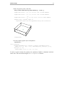
à Define the geometry
If you want to render your linkage you might want to add geometric representations to the
links, that are more detailed than the default ones. If the $LinkGeometry record has an
entry for a link it can be simple over defined using the set function. Otherwise you have to
append a whole sub-record to the $LinkGeometry record of the linkage.
LinkageDesigner provide a simple Graphics3D primitive called LinkShape, that can be
used to define the geometric representation of the links.
LinkShape@l, r1, r2, wD
is a Graphics3D primitive that draws link
shape with l length r1 and r2 radius and w width.
LinkShape primitive
† Add parametrized link geometries to the three moving links
fourBarMechanism@@"$LinkGeometry", "link1"DD = Graphics3D@
8SurfaceColor@RGBColor@1, 1, 0DD, LinkShape@l1, 1, 1, .1D<D;
fourBarMechanism@@"$LinkGeometry", "link2"DD =
PlaceShape@Graphics3D@8SurfaceColor@[email protected], 0.5, 1DD,
LinkShape@l2, 1, 1, .1D<D, MakeHomogenousMatrix@80, 0, 0.2<DD;
fourBarMechanism@@"$LinkGeometry", "link3"DD = Graphics3D@
8SurfaceColor@[email protected], 0, 0.9DD, LinkShape@l3, 1, 1, .1D<D;
† Add parametrized link geometries to the fixed link
fourBarMechanism@@"$LinkGeometry", "link0"DD =
PlaceShape@Graphics3D@8SurfaceColor@[email protected],
LinkShape@l0, 0.5, .5, .2D<D, MakeHomogenousMatrix@80, 0, −0.3<DD;
You can change the posture of the mechanism by setting its driving variable (q1) to a
different
substitutional
value
using
the
SetDrivingVariables
or
SetDrivingVariablesTo functions.
If the LinkageData object specified as the argument of SetDrivingVariables or
SetDrivingVariablesTo
functions has $DerivedParametersB record, the
18
Linkage Designer:Getting Started
constraint equations specified in this record are solved with the in-build FindRoot
function. SetDrivingVariables and SetDrivingVariablesTo functions,
therefore accept all options of FindRoot function.
† Set q1 driving variable of fourBarMechanism to 45°
SetDrivingVariablesTo@fourBarMechanism, 8θ1 → 45 °<, MaxIterations → 50D
−LinkageData,8−
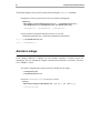
† Display fourBarMechanism
Show@Linkage3D@fourBarMechanism, LinkMarkers → All, Axes → TrueDD
z
xy
yz x
zy
y
xx
1
0.5
0
10
0
5
5
10
0
15
Graphics3D
Since the fourBarMechanism defined parametrically, changing the parameter values
new four-bar mechanism can be obtained without redefining the whole linkage.
Linkage Designer:Getting Started
19
SetSimpleParameters@linkage, newparam D
reset the simple parameters of linkage to newparam and returns
the new LinkageDate object.
SetSimpleParametersTo@linkage, newparam D
reset the simple parameters of linkage to newparam and reset the
resulted LinkageDate object to linkage.
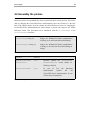
Caption describing the definition box.
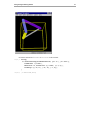
† Set f parameter value to 30°
SetSimpleParametersTo@fourBarMechanism, 8φ → 30 °<D
−LinkageData,8−
† Re-display fourBarMechanism
Show@Linkage3D@fourBarMechanism,
LinkMarkers → All, PlotRange → All, Axes → TrueDD
z
y
x
15
z
y x
yzyyxx
x
1
0.5
0
10
0
5
5
10
Graphics3D
0
20
Linkage Designer:Getting Started
Template based solver
The kinematic graph of fourBarMechanism contains one loop. A loop in the graph
structure is defined with list of loop closure equation, that is stored in the
$DerivedParametersB record.
† Get the $DerivedParametersB record of fourBarMechanism
fourBarMechanism@@"$DerivedParametersB"DD
88FourBar@RotationalJoint−4, 8θ2 → 0.40727, θ3 → −2.21875<,
8−l3 − l2 Cos@θ3D − l1 Cos@θ2D Cos@θ3D + l1 Sin@θ2D Sin@θ3D +
l0 H−Sin@θ1D HCos@θ3D Sin@θ2D + Cos@θ2D Sin@θ3DL +
Cos@θ1D HCos@θ2D Cos@θ3D − Sin@θ2D Sin@θ3DLL == 0,
l1 Cos@θ3D Sin@θ2D + l2 Sin@θ3D + l1 Cos@θ2D Sin@θ3D +
l0 HCos@θ1D H−Cos@θ3D Sin@θ2D − Cos@θ2D Sin@θ3DL −
Sin@θ1D HCos@θ2D Cos@θ3D − Sin@θ2D Sin@θ3DLL == 0<<<
The loop-closure equations defines the {q1,q2} derived parameters. If any independednt
variables of the system is changing the loop closure equation has to be solved. To solve the
loop-closure in closed form one has to express q1 and q2 variables as the function of the
driving variables {q1} and simple parameters 8l0 , l1 , l2 , l3 , φ<. To arrive the closed
form solution you can use the in-builded Solve function. In case of numerous parameters
the Solve function might required exceesive time and memory resources to arrive to the
solution.
The loop closure equations in case of four-bar mechanism can be specified as inverse
kinematic problem of the 3R manipulator. The inverse kinematic problem of linkages very
often result in equations that matches certain pattern. LinkageDesigner introduced a new
function called PatternSolve to support the solution of inverse kinematic problem of
linkages. PatternSolve function uses template equations to search for posible explicit
expression of the unknown variables.
Linkage Designer:Getting Started
21
à Solve the loop-closure constraint equation
Let's assume that the fourth rotational joint does not exist, because the mechanism is cut at
point D on Figure 1. The four-bar mechanism then become a RRR manipulator. Let's define
the tool center point (TCP) of this manipulator with the 8l3 , 0, 0< vector from the LLRF
of link3. Similarly define the base point (BP) with 8l0 , 0, 0< vector from the LLRF of
link0. The inverse kinematic problem can be formulated as follows:Given the distance vector
of TCP from BP, specify the corresponding joint values. The fourth rotational joint than can
be than defined by restricting the TCP to be coincide with BP.
Since the RRR manipulator redundant, therefore only two joint variable can be expressed
out of the inverse kinematic problem. The first joint variable (q1) assumed to be known in
the solution procedure.
The Template Based technique is an iterative solution method. It can be applied on a set of
redundant or non-redundant equations. The solution contains four main steps:
1. Generate the equations of the inverse kinematic problem
2. Convert to normal form the equation with respect to the list of unknown variables
3. Search for matching equations
4. Select and store the solution for the matched variable.
After step 4. the matched variable is removed from the list of unknown variables and the
algorithm continues at step 2. The iteration continues until all unknown variables are
expressed. For detailed discussion of the template based solution techique refer the
Chapter 6 of this manual.
22
Linkage Designer:Getting Started
† Generate the starting equations of the inverse kinematic problem
Timing@eqlist = GenerateInvKinEquations@fourBarMechanism,
8"link3", MakeHomogenousMatrix@8l3, 0, 0<D<,
8"link0", MakeHomogenousMatrix@8l0 , 0, 0<D<,
TargetMarker → IdentityMatrix@4DD;D
ColumnForm@eqlistD
80.15 Second, Null<
−Cos@θ1D Cos@θ2D + Cos@θ3D + Sin@θ1D Sin@θ2D == 0
l2 + l1 Cos@θ2D + l3 Cos@θ3D − l0 HCos@θ1D Cos@θ2D − Sin@θ1D Sin@θ2DL == 0
−Cos@θ2D Sin@θ1D − Cos@θ1D Sin@θ2D − Sin@θ3D == 0
Cos@θ2D Sin@θ1D + Cos@θ1D Sin@θ2D + Sin@θ3D == 0
−l1 Sin@θ2D − l0 H−Cos@θ2D Sin@θ1D − Cos@θ1D Sin@θ2DL + l3 Sin@θ3D == 0
−Sin@θ1D − Cos@θ3D Sin@θ2D − Cos@θ2D Sin@θ3D == 0
Sin@θ1D + Cos@θ3D Sin@θ2D + Cos@θ2D Sin@θ3D == 0
−Cos@θ1D + Cos@θ2D Cos@θ3D − Sin@θ2D Sin@θ3D == 0
−1 + Cos@θ3D HCos@θ1D Cos@θ2D − Sin@θ1D Sin@θ2DL + H−Cos@θ2D Sin@θ1D − Cos@θ1
−1 + Cos@θ3D HCos@θ1D Cos@θ2D − Sin@θ1D Sin@θ2DL − HCos@θ2D Sin@θ1D + Cos@θ1D
Cos@θ3D H−Cos@θ2D Sin@θ1D − Cos@θ1D Sin@θ2DL − HCos@θ1D Cos@θ2D − Sin@θ1D Sin
Cos@θ3D HCos@θ2D Sin@θ1D + Cos@θ1D Sin@θ2DL + HCos@θ1D Cos@θ2D − Sin@θ1D Sin@
l0 Sin@θ1D + l2 Sin@θ2D + l3 HCos@θ3D Sin@θ2D + Cos@θ2D Sin@θ3DL == 0
l1 − l0 Cos@θ1D + l2 Cos@θ2D + l3 HCos@θ2D Cos@θ3D − Sin@θ2D Sin@θ3DL == 0
1 − Sin@θ1D H−Cos@θ3D Sin@θ2D − Cos@θ2D Sin@θ3DL − Cos@θ1D HCos@θ2D Cos@θ3D −
1 + Sin@θ1D HCos@θ3D Sin@θ2D + Cos@θ2D Sin@θ3DL − Cos@θ1D HCos@θ2D Cos@θ3D − S
−Cos@θ1D HCos@θ3D Sin@θ2D + Cos@θ2D Sin@θ3DL − Sin@θ1D HCos@θ2D Cos@θ3D − Sin
−Cos@θ1D H−Cos@θ3D Sin@θ2D − Cos@θ2D Sin@θ3DL + Sin@θ1D HCos@θ2D Cos@θ3D − Si
−l0 + l1 Cos@θ1D + l2 HCos@θ1D Cos@θ2D − Sin@θ1D Sin@θ2DL + l3 HCos@θ3D HCos@θ1
l1 Sin@θ1D + l2 HCos@θ2D Sin@θ1D + Cos@θ1D Sin@θ2DL + l3 HCos@θ3D HCos@θ2D Sin
l3 + l2 Cos@θ3D + l1 Cos@θ2D Cos@θ3D − l1 Sin@θ2D Sin@θ3D − l0 H−Sin@θ1D HCos@θ
−l1 Cos@θ3D Sin@θ2D − l2 Sin@θ3D − l1 Cos@θ2D Sin@θ3D − l0 HCos@θ1D H−Cos@θ3D S
Linkage Designer:Getting Started
23
† Search for pattern solution for the variables {q2, q3}
Timing@sol = PatternSolve@eqlist, 8θ2, θ3<DD
92.113 Second,
998T7<, 99θ2 → ArcTan@l0 Sin@θ1D, −l1 + l0 Cos@θ1DD − ArcTanA−l3 - J1 −
1
HH−l22 − l32 + Hl1 − l0 Cos@θ1DL2 + l02 Sin@θ1D2 L ^ 2LN,
4 l22 l32
−l22 − l32 + Hl1 − l0 Cos@θ1DL2 + l02 Sin@θ1D2
l2 +
E,
2 l2
−l22 − l32 + Hl1 − l0 Cos@θ1DL2 + l02 Sin@θ1D2
θ3 → ArcTanA
,
2 l2 l3
2
2
+ Hl1 − l0 Cos@θ1DL
+ l02 Sin@θ1D
L
H−l22 − l32%%%%%%%%%%%%%%%%%%%%%%%%%%%%%%%%
$%%%%%%%%%%%%%%%%%%%%%%%%%%%%%%%%
%%%%%%%%%%%%%%%%%%%%%%%%%%%%%%%%
%%%%%%%%%%%%%%%%%%%%%%%%
1−
E=,
2
2
4 l2 l3
2
9θ2 → ArcTan@l0 Sin@θ1D, −l1 + l0 Cos@θ1DD − ArcTanAl3 - J1 −
1
HH−l22 − l32 + Hl1 − l0 Cos@θ1DL2 + l02 Sin@θ1D2 L ^ 2LN,
4 l22 l32
−l22 − l32 + Hl1 − l0 Cos@θ1DL2 + l02 Sin@θ1D2
l2 +
E,
2 l2
2
2
2
2
−l2 − l3 + Hl1 − l0 Cos@θ1DL + l0 Sin@θ1D2
θ3 → ArcTanA
,
2 l2 l3
2
i
H−l22 − l32 + Hl1 − l0 Cos@θ1DL2 + l02 Sin@θ1D2 L y
z
j
z
−- j
j
z
j1 −
zE==, 8<===
4 l22 l32
k
{
24
Linkage Designer:Getting Started
† Simplify the solution
sol = FullSimplify@sol@@1, 2DDD
H−l02 − l12%%%%%%%%%%%%%%%%%%%%%%%%%%%%%%%%
+ l22 + l32 + 2%%%%%%%%%%%%%%%%
l0 l1 Cos@θ1DL
%%%%%%%%%%%%%%%%%%%%%%%% ,
1−
99θ2 → −ArcTanA−2 l3 $%%%%%%%%%%%%%%%%%%%%%%%%%%%%%%%%
4 l22 l32
2
l02 + l12 + l22 − l32 − 2 l0 l1 Cos@θ1D
E+
l2
ArcTan@l0 Sin@θ1D, −l1 + l0 Cos@θ1DD,
l02 + l12 − l22 − l32 − 2 l0 l1 Cos@θ1D
θ3 → ArcTanA
,
l2 l3
+ l22 + l32 + 2%%%%%%%%%%%%%%%%
l0 l1 Cos@θ1DL
H−l02 − l12%%%%%%%%%%%%%%%%%%%%%%%%%%%%%%%%
%%%%%%%%%%%%%%%%%%%%%%%% E=,
2 $%%%%%%%%%%%%%%%%%%%%%%%%%%%%%%%%
1−
4 l22 l32
2
H−l02 − l12%%%%%%%%%%%%%%%%%%%%%%%%%%%%%%%%
+ l22 + l32 + 2%%%%%%%%%%%%%%%%
l0 l1 Cos@θ1DL
%%%%%%%%%%%%%%%%%%%%%%%% ,
9θ2 → −ArcTanA2 l3 $%%%%%%%%%%%%%%%%%%%%%%%%%%%%%%%%
1−
4 l22 l32
2
l02 + l12 + l22 − l32 − 2 l0 l1 Cos@θ1D
E+
l2
ArcTan@l0 Sin@θ1D, −l1 + l0 Cos@θ1DD,
l02 + l12 − l22 − l32 − 2 l0 l1 Cos@θ1D
θ3 → ArcTanA
,
l2 l3
H−l02 − l12%%%%%%%%%%%%%%%%%%%%%%%%%%%%%%%%
+ l22 + l32 + 2%%%%%%%%%%%%%%%%
l0 l1 Cos@θ1DL
%%%%%%%%%%%%%%%%%%%%%%%% E==
1−
−2 $%%%%%%%%%%%%%%%%%%%%%%%%%%%%%%%%
4 l22 l32
2
à Define two resolved linkage
The PatternSolve function found two solution of the inverse kinematic problem. The
solution express the derived parameters {q2,q3} as the explicit function of the
independendent variables ( driving variables and simple parameters). The closed form
solution of the inverse kinematic problem can be added as $DerivedParametersA
record of the LinkageData object. Since {q2, q3} are defined explicitly the implicit definition
specified in the $DerivedParametersB record is redundant and can be deleted. This
way you can define two resolved linkage, that has its loop closure equations solved in closed
form.
Linkage Designer:Getting Started
25
† Append the first solution branch of the inverse kinematic problem to the
$DerivedParametersA record and remove $DerivedParametersB
record
fourBarMechanism1 =
Append@fourBarMechanism, 8"$DerivedParametersA", sol@@1DD<D
−LinkageData,9−
fourBarMechanism1 = Delete@fourBarMechanism1, "$DerivedParametersB"D
−LinkageData,8−
† Append the second solution branch of the inverse kinematic problem to the
$DerivedParametersA record and remove $DerivedParametersB
record
fourBarMechanism2 =
Append@fourBarMechanism, 8"$DerivedParametersA", sol@@2DD<D
−LinkageData,9−
fourBarMechanism2 = Delete@fourBarMechanism2, "$DerivedParametersB"D
−LinkageData,8−
sol =.
eqlist =.
Save linkage
You can save the LinkageData object of the four-bar mechanism to a text file. This way you
can share your mechanism with other LinkageDesigner users or use it later without
redefining the kinematic pairs and geometries of the linkage.
† This saves the definition of fourBarMechanism in the file fourBarMechanism.txt
Save@ToFileName@8$LinkageExamplesDirectory<, "fourBarMechanism.txt"D,
8fourBarMechanism, fourBarMechanism1, fourBarMechanism2<D
26
Linkage Designer:Getting Started
The defined linkages can be saved in binary format using the DumpSave command.
† DumpSave in binary format the three four-bar mechanism LinkageData
DumpSave@
ToFileName@8$LinkageExamplesDirectory<, "fourBarMechanism.mx"D,
8fourBarMechanism, fourBarMechanism1, fourBarMechanism2<D
8−LinkageData,8−, −LinkageData,8−, −LinkageData,8−<
† This reload the LinkageData definitions from the text file (The
$LinkageExamplesDirectory is added to the $Path during initialization)
In[5]:=
<< fourBarMechanism.txt
Out[5]=
−LinkageData,8−
Animate Linkage
If the linkage definition is finished you can animate, syntethise or further process the
mechanism. You can animate the linkage in Mathematica notebook, in Dynamic Visualizer
or in a VRML97 viewer.
† Load the LinkageDesigner package and the pre-defined four-bar linkage
<< LinkageDesigner`
<< fourBarMechanism.txt
† Animate fourBarMechanism in Dynamic Visualizer
Timing@
DVAnimateLinkage@fourBarMechanism, 88θ1 → 0.<, 8θ1 → 360 °<<D;D
81.542 Second, Null<
Linkage Designer:Getting Started
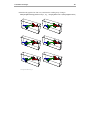
† Generate animation of fourBarMechanism1 in the notebook
In[81]:=
Out[81]=
Timing@
ls = AnimateLinkage@fourBarMechanism1, 88θ1 → 0.<, 8θ1 → 360 °<<,
LinkMarkers → 8"link2"<,
MarkerSize → 5, TracePoints → 88"link2", 80, 5, 0<<<,
PlotRange → 88−10, 17<, 8−15, 15<, 8−1, 4<<D;
D
83.585 Second, Null<
27
28
Linkage Designer:Getting Started
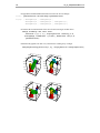
In[90]:=
Show@GraphicsArray@Partition@ls, 3DDD
x
y
z
y
x
zy
x
Out[90]=
z
z
z
x
z
y
x
zy
y
x
z
y
y
x
z
x
y
x
GraphicsArray
† Export animation of fourBarMechanism2 to VRML97 world
Timing@
WriteVRMLAnimation@fourBarMechanism2,
ToFileName@8$LinkageExamplesDirectory<, "fourBarAnimation.wrl"D,
88θ1 → 0.<, 8θ1 → 360 °<<,
Resolution → 20, LinkMarkers → 8"link2"<,
MarkerSize → 5, TracePoints → 88"link2", 80, 5, 0<<<,
Axes → True, PlotRange → 88−10, 17<, 8−15, 15<, 8−1, 4<<D;
D
86.89 Second, Null<
Linkage Designer:Getting Started
29
† This display the resulted VRML file in Internet explorer (this command works in
Windows )
In[11]:=
Run@"start", "explorer " <>
ToFileName@8$LinkageExamplesDirectory<, "fourBarAnimation.wrl"DD;
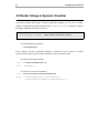
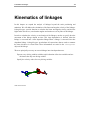
1. Principles of linkage definition
31
Principles of linkage
definition
This chapter introduces the basic notations for building linkages with LinkageDesigner.
Linkages are multi-body system built from rigid bodies and constraints. This guide
introduce the basic definition of multi-body systems , however by no means substitute to a
standard text book of multi-body kinematics.
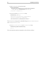
1.1 Rigid body representation
The rigid body is an "undistortable" body, that preserves the distance between two arbitrarily
chosen points. This implies, that to keep track of the motion of a rigid body, it is enough to
know the position of one point and the rotation of the body around this point. In
LinkageDesigner this information of the rigid body placement is captured by keeping track
the placement of a body attached Cartesian coordinate frame. This frame is called as Local
Link Reference Frame (LLRF), while the rigid bodies are referred later in this text as links.
During the motion of a link we keep track of the position and orientation of the LLRF
relative to a reference frame. The position and orientation of the LLRF relative to a reference
frame is represented in LinkageDesigner with a 4x4 homogenous matrix.
32
LinkageDesigner User Manual
y
z
LLRFx
T
z
p
¯
p
¯
y
x1 y1 z1 o1 y
i
j
z
j
j
z
x2 y2 z2 o2 z
j
z
j
z
T=j
z
j
x3 y3 z3 o3 z
j
z
j
z
j
z
k 0 0 0 1 {
Reference
x
Local Link Reference Frame
T homogenous matrix can be interpreted as coordinate transformation between x'y'z' and
xyz coordinate systems or as an displacement operation that place xyz frame into x'y'z' frame.
It is important to understand the differences between the two interpretation, because
LinkageDesigner use both of them.
If T matrix is interpreted as coordinate transformation, than it maps the coordinates of a
point in x'y'z' to the coordinates in the xyz coordinate systems. Given a point P on the link
specified by the èè
p' vector relative to x'y'z' coordinate system. The coordinates of this point
relative to the xyz coordinate system is specified by the èè
p vector. The connection between
the two vector is defined by equation (1).
py
'y
i
ip
j
j¯z
z = T.j
j¯ z
z
k1{
k 1 {
(1)
If T is interpreted as displacement operation it moves a frame from an original placement to
its present placement. This interpretation can be used to determine the elements of T matrix.
The 3-tuple of every column in
T matrix represent a vector. 8x1 , x2 , x3 <,
8y1 , y2 , y3 <,8z1 , z2 , z3 < vectors are the unit axis direction vectors of x', y' and z' axis relative to
xyz coordinate system. 8o1 , o2 , o3 < vector represents the position vector of the origin of x'y'z'
coordinate system relative to xyz. In the linkage definition we will use extensively
homogenous matrix as a displacement operation that specifies the joint markers with respect
to the LLRF of the link. Before we go further let's get a little bit familiar with the
homogenous matrix.
1. Principles of linkage definition
33
1.2 Homogenous matrixes
You can use the standard list operation of Mathematica to create a homogenous matrix, but
LinkageDesigner introduce the MakeHomogenousMatrix function to simplify the task of
homogenous matrix definition.
MakeHomogenousMatrix@m,vD
Assembly a homogenous matrix out of a
3x3 rotational matrix m and 3x1 vector v
MakeHomogenousMatrix@mD
Assembly a homogenous matrix out of a
3x3 rotational matrix m and {0,0,0} vector
MakeHomogenousMatrix@vD
Assembly a homogenous matrix out of
a 3x3 identity matrix and v vector
MakeHomogenousMatrix@t,ang,vD
Assembly a homogenous matrix out
rotational matrix calculated as a rotation
with ang angle around the vector t and
3x1 vector v
MakeHomogenousMatrix@o,zD
Assembly a homogenous matrix having
that origin is o and the z axis direction is z
Different ways to create homogenous matrix
† Load LinkageDesigner package
<< LinkageDesigner`
† This create a homogenous transformation that displace the reference marker by 2
units along x axis
MatrixForm@T = MakeHomogenousMatrix@82, 0, 0<D D
i1
j
j
j
0
j
j
j
j
j
j
0
j
j
k0
0
1
0
0
0
0
1
0
2
0
0
1
y
z
z
z
z
z
z
z
z
z
z
z
{
34
LinkageDesigner User Manual
You can display the coordinate frame (sometimes called marker) represented by a
homogenous matrix. Marker3D function returns a Graphics3D primitive of cartesian
coordinate frame corresponding to the homogenous matrix in its argument.
Create a Graphics3D primitive of coordinate
frame corresponding to mx homogenous matrix
Marker3D@mxD
Three-dimensional graphics primitive of a marker
† Display the reference frame in green and the T marker in red
Show@Graphics3D@
[email protected], Marker3D@IdentityMatrix@4DD, Hue@1D, Marker3D@TD<D,
Axes → True, Lighting → FalseD
z
y
z
y
0
x
1
2
1
0.75
0.5
0.25
0
0
1
0.75
0.5
x 0.25
0
3
Graphics3D
† This create a homogenous matrix that displace the reference marker by 2 units
along x axis and rotate it in such way that the z axis is unidirectional with {1,1,0}
vector
MatrixForm@T = MakeHomogenousMatrix@82, 0, 0<, 81, 1, 0<D D
1
− è!!!!
i
j
2
j
j
j
j
1
j
j
è!!!!
j
2
j
j
j
j
j
0
j
j
j
k 0
0
0
1
0
1
è!!!!
2
1
è!!!!
2
0
0
2y
z
z
z
z
z
0z
z
z
z
z
z
z
0z
z
z
z
1{
1. Principles of linkage definition
35
† Display the reference frame in green and the T marker in red
Show@Graphics3D@
[email protected], Marker3D@IdentityMatrix@4DD, Hue@1D, Marker3D@TD<D,
Axes → True, Lighting → False, FaceGrids → 880, 0, −1<<D;
z
1
0.75
0.5
0.25
0
0
z 1
0.75
0.5
0.25
0
y
y
x
0
x
1
2
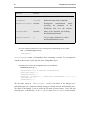
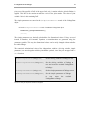
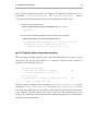
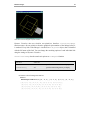
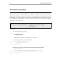
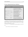
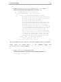
1.3 Kinematic graph
Every kinematic structure can be described in terms of its joints and links. Joints constrain
the motion of two links. This constrained two links constitute a kinematic pair. In
LinkageDesigner, kinematic structures (linkages, mechanisms,...) are represented by graphs,
where the links represent the vertices of the graph, and the joints represent the edges. This
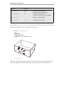
graph is called the kinematic graph of the linkage.The links represented kinematically with
LLRFs and geometrically in terms of their associated shape representation. The kinematical
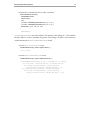
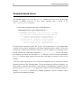
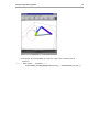
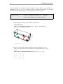
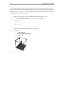
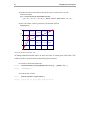
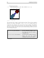
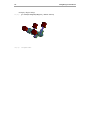
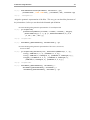
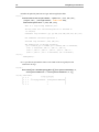
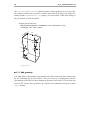
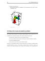
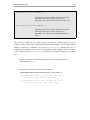
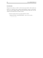
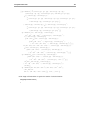
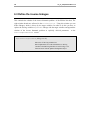
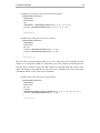
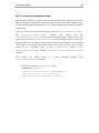
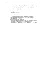
and geometrical representation of the crank-slider mechanism is shown below.
6
ConnectingRod
Crank
024
4
2
WorkBench
0
Ground
Slider
-2
0
Kinematic graph of the crank-slider mechanism
5
10
15
36
LinkageDesigner User Manual
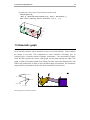
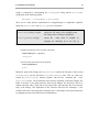
LinkageDesigner represent kinematic graph as non oriented graph
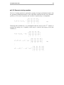
The kinematic graph is represented in LinkageDesigner by a list of kinematic pairs stored in
the $Structure record of the LinkageData object. We will discuss in detail the records
of the LinkageData data type in Chapter 2. For the time being it is enough to now,
that LinkageData wraps all informations of the linkage. As you are building your
linkage, your main task is to build the kinematic graph by enumerating the kinematic pairs
of the linkage.
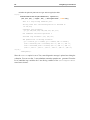
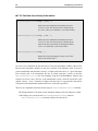
You can display the graph representation of a linkage using the MakeLinkageGraph
funtion. This function returns a Graph object, that can be manipulated with the functions of
the standard DiscreteMath`Combinatorica` package.
MakeLinkageGraph@linkage,fD
returns the non-oriented graph object of
linkage LinkageData and fills up the f
link name mapping function.
ShowLinkageGraph@linkageD
display the kinematic graph of linkage.
Generate and display the kinematic graph of linkages
† Load LinkageDesigner and the predefined crank-slider mechanism
In[26]:=
<< LinkageDesigner`
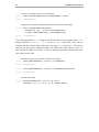
<< crankSliderMechanism.txt
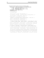
† Create the kinematic graph of the crank-slider mechanism
In[28]:=
Out[28]=
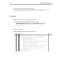
gr = MakeLinkageGraph@crankSliderMechanism, nameMapD
Graph:<5, 5, Undirected>
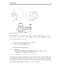
1. Principles of linkage definition
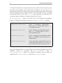
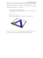
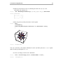
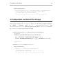
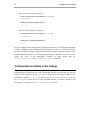
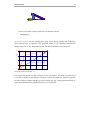
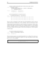
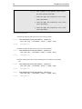
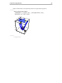
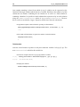
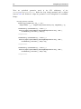
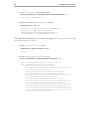
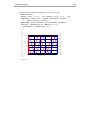
† Display the graph
In[29]:=
ShowLabeledGraph@grD
1
2
5
3
4
Out[29]=
Graphics
† Display the nameMap definition
In[30]:=
? nameMap
Global`nameMap
Attributes@nameMapD = 8Listable<
nameMap@1D := CrankSlider@ConnectingRod
nameMap@CrankSlider@ConnectingRodD := 1
nameMap@2D := CrankSlider@Crank
nameMap@CrankSlider@CrankD := 2
nameMap@3D := CrankSlider@Ground
nameMap@CrankSlider@GroundD := 3
nameMap@4D := CrankSlider@Slider
nameMap@CrankSlider@SliderD := 4
nameMap@5D := CrankSlider@Workbench
nameMap@CrankSlider@WorkbenchD := 5
37
38
LinkageDesigner User Manual
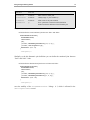
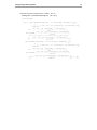
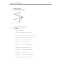
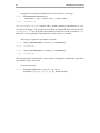
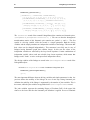
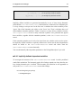
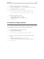
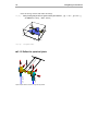
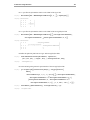
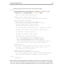
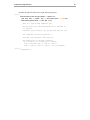
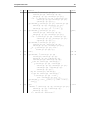
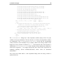
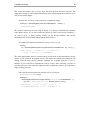
† Show the graph
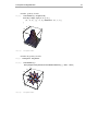
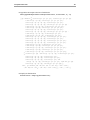
In[31]:=
ShowLabeledGraph@gr, GetStrippedName@Array@nameMap, 5DDD
Connecti
Crank
W
Ground
Slider
Out[31]=
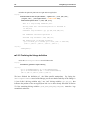
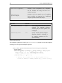
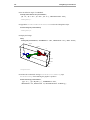
In[32]:=
Graphics
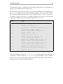
ShowLinkageGraph@crankSliderMechanismD
ConnectingRod
Crank
Workbench
Ground
Slider
Out[32]=
Graphics
1. Principles of linkage definition
39
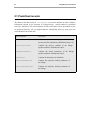
1.4 How to define kinematic pair
RotationalJoint
allows relative rotation of the two links
of the kinematic pair around a common axis.
TranslationalJoi
nt
allows relative translation of the two links of the kinematic pair
along a common axis, but no relative rotation of the links.
UniversalJoint
allows relative rotation of the two links of
the kinematic pair around two perpendicular axis.
PlanarJoint
allows relative translation of the two links of
the kinematic pair in a common plane and relative
rotation around an axis perpendicular to the plane.
CylindricalJoint
allows relative translation and rotation of the
two links of the kinematic pair along a common axis.
SphericalJoint
allows relative rotation of the two links
of the kinematic pair around a common point.
FixedJoint
connects the two links of the kinematic pair rigidly.
Kinematic pairs available in LinkageDesigner
LinkageDesigner
provides
two
functions,
DefineKinematicPair
and
DefineKinematicPairTo , whose add new kinematic pairs to the kinematic graph. You
can define kinematic pairs based on tree scenarios:
1. The links of the kinematic pairs are not pre-assembled, therefore they are
"Out-Of-Place". In this scenario the joint markers has to be specified on both link
separately. Joint markers has to be defined relative to the LLRFs of the
corresponding links. The kinematic pair definition will assembly the links into their
constrained placement.
2. The links of the kinematic pairs are "In-Place", or pre-assembled. In this scenario
the LLRF of the two links and the joint marker has to be specified relative to a
common reference frame. This scenario can be used for example to import linkage
definition from a CAD system.
40
LinkageDesigner User Manual
3. The kinematic pair is defined with Denavith-Hartenberg variables. This scenario can
be used to define rotational or translational joint using the 4 Denavith-Hartenberg
variables.
à 1.4.1 "Out-Of-Place" kinematic pair definition
DefineKinematicPair@linkage,"type",8q1,q2,..<,8"linki",mxi<, 8"linkj",mxj<D
function appends a kinematic pair definition to linkage and returns the resulted
linkage The kinematic pair is defined between "linki" and "linkj" links. "type" string
specifies the type of the kinematic pair to be defined. The joint markers of "linki"
and "linkj" links are specified with mxi and mxj homogenous matrixes. The list of
joint variable(s) of the kinematic pair is defined with {q1,q2,..}.
Define kinematic pair for the "Out-Of-Place" scenario
In this scenario kinematic pairs are defined with the constrained movement of the joint
markers. The joint marker is a cartesian coordinate system, that is rigidly attached to its
owner link. The joint markers are defined with homogenous transformation matrixes (mxi
and mxj), which represent the displacements of the corresponding LLRFs.
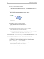
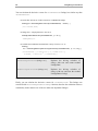
To illustrate the kinematic pair definition let's define a simple linkage having only a
rotational joint. Since it is easier to visualize a link, if the bounding geometry is assigned, we
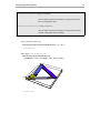
start the linkage definition with defining the geometries for link1 and link2 links.
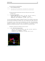
† Load the LinkageDesigner package
<< LinkageDesigner`
1. Principles of linkage definition
41
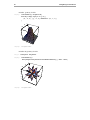
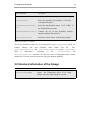
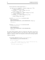
† Define geometry for link1
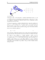
link1Geometry = Graphics3D@
Plot3D@5 ∗ Exp@−Sqrt@x ^ 2 + y ^ 2DD,
8x, −3, 3<, 8y, −3, 3<, BoxRatios → 81, 1, 1<D
D
In[33]:=
2
0
-2
2
1
0
-2
0
2
Out[33]=
Graphics3D
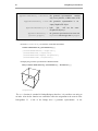
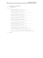
† Define the geometry for link2
In[34]:= <<Graphics`Polyhedra`
In[35]:=
link2Geometry =
Show@Graphics3D@GreatStellatedDodecahedron@DD, Axes → TrueD
2
0
-2
2
1
0
-1
-2
-2
0
2
Out[35]=
Graphics3D
The LLRF of the links can be chosen freely, but the geometric representation should be
specified relative to the LLRF. For simplicity we choose the LLRFs of link1 and link2 to be
coincide with the reference coordinate system of their geometric representation.
42
LinkageDesigner User Manual
The rotational joint restrict the relative motion of the links in such manner, that the origin of
the two joint markers are superpositioned and they are allowed to rotate only around the
common z-axis. In order to define the rotational joint between link1 and link2 the joint
markers of both link has to be specified
† Define the joint marker for link1 by translating the LLRF with {0,0,5} vector.
Hmx1 = MakeHomogenousMatrix@80, 0, 5<DL êê MatrixForm
In[37]:=
1
i
j
j
j
0
j
j
j
j
j
j
0
j
j
k0
Out[37]//MatrixForm=
0
1
0
0
0
0
1
0
0
0
5
1
y
z
z
z
z
z
z
z
z
z
z
z
{
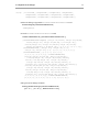
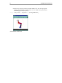
† Show the geometry and the joint marker of linki together
Show@
link1Geometry,
Graphics3D@Marker3D@mx1DD
, PlotRange → AllD
In[38]:=
2
0
-2
z
y
x
6
4
2
0
-2
0
2
Out[38]=
Graphics3D
1. Principles of linkage definition
43
† Define the joint marker for link2 by translating the LLRF with {0,0,1.2} vector
and rotating 180° around x-axis.
In[40]:=
Hmx2 = MakeHomogenousMatrix@80, 0, 1.2<, 80, 0, −1<DL êê MatrixForm
1 0
0
0 y
i
z
j
j
z
j
0 −1 0
0 z
z
j
z
j
z
j
z
j
j
z
j
0 0 −1 1.2 z
z
j
j
z
0
1 {
k0 0
Out[40]//MatrixForm=
† Show the geometry and the joint marker of link2 together
In[44]:=
Show@
link2Geometry,
Graphics3D@Marker3D@mx2, MarkerSize → 2, MarkerLabels → NoneDD
D
2
0
-2
2
1
0
-1
-2
-2
0
2
Out[44]=
Graphics3D
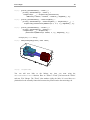
You can see that the joint marker definition for link1 and link2 places the link2 "upside
down" on the top of the peek of link1.
† Create a test linkage with link1 as the Workbench
In[45]:=
test1 = CreateLinkage@"test1", WorkbenchName → "link1"D
Out[45]=
−LinkageData,6−
44
LinkageDesigner User Manual
† Append the rotational joint definition between link1 and link2 to test linkage
In[46]:=
DefineKinematicPairTo@test1,
"Rotational", 8q1<, 8"link1", mx1<, 8"link2", mx2<D
Out[46]=
−LinkageData,6−
DefineKinematicPairTo function adds a default geometric representation to every
new link of the linkage. The geometries are defined as Graphics3D object and stored in the
LinkageData. To get the graphics representation of ther link use the overloaded Part
function. To set new geometric representation to a link, use the Set function.
† Re-assign the geometric representation of the links
In[47]:=
Out[47]=
In[48]:=
Out[48]=
test1@@$LDLinkGeometry, "link1"DD = link1Geometry
Graphics3D
test1@@$LDLinkGeometry, "link2"DD = link2Geometry
Graphics3D
The rotational joint is defined with q1 joint variable. Changing the substitutional value of the
joint variable rotates "link2" link.
† Animate the linkage
In[54]:=
AnimateLinkage@test1, 88q1 → 0<, 8q1 → 65 °<<,
PlotRange → 88−3, 3<, 8−3, 3<, 80, 9<<, Boxed → FalseD;
1. Principles of linkage definition
45
à 1.4.2 "In-Place" kinematic pair definition
DefineKinematicPair@linkage,"type",8q1,q2,..<,8"linki",llrfi<, 8"linkj",llrfj<, jcmD
function appends a kinematic pair definition to linkage and returns the resulted
linkage The kinematic pair is defined between "linki" and "linkj" links. "type"
string specifies the type of the kinematic pair to be defined. The LLRFs of linki
and linkj are given with llrfi and llrfj homogenous matrixes. The joint center
marker is given with jcm homogenous matrixes. llrfi, llrfi, jcm markers are
given relative to the reference coordinate frame. The list of joint variable(s) of the
kinematic pair is defined with {q1,q2,..}.
Define kinematic pair for the "In-Place" scenario
If the linkage is pre-assembled the geometries of the links are placed in their constrained
position. If you know the LLRF of the links and the joint marker relative to a common
reference frame you can use the "In-Place" kinematic pair definition. This scenario might be
useful if the mechanism is assembled in a CAD system and you want to import to
Mathematica.
To illustrate the kinematic pair definition let's use the same example as in Section 1.4.1
† Load the LinkageDesigner package
<< LinkageDesigner`
46
LinkageDesigner User Manual
† Define geometry for link1
link1Geometry = Graphics3D@
Plot3D@5 ∗ Exp@−Sqrt@x ^ 2 + y ^ 2DD,
8x, −3, 3<, 8y, −3, 3<, BoxRatios → 81, 1, 1<D
D
In[55]:=
2
0
-2
2
1
0
-2
0
2
Graphics3D
Out[55]=
† Define the geometry for link2
In[3]:= <<Graphics`Polyhedra`
link2Geometry =
Show@Graphics3D@GreatStellatedDodecahedron@DD, Axes → TrueD
In[56]:=
2
0
-2
2
1
0
-1
-2
-2
0
2
Out[56]=
Graphics3D
1. Principles of linkage definition
47
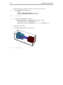
The geometries of the two links can be pre-assembled by placing them in their constrained
position. The geometry of link2 is placed upside-down on the top the geometry of link1. To
place the geometries you can use the PlaceShape function of LinkageDesigner:
PlaceShape@shape,mx,sD
places shape Graphics3D primitives with mx
homogenous transformation matrix and scale it
with s.
PlaceShape@shape,mxD
places shape Graphics3D primitives with
mx homogenous transformation matrix
Place Graphics3D with homogenous transformation
† Place link2Geometry to its constrained place
link2GeometryConstrained = PlaceShape@
link2Geometry, MakeHomogenousMatrix@80, 0, 6.2<, 80, 0, −1<DD
In[57]:=
Graphics3D
Out[57]=
† Show the geometries of link1 and link2 in their constrained place
Show@8link1Geometry, link2GeometryConstrained<,
PlotRange → 88−3, 3<, 8−3, 3<, 80, 9<<D
In[63]:=
2
0
-2
8
6
4
2
0
-2
0
2
Out[63]=
Graphics3D
48
LinkageDesigner User Manual
† Create a test linkage with link1 as the Workbench
In[64]:=
test2 = CreateLinkage@"test2", WorkbenchName → "link1"D
Out[64]=
−LinkageData,6−
† Append the rotational joint definition between link1 and link2 to test linkage
In[65]:=
test2 = DefineKinematicPair@test2,
"Rotational", 8q1<, 8"link1", IdentityMatrix@4D<,
8"link2", IdentityMatrix@4D<, IdentityMatrix@4DD
Out[65]=
−LinkageData,6−
You might noticed that test2 linkage uses different LLRF and joint markers than test1
linkage specified in Section 1.4.1. In case of test2 both LLRF of the links are
identical with the reference frame (well, this is true only if q1 is equal to 0 ). This follows
from the fact, that you can arbitrarily choose the LLRF of the links. However, once you
have selected the LLRF of the links, you have to define the geometric representation of the
links relative to the LLRF.
† Add the geometric representation of the links to the linkage
In[66]:=
Out[66]=
In[67]:=
Out[67]=
test2@@$LDLinkGeometry, "link1"DD = link1Geometry
Graphics3D
test2@@$LDLinkGeometry, "link2"DD = link2GeometryConstrained
Graphics3D
† Animate the linkage
In[68]:=
AnimateLinkage@test2, 88q1 → 0<, 8q1 → 65 °<<,
PlotRange → 88−3, 3<, 8−3, 3<, 80, 9<<, Boxed → FalseD;
1. Principles of linkage definition
49
à 1.4.3 Kinematic pair definition with Denavith-Hartenberg variables
DefineKinematicPair@linkage,"type",8"linki","linkj"<,8a,d,a ,q <D
function appends a kinematic pair definition to linkage and returns the resulted
linkage The kinematic pair is defined between "linki" and "linkj" links.
"type"string specifies the type of the kinematic pair to be defined. The four D-H
parameters specifies the transformation between the LLRFs of the two links. Only
Rotational and Translational joint definition is allowed in this way.
Define kinematic pair with Denavith-Hartenberg parameters
The Denavith-Hartenberg notation is widely used in robotics to describe mechanism with
open kinematic chain. LinkageDesigner also support kinematic pair definition with D-H
parameters. The D-H parameters defines the homogenous transformations betwen the LLRF
of the upper and the LLRF of the lower one. Since there are only four D-H variable the
relative placements of the LLRFs are restricted. Also the applicable joint type is restricted,
since only rotational and translational joint definition is allowed in this scenario. There is no
joint variable specification in the DefineKinematicPair function unlike before. This is
so because q and d D-H parameters are the joint variables in case of rotational and
translational joint definition.
To illustrate the kinematic pair definition of this scenario you can define the test mechanism
using D-H parameters.
† Load the LinkageDesigner package
In[34]:=
<< LinkageDesigner`
† Create a test linkage with link1 as the Workbench
In[35]:=
test3 = CreateLinkage@"test3", WorkbenchName → "link1"D
Out[35]=
−LinkageData,6−
Since the joint to be defined is a rotational one, the q variable will be the joint variable.
Therefore you specify the 4th parameter with a symbol.
50
LinkageDesigner User Manual
† Append the rotational joint definition between link1 and link2 to test linkage
In[36]:=
test3 = DefineKinematicPair@test3,
"Rotational", 8"link1", "link2"<, 80, 6.2, 0, q1<D
Out[36]=
−LinkageData,6−
† Display the LLRF markers of test3 linkage
Show@Linkage3D@test3, LinkMarkers → All, MarkerSize → 3D,
PlotRange → 88−3, 3<, 8−3, 3<, 80, 9<<, Axes → TrueD
In[37]:=
2 -2
0
0
-2
2
z
y
8
6
link2
4
z
x
y
2
0
Out[37]=
link1
Graphics3D
x
1. Principles of linkage definition
† Define geometry for link1
link1Geometry = Graphics3D@
Plot3D@5 ∗ Exp@−Sqrt@x ^ 2 + y ^ 2DD,
8x, −3, 3<, 8y, −3, 3<, BoxRatios → 81, 1, 1<D
D
In[75]:=
2
0
-2
2
1
0
-2
0
2
Graphics3D
Out[75]=
† Define the geometry for link2
In[9]:= <<Graphics`Polyhedra`
In[76]:=
link2Geometry =
Show@Graphics3D@GreatStellatedDodecahedron@DD, Axes → TrueD
2
0
-2
2
1
0
-1
-2
-2
0
2
Out[76]=
Graphics3D
51
52
LinkageDesigner User Manual
† Add the geometric representation of the links to the linkage
In[77]:=
Out[77]=
In[78]:=
Out[78]=
test3@@$LDLinkGeometry, "link1"DD = link1Geometry
Graphics3D
test3@@$LDLinkGeometry, "link2"DD = link2Geometry
Graphics3D
† Animate the linkage
In[79]:=
AnimateLinkage@test3, 88q1 → 0<, 8q1 → 65 °<<,
PlotRange → 88−3, 3<, 8−3, 3<, 80, 9<<, Boxed → FalseD;
2. LinkageData: A new datatype
53
LinkageData: A new
datatype
In order to simulate or synthesize linkages one has to store the relevant data of the linkage in
a database. The data model of this database should contain all the information required by
the processing functions, and also flexible enough to enable the extension. LinkageDesigner
introduce a new datatype called LinkageData, that conforms these requirements.
LinkageData data object wraps all information of a linkage. It wraps basically a List,
whose elements have to conform to a simple pattern. The element of this list should match
the {_String, _List} pattern. The elements of the main list in the LinkageData
wrapper are called records. The first part of the record ( _String ) is the record identifier,
while the last part ( _List) is the record data.
† Load LinkageDesigner package
In[1]:=
<< LinkageDesigner`
† Create a simple LinkageData object with only one record
LinkageData@88"MyID", 81, 2, 3<<<D
−LinkageData,1−
LinkageData object is formatted as -LinkageData,n-, where n stands for the number of
records of the object.
54
LinkageDesigner User Manual
2.1 Predefined records
The format of the data records in LinkageData is not strictly defined. In order to find the
information required by the functions of LinkageDesigner, certain number of predefined
record are introduced. The record identifier and the record data of these predefined records
are specified rigorously, but you might extend the LinkageData object by using your own
record identifier and record data.
Record Identifier
Description
$MechanismID
Defines the name of the linkage and other linkage
instance specific informations (WorkBench name, etc.)
$DrivingVariables
Contains the driving variables of the linkage
together with their substitutional values.
$SimpleParameters
Contains the simple parameters of the linkage
together with their substitutional values.
$Structure
Contains the kinematic pair definitions.
$DerivedParmetersA
Contains the explicitly defined parameters of
the linkage.
$DerivedParametersB
Contains the implicitly defined parameters of
the linkage.
Predefined record identifiers of LinkageData
2. LinkageData: A new datatype
55
Record Identifier
Description
$LowOrderJoint
Stores data of the low order joints( name, limits, etc)
$LinkGeometry
Stores the geometric representation of the links
as Graphics3D objects.
$LinkGroundTransformat
ion
Stores the transformation matrix of all LLRFs to
the Global Reference Frame.
$TimeDependentVariables
Contains the list of time dependent variables
together with their first derivative.
$DrivingVelocities
Stores the velocity values of the driving variables.
Predefined record identifiers of LinkageData
Not all the predefined records have to be presented in every LinkageData record. For
example linkages with open kinematic chain usually does not
have
$DerivedParametersA and $DerivedParametersB records. LinkageData
object
is
manipulated
principally
by
the
CreateLinkage
and
DefineKinematicPair functions. The first one creates a LinkageData object with the
minimal set of records, while the second one fills up the database gradually.
2.2 Structural information of the linkage
CreateLinkage@nameD
Create an empty LinkageData object
returns the LinkageData object of an empty
linkage. The name of the linkage set to name
56
LinkageDesigner User Manual
option name
default value
WorkbenchName
'' Workbench'' Defines the name of the Workbench link
GroundName
'' Ground''
WorkbenchPlacement Automatic
PlacementName
Automatic
SimpleParameters
8<
Defines the name of the Ground link
Homogenous
transformation
matrix
specifying the placement of the
Workbench link w.r.t. the reference
Name of the kinematic pair defining
the Workbench placement.
List of simple parameters to add to
the $SimpleParameters record
Options of CreateLinkage
† Create a linkage with the name "test" and assign the resulted linkage to test symbol
test = CreateLinkage@"test"D
−LinkageData,6−
CreateLinkage returns a LinkageData object containing 6 records. To investigate the
contents of the records list the first part of the LinkageData object:
† Display the records of the LinkageData object in ColumnForm
ColumnForm@test@@1DDD
8$MechanismID, 8test, test@Ground, test@Workbench<<
8$DrivingVariables, 8<<
8$SimpleParameters, 8<<
8$Structure, 88test@Base−0, 88test@Ground, test@Workbench<, 881, 0, 0, 0<,
8$LowOrderJoint, 8<<
8$LinkGeometry, 8<<
The first data stored in $MechanismID record is the name of the linkage (test).
LinkageDesigner use a composite naming strategy to identify the links and kinematic pairs.
The name of the linkage is used to create the full name of entity names. Every link and
kinematic pair is identified by an EntityName string. The FullName of this identifier
2. LinkageData: A new datatype
57
strings is composed by concatenating the LinkageName string and the EntityName
string based on the following pattern:
FullName = LinkageName @ EntityName
There are two help function implemented in LinkageDesigner to manipulate composite
names, the GetFullName and GetStrippedName functions.
GetFullName@linkage, stringIDD
returns the full name of the stringID using
the linkage name of linkage LinkageData
GetStrippedName@stringIDD
returns the
entity name of stringID, by
dropping the substrings up to the first @
Functions for composite name manipulation.
† Define the full name of the "myLink" entity name
GetFullName@test, "myLink"D
test@myLink
† Get the entity name back form the full name
GetStrippedName@%D
myLink
Beside the name of the linkage the $MechanismID contains the full name of the Ground
(test@Ground) and the Workbench (test@Workbench) links. This two links were
created by CreateLinkage function, together with the first kinematic pair of the
$Structure record. The Ground link is the reference rigid body of the entire linkage. The
LLRF of Ground is the global reference frame for the linkage. The Workbench link is by
default connected with a fixed joint to the ground link, and represents the local reference
body of the linkage. This duplication of the reference links has two advantages: i.) the
reference link can be described with a kinematic pair ii.) the linkage can be placed anywhere
by changing only the Ground-Workbench transformation.
58
LinkageDesigner User Manual
CreateLinkage function appends a sub-record to the $Structure record beside the
$MechanismID record. The $Structure record stores the informations of the kinematic
pairs:
† Get the $Structure record of test LinkageData
test@@"$Structure"DD
88test@Base−0, 88test@Ground, test@Workbench<,
881, 0, 0, 0<, 80, 1, 0, 0<, 80, 0, 1, 0<, 80, 0, 0, 1<<<,
88test@Workbench, test@Ground<,
881, 0, 0, 0<, 80, 1, 0, 0<, 80, 0, 1, 0<, 80, 0, 0, 1<<<<<
The $Structure record stores three information of the kinematic pair:
1. String identifier of the kinematic pair ( test@Base-0 )
2. String identifier of the two links ( {test@Ground,test@Workbench} )
3. Homogenous transformations of the LLRF of the upper link to the lower one and
vice versa. ( {{1,0,0,0},{0,1,0,0},{0,0,1,0},{0,0,0,1}} )
The default settings of CreateLinkage can be changed by using one or more options of
this function:
† Create a linkage with the name "test1" by overriding the default settings
In[2]:=
test1 = CreateLinkage@"test1",
WorkbenchName → "MyWorkbench", GroundName → "MyGroundName",
WorkbenchPlacement → MakeHomogenousMatrix@810, 0, 10<D,
PlacementName → "FirstKinematicPair"D
Out[2]=
−LinkageData,6−
† Get the $MechanismID and the $Structure records of test1 LinkageData
test1@@"$MechanismID"DD
8test1, test1@MyGroundName, test1@MyWorkbench<
2. LinkageData: A new datatype
59
test1@@"$Structure"DD
88test1@FirstKinematicPair, 88test1@MyGroundName, test1@MyWorkbench<,
881, 0, 0, 10<, 80, 1, 0, 0<, 80, 0, 1, 10<, 80, 0, 0, 1<<<,
88test1@MyWorkbench, test1@MyGroundName<,
881, 0, 0, −10<, 80, 1, 0, 0<, 80, 0, 1, −10<, 80, 0, 0, 1<<<<<
2.3 Independent variables of the linkage
After you have defined your LinkageData object, you can build your database gradually
by
adding
kinematic
pairs
to
it.
DefineKinematicPair
and
DefineKinematicPairTo functions append an entry to the $Structure record of
the LinkageData object each time they are called.
† Define a kinematic pair to test linkage and store the resulted linkage in
testResult
testReturn = DefineKinematicPairAtest, "Rotational",
8q1<, 8"Workbench", MakeHomogenousMatrix@80, 0, 0<D<,
l1
9"link1", MakeHomogenousMatrixA90, 0,
=E=, Parameters → 8l1 → 10<E
2
−LinkageData,6−
† Get the $Structure record of testReturn
test@@"$Structure"DD
88test@Base−0, 88test@Ground, test@Workbench<,
881, 0, 0, 0<, 80, 1, 0, 0<, 80, 0, 1, 0<, 80, 0, 0, 1<<<,
88test@Workbench, test@Ground<,
881, 0, 0, 0<, 80, 1, 0, 0<, 80, 0, 1, 0<, 80, 0, 0, 1<<<<<
60
LinkageDesigner User Manual
testReturn@@"$Structure"DD
98test@Base−0, 88test@Ground, test@Workbench<,
881, 0, 0, 0<, 80, 1, 0, 0<, 80, 0, 1, 0<, 80, 0, 0, 1<<<,
88test@Workbench, test@Ground<, 881, 0, 0, 0<, 80, 1, 0, 0<,
80, 0, 1, 0<, 80, 0, 0, 1<<<<, 9test@RotationalJoint−1,
98test@Workbench, test@link1<, 98Cos@q1D, −Sin@q1D, 0, 0<,
l1
8Sin@q1D, Cos@q1D, 0, 0<, 90, 0, 1, −
=, 80, 0, 0, 1<==,
2
98test@link1, test@Workbench<, 98Cos@q1D, Sin@q1D, 0, 0<,
l1
8−Sin@q1D, Cos@q1D, 0, 0<, 90, 0, 1,
=, 80, 0, 0, 1<====
2
The $Structure record of the returned LinkageData object contains two kinematic pairs (
{test@Base-0,test@RotationalJoint-1} ). You can see that the homogenous
transformation matrix of this kinematic pair contains two symbol q1 and l1. The first
symbol is a driving variable, while the second is a simple parameter. Both the driving
variables and the simple parameters are independent variables of the linkage. This means that
their values can be changed independently ( This statement is not fully true in case of
linkages having kinematic graph, that contains loop(s). In this case the values of the
independent variables are restricted by the loop closure equations. Certain combinations of
independent variable values result non solvable loop closure equations, which means that
linkage would "break" to arrive to the prescribed independent values.)
The driving variables of the linkage are stored in the $DrivingVariables record of the
LinkageData object.
† Get the $DrivingVariables record of testReturn LinkageData object
testReturn@@"$DrivingVariables"DD
8q1 → 0<
The most important difference between driving variables and simple parameters is that, the
previous defines the mobility of the linkage. In case of non loop closing kinematic pair
definition the mobility of the linkage is augmented by the number of joint variables. This is
the reason, while the joint variables are appended to the $DrivingVariables record.
The joint variables represent the remaining Degree of Freedom (DoF) of the upper link
relative to the lower link after the kinematic pair definition is applied. In case of rotational
2. LinkageData: A new datatype
61
joint, out of the possible 6 DoF of the upper link, only 1 remains after the joint definition is
applied. This DoF is the rotation around the z-axis of the joint marker. The value of joint
variable "drives" this remaining DoF.
The simple parameters are stored in the $SimpleParameters record of the LinkageData
object.
† Get the $SimpleParameters record of testReturn LinkageData object
testReturn@@"$SimpleParameters"DD
8l1 → 10<
The simple parameters are basically placeholders for dimensional values. If they are used
instead of numbers, all kinematic equations or transformation are generated using the
parameter symbols. This way the dimensional values can be easily changed without redefine
the whole linkage.
The numerical substitutional value of the independent variables ( driving variable, simple
parameter ) are stored together with the placeholder symbols, since they are wrapped with a
Rule function.
SetDrivingVariables@linkage, newD
Set the driving variables of linkage to new
SetDrivingVariablesTo@linkage, newD
Set the driving variables of linkage to
new and resets the resulted LinkageData
to linkage.
SetSimpleParameters@linkage, newD
Set the simple parameters of linkage to new
SetSimpleParametersTo@linkage, newD
Set the simple parameters of linkage
to
new
resets
the
resulted
LinkageData to linkage
Functions for setting the independent variables of LinkageData
62
LinkageDesigner User Manual
† Set the driving variables of testReturn
SetDrivingVariablesTo@testReturn, 8q1 → 15 °<D
−LinkageData,6−
testReturn@@"$DrivingVariables"DD
8q1 → 15 °<
† Set the simple parameters of testReturn
SetSimpleParametersTo@testReturn, 8l1 → 5<D
−LinkageData,6−
testReturn@@"$SimpleParameters"DD
8l1 → 5<
In case of linkages with simple kinematic graph (serial chain or tree) setting the independent
variable is nothing else than replacing the second argument of the Rule function. However
for more complicated linkages, setting the independent variables includes the solution of the
constraint equations for the new set of independent variables. Therefore it is advised to never
change the value of the independent variables by other means than the
SetDrivingVariables and SetSimpleParameters functions.
2.4 Dependent variables of the linkage
LinkageDesigner distinguishes two kind of dependent variables, based on the way they are
defined. If the dependent variable (y) can be expressed as the explicit function of the
independent variables ( x1 , x2 , ...) it is stored in the $DerivedParametersA record of
the LinkageData object. However if the dependent variable y is defined implicitly with
an equation, it is stored in the $DerivedParametersB record.
2. LinkageData: A new datatype
63
y = f@x1 ,x2 ,...D y is an explicitly defined variable
g@y,x1 ,x2 ,...D
0 y is an implicitly defined variable
Different type of dependent variables.
Implicitly defined variables are generated automatically in case of loop closing kinematic
pair definition. DefineKinematicPair function detects, whether the new kinematic pair
is a loop closing or an open one. In the first case it calculates the relative mobility of the
"upper" link of the kinematic pair relative to the "lower" one. Then it calculates the set of
non-redundant constraint equations. Finally it removes as many driving variables from the
$DrivingVariables record as many constraint equations were generated and append
these variables ( together with the constraint equations) to the $DerivedParametersB
record.
If the constraint equations can be solved in closed form, the solution can be used to replace
the implicitly defined variables to explicitly defined ones. In this case the derived parameters
should be added to the $DerivedParametersA record and delete from the
$DerivedParametersB record manually.
You can add naturally other dependent parameters to the LinkageData object if you wish.
à 2.4.1 Implicitly defined dependent variables
To investigate the structure of the $DerivedParametersB record load the predefined
crank-slider mechanism. The kinematic graph of this linkage contains one loop, therefore one
loop closing kinematic pair is defined. This kinematic pair definition in turn appended an
entry to the $DerivedParametersB record of the linkage.
† Load LinkageDesigner package
<< LinkageDesigner`
64
LinkageDesigner User Manual
† Load the pre-defined crankSlider mechanism
Get@
ToFileName@8$LinkageExamplesDirectory<, "crankSliderMechanism.txt"DD;
† Display the linkage
Show@Linkage3D@crankSliderMechanismD, Boxed → FalseD
Crank
orkbench
ConnectingRod
Slider
Graphics3D
† Get the driving variables of crank-slider mechanism
crankSliderMechanism@@"$DrivingVariables"DD
8θ1 → 0<
† Get the implicitly defined dependent variables of crank-slider mechanism
crankSliderMechanism@@"$DerivedParametersB"DD
88CrankSlider@TranslationalJoint−4, 8θ2 → 2.69152 × 10−20 , θ3 → 0.0008658<,
8l0 Sin@p1 + θ1 + θ2 + θ3D == loffs Cos@p1 + θ1 + θ2 + θ3D +
l2 Sin@θ3D + l1 Sin@θ2 + θ3D, Cos@p1 + θ1 + θ2 + θ3D == 1<<<
Every elements of the $DerivedParametersB record contains the informations of one
set of implicitly defined dependent variables. These sub-list contains three data:
1. String Identifier (CrankSlider@TranslationalJoint-4)
2. List of dependent variables and the actual solution of the constraint equations
(θ2 → 2.69152 × 10−20 , θ3 → 0.0008658)
3. List of constraint equations. ({l0 Sin[p1+θ1+θ2+θ3]==
loffs Cos[p1+θ1+θ2+θ3]+l2 Sin[θ3]+
l1 Sin[θ2+θ3],Cos[p1+θ1+θ2+θ3]==1})
2. LinkageData: A new datatype
65
Every time the independent variables are changing, the dependent variables have to be
recalculated. SetDrivingVariables and SetSimpleParameters function
re-calculates the constraint equations using the new independent variable values.
† Set the q1 driving variables to 30°
SetDrivingVariablesTo@crankSliderMechanism, 8θ1 → 30 °<D
−LinkageData,7−
† Get the implicitly defined dependent variables of crank-slider mechanism
crankSliderMechanism@@"$DerivedParametersB"DD
88CrankSlider@TranslationalJoint−4, 8θ2 → −0.77638, θ3 → 0.253774<,
8l0 Sin@p1 + θ1 + θ2 + θ3D == loffs Cos@p1 + θ1 + θ2 + θ3D +
l2 Sin@θ3D + l1 Sin@θ2 + θ3D, Cos@p1 + θ1 + θ2 + θ3D == 1<<<
à 2.4.2 Explicitly defined dependent variables
The loop closing constraint equations of the crank-slider mechanism can be easily solved in
closed form. You can use the in-build Solve function to find the explicit solution of
equation (1) for variable q2 and q3 (2):
l0 Sin@p1 + θ1 + θ2 + θ3D ==
loffs Cos@p1 + θ1 + θ2 + θ3D + l2 Sin@θ3D +
l1 Sin@θ2 + θ3D Cos@p1 + θ1 + θ2 + θ3D == 1
θ2 → −p1 − θ1 − θ3
,
θ3 → ArcTanA± H1 − H−loffs + l1 Sin@p1 + θ1DL2 ê l22 L,
H−loffs + l1 Sin@p1 + θ1DL ê l2E
(1)
(2)
Instead of using the implicitly derived parameters of crankSliderMechanism you can
exchange the $DerivedParametersB record with $DerivedParametersA record.
You might noticed that there are two solution of the constraint equations (the 2p periodicity
is not important from this point of view, since it does not result a different pose of the
linkage). This means that you can define different linkage using the first or second solution
branch of the constraint equations.
66
LinkageDesigner User Manual
† Set the solution of the constraint equation equal to sol
,
sol = 99θ2 → −p1 − θ1 − ArcTanA H1 − H−loffs + l1 Sin@p1 + θ1DL2 ê l22 L,
H−loffs + l1 Sin@p1 + θ1DL ê l2E,
,
θ3 → ArcTanA H1 − H−loffs + l1 Sin@p1 + θ1DL2 ê l22 L,
H−loffs + l1 Sin@p1 + θ1DL ê l2E=,
,
9θ2 → −p1 − θ1 − ArcTanA− H1 − H−loffs + l1 Sin@p1 + θ1DL2 ê l22 L,
H−loffs + l1 Sin@p1 + θ1DL ê l2E,
,
θ3 → ArcTanA− H1 − H−loffs + l1 Sin@p1 + θ1DL2 ê l22 L,
H−loffs + l1 Sin@p1 + θ1DL ê l2E==;
† Append to $DerivedParametersA record the first solution
crankSliderMechanism1 =
Append@crankSliderMechanism, 8"$DerivedParametersA", sol@@1DD<D
−LinkageData,8−
† Delete the $DerivedParametersB record from the resulted
crankSliderMechanism1
crankSliderMechanism1 =
Delete@crankSliderMechanism1, "$DerivedParametersB"D
−LinkageData,7−
The explicitly defined dependent variables are wrapped into a Rule function, where the first
argument is the variable the second is its value. You have to make sure that the second
argument is evaluated to a number if the independent variables and the remaining dependent
variables are substituted.
† Get the $DerivedParametersA record of crankSliderMechanism1
crankSliderMechanism1@@"$DerivedParametersA"DD
9θ2 → −p1 − θ1 − ArcTanA
,
H1 − H−loffs + l1 Sin@p1 + θ1DL2 ê l22 L, H−loffs + l1 Sin@p1 + θ1DL ê l2E,
,
θ3 → ArcTanA H1 − H−loffs + l1 Sin@p1 + θ1DL2 ê l22 L,
1
H−loffs + l1 Sin@p1 + θ1DLE=
l2
2. LinkageData: A new datatype
67
† Set the q1 driving variable to 70° of crankSliderMechanism1 and display
the linkage
Show@Linkage3D@SetDrivingVariables@crankSliderMechanism1, 8θ1 → 70 °<DD,
Boxed → FalseD
Crank
Workbench
ConnectingRod
Slider
Graphics3D
2.5 Auxiliary records
LinkageData contains some auxiliary records, which are used in the visualization or the
simulation of the linkage.
$LinkGeometry
Stores the geometric representation of the links.
$LowOrderJoint
Stores data of the low order joints.
$LinkGroundTransfo
rmation
Stores the transformation of every
Global Reference Frame.
LLRF
to the
Auxiliary records
In order to visualize a linkage, the geometric representation of the links should be stored. The
$LinkGeometry record stores the geometric representations of the links. The geometric
representation of a link is a Graphics3D object.
DefineKinematicPair appends a geometric representation for every new links. The
default geometric representation can be overridden by the AppendLinkGeometry
options.
68
LinkageDesigner User Manual
AppendLinkGeometry → Automatic the geometric representation
contains
only a text primitive, withthe name of the
AppendLinkGeometry → None the
geometric representation is an
empty Graphics3D object
AppendLinkGeometry → gr both
link
will use the same
Graphics3D object gr
AppendLinkGeometry →
8grLower,grUpper<
the geometric representation of the lower link
is grLower while the upper link is grUpper
Settings for the AppendLinkGeometry options of the DefineKinematicPair function.
† Get the $LinkGeometry record of the crank-slider mechanism
crankSliderMechanism@@"$LinkGeometry"DD
88CrankSlider@Workbench, Graphics3D <,
8CrankSlider@Crank, Graphics3D <,
8CrankSlider@ConnectingRod, Graphics3D <,
8CrankSlider@Slider, Graphics3D <<
† Display the geometric representation of Workbench link
Show@crankSliderMechanism@@"$LinkGeometry", "Workbench"DDD
Workbench
Graphics3D
The Part function is extended in LinkageDesigner, therefore it is possible to use string as
an index. Also the Set function was extended to allow the assignment to the records of the
LinkageData. If
a link of the linkage have a geometric representation
in the
2. LinkageData: A new datatype
69
$LinkGeometry record, it can be easily replaced by simply re-assigning a new
Graphics3D object with the Set function.
† Exchange the geometric representation of the Workbench link
crankSliderMechanism@@"$LinkGeometry", "Workbench"DD =
Graphics3D@[email protected], RGBColor@1, 0, 0D, Point@80, 0, 0<D<D
Graphics3D
† Display the geometric representation of Workbench link
Show@crankSliderMechanism@@"$LinkGeometry", "Workbench"DDD
Graphics3D
† Display the whole crank-slider linkage
In[57]:=
Show@Linkage3D@crankSliderMechanismDD
Crank
ConnectingRod
Slider
Out[57]=
Graphics3D
During the simulation of the linkage the position of every LLRF should be calculated
relative to the global reference frame. These transformation matrixes are calculated using the
kinematic graph of the linkage. If you want to animate your linkage you might find useful to
70
LinkageDesigner User Manual
generate the link-ground transformation in advance to spare the time of calculations before
each animation steps. The $LinkGroundTransformation record is calculated and
appended if the PlaceLinkage function is called. All animation function recognize the
presence of $LinkGroundTransformation record and use it if it is defined.
The presence of the $LinkGroundTransformation record speeds up the animation in only if
there are not too many parameters in the LinkageData ( > 20 ). In case of numerous
parameter the $LinkGroundTransformation might contains so long expressions that the
evaluation of these expressions might take more time than generate the transformation
based on the kinematic graph.
PlaceLinkage@linkage,mxD
change the Workbench-Ground transformation
of linkage to mx and return the resulted linkage
PlaceLinkage@linkage,mxD
change the Workbench-Ground transformation of
linkage to mx and reset the resulted linkage to linkage
Change the Ground-Workbench transformation
option name
default value
AppendLinkGround
Transformation
True
Specifies whether to calculate and append
the $LinkGroundTransformation
record to the linkage.
Option of PlaceLinkage
† Animate the linkage
In[58]:=
Timing@AnimateLinkage@crankSliderMechanism,
88θ1 → 0.<, 8θ1 → 2 π<<, MaxIterations → 50DD
Crank
ConnectingRod
Slider
2. LinkageData: A new datatype
Out[58]=
71
81.071 Second, 8 Graphics3D , Graphics3D , Graphics3D ,
Graphics3D , Graphics3D , Graphics3D , Graphics3D ,
Graphics3D , Graphics3D , Graphics3D , Graphics3D <<
† Place the linkage to append the $LinkGroundTransformation record
PlaceLinkageTo@crankSliderMechanismD
−LinkageData,8−
† Get the $LinkGroundTransformation record
crankSliderMechanism@@"$LinkGroundTransformation"DD
88CrankSlider@ConnectingRod, 88Cos@p1 + θ1D Cos@θ2D − Sin@p1 + θ1D Sin@θ2D,
−Cos@θ2D Sin@p1 + θ1D − Cos@p1 + θ1D Sin@θ2D, 0, l1 Cos@p1 + θ1D<,
8Cos@θ2D Sin@p1 + θ1D + Cos@p1 + θ1D Sin@θ2D, Cos@p1 + θ1D Cos@θ2D −
Sin@p1 + θ1D Sin@θ2D, 0, l1 Sin@p1 + θ1D<, 80, 0, 1, 0<, 80, 0, 0, 1<<<,
8CrankSlider@Crank, 88Cos@p1 + θ1D, −Sin@p1 + θ1D, 0, 0<,
8Sin@p1 + θ1D, Cos@p1 + θ1D, 0, 0<, 80, 0, 1, 0<, 80, 0, 0, 1<<<,
8CrankSlider@Ground, 881, 0, 0, 0<, 80, 1, 0, 0<,
80, 0, 1, 0<, 80, 0, 0, 1<<<, 8CrankSlider@Slider,
88Cos@θ3D HCos@p1 + θ1D Cos@θ2D − Sin@p1 + θ1D Sin@θ2DL +
H−Cos@θ2D Sin@p1 + θ1D − Cos@p1 + θ1D Sin@θ2DL Sin@θ3D,
Cos@θ3D H−Cos@θ2D Sin@p1 + θ1D − Cos@p1 + θ1D Sin@θ2DL −
HCos@p1 + θ1D Cos@θ2D − Sin@p1 + θ1D Sin@θ2DL Sin@θ3D, 0,
l1 Cos@p1 + θ1D + l2 HCos@p1 + θ1D Cos@θ2D − Sin@p1 + θ1D Sin@θ2DL<,
8Cos@θ3D HCos@θ2D Sin@p1 + θ1D + Cos@p1 + θ1D Sin@θ2DL +
HCos@p1 + θ1D Cos@θ2D − Sin@p1 + θ1D Sin@θ2DL Sin@θ3D,
Cos@θ3D HCos@p1 + θ1D Cos@θ2D − Sin@p1 + θ1D Sin@θ2DL −
HCos@θ2D Sin@p1 + θ1D + Cos@p1 + θ1D Sin@θ2DL Sin@θ3D, 0,
l1 Sin@p1 + θ1D + l2 HCos@θ2D Sin@p1 + θ1D + Cos@p1 + θ1D Sin@θ2DL<,
80, 0, 1, 0<, 80, 0, 0, 1<<<, 8CrankSlider@Workbench,
881, 0, 0, 0<, 80, 1, 0, 0<, 80, 0, 1, 0<, 80, 0, 0, 1<<<<
† Re-generate the linkage animation
Timing@AnimateLinkage@crankSliderMechanism,
88θ1 → 0.<, 8θ1 → 2 π<<, MaxIterations → 50DD
72
LinkageDesigner User Manual
Crank
ConnectingRod
Slider
80.721 Second, 8 Graphics3D , Graphics3D , Graphics3D ,
Graphics3D , Graphics3D , Graphics3D , Graphics3D ,
Graphics3D , Graphics3D , Graphics3D , Graphics3D <<
2.6 Records of the time dependent linkage
If the velocity or acceleration of the links must be calculated, LinkageDesigner uses the data
stored in the $TimeDependentVariables and $DrivingVelocities records.
These records are appended by the ToTimeDependentLinkage function.
ToTimeDependentLinkage@linkage,tD
Calculates the first derivatives of the
time dependent variables in closed form
with respect to t.
NToTimeDependentLinkage@linkage,tD
Calculates the equations
derivatives of the time
variables with respect to t.
Convert the linkage to time dependent linkage.
option name
default value
TimeFunctions
Automatic
Specifying the driving velocities
Velocity functions of the driving
variables. The default value is 1.
of first
dependent
2. LinkageData: A new datatype
73
† Load LinkageDesigner package
<< LinkageDesigner`
† Load the pre-defined crankSlider mechanism
In[3]:=
<< crankSliderMechanism.txt
† Convert crank-slider mechanism to time dependent linkage
In[4]:=
testT1 = ToTimeDependentLinkage@crankSliderMechanism, tD
General::spell1 :
Possible spelling error: new symbol name "testT1" is
similar to existing symbol "test1". More…
Out[4]=
−LinkageData,9−
† Get the $TimeDependentVariables of the resulted LinkageData object
In[6]:=
Out[6]=
testT1@@"$TimeDependentVariables"DD
9D@θ1, t, NonConstants → 8θ1, θ2, θ3<D → θ1 @tD,
D@θ2, t, NonConstants → 8θ1, θ2, θ3<D →
−Hl2 θ1 @tD + l1 Cos@θ2 + θ3D Sec@θ3D θ1 @tDL ê l2,
1
D@θ3, t, NonConstants → 8θ1, θ2, θ3<D →
l2
Hl1 Cos@θ2 + θ3D Sec@θ3D θ1 @tDL=
The $TimeDependentVariables stores the first derivative of the non-constant
independent or dependent variables. The record data contains the first time derivative as
explicit defined variables. They are depend on the independent, dependent variables of the
linkage and the driving velocities.
† Get the $DrivingVelocity of crankSliderMechanismT
In[7]:=
Out[7]=
testT1@@"$DrivingVelocities"DD
8θ1 @tD → 1<
The $DrivingVelocities record stores the first time derivative of the driving variables.
The driving velocities are set by default to 1. You can override the default value with the
TimeFunctions options of ToTimeDependentLinkage function. If the linkage has
74
LinkageDesigner User Manual
only one driving variables and this variable represent the time, the
$DrivingVelocities record is not generated since the first derivative of the driving
variable is 1.
† Convert crank-slider mechanism to time dependent linkage using the q1 as time
variable
In[8]:=
testT2 = ToTimeDependentLinkage@crankSliderMechanism, θ1D
Out[8]=
−LinkageData,8−
† Get the $TimeDependentVariables of the resulted LinkageData object
In[9]:=
Out[9]=
In[10]:=
testT2@@"$TimeDependentVariables"DD
9D@θ2, θ1, NonConstants → 8θ2, θ3<D → −Hl2 + l1 Cos@θ2 + θ3D Sec@θ3DL ê l2,
1
D@θ3, θ1, NonConstants → 8θ2, θ3<D →
Hl1 Cos@θ2 + θ3D Sec@θ3DL=
l2
testT1 =.
testT1 =.
3 Render linkages
75
Render linkages
If your LinkageData object contains geometric representation of the links you can render or
animate your linkage. LinkageDesigner support various ways to display and animate
linkages:
Render in Mathematica notebook
Render in Dynamic Visualizer
Render in VRML97 viewer
Also you can use rendering devices capable to display Graphics3D object from
Mathematica notebook ( LiveGraphics3D, OpenGL viewer, etc). Each rendering devices has
advantages and disadvantages comparing to the others ( speed of rendering, quality, user
interface etc. ) You might use the one, that fits most to your needs.
3.1 Render linkage in Mathematica notebook
Section 2.5 discussed how to add geometric representation to the LinkageData object. If the
links of the linkages have geometry assigned they can be rendered in the pose of its driving
variables. Linkage3D function transform every link's geometries in their constrained
placement and assembles them into a Graphics3D object. Both the placement
transformation and the geometric representation of the links can contain dependent and
independent variables of the linkage. Linkage3D substitute all variables and parameters of
the linkage into the generated Graphics3D object
Linkage3D@linkageD
returns the Graphics3D object of the linkage.
Rendering linkage in Mathematica notebook
76
LinkageDesigner User Manual
† Load LinkageDesigner package
<< LinkageDesigner`
† Load the predefined crank-slider mechanism
In[12]:=
<< crankSliderMechanism.txt
† Display the linkage
In[13]:=
Show@Linkage3D@crankSliderMechanismDD
Crank
Workbench
ConnectingRod
Slider
Out[13]=
Graphics3D
The geometric representations of the links in crankSliderMechanism defined
parametrically, using the simple parameters of the linkage. If you try to render for example
the geometry of the "Crank" link Mathematica returns an error because the Graphics3D
object is not defined with numbers.
3 Render linkages
77
† Show the geometry of the "Crank" link
Show@crankSliderMechanism@@$LDLinkGeometry, "Crank"DDD
Graphics3D::nlist3 : 8l1, 0, 0< is not a list of three numbers.
Graphics3D::nlist3 : 8l1, 0, 0< is not a list of three numbers.
Graphics3D::nlist3 : 9
l1
, 0, 0.5= is not a list of three numbers.
2
General::stop : Further output of
Graphics3D::nlist3 will be suppressed during this calculation.
Graphics3D
† List the complete graphics object with InputForm
InputForm@%D
Out[5]//InputForm=
Graphics3D[{RGBColor[0, 0.500008, 0.250004], Thickness[0.0071],
Line[{{0, 0, 0}, {l1, 0, 0}}], PointSize[0.03], Point[{0, 0, 0}],
Point[{l1, 0, 0}],
Text["Crank", {l1/2, 0, 0.5}, {-1, 0}]}]
In order to render correctly the geometry the parameters should be substituted with their
actual value. This can be done using the GetLinkageRules function.
78
LinkageDesigner User Manual
† Show the geometry of the "Crank" link
Show@crankSliderMechanism@@$LDLinkGeometry, "Crank"DD ê.
GetLinkageRules@crankSliderMechanismD, Axes → TrueD
Crank
0
2
4
0.4
0.2
0
1
0.5
0
-0.5
-1
Graphics3D
The geometry of the links are defined relative to the LLRF. You can display the LLRF of the
linkage together with the geometry of the links.
option name
default value
LinkMarkers
None
specifies which link markers to display
LinkGeometry
All
specifies which link geometry to display
Basic options of Linkage3D
† Display the crankSliderMechanism together with its LLRFs
In[14]:=
Show@Linkage3D@SetDrivingVariables@crankSliderMechanism, 8θ1 → 40 °<D,
LinkMarkers → All, MarkerSize → 4DD
z
y
z
y
Crank
x
z
Workbench
x
x ConnectingRod
y
y
Slider
x
Out[14]=
Graphics3D
3 Render linkages
79
You can specify other link attached coordinate frame, to be displayed with the
LinkMarkers option . Using the LinkGeometry option you can select the links to be
displayed.
LinkMarkers → All draws all LLRF of the linkage
LinkMarkers → 8link1, link2,…< draws the LLRF of the specified links
LinkMarkers→88linki, mx1, mx2,…<,…< draws
the markers defined with
homo-genous
matrixes
mx1,mx2...
relative to the LLRF of linki
Possible values of LinkMarkers option.
† Display the crankSliderMechanism with the mxlist markers relative to the LLRF
of "Slider" link
mxlist =
MakeHomogenousMatrix ê@ 88−2, −4, 0<, 8−2, 4, 0<, 86, 4, 0<, 86, −4, 0<<
8881,
881,
881,
881,
0,
0,
0,
0,
0,
0,
0,
0,
−2<, 80, 1, 0, −4<, 80, 0, 1, 0<, 80, 0, 0, 1<<,
−2<, 80, 1, 0, 4<, 80, 0, 1, 0<, 80, 0, 0, 1<<,
6<, 80, 1, 0, 4<, 80, 0, 1, 0<, 80, 0, 0, 1<<,
6<, 80, 1, 0, −4<, 80, 0, 1, 0<, 80, 0, 0, 1<<<
Show@Linkage3D@SetDrivingVariables@crankSliderMechanism, 8θ1 → 40 °<D,
LinkMarkers → 88"Slider", Sequence @@ mxlist<<,
MarkerSize → 3D, Axes → TrueD
Crank
Workbench
0
10
Graphics3D
z
y
ConnectingRod z
3
2
y
x
1
zy
0
Slider x 5
zy
2.5
x
0
20
x -2.5
80
LinkageDesigner User Manual
3.2 Render linkage in Dynamic Visualizer
If you have installed the Dynamic Visualizer application package you can use it to render
linkages. LinkageDesigner package provides the VisualizeLinkage function to support
the linkage rendering in Dynamic Visualizer.
VisualizeLinkage@linkageD
renders linkage in Dynamic Visualizer
Rendering linkage in Dynamic Visualizer
† Load LinkageDesigner package
<< LinkageDesigner`
If the Dynamic Visualizer application package is installed on your system it is loaded
together with LinkageDesigner package, therefore it is not necessary to load.
† Load the crank-slider mechanism
In[15]:=
<< crankSliderMechanism.txt
Out[15]=
−LinkageData,7−
† Visualize the crank-slider mechanism
In[16]:=
Out[16]=
VisualizeLinkage@crankSliderMechanismD
88CrankSlider@Workbench, CrankSlider@Crank,
CrankSlider@ConnectingRod, CrankSlider@Slider<, 8<<
3 Render linkages
81
Crank-slider mechanism displayed in Dynamic Visualizer
Dynamic Visualizer does not visualize text primitives, therefore VisualizeLinkage
function remove all text primitives from the graphical representation of the linkage before it
is rendered. Every link of the linkage is visualized as a Object3D object, that is identified
with the full name of the link. You can change the rendering options of each individual link
using the settings of Dynamic Visualizer.
VisualizeLinkage has the same basic options as Linkage3D function
option name
default value
LinkMarkers
None
specifies which link markers to display
LinkGeometry
All
specifies which link geometry to display
Basic options of VisualizeLinkage
† Generate a list of homogenous matrixes
mxlist =
MakeHomogenousMatrix ê@ 88−2, −4, 0<, 8−2, 4, 0<, 86, 4, 0<, 86, −4, 0<<
8881,
881,
881,
881,
0,
0,
0,
0,
0,
0,
0,
0,
−2<, 80, 1, 0, −4<, 80, 0, 1, 0<, 80, 0, 0, 1<<,
−2<, 80, 1, 0, 4<, 80, 0, 1, 0<, 80, 0, 0, 1<<,
6<, 80, 1, 0, 4<, 80, 0, 1, 0<, 80, 0, 0, 1<<,
6<, 80, 1, 0, −4<, 80, 0, 1, 0<, 80, 0, 0, 1<<<
82
LinkageDesigner User Manual
† Visualize the crankSliderMechanism together with the mxlist frames attached to
the "Slider" link
VisualizeLinkage@SetDrivingVariables@crankSliderMechanism, 8θ1 → 40 °<D,
LinkMarkers → 88"Slider", Sequence @@ mxlist<<, MarkerSize → 3D
88CrankSlider@Workbench, CrankSlider@Crank, CrankSlider@ConnectingRod,
CrankSlider@Slider<, [email protected]−2, −4, 0<,
[email protected]−2, 4, 0<, [email protected], 4, 0<,
[email protected], −4, 0<<<
Crank-Slider mechanism with modified Slider color
To profit the capabilities of the real time three-dimesional object manipulation of Dynamic
Visualizer, you can change the geometric representation of the links with more detailed CAD
geometries. You can import CAD geometries into Graphics3D object using the in-build
Import function.
3 Render linkages
83
Dimension of the piston parts
The 3D-graphics of the piston's part shown above is stored in the head.stl,
crank.stl, ConRod.stl files located in the STL subdirectory of the
$LinkageExamplesDirectory.
† Copy the crank-slider mechanism into a new variable
In[17]:=
piston = crankSliderMechanism;
† Load the stl files of the piston's parts
In[22]:=
Out[22]=
geomList =
Import@ToFileName@8$LinkageExamplesDirectory, "STL"<, #DD & ê@
8"crank.stl", "ConRod.stl", "head.stl"<
8 Graphics3D ,
Graphics3D ,
Graphics3D <
All link geometry should be defined relative to the LLRF of the link. Since the LLRF of the
link might not known at the time the link's geometry is created, you might need to displace
the geometry before assign it to the link. You can place and/or scale the exported geometry
into its correct reference frame by using the PlaceShape function.
84
LinkageDesigner User Manual
PlaceShape@graphics, mxD
Transform
the
graphics
homogen-ous transformation
with
mx
PlaceShape@graphics, mx, sD
Transform
the
graphics
with
mx
homoge-nous transformation and scale it
Place a Graphics3D object
† Set the geometries of the Crank link
In[23]:=
piston@@"$LinkGeometry", "Crank"DD = geomList@@1DD;
† Set the geometry of the ConnectingRod link, after translating with {0,0,10} vector
In[24]:=
piston@@"$LinkGeometry", "ConnectingRod"DD =
PlaceShape@geomList@@2DD, MakeHomogenousMatrix@80, 0, 10<DD;
† Set the geometry of the Slider link, after translating with {0,0,15} vector
In[25]:=
piston@@"$LinkGeometry", "Slider"DD =
PlaceShape@geomList@@3DD, MakeHomogenousMatrix@80, 0, 15<DD;
† Set the simple parameters of the piston
In[26]:=
SetSimpleParametersTo@piston, 8l0 → 100, l1 → 45, l2 → 100<D
Out[26]=
−LinkageData,7−
In[27]:=
ClearVisualizer@D
† Visualize the new crank-slider mechanism
In[28]:=
VisualizeLinkage@SetDrivingVariables@piston, 8θ1 → 40 °<DD;
3 Render linkages
85
Crank-slider mechanism with detailed geometry
3.3 Render linkage in VRML97 viewer
As the third possibility, LinkageDesigner support the rendering linkages in VRML97
viewer. This is done by exporting linkage into a WRML( Virtual Reality Modelling
Language) file that can be loaded into the VRML97 viewer. The VRML world has many
features that can be useful in design a linkage. It is capable to display text and geometry in a
real time 3D environment, therefore almost all display options of Graphics3D object ( Axes,
FaceGrids, BoundingBox, Scaling, etc) is exported. VRML World has ceratin features transparent surface rendering, multiple viewpoint, viewpoint defined in LLRF of the links,
etc.- that has no correspondent options in the Graphics3D object. These extra features can be
controlled by the options of the VRML export functions. To export a linkage into a WRL
file use the WriteVRMLLinkage function.
86
LinkageDesigner User Manual
WriteVRMLLinkage@linkage, fileD
export the geometric representation
linkage into a VRML97 file.
of
WriteVRMLLinkage@linkageD
export the geometric representation
linkage into the default a VRML97 file.
of
Export linkage to VRML97 world
option
default value
description
LinkMarkers
None
which LLRF markers to display
LinkGeometry
All
which link geometry to display
VRMLFontSize
Automatic
Defines the fontsize explicitly in VRML units
VRMLFontScale
250
Define the scaling between the
Graphics3D and VRML fontsize
VRMLViewPoints
Automatic
Specifies the ViewPoint
list of the VRML World
VRMLTransparency
Automatic
Defines the transparency
of the links in the VRML World
HAutomatic set opaque every linkL
VRMLTexture
None
Defines the texture node of
the graphics in the VRML world
VRMLTextureTransform
None
Defines the textureTransform node
of the graphics in the VRML world
Options of WriteVRMLLinkage
WriteVRMLLinkage function can take any Graphics3D options to modify the
visualization. LinkageDesigner introduced the $LinkageVRMLFile constant to store the
default path of the exported WRL file. If no file path is defined the WriteVRMLLinkage
use this path.
3 Render linkages
87
$LinkageVRMLFile
Contains the default filename for VRML97
worl export functions
$LinkageExamplesDirectory
Points to the directory of the pre-defined linkages
Path constants of LinkageDesigner package.
† Load LinkageDesigner package
<< LinkageDesigner`
† Load the crank-slider mechanism
<< crankSliderMechanism.txt
† Show the crank-slider mechanism in the q1 = 40° rotated pose
In[29]:=
Show@Linkage3D@SetDrivingVariables@crankSliderMechanism, 8θ1 → 40 °<D,
LinkMarkers → All, MarkerSize → 4,
Axes → True, FaceGrids → 880, 0, −1<<DD
z
y
z
y
Crank
x
z
Workbench
x
x ConnectingRod
y
y
0
5
10
15
Out[29]=
4
3
2
1
0
Slider 5
x
2.5
0
-2.5
Graphics3D
† Export the crank-slider mechanism in the q1 = 40° rotated pose to VRML97 world
In[30]:=
WriteVRMLLinkage@
SetDrivingVariables@crankSliderMechanism, 8θ1 → 40 °<D,
LinkMarkers → All, MarkerSize → 4, Axes → True, FaceGrids → 880, 0, −1<<D
Out[30]=
C:\Documents and Settings\erdos\Application Data\Mathematica\
Applications\LinkageDesigner\Examples\VRMLOutput.wrl
88
LinkageDesigner User Manual
The way you visualize the VRML97 world might depend on both the operating system and
the configuration of the viewer. Please refer to the reference manual of your VRML97
viewer. If your VRML97 viewer is installed on your system as the plug-in of your browser
you can simply open the generated file with your browser.
† Start netscape/explorer with the generated VRML97 file (In order to see the
VRML world you must have installed a plug-in on your system)
In[33]:=
Run@"start", "explorer " <> $LinkageVRMLFileD
Out[33]=
0
Crank-slider mechanism rendered in VRML97 viewer
3.4 Animate Linkage
Linkage animations, similarly to linkage display, can be rendered in different viewers. The
animations are generated by changing the driving variables of the linkage. The driving
variables (as its name suggest it) independent variables of the linkage, which drives the
mechanism from one pose to another. LinkageDesigner provides three function that generate
linkage animation for three rendering devices: i.) Mathematica notebook ii.) Dynamical
Visualizer and iii.) VRML97 viewer.
3 Render linkages
89
AnimateLinkage@linkage,88q1-> x,q2-> y<,..<D
Animate linkage in the notebook by interpolating the specified driving
variable values. Returns a list of Graphics3D object.
DVAnimateLinkage@linkage,88q1-> x,q2-> y<,..<D
Animate linkage in Dynamic Visualizer by interpolating the specified
driving variable values.Returns a list of transformation matrixes of the
links.
WriteVRMLAnimation@linkage,88q1-> x,q2-> y<,..<D
Export linkage animation to the default WRL file. The animation is
generated by interpolating the specified driving variable values. Returns
the exported file's name.
WriteVRMLAnimation@linkage, file,88q1-> x,q2-> y<,..<D
Export linkage animation to file. The animation is generated by
interpolating the specified driving variable values.Returns the exported
file's name
Functions of linkage animation
option name
default value
LinkGeometry
Automatic
list of link to be displayed
LinkMarkers
Automatic
list of link markers to be displayed
Resolution
10
number of interpolated points
between the driving variable values
TracePoints
None
link attached points that draws trace during the animation
TraceStyle
Automatic
graphics directives that
specify how to render the trace curves
Common options of linkage animation functions
90
LinkageDesigner User Manual
Like other animation in Mathematica notebook AnimateLinkage generates a list of
frames which can be displayed in quick succession to produce an animated “movie”.
DVAnimateLinkage and WriteVRMLAnimation generates only the list of
transformation matrixes of the links corresponding to the frames of the "movie".
† Load LinkageDesigner package
In[1]:=
<< LinkageDesigner`
If the number of driving variables of a linkage is n, than the list of driving variable values
can be considered as a point in n . In the second argument of the linkage animation
function a series of such point is specified. These point are base point of the linear
interpolation. Every two consecutive base points defines a linear segment.The animation
function generate a series of internal point on these segments, to arrive to the final list of
driving variable value vectors. The number of internal point to be generated is defined by the
Resolution options, which is by default 10.
† Load the fourbar mechanism
In[34]:=
<< fourbarMechanism.txt
Out[34]=
−LinkageData,8−
The four-bar mechanism has one driving variable, which specifies the angular pose of the
"link1" link. The animation base point should be defined as points in . Please notify that
the animation base points should be specified as list of Rules, where the left hand side is the
driving variable the right hand side is the value of that driving variable.
† Animate the four-bar mechanism by driving the "link1" (crank) from 0 to 2p
In[35]:=
grls = AnimateLinkage@
fourBarMechanism2, 88θ1 → 0<, 8θ1 → 2 π<<, Boxed → FalseD;
3 Render linkages
91
† This is the number of frames generated by the animation function
Length@grlsD
11
AnimateLinkage took the specified base point for q1 driving variable and divided the
[0,2p] intervall into 10 segments. The generated frames of the animation represent the
linkage in the pose of the interpolated points, which includes the two base points too.
2π
3π
2
Base points
π
π
2
Internal points
2
4
6
8
10
Internal point generation for Resolution Ø10
You can go from point 0 to point 2p along one line or a polyline. This latter one can be used
if you one to simulate a non constant velocity movements. The following animation generate
the same number of frames than the previous, but there are only 3 frame generated for the q1
e[0,p) intervall and 8 frame generated for the q1e [p,2p] intervall
92
LinkageDesigner User Manual
† Animate the four-bar mechanism by driving the "link1" (crank) from 0 to 2p with
different resolutions
grls = AnimateLinkage@fourBarMechanism2,
88θ1 → 0<, 8θ1 → π<, 8θ1 → 2 π<<, Boxed → False, Resolution → 82, 8<D;
† This is the number of frames generated by the animation function
Length@grlsD
2π
Base points
3π
2
π
Internal points
π
2
2
4
6
8
10
Internal point generation for Resolution Ø{2,8}
All linkage animation function allows to draw trace lines of certain points of the links. This
could be useful to visualize the movement of the point of interest.
† Load the pre-defined puma560 robot
In[36]:=
Get@ToFileName@8$LinkageExamplesDirectory<, "puma560.txt"DD
Out[36]=
−LinkageData,7−
† List the driving variables
In[37]:=
Out[37]=
puma560@@$LDDrivingVariablesDD
8q1 → 0, q2 → 0, q3 → 0, q4 → 0, q5 → 0, q6 → 0<
3 Render linkages
93
† List the link names of puma560 linkage
In[38]:=
Out[38]=
GetAllLinkNames@puma560D
8Puma560@Ground, Puma560@link0, Puma560@link1, Puma560@link2,
Puma560@link3, Puma560@link4, Puma560@link5, Puma560@link6<
† Animate the puma560 robot and draw the trace line of the point {150,0,0} relative
to "link6n-1" link
In[5]:=
AnimateLinkage@puma560,
88q1 → 0<, 8q2 → −70 °, q3 → 160 °<, 8q1 → 130 °, q4 → 60 °, q6 → 90 °<<,
Boxed → False, Resolution → 5, LinkMarkers → 8"link6"<,
MarkerSize → 150, TracePoints → 88"link6", 8150, 0, 0<<<D;
You can render the linkage animation in Dynamic Visualizer. The rendering is usually much
more faster than in Mathematica notebook. This is the result that not the whole scene has to
be regenerated for every frame, but the transformations of the links. DVAnimateLinkage
generates the geometries of the links only at the beginning of the animation. The link
geometries are staying in the Dynamic Visualizer until they are not explicitly deleted.
† Render the puma560 robot animation in Dynamic Visualizer
In[39]:=
grls = DVAnimateLinkage@puma560,
88q1 → 0.<, 8q2 → −70 °, q3 → 160 °<, 8q1 → 130 °, q4 → 60 °, q6 → 90 °<<,
Resolution → 5, LinkMarkers → 8"link6"<,
MarkerSize → 150, TracePoints → 88"link6", 8150, 0, 0<<<D;
puma560 animation in Dynamic Visualizer
94
LinkageDesigner User Manual
† List the returned list of transformations
In[14]:=
Short@grls, 25D
88DV`SetOptions@Object3D@Puma560@link0D,
TransformationMatrix → 881., 0., 0., 0.<,
80., 1., 0., 0.<, 80., 0., 1., 0.<, 80., 0., 0., 1.<<D,
DV`SetOptions@Object3D@Puma560@link1D,
TransformationMatrix → 881., 0., 0., 0.<, 80., 0., 1., 0.<,
80., −1., 0., 0.<, 80., 0., 500., 1.<<D,
DV`SetOptions@Object3D@Puma560@link2D,
TransformationMatrix → 881., 0., 0., 0.<, 80., 0., 1., 0.<,
80., −1., 0., 0.<, 8400., 200., 500., 1.<<D,
DV`SetOptions@Object3D@Puma560@link3D,
TransformationMatrix → 881., 0., 0., 0.<, 80., 1., 0., 0.<,
80., 0., 1., 0.<, 8400., 175., 500., 1.<<D,
DV`SetOptions@Object3D@Puma560@link4D,
TransformationMatrix → 881., 0., 0., 0.<, 80., 0., 1., 0.<,
80., −1., 0., 0.<, 8400., 175., 825., 1.<<D,
DV`SetOptions@Object3D@Puma560@link5D,
TransformationMatrix → 881., 0., 0., 0.<, 80., 1., 0., 0.<,
80., 0., 1., 0.<, 8400., 175., 825., 1.<<D,
DV`SetOptions@Object3D@Puma560@link6D,
TransformationMatrix → 881., 0., 0., 0.<, 80., 1., 0., 0.<,
80., 0., 1., 0.<, 8400., 175., 825., 1.<<D,
DV`SetOptions@Object3D@[email protected], 0, 0<D,
TransformationMatrix → 881., 0., 0., 0.<, 80., 1., 0., 0.<,
80., 0., 1., 0.<, 8400., 175., 825., 1.<<D<,
9 ,
8 1 ,
6 , DV`SetOptions@Object3D@[email protected], 0, 0<D,
TransformationMatrix → 8 1 ,
2 , 8−430.902,
2 , 1.<<D<<
Out[14]//Short=
In[15]:=
grls =.
3 Render linkages
95
option name
default value
VRMLCycleTime
10
Time frame of the animation
VRMLTraceName
Automatic
PROTO name of the trace
VRMLViewPoints
Automatic
Specifies the ViewPoint
list of the VRML World
VRMLPROTOLibFile
None
Specify the PROTO library file name
VRMLTransparency
Automatic
Defines the transparency
of the links in the VRML World
HAutomatic set opaque every linkL
VRMLTexture
None
Defines the texture node of
the graphics in the VRML world
VRMLTextureTransform
None
Defines the textureTransform node
of the graphics in the VRML world
VRMLInterpolation
Automatic
Switch on or off the
interpolation between the states.
Caption describing the option box.
† Export the puma560 robot animation to a VRML97 file
In[40]:=
WriteVRMLAnimation@puma560,
88q1 → 0.<, 8q2 → −70 °, q3 → 160 °<, 8q1 → 130 °, q4 → 60 °, q6 → 90 °<<,
Resolution → 5, LinkMarkers → 8"link6"<, Boxed → False,
MarkerSize → 150, TracePoints → 88"link6", 8150, 0, 0<<<D;
96
LinkageDesigner User Manual
† Start netscape/explorer with the generated VRML97 file ( Start netscape/explorer
with the generated VRML97 file (In order to see the VRML world you must have
installed a plug-in on your system))
In[41]:=
Run@"start", "explorer " <> $LinkageVRMLFileD;
puma560 animation in VRML97 viewer
4 Join linkages
97
Join linkages
Very often linkages share the same kinematic principles, that one might want to reuse as
building blocks of more complicated mechanism. LinkageDesigner support this kind of
"copy and paste" linkages through the AttacheLinkage function. This function allows
you to "glue" two or more linkages together to arrive a more complex mechanism with
minimum effort.
AttacheLinkage function is especially useful in defining mechanism having replicate
base mechanism like an engine. To illustrate this linkage definition technique, we will build
a V-engine having four piston.
V-engine with four piston
98
LinkageDesigner User Manual
4.1 Create one piston
The first step of the V-engine definition is to define one piston. For this we will use the
pre-defined crank-slider mechanism, which will be copied and customized. Since all
information of a specific linkage is stored in the LinkageData object you can easily copy it
by assigning the LinkageData to another variable. Also you can rename the linkage by
changing its mechanism name.
RenameLinkage@linkage, "newName"D
Change the the name of linkage
to "newName".
Rename linkage
† Load LinkageDesigner package
In[174]:=
<< LinkageDesigner`
Off@General::"spell"D; Off@General::"spell1"D;
† Load the predefined crank-slider mechanism
In[42]:=
<< crankSliderMechanism.txt
Out[42]=
−LinkageData,7−
† Rename the crank-slider mechanism and assign the resulted LinkageData to
piston variable.
In[43]:=
piston = RenameLinkage@crankSliderMechanism1, "Piston"D
Out[43]=
−LinkageData,7−
4 Join linkages
99
The geometric representation of the piston's parts are designed in a CAD system and stored
in STL files (3D Systems Stereophotography Rapid Prototyping CAD format). This
graphics exchange file can be imported into Mathematica by the Import function. The
dimensional values of the part's geometries together with their reference coordinate frames
show in the figure below.
Dimension of the piston parts
† Change the simple parameters of piston to match the dimension values of the
geometries
In[44]:=
piston@@"$SimpleParameters"DD
Out[44]=
8p1 → 0, l1 → 5, l2 → 10, l0 → 15, loffs → 0<
In[45]:=
SetSimpleParametersTo@piston, 8l1 → 45, l2 → 100<D
Out[45]=
−LinkageData,7−
The geometries of the linkage are found
in the STL subdirectory of
$LinkageExamplesDirectory . After you have loaded the .stl files set to the
$LinkGeometry record of piston.
100
LinkageDesigner User Manual
You can reassign the geometry of those link that has had geometry already assigned in the
$LinkGeometry record. Otherwise you should use the Append function to add the geometry
to the link
† Import the geometries from the STL files
In[46]:=
piston@@"$LinkGeometry", "Crank"DD = Import@
ToFileName@8$LinkageExamplesDirectory, "STL"<, "PistonCrank.stl"DD;
In[47]:=
piston@@"$LinkGeometry", "ConnectingRod"DD = Import@ToFileName@
8$LinkageExamplesDirectory, "STL"<, "PistonConnectingRod.stl"DD;
In[48]:=
piston@@"$LinkGeometry", "Slider"DD = Import@ToFileName@
8$LinkageExamplesDirectory, "STL"<, "PistonSlider.stl"DD;
† Delete the geometric representation of Workbench link from the
$LinkGeometry record.
In[49]:=
piston = Delete@piston, "$LinkGeometry", "Workbench"D
Out[49]=
−LinkageData,7−
† Display the piston linkage
In[50]:=
Show@Linkage3D@pistonD, Axes → TrueD
0
50
100
150
Out[50]=
40
20
0
-20
40
20
0
-20
-40
200
Graphics3D
You can enhance the rendering by assigning SurfaceColor to the part's geometries and
disabling the edge drawing.
4 Join linkages
101
In[51]:=
piston@@"$LinkGeometry", "Crank"DD =
piston@@"$LinkGeometry", "Crank"DD ê.
Graphics3D@a : __D −> Graphics3D@8SurfaceColor@
[email protected], 0.664073, 0.664073DD, EdgeForm@D, a<D;
In[52]:=
piston@@"$LinkGeometry", "ConnectingRod"DD =
piston@@"$LinkGeometry", "ConnectingRod"DD ê. Graphics3D@a : __D −>
Graphics3D@8SurfaceColor@[email protected], 0.5, 1DD, EdgeForm@D, a<D;
In[53]:=
piston@@"$LinkGeometry", "Slider"DD =
piston@@"$LinkGeometry", "Slider"DD ê.
Graphics3D@a : __D −> Graphics3D@
8SurfaceColor@[email protected], 0, 0DD, EdgeForm@D, a<D;
† Display the piston linkage
In[54]:=
Show@Linkage3D@pistonD, Axes → TrueD
40
20
0
-20
40
20
0
50
100
150
Out[54]=
0
-20
-40
200
Graphics3D
You can add new links to the linkage any time you want using the
DefineKinematicPair function. Here we define a "Fixed" join between the "Slider"
and new "Pin" linkage. The "Fixed" joint attaches rigidly the links. It is used here as a
placeholder for the assembly feature that connects the piston's head to the connecting rod.
102
LinkageDesigner User Manual
† Extend the linkage by adding a new link that is rigidly attached to the Slider
In[55]:= DefineKinematicPairTo[piston,
"Fixed",
{"Slider",MakeHomogenousMatrix[{0,0,0}]},
{"Pin",MakeHomogenousMatrix[{0,0,0}]}]
Out[55]=
−LinkageData,7−
In[56]:=
piston@@"$LinkGeometry", "Pin"DD =
Import@ToFileName@8$LinkageExamplesDirectory, "STL"<,
"PistonPin.stl"DD ê. Graphics3D@a : __D −>
Graphics3D@8SurfaceColor@RGBColor@1, 1, 0DD, EdgeForm@D, a<D;
† Display the piston linkage
In[57]:=
Show@Linkage3D@pistonD, Axes → TrueD
40
20
0
-20
40
20
0
50
100
150
Out[57]=
Graphics3D
0
-20
-40
200
4 Join linkages
103
4.2 Assembly the pistons
Before the pistons are assembled, they have to placed into their correct position. This can be
done by changing the Ground-Workbench transformation. Since the Workbench is the base
link of the linkage and the Ground contains the Global Reference Frame, by changing the
Ground-Workbench transformation the whole linkage is placed with respect to the Global
Reference Frame. This placement can be introduced with the PlaceLinkage or the
PlaceLinkageTo functions.
PlaceLinkage@linkage,mxD
change the Workbench-Ground transformation
of linkage to mx and return the resulted linkage.
PlaceLinkageTo@linkage,mxD
change the Workbench-Ground transformation
of linkage to mx and reset the resulted linkage to
linkage.
Change the Ground-Workbench transformation
option name
default value
AppendLinkGroundT
ansformation
True
Specifies whether the $LinkGround
Transformation record should be
filled up or deleted.
AbsolutePlacement
True
In case of True the placement
transformation
replaces
the
old
Ground-Workbench transformation. In case
of False they are multiplied.
Options of PlaceLinkage
104
LinkageDesigner User Manual
† Place the piston in the upright position by rotating 90° around the y-axis
In[58]:=
PlaceLinkageTo@piston,
MakeHomogenousMatrix@RotationMatrix@80, −1, 0<, π ê 2DDD
Out[58]=
−LinkageData,8−
† Display the displaced piston linkage
In[59]:=
Show@Linkage3D@pistonD, Axes → TrueD
-20
0
-40
200
-200
40 -40
20
20
0
150
100
50
0
Out[59]=
Graphics3D
We will introduce a further placement of the piston where the inclination angle f of the
piston axis is introduced. Since f is an independent variable but does not influence the
degree-of-freedom of the piston, therefore it is appended to the $SimpleParameters
record of the LinkageData.
4 Join linkages
105
φ
Inclination angle of the piston in the v-engine
† Append the f parameter to the $SimpleParameters record
In[60]:=
Out[60]=
AppendTo@piston@@$LDSimpleParametersDD, φ → 45 °D
8p1 → 0, l1 → 45, l2 → 100, l0 → 15, loffs → 0, φ → 45 °<
† Place the piston relative to the current pose by rotating around the x-axis with f
In[61]:=
PlaceLinkageTo@piston,
MakeHomogenousMatrix@RotationMatrix@8−1, 0, 0<, φDD,
AbsolutePlacement → FalseD
Out[61]=
−LinkageData,8−
106
LinkageDesigner User Manual
† Display the piston linkage
In[62]:=
Show@Linkage3D@pistonD, Axes → True, ViewPoint → 85, 0, 0<D
0
50
100
150
150
100
50
0
-40
-20
0
20
Out[62]=
Graphics3D
The four pistons of the V-engine is copied from the base piston. The base piston is translated
along the x-axis with an offset distance d. The AttacheLinkage function "glues" the
Ground link of the attachment links to the base link of the base linkage. The attachment
operation is basically replacing the Ground links of the attachment linkages with the base
link of the base linkage. This is the reason why the attachment linkages should be positioned
before attaching them together.
AttacheLinkage@base, attachmentD
Join the attachement linkages to the
base linkage and return the resulted
LinkageData object.
AttacheLinkageTo@base, attachmentD
Join the attachement linkages to the base
linkage
and
reset
the
resulted
LinkageData object to the base linkage.
Join linkages together
4 Join linkages
107
option name
default value
BaseLink
Automatic
Specifies the link's name of the base linkage
where the workbench of the attachement linkages
are glued.
CommonParameters
None
Specifies the list of symbols that are
common in the attachement and base
Options of the AttacheLinkage function
We will append one more simple parameter d to the piston linkage. This parameter is the
placeholder for the offset distance between the pistons, that is used in the placement
operations.
† Append the d parameter to the $SimpleParameters record
In[63]:=
Out[63]=
AppendTo@piston@@$LDSimpleParametersDD, d → 70D
8p1 → 0, l1 → 45, l2 → 100, l0 → 15, loffs → 0, φ → 45 °, d → 70<
† Define the placement transformations for the four pistons
In[64]:=
Out[64]=
mxList = MakeHomogenousMatrix@8#, 0, 0<D & ê@ 80, d, 2 d, 3 d<
8881,
881,
881,
881,
0,
0,
0,
0,
0,
0,
0,
0,
0<, 80, 1, 0, 0<, 80, 0, 1, 0<, 80, 0, 0, 1<<,
d<, 80, 1, 0, 0<, 80, 0, 1, 0<, 80, 0, 0, 1<<,
2 d<, 80, 1, 0, 0<, 80, 0, 1, 0<, 80, 0, 0, 1<<,
3 d<, 80, 1, 0, 0<, 80, 0, 1, 0<, 80, 0, 0, 1<<<
† Place piston linkage with the placement matrixes of mxList.
In[65]:=
Out[65]=
pistonList =
PlaceLinkage@piston, #, AbsolutePlacement → FalseD & ê@ mxList
8−LinkageData,8−, −LinkageData,8−,
−LinkageData,8−, −LinkageData,8−<
108
LinkageDesigner User Manual
† Rename resulted four LinkageData object to piston1, piston2, piston3, piston4
In[66]:=
Out[66]=
pistonList = Table@
RenameLinkage@pistonList@@iDD, "piston" <> ToString@iDD,
8i, 1, Length@pistonListD<D
8−LinkageData,8−, −LinkageData,8−,
−LinkageData,8−, −LinkageData,8−<
† List the $SimpleParameters record of the four piston
In[67]:=
Out[67]=
#@@$LDSimpleParametersDD & ê@ pistonList
88p1 → 0,
8p1 → 0,
8p1 → 0,
8p1 → 0,
l1 → 45,
l1 → 45,
l1 → 45,
l1 → 45,
l2 → 100,
l2 → 100,
l2 → 100,
l2 → 100,
l0 → 15,
l0 → 15,
l0 → 15,
l0 → 15,
loffs → 0,
loffs → 0,
loffs → 0,
loffs → 0,
φ → 45 °,
φ → 45 °,
φ → 45 °,
φ → 45 °,
d → 70<,
d → 70<,
d → 70<,
d → 70<<
There are only two parameters of the pistons, that will hold different values for the four
pistons when they are attached, the p1 and φ parameters. The first is the joint pose of the
rotational joint between the Workbench and the Crank links. The joint pose is used to set the
separate offset angles of the four pistons in the V-Engine, therefore it is a non common
parameter. f parameter stands for the inclination angle of the pistons. This parameter should
be kept non common, since the pistons on the left side and right side have the opposite
inclination angle.
† Create the bas linkage of the join operation
In[68]:=
vEngine = CreateLinkage@"V−Engine"D
Out[68]=
−LinkageData,6−
The non-common parameters are renamed automatically for every linkage. If you want to use
different names than the automatically assigned ones, replace the parameters before calling
the AttacheLinkage function.
p1 8p1,p1$1,p1$2,...<
Non-common parameter renaming in AttacheLinkage.
4 Join linkages
109
† Replace the f parameters with unique symbols in the four piston
In[70]:=
In[71]:=
Out[71]=
pistonList = MapThread@#1 ê. φ −> #2 &, 8pistonList, 8φ1, φ2, φ3, φ4<<D;
#@@$LDSimpleParametersDD & ê@ pistonList
88p1 → 0,
8p1 → 0,
8p1 → 0,
8p1 → 0,
l1 → 45,
l1 → 45,
l1 → 45,
l1 → 45,
l2 → 100,
l2 → 100,
l2 → 100,
l2 → 100,
l0 → 15,
l0 → 15,
l0 → 15,
l0 → 15,
loffs → 0,
loffs → 0,
loffs → 0,
loffs → 0,
φ1 → 45 °,
φ2 → 45 °,
φ3 → 45 °,
φ4 → 45 °,
d → 70<,
d → 70<,
d → 70<,
d → 70<<
† Attache the four piston to the base linkage
In[72]:=
AttacheLinkageTo@vEngine, pistonList,
CommonParameters → 8l0, l1, l2, loffs, θ1, d<D
Out[72]=
−LinkageData,8−
4.3 Finalize the V-Engine definition
vEngine linkage is a parametrized engine mechanism. By changing the simple parameters
of the LinkageData object you can customize the linkage to your particular need.
† List the $SimpleParameters record of the vEngine linkage
In[73]:=
Out[73]=
vEngine@@$LDSimpleParametersDD
8d → 70, l0 → 15, l1 → 45, l2 → 100, loffs → 0, p1 → 0, p1$1 → 0,
p1$2 → 0, p1$3 → 0, φ1 → 45 °, φ2 → 45 °, φ3 → 45 °, φ4 → 45 °<
† Set the pose and the inclination offset for the four pistons to have 45° inclination
v-engine
In[74]:=
SetSimpleParametersTo@vEngine, 8φ1 → −45 °, φ2 → 45 °,
φ3 → −45 °, φ4 → 45 °, p1 → 0, p1$1 → 90 °, p1$2 → −90 °, p1$3 → 0<D
Out[74]=
−LinkageData,8−
110
LinkageDesigner User Manual
† Display vEngine linkage
In[75]:=
Out[75]=
gr = Show@Linkage3D@vEngineD, Boxed → FalseD
Graphics3D
4 Join linkages
111
† Display the kinematic graph of the vEngine linkage
In[76]:=
ShowLinkageGraph@vEngineD
piston1@Workbench
piston1@Slider
piston2@ConnectingRod
piston1@Pin
piston2@Crankpiston1@Crank
piston2@Pin
piston1@ConnectingRod
piston2@Slider
Ground
piston2@Workbench
Workbench
piston3@ConnectingRod
piston4@Workbench
piston3@Crank
piston4@Slider
piston3@Pin piston4@Pin
piston3@Slider
piston4@Crank
piston3@Workbench
piston4@ConnectingRod
Out[76]=
Graphics
† Generate animation of vEngine. Setting RasterFunction→Identity stops
AnimateLinkage from rendering the graphics it produces.
In[79]:=
AnimateLinkage@vEngine, 88θ1 → 0<, 8θ1 → 310 °<<, Resolution → 5D
5. Advanced Linkage Definition
113
Advanced linkage definition
In Chapter 4 we have defined a multi-loop mechanism starting from a simple mechanism
having only one loop. This was possible, because the loops of the sub-linkages were
independent from each other. In case of a more complex multi-looped mechanism, like the
parallel manipulators, it is not possible to divide the multi-loops into simpler mechanism,
because the loops in the kinematic graph are not independent from the other. I this section we
will define a parallel manipulator having multiple loops, to illustrate the advanced features of
DefineKinematicPair function.
z
y
x
driveArm2
driveArm3 driveArm1
Ground
basePlatform
leg1A
movingPlatform
leg1B
leg3B
leg2A
leg3A
leg2B
Delta parallel manipulator
The "Delta" parallel manipulator has 11 rigid body connected by rotational and spherical
joints. The kinematic graph of this manipulator has 5 loops. The linkage definition process
for this mechanism is divided into two phases: First th eopen kinematic pairs of the linkage
are defined , then the loop closing ones. This way first the spanning tree of the kinematic
graph is created.
114
LinkageDesigner User Manual
5.1 Open kinematic pair definitions
† Load LinkageDesigner package
In[63]:=
<< LinkageDesigner`
† Set the default display option for Marker3D
In[64]:=
SetOptions@Marker3D, MarkerLabelStyle →
8FontWeight → "Bold", FontSize → 12<, MarkerSize → 3D;
In[65]:=
Off@General::"spell"D
Off@General::"spell1"D
If you want to define a parametrized linkage you can introduce the parameters either when
you create the linkage with the CreateLinkage function or when you define the
kinematic pairs with the DefineKinematicPair function. DefineKinematicPair
function however allows to introduce only those simple parameters, that were used in that
kinematic pair definition.
† Create the LinkageData object with the simple parameters of the "Delta"
manipulator
In[67]:=
deltaRobot =
CreateLinkage@"DeltaRobot", WorkbenchName −> "basePlatform",
SimpleParameters → 8legLength → 20, armLength → 5, armWidth → 3,
basePlatformRadius → 10, movingPlatformRadius → 5,
movingPlatformChamfer → 3, p1 → 0, p2 → 0, p3 → 0<D
Out[67]=
−LinkageData,6−
5. Advanced Linkage Definition
115
à 5.1.1 Define the rotational joints
y z
dr
iv
eA
rm
1
z
y
x
yx
y y
z
x
x
basz
ePl
a
tfo
rm
z
x
Rotational joint between the basePlatform and driveArm1 link
In order to define the rotational joint between the basePlatform and driveArm1 links, the
joint frame has to be defined relative to the LLRF of the two links. In the figure above the
joint frame displayed in red, while the LLRF of the links are black.
† mx1 specifies the joint marker relative to the LLRF of the basePlatform link
In[68]:=
MatrixForm@mx1 = MakeHomogenousMatrix@
RotationMatrix@81, 1, 1<, 120 °D, 80, −basePlatformRadius ê 2, 0<DD
0
i
j
j
j
j
1
j
j
j
j
j
j
0
j
j
j
k0
Out[68]//MatrixForm=
0 1
0 0 −
1 0
0 0
0
basePlatformRadius
2
0
1
y
z
z
z
z
z
z
z
z
z
z
z
z
z
{
116
LinkageDesigner User Manual
† mx2 specifies the joint marker relative to the LLRF of the driveArm1 link
In[69]:=
MatrixForm@mx2 = MakeHomogenousMatrix@
RotationMatrix@81, 1, 1<, 120 °D, 80, armLength, 0<DD
i0
j
j
j
1
j
j
j
j
j
j
0
j
j
k0
1
0
y
z
z
0 armLength z
z
z
z
z
z
z
0
0
z
z
0
1
{
Out[69]//MatrixForm=
0
0
1
0
† Define the rotational joint between basePlatform and driveArm1 links
In[70]:=
DefineKinematicPairTo@deltaRobot, "Rotational", 8q1<,
8"basePlatform", mx1<, 8"driveArm1", mx2<, JointPose → p1D
Out[70]=
−LinkageData,6−
The remaining two rotational joints, that connects driveArm2 and driveArm3 links to
basePlatform can be defined in a similar manner. The only difference is that the joint marker
of the basePlatform link should be rotated with 120° and 240° around the z-axis
respectively.
† Define the placement transformation of the 120° rotation
In[71]:=
MatrixForm@
rotMx = MakeHomogenousMatrix@RotationMatrix@80, 0, 1<, 120 °DDD
i
− 12
j
j
j
j
è!!!!
j
j
3
j
j
j
2
j
j
j
j
0
j
j
j
k 0
è!!!!
3
2
Out[71]//MatrixForm=
−
− 12
0
0
0 0y
z
z
z
z
z
z
0 0z
z
z
z
z
z
1 0z
z
z
z
0 1{
† Define rotational joint between basePlatform and remaining two arm driveArm2
and driveArm3 links
In[72]:=
DefineKinematicPairTo@deltaRobot, "Rotational", 8q2<,
8"basePlatform", rotMx.mx1<, 8"driveArm2", mx2<, JointPose → p2D
Out[73]=
−LinkageData,6−
5. Advanced Linkage Definition
117
In[73]:=
DefineKinematicPairTo@deltaRobot, "Rotational", 8q3<,
8"basePlatform", rotMx.rotMx.mx1<, 8"driveArm3", mx2<, JointPose → p3D
Out[73]=
−LinkageData,6−
Assign the geometric representation of the links . This way you can check the placement of
the joint markers , before you use them in the kinematic pair definition.
† Create and assign the geometric representation of basePlatform link
In[74]:=
Out[74]=
In[75]:=
gr = Graphics3D@
8SurfaceColor@[email protected], 0.574228, 0.996109DD, Polygon@
HRotationMatrix@80, 0, 1<, #D.80, basePlatformRadius, 0<L & ê@
80, 120 °, 240 °, 360 °<D<D
Graphics3D
deltaRobot@@$LDLinkGeometry, "basePlatform"DD = gr;
† Create and assign the geometric representation of driveArm1, driveArm2,
driveArm3 links
In[76]:=
Out[76]=
In[77]:=
gr = Graphics3D@[email protected], SurfaceColor@RGBColor@1, 1, 0DD,
Line@88−armWidth ê 2, 0, 0<, 8armWidth ê 2, 0, 0<<D,
Line@88−armWidth ê 2, armLength, 0<, 8armWidth ê 2, armLength, 0<<D,
Polygon@88−armWidth ê 4, 0, 0<, 8−armWidth ê 4, armLength, 0<,
8armWidth ê 4, armLength, 0<, 8armWidth ê 4, 0, 0<<D<D
Graphics3D
deltaRobot@@$LDLinkGeometry, "driveArm3"DD =
deltaRobot@@$LDLinkGeometry, "driveArm2"DD =
deltaRobot@@$LDLinkGeometry, "driveArm1"DD = gr;
118
LinkageDesigner User Manual
† Set the driving variables and render the linkage
In[78]:=
Show@Linkage3D@SetDrivingVariables@deltaRobot, 8q1 → −30 °, q2 → 30 °<D,
LinkMarkers → AllD, Axes → TrueD
z
x y
zy
z
x y x z 10
5
y
x
0
4
2
0
-2
-10
0
-5
-5
0
5
-10
Graphics3D
Out[78]=
z
z
dr
y
iv
eA
rm
1
à 5.1.2 Define the spherical joints
yz
y
x
leg1B
leg1A
x
x
Spherical joints between driveArm1, leg1A and leg1B links
5. Advanced Linkage Definition
119
† mx1A specifies the joint marker relative to the LLRF of the driveArm1 link
In[79]:=
MatrixForm@mx1A = MakeHomogenousMatrix@8−armWidth ê 2, 0, 0<DD
i1
j
j
j
j
j
0
j
j
j
j
j
0
j
j
j
k0
Out[79]//MatrixForm=
0
1
0
0
0 −
0
1
0
armWidth
2
0
0
1
y
z
z
z
z
z
z
z
z
z
z
z
z
z
{
† mx1B specifies the joint marker relative to the LLRF of the driveArm1 link
In[80]:=
MatrixForm@mx1B = MakeHomogenousMatrix@8armWidth ê 2, 0, 0<DD
1
i
j
j
j
j
j0
j
j
j
j
j0
j
j
j
k0
Out[80]//MatrixForm=
0
1
0
0
0
0
1
0
armWidth
2
0
0
1
y
z
z
z
z
z
z
z
z
z
z
z
z
z
{
† mx2 specifies the joint marker relative to the LLRF of the leg1A and leg1B links
In[81]:=
MatrixForm@mx2 = MakeHomogenousMatrix@80, 0, legLength ê 2<DD
1
i
j
j
j
0
j
j
j
j
j
j
0
j
j
j
j
0
k
Out[81]//MatrixForm=
0 0
1 0
0
0
0 1
0 0
legLength
2
1
y
z
z
z
z
z
z
z
z
z
z
z
z
z
{
When you define a low-order joint with the DefineKinematicPair function you have
to specify a list of symbols, called joint variables, that controls the non-constrained DOF of
the two links. In case of open kinematic pair definition the joint variables are appended to the
$DrivingVariables record of the linkage, since the mobility of the linkage is raised by
the non-constrained DOF of the kinematic pair. Each joint variables controls a specific
relative movement of the kinematic pair.
120
LinkageDesigner User Manual
8θ,φ,ψ< joint variables of the spherical joints controls
the relativ rotation of the links
q rotate the upper link around the z-axis of the
joint center marker
f rotate the upper link around the x-axis of the
joint center marker
y rotate the upper link around the z-axis of the
joint center marker
Joint variables of the spherical joint
† Define the spherical joint between driveArm1 and leg1A links
In[82]:=
DefineKinematicPairTo@deltaRobot, "Spherical",
8θ1A, φ1A, ψ1A<, 8"driveArm1", mx1A<, 8"leg1A", mx2<D
Out[82]=
−LinkageData,6−
† Define the spherical joint between driveArm1 and leg1B links
In[83]:=
DefineKinematicPairTo@deltaRobot, "Spherical",
8θ1B, φ1B, ψ1B<, 8"driveArm1", mx1B<, 8"leg1B", mx2<D
Out[83]=
−LinkageData,6−
† Define spherical joint between the remaining drive arms and the corresponding
legs
In[84]:=
DefineKinematicPairTo@deltaRobot, "Spherical",
8θ2A, φ2A, ψ2A<, 8"driveArm2", mx1A<, 8"leg2A", mx2<D
Out[84]=
−LinkageData,6−
In[85]:=
DefineKinematicPairTo@deltaRobot, "Spherical",
8θ2B, φ2B, ψ2B<, 8"driveArm2", mx1B<, 8"leg2B", mx2<D
Out[85]=
−LinkageData,6−
5. Advanced Linkage Definition
In[86]:=
DefineKinematicPairTo@deltaRobot, "Spherical",
8θ3A, φ3A, ψ3A<, 8"driveArm3", mx1A<, 8"leg3A", mx2<D
Out[86]=
−LinkageData,6−
In[87]:=
DefineKinematicPairTo@deltaRobot, "Spherical",
8θ3B, φ3B, ψ3B<, 8"driveArm3", mx1B<, 8"leg3B", mx2<D
Out[87]=
−LinkageData,6−
† Create and assign the geometric representation of the legs
In[88]:=
gr = PlaceShapeAGraphics3D@8RGBColor@0, 0, 1D,
LinkShape@legLength, 1.5, 1.5, .5, PolygonNumber → NoneD<D,
MakeHomogenousMatrixARotationMatrix@80, −1, 0<, 90 °D,
1
90, 0,
H−legLengthL=EE
2
Out[88]=
In[89]:=
Out[89]=
Graphics3D
deltaRobot@@$LDLinkGeometry, "leg3B"DD =
deltaRobot@@$LDLinkGeometry, "leg3A"DD =
deltaRobot@@$LDLinkGeometry, "leg2B"DD =
deltaRobot@@$LDLinkGeometry, "leg2A"DD =
deltaRobot@@$LDLinkGeometry, "leg1B"DD =
deltaRobot@@$LDLinkGeometry, "leg1A"DD = gr
Graphics3D
121
122
LinkageDesigner User Manual
† Set the driving variables and render the linkage
In[90]:=
Show@
Linkage3D@SetDrivingVariables@deltaRobot, 8φ1A → −30 °, φ2B → 10 °<D,
LinkMarkers → AllD, Axes → TrueD
10
0
z
x y z
z
y yx
x
zzz
yy
x
z
x yx
y x xz
y
z zy
yx x
-10
-20
20
0
-5
-10
-15
-20
-10
-5
0
5
10
Out[90]=
Graphics3D
There is only one open kinematic pair left to define. This kinematic pair is spherical joint
between the movingPlatform and leg1A links. The geometry of the movingPlatform link with
its LLRF and joint center marker is shown in the figure below:
leg1A
z
z
y
y
v
mo
in
xm
or
tf
a
l
gP
x
Spherical joint between the movingPlatform and leg1A links
5. Advanced Linkage Definition
123
† mx1 specifies the joint marker relative to the LLRF of the leg1A link
In[91]:=
MatrixFormAmx1 = MakeHomogenousMatrixA90, 0,
i1
j
j
j
0
j
j
j
j
j
j
0
j
j
j
j
k0
Out[91]//MatrixForm=
0 0
1 0
0
0
0 1 −
0 0
legLength
2
1
1
2
H−legLengthL=EE
y
z
z
z
z
z
z
z
z
z
z
z
z
z
{
† mx2 specifies the joint marker relative to the LLRF of the movingPlatform link
In[92]:=
H−movingPlatformChamferL,
2
è!!!!
−movingPlatformRadius + 3 movingPlatformChamferê 2, 0=EE
MatrixFormAmx2 = MakeHomogenousMatrixA9
i1
j
j
j
j
j
j
j0
j
j
j
j
j0
j
j
j
k0
Out[92]//MatrixForm=
0 0
1 0
0 1
0 0
−
1
y
z
z
z
z
z
− movingPlatformRadius z
z
z
z
z
z
z
0
z
z
z
1
{
movingPlatformChamfer
2
è!!!!
3 movingPlatformChamfer
2
† Define the spherical joint between leg1A and movingPlatform links
In[93]:=
DefineKinematicPairTo@deltaRobot, "Spherical",
8θ1C, φ1C, ψ1C<, 8"leg1A", mx1<, 8"movingPlatform", mx2<D
Out[93]=
−LinkageData,6−
† Create and assign the geometric representation of the movingPlatform link
In[94]:=
gr = Graphics3DA9SurfaceColor@Hue@0DD, PolygonAFlattenA
TableA
RotationMatrix@80, 0, 1<, iD.# & ê@ 99
H−movingPlatformChamferL,
2
è!!!!
−movingPlatformRadius + 3 movingPlatformChamferê 2, 0=,
è!!!!
9movingPlatformChamferê 2, −movingPlatformRadius + 3
1
movingPlatformChamferê 2, 0==, 8i, 0, 240 °, 120 °<E, 1EE=E;
In[95]:=
Out[95]=
deltaRobot@@$LDLinkGeometry, "movingPlatform"DD = gr
Graphics3D
124
LinkageDesigner User Manual
† Render linkage
In[96]:=
Show@
Linkage3D@deltaRobot, LinkMarkers → All, MarkerSize → 4D, Axes → TrueD
5
0
-5
-10
10
10
z
y zy
zz z
xy
0
y
xxyy
x
y
y
-10
z yz
y
x
z yx
-20
-10
x
-5
x
0
z
x
xzz
x
5
10
Out[96]=
Graphics3D
† Move the links closer to the loop closing position
In[97]:=
SetDrivingVariablesTo@deltaRobot,
8q1 → 20 °, q2 → 20 °, q3 → 20 °, φ1C → −20 °<D
Out[97]=
−LinkageData,6−
5. Advanced Linkage Definition
125
5.2 Loop closing kinematic pair definitions
option name
default value
CandidateLoopVari
ables
Automatic
list of driving variables names that
can be selected to be removed from the
$DrivingVariables record and
appended to $DerivedParametersB
record in case the kinematic pair defines a loop.
CheckRedundantEqu
ations
True
witch on or off the redundant
constraint equation checking functionality.
ConstraintEpsilon
Automatic
Specify the error limit for
the constraint equation satisfaction
ConstraintWorking
Precision
16
Specify the working precision
for the constraint equations generation
LockingEnabled
False
allows kinematic pair definition
that locks up the mechanism,
by having mobility equal to 0.
Verbose
False
Switch on or off the diagnostic printing.
EnforceDOF
None
defines the number of rotational and translational
DOF used in the constraint equation selection
Selected options of DefineKinematicPair function
The remaining 5 spherical joints, that connect the legs to the movingPlatform, are loop
closing kinematic pairs. The loop-closing kinematic pairs decrease the mobility of the
linkage. This change in the DOF is reflected in the LinkageData object of the linkage,
because as many driving variables are moved to the $DerivedParametersB as many
independents constraint equations are generated.
DefineKinematicPair function defines the loop-closing kinematic pairs in three main
steps:
1. Moves the links into constrained position and orientation.
126
LinkageDesigner User Manual
2. Calculates the set of non-redundant constraint equations, based on the relative DOF
of the two links.
3. Delete the loop-variables from the $DrivingVariables record and move it to
the $DerivedParametersB record together with the generated constraint
equations.
The first step is done by calculating the constrained positions and orientation of the two links
using the FindMinimum built-in function. You can influence this calculation by specifying
one or more options of FindMinimum function in the options of
DefineKinematicPair. Since FindMinimum use a numerical procedure to arrive to
the result it is advisable to move the linkage pair as close to its constrained position as
possible.
In the second phase of the kinematic pair definition, the non-redundant constraint equations
are calculated. Every kinematic pair restricts the relative position and orientation of its link
pair. This restriction can be expressed in constraint equations. For example the rotational
joint restricts 5 DOF of the linkage, which can be expressed by 5 independent constraint
equations. However it might happen that not all the 5 DOF was free before the kinematic pair
was defined. This is the case for example in the four-bar mechanism. Before defining the
loop closing rotational joint between the third link and the workbench link, they have only 3
relative DOF. In this case not all the 5 constraint equations of the rotational joint are
independent, since the rotational joint "bind" only 2 DOF.
DefineKinematicPair function generates the constraint equations corresponding to
the type of the kinematic pair and select the non-redundant ones. The redundant equations
should be satisfied automatically. The redundant equation is checked also by the
DefineKinematicPair function. If you don't want to have this check use the
CheckRedundantEquations→False . In some particular case you might want to
override the calculated relative DOF of the link pair, in order to change the number of
generated equation. This can be done by setting the relative rotational (r) and
translational(t) DOF with the EnforceDOF→{r,t} option. Use this option carefully,
because overriding the relative DOFs might result incorrect linkage definition!!!
In the third step the loop variables are selected from the non-redundant constraint equations.
The driving variables, that are selected to move into $DerivedParametersB record are
called loop variables. Normally there are many possibilities to select the loop variables. Any
5. Advanced Linkage Definition
127
driving variable that appear in the generated constraint equations are potential candidates to
become a loop variable, and called candidate loop variable. DefineKinematicPair
function select automatically the loop variables from the list of candidate loop variables by
removing the candidate loop variables from the end of the $DrivingVariables record.
If you want to change the order of selection of the loop variables, specify the list of candidate
loop variables with the CandidateLoopVariables option.
In complicated multi-looped mechanism you must almost always override the automatic
loop-variable selection, because the automatic selection result incorrect set of loop variables.
To illustrate this we will define two loop closing kinematic pair using the automatic loop
variable selection algorithm.
† Change the default options of DefineKinematicPair function
SetOptions@DefineKinematicPair, Verbose → True, MaxIterations → 200D;
In[98]:=
† Copy the LinkageData object of Delta robot
deltaRobotTest = deltaRobot;
In[99]:=
à 5.2.1 Automatic loop variables selection
† List the driving variables of the linkage
In[100]:=
deltaRobotTest@@$LDDrivingVariablesDD@@All, 1DD
8q1, q2, q3, θ1A, φ1A, ψ1A, θ1B, φ1B, ψ1B, θ2A, φ2A, ψ2A,
θ2B, φ2B, ψ2B, θ3A, φ3A, ψ3A, θ3B, φ3B, ψ3B, θ1C, φ1C, ψ1C<
Out[100]=
128
LinkageDesigner User Manual
† Define the spherical joint between leg2A and movingPlatform links
In[101]:=
DefineKinematicPairTo@deltaRobotTest, "Spherical",
8θ2C, φ2C, ψ2C<, 8"leg2A", mx1<, 8"movingPlatform", rotMx.mx2<D
This is a loop−closing kinematic pair.
Placing links into constrained position is finished in
14.211@secD
Candidate loop variables:
8q1, q2, θ1A, φ1A, ψ1A, θ2A, φ2A, θ1C, φ1C, ψ1C<
Non redundant constraint equations: 3
Selected loop variables: 8ψ1C, φ1C, θ1C<
The updated list of driving variables:
8q1 → 0.362378, q2 → 0.359292, q3 → 0.349066, θ1A → 0.0023813,
φ1A → 0.00662784, ψ1A → 0.00224508, θ1B → 0., φ1B → 0., ψ1B → 0.,
θ2A → 0.000126444, φ2A → 0.0147508, ψ2A → 0., θ2B → 0., φ2B → 0.,
ψ2B → 0., θ3A → 0., φ3A → 0., ψ3A → 0., θ3B → 0., φ3B → 0., ψ3B → 0.<
Out[101]=
−LinkageData,7−
Since the Verbose option is set to True, some diagnostic message is printed out during the
evaluation. You can see that 3 non-redundant constraint equations are generated. From the
list of candidate loop variables the 3 last driving variables of the $DrivingVariables
record were selected .
5. Advanced Linkage Definition
129
† Define the spherical joint between leg3A and movingPlatform links
DefineKinematicPairTo@deltaRobotTest, "Spherical", 8θ3C, φ3C, ψ3C<,
8"leg3A", mx1<, 8"movingPlatform", rotMx.rotMx.mx2<D
In[102]:=
This is a loop−closing kinematic pair.
FindRoot::cvnwt : Newton's method failed to
converge to the prescribed accuracy after 200 iterations.
SetDrivingVariables::fdrootfail :
There might be no solution for the linkage at
8q1 → 0.372231, q2 → 0.359292,
17 , φ3B → 0., ψ3B → 0.<
driving variable values! Check the simple
parameters or change the FindRoot options!
Placing links into constrained position is finished in
9.123@secD
Candidate loop variables: 8q1, q3, θ1A, φ1A, ψ1A, θ3A, φ3A<
Non redundant constraint equations: 3
Selected loop variables: 8φ3A, θ3A, ψ1A<
The updated list of driving variables:
8q1 → 0.3623775294252710, q2 → 0.3592919567957640,
q3 → 0.3490658503988659, θ1A → 0.002381303178132191,
φ1A → 0.006627844125654803, θ1B → 0, φ1B → 0, ψ1B → 0,
θ2A → 0.0001264444043871131, φ2A → 0.01475083698013977, ψ2A → 0,
θ2B → 0, φ2B → 0, ψ2B → 0, ψ3A → 0, θ3B → 0, φ3B → 0, ψ3B → 0<
FindRoot::jsing :
Encountered a singular Jacobian at the point 8θ1C, φ1C, ψ1C, ψ1A,
θ3A, φ3A< = 80.00224508, − 0.35161, 21 , 43 , 0., 0.<.
Try perturbing the initial pointHsL.
SetDrivingVariables::fdrootfail :
There might be no solution for the linkage at
8q1 → 0.3623775294252710,
16 , ψ3B → 0< driving variable values!
Check the simple parameters or change the FindRoot options!
Out[102]=
−LinkageData,7−
In the second loop-closing kinematic pair definition you have received some error messages.
This is the result of the incorrect loop variable selection. The loop variables are responsible
to move the link pairs into their constrained position if some of the driving variable values
130
LinkageDesigner User Manual
are changed. This can be achieved only if the loop variable really influencing the loop
closing constraints. The loop variables {y1C,f1C,q1C} are not influencing ones, since for
example y1C variable rotates the leg1A link around its axis. This movement can not place
the movingPlate link into its constrained position if the linkage is moved out from the pose
of the definition. After some practice you can build the capability to find the correct loop
variables of the loop. Also you can use DefineKinematicPair function to "look and
try" the different set of candidate loop variables until you find the correct ones..
† List the driving variables of the linkage
In[103]:=
deltaRobotTest@@$LDDrivingVariablesDD@@All, 1DD
8q1, q2, q3, θ1A, φ1A, θ1B, φ1B, ψ1B,
θ2A, φ2A, ψ2A, θ2B, φ2B, ψ2B, ψ3A, θ3B, φ3B, ψ3B<
Out[103]=
à 5.2.2 Manual loop variables selection
The automatic loop variable selection assumes that the driving variables of the final linkage
is located in the beginning of the $DrivingVariables record. In case of the Delta robot
the three driving variable of the final linkage {q1,q2,q3} located at the beginning of the
list, but as it will turn out there are 6 other driving variables of the linkage namely {ψ1A,
ψ1B,ψ2A,ψ2B,ψ3A,ψ3B}. These variables are not "useful" driving variables since they
are turning the leg links around their axis. In order to prevent the
DefineKinematicPair function from selecting the final driving variables we will
specify the loop variables explicitly using the CandidateLoopVariables option.
5. Advanced Linkage Definition
131
† You can check graphically the position of link markers to be used in the
DefineKinematicPair function
In[104]:=
Show@Linkage3D@deltaRobot,
LinkMarkers → 88"leg2A", mx1<, 8"movingPlatform", rotMx.mx2<<,
MarkerSize → 8D, Axes → TrueD
10
5
0
-5
-10
10
0
-5
-10
z
xx z
-15
y
y
-20
-5
0
5
Out[104]=
Graphics3D
132
LinkageDesigner User Manual
† Define the spherical joint between leg2A and movingPlatform links
In[105]:=
DefineKinematicPairTo@deltaRobot, "Spherical",
8θ2C, φ2C, ψ2C<, 8"leg2A", mx1<, 8"movingPlatform", rotMx.mx2<,
CandidateLoopVariables → 8θ2A, φ2A, φ1A<D
This is a loop−closing kinematic pair.
Placing links into constrained position is finished in
14.27@secD
Candidate loop variables:
8q1, q2, θ1A, φ1A, ψ1A, θ2A, φ2A, θ1C, φ1C, ψ1C<
Non redundant constraint equations: 3
Selected loop variables: 8θ2A, φ2A, φ1A<
The updated list of driving variables:
8q1 → 0.362378, q2 → 0.359292, q3 → 0.349066, θ1A → 0.0023813,
ψ1A → 0.00224508, θ1B → 0., φ1B → 0., ψ1B → 0., ψ2A → 0., θ2B → 0.,
φ2B → 0., ψ2B → 0., θ3A → 0., φ3A → 0., ψ3A → 0., θ3B → 0., φ3B → 0.,
ψ3B → 0., θ1C → 0.00224508, φ1C → −0.35161, ψ1C → 0.0041245<
Out[105]=
−LinkageData,7−
5. Advanced Linkage Definition
133
† Show the link markers of the spherical joint between leg3A and movingPlatform
links
In[106]:=
Show@Linkage3D@deltaRobot,
LinkMarkers → 88"leg3A", mx1<, 8"movingPlatform", rotMx.rotMx.mx2<<,
MarkerSize → 8D, Axes → TrueD
10
5
0
-5
-10
10
0
-5
zz
-10
-15
y
y
x
-20
-5
0
5
Out[106]=
Graphics3D
134
LinkageDesigner User Manual
† Define the spherical joint between leg3A and movingPlatform links
DefineKinematicPairTo@deltaRobot, "Spherical", 8θ3C, φ3C, ψ3C<,
8"leg3A", mx1<, 8"movingPlatform", rotMx.rotMx.mx2<,
CandidateLoopVariables → 8θ3A, φ3A, φ1C<D
In[107]:=
This is a loop−closing kinematic pair.
Placing links into constrained position is finished in
13.129@secD
Candidate loop variables: 8q1, q3, θ1A, ψ1A, θ3A, φ3A, θ1C, φ1C, ψ1C<
Non redundant constraint equations: 3
Selected loop variables: 8θ3A, φ3A, φ1C<
The updated list of driving variables:
8q1 → 0.365532, q2 → 0.359292, q3 → 0.355589, θ1A → 0.000026266,
ψ1A → −0.0000397087, θ1B → 0., φ1B → 0., ψ1B → 0.,
ψ2A → 0., θ2B → 0., φ2B → 0., ψ2B → 0., ψ3A → 0., θ3B → 0.,
φ3B → 0., ψ3B → 0., θ1C → −0.0000397087, ψ1C → 0.00180307<
Out[107]=
−LinkageData,7−
† mx2 specifies the joint marker relative to the LLRF of the movingPlatform link
used for the "B" legs
In[108]:=
MatrixFormAmx2 = MakeHomogenousMatrixA9movingPlatformChamferê 2,
è!!!!
−movingPlatformRadius + 3 movingPlatformChamferê 2, 0=EE
1
i
j
j
j
j
j
j0
j
j
j
j
j
j
0
j
j
j
k0
Out[108]//MatrixForm=
0 0
1 0
0 1
0 0
y
z
z
z
z
z
− movingPlatformRadius z
z
z
z
z
z
z
0
z
z
z
1
{
movingPlatformChamfer
2
è!!!!
3 movingPlatformChamfer
2
5. Advanced Linkage Definition
135
† Show the link markers of the spherical joint between leg1B and movingPlatform
In[109]:=
Show@Linkage3D@deltaRobot,
LinkMarkers → 88"leg1B", mx1<, 8"movingPlatform", mx2<<,
MarkerSize → 8D, Axes → TrueD
10
5
0
-5
-10
10
0
-5
-10
z y
z y
-15
-20
x
-5
0
5
Out[109]=
Graphics3D
136
LinkageDesigner User Manual
† Define the spherical joint between leg1B and movingPlatform
In[110]:=
DefineKinematicPairTo@deltaRobot, "Spherical",
8θ1D, φ1D, ψ1D<, 8"leg1B", mx1<, 8"movingPlatform", mx2<,
CandidateLoopVariables → 8θ1B, φ1B, θ1A<D
This is a loop−closing kinematic pair.
Placing links into constrained position is finished in
Candidate loop variables: 8θ1A, ψ1A, θ1B, φ1B, θ1C, ψ1C<
3.745@secD
Non redundant constraint equations: 3
Selected loop variables: 8θ1B, φ1B, θ1A<
The updated list of driving variables:
8q1 → 0.365532, q2 → 0.359292, q3 → 0.355589, ψ1A → −0.00121527,
ψ1B → 0., ψ2A → 0., θ2B → 0., φ2B → 0., ψ2B → 0., ψ3A → 0., θ3B → 0.,
φ3B → 0., ψ3B → 0., θ1C → −0.00121527, ψ1C → 0.0000113797<
Out[110]=
−LinkageData,7−
5. Advanced Linkage Definition
† Define the spherical joint between leg2B and movingPlatform
In[111]:=
DefineKinematicPairTo@deltaRobot, "Spherical",
8θ2D, φ2D, ψ2D<, 8"leg2B", mx1<, 8"movingPlatform", rotMx.mx2<,
CandidateLoopVariables → 8θ2B, φ2B, θ1C<D
This is a loop−closing kinematic pair.
Placing links into constrained position is finished in
11.046@secD
Candidate loop variables: 8q1, q2, ψ1A, θ2B, φ2B, θ1C, ψ1C<
Non redundant constraint equations: 3
Selected loop variables: 8θ2B, φ2B, θ1C<
The updated list of driving variables:
8q1 → 0.362607, q2 → 0.361729, q3 → 0.355589,
ψ1A → 0.00047878, ψ1B → 0., ψ2A → 0., ψ2B → 0.,
ψ3A → 0., θ3B → 0., φ3B → 0., ψ3B → 0., ψ1C → 0.00396614<
Out[111]=
−LinkageData,7−
137
138
LinkageDesigner User Manual
† Define the spherical joint between leg3B and movingPlatform
DefineKinematicPairTo@deltaRobot, "Spherical", 8θ3D, φ3D, ψ3D<,
8"leg3B", mx1<, 8"movingPlatform", rotMx.rotMx.mx2<,
CandidateLoopVariables → 8θ3B, φ3B, ψ1C<D
In[112]:=
This is a loop−closing kinematic pair.
Placing links into constrained position is finished in
10.906@secD
Candidate loop variables: 8q1, q3, ψ1A, θ3B, φ3B, ψ1C<
Non redundant constraint equations: 3
Selected loop variables: 8θ3B, φ3B, ψ1C<
The updated list of driving variables:
8q1 → 0.373209, q2 → 0.361729, q3 → 0.3572, ψ1A → −0.00167222,
ψ1B → 0., ψ2A → 0., ψ2B → 0., ψ3A → 0., ψ3B → 0.<
Out[112]=
−LinkageData,7−
à 5.2.3 Finalizing the linkage definition
† List the $DrivingVariables record of Delta robot
In[113]:=
deltaRobot@@$LDDrivingVariablesDD
8q1 → 0.3732088493293637, q2 → 0.3617288840018200,
q3 → 0.3572004446495979, ψ1A → −0.001672221892288313,
ψ1B → 0, ψ2A → 0, ψ2B → 0, ψ3A → 0, ψ3B → 0<
Out[113]=
We have finished the definition of the Delta parallel manipulator. By listing the
$DrivingVariables record of the linkage you can see that the mobility of the linkage is
9. Out of this 9 driving variables only 3 are "real" driving variables {q1,q2,q3}, that
influence the position of the movingPlatform link. As we have already discussed in Section
5.2.2 the remaining driving variables {ψ1A,ψ1B,ψ2A,ψ2B,ψ3A,ψ3B} rotate the legs
around their main axes.
5. Advanced Linkage Definition
139
There is one important implication of the this linkage definition. It indicates that the last
degree of freedom of the spherical joints, connecting the legs with the arms, are not used,
therefore they can be "frozen". Freezing means that the symbol of the driving variables are
substituted by their value this way preventing to change the value of these variables.
However if we freeze these driving variables it result a linkage where the upper spherical
joints are functionally equivalent with universal joints. In this way we have arrived to the
conclusion that it is sufficient to define universal joint between the arms and legs instead of
spherical joints.
You can try to re-define the delta robot with universal joints between its arm and legs.
† Freeze the unused driving variables
In[114]:=
sub = Drop@deltaRobot@@$LDDrivingVariablesDD, 3D
8ψ1A → −0.001672221892288313, ψ1B → 0, ψ2A → 0, ψ2B → 0, ψ3A → 0, ψ3B → 0<
Out[114]=
deltaRobot = deltaRobot ê. sub
In[115]:=
Out[115]=
−LinkageData,7−
† Re-assigned the driving variables
In[116]:=
deltaRobot@@$LDDrivingVariablesDD =
Drop@deltaRobot@@$LDDrivingVariablesDD, −6D
8q1 → 0.3732088493293637,
q2 → 0.3617288840018200, q3 → 0.3572004446495979<
Out[116]=
† Set The driving variables to 0
In[117]:=
SetDrivingVariablesTo@deltaRobot,
8q1 → 0, q2 → 0, q3 → 0<, MaxIterations → 500D
Out[117]=
−LinkageData,7−
140
LinkageDesigner User Manual
† Change the simple parameters to customize the robot geometry
In[118]:=
deltaRobot@@$LDSimpleParametersDD
8legLength → 20, armLength → 5, armWidth → 3,
basePlatformRadius → 10, movingPlatformRadius → 5,
movingPlatformChamfer → 3, p1 → 0, p2 → 0, p3 → 0<
Out[118]=
In[119]:=
SetSimpleParametersTo@deltaRobot,
8legLength → 40, armLength → 10, armWidth → 3<D
Out[119]=
−LinkageData,7−
In case of linkages having many links, the pre-calculation of the
$LinkGroundTransformation record could speed up the rendering considerably. To
illustrate this render the Delta robot, than call the PlaceLinkageTo function which will
calculate and add the $LinkGroundTransformation record to the LinkageData
object of delta robot and redisplay the resulted linkage
5. Advanced Linkage Definition
141
† Display the linkage having no precalculated $LinkGroundTransformation
record
Timing@Show@Linkage3D@deltaRobot, LinkMarkers → 8"movingPlatform"<D,
Axes → True, PlotRange → AllDD
In[120]:=
10-10
0
0
10
-10
0
-10
-20
-30
811.807 Second,
Out[120]=
zy
x
Graphics3D <
† Calculate and append the $LinkGroundTransformation record
In[121]:=
PlaceLinkageTo@deltaRobotD
Out[121]=
−LinkageData,8−
Template based solver
The solution of inverse kinematics problem is one of the most challenging problem in
manipulator design. The problem is formulated as follows: Given the desired position and
orientation of the tool relative to the reference coordinate frame, how do we compute the set
of joint angles which will achieve this result. There are numerous solution technique has
been developed ranging from the numerical solution to the closed form solutions. For a
summary of the existing techniques you can consult any standard textbook on robotics like
([1], [2], [3]). LinkageDesigner has a support to formulate and solve the equations of inverse
kinematics problem in closed form. It applies a technique called template equation based
solver, to arrive the result.
The inverse kinematic problem is basically equivalent to solving a set of trigonometric
polinom equations. The standard solution technique to solve these equations is to convert
them into polynomial equation using the Tan@ ÅÅÅÅa2Å D substitution, or the unit circle substitution
rule. The polynomialial equations can be solved then by a Groebner based solver like the
in-build Solve function of Mathematica. The resulted polynomial can be solved in closed
form if it has a degree less or equal to 4. Unfortunately the resulted polynomials usually
containing many parameters, and they could be quite long, therefore even if in theory they
are solvable in practice not, because of time and memory constraints.
The template equation based solution technique is originated by Pieper and Paul, who found
that the solution of the inverse kinematic equation of typical industrial robots leads to the
solution of trigonometric polynomial conforming some simple pattern. The solution of these
simple template equation ( sometimes they are called in the literature as prototype equations)
is known, therefore if one can identify an equation matching the template only the
parameters should be extracted and the solution can be generated symbolically. The template
equations can be considered as knowledge representation, which speeds up the solution of
the inverse kinematic problem in case of certain special linkages.
As we have seen in the Quick Tour the inverse kinematic problem can be used to resolve
loop closing constraints in closed form too. LinkageDesigner implemented an algorithm of
144
Ch_06_TemplateBasedSolver.nb
the template solver that basically the same as Paul's one ( for further references see [4] ) . In
this chapter we will define the PUMA 560 robot and solve its inverse kinematic problem
using the template based solver.
zy
x
PUMA 560 industrial robot with the tool frame
6.1 Define the PUMA 560 robot
It is quite common in the robotics literature to define the open kinematic chain of the
manipulators with the Denavith-Hartenberg parameters. For the definition of these
parameters you can refer any standard text book on robotics. In LinkageDesigner you can
define kinematic pairs using Denavith-Hartenberg (DH) parameters ( see Section 1.4.3
).
DefineKinematicPair@linkage,"type",8"linki","linkj"<,8a,d,a ,q <D
function appends a kinematic pair definition to linkage and returns the resulted
linkage The kinematic pair is defined between "linki" and "linkj" links. "type"
string specifies the type of the kinematic pair to be defined. The four D-H
parameters specifies the transformation between the LLRFs of the two links. Only
Rotational and Translational joint definition is allowed.
Define kinematic pair with Denavith-Hartenberg parameters
6 Template based solver
145
† Load LinkageDesigner package
<< LinkageDesigner`
† Create a list of link names
linkNameList = Table@"link" <> ToString@iD, 8i, 0, 6<D
8link0, link1, link2, link3, link4, link5, link6<
† Specifies the list of D-H parameters
DHParameters = 880, d1, −π ê 2, q1<, 8a2, d2, 0, q2<, 80, −d3, π ê 2, q3<,
80, d4, −π ê 2, q4<, 80, 0, π ê 2, q5<, 80, 0, 0, q6<<;
† List the D-H parameters in a table
TableForm@DHParameters, TableHeadings →
8Automatic, StyleForm@#, FontColor → Hue@0DD & ê@ 8"a", "d", "α", "θ"<<D
1
2
3
a
0
a2
0
d
d1
d2
−d3
α
−
0
4
0
d4
−
5
6
0
0
0
0
π
2
π
2
π
2
0
π
2
θ
q1
q2
q3
q4
q5
q6
† Create a LinkageData object and add the a and d parameters to the
$SimpleParameters record
puma560 = CreateLinkage@"Puma560", WorkbenchName → "link0",
SimpleParameters → 8d1 → 500, d2 → 200, a2 → 400, d3 → 25, d4 → 325<D
−LinkageData,6−
† Define the kinematic pairs specified by the D-H parameters
Table@DefineKinematicPairTo@puma560,
"Rotational", 8linkNameList@@iDD, linkNameList@@i + 1DD<,
DHParameters@@iDDD, 8i, 1, 6<D
8−LinkageData,6−, −LinkageData,6−, −LinkageData,6−,
−LinkageData,6−, −LinkageData,6−, −LinkageData,6−<
146
Ch_06_TemplateBasedSolver.nb
The DefineKinematicPairTo function assigns a default geometry for every new link.
The geometry contains the text primitive with the short name of the link. If you display the
linkage with the LinkMarkers→ All options, you can see all the LLRF of the linkage as
they are defined by the D-H variables.
† Display the puma560 robot
Show@Linkage3D@puma560, LinkMarkers → All, MarkerSize → 150D,
PlotRange → All, Axes → TrueD
3000
200
100
0
200
400
z
z
y
750
z
500
link1 x
y
250
z y
0
link0 x
link4 x
link6
link5
y
z
yz
link2 xx
link3
y
Graphics3D
à 6.1.1 Add geometry
You might want to add geometric representation to the links of the robot more detailed, than
the one containing only an Text primitive. This you can do by re-assigning the geometric
representation of the links. We have designed the geometry of the links in a CAD system and
saved in STL format. These geometries are imported into mathematica using the in-build
Import function.
6 Template based solver
147
† Create the list of filenames of the link geometries
nameList = Table@ToFileName@8$LinkageExamplesDirectory, "STL"<,
"Puma560_link" <> ToString@iD <> ".stl"D, 8i, 0, 6<D;
† Import the 3D geometries from the STL files
geometryList = Import ê@ nameList
8 Graphics3D ,
Graphics3D ,
Graphics3D ,
Graphics3D ,
Graphics3D ,
Graphics3D ,
Graphics3D <
† Append a SurfaceColor attribute to each Graphics3D object
ChangeColor@gr_Graphics3D, col_D := gr ê.
Graphics3D@a : __D −> Graphics3D@8SurfaceColor@colD, EdgeForm@D, a<D;
geometryList =
MapThread@ChangeColor, 8geometryList, Table@Hue@iD, 8i, 0, 1, 1 ê 6<D<D
8 Graphics3D ,
Graphics3D ,
Graphics3D ,
Graphics3D ,
Graphics3D ,
Graphics3D ,
Graphics3D <
Keep in mind that the geometric representation of the links should be specified relative to the
LLRF. If for some reason the geometry is defined in a different coordinate system, you
should apply the PlaceShape function on the Graphics3D object to transform it into its
correct placement, before it is assigned to the LinkageData.
† Assign the Graphics3D objects to the links of puma560 robot
MapThread@Hpuma560@@$LDLinkGeometry, #1DD = #2L &,
8Table@"link" <> ToString@iD, 8i, 0, 6<D, geometryList<D
8 Graphics3D ,
Graphics3D ,
Graphics3D ,
Graphics3D ,
Graphics3D ,
Graphics3D ,
Graphics3D <
148
Ch_06_TemplateBasedSolver.nb
† Display the puma560 robot
Show@Linkage3D@puma560, LinkMarkers → All, MarkerSize → 200, Axes → TrueD,
PlotRange → AllD
400 0
200
200
0
400
600
z
1000
y
z
750
z
y yz
z
500
250
x
y
z y
0
x
xx
y
x
Graphics3D
6.2 Solve the inverse kinematics problem
The Template Based technique is an iterative solution method. It can be applied on a set of
redundant or non-redundant equations. The solution contains four main steps:
1. Generate the equations of the inverse kinematic problem
2. Convert to normal form the equation with respect to the list of unknown variables
3. Search for matching equations
4. Select and store the solution for the matched variable.
After step 4. the matched variable is removed from the list of unknown variables and the
algorithm continues at step 2. The iteration continues until all unknown variables are
expressed. The iterative algorithm of the Template Based technique is not encapsulated into
6 Template based solver
149
one function but kept in a component level.This might requires more user interactions, but
also gives the freedom to alter the solution steps.
The main design concept was to provide a set of tool, that additional to the existing functions
like Solve, can help to solve the inverse kinematic problem. The success of the Template
Based solution technique depends heavily on the template equations. For this very reason it
is possible to define your own set of template equations and use them with the same
functions but changing the set of base template equations to your own set.
Name
Pattern
T1
$a_+$b_. Sin@$n_. $t_D
0
T2
Cos@$n_. $t_D $b_.+$a_
0
T3
$c_.+Cos@$n_. $t_D $b_+$a_ Sin@$n_. $t_D
T4
Cos@$t1_D $a_+Cos@$t2_D $b_+$c_
$d_+$a_ Sin@$t1_D+$b_ Sin@$t2_D
T5
$a_+$b_. Sin@$n_. $t_D
Cos@$n_. $t_D $c_.+$d_
T6
Cos@$t_D $b_+$c_+$a_ Sin@$t_D
Cos@$t_D $a_+$d_+$b_ Sin@$t_D
T7
Cos@$t1_D $a_+Cos@$t1_+$t2_D $b_+$c_
$d_+$a_ Sin@$t1_D+$b_ Sin@$t1_+$t2_D
0
0
T8
Cos@$t1_D $a_+Cos@$t1_−$t2_D $b_+$c_
$d_+$a_ Sin@$t1_D+$b_ Sin@$t1_−$t2_D
0
0
T9
Cos@$t1_D $a_+$c_+$b_ Sin@$t1_+$t2_D
Cos@$t1_+$t2_D $b_+$d_+$a_ Sin@$t1_D
0
0
T12
$b_.+$a_. $t_
0
0
0
0
0
0
0
0
Base template equations
In the base template equations the $a,$b,$c,$d,$e symbols stands for the expressions
containing no variables while the $t,$t1,$t2 are the placeholders for the variables.
Before we solve the inverse kinematic problem of the PUMA 560 robot let's take a look how
LinkageDesigner represent the template equations.
150
Ch_06_TemplateBasedSolver.nb
à 6.2.1 TemplateEquation data type
Similarly to LinkageData data type the informations of a template equation are also
wrapped into a new data object called TemplateEquation. TemplateEquation data
object wraps all information of a template equation. It wraps basically a List, which
elements have to conform a simple form. The element of the list should match the
{_String, _List} pattern. The elements of the main list in the TemplateEquation
wrapper are called records. The first part of the record ( _String ) is the record identifier,
while the last part ( _List) is the record data. TemplateEquation object is formatted as
-TemplateEquation,n-, where n stands for the number of records of the object.
CreateTemplateEquation@name, eqD
Creates a TemplateEquation object from eq pattern
equation identified with name.
ConstantExprQ@expr, varlistD
Returns True if expr is free from any variables of varlist
Functions to create template equation
When you define the template equation the parameters ( known expression) should be
distinguished from the variables ( unknowns ). In CreateTemplateEquation function
you have to specify the variables as Pattern , while the parameters as PatternTest
objects. The $Solution and the $Condition records than should be set separately.
If the parameter test is the ConstantExprQ function, than its second argument is
automatically appended by the PatternSolve function. Therefore it can be specified in the
CreateTemplateEquation as a one parameter function. The reason for this
"awkward" function design is that the variable list is known only in the PatternSolve
function, and the template equation has to be defined before this function is called.
If there are multiple solutions, you can set them as a list of substitution rule similarly to the
return list of the Solve function. The $Condition record is optional. Since we are
interested only the real solution of the inverse kinematics problem, in the $Condition
6 Template based solver
151
record you can specify any boolean expression, that constraints the template solution to be
real. These conditions naturally only neccesary but not sufficient.
† Create a template equation for the linear equation
t1 = CreateTemplateEquation@"MyTemplateEq",
a_ ? ConstantExprQ + b_ ? ConstantExprQ ∗ x_
−TemplateEquation::MyTemplateEq−
† Define the solution
t1@@"$Solution"DD = 8x → −a ê b<
9x → −
a
=
b
† Add condition for the solution
t1@@"$Condition"DD = 8b ≠ 0<
8b ≠ 0<
† List the records of the TemplateEquation record
TableForm@t1@@1DDD
$Name
$Pattern
$Parameters
$Variables
$Solution
$Condition
MyTemplateEq
a_ + b_ x_ == 0
a ConstantExprQ
b ConstantExprQ
x
x → − ab
b≠0
0D
152
Ch_06_TemplateBasedSolver.nb
PatternSolve@eqns,varsD
attemps to solve an equation or set of equations
for the variables vars using the base set of
template equations.
PatternSolve@
eqns,vars,tempeqnsD
attempts to solve an equation or set of equations
for the variables vars using the list of additional
template equations defined in patteqns.
PatternSolve function
option name
default value
ExcludedParameters
None
List of symbols that filters the resulted
solutions. The tempalate solutions
containing any of these symbols will
be dropped.
UseBaseTemplates
True
Specify whether the base template
equations should be included in
the template equations used for
pattern matching.
Options of PatternSolve function
The template equations are used by the PatternSolve function to select the equation
matching one of the specified template equations.
† Solve a linear equation with the PatternSolve function using the "MyTemplateEq"
template equation
PatternSolveA9Tan@c + 2D ∗ Sin@aD2 +
,
HCos@sD − b Sin@tDL − Cos@c + aD ∗ u
Sin@xD + Cos@xD=, 8u<, 8t1<, UseBaseTemplates → FalseE
998MyTemplateEq<, 9u →
1
Sec@a + cD
4
I−4 Cos@xD − Sec@2 + cD Sin@2 − 2 a + cD − Sec@2 + cD Sin@2 + 2 a + cD +
,
4 HCos@sD − b Sin@tDL − 4 Sin@xD + 2 Tan@2 + cDM=, 8−Cos@a + cD ≠ 0<==
6 Template based solver
153
à 6.2.2 Generate starting equation
The list of starting equations is generated by equating the target transformation matrix with
the placement transformation matrix of the end-effector obtained from the direct kinematic
problem (1). This result 12 equations, but out of the 12 equation only 6 is independent.
$x1 $y1 $z1 $O1 y
i
j
z
j
z
j
z
j
j $x2 $y2 $z2 $O2 z
z
j
z
j
z
j
$x3 $y3 $z3 $O3 z
j
z
j
z
j
z
0
0
0
1
k
{
n−1 .T n
T01 .T12 .T23 … Tn−2
n−1
(1)
Following Paul's method the (1) is premultiplied with the inverse of the Tii+1 matrices to
generate the starting set of equations, which may be resolved with respect to the joint
variables (2)
HT10 L
−1
n
T21 .T32 … Tn−1
n−2 .Tn−1
n
T32 … Tn−1
n−2 .Tn−1
i $x1 $y1 $z1 $O1 z
y
j
j
z
j
$x2 $y2 $z2 $O2 z
j
z
j
z
j
z
j
z
j
$x3 $y3 $z3 $O3 z
j
z
j
z
j
z
0
0
1 {
k 0
HT21 L .HT10 L
−1
−1
$x1 $y1 $z1 $O1 y
i
j
z
j
z
j
$x2 $y2 $z2 $O2 z
j
z
j
z
j
z
j
z
j
z
j
$x3
$y3
$z3
$O3
z
j
z
j
z
0
0
0
1
k
{
ª
Tnn−1
−1
HTn−1
n−2 L
...
−1
−1
HT21 L .HT10 L
$x1 $y1 $z1 $O1 y
i
j
z
j
z
j
z
j
j $x2 $y2 $z2 $O2 z
z
j
z
j
z
j
z
j
$x3
$y3
$z3
$O3
z
j
z
j
z
0
0
1 {
k 0
(2)
154
Ch_06_TemplateBasedSolver.nb
GenerateInvKinEquations@linkage, endlink, startlinkD
Generates a list of starting equations of the inverse kinematic problem. The
target transformation matrix is equated with the placement transformation
of the endlink's LLRF to the startlink's one.
GenerateInvKinEquations@
linkage,8endlink,endmarker<,8startlink.startmarker<D
Generates a list of starting equations of the inverse kinematic problem. The
target transformation matrix is equated with the placement transformation
of the endmarker to the startmarker.
Function to generate the starting equations of the inverse kinematic problem
The target variables are the elements of the target matrix. By default
GenerateInvKinEquations use the target variables as it is indicated in (1) . If you
want to specify other symbols as the target variables you can specify it with the
TargetMarker option. In case of the PUMA 560 robot the target matrix specifies the
position and orientation of link6's LLRF relative to link0.
† Generate the starting set of equations
eqlist = GenerateInvKinEquations@puma560, "link6", "link0"D;
6 Template based solver
155
Short@eqlist, 10D
8d2 − d3 − $O2 Cos@q1D + $O1 Sin@q1D == 0,
−d1 Cos@q2D + $O3 Cos@q2D − d4 Cos@q3D +
$O1 Cos@q1D Sin@q2D + $O2 Sin@q1D Sin@q2D == 0,
65 , −$z3 H−Sin@q2D H−Cos@q6D Sin@q3D Sin@q5D +
Cos@q3D HCos@q4D Cos@q5D Cos@q6D − Sin@q4D Sin@q6DLL −
Cos@q2D HCos@q3D Cos@q6D Sin@q5D + Sin@q3D
HCos@q4D Cos@q5D Cos@q6D − Sin@q4D Sin@q6DLLL −
$z1 H−Sin@q1D HCos@q5D Cos@q6D Sin@q4D + Cos@q4D Sin@q6DL +
Cos@q1D HCos@q2D H−Cos@q6D Sin@q3D Sin@q5D +
Cos@q3D HCos@q4D Cos@q5D Cos@q6D − Sin@q4D Sin@q6DLL −
Sin@q2D HCos@q3D Cos@q6D Sin@q5D + Sin@q3D
HCos@q4D Cos@q5D Cos@q6D − Sin@q4D Sin@q6DLLLL −
$z2 HCos@q1D HCos@q5D Cos@q6D Sin@q4D + Cos@q4D Sin@q6DL +
Sin@q1D HCos@q2D H−Cos@q6D Sin@q3D Sin@q5D +
Cos@q3D HCos@q4D Cos@q5D Cos@q6D − Sin@q4D Sin@q6DLL −
Sin@q2D HCos@q3D Cos@q6D Sin@q5D + Sin@q3D
HCos@q4D Cos@q5D Cos@q6D − Sin@q4D Sin@q6DLLLL == 0<
à 6.2.3 Search for matching equations
After the starting equations were defined the pattern matching can be started. Initially all
driving variables of the puma560 linkage 8q1, q2, q3, q4, q5, q6< are unknown, therefore in
the first iteration cycle the PatternSolve function is called with all the variable.
PatternSolve function does basically two things: i.) converts the equations into their
normal form depending on the specified variable list ii.) search for matching equations. The
normal form of the pattern matching is introduced, because a trigonometric polynomial might
have different equivalent form after applying equivalent transformation on it. The normal
form of the pattern matching is depend on a list of variables.
ConvertToNormalForm@expr, varsD
Convert equations to their normal form
Converts expr to the normal form of
pattern matching with respect to the list of
variables vars .
156
Ch_06_TemplateBasedSolver.nb
† Define a formatting function
FormattedTemplateSolutions@solutionSet_List, l_D := Module@8disp<,
disp = Transpose@Prepend@
Transpose@solutionSetD, Table@i, 8i, Length@solutionSetD<DDD;
disp = MapAt@Short@#, lD &, #, 883<, 84<<D & ê@ disp;
disp = Prepend@disp, 8"No.", "Name", "Solution", "Condition"<D;
Return@DisplayForm@
GridBox@
disp, ColumnWidths → 82, 3, 30, Automatic<, ColumnSpacings → 0,
ColumnLines → True, RowLines → 80.5, 0<, ColumnAlignments → Left
D
DD
D
First Iteration
† Search for template solution on {q1,q2,q3,q4,q5,q6}unknown variables
solutionSet = PatternSolve@eqlist, 8q1, q2, q3, q4, q5, q6<D;
† Display the solutions
FormattedTemplateSolutions@solutionSet, 10D
Conditio
è!!!!!!!!!!!!!!!!!!!!!!!!!!!!!!!!
!!!!!!!!!!!!!!!!!!!!!!!
8T3< 99q1 → ArcTanAHd2 − d3L $O2 − $O1 −Hd2 − d3L2 + $O12 + $O22 , 8$O12 + $
è!!!!!!!!!!!!!!!!!!!!!!!!!!!!!!!!
!!!!!!!!!!!!!!!!!!!!!!!
−Hd2 − d3L $O1 − $O2 −Hd2 − d3L2 + $O12 + $O22 E=,
è!!!!!!!!!!!!!!!!!!!!!!!!!!!!!!!!
!!!!!!!!!!!!!!!!!!!!!!!
9q1 → ArcTanAHd2 − d3L $O2 + $O1 −Hd2 − d3L2 + $O12 + $O22 ,
è!!!!!!!!!!!!!!!!!!!!!!!!!!!!!!!!
!!!!!!!!!!!!!!!!!!!!!!!
−Hd2 − d3L $O1 + $O2 −Hd2 − d3L2 + $O12 + $O22 E==
No. Name Solution
1
The pattern solve function found one matching equation, from that q1 variable can be
expressed.
6 Template based solver
157
AppendTemplateSolution@old, new, iD
Appends the i part of new template solution to old, which
is the final solution list. new is the return value of
PatternSolve. The function returns the updated solution list.
AppendTemplateSolutionTo@old, new, iD
Appends the i part of new template solution to old, which
is the final solution list. new is the return value of
PatternSolve. The function reset the updated solution list
to old.
Collect the final solution.
There are two solution for q1 variable, which represent two solution branch. In case of
multiple solution for the other variables the different solution branches can be obtained if the
multiple solutions are combined. AppendTemplateSolution function take care of
combining the multiple solutions to arrive all possible solution branches.The final solution
will be collected in the FinalSolution list which is to be defined originally as an empty
list.
† Define an empty list that will hold the solution of the inverse kinematic problem
FinalSolution = 8<
8<
† Append the first template solution to the FinalSolution
,
99q1 → ArcTanAHd2 − d3L $O2 − $O1 H−Hd2 − d3L2 + $O12 + $O22 L,
,
−Hd2 − d3L $O1 − $O2 H−Hd2 − d3L2 + $O12 + $O22 LE=,
,
9q1 → ArcTanAHd2 − d3L $O2 + $O1 H−Hd2 − d3L2 + $O12 + $O22 L,
,
−Hd2 − d3L $O1 + $O2 H−Hd2 − d3L2 + $O12 + $O22 LE==
AppendTemplateSolutionTo@FinalSolution, solutionSet, 1D
158
Ch_06_TemplateBasedSolver.nb
Second Iteration
During the first iteration q1 variable is solved for the target variables. In this iteration step
therefore it is considered as known variable and the PatternSolve function is called with the
{q2, q3, q4, q5, q6} unknown variables. This will result different normal form of the same
equations, which might match some template equation.
† Search for template solution on {q2,q3,q4,q5,q6}unknown variables
Timing@solutionSet = PatternSolve@eqlist, 8q2, q3, q4, q5, q6<D;D
81.703 Second, Null<
6 Template based solver
159
† Display the solutions
FormattedTemplateSolutions@solutionSet, 14D
8T9< 99q2 → ArcTanA−a2 H−$O1 Cos@q1D − $O2 Sin@q1DL Ha2 − d4 + 94 d42 HH
No. Name Solution
1
Conditio
Hd1 − $O3L2 + H−$O1 Cos@q1D − $O2 Sin@q1DL2 L +
IHd1 − $O3L , Ia22 H−$O1 Cos@q1D − $O2 Sin@q1DL2
2
2
I4 d42 HHd1 − $O3L2 + H−$O1 Cos@q1D − $O2 Sin@
q1DL2 L − H−a22 + d42 + Hd1 − $O3L2 +
H−$O1 Cos@q1D − $O2 Sin@q1DL2 L MMM ë
H−$O1 Cos@q1D − $O2 Sin@q1DL, a2 Hd1 − $O3L
Ha22 − d42 + Hd1 − $O3L2 +
H−$O1 Cos@q1D − $O2 Sin@q1DL2 L +
, Ia22 H−$O1 Cos@q1D − $O2 Sin@q1DL2 I4 d42
2
HHd1 − $O3L2 + H−$O1 Cos@q1D − $O2 Sin@q1DL2 L −
H−a22 + d42 + Hd1 − $O3L2 +
H−$O1 Cos@q1D − $O2 Sin@q1DL2 L MME,
q3 → ArcTanA−I, Ia22 H−$O1 Cos@q1D − $O2 Sin@q1DL2
2
I4 d42 HHd1 − $O3L2 + H−$O1 Cos@q1D − $O2 Sin@
q1DL2 L − H−a22 + d42 + Hd1 − $O3L2 +
H−$O1 Cos@q1D − $O2 Sin@q1DL2 L MMM ë
Ha22 d4 H−$O1 Cos@q1D − $O2 Sin@q1DLL,
−a22 −d42 +Hd1−$O3L2 +H−$O1 Cos@q1D−$O2 Sin@q1DL2
a2 d4
2
E=,
9q2 → ArcTanA−a2 H−$O1 Cos@q1D − $O2 Sin@q1DL
Ha22 − d42 + Hd1 − $O3L2 +
H−$O1 Cos@q1D − $O2 Sin@q1DL2 L −
IHd1 − $O3L , Ia22 H−$O1 Cos@q1D − $O2 Sin@q1DL2
I4 d42 HHd1 − $O3L2 + H−$O1 Cos@q1D − $O2 Sin@
q1DL2 L − H−a22 + d42 + Hd1 − $O3L2 +
H−$O1 Cos@q1D − $O2 Sin@q1DL2 L MMM ë
H−$O1 Cos@q1D − $O2 Sin@q1DL, a2 Hd1 − $O3L
Ha22 − d42 + Hd1 − $O3L2 +
H−$O1 Cos@q1D − $O2 Sin@q1DL2 L −
, Ia22 H−$O1 Cos@q1D − $O2 Sin@q1DL2 I4 d42
2
HHd1 − $O3L2 + H−$O1 Cos@q1D − $O2 Sin@q1DL2 L −
H−a22 + d42 + Hd1 − $O3L2 +
H−$O1 Cos@q1D −
q3 → ArcTanA
1
a22 d4 H
1
L
,
1
a2 d4
L2 L MME,
E==
1
2
160
Ch_06_TemplateBasedSolver.nb
One template matching is found, from which q2 an q3 variables can be expressed as the
function of the target variables and the known q1 variable. Similarly to the solution of q1 this
solution has two branch. Combining the two solution set we arrive to a final solution set
containing 4 branches. It is possible to back substitute the expression of q1 in to this solution
using the SubstituteSolution option of AppendTemplateSolution . However
this is result in a considerably bigger expression, which slows down the calculations.
† Append the template solution found for q2 and q3 to FinalSolution
Short@AppendTemplateSolutionTo@FinalSolution, solutionSet, 1D, 15D
1
† The length of FinalSolution is equal to the number of solution branches
Length@FinalSolutionD
4
Third Iteration
After the second iterative step there are only three unknown variables left 8q4, q5, q6<. The
new PatternSolve is called for this variable list.
† Search for template solution on {q4,q5,q6}unknown variables
In[32]:=
Out[32]=
Timing@solutionSet = PatternSolve@eqlist, 8q4, q5, q6<D;D
822.293 Second, Null<
† Display the solutions
FormattedTemplateSolutions@solutionSet, 6D
6 Template based solver
161
8T2< 98q5 → ArcTan@ H$z2 Cos@q1 − q2 − q3D +
8
2 $z3 Cos@q2 + q3D − $z2 Cos@q1 + q2 + q3D −
$z1 Sin@q1 − q2 − q3D + $z1 Sin@q1 + q2 + q3DL,
− , H1 − 14 H−$z2 Cos@q1 − q2 − q3D − 2 $z3 Cos@q2 + q3D +
$z2 Cos@q1 + q2 + q3D + $z1 Sin@q1 − q2 − q3D −
$z1 Sin@q1 + q2 + q3DL2 LD<,
9q5 → ArcTanA 12 H$z2 Cos@q1 − q2 − q3D + 2 $z3 Cos@q2 + q3D −
$z2 Cos@q1 + q2 + q3D − $z1 Sin@q1 − q2 − q3D +
$z1 Sin@q1 + q2 + q3DL, "################
1 − 1 H ########
1 ########
L2## E==
No. Name Solution
1
Conditio
1
2
3
4
1
2
Abs@−
8
8T3< 8
8Hd2 − d3
<
$z1 Sin@q1 + q2 + q3DL2 LD<<
8T3< 98q4 → ArcTan@− H$O1 Cos@q1 − q2 − q3D −
2 a2 Cos@q3D + $O1 Cos@q1 + q2 + q3D +
$O2 Sin@q1 − q2 − q3D + 2 d1 Sin@q2 + q3D −
2 $O3 Sin@q2 + q3D + $O2 Sin@q1 + q2 + q3DL
, HHd2 − d3 − $O2 Cos@q1D + $O1 Sin@q1DL2 +
1
H$O1 Cos@q1 − q2 − q3D − 2 a2 Cos@q3D +
4
$O1 Cos@q1 + q2 + q3D + $O2 Sin@q1 − q2 − q3D +
2 d1 Sin@q2 + q3D − 2 $O3 Sin@q2 + q3D +
$O2 Sin@q1 + q2 + q3DL2 L,
Hd2 − d3 − $O2 Cos@q1D + $O1 Sin@q1DL
, HHd2 − d3 − $O2 Cos@q1D + $O1 Sin@q1DL2 +
1
H$O1 Cos@q1 − q2 − q3D − 2 2 +
4
1
1
2
9q4 → ArcTanA
5
Abs@−
8T2< 88q5 → ArcTan@ 12 H$z2 Cos@q1 − q2 − q3D +
2 $z3 Cos@q2 + q3D − $z2 Cos@q1 + q2 + q3D −
$z1 Sin@q1 − q2 − q3D + $z1 Sin@q1 + q2 + q3DL,
− , H1 − 14 H$z2 Cos@q1 − q2 − q3D + 2 $z3 Cos@q2 + q3D −
$z2 Cos@q1 + q2 + q3D − $z1 Sin@q1 − q2 − q3D +
$z1 Sin@q1 + q2 + q3DL2 LD<,
8q5 → ArcTan@ 12 H$z2 Cos@q1 − q2 − q3D +
2 $z3 Cos@q2 + q3D − $z2 Cos@q1 + q2 + q3D −
$z1 Sin@q1 − q2 − q3D + $z1 Sin@q1 + q2 + q3DL,
, H1 − 1 H$z2 Cos@q1 − q2 − q3D + 5 +
4
4
2
1
2
8T3< 98q4 →
1
E==
5
1
2
+ $O2 Sin@q1 + q2 + q3DL2 LD<,
################
H 1 L "################################
H 1 L2 + 14 H################
8 +
1 #####
L2# ,
ArcTan@− H$z1 Cos@q1 − q2 − q3D + $z1 Cos@q1 + q2 + q3D +
$z2 Sin@q1 − q2 − q3D − 2 $z3 Sin@q2 + q3D +
$z2 Sin@q1 + q2 + q3DL
, HH $z2 Cos@q1D + $z1 Sin@q1DL2 +
1
2
8Hd2 − d3
8H−$z2 C
162
Ch_06_TemplateBasedSolver.nb
In this template matching step 5 matching equation is found. Out of the 5 candidate solution
you have to decide which one to take. It is possible to select more than one because there are
solution for q4 and q5. It is difficult to give a criteria how to choose from multiple template
solutions, because they are not necessarily equivalent one. The condition might give a hint,
because they constraint the domain of validity of the solution. In our solution we choose the
5th template solution, that express q4 variable.
† Append the 5th template solution for q4 to FinalSolution
Short@AppendTemplateSolutionTo@FinalSolution, solutionSet, 5D, 15D
6 Template based solver
163
99q4 → ArcTanA−
1
H$z1 Cos@q1 − q2 − q3D + $z1 Cos@q1 + q2 + q3D +
2
$z2 Sin@q1 − q2 − q3D − 2 $z3 Sin@q2 + q3D + $z2 Sin@q1 + q2 + q3DL
- JH−$z2 Cos@q1D + $z1 Sin@q1DL2 +
1
H$z1 Cos@q1 − q2 − q3D + $z1 Cos@q1 + q2 + q3D + $z2 Sin@q1 − q2 − q3D −
4
2 $z3 Sin@q2 + q3D + $z2 Sin@q1 + q2 + q3DL2 N,
H−$z2 Cos@q1D + $z1 Sin@q1DL - JH−$z2 Cos@q1D + $z1 Sin@q1DL2 +
1
H$z1 Cos@q1 − q2 − q3D + $z1 Cos@q1 + q2 + q3D + $z2 Sin@q1 − q2 − q3D −
4
2 $z3 Sin@q2 + q3D + $z2 Sin@q1 + q2 + q3DL2 NE,
q2 → ArcTanA−a2 H−$O1 Cos@q1D − $O2 Sin@q1DL
Ha22 − d42 + Hd1 − $O3L2 + H−$O1 Cos@q1D − $O2 Sin@q1DL2 L −
1 ê H−$O1 Cos@q1D − $O2 Sin@q1DL
IHd1 − $O3L , Ia22 H−$O1 Cos@q1D − $O2 Sin@q1DL2
I4 d42 HHd1 − $O3L2 + H−$O1 Cos@q1D − $O2 Sin@q1DL2 L −
H−a22 + d42 + Hd1 − $O3L2 + H−$O1 Cos@q1D − $O2 Sin@q1DL2 L MMM,
2
a2 Hd1 − $O3L Ha22 − d42 + Hd1 − $O3L2 + H−$O1 Cos@q1D − $O2 Sin@q1DL2 L −
, Ia22 H−$O1 Cos@q1D − $O2 Sin@q1DL2
I4 d42 HHd1 − $O3L2 + H−$O1 Cos@q1D − $O2 Sin@q1DL2 L −
H−a22 + d42 + Hd1 − $O3L2 + H−$O1 Cos@q1D − $O2 Sin@q1DL2 L MME,
q3 → ArcTanAI, Ia22 H−$O1 Cos@q1D − $O2 Sin@q1DL2
2
I4 d42 HHd1 − $O3L2 + H−$O1 Cos@q1D − $O2 Sin@q1DL2 L −
H−a22 + d42 + Hd1 − $O3L2 + H−$O1 Cos@q1D −
L2 L MMM ë
Ha22 d4 H−$O1 Cos@q1D − $O2 Sin@q1DLL,
H−a22 − d42 + Hd1 − $O3L2 + H−$O1 Cos@q1D − $O2 Sin@q1DL2 L ê
Ha2 d4LE,
,
q1 → ArcTanAHd2 − d3L $O2 − $O1 H−Hd2 − d3L2 + $O12 + $O22 L,
−Hd2 − d3L $O1 −
,
$O2 H−Hd2 − d3L2 + $O12 + $O22 LE=,
6 , 8 1 <=
1
† The length of FinalSolution is equal to the number of solution branches
Length@FinalSolutionD
8
2
164
Ch_06_TemplateBasedSolver.nb
Fourth Iteration
In this iteration only q5 and q6 variables left unknown. From the structure of the robot it is
known that these variable does not depend on the 8$O1, $O2, $O3< target variables, since
these variables specify the position of the link6's LLRF. Therefore the equations containing
these target variables can be excluded from the search. Also you can exclude the equations
containing 8$y1, $y2, $y3< since they are not indepedndent target variables.
BaseTemplateEquations@sD
Return the s base template equation
Get the base template equations
You might want to use only a limited set of template equations, which will speed up the
calculation. This can be done by specifying explicitly the list of template equations to be
used in the third argument of the PatternSolve function. Also you have to switch off the
base template equations by setting the UseBaseTemplates option to False.
† Search for template solution on {q5,q6}unknown variables using only "T5"
template equation
Timing@solutionSet = PatternSolve@eqlist, 8q5, q6<,
8BaseTemplateEquations@"T5"D<, UseBaseTemplates → False,
ExcludedParameters → 8$O1, $O2, $O3, $y1, $y2, $y3<D;D
86.799 Second, Null<
6 Template based solver
165
† Display the solutions
FormattedTemplateSolutions@solutionSet, 3D
No. Name Solution
1
8T5< 88q5 →
ArcTan@ 12 H−$z2 Cos@q1 − q2 − q3D − 2 $z3 Cos@q2 + q3D +
$z2 Cos@q1 + q2 + q3D + $z1 Sin@q1 − q2 − q3D −
$z1 Sin@q1 + q2 + q3DL,
1
H 21 + 2 $z3 Sin@q2 + q3 + q4D −
4
$z2 Sin@q1 + q2 + q3 + q4DLD<<
2
3
4
5
6
Conditio
8<
8T5< 88q5 → ArcTan@
8<
− 12 Csc@q4D H−$z2 Cos@q1 − q2 − q3D − 2 $z3 Cos@q2 + q3D +
$z2 Cos@q1 + q2 + q3D + $z1 Sin@q1 − q2 − q3D −
$z1 Sin@q1 + q2 + q3DL, $z2 Cos@q1D − $z1 Sin@q1DD<<
8T5< 88q5 → ArcTan@− 12 Sec@q4D H−$z2 Cos@q1 − q2 − q3D −
2 $z3 Cos@q2 + q3D + $z2 Cos@q1 + q2 + q3D +
$z1 Sin@q1 − q2 − q3D − $z1 Sin@q1 + q2 + q3DL,
1
H$z1
Cos@q1 − q2 − q3D + $z1 Cos@q1 + q2 + q3D +
2
$z2 Sin@q1 − q2 − q3D − 2 $z3 Sin@q2 + q3D +
$z2 Sin@q1 + q2 + q3DLD<<
8T5< 88q5 → ArcTan@ 12 H$z2 Cos@q1 − q2 − q3D +
2 $z3 Cos@q2 + q3D − $z2 Cos@q1 + q2 + q3D −
$z1 Sin@q1 − q2 − q3D + $z1 Sin@q1 + q2 + q3DL,
1
H−2
$z1 Cos@q1 − q4D + $z1 Cos@q1 − q2 − q3 − q4D +
4
14 + $z2 Sin@q1 + q2 + q3 + q4DLD<<
8<
8<
8T5< 88q5 → ArcTan@
8<
− 12 Csc@q4D H$z2 Cos@q1 − q2 − q3D + 2 $z3 Cos@q2 + q3D −
$z2 Cos@q1 + q2 + q3D − $z1 Sin@q1 − q2 − q3D +
$z1 Sin@q1 + q2 + q3DL,
−$z2 Cos@q1D + $z1 Sin@q1DD<<
8<
8T5< 88q5 → ArcTan@
− 12 Sec@q4D H$z2 Cos@q1 − q2 − q3D + 2 $z3 Cos@q2 + q3D −
$z2 Cos@q1 + q2 + q3D − $z1 Sin@q1 − q2 − q3D +
$z1 Sin@q1 + q2 + q3DL,
1
H−$z1 Cos@q1 − q2 − q3D − $z1 Cos@q1 + q2 + q3D −
2
$z2 Sin@q1 − q2 − q3D + 2 $z3 Sin@q2 + q3D −
$z2 Sin@q1 + q2 + q3DLD<<
166
Ch_06_TemplateBasedSolver.nb
† Append the 4th template solution to FinalSolution
Short@AppendTemplateSolutionTo@FinalSolution, solutionSet, 4D, 15D
8
1
<
Fith Iteration
† Search for template solution on {q6}unknown variables
Timing@solutionSet = PatternSolve@eqlist, 8q6<,
8BaseTemplateEquations@"T5"D<, UseBaseTemplates → False,
ExcludedParameters → 8$O1, $O2, $O3, $y1, $y2, $y3<D;D
846.287 Second, Null<
† Display the solutions
FormattedTemplateSolutions@solutionSet, 3D
No. Name Solution
1
8T5< 88q6 →
ArcTan@ 12 H−$x2 Cos@q1 − q2 − q3D − 2 $x3 Cos@q2 + q3D +
$x2 Cos@q1 + q2 + q3D + $x1 Sin@q1 − q2 − q3D −
$x1 Sin@q1 + q2 + q3DL,
− 14 Csc@q5D H−2 $x2 Cos@q1 − q4D +
$x2 Cos@q1 − q2 − q3 − q4D − 2 $x3 Cos@q2 + q3 − q4D +
14 + $x1 Sin@q1 − q2 − q3 + q4D +
$x1 Sin@q1 + q2 + q3 + q4DLD<<
2
3
4
Conditio
8<
8T5< 88q6 → ArcTan@ 12 H$x2 Cos@q1 − q2 − q3D + 2 $x3 Cos@q2 + q3D − 8<
$x2 Cos@q1 + q2 + q3D − $x1 Sin@q1 − q2 − q3D +
$x1 Sin@q1 + q2 + q3DL, 14 Csc@q5D H 1 LD<<
8T5< 88q6 → ArcTan@ 1 D<<
8<
8T5< 88q6 → ArcTan@ 1 D<<
8<
6 Template based solver
167
† Append the 4th template solution to FinalSolution
Short@AppendTemplateSolutionTo@FinalSolution, solutionSet, 4D, 15D
99q6 → ArcTanA
1
H2 $x1 Cos@q1 − q2 − q3 − q5D − 2 $x1 Cos@q1 + q2 + q3 − q5D −
8
2 $x1 Cos@q1 − q4 − q5D + $x1 Cos@q1 − q2 − q3 − q4 − q5D +
$x1 Cos@q1 + q2 + q3 − q4 − q5D + 2 $x1 Cos@q1 + q4 − q5D +
$x1 Cos@q1 − q2 − q3 + q4 − q5D + $x1 Cos@q1 + q2 + q3 + q4 − q5D −
2 $x1 Cos@q1 − q2 − q3 + q5D + 2 $x1 Cos@q1 + q2 + q3 + q5D −
2 $x1 Cos@q1 − q4 + q5D + $x1 Cos@q1 − q2 − q3 − q4 + q5D +
$x1 Cos@q1 + q2 + q3 − q4 + q5D + 2 $x1 Cos@q1 + q4 + q5D +
$x1 Cos@q1 − q2 − q3 + q4 + q5D + $x1 Cos@q1 + q2 + q3 + q4 + q5D +
2 $x2 Sin@q1 − q2 − q3 − q5D + 4 $x3 Sin@q2 + q3 − q5D −
2 $x2 Sin@q1 + q2 + q3 − q5D − 2 $x2 Sin@q1 − q4 − q5D +
$x2 Sin@q1 − q2 − q3 − q4 − q5D − 2 $x3 Sin@q2 + q3 − q4 − q5D +
$x2 Sin@q1 + q2 + q3 − q4 − q5D + 2 $x2 Sin@q1 + q4 − q5D +
$x2 Sin@q1 − q2 − q3 + q4 − q5D − 2 $x3 Sin@q2 + q3 + q4 − q5D +
$x2 Sin@q1 + q2 + q3 + q4 − q5D − 2 $x2 Sin@q1 − q2 − q3 + q5D −
4 $x3 Sin@q2 + q3 + q5D + 2 $x2 Sin@q1 + q2 + q3 + q5D −
2 $x2 Sin@q1 − q4 + q5D + $x2 Sin@q1 − q2 − q3 − q4 + q5D −
2 $x3 Sin@q2 + q3 − q4 + q5D + $x2 Sin@q1 + q2 + q3 − q4 + q5D +
2 $x2 Sin@q1 + q4 + q5D + $x2 Sin@q1 − q2 − q3 + q4 + q5D −
2 $x3 Sin@q2 + q3 + q4 + q5D + $x2 Sin@q1 + q2 + q3 + q4 + q5DL,
1
H2 $x2 Cos@q1 − q4D − $x2 Cos@q1 − q2 − q3 − q4D + 2 $x3 Cos@q2 + q3 − q4D −
4
$x2 Cos@q1 + q2 + q3 − q4D + 2 $x2 Cos@q1 + q4D +
$x2 Cos@q1 − q2 − q3 + q4D − 2 $x3 Cos@q2 + q3 + q4D +
$x2 Cos@q1 + q2 + q3 + q4D − 2 $x1 Sin@q1 − q4D + $x1
Sin@q1 − q2 − q3 − q4D + $x1 Sin@q1 + q2 + q3 − q4D − 2 $x1 Sin@q1 + q4D −
$x1 Sin@q1 − q2 − q3 + q4D − $x1 Sin@q1 + q2 + q3 + q4DLE,
,
4 , q1 → ArcTanAHd2 − d3L $O2 − $O1 H−Hd2 − d3L2 + $O12 + $O22 L,
,
−Hd2 − d3L $O1 − $O2 H−Hd2 − d3L2 + $O12 + $O22 LE=,
6 , 8 1 <=
† Simplify the FinalSoultion
FinalSolution = Simplify@FinalSolutionD;
168
Ch_06_TemplateBasedSolver.nb
6.3 Define the inverse linkages
This conclude the solution of the inverse kinematic problem of the PUMA 560 robot. The
eight solution branch are collected in the FinalSolution. Using this solution you can
define linkages, which is driven by the target variables. In order to do this you have to
replace the driving variables of puma560 linkage with the target variables and append the
solution of the inverse kinematic problem as explicitly derivied parameters to the
$DerivedparametersA record.
ReplaceDrivingVariables@linkage,new,oldD
Moves the old driving variables into
$DerivedparametersA record and adds the new driving
variables to the $DrivingVariables record of linkage. The
function returns with the updated LinkageData object.
Define new driving variables
6 Template based solver
169
† Replace the driving variables with the target variables
puma560Inverse = ReplaceDrivingVariables@puma560,
8$x1 → 1., $x2 → 0., $x3 → 0., $z1 → 0, $z2 → 0., $z3 → 1.,
$O1 → 300., $O2 → 300., $O3 → 600.<, #D & ê@ FinalSolution
ReplaceDrivingVariables::dofchg :
Warning! The number of driving variables are changed from 6
to 9! This might cause error in the D.O.F. calculations!
ReplaceDrivingVariables::dofchg :
Warning! The number of driving variables are changed from 6
to 9! This might cause error in the D.O.F. calculations!
ReplaceDrivingVariables::dofchg :
Warning! The number of driving variables are changed from 6
to 9! This might cause error in the D.O.F. calculations!
General::stop :
Further output of ReplaceDrivingVariables::dofchg will
be suppressed during this calculation.
8−LinkageData,7−, −LinkageData,7−, −LinkageData,7−, −LinkageData,7−,
−LinkageData,7−, −LinkageData,7−, −LinkageData,7−, −LinkageData,7−<
You get a warning since the you changed the number of driving variables from 6 to 9. As
you build the linkage with the DefineKinematicPair function the number of driving
variables has important signification. It defines the mobility ( or DOF ) of the linkage,
therefore if you change the number of driving variables this leads to incorrect mobility
calculation. However, in this case we don't want to further build the linkage therefore the
DOF calculation will be not performed.
The reason of this changes in the mobility number is that the 8$x1, $x2, $x3, $z1, $z2, $z3<
target variables are not independent. Only three out of the six variables are independent. It is
possible to define the target variables that are equal in number with the old driving variables,
but it would require the introduction of more dependent variables. This would unnecessary
complicate the expressions. The only thing that you have to take care that the
8$x1, $x2, $x3, $z1, $z2, $z3< are the coordinates of two perpendicular unit vectors.
170
Ch_06_TemplateBasedSolver.nb
† Append the $LinkGroundTransformation record to the inverse linkages
In[46]:=
Out[46]=
puma560Inverse = PlaceLinkage ê@ puma560Inverse
8−LinkageData,8−, −LinkageData,8−,
−LinkageData,8−, −LinkageData,8−, −LinkageData,8−,
−LinkageData,8−, −LinkageData,8−, −LinkageData,8−<
† Generate the 8 solution branch of the robot for the same target variable values.
Show@#, PlotRange → All, Axes → True,
FaceGrids → 880, 0, −1<<, DisplayFunction → IdentityD & ê@
HLinkage3D@#, LinkMarkers → 8"link6"<, MarkerSize → 200D & ê@
puma560InverseL;
† Partition the graphics into four rows, and show the resulting array of images.
Show@GraphicsArray@Partition@%, 2DD, DisplayFunction → $DisplayFunctionD
400 0 200
400
200
0
-200
200
z
y
800
x
600
400
200
0
400
200
0
-200
200
800
z
y
x
600
400
200
0
0
200
400
-2000
400
200400
200
0
800
600
400
200
0
z
y
x
-2000
400
200400
200
0
z
800
y
600
x
400
200
0
6 Template based solver
171
400 0 200
400
200
0
-200
200
z
y
800
x
600
400
200
0
400
200
0
-200
200
800
z
y
x
600
400
200
0
0
200
400
GraphicsArray
-2000
400
200400
200
0
800
600
400
200
0
z
y
x
-2000
400
200400
200
0
z
800
y
x
600
400
200
0
7. Kinematics of linkages
173
Kinematics of linkages
In this chapter we expand the analysis of linkages beyond the static positioning and
animation. We will address the calculation of the linear and angular velocity of the linkages.
LinkageDesigner provide function to calculate the linear and angular velocity and also the
higher order derivatives ( acceleration angular acceleration etc) of any links of the linkages.
In order to calculate the velocity or acceleration of the linkages, one has to specify how the
movement of the linkage depend on time. This time dependencies is defined, when the
linkage is converted into a time dependent linkage.When a linkage is converted into time
dependent linkage LinkageDesigner precalculates all expressions, that are used to construct
the time derivatives in closed form. These informations are stored in the LinkageData
object of the linkage.
There are principally two ways to convert linkages into time dependent ones:
Express every driving variables with the explicit function of the time variables and use
the time as the only one driving variable.
Specify the velocity values for every driving variables.
zz
x
zx y
Cardan shaft mechanism
y
y
zy
x
Workbench
174
LinkageDesigner User Manual
In this chapter you will build an example of a simple spatial mechanism, the cardan shaft,
and convert it into time dependent linkage in both way. The kinematic analysis of the linkage
including the angular velocity and acceleration plot of the driven shaft will be also presented.
7.1 Define the cardan shaft linkage
The cardan shaft mechanism is used to transmit rotation ( and torque ) between two
non-coaxial shaft. If the driving and driven axis is connected with one universal joint the
angular velocity of the driven shaft would oscillate, even if the angular velocity of the
driving shaft is constant. These variations in velocity give rise to inertia forces, torques,
noise, and vibration. By using a double joint the variation of angular motion can be avoided,
provided that :
† The two forks of the intermediate shaft (link2) lies in the same plane.
† The angle between the first shaft (link1) and the intermediate shaft (link2) must
exactly be the same with that between the intermediate shaft (link2) and the last
shaft (link3).
In order to model the different configuration of the cardan shaft linkage the deflection angles
of the shafts will be defined as simple parameters.
† Load LinkageDesigner package
<< LinkageDesigner`
Off@General::"spell"D; Off@General::"spell1"D;
† Create linkage with link length and deflection angle parameters
cardanShaft = CreateLinkage@"cardanShaft",
SimpleParameters → 8l1 → 150, l2 → 310, φ1 → 0, ψ1 → 0, φ2 → 0, ψ2 → 0<D
−LinkageData,6−
7. Kinematics of linkages
175
† Define the rotational joint between the Workbench and link1
DefineKinematicPairTo@
cardanShaft,
"Rotational",
8q1<,
8"Workbench", MakeHomogenousMatrix@80, 0, 0<, 81, 0, 0<D<,
8"link1", MakeHomogenousMatrix@80, l1, 0<, 80, 1, 0< D<
D
−LinkageData,6−
† Define the universal joint between link1 and link2
DefineKinematicPairTo@
cardanShaft,
"Universal",
8θ2, θ3<,
8"link1", MakeHomogenousMatrix@80, 0, 0<D<,
8"link2", MakeHomogenousMatrix@80, 0, 0<D<
D
−LinkageData,6−
The two forks of the intermediate shaft (link2) lies in the same plane, therefore the joint
marker of link2 should be rotated 90° around the y-axes. This rotation is needed because the
universal joint is defined in such way that it allows to rotate the lower link relative to the
upper link along two perpendicular axis. These two axis is defined by the z-axis of the upper
joint marker and the x-axes of the lower joint marker.
† Define the universal joint between link2 and link3
DefineKinematicPairTo@
cardanShaft,
"Universal",
8θ4, θ5<,
8"link2",
MakeHomogenousMatrix@RotationMatrix@80, 1, 0<, π ê 2D, 80, −l2, 0<D<,
8"link3", MakeHomogenousMatrix@80, 0, 0<D<
D
−LinkageData,6−
176
LinkageDesigner User Manual
There are predefined geometries stored in the STL subdirectory of the
$LinkageExamplesDirectory . Before the loop closing rotational joint is defined
between link3 and Workbench assign the geometries to the LinkageData of cardanShaft
linkage.
† Assign geometry to the links
SetColor@gr_Graphics3D, col_D := gr ê.
Graphics3D@a : __D −> Graphics3D@8SurfaceColor@colD, EdgeForm@D, a<D
cardanShaft@@"$LinkGeometry", "link1"DD =
SetColor@Import@ToFileName@8$LinkageExamplesDirectory, "STL"<,
"CardanShaft_link1.STL"DD, Hue@0DD
Graphics3D
cardanShaft@@"$LinkGeometry", "link2"DD =
SetColor@Import@ToFileName@8$LinkageExamplesDirectory, "STL"<,
"CardanShaft_link2.STL"DD, [email protected]
Graphics3D
cardanShaft@@"$LinkGeometry", "link3"DD =
SetColor@Import@ToFileName@8$LinkageExamplesDirectory, "STL"<,
"CardanShaft_link3.STL"DD, [email protected]
Graphics3D
7. Kinematics of linkages
177
† Set the driving variables to arbitrary values and display the cardanShaft
linkage
Show@Linkage3D@
SetDrivingVariables@cardanShaft, 8q1 → 30 °, θ2 → 30 °, θ4 → 10 °<D,
LinkMarkers → All, MarkerSize → 70D, Axes → TrueD
z
y z
50
y
y
0
x x Workbench
x -50
-100
-150
0
y
x
z
-400
-200
-100
0
-200
Graphics3D
Before the loop closing kinematic pair is defined between link3 and Workbench the joint
markers are defined. The joint marker on link3 can be easily defined since the axis of rotation
is defined by the y axis of the LLRF. The origin of the link marker is placed at the "end of
the link" specified by the {0, -l1,0} vector.
† Create the joint marker of link3
JointMarker1 = MakeHomogenousMatrix@80, −l1, 0<, 80, 1, 0< D
88−1, 0, 0, 0<, 80, 0, 1, −l1<, 80, 1, 0, 0<, 80, 0, 0, 1<<
The corresponding joint marker on the Workbench link is a little bit more complicated to
obtain. The cardan shaft mechanism so far is basically a serial manipulator having 5 DOF.
Setting any of its driving variables the "end-effector" of the manipulator ( link3 ) can be
placed into different position and orientation. In order to calculate the corresponding joint
marker on the Workbench ( JointMarker2 ) the JointMarker1 specified in the
LLRF of link3 should be transformed in to the LLRF of the Workbench. Naturally the two
joint marker are coincide in every pose of the cardan shaft. Since we would like to
parametrize the deflection angles between the shaft we can change the joint variables of the
178
LinkageDesigner User Manual
two universal joint with the simple parameters {θ2→φ1, θ3→ψ1, θ4→φ2, θ5→ψ2}.
Also the remaining driving variable should be substituted with a numerical value ( q1Ø0 )
since the joint marker can not depend on driving variables and this driving variable represent
a rotation that is not necessary to parametrize.
With this construction method we have obtained a parametrized joint marker on the
Workbench link, that can be placed in different position and orientation depending on the
values of the simple parameters. Since this two joint marker define a loop closing kinematic
pair, if the simple parameter values changing, the loop closing constraint equations have to
be simple re-evaluated, in order to place the joint marker in their new constrained placement.
† Create the joint marker of Workbench
JointMarker2 = Simplify@
GetLLRFMatrix@cardanShaft, "link3", ReferenceFrame −> "Workbench"D.
JointMarker1 ê. 8q1 → 0, θ2 → φ1, θ3 → ψ1, θ4 → φ2, θ5 → ψ2<D
88−Cos@φ1D Sin@φ2 + ψ1D, Cos@ψ2D Sin@φ1D − Cos@φ1D Cos@φ2 + ψ1D Sin@ψ2D,
Cos@φ1D Cos@φ2 + ψ1D Cos@ψ2D + Sin@φ1D Sin@ψ2D,
−Cos@φ1D HCos@ψ1D Hl2 + l1 Cos@φ2D Cos@ψ2DL − l1 Cos@ψ2D Sin@φ2D Sin@ψ1DL −
l1 H1 + Sin@φ1D Sin@ψ2DL<,
8−Sin@φ1D Sin@φ2 + ψ1D, −Cos@φ1D Cos@ψ2D − Cos@φ2 + ψ1D Sin@φ1D Sin@ψ2D,
Cos@φ2D Cos@ψ1D Cos@ψ2D Sin@φ1D − Cos@ψ2D Sin@φ1D Sin@φ2D Sin@ψ1D −
Cos@φ1D Sin@ψ2D, −Cos@ψ1D Hl2 + l1 Cos@φ2D Cos@ψ2DL Sin@φ1D +
l1 HCos@ψ2D Sin@φ1D Sin@φ2D Sin@ψ1D + Cos@φ1D Sin@ψ2DL<,
8Cos@φ2 + ψ1D, −Sin@φ2 + ψ1D Sin@ψ2D, Cos@ψ2D Sin@φ2 + ψ1D,
−l2 Sin@ψ1D − l1 Cos@ψ2D Sin@φ2 + ψ1D<, 80, 0, 0, 1<<
7. Kinematics of linkages
179
† Display cardanShaft with the two loop closing joint marker
Show@Linkage3D@cardanShaft,
LinkMarkers → 88"link3", JointMarker1<, 8"Workbench", JointMarker2<<,
MarkerSize → 70DD
x
y
z
Workbenc
Graphics3D
† Define the loop-closing kinematic pair between link3 and Workbench
DefineKinematicPairTo@
cardanShaft,
"Rotational",
8θ6<,
8"link3", JointMarker1<,
8"Workbench", JointMarker2<, Verbose → True
D
This is a loop−closing kinematic pair.
FindMinimum::fmgz :
Encountered a vanishing gradient. The result returned may
not be a minimum; it may be a maximum or a saddle point.
Placing links into constrained position is finished in
Candidate loop variables: 8q1, θ2, θ3, θ4, θ5<
Non redundant constraint equations: 4
Selected loop variables: 8θ5, θ4, θ3, θ2<
The updated list of driving variables: 8q1 → 0.<
−LinkageData,7−
1.953@secD
180
LinkageDesigner User Manual
† Set the deflection angle of cardanShaft
SetSimpleParametersTo@cardanShaft,
8φ1 → 0., φ2 → −30 °, ψ1 → 30 °, ψ2 → 0 °<, MaxIterations → 120D
−LinkageData,7−
† Append the $LinkGroundTransformation record to the LinkageData object
PlaceLinkageTo@cardanShaftD
−LinkageData,8−
† Display the linkage
Show@
Linkage3D@cardanShaft, LinkMarkers −> All, MarkerSize → 70D, Axes → TrueD
-400
-200
0
zz
x
z
y
x
z
y
y
y
0
Workbench
x
-100
-200
50
0
-50
Graphics3D
† Animate the cardan shaft. Setting RasterFunction→Identity stops
AnimateLinkage from rendering the graphics it produces.
AnimateLinkage@cardanShaft,
88q1 → 0.<, 8q1 → N@360 °D<<, LinkMarkers → All,
MarkerSize → 70, Resolution → 5, RasterFunction → IdentityD;
7. Kinematics of linkages
181
† Partition the graphics into four rows, and show the resulting array of images.
Show@GraphicsArray@Partition@%, 2DD, DisplayFunction → $DisplayFunctionD
zz
zx y
x
y zy
y
x
Workbench
x
y
z
y z
zz y y
x
xWorkbench
x
xx
xxyy zy
x
zzWorkbench
x
zy
z
x
y
xxzz
y zy
y
x
Workbench
GraphicsArray
x
y z
zzy y
x
Workbench
z
y
zz
zx y
x
y zy
y
x
Workbench
182
LinkageDesigner User Manual
7.2 Kinematics of the cardan shaft
ToTimeDependentLinkage@linkage,tD
Calculates the first derivatives of the time dependent variables with
respect to t and fill up the $TimeDependentVariables and
$DrivingVelocities records of linkage.
NToTimeDependentLinkage@linkage,tD
Generates the equations of the first derivatives of the time dependent
variables with respect to t. The generated equations are appended to the
$DerivedParametersB record.
Convert linkages into time dependent ones.
In order to calculate the derivatives of the motion, the linkage has to be converted into a time
dependent linkage. This can be done by the ToTimeDependentLinkage and the
NToTimeDependentLinkage functions. The primary task of these functions is to
calculate the first derivatives of all time dependent variables and store them in the
$TimeDependentVariables record.
Even if in theory the first derivative of the time dependent variables can always be solved in
closed form, sometimes the expressions are so big, that the solution would require
considerable time and memory resources. To overcome this problem LinkageDesigner
introduced the NToTimeDependentLinkage function, which only generates the set of
linear equations but not solve them. The equations determining the first derivatives are
appended to the $DerivedParametersB record and solved simultaneously with the
other constraint equations. The equations of this record are solved numerically with the
FindRoot function, which is usually much more faster than the closed form solution.
7. Kinematics of linkages
183
à 7.2.1 Create time dependent linkage
You can define a linkage in such a way, that the only driving variable is the time. This can be
done for example by defining the explicit dependencies of the old driving variables on the
time. ReplaceDrivingVariables function can be used to exchange the old driving variables
with the time.
If the only one driving variable of the linkage is the time ToTimeDependentLinkage
and
NToTimeDependentLinkage
functions
will
append
only
the
$TimeDependentVariables record to the LinkageData object. Otherwise they will
create a new record the $DrivingVelocities record and add the velocity values of the
driving variables to it. The driving velocities are also independent variables if the kinematics
of the linkage is investigated. The default values of the driving velocities are 1, but these
values can be overridden either by the TimeFunctions options of the
ToTimeDependentLinkage function or by the SetDrivingVelocities(To)
functions.
First convert the cardan shaft
ToTimeDependentLinkage function:
to
a
time
dependent
† List the record identifier of cardanShaft linkage
cardanShaft@@1, All, 1DD
8$MechanismID, $DrivingVariables, $SimpleParameters,
$Structure, $LowOrderJoint, $LinkGeometry,
$DerivedParametersB, $LinkGroundTransformation<
linkage
using
184
LinkageDesigner User Manual
† Create cardanShaftT1 time dependent linkage
Timing@cardanShaftT1 = ToTimeDependentLinkage@cardanShaft, tDD
84.997 Second, −LinkageData,10−<
† List the record identifier of cardanShaftT1 linkage
cardanShaftT1@@1, All, 1DD
8$MechanismID, $DrivingVariables, $SimpleParameters,
$Structure, $LowOrderJoint, $LinkGeometry,
$DerivedParametersB, $LinkGroundTransformation,
$DrivingVelocities, $TimeDependentVariables<
You might noticed that there are two new record appeared $DrivingVelocities and
$TimeDependentVariables.
† List the $DrivingVelocities record
cardanShaftT1@@$LDDrivingVelocitiesDD
8q1 @tD → 1<
† List the $TimeDependentVariables record
Short@cardanShaftT1@@$LDTimeDependentVariablesDD, 15D
9D@q1, t, NonConstants → 8q1, θ2, θ3, θ4, θ5<D → q1 @tD,
D@θ2, t, NonConstants → 8q1, θ2, θ3, θ4, θ5<D →
−H−l2 Cos@q1D Cos@θ3D Cos@φ2 + ψ1D Sin@θ2D q1 @tD −
l1 Cos@q1D Cos@θ3D Cos@θ4D Cos@θ5D Cos@φ2 + ψ1D Sin@θ2D q1 @tD +
l2 Cos@φ2 + ψ1D Sin@q1D Sin@θ3D q1 @tD +
l1 Cos@θ4D Cos@θ5D Cos@φ2 + ψ1D Sin@q1D Sin@θ3D q1 @tD +
l1 Cos@θ3D Cos@θ5D Cos@φ2 + ψ1D Sin@q1D Sin@θ4D q1 @tD +
l1 Cos@q1D Cos@θ5D Cos@φ2 + ψ1D Sin@θ2D Sin@θ3D Sin@θ4D q1 @tD +
l1 Cos@q1D Cos@θ2D Cos@φ2 + ψ1D Sin@θ5D q1 @tD −
l2 Cos@θ3D Sin@q1D Sin@θ2D Sin@φ1D Sin@φ2 + ψ1D q1 @tD −
l1 Cos@θ3D Cos@θ4D Cos@θ5D Sin@q1D Sin@θ2D Sin@φ1D Sin@φ2 + ψ1D
q1 @tD − l2 Cos@q1D Sin@θ3D Sin@φ1D Sin@φ2 + ψ1D q1 @tD −
l1 Cos@q1D Cos@θ4D Cos@θ5D Sin@θ3D Sin@φ1D Sin@φ2 + ψ1D q1 @tD −
l1 Cos@q1D Cos@θ3D Cos@θ5D Sin@θ4D Sin@φ1D Sin@φ2 + ψ1D q1 @tD +
l1 Cos@θ5D Sin@q1D Sin@θ2D Sin@θ3D Sin@θ4D Sin@φ1D Sin@φ2 + ψ1D
q1 @tD + l1 Cos@θ2D Sin@q1D Sin@θ5D Sin@φ1D Sin@φ2 + ψ1D q1 @tDL ê
H−l2 Cos@θ2D Cos@θ3D Cos@φ2 + ψ1D Sin@q1D −
7. Kinematics of linkages
185
l1 Cos@θ2D Cos@θ3D Cos@θ4D Cos@θ5D Cos@φ2 + ψ1D Sin@q1D +
l1 Cos@θ2D Cos@θ5D Cos@φ2 + ψ1D Sin@q1D Sin@θ3D Sin@θ4D −
l1 Cos@φ2 + ψ1D Sin@q1D Sin@θ2D Sin@θ5D −
l2 Cos@θ3D Cos@φ1D Sin@θ2D Sin@φ2 + ψ1D −
l1 Cos@θ3D Cos@θ4D Cos@θ5D Cos@φ1D Sin@θ2D Sin@φ2 + ψ1D +
l1 Cos@θ5D Cos@φ1D Sin@θ2D Sin@θ3D Sin@θ4D Sin@φ2 + ψ1D +
l1 Cos@θ2D Cos@φ1D Sin@θ5D Sin@φ2 + ψ1D +
l2 Cos@q1D Cos@θ2D Cos@θ3D Sin@φ1D Sin@φ2 + ψ1D +
l1 Cos@q1D Cos@θ2D Cos@θ3D Cos@θ4D Cos@θ5D Sin@φ1D Sin@φ2 + ψ1D −
l1 Cos@q1D Cos@θ2D Cos@θ5D Sin@θ3D Sin@θ4D Sin@φ1D Sin@φ2 + ψ1D +
l1 Cos@q1D Sin@θ2D Sin@θ5D Sin@φ1D Sin@φ2 + ψ1DL +
1
1
1 ê HH 1 L H 1 LL + JH 1 L J
−
NN í
1
1
1 +
HH−l2 Cos@q1D Cos@θ3D Cos@φ2 + ψ1D − l1 Cos@q1D Cos@θ3D Cos@θ4D Cos@θ5D
Cos@φ2 + ψ1D + l2 Cos@φ2 + ψ1D Sin@q1D Sin@θ2D Sin@θ3D + 19 +
l1 Cos@θ5D Sin@q1D Sin@θ3D Sin@θ4D Sin@φ1D Sin@φ2 + ψ1DL
1 HH−H 1 L H 19 + 1 L + 1 L ê
HH 16 + 1 L H 1 L 1 H 1 L H 1 LL − 1 − 1 LL ê
H−l2 Cos@θ2D Cos@θ3D Cos@φ2 + ψ1D Sin@q1D − l1 Cos@θ2D Cos@θ3D
Cos@θ4D Cos@θ5D Cos@φ2 + ψ1D Sin@q1D + 13 +
l1 Cos@q1D Sin@θ2D Sin@θ5D Sin@φ1D Sin@φ2 + ψ1DL,
2 , D@θ5, t, NonConstants → 8q1, θ2, θ3, θ4, θ5<D →
1
−
=
1
The cardanShaftT1 linkage has 5 time dependent variables namely all the five joint
variables of the open mechanism. The first derivative of all these time dependent variables
are enumerated in the $TimeDependentVariables record and the corresponding
velocity function is also calculated. For q1 variable, which is the driving variable of the
linkage the velocity function is defined as q1 @tD. The numerical value of this function is
defined in the $DrivingVelocities record. All other velocity functions are defined as a
closed form expression. ( You might noticed that these closed form expressions are
containing implicitly derived variables(q2,q3,q4,q5), whose values are determined
numerically!!)
Now convert the cardan shaft to a time dependent linkage after the driving variable is
replaced with time.
186
LinkageDesigner User Manual
† Create cardanShaftT2 time dependent linkage
Timing@cardanShaftT2 =
ToTimeDependentLinkage@ReplaceDrivingVariables@cardanShaft,
8t → 0<, 8q1 → ω t<, SimpleParameters → 8ω → 1<D, tDD
85.538 Second, −LinkageData,10−<
† List the record identifier of cardanShaftT2 linkage
cardanShaftT2@@1, All, 1DD
8$MechanismID, $DrivingVariables, $SimpleParameters,
$Structure, $LowOrderJoint, $LinkGeometry,
$DerivedParametersB, $LinkGroundTransformation,
$DerivedParametersA, $TimeDependentVariables<
There are two new record appeared to cardanShaft linkage, the $DerivedParametersA
and $TimeDependentVariables.
† List the $DerivedParametersA record of cardanShaftT2 linkage
cardanShaftT2@@$LDDerivedParametersADD
8q1 → t ω<
This record contains the explicit time dependencies of the old driving variable q1.
7. Kinematics of linkages
187
† List the $TimeDependentVariables record of cardanShaftT2 linkage
Short@cardanShaftT2@@$LDTimeDependentVariablesDD, 15D
9D@q1, t, NonConstants → 8q1, θ2, θ3, θ4, θ5<D → ω,
3 , D@θ5, t, NonConstants → 8q1, θ2, θ3, θ4, θ5<D →
1
−
H−H 1 − HH−l2 Cos@θ2D Cos@θ3D Cos@φ2 + ψ1D Sin@q1D −
1
l1 Cos@θ2D Cos@θ3D Cos@θ4D Cos@θ5D Cos@φ2 + ψ1D Sin@q1D +
l1 Cos@θ2D Cos@θ5D Cos@φ2 + ψ1D Sin@q1D Sin@θ3D Sin@θ4D −
l1 Cos@φ2 + ψ1D Sin@q1D Sin@θ2D Sin@θ5D −
l2 Cos@θ3D Cos@φ1D Sin@θ2D Sin@φ2 + ψ1D −
l1 Cos@θ3D Cos@θ4D Cos@θ5D Cos@φ1D Sin@θ2D Sin@φ2 + ψ1D +
l1 Cos@θ5D Cos@φ1D Sin@θ2D Sin@θ3D Sin@θ4D Sin@φ2 + ψ1D +
l1 Cos@θ2D Cos@φ1D Sin@θ5D Sin@φ2 + ψ1D + l2 Cos@q1D
Cos@θ2D Cos@θ3D Sin@φ1D Sin@φ2 + ψ1D + l1 Cos@q1D Cos@θ2D
Cos@θ3D Cos@θ4D Cos@θ5D Sin@φ1D Sin@φ2 + ψ1D − l1 Cos@q1D
Cos@θ2D Cos@θ5D Sin@θ3D Sin@θ4D Sin@φ1D Sin@φ2 + ψ1D +
l1 Cos@q1D Sin@θ2D Sin@θ5D Sin@φ1D Sin@φ2 + ψ1DL
H 13 + Cos@θ5D 3 H 1 L − Cos@θ2D Cos@θ4D Cos@θ5D
Sin@θ3D HCos@φ1D Cos@φ2 + ψ1D Cos@ψ2D + Sin@φ1D Sin@ψ2DL −
Cos@θ2D Cos@θ3D Cos@θ5D Sin@θ4D HCos@φ1D Cos@φ2 + ψ1D
Cos@ψ2D + Sin@φ1D Sin@ψ2DLL − H 23 + l1 Cos@θ5D
Sin@q1D Sin@θ3D Sin@θ4D Sin@φ1D Sin@φ2 + ψ1DL H 1 LL
H 1 − H 19 + l1 ω Cos@θ2D Sin@q1D Sin@θ5D
Sin@φ1D Sin@φ2 + ψ1DL H 1 LLL
H 1 + 1 L + H 1 L H 1 + 1 LL=
This record contains the velocity functions of the 5 time dependent variables of cardanShaft.
Finally convert the cardan shaft
NToTimeDependentLinkage function.
to
a
time
dependent
linkage
† Create cardanShaftT3 time dependent linkage
Timing@cardanShaftT3 = NToTimeDependentLinkage@cardanShaft, tDD
80.43 Second, −LinkageData,10−<
with
188
LinkageDesigner User Manual
† List the record identifier of cardanShaftT3 linkage
cardanShaftT3@@1, All, 1DD
8$MechanismID, $DrivingVariables, $SimpleParameters,
$Structure, $LowOrderJoint, $LinkGeometry,
$DerivedParametersB, $LinkGroundTransformation,
$DrivingVelocities, $TimeDependentVariables<
There are two new record appended to cardanShaft linkage, the
$DerivedParametersA and $TimeDependentVariables like in case of
cardanShaftT1. However in this case the $TimeDependentVariables record is
different.
† List the $DrivingVelocities record
cardanShaftT3@@$LDDrivingVelocitiesDD
8q1 @tD → 1<
† List the $TimeDependentVariables record of cardanShaftT3 linkage
cardanShaftT3@@$LDTimeDependentVariablesDD
8D@q1,
D@θ2,
D@θ3,
D@θ4,
D@θ5,
t,
t,
t,
t,
t,
NonConstants → 8q1,
NonConstants → 8q1,
NonConstants → 8q1,
NonConstants → 8q1,
NonConstants → 8q1,
θ2,
θ2,
θ2,
θ2,
θ2,
θ3,
θ3,
θ3,
θ3,
θ3,
θ4,
θ4,
θ4,
θ4,
θ4,
θ5<D → q1 @tD,
θ5<D → θ2$49870,
θ5<D → θ3$49870,
θ5<D → θ4$49870,
θ5<D → θ5$49870<
The difference between cardanShaftT1 and cardanShaftT3 lays in the velocity
functions of the time dependent variables. In case of cardanShaftT3 each velocity functions
are represented with a unique variable. These variables are appended to the
$DerivedParametersB record together with the equations, that determines these values.
The record identifier of this subrecord is TimedependentVariables. The equations in
$DerivedParametersB are solved simultaneously using the FindRoot functions when
functions like SetDrivingVariables, GetLinkageRules,etc are called.
7. Kinematics of linkages
189
† List the TimeDependentVariables of $DerivedParametersB record
Short@
cardanShaftT3@@$LDDerivedParametersB, "TimeDependentVariables"DD, 15D
88θ2$49870 → 0.577229, θ3$49870 → 0, θ4$49870 → 0, θ5$49870 → 0.577067<,
8−Cos@φ1D Hl2 θ2$49870 Cos@θ3D Sin@θ2D + l2 θ3$49870 Cos@θ2D Sin@θ3D −
l1 Hθ5$49870 Cos@θ5D Sin@θ2D − θ2$49870 Cos@θ3D Cos@θ4D Cos@θ5D
Sin@θ2D − θ3$49870 Cos@θ2D Cos@θ4D Cos@θ5D Sin@θ3D − θ4$49870
Cos@θ2D Cos@θ4D Cos@θ5D Sin@θ3D − θ3$49870 Cos@θ2D Cos@θ3D
Cos@θ5D Sin@θ4D − θ4$49870 Cos@θ2D Cos@θ3D Cos@θ5D Sin@θ4D +
θ2$49870 Cos@θ5D Sin@θ2D Sin@θ3D Sin@θ4D + θ2$49870
Cos@θ2D Sin@θ5D − θ5$49870 Cos@θ2D Cos@θ3D Cos@θ4D Sin@θ5D +
θ5$49870 Cos@θ2D Sin@θ3D Sin@θ4D Sin@θ5DLL Sin@φ2 + ψ1D +
Cos@φ2 + ψ1D H−l2 Hθ3$49870 Cos@q1D Cos@θ3D + θ2$49870 Cos@θ2D
Cos@θ3D Sin@q1D − θ3$49870 Sin@q1D Sin@θ2D Sin@θ3D +
Cos@q1D Cos@θ3D Sin@θ2D q1 @tD − Sin@q1D Sin@θ3D q1 @tDL −
l1 H−θ5$49870 Cos@θ2D Cos@θ5D Sin@q1D + 11 +
Cos@θ5D Sin@θ4D H−θ3$49870 Cos@θ3D Sin@q1D Sin@θ2D −
θ3$49870 Cos@q1D Sin@θ3D − θ2$49870 Cos@θ2D Sin@q1D Sin@θ3D −
Cos@θ3D Sin@q1D q1 @tD − Cos@q1D Sin@θ2D Sin@θ3D q1 @tDLLL −
Sin@φ1D Sin@φ2 + ψ1D H−l2 Hθ2$49870 Cos@q1D Cos@θ2D Cos@θ3D −
θ3$49870 Cos@θ3D Sin@q1D − θ3$49870 Cos@q1D Sin@θ2D Sin@θ3D −
Cos@θ3D Sin@q1D Sin@θ2D q1 @tD − Cos@q1D Sin@θ3D q1 @tDL −
l1 H−θ5$49870 Cos@q1D Cos@θ2D Cos@θ5D + θ4$49870 Cos@θ4D
Cos@θ5D H−Cos@θ3D Sin@q1D − Cos@q1D Sin@θ2D Sin@θ3DL −
θ4$49870 Cos@θ5D HCos@q1D Cos@θ3D Sin@θ2D − Sin@q1D Sin@θ3DL
Sin@θ4D + θ2$49870 Cos@q1D Sin@θ2D Sin@θ5D − θ5$49870
Cos@θ4D HCos@q1D Cos@θ3D Sin@θ2D − Sin@q1D Sin@θ3DL Sin@θ5D −
θ5$49870 H−Cos@θ3D Sin@q1D − Cos@q1D Sin@θ2D Sin@θ3DL
Sin@θ4D Sin@θ5D + Cos@θ2D Sin@q1D Sin@θ5D q1 @tD +
Cos@θ4D Cos@θ5D Hθ2$49870 Cos@q1D Cos@θ2D Cos@θ3D −
θ3$49870 Cos@θ3D Sin@q1D − θ3$49870 Cos@q1D Sin@θ2D Sin@θ3D −
Cos@θ3D Sin@q1D Sin@θ2D q1 @tD − Cos@q1D Sin@θ3D q1 @tDL +
Cos@θ5D Sin@θ4D H−θ3$49870 Cos@q1D Cos@θ3D Sin@θ2D −
θ2$49870 Cos@q1D Cos@θ2D Sin@θ3D + θ3$49870 Sin@q1D Sin@θ3D −
Cos@q1D Cos@θ3D q1 @tD + Sin@q1D Sin@θ2D Sin@θ3D q1 @tDLLL ==
0,
1 , H 15 + θ5$49870 Cos@θ2D Sin@θ3D Sin@θ4D Sin@θ5DL
HCos@ψ2D Sin@φ1D − Cos@φ1D Cos@φ2 + ψ1D Sin@ψ2DL −
1 +
H−Cos@φ1D Cos@ψ2D − Cos@φ2 + ψ1D Sin@φ1D Sin@ψ2DL
H 1 L == 0,
1 == 0<<
190
LinkageDesigner User Manual
à 7.2.2 Calculate the velocity of the motion
GetLinkageDerivative@linkage, 8s, pos<, nD
Returns the n-th translational and rotational derivative
vector of "s" link. The reference point is defined by the
pos vector, where pos is defined w.r.t. the LLRF of link s.
GetLinkageDerivative@linkage, 8s,mx<, nD
Returns the n-th translational and rotational derivative
vector of "s" link. The reference point is defined by the
origin of the frame specified by mx homogenous matrix.
vector. mx is defined w.r.t. the LLRF of link s.
GetLinkageDerivative@linkage, sD
Returns the velocity and angular velocity vector of the
origin of the LLRF of link s.
Function for calculating derivative functions.
So far we have calculated the first derivative of the time dependent variables. Most of the
time the time dependent variables are the joint variables of the kinematic pairs. In order to
get the translational and rotational velocity ( or higher order derivative) of a given link these
joint velocities has to be transformed into the so called "cartesian" velocity of the link.
GetLinkageDerivative does this mapping using the LinkJacobiMatrix function and
returns a list of two vector. The first is the translational velocity, while the second one is the
angular velocity vector. ( Naturally if higher order derivative is requested the returned list
correspond to the translational rotational derivative of the order specified. )
There are two important restrictions for the usage of GetLinkageDerivative function:
The linkage should be converted to time dependent linkage before this function is called.
If the linkage was converted with NToTimeDependentLinkage function,
GetLinkageDerivative calculates only the first derivatives.
7. Kinematics of linkages
191
This second restriction is not so severe since, based on the first derivative functions any
higher order derivative can be approximated using some in-build interpolation function as we
will see later in this chapter.
† Get the first derivatives of link3's motion in cardanShaftT1 linkage
Timing@v1 = GetLinkageDerivative@cardanShaftT1, "link3"D;D
85.218 Second, Null<
The resulted expressions are quite long to display. It is better to substitute the parameter
values before show it. If you want to know the velocity of "link3" at the driving variable q1Ø
30° pose at q1'[t] Ø1 [rad/s] driving velocity, set the driving variables, than get the
substitution rules of the resulted linkage and substitute it into v1.
† Calculate the translational and rotational velocity of link3 at q1Ø30°
Timing@
v1 ê. GetLinkageRules@SetDrivingVariables@cardanShaftT1, 8q1 → 30 °<DDD
811.977 Second, 88−8.80362 × 10−12 , 0., 1.52625 × 10−11 <,
81.00001, −1.11573 × 10−10 , 0.0000226906<<<
The result approximates what we expected namely a null vector for the translational velocity
and the {1,0,0} vector for the angular velocity. The imprecision rooted in the numerical root
finding, since the loop closing constraint equations are evaluated with the FindRoot
function. If you would like to calculate the velocity vectors more accurately, you have to
raise the precision of the constraint equations and re-evaluate the function by requesting a
bigger working precision.
† Re-calculate the translational and rotational velocity by setting the
WorkingPrecision to 30 digit
Timing@v1 ê.
GetLinkageRules@SetDrivingVariables@SetPrecision@cardanShaftT1, 40D,
8q1 → 30 °<, WorkingPrecision → 30, MaxIterations → 150DDD
876.81 Second, 88−0. × 10−17 , 0. × 10−16 , −0. × 10−16 <,
81.000000000003123373, −0. × 10−19 , 1.081968 × 10−11 <<<
192
LinkageDesigner User Manual
You can calculate the derivative vectors for cardanShaftT2 linkage in a similar way than
cardanShaftT1.
† Get the first derivatives of link3's motion in cardanShaftT2 linkage
Timing@v2 = GetLinkageDerivative@cardanShaftT2, "link3"D;D
85.177 Second, Null<
† Change the w simple parameter's value to 2p
SetSimpleParametersTo@cardanShaftT2, 8ω → 2 π<D
−LinkageData,10−
† Calculate the translational and rotational velocity of link3 at tØ1/12
Timing@
v2 ê. GetLinkageRules@SetDrivingVariables@cardanShaftT2, 8t → 1 ê 12<DDD
812.158 Second, 88−5.53371 × 10−11 , 0., 9.59517 × 10−11 <,
86.28323, −7.01031 × 10−10 , 0.000142569<<<
SetDrivingVelocities@linkage, newD
Replaces the driving velocities of
linkage with new and return resulted
LinkageData.
SetDrivingVelocitiesTo@linkage, newD
Replaces the driving velocities of
linkage with new and reset the resulted
LinkageData to linkage
Change the driving velocities
Finally you can calculate the derivative vectors for cardanShaftT2. This linkage was
converted with NToTimeDependentLinkage function, therefore the calculation time are
considerably shorter than in case of the two other time dependent linkages.
7. Kinematics of linkages
193
† Get the first derivatives of link3's motion in cardanShaftT3 linkage
Timing@v3 = GetLinkageDerivative@cardanShaftT3, "link3"D;D
80.48 Second, Null<
† Calculate the translational and rotational velocity of link3 at q1Ø30°
Timing@
v3 ê. GetLinkageRules@SetDrivingVariables@cardanShaftT3, 8q1 → 30 °<DDD
80.561 Second, 88−0.000340819, 2.32804 × 10−8 , 0.000590334<,
81.00001, −3.93559 × 10−6 , 0.0000226903<<<
† Set the driving velocity of q1 variable to 2
SetDrivingVelocitiesTo@cardanShaftT3, 8q1 → 2<D
−LinkageData,10−
† Calculate the translational and rotational velocity of link3 at q1Ø30°
Timing@
v3 ê. GetLinkageRules@SetDrivingVariables@cardanShaftT3, 8q1 → 30 °<DDD
80.551 Second, 88−0.000170513, 1.49553 × 10−8 , 0.000295339<,
82., −1.96883 × 10−6 , 0.0000113448<<<
à 7.2.3 Plot velocity and acceleration diagrams
Most of the time when you do kinematics analysis on a linkage you want to plot the velocity
and/or acceleration diagrams. In LinkageDesigner you can easily create plots using the
in-build plotting function of Mathematica.Here we will plot the angular velocity and
acceleration diagrams of the driven shaft ( link3 ). In order to illustrate the benefits of the
parametric design the deflection angle will be changed to model the effect of the small
angular error of the assembly. We will introduce 1° of misalignment between the driving and
driven shaft. Also in order the speed up the calculation we use NToTimeDependentLinkage
to convert the linkage into time dependent linkage
194
LinkageDesigner User Manual
† Convert to time dependent linkage the cardanShaft
Timing@cardanShaftT4 =
NToTimeDependentLinkage@ReplaceDrivingVariables@cardanShaft,
8t → 0<, 8q1 → ω t<, SimpleParameters → 8ω → 2 π<D, tDD
81.021 Second, −LinkageData,10−<
† Introduce 1° of error in the deflection angles
SetSimpleParametersTo@cardanShaftT4,
8φ2 → 30 °, ψ1 → −31 °<, MaxIterations → 120D
−LinkageData,10−
† Calculate the translational and rotational velocity of link3 at q1Ø30°
Timing@v4 = GetLinkageDerivative@cardanShaftT4, "link3"D;D
80.5 Second, Null<
† Get the list of substitutions as the driving shaft is rotating
Timing@sub4 = GetLinkageRules@cardanShaftT4,
88t → 0<, 8t → 1<<, Resolution → 50, MaxIterations → 50D;D
830.574 Second, Null<
† Calculate the translational and rotational velocity of link3 at tØ0
v4 ê. sub4@@1DD
880., −5.61247 × 10−7 , 0.<, 86.34702, 0., −0.110557<<
The velocity values are always calculated relative to World reference frame ( the one
attached to the Ground link). Since the two shaft are slightly misaligned the x-axis of the
ground frame not parallel with the axis of the driven shaft( link3 ). But you can transform the
velocity vector into the LLRF of the link3 and this way the y coordinate of the transformed
vector correspond to the magnitude of the angular velocity vector. As an alternative you can
take the absolute value of the angular velocity vector.
7. Kinematics of linkages
195
† Get 3x3 rotation matrix
mx = ExtractRotationMatrix@GetLLRFMatrix@cardanShaftT4, "Ground",
ReferenceFrame −> "link3", SubstituteParameters → TrueDD
88−0.0174161, 0., −0.999848<, 80.999848, 0., −0.0174161<, 80., −1., 0.<<
† Transform the velocity vectors to the LLRF of link3
mx.# & ê@ v4 ê. sub4@@1DD
880., 0., 5.61247 × 10−7 <, 8−2.30391 × 10−9 , 6.34799, 0.<<
† Create the base points for the angular velocity interpolation
angVelocity = 8t, Hmx.v4@@2DDL@@2DD< ê. sub4
980, 6.34799<, 9
9
3
50
7
9
50
11
9
50
3
9
10
19
9
50
23
9
50
27
9
50
31
9
50
7
9
10
39
9
50
43
9
50
47
9
50
,
,
,
,
,
,
,
,
,
,
,
,
1
1
, 6.34595=, 9
, 6.33988=,
50
25
2
1
3
6.33022=, 9
, 6.3176=, 9
, 6.30285=, 9
, 6.2869=,
25
10
25
4
9
1
6.27081=, 9
, 6.25551=, 9
, 6.24201=, 9 , 6.23111=,
25
50
5
13
7
6
, 6.21952=, 9
, 6.22346=,
6.22346=, 9
, 6.21952=, 9
50
25
25
8
17
9
6.23111=, 9
, 6.24201=, 9
, 6.25551=, 9
, 6.27081=,
25
50
25
2
21
11
6.2869=, 9 , 6.30285=, 9
, 6.3176=, 9
, 6.33022=,
5
50
25
12
1
13
6.33988=, 9
, 6.34595=, 9 , 6.34802=, 9
, 6.34595=,
25
2
25
14
29
3
6.33988=, 9
, 6.33022=, 9
, 6.3176=, 9 , 6.30285=,
25
50
5
16
33
17
6.2869=, 9
, 6.27081=, 9
, 6.25551=, 9
, 6.24201=,
25
50
25
18
37
19
6.23111=, 9
, 6.22346=, 9
, 6.21952=, 9
, 6.21952=,
25
50
25
4
41
21
6.22346=, 9 , 6.23111=, 9
, 6.24201=, 9
, 6.25551=,
5
50
25
22
9
23
6.27081=, 9
, 6.2869=, 9
, 6.30285=, 9
, 6.3176=,
25
10
25
24
49
6.33022=, 9
, 6.33988=, 9
, 6.34595=, 81, 6.34802<=
25
50
† Interpolate the angular velocity of link3
f1 = Interpolation@angVelocityD
InterpolatingFunction@880., 1.<<, <>D
196
LinkageDesigner User Manual
† Interpolate the angular acceleration of link3
f2 = Derivative@1D@f1D
InterpolatingFunction@880., 1.<<, <>D
† Plot the angular velocity of link3
plot1 = Plot@f1@tD, 8t, 0, 1<, PlotStyle → 8Hue@0D<D
6.34
6.32
6.28
6.26
6.24
6.22
0.2
0.4
0.6
0.8
1
Graphics
† Plot the angular acceleration of link3
plot2 = Plot@f2@tD, 8t, 0, 1<, PlotStyle → [email protected]<D
0.75
0.5
0.25
0.2
-0.25
-0.5
-0.75
Graphics
0.4
0.6
0.8
1
7. Kinematics of linkages
197
† Display the velocity and acceleration in the same coordinate system
Show@plot1 , plot2 D
6
5
4
3
2
1
0.2
0.4
0.6
0.8
1
Graphics
Since the velocity does not change too much you might want to display the velocity and
acceleration curve in a two axis plot. The definition of the TwoAxisPlot function is described
in the Wolfram research Techniqual FAQ.
(http://support.wolfram.com/mathematica/graphics/decorations/twoaxisgraph.html ). Here I
copied the function definition
<< Graphics`MultipleListPlot`
198
LinkageDesigner User Manual
TwoAxisListPlot@f_List, g_List, Hopts___L ? OptionQD := BlockA
8old, new, scale, invscale, gmax, gmin, fmax, fmin, newg, a, b, plrange<,
gmax = Max@Transpose@gD@@2DDD; gmin = Min@Transpose@gD@@2DDD;
fmax = Max@Transpose@fD@@2DDD;
fmin = Min@Transpose@fD@@2DDD;
a = Hfmax − fminL ê Hgmax − gminL; b = fmin − a ∗ gmin;
scale@x_D := a ∗ x + b;
x−b y
z
j
invscale@x_D := i
z;
j
k a {
invscale@x_StringD := x;
8old, plrange< =
FullOptions@ListPlot@f, Frame → True, DisplayFunction → Identity,
FilterOptions@ListPlot, optsDD, 8FrameTicks, PlotRange<D;
new = MapAt@SetPrecision@invscale@#D, 2D &, #, 2D & ê@ old@@2DD;
newg = MapAt@scale, #, 2D & ê@ g;
MultipleListPlot@f, newg, Frame → True,
FrameTicks → 8Automatic, Automatic, None, new<, PlotRange −> plrange,
SymbolStyle → 88RGBColor@1, 0, 0D<, 8RGBColor@0, 0, 1D<<,
FrameStyle → 88<, 8RGBColor@1, 0, 0D<, 8<, 8RGBColor@0, 0, 1D<<, optsDE
7. Kinematics of linkages
199
† Plot the angular acceleration and angular velocity in a two axis plot
angular velocity HradêsecL
angular acceleration Hradêsec2 L
TwoAxisListPlot@
Table@8t, f2@tD<, 8t, 0, 1, .02<D, Table@8t, f1@tD<, 8t, 0, 1, .02<D,
FrameLabel → 8"Time HsecL", "angular acceleration Hradêsec2 L",
"", " angular velocity HradêsecL"<,
SymbolShape → None, PlotJoined → True, GridLines → Automatic,
PlotStyle → [email protected], RGBColor@1, 0, 0D<,
[email protected], RGBColor@0, 0, 1D<<
D
0.75
6.3
0.5
6.3
0.25
6.3
0
6.3
-0.25
6.3
-0.5
6.2
-0.75
6.2
Graphics
0
0.2
0.4
0.6
Time HsecL
0.8
1
Index
Linkage3D
LinkGeometry option, 78
LinkMarkers option, 78
AnimateLinkage, 27, 89
Resolution, 91
TracePoints, 89
TraceStyle, 89
AppendTemplateSolution, 157
AttacheLinkage, 106
BaseLink option, 107
CommonParameters option, 107
AttacheLinkageTo, 106
BaseTemplateEquations, 164
ConstantExprQ, 150
ConvertToNormalForm, 155
CreateLinkage, 6
GroundName, 7
PlacementName, 7
SimpleParameters, 7
WorkbenchName, 7
WorkbenchPlacement, 7
CreateTemplateEquation, 150
DefineKinematicPair, 8
CandidateLoopVariables, 14
CandidateLoopVariables option, 125, 132
CheckRedundantEquations option, 125
ConstraintEpsilon option, 125
ConstraintWorkingPrecision option, 125
Denavith-Hartenberg, 49, 144
EnforceDOF option, 125
In-Place, 45
JointLimits, 13
JointName, 13
JointPose, 13
LockingEnabled, 14
LockingEnabled option, 125
Ou-Of-Place, 40
Parameters, 13
Verbose option, 125
DefineKinematicPairTo, 8
DVAnimateLinkage, 26, 89
GenerateInvKinEquations, 154
GetLinkageDerivative, 190
Joint
Cylindrical, 39
Fixed, 39
Planar, 39
Rotational, 39
Spherical, 39
Translational, 39
Universal, 39
Linkage3D, 10, 75
LinkGeometry, 11
LinkMarkers, 11
MarkerLabels, 11
MarkerSize, 11
LinkShape, 17
LLRF, 31
MakeHomogenousMatrix, 12, 33
MakeLinkageGraph, 36
Marker3D, 34
NToTimeDependentLinkage, 182
PatternSolve, 152
ExcludedParameters option, 152
UseBaseTemplates option, 152
PlaceLinkage, 16, 103
AbsolutePlacement option, 103
AppendLinkGroundTansformation option, 103
PlaceLinkageTo, 16, 103
PlaceShape, 47, 84
RenameLinkage, 98
ReplaceDrivingVariables, 168
Save Linkage, 25
SetDrivingVariables, 9
SetDrivingVariablesTo, 9
SetDrivingVelocities, 192
SetSimpleParameters, 19
SetSimpleParametersTo, 19
ShowLinkageGraph, 36
template equation, 149
Template equation, 143
ToTimeDependentLinkage, 182
TwoAxisListPlot, 198
VisualizeLinkage, 80
WriteVRMLAnimation, 28, 89
VRMLCycleTime, 95
VRMLInterpolation, 95
VRMLPROTOLibFile, 95
VRMLTraceName, 95
VRMLViewPoints, 95
WriteVRMLLinkage, 86
LinkGeometry option, 86
LinkMarkers option, 86
VRMLFontScale option, 86
VRMLFontSize option, 86
VRMLTextureTransform option, 86
VRMLViewPoints option, 86
$LinkageExamplesDirectory, 87
$LinkageVRMLFile, 87