Download ARTA-HANDBOOK

ARTA-HANDBOOK
A guide to the ARTA family of programs
Based on the original ARTA Manuals
Original tutorial in German by Dr Heinrich Weber
Original manuals in English prepared by Dr Ivo Mateljan
© Weber/Mateljan
Translation into English of Version 2.30D (ARTA 1.80)
Christopher J. Dunn, Hamilton, New Zealand, September 2014
Contents
1.
First steps with ARTA .................................................................................................................... 5
1.1.
Setup ....................................................................................................................................... 5
1.2.
Equipment ............................................................................................................................... 5
1.3.
Pin assignment for cables and connectors............................................................................. 10
1.4.
Measurement setup ............................................................................................................... 11
2.
Quick setup with ARTA ............................................................................................................... 13
3.
The ARTA measurement box ....................................................................................................... 17
4.
3.1.
Two-channel calibrated measurements with the ARTA measurement box .......................... 19
3.2.
Single-channel measurement calibration .............................................................................. 22
Soundcard setup and testing .......................................................................................................... 24
4.1.
4.1.1.
Windows 2000/XP WDM driver setup ......................................................................... 25
4.1.2.
Vista/Windows 7 WDM driver setup ............................................................................ 27
4.1.3.
ASIO driver setup ......................................................................................................... 30
4.2.
5.
Testing the soundcard ........................................................................................................... 31
Calibration of the measurement chain .......................................................................................... 40
5.1.
Soundcard calibration ........................................................................................................... 40
5.1.1.
Calibration of the output channel .................................................................................. 41
5.1.2.
Calibration of the input channel .................................................................................... 42
5.2.
Microphone calibration ......................................................................................................... 44
5.2.1.
Use of manufacturer's data ............................................................................................ 44
5.2.2.
Nearfield method........................................................................................................... 45
5.2.3.
Tweeter method............................................................................................................. 49
5.3.
Microphone frequency compensation ................................................................................... 51
5.3.1.
Calibration using a reference quality microphone >200Hz .......................................... 52
5.3.2.
Calibration below 500Hz with a pressure chamber ...................................................... 55
5.4.
6.
Soundcard setup .................................................................................................................... 24
Testing the amplifier ............................................................................................................. 58
Measurement with ARTA ............................................................................................................. 65
6.1.
General .................................................................................................................................. 65
6.1.1.
Test leads ...................................................................................................................... 65
6.1.2.
The signal-to-noise ratio of the measurement system ................................................... 66
6.1.3.
Averaging ...................................................................................................................... 68
6.2.
ARTA excitation signals ....................................................................................................... 70
6.2.1.
Impulse responses: theory and practice......................................................................... 74
6.2.2.
Phase and group delay................................................................................................... 78
6.3.
Where to measure: the measurement environment ............................................................... 83
2
6.4.
In-room measurement ........................................................................................................... 88
6.5.
Determination of the reverberation time – characterization of the measurement space ..... 100
6.5.1.
6.6.
Automatic evaluation of reverberation time ............................................................... 105
Setup for loudspeaker acoustic measurements .................................................................... 109
6.6.1.
6.7.
Measuring and simulating ........................................................................................... 115
Scaling and splicing of near- and farfield measurements ................................................... 122
6.7.1.
Closed box .................................................................................................................. 122
6.7.2.
Bass reflex enclosure .................................................................................................. 128
6.8.
Load and Sum ..................................................................................................................... 133
6.9.
Working with targets........................................................................................................... 137
6.10.
7.
Electrical measurements on crossovers with ARTA ....................................................... 147
Special measurements and examples .......................................................................................... 154
7.1.
Measurement of harmonic distortion with a sine signal ..................................................... 154
7.2.
Sound pressure level (SPL) measurements with ARTA ..................................................... 158
7.3.
Detection of resonance (including downsampling)............................................................. 163
7.4.
Create WAV files for external signal excitation with ARTA ............................................. 172
8.
Dealing with measurement data, data files, shortcuts, etc. ......................................................... 173
8.1.
Graphical representations in ARTA .................................................................................... 173
8.1.1.
Outputting and formatting charts ................................................................................ 173
8.1.2.
Working with overlays ................................................................................................ 174
8.2.
Editing measurement data and data files............................................................................. 179
8.3.
Scale and Scale Level ......................................................................................................... 183
8.4.
Keyboard shortcuts ............................................................................................................. 184
9.
Recommended speaker specifications ........................................................................................ 185
9.1.
Determination of Xmax ......................................................................................................... 188
10.
ARTA Application Notes........................................................................................................ 192
11.
References ............................................................................................................................... 192
12.
Formulae and figures .............................................................................................................. 194
3
Foreword
This handbook has been written to assist first-time users of the ARTA family of speaker measurement
programs, and is intended to be used in conjunction with the original user manuals issued with the
software. You can find these, together with other user information and application notes, on the
ARTA website http://www.artalabs.hr/
While every effort is made to keep the handbook up to date, the ARTA programs are nevertheless
under constant development. Thus, you may occasionally come across illustrations or examples in the
Handbook that differ slightly from the version of ARTA, STEPS and LIMP that you may be running.
This is unavoidable, but in the very large majority of cases will not cause significant problems. We
ask for your patience and understanding, and welcome any comments or suggestions for
improvement.
With the growth of ARTA, STEPS and LIMP, and in light of comments received, the original
Handbook which was published as a single document has, as of Version 2.4, been split into three, with
each program having its own dedicated volume.
Please note also that this Handbook in English is a translation of the German original. We have tried
as far as possible to update and amend all figures and tables; where German continues to appear in
this translation because it has not been possible to amend figures, etc. without obscuring detail,
English translations are given in the figure legend.
The programs of the ARTA family currently include ARTA, STEPS and LIMP, as mentioned above.
The tasks carried out by these programs are as follows:
ARTA – Measurement of impulse response, transfer functions and real-time analyzer
STEPS – Transfer functions, distortion measurements, linearity measurements
LIMP – Impedance measurement and determination of Thiele-Small parameters
Note that some of the methods described in these handbooks are suitable for DIY use only. We realise
that most DIY speaker designers do not have access to professional measuring equipment and
facilities. The methods described here, if followed correctly, should therefore give good and reliable
results, more than sufficient for the home builder.
4
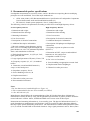
1. First steps with ARTA
1.1. Setup
To use the ARTA suite of programs you will need:



Operating system: Windows 98/ME/2000/XP/VISTA/Windows 7/Windows 8;
Processor: Pentium 400MHz or higher, memory 128k;
Soundcard: full duplex.
Installation is very simple. Copy the files to a directory and unzip them. That's it! All registry entries
are automatically saved at first start-up.
1.2. Equipment
The following is a brief summary of the equipment required accompanied by some basic directions
and cross-referenced to more detailed information elsewhere.
Soundcard
There are three types of soundcard:



Standard onboard soundcard, found typically on a computer motherboard;
Plug-in cards for PCI or ISA bus;
Soundcards connected via USB or firewire.
Cards vary according to type of use, quality and connectivity. For standard connections and cables see
section 1.3.
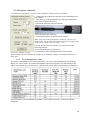
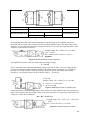
Standard soundcards use a stereo cable and 3.5mm jack sockets (Figure 1.1). Semi-pro, high-quality
soundcards usually have RCA jacks and unbalanced connectors (Figure 1.2). Professional soundcards
have 6.3mm stereo jacks for balanced connection, 6.3mm mono jacks for unbalanced connections and
XLR connectors for balanced microphone inputs (Figure 1.3).
Standard stereo soundcards have three channels (1, 2, 3), while 5 + 1 surround sound systems have
three more ports (4, 5, 6) on the motherboard. One of the outputs is designed for use with headphones
5
with 32 Ohm nominal impedance. For soundcard testing a loopback connection from line-in (blue) to
line-out (green) is made using a stereo cable with 3.5mm jack plugs. The line-in input impedance of
most PC soundcards is between 10 and 20 kOhms.
1. Line-in/AUX input, stereo (blue)
2. Line-out – headphones/front speaker, stereo (green)
3. Mic In – microphone input, mono (pink)
4. Out – centre and subwoofer (orange)
5. Out – rear speakers, stereo (black)
6. Out – side speakers, stereo (grey)
Figure 1.1 Audio connections on a PC motherboard for a 5+1 surround sound system
Laptops and notebooks usually carry only a stereo headphone output and a mono microphone input.
This configuration is severely limiting for measurement purposes because the mono input channel
does not permit dual channel use or impedance measurements.
Figure 1.2 PCI card with RCA connectors (e.g. M-Audio Audiophile 24/96)
Examples of plug-in cards include the Basic Terratec 24/96 or the M-Audio Audiophile 24/96.
Typically, these cards each have separate input and output RCA connectors with left (white) and right
(red) channels.
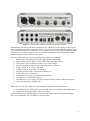
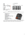
Figure 1.3 shows a professional high quality soundcard with firewire port. On the front there are two
XLR microphone inputs. This input is a combo jack (the centre of the XLR socket can accept a
6.3mm plug) and serves as an instrument input with impedance between 470 kOhms and 1 MOhm.
Both inputs have a volume control.
6
Figure 1.3 Professional soundcard system with firewire interface
Microphone inputs can be switched to phantom power, which gives power supply of 48V to pins 2
and 3 of the XLR microphone connector. There is also a master volume control for adjusting output
level and input monitor level. Finally, there is a headphone volume control and a headphone stereo
TSR connector. On the back panel, there are two balanced inputs, two balanced outputs, SPDIF
optical connectors and two firewire connectors.
Up to now ARTA has been used successfully with a following soundcards:












RME Fireface 800, RME Fireface 400, RME DIGI96, RME HDSP
Duran Audio D-Audio, EMU 1616m, EMU 0404 USB, EMU Tracker
Echo Gina24, Echo AudioFire 4, Echo Layla 24, Echo Indigo
M-audio Audiophile 2496, Firewire Solo, USB Transit, Delta 44,
Terratec EWX 24/96, Firewire FW X24
YAMAHA GO46, Sound Devices USBPre2
Digigram VxPocket 440 - a notebook PCMCIA card
TASCAM US-122 - USB audio
ESI Quatafire 610, Juli, U24 USB and Waveterminal
Soundblaster X-Fi, Infrasonic Quartet
Soundblaster Live 24, Audigy ZS, Extigy-USB (but only at 48kHz sampling frequency)
Turtle Beach Pinnacle and Fuji cards
ARTA may be used with a slight loss of performance with the following soundcards:


Soundblaster MP3+ USB (note: don't install SB driver, use a Windows XP default driver)
Soundcards and on-board audio with AC97 codecs.
Further information on soundcards that can be used with ARTA can be found at the homepage
http://www.artalabs.hr/. See also Müller (1) and section 2.1.
7
Amplifier
A power amplifier with linear frequency response and power 5–10 watts is adequate. The output
impedance should be <0.05 Ohms. Do not use an amplifier with a bridge amplifier virtual ground:
this may damage your soundcard. Check the manufacturer's specifications before first use if in any
doubt. An inexpensive solution that meets the above requirements and is small and easily portable is
the Thomann t.amp PM40C (see also section 5.4).
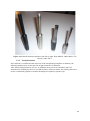
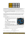
Microphone
Affordable measurement microphones are available, but whatever model is used, it must be
omnidirectional (Figure 1.4) with a linear frequency response. Inexpensive options such as the
Behringer ECM8000 with frequency response
compensation are suitable for loudspeaker
design.
When the microphone is to be used at higher
output levels or to measure distortion, a more
expensive model may be required.
Medium-priced recommendations (€150–€300)
include the Beyerdynamic MM1 and the Audix
TM-1 (see also section 5.2.1 and the STEPS
Handbook).
Figure 1.4 Polar radiation of the Audix TM1
DIY microphones based on the Panasonic WM61A electret capsule provide yet another option. See
the ARTA Hardware and Tools manual (http://www.artalabs.hr/support.htm) for more on this,
including notes on construction.
Microphone preamplifier
Depending on the microphone and/or soundcard, different extras are required. If you have chosen a
soundcard with integrated preamplifier and 48V phantom power, you are ready to go!
If you have a standalone soundcard you will need a separate preamplifier, ideally with phantom
power. The Monacor MPA 102 is recommended because it is currently the only affordable model
with stepped (and therefore reproducible) gain control (see Figure 3.5).
If you decide to go down the DIY route, you can use either the soundcard's microphone input (see
also section 1.4) or a preamplifier kit off the internet. Ralf Grafe's website (http://www.mini-cooperclubman.de/html/hifi_projects.html) has details of several tried and trusted kits, and PCBs may also
be available.
ARTA Measuring Box
The ARTA Measuring Box is not absolutely necessary but can make measurements a lot easier (see
Chapter 3 and ARTA Application Note AP1). Both wired and PCB solutions are available
(http://www.mini-cooper-clubman.de/html/hifi_projects.html).
Cables
Several cables are required, all of which should be of good quality. Poor connections, inadequate
shielding, etc. can interfere with measurements. The following will be required:
8




Microphone cable (XLR, TRS, RCA, depending on microphone and preamplifier – see also
Figure 1.6);
Soundcard cable (Measuring Box);
Amplifier cable (Measuring Box);
Speaker cable (1.5–2.5mm2).
Keep all cables as short as possible.
Other useful equipment




Loopback cable (to calibrate the soundcard; see chapter 4).
Voltage divider (for level adjustment; see chapter 5).
Y-cable (for semi-dual channel measurement; see chapter 2).
Block connectors and alligator clips (for temporary connections).
Multimeter (DMM)
A good multimeter is essential for the calibration of measuring equipment (and is also generally
useful). If you do not have one already, you should ideally select a true RMS meter. A wide range is
available, with many suitable devices on sale for under € 100.
If you already have a DMM or are considering a cheaper device that is not categorised as described
above, you should carry out the following test before using it for calibration and measurements.
a. Connect your multimeter to the left line
output of the soundcard and set the
measuring range to 2 volts AC.
b. Open the signal generator in STEPS
(Setup – Measurements or
).
c. Measure the output voltage of the
soundcard at different frequencies from
20Hz to 1000Hz and record the values.
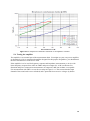
Figure 1.5 Multimeter comparison
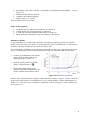
Plot the values measured at each frequency (either absolute or relative). Figure 1.5 shows results for a
good average meter and for a True RMS device. Up to around 1000Hz, variation with frequency is
within 2–3%. Thus, the device is suitable for calibration of ARTA using preset values (500Hz) (see
also section 5.1.1).
9
1.3. Pin assignment for cables and connectors
Unbalanced
Balanced
STEREO JACK
XLR
Sleeve: earth (GROUND/SHIELD)
Pin 1: earth (GROUND/ SHIELD)
Tip: +
Pin 2: +
Ring: –
Pin 3: –
Figure 1.6 Cable pin assignment
For a range of ready-made cables, see 'Cable Guy' at the Thomann homepage (www.thomann.de).
10
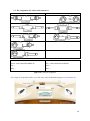
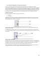
1.4. Measurement setup
The measurement setups presented here are:






Single channel measurement
Semi dual channel measurement
Dual channel measurement
Impedance measurement setup
Loopback for soundcard testing
Voltage probe setup
The soundcard left line output channel is used as a signal generator output. The left line input is used
for recording a DUT output voltage and the right line input is used for recording a DUT input voltage.
In a single channel setup, only a DUT output voltage is recorded. In a semi dual channel setup the
right line input is used to measure the right line output voltage. In a loopback setup, the left line
output is connected to the left line input and the right line output is connected to the right line input.
Acoustic measurements
Single channel measurement
A single signal from the DUT is detected.
Soundcard and amplifier artefacts are
included in the measurement as they cannot
be compensated for.
Semi dual channel measurement
The right channel serves as a partial
reference, compensating for soundcard
artefacts.
Dual channel measurement
Soundcard and amplifier artefacts are
compensated (see also the ARTA
measurement box in Chapter 3).
11
Impedance measurements
Impedance measurement with a power
amplifier
See also ARTA measurement box in Chapter 3.
Headphone impedance measurement soundcard output
Note that headphone outputs on soundcards are
not usually designed for connection to low
impedance loads.
Testing and calibration
Soundcard loopback setup
Each output is connected to the corresponding
line input. This is used for soundcard testing (see
also Chapter 4)
Soundcard protection
Voltage probe with soundcard input
channel overload protection
The probe shown provides 20dB attenuation
when R1 = 8k2 and R2 = 910, assuming that
the soundcard's input impedance is 10kΩ.
Note that this protection circuit is built into
the ARTA measurement box (Chapter 3).
12
2. Quick setup with ARTA
Understandably, you may want to start using ARTA straight away. This section is therefore provided
to address various issues related to the setting up of the measurement system, single channel
frequency response measurement and impedance measurement. Further and more detailed
explanations can be found in the respective chapters dedicated to these subjects.
Mixer adjustment
The most common mistake made during a quick setup is the overdriving of the soundcard. To avoid
this, ensure that your audio devices and sounds are adjusted appropriately (access via Control
Panel/Windows Mixer, depending on your operating system).
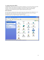
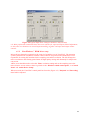
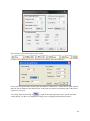
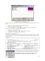
The following shows the setup for Windows XP (n.b. example in German).
13
Basically, the screen shots show that the line-in recording mixers should be enabled; the recording
volume should be set almost to minimum; the output mixer line-in should be disabled; and the mixer
output volume should be set almost to maximum. Note that the playback and recording levels should
be set similarly in Windows Vista/7/8; the mixers for these operating systems are easier to access and
adjust than the XP mixer.
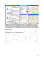
Loopback testing
We are now almost ready for the first measurement with ARTA. Connect the inputs and outputs of
your soundcard as shown in the loopback measurement diagram in Section 1.4. The types of cable
required (RCA, TRS, etc.) will depend on the soundcard.
Refer to Section 4.2 onwards for information on matching input and output levels, and for
ascertaining the quality of your soundcard.
Having carried out the loopback measurement for setting the mixer and testing your soundcard, you
will probably want to measure the frequency response of your speakers. For this you will need a
measurement microphone. If your soundcard can provide a supply voltage to power the microphone
you can work with a simple DIY electret – check the specification of the soundcard to ascertain
whether this will be possible.
It is very easy to make a measurement microphone: see the ARTA Hardware and Tools guide for
details.
14
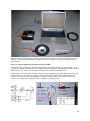
With the minimum equipment for acoustic measurements (computer with onboard soundcard, power
amplifier, measurement microphone) and the above basic settings you can now perform your first
measurements.
Easy test setup for impedance measurement with LIMP
For impedance measurements, onboard soundcards are not usually suitable (see also Section 4.1). If
you have a soundcard with stereo Line In and a headphone output, use the headphone output test setup
shown above. You will need a 100 Ohm reference resistor and some shielded cable.
In the absence of a headphone output, use the following: depending on whether the input jack on your
soundcard is RCA or 3.5mm (for example), take a proprietary cable and cut off the end that is not
required. You will also need a banana plug, a socket, a 27 Ohm (5W) resistor, and two reference
resistors of 8.2 Ohm and 1.0 Ohm (0.25W). Assembly is as shown below.
15
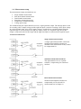
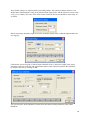
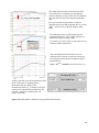
Three further settings are required before proceeding further. The reference channel must be set to
'Right' under 'Measurement Config' in the 'Measurement Setup' menu, and the reference resistor value
set (e.g. to 27 Ohms). The exact value of the resistor should be known and should be in the range 10–
47 Ohms.
Before measuring, adjust the output level in the 'Generator Setup' menu so that the input channels are
not clipping.
Calibrate the system using the 'Calibrate Input Channels' menu. Connect the output of the signal
generator (Line Out) to the left and right channel inputs of the soundcard, perform the calibration
('Calibrate') and exit by clicking on 'OK'.
You can read more about impedance measurement and Thiele-Small parameters in the LIMP
Handbook.
16
3. The ARTA measurement box
The ARTA measurement box is recommended to simplify measurements with ARTA, STEPS and
LIMP. It is designed for impedance and two-channel frequency response measurements, and
eliminates the need for cumbersome test leads.
See Figures 3.1 to 3.3 and ARTA Application Note 1 and the ARTA Hardware & Tools Manual (2).
Note that use of the measurement box with the optional resistor separating the power amplifier and
the soundcard eliminates the risk of ground loops between the soundcard output and input.
Figure 3.1 The finished measurement box (conventional wired version left, PCB version right).
Figure 3.2 Interior (conventional wired version left, PCB version right).
17
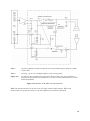
Note 1
the power amplifier and the soundcard can be separated using an optional 1 kOhm
resistor (R6).
Note 2
warning – do not use a bridged amplifier with virtual ground.
Safety note
the inputs of the soundcard are protected by Zener diodes. The power amplifier is
protected as specified by the manufacturer. Do not exceed the manufacturer's stated
nominal impedance.
Figure 3.3 Schematic of the ARTA measurement box.
Note: The measurement box is not necessary for single channel measurements. When such
measurements are performed, however, the microphone input should be calibrated.
18
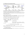
3.1. Two-channel calibrated measurements with the ARTA measurement box
For calibrated frequency response measurements with ARTA and STEPS in dual channel mode, you
should enter gain values for both input channels (External preamp gain). Note that the default
programming defines the right input channel of the soundcard as the reference channel while the left
channel is used as the measurement channel.
The ARTA measurement box is designed to be suitable for most users. If you need to adapt it for your
own special requirements, some calculations will be required. This section shows you how to use the
standard measurement box settings, how to adjust them if necessary, and how to calculate the Ext
Preamp Gain values to be used in Audio Devices Setup.
Matching the measurement box to the power amplifier (line in, right)
The resistors R1, R2 form, together with the input impedance ZIN of the soundcard, a voltage divider
k, defined by:
k = (R2 ǁ ZIN) / (R1 + R2 ǁ ZIN) where (R2 ǁ ZIN) = R2 * ZIN /(R2 + ZIN).
The maximum voltage that the power amplifier can send to the line in right channel of the soundcard
is:
VMAX = S [Volt RMS] / k
where S = input sensitivity of the soundcard (see also Section 5.1).
The maximum power that can be used in the measurement is:
PMAX = (S[Volt RMS]/k)2 / ZSpeaker
With the values chosen for the measurement box for R1 = 8k2, R2 = 910, and assumed standard
values for ZIN = 10k and input sensitivity of the soundcard = 1V, we can calculate the gain in the right
input channel (Ext. right preamp gain; see Figure 3.4).
Right channel = (R2ǁZIN)/(R1+R2ǁZIN) = (910ǁ10k)/(8k2+(910ǁ10k)) = 0.0923
when PMAX = 29W or 14.5W for speakers with nominal impedance 4 or 8 Ohms, respectively.
If your amplifier cannot deliver these power levels or you wish to take measurements using higher
power levels, the voltage divider must be adjusted accordingly. For example, if your amplifier has a
rated output of 56W at 8 Ohms, and you want to take advantage of its full power, you must make the
following modifications to the ARTA measurement box:
k = S[Volt RMS]/√PMAX*ZSpeaker = 1V/√56W*8 Ohms = 0.0472
When R2 = 910 and ZIN = 10K, R1 is calculated as:
R1 = (R2 ǁ ZIN) / k – (R2 ǁ ZIN) = 834.1/0.0472–834.1 = 16837 Ohms
Note: the sensitivity of the soundcard is specified in the calibration menu under mVPEAK. The
adjustment calculation for the measurement box requires that VRMS = VPeak * 0.707
19
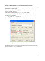
Matching the measurement box to the microphone preamplifier (Line in left)
For the calculation of the gain of the left channel input (Ext. left preamp gain; Figure 3.4), you will
need the details of your mic preamp.
In the example shown here, values for the Monacor 102 MPA are shown (Figure 3.5):
VMicPreAmp = 10 (20dB, see below),
output impedance of the mic preamp ZOUT = 100, R5 = 719, ZIN = 10000
Left channel = VMicPreAmp * ZIN / (ZOUT + R5 + ZIN) = 10*10000/10819 = 9.243
The value of R5 is calculated as
R5 = R1 ǁ R2 – ZOUT = 819–100 = 719
This relationship results from both input channels having the same source impedance.
Figure 3.4 Audio devices setup menu for ARTA and STEPS.
Note: the ARTA calibration menu specifies the expected gain (gain) as an absolute and not a dB
value. It is calculated as: Gain = 10^(dB level/20).
20
VMicPreAmp = 10^ ( x dB / 20 )
20 dB = 10
40 dB = 100
60 dB = 1000
Figure 3.5. MPA 102 (Monacor) microphone preamplifier. Note that the low-pass filter cut-off (LP
overlay file) comment is not correct: it should read 10.5kHz.
21
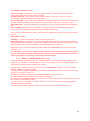
3.2. Single-channel measurement calibration
If you want to perform calibrated measurements in single channel mode, you must also enter the gain
of the power amplifier (Power amplifier gain).
Figure 3.6. Audio devices setup menu in ARTA and STEPS.
To measure the power amplifier gain, use one of the following two procedures:
1. Take a frequency response recording in single channel mode. Determine and record the sound
level with the cursor at 1kHz.
2. Repeat in dual channel mode. Determine and record the sound level at 1kHz as before.
3. Determine the difference between the two measurements and calculate the power amplifier
gain as:
Power amplifier gain = 10(difference in level @ 1kHz)/20)
Note that this approach requires a circuit as shown in Section 1.4 above, or the ARTA Measurement
Box.
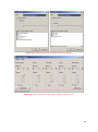
e.g. After running FR recordings, the following values were obtained at 1kHz (Figure 3.7): single
channel = 106.21dB; dual channel = 96.25dB. Thus, the difference is 9.96dB and the power amplifier
gain = 10(9.96/20) = 3.148. After entering this value in the 'Power amplifier gain' field (Figure 3.6),
single and dual channel measurements taken within the limits of error of the soundcard and amplifier
should match.
Note that this procedure must be repeated every time the gain (volume) of the power amplifier is
changed.
22
Figure 3.7. Power amplifier gain: single vs dual channel.
Alternatively, you can use the following slightly more accurate procedure in dual channel mode
(FR2):
1. Connect the left channel input with the selected
output channel of the soundcard.
2. Connect the right input channel via a voltage
divider with the output of the power amplifier
(GAMP).
3. Enter the absolute value of the voltage divider G as
'Ext right preamp gain' (see Figure 3.6).
4. Set the signal generator to 'Periodic Noise'. To
protect the soundcard reduce the output level to
about -10dB.
5. Measure in FR2 mode and note the amplitude at
1kHz. This measured value corresponds to the gain
of the power amplifier in dB. The power amplifier
gain value to be entered in 'Audio Devices Setup' =
10(FR level @ 1kHz)/20)
23
4. Soundcard setup and testing
4.1. Soundcard setup
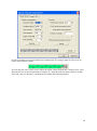
Before you start measuring, you must set up your soundcard and hardware. To do this, go 'Setup' and
'Audio Devices Setup' or click the toolbar icon
. The dialog box shown in Figure 4.1 will open.
Figure 4.1 Audio devices setup menu.
The dialog has the following controls:
Soundcard section –
Soundcard driver - chooses the type of soundcard driver (WDM – windows multimedia driver or an
installed ASIO driver).
Input channels - chooses the soundcard input stereo channels. An ASIO driver can have many
channels.
Output Device - chooses the soundcard output stereo channels (the input and output channels of a
single soundcard are normally selected (mandatory when in ASIO driver mode).
Control panel button – if a WDM driver is chosen, the Windows 2000/XP or Sound control panel in
Vista/Win7 is opened. If an ASIO driver is chosen, this opens the ASIO control panel.
Wave format –in Windows 2000/XP, select Windows wave format: 16 bit, 24 bit, 32 bit or Float
('float' = IEEE floating point single precision 32-bit format). Use 24-bit or 32-bit modes when using a
high quality soundcard. Note that many cheaper soundcards are claimed to be 24-bit, but their true bit
resolution is often less than 16 bits). Select 'Float' for Windows Vista/Windows 7. 'Wave format' has
no effect when in ASIO mode, as the bit resolution has to be setup in the ASIO control panel.
24
I/O Amplifier Interface section –
LineIn sensitivity - specifies the sensitivity of the line input (i.e. the peak voltage in mV that
corresponds to the full excitation of the line input).
LineOut sensitivity - the sensitivity of the left line output (i.e. the peak voltage in mV that
corresponds to the full excitation of the line output).
Ext. preamp gain - If you connect a preamplifier or voltage probe to the line inputs you should enter
the gain of the preamplifier or probe attenuation in the edit box; otherwise set the gain to unity.
LR channel diff. - enters the difference between the levels of the left and the right input channels in
dB.
Power amplifier gain - the power amplifier voltage gain is needed for calibrated results if you
connect the power amplifier to the line output in a single channel setup.
The best way to determine these values is to follow the calibration procedure as described in the next
chapter.
Microphone section –
Sensitivity - specifies the sensitivity of the microphone in mV/Pa.
Microphone used - check the box if you use a microphone and want the plot to be scaled in dB per
20μPa or dB per 1Pa. In addition, select the microphone input channel from the drop-down menu (the
default setting in ARTA is the left channel; use this setting wherever possible).
Setup data may be saved and loaded using 'Save setup' and 'Load setup'. The setup files have the
extension '.cal'.
n.b. Remember to mute the line and microphone channels in the output mixer of the soundcard in
order to avoid positive feedback during measurements. If you use a professional audio soundcard,
switch off any direct or zero latency monitoring on the line inputs.
4.1.1. Windows 2000/XP WDM driver setup
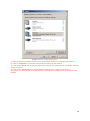
After selecting the soundcard (Figure 4.2), disable (mute) the line-in and microphone inputs in the
output mixer. In addition, select the input to be used for recording: Line In or Microphone (Mic). For
a standard PC soundcard, the procedure is as follows:
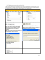
1) In the ARTA Audio device setup dialog click the ‘Control panel’ button to open the Windows
‘Master Volume’ or 'Volume control'.
2) Click on menu ‘Options->Property’ and select the soundcard channel that will be used for output
(playback), as shown in Figure 4.3.
3) Mute Line In and Mic channels in the ‘Master Volume’ dialog (Figure 4.3).
4) Set the Master Volume and Wave Out volume to maximum.
5) Click on menu ‘Option->Property’ and select the soundcard input channel, and enable Line In and
Mic channels in therecording mixer.
6) Choose Line In or Mic Input. Normally, ARTA uses Line In, to which the external microphone
amplifier should be connected.
7) Set the Line-in volume control to a lower position. This will be set more precisely later.
25
Figure 4.2 Soundcard input/output channel dialog (in German).
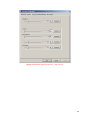
Figure 4.3 Typical soundcard output mixer settings in Windows XP.
26
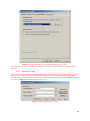
Figure 4.4 Typical input mixer settings in Windows XP (German).
n.b. Most professional soundcards have their own software for input and output channel adjustment,
or have their own hardware to control input monitoring, together with input and output volume
controls.
4.1.2. Vista/Windows 7 WDM driver setup
Microsoft has changed its approach to the control of sound devices in Vista/Win7. The operating
system (sometimes in conjunction with the control software for professional soundcards) is now
responsible for setting the soundcard native sampling rate and bit resolution. The OS changes the
native resolution to the floating point format for high quality mixing and ultimately for sample rate
conversion.
ARTA users should therefore select the ‘Float’ resolution setting and set the sampling rate to the
native format. Access to these values is gained via the ‘Windows sound control panel’, in ‘Control
Panel’ and ‘Audio Device Setup’.
When accessed, the Vista/Win7 control panel has four tabs (Figure 4.5). 'Playback' and 'Recording'
must both be adjusted:
27
Figure 4.5 Vista sound control panel.
1) Select the playback channel (do not use the measurement channel as a default audio channel).
2) Click on ‘Properties’ to open the sound properties dialog for that channel.
3) Click on the ‘Levels’ tab to open the output mixer (Figure 4.6). Mute the Line In and Mic channels,
if they are shown.
4) Click on the ‘Advanced' tab to set the channel resolution and a sample rate (Figure 4.7).
5) Repeat 1 to 4 above for the recording channel; choose the same sampling rate as for the playback
channel.
28
Figure 4.6 Playback channel properties – output levels.
29
Figure 4.7 Setting the native bit resolution and sample rate in Vista.
Note that many drivers are unstable in Windows 7, in which case an ASIO driver should be used if
available.
4.1.3. ASIO driver setup
ASIO drivers are decoupled from the operating system. They have their own control panel for native
resolution and memory buffer size adjustment. The buffer is used for the transfer of sampled data
from the driver to the user program. The ASIO control panel is opened by clicking ‘Control Panel’ in
the ARTA ‘Audio Device Setup’ dialog (Figure 4.8).
Figure 4.8 ASIO audio devices setup.
30
Figure 4.9 Adjusting resolution and buffer size in ASIO.
For music applications, the buffer size is usually set as small as possible while retaining stability in
order to yield the lowest input/output latency (system-introduced delay).
In ARTA, latency is not the main problem, because it is encountered in software anyway, but the
choice of buffer with size exceeding 2048 samples or smaller than 256 samples is not recommended.
Some ASIO control panels express the buffer size in samples, while others use time in msec. When
the latter is used, the buffer size in samples can be calculated as follows:
buffer size [samples] = buffer size[msec] * sample rate[kHz]/number of channels
Some ASIO drivers allow buffer sizes (in samples) that are a power of 2 (256, 512, 1024, etc.), in
which case ARTA adjusts the buffer size automatically.
ARTA always works with two input and two output channels, treating them as stereo left and right.
As ASIO supports multichannel devices, the user has to choose the pair of channels to be used in the
ARTA 'Audio Device Setup' dialog (i.e. 1/2, 3/4, etc.).
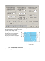
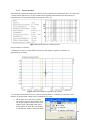
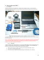
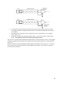
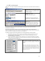
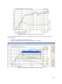
4.2. Testing the soundcard
The easiest way to test the quality of the soundcard is in the Spectrum analyzer mode.
Click on the SPA symbol as shown in the above toolbar. Connect the line inputs of the soundcard to
the signal outputs (loopback connection - an example is shown below).
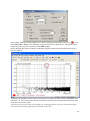
Click Generator->Setup or click the toolbar icon
values shown in the red box.
. You will get the following dialog. Enter the
31
Now enter the values shown below in the toolbar.
Or select 'Setup Spectrum Analysis' from the menu ('Setup', then 'Measurement').
Choose the left input channel, then prepare the Windows sound mixer - enable the line-input channel;
mute the line-in channel in the output mixer; set the line-out volume at maximum, and set the line-in
volume at a low level.
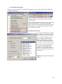
Use 'Setup', 'Spectrum Scaling' or
(or right click in the graph title area) to get the spectrum
scaling dialog. Use this to set magnitude scaling, power weighting and distortion measures.
32
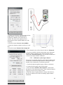
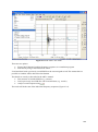
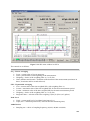
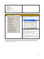
Check THD, THD+N, and Show RMS Level. Start recording by clicking the toolbar icon
(or via
menu 'Recorder'->'Run'). You should get a response like the one shown below. This figure can be
copied using the copy/paste operation (menu Edit->Copy).
Slowly increase the volume of the line-in channel using the soundcard mixer until the peak level is
close to -3dB FS.
Frequency and amplitude values at the cursor position are displayed under the chart with RMS, THD
and THD + N. The cursor itself is shown as a thin line and can be moved using the left mouse button
or the arrow keys left or right.
Note that you can reset the type of averaging, the sampling frequency, the type of excitation signal
and the FFT length during measurements via the control bar.
33
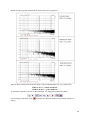
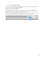
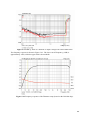
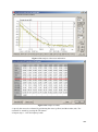
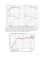
Results for three popular soundcards are shown below for comparison.
What do these results tell us about the utility of the soundcard under test? As a general rule:
THD+N <0.1% = usable soundcard.
THD+N <0.01% = good soundcard.
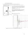
To check the frequency response of the soundcard, use impulse measurements (IMP):
Use the single point mode (click
empty).
and make sure the dual channel measurement checkbox is
34
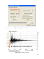
Check by clicking on 'Generate' whether the soundcard line-in is being overdriven. The levels are
shown in the peak level meter.
If levels enter the red or yellow zones, reduce the output volume until the bar is entirely green. Click
'Record' and wait for the measurement to complete (i.e. until the peak level meter shows no sound).
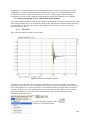
Click 'OK', and you should see something that resembles the following impulse.
35
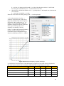
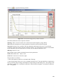
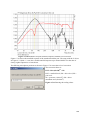
Click on the frequency response icon
soundcard.
in the toolbar to see the frequency response of your
If your sound card is of good quality, you should see a straight line. However, note the resolution of
your measurement chart. You can change the settings of the chart by clicking 'Fit' to automatically
find the upper limit of the Y-axis, or you can manually search using the two arrows on the left next to
36
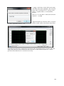
the 'Fit' button. The measurement range can be adjusted in the same way by using the two arrow
buttons to the left of 'Range'. If you click on 'Set', the following menu appears.
In this menu you can adjust all graphic parameters. Magnification of the Y axis shows more detail for
the frequency response, with a variation of approximately 1dB for the M-Audio Transit USB
soundcard that was measured.
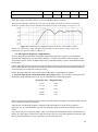
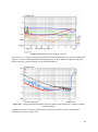
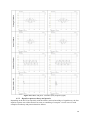
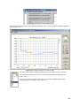
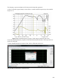
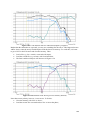
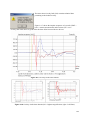
The following traces show responses for several other popular soundcards.
37
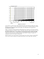
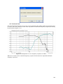
For measurement purposes, a soundcard should have a low frequency cut-off (–3dB) below 10Hz, or
preferably 5Hz. The card should have a usable range from 20Hz to 20kHz, with variations no greater
than 0.5dB.
Any noise intrinsic to the soundcard should also be taken into consideration.
38
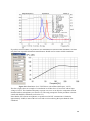
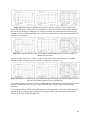
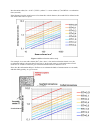
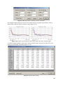
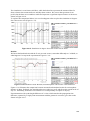
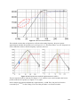
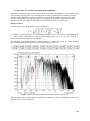
The following example illustrates the effect of high noise levels:
The Realtek card referred to above has a noise level of about -80 dBFS at 20Hz, whereas the M-Audio
Transit records around -120 dBFS. Excitation signals consisting of MLS or white noise were selected,
with an FFT sequence of N = 32768 values. This sequence has N/2 = 16384 spectral components with
a power of P = 10*log(1/16384) = –42dB (below RMS level). Crest factors of approximately 10–
11dB for white noise and 6–9dB for MLS should also be taken into consideration.
n.b. Crest factor = the ratio between peak and RMS value of an alternating quantity (CF = US/VRMS).
The excitation signal will therefore be roughly 50dB below the full scale level (between 48dB and
53dB, depending on the signal used). This leaves a dynamic range of D = –excitation level–noise
(dB). For the M-Audio Transit D = –50–120 = 70dB; Realtek D = –50–80 = 30dB. Thus, we can see
that soundcards with a noise floor of –80dB are of no use in measurements using noise excitation.
Such cards may be used, however, for measurements using sine excitation (see STEPS).
39
5. Calibration of the measurement chain
While it is possible to carry out measurements without calibration, reliable results cannot be obtained
if the individual components of the measurement system are not well matched.
The measurement chain should therefore be analysed at the level of each component to ensure that the
different parts of the setup are suited to each other, and that amplifier outputs and devices such as
voltage dividers are arranged such that the system is not over- or underdriven.
As an example, consider the nearfield measurement of a speaker cone to determine SPL. For this to be
carried out effectively, the measurement system must be set up so that the soundcard input can cope
with levels as high as 130dB.
The following parameters are known:
Maximum input voltage of the soundcard UIN MAX = 0.988V RMS (see definition below); microphone
gain GPRE = 20dB = 10; sensitivity SMIC = 11mV@94dB at 1kHz.
At 130dB (36dB difference from 94dB), the output voltage of the microphone is 10(36/20) = 63.1*11 =
694mV RMS. This is amplified further by the microphone by a factor of 10.
GIN = UIN MAX/UOUT SENSOR MAX = 0.9988/(10*0.694) = 0.1439 = –16.84dB
A voltage divider giving 16–17dB of attenuation is therefore required.
Rx = (ZIN * R2)/(ZIN + R2) [1]
G = Rx/(R1+ Rx) [2]
R1 = (Rx/G) – Rx [3]
If the input impedance of the sound card ZIN = 10kOhm,
and the value of R2 = 1 kOhm, R1 calculated by [1] and [3]
is as follows:
Rx = (10000*1000)/(10000+1000) = 909.09 Ohm
R1 = (Rx/G) – Rx = (909.09/0.1439) – 909.09 = 5408.42 Ohm –> 5,6 kOhm
And, GIN = 909.09/(5600+909.09) = 0.1397 = –17.01dB
Step-by-step management of the measurement system is described in detail in the following sections.
5.1. Soundcard calibration
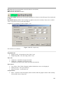
The soundcard and microphone calibration dialogue is found under 'Setup' - 'Calibrate devices'. The
following shows the preset default values.
40
Figure 5.1.1 Calibration dialogue.
The calibration dialog is divided into three sections.
(a) sound card, left channel, output;
(b) sound card, left and right channel input;
(c) microphone level calibration.
Note: full scale input and output for the
soundcard are given as mV peak in
'Soundcard and Microphone Calibration'.
For the adjustment calculation with the
ARTA measurement box, use mV RMS =
0.707 * mV peak (see Section 3.1).
VS = VPeak
Veff = VRMS = 0.707 * VS
VSS = VPeak Peak
Vmom = current value.
5.1.1. Calibration of the output channel
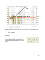
Use the following procedure to calibrate the output channel of your soundcard.
41
1. Connect an electronic voltmeter to the left line
output channel. Any meter that measures
accurately at 400Hz or an oscilloscope is
suitable. The chart to the right shows how
measurements from a quality DMM vary with
frequency.
2. Press the button 'Generate sinus (400Hz)'
3. Enter the voltmeter readout in edit box (in mV
rms).
4. Press the button 'Estimate Max Output mV'
5. The estimated value will be shown in the box 'Estimated'.
6. If you are satisfied with the measurement, press the button
'Accept', and the estimated value will become the current
value of the 'LineOut Sensitivity'. This will also be entered as
a value for the input channel calibration.
5.1.2. Calibration of the input channel
You can use an external generator or the output channel of the
soundcard to calibrate the input channels. If using the output
channel of the soundcard as a calibrated generator:
1. Set the left and the right line input volume to maximum.
2. Connect the left output to the left line input.
3. Press the button 'Estimate Max Input mV', and monitor
the input level at bottom peak-meters. If the soundcard input is
clipping, lower the level of input volume.
4. Enter the value of signal generator voltage in the edit box,
but only if it differs from value used during output channel
calibration.
42
5. Press the button 'Estimate Max Input mV'.
6. If you are satisfied with the measurement press the button 'Accept', and the estimated value will
become the current value of the 'LineIn Sensitivity'.
7. Repeat 1-6 for the right input channel.
Note: This procedure is recommended as it guarantees that you can connect the soundcard in
loopback mode. If you want to calibrate input channels with input volume set to maximum, many
soundcards require a reduction of the level of the output channel.
Note also that the standard calibration sampling rate was previously 44.1kHz. Because of problems
with some soundcards when using this rate, 48kHz has been available since release 1.8.
43
5.2. Microphone calibration
To calibrate the microphone, you need a level calibrator. The procedure is as follows:
1. Connect the microphone pre-amplifier to the soundcard line-in
(left channel).
2. Enter the gain of the preamplifier (preamp gain) and the SPL
value of the calibrator (Pressure).
3. Present the calibrator to the microphone.
4. Press 'Estimate mic sensitivity'.
5. If the measurement is acceptable, press 'Accept'.
Note: If the gain of the preamplifier is unknown, you can set a
default value, but this value must also be entered as the gain in the
'Audio Devices Setup '(see also Figure 5.2.3).
If you do not have a level calibrator, you can use one of the
following methods:
a) Use of manufacturer's specification;
b) Calculation of Thiele-Small parameters and nearfield;
c) Use of a reference tweeter.
These methods are not substitutes for a proper level calibrator, but they are suitable for DIY use in
most cases.
5.2.1. Use of manufacturer's data
If you have a microphone with a reliable data sheet, you can use the manufacturer's specifications.
Below you will see values for common microphones and electret capsules. For data relating to the
ARTA measurement box, see Section 3.1 (specifications for the MPA102 microphone preamplifier).
More information on measurement microphones can be found in Section 1.2 and in the STEPS
Handbook.
44
Figure 5.2.1 Measurement microphones (from left to right): Haun MB550, t-Bone MM1, NTI
M2210, Audix TM-1.
5.2.2. Nearfield method
If no calibrator is available and the sensitivity of the microphone/preamplifier is unknown, the
following method can be used to provide an approximate level calibration.
After Thiele-Small parameters of a low- or midrange driver have been calculated, and VAS
determined by installing the driver in a sealed enclosure of known volume, the resulting data can be
used in a simulation program to calculate the half-space frequency response (2pi).
45
If you have not used LIMP, it is possible to use manufacturer's data for initial simulation. Note that
only data from reputable mainstream manufacturers should used to ensure reliable simulations.
Figure 5.2.2 Simulation of a 6" TMT driver with AJHorn (half-space, 2.83V).
The above figure shows an example of a simulation in AJHorn for a 16cm woofer with an input
voltage of 2.83V. The simulated frequency response can serve as an objective comparator for data
obtained with our microphone (see Section 6.6). The only prerequisite for the procedure is that the
sound card should be calibrated (see Section 5.1).
Note that the SPL of most microphones or capsules used in DIY constructions is limited to
approximately 120dB, so start with low levels and avoid overdriving the input channels of the
soundcard.
46
Note that we assume that we have
no data on the microphone or its
preamplifier, so we must use
arbitrary values for now in the
Audio Devices Setup.
Set the left preamp gain and the
microphone sensitivity to 1.
Figure 5.2.3 Audio Devices Setup.
A two-channel nearfield measurement is taken and the level
adjusted to a measuring distance of 1 metre (PFF).
PFF = PNF + 20 log(a/2d)
d = measuring distance
a = driver membrane radius
PFF = PNF + 20 log([12.7cm/2]/2*100cm)
PFF = PNF – 29.97dB
The measured nearfield level PNF must therefore be corrected
by –29.97dB to obtain the farfield level PFF at 1 metre.
Figure 5.2.4 Procedure for estimating microphone sensitivity
by nearfield measurement.
47
The image left shows the uncorrected nearfield
level (black line) recorded by the microphone,
which is arbitrary because of the lack of calibration
data. The red line shows the imported simulation
data.
First, the uncorrected nearfield level must be
adjusted for the 29.97dB calculated above by using
'Edit –> Scale Level' (in the FR window under
IMP).
The calibration factor is determined from the
remaining difference. The example left shows a
difference of approximately 36dB.
Use 'Scale Level' once again to reduce the trace by
a further 36dB as shown here.
The simulated and measured traces are now
superimposed. From the second correction step,
the correction factor for the microphone and its
preamplifier is:
Gain = 10(36/20) = 63.0957 (see also Section 3.1).
Finally, enter this value in the Sensitivity field
of the 'Audio Device Settings' dialog.
Remember that any change in the
measurement chain (e.g. a change in the gain
setting of the microphone preamplifier) will
result in a change in sensitivity that will
require correction.
Figure 5.2.5 Microphone calibration using nearfield measurement.
48
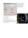
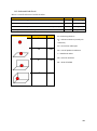
5.2.3. Tweeter method
This following calibration method relies heavily on the reliability of manufacturer data. You will need
a tweeter and its data sheet. Use only products from reputable manufacturers for this method, as
unreliable data will yield misleading results that are of no use.
Figure 5.2.6 Data sheet for a known tweeter.
The procedure is as follows:
1. Mount the tweeter in a small baffle and measure the impulse response at a distance of
approximately 20–40cm.
Figure 5.2.7 Gated impulse response of the tweeter.
2. Correct the measurement level to 1 metre measuring distance. To do this we need the actual
distance of measurement, which can be estimated in two ways:

Set the gate: move the cursor (yellow
line) until it registers 300 samples. Then
set the gate marker (red line) on the first
impulse peak. The length of the gate is
shown below the chart. We can use this
to calculate the distance of measurement:
49

d = 0.917ms * 0.344m (speed of sound) = 0.3154m. Note that since release 1.2 ARTA has
been doing the calculation for you – it is shown below the chart.
Alternatively, calculate the distance as d = c * (peak position – 300)/sample rate, which in this
case would be:
d = 344*(344–300)/48kHz = 0.3154m
Enter this value in the 'Pir Scaling' dialog ('Edit' –> 'Scale amplitude').
3. Go to the menu item 'Overlay' –>
'Generate Target Response', and select a
target that resembles the roll-off response
illustrated by the manufacturer (e.g. see
Figure 5.2.6). Various filter options are
available, ranging from first to sixth order.
Filter type, sensitivity and cut-off
frequency are entered by the user.
Figure 5.2.8 shows the measured frequency
response together with the response
corrected to 1 metre alongside the target
function (12dB Butterworth, Fc = 900Hz).
Figure 5.2.8 Measured frequency response and target.
4. Calculate the correction factor. From the frequency response we can set the cursor to frequencies
that are at least one octave above resonance, and read off the corresponding level values.
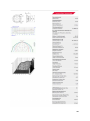
KE 4-211-2
3000Hz
4000Hz
5000Hz
6000Hz
7000Hz
Simulation
92.00
92.00
92.00
92.00
92.00
ARTA
104.49
102.94
102.99
103.08
103.51
Difference (simulated–measured)
12.49
10.94
10.99
11.08
11.51
4.2121
3.5237
3.5441
3.5810
3.7627
10
(Difference/20)
50
Assumed amplification
1
1
1
1
1
Adjusted amplification
4.2121
3.5237
3.5441
3.5810
3.7627
Thus, the average correction value is 3.7247 (standard deviation = 0.2884).
Note that this method is influenced by the effect of the baffle on which the tweeter is mounted.
Inclusion of baffle effects can be simulated with software such as The Edge (see Figure 5.2.9).
Figure 5.2.9 Influence of a simulated (red trace) 25cm x 25cm baffle at 30cm.
Ideally, you should use a baffle that has a minimal effect on the frequency range used for the
calibration (see also IEC baffle in Chapter 9).
5.3. Microphone frequency compensation
The use of a good measurement microphone with a linear frequency response is recommended.
Suitable DIY microphones are described in Section 5.2. When you purchase the microphone or the
microphone capsule, ensure in addition that it has a smooth frequency response and omnidirectional
polar pattern.
ARTA and STEPS offer the means for correction of the frequency response of your microphone, but
bear in mind that the correction will be limited to the on-axis response. Off-axis frequency response
errors will not be accounted for in the correction.
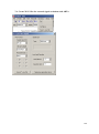
Follow the steps under the menu item 'Frequency Response Compensation' as follows.
1. 'Load' the appropriate compensation file (.mic) (Figure 5.3.1). This should be a normal ASCII
file that has been renamed from .txt to .mic. It should have the following structure:
Frequency (Hz) Magnitude (dB)
17.527
0.99
17.714
0.95
17.902
0.91
18.093
0.87
18.286
0.83
If necessary you can read the correction values from the reference frequencies and enter them yourself
into an ASCII file with no formatting.
After the file is loaded, the frequency response of the microphone as in the above example is
displayed. n.b. It is important that you enter the frequency response and not the already corrected
values.
If you have only a few measured values, ARTA can interpolate intermediate values automatically by
means of a cubic spline. Note however that at least one value in every three should be measured, with
these values distributed as evenly as possible over the correction area.
51
2. Activate the compensation curve in 'Use FR Compensation'. You can see in the ARTA main
menu if the microphone compensation file is active. If 'FR Compensation' is ticked, the file is in use.
Click on 'FR Compensation' again to disable the compensation file.
You can also use the toolbar icon to control and enable/disable the
compensation file.
Figure 5.3.1 Frequency response compensation window.
Use of the above procedure assumes that you know your microphone's frequency response. There are
several ways to obtain this.



Use the manufacturer's specification.
Have the microphone calibrated professionally.
Carry out the calibration yourself if you have access to the necessary equipment.
Substitution method (F>200Hz).
Pressure chamber method (F<200Hz).
5.3.1. Calibration using a reference quality microphone >200Hz
If you can obtain a high-quality measurement microphone (e.g. see Figure 5.3.2a), you can use it to
calibrate your own.
A good description of the procedure can be found on the Earthworks homepage in the article 'How
Earthworks Measures Microphones' (3). For frequencies above 500Hz, Earthworks uses the
substitution method in which a test driver is measured in an infinite baffle with a reference
microphone. The problem is that it is difficult to find a suitable (large enough) anechoic chamber for
the measurement of low frequencies. To solve this problem, Earthworks uses a small pressure
chamber for calibration at lower frequencies (see Section 5.3.2).
52
Figure 5.3.2a The MK221 Reference Microphone by Mikrotech Gefell.
Figure 5.3.2b shows responses for the reference microphone and the test microphone (MB550). Note
the differences in level and response. The first job is to compensate for the difference in levels.
53
Figure 5.3.2b Reference microphone (MK 221, blue) and test microphone (MB550).
Use 'Scale Level' ('Scale Magnitude' dialog) in the Edit menu of
the FR window to reduce the level of the MB550 until it is
superimposed as much as possible over the reference response
(Figure 5.3.3). You may need to experiment a little with this, as
the best value is not always obvious at first glance.
Figure 5.3.3 Scaling and subtraction.
We then use 'Subtract Overlay' to account for the difference between the two frequency responses (as
shown in Figure 5.3.3).
54
Figure 5.14 shows the result of this operation. There is a maximum variance between microphones
from 150Hz to 20KHz of 1.25dB.
Figure 5.3.4 On-axis frequency response correction.
'Export ASCII' can then be used to create the compensation file. Rename the .txt file to .mic and
import it as described earlier.
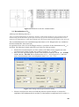
5.3.2. Calibration below 500Hz with a pressure chamber
As noted above, Earthworks uses a pressure chamber for microphone calibration below 500Hz.
Construction and operation of the pressure chamber are described in detail in ARTA Application Note
No. 5. The largest dimension of the chamber should not exceed 1/6 to 1/8 the wavelength of the upper
cut-off frequency of 500Hz (i.e. 11.5–8.4 cm).
Figure 5.3.5 Design and application of the measurement pressure chamber.
The use of the pressure chamber is illustrated in Figure 5.3.5. The test microphone is inserted into the
chamber via an adapter that creates a good seal, and measurements are made with ARTA/STEPS in
the frequency range of interest. The chamber seals the microphone off from its surroundings and
provides a suitable measuring environment, but be aware that very high sound pressure levels can be
55
expected if normal voltages are used (e.g. 2.83V is likely to yield 145dB). Because of this, small
excitation signals only (c. 0.01V) should be used to avoid damage to the microphone. Figure 5.3.6
shows the frequency response of the MK221 with STEPS when the pressure chamber is used. The
figure illustrates how the reference and measurement curves can be used for calibration.
Figure 5.3.6 Reference (red) and MB550 (black) frequency responses.
The microphones will usually have differing sensitivities, and an initial level adjustment will therefore
be required. The easiest way to do this is to choose a reference frequency and use the cursor to read
off the respective sensitivities. The difference is then compensated for by using the 'Scale' function.
If the measurement is made using ARTA, the correction can be made via 'Edit' –>'Subtract Overlay' as
described above. If STEPS is used for its superior reproducibility, some manipulation of data in Excel
and a suitable simulation program (e.g. CALSOD) will be needed.
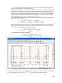
Figure 5.3.7 shows the trace obtained with STEPS for the MB550 microphone from 5 to 500Hz.
Using this compensation curve together with the results from the previous section (see Figure 5.3.4),
you can obtain a compensation file for the full frequency range of about 5Hz to 20kHz, as shown in
Figure 5.3.1.
56
Figure 5.3.7 MB550: deviations from reference frequency response.
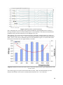
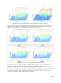
Results with other microphones are summarised in Figure 5.3.8. They show that significant
irregularities can be expected at frequencies below 100 with different DIY microphones. Even with
high quality microphone capsules (e.g. 211-KE 4), there is no guarantee that there will be no
significant deviations from specifications.
Figure 5.3.8 Results with various microphones: black = MB550; red = 211-KE 4, No. 1; light blue =
211-KE 4, No. 2, Nr2K; Blue = MCE 2000; orange = Panasonic WM60.
Figure 5.3.9 illustrates that there are in addition other factors to be taken into consideration. These
harmonic distortion traces clearly show the reason for the extra cost associated with professional
quality microphones.
57
Figure 5.3.9 Comparison of harmonic distortion of microphones at 300Hz.
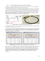
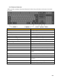
5.4. Testing the amplifier
The amplifier is an essential part of the measurement chain. You might use your own power amplifier,
or alternatively a kit or custom-built amplifier designed for this purpose. Regardless, you should know
the basic characteristics of the device used.
If the amplifier is to be used for frequency response and impedance measurements, a device with
linear frequency response from 10Hz to 20kHz and power output of 6–10W is sufficient. For
distortion and power compression measurements, an output of 100W into 8 Ohms is acceptable.
For measurements with ARTA we use the test setup in Figure 5.4.1. This ensures that the input
channel of the sound card is not overloaded, and is protected from excessive voltages by diodes.
58
A = 20*log (Rx/R2+Rx)
Rx = ZIN*R1/(ZIN+R1)
Example:
ZIN = input impedance of soundcard = 10 kOhm
Attenuation A R1 (Ω) R2 (Ω)
–10dB
510
1047
–20dB
510
4.4k
–30dB
510
15k
Figure 5.4.1 Voltage divider for amplifier measurement.
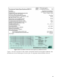
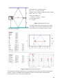
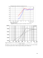
As an example, the Thomann 't.amp' PM40C was selected. The manufacturer's specifications are as
follows:
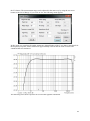
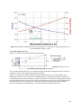
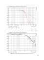
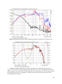
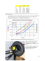
Figure 5.4.2 shows the harmonic distortion of the t.amp into 4.1 Ohms (black) and 8.2 Ohms (red) in
response to output voltage. The t.amp delivers about 34W into 4 Ohms and 23.2W into 8 Ohms
without distortion: 10V RMS into 4.1 Ohms (24W) is safe for measurement purposes.
59
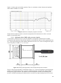
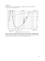
Figure 5.4.2 THD @ 1kHz as a function of output voltage with 4 and 8 Ohm loads.
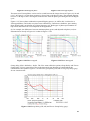
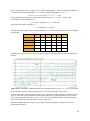
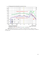
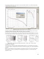
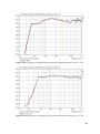
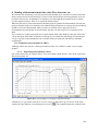
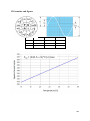
The frequency response is shown in Figure 5.4.3. The lower cut-off frequency (-3dB) is
approximately 16Hz, while the upper limit is about 60kHz.
Figure 5.4.3 Frequency response of the Thomann t.amp (based on the LM3886 chip).
60
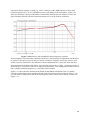
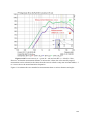
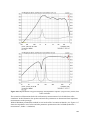
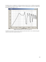
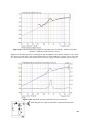
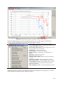
Figure 5.4.4 THD+N @ 1kHz and –1dB.
Figure 5.4.4 shows THD + N for the t.amp. The values are within the manufacturer's specifications.
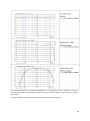
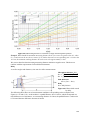
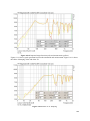
Figures 5.4.5 and 5.4.6 show distortion against frequency for the t.amp at 1 and 16W into 8 Ohms.
The t.amp remains stable at outputs up to 16W.
Figure 5.4.5 Distortion versus frequency at 1W.
61
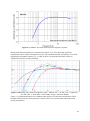
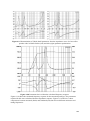
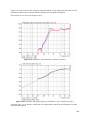
Figure 5.4.6 Distortion versus frequency at 16W.
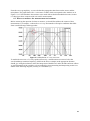
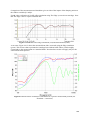
Since release 1.3, voltage- or output-related distortion measurements have been possible with STEPS.
Figure 5.4.7 shows voltage-dependent harmonic distortion at three different frequencies. For more
details of this type of measurement, see the STEPS Handbook.
Figure 5.4.7 Voltage-dependent harmonic distortion (THD) of the amplifier at 4.1 Ohms at 100Hz,
1kHz and 10kHz.
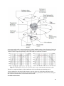
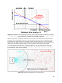
Amplifier parameters of interest (besides power, frequency and phase response, and harmonic
distortion) are shown in Figure 5.4.8.
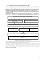
62
Signal source
Amplifier
Load
Input voltage (UE)
Voltage gain (V=UA/UE)
Output voltage (UA)
Internal impedance (RS)
Input impedance (RE) Output impedance (RA)
RS<<RE
RA<<RL
Load impedance (RL)
Figure 5.4.8 Amplifier schematic.
The input impedance RE is the internal impedance of the input side of the amplifier, and can be
measured with a resistance RV connected in series with the amplifier input. The input voltage drops
from UE1 to UE2, and with it the output voltage falls from UA1 to UA2. The input impedance of the
amplifier is characterised as follows:
Example t.amp: RV = 47kΩ; UA1 = 10.502V;
UA2 = 3.144V
RE = 47kΩ*3.144V/(10.502V–3.144V) =
20.082kΩ
Figure 5.4.9 Measurement of input impedance.
The amplification (gain) is the ratio of the output and input voltages
V = UA/UE
This is measured with a sinusoidal alternating voltage, typically at 1kHz. A precise voltage divider
between the generator and the amplifier facilitates the measurement at high gain (e.g. microphone
preamp). If a voltage divider is used, measure the voltage UE' before the voltage divider, then
calculate u = the voltage divider ratio (R1+R2)/R2. Then V = UA*u/UE'.
V=UA/UE
Example t.amp: UE = 0.8493V; UA = 18.539V
V = UA/UE = 18.539/0.8493
V = 21.83 = 26.7dB
Figure 5.4.10 Measurement of amplifier gain.
Output impedance is the internal impedance of the output side of the amplifier and can be determined
from a load resistance RL. The output voltage of an open circuit (UO) is reduced by a load to the load
voltage UL. Under these conditions
RA = RL * (UO/UL–1)
Example t.amp: UO = 5.47V; UL = 5.462V; RL
= 8.2Ω
RA = 8.2*(5.47/5.462–1) = 0.012Ω
Figure 5.4.11 Measurement of output
63
impedance.
The measured values as shown in Figures 5.4.9 to 5.4.11 match the manufacturer's specification.
64
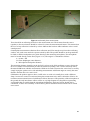
6. Measurement with ARTA
6.1. General
After the calibration of the equipment is complete and everything is ready, we can start actual
measurements. Be sure to check all cable connections and settings thoroughly and carefully before
each measurement session.
Figure 6.1.1 Measuring equipment (minus microphone connection and stand).
Avoid poor quality cables and connections. Attention to detail in this respect will save much time and
effort in the long run.
Note: a well thought-out and constructed system consisting of high quality equipment, clearly marked
connections and an ARTA measuring box will enable you to minimise the risk of errors and damage.
This is particularly important where the system has not been used for an extended period and
familiarity with it has consequently diminished.
6.1.1. Test leads
Attention should be paid to the test leads, as we are using small analogue voltages. Signal quality will
suffer as a result of noise if transmission over large distances is attempted. To avoid earthing and
interference problems, the following guidelines (4) should be followed:



Make cables as short as possible, especially when using high impedance sources;
If possible, use double shielded cables;
If necessary, take an additional earth lead and place the shielding on one side only;
65



Avoid ground loops. Ensure that earth potentials are the same between the source and the
measuring instrument (soundcard). Measure between earths beforehand with a meter (both
AC and DC);
Do not place the signal cable near any interference source (transformers, power supplies,
power cables, etc.);
If possible, disconnect the computer from the mains – if you have a laptop, use the battery.
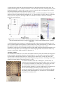
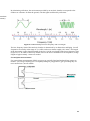
6.1.2. The signal-to-noise ratio of the measurement system
The S/N ratio is important and should be determined before each measurement session, as meaningful
frequency and phase measurements can be obtained only if the useful signal level is greater than the
noise level.
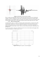
Measure sound levels with and without speakers (DUT) and compare levels (Figure 6.1.2). The noise
level in the region of interest should be at least 20dB below the signal – the greater the separation
between the two, the better.
66
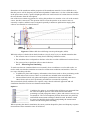
Figure 6.1.2 Determination of signal levels and S/N ratio.
If the separation is insufficient, there are several options:




Reduce the noise level or change the room or measurement environment;
Increase the level of the excitation signal;
Do not use excitation signals with low energy content (e.g. MLS);
Use averaging (see Section 6.1.3).
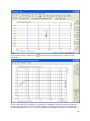
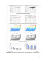
Phase transition is very sensitive to an unfavourable S/N ratio, especially when measuring speakers
that do not cover the entire frequency range. Generally, the phase-frequency response can only be
reliably calculated with a sufficiently large S/N ratio.
67
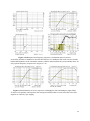
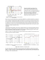
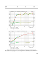
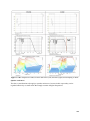
Figure 6.1.3 Frequency and phase response of a tweeter in a normal living room.
Individual drivers do not usually cover the entire frequency range. Thus, a tweeter radiates so little
acoustic energy at 100Hz that the transfer function in this region is overshadowed by noise, and the
phase response calculated in this area is of no use.
6.1.3. Averaging
As indicated above, measurements are rarely made under optimal conditions. Traffic noise, fans in
computers, heating or air conditioning, wind, and general background noise can all spoil
measurements.
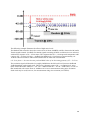
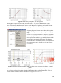
To obtain measurements with tolerable accuracy, we rely on
averaging. In 'IMP' mode, in the menu 'Impulse Response
Measurement', there is a field entitled 'Number of Averages'. In
FR1, FR2 and SPA, see in the 'Averaging' submenu (in
'Frequency Response Measurement Setup') the field 'Max
Averages'.
68
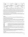
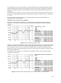
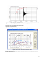
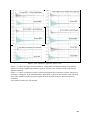
Figure 6.1.4 Averaging in IMP mode.
These fields specify the number of measurements to be made by ARTA, after which the mean of the
measurements is calculated automatically.
Doubling the number of measurements increases the S/N ratio by 1/√n (3dB), although other factors
such as jitter limit the extent to which this can be achieved.
The effectiveness of averaging is illustrated in Figure 6.1.4, where measurement results with 2 to 32
averages are shown for noise floor levels.
69
6.2. ARTA excitation signals
ARTA has a wide range of integral excitation signals, and can also be used with external excitation, as
follows:
Impulse response
Periodic noise (PN: pink, white, speech);
Sweep: sine (linear, log); MLS; External
excitation (Trigger)
FR1, FR2, SPA
Random: pink, white
Periodic: white, pink, speech
The difference between periodic and
random noise is explained in Figure 6.2.1
Signal Time Record (available from
release 1.6.2)
Signal generator with a wide range of
continuous signals (sine, square, multitone, etc.) and pulse and burst signals
The selection of the best excitation signal depends on the quality of the sound card and the
measurement environment.
Dual channel measurements should be used with high quality sound cards with flat frequency
response and tight tolerances for the sensitivities of the input channels. Single channel measurements
can be used with lower quality sound cards (see also Chapter 4).
Ivo Mateljan suggests the following guidelines for selecting appropriate excitation signals:


Periodic noise (PN) gives the best results in environments with high ambient noise levels.
Averaging improves the S/N ratio, and the effects of random and stationary noise and
nonlinear distortion are minimised.
In quiet surroundings, a high crest factor makes the sine sweep ideal for high power speaker
testing. In this case averaging does not always improve the S/N ratio, and it is therefore better
to increase the duration of the sweep.
For periodic noise (pink) ARTA can protect the
DUT against low frequency high energy signal
components by including a high-pass filter (Pink
cutoff).
The effect of the Pink cutoff is shown in Figure
6.2.1. By increasing the cutoff frequency, we cut
the lowest frequencies off at progressively lower
levels. ARTA automatically compensates for the
frequency level cap.
70
Figure 6.2.1 Effect of Pink cutoff at 10, 20, 50 and 500Hz.
The following illustrations show other signals (Figures 6.2.2 and 6.2.3). For more detail, please see
the ARTA manual and Mateljan & Ugrinović (5).
Figure 6.2.2 Difference between random and periodic noise.
71
Figure 6.2.3 Multisine.
As of version 1.6.2, ARTA comes with an additional generator with continuous signals (sine, square,
multisine, etc.), pulses (e.g. Dirac), and sine bursts of various types. See Siegfried Linkwitz's website
for information on application of the sine burst (http://www.linkwitzlab.com 'Triggered burst
measurements of tweeters').
Figure 6.2.4 shows the 'Signal Generation and Recording' menu. The choice of waveform is made by
clicking the checkboxes 'Continuous', 'Pulse' or 'Sine burst'. Once this is done, the signal can be given
more specific characteristics (e.g. type, frequency) and the frequency transients adjusted using the
'Repetition' drop-down. Thus, 16,384 might prove to be a high repetition rate, while 262,144 might
contain only one repetition per recording; it depends on the number of samples ('Length') and
sampling rate chosen in the 'Signal recording' field.
With the checkbox 'Invert output signal', the output signal can be inverted. 'Trigger on right channel'
can be used to control recording of two-channel measurements via the output of the sound card.
72
Figure 6.2.4 Signal Generation and Recording menu.
The 'Link' checkbox between the 'Generate' and 'Record' buttons automates the trigger process by
linking the two processes.
The 'Signal recording' and 'Trigger' fields are largely self-explanatory.
Figure 6.2.5 shows a collection of signals from the 'Transient Generator'. Excitation signals are shown
on the left, while the right half shows the tweeter response at 3kHz recorded with a high-quality
microphone.
73
Figure 6.2.5 Burst and pulse: excitation (left), response (right).
6.2.1. Impulse responses: theory and practice
Depending on the DUT (but especially with subwoofers) and our knowledge of signal theory, the first
impulse response seen on the monitor can come as something of a surprise. A brief overview with
examples from theory and practice therefore follows.
74
Figure 6.2.6 Step response (middle) and frequency response (right) of a Dirac impulse (left).
To describe the theory, a Dirac pulse was evaluated as a WAV file in ARTA with reference to target
filters (low-pass, band-pass and high-pass). Using this method, the generated impulse and step and
frequency responses should match the curves predicted by filter theory as long as the bandwidth limit
does not cause problems.
Figure 6.2.7 Impulse response (left), step response (middle) and frequency response (right) of a
1000Hz low-pass filter.
The first example, Figure 6.2.7, shows a 12dB low-pass filter with a cutoff frequency of 1000Hz.
Note the changes in impulse and step response in comparison to Figure 6.2.6.
Figure 6.2.8 Impulse response (left), step response (middle) and frequency response (right) of a bandpass filter with 100Hz/1000Hz crossover frequencies.
The second example in Figure 6.2.8 shows a 12dB band-pass with 100Hz and 1000Hz cutoffs. See the
changes in impulse and step response compared with the Dirac impulse. Note also the different
timescales.
To illustrate the effect of different cutoff frequencies on the appearance of the step response, the next
illustration shows 12dB low-pass, band-pass and high-pass filters. Note particularly the band-pass
filter, as all speakers exhibit this behaviour.
75
Figure 6.2.9 Influence of cutoff frequency on the appearance of the step response.
In the final example, a tweeter connected to a 12dB high-pass filter with a corner frequency of
1000Hz was simulated. Figure 6.2.10 shows the simulation (top) and the measured frequency
response of the tweeter. Note the significant differences between the measured and theoretical curves.
The individual characteristics of the tweeter, the driver setup, and the measurement conditions
(distance, room, ambient noise, etc.) are all evident in the impulse response and ultimately in the
derived analysis. The peculiarities of the phase response are discussed in Section 6.2.2.
76
Figure 6.2.10 Impulse and frequency responses of simulated and real tweeters.
It would be desirable in addition to describe the behaviour of a bandpass filter with a tweeter, but the
bandwidth limitations of the simulation software (22kHz) and measurement system (24kHz) allow for
only a partial frequency response trace (Figure 6.2.11).
Figure 6.2.11 Simulation of tweeter responses with highpass (left) and bandpass (right) filters.
To answer a frequently asked question, the unexpected artefacts that are seen before the start of the
impulse are caused by 'pre-ringing'.
77
Figure 6.2.12 Impulse response with pre-ringing.
This is caused by the bandwidth limitations of the measurement system, and is seen each time the
frequency is half the sampling rate. With current soundcards these frequencies are usually 24kHz
(48kHz sample rate) and 48kHz (96kHz). Pre-ringing can be partially corrected by checking the 'Dual
channel impulse response filter' in the 'Impulse Response Measurement/Signal Generator' window.
6.2.2. Phase and group delay
An understanding of the use of ARTA for analyzing phase and group delay is important when fully
characterizing a sound source. The reader is therefore advised to revisit Section 5 briefly, and to
consult relevant literature (6) as well as the ARTA User Manual (2). Note also the importance of
using two-channel measurements, as this is the only way in which specific phase relationships can be
characterized.
The following analysis is based on a 96kHz Dirac pulse with a 3rd order Butterworth highpass filter
with a corner frequency of 800Hz (Figure 6.2.13).
Figure 6.2.13 Impulse response, 3rd order highpass.
78
Figure 6.2.14 Frequency and phase, 3rd order highpass.
The highpass response (tweeter model, shown in black) is very close to the theoretical or ideal
response, but shows significant deviation in terms of both amplitude and phase below 100Hz because
of the computational limitations of the software. Note that phase is apparently more sensitive in this
respect than amplitude; this is used to advantage in procedures described in Chapter 5.
As shown on the left, the 'View' menu in the Smoothed
Frequency Response window shows the available options
in ARTA for depicting and manipulating phase and group
delay.
Figure 6.2.15 (right panel) shows the frequency and phase
response (Magn+Phase) of the modelled tweeter. The
phase can be seen 'wrapping' as a result of inclusion of the
time elapsing between the propagation of sound from the
tweeter and its arrival at the microphone. The distance
between the cursor and marker (34.33cm) corresponds to a
time of 0.998msec and is referred to as the 'gate' (Figure
6.2.15 left).
Figure 6.2.15 Phase response, including flight time from source (cursor) to microphone: wrapped
phase.
We can move the cursor towards the peak of the impulse response in the Impulse Response window
or use 'Delay for Phase Estimation' under the 'Edit' menu to reduce or eliminate pre-delay. This will
results in phase responses similar to those shown in Figures 6.2.16 to 6.2.19.
79
Figure 6.2.16 Phase with pre-delay = 0.5msec.
Figure 6.2.17 Phase with pre-delay = 0.8msec.
Figure 6.2.18 Phase with pre-delay = 0.998msec.
Figure 6.2.19 Black = phase with 0.998msec predelay (black); red = calculated 'ideal' HP phase.
Removal of the excess phase associated with the flight time between the source and the microphone –
in this case by using pre-delay - should reveal the 'pure' phase response of the highpass filter (Figure
6.2.20). Comparison of the calculated ideal highpass phase (red) with the phase corrected using
0.998msec pre-delay confirms this (Figure 6.2.19).
Figure 6.2.20 Phase with pre-delay = 0.998 msec
Figure 6.2.21 Phase with pre-delay = 1.043 msec.
If the delay is longer than the flight time (increased for example to 1.043 msec, which corresponds to
two samples), the phase graph reverses back on itself as shown in Figure 6.2.21. If we were to achieve
this effect by placing the cursor two samples behind the impulse peak as shown in Figure 6.2.22, the
frequency response would become distorted as in Figure 6.2.23.
80
Figure 6.2.22 Cursor placed two samples after
impulse peak.
Figure 6.2.23 Cursor placed two samples after
impulse peak.
The difference between using pre-delay and moving the cursor is caused by the software not applying
the FFT transformation to the part of the pulse that lies before the cursor.
If we tick 'Minimum Phase' under the View menu, the software calculates the minimum phase
response of the tweeter by using a Hilbert transform. Theoretically, when the measured phase is
adjusted accurately using the correct pre-delay, the response should be identical to the calculated
minimum phase.
Figure 6.2.24 Minimum phase, Hilbert
transformation (green), and real phase (red).
Figure 6.2.25 Excess phase (blue), real phase
(red), and minimum phase (green).
In reality, there may be differences caused for example by diffraction effects (Figure 6.2.24). The
calculated minimum phase (green) and adjusted real phase (red) differ by the excess phase (blue), as
shown in Figure 6.2.25.
81
Figure 6.2.26 Wrapped phase.
Figure 6.2.27 Unwrapped phase.
The menu item 'Unwrap Phase' can be used to switch between the images shown in Figures 6.2.26 and
6.2.27. In Figure 6.2.26, the phase response is 'forced' into a 360 degree range. The repeated 'flipping'
between –180 degrees and +180 degrees indicates how often the phase goes through a full 360 degree
cycle.
Figure 6.2.27 shows phase without this repeated flipping process; in ARTA, this is referred to as
'Unwrapped Phase', and in this case phase runs continuously. Under these conditions, pure running
phase should yield a straight line on a linear frequency axis. Both types of phase representation are
equivalent, and whichever is used depends on the application.
So, for example, the differences between minimum phase (green) and adjusted real phase (red) are
illustrated more clearly in Figure 6.2.29 than in Figure 6.2.28.
Figure 6.2.28 Phase wrapped.
Figure 6.2.29 Phase unwrapped.
Group delay (GD) is defined as –dφ/dω. The View menu offers the options 'Group Delay' and 'Excess
Group Delay'. Excess group delay refers to the theoretical pure duration of sound without the
contribution of the speaker. Figure 6.2.30 shows the group delay (red) and excess group delay (grey)
for our virtual tweeter.
Figure 6.2.30 Group Delay (GD, red) and Excess Group Delay (grey).
82
From the excess group delay, we can calculate the propagation time between the source and the
microphone. The graph shows GD = 0.999 msec at 3kHz, which corresponds to the window set in
Figure 6.2.15. Note that these observations were made with an idealized modelled tweeter; Section
6.3 shows how these compare with 'real-world' measurements.
6.3. Where to measure: the measurement environment
Before answering the question of where to measure, we should first address the context of that
measurement. For example, a subwoofer or a 3-way floorstander will require conditions that differ
from a small full-range desktop speaker.
Figure 6.3.1 Simulation of 3-way crossover.
To model the crossover of a 3-way speaker effectively, a measurement two octaves below the
woofer/midrange transition frequency (300Hz in the above example) at the appropriate distance
should give enough resolution to allow the integration of both drivers and to include enclosure effects.
A good illustration of the variables to be accounted for when measuring and interpreting results is as
shown in the following diagram (courtesy of J. Backman (7)).
83
A two-way speaker with a crossover frequency of about 2000Hz requires a lower frequency limit of at
least 500Hz (Figure 6.3.2). If the baffle step (right panel) is to be accounted for, measurement at 200–
150Hz would be required (depending on the baffle width) for sufficient resolution.
Figure 6.3.2 Simulation of two-way crossover (left); woofer with/without baffle step (right).
The task is complicated further by the contribution of room reflections and standing waves.
Various methods are described in the literature (8)(9)(2)(10)(11)(4) for dealing with these issues:
freefield measurement, measurement in an anechoic chamber, ground-plane measurement, half-space
and windowed measurements, and nearfield measurement.
Freefield measurements
84
As suggested by its name, the first and oldest method is to take measurements out in the open. The
speaker and microphone are situated so that there is no interference from any reflecting surfaces (most
notably the ground). To achieve this, a crane or tower is required, and the equipment must be lifted
into the measurement position as shown in Figure 6.3.3 (9).
Sound reflected from the ground takes (2H+d)/344 seconds to reach the microphone. The left panel
shows the effect of ground reflection at heights of 1, 2, 4 and 10 metres. Clearly, where a reverberant
floor (worst case) is present, the height of the tower should be around 10 metres for reasonably
trouble-free measurements.
Figure 6.3.3 Freefield measurement, simulation, ground clearance
(left) and measurement setup (9) (right). Direktschall = direct sound; Bodenreflexion = ground
reflection.
A freefield setup has the advantage of creating theoretically ideal measurement conditions, but is of
course weather-dependent. Precipitation, wind and other noise make measurements very difficult, and
this method is therefore only applicable in benign climates with perfectly calm weather.
Nevertheless, anybody with a reasonably peaceful garden might attempt freefield measurements. Even
if the tower is only three or four feet high, use of windowing might make measurements all the way
down to a cut-off of 40–50Hz possible (see Section 6.4).
Anechoic chamber
If freefield measurements are to be carried out without interference from the weather and background
noise at any time, an anechoic chamber is needed (Figure 6.3.4). The walls of an anechoic chamber
are lined with a sound absorbing material - usually glass or mineral wool -in order to achieve the
fullest possible sound absorption across the entire frequency range of interest. The lining is also often
arranged in wedge shapes as shown in Figure 6.3.4 (10).
An anechoic chamber can be full- or half-space. In a full room, all
boundaries are lined with absorbent material, and the room is accessed
via a recessed or tensioned wire mesh floor. For half-space, the room
has a normal floor and is thus accessible with no restrictions.
The best anechoic chambers are 'rooms within rooms', decoupled from
the rest of the building by mounting on springs. This type of
construction minimises the transmission of sound transmitted through
the building itself and through the air, and allows for an environment
virtually free of ambient noise.
85
By eliminating reflections, the environment provided by an anechoic chamber corresponds to the
outdoors at a distance far from the ground, with the signal unaffected by reflections.
4 Anechoic
Visaton).
Figure 6.3.5 Relationship between frequency and wavelength.
The low frequency limit of the anechoic chamber is determined by its dimensions and lining. Cut-off
frequencies are usually in the range of 70–125Hz, and room volume roughly 350–360m3. The length
of the absorption wedges should normally be about 1/4 of the wavelength of the lower frequency limit
(Figure 6.3.5). In order to effectively absorb down to the above-mentioned cut-off frequencies, wedge
lengths of approximately 1 metre are needed.
Ground plane measurements
For ground plane measurements (GPM), no towers or specially lined and insulated large rooms are
needed – just a large reflecting area. An asphalt parking lot, playground or gym (providing they are
not in normal use!) are all suitable.
86
Figure 6.3.6 Ground plane measurement.
There should be no reflecting obstacles in the measurement area. The distance from the source
(speaker) to the next obstacle should be at least five times the measurement distance. This ensures that
the level of any reflection is reduced by at least 20dB so that less than 1dB contributes to the overall
sound pressure.
Ground plane measurements eliminate floor reflections and if far enough away from other reflecting
surfaces will yield a true anechoic response raised by 6dB. The speaker should be on the ground and
be tilted so that the loudspeaker axis points directly at the measuring microphone. The microphone
must be located directly on the floor (Figure 6.3.6). The angle α is calculated as follows:
α = arctan = H/d
H =Floor-diaphragm center distance;
d = Microphone-loudspeaker distance.
The measuring distance should be in the far field. As long as far field conditions are met, placing the
driver at 2 metres for measurement provides the benefit of yielding a true 1 metre sensitivity due to
the natural 6dB boost with this measurement. GPM can be used to measure the vertical axis as well by
simply laying the speaker on its side and taking measurements at different angles at exactly the same
distance from the driver in a semi circle.
GPM makes the speaker appear to have a baffle twice as wide as it actually does, with a different
shape, because two sources are mirrored along the measurement axis, and it is therefore effective for
resonance measurements but not for diffraction effects. Because of the proximity of the microphone to
the ground, the only interference effects will be at very high frequencies (frequencies representing
wavelengths that are smaller than the microphone diaphragm). Enclosure effects should also be
considered. As these are essentially vertical effects, polar or distortion measurements can be carried
out as usual.
87
Figure 6.3.7 GPM, freefield and half-space measurements at 1 metre.
Provided that the same input power is used, a 2-metre GPM measurement has the same sensitivity at
mid and high frequencies as a 2π or 4π measurement at 1 metre. At low frequencies, the level is the
same as a 2π measurement. In between there is a region in which the radiation characteristic of the
source changes gradually (depending on the size of the baffle and its reflection) from 2π to 4π.
Half-space
For half-space (2π) measurements, a wall or floor mounting serves as an
'infinite baffle'. In unobstructed outdoor areas a hole may be dug, while
in a building the speaker has to be mounted flush with a floor or wall –
this potentially involves structural alterations (see e.g. www.hobbyhifi.de
– measurement room). Measurements in the open are essentially
freefield. For measurements in rooms, see Section 6.4.
6.4. In-room measurement
DIY speaker builders do not usually have the luxury of access to gymnasia, 10m high measurement
towers or anechoic chambers, and must make do with whatever living or basement rooms are
available, or possibly a garden/parking area outside in summer when the weather is calm with no
wind.
So, how do measurements in confined spaces work, and how can ARTA help us? How do the
measuring environments used by professionals differ from normal living rooms? To answer these
questions, two different measurement areas were compared. The DUT and measurement conditions
were clearly defined (http://www.visaton.de/vb/ – keyword 'Ringversuch' (proficiency test)) and kept
constant in both measurements. The sole difference was in the measuring rooms themselves, indicated
at the bottom of Figure 6.4.2a by reverberation times. While the anechoic chamber had RT well below
0.15 seconds, the normal room had an average RT of 0.35 seconds.
88
The measuring distance was 30cm, the DUT, an 8cm full-range Visaton loudspeaker, was flush
mounted on a small baffle. The speaker and measurement microphone were set up at approximately
half the height of the room.
The unsmoothed frequency response is shown in the top row in Figure 6.4.2a. The room reflections
are clearly visible in the right hand panel. The second shows the traces after 1/24 octave smoothing
(black line); the irregularities are still present. The only way to eliminate the reflections is to measure
within a defined 'window' of time.
Figure 6.4.1 Elimination of room reflections by windowing.
The room is also 'visible' in the waterfall plot. The irregular frequency response between 200 and
2000Hz is caused by the slower decay of the room energy.
89
Frequency response without smoothing
Frequency response with 1/24 oct. smoothing (black) and additional gating (red)
Period-based waterfall (burst decay)
Normal waterfall (CSD)
Reverberation time of measurement oom
Figure 6.4.2a Comparison of two measuring rooms (anechoic chamber left, normal room right).
90
Figure 6.4.2b Characterization of the measurement environment (length L = 4.95m; width W =
3.85m; height H = 2.25m; reverberation time, RT = 0.38s).
I.
Pressurisation range: f = c/2L), where c = 344 m/s; L = room length.
II.
Resonance range (room modes): f2000(√V/RT), where V = room volume; RT =
reverberation time.
III.
Random range (diffuse or reverberant field): f≥2000(√V/RT), where V = room volume; RT =
reverberation time.
Despite these problems, freefield measurements can be simulated in normal rooms (6) by splicing
near- and farfield measurements (Figure 6.4.3). Near- and farfield refers to the distance from the
sound source, while free- (or direct) and diffuse-field depends on the environment in which the source
is placed. Free and diffuse fields are independent of the type of source and are influenced by the
acoustic properties of the surrounding space. If sound is able to radiate from the source without
encountering any obstacles or scattering, these conditions are referred to as 'freefield'.
91
Figure 6.4.3 Definitions of sound fields. Freefield = direct sound only with no reflections; nearfield =
measuring distance < wavelength; farfield = radiated wavelength > dimensions of source – sound
pressure decreases by 6dB for every doubling of distance.
When a sound source is located in a normal room, sound waves are reflected from room surfaces or
furnishings. The overall radiated sound is a mix of multiple reflections: thus, at each point in space,
incident sound is equally likely to be picked up from any direction in that space. The local sound
energy density is equal at all points in the mixing field if the microphone is far away enough from the
sound source and from all reflective surfaces. This is referred to as 'the diffuse sound field'.
At a certain distance from the source, freefield conditions are lost and the sound wave enters the
reverberant field. The boundary between the free and reverberant fields, where the contributions of
the two fields are equal, can be calculated.
Figure 6.4.4 Sound fields and radius of reverberant field.
92
Reverberation radius, RH = 0.057 √(V/RT60), where V = room volume (m3) and RT60 = reverberation
time (seconds).
Critical distance in metres
If the distance from the sound source is less than this critical distance, the sound field is defined as the
free field of the source in space.
Room volume in m3
Figure 6.4.5 Reverberation radius study.
For example, in a room with volume 50m3 (5m x 4m x 2.5m) and reverberation time 0.4 sec, the
reverberation radius is about 0.64m (Figure 6.4.5). In the same room, a reverberation time of well
under 0.2 sec would be needed to give a freefield measurement at a distance of 1m.
How does this information help us? It allows us to estimate the kinds of measurements we can make,
and their likely quality, in a given room.
Figure 6.4.6 Position of microphone: near- and farfield.
Nearfield measurements:
93



Position the microphone as close as possible to the centre of the speaker cone.
Measuring distance <0.11m x source dimensions → error <1dB.
Upper frequency limits for nearfield measurements are illustrated in Figure 6.4.7.
Upper frequency (Hz)
Bear in mind when making nearfield measurements that care must be taken not to drive the
microphone into distortion, and that there is an upper frequency limit to this type of measurement
(dependent on the size of the source but generally up to approximately 300Hz; Figure 6.4.7).
Largest dimension of source (cm)
Figure 6.4.7 Upper frequency limits for nearfield measurements.
94
Level correction (dB)
Measurement distance (cm)
Figure 6.4.8 Estimation of level correction (Pegelkorrectur) for nearfield measurements.
Messabstand = measurement distance.
Figure 6.4.8 allows us to estimate whether a microphone is likely to be overdriven in the nearfield. If
the DUT has for example a specified output of 86dB/W/m and an effective membrane diameter of
8cm, we can assume that the output will be approximately 86dB + 32dB = 118dB at a power of 1W at
a distance of 1cm. This puts us within the SPL range of conventional electret measurement
microphones.
Note 1: In Figure 6.4.6, The difference between the 'acoustic center' and the reference plane (baffle)
of the speaker is illustrated. It is clear from this that the selected reference point and the actual sound
origin do not coincide, and this is evident from an analysis of impulse responses. The difference
between the two, which may be several inches and can be measured with a ruler, affects sound transit
times. The degree of resolution of this method is dependent on the sampling rate of the sound card
(7.2mm @ 48kHz; 3.58mm @ 96kHz).
Note 2: Use of the largest dimension of the source (diagonal measurement across the speaker cabinet)
usually results in a measuring distance that is not feasible in a normal domestic situation. As a
compromise, perform the calculation using three times the diameter of the largest driver, or (for high
frequency measurements) use at least six times the distance to the nearest edge of the cabinet.
Farfield measurements:


Measuring distance d >3 x largest dimension of the source.
The lower frequency limit fU depends on the maximum time window (gate) (see below).
Basically, when making farfield measurements we have to make sure that both the source and
microphone are placed as far as possible from reflecting surfaces. In normal rooms the limiting
dimension is usually the ceiling height of about 2.50m.
95
Path of the floor or ceiling reflection:
Dfloor/ceiling = 2 x √((d/2)2+h2) [m]
Difference between direct sound and reflected sound:
Delta = Dfloor/ceiling – d [m]
Travel time difference:
T = Delta/c [s], where c = 344 m/s
Lower frequency limit:
fU = 1/T [Hz]
Figure 6.4.9 Measurement setup.
You should analyze the measurement space in this
way (Figure 6.4.9) in order to identify more easily
room reflections in the impulse response. Figure
6.4.10 shows an example.
Figure 6.4.10 Measurement room analysis.
The dimensions in the upper panel allow us to pinpoint the main reflection positions in the impulse
response. This may be helpful if the characteristics of the room do not allow for pronounced
reflections that are easy to see in the impulse chart.
96
The second example refers to Figure 6.4.11. With ceiling height H = 2.20m, measurement distance D
= 0.53m, and measurement height h1 = 1.37m, the acoustic path length Dfloor/ceiling is:
Dfloor/ceiling = 2 x ((0.53x0.5)2 + 1.372)1/2 = 2.79m
The resulting difference between direct and reflected sound is 2.79 – 0.53m = 2.26m. This
corresponds to a time difference of:
T = 2.26/344 = 0.0065697 sec = 6.5697 msec
Thus, the lowest usable frequency is:
fU =1/0.0065697 = 152.2Hz
The following table shows other measuring distances for a measurement height equivalent to half the
room height.
d (m)
0.030 0.060 0.120 0.240 0.480 0.960
h (m)
1.100 1.100 1.100 1.100 1.100 1.100
Dfloor/ceiling (m) 2.200 2.201 2.203 2.213 2.252 2.400
Delta (m)
2.170 2.141 2.083 1.973 1.772 1.440
T (msec)
6.309 6.223 6.056 5.736 5.150 4.187
fU (Hz)
158.5 160.7 165.1 174.3 194.2 238.8
The following figures show how the low frequency response changes with increasing measurement
distance.
Figure 6.4.11 Nearfield to farfield transitions for measuring distances of 0, 3, 6, 12, 24, 48 and 96cm.
Room influences start to become apparent at 6cm, with overt interference from 12cm.
As discussed earlier, a measurement distance <0.11 x dimension of the sound source should yield an
error of <1dB. The largest dimension of the speaker in the above example (FRS 8 in a 2.0L closed
box) is approximately 26cm. Thus, as 0.11 x 26 = 2.86cm, we should be able to keep the margin of
error below 1dB with measuring distances below about 3cm.
What about high frequencies? Figure 6.4.12 shows 'windowed' frequency responses at various
measurement distances.
97
Figure 6.4.12 Farfield to nearfield transitions.
We see that the traces are no longer truly parallel and that the expected 6dB increase in SPL per
halving of distance starts to be lost from the 24cm to 12cm transition. This shows the measurement
gradually moving into the nearfield (see also Klippel AN 4 (12)).
What happens if we increase the measurement distance still further. Measurements were taken in a
gym with dimensions 27m x 15m x 5.5m at a measurement height of 2.80m and measuring distances
from 1.35m to 3.79m. The reverberation time was also determined. Figure 6.4.13 shows the results:
the mean reverberation time was approximately 3 seconds.
Figure 6.4.13 Reverberation time (blue) and reverberation radius (red) in a gym with dimension 27m
x 15m x 5.5m.
The results suggest an overall reverberation radius of about 1.40m, which means that up to this
distance the influence of the room on measurements should be low – but is this true?
98
Gated (red)
Ungated: 1/3 oct. (blue); 1/24 oct. (grey)
Burst decay
Figure 6.4.14 Measurement of a Solo 20 in a gym at various microphone distances.
Estimation of the other parameters derived from the room boundary measurements (as above) is
shown in the following table. The measurement conditions stipulate a measurement time window of
8.6 to 12.8 msec.
d (m)
1.35
1.80
2.72
3.79
99
h (m)
2.80
2.80
2.80
2.80
Dfloor/ceiling (m)
5.76
5.88
6.23
6.76
Delta (m)
4.41
4.08
3.51
2.97
T (msec)
12.82 11.87 10.19
8.64
fU (Hz)
78.00 84.27 98.13 115.75
The left-hand panels in Figure 6.4.14 show measurements with 1/24 octave (gray) and 1/3 octave
smoothing (blue) without windowing (gating). The red lines show windowed measurements (i.e. room
effects eliminated). The right-hand panels show quite clearly the increasing influence of the
measurement space as the measuring distance increases. The transition from freefield to reverberant
field is easy to see (reverberation radius of approximately 1.40m). Unfortunately, no measurements
were made at smaller distances to demonstrate this further.
6.5. Determination of the reverberation time – characterization of the measurement
space
As previously noted, the measurement space significantly influences results. Echo and reverberation
effects make it difficult to characterize the speaker as it would behave in isolation. ISO 3382 lists
reverberation time (RT60) as one of the most important room acoustic parameters. A very short
reverberation time is desirable, and for domestic rooms an RT60 of approximately 0.4 seconds is
recommended (13).
ARTA supports the determination of RT60 as per ISO 3382. The following boundary conditions are
required by the standard:

The microphone should be positioned at least 1m from
any reflective surfaces and not too close to the source
(speaker). The minimum distance from the source can
be calculated as follows:
𝑉
𝑑𝑚𝑖𝑛 = 2√𝑇 [m]





where V = room volume (m3), c = speed of sound
(m/sec), T = estimated reverberation time (sec).
The sound source should have a radiation pattern that
is as spherical as possible. A particularly suitable
source is illustrated here.
The microphone should be omnidirectional.
The excitation signal level should be 45dB above the
noise floor. Under normal domestic conditions a level >90dB is required.
The excitation signal should be as energetic as possible. A sine sweep is recommended. To
improve the SNR further, set the 'number of averages' in the 'Impulse response measurement'
menu to '4'.
The duration of excitation of the room should be significantly longer than the estimated
reverberation time.
The reverberation time can be estimated with the following equation:
RT60 = 0.163*V/A
3
where V = room volume in m ; A = equivalent sound absorption area in m2.
A = ai*Si
ai = surface sound absorption coefficient; Si = surface area in m2.
Material
Unit
63Hz
125Hz
250Hz
500Hz
1000Hz
2000Hz
4000Hz
8000Hz
100
m2
0.016
0.026
0.044
0.090
0.222
0.375
0.542
0.680
2
0.020
0.030
0.040
0.040
0.050
0.050
0.050
0.050
2
0.020
0.020
0.030
0.040
0.050
0.060
0.080
0.080
Plaster, concrete, natural stone
2
m
0.020
0.020
0.020
0.030
0.040
0.060
0.070
0.080
Door, lacquered wood
m2
0.150
0.100
0.080
0.060
0.050
0.050
0.050
0.050
2
0.150
0.200
0.150
0.100
0.050
0.030
0.020
0.020
2
0.240
0.410
0.620
0.770
0.820
0.820
0.860
0.950
2
m
0.410
0.450
0.480
0.480
0.480
0.510
0.530
0.620
Upholstered chair
Piece
0.220
0.380
0.470
0.490
0.520
0.530
0.560
0.640
Armchair
Piece
0.310
0.440
0.570
0.620
0.700
0.710
0.740
0.780
Sofa, two-seater
Piece
0.620
0.880
1.140
1.240
1.400
1.420
1.480
1.560
Carpet
m
Parquet
m
Wallpaper, plasterboard
Windows, glazing
m
m
Curtains
Shelving
The above table shows absorption coefficients for common absorbing materials at several frequencies.
Use the 125Hz values for estimating the required excitation time.
Example:
A room has dimensions 4.9m x 3.8m x 2.2m and a volume of 40.96m3, and is furnished as follows:
18.6m2 carpet, 58m2 of concrete/stone, 10m2 shelving, 1.0m2 glazing, 3.6m2 doors, two upholstered
chairs.
A = 18.6*0.026 + 58*0.02 + 10*0.45 + 1*0.20 + 3.6*0.10 + 2*0.38 = 7.46m2
and
RT60 = 0.163*40.96/7.46 = 0.89 seconds at 125Hz
The length of the excitation signal should therefore significantly exceed 0.89 seconds.
Figure 6.5.1 shows the setting of the excitation signal duration in ARTA (outlined in red), where
Excitation signal duration  Sequence Length/Sampling Rate
Sequence lengths of 16k, 32k, 64k and 128k give sampling excitation durations at 48kHz of 0.33s,
0.66s, 1.33s and 2.66s, which should suffice for normal living rooms. A longer excitation time can be
achieved by reducing the sampling rate if this is desired.
Note: To obtain absorption coefficients of materials by in-situ measurement, see ARTA Application
Note No. 8 (2).
101
Figure 6.5.1 Setting the excitation signal time.
The impulse response of the room is shown in Figure 6.5.2. The position of the first room reflection is
marked, as this would normally be used for loudspeaker measurements.
Figure 6.5.2 Impulse response of the room.
102
Click on
to open the following window:
Figure 6.5.3 Acoustical Energy Decay window controls.
The fields outlined in red are required as follows.
Filtering: Choice of octave band to be evaluated or the entire frequency range (Wide).
T60: Starts the calculation of acoustic parameters. Results are shown below the graph.
Noise tail: Consists of two variables: the first determines which part of the curve is used for the
evaluation, while the second is the noise reduction setting. Trun: The portion selected is not included
in the calculation; Sub: the mean noise level of the 'tail' is subtracted from the curve.
dB range: Sets the Y axis.
Log: Outputs report with the calculated room acoustic parameters.
Zoom: Horizontal zoom – 'Max' or 'All'.
Scroll: Moves the trace to the left or right.
The procedure is as follows:
1. Select the frequency band to be evaluated under 'Filtering'.
2. Specify the portion of the curve to be evaluated with 'Noise tail'. The aim should be to optimize the
trace by choosing the percentage and method of compensating for the falling curve. The quality of the
adjustment is shown as a correlation coefficient 'r' directly below the graph. A correlation coefficient
of r = 1 is optimal.
103
Figure 6.5.4 Analysis with cursor and marker.
Figure 6.5.5 Output of results.
3. Specify the area to be evaluated by positioning the cursor (yellow) and the marker (red). The
evaluation is started by pressing the T60 button.
4. Repeat steps 1–3 for all frequency bands.
104
5. Generate the output for the room acoustic parameters by pressing the 'Log' button. The results can
be displayed as a screenshot or as a CSV file that can be imported directly into Excel to facilitate
statistical analysis. Ensure that in setup under 'CSV format' that the comma is selected (see below).
Figure 6.5.6 shows the statistical analysis of three measurement positions with Excel. The red bars
show the standard deviation (spread) of the measurements.
Figure 6.5.6 Statistical analysis of individual results.
6.5.1. Automatic evaluation of reverberation time
As of Version 1.5, ARTA provides for automatic evaluation of room acoustic parameters according to
ISO 3382. This facility is in the 'Acoustical Energy Decay' menu under 'Automatic ISO 3382
Evaluation'. Five options are available as shown below.
105
Select the desired menu item to carry out the evaluation. The 1/1 octave graphic should resemble the
trace in Figure 6.5.7.
Figure 6.5.7 Graphical analysis of octave bands.
The chart can be edited with the usual functions, and results saved as overlays.
The 'Parameters' field can be used to view acoustic parameters graphically (see
picture left).
Axes can be scaled using 'Set'. See Figure 6.5.8 for the available options. The
'Update' button can be used to show a preview.
106
Figure 6.5.8 Setup menu for charting acoustic parameters.
The 'Stepped Graph' checkbox can be used to control the type of graphic representation. If this is
checked, the results are shown as bands or steps (Figure 6.5.9).
Figure 6.5.9 Graphic representation in third octave bands: line (left), stepped (right).
As with the manual method, results can be output in tabular format. Note however that T60 is not
shown by the automatic evaluation (Figure 6.5.10).
Figure 6.5.10 Tabulated results.
107
108
6.6. Setup for loudspeaker acoustic measurements
Together with some background knowledge and technical ability, the combination of ARTA
measurements and listening tests is sufficient for the development of a loudspeaker. The development
process can be further assisted, however, by the use of simulation software (e.g. BoxSim, CALSOD),
which can help to reduce the need for testing time and materials. Simulation results can be very close
to reality, but they are heavily dependent on the frequency response and impedance data required by
the programs. The following discussion gives some suggestions for use of simulation software.
Simulation programs
We will examine two commonly used pieces of software:


BoxSim
CALSOD
BoxSim allows for the free positioning of individual drivers on the baffle (X & Y axes), as well as
input of the acoustic source (Z axis). As the virtual microphone is positioned at an infinite distance,
the individual drivers cannot be misaligned.
Because of this configuration, the speaker must be measured on-axis and the FRD and ZMA files
imported into BoxSim.
CALSOD is more flexible in this respect. It allows for free positioning of the driver on the baffle as
well as the microphone. In this way, any measurement or listening position can be simulated, at least
in principle.
Measurement environment
Speakers have to meet the requirements of the listener in the listening environment. It would therefore
be logical to measure and develop the speaker under these conditions, but as we have seen those same
conditions cause problems in measurement. Ultimately, acoustic measurements taken in a room
provide results that are actually the sum of the loudspeaker and the room itself.
We can eliminate the contribution of the room and simulate freefield conditions by gating but may
compromise data in terms of low frequency limits and resolution (Figure 6.6.1).
109
Figure 6.6.1 Window length and lower cut-off frequency as a function of measuring distance for a
room of height H 2.40m (h = H/2).
Test setup: alignment errors
Figure 6.6.2 shows a measurement/listening arrangement.
Horizontal angle
mic–hHT)/D)
mic–hTT)/D)
Figure 6.6.2 Geometry of a
typical measurement/listening arrangement.
For a real measurement, however, we would not usually position the microphone off-axis relative to
both drivers. The reasons for this are explained as follows.
Figure 6.6.3a shows two different distance measurement positions for a two-way speaker. The
microphone is place on-axis to the tweeter, while the woofer is measured at positions A and B. The
corresponding on-axis woofer reference positions are shown as A' and B'. Not surprisingly, the shorter
the measurement distance, the greater the angle of measurement for the woofer and consequently the
deviation from the on-axis response. If we input these frequency measurements into simulation
software and simulate for other distances, we will inevitably encounter further errors.
110
Figure 6.6.3a Woofer on-axis (A' = green, B' = red) and axis HT (A = black, B = blue).
Figure 6.6.3b shows the measurements for the tweeter. The angle error at 60cm starting at 1.5kHz can
be clearly seen.
111
Figure 6.6.3b Tweeter on-axis (A' = green, B' = red) and axis HT (A = black, B = blue).
However, at when the measurement distance is increased to 150cm, the error caused by angle of
measurement can be tolerated as deviations from the on-axis reference only start at around 10kHz, 1.5
to 2 octaves above the normal transition frequencies.
Figure 6.6.4 estimates the error attached to measurements taken at various distances and angles.
112
Figure 6.6.4 Measuring distance as a function of angle and microphone position.
Example: What should the minimum measuring distance D be if α is not to be greater than 10°, when
d = 21cm between the two driver centres? If we look at the intersect corresponding to d =0.21m in the
10° line, the minimum working distance D can be seen to be approximately 1.18m.
We can see therefore that increasing measuring distance minimizes angular errors. This however
conflicts with the requirements for freefield measurements.
Delay
As well as angles and distances, time can also affect measurements.
Microphone distance - LS
𝐷𝐻𝑇 = √(ℎ𝑚𝑖𝑐 − ℎ𝐻𝑇 )2 + 𝐷 2
𝐷𝑇𝑇 = √(ℎ𝑚𝑖𝑐 − ℎ 𝑇𝑇 )2 + 𝐷 2
Path difference
∆𝐷 = (𝐷𝑇𝑇 − 𝐷𝐻𝑇 )
Delay
∆𝑡 = ∆𝐷/344 m/s
Figure 6.6.5 Phase shift caused
by delay.
The following table shows in red measurement conditions corresponding to the examples from
Figures 6.6.3a and 6.6.3b. At 60cm there is a path difference D of 1.85cm, which corresponds to a
time difference t of 0.054msec. At a measuring distance of 150cm, the path difference is reduced to
0.75cm and the time difference becomes 0.022ms.
113
The time difference is equivalent to a delay which corresponds to a phase shift that increases with
frequency.
dPhi [] = Delay [m] * Frequency [Hz] / Speed of sound [m/s] * 360
So, for the commonly used transition frequency of 3000Hz, a path difference of 1.847cm will
correspond to a phase shift of:
dPhi [] = 0.01847 [m] * 3000 [Hz] / 344 [m/s] * 360
relative to the tweeter. The simulation in Figure 6.6.6 gives an idea of the effect that this 1.847cm
path difference can have under the conditions stated on an idealized loudspeaker with a LinkwitzRiley second order crossover.
Figure 6.6.6 Impact of time difference (left = without; right = with delay).
The acoustic source
So far we have assumed that the acoustic source is a simple driver mounted on a baffle.
Unfortunately, reality is a little more complicated than this.
After excitation by a signal, the speaker cone driven by the voice coil produces sound. This membrane
deflection does not correspond purely to piston-like radiation, however, as distortion and resonances
are present in the membrane. The processes that take place between the voice coil and the individual
sections of the membrane and that lead to the propagation of the sound take a certain amount of time
to elapse; the duration of this interval between excitation and sound production depends on the
114
dimensions of the membrane and the properties of the membrane materials. It is not difficult to see
that this process will be frequency-and location-dependent. Furthermore, it is also evident that, unlike
in the point source model, a speaker diaphragm in the real world consists of sections that are not all at
the same distance from the microphone.
One of the most common suggestions for solving this problem is to treat the voice coil as the acoustic
source, but this is inaccurate. The question of how to treat the speaker as an acoustic source is
extremely complex, and has been investigated repeatedly in numerous publications ranging from
software user manuals to scientific theses.
Figure 6.6.7 Phase shift due to differing acoustic path lengths (SEO).
While this subject is dealt with in detail elsewhere (14)(15)(16)(17)(18), we should remember that:
1. The acoustic source is but one of many factors affecting simulation results;
2. The simulation does not depend on absolute values but on relative differences between drivers;
3. The crossover has a significant effect on time behaviour.
6.6.1. Measuring and simulating
To make sure that our simulated data bear a reasonably close resemblance to real-world results, we
need to make sure that the simulation accounts for measurement conditions and artefacts. There are
two ways of dealing with this:
a. In addition to phase and frequency information, other factors such as driver positioning on the
baffle and acoustic sources relative to each other are included in the measured data.
b. Measured data include only phase and frequency information from each individual driver.
Other factors such as driver positioning are added or accounted for separately.
This section deals briefly with these two options, using a broad 'cookbook' approach. n.b. All
simulations should be based on two-channel measurements.
Option A
Conditions for option A are satisfied when all drivers are measured from
the same microphone position. This means that all information
pertaining to sound propagation time(s), phase and acoustic source(s) are
accounted for. The two microphone positions shown here are preferred,
and farfield measurement techniques should be used. Problems caused
by room size should be dealt with by manipulating the measurement
window and increasing data smoothing.
When exporting the data for simulation, the cursor position adopted for phase and frequency response
measurements must remain the same for all drivers.
115
The cursor should be positioned a few
samples before the rising impulse of the
driver with the shortest propagation time
(usually the tweeter, T). The exact position of
the cursor is not crucial, although a point near
the start of the impulse is preferred to
minimise phase wrapping. The most
important consideration is that the position
should be the same for both drivers.
Figure 6.6.8 Impulse responses: tweeter (black);
woofer (red).
Data for the woofer (W) and tweeter are exported as FRD files. No further information is required as
we are working with actual measured phase with both drivers in the same reference position relative
to the microphone. Additional data dealing with relative driver positioning are therefore unnecessary.
Exceptions to this rule include simulation programs that simulate an infinite measurement distance
(e.g. BoxSim). In such cases, driver positioning data may be entered optionally with no effect on the
simulation. Note, however, that acoustic source/path length information must not be entered, as this
will interfere with the simulation results.
Validation
Although this method should work with any simulation program, the measuring equipment and data
should ideally be validated before the actual simulation. For example, measured data for the tweeter
and woofer should be summed without the crossover using the simulation program, and the results
compared with measured data using both drivers in parallel.
Figure 6.6.9 shows an example using two programs (BoxSim and CALSOD). The measured data are
in perfect agreement with the simulation.
CALSOD. Simulation = dotted line; measured =
solid line.
BoxSim. Simulation = red; measured = black.
Figure 6.6.9 Validation of simulated data.
In order to demonstrate what happens when measurement and simulation conditions do not match,
Figure 6.6.10 shows results for a measurement taken at 40cm compared with a simulated distance of
80cm in CALSOD. The relative phase relationships of the woofer and tweeter have been affected by
the change in the simulated distance.
116
Figure 6.6.10 Simulation at 80cm compared with measurement at 40cm.
The difference between the simulated and measured data is more apparent when the microphone is
positioned on the tweeter axis (left panel) rather than mid-way between the two drivers (right).
If the measurement and simulation coordinates are identical, option A works perfectly for crossover
development. However, a sufficiently large measurement distance should be used; if the room used
creates reflection problems, it is nevertheless better to use as wide a window as possible while
attempting to iron out irregularities with additional smoothing.
Note however that applicability of any results obtained in this way to other measuring distances or
microphone/listening levels is very limited, as even small changes in simulation coordinates can lead
to significant deviations from reality.
Option B
This involves the use of ' pure' phase data for each driver, with no information relating to the
propagation time from each source. Acoustic source information must therefore be entered separately.
Acoustic source determination with ARTA
The most basic speaker design approaches assume that each acoustic source is in the same plane.
This, unfortunately, is rarely the case. There is currently no universally accepted method to address
this problem – what we are therefore looking for is a workable solution that allows us to simulate
speakers with reasonable accuracy.
As a rule, the acoustic source is determined directly or indirectly from the measured impulse response.
However, there are also some particular procedures that rely on a combination of measurement and
simulation.
Both single-point and parallel measurements may be used (left). Both methods
are in principle equivalent, but the single-point measurement has the advantage of
reducing the influence of microphone positioning. The difference in delay times
between the drivers is accounted for by determining the relative Pythagorean
geometry of the drivers.
Parallel measurement allows for direct measurement of the acoustic sources, and should allow for
improved scalability of measurements in terms of distance changes during the simulation as both
drivers are measured on axis. The parallel method is recommended as overall it is less prone to errors
than the single-point method.
Note that the method described here employs an ' averaging' process for determining the acoustic
source, as it averages out uncertainties introduced by the measurement procedure and by the
resolution of the system. Note also that we are not treating each driver as an 'absolute' acoustic source,
but are using one driver (usually the tweeter) as a reference.
Group delay
This method applies the 'Excess Group Delay' function to the planned crossover region. The
measurement window should be sized so as to be as free as possible from reflections. The first step is
117
to determine the excess group delay for both the tweeter and the woofer. The first trace generated
should be saved by using the overlay function (Figure 6.6.11, left).
Note that the group delay curve shows considerable variation when
the time axis is set at the desired resolution. This can be adjusted
for by identifying the difference between the acoustic sources
across a wider range than just the transition frequency.
For a parallel measurement this can be done directly. 'Delay for
Phase Estimation' is adjusted until the curves coincide within the
desired range (Figure 6.6.11, right). The difference in the example
is 0.064msec or 2.20cm. The frequency and phase responses for
export to the simulation must cover the delay of each individual
driver in the region around the crossover frequency.
Figure 6.6.11 Excess Group Delay: matching: parallel measurements.
Phase
Phase and group delay represent two sides of the same coin, and phase can also be used for the
determination of an acoustic source. One method relies on the approximation of the measured phase
to the minimum phase. 'Minimum Phase' is checked under the View menu, and minimum phase is
then stored as an overlay. 'Minimum Phase' is then unchecked, which reveals the normal phase
response. Now, by selecting 'Delay for Phase Estimation', the phase can be approximated to the
minimum phase by means of added delay. This method should always give good results when applied
around the crossover frequency.
Woofer delay = 1.2429msec
Tweeter delay = 1.1799msec
Figure 6.6.12 Acoustic source determination by minimum phase alignment.
118
To speed up the process, an initial reference value for the delay can be obtained by setting a window
from the 300th sample to the peak of the impulse response. This can then be adjusted by fine tuning.
Frequency and phase responses for the simulation are then exported with the delay determined for
each driver.
The difference between the two acoustic sources can be deduced from the difference between the two
delay values. In the example shown above, the difference is between 1.2429 and 1.1799 = 0.063msec
or 2.17cm.
We see that the two methods described give slightly different results, but this should have no
significant effect on the simulation.
Validation of the acoustic source simulation
Simulated and measured data should also be validated when using option B before simulating
crossovers. As for option A, the measured and simulated summed frequency responses should be
compared.
Path difference = 2.2cm
Figure 6.6.13 CALSOD simulation results.
Figure 6.6.13 shows results obtained using CALSOD. The right panel show the superimposition of the
simulation coordinates over the measured data. The difference between the two acoustic sources can
be seen under the woofer's Z axis. Overall, the simulation looks very similar to the measurements.
While not as good a fit as the data shown in Figure 6.6.9, these results are perfectly acceptable as they
vary by only around 1dB.
In contrast to option A, Figure 6.6.14 illustrates what happens when the measured and simulated
coordinates do not match.
FR & Minimum Phase, path difference =
2.2cm
Figure 6.6.14 CALSOD: minimum phase with acoustic centres simulated at 80cm.
119
The simulation is set at 80cm (solid line), while the broken line represents the measured data for
80cm, whereas the measurement was actually taken at 40cm. We can see that agreement is not
perfect, but the data are nevertheless usable and represent a significant improvement over the traces
shown in Figure 6.6.10.
To explore this comparison further, let's see what happens when we place the simulation 10 degrees
above the tweeter axis (Figure 6.6.15).
FR & Minimum Phase, path difference =
2.2cm
Figure 6.6.15 Simulation 10 degrees above the tweeter axis at 40cm.
BoxSim
We know that BoxSim deals with the Z axis (acoustic source) somewhat differently to CALSOD, so
what happens if we repeat the experiment in Figure 6.6.14?
FR & Minimum Phase, path difference =
2.2cm
Figure 6.6.16 Simulation results: BoxSim, minimum phase with acoustic centre difference.
Figure 6.6.16 illustrates the comparison between measured and simulated results for a microphone
distance of 40cm. Evidently, the simulation has not worked very well, and the results would not be of
any use. Admittedly, under these circumstance we would probably use option A anyway.
Experimentation with a path length difference of 3.93cm, which matches the propagation time
difference captured by a single-point measurement without geometric correction, gives the results
shown in Figure 6.6.17.
120
Minimum Phase Match, SEO = 3,93 cm
Figure 6.6.17 Simulation results: BoxSim with matched minimum phase.
We suggested earlier that BoxSim would cope better with measured data taken on each driver axis. To
test this, Figure 6.6.18 shows results for a simulation based on parallel measurements. The two traces
match perfectly. Positional data for each driver on the baffle were not entered, as this would influence
the results in terms of diffraction effects only.
FR & MinPhase Match, path difference =
2.2cm
Figure 6.6.18 Simulation results: BoxSim, parallel measurements, target minphase with acoustic path
difference.
Summary
The realism of a simulation depends on the quality of measured data, which must accurately reflect
the speaker setup and measurement conditions. Neither nearfield measurements, nor conditions
allowing the effects of the room to predominate, are ideal for this.
The simplest way to carry out measurements and process the data is to make sure that the
measurement and simulation coordinates are identical (option A). Measurements for woofers and
tweeters are performed from a single reference point, and the distance from the source to the
microphone should not be excessively short. Frequency and phase responses for export should be
processed with the cursor in the same position for all drivers. The only drawback is that the data will
have only very limited utility for simulations involving other distances and heights.
Option B is more flexible in this respect. For simulation, the acoustic path difference in addition to
frequency and phase response data is needed. The relative acoustic path difference should be
determined using parallel measurements and averaging, as this gives results with the least error. The
FRD files for export should be as free as possible from running phase (which leads to excessive phase
wrapping), so use either minimum phase or match the cursor position to determine the difference
between acoustic centres.
121
Despite great care being taken during measurements and data processing, the characteristics of the
loudspeaker (size, driver separation, location on baffle, driver type, etc.) and the distance used for
measurement can still be associated with errors to a greater or lesser degree. Before running a
simulation it is always worth validating measurement data against the conditions to be simulated.
6.7. Scaling and splicing of near- and farfield measurements
For further simulation analysis, full response information (amplitude and phase) is required. Near- and
farfield measurements have to be combined to achieve this. The process is illustrated in the following
two examples: (i) a 2L closed box with a Visaton FRS8 full-range driver; (ii) an 8L bass reflex
enclosure with a 5" driver.
6.7.1. Closed box
Take a nearfield impulse response measurement.
Figure 6.7.1 Nearfield impulse response.
Place the cursor (yellow line) at the beginning of the impulse response to obtain the correct phase
relationship. Take care, however, as placement of the cursor too close to the impulse peak will result
in loss of information. It is better to place the cursor further back and later apply delay correction if
necessary. With the cursor (left mouse button) about 1msec before the first pulse, place the marker
(right mouse button) precisely on the pulse maximum and click 'Get' next to 'Delay for phase
estimation' on the top menu bar.
To get the frequency response, click on
Under 'View', tick 'Magn+Phase'.
122
The frequency response and phase will be shown in the chart thus generated.
A driver of diameter approximately 6.4cm will have a usable nearfield response up to about 900Hz
(Figure 6.7.2).
Figure 6.7.2 Nearfield frequency response. Usable range is marked by the cursor.
Correct the nearfield frequency response to the farfield measurement distance. ARTA provides two
options for doing this.
1. In the 'Smoothed frequency response' chart, click on 'Edit, then 'Scale level'.
Enter the dB level difference to align the traces.
123
2. Apply a scale factor: in the ARTA main menu
click 'Edit', then 'Scale amplitude'. The correction
factor (2Pi) is calculated as FF = 20*log (a/2d),
where a = speaker radius; d = measurement
distance.
Thus, if a = 3.18cm and d = 48cm, the correction
factor FF = –29.6dB.
Apply the baffle step correction. This is a special
feature of ARTA that is described in more detail
in ARTA Application Note no. 4 (2).
The baffle step correction is found in the 'Edit' menu in the smoothed frequency response. Enter the
shape of the enclosure and its dimensions and click 'OK'. A chart similar to Figure 6.7.3 will be
generated. Note that the curve is stored as an overlay.
124
Figure 6.7.3 Nearfield frequency response with baffle correction (black).
Load or measure the farfield frequency response. Open the impulse response file and set the gate with
the yellow and red markers.
Figure 6.7.4 Farfield impulse response at 48cm with gating.
Note the proximity of the floor and ceiling reflections, which demonstrates the accurate positioning of
the speaker at very close to half the room height.
The gate length is shown under the impulse trace. 5.146msec corresponds to a sound travel distance of
1.77m, which is in agreement with the theoretical prediction based on the example given in the last
chapter.
125
A preliminary look at the resulting frequency response trace
has worked well (Figure 6.7.5).
shows that the level adjustment
Figure 6.7.5 Near- and farfield raw frequency response.
Now we can determine the transition frequency, or the point where the near- and farfield traces are to
be spliced together. In the above example, we would splice at around 240Hz.
Place the cursor (yellow line) over the desired transition frequency and go to the drop-down menu
under 'Edit'.
Click on 'Merge overlay below cursor'. The nearfield
response that has been defined as an overlay is added to the
left of the cursor, while the farfield response is erased in this
area while continuing to appear to the right of the cursor
(Figure 6.7.6).
Use the options under the 'Overlay' menu to delete any
remaining overlays to see the overall frequency response.
The trace in Figure 6.7.6 shows a clean transition with clear
phase response.
126
Figure 6.7.6 Overall frequency response (quasi-farfield).
To export the spliced frequency response to a simulation program, go to 'File', 'Export ASCII. This
gives two options:


Export as an ASCII file (with comments, etc.);
Export in FRD format (ASCII file with no headers or comments).
Figure 6.7.7 Exporting the combined frequency response.
127
6.7.2. Bass reflex enclosure
A bass reflex enclosure consists of two sources: the speaker cone and the port.
In the following example, port diameter (DP) = 4.80cm and the effective diameter of the speaker
diaphragm (DD) = 10.20cm.
Figure 6.7.8 shows the positioning of the microphone for the
driver membrane and the port. The distance used should be
chosen to keep errors <1dB, the (see Struck & Temme (6) or
Section 6.4).
Port = 0.26cm; speaker cone = 0.56cm.
Figure 6.7.9 shows the impulse responses of the membrane
(black) and the port (red). The port impulse has a delay of
approximately 0.72msec (24.72cm) relative to the
microphone.
Figure 6.7.8 Measurement positioning.
Figure 6.7.9 Impulse responses of driver membrane (black) and port (red).
128
Figure 6.7.10 Membrane and port nearfield responses without level correction.
Figure 6.7.10 shows the nearfield response of the membrane and the port. The setup with the 5" driver
in Figure 6.7.8 (RD = 5.1 cm) has a usable nearfield response up to around 500Hz. For the sake of
clarity, higher frequencies are not shown.
The differing microphone positions as shown in Figure 6.7.8 necessitate a level correction.
The correction factor is:
PNF = PD+(SP/SD)0.5 * PP
PNF = nearfield level; PD = driver level; PP =
port level.
SP = port area (18.01cm2); SD = driver
membrane area (82.00cm2).
Figure 6.7.11 Entering the scaling values.
129
Figure 6.7.12 Nearfield membrane and port responses with level correction.
Figure 6.7.13 Summed frequency response (black).
130
Use 'Load and sum' to get the combined nearfield frequency response (Figure 6.7.13). The response
up to around 500Hz can be used in this setup.
a. Farfield frequency response, calibrated
b. Near- and farfield without level correction
c. Near- and farfield with level correction
d. Nearfield with baffle step correction
e. Near- and farfield; merge overlay
f. Quasi-freefield response
Figure 6.7.14 Modelling of the quasi-freefield frequency response for a bass reflex enclosure.
We still need the farfield response to model the complete quasi-freefield response. The procedure for
this is shown in Figure 6.7.14. The level adjustment (panel c) is carried out as described in Section 6.6
(final visual fine tuning). Remember to apply the baffle step correction to the nearfield frequency
response (panel d). Then splice the near- and farfield responses by using 'Merge Overlay'. In the
above example the splice is applied at 240 Hz (panels e and f).
Level matching using the volume flow method
131
Figure 6.7.15 LSP-Cad simulation.
This method assumes that, at frequencies well below the tuning frequency, the port response
approximately matches the speaker level (see Figure 6.7.15). Note that at these very low frequencies it
can be difficult to achieve smooth frequency responses, however.
Figure 6.7.16 Displacement method implementation in ARTA.
The port response must be reduced as in Figure 6.7.16, left blue arrow, until it matches the lowest
portion of the driver response (see Figure 6.7.16, right).
In the example, the required adjustment is approximately –6.5dB. Thus, the port level must be
corrected by 10(–6.5/20) via 'Pir scaling'. The rest of the procedure is as described earlier.
132
6.8. Load and Sum
The 'Load and Sum' function receives only cursory attention in the ARTA manual, and is hard to find.
In ARTA, the overlay function is able cache any number of individual frequency responses(as already
been described (Figure 6.8.1).
Figure 6.8.1 Preparation of 1 to n frequency responses in ARTA.
What if we wish to create a summed frequency response from measured or imported individual
frequency responses?
133
Figure 6.8.2 The ARTA File menu
There are two options:


Export ASCII data and combine frequency responses in a simulation program.
Sum directly using 'Load and Sum' in ARTA.
'Load and Sum' loads a previously saved PIR file to the current signal record. This means that it is
possible to combine ARTA data in the time domain.
The details are exactly as described in the ARTA manual:



First measure or load the PIR file (e.g. tweeter).
Load a previously saved PIR file with 'Load and Sum' (e.g. woofer).
Analyse overall response using
The result will be the sum of the individual frequency responses (Figure 6.8.3).
134
Figure 6.8.3 Load and Sum with two individual frequency responses.
Rather than the summed trace expected, you may see something like the above. This happens because
ARTA always sums the newly loaded impulse with the data in its memory. To avoid this, it is better
to go to 'New' in the File menu and clear the memory. Then:



Load a file (e.g. for a woofer) as normal with 'Open';
Load the second file (e.g. tweeter) with 'Load and Sum';
The final combined analysis will shown as in Figure 6.8.4.
Figure 6.8.4 Summation with ARTA (previous memory deleted).
Note that tweeter polarity, however, is not correct. To fix this:


Clear the memory with 'New' as above;
Load the tweeter file as normal and use 'Inv' to invert the phase;
135


Load the woofer file using 'Load and Sum';
The result should resemble Figure 6.8.5.
Figure 6.8.5 'Load and Sum' with inverted tweeter.
136
6.9. Working with targets
Targets, or objective function, are useful for developing crossovers, determining baffle effects and
confirming simulations.
Target responses are found under 'Imp' in 'Smoothed
Frequency Response' and as shown on the left in the
'Overlay' menu.
Common standard filter functions can be generated using
'Generate target response', or by using 'Load target
response' to load a file generated by third-party software
(txt and frd files are accepted). 'Delete target response'
erases all displayed targets.
Standard filter functions
The 'Target Filter Response' window
opens when you click on 'Generate
filter response' in the 'Overlay' menu.
You can select the filter type (low-,
high- or bandpass; Butterworth,
Bessel, Linkwitz-Riley), the filter
order and the transition frequencies.
Click 'OK' to plot the target function.
The process can be repeated (Figure
6.9.2), and all targets generated
remain active until 'Delete target
response' is used. Note that selective
deletion of individual target curves is
not possible.
Figure 6.9.1 'Target Filter Response'
window.
137
Figure 6.9.2 Target examples: filter functions with differing orders.
Standard filter functions can be useful in the development of crossovers. You choose the desired
target function and then vary filter components in order to fit the target (Figure 6.9.3).
Figure 6.9.3 Target and measured frequency response of a crossover.
138
In modes FR1 and FR2, this can be done in a dynamic fashion, which is very effective when using
variable inductors and capacitors.
Figure 6.9.4 Target and measured crossover phasing.
Targeting can also be applied to the phase response (Figure 6.9.4). Target functions can be used in
conjunction with phase estimation ('Edit', then 'Delay for phase estimation').
By adding delay, the measured phase can be approximated to the target function (Figure 6.9.5). The
source data remain unchanged, and the added delay is taken into account when the data are exported.
Figure 6.9.5 Target and measured phase with 0.0msec, 1.0msec and 1.3639msec delay.
Loading your own targets
If the desired target cannot be mapped with the standard functions, you can import your own using
'Load target response'. Exported data from all known simulation programs (TXT, ZMA and FRD) are
accepted.
Below is a representation of typical frequency and impedance responses. The data are loaded either
from LIMP or as a zma or a txt file into an existing frequency response via 'Overlay' and 'Load
impedance overlay'.
139
Loading of the impedance overlay opens up a secondary Y-axis. This can be manipulated in 'Graph
setup'.
140
Figure 6.9.6 Representation of typical frequency-and impedance response: (top) tweeter, (below) bass
reflex enclosure.
The second set of illustrations deal with verification by measurement of a CALSOD bass reflex
simulation. In this illustration, the speaker and enclosure parameters are determined from impedance
measurements on the prototype.
Withold Waldman presented this method in 1993 at the AES Convention in Munich (19). Figure 6.9.7
shows the impedance curve before and after parameter optimisation with CALSOD (dotted line =
measurement ;·dashes = simulation).
141
Figure 6.9.7 Determination of Thiele-Small parameters from the impedance curve of a bass reflex
speaker with CALSOD. Before (left) and after (right) parameter optimization.
Figure 6.9.8 Parameters derived from the calculated frequency response.
Figure 6.9.8 shows the calculated frequency response for the measured prototype. The parameters
required for this were calculated from the impedance response. Figures 6.6.9 and 6.6.10 show
comparisons between measured (black) and simulated (red) data for two different enclosures and
tuning frequencies.
142
Figure 6.9.9 Comparison of simulated (red) and measured (black) responses for Vb = 18L.
Figure 6.9.10 Comparison of simulated (red) and measured (black) responses for Vb = 31L.
143
The third set shows a simulation of a 1M long transmission line (TL) to be verified by measurement.
The simulation was carried out using AJHorn 5.0 (www.aj-systems.de) by Armin Jost, with the data
then being exported (Figure 6.9.11).
Figure 6.9.11 Simulation of a 1m TL in AJHorn 5.0.
Nearfield measurements for the speaker membrane and the end of the TL were calculated using the
combined volume flow method in Section 6.7.2.
144
Figure 6.9.12 Imported target function (red) and measurement (yellow).
Figure 6.9.12 shows good agreement between the simulation and measurement. Figure 6.9.13 shows
the effect of damping of the end of the TL.
Figure 6.9.13 Effect of TL damping.
145
Comparison of the measurement and simulation gives an idea of the impact of the damping action on
the AJHorn variables β1 and β2.
Fourth is the verification of a baffle effect simulation using 'The Edge' (www.tolvan.com/edge). Note
that The Edge is able to export simulated data.
Figure 6.9.14 Baffle effect: Edge simulation (red) and measurement (black).
As an extra, Figure 6.9.15 shows the measured data (blue) corrected using the Edge simulation
(green). The red curve thus represents the sound pressure without baffle effects, which roughly
corresponds to the measurement on a standard baffle. Note that these results will apply only for the
same measurement position.
Figure 6.9.15 Correction of influence of the baffle for a specific measurement position (n.b.
Korrektur = correction).
146
6.10.
Electrical measurements on crossovers with ARTA
Electrical measurements in addition to acoustic measurements are useful in crossover development.
Note however that this section does not deal with crossover design.
As mentioned previously, caution is advised when making electrical measurements. Use a multimeter
to measure the voltages at the crossover and protect the soundcard with a voltage divider (Chapter 5).
Figure 6.10.1 shows the electrical test setup: the probe with its voltage protection is shown in red on
the left, while the circuit implementation is shown on the right. It is possible to use the microphone
input of the ARTA Measuring Box – depending on the input impedance of the card, this will add
approximately 0.5dB of attenuation to the effect of the voltage divider.
Figure 6.10.1 Setup for electrical crossover measurement.
The voltage divider shown in Section 1.4 should be suitable under normal conditions. With 1W input
the voltage at 8 Ohms will be U=1.8=2.83V.
The PassFil program offered by Bullock & White (http://users.hal-pc.org/~bwhitejr/) is recommended
for those who wish to examine voltage and current in crossovers. The following example shows the
mean PassFil voltage curve in a highpass 2-way crossover at 15W (note that this is close to the limit
of the capacity of the 1:10 voltage divider).
Figure 6.10.2 Voltage curve in crossover components as shown by PassFil.
Figure 6.10.3 shows the frequency response of the tweeter without (red) and with (blue) the crossover.
The crossover is very simple, with only a 6.8F capacitor. Neither the amplitude response nor the
measured slope resemble a first-order filter, however. The high acoustic slope is explained by the
superposition of the electric filter on the acoustic highpass of the tweeter. Although the slope should
be 6dB + 12dB = 18dB per octave (Q = 1.6, f = 1400Hz) it is closer to 24dB/octave (see also
simulation in Figure 6.10.4). This illustrates the pitfalls of relying on formulaic assessment of
crossovers.
147
Figure 6.10.3 Frequency response with/without a 6dB crossover.
Figure 6.10.4 6dB crossover simulated with a resistive load. ( ___ tweeter (Q=1,6), _ _ _ Filter 6dB,
…. Filter + tweeter).
The difference is due to the two acoustic frequency responses (see Figure 6.10.5), the result of which
is (except for the peak at about 1.2kHz) an apparent filtering effect of 6dB/octave.
148
Figure 6.10.5 Variance from target response with 6dB crossover (acoustic). Differenz mit/ohne
Weiche = Difference with/without crossover.
Suppose now that the signal is not coming from the microphone but (as shown in Figure 6.10.1) from
the crossover via the probe. The electrical filter effect is clearly 6dB/octave (Figure 6.10.6). The peak
at 1.2kHz seems to be due to the interaction of the tweeter (grey) with the capacitor in the crossover.
Figure 6.10.6 Amplitude response with 6dB crossover (electrical).
What happens if we add a parallel RLC compensation network?
149
Figure 6.10.7 shows the acoustic response compared with the circuit without the RLC network. The
interaction of the tweeter resonance and the capacitor has been almost eliminated.
The response is now first-order (Figure 6.10.8).
Figure 6.10.7 Response with/without RLC network (acoustic).
Figure 6.10.8 Variation from target response with 6dB XO + RLC network (acoustic).
Checking again, we see that the 1.2kHz peak was significantly reduced but not eliminated. The RLC
network is not optimal.
150
Figure 6.10.9 Amplitude response of 6dB XO + RLC network (electrical).
What can be achieved by further optimisation of the RLC network? Figure 6.10.10 shows the
electrical filter response (black) virtually superimposed on the 6dB target. The amplitude peak (red) at
the resonance frequency has been eliminated.
Figure 6.10.10 Amplitude response with 6dB XO + optimised RLC network (electrical).
Figures 6.10.11 (acoustic) and 6.10.12 (electrical) show the optimisation of the RLC network.
Trace (Figures
6.10.11 & 6.10.12)
R (ohm)
L (mH)
C (F)
151
Blue
8.2
1.17
27.0
Green
8.2
1.17
17.0
Red
8.2
1.17
13.3
Figure 6.10.11 Amplitude and impedance response of optimised RLC network (acoustic).
Figure 6.10.12 Amplitude and impedance response of optimised RLC network (electrical).
This example shows how electrical crossover measurement can yield additional useful information. It
is therefore worth having the probe illustrated in Figure 6.10.1 in your measurement kit.
152
153
7. Special measurements and examples
7.1. Measurement of harmonic distortion with a sine signal
Although not fully validated, and not free from other types of distortion, noise and artefacts, the
method suggested by Farina (20) may be used for rapid sine determination of frequency response and
harmonic distortion. The method is useful because it is quick to perform, but it needs to be carried out
in environments with low reverberation and noise (5)(21).
To determine frequency response and harmonic distortion using this method:
Figure 7.1.1 ARTA setup for impulse and sine response.
1. Enable single point mode in Sweep mode (disable dual channel measurement mode by unchecking
the box).
2. Check 'Center peak of impulse response'.
3. Perform the measurement (Record). The length of the excitation sequence must be at least 64k. The
measured impulse response should look something like Figure 7.1.2.
154
Figure 7.1.2 Impulse response (IR). The sections in red show the gates for the linear IR and the IRinduced distortion for the second, third and fourth harmonics.
4. Place the cursor <250 samples before the peak, and
5. hit Shift+F12 on the keyboard.
ARTA automatically generates a frequency and distortion trace (Figure 7.1.3).
Figure 7.1.3 Frequency Response and Distortion window.
The top curve shows the frequency response and the lower traces are the second, third and fourth
harmonic distortion curves.
155
Manipulation of the graph is comparable to that of ARTA in the 'Smoothed Frequency Response'
window. The complete setup menu is obtained via 'View – Setup' or by right-clicking on the graph.
This opens the dialogue box 'Magnitude/Distortion Graph setup' as shown in Figure 7.1.4.
Figure 7.1.4 Graphic setup dialogue.
Figure 7.1.5 shows a comparison of the Farina method and STEPS in single channel mode at four
different levels. Test conditions were identical. The results are very similar for both distortion traces
and levels – the user just has to take note of the limitations of the Farina method referred to above.
Notice that the acoustic levels of the STEPS traces decrease with reducing excitation signal levels.
This is because ARTA works with reference levels, while STEPS identifies the absolute level in
single channel mode. For this reason, single channel measurement is well suited for the determination
of absolute sound levels at the microphone, and to determine peak sound pressure levels.
For more information on distortion measurement, see the STEPS Handbook.
Note: from version 1.4, export of ASCII and CSV for processing in other programs is supported.
156
Figure 7.1.5 Comparison of Farina and STEPS methods at four different levels.
157
7.2. Sound pressure level (SPL) measurements with ARTA
Music is not always perceived as beautiful because it may be regarded simply as noise, but how do we
define 'loud' or 'quiet'? Some guidance is available from official directives, technical manuals and
standards, e.g. Directive 2003/10/EC or DIN 15905-5: event equipment - sound equipment - Part 5:
Measures to prevent the risk of hearing loss by the audience from high noise level emissions from
electroacoustic sound systems (Veranstaltungstechnik - Tontechnik - Teil 5: Maßnahmen zum
Vermeiden einer Gehörgefährdung des Publikums durch hohe Schallemissionen elektroakustischer
Beschallungstechnik).
The measurement of sound levels, and the equipment required for this purpose, is defined in IEC
61672-1:2002. As of version 1.4, a virtual SPL meter has been included with ARTA (Figure 7.2.1).
Microphone input – input amplifier – clipping indicator
A, C, Z (Lin)
Weighting filter
C filter
Squaring
Linear integration
Exponential integration
(fast, slow, impulse)
Peak detector
Square root
Logarithm (dB)
Figure 7.2.1 Block diagram of the SPL meter.
The microphone signal enters through the input amplifier via the clipping indicator that indicates the
status of the input amplifier and the A/D converter of the sound card.
From there, the signal goes to the weighting filter A, C or Z (see IEC 61627-1 or Figure 7.2.2), where
Z is unweighted or linear. Weighting is used for RMS level measurement, whereas the C filter is used
for peak level measurements. At the next stage, the signal is squared and then goes to the integrator or
the peak detector. The square root and logarithm of the signal are then taken and the final display
shown as the sound level in dB.
158
Figure 7.2.2 Weighting filters A, C, Z.
The sound level meter in ARTA is activated by 'Tools' – 'SPL meter'. This will open a window as
shown in Figure 7.2.3.
159
Figure 7.2.3 SPL meter window in ARTA.
The controls are as follows:
Leq – Linear Averaging




LAeq = current value of Leq in uppercase.
Time = period relative to the beginning of the measurement.
Weighting = choice of the weighting filter A, C or Z (lin).
Hours, Minutes and Seconds = definition of the duration of the measurement (maximum 24
hours, 59 minutes and 59 seconds allowed).
SPL – Exponential Averaging





LAS = current value of the time-weighted SPL (with weighting filter A).
LAmax = maximum value of the time-weighted SPL for the entire measurement period.
LAmin = minimum value of the time-weighted SPL for the entire measurement period.
Weighting = choice of the weighting filter A, C or Z (lin).
Integration time = selection of the time weighting F (fast), S (Slow) or I (pulses).
Peak Level


LCpk = current peak level (C-weighted, time interval 1 s).
LCpk, max = maximum peak level (C-rated for the total measuring time).
Audio Devices

Sampling rate = choice of sampling frequency (44,100; 48,000 or 96,000).
160
Rec/reset starts the measurement or sets all values to zero (Reset).
Stop stops the measurement.
OK closes the 'SPL Meter' window.
Peak meter dBFS displays the current peak operating level relative to the full range of the sound card
in dBFS.
Record SPL history enables data recording in graphics mode (level recorder). There are 5 recorded
values: Leq, LSlow, Lfast, Lpeak and Limpulse.
Graphics are as elsewhere in ARTA (Figure 7.2.4).
Figure 7.2.4 SPL Graph setup.
The controls are as follows:
Magnitude axis


Magn top (db) = the maximum value of the Y-axis
Magn range (dB) = the value range of the Y-axis
Time axis


Graph max = Definition of upper time limit
Graph min = Definition of lower time limit
All figures are relative time values (no actual time entered).
Show curves



Leq, LSlow, Lfast, LPeak, LImpulse enables/disables the curves to be displayed.
Thick plot lines = line style, thickness.
Show local time = sets the time axis.
Graph window

Show = Selection of the data display mode. Enables either the graphics mode or the currently
selected SPL value in large font.
161
Update updates graphics after entering new parameters.
Default sets default values.
Figure 7.2.5 SPL statistics.
The main menu includes the following commands:
File


Save SPL history file = save the SPL data as a .spl file.
Open SPL history file = Load from .spl files.
Export (exports data in text format)




ASCII (1s logged): Exports Leq, SPL and Lpeak in second increments
ASCII (100ms logged): Exports SPL(Fast) in 100msec increments
CSV (1s logged): Exports Leq, SPL and Lpeak in second increments in CSV format
CSV (100ms logged): Exports SPL(Fast) in 100msec increments in CSV format.
File statistics and user info: SPL statistics and user-entered information on the current .spl file (see
Figure 7.2.5). With 'Copy' the data will be copied to the clipboard.
Edit


Copy: copies the chart to the clipboard
B/W background color: switch to black/white.
Setup


Calibrate audio device: opens the calibration menu
Setup audio devices: opens the soundcard setup menu.
162
7.3. Detection of resonance (including downsampling)
Resonances, whether from the room, speaker enclosure or speaker diaphragm, are not wanted in most
cases, but they are impossible to prevent altogether so must be minimised. This assumes, however,
that they can be identified. In some cases this can be achieved with simple means, in others more
effort is required. More detailed discussion can be found in the publication 'Detection of Audible
Resonances' (10). The examples presented here are intended to serve as a primer only.
Room resonances
In rectangular rooms, the formula for room resonances is:
f = frequency of the mode in Hz; c = speed of sound 344m/s at 21°C; nx = order of room length mode;
ny = order of room width mode; nz = order of room height mode (nx, ny, nz = 0,1,2,3, etc.); L, B, H =
length, width and height of the room in metres.
The following is an example based on a room measuring L = 5.00m, B = 3.90m, H = 2.20m. Compare
the calculated and measured positions of room resonances (Figure 7.3.1).
Figure 7.3.1 In-room loudspeaker measurement (see also Section 6.4).
When, in addition to resonance position, quality/decay duration are also to be determined, this may be
achieved using CSD or burst decay.
163
Figure 7.3.2 CSD and burst decay for the determination of room resonances.
Figure 7.3.2 shows the evaluation for the environment depicted by Figure 7.3.1 with a sampling
frequency (rate) of 48kHz. In the burst decay, the resonances can be identified easily below 200Hz
regardless of sampling frequency. With CSD, more guesswork is involved.
Figure 7.3.3 CSD with different sampling frequencies.
The problem can be solved by reducing the sampling frequency. Figure 7.3.3 shows that the lowfrequency resolution increases with decreasing sampling frequency. At 8kHz and 16kHz, the lowest
modes can be readily characterised with respect to location and decay duration.
As of version 1.6.2 ARTA provides a downsampling function which allows for the production of PIR
files of any resolution at reduced sampling rates for the analysis of low frequency room modes. A
sampling rate of 4kHz to 8kHz should deliver good results.
164
Load the desired PIR file and then go to the impulse response view in the 'Edit' menu, then select
'Resample to lower frequency'. Now you can use the new sampling rate and the anti-aliasing factor
(cut-off frequency of the anti-aliasing filter, see Figure 7.3.4a). Factors in the range 0.5 to 0.95 give
good results, but the default value of 0.9 is recommended.
After downsampling the frequency response is cut
off above fsampling/2 = 4kHz/2 (see Figure 7.3.4b,
right middle panel).
Figure 7.3.4a Effect of the anti-aliasing factor (0.5 = black, 0.95 = red).
165
Figure 7.3.4b Comparison of PIR, FR and CSD before (left) and after (right) downsampling to 4kHz.
Speaker enclosures
The above considerations also apply to speaker enclosures, because in this respect they can be
regarded effectively as small rooms that simply resonate at higher frequencies.
166
Closed
Open, undamped
Open, damped
Figure 7.3.5 Resonance detection in different speaker cabinets.
Figure 7.3.5 shows measurements on a 1m long open (middle) and closed (left) transmission line. In
addition, light damping of the line has been measured (right). All measurements shown (frequency,
phase, impedance, distortion burst decay, CSD) are affected by resonance, particularly impedance.
The next example shows the re-evaluation of a materials study by Ahlersmeyer (16). The full results
are not reproduced here; the following is restricted to evaluation of the study WAV files with ARTA.
The impulse responses for the combinations of materials studied are shown below.
167
Figure 7.3.6 Decay behaviour of different material combinations (16). Weichfaser = softboard;
Kleber = glue; Sperrholz = plywood; Fliese = tiles.
Figure 7.3.6 shows the range of measurement for 16mm MDF with different linings. Plain MDF is
shown as a reference underneath each trace (green). Note the scale variations when comparing the
different materials.
Figure 7.3.7 shows an alternative analysis of the measurement files (frequency response, burst decay,
burst decay sonogram). In the left-hand panels 16mm MDF is shown as the reference (red). The burst
decay plots (middle) and the sonograms (right) illustrate the effectiveness of different enclosure
treatments.
Accelerometer studies are also planned.
168
Figure 7.3.7 Decay behaviour of different material combinations (16). Weichfaser = softboard;
Kleber = glue; Sperrholz = plywood; Fliese = tiles.
169
Loudspeaker
Membrane resonances are of particular interest in loudspeaker drivers because impedance
measurements are very sensitive to them.
Figure 7.3.8 Impedance trace of a tweeter.
Figure 7.3.8 shows the impedance profile of a classic tweeter, the KEF B139. The membrane of this
driver has resonance problems between 700Hz and 2kHz. Figure 7.3.8 shows measurements taken
with different sensors: microphone (blue), accelerometer (red) and laser (black). Both the microphone
and the accelerometer are suitable for the detection of diaphragm resonances.
170
Figure 7.3.9 Frequency response (blue), diaphragm deflection (black) and acceleration (red).
Figure 7.3.10 Surround frequency response (black), dust cap (red) and impedance (grey).
Figure 7.3.10 shows two nearfield measurements. The black curve is the mid-surround, the red is the
centre of the dust cap. In the region around 300Hz, the curves start to diverge. This can also be seen in
the impedance response as an irregularity. Artefacts like this can be caused by resonances in the
basket, membrane or dust cap.
171
7.4. Create WAV files for external signal excitation with ARTA
172
8. Dealing with measurement data, data files, shortcuts, etc.
We all know how frustrating it is to take measurements and then try to remember at some point in the
future exactly what we did, particularly if certain crucial details like the measuring distance were not
recorded. We may have an impedance or frequency trace but might then remember that we did not
save the impulse response. How do we repeat the measurement?
What does this tell us? Each measurement should be properly planned and documented. The aim and
purpose should be defined, it should be clear what the main parameters are, and any special conditions
should be stored and documented. ARTA provides us with the tools to apply this level of
documentation and traceability of measurements, but they can only help us if we remember to use
them.
Try to retain/save each measurement in its original format (PIR, LIM, HSW) because this will be the
source data upon which other evaluations are based. If you evaluate the data during the measurement
session, copy the results immediately into a suitable word processing file and add any comments
straight away.
8.1. Graphical representations in ARTA
Although ARTA does not have a direct print function, there are a number of other ways to output
graphics.
8.1.1. Outputting and formatting charts
One of the easiest ways to output a chart is via a screen dump ('Print Screen'). This can be copied into
Word, Powerpoint, etc.
Figure 8.1.1 Screen dump of a frequency response window.
Alternatively, to get just the chart on its own, use Ctrl-C or 'Edit' and 'Copy' in ARTA. In the main
window the copy function is also displayed as an icon
. The command opens the window below.
173
Figure 8.1.2 Copy menu window.
This has four functions.
1.
2.
3.
4.
A field for text entry; this appears in the output directly below the chart.
You can 'Add filename and date': this outputs this information below the chart.
You can 'Save text': this can then be recalled and modified later.
'Choose bitmap size': determines the size of the chart.
The options with defined size have a fixed width:height ratio of 3:2. Click 'OK' to copy the chart to
the clipboard, 'Cancel' aborts the operation.
A sample output illustrating these options is shown in Figure 8.1.3. Note that the text is limited to 128
characters.
Figure 8.1.3 Sample chart output from ARTA.
8.1.2. Working with overlays
Overlays are temporary traces that can be displayed or hidden. They facilitate direct comparisons
between different crossovers and enclosures, etc.
Overlays are used chiefly in the frequency domain, but can also be useful in the time domain.
174
Figure 8.1.4 Smoothed frequency response window with overlay.
In the 'Smoothed frequency response' window the current curve or filter targets are defined as
overlays. Further manipulation is possible with menu items as follows:
Set as overlay - saves the current graph as an overlay
Set as overlay Below cursor - stores the part of the curve to
the left of the cursor as an overlay
Set as overlay Above cursor - stores the part of the curve to
the right of the cursor as an overlay
Load Overlays - loads an overlay file
Save Overlays - saves a file as an overlay
Manage Overlays - enables 'FR Overlay Manager' for
editing
Delete last - deletes the last overlay
Delete all - deletes all overlays
Generate target response - generate targets for standard
crossovers
Load target response - loads.txt format files as targets
Delete target response - deletes standard crossover target
Load impedance overlay - loads impedance files (txt, zma,
imp) for simultaneous representation of frequency and
Impedance transitions
Delete impedance overlay - deletes the impedance overlay
Further processing of overlays is possible in the 'FR Overlay Manager' screen (Figure 8.1.5). This is
opened with the command 'Overlay', 'Manage overlays'.
175
Figure 8.1.5 FR Overlay Manager menu.
Some commands (Add, Add above crs, crs below Add, Delete all) are already familiar; the rest are as
follows:



Replace sel - replaces the selected curve with the current one;
Sel Delete - deletes all selected overlays;
Color - Changes the colour of the highlighted overlay on the 'Overlay Colors' menu.
Use the mouse to click on the overlays themselves as follows:



Single click - select the desired item;
Single click on the check box - makes overlay visible or invisible;
Double click - enables editing of the overlay name.
'Check all' activates all the overlays.
Note that the space available below each chart is quite limited, so keep file names as short as possible.
To assist with this, you can select the corresponding item in the FR Overlay Manager and overwrite
text (Figure 8.1.6).
Figure 8.1.6 Adjusting a caption. Voller Text = full text; Reduzierter Text = reduced text.
As of version 1.4, overlays are available in the impulse response window.
See the relevant menu located at the top of the main menu bar (left)
The daughter menu items are very similar to those in the Smoothed
Frequency Response window; there are just fewer of them.
176
The menu item 'Overlay Info' (left) contains technical data
pertaining to the loaded overlay.
Figure 8.1.7 shows the impulse responses of a woofer (TMT =
blue = current measurement) and a tweeter (HT = red =
overlay).The chart shows to good effect the time offset between the two drivers.
Figure 8.1.7 Overlays in the time domain.
Figure 8.1.8 Overlays in the time domain (left = highest magnification; right = bold lines).
177
178
8.2. Editing measurement data and data files
ARTA provides functions for documentation, processing and manipulation of measured data. Access
to these functions is available via three menus. Be aware that these functions are somewhat different
to commands in the time and frequency domains that have very similar names.
Time domain
New - clears the memory
Invert - inverts the impulse response (see 8.1)
Open - opens PIR data files
Save - saves PIR data files
Save as - saves PIR data files under another
name. Note: ARTA overwrites files without
asking you first! If you summed or scaled a
modified PIR file always save with this
command.
Rotate at cursor - cuts the impulse response
before the cursor start position.
Scale - Scales the impulse response by means of a
mathematical operation (see example)
Info - plenty of space provided for comments on
the measurement. Add your text here.
Export - export in another data format.
179
Import - import a file with another data format.
Load and Sum - Sum impulse responses (see
8.1).
Frequency domain
Cut below/above cursor - deletes the part of the
current response to the left/right of the cursor
Scale Level - scales the frequency response to the
desired level
Subtract overlay - Subtracts the overlay from
the current frequency response
Subtract from overlay - Subtracts the current
frequency response from the overlay
Power average overlays - Averages all existing
overlays.
Merge overlay below/above cursor - Links the
current overlay to the left or right of the cursor to
the current trace.
The upper half of Figure 8.2.1 shows the 'Cut below/above cursor' operation. In this case, the left
portion of the curve (below cursor) was cut. The lower half shows the effect of 'Cut below cursor' on
the 'Time Bandwidth Requirement'.
180
Figure 8.2.1 'Cut below cursor' function and 'Time Bandwidth Requirement'.
Figure 8.2.2 shows the measurement of a small full-range loudspeaker with two different microphones
(NTI M2210, T-Bone MM-1). The NTI M2210 is a Class I microphone and is used here as a
reference for generating a compensation file for the inexpensive MM-1. Figure 8.2.3 shows the effect
of the 'Subtract overlay' and 'Subtract from overlay functions. In the arrangement shown here, you
would use 'Subtract overlay file' as a compensation function for the MM-1.
Figure 8.2.2 Overlay = NTI M2210; measurement = T-Bone MM-1.
181
Figure 8.2.3 Effect of 'Subtract overlay' and 'Subtract from overlay'.
Figure 8.2.4 shows the effect of 'Power average overlays' on measurements taken from a small
midrange speaker and a tweeter in 10-degree increments. The red curve in each case shows the
averaging over all overlays.
Figure 8.2.4 'Power average overlays' function.
This feature has been recommended by Joseph D'Appolito (22)(23) and Floyd E. Toole (24).
182
8.3. Scale and Scale Level
Below is a small collection of useful formulae:
Scale
Scale Level
Level normalized to dN in the farfield
d/dN
20 log(d/dN)
Nearfield level PNF adjustment for farfield level PFF (half space, 2pi)
(r/2d)
20 log(r/2d)
Nearfield level PNF adjustment for farfield level PFF (full space, 4pi)
(r/4d)
20 log (r/4d)
Level adjustment of bass reflex port PP to membrane PD in the nearfield (SP/SD)0.5 20 log (SP/SD)0.5
Location of source
Radiation pattern
Level
4π
0dB
D = measuring distance
dN = reference distance (usually 1m
reference)
SP = area of bass reflex port
2π
+6dB
SD = area of speaker membrane
r = membrane radius
π
+12dB
PNF = level of nearfield
PFF = level of farfield
π/2
+18dB
183
8.4. Keyboard shortcuts
ARTA provides a number of keyboard shortcuts for those who prefer them to the mouse for certain
operations.
Key/key combination
Up and Down
Change the gain shown on the screen
Ctrl+Up and Ctrl+Down
Changes the offset (the overlay is unaffected)
Left and Ctrl+Left
Moves the graph to the left
Right and Ctrl+Right
Moves the graph to the right
Left Shift+Left or Right
Moves the cursor left or right
Right Shift+Left or Right
Moves the marker to the left or right (if available)
PgUp and PgDown
Changes the zoom factor
Ctrl+S
Saves the current file
Ctrl+O
Opens a file
Ctrl+C
Copies a picture to the clipboard (user-defined)
Ctrl+P
Copies the current window to the clipboard
Ctrl+B
Changes the background colour (colour/black &
white)
Shift + F12
Farina sweep evaluation (see Section 7.1)
2 x ALT+R
Repeats a measurement with the same setting
ALT+M
Displays the magnitude window (frequency
response)
ALT+P
Displays the phase window (phase transition)
ALT+G
Displays the group delay window
184
9. Recommended speaker specifications
Loudspeaker measurement is not a new science, and it is therefore not surprising that its underlying
principles are well established. Two of the major standards are:


AES2-1984 (r2003): AES Recommended Practice, Specification of Loudspeaker Components
Used in Professional Audio and Sound Reinforcement (25)
IEC 60268-5: Sound system equipment - Part 5: Loudspeakers (26)
The following is the list of requirements according to AES2 for low and high frequency drivers.
Low-Frequency Drivers
High-Frequency Drivers
1. Dimensions and weight
1. Dimensions and weight
2. Dimensioned line drawings
2. Dimensioned line drawing
3. Mounting information
3. List of accessories
4. List of accessories
4. Description of electrical connections
5. Description of electrical connections
5. Additional descriptive information
6. Additional descriptive information
6. Description of diaphragm and diaphragm
construction
7. Physical constants; piston diameter, moving
mass, voice-coil winding depth and length, top
7. Frequency response on plane-wave tube
plate thickness at voice coil, minimum impedance (PWT***)
Zmin , and transduction coefficient.
8. Distortion on PWT; swept second and third
8. Thiele-Small parameters: ƒS, QTS, η0, VAS,
harmonics at 10% rated power.
QES, QMS, RE, SD
9. Impedance on PWT; swept
9. Large-signal parameters: PE(max), X max, VD
10. DC voice-coil resistance
10. Frequency response (0° , 45° ) in standard
11. Power handling on appropriate acoustic load
baffle*
12. Displacement limit of diaphragm
11. Distortion (second and third harmonic),
13. Thermal rise after power test
swept, at 10% rated power
12. Impedance response, free air
13. Power handling in free air, 2h
14. Displacement limit**
15. Thermal rise after power test
16. Recommended enclosures
Notes:
* For the dimensions of standard baffles see Figure 9.2
** This recommendation has now been extended (see STEPS)
*** See AES-1id 1991 (27)
Manufacturers should follow the recommendations of the AES in their data sheets. Mainstream
manufacturers usually do this as a rule, but the published specifications of generic products should be
treated with more caution. ARTA, STEPS and LIMP can of course assist in this respect.
Dimensions and mounting information (1-6) are usually given. The physical information in item 7 is
partly dependent on manufacturer's specifications; it may be possible to gather other data although
this may require partial dismantling of the driver. The measurement of Thiele-Small parameters (item
8, 12) is carried out with LIMP as described elsewhere. Large signal parameters such as Xmax (items
185
9 and 14) are dealt with in Section 9.1, or in Application Note No. 7. Frequency response (including
off-axis) is measured with ARTA (Chapter 6, Application Note No. 6). For notes on the Standard
Baffle, see the end of this section (Figure 9.2).
Item 11 can be dealt with using ARTA (Farina method, Section 7.1) or STEPS. For maximum
electrical load (items 13 and 15), we must usually depend on the manufacturer's data. It is difficult to
measure a speaker at maximum output for 2 hours without causing a significant noise nuisance.
Figure 9.1 shows the data sheet of a midrange speaker by Visaton. With the exception of point 11 and
some parameters which can be calculated from the given data, all required information is included.
Instead of the frequency response at 45°, a polar response diagram for representative frequencies is
shown.
186
187
Figure 9.2 Dimensions of the IEC standard baffles.
9.1. Determination of Xmax
AES2 says the following about Xmax:
Voice-coil peak displacement at which the 'linearity' of the motor deviates by 10%. Linearity may be
measured by percent distortion of the input current or by percent deviation of displacement versus
input current. Manufacturer shall state method used. The measurement shall be made in free air at fS.
This recommendation has been extended through the initiative of W. Klippel and is now included in
the draft standard IEC PAS 62458 (28).
In Application Note AN4 (12) for the Klippel Analyzer, a procedure for the determination of Xmax is
described. The following example with ARTA gives the gist of this procedure.
1. Measure the resonant frequency fs of the speaker with LIMP. Choose stepped sine as the
excitation signal. In this example, the resonance frequency fs = 43.58Hz.
2. Run a two-tone signal through the speaker under freefield conditions with f1 = fs = 43.58Hz
and f2 = 8.5 fs = 370.43Hz and an amplitude ratio of U1 = 4*U2 (Figure 9.1.1), and run a
series of measurements with varied amplitudes from USTART <U1 < UEND.
Figure 9.1.1 Settings under Signal Generator Setup.
3. Measure sound pressure in the near field and perform a spectral analysis to measure the
amplitude of the fundamental P(f1) and P(f2), of the harmonic components P(k*f1) with k= 2,
188
3, ...,K and of the summed-tone component P(f2+(n-1)*f1) and difference-tone components
P(f2-(n-1)*f1) with n=2, 3 versus amplitude U1.
4. Measure the peak displacement X(f1) versus amplitude U1. A simple method for determining
the deflection is as follows. Using a vernier caliper with depth gauge, the distance to the dust
cap is first measured without a signal and the value recorded as zero. Then the speaker is
excited with a sine signal generated by ARTA in SPA mode at fs, and the depth gauge pushed
carefully towards the dome until contact noise is heard. The value of the excitation voltage
value subtracted from zero gives the corresponding deflection.
5. Determine THD with ARTA in SPA mode at the resonance frequency with sine excitation as
a function of the amplitude U1:
Enable 'Two Sine excitation' and choose a frequency range between f2 +/–2.5 * fs in a linear
representation. Rest the cursor on the marked frequencies as shown in Figure 9.1.2 and note
their values. The second-order modulation distortion
and the third order modulation distortion
Figure 9.1.2 Determination of second and third order modulation distortion.
are calculated as indicated above in the formulae. Note that the level values read off the chart must be
converted to absolute values by Abs = 10(dB/20). The following table shows an example.
189
From these values the second and third order modulation distortion values d2 and d3 = 1.98% and
1.49%, respectively.
6. Find the smallest value of U in the range between USTART and UEND where either the harmonic
distortion dt or the second- or third-order modulation distortion d2 or d3 equals 10%.
7. Determine the deflection Xmax corresponding to amplitude U10%.
Figure 9.1.3 Determination of linear displacement according to (12).
Figure 9.1.3 shows the result. In this
example, THD first reaches the 10%
threshold as shown and thereby
corresponds to Xmax = 3.4mm (see green
arrows).
Note: As of version 1.4, this procedure
has been automated. A detailed
description can be found in ARTA
Application Note No. 7 (2).
190
191
10. ARTA Application Notes
[I]
AP1. ARTA – Measuring Box.
[II]
AP2. RLC Measurement With LIMP.
[III]
AP3. Why 64-Bit Processing?
[IV]
AP4. Loudspeaker Freefield Response.
[V]
AP5. ARTA Chamber for the Lower End Microphone Calibration.
[VI]
AP6. Directivity Measurements.
[VII]
AP7. Estimation of Linear Displacement With STEPS.
[VIII] AP8. Repetitive measurements with script language AutoIT.
11. References
1.
Müller M. TSP checken einfach gemacht [Internet]. Technische Eigenschaften von Soundkarten
im PC. 2005 [cited 2014 Sep 20]. Available from: https://hifi-selbstbau.de/grundlagenmainmenu-35/verschiedenes-mainmenu-70/199-tsp-checken-einfach-gemacht
2.
ARTA Support [Internet]. [cited 2014 Sep 21]. Available from:
http://www.artalabs.hr/support.htm
3.
Khenkin A. How Earthworks measures microphones [Internet]. Earthworks Technical Articles.
[cited 2014 Sep 21]. Available from: http://www.earthworksaudio.com/support/technicalarticles/
4.
Melon M, Langrenne C, Rousseau D, Herzog P. Comparison of Four Subwoofer Measurement
Techniques. J Audio Eng Soc. 2007;55:1077–91.
5.
Mateljan I, Ugrinović K. The Comparison of Room Impulse Response Measuring Systems.
Proceedings of the First Congress of Alps Adria Acoustics Association and Third Congress of
Slovenian Acoustical Society. Portorož, Slovenija; 2003.
6.
Struck CJ, Temme SF. Simulated Free Field Measurements. J Audio Eng Soc. 1994;42:467–82.
7.
Havelock DI, Kuwano S, Vorländer M, editors. Handbook of signal processing in acoustics.
New York, NY: Springer; 2008. 2 p.
8.
D’Appolito JA. Testing loudspeakers. Peterborough, N.H.: Audio Amateur Press : Distribution
agents, Old Colony Sound Lab; 1998.
9.
Sanfilipo M. Subwoofer Measurement Tactics: A Brief, Topical Overview & Method
Comparison | Audioholics [Internet]. Audioholics Online A/V Magazine. 2007 [cited 2014 Sep
21]. Available from: http://www.audioholics.com/loudspeaker-design/subwoofer-measurements
10.
Messbedingungen bei Visaton - Visaton Diskussionsforum [Internet]. Visaton: der
Lautsprecherspezialist. 2006 [cited 2014 Sep 21]. Available from:
http://www.visaton.de/vb/showthread.php?t=12754
11.
Gander MR. Ground Plane Acoustic Measurement of Loudspeaker Systems. J Audio Eng Soc.
1982;30(10):723–31.
12.
Klippel GmbH. Measurement of Peak Displacement Xmax (performance-based method)
[Internet]. 2012 [cited 2014 Jul 26]. Available from: http://www.klippel.de/nc/knowhow/application-notes.html?sword_list%5B0%5D=an4
13.
Fasold W, Veres E. Schallschutz und Raumakustik in der Praxis: Planungsbeispiele und
konstruktive Lösungen. Berlin: Huss-Medien, Verl. für Bauwesen; 2003.
14.
Vanderkooy J. Applications of the Acoustic Centre. 122ns AES Convention. 2007.
192
15.
Fuhs S, Höldrich R, Thomberger G. Validierung des Entfernungsgesetzes und Korrektur der
Gruppenlaufzeit und des akustischen Zentrums des Lautsprechers im Adrienne-Verfahrens.
DAGA 2006 - 32 Deutsche Jahrestagung für Akustik. Braunschweig, Germany; 2006.
16.
Ahlersmeyer T. Akustisch „optimale“ Materialien für Lautsprechergehäuse [Internet].
Picosound.de. [cited 2014 Sep 21]. Available from: http://urlm.de/www.picosound.de
17.
Mateljan I, Weber H, Doric A. Detection of Audible Resonances. Proceedings of the Third
congress of Alps Adria Acoustics Association. Graz, Austria; 2007.
18.
Freeman J. Techniques to enhance op amp signal integrity in low-level sensor applications
[Internet]. Planet Analog - Articles. 2008 [cited 2014 Sep 21]. Available from:
http://www.planetanalog.com/document.asp?doc_id=527763
19.
Waldman W. Nonlinear Least Squares Estimation of Thiele-Small Parameters from Impedance
Measurements. AES Convention. Munich, Germany; 1993.
20.
Farina A. Simultaneous Measurement of Impulse Response and Distortion with a Swept-Sine
Technique. 108th AES Convention. 2000.
21.
Müller S, Massarini P. Transfer-Function Measurement with Sweeps. J Audio Eng Soc.
2001;49:443–71.
22.
D’Appolito JA. Testing Loudspeakers: Which Measurements Matter, Part 1. AudioXpress;
2009.
23.
D’Appolito JA. Testing Loudspeakers: Which Measurements Matter, Part 2. AudioXpress;
2009.
24.
Toole FE. Sound reproduction: loudspeakers and rooms. Amsterdam ; Boston: Elsevier; 2008.
550 p.
25.
AES Recommended Practice Specification of Loudspeaker Components Used in Professional
Audio and Sound Reinforcement. Audio Engineering Society; 1984. Report No.: AES2-1984
(r2003).
26.
IEC. Sound system equipment – Part 5: Loudspeakers. Geneva, Switzerland: International
Electrotechnical Commission; 2003. Report No.: IEC 60268-5.
27.
AES Information Document for Acoustics - Plane wave tubes - Design and practice. Audio
Engineering Society; 2012. Report No.: AES-1id-2012.
28.
Sound system equipment - Electroacoustical transducers - Measurement of large signal
parameters. International Electrotechnical Commission; 2010 Jan. Report No.: IEC 62458 ed1.0.
193
12.Formulae and figures
Veff
Vs
Vss
-
0.7071
0.3535
Vs
1.4140
-
0.5000
Vss
2.8280
2.0000
-
Veff
194
Series and parallel driver connection
When multiple drivers of the same type are connected in series or parallel, their parameters may be
affected. Drivers can be connected together in series (Ser) and parallel (Par) electrically; they may
also be in series (compound enclosure) or in parallel (mounted next to each other) acoustically.
Possible combinations and their effects on driver parameters are shown in the following table.
1 Driver
2 Drivers
2 Drivers
2 Drivers
2 Drivers
Electrical
Ser
Par
Ser
Par
Acoustic
Par
Par
Ser
Ser
fs (Hz)
1
1
1
1
1
Re (Ohm)
1
2
0.5
2
0.5
SD (cm2)
1
2
2
1
1
Mms (g)
1
2
2
2
2
Cms (mm/N)
1
0.5
0.5
0.5
0.5
VAS (L)
1
2
2
0.5
0.5
Rms (Ns/m)
1
2
2
2
2
BxL (Tm)
1
2
1
2
1
Le (mH)
1
2
0.5
2
0.5
Qm
1
1
1
1
1
Qe
1
1
1
1
1
Qt
1
1
1
1
1
SPL (dB/V)
1
0
6
–6
0
SPL (dB/W)
1
3
3
–3
–3
195