Download USER MANUAL - Quark Nova Project

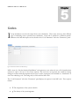
1
Version
r-JAVA
r-Process code for the Java platform
USER
MANUAL
QUARK NOVA PROJECT
r-Java User Manual
 Quark Nova Project
University of Calgary
2500 University Dr. NW
Calgary, Alberta, Canada
T2N 1N4
http://quarknova.ucalary.ca
Table of Contents
Introduction .............................................................................. 1
Quick Start ............................................................................... 2
Graphical User Interface .......................................................... 4
Main Menu ...................................................................................... 4
Toolbar ............................................................................................ 5
Main Panel ...................................................................................... 5
Parameters Panel ........................................................................... 8
Importing Data.......................................................................... 9
Codes..................................................................................... 11
NSE............................................................................................... 11
Static ............................................................................................. 12
Dynamic ........................................................................................ 13
Graphs ................................................................................... 14
Animations ............................................................................. 16
Q U A R K
N O V A
1
Chapter
P R O J E C T
Introduction
T
He r-process is needed to explain the origin of many heavy neutron–rich nuclei. The astrophysical site
where the r-process occurs, however, has not been positively identified. One fruitful avenue of
research involves the study of decompressing neutron matter from the surface of neutron stars.
Several mechanisms may play a role in this decompression, include the quark nova.
Code has been developed at the Quark Nova Project (QNP) to simulate the ejection of neutron matter from
the surface of a neutron star and calculate the abundance of elements via the r-process that results. r-Java is a
graphical user interface to this code that makes exploring the parameter space simple and intuitive
This manual describes the functionality of this graphical interface and assists in the use of the software. The
underlying code and methods for the r-process calculation are not described here. For an in-depth review of
the code and its application please see the paper:
“Nucleosynthesis in neutron-rich ejecta from Quark-Novae”, Prashanth Jaikumar, Bradley S. Meyer,
Kaori Otsuki and Rachid Ouyed.
This paper is available on the Quark Nova Project (QNP) website at: http://quarknova.ucalgary.ca
1
Q U A R K
N O V A
2
Chapter
P R O J E C T
Quick Start
r
-Java was designed to be user friendly and easy to use. As such, starting and running a project involves
very few steps. This chapter will present you with a quick no-details list of commands to get started.
Once started you can explore the interface on your own or read further to understand the full details of the
software.
1. Launch r-Java via java webstart on the QNP website.
2. Save the isotope data file (“r-java_input.ascii”) from the QNP website to disk.
3. In r-java, choose the menu option “File” and then “Import” to load the isotope data file.
4. You will be presented with a dialog where you can enter the name of the data file. Browse to the
location you saved your file in step 2 and select the file.
5. The column separator in the file is a “tab” character, so select the “Tab” option under “Column
Separator”.
6. Click “import” (the rest of the options are correct for the input file from the QNP website).
7. Click “Close” to close the import dialog.
8. If you now click on the “Table” tab in the main window you will be presented with a table of all the
isotopes imported from the file. Several of these fields are editable, including the “color” of the isotope
which is useful for some types of graphs.
9. Click on the “Graphs” tab in the main window and then click on the green “Plus” icon in the toolbar
to open a dialog of possible graph types.
10. Choose “Isotope” from the dialog and click “Accept”
11. Click on the “Code Parameters” tab in the “Parameters” panel at the bottom of the main window.
12. Choose “NSE” (Nuclear Statistical Equilibrium) as the code type and enter the following values (press
“Enter” after you input the values for each): T = 3.5E9, ρ = 1E7, Ye = 0.5.
2
Q U A R K
N O V A
P R O J E C T
13. Click on the “Calculator” icon in the main toolbar. The abundances will then be calculated and
displayed on the graph you created in step 10.
14. Click on the “Graph Parameters” tab in the “Parameters” panel at the bottom of the main window.
Set the x-axis to “A”. You will notice that you do not have to re-calculate for the changes to be
displayed on the graph.
15. Click on the “Code Parameters” tab and select “Dynamic” as the code type.
16. Enter the following values in the “QN Parameters” section (again remember to press “Enter” after
each entry): M star: 1.4, R star: 10, M ejecta: 1E-2, Zeta: 0.01.
17. Click the red “Import” button to calculate the necessary input parameters. These will be displayed in
the left section of the panel, “Input Parameters”. Of course you can enter the general input parameters
without “importing” them from the “QN parameters” section.
18. Set Z0 = 26 and Duration = 1.0 in the “Input Parameters” section.
19. Click the “Calculate” button in the main toolbar to start the calculation. This will take a few seconds to
complete and you can see how the graph changes during the calculation. Adjusting the “Update” field
will add more or less animation steps.
20. To save the graph, right click anywhere on the graph and choose “Save Ascii” or “Save Image”
depending on if you want to save the text data, or the image respectively.
21. To change the scale of the graph, right click anywhere on the graph and choose “Graph Properties”.
Under the “Axes” tab (default) set the “Scale” to “log10(x)” in the Y-axis section and set the “Min” to 20 and the “Max” to 0.
22. Save the project by clicking the “Save” icon in the main toolbar or selecting “Save Project” in the “File”
menu. You can then open this project at a future time by using the “Open” icon in the toolbar, or the
“Open Project” entry in the “File” menu.
The above steps should get you started in exploring the user interface. Feel free to change parameters and
options to see what the program can do.
3
Q U A R K
N O V A
3
Chapter
P R O J E C T
Graphical User Interface
r
-Java is graphical user interface to the r-process code. Navigating the toolbars, menus and graphs is meant
to be intuitive. This section will briefly cover the function of each interface component. An important
point to note is that when you enter a value in a text box, you must press “Enter” for the change to be
recorded. r-java does not monitor key presses and will not update unless “Enter” is pressed.
Main Menu
Figure 1: File menu
The main menu consists of one sub-menu, the “File” menu. This menu allows you to open and save projects
as well as import and export isotope data.

New Project: This creates a new, blank project. When r-java is first started, a new project is
automatically created. This menu item is useful if you have a project loaded and you want to start a
new one.

Open Project: Opens a saved project.

Save Project: Saves the current project to the current filename of the project. If the project has not yet
been saved, a dialog will be displayed asking for the name of the file you wish to save to.

Save Project As…: Saves the project to a filename of your choice.
4
Q U A R K
N O V A
P R O J E C T

Import: Imports isotope data from a text file. A dialog is displayed requesting information about the
file.

Export: Writes the current isotope information to a text file.

Exit: Closes r-java
Toolbar
Figure 2: Main toolbar
The toolbar provides a graphical interface to some common commands in r-Java. The icons represent:

Calculate Icon: This is the main icon which starts off any abundance calculation. When pressed, rJava will calculate the resulting abundances of isotopes and create the necessary graphs.

Open Icon: Opens a saved project.

Save Project Icon: Saves the current project.

Add Graph Icon: Adds a new graph to the graph panel.

Remove Graph Icon: Removes the selected graph from the graph panel.

Animate Icon: Runs an animation based on the “Animation Parameters” in the “Parameters” panel.

Clear Icon: Clears the data from all graphs.

Maximize/Restore Icon: Maximizes or restores the currently selected graph.
Main Panel
Figure 3: Tabs located on the main panel
5
Q U A R K
N O V A
P R O J E C T
The main panel is located directly below the Toolbar and consists of three tabs:

Graphs: This panel displays all of the graphs. You can add as many graphs as you like to this panel
(see “Add Graph Icon” above) and can arrange them using the “Project Parameters” tab in the
“Parameters Panel”.
Figure 4: Example of graphs layed out in the graph tab

Table: This panel displays a list of isotopes currently loaded in the project. Several of these fields are
editable including the “color” of the isotope which is useful for some types of graphs. Also available
in the table view is the ability to "select" isotopes. Selected isotopes are used in some graphs, such as
the animation graphs and time step graphs.
Figure 5: The table tab allows you to view which isotopes are currently loaded in the project
6
Q U A R K

N O V A
P R O J E C T
Periodic Table: The periodic table in r-Java is used to visually display which elements are created in
the calculations. At the beginning of the calculation, all elements are "blue" which indicates there are
no elements produced. As the calculation runs and new elements are created, the periodic table will
convey this by turning these elements "red". Hovering your mouse over the element will display the
name and current mass fraction of that element. Only elements with a mass fraction greater than the
cutoff defined in the Parameters panel will be turned red.
Figure 6: The periodic table tab gives a visual aid to which elements are being produced in the current calculation.

Messages: This panel displays all of the messages from the underlying code, including possible errors.
The “Clear” icon at the top of this panel will clear all messages.
Figure 7: The message tab shows information sent from the calculation code, including errors.
7
Q U A R K
N O V A
P R O J E C T
Parameters Panel
The parameters panel is located at the bottom of the main window. You can expand and collapse the panel by
clicking on the “minus” or “plus” icon in the far right of the title bar. The panel consists of four tabs:

Project Parameters: This panel allows you to set the layout for the “Graphs” panel in the main panel.
You can specify the number of rows and columns for your display. In addition there is an "MF
Cutoff" field that specifies the minimum isotope mass fraction needed to be included in the graphs.

Code Parameters: This panel allows you to select the type of code to run and input the parameters
for the calculation.

Animation Parameters: This panel sets up an animation run. It allows you to specify what variable is
animated and which isotopes participate in the animation.

Graph Parameters: This panel allows you to edit the attributes of the currently selected graph
including the axis variables.
8
Q U A R K
N O V A
4
Chapter
P R O J E C T
Importing Data
S
ince r -Java calculates abundances of isotopes, certain isotope data is needed before the calculations can
commence. This data is loaded into r-Java via the “Import” command in the “File menu” Clicking on
the “Import” command will display the import dialog (Figure 8):
Figure 8: The import dialog is the interface through which isotope data is loaded into r-java
9
Q U A R K
N O V A
P R O J E C T
This dialog provides the interface for loading isotope data into r-Java. There are several inputs that need to be
defined before any data can be loaded:

Filename: The name of the input file. This is a text file separated into columns by some delimiting
character (such as a tab or a space).

Comment String: Often data files have comments that should not be read as data. This field allows
you to specify the string of characters at the beginning of a line that signals a comment. Usually this is
the “#” character.

Clear Isotopes: When selected, all isotopes previously loaded into r-Java will first be removed. If this
is not selected, the list of isotopes is appended to by the import. If the isotope already exists in r-Java, it
will be altered to reflect the new values read.

Column Separator: This is the character that signals a new column in a row of data from the text file.
Usually this is a space or tab character but can be anything. Make sure this is selected properly or the
data will not be read correctly.
The format of the input file does not need to follow any convention. It is possible to define which columns of
the data file correspond to what attributes of the isotopes. The “Input Columns” section of the dialog allows
you to make this assignment. The only required values for each isotope are the “Z” and “A” values. These
values define the isotope. The other columns are not necessary but some calculations may not proceed
correctly without them (i.e. mass). Figure 9 shows an example input file for r-Java.
Figure 9: Example input file for r-Java. Each column is tab separated.
10
Q U A R K
N O V A
5
Chapter
P R O J E C T
Codes
I
sotope abundances are the main output from r-Java calculations. There exists, however, three different
types of underlying code to perform these calculations. Each code is suitable for a different scenario.
Different codes and their inputs can be selected via the “Code Parameters” tab in the “Parameters” panel.
NSE
Figure 10: Parameters available to the NSE code type
NSE is short for “Nuclear Statistical Equilibrium” and represents a state where the rate of all forward nuclear
reactions is equal to the rate of the reverse reactions. This code does not represent the conditions existing
during the neutron matter decompression that r-Java is used to investigate, but is included as a “benchmark” or
test of the underlying code. This being said, it is still useful for NSE work.
The “Code Parameters” tab in the “Parameters” panel displays the options for the NSE code. These options
include:

T: The temperature of the system in Kelvin

ρ: The density of the system in
-
11
Q U A R K

N O V A
P R O J E C T
Ye: The electron fraction
Static
Figure 11: Parameters available to the static code type
The static code is an r-process code, but does not allow for the expansion and cooling of the system with time.
This provides a “snapshot” of isotopes produced under the conditions supplied. The parameters for the code
include:

T: The temperature of the system in K

n: The number density of the system in

Ye: The electron fraction

Duration: How long the simulation is run for in seconds

Z0: The “seed” element the neutrons are bombarding.
-
12
Q U A R K
N O V A
P R O J E C T
Dynamic
Figure 12: Parameters available to the dynamic code type
The dynamic code is the main code in r-java. It is similar to the static code but allows for the expansion of the
system and hence cooling and a reduction in density. The dynamic code is like a series of static calculations and
as such takes longer to run. The parameters for the code include:

T: The temperature of the system in K

ρ: The density of the system in

Ye: The electron fraction

τ: Expansion timescale in seconds

Duration: How long the simulation is run for in seconds

Z0: The “seed” element the neutrons are bombarding.

Update: This specifies how many steps in the calculation before the graphs are updating. Setting this
to a lower number allows you to see how the abundances are changing, but may take longer to
calculate.
-
Instead of these inputs, one can alternatively specify quark nova parameters. The input parameters are then
calculated based on these values. The QN parameters include:

M star: The mass of the neutron star in solar masses

R star: The radius of the neutron star in km

M ejecta: The mass of the neutron star ejecta

Zeta:
13
Q U A R K
N O V A
6
Chapter
P R O J E C T
Graphs
G
raphs are the main component by which the abundance information is conveyed to the user. Several
types of graphs are available for plotting. The graphs are displayed in the “Graphs” tab in the “Main
Panel” and can be arranged via the “Project Parameters” tab of the “Parameters Panel”.
Each graph can be selected by clicking on the graph. A red line will then appear around the graph indicating its
currently selected state. Once a graph is selected, its parameters will become available in the “Graph
Parameters” tab in the “Parameters panel” and will be available for removal via the “Remove Graph Icon” in
the toolbar.
Individual graph properties can be adjusted by right
clicking anywhere on the graph. Here you can save the
graph information as a text file, or save it as an image.
Additionally you can edit the “properties” of the
graph. Many aesthetic options are available so that you
can customize your graph any ways you like. There is
also an option to set the “scale” of the axes. For
example, if you want a Log scale for the y axis, click on
the “Axes” tab and enter “log10(x)” in the “Scale”
field for the “Y-Axis”. Similarly the range of the axes
can be set and locked if necessary (so they don’t
change automatically).
Several types of graphs are available including:
Figure 13: Graph properties available when you right click on a graph and select
"Graph Properties"

Isotope: This is the main graph type in r-Java
and plots attributes of all the loaded isotopes. The variables plotted on the axes can be selected via the
parameters in the “Graph Parameters” tab in the “Parameters” panel. Attributes you can plot include
Z, A, N, Mass Fraction, population coefficients and even solar abundances.

Time Step: This graph allows you to plot values for every time step in the dynamic code calculation.
The axis variables available to this graph type include time, temperature, Q heat, and neutron density.
It is also possible to plot isotope attributes for each time step by selecting an appropriate y-axis. Any
isotope that is "selected" in the "Tab" panel of the "Main Panel" will be plotted in this graph.
14
Q U A R K

N O V A
P R O J E C T
Animation: This graph will plot an attribute of one or more isotopes versus temperature, density or
electron fraction. The animation parameters can be defined in the “Animation Parameters” tab of the
“Parameters” panel.
15
Q U A R K
N O V A
7
Chapter
P R O J E C T
Animations
A
nimations are used to study how specific isotope attributes change with
temperature. The animations require an animation graph to be created via the
“Create Graph Icon” in the toolbar. Once created, attributes to plot can be
selected via the “Graph Parameters” tab in the “Parameters Panel”.
Figure 14: Animation parameters
Before an animation is run, you will need to adjust the “Animation Parameters” in the
“Parameters Panel”. The options you can adjust are:

X-axis: This defines the axis of the animation plot.
temperature, neutron density and electron fraction.

Max: The maximum value for the animation to reach (i.e. the max value on
the x-axis)

Min: The starting value for the animation (i.e. the min value on the x-axis)

Num Steps: The number of steps in the animation. The more steps allow for
a smoother the graph, but will take longer.
16
Values include

Output Dir: This directory is where images or data will be stored for each
frame of the animation. These images can then be used to create a movie of
the run with external software (SHAPE is an astrophysical modeling tool that
has the capability to create such movies and can be downloaded from:
http://bufadora.astrosen.unam.mx/shape/)

Save Ascii: When selected, ascii data from the graph will be saved in the
output directory for each frame of the animation.

Save Images: When selected, images of the graphs will be saved in the output
directory for each frame of the animation.
In addition to the above options, one must specify which isotopes to include in the
animation. This can be accomplished through the "Table" tab on the "Main Panel".
Simply click the radio button in the far right column to select the isotope.
It is useful to note at this point that the “color” of the isotope can also be changed in
the “Table” tab of the “Main Panel”. This makes identification of the plotted isotope
much simpler.
Once the parameters for an animation are setup, clicking on the “Animation Icon” in
the Toolbar will start the animation. The animation uses the currently selected “Code”
and the parameters associated with it.
Figure 15: Resulting animation graph from a test run. The different colors represent different isotopes.
17