Download User Guide: Liquids NMR

User Guide:
Liquids NMR
Varian NMR Spectrometer Systems
With VNMR 6.1C Software
Pub. No. 01-999161-00, Rev. B0801
User Guide:
Liquids NMR
Varian NMR Spectrometer Systems
With VNMR 6.1C Software
Pub. No. 01-999161-00, Rev. B0801
User Guide: Liquids NMR
Varian NMR Spectrometer Systems
With VNMR 6.1C Software
Pub. No. 01-999161-00, Rev. B0801
Revision history:
A0800 – Initial release for VNMR 6.1C software.
B0601 – Updated Chapter 13 for LC-NMR2000 and STAR 5.5
B0801 – Added setLP1 macro to chapter 3.
Applicability of manual:
UNITYINOVA,
MERCURY VxWorks Powered NMR spectrometer systems
(shortened to MERCURY-VX throughout this manual), MERCURY, UNITYplus,
GEMINI 2000, UNITY, and VXR-S NMR superconducting spectrometer systems with
VNMR 6.1C software installed.
Technical contributors: Greg Brissey, Steve Cheatham, Bayard Fetler, Phil Hornung,
Dan Iverson, Boban John, Frits Vosman, Evan Williams
Technical writers: Michael Carlisle, Everett Schreiber
Technical editor: Dan Steele
Copyright 2001 by Varian, Inc.
3120 Hansen Way, Palo Alto, California 94304
http://www.varianinc.com
All rights reserved. Printed in the United States.
The information in this document has been carefully checked and is believed to be
entirely reliable. However, no responsibility is assumed for inaccuracies. Statements in
this document are not intended to create any warranty, expressed or implied.
Specifications and performance characteristics of the software described in this manual
may be changed at any time without notice. Varian reserves the right to make changes in
any products herein to improve reliability, function, or design. Varian does not assume
any liability arising out of the application or use of any product or circuit described
herein; neither does it convey any license under its patent rights nor the rights of others.
Inclusion in this document does not imply that any particular feature is standard on the
instrument.
UNITYINOVA, MERCURY, Gemini, GEMINI 2000, UNITYplus, UNITY, VXR, XL, VNMR,
VnmrS, VnmrX, VnmrI, VnmrV, VnmrSGI, MAGICAL II, AutoLock, AutoShim,
AutoPhase, limNET, ASM, and SMS are registered trademarks or trademarks of Varian,
Inc. Sun, Solaris, CDE, Suninstall, Ultra, SPARC, SPARCstation, SunCD, and NFS are
registered trademarks or trademarks of Sun Microsystems, Inc. and SPARC
International. Oxford is a registered trademark of Oxford Instruments LTD.
Ethernet is a registered trademark of Xerox Corporation. VxWORKS and VxWORKS
POWERED are registered trademarks of WindRiver Inc. Dell is a registered trademark
of Dell Computer Corporation. Windows is either a registered trademark of Microsoft
Corporation in the United States and or other countries.Other product names in this
document are registered trademarks or trademarks of their respective holders.
Overview of Contents
SAFETY PRECAUTIONS .................................................................................. 25
Introduction ...................................................................................................... 29
Chapter 1. Advanced 1D NMR ......................................................................... 31
Chapter 2. 1D Experiments.............................................................................. 73
Chapter 3. Multidimensional NMR .................................................................. 89
Chapter 4. Multidimensional and Advanced Experiments ......................... 137
Chapter 5. Indirect Detection Experiments.................................................. 171
Chapter 6. Data Analysis ............................................................................... 201
Chapter 7. Pulse Analysis ............................................................................. 225
Chapter 8. Variable Temperature Operation ................................................ 259
Chapter 9. Carousel, SMS, and NMS Automation ....................................... 267
Chapter 10. VAST Accessory Operation ...................................................... 309
Chapter 11. PFG Modules Operation............................................................ 369
Chapter 12. PFG Modules Experiments ....................................................... 391
Chapter 13. LC-NMR Accessory Operation ................................................. 399
Chapter 14. LC-NMR Accessory Experiments............................................. 465
Index ................................................................................................................ 487
01-999161-00 B0801
VNMR 6.1C User Guide: Liquids NMR
3
4
VNMR 6.1C User Guide: Liquids NMR
01-999161-00 B0801
Table of Contents
Table of Contents
SAFETY PRECAUTIONS .................................................................................. 25
Introduction ...................................................................................................... 29
Chapter 1. Advanced 1D NMR ........................................................................ 31
1.1 Working with Experiments ..........................................................................................
1.2 Multi-FID (Arrayed) Spectra .......................................................................................
Arrayed Parameters ............................................................................................
Multiple Arrays ..................................................................................................
Setting Array Order and Precedence ..................................................................
Interactively Arraying Parameters ......................................................................
Resetting an Array ..............................................................................................
Array Limitations ...............................................................................................
Acquiring Data ...................................................................................................
Processing ...........................................................................................................
Display and Plotting ...........................................................................................
Saving and Retrieving ........................................................................................
Pulse Width Calibration Step-by-Step ................................................................
1.3 T1 and T2 Analysis .......................................................................................................
Setting Up The Experiment ................................................................................
Processing the Data ............................................................................................
Analyzing the Data .............................................................................................
Exponential Analysis Menu ...............................................................................
T1 Data Workup: Step-by-Step ...........................................................................
1.4 Kinetics ........................................................................................................................
Setting Up the Experiment .................................................................................
Processing the Data ............................................................................................
Kinetics Step-by-Step .........................................................................................
1.5 Diffusion Experiments/DOSY .....................................................................................
Pulsed Gradient Experiments .............................................................................
Pulsed Gradient Experiment Setup .....................................................................
Gradient Calibration ...........................................................................................
Data Reduction ...................................................................................................
Data Display .......................................................................................................
Variations on the pge Pulse Sequence ................................................................
DOSY Experiments ............................................................................................
Filter Diagonalization Method ...........................................................................
Using FDM .........................................................................................................
31
32
32
33
34
34
34
35
35
35
35
36
37
37
38
38
38
39
39
39
39
40
40
40
40
42
44
44
47
48
48
68
68
Chapter 2. 1D Experiments ............................................................................. 73
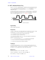
2.1 APT—Attached Proton Test ........................................................................................
Applicability .......................................................................................................
Parameters ..........................................................................................................
Technique ...........................................................................................................
References ..........................................................................................................
Related Commands and Macros .........................................................................
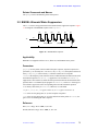
2.2 BINOM—Binomial Water Suppression ......................................................................
01-999161-00 B0801
VNMR 6.1C User Guide: Liquids NMR
74
74
74
74
74
75
75
5
Table of Contents
Applicability .......................................................................................................
Parameters ..........................................................................................................
Reference ............................................................................................................
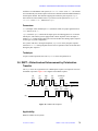
2.3 CPMGT2—Carr-Purcell Meiboom-Gill T2 Measurement ..........................................
Applicability .......................................................................................................
Parameters ..........................................................................................................
T2 Measurement .................................................................................................
Acquisition and Processing ................................................................................
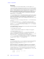
2.4 CYCLENOE—Cycled NOE Difference Experiment ..................................................
Applicability .......................................................................................................
Parameters ..........................................................................................................
Technique ...........................................................................................................
2.5 D2PUL—Standard Two-Pulse Using Decoupler as Transmitter .................................
Applicability .......................................................................................................
Parameters ..........................................................................................................
Technique ...........................................................................................................
2.6 DEPT—Distortionless Enhancement by Polarization Transfer ...................................
Applicability .......................................................................................................
Parameters ..........................................................................................................
Technique ...........................................................................................................
Potential Problems ..............................................................................................
Reference ............................................................................................................
Related Commands and Macros .........................................................................
2.7 INEPT—Insensitive Nuclei Enhanced by Polarization Transfer .................................
Applicability .......................................................................................................
Parameters ..........................................................................................................
Technique ...........................................................................................................
Reference ............................................................................................................
2.8 JUMPRET—Jump-and-Return Water Suppression .....................................................
Applicability .......................................................................................................
Parameters ..........................................................................................................
Reference ............................................................................................................
2.9 NOEDIF—NOE Difference Experiment .....................................................................
Applicability .......................................................................................................
Parameters ..........................................................................................................
Phase Cycling .....................................................................................................
Procedure ............................................................................................................
Reference ............................................................................................................
2.10 PRESAT—1D Water Suppression .............................................................................
Applicability .......................................................................................................
Parameters ..........................................................................................................
2.11 S2PUL—Standard Two-Pulse Sequence ...................................................................
Applicability .......................................................................................................
Parameters ..........................................................................................................
2.12 S2PULR—Standard Two-Pulse in Reverse Configuration ........................................
Applicability .......................................................................................................
Parameters ..........................................................................................................
Technique ...........................................................................................................
6
VNMR 6.1C User Guide: Liquids NMR
01-999161-00 B0801
75
75
75
76
76
76
76
76
77
77
77
78
78
78
79
79
79
79
80
80
81
81
81
82
82
82
83
83
83
83
83
83
84
84
84
84
85
87
87
87
87
87
87
87
88
88
88
88
Table of Contents
Chapter 3. Multidimensional NMR ................................................................. 89
3.1 Interferograms .............................................................................................................. 89
3.2 2D NMR Step-by-Step ................................................................................................. 90
To Process Stored Data ....................................................................................... 90
To Acquire a Simple COSY ............................................................................... 91
3.3 Phase-Sensitive 2D NMR ............................................................................................ 91
3.4 Data Acquisition: Arrayed 2D ..................................................................................... 92
Hypercomplex Method ....................................................................................... 92
TPPI Method ...................................................................................................... 93
Real-Time 2D ..................................................................................................... 94
Macros for 2D Experiments ............................................................................... 94
3.5 Weighting ..................................................................................................................... 95
Parameters .......................................................................................................... 95
Setting Values ..................................................................................................... 95
Interactive Weighting .......................................................................................... 96
3.6 Phasing Before the 2D Transform ............................................................................... 97
3.7 Baseline Correction ...................................................................................................... 98
First-Point Multiplier .......................................................................................... 99
Baseline Correction .......................................................................................... 100
FID Drift Correction ......................................................................................... 100
Spectral Drift Correction .................................................................................. 101
3.8 Processing Phase-Sensitive 2D and 3D Data ............................................................. 101
Processing Programs ........................................................................................ 103
Common Coefficients for wft2d Processing .................................................... 104
Sign of f1 Frequencies ...................................................................................... 105
2D Solvent Subtraction Filtering ...................................................................... 106
Left Shift, Frequency Shift, Phase Rotation ..................................................... 106
2D Processing of 3D Data ................................................................................ 106
3.9 2D and 3D Linear Prediction ..................................................................................... 107
3.10 Phasing the 2D Spectrum ......................................................................................... 108
3.11 Display and Plotting ................................................................................................. 109
Display Modes .................................................................................................. 109
Display and Plot Limits .................................................................................... 109
Maximum Intensity .......................................................................................... 111
Axis Label and Direction .................................................................................. 111
Display Scaling ................................................................................................. 112
Grid Lines ......................................................................................................... 112
Color Maps and Contour Plots ......................................................................... 112
Whitewashed Spectra ....................................................................................... 113
Label Display .................................................................................................... 113
Projection of 2D Data ....................................................................................... 113
2D Referencing ................................................................................................. 114
Rotating Homonuclear 2D-J Spectra ................................................................ 114
Symmetrizing Data ........................................................................................... 114
Setting Negative Intensities to Zero ................................................................. 114
Automatic Analysis .......................................................................................... 115
3.12 Interactive 2D Color Map Display ........................................................................... 115
Interactive 2D Display Menus .......................................................................... 117
Controlling the Display with the Mouse .......................................................... 118
01-999161-00 B0801
VNMR 6.1C User Guide: Liquids NMR
7
Table of Contents
Changing the Display .......................................................................................
Treating 2D Traces as 1D Spectra ....................................................................
3.13 Interactive 2D Peak Picking .....................................................................................
Interactive 2D Peak Picking Menus .................................................................
Automatic 2D Peak Picking .............................................................................
Interactive Peak Picking or Editing ..................................................................
Automatic Integration .......................................................................................
Interactive Integration and Editing ...................................................................
Labeling and Commenting Peaks .....................................................................
Displaying Peaks in dconi ................................................................................
Peak File Manipulations ...................................................................................
3.14 3D NMR ..................................................................................................................
3D Acquisition ..................................................................................................
3D Processing ...................................................................................................
3D Display ........................................................................................................
3D Pulse Sequences ..........................................................................................
Experiment Setup .............................................................................................
Data Processing ................................................................................................
3.15 4D NMR Acquisition ...............................................................................................
118
120
120
123
127
127
128
128
128
129
129
129
130
131
132
132
132
133
134
Chapter 4. Multidimensional and Advanced Experiments ........................ 137
4.1 Absolute-Value COSY, RELAY-COSY, Double RELAY-COSY ..............................
Applicability .....................................................................................................
Parameters ........................................................................................................
Technique .........................................................................................................
Potential Problems ............................................................................................
4.2 COSY—Correlated Spectroscopy .............................................................................
Applicability .....................................................................................................
Parameters ........................................................................................................
Technique .........................................................................................................
4.3 COSYPS—Phase-Sensitive COSY ............................................................................
Applicability .....................................................................................................
Parameters ........................................................................................................
Phase Cycling ...................................................................................................
Technique .........................................................................................................
References ........................................................................................................
4.4 DQCOSY—Double-Quantum Filtered COSY ..........................................................
Applicability .....................................................................................................
Parameters ........................................................................................................
Phase Cycling ...................................................................................................
Technique .........................................................................................................
Potential Problems ............................................................................................
References ........................................................................................................
4.5 HET2DJ—Heteronuclear 2D-J ..................................................................................
Applicability .....................................................................................................
Parameters ........................................................................................................
Technique .........................................................................................................
Potential Problems ............................................................................................
References ........................................................................................................
8
VNMR 6.1C User Guide: Liquids NMR
01-999161-00 B0801
138
139
139
139
141
141
141
141
141
141
141
141
142
143
143
143
143
143
144
144
145
145
145
145
145
146
146
147
Table of Contents
4.6 HETCOR—Heteronuclear Chemical Shift Correlation ............................................
Applicability .....................................................................................................
Parameters ........................................................................................................
Technique .........................................................................................................
Potential Problems ............................................................................................
References ........................................................................................................
4.7 HETCORPS—Absolute-Value and Phase-Sensitive HETCOR ................................
Applicability .....................................................................................................
Parameters ........................................................................................................
Recommendations ............................................................................................
4.8 HOM2DJ—Homonuclear J-resolved 2D ...................................................................
Applicability .....................................................................................................
Parameters ........................................................................................................
Technique .........................................................................................................
Potential Problems ............................................................................................
References ........................................................................................................
4.9 INADEQUATE—Double-Quantum Transfer Experiment ........................................
Applicability .....................................................................................................
Parameters ........................................................................................................
Technique .........................................................................................................
4.10 MQCOSY—Multiple-Quantum Filtered COSY .....................................................
Applicability .....................................................................................................
Parameters ........................................................................................................
Technique .........................................................................................................
References ........................................................................................................
4.11 NOESY—Nuclear Overhauser Effect Spectroscopy ...............................................
Applicability .....................................................................................................
Parameters ........................................................................................................
Phase Cycling ...................................................................................................
Technique .........................................................................................................
Potential Problems ............................................................................................
Reference ..........................................................................................................
4.12 ROESY—Rotating Frame Overhauser Effect Spectroscopy ...................................
Applicability .....................................................................................................
Parameters ........................................................................................................
Phase Cycling ...................................................................................................
Technique .........................................................................................................
Reference ..........................................................................................................
4.13 TNCOSYPS—COSYPS with Water Suppression ...................................................
Applicability .....................................................................................................
Parameters ........................................................................................................
4.14 TNDQCOSY—DQCOSY with Water Suppression ................................................
Applicability .....................................................................................................
Parameters ........................................................................................................
4.15 TNMQCOSY—MQCOSY with Water Suppression ...............................................
Applicability .....................................................................................................
Parameters ........................................................................................................
References ........................................................................................................
4.16 TNNOESY—NOESY with Water Suppression ......................................................
01-999161-00 B0801
VNMR 6.1C User Guide: Liquids NMR
147
147
147
148
149
149
149
150
150
150
150
150
151
151
152
152
152
152
152
153
153
153
153
154
154
155
155
155
156
156
157
158
158
158
158
159
159
160
160
160
160
160
160
160
161
161
161
161
161
9
Table of Contents
Applicability .....................................................................................................
Parameters ........................................................................................................
4.17 TNROESY—ROESY with Water Suppression .......................................................
Applicability .....................................................................................................
Parameters ........................................................................................................
Technique .........................................................................................................
4.18 TNTOCSY—TOCSY with Water Suppression .......................................................
Applicability .....................................................................................................
Parameters ........................................................................................................
References ........................................................................................................
4.19 TOCSY—Total Correlation Spectroscopy ...............................................................
Applicability .....................................................................................................
Parameters ........................................................................................................
Phase Cycling ...................................................................................................
Technique .........................................................................................................
References ........................................................................................................
Related Macros .................................................................................................
4.20 TROESY—Transverse ROESY ...............................................................................
Applicability .....................................................................................................
Parameters ........................................................................................................
Reference ..........................................................................................................
4.21 HCCHTOCSY Pulse Sequence ...............................................................................
Applicability .....................................................................................................
Parameters ........................................................................................................
Technique .........................................................................................................
4.22 HMQCTOCSY Pulse Sequence ..............................................................................
Applicability .....................................................................................................
Parameters ........................................................................................................
Technique .........................................................................................................
4.23 HMQC-TOCSY 3D Pulse Sequence .......................................................................
Applicability .....................................................................................................
Parameters ........................................................................................................
Technique .........................................................................................................
4.24 HSQC-TOCSY 3D Pulse Sequence .........................................................................
Applicability .....................................................................................................
Parameters ........................................................................................................
162
162
162
162
162
163
163
163
163
164
164
164
164
165
165
165
165
166
166
166
166
166
166
166
167
168
168
168
168
168
168
168
169
169
169
170
Chapter 5. Indirect Detection Experiments ................................................. 171
5.1 Requirements for Indirect Detection Experiments ....................................................
Probes ...............................................................................................................
RF System ........................................................................................................
Pulse Sequences ................................................................................................
HMQC Pulse Sequence ....................................................................................
HMQCR Pulse Sequence .................................................................................
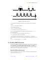
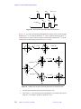
5.2 The Basic HMQC Experiment ...................................................................................
Spin-Echo Difference Experiment ....................................................................
BIRD Nulling ...................................................................................................
Transmitter Presaturation for High-Dynamic Range Signals ...........................
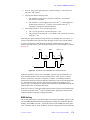
5.3 Phase-Sensitive Aspects of the Sequence ..................................................................
10
VNMR 6.1C User Guide: Liquids NMR
01-999161-00 B0801
171
172
172
174
174
176
177
177
179
180
181
Table of Contents
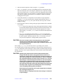
5.4 Cancellation Efficiency ..............................................................................................
5.5 Pros and Cons of Decoupling ....................................................................................
5.6 Specifications Testing ................................................................................................
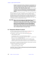
5.7 Using the HMQC and HMQCR Sequences ...............................................................
5.8 Recabling Single-Broadband Systems .......................................................................
5.9 Recabling Dual-Broadband Systems .........................................................................
5.10 Filters for Indirect Detection ....................................................................................
5.11 Tuning the Probe in the Reverse Mode ....................................................................
Tune the 1H Channel ........................................................................................
Tune the X Channel ..........................................................................................
5.12 Controlling Transmitter Power in the Reverse Mode ..............................................
5.13 Indirect Detection Calibration .................................................................................
5.14 Typical Experimental Protocol for HMQC Experiments .........................................
5.15 Differences for 15N Indirect Detection ....................................................................
5.16 HSQC Experiment ...................................................................................................
Applicability .....................................................................................................
Parameters ........................................................................................................
181
182
183
184
185
185
186
186
186
186
187
187
194
199
199
199
199
Chapter 6. Data Analysis .............................................................................. 201
6.1 Spin Simulation ..........................................................................................................
Spin Simulation Step-by-Step ..........................................................................
Spin Simulation Menus ....................................................................................
Entering a Spin System ....................................................................................
Spin Simulation Parameters .............................................................................
Performing a Spin Simulation ..........................................................................
Iterative Mode ...................................................................................................
Spin Simulation Files .......................................................................................
6.2 Deconvolution ............................................................................................................
Deconvolution Step-by-Step .............................................................................
Performing Deconvolution ...............................................................................
Display and Plotting .........................................................................................
Deconvolution Menu ........................................................................................
6.3 Reference Deconvolution ...........................................................................................
Reference Deconvolution of 1D Spectra ..........................................................
Reference Deconvolution of 2D Spectra ..........................................................
References ........................................................................................................
6.4 Addition and Subtraction of Data ..............................................................................
Add/Subtract Menu ..........................................................................................
Noninteractive Add/Subtract ............................................................................
Interactive Add/Subtract ...................................................................................
6.5 Regression Analysis ...................................................................................................
Regression Commands and Menus ..................................................................
Regression Analysis Step-by-Step ...................................................................
Contents of “analyze.out” File .........................................................................
Contents of “regression.inp” File .....................................................................
6.6 Chemical Shift Analysis ............................................................................................
201
202
204
204
204
205
205
206
207
207
208
209
210
210
211
212
213
213
213
214
216
218
218
219
220
222
223
Chapter 7. Pulse Analysis ............................................................................ 225
7.1 Pulse Shape Analysis ................................................................................................. 225
01-999161-00 B0801
VNMR 6.1C User Guide: Liquids NMR
11
Table of Contents
Directory and File Operations ..........................................................................
Attribute Selection ............................................................................................
Scale and Reference .........................................................................................
Cursors ..............................................................................................................
Simulation Overview ........................................................................................
Simulation Parameters ......................................................................................
Performing a Simulation ...................................................................................
Creating a Pulse ................................................................................................
7.2 Pandora’s Box ............................................................................................................
Getting Started ..................................................................................................
Calibrating the RF Field ...................................................................................
Creating Waveforms from Macros ...................................................................
Creating Waveforms from UNIX .....................................................................
Pbox File System ..............................................................................................
Pbox VNMR Parameters ..................................................................................
Wave String Variables .......................................................................................
Creating Waveforms Using Menus ...................................................................
Pbox Macro Reference .....................................................................................
Pbox PSG Statements .......................................................................................
Pulse Shaping “On-Fly” ...................................................................................
Pbox_psg.h include Pulse Sequence Statements ..............................................
shonfly.c Sequence ...........................................................................................
Pbox UNIX Commands ....................................................................................
226
227
227
227
228
228
229
230
230
231
231
232
233
233
237
239
240
242
243
254
254
256
258
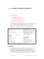
Chapter 8. Variable Temperature Operation ............................................... 259
8.1 Startup ........................................................................................................................
8.2 Operating Procedures .................................................................................................
8.3 Temperature-Related Command ................................................................................
8.4 Operating Recommendations .....................................................................................
8.5 VT Controller Safety Circuits ....................................................................................
8.6 VT Interlock Parameters ............................................................................................
259
260
262
263
264
265
Chapter 9. Carousel, SMS, and NMS Automation ...................................... 267
9.1 Carousel Autosampler ................................................................................................
Configuring VNMR for the Carousel ...............................................................
Checking Out the Carousel ...............................................................................
Mounting and Removing the Carousel .............................................................
Adjusting the Eject Air .....................................................................................
Loading and Unloading Samples ......................................................................
Running NMR on One Sample at a Time .........................................................
Running Automated NMR on Up to Nine Samples .........................................
Inserting Samples Manually with the Carousel Attached ................................
Carousel Error Codes and Recovery ................................................................
9.2 SMS Autosampler ......................................................................................................
Configuring VNMR for the SMS Autosampler ...............................................
Preparing Sample Tubes ...................................................................................
Running NMR on One Sample at a Time .........................................................
Running Automated NMR ...............................................................................
SMS Error Codes and Recovery .......................................................................
9.3 NMS Autosampler .....................................................................................................
12
VNMR 6.1C User Guide: Liquids NMR
01-999161-00 B0801
267
268
269
271
272
273
274
275
276
277
278
279
280
280
280
282
283
Table of Contents
Before Using NMS ...........................................................................................
Configuring VNMR for the NMS Autosampler ...............................................
Running NMR on One Sample at a Time .........................................................
Running Automated NMR ...............................................................................
9.4 General Automation Tasks For All Sample Changers ...............................................
Preparing and Initiating an Automation Run ....................................................
Setting Up an Automation Run for Multiple Users ..........................................
Monitoring an Automation Run .......................................................................
Using Sample Changers in Continuous Walkup Mode ....................................
Adding Samples to an Automation Run in Progress ........................................
9.5 Changing Sample Changers or Serial Ports ...............................................................
9.6 Using Gradient Autoshimming with Automation ......................................................
9.7 Automation Run Description .....................................................................................
Basic Automation Run .....................................................................................
Automation Behind the Scenes ........................................................................
While an Automation Run is in Progress .........................................................
When an Automation Run is Finished ..............................................................
Parameters for Automation ...............................................................................
Variable Temperature Control During Automation ..........................................
9.8 Customizing the Sample Entry Window ....................................................................
9.9 Automated Data Acquisition .....................................................................................
Optimizing Acquisition Macros .......................................................................
Customizing Macro Operation .........................................................................
Example of Customizing a Macro ....................................................................
9.10 Automated Data Processing .....................................................................................
9.11 File Structures in an Automation Run .....................................................................
284
284
284
285
287
287
288
289
291
292
293
293
293
294
295
296
297
297
297
298
299
300
300
302
306
306
Chapter 10. VAST Accessory Operation ..................................................... 309
10.1 Using the VAST Accessory .....................................................................................
To Prepare VAST for Use .................................................................................
To Set Up NMR Experiments for VAST ..........................................................
To Change Samples with VNMR .....................................................................
To Shut Down a VAST System ........................................................................
10.2 Solvent Suppression in VAST ..................................................................................
Setting Up Solvent Suppression .......................................................................
Troubleshooting Solvent Suppression ..............................................................
Evaluating Solvent Mixture Equilibration ........................................................
Solvent Suppression: Background Information ................................................
10.3 Processing, Displaying, and Plotting VAST Data Sets ............................................
Creating a Pseudo 2D Data Set ........................................................................
Processing, Displaying, and Plotting Glued VAST Data .................................
Defining a Custom Display Order with plate_glue ...................................
Examples of Plots of a VAST Data Set ............................................................
Summary of VAST Display and Plot Options ..................................................
10.4 Using CombiPlate to Analyze Data .........................................................................
Preparing VNMR Data For Analysis Using CombiPlate .................................
Data Analysis Using CombiPlate And VNMR ................................................
Analyzing Data Using CombiPlate Without VNMR. ......................................
Checking And Fixing The Color Map. .............................................................
01-999161-00 B0801
VNMR 6.1C User Guide: Liquids NMR
309
310
312
312
314
315
315
319
320
320
321
321
323
325
326
327
329
329
330
332
334
13
Table of Contents
10.5 Vast Process, Display, and Plot Macros ...................................................................
10.6 Preparing the Hardware and Configuring VNMR ...................................................
Connecting the Transfer Tube ..........................................................................
Connecting the Air Tubing ...............................................................................
Connecting Signal and Power Cables ...............................................................
Configuring VNMR for VAST .........................................................................
10.7 Calibrating Volumes and Flow Rates .......................................................................
To Calibrate Probe Volume ...............................................................................
To Calibrate Sample Volume ............................................................................
To Calibrate Flow Rate Parameters ..................................................................
To Calibrate XYZ Positions of the Arm ...........................................................
10.8 Acquiring Data on Standard Test Samples ..............................................................
10.9 Evaluating Carryover ...............................................................................................
10.10 VAST Interface Description ...................................................................................
SAMPLE Def. ..................................................................................................
Rack Def. Pane .................................................................................................
Main Control ....................................................................................................
Calibrations .......................................................................................................
10.11 Customizing the enter Window forVAST .............................................................
10.12 Files that Control VAST Operation ........................................................................
10.13 Writing VAST Protocols ........................................................................................
335
339
339
340
340
342
343
343
348
349
352
352
353
353
354
357
357
359
360
361
361
Chapter 11. PFG Modules Operation ........................................................... 369
11.1 Configuring the Software .........................................................................................
11.2 PFG Amplifier Operation ........................................................................................
11.3 Shimming PFG Systems ..........................................................................................
Performa I and Performa II ...............................................................................
Performa XYZ ..................................................................................................
11.4 Setting Up Software for Imaging Pulse Sequences .................................................
Calibrating the Gradients ..................................................................................
Creating a Gradient Table .................................................................................
Setting the System Gradient Coil .....................................................................
11.5 Homospoil Gradient Type ........................................................................................
11.6 Gradient Shimming ..................................................................................................
Configuring Gradients and Hardware Control .................................................
Gradient Shimming Method .............................................................................
Mapping the Shims ...........................................................................................
Starting Gradient Shimming .............................................................................
Quitting the Gradient Shimming System Menu ...............................................
General User Gradient Shimming ....................................................................
How Gradient Shimming Works ......................................................................
References ........................................................................................................
How Making a Shimmap Works ......................................................................
Shimmap Files and Parameters ........................................................................
How Automated Shimming Works ...................................................................
Deuterium Gradient Shimming ........................................................................
Homospoil Gradient Shimming for 1H or 2H ...................................................
Full Deuterium Gradient Shimming Procedure for Lineshape .........................
Setting Up Automation .....................................................................................
14
VNMR 6.1C User Guide: Liquids NMR
01-999161-00 B0801
369
370
372
372
372
372
372
372
373
373
374
375
375
375
376
376
377
377
378
379
380
381
381
383
384
384
Table of Contents
Suggestions for Improving Results .................................................................. 385
Gradient Shimming Menus ............................................................................... 386
Chapter 12. PFG Modules Experiments ...................................................... 391
12.1 GCOSY—PFG Absolute-Value COSY ...................................................................
Parameters ........................................................................................................
Processing .........................................................................................................
12.2 GHMQC—PFG HMQC ..........................................................................................
Parameters ........................................................................................................
Processing .........................................................................................................
12.3 GHMQCPS—PFG HMQC, Phase Sensitive ...........................................................
Processing .........................................................................................................
Recommendations ............................................................................................
12.4 GHSQC—PFG HSQC, Absolute Value or Phase Sensitive ....................................
Parameters ........................................................................................................
Processing .........................................................................................................
12.5 GMQCOSY—PFG Absolute-Value MQF COSY ...................................................
Parameters ........................................................................................................
Processing .........................................................................................................
12.6 GNOESY—PFG NOESY ........................................................................................
Parameters ........................................................................................................
Processing .........................................................................................................
12.7 GTNNOESY—PFG TNNOESY .............................................................................
Parameters ........................................................................................................
Processing .........................................................................................................
12.8 GTNROESY—PFG Absolute-Value ROESY .........................................................
Parameters ........................................................................................................
Processing .........................................................................................................
12.9 PFG Selective Excitation .........................................................................................
Parameters ........................................................................................................
Reference ..........................................................................................................
391
391
392
392
392
392
392
393
393
393
393
394
394
394
394
395
395
395
396
396
396
396
396
398
398
398
398
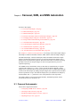
Chapter 13. LC-NMR Accessory Operation ................................................ 399
13.1 LC-NMR Experiments Overview VNMR ...............................................................
13.2 LC-NMR Software for VNMR ................................................................................
13.3 Optimizing Solvent Suppression in LC-NMR .........................................................
Setting Up Solvent Suppression .......................................................................
Troubleshooting Solvent Suppression ..............................................................
Evaluating Solvent Mixture Equilibration ........................................................
WET Experiments ............................................................................................
WET Shapes .....................................................................................................
Important Parameters ........................................................................................
13.4 On-Flow LC-NMR Experiments .............................................................................
Number of Transients in On-Flow Experiments ..............................................
Sensitivity in On-Flow Experiments ................................................................
Scout ScanTM Solvent Suppression ..................................................................
Acquiring Isocratic On-Flow LC-NMR Data ...................................................
Aborting the Experiment ..................................................................................
Processing NMR Data ......................................................................................
01-999161-00 B0801
VNMR 6.1C User Guide: Liquids NMR
400
401
402
402
407
407
407
408
408
408
409
409
409
409
411
411
15
Table of Contents
NMRgram .........................................................................................................
Manipulating the LC-NMR 2000 Data File After the Run ..............................
13.5 Acquiring Gradient On-Flow LC-NMR Data ..........................................................
Scout Scan Solvent Suppression ......................................................................
Ending the Experiment .....................................................................................
Processing the Data ..........................................................................................
Manually Processing Gradient On-Flow (Scout-Scan) Data ............................
13.6 Manual Stop-Flow LC-NMR Experiments ..............................................................
How Manual Stop-Flow LC-NMR Works .......................................................
Starting a Manual Stop Flow Run in LC-NMR 2000 .......................................
Preparing the NMR for Stop-Flow Experiments ..............................................
Acquiring 2D LC-NMR Data Manually ...........................................................
13.7 Manual Stop-Flow Experiment with Automatic Peak-Picking ...............................
How Stop-Flow LC-NMR with Automatic Peak-Picking Works ....................
Setting the Threshold for Automatic Peak Detection .......................................
Manual Stop Flow Run with Automatic Peak Detection .................................
Stopping on Peaks That Do Not Reach Threshold ...........................................
Preparing the NMR for Stop-Flow Experiments ..............................................
Sensitivity in Stop-Flow Experiments ..............................................................
13.8 Automatic Stop-Flow Using Scout ..........................................................................
How Stop-Flow LC-NMR Works .....................................................................
Acquiring Stop-Flow LC-NMR Data Using Scout ..........................................
13.9 Time-Slice Stop-Flow Experiments .........................................................................
How Time Slice Works .....................................................................................
Acquiring Time-Slice Stop-Flow Data—Semiautomatic .................................
13.10 Acquiring Stop-Flow LC-NMR Data Using Enter ................................................
How Custom Stop-flow Works with ENTER ...................................................
Acquiring Stop-Flow LC-NMR Data Using ENTER ......................................
Acquiring 2D LC-NMR Data Using ENTER Program ....................................
13.11 Acquiring Stop-Flow Data From an Analyte Collector .........................................
How Analyte Collection and Elution Experiments Work ................................
Acquiring Stop-Flow Data Using an Analyte Collector ...................................
13.12 STAR Chromatography Software for LC-NMR ....................................................
Standards Used for LC-NMR Chromatography ...............................................
Starting the LC pump .......................................................................................
Setting Up STAR Software ...............................................................................
Naming Data Files in STAR 5.5 .......................................................................
Printing a Chromatogram .................................................................................
Typical Chromatograms ...................................................................................
Setting Up an Automation Run in STAR Chromatography .............................
Hints for Good LC-NMR Chromatography .....................................................
13.13 LC-NMR 2000 Stop-Flow Program ......................................................................
Using LC-NMR 2000 Software ........................................................................
13.14 Transfer Time Calibration ......................................................................................
Calibrating from the LC Detector to the Microflow Probe ..............................
Calibrating from the LC Detector to the Analyte Collector .............................
Calibrating from the Analyte Collector to the Microflow Probe ......................
16
VNMR 6.1C User Guide: Liquids NMR
01-999161-00 B0801
412
412
412
412
414
414
414
415
415
415
417
418
419
419
419
420
421
422
422
422
423
423
426
426
427
429
429
430
432
433
433
433
435
435
436
436
442
442
443
443
445
445
445
456
456
460
461
Table of Contents
Chapter 14. LC-NMR Accessory Experiments ............................................ 465
14.1 LC1D—LC-NMR 1D Pulse Sequence ....................................................................
Applicability .....................................................................................................
Macro ................................................................................................................
Parameters ........................................................................................................
Calibrations .......................................................................................................
14.2 WET1D—Water Eliminated through Transverse Gradients 1D ..............................
Applicability .....................................................................................................
Macro ................................................................................................................
Parameters ........................................................................................................
14.3 WETDQCOSY—WET Double-Quantum Filtered COSY ......................................
Applicability .....................................................................................................
Macro ................................................................................................................
Parameters ........................................................................................................
Phase Cycling ...................................................................................................
Technique .........................................................................................................
Potential Problems ............................................................................................
References ........................................................................................................
14.4 WETGCOS—WET PFG Absolute-Value COSY ....................................................
Applicability .....................................................................................................
Macro ................................................................................................................
Parameters ........................................................................................................
Processing .........................................................................................................
14.5 WETGHMQCPS—WET PFG HMQC (Phase Sensitive) .......................................
Applicability .....................................................................................................
Macro ................................................................................................................
Parameters ........................................................................................................
Processing .........................................................................................................
14.6 WETGHSQC—WET PFG HSQC, Absolute Value or Phase Sensitive ..................
Applicability .....................................................................................................
Macro ................................................................................................................
Parameters ........................................................................................................
Processing .........................................................................................................
14.7 WETGMQCOSY—WET PFG Absolute-Value MQF COSY .................................
Applicability .....................................................................................................
Macro ................................................................................................................
Parameters ........................................................................................................
Processing .........................................................................................................
14.8 WETNOESY—WET Nuclear Overhauser Effect Spectroscopy .............................
Applicability .....................................................................................................
Macro ................................................................................................................
Parameters ........................................................................................................
Phase Cycling ...................................................................................................
Technique .........................................................................................................
Potential Problems ............................................................................................
Reference ..........................................................................................................
14.9 WETPWXAL—WET Pulse Width X Channel Calibration ....................................
Applicability .....................................................................................................
Macro ................................................................................................................
01-999161-00 B0801
VNMR 6.1C User Guide: Liquids NMR
465
465
465
465
466
467
467
467
467
468
468
468
468
469
470
470
470
470
470
470
471
472
472
472
472
472
473
473
473
473
473
474
475
475
475
475
476
476
476
476
476
477
478
479
479
479
479
479
17
Table of Contents
Parameters ........................................................................................................
Technique .........................................................................................................
14.10 WETRELAYH—WET Relay-COSY, WET Double Relay-COSY .......................
Applicability .....................................................................................................
Macro ................................................................................................................
Parameters ........................................................................................................
Technique .........................................................................................................
Potential Problems ............................................................................................
14.11 WETTNTOCS—WET TOCSY with Water Suppression .....................................
Applicability .....................................................................................................
Macro ................................................................................................................
Parameters ........................................................................................................
References ........................................................................................................
480
480
481
481
481
481
482
484
484
484
484
484
485
Index ................................................................................................................ 487
18
VNMR 6.1C User Guide: Liquids NMR
01-999161-00 B0801
List of Figures
Figure 1. PGE Pulse Sequences .................................................................................................... 41
Figure 2. Data Processing Macros Flowchart ............................................................................... 45
Figure 3. Sample analyze.inp File ........................................................................................ 45
Figure 4. Gradient Stimulated Echo Element ............................................................................... 49
Figure 5. Tcl-Tk Acquisition Panel of Doneshot Pulse Sequence ................................................ 52
Figure 6. Dbppste Experiment ...................................................................................................... 52
Figure 7. DgcsteSL Experiment .................................................................................................... 53
Figure 8. Oneshot DOSY Experiment .......................................................................................... 54
Figure 9. Tcl-Tk Process Panel for 2D_DOSY Pulse Sequences ................................................. 57
Figure 10. Dgcstecosy (AV Mode) Experiment ............................................................................ 59
Figure 11. Dgcstehmqc Experiment (AV Mode) .......................................................................... 59
Figure 12. Tcl-Tk Process2 Panel for the 3D-DOSY Pulse Sequences ........................................ 62
Figure 13. fdm1.inparm File ................................................................................................... 71
Figure 14. APT Pulse Sequence ................................................................................................... 74
Figure 15. BINOM Pulse Sequence .............................................................................................. 75
Figure 16. CPMGT2 Pulse Sequence ........................................................................................... 76
Figure 17. D2PUL Pulse Sequence ............................................................................................... 78
Figure 18. DEPT Pulse Sequence ................................................................................................. 79
Figure 19. INEPT Pulse Sequence ................................................................................................ 82
Figure 20. NOEDIF Pulse Sequence ............................................................................................ 84
Figure 21. S2PULR Pulse Sequence ............................................................................................. 88
Figure 22. Data Flow in Phase-Sensitive 2D Transformation .................................................... 101
Figure 23. Interactive 2D Contour Display (dconi Program) ..................................................... 116
Figure 24. Interactive 2D Peak Picking (ll2d Program) .............................................................. 123
Figure 25. Absolute-Value COSY Pulse Sequence .................................................................... 138
Figure 26. RELAY- COSY Pulse Sequences .............................................................................. 138
Figure 27. COSYPS Pulse Sequence .......................................................................................... 142
Figure 28. DQCOSY Pulse Sequence ......................................................................................... 143
Figure 29. HET2DJ Pulse Sequence ........................................................................................... 145
Figure 30. HETCOR Pulse Sequence ......................................................................................... 147
Figure 31. HOM2DJ Pulse Sequence ......................................................................................... 151
Figure 32. INADEQUATE Pulse Sequence ................................................................................ 152
Figure 33. MQCOSY Pulse Sequence ........................................................................................ 154
Figure 34. NOESY Pulse Sequence ............................................................................................ 155
Figure 35. ROESY Pulse Sequence ............................................................................................ 158
Figure 36. TOCSY Pulse Sequence ............................................................................................ 164
Figure 37. HMQC-TOCSY 3D Pulse Sequence ......................................................................... 168
Figure 38. HMQC Pulse Sequence with null<>0 and mbond='n' ........................................ 175
Figure 39. HMQCR Pulse Sequence .......................................................................................... 177
Figure 40. Heteronuclear Spin-Echo Difference Experiment ..................................................... 178
01-999161-00 B0801
VNMR 6.1C User Guide: Liquids NMR
19
List of Figures
Figure 41. HMQC Pulse Sequence, Showing Movement of Attached Protons ..........................
Figure 42. Evolution Time Added Between X-Nucleus Pulses ..................................................
Figure 43. HMQC with BIRD Pulse Nulling Effects .................................................................
Figure 44. Basic HMQC Pulse Sequence ...................................................................................
Figure 45. Normal 13C Spectrum of 13CH3I ...............................................................................
Figure 46. Normal 1H Spectrum of 13CH3I ................................................................................
Figure 47. HMQC Without and With X-Nucleus Pulses ............................................................
Figure 48. Calibration of pwx, Coarse and Fine ........................................................................
Figure 49. HMQC 4-Pulse Cancellation without 2H Bandpass Filter ........................................
Figure 50. HMQC 4-Pulse Cancellation with 2H Bandpass Filter .............................................
Figure 51. HMQC Without and With 13C Decoupling ...............................................................
Figure 52. Coupled HMQC Spectrum of 13CH3I .......................................................................
Figure 53. Verifying Cancellation with pwx=0,90 ..................................................................
Figure 54. Optimizing the BIRD Nulling Time ..........................................................................
Figure 55. Coupled HMQC Spectrum of 3-Heptanone ..............................................................
Figure 56. Expansion of Coupled 3-Heptanone HMQC Showing Multiplets ............................
Figure 57. Decoupled HMQC Spectrum of 3-Heptanone ..........................................................
Figure 58. Display of Regression Fittings (expl Program) .........................................................
Figure 59. Temperature Control Window ...................................................................................
Figure 60. Carousel Autosampler Carousel and Driver ..............................................................
Figure 61. Carousel with Sensor Arm in Locked and in Run Positions .....................................
Figure 62. Lock Pin on Sensor Arm Disengaged and Engaged ..................................................
Figure 63. Bottom View of Carousel, Showing Connector and Groove .....................................
Figure 64. Optical Sensor and Proper Sample Floating Height ..................................................
Figure 65. Sample Entry Form Window for the Carousel Autosampler .....................................
Figure 66. Manually Loading and Unloading Samples Through Position 1 ..............................
Figure 67. SMS Autosampler .....................................................................................................
Figure 68. Sample Entry Form Window (100 samples) for the SMS Autosampler ...................
Figure 69. NMS Window ............................................................................................................
Figure 70. Sample Entry Form Window for the NMS Autosampler ..........................................
Figure 71. Sample Status Window (status Program) .............................................................
Figure 72. Locate Window (status Program) .........................................................................
Figure 73. Sample Entry Form Window for Walkup Operation .................................................
Figure 74. Gilson 215 Liquid Handler ........................................................................................
Figure 75. VAST Sample Entry Form Window (enter program) ................................................
Figure 76. LC-NMR Pane for VAST ..........................................................................................
Figure 77. VAST Sequence Pane ................................................................................................
Figure 78. VAST Pane ................................................................................................................
Figure 79. VAST Acq & Obs Pane .............................................................................................
Figure 80. VAST Sequence Pane and Frequency Suppression Options .....................................
Figure 81. Partial doneQ File ....................................................................................................
Figure 82. Queue Name and Scout Directory Fields ..................................................................
Figure 83. plate_glue Window and e4x4 glue order. .........................................................
Figure 84. Array of 1D Spectra from a VAST Data Set .............................................................
Figure 85. Plot of a Subset from a 96-Well Sample Plate ..........................................................
Figure 86. Contour Plot of a VAST Data Set ..............................................................................
20
VNMR 6.1C User Guide: Liquids NMR
01-999161-00 B0801
178
179
180
184
188
188
189
190
191
191
192
193
195
196
197
198
198
220
263
268
269
269
270
272
275
277
279
281
284
286
290
290
291
310
313
314
316
316
317
318
322
322
325
326
326
327
List of Figures
Figure 87. Stacked Plot of a VAST Data Set ..............................................................................
Figure 88. Spectrum of the Sample in Well F6 ...........................................................................
Figure 89. CombiPlate Started by combishow From vnmr ........................................................
Figure 90. CombiPlate Display - Binary Display For Each Region ...........................................
Figure 91. CombiPlate Save File Window ..................................................................................
Figure 92. CombiPlate Column and Row Input Screen ..............................................................
Figure 93. CombiPlate Field Box ...............................................................................................
Figure 94. CombiPlate Window for VAST Data Analysis .........................................................
Figure 95. Connection Between the Rheodyne Injector Valve and Transfer Tube .....................
Figure 96. VAST Air Connections ..............................................................................................
Figure 97. VAST Signal Cable Connections ...............................................................................
Figure 98. Microflow Probe and Transfer TubeVolumes ...........................................................
Figure 99. Injecting Solution into a Microflow Probe ................................................................
Figure 100. Microflow Probe Flow Cell .....................................................................................
Figure 101. Finding the Optimum Sample Volume ....................................................................
Figure 102. Sample Definition Window, Expanded View ..........................................................
Figure 103. Rack Definition Window .........................................................................................
Figure 104. Main Control Window .............................................................................................
Figure 105. Calibrations Window ...............................................................................................
Figure 106. Gradient Shimming Pulse Sequence .......................................................................
Figure 107. Mapping the z1 Shim ..............................................................................................
Figure 108. Shimmap Plot ..........................................................................................................
Figure 109. Curve Fit Plot ..........................................................................................................
Figure 110. Display of Shim Adjustments for Each Iteration ....................................................
Figure 111. LC-NMR Block Diagram ........................................................................................
Figure 112. LC-NMR Spare Pane ...............................................................................................
Figure 113. lc1d Sequence Pane .................................................................................................
Figure 114. LC-NMR Pane .........................................................................................................
Figure 115. LC-NMR Pane Solvent Suppression Choices .........................................................
Figure 116. lc1d Acq & Obs Pane ..............................................................................................
Figure 117. lc1d Sequence Pane and Frequency Suppression Options ......................................
Figure 118. Process LC-NMR Button in LCNMR/STARS Pane ...............................................
Figure 119. Communication Window - Uploading .lcd File ...................................................
Figure 120. Stop-flow Chromatographic and NMR Data ...........................................................
Figure 121. LC-NMR Sample Entry Form Window ..................................................................
Figure 122. STAR Configuration Window .................................................................................
Figure 123. STAR System Control Window ...............................................................................
Figure 124. STAR Pump Method Window .................................................................................
Figure 125. Detector Method Windows ......................................................................................
Figure 126. Isocratic Run of the Three Benzoates with the 9050 UV-Vis Detector ...................
Figure 127. STAR Sequence List Window .................................................................................
Figure 128. LC-NMR 2000 Main Monitor Window ..................................................................
Figure 129. LC-NMR 2000 Main Monitor Window File Menu .................................................
Figure 130. LC-NMR 2000 Main Monitor Window Edit Menu ................................................
Figure 131. LC-NMR 2000 Main Monitor Window Setup Menu ..............................................
Figure 132. LC-NMR 2000 Satellite Window for System Configuration ..................................
01-999161-00 B0801
VNMR 6.1C User Guide: Liquids NMR
328
328
330
331
332
333
333
334
339
341
342
343
344
346
350
354
358
358
359
377
378
379
382
382
400
401
403
403
404
404
405
411
417
426
431
438
439
440
441
443
444
448
449
450
450
453
21
List of Figures
Figure 133. LC-NMR 2000 Satellite Window Event Table ........................................................
Figure 133. LC-NMR 2000 Satellite Window for Communications ..........................................
Figure 134. Estimating the Transfer Time ..................................................................................
Figure 135. Profile Showing Transfer Time is Correct ...............................................................
Figure 136. Profile Showing the Transfer Time is Too Short .....................................................
Figure 137. Profile Showing the transfer time is Too Long ........................................................
Figure 138. Transfer Time Calibration .......................................................................................
Figure 139. LC1D Pulse Sequence .............................................................................................
Figure 140. WETDQCOSY Pulse Sequence ..............................................................................
Figure 141. WETGCOSY Pulse Sequence .................................................................................
Figure 142. NOESY Pulse Sequence ..........................................................................................
Figure 143. Absolute-Value COSY Pulse Sequence ..................................................................
Figure 144. RELAY- COSY Pulse Sequences ............................................................................
22
VNMR 6.1C User Guide: Liquids NMR
01-999161-00 B0801
455
455
457
459
459
459
461
466
468
471
476
481
481
List of Tables
Table 1. Commands and Macros for Working with Experiments ................................................. 31
Table 2. Arrayed Spectra Commands and Parameters .................................................................. 33
Table 3. T1 and T2 Analysis Commands and Parameters .............................................................. 37
Table 4. Kinetics Analysis Commands and Parameters ................................................................ 40
Table 5. Diffusion Analysis Commands ....................................................................................... 41
Table 6. Gradient Control Parameter Set ...................................................................................... 42
Table 7. Tools for the DOSY Experiment ..................................................................................... 49
Table 8. Dbppste Parameters ......................................................................................................... 53
Table 9. DgcsteSL Parameters ...................................................................................................... 53
Table 10. Oneshot DOSY Parameters ........................................................................................... 54
Table 13. Dgcstecosy Parameters .................................................................................................. 59
Table 14. Dgcstehmqc Parameters ................................................................................................ 60
Table 16. Arrayed 2D & 3D Data Acquisition Commands and Parameters ................................ 93
Table 17. Macros for 2D Experiments .......................................................................................... 94
Table 18. Weighting Parameters for ni and ni2 Dimensions ......................................................... 95
Table 19. Commands and Macros for Setting 2D Weighting Values ............................................ 96
Table 20. Commands and Parameters for Phasing Before the 2D Transform .............................. 98
Table 21. Baseline and Drift Correction Commands and Parameters ........................................... 99
Table 22. Tools for Processing Phase-Sensitive 2D and 3D Data ............................................... 102
Table 23. 2D and 3D Linear Prediction (LP) Commands and Parameters ................................. 107
Table 24. Commands and Parameters for Phasing the 2D Spectrum .......................................... 108
Table 25. 2D Display and Plotting Commands and Parameters (Part 1 of 2) ............................. 110
Table 26. 2D Display and Plotting Commands and Parameters (Part 2 of 2) ............................. 111
Table 27. Interactive 2D Color Map Display Commands and Parameters ................................. 116
Table 28. Interactive 2D Peak Picking Commands and Parameters ........................................... 120
Table 29. 3D NMR Commands and Parameters (Part 1 of 2) ..................................................... 130
Table 30. 3D NMR Commands and Parameters (Part 2 of 2) ..................................................... 131
Table 31. 4D NMR Acquisition Commands and Parameters ..................................................... 135
Table 32. Parameters for HMQC and HMQCR Pulse Sequences .............................................. 184
Table 33. System Bandpass Filters for Indirect Detection Probes. ............................................. 186
Table 34. Parameter Values for HMQCR on Natural Abundance Sample .................................. 197
Table 35. Spin Simulation Commands and Parameters .............................................................. 202
Table 36. Deconvolution Commands and Parameters ................................................................. 209
Table 37. Reference Deconvolution Commands ......................................................................... 211
Table 38. Add/Subtract Experiment Commands and Parameters ............................................... 214
Table 39. Regression Commands ................................................................................................ 218
Table 40. Curve Types. ................................................................................................................ 221
Table 41. Chemical Shift Analysis Commands .......................................................................... 223
Table 42. Pulse Shape Analysis Commands and Parameters ...................................................... 225
Table 43. Pbox Commands and Parameters ............................................................................... 258
01-999161-00 B0801
VNMR 6.1C User Guide: Liquids NMR
23
List of Tables
Table 44. Variable Temperature Unit Operation Commands and Parameters .............................
Table 45. Automation Mode Commands and Parameters ...........................................................
Table 46. Basic Parameters for Automation ...............................................................................
Table 47. Commands and Parameters for Customizing Macro Operation ..................................
Table 48. Typical Default Values in Liquid Handler Windows ...................................................
Table 49. Approximate Probe Volume Values for the Various Probes and Transfer Tubes ........
Table 50. Typical Flow Rates for Common Solvents ..................................................................
Table 51. Pulsed Field Gradients Commands and Parameters ....................................................
Table 52. Homospoil Control ......................................................................................................
Table 53. Gradient Shim Availability ..........................................................................................
Table 54. Gradient Shimming Commands and Parameters ........................................................
Table 55. Deuterium Parameters ................................................................................................
Table 56. GCOSY Parameters ....................................................................................................
Table 57. GHMQC Parameters. ..................................................................................................
Table 58. GHSQC Parameters ....................................................................................................
Table 59. GMQCOSY Parameters .............................................................................................
Table 60. GNOESY Parameters ..................................................................................................
Table 61. GTNNOESY Parameters ............................................................................................
Table 62. GTNROESY Parameters .............................................................................................
Table 63. Selective Excitation Parameters ..................................................................................
Table 64. Approximate Transfer Times ......................................................................................
24
VNMR 6.1C User Guide: Liquids NMR
01-999161-00 B0801
259
294
298
302
311
347
351
370
374
375
376
383
391
392
394
395
395
396
397
398
458
SAFETY PRECAUTIONS
The following warning and caution notices illustrate the style used in Varian manuals for
safety precaution notices and explain when each type is used:
WARNING: Warnings are used when failure to observe instructions or precautions
could result in injury or death to humans or animals, or significant
property damage.
CAUTION:
Cautions are used when failure to observe instructions could result in
serious damage to equipment or loss of data.
Warning Notices
Observe the following precautions during installation, operation, maintenance, and repair
of the instrument. Failure to comply with these warnings, or with specific warnings
elsewhere in Varian manuals, violates safety standards of design, manufacturing, and
intended use of the instrument. Varian assumes no liability for customer failure to comply
with these precautions.
WARNING: Persons with implanted or attached medical devices such as
pacemakers and prosthetic parts must remain outside the 5-gauss
perimeter from the centerline of the magnet.
The superconducting magnet system generates strong magnetic fields that can
affect operation of some cardiac pacemakers or harm implanted or attached
devices such as prosthetic parts and metal blood vessel clips and clamps.
Pacemaker wearers should consult the user manual provided by the pacemaker
manufacturer or contact the pacemaker manufacturer to determine the effect on
a specific pacemaker. Pacemaker wearers should also always notify their
physician and discuss the health risks of being in proximity to magnetic fields.
Wearers of metal prosthetics and implants should contact their physician to
determine if a danger exists.
Refer to the manuals supplied with the magnet for the size of a typical 5-gauss
stray field. This gauss level should be checked after the magnet is installed.
WARNING: Keep metal objects outside the 10-gauss perimeter from the centerline
of the magnet.
The strong magnetic field surrounding the magnet attracts objects containing
steel, iron, or other ferromagnetic materials, which includes most ordinary
tools, electronic equipment, compressed gas cylinders, steel chairs, and steel
carts. Unless restrained, such objects can suddenly fly towards the magnet,
causing possible personal injury and extensive damage to the probe, dewar, and
superconducting solenoid. The greater the mass of the object, the more the
magnet attracts the object.
Only nonferromagnetic materials—plastics, aluminum, wood, nonmagnetic
stainless steel, etc.—should be used in the area around the magnet. If an object
is stuck to the magnet surface and cannot easily be removed by hand, contact
Varian service for assistance.
01-999161-00 B0801
VNMR 6.1C User Guide: Liquids NMR
25
SAFETY PRECAUTIONS
Warning Notices (continued)
Refer to the manuals supplied with the magnet for the size of a typical 10-gauss
stray field. This gauss level should be checked after the magnet is installed.
WARNING: Only qualified maintenance personnel shall remove equipment covers
or make internal adjustments.
Dangerous high voltages that can kill or injure exist inside the instrument.
Before working inside a cabinet, turn off the main system power switch located
on the back of the console, then disconnect the ac power cord.
WARNING: Do not substitute parts or modify the instrument.
Any unauthorized modification could injure personnel or damage equipment
and potentially terminate the warranty agreements and/or service contract.
Written authorization approved by a Varian, Inc. product manager is required
to implement any changes to the hardware of a Varian NMR spectrometer.
Maintain safety features by referring system service to a Varian service office.
WARNING: Do not operate in the presence of flammable gases or fumes.
Operation with flammable gases or fumes present creates the risk of injury or
death from toxic fumes, explosion, or fire.
WARNING: Leave area immediately in the event of a magnet quench.
If the magnet dewar should quench (sudden appearance of gasses from the top
of the dewar), leave the area immediately. Sudden release of helium or nitrogen
gases can rapidly displace oxygen in an enclosed space creating a possibility of
asphyxiation. Do not return until the oxygen level returns to normal.
WARNING: Avoid liquid helium or nitrogen contact with any part of the body.
In contact with the body, liquid helium and nitrogen can cause an injury similar
to a burn. Never place your head over the helium and nitrogen exit tubes on top
of the magnet. If liquid helium or nitrogen contacts the body, seek immediate
medical attention, especially if the skin is blistered or the eyes are affected.
WARNING: Do not look down the upper barrel.
Unless the probe is removed from the magnet, never look down the upper
barrel. You could be injured by the sample tube as it ejects pneumatically from
the probe.
WARNING: Do not exceed the boiling or freezing point of a sample during variable
temperature experiments.
A sample tube subjected to a change in temperature can build up excessive
pressure, which can break the sample tube glass and cause injury by flying glass
and toxic materials. To avoid this hazard, establish the freezing and boiling
point of a sample before doing a variable temperature experiment.
26
VNMR 6.1C User Guide: Liquids NMR
01-999161-00 B0801
SAFETY PRECAUTIONS
Warning Notices (continued)
WARNING: Support the magnet and prevent it from tipping over.
The magnet dewar has a high center of gravity and could tip over in an
earthquake or after being struck by a large object, injuring personnel and
causing sudden, dangerous release of nitrogen and helium gasses from the
dewar. Therefore, the magnet must be supported by at least one of two methods:
with ropes suspended from the ceiling or with the antivibration legs bolted to
the floor. Refer to the Installation Planning Manual for details.
WARNING: Do not remove the relief valves on the vent tubes.
The relief valves prevent air from entering the nitrogen and helium vent tubes.
Air that enters the magnet contains moisture that can freeze, causing blockage
of the vent tubes and possibly extensive damage to the magnet. It could also
cause a sudden dangerous release of nitrogen and helium gases from the dewar.
Except when transferring nitrogen or helium, be certain that the relief valves are
secured on the vent tubes.
WARNING: On magnets with removable quench tubes, keep the tubes in place
except during helium servicing.
On Varian 200- and 300-MHz 54-mm magnets only, the dewar includes
removable helium vent tubes. If the magnet dewar should quench (sudden
appearance of gases from the top of the dewar) and the vent tubes are not in
place, the helium gas would be partially vented sideways, possibly injuring the
skin and eyes of personnel beside the magnet. During helium servicing, when
the tubes must be removed, carefully follow the instructions and safety
precautions given in the manual supplied with the magnet.
Caution Notices
Observe the following precautions during installation, operation, maintenance, and repair
of the instrument. Failure to comply with these cautions, or with specific cautions
elsewhere in Varian manuals, violates safety standards of design, manufacturing, and
intended use of the instrument. Varian assumes no liability for customer failure to comply
with these precautions.
CAUTION:
Keep magnetic media, ATM and credit cards, and watches outside the
5-gauss perimeter from the centerline of the magnet.
The strong magnetic field surrounding a superconducting magnet can erase
magnetic media such as floppy disks and tapes. The field can also damage the
strip of magnetic media found on credit cards, automatic teller machine (ATM)
cards, and similar plastic cards. Many wrist and pocket watches are also
susceptible to damage from intense magnetism.
Refer to the manuals supplied with the magnet for the size of a typical 5-gauss
stray field. This gauss level should be checked after the magnet is installed.
01-999161-00 B0801
VNMR 6.1C User Guide: Liquids NMR
27
SAFETY PRECAUTIONS
Caution Notices (continued)
CAUTION:
Keep the PCs, (including the LC STAR workstation) beyond the 5gauss perimeter of the magnet.
Avoid equipment damage or data loss by keeping PCs (including the LC
workstation PC) well away from the magnet. Generally, keep the PC beyond
the 5-gauss perimeter of the magnet. Refer to the Installation Planning Guide
for magnet field plots.
CAUTION:
Check helium and nitrogen gas flowmeters daily.
Record the readings to establish the operating level. The readings will vary
somewhat because of changes in barometric pressure from weather fronts. If
the readings for either gas should change abruptly, contact qualified
maintenance personnel. Failure to correct the cause of abnormal readings could
result in extensive equipment damage.
CAUTION:
Never operate solids high-power amplifiers with liquids probes.
On systems with solids high-power amplifiers, never operate the amplifiers
with a liquids probe. The high power available from these amplifiers will
destroy liquids probes. Use the appropriate high-power probe with the highpower amplifier.
CAUTION:
Take electrostatic discharge (ESD) precautions to avoid damage to
sensitive electronic components.
Wear a grounded antistatic wristband or equivalent before touching any parts
inside the doors and covers of the spectrometer system. Also, take ESD
precautions when working near the exposed cable connectors on the back of the
console.
Radio-Frequency Emission Regulations
The covers on the instrument form a barrier to radio-frequency (rf) energy. Removing any
of the covers or modifying the instrument may lead to increased susceptibility to rf
interference within the instrument and may increase the rf energy transmitted by the
instrument in violation of regulations covering rf emissions. It is the operator’s
responsibility to maintain the instrument in a condition that does not violate rf emission
requirements.
28
VNMR 6.1C User Guide: Liquids NMR
01-999161-00 B0801
Introduction
This manual is designed to help you perform liquids NMR experiments on your Varian
NMR spectrometer system using VNMR software (VNMR is Varian’s NMR application
software package). The manual contains the following chapters:
• Chapter 1, “Advanced 1D NMR,” covers working with 1D experiments at a more
advanced level, such as handling multi-FID spectra, kinetics, and T1 and T2 analysis.
• Chapter 2, “1D Experiments,” describes a number of common 1D pulse sequences for
“everyday” use.
• Chapter 3, “Multidimensional NMR,” describes data acquisition, processing, and
display for 2D and 3D NMR. Acquisition of 4D NMR is also covered.
• Chapter 4, “Multidimensional and Advanced Experiments,” describes a number of 2D,
3D, and advanced liquids experiments.
• Chapter 5, “Indirect Detection Experiments,” covers indirect detection experiments,
also known as heteronuclear multiple-quantum coherence (HMQC) experiments.
• Chapter 6, “Data Analysis,” covers spin simulation, deconvolution, addition and
subtraction of data, regression analysis, and pulse shape analysis.
• Chapter 7, “Pulse Analysis,” describes the Pulsetool and Pandora’s Box tools.
• Chapter 8, “Variable Temperature Operation,” describes VT startup and operation.
• Chapter 9, “Carousel, SMS, and NMS Automation,” covers automation run acquisition
and operation, including user programming of the sample entry window.
• Chapter 10, “VAST Accessory Operation,” covers setting up and using the VAST
sample changer.
• Chapter 11, “PFG Modules Operation,” describes operation using Varian Pulsed Field
Gradient modules.
• Chapter 12, “PFG Modules Experiments,” describes experiments using PFG modules.
• Chapter 13, “LC-NMR Accessory Operation,” describes operation using the LC-NMR
accessory.
• Chapter 14, “LC-NMR Accessory Experiments,” describes experiments that can be
performed on a system equipped with the LC-NMR accessory.
Notational Conventions
The following notational conventions are used throughout all VNMR manuals:
• Typewriter-like characters identify VNMR and UNIX commands,
parameters, directories, and file names in the text of the manual. For example:
The shutdown command is in the /etc directory.
• Typewriter-like characters also show text displayed on the screen,
including the text echoed on the screen as you enter commands. For example:
Self test completed successfully.
01-999161-00 B0801
VNMR 6.1C User Guide: Liquids NMR
29
Introduction
• Text shown between angled brackets(<>) in a syntax entry is optional. For example, if
the syntax is seqgen s2pul<.c>, entering the “.c” suffix is optional, and typing
seqgen s2pul.c or seqgen s2pul is functionally the same.
• Lines of text containing command syntax, examples of statements, source code, and
similar material might not fit the width of the page. In such cases, lines are broken at a
convenient point (such as at a comma), a backslash (\) is inserted at the break, and the
line is continued as the next line of text. This notation will be familiar to
C programmers. The backslash is not part of the line and, except for Csource code,
should not be typed when entering the line.
• Because pressing the Return key is required at the end of almost every command or
line of text you type, the Return key is mentioned only in cases where it is not used.
This convention avoids repetition of the instruction “press the Return key.”
• Text with a change bar (like this paragraph) identifies material new to VNMR 6.1C that
was not in the previous version of VNMR. Refer to the Release Notes for a description
of new features of the software.
Other Manuals
This manual should be your basic source of information on intermediate and advanced
liquids NMR. Other VNMR 6.1 manuals you might need to reference include:
• Getting Started
• VNMR Command and Parameter Reference
• Walkup NMR
• VNMR User Programming
• VNMR and Solaris Software Installation
• User Guide: Solid-State NMR
• User Guide: Imaging
All of these manuals are shipped with the VNMR software. Note that these manuals, other
Varian hardware and installation manuals, and most Varian accessory manuals are also
provided online so that you can view the pages on your workstation and print copies.
Types of Varian Spectrometer Systems
In parts of this manual, the type of system ( UNITYINOVA, MERCURY-VX, MERCURY,
GEMINI 2000, UNITYplus, UNITY, or VXR-S) must be considered in order to properly
use the software.
•
UNITY
INOVA and MERCURY-VX are the current systems sold by Varian.
• UNITYplus, UNITY, and VXR-S are spectrometer lines that preceded the UNITYINOVA.
• GEMINI 2000 is a separate line of spectrometers that preceded the MERCURY and
MERCURY-VX.
30
VNMR 6.1C User Guide: Liquids NMR
01-999161-00 B0801
Chapter 1.
Advanced 1D NMR
Sections in this chapter:
• 1.1 “Working with Experiments,” this page
• 1.2 “Multi-FID (Arrayed) Spectra” on page 32
• 1.3 “T1 and T2 Analysis” on page 37
• 1.4 “Kinetics” on page 39
• 1.5 “Diffusion Experiments/DOSY” on page 40
This chapter describes working with 1D NMR liquids experiments at a more advanced
level than the manual Getting Started
1.1 Working with Experiments
Table 1 lists commands for working with experiments.
Table 1. Commands and Macros for Working with Experiments
Command
explib
jexp1, jexp2, ...,jexp9999
md(<from_exp,>to_exp)
mf(<from_exp,>to_exp)
mp(<from_exp,>to_exp)
Display experiment library
Join existing experiment
Move display parameters between experiments
Move FIDs between experiments
Move parameters between experiments
Macros
cexp(<exp_dir,>exp_number)
delexp(exp_number)
Create a VNMR experiment
Delete an experiment
To obtain a view of the experiments on a system, type explib. The monitor displays the
experiment library of the currently available experiment files (exp1, exp2, ...,
exp9999).
For each experiment, the following is displayed:
• The name of the experiment and its current size.
• The pulse sequence currently active in the experiment.
• The first 50 characters of the text file in the experiment.
• The names contained in subexperiments.
An experiment is created with the macro cexp(n), where n is a number from 1 to 9999
(e.g., cexp(4) creates the experiment exp4). An experiment is deleted by the macro
delexp(n), where n is a number from 2 to 9999 (exp1 cannot be deleted). For example,
entering delexp(4) deletes exp4.
01-999161-00 B0801
VNMR 6.1C User Guide: Liquids NMR
31
Chapter 1. Advanced 1D NMR
When multiple experiments are created, an issue arises concerning how to individually
work with each experiment. To handle this matter, only one experiment is allowed at a time
to be currently active (i.e., in the foreground for manipulation), although background
processing can be occurring in other experiments at the same time.
To make another experiment currently active (provided it has been created), you “join” it
by entering the jexp command with the experiment number as an argument. For example,
to join exp6, enter jexp6.
The macros jexp1 to jexp9999 have a number of convenient uses. For example, they
clear the graphics window, display a parameter set appropriate to the newly joined
experiment, and restart the main menu. To prevent any of these actions, use the jexp
command with an experiment number as an argument. For example, perhaps you want to
simultaneously display a second spectrum from another experiment, but do not want the
currently displayed spectrum to be erased. In this case, enter jexp(6) rather than jexp6.
The mp, mf, and md commands move FIDs and parameters between experiments:
• mp(<n,>m) moves parameters from experiment n to experiment m, for example,
mp(4,5). If n is omitted, parameters are moved from the currently active experiment
to experiment m.
• mf(<n,>m) moves the last acquired FID and the associated parameters.
• md(<n,>m) moves only those “saved display” parameters associated with the
commands s1 through s9.
The Workspace menu contains most of the commands for working with experiments:
To enter this menu, click on the Main menu button, then select the Workspace button.You
can also display this menu by entering the command menu('workspace'). The
number of buttons in this menu depends on how many experiments have been created on
your system. In the Workspace menu shown above, you see that five experiments have been
created (remember that exp1 is always present by default and cannot be deleted).
1.2 Multi-FID (Arrayed) Spectra
Many experiments require obtaining a series of FIDs, related to each other through the
variation of one or more parameters. For example, suppose it is necessary to run a series of
spectra at four different temperatures: 30°C, 50°C, 70°C, and 90°C. Instead of acquiring
four separate sets of data, it is possible to create an array in which the temp parameter is
given four successively different values. These four subexperiments are now all treated as
a single experiment. Entering go begins successive acquisition of all four experiments. One
command can be used to transform all the spectra, one command to display all the spectra
on the screen simultaneously, one command to plot all the spectra, and one command to
save all the spectra.
Arrayed Parameters
Table 2 lists command and parameters used with arrayed parameters.
To create an array for a numeric parameter, enter the arrayed values separated by commas,
(e.g., temp=30,50,70,90 or pw=5,10,15,20,25). Alphanumeric parameters can
32
VNMR 6.1C User Guide: Liquids NMR
01-999161-00 B0801
1.2 Multi-FID (Arrayed) Spectra
Table 2. Arrayed Spectra Commands and Parameters
Commands
array*
Easy entry of linearly spaced array values
da<(param1<,param2,...>)>
Display acquisition parameter arrays
ds<(index)>
Display trace from arrayed 1D spectra
dss*
Display stacked spectra
dssa*
Display stacked spectra automatically
dssan*
Display stacked spectra automatically without erasing
dssh*
Display stacked spectra horizontally
dsshn*
Display stacked spectra horizontally without erasing
dssn*
Display stacked spectra without erasing screen
ft*
Fourier transform 1D data
pl*
Plot spectra
rt<(file<,'nolog'>)>
Retrieve FIDs
svf<(file<,'nolog'><,'arch'>)> Save FIDs in current experiment
wft*
Weight and Fourier transform 1D data
* array<(parameter<,num_steps,start,step_size)>
dss<(start,finish<,step>)><,options>)>
dssa<(start,finish<,step>)><,options>)>
dssan<(start,finish<,step>)><,options>)>
dssh<(start,finish<,step>)><,options>)>
dsshn<(start,finish<,step>)><,options>)>
dssn<(start,finish<,step>)><,options>)>
ft<(<options,><'nf'><,start><,finish><,step>)>,
ft('inverse', exp_num, expansion_factor)
pl<(<start,finish<,step>><,'int'><,'all'><,options>)>
wft<(<options,><'nf'><,start><,finish><,step>)>,
wft('inverse', exp_num, expansion_factor)
Parameters
array {string}
ho {number}
il {'y', 'n'}
vo {number}
Parameter order and precedence
Horizontal offset
Interleave arrayed and 2D experiments
Vertical offset
also be arrayed. To perform two experiments in which the decoupler is off in one case and
on in the other, for example, you can use dm='n','y'.
Not all parameters can be arrayed. Non-arrayable acquisition parameters include
processing parameters, display parameters, and any parameter that changes the number of
data points to be acquired, such as np, sw, dp, and at.
To display the values of the arrayed parameter, the da command is used. da displays all
values of arrayed parameters if entered without an argument. If one or more parameters are
listed as an argument, da displays only the specified parameters.
Multiple Arrays
Two or more parameters can be arrayed in an experiment. For example, an experiment to
perform a series of decoupling experiments using an array of decoupler power levels and
an array of decoupler frequencies might be set up with dpwr=17,20,23 and
dof=295.1,345.6,507.2,1245.5. In this example, twelve experiments are
performed (i.e., three different values of decoupler power dpwr are used), and for each of
those values, four different values of the decoupler offset dof are used.
01-999161-00 B0801
VNMR 6.1C User Guide: Liquids NMR
33
Chapter 1. Advanced 1D NMR
Setting Array Order and Precedence
Whenever an array of one or more parameters is set up, the parameter array becomes
important. This parameter tells the system the name of the parameter or parameters that are
arrayed, and the order and precedence in which the arraying is to take place.
The string parameter array can have one of several forms:
• array='' means no parameter is arrayed (this value is two single quotation marks
with no space between, not a double quotation mark).
• array='x' means parameter x is arrayed.
• array='y,x' means parameters x and y are arrayed, with x taking precedence. The
order of the experiments is x1y1, x2y1, ...xny1, x1y2, x2y2, ...xmy2 ...xmyn, with a
total of m×n experiments being performed.
• array='x,y' means parameters x and y are arrayed, with y taking precedence. The
order of the experiments is x1y1, x1y2,...x1yn, x2y1, x2y2,...x2yn,...xmyn, with a total
of m×n experiments being performed.
• array='(x,y)' means parameters x and y are jointly (“diagonally”) arrayed. The
number of elements of the parameters x and y must be identical, and the order of
experiments is x1y1, x2y2, ...xnyn, with n experiments being performed.
As you enter one or more arrayed parameters, array is automatically set for you. Only if
you want to change the order or precedence is it necessary to enter array directly.
Interactively Arraying Parameters
Separate from the array parameter is the array macro. If you enter the array macro
without an argument, an interactive mode is started in which you are asked for the
following information, in this order:
• The name of the parameter to be arrayed.
• The number of values of the parameter.
• The starting value.
• The magnitude of the difference between elements in the array.
Using the information you provide, an arrayed parameter is set up. The restrictions are that
only numeric parameters can be arrayed and all values of the array must satisfy the limits
of the parameter.
Entering array with a parameter name as an argument, (e.g., array('pw')) still starts
an interactive mode but the program only asks for the remaining three items of information.
If you enter the macro with all four pieces of information as arguments (in this order—
parameter name, number of steps, starting value, and step size), array bypasses the
interactive mode completely. For example, entering array('tof',5,1000,–50) sets
the tof parameter to have 5 elements with the values in the order 1000, 950, 900, 850, 800.
Resetting an Array
Once an array is created, it is possible to change the value of a single element of the array
by typing, for example, pw[2]=11.3, where the 2 enclosed in brackets indicates which
element of the array to modify (array elements are counted starting at 1).
To reset an arrayed parameter to a single value, enter a single value for the parameter (e.g.,
pw=10). The array parameter is automatically modified to reflect this change.
34
VNMR 6.1C User Guide: Liquids NMR
01-999161-00 B0801
1.2 Multi-FID (Arrayed) Spectra
Array Limitations
Regular multiple arrays can include up to 20 parameters, each of which can be a simple
parameter or a diagonal array (a set of parameters), which can include up to 10 parameters.
The total number of elements of all arrays is essentially unlimited (2 32–1).
Acquiring Data
Once any parameter is an array, entering go (or related commands and macros) generates
not just one, but an entire array of spectra. These spectra can then be examined either
individually or as a group, as described below.
Autogain cannot be used in an arrayed experiment. You can either use gain='y', which
sets the gain to the previously determined value, or set gain equal to a fixed value.
Arrayed acquisitions can be interleaved, in which a part of each experiment is done in turn
rather than starting and finishing each experiment sequentially. The interleave function is
controlled by the parameter il.
• If il='y', experiments are interleaved. bs transients are performed for each member
of the array, followed by bs more transients for each member of the array, and so on
until nt transients are collected for each member of the array. Thus, il is relevant only
if bs (block size) is less than nt (number of transients).
• If il='n', all transients are acquired for the first experiment in the array, then all
transients for the second experiment, etc.
Processing
The command ft or wft is used to transform all of the spectra. Both commands take the
same arguments and options:
• 'acq' does not transform elements that have already been transformed.
• 'nodc' does not perform FID drift correction.
• 'nods' prevents an automatic spectral display (sane as ds command).
• 'zero' zeroes the imaginary channel of the FID before Fourier transform.
Phasing can be done on any spectrum. Only one set of phase correction parameters exists,
so all spectra have the same phase at any one time (although the phase can of course be
changed when examining different spectra).
Display and Plotting
The command ds(index) displays interactively the requested spectrum from the array.
The index can have one, two, or three numbers, depending on the dimensionality of the
spectral array. Spectra are always scaled according to the number of completed transients
ct; if nt is arrayed (nt=1,2,4,8), each spectrum is scaled by its own ct.
Other spectra display commands are dss, dssn, dssa, dssan, dssh, dsshn and
dssl. These are not interactive like the ds command. They display stacked spectra in
which each spectrum is offset with respect to the previous spectrum. The order of stacking
can be left to right, right to left, top to bottom, or bottom to top, depending on whether the
horizontal offset (ho) and vertical offset (vo) parameters are positive or negative. Some of
these commands set ho and vo automatically.
The spectra display commands function as follows:
01-999161-00 B0801
VNMR 6.1C User Guide: Liquids NMR
35
Chapter 1. Advanced 1D NMR
• dss displays stacked spectra using the current values of ho and vo to set the order of
stacking.
• dssn displays stacked spectra the same as dss, but the graphics window is not erased
before starting the display. This allows composite displays of many spectra to be
created.
• dssa displays stacked spectra automatically (i.e., vo and ho are automatically
adjusted to fill the screen in a lower left to upper right presentation).
• dssan displays stacked spectra automatically the same as dssa, but the graphics
window is not erased before starting the display.
• dssh displays stacked spectra horizontally (i.e., vo is set to zero and ho is adjusted
to fill the screen from left to right).
• dsshn displays spectra horizontally the same as dssh, but the graphics window is
not erased before starting the display.
• dssl displays a label for each element in a set of stacked spectra. The label is an
integer value starting with 1 and extending up to the number of spectra in the display.
The command pl plots stacked spectra with the same format as displayed by dss.
The argument syntax <(start,finish<,step>)><,options>)> is used by the
dss command, variants of dss, and by the pl command. The arguments are the
following:
• start is the index of the first spectra when displaying multiple spectra. It is also the
index number of a particular trace to be viewed when displaying arrayed 1D spectra or
2D spectra.
• finish is the index of the last spectra when displaying multiple spectra. Because the
parameter arraydim is automatically set to the total number of spectra, it can be used
to set finish to include all spectra.
• step is the increment for the spectral index when displaying multiple spectra. The
default step is 1.
• options can be any of the following:
'all' is a keyword to display all of the spectra.
'int' is a keyword to only display the integral, independently of the value of the
parameter intmod.
'top' or 'side' are keywords that cause the spectrum to be displayed either above
or at the left edge, respectively, of a contour plot. This assumes that the parameters sc,
wc, sc2, and wc2 are those used to position the contour plot. This option does not
apply to dssa, dssan, dssh, or dsshn.
'dodc' is a keyword for all spectra to be drift corrected independently.
'red', 'green', 'blue', 'cyan', 'magenta', 'yellow', 'black', and
'white' are keywords that select a color. This option does not apply to dssa,
dssan, dssh, dsshn, or pl.
'pen1', 'pen2', 'pen3', etc. specify a pen number on a plotter. This option does
not apply to dss or any of its variants.
Saving and Retrieving
The commands rt and svf retrieve and save arrayed data, just like single 1D data sets.
The entire data, consisting of a number of FIDs, is stored and retrieved together as a single
file.
36
VNMR 6.1C User Guide: Liquids NMR
01-999161-00 B0801
1.3 T1 and T2 Analysis
Pulse Width Calibration Step-by-Step
To illustrate using arrays, note how the following steps perform a pulse width calibration:
1.
Set up parameters and obtain a normal spectrum of any sample. For best results, one
or more intense signals should appear near the center of the spectrum.
2.
Enter pw=5. You can use some other small value if you wish.
3.
Enter nt=1.
4.
Obtain a spectrum and phase it properly. Set d1 to 5*T1.
5.
Enter pw=5,10,15,20,25,30 ai go.
You can use some other set of suitable values for the pw array.
6.
After the experiment finishes acquisition, enter wft dssh.
7.
Find the experiment where the signal goes through its 180° or 360° null. Enter da to
remind yourself of the values of the pw array.
8.
To reset the array, enter pw=10.
1.3 T1 and T2 Analysis
One relatively common form of arrayed experiment is the inversion-recovery T1
experiment. In this experiment, the nuclei are allowed to relax to equilibrium (d1), then
inverted with a 180° pulse (p1), given a variable time to return to equilibrium (d2), and
finally given a monitoring 90° pulse (pw) to measure their peak height as a function of d2.
Under most circumstances, the behavior of the peak heights as a function of d2 will be
exponential, and this exponential time is the T1.
Table 3 lists commands and parameters associated with the T1 and T2 analysis.
Table 3. T1 and T2 Analysis Commands and Parameters
Commands
autoscale
Resume autoscaling after limits set by scalelimits
dels(index1<,index2,...>)
Delete spectra from T1 or T2 analysis
dot1*
Set up a T1 experiment
expl<(<options,>line1,line2,...)> Display exponential or polynomial curves
fp*
Find peak heights
pexpl*
Plot exponential or polynomial curves
scalelimits*
Set limits for scales in regression
t1
T1 exponential analysis
t1s
T1 exponential analysis with short output table
t2
T2 exponential analysis
t2s
T2 exponential analysis with short output table
* dot1<(minimum_T1_estimate,maximum_T1_estimate,time)>
fp<(<'phase',><index1,index2,...>)>
pexpl<(<options,>line1,line2,...)>
scalelimits(x_start,x_end,y_start,y_end)
Parameter
npoint {1 to fn/4}
01-999161-00 B0801
Number of points for fp peak search
VNMR 6.1C User Guide: Liquids NMR
37
Chapter 1. Advanced 1D NMR
Setting Up The Experiment
The standard two-pulse sequence is set up to perform the T1 experiment. You can start if
you wish by entering appropriate values for p1, pw, d1, and an array of values for d2.
Alternatively, you can use the dot1 macro. dot1 sets up all parameters to perform a T1
experiment, including d1, pw, p1, nt, and an array of d2 values, based on information you
enter. The three arguments that can be input are the minimum expected T1, the maximum
expected T1, and the total time in hours the experiment should take. If no arguments are
provided, dot1 prompts the user for the information.
Be sure that the parameter pw90 is set properly and contains the correctly calibrated 90degree pulse width, because dot1 uses this information.
Processing the Data
Once the data is acquired, process the data as follows:
1.
Enter wft ds(arraydim) to display the last spectrum (or ds(1) for a T2
experiment to display the first spectrum).
2.
Phase this spectrum properly.
3.
Select a threshold and adjust the threshold line position.
4.
Enter dpf or dll to display a line list and locate lines for the system.
5.
Enter fp to measure the peak height of each peak in an array of spectra. If optional
line indexes are supplied to fp as arguments (e.g., fp(1,3)), only the peak heights
of the corresponding lines are measured.
The npoint parameter (if defined and set “on”) determines the range of data points
over which the fp command searches for a maximum for each peak.
Analyzing the Data
T1 and T2 analysis is performed by the t1 and t2 macros, respectively. t1 and t2 measure
relaxation times for all lines in the line listing and display an extended listing of observed
and predicted peak intensities. t1s and t2s perform the same calculation as t1 and t2
but produce a shorter output, showing only a summary of the measured relaxation times.
The command expl displays exponential/polynomial curves resulting from T1, T2, or
kinetic analysis. Optional input of line numbers as arguments allows displaying only
selected lines. Similarly, the command pexpl plots the same curves.
The macro autoscale returns the command expl to autoscaling in which scale limits
(set by scalelimits) are determined that will display all the data in the expl input file.
The macro scalelimits causes the command expl to use typed-in scale limits. If no
arguments are given, scalelimits asks for the desired limits. The limits are retained as
long as an expl display is retained.
To delete spectra from the t1 or t2 analysis (or from t1s or t2s), enter
dels(index1<, index2>...). This command deletes the spectra selected by the
indexes from the output file fp.out of the fp command used by the t1 or t2 analysis.
Spectra can be restored by rerunning fp.
38
VNMR 6.1C User Guide: Liquids NMR
01-999161-00 B0801
1.4 Kinetics
Exponential Analysis Menu
Most of the commands for working with T1 and T2 analysis are available by clicking on
Main Menu button, followed by the Analyze button, and then the Exponential button. The
following menu, called the Exponential Analysis menu, is displayed
This menu can also be displayed by entering the command menu('t1t2anal').
T1 Data Workup: Step-by-Step
The following procedures accomplish the same result.
Using Menus
1.
From the Permanent menu, click on Main Menu > File > Set Directory > Parent
The text output window shows a list of directories (entries with a slash as last
character) and files (if any). The status window (at the top of the screen) shows the
directory path you are in currently.
2.
Click the Parent button as many times as necessary on until the message
“Directory now /” appears in the status window.
3.
Click the mouse on vnmr/ so it turns to inverse video, then click on the Change
button. You are now in the vnmr directory.
4.
Click the mouse on fidlib/ so it turns to inverse video, then click on the Change
button. You are now in the fidlib directory.
5.
Click the mouse on the t1data.fid so it turns to inverse video, then click on the
buttons Return > Load.
6.
Click on Analyze > Exponential > T1 Proc > T1 Analysis.
The T1 analysis appears in the text output window.
Using Commands
1.
Enter rt('/vnmr/fidlib/t1data.fid').
2.
Enter wft dssh full ds(arraydim) aph.
3.
Click on Next > Th. Use the left mouse button to set the threshold.
4.
Enter dll fp t1 center expl.
1.4 Kinetics
The arraying capability of the VNMR software provides for the acquisition of data for the
study of kinetics. Table 4 lists commands and a parameter for kinetics analysis.
Setting Up the Experiment
Usually, the best procedure is to array the preacquisition delay parameter pad. For
example, if pad=0,3600,3600,3600,3600, the system acquires the first spectrum
immediately (pad[1]=0), waits 3600 seconds (pad[2]=3600), acquires the second
01-999161-00 B0801
VNMR 6.1C User Guide: Liquids NMR
39
Chapter 1. Advanced 1D NMR
Table 4. Kinetics Analysis Commands and Parameters
Commands
kind
kinds
kini
kinis
Kinetics analysis, decreasing intensity
Kinetics analysis, decreasing intensity, short form
Kinetics analysis, increasing intensity
Kinetics analysis, increasing intensity, short form
Parameter
pad {number, in sec}
Preacquisition delay
spectrum, waits another 3600 seconds, etc. Because 3600 seconds is 1 hour, this inserts a
wait of one hour between acquisitions. After all the spectra have been obtained, they are
processed much like T1 or T2 data.
Processing the Data
If the signal decreases exponentially with time, the output is matched to the equation
I=A1*EXP(–T/TAU)+A3. The analysis is done by the macro kind, or by macro kinds
if a short output table is desired.
If the signal increases exponentially with time, the output is matched to the equation
I=–A1*EXP(–T/TAU)+A3–A1 with analysis done by the macro kini, or by the macro
kinis for a short output table.
Kinetics Step-by-Step
The following steps are typical in processing a kinetics experiment:
1.
Enter wft dssh full ds aph.
2.
Click on Next > Th. Use the left mouse button to set the threshold.
3.
Enter dll fp.
4.
Enter kind, kini, kinds, or kinis, as appropriate (see Table 4).
5.
If desired, adjust sc, wc, sc2, and wc2 by entering center or full.
6.
Enter expl.
1.5 Diffusion Experiments/DOSY
Software for diffusion measurements using a pulsed Z-gradient probe is an optional feature
of Varian NMR systems. This section describes the pulsed gradient experiment and its
analysis. Table 5 summarizes the commands used in diffusion experiments. See the PFG
installation manual concerning installing the Performa PFG module, and see the VNMR
and Solaris Software Installation manual for instruction on loading the diffusion software.
Pulsed Gradient Experiments
The pulse sequences diagrammed in Figure 1 illustrate the two pulsed gradient
experiments. These experiments are fully described in the literature by Stejskal and Tanner
(Stejskal, E. O.; Tanner, J. E. J. Chem. Phys. 1965, 42, 288-292, and Tanner, J. E. J. Chem.
Phys. 1970, 52, 2523–2526).
40
VNMR 6.1C User Guide: Liquids NMR
01-999161-00 B0801
1.5 Diffusion Experiments/DOSY
Table 5. Diffusion Analysis Commands
Commands
analyze*
Generalized curve fitting
expfit*
Make least-squares fit to polynomial or exp. curve (UNIX)
expl
Display exponential or polynomial curves
expladd(integral_region)
Add another diffusion analysis to current display
pexpladd(integral_region)
Add another diffusion analysis to current plot
pge
Convert parameter set to PGE pulse sequence
pge_calib
Calibrate gradient strengths for PGE pulse sequence
pge_data(array_index)
Extract data from single element of PGE pulse sequence
pge_output
Output results from PGE pulse sequence
pge_process
Automated processing of data from PGE pulse sequence
pge_results*
Calculate diffusion constant for integral region
pge_setup<('no')>
Set up gradient control parameters for PGE pulse sequence
* analyze('expfit”,xarray,<,option,option,...>)
expfit options <analyze.inp >analyze.list (UNIX)
pge_results(integral_region<,reference_region>)
p1
g1
d1
grad_p1
pw
d2
d0
grad_p1
g2
d3
d4
acquisition
grad_cw
τ
δ
t
∆
t
1
2
pge — Pulsed Gradient Experiment (stim='n')
p1
d1
g1
grad_p1
p2
d2
d0
pw
d5
g2
d3
grad_p1
d4
acquisition
grad_cw
τ
δ
∆
t
t
2
1
pge — Stimulated Echo Experiment (stim='y')
Figure 1. PGE Pulse Sequences
01-999161-00 B0801
VNMR 6.1C User Guide: Liquids NMR
41
Chapter 1. Advanced 1D NMR
A pulse sequence named PGE and its associated help file are provided. A parameter set
/vnmr/parlib/pge is used as the master parameter set. Table 6 lists the new gradient
control parameters.
Table 6. Gradient Control Parameter Set
Name
Description
Units
Used In
stim
select normal echo or stimulated echo
experiment
'n','y'
pulse sequence
d0–d5
acquisition delays
sec
pulse sequence
p1,p2,pw
RF pulse widths
msec
pulse sequence
g1,g2
gradient pulse widths
msec
pulse sequence
grad_cw
continuous-wave gradient amplitude
gauss/cm
pulse sequence
grad_p1
pulsed gradient amplitude
gauss/cm
pulse sequence
grad_p2
pulsed gradient amplitude
gauss/cm
pulse sequence
dac_cw
continuous-wave gradient amplitude
dac units
pulse sequence
dac_cw
pulsed gradient amplitude
dac units
pulse sequence
dac_cw
pulsed gradient amplitude
dac units
pulse sequence
g_max
maximum gradient value
macro pge_setup
g_min
minimum gradient value
macro pge_setup
g_steps
number of gradient values
macro pge_setup
g_array
type of gradient array
macro pge_setup
nt_array
type of nt array
macro pge_setup
nt_first
first nt value
macro pge_setup
nt_fract
fractional nt increment
macro pge_setup
The parameters p2 and d5 are only used for the stimulated echo experiment (stim='y').
The parameter p1 defines the first rf pulse, pw defines the last rf pulse. Delay d1 occurs
before the first rf pulse.
With the current pulse sequence, grad_p1 defines the amplitudes of both pulsed
gradients: g1 and g2. Unused parameters grad_p2 and dac_p2 are provided if you wish
to modify the pulse sequence to use different gradients. These parameters are unused by the
pge pulse sequence that is provided.
The PGE pulse sequence checks the average power output of the gradient coils for a safe
value. Maximum value is 100 gauss/cm for a continuous wave gradient. This value is hardcoded into the pulse sequence by defining a numerical value in the pulse sequence for the
variable dutycycle. The value is calculated from the following expression:
2
dutycycle =
2
(--------------------------------------------------------------------------------------------------------------------------grad_sw ) × time + ( grad_p1 ) × ( g1 + g2 )time
where time=g1+g2+d0+d1+d2+d4+d5+p1+p2+pw+at.
The user should change this to fit the needs of a specific probe. Comments in the pulse
sequence file /vnmr/psglib/pge.c contain more details about the sequence.
Pulsed Gradient Experiment Setup
There are two ways to retrieve a set of parameters for the pulsed gradient experiment:
42
VNMR 6.1C User Guide: Liquids NMR
01-999161-00 B0801
1.5 Diffusion Experiments/DOSY
• Enter rt('/vnmr/parlib/pge'). This command returns a complete parameter
set into the active experiment.
• Enter pge(macro_name). This appends the required parameters to those already
present in the active experiment.
For the data from a diffusion experiment to be analyzed properly, it is necessary to define
integral regions in the Fourier transformed spectra. The simplest way to define these
regions is to run the pulsed gradient experiment as a simple echo experiment
(grad_p1=0): first, to check that the values of τ and 2τ start the data acquisition at the top
of the echo, and second, to define integral regions in the experiment where the pulsed field
gradient experiment will be subsequently done. The phase parameters (rp and tp) should
also be determined for this spectrum. If data acquisition was started at the top of the echo,
the lp phase parameter should be zero. The easiest way to define integrals is by using the
RESETS button of the ds command.
Once the parameters are in the experiment, those associated with gradient control can be
set by entering pge_setup. This macro has a single optional argument to turn off
interactive questioning; any argument can suffice (e.g., pge_setup('no')).
The macro pge_setup performs the following three tasks.
1.
Sets the gradient (grad_p1) array.
If the interactive mode is used, pge_setup prompts for the values of g_max,
g_min, g_steps, and g_array. These parameters are used to calculate the
gradient amplitude array. Manual override is provided by typing in each value. The
value of g_array can be set to 'linear' if the gradient values are equally
spaced between g_min and g_max, or set to 'square' if the square of the
gradient values is equally spaced between the square of g_min and the square of
g_max.
2.
Sets the number of transients (nt) array.
If the interactive mode is used, pge_setup prompts for the values of nt_array
and nt_first. The values of nt_array are 'same' and 'fraction'. The
parameter nt_first is used to set to the value of the first nt array element. If
'same' is selected, all elements of the nt array are set to nt_first. If
'fraction' is selected, nt_fract is set so that elements of the nt array are
calculated according to the equation:
nti=nt_first x [1 – i x (1 – nt_fract) / g_steps]2
Manual override is provided by typing in each value.
3.
Does necessary housekeeping.
The array parameter is set so that nt and dac_p1 form a “diagonal array.” The
time macro is executed to display the experiment duration. The average gradient
level of the particular parameter combination is checked when acquisition is
attempted. The wexp parameter is set to 'pge_process' to perform appropriate
data processing at the end of the experiment.
Other acquisition parameters can be altered by typing in new values. Once a “good” set of
parameters is entered, it may be saved for future recall with the svp (save parameters)
command. The automatic processing of the diffusion data following data acquisition is
initiated with the au command if wexp is set to 'pge_process'.
01-999161-00 B0801
VNMR 6.1C User Guide: Liquids NMR
43
Chapter 1. Advanced 1D NMR
Gradient Calibration
Calibration constants, which relate DAC values (in DAC units) to resulting values (in
gauss/cm), are stored in conpar with names grad_cw_coef and grad_p_coef.
These coefficients are in units of (gauss/cm)/(dac unit). The DAC values are whole
numbers while gradient values are real numbers that may contain fractional parts.
Whenever the dac_x or grad_x parameters are changed, where x is cw, p1, or p2,
macros are available to adjust the dependent parameter, taking into account possible
minimum and maximum values and housekeeping in case the parameters are arrayed. The
mathematical relationships are defined as follows:
• When dac_x is changed:
grad_x=dac_x*grad_x_coef
• When grad_x is changed: dac_x=grad_x/grad_x_coef
grad_x=dac_x*grad_x_coef
The second step taken, when grad_x is changed, is necessary because the calculation of
dac_x is rounded to the nearest integer, which necessitates that grad_x then be
recalculated so that it corresponds to dac_x.
A macro pge_calib is provided to assist in the calibration of acquisition parameters that
control the gradient power levels (i.e., the DAC values). After phasing and selecting the
integral region of the standard sample, run a pulsed gradient experiment and process data
with the pge_process macro. The calculated diffusion constant is displayed in the text
window. Then run the pge_calib macro to recalculate the coefficient. This macro resets
the set of data, followed by processing with the pge_process macro, and should now
give the diffusion constant that was selected with the pge_calib macro. After running
pge_calib, run pge_setup again to calculate DAC values with the new coefficient.
Data Reduction
The pge_process macro performs several tasks (see Figure 2), calling macros as
appropriate.
1.
Transforms the data with the specified weighting function.
2.
For each array element (i.e., spectrum), writes into a text file the following
information: the gradient value for that spectrum, the integral amplitudes, and the
spectral parameters needed to reproduce the data.
The file is stored in the current experiment directory and its name reflects which
element of the array this information pertains to (e.g., info_1 to info_n). The
macro pge_data is called by pge_process to do this for each array element.
The pge_data macro has the element number passed as an argument. This feature
allows an operator to manually adjust the spectral parameters for a single element
and then invoke the pge_data macro to update the raw information in the
appropriate text file.
A sample information file for the second element of an array is the following:
Gradient amplitude for spectrum 2 is 63.9715
Spectral parameters:
rp= 344.604 lp= 0 lvl= 0 tlt= 0
sp= –5000 wp= 10000 is= 691.5 ins= 1 fn= 32768
2 Integral Regions
Value
7440186
–46.5117
4.58914
–325.582
–1604.65
36.8508
44
VNMR 6.1C User Guide: Liquids NMR
01-999161-00 B0801
1.5 Diffusion Experiments/DOSY
pge
pge_setup
Set up for Pulsed Gradient Experiment
go
svf
Data on Disk
Data in Experiment
wft
pge_process
Fourier Transformed Data
pge_data
info_1 to info_n files
pge_results
analyze.inp files
analyze
pge_output
regionx_results file
Plotting and Printing
of Files
Figure 2. Data Processing Macros Flowchart
To manually correct the data from a single element of the data array, the following
sequence can be used: select the desired array element with ds (e.g., ds(5));
manually adjust the phase or drift corrections; then, type pge_data(5) to write
the new integral information into the info_5 text file.
3.
The pge_process macro calls the
pge_results macro. pge_results
collects the necessary information from
the info_n files and constructs a text
file analyze.inp that is used to
calculate the diffusion coefficient.
pge_results requires a single
argument that indicates which integral
region to use when recalculating the
diffusion coefficient with the information
from info_n files.
The pge_process macro calls
pge_results once for each of the
defined integral regions. Figure 3 is a
sample analyze.inp text file.
01-999161-00 B0801
List of 8 x–y data
pairs
diffusion data for
\
integral region 2
Grad*Grad
1n(Amp)
0
4.23277
4092.35
3.60688
8192.57
3.01594
12305.2
2.37857
16369.4
1.72547
20619.8
1.13322
Figure 3. Sample analyze.inp
File
VNMR 6.1C User Guide: Liquids NMR
45
Chapter 1. Advanced 1D NMR
The diffusion coefficient is calculated using Equation 1:
2 2 3
2
2
2
1
A = A exp – γ D  --- t × grad_cw + δ  ∆ – --- δ grad_p1i
i
0


3
3


2
2
2
2 2
– δ ( t1 + t2 ) + δ ( t1 + t2 ) + --- δ – 2τ grad_p1i × grad_cw 
3

where Ai is the observed integral value of an NMR resonance for the ith element of the
gradient array. A0 is the integral value of an NMR resonance just after the first 90° pulse in
the pulse sequence. ∆ is the self-diffusion coefficient. In the case of the two-pulse echo
sequence, the variables τ, δ, ∆, t1, and t2 (refer to Figure 1) are calculated from the pulse
sequence variables as follows:
pw
( p1 )
τ = ------------ + d0 + g1 + d2 + ------2
2
δ = g1
∆ = g1 + d2 + pw + d3
p1
t1 = ------- + d0
2
t2 = d4
In the case of the stimulated-echo sequence, the equation for ∆ is as follows:
D = g1 + d2 + p2 + d5 + pw + d3
Equation 1 can be recast as the following, which becomes Equation 2:
1n(Ai) = 1n(A0) + D × C0 + D × C1 × grad_p1i + D x C2 × grad_p1i × grad_p1i
where:
2
2 2 3
C0 = --- γ τ grad_cw
3
2
2
2
2
2 2
C1 = γ δ ( t1 + t2 ) + δ ( t1 + t2 ) + --- δ – 2τ × grad_cw
3
2
1
C2 = – γ δ  ∆ – --- δ
3
The fitting program analyze accepts two arguments that instruct it to perform a
polynomial fit. The selection of which polynomial to fit depends on whether grad_cw is
zero. If it is zero, the second and third terms of Equation 2 vanish and a first-order
polynomial y = c0 + c1 × x is used where:
y = 1n(Ai)
c0 = 1n(A0) + D × C0
c1 = D × C2
x = grad_p1i
Otherwise, a second-order polynomial y = c0 + c1 × x + c2 × x × x is used, where:
46
VNMR 6.1C User Guide: Liquids NMR
01-999161-00 B0801
1.5 Diffusion Experiments/DOSY
y = 1n(Ai)
c0 = 1n(A0) + D × C0
c1 = D × C0
c2 = D × C2
x = grad_p1i
Another argument of analyze is the complete name of a text file (analyze.inp) that
contains the x–y data pairs. The output of this calculation is written into a text file in the
current experiment directory. The name of this text file reflects the integral region on which
the analysis was performed. This name has the form regionx_results, where the x is
the integral region number. Using the experimental delays, grad_cw and gamma, the
pge_results macro calculates the diffusion constant and the time-zero integral
amplitude from the fitting parameters c0, c1, and c2. The results of these calculations are
appended to the text file that contains the least-squares analysis results.
The diffusion coefficients of both components of a two component mixture can be
calculated assuming the following condition is met. It is possible to find one integral region
where the NMR resonance is due to only one component of the mixture. The diffusion
coefficient is calculated using that integral region with the processing already described.
For integral regions, where the NMR intensity results from both components of a two
component mixture, Equation 1 transforms to the following, which becomes Equation 3:
Ai = a0 × exp[D × (C0 + C1 × grad_p1i + C2 × grad_p1i × grad_p1i)]
+ a2 × exp[a1 × D × (C0 + C1 × grad_p1i + C2 × grad_p1i × grad_p1i)]
The diffusion coefficient D is available from the separate reference integral region. The
constants C0, C1, and C2 are defined in Equation 2. The fitting parameters are a0, a1, and
a2. In order to perform the non-linear least squares analysis of Equation 3, the
pge_results macro is supplied with two arguments (e.g., pge_results(1,3)).
The first argument is the region on which to perform the analysis (just as for the singlecomponent analysis case) and the second argument is the integral region used to get the
value of D. The fitting parameter a0 corresponds to the time-zero integral amplitude of the
reference component; a2 corresponds to the time-zero amplitude of the other component;
a1 corresponds to the ratio of the two diffusion coefficients.
Data Display
The macro pge_output prints the experimental parameters and the results of the
diffusion calculations. It also prints graphs of the line fitting results and the spectra.
As with any printing operation, the pge_output macro calls printon, does a cat of
the regionx_results files, and then calls printoff. The plotting is done with the
pexpl command. The analogous exp1 command displays graphs on the screen.
Two macros are supplied that add the results of the separate calculation to an existing graph.
These are called expladd and pexpladd, for graphics display and plotting, respectively.
Each requires a single argument that specifies the number of the region whose results are
to be added to the existing plot or graph.
To plot or display the results of a two-component analysis, the commands pexpl and
expl, respectively, are provided. For example, to plot the results of a two-component
analysis, enter pexpl('square','log'). This command makes a plot of the square
of the gradient versus the natural logarithm of the amplitude.
01-999161-00 B0801
VNMR 6.1C User Guide: Liquids NMR
47
Chapter 1. Advanced 1D NMR
Variations on the pge Pulse Sequence
In addition to the basic pulse sequence pge for diffusion measurements, there are pulse
sequence variations on pge:
pgeramp
Ramps gradients, unlike pge. Once the pge parameter set has been
recalled, set seqfil='pgeramp' to execute pgeramp. Use this pulse
sequence when probe impedance is highly mismatched to the gradient
amplifier output. pgeramp determines ramp length (defined in µs). When
executed, this pulse sequence determines the number of steps in ramping the
gradient based on the value of tramp (default value is 200 µs) and the
gradient strength. In arrayed series of gradients, lower gradients have fewer
steps and higher gradients have more steps.
g2pulramp
Analogous to g2pul except that the gradients are ramped and ramp time is
determined by tramp. g2pulramp is executed by setting
seqfil='g2pulramp'. It determines the number of steps in ramping
the gradient based on the value of tramp (the default value is 200 µs) and
the gradient strength.
DOSY Experiments
The DOSY (Diffusion Ordered SpectroscopY) application separates the NMR signals of
mixture components based on different diffusion coefficients. Generally speaking, DOSY
increases the dimensionality of an NMR experiment by one. In 2D DOSY the initial
diffusion weighted NMR spectra are one-dimensional; adding diffusion weighting to a
2D NMR experiment such as COSY or HMQC gives 3D DOSY spectra.
The DOSY analyzes involves two steps. These steps are executed by the dosy macro.
1.
Set up and acquire a DOSY spectrum.
2.
Determine the diffusion coefficients for each line (or cross-peak) in the spectrum.
Take line (or cross-peak) positions and diffusion coefficients and show the results in
a DOSY plot.
Table 7 shows the available tools for DOSY.
DOSY Pulse Sequences
Previous DOSY pulse sequences used an unhelpful choice of parameter names. These
names have been corrected, but compatibility with old data has largely been maintained.
The dosy macro attempts to identify the relevant information from the parameters and the
pulse sequence name; if it fails, dosy starts a dialog asking for three pieces of required
information:
• The width of the gradient pulse(s) used for dephasing before diffusion.
• The diffusion delay between dephasing and rephasing.
• For bipolar sequences, the time between the positive and negative gradient pulses.
New sequences always start with “D” and are supplied with this version of the DOSY
software. The sequences calculate the time portion of the exponent governing diffusional
attenuation, storing the calculation as dosytimecubed, and the Larmor frequency of the
diffusing spins, storing that calculation as dosyfrq.
The macros bppste and showdosy are obsolete in VNMR 6.1C.
48
VNMR 6.1C User Guide: Liquids NMR
01-999161-00 B0801
1.5 Diffusion Experiments/DOSY
Table 7. Tools for the DOSY Experiment
Command
Function
cleardosy
Delete any temporarily saved data in the current (sub) experiment.
ddif
Synthesize and display DOSY plot.
Dgcstecosy
Set up parameters for the Dgcstecosy.c pulse sequence.
Dgcstehmqc
Set up parameters for the Dgcstehmqc.c pulse sequence.
DgsteSL
Set up parameters for the DgsteSL.c pulse sequence.
Doneshot
Set up parameters for the Doneshot.c pulse sequence.
dosy
Process DOSY experiments.
Dbppste
Set up parameters for the Dbppste.c pulse sequence.
Dbppsteinept
Set up parameters for the Dbppsteinept.c pulse sequence.
fbc
Apply baseline correction for each spectrum in the array.
fiddle*
Perform reference deconvolution.
makedosyparams
Create DOSY-related parameters (called by setup macros).
makeslice
Synthesize 2D projection of a 3D DOSY spectrum in diffusion limits.
redosy
Restore the previous 2D DOSY display from the subexperiment.
setup_dosy
Start dialog to set up gradient levels for DOSY experiments.
sdp
Show diffusion projection.
setgcal
Set the gradient calibration constant.
showoriginal
Restore the first 2D spectrum in a 3D DOSY experiment.
undosy
Restore the original 1D NMR data from the subexperiment.
* fiddle(option<,file><,option<,file>><,start><,finish><,increment>)
General Considerations
The DOSY experiments are probably the most demanding gradient sequences in NMR. In
conventional coherence-pathway-selected-experiments, you can optimize the experimental
conditions for a given gradient setting. However, in DOSY, very often the whole scale of
available gradient power is used and the high-resolution NMR conditions still must be
maintained. Convection, i.e., moving liquid columns along the sample axis (primarily due
to temperature gradients), does not seriously hurt coherence-pathway-selected-experiments
(apart from the obvious intensity losses), but, it can make the DOSY analysis completely
useless.
DOSY pulse sequences use the gradient stimulated echo element (or one of its
modifications), shown in Figure 4.
∆
∆
δ
δ
Figure 4. Gradient Stimulated Echo Element
01-999161-00 B0801
VNMR 6.1C User Guide: Liquids NMR
49
Chapter 1. Advanced 1D NMR
In the DOSY experiments the strength of the diffusion encoding gradient is arrayed and the
diffusion coefficients are calculated according to the Stejskal-Tanner formula:
S  G  = S (0) exp( − D γ δ (G ) (∆ − δ / 3))
zi
i
2
2
zi
2
where S(Gzi) and S(0) are the signal intensities obtained with the respective gradients
strengths of Gzi and 0. D is the diffusion coefficient. γ is the gyromagnetic constant, δ is the
gradient pulse duration and ∆ is the diffusion delay.
The formula itself provides valuable hints on how to set DOSY-related parameters in
different pulse sequences.
• (γ*δ*Gzi)2 is the gradient pulse area.
Nuclei with higher γ are more sensitive to diffusion than the low-γ nuclei. If possible,
observe 1H, 19F, or at least do the diffusion encoding step on the high-γ nucleus. See
“Dbppsteinept (DOSY Bipolar Pulse Pair Stimulated Echo INEPT) Experiment,” page
54.
Shaping a gradient dramatically reduces its phase encoding efficiency. Although
VNMR software can support gradient shaping on UNITYplus or UNITYINOVA
spectrometers, no advantages are expected from using shaped gradients.
• δ is the gradient pulse duration.
During δ (and the subsequent gradient stabilization delay, gstab) the magnetization
is transverse and subject to T2 relaxation and homonuclear J-evolution. Do not use
long δ values in the presence of large homonuclear couplings or short T2 relaxation
times (δ<<T2 or 1/J).
• Gz is the gradient strength. Use as high values as possible provided high-resolution
NMR conditions are still maintained (no phase, amplitude, and line shape distortions).
• ∆ is the diffusion delay. Convection can always be an unwanted competitor to diffusion
and T1 relaxation attenuates the signal intensities. Do not use unnecessarily long
diffusion delays (∆<T1).
Some of the previous recommendations might seem contradictory. Of course, in real cases
you need to find an acceptable compromise between them.
The separation efficiency in the diffusion domain is determined by the accuracy of the
measured diffusion coefficients. DOSY does not necessarily intend to get absolute
diffusion coefficients (in mixtures, it is difficult to discuss “absolute” numbers anyway);
the relative differences in the D values might be adequate for separation.
Note: Changing the solvent of a DOSY mixture might change the diffusion coefficients
and the separation power of the method. The solvent might play a similar role in
DOSY as the different columns in HPLC.
Diffusion coefficients errors can either be statistical or systematic. The most obvious source
of statistical errors is inappropriate signal-to-noise ratio; therefore in DOSY experiments,
relatively high S/N values must be reached even with the strongest phase encoding
gradients. Systematic errors are primarily caused by instrumental imperfections (such as
gradient nonlinearity over the active sample volume, phase distortions, changes in
experimental lineshape as a function of gradient amplitude). Systematic errors can be
minimized by careful pulse sequence design (see Magn. Reson. Chem. (1998), 36: 706)
and by adding a suitable internal reference to the sample (a component producing a strong,
well isolated singlet peak in the spectrum) suitable for reference deconvolution (FIDDLE)
when processing DOSY.
When setting up DOSY experiments, consider the following recommendations:
50
VNMR 6.1C User Guide: Liquids NMR
01-999161-00 B0801
1.5 Diffusion Experiments/DOSY
• Be sure that the probe parameter is set to the probe you intend to use and
Probegcal has the right value (the setup macros extract the gradient strength, gcal,
from the probe file and store it in the local parameter DAC_to_G.) Pulse power levels
and pw90 values are also read from the probe calibration file.
• Set z0 precisely on resonance and carefully adjust the lock phase. Incorrect adjustment
might cause progressive phase errors with increasing gradient power.
• Do not spin the sample.
• Use an adequate number of data points for proper spectral digitization.
• When running long experiments, use interleaved acquisition.
• To minimize temperature gradients (and convection), avoid using extreme (low and
high) temperatures. For solutions with very low viscosity, you might prefer to
completely switch off the VT controller.
• If you can find a substance suitable for reference deconvolution, add it to the mixture
before running DOSY (in proton spectra, TMS might be an ideal candidate).
2D-DOSY Spectroscopy
The current DOSY package includes four 2D DOSY sequences:
• Dbppste
• DgcsteSL
• Doneshot
• Dbppsteinept
Setting Up 2D-DOSY Experiments
1.
Start setting up any of the four experiments by recording a normal s2pul spectrum
on the nucleus to be observed.
2.
Calibrate (or check) pulse widths if necessary.
3.
Before calling the setup macro, which always has the same name as the pulse
sequence itself, reduce the spectral window to the region of interest.
4.
Each sequence has a parameter called delflag. By setting delflag='y', the
actual DOSY sequence is activated. Setting delflag='n' enables you to go back
to the basic s2pul (Dbppste, DgcsteSL, Doneshot) or INEPT (Dbppsteinept)
sequence without changing the experiment or the parameter set.
5.
In all of the sequences, the phase encoding gradient duration is defined by the gt1
parameter (the total defocusing time). Its strength is defined by the gzlvl1
parameter and the diffusion delay by the del parameter. The actual DOSY setup
determines the proper relationship among these three parameters. The best setting
primarily depends on the sample itself (e.g., solvent, viscosity, molecular size and
shape, the isotope to be detected) and on the experimental conditions
(e.g., temperature). Therefore, it is recommended that you use the DOSY sample to
optimize the experimental parameters. For small or medium sized molecules, it
might be useful to set gt1=0.002 and del=0.05 sec and to array the gradient
strength:
gzlvl1=500,5000,15000,20000,25000,30000 for Performa II
gzlvl1=50,500,1000,1500,2000 for Performa I gradient systems
6.
For the maximum gradient power used in the DOSY experiment, select the gzlvl1
value, which attenuates the signal intensities to 5% to 15% of the intensities obtained
01-999161-00 B0801
VNMR 6.1C User Guide: Liquids NMR
51
Chapter 1. Advanced 1D NMR
with the weakest gradient pulse. If the intensity drop is not sufficient at the end of
the array, you can increase del or gt1. If no signal is detected towards the end of
the array, decrease del or gt1 and repeat the procedure again.
7.
Before the final setup, optimize the alfa delay to reach ideal baseline performance.
8.
After having determined suitable values for gt1, del, and the maximum gradient
power, call the setup_dosy macro.
setup_dosy asks for the number of gradient levels, for the weakest and strongest
gradient power to be used in the experiment and sets up a range of gzlvl1 values
with their squares evenly spaced. The minimum gradient strength may be set to 0.30.5 G/cm.The number of different pulse areas to use depends on the range of
diffusion coefficients to be covered and the balance between systematic and random
errors but typically is in the range of 10 to 30. As in any quantitative experiment,
there is a balance to be struck when choosing a repetition rate between signal-tonoise and accuracy. But in DOSY experiments, a delay of 1-2 T1 suffices, provided
that care is taken to establish a steady state before acquiring data. It is recommended
to set ss<0 to have steady-state pulses at every new array element and run the
acquisition interleaved (il='y').
Each sequence is equipped with a Tcl-Tk acquisition panel, which provides direct access
to parameters and setup related commands. Figure 5 shows the acquisition panel of the
Doneshot sequence.
Figure 5. Tcl-Tk Acquisition Panel of Doneshot Pulse Sequence
Dbppste (DOSY Bipolar Pulse Pair Stimulated Echo Experiment)
del
de
GRD
Figure 6. Dbppste Experiment
52
VNMR 6.1C User Guide: Liquids NMR
01-999161-00 B0801
1.5 Diffusion Experiments/DOSY
Table 8. Dbppste Parameters
Parameters
Function
calibflag
DAC_to_G
del
delflag
Correct systematic errors in DOSY experiments.
Store gradient calibration value in DOSY sequences.
Actual diffusion delay.
y runs the Dbppste sequence.
n runs the normal s2pul sequence.
Fourier number to build up the 2D display in F2.
Gradient stabilization delay (~200-300 us)fn2D.
Total diffusion-encoding pulse width.
Diffusion-encoding pulse strength.
fn2D
gstab
gt1
gzlvll
DgcsteSL (DOSY Gradient Compensated Stimulated Echo with Spin
Lock) Experiment
del
GRD
Figure 7. DgcsteSL Experiment
Table 9. DgcsteSL Parameters
Parameters
Function
calibflag
DAC_to_G
del
delflag
Correct systematic errors in DOSY experiments.
Store gradient calibration value in DOSY sequences.
Actual diffusion delay.
y runs the DgcsteSL sequence.
n runs the normal s2pul sequence.
Fourier number to build up the 2D display in F2.
Gradient stabilization delay (~200-300 us).
Total diffusion-encoding pulse width.
Flag to invert the gradient sign on alternating scans
(default is n).
Diffusion-encoding pulse strength.
y selects purging trim pulse (default).
n omits purging pulse.
Power level for the purge pulse.
Purging pulse length (in second).
Tuning factor to limit eddy currents. It can be set between 0 and
1, usually set to 0.0.
fn2D
gstab
gt1
gz_alt
gzlvl1
prg_flg*
prgpwr*
prgtime*
tweek
* The optional purging pulse can effectively eliminate the dispersion signal components.
Be careful not to create convection in the sample by the trim pulse.
01-999161-00 B0801
VNMR 6.1C User Guide: Liquids NMR
53
Chapter 1. Advanced 1D NMR
The “Oneshot” Experiment
The total gradient power transmitted to the sample remains independent on the phase
encoding gradient power. Although the sequence design makes phase cycling unnecessary
and, unlike other DOSY sequences, the Doneshot sequence can be run with a single
transient per array element, it is recommended to turn on the cyclops cycle:
phasecycleflag='y'
del
de
GRD
„Dummy“ heating
Spoiler
Phase encodind
Lock refocusing
Figure 8. Oneshot DOSY Experiment
The lock refocusing gradient is determined by kappa and gzlvl1. The dummy heating
gradients are automatically adjusted by the sequence. For the maximum gradient power
available in the experiment, use:
gzlvl_max > gzlvl1*(1+kappa)
Table 10. Oneshot DOSY Parameters
Parameters
Function
calibflag
DAC_to_G
del
delflag
Correct systematic errors in DOSY experiments.
Store gradient calibration value in DOSY sequences.
Actual diffusion delay.
y runs the Doneshot sequence.
n runs the normal s2pul sequence.
Fourier number to build up the 2D display in F2.
Gradient stabilization delay (~200-300 µs).
Total diffusion-encoding pulse width.
Spoiling gradient duration (sec).
Diffusion-encoding pulse strength.
Spoiling gradient strength.
Maximum gradient strength accepted.
(32767 with Performa II or III, 2047 with Performa I)
Unbalancing factor between bipolar pulses as a proportion of
gradient strength (recommended:~0.2).
Flag to turn on or off the phase cycle.
fn2D
gstab
gt1
gt3
gzlvl1
gzlvl3
gzlvl_max
kappa
phasecycleflag
Dbppsteinept (DOSY Bipolar Pulse Pair Stimulated Echo INEPT)
Experiment
This sequence uses the higher “resolving power” of the wide 13C chemical shift range,
while the phase encoding and decoding step is more effectively done on the
1
H magnetization.
54
VNMR 6.1C User Guide: Liquids NMR
01-999161-00 B0801
1.5 Diffusion Experiments/DOSY
Table 11. Dbppsteinept Parameters
Parameters
Function
calibflag
DAC_to_G
del
delflag
Correct systematic errors in DOSY experiments.
Store gradient calibration value in DOSY sequences.
Actual diffusion delay.
y runs the Dbppsteinept sequence.
n runs the normal INEPT sequence.
Fourier number to build up the 2D display in F2.
Gradient duration of the spoiler gradient (for satflag='y').
Total diffusion-encoding pulse width.
Spoiling gradient power.
Diffusion-encoding pulse strength.
One-bond H-X coupling.
Carbon multiplicity.
2 selects CHs (doublets).
3 gives CH2s down and CHs CH3s up.
4 enhances all protonated carbons.
90° hard 1H pulse.
Decoupler power level for pp pulses.
y gives a grad-90(X) grad sequence during the diffusion delay to destroy the
X-magnetization not originated from INEPT transfer.
fn2D
gt0
gt1
gzlvl0
gzlvl1
j1xh
mult
pp
pplvl
satflag
Processing 2D-DOSY Experiments
After DOSY data has been acquired, it must be processed to give a 2D DOSY spectrum.
Processing data involves the following stages:
1.
Reference deconvolution with the command fiddle (optional, but useful if there
is a suitable reference line that slowly diffuses).
2.
Baseline correction with the macro fbc (also optional, but strongly recommended).
3.
Extraction of diffusion data from the spectra and synthesis of a 2D DOSY spectrum
with the macro dosy.
fiddle
The fiddle program enables you to use reference deconvolution to correct the line
shapes, frequencies, phases, etc. of the signals caused by instrumental imperfections. Full
instructions for its use are given in section 6.2 “Deconvolution” on pag e207 and in the
Command and Parameter Reference manual. Reference deconvolution of DOSY spectra
removes systematic errors caused by the disturbance of the magnetic field and field/
frequency lock caused by gradient pulses. It is best to use fiddle with the writefid
option to store the corrected data, recall the corrected data, and set all the weighting
parameters to n before Fourier transforming and proceeding to the next step.
fbc
The fbc macro applies bc type baseline correction to all spectra in an array. Use the
partial integral mode to set integral regions to include all significant signals. Leave blank
as large an area of baseline as you possible can; this minimizes systematic errors in
diffusion coefficient fits caused by baseline errors.
01-999161-00 B0801
VNMR 6.1C User Guide: Liquids NMR
55
Chapter 1. Advanced 1D NMR
dosy
This macro uses the commands dll and fp to determine the heights of all signals above
the threshold defined by the parameter th. Then it fits the decay curve for each signal to a
Gaussian using the program dosyfit, storing a summary of all diffusion coefficients and
their estimated standard errors and various other results as follows:
In the directory $HOME/vnmrsys/Dosy:
• diffusion_display.inp
• general_dosy_stats
• calibrated_gradients
• fit_errors
• diffusion_spectrum
In the current experiment:
• A second copy of diffusion_display.inp.
The dll program is limited to handling 512 lines, so very crowded spectra might need to
be processed in sections by appropriately choosing sp and wp. dosy then runs the
command ddif to synthesize the 2D DOSY spectrum.
The peak representation and the accuracy of the peak heights might increase with higher
digital resolution, i.e., zero-filling the FIDs (fn>np) can occasionally improve the quality
of the DOSY data. In extreme cases, even fn=512k is allowed by the software. Building
up a 2D data set (and a 2D display) with this data size would not make sense; therefore a
new parameter, fn2D (with a maximum limit of 64k), is introduced in the 2D-DOSY
sequences, replacing fn when setting up the 2D display.
Note: The 2D DOSY display is set up in the same experiment where the data processing
takes place.
The synthesized spectrum contains fn1/2 traces in the diffusion domain (f1), and fn2D
real data points in the spectral domain (f2); fn1 is limited to the range 128-1024.
Normally fn2D of 16k suffices. If fn2D*fn1 is too large, spectral synthesis and display
will be slow and/or VNMR might run out of disk space.
Note: After displaying a 2D spectrum, the variable ni is set to fn1/2 (this setting is
required by dconi). So if more data is to be acquired or the sequence is to be
displayed (dps) you must set ni back to zero.
By default, dosy uses all the experimental spectra and covers the whole diffusion range
seen in the experimental peaks. Either one or three arguments, shown in Table 12, can be
supplied to dosy to change the defaults.
.
Table 12. dosy Commands
56
Command
Function
dosy('prune')
dosy(d1,d2)
Start a dialog to allow one or more spectra to be omitted from
the analysis.
d1 and d2 are numbers causing the diffusion range of the
synthesized spectrum to be limited to d1*10-10 m2/sec and
d2*10-10 m2/sec.
dosy('prune',d1,d2)
Combine the previously described arguments.
VNMR 6.1C User Guide: Liquids NMR
01-999161-00 B0801
1.5 Diffusion Experiments/DOSY
The message Systematic Gz deviations indicates that the random errors in the
data are sufficiently small. It might be worthwhile correcting for the small systematic errors
in the field gradients, produced by the spectrometer hardware, by using the decay curves of
selected signals to provide an internal calibration of the relative gradient strengths. To
correct for systematic gradient errors, do the following procedure:
1.
Set the display/threshold parameters to select a few strong, well-resolved signals,
which are known to arise from single species (i.e., the signals are not composites of
overlapping signals from species with different diffusion coefficients). Enter dosy
to perform the analysis a first time, readjust the display and threshold to contain all
the signals of interest.
2.
Enter undosy calibflag='y' dosy. The second analysis uses the shapes of
the decay curves in the first analysis to correct for systematic errors. Remember to
set calibflag back to 'n' if you wish to stop using the internal gradient
calibration.
WARNING: If the argument prune was used for the initial run of the dosy macro,
you must ensure that the same increments are deleted in the second
run. Use undosy calibflag='y' dosy('prune') and specify the
same increment number(s).
The two-dimensional DOSY display (and plot) is constructed by taking the bandshape of a
given signal from the first (lowest gradient area) spectrum and convoluting it in a second
dimension with a Gaussian line centred at the calculated diffusion coefficient and with a
width determined by the estimated error of the diffusion coefficient obtained from the
fitting process.
To extract spectra of the mixture components separated along the diffusion axis, select the
region of interest using the two cursors in the interactive 2D display (dconi) mode and
click on Proj (projection) and Hproj(sum) (horizontal projection). The spectrum can
be plotted with the Plot menu.
When processing 2D DOSY spectra, you might find the Tcl-Tk process panel, shown in
Figure 9, useful..
Figure 9. Tcl-Tk Process Panel for 2D_DOSY Pulse Sequences
WARNING: Do not process the data with the dosy macro until the acquisition has
been completed.
01-999161-00 B0801
VNMR 6.1C User Guide: Liquids NMR
57
Chapter 1. Advanced 1D NMR
sdp
The sdp macro (show diffusion projection) displays the integral projection of a DOSY
dataset onto the diffusion axis. sdp uses the file userdir+'/Dosy/
diffusion_spectrum' as input for the sdp command. Only use sdp in an
experiment in which data can be overwritten because it modifies parameters such as sw and
at.
3D-DOSY Experiments
3D DOSY adds a diffusion domain to “conventional” 2D experiments such as COSY or
HMQC. The package contains sequences for DOSY-COSY (Dgcstecosy) and
DOSY-HMQC (Dgcstehmqc), but it is easy to add diffusion encoding to many other
2D experiments. The 3D DOSY sequences provide better resolving power than the
2D counterparts (the probability of overlapping cross-peaks in 2D is much lower than the
probability of overlapping lines in 1D proton detected experiments), at the expense of data
size and experiment time.
An arrayed set of 2D experiments is performed using different values of gradient strength
(gzlvl1). The data is doubly Fourier transformed, and the first 2D spectrum is used to
manually define 2D integral regions. dosy analyzes then fits the integral volumes in
successive increments to Gaussians and synthesizes 2D integral projections of the
3D dataset between defined diffusion limits. Full 3D display is not implemented; although
with patience, you can achieve a similar effect by performing a series of projections.
Setting Up 3D-DOSY Experiments
1.
Make sure that the “conventional” parameters of the COSY / HMQC experiment,
such as pulse widths, transmitter offset, spectral window are correctly set.
2.
As with 2D DOSY, try to find suitable lower and upper bounds for the gradient
strength gzlvl1. There is no need to run 2D experiments for this purpose; the first
increment from a 2D run is normally adequate (ni=1).
3.
In a COSY experiment with higher quantum filter (qlvl>1), the first increment
does not contain signals. Set the incremented delay (d2) to 0.05-0.1 during the
gradient optimization process. Set d2 back to zero when starting the DOSY-COSY
experiment.
4.
Use the setup_dosy macro to set up an array of 5 to 10 different gzlvl1 values.
The full 3D experiments then can be acquired. Note the total experiment time when
choosing the number of gzlvl1 values, ni and nt. Both sequences are equipped
with a Tcl-Tk acquisition panel.
58
VNMR 6.1C User Guide: Liquids NMR
01-999161-00 B0801
1.5 Diffusion Experiments/DOSY
Dgcstecosy (DOSY Gradient Compensated Stimulated Echo COSY)
Experiment (AV mode)
del
de
t1
Diffusion encoding
Coherence patway selection
Figure 10. Dgcstecosy (AV Mode) Experiment
Using the ('t2dc') argument to wft2d can be useful.
Table 13. Dgcstecosy Parameters
Parameters
Function
calibflag
DAC_to_G
del
gt1
gzlvl1
gstab
tweek
Correct systematic errors in DOSY experiments.
Store gradient calibration value in DOSY sequences.
Actual diffusion delay.
Total diffusion-encoding pulse width.
Diffusion-encoding pulse strength.
Gradient stabilization delay (~200-300 us).
Tuning factor to limit eddy currents.
(can be set between 0 and 1, usually set to 0.0).
Gradient duration for pathway selection.
Gradient power for pathway selection.
Quantum filter level (1= single quantum, 2=double quantum).
gt2
gzlvl2
qlvl
Dgcstehmqc (DOSY Gradient Compensated Stimulated Echo
HMQC) Experiment (AV mode)
Process N-type data with wft2d(1) to process the first 2D experiment.
del
1
de
H
t1
X
Diffusion encoding
Coherence patway selection
Figure 11. Dgcstehmqc Experiment (AV Mode)
01-999161-00 B0801
VNMR 6.1C User Guide: Liquids NMR
59
Chapter 1. Advanced 1D NMR
Table 14. Dgcstehmqc Parameters
Parameters
Function
del
gt1
gzlvl1
gt2
gzlvl2
gt3
gzlvl3
gt4
gzlvl4
gstab
pwx
pwxlvl
j
mbond
taumb
c180
Actual diffusion delay.
Total diffusion-encoding pulse width.
Diffusion-encoding pulse strength.
First coherence pathway selection gradient in HMQC.
Gradient power for gt2.
Second coherence pathway selection gradient in HMQC.
Gradient power for gt3.
Refocusing gradient in HMQC.
Gradient power for gt4.
Gradient stabilization delay (~200-300 us).
90° X pulse.
Power level for pwx.
One-bond H-X coupling.
Flag to select multiple-bond correlation (HMBC).
Delay for magnetization transfer for mbond='y'.
Flag to use the 180° X pulse a composite pulse.
If gzlvl4 has the same sign as gzlvl2 and gzlvl3 (N-type selection), use wft2d to
process the data.
If gzlvl4 has opposite sign to gzlvl2 and gzlvl3 (P-type selection), use
wft2d(‘ptype’,1) to process the data. Using the ('t2dc') argument to wft2d can
be useful.
Before using the sequence for the first time the coherence pathway selected gradients needs
to be calibrated for a given probe and gradient amplifier.
The choice of decoupling method in the DOSY-HMQC experiment is crucial, as even
relatively low values of dpwr can cause sufficient convection currents to invalidate DOSY
results. On UNITYplus or UNITYINOVA systems equipped with a PPM module in the
13
C channel adiabatic decoupling schemes (WURST, STUD) is recommended.
Processing 3D-DOSY Experiments
In order to analyze 3D results, it is necessary to manually define the individual signal
regions in the 2D spectrum.
60
1.
2D Fourier transform the first increment of the 3D data set (i.e., the increment with
the lowest gzlvl1 value), using proper weighting functions in both dimensions:
wft2d(1) for COSY
wft2d(‘ptype’,1) for HMQC
2.
Correctly set vs2d and th, then define the signal regions in the first spectrum using
the standard ll2d command and its options (e.g., 'reset', 'volume',
'clear', 'combine') The options are easily accessible via the dconi/Peak/
Edit menu set.
3.
Include all the components of a given multiplet (cross-peak) in a single integral
region, provided that there is no contamination by other signals. Grouping signals in
this way maximizes the signal-to-noise ratio available for data fitting.
VNMR 6.1C User Guide: Liquids NMR
01-999161-00 B0801
1.5 Diffusion Experiments/DOSY
This step offers you the unique opportunity to exclude apparent spectral artifacts
(t1-noise, decoupling sidebands, spurious peaks, etc. from the DOSY analysis.)
Because the manual peak selection is probably the most boring and time-consuming
step of the whole procedure, after it is completed, it is worth storing the file (using
the command ll2dbackup) in the same directory where the FID is stored for later
processing.
4.
After the signal regions have been defined, enter the command dosy.
The macro extracts the volume of each region for every value of gzlvl1 (this step
involves, among other things, as many 2D Fourier transforms as there are gzlvl1
increments). dosy then fits the volumes as functions of gzlvl1, returning with a
display in which each signal region is labelled with its diffusion coefficient (10-10
m2/sec) and with its standard error in brackets. The coefficients are automatically
displayed when the dosy macro is completed using the label facility of the ll2d
command. Thus, 6.05(0.05) means a diffusion coefficient of 6.05*10-10 m2/sec (+/0.05*10-10 m2/sec). The 2D spectrum on which the display is based is that of the first
2D increment of the 3D experiment. A copy of the diffusion results is available from
the file userdir+/Dosy/diffusion_display_3D.inp. This file contains
three columns:
• The peak number (as obtained by ll2dmode='nynn')
• The diffusion coefficient
• The standard error
5.
The display of diffusion coefficients as numbers on the screen can result in very
crowded display. You can change the type of information shown by using the
ll2dmode parameter (for details see the Command and Parameter Reference
Manual and Figure 12).
6.
In order to make the analysis easier, use sdp to obtain the integral projection of the
3D data set onto the diffusion axis. You can use this diffusion spectrum to choose
suitable diffusion regions for which to examine 2D projections of the 3D DOSY
data.
WARNING: Warning: Be sure to use sdp in an experiment in which data can be
overwritten!
7.
In the experiment containing the 3D data, enter the command:
makeslice(d1,d2)
where d1 and d2 are the diffusion limits (in units of 10-10 m2/s) between which the
2D projection of the 3D DOSY spectrum is required. The makeslice macro
builds the slice and displays it after a few seconds. makeslice uses, among other
things, the diffusion information in the file userdir+'/Dosy/
diffusion_display_3D.inp'.
8.
To return to the original spectrum, enter showoriginal. This command reverts
to the original 2D spectrum for the first value of gzlvl1.
9.
You can repeat the sequence makeslice – showoriginal as needed with
different diffusion values (or slice thicknesses), but you must use showoriginal
in between the display of two slices.
01-999161-00 B0801
VNMR 6.1C User Guide: Liquids NMR
61
Chapter 1. Advanced 1D NMR
Both sequences are equipped with a Tcl-Tk Process2 panel, shown in Figure 12,
providing access to necessary functions and parameters to process 3D DOSY data.
Figure 12. Tcl-Tk Process2 Panel for the 3D-DOSY Pulse Sequences
Sample FIDs to Practice DOSY Processing
The package includes a few 2D and 3D FIDs (in /vnmr/fidlib/Dosy) to practice
DOSY processing. Except for Doneshot, every pulse sequence has an example. Processing
Doneshot data is not unique; it requires the same procedure as the Dbppste or the DgcsteSL
sequences.
Dbppste.fid
The sample is a mixture of three dipeptides (Phe-Val, Phe-Glu, and Phe-Gly) and
3 (trimethylsilyl)-1-propane-sulfonic acid dissolved in D2O.
1.
Load the data file into the experiment:
cd('/vnmr/fidlib/Dosy') rt('Dbppste.fid')
2.
Enter ft and adjust the phase of the first spectrum.
3.
Set the cursor to the TSP singlet and enter nl rl(0).
4.
Change to a directory (cd) in which you have write permission.
5.
Set the cursors 30 Hz either side of the TSP singlet, set lb='n' and gf=0.75, and
enter the command
fiddle('satellites','TMS','writefid','temp')
to perform reference deconvolution on all the data, regularizing the lineshapes so
that the peak heights in successive spectra accurately reflect the signal integrals.
6.
Recall the FID created in the previous step and retransform it:
rt('temp') gf='n' lb='n' ft
7.
The integral regions have already been set in the supplied parameters. Display the
integral to see where the resets have been positioned.
8.
Enter fbc to perform baseline correction.
9.
Set the threshold below the peaks of interest:
(vs=500, th=3)
10. Enter dosy.
11. To zoom into the diffusion region of interest, enter undosy dosy(4,7).
62
VNMR 6.1C User Guide: Liquids NMR
01-999161-00 B0801
1.5 Diffusion Experiments/DOSY
The following examples describe how to process DOSY data in the command mode
(Commands column) or by using the Tcl-Tk Process (2D-DOSY) or Process2 (3D-DOSY)
panels (Buttons in the Process Window column). The middle column has instructions or
comments about both types of operations.
DgcsteSL.fid
The sample is a mixture of adenosine mono-, di-, tri-phosphate (AMP, ADP, ATP) and
K2HPO4 in D2O (pH=7). The data was acquired in a 3mm probe with direct 31P observe.
Commands
Comments, Instructions for Both
Buttons in the Process Window
Recall the FID:
cd('/vnmr/fidlib/Dosy')
rt('DgcsteSL.fid')
Fourier transform
Process
fbc
Do baseline correction
Baseline correct All spectra
dosy
Execute dosy.
Calculate full DOSY
spectrum
lb=2 wft
To have better diffusion resolution,
calculate a partial dosy spectrum:
undosy
Recall original NMR data
dosy(6.1,7.1)
Calculate partial DOSY
spectrum
To display (and plot) the diffusion
spectrum, join another experiment and
execute sdp.
Dbppsteinept.fid
The sample is a mixture of sucrose, methyl-alfa-D-glucopyranosid, 1,3,5,-O-methylidenemio-inosytol, and dioxane (as internal reference) in D2O. The experiment was run using an
AutoSwitchable gradient probe.
Command
Comments, Instructions for Both
Buttons in the Process Window
Recall the FID:
cd('/vnmr/fidlib/Dosy')
rt('Dbppsteinept.fid')
ft
Fourier transform
Process (unset lb and gf)
fbc
Do baseline correction
Baseline correct All spectra
lb=-0.4 gf=0.7
Set weighting functions.
Expand the spectrum and put the two
cursors around the most intense line
dixonane ± 15 Hz.
(Activate lb and gf)
fiddle
Execute fiddle.
FIDDLE (No TMS)
Display full spectrum and set
threshold.
Execute dosy.
dosy
Calculate full DOSY
spectrum
To have better diffusion resolution,
calculate a partial dosy spectrum:
undosy
01-999161-00 B0801
Recall original NMR data
VNMR 6.1C User Guide: Liquids NMR
63
Chapter 1. Advanced 1D NMR
Command
Comments, Instructions for Both
Buttons in the Process Window
Calculate partial DOSY
spectrum
dosy(2.0,5.0)
To display (and plot) the diffusion
spectrum, join another experiment and
execute sdp.
Dgcstecosy.fid
The sample is a mixture of sucrose, methyl-alfa-D-glucopyranosid, and 1,3,5,-Omethylidene-mio-inosytol in D2O. The experiment was run using an AutoSwitchable
gradient probe.
Command
Comments, Instructions for Both
Buttons in the Process2 Window
Recall the FID:
cd('/vnmr/fidlib/Dosy')
rt('Dgcstecosy.fid')
wft2d(1)
Fourier transform.
Retransform the 1st
2D spectrum
Signal regions for this file have already
been saved. Recall 112d file:
112d 112d('read'
'Dgcstecosy.112d')
112dmode='nnyn'
Check preset regions. Each cross peak
of interest is boxed.
Labelling options: nnyn
Redisplay spectrum
dconi
Execute dosy.
dosy
Calculate DOSY spectrum
When ready, COSY spectrum is
displayed again with each cross peak
labelled by its diffusion coefficient and
its error.
Join another experiment and display
diffusion projection:
sdp
A set of signals appear:
4.1-4.8–1,3,5,-O-methylidenemio-inosytol
3.6-3.9–methyl-alphaD-glucopyranosid
2.8-3.1–sucrose
Other three lines between 3.2 and 3.6
D (10-10 m2/sec) are overlapping
diagonal peaks.
Rejoin DOSY experiment.
112dmode='nnnn'
Reset peak labels.
Labelling options: nnnn
Redisplay spectrum
dconi
To display inosytol spectrum:
64
VNMR 6.1C User Guide: Liquids NMR
01-999161-00 B0801
1.5 Diffusion Experiments/DOSY
Command
Comments, Instructions for Both
Buttons in the Process2 Window
Low Lim.: 4.1, Up. Lim: 4.8
makeslice(4.1,4.8)
Show 2D projection
within . . .
To display glucopyranosid projection,
recall original 2D.
Show original 2D
(first spectrum)
showoriginal
makeslice(3.6,3.9)
Display glucopyranosid.
Low. Lim.: 3.6, Up. Lim: 3.9
To display the last projection, recall the
original 2D.
Show original 2D
(first spectrum)
showoriginal
makeslice(2.8,3.1)
Display sucrose.
Low Lim.: 2.8, Up. Lim: 3.1
Show 2D projection
within . . .
Note: By accident, this cosy spectrum was run with an unusual parameter setting
(sw<>sw1). The setting was absolutely unintended and should not affect the DOSY
processing. The operator (P.Sandor, Darmstadt) assures you that the sequence also
gives proper results with adequate parametrization.
Dgcstehmqc.fid
The sample is a mixture of quinine, geraniol, and camphene (and TMS) in deuteromethanol. See J. Magn. Reson. (1998), 131: 131-138.
Commands
Comments, Instructions for Both
Buttons in the Process2 Window
Recall FID:
cd('/vnmr/fidlib/Dosy')
rt('Dgcstehmqc.fid')
wft2d('ptype',1)
Fourier transform.
Retransform the first
2D spectrum
Signal regions for this file have already
been saved. Recall ll2d file:
ll2d
ll2d('read','Dgcstehmqc.ll
2d')
ll2dmode='nnyn'
Check preset signal regions. Each cross
peak of interest is boxed
Labelling options:
nnyn
Redisplay spectrum
dconi
Execute dosy.
dosy
01-999161-00 B0801
Calculate DOSY spectrum
VNMR 6.1C User Guide: Liquids NMR
65
Chapter 1. Advanced 1D NMR
Commands
Comments, Instructions for Both
Buttons in the Process2 Window
When ready, HMQC spectrum is
displayed again with each cross peak
labelled by its diffusion coefficient and
its error.
Join another experiment and display
diffusion projection:
sdp
A set of signals appears:
7.0-8.5 – quinine
10.0-11.6 – geraniol
14.0-15.4 – camphene
Other lines around 18 D (10-10 m2/sec)
are methanol and TMS.
Rejoin DOSY experiment.
ll2dmode='nnnn'
Labelling options: nnnn
dconi
Redisplay spectrum
To display quinine spectrum:
Low. Lim.: 7.0, Up. Lim: 8.5
makeslice(7.0,8.5)
Show 2D projection
within . . .
To display another projection, you
need to recall the original 2D.
Show original 2D
(first spectrum)
showoriginal
makeslice(10.0,11.6)
Display geraniol.
Low. Lim.: 10.0,
Up. Lim: 11.6
Show 2D projection
within . . .
To display last projection, recall
original 2D.
Show original 2D
(first spectrum)
showoriginal
makeslice(14.0,15.4)
Display camphene.
Low. Lim.: 14.0,
Up. Lim: 15.4
Show 2D projection
within …
DOSY-Related Literature
Morris, K.F.; Johnson, C.S., Jr. “Resolution of Discrete and Continuos Molecular Size
Distributions by Means of Diffusion-Ordered 2D NMR Spectroscopy,” J. Am. Chem. Soc.
(1993), 115: 4291-4299.
Wider, G.; Dötsch, V.; Wütrich, K. “Self-Compensating Pulsed Magnetic-Field Gradients
for Short Recovery Times,” J. Magn. Reson. (1994), 108 (Series A): 255-258.
66
VNMR 6.1C User Guide: Liquids NMR
01-999161-00 B0801
1.5 Diffusion Experiments/DOSY
Barjat, H.; Morris, G.A.; Smart, S.; Swanson, A.G.; Williams, S.C.R. “High-Resolution
Diffusion-Ordered 2D Spectroscopy (HR-DOSY) – A New Tool for the Analysis of
Complex Mixtures,” J. Magn. Reson. (1995), 108 (Series B): 170-172.
Wu, D.; Chen, A.; Johnson, C.S.,Jr. “An Improved Diffusion-Ordered Spectroscopy
Experiment Incorporating Bipolar-Gradient Pulses,” J. Magn. Reson. (1995),
115 (Series A: 260-264.
Gozansky, E.K.; Gorenstein, D.G. “DOSY-NOESY: Diffusion-Ordered NOESY,” J. Magn.
Reson. (1996), 111, (Series B): 94-96.
Wu, D.; Chen, A.; Johnson, C.S.,Jr. “Three-Dimensional Diffusion-Ordered NMR
Spectroscopy: The Homonuclear COSY-DOSY Experiment,” J. Magn. Reson. (1996),
121 (Series A): 88-91.
Wu, D.; Chen, A.; Johnson, C.S.,Jr. “Heteronuclear-Detected Diffusion-Ordered NMR
Spectroscopy through Coherence Transfer,” J. Magn. Reson. (1996),
123 (Series A): 215-218.
Jerschow, A.; Müller, N. “3D Diffusion-Ordered TOCSY for Slowly Diffusing Molecules,”
J. Magn. Reson. (1996), 123 (Series A): 222-225.
Birlikaris, N,; Guittet, E. “A New Approach in the Use of Gradients for Size-Resolved
2D-NMR Experiments,” J. Am. Chem. Soc. (1996), 118: 13083-13084.
Jerschow, A.; Müller, N. “Suppression of Convection Artifacts in Stimulated Echo
Diffusion Experiments. Double-Stimulated-Echo Experiments,” J. Magn. Reson. (1997),
125: 372-375.
Barjat, H.; Morris, G.A.; Swanson, A.G., “A Three-Dimensional DOSY-HMQC
Experiment for the High-Resolution Analysis of Complex Mixtures,” J. Magn. Reson.
(1998) 131: 131-138.
Pelta, M.D.; Barjat, H.; Morris, G.A.; Davis, A.L., Hammond, S.J. “Pulse Sequences for
High Resolution Diffusion-Ordered Spectroscopy (HR-DOSY),” Magn. Reson. Chem.
(1998), 36: 706.
Tillett, M.L.; Lian, L.Y.; Norwood, T.J. “Practical Aspects of the Measurement of the
Diffusion of Proteins in Aqueous Solution.,” J. Magn. Reson. (1998), 133: 379-384.
Gounarides, J.S.; Chen, A.; Shapiro, M.J. “Nuclear Magnetic Resonance Chromatography:
Applications of Pulse Field Gradient Diffusion NMR to Mixture Analysis and LigandReceptor Interactions,” Journal of Chromatography B (1999), 725: 79-90.
DOSY Review Papers
Morris, G.A.; Barjat, H., “High Resolution Diffusion Ordered Spectroscopy,” Methods for
Structure Elucidation by High Resolution NMR, ed. K. Kövér, Gy. Batta, Cs. Szántay, Jr.
(Amsterdam: 1997), pp. 209-226.
Morris, G.A.; Barjat, H.; Horne, T.J. “Reference Deconvolution Methods (FIDDLE),”
Progress in Nuclear Magnetic Resonance Spectroscopy (1997), 31: 197-257.
Johnson C.S. Jr., “Diffusion-Ordered Nuclear Magnetic Resonance Spectroscopy:
Principles and Applications,” Progress in Nuclear Magnetic Resonance Spectroscopy
(1999), 34: 203-256.
01-999161-00 B0801
VNMR 6.1C User Guide: Liquids NMR
67
Chapter 1. Advanced 1D NMR
Filter Diagonalization Method
Filter Diagonalization Method (FDM) is a non-Fourier data processing method that extracts
spectral parameters (peak positions, line widths, amplitudes, and phases) of Lorentzian
lines directly from the time-domain signal by fitting FID data to a sum of damped complex
sinusoids. The spectral parameters (saved in curexp/datdir/fdm1.parm) are also
called “line list” and are used to construct an “ersatz” spectrum of the NMR data.
FDM is slower than Fast Fourier Transform, but it offers better resolution in the case of
truncated signals and the option of processing only a selected spectrum region. FDM has
the potential to work well with corrupted data, and the potential to produce a line list with
each line represents a true NMR peak.
FDM reads input parameters from a file created by the fdm1 macro, using default (optimal)
values. You can change any of the parameters from the command line. Table 15 lists fdm1
parameters. If the spectrum is not referenced with rl, the reference rfl is also read from
curpar. The section “Changing Local Variables,” page 70 describes how you can override
the default setting.
In most cases, you only need to decide the number of data points to be used and the
spectrum window to be processed. By default, half of the FID data or 3000 data points,
whichever is smaller, is used.
The window to be processed is determined by VNMR parameters sp and wp. If the data is
already processed (using FT or FDM) and displayed, you can process the displayed region
again with FDM by typing fdm1. If the data is not processed and displayed, sp and wp are
read from the curpar file, but sp and wp might not be what you want.
Using FDM
The following steps describe how to do normal activities such as phasing, zooming in,
zooming out, and processing a spectrum window with the fdm1 macro.
Table 15. fdm1 Parameters
Parameter
cheat
cheatmore
error
fdm
Gamm*
Gcut
idat
kcoef
Nb*
Nbc*
Nsig*
Nskip*
rho
ssw
t0
theta
wmin
wmax
Description
No cheat if cheat=1, lines are narrower if cheat<1.
No cheatmore if cheatmore=0.
Error threshold for throwing away poles.
1 for fdm, −1 for dft.
Smoothing width (line broadening).
Maximum width for a pole.
−4 for ASCII complex FID file, −5 for VNMR FID file.
kcoef>0; use “complicated” dk(k). −1 always preferred.
Number of basis function in a single window.
Number of coarse basis vectors.
Number of points to use, 3000 is ok.
Number of points to skip.
rho=1 is optimal.
A test parameter.
Delay of the first point.
Overall phase of FID (rp in radians).
Minimum spectrum frequency in hertz.
Maximum spectrum frequency in hertz.
* Global; see “Global Parameters,” page 69 for more information.
68
VNMR 6.1C User Guide: Liquids NMR
01-999161-00 B0801
1.5 Diffusion Experiments/DOSY
1.
Display the FID data and use the right mouse button to select the data points to be
used by FDM.
2.
Process the data with ft (it uses all FID points), then display and reference the
spectrum.
3.
Place the cursor on a region of interest, zoom in on it, then type fdm1 or select the
Process2 panel and click on 1D FDM to process the data. If you select but do not
zoom in on a region, the whole spectrum in display is processed.
A new menu appears with Stop FDM and Display buttons. The calculation might
take a few seconds to a few minutes depending on the number of data points used
and the size of spectrum window to be processed. To abort the process, click on
Stop FDM. To check if the process is finished, click on Display. If the process is
finished, display the spectrum.
Reprocessing a Spectrum
The 1D FDM button is displayed on the Process2 panel. Use this button to reprocess a
spectrum.
Changing Parameters
Relevant fdm1 global parameters are displayed on the Process2 panel with current values.
You can change these parameters. The value of a global parameter is saved to curpar and
it remains the same until you change it from the parameter panel or make a new assignment
using the command line. You can also change the parameters from the fdm1 command line
as described in the section “Changing Local Variables,” page 70.
Global Parameters
The following FDM parameters are global.
• Nsig is the number of FID points to use. You initialize it with the right mouse button
position (crf + deltaf) *sw. If Nsig=0, half of the FID data points or 3000,
whichever is smaller, is used. Nsig can be changed from the parameter panel, the
command line Nsig=nnnn, the right mouse button (when the FID is displayed), or
the command line fdm1('Nsig',nnnn). In general, the more peaks you have, the
more data points it takes to fit the spectrum. To check the reliability of the FDM
method, change Nsig a few times and reprocess the data to see if you get the same
result.
• Nskip is the number of data points to skip at the beginning of a FID. By default, zero
points are skipped. In some cases, you can improve baseline by skipping the first one
or two points.
• Nb is the number of basis functions (poles) used to fit each of the windows in an FDM
calculation. The default is 10. FDM breaks down the specified window into smaller
windows. In general, bigger Nb gives better results, especially better baseline. Sensible
values for Nb are between 10 and 50.
• Nbc is the number of additional poles (coarse basis functions) to be used. The default
is zero, but setting Nbc to an integer larger than zero (typically 4-10) might improve
the baseline.
• Gamm is the smoothing width (line broadening). The default is 0.2*sw/Nsig, which
is about a tenth of the FT resolution. Typical values are 0.1 to 1.0.
Using bigger Nsig, Nb, Nbc, or a spectral window significantly slows down the
calculation.
01-999161-00 B0801
VNMR 6.1C User Guide: Liquids NMR
69
Chapter 1. Advanced 1D NMR
Changing Local Variables
FMD parameters that are not commonly used are set as fdm1 local variables. These
parameters are listed with global parameters in Table 15. You can change local variables
only from the fdm1 command line. Parameter values are lost after the completion of the
macro. To use a value again, you must reenter it; otherwise, fdm1 sets the value to the
default. To change more than one local variable, enter the variables from the same
command line.
You can change any of the FDM parameters from the fdm1 command line and you can
change both global and local variables. Values entered from the fdm1 command line
override the default, the change from the Process2 panel, and the value that you select with
the cursor. Enter command line arguments by giving the parameter name in single quotation
marks and a value separated by a comma, for example:
fdm1('cheat',0.8)
fdm1('Nsig',3000)
fdm1('Nsig',3050)
fdm1('Nb',20)
fdm1('Nbc',10,'Nb',20)
fdm1('Nsig',3000,'Nb',20,'Gamm',0.5)
fdm1('wmin',-1600,'wmax',1600)
fdm1('wmin',-1600,'wmax',0)
cheat is a factor multiplied to the line width. There is no cheat when cheat=1; lines are
narrower when cheat<1.
wmin is the minimum spectrum frequency in Hz. The default is sp+rfl-sw/2. wmin is
the upper field.
wmax is the maximum spectrum frequency in Hz. The default is wmin+wp. wmax is the
lower field.
The center of the full spectrum is zero.
Seeing Parameter Values
Parameters are set to their default values. Normally, you do not need to change these
parameters or you might change some of the global parameters. You cannot inquire values
of local fdm1 parameters in the same way that you inquire global VNMR parameters with
echo or ?. To see the values of all parameters used, look in the fdm1.inparm file
created by the fdm1 macro in the datdir directory of the current experiment. Figure 13
shows the format of the fdm1.inparm file; the number of spaces and tabs is arbitrary.
References
J. Chen and V. A. Mandelshtam, J. Chem. Phys. (2000) 112: 4429-4437.
V. A. Mandelshtam, J. Magn. Reson. (2000) 144: 343-356.
A. A. De Angelis, H. Hu, V. A. Mandelshtam and A.J. Shaka, J. Magn. Reson. (2000) 144:
357-366.
70
VNMR 6.1C User Guide: Liquids NMR
01-999161-00 B0801
1.5 Diffusion Experiments/DOSY
fid_filename
idat
t0
theta
fdm
par
fn_Sp1D
spectype
axis
wmin
wmax
Nsig
Nskip
rho
Nb
error
Npower
Gamm
cheat
cheatmore
Nbc
kcoef
ssw
sw
fidmt
specfmt
i_fid
Gcut
Figure 13. fdm1.inparm File
01-999161-00 B0801
VNMR 6.1C User Guide: Liquids NMR
71
Chapter 1. Advanced 1D NMR
72
VNMR 6.1C User Guide: Liquids NMR
01-999161-00 B0801
Chapter 2.
1D Experiments
Sections in this chapter:
• 2.1 “APT—Attached Proton Test,” page 74
• 2.2 “BINOM—Binomial Water Suppression,” page 75
• 2.3 “CPMGT2—Carr-Purcell Meiboom-Gill T2 Measurement,” page 76
• 2.4 “CYCLENOE—Cycled NOE Difference Experiment,” page 77
• 2.5 “D2PUL—Standard Two-Pulse Using Decoupler as Transmitter,” page 78
• 2.6 “DEPT—Distortionless Enhancement by Polarization Transfer,” page 79
• 2.7 “INEPT—Insensitive Nuclei Enhanced by Polarization Transfer,” page 82
• 2.8 “JUMPRET—Jump-and-Return Water Suppression,” page 83
• 2.9 “NOEDIF—NOE Difference Experiment,” page 84
• 2.10 “PRESAT—1D Water Suppression,” page 87
• 2.11 “S2PUL—Standard Two-Pulse Sequence,” page 87
• 2.12 “S2PULR—Standard Two-Pulse in Reverse Configuration,” page 88
This chapter describes a number of common 1D pulse sequences for “everyday” use. Each
pulse sequence has a macro, with the same name as the pulse sequence, to help you set up
the experiment. Many macros are written with the assumption that you have done a
“normal” 1D experiment on the sample first. For example, after you have obtained a carbon
spectrum, you can type apt to set up an APT experiment.
Each macro retrieves an associated file with parameters such as pw90, tpwr, dmf, etc.
from a central location like /vnmr/probe or $vnmruser/probe. Other specific
parameters, such as mult for DEPT and d2 for APT, come from your user’s parlib
directory or, if the file is not found there, from the system directory /vnmr/parlib.
It is important that these parameters be correct. The first time the macro for an experiment
is entered (by typing apt, for example), the system retrieves the default parameters and
values.
To change any of these values (for example, the default d2 time in apt is 7 ms and you
want the default to be 3 ms), make the appropriate change in the displayed parameters, and
then save the modified parameters either in your user’s parlib or in the system /vnmr/
parlib. Notice that because files in the directory /vnmr/parlib are available to all
users, only the system administrator vnmr1 has permission to save the files in this
directory.
To view complete listings of each pulse sequence, print out or look at the contents of the
files in the directory /vnmr/psglib on your system disk. You can also enter dps to view
a graphical representation.
01-999161-00 B0801
VNMR 6.1C User Guide: Liquids NMR
73
Chapter 2. 1D Experiments
2.1 APT—Attached Proton Test
The apt<(solvent)> macro converts a 13C parameter set to an APT experiment, where
solvent is the name of the solvent to be used. If solvent is not supplied, solvent
either defaults to CDCl3 or, if in automation mode, solvent is read from the
sampleinfo file.
Use half as many transients as the normal carbon 13, assuring multiples of 4. This must be
done before changing other parameters because as soon as any parameter is changed, the
number of completed transients is zero (ct=0). Figure 14 is a diagram.
pw
Tx
180
d2
d1
180
d2+d3
d3
Dec
Figure 14. APT Pulse Sequence
Applicability
APT is available on all systems.
Parameters
d2 is the tau delay (in sec): 3 ms nulls aromatic CH; 4 ms nulls all else except J > 125 Hz
and quaternaries; 6 to 8 ms gives quaternaries, CH2’s up methyls; CH’s down.
p1 is a 180° pulse for observe nucleus (composite pulses used).
pw is a normal observe pulse. It need not be 90°.
d3 is a short delay (typically 1 ms); if d3=0, the second 180° pulse is omitted and pw
should be set to 90° or greater (θ=180–θ).
dm='yny' for an APT spectrum; dm='yyy' for a simple spin-echo spectrum.
rof1 is set to 0 to turn receiver off during the entire pulse sequence.
rof2 is the receiver dead time after last pulse in sequence.
Technique
To set up the experiment, enter apt. The apt macro sets up the experiment either by
modifying an existing 13C parameter set or by using default 13C parameters. apt also sets
the τ delay d2 to 7 ms, which gives CH’s, CH3’s down and CH2’s up.
References
Rabenstein; Nakashima, T. Anal. Chem. 1979, 51, 14651A.
Lecocq, C.; Lallemand, J. J. Chem. Soc. Chem Comm. 1981, 150.
Patt, S.; Shoolery, J. J. Magn. Reson. 1982, 46, 535.
74
VNMR 6.1C User Guide: Liquids NMR
01-999161-00 B0801
2.2 BINOM—Binomial Water Suppression
Related Commands and Macros
The aptaph macro automatically phases APT spectra.
2.2 BINOM—Binomial Water Suppression
The binom macro sets up parameters for the binomial water suppression sequence. Figure
15 is a diagram of the BINOM sequence with seq=1510.
p1
Tx
p2
p3
p3
p2
p1
d1
d2-p1/2-p2/2
d2-p3
d2-p2/2-p1/2
d2-p2/2-p3/2
p2-p3/2-p2/2
A
B
C
Figure 15. BINOM Pulse Sequence
Applicability
BINOM is not supplied on MERCURY-VX, MERCURY, and GEMINI 2000 systems.
Parameters
p1, p2, p3 are the pulses of the first half of the pulse sequence; all pulse sequences are
symmetric (p3 is used only for 1-5-10-10-5-1). If p2=0 or p3=0, those pulses are derived
from p1. If p1=0, p1 is derived from pw, which is assumed to be a 90° pulse.
offset is the frequency, in Hz, from the carrier at which maximum excitation occurs with
the binomial sequences. If offset > 0, suppression is on-resonance. If offset < 0,
suppression is off-resonance (a null at the offset specified in Hz from the transmitter offset
position) and d2 is calculated by the program. If offset=0, a value of d2 entered gives
off-resonance suppression at the corresponding offset from the transmitter position.
d2 is directly entered only if offset=0; otherwise, it is calculated.
seq is 11,121,1331,146 (gives 1-4-6-4-1), or 1510 (gives 1-5-10-10-5-1).
rof2 is the receiver gating time, in µs, after last pulse in sequence.
rof1 is the receiver gating time, in µs, before and after all other pulses. If rof1=0, the
gate receiver is off during the entire sequence.
Reference
Hore, P. J. J. Magn. Reson. 1983, 55, 83–300.
Starcuk; Sklenar J. Magn. Reson. 1985, 61, 567–570.
01-999161-00 B0801
VNMR 6.1C User Guide: Liquids NMR
75
Chapter 2. 1D Experiments
2.3 CPMGT2—Carr-Purcell Meiboom-Gill T2 Measurement
The cpmgt2 macro modifies a parameter set to perform a Carr-Purcell Meiboom-Gill T2
measurement. Figure 16 is a diagram of the CPMGT2 sequence.
d1
pw
p1
p1
90
180
180
(
d2
2*d2
at
d2
)
n
Figure 16. CPMGT2 Pulse Sequence
Applicability
CPMGT2 is available on all systems.
Parameters
pw is set for 90° pulse.
p1 is set for 180° pulse.
d1 is set for 1 to 3 times the T1 value.
d2 is the spin-echo cycle time; typical value is 1 to 10 ms.
bt (“big tau”) is 4n × d2, the total time for T2 relaxation. Typically, bt is arrayed for a T2
experiment. If bt is not a multiple of 4 × d2, it is rounded automatically so that it is.
T2 Measurement
1.
Run a spectrum of the material. Then enter the macro cpmgt2.
This macro sets up the T2 measurement parameters.
2.
Create an array of bt. Values are entered in seconds. This array differs depending
on the T2's to be measured. An example is
bt=.020,.040,.080,.1,.120,.140
The computer determines the actual values used (selected as close as possible to the
values you entered but still satisfying the equality bt=4n × d2). In the sequence
diagram shown in <Red>Figure 12, the part in parentheses is repeated n times. The
length of bt is limited, usually to about 0.5 seconds, but the upper limit varies
depending on a variety of factors.
Acquisition and Processing
76
1.
Enter ga to start data collection. After data collection completes, enter the
commands below to process the data.
2.
Enter ds(1) to display the first spectrum,
3.
Click the mouse on the th button to obtain a threshold line, then place the threshold
below the tops of the peaks of interest.
VNMR 6.1C User Guide: Liquids NMR
01-999161-00 B0801
2.4 CYCLENOE—Cycled NOE Difference Experiment
4.
Enter nll to find the peak frequency.
5.
Enter fp to find the top of the peak.
6.
Enter t2 to calculate and print T2’s of the peak.
7.
If the exponential curve is not displayed, enter expl.
8.
To plot the exponential curves, enter pexpl.
9.
To plot the data, enter dssh pl('all') pap page.
2.4 CYCLENOE—Cycled NOE Difference Experiment
The cyclenoe macro sets up parameters for a cycled NOE difference experiment.
Applicability
CYCLENOE requires that the observe channel be equipped with direct synthesis rf and a
linear amplifier. This experiment does not apply to MERCURY-VX, MERCURY, or
GEMINI 2000 systems; see the NOEDIF experiment instead.
Parameters
pw is a 90° excitation pulse (at power tpwr).
intsub='y' sets internal subtraction of data acquired by on-resonance and offresonance selective excitation on alternate scans. intsub='n' makes data acquired by
on-resonance and off-resonance selective excitation to be stored separately; only 1D with
satfrq is collected.
satfrq is the frequency of selective saturation (on-resonance).
control is the off-resonance selective saturation frequency (an inactive parameter if
intsub='n'). If control is inactive, off-resonance spectra is not collected.
cycle='y' does on-resonance saturation using frequency cycling around the frequency
satfrq given by spacing and pattern; cycle='n' does off-resonance saturation
at control.
spacing is the spacing, in Hz, of the multiplet.
pattern is the pattern type (1 for singlet, 2 for doublet, etc.). Fit the desired pattern to
some value, even if some frequencies do not fall on NMR lines
tau is the time spent on a single irradiation point during cycling.
satpwr is the power of selective irradiation (typical values are at lowest power).
sattime is the total length of irradiation at frequency satfrq.
mix is the mixing time.
sspul='y' does trim(x)–trim(y) before d1.
nt is a multiple of 16 if intsub='n', nt is a multiple of 32 if intsub='y'.
01-999161-00 B0801
VNMR 6.1C User Guide: Liquids NMR
77
Chapter 2. 1D Experiments
Technique
CYCLENOE does alternate scan subtraction of two FIDs in which the saturation frequency
is moved on-resonance and off-resonance (for intsub='n'). Separate data tables are
stored for intsub='n'. Power may be reduced from ordinary NOE experiments because
the irradiation can be cycled (cycle='y') through the lines of a multiplet.
1.
One way to set up satfrq is by entering dn='H1' and using sd the same as in
homodecoupling. Then enter satfrq=dof and dn='C13'.
2.
Adjust proper satpwr by setting nt=1 and arraying satpwr from 3 to –16 on
INOVA and UNITYplus systems, and from 3 to 0 on UNITY and VXR-S
systems. Enter proper values for pattern and spacing. tau is typically a few
hundred milliseconds. sattime is usually several seconds.
UNITY
3.
Acquire the data and select the power necessary for 50 to 75% saturation. Then set
nt to a large number (several hundred).
4.
Set the control frequency as near as possible to satfrq to make the control and
satfrq conditions as close as possible. The control frequency should be “in the
noise,” not on top of a multiplet. Several protons may be done simultaneously for
one control frequency.
5.
Enter appropriate frequencies for patterns and spacings.
6.
Set array='(satfrq,pattern,spacing)'. This performs the proper
number of experiments.
7.
Run nonspin and temperature-regulated. A large number of transients result in better
subtraction.
2.5 D2PUL—Standard Two-Pulse Using Decoupler as
Transmitter
The d2pul macro sets up parameters for a two-pulse sequence with the decoupler
configured as a transmitter. Figure 17 is a diagram of the D2PUL sequence.
Tx
d2
d1
p1
pw
Dec
A
B
C
Figure 17. D2PUL Pulse Sequence
Applicability
D2PUL is available on all UNITY-series systems. On MERCURY-VX and MERCURY systems,
the high-band transmitter is used as observe and decoupler—use S2PUL. On MERCURY-VX
78
VNMR 6.1C User Guide: Liquids NMR
01-999161-00 B0801
2.6 DEPT—Distortionless Enhancement by Polarization Transfer
and MERCURY and GEMINI 2000 systems, if tn is 'H1' and dn is not 'H1', the software
now automatically uses the decoupler as the observe channel and the broadband channel as
the decoupler channel. This channel swapping also makes the pulse sequence d2pul
macro obsolete on the GEMINI 2000. If you want to run the equivalent of d2pul, set
tn='C13' and dn='H1', and then run s2pul.
Parameters
dof (decoupler offset) should equal tof (transmitter offset) for proper signal detection.
homo must be set to 'n'.
tpwr, instead of dpwr, controls the decoupler power level during pulses on UNITYINOVA,
UNITYplus, and UNITY systems equipped with a linear amplifier on the decoupler rf
channel. dpwr controls the decoupler power level at all other times during a pulse sequence
for this type of system configuration.
For systems with class C decoupler amplifiers, dhp is set to 255 by the pulse sequence
statement declvlon during all pulses and is reset to its parameter value for all other times
during the pulse sequence.
Technique
Acquire a normal spectrum, then enter d2pul to convert the parameter set.
2.6 DEPT—Distortionless Enhancement by Polarization
Transfer
The dept macro sets up parameters for a DEPT pulse sequence, an improved version of
the INEPT experiment. Figure 18 is a diagram of the DEPT sequence.
pp
(v1)
(H)
d1
pp
(v5)
2pp
(v2)
tau
pp
(v5)
q=mult*pp
(one)
tau
pw
(v3)
pw
(oph)
tau
2pw
(v4)
pw
(oph)
BB decouple
at
(X)
Figure 18. DEPT Pulse Sequence
Applicability
DEPT is available on all systems.
01-999161-00 B0801
VNMR 6.1C User Guide: Liquids NMR
79
Chapter 2. 1D Experiments
Parameters
pw is the 90° pulse (in µs) on the X-nucleus (usually 13C) at power equal to tpwr.
pp is the proton 90° pulse width supplied from decoupler (refer to the decoupler 90° pulse
width test using polarization transfer in the manual Getting Started). pp is set at the power
level pplvl if linear amplifiers are present, or at full power if class C amplifiers are used.
Optimum spectral editing requires a carefully calibrated value of pp. MERCURY-VX,
MERCURY, and GEMINI 2000 broadband systems use linear amplifiers and the parameter
pplvl must be set correctly. GEMINI 2000 1H/13C spectrometers do not have linear
amplifiers and pplvl has no meaning.
dmf sets the modulation frequency for broadband decoupling of protons at power equal to
dhp (if class C amplifier) or dpwr (if linear amplifiers). On GEMINI 2000, UNITY, and
VXR-S systems, the modulation mode is WALTZ. On UNITYINOVA, MERCURY-VX,
MERCURY, and UNITYplus systems, a variety of modulation modes can be used. dmf sets
the frequency for all modes.
j is an average X-H (usually C-H) coupling constant in Hz (tau is an internal parameter
set to 1/2J).
mult is an arrayed parameter (0.5, 1, 1, 1.5) that leads to a value for the θ pulse of
mult*pp: mult=0.5 (θ = 45°) gives approximately equal excitation of all protonated
carbons; mult=1.0 (θ = 90°) excites CH’s only (or mainly); mult=1.5 (θ = 135°) gives
CH’s, CH3’s up, CH2’s down.
d1 is a relaxation delay (1 to 3 times the value of t1) for the protons connected to the NMR
active nucleus, for example, 13C or 15N.
at is the acquisition time (t2 period).
nt (number of transients) should be a multiple of 4. A multiple of 16 is suggested.
dm (decoupler modulation) is set to 'nny'.
satdly is an optional saturation delay. If satdly is greater than 0, PW(90)-HSSATDLY 13C presaturation occurs immediately following the d1 delay. If satdly=0, no
PW(90)-HS-SATDLY 13C presaturation occurs. The recommended value is
satdly=0.00. (satdly is not available on MERCURY-VX, MERCURY, or GEMINI 2000.)
hs='nn' for no homospoil is recommended. If homospoil is used, hst (homospoil time)
is typically 10 ms (hs must be 'nn' on a GEMINI 2000).
Technique
To set up the experiment, enter dept. If a 13C parameter set is present in the experiment,
the dept macro modifies existing parameters; otherwise, it uses the default 13C
parameters. dept also sets mult=0.5,1,1,1.5.
Specific parameters for dept not found in the 13C parameter set are retrieved from the
user’s parlib directory, or if not found there, from the /vnmr/parlib system
directory. In either case, it is important that the parameters in these directories be correct.
To initiate acquisition, enter au if you wish automatic processing, spectral editing, and
plotting. For auto processing, the parameter wexp should be set to wexp='deptp'. The
edited spectrum is constructed as follows:
80
1. ALL:
0.23*(s1 + s2) + 2*s1
2. CH:
s2 + s3
VNMR 6.1C User Guide: Liquids NMR
01-999161-00 B0801
2.6 DEPT—Distortionless Enhancement by Polarization Transfer
3. CH2:
s1 – s4
4. CH3:
–0.77*(s1 + s3) + s1 + s4
where s1 represents spectrum 1, s2 represents spectrum 2, etc. Note that quaternary
carbons are suppressed in the DEPT spectrum.
The dept experiment may be set up and run manually or by using the menu system. The
following description uses the standard VNMR system menus and commands.
Alternatively, the GLIDE system can be used to run the spectrum in a completely
automated fashion.
1.
A good sample to use the first time you run the experiment is 30% menthol in
CDCl3. Set up a carbon experiment by clicking on the setup menu button followed
by the C,CDCl3 button.
2.
Set nt=4 and enter dept. This sets up the experiment.
3.
Enter ga to acquire the data. Four spectra are acquired, which you can edit.
4.
After data acquisition, display the first spectrum by entering ds(1).
5.
Click on the th button to obtain a threshold line. Select a threshold level below the
top of all peaks.
6.
Enter adept dssa to analyze the spectra.
7.
Enter pldept to plot the DEPT spectra.
Potential Problems
The most common failure of dept is poor subtraction in the edited spectra. Poor
subtraction is usually caused by improper calibration of the decoupler 90° pulse pp. If the
dept does not work, check the 13C 90° pulse width, and decoupler 90° pulse width
calibrations. Other causes of poor cancellation are lock saturation, leading to unstable lock,
improper vibration isolation of the system, or temperature change during the experiment.
Reference
Doddrell, D.; Pegg, D.; Bendall, M. J. Magn. Reson. 1982, 48, 323.
Related Commands and Macros
The following macros assist in processing, analyzing, and plotting DEPT data:
• The adept command automatically analyzes a set of four DEPT spectra and edits the
spectra so the spectra is arrayed in the following order: CH3 carbons only, CH2
carbons, CH carbons only, and all protonated carbons. adept produces a text file
dept.out in the current experiment directory that contains the result of the analysis.
Refer to the description of adept in the VNMR Command and Parameter Reference
for the arguments available with adept and other information about the command.
• The autodept macro process DEPT spectra, plots the unedited spectra, edits the
spectra, plots the edited spectra, and prints out editing information.
• The deptgl macro sets up parameters for a DEPTGL sequence (not distributed with
MERCURY-VX, MERCURY, or GEMINI 2000 systems) for spectral editing and
polarization transfer experiments. Refer to the description of deptgl in the VNMR
Command and Parameter Reference for the parameters used with deptgl and a
reference to the literature.
01-999161-00 B0801
VNMR 6.1C User Guide: Liquids NMR
81
Chapter 2. 1D Experiments
• The deptproc macro weights, Fourier transforms, and phases each spectrum in a
DEPT data set.
• The padept command performs the adept analysis and plots the resulting spectra
with a scale and the assigned line listing. Refer to the description of padept in the
VNMR Command and Parameter Reference for the keyword arguments used with
padept and other information.
• The pldept macro plots out DEPT data, edited or not edited.
2.7 INEPT—Insensitive Nuclei Enhanced by Polarization
Transfer
The inept macro sets up parameters for an INEPT pulse sequence. Figure 19 is a diagram
of an INEPT sequence with mult=3.
2*pw
180.0
Tx
d1
pw
90.0
2*pw
180.0
d3/2-2*rof1-3*pp/2
d3/2-2*rof1-3*pp/2
d2/2-rof2-pp
d2/2-rof1-pp
pp
90.0
2*pp
180.0
pp
90.0
2*pp
180.0
Dec
A
B
C
Figure 19. INEPT Pulse Sequence
Applicability
INEPT is available on all systems.
Parameters
j is a coupling constant (0 allows entry of d2, d3).
pw is a 90° pulse on the observe nucleus.
pp is a 90° pulse on protons using the decoupler.
mult selects multiplicity:
mult=0 gives a normal experiment (d1–pw–at sequence);
mult=2 selects ch’s (doublets);
mult=3 gives ch2’s down, ch’s and ch3’s up; and
mult=4 enhances all protonated carbons.
dm='nny' gives decoupled spectrum; dm='nnn' gives coupled spectrum.
dmm is set to 'ccw' or 'ccf'.
82
VNMR 6.1C User Guide: Liquids NMR
01-999161-00 B0801
2.8 JUMPRET—Jump-and-Return Water Suppression
focus='y' gives refocusing for coupled spectrum (decoupled spectra are always
refocused).
normal='y' gives normal multiplets in coupled spectra.
If the decoupler channel uses a linear amplifier, pplvl is the power level for the proton
decoupler pulse and dpwr is the power level for broadband proton decoupling. If the
decoupler channel uses a class C amplifier, maximum power is used for the proton
decoupler pulse and dhp specifies the power level for broadband proton decoupling.
d1 is a relaxation delay (1 to 3 times the value of t1) for the protons connected to the NMR
active nucleus, for example, 13C or 15N.
Technique
To set up the experiment, enter inept. If a parameter set is present in the experiment, the
inept macro modifies existing parameters; otherwise, it uses the default parameters.
Specific parameters for inept not found in the spectral parameter set are retrieved from
the user’s parlib directory, or if not found there, from the /vnmr/parlib directory. In
either case, it is important that the parameters in these directories be correct.
Reference
Morris, G.A.; Freeman, R. J. Am. Chem. Soc. 1979, 101, 760.
2.8 JUMPRET—Jump-and-Return Water Suppression
The jumpret macro sets up parameters for the JUMPRET pulse sequence.
Applicability
JUMPRET is available on all systems except MERCURY-VX, MERCURY, and GEMINI 2000.
Parameters
pw is the 90° pulse width at power tpwr.
p1 is a correction to second pulse width, typically 0 to 1 µs. Try increments of 0.025 µs.
d2 is set for desired excitation maximum (typically 100 to 200 µs).
lp should be able to phase spectrum with small lp (use calfa).
lfs, zfs: try solvent suppression digital filtering:
for wft('zfs'), try ssfilter=300, ssntaps=11, and ssorder=7.
for wft('lfs'), try ssfilter=100, ssntaps=200, and ssorder='n'.
Reference
Plateau, P.; Gueron, M. J. Amer. Chem. Soc. 1982, 104, 7310.
01-999161-00 B0801
VNMR 6.1C User Guide: Liquids NMR
83
Chapter 2. 1D Experiments
2.9 NOEDIF—NOE Difference Experiment
The noedif macro converts a 1H parameter set to perform the NOE (Nuclear Overhauser
Enhancement) difference experiment. Figure 20 is a diagram of the sequence. The NOEDIF
experiment performs subtraction directly in the computer memory, avoiding the necessity
for an add–subtract step.
pw
(v1)
at
(oph)
Pre-radiation
d1
d2
A
B
C
Figure 20. NOEDIF Pulse Sequence
Applicability
NOEDIF is available on MERCURY-VX, MERCURY, and GEMINI 2000 only. For
UNITY-Series systems, see CYCLENOE.
Parameters
d2 is set to 0 seconds.
f0 to f5 are individual decoupling frequencies through which to cycle (set unused
frequencies to 0). f6, f7, f8, and f9 are . . . can also be used.
You must start entering irradiation frequencies at f0 through f5. If f0 is left empty (0.0),
then the entire irradiation period is skipped (as if d1=0).
tau is the time per individual decoupling (number of cycles equals d1/(tau × n), where
n is the number of different frequencies).
dofoff is the position of decoupler during d1 of control experiment.
dof is the position of decoupler during d2 and acquisition.
ctrl is set to 'y' for control experiment; set to 'n' for decoupling cycling.
Phase Cycling
If ctrl='y':
v1 =
oph =
+x
+x
-x
-x
+y
+y
-y
-y
+x
+x
–x
–x
+y
+y
–y ...
–y ...
+y
–y
+y
+y
–x
+x
–x
–x
–y
+y
–y ...
–y ...
If ctrl='n':
v1 =
oph =
84
+x
–x
+x
+x
VNMR 6.1C User Guide: Liquids NMR
01-999161-00 B0801
2.9 NOEDIF—NOE Difference Experiment
Procedure
The following procedure performs the NOE difference experiment on MERCURY-VX,
MERCURY, and GEMINI 2000 spectrometers. The order of the first three steps is critical.
1.
Run a proton spectrum in the usual way, store the spectrum in exp1, then enter
mf(1,2) to move the FID to exp2. Enter wft.
2.
Enter noedif.
The noedif macro converts the pulse sequence from S2PUL to NOEDIF and
creates the parameters to set up the experiment. The screen displays instructions.
3.
Enter ds. Find the peak or multiplet to be irradiated in the NOE difference
experiment and expand the spectral region around it so that it occupies about 20
percent of the width of the screen. Display a cursor and select the frequencies for
cycling during irradiation as follows:
• If the line is a single line, multiple irradiation points may be chosen by setting
the cursor at the point halfway up the line on the left side, then enter sd
followed by f0=dof. Reset the cursor at the peak of the line, then enter sd
followed by f2=dof. Next, set the cursor at the point halfway up the line on
the right side, enter sd followed by f3=dof. The decoupler now cycles over
these three frequencies, remaining at each frequency for a time equal to the
parameter tau seconds. Enter tau=0.1 unless it is already set to this value.
• If the proton to be irradiated is a doublet, f1 through f4 are normally used,
leaving f5 at 0. Set up the frequencies f1 to f4 as described above, setting the
cursor in sequence on the side of the first line, then on the second, then on the
other side of the first line, and finally on the other side of the second.
• Triplets and higher multiplets are usually cycled over the frequencies of each of
the lines in the multiplet. Set the frequencies f1 to f# (where # is the number
of lines in the multiplet) as described above, putting the cursor on the peak of
each line.
4.
Enter ss=16 to set the steady-state parameter ss to perform the sequence 16 times
before acquiring data, allowing the magnetization of the nuclei to reach equilibrium
state.
5.
Enter d1=4 to set the delay d1 to 4 seconds. In samples with very long T1 values, a
longer delay is necessary to achieve equilibrium. Conversely, some samples with
shorter T1’s may give good results with a shorter delay.
The total number of steps equals d1/tau. Do not exceed 60 steps. If the number of
steps exceeds 60, the acquisition parameters may be loaded into the acquisition
computer by the host computer when the go command is given, but the acquisition
computer may not be able to hold so many instructions and will not start to acquire
data.
If the values of d1 and tau create more than 60 steps, increase the tau delay. For
example, a d1 of 10 seconds with a tau=.1 produces 100 steps, which is too many.
Increasing tau to 0.2 produces 50 steps, an acceptable number.
An integral number of frequency cycles (f1 through f#) is performed during d1.
The computer changes tau if necessary to accomplish this.
6.
Set dm='ynn' to turn on the decoupler during the delay period d1.
7.
Set dofoff to determines where the decoupler is set to irradiate during alternate
pulses when it does not irradiate the multiplet.
01-999161-00 B0801
VNMR 6.1C User Guide: Liquids NMR
85
Chapter 2. 1D Experiments
The default value of doff is –10000 Hz, but it can be set anywhere in the spectrum
that is not close to a line, even within the spectral range of the observed lines. The
exact position should not matter, but more than one setting may be tried to determine
experimentally whether it does or not.
8.
Set ctrl='n' to cycle the decoupler during the NOE difference experiment.
Alternate FIDs are subtracted, beginning with the second pulse for which the
decoupler is set to the doff position. This results in positive peaks for positive
NOEs and a large negative signal for the irradiated peak or multiplet.
If ctrl='y', the decoupler is not cycled and alternate FIDs are not subtracted, so
the resulting spectrum is the normal proton spectrum, obtained with the same pulse
width and delay time as the NOE experiment. This gives the control spectrum to
compare with the NOE difference spectrum. Both spectra can be obtained in one
experiment by entering ctrl='y','n' to array the value of ctrl.
9.
Set dpwr for MERCURY-VX, MERCURY, and GEMINI 2000 broadband systems, or
dlp for 1H/13C GEMINI 2000, to give a value of decoupling field strength at the
sample of about 2 to 3 Hz. This requires that the homonuclear decoupler is
calibrated.
• For MERCURY-VX and MERCURY, dpwr controls decoupler power in 1-dB steps,
from 0 to 63.
• For GEMINI 2000 broadband, dpwr controls the homonuclear decoupler field
strength, set in 0.5 dB steps from 0 to 50. If equipped with PIN-diode
attenuators, additional fine control can be used through dlp on BB systems.
• For GEMINI 2000 1H/13C, dlp controls the proton homodecoupler power level
(if present) from 0 to 2047 in arbitrary units, where 2047 is full power.
The actual field strength can be calibrated exactly, but extreme accuracy is usually
not necessary. Typical values vary widely from system to system:
• On MERCURY-VX and MERCURY, use dpwr set to 10.
• On GEMINI 2000 broadband systems, start at dpwr=5 and increase or decrease
as necessary.
• On GEMINI 2000 1H/13C systems, start at dlp=1650 and increase in units of
50 until the correct power is obtained.
A simple method to calibrate the decoupler for NOEDIF is to irradiate the peak of
interest with a small amount of power and partially saturate the peak. Compare the
spectra with and without irradiation (set dm='ynn','nnn'). When the peak
intensity has decreased by 50 to 75%, the power is optimum for NOE difference.
10. Set bs='n' to disable block size storage.
11. Turn off the spinner and control sample temperature.
12. Run the NOE difference experiment for 512 pulses (if time permits). In general, the
number of repetitions of the pulse sequence should be large enough to build up good
signal-to-noise, since the NOE difference peaks are only a few percent of the normal
spectral intensity, and should also be large enough to statistically average
unavoidable perturbations of the field or frequency. A value of nt between 256 and
1024 should be suitable for most work unless very small samples are studied.
Because the NOE difference experiment measures small differences between large
signals, stability is very important. Be sure the spectrometer is protected from
perturbing effects such as building vibrations, magnetic noise in the immediate
vicinity (like moving iron objects and scanning magnetic fields), or strong air
currents.
86
VNMR 6.1C User Guide: Liquids NMR
01-999161-00 B0801
2.10 PRESAT—1D Water Suppression
13. One possible cause of poor cancellation in this experiment is the noise in the lock
channel. Set lock power to just below (3 dB) saturation and turn lock gain down as
far as possible. The system remains locked at lock levels of 20%.
The optimum combination of lock gain and lock power must be determined for each
sample. A series of experiments with nt set to 16 or 32 should allow the best
combination to be found without investing too much time. Then the value of nt
should be increased and the data collected.
Reference
Kinns, M.; Sanders, J. K. M. J. Magn. Reson., 1984, 56, 518.
2.10 PRESAT—1D Water Suppression
The presat macro sets up a standard two-pulse sequence with optional composite
observe pulse: {trim(x)trim(y)}..d1..satdly..p1..d2..pw..at.
Applicability
PRESAT is available on all systems with a linear amplifier on the observe channel. It is not
available on GEMINI 2000 systems.
Parameters
satmode set to 'y' gives observe transmitter saturation at satfrq with power satpwr
(use like dm, e.g., satmode='yyn' or satmode='ynn')
sspul='y' does trim(x)trim(y) to destroy all magnetization.
composit='y' uses composite 90° for pw (discriminates relative to B1).
2.11 S2PUL—Standard Two-Pulse Sequence
The s2pul macro converts the current experiment into an experiment suitable for the
S2PUL pulse sequence.
Applicability
S2PUL is available on all systems.
Parameters
A full description of S2PUL, including a diagram of the sequence, is provided in the
manual Getting Started.
01-999161-00 B0801
VNMR 6.1C User Guide: Liquids NMR
87
Chapter 2. 1D Experiments
2.12 S2PULR—Standard Two-Pulse in Reverse
Configuration
The s2pulr macro sets up parameters for a S2PULR pulse sequence. Figure 21 is a
diagram of the sequence. The local oscillator (L.O.) signal must be taken from the
decoupler board. No decoupling is supported in this sequence.
d1
Tx
d2
p1
pw
180.0
90.0
Dec
Figure 21. S2PULR Pulse Sequence
Applicability
S2PULR applies to VXR and UNITY systems only.
Parameters
The observe channel uses the decoupler hardware and is controlled by the parameters dn
(which must be set to 'H1'), dof, dpwr (or dhp), p1, and pw.
The macros movetof and movesw cannot be used with this sequence except in the
following way: tof=dof movetof (or movesw) dof=tof.
Technique
88
1.
Acquire a 1H spectrum in the normal manner.
2.
Enter s2pulr to convert the parameter set.
VNMR 6.1C User Guide: Liquids NMR
01-999161-00 B0801
Chapter 3.
Multidimensional NMR
Sections in this chapter:
• 3.1 “Interferograms,” this page
• 3.2 “2D NMR Step-by-Step,” page 90
• 3.3 “Phase-Sensitive 2D NMR,” page 91
• 3.4 “Data Acquisition: Arrayed 2D,” page 92
• 3.5 “Weighting,” page 95
• 3.6 “Phasing Before the 2D Transform,” page 97
• 3.7 “Baseline Correction,” page 98
• 3.8 “Processing Phase-Sensitive 2D and 3D Data,” page 101
• 3.9 “2D and 3D Linear Prediction,” page 107
• 3.10 “Phasing the 2D Spectrum,” page 108
• 3.11 “Display and Plotting,” page 109
• 3.12 “Interactive 2D Color Map Display,” page 115
• 3.13 “Interactive 2D Peak Picking,” page 120
• 3.14 “3D NMR,” page 129
• 3.15 “4D NMR Acquisition,” page 134
In some respects, 2D NMR is similar to an arrayed 1D experiment. In both, as a function
of time (one of the time variables in the pulse sequence), we obtain a series of FIDs that we
then transform to become a series of spectra. For 2D experiments, however, the times for
each experiment are not explicitly specified. Instead, two new parameters are used: sw1,
which describes our “2D” spectral width (to be discussed shortly), and ni, the number of
increments, which sets the number of different experiments we will do. The implicit time
variable will then be incremented from experiment to experiment as determined by sw1.
3.1 Interferograms
Once the data are obtained and transformed along the acquisition dimension, we have a
series of spectra. If this were a 1D arrayed experiment, like an inversion-recovery T1
experiment, we would see that the peak heights behave exponentially as a function of time.
In 2D experiments, however, the peaks heights will oscillate as a function of time, and that
oscillation is the information of interest. To unravel this information, we first transpose the
matrix to form a series of interferograms.
Each interferogram contains a series of points that represent the peak height at a particular
frequency in the original spectrum as a function of time. Of course, most of these
interferograms contain only noise, because many of the frequencies in the original
01-999161-00 B0801
VNMR 6.1C User Guide: Liquids NMR
89
Chapter 3. Multidimensional NMR
spectrum also contained noise. However, some interferograms, namely those
corresponding to the peaks in the original spectrum, contain useful information.
The time that is varied in a 2D experiment is known as the evolution time or t1, because it
is the first of two key time periods in the 2D experiment. Evolution time is controlled in
VNMR software by the parameter d2. This time is normally calculated by setting the
number of increments to the value of the parameter ni and the increment value to 1/sw1.
The value of ni determines if a 2D experiment will be run. Initially, d2 can be set to any
value but is usually set to zero.
The d2 array does not appear in the display da (i.e., d2 is “implicitly” arrayed). Only the
first value of d2 appears as the parameter value in the display dg. A minimum of eight
increments must be used for ni to do a 2D transform. Typical numbers range from 32 to
512. The addpar('2d') macro creates the 2D acquisition parameters ni, sw1, and
phase (par2d functions the same).
The time during which the signal is detected is known as the detection time or t2, because
it is the second of the two key time periods. After transform of the signals detected during
the time t2, the “normal” spectrum appears along the f2 axis. The second transform reveals
information about the frequencies of oscillations during the t1 time period along the f1 axis.
Many parameters that refer to the new f1 axis in a 2D experiment are identified by the
number 1 (e.g. sw1, lb1, fn1), whereas the normal 1D parameters control f2.
The process of transformation, transposition to interferograms, and second transformation
may seem complicated, however, it can all be reduced to literally a single command, or
even a single menu choice, that starts an acquisition of a 2D experiment and performs all
the necessary processing when the experiment is done. So the process can be fairly simple.
3.2 2D NMR Step-by-Step
The examples in this section provide an excellent way to get started in 2D NMR. The 2D
concepts involved are described in greater detail later in this chapter.
To Process Stored Data
1.
In the VNMR menus, click on Main Menu > Workspace.
The Workspace menu appears on the lower row of menus.
2.
Join the experiment in which you want to perform the 2D processing by clicking on
the button for the experiment: Exp2, Exp3, etc. If the experiment does not exist, click
on Create New, then click on the button to join the experiment.
3.
Enter rt('/vnmr/fidlib/fid2d').
The text window displays the parameters values for the 2D sample data.
4.
Click on Process > Select Params > Sinebell > Large > Return.
This establishes reasonable initial choices for the processing parameters for your
experiment. A number of other choices are available for processing.
5.
Click on Full Transform.
This initiates 2D processing. The processing ends with the display of a color map of
the 2D frequency data.
90
VNMR 6.1C User Guide: Liquids NMR
01-999161-00 B0801
3.3 Phase-Sensitive 2D NMR
6.
Adjust the vertical scale vs2d and threshold th to display the data in an appropriate
fashion. Each time you change vs using the keyboard, be sure to click the Redraw
button to redisplay the color map.
7.
To symmetrize the data, enter foldt.
8.
To produce a 2D contour plot, enter pcon page.
To Acquire a Simple COSY
1.
Perform a 1D 1H experiment on a sample of interest. After processing, display two
cursors and place them around a region containing only the peaks, omitting most of
the baseline region at both ends of the spectrum.
Certain peaks, such as a small residual CHCl3 peak in a spectrum otherwise
containing only aliphatic resonances, can be ignored if they are far enough away not
to “fold back into” the spectrum.
2.
Enter movesw ga.
This moves the spectrum window and then obtains a narrowed spectrum.
3.
Use the mp(<from,>to) command to move the 1D parameters to another
experiment. For example, enter mp(1,4) if you performed the 1D experiment in
exp1 and you want to perform the 2D experiment in exp4. Then join the 2D
experiment by entering, for example, jexp4.
4.
Enter cosy.
This is a macro that will modify your parameter set to perform an absolute-value
COSY experiment. The total estimated time for the experiment should be displayed
on the screen. If you wish, change nt and type time to alter the conditions. For
your first experiment, nt=16, ss=1, and d1=1 is recommended.
5.
Enter wexp='do2d'.
The value of the wexp parameter specifies the end of experiment process.
6.
Enter au.
This starts the acquisition. When the data acquisition is complete, the data is
automatically processed and displayed.
7.
Adjust the vertical scale vs and threshold th to display the data in an appropriate
fashion. Most of the screen should be black when vs and th are properly adjusted,
with colored spots representing the diagonal and cross peaks. Each time you change
vs using the keyboard, be sure to enter dconi to redisplay the contour plot. The
parameter th can be adjusted interactively.
8.
To symmetrize the data, enter foldt.
9.
To plot the data, enter pcon page.
3.3 Phase-Sensitive 2D NMR
For many years, 2D NMR experiments were performed and displayed in an absolute- value
mode. Just as in 1D NMR, phase-sensitive processing and display offers better sensitivity
and resolution. Phase-sensitive 2D NMR by itself is simply the ability to display and plot
phased data, as opposed to absolute-value data. There are four kinds of experiments in
which a user might want to examine phase-sensitive data:
01-999161-00 B0801
VNMR 6.1C User Guide: Liquids NMR
91
Chapter 3. Multidimensional NMR
• A 2D experiment in which the data are not expected to appear in absorption mode in
both directions, but in which it is nonetheless desirable to observe the data in a phasesensitive presentation.
• A 2D experiment in which the data, processed in a suitable way, are expected to appear
in absorption mode in both directions. Heteronuclear 2D-J is such an experiment.
• An experiment in which two different experiments are performed for each value of t1,
typically using different phase cycles, producing a full complex data set for the second
transformation. We shall refer to this method, popularized by States, Haberkorn, and
Ruben (J. Magn. Reson. 1982, 48, 286), as the hypercomplex method
• An experiment in which the phase of the excitation pulse is incremented as a function
of t1 (TPPI or Time Proportional Phase Incrementation, see Marion and Wuthrich,
Biochem. Biophys. Res. Commun. 1983, 113, 967) and which produces real data along
the t1 axis.
Each of the experiments referred to above can be performed and processed with the VNMR
software. Complex transforms are usually performed along t1, which is the ideal situation
for the hypercomplex method. TPPI data can be processed along t1 with either a complex
FT or a real FT, depending upon the method of data collection.
In general, the hypercomplex method is the method of choice using VNMR software. A
natural first reaction, since this method requires two data tables instead of one, is to assume
that it requires twice as much storage as the TPPI method. This is untrue, however, for the
same reason that a real 1D transform covering a given spectral width requires exactly as
much data as a complex 1D transform— the sampling rate must be twice as high in the real
case to produce the same result. In the same way, the TPPI method requires only one data
table, but requires sampling to occur twice as frequently along t 1, thereby incurring twice
the data size per data table to produce the same real resolution. So in this sense the two
experiments are equivalent in data storage requirements and experimental time.
3.4 Data Acquisition: Arrayed 2D
2D experiments have one implicitly “arrayed” parameter, d2. Like 1D experiments,
however, 2D experiments can also have other parameters explicitly arrayed. This feature
can be used, of course, for purposes that have nothing to do with phase-sensitive 2D, such
as running a series of 2D-NOE experiments using different mixing times. As we shall see
below in discussing the processing of such data, this feature alone opens up a variety of
experiments, including addition/subtraction of two or more 2D experiments. Table 16 lists
commands and parameters associated with arrayed 2D and 3D data acquisition.
Hypercomplex Method
The hypercomplex method of phase-sensitive 2D NMR requires the use of two data tables.
Appropriate pulse sequences must be created (see below for more details of this point)
which, as a function of some parameter, generate a different sequence of pulses or pulse
phases suitable for generating the two component experiments of the hypercomplex
method.
Any parameter may be used for this purpose. As a convention, we use the parameter
phase, which takes on values of 0, 1, or 2:
• A value of phase=0 can be used to produce a phase cycle suitable for a conventional
(non-phase-sensitive) 2D experiment.
92
VNMR 6.1C User Guide: Liquids NMR
01-999161-00 B0801
3.4 Data Acquisition: Arrayed 2D
Table 16. Arrayed 2D & 3D Data Acquisition Commands and Parameters
Commands
addpar('2d'|'3d')
Add 2D or 3D parameters to the current experiment
par2d
Create 2D acquisition parameters
wft2d*
Weight and Fourier transform 2D data
* wft2d<(<options,>coefficients)>
Parameters
d2*
Incremented delay for 1st indirectly detected dimension
d3 {number, in seconds}
Incremented delay for 2nd indirectly detected dimension
ni {number}
Increments in 1st indirectly detected dimension
ni2 {number}
Increments in 2nd indirectly detected dimension
phase {number}
Phase selection
phase2 {number}
Phase selection for 3D acquisition
sw1 {100 to 100000, in Hz}
Spectral width in 1st indirectly detected dimension
sw2 {100 to 100000, in Hz}
Spectral width in 2nd indirectly detected dimension
* d2 {0 to 4095,in sec} GEMINI 2000, {0 to 8190, in sec} other systems
• Running instead an array of experiments with phase=1,2 produces the two
experiments suitable for the hypercomplex method.
You may ascertain the possible values of phase by reading the source code in the psglib
directory for any particular pulse sequence.
TPPI Method
The TPPI method of phase-sensitive 2D NMR requires one data table when phase=3. The
data must be processed along t1 with a complex Fourier transform by setting proc1 (which
sets the type of data processing to be performed on the t1 interferogram) to 'ft'. This
manner of implementing TPPI leads to a doubling of the f1 frequency axis.
When an arrayed 2D experiment is run in this manner, there is in reality a double array: d2
(the evolution time) and phase. The order of these arrays is such that the phase array is
cycled the most rapidly, so that the order of the experiments is, for example:
d2=0
phase=1
d2=0
phase=2
d2=1/sw1
phase=1
d2=1/sw1
phase=2
d2=0
phase=3
d2=1/sw1
phase=3
d2=2/sw1
phase=3
d2=3/sw1
phase=3
States-Haberkorn
TPPI (non-arrayed)
Not all pulse sequences have the TPPI method incorporated.
When an experiment is in progress, the acquisition status window displays a count of the
current FID and the number of completed transients (ct) in that FID. As indeed happens
with a 1D arrayed experiment, the current FID number is actually the total count of the
completed FIDs to this point, including all arrays. Since the phase parameter is cycling
the most rapidly, and since typically phase is an array of two values, the current FID
number is typically twice the number of the current increment. For example, when the
counter reads FID 54, this means that 27 FIDs of the first type of experiment have been
01-999161-00 B0801
VNMR 6.1C User Guide: Liquids NMR
93
Chapter 3. Multidimensional NMR
completed, 26 of the second type, and the system is working on the 27th experiment of the
second type.
Real-Time 2D
VNMR software can perform real-time 2D, that is, 2D actions while the experiment is still
in progress. Once eight or more increments have been completed, you can enter the wft2d
command to perform the full 2D transform on the data that exists up to that point.
For some experiments, such as heteronuclear chemical shift correlation and homonuclear
2D-J experiments, you will be surprised at how few increments are needed to resolve the
resonances of interest. Others may require more increments. In any case, if you find you
have sufficient data to solve the problem, you can always abort the experiment, so that the
remaining increments are not performed, and proceed to the next problem.
Macros for 2D Experiments
Table 17 lists pulse sequences for 2D experiments that have a macro on the system to help
you set up the experiment.
Table 17. Macros for 2D Experiments
Macros
cosy
Set up COSY, correlated spectroscopy
cosyps
Set up COSYPS, phase-sensitive COSY
dqcosy
Set up DQCOSY, double-quantum filtered COSY
het2dj
Set up HET2DJ, heteronuclear 2D-J experiment
hetcor<(exp_num)> Set up HETCOR, heteronuclear chemical shift correlation
hmqc<(isotope)>
Set up HMQC, reverse detection heteronuclear multiple quantum
hmqcr
Set up HMQCR, HMQC with “reverse configuration”
hom2dj
Set up HOM2DJ, homonuclear J-resolved 2D experiment
inadqt**
Set up INADEQUATE experiment
mqcosy<(level)>
Set up MQCOSY, multiple quantum filtered COSY
noesy
Set up NOESY, laboratory frame Overhauser experiment
relayh
Set up absolute valueCOSY or single or double RELAY-COSY
roesy<(ratio)>**
Set up ROESY, rotating frame Overhauser experiment
tncosyps*
Set up TNCOSYPS, COSYPS with water suppression
tndqcosy*
Set up TNDQCOSY, DQCOSY with water suppression
tnmqcosy*
Set up TNMQCOSY, MQCOSY with water suppression
tnnoesy*
Set up TNNOESY, NOESY with water suppression
tnroesy*
Set up TNROESY, ROESY with water suppression
tntocsy*
Set up TNTOCSY, TOCSY with water suppression
tocsy**
Set up TOCSY, total correlation spectroscopy
* Not available on MERCURY-VX, MERCURY, and GEMINI 2000 systems
** Not available on GEMINI 2000 system
Each macro displays suggestions on how to select values for the parameters in that
experiment. Complete listings of each pulse sequence are found on your system disk in the
directory /vnmr/psglib. Note that the INADEQUATE, MQCOSY, ROESY, and
TOCSY sequences are not available on GEMINI 2000 systems. None of the tn sequences
are available on GEMINI 2000, MERCURY-VX, or MERCURY systems.
For further information, including diagrams and literature references, see Chapter 4,
“Multidimensional and Advanced Experiments,” .
94
VNMR 6.1C User Guide: Liquids NMR
01-999161-00 B0801
3.5 Weighting
3.5 Weighting
This section describes weighting functions for processing in the ni and ni2 dimensions.
Parameters
Each 2D weighting parameter (the parameters ending with “1”) listed in Table 18 is
analogous to a similarly named parameter for 1D experiments listed the manual Getting
Started (the same parameter name but without the 1).
Table 18. Weighting Parameters for ni and ni2 Dimensions
Parameters
awc1 {'n', number}
awc2 {'n', number}
fn1 {'n', number}
fn2 {'n', number}
gf1 {'n', number in sec}
gf2 {'n', number in sec}
gfs1 {'n',number in sec}
gfs2 {'n',number in sec}
lb1 {'n',number in Hz}
lb2 {'n',number in Hz}
sb1 {'n',number in sec}
sb2 {'n',number in sec}
sbs1 {'n',number in sec}
sbs2 {'n',number in sec}
wtfile1 {'',file}
wtfile2 {'',file}
Additive weighting const. in 1st indirectly detected dimension
Additive weighting const. in 2nd indirectly detected dimension
Fourier number in 1st indirectly detected dimension
Fourier number in 2nd indirectly detected dimension
Gaussian function in 1st indirectly detected dimension
Gaussian function in 2nd indirectly detected dimension
Gaussian shift constant in 1st indirectly detected dimension
Gaussian shift constant in 2nd indirectly detected dimension
Line broadening in 1st indirectly detected dimension
Line broadening in 2nd indirectly detected dimension
Sinebell constant in 1st indirectly detected dimension
Sinebell constant in 2nd indirectly detected dimension
Sinebell shift constant in 1st indirectly detected dimension
Sinebell shift constant in 2nd indirectly detected dimension
User-defined weighting in 1st indirectly detected dimension
User-defined weighting in 2nd indirectly detected dimension
Parameters for 2D experiments are used for processing the t1 domain (the interferograms)
or ni (first indirectly detected) dimension. Parameters ending with a “2” are used for
processing the ni2 (second indirectly detected) dimension.
In non-phase-sensitive (absolute-value and power) 2D experiments, “pseudo-echo,”
sinebell, or sinebell-squared weighting is typically used to attenuate long dispersion tails.
This weighting is often responsible for a significant loss in sensitivity in such 2D
experiments.
In phase-sensitive 2D experiments, the key in using weighting functions is to ensure that
the weighted FID or interferogram decays to zero by the end to avoid “truncation wiggles.”
The Gaussian function (gf and gf1 parameters) is ideally suited for this; typical values
might be gf=0.6*at, gf1=0.6*ni/sw1 (=0.6*at1). Resolution enhancement
(using negative lb or negative lb1) may be helpful in cases of spectral overlap, but can
also be dangerous, since the “dips” that it can induce around the sides of peaks show up as
peaks of opposite sign in the 2D plot, complicating analysis.
Setting Values
Setting values for 2D weighting parameters can be done through various macros and an
interactive program (described in the next section). Table 19 lists these tools.
The following macros are available to generate values for 2D weighting parameters:
01-999161-00 B0801
VNMR 6.1C User Guide: Liquids NMR
95
Chapter 3. Multidimensional NMR
Table 19. Commands and Macros for Setting 2D Weighting Values
Commands
pseudo<(C1,C2,C3,C4)>
sine<(shift<,npoints<,domain>)>
sinebell
sinesq<(shift<,npoints<,domain>)>
wti<(element_number)>
wtia<(element_number)>
Set parameters for pseudo-echo weighting
Find values for a sine window function
Select default parameters for sinebell weighting
Find values for a sine-squared window function
Interactive weighting
Interactive weighting for 2D absorptive data
Macros
gaussian
pi3ssbsq
pi4ssbsq
sqcosine
sqsinebell
Set up unshifted Gaussian window
Set up pi/3 shifted sinebell-squared window
Set up pi/4 shifted sinebell-squared window
Set up unshifted cosine-squared window
Set up unshifted sinebell-squared window
• gaussian sets up an unshifted Gaussian window function in 1, 2, or 3 dimensions.
This macro checks whether data is 1D, 2D, or 3D. The argument t1_inc is the
number of t1increments; the default is ni. The argument t2_inc is the number of t2
increments; the default is ni2.
• pi3ssbsq and pi4ssbsq are macros that respectively set up pi3 and pi4 shifted
sinebell-squared window functions in 1, 2, or 3 dimensions and check whether data is
1D, 2D, or 3D. Both macros use the t1_inc and t2_inc arguments, described in
the previous description of the gaussian macro.
• pseudo<(C1,C2,C3,C4)> generates an initial guess at good values for lb, gf,
lb1, and gf1 for absolute-value 2D experiments. To generate modified guesses, four
coefficients (described in the VNMR Command and Parameter Reference) are
available.
• sinebell sets sb and sb1 to one-half the acquisition time. Other weighting is
turned off. Use sinebell in absolute-value 2D experiments only.
• sine(<shift><,npoints><,domain>) calculates appropriate values for sb
and sbs (if argument domain is 'f2') or for sb1 and sbs1 (if domain is 'f1')
to achieve a sine window function. If shift is greater than 0, the starting value for
the window function is given by sine(pi/shift); otherwise, the starting value is
0. npoints specifies the number of real points the window function spans. If
domain is not specified, the value of the parameter trace is used as the default.
• sinesq(<shift><,npoints><,domain>) calculates appropriate values for
sb and sbs (if domain='f2') or for sb1 and sbs1 (if domain='f1') to achieve
a sine squared window function. The arguments are used the same as the sine
command.
• sqcosine and sqsinebell are macros that respectively set up unshifted cosinesquared and sinebell-squared window functions in 1, 2, or 3 dimensions and check
whether data is 1D, 2D, or 3D. Both macros use the t1_inc and t2_inc arguments,
described in the previous description of the gaussian macro.
Interactive Weighting
The wti<(element_number)> command allows interactive setting of weighting
parameters for both t2 FIDs and t1 interferograms (both the ni and ni2 dimension). The
optional argument element_number specifies which FID element or interferogram
96
VNMR 6.1C User Guide: Liquids NMR
01-999161-00 B0801
3.6 Phasing Before the 2D Transform
trace is to be used in adjusting the weighting parameters. The default value is the currently
active element or trace. wti responds appropriately to phfid and lsfid for t2 FIDs,
phfid1 and lsfid1 for t1 interferograms defined by ni, and lsfid2, and phfid2 for
t1 interferograms defined by ni2.
The following parameters are used with interactive weighting:
• awc, awc1, and awc2 set the additive weighting constant; added in to the weighting
function after the lb and sb (sbs) contributions but before the gf (gfs)
contributions.
• gf, gf1, and gf2 set the Gaussian apodization constant, in seconds.
• gfs, gfs1, and gfs2 set the Gaussian function shift, in seconds. This shifts the
origin of the Gaussian function; active only if gf (or gf1) is active.
• lb, lb1, and lb2 set the line broadening factor, in Hz; a positive value gives
sensitivity enhancement; a negative value gives resolution enhancement.
• sb, sb1, and sb2 set the sinebell time period, in seconds; a negative value gives a
sine squared bell.
• sbs, sbs1, and sbs2 set the sinebell shift, in seconds; shifts the origin of the
sinebell; active only if sb (or sb1) is active.
These parameters can be typed in or changed with the left mouse button in the proper field.
The right mouse button turns off the spectrum for a faster response to changes in the
weighting function.
The wtia<(element_number)> command allows the same weighting parameters to
be set interactively for 2D absorptive data. The argument element_number is used the
same as in the wti command.
3.6 Phasing Before the 2D Transform
Table 20 summarizes the commands and parameters discussed in this section.
For a phase-sensitive 2D display, only the ph (phase-sensitive along f2) command and the
ph1 (phase-sensitive along f1) command are relevant to ensure that phasing either is
performed during the 2D FT or can be performed after the 2D FT along each dimension.
ph and ph1 should be executed according to the following rules:
• pmode='' is both ph and ph1 must be executed before performing 2D FT.
• pmode='partial' is only ph must be executed before performing 2D FT.
• pmode='full' is either command must be executed before 2D FT.
To obtain pure 2D absorptive lineshapes requires a properly phased spectrum in the first
dimension, that is, along f2. To facilitate this operation, the wft and ft programs (actually
the same program) allow normal 1D transforms on 2D data. After an experiment is
complete, or while it is in progress, type wft(1) or ft(1). The first FID will be
transformed. After the transform, the spectrum will be displayed. Phase this spectrum in the
usual way. If pmode='full', all phasing along f 2 can be performed after the 2D FT if
corrections in f2 phasing are required. To prevent automatic spectral display (ds), type
wft('nods').
One subtle point remains. In, for example, a COSY experiment acquired using the
hypercomplex method, the first spectrum of the first array element contains data resulting
from the summing of the signal from 90x–90x and 90x–90–x pulse sequences. But both of
these experiments produce in principle no signal in the xy plane! In this case, phasing is
01-999161-00 B0801
VNMR 6.1C User Guide: Liquids NMR
97
Chapter 3. Multidimensional NMR
Table 20. Commands and Parameters for Phasing Before the 2D Transform
Commands
ds*
Display a spectrum
ft*
Fourier transform 1D data
ft2d*
Fourier transform 2D data
ph
Set phased mode along directly detected dimension
ph1
Set phased mode along 1st indirectly detected dimension
wft*
Weight and Fourier transform 1D data
* ds<(index)>, ds<(options)>
ft<(<options,><'nf'><,start><,finish><,step>)>
ft('inverse',exp_number,expansion_factor),
ft2d(array_element)
ft2d<(<options,><plane_number,><coefficients>)>,
ft2d('ni'|'ni2',element_number,increment),
('ni'|'ni2',increment,<coefficients>)
wft<(<options,><'nf'><,start><,finish><,step>)>,
wft('inverse',exp_number,expansion_factor)
Parameters
lp1 {–3600 to 3600, in deg}
lp2 {–3600 to 3600, in deg}
pmode {'','partial','full'}
rp1 {–360 to 360, in deg}
rp2 {–360 to 360, in deg}
First-order phase in 1st indirectly detected dimension
First-order phase in 2nd indirectly detected dimension
Processing mode for 2D data
Zero-order phase in 1st indirectly detected dimension
Zero-order phase in 2nd indirectly detected dimension
performed on the first spectrum of the second experiment, which is displayed by ds(2).
Different experiments may require different first domain phasing procedures. With the
standard pulse sequences, both array elements can be phased for pure absorption
simultaneously. For cases where one data set is “in phase” and the other is “out of phase”
for a given set of phase parameters (lp and rp), the ft2d program can be instructed to
extract the properly phased data from each experiment.
After the full transform, f1 phasing is possible using the lp1 and rp1 parameters if pmode
has been set to 'partial' or 'full'. f1 phasing for the ni2 dimension is done using
the parameters lp2 and rp2. Once satisfactory f1 and f2 phasing has been obtained, future
retransforms may be done with pmode='' (two single quotes with no space between the
quotes). This results in a faster initial display of the processed data.
3.7 Baseline Correction
Table 21 lists commands and parameters covered in this section.
The ft and ft2d commands (and related commands) multiply the first point of each FID
by fpmult (the default value is 1.0, except that if the processing involves backward
extension of the time-domain data with linear prediction, the default value is then 0.5) and
the first point of each interferogram by fpmult1 (default value is 0.5) for the ni
dimension or fpmult2 (default value is 0.5) for the ni2 dimension. fpmult attempts to
compensate for the first point distortion caused by analog filters (see Otting, Widmer,
Wagner and Wüthrich, J. Magn. Reson. 1986, 66, 187).
The effect of using the fpmult is to perform a linear baseline correction on all f2 data,
reducing negative-going ridges along f2 in phase-sensitive 2D data.This correction is not
needed in experiments such as COSY where the FID starts at zero and grows or in absolute-
98
VNMR 6.1C User Guide: Liquids NMR
01-999161-00 B0801
3.7 Baseline Correction
Table 21. Baseline and Drift Correction Commands and Parameters
Commands
bc*
2D baseline correction
calfa
Recalculate alfa so that the left phase is zero
cdc
Cancel drift correction
cfpmult
Calculate first-point multiplier for 2D experiments
crof2<(alfa)>
Recalculate rof2 so that lp=0
dc
Calculate spectral drift correction
dc2d('f1'|'f2')
Apply drift correction to 2D spectra
ft*
Fourier transform 1D data
ft2d*
Fourier transform 2D data
wft*
Weight and Fourier transform 1D data
* bc(trace_direction<,order><,trace_start><,trace_end>)
ft<(<options,><'nf'><,start><,finish><,step>)>
ft('inverse',exp_number,expansion_factor),ft2d(array_element)
ft2d<(<options,><plane_number,><coefficients>)>,
ft2d('ni'|'ni2',element_number,increment),
ft2d('ni'|'ni2',increment,<coefficients>)
wft<(<options,><'nf'><,start><,finish><,step>)>,
wft('inverse',exp_number,expansion_factor)
Parameters
alfa {0 to 1e8, in µs}
dcg {'dc', 'cdc'}
fpmult {'n', number}
fpmult1 {'n', number}
fpmult2 {'n', number}
lp {–3600 to 3600, in deg}
rof2 {0 to 8190, in ms}
Set alfa delay before acquisition
Drift correction group
First point multiplier for np FID data
First point multiplier for ni interferogram data
First point multiplier for ni2 interferogram data
First-order phase along directly detected dimension
Receiver gating time following pulse
value mode presentation if pseudo-echo or sinebell processing is used, because the
processing function goes to zero at t2=0, forcing all FIDs to start at zero amplitude.
Unless lp is approximately zero, fpmult will affect both the dc offset and the curvature
of the spectrum during 2D data processing. Obtaining a trial spectrum and phasing it to pure
absorption will provide from the spectrum the current values of the parameters alfa and
lp. Using these parameters, the calfa macro can calculate a new value for alfa so that
lp is rendered approximately 0.
The crof2 macro recalculates a new value for rof2 (receiver gating time following a
pulse) based upon the current rof2 and lp (first-order phase) values, so that lp is
rendered approximately 0. For crof2 to work properly, a trial spectrum must be obtained
and phased to pure absorption. This spectrum provides the current rof2 and lp values for
crof2. The value of the alfa delay is left constant, provided rof2 does not become less
than 1 µs.
First-Point Multiplier
The best value of fpmult is a function of the filter setting and should be determined
empirically. It can be determined before, during, or after the 2D experiment by using
wft(1).
1.
With a properly phased first increment spectrum on the screen, enter dc.
01-999161-00 B0801
VNMR 6.1C User Guide: Liquids NMR
99
Chapter 3. Multidimensional NMR
2.
Position the mouse-controlled arrow at the right edge of spectrum baseline (to keep
track of the ideal baseline position).
3.
Enter cdc and observe the new position of the baseline. It typically drops.
• If the baseline goes negative, set fpmult to greater then 1.0 (try 1.5) and enter
wft(1).
• If the baseline rises but does not return to the position indicated by the mouse
arrow, increase the value of fpmult and enter wft(1) again. If in doing so
the baseline rises above the ideal level, reduce fpmult and try again.
Only a few tries are required before the proper value of fpmult is found.
The macro cfpmult is provided that does the procedure above automatically. This applies
only to data in t2. No equivalent macro for t1 data is provided. Normally, no correction for
fpmult1 is necessary.
Setting fpmult='n' and fpmult1='n' disables these features of the ft and ft2d
programs. This would be the usual value for sinebell or pseudo-echo processing.
Baseline Correction
An alternative to the use of fpmult is the use of the baseline correction command bc. The
implementation of bc in 2D processing uses the spline or second to twentieth order
polynomial fitting of predefined baseline regions. These regions are set up prior to the use
of bc by setting integral resets (set intmod='partial') so that integrals appear only
over regions of the spectrum with signals present. These may be set after a wft(1), as
described in the manual Getting Started. The quality of the baseline correction may be
assessed by bc(1). In setting baseline regions near the ends of the spectrum, the bc
operation does essentially the equivalent of fpmult because this represents a simple dc
correction.
If this mode is used, the wft2d command must have an argument 'bc' and an optional
order value such as wft2da('bc',1). After the first (t2) transform, the bc program
executes, and the interferograms are then calculated from the baseline-corrected data. After
the second transform, bc may be used again, this time along f 1 using the command
bc('f1'). Make sure that the resets are appropriate. They will automatically be so if
sw=sw1 in a homonuclear experiment. Of course, in a heteronuclear shift correlation
experiment no proper reset points may be set, in general.
FID Drift Correction
A dc offset in time-domain data transforms into a “center glitch” in the frequency
spectrum. For 1D data, the ft program automatically applies a dc correction to the FID.
Such a correction is not applied to 2D FIDs or interferograms unless explicitly requested.
The command ft2d('t2dc') causes a dc correction to be applied to each t2 FID before
the first FT and ft2d('t1dc') causes a dc correction to be applied to each t1
interferogram prior to the second FT. In both cases, the last one-sixteenth of the timedomain data is used to calculate the dc correction.
The dcg parameter contains the results of the dc or cdc command. This parameter cannot
be set in the usual way but it can be queried (dcg?) to determine whether drift correction
is active.
100
VNMR 6.1C User Guide: Liquids NMR
01-999161-00 B0801
3.8 Processing Phase-Sensitive 2D and 3D Data
Spectral Drift Correction
The command dc2d('f1'|'f2') is the 2D equivalent of dc and is run only after the 2D
transform. Use dc2d('f1') for corrections along f1 and dc2d('f2') for corrections
along f2. The drift correction calculation is done separately for each trace in the 2D data set.
3.8 Processing Phase-Sensitive 2D and 3D Data
After 2D data has been acquired, the complete 2D transformation can be performed with a
single command, with or without weighting as appropriate. Table 22 lists commands and
parameters associated with this processing.
The general flow of information during the process of phase-sensitive 2D transformation is
depicted in Figure 22 for pmode='partial'.
optional
FID set # 1
real
FID set #2
imag
real
weighting, FT, phasing
weighting, FT, phasing
spectra set #1
abs
imag
spectra set #2
disp
abs
disp
RR!, IR1, RR2, IR2, etc
real
imag
interferograms
weighting, FT, phasing
2D spectrum
abs
disp
Figure 22. Data Flow in Phase-Sensitive 2D Transformation
A series of complex FIDs, obtained as a function of t1, are transformed to become a series
of spectra. Each spectrum consists of a real and imaginary part. Each spectrum is then phase
rotated, according to the phase correction determined from an individual spectrum. We now
have a series of spectra, each consisting of an absorptive and a dispersive part, formed as
linear combinations of the original real and imaginary parts. Complex interferograms are
01-999161-00 B0801
VNMR 6.1C User Guide: Liquids NMR
101
Chapter 3. Multidimensional NMR
Table 22. Tools for Processing Phase-Sensitive 2D and 3D Data
Commands
addpar('2d'|'3d')
Add selected 2D or 3D parameters to current experiment
dg2
Display group of 3rd and 4th channel/3D parameters
foldt<('symm'|'triang')>
Fold COSY-like spectrum along diagonal axis
ft1d*
Fourier transform of 2D data
ft1da<(options)>
Fourier transform “halfway” for pure absorption 2D data
ft2d*
Fourier transform 2D data
ft2da<(options)>
Fourier transform for pure absorption 2D data
ft3d*
Perform a 3D FT on a 3D FID data set (VNMR, UNIX)
par3d
Create 3D acquisition, processing, display parameters
parlp
Create parameters for linear prediction
wft1d*
Weight and Fourier transform f2 for 2D data
wft1da<(options)>
Weight and FT “halfway” for pure absorption 2D data
wft2d*
Weight and Fourier transform 2D data
wft2da<(options)>
Weight and Fourier transform for pure absorption 2D data
* ft1d(element_number), ft1d<(<options,><coefficients>)>
ft2d<(<options,><plane_number,><coefficients>)>,
ft2d('ni'|'ni2',element_number,increment)
ft2d('ni'|'ni2',increment,<coefficients>)
ft3d<(<data_dir><,number_files><,'nocoef'><,plane_type>)> (VNMR)
ft3d –e exp_number –f –r <options> (UNIX)
wft1d(element_number), wft1d<(<options,><coefficients>)>
wft2d<(<options,>coefficients)>
Parameters
daslp
fn {'n',number}
fn1 {'n',number}
fn2 {'n',number}
intmod {'off','partial','full'}
lsfid {'n',number}
lsfid1 {'n',number}
lsfid2 {'n',number}
lsfrq {number, in Hz}
lsfrq1 {number, in Hz}
lsfrq2 {number, in Hz}
pmode {'','partial','full'}
proc {'ft', 'rft', 'lp'}
proc1 {'ft', 'rft', 'lp'}
proc2 {'ft', 'rft', 'lp'}
sw {100 to 100000, in Hz}
sw1 {100 to 100000, in Hz}
sw2 {100 to 100000, in Hz}
Increment for t1 dependent first-order phase correction
Fourier number along directly detected dimension
Fourier number in 1st indirectly detected dimension
Fourier number in 2nd indirectly detected dimension
Integral display mode
Number of complex points to left shift np FID
Number of complex points to left-shift ni interferogram
Number of complex points to left-shift ni2 interferogram
Frequency shift of the fn spectrum
Frequency shift of the fn1 spectrum
Frequency shift of the fn2 spectrum
Processing mode for 2D data
Type of processing on np FID
Type of processing on ni interferogram
Type of processing on ni2 interferogram
Spectra width
Spectral width in 1st indirectly detected dimension
Spectral width in 2nd indirectly detected dimension
then formed out of corresponding points along the frequency axis from each of the spectra,
and transformed to produce the final 2D spectrum.
The eight lines with arrows in the center of Figure 22 represent coefficients used during the
process of transformation. The real and imaginary part of the interferograms can be formed
from any linear combination of the real and imaginary parts of one or more spectral sets
after the first Fourier transformation. We shall refer to these coefficients below according
to the following scheme: RR1 is the coefficient used to multiply the real part (first R) of
spectra in set 1 (the 1) before it is added to the real part (second R) of the interferogram.
102
VNMR 6.1C User Guide: Liquids NMR
01-999161-00 B0801
3.8 Processing Phase-Sensitive 2D and 3D Data
IR2 would thus represent the contribution from the imaginary part of spectra in set 2 to the
real part of the interferogram, and so on.
For pmode='full', another set of complex interferograms are formed from these two
sets of f2 spectra. This set of interferograms is 90° out-of-phase in f2 to the previous set and
can be constructed without any additional coefficients.
Different experiments will require different coefficients. Some, such as heteronuclear 2DJ experiments, consist of only one FID and spectral set, and hence there will be a total of
four coefficients. Others, including hypercomplex 2D experiments, will consist of two
original data sets and hence a total of eight coefficients. Other experiments are possible
with three or even more data sets, requiring in each case four times as many coefficients as
the number of data sets (see the macro wft2dac).
If there are n data sets to be transformed, as in typical phase-sensitive experiments, 4n
coefficients must be supplied. The first 2n coefficients are the contributions to the real part
of the interferogram, alternating between real and imaginary parts of the successive data
sets. The next 2n coefficients are the contributions to the imaginary part of the
interferogram, in the same order.
Thus, using the definition that
the first letter refers to the
source data set, the second
letter refers to the
interferogram, and the number
identifies the source data set,
we have the cases shown in the
table on the right.
Data Sets
Coefficient Order
1
RR1, IR1, RI1, II1.
2
RR1, IR1, RR2, IR2, RI1, II1, RI2, II2.
3
RR1, IR1, RR2, IR2, RR3, IR3, RI1, II1,
RI2, II2, RI3, II3.
...
...
The coefficients are generally
1, 0, or –1, but other coefficients are acceptable. Any real coefficient can be used, and as
many coefficients can be non-zero as is desired. Up to 32 coefficients can be supplied,
which at four per data set allows the addition, subtraction, etc., of eight 2D data sets (that
is, eight different phase cycles). See the macro wft2dac for more information.
Processing Programs
A number of processing programs are available:
• ft1d(coefficients) performs only the first Fourier transformation along the f2
dimension (without weighting) and matrix transposition, allowing the display of
interferograms with the wti, dcon, and dconi commands.
• wft1d(coefficients) functions the same as ft1d except weighting is
included.
• ft2d<(<option,>coefficients)> performs a complete transformation in
2D, without weighting, after 2D data has been acquired. If the first Fourier
transformation has already been done using ft1d, wft1d, ft1da, or wft1da, then
ft2d performs only the second (t1) transform. 'ptype' or 'ntype' can be used
as the first argument to select P-type or N-type peak selection. The coefficients
argument are discussed below.
• wft2d<(<option,>coefficients)> performs the same as ft2d except
weighting is included. To perform a normal 2D transform on the n-th element in an
arrayed 2D experiment, type wft2d(n).
• ft2da<('bc',polynomial_order)> runs complete phase-sensitive Fourier
transform after the 2D FID data has been acquired. 'bc' is a keyword to perform a
01-999161-00 B0801
VNMR 6.1C User Guide: Liquids NMR
103
Chapter 3. Multidimensional NMR
baseline correction on the f2 spectra prior to the Fourier transform along f1.
polynomial_order is the order of the polynomial used in the baseline correction.
• wft2da<('bc',polynomial_order)> functions the same as ft2da except
weighting is included.
• ft1da functions the same as ft2da except a Fourier transform along f1 is omitted.
• wft1da functions the same as ft1da except weighting is included.
For some 2D data sets, you can save much time by selectively transforming the t1
interferograms. ft2d('f2sel') allows only preselected f2 regions to be transformed
along t1; the t1 interferograms in the non-selected f2 regions are zeroed but not transformed.
The same mechanism used to select baseline regions for baseline correction (bc) is used to
select the f2 regions that are to be transformed along t1. Set intmod='partial' and
partition the integral of the spectrum into several regions. The even numbered f2 regions,
e.g., 2, 4, etc., will be transformed along t1; the odd numbered ones will not be transformed
along t1.
Unreliable peak heights can be caused by Fourier transformation of truncated time-domain
data, instead of Fourier numbers fn and fn1 being too low, as might be intuitively
expected. To obtain properly defined signals, take one of the following steps:
• Collect data until the signal has decayed to zero in the time domain, or
• Transform the data with zero-filling (fn>=2*np, fn1>=4*ni).
Taking one of these steps is particularly important in 2D spectra with antiphase or
dispersive signals, where underdigitization can lead to signal cancellation.
Common Coefficients for wft2d Processing
A magnitude-mode transform, in which the real part of the interferogram is formed from
the real part of the spectra and the imaginary part of the interferogram is formed from the
imaginary part, would require wft2d(1,0,0,1). Changing the sign of the imaginary part
of the interferogram serves to change the effective direction of the f1 frequency axis, as is
required for data in which N-type peaks are detected. This can be done with
wft2d(1,0,0,-1).
In some experiments, including heteronuclear 2D-J, the basic data are purely amplitude
modulated, with a starting amplitude of +1. After the first transformation and phasing
operation are complete, the dispersion part of each spectrum serves only to produce a
phase-twist in the final spectrum without contributing any information. Setting the
imaginary part of the second transform to zero produces a pure absorption display in both
domains. To do this, type wft2d(1,0,0,0) or ft2d(1,0,0,0).
In the hypercomplex method for pure absorption 2D data, we have two complete sets of
spectra and must therefore provide eight coefficients to specify the composition of the
interferograms. A typical execution of the method described by States, Haberkorn, and
Ruben, assuming that the first spectrum of the first data block has been phased for
absorption, requires wft2d(1,0,0,0,0,0,1,0) to produce pure absorption spectra. For
this coefficient set, the standard macro wft2da (or ft2da) is supplied; thus, in the most
common case, you do not need to enter coefficients but simply type wft2da.
Other manipulations of two data blocks are formatted similarly. A magnitude-mode 2D
experiment that is the sum of the two different experiments can be constructed by
wft2d(1,0,1,0,0,1,0,1). For a COSY experiment, this would produce the P-type
experiment. Subtracting data block two from block one, which for a COSY experiment
gives the N-type COSY, would be accomplished by wft2d(1,0,–1,0,0,1,0,–1). Thus
104
VNMR 6.1C User Guide: Liquids NMR
01-999161-00 B0801
3.8 Processing Phase-Sensitive 2D and 3D Data
two different absolute-value 2D experiments (P-type and N-type), and a phase-sensitive 2D
experiment, can all be produced from the same data set, without acquiring the data again.
Different combinations of data sets with appropriate phase cycling might allow selection of
various quantum orders in a single experiment. Note that since the coefficients may be
different from one, it is possible essentially to phase shift each experiment separately
(phase shift the receiver) after the experiment is done. For TPPI data with phase=3, only
one data set is collected, and the imaginary part of the second transform is set to zero:
wft2d(1,0,0,0).
The parameters proc and proc1 can be used to select the type of processing to be
performed along t2 and t1, respectively. proc (or proc1) accepts the value 'ft'
(complex FT, the default if proc or proc1 is not defined), 'rft' (real FT), or 'lp'
(linear prediction processing on complex data):
• All Varian data and simultaneously sampled Bruker FID data should be processed with
a complex FT along t2, i.e., proc='ft'.
• Sequentially sampled Bruker FID data should be processed with a real FT along t 2,
i.e., proc='rft'.
• Varian hypercomplex (phase=1,2) and standard TPPI (phase=3) 2D FID data
should be processed along t1 with proc1='ft'.
• If 2D Bruker data is converted with the convertbru program or if the new method
for acquiring TPPI data on a Varian system is used, a real FT should be performed
along t1, i.e., proc1='rft'. The command wft2da, which is equal to
wft2d('ptype',1,0,0,0,0,0,1,0), then properly processes 2DBruker
data.
• If the 'lp' processing option is selected, additional parameters must be set to fully
define how the time-domain data is to be manipulated. Refer to the description of the
addpar or parlp macros in the VNMR Command and Parameter Reference for
more information.
Occasionally, you may process a non-phase-sensitive data set in the phased (ph) mode by
accident. Especially if pseudo-echo weighting has been used, the resulting data will not
appear very pleasant! This problem cannot be cured if pmode='' without reprocessing the
data. If pmode='partial', enter the absolute-value mode command av1 and redisplay
the data with dcon. If pmode='full', any mode of display along both frequency
dimensions is fully accessible without having to reprocess the data.
Sign of f1 Frequencies
Different experiments have the potential to produce sign reversals along f1. Certain
programs in the system, however, require that the sign of frequencies be the same in both
dimensions. These include the axis labeling programs and the symmetrization program
foldt. A simple method exists to overcome this problem without altering the experiment
to be performed. Leaving the sign of the real part of a transform unchanged while reversing
the sign of the imaginary part has exactly the effect of reversing the f1 frequencies after
transformation. Thus, multiplying all of the coefficients for the imaginary spectral part after
the first transform by –1 will reverse the f1 frequencies as desired. As an even simpler
alternative, the keyword 'ptype' may be supplied as an argument to the transform
program such as wft2d('ptype'). In the absence of either the 'ntype' or 'ptype'
keyword, wft2d defaults to the 'ntype' option.
Once a particular set of coefficients is decided upon, a macro can be used to eliminate the
necessity of typing four or eight coefficients each time. For example, if you perform the
heteronuclear 2D-J experiment described above, you could create an appropriate macro.
01-999161-00 B0801
VNMR 6.1C User Guide: Liquids NMR
105
Chapter 3. Multidimensional NMR
wft2da is in fact a macro equivalent to wft2d(1,0,0,0,0,0,1,0) in some cases.
Other macros for other combinations of coefficients can be created (see wft2da for an
illustration).
2D Solvent Subtraction Filtering
In a 2D transform, solvent subtraction is invoked on t2 FIDs in the same manner as 1D
usage. The parameters ssfilter and ssorder select the processing option as follows:
• The zfs (zero-frequency suppression) option is selected if both ssfilter and
ssorder are set to a value other than “Not Used.”
• The lfs (low-frequency suppression) option is selected if ssfilter is set to a value
other than “Not Used” and ssorder is set to “Not Used.”
• The zfs and lfs options are both turned off if ssfilter is set to “Not Used.”
These options are used with the ft1d, wft1d, ft2d, and wft2d commands, or with the
ft1da, wft1da, ft2da, and wft2da macros.
Left Shift, Frequency Shift, Phase Rotation
If the parameter lsfid1 is set to a value other than 'n', the interferogram is left-shifted
by lsfid1 complex (or hypercomplex) points before weighting and Fourier
transformation are performed. The value of lsfid1 must lie between 0 and ni–1.
The parameter lsfrq sets a frequency shift of fn spectral data, in Hz, with a negative
value resulting in peaks being shifted upfield (to the right) and a positive value in peaks
being shifted downfield (to the left). lsfrq is the time-domain equivalent of lp within
VNMR. lsfrq operates on complex np FID data, referred to as the t2 dimension in a 2D
experiment. Similarly, the parameters lsfrq1 and lsfrq2 set a frequency shift of the
fn1 and fn2 spectrum, respectively.
If the parameter phfid1 is set to a value other than 'n', the interferogram is phaserotated by phfid1 degrees (zero-order phase rotation) before weighting and Fourier
transformation are performed.
If the parameter daslp exists, each interferogram is phase-rotated by daslp times
(interferogram number) degrees before weighting and Fourier transformation are
performed. This phase-rotation has the effect of “shearing” f1 traces of a 2D data set.
2D Processing of 3D Data
Acquisition and full processing of 3D data using VNMR is available provided the
parameters ni2 and sw2 have been created (d3 is the incremented delay in the ni2
dimension). Also available is 2D processing of “slices” of the 3D data matrix, which can
be performed as described below.
ft2d('ni2') transforms non-arrayed 2D data that have been collected with ni2 and
sw2 (instead of ni and sw1). The addpar('3d') macro creates the necessary
processing parameters for the ft2d('ni2') operation (par3d functions the same as
addpar('3rf')).
ft2d('ni',#) is used to selectively transform a particular np–ni 2D plane within a
non-arrayed 3D data set; # is an integer that can range from 1 to ni2 in this example.
ft2d('ni2',#) is used to selectively transform a particular np–ni2 2D plane within
a non-arrayed 3D data set; # is an integer that can range from 1 to ni in this example.
106
VNMR 6.1C User Guide: Liquids NMR
01-999161-00 B0801
3.9 2D and 3D Linear Prediction
If an arrayed 3D data set is to be selectively processed, the format of the arguments to ft2d
changes. For example, ft2d('ni',#1,#2) performs a 2D transform along np and ni
of the #2-th ni2 increment and the #1-th element within the explicit array. This yields a
2D np–ni frequency plane. #1 ranges from 1 to ni2; #2 ranges from 1 to [arraydim/
(ni*ni2)].
Arrayed 3D data sets can also be subjected to 2D processing to yield 2D absorptive spectra.
If the States-Haberkorn method is used along both f1 (ni2 dimension) and f2 (ni
dimension), there will generally be four spectra per (ni,ni2) 3D element. In this case, the
command ft2d('ni2',#1,<16 coefficients>) would perform a 2D transform
along np and ni2 of the #1-th ni increment using the ensuing 16 coefficients to construct
the 2D t1-interferogram from appropriate combinations of the four spectra per (ni,ni2)
3D element. Use the proc2 parameter to specify the type of data processing to be
performed on the ni2 interferogram (3D): 'ft' for complex FT, 'rft' for real FT, or
'lp' for linear prediction processing on complex data. The macro dg2 displays 3D
processing parameters.
3.9 2D and 3D Linear Prediction
Just as in 1D linear prediction, the technique of linear prediction can be used in 2D and 3D
data processing. Table 23 lists 2D and 3D linear prediction (LP) parameters and macros to
create and display the parameters. For more information on the specific parameters, refer
to the manual VNMR Command and Parameter Reference.
Table 23. 2D and 3D Linear Prediction (LP) Commands and Parameters
Commands
addpar('lp')
dglp
parlp
setLP1
Add LP parameters to current experiment
Display group of LP parameters
Create parameters for LP
Sets F1 linear prediction parameters.
Parameters
lpalg1 {'lpfft', 'lparfft'}
lpalg2 {'lpfft', 'lparfft'}
lpext1 {number}
lpext2 {number}
lpfilt1 {number}
lpfilt2 {number}
lpnupts1 {number}
lpnupts2 {number}
lpopt1 {'b', 'f'}
lpopt2 {'b', 'f'}
lpprint1 {number}
lpprint2 {number}
lptrace1 {number}
lptrace2 {number}
proc1 {'ft', 'rft', 'lp'}
proc2 {'ft', 'rft', 'lp'}
strtext1 {1 to ni/2}
strtext2 {1 to ni2/2}
strlp1 {number}
strlp2 {number}
LP algorithm for ni dimension
LP algorithm for ni2 dimension
LP data extension for ni dimension
LP data extension for ni2 dimension
LP coefficients to calculate, ni dimension
LP coefficients to calculate, ni2 dimension
LP number of data points, ni dimension
LP number of data points, ni2 dimension
LP algorithm data extensions, ni dimension
LP algorithm data extension, ni2 dimension
LP print output for ni dimension
LP print output for ni2 dimension
LP output spectrum, ni dimension
LP output spectrum, ni2 dimension
Type of processing on ni interferogram
Type of processing on ni2 interferogram
Starting point for LP data extension, ni dimension
Starting point for LP data extension, ni2 dimension
Starting point for LP calculation, ni dimension
Starting point for LP calculation, ni2 dimension
01-999161-00 B0801
VNMR 6.1C User Guide: Liquids NMR
107
Chapter 3. Multidimensional NMR
Linear prediction parameters are created for the evolution axes by entering
addpar('lp',1) to create parameters for the t1 axis, or by addpar('lp',2) to
create parameters for the t2 axis (3D experiments only). Macros parlp(1) and
parlp(2) function the same as addpar('lp',1) and addpar('lp',2),
respectively.
The dglp macro displays the linear prediction parameters for both (or all three) domains.
The parameter proc1 controls the transformation process along t1, and proc2 controls
the transformation process along t2. Using the same method of transformation is not
necessary along two (or three axes). You might, for example, employ a backwards linear
prediction in t2 of a 2D experiment and a forwards linear prediction along t1, or perhaps a
simple Fourier transformation along t2 and a backwards linear prediction along t1.
3.10 Phasing the 2D Spectrum
Table 24 summarizes the commands and parameters discussed in this section.
Table 24. Commands and Parameters for Phasing the 2D Spectrum
Commands
ds<(index)>,ds<(options)>
Display a spectrum
Parameters
lp1 {–3600 to +3600, in deg}
pmode {'', 'partial', 'full'}
rp1 {–360 to +360, in deg}
trace {'f1', 'f2', 'f3'}
Left phase in 1st indirectly detected dimension
Processing mode for 2D data
Zero-order phase in 1st indirectly detected dim.
Mode for n-dimensional data display
The phase constants lp1 and rp1 control the phase correction along f1 in phase-sensitive
data. In most 2D experiments, these should be near zero, but because of finite pulse widths
and delays present in the pulse sequence, they may be far from zero. If the pulse sequence
properly compensates for these pulse widths and delays, it is possible to have zero lp1 and
rp1. Most of the setup macro set lp1 and rp1 to zero so that the first display will indicate
the need (if any) for phase correction in f1. The same techniques as used in 1D phasing are
employed here, with a minor difference.
108
1.
Enter f full to display the full data matrix in a full chart display.
2.
To phase the 2D spectrum, use the horizontal cursor present in the interactive display
to identify a peak toward the right-hand edge of the spectrum. Note the trace number
indicated at the top of the display (you can “memorize” this by setting r1 equal to
its value.)
3.
Select one or more other traces at f1 values more toward the center and left parts of
the spectrum. If there is a diagonal in the spectrum with large peaks, these will be
the most sensitive with which to work. Use r2, r3, etc. to “memorize” these trace
values. A minimum of two is needed, one at the far right and one at the far left.
4.
Enter ds(r1). Phase this spectrum as you would a 1D spectrum using the Phase
button in the displayed menu. Click the mouse on the peak displayed near the right
edge of the spectrum. Phase up this spectrum (thus setting rp1). Do not “click” in
the left part of the spectrum at this time.
5.
Enter ds(r2). The second trace appears. Click the mouse near the right edge of the
spectrum (to fix rp1 at the previously determined value) and do not rephase. Move
the mouse to the peak at the left, click and phase it (thus setting lp1).
VNMR 6.1C User Guide: Liquids NMR
01-999161-00 B0801
3.11 Display and Plotting
6.
Enter ds(r1) to recheck rp1. Repeat the process again if necessary.
In homonuclear correlation spectra (such as NOESY, TOCSY, and ROESY), use the
diagonal peaks for phasing. It there are strong cross-peaks, you can phase an f1 trace
exactly like a 1D spectrum. Phase HMQC spectra by progressively working from right to
left, with several peaks selected along the way to make sure that lp1 does not go through
an extra revolution that would induce some baseline roll.
Corrections in f2 phasing may be obvious in the 2D data when they are not in the first
increment 1D spectrum. If pmode='full' before the 2D transform, f2 phasing may be
corrected without retransforming by setting trace='f2' and using the same approach as
described for f1 phasing. Transformation of the data again is necessary if pmode='' or
pmode='partial'. No f1 phasing is possible after transformation if pmode=''; f1
rephasing after the transform is possible (but not f2 rephasing) if pmode='partial'. Do
baseline corrections such as dc2d or bc only after data are properly phased in f1 and f2.
3.11 Display and Plotting
This section discusses noninteractive 2D display and plotting. Table 25 lists the many
commands and parameters available. Interactive 2D color map display (the dconi
program) and interactive 2D peak picking (the ll2d program) are covered on page 115 and
page 120, respectively.
Display Modes
The commands for 2D display modes are analogous to the command and modes in f2:
• ph1 selects the phase-sensitive mode in f1. This is equivalent to the ph mode in f2.
• pa1 selects the phase angle mode in f1. This is equivalent to the pa mode in f2.
• av1 selects the absolute-value mode in f1. This is equivalent to the av mode in f2.
• pwr1 selects the power mode in f1. This is equivalent to the pwr mode in f2.
The dmg1 parameter stores the display mode ('ph1', 'pa1','av1', or 'pwr1') for f1.
It can be set with the commands ph1, pa, av1, and pwr1, respectively. If dmg1 is not set
to one of these values, the display mode for f1 is then selected based upon dmg, the display
mode parameter both for f2 in 2D data and for 1D data.
Display and Plot Limits
The center, left, right, and full commands set the parameters sc, wc, sc2, and
wc2 as appropriate to produce a display (and subsequent plot) in the relevant portion of the
screen (and page) described by the command. The parameter sc2 is the start of the chart
in the second direction and the parameter wc2 is the width of the chart. Together, sc2 and
wc2 control the dimensions of the second axis (or the y axis) in a 2D contour plot.
The asize macro adjusts the parameters sc, wc, wc2, and sc2 so that the displayed
resolution along both f1 and f2 is the same. The use of asize is not suggested for
heteronuclear experiments where the chemical shift spread of one nucleus is much greater
than that of the other.
Another command, fullt, sets display limits for a full screen with room for traces. The
parameter sp1 is the start of the plot in f1, and wp1 is the width of the plot. Both are
analogous to the corresponding sp and wp 1D parameters.
01-999161-00 B0801
VNMR 6.1C User Guide: Liquids NMR
109
Chapter 3. Multidimensional NMR
Table 25. 2D Display and Plotting Commands and Parameters (Part 1 of 2)
Command
acosy
acosyold
asize
av1
center
centersw1
crl1
dcon<(options)>
df2d<(array_index)>
dpcon*
dpconn*
ds<(index)>, ds<(options)>
ds2d<(options)>
ds2dn<(options)>
dss*
dsww*
foldcc
foldj
foldt
full
fullt
grid<(<spacing,><colors>)>
image
imageprint
left
nm2d<(noise_mult)>
noisemult<(noise_mult)>
pa1
Automatic analysis of COSY data
Automatic analysis of COSY data, old algorithm
Make plot resolution along f1 and f2 the same
Select AV mode along 1st indirectly detected dimension
Set display limits for center of screen
Move cursor to center of spectrum in 1st indirect dimension
Clear reference line in 1st indirectly detected dimension
Display noninteractive color intensity map
Display FIDs of 2D experiment
Display plotted contours
Display plotted contours without erasing screen
Display a spectrum
Display 2D spectra in whitewash mode
Display 2D spectra in whitewash mode without erasing
Display stacked spectra
Display spectra in whitewash mode
Fold INADEQUATE data about 2-quantum axis
Fold J-resolved 2D spectrum about f1=0 axis
Fold COSY-like spectrum along diagonal axis
Set display limits for a full screen
Set display limits for a full screen with room for traces
Draw a grid on a 2D display
Display noninteractive gray scale image
Plot noninteractive gray scale image
Set display limits to left half of screen
Normalize intensity of 2D spectrum
Control noise multiplier for automatic 2D processing
Set phase angle mode in 1st indirectly detected
dimension (C)
pa
Set phase angle mode in indirectly detected dimension (C)
pacosy
Plot automatic COSY analysis
pcon*
Plot contours on a plotter
peak2d*
Return information about maximum in 2D data
ph1
Select phased mode on 1st indirectly detected dimension
pl*
Plot spectra
pl2d*
Plot 2D spectra in whitewash mode
plgrid*
Plot a grid on a 2D plot
plww*
Plot spectra in whitewash mode
* dpcon(<options,><levels,spacing>)
dpconn(<options,><levels,spacing>)
dss<(<start,finish<,step>><,options>)>
dsww<(<start,finish<,step>><,'int'>)>
pcon<(<'pos'|'neg'><,'noaxis'><,levels><,spacing>)>
peak2d:$maximum_intensity<,$trace,$point>
pl<(<start,finish<,step>><,'int'><,'all'><,options>)>
pl2d*<('nobase'|'fill'|'fillnb')>
plgrid<(<spacing><,><pen>)>
plgrid<(start_f2,increment_f2,start_f1,increment_f1<,pen>)>
plww<(start,finish,step><,'all'>)>
Continued on next page
110
VNMR 6.1C User Guide: Liquids NMR
01-999161-00 B0801
3.11 Display and Plotting
Table 26. 2D Display and Plotting Commands and Parameters (Part 2 of 2)
Command
proj*
Project 2D data
pwr1
Select power mode on 1st indirectly detected dimension
right
Set display limits to right half of screen
rl1<(frequency)>
Set reference line in 1st indirectly detected dimension
rotate<(number_degrees)> Rotate 2D data
setsw1*
Set spectral width in 1st indirectly detected dimension
* proj(exp_number<,'sum'><,start<,width>>)
setsw1(nucleus,downfieldppm,upfieldppm):offset
Parameter
axis*
Axis label for displays and plots
cr1 {frequency, in Hz}
Cursor position in 1st indirectly detected dimension
dmg {'pa','ph','av','pwr'}
Display mode for data
dmg1 {'pa1','ph1','av1','pwr1'}
Display mode along 1st indirectly detected dimension
sc {0 to wcmax, in mm}
Start of chart
sf {0 to the value of at, in sec}
Start of FID
sf1 {0 to (2xni)/sw1, in sec}
Start of interferogram in 1st indirectly detected dimension
sc2 {0 to wc2max, in mm}
Start of chart in second direction
sp {number, in Hz}
Start of plot in directly detected dimension
sp1 {number, in Hz}
Start of plot in 1st indirectly detected dimension
scalesw1 {'n', number > 0.0}
Scale spectra width in 1st indirectly detected dimension
trace {'f1','f2','f3'}
Mode for n-dimensional data display
vs2d
Vertical scale for 2D displays
wc {5 to wcmax, in mm}
Width of chart
wc2 {number, in mm}
Width of chart in second direction
wf {0 to the value of at, in sec}
Width of FID
wf1 {0 to (2xni)/sw1, in sec}
Width of interferogram in 1st indirectly detected dimension
wp{number, in Hz}
Width of plot in directly detected dimension
wp1 {number, in Hz}
Width of plot in 1st indirectly detected dimension
* axis {'1','2','3','c','d','h','k','m','n','p','u'}
Maximum Intensity
The peak2d command searches the area defined by sp, wp, sp1, and wp1 in a 2D data
set for a maximum intensity. It returns the maximum intensity value found, the trace
number of the maximum, and the data point number of the maximum on that trace.
Axis Label and Direction
For 2D, the parameter axis has two letters, with the first letter describing the detected
spectral axis (f2), and the second letter describing the indirectly detected axis (f1). The
special letter d is added to reference any indirectly detected axis to the parts per million of
the decoupler channel. The special letter e is added to reference any indirectly detected axis
to the parts per million of the second decoupler channel. The letter n is used to suppress the
axis display on one or both axes.
The parameter trace selects the horizontal axis. trace='f1' displays f1 axis
horizontally so that f1 traces can be displayed. trace='f2' displays f2 axis horizontally
so that f2 traces can be displayed.
01-999161-00 B0801
VNMR 6.1C User Guide: Liquids NMR
111
Chapter 3. Multidimensional NMR
Display Scaling
The nm2d<(noise_mult)> macro sets up the parameters vs2d and th automatically
for a 2D contour plot and color map display. nm2d measures the highest signal in the
spectrum and sets vs2d such that the highest signal is in the range of the highest color
level. It then measures the root-mean-square noise in the second trace, both in f1 and f2 (the
f1 trace may contain an f1 axial signal if FAD was applied). From both traces, nm2d
measures two regions, avoiding the center and both ends of the trace. From the four
resulting root-mean-square noise figures, the lowest value is taken and multiplied with a
noise multiplier, either the value specified by the argument noise_mult or the default
(8 for 1H, 19F and 31P [high-dynamic-range nuclei] and homonuclear spectra in general, or
3 for other spectra) if no argument is present. If the multiplied noise figure is below th=1,
vs2d is scaled up; otherwise, th is increased to the desired level. nm2d works both with
absolute-value and phase-sensitive spectra. trace can be set to 'f1' or 'f2'.
The macro noisemult<(noise_mult)> predetermines the noise multiplier used by
nm2d when starting automatic 2D experiments. The default is 8 for homonuclear 2D
spectra or 4 for other spectra. The argument noise_mult overrides the default.
Grid Lines
A grid of horizontal and vertical lines over a 2D display can be drawn by the grid macro.
By default, grid lines are drawn in blue at approximately 1 cm intervals, rounded so that the
intervals fall at a multiple of 1, 2, or 5 of Hz or ppm. To change the defaults, enter grid
with a different spacing (in cm) or a different color ('red', 'green', etc.); for example,
grid(2,'white') gives white grid lines at 2 cm intervals.
The grid command also can define a grid, using the following syntax:
grid<(startf2,incrf2,startf1,incrf1,color)>
The arguments define the frequency and increments between grid lines in the f2 and f1
directions and the color of the grid lines.
The plgrid macro uses the same arguments as grid, but plots the grid instead.
Color Maps and Contour Plots
The main command for 2D color map display is dconi, but it is interactive and described
separately on page 115. The rest of the 2D display commands are noninteractive.
• dcon produces a “contour plot” (actually a color intensity map) on the screen. dconn
performs the same as dcon except dconn does not erase the screen before starting the
display. Both dcon and dconn accept various options as arguments.
• image macro displays a dcon noninteractive display of an image using grayscale and
linear scaling of the intensity. This macro is useful for adjusting the display while using
the dconi command.The imageprint macro can send the same image to the
plotter.
• dpcon(<mode,><levels,spacing>) produces a true contour plot display, and
pcon<(mode,><levels,spacing)> produces a contour plot on the plotter.
levels represents the maximum number of contour levels that will be shown; the
default is 4. spacing represents the spacing of successive contour levels; the default
is 2. dpconn(<mode,><levels,spacing>) produces the same display as
dpcon but does not erase the screen before starting. In phase-sensitive spectra, mode
can be 'pos', to display positive peaks only, or 'neg', to display negative peaks
only.
112
VNMR 6.1C User Guide: Liquids NMR
01-999161-00 B0801
3.11 Display and Plotting
• df2d<(array_index)> produces a color intensity map of the raw 2D FIDs as a
function of t1 and t2, where array_index is the index of the array to display. The
display can be modified by subsequent display commands.
Whitewashed Spectra
The dsww<(start,finish,step)> command displays one or more spectra with
whitewashing (traces in front “block” the view of traces behind them). Use the argument
'all' to display all spectra. plww<(start,finish,step)> plots the same spectra.
The ds2d<(options)> command produces a stacked display of 2D spectra in the
whitewash mode. Certain options are available: 'nobase' activates the th parameter to
suppress all intensity below th, 'fill' fills in the peaks, and 'fillnb' combines base
suppression and peak filling. The ds2dn<(options)> command creates the same
stacked display as ds2d but does not erase the screen before starting. A stacked plot is
produced by pl2d<(options)>.
Equivalent nonwhitewashed stacked displays and plots may be obtained with dss and pl,
respectively.
Label Display
The dssl macro displays a label for each element in a set of stacked spectra. The label is
an integer value starting with 1 and ranging to the number of spectra in the display.
If wysiwyg='n', labels can appear at incorrect positions. The positions were empirically
determined for a large screen display and are not guaranteed to be correct for all displays.
The following options control the dssl display (more than one option can be entered
as long as the options do not conflict with each other):
• 'center', 'left', 'right', 'top', 'bottom', 'above', and 'below'
are keywords setting the position of the displayed index relative to each spectrum.
• 'value' is a keyword that produces a display of the values of each array element,
instead of an integer index.
• 'list=xxx' produces a display of the values contained in the arrayed parameter
xxx.
• 'format=yyy' uses the format yyy to control the display of each label. See the
write command for information about formats.
Projection of 2D Data
The proj(exp_number<,'sum',start,width>) command projects data onto
the axis parallel to the screen x-axis, which can be either the f1 or f2 axis, depending upon
the parameter trace
• In a skyline projection, the data is searched and the maximum intensity at any given
frequency becomes the intensity in the projection.
• In a summing projection, the data at each frequency are summed and the result
becomes the projection. start and width (in Hz) define the traces to be projected.
• If omitted, the whole data set is projected.
The argument exp_number is the number of the experiment in which the resulting
spectrum is stored. If the 'sum' keyword is given, the projection is calculated as the sum
of the data; otherwise, as the maximum (skyline projection).
01-999161-00 B0801
VNMR 6.1C User Guide: Liquids NMR
113
Chapter 3. Multidimensional NMR
2D Referencing
The macros rl and rl1 set the direct dimension and first indirectly detected dimension
reference lines, respectively. By default, each reference line is set at the cursor position (cr
for direct dimension and cr1 for the first indirect dimension) after taking into account any
frequency scaling with the scalesw or scalesw1 parameters, respectively.
To set the reference lines to other than the cursor position, include the frequency
argument. A number for frequency with no suffix (e.g., rl1(0)) indicates the
frequency in hertz. A number with the suffix p, d, or k (e.g., rl1(7.2p)) indicates the
frequency in ppm, decoupler ppm, or kilo, respectively. These suffixes are defined by the
unit command. The default definition is multiplication by (respectively) reffrq, dfrq,
and 1000. Thus, if you are doing a 2D experiment in which the indirect axis is determined
by the decoupler channel (e.g., HMQC or HETCOR experiment), you might enter, for
example, rl1(10d), which is equivalent to rl1(10*dfrq). The refsource1
parameter is used to signify whether the frequency along the indirect dimension is related
to the observe transmitter (refsource1='sfrq') or if it is related to the decouple
frequency (refsource1='dfrq').
The command crl sets the reference parameters rfl and rfp to zero and sets
refpos1='n'. In 2D spectra, this clears the referencing along f2. In 2D spectra the
command crl1 can be used to set rfl1 and rfp1 to zero and refpos1='n', therefore
clearing referencing along f1.
The macro setsw1(nucleus,downfieldppm,upfieldppm) sets the spectral
width parameter sw1 for a given spectral window. setsw1 also does referencing.
The macros centersw and centersw1 set the cursor to the center of the spectrum in
the directly detected dimension and the first indirect dimension, respectively.
The macros setref1 and setref2 set frequency referencing using the setref macro.
Given a nucleus (e.g., tn or 'C13'), setref1(nucleus) calculates the value of
rfl1, rfp1, refpos1, and reffrq1; and setref2(nucleus) calculates rfl2,
rfp2, refpos2, and reffrq2.
Rotating Homonuclear 2D-J Spectra
The rotate<(angle)> command rotates homonuclear 2D-J data 45° (rotation in
frequency-space) to line up multiplets. Use the angle argument to specify other angles.
Symmetrizing Data
The foldt, foldj, and foldcc commands symmetrize data as follows:
• foldt symmetrizes or triangularizes COSY, NOESY, or similar 2D spectra, by
“folding” about the diagonal; it requires fn=fn2 and sw=sw1.
• foldj symmetrizes heteronuclear 2D-J or rotated homonuclear 2D-J experiments by
“folding” along f1=0 (J=0) axis.
• foldcc symmetrizes 2D INADEQUATE data along the appropriate axis and also
applies an automatic dc correction.
Setting Negative Intensities to Zero
The command zeroneg is used for the projection of proton 2D-J spectra at 45° to strip a
high resolution proton spectrum down to a list of chemical shifts. zeroneg sets all
negative intensities to zero.
114
VNMR 6.1C User Guide: Liquids NMR
01-999161-00 B0801
3.12 Interactive 2D Color Map Display
Automatic Analysis
The acosy and acosyold commands automatically analyze a COSY data set with
fn=fn1 and sw=sw1 (acosyold uses an older algorithm from previous VNMR
software versions). Symmetrization of the data with the command foldt is
recommended, but not required.
1.
Select a proper threshold and perform a 2D line listing with the command
ll2d('peak','volume').
2.
Display the 2D data with the command dcon, leaving enough room at the left side
of the display for the connectivity table.
3.
Enter acosy or acosyold to analyze the data and display the connectivities on
the screen.
The command pacosy performs the same analysis as acosy and plots the connectivities
on a plotter.
3.12 Interactive 2D Color Map Display
The dconi<(options)> command interactively displays 2D traces and projections,
which can also be plotted. The following keywords can be used as optional arguments:
• 'again' means identify current screen mode and redraw the screen in that mode.
• 'avcolor' means use absolute-value color set and display positive peaks only.
• 'dpcon' means display true contour plot.
• 'ds2d' means display “whitewashed” stacked plot.
• 'gray' means use grayscale color set.
• 'linear' means display in linear instead of logarithmic increments.
• 'phcolor' means use phased color set, and display positive and negative peaks.
• 'restart' means activate dconi without redrawing the 2D data set (make sure
that 2D data is already displayed).
When dconi in invoked with the 'dpcon' keyword, it draws the 2D data on the screen
similar to Figure 23.
At the top of the display (directly below the Permanent menu) is the Main menu for dconi.
Below the menu is a graphics window with a 2D display box and, if the 'dcon' option is
selected, a color/grayscale adjustment bar to the right of the box. The default display mode
is the color map drawn by dcon, but optional keywords 'dpcon' and 'ds2d' can be
used to override the default.
Readouts for parameters such as the following appear in the lower part of the screen:
• cr shows the current cursor position.
• cr1 shows the current cursor position along the first indirectly detected dimension.
• delta shows the cursor difference.
• delta1 shows the cursor difference along the first indirectly detected dimension.
• vs2d shows the vertical scale of the display.
• vsproj shows the vertical scale of the trace or projection.
Table 27 lists commands and parameters associated with the dconi program.
01-999161-00 B0801
VNMR 6.1C User Guide: Liquids NMR
115
Chapter 3. Multidimensional NMR
Figure 23. Interactive 2D Contour Display (dconi Program)
Table 27. Interactive 2D Color Map Display Commands and Parameters
Commands
boxes<('graphics'|'plotter')>
dconi<(options)>
vsadj
Draw boxes selected by the mark command
Interactive 2D contour display
Automatic vertical scale adjustment
Parameters
cr {number}
Current cursor position
cr1 {number}
Cursor position along 1st indirectly detected dimension
dconi*
Control display selection for the dconi program
delta {pos. number, in Hz}
Difference of two frequency cursors
delta1 {pos. number, in Hz}
Cursor difference in 1st indirectly detected dimension
grayctr {0 to 64}
Gray level window adjustment
graysl {–10 to +10}
Gray level slope adjustment
sp {number, in Hz}
Start of plot in directly detected dimension
sp1 {number, in Hz}
Start of plot in 1st indirectly detected dimension
vs2d {1e–6 to 1e9}
Vertical scale for 2D displays
vsproj
Vertical scale for projections and traces
wp {number, in Hz}
Width of plot
wp1 {number, in Hz}
Width of plot in 1st indirectly detected dimension
* dconi {'','display_program',' display_program,option1,option2'}
The string parameter dconi also controls the display selection. For example, if the
parameter dconi is set equal to the string 'dpcon,pos,12,1.2', the dconi
command displays twelve positive contours with dpcon, using a spacing of 1.2. For details
on using the dconi parameter, refer to the VNMR Command and Parameter Reference.
116
VNMR 6.1C User Guide: Liquids NMR
01-999161-00 B0801
3.12 Interactive 2D Color Map Display
Interactive 2D Display Menus
Upon starting the dconi program, the 2D Display Main Menu is active with the following
buttons:
By clicking on the Proj button, the following 2D Display Projection Menu replaces the 2D
Display Main Menu:
Each of the buttons on these menus is described in the sections below.
Interactive 2D Color Map Display Main Menu
The buttons the Interactive 2D Color Map Display Main Menu function as follows:
Box
The first button is labeled Box or Cursor, depending on the display
mode you are in. If labeled Box, you are in the cursor mode, and this
button changes the display to he box mode with two pairs of cursors.
Cursor
If labeled Cursor, you are in the box mode, and this button changes
the display to the cursor mode with one pair of cursors.
Trace
Selects the trace display mode.
Proj
Displays the Interactive 2D Display Projection Menu, see below.
Expand
The fourth button is labeled Expand or Full depending on the mode
you are in. If labeled Expand, you are in the box mode and this
button expands the area between the cursors.
Full
If labeled Full, you are in the cursor mode and this button displays
the full area.
Redraw
Repeats the last 2D or image display with current parameters.
Plot
Plots the current trace.
Peak
Displays the Interactive 2D Peak Picking Main Menu—ll2d
program (see page 123).
Return
Returns to the previous menu.
Interactive 2D Display Projection Menu
The buttons the 2D Display Projection Menu function as follows:
Hproj (max)
Displays a horizontal projection of the maximum intensity at each
frequency.
Hproj (sum)
Displays a horizontal projection of the summed intensity at each
frequency.
Vproj (max)
Displays a vertical projection of the maximum intensity at each
frequency.
Vproj (sum)
Displays a vertical projection of the summed intensity at each
frequency.
Plot
Plots the current projection.
Cancel
Returns to the Interactive 2D Color Map Display Main Menu, see
above.
01-999161-00 B0801
VNMR 6.1C User Guide: Liquids NMR
117
Chapter 3. Multidimensional NMR
Controlling the Display with the Mouse
The left and right mouse buttons are used to move cursors, the center button to adjust the
vertical scale of traces, projections and contour maps, as well as to adjust the threshold in
the color bar. The cursors can be used to select regions for expansions of the display. The
cursors can also be used to select positions to “mark” using either the mark command or
the ll2d('mark') command. Both commands display and record spectral frequencies,
maxima, intensities, and volumes. ll2d('mark') is recommended, however, because it
also allows for interactive display and editing of mark locations.
Left Mouse Button
The left mouse button adjusts the position of the 2D cursor. The corresponding frequencies
are displayed at the bottom of the graphics window. Both the horizontal and vertical cursors
move if the left mouse button is pressed within the 2D display box.
Above and below the box, only the vertical cursor can be moved; at the left and the right of
the box, only the horizontal cursor. In addition, holding the mouse button down and then
moving the mouse moves the cursor with the mouse. This “dragging” mode is not available
on the GraphOn terminal for speed reasons.
Center Mouse Button
The function of the center mouse button depends on the location of the cursor:
• If the cursor is within the 2D display box, in gray scale images, pressing the center
button sets the point to medium gray. Otherwise, for color map and contour displays,
if there is no intensity at that point, the center button changes vertical scale to show
intensity at that point. If there is intensity at the point, the center button changes the
scale to show no intensity, then changes the parameter vs and redraws.
• If the cursor is near an active trace and active horizontal or vertical projection, pressing
the center button changes the vertical scale of trace or projection, so that spectrum goes
through the current mouse position.
• If the cursor is near the color/grayscale bar and in the color mode, pressing the center
button sets the threshold to remove low intensity peaks. If in the grayscale mode,
pressing the center button sets the grayscale intensity (the right button adjusts
contrast).
Right Mouse Button
A second cursor pair is displayed with the right mouse button. The second pair can be
moved in exactly the same way as the first pair, and is used to select a box within the 2D
display. The right mouse button also switches the display into the box mode, the same as
clicking on the Box button in the menu.
Changing the Display
The user interactively modifies the display through selecting buttons on the menus,
pressing the buttons on the mouse, and moving the mouse. If desired, commands and
macros can also be typed in at any time.
118
VNMR 6.1C User Guide: Liquids NMR
01-999161-00 B0801
3.12 Interactive 2D Color Map Display
Displaying Traces
The Trace button can be used to display a trace at the current position of the first horizontal
cursor. The left mouse button still moves the cursor, and different traces will be selected
and displayed accordingly.
The vertical scale of the trace can be adjusted with the center mouse button, by placing the
mouse arrow above the spectrum at the requested height and then pressing this button. Do
not press the center button at this time within the 2D display box.
The trace mode can be left by displaying a box with the right mouse button, or by selecting
any other display mode.
Displaying Projections
With the Proj button, you can display projections from the 2D Display Projection Menu.
Projections can be made in horizontal and vertical direction, and are available as the sum
or maximum of the data. Select one of the four available modes or cancel the operation with
the Cancel button. Again, the center mouse button adjusts vertical scales.
Expanding the Display
Once a box is selected, you can click on the Expand button to obtain an expanded display.
Alternatively, if you are in the one cursor mode, you can click on the Full button to display
the full 2D display. In this case, the two cursor pairs mark the last expanded region and the
Full/Expand button toggles between the full and expanded mode.
An alternative way to select an expansion is to type in new values for the parameters sp,
wp, sp1, and wp1 (e.g., sp=100 wp=50 sp1=100 wp1=50), then use the Redraw
button to redisplay.
Setting the Vertical Scale
The vertical scale can be adjusted in a number of ways. If a peak is expected at a certain
position in the spectrum but is not visible, the mouse arrow can be moved to that position
and then the center mouse button pressed once. This selects a new vertical scale, so that the
intensity at that point is by a factor of 2 above the threshold, and the display is redrawn. Be
careful in this mode not to queue up several redraw operations.
Adjusting the Threshold
If noise is visible at a certain position in a spectrum, but should be suppressed below the
threshold, move the mouse arrow to that position and press the center button. A vertical
scale is calculated so that this intensity falls by a factor of 2 below the threshold, and again
the spectrum is redrawn. If the peak is visible but is not a factor of 2 above the threshold,
clicking on the center button increases vs2d.
On Sun color screens only, the threshold of the 2D display can be adjusted in real time. For
color displays, the threshold is adjusted by placing the mouse button on the color bar at the
right edge of the display, selecting one of the colors and pressing the center mouse button.
All colors below that level are set to black. For grayscale images on the Sun color display,
the center of the grayscale is adjusted in the same way. At the same time, the grayscale is
expanded by a factor of 4. On monochrome terminals, this mode is not available.
In order to perform threshold adjustment on grayscale images, two new parameters must be
created: grayctr, which controls the center of the grayscale, and graysl, which
01-999161-00 B0801
VNMR 6.1C User Guide: Liquids NMR
119
Chapter 3. Multidimensional NMR
controls the slope of the grayscale. Enter the parim macro to create grayctr and
grays1, or create the parameters by hand as follows:
• To create grayctr, enter
create('grayctr','real')
setgroup('grayctr','display')
setlimit('grayctr',64,0,1).
• To create graysl, enter
create('graysl','real')
setgroup('graysl','display')
setlimit('graysl',10,-10,0.01).
If these parameters do not exist, the interactive display still lets you adjust the grayscale
threshold and contrast, but these adjustments are not retained.
Treating 2D Traces as 1D Spectra
After a trace has been selected in the interactive 2D display program, entering the command
ds allows the trace to be displayed as if it were a simple 1D spectrum. All standard 1D data
manipulations, including line listing, integration, etc., are then accessible for that trace. The
command ds(tracenumber) also can be used to display an f1 or f2 trace, depending on
the value of trace.
3.13 Interactive 2D Peak Picking
The ll2d program is used to automatically or interactively pick peaks in 2D spectra or 2D
planes of 3D spectra. The peaks can be displayed on top of the spectrum in the dconi
display or can be plotted using the pll2d command. Table 28 lists commands and
parameters related to the ll2d program.
Table 28. Interactive 2D Peak Picking Commands and Parameters
Commands
addpar('ll2d')
Add ll2d parameters to the current experiment
dconi<(options)>
Interactive 2D contour display
ll2d*
Automatic and interactive 2D peak picking
ll2dbackup<(file)>
Copy current ll2d peak file to another file
parll2d
Create parameters for 2D peak picking
pll2d<(options)>
Plot results of 2D peak picking
* ll2d<(options)><:$num>,
ll2d('info'<,#>):$peak_number,$f1,$f2,$amplitude,$volume,$label,
$comment,$FWHH1,$FWHH2,$f1_min,$f1_max,$f2_min,$f2_max
Parameters
ins {number}
2D volume value
ins2ref {number}
Fourier number scaled volume of a peak
ll2dmode*
Control display of peaks picked by ll2d program
th2d {0.0 to 1.0]
Threshold for integrating peaks in 2D spectra
xdiag {number, in Hz}
Threshold for excluding diagonal peaks when peak picking
* ll2dmode {4 characters from 'y' and 'n'}
The results of all peak picking operations are stored in a binary file in the ll2d
subdirectory of the current experiment directory:
• For 2D spectra, the results are stored in the file peaks.bin.
120
VNMR 6.1C User Guide: Liquids NMR
01-999161-00 B0801
3.13 Interactive 2D Peak Picking
• For 2D planes of 3D spectra, the results are stored in peaks_f#f#_#.bin, where
f#f# denotes the orientation of the plane being picked (e.g., f1f3 or f2f3) and the
last # denotes the number of the plane.
Binary peak files can be converted to text files for printing or for export to other programs.
For each peak in a peak file, the following information is stored:
• Peak number
• Interpolated peak frequency in both dimensions
• Interpolated peak amplitude
• Full width at half-height (FWHH) in both dimensions
• Bounds of the peak in both dimension
• Volume of the peak
• 15-character peak label
• 80-character comment
The parameter ins2 adjusts the 2D volume value. Volume is independent of is and vs2d.
It is scaled by Fourier numbers for the two dimensions.
The parameter ins2ref is set to the Fourier number scaled volume of the selected peak.
The reported volume is volume*ins2/ins2ref/fn/fn1. If ins2ref is “not used,”
the sum of all volumes is ins2. The “not used” mode is equivalent to a “normalized”
volume mode. If ins2ref is zero or not defined, the reported volumes will be
volume*ns2/fn/fn1.
A typical use of ins2ref would be to position a cursor within a peak region and set
ins2ref equal to the scaled volume returned by the command ll2('info'). The
reported volume of that peak would then be the value of ins2. This operation is analogous
to the 1D integral scheme.
• vs2d shows the vertical scale of the display.
• vsproj shows the vertical scale of the projection or trace.
The options listed below are available for ll2d:
• 'peak' is a keyword to find all peaks above the current threshold in the area of the
spectrum displayed in dconi (if in cursor mode) or the area defined by the cursors (in
box mode). This option gives each peak a number and determines peak frequencies and
amplitude.
• 'volume' is a keyword that, for all peaks picked using the 'peak' option, finds the
bounds, volume, and FWHH) of the peak in both dimensions.
• 'adjust' is a keyword to adjust the bounds of all peaks in the displayed area so that
none overlap, and then to recalculate volumes.
• 'reset' is a keyword to delete all peaks in the spectrum.
• 'read' is a keyword to prompt for a binary peak file name and read in that file.
• 'read',file reads in a binary peak file named file.
• 'readtext' is a keyword to prompt for a text peak file name and read in that file.
• 'readtext',file reads in a text peak file named file.
• 'writetext' is a keyword to prompt for a file name for a peak file and write out
a text file with that filename.
• 'writetext',file writes a peak file to a text file with the name given by file.
• 'draw' is a keyword to draw peaks in the peak file to the graphics window.
01-999161-00 B0801
VNMR 6.1C User Guide: Liquids NMR
121
Chapter 3. Multidimensional NMR
• 'mark' is a keyword to insert a peak at the current cursor location (in the dconi
cursor mode) or to use the area defined by the cursors as peak bounds and calculate the
volume in this area (in the dconi box mode). This option assigns these bounds to each
peak within this area that does not have its bounds already defined. If a peak without
bounds defined does not exist in this area, it finds the highest point in this area, marks
it as a peak, and assigns it the bounds defined by the cursors.
• 'unmark' is a keyword to delete the peak nearest the cursor (in dconi cursor mode)
or to delete all peak bounds which are completely within the area defined by the
cursors (in box mode). The peaks are not deleted in box mode.
• 'unmark',# deletes peak number #.
• 'clear' is a keyword to delete all peaks within the displayed area (in dconi cursor
mode) or to delete all peaks within the area defined by the cursors (in box mode).
• 'label' is a keyword to prompt for a 15-character label. The label is assigned to the
nearest peak (dconi cursor mode) or to all peaks within the area defined by the
cursors (dconi box mode).
• 'label',string executes the 'label' option using the string argument instead
of prompting for a label.
• 'label',string,# assigns string to be the label of peak number #.
• 'comment' is a keyword to prompt for a 80-character comment. The comment will
be assigned to the nearest peak (cursor mode) or to all peaks within the area defined by
the cursors (box mode).
• 'comment',string executes the 'comment' option using the string argument
instead of prompting for a comment.
• 'comment',string,# assigns string to be the comment of peak number #.
• 'info' is a keyword to print information to the text window about the peak nearest
the cursor.
• 'info','total' prints the total number of peaks in the spectrum, or if a return
value is requested, returns the total number of peaks in the spectrum.
• 'info',# prints information to the text window about peak number #. If return
values are requested, then printing is suppressed and the values are returned in this
order: peak_number, f1, f2, amplitude, volume, label, comment,
FWHH1, FWHH2, f1_min, f1_max, f2_min, f2_max.
• 'combine' is a keyword to combine all peaks within the area defined by the cursors
into a single peak (in dconi box mode only). The individual peaks to be combined
are permanently deleted. You may wish to back up the peak file before using this
option, since it is not possible to undo combining peaks.
• 'combine',#1,#2,... performs the 'combine' option on the list of peaks with
numbers #1, #2,.... If a return value is requested, the value returned is the peak number
of the new combination peak.
• 'pos' or 'neg' can be used in addition to 'peak', 'volume', or 'clear' to
operate only on either positive or negative peaks.
Display of peaks in dconi is controlled by the global parameter ll2dmode. This
parameter has four characters, each of which can take the value 'y' or 'n'. The first
character controls display of a “+” to mark the peak maximum, the second controls display
of the peak number, the third controls display of the peak bounds, and the fourth controls
display of the peak label.
The parameter th2d controls the threshold for integrating peaks, and the parameter
xdiag excludes diagonal peaks within xdiag Hz of the diagonal from peak picking. If
122
VNMR 6.1C User Guide: Liquids NMR
01-999161-00 B0801
3.13 Interactive 2D Peak Picking
these parameters do not exist, a default value is used for each. To use different values than
the defaults, create both parameters by entering addpar('ll2d') and then setting the
values as usual (the macro parll2d functions the same as addpar('ll2d')).
Interactive 2D Peak Picking Menus
Most of the above options are accessible through a series of user-programmable menus of
the dconi program (described in “Interactive 2D Color Map Display,” page 115). From
the 2D Display Main Menu of dconi, the Peak button brings up the 2D Peak Picking Main
Menu of the ll2d program with the following buttons:
These buttons provide access to the following menus (the labels on some buttons change
depending on what mode you are in):
• 2D Peak Picking Automatic Menu for automatically picking peaks, selected by the
Auto button in the 2D Peak Picking Main Menu (Figure 24 shows this menu with a
typical ll2d screen):
• 2D Peak Picking Edit Menu for interactively editing peaks, selected by the Edit button
in the 2D Peak Picking Main Menu:
• 2D Peak Picking File Menu for manipulating peak files, selected by the File button in
the 2D Peak Picking Main Menu:
Figure 24. Interactive 2D Peak Picking (ll2d Program)
01-999161-00 B0801
VNMR 6.1C User Guide: Liquids NMR
123
Chapter 3. Multidimensional NMR
• 2D Peak Picking Display Menu for controlling the display of peaks, selected by the
Display button in the 2D Peak Picking Main Menu.
Each of the buttons on these menus is described in the sections below.
2D Peak Picking Main Menu
This menu selects another 2D peak picking menu. The buttons function as follows:
2D Peak Picking Automatic Menu
Auto
Displays the 2D Peak Picking Automatic Menu (see below)
Edit
Displays the 2D Peak Picking Editing Menu (see below)
File
Displays the 2D Peak Picking File Menu (see below)
Display
Displays the 2D Peak Picking Display Menu (see below)
Return
Displays the 2D Display Main Menu (see page 117).
This menu provides automatic peak picking. The buttons functions as follows:
124
Box
The first button is labeled Box or Cursor, depending on the dconi
display mode you are in. If labeled Box, you are in the dconi
cursor mode, and this button changes the display to the dconi box
mode with two pairs of cursors.
Cursor
If labeled Cursor, you are in the dconi box mode, and this button
changes the display to the dconi cursor mode with one pair of
cursors.
Peak
Automatically finds peaks in the 2D spectrum. If one cursor is
visible (dconi cursor mode), all peaks above the current threshold
in the currently displayed region of the spectrum are found and
marked. A peak is defined as a data point that is higher than the eight
points around it. Once such a point is found, the actual peak location
is determined by interpolation in both dimensions.
Volume
Automatically finds the bounds of a peak and the integral of all
points within these bounds. The bounds are found by descending
down the sides of a peak until the point is reached where the
amplitude of a data point is less than th2d times the current
threshold. Thus, using a smaller value for th2d will cause ll2d to
find and integrate a larger area for the bounds of the peaks. The peak
volume is calculated by summation of all data points within these
bounds. If the bounds of a peak already exist, the volume is
recalculated.
Expand
The fourth button is labeled Expand or Full depending on the mode
you are in. If labeled Expand, you are in the box mode and this
button expands the area between the cursors.
Full
If labeled Full, you are in the cursor mode and this button displays
the full area.
Both
Pick peaks and calculate volumes. The Both button does both the
peak and volume operations at once.
VNMR 6.1C User Guide: Liquids NMR
01-999161-00 B0801
3.13 Interactive 2D Peak Picking
Adjust
Adjust peak bounds so that none overlap. The Adjust button adjusts
all peak bounds in the displayed region of the spectrum so that none
overlap and recalculates peak volumes with the new peak bounds.
Reset
Deletes all peaks that have been found in the current spectrum.
Return
Display the 2D Peak Picking Main Menu (see above).
2D Peak Picking Edit Menu
This menu provides interactive peak editing. The buttons functions as follows:
Box
The first button is labeled Box or Cursor, depending on the display
mode you are in. If labeled Box, you are in the cursor mode, and this
button changes the display to he box mode with two pairs of cursors.
Cursor
If labeled Cursor, you are in the box mode, and this button changes
the display to the cursor mode with one pair of cursors.
Mark
In dconi cursor mode, this button inserts a peak at the current
cursor location. In dconi box mode, the cursors are taken as peak
bounds and the area inside the cursors is integrated. These peak
bounds are then assigned to all peaks within the cursors that do not
already have their bounds defined. If a peak without bounds does not
exist inside the area defined by the cursors, the highest point within
that area is found, marked as a peak, and assigned the bounds
defined by the cursors.
Unmark
In dconi cursor mode, this button deletes the peak nearest the
cursor. In dconi box mode, this button deletes peak bounds from
peaks whose bounds are entirely within the area defined by the
cursors.
Expand
The fourth button is labeled Expand or Full depending on the mode
you are in. If labeled Expand, you are in the box mode and this
button expands the area between the cursors.
Full
If labeled Full, you are in the cursor mode and this button displays
the full area.
Clear
In dconi cursor mode, this button deletes all peaks in the area of
the spectrum displayed in dconi. In dconi box mode, the Clear
button deletes all peaks that are within the area defined by the
cursors.
Combine
This button works only in dconi box mode. It combines all peaks
within the area defined by the cursors into a single peak. This
combination peak is located at the average frequencies of all of the
original peaks and has bounds that encompass all of the original
bounds of the peaks. The volume of the combination peak is
calculated by summation of all data points within its bounds. You
may wish to back up the peak file using the Backup File button in
the 2D Peak Picking File Menu (see below) prior to using this
button, because the original peaks are permanently deleted when the
combination peak is created.
Label
Prompts for a 15-character label to be assigned to the peak nearest
the cursor (dconi cursor mode) or to all peaks within the area
defined by the cursors (dconi box mode). Based on the value of the
parameter ll2dmode, this label can be displayed next to the peak
in dconi.
01-999161-00 B0801
VNMR 6.1C User Guide: Liquids NMR
125
Chapter 3. Multidimensional NMR
Comment
Prompts for an 80-character string to be assigned to the peak nearest
the cursor (cursor mode) or to all peaks within the area defined by
the cursors (box mode).
Info
Prints the peak file information about the peak nearest the cursor to
the text window.
Set Int
Set the value of the peak volume.
Return
Display the 2D Peak Picking Main Menu (see above).
2D Peak Picking File Menu
Read
Prompts for the filename of a binary peak file and reads that file into
VNMR. When a file is read in, the current peak file (peaks.bin
for 2D spectra) is overwritten by a copy of the peak file that was read
in.
Read Text
Prompts for the file name of a text peak file and reads that file into
VNMR. When a file is read in, the current peak file (peaks.bin
for 2D spectra) is overwritten by a new binary copy of the peak file
that was read in.
Write Text
Prompts for a filename to write a text version of the current ll2d
peak file.
Backup
File
Prompts for a file name to copy the current binary peak file. It is a
good idea to do this occasionally when doing a significant amount
of interactive peak editing, so that intermediate versions of the peak
file can be recovered in the event of an error (such as inadvertently
selecting the Clear or Reset button or making a mistake using the
Combine button).
Return
Display the 2D Peak Picking Main Menu (see above).
2D Peak Picking Display Menu
126
Sh Pk
The first button is labeled either Sh Pk (for “show peak”) or Hd Pk
(for “hide peak”), which is used to select whether or not dconi
automatically displays a “+” to mark each peak. If labeled Sh Pk, the
“+” is hidden and this button shows a “+” at the location of each
peak.
Hd Pk
If labeled Hd Pk, the “+” is shown and this button hides the “+” at
the location of each peak.
Sh Num
The second button is labeled either Sh Num (for “show number”) or
Hd Num (for “hide number”), which is used to select whether or not
dconi automatically displays the peak number next to each peak.
If labeled Sh Num, the peak numbers are now hidden and this button
shows a peak number next to each peak.
Hd Num
If labeled Hd Num, the peak numbers are now shown and this button
hides the peak numbers.
Sh Box
The third button is labeled either Sh Box (for “show box”) or Hd
Box (for “hide box”), which is used to select whether or not dconi
automatically displays the peak bounds of each peak. If labeled Sh
Box, the box is now hidden and this button shows a box with the area
integrated to get the volume of the peak.
VNMR 6.1C User Guide: Liquids NMR
01-999161-00 B0801
3.13 Interactive 2D Peak Picking
Hd Box
If labeled Hd Box, the box is now shown and this button hides this
box.
Sh Lbl
The fourth button is labeled either Sh Lbl (for “show label”) or Hd
Lbl (for “hide label”), which is used to select whether or not dconi
automatically displays the peak label next to each peak. If labeled
Sh Lbl, the peak labels are now hidden and this button shows a peak
label next to each peak.
Hd Lbl
If labeled Hd Lbl, the peak labels are now shown and this button
hides peak labels.
Sh All
The fifth button is labeled either Sh All (for “show all”) or Hd All (for
“hide all”), which is used to make dconi automatically display a
“+”, the peak number, the peak bounds, and the peak label for each
peak. If labeled Sh All, the “+”, number, box, and label are now
hidden and this button shows “+”, number, box, and label for all
peaks.
Hd All
If labeled Hd All, the “+”, number, box, and label are now shown and
this button hides the “+”, number, box, and label for all peaks. The
Hd All button is used to make dconi display no peak information.
Return
Display the 2D Peak Picking Main Menu (see above).
Automatic 2D Peak Picking
This section and the next few sections describe techniques for using the ll2d program.
Once a 2D spectrum has been Fourier transformed and the threshold has been adjusted to a
suitable level in dconi, select the Peak button from the 2D Display Main Menu in dconi
to display the 2D Peak Picking Main Menu. Then select the Auto button in that menu to
display the 2D Peak Picking Automatic Menu.
If there are not many unwanted peaks visible above the threshold, then with one cursor
showing (dconi cursor mode) selecting the Peak button will pick all peaks in the
displayed region of the spectrum and write the frequencies and amplitude of each peak to
the current peak file. If there are many artifacts or unwanted peaks in the spectrum, it is
often better to either expand the display to show only regions of interest or select dconi
box mode (two cursors showing) to enclose regions of interest with the cursors before
selecting the Peak button. In dconi box mode, only peaks in the region enclosed by the
cursors are picked.
As a general rule, it is more efficient to be selective when picking peaks and only pick peaks
that you want, rather than picking all peaks and artifacts in a spectrum and later deleting the
unwanted peaks.
Interactive Peak Picking or Editing
If unwanted peaks have been picked while using the 2D Peak Picking Automatic Menu,
return to the 2D Peak Picking Main Menu and select the Edit button to display the 2D Peak
Picking Edit Menu.
Individual peaks can be deleted by placing the cursor near the peak to be deleted and
selecting the Unmark button. Groups of peaks can be deleted by entering the dconi box
mode and enclosing the peaks to be deleted with the cursors prior to selecting the Clear
button. The Clear button can also be used to delete all peaks in the currently displayed
region of the spectrum if only a single cursor is visible (dconi cursor mode). A new peak
can be interactively marked by placing the cursor in dconi cursor mode on a peak and
01-999161-00 B0801
VNMR 6.1C User Guide: Liquids NMR
127
Chapter 3. Multidimensional NMR
selecting the Mark button. In this case the peak location is set to be exactly at the cursor
location. Subsequent automatic peak picking on the same peak will not necessarily coincide
with peaks marked in this way.
Automatic Integration
Once peaks of interest have been picked, the peak bounds, full width at half-height
(FWHH), and volume can be automatically determined using the Volume button in the 2D
Peak Picking Automatic Menu. The volume is calculated by summing all data points within
the bounds of the peak. The size of a peak’s bounds that ll2d finds is determined by the
current threshold and the value of the parameter th2d. If th2d is set to its maximum value
of 1.0, the peak bounds will be selected so that they contain just the portion of the peak
which is visible in dconi above the current threshold.
To make ll2d integrate a larger area, the value of th2d must be decreased. A value of
th2d of 0.5, for example, will cause ll2d to find peak bounds that contain all portions of
a peak greater than 0.5 times the current threshold in amplitude. Selecting too small of a
value for th2d can cause extensive overlap of bounds of neighboring peaks. The Adjust
button will attempt to adjust the bounds of all peaks within the displayed region of the
spectrum, so that none overlap, and then recalculate peak volumes. In cases of extensive
overlap of several peaks, however, this function may not always adjust the peak bounds in
an optimal way.
Interactive Integration and Editing
The bounds of peaks can be interactively added or deleted using buttons in the 2D Peak
Picking Edit Menu. To delete peak bounds, enclose the bounds of the peak(s) to be deleted
entirely with the cursors in dconi box mode and select the Unmark button. This operation
deletes the bounds, but not the peaks. To insert peak bounds on a peak without bounds,
place the cursors in dconi box mode so they enclose the peak and the area to be integrated
for that peak and select the Mark button. This mode can also be used to mark and integrate
peaks. If the Mark button is selected when the two cursors in dconi box mode enclose a
region where no peaks have yet been picked, it will find the highest point within the area
defined by the cursors, interpolate, mark this as a peak, integrate the area inside the cursors,
and assign these bounds and volume to the peak.
Peak information from the peak file can be written to the text window using the Info button
in the 2D Peak Picking Edit Menu. This button writes out the peak table entry for the peak
nearest the cursor in dconi. Adjust the value of the peak by using the Set Int button in the
following manner:
1.
Position the cursor over the peak.
2.
Press the Set Int button.
The program displays the prompt:
Current integral is xx. New value?
3.
Type in the value you want to assign to that peak.
Labeling and Commenting Peaks
The Label and Comment buttons in the 2D Peak Picking Edit Secondary Menu can be used
to store additional information with a peak. The Label button prompts for a 15-character
label to be assigned to the peak nearest the cursor (dconi cursor mode) or all peaks within
the area defined by the cursors (dconi box mode). Assigning peak labels or comments to
128
VNMR 6.1C User Guide: Liquids NMR
01-999161-00 B0801
3.14 3D NMR
a group of peaks in dconi box mode has no special significance in the ll2d program—
the label or comment is simply stored in the peak file record of each peak in the group. The
label can be displayed next to the peak in dconi based on the value of the parameter
ll2dmode. An 80-character comment can be assigned to a peak or group of peaks using
the Comment button. This comment is stored in the peak file with the peak entry and can
contain any information desired.
Displaying Peaks in dconi
Peak information— a “+” to mark the peak top, the peak number, a box to mark the peak
bounds, and the peak label—will be automatically displayed in dconi based on the value
of the parameter 112dmode, as described above. The 2D Peak Picking Display Menu
provides buttons to set ll2dmode for easy selection of which peak attributes are displayed
in dconi or plotted with pll2d.
Peak File Manipulations
As described above, the default binary peak file for an experiment is stored in the ll2d
subdirectory of the current experiment directory. The 2D Peak Picking File Menu provides
buttons to read, write and backup peak files. The Backup button prompts for a file name to
which the current default ll2d peak file should be copied. Unless a full UNIX (starting
with a “/”) is specified, the file is copied to the specified filename in the current working
directory. If a full UNIX path is specified, the peak file is copied to the specified file in the
specified directory. If no file name is specified at the prompt, the peak file is copied to the
default peak filename with .bck appended (peaks.bin.bck for 2D peak files) in the
current working directory.
The other buttons in this menu are used to read and write binary and text peak files. Each
prompts for the name of a file, which is searched for by the following rules. If a full UNIX
path is given, the specified file is read or written, otherwise a “read” searches for the file
first in the current working directory and then in the ll2d subdirectory of the current
experiment directory, while a “write” writes the file to the current working directory.
3.14 3D NMR
VNMR includes full support for 3D NMR, including acquisition, processing, and display.
Table 29 and Table 30 list commands and parameters connected with 3D NMR.
Many of the 3D-related macros and parameters—for example, centersw2, cr2, crl2,
delta2, dmg2, lp2, lsfid2, phfid2, rfl2, rfp2, rp2, sp2, wp2—are normally
used in the same manner as their 1D and 2D counterparts and are not described further in
this section.
In a non-arrayed 3D experiment, there are two implicitly arrayed parameters: d2 and d3.
d2 is associated with ni and sw1, d3 with ni2 and sw2. The order of these two arrayed
parameters is such that d2 is cycled the most rapidly.
In an arrayed 3D experiment, such as a single 3D with “superhypercomplex” data
acquisition (States-Haberkorn method applied along both t1 and t2), there are, in reality, at
least three arrayed elements. By convention, such an arrayed 3D experiment is
implemented using four arrayed elements: d3 (t1 evolution time), phase2, d2
(t2 evolution time), and phase.
01-999161-00 B0801
VNMR 6.1C User Guide: Liquids NMR
129
Chapter 3. Multidimensional NMR
Table 29. 3D NMR Commands and Parameters (Part 1 of 2)
Commands
addpar('3d')
Add selected 3D parameters to the current experiment
av2
Select AV mode on 2nd indirectly detected dimension.
centersw2
Move cursor to center of spectrum in 2nd indirect dimension
crl2
Clear reference line in 2nd indirectly detected dimension
dplane*
Display a 3D plane
dproj<(plane_type)>
Display a 3D plane projection
dsplanes*
Display a series of 3D planes
ft3d*
Perform a 3D FT on 3D FID data set (VNMR, UNIX)
getplane*
Extract planes from a 3D spectral data set
killft3d(exp_number)
Terminate any ft3d process started in an experiment
nextpl
Display the next 3D plane
par3d
Create 3D acquisition, processing, display parameters
ph2
Select phased mode on 2nd indirectly detected dimension
plplanes*
Plot a series of 3D planes
prevpl
Display the previous 3D plane
pwr2
Select power mode on 2nd indirectly detected dimension
resetf3
Reset parameters after a partial 3D Fourier transform
rl2<(frequency)>
Set reference line in 2nd indirectly detected dimension
set3dproc*
Set 3D processing
setsw2*
Setspectral width in 2nd indirectly detected dimension
wft*
Weight and Fourier transform 1D data
wft1d*
Weight and Fourier transform f2 for 2D data
wft2d*
Weight and Fourier transform 2D data
wftt3
Process f3 dimension during 3D acquisition
wti<(element_number)> Interactive weighting
* dplane(<plane_type,>plane_number)
dsplanes(start_plane,stop_plane)
ft3d<(<data_dir><,number_files><,'nocoef'><,plane_type>)> (VNMR)
ft3d –e exp_number –f –r <options> (UNIX)
getplane<(data_directory><,place_directory><,plane_type>)>
plplanes(start,stop<,'pos'|'neg'><,number_levels><,spacin g>)
set3dproc<(<'nocef'><,direectory>)>
setsw2(nucleus,downfieldppm,upfieldppm):offset
wft<(<options,><'nf'><,start><,finish><,step>)>,
wft('inverse',exp_number,expansion_factor)
wft1d(element_number), wft1d<(<options,><coefficients>)>
wft2d<(<options,><coefficeints)>
(Continued on next page)
Assuming that array='phase,phase2' (see below), the order of arrays is such that
the phase2 array is cycled the most rapidly, followed by the phase, d2, and d3 arrays.
3D Acquisition
3D data acquisition is accomplished with pulse sequences using the parameter d3, which
is incremented according to the parameters ni2 and sw2. This is analogous to d2, which
is incremented according to ni and sw1 for 2D NMR (of course, d2, ni, and sw1 are
active in 3D as well). In addition, the parameter phase2 is used to control the “mode” of
acquisition (hypercomplex, TPPI, or absolute value) in the third frequency domain, just like
phase in the second domain. All of these 3D parameters are created with the macro
130
VNMR 6.1C User Guide: Liquids NMR
01-999161-00 B0801
3.14 3D NMR
Table 30. 3D NMR Commands and Parameters (Part 2 of 2)
Parameter
cr2 {number}
Cursor position along 2nd indirectly detected dimension
d3 {number, in sec}
Incremented delay for 2nd indirectly detected dimension
delta2 {pos. number,in Hz}
Cursor difference in 2nd indirectly detected dimension
dmg2 {'ph2','av2','pwr2'}
Display mode along 2nd indirectly detected dimension
f1coef
Coefficient to construct F1 interferogram
f2coef
Coefficient to construct F2 interferogram
fiddc3d {3-char string}
3D time-domain dc correction
index2 {0, 1 to fn/2}
Projection or 3D plane index selected
lp2 {–3600 to +3600,in deg.}
First-order phase in 2nd indirectly detected dimension
lsfid2 {'n',number}
Number of complex points to left-shift ni2 interferogram
lsfrq2 {number,in Hz}
Frequency shift of the fn2 spectrum, in Hz
ni {number}
Increments in 1st indirectly detected dimension
ni2 {number}
Increments in 2nd indirectly detected dimension
path3d {path}
Path to currently displayed 2D planes from a 3D data set
phfid2 {number}
Phase selection for 3D acquisition
phfid2*
Zero-order phasing constant for ni2 interferogram
plane*
Currently displayed 3D plane type
ptspec3d {3-char string}
Region-selective 3D processing
rfl2 {number,in Hz}
Reference peak position in 2nd indirectly detected dimension
rfp2 {number,in Hz}
Reference peak frequency in 2nd indirectly detected dimension
rfp2 {–360.0 to +360.0,in deg.}
Zero-order phase in 2nd indirectly detected dimension
sp2 {number,in Hz}
Start of plot in 2nd indirectly detected dimension
ptspec3d {3-char string}
Flag for 3D spectral dc correction
scalesw2 {'n',n > 0}
Scale spectral width in 2nd indirectly detected dimension
sw2 {number, in Hz}
Spectral width in 2nd indirectly detected dimension
trace {'f1','f2','f3'}
Mode for n-dimensional data display
wp2 {number, in Hz}
Width of plot in 2nd indirectly detected dimension
* plane {'f1f3','f3f1','f2f3','f3f2','f1f2','f2f1'}
phfid2 {'n',–360.0 to +360.0,in deg}
addpar('3d') along with other 3D parameters, including fiddc3d for 3D timedomain dc correction, ptspec3d for region-selective 3D processing, and path3d for the
path to the currently displayed 2D planes extracted from a 3D data set. (The macro par3d
is functionally equivalent to addpar('3d').)
By convention, 3D sequences are described with the first evolution time being known as t1,
the second evolution time as t2, and the time during which data are acquired as t3. After
transformation, these same dimensions are called the f1, f2, and f3 dimensions.
3D Processing
Data processing includes the ft3d command for full 3D processing, governed by the usual
parameters to control transform sizes, weighting, phasing, etc., with a “2” at the end of the
parameter name signifying the third dimension. Unlike other VNMR commands, ft3d
occurs in the background by default; that is, it is run as a separate task by UNIX, leaving
VNMR free to continue with other tasks (including 1D and 2D processing of the same data
set!). To increase the speed of 3D transforms further, the wftt3 macro allows the software
to process one dimension (the acquisition or t3 dimension) as the data are being acquired.
Also, the ft3d software can be configured to run on several computers simultaneously, for
01-999161-00 B0801
VNMR 6.1C User Guide: Liquids NMR
131
Chapter 3. Multidimensional NMR
even greater speeds. The killft3d macro terminates any ft3d program that has been
started in an experiment.
3D Display
Once the data are processed, the data can be displayed as two-dimensional planes of the 3D
data set in any of the three orthogonal directions. Skew planes are not supported, nor are
“full 3-dimensional” displays. One command, getplane, extracts the 2D planes from the
3D data set in one or more of the three orientations. After the planes are “extracted” in this
manner, they are displayed with the dplane macro. The parameter index2 keeps track
of which plane is on display. The macro nextpl displays the next plane from the plane
currently on view. Another macro, prevpl, shows the previous plane from the current
plane.
The dsplanes(start_plane,stop_plane) macro produces a graphical 2D color
or contour map for a subset of 3D planes specified by the arguments. The dconi program
is used to display the planes. The plplanes macro is available to plot a series of 3D
planes.
The new concept of time-domain frequency shifting can be employed to good use in 3D
NMR, where spectra in the indirectly detected directions are often “folded” by accident or
by choice. The parameters lsfrq, lsfrq1, and lsfrq2 cause the frequency of the
spectrum to be shifted as part of the Fourier transformation process.
3D Pulse Sequences
No standard and fully documented pulse sequences are provided for 3D NMR in the
released software, although a number of sequences will be found in the user library. If you
are writing your own sequences, you simply need to write a sequence that includes a d2
and d3 delay (these delays may also be d2/2 or d3/2). If your sequence is to operate in
the hypercomplex (or the hyper-hypercomplex) mode, you should use the parameters
phase and phase2 to select between the two orthogonal components of the
hypercomplex experiment in the relevant domain. To ensure that your experiment is
processed correctly using the default processing coefficients, you should write your pulse
sequence so that the phase=2 (and phase2=2) experiments leave the receiver
unchanged (compared to phase=1) and either increment the phase of the pulse (or pulse
sandwich) just prior to the relevant evolution, or decrement the phase of the pulse following
evolution by 90 degrees (or for multiple-quantum experiments, by 90/n).
Experiment Setup
Setup is necessary in 3D experiments to position transmitters and decoupler, adjust pulse
widths, etc. Just as the setup of 2D experiments can often be assisted by performing “first
increment” experiments (i.e., a 1D experiment that represents the first increment of the 2D),
so 3D experiments can be assisted not only by 1D setup experiments, but also by “first
plane” 2D experiments (not available on GEMINI 2000 systems). To perform a 2D
experiment in the sw1 dimension, set ni2=1 and phase2=1, with ni greater than 1
and phase=1,2 (or phase=3 for TPPI experiments). This combination of parameters
will perform a “normal” 2D experiment, incrementing d2, and the data can be processed
with the wft2da command (or its variants).
The “third dimension” 2D experiment is performed by setting ni=1 and phase=1, with
ni2 greater than 1 and phase2=1,2 (or phase2=3, as desired). These parameters will
produce a 2D experiment in which d3 is incremented, resulting in a spectral width sw2.
132
VNMR 6.1C User Guide: Liquids NMR
01-999161-00 B0801
3.14 3D NMR
The wft2d command must be given the special argument ni2 to process this data
correctly, for example, wft2d('ni2',1,0,0,0,0,0,-1,0). You cannot use the
wft2da('ni2') because the wft2da macro does not support this argument.
Notice that when you process a “first plane” 2D experiment, the axes are always labeled f1
and f2 because this is considered to be a 2D experiment, and hence the axis labeling
corresponds to conventions used in 2D NMR.
When you are finished setting up the 3D experiment, reset ni, ni2, phase, and phase2
to their desired values. Check the value of the parameter array and make sure that
array='phase,phase2' and not 'phase2,phase', which will acquire data in the
incorrect order. To ensure the correct order, always enter phase before phase2, or simply
enter array='phase,phase2'.
Data Processing
Just like processing 2D NMR, the proper processing of 3D NMR requires coefficients to
select various components of the data to be combined to form the final data set. There are
actually up to 40 coefficients required that are explained in more detail in the VNMR
Command and Parameter Reference. In normal operation, the coefficients will be
transparent to you, just as the 2D coefficients are. The set3dproc command can create
a 3D coefficient file for processing 3D FID data under certain conditions.
The ft3d command determines from the values of phase and phase2 what the
expected coefficients are, based on whether a hypercomplex (“States-Haberkorn”) or TPPI
experiment has been performed in a particular dimension. This assumes that the pulse
sequence has been written to perform “standard” phase cycling as described above. If your
data are reflected along a particular dimension, it is possible (or probable) that different
coefficients are required for data processing. In this case, the ft3d('nocoef') form is
used to allow you to specify you own coefficients (which are found in a text file named
coef in the 3D experiment directory, unlike in ft2d, where they are given as arguments
to the command). By default, ft3d calls the make3dcoef macro to create a coefficient
file using the f1coef and f2coef string parameter values.
The format for the 3D coefficient file is an extension of that used for 2D coefficients. The
coefficient file contains four rows of eight coefficients used to construct the t 2
hypercomplex interferograms and a final row of eight coefficients used to construct the t1
interferogram. The actual values of the coefficients depends on the order in which the
States-Haberkorn components of the 3D FID data set were collected. This order depends in
turn on the values of the parameters phase, phase2, and array.
If TPPI phase cycling is used to collect data along one or both of the indirectly detected
dimensions, instead of four data sets per (ni,ni2) increment, there are only two or one data
sets, respectively, per (ni,ni2) increment. If there are only two data sets per (ni,ni2)
increment, the coef file contains four rows of four coefficients that are used to construct
the t2 hypercomplex interferograms, and a final row of eight coefficients that are used to
construct the t1 interferogram. If there is one data set per (ni,ni2) increment, the coef
file contains four rows of two coefficients that are used to construct the t 2 hypercomplex
interferograms and a final row of eight coefficients that are used to construct the t1
interferograms.
Phasing a 3D data set is best accomplished using 2D transforms. In general, the
recommended method in writing 3D pulse sequences is to attempt to minimize frequencydependent phase shifts in f1 and f2. Even so, there are generally small phase shifts that must
be dealt with. The following steps are suggested:
1.
Set pmode='full' to allow full phasing in both dimensions after a 2D transform.
01-999161-00 B0801
VNMR 6.1C User Guide: Liquids NMR
133
Chapter 3. Multidimensional NMR
2.
Adjust rp and lp on a 1D spectrum (the first increment of the 3D), just as you
would for 2D (e.g., by typing wft(1)).
3.
Enter wft2d('ni',1,1,0,0,0,0,0,0,0,0,0,0,0,–1,0,0,0) to
adjust f1 phasing (there are 11 consecutive zeros in the middle of this argument).
4.
You now have an f1f3 2D spectrum (with incorrectly labeled axes). Set
trace='f1' to adjust the f1 phase, then set trace='f2' to trim the f3 phasing.
You can now adjust rp1 and lp1 (as well as rp and lp).
5.
Enter wft2d('ni2',1,1,0,0,0,0,0,0,0,0,0,–1,0,0,0,0,0) to
adjust f2 phasing (note that this argument has nine consecutive zeros in the middle
and five zeros at the end).
6.
You now have an f2f3 2D spectrum. Set trace='f1' to adjust the f2 phasing (rp2
and lp2), then set trace='f2' to trim the f3 phasing if necessary.
One additional point on phasing. Some pulse sequences are written to result in a 180° phase
shift across the spectrum. Remember that in VNMR, the “origin” for phasing is defined as
the right edge of the spectrum; however, in “real” terms, the actual origin of phasing (i.e.,
the zero-frequency point) is at the center of the spectrum. Thus, if you expect a certain lp1
or lp2 value, such as –180°, you should simultaneously use a value of rp1 or rp2 equal
to –lp1/2 or –lp2/2 (e.g., 90°).
If you want to adjust the weighting functions for the 3D transform by using the wti
command and examine interferograms, you can do so along either the t1 or t2 axes. Use the
same commands given above to adjust the phasing (the commands with the long series of
zeros), but use wft1d instead of wft2d.
For the final transformation, the specdc3d parameter controls the dimensions in which a
spectral drift correction is performed on the data. A three-letter value of 'ynn' gives drift
correction along f3 (the first letter) but not along f1 (the second letter) or f2 (the third letter);
this value is probably a good starting point for your efforts.
The pmode parameter is ignored by the 3D transformation; no phasing is possible after the
3D transform.
The 3D transformation process needs to be followed by the process of extracting the 2D
planes from the full 3D data set. This can be done separately, with the getplane
command, but most often is combined with the ft3d command. In general, and especially
for heteronuclear experiments, the f1f3 and f2f3 planes are the most interesting. The f1f2
plane is not only generally less useful, but also is considerably slower to extract from the
data. The recommended command to use for 3D transformation, therefore, is
ft3d('f1f3','f2f3'), which performs the 3D transform and extracts the two
interesting planes in one step.
Solvent suppression works on t3 FIDs of 3D spectra just like in the 1D and 2D cases.
Following the transform, set plane='f1f3' or 'f2f3' and then use the dproj macro
to display the projection of the data on that plane, or dplane(n) to display the nth plane.
The resetf3 macro will reset parameters after a partial 3D Fourier transform.
3.15 4D NMR Acquisition
The addpar('4d') macro creates the parameters ni3, sw3, d4, and phase3 that can
be used to acquire a 4D data set (the macro par4d functions the same as
addpar('4d')).
134
VNMR 6.1C User Guide: Liquids NMR
01-999161-00 B0801
3.15 4D NMR Acquisition
The parameter ni3 is the number of t2 increments, sw3 is the spectral width along the third
indirectly detected dimension, d4 is the incremented delay, and phase3 is the phase
selection for 4D acquisition. Processing and display in 4D is currently not available in
VNMR.
Table 31 summarizes 4D acquisition commands and parameters.
Table 31. 4D NMR Acquisition Commands and Parameters
Commands
addpar('4d')
par4d
Add 4D parameters to the current experiment
Create 4D acquisition parameters
Parameters
d4 {number,in sec}
ni3 {number}
phase3 {number}
sw3 {number,in Hz}
Incremented delay for 3rd indirectly detected dimension
Number of t2 increments in 4D acquisition
Phase selection for 4D acquisition
Spectral width along the 3rd indirectly detected dimension
01-999161-00 B0801
VNMR 6.1C User Guide: Liquids NMR
135
Chapter 3. Multidimensional NMR
136
VNMR 6.1C User Guide: Liquids NMR
01-999161-00 B0801
Chapter 4.
Multidimensional and Advanced
Experiments
Sections in this chapter:
• 4.1 “Absolute-Value COSY, RELAY-COSY, Double RELAY-COSY,” page 138
• 4.2 “COSY—Correlated Spectroscopy,” page 141
• 4.3 “COSYPS—Phase-Sensitive COSY,” page 141
• 4.4 “DQCOSY—Double-Quantum Filtered COSY,” page 143
• 4.5 “HET2DJ—Heteronuclear 2D-J,” page 145
• 4.6 “HETCOR—Heteronuclear Chemical Shift Correlation,” page 147
• 4.7 “HETCORPS—Absolute-Value and Phase-Sensitive HETCOR,” page 149
• 4.8 “HOM2DJ—Homonuclear J-resolved 2D,” page 150
• 4.9 “INADEQUATE—Double-Quantum Transfer Experiment,” page 152
• 4.10 “MQCOSY—Multiple-Quantum Filtered COSY,” page 153
• 4.11 “NOESY—Nuclear Overhauser Effect Spectroscopy,” page 155
• 4.12 “ROESY—Rotating Frame Overhauser Effect Spectroscopy,” page 158
• 4.13 “TNCOSYPS—COSYPS with Water Suppression,” page 160
• 4.14 “TNDQCOSY—DQCOSY with Water Suppression,” page 160
• 4.15 “TNMQCOSY—MQCOSY with Water Suppression,” page 161
• 4.16 “TNNOESY—NOESY with Water Suppression,” page 161
• 4.17 “TNROESY—ROESY with Water Suppression,” page 162
• 4.18 “TNTOCSY—TOCSY with Water Suppression,” page 163
• 4.19 “TOCSY—Total Correlation Spectroscopy,” page 164
• 4.20 “TROESY—Transverse ROESY,” page 166:
• 4.21 “HCCHTOCSY Pulse Sequence,” page 166
• 4.22 “HMQCTOCSY Pulse Sequence,” page 168
• 4.23 “HMQC-TOCSY 3D Pulse Sequence,” page 168
• 4.24 “HSQC-TOCSY 3D Pulse Sequence,” page 169
In these experiments, each pulse sequence has a macro, usually with the same name as the
pulse sequence, that sets up the parameters for the experiment and then displays
information on the experiment. The macro retrieves parameters such as pw90, tpwr, dmf,
etc. from a central location like /vnmr/probe or $vnmruser/probe. Other specific
parameters, such as mix for NOESY, come from /vnmr/parlib.
It is important that these parameters be correct. The first time the macro for an experiment
is entered (e.g., by typing noesy), the system retrieves the default parameters and values.
01-999161-00 B0801
VNMR 6.1C User Guide: Liquids NMR
137
Chapter 4. Multidimensional and Advanced Experiments
To change any of these values (e.g., the default mix time in noesy is 0.2 seconds and you
want the default to be 0.5 seconds), make the appropriate change in the displayed
parameters, and then save the modified parameters either in your user’s parlib or in the
system /vnmr/parlib. Notice that because files in the directory /vnmr/parlib are
available to all users, only the system administrator vnmr1 has permission to save the files
in this directory.
To view complete listings of each pulse sequence, print out or look at the contents of the
files in the directory /vnmr/psglib on your system disk. You can also enter e dps to
view a graphical representation.
The 2D pulse sequences HMQC (Heteronuclear Multiple-Quantum Coherence) and
HMQCR (HMQC in Reverse Configuration) are described in Chapter 5, “Indirect
Detection Experiments,” of this manual.
4.1 Absolute-Value COSY, RELAY-COSY, Double RELAYCOSY
The relayh macro sets up parameters for absolute-value COSY, single RELAY-COSY, or
double RELAY-COSY pulse sequences. Figure 25 is a diagram of the absolute-value
COSY sequence, and Figure 26 is a diagram of RELAY-COSY, single and double.
pw
(v1)
p1
(oph)
(v2)
at
Tx
d1
d2 + tau
tau
A
C
B
Figure 25. Absolute-Value COSY Pulse Sequence
pw
(v1)
Tx
d1
2*pw
p1
(v2)
d2
pw
(v5)
(v2)
tau/2
at
tau/2
(relay)
A
B
C
Figure 26. RELAY- COSY Pulse Sequences
138
VNMR 6.1C User Guide: Liquids NMR
01-999161-00 B0801
4.1 Absolute-Value COSY, RELAY-COSY, Double RELAY-COSY
Applicability
These sequences are available on all systems.
Parameters
relay is the number of relays to be performed:
if relay=0, a normal absolute value COSY is performed.
if relay=1, a RELAY-COSY is performed.
if relay=2, a double-RELAY-COSY is performed.
pw is a 90° pulse.
p1 is a 90° pulse if relay is not equal to 0; if relay is equal to 0, diagonal peaks can be
deemphasized by using pulses greater than 90° when doing P-type peak selection or by
using pulses less than 90° when doing N-type peak selection.
d1 is a delay set to 1 to 3 times T1.
d2 is the evolution time (t1 period).
at is the acquisition time (t2 period).
sw is the spectral width (sw1=sw).
v1, v2, and v5 are pulse phases. oph denotes the phase of the receiver.
ni is the number of t1 increments (set so that sw1/ni equals 6 by default). If speed is
essential, ni can be decreased.
tau is the propagation time for long-range COSY (relay=0) and for relayed COSY
(relay greater than 0).
Technique
The COSY experiment, as implemented on UNITYINOVA, MERCURY-VX, MERCURY,
UNITYplus, GEMINI 2000, and UNITY systems, can be run several different ways. The
experiment macro called is relayh. If the parameter relay is set to 0 (the default), a
normal COSY is performed.
The standard setup uses two 90° pulses and is the traditional way to run COSY experiments.
The second pulse can be changed to a 45° pulse to decrease the size of the diagonal. This
technique is called “COSY-45.” Besides decreasing the diagonal, COSY-45 emphasizes
active coupling partners relative to passive couplings so if sufficient digital resolution is
present, the crosspeaks may show an interesting multiplet structure. To emphasize longrange couplings, increase the setting of the parameter tau to 0.2 seconds.
To set up and acquire:
1.
Set up by acquiring a 1D proton experiment in expn, where n is 1, 2, 3, etc.
2.
Narrow the 1H spectral window to leave approximately 1 ppm on either side of the
peaks of interest by using two cursors and entering movesw.
3.
Reacquire the 1H with the new spectral window.
4.
Phase the 1H spectra.
5.
Move the FID to another experiment (e.g., to move the FID from exp1 to exp2,
enter mf(1,2)).
01-999161-00 B0801
VNMR 6.1C User Guide: Liquids NMR
139
Chapter 4. Multidimensional and Advanced Experiments
6.
Enter relayh to modify the parameters for the RELAYH experiment. The
relayh macro calculates appropriate weighting functions.
7.
Turn the spinner off.
8.
Enter au to acquire data.
To Fourier transform:
1.
Enter wft2d. This performs weighted Fourier transforms in both dimensions and
displays the data as a contour map.
2.
Adjust the threshold and vertical scale.
To interactively adjust weighting during processing:
1.
Enter wft(1) to Fourier transform the first increment of data.
2.
Enter wti to start interactive weighting.
3.
Absolute-value data is usually processed using sinebell weighting. This is the default
weighting function calculated by the macro setting up the experiment. Adjust the
sinebell so that data decays to zero before the end of the window. Adjusting the
weighting function on the first increment of data sets the weighting function in the
2D time dimension t2.
4.
Enter wft1d to Fourier transform the t2 dimension. A contour map of f2,t1 is
displayed, showing the individual interferograms.
5.
Click on the trace button and choose a trace through one of the horizontal
interferograms.
6.
Enter wti to bring up interactive weighting of the interferogram. Adjust the
weighting function the same as before.
7.
Enter wft2d to complete the Fourier transformation.
8.
Enter foldt to symmetrize the data.
9.
You can adjust the vertical scale and threshold to provide a better display in which
the cross peaks and diagonal are more easily seen. Adjust the vertical scale by
changing the value of the parameter vs (e.g., vs=12).
If the vertical scale is very high, you can decrease it by typing vs=vs/10 (or a
similar divisor) to drop the vertical scale by that amount. Adjust the threshold by
using the mouse to adjust the sliding color scale beside the 2D contour plot.
10. Enter dcon to display a non-interactive color intensity map, or enter dconi to
permit interaction.
11. Enter dpcon(12,1.3) to see what your data will look like if plotted with 12
contours spaced 1.3 levels apart. If you wish, try other arguments for dpcon to see
how other values of contours and levels will look when plotted.
12. Enter plcosy(8,1.5) to plot the COSY or RELAYH data with eight contours
spaced 1.5 levels apart. Try other values if you want. The macro plcosy actually
takes three arguments: the number of contours, the spacing of levels, and the
experiment number that contains the 1D data. If there is no third argument, plcosy
assumes that the 1D data is in experiment 1. Therefore, plcosy(8,1.5) plots the
contour, retrieves the 1D data, and plots it above the contour.
13. Enter dconi to make an expansion of the data and redisplay the contour map if it is
not present. Expand around the upfield region by using the left mouse button to
140
VNMR 6.1C User Guide: Liquids NMR
01-999161-00 B0801
4.2 COSY—Correlated Spectroscopy
determine the lower left corner and the right mouse button to determine the upper
right corner, then click the expand button.
14. Click on the expand button.
15. Enter plcosy to plot this expanded region. Note that the appropriate 1D region is
plotted on the top and to the side of the 2D plot.
Potential Problems
The COSY experiment is very forgiving and usually works (to a greater or lesser extent)
with a slightly incorrect 90° pulse width. The most common reason for failure of the
experiment is that the value for p1 is incorrect. Make sure that the 90° pulse is correct
before beginning the experiment. Remember that pw, the second pulse, may be set to 45°
to deemphasize the diagonal and provide a filter for passive couplings.
A second problem that can arise are artifacts caused by pulsing too rapidly. If you
symmetrize the spectrum with foldt (normal in COSY), these should be minimized.
4.2 COSY—Correlated Spectroscopy
The cosy macro converts a parameter set to a COSY experiment.
Applicability
COSY is available on all systems.
Parameters
For information on COSY parameters, refer to page 138.
Technique
To set up, acquire, and process, use the technique given in “Absolute-Value COSY,
RELAY-COSY, Double RELAY-COSY,” page 138.
4.3 COSYPS—Phase-Sensitive COSY
The cosyps macro sets up a phase-sensitive COSY pulse sequence. Figure 27 is a diagram
of the COSYPS sequence.
Applicability
COSYPS is available on all systems.
Parameters
pw is a 90° pulse.
p1 is 90° if phase is not equal to 0; if phase equals 0, pulses greater than 90° deemphasize diagonal peaks for P-type peak selection.
01-999161-00 B0801
VNMR 6.1C User Guide: Liquids NMR
141
Chapter 4. Multidimensional and Advanced Experiments
pw
(v1)
p1
(oph)
(v2)
at
Tx
d1
d2
A
B
C
Figure 27. COSYPS Pulse Sequence
d1 is set to equal 1 to 3 times the value of T1.
d2 is the evolution time (t1 period).
at is the acquisition time (t2 period).
sw is spectral width (usually sw1=sw, except for phase=3).
ni is the number of t1 increments (by default sw1/ni=12); it may be decreased if speed
is essential.
ss is the number of complete executions of the pulse sequence not accompanied by data
collection prior to the acquisition of the real data: if ss is positive, ss steady-state pulses
are applied on the first increment only; if ss is negative, –ss transients are applied at the
start of each increment.
presat is decoupler presaturation period using a decoupler power specified by dhp or
dpwr. presat does not depend on dm but does depend on dmm and is activated as a part
of d1 if presat is greater than 0. presat is available on MERCURY-VX and MERCURY
systems with GLIDE (uppercase pulse sequences only). presat is not active on GEMINI
2000 systems.
phase=1,2 (suggested value) for phase-sensitive data. phase=0 for 2D data in an av
display (P-type peaks). phase=1,2 for 2D hypercomplex data (States-Haberkorn
method). phase=3 for 2D TPPI data. For phase=3, remember that sw1=2*sw.
nt is multiple of 8 (minimum, phase=0) or multiple of 4 (minimum, phase=1,2 or 3).
Notice that for all TPPI experiments, the resulting spectrum appears doubled. Just display
and phase one-half of the data.
Phase Cycling
v1 is the phase for first pulse.
v2 is the phase for second pulse.
oph is the phase for the receiver.
v1 = x –x y –y y –y x –x
v2 = x x y y y y x x
oph = x –x y –y y –y x –x
These phases are for phase=1. For phase=2, add 90° to v1. For phase=3, add
90*(ix – 1)° to v1, where ix is the increment counter. For phase=0, the subcycle of
P-type peak selection is mixed into v2.
142
VNMR 6.1C User Guide: Liquids NMR
01-999161-00 B0801
4.4 DQCOSY—Double-Quantum Filtered COSY
Technique
To set up and acquire data, use the technique given in “Absolute-Value COSY, RELAYCOSY, Double RELAY-COSY,” page 138.
To process the data, enter wft(2) to display the first increment with phase=2 in t1,
phase it to be pure absorptive, then add 90° to rp. Set rp1=90 and lp1=0 initially. If the
f1 phasing is not satisfactory, adjust rp1 and lp1 so that the diagonal peaks are pure
absorptive and then add 90° to rp1.
References
Bodenhausen, G.; Freeman, R.; Niedermeyer, R.; Turner, D. L. J. Magn. Reson. 1977, 26,
133–164.
Bachmann, P.; Aue, W. P.; Muller, L; Ernst, R. R. J. Magn. Reson. 1977, 28, 29–39.
4.4 DQCOSY—Double-Quantum Filtered COSY
The dqcosy macro sets up parameters for the DQCOSY pulse sequence. Figure 28 is a
diagram of the sequence.
pw
(v1)
pw
(v2)
pw
(v3)
(oph)
at
Tx
d1
d2
A
B
C
Figure 28. DQCOSY Pulse Sequence
Applicability
DQCOSY is available on all systems.
Parameters
pw is a 90° pulse on the observed nucleus.
d1 is a relaxation delay (1 to 3 times the value of t 1).
d2 is the evolution time (t1 period).
at is the acquisition time (t2 period).
sw is the spectral width (usually sw1=sw, except for phase=3).
ni is the number of t1 increments (set so that sw1/ni=12).
phase=0 for 2D data in an av display (P-type peaks); phase=1,2 for 2D hypercomplex
data (States-Haberkorn method); phase=3 for 2D TPPI data.
01-999161-00 B0801
VNMR 6.1C User Guide: Liquids NMR
143
Chapter 4. Multidimensional and Advanced Experiments
sspul='y' activates a homospoil–90–homospoil sequence that precedes d1; this is used
to achieve a less oscillatory steady-state for 2D experiments where the recycle time is
shorter than t1. sspul is not active on MERCURY-VX, MERCURY, and GEMINI 2000
systems.
ss is the number of complete executions of the pulse sequence not accompanied by data
collection prior to the acquisition of the real data: if ss is positive, ss steady-state pulses
are applied on the first increment only; if ss is negative, –ss transients are applied at the
start of each increment.
presat is decoupler presaturation period using a decoupler power specified by dhp or
dpwr. presat does not depend on dm, but does depend on dmm, and is activated as a part
of d1 if presat is greater than 0. presat is available on MERCURY-VX and MERCURY
systems with GLIDE (uppercase pulse sequences only). presat is not active on GEMINI
2000 systems.
nt is a multiple of 8 (phase=0) (minimum) or multiple of 4 (phase=1,2, or 3)
(minimum).
Phase Cycling
v1 is the phase for first pw pulse.
v2 is the phase for second pw pulse.
v3 is the phase for third pw pulse.
oph is the phase for receiver.
v1 =
x x x x y y y y x x x x y y y y
–x –x –x –x –y –y –y –y –x –x –x –x –y –y –y –y
v2 = x x x x y y y y –x –x –x –x –y –y –y –y
v3 = x y –x –y y –x –y x
oph= x –y –x y y x –y –x –x y x –y –y –x y x
–x y x –y –y –x y x x –y –x y y x –y –x
These phases are for phase=1. For phase=2, add 90° to v1. For phase=3, add
90∗ (ix – 1)° to v1, where ix is the increment counter. For phase=0, the subcycle of
p-type peak selection is added in after the basic four-step cycle of v3.
Technique
To set up and acquire data, use the technique given in “Absolute-Value COSY, RELAYCOSY, Double RELAY-COSY,” page 138.
No phasing should be necessary for processing. For full processing, use menus or enter
wft2da. For processing, proceed as follows:
144
1.
Enter wft(1) to Fourier transform the first increment of data. There should be no
signals in the first increment of a DQCOSY.
2.
Enter wti to start interactive weighting. Data from DQCOSY is phase-sensitive and
usually processed using Gaussian weighting, which is the default weighting
function. Adjust the Gaussian weighting so that the data decays to zero before the
end of the window. Adjusting the weighting function on the first increment of the
data sets the weighting function in the 2D time dimension t2.
3.
Enter wft1da to Fourier transform the t2 dimension and display a contour map of
f2,t1 showing individual interferograms. Click on the trace button and choose a trace
through one of the interferograms. Enter wti to bring up interactive weighting of
the interferogram. Adjust the weighting function as before.
VNMR 6.1C User Guide: Liquids NMR
01-999161-00 B0801
4.5 HET2DJ—Heteronuclear 2D-J
4.
Enter wft2da to complete the Fourier transformation.
5.
Display and plot using the procedures described in “Absolute-Value COSY,
RELAY-COSY, Double RELAY-COSY,” page 138.
Potential Problems
The DQCOSY experiment is much more sensitive to artifacts than the COSY experiment.
DQCOSY experiments are not symmetrized so t1 noise is a much greater problem. To
minimize t1 noise, make sure that the 90° pulse is correct before beginning the experiment.
Another problem that can arise is the presence of artifacts due to pulsing too rapidly. Make
sure you set d1 to at least 1 to 3 times the T1 value of the protons in the sample. Run the
sample nonspinning and use homospoil pulses (homospoil is not available on GEMINI
2000 systems).
References
Piatini U.; Sorenson, O. W.; Ernst, R. R. J. Am. Chem. Soc. 1982, 104, 6800–6801.
Rance, M. et al Biochem. Biophys. Res. Comm. 1983, 117, 479–485.
4.5 HET2DJ—Heteronuclear 2D-J
The het2dj macro sets up parameters for the HET2DJ experiment. Absolute-value (av)
mode is required. The experiment can be performed either in a gated or a non-gated mode.
Figure 29 is a diagram of the sequence.
p1
pw
(v1)
X
d1
(v2)
at
d2/2
d2/2
1H
(gated)
1H or
2*pp
1H
(pulsed)
Figure 29. HET2DJ Pulse Sequence
Applicability
HET2DJ is available on all systems.
Parameters
pw is the observe 90° pulse (X nucleus).
pp is the proton 90° pulse width supplied from decoupler.
01-999161-00 B0801
VNMR 6.1C User Guide: Liquids NMR
145
Chapter 4. Multidimensional and Advanced Experiments
p1 is the observe 180° pulse (if p1=0, 2*pw is used).
tpwr is the power level for observe pulses (systems with linear amplifiers).
pplvl is the power level for proton pulses (systems with linear amplifiers).
sw1 should cover the maximum multiplet pattern.
dm='ynyy' for decoupler gating during the evolution period. dm='ynny' for no
decoupler gating during the evolution period (proton flip experiment).
dmm='wcw' (WALTZ) or dmm='fcf' (no WALTZ).
nt is a multiple of 2 (minimum) or a multiple of 16 (maximum and recommended). Note
that 1 is possible.
If decoupler gating is used during the evolution period, the actual J value is twice the
measured J (Jact = 2*Jmeas).
Technique
1.
A good sample to try the first time is 30% menthol in CDCl 3. This sample is
concentrated enough that good data can be obtained in a short period of time.
2.
Enter jexp2 to join experiment 2 (this can also be done from the Workspace menu).
3.
Set up a carbon experiment by clicking the C13,CDCl3 button in the setup menu.
4.
Acquire a 13C spectrum.
5.
Enter mp(2,3) jexp3 to move the parameters from experiment 2 to experiment
3 and join experiment 3.
6.
Enter het2dj to set up the HET2DJ experiment.
7.
Enter go to acquire the data.
8.
Enter wft2d to Fourier transform.
9.
After transformation, the data is tilted along a 45° angle. To rotate the data, enter
rotate(45.0).
10. Enter foldj to symmetrize the data.
11. Display the data the same as described in “COSY—Correlated Spectroscopy,” page
141.
12. Enter pcon(8,1.5) page to plot the data with 8 contours spaced 1.5 levels
apart. If you wish, try other values for the arguments to see various plots.
The pcon command actually takes three arguments: positive or negative, the
number of contours, and the spacing of levels. Positive or negative refers to the
ability to plot exclusively positive or negative contours. The default is to plot both
positive and negative contours. Since the HET2DJ data has no negative contours,
this option can be ignored.
Potential Problems
The most common reason for failure of the HET2DJ experiment is that the values for pp
and pw are incorrect. Make sure that the 90° pulse on the decoupler, pp and the 90° pulse
on 13C, pw are correct before beginning the experiment.
146
VNMR 6.1C User Guide: Liquids NMR
01-999161-00 B0801
4.6 HETCOR—Heteronuclear Chemical Shift Correlation
Another possible problem is the presence of artifacts due to pulsing too rapidly. This
experiment is carbon detected. Make sure you set d1 to a value that permits sufficient
relaxation, the T1 value of the protonated carbons.
References
Bodenhausen, G.; Freeman, R.; Turner, D. J. Magn. Reson. 1977, 27, 511.
Freeman, R.; Keeler, J. J. Magn. Reson. 1981, 43, 484–487.
4.6 HETCOR—Heteronuclear Chemical Shift Correlation
The hetcor<(exp_number)> macro sets up parameters for HETCOR pulse sequence,
where the optional argument exp_number is the number of the experiment, from 1
through 9, in which a proton spectrum of the sample already exists, (e.g., hetcor(2)
specifies experiment 2).
hetcor includes a presaturation option, composite 180° pulses, and simultaneous pulses
on transmitter and decoupler rf channels. Figure 30 is a diagram of HETCOR set for
decoupled multiplets (hmult='n').
2.0*pw
pw
3.0*pw
pw
Tx
d2/2.0
d2/2.0
d1
pp
pp
pw
2.0*pp
pp
pp
Dec
A
B
C
Figure 30. HETCOR Pulse Sequence
Applicability
HETCOR is available on all systems.
Parameters
nt should be a multiple of 4.
d1 is 1 to 2 times the proton T1 recommended; it must not equal 0.
j1xh is an average one-bond X-H coupling constant.
jnxh is an average 2 or 3-bond coupling constant; set it only if long-range correlations are
wanted (hmult='y' only in this case).
hmult='y' for H-H multiplets; hmult='n' for decoupled multiplets.
pp is a 90° pulse on protons.
01-999161-00 B0801
VNMR 6.1C User Guide: Liquids NMR
147
Chapter 4. Multidimensional and Advanced Experiments
pw is a 90° pulse on observe nucleus.
pplvl is the power level for the proton pulse on the decoupler channel (systems with a
linear amplifier on the decoupler rf channel).
tpwr is the power level for the heteronuclear pulse on the observe channel (systems with
a linear amplifier on the observe rf channel).
sw1 should equal the spectral width sw used to obtain proton spectrum.
dof should equal the value of tof used to obtain proton spectrum.
presat='y' gives presaturation pulse train; preset='n' for no presaturation
presat is available on MERCURY-VX and MERCURY systems with GLIDE (uppercase
pulse sequences only). presat is not active on GEMINI 2000 systems.
rfl1, rfp1, wp1, sp1 should be set to the corresponding 1D parameters from the 1H
spectrum.
sw1 and dof should be set before typing ga.
Technique
The experiment can be run two different ways: (1) the standard setup optimizes for onebond proton-carbon couplings, or (2) setting jnxh to the average two- or three-bond
coupling constant emphasizes three-bond (and two- or four-bond) couplings.
1.
A good sample to try the first time is 30% menthol in CDCl 3. This sample is
concentrated enough that good data can be obtained in a short period of time.
2.
If not in experiment 1 already, join experiment 1 by entering jexp1 or by using
menu buttons.
3.
Set up a proton in CDCl3 experiment by clicking the H1,CDCl3 button in the Setup
menu. If you are using the 30% menthol sample, set pw=1, gain=0, nt=1;
otherwise, acquire the spectrum with the standard parameters.
4.
Narrow the spectral window to include only the peaks of interest by placing a cursors
approximately 1 ppm upfield and 1 ppm downfield of the region containing the
peaks of interest and entering movesw.
5.
Enter ga to acquire the spectrum with the new window and phase the data. This
spectrum serves as a reference spectrum for the proton section of the HETCOR.
6.
Enter jexp2 to join experiment 2 and set up a carbon experiment by clicking the
C13,CDCl3 button in the Setup menu. Acquire a spectrum. If your are using the
menthol or a similar sample, the sample is concentrated enough that one scan should
be sufficient to see a carbon spectrum with good signal to noise.
7.
Place a cursor upfield and a cursor downfield of the carbon signals. Narrow the
spectral window by entering movesw. Set nt=16 and reacquire the carbon
spectrum. Phase the spectrum. This spectrum will be used as the reference for the
13
C dimension of the HETCOR.
8.
Enter mp(2,3) jexp3 to move the 13C parameters from experiment 2 to
experiment 3 and join experiment 3.
9.
Enter hetcor to set up the HETCOR experiment and show a time estimate for
performing the experiment.
10. If you are using a concentrated sample such as the menthol sample, you can modify
the default parameters to produce acceptable data in a much shorter time: set
148
VNMR 6.1C User Guide: Liquids NMR
01-999161-00 B0801
4.7 HETCORPS—Absolute-Value and Phase-Sensitive HETCOR
nt=16, ni=64, np=1024, fn=1024, fn2=256, and d1=1. Then enter time to
check the experiment time. These parameter values should reduce the time to 20
minutes yet provide data with sufficient resolution to assign the spectrum.
11. Enter go to acquire the data.
12. Enter wft2d to Fourier transform the data. Adjust vertical scale and threshold
according to the procedures outlined in “Absolute-Value COSY, RELAY-COSY,
Double RELAY-COSY,” page 138.
13. Enter plhxcor(8,1.5) to plot HETCOR data with 8 contours spaced 1.5 levels
apart.
If you wish, try other values to create different plots. plhxcor can have up to four
arguments: number of contours, spacing of levels, experiment number for the proton
data, and experiment number for the carbon data. If the third or fourth argument is
omitted, plhxcor assumes that the proton 1D data is in experiment 1 and that the
carbon 1D data is in experiment 2. Therefore, plhxcor plots the contour, retrieves
the 1D data, and plots them above the contour. plhxcor also plots expansions with
the appropriate 1D plots on the side.
Potential Problems
The most common reason for failure is that the values for pp and pw are incorrect. Make
sure that the 90° pulse on the decoupler, pp and the 90° pulse on 13C, pw are correct before
beginning the experiment.
Since both DEPT and HETCOR rely on polarization transfer between proton and carbon, a
simple method to troubleshoot a HETCOR is to run DEPT on the sample. If the DEPT does
not work, HETCOR probably will not work either. Once the DEPT has been properly
calibrated and is working, the same values of pw90, pp (and pplvl if the parameter
exists) should be used for the HETCOR.
Another possible problem is the presence of artifacts from pulsing too rapidly. Because of
the nature of the experiment, the critical T1s are the proton T1s (usually 1 to 10 seconds),
not the relaxation times of the carbons (which may be much longer). Make sure you set d1
to at least the time of T1 of the protons in the sample. A common type of artifact is an extra
peak exactly between the correlations of two non-magnetically equivalent protons attached
to the same carbon.
References
Bax, A.; Morris, G. A. J. Magn. Reson. 1981, 42, 501.
Bax, A. J. Magn. Reson. 1983, 53, 51.
Rutar, V. J. Magn. Reson. 1984, 58, 306.
Wilde, J.; Bolton, P. J. Magn. Reson. 1984, 59, 343–346.
4.7 HETCORPS—Absolute-Value and Phase-Sensitive
HETCOR
The hetcorps macro sets up parameters for a HETCORPS (Heteronuclear ChemicalShift Correlation, Absolute Value and Phase Sensitive) pulse sequence.
01-999161-00 B0801
VNMR 6.1C User Guide: Liquids NMR
149
Chapter 4. Multidimensional and Advanced Experiments
Applicability
HETCORPS is not available on MERCURY-VX, MERCURY, or GEMINI 2000 systems.
Parameters
pw is a 90° pulse on the observe nucleus.
tpwr is transmitter power level; only for systems with a linear amplifier on the transmitter
channel.
pp is a proton 90° pulse on the decoupler channel.
pplvl is decoupler power level; only for systems with a linear amplifier on the decoupler
channel; otherwise, the decoupler is turned to full-power for pulses on systems that have
bilevel decoupling capability.
dhp is decoupler power level during acquisition.
dpwr is decoupler power level during acquisition for systems with linear amplifiers.
hmult='n' removes non-geminal proton-proton couplings in F1; hmult='y'
preserves all proton-proton couplings in F1.
chonly='y' gives CH only spectrum.
oddeven='y' gives CH and CH3 positive and CH2 negative; oddeven='n' gives all
positive. oddeven is irrelevant in av (phase=0) spectrum or if chonly='y'.
j1xh is a one-bond heteronuclear coupling constant.
phase=1,2 gives hypercomplex; phase=0 gives absolute value.
nt=1 is the minimum for hypercomplex; nt=2 is the minimum for absolute value. nt set
to a multiple of 2 is recommended for hypercomplex; nt=4 is recommended for absolute
value.
Recommendations
HETCORPS cannot and should not be used for long-range correlation. For long-range
correlation, use lrhetcor.c.
If 13C parameters (after phase correcting a 13C spectrum) are moved to set up HETCORPS,
there should be no need to phase correct either F1 or F2.
Use gaussian windows.
4.8 HOM2DJ—Homonuclear J-resolved 2D
The hom2dj macro sets up parameters for a HOM2DJ pulse sequence. Absolute-value
mode is required. Figure 31 is a diagram of the sequence.
Applicability
HOM2DJ is available on all systems.
150
VNMR 6.1C User Guide: Liquids NMR
01-999161-00 B0801
4.8 HOM2DJ—Homonuclear J-resolved 2D
pw
(v1)
d1
p1
(v2)
d2/2
at
d2/2
Figure 31. HOM2DJ Pulse Sequence
Parameters
pw is a 90° observe pulse.
p1 is a 180° observe pulse.
nt is a multiple of 2 (minimum) to a multiple of 16 (maximum and recommended).
d1 is set for 1 to 3 times T1 (maximum); default is 1.0 seconds.
sw1 should cover maximum multiplet pattern; the default is 50 Hz.
Technique
HOM2DJ is one of the earliest and simplest 2D experiments. Rarely used today, it has been
mostly replaced by phase-sensitive COSY experiments such as DQCOSY.
1.
A good sample to try at first is a 5% heptanone sample in CDCl3. This sample is
concentrated enough that good data can be obtained in a short time. If not there
already, join experiment 1 by entering jexp1. Set up a proton in CDCl3 by using
the H1,CDCl3 button in the Setup menu. Acquire a spectrum.
2.
Narrow the spectral window to include only the peaks of interest by placing a cursors
about 1 ppm upfield and 1 ppm downfield of the region containing the menthol
peaks and entering movesw. If a peak is present from residual CHCl3, do not include
this peak because the peak will fold in but the filters will remove most of the peak.
This greatly decreases the amount of spectrum that is just noise and provides better
digital resolution in the spectrum and decreased experiment time.
3.
Enter ga to acquire the spectrum with the new window and phase the data.
4.
Enter mp(1,2) jexp2 to move the parameters from experiment 1 to experiment
2 and join experiment 2.
5.
Enter hom2dj to set up the HOM2DJ experiment and display an estimate of the
time required to perform the experiment.
6.
You can modify the default parameters to produce acceptable data in a much shorter
period of time. If you are using the heptanone sample, set nt=8, ni=64, np=512,
fn=128, fn2=512, and d1=1. This provides an experiment time of 12.5 minutes
yet gives sufficient resolution to assign the spectrum.
7.
Enter go to acquire the data.
8.
Enter wft2d to Fourier transform the data.
9.
If you wish to interactively process the data, the data is in absolute-value mode and
interactive processing is the same as for COSY (see page 138).
01-999161-00 B0801
VNMR 6.1C User Guide: Liquids NMR
151
Chapter 4. Multidimensional and Advanced Experiments
10. After transformation, the data is tilted along an angle of 45°. Enter rotate(45.0)
to rotate the data.
11. Enter foldj to symmetrize the data.
12. Display the data contours in the manner described in “Absolute-Value COSY,
RELAY-COSY, Double RELAY-COSY,” page 138.
13. Plot the data using the procedure described in “HET2DJ—Heteronuclear 2D-J,”
page 145.
Potential Problems
The HOM2DJ experiment is very forgiving and usually works (to a greater or lesser extent)
with slightly incorrect pw and p1 values. The most common reason for failure of the
experiment is that the values for pw are incorrect. Make sure that the 90° pulse is correct
before beginning the experiment.
A major problem, inherent to the experiment, is that HOM2DJ results in phase twisted
lineshapes that can make interpretation difficult in crowded regions and causes artifacts
(which show up as extra peaks) due to strong coupling.
References
W. Aue, J. Karhan, and R. Ernst, J. Chem. Phys. 64:4226 (1976).
K. Nagayama, O, Backmann, K. Wuthrich, and R. Ernst, J. Magn. Reson. 31:133 (1978).
4.9 INADEQUATE—Double-Quantum Transfer Experiment
The inadqt macro sets up parameters for an INADEQUATE (Incredible Natural
Abundance Double-Quantum Transfer Experiment) pulse sequence. Figure 32 shows a
diagram of the sequence.
pw
(v1)
2*pw
(v2)
pw
(v9)
pw
(v3)
(oph)
at
d1
tau
tau
d2
Figure 32. INADEQUATE Pulse Sequence
Applicability
INADEQUATE is available on all systems except GEMINI 2000.
Parameters
pw is a 90° pulse on observed nucleus (e.g., carbons) at power equal to tpwr.
152
VNMR 6.1C User Guide: Liquids NMR
01-999161-00 B0801
4.10 MQCOSY—Multiple-Quantum Filtered COSY
tau is set to 1/(4*JCC).
jcc is the average scalar coupling constant between the two heteronuclei (usually onebond constants).
ss is the number of complete executions of the pulse sequence not accompanied by data
collection prior to the acquisition of the real data: if ss is positive, ss steady-state pulses
are applied on the first increment only; if ss is negative, –ss transients are applied at the
start of each increment.
dmf sets the modulation frequency for WALTZ-16 broadband decoupling of protons at
power equal to dhp or dpwr throughout the pulse sequence.
nt is a multiple of 8 (minimum: phase=0), a multiple of 128 (maximum: phase=0), a
multiple of 4 (minimum: phase=1,2 or phase=3), or a multiple of 64 (maximum:
phase=1,2 or phase=3).
dm is set to 'y'.
dmm is set to 'w'.
hs is set to 'yn'.
hst is set to 0.01.
phase=0 for 2D absolute-value data, phase=1,2 for 2D hypercomplex data (StatesHaberkorn method), or phase=3 for 2D TPPI data. phase=1,2 is the suggested value.
For phase=3, remember that sw1 must be set to twice the desired value.
Technique
Set up the sequence from an existing 13C spectra.
If data was acquired with phase=0, process with wft2d, but if data was acquired with
phase=1,2 or phase=3, process with wft2da. If phase-sensitive data without f1
quadrature are desired, set phase=1 and process with wft2da.
This experiment must be performed non-spinning and with VT regulation. To obtain
reasonable results within 24 hours, a one-transient 13C spectrum should present a signal-tonoise ratio of at least 25:1 (1.5 sec. recycle time, 24 hours total acquisition time, 128 total
increments). For 1D spectra, set phase=1 for maximum sensitivity.
4.10 MQCOSY—Multiple-Quantum Filtered COSY
The mqcosy<(level)> macro sets up parameters for a MQCOSY pulse sequence,
where the optional argument level is the desired quantum level of filtration (e.g.,
mqcosy(3)). Figure 33 is a diagram of the sequence.
Applicability
MQCOSY is available on all systems except MERCURY-VX, MERCURY, and GEMINI 2000.
Parameters
pw is the 90° pulse on the observed nucleus.
d1 is the relaxation delay (1 to 3 times the value of t 1).
01-999161-00 B0801
VNMR 6.1C User Guide: Liquids NMR
153
Chapter 4. Multidimensional and Advanced Experiments
pw
(v1)
pw
(v2)
pw
(v3)
(oph)
at
d2
d1
A
B
C
Figure 33. MQCOSY Pulse Sequence
sw is the spectral width (usually sw1=sw, except for phase=3).
qlvl is the quantum level of filtering desired in the experiment.
phase=1,2 for 2D hypercomplex data (States-Haberkorn method) or phase=3: 2D
TPPI data. phase=1,2 is suggested. Note: For phase=3, remember that sw1=2*sw
(for homonuclear experiments) or that sw1 must be set to twice the desired value (for
heteronuclear experiments).
sspul='y' activates a homospoil-90-homospoil sequence that precedes d1; this is used
to achieve a less oscillatory steady-state for 2D experiments where the recycle time is
shorter than t1.
ss is the number of complete executions of the pulse sequence not accompanied by data
collection prior to the acquisition of the real data: if ss is positive, ss steady-state pulses
are applied on the first increment only; if ss is negative, –ss transients are applied at the
start of each increment.
presat is decoupler presaturation period using a decoupler power specified by dhp or
dpwr. presat does not depend on dm but does depend on dmm and is activated as a part
of d1 if presat is greater than 0.
nt is a multiple of qlvl (minimum) or a multiple of 2*qlvl (recommended).
Technique
Set up the MQCOSY in the same manner that you set up DQCOSY. Set the parameter
glvl to the desired multiple-quantum level.
To process, enter wft2da or use the menu buttons to perform full processing.
To interactively process, use the technique given in “DQCOSY—Double-Quantum Filtered
COSY,” page 143.
References
Piantini, U.; Sorenson, O.; Ernst, R. J. Am. Chem. Soc. 1982, 104, 6800–6801.
Rance, M. et al. Biochem. Biophys. Res. Comm. 1983, 117, 479–485.
154
VNMR 6.1C User Guide: Liquids NMR
01-999161-00 B0801
4.11 NOESY—Nuclear Overhauser Effect Spectroscopy
4.11 NOESY—Nuclear Overhauser Effect Spectroscopy
The noesy macro sets up parameters for a NOESY Laboratory Frame Overhauser or 2D
Exchange pulse sequence. It can be performed in either a phase-sensitive or absolute-value
mode. Either TPPI or the hypercomplex method can be used to achieve f1 quadrature in a
phase-sensitive presentation. No attempt is made to suppress J-cross peaks. Figure 34 is a
diagram of the sequence.
pw
(v2)
pw
(v1)
pw
(v3)
(oph)
at
d1
d2
mix
A
B
C
D
Figure 34. NOESY Pulse Sequence
Applicability
NOESY is available on all systems.
Parameters
pw is a 90° pulse on the observed nucleus (power = tpwr).
d1 is the relaxation delay (1 to 3 times the value of T1).
d2 is the evolution time (t1 period).
at is the acquisition time (t2 period).
sw is the spectral width (sw1=sw usually, except for phase=3).
ni is the number of t1 increments (set up by default so that sw1/ni=12).
mix is the mixing time for magnetization exchange.
phase=1,2 is the suggested value; use phase=0 for P-type peak selection for av
display; phase=1,2 for 2D hypercomplex data (States-Haberkorn method); phase=3
for 2D TPPI data.
sspul='y' activates a homospoil-90-homospoil sequence that precedes d1; this
achieves a less oscillatory steady-state for 2D experiments where recycle time is shorter
than T1. sspul has no effect on MERCURY-VX, MERCURY, and GEMINI 2000 systems.
ss is the number of complete executions of the pulse sequence not accompanied by data
collection prior to the acquisition of the real data: if ss is positive, ss steady-state pulses
are applied on the first increment only; if ss is negative, –ss transients are applied at the
start of each increment.
presat is decoupler presaturation period using a decoupler power specified by dhp or
dpwr. presat does not depend on dm but does depend on dmm and is activated as a part
of d1 if presat is greater than 0. presat is available on MERCURY-VX and MERCURY
01-999161-00 B0801
VNMR 6.1C User Guide: Liquids NMR
155
Chapter 4. Multidimensional and Advanced Experiments
systems with GLIDE (uppercase pulse sequences only). presat is not active on GEMINI
2000 systems.
dm='nnnn' is no decoupler presaturation (unless presat>0);
dm='nynn': decoupler presaturation during evolution period;
dm='nnyn': decoupler presaturation during mixing period;
dm='nnny': homonuclear decoupling during t2;
dm='nyyn' is recommended when solvent saturation is needed.
nt is a multiple of 8 (minimum) for phase=1,2 or phase=3; nt is a multiple of 16
(minimum) for phase=0.
Phase Cycling
v1 is the phase for the second pw pulse.
v2 is the phase for the first pw pulse.
v3 is the phase for the third pw pulse.
oph is the phase for receiver.
v1 = x x x x x x x x y
y y y y y y y
-x -x -x -x -x -x -x -x -y -y -y -y -y -y -y -y
v2 = x -x x -x x -x x -x y -y y -y y -y y -y
v3 = x x y y -x -x -y -y y y -x -x -y -y x x
oph = x -x y -y -x x -y y y -y -x x -y y x -x
–x x -y y x -x y -y -y y x -x y -y -x x
These phases are for phase=1. For phase=2, add 90° to v1. For phase=3, add
90*(ix – 1)° to v1, where ix is the increment counter. For phase=0, the P-type selection
subcycle is added in after the first eight steps in the phase cycle.
For phase=3, remember that sw1 equals 2*sw (for homonuclear experiments) or that
sw1 must be set to twice the desired value (for heteronuclear experiments).
If mix is arrayed, then phase=3 is necessary in order to be able to process the data with
the wft2dac macro.
Technique
Because NOESY is a phase-sensitive 2D experiment, NOESY spectra may need to be
phased before good results are obtained.
156
1.
A good sample to try the first time would be a 5% sucrose sample in D2O. This
sample is concentrated enough that good data can be obtained in a relatively short
time. If not there already, join experiment 1 by entering jexp1 or by using menu
buttons. Set up a proton in D2O by clicking on the following buttons from the Main
Menu: Setup > Nucleus, Solvent > H1 > D2O. Acquire a spectrum.
2.
Narrow the spectral window to include only the peaks of interest by placing a cursors
about 1 ppm upfield and 1 ppm downfield of the region containing the peaks and
enter movesw. This greatly decreases the amount of spectrum that is just noise and
provides better digital resolution in the spectrum and decreased experiment time.
Generally you want to obtain better digital resolution in phase-sensitive experiments
than in absolute-value experiments.
3.
Enter go to acquire the spectrum with the new window and phase the data. This
spectrum will serve as a reference spectrum for the NOESY.
4.
Enter mp(1,4) jexp4 to move the parameters from experiment 1 to experiment
4 and join experiment 4.
VNMR 6.1C User Guide: Liquids NMR
01-999161-00 B0801
4.11 NOESY—Nuclear Overhauser Effect Spectroscopy
5.
Enter noesy to set up the NOESY experiment and display an estimate of the time
required to perform the experiment.
6.
If you are running the sucrose sample, set nt=16, ni=128, np=1024, fn=1024,
fn2=1024, and d1=2. The experiment takes about three hours.
7.
Enter go to acquire the data.
8.
Enter wft(1) to Fourier transform the first increment of data. The spectrum
appears inverted, but this is normal. When the spectra are Fourier transformed, the
diagonal is below the plane of the 2D, and NOE crosspeaks due to positive NOEs
appear positive, and crosspeaks due to negative NOEs are negative. Phase the
spectrum, leaving it properly phased but inverted. This sets the phase for the f2
dimension of the 2D.
9.
Enter wti to start interactive weighting. NOESY data is phase-sensitive and usually
processed using Gaussian weighting, the default weighting function calculated by
the setup macro. Adjust the Gaussian weighting so that data decays to zero before
the end of the window. Adjusting the weighting function on the first increment of the
data sets the weighting function in the 2D time dimension t2.
10. Enter wft1da to Fourier transform the t2 dimension. A contour map of f2,t1 is
displayed, showing individual interferograms. Click on trace and choose a trace
through one of the interferograms. Enter wti to bring up interactive weighting of
the interferogram. Adjust the weighting function as before.
11. Enter wft2da to complete the Fourier transformation.
12. The f1 dimension may now need phasing. To phase f1, click on trace and select a
trace at the top (upfield) section of the 2D. Enter ds to display the trace, and phase
normally using the parameter rp.
13. Enter dconi to redisplay the contour map with a new rp. Click on trace again, and
select a trace at the bottom (downfield) section of the 2D. Enter ds and click on
phase. Move the cursor upfield and click. Do not adjust the phase at this point.
Clicking at this point sets rp and retains the rp value obtained previously. Move
downfield and click. Adjust phase normally. This adjusts lp. Enter dconi to
redisplay the properly phased 2D.
14. Enter plcosy to plot the data. The plcosy macro is general and plots all
homonuclear correlated data.
Potential Problems
Unlike the COSY experiment, obtaining good NOESY spectra requires proper values of
90° pulse width and a consideration of delay times. Make sure that the 90° pulse is correct
before beginning the experiment. If 90° pulse is incorrect, many “COSY type” (i.e.
antiphase cross-peaks) appear, complicating the analysis. In small molecules, some
“COSY-type” cross-peaks may be unavoidable even when everything is carefully
calibrated. Fortunately these can be easily distinguished because of their antiphase nature,
i.e., the cross-peaks have both positive and negative components but true NOE peaks are
pure absorptive.
Another possible problem is the presence of artifacts due to pulsing too rapidly. Make sure
you set d1 to at least 1 to 3 times the T1 of the protons in the sample. The NOESY
experiment must be interpreted more carefully than the COSY experiment because crosspulses arise from COSY interaction as well as dipolar interaction.
01-999161-00 B0801
VNMR 6.1C User Guide: Liquids NMR
157
Chapter 4. Multidimensional and Advanced Experiments
Reference
States, D. J.; Haberkorn, R. A.; Ruben, D. J. J. Magn. Reson. 1982, 48, 286–292.
4.12 ROESY—Rotating Frame Overhauser Effect
Spectroscopy
The roesy<(ratio)> macro sets up parameters for a ROESY pulse sequence, where
the optional argument ratio is the desired value of the parameter ratio used in the
sequence (ratio is not used in the ROESY sequence provided with MERCURY-VX and
MERCURY). Either time-shared or a continuous-wave spin lock can be used. Compensation
for off-resonance effects is performed. Figure 35 shows the sequence.
p1
(v2)
p1
(v1)
d1
d2
A
pw
(v2)
p1
(v2)
(oph)
at
spin-lock
B
C
Figure 35. ROESY Pulse Sequence
Applicability
ROESY is available on all systems except GEMINI 2000 systems; however, the ROESY
pulse sequence on MERCURY-VX and MERCURY systems are slightly different from other
systems. MERCURY-VX and MERCURY use a simple CW spinlock, and there are only two
parameters that determine the spinlock: slpwr is the power for the CW spinlock and mix
is the time. sspul and ratio do not exist in the MERCURY-VX and MERCURY parameter
sets. presat is available on MERCURY-VX and MERCURY systems with GLIDE (uppercase
pulse sequences only).
Parameters
ratio is used to adjust the effective spin-lock field strength provided by the transmitter
during the spin-lock period. As ratio is increased, the effective spin-lock field strength
is decreased. If ratio is set too short, TOCSY peaks begin to appear regardless of the
value for pw. If ratio is set too long, the protons are not spin locked in the rotating frame
and therefore do not exchange magnetization via cross relaxation in the rotating frame. The
parameter ratio should be increased until the protons of interest begin to show sufficient
amplitude and phase stability.
mix (the mixing time) is the length of the spin-lock, which can be a continuous wave
(ratio=0) or pulsed (ratio is not 0). If pulsed, a series of pulses of length pw and delays
of length ratio*pw are applied to form the spin-lock period. The effective spin-lock field
strength (B(spinlock)) can be calculated by the relation B (spin-lock) = (x/(360*pw)/
(ratio + 1), where x is the flip angle of the pw pulse.
158
VNMR 6.1C User Guide: Liquids NMR
01-999161-00 B0801
4.12 ROESY—Rotating Frame Overhauser Effect Spectroscopy
Note that to achieve resonance offset compensation, this sequence employs two hard 90°
pulses on both sides of the spin-lock. If resonance offset compensation is not desired, set
rocomp='y'.
p1 is a 90° pulse on the observed nucleus (power is p1lvl).
pw is an x° (default is 30°) pulse on the observed nucleus (power is tpwr); note that pw
and ratio are used to define the B1 field for the spin-lock. A typical value of ratio is
10 for a 30° pw pulse.
d1 is the relaxation delay (1 to 3 times the value of T1).
d2 is the evolution time (t1 period).
at is the acquisition time (t2 period).
sw is the spectral width (sw1=sw usually, except for phase=3).
ni is the number of t1 increments (set up so that sw1/ni equals 12).
phase=1,2 (suggested value), phase=1,2 for 2D hypercomplex data (StatesHaberkorn method), or phase=3 for 2D TPPI data.
sspul='y' activates a homospoil-90-homospoil sequence that precedes d1; this is used
to achieve a less oscillatory steady-state for 2D experiments where the recycle time is
shorter than t1.
ss is the number of complete executions of the pulse sequence not accompanied by data
collection prior to the acquisition of the real data: if ss is positive, ss steady-state pulses
are applied on the first increment only; if ss is negative, –ss transients are applied at the
start of each increment.
presat is decoupler presaturation period using a decoupler power specified by dhp or
dpwr. presat does not depend on dm but does depend on dmm and is activated as a part
of d1 if presat is greater than 0.
nt is the multiple of 4 (phase=1,2 or phase=3) (minimum).
Phase Cycling
v1 is the phase for pw pulse.
v2 is the phase for the spin lock.
oph is the phase for receiver.
v1 =
v2 =
oph =
y –y –x
x x y
y –y –x
x
y –x –x –y –y
x
These phases are for phase=1. For phase=2, add 90° to v1. For phase=3, add
90*(ix-1)° to v1, where ix is the increment counter.
For phase=3, remember that sw1 equals 2*sw (for homonuclear experiments) or that
sw1 must be set to twice the desired value (for heteronuclear experiments).
Technique
To set up and acquire, use the technique given in “NOESY—Nuclear Overhauser Effect
Spectroscopy,” page 155.
To process for normal phase=1,2, use the technique (except spectra are not inverted)
given in “NOESY—Nuclear Overhauser Effect Spectroscopy,” page 155. If mix is
arrayed, phase=3 is necessary to be able to process the data with the wft2dac macro.
01-999161-00 B0801
VNMR 6.1C User Guide: Liquids NMR
159
Chapter 4. Multidimensional and Advanced Experiments
Reference
Kessler, et al. J. Am. Chem. Soc. 1987, January.
4.13 TNCOSYPS—COSYPS with Water Suppression
The tncosyps macro sets up parameters for homonuclear correlation (phase-sensitive
version) that uses transmitter solvent saturation.
Applicability
TNCOSYP requires a system with a linear amplifier on the observe channel and a T/R
switch. It is not available on MERCURY-VX, MERCURY, and GEMINI 2000 systems. See page
141 for a discussion of COSYPS.
Parameters
satmode determines when the saturation happens. satmode should be set analogously
to dm, (e.g., satmode='yyn' or satmode='ynn').
satpwr is the power level during saturation period(s).
satdly is the length of presaturation period (saturation may also occur in d2 as
determined by satmode).
sspul='y' selects for trim(x)-trim(y) sequence at start of pulse sequence
(recommended)
4.14 TNDQCOSY—DQCOSY with Water Suppression
The tndqcosy macro sets up parameters for a DQCOSY experiment with transmitter
solvent saturation only. The experiment assumes an on-resonance solvent (tof is at solvent
position).
Applicability
DQCOSY requires a system with a linear amplifier on the observe channel and a T/R
switch. It is not available on MERCURY-VX, MERCURY, and GEMINI 2000 systems. See page
143 for a discussion of DQCOSY.
Parameters
satmode determines when the saturation happens. satmode should be set analogously
to dm (e.g., satmode='yyn' or satmode='ynn').
satpwr is the power level during saturation period(s).
satdly is the length of presaturation period (saturation may also occur in d2 as
determined by satmode).
sspul='y' selects for trim(x)-trim(y) sequence at start of pulse sequence
(recommended)
160
VNMR 6.1C User Guide: Liquids NMR
01-999161-00 B0801
4.15 TNMQCOSY—MQCOSY with Water Suppression
4.15 TNMQCOSY—MQCOSY with Water Suppression
The tnmqcosy macro sets up parameters for a multiple-quantum filtered COSY
experiment with transmitter saturation.
Applicability
TNMQCOSY uses the hardware digital phaseshifter for the transmitter with direct
synthesis rf. It uses the software small-angle phaseshifter for the transmitter with old-style
rf. It is not available on MERCURY-VX, MERCURY, and GEMINI 2000 systems. See page 153
for a discussion of MQCOSY.
Parameters
pw is a 90° excitation pulse (at power level tpwr).
phase=1,2 for hypercomplex phase-sensitive experiment or phase=3 for TPPI phasesensitive experiment. If phase=3, remember that sw1 must be set to twice the desired
value.
satmode='ynn' saturates during relaxation delay.
satdly is the saturation time.
satpwr is the saturation power.
sspul='y' selects for trim(x)-trim(y) sequence at start of pulse sequence;
sspul='n' selects a normal MQCOSY experiment.
Note: Earlier versions included the following sequence at the beginning of the pulse
sequence: homospoil - 90° pulse - homospoil. This was used to eliminate both the DQ-like
artifacts in the 2D spectrum and the oscillatory nature of the steady-state. This inclusion
was selected if sspul='y'.
ss is the number of complete executions of the pulse sequence not accompanied by data
collection prior to the acquisition of the real data: if ss is positive, ss steady-state pulses
are applied on the first increment only; if ss is negative, –ss transients are applied at the
start of each increment.
qlvl selects the quantum order for filtering (2, 3, etc.).
nt minimum is a multiple of 2*qlvl; nt maximum is a multiple of 8*qlvl.
References
Piantini, U.; Sorenson, O. W.; Ernst, R. R. J. Am. Chem. Soc. 1982, 104, 6800–6801.
Rance, M.; et al. BBRC, 1983, 117, 479-485.
4.16 TNNOESY—NOESY with Water Suppression
The tnnoesy macro sets up parameters for a 2D cross-relaxation experiment with
transmitter saturation. It assumes an on-resonance solvent (tof is at solvent position)
01-999161-00 B0801
VNMR 6.1C User Guide: Liquids NMR
161
Chapter 4. Multidimensional and Advanced Experiments
Applicability
TNNOESY requires a system with a linear amplifier on the observe channel and a T/R
switch. It is not available on MERCURY-VX, MERCURY, and GEMINI 2000 systems. See page
155 for a discussion of NOESY.
Parameters
satmode determines when the saturation happens. satmode should be set analogously
to dm (e.g., satmode='yyyn' or satmode='ynyn').
satpwr is the power level during saturation period(s).
satdly is the length of presaturation period (saturation may also occur in d2 and mix as
determined by satmode).
sspul='y' selects for trim(x)-trim(y) sequence at start of pulse sequence.
4.17 TNROESY—ROESY with Water Suppression
The tnroesy macro sets up parameters for a rotating frame NOE experiment. Observe
transmitter should be set at solvent position. Saturation, spin lock, and pulses all use the
observe transmitter.
Applicability
TNROESY is not available on MERCURY-VX, MERCURY, and GEMINI 2000 systems. See
page 158 for a discussion of ROESY.
Parameters
p1 is the 90° pulse on protons (power level at p1lvl).
pw is a small (30°) pulse on protons (active only if ratio is greater than 0).
If pw=0, pw is set to p1/3.
p1lvl is the power level for the p1 pulse.
tpwr is the power level for the spin lock pulse(s).
A cw lock is used if ratio is zero.
phase=1,2 gives f1 quadrature by the hypercomplex method (uses f1 axial peak
displacement). phase=3 gives f1 quadrature by the TPPI method.
mix is the mixing time.
sspul='y' selects for trim(x)-trim(y) sequence at start of pulse sequence.
rocomp='n' sets no resonance offset compensation
rocomp='y' sets resonance offset compensation (recommended).
satmode is the saturation mode. Use analogously to dm, for example,
satmode='nnn', satmode='ynn', or satmode='yyn' (recommended).
satdly is the length of saturation during relaxation delay.
satpwr is the power level for solvent saturation.
162
VNMR 6.1C User Guide: Liquids NMR
01-999161-00 B0801
4.18 TNTOCSY—TOCSY with Water Suppression
nt minimum is a multiple of 2; nt maximum is multiple of 8 (recommended)
d2corr is an empirical correction, in µs, of d2 (dependent on effective field of spin lock,
i.e., tpwr and ratio). It can be determined from the lp1 and sw1 values from a properly
phased spectrum by d2corr=(lp1*1e6)/(360*sw1). Note that the d2corr seems
to be dependent on sw1; however, it is independent of sw1 since changes in sw1 result in
corresponding changes in lp1 so that their ratio is constant.
Technique
The following procedure finds d2corr so that lp1 is 0, giving better baselines in f1:
1.
Run a TNROESY experiment with d2corr set either at 0 or at a value found
previously. (nt and ni can be smaller, and the spectrum can be transformed early
to do step 2.)
2.
Phase the resulting spectrum in f1. Determine lp1 and calculate d2corr from the
relationship d2corr=(lp1*1e6)/(360*sw1).
3.
Add this value to the value of d2corr used in step 1.
4.
Rerun the experiment. lp1 should be close to zero.
5.
Note this value for any future experiment with the same value of tpwr and ratio.
Use of any method to make lp1=0 will result in a dc offset of F1 slices. This should be
removed by dc2d('f1') after the 2D transform. Enough noise should be left on the
edges (in F1) to permit this dc correction.
4.18 TNTOCSY—TOCSY with Water Suppression
The tntocsy macro sets up parameters for total correlation spectroscopy (also known as
HOHAHA) using transmitter presaturation. It features “clean” TOCSY with optional
windowing and MLEV16 + 60° spin lock. The transmitter must be positioned at the solvent
frequency.
Applicability
TNTOCSY requires a T/R switch, and linear amplifiers and computer-controlled
attenuators on the observe channel. It is not available on MERCURY-VX, MERCURY, and
GEMINI 2000 systems. See page 164 for a discussion of TOCSY.
Parameters
pw is a 90° pulse during mlev periods, at power level tpwr.
p1 is a 90° excitation pulse, at power p1lvl.
window is a clean-TOCSY window, in µs.
satdly is the length of presaturation.
satmode='yn' for presat control during relaxation delay only, satmode='yy' for
presat control during both the “relaxation delay” and d2.
phase=1,2 for hypercomplex phase-sensitive f1 quadrature, or phase=3 for TPPI
phase-sensitive f1 quadrature.
01-999161-00 B0801
VNMR 6.1C User Guide: Liquids NMR
163
Chapter 4. Multidimensional and Advanced Experiments
sspul='y' gives the trim(x)-trim(y) sequence at beginning of d1 delay;
sspul='n' gives the normal d1 delay.
trim is a spinlock trim pulse time (0.002 recommended).
mix is the mixing time (can be arrayed).
nt minimum is a multiple of 2, nt maximum is a multiple of 8 (recommended).
References
Bax, A.; Davis, D. G. J. Magn. Reson. 1985, 65, 355.
Levitt, M.; Freeman, R.; Frenkiel, T. J. Magn. Reson. 1982, 47, 328.
4.19 TOCSY—Total Correlation Spectroscopy
The tocsy macro sets up parameters for the TOCSY pulse sequence. Figure 36 is a
diagram of this sequence. TOCSY is also known as the Homonuclear Hartmann-Hahn
experiment (HOHAHA).
p1
(v1)
d2
d1
A
(v13)
pw
(v2)
trim
sl
(oph)
at
B
C
Figure 36. TOCSY Pulse Sequence
Applicability
TOCSY requires systems having linear amplifiers with computer-controlled attenuators on
the observe transmitter channel. It is not available on the GEMINI 2000.
Parameters
p1 is the 90° pulse on the observed nucleus (at power equals p1lvl)
pw is the 90° pulse on the observed nucleus (at power equals tpwr); note that tpwr is used
to define the B1 field for both the trim (trim) pulses and the MLEV-16 spin lock. The B1
field at tpwr should be on the order of 15 ppm (in Hz).
trim is the trim pulse time (CW transmitter irradiation).
sl is MLEV-16 spin lock. mix is the duration of the spin lock, recommended mixing time
is 30 to 80 ms. mix can be arrayed.
d1 is a relaxation delay (1 to 3 times the value of t 1).
phase=1,2 (suggested value) for 2D hypercomplex data (States-Haberkorn method);
phase=3 for 2D TPPI data. For phase=3, remember that sw1=2*sw (for homonuclear
164
VNMR 6.1C User Guide: Liquids NMR
01-999161-00 B0801
4.19 TOCSY—Total Correlation Spectroscopy
experiments) or that sw1 must be set to twice the desired value (for heteronuclear
experiments).
sspul='y' activates a homospoil-90-homospoil sequence that precedes d1; This is used
to achieve a less oscillatory steady-state for 2D experiments where the recycle time is
shorter than t1.
ss is the number of complete executions of the pulse sequence not accompanied by data
collection prior to the acquisition of the real data: if ss is positive, ss steady-state pulses
are applied on the first increment only; if ss is negative, –ss transients are applied at the
start of each increment.
presat is decoupler presaturation period using a decoupler power specified by dhp or
dpwr. presat does not depend on dm but does depend on dmm and is activated as a part
of d1 if presat is greater than 0. presat is available on MERCURY-VX and MERCURY
systems with GLIDE (uppercase pulse sequences only).
nt is a multiple of 4 (minimum, phase=1,2 or phase=3).
Phase Cycling
v1 is the phase for p1 pulse
v13 is the phase for trim pulses
v2 is the master phase for the MLEV-17 spin lock
oph is a phase for receiver
v1
v13
v2
oph
=
=
=
=
y -y -x x
x x y y
y y -x -x -y -y x
y -y -x x y -y -x
x
x
These phases are for phase=1. For phase=2, add 90° to v1. For phase=3, add
90*(ix–1)° to v1, where ix is the increment counter.
Technique
To set up and acquire, use the technique given in “NOESY—Nuclear Overhauser Effect
Spectroscopy,” page 155. Set mix to 0.060.
To process simple TOCSY, use the technique (except spectra in the first increment are not
inverted) given in “NOESY—Nuclear Overhauser Effect Spectroscopy,” page 155.
For a series of TOCSY experiments acquired in an interleaved fashion, each with a different
mixing time, process the data with the wft2dac(mult1,mult2,...) command. Up to
eight interleaved experiments can be processed, which means that mix can be given up to
eight different values. Note that if mix is arrayed, phase=3 is necessary in order to be
able to process the data with the wft2dac macro.
References
Levitt, M.; Freeman, R.; Frenkiel, T. J. Magn. Reson. 1982, 47, 328.
Bax, A.; Davis, D. J. Magn. Reson.1985, 65, 355.
Related Macros
The following macro are used with TOCSY (with multiple mixing times):
01-999161-00 B0801
VNMR 6.1C User Guide: Liquids NMR
165
Chapter 4. Multidimensional and Advanced Experiments
• ft1dac and ft2dac combine 2D FID matrices within the 2D Fourier transform
framework.
• wft1dac and wft2dac also combine 2D FID matrices within the 2D Fourier
transform framework but with weighting added.
Refer to description of these macros in the VNMR Command and Parameter Reference for
further information, including the arguments used with each macro.
4.20 TROESY—Transverse ROESY
The troesy macro sets up parameters for the TROESY pulse sequence, a transverse
cross-relation experiment in a rotating frame.
Applicability
TROESY is not available on MERCURY-VX, MERCURY, or GEMINI 2000 systems.
Parameters
TROESY uses typical ROESY parameters. Note that ratio is not a parameter.
Set slpwr to the spinlock desired region.
slpw is the 90° pulse width at slpwr.
Reference
Shaka, et. al. J. Am. Chem. Soc. 1992, 114, 3157.
4.21 HCCHTOCSY Pulse Sequence
The hcchtocsy macro sets up parameters for the HCCHTOCSY pulse sequence, used
for sidechain assignments in fully 13C-enriched biopolymer.
Applicability
Not supplied with MERCURY-VX, MERCURY, and GEMINI 2000 systems.
Parameters
coshape is the decoupler pattern for CO decoupling.
fhfdwt1 is a flag to indicate half dwell start in t1.
fhfdwt2 is a flag to indicate half dwell start in t2.
tof is set in center of proton spectrum or on H2O frequency if in H2O.
dof is set in center of the 13C aliphatic region.
satfrq is the presaturation frequency.
pwca is the 90° pulse width for the 13C nucleus.
166
VNMR 6.1C User Guide: Liquids NMR
01-999161-00 B0801
4.21 HCCHTOCSY Pulse Sequence
pwco is the 90° pulse width for the 13C carbonyl decoupling.
satpwr is the low-level 1H transmitter power for presat.
pwcalvl is the power level for 13C pulses.
pwcolvl is the power level for C=O decoupling pulse.
jch is coupling for C-C (set to 40 Hz).
ncyc is the number of cycles through the dipsi loop.
trim is the trim pulse length, in seconds.
dipsipwr is the power level for 13C spin lock.
p1 is the 90° pulse width for dipsi.
cycletime is an informational parameter (do not enter).
Technique
Optional 13C decoupling of carbonyl carbons during t2 uses a 180° pulse done through a
shaped SLP (phase-ramped) pulse. The 13C transmitter is normally in aliphatic region (do
not try for both aliphatic and aromatic hcchtocsy because the bandwidth is too large for
good spinlock). The pulse is of length pwco at power pwcolvl and of name coshape.
1.
Determine the length, nature and power for this 180 in an on-resonance calibration
experiment.
2.
Prepare this pulse by preparing a “template” pulse that has 5 times as many steps as
width, in µs.
3.
Convolute this to prepare the SLP pulse. For example, if pwcolvl is 38, a sinc
pulse does a 180° pulse in 250 µs when on-resonance; therefore, for the most
accuracy you would need a sinc.RF file of 250*5 steps from shapelib.
For rectangular pulses, you can run makehard(number_steps) to do this. For
complex shapes, you can generate it out of pulsetool or by a separate program.
If the sinc pulse has the name sinc1250.RF, and the distance from the 13C
transmitter is, say, 15000 Hz, enter
convolute('sinc1250','co180_1250us_+15000',250,15000)
to prepare the new shape. This gives you a shape that is used by
decshaped_pulse to do a 180 on the carbonyl region when dof is positioned in
the aliphatic region. Use pulsetool to verify that your shape is correct.
It is not necessary to do carbonyl decoupling. The only visible effect is CC splitting
in f2 for alpha carbons. Setting pwco=0 is not desirable.
4.
Set dm='nny' to do 13C decoupling during acquisition. One dipsi-3 cycle is
217.33*p1.
For example, if p1 is 36 µs, a single dipsi cycle is 7.8 ms.
5.
Set phase=1,2 and phase2=1,2 for hypercomplex in t1 and t2.
Typical acquisition times are 28 ms for t1, 10 ms for t2, and 47 ms for t3, with 128
complex points for t1, 32 complex for t2, and 512 real for t3.
01-999161-00 B0801
VNMR 6.1C User Guide: Liquids NMR
167
Chapter 4. Multidimensional and Advanced Experiments
4.22 HMQCTOCSY Pulse Sequence
The hmqctocsy macro sets up parameters for HMQCTOCSY pulse sequence, with an
option to null or invert the direct responses.
Applicability
Not supplied with MERCURY-VX, MERCURY, and GEMINI 2000 systems.
Parameters
p1 is the 90° pulse during the clean-TOCSY period.
p1lvl is the power level for pulse p1.
window is the off-time for clean-TOCSY. If p1=25, window=50 (in µs) is typical.
pw is the 1H 90° pulse during the pulse sequence outside of the mlev period.
tpwr is the power level for pw.
mix and trim are the isotropic mixing period, 0.020 and 0.002 are typical values.
mult controls the direct responses:
mult=0 gives a normal HMQCTOCSY (direct and relayed in-phase).
mult=1 nulls the direct responses. dm='nnnn' is best for this.
mult=2 inverts the direct responses.
Technique
Remember to enter dps to check things before entering go.
4.23 HMQC-TOCSY 3D Pulse Sequence
The hmqctocsy macro sets up parameters for HMQC-TOCSY 3D pulse sequence with
presaturation option, written in hypercomplex phase-sensitive mode only. Figure 37 is a
diagram of the sequence.
status
: A|--------------B-----------------|C-|---D----|-E1H : 90-1/2J180
-1/2J-t2-spinlock-Acq (t3)
X :
90-t1/2- -t1/2-90 -BB-BB
phtable : t1
t2
t6
t6
t3 t4 or t5
Figure 37. HMQC-TOCSY 3D Pulse Sequence
Applicability
Not supplied with MERCURY-VX, MERCURY, and GEMINI 2000 systems.
Parameters
d2 is first evolution time.
d3 is second evolution time.
168
VNMR 6.1C User Guide: Liquids NMR
01-999161-00 B0801
4.24 HSQC-TOCSY 3D Pulse Sequence
mix is the TOCSY mixing time.
pwxlvl is the power level for X pulses.
pwx is a 90° X pulse.
j1xh is a X-H coupling constant.
dpwr is the power level for X decoupling.
tpwr is the power level for H pulses.
pw is a 90° H hard pulse.
slpwr is the power level for spinlock.
slpw is a 90° H pulse for mlev17.
trim is a trim pulse preceding mlev17.
phase=1,2 gives hypercomplex (t1) acquisition; ni is number of t1 increments.
phase2=1,2 gives hypercomplex (t2) acquisition; ni2 is number of t2 increments
satflg='y' is presaturation during satdly.
satfrq is the presaturation frequency.
satdly is the saturation time during the relaxation period.
satpwr is the saturation power for all periods of presaturation with the transmitter.
wdwfctr is multiplication “window” factor of slpw.
nullflg is TANGO nullflg flag for protons not attached to X.
hmqcflg='n' turns off HMQC part of the sequence.
Technique
For F1 x F3, use wft2d(1,0,0,0,0,0,-1,0) (i.e., wft2da).
For F2 x F3, use wft2d(1,0,0,0,0,0,-1,0) if hmqcflg='n' (i.e., wft2da) or
wft2d(1,0,0,0,0,0,1,0) if hmqcflg='y'.
For 3D processing: create 3D coefficients using make3dcoef macro:
f1coef='1 0 0 0 0 0 -1 0' and f2coef='1 0 0 0 0 0 1 0'.
4.24 HSQC-TOCSY 3D Pulse Sequence
The hsqctoxySE macro sets up parameters for HSQC-TOCSY 3D pulse sequence with
many features: HSQC and TOCSY are each “sensitivity enhanced” as per Rance et. al. The
sequence features a dipsi or mlev-17 spinlock option (dipsiflg flag). F1 dimension can
be band selected with shaped pulse. (Use of shaped pulse introduces a small phase error
along F1. rp1 and lp1 values can be obtained by examining first np x ni plane) The
sequence has a gradient to kill unwanted signals during H-X INEPT. Water presaturation
can be on- or off- resonance.
Applicability
Not supplied with MERCURY-VX, MERCURY, and GEMINI 2000 systems.
01-999161-00 B0801
VNMR 6.1C User Guide: Liquids NMR
169
Chapter 4. Multidimensional and Advanced Experiments
Parameters
phase=1,2,3,4 and phase2=1,2,3,4.
dm='nnyny' (on during t2 and t3).
f2coef='1 0 0 1 1 0 0 -1 0 1 -1 0 0 -1 -1 0' and
f1coef='1 0 0 1 1 0 0 -1 0 1 -1 0 0 -1 -1 0'.
f1coef and f2coef are processing parameters used by the make3dcoef macro.
170
VNMR 6.1C User Guide: Liquids NMR
01-999161-00 B0801
Chapter 5.
Indirect Detection Experiments
Sections in this chapter:
• 5.1 “Requirements for Indirect Detection Experiments,” this page
• 5.2 “The Basic HMQC Experiment,” page 177
• 5.3 “Phase-Sensitive Aspects of the Sequence,” page 181
• 5.4 “Cancellation Efficiency,” page 181
• 5.5 “Pros and Cons of Decoupling,” page 182
• 5.6 “Specifications Testing,” page 183
• 5.7 “Using the HMQC and HMQCR Sequences,” page 184
• 5.8 “Recabling Single-Broadband Systems,” page 185
• 5.9 “Recabling Dual-Broadband Systems,” page 185
• 5.10 “Filters for Indirect Detection,” page 186
• 5.11 “Tuning the Probe in the Reverse Mode,” page 186
• 5.12 “Controlling Transmitter Power in the Reverse Mode,” page 187
• 5.13 “Indirect Detection Calibration,” page 187
• 5.14 “Typical Experimental Protocol for HMQC Experiments,” page 194
• 5.15 “Differences for 15N Indirect Detection,” page 199
• 5.16 “HSQC Experiment,” page 199
This chapter describes indirect detection experiments, also known as heteronuclear
multiple-quantum coherence (HMQC) experiments. Indirect detection experiments show
correlations between heteronuclei while detecting high-sensitivity protons. HMQC differs
from the more traditional heteronuclear correlation techniques that detect the lowsensitivity heteronucleus (for example, 13C or 15N).
5.1 Requirements for Indirect Detection Experiments
Indirect detection experiments have three basic requirements:
• A probe with a proton channel and an X-nucleus channel.
• An rf (radio-frequency) system capable of generating pulses on 1H and X and possibly
decoupling X while observing 1H.
• One or more pulse sequences that perform the relevant experiments.
Each of these requirements is described in more detail in the following sections.
01-999161-00 B0801
VNMR 6.1C User Guide: Liquids NMR
171
Chapter 5. Indirect Detection Experiments
Probes
The most commonly used probes for indirect detection experiments are the “indirect
detection” probes, such as the Varian Indirect•nmr probe and triple-resonance probes,
such as the Varian Triple•nmr probe. Indirect detection probes have a 1H coil and an Xnucleus coil with the 1H coil positioned closer to the sample for the highest possible
sensitivity of the observed nucleus.
Normal “broadband” probes similarly have a 1H coil and an X-nucleus coil and can be used
for indirect detection. But broadband probes have significantly lower proton sensitivity
(about half that of indirect detection probes) and so are not optimum for indirect detection
experiments. Nevertheless, broadband probes usually provide some sensitivity
improvement over direct detection heteronuclear correlation experiments. Four-nucleus
and “Switchable” probes also have a 1H coil and an X-nucleus coil, with the X coil closer
to the sample, and can satisfy the needs for indirect detection experiments.
Probe types are not discussed further in this chapter. See the manual Getting Started and
the probe installation manual for tuning instructions. When connecting cables to the probe,
ignore words like “observe” and “decouple” and think of 1H (for observe) and X (for
decouple) for connections.
RF System
The rf (radio frequency) part of a spectrometer has at least four relevant aspects to indirect
detection that exist in various combinations on the various systems:
• Generation of rf for the transmitter and receiver
• Amplifiers
• Filters
• Routing of rf signals
RF Generation
The first aspect is the most basic—generation of rf for the transmitter and the receiver
(specifically the local oscillator or L.O. frequency). Most high-field systems, and a few
specially-configured lower-field systems, are “dual-broadband” systems. Because both of
the rf channels in the system are broadband, performing an indirect detection experiment
involves setting the transmitter nucleus parameter to proton and the decoupler nucleus to
the appropriate X-nucleus; the rf is generated correctly.
The remaining systems, including virtually all 200-, 300-, and 400-MHz systems, are
“single-broadband” systems, in which the “observe” channel is broadband but the
“decoupler” channel can generate only 1H frequencies. These systems, therefore, must
operate in a “reverse” configuration, in which the observe channel (controlled by the
transmitter nucleus parameter) generates the X-nucleus decoupling frequency, while the
decoupler channel (controlled by the decoupler nucleus frequency) generates the 1H
frequency. Insofar as generating the transmitter frequencies, this process is straightforward,
but to allow the decoupler channel to be used as the reference frequency for detection (that
is, to be the observe channel), the L.O. frequency must first be generated from the
“decoupler” board and then properly connected to the receiver section of the spectrometer.
Single-broadband systems may involve changing the cabling, which is discussed later in
this manual.
172
VNMR 6.1C User Guide: Liquids NMR
01-999161-00 B0801
5.1 Requirements for Indirect Detection Experiments
Amplifiers
Amplifiers represent the second aspect of rf relevant to indirect detection. There are two
configurations: systems with linear amplifiers and systems with class C amplifiers. All
UNITY
INOVA, MERCURY-VX, MERCURY, UNITYplus, UNITY, broadband GEMINI 2000,
VXR-500, and late-model VXR-S systems have linear amplifiers. Such amplifiers have
computer-controlled output and can sustain power levels appropriate for X-nucleus
decoupling indefinitely (MERCURY-VX, MERCURY, and GEMINI 2000 broadband systems
cannot do presaturation but can do X-nucleus decoupling).
Systems without linear amplifiers have class C amplifiers with power output that cannot be
switched rapidly under computer control. Class C amplifiers preclude experiments (such as
presaturation) that require power level switching during the sequence. Furthermore, on
systems with class C amplifiers, the X-nucleus amplifier cannot be left on for long periods
of time at the power levels appropriate for X-nucleus decoupling. If X-nucleus decoupling
during acquisition is not desired, these systems pose no problem. If X-nucleus decoupling
is desired, however, a limiting acquisition time of 50 to 100 ms is required unless some
hardware is modified.
GARP modulation is available on UNITYINOVA and UNITYplus systems and should be used
for X decoupling.
When WALTZ decoupling is used, the maximum power level for decoupling is the level
that provides an rf field strength (in Hz) comparable to half the range of expected X shifts.
The normal spread of protonated carbons is 150 ppm, which is 15 kHz on a 400-MHz
system, and, consequently, a 13C 90° pulse of 25 µs (corresponding to an rf field strength
of 8 kHz) is adequate. The somewhat long proton pulses on broadband and switchable
probes does not seem to present a problem because indirect detection experiments demand
no more proton pulse power than DEPT or HETCOR.
Filters
Filters are the third aspect of rf that is relevant to indirect detection experiments. Filters may
be needed on the transmitter, receiver, decoupler, and lock channels. Filters are part of the
probe kit shipped with each indirect detection probe that Varian sells.
RF Signal Routing
The routing of rf signals is the fourth and final relevant aspect of rf. Here the major
difference between systems arises from the “switchable relays” in the magnet leg. The
relays are designed to allow the user to switch between 1H observation and X-nucleus
observation when using a normal switchable probe. Most systems are equipped with these
relays, but some are not, and cable routing differs between these two configurations. An
additional difference arises on systems with linear amplifiers (mostly UNITYINOVA,
UNITYplus, and UNITY systems) that also have a relay intended for switching the L.O.
between two sources (the “observe” and “decouple” slots). The control signal for this relay
is wired on all UNITYINOVA, UNITYplus, and UNITY systems, while the rf cabling to the
relay is installed on most, if not all, systems that have a factory-installed L.O. SELECT
switch.
All UNITYINOVA and UNITYplus spectrometers and all single-broadband UNITY
spectrometers produced after October 1990 have a configuration that allows full computercontrolled switching between direct and indirect detection. These systems have a relay in
the magnet leg that accomplishes the relevant rf signal routing and computer-controlled
L.O. selection, instead of the L.O. SELECT switch described above. These systems are
01-999161-00 B0801
VNMR 6.1C User Guide: Liquids NMR
173
Chapter 5. Indirect Detection Experiments
easily identified because most of the connectors in the magnet leg, including those attached
to the relay, are N-type connectors.
MERCURY-VX, MERCURY, and GEMINI 2000 broadband systems have relays to enable full
computer-controlled switching between direct and indirect detection. The GEMINI 2000
1 13
H/ C system does not do indirect detection.
There is a “catch” with this configuration—the filters used for indirect detection tend to
degrade specifications approximately 10% in terms of longer pulse widths and lower
signal/noise. The user thus faces a classic trade-off of performance (manually insert filters
only when needed but achieve better specs) versus convenience (leave filters in place
continuously and achieve worse specs). The convenience factor, of course, is nonexistent
if the instrument does anything other than 13C and 1H, because one cannot leave the 13C
bandpass filter in place on the X line while doing 31P, 15N, or anything else. All standard
specifications are given with the indirect detection filters not in place.
Pulse Sequences
There are three different data systems that users of UNITYINOVA, MERCURY-VX, MERCURY,
UNITYplus, UNITY, GEMINI 2000, Gemini, VXR, and XL spectrometers can have on
their spectrometer systems—the Sun-based data system used with the UNITYINOVA,
MERCURY-VX, MERCURY, UNITYplus, UNITY, GEMINI 2000, and VXR-S (the Sun-based
VXR, originally named the VXR-5000 data system), the data system used with VXR-4000
and Gemini spectrometers, and the V77-200-based data system used with XL
spectrometers. This chapter covers only the Sun-based data system.
Combining the Sun-based data system with the two different rf generation types discussed
previously (single- and dual-broadband) gives two fundamentally different system
configurations and hence two sets of pulse sequences:
• For Sun-based dual-broadband systems, the standard system pulse sequence library
contains the macros hmqc and hmqcr for setting up parameters for the HMQC and
HMQCR pulse sequences, respectively. An option in hmqc selects another pulse
sequence of interest, HMBC (Heteronuclear Multiple-Bond Coherence, the long-range
sequence). Another version of HMQC, which uses decoupler 2 for the X nucleus, is
also available. A compiled version of each of these sequences is in the library and
ready to use; documentation on using these sequences is contained in the pulse
sequence listings produced by running the macros.
• The HMQC pulse sequence can be used on single-broadband UNITYINOVA,
MERCURY-VX, MERCURY, GEMINI 2000, and UNITYplus. Beginning with VNMR
version 5.1 (5.2F for GEMINI 2000), channels 1 and 2 are automatically swapped, if
tn='H1' and dn='X' with channel 2 used for observe. On UNITY and VXR-S
single-broadband systems, only HMQCR can be used.
• On the UNITYINOVA, MERCURY-VX, MERCURY, GEMINI 2000, and UNITYplus, the
sequence S2PUL pulses the decoupler channel in the “reverse” configuration if
tn='H1' and dn='X', for testing and calibration purposes. On the UNITY and
VXR-S, the pulse sequence S2PULR and its corresponding macro s2pulr are
provided for this purpose.
HMQC Pulse Sequence
The hmqc<(isotope)> macro sets up parameters for a HMQC (heteronuclear multiplequantum coherence) pulse sequence. The optional isotope argument is the isotope
number of the heteronucleus of interest, for example, hmqc(1) for 1H (the default is 13C).
174
VNMR 6.1C User Guide: Liquids NMR
01-999161-00 B0801
5.1 Requirements for Indirect Detection Experiments
Figure 38 is a diagram of this sequence. The first 2*pwx pulse on the X heteronucleus is a
composite 180 consisting of 90(v9) – 180(v1) – 90(v9).
pw
(v1)
2*pw
(v1)
pw
(v2)
pw
(v1)
2*pw
(v4)
(oph)
at
1H
d1
D
D
2*pwx
(v9,v1,v9)
null
D
d2/2
d2/2
pwx
(v3)
D
pwx
(v5)
bbd
X
Figure 38. HMQC Pulse Sequence with null<>0 and mbond='n'
Parameters
pw is a 90° pulse on the observed nucleus (protons) at power equal to tpwr.
pwx is a 90° pulse on the heteronucleus at power equal to pwxlvl.
dpwr is the decoupler power level for broadband X-decouphng.
dmf sets the modulation frequency (4*γB1) at decoupler power (dpwr).
dmm is decoupler modulation mode. For UNITYINOVA, MERCURY-VX, MERCURY, and
UNITYplus, dmm='ccg' is recommended; otherwise, set dmm to 'ccw' or 'ccp'.
dm='nny' activates heteronuclear broadband decoupling (recommended) during
acquisition. Note that dm can be set to either 'nnn' or 'nny', and that the duty cycle for
the decoupler should be less than 20%.
j is the average scalar coupling constant between the protons and the heteronucleus
(usually one-bond constants). j is 140 for 13C or 90 for 15N. The time ∆, shown in Figure
38, is calculated as 1/2j.
null is a WEFT-like delay used to improve the suppression of the protons connected to
12
C (and not to 13C) that have been inverted by the preceding BIRD pulse. Try a null
value of 0.3 for 13C, 1.0 for 15N, and 0 for macromolecules. To optimize, set ss=–8 and
array null with nt=1 and phase=1. This selects the value of null that best minimizes
the sample’s signals (typically 0.2 to 0.7 seconds). If null is set to 0, the BIRD element is
omitted from the pulse sequence.
at is the acquisition time (t2 period).
ni is the number of t1 increments (set up with default values for either 13C or 15N).
ss is the number of complete executions of the pulse sequence not accompanied by data
collection prior to the acquisition of the real data: if ss is positive, ss steady-state pulses
are applied on the first increment only; if ss is negative, –ss transients are applied at the
start of each increment.
nt is a multiple of 4 (minimum) or multiple of 8 (recommended).
phase=1,2 (2D hypercomplex data with hypercomplex-TPPI method) or phase=3 2D
TPPI data). phase=1,2 is suggested. For phase=3, remember that hmqc sets sw1 to
twice the desired value for heteronuclear experiments.
01-999161-00 B0801
VNMR 6.1C User Guide: Liquids NMR
175
Chapter 5. Indirect Detection Experiments
satflg='yn' gives presaturation during satdly, and satflg='yy' gives
presaturation during satdly and null (not on MERCURY-VX, MERCURY, and
GEMINI 2000).
satfrq=x is the presaturation frequency (using the transmitter), satdly is the length of
saturation time during the relaxation period (immediately after d1), satpwr is the power
level for presaturation using the transmitter (not on MERCURY-VX, MERCURY, and
GEMINI 2000).
hs='yn' gives a homospoil pulse at beginning of d1 (length=hst). hs='yy' gives a
homospoil pulse at beginning of both d1 and null. For GEMINI 2000, homospoil is not
supported and hs must be 'nn'.
taumb is a fixed delay associated with the multiple-bond HMQC experiment
(taumb=0.055 is recommended).
mbond='n' is a normal HMQC experiment. mbond='y' is a multiple-bond HMQC
experiment (HMBC).
To run HMBC (mbond='y'): (1) set null=0, otherwise, only protons that are both longrange and short-range (one-bond) coupled to a given heteronucleus (13C, for example) will
not be suppressed, (2) set dm='nnn', (3) set taumb, and (4) run the single-bond (HMQC)
and multiple-bond (HMBC) experiments with phase=1,2 or phase=3.
Phase Cycling
The phase cycling is the following:
v1, v2, v3, v4, v5, v9 are phases for pulses. oph is the phase for receiver.
v1
v2
v3
v4
v5
v9
oph
= x x y y
= -x -x -y -y
= x -x y -y
= x x y y
= x x y y
= y y -x -x
= x -x y -y
y
x
y -x -x
x y y
These phases are for phase=1. For phase=2, add 90° to v3. For phase=3, add
90*(ix - 1)° to v3, where ix is the increment counter.
Technique
The usual setup is to place a 1H bandpass filter between the observe port on the probe and
the 1H/19F preamplifier, and to place a 250-MHz lowpass LC filter and either a 13C
bandpass or a 15N bandpass filter in the decoupler line just before the probe connection.
The experiment should be performed non-spinning and with VT regulation.
HMQCR Pulse Sequence
The hmqcr macro sets up a HMQCR (heteronuclear multiple-quantum coherence in
reverse configuration) pulse sequence. This sequence is normally used in systems with a
1
H only decoupler, without automatic channel reversing. For best results, perform the
HMQCR experiment non-spinning. Figure 39 is a diagram of the sequence.
Parameters
j is the X-H spin coupling constant.
176
VNMR 6.1C User Guide: Liquids NMR
01-999161-00 B0801
5.2 The Basic HMQC Experiment
2*pwx
pwx
pwx
Tx
d1
rof1
pwx
D
D
null
pwx
D
D
d2/2+rof1 d2/2
pw
2*pw
pw
pw
2*pw
Dec
A
C
B
Figure 39. HMQCR Pulse Sequence
null is nulling time for protons not attached to X (if 0, nulling section of sequence is
omitted).
dn and dof set 1H (observe) frequency.
pw is a 90° pulse for protons.
tn and tof set X nucleus frequency.
pwx is a 90° pulse for X nucleus at power level pwxlvl.
dm='nny' gives softwareWALTZ-4 decoupling of X during acquisition; dm='nnn'
gives coupled spectrum.
pwxw is a 90° pulse for X nucleus decoupling at power level dpwr.
nt=8 for best results; multiple of 2 is minimum.
ss is the number of steady-state transients. If ss less than 0, then –ss transients are
performed before each increment (recommended for calibration/setup experiments, not for
2D).
phase=1,2 for hypercomplex; phase=3 for TPPI.
5.2 The Basic HMQC Experiment
The essence of the HMQC experiment is the cancellation or elimination of the signals from
protons attached to 12C, leaving only signals from protons attached to 13C, contributing to
a 13C–1H chemical shift correlation spectrum. There are three basic, independent
mechanisms to generate this discrimination: the spin-echo difference experiment, BIRD
(Bilinear Rotation Decoupling) nulling, and presaturation.
Spin-Echo Difference Experiment
The heart of the HMQC sequence can be reduced to a heteronuclear spin-echo difference
experiment that looks like Figure 40.
01-999161-00 B0801
VNMR 6.1C User Guide: Liquids NMR
177
Chapter 5. Indirect Detection Experiments
90∞
x
180∞
x
oph = x,–x
D
1
H
D
90∞x,-x
90∞x
D =1/(2JXH)
X
Figure 40. Heteronuclear Spin-Echo Difference Experiment
In Figure 41, a, b, and c represent the protons attached to carbons, where a are the protons
attached to up-13C, b are protons attached to 12C, and c are protons attached to down-13C.
Assume that we are at the resonance frequency of the protons attached to the 12Cs. In the
rotating form, the following steps (shown in Figure 41) occur:
c
abc
∆ = 1/(2J)
b
180°x(1H)
a
1
2
c
∆ = 1/(2J) a b c
b
90°x90°–x(13C)
a
c
b
4a
a
3
90°x90°x(13C)
5a
c
∆ = 1/(2J)
b
ac
b
a
4b
5b
Figure 41. HMQC Pulse Sequence, Showing Movement of Attached Protons
178
1.
The first proton 90° pulse places all protons along the y axis.
2.
After a time ∆ = 1/(2J), the b protons are still along the y axis, but the a protons are
along the –x axis and the c protons are along the +x axis.
VNMR 6.1C User Guide: Liquids NMR
01-999161-00 B0801
5.2 The Basic HMQC Experiment
3.
Next, the 180°X proton pulse places the b protons along the –y axis but does not
affect the a and c protons.
4.
The next pulse has the following effect:
5.
a.
The 90°X90°–X carbon pulse is effectively a null pulse. All rotational
directions are maintained.
b.
The 90°X90°X (= 180°X) carbon pulse reverses the 13C, which makes the a
protons attach to the down-13C and the c protons attach to the up-13C,
essentially reversing their rotational direction.
After another period ∆ = 1/(2J), the following occurs:
a.
The a, b, and c protons are refocused along the –y axis.
b.
The b protons are still along the –y axis, and the a and c protons are refocused
along the +y axis.
Subtracting the signal resulting from step 5b and 5a, by changing the receiver phase oph,
results in cancellation of the b protons, while the signal for the a and c protons doubles.
To create a 2D experiment with information about heteronuclear chemical shifts, we
introduce an evolution time t1 that occurs between the two X-nucleus 90° pulses, as shown
in Figure 42.
180∞
x
90∞x
1
H
D
t1
/2
90∞x,-x
oph = x,–x
t1/2
D
90∞x
X
Figure 42. Evolution Time Added Between X-Nucleus Pulses
In this 2D experiment, which is now a full HMQC experiment, protons attached to 12C
show no different behavior and are still cancelled after two scans. For the 13C nuclei,
however, whether they experience a 180° pulse, a 0° pulse, or something in between,
depends on the time between the two 90° pulses and their rate of precession during that time
(i.e., their chemical shift). Therefore, this experiment produces a modulation of the
intensity of the 13C-bound protons, and the Fourier transform of that modulation yields the
chemical shift of the 13C bound to that proton.
In this way we detect 13C chemical shifts with the intensity of protons, and simultaneously
we obtain a correlation of the 13C and 1H chemical shifts. Appropriate variations of the
experiment produce long-range coupling information.
BIRD Nulling
The second (optional) type of cancellation that can occur during an HMQC sequence is the
so-called BIRD (Bilinear Rotation Decoupling) pulse nulling effect (Summers, Marzilli,
and Bax, JACS, 1986, 108, 4285 ). A particular sequence of the BIRD pulse, three pulses
on the 1H channel and one on the X channel, inverts the z-magnetization of protons bound
01-999161-00 B0801
VNMR 6.1C User Guide: Liquids NMR
179
Chapter 5. Indirect Detection Experiments
to 12C and leaves the z-magnetization of protons bound to 13C unaffected. The full
sequence is illustrated in Figure 43, where ∆=1/2JXH.
90∞x
1
H
D
90∞
x
90∞
-x
180∞x
D
180∞ x
t
oph = x,–x
180∞ x
D
t1
/2
90∞x,-x
t1/2
D
90∞x
X
BIRD Pulse
Figure 43. HMQC with BIRD Pulse Nulling Effects
After the BIRD pulse, a variable waiting period (τ in Figure 43) is inserted, allowing the
12C-bound protons to relax back to equilibrium. If τ is adjusted so that the 12C-bound
protons are approximately at a null, then when the remainder of the pulse sequence (the
normal HMQC sequence) is executed, cancellation of the 12C-bound protons is enhanced
(since those protons had very little magnetization at the start of the HMQC sequence).
Obviously, not all protons will have the same relaxation time, so the choice of τ must be a
compromise; generally, unless only one proton is involved, the additional suppression from
the BIRD nulling will be a factor of two to five.
For systems that exhibit a negative NOE, such as macromolecules, cross-relaxation
between the inverted protons on 12C and the noninverted protons on 13C will decrease the
intensity of the desired proton signal. The extent of this decrease can vary between 0% and
100%. For this reason, omission of the BIRD part of the sequence is advised for
macromolecules.
BIRD pulse nulling is also not possible when long-range indirect detection experiments
(Heteronuclear Multiple-Bond Coherence, or HMBC) are performed. In this case, protons
that have long-range couplings to 13C are directly bonded to 12C (99% of them, anyway)
so that BIRD pulse nulling would lose all intensity in the protons of interest.
Transmitter Presaturation for High-Dynamic Range Signals
When high-dynamic range situations, such as observing signals in H2O, are involved,
HMQC phase cycling and/or BIRD pulse nulling may be insufficient to produce
cancellation of the large proton signals. For this reason a third mechanism, presaturation,
may be necessary. Since one channel of the instrument is set to an X-nucleus like 13C or
15N, this presaturation must be accomplished with the other channel; that is, the same
channel that will be applying observe pulses to the protons. During one or two different
periods of the sequence (during the initial delay and during the τ delay), a change in power
level and possibly frequency may be appropriate in order to perform the presaturation.
In the pulse sequences discussed in this chapter, presaturation is only supported on
UNITY
INOVA and UNITYplus systems running VNMR 5.1 or later, and on dual-broadband
UNITY and VXR-S systems (presaturation is not supported on fixed-frequency decoupler
UNITY, VXR-S, MERCURY-VX, MERCURY, or GEMINI 2000 systems). With appropriate
pulse sequence modification, single-broadband systems with linear amplifiers could
perform these experiments.
180
VNMR 6.1C User Guide: Liquids NMR
01-999161-00 B0801
5.3 Phase-Sensitive Aspects of the Sequence
5.3 Phase-Sensitive Aspects of the Sequence
The parameter phase, as in other phase-sensitive 2D experiments, controls the f1 phase
detection. For 1D setup experiments or a 2D experiment without quadrature detection in f1,
use phase=1. For a normal 2D experiment using the States-Haberkorn-Ruben
(hypercomplex) method, use phase=1,2. To acquire data with TPPI, use phase=3, and
make sure sw1 is twice the expected range.
The original HMQC experiments, including the experiments found in earlier software
distributions from Varian (VNMR versions 2.2, 2.3, 3.1, and 3.2), were quite subject to
axial artifacts (at f1=0) when performed using the hypercomplex method. TPPI is
preferable because the axial artifacts are shifted to the edge of the spectral region of interest
(instead of falling in the center of the region of interest).
A newer technique was invented (Marion, D.; Ikura, M.; Tschudin,R.; Bax, A. J. Magn.
Reson. 1989, 85, 393) involving only a change of phase cycling that shifts the axial artifacts
in a hypercomplex experiment to the edge of the spectrum, giving the hypercomplex
version the benefit of TPPI with none of the disadvantages. We have termed this technique,
which is applicable to all 2D experiments, the name FAD, for “F1 Axial Displacement.” It
is also referred to as “States-TPPI.” The hmqc and hmqcr macros in VNMR version 4.1
and later include FAD. Once implemented, use of the technique is totally transparent—just
perform a standard hypercomplex experiment with phase=1,2.
5.4 Cancellation Efficiency
Because indirect detection experiments involve cancellation of non-13C-bound protons
that are two orders of magnitude more intense (assuming unlabeled compounds),
cancellation efficiency is critical. Cancellation efficiency, in turn, depends on the
fundamental stability of the system rf and the reproducibility of anything else that can affect
the signal. While stability is fixed by the instrumentation, you can control a number of
operating conditions that can influence the quality of any cancellation experiment (NOE
difference experiments are another good example). Some of these conditions are discussed
here, roughly in order of importance:
• Run experiments non-spinning. This is a must.
• Use the highest lock power at which the lock is stable (be sure to shim with a nonsaturating level, however) and keep the lock gain as low as possible, sufficient only to
be sure that you don’t lose lock during the experiment.
• Use a 2H band-pass filter in the lock line. Interference between X-nucleus decoupling
or even X-nucleus pulses can affect the lock and cause field instabilities, limiting the
ability to perform cancellation experiments (if you don’t have such a filter and want to
prove this to yourself, try a short-term experiment in the unlocked mode).
• Use VT regulation, even at room temperature. Large changes in temperature of the
environment can affect the VT gas stream. The frequency of peaks in the spectrum and
of the lock resonance (which affects all peaks) is temperature-sensitive to some degree.
Shimming may also change if the probe temperature varies, which can affect the
lineshape.
• Be sure the system is in thermal equilibrium. If you are performing experiments with
X-nucleus decoupling, you are applying large amounts of power to the system, which
is almost certain to change the temperature of the probe, the sample, or both, even
when you are performing VT regulation. The best way to ensure thermal equilibrium
is to set up a “dummy” experiment with identical conditions (in terms of duty cycle)
to your actual experiment, but which runs for perhaps several minutes (easily
01-999161-00 B0801
VNMR 6.1C User Guide: Liquids NMR
181
Chapter 5. Indirect Detection Experiments
accomplished by setting ni to a small number). Now, if you queue your real experiment
to follow the dummy one, the sample and probe are properly equilibrated.
• Be sure the system is in an NMR steady-state by using steady-state pulses.
• Use a large value of nt. Cancellation improves with larger nt, so the relevant
cancellation is that which occurs at nt comparable to what you will be using in an
indirect detection experiment (16 to 1024). Do not expect perfect results with nt=2.
• Minimize floor vibration. Where this cannot be fixed by spectrometer placement, an
antivibration system should be installed.
• Use a moderate flow of body air through the probe to eliminate “rattling” from
turbulent flow.
• Use lengthened pulses (attenuated rf) if you have a rise time or phase glitch problem.
Before beginning an HMQC experiment, you should assess the quality of your
reproducibility by performing some simple difference experiments. The standard S2PUL
pulse sequence is a good one to use for this purpose. The first pulse of S2PUL, controlled
by p1, is held at a constant phase, while the receiver varies in phase. Thus, after four scans
with p1 set to the 90° value, pw=0, no signal should be seen. This can be compared to four
scans with pw set to the 90° value, p1=0, which produces a full signal. Taking the ratio of
these two spectra gives a concrete measurement of your cancellation efficiency, while
repeating the null spectrum a number of times gives a measure of the reproducibility of the
cancellation. Use this test to assess the value of the various steps and modifications
described above, or of other differences (for example, the relative cancellation efficiency
of experiments with and without X-nucleus decoupling).
Because rf stability is an issue and rf generation on single-broadband systems differs
between observe and decoupler channels, on systems prior to the UNITYplus you should
repeat the same experiment using S2PULR to pulse the decoupler channel (on
MERCURY-VX, MERCURY, and GEMINI 2000 running VNMR 5.2F or later, and on
UNITY
INOVA and UNITYplus running VNMR 5.1 or later, use S2PUL with tn='H1' and
dn=X instead of both tn and dn set to 'H1'). While the overall cancellation ratio depends
on all factors (vibration, lock channel, etc.), the ratio of the cancellation achieved gives you
a measure of the relative performance of your decoupler channel in comparison to the
observe channel.
5.5 Pros and Cons of Decoupling
It may seem that decoupling of X during acquisition is always better. The advantages are
clear—the spectrum is less crowded, with only half as many peaks, and each peak has twice
the sensitivity. This is, however, a simplistic view.
The disadvantage of X-nucleus decoupling stems from the need to use large (up to 8 kHz)
decoupling fields. This high power can cause significant heating, particularly in lossy
samples. As a consequence of sample heating, experiments with X-nucleus decoupling are
generally limited to relatively short acquisition times, which in turn may produce less
resolution in f2 as well as less sensitivity for molecules with long T2. Furthermore, the
heating that does occur frequently produces worse cancellation efficiency. And finally, to
prevent the buildup of heat in the sample, the duty cycle of the experiment may need to be
limited to 10 to 20%, again possibly reducing sensitivity. For all these reasons, experiments
performed without X-nucleus decoupling are perfectly reasonable, and may well be
preferable.
If X-nucleus decoupling is desired, it is important to avoid sample heating. This form of
sample heating can be non-uniform within the sample and can cause microconvection,
182
VNMR 6.1C User Guide: Liquids NMR
01-999161-00 B0801
5.6 Specifications Testing
producing poor cancellation. Keep the acquisition time short and the overall duty cycle less
than 20%. To lower the decoupler power to tolerable levels, it may be necessary to add a
fixed 6-dB attenuator to the X-nucleus channel on systems in which that power is not under
computer control; this can have the unavoidable consequence of lengthening the pulse
widths of the X-nucleus pulses.
Dual-broadband and GEMINI 2000 broadband systems have no problem performing
modulated decoupling, because the decoupling is being performed by the normal
spectrometer decoupling channel. On single-channel broadband UNITY and VXR-S
systems, however, the decoupling is being performed by the normal observe channel, and
the standard modulation (WALTZ, for example) is not present.
In the sequences described here, broadband decoupling is achieved by using the acquisition
computer to provide WALTZ-4 modulation of the X-nucleus channel through explicit
software control. This requires hardware looping capability and explicit acquisition, which
UNITY and VXR‘-S systems support. It also imposes some limitation on spectral widths
and pulse widths, since theWALTZ-4 sequence (whose length is 6*pw90) must fit in
between successive data point samplings (which occur at time intervals of 1/sw).
GARP modulation is available on UNITYINOVA, MERCURY-VX, MERCURY, and UNITYplus
systems and should be used for X decoupling.
5.6 Specifications Testing
Before performing any calibrations or specifications testing, connect the cables to the
system as if it were a standard broadband probe, and tune both 1H and X-nucleus channels
of the probe just as you would a broadband probe, using tuning procedures described in the
indirect detection probe section of the probe installation manual. Now using the standard
samples and standard tests (see the acceptance tests procedures manual for the system),
measure the pulse width, lineshape, linewidth, spinning sidebands, and 1H signal/noise.
Note: All specifications on Varian indirect detection probes are guaranteed in the “normal”
(i.e., direct observation) configuration. Changes in cabling, filters, and signal
routing for indirect detection experiments may affect performance.
Before proceeding for the first time to indirect detection experiments on single-channel
broadband systems, one basic test is important: verify that the local oscillator (L.O.) signal
from the decoupler board is both enabled and of sufficient amplitude and quality to produce
an acceptable NMR signal. The steps below show how to do so:
1.
Measure the S/N of the system using any sample (the standard S/N test sample is
useful but certainly not required).
2.
Use s2pul with tn='H1' and dn=X (X can be 'C13') to switch to the “reverse”
mode, changing the cabling if necessary (described later in this chapter) for
UNITY
INOVA and UNITYplus running VNMR 5.1 or later, and on MERCURY-VX,
MERCURY, and GEMINI 2000 running VNMR 5.2F or later. Use S2PULR on single
broadband UNITY and VXR-S.
3.
Recalibrate the 90° pulse width, and check the setting of the gain parameter to
ensure that you are filling the ADC with the signal (using ddff(1) to digitally
examine the FID).
4.
Measure the S/N again in the reverse configuration. The measured value should be
approximately the same as in the normal mode.Values in the range of ±15% from
the “normal” value seem typical. If the S/N drops more than 15%, the L.O. signal on
the decoupler board probably needs to be adjusted.
01-999161-00 B0801
VNMR 6.1C User Guide: Liquids NMR
183
Chapter 5. Indirect Detection Experiments
5.7 Using the HMQC and HMQCR Sequences
Figure 44 shows again a diagram of the basic HMQC sequence. The parameters that
correspond to this diagram depend on which sequence is used—HMQC or HMQCR. Table
32 lists the associated parameters.
90∞x
180∞x
D
1
H
90∞-x
D
90∞x
t
180∞x
t1/2
D
180∞x
oph=x,–x
t1/2
D
90∞x
90∞x,-x
X
Figure 44. Basic HMQC Pulse Sequence
Table 32. Parameters for HMQC and HMQCR Pulse Sequences
Parameter
HMQC
HMQCR
1H
90° pulse
1H
180° pulse
pw
derived from pw
pw
derived from pw
1H
amplifier power (if appropriate)
tpwr
dpwr
1H
frequency
tn, tof
dn, dof
1H
spectral width
sw
sw
X 90° pulse
pwx
pwx
X 90° pulse for WALTZ decoupling
1/(4¥dmf)
pwxw
X 180° pulse
derived from pwx
derived from pwx
X amplifier power for pulses (if appropriate)
pwxlvl
pwxlvl
X amp power for decoupling (if appropriate)
dpwr
tpwr
X frequency
dn, dof
tn, tof
X spectral width
sw1
sw1
∆ delay
1/(2j) [if j=0, D=0]
1/(2j)
τ delay for BIRD nulling (if null=0, entire
BIRD sequence is skipped)
null
null
Coupled experiment
dm='nnn'
dm='nnn'
X decoupling during acquisition
dm='nny'
dm='nny'
Setup experiments
phase=1
phase=1
Hypercomplex experiment
phase=1,2
phase=1,2
TPPI
phase=3
phase=3
Minimum nt possible
2
2
Presaturation and/or multiple-bond correlation
see text
not applicable
Axis parameter for proper ppm on both axes
pd
dp
184
VNMR 6.1C User Guide: Liquids NMR
01-999161-00 B0801
5.8 Recabling Single-Broadband Systems
5.8 Recabling Single-Broadband Systems
On systems with computer-controlled switching between normal and reverse modes
(described above), the spectrometer switches automatically to reverse mode when you use
either HMQCR or S2PULR sequences. If you have such a system, ignore any further
recabling instructions in this chapter.
MERCURY-VX, MERCURY, and GEMINI 2000 have automatic switching. If you have a
MERCURY-VX, MERCURY, and GEMINI 2000 broadband system, skip to “Filters for Indirect
Detection,” page 186.
To manually switch single-broadband systems to a reverse configuration, perform the
following steps:
1.
Toggle the L.O. SELECT switch that enables the local oscillator (L.O.) gate on the
decoupler channel of the instrument. This switch is installed as follows:
• As part of the Indirect Detection Modification Kit 00-990841-00 (see Magnetic
Moments Vol. IV, No. 2, p. 16)
• By service personnel using Varian Service Bulletin MP880002
• Customer-installed using Magnetic Moments Vol. III, No. 4, p. 7
• Factory-installed
2.
Unplug the L.O. cable from the transmitter board (J2X5 on UNITYINOVA or
UNITYplus, J3402 on other systems) and plug it instead into the L.O. connector of
the decoupler board (J2X5 on UNITYINOVA or UNITYplus, J3302 otherwise).
3.
Reconnecting the cables carrying the transmitter and decoupler signals depends on
the system configuration. You may need to try more than one variation to find the
correct method for your system; this can be done by either using the HMQCR pulse
sequence itself or by using an oscilloscope:
• Spectrometers shipped after October, 1990, with “N-type” connectors, should
require no recabling.
• The following method should work on earlier UNITY spectrometers:
Disconnect the decoupler cable from the Bird wattmeter inside the magnet leg,
and connect it directly to the X-decouple input to the probe (via the appropriate
filter).
• The following method has been found applicable on some systems: Reverse the
observe and decoupler inputs to the probe; that is, take the cables (and
associated filters) normally connected to the 1H/OBS/DEC BNC jack and the
NORMAL jack on the inside of the magnet leg and reverse them.
5.9 Recabling Dual-Broadband Systems
Because dual-broadband systems are operated in the “normal” mode, there is little
recabling necessary (with the exception of filter placement; see the next section). Both lock
and 1H observe signals follow their normal pathway.
The X channel, however, does have to be recabled. Under conventional (direct observation
of the X-nucleus) circumstances, the X channel of the probe will be connected to the
NORMAL jack on the inside of the magnet leg; for indirect detection, the X channel of the
probe must be connected to the (now mislabeled) 1H/OBS/DEC jack. (The above
information applies to 500-MHz and 600-MHz system only; dual-broadband systems at
other frequencies require different cabling).
01-999161-00 B0801
VNMR 6.1C User Guide: Liquids NMR
185
Chapter 5. Indirect Detection Experiments
5.10 Filters for Indirect Detection
A number of filters are necessary for optimum performance of indirect detection
experiments, regardless of whether a single- or dual-broadband system is used.
In the lock channel line, install a 2H band-pass filter. When the filter is added, expect the
lock phase to change. This filter can be left in the system at all times; it will, however, cause
a small (about 3 dB) loss in lock sensitivity.
Route the cable attached to the probe connector marked {x} decouple through an X-nucleus
band-pass filter. Route the cable attached to the 1H OBSERVE spigot through a 1H highpass filter; route it through a 2H band reject filter as well (not supplied) if 2 kHz lock birds
are seen (5 kHz on MERCURY-VX, MERCURY, and GEMINI 2000).
Table 33 lists part numbers for the filters supplied with UNITYINOVA, MERCURY-VX,
MERCURY, UNITYplus, GEMINI 2000, and UNITY indirect detection probes. If you are
performing indirect detection experiments on other probes (Varian broadband or switchable
probes, or probes purchased from other vendors), you may need to purchase these filters
separately.
Table 33. System Bandpass Filters for Indirect Detection Probes.
Filter
300-MHz System
400-MHz System
500-MHz System 600-MHz System
750-MHz System
15N
2H
BE30.4-7.6-9BB
BE40-10-9BB
BE53-15-8BB
BE61-10-8BB
BE77-15-4BB
BE46-4.5-6BB
BE61-10-8BB
BE77-3.8-8BB
BE92-9-6BB
BE115-11-6BB
BE75-15-8BB
BE109-22-8BB
BE135-35-8BB
BE151-40-8BB
BE188-20-7BB
BE135-35-8BB
BE151-40-8BB
BE175-60-8BB
BE240-100-8BB
BE301-46-8BB
13C
31P
5.11 Tuning the Probe in the Reverse Mode
The probe can easily be tuned once the recabling described above is performed. On
MERCURY-VX, MERCURY, and GEMINI 2000, use a separate experiment with the standard
parameters to tune the probe (see the NMR Probes Installation manual for further
information).
Tune the 1H Channel
1.
Make sure the spectrometer is transmitting the proton frequency by entering
tn='H1' su.
2.
Connect the cable that comes from the 1H channel of the probe to the TUNE
connector on the preamplifier or magnet leg.
3.
Tune as described in the probe installation manual. After tuning, put the cables back
the way they were.
Tune the X Channel
186
1.
Enter the nuclei for the X channel (e.g., to use 13C, enter tn='13C' su).
2.
Connect the cable that comes from the X channel of the probe to the TUNE
connector on the preamplifier or magnet leg.
VNMR 6.1C User Guide: Liquids NMR
01-999161-00 B0801
5.12 Controlling Transmitter Power in the Reverse Mode
3.
Reconnect the cables containing the transmitter and decoupler signals as described
in step 3 on page 185.
4.
Tune as described in probe installation manual. After tuning, put the cables back the
way they were.
5.12 Controlling Transmitter Power in the Reverse Mode
On a Sun-based system, you will generally find that the parameter dpwr is limited to a
value of 49 to prevent excessive decoupling power. When dpwr is used to control the 1H
transmitter power, as it is in the S2PULR and HMQCR sequences, this will be insufficient
power. To remove this limitation, you can use the config program to reset the Upper
Limit of the coarse attenuator for the decoupler.
5.13 Indirect Detection Calibration
On both single- and dual-broadband systems, calibrations are not the same after cabled for
indirect detection as in “normal” mode, and so it is necessary to calibrate the system after
recabling. The first system calibration should be done with the standard sample (Part No.
00-968120-96), which contains 1% 13CH3I (as well as a number of other species). This
sample also enables running a quick HMQC spectrum to verify overall operation of the
system.
Note: Throughout the following instructions, refer to Table 32 to see which parameters
control the features in your configuration.
1.
The first time you perform this experiment, cable the system for normal 13C observe,
and obtain a normal 13C spectrum in the usual way. The 13C signal from 13CH3I is
extremely far upfield (22.3 ppm), so depending on your standard parameters you
will probably need to either increase your spectral width or move your transmitter
offset upfield (to small or more negative numbers) to prevent foldover of the signal.
A typical result is illustrated in Figure 45 in which the peak at 22 ppm is the 13CH3I
signal. Note that the decoupler should be on. Increase scans for low field systems
(for example, 16 for 300 MHz).
Once you have identified the signal 22 ppm (it should be easily visible with a single
pulse—this is a 50% enriched sample!), position the cursor near the line and type nl
movetof. The software will change the transmitter offset tof so that it is onresonance for this 13C resonance. Make a record of this value of tof for future use.
Now, if needed, re-cable the system to the indirect detection configuration.
2.
Obtain a normal 1H spectrum. On the UNITYINOVA, MERCURY-VX, MERCURY,
GEMINI 2000, UNITYplus, and dual-broadband UNITY and VXR-S systems, use
S2PUL with tpwr set to the desired value (it will also be active in HMQC), tn set
to 'H1', and dn to the appropriate X nucleus. On single-broadband UNITY and
VXR-S systems, use S2PULR to pulse the decoupler, positioning the spectrum with
dn and dof the same as in the indirect detection experiment (and also set tn to the
proper X-nucleus at this time). S2PULR pulses the decoupler at a power level
controlled by the parameter dpwr.
If you observe a proton spectrum, you have confirmed that you have properly recabled the 1H channel. Using the movesw command, narrow the spectral width to
the region containing the full proton spectrum, as seen below (note that if you are
operating in the reverse mode with S2PULR, the commands movesw and
01-999161-00 B0801
VNMR 6.1C User Guide: Liquids NMR
187
Chapter 5. Indirect Detection Experiments
90
80
70
60
50
40
30
20
10
0
-10
-20
-30
ppm
Figure 45. Normal 13C Spectrum of 13CH3I
movetof are not appropriate, since they change the value of tof rather than dof.
Either recalculate the proper values “by hand,” or use a series of commands like
r1=tof tof=dof movesw dof=tof tof=r1).
The large three-line pattern (approximately 1:1:1) in the spectrum, illustrated in
Figure 46, (centered at 2.2 ppm) represents unenriched CH3I (the central line) and
4.0
3.5
3.0
2.5
2.0
1.5
ppm
Figure 46. Normal 1H Spectrum of 13CH3I
the enriched 13CH3I (the outer two lines). The peaks centered at 1.5 ppm in the
spectrum are a 13C enriched impurity peaks, and the peaks near 3.7 ppm are
trimethylphosphite, which is also present in the sample (for 31P indirect detection
experiments). Now calibrate the proton pulse width pw in the usual way.
3.
188
Enter hmqc or hmqcr (as appropriate) to set up the HMQC experiment.
VNMR 6.1C User Guide: Liquids NMR
01-999161-00 B0801
5.13 Indirect Detection Calibration
Before you proceed any further, make sure the spinner is off by setting spin=0 or
by using the acqi window. Listen for the spinner air to turn off and check in the
acquisition status window that the spinner is off and actually shows 0 Hz.
4.
Verify that the proton amplifier power (if appropriate) and pw are what you
established in step 2. If you have a linear amplifier on your X channel, set its pulse
power level with pwxlvl. Set the position of the 13C channel to the on-resonance
position measured in step 1. Enter phase=1 ni=1 nt=1 dm='nnn' null=0
ss=0 j=151 spin=0 ai pwx=0,15 wexp='wft dssh' au.
Two spectra are collected. In the first, no X-nucleus pulses are used (pwx=0), so a
normal spectrum should appear (inverted); in the second, X-nucleus pulses are used,
and if the value of pwx is correct, the 13C satellites of the 13CH3I should appear
right side up, as seen in Figure 47. If the two spectra are identical, you have either
HMQC nt=1 pwx=0,90 degrees
Without X-Nucleus Pulses
With X-Nucleus Pulses
Figure 47. HMQC Without and With X-Nucleus Pulses
entered a value for pwx that is exactly 360° (unlikely but you can easily find out),
you have not cabled the X channel correctly, or dof might be set wrong.
Note two occurrences in this experiment:
• Because the pulse sequence involves spin echoes whose timing may not be
perfectly adjusted, it may not be possible to perfectly phase the first spectrum;
the spectrum on the left in Figure 47 is typical. If the spectrum phases poorly,
recheck the proton 90° pulse width.
• Because the pulse sequence is very much optimized for a particular coupling
constant, the 13C satellites of the upfield impurity, which have a coupling of 128
Hz, exhibit a strange phase in the spectrum obtained with a 90° pwx pulse on the
right. This is a consequence of the sequence and you should not attempt to phase
this spectrum “properly;” since you will be unable to do so.
5.
Assuming you see a difference between the two spectra in step 4, perform an array
of values for pwx and select the one for which the 13C satellite signals are
maximized (make sure to set d1 sufficiently long for this experiment, say, 10
seconds). In the spectra shown in Figure 48, the series on the left represents a broad
array of pwx values from 0 to 52 µs in steps of 4 µs. Such a series can be used to get
the “big picture” when you have no idea of the proper value of pwx.
01-999161-00 B0801
VNMR 6.1C User Guide: Liquids NMR
189
Chapter 5. Indirect Detection Experiments
Coarse
Fine
Figure 48. Calibration of pwx, Coarse and Fine
Note that unlike a standard pulse calibration, the “null points” in this calibration are
not the points of interest. The signal starts out inverted at 0°, becomes maximally
upright at 90°, inverts at 180°, etc. In the series on the right, pwx has been varied
from 12 to 16 µs in steps of 0.5 µs to more properly select the 90° value. Note also
that this calibration will be severely impacted if the X-nucleus transmitter is not
placed on-resonance during the experiment, even though the nucleus you are
observing is 1H. Note that the view is set to ai (absolute intensity) so that peak
heights can be compared.
The calibration of pwx can also be done with the pwxcal macro and sequence (not
supplied with the MERCURY-VX, MERCURY, and GEMINI 2000). Refer to the manual
Getting Started for the procedure.
6.
For systems without linear amplifiers, skip to step 7.
For systems with linear amplifiers, the following is optional: Increase the power of
the amplifier (using pwxlvl) by 1 or 2 units and repeat step 5. pwx should decrease
as you increase the X-nucleus pulse power. When pwx no longer decreases, the
probe is arcing; decrease the power by 3 units to be safe and do not go above this
value. Proceed to step 7.
7.
Check cancellation. Set nt=4 d1=10 ss=1 and array pwx with the 0° and 90°
pulse widths. The two spectra that result should show no signal in the first case and
13C satellites only in the second case. If the cancellation is worse when the Xnucleus pulses are present, as in Figure 49, this is an almost certain indication of a
lock interference problem. The spectrum in Figure 49 was performed without a 2H
band-pass filter on the lock channel. Compare it to the spectrum in Figure 50, a
repeat of the same experiment with a 2H band-pass filter.
When you repeat this experiment on a “real” (i.e., natural abundance) sample, the
difference between these two spectra will give you confidence that what you are
observing are indeed 13C satellites and not residual uncanceled signals.
8.
Choose either step a or b—on systems other than single-broadband UNITY and
VXR-S, perform step a and skip step b below. On single-broadband UNITY and
VXR-S systems, skip step a and perform step b.
After this step, the carbon parameters need to be calibrated.
190
VNMR 6.1C User Guide: Liquids NMR
01-999161-00 B0801
5.13 Indirect Detection Calibration
HMQC 4-Pulse Cancellation
Without X-Nucleus Pulses
With X-Nucleus Pulses
Figure 49. HMQC 4-Pulse Cancellation without 2H Bandpass Filter
HMQC 4-Pulse Cancellation
Without X-Nucleus Pulses
With X-Nucleus Pulses
Figure 50. HMQC 4-Pulse Cancellation with 2H Bandpass Filter
a.
Systems other than single-broadband UNITY and VXR-S – Modify the
parameters to perform two single-frequency, off-resonance decoupled
experiments in order to calibrate γB2. Set axis='h' dpwr=43 dm='nny'
dmm='c' at=0.256 lb=2. Enter an array of dof values that are ±4000
Hz from the on-resonance position. h2cal returns γH2=xxxhz, pw90 at that
power, and coelesc frequency. Set dmf=1/90 or 4*γH2.
Obtain two spectra and measure the residual coupling between the two lines.
To do this, enter ds(1), place two cursors on the two outer lines, and enter
r1=delta. This will save the first splitting in the variable r1. Now enter
ds(2), place two cursors on the two outer lines, and enter r2=delta. Now
enter h2cal(r1,r2,151) (151 is the full coupling constant), and the
01-999161-00 B0801
VNMR 6.1C User Guide: Liquids NMR
191
Chapter 5. Indirect Detection Experiments
computer will display the value of γB2 (to obtain a printed copy, enter
printon h2cal(r1,r2,151) printoff).
Increase or decrease dpwr by 1 or 2 units and repeat step 2. The highest
possible value of dpwr that you will be able to use forWALTZ or GARP
modulated decoupling may be limited by the maximum decoupler
modulation frequency, dmf. For 13C indirect detection, this will be a
reasonable power level if you wish to decouple the full 13C spectrum.
If you wish to decouple only part of the 13C spectrum, you should decrease
γB2 accordingly; the lower the amount of decoupler power used, the less
sample heating and convection that will occur, and the better will be your
cancellation in indirect detection experiments. The greater the decoupling
power used, the more critical it is to establish a temperature steady-state in the
experiment and to keep the duty cycle low (see discussion above in the
section “Cancellation Efficiency”).
b.
Single-broadband UNITY and VXR-S systems – Now that you are convinced
you are seeing 13C satellites, check your decoupling. Set pwx to the 90°
value, pwxw to the same value and tpwr=pwxlvl dm='nnn','nny'
at=0.256 lb=2 au. These two spectra should now both contain 13C
satellite signals, in the first case coupled, and in the second case 13Cdecoupled, as seen in Figure 51.
Without 13C Decoupling
With 13C Decoupling
Figure 51. HMQC Without and With 13C Decoupling
Note that these two spectra may not have precisely the same phase, due to the
nature of the pulse sequence; this is of no consequence. Further note that the
peaks in the decoupled spectrum, even after optimizing the decoupling, will
generally only be approximately the same size or slightly larger than the
coupled spectrum, although you might have expected a peak twice as large.
13C decoupling requires the ability to spread the decoupling power over a
very wide range, and even with modern decoupling techniques such as
WALTZ, this is typically accompanied by a line broadening in the decoupled
spectrum compared to the coupled spectrum.
Once you have verified decoupling is functional by comparing these two
spectra, set dm='nny' and array pwxw to find the value that gives optimum
192
VNMR 6.1C User Guide: Liquids NMR
01-999161-00 B0801
5.13 Indirect Detection Calibration
decoupling. This value should be close to pwx but may be a few
microseconds longer.
We started with the X-nucleus power the same for pulses (pwxlvl) and
decoupler (tpwr). It may be desirable to use less power for decoupling (see
“Cancellation Efficiency,” page 181). If you wish to do so, you should
decrease tpwr. For every 3 units (3 dB) tpwr is decreased, pwxw by should
be increased by about a factor of 2 (1.414), or by a factor of 2 for a 6 dB
decrease in tpwr. A constraint is placed on the length of pwxw by the fact
that 6*pwxw must be less than 1/sw.
9.
You have now determined proper values for a number of parameters. A good idea is
to save the parameters in one of the following ways:
• Enter the parameters into the appropriate probe calibration file.
• Join another experiment and recall the standard parameters by entering
rtp('/vnmr/parlib/hmqc13') or rtp('/vnmr/parlib/
hmqcr'). Enter the correct values for the various parameters and save the
parameter set by using svp to save the parameters in a file of the same name.
Now these parameters will be reestablished when you use macros to set up
future experiments.
10. Perform a simple 2D experiment on the enriched sample. Starting with the
experiment in which you have been performing all the calibrations, set ni=128
nt=4 phase=1,2. Move the 13C transmitter position 17 ppm downfield (to high
frequency) from the on-resonance position for the 13CH3I by entering
dof=dof+17d (for hmqc) or tof=tof+17p (for hmqcr). Set the 13C spectral
width sw1 to 50 ppm by entering sw1=50d (for hmqc) or sw1=50p (for hmqcr).
To acquire a coupled 2D spectrum, set dm='nnn'; to obtain a decoupled spectrum,
set dm='nny'.
Now acquire the data by entering go. Following acquisition, set fn=2*np
fn1=512 gf=.5*at and gf1=.5*ni/sw1 and process with wft2da; the
result should look something like Figure 52.
F2
(ppm)
1.5
2.0
2.5
3.0
3.5
4.0
15
10
5
0
-5
-10
F1 (ppm)
-15
-20
Figure 52. Coupled HMQC Spectrum of 13CH3I
01-999161-00 B0801
VNMR 6.1C User Guide: Liquids NMR
193
Chapter 5. Indirect Detection Experiments
11. When processing the data, one of the trickiest aspects of this experiment is phasing
in the f1 direction (phasing in f2 is accomplished simply by performing a 1D
transform on the first increment with wft(1) and phasing the spectrum, paying
attention only to the 13C satellite peaks). In F1, the combination of the usually large
spectral width and the pulse in the center of the evolution time produces large
negative values for lp1.
Reasonably good starting points for the F1 phase can be calculated according to the
following formulas:
lp1= –sw1 × 360° × (2*rof1+2*pw+4*pwx/p
lp1= –sw1 × 360° × (4*pwx/p)
rp1= –lp1/2
(for hmqcr)
(for hmqc)
5.14 Typical Experimental Protocol for HMQC Experiments
To run HMQC experiments on a “normal” sample, you use a procedure similar to that
described above for the standard (enriched) sample. The following instructions mostly
emphasize the small differences in operation. Where the instructions are cryptic, refer back
to the instructions in the previous section for detail.
A good “normal” sample to use for your first natural abundance sample is the Varian 1H
App Test sample (Part No. 00-968120-93), which is 1% 3-heptanone in CDCl 3.
Throughout the following instructions, refer to Table 32 to understand which parameters
control the features in your configuration.
194
1.
Insert the sample and, after shimming, leave the spinner off. If you are going to run
the experiment at a controlled temperature, enter temp=x su to start the
temperature regulation process.
2.
Set up to obtain a normal carbon spectrum and narrow the spectral width to the
appropriate region. In some cases, the 13C spectrum will be too weak to observe in
a reasonable amount of time. To set the parameters controlling the 13C frequency
and spectral width if this is the case, you can take two approaches. First, if you have
done similar experiments in the past on similar samples, just use the same
parameters. Alternatively, if you use the standard command
setup('C13','CDCl3') (or whatever solvent is appropriate), the spectrum
obtained should be properly referenced. Now even if you can’t see the peaks in the
spectrum, you can apply the appropriate knowledge of the expected chemical shift
range to place two cursors where you think the edges of that range will be, and use
the movesw command to narrow the spectral width.
3.
Obtain a proton spectrum using the same cabling you will use for indirect detection
(and s2pulr if appropriate) and narrow the spectral width (remember, when using
s2pulr you move dof and not tof). Check the calibration of the pulse width by
entering pw=4*pw ga. Look only at the signals near the center of the spectrum and
see if they produce a null signal. If they are negative, enter pw=pw+0.8 ga; if they
are positive, enter pw=pw–0.8 ga; repeat until a good null is found, then enter
pw=pw/4.
4.
Switch to the HMQC experiment, and set the relevant parameters based on the
results of steps 2 and 3.
5.
Enter phase=1 ni=1 dm='nnn' null=0 ai wexp='wft dssh'. Set j to an
appropriate value (normally 140 for C–H), and set nt to 4 or more transients,
depending on the concentration of the sample (signal to noise needs to be sufficient
VNMR 6.1C User Guide: Liquids NMR
01-999161-00 B0801
5.14 Typical Experimental Protocol for HMQC Experiments
to allow you to see the 13C satellites). Now set pwx to an array of 0 and 90° and enter
au to acquire two spectra. Proceed only if the two spectra are sufficiently different
to give you confidence that the second spectrum is showing you satellite peaks only
and not just residual uncanceled intensity of the protons attached to 12C.
If you are convinced that you are correctly connected but not happy with the quality
of the spectra achieved at this step, skip ahead to step 8 and optimize the null
parameter, then return here to check and optimize pwx. In either case, this is a good
time to go over the checklist in the section “Cancellation Efficiency,” page 181,
making sure you have done everything possible to optimize cancellation.
The spectrum in Figure 53 shows the result of this experiment on a sample of 1%
3-heptanone at 300 MHz, using nt=64 null=2.0 and d1=2.
Figure 53. Verifying Cancellation with pwx=0,90
6.
Now run an array of pwx around your expected 90° value, picking the one that gives
you the largest satellite signals.
7.
If you will be decoupling during acquisition, set pwx to its 90° value and enter an
array of dm='nnn','nny'. These two experiments should show coupled and
decoupled spectra, respectively.
8.
Now, if appropriate, optimize the parameter null. Set nt=1 ss=4 and enter an
array of null values with at least one very short value (e.g., 0.001) and one very
long value (e.g., 2.0). Because this experiment depends on the relaxation times of the
spins involved, you’ll also want to set at and d1 to the same values you’ll be using
in the 2D experiment. Now run the array and select the value of null for which
either most of the peaks, or the biggest peaks, or the peaks you are most interested
in (the criterion is up to you), are approximately zero; remember, no one value of
null will be correct for all peaks. Figure 54 shows this experiment run on a sample
of 28 mg of gramicidin, with null arrayed over the range of values: 0.001,
0.05,0.1,0.2,0.3,0.4,0.5, and 2.0; examination of the spectra shows clearly how
different values of null might be chosen.
9.
If presaturation is desired (hmqc only, and not on MERCURY-VX, MERCURY, and
GEMINI 2000), you can set it up in the following manner. We will need to observe
01-999161-00 B0801
VNMR 6.1C User Guide: Liquids NMR
195
Chapter 5. Indirect Detection Experiments
Null Array (nt=1) 0.001, 0.05, 0.1, 0.2, 0.3, 0.4, 0.5, 2.0
Figure 54. Optimizing the BIRD Nulling Time
the 12C-bound protons, so set nt=1 dm='nnn', and set null=0 to omit the
nulling period (for now at least).
a.
Enter ga and a proton spectrum will be observed.
b.
Move the FID to a different experiment, join the different experiment, and retransform the data (e.g., mf(1,2) jexp2 wft).
c.
Set the cursor on a peak that is to be removed by presaturation, and enter nl
movetof. Note the value of tof selected and then copy this value back to
your original experiment into the parameter satfrq (e.g., jexp1
satfrq=x).
d.
Now set satflg='yn' and satdly equal to a time significant compared
with T1 of the peaks (e.g., satdly=1).
e.
Array satpwr to find the minimum value for which the peak will be
removed (e.g., satpwr=10,7,4,1 au). When this is determined, if you
wish to use presaturation, set satflg='yy', reset null, and set satpwr
to the value determined. If you do not wish to use presaturation, set
satflg='nn'.
10. Set up the 2D experiment. Set ni between 128 and 256, phase=1,2, and nt to
an appropriate number (comparable to what you were using in step 5).
11. Phasing in f2 is accomplished by performing a 1D transform on the first increment
with wft(1) and phasing the spectrum, paying attention only to the 13C satellite
peaks. In f1, the combination of the usually large spectral width and the pulse in the
center of the evolution time produces large negative values for lp1.
Reasonably good starting points for the f 1 phase can be calculated according to the
following formulas:
lp1= –sw1 × 360° × ((2×rof1)+(2 × pw)+(4 × pwx/π) (for hmqcr)
lp1= –sw1 × 360° × ((4 × pwx)/π)
(for hmqc)
rp = –lp1/2
Table 34 lists typical parameters for a quick 2D experiment on the 1% 3-heptanone sample
on UNITY and VXR-S systems. Expect to see artifacts in these spectra. The residual
196
VNMR 6.1C User Guide: Liquids NMR
01-999161-00 B0801
5.14 Typical Experimental Protocol for HMQC Experiments
uncanceled signals from protons attached to 12C show up as stripes parallel to the f 1 axis
at the frequency of each 1H peak. This artifacts will be larger for peaks with long T1, such
as solvent peaks (e.g., residual protons on a deuterated solvent) or methyl groups. In Figure
55 they are seen at 2.4 ppm, 1.0 ppm, and 0.9 ppm.
Table 34. Parameter Values for HMQCR on Natural Abundance Sample
Parameter
300 MHz
400 MHz
Proton spectral width
1000
1000
Carbon spectral width
4000
4000
Number of transients (nt)
16
16
tof
–5732.9
–7060.7
dof
–598.6
–1761.1
Number of increments (ni)
32
32
Mode
Hypercomplex
(phase=1,2)
Hypercomplex
(phase=1,2)
d1
2.0
2.0
null
2.0
2.0
at
0.256
0.256
gf
0.128
0.128
gf1
0.008
0.008
Solvent
CDCl3
CDCl3
j
130
130
lp1
–125.2
–125.2
rp1
62.6
62.6
F2
(ppm)
0.8
1.0
1.2
1.4
1.6
1.8
2.0
2.2
2.4
2.6
2.8
45
40
35
30
25
F1 (ppm)
20
15
10
5
Figure 55. Coupled HMQC Spectrum of 3-Heptanone
Axial peak artifacts, which are common, will show up either at f1=0 (the center of the
spectrum in f1) or, as in Figure 55, at the edges of the spectrum in f1 (if FAD is used), again
01-999161-00 B0801
VNMR 6.1C User Guide: Liquids NMR
197
Chapter 5. Indirect Detection Experiments
at f2 frequencies corresponding to each 1H peak and possibly through the entire spectrum.
Another common artifact seen in Figure 55 is the “0,0” artifact in the exact center of the
spectrum. Some peaks in the 1H spectrum, of course, will not appear in the HMQC
spectrum, because they represent protons that are not bound to 13C (e.g., protons from
water or NH groups). This is not the case with 3-heptanone, however.
If you are unfamiliar with HMQC spectra, you may be surprised to see multiplet structures.
You should realize that during the detection period we are detecting a normal (i.e., with 1H1H couplings) proton spectrum, albeit a spectrum of only those protons attached to 13C.
Thus, in Figure 56, we see that the proton attached to the carbon at 37.2 ppm is a quartet
(it’s adjacent to a CH3 group), while the proton attached to the carbon at 43.4 ppm is a
1
triplet (it’s adjacent to a CH2 group). In the H spectrum itself, these two groups of protons
are heavily overlapped (see Figure 57).
F2
(ppm)
2.1
2.2
2.3
2.4
2.5
2.6
2.7
44
43
42
41
40
39
F1 (ppm)
38
37
36
Figure 56. Expansion of Coupled 3-Heptanone HMQC Showing Multiplets
Figure 57. Decoupled HMQC Spectrum of 3-Heptanone
198
VNMR 6.1C User Guide: Liquids NMR
01-999161-00 B0801
5.15 Differences for 15N Indirect Detection
5.15 Differences for 15N Indirect Detection
Calibrations and operations for 15N proceed largely along the lines outlined above for 13C.
In the standard sample, 2% 15N-benzamide (Part No. 00-968120-97), the 15N satellite lines
are partially obscured by other resonances in the conventional 1D spectrum, and so the 15N
pulse width calibration must be done using multi-transient HMQC experiments as
described in “Typical Experimental Protocol for HMQC Experiments,” page 194. Be sure
to use a J appropriate for NH couplings (90 Hz) in this case.
A step that can often be done in 15N work of peptides is to make sure that the γB2 is
sufficient to decouple the relatively narrow range of 15N chemical shifts expected in such
samples but no more. This minimizes heating effects and improves cancellation. Typical
acquisition times (at) are 0.075 to 0.1 seconds.
5.16 HSQC Experiment
The hsqc macro sets up parameters for the HSQC pulse sequence, a heteronuclear
Overbodenhousen experiment using REVINEPT.
Applicability
Not supplied with MERCURY-VX, MERCURY, and GEMINI 2000 systems.
Parameters
sspul='y' selects for trim(x)-trim(y) sequence at the start of the pulse sequence;
sspul='n' selects a normal experiment.
satmode='yn' gives presaturation during relaxation period (satdly) with the
transmitter; satmode='nn' gives no presaturation during relaxation period (satdly);
satmode='ny' gives presaturation during only the null period.
satfrq sets the presaturation frequency.
satdly sets the saturation time during the relaxation period.
satpwr sets the saturation power for all periods of presaturation with xmtr.
hs='yn' sets a homospoil pulse (hst) during the d1 relaxation delay.
null is the delay associated with the BIRD nulling.
tpwr is the power level for 1H transmitter pulses.
pw is a 90° transmitter pulse length for protons (the observed nucleus).
pwxlvl is the power level for X decoupler pulses.
pwx is a 90° decoupler pulse length for X.
jxh is a one-bond heteronuclear coupling constant to X (in Hz).
phase=1,2 for hypercomplex experiment with F1 quadrature (complex F1-FT).
01-999161-00 B0801
VNMR 6.1C User Guide: Liquids NMR
199
Chapter 5. Indirect Detection Experiments
200
VNMR 6.1C User Guide: Liquids NMR
01-999161-00 B0801
Chapter 6.
Data Analysis
Sections in this chapter:
• 6.1 “Spin Simulation,” this page
• 6.2 “Deconvolution,” page 207
• 6.3 “Reference Deconvolution,” page 210
• 6.4 “Addition and Subtraction of Data,” page 213
• 6.5 “Regression Analysis,” page 218
• 6.6 “Chemical Shift Analysis,” page 223
6.1 Spin Simulation
VNMR software includes an iterative spin simulation program based on the FORTRAN
program LAME, also known as LAOCOON with magnetic equivalence added. LAME
calculates the theoretical spectrum for spin-1/2 nuclei, given the chemical shifts and the
coupling constants.
Up to eight closely coupled, non-equivalent spins (ABCDEFGH) can be handled.
Equivalent spins can be treated by magnetic equivalence factoring to extend the simulation
to systems such as A3B2CD3. The X-approximation can be used to handle different types
of nuclei. Nuclei are treated as different types if there is at least one spare letter in the
alphabet between their groups (e.g., ABD and ABX are both systems using the Xapproximation.) Frequencies, intensities, energy levels and transitions can be listed, and
simulated spectra can be displayed and plotted.
Parameters can be adjusted by iteration to approach a given experimental spectrum. For
iterative runs, one or several parameters can be kept constant. In addition, one or several
parameters can be set equal to each other and held equal during the course of the iteration.
To acquaint yourself with the spin simulation software, we suggest you work through the
next section, “Spin Simulation Step-by-Step.” Note how the regression menus simplify the
procedure. A number of specialized commands and parameters are also available. Table 35
lists these commands and parameters.
For more information about the spin simulation algorithms, refer to the following:
• Bothner-by, A.A. and Castellano, S., J. Chem. Phys., 41, 3863 (1964).
• Emsley, Feeney, and Sutcliffe, eds. 1966. Progress in Nuclear Magnetic Resonance
Spectroscopy, Vol.1, Chap. 3. Oxford: Pergamon Press.
• Stanley, R.M.; Marquardt, D.W.; and Ferguson, R.C., J. Chem. Phys., 41, 2087 (1964).
01-999161-00 B0801
VNMR 6.1C User Guide: Liquids NMR
201
Chapter 6. Data Analysis
Table 35. Spin Simulation Commands and Parameters
Commands
assign*
Assign transitions to experimental lines
cla
Clear all line assignments
dga
Display group of spin simulation parameters
dla<('long')>
Display spin simulation parameters arrays
dlalong
Long display of spin simulation parameter arrays
dll*
Display listed line frequencies and intensities
dsp<(file)>
Display calculated spectrum
initialize_iterate
Set iterate string to contain relevant parameters
spinll<('mark')>
Set up a slfreq array
spins<(options)>
Perform spin simulation calculation
spsm(spin_system)
Enter spin system
undospins
Restore spin system as before last iterative run
* dll<('pos'<,noise_mult>)><:lines>
assign<('mark')>, assign(transistion_number,line_number)
Parameters
cla {array of real values}
clamp {array of real values}
clfreq {real values}
clindex {array of real values}
iterate {string of parameters}
niter {1 to 9999}
slfreq {real values}
slw {0.01 to 1e6}
smaxf {–1e10 to 1e10}
sminf {–1e10 to 1e10}
sth {0 to 1.00}
svs {0 to 1e10}
Calculated transition number
Calculated transition amplitude
Calculated transition frequency
Index of experimental frequency of a transition
Parameters to be iterated
Number of iterations
Measured line frequencies
Spin simulation linewidth
Maximum frequency of any transition
Minimum frequency of any transition
Minimum intensity threshold
Spin simulation vertical scale
Spin Simulation Step-by-Step
The simplest way to get acquainted with the spin simulation software is to work through a
step-by-step example. The following example is complete with comments to help you
understand what you are doing at each step.
1.
Click on Main Menu > File > Set Directory > Parent.
The text window displays a list of directories (entries with a backslash as the last
character in the name) and files (if any). The status window (near the top of the
screen) displays the pathname of the current directory.
2.
Click on Parent as many times as necessary until the status window displays the
message: Directory now "/".
3.
Click the mouse on the directory entry vnmr/ in the text window until it turns to
inverse video. Then click on the Change button.
The text window displays the list of subdirectories and files (if any) in vnmr.
4.
Click the mouse on the directory entry fidlib/ in the text window until it turns to
inverse video. Then click on the Change button.
The text window displays the list of subdirectories and files (if any) in fidlib.
5.
202
Click the mouse on the directory fid1d.fid/ until it turns to inverse video.
VNMR 6.1C User Guide: Liquids NMR
01-999161-00 B0801
6.1 Spin Simulation
6.
Click on Return > Load > Process > Transform.
The graphics windows displays a spectrum and the opening menu from the
interactive spectrum display program (ds) appears.
7.
Click on Next > Dscale.
A scale is displayed under the spectrum.
8.
Click the left mouse button near 3.5 ppm and the right mouse button near 3.2. Then
click on Expand.
The six-line pattern shown will be simulated as an AX2Y system.
9.
Click on Th.
A horizontal line for the threshold appears.
10. Use the left mouse button to move the threshold line below the tops of the peaks.
11. Enter dll.
The text window displays a line listing, which will be used later.
With a spectrum now set up, you are ready to use the spin simulation menus to display a
simulated spectrum.
1.
Click on Main Menu > Analyze > Simulation.
You are now in the Spin Simulation Main Menu.
2.
Click on Spin System > other > other > AX2Y.
This picks the spin system and initializes its parameters.
3.
Click on Set Params.
The spectrum reappears.
4.
Click the left button in the center of the six-line pattern and enter A=cr.
This sets the chemical shift of spin A to the position of the cursor.
5.
Click the left button on the center of the left-most line, the right button in the center
of the second left-most line, and enter JAY=delta.
This sets the JAY coupling constant to match the difference frequency.
6.
Click the right button on the center of the third line, and enter JAX=delta. Then
click on Return.
7.
Click on Show Params.
This confirms your entry of the spin system parameters.
8.
Click on Simulate.
After a brief moment, the simulated spectrum will appear.
If you want to continue with iterative spin-simulation, take the following steps:
1.
Enter iterate?.
The status window displays iterate='A,JAX,JAY', which confirms that the
iterate parameter was automatically set.
2.
Click on assign > auto assign.
The assign macro is executed, which assigns the lines from the dll listing to the
lines from the previous simulation.
3.
Click on iterate.
01-999161-00 B0801
VNMR 6.1C User Guide: Liquids NMR
203
Chapter 6. Data Analysis
This performs an iterative optimization and displays the resulting spectrum.
4.
Click on list.
The listing contains the values of the A, JAX, and JAY parameters that give the best
iterated fit to the experimental spectrum.
Spin Simulation Menus
Almost the entire spin simulation analysis is available through six menus:
• Spin Simulation Main Menu
• Spin Simulation First Menu
• Spin Simulation Second Definition Menu
• Spin Simulation Third Definition Menu
• Spin Simulation Secondary Menu
• Spin Simulation Line Assignment Menu
The Spin Simulation Main menu is the opening menu. Each of the other menus is entered
through buttons on this menu or submenus of this menu. To open the Spin Simulation Main
menu, click on Main Menu > Analyze > Simulation.
Entering a Spin System
The command spsm(spin_system) enables creating a spin system as an alphanumeric
string of upper-case letters, and creates and initializes appropriate parameters to describe
the various chemical shifts and coupling constants. Chemical shifts are stored in parameters
A through Z, and the coupling constants are stored in the parameters starting with JAB and
ending with JYZ. Different nucleus types are handled by using letters starting with A for
the first type, X for the second, and M for the third.
Spin Simulation Parameters
Spin simulation commonly uses the following global parameters:
• cla and clfreq together make up a table consisting of line numbers assigned by the
spin simulation program and the corresponding frequency of a measured line when the
intensity of the line is above a threshold value set by the parameter th.
204
VNMR 6.1C User Guide: Liquids NMR
01-999161-00 B0801
6.1 Spin Simulation
• clamp stores the transition amplitude of calculated transitions when they are above a
threshold set by parameter sth.
• clindex is an index of experimental frequency of a transition.
• slfreq is a list of measured line frequencies.
• sminf and smaxf are the minimum and maximum frequency limits for calculation
of the final simulated spectrum. These should be set before the calculation is
performed. If the Set Params button is used, sminf is initialized to sp, and smaxf
is initialized to sp+wp.
• sth is the minimum intensity threshold above which transitions are listed and
included in the simulated spectrum. A typical value is 0.05.
• svs is the maximum intensity of calculated transitions.
The command dga displays the file of simulation parameters.
Performing a Spin Simulation
The command spins performs a spin simulation, using the current spin system
parameters. The following variations are available:
• spins('calculate','energy') puts an energy level table in the output file.
• spins('calculate','transitions') puts a second table of transitions
ordered by transition number in the output file.
• spins('iterate') runs in an iterative mode to match experimental and
calculated lines.
• spins('iterate','iteration') lists parameters after each iteration in the
output file.
The output file is spins.list in the current experiment. This file always includes the
calculated transitions ordered by frequency.
Using the current table of transitions and intensities, dsp<(file)> calculates the
simulated spectrum (using the current value of parameter slw for the linewidth) and
displays the spectrum. dsp can only be used after the spins program has been run. When
dsp has a filename as an argument, the spectral information is taken from that file. After
the display appears, it may be modified and plotted like any other 1D spectrum.
Iterative Mode
The following commands are used to set up files for the “iterative” mode of spin simulation
in which the calculated spectrum approximates an experimental spectrum.
• spins('iterate') performs the simulation in the iterative mode.
• initialize_iterate selects a default value for the parameter iterate that
will cause all parameters to be iterated. iterate is a string parameter that contains a
list of parameters (separated by commas) to be iterated during iterative spin
simulations. Typical value is 'A,B,JAB'. If the Set Params button is used, iterate
is initialized to a string containing parameters appropriate to the current spin system.
The parameter niter is the maximum number of iterations that will be used by an
iterative simulation. If the Set Params button is used, niter is initialized to 20.
• cla clears the file of line assignments used for iteration (matching simulated spectra
to actual data). dla displays this file.
01-999161-00 B0801
VNMR 6.1C User Guide: Liquids NMR
205
Chapter 6. Data Analysis
• dlalong stores the line assignments in the file spini.la of the current
experiment. This command is most useful in more complex problems where the text
window is too small for the dla display. dlalong displays the file in the text
window.
• spinll copies the list of frequencies from the last line listing by nll or dll
(contained in the parameter llfrq) into the simulation line frequency parameter
slfreq. spinll also clears the previous line assignments and runs dla.
• spinll(‘mark’) places the line positions in the file mark1d.out into the
parameter slfreq. This is useful if you want to manually assign the lines.
• assign without an argument assigns the nearest calculated transitions to the lines
from a dll or nll listing after spinll has placed them in slfreq. For positive
lines only, use dll(‘pos’). All lines may not be assigned and transitions must be
greater than sth, which should be 0.05 or greater to prevent assignment of extremely
small lines. assign can also be run by clicking on the auto assign button.
• assign(‘mark’) is the same as assign except that the file mark1d.out is used
instead of the dll listing. Use the cursor and the mark button to place the lines to be
assigned in the mark1d.out file. This file is cleared by mark(‘reset’). Use nl
to move the cursor to the center of a selected line.
• assign(t#,l#) assigns a single calculated transition number (t#) to a line from a
dll listing (the index is l#). assign(t#,0) removes the calculated transition
assignment.
• undospins restores a spin system as it was before the last iterative run. Chemical
shifts, coupling constants, and transition assignments are returned to those existing
immediately before an iterative spin simulation.
The experimental line listing for assign should be made from the part of the spectrum
whose limits are sminf and smaxf. If a frequency in slfreq has already been assigned
a line number, a new entry will be made with the same frequency. If the line assignments
produced by assign needs to be modified, refer to the description of the spins
command in the VNMR Command and Parameter Reference for details.
The Spin Simulation Line Assignment menu is especially useful for iterative spin
simulation. However, individual assignments are made using the assign command as
previously described.
Spin Simulation Files
The spins.list file is an output table made by the spin simulation program. This file
can be displayed by clicking on the list button. The following files can exist in the current
experiment but, except for the file spini.la, are not normally of interest when spin
simulation is run from VNMR:
• spini.la is the current transition assignments for an iterative spin simulation
(produced by the dlalong command).
• spini.savela is the transition assignments for iterative spin simulation in a format
readable by the macro undospins.
• spini.outpar are the values of the chemical shifts and coupling constants after an
iterative spin simulation.
• spini.indata is the line assignment input for the UNIX-level program spins
(deleted by spins after iterations are completed).
• spini.inpar is a list of parameters whose values are to be determined by
spins('iterate').
206
VNMR 6.1C User Guide: Liquids NMR
01-999161-00 B0801
6.2 Deconvolution
• spins.inpar is a list of initial settings of a number of spin simulation parameters.
• spins.outdata is a file of frequencies, amplitudes, and transition numbers from a
spin simulation. It is used in calculating the displayed spectrum.
• spins.stat contains constants related to iteration (deleted by the spins program).
6.2 Deconvolution
The VNMR software allows the deconvolution of observed spectra into individual
Lorentzian and/or Gaussian lines. Up to 2048 data points from an expansion of an
experimental spectrum can be deconvoluted at one time, and up to 25 lines can be fit to this
section of the observed spectrum. For each line, the line shape can be defined to be
Lorentzian, Gaussian, or a combination of both.
The following parameters are available for each line:
• Frequency (in Hz) of line
• Intensity of line
• Linewidth (in Hz) at half-height of line
• Gaussian fraction of line: 0.0 (completely Lorentzian) to 1.0 (completely Gaussian)
All parameters can be fit at the same time, or selected parameters can be removed from the
fit. In addition, a linear baseline correction is always added to the fit to avoid large errors
produced by base line offsets.
Deconvolution accomplishes much of its work by means of text files, which are written into
the user’s current experiment directory:
• fitspec.inpar contains the starting parameters (frequency, intensity, linewidth,
and Gaussian fraction) for a subsequent fitting operation.
• fitspec.indata contains the point-by-point intensity of the spectrum in the
region of interest (the region that is displayed when the fitting is begun).
• fitspec.outpar contains the final parameters (frequency, intensity, linewidth, and
Gaussian fraction) after a fit has been done.
• mark1d.out contains the result of a mark operation during a spectral display. By
using the Use Mark button, this file may be used as an alternative to the last line list in
setting up initial guesses for a fitting operation.
For best results, use the following settings:
• Use fn at least 2*np if not larger for adequate digitalization of the line shapes.
• For complex problems, use the macro usemark (see the description below) to set the
best possible initial guesses.
Deconvolution Step-by-Step
1.
Retrieve a sample 1D FID by entering rt('/vnmr/fidlib/fid1d').
2.
Enter fn=65000.
For proper digitalization of the line shape, you should almost always use a larger
Fourier transform size than “normal” when the spectrum is to be deconvoluted.
3.
Transform the FID by entering wft.
01-999161-00 B0801
VNMR 6.1C User Guide: Liquids NMR
207
Chapter 6. Data Analysis
4.
Using standard spectral manipulation operations, expand the two-line pattern near
8.0 ppm until it fills the center third of the display, with baseline on both sides. Enter
ai (or click on buttons to select the ai mode) to select the absolute intensity mode,
which is always required for deconvolutions, simulations, etc. Set a threshold that
lists exactly two lines, then enter dll.
5.
Click on Main Menu > Analyze > Deconvolution.
The Deconvolution Menu is displayed.
6.
Click on Use Line List.
This produces a line list and a file containing the starting point for the deconvolution.
This button automatically measures the linewidth of the tallest line on the screen and
uses that as the starting linewidth for the calculation.
7.
Click on Fit.
The analysis is performed. This particular example is a 6 parameter fit (2
frequencies, 2 intensities, and 2 linewidths). When the analysis is done, the
calculated spectrum is displayed in the graphics window, and the numerical results
appear in the text window (click on Flip as necessary to alternate between the two).
The numerical output should be similar to this:
Number of data points:
404
Final chi square:
318046.844
Total number of iterations: 19
Successful iterations:
19
Digital resolution
0.365 Hz/point
ITERATION HAS CONVERGED
Parameters:
line frequency intensity integral linewidth gaussian fraction
1
3176.780 125.293
423.948
2.154
0.000*
2
3168.700 135.451
421.147
1.979
0.000*
8.
Click on Plot.
The original spectrum, the calculated spectrum, and each of the component lines is
plotted automatically, along with the numerical results of the calculation. At the end
of this operation, the original spectrum replaces the calculated one.
9.
Click on Show Fit to return to viewing the calculated spectrum. Click on Add/Sub
to view the original spectrum simultaneously with the calculated one. Select sub
from the menu to view the difference between the two.
Performing Deconvolution
Table 36 lists the commands and parameters associated with deconvolution.
The parameter slw is the starting default linewidth for deconvolution calculations. This
linewidth is set automatically when deconvolution is operated using the menu mode and is
bypassed if the usemark macro has been used in conjunction with two cursor input.
Typical value for slw is 1.
The command fitspec performs spectrum deconvolution by fitting experimental data to
Lorentzian and/or Gaussian line shapes. fitspec uses as a starting point data in a file
fitspec.inpar, which must be prepared prior to performing the calculation. This file
contains the frequency, intensity, linewidth, and (optionally) the Gaussian fraction of the
line shape. Any number followed by an asterisk (*) is held fixed during the calculation; all
other parameters are varied to obtain the best fit.
fitspec creates a file fitspec.indata, which is a text representation of the spectral
data (that part of the spectrum between sp and sp+wp). After the calculation is finished,
208
VNMR 6.1C User Guide: Liquids NMR
01-999161-00 B0801
6.2 Deconvolution
Table 36. Deconvolution Commands and Parameters
Commands
dsp<(file)>
Display calculated spectrum
fitspec<(<'usell'><,><‘setfreq’>)>
Perform spectrum deconvolution (VNMR)
fitspec
Perform spectrum deconvolution (UNIX)
mark*
Determine intensity of spectrum at a point
plfit
Plot deconvolution analysis
setgauss(fraction),
Set a Gaussian fraction for line shape
setgauss(fraction*)
showfit
Display numerical results of deconvolution
usemark
Use mark as deconvolution starting point
* mark<(f1_position)><:intensity>,
mark<(left_edge,region_width)><:intensity,integral>
mark<(f1_position,f2_position)><:intensity>
mark<(f1_start,f1_end,f2_start,f2_end)><:intensity,integral,c1,c2>
mark<('trace',<options>)><:intensity,integral,c1,c2>,
mark('reset')
Parameter
slw {0.01 to 1e6}
Spin simulation linewidth
the results of the fit are contained in a file fitspec.outpar, with a format identical to
fitspec.inpar. All lines are set to have a linewidth of slw, and a fixed Gaussian
fraction of 0. (Refer to the VNMR Command and Parameter Reference for information
about keyword options available with fitspec.)
The setgauss macro modifies the output of the last deconvolution
(fitspec.outpar) and makes it the input for a subsequent analysis
(fitspec.inpar), after first modifying the Gaussian fraction:
• To allow this fraction to vary, use the format setgauss(fraction) where
fraction is the Gaussian fraction of the line shape, a number naturally limited from
0 to 1, for example, setgauss(0.4).
• To fix the fraction, use the format setgauss(fraction*), suffix the fraction
value (defined the same as above) with an asterisk and enclose the value in single
quotes, for example, setgauss('1.0*').
In some cases it will not be possible to produce a line list that is a suitable starting point for
a deconvolution. In this case, or in any case, the results of using the Mark button during a
previous spectral display (ds program) may be used to provide a starting point. If the mark
has been made with a single cursor, the information in the file mark1d.out contains only
a frequency and intensity, and the starting linewidth is taken from the parameter slw. If the
mark is made with two cursors, placed symmetrically about the center of each line at the
half-height point, mark1d.out will contain two frequencies, an intensity and an integral.
In this case, the starting frequency is taken as the average of the two cursor positions; the
starting linewidth is taken as their difference.
Display and Plotting
After a deconvolution, the results are written into a file fitspec.outpar in an
abbreviated format. The macro showfit converts these data to an output format more
suitable for examination and printing.
The command dsp('fitspec.outpar') displays the theoretical spectrum described
by the parameters produced by a deconvolution calculation. The macro plfit produces a
01-999161-00 B0801
VNMR 6.1C User Guide: Liquids NMR
209
Chapter 6. Data Analysis
complete output plot of a deconvolution analysis, plotting the observed spectrum, the full
calculated spectrum, each individual component, as well as the numerical results of the
analysis. It can be invoked with the Plot button in the Deconvolution menu.
Deconvolution Menu
All actions necessary for deconvolution are accessible from the Deconvolution Menu.
This menu is opened by clicking on Main Menu > Analyze > Deconvolution. The
Deconvolution Menu can also be opened by the command menu('fitspec').
6.3 Reference Deconvolution
The fiddle program performs reference deconvolution, using a reference signal with
known characteristics to correct instrumental errors in experimental 1D or 2D spectra. The
main command to start the program can take multiple string and numeric arguments:
fiddle(option<,file><,option<,file>><,start><,finish><,increment>)
option can be the following keywords:
'alternate'
Alternate reference phase + / − (for phase sensitive gradient 2D data).
'autophase'
Automatically adjust phase.
'displaycf'
Stop at the display of the correction function.
'fittedbaseline'
Use cubic spline baseline correction defined by the choice of integral
regions.
'invert'
Invert the corrected difference spectrum/spectra.
'noaph'
Do not automatically adjust zero order phase of the reference region.
'nodc'
Do not use dc correction of the reference region.
'nohilbert'
Do not use Hilbert transform algorithm; use the extrapolated
dispersion mode reference signal unless 'noextrap' is also used
as an option.
'normalise'
Keep the corrected spectrum integrals equal to that of the first
spectrum.
'readcf'
Read the correction function from file; the argument file must
immediately follow 'readcf'.
'satellites'
Use the satellites defined in file in the ideal reference region; file
should be in /vnmr/satellites.
'stop1'
Stop at the display of the experimental reference FID.
'stop2'
Stop at the display of the correction function.
'stop3'
Stop at the display of the corrected FID.
'stop4'
Stop at the display of the first corrected FID.
'verbose'
Show information about processing in the main window.
'writecf'
Write the correction function to file; the argument file must
immediately follow 'writecf'.
'writefid'
Write out the corrected FID to file; if 'file does not begin with /
it is assumed to be in the current working directory.
Table 37 list other commands for 1D and 2D variations of the fiddle program.
210
VNMR 6.1C User Guide: Liquids NMR
01-999161-00 B0801
6.3 Reference Deconvolution
Table 37. Reference Deconvolution Commands
Commands
fiddle*
Perform reference deconvolution
fiddled*
Perform reference deconvolution subtracting alternate FIDs
fiddleu*
Perform reference deconvolution subtracting successive FIDs from first
fiddle2d*
Perform 2D reference deconvolution
fiddle2D*
Perform 2D reference deconvolution
fiddle2dd*
Perform 2D reference deconvolution subtracting alternate FIDs
fiddle2Dd*
Perform 2D reference deconvolution subtracting alternate FIDs
* (option<,file><,option<,file>><,start><,finish><,increment>)
Reference Deconvolution of 1D Spectra
Only spectra that contain a well-resolved reference signal dominated by a single
component (i.e. not a simple multiplet) are suitable for reference deconvolution.
1.
Fourier transform the raw FID with ft, preferably having zero filled (i.e. set fn >=
2*np). (If there are sinc wiggles, use wft with gf = at*0.6.)
2.
Set the reference line to the chosen signal using the rl command, and then use two
cursors on either side of the line to define a region of spectrum that includes all of
the reference signal plus a little clear baseline but no other signals. This reference
region will be used to define the instrumental line shape.
3.
Decide what line shape you would like to convert the instrumental line shape to, and
set the weighting parameters accordingly. Thus, if you want a 1-Hz wide Lorentzian,
set lb to 1 and all other weighting parameters to 'n'.
Bear in mind the signal-to-noise ratio penalty for resolution enhancement: if the
experimental line is 2 Hz wide and you set lb=0, you get an infinitely sharp line
with infinitely poor signal-to-noise. For most purposes, a sensible strategy is to set
lb to minus the expected natural linewidth, and choose gf to give reasonable S/N;
this strategy should convert the instrumental line shape to Gaussian. Where the
signals of interest are broader than those of the reference, resolution enhancement
can easily be obtained by making lb more negative.
4.
Enter the fiddle command to carry out the reference deconvolution and display
the corrected spectrum. The integral should remain unchanged, so any resolution
enhancement will result in an increase in the amplitude of both signal and noise.
5.
To save the corrected data, use the option 'writefid' when doing the reference
deconvolution. For example, to store the file correctedfid.fid in the current
working directory, enter fiddle('writefid','correctedfid').
The options 'writecf'<,file> and 'readcf'<,file> respectively write
and read the correction function. Therefore, when you perform reference
deconvolution on one FID using fiddle with the 'writecf' option and then use
fiddle with 'readcf' to process another FID, the first correction function
corrects the second FID. Reference deconvolution can be useful for heteronuclear
lineshape correction (provided that the spectral widths for the two nuclei are in the
ratio of the respective magnetogyric ratios) or for correcting spectra in which a
reference signal has been suppressed (e.g., you could correct an INADEQUATE
spectrum for lineshape errors by using a correction function derived from the normal
carbon spectrum).
01-999161-00 B0801
VNMR 6.1C User Guide: Liquids NMR
211
Chapter 6. Data Analysis
To correct a series of spectra in an arrayed or 2D experiment, use numeric arguments, as
with ft: fiddle(1) corrects spectrum 1, fiddle(2,3) spectra 2 and 3, etc.
Many reference signals have satellites. Like the familiar one-bond 13C satellites, for
example, TMS has singlet satellite signals from coupling to 29Si and quartet satellites
(normally unresolved) from three-bond coupling to 13C. For most purposes, 13C satellites
are small enough to be ignored, but where high accuracy is required or there are stronger
(e.g. 29Si) satellites, satellite signals can be included in the specified form of the ideal
reference signal by invoking the 'satellites' option.
The /vnmr/satellites directory contains the file TMS with details of the TMS
satellite signals. The command fiddle('satellites','TMS') allows for the
satellite signals when deconvoluting using TMS as a reference.
The format for satellite files is that each line in the file consists of three real numbers in the
following order:
• Separation of the satellite line from the parent signal, in Hz (0.5 JXH in the absence of
homonuclear coupling).
• Intensity relative to the parent signal (natural abundance divided by the number of
satellite lines [usually 2]).
• Isotope shift to high field, in ppm.
For example, the line
3.3
0.023
0.001
would correspond to a pair of satellite signals from a spin-1/2 isotope with an abundance of
4.6%, a coupling to the observed nucleus of 6.6 Hz, and an isotope shift to high field of
0.001 ppm.
Multiple lines in the satellite file account for multiple satellite signals on the parent peak.
To perform corrected-difference spectroscopy, use the command fiddled to produce the
corrected difference between successive spectra, which divides arraydim in half. The
difference spectrum is written into the second element of the pair. Because the main aim of
reference deconvolution here is to optimize the purity of the difference spectrum, the target
line shape would normally be chosen to give the best possible S/N; this method corresponds
to choosing a target line shape approximately twice the width of the raw experimental
signals of interest. The command fiddleu produces corrected differences between
successive FIDs and the first FID.
Reference Deconvolution of 2D Spectra
The commands fiddle2d, fiddle2D, fiddle2dd, and fiddle2Dd function in just
the same way as the parent fiddle program. Because the principal objective in 2D
reference deconvolution is usually the reduction of t1-noise, ideal line shape parameters are
normally chosen for optimum S/N ratio rather than resolution enhancement.
To perform 2D reference deconvolution:
1.
Choose fn (preferably with fn>=2*np) and fn1.
2.
Enter ft to transform the raw data (as mentioned earlier, if there is significant signal
left at the end of at, it might be necessary to use wft with gf set).
3.
Display the first increment with ds(1), adjust the phase of the reference signal, and
use rl to select the reference signal.
In earlier versions of fiddle, it was necessary to create a parameter, phinc, to
anticipate the changes in the reference signal phase with increasing evolution time.
212
VNMR 6.1C User Guide: Liquids NMR
01-999161-00 B0801
6.4 Addition and Subtraction of Data
The current algorithm automatically adjusts the phase (unless you select the
'noaph' option). Deconvolution will set the reference signal phase as a function
of t1 to place the reference signal at frequency rfp1 in f1. Therefore, remember
to set rfl1 and rfp1 before using fiddle2D or the f1 frequencies might
unexpectedly change.
4.
Define the reference region with the two cursors, and then enter the command
fiddle2D('writefid',<file>) (or fiddle2Dd if a 2D difference
spectrum is required, as with corrected HMBC). The 'writefid' option is
essential, because fiddle2D alone does not store the corrected time-domain data.
If phase-sensitive gradient-enhanced 2D data is to be processed, alternate FIDs will
have opposite phase modulations (i.e., the experimental array will alternate N-type
and P-type pathways); in such a case, use the 'alternate' option.
After deconvolution is complete, the corrected 2D FID data can be read into an experiment
and processed as normal (although if fiddle2Dd has been used, arraydim no longer
matches the arrays set and it might be necessary to set the arguments to wft2d explicitly
rather than using wft2da).
References
Further information on reference deconvolution can be found in the following literature:
Taquin, J. Rev. Physique App. 1979, 14, 669.
Morris, G. A. J. Magn. Reson. 1988, 80, 547.
Morris, G. A.; Cowburn, D. MRC 1989, 27, 1085.
Morris, G.A., Barjat, H., Horne T.J., Prog. NMR Spectrosc.1997, 31, 197.
Gibbs, A; Morris, G. A. J. Magn. Reson. 1991, 91, 77.
Gibbs, A.; Morris, G. A.; Swanson, A.; Cowburn, D. J. Magn. Reson. 1983, 101, 351–356.
Rutledge, D. N. Ed. Signal Treatment and Signal Analysis in NMR, Chapter 16. Elsevier
Science, 1996.
6.4 Addition and Subtraction of Data
The process of addition and subtraction of data is implemented using experiment 5 (exp5)
as the add/subtract buffer file (overwriting any data that may have existed in exp5). Tools
available for working with the add/subtract experiment include:
• Add/Subtract menu.
• Noninteractive commands.
• Interactive add/subtract program.
Table 38 lists the commands and parameters used with the add/subtract experiment.
Add/Subtract Menu
The Add/Subtract menu in the main menu system provides choices that activate command
for clearing the add/subtract experiment (clradd command), activating an interactive
01-999161-00 B0801
VNMR 6.1C User Guide: Liquids NMR
213
Chapter 6. Data Analysis
Table 38. Add/Subtract Experiment Commands and Parameters
Commands
add*
Add current FID to add/subtract experiment
addi
Start interactive add/subtract mode
clradd
Clear add/subtract experiment
jexp1, ..., jexp9999
Join existing experiment
select*
Select a spectrum or 2D plane without displaying it
setvalue*
Set value of a parameter in a tree
spadd*
Add current spectrum to add/subtract experiment
spmin
Take minimum of two spectra in add/subtract experiment
spsub*
Subtract current spectrum from add/subtract experiment
sub*
Subtract current FID from add/subtract experiment
* add<(multiplier<,'new'>)>, add('new'), add('trace',index)
select<('next'|'prev'|selection)><:index>,
select<(<'f1f3'|'f2f3'|'f1f2'><,'proj'><,'next'|'prev'|plane>)><:i>
setvalue(parameter,value<,index><,tree>)
spadd<(multiplier<,shift>)>, spadd('new'), spadd('trace',index)
spsub<(multiplier<,shift>)>, spsub('new'), spsub('trace',index)
sub<(multiplier<,'new'>)>, sub('new'), sub('trace',index)
Parameters
arraydim {number}
lsfid {'n',–fn/2 to ni or fn/2}
phfid {'n',–360 to 360, in deg}
Dimension of experiment
Number of complex points to left-shift np FID
Zero-order phasing constant for np FID
spectral add/subtract mode (addi), performing noninteractive spectral addition (spadd)
and subtraction (spsub), and taking the minimum of two spectra (spmin):
Typical entry into this menu is by clicking on Main Menu > Analyze > Add/Sub. The menu
can also be opened by entering the command menu('addsub'). The commands
activated by the buttons are described in more detail in the next section.
Noninteractive Add/Subtract
The buffer used as for the add/subtract experiment (exp5) is first cleared using clradd,
then different FIDs or spectra are added to or subtracted from the accumulating total by the
commands add, sub, spadd, and spsub.
Adding and Subtracting FIDs
The add and sub commands add and subtract the last displayed or selected FID to and
from the contents of the add/subtract experiment, respectively. An optional argument
allows the FID to first be multiplied by a multiplier (the default is 1.0). The parameters
lsfid and phfid can be used to shift or phase rotate the selected FID before it is
combined with the data in the add/subtract experiment.
A multi-FID add/subtract experiment with FIDs 1 and 2 can be created with the add or
sub command using the 'new' keyword as follows:
1.
Create the add/subtract experiment with a single FID by entering the following
commands from some experiment:
clradd select(1) add
214
VNMR 6.1C User Guide: Liquids NMR
01-999161-00 B0801
6.4 Addition and Subtraction of Data
2.
Make the add/subtract experiment contain an array of two FIDs corresponding to the
original FIDs 1 and 2 by entering:
select(2) add('new')
If you had entered select(2) add in step 2, a single FID that is the sum of the
original FIDs 1 and 2 would have been made instead of an array.
The arraydim parameter may need to be updated after constructing a multi-FID add/
subtract experiment. To do this, join exp5 by entering jexp5 and then enter
setvalue('arraydim',numFIDs,'processed')
where numFIDs is the number of FIDs in that experiment. (e.g., if 12 FIDs were put into
exp5, enter setvalue('arraydim',12,'processed')).
Individual FIDs in a multi-FID add/subtract experiment can be added to and subtracted
from. The add and sub commands without a 'trace' keyword adds or subtracts from
the first FID in the add/subtract experiment. Adding the 'trace' keyword followed by a
required index number selects another FID to be the target of the add/subtract.
For example, select(4) add('trace',6) takes the fourth FID from the current
experiment and adds it to the sixth FID in the add/subtract experiment.
When using the 'trace' keyword, that FID must already exist in the add/subtract
experiment by using an appropriate number of add('new') or sub('new')
commands.
Adding and Subtracting Spectra
Noninteractive spectral addition and subtraction uses the spadd and spsub commands.
The last displayed or selected spectrum is added to (spadd) or subtracted from (spsub)
the current contents of the add/subtract experiment.
Each spectrum can be optionally multiplied and shifted using the multiplier and
shift arguments, respectively. For example, entering spadd(0.75,10) multiplies the
spectrum by 0.75 and shifts the spectrum by 10 to the left. A positive value of shift shifts
the spectrum being added or subtracted to higher frequency, or to the left. A negative value
of shift shifts the spectrum being added or subtracted to lower frequency, or to the right.
To shift a spectrum without multiplying it, use a multiplier of 1.0.
A multi-element add/subtract experiment can be created with the spadd or spsub
command. Using the keyword 'new' creates a new spectrum in the add/subtract
experiment, for example:
1.
Create the add/subtract experiment with a single spectrum in it by entering
clradd select(1) spadd from some experiment.
2.
Enter select(2) spadd('new') to make the add/subtract experiment contain
an array of two spectra corresponding to the original spectra 1 and 2, respectively.
If you instead entered select(2) spadd, a single spectrum that is the sum of the
original spectra 1 and 2 would have been made instead of an array.
Individual spectra in a multi-element add/subtract experiment can subsequently be added
to and subtracted from. The spadd and spsub command without a 'trace' keyword
adds to or subtracts from the first spectrum in the add/subtract experiment. Adding the
'trace' keyword followed by a required index number selects another spectrum to be
the target of the add/subtract. For example, select(4) spadd('trace',6) takes the
fourth spectrum from the current experiment and adds it to the sixth spectrum in the add/
subtract experiment.
01-999161-00 B0801
VNMR 6.1C User Guide: Liquids NMR
215
Chapter 6. Data Analysis
When using the 'trace' argument, the indexed spectrum must already exist in the add/
subtract experiment by using an appropriate number of spadd('new') or
spsub('new') commands. The results can be examined by joining experiment 5
(jexp5) and using the normal spectral display (e.g., ds) and plotting commands.
Interactive Add/Subtract
Interactive add/subtract provides a convenient way to manipulate two different spectra. A
“spectrum” may be a 1D spectrum, a trace from a 2D spectrum, or even a spin simulated
spectrum. Both horizontal displacement and vertical scale of the two spectra to be added or
subtracted are under interactive control. If the spectra can be phased, they can be phased
independently. The result can be manipulated using any of the standard software (e.g., the
command pl), including further interactive add/subtract with another data set.
Interactive add/subtract is a multi-step process using the command addi. The same as
noninteractive add/subtract, interactive add/subtract uses exp5 as an add/subtract buffer
file, so no important data should be present in that experiment when you begin the process.
To Start Interactive Add/Subtract
Interactive add/subtract starts exactly the same as noninteractive add/subtract:
1.
Enter clradd to clear the buffer.
2.
Enter spadd to add in the current spectrum as the starting point.
3.
Enter addi to start the interactive add/subtract program. The addi program can
also be opened by clicking on the Interactive Mode button in the Add/Subtract Menu
or by clicking on the Add/Sub button in the Deconvolution Menu.
Upon opening the addi program, a second spectrum is selected and the interactive process
is started.
Spectrum 1, the spectrum selected by the spadd command, appears in the center of the
display. Spectrum 2, the spectrum which was active when addi was typed, appears on the
bottom. The sum or difference of these spectra appears on top of the screen; when addi is
first entered, this spectrum is the sum (1 + 2) by default. The Interactive Add/Subtract menu
(described in the next section) also appears.
Displayed at the bottom of the screen is the name of the currently active spectrum (the
interactive one). Also displayed there is the current result mode (add, sub, or min).
Interactive Add/Subtract Menu
The Interactive Add/Subtract Menu has the following buttons (the labels on some buttons
change depending on what mode you are in):
Each button functions as follows:
216
Box
The first button is labeled Box or Cursor. When Box appears, you
are in the cursor mode, and clicking on this button changes you to
the box mode with two cursors.
Cursor
When Cursor appears, you are in the box mode, and clicking on this
button changes you to the cursor mode with one cursor.
VNMR 6.1C User Guide: Liquids NMR
01-999161-00 B0801
6.4 Addition and Subtraction of Data
Select
Selects whether the current, add/sub, or result spectrum is active.
Expand
The third button is labeled Expand or Full, depending on whether
you are in the box or cursor mode. When Expand appears, you are
in the box mode, and clicking on this button expands the area
between the cursors.
When Full appears, you are in the cursor mode, and clicking on
this button displays the full area.
Adjusts the start and width of the active spectrum.
The fifth button is labeled sub, min, or add. When sub appears,
clicking on the button makes the result spectrum to be the difference
between the current and the add/sub spectra.
When min appears, clicking on the button makes the result spectrum
to be a minimum intensity of either the current or the add/sub
spectra.
When add appears, clicking the button makes the result spectrum to
be a sum of the current and the add/sub spectra.
Saves the result spectrum in the add/sub experiment and returns to
the last menu.
Returns to the last menu without saving the result.
Full
sp wp
sub
min
add
save
return
This menu is not user-programmable.
To Manipulate Spectra
Manipulation of the spectra is performed using the mouse:
• Left button positions the cursor or pair of cursors. If the sp wp button is selected, the
left mouse button adjusts the start of the display.
• Center button changes the vertical scale of the spectrum so that it goes through the
current mouse position. If the mouse is positioned at the left edge of the spectrum, the
horizontal position of the spectrum is adjusted.
• Right button positions the second cursor relative to the first cursor. If the sp wp button
is selected, the right mouse button adjusts the width of the display.
The important points to understand are few. The Select button is used to toggle between
different modes of control. When the label at the bottom of the screen reads “active:
current,” all of the parameters (except wp) control spectrum 2, and spectrum 2 can be
phased, scaled, or shifted relative to spectrum 1.
After clicking on the Select button, the label at the bottom of the screen reads “active:
addsub,” and all of the parameters except wp control spectrum 1.
Clicking on Select again toggles the label to read “active: result,” so now parameter
changes affect only the sum or difference spectrum. Note that wp always controls all
spectra, since differential expansions of the two spectra are not supported. Note also that
the colors of the labels change to match the colors of the different spectra.
The sum/difference spectrum displayed on the screen while addi is active is strictly a
temporary display. Once all manipulations have been performed, and assuming the sum/
difference is something you wish to perform further operations with (such as plotting), it
must be saved into the add/subtract buffer (exp5) by clicking on the save button. At this
point spectrum 1, which was in the add/subtract buffer, will be overwritten by the sum or
difference spectrum, and addi will cease operation.
01-999161-00 B0801
VNMR 6.1C User Guide: Liquids NMR
217
Chapter 6. Data Analysis
In most cases, you enter jexp5 ds to display the difference spectrum on the screen, ready
for further manipulation (expansion, line listing, etc.) and plotting. If you wish to continue
with the add/subtract process by adding in a third spectrum, display that spectrum in the
usual way and enter addi again.
6.5 Regression Analysis
The process of establishing correlations between two or more variables is called regression
analysis or correlation analysis. The established regression or correlation can then be used
to predict one variable in terms of the others. Often, paired data indicate that a regression
may have a certain functional form, but we do not want to make assumptions about any
underlying probability distributions of the data.
This type of problem is often handled by the least squares curve-fitting method. Specific
examples of this were used for the analysis of T1 and T2 NMR data and for the analysis of
kinetics data. Also available within VNMR are tools for fitting arbitrary data to selected
functional forms.
The regression process in VNMR takes a set of data pairs from the file regression.inp
and attempts to fit a curve to the set. The implemented curves are first, second, and third
order polynomials and an exponential in the form:
y = a1 * exp(-x/tau) + a3
There are further possibilities as the original data may be displayed against a choice of
linear, squared, or logarithmic scales.
Regression Commands and Menus
Table 39 lists the commands associated with regression analysis.
Table 39. Regression Commands
Commands
analyze*
Generalized curve fitting in regression mode
autoscale
Resume autoscaling after limits set by scalelimits
expfit*
Make least-squares fit to exp. or poly. curve (UNIX)
expl<(<options,>line1,...>)>
Display exponential or polynomial curves
pexpl<(<options,>line1,...>)>
Plot exponential or polynomial curves
poly0
Display mean of data in regression.inp file
rinput
Input data for regression analysis
scalelimits*
Set limits for scales in regression
* analyze('expfit',xarray<,option,option,...>)
expfit options <analyze >analyze.list
scalelimits(x_start,x_end,y_start,y_end)
To remove the need to determine the correct arguments for the commands involved,
especially expl and analyze, regression can be performed almost completely through
the following menus.
Regression 1 menu:
218
VNMR 6.1C User Guide: Liquids NMR
01-999161-00 B0801
6.5 Regression Analysis
Regression 2 menu:
Regression 3 menu:
These menus are accessible by selecting Analyze in the Main Menu, and then selecting
Regrs from the Analyze Menu.
The actions of the buttons 1 through 6 on each menu are described below. The next button
in the Regression 1 selects the Regression 2 menu, the next button in the Regression 2
selects the Regression 3 menu, selects the next regression menu. The Return button in the
Regression 3 menu returns to the Regression 1 menu.
Regression Analysis Step-by-Step
1.
Write and save the text file regression.inp that contains the data pairs you
wish to analyze. The next section describes the format of this file. Create it by one
of the following methods:
• Use the macro rinput. This program displays a series of prompts requesting
the axis label titles and the data pairs. When you finish, rinput creates the file
regression.inp in the correct format. rinput does not allow you to edit
the data; correct errors using a text editor after you complete the program.
• Use a text editor such as vi or textedit.
• Create a MAGICAL II macro for this purpose.
2.
Enter the command expl('regression'). Alternatively, select any one of the
buttons x-linear, y-linear, x-square, y-square, x-log, and y-log. Each of the buttons
also scales for displays and plots either the x or y axis as labeled on the button. In
the case of multiple data sets in the input file, data sets may be selected with the
command expl('regression1',line#,line#...).
The expl command uses the values in the regression.inp file to display a
graph of the data points. It also creates the files analyze.inp (needed by
analyze to run the analysis) and expl.out (display information for expl).
You might also want to use the poly0 macro to calculate and display (as horizontal
lines) the mean of the data in the file regression.inp.
3.
Run the analyze('expfit','regression',option,'list')
command, where option is 'poly1', 'poly2', 'poly3', or 'exp', and
then enter expl to see the results as a graph. Alternatively, click on one of the
buttons dp-linear, dp-quad, dp-cubic, or dp-exp. These buttons include displaying
the results using expl.
analyze('expfit','regression',option,'list') calls the UNIX
program expfit, which creates the files analyze.out (used by expl to display
the results) and analyze.list (a table of results). The type of fitting is
determined by analyze option or button you provide:
Fitting
analyze option
Button
linear
'poly1'
dp-linear
quadratic
'poly2'
dp-quad
01-999161-00 B0801
VNMR 6.1C User Guide: Liquids NMR
219
Chapter 6. Data Analysis
Fitting
analyze option
Button
cubic
'poly3'
dp-cubic
exponential curve
'exp'
dp-exp
The menu system allows immediate display of the regression results and selection
of another type of regression if results are not satisfactory. Figure 58 shows quadratic
fittings for the data given in the example of the regression.inp file in the next
section.
Figure 58. Display of Regression Fittings (expl Program)
4.
To plot the analysis, select the plot button in the Regression 3 menu or enter pexpl
page. To plot selected lines, enter pexpl(index#,index#,...).
Because expl and pexpl set the scale automatically to show all points (if
possible), you may want to enter the scalelimits macro to set limits for the
scales. Entering scalelimits with no argument starts an interactive process in
which you are prompted for the four scale limits. You can also enter the limits for
the x-axis and y-axis as arguments: scalelimits(x_start,x_finish,
y_start,y_finish). The limits are retained as long as an expl display is
retained. To return to automatic scaling by expl, enter autoscale.
5.
To show the results of the analysis in the text window, select the dp output button
from the Regression 3 menu or enter cat(curexp+'/analyze.list’).
Contents of “analyze.out” File
The data input file is analyze.out, except for regression when the input file is
regression.inp. The file expl.out saves certain display and plot parameters.
Values can be 2048 points maximum from a data set, 2048 points maximum from all sets
displayed/plotted, 8 data sets maximum displayed, and 128 data sets maximum are read.
The following is an example of analyze.out. Numbers ❶, ❷, etc. identify lines in the
example and are not part of the actual file:
❶ exp 7 regression
❷ D1 C0 C1 C2
220
VNMR 6.1C User Guide: Liquids NMR
01-999161-00 B0801
6.5 Regression Analysis
❸
1 5
linear linear
❹ Exponential Data Analysis
time
amp
❺
❻1
❼
NEXT 5
-248.962
2
3
4
5
6
22.8025
4
9
16
25
36
226.157
The following is a description of the numbered parts of this file:
❶ The keyword exp is followed by a number for a curve type from Table 40.
Table 40. Curve Types.
Type
Function
Functional Form
0
T1/T2
(a0 – a2)*exp(–t/a1) + a2
1
Increasing kinetics
a0*exp(–t/a1) + a2
2
Decreasing kinetics
–a0*exp(–t/a1) + a2 + a0
3
Diffusion
a0*exp(–D1*uu) + a2*exp(–a1*D1*uu) where
uu=C0+C1*t+C2*t2
4
None
No theoretical curve (use 'link')
5
Linear
a0 + a1*t
6
Quadratic
a0 + a1*t + a2*t2
7
Exponential
a0 * exp(–t/a1) + a2
8
Contact time
9
Cubic
(a3 –(a3 – a0)*exp(–t/a1)) *exp(–t/a2) + a0
a0 + a1*t + a2*t2 + a3*t3
The keyword regression, if present, indicates regression output
❷ Floating point constants D1, C0, C1, and C2, if present, are used only with the diffusion
function (curve type 3).
❸ An integer for the number of data sets (curves), followed by an integer for the number
of data point pairs in the set. For regression, the words are scale types for the x and y axes:
linear, square, and log.
❹ Title line. Use No Title when a title is not desired. Two additional text lines for the x
and y axis titles are present in output from regression.
❺ The keyword NEXT identifies the start of a data set, and the integers that follow give the
number of data point pairs in the data set.
❻ The first integer specifies the number (usually 1) of the data point symbol used for the
data set. The next three integers are the coefficients a0, a1, and a2 (see Table 40) and must
all be present, even for functions that do not use all three (e.g., first-order polynomial). If a
particular number is not appropriate, put any number there. a3 must be also be present for
cubic and contact time functions (curve types 7 and8).
❼ Data point pairs in the set.
01-999161-00 B0801
VNMR 6.1C User Guide: Liquids NMR
221
Chapter 6. Data Analysis
Next is an example of regression.inp file for generalized curve fitting:
❶ time
❷ amp
❸
0
0
❹
NEXT
❺
2.000000 4.000000
3.000000 9.000000
4.000000 16.000000
5.000000 25.000000
6.000000 36.000000
Description of this example:
❶ Line with text for x-axis label displayed by expl('regression').
❷ Line with text for y-axis label (line must not be too long, usually less than 20 characters).
The first non-blank character must not be a digit.
❸ Line containing an integer for the number of data sets followed by another integer for
the number of pairs per data set. Both values are 0 if the number of pairs is variable.
❹ A line beginning with the keyword NEXT is inserted at the start of each data set when
the number of pairs per peak is variable.
❺ The data pairs, listed one pair to a line.
The final example uses the 'file' argument to the expl command:
❶ exp 4
❷
1
❸
time
❹ 1 0 0
❺
2
3
4
5
6
5
0
4
9
16
25
36
Description of this example:
❶ Keyword exp followed by curve type number.
❷ Number of data sets, followed by number of data point pairs.
❸ Title.
❹ Data point symbol number, followed by three coefficients.
❺ Data point pairs in the set.
Contents of “regression.inp” File
The data input text file regression.inp contains a listing of axis labels and data
pairs.The data file can contain up to 128 data sets. Data sets are selected by expl indexes
(up to 6, depending upon length of data sets) with a default to the beginning data sets. The
analysis is limited to 1024 data points, with the first part of larger data sets selected.
The following is an example of a regression.inp file that shows the format used.
Numbers ❶, ❷, etc. identify lines in the example and are not part of the actual file:
❶ time
❷ temp
❸
0
222
0
VNMR 6.1C User Guide: Liquids NMR
01-999161-00 B0801
6.6 Chemical Shift Analysis
❹ NEXT
❺ 0.000000
1.000000
2.000000
3.000000
4.000000
5.000000
❹ NEXT
❺ 0.000000
1.000000
2.000000
3.000000
4.000000
5.000000
5.000000
9.000000
12.000000
20.000000
33.000000
42.000000
20.000000
22.000000
27.000000
29.000000
37.000000
45.000000
Description of this file:
❶ X-axis label for display by expl('regression'). The label is optional. If used, the
first non-blank character in the label must not be a digit.
❷ Y-axis label for display by expl('regression'). The label is optional. If used, it
must be less than about 20 characters and the first non-blank character in the label must not
be a digit.
❸ If the number of pairs per data set is fixed, this line contains an integer for the number
of data sets, followed by another integer for the number of data pairs per data set. If the
number of pairs per data set is variable (as in this example), both integers are set equal to 0.
❹ If the number of pairs per data set is variable, a line with the word NEXT is inserted at
the start of each data set.
❺ Data pairs, one to a line, are listed for each data set, in this order:
first pair of first set
second pair of first set
third pair of first set
...
first pair of second set
second pair of second set
...
6.6 Chemical Shift Analysis
Chemical shifts can be analyzed using the commands pcss and do_pcss listed in Table
41. When you use pcss and do_pcss, the list of chemical shifts that is created is saved
in the file pcss.outpar.
Table 41. Chemical Shift Analysis Commands
Commands
do_pcss
pcss
01-999161-00 B0801
Calculate proton chemical shifts spectrum
Calculate and show proton chemical shifts spectrum
VNMR 6.1C User Guide: Liquids NMR
223
Chapter 6. Data Analysis
224
VNMR 6.1C User Guide: Liquids NMR
01-999161-00 B0801
Chapter 7.
Pulse Analysis
Sections in this chapter:
• 7.1 “Pulse Shape Analysis,” this page
• 7.2 “Pandora’s Box,” page 230
7.1 Pulse Shape Analysis
The pulsetool program is designed to display and examine shaped rf pulses. The
standard pulse template file format is the same as for shaped pulses in /vnmr/
shapelib. Data points are listed as phase amplitude time-count, where phase
is in degrees, amplitude is a value between 0 and 1023, and time-count is an integer
which describes the relative time duration of the step. The program is started by entering
the command pulsetool in a UNIX window. Table 42 summarizes the command and
parameters associated with pulse shape analysis.
Table 42. Pulse Shape Analysis Commands and Parameters
Command
pulsetool <-shape filepath>
RF pulse shape analysis (UNIX)
Parameters
phi
theta
Amount of rotation about the Z-axis
Declination relative to XY-plane
The amplitude and phase are displayed in the small windows at the top of the display,
along with the effective frequency of the pulse, the quadrature components of the pulse, and
its Fourier transform. You can select the contents of any of the smaller windows for display
in the large graphics window in the center of the screen.
Between the small windows at the top of the display and the large central, graphics window
is the control panel, home to a number of buttons that perform various operations or activate
the routines described below.
Below the main graphics window is a panel that contains miscellaneous information about
the current pulse and display status. The directory file name, pulse name, vertical scale, and
vertical reference fields display current information that can be altered by the user.
The Steps, Fourier size, Power factor, and Integral fields are advisory only, and may not be
entered or changed by the user. Power factor is calculated when a pulse is loaded, and is the
mean square amplitude of the pulse. A square pulse has a power factor of 1. The integral of
01-999161-00 B0801
VNMR 6.1C User Guide: Liquids NMR
225
Chapter 7. Pulse Analysis
the pulse is an attempt to calculate the tip-angle per unit time and B1 field strength. This
number is strictly valid only for pulses that are modulated in amplitude only and can be
used to determine the B1 field required to obtain, for example, a 90° tip with a sinc pulse.
To do this, divide the desired tip angle (in revolutions) by the product of the integral value
and the pulse length (in milliseconds). The result is the required B1 field strength, in kHz.
The directory system may be viewed, and pulse files selected for loading through the use
of the Files button.
Simulation of the actual response to a pulse, based on Bloch equation calculations, is
available by selecting the Simulation button.
A number of standard pulses can be created, with attributes tailored through the Create
utility. The data currently displayed in the main graphics window can be saved with the
Save button.
Directory and File Operations
In selecting files, both the working directory and the pulse template file name can be
specified by direct entry into the Directory and Pulse name fields found in the panel at the
bottom of the display (use the Delete key to erase characters, if necessary, and type in the
desired name, followed by Return to indicate completion). When the Pulse name field is
selected, pressing Return causes the named file to be loaded and displayed.
Alternatively, the Files button causes a popup window to be displayed, listing the contents
of the current directory. A trailing slash “/” following a member of the list indicates a
subdirectory, and an asterisk “*” an executable file. The Load, Chdir, and Edit buttons
operate on an item selected from this listing with the left mouse button:
The Load button causes the selected file to be read, and displayed in the graphics windows.
If the file does not correspond to the proper format for pulse template files, an error message
is displayed. Comment lines beginning with the pound character “#” are ignored.
Descriptive information about the pulse is displayed in the bottom panel—the name of the
file, the number of steps in the pulse, the Fourier size required to do the FFT of the pulse,
and a “power factor” calculated for the pulse. The power factor is based on the mean square
amplitude of the pulse.
The Chdir button changes to and then lists the selected directory.
The Parent button changes to and then lists the parent of the current directory.
The Save button located in the main control panel can be used to save data currently
displayed in the main graphics window to a file. When this button is selected, a second
button labeled Done appears, along with a type-in field that holds the name of the file that
will be created. First, enter an appropriate name, then select the Save button once again to
write the file. Once you have entered the Save mode, you can repeat this as many times as
you like— display a different attribute in the main window, enter a new file name, and
select Save. To exit from this mode, select Done.
The Print button located in the main control panel can create a file that can be used to print
the main graphics window on a PostScript printer. When this button is selected, a second
button labeled Done appears, along with a type-in field that holds the name of the file that
will be created. Selecting the Print button with a appropriate file name in the type-in field
writes the file. The file can subsequently be sent to a PostScript printer with the UNIX lp
command.
226
VNMR 6.1C User Guide: Liquids NMR
01-999161-00 B0801
7.1 Pulse Shape Analysis
Attribute Selection
The six small graphics windows at the top of the tool initially display the different attributes
of the current pulse:
• Amplitude
• Phase
• Effective off-resonance frequency
• Real and imaginary quadrature components
• Fourier transform
Any of these six windows can be displayed in the large graphics window by clicking in the
appropriate small window with either the left or middle mouse buttons:
• The left mouse button causes the large window to be cleared before drawing and sets
the clear mode to on.
• The middle mouse button turns off the clear mode and displays the selected attribute,
overlaying any current display in the large graphics window.
Repeated selection of the small Fourier transform window will result in the large window
cycling through the magnitude of the Fourier transform, the real component, and the
imaginary component.
Scale and Reference
The vertical scale can be adjusted either by clicking the middle button inside the boundary
of the large graphics window or by manually entering a value in the Vertical scale field of
the bottom panel, ending by pressing Return. Using the middle mouse button causes the
scale to be adjusted interactively so that the active curve passes through the mouse arrow.
Note that no rescaling occurs if the y-value specified with the middle button does not have
the same sign as the actual attribute value at that point on the x-axis. A negative value can,
however, be entered as a vertical scale if so desired.
The vertical reference controls the vertical position of the active curve on the large graphics
window, representing the offset from zero measured in y-axis units. A positive value moves
the curve up, and a negative value moves it down. Like the vertical scale, the vertical
reference can be adjusted in one of two ways—a value may be entered manually into the
Vertical reference field in the bottom panel, or the middle mouse button can be used
interactively anywhere in the large graphics window, while simultaneously holding down
the Control key. In the second case, the vertical reference is set so that the curve passes
through the mouse arrow.
The vertical scale and reference are reset whenever an attribute is selected from any of the
small graphics windows. If things get out of hand, use this by reselecting the current small
window with the left mouse button.
Cursors
Interactive left, right, and horizontal cursors are available, and display a readout of position
at the bottom of the large window when active. The left cursor is activated by clicking the
left mouse button inside the large window. When the left cursor is present, the right cursor
can be activated by clicking the right mouse button anywhere to the right of the left cursor.
At this point, the right mouse button controls the position of the right cursor independently,
while the left mouse button moves both cursors in tandem.
01-999161-00 B0801
VNMR 6.1C User Guide: Liquids NMR
227
Chapter 7. Pulse Analysis
When both cursors are active, the control panel button normally marked Full will read
Expand, and can be used to display an expanded view of the region selected between the
two cursors. (Note that the clear mode will always be set to on after an Expand or Full
operation.) The left and right cursors are turned off by clicking the appropriate mouse
button in the large window while simultaneously pressing the Control key.
The horizontal cursor is activated with the Thresh button located in the control panel. When
this cursor is active, it is controlled interactively with the middle mouse button. The
interactive scale and reference functions normally controlled with the middle mouse are not
available when the horizontal cursor is present. Select the Scale button in the control panel
to turn off the horizontal cursor and reactivate the scale and reference functions (vertical
scale and reference can be adjusted even with the horizontal cursor active by direct entry in
the appropriate fields in the bottom panel).
Simulation Overview
The simulation routine simulates the effects of an rf pulse by use of the classical model of
nuclear spin evolution described by the Bloch equations. T1 and T2 relaxation effects are
ignored, in which case the evolution of a magnetization vector in the presence of an applied
rf magnetic field can be evaluated by multiplication with a 3 by 3 rotation matrix. The
simulation consists of repeated multiplication by such a matrix, whose elements are
determined at each step by the values of amplitude and phase found in the pulse template
file, and by user input values of initial magnetization, B 1 field strength, pulse length, and
resonance offset. The simulation is performed over one of three possible independent
variables— resonance offset, B1 field strength, or time, and is determined by the Sweep
cycle in the small button panel.
Simulation Parameters
Select the Simulation button in the control panel to activate the Bloch Simulation
subwindow. This window consists of a panel containing all required parameters (the pulse
length is taken from the value in the bottom panel of the main window) and a small button
panel at the bottom of the window. To change the value of any parameter, select it with the
left mouse button, then delete the appropriate characters and enter the desired value from
the keyboard. Parameters are updated each time the Go button is selected or when the Steps
button is selected with Index equal to zero.
The first three parameters in the left hand column describe the starting values for the
magnetization components Mx, My, and Mz, whose vector sum must be less than or equal
to 1.
The next three fields change to reflect the state of the Sweep cycle, which can be toggled
between B1, Freq, and Time. When Freq is selected, the first of these fields will read B1max,
the value of B1 at the maximum pulse amplitude. The second and third fields determine the
lower and upper off-resonance frequency boundaries. When the Sweep cycle is set to B 1,
these three fields are reversed so that the first determines a constant off-resonance
frequency and the remaining two determine the lower and upper boundaries of the
maximum B1 amplitude. Selecting Time will yield a display of the magnetization as a
function of progression through the pulse, at the frequency and B1 field strength specified
by the parameter values displayed. In this last case, the number of steps in the simulation
is taken from the number of points in the pulse template and may not be altered externally.
To get finer resolution in the simulation, use a pulse template with a greater number of
steps.
228
VNMR 6.1C User Guide: Liquids NMR
01-999161-00 B0801
7.1 Pulse Shape Analysis
The Initialize cycle determines if the magnetization is reinitialized to the values of Mx, My,
and Mz, or if the simulation uses the values at each point that were the result of the previous
simulation. In this way, the effect of a series of pulses can be evaluated by loading the pulse
and performing the simulation with Initialize set to Yes, then loading the next pulse, setting
Initialize to No, and selecting Go. Any number of pulses can be concatenated in this
fashion. This feature works only for Frequency and B 1 sweep, but not Time.
When Time sweep is selected, the results can also be displayed in the form of a projected
three-dimensional coordinate system, showing the path of the magnetization over the
course of the pulse. This display is obtained by selecting the 3D button after first selecting
the Go button. When the 3D display is active, the left mouse button controls the viewing
angle from within the canvas region delineated by the blue corner markers. This viewing
angle is described by the two parameters phi (the amount of rotation about the Z-axis) and
theta (the declination relative to the XY-plane). A “family” of trajectories can be
displayed by first selecting any of the small canvases with the middle mouse button, then
selecting the 3D button. Changing either the B1 field strength or the resonance offset
followed by the Go button will result in display of the result without clearing the display.
To reactivate the automatic clearing feature, select any of the small canvases with the left
mouse button. To see the 3D display drawn in real-time, enter a nonzero integer value in
the Time field. The appropriate value depends on the number of steps in the pulse and the
type of computer you have. Try a value like 100 for a SPARCstation.
The last parameter in this column determines the number of points at which the simulation
will be performed along the y-axis. A larger number will give more detail in the result, but
will require proportionally more time to complete.
The Index parameter is a counter that updates the status of the simulation, and cannot be set
externally. The value displayed is the number of steps in the pulse template that have been
completed.
The Step Inc parameter is used by the Step button, described in the section, “Performing a
Simulation,” to control the number of intermediate steps to be calculated.
Performing a Simulation
When you have adjusted the parameters to your liking, you will probably want to select the
Go button. This does simulation calculations and then displays the results in the first five
small graphics windows, replacing (but not destroying!) the pulse information that was
displayed there. The Fourier transform information remains unaffected, so that
comparisons can be made between this and the exact simulation results.
All of the display functions described elsewhere are active as well, with the simulation data.
Additionally, the original pulse data is still present in the background and can be swapped
into view with the Display cycle found in the main control panel.
The Step button offers the ability to view the course of the magnetization at intermediate
stages through the pulse. When this function is selected, the next Steps Inc steps of the pulse
are simulated, starting at the current value of Index. The intermediate result is then
displayed in the normal fashion.
During a Go simulation, a small panel containing a Cancel button will pop into view. Use
this to stop the simulation if necessary (there may be some delay between selecting the
button and the end of the process; it won't do any good to click on Cancel more than once).
01-999161-00 B0801
VNMR 6.1C User Guide: Liquids NMR
229
Chapter 7. Pulse Analysis
Creating a Pulse
The pulse creation routine currently offers the following pulse types:
Square
Sinc
Gaussian
Hermite 90
Hermite 180
Hyperbolic secant inversion
Tan swept inversion
Sin/cos 90
A file containing the pulse template for any of these pulses can be created from scratch with
this utility. Alternatively, pulses can be created for examination only, using the display
capabilities of pulsetool. Each pulse is generated with user-definable parameters
appropriate for the pulse in question.
When the Create button is selected, a menu of pulse types appears. Hold the right mouse
button down on the Create button, select one of the pulses in the resulting menu, and release
the mouse button. If you decide you don't like any of the possibilities, move the mouse
arrow out of the menu area and release the button. When a pulse type is selected, a small
window appears with a brief description of the characteristics of the pulse and a set of
changeable attributes whose values you may alter if so desired. The number of steps in the
pulse is limited to powers of 2 and can be set by clicking the left mouse button, or by
holding the right mouse button down and selecting the desired value from the resulting
menu. All other attributes, which vary depending on the pulse type, can be altered from
their default values by first selecting the appropriate field with the left mouse button,
deleting with the Delete key, and typing in the desired value (pressing Return is not
required).
At this point, you may select one of the three buttons at the bottom of the window: Preview,
Execute, or Done:
• Preview uses the attributes as they appear on the screen to create a pulse that is loaded
internally into pulsetool. All pulsetool features can then be used to examine
and evaluate the new pulse. Any previous pulse information is deleted.
• Execute uses the attributes as they appear on the screen to create a pulse, which is
written to a standard UNIX file. The name of the file is taken from the file name field
in the Create window and written into the current directory, listed in the Directory field
in the bottom panel. If a file of the same name already exists, you are asked to confirm
your request. If, for any reason, the program is unable to write to the named file, an
error message appears. This is generally symptomatic of not having write permission
in the current directory.
Currently, there is no convenient way for a user to add new pulse types to those listed above.
Suggestions for those pulse types that should be included in the future are welcomed.
However, any user-created shaped pulse may be examined using the Files button.
7.2 Pandora’s Box
Pandora’s Box (Pbox) software creates shape pattern files for experiments involving
shaped rf pulses, composite pulses, decoupling and mixing patterns, adiabatic rf sweep
waveforms, and pulsed field gradient shapes. The goal of Pbox is to simplify generation and
use of different waveforms in NMR experiments to a level where the user does not need to
be an expert in selective excitation. Pbox makes the use of complex waveforms as simple
as using ordinary rectangular pulses. Indeed, not only does Pbox provide all the necessary
parameters (pulse width, power, dmf, dres, etc.) when the shape files are created, but this
information can be extracted at any time from Pbox shape files by macros or directly within
pulse sequences. More than 160 different shapes are available from the Pbox library.
230
VNMR 6.1C User Guide: Liquids NMR
01-999161-00 B0801
7.2 Pandora’s Box
Getting Started
The simplest mode of operation is from Pbox menus:
1.
Enter ds to display a spectrum.
2.
Click on Pbox.
The Pbox menu system appears:
These buttons have the following actions:
Wavelib
90
180
Homo-dec
Het-dec
Mixing
Grad
Quit
Selects the wavelib directory and provides file system utility for
selection of shapes.
Prompts for cursors to be placed around the signals to be excited and
displays the Pbox menu for the definition of 90° excitation pulse
shapes.
Prompts for cursors to be placed around the signals to be excited and
displays the Pbox menu for definition of 180° inversion/refocusing
pulse shapes.
Prompts for cursors to be placed around the signals to be
homodecoupled and displays the Pbox menu for definition of
decoupling waveforms.
Displays the Pbox menu for the definition of decoupling waveforms.
By default, it assumes 1H decoupling over 10 ppm
Displays the Pbox menu for the definition of mixing waveforms. By
default, it assumes bandwidth of 10 ppm (1H).
Displays the Pbox menu for the definition of gradient shapes.
Exits Pbox and displays the 1D Interactive Display menu.
The following steps are typical for creating an excitation pulse:
1.
Click on Pbox > 90.
2.
Select an excitation band using cursors.
3.
Click on e-Burp1 > Close > Name > Close.
For help in understanding Pbox menus, click on the Help button.
Calibrating the RF Field
To obtain the pulse calibration numbers in the Pbox output, provide the rf field calibration
data ref_pwr and ref_pw90 in the input. If menus are used for the first time in the
current experiment, Pbox prompts you to provide the necessary information. Therefore,
before waveform creation, make sure the rf field has been calibrated and you know the
length of the 90° pulse at a given power level.
If the spectrometer amplifiers are linear, which is standard on Varian NMR spectrometer
systems, it does not matter at what power level the rf field is being calibrated. However, for
maximum accuracy, do the calibration close to the field used in the experiment. An estimate
of the rf field is obtained by providing approximate calibration data and using cal as an
output file name. No waveform is created in this case, and only the calibration results
appear in the output.
01-999161-00 B0801
VNMR 6.1C User Guide: Liquids NMR
231
Chapter 7. Pulse Analysis
Creating Waveforms from Macros
Pbox macros provide useful tools for customizing NMR experiments. The simplest way to
create a shape is using the pxshape macro. For example, a single band excitation pulse
using the E-BURP-1 shape, covering 400 Hz, and shifted off-resonance by –880 Hz from
the carrier frequency (middle of the spectrum) can be created and stored in the alpha.RF
file as follows:
pxshape('eburp1 400.0 -880','alpha.RF')
The following steps are necessary to create multiply-selective pulses. If the spectrum of
interest is on the screen, use the cursors.
1.
Enter opx('hadamard.RF') to open the Pbox.inp file and write the file
header.
2.
Select an excitation band using cursors.
3.
Enter selex('rsnob').
4.
Select the second excitation band using cursors.
5.
Enter selex('rsnob').
6.
Repeat steps 2 to 5 as many times as needed.
7.
Enter cpx to close the Pbox.inp file.
8.
Enter dshape to display the last created shape.
If an experimental spectrum is not available, the following slightly different set of macros
are used:
1.
Enter opx('myshape') to open Pbox and provide a file name.
2.
Enter setwave('sech 400.0 -880.0') to select first band at –880 Hz.
3.
Enter setwave('sech 400.0 1240.0') to select second band at 1240 Hz.
4.
Enter cpx(ref_pw90, ref_pwr) to close Pbox.
5.
Enter dshape to display the shape file.
The pbox_pw and pbox_pwr macros are used to load the parameters of the last created
shape file into the current experiment:
pbox_pw:selpw
pbox_pwr:selpwr
Alternatively, the calibration data is directly retrieved from the shape file provided as an
argument to the pbox_dmf and pbox_dres macros:
pbox_dmf('ccdec.DEC'):dmf
pbox_dres('ccdec.DEC'):dres
where ccdec.DEC is the name of the decoupling shape file.
The excitation profile of shaped pulses is conveniently verified using the Pbox Bloch
simulator:
232
1.
Enter opx to open Pbox.
2.
Enter setwave('iburp2 400.0 -880') to select first band at –880 Hz.
3.
Enter setwave('iburp2 400.0 1240.0') to select second band at 1240 Hz.
4.
Enter pbox_rst to reset par-s and write comments.
5.
Enter pboxpar('name','test.DEC') to define the output file name.
VNMR 6.1C User Guide: Liquids NMR
01-999161-00 B0801
7.2 Pandora’s Box
6.
Enter pboxpar('bsim','y') to activate the Bloch simulator.
7.
Enter cpx to close Pbox.
8.
Enter dshape to display the shape file.
9.
Enter dprofile('z') to display inversion (Mx) profile.
In the vast majority of cases, you don’t have to tell Pbox whether you are creating a 90°
excitation pulse or 180° inversion pulse, or even whether an .RF, .DEC, or .GRD type of
waveform is needed, because this information is stored with the corresponding wave file in
the wavelib directory. Pbox can be forced to change the waveform type by you simply
providing the required extension to the output shape file name. Wave files are modified, if
necessary, by copying it into your wavelib and editing the text file as required. See “Pbox
Macro Reference,” page 242, for a more complete description of macros.
Creating Waveforms from UNIX
It is sometimes more convenient to create waveforms from the UNIX shell:
> Pbox
The name of the output shape file is passed as an argument:
> Pbox filename
The input data are typically stored in the Pbox.inp file in your vnmrsys/shapelib
directory and are modified using standard text editors. Alternatively, most of the necessary
data can be provided as arguments to the Pbox command. For example,
> Pbox myfile -w 'eburp1 480 -1200' -p 40 -l 104
generates an E-BURP-1 excitation pulse covering 480-Hz-wide band and shifted –1200 Hz
off-resonance using for calibration 104 µs long pw90 at 40 dB power level and stored in
myfile.RF. Note that the name of the output shape file is always passed as the first
argument.
Several other options are accepted by Pbox; for example, -b activates the Bloch simulator,
-c calibrates the waveform without creating a shape file, and -o print out the available
options. (see “Pbox UNIX Commands,” page 258, for further information).
Pbox File System
All the information about the waveform to be created (e.g. calibration data, output file
name, excitation band definition) is stored in the Pbox.inp text (ASCII) file in the user
directory vnmrsys/shapelib. This file is generated whenever Pbox menus or macros
are used. You can also create it by using one of the standard text editors.
Any shape file can consist of one or several shaped pulses that are combined into a single
waveform. Each excitation band is defined by a wave definition string (a string of wave
variables enclosed between delimiters {and}). The number of wave definition strings in a
single Pbox.inp file is unlimited. In order to simplify the input file format, the wave
variables are entered without names in a strongly predefined order:
sh bw(/pw) ofs st ph fla trev d1 d2 d0 wrap
The following list describes each of the variables.
sh
bw(/pw)
ofs
01-999161-00 B0801
Shape name as stored in wavelib
Bandwidth in Hz, or pulsewidth in sec, or both
Offset from transmitter offset or carrier in Hz
VNMR 6.1C User Guide: Liquids NMR
233
Chapter 7. Pulse Analysis
st
ph
fla
trev
d1
d2
d0
wrap
Spin status (0 for Mz or 1 for Mxy)
Phase or phase cycle
Flip angle
Time reversal flag
Prepulse delay
Postpulse delay
Delay before the pulse
Wraparound parameter
The order of parameters has been chosen such that the importance of parameters is
decreasing and rarely used parameters can be omitted or defaulted by assigning a value of
n (not used). The following examples are valid wave definition strings.
{qsneeze}
q-SNEEZE pulse applied on resonance, the pulse length will
be internally defaulted to 5 ms.
{G3 800}
G3 pulse covering bandwidth of 800 Hz and applied onresonance.
{sech 400/0.05 -1200}
50 ms long hyperbolic secant pulse covering 400Hz and
shifted off-resonance by –1200 Hz.
{WURST2 2k/5m 12k n t5}
5 ms long WURST-2 decoupling pulse covering 2 kHz and
shifted off-resonance by 12 kHz uses t5 phase cycle.
{eburp1 450 0.0 n 180}
{eburp1 450 820 1 0.0}
Two E-BURP-1 pulses mixed in a single waveform, both
covering 450 Hz wide band. The first pulse is applied onresonance with a phase of 180 deg. The second pulse is
shifted to 820 Hz of-resonance, has zero phase and is a deexcitation pulse (status 1). By default such a pulse is time
reversed.
A set of Pbox parameters can be used to define the waveform to be generated. The syntax
of the Pbox.inp file is straightforward, parameter=value, for instance, name=
myshape.RF, or simply name=myshape. The following list describes Pbox
parameters and their default values (see “Pbox VNMR Parameters,” page 237, for more
details):
234
name=Pbox
Shape file name, the extension is optional.
type=r
Shape type, r - RF, d - DEC, g - GRD.
dres=9.0
As in VNMR, deg. The default value is stored in wavefile.
steps=200
Minimum number of steps (< 64k). The default value is stored in a
wave file.
maxincr=30
Max phase incr, deg (<<180).
attn=i
Attenuation, i (internal), e (external) or d (nearest dB step)
sfrq=0
Spectrometer frequency, MHz.
refofs=0
Reference offset, Hz (/ppm).
sucyc=d
Super Cycle, d (default), n (no), name as in wavelib/
supercycles. The default value is stored in wavefile.
reps=2
Amount of reports (0-4).
stepsize=n
Size of a single step (ms).
wrap=0
Wraparound parameter (0-1).
header=y
Shape header, y (yes) n (no) i (imaging).
bsim=n
Bloch simulation, y (yes), n (no), a (add), s (subtract), 200 (time in
sec).
VNMR 6.1C User Guide: Liquids NMR
01-999161-00 B0801
7.2 Pandora’s Box
T1=n
Relaxation time T1 (sec).
T2=n
Relaxation time T2 (sec).
dcyc=1
Duty cycle (0 - 1).
sw=0
Spectral width (Hz)
ptype=selective
pulse type (for imaging only).
The number and order of input parameters is optional and not important.
You can redefine the internally defaulted Pbox parameters by entering the default values
in the .Pbox_globals file.
Parameters describing software and hardware limitations are also pre-defined internally
and can be redefined by the user in the .Pbox_globals file that is stored in user’s home
directory. The following list describes global parameters and their default values.
shdir=$HOME/vnmrsys/shapelib/
default shape directory
wvdir=/vnmr/wavelib
default wave directory
maxst=65500
maximum number of steps in waveform
defnp=100
default number of steps
minpw=0.2
minimum step length, in µs
minpwg=2.0
minimum gradient step length, in µs
drmin=1.0
minimum dres
maxamp=1024.0
maximum amplitude
maxgr=32767.0
maximum gradient amplitude
amres=1.0
amplitude resolution
phres=0.1
phase resolution, in degrees
tmres=0.05
time resolution, in µs
dres=9.0
default dres
maxpwr=63
maximum power level, in dB
minpwr=-16
minimum power level, in dB
maxitr=5
maximum number of iterations
maxdev=2.0
maximum deviation, in percent
cmpr=y
waveform compression
minstps=64
minimum steps in Bloch simulation
pw=0.005
default .RF and .DEC pulse length, in sec
pwg=0.001
default .GRD pulse length, in sec
The parameters of individual shapes—Gaussian, E-BURP-1, or hyperbolic secant pulse,
etc.—are stored in the wavelib directory, which has several subdirectories, such as
excitation, inversion, refocusing. Every individual shape is defined by a set of parameters
that can be grouped in several categories.
Wave definition parameters are the following:
amf
amplitude modulation function
fmf
frequency modulation function
su
default supercycle
fla
default flip angle on resonance
pwbw
pulsewidth to bandwidth product
pwb1
pulsewidth to B1max product
pwsw
pulsewidth to sweepwidth product
adb
adiabaticity on resonance
01-999161-00 B0801
VNMR 6.1C User Guide: Liquids NMR
235
Chapter 7. Pulse Analysis
ofs
offset of excitation bandwidth
dres
default tipangle resolution, in degrees
dash
dash variable
wf
window function
st
default status
dutyc
duty cycle
c1
constant
c2
constant
c3
constant
steps
default number of steps
Wave truncation parameters are the following:
min
minimum truncation threshold (0 to 1)
max
maximum truncation threshold (0 to 1)
left
truncation from left (0 to 1)
right
truncation from right (0 to 1)
cmplx
flag, retain real (1), imag (–1) or complex(0) part of wave
wrap
wraparound factor (0 to 1)
trev
time reversal flag (yes = 1, no = 0)
srev
frequency sweep reversal flag (0 to 1)
stretch
stretching factor (>= 0)
dcflag
dc correction, y/n
Additional parameters are usually data matrices, such as Fourier coefficients or square
wave parameters e.g. length, phase, amplitude, etc. These matrices are listed without
parameter names. The size of the data matrix given is defined by:
cols
number of columns
rows
number of rows
Pbox incorporates the following amplitude modulation (AM) functions:
236
sq
square (constant amplitude)
sqa
square wave amplitude modulation (used for “composite” pulses)
gs
Gaussian
lz
Lorentzian
sch
sech (hyperbolic secant)
hta
tanh (hyperbolic tangent)
tra
triangular amplitude (ramp)
sc
sinc function
csp
cosine power
wr
wurst (wideband uniform rate smooth truncation)
sed
seduce-1, mixture of sech and sin
qp
quadrupolar
ata
amplitude mod for CA atan frequency sweep pulse
exa
exponential amplitude
tna
tangential amplitude
fs
Fourier Series
ft
inverse Fourier Transform
VNMR 6.1C User Guide: Liquids NMR
01-999161-00 B0801
7.2 Pandora’s Box
Pbox incorporates the following frequency modulation (FM) functions:
ls
linear sweep (chirp)
tns
tangential sweep (tan)
ht
hyperbolic tangent sweep (tanh)
lzs
constant adiabaticity Lorentzian sweep
ca
constant adiabaticity (CA) sweep (frequency modulated frame)
cas
constant adiabaticity sweep (phase modulated frame)
cs
cosine / sine pulse frequency sweep
cs2
CA cosine square frequency sweep
ccs
CA cosine frequency sweep
sqw
squarewave phase modulation
fsw
frequency switch (step function)
fslg
frequency switched as per Lee-Goldburg
Pbox VNMR Parameters
The following list describes Pbox VNMR parameters.
name
Name and extension of the output shape file. If the extension is not given, the shape
type is set according to the type parameter. The default name is internally set as
Pbox. This can be changed in the .Pbox_globals file.
type
Shape type. Allowed values are r (.RF type), d (.DEC) or g (.GRD). If the shape
type is not defined and the shape file is given without an extension, the shape file
type is determined from the wave file according to the following criteria:
• type is set to r if pwbw > 0.0.
• type is set to d if dres > 0.0.
• type is set to g otherwise.
dres
Corresponds to dres parameter in VMNR. Active only with .DEC files.
steps
Defines the required number of steps in the waveform. The default number of steps
is stored with each individual shape in the corresponding wave file. This number
can be overridden by Pbox if it is smaller than the internally calculated minimum
number of steps, which is necessary to maintain the functionality of the waveform.
This number is defined according to the following criteria:
• By the minimum number of steps necessary for adequate representation of
the waveform (as in wave file).
• If the waveform is shifted off-resonance, by the Nyquist condition (see
maxincr).
maxincr
Maximum phase increment. By default, set to 30°. This number is active only if
the waveform is shifted off-resonance or the shape itself is frequency modulated
(e.g., adiabatic sweeps). In order to satisfy the Nyquist condition, maxincr
should not exceed 180°, otherwise the waveform gets folded back. In fact, the
degradation of performance and interference with sidebands can be observed even
with a maxincr of greater than 90°, but a maxincr of less than 90° is
recommended.
01-999161-00 B0801
VNMR 6.1C User Guide: Liquids NMR
237
Chapter 7. Pulse Analysis
238
attn
Fine attenuation mode, which uses the following allowed values:
i
(Internal), default.Fine attenuation is implemented by internally
rescaling the waveform within the amplitude range set by maxamp
(0 to 1023).
e
(External) Fine attenuation is implemented by externally rescaling the
waveform using linear modulators. The internal amplitude is set to
maxamp (1023.0) and the required fine attenuator setting is produced in
the output.
d
Attenuate to the nearest dB step by changing the pulse width, which will
affect the excitation bandwidth typically within 5%, which is tolerable
in most applications. The internal amplitude is set to maxamp (1023.0)
4.5i
Internally attenuate to a given (4.5 kHz) B1 field strength by adjusting
the pulse length.
4.5e
Externally attenuate to a given (4.5 kHz) B1 field strength by adjusting
the pulse length.
4.5I
Internally attenuate, keeping course power level at a given (45 dB)
power level.
4.5E
Externally attenuate (with fine power), keeping course power level at a
given (45 dB) power level.
45d
Attenuate to a given (45 dB) power level by changing the pulse width.
The internal amplitude is set to maxamp (1023.0).
sfrq
Spectrometer frequency in MHz.
refofs
Reference offset, usually 0.0. Can be specified if the excitation bands are shifted
by or referenced to some frequency. Units: Hz, kHz, or ppm (if sfrq is defined).
sucyc
Super cycle. Allowed values are n (no), d (default) or any name of a super cycle
stored in the wavelib/supercycles directory. By default, it is internally set
to d. Super cycles can be nested by separating the names with a comma, for
example, t5,m4 represents 5 step TPG super cycle nested in four step MLEV-4
super cycle.
reps
Defines level of reporting. Allowed values are 0-4: 0 =silent, 1=single line,
2=minimum, 3=medium, 4=maximum. The default is 2.
stepsize
The length of a single step in a waveform. The default units are µs. Note that
stepsize disables the maxincr parameter.
bscor
Initiates correction for Bloch-Siegert effect in multiple band excitation, inversion
or refocusing pulses. Allowed values are y (yes) or n (no, default). Active only if
the number of bands is two or more. Reduces the rf interference effects (see M.
Steffen, L.M.K. Vanderseypen and I.L.Chuang, Abstracts of the 41st ENC, p. 268,
Asilomar 2000).
wrap
Wraparound parameter. It allows wrapping around the waveform. The allowed
values are between 0 and 1.0.
header
Shape file header. Allowed values are y (yes, default), n (no shape file header) and
i (imaging). Information required for imaging systems is stored in the shape file
header.
bsim
Bloch simulator. Performs Bloch simulation for the given waveform at the moment
of waveform generation. Allowed values are y (yes), n (no, default), a (add to the
previous simulation), s (subtract from the previous simulation) and any positive
integer limiting the simulation time in seconds. The default maximum length of
simulation is internally set to 60seconds and can be redefined in
the .Pbox_globals file. Note, that Bloch simulator can also be externally
activated, e.g., from menus or using the dprofile macro.
T1
Longitudinal relaxation time, T1 in seconds. Can be required by some waveforms
(e.g. SLURP pulses). Optional for the Bloch simulation.
T2
Transversal relaxation time T2, in seconds. Can be required by some waveforms
(e.g. SLURP pulses). Optional for the Bloch simulation.
VNMR 6.1C User Guide: Liquids NMR
01-999161-00 B0801
7.2 Pandora’s Box
dcyc
Duty cycle. Usually required for homonuclear decoupling applications. Only
values between 0.0 and 1.0 are active. Outside these boundaries dcyc is reset to
1.0 (default).
sw
Spectral width. If given, the step size of waveform is set equal to the dwell time (1/
sw). Recommended for H-H homo-decoupling applications. It also helps to make
sure that excitation sidebands are kept outside the spectral window. Also required
for Bloch simulation.
ref_pw90
Reference 90° pulse width (in µs) at ref_pwr. Required for calibration of
waveforms. If set to 0.0, the maximum B1 field intensity (in kHz) is reported
instead of the power setting.
ref_pwr
Reference power level (in dB steps). See ref_pw90.
ptype
Pulse type. Only necessary with imaging header. By default, set to selective.
Wave String Variables
A reminder is given in Pbox.inp files generated by menus and macros because these
parameters appear without names. The wave string variables are listed as they appear in the
reminder.
sh
Shape name as in wavelib.
bw/pw
Bandwidth and/or pulsewidth. For most waveforms, only one of the two
parameters is required. Pbox distinguishes between bw (in Hz), which is always
greater than 1.0, and pw (in sec), which is always less than 1.0. It is up to you which
of the two parameters to provide for input, because they are mutually related via
the pw*bw product, which is stored with each individual shape in wavelib.
Some waveforms (e.g., adiabatic sweep pulses) can require both bw and pw. In
such cases, both variables can be provided in a single string using the “/” separator.
For example, {WURST2 200.0/0.05} denotes a 50-ms long WURST-2 pulse
covering 200 -Hz-wide band. Alternatively, units can be used for clarity, e.g.,
{WURST2 0.2k/50m}. If the sfrq parameter is defined, bandwidth can also be
specified in ppm, e.g., {WURST 20p/5m}.
ofs
Offset of the center of the excitation band in Hz with respect to the carrier
frequency (middle of the spectrum). Note that if the sfrq spectrometer frequency,
(in MHz) is defined, ofs can also be specified in ppm. In order to specify ofs in
terms of absolute frequency, the reference offset refofs (i.e., chemical shift
value of carrier frequency) must be defined. For instance, {WURST2 20p/5m
170p} sfrq=225.0 refofs=55p.
st
Spin status. Defines whether the waveform is used for excitation (st=0),
refocusing (st=0.5) or de-excitation (st=1), which, in turn, defines whether the
wave starts with phase defined by ph (st=1), the ph occurs in the middle of the
pulse (st=0.5), or the pulse ends with phase ph (status 0). In addition, the
waveforms are time reversed if status is 1, as required for proper de-excitation.
Undesired time reversal can be undone using the trev parameter. Furthermore, if
several waves of different width are generated, they are bound to the beginning
(st=1), middle (st=0.5), or end (st=0) of the waveform. The spin status of the
first wave is also used by Bloch simulator as the starting magnetization.
ph
Phase in degrees or phase cycle (super cycle). Usually phase is externally set in the
pulse program and this parameter is not required. You can also apply any
phasecycle (super cycle) from wavelib/supercycles. The difference
between this phase cycle and the sucyc parameter is that phase cycling is carried
out before waveform mixing and is therefore independent of other Super cycles,
whereas sucyc is applied to the final (mixed) waveform. In this way, several
waves of different width can be independently phase cycled and use different super
cycles.
01-999161-00 B0801
VNMR 6.1C User Guide: Liquids NMR
239
Chapter 7. Pulse Analysis
fla
Flip angle, in degrees. Usually, fla is defined in the wave file and there are very
few applications where intermediate flip angles are required.
trev
Time reversal flag (see st). Allowed values are y (yes) and n (no, default).
d1
Prepulse delay, in seconds. Normally not required. If defined, it disables the
internal wave shifting according to the spin status.
d2
Postpulse delay, in seconds. Normally not required. If defined, it disables the
internal wave shifting according to the spin status.
d0
Pre-d1 delay, in seconds. Essentially repeats d1. It is used only for convenience,
e.g., if internal duty cycle is defined in shape parameters in wavelib. If set to
'a', the wave is appended to the previous wave.
wrap
Wraparound parameter. Can take values between 0 and 1.0.
Creating Waveforms Using Menus
A set of menus is provided for convenience of pulse shaping from the VNMR window:
Pbox
Pbox180r
PboxDec
PboxHoDeca
PboxOpt2
Pbox180
Pbox90
PboxDec2
PboxLib
PboxSol
Pbox180a
Pbox90a
PboxGrad
PboxMix
PboxWva
Pbox180b
Pbox90b
PboxHoDec
PboxOpt
PboxWvb
To enter Pbox menus, do the following steps:
1.
Enter ds in the VNMR input window.
2.
Click on Pbox.
For example, to create a simple excitation pulse, such as an E-BURP-1 shaped pulse, do the
following steps:
1.
Click on Pbox > 90.
2.
Select an excitation region using cursors
3.
Click on e-Burp1 > Close > Name > Close.
The Name button is optional and can be omitted. The shape files are stored under a default
name (usually Pbox.RF).
To create a multiply-selective pulse, do the following steps:
1.
Click on Pbox > 90.
2.
Select an excitation region using cursors.
3.
Click on e-Snob.
4.
Select the next region using cursors.
5.
Click on e-Snob.
6.
Repeat steps 4 and 5 as many times as required.
7.
Click on Close > Close.
To create 4-ply selective excitation pulses for phase encoding (e.g., in experiments using
the Hadamard transform), use the following sequence:
1.
240
Click on Pbox > 90.
VNMR 6.1C User Guide: Liquids NMR
01-999161-00 B0801
7.2 Pandora’s Box
2.
Click on Options > Phase > Return.
3.
Select an excitation region using cursors
4.
Click on e-Burp1.
5.
Repeat steps 1 through 4 as required.
6.
Click on Close > Name > Close.
To create inversion and refocusing pulses:
1.
Click Pbox > 180.
2.
Select an inversion band using cursors.
3.
Click on iBurp2 > Close > Bloch, enter y, and click on Close.
In the last example, a Bloch simulation is activated and the inversion profile is displayed
on top of the spectrum. A relaxation-sensitive simulation on a refocusing pulse can be
carried out by using the following menus:
1.
Click on Pbox > 180 > Refoc.
2.
Select a refocusing band using cursors.
3.
Click on reBurp > Close > T1 > T2 > Bloch, enter y, and click on Close.
If the spectrum is not available, as is frequently the case with homo-decoupling in indirectly
detected experiments, the bandwidth and offset can be manually entered, using the Options
button. For example, off-resonance SEDUCE-1 decoupling centered on carbonyls can be
created as follows:
1.
Click on Pbox > Homo-dec > Options > Offset > Bandwidth > Return
2.
Click on Seduce1 > Close > Name > Close.
For homodecoupling in the directly detected dimension, it is necessary to specify the
decoupler duty cycle. For adiabatic decoupling, the J-coupling must also be specified:
1.
Click on Pbox > Homo-dec > Adiabatic (set J = 10 Hz for H-H decoupling).
2.
Select decoupling band using cursors.
3.
Click on WURST-2 > Close > Dutycyc > Name > Close.
Heteronuclear decoupling and mixing sequences usually do not need to be shifted offresonance and the menu sequence can be very simple:
1.
Click on Pbox.
2.
Click on Mixing > bw (Hz) > DIPSI-3 > Name > Close.
A default supercycling is usually assigned to all waveforms in the directories wavelib/
decoupling and wavelib/mixing. However, the supercycle can be changed or
assigned to other (nondecoupling) shapes either by using the Phase button in the Options
menu or using the Sucyc button in the Close menu. It is necessary to click the Sucyc button
several times in order to create a nested supercycle:
1.
Click on Pbox > Het-dec > bw (Hz) > WALTZ16 > Name.
2.
Click on Sucyc, enter t5, click on Sucyc, enter m4, and click on Close.
It is even simpler to create shaped gradients:
• Click on Pbox > Grad > h-Sine.
01-999161-00 B0801
VNMR 6.1C User Guide: Liquids NMR
241
Chapter 7. Pulse Analysis
The Other button in different menus or the Wavelib button provide access to all wavelib
items. The Wavelib sequence of menus is slightly different from the usual menus. For
example, a multiply selective adiabatic inversion pulse using sech (hyperbolic secant)
shape is created as follows:
1.
Click on Pbox > Wavelib > (select inversion/) Ch Dir > (select sech).
2.
Click on Set Shape.
3.
Select inversion region using cursors.
4.
Click on Set Wave.
5.
Repeat step 4 as required.
6.
Click on Close > Name > Close.
Information about various shapes is also accessed through the Wavelib menu:
1.
Click on Pbox > Wavelib.
2.
Select decoupling/ and click on Ch Dir.
3.
Select MPF7 and click on i?
4.
Repeat step 3 as required.
Pbox Macro Reference
Although most of needs for generating selective pulses can be satisfied by using Pbox
menus, a set of macros is provided for those who prefer macros over menus. The following
table lists the macros in the order of decreasing importance. For additional information on
Pbox macros, refer to the manual VNMR Command and Parameter Reference.
242
opx
Opens Pbox, writes the Pbox.inp file header, and resets parameters r1r7 and n1-n3.
selex
Defines the excitation band from the position of cursors in the graphics
window and reports them to the user. It also sets r1 to excitation
bandwidth and r2 to offset. selex uses the pbox_bw and putwave
macros.
cpx
Calls the Pbox command, which generates the specified waveform as
defined by the Pbox.inp file. cpx also checks if parameters ref_pwr
and ref_pw90 exist in the current experiment and puts their values into the
Pbox.inp file. If the parameters do not exist, cpx creates them and asks the
user for parameter magnitudes.
setwave
Sets up a single excitation band in the Pbox.inp file. An unlimited
number of waves can be combined by reapplying setwave.
putwave
Sets up a single excitation band in the Pbox.inp file. An unlimited
number of waves can be combined by reapplying putwave.
pxshape
Generates a single-band waveform based on wave definition provided as a
single string of wave parameters.
pboxpar
Adds a parameter definition to the Pbox.inp file.
pboxget
Extracts calibration data from the file shapefile.ext generated by
Pbox or, if the file name is not provided, from the pbox.cal file
containing parameters of the last created Pbox shape file. Note that the
parameter is not changed by this macro if it was set to 'n' (not used)!
pbox_pw
Extracts pulse length from the file shapefile.RF generated by Pbox or,
if the file name is not provided, from pbox.cal file containing parameters
of the last created Pbox shape file.
VNMR 6.1C User Guide: Liquids NMR
01-999161-00 B0801
7.2 Pandora’s Box
pbox_pwr
Extracts the power lever from the file shapefile.ext generated by
Pbox or, if the file name is not provided, from the pbox.cal file
containing parameters of the last created Pbox shape file. Note that the
parameter will not be changed by this macro if previously set to 'n' (not
used).
pbox_pwrf
Extracts the fine power lever from the file shapefile.ext generated by
Pbox or, if the file name is not provided, from the pbox.cal file
containing parameters of the last created Pbox shape file. Note that the
parameter will not be changed by this macro if it was previously set to 'n'
(not used).
pbox_dmf
Extracts the dmf value from the file shapefile.DEC created by Pbox
or, if the file name is not provided, from the pbox.cal file containing
parameters of the last created Pbox shape file.
pbox_dres
Extracts the dres value from the file m shapefile.DEC created by
Pbox or, if the file name is not provided, from the pbox.cal file
containing parameters of the last created Pbox shape file.
pbox_name
Extracts name of the last shape file generated by Pbox and stored in the
pbox.cal file. Note, that the file name extension is not stored explicitly
and is not provided by this macro.
dshape
Displays real (X) and imaginary (Y) components of a shaped pulse. Any
type of waveform (.RF, .DEC or .GRD) can be displayed.
pshape
Generates a single-band waveform based on wave definition provided as a
single string of wave parameters.
dshapef
Displays the real (X) and imaginary (Y) components of last generated
shaped pulse, stored in pbox.fid file.
dshapei
Interactively displays the real (X) and imaginary (Y) components of last
generated shaped pulse, stored in pbox.fid file
dprofile
Displays the X, Y, and Z excitation (inversion) profile for a pulse shape
generated by the Pbox software.
pprofile
Plots the X, Y, and Z excitation (inversion) profile for a pulse shape that has
been generated with the Pbox software. If a shape name is not provided, the
last simulation data stored in shapelib/Pbox.sim are plotted.
pph
Prints out the shape file header (i.e., all lines starting with #).
pbox_bw
Defines the excitation band from the position of cursors in the graphics
window and reports them to the user. It also sets r1 to excitation bandwidth
and r2 to offset. This macro is used mainly in Pbox menus and macros.
pbox_bws
Defines the excitation band from the position of cursors in the graphics
window and reports them to the user. It also sets r1 to excitation bandwidth
and r2 to offset. Note, the left cursor should be placed on the left side of the
excitation band and the right cursor on resonance of the solvent signal. This
macro is mainly used in Pbox menus and macros.
pbox_rst
Resets r1=0, r2=0, r3=0, r4=0, n2='n', n3='', and adds some
standard comment lines to the Pbox.inp file. This macro is used in menus
and other Pbox macros.
pbox_files
This macro is used only in conjunction with Pbox file menus.
Pbox PSG Statements
Pulse programs can be significantly simplified using a set of Pbox PSG statements. Because
the calibration parameters are stored in the shape file header in a predefined form, they can
be directly retrieved from the Pbox shape file within the pulse program. Storage reduces the
number of statements in the pulse program and also the number of created and displayed
parameters in the current experiment, especially in the case of complex multidimensional
01-999161-00 B0801
VNMR 6.1C User Guide: Liquids NMR
243
Chapter 7. Pulse Analysis
pulse sequences. Because parameters like dres, dmf, and selpw are normally not
changed, there is no need to create and display them.
The Pbox psg statements are provided as Pbox_psg.h include file, which is normally
stored in the /vnmr/psg directory. Compare the two DPFGSE pulse programs in
Listing 1 and Listing 2.
Listing 1. Text of DPFGSE Pulse Program, Version A
/* dpfgse.c - version A */
#include <standard.h>
#include <Pbox_psg.h>
/* Pbox psg-functions included */
static int ph1[2] = {0,2};
static int ph2[8] = {0,0,2,2,1,1,3,3}
pulsesequence()
{
double gzlvl1 = getval("gzlvl1"),
gzlvl2 = getval("gzlvl2");
/* Declare & retrieve shape parameters */
/* .GRD shape */
shape
grdpat = getGshape("grdpat"),
pwpat = getRshape("pwpat"),
/* .RF shape */
/* .DEC shape */
decseq = getDshape("decseq");
char
Hdecflg[MAXSTR];
getstr('Hdecflg', Hdecflg);
decseq.pwr = getval('decpwr');
settable(t1, 2, ph1);
settable(t2, 8, ph2);
/* Pulse sequence starts here */
status(A);
delay(d1);
/* optional */
status(B);
obspower(tpwr);
rgpulse(pw, t2, rof1, rof2);
/* hard ninety */
pbox_grad(grdpat, gzlvl1, 0.0, d2);
pbox_pulse(pwpat, t1, rof1, rof2);
pbox_grad(grdpat, gzlvl1, 0.0, d2);
/* Pbox shaped gradient */
/* Pbox selective 180 pulse */
/* Pbox shaped gradient */
pbox_grad(grdpat, gzlvl2, 0.0, d2);
pbox_pulse(pwpat, t1, rof1, rof2);
pbox_grad(grdpat, gzlvl2, 0.0, d2);
status(C);
setreceiver(t2);
if (Hdecflg[0] == 'y') /* Pbox homo-decoupling */
homodec(decseq);
}
Note that power, fine power, and pulse length of shaped pulses are internally adjusted by
the pbox_pulse statement making pulse program code compact and easy to read. Fine
power is set only if the external attenuation mode (attn=e in Pbox.inp) was used to
generate the shape file. Although, you can still have access to all experimental parameters
via the getval statements, in the majority of applications, these parameters do not need
to be changed. For example, because of the high tolerance of adiabatic pulses to
B1-inhomogeneity, possible incorrect calibration of this pulse is not a concern, and the only
244
VNMR 6.1C User Guide: Liquids NMR
01-999161-00 B0801
7.2 Pandora’s Box
Listing 2. Text of DPFGSE Pulse Program, Version B
/* dpfgse.c - version B */
#include <standard.h>
static int ph1[2] = {0,2};
static int ph2[8] = {0,0,1,1,2,2,3,3};
pulsesequence()
{
double
selpwr = getval("selpwr"),
selpw = getval("selpw"),
gt1 = getval("gt1"),
gzlvl1 = getval("gzlvl1"),
gt2 = getval("gt2"),
gzlvl2 = getval("gzlvl2"),
gof1 = 0.05*d2,
gof2 = 0.95*d2,
dutyc = getval("dutyc"),
decpwr = getval("decpwr"),
decres = getval("decres"),
decdmf = getval("decdmf"),
dpls90 = 1.0/decdmf,
decdel = dutyc/sw,
acqdel = (1.0-dutyc)/sw;
char
decflg[MAXSTR], decseq[MAXSTR];
getstr("pwpat", pwpat);
getstr("decflg", decflg);
getstr("decseq", decseq);
getstr("satmode", decseq);
satpwr = getval("satpwr");
satdly = getval("satdly");
if ((dutyc > 0.2) && (decpwr > 49.0))
{
printf("decpwr too high! Aborting...\n");
abort(1);
}
if( satpwr > 10.0)
{
printf("satpwr too high! Aborting...\n");
abort(1);
}
settable(t1, 8, rec);
settable(t2, 2, phb);
status(A);
if (satmode[0] == 'y')
{
obspower(satpwr);
rgpulse(satdly, zero, rof1, rof2);
delay(d1-satdly);
01-999161-00 B0801
VNMR 6.1C User Guide: Liquids NMR
245
Chapter 7. Pulse Analysis
Listing 2. Text of DPFGSE Pulse Program, Version B (continued)
}
else
{
delay(d1);
}
status(B);
obspower(tpwr);
rgpulse(pw, t1, rof1, rof2);
obspower(selpwr);
/* hard 90 */
delay(gof1);
rgradient('z',gzlvl1);
delay(gt1);
rgradient('z',0.0);
delay(gof2);
shaped_pulse(pwpat, selpw, t2, rof1, rof2);
delay(gof1);
rgradient('z',gzlvl1);
delay(gt1);
rgradient('z',0.0);
delay(gof2);
delay(POWER_DELAY);
delay(gof1);
rgradient('z',gzlvl2);
delay(gt2);
rgradient('z',0.0);
delay(gof2);
shaped_pulse(pwpat, selpw, t2, rof1, rof2);
delay(gof1);
rgradient('z',gzlvl2);
delay(gt2);
rgradient('z',0.0);
delay(gof2);
status(C);
setreceiver(t1);
if (decflg[0] == 'y')/* homo-decoupling */
{
delay(alfa + 1/(1.3*fb) - PRG_START_DELAY - PRG_STOP_DELAY);
txphase(zero);
obsprgon(decseq, dpls90, decres);
initval(np/2.0, v14);
starthardloop(v14);
acquire(2.0, acqdel);
/* explicit acquisition */
rcvroff(); xmtron();
delay(decdel); xmtroff(); rcvron();
endhardloop();
obsprgoff();
}
}
246
VNMR 6.1C User Guide: Liquids NMR
01-999161-00 B0801
7.2 Pandora’s Box
parameter requiring adjustment in the previous example is power level for homonuclear
decoupling.
Pbox PSG statements can also be used to generate the shaped gradient:
pbox_grad(pattern, amp, gof1, gof2)
where gof1 and gof2 are (recovery) delays. The gradient pulse width is retrieved from
the .GRD file shape header (defaulted to 1 ms by Pbox).
Shaped gradients for spectrometers with no PFG waveform generators is another feature
available with the Pbox_psg.h include file, and the syntax is almost the same (except
loops is substituted by number of steps, np):
shapedgradient(pattern, width, amp, channel, np, wait);
The shapedgradient macro in the /vnmr/psg/macros.h file needs to be
redefined to implement shaped gradients on spectrometers with no gradient WFG as
follows:
#define
shapedgradient(pulsefile,pulsewidth,gamp0,which,loops,
wait_4_me)shaped_gradient((int)(loops), \
(double)(gamp0),(double)(pulsewidth),which)
\
Standard Pbox PSG Statements
Declares shape parameters in VNMR pulse program
shape
Description: Declares shape parameters in VNMR pulse program.
Examples: shape grdpat, pwpat, decpat;
getRshape
Retrieves shape parameters fro m.RF shape file header
Syntax: getRshape("parname");
Description: Retrieves shape name, pulse length, power and fine power from the
parname.RF shape file header provided that parname exists in the current
experiment. Note that shape parameters can be altered if necessary.
Examples: (shape) pwpat=getRshape("pwpat");
pwpat.pwr=getval("selpwr");
/* optional */
getDshape
Retrieves shape parameters fro m.DEC shape file header)
Syntax: getDshape("parname");
Description: Retrieves shape name, pulse length, dres, dmf, power and fine power from the
parname.DEC shape file header provided that parname exists in the current
experiment. Note that shape parameters can be altered if necessary.
Examples: (shape) decpat=getDshape(decpat);
decpat.dmf=getval(dmf2);
/* optional */
getGshape
Retrieves shape parameters fro m.GRD shape file header
Syntax: getRshape("parname");
Description: Retrieves shape name and pulse length from the parname.GRD shape file
header provided that parname exists in the current experiment. Note that
shape parameters can be altered if necessary.
01-999161-00 B0801
VNMR 6.1C User Guide: Liquids NMR
247
Chapter 7. Pulse Analysis
Examples: (shape) grdpat=getGshape("grdpat");
grdpat.pwr=getval("gt1");
/* optional */
Retrieves shape parameters directly from .RF shape file header
getRsh
Syntax: getRsh('shname');
Description: Retrieves pulse length, power and fine power directly from the shname.RF
shape file header.
Examples: (shape) pwpat=getRsh('esnob_12k');
Retrieves shape parameters directly from .DEC shape file header
getDsh
Syntax: getDsh('shname');
Description: Retrieves pulse length, dres, dmf, power and fine power directly from
shname.DEC shape file header.
Examples: (shape) decpat=getDsh('COdec');
Retrieves shape parameters from .GRD shape file header
getGsh
Syntax: getGsh('shname');
Description: Retrieves shape pulse length directly from the shapename.GRD shape file
header.
Examples: (shape) grdpat=getGsh('waterg');
pbox_pulse
Sets power, performs a shaped pulse
Syntax: pbox_pulse(shpat,v1,rof1,rof2);
shape
shpat
codeint v1;
/* phase */
double rof1, rof2;
Description: The pulse length and power are internally set, within the Pbox PSG statements.
Note, that power is not automatically reset to the previous magnitude.
Examples: pbox_pulse(shpat,v9,rof1,rof1);
pbox_pulse(getRshape('pwpat'),oph,rof1,rof2);
pbox_pulse(getRsh('water_snob'),zero,rof1,rof1);
pbox_decpulse Sets power, performs a shaped pulse on first decoupler
Syntax: pbox_decpulse(decsh,v1,rof1,rof2);
shape
decsh;
codeint v1;
/* phase */
double
rof1, rof2;
Description: Sets power and performs a shaped pulse on the first decoupler channel. The
pulse length and power level is internally set.
Examples: pbox_decpulse(decsh,v5,rof1,rof1);
pbox_dec2pulse Sets power, performs a shaped pulse on second decoupler
Syntax: pbox_dec2pulse(dec2pat,v1,rof1,rof2);
shape
dec2pat;
248
VNMR 6.1C User Guide: Liquids NMR
01-999161-00 B0801
7.2 Pandora’s Box
codeint v1;
/* phase */
double rof1, rof2;
Description: The pulse length and power are internally set, within the Pbox statements. Note,
that decoupler power is not automatically reset to the previous magnitude.
Examples: pbox_dec2pulse(dec2sh,zero,rof1,rof2);
pbox_dec3pulse Sets power, performs a shaped pulse on third decoupler
Syntax: pbox_dec3pulse(dec3pat,vi,vj,rof1,rof2);
shape
dec3pat;
codeint vi;
/*phase*/
double rof1, rof2;
Description: The pulse length and power are internally set, within the Pbox PSG statements.
Note, that decoupler power is not automatically reset to the previous magnitude.
Examples: pbox_dec3pulse(dec3sh,v2,rof1,rof2);
pbox_simpulse Sets power, performs simultaneous shaped pulse
Applicability: Not applicable on MERCURY.
Syntax: pbox_simpulse(shpat,decpat,vi,vj,rof1,rof2)
shape
shpat, decpat;
codeint vi, vj;
/* phases */
double rof1, rof2;
Description: Sets power and performs a simultaneous shaped pulse on the transmitter and the
first decoupler channels. The pulse lengths and power levels are internally set
within the Pbox statement. Note, that both transmitter and decoupler power
levels are not automatically reset to the previous magnitude.
Examples: pbox_simpulse(shpat, decpat, zero, v4, rof1, rof2);
pbox_sim3pulseSets power, performs a simultaneous shaped pulse
Syntax: pbox_sim3pulse(pwpat,decpat,dec2pat,vi,vj,vk,
rof1,rof2);
shape
pwpat,decpat,dec2pat;
codeint vi,vj,vk;
/* phases */
double rof1,rof2;
\
Description: Sets power and performs a simultaneous shaped pulse on the transmitter, the
first and the second decoupler channels. The pulse lengths and power levels are
internally set, within the Pbox statements. Note, that both transmitter and
decoupler power levels are not automatically reset to the previous magnitudes.
Examples: pbox_sim3pulse(pwpat,decpat,dec2pat,zero,v5,three, \
rof1,rof2);
pbox_sim4pulseSets power, performs a simultaneous shaped pulse
Syntax: pbox_sim4pulse(pwpat,decpat,dec2pat,dec3pat,
vi,vj,vk,vn,rof1,rof2);
shape
pwpat,decpat,dec2pat,dec3pat
codeint vi,vj,vk,vn;
/* phases */
double
rof1,rof2;
01-999161-00 B0801
\
VNMR 6.1C User Guide: Liquids NMR
249
Chapter 7. Pulse Analysis
Description: Sets power and performs a simultaneous shaped pulse on four RF channels. The
pulse lengths and power levels are internally set, within the Pbox statements.
Note, that both transmitter and decoupler power levels are not automatically
reset to the previous magnitudes.
Examples: pbox_sim4pulse(shpat,decpat,dec2pat,dec3pat,
\zero,two,v2,v9,rof1,rof2);
pbox_xmtron
Sets power, dmf, and dres, initiates a programmable rf irradiation
Applicability: Not applicable on MERCURY.
Syntax: pbox_xmtron(mixpat);
shape
mixpat
Description: Sets power, dmf, and dres and initiates a programmable rf irradiation via the
observe transmitter channel. The gating of the observe transmitter (xmtron) is
automatically executed within the pbox_xmtron statement.
Examples: pbox_xmtron(mixpat); pbox_xmtron(getDshape(decpat));
pbox_xmtroff Terminates a programmable rf irradiation
Applicability: Not applicable on MERCURY.
Syntax: pbox_xmtroff();
Description: Terminates a programmable rf irradiation via the observe transmitter channel.
Note that the power level is not automatically reset to its previous magnitude.
pbox_decon
Sets power, dmf and dres, initiates a programmable rf irradiation
Applicability: Not applicable on MERCURY.
Syntax: pbox_decon(decsh);
shape
decsh
Description: Sets power, dmf, and dres and initiates a programmable rf irradiation via the
first decoupler channel. The gating of the first decoupler [decon()] is
internally executed within the pbox_decon statement.
Examples: pbox_decon(decsh);
pbox_decon(getDshape(dseq));
pbox_decon(getDsh("WALTZ16"));
pbox_decoff
Terminates a programmable rf irradiation
Applicability: Not applicable on MERCURY.
Syntax: pbox_decoff();
Description: Terminates a programmable rf irradiation via the first decoupler channel. Note
that the power level is not automatically reset to the previous value.
pbox_dec2on
Sets power, dmf and dres, initiates programmable rf irradiation
Syntax: pbox_dec2on(dec2sh);
shape
dec2sh;
Description: Sets power, dmf and dres and initiates a programmable rf irradiation via the
second decoupler channel. Gating of the second decoupler [dec2on()] is
internally executed within the pbox_dec2on statement.
250
VNMR 6.1C User Guide: Liquids NMR
01-999161-00 B0801
7.2 Pandora’s Box
Examples: pbox_dec2on(dec2sh);
pbox_dec2on(getDshape(dseq2));
pbox_dec2on(getDsh(garp1));
pbox_dec2off
Terminates a programmable rf irradiation
Syntax: pbox_dec2off();
Description: Terminates a programmable rf irradiation via the second decoupler channel.
Note that the power level is not automatically reset to the previous value.
pbox_dec3on
Sets power, dmf, and dres, initiates a programmable rf irradiation
Syntax: pbox_dec3on(dec3sh);
shape
dec3sh;
Description: Sets power, dmf, and dres, and initiates a programmable rf irradiation via the
third decoupler channel. Gating of the third decoupler [dec3on()] is
internally executed within the pbox_dec3on statement.
Examples: pbox_dec3on(dec3sh);
pbox_dec3on(getDshape(dseq3));
pbox_dec3on(getDsh("WALTZ16"));
pbox_dec3off Terminates a programmable rf irradiation
Syntax: pbox_dec3off();
Description: Terminates a programmable rf irradiation via the third decoupler channel. Note
that the power level is not automatically reset to the previous value.
pbox_spinlock
Sets power and phase, executes a programmable spin lock
Applicability: Not applicable on MERCURY.
Syntax: pbox_spinlock(mixshape,mixtime,mixphase);
shape
mixshape;
double
mixtime;
codeint
mixphase;
Description: Sets power, fine power, dmf, dres, calculates the required number of loops
and executes a programmable spin lock via the observe transmitter channel.
Examples: pbox_spinlock
(mixsh,mix,zero);
pbox_spinlock(getDshape(mixpat),mix,zero);
pbox_spinlock(getDsh(dipsi2),mix,v2);
pbox_decspinlock Sets power and phase, executes a programmable spin lock
Applicability: Not applicable on MERCURY.
Syntax: pbox_decspinlock(mixshape,mixtime,mixphase);
shape
mixshape;
double
mixtime;
codeint
mixphase;
Description: Sets power, fine power, dmf, dres, calculates the required number of loops
and executes a programmable spin lock via the first decoupler channel.
01-999161-00 B0801
VNMR 6.1C User Guide: Liquids NMR
251
Chapter 7. Pulse Analysis
Examples: pbox_decspinlock(mixsh,mix,zero);
pbox_decspinlock(getDshape(mixpat),mix,zero);
pbox_decspinlock(getDsh(flopsy8),mix,v2);
pbox_dec2spinlock
Sets power and phase, executes a programmable spin lock
Syntax: pbox_dec2spinlock(mixshape,mixtime,mixphase);
shape
mixshape;
double
mixtime;
codeint
mixphase;
Description: Sets power, fine power, dmf, dres, calculates the required number of loops
and executes a programmable spin lock via the second decoupler channel.
Examples: pbox_dec2spinlock(mixsh,mix,zero);
pbox_dec2spinlock(getDshape(mixpat),mix,zero);
pbox_dec2spinlock(getDsh(dipsi3),mix,v2);
pbox_dec3spinlock
Sets power and phase, executes a programmable spin lock
Syntax: pbox_dec3spinlock(mixshape,mixtime,mixphase);
shape
mixshape;
double
mixtime;
codeint
mixphase;
Description: Sets power, fine power, dmf, dres, calculates the required number of loops
and executes a programmable spin lock via the third decoupler channel.
Examples: pbox_dec3spinlock(mixsh,mix,zero);
pbox_dec3spinlock(getDshape(mixpat),mix,zero);
pbox_dec3spinlock(getDsh(clnmlev),mix,v2);
pbox_grad
Sets gradient length and performs shaped z gradient pulse
Applicability: Systems with no WFG on PFG module (see page 243). On MERCURY,
installation is not required.
Syntax: pbox_grad(grdpat,gzlvl,gof1,gof2);
shape grdpat;
double gzlvl, gof1, gof2;
Description: Sets the gradient length and performs a shaped 'z' gradient pulse. Unlike the
standard shapedgradient statement, the gradient is turned off
automatically. gof1 and gof2 are pregradient and postgradient (recovery)
delays.
pbox_xgrad
Sets the gradient length and performs shaped x gradient pulse
Applicability: Systems with no WFG on PFG module (see page 243). Not applicable on
MERCURY.
Syntax: pbox_xgrad(grdpat,gw,gxlvl,gof1,gof2);
shape
grdpat
double
gxlvl, gof1, gof2 gw;
Description: Performs a shaped 'x' gradient pulse of length gw. Unlike the standard
shapedgradient statement, the gradient is automatically turned off. gof1
and gof2 are pregradient and postgradient (recovery) delays.
252
VNMR 6.1C User Guide: Liquids NMR
01-999161-00 B0801
7.2 Pandora’s Box
pbox_ygrad
Sets the gradient length and performs shaped y gradient pulse
Applicability: Systems with no WFG on PFG module (see page 243). Not applicable on
MERCURY.
Syntax: pbox_ygrad(grdpat,gw,gylvl,gof1,gof2);
shape
grdpat;
double
gylvl,gof1,gof2, gw;
Description: Performs a shaped 'y' gradient pulse of length gw. Unlike the standard
shapedgradient statement, the gradient is automatically turned off. gof1
and gof2 are pregradient and postgradient (recovery) delays.
pbox_zgrad
Sets the grad length and performs a shaped z grad pulse
Applicability: Systems with no WFG on PFG module (see page 243). On MERCURY,
installation is not required.
Syntax: pbox_zgrad(grdpat,gw,gzlvl,gof1,gof2);
shape
grdpat
double
gzlvl,gof1,gof2
Description: Performs a shaped 'z' gradient pulse of length gw. Unlike the standard
shapedgradient statement, the gradient is automatically turned off. gof1
and gof2 are pregradient and postgradient (recovery) delays.
Miscellaneous PSG Statements
homodec
Set power, dutyc, dmf, and dres, then executes irradiation
Applicability: Not applicable on MERCURY.
Syntax: homodec(decseq)
shape decseq
Description: Sets power, dmf, and dres, and executes a programmable rf irradiation via
the observe transmitter during the acquisition in a time-shared mode.
Examples: homodec(Hdecsh);
homodec(getDshape(Hdecsh));
homodec(getDsh(Hhwurst));
pfg_pulse
Perform a rectangular z gradient pulse
Syntax: pfg_pulse(gzlvl,gw,gof1,gof2);
double gzlvl, gw, gof1, gof2
Description: gw is gradient pulse width, gof1 and gof2 are pregradient and postgradient
(recovery) delays.
Examples: pfg_pulse(gz2lvl,gt2,rof1,grec);
presat
Performs a long rf pulse (presaturtion)
Syntax: presat();
Description: Performs a long rf pulse (presaturtion) via the observe transmitter. Uses the
standard presat parameters satpwr, satdly, and d1. presat() is
executed only if satdly is greater than 0.0 (satflg and satfrq are not
active).
Examples: presat();
01-999161-00 B0801
VNMR 6.1C User Guide: Liquids NMR
253
Chapter 7. Pulse Analysis
pre_sat
Performs a long rf pulse (presaturtion)
Syntax: pre_sat();
Description: Performs a long rf pulse (presaturtion) via the observe transmitter. It uses the
standard presat parameters satmode and satfrq in addition to satpwr,
satdly, and d1.
Examples: pre_sat();
setlimit
Sets a (safety) limit for the given parameter
Syntax: setlimit(name, parameter, limit);
char name[MAXSTR];
double parameter, limit;
Description: Sets a (safety) limit for the given parameter. The execution of the pulse program
is terminated if the parameter magnitude exceeds the given (safety) limit.
Examples: setlimit('dpwr2', dpwr2, 49);
Pulse Shaping “On-Fly”
It is often convenient to create pulse shapes from within a pulse program (on-fly), i.e.
during acquisition (go), which enables you to keep the experiment setup very simple and
independent of spectrometer frequency. In “C,” pulse shaping is implemented using the
system()statement. For example:
system("Pbox sh.RF -w \"esnob 20p 170p\" -attn e -refofs 55p
-sfrq 150.05 -ref_pwr 51 -ref_pw90 60.2");
A more convenient and flexible approach is to construct the command line first and then
execute it using the system() statement. This method enables you to retrieve the
necessary parameters from the experiment. The following example shows how to create
and use a wide-band adiabatic inversion pulse with the maximum efficiency:
...
char cmd[MAXSTR];
double pwxlvl, pwx;
...
if((getval("arraydim") < 1.5) || (ix==1)) /* execute only once */
{
sprintf(cmd, "Pbox ad180.RF -w \"cawurst-10 %.1f/%.6f\" -s
1.0 -0",1.0/pwx, 20.0*pwx);
system(cmd);
}
...
decpower(pwxlvl);
decshaped_pulse("ad180", 20.0*pwx, zero, rof1, rof1);
...
Pbox_psg.h include Pulse Sequence Statements
For even more convenience and readability, the following pulse sequence statements are
provided in the Pbox_psg.h include file.
opx
Initiates Pbox within pulse program
Syntax: opx(shname);
char shname[MAXSTR];
254
VNMR 6.1C User Guide: Liquids NMR
01-999161-00 B0801
7.2 Pandora’s Box
Description: Initiates Pbox from within a pulse program. Similar to the opx macro, except
the Pbox.inp file is not created.
Examples: opx("water");
setwave
Writes wave string into Pbox buffer
Syntax: setwave(wvstr);
char wvstr[MAXSTR];
Description: Writes a wave definition string into a Pbox buffer. Used for pulse shaping from
within a pulse program (on fly). Similar to the setwave macro, except the
Pbox.inp file is not created.
Examples: setwave("eburp1 200.0 -1.2k");
setwave("esnob 20p 170p");
putwave
Writes wave string into Pbox buffer
Syntax: putwave(sh,bw,ofs,st,pha,fla);
char
sh[MAXSTR];
double
bw,ofs,st,pha,fla;
Description: Writes a wave definition string into a Pbox buffer. Used for pulse shaping from
within a pulse program (on fly). Similar to the putwave macro, except the
Pbox.inp file is not created. Unlike the macro, a full set of arguments is
required. Zero can be used to request a default value.
Examples: putwave("eburp1",200.0,-1200.0,1.0,90.0,0.0);
pboxpar
Writes a Pbox parameter into Pbox buffer
Syntax: pboxpar(parname, parval);
char
parname[MAXSTR];
double parval;
Description: Writes a Pbox parameter into a Pbox buffer. Used for pulse shaping from within
a pulse program (on fly). Note that parval is a real number.
Examples: pboxpar("stepsize",2.0);
pboxpar("sfrq",dfrq);
pbox_par
Writes a Pbox parameter into Pbox buffer
Syntax: pboxpar(parname,parval);
char
parname[MAXSTR],parval[MAXSTR];
Description: Writes a character type Pbox parameter into a Pbox buffer. Used for pulse
shaping from within a pulse program (on fly). Note that parval is a string
variable.
Examples: pboxpar("attn","e");
pboxpar("sucyc","t5,m4");
pboxpar("refofs","55p");
cpx
Executes Pbox within pulse program
Syntax: cpx(ref_pw90,ref_pwr);
double ref_pwr,ref_pw90;
Description: Executes Pbox from within a pulse program. Similar to the cpx macro.
01-999161-00 B0801
VNMR 6.1C User Guide: Liquids NMR
255
Chapter 7. Pulse Analysis
Examples: cpx(ref_pw90,ref_pwr);
cpx(compH*pw90,tpwr);
pbox_get
Retrieves shape parameters within pulse program
Syntax: pbox_get();
Description: Retrieves shape parameters from the pbox.cal file and sets pbox_pw,
pbox_pwr, pbox_pwrf, pbox_dres and pbox_dmf from within a pulse
program. These parameters can then be assigned to appropriate variables.
Examples: pbox_get();
selpw=pbox_pw;
selpwr=pbox_pwr;
isarry
Checks whether given parameter is arrayed
Syntax: isarry(parname);
char parname[MAXSTR];
Description: Returns 1 if parameter is arrayed and zero otherwise.
Examples: isarry("selpwr");
shonfly.c Sequence
The following two examples show a simple shonfly.c sequence. You must check the
arraydim and ix parameters to avoid excessive pulse shaping in arrayed experiments.
Version A
/* shonfly.c - version A, allows to array ofs */
#include <standard.h>
#include <Pbox_psg.h>
static double selpw=0.0, selpwr=0.0;
static char
sharr[MAXSTR];
pulsesequence()
{
double
n=0.0,
ofs = getval("ofs"),
/* frequency offset */
ref_pwr = getval("ref_pwr"),
ref_pw90 = getval("ref_pw90");
char
repflg[MAXSTR];
getstr("pwpat", pwpat);
getstr("repflg", repflg);
/* Retrieve the variables */
/* create a shaped pulse using Pbox macros only when needed */
if((getval('arraydim') < 1.5) || (ix==1) || isarry("ofs"))
{
sprintf(sharr, "%s_%ld", pwpat, ix);
opx(sharr);
/* open Pbox */
putwave("qsneeze", 200.0, ofs, n, n, n);
/* stepsize in us */
pboxpar("stepsize", 10.0);
if (repflg[A] == 'y')pbox_par( "reps", "2");
else
pbox_par("reps", "0"); /* silent mode */
256
VNMR 6.1C User Guide: Liquids NMR
01-999161-00 B0801
7.2 Pandora’s Box
cpx(ref_pw90, ref_pwr);
pbox_get();
selpwr = pbox_pwr;
selpw = pbox_pw;
/* close Pbox */
/* retrieve shape data */
/* use Pbox power */
/* use Pbox pw
*/
}
/* THE PULSE PROGRAM STARTS HERE */
status(A);
obspower(selpwr);
delay(d1);
status(B);
shaped_pulse(sharr, selpw, oph, rof1, rof2);
status(C);
}
Version B
/* shonfly.c - version B, allows to array ofs */
#include <standard.h>
#include <Pbox_psg.h>
static char
sharr[MAXSTR];
pulsesequence()
{
double reps=0.0,
ofs = getval("ofs"),
ref_pwr = getval("ref_pwr"),
ref_pw90 = getval("ref_pw90");
char
repflg[MAXSTR], cmd[MAXSTR];
/* silent mode */
/* frequency offset */
/* Retrieve the variables */
getstr("repflg", repflg);
if (repflg[A] == 'y') reps = 2.0;
/* create a shaped pulse using Pbox macros only when needed */
if((getval("arraydim") < 1.5) || (ix==1) || isarry("ofs"))
{
sprintf(sharr, "shtst_%ld", ix);
sprintf(cmd, "Pbox %s -w \"qsneeze 200.0 %.2f\" -s 10",
sharr, ofs);
sprintf(cmd, "%s -p %.0f -l %.2f %.0f", cmd, ref_pwr,
ref_pw90*1.0e6, -reps);
system(cmd);
}
/* THE PULSE PROGRAM STARTS HERE */
status(A);
delay(d1);
status(B);
pbox_pulse(getRsh(sharr), oph, rof1, rof2);
status(C);
}
Although version B is less readable, it is clearly more compact and efficient.
01-999161-00 B0801
VNMR 6.1C User Guide: Liquids NMR
257
Chapter 7. Pulse Analysis
Pbox UNIX Commands
The Pbox program is always executed when a shaped pulse is created. Any of the Pbox
parameters can be used as an argument followed by the parameter value. The arguments
and shortcuts listed in Table 43 are available. Note that the output filename is optional and
is always the first argument. .
Table 43. Pbox Commands and Parameters (continued)
Command
Parameter
Action
Pbox*
-b time
Activate Bloch simulator, opt=a (add), s (subtract), or time in
sec.
-c
Calibrate only, do not create a shape file.
-f file
Set name of the output file.
-h wave
Print wave file header.
-i wave
Print wave file parameters.
-l ref_pw90
Length (in µs) of reference pw90 pulse.
-o
List options.
-p ref_pwr
Reference power level (dB).
-r file
Reshape Pbox pulse.
-s stepsize
Define the length (in µs) of a single step in the waveform.
-t wave
Print shape title from wave file.
-u userdir
Set user home directory.
-w wavestr
Set wave definition string.
-v
Run in verbose mode. Also print Pbox version.
-x
Prints all Pbox parameters.
-value
Sets reps to value.
Pxsim
Used in Pbox menus and macros for simulation of excitation
profiles of shaped pulses.
Pxfid
Used by dshape and dshapei to format shape file into a
FID-format text file.
Pxspy
Converts alien shapes (.RF, .DEC and .GRD) into Pbox compatible
file format. Essentially converts a time-domain shape file into
(frequency-domain) Fourier coefficients, which can be used to
create a wave file in the wavelib directory.
Examples:
Pbox -i eburp2
Pbox newshape -wc 'eburp1 450 -1280.0' -1
Pbox sel.RF -w 'eburp1 420 -800' 'eburp1 420 1200'
Pbox -w 'eburp1 200 -1200' -attn e -pl 45 54.2 -b
Pbox tst.RF -w 'esnob 20p 170p' -sfrq 150.02 -refofs 55p -refpwr 45
-ref_pw90 54.2
258
VNMR 6.1C User Guide: Liquids NMR
01-999161-00 B0801
\
Chapter 8.
Variable Temperature Operation
Sections in this chapter:
• 8.1 “Startup,” this page
• 8.2 “Operating Procedures,” page 260
• 8.3 “Temperature-Related Command,” page 262
• 8.4 “Operating Recommendations,” page 263
• 8.5 “VT Controller Safety Circuits,” page 264
• 8.6 “VT Interlock Parameters,” page 265
This chapter describes startup and operation of the optional variable temperature (VT) unit.
A VT unit is available for all Varian NMR spectrometers to vary the temperature of the
sample.Table 44 lists commands and parameters associated with VT operation.
Table 44. Variable Temperature Unit Operation Commands and Parameters
Command
acqmeter<('host')>
dgs
ga<('nocheck')>
go<(<'acqi><,'nocheck'><,'nosafe'>)>
sethw('vt','reset')
su
tempcal(solvent)<:temperature>
Open the Acqmeter window
Display group shims, automation parameters
Submit experiment to acquisition and FT result
Submit experiment to acquisition
Reset VT controller (not on GEMINI 2000)
Submit a setup experiment to acquisition
Temperature calculation
Parameter
in {'n','w','y'}
Lock and spin interlock
pad*
Preacquisition delay
temp {–150 to +2000, in deg. C}
Sample temperature
tin {'n','w','y'}
Temperature interlock
vtc {0 to 50, in deg. C}
Variable temperature cutoff point
vttype {2,0}
Variable temperature controller type
vtwait {number, in sec}
Variable temperature wait time
* pad {0 to 4095 (GEMINI 2000), 0 to 8190 (others), in seconds}
8.1 Startup
On systems equipped with the VT unit, the parameter temp, set by the user, changes the
internal probe temperature. A thermocouple senses the temperature, which the
VT controller continuously displays on the front panel. The controller compares the userrequested value with the current probe temperature and changes the heater current
accordingly. The VT controller then reports the temperature of the gas flow and status to
the spectrometer through a serial port at the rear of the console. The vtc parameter (for
01-999161-00 B0801
VNMR 6.1C User Guide: Liquids NMR
259
Chapter 8. Variable Temperature Operation
“variable temperature cutoff”), also set by the user, determines the temperature below
which the gas is cooled. The values of the temp and vtc parameters are shown in the
“SPECIAL” section of the parameter display called by the dgs macro.
Starting up the VT unit takes the following steps:
1.
Refer to the installation manual to make sure that the hardware is installed and
connected properly, and that the VT controller is calibrated correctly.
2.
If the system power has been off or the VT unit has been disconnected from the
probe, reset the VT controller by pressing the POWER switch to turn the unit off,
then pressing POWER again to turn it on. The VT controller also can be reset from
the Temperature Control window (see page 262) or by entering the VNMR
command sethw('vt','reset').
CAUTION:
3.
For VT and probe operation, use either dry nitrogen gas or air. A
mixture of nitrogen gas and air can cause spikes in the baseline
adjacent the large peaks in the spectra. For temperatures above
100°C, the use of air as the VT gas is not recommended. Such use will
destructively oxidize the heater element and the thermocouple.
Use dry nitrogen gas if the requested temperature is over 100°C or below the dew
point or 0° C, whichever is higher. Otherwise, air may be used as the VT gas. If the
requested temperature is below –40°C, dry nitrogen gas is recommended for cooling
the bearing, spinner, and decoupler. This prevents moisture condensation in the
probe and spinner housing.
The source of heating or cooling gas is not automatically selected. To use nitrogen,
you must attach a nitrogen gas source to the VT system. The same is true when using
air. The VT system only selects the routing of the gas flow.
4.
Use the flow control meter on the magnet leg to adjust the flow to about 10 LPM (as
shown on the flow gauge).
5.
A sample that can be handled at ambient temperature can now be placed in the probe,
NMR lock obtained, and field homogeneity adjusted. Samples that cannot be
handled at ambient temperature should wait until the system reaches the requested
temperature.
8.2 Operating Procedures
The following procedures are recommended:
1.
(Highland VT units) The power switch is located on the back panel. The heater on/
off switch is located on the front panel.
(Oxford VT units) Although the VT unit should be left on at all times, it’s a good
idea to check that the VT controller power is on (front panel button pressed in with
the light on).
If the VT controller is off and you cannot turn it on, run the config program and
check that the VT Controller label is set to Present.
260
2.
Enter the acquisition parameters for the experiment as usual.
3.
Enter acqmeter to open the Acqmeter display. Click in the display and select VT
in the popup menu. To change the look of the display, select Properties from the
popup menu.
VNMR 6.1C User Guide: Liquids NMR
01-999161-00 B0801
8.2 Operating Procedures
4.
Enter the desired temperature value(s) using the temp parameter.
5.
If the temp parameter is an array, set the pad parameter for preacquisition delay
that allows sufficient time for the sample to equilibrate after a temperature change.
The system will then wait pad seconds in between each temperature before starting
data acquisition. Delays of several minutes are optimum because the sample will
take longer to equilibrate than it takes the VT controller to stabilize the heating/
cooling gas at the set point.
6.
Set the vtc parameter to a temperature near the ambient VT gas temperature
(normally vtc is correct and need not be changed). Based upon the value of vtc
compared to the value of temp, the system will route the VT gas flow for either
heating or cooling.
7.
Start temperature control by entering a su, go, or ga command. These commands
act as follows:
• If su is entered, the temperature control and acquisition hardware controls
are set and the sample temperature changed to the desired temperature. The
experiment will not be started when the desired temperature is reached.
After waiting pad seconds, go or ga must be issued before data acquisition
will begin.
• If a go or ga is entered, the same actions as su occur, except that after
reaching the desired temperature, the system waits pad seconds then begins
the pulse sequence and data acquisition. The pad time delay will occur
every time the temperature is changed under program control.
CAUTION:
Do not use aromatic, ketone (including acetone), and chlorinated
solvents in the coolant bucket. Such coolant media attack the
standard polystyrene bucket. Another type of container must be used
(not supplied by Varian).
After entering su, go, or ga, the selection of the VT gas routing occurs, and the
VT controller begins to control the gas temperature in the probe at the requested value of
temp. The temperature readout will begin to change and the VT indicator light will begin
flashing. At this time, if the requested temperature is below ambient, add coolant liquid to
the coolant bucket.
CAUTION:
Operating the system with the coolant bucket filled with liquid
nitrogen and with the value of temp greater than the value of vtc
results in the condensation of liquid nitrogen inside the exchanger coil
tube. If the exchanger coil is then warmed above –210°C or if nitrogen
gas is passed through the coil (when temp is less than vtc), very cold
liquid nitrogen is forced through the transfer line and into the probe.
This will cause a sudden pressure surge in the transfer lines and probe
as the liquid nitrogen boils, and it can blow the flexible connector
apart. If the liquid nitrogen reaches the glass components of the probe
and sample tube, the glass will probably break. Instrument damage
can be avoided by following these precautions:
Do not immerse the exchanger coil in liquid nitrogen when no nitrogen
gas is flowing through the coil.
Do not stop the VT nitrogen gas flow while the exchanger is immersed
in liquid nitrogen.
01-999161-00 B0801
VNMR 6.1C User Guide: Liquids NMR
261
Chapter 8. Variable Temperature Operation
Arrayed VT experiments that have a temperature range from above vtc
to below vtc should be set up starting at the lowest temperature and
ending at the highest temperature. When the experiment passes the
vtc crossover, remove the liquid nitrogen coolant.
To avoid water in the exchanger when the low temperature experiment
is complete, warm up the exchanger by removing it from the liquid
nitrogen and maintain a flow of dry nitrogen until room temperature is
reached.
When the temperature reaches the value requested by temp (it may initially overshoot), the
VT indicator light stays on steadily. A sample that could not be handled at ambient
temperature can now be transferred into the probe. The VT readout is the temperature of
the cooling/heating gas and may be different from the true sample temperature. The exact
temperature of the sample is correctly determined by a calibration curve that must be
constructed for each probe, and must include flow rate and equilibration time. Refer to the
VT installation manual for the NMR calibration method.
CAUTION:
Before running sealed samples at elevated temperatures, check the
samples in an oven at a temperature higher than the highest
temperature during the experiment. When heated, volatile materials in
a sealed tube can build up high pressures. If the tube ruptures while in
the probe, the glass components and insert coil will probably be
destroyed. For the same reason, do not insert into the probe any
sealed sample of volatile material that must be kept cold to avoid
excessive pressure buildup. Be sure the probe has equilibrated to a
safe, cold temperature before inserting the sample.
8.3 Temperature-Related Command
For systems equipped with the optional variable temperature controller, the temp
command opens the Temperature Control window, shown in Figure 59.
The Temperature Control window can be used for the following purposes
• Turn off temperature control.
• Set temperature control on at a specified temperature in degrees C.
• Enable temperature control from within an experiment using the temp parameter and
the su, go, ga, or au commands and macros.
• Alternatively, turn off experiment control of the temperature and allow only the
Temperature Control window (and the command sethw) to set the temperature.
• Reset the temperature controller when the temperature cable is reconnected to a probe.
If the temperature is controlled only through the Temperature Control window, two actions
(to be taken after a temperature error) can be selected:
• Display a warning but continue acquisition.
• Stop acquisition and display a warning.
If experiment control of temperature is selected, the two previous selections appear faded
because they are inoperative, and the selection of the action to be taken after a temperature
error is provided by the parameter tin.
262
VNMR 6.1C User Guide: Liquids NMR
01-999161-00 B0801
8.4 Operating Recommendations
Figure 59. Temperature Control Window
8.4 Operating Recommendations
The following recommendations should help achieve better VT performance.
• The spectrometer system was designed and tested with a VT gas flow rate of about 10
LPM. Sizable deviation from this rate can result in significant inaccuracy in
temperature calibration and reduce the attainable temperature limits.
• Initial cool-down of the exchanger and transfer tubing after the coolant is added
increases the initial time required to reach regulation (about 5 to 10 minutes for
–40°C with liquid nitrogen). Because this may be longer than the vtwait parameter,
an su command is the best way to start up.
• Below –40°, using dry nitrogen gas for the spinner and bearing air supply avoids
moisture and frost buildup on the spinner housing and turbine. Should this happen, the
sample spinning can become erratic or stop altogether.
• Every sample has some vertical temperature gradient. Minimize the gradient by not
filling the sample tube more than about 25 to 32 mm (1 to 1.25 in.), by inserting a
vortex plug or glass wool plug in the tube just above the sample solution, and by
entering the liquid column to the probe coil center lines. The plug reduces refluxing of
the solvent in the upper portion of the tube. Any mass movement, such as refluxing or
convection, can seriously degrade resolution and lock stability.
• Above 100°C, use dry nitrogen gas to reduce heater and thermocouple oxidation.
• High-power decoupling adds heat to the sample. The increase in temperature depends
on the dielectric of the solution and the power level. Under these conditions, the
temperature accuracy under VT control is significantly affected. If necessary, reduce
decoupler power and use a more efficient decoupling mode, such as WALTZ-16 or
GARP.
• Overnight or long-term unattended VT operation at low temperatures is hampered by
the fact that the usual coolant, liquid nitrogen, provides only about 1 to 2 hours of
operation on a single fill of the coolant bucket. Some other coolant that lasts longer can
01-999161-00 B0801
VNMR 6.1C User Guide: Liquids NMR
263
Chapter 8. Variable Temperature Operation
be used if the operating temperature does not require the low temperature of liquid
nitrogen. A common alternative is a mixture of dry ice and acetone. Another option is
a fluid such as isopropyl alcohol or ethylene glycol cooled indirectly by a refrigerating
device. Do not use aromatic, ketone, and chlorinated solvents (including acetone) in
the coolant bucket. Such coolant media attack the standard polystyrene bucket.
• The ability of the VT unit to achieve temperature stability is directly affected by the
stability of the room temperature. The VT unit compensates for about 80% of external
changes (leaving 20% uncompensated for). Thus if the temperature of the room
changes by 1°, the sample temperature will change by about 0.2°, which will not be
reflected in a change in the numerically displayed temperature. For best results, the
room temperature should be made as stable as possible. Any cycling of the temperature
due to air conditioning or heating should be accomplished with the shortest possible
cycle time and the minimum possible temperature variation.
• High-stability and independence from room temperature can be achieved if the VT
controller is equipped with an optional cold junction (CJ) compensator. With the highstability feature, the VT controller is no longer compensated for room temperature
changes, but instead receives its reference from the cold junction devices mounted in
the magnet leg. As the CJ compensator reduces the room temperature influences on the
system, the influences of the VT gas supply become more apparent. For optimum
performance of the CJ compensator, the flow and temperature of the VT gas supply
must be as stable as possible.
• A possible setup to help stabilize the VT gas supply is to run the VT gas through a heatexchanger coil in a water bath at a regulated temperature. For best results, use an ice
bath to cool down the VT gas to between 5°C and 10°C, and keep the flow as stable as
possible for experiments below 40°C. Generally, for best performance of the VT
controller and heater in the probe, the VT gas supply temperature should be a minimum
of 10°C below the set temperature.
• For exact determination of sample temperature, a temperature calibration curve must
be made for each probe used. All data, such as gas flow, must be noted. Samples of
ethylene glycol are used for high-temperature calibration, and samples of methanol are
used for low-temperature calibration.
a.
After bringing the sample to the desired temperature and allowing sufficient
time for equilibration, obtain a spectrum.
b.
Display two cursors and align them on the two resonances in the spectrum.
c.
If the sample is ethylene glycol, enter tempcal('e'); if the sample is
methanol, enter tempcal('m').
d.
The temperature is calculated and displayed based on the difference
frequency between the cursors.
8.5 VT Controller Safety Circuits
The VT controller includes safety circuits to avoid damage to the heating element and
probe. The following error conditions produce an error code in acqstatus[2]:
• Open circuit in the thermocouple circuit.
• Open circuit, short circuit, or over-temperature at safety sensor.
• Short circuit or software/microprocessor failure at the output transistor.
Over-temperature at the safety sensor initially turns off the heater. If this method fails to
correct the condition within 5 seconds, either the gas flow has been interrupted or an output
264
VNMR 6.1C User Guide: Liquids NMR
01-999161-00 B0801
8.6 VT Interlock Parameters
transistor failure has occurred, whereupon a protective relay operates, isolating the heater
from the control electronics. Failure of any of the sensors also results in this relay operating.
Once the protective relay has operated, the output will remain off. A power-down and
power-up cycle of the VT controller is required to release the relay.
The over-temperature circuit can be inadvertently tripped if the VT is started at a below
ambient temperature and the temperature is increased greater than 70°C. If the circuit is
tripped, reset it by turning the VT off and on, then change to the desired temperature in
50°C steps.
Excessive heat requirements that cause the current to remain near the maximum can also
trip the second circuit. Therefore, when using liquid nitrogen for cooling and when
operating from 0°C through +25°C, reduce the gas flow rate to between 8 and 9 LPM. Reset
will also occur if the VT cable is removed from the probe while the VT is on.
Refer to the VT installation manual for system failure analysis.
8.6 VT Interlock Parameters
The tin (temperature interlock) and vtwait (VT wait time) parameters check VT
operation and stop the experiment if temperature regulation is lost. The tin parameter
functions much the same as the in (lock and spin interlock) parameter:
• If tin='y', the VT regulation light is monitored during the course of the experiment,
and if it starts to flash (regulation lost), the current data acquisition is stopped. The
acquisition does not resume automatically if regulation is regained.
• If tin='w', the VT regulation light is monitored during the course of the experiment,
and if it starts to flash (regulation lost), a warning is generated but acquisition is not
stopped.
• If tin='n', the temperature interlock feature is turned off.
For both tin='y' and tin='w', the lost regulation causes werr processing to occur,
thus providing a user-selectable mechanism to respond to VT failure.
The interlock operation does not apply to the cases when VT regulation is temporarily lost
as a result of a programmed temperature change in an experiment where temp is an array.
Also if tin='y', a maximum limit is imposed on the time that the system waits for
regulation to be established. This limit is determined by the vtwait parameter and is
independent of the pad parameter. If regulation is not established after the vtwait time
(normally set to 180 seconds), the system displays the message VT FAILURE and does
not proceed with the experiment. If the regulation problem is later corrected, the experiment
can be resumed with the go and ga commands.
The VT gas flow has no sensor or interlock. If gas flow stops, the heater is protected by an
internal temperature limit sensor that turns off the heater current before the element
overheats. Because a loss of gas flow will result in a loss of regulation, any experiment in
progress is stopped if tin='y'. Only the sample is left unprotected if VT gas stops.
Although tin and vtwait are not part of a parameter display group, each can be checked
and changed in value the same as other parameters (e.g., by entering tin? to check the
value or by entering tin='y' to set the value).
CAUTION:
Do not run unattended a sealed sample of highly volatile materials that
must be kept cold to avoid excessive pressure buildup. The
undetected loss of VT gas or exchanger coolant could result in the
rupture of the sample tube and damage to the probe components.
01-999161-00 B0801
VNMR 6.1C User Guide: Liquids NMR
265
Chapter 8. Variable Temperature Operation
266
VNMR 6.1C User Guide: Liquids NMR
01-999161-00 B0801
Chapter 9.
Carousel, SMS, and NMS Automation
Sections in this chapter:
• 9.1 “Carousel Autosampler,” this page
• 9.2 “SMS Autosampler,” page 278
• 9.3 “NMS Autosampler,” page 283
• 9.4 “General Automation Tasks For All Sample Changers,” page 287
• 9.5 “Changing Sample Changers or Serial Ports,” page 293
• 9.6 “Using Gradient Autoshimming with Automation,” page 293
• 9.7 “Automation Run Description,” page 293
• 9.8 “Customizing the Sample Entry Window,” page 298
• 9.9 “Automated Data Acquisition,” page 299
• 9.10 “Automated Data Processing,” page 306
• 9.11 “File Structures in an Automation Run,” page 306
See Chapter 10, “VAST Accessory Operation,” for coverage of the VAST sample changer.
This chapter is limited to the SMS, Carousel, NMS, and the ASM-100 sample changers.
The SMS autosampler, Carousel autosampler, NMS, and ASM-100 automatic sample
changers mechanically manage the process of removing and inserting samples from a
magnet as part of spectrometer operation. With a minor extension of “normal” operating
procedures, however, the sample changer can also be integrated into the process of
experiment queueing.
The VNMR software can handle as many as 9999 data sets simultaneously in separate
experiment files labeled exp#, where # is the experiment number. Without a sample
changer, these experiment files can be used to queue up a series of NMR experiments (up
to nine) on the same sample. By adding a sample changer, these experiments can instead be
used for experiments on up to 100 different samples; the system identifies the sample by
location number (the loc parameter) as one of the parameters in the experiment.
The sample changer is most useful in fully automatic, unattended operation, called
automation mode, or an automation run.
9.1 Carousel Autosampler
This section is organized as follows:
• “Configuring VNMR for the Carousel,” page 268
• “Checking Out the Carousel,” page 269
• “Mounting and Removing the Carousel,” page 271
• “Adjusting the Eject Air,” page 272
01-999161-00 B0801
VNMR 6.1C User Guide: Liquids NMR
267
Chapter 9. Carousel, SMS, and NMS Automation
• “Loading and Unloading Samples,” page 273
• “Running NMR on One Sample at a Time,” page 274
• “Running Automated NMR on Up to Nine Samples,” page 275
• “Inserting Samples Manually with the Carousel Attached,” page 276
• “Carousel Error Codes and Recovery,” page 277
A typical use scenario for the
Carousel autosampler is as
follows:
• Remove the carousel from
the driver (Figure 60 is an
illustration of the carousel
and driver).
• Load samples and
turbines.
Sensor arm
Lock pin and
optical sensor
Carousel
• Place loaded carousel
onto the driver.
• Use the enter program
to set up the automation
run.
• Enter autogo to begin
the automation run.
Air adjust
knob
Carousel
driver
If you have not used the
Carousel autosampler before
or if you want to reacquaint
yourself with it, follow the
steps in the next three sections.
After you are familiar with the
carousel and have attached it
to the driver, go to “Adjusting
the Eject Air,” page 272.
Figure 60. Carousel Autosampler Carousel and Driver
Configuring VNMR for the Carousel
Before you can use the carousel, you must select the carousel in the VNMR configuration
window and edit the enter.conf file.
1.
Log in as vnmr1.
2.
Enter config in the VNMR input window.
3.
In the VNMR Configuration window:
• Set Sample Changer to Carousel.
• Set Sample Changer Serial Port to Port A or Port B, depending on which port
is used to connect the sample changer.
• Click Exit and Save.
268
4.
Using a text editor, such as vi, open the file /vnmr/asm/enter.conf.
5.
Find the line set loc(max) at about line 22 in the file. Change the number, if
necessary, so that the line is the same as the following:
VNMR 6.1C User Guide: Liquids NMR
01-999161-00 B0801
9.1 Carousel Autosampler
set loc(max) 9
6.
Save the changes.
VNMR is now configured to use the carousel.
Checking Out the Carousel
Inspecting the carousel before mounting it on the driver helps you understand how it works.
1.
With the sensor arm locked (See Figure 61 and Figure 62), look into the carousel
tubes. The sensor arm is locked when the arm is positioned between position 9 and
position 1 and when the arrow on the knurled knob is pointing to the left or right.
The pin of the knurled knob should be in the hole located between positions 9 and 1
on the upper white disk of the carousel (see Figure 62).
Locked position
Run position
Knurled knob
All samples are
held in place.
The sample in position 9
can drop into the
magnet.
Figure 61. Carousel with Sensor Arm in Locked and in Run Positions
Lock Pin Disengaged
Knurled knob
Pull out and
rotate 90°
arrow up or down
Lock Pin Engaged
Rotate 90°°
until it snaps
into recess
arrow left or right
Figure 62. Lock Pin on Sensor Arm Disengaged and Engaged
01-999161-00 B0801
VNMR 6.1C User Guide: Liquids NMR
269
Chapter 9. Carousel, SMS, and NMS Automation
In locked mode, the retaining disk appears in all nine tubes, preventing samples from
falling through the bottom. In “run mode,” the retaining disk leaves a gap in the tube
over the upper barrel, allowing the sample to drop into the magnet.
2.
If the sensor arm is locked, disengage the lock pin by pulling out the knurled knob
and rotating it 90°. The arrow on the knurled knob now points up or down. See
Figure 62. Notice how the sensor arm is free to rotate.
3.
Move the sensor arm to the right, from between positions 9 and 1 to directly over
position 9. When the carousel is mounted to the driver, the arm only moves between
the run and locked positions, shown in Figure 61.
4.
Look through the tubes.
Notice that the white retaining disk inside the carousel has a cutout that aligns with
the sensor arm. This cutout allows one sample to drop into the magnet, while the
other eight samples rest on the retaining disk.
5.
Look at the bottom of the carousel. You see a connector and a groove that fit into the
connector and alignment bar on the top of the driver, as shown in Figure 63. Notice
the orientation of the connector and the alignment groove and compare this to the
driver connector and alignment bar.
Electrical connector
and drive pin
Alignment
groove
Figure 63. Bottom View of Carousel, Showing Connector and Groove
6.
Move the sensor arm to between position 9 and position 1, and then engage the lock
pin by rotating it 90°° and allowing it to fall into the hole in the upper white disk.
7.
Place the empty carousel on the driver according to the instructions in the next
section, “Mounting and Removing the Carousel.”
After the empty carousel is mounted, it is ready to be used in walk-up mode, as described
in “Inserting Samples Manually with the Carousel Attached,” page 276.
270
VNMR 6.1C User Guide: Liquids NMR
01-999161-00 B0801
9.1 Carousel Autosampler
Mounting and Removing the Carousel
To Mount the Carousel
This procedure describes how to mount the carousel on the driver.
1.
Make sure the sensor arm on the carousel is locked in between positions 9 and 1. The
groove in the bottom of the carousel (see Figure 63) should be 90° (perpendicular)
to position 9.
2.
Make sure the driver has position 9 over the upper barrel. If not, use the manual index
button to rotate the driver.
3.
Align the numbers on the carousel to the numbers on the driver.
4.
Push down on the carousel until it seats. This engages the electrical connector and
drive pin (see Figure 63).
5.
At the console, turn on the eject air.
6.
Disengage the lock pin by pulling out the knurled knob and rotating it 90°. The arrow
on the knurled knob will point up or down.
7.
Move the sensor arm to the right, until it is over position 9. This is the run position.
You will notice some resistance as you move the arm.
The carousel is now ready to use for NMR experiments.
To Remove the Carousel
This procedure describes how to remove the carousel from the driver. Position 9 must be
over the upper barrel before the carousel is removed.
CAUTION:
Samples could fall through and break if the carousel is not in the
locked mode. Before removing the carousel, rotate the carousel so
that position 1 is over the upper barrel. The sensor arm must be in the
locked position, as shown in Figure 61, with the lock pin engaged and
the arrow on the knurled knob pointing to the left or right.
1.
After an automated run is finished, turn on the eject air at the console.
2.
Use the manual index button to rotate the carousel, until position 9 aligns with the
upper barrel.
3.
Move the sensor arm to the left, from run to lock mode (see Figure 61), until the arm
stops between position 9 and position 1.
In the lock position, all the samples rest on the retaining disk.
4.
Engage the lock pin by pulling the knurled knob and turning it 90°. The lock pin fits
into the hole in the white upper disk of the carousel.
The locking pin keeps the sensor arm from moving out of the lock position.
5.
Remove the carousel by pulling up on the carousel while holding down the driver,
rocking gently if necessary. The upper barrel may lift slightly. The sensor arm
provides a convenient, central gripping point.
01-999161-00 B0801
VNMR 6.1C User Guide: Liquids NMR
271
Chapter 9. Carousel, SMS, and NMS Automation
CAUTION:
Without the carousel mounted, the eject air pressure is too high and
samples may launch out of the magnet when ejected. The procedure
in “Inserting Samples Manually with the Carousel Attached,” page 276,
is recommended for nonautomated work. Otherwise, lower the eject
air pressure if you intend to use the magnet without the carousel. Refer
to the next section, “Adjusting the Eject Air.”
Adjusting the Eject Air
This procedure describes how to
adjust the eject air pressure so that
the sample and turbine float where
the optical sensor on the sensor arm
can see the sample. Figure 64 shows
the optical sensor and the correct
sample floating height. The empty
carousel should be mounted on the
driver as described in the procedure
for mounting the carousel on the
previous page.
Variation in supply air pressure can
cause failures. Adjust the eject air to
the lowest level expected from the
supply air during a 24-hour period
that maintains an acceptable turbine
float height for the sensor.
1.
Turbine should cover
half of the hole.
Optical
sensor
Optical sensor
detects turbine
through hole.
Figure 64. Optical Sensor and Proper Sample
Floating Height
Make sure the air hoses for
body and VT air are attached
to the probe and flow meters are set for about 11 cfm.
Some probes require more eject air than others. If the pressure required to eject the
sample and float the turbine adequately exceeds 65 psi, check for the guide hole at
the bottom of the probe.
If your probe has a guide hole in the bottom for a capacitor or inductor stick and if
your experiment does not require the stick, plug the guide hole with the provided
rubber stopper.
2.
In VNMR, turn on the eject air by typing e and then pressing Return.
3.
With the knurled knob disengaged (see Figure 62), move the sensor arm to the left
so that it clicks between positions 9 and 1 (see Figure 61).
4.
Place a sample in position 9 of the carousel.
5.
Move the sensor arm back in front of position 9.
6.
Look through the round hole in the position 9 tube of the carousel.
The sample should be floating high enough for the optical sensor to see the turbine,
as shown in Figure 64. In other words, the turbine should cover at least half of the
inside of the round hole.
• If the turbine is too low, turn up the eject air at the source pressure regulator. If
eject air is still insufficient, air may be leaking through a tuning capacitor or
inductor guide hole in the bottom of the probe. Use the provided rubber stopper
to plug the hole.
272
VNMR 6.1C User Guide: Liquids NMR
01-999161-00 B0801
9.1 Carousel Autosampler
• If the turbine is too high, turn down the eject air at the source pressure regulator.
7.
After the sample is floating at the correct height, insert the sample using VNMR by
typing i and pressing Return.
The sample should drop into the probe. If the sample drops too rapidly, adjust the
SLO-DROP air in the magnet leg.
8.
Eject the sample again and recheck the height. Adjust the eject air again if necessary.
The Carousel autosampler can now be used for automation. You may have to lower the
bearing air to compensate for the higher eject air. Proceed to the next section, which
describes how to load samples into the carousel.
Loading and Unloading Samples
The Carousel autosampler provides two methods for loading and unloading samples. The
only difference between the two procedures is whether the carousel is left on the driver or
removed.
Do not mix turbine types within the carousel, and be sure that eject air is on before the
sensor arm is moved from the locked to the run position.
WARNING: Removing the carousel while reaching over a high-field magnet (such
as 400-, 500-, 600-, or 750-MHz) could cause injury if you to lose your
balance and fall. Take care when removing the carousel from a highfield magnet.
To Load and Unload Samples with the Carousel Installed
This procedure describes loading and unloading samples from the carousel while it is still
attached to the driver. If you want to remove the carousel before loading and unloading
samples, use the next procedure.
1.
Enter e to turn on the eject air.
2.
Move the sensor arm to the left, until it stops between position 9 and position 1.
3.
Remove the sample from position 9. Then, remove the rest of the samples.
4.
With the eject air still on, insert the samples into the carousel in any order. Be sure
to remember which samples are in which positions.
5.
Move the sensor arm back to the right, until it aligns with position 9.
The sample in position 9 will float. Now is a good time to check sample float height.
Adjust eject air if necessary, as described in “Adjusting the Eject Air,” page 272.
The Carousel autosampler can now be used for NMR.
To Remove the Carousel and Load Samples
This procedure describes removing the carousel then loading or unloading samples from
the carousel.
1.
Enter e in VNMR to turn on the eject air.
2.
If position 9 is not already aligned over the upper barrel, use the manual index button
to index the carousel to position 9, or enter loc=9 change in VNMR.
01-999161-00 B0801
VNMR 6.1C User Guide: Liquids NMR
273
Chapter 9. Carousel, SMS, and NMS Automation
3.
Move the sensor arm to the locked position and engage the lock pin as follows.
Carousel must be in the lock position when removed; otherwise, samples could fall
through the carousel and remounting the carousel would be extremely difficult.
a.
Move sensor arm to the left, until it stops between position 9 and position 1.
b.
Engage the lock pin by rotating the knurled knob 90°, until the arrow points
left or right.
4.
Remove the carousel by pulling up on the carousel while holding down the driver,
rocking gently if necessary. The upper barrel may lift slightly. The sensor arm
provides a convenient, central gripping point.
5.
Place the carousel on a table.
6.
Remove the samples from the carousel.
7.
Load the new samples into the carousel.
8.
Mount the carousel on the driver. Match the sample position numbers on the carousel
to the numbers on the driver. Press down on the carousel until it seats.
9.
Enter e in VNMR to turn on the eject air.
10. Disengage the lock pin and move the sensor arm to the right, until it aligns with
position 9.
The sample in position 9 should float at the correct height. If not, adjust the eject air
as described in “Adjusting the Eject Air,” page 272.
The Carousel autosampler can now be used for NMR.
Running NMR on One Sample at a Time
You can run NMR on any individual sample in the carousel using the loc parameter and
the change command.
1.
Make sure the carousel is loaded with nine samples and is installed on the carousel
driver, as described in previous sections.
2.
Enter e in VNMR to turn on the eject air.
3.
Disengage the lock pin and then move the sensor arm to the right until it stops in
front of position 9.
4.
Check that the eject air pressure is sufficient to float the turbine/sample to the correct
height. If not, adjust the eject air as given in “Adjusting the Eject Air,” page 272.
5.
Using the manual index button, rotate the carousel through all positions. Check the
turbine/sample float height for each position. Stop when position 9 is over the upper
barrel.
6.
Enter loc=1 change to change to position 1.
The carousel does the following:
• The message exp1: Experiment started appears on the Sun computer.
• The carousel rotates a half position (in this case between positions 9 and 1).
• The carousel rotates to position 1 and inserts the sample.
• The message exp1:Setup complete appears on the Sun computer.
274
7.
Run the desired NMR experiment.
8.
Enter loc=2 change to change to position 2. Run an experiment if desired.
VNMR 6.1C User Guide: Liquids NMR
01-999161-00 B0801
9.1 Carousel Autosampler
Running Automated NMR on Up to Nine Samples
To run a series of NMR experiments on some or all of the samples in the carousel, load up
to nine samples into the carousel and use the enter program to set up the automation run.
Begin the automation run with the sample in position 9 inserted into the magnet. When the
automation run begins, the Carousel ejects the sample from location 9, rotates to location
1, and inserts the sample from location 1.
After an automation run finishes, the last sample location run is left in the magnet.
1.
Prepare your samples and have a list of samples and experiments ready.
2.
Load up to 9 samples as described in “Loading and Unloading Samples,” page 273.
3.
If not already done, insert the sample from location 9.
When the automation run begins, the Carousel ejects the sample from location 9,
rotates to location 1, and inserts the sample from location 1.
4.
Enter cd to change to your home directory.
5.
Type enter in the VNMR input window.
You are prompted for a directory name that stores the information set by the enter
program.
You can also use the command enter('abc') creates a directory named abc.
In the abc directory, there is a file named abc, which contains experiment
information. Also in the directory is a directory named abc.macdir, which
contains GLIDE-related information for an automation run.
The Sample Entry Form window (see Figure 65) appears.
Figure 65. Sample Entry Form Window for the Carousel Autosampler
6.
Fill in the Sample Entry Form window.
• Sample Number – select one or more sample locations on which to run
experiments.
01-999161-00 B0801
VNMR 6.1C User Guide: Liquids NMR
275
Chapter 9. Carousel, SMS, and NMS Automation
• User Identification – select the user.
• Solvent Selection – select the solvent for the chosen locations(s).
• Experiment Selection – select one or more experiments for the chosen
locations(s).
• Text – enter information about the experiment, if desired.
• To customize any of the experimental parameters, including spectral width,
number of scans, delays, and pulse angles, click the Customize Parameters
button.
Click on the item you want to customize. A new window opens and provides
appropriate parameters to change.
• When finished with this location (or locations), click Add Entry.
When you are done adding entries, click Exit and Save.
7.
To start the automation run, enter autogo.
• When the system asks Location of automation queue, enter the
directory name you used in step 5.
• When the system asks Location of automation data, accept the default or enter
a new directory name.
You can also enter autogo('MySamples') or
autogo('MySamples','AutoRun_621').
The data is stored in the automation directory, with the usual automation-style file
names (as specified by autoname if desired). The acquisition takes place in
background within VNMR, allowing the user complete freedom to process other
dataset in any desired experiment location.
8.
If any error messages appear, refer to “Carousel Error Codes and Recovery,” page
277 for an explanation.
9.
To monitor the automation run, enter status to bring up the Status window. Refer
to “Monitoring an Automation Run,” page 289 for more details.
10. Return later to retrieve your results.
For each experiment, a plot is created and a FID file is saved in the automation
directory (e.g., AutoRun_621).
The FID files and the fid extension are the data files collected during the
acquisition run. Normally, as data is collected, the FIDs are placed into the
automation directory with the name xxyy.fid, where xx is the sample location
number and yy is an “experiment number” on that particular sample (1 through n,
where n experiments have been run on the same sample).
Inserting Samples Manually with the Carousel Attached
Since the eject air is higher than normal, the carousel should remain attached to the driver,
even when empty. Therefore, the Carousel autosampler provides a mode that allows you to
insert and eject samples when the carousel is not being used for automation. In other words,
if you want to run one sample at a time, as in normal operation, you should do so with the
carousel in place.
This procedure describes how to insert and eject samples, one at a time, through the
carousel. The carousel must be on the magnet with no sample in position 9.
1.
276
Enter e in VNMR to turn on eject air.
VNMR 6.1C User Guide: Liquids NMR
01-999161-00 B0801
9.1 Carousel Autosampler
2.
Make sure no sample is in position 9, and make sure position 9 is aligned over the
upper barrel.
3.
If the sensor arm is over position 9, move it to the left until it stops between position
9 and position 1, as shown in Figure 66. You will notice some resistance moving the
arm. Do not engage the locking pin.
Run position
Locked position
Run position
Position 9 is accessible
for loading or unloading
samples
Figure 66. Manually Loading and Unloading Samples Through Position 1
4.
Place your sample and turbine in position 9.
5.
With eject air still on, rotate the sensor arm back to position 1.
The sample can be inserted and ejected, as in normal, nonautomated operation.
6.
To remove the floating sample from the magnet, rotate the sensor arm to the left until
it stops between position 9 and position 1. Then lift the sample straight up and out.
Carousel Error Codes and Recovery
This section defines the error codes and suggests ways to recover from the errors. The
following messages are common to allVarian autosamplers. The accompanying
descriptions and remedies, however, refer to the Carousel autosampler.
Sample changer arm unable to move sideways during retrieve.
Index air is too low. Check and adjust the index air regulator to increase the air pressure
to 38 psi.
Sample tray size is not consistent.
System is configured with wrong tray size. Open the CONFIG window and make sure
Sample Tray Size is set to 9.
01-999161-00 B0801
VNMR 6.1C User Guide: Liquids NMR
277
Chapter 9. Carousel, SMS, and NMS Automation
Invalid sample number during retrieve.
Location value too high for Carousel and traymax configuration incorrect. Only
positions 1 through 9 are valid for the Carousel. Open the CONFIG window and make
sure Sample Changer is set to Carousel (or Sample Tray Size is set to 9).
Sample out of range during automatic retrieve.
Sample tube is floating too low. Slightly increase the system eject air one of the
following ways:
• Increase the cooling air flow.
• Make sure the body air and VT air hoses are connected to the probe and the flow
meters are set to 11 cfm.
• Increase supply air pressure.
• Plug the capacitor/inductor guide hole in the bottom of the probe with the
provided rubber stopper.
Robot arm failed to find home position during retrieve.
Carousel is not in an indexed position. Adjust the air adjust knob on the driver so that
the carousel rotates properly. The micro switch should insert fully into the recess on
the underside of the white disk of the driver.
• If the carousel rotated too far, turn the air adjust knob 1/16 of a turn at a time in
the clockwise direction. Test using the manual index button (press and hold the
manual index button and wait for motion).
• If the carousel does not rotate far enough, turn the air adjust knob 1/16 of a turn
in the counter-clockwise direction. Test using the manual index button (press
and hold the manual index button and wait for motion).
Air supply to sample changer failed during retrieve.
No tube or sample is detected. Verify that a sample is in the magnet or carousel.
• If no sample is present, do an eject and place a sample in the carousel. Then,
continue to the next sample.
• If a sample is present, check the eject air and adjust if necessary, as described in
“Adjusting the Eject Air,” page 272.
• If the sample sticks in the lower part of the barrel, be sure the carousel is fully
seated on the driver.
9.2 SMS Autosampler
This section is organized as follows:
• “Configuring VNMR for the SMS Autosampler,” this page
• “Preparing Sample Tubes,” page 280
• “Running NMR on One Sample at a Time,” page 280
• “Running Automated NMR,” page 280
• “SMS Error Codes and Recovery,” page 282
278
VNMR 6.1C User Guide: Liquids NMR
01-999161-00 B0801
9.2 SMS Autosampler
The SMS (Sample Management System)
autosampler accessory (illustrated in Figure 67) is
an electromechanical, robotic device designed to
automatically insert and retrieve samples from the
bore of the magnet. The system is designed for
completely automatic, unattended operation and
can handle from 1 to 100 samples.
When installed, the robot is attached to a table
next to the magnet, where the robot is calibrated
and “taught” the magnet and sample rack
positions.
Two sample tray configurations are available:
• A 50-sample tray accommodates 5-mm and
10-mm sample tubes.
• Two 50-sample trays accommodate one
hundred 5-mm and 10-mm sample tubes.
Each sample position is individually encoded so
that the computer can address a position either
Figure 67. SMS Autosampler
randomly or sequentially. In addition, sample
locations are staggered to improve the
identification of each sample position. Sample zero is a default position accessible by the
autosampler for various error recovery scenarios, including power failures.
The autosampler and the acquisition system communicate through a standard RS-232C
serial link at 9600 baud. Time between sample changes is about 35 seconds for a complete
cycle—retrieve the sample from the magnet, return it to the sample tray, locate and pick up
the next sample, and deliver it to the magnet.
Configuring VNMR for the SMS Autosampler
Before you can use the SMS, VNMR must be configured as follows:
1.
Log in as vnmr1, and enter config.
2.
In the VNMR configuration window, make the following changes:
• Sample Changer to SMS 50 Sample or SMS 100 Sample.
• Sample Changer Serial Port to Port A or Port B, depending on which one of
the Sun serial ports is used for the sample changer.
• Click Exit and Save.
3.
To get the 100 sample positions (for dual 50-sample trays) to appear in the Sample
Entry Form window, use a text editor, such as vi, to edit the file
/vnmr/asm/enter.conf.
4.
Find the line set loc(max) at about line 22 in the file. Change the number, if
necessary, so that the line is the same as the following:
set loc(max) 100
5.
Save the changes.
VNMR is now configured to use the SMS autosampler.
01-999161-00 B0801
VNMR 6.1C User Guide: Liquids NMR
279
Chapter 9. Carousel, SMS, and NMS Automation
Preparing Sample Tubes
Every automation run starts with sample preparation. Tube lengths are constrained by the
geometry of the sample changer to be either 7 in. or 8 in. tubes.
Do not attempt to use longer (e.g., 9 in.) tubes because the top of such a tube may come into
contact with the bottom of a tube being held by the gripper arm.
Positioning the sample in the spinner and adjusting the height of the liquid in the tube are
both done the same way as in manual operation, but position and sample height are much
more critical in automated operation. The more precise your tube position and the more you
are careful to adjust each sample to exactly the same height, the fewer problems you will
have with automatic locking and shimming, and the less time you will have to take for these
operations to occur.
If at all possible, fill tubes to a height of 50 mm (about 2 inches).
Running NMR on One Sample at a Time
You can run NMR on any individual sample in the sample tray using the loc parameter
and the change command.
1.
Prepare the samples you want to run and place them in the sample tray. It might be
helpful to write down the location of each sample.
2.
Enter loc=# change, where # is the location of the sample you want to run.
For example, to insert the sample at location 3, enter loc=3 change.
The SMS does the following:
• The message exp1: Experiment started appears on the Sun computer.
• The SMS arm retrieves the sample from the specified location.
• The eject air turns on, the SMS inserts the sample, and the sample inserts into
the probe.
• The message exp1:Setup complete appears on the Sun computer.
3.
Run the desired NMR experiment.
4.
Enter loc=# change, where # is the location of the next sample you want to run.
The previous sample is removed from the magnet and returned to its location. The
next sample is retrieved from the tray and inserted into the magnet.
Run an experiment if desired.
Running Automated NMR
To run a series of NMR experiments on some or all of the samples in the sample tray(s),
load up to 50 samples for a single 50-sample tray, or up to 100 samples for dual 50-sample
trays, and use the enter program to set up the automation run.
1.
Prepare the samples you want to run and place them in the sample tray. It might be
helpful to write down the location of each sample.
2.
Enter cd to change to your home directory.
3.
Type enter in the VNMR input window.
You are prompted for a directory name to store the information set by enter.
280
VNMR 6.1C User Guide: Liquids NMR
01-999161-00 B0801
9.2 SMS Autosampler
You can also invoke the command enter(directory) to create a directory. For
example, enter('abc') creates a directory named abc. In abc, a file named
abc contains experiment information. Also in the abc directory, the directory
abc.macdir contains GLIDE-related information for an automation run.
The Sample Entry Form window (see Figure 68) appears.
Figure 68. Sample Entry Form Window (100 samples) for the SMS Autosampler
4.
Fill in the Sample Entry Form window.
• Sample Number – select one or more sample locations on which to run
experiments.
• User Identification – select the user.
• Solvent Selection – select the solvent for the chosen location(s).
• Experiment Selection – select one or more experiments for the chosen
location(s).
• Text – enter information about the experiment, if desired.
• To customize any of the experimental parameters, including spectral width,
number of scans, delays, and pulse angles, click the Customize Parameters
button.
Click on the item you want to customize. A new window opens and provides
appropriate parameters to change.
• When finished with this location (or locations), click Add Entry.
When you are done adding entries, click Exit and Save.
5.
To start the automation run, enter autogo.
01-999161-00 B0801
VNMR 6.1C User Guide: Liquids NMR
281
Chapter 9. Carousel, SMS, and NMS Automation
• When the system asks Location of automation queue, enter the
directory name you used in step 3.
• When the system asks Location of automation data, accept the default or enter
a new directory name.
You can also enter autogo('MySamples') or
autogo('MySamples','AutoRun_621').
The data is stored in the automation directory, with the usual automation-style file
names (as specified by autoname if desired). The acquisition takes place in
background within VNMR, allowing the user complete freedom to process other
dataset in any desired experiment location.
6.
If any error messages appear, refer to “SMS Error Codes and Recovery” for an
explanation.
7.
To monitor the automation run, enter status to bring up the Status window. Refer
to “Monitoring an Automation Run,” page 289, for more details.
8.
Return later to retrieve your results.
For each experiment, a plot is created and a FID file is saved in the automation
directory (e.g., AutoRun621).
The FID files the fid extension and are the data files collected during the
acquisition run. Normally, as data is collected, the FIDs are placed into the
automation directory with the name xxyy.fid, where xx is the sample location
number and yy is an “experiment number” on that particular sample (1 through n,
where n experiments have been run on the same sample).
SMS Error Codes and Recovery
This section contains a list of the error messages returned by the spectrometer when there
is a problem. Under each error message is an explanation and correction.
General Operation Errors
The following errors indicate a problem with the general operation of the autosampler.
• ERROR 96
SMS autosampler is plugged into the RS-232C but not turned on.
• ERROR 97
SMS autosampler is not plugged into the RS-232C connector.
• ERROR 98
If you receive ERROR 98 while executing loc=x or LOC=X change command or
while attempting an automation run, reinitialize the System V Controller by turning its
power off and then on. Wait for the beep to indicate that it is ready. Try the operation
from the console.
• ERROR 99
SMS autosampler is not responding to issued commands.
Sample Removal Errors
The following errors indicate a problem with removing samples from the sample tray.
• ERROR 01 NO SAMPLE
282
VNMR 6.1C User Guide: Liquids NMR
01-999161-00 B0801
9.3 NMS Autosampler
The gripper has been commanded to close with no sample because the fingers close
completely. This may be a normal indication, for example, when executing R0 (retrieve
sample 0) to check the magnet for a sample. If a fault occurs, the sample switch may
need adjustment.
• ERROR 05 INVALID SAMPLE NUMBER
The sample number exceeds the positions available on the tray. This error message
appears if you attempt to load sample 0.
• ERROR 07 GRIPPER ABORT
The gripper is compressed and unable to operate, usually because it has contacted
another surface.
• ERROR 13 ILLEGAL COMMAND (shutdown?)
An illegal character has been received. This is a normal response to any command
except E (energize) or H (help) when in the shutdown mode.
Sample Loading Errors
If a sample removal error occurs during sample loading, the same error message will appear
on the monitor. However, the error number will be different; the error number will equal the
corresponding sample removal error number plus 20. For example, if a gripper abort error
occurs during sample loading, error number 27 (7 + 20) will appear on the monitor.
9.3 NMS Autosampler
This section is organized as follows:
• “Configuring VNMR for the NMS Autosampler,” page 284
• “Running NMR on One Sample at a Time,” page 284
• “Running Automated NMR,” page 285
The Nano Multisampler (NMS) automates the steps required to position a 4-mm rotor into
the bore of a magnet for NMR analysis. The rotor is spun at a magic angle of 54.7° in a
stator within the body of a Nano probe. The probe is subsequently lifted into the bottom
bore of an NMR magnet.
The NMS is comprised of the following main units:
• Probe elevator – Attaches to the shim coil flange at the bottom of the magnet, in place
of a probe. This unit lifts the probe into the magnet bore and lowers the probe out of
the magnet bore.
• Probe flange – Fits onto the probe shield and then snaps into the elevator.
• NMS Controller – Sits on the floor near the magnet. The NMS controller provides
serial (RS-232) communications between the NMS and the NMR host computer. The
NMS controller also provides signal and pneumatic connections to the probe elevator
and the carousel.
01-999161-00 B0801
VNMR 6.1C User Guide: Liquids NMR
283
Chapter 9. Carousel, SMS, and NMS Automation
• Carousel – Sits on the floor
aligned with the tilted probe.
The carousel holds a 48-sample
rack and replaces the sample in
the probe with a new one from
the rack.
The probe elevator and NMS
controller can be used together to
provide a semi-automated means of
inserting a Nano probe into the
NMR magnet. The addition of the
carousel provides an automated
means for loading each of 48 rotors
into a probe.
Opens when
Install button
is clicked
The NMS window, shown in Figure
69, provides general controls for
installing and operating the NMS
sample changer.
Before Using NMS
Figure 69. NMS Window
Before the NMS autosampler is used, the probe elevator must be attached to the shim coil
and the carousel must be properly positioned. No sample can be in the probe when you
begin using the NMS autosampler.
Configuring VNMR for the NMS Autosampler
Before you can use the NMS, make sure VNMR is configured as follows:
1.
Log in as vnmr1, enter config.
2.
In the VNMR configuration window, make the following selections:
• Sample Changer to NMS.
• Sample Changer Serial Port to Port A or Port B, depending on which one of
the Sun serial ports is used for the sample changer.
• Click Exit and Save.
3.
To get the proper number of sample positions to appear in the Sample Entry Form
window, use a text editor, such as vi, to edit the file /vnmr/asm/enter.conf.
Find the line set loc(max) at about line 22 in the file. Change the number, if
necessary, so that the line is the same as the following:
set loc(max) 48
4.
Save the changes.
VNMR is now configured to use the NMS.
Running NMR on One Sample at a Time
You can run NMR on any individual sample in the sample tray using the loc parameter
and the change command.
284
VNMR 6.1C User Guide: Liquids NMR
01-999161-00 B0801
9.3 NMS Autosampler
1.
Prepare the samples you want to run and place them in the sample tray. It might be
helpful to write down the location of each sample.
2.
Enter loc=# change, where # is the location number of the sample you want to
run. For example, to insert the sample at location 3, you would enter
loc=3 change.
The NMS does the following:
• The message exp1: Experiment started appears on the Sun computer.
• The probe elevator lowers the probe out of the magnet and tilts the probe.
• The suction cup arm on the carousel unit removes the sample from the probe
stator and returns it to the tray, the sample tray rotates to the desired location,
and the suction cup arm retrieves the desired sample and places it into the probe
stator.
• The message exp1:Setup complete appears on the Sun computer.
3.
Run the desired NMR experiment.
4.
Enter loc=# change, where # is the location of the next sample you want to run.
The previous sample is removed from the magnet and returned to its location. The
next sample is retrieved from the tray and inserted into the magnet.
Run an experiment if desired.
Running Automated NMR
To run a series of NMR experiments on some or all of the samples in the sample tray, load
up to 48 samples, and use the enter program to set up the automation run.
1.
Prepare the samples you want to run and place them in the sample tray. It might be
helpful to write down the location of each sample.
2.
Enter cd to change to your home directory.
3.
Type enter in the VNMR input window.
You are prompted for a directory name to store the information set by enter.
You can also invoke the command enter(directory) to create a directory. For
example, enter('abc') creates a directory named abc. In abc, a file named
abc contains experiment information. Also in the abc directory, the directory
abc.macdir contains GLIDE-related information for an automation run.
The Sample Entry Form window (see Figure 70) appears.
4.
Fill in the Sample Entry Form window.
• Sample Number – select one or more sample locations on which to run
experiments.
• User Identification – select the user.
• Solvent Selection – select the solvent for the chosen locations(s).
• Experiment Selection – select one or more experiments for the chosen
locations(s).
• Text – enter information about the experiment, if desired.
• To customize any of the experimental parameters, including spectral width,
number of scans, delays, and pulse angles, click the Customize Parameters
button.
01-999161-00 B0801
VNMR 6.1C User Guide: Liquids NMR
285
Chapter 9. Carousel, SMS, and NMS Automation
Figure 70. Sample Entry Form Window for the NMS Autosampler
Click on the item you want to customize. A new window opens and provides
appropriate parameters to change.
• When finished with this location (or locations), click Add Entry.
When you are done adding entries, click Exit and Save.
5.
To start the automation run, enter autogo.
• When the system asks Location of automation queue, enter the
directory name you used in step 3.
• When the system asks Location of automation data, accept the default
or enter a new directory name.
You can also enter autogo('MySamples') or
autogo('MySamples','AutoRun_621').
The data is stored in the automation directory, with the usual automation-style file
names (as specified by autoname if desired). The acquisition takes place in
background within VNMR, allowing the user complete freedom to process other
dataset in any desired experiment location.
6.
If any error messages appear, refer to “Carousel Error Codes and Recovery,” page
277, for an explanation.
7.
To monitor the automation run, enter status to bring up the Status window. Refer
to “Monitoring an Automation Run,” page 289, for more details.
8.
Return later to retrieve your results.
For each experiment, a plot is created and a FID file is saved in the automation
directory (e.g., AutoRun_621).
286
VNMR 6.1C User Guide: Liquids NMR
01-999161-00 B0801
9.4 General Automation Tasks For All Sample Changers
The FID files and the fid extension are the data files collected during the
acquisition run. Normally, as data is collected, the FIDs are placed into the
automation directory with the name xxyy.fid, where xx is the sample location
number and yy is an “experiment number” on that particular sample (1 through n,
where n experiments have been run on the same sample).
9.4 General Automation Tasks For All Sample Changers
The procedures in this section (listed below) and general automation tasks that can apply
to all sample changers:
• “Preparing and Initiating an Automation Run,” this page
• “Setting Up an Automation Run for Multiple Users,” page 288
• “Monitoring an Automation Run,” page 289
• “Using Sample Changers in Continuous Walkup Mode,” page 291
• “Adding Samples to an Automation Run in Progress,” page 292
Preparing and Initiating an Automation Run
1.
Prepare your samples and have a list of samples and experiments ready.
2.
Insert the samples in the carousel or sample tray (an automation run should not be in
progress).
3.
Enter cd to change to your home directory.
4.
Type enter in the VNMR input window.
You are prompted for a directory name to store the information set by enter.
You can also invoke the command enter(directory) to create a directory. For
example, enter('abc') creates a directory named abc. In abc, a file named
abc contains experiment information. Also in the abc directory, the directory
abc.macdir contains GLIDE-related information for an automation run.
The Sample Entry Form window appears (an example is shown in Figure 70).
5.
Fill in the Sample Entry Form window:
• Sample Number – select one or more sample locations on which to run
experiments.
• User Identification – select the user.
• Solvent Selection – select the solvent for the chosen peak(s).
• Experiment Selection – select Autoscout, Autowettocsy, or both for the chosen
peaks.
• Text – enter information about the experiment, if desired.
• Customize Parameters – Click this button to customize any of the
experimental parameters, including spectral width, number of scans, delays, and
pulse angles.
Click on the item you want to customize. A new window opens and provides
appropriate parameters to change.
• When finished with this peak (or peaks), click Add Entry.
6.
Repeat step 5 for each sample.
01-999161-00 B0801
VNMR 6.1C User Guide: Liquids NMR
287
Chapter 9. Carousel, SMS, and NMS Automation
7.
Click on the Exit and Save button when you are finished.
8.
Enter autogo('mydata','myauto') to start the automation run.
The command autogo('mydata','myauto') creates a new automation
directory (called myauto) in the users home directory and submits the experiment
information contained in the mydata directory to the new myauto directory.
9.
To monitor the automation run, enter status to bring up the Status window. Refer
to “Monitoring an Automation Run,” page 289, for more details.
10. Return later to retrieve your results.
For each experiment, a plot is created and a FID file is saved in the automation
directory (e.g., myauto).
The FID files and the fid extension are the data files collected during the
acquisition run. Normally, as data is collected, the FIDs are placed into the
automation directory with the name xxyy.fid, where xx is the sample location
number and yy is an “experiment number” on that particular sample (1 through n,
where n experiments have been run on the same sample).
Setting Up an Automation Run for Multiple Users
Automation runs can be set up for multiple users.
The sample entry process might typically occur during the course of the day (assuming a
common case of open access operation during the day, and sample changer run at night).
One or more operators can use the enter program to create a file of information about the
samples and experiments they wish to run.
All the information created by individual users must reside in a single file before the
automation run is started. To get this final, single file, multiple users could do one of the
following:
• Enter information into a single file consecutively.
• Enter information into different files simultaneously. The system operator must
eventually merge the various files into a single file using a text editor.
Below are two examples of how this could be implemented.
Example of Using a Common File
288
1.
The system operator vnmr1 creates an empty file in a location where everyone can
access it. A simple way to create a file is to log in as vnmr1 and enter the command
touch /vnmr/samples. Also enter chmod a+w /vnmr/samples to give
the file write access to all. Notify each user about the name of the file and give them
a time to use it.
2.
To add information to the agreed upon text file, each user runs the enter program
by entering enter('/vnmr/samples'), clicking on the Add Entry and then
the Exit and Save buttons.
3.
The sample changer operator supplies the name of the common file as the first
argument to autogo, as shown in step 8 of the procedure “Preparing and Initiating
an Automation Run,” page 287.
VNMR 6.1C User Guide: Liquids NMR
01-999161-00 B0801
9.4 General Automation Tasks For All Sample Changers
Example of Using UNIX Mail to Gather Files
1.
Each user enters the command enter mydata from the UNIX level, on any
computer on the network that has VNMR software on it.
2.
Next, the user enters sample information as noted in step 5 in “Preparing and
Initiating an Automation Run,” page 287, and then mails a message to the sample
changer operator, like this:
mail bill
Subject: sample changer
my sample changer info is in file /home/jim/mydata
Press Control-D to end the message.
3.
The sample changer operator enters the following command (on one line):
cat /export/home/jim/samples \
export/home/george/samples \
export/home/expts > /export/home/vnmr1/asm
This command combines files from all users and must be typed on a single line. Note
that the order in which experiments are entered into this file will determine the order
in which they are run.
4.
The sample changer operator, using a UNIX text editor such as vi, edits the file just
created, changing the sample location numbers to correspond to actual location
numbers as samples are entered into the tray (as an alternative, the operator might
preassign particular locations to certain users, and require them to have entered the
correct numbers themselves in step 1).
5.
The sample changer operator supplies the name of the common file as the first
argument to autogo, as shown in step 8 of the procedure “Preparing and Initiating
an Automation Run,” page 287.
Monitoring an Automation Run
During an automation run, you can check to see if an experiment is queued, active, or
completed.
• To monitor an automation run, enter status in the VNMR input window.
The Sample Status window appears, as shown in Figure 71.
At the top of the Sample Status window, a table summarizes how many samples are
queued, how many are active, etc. The color coding in the table identifies the status of
each sample in the list below. For example, if the row in the table for queued samples
is blue, each entry in the list below displayed in blue indicates a queued sample.
• To see detailed information of a particular entry, click on the entry to highlight it. The
detailed information appears in the Log information section of the Status window.
• To retrieve the selected entry into the currently-joined experiment, click on Retrieve
Data. This button is active only if data is present in the selected entry.
01-999161-00 B0801
VNMR 6.1C User Guide: Liquids NMR
289
Chapter 9. Carousel, SMS, and NMS Automation
Table
Samples list
Sample
information
Figure 71. Sample Status Window (status Program)
• To sort the entries or find a particular
entry in the Status window, click on
Find Entry. The locate window
appears (see Figure 72).
You can sort the list chronologically,
by user, by location, or by status.
Additionally, if you click on the label
of one of the sort types, a pull-down
menu is displayed so that you can
further refine the sort. For example, if
290
VNMR 6.1C User Guide: Liquids NMR
Figure 72. Locate Window
(status Program)
01-999161-00 B0801
9.4 General Automation Tasks For All Sample Changers
you click on the by User label, a list of user names appears. Select the user you want
to put at the top of the list, and automatically the entries in the list change position
according to your selection.
Using Sample Changers in Continuous Walkup Mode
You can use a sample changer throughout the day in a continuous walkup mode. This mode
enables you to add samples to the queue throughout the day.
1.
Prepare your sample and place it in an available location in the carousel or in a
sample tray.
2.
Enter walkup in the VNMR input window.
The Sample Entry Form window (see Figure 73) appears.
Figure 73. Sample Entry Form Window for Walkup Operation
3.
Fill in the Sample Entry Form window.
• Sample Number – select the location(s) to which you added samples. The
sample locations that are grayed out are already in the day’s queue.
• User Identification – select the user.
• Solvent Selection – select the solvent for the chosen location(s).
• Experiment Selection – select one or more experiments for the chosen
location(s).
• Text – enter information about the experiment, if desired.
• To customize any of the experimental parameters, including spectral width,
number of scans, delays, and pulse angles, click the Customize Parameters
button.
Click on the item you want to customize. A new window opens and provides
appropriate parameters to change.
01-999161-00 B0801
VNMR 6.1C User Guide: Liquids NMR
291
Chapter 9. Carousel, SMS, and NMS Automation
• When finished with this location (or locations), click Add Sample or Priority
Sample.
Add Sample – appends your requested samples and experiment to the current
enterQ file.
Priority Sample – puts your requested samples and experiment at the head of
the enterQ file. You can configure this button to request a password.
Quit – exits the program without adding samples to enterQ.
The walkup macro creates a new daily automation directory named auto_dd.mm.yy,
where dd is the current day of the month, mm is the month, and yy is the year (e.g.,
auto_01.04.99). The automation directory for each day is saved in the directory
specified by the global parameter globalauto. If the parameter and/or directory do not
exist, the walkup macro creates them.
An alternative is to call the walkup macro from a menu button. A prototype asm menu
with the buttons Walkup, Status, and Return has been put in menulib. The Status button
is useful because it runs the status program to monitor the status of an automation run and
it can retrieve data into VNMR for viewing. The asm menu can be made accessible from
the Main menu by removing the comment symbols on the lines near the bottom of the
menulib/main file.
The walkup macro also permits a fully continuous automation queue in which only the
sample being run and any queued locations are inaccessible (grayed out). To enable this
mode of operation, change the following line in the file /vnmr/asm/auto.conf:
From –
set exList {exp1/sampleinfo locQ}
To –
set exList {exp1/sampleinfo}
Adding Samples to an Automation Run in Progress
You can add samples or experiments to an automation run already in progress.
1.
Prepare your sample and place it in an available location in the carousel or in a
sample tray.
2.
Type enter in the VNMR input window.
A Sample Entry Form window appears, similar to Figure 73.
3.
Fill in the Sample Entry Form window.
• Sample Number – select the location(s) to which you added samples. The
sample locations that are grayed out are already in the day’s queue.
• User Identification – select the user.
• Solvent Selection – select the solvent for the chosen location(s).
• Experiment Selection – select one or more experiments for the chosen
location(s).
• Text – enter information about the experiment, if desired.
• Customize Parameters – Click on this button to customize any of the
experimental parameters, including spectral width, number of scans, delays, and
pulse angles. Click on the item you want to customize. A new window opens
and provides appropriate parameters to change.
292
VNMR 6.1C User Guide: Liquids NMR
01-999161-00 B0801
9.5 Changing Sample Changers or Serial Ports
• When finished with this location (or locations), click Add Sample or Priority
Sample.
Add Sample – appends your requested samples and experiment to the current
enterQ file.
Priority Sample – puts your requested samples and experiment at the head of
the enterQ file. You can configure this button to request a password.
• Quit – exits the program without adding samples to enterQ.
9.5 Changing Sample Changers or Serial Ports
To change to a different sample changer or to change to a different serial port, you must
stop and restart acqproc by entering su acqproc twice:
>su acqproc
>su acqproc
9.6 Using Gradient Autoshimming with Automation
Gradient autoshimming requires the Automated Deuterium Gradient Shimming module to
be installed.
Before you can run gradient shimming in automation, you must set up gradient shimming
and map the shims with deuterium as described in the section on gradient autoshimming in
the section “Deuterium Gradient Shimming,” page 381.
After the shims are mapped, set wshim='g' in the parameter sets to be used with the
automation run.
You might also wish to customize the macros setlk and gmapz for gradient shimming
with different solvents. See “Example of Customizing a Macro,” page 302, for more
information.
9.7 Automation Run Description
Table 45 lists the commands and parameters related to automation run operation.
In an automation run, the user starts by using the enter program to provide information
about the nature of up to 100 samples and the experiments to be performed on them.
After the information is entered and the automation run started, the user can run the
status program to find out which experiment have been completed, which are in
progress, and which are still in the queue. As part of an automation run, a single directory
is created to handle the data collection. You can choose where the acquired data sets are to
be distributed.
The enter program keeps track of which locations in the sample tray have been assigned,
which are not assigned, and allows entry of information about each sample in a simple
format. The enter program can be considered the “tray manager.” The enter program
requires the user to input information about the sample and the experiments to be run on a
particular sample. If a method is already defined for performing a typical experiment, the
name of the macro that describes that method (for example, h1 or hc) can be entered or
selected, and that experiment or experiments will be run.
01-999161-00 B0801
VNMR 6.1C User Guide: Liquids NMR
293
Chapter 9. Carousel, SMS, and NMS Automation
Table 45. Automation Mode Commands and Parameters
Commands
aa
auto<(automation_dir>
auto_au
autogo<(file<,automation_dir>)>
autogo<(file<,automation_dir>)>
autosa
enter<(file<,<config_file>)>
enter <file> <config_file>
gilson
halt
status<(directory<config_dir>)>
status directory <config_dir>
walkup
Abort acquisition with error
Prepare for an automation run
Controlling macro for automation
Start automation run
Start automation run
Suspend current automation run
Enter sample information for automation run (VNMR)
Enter sample information for automation run (UNIX)
Open the Gilson Control window
Abort acquisition with no error
Display status of sample changer (VNMR)
Display status of sample changer (UNIX)
Walkup automation
Parameter
auto {'y','n'}
autoname
gilpar {array of 4 integers}
loc {0, 1 to traymax}
saveglobal {array of parameter names}
Automation mode active
Prefix for automation data file
VAST sample changer values
Location of sample in tray
Save selected parameters from global tree
Sometimes, however, a particular sample requires other conditions for data acquisition; this
is not a problem because enter also allows a complete line of keyboard entry to describe
the experiment to be run; for example, setup('H1','dmso') nt=4 pw=10 would
be a legitimate entry. You can customize the selection of what information is requested and
in what manner the information is requested. See the manual VNMR User Programming for
details.
During the automation run, three files in the automation directory keep track of the status
of different experiments:
• enterQ file holds the entries for the experiments waiting to be submitted.
• psgQ holds the experiment in the process of being submitted.
• doneQ file holds both active and completed experiments.
The status window automatically displays the contents of these files and enables the user
to closely examine individual files. As the automation run proceeds, the status program
updates its display to reflect the current status of the run.
An automation run uses its own experiment files, exp1 through exp4, which reside in the
automation directory; thus the “automation” experiments are separate and distinct from any
experiments in the files of individual users. After data is accumulated, you can choose
where the collected data is stored. Data can be saved in the following locations:
• In the automation directory
• In subdirectories of the automation directory
• At any arbitrary directory
Basic Automation Run
An automation run involves three basic steps:
1.
294
Enter information about the samples to be run during the sample changer run.
VNMR 6.1C User Guide: Liquids NMR
01-999161-00 B0801
9.7 Automation Run Description
The enter program provides a mechanism to define essential information about the
sample and the experiment to perform. Depending on the specific details of the
enter program configuration, sample and experiment information might be
selected by pressing a button or typing in information.
The sample entry process might typically occur during the course of the day
(assuming a common case of open access operation during the day, and sample
changer run at night). One or more operators can use the enter program to create
a file of information about the samples and experiments they wish to run.
If multiple users are involved, the situation becomes slightly complicated because all
the information must in the end reside in a single file. Either different users could
enter information into a single file consecutively or they could enter information into
different files simultaneously, with the system operator required to then merge these
various files into a single file before the automation run is started. Since the file that
is created is a simple text file, the latter task is easily accomplished with standard
UNIX tools.
2.
Create a directory for your “automation directory” to hold the various “queues,” the
automation experiments, and perhaps the data collected during the run.
To do this, use the auto program. This can be done before or after step 1, or even
automatically when the automation run is started.
3.
Enter autogo to start the run.
The autogo command starts the automation run, submitting the first experiment
and holding subsequent experiments in a queue, ready to be submitted one at a time
as the previous experiment terminates.
Note that the experiment queueing facility is not used, and that only one experiment
is typically submitted at a time. This fact makes it easier to change the order of
experiments in the queue once the automation run is in progress, to add experiments
to the queue, etc.
Sometimes at the start of an automation run, there is a sample already in the magnet. Often,
the system does not know the tray location to which that sample should be returned. The
result is that the sample is returned to position zero in the sample tray. The sethw
command provides a convenient method of identifying the location the sample should be
returned to (e.g., sethw('loc',22) causes the sample to be returned to location 22 in
the sample tray).
Automation Behind the Scenes
An automation run consists of two main items: a file containing information on the samples
to be run and a directory containing the data along with supporting automation files.
Samples are entered using the enter program, which is specifically designed for
automatic sample entry. You should enter the proper information. Once the information is
entered, it is saved as a simple text file named by you. If you examine this file, you will see
that the last item of each entry, Status, is set to queued.
An automation run does not begin until the command autogo is issued. You can enter
autogo at the command line in VNMR to initiate automation (see the VNMR Command
and Parameter Reference for further details about autogo).
Several things happen when autogo is issued. First, a directory is created to hold the
automation data. The directory path is contained in the VNMR global variable autodir.
Next, several subdirectories and files are created within this main data directory.
Automation creates a new set of experiments (exp1 to exp4) to temporarily hold the data
01-999161-00 B0801
VNMR 6.1C User Guide: Liquids NMR
295
Chapter 9. Carousel, SMS, and NMS Automation
during acquisition. The experiments reside in $autodir. Other critical files created are
enterQ, doneQ, psgQ, locQ, and sampleinfo.
To examine what the system is doing during an automation run, open a console window.
This window echoes each event as it happens. Experiments to be performed are copied by
autogo from the file created by the enter program to the enterQ file. As each sample
is submitted for acquisition, the information about the sample is removed from the enterQ
file and placed in the sampleinfo file. After submission, the information is written into
the doneQ file.
The psgQ file holds information generated by a pulse sequence, e.g., S2PUL. psgQ is used
by the automation system to start an acquisition.
The locQ file contains loc values that have been used during the automation run. This file
is created by the auto_au macro. During walkup operation, the enter program uses the
locQ file to determine which sample locations are available for another user.
The sampleinfo file contains information on the sample currently being run. This file is
accessed by the acquisition macros to retrieve needed information. The sampleinfo file
is placed in the appropriate experiment directory. The doneQ file contains information
about both active and complete experiments.
The enterQ file is the critical file for sample management. Once an automation run is
started, the only way to add more samples, delete samples, and so forth, is to directly
modify the enterQ file. enterQ can be updated manually according to the procedures
given later in this chapter. When the enterQ file contains no entries, the system recognizes
that automation is complete.
While an Automation Run is in Progress
Automation mode is a separate mode of operation from the normal multiexperiment mode
and must be kept distinct from it. An automation run can only be initiated when all other
acquisitions are finished. Likewise, all data acquisition of an automation run must be
finished (or at least paused) before the system can be returned to the multiexperiment mode
of data acquisition. You should realize that these statements apply only to acquisition. Data
processing is possible using any experiment. Data can be recalled, processed, and plotted
in the normal way. Because the automation run acts in effect as a separate user, you will
have no problems trying to plot at the same time as the automation run.
Also, by using the status command (see Figure 71), data that is part of the automation
run and already finished (including 2D runs that are still in progress but for which some of
the FIDs have already been acquired) can be recalled using the mouse and then processed
or reprocessed. Of course, any processing that has been specified to take place as part of the
automation run will occur at the appropriate time separately and concurrently with any
processing you may be doing.
Interacting with the acquisition itself during an automation run is more limited than in
multiexperiment mode. You cannot start an acquisition, but can abort the current acquisition
using the Abort Acquisition button or by issuing the aa command. Depending on what you
have used for the werr parameter, it is likely that an abort of an acquisition in progress
terminates the acquisition with no processing whatsoever. Instead of entering aa, you can
enter halt, in which case the normal end of experiment (wexp) processing occurs.
As the automation run progresses, experiments are removed from the enterQ file, placed
the sampleinfo file, and then placed into the doneQ file as they are active or completed.
All processing messages that occur during the automation run appear in the console
296
VNMR 6.1C User Guide: Liquids NMR
01-999161-00 B0801
9.7 Automation Run Description
window, and thus the progress of the automation run can be easily monitored by leaving the
console window open. The status command can be used to monitor this progression.
When an Automation Run is Finished
At the finish of an automation run, the system automatically returns to the “normal” mode
and normal data acquisition can be initiated with the go or au commands.
If you reach the end of the automation run and wish to continue the run with more samples,
use the enter program to enter new samples into a new sample file (or perhaps you
already did this while the automation run was in progress). Then enter autora.
The autoname parameter controls the file names to be used and can use the value of
VNMR parameters as part of the file name. For a complete description of the autoname
parameter, see the Command and Parameter Reference manual.
Parameters for Automation
Basic parameters for automation are recalled from the directory stdpar. This directory
can be owned by the user who started autogo or it can reside in the /vnmr directory, in
which case the directory is not alterable by anyone other than vnmr1.
stdpar should contain an entry for each nucleus. For example, the stdpar/H1.par
file is retrieved by the macro h1 and used to run the proton NMR spectrum. To a significant
extent, acquisition, processing, and plotting can be controlled by parameters preset in
stdpar. Some parameters in stdpar that directly affect functioning of automation (not
including general parameters such as pw) are listed in Table 46 with descriptions of values.
Certain global parameters are also important for the correct submission of additional
acquisitions. The saveglobal global parameter saves an array of these global parameter
names. Whenever a go, ga, or au is entered, the parameters listed in the array are copied
to the current experiment parameter tree, and an underscore is appended to the parameter
names (e.g., loc becomes loc_). Some of the global parameters saved are loc,
lockpower, lockphase, lockgain, z0, lkof, gilpar, pkpick, and
parstyle. Additional global parameter names can be added to the saveglobal array.
The saveglobal parameter is also saved as saveglobal_, even though it is not an
explicit member of the array.
Whenever any conditional processing occurs, the saveglobal_ list of parameters is
copied back into the global tree. By doing this, the processing macros have access to the
values used to initiate the acquisition. Whenever a go, ga, or au is executed, any
parameters listed in the experiment’s saveglobal_ parameter are deleted before the new
parameters from the global saveglobal parameter are copied.
Variable Temperature Control During Automation
Variable temperature operation during an automation run proceeds in a straightforward
way. The sequence of events is the following:
1.
The current sample is removed from the magnet by the sample changer.
2.
The new temperature is set and the temperature starts to change, at a rate of no more
than 12 degrees per minute.
3.
When the new temperature is reached, the system checks if the tin parameter is set
to 'y'. If so, the system waits for the temperature controller to achieve regulation.
01-999161-00 B0801
VNMR 6.1C User Guide: Liquids NMR
297
Chapter 9. Carousel, SMS, and NMS Automation
Table 46. Basic Parameters for Automation
Parameter Value
Description
alock
Autolock only on sample insert.
Lock using parameters based on the solvent. Lock phase and lock gain
are not adjusted (quick lock mode).
Do not lock (does not apply to MERCURY or GEMINI 2000).
Autolock searches for lock resonance and adjusts parameters
lockpower and lockgain.
's'
'y'
'u'
'a'
wshim
's'
'g'
Shim using shim method specified by the parameter method.
Automatic shimming using gradient shimming is done only at beginning of
the first experiment, following the sample change. method is ignored.
This value is available only in automation; it is not used with go, ga, or
au.
method
'z1z2'
Shim gradients Z1 and Z2 with a criterion of medium to medium, total
time 60 seconds or less (default method).
gain
'n'
System adjusts gain before acquisition.
spin
'n'
20
System does not regulate spinning before acquisition.
System tries to adjust spin speed to 20 Hz before starting acquisition.
If speed does not regulate and in='y', ejects the
sample and proceeds to the next sample. If in='w', only a warning
message is added to the log file and acquisition continues with the
unregulated speed.
intmod
'off'
'partial'
No integrals are plotted (typical for c13 parameter set).
Integrals are plotted for each peak separately (typical for h1 parameter
set). The region command determines integrals.
pltmod
'off'
Suppress plotting. If an error occurs when processing (e.g., aph
failure), the processing macro sets pltmod to off and no plotting
occurs.
Plot spectrum using stdpar parameters. This allows setting all
plotting-related parameters when stdpar is saved.
'fixed'
The VNMR parameter vtwait determines how long the system waits for the VT to
regulate. The default is 300 seconds (5 minutes). If you are making a large
temperature change, or have the VT controller slow rate set to very slow, you might
need to change this default. If the VT does not regulate before this time and
tin='y', the system will move to the next sample.
4.
The sample changer inserts the sample into the magnet.
5.
If spinning is requested, the sample spin regulation system starts.
6.
If a pad delay is requested, that delay occurs. This delay allows the sample
temperature to come to equilibrium.
7.
The sequence then proceeds in the normal fashion, doing locking, shimming, and
receiver gain adjustment, as requested.
9.8 Customizing the Sample Entry Window
The choices displayed by the enter program can be customized. The users, solvents, and
experiments are specified in text files in the /vnmr/asm directory. Each text file is
specified as pairs of lines of entries. The first line of each pair is the label that will be
298
VNMR 6.1C User Guide: Liquids NMR
01-999161-00 B0801
9.9 Automated Data Acquisition
displayed in the Sample Entry Form window by the enter program. The second line is
what will be written into the text file generated by the enter program when that particular
labeled item is selected.
Listing 3 shows the default contents of the experiments text file. The solvents file
and user file are similarly constructed.
Listing 3. Contents of Default /vnmr/asm/experiments File
H1
AuHexp
C13
AuCexp
F19
AuF
P31
AuP
HC
AuHexp(solvent,`CARBON`)
H-gCOSY
AuHexp(solvent,`gCOSY`)
H-TOCSY
AuHexp(solvent,`TOCSY`)
H-gHSQC
AuHexp(solvent,`gHSQC`)
H-gCOSY-gHSQC
AuHexp(solvent,`gCOSY`,`gHSQC`)
H-gCOSY-HSQC-gHMBC
AuHexp(solvent,`gCOSY`,`HSQC`,`gHMBC`)
H-gCOSY-HSQC-gHMBC-HSQCTOXY
AuHexp(solvent,`gCOSY`,`HSQC`,`gHMBC`,`HSQCTOXY`)
H-COSY-C-DEPT-HETCOR
AuHexp(solvent,`COSY`,`CARBON`,`DEPT`,`HETCOR`)
H-COSY-C-APT
AuHexp(solvent,`COSY`,`CARBON`,`APT`)
H-TOCSY-NOESY
AuHexp(solvent,`TOCSY`,`NOESY`)
H-TOCSY-ROESY
AuHexp(solvent,`TOCSY`,`ROESY`)
H-TOCSY-HMQC
AuHexp(solvent,`TOCSY`,`HMQC`)
9.9 Automated Data Acquisition
As previously stated, when entering information about the sample, experiments are most
easily begun by selecting the name of a macro from the enter program. Any user-created
macro, with associated arguments (if any), can also be selected by the enter program, so
that any particular experiment needed can be specifically programmed. A complete
description of automation macros appears in the VNMR Command and Parameter
Reference.
In the enter program, these macros are typically used as a simple name and without any
of the optional arguments that may be used if the macro is used “by itself.” The solvent,
01-999161-00 B0801
VNMR 6.1C User Guide: Liquids NMR
299
Chapter 9. Carousel, SMS, and NMS Automation
which is required by each of these macros when run in the multi-experiment mode, is
automatically added by the enter program.
Note that multiple entries in the enter file may refer to the same sample. Thus it is not
necessary to use a “combined” experiment like hc to run a proton and carbon experiment
on a particular sample. Instead, you can fill out one entry with h1 and then a second for the
same sample with c13.
All of the standard single-experiment automation macros set the wexp parameter to
'procplot'. All of the standard combined-experiment automation macros set the wexp
parameter to 'autolist'. None of the standard automation macros include a call to au
(this is a change from earlier operation of these macros because they used to include the
call to au). Therefore, customization in the enter program is possible by entering the
standard macro followed by the changes (e.g., h1 nt=4 selects the standard h1
experiment but runs it with four transients).
During an automation run, the experiment information from the enterQ file is placed in
exp1 and in the autodir directory. The auto_au macro is then called. This macro
reads the sampleinfo file and sets the solvent and loc parameters, fills in the text,
and executes the command defined by MACRO. After that, auto_au examines the value
of the wexp parameter. If wexp is set to 'procplot', then auto_au calls au. If wexp
is set to 'autolist', then auto_au inserts 'auto' as the first argument to
autolist and calls au('wait'). If wexp is set to anything else, auto_au does not
call au. As a result, any existing automation macros with a built-in call to au will still work
as long as wexp is not set to 'procplot' or 'autolist'.
When au is executed, the global parameters listed in the saveglobal parameter are
copied into the experiment parameter list. Each parameter name is appended with an
underscore (_). Whenever any conditional processing occurs (e.g., wexp), the previously
saved parameters are returned to the global tree. The conditional processing macros
therefore have access to the correct values of global parameters, such as loc and the lock
parameters.
Optimizing Acquisition Macros
Acquisition in automation is usually initiated by macros such as h1 and c13. By
understanding the order of events in acquisition, automation can be optimized.
The macro first retrieves the appropriate stdpar file. Important parameters such as pw90
and tpwr are retrieved from the probes file. The .def files determine default sw, nt,
etc. In addition, the parameters that directly affect automation (alock, wshim, etc.)
should be set appropriately. These parameters are listed in Table 46 with explanations of
reasonable values. Once the stdpar file has been retrieved, the macro calls setlk. After
calling setlk, acquisition begins.
Listing 4 is the text of the AuHexp macro.
Data is processed by the macro procplot, which is called by autolist. The
procplot macro processes and plots both 1D and 2D data. A full explanation of
procplot and associated macros is provided in the VNMR Command and Parameter
Reference.
Customizing Macro Operation
Extensive opportunity exists for customizing the operation of existing macros—this
customization can always occur on either the systemwide level (in the /vnmr directory) or
at the user level (in the user’s personal vnmrsys directory). The starting parameter sets
300
VNMR 6.1C User Guide: Liquids NMR
01-999161-00 B0801
9.9 Automated Data Acquisition
Listing 4. Contents of AuHexp Macro
if ($# > 0) then $solv=$1 else $solv=solvent endif
setup('H1',$solv)
Autoclrexp
wexp=''
Autosetgpar
if (auto <> 'y') then
explist='PROTON','glidewexp'
else
explist='PROTON' setlk(solvent)
endif
if ($# > 1) then
$arg=''
$x = 2
repeat
format($x,0,0):$arg
if typeof('$'+$arg) then
AutoAddEXP(${$x},'nodialog')
endif
$x=$x+1
until $x > $#
endif
macro=$0 pw(45) seqfil='s2pul'
nt=8 clear(2) d1=1 wbs='' wnt=''
setsw(14,-2)
Automacrodir('make')
Autosetwexp
dg
can be modified to contain parameters of your choosing. And finally, the macros themselves
(h1, c13, setlk, etc.) can be modified. An obvious recommendation is to make such
changes at the single-user level first, and then determine their acceptability before making
the changes at the system-wide level.
Other possibilities for customizing include macros used during an automation run:
• h1p, c13p, f19p, and p31p for processing.
• hregions to select integral regions in a proton spectrum.
• react for error processing.
• getsn to get a signal-to-noise estimate and testsn (which uses the testct macro
and the sn parameter) for signal-to-noise checking.
• cleanexp to remove old experiment files and directories.
• cptmp to copy experiment data into an experiment subfile.
• setlk for setting up automatic locking choices (see example in next section).
Table 47 lists commands and parameters related to customizing macro operation.
A number of commands (au, halt, resume, etc.) are important in constructing macros
for sample changer operation and are more or less unique to that mode in that they are rarely
if ever used at other times. Note that jexp cannot be used in an automation macro. A
01-999161-00 B0801
VNMR 6.1C User Guide: Liquids NMR
301
Chapter 9. Carousel, SMS, and NMS Automation
Table 47. Commands and Parameters for Customizing Macro Operation
Commands
au*
Submit experiment to acquisition and process data
auto_au
Controlling macro for automation
c13p
Process 1D carbon spectra
cleanexp<(file1<,file2,...>)> Remove old files and directories from an experiment
cptmp<(file)>
Copy experiment data into experiment subfile
f19
Process 1D fluorine spectra
fixup
Adjust parameter values selected by setup macros
getsn:current_sn,predicted_sn Get signal-to-noise estimate of a spectrum
h1p
Process 1D proton spectra
halt
Abort acquisition with no error
hregions
Select integral regions in proton spectrum
p31p
Process 1D phosphorus spectra
react<('wait')>
Recover from error conditions during werr processing
resume
Resume paused acquisition queue
setlk(solvent)
Set up lock parameters
testct
Check ct for resuming signal-to-noise testing
testsn
Test signal-to-noise of a spectrum
* au<(<'nocheck' ><,><'next'><,><'wait'>)>
Parameters
auto {'y','n'}
autodir {string}
autoname {string}
lastlk {string}
sn {number}
Automation mode active
Automation directory absolute path
Prefix for automation data file
Last lock solvent used
Signal-to-noise ratio
number of parameters are also important in constructing macros for sample changer
operation. These parameters are rarely if ever used at other times.
Example of Customizing a Macro
The macro setlk can be customized for each system to enhance autolocking and
autoshimming. Because many of these enhancements are system specific, various lines in
setlk are commented out and the system macro is nonfunctional until modified by the
system administrator. As a result, it is advisable to explicitly set the values for the z0,
lockpower, and lockgain parameters as discussed in item 3 below. Listing 5 provides
an example of a modified setlk macro.
For each sample, setlk permits the system to perform the following adjustments:
1.
Retrieve solvent-based shim sets. Starting from a shim set for each solvent has
proven useful on many automation systems. To retrieve a set of shims for each
solvent, remove the quotes around the following line in setlk:
rts($1):$e
Alternatively, separate shims for each solvent may not be necessary but specific
shims for only one or two solvents may be desirable. The following statements show
how to implement this scheme:
format($1,'lower'):$solv
if ($solv='d2o')
then rts('d2o')
else rts('cdcl3')
endif
302
VNMR 6.1C User Guide: Liquids NMR
01-999161-00 B0801
9.9 Automated Data Acquisition
In this example, if the solvent is d2o, then specific shims for d2o are called;
otherwise, cdcl3 shims are used as a starting point for all organic solvents.
2.
Choose a specific shim method based upon the T1 of the individual solvents. Quotes
should be removed from the following lines in setlk:
if ($solv='acetone')or($solv='cd3od')or($solv='cd2cl2')
then method='longt1'
else if ($solv='c6d6')or($solv='cdcl3')
then method='medt1'
else if ($solv='dmso')or($solv='d2o')
then method='shrtt1'
else method='zall'
endif
endif
endif
3.
Explicitly set z0, lockpower, and gain. This is a useful technique to improve the
autolock reliability. This is especially apparent for the first sample of an automation
run. If the lock power has been low, this first sample may not be run because of an
autolock failure.
To use this feature effectively, lock and shim on a sample in each one of the solvents
that you will normally use. Record the values of z0, lockpower, and gain that
produce a stable lock.
Remove the quotes from the following lines in setlk and input the appropriate
values of z0, lockpower, and gain. Notice that the example below shows some
of the entries with the z0 values inserted. The number represents the value of z0 as
shown by the lock display in acqi. Replace the numbers with the appropriate values
for your system.
if $solv='cdcl3'
then Z0=128 lockpower=37 lockgain=41
else if $solv='d2o'
then Z0=35lockpower=37 lockgain=48
else if $solv='acetone
then Z0=12 lockpower=21 lockgain=39
else if $solv='dmso'
then lockpower=33 lockgain=36
else if $solv='c6d6'
then lockpower=20 lockgain=39
else if $solv='cd3od'
then lockpower=25 lockgain=35
else lockpower=30 lockgain=40
endif
endif
endif
endif
endif
In addition, the macro gmapz can be customized to run gradient shimming on different
solvents. Uncomment the appropriate lines in the following section of the macro:
"uncomment this section for automation (wshim='g')"
if (auto='y' and tn='lk') then
$solv='' format(solvent,'lower'):$solv
"add other solvents with long T1"
if ($solv='acetone') then
d1=d1*2
01-999161-00 B0801
VNMR 6.1C User Guide: Liquids NMR
303
Chapter 9. Carousel, SMS, and NMS Automation
endif
"add other solvents with weak signal"
if ($solv='cdcl3') then
nt=nt*4
endif
endif
Listing 5 shows a more extensively customized setlk macro that handles multiple probes
and provides solvent-based parameter sets, all based upon the system probe files.
Listing 5. Modified setlk Macro
exists('probe','parameter','global'):$ep
if ($ep > 0.5) and (probe <> '') then
$ep = $ep
else
$ep = 0
endif
if ($# < 1) then
$solv = solvent
else
$solv = $1
endif
"if solvent-based shim sets are desired for new solvents,store"
"appropriate shim sets (if you use more than one probe you should "
"have a shims library for each) then remove quotes from the next line "
format($solv,'lower'):$solv
if $solv = 'benzene' then $solv = 'c6d6' endif
if ($ep) then "probe exists & has a value "
$shimfile = userdir+'/shims/'+probe+'/'+$solv
exists($shimfile,'file'):$eshims
if ($eshims > 0.5) then
rts($shimfile)
else
$shimfile = '/vnmr/shims/'+probe+'/'+$solv
exists($shimfile,'file'):$eshims
if ($eshims > 0.5) then
rts($shimfile)
else
write('error','Sorry, no shims for this probe and solvent')
endif
endif
else
rts($solv) "This happens if no probe-specific shim directories"
endif
"if shim method is to be determined by solvent, then remove the"
" quotes in next lines (you must create the methods given)"
if
($solv='acetone')or($solv='cd3od')or($solv='cd2cl2')or($solv='cd3cn')
then method='longt1'
else if ($solv='c6d6')or($solv='cdcl3')or($solv='thf')
then method='medt1'
else if ($solv='dmso')or($solv='d2o')
then method='shrtt1'
else method='zall' endif endif endif
304
VNMR 6.1C User Guide: Liquids NMR
01-999161-00 B0801
9.9 Automated Data Acquisition
Listing 5 .Modified setlk Macro (continued)
"if you prefer to explicitly set lockpower/lockgain for each solvent,"
"the lines below must be updated to correspond to"
"the non-saturating values for the spectrometer in use. this"
"can speed up the automatic locking process."
"z0 can also be set (for weak locks), along with lockpower/lockgain"
if ($ep > 0.5) then
if probe = 'asw305' then
if $solv='cdcl3'
then z0=415
if $solv='d2o'
then z0=536
if $solv='acetone' then z0=630
if $solv='dmso'
then z0=629
if $solv='c6d6'
then z0=420
if $solv='cd3od'
then z0=575
lockpower=20 lockgain=25 endif
lockpower=25 lockgain=32 else
lockpower=15 lockgain=29 else
lockpower=12 lockgain=24 else
lockpower=20 lockgain=26 else
lockpower=20 lockgain=24 else
lockpower=24 lockgain=26 else
endif endif endif endif endif
else if probe = 'pfgid' then
if $solv='cdcl3'
then z0=413
if $solv='d2o'
then z0=534
if $solv='acetone' then z0=628
if $solv='dmso'
then z0=630
if $solv='c6d6'
then z0=416
if $solv='cd3od'
then z0=573
lockpower=24 lockgain=40 endif
lockpower=14 lockgain=29 else
lockpower=12 lockgain=24 else
lockpower=6 lockgain=19 else
lockpower=11 lockgain=24 else
lockpower=10 lockgain=20 else
lockpower=24 lockgain=24 else
endif endif endif endif endif
else if probe = 'sw231' then
"values in this section are for the AutoSW probe "
if $solv='cdcl3'
then z0=452 lockpower=26 lockgain=29 else
if $solv='d2o'
then z0=592 lockpower=15 lockgain=29 else
if $solv='acetone' then z0=702 lockpower=12 lockgain=20 else
if $solv='dmso'
then z0=690 lockpower=20 lockgain=26 else
if $solv='c6d6'
then z0=452 lockpower=20 lockgain=24 else
if $solv='cd3od'
then z0=630 lockpower=24 lockgain=20 else
lockpower=20 lockgain=25 endif endif endif endif endif endif
else if probe = '10mm' then
if $solv='cdcl3'
then z0=414
if $solv='d2o'
then z0=533
if $solv='acetone' then z0=696
if $solv='dmso'
then z0=603
if $solv='c6d6'
then z0=415
if $solv='cd3od'
then z0=570
lockpower=24 lockgain=40 endif
lockpower=26 lockgain=46 else
lockpower=22 lockgain=42 else
lockpower=16 lockgain=30 else
lockpower=20 lockgain=42 else
lockpower=20 lockgain=40 else
lockpower=24 lockgain=40 else
endif endif endif endif endif
endif endif endif endif "close probe-specific section"
else "probe variable does not exist or is not set"
"values currently in this section are for AutoSW probe "
if $solv='cdcl3'
then z0=415 lockpower=26 lockgain=29 else
if $solv='d2o'
then z0=539 lockpower=15 lockgain=29 else
if $solv='acetone' then z0=629 lockpower=10 lockgain=20 else
if $solv='dmso'
then z0=631 lockpower=20 lockgain=26 else
if $solv='c6d6'
then z0=415 lockpower=20 lockgain=24 else
if $solv='cd3od'
then z0=570 lockpower=24 lockgain=20 else
lockpower=20 lockgain=25 endif endif endif endif endif endif
endif "end of z0/power/gain section"
" alock = 'y' "
01-999161-00 B0801
VNMR 6.1C User Guide: Liquids NMR
305
Chapter 9. Carousel, SMS, and NMS Automation
9.10 Automated Data Processing
In an automation run, any processing done as part of the experiment is governed by four
parameters: werr, wbs, wnt, and wexp.
werr contains the name of the macro that runs if an error is detected during the experiment
(receiver overflow, lost lock, etc.).
• wbs contains the name of the macro that runs after each block of the acquisition,
assuming that no other processing is occurring. wbs processing is not done, for
example, if data processing is still going on for a previous sample. In automation mode,
the basic use of wbs processing is for experiments in which it is desired to test the
signal-to-noise ratio periodically in order the stop the experiment at a point when the
desired ratio has been reached (discussed under the descriptions of c13 and testsn
in the VNMR Command and Parameter Reference).
• wnt applies to processing that must be done after each FID of a multi-FID experiment;
therefore, wnt processing is rarely used in automation mode.
• wexp normally specifies a processing macro that performs data processing appropriate
to the particular experiment that has been performed. This processing may include
setting up and starting further experiments, based on the results of the first experiment.
The most important processing to be done on each sample is selected by the wexp
parameter.
If all four of these parameters are set to the null string (wexp=''), no data processing
whatsoever is done, and the experiment is simply acquired and stored. Normally, however,
you will want automatic data processing.
Whenever wbs, wnt, wexp, or werr processing occurs, the acquisition condition that
initiated the processing is available from the parameter acqstatus. Many of the codes
are related to sample changer operation. Refer to the manual Getting Started for more
information about using acquisition codes. The codes are listed in the description of
acqstatus in the VNMR Command and Parameter Reference.
9.11 File Structures in an Automation Run
This section describes the files and directories created in an automation run.
The command enter('abc') creates a directory named abc (referred to as the
automation setup directory). The abc directory contains a file named abc, which lists
experiment information, as follows:
varian> cat /export/home/vnmr1/abc
SAMPLE#:
2
USER:
vnmr1
MACRO:
h1
SOLVENT:
acetone
TEXT:
ethyl-vanillin
USERDIR:
/export/home/vnmr1/vnmrsys
DATA:
STATUS:
Queued
-----------------------------------------SAMPLE#:
1
USER:
vnmr1
MACRO:
c13
SOLVENT:
cdcl3
TEXT:
menthol
306
VNMR 6.1C User Guide: Liquids NMR
01-999161-00 B0801
9.11 File Structures in an Automation Run
USERDIR:
/export/home/vnmr1/vnmrsys
DATA:
STATUS:
Queued
------------------------------------------
Also in the automation directory (in this case, abc) is a directory named abc.macdir,
which contains GLIDE-related information for an automation run, including the following
files:
varian> ls /export/home/vnmr1/abc/abc.macdir
curloc
loc1_AuHexp
loc2_AuCexp
For the automation run, the autogo command uses the information from the automation
setup directory created by the enter program (abc in our example) and places
information about current and completed experiments in a new directory, called the
automation directory. For example, if autogo('abc','abc1') is entered,
information is copied from the abc directory into the abc1 directory created by autogo.
varian> ls /export/home/vnmr1/abc1
autoinfo enterQ
enterQ.macdir doneQ exp1
exp3
exp4
psgQ
sampleinfo
exp2
The experiment files (exp1, exp2, etc.) are used for data acquisition and data processing.
The enterQ, psgQ, doneQ, and sampleinfo files contain information about the
experiments to be run. The autoinfo file is currently unused. The information from the
file (e.g., abc) in the automation setup directory is copied to enterQ. As each sample is
submitted for acquisition, the information about that sample is copied to sampleinfo.
After the experiment is finished, the information about completed sample is moved from
sampleinfo to doneQ. Information generated by pulse sequences is stored in psgQ.
A sampleinfo file typically looks like the following, containing information about the
sample that is just about to be run, for possible use by the macros that are being executed:
varian> cat /export/home/vnmr1/abc1/exp1/sampleinfo
SAMPLE#:
1
USER:
vnmr1
MACRO:
c13
SOLVENT:
cdcl3
TEXT:
menthol
USERDIR:
/export/home/vnmr1/vnmrsys
DATA:
STATUS:
Queued
------------------------------------------
The sampleinfo file is placed in the appropriate experiment directory and is saved with
the data. After the automation run has run for a while, it might look like this:
varian> cd /home/vnmr1; ls abc1
0101.fid
autoinfo
enterQ
exp2
exp4
0201.fid
doneQ
exp1
exp3
psgQ
lab0401.fid
The new files, all containing the fid extension, are the data files collected during the
acquisition run. Normally, as data is collected, the FIDs are placed into the automation
directory with the name xxyy.fid, where xx is the sample location number and yy is an
“experiment number” on that particular sample (1 through n, where n experiments have
been run on the same sample). If the user who started autogo sets the parameter
autoname, then autoname is interpreted to determine the directory and file name where
the data will be stored. The autoname parameter controls the version number attached to
the file name and uses the value of VNMR parameters as part of the file name.
The data files have the following internal structure:
01-999161-00 B0801
VNMR 6.1C User Guide: Liquids NMR
307
Chapter 9. Carousel, SMS, and NMS Automation
varian> cd abc1; ls 0101.fid
fid
log
procpar
sampleinfo
text
Of these files, a key file that relates to automation is the log file, which maintains a log of
everything that happens during the run, for you to examine at a later time.
varian> cat 0101.fid/log
========> Wed Dec 25 17:05:18 1996 <==== New Exper: '0101'
17:05:17
Experiment Submitted.
17:05:18
Experiment Started ID = 1
FID
Time
Error
--------------------------------17:09:06
Experiment Completed ID = 1
The doneQ file might look like this at this time:
varian> cat doneQ
SAMPLE#:
2
USER:
vnmr1
MACRO:
h1
SOLVENT:
acetone
TEXT:
ethyl-vanillin
USERDIR:
/home/vnmr1/vnmrsys
DATA:
/home/vnmr1/slptest/0201
STATUS:
Complete
-----------------------------------------SAMPLE#:
1
USER:
vnmr1
MACRO:
c13
SOLVENT:
cdcl3
TEXT:
menthol
USERDIR:
/home/vnmr1/vnmrsys
DATA:
/home/vnmr1/slptest/0101
STATUS:
Error
------------------------------------------
Another key file is /vnmr/acqqueue/acquisitioninfo, which contains
information about the state of the acquisition computer after the last sample. This file is a
text file that might look like this:
varian> cat /vnmr/acqqueue/acquisitioninfo
nt 16 ct 16 scale 0 np = 29952
gain 36 lockphase 256 lockpower 22 lockgain 53
Finally, the file /vnmr/acqqueue/lastlk contains information about the last lock
solvent:
varian> cat /vnmr/acqqueue/lastlk
last lock solvent was cdcl3
308
VNMR 6.1C User Guide: Liquids NMR
01-999161-00 B0801
Chapter 10.
VAST Accessory Operation
Sections in this chapter:
• 10.1 “Using the VAST Accessory,” page 309
• 10.2 “Solvent Suppression in VAST,” page 315
• 10.3 “Processing, Displaying, and Plotting VAST Data Sets,” page 321
• 10.4 “Using CombiPlate to Analyze Data,” page 329
• 10.5 “Vast Process, Display, and Plot Macros,” page 335
• 10.6 “Preparing the Hardware and Configuring VNMR,” page 339
• 10.7 “Calibrating Volumes and Flow Rates,” page 343
• 10.8 “Acquiring Data on Standard Test Samples,” page 352
• 10.9 “Evaluating Carryover,” page 353
• 10.10 “VAST Interface Description,” page 353
• 10.11 “Customizing the enter Window forVAST ,” page 360
• 10.12 “Files that Control VAST Operation,” page 361
• 10.13 “Writing VAST Protocols,” page 361
The VAST (versatile automatic sample transport) accessory uses the VNMR automation
capability of UNITYINOVA and MERCURY-VX NMR spectrometers to take a sample from a
vial or well on the Liquid Handler (see Figure 74) and move it into the Microflow probe.
When the sample is in place, NMR data can be acquired. When the NMR experiment is
finished, the sample is removed and either discarded into a waste container or returned to
the source container. After removing the sample, the liquid path is then washed to minimize
cross-contamination or carryover between samples.
The VAST accessory comprises the following:
• Gilson 215 Liquid Handler, Rheodyne (Gilson 819) injector and Valco valves
• VAST software interface to VNMR (sold separately, requires 6.1B or later)
• PEEK tubing, PEEK connectors, and signal cables
• Varian Microflow probe (sold separately)
10.1 Using the VAST Accessory
The VAST accessory is highly mobile and can be easily moved between spectrometers or
moved away from the spectrometer when not in use. Therefore, a certain amount of setup
might be required each time the VAST accessory is to be used.
After setting up, most of your interaction with the VAST autosampler will occur with
normal VNMR automation controls, such as the enter program and with the loc
parameter in the VNMR input window.
01-999161-00 B0801
VNMR 6.1C User Guide: Liquids NMR
309
Chapter 10. VAST Accessory Operation
Figure 74. Gilson 215 Liquid Handler
To Prepare VAST for Use
1.
Make sure the VAST accessory hardware is set up and that VNMR is configured, as
described in “Preparing the Hardware and Configuring VNMR,” page 339.
2.
Calibrate the Z position of the arm (if necessary). Z position calibration is described
in “Calibrations,” page 359.
3.
Make sure an appropriate waste container is properly installed on the rinsing station.
4.
Prepare an appropriate solvent and make sure the inlet line to the syringe assembly
is inserted into your solvent reservoir. Be sure to have enough solvent to complete
the automation run.
CAUTION:
Make sure the sample/solvent you are using is compatible with, and
does not react with, the sample container. For example, chloroform
solvents will rapidly dissolve polystyrene microtiter plates. Microtiter
plates can be made of polystyrene, polypropylene, polycarbonate,
glass, and many other materials.
5.
In the VNMR input window, enter gilson to open the Liquid Handler window.
Check the default settings in the Liquid Handler window. The default values are
listed in Table 48.
6.
Click the Rack Def. tab and configure the window for the racks to be used.
7.
Click on the Main Control tab and then click on Return Home.
This may take a few minutes. To speed up the process, press the STOP button on the
front of the Liquid Handler, lift the needle, and slide the arm toward the left.
8.
Prime the pump by clicking on the Prime pump button in the Main Control pane.
The needle should automatically move over to the rinse station before the priming
starts. Make sure to prime until you no longer see bubbles in the inlet line to the
syringe module.
The priming routine runs for about 3 minutes and uses the solvent attached to the
inlet line.
9.
Clear the NMR probe of any leftover sample or solvent by setting Air valve to ON.
Let this run for about two minutes or until you hear air hissing out of the inject port.
Be prepared to wipe up any sample or solvent that seeps out of the inject port.
310
VNMR 6.1C User Guide: Liquids NMR
01-999161-00 B0801
10.1 Using the VAST Accessory
Table 48. Typical Default Values in Liquid Handler Windows
Field
Default Value*
SAMPLE Def. pane (Figure 102)
Probe Volume
400
Sample Volume
350
Push Volume
50
Keep Sample
no
Number of Rinses
0
Rinse Delta Vol
10.0
Sample Well Rate
4.0
Sample Height
20
Sample Depth
NOSEEK
Needle Rinse Volume
1000 (for a 1000 µL syringe)
Needle Rinse Rate
16
Probe Slow Vol
100
Probe Slow Rate
0.3
Probe Fast Rate
0.3
Sample Extra Vol
25
Rinse Extra Vol
25
Mix Volume
0
Mix Time
0
Mix Flow Rate
0
Mix Height
0
Rack Def. pane (Figure 103)
Settings for racks 1 to 5 must reflect the racks that exist on the system. If incorrectly
set, severe damage to the needle (probe) can result.
Main Control pane (Figure 104)
Air Valve:
Off
Plunger:
Up
Syringe Volume:
Volume of the syringe on the Liquids Handler
Arm Z Scale (mm):
Set at installation
Calibrations pane (Figure 105)
No values at this time.
* These default values are designed for the most viscous solvents and will work for D 2O.
10. Calibrate Probe Volume, as described in “Calibrating Volumes and Flow Rates,”
page 343.
11. Acquire data on standard test samples, as described in “Acquiring Data on Standard
Test Samples,” page 352.
This verifies that theVAST hardware and software are operational.
12. If desired, calibrate Sample Volume and the flow rate parameters as described in
“Calibrating Volumes and Flow Rates,” page 343.
13. Prepare your samples and transfer them to the sample wells in a sample rack. Be sure
to note where each sample is located in the sample tray.
01-999161-00 B0801
VNMR 6.1C User Guide: Liquids NMR
311
Chapter 10. VAST Accessory Operation
The VAST accessory is now ready for use with the VNMR automation software. Refer to
the following procedures in this section:
• “To Set Up NMR Experiments for VAST,” page 312
• “To Change Samples with VNMR,” page 312
• “To Shut Down a VAST System,” page 314
To Set Up NMR Experiments for VAST
If solvent suppression is not needed, only routine parameters such as tpwr, pw90, d1, and
sw need to be optimized. The usual commands (go, ga, au) can be used to start
acquisition.
If solvent suppression is needed, use WET and Scout, as described in section 10.2 “Solvent
Suppression in VAST,” page 315. Processing, displaying, and plotting of data obtained with
VAST is described in section 10.3 “Processing, Displaying, and Plotting VAST Data Sets,”
page 321.
To Change Samples with VNMR
You can change samples manually or automatically.
Manually
Sample location is defined with a number (loc=3) or with a string (vloc='G7'), using
the loc or vloc parameters.
To change samples and not run acquisition:
• In the current zone and rack—for example, location 3—enter:
loc=3 change
You can also set vloc to a value like 'A3' or 'G7' if you know the microtiter-plate
address.
• In a different zone or rack—for example rack 1, zone 1, location 3—enter:
loc=3 vzone=1 vrack=1 change
To change samples and run acquisition (ga, go, au, or su):
• In the current zone and rack—for example, location 3—enter:
loc=3 ga
• In a different zone or rack—for example rack 1, zone 1, location 3—enter:
loc=3 vzone=1 vrack=1 ga
or
vloc='G7' ga
Automatically with the enter Program
To change samples automatically with the enter program, use the following steps.
1.
Type enter in the VNMR input window.
The enter program prompts you for a file name that stores the information set by
the enter program. You can also use the command enter('file').
The Sample Entry Form window appears, similar to Figure 75.
2.
312
Select the desired samples in the window.
VNMR 6.1C User Guide: Liquids NMR
01-999161-00 B0801
10.1 Using the VAST Accessory
If you did not configure the
racks you will see this message.
Click on Quit and configure
the racks.
Figure 75. VAST Sample Entry Form Window (enter program)
3.
Click Add Entry.
4.
Click Exit and Save.
5.
Enter autogo
You are prompted for the file set up by the enter program and for the name of a
directory in which the automation data is to be stored.
Enter the file name from step 1 and the name of a directory. You can also include the
file and directory in the command by entering
autogo('file','directory').
The automation run begins.
The autogo command by itself uses a different set of parameters than the Start
Run button on the LC-NMR pane, which is described below.
Automatically from the LCNMR/STARS Pane
A preferred alternative to using the enter program is to use the LCNMR/STARS pane
(shown in Figure 76), which has the buttons Sample Entry and Start Run. This pane is
automatically converted to a VAST Experiment Setup pane when you initialize VAST using
the menu buttons or by typing VAST1D on the command line. Unlike other sample changer
software, these buttons use the current parameter set as the starting conditions for the
subsequent Autoscout acquisition, which is described in “To Set Up NMR Experiments
for VAST,” page 312.
The LC-NMR pane makes it easier to use automation.
01-999161-00 B0801
VNMR 6.1C User Guide: Liquids NMR
313
Chapter 10. VAST Accessory Operation
Figure 76. LC-NMR Pane for VAST
1.
In VNMR click Main Menu > Setup > Flow-NMR > Initialize VAST.
2.
Click the LCNMR/STARS tab.
3.
Click the Sample Entry button.
A Sample Entry window pops up.
4.
Fill in the Sample Entry Form window.
• Peak Number – select one or more peaks on which to run experiments.
• User Identification – select the user.
• Solvent Selection – select the solvent for the chosen peak(s).
• Experiment Selection – select Autoscout, Autowettocsy, or both for the chosen
peaks.
• Text – enter information about the experiment, if desired.
• When finished with this peak (or peaks), click Add Entry.
When you are done adding entries, click Exit and Save.
The sample specified by the Queue name file is run, and the data is stored in the
specified directory.
After the automation run is started, you can click the Status button to bring up a status
window.
Using the LC-NMR pane replaces the commands enter, autogo, status. Unlike the
autogo command, however, the Start Run button saves the current parameter set
(including solvent suppression parameters) and uses this for all subsequent acquisitions
called for by the autoscout macro.
To Shut Down a VAST System
The following procedure to shut down the VAST system consists of: setting the loc
parameter to the appropriate value and then flushing the sample out of the probe with the
air valve.
1.
Set the loc parameter to 0 or 'n' as follows:
• To extract a sample from the NMR probe after a manual run (needle is in the
injector port):
loc=0 change
314
VNMR 6.1C User Guide: Liquids NMR
01-999161-00 B0801
10.2 Solvent Suppression in VAST
• To disable the Gilson Liquid Handler so samples are not changed inadvertently:
loc='n'
2.
In the VNMR input window, enter gilson to open the Liquid Handler window.
3.
Click on the Main Control tab in the Liquid Handler window.
4.
Clear the NMR probe of any leftover sample or solvent by setting Air valve to ON.
Let this run for about two minutes or until you hear air hissing out of the injector
port. Be prepared to wipe up any sample or solvent that seeps out of the injector port.
10.2 Solvent Suppression in VAST
Solvent suppression is invariably the first step needed for any VAST experiment. After the
initial solvent suppression setup is done, however, you only need to click the Trial WET
button in the VAST pane to perform further optimizations.
This section contains the following:
• “Setting Up Solvent Suppression,” page 315
• “Troubleshooting Solvent Suppression,” page 319
• “Evaluating Solvent Mixture Equilibration,” page 320
• “Solvent Suppression: Background Information,” page 320
Setting Up Solvent Suppression
1.
Retrieve a parameter set appropriate for VAST by using either the menu system
(Setup -> Flow-NMR -> Initialize VAST) or through the rtp command.
2.
Regulate the probe temperature (preferably to a value close to ambient). The value
of temp is displayed in the Acq & Obs pane.
3.
Turn the lock off. Set lockgain and lockpower to zero.
Turning off lock eliminates lock pull during each spectrum of a solvent gradient
experiment and lock jumps. Lock pull is caused by the constantly changing HOD
frequency during the signal averaging. Lock jumps occur if the concentration of the
deuterated species drops below the detection threshold (see the Noise reject
parameter).
The sudden loss of lock, with its commensurate sudden change in field, is annoying
during Trial WET setup operations. Even more critically, it can disrupt solvent
suppression during a VAST run. Although turning the lock off is not mandatory, data
is measurably better unless you are running a long experiment.
4.
Tune the probe and adjust shimming if necessary.
5.
Check if the global parameters ref_pw90 and ref_pwr exist:
ref_pw90?
ref_pwr?
or click on the Sequence tab and look at the VAST sequence pane, see Figure 77.
6.
If ref_pw90 and ref_pwr do not exist, create them:
create('ref_pw90','pulse')
create('ref_pwr','real')
01-999161-00 B0801
VNMR 6.1C User Guide: Liquids NMR
315
Chapter 10. VAST Accessory Operation
ref_pw90
ref_pwr
Figure 77. VAST Sequence Pane
7.
If they do exist, make sure they are set correctly for the probe being used (e.g.,
ref_pwr=44 and ref_pw90=25). The ref_pwr used must be within the linear
portion of the amplifier's operational range. These values are used to calculate the
power levels for the shaped pulses. Generally, pw90's determined at power levels
that are 12 to 20 db below the level used for the observe pw90 are within the linear
operating range of the amplifier.
8.
Click on the LCNMR/STARS tab to open the VAST pane see Figure 78.
Figure 78. VAST Pane
9.
Click on WET and select: Solv 1, Solv 2, Solv 3, or Solv 4 to set the number of
NMR signals (up to 4 signals using this pane see step 13 for suppression of up to 7
signals) you intend to suppress.
The first NMR signal to be suppressed must be suppressed using Sol v1. If the
spectrum contains two or more NMR signals that are to be suppressed, select Solv 2,
Solv 3, or Solv 4 until the appropriate number of signals have been chosen. S olv2
does not have to be selected to use Solv 3, or Solv 4. A more detailed discussion on
how to determine the which signal suppression option to select when 2 or more
signals are to be suppressed is given in step 13.
The value of the Center and Offset for Solv 1 is determined automatically by
searching over a wide band of frequencies.
• If Solv 2 is not selected, the tallest peak in the spectrum is suppressed.
• If Solv 2 is selected, the high field signal is assigned to Solv 1 (this may or may
not be the tallest signal in the spectrum) and then the region of the spectrum that
is to the low field side of Solv 1 is searched for the tallest signal in that region.
316
VNMR 6.1C User Guide: Liquids NMR
01-999161-00 B0801
10.2 Solvent Suppression in VAST
Center and Offset are determined automatically and displayed. These values are non
changeable on this panel. These values can, however, be entered in the
corresponding Sequence pane.
For Solv 3, or Solv 4 you must supply either a frequency for Center (in ppm) or a
value for the offset from the carrier for Offset (in Hz). These values can be entered
manually, or they can be extracted from a spectrum by placing a cursor at the
appropriate location in the displayed spectrum and pushing the appropriate Set Solv
button. When either Solv 3, or Solv 4 or both are selected, a narrow range of
frequencies, about the set frequency is searched. The frequency range of the search
is discussed in step 13.
Three additional NMR signals can be suppressed for a total of 7. The Sequence pane
provides control of the suppression of these additional signals - see step 13.
10. Select the C13WET box to suppress the 13C satellites of the solvent resonances.
This assumes the values for Dec Freq, Power, and Mod Freq (located in the
Sequence pane) have been properly set. The ON/OFF status is typically nnn,
although nny may be useful if the size of the residual 13C satellites are a problem.
11. Click on the Acq & Obs tab to open the Acq & Obs pane see Figure 79.
Figure 79. VAST Acq & Obs Pane
12. The obs pulse and power should be set to value that produce pw90 that is as short
as practical. In general, the shorter the better, although 3.0 or 4.4 microsecond
pw90s are particularly useful. see step 14.
13. VAST Multiple Frequency Suppression Options.
a.
Click on the Sequence tab to open the Sequence pane for suppression of
more than four signals.Select up to 7 signals using the LCNMR/STARS pane.
One (must be Solv 1) or two (must be Solv 1and Solv 2) frequencies can be
searched for automatically. Five additional frequencies can be searched for
over a narrow range based on the value of the center frequency. In the
Sequence pane, up to 7 signals can selected. Solv 1 must be active and search
selected if two or more signals will be suppressed.
Both Solv 1 and Solv 2 (see step 9 for description of Solv 1 and Solv 2
frequency search) use algorithms for finding the signal frequency that are
different from the algorithm used by So lv3 through So lv7 to locate the
signal frequency. If the search option is active for any one of four signals,
Solv 3 through Solv 7, the search is restricted to an approximate range of + or
- 0.2 ppm about the value displayed in the Sequence pane for the Center
01-999161-00 B0801
VNMR 6.1C User Guide: Liquids NMR
317
Chapter 10. VAST Accessory Operation
Composite shape
Noise reject
Figure 80. VAST Sequence Pane and Frequency Suppression Options
frequency. The Center frequency can be either entered manually or set by
placing the cursor over the signal and pressing any one of the SET buttons.
The value of Offset is calculated automatically.
b.
Specify acquisition and processing options for each signal. Each Solv
selection, see Figure 80, has four choices:
• Search for a signal.
• Suppress a signal using WET.
• Apply post acquisition signal suppression filtration.
• Specify the Wet Width of the signal suppression.
Each choice may be applied individually or in any combination. The choices
are only active if the Active button for a given Solv is RED, see Figure 80.
Currently the software limits post acquisition filtration to a maximum of 4
signals (more then four then filter buttons to may be set to active in the tcl
pane). If five or more filter buttons are active, only the first four active Solv
with filtration selected will be active.
Wet Width is typically set to 80 Hz (for each solvent frequency; this
corresponds to about a 20 msec pulse). You can adjust these entries to larger
or smaller values to generate a larger or smaller bandwidths of suppression
for each signal (as desired). This value of Width determines the duration of
the WET pulse, which influences the power of the WET pulse (both
parameters being displayed in the Sequence pane).
Pressing the Wet (no peak find) button will execute scan using the
parameters as they appear in the Sequence window. WET suppression and or
post acquisition Filtering will only be applied to those signals that are Active
and have either or both of these options selected.
Pressing the Trial WET button will execute a search for each active signal
with search enabled and apply all other options that are enabled for each
active solvent.
14. Select Composite observe pulse in the LCNMR/STARS pane (Figure 78) if you
can achieve a pw90 of 3.0 or 4.4 µs. This will produce better looking data. Comp
shape in the Sequence pane (Figure 80) must also be properly set (for pw=3.0 use
comp_3pos and for pw=4.4 use comp_44g).
318
VNMR 6.1C User Guide: Liquids NMR
01-999161-00 B0801
10.2 Solvent Suppression in VAST
15. In the Sequence pane, the parameters under WET Gradient Pulses are typically set
as follows:
Label
Value
Parameter Equivalent
Strength
24000
gzlvw
Time
0.002
gtw
Recovery
0.002
gswet
Null delay
0.001
dz
Because the solvent resonances are often left upside down in relation to the peaks of
interest, the Null delay can be optimized to a value between 0 and 0.005 to catch the
signals as they pass through zero (in analogy to the WEFT experiment).
16. Set Noise reject to 3 in the Sequence pane, see Figure 80.
The Noise reject parameter affects the determination of the frequencies for solvents
2 through 7, but not solvent 1. Set Noise reject to a higher or lower number as
appropriate:
• To maximize the reliability of peak-finding for large solvent resonances, set
Noise reject to a larger number (5 to 10).
• To detect smaller resonances, set Noise reject to a smaller number (1 to 3).
Noise reject does not accept values of less than 1.
• If Noise reject is set too small, the Scout Scan incorrectly detects an incorrect
frequency to suppress (e.g., a noise spike or a tall sample resonance).
• If Noise reject is set too large, the Scout Scan does not detect the peak you
intend to suppress (in which case Scout Scan sets the frequency to the last
value used, which might not be accurate for the current sample), although this
is a useful way to suppress a fixed frequency or a very tiny signal.
17. Click on the Trial WET button in the VAST pane, Figure 78, to perform further
optimizations. This starts the Scout Scan process. Two spectra are produced:
• The first spectrum is a one-transient no-solvent-suppression 1D spectrum (full
spectral width). The NMR software spends a few seconds analyzing this data,
creating the appropriate shapes, and setting up parameters.
• The second spectrum, a signal-averaged data set, is acquired using the
parameter optimization that was done after the initial acquisition completed.
The data is automatically Fourier transformed and displayed as the second
spectrum.
Troubleshooting Solvent Suppression
If the suppression does not look as good as it should, the cause might be one of the
following:
• PFG gradients are not properly connected, turned on, or configured (check the values
of gradtype and pfgon).
• Probe is not well rinsed out.
• Shims are not optimized. Note that the shims can change significantly between
acetonitrile and methanol solvent mixtures.
• Parameters ref_pwr and ref_pw90 are incorrect for the probe currently in use.
01-999161-00 B0801
VNMR 6.1C User Guide: Liquids NMR
319
Chapter 10. VAST Accessory Operation
Evaluating Solvent Mixture Equilibration
The NMR chemical shifts of the solvent signals change as a function of mobile phase
composition. You should always allow the pumped LC solvent mixture to equilibrate
before starting an NMR run. One way to evaluate this is by doing the following:
1.
In the VAST pane, press the Trial WET button.
2.
After Trial WET finishes, check the value of transmitter offset as well as the Offset
values for any selected Solv 2, Solv 3, and Solv 4 entries.
3.
Repeat 1 and 2 until these values remain constant. The system is equilibrated when
these numbers do not change after you run Trial Wet.
The offsets for Solv 1 and Solv 2 are usually determined by the Scout Scan. They
are not directly changeable by the user in the VAST pane, but manual entry is
possible in the Sequence pane.
Solvent Suppression: Background Information
For VAST, the VAST pane and the Sequence pane are of the most interest:
• Virtually all routine VAST operations are available from the VAST pane.
WET Experiments
Using a modified form of the WET (Water Eliminated through Transverse gradients)
experiments, the peaks of (dis)interest are excited with a selective 90° pulse, using a WET
waveform that has been convoluted with one or more frequencies (SLP). This pulse is then
followed with a gradient to dephase the undesired signals, and the process is repeated
multiple times. The WET shape has been found to be a suitable choice forVAST
applications.
WET Shapes
The WET shape used (set to pbx in the Sequence pane) is calculated on-the-fly by the Pbox
software package, which is now resident within VNMR. This shape is recalculated many
times during an VAST experiment. For this reason, the single shape name pbx is used by
the pulse sequence although the shape is recalculated for each use.
While a number of basic shapes can be used to apply selective pulses to solvent lines, there
are always trade-offs. Longer pulses are more selective, but require more time (which is of
the essence, particularly in flowing systems). WET (based on SEDUCE-1) is a shape taken
from the literature that has been found to be very effective in pulsed field gradient solvent
suppression experiments.
One of the two shaped pulses comp_3g.RF or comp_44g.RF is used when the
Composite observe pulse box in the VAST pane is selected. The user can define which of
these is used in the Comp shape field in the Sequence pane.
Related Parameters
Solvent suppression is achieved not only by the pulse sequence, but also (in part) by
software processing. Software processing is most frequently accomplished by using
wftlc after the parameters ssfilter and ssntaps (and perhaps ssorder) have
been set to reasonable values (typically, ssfilter and solvent
suppression:LC-NMR ssfilter is set to about 80, ssntaps is set to about 251,
and ssorder is not used).
320
VNMR 6.1C User Guide: Liquids NMR
01-999161-00 B0801
10.3 Processing, Displaying, and Plotting VAST Data Sets
Another parameter of interest is sslsfrq. This parameter shifts the location of the filter
notch (in Hz from tof). Often, the quality of solvent suppression can be improved
somewhat by setting sslsfrq to a small positive number (e.g., sslsfrq=3). This
parameter can also be arrayed to produce multiple filter notches within the same spectrum.
Selection of which signal to which the notch filter is applied is made in the Sequence pane.
Any four of the available seven signals may be selected. NOTE: the filter will be applied
only to the first four signals if more then four are selected.
10.3 Processing, Displaying, and Plotting VAST Data Sets
Spectra obtained during a VAST automation run can be processed and displayed in different
ways:
• Individually, using standard VNMR 1D processing.
• As a pseudo 2D data set.
• As an array of 1D spectra.
• Using Combiplate
Processing the spectra as a pseudo 2D data set or as an array of 1D spectra facilitates the
inspection of all the spectra at the same time.
Combiplate provides a graphical representation of the samples based predefined
conditions.
Creating a Pseudo 2D Data Set
The individual spectra from a VAST automation run can be merged into a pseudo 2D data
set. Two related display macros are used to create the pseudo 2D data set:
• vastglue
• vastglue2
The criteria for selecting which macro to use is determined by the value of the parameter
autoname.
• If autoname='' (the default and preferred value) at the beginning of an automation
run, construct the pseudo 2D data set with vastglue.
• If autoname='<user defined>' at the beginning of the automation run,
construct the pseudo 2D data set with vastglue2. The special case,
autoname='<user defined>', is not as user friendly as the autoname=''.
The macro vastglue2 must be hard coded to accommodate the user defined name.
01-999161-00 B0801
VNMR 6.1C User Guide: Liquids NMR
321
Chapter 10. VAST Accessory Operation
vastglue
The macro vastglue accepts either of two
pairs of arguments or no argument. The two
pairs of arguments for vastglue are:
rack,zone and glue order,plate.
You must provide two arguments or no
argument. The default, rack=1 zone=1, is
specified as vastglue(1,1). Where the
argument rack,zone, or the default is used,
the glue order is determined from the doneQ
file. This is the default and preferred gluing
option. Part of a doneQ file is shown Figure
81.
The order in which each spectrum was
acquired is specified by the entry on the line
DATA. In this example, the micro titer plate
was defined with each micro titer well having
a number (1 through n). The first two digits
are the well number and the second two digits
specify the experiment. In an automation run,
the first spectrum is the autoscout spectrum
and the second spectrum is the optimized wet
solvent suppressed spectrum. The macro
“glues” together the even numbered spectra to
create the pseudo 2D data set that can be
saved using svf('filename').
The doneQ file, Figure 81, is written by the
automation macro into the same directory as
the spectra. Before starting a VAST
automation run two directories were
specified, one in the Queue name field and
one in the Scout directory field, Figure 82.
The Scout directory field specifies where the
spectra doneQ, and other files are to be
stored. If you are moving data sets you should
move this entire directory, not just the spectra.
In the other directory are a Queue file and
directory used by automation software during
the automation run.
SAMPLE#: 1
RACK: 1
ZONE: 1
USER: vnmr1
MACRO: autowet
SOLVENT: D2O
TEXT: A Micro titer plate mix ACDMT
USERDIR: /export/home/vnmr1/vnmrsys
DATA: 0101
STATUS: Complete
------------------------------------------------------------------SAMPLE#: 1
RACK: 1
ZONE: 1
USER: vnmr1
MACRO: autowet
SOLVENT: D2O
TEXT: A Micro titer plate mix ACDMT
USERDIR: /export/home/vnmr1/vnmrsys
DATA: 0102
STATUS: Complete
------------------------------------------------------------------SAMPLE#: 2
RACK: 1
ZONE: 1
USER: vnmr1
MACRO: autowet
SOLVENT: D2O
TEXT: A Micro titer plate mix ACDMT
USERDIR: /export/home/vnmr1/vnmrsys
DATA: 0201
STATUS: Complete
-------------------------------------------------------------------SAMPLE#: 2
RACK: 1
ZONE: 1
USER: vnmr1
MACRO: autowet
SOLVENT: D2O
TEXT: A Micro titer plate mix ACDMT
USERDIR: /export/home/vnmr1/vnmrsys
DATA: 0202
STATUS: Complete
------------------------------------------------------------------SAMPLE#: 3
Figure 81. Partial doneQ File
Figure 82. Queue Name and Scout Directory Fields
The glue order,plate option allows the glue order to be defined by the user when
the data set is glued rather than using the doneQ order. This method will produce a pseudo
322
VNMR 6.1C User Guide: Liquids NMR
01-999161-00 B0801
10.3 Processing, Displaying, and Plotting VAST Data Sets
2D data that can be displayed with as a contour map, color map, or stacked plot. The
association of the well number with the spectrum is lost and renders the display macro,
dsvast, less useful (although still functional). The plat_glue program (see “Defining
a Custom Display Order with plate_glue” on page 325) allows the user to redefine the
order in which the spectra in a pseudo 2D data set are displayed. Since this is a post-gluing
operation, the association between the well and the spectrum can always be determined.
vastglue2
The vastglue2 macro artificially reconstructs a 2D data set from a series of 1D data sets
having similar filenames. It is crucial to ensure that the format of the file names of each of
the 1D data sets is identical. The vastglue2 macro reads each 1D file in succession, and
adds it to the previous data, but in a 2D format. It assumes that the wells will be named
using a predefined format, for example:
autoname='filename_R%RACK:%_Z%ZONE:%_S%SAMPLE#:%_'
This definition must be hard coded in the macro by the user. A different version of the
macro must be written for each variation of the autoname format.
Creating a pseudo 2D DATA Set Using vastglue
This procedure creates a pseudo 2D data set for rack 1 zone 1. See “vastglue” on page 322
for other rack and zone combinations.
1.
Start VNMR.
2.
Join any experiment other than exp5
3.
Change directories to the directory containing the VAST experiment FIDs.
4.
Type vastglue.
If the data was acquired other then in rack1 zone 1, recall the first spectrum and then
type vastglue(rack,zone).
The gluing process takes place in exp5. Once the process is finished the glued data
set is returned to the original experiment.
5.
The pseudo 2D data set can be saved using the standard command,
svf('filename').
6.
If the data set was acquired with fn>65k, set fn to a value ≤ 65 k before processing
the data set.
There are several glue order templates provided with VNMR, the default is to use the done
Q if no glue order is specified. Glue templates are found in ~/vnmr/
user_templates/glue.
Processing, Displaying, and Plotting Glued VAST Data
Process the glued data similarly to a spectrum from a 2D experiment.
1.
Set the display and display orientation, enter:
f full trace='f2'
2.
Set the 'f1' axis label:
setwell
setvalue('sw1',1,'processed')
wf1=100 dconi
01-999161-00 B0801
VNMR 6.1C User Guide: Liquids NMR
323
Chapter 10. VAST Accessory Operation
This example is for a 96 well data set. The setwell macro changes the label of the f1
axis to “well number” and setvalue('sw1',1,'processed') labels each
trace with the well number corresponding to that sample's spectrum. The number
of traces displayed is set using wf1=100 dcon.
3.
Enter pmode='full'
If pmode='full' is set before wft1da, the 2D spectrum can be phased as
needed and redisplayed using dconi without transforming all the spectra.
4.
Enter wft1da to process the glued data.
5.
Display the data set as a color map, a contour plot, or as a stacked plot.
The standard 2D display options, vs2d, trace, projection, etc. all apply. For more
flexible data presentation, use the processing macros dsvast, dsvast2d, and
vastget and the plotting macros plvast, plvast2d and plvastget.
• To generate a dss stacked display, enter vastget.
• To display on spectrum, enter vastget('well#').
• To display selected spectra, enter:
vastget('well#','well#')
where 'well#','well#' is an arbitrary list of one or more sample wells.
The names of the wells are defined as A1 through H12 and are the names
attached to each spectra by dsvast or plvast. The spectra are displayed or
plotted as a dss stacked display.
• To display spectra 1 through arraydim, use the dsvast macro.
6.
Plot the data in the same way you would plot a true 2D spectrum.
For more flexible data presentation, use the plotting macros plvast, plvast2d
and plvastget.
• Plot an individual spectrum with pl.
• Plot a series of spectra with fixed intervals or all the spectra using:
plww(<start,finish,step> or <'all'>)
• To plot spectra 1 through arraydim, use the plvast macro.
VAST display macros, dsvast and vastget, and their corresponding plotting macros,
plvast and plvastget, present or extract information from the wft1da or wft
processed pseudo 2D data. The macro dsvast (or plvast) default to display (or plot)
spectra 1 through arraydim (the number of spectra in the pseudo 2D data set) and labels
each spectrum with the name of the sample well. A preset naming convention is used: rows
A through H and columns 1 through 8. The spectra are labeled A1 through H8. These
macros accept one or two arguments to determine the format of the display (dsvast) or
plot (plvast):
dsvast<(display order),(number of columns displayed)>
plvast<(display order),(number of columns displayed)>
• If no arguments are given the default will display will 8 columns of spectra.
• If the arraydim of glueorderarray is < 8, one row of spectra is displayed.
• If dsvast or plvast is provided with one argument, the argument is defined as the
number of columns to be displayed. If two arguments are provided, the first argument,
display order, must be the name of the file containing the glue order and the second
argument is the number of columns displayed.
324
VNMR 6.1C User Guide: Liquids NMR
01-999161-00 B0801
10.3 Processing, Displaying, and Plotting VAST Data Sets
Defining a Custom Display Order with plate_glue
To define a display order that is different from the order defined in the doneQ file, use the
plate_glue program.
1.
Start plate_glue from a terminal window
by entering:
plate_glue &
The plate glue window appears, similar to
Figure 83.
2.
Select the wells you want to display.
A well turns gray when selected. As you select
more wells, a red line joins the grayed out
wells.Wells do not have to be adjacent to each
other.
• To select a well, click on it.
• To deselect a well, right-click on a selected
(grayed) well.
• To select a row, partial row, column, partial
column, or diagonal grouping of wells,
click and hold the left mouse button on the
first well, drag to the last well in the
selection, and release the mouse button.
3.
Figure 83. plate_glue
Window and e4x4 glue order.
After the display order is defined, click the save
button and save your custom glue order file in
the ~/vnmrsys/templates/glue directory with a file name of your choice. In
this example the glue order file name is e4x4.
The display and plotting macros, dsvast and plvast, look in ~/vnmrsys/
templates/glue for the glue order file.
01-999161-00 B0801
VNMR 6.1C User Guide: Liquids NMR
325
Chapter 10. VAST Accessory Operation
Examples of Plots of a VAST Data Set
The plots in this section represent the data from a 96-well titer plate in zone 1, rack 1.
Figure 84 shows an array of 96 1D spectra plotted using plvast with no arguments.
H1
G1
F1
E1
D1
C1
B1
A1
H2
G2
F2
E2
D2
C2
B2
A2
H3
G3
F3
E3
D3
C3
B3
A3
H4
G4
F4
E4
D4
C4
B4
A4
H5
G5
F5
E5
D5
C5
B5
A5
H6
G6
F6
E6
D6
C6
B6
A6
H7
G7
F7
E7
D7
C7
B7
A7
H8
G8
F8
E8
D8
C8
B8
A8
H9
G9
F9
E9
D9
C9
B9
A9
H10
G10
F10
E10
D10
C10
B10
A10
H11
G11
F11
E11
D11
C11
B11
A11
H12
G12
F12
E12
D12
C12
B12
A12
7 5 3 ppm
Figure 84. Array of 1D Spectra from a VAST Data Set
Figure 85 shows a plot of 16 spectra from the lower right corner. The plate_glue
program was used to create a glue file called e4x4 and the spectra were plotted using
plvast('e4x4',4). This produced a 4x4 matrix using the glue file e4x4 and
specifying the number of columns as 4.
D9
C9
B9
A9
D10
C10
B10
A10
D11
C11
B11
A11
C12
B12
A12
D12
8.0
7.4
6.8
6.2
ppm
Figure 85. Plot of a Subset from a 96-Well Sample Plate
326
VNMR 6.1C User Guide: Liquids NMR
01-999161-00 B0801
10.3 Processing, Displaying, and Plotting VAST Data Sets
Figure 86 shows a pseudo 2D contour plot of the VAST data set.
90
80
70
60
50
40
30
20
10
t1
(well)
8
7
6
5
4
3
2
1
-0
-1
F2 (ppm)
Figure 86. Contour Plot of a VAST Data Set
The pseudo 2D in Figure 86 was created using vastglue with no arguments. The f1 axis
of the plot is modified to display the well numbers by typing the following on the VNMR
command line:
setwell
setvalue('sw1',1,'processed')
wf1=100 dconi
Pseudo 2D data sets processed with wft1da can be displayed and plotted using the same
tools that are used for a typical 2D data set. The plot in Figure 86 was created using
pcon('pos',8).
Figure 87 shows the same data plotted as a stacked spectra using the pl2d macro.
Figure 88 shows the spectrum of the sample in well F6, extracted with vastget('F6')
and plotted with plvastget('F6') pap pscale page.
Summary of VAST Display and Plot Options
To display or plotVAST microtiter plate data, you have the following options:
• Stack of 96 spectra in the output bin of the plotter. This is the normal output from an
automation run.
• 8 x 12 matrix display of the full spectrum of each compound (similar to Figure 84).
This display gives you the feeling of the entire plate at once, including perhaps
approximate reaction yields, but little specific structural information. Use the
vastglue, dsvast, and plvast macros.
• 8 x 12 matrix display of one specific spectral expansion of each compound, showing
an interesting region (e.g., 6.5 to 9 ppm or 0.5 to 3 ppm). This display gives you more
specific information about the chemical functionality and diversity available in the
plate. Use the vastglue, dsvast, and plvast macros.
01-999161-00 B0801
VNMR 6.1C User Guide: Liquids NMR
327
Chapter 10. VAST Accessory Operation
90
80
70
60
50
40
30
20
10
t1
(well)
8
7
6
5
4
3
2
1
-0
-1
F2 (ppm)
Figure 87. Stacked Plot of a VAST Data Set
Microtiter plate mix ACDMT
exp11 lc1d
SAMPLE
date
Oct 24 1997
solvent
D2O
temp
20
savefile gilsonA1
SPECTRUM
tn
H1
sfrq
499.848
tof
-1636.8
sw
9476.4
fb
not used
at
1.729
np
32768
ACQUISITION
nt
32
ct
32
ss
2
inject
n
ntrig
0
ni
96
dp
y
gain
26
PROCESSING
fn
65536
proc
lp
lb
not used
PULSE SEQUENCE
d1
0.001
wet
y
pwwet
20045.2
wetpwr
0
wetshape
pbx
pw
3.0
tpwr
61
composit
y
GRADIENTS
gtw
0.002
gzlvlw
14000
gswet
0.002
dz
0.002000
1st DECOUPLER
dn
C13
c13wet
y
dofwet
-11700.0
dpwrwet
29
dmfwet
1157
SOLV SUBTRACTION
ssfilter
80
ssorder
not used
ssntaps
351
lsfrq
0
F6
8
7
6
5
4
3
2
1
-0
-1
ppm
Figure 88. Spectrum of the Sample in Well F6
• 8 x 12 matrix display of one specific spectral expansion, where the expansion only
includes a reference (control) resonance (e.g., TMS). This display allows you to
calibrate concentration or to verify the quality of each injection. Use the vastglue,
dsvast, and plvast macros.
• 8 x 12 matrix display of the integral of one specific spectral expansion of each
compound, showing an interesting region (e.g., reference resonance, 6.5 to 9 ppm, or
0.5 to 3 ppm). This display can give a better picture of quantitation, especially if the
328
VNMR 6.1C User Guide: Liquids NMR
01-999161-00 B0801
10.4 Using CombiPlate to Analyze Data
peak amplitudes are affected by differing NMR resolution for each well. Use the
vastglue, dsvast, and plvast macros.
• To show a contour plot of the entire plate (similar to Figure 86), enter trace='f2'
wft1da. You can look at each spectrum using the trace display to scan through each
increment as desired. You can expand around either a given chemical shift range, or a
certain number of wells (a row or column, depending upon the orientation of the plate).
Use the vastglue, dsvast, and plvast macros.
• To view region intensities by colors and color densities, use the CombiPlate window,
which is described in the next section.
10.4 Using CombiPlate to Analyze Data
CombiPlate allows you to view integral region intensities by colors and color densities. The
CombiPlate window provides a map of the microtiter plate, which allows you to click on
individual sample wells to bring up a spectrum in the VNMR display window.
Preparing VNMR Data For Analysis Using CombiPlate
The information displayed by CombiPlate is obtained from a pseudo 2D data set that was
previously created and saved.
1.
Create the pseudo 2D data set.
See “Creating a Pseudo 2D Data Set” on page321 for instructions on creating a
pseudo 2D data set. The data set should be saved with all the spectra properly phased
and referenced.
2.
Change to the directory containing the VAST pseudo 2D data set to be used to
construct the CombiPlate display.
3.
The load the pseudo 2D spectra into the current experiment and process the spectra
(wft dsvast is the most convenient processing and display method). Use any
experiment except experiment 5. Experiment 5 is used by various macros during the
processing steps. The pseudo 2D set will supply the data to be displayed by
CombiPlate.
4.
Start CombiPlate from the VNMR command line by typing:
combi_preproc.
5.
The macro will process the data in exp5 and display exp5 when it starts the
processing. When the processing is completed, a spectrum representing the sum of
all spectra is displayed in exp5. Use this spectrum is used to set the integral regions.
Adjust the phase if necessary. Only the regions for the integration need to be set at
this time so perfect phasing is not necessary. Adjust the amplitude of the integral as
needed. Tilt and Level do not need to be critically adjusted.
6.
Define up to three integral regions using the sum of spectra spectrum created in
step 4.
7.
Join the original experiment and move the parameters from exp5 to the original
experiment.
8.
Type mp(5,'original exp')
9.
Type dsvast to display all the spectra then, using vastget('well') (each well is
defined [A->H][1->8] e.g. F8), select one having the widest range of resonances.
01-999161-00 B0801
VNMR 6.1C User Guide: Liquids NMR
329
Chapter 10. VAST Accessory Operation
10. Carefully phase this spectrum, check the integral Lvl/Tlt. If necessary correct the
integral Lvl/Tlt to give proper integration. DO NOT change the integral regions.
11. Type nlivast(number of wells analyzed). The number of wells
analyzed must be an even number. The file ASCII text file, integ.out, will be created
in the current experiment's directory (~/vnmrsys/exp(#)/integ.out).
CombiPlate uses the data in integ.out to create the display. If you intend to continue
the analysis at a later time and you will be running CombiPlate from a terminal
window, copy this file to the directory containing the VAST data. Renaming the file,
although not required, is suggested. Each time nlivast is run it creates another
integ.out file. Any previous copies of this file in the current active directory are
overwritten.
Data Analysis Using CombiPlate And VNMR
Complete the section, “Preparing VNMR Data For Analysis Using CombiPlate,” page 329
before continuing with the instructions here.
1.
On the VNMR command line type:
combishow(1,2,3).
This assigns region (1) as red, region (2) as green, and region (3) as blue and starts
the CombiPlate display using the data in (~/vnmrsys/exp(#)/integ.out).
The initial colors displayed are from a synthetic data included with CombiPlate and
may not be correct, see Figure 89 and “Checking And Fixing The Color Map.,” page
334. Correcting the colors is not necessary at this time.
CombiPlate displays
synthetic data on
startup.The color map,
as shown here, may
not be correct. This is
normal.
The integral regions defined
prior to running dlivast
Color intensity control for
each integral region
Figure 89. CombiPlate Started by combishow From vnmr
330
2.
Click the OK button on the Welcome! window to close when you finish reading its
contents.
3.
Click the Display button to load the data into the CombiPlate window. Depending
upon the values of the integrals you may or may not have any colors displayed.
VNMR 6.1C User Guide: Liquids NMR
01-999161-00 B0801
10.4 Using CombiPlate to Analyze Data
• If no colors are displayed set all the log(100% color intensity) slider bars to
(log(100%)= - 2.000) and Click the Display button.
4.
Set the color intensity for each region.
The integral regions defined in step 6 of “Preparing VNMR Data For Analysis Using
CombiPlate,” page 329 are displayed in the scrolling text box at the at the bottom of
the CombiPlate window and in each color field. Color intensity for each region is
controlled independently. Each region has two preset values, 0% and 100% and a
variable. If the variable option is selected the intensity of the color can be related to
the integral area.
• If the log(100% color intensity) equals the largest integral value the color
intensity is related to the integral area.
• If log(100% color intensity) is set to a value equal to or less then the smallest
positive non zero integral value for that region the intensity is not related to
integral area. The color is binary, on or off. In this case the color is turned on (a
non zero positive integral) or it is off (integral is either zero of negative).
a.
Set all the log(100% color intensity) slider bars to (log(100%)= - 2.000). This
will set up a binary condition. The display in Figure 90 is set up to turn on the
color of a given region only if there is a positive integral for that region.
Figure 90. CombiPlate Display - Binary Display For Each Region
b.
Click on the Variable radio button.
c.
Click the Display button.
d.
To use the intensity of the color as a measure of the integral area of a region,
move the slider bar for that regions to the right. Click on the Display button.
If all the color for that region diappears, you moved the bar to far - move it
back to the left. Select a value that provides a display with both the smallest
integral value and largest integral value represented. Repeat for each region
as desired. The display does not automatically update as the slider bar is
moved. You must Click on the Display button to view all changes.
01-999161-00 B0801
VNMR 6.1C User Guide: Liquids NMR
331
Chapter 10. VAST Accessory Operation
5.
Individual spectra can be examined by selecting and clicking on the cell of interest.
In Figure 90 cell c6 has been selected. The cell is white and the label “Show values”
is displayed. The spectrum and inset spectral regions are displayed in the vnmr
window. This feature is active only when vnmr is active and CombiPlate is started
from combi_show on the vnmr command line.
6.
Save the CombiPlate display by
clicking the Save button.
In the CombiPlate save file
window, Figure 91, you specify
the directory and file name and
which region or regions the file is
to contain. A data set that was
Figure 91. CombiPlate Save File Window
analyzed with all three regions
active can be saved in three
independent files, on for each region by selecting one region. You must select one or
more colors. If you do not select any colors a message “No colors selected” is
displayed and no further actions takes place.
Analyzing Data Using CombiPlate Without VNMR.
When CombiPlate is started from a terminal window, clicking on a cell will display the
integral information for that well in the scroll box at the lower right corner of the
CombiPlate window. No spectra will be displayed, even if VNMR is running.
• Complete the instructions in “Preparing VNMR Data For Analysis Using
CombiPlate,” page 329 before continuing.
CombiPlate loads a synthetic data set that will give it an evenly graded color scheme
running from green in the top left to yellow (top right), light blue (bottom left) and white
(bottom right). If you do not see a smooth, even gradation of color, there are other programs
running that are using colors requested by CombiPlate. This makes the colors unavailable
to CombiPlate. See “Checking And Fixing The Color Map.,” page 334.
Analyzing VNMR Generated DATA
332
1.
From a shell tool or terminal window
UNIX, enter:
combiplate&
2.
Click on the Load button. An Input
screen window appears with two input
file options, From VNMR and Reload.
Click on From VNMR to open the File
Browser.
3.
Click on the VNMR file containing the
output from the macro nlivast such as
integ.out. Click the open button to load
the file. The Update button updates the
browser.
4.
The next Input screen opens, see Figure
92. Before the selected input file can be loaded, information on the number of row
and the starting and ending columns must be provided.
VNMR 6.1C User Guide: Liquids NMR
01-999161-00 B0801
10.4 Using CombiPlate to Analyze Data
The default values assume
that the microtiter plate is in
a portrait orientation and
the cell in the upper left is
H1 with columns labeled H>A and rows labeled 1->12
(top to bottom). If the
number of rows and
Figure 92. CombiPlate Column and Row Input
columns in the data set are
Screen
different (fewer then 8
columns or 12 rows) enter
the correct values in the appropriate fields. Remember to press the return key after
each entry or the change will not take affect.
5.
Click the OK button to load the file and the row and column data into CombiPlate.
6.
The File is loaded. The integral regions defined in step 6 of “Preparing VNMR Data
For Analysis Using CombiPlate,” page 329 are displayed in the scrolling text box at
the at the bottom of the CombiPlate window in the scroll box, see Figure 89.
7.
Enter the number of the integral region in the field entry box that you want
associated with this color, see Figure 93. CombiPlate does not automatically assign
Enter integral
region to be
represented by
this color.
Figure 93. CombiPlate Field Box
a region to a color. Each integral region or field must be associated with a color. You
must press the ENTER key after a value is placed in each field.
8.
Click the Display button to load the data into the CombiPlate window. Depending
upon the values of the integrals you may or may not have any colors displayed.
• If no colors are displayed set all the log(100% color intensity) slider bars to
(log(100%)= - 2.000) and Click the Display button.
9.
Set the color intensity for each region.
Color intensity for each region is controlled independently. Each region has two
preset values, 0% and 100% and a variable. If the variable option is selected the
intensity of the color can be related to the integral area.
• If the log(100% color intensity) equals the largest integral value the color
intensity is related to the integral area.
• If log(100% color intensity) is set to a value equal to or less then the smallest
positive non zero integral value for that region the intensity is not related to
integral area. The color is binary, on or off. In this case the color is turned on (a
non zero positive integral) or it is off (integral is either zero of negative).
a.
Set all the log(100% color intensity) slider bars to (log(100%)= - 2.000). This
will set up a binary condition. The display in Figure 90 is set up to turn on the
color of a given region only if there is a positive integral for that region.
b.
Click on the Variable radio button.
c.
Click the Display button.
01-999161-00 B0801
VNMR 6.1C User Guide: Liquids NMR
333
Chapter 10. VAST Accessory Operation
d.
To use the intensity of the color as a measure of the integral area of a region,
move the slider bar for that regions to the right. Click on the Display button.
If all the color for that region diappears, you moved the bar to far - move it
back to the left. Select a value that provides a display with both the smallest
integral value and largest integral value represented. Repeat for each region
as desired. The display does not automatically update as the slider bar is
moved. You must Click on the Display button to view all changes.
10. Click on any cell to view the integration data.
Analyzing CombiPlate DATA
1.
From a shell tool or terminal window UNIX, enter:
combiplate
2.
Click on the Load button. An Input screen window appears with two input file
options, From VNMR and Reload. Click on From VNMR to open the File
Browser.
3.
Click on a CombiPlate display file. Click the open button to load the file. The
Update button updates the browser.
4.
The next Input screen opens, see Figure 92. Click the OK button to load the file.
5.
Continue by following the instructions in “Analyzing VNMR Generated DATA,”
page 332 from step 6 to the end.
Checking And Fixing The Color Map.
When you start CombiPlate (see Figure 94) the plate that is displayed is filled with synthetic
data. This will give it an evenly graded color scheme running from green in the top left to
yellow (top right), light blue (bottom left) and white (bottom right).
Figure 94. CombiPlate Window for VAST Data Analysis
334
VNMR 6.1C User Guide: Liquids NMR
01-999161-00 B0801
10.5 Vast Process, Display, and Plot Macros
If the color gradation is not smooth, you have run out of color map entries. The color coding
of the results may be displayed incorrectly in the CombiPlate window. A warning will be
issued whenever CombiPlate thinks that it has run out of colors. This warning is in red in
the text window.
1.
Fixing the color map.
2.
Close any applications that may be color intensive such as:
• Acrobat Reader
• Netscape
• Frame Maker
• VNMR
Applications running on the SUN computer all use colors form the color map and
these colors are not available to CombiPlate. As a result, displays dependent upon
gradations in color may be incorrect if a color is not available.
3.
Exit CombiPlate
4.
Restart CombiPlate.
The desired color scheme should now be displayed.
5.
If VNMR is running and you run out of colors, you may wish to save results
inspection later when VNMR is not active.
10.5 Vast Process, Display, and Plot Macros
combiplate
View a color map for visual analysis of VAST microtiter plate (U)
Syntax: (From UNIX) combiplate
Description: Opens the CombiPlate window, which provides a map of microtiter plate,
allowing data to be viewed from individual sample wells. The window enables
viewing integral region intensities by colors and color densities.
combishow
Display regions as red, green, and blue in CombiPlate window (M)
Syntax: combishow(r,g,b)
Description: Displays integral regions shown on the spectrum as red (r), green (g), and blue
(b) in the CombiPlate window. CombiPlate reads the regions automatically. 1,
2, or 3 integral regions can be designated. At least one integral region must be
specified. Combishow displays spectra associated with individual wells.
dsvast
Display VAST data in a stacked 1D-NMR matrix format (M)
Applicability: Systems with the VAST accessory.
Syntax: dsvast<(display order,number of columns displayed)>
Description: dsvast will arrange and display the traces from a reconstructed 2D data set (see
(see vastglue) as an array of 1D spectra in a matrix of 1D spectra. If no
arguments are provided, the number of rows and columns will be determined by
the periodicity of the display order based on the doneQ. For example, if a block
of 96 spectra (typical for a microtiter-plate) have been acquired using VAST
01-999161-00 B0801
VNMR 6.1C User Guide: Liquids NMR
335
Chapter 10. VAST Accessory Operation
automation, the spectra will be displayed in a matrix 8 rows and 12 columns
with the well label using the format (A->H)(1->12).
The spectra can be plotted using the macro plvast.
Arguments: display order is optional and its default value is the glue order as listed in
glueorderarray. A display order can be defined using the
plate_glue program.
number of columns displayed. The default value of is deduced by
examining the periodicity of the requested display order. The number of
columns displayed can entered as the second argument or as the first
argument if the default display order is used.
dsvast2d
Display VAST data in a pseudo-2D format (M)
Applicability: Systems with the VAST accessory.
Syntax: dsvast2d(number)
Description: If an array of 1D spectra have been acquired (in particular if a block of 96
spectra has been acquired using VAST automation, especially in a microtiterplate format), and if these spectra have been glued into a reconstructed 2D data
set (see vastglue), this macro will arrange and display them (on the screen)
in a convenient pseudo-2D format (almost like an LC-NMR
chromatogram).Well labels are not attached to the spectra and spectra are
plotted with 8 spectra per row.
Arguments: The default is to display all the spectra (from 1 through arraydim) with 8
columns (spectra) and 12 rows. An optional argument dsvast2d(number)
allows one to specify that only spectra from 1 through number should be
plotted. The number of spectra displayed is rounded up to the nearest multiple
of 8.
nlivast
Produces a text file of integral regions without a sum region (M)
Applicability: Systems with VAST accessory.
Syntax: nlivast(last)
Description: Using predefined integral regions from the spectra for each well, nlivast
writes a text file, integ.out, containing the integrals of the regions. The file is
written into the current experiment. Does not add an additional region that is the
sum of all the defined regions for each well (see dlivast).
Arguments: last is the number of the last well. The default is 96.
nlivast2
Produces a text file with normalized integral regions (M)
Applicability: Systems with VAST accessory.
Syntax: nlivast(well#)
Description: Using predefined integral regions from the spectra for each well, nlivast2
writes a text file, integ.out, containing the integrals of the regions. The file is
written into the current experiment. Integrals are normalized to the integral
specified by the argument well.The macro nlivast2 does not add an
additional region that is the sum of all the defined regions for each well (see
dlivast). All of the spectra are integrated.
Arguments: well is the number of the reference sample well. The default reference is well
96.
336
VNMR 6.1C User Guide: Liquids NMR
01-999161-00 B0801
10.5 Vast Process, Display, and Plot Macros
nlivast3
Produces a text file with normalized integral regions (M)
Applicability: Systems with VAST accessory.
Syntax: nlivast(well#)
Description: Using predefined integral regions from the spectra for each well, nlivast3
writes a text file, integ.out, containing the integrals of the regions. The file is
written into the current experiment. Integrals are referenced to the integral
specified by the argument well. The integral of spectrum from the sample
specified by well is set to 1000. The macro nlivast3 does not add an
additional region that is the sum of all the defined regions for each well (see
dlivast). All of the spectra are integrated.
Arguments: well is the number of the reference sample well. Reference integral set to
1000. The default reference is well 96.
plate_glue
Define a glue order for plotting and display (U)
Applicability: Systems with VAST accessory
Syntax: plate_glue
Description: In a Unix terminal or shell window type plate_glue. The glue order is
determined by clicking on the wells to be displayed. Save the glue order file in
the user's vnmrsys/templates/glue directory.
Plot VAST data in a stacked 1D-NMR matrix format (M)
plvast
Applicability: Systems with the VAST accessory.
Syntax: plvast<(display order,number of columns plotted)>
Description: plvast will arrange and plot the traces from a reconstructed 2D data set (see
vastglue)as an array of 1D spectra in a convenient format (as a matrix of 1D
spectra). If no arguments are provided, the number of rows and columns will be
determined by the periodicity of the display order. For example, if a block of 96
spectra, as is typical for a microtiter-plate, have been acquired using VAST
automation, the spectra will be plotted in a matrix 8 rows and 12 columns.
The default is to plot the spectra from 1 through arraydim (the number of spectra
in the 2D data set). An optional argument (plvast(##)) allows one to specify
that only spectra from 1 through ## should be plotted.
Arguments: display order is optional and its default value is the glue order as listed in
glueorderarray.
number of columns plotted. The default value of is deduced by
examining the periodicity of the requested display order. The number of
columns plotted can entered as the second argument or as the first
argument if the default display order is used.
plvast2d
Plot VAST data in a stacked pseudo-2D format (M)
Applicability: Systems with the VAST accessory.
Syntax: plvast2d<(number)>
Description: If an array of 1D spectra have been acquired (in particular if a block of 96
spectra has been acquired using VAST automation, especially in a microtiterplate format) and if these spectra have been glued into a reconstructed 2D data
set (see vastglue), plvast2d will arrange and plot them (on the plotter) in a
convenient pseudo-2D format (almost like an LC-NMR chromatogram). Well
01-999161-00 B0801
VNMR 6.1C User Guide: Liquids NMR
337
Chapter 10. VAST Accessory Operation
labels are not attached to the spectra and spectra are plotted with 12 spectra per
row.
Arguments: number specifies that only spectra from 1 through number should be plotted.
The default is to plot all the spectra (from 1 through arraydim).
vastget
Selects and displays VAST spectra (M)
Applicability: Systems with VAST accessory.
Syntax: vastget(<well>,<well>, ...)
Description: Selects and displays the spectra from any arbitrary well or wells using the well
label(s) as arguments. The spectra are displayed in a dss stacked plot.
Arguments: well is the well label from which you want to select and display spectra. The
wells are labeled [A->H][1-8].
vastglue
Assemble related 1D data sets into a 2D (or pseudo-2D) data set (M)
Applicability: Systems with the VAST accessory.
Syntax: vastglue(<rack,<zone>)
vastglue(<glue order>,<plate>)
Description: Used to artificially reconstruct a 2D data set from a series of 1D data sets having
similar filenames. It is crucial to ensure that the format of the file names of each
of the 1D data sets is identical. vastglue reads in each 1D file, in succession,
and adds it to the previous data, but in a 2D format. It assumes that file names
are of the format obtained when using the default setting of autoname
(autoname=''). If autoname has been redefined, use a macro like
vastglue2. Save the resulting reconstructed 2D data set in the normal
manner using svf.
Arguments: rack is the rack number; the default is 1. If you enter a rack number, you must
also enter a zone number.
zone is the zone number; the default is 1. If you want to specify a zone
number, you must enter a rack number.
glue order is the specific glue order to be defined based on the order defined
in a plate_glue file. If glue order is specified, you can provide a
plate number as the second argument and used with the glue order
argument.
vastglue2
Assemble related 1D data sets into a 2D (or pseudo-2D) data set (M)
Applicability: Systems with the VAST accessory
Syntax: vastglue2<(number)>
Description: Used to artificially reconstruct a 2D data set from a series of 1D data sets having
similar filenames. It is crucial to ensure that the format of the file names of each
of the 1D data sets is identical. vastglue2 reads in each 1D file, in
succession, and adds it to the previous data, but in a 2D format. It assumes that
file names are of the format obtained using a non-default setting of autoname
(autoname='filename_R%RACK:%_Z%ZONE:%_S%SAMPLE#:%_').
This definition must be hard coded into the macro by the user. If autoname
has not been redefined, use a macro like vastglue. Save the resulting
reconstructed 2D data set in the normal manner using svf.
338
VNMR 6.1C User Guide: Liquids NMR
01-999161-00 B0801
10.6 Preparing the Hardware and Configuring VNMR
Arguments: number is used to specify that only spectra from 1 through number are to be
glued. The default is to glue all the spectra stored in the current directory that
have the proper file name format (from 1 through arraydim).
10.6 Preparing the Hardware and Configuring VNMR
This section describes how to prepare the VAST hardware and configure VNMR for VAST
operation. Use the procedures in this section if the Liquid Handler is being installed for the
first time or if the Liquid Handler is being reconnected after it has been moved.
• Connecting the Transfer Tube
• Connecting the Air Tubing
• Connecting Signal and Power Cables
• Configuring VNMR for VAST
Connecting the Transfer Tube
This procedure describes how to connect the transfer tube between probe IN port and the
injector valve (Gilson 819).
1.
Determine the length of the transfer tube (between injector valve and probe), and
then calculate the volume for this length using:
π 2
2
V = πr l = --- D l
4
where V is the volume in cubic inches, r is the radius of the tube in inches, l is the
length in inches, and D is the inside diameter (I.D.) in inches. To convert the volume
from cubic inches to µL, multiply V by 16387. Some examples are shown below.
Length
0.010-in. I.D.(Blue)
0.020-in. I.D.(Red)
5 ft
77 µL
308 µL
10 ft
154 µL
616 µL
20 ft
310 µL
1240 µL
2.
Connect one end of the transfer tube (blue PEEK tubing) to the IN port on the probe.
3.
Use a union to connect the other end of the transfer tube to the stainless steel tube
coming out of port 5 of the Rheodyne injector valve.
Figure 95 shows the connection and part numbers for each part.
Stainless steel tube
from port 5 on the
Rheodyne injector valve
Union
(28-211529-00)
Transfer tube
PEEK, blue
(28-408061-00)
(28-211528-01)
PEEK connectors
To the IN port
on the probe
Figure 95. Connection Between the Rheodyne Injector Valve and Transfer Tube
01-999161-00 B0801
VNMR 6.1C User Guide: Liquids NMR
339
Chapter 10. VAST Accessory Operation
4.
Place the inlet tube of the Liquid Handler (with filter on the end) into the solvent
container.
The total volume from the injector port to the probe may be reduced by making a
direct connection between the probe transfer tubing (going to the IN port on the
NMR probe) and the injector port. This will bypass the Rheodyne injector valve.
Connecting the Air Tubing
This procedure describes how to connect the air tubing between the air regulator, the Valco
valve, and the OUT port on the Microflow probe.
1.
If the Microflow probe is not installed, install it now as described in the manual
Microflow NMR Probes Installation.
2.
Connect the Tygon (HDPE) tubing between an air regulator and port 3 of the Valco
valve, as shown in Figure 96.
3.
Use a PEEK connector to connect Teflon tubing between OUT port on the probe and
port 2 of the Valco valve.
4.
Make sure port 1 is open and insert a plug into port 4. Ports 5 and 6 are not used.
Connecting Signal and Power Cables
This procedure describes how to connect the signal and power cables.
1.
Make sure the GSIOC cable is connected between the GSIOC connector on the back
of the injector valve and the GSIOC connector on the back of the Liquid Handler.
Refer to Figure 97.
2.
Make sure the Remote Switching cable is connected. Connect one end of the cable
01-905126-00 to the Remote Switching cable on the back of the Valco valve.
Connect the other end to the OUTPUT connector on the back of the Liquid Handler,
as follows:
a.
On the OUTPUT connector, locate relay 2, which is the third set of two pins
from the top.
b.
Connect the red wire to the top pin.
c.
Connect the white wire to the bottom pin.
3.
Connect the RS-232 cable between the RS-232 connector on the back of the Liquid
Handler and serial port A or B on the back of the Sun computer.
4.
On the back of the Liquid Handler (below the RS-232 connector), verify that SW1
is set to 2 and SW2 is set to 6, as shown in Figure 97.
5.
On the back of the injector valve (Gilson 819), verify that UNIT ID is set to 9, as
shown in Figure 97.
6.
Make sure the power is off in each of the following units:
• Liquid Handler
• Valco valve
• Injector valve
Connect the power cord for each unit into the power strip (with the power switch
off), and connect the power strip to a power outlet.
7.
340
Turn on the power to the units:
VNMR 6.1C User Guide: Liquids NMR
01-999161-00 B0801
10.6 Preparing the Hardware and Configuring VNMR
House
air
source
Air regulator
(00-990668-00)
50–60 psi
HDPE tubing
(28-158981-00)
To probe
OUT port
White Teflon
tubing
Must be
open
6
Not used
Plug
(28-211536-00)
5
1
4
2
HDPE tubing
(28-158981-00)
3
Connectors
(28-860045-00)
Valco Valve
(115V, 01-902718-00)
(220V, 01-902718-01)
Filter
(27-180354-00)
Washer
(28-849905-00)
Quick connect
(28-890204-00)
Figure 96. VAST Air Connections
01-999161-00 B0801
VNMR 6.1C User Guide: Liquids NMR
341
Chapter 10. VAST Accessory Operation
INDICATES
CIRCUIT
GROUND
INPUT
A
B
OUTPUT
+24 V DC
•(1A MAX)
GND
C
D
1
OUTPUT
+24 V DC
•(1A MAX)
GND
1
2
2
3
4
3
Gilson 819
GSIOC
4
KEYPAD
GSIOC
UNIT
ID
I/O
RS-232
UNIT ID = 9
SW1
SW2
Cable
01-905126-00
Valco Remote Switching connector
to Gilson OUTPUT connector.
SW1 = 2
SW2 = 6
GSIOC cable
Injector valve GSIOC connector
to Gilson GSIOC connector.
REMOTE
SWITCHING
MANUAL
SWITCHING
2 AMP
3A9
120V AC
50/60 HZ
RS-232 cable (81-839817-00)
Gilson RS-232 connector to
Serial A or B on Sun computer.
Figure 97. VAST Signal Cable Connections
• Power strip
• Liquid Handler
• Valco valve
• Injector valve
Configuring VNMR for VAST
This procedure describes how to use the VNMR configuration window to configure
VNMR for the VAST accessory.
1.
Log into VNMR as vnmr1.
2.
Enter config in the VNMR input window.
3.
Set the following values in the VNMR Configuration window:
• Set Sample Changer to VAST.
• Set Serial Port to the Sun computer serial port (A or B) that is connected to the
Liquid Handler.
342
VNMR 6.1C User Guide: Liquids NMR
01-999161-00 B0801
10.7 Calibrating Volumes and Flow Rates
4.
Click Exit and Save in the VNMR Configuration window.
5.
Enter admintool and verify the settings for the serial port used with the Liquid
Handler. Make sure Template is set to Terminal–Hardwired and that
Bidirectional is not set under Options, which is only shown if Detail is
set to More or Expert.
To make changes to the serial port configuration, log in as root and use
admintool to make the appropriate changes.
6.
In the VNMR menus, select Main–>Setup–>LCNMR–>Initialize VAST.
10.7 Calibrating Volumes and Flow Rates
This section provides procedures for calibrating the following parameters for VAST
accessory operation:
• Probe Volume
• Sample Volume
• Probe Slow Rate or Probe Slow Rate and Probe SlowVol
• Calibrate needle rinse and Z position
Also in this section are some guidelines for calibrating the XYZ positions for the Liquid
Handler arm.
To Calibrate Probe Volume
Probe Volume is the total volume of fluid contained in the transfer tube and the probe. You
calibrate Probe Volume to determine the optimum amount of fluid necessary to adequately
fill the flow cell of the Microflow probe. Figure 98 illustrates where the different volumes
are in a VAST system.
Probe Volume
Sample
Volume
Push Volume
IN
Transfer tube
OUT
Active
region
Flow cell volume
Microflow probe
Figure 98. Microflow Probe and Transfer TubeVolumes
Calibrating Probe Volume requires a comparison of several data sets to one of two control
data sets. The first control data set is acquired after using a syringe to completely fill the
Microflow probe with D2O. The second control data sets is acquired after filling the probe
01-999161-00 B0801
VNMR 6.1C User Guide: Liquids NMR
343
Chapter 10. VAST Accessory Operation
with the Liquid Handler (with either D2O or a prepared sample) by setting the Probe
Volume parameter larger than needed. Finally, several data sets are acquired (with either
D2O or a prepared sample), each with a slightly smaller value of Probe Volume, until the
optimal probe volume is found.
One of two methods can be used to find the optimal Probe Volume:
• Using D2O – For Varian installation engineers and users who do not need to have
Sample Volume calibrated. This method uses D2O to minimize chemical handling, but
D2O does not allow you to do the Sample Volume calibration.
• Using a prepared sample – For users who want to calibrate SampleVolume. This
method, which is described in “To Calibrate Sample Volume,” page 348, requires
preparing a sample, such as 1% CH 3CN or CH3OH in D2O.
Use the following procedures to calibrate the Probe Volume parameter:
• “Obtaining a Control Data Set Using a Syringe,” next
• “Verifying the Control Data Sets Using the Liquid Handler,” page 345
• “Finding the Optimum Value of the Probe Volume Parameter,” page 347
Start with a sample that provides an observable 1H NMR signal. The default is D2O. The
sample should not contain any dissolved or undissolved solids.
Obtaining a Control Data Set Using a Syringe
You obtain the first data set after using the
syringe to completely fill the Microflow probe
with D2O.
1.
Enter gilson to open the Liquid
Handler window. Select the Main
Control pane and make sure Air valve is
set to OFF.
2.
Disconnect the high-pressure air valve
from the Microflow probe OUT
connector. Connect a waste line to the
probe OUT connector. See Figure 99.
3.
Use the syringe and manually fill the
Microflow probe with D2O. Inject the
D2O until it begins to drip out of the waste
line.
Refer to the manual NMR Probes
Installation for details on filling and
flushing the Microflow probe.
4.
Inject air or solution
into probe
IN
OUT
Waste
Figure 99. Injecting Solution into a
Microflow Probe
After the probe is full:
• Tune the probe
• Lock and shim
• Acquire an NMR spectrum
Use a parameter set appropriate for determining pw90 on the Microflow probe. Use
a 90° pulse and a sufficiently long d1 delay.
5.
344
Expand around the resulting water resonance (about a 100-Hz window) and adjust
the integral reset regions to obtain an integral of the residual HOD resonance.
VNMR 6.1C User Guide: Liquids NMR
01-999161-00 B0801
10.7 Calibrating Volumes and Flow Rates
6.
Save the file and write down the lock level.
You will eventually compare the resolution, lineshape, peak height, peak area, and
lock level of future data sets to this data set.
7.
Using the syringe, flush the probe with air to remove the D2O solution.
Refer to the manual NMR Probes Installation for instructions on flushing the
Microflow probe.
8.
Disconnect the waste line from the probe OUT port and reconnect the air line.
Verifying the Control Data Sets Using the Liquid Handler
With this procedure, you use the Liquid Handler to verify the control data set. You can use
either D2O or a prepared sample.
Using D2O – Read these points and go to step 1 below:
• Change the rinse solvent for the Liquids Handler to the same D2O used above.
Currently, the Liquid Handler is supplied with a waste container for the needle rinse
station, but it is not supplied with any additional solvent reservoir containers.
• With this method, you use the same D2O solution used for both the control data sets
and the Probe Volume calibration (and for the rinse solvent).
Using a Prepared Sample – Read these points and go to step 1 below:
• With this method, you prepare a sample of your choice and fill a container in a Liquid
Handler rack (instead of using just the rinse solvent). Although this requires the end
user to make up a sample, such a sample is also required for the Sample Volume
calibration, described in the procedure “To Calibrate Sample Volume,” page 348.
• The test is easiest if the 1H spectrum of the sample contains an isolated, tall, sharp
resonance; a suggested sample is 1% CH3CN or CH3OH in D2O (with D2O as the rinse
solvent), although almost any sample with a sufficiently strong signal (signal-to-noise
greater than 100:1) can be used.
• Do not try to run the test by observing the HOD line of D2O samples stored in open
containers because such samples absorb too much H2O from the atmosphere during the
test to allow accurate peak areas to be measured.
1.
Place the Liquid Handler inlet line (fritted) into the supplied bottle of D2O.
Cover the opening of the D2O bottle to prevent the absorption of H2O.
2.
3.
If you are using a prepared sample, do the following substeps. If you are using D2O,
skip to step 3:
a.
Prepare your sample and transfer it to the sample wells in a Liquid Handler
sample rack.
b.
Make sure each sample well contains enough sample to run the calibration.
The total volume should be more than Probe Volume. Remember to write
down the locations where you place the samples; you will use these locations
in later steps.
Flush the Microflow probe with air:
a.
Enter gilson in the VNMR input window to open the Liquid Handler
window.
b.
Click on the Main Control pane.
c.
Set Air valve to ON.
01-999161-00 B0801
VNMR 6.1C User Guide: Liquids NMR
345
Chapter 10. VAST Accessory Operation
d.
Wait 1 to 2 minutes to ensure that the Microflow probe is empty.
e.
Set Air valve to OFF.
4.
Click on Prime pump in the Main Control pane of the Liquid Handler window.
Wait for the priming routine to finish.
5.
Switch to the SAMPLE Def. pane and set the following values:
• Probe Slow Rate to 0.3
• Probe Fast Rate to 0.3
• Probe Slow Vol to 250
• Number of Rinses to 0
• Keep Sample to No
6.
Set Probe Volume to a value large enough to ensure
that the active region of the Microflow probe is
completely filled. Use one of the following values as a
starting point.
To OUT
port
Sample
volume
• More than 440 µL for a 60-µL probe
• More than 600 µL for a 120-µL probe
The value needed also depends upon the length
and diameter of the transfer tube that connects the
Microflow probe IN port to the Liquid Handler
inject port. The default transfer tubing is 0.010-in.
I.D. and 10-ft. long.
This value must also be constrained to be somewhat
smaller than the available syringe volume (Sample
Volume must be less than SyringeVolume minus the
absolute value of Sample Extra Vol plus
Retrieve Extra Vol).
7.
Active
region
From IN
port
Figure 100. Microflo
w Probe Flow Cell
Set the Sample Volume value as follows:
• If you are using D2O, set Sample Volume to 0. This value ensures that all of the
fluid will come from the solvent bottle and not from the sample containers on
the racks.
• If you are using a prepared sample stored in a container in a rack, set Sample
Volume to 150 µL for a 60-µL probe or to 250 µL for a 120-µL probe.
8.
Click the Save Now button in the SAMPLE Def. pane.
9.
Make sure all racks and vials are properly placed on the bed of the Liquid Handler
so that the robotic arm will not accidently get caught on anything.
WARNING: Avoid personal injury by using caution around the Liquid Handler work
area. The Liquid Handler is capable of operating at high speeds.
Leaning into the Liquid Handler work area, placing your hand or arm
in its path, or wandering within range of the arm movements could
result in serious physical injury.
CAUTION:
Avoid damage to the Liquid Handler and other equipment by clearing
the work area around the Liquid Handler. The Liquid Handler arm
moves rapidly around its work area.
10. Enter the loc parameter as follows:
346
VNMR 6.1C User Guide: Liquids NMR
01-999161-00 B0801
10.7 Calibrating Volumes and Flow Rates
• If you are using D2O, enter loc=1 change. Note that the location used is
unimportant since all the fluid comes from the rinse solvent container.
• If you are using a prepared sample stored in a container in a rack, enter loc=#
change, where # is the location of the prepared sample.
Verify that the sample changed properly. If so, go to the next step.
11. Enter ga.
12. Compare the resulting spectrum to the control spectrum.
The spectrum you just obtained should be as good as the first control spectrum in all
aspects (lock level, resolution, lineshape, peak height, and peak area/integral).
• If the peak height and peak area differ, but the lineshape and lock level are as
good, it could be because of a different amount of H 2O absorbed from the
atmosphere—if so, save this spectrum as control #2 for future comparisons.
• If the resolution is worse, or especially if the lock level is lower, either the
current Probe Volume is not large enough to fill the NMR probe or something
else is wrong that needs to be corrected before continuing.
13. If the two spectra compare favorably and you have saved the second spectrum, enter:
loc=0 change.
14. After the sample change finishes, manually turn on the air valve to ensure that the
Microflow probe is completely empty before continuing with the rest of this
procedure.
If part of the sample is not being recovered (for example, if Probe Fast Rate or Probe
Slow Rate is too large), you can still perform the Probe Volume calibration but you
need to perform the air-valve routine between each spectrum to blow the probe
empty.
Finding the Optimum Value of the Probe Volume Parameter
The ideal Probe Volume value should be just slightly bigger than the minimum required
volume (adding 10 to 20 µL of extra volume) to ensure reliable filling during routine
operation. Write down this optimized Probe Volume value should for future use.
Because the value obtained depends upon the probe and the transfer tubing being used, both
of these variables should be documented. Table 49 lists typical Probe Volume values for
various probe and transfer tube combinations.
Table 49. Approximate Probe Volume Values for the Various Probes and Transfer Tubes
Microflow Probe Flow Cell
Volume, Tube Diameter
Probe Volume with 10-ft
0.01-in. ID transfer line
Probe Volume with5.5-ft
0.01-in. ID transfer line
60 µL, 0.005/0.01 in.
410 µL
320 (+20 µL)
60 µL, 0.01/0.02 in.
440 µL
350 µL
120 µL, 0.01/0.02 in.
520 µL
450 µL
240 µL, 0.01/0.02 in.
820 µL
750 µL
Note: The dead volume of a 10-ft length of 0.010-in. tubing is approximately 155 µL.
To find the optimum probe volume:
1.
Acquire a series of spectra (on different sample locations) using different values of
the Probe Volume parameter.
01-999161-00 B0801
VNMR 6.1C User Guide: Liquids NMR
347
Chapter 10. VAST Accessory Operation
Use at least 10 different values for Probe Volume, in 10 µL steps, decreasing from
the Probe Volume value used in the previous procedure (this should be greater that
the corresponding value in Table 49). Use the largest expected value of the Probe
Volume and work towards smaller values. When you run spectra with different
values of the Probe Volume, make sure the resulting value of the Push Volume
remains positive.
Remember to click the Save Now button in the SAMPLE Def. pane after each
change. It is always a good precaution to blow the probe empty once or twice during
the series of spectra.
If the Flow Rate parameters have not been calibrated, the probe should be blown
empty after each sample (the command loc=0 change can be used for this).
Invoke each change with loc=# change, where # is location of the prepared
samples.
Do not shim between spectra. All measurements should be reproducible, ideally
with minimal hysteresis, regardless of whether measurements range from
maximum-to-minimum or minimum-to-maximum values.
2.
Make a chart of the Probe Volume value versus the quality of the spectrum—lock
level, resolution, lineshape, peak height, and peak area/integral.
As long as the Probe Volume is large enough to fill the active region of the
Microflow probe, the spectral quality will be good. If the spectral quality is not good,
the Probe Volume is too small. If the active region is not filled, the spectral quality
will be poor and will rapidly deteriorate as the Probe Volume gets smaller. Also, any
samples in the future will be hard to shim.
3.
Choose the smallest value of Probe Volume that still generates good data. Write
down this Probe Volume value as well as the probe and transfer tube geometry
(length and diameter) used.
4.
After you find the optimal Probe Volume, use the same sample to calibrate Sample
Volume as described in the next section “To Calibrate SampleVolume.”
To Calibrate Sample Volume
Sample Volume can be equal to Probe Volume, or it can be a portion of Probe Volume,
where the remainder of Probe Volume is filled with Push Volume. In other words, the sum
of Sample Volume and PushVolume equals Probe Volume. Portioning Probe Volume into
Sample Volume and Push Volume allows you to use less sample because you fill the dead
volume of the transfer tube with Push Volume. Using a gas bubble to push the sample is
undesirable.
You calibrate Sample Volume to find the optimum (minimum) volume of sample to fill the
flow cell of the Microflow probe. An accurate calibration of Sample Volume depends upon
an accurate value of Probe Volume. You should verify or recalibrate Probe Volume
immediately before calibrating SampleVolume.
As a general rule, the larger the value of Push Volume, and the “stickier” the solvent, the
lower the NMR sensitivity—DMSO is “sticky,” D2O is not; other organic solvents are
intermediate. As another general rule, the bigger the difference in magnetic susceptibility
between the sample and the rinse solvent, the bigger the chance that NMR resolution will
suffer for a given SampleVolume. If the NMR resolution suffers when a push solvent is
used, then you probably need to either increase Sample Volume or match the magnetic
susceptibilities of the two solvents better; the line broadening effect usually cannot be
corrected by shimming.
348
VNMR 6.1C User Guide: Liquids NMR
01-999161-00 B0801
10.7 Calibrating Volumes and Flow Rates
The Sample Volume calibration requires some visible difference in the 1H NMR spectra
between the sample and the rinse solvent. The sample needs to have some additional 1H
NMR resonances, which are not present in the rinse solvent. You can use 1% CH 3OH,
CH3CN in D2O, or the same prepared sample used for calibrating Probe Volume. This
calibration cannot be done with D2O alone (see “To Calibrate Probe Volume,” page 343).
Note: Do not reshim during this calibration. Any given set of conditions should produce
the same spectral quality reproducibility—if not, it might be a good idea to enter
loc=0 change and then blow the probe empty with the air valve between each
run. If this is necessary, it suggests that the values of Probe Slow Rate or Probe Fast
Rate are too large.
1.
If not already done, prepare your sample and transfer it to the sample wells in a
Liquid Handler sample rack.
Make sure the sample wells contain sufficient amounts of the sample to accomplish
the calibration.
2.
Set the following values in the SAMPLE Def. pane of the Liquid Handler window:
• Sample Volume to 150 uL for a 60 uL probe or to 250 uL for a 120 uL probe
• Keep Sample to No
• Number of Rinses to 0
• Probe Volume to the value calibrated by the procedure “To Calibrate Probe
Volume,” page 343.
3.
Click the Save Now button in the SAMPLE Def. pane.
4.
Obtain a spectrum on the first sample and expand around a representative sharp peak
(other than HOD) in the 1H NMR spectrum.
5.
Save this data set and note the peak height (and lineshape).
6.
Obtain additional spectra with decreasing values of Sample Volume (Probe Volume
remains fixed) and look at the peaks heights (or S/N).
7.
Plot the peak heights (or S/N) as a function of the SampleVolume.
The NMR peak heights should decrease as the Sample Volume parameter decreases,
even when the Probe Volume parameter is kept constant. (the NMR peak heights
should drop to zero when Sample Volume is 0).
The exact nature of the curve you plot depends upon the solvent being used (DMSO
generates a curve, while D2O produces more of an angle or knee at the intersection
of two straight lines), but this chart allows you to determine how much sample must
be used to obtain the percentage of the available signal-to-noise. See Figure 101.
For a 60-uL probe in D 2O with ProbeVolume set to 350, the signal intensity when
Sample Volume is 150 should be 75 to 95% of the signal intensity obtained when
Sample Volume is 350.
To Calibrate Flow Rate Parameters
This section describes how to calibrate the parameters Probe Slow Rate, Probe Slow Vol,
and Probe Fast Rate.
• If these parameters are set too large, the sample is not completely removed from the
probe and subsequent samples are significantly contaminated.
• If these values are set too small, time is wasted by running the system at a slower than
optimal speed.
01-999161-00 B0801
VNMR 6.1C User Guide: Liquids NMR
349
Chapter 10. VAST Accessory Operation
Ideal
D2O
Average
DMSO
S/N
100% Push Volume
(0% Sample Volume)
0% Push Volume
(100% Sample Volume)
Figure 101. Finding the Optimum Sample Volume
The values obtained are very dependent upon the following:
• Sample solvent
• Rinse solvent
• Probe flow cell volume
• Tubing used, length, I.D., etc.
• Pressure of the gas delivered to the Valco valve.
Choose one of the three methods described below. In all three methods, Probe Slow Rate
and Probe Fast Rate must both be small enough (giving slow enough flow rates) that the
following are true:
• No leaks or drips occur at either the syringe vent port or the injector port when pushing
• No cavitation bubbles appear in the syringe when retrieving solvents (or in the Gilson
tubing connecting the needle to the syringe)
• When Keep Sample is set to Yes, all of the sample is recovered
Method 1: Fast Setup, Slow Runs
This method consists of just setting the parameters to be so slow that the solvent will never
leak or cavitate. This method is fast to set up (since no calibrations are done), but slow in
operation (since no parameters are optimized). This method is not recommended for highthroughput operation, but may be acceptable for testing or open-access operation.
1.
Set the following values in the SAMPLE Def. pane of the Liquid Handler window:
• Probe Slow Vol equal to Probe Volume or larger.
• Probe Slow Rate to 0.3
• Probe Fast Rate to 0.3
Larger values might be possible for your system, but 0.3 mL/min should work for
the most viscous solvent in the most narrow tubing.
If Probe Slow Vol equals Probe Volume, setting Probe Fast Rate has no effect, but
you should set it to a small value just for safety.
2.
350
Click the Save Now button.
VNMR 6.1C User Guide: Liquids NMR
01-999161-00 B0801
10.7 Calibrating Volumes and Flow Rates
Method 2: Calibrating Probe Slow Rate for Faster Runs
This method consists of performing a simple calibration to allow the Liquid Handler to run
faster. This flow rate value must be determined for the most viscous sample in the system.
This might be the rinse solvent, a push solvent, or a sample, but it must be the most viscous
sample you expect to encounter!
1.
Set the following values in the SAMPLE Def. pane of the Liquid Handler window:
• Probe Slow Vol equal to Probe Volume or larger.
• Probe Slow Rate to 0.3
• Probe Fast Rate to 0.3
• Number of Rinses to 1
2.
Click the Save Now button.
3.
Run samples with the solvents in question repeatedly, increasing the Probe Slow
Rate in 0.1 mL/min steps each time, while watching the clear glass syringe barrel on
the Liquid Handler.
If bubbles start appearing in the syringe barrel or needle tubing when the sample is
being withdrawn from the probe, Probe Slow Rate is too large (the bubbles typically
get bigger as the Probe Slow Rate value gets larger). Any cavitation bubbles formed
must disappear before the needle (probe) is pulled up out of the injector port;
otherwise, sample is left behind in the probe (all the bubbles always disappear the
moment the needle [probe] is pulled out of the injector port).
4.
Use the largest value of Probe Slow Rate that still allows complete sample recovery.
Table 50 lists some typical flow rates for common solvents.
Table 50. Typical Flow Rates for Common Solvents
Solvent
Typical Flow Rate*
CH3CN
4.4mL/min for 0.01/0.02**
50:50 CH3CN:D2O
1.5 mL/min for 0.01/0.02**
D2O
1.0 mL/min for 0.01/0.02**
0.7 mL/min for 0.005/0.01**
DMSO
0.5 mL/min for 0.01/0.02**
* Flow rates depend primarily upon the inner diameter of the inlet tubing.
** Probe inlet tubing diameter (in inches/outlet tubing diameter [in inches]).
Method 3: Calibrating Probe Slow Rate and Probe Slow Vol for
Fastest Runs
This method consists of performing a more complex, three-parameter calibration. Although
this calibration allows the system to run with the fastest possible throughput, it needs to be
reoptimized for every different solvent and plumbing geometry. The nature of the
calibration precludes a simple step-by-step description.
After the majority of a sample (or rinse) is withdrawn from the Microflow probe, the
remainder can be withdrawn faster. The remainder is withdrawn at a speed determined by
the Probe Fast Rate parameter. This calibration consists of balancing Probe Slow Vol and
Probe Slow Rate with Probe Fast Rate.
01-999161-00 B0801
VNMR 6.1C User Guide: Liquids NMR
351
Chapter 10. VAST Accessory Operation
A faster Probe Slow Rate or a smaller Probe Slow Vol necessitates a slower Probe Fast
Rate.
The criteria for optimization are as follows:
• No cavitation bubbles in the syringe or needle tubing
• The full volume of recovered samples is returned to the original sample containers
• Sample insertion and removal occur as fast as reasonably possible
• Probe Slow Vol is greater than SampleVolume
To Calibrate XYZ Positions of the Arm
You have control over the XYZ coordinates of the rinse station, injector port, and sample
racks on the Liquid Handler. You can make changes to these units through the Calibrations
pane of the Liquid Handler window See “VAST Interface Description” on page 353.
The X and Y positions of all three units will probably never need recalibration after
installation. You might possibly need to calibration the Z position for the following:
• Rinse station – You can adjust the Z position of the needle to place the needle up to 45
mm down inside the rinse station for an inside-and-outside needle rinse.See “To
Calibrate XYZ Positions of the Arm” on page 352.
• Injector port – You might have to optimize the Z position after changing the needle to
ensure a leak-free injection.
• Sample racks – No calibration of Z position needed.
10.8 Acquiring Data on Standard Test Samples
After the Probe Volume is calibrated, you can acquire data on some standard test samples
to verify that all theVAST hardware and software are operational.
1.
Fill four different sample locations with a standard sample.
This test does not require a specific sample. You can use D2O, the prepared sample,
sucrose, or methyl p_hydroybenzoate.
2.
Set the following values in the SAMPLE Def. pane of the Liquid Handler window:
• Set Probe Volume to the value determined in the section “To Calibrate Probe
Volume,” page 343.
• Sample Volume to 150 µL for a 60-µL probe or to 250 µL for a 120-µL probe
• Keep Sample to Yes
• Number of Rinses to 1
• Make sure the Push Volume is positive
3.
Click the Save Now button.
4.
Acquire spectra both manually and with the enter program.
a.
Acquire spectra manually:
loc=# ga
where # is one of the four locations filled in step 1.
b.
352
Acquire the same spectra using the enter program to obtain 1H NMR
spectra of the four samples.
VNMR 6.1C User Guide: Liquids NMR
01-999161-00 B0801
10.9 Evaluating Carryover
10.9 Evaluating Carryover
The amount of carryover from one sample to the next can never be zero in a flow probe.
The amount of carryover is affected by the probe geometry, the direction(s) of solvent flow,
the number of rinses, the effectiveness of sample recovery, and in particular by the solvents
used. Multiple rinses reduce carryover, but the additional time consumed by more that one
rinse is probably prohibitive.
To measure the amount of carryover:
1.
Select a solute that generates an NMR singlet (e.g., CH3OH, CH3CN, TSP, or DSS)
and make a concentrated solution of this solute (1 to 10%) in your solvent of choice
(e.g., D2O).
2.
Place this sample in location 1, then place pure solvent in locations 2 and 3.
3.
Set up proper parameters in the VNMR parameter set and in the Liquid Handler
window.
4.
Enter loc=1 change.
5.
Enter ga to obtain a 1H NMR spectrum. Expand the spectrum around the region of
interest, and set the vertical scale, integral resets, and integral scale.
6.
Save the data and plot the data:
svf(filename)
where filename is a name you choose (e.g., svf('mydata')).
region vp=12 pl dpir page
7.
Enter loc=2 ga.
8.
Use the resulting spectrum to quantitate the amount of carryover remaining from
sample 1.
9.
Enter loc=3 ga to repeat the process for the sample in location 3.
With one rinse, the carryover averages about 1%, but the value you obtain can be
highly variable (0 to 8%) depending upon the solvents used and other specifics of
the experiment.
10.10 VAST Interface Description
The user interface on the front panel of the Gilson 215 Liquid Handler is a display and a
STOP button.
The VAST interface to VNMR includes the LC-NMR pane (shown in Figure 76), which
provides controls for setting up VAST experiments and the gilson window and tabs shown
in figures 30 through 33.
Otherwise, the VAST accessory is set up using the Liquid Handler window in VNMR,
which provides the following four panes for setting up the VAST accessory:
• SAMPLE Def. (shown in Figure 102) – For defining sample volumes and fluid-control
parameters.
• Rack Def. (shown in Figure 103) – For defining which racks and containers are
available to the Liquid Handler.
• Main Control (shown in Figure 104) – For setting up and controlling the hardware.
• Calibrations (shown in Figure 105) – For calibrating arm positions.
01-999161-00 B0801
VNMR 6.1C User Guide: Liquids NMR
353
Chapter 10. VAST Accessory Operation
Each of these panes is described in a separate section below. Table 48 lists the default values
for the fields in the Liquid Handler window.
SAMPLE Def.
The Sample Def. pane (shown in Figure 102) contains most of the routinely used fluidcontrol parameters. These parameters allow you to
• Adjust sample volume
• Specify whether to keep the sample
• Perform probe rinses
• Specify flow rates
Clicking the Save Now button saves the values in the Liquid Handler panes and applies
them to the next injection. Clicking the Additional Parameters button expands the screen
and provides more fields, as shown in Figure 102.
Figure 102. Sample Definition Window, Expanded View
After the values are set and saved in this window, all NMR activities (typically controlled
by either the enter program or the loc command) will use the same values for every
sample, until the parameters in the Liquid Handler window are changed again.
The SAMPLE Def. window contains the following fields:
Select parameters
354
The file names of the available sets of Gilson parameters. The
files are selected by a pull-down menu. The file name of an
active file can be changed by double-clicking on the current
name.
VNMR 6.1C User Guide: Liquids NMR
01-999161-00 B0801
10.10 VAST Interface Description
ProbeVolume
Total volume, in µL, held in the probe flow cell plus the volume
held in the transfer tubing. In other words, this is the volume of
liquid that the Liquid Handler will need to fill the probe flow
cell, the dead volume in the tubing, etc. These values can vary
widely, depending upon the length and inner diameter of the
transfer tubing (see Table 49); however, typical values are as
follows:
• For a 60-µL Microflow probe, the default value of Probe
Volume is about 440 µL (with 10 ft of 0.010-in. I.D. transfer
tubing).
• For a 120-µL Microflow probe, the default value of Probe
Volume is about 520 µL.
SampleVolume
The amount of sample, in µL, needed to fill the probe flow cell.
This is the amount that will be removed from the sample
container. This value depends only on the Microflow probe that
is used and not on the transfer tube. This volume can be
calibrated to obtain the best NMR sensitivity per amount of
sample injected.
The default value is to set Sample Volume equal to Probe
Volume; however, smaller sample quantities can be used at the
expense of sensitivity. If this value is set too small, the NMR
sensitivity, and possibly the NMR resolution, decreases. If this
value is too large, you will consume more sample than is
necessary.
• For a 60-µL Microflow probe, a typical value of Sample
Volume is about 140 µL.
• For a 120-µL Microflow probe, a typical value of Sample
Volume is about 240 µL
PushVolume
The amount of solvent, in µL, used to “push” the sample into
the probe flow cell. Push Volume is automatically calculated
Probe Volume minus Sample Volume). A push volume allows
you to minimize the amount of sample used to create the Probe
Volume.
SampleKeepFlag
Sets whether or not the sample is kept after NMR is finished.
• Set to Yes to have samples returned to the vials on the sample
racks.
• Set to No to have samples placed in waste. The used sample
is flushed into the rinse station container.
NumRinses
01-999161-00 B0801
The number of NMR probe rinse cycles performed between
sample changes. Typical values are either 0 or 1, where 1 is
recommended. A needle rinse is performed between each
sample change, but a probe rinse is only performed if a value is
entered in the Number of Rinses field. More rinses (e.g.,
Number of Rinses set to 2 or more) reduces carryover, but takes
longer.
VNMR 6.1C User Guide: Liquids NMR
355
Chapter 10. VAST Accessory Operation
An NMR probe rinse cycle consists of the following actions:
After the previous sample is aspirated from the probe and
dispensed to waste or to the sample vial, the syringe aspirates
from the solvent reservoir a volume equal to Probe Volume +
Rinse Extra Vol. This volume is injected (dispensed) into the
probe, and then immediately withdrawn from the probe and
dispensed into the waste container.
RinseDeltaVol
The amount of solvent, in µL, in addition to the Probe Volume,
injected into the probe during a rinse cycle. This volume
ensures that the flow cell is thoroughly rinsed. A typical default
is 10 µL; any value over 2 µL seems sufficient.
ProbeSlowVol
The volume, in µL, removed from the NMR probe at the Probe
Slow Rate. An easy default is to set Probe Slow Vol equal to
Probe Volume.
• If Probe Slow Vol is too small, the sample might not be
completely removed from the NMR probe.
• If Probe Slow Vol is too large, turnaround times might be
longer than necessary.
After the Probe Slow Vol is removed, the rest of the Probe
Volume is removed at the faster rate (Probe Fast Rate).
ProbeSlowRate
The flow rate, in mL/min., used to remove the initial volume
specified by Probe Slow Vol.
• If this rate is too fast, bubbles will appear in the syringe when
the sample is withdrawn (because of the vacuum that is
formed) and not all of the sample is recovered when the
sample is removed from the probe.
• If this rate is too slow, turnaround times might be longer than
necessary.
Values typically range from 0.5 for DMSO to 1.0 for D2O to
1.5 for CH3CN but depend greatly on the sample and hardware.
ProbeFastRate
The flow rate, in mL/min., used to inject samples into the NMR
probe and to remove the remaining volume (after Probe Slow
Vol) from the NMR probe. Some factors that might limit this
speed are solvent composition (viscosity), NMR probe
volume, and tubing diameter.
• If the Probe Fast Rate is too fast, the pressure relief valve
next to the syringe leaks when sample is pushed into the
NMR probe, and bubbles can appear in the syringe when the
sample is withdrawn (because of the vacuum that is formed).
As a result, not all of the sample is recovered when the
sample is removed from the probe.
• If this rate is too slow, turnaround times might be longer than
necessary.
SampleExtraVol
356
The extra amount of sample, in µL, removed from the probe
when the sample is aspirated from the probe. This volume
helps ensure that all the sample is recovered and that the probe
is clear before the next sample is injected. A typical default is
25 µL; any value over 5 µL seems to be sufficient.
VNMR 6.1C User Guide: Liquids NMR
01-999161-00 B0801
10.10 VAST Interface Description
RinseExtraVol
The extra amount of solvent, in µL (in addition to Probe
Volume and Rinse DeltaVol), that is removed from the probe
during a rinse cycle. This volume ensures that more solvent is
removed than injected, thus clearing the probe. A typical
default is 25 µL; any value over 5 µL seems to be sufficient.
Save Now
This button applies the indicated values and saves the current
settings to the Sun computer.
Additional Parameters
This button expands the SAMPLE Def. pane and provides the
following parameters:
SampleWellRate
The rate, in mL/min, at which samples are aspirated from, and
dispensed to, the sample container. A typical default is 4.
SampleHeight
The height (in units of 0.1 mm) above the rack at which the
needle is placed before aspirating the sample. A value of zero
should place the needle against the metal rack; a value of 25
(2.5 mm) is commonly used (but only if Sample Depth is set to
NOSEEK. Because this may coat the outside of the needle with
sample, the needle rinse station should be recalibrated to wash
both the inside and outside of the needle.
SampleDepth
The depth of the liquid sample in the sample container. This
value is used to allow the needle to follow the sample amount
down as sample is withdrawn from the container. This
parameter is commonly set to NOSEEK (especially when the
Sample Height is set to 25) so the needle does not move down
as the sample is aspirated.
NeedleRinseVolume
The volume of rinse solvent used to wash the needle. The
default (and maximum usable value) is to set this equal to the
syringe volume.
Values that are too small could lead to increased carryover
from one sample to the next.
Values that are too large increase rinse solvent usage and
increase the turnaround time.
NeedleRinseRate
The rate at which the syringe aspirates and dispenses rinse
solvent through the needle. The default (and maximum usable
rate) is 16 (mL/min).
Mix Volume
Defined but not yet implemented.
Mix Time
Defined but not yet implemented.
Mix Flow Rate
Defined but not yet implemented.
Mix Height
Defined but not yet implemented.
Rack Def. Pane
Use the Rack Def. pane (shown in Figure 103) to set up sample racks on the Gilson Liquid
Handler.
The settings for racks 1 to 5 must reflect what racks exist on the system; otherwise, severe
damage to the needle (probe) can result.
Main Control
Use the Main Control pane (shown in Figure 104) to control the Liquid Handler hardware.
01-999161-00 B0801
VNMR 6.1C User Guide: Liquids NMR
357
Chapter 10. VAST Accessory Operation
Figure 103. Rack Definition Window
Figure 104. Main Control Window
This pane contains the following fields:
Air valve
Sets the Air valve to ON or OFF. The default is OFF, which allows
the valve to be triggered by the VNMR automation software
during normal operation.
The valve provides gas pressure to the probe outlet port for
pressure-assisted sample withdrawal. The gas pressure works in
conjunction with gravity and the syringe to speed sample
withdrawal and reduce cavitation.
For normal operation, set Air valve to OFF.
To provide continuous gas pressure to the probe (for example to
empty the probe), set Air valve to ON.
358
VNMR 6.1C User Guide: Liquids NMR
01-999161-00 B0801
10.10 VAST Interface Description
Plunger
Moves the syringe plunger up or down. During normal operation,
Plunger is set toUP, which is the default. When replacing the
syringe, select DOWN; after the new syringe is in place, select
UP.
Reset arm
Resets the Liquid Handler controller after an error or fault. If an
error or fault occurs while the VAST autosampler is running,
click on the Reset arm button to reset the Liquid Handler
controller.
Prime pump
Moves the needle to the rinse station and runs the pump priming
cycle, which takes about 3 minutes. Use this button to prime the
pump after switching to a new solvent or after the system has
been moved. When priming the pump, make sure no bubbles are
in the inlet tubing to the barrel.
Return Home
Returns the arm to the predefined home position.
Syringe Volume
The syringe volume, in µL. This number must match the value
printed on the syringe module.
Arm Z scale (mm)
Sets the arm Z scale value to accommodate the Liquid Handler
probe (needle) module installed on the system. The scale from 0
to 220 mm is printed on the side of the vertical arm assembly.
This value is normally set at installation; however, if you replace
or adjust the position of the Liquid Handler vertical arm
assembly, be sure to update the Arm Z scale value.
Calibrations
Use the Calibrations pane (shown in Figure 105) to calibrate the various positions of the
Liquid Handler arm and probe (needle). The X, Y, and Z adjustments work in real time, so
you must watch the probe move as you make adjustments.
Figure 105. Calibrations Window
1.
In the Cal. Selections menu, select rinse, sample, or inject.
01-999161-00 B0801
VNMR 6.1C User Guide: Liquids NMR
359
Chapter 10. VAST Accessory Operation
2.
Use the X and Y adjustment arrows to center the Liquid Handler probe over the
position you are calibrating.
3.
Use the Z adjustment arrows to calibrate the height of the Liquid Handler probe as
follows:
• rinse – For an inside wash, lower the needle until the tip is centered directly
above the center of the rinse station. For an inside and outside wash, lower the
needle until the tip is inserted several centimeters into the rinse station
(depending on how much of the outside of the needle is contaminated; refer to
the Sample Height parameter).
• rack – Lower the needle below the level of the sample. Keep in mind that the
needle lowers as it draws sample out of the container, unless the NOSEEK
option is used for Sample Depth.
• inject – Lower the needle 0.1 mm (x1) at a time until the needle makes snug
contact with the injector port. If the needle begins to bow, back off until the
needle is straight.
4.
After a position is calibrated, click on Save. Then select another position, until all
three positions are calibrated.
The values of X, Y, and Z for the center of the injector manifold, and the values of
X and Y for the racks, are written into the file /vnmr/asm/racksetup. The
XYZ coordinates of the rinse station are stored only in the Liquid Handler memory.
If bubbles appear in the transfer line (between the needle and the syringe) as the
sample is withdrawn, this usually indicates that the needle is not calibrated to go
deep enough into the inject port.
10.11 Customizing the enter Window for VAST
The file entervast.conf, located in /vnmr/asm, controls the appearance of the
enter window, when Sample Changer is set to VAST in the VNMR configuration
window.
The entervast.conf file uses information in the files experiments.vast,
solvents.vast, users.vast and protocol.vast to determine which buttons
are displayed. If you want to define protocols for injecting and removing samples, you will
also need to uncomment the infield line in entervast.conf. The
experiments.vast file typically points to the autoscout macro (among others).
After you click Exit and Save in the enter program, the text file to be used by
autogo is written out. This text file (the enter queue) can be edited, if desired, before
running autogo. For further information on customizing the enter program, refer to the
manual VNMR User Programming.
An example of an autoname value that is especially useful for VAST is
autoname='sucrose_R%RACK:%_Z%ZONE:%_S%SAMPLE#:%_'
360
VNMR 6.1C User Guide: Liquids NMR
01-999161-00 B0801
10.12 Files that Control VAST Operation
10.12 Files that Control VAST Operation
The files that control VAST automation are located in the directory /vnmr/asm.
contains information that indicates the current sample in the magnet.
Additionally, the sampleInfo file (a link to samp0 to samp9
files) is appended into this file.
current
default
contains all the possible parameters, set to appropriate default values.
info
directory that contains the sample definition files.
racks
contains the supported Gilson rack definition files (e.g.,
code_205.grk). This directory also contains the file (rackInfo)
used by the gilson program that defines the graphical
characteristics of the racks.
racksetup
contains the injector and all racks and alignment values.
samp0 to samp9
are in the info directory and contain the parameters and values as set
by the user (using the gilson program) to override any defaults. The
gilson program modifies the parameter values in these files. These
parameters define the conditions for injecting and removing a sample
from the probe.
tcl
contains the standard set of Tcl scripts provided by Varian NMR.
protocols
a directory to hold VAST protocols.
10.13 Writing VAST Protocols
This section describes the elements for programming customVAST protocols. Some
familiarity with the Tcl programming language will be useful. Sample protocols are in the
/vnmr/asm/protocols directory.
gWriteDisplay
Display message on Gilson display (8 characters maximum)
Syntax: WriteDisplay message
Arguments: message is a string of 8 characters maximum.
Description: Displays the string message on the LED display of Gilson 215.
Examples: gWriteDisplay "Rinse"
set msg [format "Samp: %d" $SampleNumber]
gWriteDisplay "$msg"
gMoveZ2Top
Move needle to further most upward position
Syntax: MoveZ2Top
Description: Moves the Gilson 215 needle to the fully retracted position.
Examples: gMoveZ2Top
gMove2RinseStation
Move to Rinse Station
Syntax: gMove2RinseStation
Description: Moves the Gilson 215 needle to the Gilson's Rinse Station and lowers the
needle. Note the Rinse Station position is maintained within the Gilson's
internal EEPROM.
Examples: gMove2RinseStation
01-999161-00 B0801
VNMR 6.1C User Guide: Liquids NMR
361
Chapter 10. VAST Accessory Operation
gFlush
Draws from the solvent reservoir and expels it through the needle
Syntax: gFlush Volume InFlow OutFlow
Arguments: Volume is the volume in µl.
Inflow is the flow rate in ml/min in which solvent is drawn from solvent
reservoir; if set to zero, then no solvent in drawn.
OutFlow is the flow rate in ml/min in which the solvent is expelled through the
Gilson needle. If Zero, then no solvent is expelled.
Description: Draws the given volume from the solvent reservoir at the given flowrate and
expels the same volume of solvent through the Gilson needle at given flowrate.
Examples: gFlush gFlush $NeedleRinseVolume $NeedleRinseRate
$NeedleRinseRate
gFlush $RinseVol $MaxFlow $ProbeFastRate
gMove2InjectorPort
Move to Injector port
Syntax: gMove2InjectorPort
Description: Moves the Gilson 215 needle to the Gilson's Injector Port and lowers the needle.
Examples: gMove2InjectorPort
gDelayMsec
Delays TCL instruction execution
Syntax: gDelayMsec delaytime
Arguments: delaytime is the time in milliseconds to delay Tcl execution.
Description: Delays Tcl instruction execution for the given number of milliseconds.
Examples: gDelayMsec 500
gDelayMsec 1000 (sets a 1 second delay)
gSetContacts
Sets output contacts on Gilson 215
Syntax: gSetContacts contact# state
Arguments: contact# is the contact number (1 to 4) to connected or disconnected.
state is 1 for connected or 0 for disconnected.
Description: Sets the Gilson's output contacts to connected or disconnected.
Examples: gSetContacts 2 1 switches the gas valve to put pressure on NMR Probe.
gSetContacts 2 0 switches the gas valve off.
gAspirate
Draw in liquid through Gilson needle
Syntax: gAspirate volume flow Zspeed
Arguments: volume is the volume in µl to draw.
flow is the flowrate in ml/min.
Zspeed is the speed in mm/sec to lower Gilson needle while drawing in liquid
through the needle. If Zspeed is set to zero, the needle is not lowered.
Description: Draws the specified volume in through Gilson needle at the given flowrate, with
needle lowering at the speed given. The speed depends on the flowrate and
sample well dimensions.
362
VNMR 6.1C User Guide: Liquids NMR
01-999161-00 B0801
10.13 Writing VAST Protocols
Examples: gAspirate 250 4 0.0
gAspirate $SampleVolume $SampleWellRate $SampleZSpeed
gDispense
Expel liquids though Gilson needle
Syntax: gDispense volume flow Zspeed
Arguments: volume is the volume in µl to draw.
flow is the flowrate ml/min.
Zspeed is the speed in mm/sec to lower Gilson needle while expelling liquid
through the needle. If Zspeed is zero, the needle is not lowered.
Description: Expels the specified volume out through Gilson needle at the given flowrate,
with needle lowering at the speed given. Speed depends on flowrate and sample
well dimensions.
Examples: gDispense 250 4 0.0
gDispense $SampleVolume $ProbeFastRate 0.0
gMoveZ
Move Gilson needle to a Z position
Syntax: gMoveZ Z_location
Arguments: Z_location is the Z location in tenths of a millimeter.
Description: Move Gilson needle to the given Z location.
Examples: gMoveZ $SampleZTop
gMove2Sample
Move Gilson needle to sample well location
Syntax: gMove2Sample
Rack Zone Sample
Arguments: Rack is the rack location 1 to 7.
Zone is the rack zone, which is rack dependent.
Sample is the sample tray number.
Description: Move Gilson needle to the sample well location.
Examples: gMove2Sample $RackLoc $SampleZone $SampleNumber
gInjector2Load
Switch Rheodyne injector valve to the load position
Syntax: gInjector2Load
Description: Switches the Rheodyne injector valve to the load position.
Examples: gInjector2Load
gInjector2Inject Switch Rheodyne injector valve to the Inject position
Syntax: gInjector2Inject
Description: Switches the Rheodyne injector valve to the inject position.
Examples: gInjector2Inject
gCurrentSyrVol
Return current liquid volume in syringe
Syntax: SetCurrentVolume [gCurrentSyrVol]
01-999161-00 B0801
VNMR 6.1C User Guide: Liquids NMR
363
Chapter 10. VAST Accessory Operation
Arguments: CurrentVolume is the current volume in µl in Gilson syringe pump.
Description: Returns the current volume in µl in Gilson syringe pump.
Examples: SetCurrentVolume [gCurrentSyrVol]
gAspirateAsync Draw in liquid through Gilson needle
Syntax: gAspirateAsync volume flow Zspeed
Arguments: volume is the volume in µl to draw.
flow is the flowrate in ml/min.
Zspeed is the speed in mm/sec to lower Gilson needle while drawing in liquid
through the needle. If Zspeed is zero the needle is not lowered.
Description: Draws the specified volume in through Gilson needle at the given flowrate, with
needle lowering at the speed given. This function returns immediately, so other
operation can be accomplished while aspirating. The speed depends on flowrate
and sample well dimensions. Use gStopTestAll before performing any axis
moves.
Examples: gAspirateAsync 250 4 0.0
gAspirateAsync $SampleVolume $SampleWellRate
$SampleZSpeed (starts aspiration operation)
gSetContacts relay state (while still aspirating switch a relay)
gStopTestAll (now wait for syringe operation to complete before moving)
gilMoveZ2Top (move needle up)
gMove2InjectorPort (move to injector port)
gDispenseAsync Expel liquids though Gilson needle
Syntax: gDispenseAsync volume flow Zspeed
Arguments: volume is the volume in µl to draw.
flow is the flowrate in ml/min.
Zspeed is the speed in mm/sec to lower Gilson needle while expelling out
liquid through the needle. If Zspeed is zero the needle is not raised.
Description: Expels the specified volume out through Gilson needle at the given flowrate,
with needle lowering at the given speed. This function returns immediately, so
other operation can be accomplished while dispensing. Speed will depend on
flowrate and sample well dimensions
Use gStopTestAll before performing any axis moves.
Examples: gDispenseAsync 250 4 0.0
gDispenseAsync $SampleVolume $SampleWellRate
$SampleZSpeed (start dispensing operation)
gSetContacts relay state (while still aspirating switch a relay)
gStopTestAll (now wait for syringe operation to complete before moving)
gilMoveZ2Top (move needle up)
gMove2RinseStation (move to rinse station)
364
VNMR 6.1C User Guide: Liquids NMR
01-999161-00 B0801
10.13 Writing VAST Protocols
gStopTestAll
Wait for all axis motion and syringe operation to complete
Syntax: gStopTestAll
Description: Return when all axes and syringe operations have completed.
Examples: gStopTestAll
gAspirateAsync $SampleVolume $SampleWellRate
$SampleZSpeed (start aspiration operation)
gSetContacts relay state (while still aspirating switch a relay)
gStopTestAll (now wait for syringe operation to complete before moving)
gilMoveZ2Top (move needle up)
gMove2InjectorPort (move to injector port)
gZSpeed
Returns the Z speed (mm/sec) to follow the liquid while aspirating
Syntax: set zspeed [gZSpeed rackloc zone sample flowrate]
Arguments: zspeed is the variable that contains the zspeed.
rackloc is the location of rack on the Gilson bed.
zone is the sample zone.
sample is the sample number.
flowrate is the flowrate for sample (ml/min).
Description: Return when all axes and syringe operations have completed.
Examples: set SampleZSpeed [gZSpeed $RackLoc $SampleZone
$SampleNumber $SampleWellRate]
gMix
Mix a Sample in place
Syntax: gMix rackloc zone sample height mixvolume mixtimes
mixflow
Arguments: rackloc is the location of rack on the Gilson bed.
zone is the sample zone.
sample is the sample number.
height is the height above bottom of tube to place needle during mixing
operation.
mixvolume is the volume that is aspirated and dispense for mixing.
mixtimes is the number of time the aspirating and dispensing are done.
mixflow is the flowrate for mixing sample (ml/min).
Description: Mixes a sample in the given sample position by aspirating the sample into the
syringe then dispensing back into the sample well. This is done for the volume,
flow, and number of times given.
Examples: gMix $RackLoc $SampleZone $SampleNumber $SampleHeight
$MixVolume $MixTimes $MixFlow
gTransfer
Transfer sample from one well to another
Syntax: gTransfer racksrc zonesrc samplesrc heightsrc flowsrc
rackdst zonedst sampledst heightdst flowdst
Arguments: racksrc is the sample source location of rack.
zonesrc is the sample source zone.
samplesrc is the sample source number.
01-999161-00 B0801
VNMR 6.1C User Guide: Liquids NMR
365
Chapter 10. VAST Accessory Operation
heightsrc is the source height above bottom of tube to place needle.
flowsrc is the source flowrate for sample (ml/min.)
rackdst is the sample destination location of rack.
zonedst is the sample destination zone.
sampledst is the sample destination number.
heightdst is the destination height above bottom of tube to place needle.
flowdst is the destination flowrate for sample (ml/min).
Description: Transfer the source sample to the destination sample location.
Examples: gTransfer $XferLoc $XferZone $ZferNumber $XferHeight
$XferFlowRate $RackLoc $SampleZone $SampleNumber
$SampleHeight $SampleWellRate
gTubeX
Returns the X location of the sample tube
gTubeY
Returns the Y location of the sample tube
gMoveZLQ
Move until liquid is detected
gMove2LiqLevel Move needle to the liquids level
Syntax: gMove2LiqLevel rackloc zone sample height depth
Arguments: rackloc is the location of rack on the Gilson bed.
zone is the sample zone.
sample is the sample number.
height is the height above the tube bottom to initially place the needle.
depth is the depth that the needle is extended into the sample. If depth is
equal to NOSEEK then no further action is taken. If depth is not equal to
NOSEEK then the needle is moved down from the detected liquid level or the
height to the depth. The needle for safety reason will not be placed below the
tube bottom or above the tube top as specified the Gilson rack definition file.
Description: Moves needle down into sample based on height and depth.
Examples: gMove2LiqLevel $RackLoc $SampleZone $SampleNumber
$SampleHeight $SampleDepth
gMove2LiqLevel 1 1 10 30 NOSEEK
This example places needle 3 mm from the bottom of the sample tube.
gMove2LiqLevel 1 1 10 180 100
This example moves needle down attempting to detect liquid level using the
Gilson liquid sensor until the liquid is detected or needle is 18-mm above the
sample tube bottom. Then the needle is extended down another 10-mm (depth)
into the sample.
gRackZoneSequenceOrder
Sample sequencing order by zone
Syntax: gRackZoneSequenceOrder rackloc zone startloc pattern
Arguments: rackloc is the location of rack on the Gilson bed.
zone is the sample zone.
startloc is the position of sample number 1 (NW, NE, SW, SE).
pattern is the sequencing pattern (HST, HZZ, VST, VZZ).
HST is the horizontal straight.
366
VNMR 6.1C User Guide: Liquids NMR
01-999161-00 B0801
10.13 Writing VAST Protocols
HZZ is the horizontal zig-zag.
VST is the vertical straight.
VZZ is the vertical zig-zag.
Description: Defines the sample sequencing order for the rack and zone.
Examples: gRackZoneSequenceOrder $RackLoc $SampleZone NW HST
gRackSequenceOrder Sample sequencing order by rack
Syntax: gRackSequenceOrder rackloc startloc pattern
Arguments: rackloc is the location of rack on the Gilson bed.
startloc is the Position of Sample number 1 (NW, NE, SW, SE).
pattern is the Sequencing pattern (HST, HZZ, VST, VZZ).
HST is the horizontal straight.
HZZ is the horizontal zig-zag.
VST is the vertical straight.
VZZ is the vertical zig-zag.
Description: Defines the sample sequencing order for all zones on the rack.
Examples: gRackSequenceOrder $RackLoc NW HST
gRackLocTypeMap
Maps the type of rack to a location on the Gilson 215 bed
Syntax: gRackLocTypeMap rackloc racktype
Arguments: rackloc is the location of rack on the Gilson bed.
racktype is the Gilson rack type (205, 205H, 505, etc).
Description: Maps the type of rack to a location on the Gilson 215 bed. These calls are
created by the Gilson program and place in the /vnmr/asm/info/racks
file.
Examples: gRackLocTypeMap 1 205
This example shows that in position one there is a 205 rack.
ResumeAcq
Allows acquisition to start while Tcl script still runs
Syntax: ResumeAcq
Description: Sends a signal to console that sample change is complete, this allows acquisition
to continue even while the Gilson is still performing other operations.
Any operation must be complete by the time the next sample is to be changed.
Otherwise, unpredictable results will occur.
Examples: ResumeAcq
gPuts
Diagnostic output for Tcl scripts
Syntax: gPuts "'string' $parmeter \n"
Description: Prints function for diagnostic output. Output is inhibited when Tcl parameter
debug is zero (default). Output is enabled when Tcl parameter debug is 1
Examples: gPuts "My parmeter value is $myparmeter \n"
Outputs My parameter value is 42 and sets debug 1.
01-999161-00 B0801
VNMR 6.1C User Guide: Liquids NMR
367
Chapter 10. VAST Accessory Operation
368
VNMR 6.1C User Guide: Liquids NMR
01-999161-00 B0801
Chapter 11.
PFG Modules Operation
Sections in this chapter:
• 11.1 “Configuring the Software,” this page
• 11.2 “PFG Amplifier Operation,” on page 370
• 11.3 “Shimming PFG Systems,” on page 372
• 11.4 “Setting Up Software for Imaging Pulse Sequences,” on page 372
• 11.5 “Homospoil Gradient Type,” on page 373
• 11.6 “Gradient Shimming,” on page 374
This chapter covers operation of the Varian Performa pulsed field gradient (PFG) modules.
The Performa I, Performa II, Performa III, and Performa XYZ PFG modules add new
capabilities to high-resolution liquids experiments on most systems. Only the Performa I is
available on the GEMINI and GEMINI 2000. The MERCUYRY series spectrometers
support all Z axis single gradient options. Single-axis systems apply a gradient in B0 at
programmed parts of the pulse sequence. This gradient can perform several functions,
including solvent suppression and coherence pathway selection. Triple-axis systems can
also perform solvent suppression and coherence pathway select as well as imaging.
The gradient subsystem produces an intense gradient of up to 65 gauss/cm for a time and
then returns to spectroscopic conditions quickly. The relevant parameters are: gradient
strength and stability, duty cycle of the gradient system, and time to recover to
spectroscopic conditions.
The PFG module installation manual covers installation, calibration, and test procedures
for PFG modules.
11.1 Configuring the Software
When the PFG module is installed, values are set in the CONFIG window for PFG by
selecting from the choices provided. Only choices appropriate for the system are provided
in the CONFIG window. The CONFIG window is opened by entering the config
command. The configuration process is described in the manual VNMR and Solaris
Software Installation.
From the choices made in the CONFIG window, the parameter gradtype is set as a string
of three characters (e.g., gradtype='nnp'):
• The first character is the gradient for the X axis, the second for the Y axis, and the third
for the Z axis.
• Each axis is 'n' (None choice in CONFIG window), 'w' (WFG+GCU), 'l'
(Performa I), 'p' (Performa II/III), 'q' (Performa II/III + WFG), 't' (Performa
XYZ), 'u' (Performa XYZ + WFG), 's' (SIS (12 bit), or 'h' (Homospoil). WFG
01-999161-00 B0801
VNMR 6.1C User Guide: Liquids NMR
369
Chapter 11. PFG Modules Operation
stands for the waveform generation, and GCU stands for the gradient compensation
unit. Homospoil is functional only on the Z axis.
Standard PFG operation with the single-axis probe uses the following parameter settings:
• gradtype='nnl' is for Performa I hardware with only the Z channel available.
• gradtype='nnp' is for Performa II hardware with only the Z channel available.
Performa XYZ operation with the triple-axis probe uses the following parameter settings:
• gradtype='ttt' is for Performa XYZ hardware with all three channels available.
• gradtype='nnt' is for Performa XYZ hardware with only the Z channel available.
After the software is configured, the system is ready to use. Table 51 summarizes the
commands and parameters associated with PFG.
Table 51. Pulsed Field Gradients Commands and Parameters
Command
creategtable
grecovery
setgcoil<(file)>
updtgcoil
Generate system gradient table
Eddy current testing
Assign sysgcoil configuration parameter
Update gradient coil
Parameters
boresize {number, in cm}
Magnet bore size
gcal {number, in G/cm-DAC}
Gradient calibration constant
gcoil {string}
Current gradient coil
gmax {number, in gauss/cm}
Maximum gradient strength
gradtype*
Gradients for x, y, and z axes
gxmax,gymax,gzmax*
Maximum gradient strength for each axis
pfgon*
PFG amplifiers on/off control
sysgcoil {string}
System gradient coil
trise {number, in sec}
Gradient rise time
* gradtype (3-character string from 'n','w','l','p', 'q', 's','t','u','h')
gxmax,gymax,gzmax {number, in gauss/cm)
pfgon (3-character string from 'n' and 'y')
11.2 PFG Amplifier Operation
The PFG current amplifier is left on during the experiment, eliminating the need for current
blanking. Although the PFG amplifiers are quiet, they do produce a small amount of
quiescent current, resulting in a shift of the Z1 shimming. The Performa XYZ PFG
amplifier produces a small amount of quiescent current into each of the X, Y, and Z gradient
coils, resulting in a change to the X1, Y1, and Z1 shimming.
Although leaving the amplifier on to have the shimming stable is a reasonable procedure,
it may be disabled by the global string parameter pfgon to check for noise sources or to
change probes. pfgon is a three-character string with the first character controlling the X
channel, the second controlling the Y channel, and the third controlling the Z channel. The
value for each channel is y or n (e.g., pfgon='nny' turns on the PFG amplifier on the Z
channel only). A su or go command must be sent to activate pfgon.
370
VNMR 6.1C User Guide: Liquids NMR
01-999161-00 B0801
11.2 PFG Amplifier Operation
It is useful to translate the gradient control in DAC units to G/cm by a constant that
represents G/cm-DAC units. The parameter gcal, a user global real-valued parameter,
makes this translation.
The amplifier system is well-behaved during power up and other exceptional conditions.
For example, if the console is on and the current amplifier is subsequently switched on, the
unit warms up but its output is disabled by the internal logic. During the setup, the interface
transmits a zero to the unit. The output is enabled whenever a su or go operation is
requested with pfgon='nny'. The enable logic in the current driver is edge-triggered so
that the output current is not enabled unless an explicit command is sent.
If the amplifier was on and the console power cycled or rebooted, the AP bus control of the
enable is off, disabling the current. An su then restores normal functioning. If an
experiment requiring the gradient is started without the su command, the experiment fails.
As an extra safety precaution with Performa II systems, pressing the reset button on the
interface board zeroes the main DAC. Similarly, a reset aborts zero but does not disable the
output current. Using pfgon='nnn', or setting the amplifier standby switch disables
amplifier output.
PFG amplifiers have a series of lights to enable you to diagnose operation:
• Performa I amplifier lights:
POWER
Power is on.
ON
Amplifier is active.
ACK
AP response.
DATA
Flickers when data is sent to it, indicating the interface to the amplifier
from the system is working.
ERR
Duty cycle exceeded or internal overload.
LOAD
Amplifier sees a short or open circuit. Check probe and probe
connections.
• Performa II and Performa III amplifier lights:
POWER
Power is on.
ON
Amplifier is active.
DATA
Flickers when data is sent to it, indicating the interface to the amplifier
from the system is working.
HITEMP
fault: internal thermal overload.
ERROR
Duty cycle exceeded.
WARMUP
Warming up (operation not recommended).
LOAD
Amplifier sees a short or open circuit. Check probe and probe
connections.
• Performa XYZ amplifier lights:
POWER
Power is on.
ON
Amplifier is enabled.
DATA
Flickers when data is sent to it, indicating the interface to the amplifier
from the system is working.
PULSE
Gradient pulse is active.
ERROR
Duty cycle exceeded, open load, or blown coil fuse.
01-999161-00 B0801
VNMR 6.1C User Guide: Liquids NMR
371
Chapter 11. PFG Modules Operation
11.3 Shimming PFG Systems
The procedures in this apply to the Performa I, Performa II, and the Performa XYZ systems.
Once in operation, leave the amplifier on while using the gradient system, to allow the
amplifier to reach a long-term equilibrium.
Performa I and Performa II
1.
Enter pfgon='nnn' su to turn off the amplifier. Verify a drop in the lock level
from the small dc zero current from the amplifier.
2.
Shim the system to the desired level.
3.
Enter pfgon='nny' su to turn on the amplifier. The shimming changes from the
small dc offset current.
4.
Adjust Z1 to restore the homogeneity. The lock level should have identical stability
on the meter.
This two-stage approach is not strictly necessary, but it does separate any problems that
might arise.
Performa XYZ
1.
Prepare the amplifier by moving the switch from STANDBY position to ON.
2.
Enable the amplifier by entering pfgon='yyy' gradtype='ttt' su (or
gradtype='uuu' for Performa XYZ with waveshaping). The yellow RUN lights
turns on. Shim the system to the desired level.
11.4 Setting Up Software for Imaging Pulse Sequences
After the gradient configuration has been selected, to make use of the imaging, obliquing,
and variable angle pulse sequences and pulse sequence statements, calibrate the gradients,
create a gradient table, and set the configuration parameter sysgcoil to the desired
gradient coil. Each of these steps is explained in the next sections.
Calibrating the Gradients
Follow the steps in the “PFG Test Procedure” section in the PFG installation manual to
calibrate the gradients. Calibrate each axis and save the values for the maximum gradient
strength in gauss/cm. These values will be needed when creating a gradient table.
Creating a Gradient Table
A gradient table should be created for each gradient coil/amplifier combination. Run the
creategtable macro, then enter the following information:
• Maximum gradient strength of each axis
• Gradient rise time
• Gradient bore size
372
VNMR 6.1C User Guide: Liquids NMR
01-999161-00 B0801
11.5 Homospoil Gradient Type
Setting the System Gradient Coil
Once a gradient table has been created, it can then be configured in the system. Any number
of gradient tables can be created, although the config program can only handle 30.
Configuring a table in the system means setting the system gradient coil parameter,
sysgcoil to the name of the gradient table. To set sysgcoil, use the CONFIG window
or the setgcoil macro.
• In the CONFIG window, select the Gradient window to initially configure the
gradients. Notice the field for Imaging Gradient Coil. Select the desired table from the
list of choices. If the name does not exist, it means a table has not been created. For a
list of configuration items, see the manual VNMR and Solaris Software Installation.
• To configure a gradient table using setgcoil, enter setgcoil(file), where
file is the file name of the table (e.g. setgcoil('tbl')). This updates the values
of sysgcoil and gcoil as well as related parameters in the current experiment.
After a system gradient coil has been configured, any experiments that have a gcoil
parameter will automatically be updated whenever that experiment is “joined” or new
parameters are retrieved. When the gcoil parameter is updated, all the parameters
corresponding to the entries in the gradient table file (gxmax, gymax, gzmax, trise,
and boresize) are also updated. These parameters are then used by the pulse sequence.
gxmax, gymax, and gzmax, in particular, are used by the obliquing PSG elements to
convert gauss/cm to DAC units. To create and set a gcoil parameter for an experiment
parameter set, type updtgcoil.
11.5 Homospoil Gradient Type
Starting with VNMR 6.1A, it is possible to use homospoil (room temperature Z1 shim coil)
as a general gradient type. It does not require the use of a pulsed field gradient module and
thus is available on systems without PFG. Homospoil gradients are implemented only on
the Z axis.
When homospoil is switched on in a pulse sequence, the shim current is set to maximum
for a given period of time. Homospoil control within a pulse sequence is done in the
following manner:
• To use homospoil as a quick homogeneity spoil, use hsdelay. This is the traditional
homospoil method, and is usually done at the beginning of a relaxation recovery delay
(e.g., hsdelay(d1)). The parameter gradtype is ignored. See the User
Programming manual for details of how to use hsdelay.
• To use homospoil as a general gradient type, first select the homospoil gradient type.
Enter config and under Gradients select Homospoil (this sets
gradtype='nnh'). The parameter pfgon is ignored, since a separate gradient
amplifier is not needed. Homospoil is then triggered by gradient statements such as
rgradient('z',gzlvl1). If the value of gzlvl1 is non-zero, homospoil is
switched on; if the value of gzlvl1 is zero, homospoil is switched off. Only one sign
and strength of gradient current is available during a pulse sequence, and is set by
hardware.
Homospoil gradients may be switched on only for a limited period of time, usually 20 ms.
This time limit is determined by hardware in UNITYINOVA and UNITYplus systems (see
Table 52 for system configurations). Check your pulse sequences to ensure this time limit
is not exceeded.
01-999161-00 B0801
VNMR 6.1C User Guide: Liquids NMR
373
Chapter 11. PFG Modules Operation
Table 52. Homospoil Control
System
Shim Supply
Homospoil Time Limit
UNITY
Varian 14
20 ms/200 msa
UNITYINOVA
Varian 18 to 40
20 ms/200 msa,b
UNITY
RRI Ultrashims
20 ms/200 msa
UNITYplus
Varian 13
20 ms/200 msc
UNITYplus
Varian 18 to 40
20 ms/200msa,b
UNITYplus
RRI Ultrashims
20 ms/200 msa
UNITY/VXR-S
Oxford 18
Weak homospoild
MERCURY-VX, MERCURY
Varian 14
No time limite
GEMINI 2000
Varian 13
No homospoil
INOVA
INOVA
a. Hardware upgrade to 200 ms with the Automated Deuterium Gradient Shimming
module is required for compatibility with 2H gradient autoshimming.
b. Hardware adjustment required for both 1H and 2H gradient autoshimming. Adjust
homospoil potentiometer resistor labeled HOMO (blue square) on front of Z0/Z1
board to maximum in either direction for maximum homospoil gradient strength.
c. Hardware upgrade required for both 1H and 2H gradient autoshimming. Homospoil
gradient strength is too weak for autoshimming without hardware upgrade.
d. Hardware upgrade not available. Homospoil gradient strength is too weak for
gradient autoshimming.
e. A homospoil time limit of 20 ms is set by software for hsdelay.
The behavior of homospoil gradients is quite different from that of a pulsed field gradient.
The gradient strength is much weaker than the traditional PFG, and the recovery time is
much longer because of eddy currents. The strength and recovery of the gradient depends
on the shim coils and system hardware. Typically, these gradients are suitable only for
profile-type experiments and unsuitable for gradient coherence-selection experiments such
as GCOSY and GNOESY. For all gradient experiments, pulsed field gradients are preferred
if available.
Homospoil gradients are suitable for 1H and 2H gradient shimming on some systems (see
Table 52 for system configurations). The Automated Deuterium Gradient Shimming
module (see Getting Started and Accessories Installation manuals) is required on
UNITY
INOVA and UNITYplus systems to upgrade the homospoil hardware for compatibility
with deuterium gradient shimming.
11.6 Gradient Shimming
Gradient shimming provides rapid, automatic shim adjustment and applies to all systems
with PFG or homospoil and gradient shimming software installed.
Proton gradient autoshimming with PFG is available on all systems configured with a PFG
accessory. Deuterium gradient shimming is only available on UNITYINOVA, UNITYplus,
MERCURY-VX, and MERCURY systems and not on GEMINI 2000, UNITY, and VXR-S
systems because lock sample and hold capability is required to perform deuterium gradient
374
VNMR 6.1C User Guide: Liquids NMR
01-999161-00 B0801
11.6 Gradient Shimming
shimming. A hardware upgrade is also required to perform deuterium gradient shimming.
System configuration requirements are summarized in Table 53.
Table 53. Gradient Shim Availability
System
UNITYINOVA,
Gradient Shim Availability
1H
or 2H with PFG or Homospoil a
MERCURY-VX, MERCURY
1H
or 2H with PFG or Homospoil b
UNITY, VXR-S, GEMINI 2000
1H with PFG only
UNITYplus
a Automated deuterium gradient shimming module required for deuterium
gradient shimming with PFG or homospoil.
b Automated liquids/solids spinner controller and automated deuterium gradient
shimming module required for deuterium gradient shimming.
Configuring Gradients and Hardware Control
1.
Confirm that PFG or homospoil gradients are installed on your system. See the
previous sections in this chapter.
2.
Confirm that the gradients are active by checking that gradtype and pfgon are
set appropriately for your system. Use config to change settings if necessary.
3.
If you have the Ultra•nmr shim system, enable control of the shims from the
Acquisition window, as described in the section “Shimming Using the Ultra•nmr
Shim System” in the manual Getting Started.
Gradient Shimming Method
The full gradient shimming method consists of these steps:
1.
Map the shims.
2.
Perform autoshimming.
The shims must be mapped before autoshimming is used. Mapping the shims is necessary
when a new probe is installed, but can be repeated at any time.
Table 54 summarizes gradient shimming commands and parameters.
CAUTION:
Spinning the sample during gradient shimming can cause motion
artifacts.
Mapping the Shims
Mapping the shims is necessary after installing a new probe. 90% H2O is recommended for
first time shimming on 1H and 1%H2O/99%D2O is recommended for 2H.
1.
Insert a sample and find lock.
2.
Stop sample spinning (spin=0). Disable sample changer control (loc='n').
3.
Adjust lock power, lock gain, and lock phase. Make coarse shim adjustments on Z1,
Z2, X1, and Y1.
4.
Use s2pul to find the 90° pulse for tn='H1' or tn='lk', as appropriate.
01-999161-00 B0801
VNMR 6.1C User Guide: Liquids NMR
375
Chapter 11. PFG Modules Operation
Table 54. Gradient Shimming Commands and Parameters
Commands
dg2
Display group of parameters.
gmapshim<('files'|'quit')> Run gradient autoshimming, get files and parameters, quit.
gmapsys*
Enter Gradient Shimming System menu, make shimmap.
gmapz<(mapname)>
Get parameters/files for gmapz pulse sequence.
* gmapsys<'shimmap'<,'auto'|'manual'|'overwrite'|mapname>
Parameters
d2
d3
Incremented delay for 1st indirectly detected dimension.
Incremented delay for 2nd indirectly detected dimension;
arrayed to two values
gradtype*
Gradients for x, y, and z axes
gzlvl {DAC value}
Pulsed field gradient strength
gzsize {integer,1 to 8}
Number of z-axis shims used by gradient shimming
gzwin {0 to 100}
Percentage of spectral window used by gradient shimming
p1
First pulse width—If > 0, it is used between the gradient
pulses as a 180 refocusing pulse, and the gradients have the
same sign.
pfgon{'nny' if on}
PFG amplifiers on/off control
pw
Pulse width; it can be <90° if p1=0.
*
gradtype {3-character string from 'n','w','l','p','q','s','t','u','h'}
5.
Enter gmapsys to display the Gradient Shimming System menu.
Standard parameters are retrieved from gmapz.par the first time gmapsys is
entered, or if a shimmap was previously made, parameters are retrieved from the
current shimmap. If desired, enter gmapz to retrieve standard parameters from
gmapz.par.
6.
To set parameters for a particular gradient and nucleus, enter gmapsys and click on
Set Params > Gradient, Nucleus, and then click on the appropriate button (Pfg H1,
Pfg H2, Homospoil H1, or Homospoil H2). Next, set pw as follows:
• For PFG, set pw to the 90° pulse or less.
• For homospoil, set pw to 90° pulse and p1 to 180° pulse.
7.
Test the parameters. Enter gmapsys and click on Set Params > Go, dssh.
You should see two profile spectra. If you don’t, check that the gradients are active
and check pw, tpwr, and gain.
8.
To make a shimmap, again enter gmapsys and click on Shim Maps > Automake
Shimmap. Enter a mapname (any string valid for a file name) at the prompt.
Starting Gradient Shimming
To start shimming as a system administrator, enter gmapsys and then click on Autoshim
on Z. This button starts gradient shimming using current parameters, and displays the curve
fit and shim adjustments for each iteration.
Quitting the Gradient Shimming System Menu
Enter gmapsys and click on Quit to exit from the gmapsys menu system. This also
retrieves the previous parameter set and data, including any data processing done on the
previous data set.
376
VNMR 6.1C User Guide: Liquids NMR
01-999161-00 B0801
11.6 Gradient Shimming
General User Gradient Shimming
For the general user, gradient shimming can be run from outside gmapsys from any
experiment. Any one of the following methods is recommended for routine use:
• Click on Main Menu > Setup > Shim > Gradient Autoshim on Z. Parameters are
retrieved from the current mapname, which is displayed at the start of shimming, and
the spinner is automatically turned off. The curve fit and shim adjustments are not
displayed. The previous parameter set and data are retrieved when shimming is
finished. This button only functions after a shimmap is made.
• Enter gmapshim. This performs the same action as clicking on Gradient Autoshim
on Z.
• Within automation parameter sets, use wshim='g' (UNITYINOVA, MERCURY-VX,
UNITYplus, and MERCURY only).
To stop gradient shimming before it is completed, use one of the following methods:
• Click on Main Menu > Setup > Shim > Quit Gradient Shim. Quitting aborts the
experiment and retrieves the previous parameter set and data.
• Enter gmapshim('quit'). This performs the same action as Quit Gradient Shim.
• Abort the acquisition with aa and click on Cancel Cmd. Then enter
gmapshim('quit') to retrieve previous data set and parameters.
How Gradient Shimming Works
The basis of gradient shimming is differential phase accumulation from shim gradients
during an arrayed delay. The phase is spatially encoded by a pulsed field gradient. Figure
106 shows the gradient shimming pulse sequence.
at
P1
pw
B1
d3
at/2 + d2
d2
at + 2*d2
Gz
dG
A
B
Figure 106. Gradient Shimming Pulse Sequence
01-999161-00 B0801
VNMR 6.1C User Guide: Liquids NMR
377
Chapter 11. PFG Modules Operation
The gradient shimming pulse sequence in Figure 106 is shown with p1=0, in which case
pw can be set to a small flip angle. If p1>0, the pulse field gradients are both set to the same
sign, and p1 should be set to 180 ° and pw to 90°, so that rf inhomogeneities are refocused.
p1=0 is usually sufficient for most cases.
Phase accumulation from all gradients present is as follows:
φ = z Gz(-at/2 + t) + dG(d3 + at/2 + 3*d2 + t)
where t is the time during acquisition at, Gz is the z-axis pulsed field gradient strength,
and dG is the sum of the shim gradient fields, shown as being on during relevant times in
the pulse sequence.
The effect of the shim gradients dG can be isolated by arraying d3 and taking the difference
in the phases:
∆φ = φ2 - φ1 = dG*(d3[2] - d3[1])
For example, at a particular point, ∆φ can be 2π * 100 Hz * 10 ms, or 2π radians. Thus, a
pair of profiles with different d3 values can be used to calculate the B0 field along z.
The effect of any one shim gradient can be isolated by arraying the shim value, represented
by dG, and taking the difference in the phase differences:
∆(∆φ) = ∆φ2 - ∆φ1 = dG2*(d3[2]-d3[1]) - dG1*(d3[2]-d3[1])
=(dG2 - dG1)*(d3[2] - d3[1])
Therefore, two pairs of profiles can be used to map out the effect of a shim. By arraying all
the shim values, a set of phase difference maps or shim field maps can be constructed for a
given shim set. Shimming can then be performed by constructing a background field map
for the starting shim values (∆φ) and fitting the result to the shim field maps. The
calculations are quite fast, so the entire shimming process is usually limited by the data
acquisition time, typically taking only a few minutes.
In practice, the phase is calculated from φ=arctan(x,y) from the real and imaginary
values at each point in the spectrum, and ∆φ is calculated from the difference in the phases
of a pair of spectra with d3 arrayed. Figure 107 shows an example of mapping the z1 shim.
background + z1 (∆φ2)
background (∆φ1)
z1 (∆φ2-∆φ1)
Figure 107. Mapping the z1 Shim
References
Van Zijl, P. C. M., et al. J. Magn. Reson. 1994, 111 (Series A), 203–207.
Sukumar, S., et al. J. Magn. Reson. 1997, 125 (Series A), 159–162.
Barjat, H., et al., J. Magn. Reson. 1997, 125 (Series A), 197–201.
378
VNMR 6.1C User Guide: Liquids NMR
01-999161-00 B0801
11.6 Gradient Shimming
How Making a Shimmap Works
Automake Shimmap first runs an experiment that calibrates gzwin and tof to set the
spectral window. Next, it runs an experiment with the shims arrayed to map the shims, and
processes the experiment when done. Coarse shims are used if present. The parameters and
data for the shimmap are stored in the file userdir + '/gshimlib/shimmaps/'
+ mapname + '.fid'. These parameters are retrieved the next time gradient shimming
is run if the gradient shimming system menu is exited.
Displaying the Shimmap
After the shims are mapped, display the shimmap by entering gmapsys and clicking on
Display > Display Shimmap. The shimmap display is a multicolored plot of the shimmap,
with Z1 as #1 and Z2 as #2, and so on (see Figure 108).
Figure 108. Shimmap Plot
The shimmap is specific to the probe used, and can also be dependent on sample volume
for small volumes. The shimmap shows the actual field dependence of the shims, except
for a dc offset added for display purposes. Good signal-to-noise in the shimmap is needed
for the shimming to work well. Poor signal-to-noise might result in incorrectly set shims.
Calibrating gzwin (optional)
The parameter gzwin is the percentage of the spectral window used in calculating the field
maps. gzwin should be adjusted only when making a new shimmap. If this parameter is
not calibrated correctly, you may see excess noise data at the edge of the shimmaps, which
corresponds to the region in the profile spectrum where the signal goes to zero. It is normal
to have a few noise data points at the edge of the shimmap, but if it is more than a few data
points (greater than 25% of the window), gzwin may be miscalibrated. This can occur if
there is low signal-to-noise or if gzwin has not previously been calibrated for the current
parameter set. If the gain is too high, “wings” will appear on the sides of the spectra and
01-999161-00 B0801
VNMR 6.1C User Guide: Liquids NMR
379
Chapter 11. PFG Modules Operation
may result in miscalibrated gzwin. This can also occur if there are multiple chemical shifts
in the presence of a weak gradient.
Automatic Calibration of gzwin
Clicking the Automake Shimmap button causes the following actions:
1.
Enter gmapsys and click on Set Params > Find gzwin, which calibrates gzwin
and sets tof to center the window used for calculation.
2.
Click on Return > Shim Maps > Make Shimmap, which makes the shimmap with
the current values of gzwin and tof.
You may click through these steps separately to see if gzwin is calibrated correctly. The
box cursors at the end of step 1 should be at either edge of the profile.
Manual Calibration of gzwin
Manual calibration of gzwin may be used to avoid noise spikes in the spectrum, or other
artifacts. To manually calibrate gzwin, do the following:
1.
Click on Set Params > Go, dssh. Wait until the experiment is done.
2.
Enter ds, and set the box cursors near the edges of the profile.
3.
Enter gmapsys, and click on Set Params > Calculate gzwin.
4.
Click on Return > Shim Maps > Make Shimmap.
The parameter gzwin should be adjusted only when making a new shimmap. The
calibrated value of gzwin is saved when the new shimmap is saved at the end of the
mapping experiment. The same value of gzwin must be used in shimming as in making a
shimmap, and should not be adjusted when shimming.
Shimmap Files and Parameters
The parameters and shimmap files saved under a mapname are retrieved when that
mapname is retrieved. When reinserting a probe, reload the shimmap for that probe. If you
are unsure if the shimmap is correct, make a new shimmap, which typically only takes a
few minutes. The last parameters and files used are automatically retrieved the first time
gmapsys is entered. If gmapsys is entered again, the parameters are not retrieved.
Gradient shimming uses the current parameters after the pulse sequence is loaded
(seqfil='gmapz').
Standard parameters can be loaded before making a shimmap by entering gmapz or by
using the Gradient,Nucleus menu button. Parameters and files can also be explicitly
loaded and distributed, as described in the following subsections:
Loading a Shimmap
To change shimmaps as a system administrator, do the following:
380
1.
Enter gmapsys.
2.
Click on Shim Maps > Shimmap Files > Cd to Userdir.
3.
Select a file.
4.
Click on Load Shimmap (loads the shimmap files gshim.list and gshim.bas
from gshimlib/shimmaps/mapname.fid into gshimlib/data, but does
VNMR 6.1C User Guide: Liquids NMR
01-999161-00 B0801
11.6 Gradient Shimming
not load the parameters) or click on Load Shimmap & Params (loads shimmap
files and parameters).
The general user can also change shimmaps by entering gmapshim('files') from any
experiment to display the Gradient Autoshimming Files menu, and then clicking on either
the Load Shimmap or Load Shimmap &Params buttons.
Distributing a Shimmap
The system administrator can copy a shimmap file from vnmrsys/gshimlib/
shimmaps into the directory /vnmr/gshimlib/shimmaps so that the file is
accessible to all users. To copy files, do the following steps:
1.
Log in as vnmr1.
2.
Enter gmapsys.
3.
Click on Shim Maps > Shimmap Files > cd to Userdir.
4.
Select a file.
5.
Click on Copy to Systemdir.
6.
Become the new user to be given access to gradient shimming.
7.
Enter gmapsys.
8.
Click on Shim Maps > Shimmap Files > cd to Systemdir.
9.
Select a file.
10. Click on Load Shimmap.
How Automated Shimming Works
The shims must be mapped before gradient autoshimming is used. See “Mapping the
Shims,” on page 375 for details.
When gradient shimming is run from the gmapsys menu, the curve fit plot is displayed
for each iteration. The plot shows the raw data as #1 and the curve fit as #2 (see Figure 109).
Shim adjustments for each iteration are also displayed (see Figure 110) and have converged
when the rms error number is less than 1.0. Gradient shimming continues until convergence
or until a maximum of 10 iterations are reached.
If a shim goes out of range, the shim is set to maximum and shimming continues with the
remaining shims. If convergence is then reached, shimming is tried once more with all Z
shims and continues unless a shim goes out of range again.
If the parameter gmap_z1z4 is set to 'y', then if gzsize is greater than 4, shimming is
done first on Z1–Z4 and then proceeds with all shims specified by gzsize. Gradient
shimming takes longer and goes through more iterations, but this may avoid the problem
on some systems where a high-order shim (i.e. Z5, Z6) goes out of range because it contains
impurities from lower-order shims. This parameter may be set at any time while shimming
from gmapsys. In order to use this parameter in user autoshimming, set it before making
a shimmap, or in the corresponding parameter set in gshimlib/shimmaps.
Deuterium Gradient Shimming
Deuterium gradient shimming is feasible for most deuterated solvents for which lock
solvent has a single, strong deuterium resonance with sufficient signal.
01-999161-00 B0801
VNMR 6.1C User Guide: Liquids NMR
381
Chapter 11. PFG Modules Operation
Figure 109. Curve Fit Plot
mapname 5mm_Triax_01
shimset 4 gzsize 6
rms err 1.892
Shim
Offset
Old
New
Diff
Error
---------------------------------------------------------z1
800
-9405
-9269
-136
48
z2
800
-3118
-3104
-14
13
z3
3200
-4356
-4321
-35
37
z4
-3200
4049
4885
-836
104
z5
-3200
13443
14537
-1094
322
z6
3200
-15619
-12568
-3051
467
z7
3200
0
0
0
0
z8
3200
0
0
0
0
----------------------------------------------------------
Figure 110. Display of Shim Adjustments for Each Iteration
The automated deuterium gradient shimming module is required to run deuterium gradient
shimming. If present, this module automatically holds the lock at its current value and
switches the transmitter cable to pulse the lock coil when an experiment is run with
tn='lk'. The module is strongly recommended for all users who wish to run deuterium
gradient shimming in automation. See Table 53 for system configurations supported.
The system administrator must make a shimmap on deuterium before deuterium gradient
shimming can be used. Follow the procedure “Mapping the Shims,” on page 375, using the
deuterium signal for all steps, (use tn='lk' for step 4, and select Pfg H2 at step 6). The
transmitter power (tpwr) should be kept low to avoid probe arcing, with a 90° pulse
greater than about 200 µs.
The recommended parameters for different solvents are shown in Table 55.
382
VNMR 6.1C User Guide: Liquids NMR
01-999161-00 B0801
11.6 Gradient Shimming
The deuterium parameters are saved for future use when the shimmap is saved, and are used
the next time gradient autoshimming is run.
Table 55. Deuterium Parameters
Solvent
nt
d1 (sec)
Gain
Inova
Mercury
deuterochloroform
8-32
3
36
18
dmso-d6
4-16
3
28
10
D2O
1-4
3
24
6
deuterobenzene
1-4
3
24
6
deuteroacetone
1-4
6-12
24
6
Note: Actual parameters might vary, depending on solvent concentration, probe, and
system hardware.
Homospoil Gradient Shimming for 1H or 2H
It is also possible to use the Z1 room temperature shim as a homospoil gradient, instead of
using a pulsed field gradient or PFG. Use of this option is recommended only if a PFG
amplifier or probe is not available. For details on how to configure a homospoil gradient,
see the section “Homospoil Gradient Type” in the chapter on PFG modules operation in the
manual User Guide: Liquids NMR. The system administrator must make a shimmap using
homospoil before homospoil gradient shimming can be used. Follow the procedure in
“Mapping the Shims,” on page 375.
At step 4 select tn as appropriate, set tof on resonance, and then find the 90° pulse. If
deuterium is used, tpwr should be kept low, with a 90° pulse greater than about 200 µs.
At step 6, select either Homospoil H1 for proton parameters or Homospoil H2 for
deuterium parameters, as appropriate. Homospoil gradients must be configured at this step
(use config or set gradtype='nnh').
At step 7, further testing of the gradient shimming parameters for homospoil can be done
as follows:
1.
Enter gmapsys, and click on Set Params > Go,dssh.
2.
Using the 90° pulse from step 4, calibrate the 90° and 180° pulses to obtain an echo.
Enter df to display the FID. You should see an echo forming in the middle of the
FID.
3.
If needed, adjust sw so that the gradient covers at least 10% of the spectral window.
Increase np to 512 to improve Hz/point resolution. However, np should be adjusted
so that at is not longer than the homospoil time limit (20 ms on standard UNITYINOVA
and UNITYplus and 200 ms with the automated deuterium gradient shimming
module). The acquisition time (at) should also be shorter than T2. Set d2=at/4.
Once all the parameters are set, click on Automake Shimmap (step 8). The parameters are
saved when the shimmap is done and are used the next time gradient autoshimming is run.
To use homospoil deuterium gradient shimming with different solvents, set the parameter
gmap_findtof='y'. This should be done before making the shimmap, or may be set in
the corresponding parameter set in gshimlib/shimmaps. Gradient shimming will then
perform a calibration to find tof before autoshimming starts. This takes an extra iteration in
01-999161-00 B0801
VNMR 6.1C User Guide: Liquids NMR
383
Chapter 11. PFG Modules Operation
the shimming procedure, but is essential for homospoil deuterium gradient shimming to
function correctly in automation.
Full Deuterium Gradient Shimming Procedure for Lineshape
The automated deuterium gradient shimming module must be installed to use this
procedure.
1.
Insert the appropriate lineshape sample (chloroform in acetone-d6) and find lock.
Turn off spinning and disable sample changer control. Adjust lock power, lock gain,
and lock phase as necessary. Do quick shimming on z1, z2, x1, y1 (use z1c, z2c, if
present).
2.
Find the 90° pulse on 2H as follows:
3.
a.
Enter s2pul tn='lk' tpwr=42 pw=200.
b.
Enter ga and wait for acquisition to finish. You should see only a single line.
Place the cursor on resonance and enter nl movetof.
c.
Enter array('pw',20,100,100). Enter ga and wait for acquisition to
complete.
d.
Set pw90 to the first maximum.
Set up gradient shim parameters. Enter gmapsys and click on Set Params >
Gradient, Nucleus.
a.
If you have PFG, click on Pfg H2, set pw to one half the 90° pulse found in
step 2 and set d1=6.
b.
If you have homospoil, click on Homospoil H2, set pw to the 90° pulse, p1
to the 180° pulse, and d1=6.
4.
Enter gmapsys, click on Set Params > Go, dssh, and wait for acquisition to
complete. You should see two profile spectra.
5.
Map the shims. Enter gmapsys and click on Shim Maps > Automake Shimmap.
At the mapname prompt, enter a file name. Wait for acquisition to complete and the
message to be displayed: shimmap done!
6.
Perform shimming on z’s. Enter gmapsys and click on Autoshim on Z. Wait for
the acquisitions to complete, and the message to be displayed: Gradient
Autoshimming on Z done! N iterations.
7.
Enter acqi and adjust lock phase. Shim only on low-order nonspins (x1, y1, xz, yz,
etc.). Do not shim on z’s (z1, z2, etc.).
8.
Perform shimming on z’s. Repeat step 6.
9.
Measure proton lineshape. Turn on spinner if appropriate, and enter acqi to make
fine shim adjustment. Shim on all shims as necessary.
Setting Up Automation
You must have the deuterium gradient shimming module installed to perform deuterium
gradient shimming in automation.
1.
Find your 90° pulse on deuterium:
• Enter s2pul tn='lk' tpwr=42 pw=200 gain=20.
• Enter ga.
384
VNMR 6.1C User Guide: Liquids NMR
01-999161-00 B0801
11.6 Gradient Shimming
• Array pw to find the 90° pulse.
2.
Set the parameters:
• Enter gmapsys.
• Click on Set Params.
• Click on Gradient, Nucleus.
• If you have pulsed field gradient, click on Pfg H2 to select the parameter for
deuterium with pfg. If you have homospoil gradients, select Homospoil H2
instead.
• Set tpwr and pw for 90° pulse and set gain as appropriate for your solvent.
• Click on Return, then Go, dssh to test the parameters.
You should see two top-hat profile spectra. Adjust gain and nt to see good
signal-to-noise with no ADC overflow.
The recommended parameters for different solvents are listed in Table 55.
3.
Make a shimmap for a particular solvent using parameters for good signal-to-noise.
If the solvent you most often use has a weak signal, make the map on a solvent with
more signal. To make the map, click on Shim Maps, then Automake Shimmap.
When prompted, enter a map name.
4.
Test autoshimming by entering gmapsys, then click on Autoshim on Z.
5.
When you are satisfied that autoshiming works well for your particular solvent, open
a shell window and edit the gmapz macro. Go to the bottom of the macro and
uncomment the section appropriate for your solvent (the solvent on which the
shimmap was made). Use parameters as in step 2. Repeat step 2 for all solvents of
interest.
6.
Edit the setlk macro and uncomment the section setting lockpower,
lockgain, and z0 for different solvents (you must first determine the appropriate
values for different solvents).
7.
Change the appropriate parameter sets in /vnmr/stdpar to use wshim='g'
spin='y' spin=20 (or another appropriate spin value). Use alock='y' if you
use the setlk macro.
Note: Use config to set the gradient type to Homospoil or PFG for use in automation.
Setting gradtype from the command line does not set the gradient type for
automation.
Suggestions for Improving Results
Calibrate the 90° pulse and adjust tpwr, pw, and gain to optimize signal-to-noise. Reduce
gain if ADC overflow occurs, which may appear as wings on the profile.
For solvents with long T1, set d1 to 3 to 5 times T1, or use a small flip angle for pw.
Stimulated echoes may otherwise result, which may appear as excess noise or a beat pattern
in the spectrum, or as secondary echoes in the FID (use df to observe this).
The phase encode delay d3 is arrayed to two values, the first of which is zero. The second
value can be increased for better signal-to-noise in the phase maps, up to about the point
where the amplitude of the second profile is half that of the first (about 2/3 T2 without
radiation damping; radiation damping can be severe in water 1H). However, longer d3
values increase the phase excursion, and can make it difficult to shim large shim corrections
(especially Z1). Typical 1H values are 5 to 30 ms, and typical 2H values are 30 to 200 ms.
01-999161-00 B0801
VNMR 6.1C User Guide: Liquids NMR
385
Chapter 11. PFG Modules Operation
If the shims are far off when making a shimmap, the second value of d3 might be too small.
If this problem occurs, decrease the second value of d3 to temporarily one-half to onequarter its value.
When reinstalling a probe, make sure it is in the same vertical position in the magnet barrel
as when the shimmap was made. If you are unsure, make a new shimmap, which typically
takes only a few minutes.
Alternate between z-axis gradient shimming and shimming the low-order x- and y-axis
shims by other methods (e.g., on lock level). The z-axis shims account for the majority of
sample volume changes (changes in height), and the x- and y-shims are relatively
insensitive to change in height. Evaluate shimming for a particular application, since the
ideal lineshape may vary with the application.
The high-order shims can sometimes be set off-scale during shimming. This may occur if
the sample is short, or if the sample is improperly seated in the probe, or if the high-order
shims are weak or other effects. In such cases, the off-scale shim is set to maximum, and
shimming continues with lower-order shims. Superior results can be obtained in some cases
by first setting gzsize=4 and clicking on Autoshim on Z to shim on z1–z4, and then
shimming the low-order transverse shims, and then increasing gzsize and shimming
again. This may also be done using gmap_z1z4='y'. On a short sample it also can be
useful to remap the shims.
Some shim systems may need additional time when running the shim mapping experiment
to allow the shims to settle. The added time is especially noticeable on some systems for
Z4. To account for added time, lengthen the d1 delay or add dummy scans in between each
array element (e.g., ss=-2). Decreasing the amount a shim is offset also allows the shim
to settle more quickly. Enter gmapsys('vi') to edit the values in the Offset column, and
then enter gmapsys('shimmap','manual') to map the shims with user-defined
offsets. A new mapname may also be set using gmapsys('vi').
Coarse shims are used on systems on which they are available. To use fine shims on these
systems, enter gmapsys('vi') to edit the entries in the shim column (e.g., change z1c
to z1), and then enter gmapsys('shimmap','manual') to map the shims.
For samples in H20, the water protons provide sufficient signal for shimming. For samples
other than water, deuterium gradient shimming is strongly recommended if there is
sufficient deuterium signal. Proton gradient shimming can be made to work in samples
other than water if there is sufficient proton signal and the signal is well-resolved (does not
overlap with other strong resonances). Gradient shimming can also be done on a water
sample of equal height of the sample of interest, and then the sample of interest can be
inserted.
For further information, refer to the entries for gmapshim, gmapsys, and gmapz in the
VNMR Command and Parameter Reference.
Gradient Shimming Menus
The top-level gradient shimming menu is the Gradient Shimming System menu, which is
opened by entering gmapsys.
From this menu and submenus, there are buttons to open the following menus:
• Gradient Shimming Setup menu
386
VNMR 6.1C User Guide: Liquids NMR
01-999161-00 B0801
11.6 Gradient Shimming
• Gradient Nucleus Parameter Setup menu
• Gradient Shimming Map menu
• Gradient Shimming Files menu
• Gradient Shim Setting menu
• Gradient Shimming Display menu
• Gradient Shimming Plot menu
Two other gradient shimming menus are available for the general user:
• Automated Shimming menu. To open, click on Main Menu | Setup | Shims.
• Gradient Autoshimming Files menu. To open, enter gmapshim('files').
A description of each menu (in the same order as above), the button or command for
opening the menu, and the action of each button in the menu is given in the following
sections. On all menus, the left mouse button is used to click on the desired choice in the
menu. The other mouse buttons are not active.
Gradient Shimming System Menu
The Gradient Shimming System menu is the top-level menu for gradient shimming setup
and shim mapping. To open this menu, enter gmapsys.
Button
Description
Set Params
Enter Gradient Shimming Setup menu.
Shim Maps
Enter Gradient Shimming Map menu.
Autoshim on Z
Start gradient shimming using current parameters. Fit is displayed
with each iteration.
Set Shims
Enter Gradient Shim Setting menu.
Display
Enter Gradient Shimming Display menu.
Quit
Return to previous experiment.
01-999161-00 B0801
VNMR 6.1C User Guide: Liquids NMR
387
Chapter 11. PFG Modules Operation
Gradient Shimming Setup Menu
The Gradient Shimming Setup menu is used for calibrating gradient shimming parameters.
To open this menu, click on Set Up in the Gradient Shimming System menu.
Button
Description
Go, dssh
Run and display profile spectra.
Gradient,Nucleus
Enter Gradient,Nucleus parameter setup menu.
Find gzwin
Run a calibration experiment to set parameters tof and gzwin,
to optimize the spectral window for a given gzlvl. Pulse length
and gain should be correctly set before using this button.
Calculate gzwin
Determine tof and gzwin from the profile spectrum using
cursor positions.
Find tof
Run a calibration experiment to set tof. Pulse length and gain
should be correctly set before using this button
Add Params
Add parameters for gradient shimming.
Return
Return to the Gradient Shimming System menu.
Gradient Nucleus Parameter Setup Menu
The Gradient Nucleus Parameter Setup menu is used for setting parameters according to
type of gradient and nucleus. Recabling may be required to observe 1H or 2H nucleus.
Check the value of gradtype when done. To open this menu, click on Gradient,Nucleus
in the Gradient Shimming Setup menu.
Button
Description
Pfg H1
Set parameters for pulsed field gradient on 1H.
Pfg H2
Set parameters for pulsed field gradient on 2H.
Homospoil H1
Set parameters for homospoil gradient on 1H.
Homospoil H2
Set parameters for homospoil gradient on 2H.
Return
Return to the Gradient Shimming Setup menu.
Gradient Shimming Map Menu
The Gradient Shimming Map menu is used for making and retrieving shimmaps. To open
this menu, click on Shim Maps in the Gradient Shimming System menu.
388
Button
Description
Automake Shimmap
Find gzwin and then run shimmap experiment.
Make Shimmap
Run shimmap experiment.
Shimmap Files
Enter Gradient Shimming Files menu.
Current Mapname
Show current mapname used for gradient shimming.
Save As
Save current parameter set and shimmap files. Enter mapname
when prompted.
Return
Return to the Gradient Shimming System menu.
VNMR 6.1C User Guide: Liquids NMR
01-999161-00 B0801
11.6 Gradient Shimming
Gradient Shimming Files Menu
The Gradient Shimming Files menu is used for loading and copying shimmaps. To open
this menu, click on Shimmap Files in the Gradient Shimming Map menu.
Button
Description
Cd to Userdir
or
Change directory to userdir shimmap.
Cd to Systemdir
Change directory to systemdir shimmap.
Copy to Userdir
or
Copy selected shimmap into user shimmap directory.
Copy to Systemdir
Copy selected shimmap into system shimmap directory.
Load Shimmap
Load files for selected shimmap.
Load Shimmap & Params
Load files and parameters for selected shimmap.
Rename
Rename selected shimmap under a new mapname.
Return
Return to the Gradient Shimming Map menu.
Gradient Shim Setting Menu
The Gradient Shim Setting menu sets shim values. To open this menu, click on Set Shims
in the Gradient Shimming System menu.
Button
Description
Old Shims
Set shims from before first iteration of gradient shimming.
New Shims
Set shims from last iteration of gradient shimming.
Min Shims
Set shims from minimum rms err in last set of gradient shimming
iterations.
Return
Return to the Gradient Shimming System menu.
Gradient Shimming Display Menu
The Gradient Shimming Display menu is used for displaying items associated with gradient
shimming. To open this menu, click on Display in the Gradient Shimming System menu.
Button
Description
dgs
Display shim parameters.
List Shims
Display current mapname and last shim changes.
Display Shimmap
Display current shimmap used by gradient shimming.
Display Fit
Display shim fit from last iteration of gradient shimming.
Show Record
Display record of shim adjustments from last gradient
shimming run.
Plot
Enter Gradient Shimming Plot menu.
Return
Return to the Gradient Shimming System menu.
01-999161-00 B0801
VNMR 6.1C User Guide: Liquids NMR
389
Chapter 11. PFG Modules Operation
Gradient Shimming Plot Menu
The Gradient Shimming Plot menu is used for printing and plotting shim parameters and
files. To open this menu, click on Plot in the Gradient Shimming Display menu.
Button
Description
Print dgs
Print shim parameters.
Print Shims
Print current mapname and last shim changes.
Plot Shimmap
Plot current shimmap.
Plot Fit
Plot last iteration shim fit.
Plot b0
Plot b0 shim plot.
Return
Return to the Gradient Shimming Display menu.
Automated Shimming Menu
The Automated Shimming menu is used for running automated gradient shimming after a
shimmap is made. To open this menu, click on Main Menu | Setup | Shim.
Button
Description
Lock Autoshim
Start lock autoshim using current method.
Lock Autoshim z1z2
Start lock autoshim on z1z2.
Gradient Autoshim on Z
Start gradient autoshim on z-axis shims
Return
Return to Acquisition Parameter Setup menu.
Gradient Autoshimming Files Menu
The Gradient Autoshimming Files menu is used for loading shimmaps. To open this menu,
enter gmapshim('files').
390
Button
Description
Cd to Userdir
or
Change directory to userdir shimmaps.
Cd to Systemdir
Change directory to systemdir shimmaps.
Current Mapname
Show current mapname used for gradient shimming.
Load Shimmap
Load files and parameters for selected shimmap.
Load Shimmap & Params
Load files and parameters for selected shimmap.
Rename
Rename selected shimmap under a new mapname.
Return
Return to Main menu.
VNMR 6.1C User Guide: Liquids NMR
01-999161-00 B0801
Chapter 12.
PFG Modules Experiments
Sections in this chapter:
• 12.1 “GCOSY—PFG Absolute-Value COSY,” this page
• 12.2 “GHMQC—PFG HMQC,” page 392
• 12.3 “GHMQCPS—PFG HMQC, Phase Sensitive,” page 392
• 12.4 “GHSQC—PFG HSQC, Absolute Value or Phase Sensitive,” page 393
• 12.5 “GMQCOSY—PFG Absolute-Value MQF COSY,” page 394
• 12.6 “GNOESY—PFG NOESY,” page 395
• 12.7 “GTNNOESY—PFG TNNOESY,” page 396
• 12.8 “GTNROESY—PFG Absolute-Value ROESY,” page 396
• 12.9 “PFG Selective Excitation,” page 398
This chapter describes pulse sequences used with Varian PFG (Pulsed Field Gradient)
modules. Each pulse sequence has a macro on the system that converts a 1D S2PUL
parameter set into a parameter set ready to run the PFG experiment named.
The exact numbers used for gradient levels depends on the gradient amplifier and probe.
For this reason, values listed are expressed in terms of gauss/cm.
12.1 GCOSY—PFG Absolute-Value COSY
The gcosy macro sets up parameters for the pulse sequence GCOSY (Pulsed Field
Gradient Absolute-Value Correlated Spectroscopy). GCOSY is available on all systems
with the PFG module.
Parameters
Table 56 lists the parameters used in GCOSY.
Table 56. GCOSY Parameters
qlvl
gzlvl1
grise
gstab
gt1
phase=1
phase=2
01-999161-00 B0801
1 (quantum selection level)
Gradient amplitude (–32768 to +32767; use 3 gauss/cm)
Gradient rise and fall time (in seconds, 0.00001)
Optional delay for stability (in seconds)
Gradient duration (in seconds, 0.002)
Selects echo N-type coherence selection (default)
Selects anti-echo P-type coherence selection
VNMR 6.1C User Guide: Liquids NMR
391
Chapter 12. PFG Modules Experiments
Processing
Process N-type data with wft2d(1,0,0,1). Process P-type data with
wft2d(1,0,0,-1). The optional 't2dc' argument to wft2d can be useful.
12.2 GHMQC—PFG HMQC
The ghmqc macro sets up parameters for the pulse sequence GHMQC (Pulsed Field
Gradient Heteronuclear Multiple-Quantum Correlation). GHMQC is available on all
systems with the PFG module.
Parameters
Table 57 lists the parameters used in GHMQC.
Table 57. GHMQC Parameters.
grise
Gradient rise and fall time (in seconds; 0.00001).
gstab
Optional delay for stability (in seconds).
gt1
Gradient duration (in seconds, 0.001).
gt2
Gradient duration (in seconds, 0.001).
gt3
Gradient duration (in seconds, 0.001).
gzlvl1*
Gradient amplitude (–32768 to +32767).
gzlvl2*
Gradient amplitude (–32768 to +32767).
gzlvl3*
Gradient amplitude (–32768 to +32767).
j
1JXH (in Hz, 140 typical for 1H-13C).
pwx
Decoupler pulsed pw90.
pwxlvl
Decoupler pulse power level.
* For more information, see the text in the section that contains this table.
gzlvl1, gzlvl2, and gzlvl3 and their times (gt1, gt2, and gt3) can eventually be
fixed in their relationship (i.e., 2:2:-1, 0:4:-3, etc.).
For 13C, try gzlvl1=10 (gauss/cm), gt1=0.002, gzlvl2=10 (gauss/cm)
gt2=0.00, gzlvl3=5 (gauss/cm), gt3=0.002, array gzlvl3 for maximum signal.
Processing
If gzlvl3 is the same sign as gzlvl1 and gzlvl2 (N-type data), process with
wft2d('t2dc').
If gzlvl3 is opposite in sign to gzlvl1 and gzlvl2 (P-type data), process with
wft2d('t2dc','ptype'). The sequence sets three gradients, all separately.
12.3 GHMQCPS—PFG HMQC, Phase Sensitive
The ghmqcps macro sets up parameters for GHMQCPS (Pulsed Field Gradient HMQC,
Phase-Sensitive Version). Note that GHMQCPS does not do gradient HMBC. Features of
this pulse sequence include:
• Two gt1's precede and follow d2, instead of follow and precede X 90’s.
• TANGO pulse followed by a homospoil gradient precede the actual sequence.
392
VNMR 6.1C User Guide: Liquids NMR
01-999161-00 B0801
12.4 GHSQC—PFG HSQC, Absolute Value or Phase Sensitive
• sspul option included.
• FAD on both first X 90 and first X 180.
• Two-step phase cycling on X 90's.
GHMQCPS is available on all systems, except MERCURY-VX, MERCURY, and
GEMINI 2000, with the PFG module.
Processing
Use wft2d(1,0,1,0,0,1,0,-1) with rp and lp the same as in s2pul spectrum.
rp1 and lp1 will be close to zero. (wft2dnp can also be used with the “usual” 45° shift
in f1 and f2).
Recommendations
For small molecule in H2O and 13C:
gzlvl1=10000
gt1=0.001
gzlvl3=5025
gt3=0.001
gstab=0.0005
hsgpwr=10000
hsgt=0.005
nt=1 per inc. (FADed axials, though substantially reduced compared to original
ghmqcps).
nt=2 per inc. (no significant axials or FADed axials even with high
concentration samples, recommended).
nt=4 per inc. (more improvement in axial suppression).
12.4 GHSQC—PFG HSQC, Absolute Value or Phase Sensitive
The ghsqc<(nucleus)> macro sets up parameters for the pulse sequence GHSQC
(Pulsed Field Gradient Heteronuclear Single-Quantum Correlation), absolute value or
phase sensitive. The optional argument nucleus is 13C or 15N (e.g., ghsqc(15N)).
GHSQC is available on all systems, except MERCURY-VX, MERCURY, and GEMINI 2000,
with the PFG module.
Parameters
Table 58 lists the parameters used in GHSQC.
Gradients need to maintain an approximately 4:1 (13C) or 10:1 (15N) ratio. The exact value
can be determined from a ratio of the gyromagnetic ratios of the nuclei. The ratio can be
controlled with either amplitude or time.
For 13C, try gzlvl1=20 (gauss/cm), gt1=0.002, gzlvl2=20 (gauss/cm),
gt2=0.0005.
For 15N, try gzlvl1=30 (gauss/cm), gt1=0.0025, gzlvl2=15 (gauss/cm),
gt2=0.0005.
01-999161-00 B0801
VNMR 6.1C User Guide: Liquids NMR
393
Chapter 12. PFG Modules Experiments
Table 58. GHSQC Parameters
bigt
Constant time for X evolution (try 3 milliseconds).
dmf
Decoupler modulation frequency for 1st decoupler; controlled by dpwr.
dpwr
Power level for decoupling.
f1180
y/n flag for 1/2 dwell starting t1 evolution delay.
gt1
First gradient duration.
gt2
Second gradient duration.
gzlvl1*
First gradient power level.
gzlvl2*
Second gradient duration.
j
One-bond heteronuclear coupling constant (140 for 13C, 90 for 15N).
nt
Number of transients; works with nt=1, but 2 or higher improves data.
phase=1
Use to generate an absolute-value data set.
phase=1,2
Use to select N,P-type selection (to be sorted later).
pwx
Pulse width for hard decoupler pulses.
pwxlvl
Decoupler power level for hard decoupler pulses.
satmode
Saturation mode; 'y' for transmitter presaturation.
satdly
Presaturation delay used if satmode='y'.
satfrq
Frequency desired for presaturation.
satpwr
Presaturation power.
* For more information, see the text in the section that contains this table.
Processing
Use wft2d('t2dc',1,0,1,0,0,1,0,-1) for phase=1,2 (phase up the first
increment). The t2dc argument is optional. If the peaks appear to be reversed along the F1
axis, multiply the last half of the coefficients by -1 to produce wft2d(1,0,1,0,0,
-1,0,1). This sequence depends on the sign of the gradients used and on the order of
phase (phase=1,2 versus phase=2,1).
Use wft2d(1,0,0,1) for phase=1.
12.5 GMQCOSY—PFG Absolute-Value MQF COSY
The gmqcosy macro sets up parameters for the pulse sequence GMQCOSY (Pulsed Field
Gradient Multiple-Quantum Filtered Correlated Spectroscopy). GHMQOSY is available
on all systems with the PFG module.
Parameters
Table 59 lists the parameters used in GMQCOSY.
Gradient levels for organic samples: try gzlvl1=10 (gauss/cm), gt1=0.003. Gradient
levels for H2O samples: try gzlvl1=10 (gauss/cm), gt1=0.008
Processing
Process N-type data with wft2d(1,0,0,1). Process P-type data with
wft2d(1,0,0,-1). The optional 't2dc' argument to wft2d can be useful.
394
VNMR 6.1C User Guide: Liquids NMR
01-999161-00 B0801
12.6 GNOESY—PFG NOESY
Table 59. GMQCOSY Parameters
2 (quantum selection level for DQF COSY).
Gradient rise and fall time (in seconds, 0.00001).
An Optional delay for stability (in seconds).
Gradient duration (in seconds, 0.001).
Gradient amplitude (use 10 to 15 gauss/cm because it is
multiplied by qlvl+1).
phase=1
Selects echo N-type coherence selection (this is the default)
phase=2
Selects anti-echo P-type coherence selection.
* For more information, see the text in the section that contains this table.
qlvl
grise
gstab
gt
gzlvl1*
12.6 GNOESY—PFG NOESY
The gnoesy macro sets up parameters for the pulse sequence GNOESY (Pulsed Field
Gradient Nuclear Overhauser Effect Spectroscopy), absolute value or phase sensitive.
GNOESY is available on all systems with the PFG module.
Parameters
Table 60 lists the parameters used in GNOESY.
Table 60. GNOESY Parameters
grise
Gradient rise and fall time (in seconds; 0.00001).
gstab
Optional delay for stability (in seconds).
gt1
Gradient duration (in seconds, 0.003).
gt2
Gradient duration (in seconds, 0.012).
gt3
Gradient duration (in seconds, 0.003).
gzlvl1*
Gradient amplitude (–32768 to +32767; use 30 gauss/cm).
gzlvl2*
Gradient amplitude (–32768 to +32767; use 30 gauss/cm).
gzlvl3*
Gradient amplitude (–32768 to +32767; use 30 gauss/cm).
phase=1
Selects echo N-type coherence selection (phase=1 is default);
phase=2
Selects antiecho P-type coherence selection;
phase=1,2
Selects phase-sensitive acquisition (N,P).
* For more information, see the text in the section that contains this table.
For organic samples, try gzlvl=gzlvl2=gzlvl3=10 (gauss/cm),
gt1=gt3=0.003, gt2=0.012.
For H2O samples, try gzlvl1=gzlvl2=gzlvl3=30 (gauss/cm),
gt1=gt3=0.003, gt2=0.012.
Processing
Process N-type data with wft2d(1,0,0,1); process P-type data with
wft2d(1,0,0,-1). The optional 't2dc' argument to wft2d can be useful.
Process phase-sensitive data (phase=1,2) with wft2d(1,0,0,1,0,1,1,0).
01-999161-00 B0801
VNMR 6.1C User Guide: Liquids NMR
395
Chapter 12. PFG Modules Experiments
12.7 GTNNOESY—PFG TNNOESY
The gtnnoesy macro sets up parameters for the pulse sequence GTNNOESY (Pulsed
Field Gradient TN Nuclear Overhauser Effect Spectroscopy), absolute value or phase
sensitive (includes optional presaturation). GTNNOESY is available on all systems, except
MERCURY-VX, MERCURY, and GEMINI 2000, with the PFG module.
Parameters
Table 61 lists the parameters used in GTNNOESY.
Table 61. GTNNOESY Parameters
grise
gstab
gt1
gt2
gt3
gzlvl1
gzlvl2
gzlvl3
phase=1
phase=1,2
phase=2
satdly
satmode
satpwr
Gradient rise and fall time (in seconds; 0.00001).
Optional delay for stability (in seconds).
Gradient duration (in seconds, 0.003).
Gradient duration (in seconds, 0.012).
Gradient duration (in seconds, 0.003).
Gradient amplitude (–32768 to +32767; use 30 gauss/cm).
Gradient amplitude (–32768 to +32767; use 30/gauss/cm).
Gradient amplitude (–32768 to +32767; use 30 gauss/cm).
Selects echo N-type coherence selection (phase=1 is the default);
Selects phase sensitive acquisition (N,P).
Selects antiecho P-type coherence selection;
Length of saturation during relaxation delay.
Saturation mode. Use analogously to dm (i.e., satmode='nnn',
satmode='ynn', or satmode='yyn' (recommended)).
Power level for solvent saturation
For organic samples, try gzlvl1=gzlvl2=gzlvl3=10 (gauss/cm),
gt1=gt3=0.003, gt2=0.012.
For H2O samples, try gzlvl1=gzlvl2=gzlvl3=30 (gauss/cm),
gt1=gt3=0.003, gt2=0.012.
Processing
Process N-type data with wft2d(1,0,0,1). Process P-type data with
wft2d(1,0,0,-1). The optional 't2dc' argument to wft2d can be useful.
Process phase-sensitive data (phase=1,2) with wt2d(1,0,0,1,0,1,1,0).
12.8 GTNROESY—PFG Absolute-Value ROESY
The gtnroesy macro sets up parameters for GTNROESY pulse sequence (including
optional presaturation). GTNROESY is available on all systems, except MERCURY-VX,
MERCURY, and GEMINI 2000, with the PFG module.
Parameters
Table 62 lists the parameters used in GTNROESY.
396
VNMR 6.1C User Guide: Liquids NMR
01-999161-00 B0801
12.8 GTNROESY—PFG Absolute-Value ROESY
Table 62. GTNROESY Parameters
Empirical correction, in µs, of d2 (dependent on effective field of spin
lock, i.e., tpwr and/or ratio).
grise
Gradient rise and fall time (in seconds, 0.00001).
gstab
Optional delay for stability (in seconds).
gt1
Gradient duration (in seconds, 0.0015).
gt2
Gradient duration (in seconds, 0.0015).
gzlvl1
Gradient amplitude (–32768 to +32767; use 3 gauss/cm).
gzlvl2
Gradient amplitude (–32768 to +32767; use 3 gauss/cm).
mix
Mixing time.
nt
Set to 1 (min.), multiple of 2 (max.), multiple of 8 (recommended).
p1
90° pulse on protons (power level at p1lvl).
p1lvl
Power level for the p1 pulse.
phase=1
Selects P-type coherence selection (phase=1 is the default);
phase=2
Selects N-type coherence selection.
phase=1,2
For f1 quadrature by hypercomplex method (uses f1 axial peak
displacement)
phase=3
For f1 quadrature by the TPPI method.
pw
Small (30°) pulse on protons (active only if ratio > 0). If pw=0, pw is
set to p1/3
ratio
tau/pw (uses CW transmitter lock if ratio is zero).
rocomp='n'
Sets no resonance offset compensation.
rocomp='y'
Sets resonance offset compensation (recommended).
satdly
Length of saturation during relaxation delay.
satmode
Saturation mode. Use analogously to dm (i.e., satmode='nnn',
satmode='ynn', or satmode='yyn' (recommended)).
satpwr
Power level for solvent saturation
sspul='y'
Selects for trim(x)-trim(y) sequence at start of pulse sequence.
tpwr
Power level for the spin lock pulse(s).
* For more information, see the text in the section that contains this table.
d2corr*
d2corr can be determined from the lp1 and sw1 values of a properly phased spectrum
by d2corr=(lp1*1e6)/(360*sw1). Note that d2corr seems to be dependent on
sw1. They are actually independent because changes in sw1 result in corresponding
changes in lp1, which makes their ratio constant.
Do the following steps to find d2corr so that lp1=0, which gives better baselines in f1:
1.
Run a gtnroesy experiment with d2corr set either at 0 or at a value found
previously (nt and ni can be smaller, and the spectrum can be transformed early to
do step 2).
2.
Phase the resulting spectrum in f1. Determine lp1 and calculate d2corr from the
relationship d2corr=(lp1*1e6)/(360*sw1).
3.
Add this value to the value of d2corr used in step 1.
4.
Rerun the experiment—lp1 should be close to zero.
5.
Note this value for any future experiment with the same value of tpwr and ratio.
Use of any method to make lp1=0 will result in a dc offset of f1 slices. This should be
removed by dc2d('f1') after the 2D transform. Enough noise should be left on the
edges (in f1) to permit this dc correction.
01-999161-00 B0801
VNMR 6.1C User Guide: Liquids NMR
397
Chapter 12. PFG Modules Experiments
Processing
Process N-type data with wft2d(1,0,0,1); process P-type data with
wft2d(1,0,0,–1). The optional 't2dc' argument to wft2d can be useful.
12.9 PFG Selective Excitation
The selexcit macro sets up parameters for PFG selective excitation with a presat
option. Selective excitation is based on double PFG spin-echo, also known as excitation
sculpting. Available on all systems, except GEMINI 2000, with the PFG module.
Parameters
Table 63 lists parameters used in PFG selective excitation.
Table 63. Selective Excitation Parameters
gt1
gt2
gzlvl1
gzlvl2
hsgpwr
pwshape
selpw
selpwr
Echo gradient during DPFGSE; typical value is 0.00025.
Echo gradient during DPFGSE; typical value is 0.0005.
Echo gradient during DPFGSE; typical value is 8000.
Echo gradient during DPFGSE; typical value is 5000.
Homospoil gradient during DPFGSE.
Selective proton, shape; values are typically created by Pbox.
Selective proton, pulse width; values are typically created by Pbox.
Selective proton, 180 power; values are typically created by Pbox.
Presaturation option is included (using satflg, satdly, satfrq, and satpwr).
Reference
Shaka, et.al J. Am. Chem. Soc. 1995, 117, 4199.
398
VNMR 6.1C User Guide: Liquids NMR
01-999161-00 B0801
Chapter 13.
LC-NMR Accessory Operation
Sections in this chapter:
• 13.1 “LC-NMR Experiments Overview VNMR,” page 400
• 13.2 “LC-NMR Software for VNMR,” page 401
• 13.3 “Optimizing Solvent Suppression in LC-NMR,” page 402
• 13.4 “On-Flow LC-NMR Experiments,” page 408
• 13.5 “Acquiring Gradient On-Flow LC-NMR Data,” page 412
• 13.6 “Manual Stop-Flow LC-NMR Experiments,” page 415
• 13.7 “Manual Stop-Flow Experiment with Automatic Peak-Picking,” page 419
• 13.8 “Automatic Stop-Flow Using Scout,” page 422
• 13.9 “Time-Slice Stop-Flow Experiments,” page 426
• 13.10 “Acquiring Stop-Flow LC-NMR Data Using Enter,” page 429
• 13.11 “Acquiring Stop-Flow Data From an Analyte Collector,” page 433
• 13.12 “STAR Chromatography Software for LC-NMR,” page 435
• 13.13 “LC-NMR 2000 Stop-Flow Program,” page 445
• 13.14 “Transfer Time Calibration,” page 456
The Varian LC-NMR system is composed of a high-performance liquid chromatography
(HPLC) system, Microflow probe, NMR spectrometer, and an interface that coordinates the
operation of the HPLC and NMR systems. Figure 111 shows a block diagram of the LCNMR system.
This chapter provides descriptions of the LC-NMR system software, on-flow LC and stopflow LC experiments, and procedures for running various on-flow LC and stop-flow LC
experiments.
The LC-NMR system software is composed of three modules:
• LC software module for VNMR — consists of a variety of components, including pulse
sequences, pulse shapes, macros for data acquisition and processing, and highly
sophisticated solvent suppression experiments that can be run from the VNMR
LC-NMR DG panes, the command line, or the LC-NMR menu system. Procedures
described in this chapter use the LC-NMR DG panes.
• LC-NMR 2000 Stop-Flow program — runs on an Dell PC (referred to as the LCWorkstation for the remainder of this manual) with a Data Translation 16-bit ADC
board and Microsoft Windows 95/98 operating system — LC-NMR 2000 interprets
analog signals from the HPLC detector and triggers the NMR system to start or stop
flow through the HPLC system and Microflow probe. Refer to “LC-NMR Software for
VNMR,” page 401 for a description of the windows and buttons.
01-999161-00 B0801
VNMR 6.1C User Guide: Liquids NMR
399
Chapter 13. LC-NMR Accessory Operation
• STAR Chromatography Software—runs on an LC-Workstation with a GPIB board—
allows the user to set up HPLC methods and perform traditional analysis of the
chromatographic results.
LC
computer
NMR Console
LC
STAR
Magnet
4
5
Injector
Valve
2
6
1
3
Probe
Purge
valve
Waste
Detector
Waste
Column
Pump
C
1
6
2
Stop-Flow
Valve
5
3
4
I O
I O
Plug
B
Mixer
A
A
B
C
Figure 111. LC-NMR Block Diagram
13.1 LC-NMR Experiments Overview VNMR
The LC hardware must be set up, cables and plumbing connected, and the Microflow probe
installed before you can start an LC-NMR run. Also, the probe must be tuned, calibrated,
and field homogeneity touched-up as necessary.
A basic LC-NMR experiment protocol:
400
1.
Retrieve a parameter set appropriate for LC-NMR using either the menu system
(Setup -> Flow-NMR-> Initialize LC-NMR) or the rtp command.
2.
Verify that the PFG amplifier is on (pfgon=’ynn’) and working.
3.
Tune the probe.
4.
Adjust the field homogeneity as necessary.
VNMR 6.1C User Guide: Liquids NMR
01-999161-00 B0801
13.2 LC-NMR Software for VNMR
5.
Start the LC-NMR 2000 Stop-Flow program on the LC-Workstation and select the
experiment type (stop-flow, analyte collection, or loop elution) from the run
configuration window.
6.
Build and activate a method in STAR Chromatography, see “Building a Method in
STAR 5.5,” page 438 for instructions.
7.
Start pumping solvent using the LC pump by pushing the PUMP button on either
the pump or the front panel display in the system control window of STAR
Chromatography. Allow the pressure to stabilize. Monitor the equilibration of the
sample in the flow probe using the Trial Wet NMR experiment.
8.
Set the NMR experimental conditions.
• Solvent suppression — follow the steps in “Setting Up Solvent Suppression,”
page 402.
• Not using solvent suppression — make sure the 1H and 13C 90° pulse width
values are correct — calibrate these pulse width values if necessary.
9.
Run the desired LC-NMR experiment:
• Isocratic or gradient on-flow experiments — go to “On-Flow LC-NMR
Experiments,” page 408.
• Manual or automated stop-flow experiments — go to “Manual Stop-Flow LCNMR Experiments,” page 415.
13.2 LC-NMR Software for VNMR
Components of the VNMR LC software module for are:
• pulse sequences
• pulse shapes
• macros for data acquisition and processing
• highly sophisticated solvent suppression experiments
Solvent suppression experiments can be run from the LC-NMR DG panes in VNMR (the
procedures described in this chapter use these panes), VNMR command line, or the
LC-NMR menu system. The main VNMR control window for LC-MNR data acquisition
is the LC-NMR pane, shown in Figure 114.
The Spare pane, Figure 112, is the primary window for processing LC-NMR data.
Figure 112. LC-NMR Spare Pane
01-999161-00 B0801
VNMR 6.1C User Guide: Liquids NMR
401
Chapter 13. LC-NMR Accessory Operation
VNMR LC software can also be used interactively with the LC-NMR 2000 stop-flow
software on the LC-Workstation to start LC runs and resume LC runs after NMR data
acquisition is complete. VNMR LC software accepts chromatograms and run parameters
from the LC. The chromatograms and NMR data can be displayed together on the Sun
workstation and stored on the Sun workstation.
13.3 Optimizing Solvent Suppression in LC-NMR
Solvent suppression is invariably the first step needed for any LC-NMR experiment. After
the initial solvent suppression setup is done, however, you only need to click the Trial WET
button in the LC-NMR pane to perform further optimizations.
This section contains the following:
• “Setting Up Solvent Suppression,” page 402
• “Troubleshooting Solvent Suppression,” page 407
• “Evaluating Solvent Mixture Equilibration,” page 407
• “WET Experiments,” page 407
• “WET Shapes,” page 408
• “Important Parameters,” page 408
Setting Up Solvent Suppression
1.
Retrieve a parameter set appropriate for LC-NMR by using either the menu system
(Setup -> Flow-NMR -> Initialize LC-NMR) or through the rtp command.
2.
Regulate the probe temperature (preferably to a value close to ambient). The value
of temp is displayed in the Acq & Obs pane.
3.
Turn the lock off. Set lockgain and lockpower to zero.
This is recommended if you are running experiments without a deuterated solvent.
If you are using a solvent gradient and one component of the gradient is a deuterated
solvent, turning the lock off and setting both the lockgain and lockpower to
zero is optional. Turning off the lock eliminates lock pull and lock jumps during each
spectrum of a solvent gradient experiment. Lock pull is caused by the constantly
changing HOD frequency during the signal averaging. Lock jumps occur if the
concentration of the deuterated species drops below the detection threshold (see the
Noise reject parameter). The sudden loss of lock, with its commensurate sudden
change in field, is annoying during Trial WET setup operations. Even more
critically, it can disrupt solvent suppression during an LC-NMR run. Although
turning the lock off is not mandatory, data is measurably better.
Stop-flow experiments with long NMR acquisition times and a deuterated solvent in
the solvent mixture can benefit from running locked. LC-NMR experiments with
constant solvent mixture during the LC run can be run locked if one of the solvents
in the mixture is deuterated.
4.
Tune the probe and adjust shimming if necessary.
5.
Check if the global parameters ref_pw90 and ref_pwr exist:
ref_pw90?
ref_pwr?
or click on the Sequence tab and look at the lc1d Sequence pane, see Figure 113:
402
VNMR 6.1C User Guide: Liquids NMR
01-999161-00 B0801
13.3 Optimizing Solvent Suppression in LC-NMR
ref_pwr
ref_pw90
Figure 113. lc1d Sequence Pane
If they do not exist, create them:
create('ref_pw90','pulse')
create('ref_pwr','real')
6.
If they do exist, make sure they are set correctly for the probe being used (e.g.,
ref_pwr=44 and ref_pw90=25). The ref_pwr used must be within the linear
portion of the amplifier’s operational range. Typically this value will be less than 55.
These values are used to calculate the power levels for the shaped pulses. Improper
calibration will result in poor solvent suppression.
7.
Click on the LCNMR/STARS tab, see Figure 114, to open the LC-NMR pane.
Figure 114. LC-NMR Pane
8.
Click on button to the left of WET. This turns on the WET solvent suppression.
9.
Select: Solv 1, Solv 2, Solv 3, or Solv 4 according to the number of NMR signals
you intend to suppress (up to 4 signals using this pane see step 13 for suppression of
up to 7 signals).
The first NMR signal to be suppressed must be suppressed using Sol v1. If the
spectrum contains two or more NMR signals that are to be suppressed, select Solv 2,
Solv 3, or Solv 4 until the appropriate number of signals have been chosen. S olv2
does not have to be selected to use Solv 3, or Solv 4. A more detailed discussion on
how to determine the which signal suppression option to select when 2 or more
signals are to be suppressed is given in step 13.
01-999161-00 B0801
VNMR 6.1C User Guide: Liquids NMR
403
Chapter 13. LC-NMR Accessory Operation
Center and Offset values for Solv 1 are determined automatically by searching over
a wide band of frequencies.
• If Solv 2 is not selected, the tallest peak in the spectrum is suppressed.
• If Solv 2 is selected, the high field signal is assigned to Solv 1 (this may or may
not be the tallest signal in the spectrum). The low field side of Solv 1 is searched
for the tallest signal in that region of the spectrum and it is set to So lv2.
Center and Offset are determined automatically and displayed for the first two
solvents. These values can not be changed on this panel. These values can be entered
in the corresponding Sequence pane.
For Solv 3 and Solv 4 you must
supply either a frequency for Center
(in ppm) or a value for the offset from
the carrier for Offset (in Hz) in the
LC-NMR pane, see Figure 115. These
values can be entered manually, or
they can be extracted from a spectrum
Figure 115. LC-NMR Pane
by placing a cursor at the appropriate
Solvent Suppression Choices
location in the displayed spectrum
and pushing the appropriate S etSolv button in the LC-NMR pane. When either
Solv 3, or Solv 4 or both are selected, a narrow frequency range about the set
frequency is searched. The frequency range of the search is discussed in step 13.
Three additional NMR signals can be
suppressed for a total of 7. The
Sequence pane provides control of the
suppression of these additional signals see step 13.
LC_NMR pane
Sequence pane
10. Select the C13WET box in the
LC_NMR pane to suppress the 13C satellites of the solvent resonances.
This assumes the values for Dec Freq, Power, and Mod Freq (located in the Sequence
pane) have been properly set. The ON/OFF status is displayed in the Sequence pane
and defaults to nnn. If the size of the residual 13C satellites is a problem, set ON/OFF
status to nny.
11. Click on the Acq & Obs tab to open the Acq & Obs pane, see Figure 116.
Figure 116. lc1d Acq & Obs Pane
12. Set the obs pulse and power to a value that produces a short pw90 that does not
result in the probe arching. In general pw90s of 3.0 or 4.4 microsecond are
particularly useful and allow preset composite shapes to be used, see step 14.
404
VNMR 6.1C User Guide: Liquids NMR
01-999161-00 B0801
13.3 Optimizing Solvent Suppression in LC-NMR
13. Set the Multiple Frequency Solvent Suppression Options.
a.
Click on the Sequence tab to open the Sequence pane for suppression of
more than four signals. Select up to 7 signals using the LCNMR/STARS pane.
Active
Not active
Composite shape
Noise reject
Figure 117. lc1d Sequence Pane and Frequency Suppression Options
One (must be Solv 1) or two (must be Solv 1 and Solv 2) frequencies can be
searched for automatically. Five additional frequencies can be searched for
over a narrow range based on the value of the center frequency. Solv 1 must
be active and search selected if two or more signals are to be suppressed.
The algorithm for finding the signal frequency of Solv 1 and Solv 2 (see step
9 for description of Solv 1 and Solv 2 frequency search) is different from the
algorithm used to locate the signal frequencies of Solv 3 through Solv 7. If the
search option is active for any one of five signals, Solv 3 through Solv 7, the
search is restricted to an approximate range of + or - 0.2 ppm about the value
displayed in the Sequence pane for the Center frequency. The Center
frequency can be either entered manually or set by placing the cursor over the
signal and pressing any one of the SET buttons. The value of Offset is
calculated automatically.
b.
Specify acquisition and processing options for each signal. Each Solv
selection (see Figure 117), has five choices:
– Search for a signal.
– Suppress a signal using WET.
– Apply post acquisition signal suppression filtration.
– Specify the Wet Width of the signal suppression.
– Center (or Offset).
Each choice can be applied individually or in any combination. The choices
are only active if the active button for a given Solv is RED, see Figure 117.
Currently the software limits post acquisition filtration to a maximum of 4
signals (more then four filter buttons may be active in the tcl pane). If five or
more filter buttons are active, only the first four active Solv with filtration
selected are active.
Wet Width is typically 80 Hz (for each solvent frequency; this corresponds
to about a 20 msec pulse). You can adjust these entries to larger or smaller
values to generate larger or smaller bandwidths of suppression for each
signal. The value of Width determines the duration of the WET pulse, which
01-999161-00 B0801
VNMR 6.1C User Guide: Liquids NMR
405
Chapter 13. LC-NMR Accessory Operation
influences the power of the WET pulse (both parameters are displayed in the
Sequence pane).
Pressing the Wet (no peak find) button executes a scan using the parameters
as they appear in the Sequence window. WET suppression and or post
acquisition Filtering is only applied to those signals that are active and have
either or both of these options selected.
Pressing the Trial WET button executes a search for each solvent signal with
search enabled and applies all other options that are enabled for each active
solvent.
A value for Center (Offset is automatically calculated) may be set if Search
for a signal is not enabled for the selected solvent.
14. Select Composite observe
pulse in the LCNMR/
Activate composite
STARS pane (Figure 114) if
observe pulse in
you can achieve a pw90 of
LCNMR/STARS pane
3.0 or 4.4 µs, this produces
better spectra. Two composite
Specify composite shape in Sequence pane
shapes, comp_3g and
comp_4g, are provided with
the VNMR LC software. Enter the desired composite shape in the Sequence pane
(Figure 117) properly set pulse width for that shape as follows:
Composite Shape name
90o pulse width, µsec
comp_3g
3.0
comp_4g
4.4
15. In the Sequence pane, the parameters under WET Gradient Pulses are typically set
as follows:
Label
Value
Parameter Equivalent
Strength
2400
gzlvw
Time
0.002
gtw
Recovery
0.002
gswet
Null delay
0.001
dz
Arraying the value of Null delay from 0 to 0.005 and select the value for Null delay
that leaves the residual solvent signal near zero or just slightly positive. This step is
necessary if the solvent resonances are upside down in relation to the peaks of
interest. During the Null delay the solvent signals pass through zero (in analogy to
the WEFT experiment).
16. Set Noise reject to 3 in the Sequence pane, see Figure 117.
This parameter is uses a signal-to-noise measurement made during the Scout Scan
to discriminate between solvent and solute signals. The Noise reject parameter
affects the determination of the frequencies for solvents 2 through 7, but not solvent
1. Set Noise reject to a higher or lower number as appropriate:
• To maximize the reliability of peak-finding for large solvent resonances, set
Noise reject to a larger number (5 to 10).
• To detect smaller resonances, set Noise reject to a smaller number (1 to 3).
406
VNMR 6.1C User Guide: Liquids NMR
01-999161-00 B0801
13.3 Optimizing Solvent Suppression in LC-NMR
Noise reject does not accept values of less than 1.
• If Noise reject is set too small, the Scout Scan may detect the wrong signal and
suppress it (e.g., a noise spike or a tall sample resonance).
• If Noise reject is set too large, the Scout Scan does not detect the peak you
intend to suppress and sets the frequency to the last value used, which might not
be accurate for the current sample. This is a useful way to suppress a fixed
frequency or a very tiny signal.
17. Click on the Trial WET button in the LC-NMR pane (Figure 114) to perform
further optimizations. This starts the Scout Scan process. Two spectra are produced:
• The first experiment is a one-transient no-solvent-suppression 1D spectrum
(full spectral width). The NMR software spends a few seconds analyzing this
data, creating the appropriate shapes, and setting up parameters.
• The second experiment, a multiple transient experiment, is acquired using either
the lc1d or wet sequence updated with the optimized parameters obtained
during the first part of the Scout Scan process. The data is automatically Fourier
transformed and displayed as the second spectrum.
Troubleshooting Solvent Suppression
If the suppression does not look as good as it should, the cause could be one of the
following:
• The PFG gradients are turned off (not standby), properly connected, and properly
configured (check the values of gradtype and pfgon).
• Probe is not rinsed out well.
• Bubbles have formed in the flow cell.
• Shims are not optimized. Shims can change significantly as solvent mixtures change.
• Parameters ref_pwr and ref_pw90 are incorrect for the probe currently in use.
• Null delay (dz) might need adjustment.
Evaluating Solvent Mixture Equilibration
The NMR chemical shifts of the solvent signals change as a function of mobile phase
composition. You should always allow the pumped LC solvent mixture to equilibrate
before starting an NMR run. One way to evaluate this is by doing the following:
1.
Press the Trial WET button in the LC-NMR pane.
2.
Check the value of transmitter offset as well as the Offset values for any selected
Solv 2, Solv 3, and Solv 4 entries after Trial WET finishes.
3.
Repeat 1 and 2 until these values remain constant. The system is equilibrated when
these numbers do not change after you run Trial WET.
The offsets for Solv 1 and Solv 2 are usually determined by the Scout Scan. They
are not directly changeable by the user in the LC-NMR pane. Manual entry is
possible in the Sequence pane.
WET Experiments
Using a modified form of the WET (Water Eliminated through Transverse gradients)
experiments, the peaks of (dis)interest are excited with a selective 90° pulse, using a WET
01-999161-00 B0801
VNMR 6.1C User Guide: Liquids NMR
407
Chapter 13. LC-NMR Accessory Operation
waveform that has been convoluted with one or more frequencies (SLP). This pulse is
followed by a gradient to dephase the undesired signals. The process of selective excitation
and dephasing is repeated multiple times. The WET sequence has been found to be a
suitable choice for both on-flow and stop-flow LC-NMR applications.
WET Shapes
The WET shape used (set to pbx in the Sequence pane) is calculated on-the-fly by the Pbox
software package, which is resident within VNMR. This shape is recalculated many times
during an LC-NMR experiment. For this reason, the single shape name pbx is used by the
pulse sequence although the shape is recalculated for each use.
While a number of basic shapes can be used to apply selective pulses to solvent lines, there
are always tradeoffs. Longer pulses are more selective, but require more time (which is of
the essence, particularly in flowing systems). WET (based on SEDUCE-1) is a shape taken
from the literature that has been found to be very effective in pulsed field gradient solvent
suppression experiments.
Activating the Composite observe pulse box in the LC-NMR pane selects one of two
shaped pulses; comp_3g.RF or comp_44g.RF. The user can define which of these is
used in the by entering the name of the shaped pule in the Composite Shape field of the
Sequence pane.
Important Parameters
Solvent suppression is achieved not only by the pulse sequence but it is also accomplished
(in part) by post acquisition processing. This software processing is most frequently
accomplished by using wftlc after the parameters ssfilter and ssntaps (and
perhaps ssorder) have been set to reasonable values (typical values are:
ssfilter=80, ssntaps=251, and ssorder=‘n‘).
Another parameter of interest is sslsfrq. This parameter shifts the location of the filter
notch (in Hz from tof). Often, the quality of solvent suppression can be improved
somewhat by setting sslsfrq to a small positive number (e.g., sslsfrq=3). This
parameter can also be arrayed to produce multiple filter notches within the same spectrum.
Selection of which signal to which the notch filter is applied is made in the Sequence pane.
Any four of the available seven signals may be selected. Note that the filter is applied only
to the first four signals if more then four are selected.
13.4 On-Flow LC-NMR Experiments
On-flow experiments use the NMR spectrometer to monitor the effluent from the HPLC at
regular intervals without stopping the HPLC pump. This technique is useful if you have
intense, easily observed components in the sample or as a trial run of the sample. During
on-flow runs, the LC-NMR 2000 Stop-Flow program coordinates the start of the HPLC
with the beginning of NMR data acquisition.
On-flow LC runs can be run as isocratic or gradient.
• Isocratic runs require the solvent ratios to remain the same throughout the run (see
“Acquiring Isocratic On-Flow LC-NMR Data,” page 409).
• Gradient runs change the solvent ratios throughout the run (see “Acquiring Gradient
On-Flow LC-NMR Data,” page 412).
408
VNMR 6.1C User Guide: Liquids NMR
01-999161-00 B0801
13.4 On-Flow LC-NMR Experiments
Number of Transients in On-Flow Experiments
The number of transients per spectra is usually between 4 and 36, with an acquisition time
of 1 to 2 seconds per transient. For a typical chromatogram eluting from a 4 mm i.d. column
at 1 mL/min, a safe starting point is between 8 and 16 transients taken for each spectrum,
using a 1 second acquisition time and either no or very little recovery delay (d1) set.
Increase the number of transients if you are using lower flow rates.
The width of the peaks being observed is the key to deciding how many transients for each
spectrum (or increment) are required. The broader the peak, the more transients you can
use. If the time required to acquire the spectrum for a given HPLC peak is too long, you
lose sensitivity by including scans that only contain solvent (the peak has already flowed
through the probe). If the time is too short, you take several slices through the peak,
resulting in several spectra for each peak with each spectra having a low signal-to-noise.
A good rule of thumb is to choose the number of transients (nt) on the NMR system so that
the time required to complete those transients is approximately equal to the width of the
narrowest HPLC peak at one-half its height. Information on the peak width at half-height
can be measured using Star Chromatography software.
Sensitivity in On-Flow Experiments
One strategy for maximizing sensitivity of on-flow experiments is to inject as much of your
sample as possible. The trade-offs between injecting very large and moderate amounts of
material are signal strength versus resolution.
Large injections yield good signal strength but may severely overload the column. Column
overload can cause a loss of resolution between peaks that are close together. If your
chromatogram contains well-separated peaks, you should inject as much sample as is
practical and convenient.
Scout ScanTM Solvent Suppression
The method that adjusts solvent suppression parameters on-the-fly is called Scout Scan.
Scout Scan takes a quick one-pulse scout spectrum, including the solvent peaks, uses that
spectrum to determine solvent suppression parameters. After the scout spectrum is
acquired, a multiple transient experiment is acquired using either the lc1d or wet1d
sequence updated with optimized parameters from the scout spectrum. Typically 16 or
more transients are acquired for this spectrum. The NMR spectrometer alternates between
the one-pulse scout experiment and the lc1d or wet1d experiment as the LC run proceeds.
The data is automatically Fourier transformed and displayed as the second spectrum.
A small amount of the time during the run is used up by the Scout Scan, but against this
disadvantage are weighed two advantages:
• Removal of the need for the blank run, which requires time and solvent.
• Improved solvent suppression, changing conditions such as temperature, column
packing, etc. frequently mean that solvent gradients are not perfectly reproducible.
Acquiring Isocratic On-Flow LC-NMR Data
During isocratic LC runs, the solvent ratios remain constant throughout the run. This means
that the solvent-suppression frequencies determined at the beginning of the run can remain
constant throughout the entire experiment. The NMR spectrometer can be run locked if a
deuterated solvent is part of the solvent mixture.
01-999161-00 B0801
VNMR 6.1C User Guide: Liquids NMR
409
Chapter 13. LC-NMR Accessory Operation
Communication between the LC-Workstation and the Sun is required for this procedure.
1.
Set up the LC system for an isocratic run by building an LC method in STAR
Chromatography. The method will include solvent composition, detector
wavelength, how long to open the injector valve, and runtime. Save the method and
then activate it in “System Control”, see 13.12 “STAR Chromatography Software for
LC-NMR,” page 435.
2.
Verify that the LC pump is pumping solvents.
3.
Load the sample into the loop on the injector valve.
4.
Open the Communications Window of LC-NMR 2000 using the setup pull down
menu, see 13.13 “LC-NMR 2000 Stop-Flow Program,” page 445.
5.
In the Communications Window of LC-NMR 2000, select Upload Data Files after
each run.
6.
Access the System (Run) Configuration window in LC-NMR 2000.
a.
Set the run time.
b.
Choose Stop-flow as the experiment type.
c.
Click Apply and OK. This will return you to the main window of LC-NMR
2000 with the new parameters.
7.
In the main window of LC-NMR 2000, select Peak Detection Disabled. This sets
the LC-NMR 2000 to ignore peaks.
8.
If you have an Analyte Collector verify that it is in position 16 (bypass).
9.
In the main window of LC-NMR 2000, select Wait for NMR.
10. Set up solvent suppression parameters in VNMR, as described in “Setting Up
Solvent Suppression,” page 402.
11. After the mobile phase has equilibrated (about 5 minutes):
a.
Press the Trial WET button in the LC-NMR pane.
b.
Check the value of transmitter offset as well as the Offset values for any
selected Solv 2, Solv 3, and Solv 4 entries after Trial WET finishes.
c.
Repeat 1 and 2 until these values remain constant. The system is equilibrated
when these numbers do not change after you run Trial WET.
12. Select Isocratic On Flow in the LC-NMR pane.
This selection is located under LC-NMR Setup in the LC-NMR pane, see Figure
114.
13. Select Inject at Start to have the NMR trigger the start of the LC run, see Figure
118.
14. Select Real-time display to display data as it is acquired.
15. Select Auto processing if you want the acquired data to be process automatically
after the LC run is finished.
16. Select LC Stops NMR in the LC-NMR pane.
This allows NMR data acquisition to continue until VNMR receives a stop signal
from the LC. When VNMR receives the stop signal, the current NMR acquisition is
completed and automatic NMR data processing begins. VNMR displays both the LC
and NMR data upon completion of the data processing.
410
VNMR 6.1C User Guide: Liquids NMR
01-999161-00 B0801
13.4 On-Flow LC-NMR Experiments
Process LC-NMR
button
Auto processing
enabled
Figure 118. Process LC-NMR Button in LCNMR/STARS Pane
17. Click the Text entry button to update the experiment description file.
18. Click the Start LC-NMR Run button to begin the isocratic run.
This will start NMR data acquisition as well as sample injection onto the LC column.
Using a go, ga, or au to start the acquisition, does not produce the desired affect.
The Start LC-NMR Run button performs additional background calculations with
the Increments number, and these calculations are required for proper operation.
19. Save the fid data (optional) at the end of the LC run using svf(‘filename’)
command on the VNMR command line.
Aborting the Experiment
If you abort the experiment before it completes, the data must be processed manually (see
“Manually Processing Gradient On-Flow (Scout-Scan) Data,” page 414).
1.
Enter aa in the VNMR input window.
2.
Click Stop Run in the LC-NMR 2000 Stop-Flow program.
3.
Click Reset on the pump and on the detector front panel display in the “System
Control” window of the STAR Chromatography software window.
Processing NMR Data
If you did not select Auto processing, you can process the data after the LC run is finished
as follows
• Click the Process LC-NMR button in the LC-NMR pane.
— or —
• Enter wftlc in the VNMR input window.
LC-NMR spectra acquired using the isocratic conditions end up as an implicitly (using ni)
arrayed data set in a single experiment. They can then be processed as a stacked 1D data
set or as a pseudo 2D data set.
• To process data as a stacked 1D data set, enter wft('all')
• To process data as a pseudo 2D data set, enter wftlc. The wftlc macro adjusts
sw1, and runs the setmin macro, to ensure that the t1-axis is correctly labeled.
01-999161-00 B0801
VNMR 6.1C User Guide: Liquids NMR
411
Chapter 13. LC-NMR Accessory Operation
NMRgram
For some applications, using the NMR data to produce an NMRgram can be useful. An
NMRgram is a projection of the NMR data onto the time axis of an LC-NMR run. The type
of NMR data can be a peak height or projection, an integral, the sum of multiple integrals,
etc. An application of the NMRgram would be the comparison the chromatogram with what
is detected by NMR. This projection (using the VNMR menu system) can be created by
clicking on the proj button in the 2d VNMR menu. An entire or expanded region of LCNMR spectrum can be displayed. An expanded region is selected by placing the cursors
around the portion of the spectrum in f2 and pressing the expand button on the VNMR
menu.
Manipulating the LC-NMR 2000 Data File After the Run
LC-NMR 2000 saves the chromatographic data to the hard disk on the LC-Workstation at
the end of the specified run time and activates the mouse cursor for working with the chart
display. In the chart display mode the data can be manipulated as follows:
• The chromatogram can be expanded between cursors.
• An expanded region can be printed.
• Labels can also be added to the plot using the right mouse button.
• Data files can be saved to new names or stored in different directories using the File
menu commands.
• The level bar can be used to determine a value for the peak apex.
The level cursor box must be checked. Drag the level cursor box up from the bottom
of the screen by placing the cursor on the box and holding down the right mouse
bottom. Release the mouse button. The Y value is displayed in the level box.
13.5 Acquiring Gradient On-Flow LC-NMR Data
The resonance frequencies of the solvents change as the solvent ratios change during a
(solvent) gradient LC-NMR experiment. The NMR system compensates for the changes in
resonance frequencies of the solvents in real-time by using the Scout Scan method.
Scout Scan Solvent Suppression
The method that adjusts solvent suppression parameters on-the-fly is called Scout Scan.
Scout Scan takes a quick one-pulse scout spectrum, including the solvent peaks, uses that
spectrum to determine solvent suppression parameters. After the scout spectrum is
acquired, a multiple transient experiment is acquired using either the lc1d or wet1d
sequence updated with optimized parameters from the scout spectrum. Typically 16 or
more transients are acquired for this spectrum. The NMR spectrometer alternates between
the one-pulse scout experiment and the lc1d or wet1d experiment as the LC run proceeds.
The data is automatically Fourier transformed and displayed as the second spectrum.
A small amount of the time during the run is used by the Scout Scan, but against this
disadvantage are weighed two advantages:
• Removal of the need for the blank run, which requires time and solvent.
• Improved solvent suppression, because changing conditions such as temperature,
column packing, etc. frequently mean that gradients are not perfectly reproducible.
412
VNMR 6.1C User Guide: Liquids NMR
01-999161-00 B0801
13.5 Acquiring Gradient On-Flow LC-NMR Data
Communications between the LC-Workstation and the Sun is required for this procedure.
1.
Set up the LC system for a gradient run by building an LC method in STAR
Chromatography. The method includes solvent composition at the beginning and
end of the run, detector wavelength, and runtime. Save the method then activate it in
System Control. Make sure the LC pump is on and a sample has been loaded into the
injector loop, see 13.12 “STAR Chromatography Software for LC-NMR,” page 435.
2.
Verify that the LC pump is pumping solvents.
3.
Open the Communications Window of LC-NMR 2000 and select Upload Data Files
after each run, see 13.13 “LC-NMR 2000 Stop-Flow Program,” page 445.
4.
Access the System (Run) Configuration window.
a.
Choose Stop-flow as the experiment type.
b.
Click Apply and OK.
5.
In the main window of LC-NMR 2000, select Peak Detection Disabled. This sets
the LC system to ignore peaks.
6.
In the main window of LC-NMR 2000, select Wait for NMR.
7.
Verify that the Analyte Collector is in position 16 (bypass) if you have an Analyte
Collector.
8.
Set up solvent suppression parameters in VNMR, as described in “Setting Up
Solvent Suppression,” page 402.
9.
Equilibrate the mobile phase in the NMR flow cell system by pumping solvents
through the flow probe for at least 5 minutes
10. Verify the equilibration of the mobile phase and NMR flow system using the Trial
WET experiment:
a.
Press the Trial WET button in the LC-NMR pane.
b.
Check the value of transmitter offset as well as the Offset values for any
selected Solv 2, Solv 3, and Solv 4 entries after Trial WET finishes.
c.
Repeat 1 and 2 until these values remain constant. The system is equilibrated
when these numbers do not change after you run Trial WET.
11. Select Gradient On Flow with Scout in the LC-NMR pane.
This selection is located under LC-NMR Setup in the LC-NMR pane.
12. Enter a directory name in the Scout directory field.
A directory name is required for solvent-gradient operation. The data files are
acquired individually and are initially stored in a new directory called Scout
Directory. The data files themselves are assigned file names of 1.fid, 2.fid,
and so on within the parent Scout directory.
13. Select LC Stops NMR in the LC-NMR pane.
The NMR software continues to collect spectra until it receives an end of run signal
from the LC; then, NMR acquisition is aborted and automatic NMR data processing
and display of LC and NMR data are initiated.
14. Select Inject at Start to have the NMR trigger the start of the LC run.
15. Select Real-time display to display data as it is acquired.
16. Select Auto processing if you want the acquired data to be process automatically
after the LC run is finished.
01-999161-00 B0801
VNMR 6.1C User Guide: Liquids NMR
413
Chapter 13. LC-NMR Accessory Operation
17. Click the Text entry button to update the experiment description file.
18. Click on the Start LC-NMR Run button to begin the solvent-gradient run. Both the
NMR and LC will start data acquisition.
If the Confirm Inject option on the Sequence pane is selected, you are asked to
confirm that you want to inject.
Using a go, ga, or au at this point to start the acquisition does not produce the
desired results. The Start LC-NMR Run button performs some additional
background calculations, which are required for proper operation.
Ending the Experiment
Normally the LC signals the NMR that the run is completed. The NMR will then
automatically process the data. Runs acquired in the Scout Scan mode end up as a series of
1D spectra stored in separate files. These files can then be combined using the glue macro
and again processed with either the wft('all') or the wftlc command.When
automatic processing is selected, the glue macro runs automatically.
If you abort the experiment before it completes, that data must be processed manually:
1.
Enter aa in the VNMR input window.
2.
Click Stop Run in the LC-NMR 2000 Stop-Flow program.
3.
Click Reset on the pump and on the detector front panel display in the System
Control window of the STAR Chromatography software window.
Processing the Data
If you did not select Auto processing, you can process the data after the LC run is finished
as follows:
• Click the Process LC-NMR button in the LC-NMR pane.
Gradient LC-NMR data is processed using the add/sub buffer (experiment 5). Data
previously left in experiment 5 is flushed. You can start a solvent gradient LC-NMR
experiment in experiment 5, but you will be unable to process the data until processing is
initiated in an experiment other than experiment 5.
The information stored in text is replaced with the words new experiment during this
processing
Manually Processing Gradient On-Flow (Scout-Scan) Data
To process Gradient on-flow data in another experiment, use the following steps:
1.
Join the desired experiment (jexp#).
2.
Change to the parent directory.
You should be at the same directory level as the scout directory.
414
3.
Load in the file1.fid from the scout directory.
4.
Set the Increments parameter if necessary.
5.
Click the Process LC-NMR button.
VNMR 6.1C User Guide: Liquids NMR
01-999161-00 B0801
13.6 Manual Stop-Flow LC-NMR Experiments
13.6 Manual Stop-Flow LC-NMR Experiments
Stop-flow experiments allow you to stop analytes (eluted components) in the NMR probe.
Once an analyte is parked in the probe, you can signal-average for an extended time, thus
increasing your sensitivity to peaks that you would otherwise not easily observe in on-flow
experiments. Stop-flow experiments are required for those analytes that can not be
observed on-flow and for NMR experiments that require more than a few seconds to
complete.
In manual LC-NMR stop-flow experiments, the operator has complete control over both
the LC and NMR experiments. The operator decides which peaks to stop in the flow probe
for further analysis. The operator can divert large peaks away from the flowprobe so that
carryover is reduced.
The type of NMR experiment (1D or 2D) can be determined once the sample is in the probe.
The length of data acquisition can be adjusted as in conventional NMR experiments.
Simple time-slice experiments can be performed by using the Hold NOW and Abort
HOLD buttons in the LC-NMR 2000 software and acquiring NMR data when the LC flow
is stopped.
How Manual Stop-Flow LC-NMR Works
To perform stop-flow experiments, you need an HPLC detector to provide an analog signal
to the LC-NMR 2000 Stop-Flow program through the ADC board installed in the LCWorkstation workstation. When a peak apex is observed, the operator clicks the Hold
Delayed button and the LC-NMR 2000 Stop-Flow program adds the peak to the queue. The
time that the pump will be stopped incorporates the transfer time which is the time needed
to travel from the UV detector to the probe. The run time continues until the transfer time
is reached. Then the stop-flow valve is activated, triggering the analyte in the probe, and a
signal is sent to the NMR spectrometer to begin acquiring spectra. The flow in the LC pump
is also stopped.
Starting a Manual Stop Flow Run in LC-NMR 2000
1.
Activate the LC method from the System Control menu in Star Chromatography.
Make sure the pump is running.
2.
Click on Setup and in the pull down menu click configuration.
This opens the System (Run) Configuration window.
3.
Enter the desired run parameters in the System Configuration window.
a.
Verify wait for NMR complete is unchecked.
b.
Set the run time.
c.
Set the Hold Time to 9999 minutes (maximum value).
d.
Choose either Analyte Collector or stop-flow valve for the base type.
e.
Set the detector-sampling rate:
0.25 sec for short runs (10 minutes) or
0.5 to 1.0 sec for longer runs.
f.
Enable channel A.
Make sure that B and C are disabled (if only one detector is being used).
01-999161-00 B0801
VNMR 6.1C User Guide: Liquids NMR
415
Chapter 13. LC-NMR Accessory Operation
g.
Choose a root name of the.lcd runs in the Run file base name box. If using
communications to the NMR, keep the run base fewer than five letters.
h.
Choose stop-flow for experiment type.
4.
Click Apply > OK to save the parameters and return to the Monitor window.
5.
Open the communications window in the Setup Menu.
6.
Click on Upload .lcd files from disk— this disables automatic file transfer.
7.
Close the communications window and return to the main LC-NMR 2000 window.
8.
Disable peak detection in the main monitor window.
9.
Verify that the Analyte Collector is on loop 16 (bypass).
10. Add any desired run notes under the Edit Menu.
11. Click the Start Run button.
The current display is cleared and display and run parameters are loaded from the
System Configuration window. The first pane in the status bar on the bottom of the
Monitor window displays the message Run in Progress and the elapsed time
is displayed the second pane.
12. Monitor the detector output either from the display or from the signal reading in the
upper right corner of the main window.
13. Click Hold Delayed when a peak apex is observed.
A peak is added to the queue and the time the system will be stopped is displayed.
The pump continues to pump until the transfer time from the detector to the probe
has elapsed.
When the run time reaches the calculated stop time, the pump turns off and the
valves turn to isolate the flowprobe from the pump and the pump stops. The sample
is now parked in the NMR probe.
14. Start the NMR experiment
See “Preparing the NMR for Stop-Flow Experiments,” page 417 for instructions on
setting up the NMR experiments.
15. When the NMR experiment is finished, click Abort Hold in LC-NMR 2000.
The pump will restart and the valve(s) will return to a flow configuration. The run
can be continued to stop on more peaks. The run will end automatically when the run
time value is reached or the run is aborted by clicking STOP RUN.
16. The STAR run log and results can be appended to the .lcd file before it is
transferred to the NMR workstation. To do this the STAR run must be finished. Click
RESET if STAR is still running and wait until the STAR data file is completed.
(STAR.TXT files are only generated if set up in the method, see “STAR
Chromatography Software for LC-NMR,” page 435.) In the file menu, choose the
Append STAR.TXT file command. Find the correct STAR.TXT file—they are
usually in the data folder within the STAR folder.
The name of the STAR.TXT file will have the same root name as the file created by
STAR for the LC run. For example, if the root name of the LC run file is
310.03092 the STAR.TXT file will be named 310.03092.TXT. The file
name for the most recently collected LC run appears on the STAR Tool bar.
416
VNMR 6.1C User Guide: Liquids NMR
01-999161-00 B0801
13.6 Manual Stop-Flow LC-NMR Experiments
17. After the LC-NMR 2000 run finishes, stopflow data can be transferred to the Sun.
a.
Go to the communications window.
b.
Click on the radio button to Upload
.lcdfiles from disk.
c.
Click on “Browse” to find the .lcd
file. Click on “Upload”. The display
window will monitor the progress of
the file transfer, see Figure 119.
18. Experiments started using either lcgo or
Start LC-NMR button in the LCNMR/
STAR panel or by pushing the Start LC
RUN Button start the lclisten routine.
The lclisten routine will look for a
Figure 119. Communication
.lcd file to be written in /vnmr/tmp
Window
- Uploading .lcd File
and then start a UNIX process that converts
this file to a UNIX text file. This UNIX text
file is placed in the current experiment as LC data. The NMR data and LC data are
then automatically processed and displayed.
19. Display the spectrum of an individual LC peak as follows:
Enter ds(peak#).
The NMR data can then be integrated or otherwise analyzed.
20. Redisplay or rescale the Stop-flow LC-NMR data by clicking on the spare panel in
the VNMR dg screen and selecting Display LC&NMR. The NMR intensity is
adjusted using the intensity scaling buttons. The intensity LC data is adjusted in a
likewise manor.
Both LC and NMR data can be expanded using the buttons in the same spare panel
in the VNMR dg screen. Both the start of the LC run or chemical shift range and the
width must be provided. For example, to display the LC run from 2 minutes to 5
minutes you enter 2.0 as the start and 3.0 as the width. The NMR spectrum is
similarly displayed.
Preparing the NMR for Stop-Flow Experiments
1.
Set up solvent suppression parameters within VNMR, as described in “Setting Up
Solvent Suppression,” page 402. Make sure solvent mixtures are equilibrated as
described in “Evaluating Solvent Mixture Equilibration,” page 407.
2.
Make sure that the blocksize parameter bs is set to a reasonable number (e.g.,
bs=16). Set nt to a unexpectedly large number (e.g., nt=100000).
3.
Manually start the NMR acquisition after the LC-NMR 2000 Stop-Flow program
triggers the stop-flow valve and the pump is stopped.
• If solvent suppression optimization is not needed, enter lcgo or Start LCNMR button in the LCNMR/STAR panel.
• If solvent suppression optimization is needed, click the Trial WET button in the
LC-NMR pane.
To view the data being acquired, push the Process button in the LC-NMR pane (or
enter wft).
01-999161-00 B0801
VNMR 6.1C User Guide: Liquids NMR
417
Chapter 13. LC-NMR Accessory Operation
If you are satisfied with the acquired data before the set number of acquisitions are
reached, save the data set manually (using svf), abort the NMR acquisition (halt)
4.
To review the data, enter the status on the VNMR command line.
The files, which are stored in the Scout Directory, can be read back into the
current experiment and reprocessed automatically by clicking the Retrieve Data
button in the Status window. At that point, processing parameters can be altered and
the data set reprocessed by clicking the Process LC-NMR button (wftlc), or the
data set can be reprocessed without altering the processing parameters by clicking
the Process button (wft).
Note that two files are created and saved for each slice. The first file, 0#01.fid,
is from the Scout Scan run (nt=1) while the second file, 0#02.fid, is the proper
signal-averaged data with #=1 for the first pair of spectra (or first slice). The next
slice will have the file pair 0<#+1>01.fid and 0<#+1>02.fid.
These techniques can be applied to manual time slice experiments. Examples of the
application of manual time slice experiments are:
• Stopping on a small peak and acquiring additional transients until the signal-to-noise
is adequate.
• Optimization of solvent suppression is not necessary for each slice.
• The ideal or correct number of slices is unknown.
Use HOLD NOW is recommended instead of HOLD DELAYED when running a manual
time slice experiment. HOLD NOW stops the pump during NMR data acquisition.
Acquiring 2D LC-NMR Data Manually
You can acquire 2D LC-NMR data manually. In general, if you know how to set up a
standard noesy or ghsqc in VNMR, and you have learned how to set up LC-NMR
solvent suppression, the WET-2D sequences are merely a concatenation of these two
techniques.
Because 1H sensitivity is often the rate-limiting parameter in LC-NMR, more advanced 1D
or 2D NMR experiments are run on stop-flow samples. After solvent suppression has been
optimized for the sample in the probe, you can use a variety of macros to set up advanced
experiments. The macros that start with “wet” (e.g., wetdqcosy, wetgcosy,
wettntocsy, wetnoesy, wetghsqc, wetghmqc) are designed to use the same
parameters to accomplish solvent suppression as lc1d, and to bring in only those
parameters needed to run the advanced experiment.
To manually set up a wettntocsy on a sample stopped in the probe, proceed as follows:.
418
1.
Perform a stop-flow experiment as described in “Manual Stop-Flow LC-NMR
Experiments,” page 415.
2.
If the sample is to be held in the probe longer than an hour, you might want to turn
the deuterium lock back on for this experiment (depending upon the drift rate of your
particular magnet).
3.
Verify that the shims are optimized appropriately.
4.
Tune the probe if needed.
5.
When the system has equilibrated and stabilized, set up and optimize solvent
suppression as described in “Setting Up Solvent Suppression,” page 402.
VNMR 6.1C User Guide: Liquids NMR
01-999161-00 B0801
13.7 Manual Stop-Flow Experiment with Automatic Peak-Picking
Click the Trial WET button in the LC-NMR pane to finalize frequency settings for
the pbox shape.
6.
Run an appropriate 1D spectrum.
You may wish to verify pulse width calibrations (if necessary).
7.
Move the 1D parameters to a new experiment (mp), join that new experiment
(jexp#), and enter the appropriate macro (e.g., wettntocsy).
8.
Set up any sequence-specific parameters (e.g., tpwr, pw, p1lvl, p1, window,
mix) and 2D-specific parameters (e.g., ni, phase, nt).
9.
Enter go when ready.
10. Data can be saved and processed in the normal fashion for 2D NMR.
13.7 Manual Stop-Flow Experiment with Automatic PeakPicking
The automatic peak-picking feature of LC-NMR 2000 frees the operator from the task of
constantly monitoring the UV-detector output. LC-NMR 2000 peak-picking software will
watch the output signal of the UV detector and select those peaks that exceed the user
defined threshold. The software will find the peak apex and then stop the pump after the
transfer time has elapsed and park the peak in the NMR probe.
How Stop-Flow LC-NMR with Automatic Peak-Picking Works
To perform stop-flow experiments, you need an HPLC detector to provide an analog signal
to the LC-NMR 2000 Stop-Flow program through the ADC board installed in the LC STAR
workstation. When the signal from the detector exceeds the threshold criteria you have
established, the LC-NMR 2000 Stop-Flow program begins searching for an apex, adds the
peak to the queue, and displays the time the pump will be stopped. The run time continues
until the “stopping time” is reached. The time that the pump will be stopped incorporates
the transfer time which is the time needed to travel from the UV detector to the probe. Then
stop-flow valve is activated. The flow in the LC pump is also stopped.
Once the sample is in the flow probe the NMR experiment can be started.
Setting the Threshold for Automatic Peak Detection
The threshold value for peak detection must be set in LC-NMR 2000 for automatic stopflow runs. The threshold value serves as a kind of filter, allowing the LC-NMR 2000 StopFlow program to ignore peaks that are below the threshold. After a threshold is reached, the
LC-NMR 2000 Stop-Flow program begins searching for the peak apex (assuming the Peak
Detection Enabled box is checked).
The threshold can also be changed by the user during the course of a run. The threshold
value is set in the System (Run) Configuration window of LC-NMR 2000 or in the
threshold box of the main window in LC-NMR 2000.
The threshold value changes from sample to sample on the sample and should be
determined from an On-Flow run or previous chromatographic run on the Varian system.
01-999161-00 B0801
VNMR 6.1C User Guide: Liquids NMR
419
Chapter 13. LC-NMR Accessory Operation
Manual Stop Flow Run with Automatic Peak Detection
1.
Activate the LC method in System Control in Star Chromatography. Make sure the
pump is pumping.
2.
From the Setup pull down menu in LC-NMR 2000, click on configuration.
This opens the System Configuration window.
3.
Enter the desired run parameters in the System Configuration window.
a.
Verify wait for NMR complete is unchecked.
b.
Set the run time and flowrate.
c.
Set the Hold Time to 9999 minutes (maximum value).
d.
Choose either Analyte Collector or stop-flow valve for the base type.
e.
Set the detector-sampling rate — for long runs or noisy data longer sampling
rates may be required.
f.
Enable channel A unless you are using other detectors.
Make sure that B and C are disabled (if only one detector is being used).
g.
Choose a root name of the .lcd runs in the Run file base name box. If using
communications to the NMR, keep the run base to five letters or less.
h.
Choose stop-flow for experiment type.
4.
Click Apply > OK to save the parameters and return to the Monitor window.
5.
Open the communications window in the Setup Menu.
6.
Click on Upload .lcd files from disk— this disables automatic file transfer.
7.
Close the communications window and return to the main LC-NMR 2000 window.
8.
Verify that the Analyte Collector is in position 16 (bypass).
9.
Enable peak detection in the main monitor window.
10. Add any desired run notes under the Edit Menu.
11. Click the Start Run button.
The current display is cleared and display and run parameters are loaded from the
System Configuration window. The first pane in the status bar on the bottom of the
Monitor window displays the message Run in Progress and the elapsed time
is displayed the second pane.
12. The LC-NMR 2000 program will monitor the detector output. When the signal
crosses the threshold the software hunts for a peak apex.
The threshold can be changed by the user during a run.
13. When a peak apex is detected a peak is added to the queue the pump continues to
pump until the transfer time has elapsed.
If you do not want to stop on that peak, click purge next.
14. When the run time reaches the calculated stop time, the pump shuts off and the
valves turn to isolate the flowprobe from the pump.
15. Start the NMR experiment
See “Preparing the NMR for Stop-Flow Experiments,” page 417 for instructions on
setting the NMR experiments.
420
VNMR 6.1C User Guide: Liquids NMR
01-999161-00 B0801
13.7 Manual Stop-Flow Experiment with Automatic Peak-Picking
16. When the NMR experiment is finished, click Abort Hold in LC-NMR 2000. The
pump restarts and the valve(s) return to a flow configuration.
17. Continue the run and LC-NMR 2000 detects any remaining peaks above the
threshold value until the end of the run is reached.
18. The STAR run log and results can be appended to the .lcd file before it is
transferred to the NMR workstation. To do this the STAR run must be finished. Click
RESET if STAR is still running and wait until the STAR data file is completed.
(STAR.TXT files are only generated if set up in the method, see “STAR
Chromatography Software for LC-NMR,” page 435.) In the file menu, choose the
Append STAR.TXT file command. Find the correct STAR.TXT file—they are
usually in the data folder within the STAR folder.
The name of the STAR.TXT file will have the same root name as the file created by
STAR for the LC run. For example, if the root name of the LC run file is
310.03092 the STAR.TXT file will be named 310.03092.TXT. The file name
for the most recently collected LC run appears on the STAR Tool bar.
19. When the LC-NMR 2000 run is finished, the stop-flow data can be transferred to the
Sun.
a.
Go to the communications window.
b.
Click on the radio button to Upload .lcdfiles from disk.
c.
Click on Browse to find the .lcd file. Click on Upload. The progress of the
file transfer is displayed in the communications window, see Figure 119.
20. Experiments started using either lcgo or by pushing the Start LC RUN Button
start the lclisten routine. The lclisten routine will look for a .lcd file to be
written in /vnmr/tmp and then start a UNIX process that converts this file to a
UNIX text file. This UNIX text file is placed in the current experiment as LC data.
The NMR data and LC data are then automatically processed and displayed.
21. Display the spectrum of an individual LC peak as follows:
Enter ds(peak#).
The NMR data can then be integrated or otherwise analyzed.
22. Redisplay or rescale the Stop-flow LC-NMR data by clicking on the spare panel in
the VNMR dg screen and selecting Display LC&NMR. The NMR intensity is
adjusted using the intensity scaling buttons. The intensity LC data is adjusted in a
likewise manor.
Both LC and NMR data can be expanded using the buttons in the same spare panel
in the VNMR dg screen. Both the start of the LC run or chemical shift range and the
width must be provided. For example, to display the LC run from 2 minutes to 5
minutes you enter 2.0 as the start and 3.0 as the width. The NMR spectrum is
similarly displayed.
Stopping on Peaks That Do Not Reach Threshold
Peaks that do no reach the threshold value do not trigger the stop-flow sequence. However,
you can still stop on these peaks during the run. The following options are available:
1.
Stop on a peak and invoke the transfer time: click on the Hold Delayed button.
This button invokes the stop flow sequence, adds a peak to the queue and counts
down the transfer time; LC-NMR 2000 then switches the stop flow valve or switches
the valves on the Analyte Collector and also stops the LC pump.
01-999161-00 B0801
VNMR 6.1C User Guide: Liquids NMR
421
Chapter 13. LC-NMR Accessory Operation
2.
Stop immediately, without the transfer time: click on the Hold Now button.
LC-NMR 2000 stops the pump immediately without any transfer time countdown
and turns the valves to isolate the Microflow probe.
Preparing the NMR for Stop-Flow Experiments
1.
Set up solvent suppression parameters within VNMR, as described in “Setting Up
Solvent Suppression,” page 402. Make sure solvent mixtures are equilibrated as
described in “Evaluating Solvent Mixture Equilibration,” page 407.
2.
Make sure that the blocksize parameter bs is set to a reasonable number (e.g.,
bs=16). Set nt to a unexpectedly large number (e.g., nt=100000).
3.
Manually start the NMR acquisition after the LC-NMR 2000 Stop-Flow program
triggers the stop-flow valve and the pump is stopped.
• If solvent suppression optimization is not needed, enter lcgo or click on the
Start LC-NMR button in the LCNMR/STAR panel.
• If solvent suppression optimization is needed, click the Trial WET button in the
LC-NMR pane.
To view the data being acquired, push the Process button in the LC-NMR pane (or
enter wft).
If you are satisfied with the acquired data before the set number of acquisitions are
reached, save the data set manually (using svf), abort the NMR acquisition (halt)
4.
To review the data, enter the status command in VNMR.
The files, which are stored in the ScoutDirectory, can be read back into the
current experiment and reprocessed automatically by clicking the Retrieve Data
button in the Status window. At that point, processing parameters can be altered and
the data set reprocessed by clicking he Process LC-NMR button (wftlc), or the
data set can be reprocessed without altering the processing parameters by clicking
the Process button (wft).
Note that two files are created for each slice. The first files (0#01.fid) arise from
the Scout Scan run (nt=1) while the second files (0#02.fid) are the proper
signal-averaged data.
Sensitivity in Stop-Flow Experiments
While the residence time of the analyte in the probe is not an issue in stop-flow
experiments, you should still maximize the concentration of your analyte in the probe to
allow the best spectra in the least time. Realize that, in addition to the issue of the residence
time in the probe, all the other factors that influence sensitivity in an on-flow run are the
same as in a stop-flow run (i.e., good chromatography, minimal mixing, and so on) and
must be optimized.
13.8 Automatic Stop-Flow Using Scout
LC-NMR 2000 NMR automatic stop-flow using Scout is a fully automated method for:
• Automatic detection of the sample as it is eluted from the LC.
• Acquisition of NMR data when the sample is parked in the flow probe.
422
VNMR 6.1C User Guide: Liquids NMR
01-999161-00 B0801
13.8 Automatic Stop-Flow Using Scout
• Resumption of the LC to resume the run and find more peaks at the completion of the
NMR data acquisition.
• Automatic data transfer to the Sun where it is saved, processed, and displayed at the
completion of the LC run.
• Stopping on many peaks during an LC run and acquisition NMR data on each peak.
How Stop-Flow LC-NMR Works
To perform stop-flow experiments, you need an HPLC detector to provide an analog signal
to the LC-NMR 2000 Stop-Flow program through the ADC board installed in the LC STAR
workstation. When the signal from the detector exceeds the threshold criteria you have
established, the LC-NMR 2000 Stop-Flow program begins searching for an apex, adds the
peak to the queue. The run time continues until the stopping time is reached. The time that
the pump will be stopped incorporates the transfer time which is the time needed to travel
from the UV detector to the probe. Then stop-flow valve is activated, stopping the analyte
in the probe, and a signal is sent to the NMR spectrometer to begin acquiring spectra.
After the NMR is finished acquiring data it sends a signal to the LC to resume the run. The
pump begins pumping again and the chromatography continues until another peak is
detected or the end of the run is reached. At the end of the LC run, LC-NMR 2000 transfers
the .lcd file from the LC-Workstation to the Sun where it is saved and displayed along
with the processed NMR data.
Acquiring Stop-Flow LC-NMR Data Using Scout
Use this procedure if you want to run the same experiment on each sample (e.g., a 1000scan 1D spectrum). Each sample flushed into the probe triggers a Scout Scan (Trial WET)
routine, followed by a signal-averaged 1D NMR run.
1.
Activate the LC method in System Control in Star Chromatography. Make sure the
pump is pumping.
2.
From the Setup pull down window in LC-NMR 2000, click on configuration.
This opens the System Configuration window.
3.
Enter the desired run parameters in the System Configuration window.
a.
Verify wait for NMR complete is checked.
b.
Set the run time.
c.
Choose a root name of the .lcd runs in the Run file base name box. If using
communications to the NMR, keep the run base to five letters or less.
d.
Choose stop-flow for experiment type.
4.
Click Apply > OK to save the parameters and return to the Monitor window.
5.
Open the communications window in the Setup Menu.
6.
Click on Upload .lcd files from disk— this disables automatic file transfer.
Use this setting if you are planning to append STAR.TXT fils to the .lcd file (stopflow chromatorgram). If you will not be appending STAR.TXT files, choose
UPLOAD new .lck files between runs.
7.
Close the communications window and return to the main LC-NMR 2000 window.
8.
Enable peak detection in the main monitor window.
01-999161-00 B0801
VNMR 6.1C User Guide: Liquids NMR
423
Chapter 13. LC-NMR Accessory Operation
9.
Verify that the Analyte Collector is in position 16 (bypass).
10. Add any desired run notes under the Edit Menu.
11. Click the Wait for NMR button.
LC-NMR will wait for a signal from the NMR to start a run and inject the sample.
To abort the Wait click on Stop Run.
12. Set up solvent suppression parameters in VNMR as described in “Setting Up Solvent
Suppression,” page 402.
13. Select Stopped Flow with Scout in the LC-NMR pane in VNMR.
14. Enter values in the Number of transients and Steady state transients fields.
15. Enter a directory name in the Scout directory field.
This is required for solvent-gradient operation. The data files are initially acquired
one-at-a-time and are stored in the directory called entered in Scout directory. Two
files are created and saved for each slice. The first file, 0#01.fid, is from the
Scout Scan run (nt=1) while the second file, 0#02.fid, is the solvent-suppressed
(desired) data set with #=1 for the first pair of spectra (or first slice). The next slice
will have the file pair 0<#+1>01.fid and 0<#+1>02.fid.
This process starts the automation run with a predefined queue for 96 samples
(which is stored in /vnmr/asm/autoscout_enterq or in
~/vnmrsys/asm/autoscout_enterq). The sample information is used to
create the output file of the enter program, which is located in enterQ.
To check the run, enter status in the VNMR input window.
16. Select Inject at Start to inject the sample at the start of the LC run.
The Real-time display and Auto processing selections have no meaning in this
experiment. The acquisition takes place in background within VNMR, which allows
you complete freedom to process another data set in any experiment location.
17. Click the Text entry button to update the experiment description file.
18. Click the Start LC-NMR Run button in the VNMR LC-NMR pane to begin the
stop-flow run.
Using a go, ga, or au at this point to start the acquisition does not produce the
desired results. The Start LC-NMR Run button performs some additional
background calculations, which are required for proper operation.
19. If you are satisfied with the acquired data before the set number of acquisitions are
reached, enter halt in VNMR to move on to the next peak (or loop).
If you enter aa instead of halt, the program saves the data and moves on, but
wexp functions do not take place. You then need to click the Abort Hold button in
the LC-NMR 2000 Stop-Flow program to cause the LC system to progress to the
next peak (or loop).
20. To review the data, enter status in the VNMR input window.
The files, which are stored in the Scout directory, can be read back into the current
experiment and reprocessed automatically by selecting the Retrieve Data button
within the Status window. At that point, processing parameters can be altered and
the data set reprocessed (using selecting the Process button in the LC-NMR pane or
by entering wft in the VNMR input window.
Note that two files are created and saved for peak. The first file, 0#01.fid, is from
the Scout Scan run (nt=1) while the second file, 0#02.fid, is the proper signal-
424
VNMR 6.1C User Guide: Liquids NMR
01-999161-00 B0801
13.8 Automatic Stop-Flow Using Scout
averaged data with #=1 for the first pair of spectra (or first slice). The next slice
will have the file pair 0<#+1>01.fid and 0<#+1>02.fid.
When an LC-NMR 2000 run is in progress:
• The Start Run button is grayed out.
• If the threshold is set correctly and the Peak Detection is Enabled, LC-NMR
2000 detects peaks automatically as they come through the detector.
• Detection of a peak triggers the stop-flow sequence, the peak is added to the LCNMR 2000 Queue, and displays the time and the next stop.
The next stop occurs after the sample transfer time has elapsed (no marker
placed at the peak apex until the system is stopped).
Click Purge Next to exit the stop-flow countdown if an undesired peak is
detected
• After the transfer time has expired and the sample is in the Microflow probe,
LC-NMR 2000 switches the stop-flow valve or the valves on the Analyte
Collector base so that the probe is isolated. LC-NMR 2000 also stops the LC
pump.
• LC-NMR 2000 holds for NMR data acquisition while the peak is in the
Microflow probe.
• LC-NMR 2000 either counts down the NMR hold time or waits until the NMR
sends a done signal.
NMR holds can be terminated manually by clicking the Abort Hold button.
If a STAR.TXT file will not be appended and the communications window in LCNMR 2000 was set to UPLOAD new .lcd files between runs, the chromatogram is
automatically transferred to the Sun workstation when the LC-NMR 2000 run is
finished.
21. The STAR run log and results can be appended to the .lcd file before it is
transferred to the NMR workstation. To do this the STAR run must be finished. Click
RESET if STAR is still running and wait until the STAR data file is completed.
(STAR.TXT files are only generated if set up in the method, see “STAR
Chromatography Software for LC-NMR,” page 435.) In the file menu, choose the
Append STAR.TXT file command. Find the correct STAR.TXT file—they are
usually in the data folder within the STAR folder.
The name of the STAR.TXT file will have the same root name as the file created by
STAR for the LC run. For example, if the root name of the LC run file is
310.03092 the STAR.TXT file will be named 310.03092.TXT. The file name
for the most recently collected LC run appears on the STAR Tool bar.
22. When the LC-NMR 2000 run finishes, stop-flow data can be transferred to the Sun.
a.
Go to the communications window.
b.
Click on the radio button to Upload .lcdfiles from disk.
c.
Click on Browse to find the .lcd file. Click on Upload. The display window
will monitor the progress of the file transfer, see Figure 119.
Experiments started using either lcgo or by pushing the Start LC RUN Button
start the lclisten routine. The lclisten routine will look for a .lcd file to be
written in /vnmr/tmp and then start a UNIX process that converts this file to a
UNIX text file. This UNIX text file is placed in the current experiment as LC data.
The NMR data and LC data are then automatically processed and displayed.
23. Display the spectrum of an individual LC peak as follows:
01-999161-00 B0801
VNMR 6.1C User Guide: Liquids NMR
425
Chapter 13. LC-NMR Accessory Operation
Enter ds(peak#).
The NMR data can then be integrated or otherwise analyzed.
24. Redisplay or rescale the Stop-flow LC-NMR data by clicking on the spare panel in
the VNMR dg screen and selecting Display LC&NMR. The NMR intensity is
adjusted using the intensity scaling buttons. The intensity LC data is adjusted in a
likewise manor.
Both LC and NMR data can be expanded using the buttons in the same spare panel
in the VNMR dg screen. Both the start of the LC run or chemical shift range and the
width must be provided. For example, to display the LC run from 2 minutes to 5
minutes you enter 2.0 as the start and 3.0 as the width. The NMR spectrum is
similarly displayed.
An example of stop-flow data displayed with chromatographic data is shown in
Figure 120.
Figure 120. Stop-flow Chromatographic and NMR Data
13.9 Time-Slice Stop-Flow Experiments
Another stop-flow experiment is the time-slice experiment. This experiment takes multiple
spectra (or time-sliced spectra) over the chromatographic peak(s) being studied. The timeslice experiment is useful in analyzing an HPLC peak that is suspected of containing more
than one component or if a sample has no UV chromophore. The LC-NMR 2000 Stop-Flow
program stops the pump and turns the stop-flow valve, stopping whatever is currently in the
NMR probe.
How Time Slice Works
A time Slice collection run begins after the Time Slice button is pressed during an LC-NMR
2000 run. The LC-NMR 2000 program counts out the transfer time appropriate for the
experiment then stops the pump and turns the valves on the Analyte Collector or the stop
flow valve. A signal is sent to the NMR to start data acquisition. When the experiment is
426
VNMR 6.1C User Guide: Liquids NMR
01-999161-00 B0801
13.9 Time-Slice Stop-Flow Experiments
finished. The NMR sends a resume signal back to the LC-NMR 2000. The pump resumes
flow and LC-NMR 2000 continues to acquire chromatographic data for the interval set by
the time slice width. At the end of the interval, the pump is stopped and the valves are
rotated. The NMR spectrometer starts the next data acquisition. The cycle continues until
the End Slice button is clicked.
For an analyte collection run, the 16-port valve advances to the next position when the time
slice button is pressed. It will continue to increment loops at the TIME SLICE interval
until the END SLICE button is clicked.
Acquiring Time-Slice Stop-Flow Data—Semiautomatic
The time-slice experiment can be run semiautomatically (the VNMR process runs in
foreground). Some reasons for doing so include:
• You want to watch the sensitivity grow with time
• You do not want to have the solvent suppression optimized with a Trial WET for each
slice
• You are not sure how many transients of each slice you want
• You are not sure how many slices you need
Use the following steps to perform semiautomatic time-slice stop-flow experiment.
1.
Press the Pump button on the LC pump.
Solvents begin pumping through the system.
2.
Activate a method from the System Control page in STAR Chromatography
software. Look under file and choose a method and choose activate.
Allow the system to pump until the LC pressure is stable.
3.
In the LC-NMR 2000 Stop-Flow program, select System Configuration from the
Setup pull-down window to open the System Configuration window.
4.
Set the time slide width.
5.
Select Wait for NMR Complete box.
6.
Set other parameters such as experiment type and run time. Click Apply and OK to
return to the main window. Disabl