Download HydroSoft User`s Manual

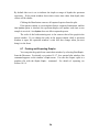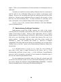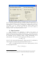
10.2.3
Show Terminal
Opens a terminal window that displays the raw output from a connected
instrument. In the terminal window you can also type commands to the instrument
and view its responses. This is not required for routine operation. Each data
window to which an instrument is connected can have its own terminal window.
See section 4.3 for details.
10.2.4
Disconnect
Severs communication with a connected instrument, and closes the
computer’s COM port. Before disconnecting, offers the opportunity to put the
instrument to sleep.
10.2.5
Reset
You should only need to use Reset in the unusual case of an instrument that
will not wake up or communicate normally. After asking you to confirm the
command, it sends a signal intended to reboot the controller in a connected
instrument. Specifically, it asserts a continuous logical high on the RS232
transmit line for a period you specify. The default period is 90 seconds, which is
sufficient to reset most HOBI Labs instruments. Note, however, that the COM
ports of some computers, especially laptops, do not produce enough voltage to
activate this function on some a-Beta and c-Beta instruments. If the reset
command fails, you may need to apply a voltage directly to the instrument’s
connector.
After a reset, you may need to use the Connect command to re-establish
communications at the instrument’s default baud rate, and you may also need to
allow the instrument some time to initialize itself before it will respond to
connection attempts. The longest time, about two minutes, is required by a c-Beta
or a-Beta with full memory. In most cases the required time will be much shorter.
10.2.6
Start/Stop
The name of this command changes depending on whether the connected
instrument is currently sending data. Start instructs the instrument to begin
sending data in accordance with its own sampling schedule (see 5.3), and Stop
instructs it to cease. If no instrument is connected when you select Start,
HydroSoft will open the Connect dialog box (section 5.1.1).
10.2.7
Sleep/Wake
The name of this command changes depending on the current state of the
instrument. Sleep puts the connected instrument into its low-power sleep state,
43