Download Active Logic and Tetris - Institutionen för datavetenskap

Active Logic and Tetris
Victor Nilsson
Examensarbete för 15 hp
Institutionen för datavetenskap, Naturvetenskapliga fakulteten, Lunds universitet
Thesis for a diploma in computer science, 15 ECTS credits
Department of Computer Science, Faculty of Science, Lund University
Active Logic and Tetris
Abstract
Active logic is a formalism intended to model ongoing reasoning in the real world,
and avoids some idealised assumptions of classical logic. Previous work has focused
on active logic, where the idea has been to use logical reasoning in a real-time system
context.
This work is a practical attempt to build an agent that uses active logic. An
agent that can play Tetris in real-time is presented.
In this work, we have developed a new implementation of of active logic. Clear
performance improvements are presented, compared with a previous implementation.
Aktiv logik och Tetris
Sammanfattning
Aktiv logik är en formalism avsedd att modellera realistiska pågående resonemang, och undviker en del idealiserade antaganden i klassisk logik. Tidigare arbete
har fokuserat på aktiv logik, där tanken varit att använda logiska resonemang i
realtidssystem.
Det här arbetet är ett praktiskt försök att bygga en agent som använder aktiv
logik. En agent som kan spela Tetris i realtid presenteras.
I det här arbetet har en ny implementation av aktiv logik utvecklats. Tydliga
förbättringar i prestanda presenteras, i jämförelse med en tidigare implementation.
Contents
1 Introduction
1.1 Background . . . . . . . . . . . . . . . . . . . . . . . . . . . . . . . . . .
1.2 Problem . . . . . . . . . . . . . . . . . . . . . . . . . . . . . . . . . . . .
1.3 Structure of the report . . . . . . . . . . . . . . . . . . . . . . . . . . . .
5
5
6
6
2 Logical reasoning
2.1 AI and logic . . . . . . . . . . . . . . . . . . . . . . . . . . . . . . . . . .
2.2 Active logic . . . . . . . . . . . . . . . . . . . . . . . . . . . . . . . . . .
2.3 An LDS-based approach . . . . . . . . . . . . . . . . . . . . . . . . . . .
7
7
7
8
3 Tetris
3.1 The game . . . . . . . . . . . . .
3.2 A Tetris-playing agent . . . . . .
3.3 Representation in first-order logic
3.4 Planning problem . . . . . . . . .
3.5 Goal generation . . . . . . . . . .
3.6 Plan execution with active logic .
3.7 Scenarios . . . . . . . . . . . . .
.
.
.
.
.
.
.
9
9
11
12
13
15
16
19
theorem prover
Background . . . . . . . . . . . . . . . . . . . . . . . . . . . . . . . . . .
Overview . . . . . . . . . . . . . . . . . . . . . . . . . . . . . . . . . . .
Predicate descriptions . . . . . . . . . . . . . . . . . . . . . . . . . . . .
22
22
22
25
5 Results
5.1 Theorem prover examples . . . . . . . . . . . . . . . . . . . . . . . . . .
5.2 Robot-day scenario . . . . . . . . . . . . . . . . . . . . . . . . . . . . . .
5.3 Tetris . . . . . . . . . . . . . . . . . . . . . . . . . . . . . . . . . . . . .
28
28
29
29
6 Conclusions
31
4 The
4.1
4.2
4.3
.
.
.
.
.
.
.
.
.
.
.
.
.
.
.
.
.
.
.
.
.
.
.
.
.
.
.
.
.
.
.
.
.
.
.
.
.
.
.
.
.
.
.
.
.
.
.
.
.
Bibliography
.
.
.
.
.
.
.
.
.
.
.
.
.
.
.
.
.
.
.
.
.
.
.
.
.
.
.
.
.
.
.
.
.
.
.
.
.
.
.
.
.
.
.
.
.
.
.
.
.
.
.
.
.
.
.
.
.
.
.
.
.
.
.
.
.
.
.
.
.
.
.
.
.
.
.
.
.
.
.
.
.
.
.
.
.
.
.
.
.
.
.
.
.
.
.
.
.
.
32
A Example specification: The Brother problem
3
33
Acknowledgements
I want to thank my supervisor Jacek Malec for his encouraging support, valuable remarks
and patience throughout this project.
4
Chapter 1
Introduction
In this report, we present our work towards making active logic usable in practice,
following up on previous work done at the department of Computer Science, Lund University. The task set out is to develop non-trivial scenarios requiring resource-bounded
reasoning, as provided by active logic.
Tetris is a game that gives the player limited time to reason, and as such has been
chosen as our testing ground. We want to create an agent that can play an actual game,
and also to specify scenarios of special interest.
This chapter gives a background to the problem and then describes the problem and
objectives in more specific terms. Section 1.3 outlines the rest of the thesis.
1.1
Background
Logic has been much studied in artificial intelligence (AI) in attempts to model reasoning. Knowledge can be expressed as logical sentences in a formal language (e.g. first-order
logic) and sentences that logically follow can be found by applying inference rules.
Classical logic assumes ideal reasoning, as if any number of inferences could be made
instantly. This is known as the problem of logical omniscience, and has often been
addressed in the literature (typically in the context of epistemic logic). Relating to
human reasoning, Fagin and Halpern [FH88] discuss different sources of the lack of
omniscience and how to model them. However, reasoning is still studied in terms of the
final set of conclusions that results, not as an ongoing process.
Active logic is different in this aspect – the notion that reasoning takes time is
fully taken into account. Every “clock tick” a set of conclusions is produced, which
may include observations of the changing world. Active logic is further described in
section 2.2.
The paper [Mal09] presented the idea of a practical reasoner based on active logic,
and the current state of this project. The theorem prover that has been created to run
the reasoning process suffers from inefficient implementation. It is not able to run the
developed scenario, which may be called “A day in the life of a service robot” [Hei09].
After running for hours, it will run out of memory, way before the scenario ends.
This thesis project uses some of the suggestions for future work in [Hei09] as a
starting point, with an improved implementation in mind. Another domain (of personal
interest) has been chosen, as it was conceived that the Tetris domain could allow for
some straightforward and interesting reasoning problems, requiring timely action.
5
1.2
Problem
The theorem prover built by Julien Delnaye [Del08] needs to be improved in order to be
useful. In particular, its speed and memory usage will be investigated. The improved
or rewritten prover should be able to solve some interesting examples specified in active
logic.
Although problems of inefficiency are clearly apparent even with toy problems, Delnaye [Del08] assumes that it will be hard to make improvements and at the same time
keep the prover flexible.1 While flexibility is not our highest priority, we aim at something that is generally better. However, we do assume that the prover will be used for
some kind of active logic.
The other part of the problem is to use active logic, in order to verify that the prover
works as expected, but also with a more general purpose: to see how it can be used in a
“realistic” scenario, that is, when resources for reasoning are limited and knowledge is
uncertain. We intend to develop scenarios that involve reasoning with an approaching
deadline and contradiction handling.
We also want to try out larger, non-trivial problems. The robot-day scenario [Hei09]
is quite large, but involves little reasoning (in its specific setting which excludes planning). Playing Tetris should be hard enough, and has obvious real-time constraints. It
may prove difficult to do everything with just logic and in our implementation of active
logic, but we will try to understand the limits of their usefulness.
1.3
Structure of the report
Chapter 2 provides a short introduction to the kind of logic that we are interested in.
Chapter 3 describes Tetris, its basic representation and the design of a real-time agent
that can play the game.
Chapter 4 describes our new theorem prover, in part in the form of a user’s manual.
Chapter 5 presents the implementations and our experimental results.
Chapter 6 presents our conclusions and some suggestions for future work.
1
Specifically, we refer to the Three-wise-men problem and the comments on page 56.
6
Chapter 2
Logical reasoning
2.1
AI and logic
Logic has played an important role in AI from its beginning in the 1950s. John McCarthy
proposed the use of logic for knowledge representation in a declarative way. An intelligent system would use knowledge in the form of explicit logical sentences representing
common-sense ideas. This “logical approach” to AI is presented in [Nil91].
Practical reasoning in the real world is always performed with limited resources,
such as time or memory. A robot may need to take into account its own computational
limitations while deliberating in order to meet deadlines. Classical logic is, however, not
easily adapted to real-time systems. In this context, active logic has been suggested as
a useful formalism [Mal09].
There are other problems with classical logic when non-ideal agents are to be described accurately. One is that anything can be inferred from a contradiction, which is
called the swamping problem in [ED88].
A realistic reasoning agent will have incomplete knowledge about the world. It could
make conclusions that are later contradicted by new knowledge, so that they have to be
retracted. Some form of non-monotonic reasoning, such as default reasoning, needs to
be handled.
2.2
Active logic
Active logic was first presented as step-logic [ED88, EDP90]. Its distinguishing feature
is that inference rules are time-sensitive. Reasoning is viewed as an ongoing process,
starting with an empty set of theorems at time 0. “Observations” may arise at discrete
time steps and take the place of axioms.
An inference rule can be used to generate conclusions (theorems) at time step i + 1
and takes as input a history of all previous steps. The previous step (the last step in the
history) consists of the set of theorems at time i and the set of observations at time i+1.
The theorems at time i (the i-theorems) means all possible conclusions from the inference rules applied to the previous history. Theorems are called beliefs of the reasoning
agent.
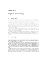
Beliefs may change over time. In other words, a theorem may be retracted in passing
from one step to the next. No formula that is not a conclusion derived with some
inference rule will be in the belief set. That is, it is necessary to explicitly state in
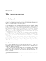
an inference rule which beliefs should not be retracted. Rule 7 in Figure 2.1 has this
7
Rule 1:
i:
i + 1 : Now (i + 1)
Rule 2:
i:
i + 1: α
Rule 3:
i : α, α → β
i + 1: β
Rule 4:
i : P1 a, . . . , Pn a, ∀x [(P1 x ∧ · · · ∧ Pn x) → Qx]
i + 1 : Qa
Extended modus ponens
Rule 5:
i: α
i + 1 : ¬K(i, β)
Negative introspection1
Rule 6:
i : α, ¬α
i + 1 : Contra(i, α, ¬α)
Contradiction is noted
Rule 7:
i: α
i + 1: α
1
2
Agent looks at clock
If α ∈ OBS (i + 1)
Modus ponens
Inheritance2
where β is not an i-theorem, but is a closed subformula of α (and not of the form K(j, γ)).
where neither Contra(i − 1, α, β) nor Contra(i − 1, β, α) is an i-theorem, and where α is not of the
form Now (β). That is, contradictions and time are not inherited.
Figure 2.1: Inference rules corresponding to INF B
purpose; it controls which beliefs are “inherited” to the next step.
Figure 2.1 illustrates an inference function, denoted INF B , which provides mechanisms for default reasoning and contradiction handling. For a detailed description, see
[EDP90].
¬K(i, β) in Rule 5 means that the agent does not know β at time i. A default can
be represented as:
∀i [(Now (i) ∧ ¬K(i − 1, P )) → ¬P ]
That is, if we didn’t know P a moment ago, then we conclude ¬P . Rule 6 will note a
contradiction if both P and ¬P appear as beliefs, which will prevent them from being
inherited. If P can still be inferred after such a contradiction, the default assumption
¬P will not be a belief at that time.
2.3
An LDS-based approach
Mikael Asker [Ask03] found that labelled deductive systems (LDS) seem to provide an
appropriate framework in which active logic can be expressed. In active logic, each
believed formula can be labelled with a time point. LDS allows us to generalise this and
use arbitrary structures as labels.
Asker presents the “memory model LDS” which extends active logic to include certain aspects based on a more realistic view of the agent’s memory. In particular, a
short-term memory of limited size is described. Labels hold additional information
about beliefs, such as their memory location.
8
Chapter 3
Tetris
3.1
The game
Tetris is a very popular game that was originally created by Alexey Pajitnov in 1984
and now exists in many variants, but the basic rules are the same. We will only relate
to game elements that were present in well-known titles from 1989 and earlier.
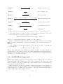
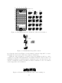
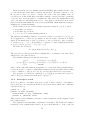
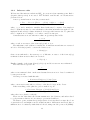
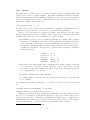
A sequence of tetrominoes – shapes composed of four blocks each – fall down one
at a time into a 10 × 22 grid, called the playfield. Each tetromino is considered to
be generated randomly, uniformly distributed over the seven different tetrominoes (see
Figure 3.1). The player can control the falling tetromino until it is “locked” in the
playfield, which happens shortly after it “hits the bottom.” A tetromino is referred to
as a piece; it can be placed once and is not seen as a unit after it has been placed, that
is, after it has been locked. When a number of pieces have been placed in such a way
that a complete row is filled with blocks, that “line” is cleared – which means that the
blocks that form the line are removed, and all blocks above it are moved down by one
row. The game ends when there is no space for a new piece to appear.
The next piece to appear is shown in a preview area, which is updated every time
a piece enters the playfield. The score, level and number of cleared lines are measures
of success. Typically, clearing several lines with one piece results in a higher score. The
level indicates the speed at which pieces fall and increases as the game progresses.
The tetrominoes are named after the letters they resemble and have up to four
orientations, denoted with index numbers. Figure 3.2 shows how they are positioned
in the playfield, with the reference cell marked with . Each tetromino enters the
playfield at (4, 19) with its first orientation (index 1). A tetromino can move left-,
right- or downwards to an adjacent cell, or rotate by 90 degrees. Rotation just changes
the orientation (and not the column-row coordinates) to the immediately following or
preceding orientation. For example, T can rotate from T1 to T2 or T4 .
A tetromino can only occupy cells inside the playfield, not already occupied by other
blocks. Further, if a tetromino can be in a certain position resulting from a move
(or rotation), then that move is possible. This actually means that some rotations are
possible that would be impossible (continuous) movements, assuming that a piece cannot
· · · ·
I
· · ·
·
J
· · ·
·
L
· ·
· ·
O
· ·
· ·
S
· · ·
·
T
Figure 3.1: The seven tetrominoes (pieces)
9
· ·
· ·
Z
2
4
6
8
10
22
20
18
hidden rows
· · ·
·
T1 at (4, 19)
I1
I2
· · · ·
16
O1
·
·
·
·
J1
J2
J3
J4
L1
L2
· ·
·
·
S2
L3
L4
·
·
· ·
Z2
·
· ·
·
T4
·
· ·
·
14
12
10
· · ·
·
S1
8
6
4
2
a goal position:
T3 at (4, 0)
·
· · ·
T1
· · ·
·
T2
·
· ·
·
·
· · ·
Z1
· ·
· ·
T3
·
· · ·
0
Figure 3.2: The playfield and the orientations of the seven tetrominoes
move right
rotate
Figure 3.3: An unnatural but possible rotation
move through other blocks. Figure 3.3 is an example of such an “impossible” rotation.
It is rather a transformation from and to discrete orientations.
Unlike the other tetrominoes, I, S and Z only rotate halfway around one centre;
rotating a second time will return them to the initial orientation. Strict rotation of S
is illustrated in Figure 3.4, with the unused orientations crossed out. One reason to use
only two orientations for these tetrominoes is that we will have a one-to-one relation
between appearance and orientation.
Figure 3.4: Rotation of S around the centre of its bounding box
10
3.2
A Tetris-playing agent
We intend to develop an intelligent agent that plays an actual game under the same
conditions as a human player. The environment of such an agent is fully observable and
quite predictable at the lower level, where a given tetromino piece is played. The piece
falls at a constant speed, which makes it reasonable to assume that the agent is able to
perform a certain number of actions at each height (unless the game is too fast). Such
an assumption would indeed make the environment essentially deterministic. In other
words, the agent could do all the reasoning and planning in advance and then act, not
watching the piece moving.
Most of the time, the piece only needs to be rotated 0–2 times and moved to the
column of the goal position. This means that planning and acting can be trivial tasks
in a simple implementation of an “AI” player.
However, we have settled on making our agent more intelligent than that, with focus
on plan execution. Our agent should be able to follow an arbitrary path in the playfield
as well as possible. More important, though, is that we want to make use of dynamic
observations in active logic. Next, we give a general description of the agent.
3.2.1
Perception
There are three kinds of percepts:
• the next piece, shown in the preview area;
• the configuration of blocks in the playfield;
• the piece in the playfield, including its position.
At the beginning of a game, the agent can see the next piece and the initial configuration
of blocks. Then, it will observe the next piece entering the playfield, and the updated
next piece. The configuration of blocks is observed every time a piece is locked in the
playfield. If the environment follows the rules of Tetris and the agent knows what its
actions do, it is sufficient to receive a percept of the piece position every time it falls
down one row.
3.2.2
Actions
The actions either move or rotate the piece. The environment lets the agent perform
an action at any time; however, (from the point of view of the agent) the piece may fall
before the action takes place.
We use the symbols Left, Right, Down, Rot + , Rot − and Drop to represent the
actions. Drop moves the piece down to the bottom, until it is locked. The others are
quite obvious already and will be further described in section 3.4.1.
Rotation can be intuitively described as a function:
rotate(xi ) = x(i mod n)+1
where {x1 , x2 , . . . , xn } is any set of tetromino symbols subscripted with the same numbers, corresponding to all the orientations of one tetromino (as given in Figure 3.2).
Then Rot + corresponds to rotate and Rot − corresponds to the inverse, rotate −1 .
11
3.2.3
Components
• The controller is responsible for the communication with the Tetris system, receiving percepts and providing them to the observation function in active logic. It
will also consult the conclusions of the reasoner, for example, in order to choose a
goal for the planner.
• The reasoner is the reasoning process, which runs step-wise and uses active logic
(the theorem prover).
• The planner creates plans to reach goal positions. It needs to know the configuration of blocks in the playfield.
Ideally, most of the work can be done in the reasoner component. In the normal case,
the reasoner generates possible placements, from which a goal is chosen, and a sequence
of actions is planned to reach the goal. Then the reasoner guides the plan execution.
3.3
Representation in first-order logic
We will not describe everything that needs to be represented in logic here, just the basic
elements of Tetris – the playfield and blocks.
The cells inside and around the playfield are objects identified by a column number
and a row number; (x, y) is a term that refers to the cell in column x, row y. We allow
ourselves some syntactic sugar: (x, y) + (m, n) stands for (x + m, y + n), where a + b is
the sum of two integers.
There are 19 fixed tetrominoes (pictured in Figure 3.2) which are defined in terms of
occupied area. If occupies(b, x, y) is true, then x and y are distances from the reference
cell to a block (which occupies one cell). For example:
∀x 0 ≤ x ≤ 2 → occupies(L3 , x, 1)
occupies(L3 , 2, 2)
A configuration of blocks is a set of occupied cells. The constant Blocks is used for
the blocks that are locked in the playfield. The term blocks(b, p) refers to a configuration
of blocks that results from placing b at p. For example, blocks(L3 , (8, 1)) contains:
(10, 3)
(8, 2) (9, 2) (10, 2)
Elements of blocks(b, p) are found using the occupies predicate:
∀b ∀p ∀q q ∈ blocks(b, p) ↔ ∃m ∃n (occupies(b, m, n) ∧ q = p + (m, n))
The predicate possible is true of legal tetromino positions. If all blocks in b at p are
inside the playfield and no cell intersects, then that position is possible:
∀b ∀p ∀x ∀y [(x, y) ∈ blocks(b, p) → (1 ≤ x ≤ 10 ∧ 1 ≤ y ≤ 22)] ∧
¬∃q (q ∈ blocks(b, p) ∧ q ∈ Blocks) → possible(b, p)
The function height returns the height of any playfield column. An empty column
has the height 0. Otherwise, the height is equal to the row number of the highest block
in the column:
∀x ∀h ∀B (x, h) ∈ B ∧ ∀y [(x, y) ∈ B → y ≤ h] → height(x, B) = h
12
where h ranges over {1, . . . , 22} and B is a configuration of blocks. The second argument
can be left out:
height(x) = height(x, Blocks)
It is also convenient to have a function that returns the row number of a cell:
row ((x, y)) = y
3.4
Planning problem
Planning in Tetris involves finding a path from the starting position of a tetromino to a
goal position, where it can be locked. Here we describe the general planning problem,
ignoring some practical issues such as whether a plan is hard to execute.
The classical representation (or STRIPS-style), where preconditions and effects are
expressed for each action, does not seem appropriate to describe our planning problem.
All actions are of the same kind: they change the position, if the resulting position is
possible. Given a (static) configuration of blocks, all possible positions (not necessarily
reachable) can be known. Recall that a position is possible if the tetromino is completely
inside the borders of the playfield and does not overlap other blocks. In other words, we
want to describe the change in position for each action and then verify with a collision
test.
3.4.1
Domain
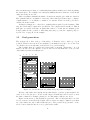
We will formalise the planning domain as a state-transition system. First, let us consider
what are meaningful states. There should be a state for every possible position of a
given tetromino. It cannot move once it has been locked, so an additional “locked”
state is needed for every position in which the tetromino may lock. If we use a predicate
at(b, p) for the position, then a state transition changes either b (rotation) or p (move to
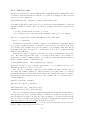
adjacent cell), or the new state locks the position. Figure 3.5 shows the different kinds
of transitions.
· ·
·
·
at(L2 , (6, 2))
s1
10
1
· ·
·
·
s2
at(L2 , (6, 1))
· ·
·
·
at(L3 , (7, 1))
s5
·
· · ·
s6
· · ·
·
s3
at(L2 , (7, 1))
at(L1 , (7, 1))
s4
at(L2 , (6, 1))
locked
s7
at(L2 , (7, 1))
locked
Figure 3.5: An example of state transitions in a Tetris planning domain
13
In the general model for a dynamic system in [GNT04], state transitions can be due
to both actions and events, where events are uncontrolled – they may or may not occur.
In our case, we have one event to consider: the event of the piece falling down one
row. However, we know that this event will necessarily occur in every state s such that
locked ∈
/ s, if no action is applied to s within some time. If we also assume that it will
only occur when we deliberately wait for it to occur, then we can model it as an action.
Our problem then fits within the restricted model [GNT04], which makes the restrictive
assumptions of classical planning.
In the restricted model, a state-transition system is a triple Σ = hS, A, γi, where:
• S is a finite set of states
• A is a finite set of actions
• γ : S × A → 2S is a state-transition function
The system is deterministic, that is, for every state s and for every action a, |γ(s, a)| ≤ 1.
If a is applicable to s, then γ(s, a) contains one successor state, otherwise it is empty.
Given Σ, an initial state s0 and a goal state sg , the problem is to find a sequence
of actions ha1 , a2 , . . . , an i, corresponding to a sequence of state transitions such that
s1 ∈ γ(s0 , a1 ), s2 ∈ γ(s1 , a2 ), . . . , sg ∈ γ(sn−1 , an ).
We define the actions as:
A = Left, Right, Down, Rot + , Rot −
The action Down can represent either a manual move or waiting for the same effect;
which is up to the plan execution.
The transition function is defined in a few steps:
 0
if locked ∈
/ s ∧ possible(s0 )
 {s }
{s ∪ {locked }} if locked ∈
/ s ∧ ¬possible(s0 ) ∧ a = Down
γ(s, a) =

∅
otherwise
where s0 is the state that results from applying a to s, say, in an empty playfield with no
borders. It is easy to compute s0 with a function that rotates the tetromino and by adding
to the coordinates, (−1, 0), (1, 0) or (0, −1), for Left, Right and Down, respectively.
The predicate possible(s0 ) is equivalent to possible(b, p) as defined in section 3.3,
where b and p are extracted from the state: at(b, p) ∈ s0 .
3.4.2
State-space search
It is now possible to use simple state-space search to find a solution. A straightforward option is to use forward search and avoid repeated states, which can be efficiently
expressed in Prolog:
plan(S, S, _, []).
plan(S1, G, Path, [A|Plan]) :transition(S1, A, S2), \+member(S2, Path),
plan(S2, G, [S1|Path], Plan).
This works by nondeterministic generation of state transitions, checked against a path
list of visited states.
The depth and exponential time complexity need attention. The depth can be limited
iteratively for an optimal-length solution. A deep search will take too long to fail, but
14
there are many ways to improve on this with plan restrictions that can be used in pruning
the search space. For example, it is extremely unlikely that more than two rotations (in
either direction) are needed.
There is a simple admissible heuristic. Consider moving the piece without obstacles.
The optimal solution cost (number of actions) of the relaxed problem is easy to compute:
column distance + row distance + number of rotations. Rows below the goal can be
excluded from the search.
A simple technique is to only follow optimal paths as guided by the heuristic. This
way, the search will be much more predictable, but completeness is sacrificed. This is
still quite acceptable in Tetris, as plans that cannot be found involve unusual goals.
Longer paths are also possible to find using subgoals (e.g. near the original goal); see
section 3.7.3 on page 21 for an example.
3.5
Goal generation
The agent needs to have some good knowledge of Tetris in order to find a good goal
position. Then it can reason about candidate goals until it is ready to choose the best
one. If there is not enough time, it should choose a goal in a hurry.
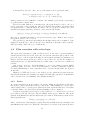
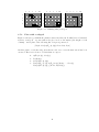
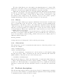
The deadline that we consider here is in terms of external “Tetris time.” A goal
must be chosen before the distance to the blocks below is less than three rows (or some
other number) as shown in Figure 3.6.
2
4
6
8
10
22
20
18
· · ·
·
L1 at (4, 19)
16
(a)
·
· · ·
14
12
10
8
6
deadline:
L1 at (4, 6)
· · ·
·
(b)
(c)
4
2
· · ·
·
Figure 3.6: Goal deliberation deadline and goal position examples
We have only built some basic knowledge that allows to generate positions that don’t
create holes below the piece. A hole is any empty cell that has some block above it in
the same column. For example, placing L1 on a flat surface will give two holes.
Figure 3.6 shows two positions that are generated. The one in (a) should be avoided
for two reasons: it increases the height; and it creates an empty column deeper than
two cells, which can only be filled with an I piece. The position in (b) seems to create
a hole, but it clears the line above it; (c) shows the result.
15
Positions where the piece “fits” on top of the surface can be generated with:
∀m ∀n [(occupies(b, m, n) ∧ ¬occupies(b, m, n − 1))
→ height(x + m) = y + n − 1] → fits(b, (x, y))
Other positions are more difficult to generate. For example, (b) depends on generation
of positions that complete lines.
The idea is that with more reasoning steps, the agent should be able to choose a
better goal based on its conclusions. One problem that arises is that of deciding when
the agent should be confident that it is ready to choose a goal. For example, we could
say that it is happy with any goal that does not increase the height:
fits(b, p) ∧ ∃x ∀q [q ∈ blocks(b, p) → row (q) ≤ height(x)] → GoalReady
It is easy to just limit the number of steps used in active logic. That is, after n steps,
the agent is ready to choose a goal.
The generated positions are just ranked after height, that is, the row number of the
highest block in the piece, where lower is better. Much more thought could be put into
this, but it falls outside the scope of this thesis.
3.6
Plan execution with active logic
The agent uses reasoning for plan execution based on the idea of a state-transition
system presented in section 3.4.1. It needs to keep track of the state (the position of the
piece) in order to follow a path. Following an exact path in real time is sometimes very
likely to fail, but as long as the piece is free to move, there are options. For example, a
plan from (4, 19) to (7, 19) will fail if the piece falls down to row 18 before column 7 is
reached.
Our focus is on how to deal with failures, so we let the planner generate highly
optimistic plans. It is also better in Tetris trying to execute a plan and replan as
necessary than finding a “safe” plan that can be executed slowly while the agent is
mostly idle.
Inspired by [PPT+ 99], we try to use active logic as a platform for plan execution.
Our system is meant as something very simple but still quite general for domains that
can be described by a deterministic state-transition function.
3.6.1
Basics
A goal is represented as Goal (g) where g is a state. When Goal (g) holds, it will cause
the agent to plan (outside the reasoner component). This planning process produces
either a single plan or ¬Goal (g) if no plan is found; the agent then knows to avoid that
goal in the future. A goal is retracted when planning for it is completed.
A plan is represented as Plan(pre, g, steps) and is to be executed as soon as its
precondition pre holds. We have only used simple states as preconditions. The agent
plans from an initial state and uses that as the precondition. If the first step is an action,
this is typically true:
Plan(s0 , g, [a1 |steps]) ∧ s0 → Do(a1 )
where a1 is the head of the list (Prolog-style). The rule actually used is not as simple, but
this illustrates the basic idea. When the action has been executed, the plan is updated
16
to Plan(s1 , g, steps) where s1 is the following state of the corresponding transition and
steps are the remaining steps.
An action here is just a symbol (see section 3.2.2). A step may also be a subgoal
of the form Goal (s) which will initiate another plan (if found). When the subgoal has
been planned for, the plan progress is updated:
Plan(α, g, [Goal (s)|steps]) ∧ Plan(β, s, γ) → Plan(s, g, steps)
The old plan, whose first step is completed, is retracted.
Rather than waiting for a percept (an observation in active logic), the agent infers
the state from its knowledge of the world:
Do(a) ∧ s1 ∧ transition(s1 , a, s2 ) → s2
This amounts to acting with “closed eyes,” assuming determinism. In addition, the
agent does use percepts, that may contradict its conclusions. Neither is really fully
reliable in the architecture due to latency.
3.6.2
Inconsistent beliefs
One aspect of active logic is that it can model a fallible reasoning agent, which is expected
to hold inconsistent beliefs at times. Even when a contradiction is noted and resolved,
inconsistent beliefs can make things difficult while they exist. Consider this example,
where the first action in the plan is executed:
t : Plan(s0 , g, [a1 |steps]), s0 , transition(s0 , a1 , s1 )
..
.
t + 2 : Plan(s1 , g, steps), s1 , Plan(s0 , g, [a1 |steps]), s0 , . . .
The action a1 will then get executed again if one is careless.
Unfortunately, there is no obvious way to deal with this kind of problem in active
logic and also keep the rules and axioms as simple as we would like. We can recognise
two approaches (that may work together):
• Inconsistency is prevented with careful retraction.
• Rules and axioms need to be written carefully so that they don’t conclude anything
harmful from inconsistent beliefs.
The first approach can work by a complicated rule of inheritance. The second approach
is more safe, but appears as difficult. We need to take into account that complicated
formulae will not work in our implementation.
It seems natural to view some rules as relevant only in a certain state of consistency.
We have come up with a solution that uses a special inference rule to mark a belief set
as consistent when there are no contradictory positions in it. This allows us to express
that a single state holds with:
at(b, p) ∧ Consistent
17
3.6.3
Inference rules
We have used the inference rules from INF B (see section 2.2) as a starting point. Rule 5
(negative introspection) is not used. The modified versions and our extensions are
presented below.
A more powerful version of modus ponens is used:
t : P1 a, . . . , Pm a, ∀x [(P1 x ∧ · · · ∧ Pm x) → (Q1 x ∧ · · · ∧ Qn x)]
t + 1 : Qj a
where j ≤ n and x stands for variables shared with any P conjunct. Put simply, if
the P conjunction is true by some substitution, then that substitution is applied to the
implication and each Q conjunct is inferred. A few special forms are also recognised in
the P conjunction, for example: a < b where a and b are integers.
Contradictions are noted when more than one (position) state holds:
t : s1 , s2
t + 1 : Contra(t, s1 , s2 )
where s1 and s2 are states of the form at(b, p) and s1 6= s2 .
The inheritance rule adds more restrictions. Contradictions and time are retracted
as before. If delete(α) and α occur in the belief set, as:
t : delete(α), α
then α is not inherited to the next step t + 1. Likewise, no state s of the form at(b, p)
is inherited when an action has been executed:
t : Do(act), s
Finally, formulae of the forms delete(α), Do(act) and Consistent are never inherited.
The next rule is a special one:
t:
t : Consistent
where no inconsistent beliefs – in the sense discussed in section 3.6.2 – have been inferred
by any previous rule.
Actions get executed with this rule:
t : Consistent, Plan(pre, g, [a|steps]), pre
t : Do(a)
where a is an action, and either a 6= Down or the head of steps is also Down.
If the next thing on the plan is a goal, we make it a goal:
t : Consistent, Plan(pre, g, [Goal (s)|steps]), pre
t : Goal (s)
where there is no plan for s already.
There are also rules that add relevant transitions to the belief set, and rules related
to goal generation, that are not necessary to present in detail here.
We want to point out that the special predicate Consistent has been introduced out
of practical need, and might seem a doubtful extension. McDermott and Doyle have a
similar notion of consistency with what is believed, using a modal operator, in [MD80].
18
3.6.4
Axioms
Now we have inference rules that allow us to write robust plan execution axioms quite
easily. Here follow some examples.
The plan is updated when its first step (an action) is completed:
Plan(s0 , g, [a|steps]) ∧ transition(s0 , a, s1 ) ∧ DONE
→ Plan(s1 , g, steps) ∧ delete(Plan(s0 , g, [a|steps]))
where DONE stands for either s0 ∧ Do(a) or s1 ∧ Consistent. That is, two axioms are
generated. Note that Do(a) implies that the belief set is consistent.
When the goal has been reached, we delete the plan:
Plan(pre, g, steps) ∧ g ∧ Consistent → delete(Plan(pre, g, steps))
State contradictions are resolved with simple axioms. The most trivial one arises
when the piece falls down one row:
Now (t) ∧ Contra(t − 1, s1 , s2 ) ∧ transition(s1 , Down, s2 ) → s2
A plan is considered to have failed when its precondition is impossible, which is easy
to detect in Tetris:
Plan(at(b, (x, y)), g, steps) ∧ at(b1 , (x1 , y1 )) ∧ Consistent ∧
y1 < y → Failed (at(b, (x, y)), g)
Another plan failure is when planning for a subgoal has failed:
Plan(pre, g, [Goal (s)|steps]) ∧ ¬Goal (s) → Failed (pre, g) ∧ ¬Goal (g)
The easiest way to deal with a failed plan is to delete it (and other plans) and replan,
possibly for the same goal. It may be better to try and use an existing plan, with little
or no change in the list of steps, from a new initial state.
3.7
Scenarios
Here are three simple Tetris scenarios that show how the agent handles some details
using active logic. First are two examples of state contradictions, and then a plan
involving a subgoal is executed.
at(Z1 , (5, 19))
s1
s2
at(Z1 , (6, 19))
at(Z1 , (5, 18))
s3
s4
at(Z1 , (6, 18))
Figure 3.7: The piece falls down while it is moved
19
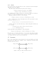
3.7.1
State contradiction 1
In this setting the piece is about to fall just when an action is executed. There are
no obstacles, so the action will succeed in practice. Figure 3.7 shows the states and
transitions involved. The bold arrows indicate the transitions that actually take place
in the environment. The most relevant beliefs at each step are shown below:
0 : Do(Right), at(Z1 , (5, 19)), transition(at(Z1 , (5, 19)), Right, at(Z1 , (6, 19)))
1 : at(Z1 , (6, 19))
2 : at(Z1 , (6, 19)), at(Z1 , (5, 18))
3 : Contra(2, s2 , s3 ), s2 , s3 , transition(s1 , Right, s2 ), transition(s1 , Down, s3 ),
transition(s3 , Right, s4 )
4 : s4
The piece falls down one row before Right gets executed in the game, which normally
means that the action takes place in the observed state s3 ∈ OBS (2). The contradiction
is resolved with this axiom:
Now (t) ∧ Contra(t − 1, s2 , s3 ) ∧ transition(s1 , a, s2 ) ∧
transition(s1 , Down, s3 ) ∧ transition(s3 , a, s4 ) → s4
Note that s2 and s3 are not inherited from step 3 as they have been noted in a contradiction. Modus ponens concludes s4 from Now (3), the contradiction and transitions
shown at step 3 and the axiom above.
3.7.2
State contradiction 2
The agent tries to rotate clockwise, from T1 to T2 , but the game rotates the piece in the
opposite direction (see Figure 3.8). The reason might be that the game is stochastic, or
that it only rotates in one direction. A contradiction is noted between at(T2 , (4, 9)) and
at(T4 , (4, 8)) a few steps later, when the correct state has been observed. This kind of
contradiction can be resolved with:
Now (t) ∧ Contra(t − 1, at(b1 , (x, y)), at(b2 , (x, y − 1))) → at(b2 , (x, y − 1))
The real problem is then to replan without repeating the same mistake, which becomes even more difficult if we consider that the piece could have been rotated more
than once before any observation is received. A basic idea is to do rotate repeatedly,
until the right orientation is observed; however, we will not attempt to go further and
tackle any technical issues.
at(T4 , (4, 9))
s3
s1
s2
at(T1 , (4, 9))
at(T4 , (4, 8))
s4
Figure 3.8: Rotation in wrong direction
20
at(T2 , (4, 9))
2
4
6
8
2
10
· ·
· ·
4
6
8
2
10
8
8
6
6
6
4
4
8
2
· ·
· ·
· ·
· ·
2
4
6
8
10
4
2
Figure 3.9: Planning using a subgoal
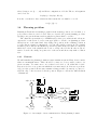
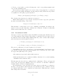
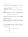
3.7.3
Plan with a subgoal
Figure 3.9 shows a goal which the planner cannot find directly. It falls back on backward
search to a subgoal – a positon where the piece is above the surface (the height of each
column) – and a plan of the following list of steps is generated:
[Right, Goal (at(Z1 , (8, 2))), Down, Left, Left]
Another plan to reach the subgoal is then needed, as soon as the first action has been
executed. Here is a selection of beliefs that we expect:
0 : at(Z1 , (4, 7)), Goal (g)
1 : Do(Right)
2 : Goal (at(Z1 , (8, 2)))
3 : Plan(at(Z1 , (5, 7)), at(Z1 , (8, 2)), [Right, . . . , Down]),
Plan(at(Z1 , (8, 2)), g, [Down, Left, Left])
21
Chapter 4
The theorem prover
4.1
Background
Julien Delnaye implemented a theorem prover in Prolog [Del08], which, in particular, was
meant to be used with active logic as formalised in [Ask03]. It also allowed customisation
for other logical systems based on LDS (see section 2.3). Our work has aimed at a more
efficient prover with basically the same functionality.1
First, we looked for sources of inefficiency. The program operates repeatedly on input
in the form of lists of beliefs, observations and inference rules, producing as output a
new list of beliefs, which is then used as input in the next iteration. The most apparent
problem in the case of the robot-day scenario is that the same list of observations (more
than a thousand items) is processed in every iteration. It is obvious that an observation
only needs to be looked at once, at the time it is new (and not before it has been made).
This could be solved without much effort though, at the same time allowing input of
observations in-between the reasoning steps.
Actually, we never got any deeper into the code, which was very hard to understand.
However, the heavy use of recursion on lists is suspected. In many places intermediate
lists are created and concatenated in an inefficient way. Just fixing these would further
obfuscate the code.
Instead, the program was entirely rewritten, after it was realised that most of the
theorem proving could be done by Prolog. Our approach is actually quite similar to
Elgot-Drapkin’s in the Prolog code to solve (for example) the Brother problem [ED88],
which we did not look at initially.
4.2
Overview
Here we describe how the new prover is used and the basics of how it works. Some
acquaintance with Prolog is recommended. Predicates are referred to as name/n, where
n is the arity (number of arguments).
The prover is typically loaded inside another Prolog program, which defines a number
of facts that provide the specification to the prover. It basically needs to know three
things: the structure used to hold a belief, the inference rules, and, at each time step,
the new observations.
1
LDS support is less general in that labels are required to hold a time point which is used as in active
logic.
22
4.2.1
Beliefs
The structure of a belief needs to be specified. It may be just a formula labelled with
a time point, or a more complex structure. The main requirement is that the structure
should contain a time point (step number), which the prover can access by the predicate
time_step/2. This predicate is also consulted whenever the belief structure needs to be
known. For example, if it is defined as:
time_step(belief(I, _), I).
we will be able to use beliefs of the form belief(I, Formula). (Variables in Prolog
begin with an uppercase letter or underscore; _ is an anonymous variable.)
The prover accepts any Prolog term as a formula. Any subterm of a belief other
than the time step is treated as a formula – that is, there is no separation between the
labelling algebra and the logic. A formula is one of the following:
• An arithmetic operation, whose operands (arguments) are formulae. The operation
is meant to be performed and replaced by its result when all variables in it have
been bound. An operation can be performed when all its operands are expressions.
An expression (in this specialised sense) is either an integer or an operation whose
operands are expressions. The supported operations all correspond to arithmetic
functions in Prolog:
addition
subtraction
negation
maximum
minimum
X + Y
X - Y
-X
max(X, Y)
min(X, Y)
• Any other compound formula, whose arguments are formulae. It may correspond
to a connective or a predicate in first-order logic. Any compound Prolog term
represents a compound formula. Note that operators are just syntactic sugar:
A -> B is identical to ’->’(A, B).
• A variable, implicitly universally quantified.
• A constant symbol, represented by any atomic Prolog term (not compound and
not a variable).
For example, the formula ∀x [(bird (x) ∧ ¬ostrich(x)) → flies(x)] could be represented
as:
(bird(X) and not(ostrich(X))) -> flies(X)
assuming ‘and’ has been defined as an operator.2
Beliefs are asserted in the Prolog database, meaning that they can be queried directly.
In order to avoid duplicate beliefs in the database, we need an operation “assert if not
already in the database.” This has been implemented with the use of a hash table in
which all asserted beliefs are stored. The predicate new_fact/1 is used to add beliefs in
this way, and may also be used by the user to add initial beliefs or axioms.
2
For example with :- op(950, xfy, and).
23
4.2.2
Inference rules
An inference rule has the form rule(Premises, Conclusion) where Premises is a list
of premises. Conclusion has the structure of a belief. For example, modus ponens in
active logic can be defined as:
rule([belief(I, A), belief(I, A->B)], belief(I+1, B)).
A premise is almost the same as a Prolog goal but may contain arithmetic operations
just like formulae in beliefs. There are also two premise goals that are given special
status:
• a belief goal that has the structure of a belief;
• an observation goal of the form obs(I, Formula), analogous to α ∈ OBS (i).
They are recognised inside negation (as failure) as well, either with:
\+ Goal or not(Goal).
Variables in goals should generally be understood as implicitly existentially quantified over the body they appear in – we may say over the rule here. A solution is the same
as a binding of the variables in a goal. One thing to keep in mind is that all solutions
in premise goals will be generated, so code that leaves a lot of choice points around will
make the rule inefficient.
The inference rules are applied to the history to bring conclusions at a given time
step. They may start from any belief or observation in the history. For example, if
apply_rule/2 is called as apply_rule(5, _), it will pick a rule and make the time step
in the conclusion equal to 5, as in this query:
?- rule(Prems,Concl), time_step(Concl,I), eq(5,I).
It may be necessary to solve a trivial equation like 5 = x + 1, which is done by eq/2.
Then the premises are ready to be proven.
The old prover works the other way around, binding the time variable only by
processing the premises. This is not only less flexible, but requires rules to be written
in an inefficient way (both in terms of performance and typing). In contrast, no premise
that binds the time variable is needed here. For example, the “clock axiom” may be
defined simply as:
rule([], belief(I, now(I))).
Also, these two rules are equivalent:
rule([belief(I, A)], belief(I+1, A)).
rule([belief(I-1, A)], belief(I, A)).
The order in which the rules are applied has significance if any rule uses premises of
the same time step as its conclusion. All the conclusions of one rule are produced before
any following rule is applied, as expected. The conclusions of one rule are visible in the
history – that is, premises can use them – when the following rules are applied, but the
same rule cannot see its own conclusions until one step later.3
3
This behaviour is due to the logical update view in Prolog; when backtracking over the beliefs in the
database, changes to the belief predicate are not seen.
24
We can see that this is a sort of incomplete reasoning that may not be desired. The
application of the rules could be repeated until no new beliefs are produced; however,
we prefer to keep the prover simple and efficient for step-wise reasoning.
This is also a point where the old prover is quite different. Rules that don’t increment
the time are only applied to the same immutable list of beliefs, “the intermediate belief
set,” producing a second list of beliefs. The two lists are then concatenated to form
the belief set of the completed step. In comparison, our prover can be said to update a
dynamic intermediate belief set every time it advances to the next rule.
4.2.3
History
Active logic defines a history as a sequence with all the belief sets and observation sets
up to a certain time point. We give the concept of history a specific meaning in the
implementation: “the history” refers to the beliefs and observations in the databases
of the prover (the Prolog databases and the hash table). The idea is that only (and
all) those previous steps that are actually used to produce the next belief set should
be kept in memory. That is, the output should be same as if the prover used a history
containing all the previous steps.
The history size is the number of (consecutive) steps to remember after all inference
rules have been applied. When the history grows beyond this size, the oldest step is
freed. For the inference function INF B described in section 2.2, a history size 1 is
sufficient, which is defined as:
history_size(1).
A larger size is needed if any rule looks beyond the previous step.
4.2.4
Observations
The easiest way to provide observations in a static way is to define the predicate obs/2
directly. For example:
obs(0, bird(tweety)).
obs(4, ostrich(tweety)).
If obs/2 is undefined, observations are looked for in the recorded database, using
the time step as key. These observations are also removed when they fall outside the
(limited) history. Observations can be added directly, as in:
:- recordz(0, bird(tweety)).
But the intended usage is to define a special predicate, observations/2, that behaves according to its description in section 4.3.2. At the beginning of each step, observations/2
is called once. The returned list of observations is expected to contain all observations
that have been made since the last call. Each belief is recorded under the current time
step.
4.3
Predicate descriptions
Here the most important predicates for the user are described. Arguments are sometimes
preceded by a mode indicator: (+) means that the argument is used as input (it must
be instantiated) and (-) that it is used as output.
25
4.3.1
Basic predicates
step(I ) runs the next reasoning step, producing beliefs at time I by backtracking over
apply_rule/2. If instantiated, I should be a natural number equal to the previous
step plus one, or, if this is the first step, either 0 or 1. The new belief set is printed
to the current output stream.
Here is an example that will run until step 5 is completed:
?- repeat, step(I), I=5.
reset frees all the history and goes back to step 0.
apply_rule(+I, -Belief ) infers one new belief at time step I and returns it in Belief.
It picks a rule with rule/2 and proves its premises, nondeterministically. Then it
asserts the conclusion with new_fact/1.
query(+Goal ) proves Goal, with special handling of beliefs and observations. It is used
in proving premises, and is an appropriate place to add more functionality.
Proving a belief goal may involve arithmetic evaluation and inverse operations.
For example:
?- query(belief(0, plus(1,X,3))), belief(0, plus(Y,Z,Y+Z)).
X = 2.
all(+Cond, +Prem) generates a list of premises and proves them in the same way as
apply_rule/2. For each solution of Cond, a copy of Prem is added with the bindings
from the solution.
This predicate is specifically used in the extended modus ponens rule and is also
generally useful. Let us take the example of proving a conjunction:
Ps = bird(X) and not(ostrich(X)),
all(conjunct(P,Ps), P).
The generated list of premises is then:
[bird(X), not(ostrich(X))]
conjunct(P, Ps) is true if P is a conjunct in Ps. It can choose an element nondeterministically from a conjunction built with and/2 lists. If Ps cannot be unified with
and(_,_) then it is considered to be a conjunction with a single conjunct.
?- conjunct(p, p).
true.
?- conjunct(X, and(p, and(q, r))).
X = p ;
X = q ;
X = r ;
false.
26
csf (A, +B ) generates closed subformulae: A is a closed subformula of B. Any subterm
(including B ) that is not one of the following is considered a closed subformula:
• a variable;
• a number;
• a term that shares variables with other subterms of B (that are not subterms
of itself).
4.3.2
User-defined predicates
These predicates need to be written by the user and should be in accordance with their
descriptions.
time_step(Belief, I ) is true if Belief has the structure of a belief or is an unbound
variable, and I can be unified with the subterm that holds the time step. Belief
should be unified with a term that has the structure of a belief (a skeleton).
It must be possible to assert a belief dynamically (with assertz/1). It is recommended that the user declares the belief predicate as dynamic, for example, with
this line:
:- dynamic belief/2.
rule(-Prems, -Concl ) returns an inference rule: a list of premise goals in Prems and
the conclusion (a belief structure) in Concl.
obs(+I, -Formula) returns an observation at time I in Formula.
If observations are static, it is easy to define this predicate with a set of facts.
Define either obs/2 or observations/2, not both.
observations(+I, -Obs) returns a list of new observations (formulae) in Obs. If there
are no new observations, Obs=[].
observations/2 should be seen as a procedure that reads observations from the
outside world everytime it is called. The observations are considered to have been
made at time I, but this argument may be ignored.
4.3.3
Database
These predicates use the clause database as a set without duplicate facts (clauses will
also work). Terms are hashed with term_hash/2 and stored in a “bucket array” that is
written in C and uses SWI-Prolog’s foreign language interface.
new_fact(+Fact) asserts Fact in the database (with assertz/1) and adds it to the hash
table. True if Fact is new and fails if it’s already in the hash table.
element(+Fact) is true if Fact is an element of the database set, that is, identical to a
term in the hash table (except for renaming of variables).
delete_facts(+Fact) deletes all facts that unifies with Fact.
27
Chapter 5
Results
5.1
Theorem prover examples
Julien Delnaye demonstrated his program on three simple problems, the wise men problems from [ED88] and the Tweety problem from [Ask03]. We have verified that the new
theorem prover is able to take the same problems, specified much the same way, and
solve them correctly.
5.1.1
Implementation
The Two-wise-men problem (2WM) was straightforward to translate and check against
the original definition after we had implemented an extended modus ponens rule (see
Appendix A and the descriptions of all/2 and conjunct/2 in section 4.3.1).
The Three-wise-men problem (3WM) did not require any further extensions; however, there was some confusion from a couple of rules that were left out – apparently,
this just leads to a slightly different solution. No significant differences between the
implementations could be seen in the output, with respect to how rules behaved.1
The Tweety problem uses some complicated rules that were implemented using auxiliary Prolog code. The output is now quite identical to Asker’s proof, whereas a few
issues were discovered in Delnaye’s implementation. In particular, some forumulae are
not properly instantiated. For example, at step 2, where ¬K(2, ¬flies(Tweety)) is expected (the agent does not know that Tweety cannot fly), ∀x ¬K(2, ¬flies(x)) is produced
instead (the agent does not know that any object cannot fly), which is not the same
thing, although it will do no harm here.
5.1.2
Performance
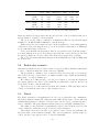
Table 5.1 shows system statistics as reported by Prolog immediately after the last step
has finished. This simple method is sufficient to show a clear difference in performance,
even if the various memory areas are unfamiliar, since the crude measures differ so much.
The tests were run using the 32-bit version of SWI-Prolog in Linux.
Next is a description of the columns, followed by some remarks and additional information.
The number of steps shown is the number of belief sets produced. Speed is indicated
by CPU time in seconds and the number of inferences in thousands. Memory require1
There were, however, a few mistyped axioms in Delnaye’s code.
28
Steps
Time
kInferences
Heap
Local
GC
Old
2WM
3WM
Tweety
10
14
10
1.44
77.40
3.93
2 131
91 188
11 808
558
566
568
768
7 008
624
4
22
5
New
2WM
3WM
Tweety
10
17
10
0.12
0.98
0.49
172
2 216
1 461
560
621
561
16
0
Table 5.1: Test runs with the old and the new implementation
ments are indicated by heap usage and the allocated size of the local stack in kilobytes,
and the number of garbage collections (GC).
The old prover is not run to completion on 3WM, as it runs out of global stack which
is limited to 32 MB. 48 MB is sufficient to run all 17 steps.
Times vary a bit between runs but can be checked against the corresponding numbers
of inferences. It is clear that the new prover is about twelve times faster on 2WM and
about eight times faster on Tweety.
Prolog uses 417 KB of heap memory when no program is loaded. It is important to
note that, with the new prover, heap usage reflects the size of the belief set produced in
the last step, while the old prover uses other memory areas (the Prolog stacks).
The local, global and trail stacks all stay at their initial allocated size (16 KB) with
the new prover.
5.2
Robot-day scenario
Our first experiments focused on the scenario developed by Thorben Heins, which failed
to run to completion using the old theorem prover [Hei09].
The specification consists of a set of inference rules and a long list of observations.
One active logic step corresponds to one minute in this scenario, which means that the
full scenario, one day, is 1440 steps.
We found a more efficient way to give the prover input of observations, which was
the only modification needed for a successful run, avoiding stack overflows. It now took
about twelve hours to run all 1440 steps.
The new prover does the same in less than three minutes. This vast improvement
could be seen with an early version of the rewritten prover.
5.3
Tetris
The Tetris agent has been implemented as a Prolog program that can communicate
through its standard input and output streams with a Tetris game. We modified an
existing implementation of Tetris to send percepts to the Prolog process and respond to
action commands. The game runs in real time just as it would with a human player.
The planner component has been implemented based on the ideas in section 3.4. In
order to make the search fast enough, we tried several techniques.
The scenarios in section 3.7 have been verified to run correctly. In particular, the
subgoal scenario is successful in real-time. The expected plans are generated and executed, but the goal position needs to be asserted manually.
29
There is nothing very impressive about the Tetris-playing abilities of our system,
and we have not much discussed methods to measure its success. That is also not the
point of this thesis. The Tetris AI is incomplete in many ways.
Reliable real-time plan execution using active logic was hard to achieve with our
approach. At higher speeds the agent is unable to determine the position of the piece and
will not act at all. This is because it receives contradictory observations too frequently
– some number of active logic steps is needed to handle each such event.
The planner is called between execution of active logic steps, in the same thread,
usually several times before the goal position is reached. Plan generation is actually
quite fast, but too much replanning (every time the piece falls down one row), which
also involves reasoning, is a trouble that may slow down plan execution awkwardly. To
accommodate this, we generate one plan in advance, from the position one row below,
which gives a significant improvement.
Another issue is that reasoning gets slower as the belief set grows in each step.
Our workaround is to reset the theorem prover every time a new piece is played, but
sometimes the agent will still get very slow.
30
Chapter 6
Conclusions
We have shown that the theorem prover could be made much more efficient, in terms of
speed and memory usage, while keeping its flexibility, which was questioned in [Del08].
Also, although it was rewritten from scratch, this did not require as much work as we
first thought. We found that much of the functionality that [Del08] implemented was
already in Prolog and could be used for better performance.
The Tetris agent uses active logic at a low level (e.g. for keeping track of the position
of the piece) which might not be its best use. It has been troublesome to develop a
system that wouldn’t be too disappointing from a Tetris point of view, and also would
use active logic in a clear way.
Reasoning with an approaching deadline (see section 3.5) has been implemented but
not clearly demonstrated in this report. Simple scenarios that involve contradiction
handling have been presented, but they are not very good examples of its usefulness.
The speed of our new active logic implementations is quite promising; however, the
problem that the set of beliefs can grow very large is still apparent in the robot-day
scenario and sometimes in our Tetris agent (despite some efforts to retract unneeded
formulae). A short-term memory of limited size, as in the LDS-based formalisation in
[Ask03], can still be very useful.
Here are the immediate improvements we envision:
• The theorem prover could be modified to more generally support LDS-like systems.
This might only require changes that avoid the special treatment of time points.
• The prover needs additions that involve new syntax for some logical symbols, for
example, in order to support quantified subformulae.
• The Tetris agent’s reasoning about goal positions is very basic. It would be interesting to see something that clearly leads to better decisions as more time is spent
on reasoning.
Prolog programs and other code is available at:
http://fileadmin.cs.lth.se/ai/xj/VictorNilsson/alcode.tar.gz
31
Bibliography
[Ask03]
M. Asker. Logical Reasoning with Temporal Constraints. Master’s Thesis,
Department of Computer Science, Lund University, 2003.
[Del08]
J. Delnaye. Automatic Theorem Proving in Active Logics. Master’s thesis,
Department of Computer Science, Faculty of Engineering, Lund University,
2008.
[ED88]
J. Elgot-Drapkin. Step-logic: Reasoning Situated in Time. PhD thesis, Department of Computer Science, University of Maryland, 1988.
[EDP90]
J. Elgot-Drapkin, D. Perlis. Reasoning Situated in Time I: Basic Concepts. Journal of Experimental and Theoretical Artificial Intelligence, 2:75–
98, 1990.
[FH88]
R. Fagin and J.Y. Halpern. Belief, Awareness, and Limited Reasoning. Artificial Intelligence, 34:39–76, 1988.
[GNT04]
M. Ghalab, D. Nau, and P. Traverso. Automated Planning: Theory and
Practice. Morgan Kaufmann, 2004.
[Hei09]
T.O. Heins. A Case-Study of Active Logic. Master’s thesis, Department of
Computer Science, Lund University, 2009.
[Mal09]
J. Malec. Active logic and practice. In proceedings of SAIS 2009, The Swedish
AI Society Workshop, pages 49–53. Linköping University Electronic Press,
2009.
[MD80]
D. McDermott and J. Doyle. Non-Monotonic Logic I. Artificial Intelligence,
13:41–72, 1980.
[Nil91]
N.J. Nilsson. Logic and artificial intelligence. Artificial Intelligence, 47:31–
56, 1991.
[PPT+ 99] K. Purang, D. Purushothaman, D. Traum, C. Andersen, and D. Perlis. Practical Reasoning and Plan Execution with Active Logic. In Proceedings of the
IJCAI’99 Workshop on Practical Reasoning and Rationality, 1999.
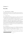
32
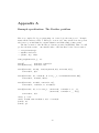
Appendix A
Example specification: The Brother problem
Here is a complete Prolog program using our “active logic theorem prover.” It implements all the inference rules of INF B (see section 2.2). Our extended modus ponens
rule is more powerful than the original definition and makes Rule 3 unnecessary.
The three scenarios of the Brother problem are presented in [EDP90]. This code will
produce the first scenario – uncomment either of the last lines for the other scenarios.
:- load_files(altp).
:- dynamic belief/2.
:- op(950, xfy, and).
time_step(belief(I,_), I).
rule([],
belief(I, now(I))).
rule([obs(I,A)], belief(I, A)).
rule([belief(I, Ps->Q), all(conjunct(P,Ps), belief(I,P))],
belief(I+1, Q)).
rule([belief(I, A), csf(B,A), B \= k(_,_), \+element(belief(I,B))],
belief(I+1, not(k(I, B)))).
rule([belief(I, not(A)), belief(I, A)],
belief(I+1, contra(I, A, not(A)))).
rule([belief(I, A), A \= now(_), \+belief(I, contra(I-1, A, _)),
\+belief(I, contra(I-1, _, A))],
belief(I+1, A)).
obs(0, p -> b).
obs(0, now(X) and not(k(X-1, b)) -> not(b)).
%obs(0, b).
%obs(0, p).
33