Download Computation of characteristic polynomials of hyperplane

AN ALGORITHM FOR DERIVING CHARACTERISTIC POLYNOMIALS OF
HYPERPLANE ARRANGEMENTS
A thesis presented to the faculty of
San Francisco State University
In partial fulfilment of
The requirements for
The degree
Master of Science
In
Computer Science
by
Eric Etu
San Francisco, California
May, 2007
Copyright by
Eric Etu
2007
CERTIFICATION OF APPROVAL
I certify that I have read AN ALGORITHM FOR DERIVING CHARACTERISTIC POLYNOMIALS OF HYPERPLANE ARRANGEMENTS by
Eric Etu and that in my opinion this work meets the criteria for approving a thesis submitted in partial fulfillment of the requirements
for the degree: Master of Science in Computer Science at San Francisco State University.
Matthias Beck
Assistant Professor of Mathematics
Dragutin Petkovic
Professor of Computer Science
Rahul Singh
Assistant Professor of Computer Science
AN ALGORITHM FOR DERIVING CHARACTERISTIC POLYNOMIALS OF
HYPERPLANE ARRANGEMENTS
Eric Etu
San Francisco State University
2007
A hyperplane arrangement is a finite set of hyperplanes. Much of the combinatorial structure of a hyperplane arrangement is encoded in its characteristic
polynomial, which is defined recursively through the intersection lattice of the
hyperplanes. For example, the number of regions that are cut out in space by the
hyperplane arrangement is a special evaluation of the characteristic polynomial.
This thesis aims to develop an algorithm and software to compute characteristic polynomials of hyperplane arrangements.
While mathematicians have computed the characteristic polynomials of hyperplane arrangements by hand for decades, it is believed that this thesis will be
the first software solution to this problem.
I certify that the Abstract is a correct representation of the content of this thesis.
Chair, Thesis Committee
Date
ACKNOWLEDGMENTS
First and foremost, I would like to thank Prof. Matthias Beck for
spending countless hours guiding me through all phases of this research. Without his support, encouragement, and patience, this thesis
would not have been realized.
I would also like to thank my thesis committee members, Profs. Dragutin
Petkovic and Rahul Singh, for their guidance.
Finally, I would like to thank Ms. Peg Carpenter, my high school calculus teacher, who first inspired me to study Mathematics and Computer Science.
v
TABLE OF CONTENTS
1
The Mathematics of Hyperplane Arrangements
1
1.1
Hyperplane Arrangements
1
1.2
The Zaslavsky Theorem
3
1.2.1
Intersection Properties
4
1.2.2
The Möbius Function
5
1.2.3
The Characteristic Polynomial
7
1.2.4
Counting the Regions
8
1.3
An Example in R3
1.4
Proof of Zaslavsky’s Theorem
13
1.5
Subspaces
18
1.5.1
Theory
18
1.5.2
Implementation
19
1.5.3
An Example
21
1.6
8
Linear Algebra
23
1.6.1
Matrices
26
1.6.2
Matrix Rank
26
1.6.3
Intersection Properties
27
1.6.4
Dimensions
28
1.6.5
Finding Intersections of Flats
29
vi
2
Algorithmic Solution
31
2.1
Algorithms
31
2.1.1
Finding Intersections
32
2.1.2
Computing Möbius Values
39
2.2
3
Architecture
44
2.2.1
Layout of Primary Subsystems
44
2.2.2
How It All Fits Together
51
Software Implementation
53
3.1
Data Structures and Methods
53
3.1.1
Lattice
54
3.1.2
LatticeNode
63
3.1.3
EquationMatrix
64
3.1.4
FileInputReader
72
3.1.5
FileOutputWriter
76
3.1.6
MatrixGenerator
76
3.1.7
TestSuite
79
3.2
3.3
Design Decisions
80
3.2.1
Programming Language
81
3.2.2
Tradeoffs
82
3.2.3
Algorithmic Efficiencies
83
Software Performance
84
vii
4
Theoretical Runtime
84
3.3.2
Practical Runtime
95
User’s Manual
106
4.1
System Requirements
106
4.2
Installation
107
4.3
Testing the Installation
108
4.4
Running the Software
112
4.4.1
Input Files
113
4.4.2
Output Files
114
4.4.3
Example Input & Output
119
4.4.4
Basic Use
125
4.4.5
Optional Parameters
126
4.5
5
3.3.1
User Trial
127
Future Work
129
5.1
Distributing the Application
129
5.2
Publishing Results
130
5.3
Subspaces
131
Bibliography
133
viii
LIST OF FIGURES
1.1
Three hyperplanes (lines) intersecting in R2 .
2
1.2
Semilattice of the hyperplane arrangement depicted in Figure 1.1.
4
1.3
Möbius values for the semilattice in Figure 1.2.
7
1.4
A labeling of the seven regions in the arrangement.
9
1.5
Arrangement of 4 hyperplanes (planes) in R3 , with equations:
x1 −
x2 + 0.3x3 = 0; x1 + x2 + x3 = −2; x1 + 3x2 − x3 = 0; and
9
x1 + 5x2 + 5x3 = 10.
1.6
The complete semilattice for the arrangement.
10
1.7
The semilattice with all Möbius values labeled.
11
1.8
4 hyperplanes intersecting in R3 , with some of the regions labeled.
12
1.9
The arrangement Ay , the arrangement induced on y.
15
1.10 The semilattice for the arrangement Ay .
15
1.11 The semilattice for arrangement A.
23
1.12 The semilattice for arrangement A, with Möbius values indicated.
24
1.13 The arrangement A, with the regions labeled.
24
1.14 Three lines intersecting in a point.
25
1.15 Two lines intersecting in a point.
27
2.1
2.2
The semilattice, with Möbius values, for the arrangement depicted
in Figure 1.5.
40
An EquationMatrix object.
46
ix
2.3
A LatticeNode object.
48
2.4
A Lattice object.
50
3.1
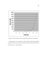
The number of hyperplanes in the braid arrangement, for dimensions 3 through 9.
3.2
98
The number of matrix tests performed to solve the braid arrangements.
99
3.3
Observed runtimes for solving the braid arrangements.
3.4
Observed matrix tests per second for solving the braid arrangements.102
3.5
Observed file sizes of the output files for the braid arrangements.
x
100
104
Chapter 1
The Mathematics of Hyperplane
Arrangements
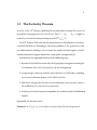
In this chapter, we will review some mathematical foundations of hyperplane
arrangements, discuss the problem of computing the characteristic polynomial
of a hyperplane arrangement, and prompt the software approach to studying
this problem.
1.1
Hyperplane Arrangements
A hyperplane is a d-1 dimensional affine subspace of Rd . More formally:
H = {x Rd : a · x = b} for some a Rd \{0}, b R.
1
2
For instance, in R2 , any hyperplane is a (1-dimensional) line; in R3 , any hyperplane is a (2-dimensional) plane.
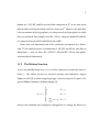
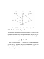
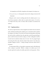
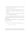
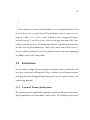
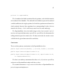
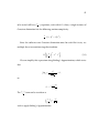
A hyperplane arrangement is a finite set of hyperplanes Rd . Figure 1.1 shows an
example of a hyperplane arrangement in R2 . We’ll call this hyperplane arrangement A.
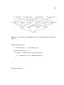
Figure 1.1: Three hyperplanes (lines) intersecting in R2 .
In A, we have three hyperplanes, which we have labeled H1, H2, and H3. We
also have three intersections, namely H1 ∩ H2, H1 ∩ H3, and H2 ∩ H3. All of
these structures — both the intersections and the hyperplanes themselves — are
known as flats. Flats of a given dimension can intersect with each other to create
flats of the next lower dimension; these flats can intersect with each other; and so
on, until we reach dimension 0.
3
1.2
The Zaslavsky Theorem
As early as the 19th century, Jacob Steiner researched how to count the regions of
hyperplane arrangements in R2 and R3 [4]. For H = {H1 , . . . , Hn }, a region is
S
defined as a maximal connected component of Rd \ nk=1 Hk .
In 1975, Thomas Zaslavsky, for his doctoral thesis in Mathematics at the Massachusetts Institute of Technology, solved the problem in the general case (for
any dimension) by finding a way to count the number of total regions, and the
number of bounded regions formed by a hyperplane arrangement [5].
Summarized, his algorithm consists of the following steps:
1. Recursively find all flats created by the hyperplane arrangement, noting the
set inclusions (the intersection properties of the arrangement).
2. Assign integer values to each flat, based on these set inclusions, according
to a recursive function known as the Möbius function.
3. Sum these integers for the flats of each dimension, and use these sums as
the coefficients of a characteristic polynomial χ.
4. Evaluate χ for certain constants to produce the numbers of total and bounded
regions.
Specifically, his theorem states:
Theorem 1.1. [5] |χA (−1)| = the number of regions formed by the arrangement A.
4
Below, we will explore each of these steps in greater detail. Afterwards, I will
present Dr. Zaslavsky’s proof.
1.2.1
Intersection Properties
The intersection properties of A are the ways in which the flats intersect with each
other. For instance, one intersection property of A is that H1 intersects with H2.
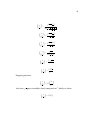
We represent these intersection properties in what is known as a meet-semilattice,
a certain partially ordered set ordered by reverse inclusion. A meet-semilattice
is a structure that represents the intersection properties of an arrangement in a
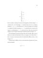
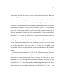
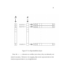
hierarchical way. In Figure 1.2, we see the meet-semilattice L of A.
Figure 1.2: Semilattice of the hyperplane arrangement depicted in Figure 1.1.
Because we order by reverse inclusion, we place R2 , the ambient space, at the
5
bottom of L. H1, H2, and H3 are each affine subspaces of R2 , so we place them
directly above and connect them with lines down to R2 . Likewise, the other flats
(the intersections of the hyperplanes) are subspaces of the hyperplanes in which
they are contained. For example, since H1 ∩ H2 is a subspace of both H1 and H2,
it is connected to each of H1 and H2 (but not to H3).
Notice that each horizontal rank of the semilattice corresponds to a dimension. R2 (the ambient space) is of dimension 2. H1, H2, and H3 are each flats of
dimension 1 — they are lines. H1 ∩ H2, H1 ∩ H3, and H2 ∩ H3 are each points,
and therefore of dimension 0.
1.2.2
The Möbius Function
A poset, or partially-ordered set, is a set whose elements are related by some relation ≤. The Möbius function is a recursive function, first defined by August
Möbius in 1831 [2], used for assigning integer values to elements of a poset. The
general Möbius function is defined through [1]:




0
if r > s,





if r = s,
µ(r, s) := 1



X



−
µ(r, u) if r < s.


r≤u<s
Since in the semilattice of a hyperplane arrangement we arrange the flats by re-
6
verse inclusion, we will define the Möbius function as follows:




0
if r ⊂ s,





if r = s,
µ(r, s) := 1



X



−
µ(r, u) if r ⊃ s.


(1.1)
r⊇u⊃s
We will use these values to calculate the characteristic polynomial of the arrangement.
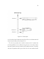
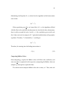
As an example, let us compute the Möbius values µ(R2 , s) for the flats s in A.
We assign a Möbius value of 1 to the ambient space — in our example, the R2 flat.
Then, according to the recursion, we assign each other flat a Möbius value equal
to the negation of the sum of the unique flats underneath it. Continuing with our
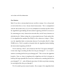
example, we get Figure 1.3.
H1 is assigned a value of (-1), because the summation of the Möbius values
of all the nodes beneath it (just the R2 flat) sum to 1. H2 and H3 will each also
receive Möbius values of (-1), for the same reason. The H1 ∩ H2 flat receives a
Möbius value of 1, because the Möbius values of the flats beneath it (R2 , H1, and
H2) sum to (-1). H1 ∩ H3, and H2 ∩ H3 likewise receive Möbius values of 1.
7
Figure 1.3: Möbius values for the semilattice in Figure 1.2.
1.2.3
The Characteristic Polynomial
The characteristic polynomial of a hyperplane arrangement, χ, is calculated from
the Möbius values of the flats in L, by summing the Möbius values on each rank
of L and using these as the coefficients of the polynomial. Given formally [1]:
χ(λ) :=
X
µ(Rd , s)λdim s .
sL
In our example arrangement, A, the Möbius values of the flats in dimension
2 (just R2 ) sum to 1. The Möbius values of the flats in dimension 1 (H1, H2, and
H3) sum to (-3). The Möbius values of flats in dimension 0 sum to 3. Therefore,
our characteristic polynomial is:
8
χ(t) = t2 − 3t + 3 .
1.2.4
Counting the Regions
According to Theorem 1.1,
|χA (−1)| = the number of regions formed by arrangement A, in Rd .
Zaslavsky also proved that
|χA (+1)| = the number of bounded regions formed by arrangement A, in Rd .
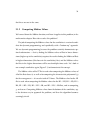
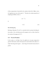
Returning to the our example, we count the regions:
χ(−1) = 7 total regions
χ(+1) = 1 bounded region,
and we verify our work by labeling the regions in Figure 1.4.
1.3
An Example in R3
Let’s walk through a slightly more challenging example, this time in R3 .
9
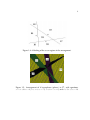
Figure 1.4: A labeling of the seven regions in the arrangement.
Figure 1.5: Arrangement of 4 hyperplanes (planes) in R3 , with equations:
x1 − x2 + 0.3x3 = 0; x1 + x2 + x3 = −2; x1 + 3x2 − x3 = 0; and x1 + 5x2 + 5x3 = 10.
10
In Figure 1.5 we see four hyperplanes, labelled H1 through H4, that form a
tetrahedron. We begin drawing the semilattice by creating a flat for R3 (the ambient space), and placing flats above it for each of the four supplied hyperplanes.
Since no two of these hyperplanes are parallel, all four of the hyperplanes intersect each of the other three, yielding a total of six 2-dimensional (line) intersections. We see that not all of these six lines intersect each other. For instance, H1 ∩
H2 does not intersect H3 ∩ H4. (From this perspective, H1 ∩ H2 passes in front
of H3 ∩ H4.) The six lines intersect to form only four points, specifically the four
vertices of the tetrahedron. Therefore, we finish drawing the semilattice in Figure
1.6.
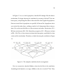
Figure 1.6: The complete semilattice for the arrangement.
Next we recursively calculate Möbius values for the flats in the semilattice.
According to the formula, we assign a Möbius value of (+1) to the R3 flat. Then,
11
H1 receives a Möbius value of (-1), since the sum of the Möbius values of all of
the flats beneath H1 (just R3 ) is (+1), and the Möbius value of H1 must sum with
it to 0. H2, H3, and H4 likewise receive Möbius values of (-1).
H1 ∩ H2 sits above the flats H1, H2, and R3 , which have Möbius values of
(-1), (-1), and (+1) respectively. We assign a Möbius value of (+1) to H1 ∩ H2.
Similarly, each of the other five flats (lines) in dimension 1 also receive Möbius
values of (+1).
H1 ∩ H2 ∩ H3 sits above the flats H1 ∩ H2, H1 ∩ H3, and H2 ∩ H3, H1, H2,
H3, and R3 . Since these Möbius values sum to (+1), we assign a Möbius value of
(-1) to the H1 ∩ H2 ∩ H4 flat. Symmetrically, the other dimension 0 flats (points)
also each receive Möbius values of (-1), yielding Figure 1.7.
Figure 1.7: The semilattice with all Möbius values labeled.
We sum across the Möbius values in each dimension and assign these sums
12
be the coefficients for the corresponding terms of the characteristic polynomial,
χ.
χ(t) = t3 − 4t2 + 6t − 4 .
Lastly, we evaluate χ at (-1) and (+1), and take the absolute values, to yield 15
total regions and 1 bounded region. We refer to Figure 1.8, to check our work.
Figure 1.8: 4 hyperplanes intersecting in R3 , with some of the regions labeled.
Of course, the one bounded region is the enclosed tetrahedron in the center
of the picture. To count the 15 total regions, we begin by counting the 6 regions
labelled R1 through R6. There are 6 more (corresponding) regions underneath
hyperplane 4 (the hyperplane that consumes the entire background of this picture. The enclosed tetrahedron itself makes 13. The fourteenth region stems from
13
the top of the enclosed tetrahedron, out toward the viewer. Finally, the fifteenth
region has a base of hyperplane 4 and extends away from the user, underneath
the enclosed tetrahedron.
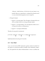
1.4
Proof of Zaslavsky’s Theorem
Let’s look at Zaslavsky’s proof of Theorem 1.1:
|χA (−1)| = the number of regions formed by arrangement A, in Rd .
We set up the proof by introducing a way to count the faces of an arrangement, discussing Möbius inversion, and then discussing what it means to induce a
hyperplane arrangement on a flat.
Let A be a hyperplane arrangement in Rd . Then, A divides the space into
regions, or open polyhedra, R1 , . . . Ri such that:
Rd = ∪ij=1 Rj ,
where Rj denotes the closure of Rj .
This is a polyhedral subdivision, whose faces (the surfaces that make up the
polyhedra’s boundaries) are the faces of the closure of the regions. Let fk denote
the number of k-dimensional faces of the subdivision. According to the Euler
14
relation, we have
d
X
(−1)k fk = (−1)d .
(1.2)
k=0
Next, Möbius inversion allows us to find a sort of inverse of a function on a
poset by using the Möbius function. It states:
f (x) =
X
g(y) ⇐⇒ g(x) =
y≥x
X
µ(x, y)f (y),
y≥x
As we saw in Equation 1.1, we will take (y ≥ x) to mean that y is above x in
the semilattice, i.e. (y ⊆ x), and we’ll rewrite the expression to read:
f (x) =
X
y⊆x
g(y) ⇐⇒ g(x) =
X
µ(x, y)f (y)
y⊆x
Finally we discuss induced arrangements. Ay , the hyperplane arrangement induced on y, is the subset of A that intersects y. More formally:
Ay = {H ∩ y : HA}.
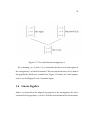
For instance, recall the arrangement of three intersecting lines in R2 , depicted
in Figure 1.1. Let’s say that H3 (one of the three lines) was y. Then, Ay would
look like this:
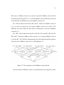
Figure 1.9 depicts a line with two points on it, formed by the intersections with
15
Figure 1.9: The arrangement Ay , the arrangement induced on y.
hyperplanes H1 and H2. The semilattice for this arrangement is given in Figure
1.10.
Figure 1.10: The semilattice for the arrangement Ay .
Let : r(y) = the number of regions of Ay .
Then r(H3) would equal 3, since there is one (bounded) region formed between the two points, and one (unbounded) region on each side of it.
Now that all the pieces are in place, let’s begin.
Let : f (x) =
X
y⊆x
(−1)dim(y) r(y).
16
We define another function, g(y):
Let : g(y) = (−1)dim(y) r(y).
Then:
f (x) =
X
g(y)
y⊆x
We apply Möbius inversion:
g(x) =
X
µ(x, y)f (y)
y⊆x
Here we’ll take an aside. f (x) =
dim(y)
r(y).
y⊆x (−1)
P
However, the regions
formed by Ay map directly to the faces of y, F , where dim(y) = dim(F ). So we
can rewrite f (x):
f (x) =
X
X
y⊆x
F face of y
dim(F ) = dim(y)
(−1)dim(F ) .
Since this is summed over all flats that are subsets of x, we can reduce this to:
f (x) =
X
(−1)dim(F ) .
F face of x
And then if we break up this sum into the sum of the number of faces of each
17
dimension:
dim(x)
f (x) =
X
(−1)k fk ,
k=0
and substituting from the Euler relation, Equation (1.2):
f (x) = (−1)dim(x) .
Returning from our aside, we substitute for f (x) and g(x):
(−1)dim(x) r(x) =
X
µ(x, y)(−1)dim(y) .
y⊆x
Evaluating for Rd gives
r(Rd ) = (−1)d
X
µ(Rd , y)(−1)dim(y) ,
y⊆Rd
and since
χ(t) =
X
µ(Rd , y)tdim(y) ,
y⊆Rd
then
r(Rd ) = (−1)d χ(−1).
18
Since r(Rd ) is always positive, we can rewrite this as
r(Rd ) = |χ(−1)|.
This proves that the number of regions formed by a given arrangement is
equal to the absolute value of the arrangement’s characteristic polynomial evaluated at (-1).
1.5
Subspaces
Typically, a user would run the software by supplying only a set of hyperplanes.
However, the user may additionally provide a subspace within which the software will intersect the provided hyperplanes.
1.5.1
Theory
The subspace must be given as an intersection of hyperplanes, where each hyperplane is of the same dimension as hyperplanes in the arrangement.
Each hyperplane in the arrangement will intersect the subspace in one of three
ways:
1. In full dimension, i.e., the subspace is a subset of the hyperplane;
2. Not at all, i.e., there is no solution to the system of equations consisting of
19
the hyperplane and all of the hyperplanes that comprise the subspace; or
3. In a generic way, i.e., the hyperplane intersects the subspace, but not in full
dimension.
Subspaces can be viewed as nothing more than the solution space to a system of linear constraints, within which we conduct other analyses. We will see
an example of this later, when we discuss other researchers’ extensions of our
software.
1.5.2
Implementation
The software implementation is fairly straightforward. Rather than the root node
of the semilattice consisting of the ambient space, it will consist of the equations
that comprise the subspace, and rather than the provided hyperplanes occupying
the first level of the semilattice above this root node, each of the provided hyperplanes would be intersected with the subspace, and the resulting flats would be
inserted into the semilattice directly above the root. Once the program begins
intersecting these flats with each other, it doesn’t know (doesn’t care) how many
equations comprise each flat — it simply attempts to intersect whatever flats it
encounters.
The dimensions of flats in a hyperplane arrangement work a little differently
when a subspace is provided. Without a subspace, the ambient space has dimension equal to the number of variables provided in each hyperplane. When a
20
subspace is provided, it is by definition some subset of that ambient space, and
therefore has a dimension less than the number of variables. The software verifies that the subspace itself is a valid flat (has a solution), and then determines
its rank, and thus dimension. As expected, the dimension of the flats formed by
intersecting each hyperplane with the subspace is one less than the dimension of
the subspace, and so on.
Rejecting Hyperplanes
When the software is supplied with a subspace not all of the hyperplanes in the
arrangement may be valid to insert into the semilattice. As we discussed above,
there are three ways in which a hyperplane can intersect the subspace: in full
dimension, not at all, or in a generic way.
The software rejects any hyperplane that intersects the subspace in full dimension, because the resulting flat would still be the entire subspace. The software
rejects any hyperplane that does not intersect the subspace at all, because (like
any other flat test the software performs) the software rejects any system of equations that has no solution. For instance, this case would trigger the error message:
WARNING: input <hyperplane> was rejected from the arrangement because it
did not intersect the supplied subspace.
21
It only retains the flats that represent hyperplanes that intersect the subspace,
but not in full dimension.
1.5.3
An Example
Let’s begin with a subspace, S, in R3 , that consists of the following planes:
S :=




x = 0,




y = 0,






y = 2.
This subspace is invalid. y = 0 and y = 2 do not intersect; therefore, the system of
equations does not have a solution. Assuming we remove y = 2, we are left with
the subspace:
S :=



x = 0,


y = 0.
Therefore, our subspace is the intersection of these two hyperplanes, otherwise
known as the z-axis.
Now, let’s say our hyperplane arrangement is the following:
22
A :=




z = 0,








z = 2,




z = x,







y = −x,







x = 2.
First, the software attempts to intersect each hyperplane with the subspace. z =
0 intersects the z-axis at the origin. z = 2 intersects the z-axis at (0, 0, 2) (for the
ordering (x, y, z)). z = x also intersects the z-axis at the origin, so it is rejected
as a duplicate of another hyperplane. y = -x is rejected because it intersects the
subspace in full dimension. x = 2 is rejected because it does not intersect the
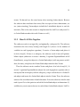
subspace at all. We begin by drawing the semilattice depicted in Figure 1.11.
Then the software recursively intersects flats with each other (like in the ordinary case), down to dimension 0. In this case though, we’re already there —
there are no more intersections to find. We calculate the Möbius values, as seen
in Figure 1.12.
We sum across the Möbius values in each dimension and produce the characteristic polynomial:
χ(t) = t − 2.
23
Figure 1.11: The semilattice for arrangement A.
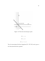
By evaluating χ at (-1) and (+1), we determine that there are 3 total regions in
the arrangement, 1 of which is bounded. This may not be obvious, so let’s look at
this graphically. Really just a number line, Figure 1.13 shows the 3 total regions,
and we see that Region 2 is the 1 bounded region.
1.6
Linear Algebra
Above, we learned that the original hyperplanes in the arrangement, the intersections of the hyperplanes, as well as all of the intersections of the intersections,
24
Figure 1.12: The semilattice for arrangement A, with Möbius values indicated.
Figure 1.13: The arrangement A, with the regions labeled.
are known as flats. Each flat can be represented by a subset of the hyperplanes
that intersect to form it. Figure 1.14 is an example of this, in R2 .
Let’s say that the equations of the hyperplanes are these:
25
Figure 1.14: Three lines intersecting in a point.
H1 : x = 2,
H2 : y = 2,
H3 : y = −x + 4.
Then, the intersection of the three hyperplanes, H1 ∩ H2 ∩ H3, can be given as
the intersection of the three equations:
26
H1 ∩ H2 ∩ H3 : (x = 2) ∩ (y = 2) ∩ (y = −x + 4).
1.6.1
Matrices
A flat is a just system of equations, so we will represent it with a matrix. Using
the convention Ax = b, if we continue our example, our matrix looks like this:



 2
 1 0 

  x  
 0 1 · = 2






y
4
1 1

1.6.2







Matrix Rank
However, we return to the graph and realize that we do not require all three
hyperplanes to form the point H1 ∩ H2 ∩ H3. We could form it with just two of
the hyperplanes (say, H1 and H2), as seen in Figure 1.15.
Any additional hyperplanes that pass through that point (e.g., H3) do not
change the nature of the flat. (Which, and how many, hyperplanes intersect in
each flat is important in calculating the Möbius function, but not important when
simply defining the flat.)
When the rank of a matrix equals the number of equations in the matrix, we
say that the matrix is of full rank. We will see in Sections 3.1.3 and 3.2.3 that for
27
Figure 1.15: Two lines intersecting in a point.
efficiency reasons, we have implemented Gaussian elimination to eliminate all
unnecessary equations at each step. In other words, we will always deal with
matrices that are of full rank.
1.6.3
Intersection Properties
A point has dimension 0, a line has dimension 1, a plane has dimension 2, etc. If
we have a matrix that has a solution, what dimension is the flat? As we saw in
our example above, the lines H1 and H2 intersected to produce the point H1 ∩
H2.
28
Generally, two flats of dimension d intersect to produce a flat of dimension d-1,
but there are two cases where this won’t happen: if the two flats are incidental, or
if the flats are parallel or skew. We will use basic matrix operations and Gaussian
elimination to solve matrices, to determine which flats intersect.
1.6.4
Dimensions
Dimensions come into play throughout hyperplane arrangement analyses. We
begin with the dimension of the ambient space, the space within which we intersect
the arrangement. Since we are considering Euclidian spaces, the ambient space
will be R1 , R2 , R3 . . . , or any Rd .
We learned earlier that each hyperplane will be of dimension 1 fewer than the
dimension of the ambient space. We also learned that two hyperplanes (or any
two flats of the same dimension) can have one of three relations with one another:
they can intersect in full dimension (not a valid flat), not intersect at all (not a flat
at all), or intersect in a generic way. Since all flats in a semilattice are linear (do not
curve), no two flats can intersect in more than one (new) flat without intersecting
in full dimension.
Just as we know that two (non-incident) lines intersect to form a point, and
two (non-incident) planes intersect to form a line, two (non-incident) 3-dimensional
linear forms intersect to form a plane, and so on. In all cases, flats of dimension
i intersect to form flats of dimension i-1. More than two flats of dimension i can
29
intersect in one place, but they still create a flat of dimension i-1.
1.6.5
Finding Intersections of Flats
Finally, we discuss the linear algebra of finding intersections between flats. There
are two cases we need to address:
1. Testing for an intersection between two flats of the same dimension; and
2. Once we have found a valid intersection between two (or more) flats, testing
whether additional flats also pass through that intersection.
We begin with what we have termed the expected dimension, which we will
abbreviate ED. In case 1, the ED will always be the dimension one less than the
dimension of the two flats we are attempting to intersect. The algorithm attempts
to build the semilattice from the bottom-up (just as would be done by hand), one
dimension at a time — any new flats inserted into the semilattice must be of the
next (lower) dimension.
In case 2, we have already found a valid intersection between two or more
flats. Let’s say those original flats had dimension c. Then the intersection we
found between them would be of dimension c − 1. At this point, we’re testing
whether another flat of dimension c also passes through this new intersection,
and so we’re testing for a solution between flats of dimension c − 1 and c, respectively. Here, the ED is c − 1, since we’re testing whether the c-dimensional flat
30
passes through the flat of dimension c − 1 — not whether it forms a new flat.
To determine if two flats intersect, we start by concatenating the two matrices, one above the other (removing any duplicate equations), and we perform
Gaussian elimination on the resulting matrix to test for a solution.
For there to be a solution to the matrix, the post-Gaussian elimination matrix,
a square matrix in upper-triangular form, must be non-singular — must not have
any 0’s on its diagonal. If there is a solution, we calculate the dimension of the
resulting (post-Gaussian elimination) matrix by subtracting the rank of the matrix
from the dimension of the ambient space. If the dimension equals the ED (one
less than the dimension of the inputted flats), there is a valid solution; otherwise
there is not.
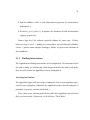
Chapter 2
Algorithmic Solution
In this chapter, we discuss our solution to the problem, beginning with two key
algorithms, followed by some important data structures and architectural aspects.
2.1
Algorithms
To review the description of the problem (Section 1.2), a mathematician would
follow the following steps to solve this problem by hand:
1. Contruct the semilattice by recursively finding all flats created by the hyperplane arrangement.
2. Calculate the Möbius values of the flats in the semilattice.
31
32
3. Sum the Möbius values in each dimension to generate the characteristic
polynomial, χ.
4. Evaluate χ at (-1) and (+1), to produce the numbers of total and bounded
regions, respectively.
From a high level, the software generally follows the same steps. Clearly,
however, steps 1 and 2 — finding the intersections and calculating the Möbius
values — present some complex challenges. Below we present our solutions to
these problems.
2.1.1
Finding Intersections
The algorithm for finding intersections is bit complicated. To understand what
the code is doing, we will first dig a little deeper into what the code needs to do;
then we will examine the algorithms used to accomplish it.
Analyzing the Problem
The algorithm begins with one major assumption: that no two equations represent the same hyperplane. (Similarly, the algorithm assumes that the subspace, if
provided, is given by a matrix of full rank.)
Then, there is one fundamental rule on which this algorithm is based (listed
first), and two results. Collectively, we’ll call these “The 3 Rules”:
33
1. Because all flats are linear, the intersection of two flats is unique — two flats
can intersect in at most one new flat.
2. Given flats A, B, and C in dimension i, if there exists a flat A ∩ B ∩ C in
dimension i - 1, there will not also exist (distinct) flats that contain any two
of A, B, and C.
3. Given the same A, B, and C, if there exists an intersection A ∩ B (but not A
∩ B ∩ C), C could still intersect A and/or B.
Each flat can potentially intersect any other flat, and because all the flats are
linear forms, any two flats of dimension d that intersect will intersect to create a
flat of dimension d-1.
Since we need to check for intersections between every pair of flats, the basic
algorithm loops as follows:
for i from 1 to (number of flats in this dimension) {
for j from i+1 to (number of flats in this dimension) {
Search for intersections
}
}
However, more than two flats can intersect in one place. To determine the
intersection properties of the arrangement and calculate the Möbius Function
34
correctly, we need to know about all of the flats that intersect in a given place.
Therefore, we need to modify the above algorithm to allow for this.
There are two possible approaches we can take:
1. Use the algorithm above to find every pair of flats that intersect, and then
intersect these intersections with each other to find any larger intersections
(formed by more than two flats); or
2. Modify the algorithm above to build up a flat representing the intersection
of as many flats as possible, first, before searching for the next intersection.
Our implementation uses option 2.
Let’s walk through an example. Assume we are looking for intersections
within a dimension containing six flats, numbered 1 to 6. Let’s say that we’ve
already searched for intersections with flat 1, and we found only one intersection: 1 ∩ 2 ∩ 4.
Now we’re beginning to search for intersections between flat 2 and the remaining flats in this dimension. We check 2 ∩ 3 — we find an intersection. So
now, we begin searching for intersections between 2 ∩ 3 and the remaining flats
in this dimension, to see if other flats also pass through this intersection. We check
2 ∩ 3 ∩ 4 — no intersection. Then we check 2 ∩ 3 ∩ 5 — there is an intersection.
Then we check 2 ∩ 3 ∩ 5 with flat 6 — no intersection.
What have we found so far? We know that flats 2, 3, and 5 all intersect in the
35
same place, and that flats 4 and 6 do not also intersect in that place. However,
based on Rule #3, flat 2 could still intersect flats 4 and/or 6, in some other place(s).
So, we continue checking for intersections with flat 2. Since we have already
found an intersection between flats 2 and 3 (at 2 ∩ 3 ∩ 5), based on Rule #2, there
is no need to search for another intersection that contains both 2 and 3. But based
on Rule #3, even though we have already checked for a flat 2 ∩ 3 ∩ 4 (which did
not exist), we still need to check 2 ∩ 4, and in fact, there is an intersection at 2 ∩ 4.
Now we’re testing 2 ∩ 4 with each of the remaining flats. Thanks to Rule #2, we
do not try 2 ∩ 4 ∩ 5 (since we already have an intersection containing 2 and 5), so
we move onto 2 ∩ 4 ∩ 6, and there is not an intersection there.
We again return to checking flat 2 against any remaining flats. Since we have
already found intersections between flat 2 and flats 3, 4, and 5, we do not check
any of these pairs again. This leaves only 6 — we check 2 ∩ 6, and there is no
intersection. Now we are done checking for intersections between flat 2 and the
others.
We discovered intersections 2 ∩ 3 ∩ 5 and 2 ∩ 4. Before we insert these two
flats into the semilattice, we first verify that these flats are not duplicates of any
other flats we had found previously. When we check, we realize that 2 ∩ 4 is a
duplicate of 1 ∩ 2 ∩ 4 (not surprisingly, according to Rule #2). Therefore, we only
insert the flat 2 ∩ 3 ∩ 5 into the semilattice. And the algorithm repeats the above
logic, searching for intersections beginning with flat 3, then 4, 5, and 6. . . and
36
we’re done with this dimension.
Our Solution
Rule #1 says that an intersection between two flats is unique. So, we keep track
of with which flats we have already found intersections. This is accomplished
with the Intersection Array (IA), an array of booleans created for each flat. When
the algorithm begins looking for intersections beginning with flat F, it creates an
IA, containing one array element for each other flat, and all array elements are
defaulted to false. Before testing for an intersection between F and another flat,
G, the algorithm first confirms that F.IA[G] is false; otherwise it skips it. Whenever the algorithm finds an intersection between F and another flat, H, it flips
F.IA[H] to true. The IA variable is discarded after the algorithm finishes looking
for intersections beginning with flat F.
If it has built up a flat F’, and it discovers that flat G also passes through F’,
it must now begin searching for flats that also pass through F’ ∩ G, as well as
continue searching for flats that pass through just F’. This is where the algorithm
branches. Since we chose to implement the algorithm such that it attempts to
build up the largest possible flat it can, first, it continues by searching for flats that
pass through F’ ∩ G. . . and will branch more times if it finds any, before returning
to searching for flats that pass through F’.
The IA variable persists across branches. For example, if the algorithm finds
37
F’ ∩ G ∩ H but can’t find any other flats that pass through this intersection, it
returns to checking for flats that pass through F’ ∩ G — but it does not check H,
since it is marked as true in the IA. Likewise, when the algorithm returns to the
branch searching for intersections that pass through only F’, it will not consider
G or H again.
The algorithm makes heavy use of a few functions:
• In the EquationMatrix class:
1. public EquationMatrix( EquationMatrix e )
2. public EquationMatrix( EquationMatrix e1, EquationMatrix e2, int expectedDimension )
3. public boolean solveMatrix()
• In the Lattice class:
1. private boolean twoFlatsAreEquivalent( LatticeNode a, LatticeNode b,
int expectedDim )
EquationMatrix( EquationMatrix e ) is the copy constructor for the EquationMatrix class. This method is vital to the intersections algorithm, because the algorithm sends a lot of matrices off to the linear algebra engine, which performs a
lot of manipulations on its inputs. The copy constructor allows the intersections
algorithm to save a copy of a flat before it sends it off to the linear algebra engine.
38
EquationMatrix( EquationMatrix e1, EquationMatrix e2, int expectedDimension )
is the “merge” constructor for the EquationMatrix — it merges two matrices into
one. This is how we test for intersections. We merge two EquationMatrix objects
and then send the result into the linear algebra engine, to test for a solution of the
correct dimension.
solveMatrix() is the linear algebra engine. It, with the help of the Gaussian
elimination method, performs all of the manipulations necessary to determine
whether the given matrix has a solution. If it does, it compares its dimension
with the expectedDimension that was passed in, to verify that the solution space is
of the correct dimension. For instance, assuming we have found a flat A ∩ B, and
we’re testing whether C also passes through that same intersection, the expectedDimension will be the same dimension as A ∩ B. If A ∩ B ∩ C has a solution, C
intersects with A and B at A ∩ B, and if A ∩ B ∩ C has the same dimension as A ∩
B, then C did not change the intersection, which means A, B, and C all intersect
in the same place. If the dimensions are not equal (A ∩ B ∩ C has dimension 1
less than A ∩ B), then we don’t want to know about A ∩ B ∩ C just yet — that flat
(which we will revisit) is for a later dimension in the semilattice.
twoFlatsAreEquivalent() does what it promises! It returns to the algorithm
whether the flats stored in two LatticeNodes are equivalent. If the algorithm has
already found an intersection A ∩ B ∩ C, and later (when searching for intersections beginning with flat B), it finds B ∩ C, it needs to be smart enough to realize
39
that these are one in the same.
2.1.2
Computing Möbius Values
We learned about the Möbius function, and how it applies to this problem, in the
mathematics chapter. How do we solve this problem?
The job of computing the Möbius values for the semilattice is a natural candidate for dynamic programming, and specifically with a “bottom-up” approach.
We use dynamic programming, because the problem certainly demonstrates optimal substructure — that is, finding the Möbius values of flats in lower dimensions (higher up in the semilattice) requires the results finding the Möbius of flats
in higher dimensions (flats lower in the semilattice) first, and the Möbius values
for flats in the higher dimensions will be used multiple times each. Let’s look at
our example semilattice again, Figure 2.1, to demonstrate this concept.
The Möbius value of the R3 flat is used when computing the Möbius values of
all of the flats above it, as well as for computing the characteristic polynomial (χ)
for the arrangement — it is used a total of 15 times. The Möbius value for the H1
flat is used when computing the Möbius values for the H1 ∩ H2, H1 ∩ H3, H1 ∩
H4, H1 ∩ H2 ∩ H3, H1 ∩ H2 ∩ H4, and H1 ∩ H3 ∩ H4 flats, and in computing
χ, and so on. Computing Möbius values from the bottom of the semilattice, up,
is the obvious way to approach the problem, and then the algorithm becomes
seemingly trivial:
40
Figure 2.1: The semilattice, with Möbius values, for the arrangement depicted in
Figure 1.5.
computeMobiusValues()
f latd1 .mobiusValue = 1; // the ambient space
for i from (dimension-1) 7→ 0 {
for j from 1 7→ (number of flats in this dimension) {
f latij .mobiusValue = ( 0 - mobiusRecursion(i, j) );
}
}
}
mobiusRecursion( i, j ) {
41
int m = f latij .mobiusValue;
for k from 1 7→ (number of flats immediately beneath this flat) {
m += mobiusRecursion( i-1, (index of f lat(i−1)k ) )
}
}
This algorithm simply follows every path down from a given node (to the
bottom of the semilattice) and sums the Möbius values of all nodes it encounters.
So, beginning in dimension 2, it computes the Möbius value for H1 by simply
encountering R3 , and assigning H1 the negative of that sum. It does the same for
H2, H3, and H4, in that order. Then it moves to dimension 1. For H1 ∩ H2, it
encounters H1 and recurses again to find R3 . It returns (+1) back to the step at
H1, where it adds the Möbius value at H1 (-1), and returns 0 to the step at H1 ∩
H2. Next, it encounters H2, followed by R3 , which returns (+1) back to H2, which
adds its (-1) and returns 0 to H1 ∩ H2. 0 + 0 = 0, and the negative of 0 is 0; the
Möbius value of H1 ∩ H2 is set to 0. (And the algorithm proceeds to the next
LatticeNode.)
Unfortunately, that computation was incorrect, because the algorithm counted
the Möbius value of R3 twice. Why did this happen? Since the semilattice is not
a tree (each flat may have multiple parents), this algorithm will frequently multicount Möbius values. The problem becomes more pronounced as the algorithm
moves further up the semilattice. For instance, when computing the Möbius
42
value for flat H1 ∩ H2 ∩ H3 the algorithm would double-count the Möbius values
for H1, H2 and H3 and count the Möbius value of the R3 flat 6 times. Clearly this
algorithm does not solve the problem.
To get around this, we introduce the concept of a dirty bit. The term is stolen
from Systems Architecture, where the term refers to a bit of memory used to note
whether a location in the a system’s page cache has been changed, and therefore may no longer be valid. In this application, we use the dirtyBit member
data (stored in the LatticeNode object) to note whether the computeMobiusValues() algorithm has already encountered this LatticeNode. Once the algorithm
encounters each LatticeNode, it marks its dirtyBit as invalid, thereby instructing
the algorithm to ignore it, should the algorithm encounter it again.
Thus, the use of the dirtyBit variables allow the algorithm to add the Möbius
value of each LatticeNode only once, and therefore to correctly compute the
Möbius value of a given LatticeNode. However, the LatticeNode objects whose
dirtyBit variables were marked will necessarily (and correctly) be re-encountered
during the computation of other LatticeNode objects’ Möbius values. (When
computing the Möbius value for H1 ∩ H3, the algorithm will encounter some of
the same LatticeNode objects it encountered when computing the Möbius value
of H1 ∩ H2.) Therefore, another method resets the dirtyBit for all affected LatticeNode objects, before beginning computation of the Möbius value of the next
LatticeNode.
43
So, our final algorithm looks like this:
computeMobiusValues()
f latd1 .mobiusValue = 1; // the ambient space
for i from (dimension-1) 7→ 0 {
for j from 1 7→ (number of flats in this dimension) {
f latij .mobiusValue = ( 0 - mobiusRecursion(i, j) );
resetDirtyBit(for the sub-lattice topped by the LatticeNode at i,j);
}
}
}
mobiusRecursion( i, j ) {
if (f latij .dirtyBit == false) {
f latij .dirtyBit = true;
int m = f latij .mobiusValue;
for k from 1 7→ (number of flats immediately beneath this flat) {
m += mobiusRecursion( i-1, (index of f lat(i−1)k ) )
}
} else {
return 0;
44
}
}
These methods have three major additions over the original methods. First,
in mobiusRecursion(), we now flag each LatticeNode as dirty as soon as we encounter it, with: “f latij .dirtyBit = true”. Second, we have wrapped the logic of
mobiusRecursion() in an if/else clause, such that the logic only runs if the LatticeNode is not already dirty. The combination of these two additions ensures that
we only visit each LatticeNode once. Third, at the end of computeMobiusValues(),
we have added a command to reset the affected dirtyBit values after computing
the Möbius value of this LatticeNode.
2.2
Architecture
In this section, we begin by discussing the layout of the primary subsystems and
how these subsystems all fit together. Then, we discuss several design decisions,
including the choice of programming langauge, the use of system resources, and
some design tradeoffs.
2.2.1
Layout of Primary Subsystems
The architecture of the application is primarily comprised of three data structures:
the EquationMatrix, the LatticeNode, and the Lattice. We will build up the overall
45
architecture by discussing each of these structures, in that order. We will examine
what each of these structures look like and how they map to the mathematics
discussed in the prior chapter.
EquationMatrix
The primary purpose of an EquationMatrix object is to store the data for the equations of a flat. As we saw above, when discussing the FileInputReader, it attempts
to read in the data of an input file such that it represents the underlying matrix
multiplication:


















b1  
 

b2 
 
 
 
.  
=
 

. 
 
 

. 
 
 
bj
a11 a12 a13 . . .
a21 a22 a22 . . .
.
.
.
.
.
.
aj1 aj2 aj3 . . .
 

a1k  
 

a2k 
 
 
 
 
·
 
 
 
 
 
 
 
ajk
x1 

x2 



. 


. 


. 


xj
The architectural parts of the EquationMatrix member data are:
private double[][] A;
private double[] B;
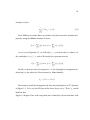
And when we draw a picture of A and B (see Figure 2.2), we see that this
representation mimics the matrix representation very closely.
46
Figure 2.2: An EquationMatrix object.
Since the x1 . . . xn elements are variables (not values), they are obviously not
stored in memory. Otherwise, the mapping from matrix representation to data
structure representation is very straightforward.
47
LatticeNode
LatticeNode objects exist primarily to connect EquationMatrix objects to one another, across dimensions. As we read earlier in this chapter, a LatticeNode object
contains the following architectural member data:
private EquationMatrix em;
private Vector parentVector;
private Vector childVector;
First, we see the EquationMatrix object, em, that this LatticeNode contains.
After that are the childVector and the parentVector. These member data allow the
software to attach this LatticeNode to the LatticeNode objects below and above
it in the Lattice, respectively. The childVector is a Vector of references to the LatticeNode objects which hold the EquationMatrix objects that intersected to form
em in this LatticeNode. Conversely, the parentVector contains references to LatticeNode objects containing EquationMatrix objects which are subsets of em. We
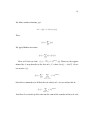
see a depiction of a LatticeNode in Figure 2.3.
The childVector and parentVector contain references to other LatticeNode objects. Likewise, the childVector and parentVector Vectors of other LatticeNode objects point to this object (not shown).
If the em contained in this LatticeNode is of dimension i, its parents will be of
dimension i - 1 and its children will be of dimension i+1. A LatticeNode can have
48
Figure 2.3: A LatticeNode object.
any number of parents, including 0. Obviously, flats of dimension 0 (points),
which live at the top of the semilattice, will never have parents.
LatticeNode objects must have at least two children (since all new flats are
formed by the intersection of two or more existing flats) with two exceptions.
The root node — the sole LatticeNode in dimension d — has no children. And
the original hyperplanes (each of which is of dimension d-1) each only have one
child: the root node.
49
Lattice
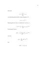
The primary architectural component of the Lattice object is its:
private Vector[] latticeArray;
This array of Vectors is the container for all of the LatticeNode objects. We see
this visually in Figure 2.4.
The vertical series of boxes (on the left-hand side) is the array. Each element in
that array points to a Vector object — these Vectors are depicted by the horizontal
series of boxes. Each of these boxes contains exactly one LatticeNode. The arrows
connecting these LatticeNodes are the references stored in each LatticeNode object’s childVector and parentVector Vectors. (childVector and parentVector references
are depicted as double-ended arrows to reduce clutter — in reality, there are two
(parallel) single-ended arrows connecting each pair of LatticeNode objects.)
Each element of the array corresponds to a dimension, such that all of the flats
of a particular dimension lie in that dimension’s Vector. Since the dimensions of
a semilattice run from 0 7−→ d, the array must be of length d+1. Dimension d
(array element d) will always contain a Vector of just one LatticeNode — the LatticeNode that holds the EquationMatrix representing the root node. The Vector
in dimension d - 1 (stored in array element d - 1) will always hold one LatticeNode per equation read in from the user’s input file (less any equations that were
rejected for their failure to intersect properly with the subspace). After d - 1, how-
50
Figure 2.4: A Lattice object.
ever, the software doesn’t know how many flats will live in each dimension until
it does the math. (More on this in Section 3.3.1.)
The latticeArray member data is similar in structure to the A member data
of an EquationMatrix, the key difference being that, for A, the software knows
how many elements each array element needs to hold at the time A is instantiated (since all equations within a given Lattice have the same number of coeffi-
51
cients). We do not have the same luxury when creating Lattice objects. Because
the software does not know how many flats to expect in lower dimensions, we
use (auto-extending) Vector objects to hold the LatticeNode objects in each dimension. (This is the same reason we implemented the childVector and parentVector LatticeNode member data with Vectors as well.)
2.2.2
How It All Fits Together
The software reads in an input file, and optionally, a subspace file. The software
instantiates the latticeArray Vector[] with length d+1 (where d is the number of
variables in each hyperplane equation). It creates a Vector object and places it
in latticeArray[d]. If there is a subspace, the software reads it into an EquationMatrix object (otherwise it creates a dummy, 1-equation EquationMatrix of all
0-coeffcients), wraps that object in a LatticeNode object (with no parents or children, for now), and places that LatticeNode object into that lone Vector.
Then the software creates another Vector and places it in latticeArray[d-1]. It
creates 1-equation EquationMatrix objects for each hyperplane equation (that is
not rejected for its interplay with the subspace), wraps each of these in a LatticeNode object and inserts the LatticeNode objects into the Vector. Then, the software
connects the two dimensions in both directions. It inserts references into the root
node’s parentVector that point to each of the LatticeNode objects in dimension d-1,
and likewise, creates one reference in each of those LatticeNodes objects’ childVec-
52
tor Vectors which point back to the root node.
The software begins to search for intersections. It loops over the LatticeNode objects in dimension d-1, and intersects them according to the intersection
algorithm (coming in just a moment!) to form LatticeNode objects that are inserted into the Vector of LatticeNode objects of dimension d-2. These are connected down to the LatticeNode objects that intersected to form them, and those
children are connected up to these LatticeNode objects they just formed. This
process continues until we reach dimension 0 (or until the flats at the top of the
semilattice fail to intersect with each other). . . and the semilattice is formed.
Chapter 3
Software Implementation
Now that we understand the mathematical background of the problem and have
presented our solution, we discuss our implementation. We will look at the primary data structures and methods and then analyze the runtime complexity and
the observed performance for the application.
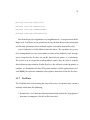
3.1
Data Structures and Methods
There are seven major classes in the application:
1. Lattice
2. LatticeNode
3. EquationMatrix
53
54
4. FileInputReader
5. FileOutputWriter
6. MatrixGenerator
7. TestSuite
We will discuss these classes in that order. (We will begin to discuss how
these classes interact with one another here, but will address that in more detail
in Section 2.2.) For each class, we will look at the following three areas:
1. Member Data
2. Constructors
3. Methods
(Additionally, for the FileInputReader class, we include Section 3.1.4, regarding input format.) Unimportant and/or uninteresting items (e.g., default constructors and “get” and “set” methods) are omitted. We will dive a little deeper
into the most critical algorithms in this section, and a little more in Section 2.1
later in this chapter.
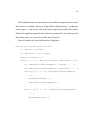
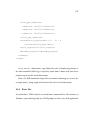
3.1.1
Lattice
The Lattice class is the most important class in the application. Among other
things, it contains the main() method for the application, the logic for searching
55
for intersections of flats, and the algorithm for computing Möbius values. The
Lattice data structure is the outermost data structure in the application — it forms
the structure of the semilattice.
Member Data
These are the most important pieces of member data in the Lattice class:
private int dimension;
private EquationMatrix[] arrangementArray;
private EquationMatrix subspaceEM;
private Vector[] latticeArray;
private int numFlatTests;
private int[] charPoly;
private int numberOfRegions = 0;
private int numberOfBoundedRegions = 0;
private String output;
The dimension holds the dimension of the ambient space. In the typical case,
for Rd , dimension = d; when a subspace is provided, the dimension equals the dimension of the subspace.
The arrangementArray is an array of 1-equation EquationMatrix objects, where
each EquationMatrix objects holds one of the equations provided by the user in
the input file.
56
subspaceEM is the EquationMatrix that holds the subspace provided by the
user. If no subspace is provided, subspaceEM is null.
The latticeArray is a data structure that holds the entire semilattice. It consists
of an array of Vector objects. Each Vector object contains all of the LatticeNode
objects (that hold flats) of a particular dimension — since Vectors auto-extend in
size, the software is able to insert new LatticeNode objects without any explicit
data structure management. The array of Vectors is of length dimension + 1, where
each array slot corresponds to the dimension of the flats stored within it. For
example, array slot 0 consists of all of the flats of dimension 0, namely all of the
points; array slot 1 contains all the lines; array slot dimension consists of only the
ambient space flat, be that the Rd flat, or the subspace (if provided). The setinclusion relationships are managed by the LatticeNode objects themselves, not
by the Lattice data structure.
numFlatTests is a counter of how many EquationMatrix objects are sent to the
linear algebra engine for solving (primarily for testing / performance analysis).
The charPoly holds the characteristic polynomial of the arrangement, χ. It is
stored as an array of integers, where each array slot holds a coefficient of χ. numberOfRegions and numberOfBoundedRegions are just what they say, and are computed by evaluating charPoly at (-1) and (+1), respectively.
output is the buffer that holds the text that will be written out to the output file.
The software appends to this String as it generates more output, and the entire
57
String is written to the output file when the software completes its work.
Constructors
There are two primary constructors:
public Lattice( EquationMatrix[] arrArray, int dim )
public Lattice( EquationMatrix[] arrArray, int dim,
EquationMatrix subspace )
The first constructor is for the case in which there is no subspace provided.
It takes as parameters an array of 1-equation EquationMatrix objects (which is
stored in the arrangementArray) and the dimension of the ambient space. (Since
there is no subspace, the ambient space is Rd , and thus, the dimension of it is d).
The second constructor is used when there is a subspace provided. It takes the
same parameters, plus an EquationMatrix defining the subspace.
Methods
These are the major methods in the Lattice class:
public void initializeLattice( EquationMatrix[] arrArray,
int dim, EquationMatrix subspace )
public void buildLattice()
private void findIntersections( int i, int j, int kInit,
58
boolean[] IA )
private boolean twoFlatsAreEquivalent( LatticeNode a,
LatticeNode b,
int expectedDim )
private static void connectParentToChild( LatticeNode
parent, LatticeNode child )
public void computeMobiusValues()
private void computeCharPoly()
public void latticeArrayTraversal()
public static void main(String[] args) throws Exception
initializeLattice() begins by initializing the private member data for this Lattice
object. It creates an empty Vector[] of length dimension + 1, and populates array
slot d with a single LatticeNode (the root node) that represents either Rd or the
subspace, as applicable. Note: if a subspace is provided, it performs some validation on the provided subspace and eliminates equations that are unnecessary
— make the subspace flat not be of full rank — and rejects any equations from
the inputted hyperplane arrangement that either do not intersect the subspace or
else wholly contain the subspace. Next, initializeLattice() inserts LatticeNode objects into array slot d-1 to represent all of the (remaining) hyperplanes, and calls
connectParentToChild() to create the set-inclusion relationships between these LatticeNode objects and the root node.
59
buildLattice() loops over the dimensions, from dimension d-1 7−→ 0, loops over
the flats contained in each of these dimensions, and calls findIntersections() to
search for the flats with which each of these flats intersects.
findIntersections() is where most of the heavy lifting is done, when building the
semilattice. Here is some pseudo-code, to explain what it does:
findIntersections( flat F ){
Create an "intersection array", IA, of booleans, to
store with which flats we have successfully
intersected F; initialize to all false
Create an EquationMatrix, X, consisting of just the
equations in F
For each other flat, Y, in this dimension {
If IA[Y] is false {
X’ = X (call the EquationMatrix copy
constructor, to preserve the state of X)
X’ = (X’ union Y)
If X’ has a solution of the expected rank {
X = X’
IA[Y] = true
}
}
60
}
If we found an intersection between X and any number of
other flats {
Create and initialize a LatticeNode, L, for
EquationMatrix X
Insert L into the Lattice
Attach L as the "parent" of all of the LatticeNode
objects, M’s, that intersected to create it
Attach each M as a "child" of L
Call findIntersections() to look for intersections
between X and any flats still marked as false
in the IA[], beginning with the first flat
after the first Y that successfully
intersected with F
}
}
So, findIntersections() has three major steps:
1. Beginning with the flat we’re working with (F), try to build up an intersection between as many flats as possible.
2. If we found an intersection:
61
(a) Insert this new flat into the semilattice.
(b) Recursively call findIntersections() to search for other intersections containing F.
F can intersect any number of the other flats in its dimension, but since all of
these flats are linear, it can only intersect each other flat in one place. Therefore,
if a flat F intersects with flats G and H, to form a flat A, F cannot also intersect
with G or H anywhere else (creating new flats). However, after finding F ∩ G ∩
H, the algorithm will test F ∩ G ∩ H ∩ I — if there is not a solution, the algorithm
will then test F ∩ G ∩ H ∩ J, and so on, but it must return later to test F ∩ I. And
that’s only the beginning. We will discuss this algorithm in much greater detail
in Section 2.1.
twoFlatsAreEquivalent() is a helper method, which simply tests whether two
flats are equivalent. To avoid unnecessary calls to the linear algebra engine, the
software first checks to see whether the set of equations in one of the flats is a
subset of the set of equations of the other flat. If this is the case, and the two flats
are of the same dimension, the flats are equivalent; otherwise, twoFlatsAreEquivalent() merges the two flats and sends the result to the linear algebra engine — if
and only if the merged flat has a solution and has the same rank as either of the
original flats, then the two flats are declared equivalent.
connectParentToChild() is a helper method that takes two LatticeNode objects
(A and B) as parameters, and calls methods in the LatticeNode class to connect A
62
as a parent of B and connect B as a child of A.
computeMobiusValues() recursively traverses the semilattice to compute the
Möbius values of all of the flats. This algorithm is explained in much more detail
in Section 2.1.
latticeArrayTraversal() traverses the semilattice to output the flats and their
Möbius values, in order (by dimension), to the output String.
computeCharPoly() sums the Möbius values of all the flats in each dimension
to obtain the coefficients of the characteristic polynomial, χ, and stores these integers in the member data charPoly. Then it computes the number of total regions
and bounded regions and stores these values in numberOfRegions and numberOfBoundedRegions, respectively, and outputs all this data to the output String.
The main() method does several things. First it reads in optional parameters
from the user. The user can supply switches to have the software output timing
statistics, suppress most of the software’s output (instruct it not to run latticeArrayTraversal()), and/or provide a subspace. Then it calls the FileInputReader class
to read in the user’s hyperplane arrangement, and if applicable, the subspace.
Next, it calls the various Lattice class methods in order, to initialize the Lattice,
build the Lattice, compute the Möbius values, (optionally) output the contents of
the Lattice, and output χ and the counts of regions. Finally, it calls the FileOutputWriter class to write the output String out to file.
63
3.1.2
LatticeNode
LatticeNode objects represent the flats in the Lattice, and the set-inclusion relationships between them. The LatticeNode class has no interesting methods —
mostly just get’s and set’s.
Member Data
private EquationMatrix em;
private Vector parentVector;
private Vector childVector;
private int mobiusValue = 0;
private int dirtyBit = 0;
A LatticeNode primarily consists of an EquationMatrix, em, (to hold the matrix of equations that define this flat), a parentVector of references to parent LatticeNode objects, a childVector of references to child LatticeNode objects, an integer
to hold the mobiusValue of this flat, and an integer to hold the dirtyBit.
“Parent” refers to a flat that lies immediately above this flat in the semilattice
— that is, a flat that is a subset of this flat, and is one dimension less than this flat.
A “child” LatticeNode is, of course, the opposite — a flat that is a superset of this
flat, lies immediately below this flat in the semilattice, and is of one dimension
greater than this flat.
64
The software uses Vector’s to hold the sets of parent and child LatticeNodes,
since at the moment the software creates a new LatticeNode object, it does not
know how many parent or child LatticeNodes to which it must be attached in the
semilattice. (Vector objects are self-extending, versus simple arrays).
The Möbius value integer is self-explanatory, and the dirtyBit is an integer
used by the software during the process of computing the Möbius values.
3.1.3
EquationMatrix
An EquationMatrix object holds a matrix of linear equations and some data about
the matrix, such as its rank and dimension. This class also contains all of the
methods used in testing matrices for solutions (including all the linear algebra
code), and a method that outputs an matrix to text (as used in the output file
produced by the software).
Member Data
The equations of an EquationMatrix object are stored in the following data structures:
private double[][] A;
private double[] B;
private int rank;
private int dimension;
65
private int expectedDim;
The A member data holds an ordered list of equations, each of which consists
of an ordered list of doubles. The ordered list of doubles represent the ordered
variable coefficients of a single equation; the list of the equations must themselves
also be ordered, because these equations have corresponding B values, that are
stored in the B array — the A and B arrays must have the same orderings.
The EquationMatrix class also holds integer values for its matrix’ rank, dimension, and expected dimension, expectedDim. expectedDim is the dimension the
calling method expects the matrix to be. If it does not match, the matrix is not a
valid flat for the given dimension of the semilattice.
Constructors
There are three primary constructors in the EquationMatrix class:
public EquationMatrix(double[][] matrixA, double[] vectorB)
public EquationMatrix(EquationMatrix e)
public EquationMatrix(EquationMatrix e1, EquationMatrix e2,
int expectedDimension)
The first is an ordinary constructor that takes an A, a B, and an expectedDim,
and creates an EquationMatrix object with these values.
The second constructor is a copy constructor that takes an EquationMatrix object as its input and duplicates it.
66
The last constructor is a “merge” constructor, that takes two EquationMatrix
objects and creates a new EquationMatrix object consisting of all of the equations of the first EquationMatrix object followed by all the equations of the second EquationMatrix object, less any equations that are duplicated from the first
EquationMatrix object (in that order).
Since the linear algebra code performs a great deal of manipulations on EquationMatrix objects, the software uses the copy constructor to save the original
state of an EquationMatrix prior to these manipulations. This merge constructor
is used when attempting to find an intersection between two flats — the matrices
are merged into one, and the linear algebra code searches for a solution to that
matrix.
Methods
The most important methods of the EquationMatrix class are solveMatrix(), which
tests for a solution to a matrix, and its helper method gaussianElimination(). We’ll
begin by looking at solveMatrix():
public boolean solveMatrix(){
int numvars = A[0].length;
gaussianElimination();
dropAllZeroRows();
if( A[0].length >= A.length) {
67
rank = A.length;
} else {
if( !extraRowsAreEquivalent() ) {
return false;
}
dropExtraRows( A.length - A[0].length );
rank = A[0].length;
}
dimension = numvars - rank;
return (expectedDim == dimension) && isNonsingular();
}
Let i be the number of equations in the matrix (the height of the matrix);
Let j be the number of variables in each equation (the width of the matrix);
Let the diagonal be the set of elements for which the row number equals the column number;
It begins by calculating i. Then it performs Gaussian elimination on the matrix,
which we’ll look at more closely in a moment. Next, it eliminates any rows in the
matrix which now consist solely of 0’s (including the B value), since these represent equations that were found to be linear combinations of other equations, and
are therefore unnecessary.
68
Then the algorithm looks at the shape of the resulting matrix. If it is square (i
= j), or has more columns than rows (j > i), the algorithm decides that the rank of
the matrix equals j.
Otherwise — if i > j — additional work is required. Since the algorithm has
already performed Gaussian elimination, the matrix should be in upper-triangular
form, meaning that all values below the diagonal are 0’s. Reusing an example from
the Mathematics chapter:



2
5 2.5 −1








 0 1

1
0








 0 0
2 

  −4 






C   −6 
 0 0



8
0 0 D
We are left with a square matrix (in upper-triangular form) and some additional equations, which should each consist of all 0’s except for the far-right value
in the A matrix and its B value. In this example, we have two such equations. For
there to be a solution to this matrix, the bottom equation of the square matrix
(in this case, the third row) must be equivalent to both of the additional equations. (This will only be the case if C = 3 and D = -4.) The algorithm passes
off responsibility for checking for these equivalences to a helper method named
extraRowsAreEquivalent().
69
If the additional rows are not equivalent, solveMatrix() reports that this matrix
does not have a solution; otherwise, it lops off the additional rows — making the
matrix square — and sets the rank of the matrix equal to the width of the matrix.
Finally, the algorithm reports that the matrix has a solution if it is has the expected
dimension and is non-singular (has no 0’s on its diagonal).
Now let’s look at the gaussianElimination() algorithm:
private void gaussianElimination(){
int numrows = A.length;
int numcolumns = A[0].length;
double multiplier = 1;
for(int i = 0; i < Math.min(numrows, numcolumns); i++){
int numRowsAvailableToSwapWith = numrows - i - 1;
int numColsAvailableToSwapWith = numcolumns - i - 1;
while(A[i][i] == 0 && numColsAvailableToSwapWith
> 0) {
sendColumnToRight( i );
numColsAvailableToSwapWith--;
}
while( A[i][i] == 0 && numRowsAvailableToSwapWith
> 0 ){
sendRowToBottom( i );
70
numRowsAvailableToSwapWith--;
}
if( A[i][i] != 0 ) { // if we eliminated the 0-pivot
for( int j = i + 1; j < numrows; j++ ){
if( A[j][i] != 0 ){ // then we need to make
// it be a 0
multiplier = -( A[i][i] / A[j][i] );
for( int k = i; k < numcolumns; k++ ){
A[j][k] = A[i][k] + (A[j][k]
* multiplier);
}
B[j] = B[i] + (B[j] * multiplier);
}
}
}
}
}
Gaussian elimination iterates down the diagonal, and performs the following
steps:
1. If this diagonal element is a 0:
71
(a) Repeatedly send the values in this column all the way to the right of
the A matrix, shifting all other columns left one place, until we either
eliminate the 0 on the diagonal, or run out of columns with which to
swap.
(b) If we ran out of columns, continue trying to eliminate the 0 on the
diagonal by sending rows of values to the bottom of the matrix, shifting
all other rows up one place, until we eliminate the 0 or run out of rows
with which to swap.
2. If we successfully eliminated the 0 on the diagonal, attempt to make all values underneath this diagonal element be 0’s. For each value beneath this
diagonal element:
(a) Determine the factor that, when multiplied times this non-diagonal element, will produce the negative of the diagonal element.
(b) Multiply all values in this row by that factor.
(c) Add the values in the row containing the diagonal element to their corresponding values in this row. This will make the element beneath the
diagonal element (in this row) become a 0.
In so doing, this algorithm uses legal row and column operations to attempt
to reform the matrix such that it contains non-zero values for all of its diagonal
elements and all 0’s beneath the diagonal, to achieve upper-triangular form.
72
The printMatrix() method simply loops over the matrix and outputs the values
in the format seen in the output files produced by the software.
All other methods in the EquationMatrix class are helper methods to those
already described, such as one that sends a column of data to the right of the A
matrix, another that sends a row of data to the bottom of the matrix, and one that
drops rows that are all 0’s.
3.1.4
FileInputReader
The FileInputReader class reads in text files — hyperplane arrangement input
files and subspace files — for the Lattice class.
Member Data
The only important member data is:
private EquationMatrix[] hyperplaneEquations;
This is the structure that holds the result of what is read in. It will either contain one EquationMatrix consisting of any number of equations, or any number
of EquationMatrix objects each consisting of just one equation.
Constructors
There are three constructors in the FileInputReader class:
73
public FileInputReader( String filename, boolean
parseIndivEMs )
public FileInputReader( String filename )
public FileInputReader( File file )
The first constructor takes a filename (and path) of a file to read in, and gives
the caller an option on how to read in the equations found in the file. As alluded
to above, the caller can request that the constructor read in the input file as one
large matrix (parseIndivEMs = false), or as a series of 1-equation matrices (parseIndivEMs = true).
The other two constructors assume parseIndivEMs = true, and they allow the
caller to read in an input file either by filename or from a File object.
This choice of how to read in an input file is for supporting subspaces. Normally the software would read the equations into separate, 1-equation EquationMatrix objects, so they can each be inserted into dimension d-1 of the Lattice
structure. In the case of subspaces, the caller should call the first constructor
with parseIndivEMs = false, to instruct it to read the input file into just one EquationMatrix object, since this will be inserted into the Lattice as the root node, in
dimension d.
Methods
The only important method is:
74
public void readInput( File file, boolean parseIndivEMs )
This method (called by the constructors), simply reads in the input file to the
hyperplaneEquations member data, in the format prescribed by parseIndivEMs. It
performs validation on the format of the data contained in the input file on a
purely structural level (e.g. it ensures there are the correct number of equations
and coefficients within each equation). It is ignorant of all things mathematical
(e.g. it does not check the rank of the resulting matrix). The proper format of the
input file is given here:
Input Format
Linear equations are often written in the form:
A·x=b
However, the equations in the input file must conform to the following standard:
b| − A
For example,
5x1 + 2x2 − 0.4x3 = 17
75
would be rewritten as:
17 −5 −2 0.4
Before listing the hyperplane equations, one header line is required, consisting
of the number of equations in the arrangement followed by the dimension of the
space. Since each hyperplane equation must be of dimension equal to one fewer
than the dimension of the entire space, the dimension of the space will be equal
to the number of tokens given for each equation.
Generally, an inputted hyperplane arrangement should be of the form:
j
k
b1 −a11 −a12 −a13 . . .
−a1k
b2 −a21
−a2k
.
.
.
.
.
.
a22
−a23 . . .
.
.
.
bj −aj1 −aj2 −aj3 . . .
−ajk
The software will intrepret the above input to represent the following system of
equations:
76
a11 · x1 + a12 · x2 + a13 · x3 . . .
= b1
a21 · x1 + a22 · x2 + a23 · x3 . . .
= b2
.
.
.
.
.
.
aj1 · x1 + aj2 · x2 + aj3 · x3 . . .
3.1.5
=
.
=
.
=
.
= bj
FileOutputWriter
The FileOutputWriter class does not contain any member data, and its only constructor is the default constructor, which does nothing. It contains just one method:
public void writeFile( String filename, String output )
writeFile() writes the output String to a file with the path and filename filename.
It will overwrite any existing file with the same path and filename.
3.1.6
MatrixGenerator
The MatrixGenerator class is a standalone tool that generates test cases for several
special hyperplane arrangements, in any given dimension.
Member Data
The user must supply three pieces of data on the commandline, which are:
77
private int numHyperplanes;
private int dimension;
private String filename;
These pieces of member data correspond to the number of hyperplanes the
user would like in the arrangement (if applicable), the dimension of the arrangement, and the path and filename of the file to be written, respectively.
Constructors
public MatrixGenerator( String[] args )
There is just one constructor. It takes the args parameter from the commandline, and validates that the first three array elements are the three pieces of member data above (in that order). Optionally, the user can supply a fourth parameter
via the commandline: the arrangement type. Currently, eight types of arrangements are supported:
1. rand (default): a matrix of random doubles
2. braid: “braid arrangement” matrix of all equations Xi =Xj for all i,j: 1 ≤ i <
j≤d
3. genbraid: “generic braid arrangement” matrix of all equations Xi - Xj = Aij
for all i,j: 1 ≤ i < j ≤ d, Aij ’s are generic (relatively prime)
78
4. shi: “Shi arrangement” matrix of all equations Xi -Xj =0,1 for all i,j: 1 ≤ i < j
≤d
5. linial: “Linial arrangement” matrix of all equations Xi -Xj =1 for all i,j: 1 ≤ i
<j≤d
6. catalan: “Catalan arrangement” matrix of all equations Xi -Xj ={-1,0,1} for
all i,j: 1 ≤ i < j ≤ d
7. semiorder: “semiorder arrangement” matrix of all equations Xi -Xj ={-1,1}
for all i,j: 1 ≤ i < j ≤ d
8. threshold: “threshold arrangement” matrix of all equations Xi +Xj =0 for all
i,j: 1 ≤ i < j ≤ d
The rand arrangement is commonplace. The other seven of these arrangements are defined by Stanley[3].
Methods
There is one method for generating each of the eight types of arrangements:
private void matrixRandom()
private void matrixBraid()
private void matrixGenBraid()
private void matrixShi()
79
private void matrixLinial()
private void matrixCatalan()
private void matrixSemiorder()
private void matrixThreshold()
For the most part, the algorithms are straightforward — a couple of nested forloops each. And there are no parameters to any of them because the constructor
sets the only parameters these methods require as member data for the class.
matrixGenBraid() is a little different than the others. The equations of a generic
braid arrangement have the same format as those of the ordinary braid arrangement, except that the B values are not 0’s, but relatively prime Aij ’s (constants).
The easiest way to ensure linear independence across these B values is to make
them distinct prime numbers. Rather than have the software search for primes at
runtime, we hardcoded the first 1229 prime numbers (all the primes between 1
and 10,000); the software randomly selects primes from this list for the B values.
3.1.7
TestSuite
The TestSuite class is for running the suite of test cases. It contains only a main()
method, which does the following:
1. Examine the “test” directory (located immediately within the “hyperplanes”
directory) to compose a list of test files to read in.
80
2. For each test file:
(a) Call the main() method of the Lattice class with the same commandline
parameters the user supplies, for this file.
(b) If this failed, report an applicable error message for this test case and
proceed to the next test case. Otherwise, attempt to read in the expected result file. This file has the same name as the input file, except
it has a “.out” extension and is located in the “output” directory.
(c) If this failed, give an error message and proceed to the next test case.
Otherwise, compare the obtained result with the expected result —
character-by-character.
(d) If there is any discrepancy, report an error message. Otherwise, report
success. In either case, proceed to the next test case.
The TestSuite will also report the number of flat tests (calls to the linear algebra
engine) and the time (in seconds) it took to run each test case. There are no output
files written by the TestSuite — all outputs are written to the System.out stream.
3.2
Design Decisions
Here we discuss the decisions that led to our choice of programming language,
led us to design the software to run as a standalone program (rather than a webbased tool), and led to some substantial performance gains.
81
3.2.1
Programming Language
The software is written in Java, specifically:
java version ”1.5.0 06”
Java(TM) 2 Runtime Environment, Standard Edition (build 1.5.0 06-b05)
Java HotSpot(TM) Client VM (build 1.5.0 06-b05, mixed mode)
I discuss the version of Java further when discussing system requirements in
Section 4.1.
We wrote the software in Java for a couple of reasons. First, Java is platformindependent. With the exception of the interactions with the file system performed in the TestSuite (see Section 4.2), the software can theoretically be run,
as-is, on any platform for which there is a Java distribution. In testing, we have
found that the software runs as expected on Windows, Linux, and Mac platforms.
Since the software’s users are generally going to be from the academic community, and since the academic community uses non-Windows environments at a
far greater rate than does the community of general computer users, platformindependence is especially advantageous.
Second, Java is one of the most popular programming languages in use today.
Since so many would-be users already use Java, this choice should increase the
adoption rate and usage of the software. It also increases the number of open-
82
source developers who might offer to extend the software, as well as the number
of developers who might choose to use the software as a module within their
own software applications.
Speaking of open-source development, the software is available for download
and development on Sourceforge, under UNIX name “thac”.
3.2.2
Tradeoffs
The software generates a lot of output, and this led to a few major design decisions. We designed the software to write its results to a file, rather than to the
terminal stream, for obvious reasons. We built in a few optional parameters that
allow the user to suppress portions of the output, both to speed up the execution
of the program, as well as to allow the user to manage the size of each output file.
More interestingly, we recognized that the output of the software is really
only useful if it is complete — if the program runs successfully to the end. Thus,
we decided the software should not write matrices to the output file as they are
discovered, but instead write all of the output to file at once, at the very end of
the program. While this strategy comsumes a little more memory (to store the
output as it is being generated), it saves a huge amount of disk I/O. Testing has
confirmed that this strategy runs much faster, particularly for large hyperplane
arrangements.
We designed the software to run as a standalone program, not as an internet
83
application, because it consumes a huge amount of resources and typically takes
far too long to complete for the results to be served over a web request. (Some,
even very reasonably-sized, arrangements can take hours or even days to compute.) See Section 3.3.2 for more information on the problem size limitations of
the software.
3.2.3
Algorithmic Efficiencies
There were a few places where we were able to achieve substantial runtime gains.
For one, we found that by spending a few extra cycles to reduce matrices to the
smallest size possible (for instance, just by eliminating duplicate equations within
a given matrix), it saved a tremendous amount of time in later calculcations.
Also, since the code that solves the matrices is one of the least novel parts
of the software, we originally chose to use an existing software package for this
purpose. However, we later realized the package we were using spent a lot of
cycles trying to compute the exact solution to a given matrix, but we didn’t need
that — we only needed to calculate whether a solution existed. We experienced
a greater than two-fold speed improvement simply by writing our own matrix
solution code.
84
3.3
Software Performance
In this section, we will demonstrate that the runtime of the software is exponential, and therefore, the expected runtime of THAC is heavily dependent upon the
problem size. We’ll first perform a theoretical runtime analysis, and then discuss
some practical benchmarking results.
3.3.1
Theoretical Runtime
Let: n be the number of hyperplanes in the arrangement.
Let: d be the dimension of the arrangement.
Let: num flats be the number of flats in the computed semilattice (we will compute this number later).
Let: flat tests be the number of times the software runs Gaussian elimination to
test for a valid flat.
Then: There are six major steps that the software takes to compute its output.
They are:
1. Reading data in from the input file
2. Initializing the lattice
3. Finding the intersections / building the lattice
85
4. Computing the Mobius values
5. Outputting the lattice
6. Outputting the polynomial and regions
Steps 1 and 2 are both achieved in O(n) time, as they both consider the hyperplane equations once each. Steps 5 and 6 are achieved in O(num flats), as they
both consider the flats in the semilattice once each. Steps 3 and 4 do the heavy
lifting. We will look at them more closely in a moment, but we need to compute
a few other things first.
The Number of Flats in the Arrangement
The largest semilattice, in terms of number of flats (and therefore our worst case,
in terms of runtime complexity) is created by arrangements in which all hyperplanes intersect with all others, but no three flats intersect in the same place.
For two hyperplanes to be parallel, their coefficients must be a constant multiplier of one another, with the exception of the constant (b) term. For example,
the following two hyperplanes are parallel, since the coefficients of the second
equation are a multiple of (-2) of the first, with the exception of the constant term:
3
5x1 + 2x2 − x3 = 5,
2
−10x1 − 4x2 + 3x3 = 12.
86
Given the first equation and the first coefficient of the second equation (the
-10), the only coefficient for x2 in the second equation that would allow these
equations to (possibly) be parallel is (-4), which leaves an infinite number of other
possibilities that would cause these equations to not be parallel. Thus, since we
are only working with finite hyperplane arrangements, the probability of choosing two equations (of at least two variables each) that are parallel is 0.
Likewise, if two flats intersect at some location, the probability that a third
hyperplane (chosen at random) intersects with them at that same location is also
0.
(The software’s Matrix Generator tool gives the user the option to generate
arrangements consisting of random coefficients, to test this random case.)
Getting back to runtime complexity, there is another result of this analysis:
since the random arrangement occurs with probability 1, it is not only our worst
case, but our average case as well. Our best case, in terms of number of flats in the
semilattice, is also the trivial case: the case in which all hyperplanes are parallel
to one another, and therefore, the case in which there are no intersections at all.
In the random arrangement, every matrix will be of full rank — every combination of hyperplanes will constitute a flat somewhere in the semilattice. So, how
many flats are there in total? Let’s start by looking at the case in which n = d.
In dimension d, there is 1 (or
n
0
) flat consisting of 0 hyperplanes — the ambi-
87
ent space;
In dimension d-1, there are n (or
n
1
) flats consisting of 1 hyperplane each — the
original hyperplanes;
In dimension d-2, there is one flat for every pair of hyperplanes, or
In dimension d-3, there are n3 flats;
n
2
flats;
...
In dimension d-(n-1), there are
n
n−1
flats;
In dimension d-n, there is 1 flat — the point formed by the intersection of all hyperplane equations.
We add these all together:
n
n
n
n
+
+
+ ··· +
= 2n
0
1
2
d
Take for example a 10-hyperplane random arrangement in R10 . The software
produces this summary:
Number of flats per dimension:
Dimension 10: 1
Dimension 9: 10
Dimension 8: 45
Dimension 7: 120
Dimension 6: 210
88
Dimension 5: 252
Dimension 4: 210
Dimension 3: 120
Dimension 2: 45
Dimension 1: 10
Dimension 0: 1
These subtotals sum to 1024, which equals 210 .
Thus, num flats = 2n for the random arrangement where n = d. And since two
hyperplanes can only intersect with each other in one and only location, and since
the random arrangement produces flats consisting of every possible combination
of hyperplane equations, 2n is an upper-bound for num flats for any hyperplane
arrangement of size n.
The Effect of Dimension
The dimension of the arrangement has an interesting, but not all that surprising
effect on the semilattice. We just saw that in the case where n = d, the semilattice
converged to just a single flat in dimension 0. But what if n 6= d?
Since random arrangements yield flats represented by matrices that are always of full rank, the intersection of two hyperplanes (each of dimension d-1)
will result in a flat in dimension d-2. Flats in dimension d-3 will consist of three
flats, and so on. Then, if n < d, we would expect the semilattice to converge to
89
that single flat, consisting of all n hyperplane equations, in dimension d-n. And
this is exactly what happens.
The software produces the following summary for the same arrangement, but
in R15 :
Number of flats per dimension:
Dimension 15: 1
Dimension 14: 10
Dimension 13: 45
Dimension 12: 120
Dimension 11: 210
Dimension 10: 252
Dimension 9: 210
Dimension 8: 120
Dimension 7: 45
Dimension 6: 10
Dimension 5: 1
Dimension 4: 0
Dimension 3: 0
Dimension 2: 0
Dimension 1: 0
Dimension 0: 0
90
We see that dimensions 4 down to 0 do not contain any flats. The reason for
this is simple. In dimension 5, there is only one flat — there are no other flats
with which it can intersect.
But what if n > d? The answer is that the semilattice gets cut off before all
hyperplane equations can be intersected with each other. Using the same 10hyperplane arrangement from above, but in R5 , the semilattice looks like this:
Number of flats per dimension:
Dimension 5: 1
Dimension 4: 10
Dimension 3: 45
Dimension 2: 120
Dimension 1: 210
Dimension 0: 252
In any case, num flats is still bounded by 2n .
Finding Intersections
In the random case, the algorithm discovers 2n actual flats. Being the worst case,
every pair of flats intersects to form a new flat. And while there are never more
than 2 flats that intersect to form each newly-discovered flat, the algorithm doesn’t
know this – it must test for the existence of flats created by the intersection of 3
or more flats.
91
If there are 2n flats in the entire semilattice, we can bound the number of flats
that the algorithm must test at the maximum number of flats in any given dimen
sion, which in the random case will be b nn c . To bound a little tighter, we recognize
2
that since the intersections will be discovered uniformly across each dimension
of flats, on average, the software will need to perform this test on just half of the
flats in that dimension. This yields:
n
1
·
· 2n
b n2 c
2
However, for each flat that it discovers, it must also verify that the flat is not a
duplicate of any flat it has already discovered in that dimension. We also bound
the number of potential duplicate flats the algorithm will need to check at 12 · b nn c ,
2
with the same reasoning as above, yielding:
n
n
1
1
·
· ·
· 2n
b n2 c
b n2 c
2
2
Dropping the constants and combining terms:
f lat tests = O
n
b n2 c
2
!
· 2n
For each flat test, the algorithm performs Gaussian elimination one time. Since
Gaussian elimination consists of 3 nested for loops, each iterating over the variables (and constant value) of the equations in a matrix, and since the average flat
92
to be tested will have ( 12 · n) equations, each with d+1 values, a single instance of
Gaussian elimination has the following runtime complexity:
1
· (d + 1)3 = O(d3 )
2
Since the software runs Gaussian elimination once for each flat it tests, we
multiply these two runtimes together to obtain:
O
2
n
b n2 c
!
· 2n · d3
(3.1)
We can simplify this expression using Stirling’s Approximation, which states
that
lim = √
n→∞
n!
= 1,
2πn( ne )n
or
n! ∼
The
n
c
bn
2
√
2πn
nn
.
en
term can be rewritten as
n
b n2 c
and we apply Stirling’s Approximation:
=
n!
n n ,
! !
2 2
93
√
n
∼
b n2 c
n
2πn( nen )
n
2π( n2 )
√
n
∼
b n2 c
∼
b n2 c
∼
n
b n2 c
2π( n2 )
n
(n
)n
2
en
2πn(nn )
2π( n2 )( n2 )n
√
b n2 c
n
2πn( nen )
n
n
n
e( 2 ) e( 2 )
√
n
n
(n
)( 2 ) ( n
)( 2 )
2
2
2πn
2π( n2 )( 21 )n
√
2n 2πn
∼
πn
b n2 c
√
2n 2
∼ √ .
πn
Dropping constants:
n
b n2 c
And since
√
=O
2n
√
n
n grows incredibly slowly compared to 2n , finally we claim:
n
b n2 c
= O(2n ).
94
Substituting into Equation 3.1, we claim that the algorithm to find intersections
runs in time
O(8n · d3 ).
When quantifying num flats, we learned that, if d > n, the algorithm will find
all of the flats in the semilattice by dimension d-n, but after the first n dimensions,
there’s really no work left to do. And if n > d, the semilattice gets cut off, such
that it does not need to compute all 2n (potential) combintations of hyperplane
equations. Therefore, d3 is bounded by n3 , resulting in
O(8n · n3 ).
Therefore, the running time for finding intersections is
O(8n ).
(3.2)
Computing Möbius Values
Since computing χ requires the Möbius values of all flats in the semilattice, and
since num flats is exponential with respect to n, computing the Möbius values (to
compute χ) also requires exponential time.
The software must compute Möbius values for as many as 2n flats, and each
95
of these computations is bounded by the number of other flats’ Möbius values
the algorithm must sum, which again is 2n . Therefore, the runtime complexity of
computing the Möbius values is:
O(2n · 2n ),
or
O(4n ).
(3.3)
Rate-Limiting Step
Referring to Equations 3.2 and 3.3, we conclude that the runtime for finding the
intersections is the rate-limiting step of the program, and we claim a bound on
the runtime of the program of O(8n ).
3.3.2
Practical Runtime
In this section, we will look at how the problem size can grow compared to
growth in dimension, and how this impacts the actual runtime of the software. A
couple interesting trends appear — some things the theoretical analysis doesn’t
predict.
96
Growth of the Problem
For this study, we will step away from the random arrangement to use a slightly
more interesting and very well-known hyperplane arrangement, known as the
braid arrangement, as defined by Stanley[3]:
The braid arrangement Bd consists of the hyperplanes:
xi − xj = 0,
1 ≤ i < j ≤ d.
For instance, in R5 , the input file for B5 is:
10 6
0 1 -1 0 0 0
0 1 0 -1 0 0
0 1 0 0 -1 0
0 1 0 0 0 -1
0 0 1 -1 0 0
0 0 1 0 -1 0
0 0 1 0 0 -1
0 0 0 1 -1 0
0 0 0 1 0 -1
0 0 0 0 1 -1
97
Since the arrangement consists of all of the equations such that each variable
is set equal to each other variable, we can define a function to count the number
of hyperplanes in a braid arrangement in any dimension:
N umHyps(Bd ) = (d − 1) + (d − 2) + · · · + 1 + 0 =
d−1
X
i=1
i =
d · (d − 1)
2
We ran tests for the first 7 non-trivial braid arrangements, namely B3 through
B9 . As seen in Figure 3.1, the number of hyperplanes grows according the function above.
To generate the semilattice of the hyperplane arrangement, the software begins by attempting to intersect each hyperplane with each other hyperplane. To
test each of these combinations, the software creates a matrix consisting of the
intended equations, and tests for a solution of the expected rank using Gaussian elimination. The number of these matrix tests grows exponentially with the
problem size, as seen in Figure 3.2.
There are two reasons for the rapid growth. First, as the dimension (d) grows,
so does the number of hyperplanes (as seen in the first graph, above), and as the
number of hyperplanes grows, the number of combinations of hyperplanes to
test grows geometrically. Second, as d grows, obviously so does the number of
dimensions through which the software must intersect flats — an arrangement in
a higher dimension will generally yield a taller semilattice.
98
Figure 3.1: The number of hyperplanes in the braid arrangement, for dimensions
3 through 9.
Timing Actuals
Next, we investigate how long it takes to run the software for these different
problem sizes. Not surprisingly, the runtimes grow rapidly with the number of
matrix tests required. In Figure 3.3, we notice that the curve looks similar to the
99
Figure 3.2: The number of matrix tests performed to solve the braid arrangements.
curve showing the growth in the number of matrix tests.
There are a few interesting things happening here. Looking at the first few
data points, we see a logarithmic-like growth in the runtimes per number of matrix tests performed. For instance, the second data point represents about 15 times
the matrix tests of the first data point, but only twice the runtime; the third data
100
Figure 3.3: Observed runtimes for solving the braid arrangements.
point represents about 20 times the matrix tests of the second data point, but only
1.5 times the runtime.
There are two reasons for this behavior. First, the software is achieving efficiency gains at the larger problem sizes, because the percentage of time it spends
on overhead drops. Java requires a small (and more or less fixed) amount of time
101
to startup and shutdown; the software requires some amount of time to read in
the input file(s); etc. With such small total runtimes, these overheads can constitute a large percentage of the total runtime. If we subtract out a constant amount
of time from each of these first few data points, the odd growth rate becomes less
pronounced.
Second, we consider the notion of context switching. People typically accomplish tasks more efficiently when they repeat the same task many times in succession, versus when they have to continually stop what they’re doing, attend
to something else, and return to the task. This idea of moving between different
tasks is known as context switching. For small problem sizes, THAC is almost
constantly switching gears, because its loops are so short. For larger problem
sizes, there are more flats at each level — it will attempt to do many matrix tests
in succession, and will therefore lose less time to context switching.
To see this graphically, we divide the number of matrix tests by the runtime,
for each problem size, giving us Figure 3.4.
Not surprisingly, with lower percentages of time being spent on overhead and
context switching, the efficiency of the software rises rapidly. However, this rise
in the curve stops abruptly at dimension 6, falls until the data point at dimension
8. What is happening?
At some point, the number of computations required per matrix test overcomes these earlier efficiency gains — at some point, the software is just doing
102
Figure 3.4: Observed matrix tests per second for solving the braid arrangements.
more work per matrix test! Each equation in dimension 7 has 1 more variable
than each equation in dimension 6. Also, higher-dimension arrangements test
flats that contain more equations each than lower-dimension arrangements. In
other words, matrices in higher-dimension arrangements are taller and wider
than those in lower dimensions.
103
But matrix tests took almost twice as long in B7 than they did in B6 . Slightly
larger matrices cannot explain the entire time difference. There must be something else going on, and in fact there is.
Until now, we have assumed that overhead and matrix tests are the only major
contributors to the total runtime of the application, but there is another contributor that we have not yet explored. By employing one of the software’s optional
parameters, -t, we receive timing outputs for each step of the work. . . and we see
that the creation of the output file has begun to consume a huge percentage of the
runtime. This shouldn’t be all that surprising, since the sizes of the output files
also grow rapidly, as seen here in Figure 3.5.
Notably, for B6 , approximately 12% of the runtime is spent writing the output, compared to 37% for B7 . Viewed another way, building the semilattice took
31 times longer for B7 than for B6 , but generating the output took 135 times longer.
Since the overhead of the output step grew faster than the step to build the semilattice, the efficiency of the program — as measured by the speed of performing
matrix tests — declined.
Moving from B7 to B8 , the math work grew by a factor of 39, and the output
work grew by only a factor of 66. As we would expect, the efficiency (again,
as measured by the speed of performing matrix tests) further declined, but at a
softer slope, given the proportionately smaller rate of increase in the output work
versus the computational work.
104
Figure 3.5: Observed file sizes of the output files for the braid arrangements.
Moving from B8 to B9 , the growth in output work has finally succumbed to
the growth in math work. In other words, the software is able to focus on what it
was meant to do — crunch numbers.
105
Upper Limits
As with any exponential problem, THAC reaches its upper limits quickly. For instance, staying with the braid arrangement, we have not successfully completed
the program for B10 . In testing, B9 required over 8 hours to complete, and that
was 28 times longer than B8 . Using the same multiplier, we might estimate B10
to run for 10 days (and that assumes that the machine doesn’t run into memory
limitations).
Similarly, the random arrangement of 10 hyperplanes in R10 ran for 24 hours;
we have not successfully computed the random arrangement of 11 hyperplanes
in R11 .
Chapter 4
User’s Manual
THAC is a commandline application, meaning that is run by typing a command
at a prompt. It was written for Windows (to be run at a DOS prompt), but can
be easily modified to run on Linux or Mac systems (see instructions below). It
can be run as a standalone application, called from within another application,
or easily extended for other purposes. THAC comes packaged with documentation for installing and running the application; the text below comlpiments that
documentation.
4.1
System Requirements
The software runs quickly for small arrangements in low dimension, but since
the problem size grows exponentially, observed runtimes grow rapidly. For more
106
107
on hardware requirements, please see section 3.3.2. For now, suffice it to say that
performance appears to be limited by the CPU, not by memory.
THAC is written in Java, and requires a compatible version of Java to be installed. The application was developed using the version of Java described in
Section 3.2.1. I assume Java to be generally backwards compatible — newer versions of Java should also work.
If you haven’t already, add Java to your Windows environment variable, so
that you can run commands from the command line without specifying a full
path.
4.2
Installation
To install the software, simply unzip the archive into a directory, navigate to that
directory within a DOS Shell, and run the program using the syntax outlined in
section 4.4.4 below.
THAC was developed in a Windows XP environment. Thanks to Java’s platformindependent nature, preliminary testing suggests that only a small modification
is necessary to run THAC on a Linux or Mac operating system:
1. In TestSuite.java, replace all double back slashes (“\\”) with single forward
slashes (“/”).
2. Recompile TestSuite.java.
108
This change is necessary to account for differences in how the file systems
delimit file paths, because of the way that TestSuite.java interacts with the file
system. Windows uses single back slashes (“\”) to separate portions of a file
path. The software requires another back slash to escape each back slash, since
Java considers “\” to be an escape character — thus the double back slash. The
Linux and Mac operating systems use single forward slashes (“/”) to separate
portions of a file path, and forward slashes are not escape characters in Java, so
an escape character is not necessary.
Note: installation instructions are also included in the documentation packaged with THAC.
4.3
Testing the Installation
THAC contains a basic test suite, that when invoked, runs a battery of various
test inputs and compares them against human-verified output files. To run the
test suite:
java TestSuite
This assumes that the user is in the “hyperplanes” directory (the top-level
directory in the archive). This command will run the software once against each
hyperplane arrangement contained in the “test/input” directory and compare
109
the results against the output files located in the “test/output” directory with the
same name (except the file extension is changed from “.txt” for inputs to “.out”
for outputs).
When developing the software, I worked with my adviser to come up with a
somewhat exhaustive set of test cases — a set of test cases that should catch just
about any corner case that could be present in the set of all hyperplane arrangements. For instance, there are cases that contain different configurations of parallel hyperplanes, ones that contain very long decimals (for testing software rounding issues), as well as many special cases (e.g., Braid and Shi arrangements), as
identified by Stanley[3] and others.
The TestSuite will test all input files located in the “test/input” directory.
This means that if the user removes input files from that directory it will test
fewer test cases, and therefore may miss some corner case. If the user adds
cases to the “test/input” directory, s/he must also add corresponding files to the
“test/output” directory that contain the expected outputs, which implies that the
user is responsible for verifying the accuracy of any expected output files s/he
adds to the “test/output” directory. The opposite is not true — there does not
need to be a corresponding input file in the “test/input” directory for each output
file in the “test/output” directory. No changes to the Java software are necessary
to change the set of test cases — the user must only create and/or move files into
or out of these two directories.
110
For each test case it runs, the software will output a couple of statistics, followed by a “Pass” or “FAIL”. Failures are obvious, as they are surrounded by
rows of asterisks (“*”). For example, consider the following output:
C:\Documents and Settings\eetu\workspace\hyperplanes>java
TestSuite
Number of flat tests = 44
Runtime = 0.031s
Pass: unit_test1.txt
---------Number of flat tests = 28
Runtime = 0.016s
Pass: unit_test2.txt
---------Number of flat tests = 13
Runtime = 0.015s
************************************
* FAIL: unit_test3.txt
* ERROR: TestSuite: output does not match expected; file
written to: C:\Documents and Settings\eetu\workspace\hyp
erplanes\.\test\output\unit_test3.out.ERROR
************************************
111
Number of flat tests = 2
Runtime = 0.0s
Pass: unit_test4.txt
---------Number of flat tests = 383
Runtime = 0.031s
Pass: unit_test5.txt
---------Number of flat tests = 41
Runtime = 0.016s
Pass: unit_test6.txt
---------Number of flat tests = 9
Runtime = 0.015s
Pass: unit_test7.txt
---------Number of flat tests = 20
Runtime = 0.0s
Pass: unit_test8.txt
---------Here, unit test3.txt failed, and the other 7 test cases passed. For the test cases
112
that passed, the first line of output lists the number of flat tests, or the number
of times the software passed a system of equations to the algorithm that solves
matrices. Second, the output lists the runtime, in seconds, the software required
to execute that test case. Finally, the output gives the name of the input file used
in that test case.
For the test case that failed, the output that was generated by the software did
not match the expected output, so the generated output was written to a new file,
with a file extension of “ERROR”. Note that subsequent failures of the same unit
test will overwrite this “ERROR” output file.
Note that the success of any test case depends on the exact — character-forcharacter — match of the results of the test execution and the expected results in
the “test/output” directory. Even an additional <space> character somewhere in
the file can cause the test case to fail. For this reason, the files of expected output
given in the TestSuite do not include timings, since timings will vary across runs.
All other possible output is included however, since it should never vary.
4.4
Running the Software
For its basic usage, the software reads in a text file that specifies a hyperplane
arrangement. When supplying a subspace, the software additionally reads in a
second text file that specifies the subspace. In both cases, the software outputs all
of the flats in the semilattice, followed by some statistical data, the characterstic
113
polynomial, and the numbers of regions in the arrangement.
4.4.1
Input Files
Here is an example input matrix:
3
4
2
0
−1 1
6 −3 −1 0
9 −4 0.5 2
The top line describes the dimensions of the matrix. In the top line, the 3
indicates there are 3 equations in the matrix (3 lines following). The 4 indicates
there should be 4 numbers in each line, which implies that that the hyperplane
arrangement is in R3 .
Each line after the first represents an equation in the form:
B = −A1 · x1 − A2 · x2 · · · − An · xn
In our example above, n = 3. So, the last equation in the example above (9 -4
0.5 2) translates to:
9 = 4x1 − 0.5x2 − 2x3
114
Input files must contain exactly one matrix, including the header line, and the
data in the header line must correctly correspond to the equation data that follows. If the value that specifies the number of equations is larger than the number
of equations actually present, the software will error; if that number is smaller
than the number of equations present, it will read in that many equations and
ignore the rest. Likewise, the software will error if the header line overpromises
how many values will be provided on each line, and ignore values that exceed the
number specified in the header line. All equations must have the same number
of values for a given input file.
Subspace input files should be given in the same format as any other input
file, and the equations for a given subspace file must be of the same dimension as
the equations of the associated input file, meaning that all equations in both the
input file and the subspace file must have the same number of values.
4.4.2
Output Files
By default, output files are given in plaintext. However, the user can specify an
optional parameter, to instruct the software to give the output in XML format.
We discuss both formats below.
As mentioned earlier, there are several components that comprise the (full)
output of the software. They are, in order:
1. A representation of the semilattice
115
2. The numbers of flats that were found in each dimension
3. The characteristic polynomial (χ) of the arrangement
4. The numbers of total regions and bounded regions formed by the arrangement
The first, and longest, component of the output is the representation of the
semilattice. It begins with the dimension of the ambient space, which we will
denote D. D will either be one larger than the dimension of any of the inputted
hyperplanes, or equal to the dimension of the subspace, if a subspace is provided.
Flats are outputted for each dimension down to and including dimension 0. The
dimensions of the semilattice are delimitted by a header that specifies the number
of the dimension and the number of flats that exist in that dimension, which
follow immediately.
How this data is presented depends on the choice of output format.
Plaintext Output
By default, output files are given in plaintext format. Within each dimension,
flats are listed in a format very similar to the input file format. Here is an example
outputted flat:
116
2
3
4
2
0
−1 1
6 −3 −1 0
9 −4 0.5 2
The 2 is the Möbius value of the flat. In the second line, the 3 implies that 3
equations follow, and the 4 implies that each equation contains 4 values (1 value
for the B followed by 3 variable coefficients). Finally, the 3 equations of the hyperplanes that intersect to form this flat are given.
Despite the format appearing to be very similar to the format of an input file,
the data that comprises an outputted flat means something slightly different. In
an input file, the equations given represent individual hyperplanes — the input
file represents many flats — that the software will attempt to intersect with each
other to find other flats, whereas the equations in an outputted flat are some
subset of the inputted hyperplane equations (and the equations that make up
the subspace, if a subspace is provided), and collectively specify just one flat. A
subspace file is an exception to this rule. A subspace is itself a flat, and therefore
will have the same format (and meaning) as an outputted flat, only without a
Möbius value.
In the example flat above, there are 3 equations given. Note that more than 3
117
hyperplanes may actually intersect to form this flat, but only these 3 are required
to specify the flat. (For instance, while only two intersecting lines are required to
form a point, additional lines may also pass through that point — the equations
of those additional lines would not be specified in the flat output.) The value
that specifies how many equations comprise a given flat will equal the number of
equations that are listed (the minimal number of equations necessary to specify
the flat), not the number of hyperplanes that actually intersect in that flat.
There is a snippet of code in the Lattice class, in the latticeArrayTraversal
method, that additionally outputs parent/child relationships between flats, to
give the user a little more insight into the structure of the semilattice. Since the
primary goal of the software is to calculate the characteristic polynomial, we
viewed these relationships as little more than work product toward acheiving
that goal, and therefore, this code is commented out. If the user would like, s/he
can un-comment out this code and recompile the class to generate this output.
The second component of the output is the numbers of outputted flats in each
dimension. This is included purely for the sake of convenience, and is in fact
redundant data, since the same counts are provided in the headers of the dimensions found within the semilattice output.
The third component of the output is the characteristic polynomial, χ, of the
arrangement. Computing this is the primary goal of the software.
Finally, the output contains the number of total regions, and the number of
118
bounded regions, formed by the arrangement. These are computed by simply
evaluating χ at (-1) and (+1), respectively.
XML Output
If the user supplies the “-x” parameter, the output will be given in XML format.
The same data is returned and is presented in the same order as in plaintext format, but data elements are wrapped in XML tags. The tags are self-explanatory, as
we will see in a moment. The only other deviation from the plaintext output format is the addition of XML comments, to make the output more human-readable.
Here is an example flat:
<flat id="0" mobius="2" equations="2" tokens="4">
<equation id="0"><!-- 0.0 = 1.0*x0 + -1.0*x1 + 0.0*x2 -->
<b>0.0</b><x0>1.0</x0><x1>-1.0</x1><x2>0.0</x2>
</equation>
<equation id="1"><!-- 0.0 = 1.0*x0 + 0.0*x1 + -1.0*x2 -->
<b>0.0</b><x0>1.0</x0><x1>0.0</x1><x2>-1.0</x2>
</equation>
</flat>
119
The flat id parameter is just a counter of the flats in this dimension (the next
flat in this dimension would have id = 1). The following three parameters to the
<flat> tag are the same three values supplied in the plaintext format, preceding
the equations, namely, the Möbius value, the number of equations, and the number
of tokens in each equation (which is equal to D + 1).
<equation> tags are numbered with id parameters in the same way as <flat>
tags. Within each <equation> tag, there is a comment containing the humanreadable version of the equation, followed by the XML-formatted version of the
same equation.
4.4.3
Example Input & Output
As an example, if the software were instructed to read in a file containing the
following text:
5 3
0 1 -4
0 1 -2
0 1 -1
0 2 -1
0 4 -1
120
it would interpret this input as an arrangement of 5 hyperplanes, where each
equation represents a hyperplane in R2 . In plaintext format, the software would
write out the following output to a file named by the user:
DIMENSION = 2 (1 flats)
----------------
1
1 3
0.0 0.0 -0.0
DIMENSION = 1 (5 flats)
----------------
-1
1 3
0.0 1.0 -4.0
-1
1 3
0.0 1.0 -2.0
121
-1
1 3
0.0 1.0 -1.0
-1
1 3
0.0 2.0 -1.0
-1
1 3
0.0 4.0 -1.0
DIMENSION = 0 (1 flats)
----------------
4
2 3
0.0 1.0 -4.0
0.0 1.0 -2.0
122
Number of flats per dimension:
Dimension 2: 1
Dimension 1: 5
Dimension 0: 1
The characteristic polynomial is: tˆ2 - 5t + 4
The total number of regions is: 10
The number of bounded regions is: 0
With XML-formatted output, <flat> tags are wrapped inside <dimension>
tags, which are wrapped inside a single <data> . . . </data> tag. The <data>
. . . </data> tag is followed by the <summary> data, which is the same data
given as in the plaintext output. The following output file represents the same
solution as above, but this time given in XML format:
<output>
<data>
<dimension id="2">
<flat id="0" mobius="1" equations="1" tokens="3">
<equation id="0"><!-- 0.0 = 0.0*x0 + -0.0*x1 -->
<b>0.0</b><x0>0.0</x0><x1>-0.0</x1>
123
</equation>
</flat>
</dimension>
<dimension id="1">
<flat id="0" mobius="-1" equations="1" tokens="3">
<equation id="0"><!-- 0.0 = 1.0*x0 + -4.0*x1 -->
<b>0.0</b><x0>1.0</x0><x1>-4.0</x1>
</equation>
</flat>
<flat id="1" mobius="-1" equations="1" tokens="3">
<equation id="0"><!-- 0.0 = 1.0*x0 + -2.0*x1 -->
<b>0.0</b><x0>1.0</x0><x1>-2.0</x1>
</equation>
</flat>
<flat id="2" mobius="-1" equations="1" tokens="3">
<equation id="0"><!-- 0.0 = 1.0*x0 + -1.0*x1 -->
<b>0.0</b><x0>1.0</x0><x1>-1.0</x1>
</equation>
</flat>
<flat id="3" mobius="-1" equations="1" tokens="3">
<equation id="0"><!-- 0.0 = 2.0*x0 + -1.0*x1 -->
124
<b>0.0</b><x0>2.0</x0><x1>-1.0</x1>
</equation>
</flat>
<flat id="4" mobius="-1" equations="1" tokens="3">
<equation id="0"><!-- 0.0 = 4.0*x0 + -1.0*x1 -->
<b>0.0</b><x0>4.0</x0><x1>-1.0</x1>
</equation>
</flat>
</dimension>
<dimension id="0">
<flat id="0" mobius="4" equations="2" tokens="3">
<equation id="0"><!-- 0.0 = 1.0*x0 + -4.0*x1 -->
<b>0.0</b><x0>1.0</x0><x1>-4.0</x1>
</equation>
<equation id="1"><!-- 0.0 = 1.0*x0 + -2.0*x1 -->
<b>0.0</b><x0>1.0</x0><x1>-2.0</x1>
</equation>
</flat>
</dimension>
</data>
<summary>
125
<flats_per_dimension>
<dimension id="2">1</dimension>
<dimension id="1">5</dimension>
<dimension id="0">1</dimension>
</flats_per_dimension>
<characteristic_polynomial>tˆ2 - 5t + 4
</characteristic_polynomial>
<total_regions>10</total_regions>
<bounded_regions>0</bounded_regions>
</summary>
<output>
As we can see, <dimension> tags follow the same id numbering schema as
the other numbered XML tags, except they count from D down to 0, since these
numbers represent the actual dimensions.
Note: the XML-formatted output files do contain indenting (as seen in the
example above), using single tab characters for each level of indentation.
4.4.4
Basic Use
As noted above, THAC must be executed from a command line. For instance, in
Windows, you would typically use a DOS prompt; in Linux, any shell application
126
should do.
THAC is run by executing the main() function found within the Lattice class,
and then supplying an input file and a destination for writing the output file (relative paths are supported). For example:
java Lattice test/input/input1.txt test/output/output1.out
This assumes that the user is in the “hyperplanes” directory (the top-level
directory in the archive). This command will run the application with the input
file: “test/input/input1.txt”, and write the output of the software invocation to:
“test/output/output1.out”. Note: the application will overwrite any existing file that
has the same directory and filename as the filename supplied as the output location.
4.4.5
Optional Parameters
There is one optional parameter that may be specified to change the way in which
the software executes, and two that may be specified to change the data that is
included in the output file.
• Changes the way the software operates:
1. Append “-s <filename>” to supply a subspace in which to intersect the
hyperplanes, instead of intersecting them in the ambient space. The
127
<filename> should reference a file that has the same format as any
input file. However (as noted above), a subspace file will not be treated
as a series of individual hyperplanes, but as a single flat.
• Changes the output:
1. Append “-q” for quiet mode. This will suppress all output of flats and
will save runtime and file size when generating the output.
2. Append “-t” to output timings. This will output the runtimes of several steps of the software execution process.
3. Append “-x” to output in XML format.
Therefore, the usage may be summarized:
java Lattice <input file> <output file> [-s <subspace file>] [-q] [-t] [-x]
Optional parameters may be given in any order.
4.5
User Trial
I ran a user trial with an SFSU mathematics graduate student to confirm that
the software was useful and useable by members of the mathematics community. He reported that the software documentation we wrote was sufficient for
128
installing and running the program — he didn’t have any major problems. But
he suggested adding documentation on how to download and install Java. (As a
computer science researcher, I guess I took this for granted!) I have since updated
the documentation to address this issue.
While the software’s output is scientific (minimalist) in nature, the user reported that the “data in the output file is totally readable and well organized.”
However, he suggested moving some of the summary data (currently at the end
of the output file) to the beginning of the file, since he consistently found himself
scrolling to the bottom of the output file to view the summary data first.
He also reported trying to run the software on some very large arrangements
in high dimension. Arrangements like these are expected to take a great deal
of time to compute, but my documentation did not forewarn the user of this,
such that, as he waited for the software to complete, he was left wondering if the
software was even working properly. I addressed this in two ways: by editing
the software to report certain milestones (a progress meter of sorts) as well as by
updating the documentation to give the user some expectation for runtimes.
All in all, the user was pleased with the software and thankful for the opportunity to use it in his research.
Chapter 5
Future Work
There are many improvements that can be made to the application, for instance,
to improve its performance or publish its results for reuse. Other researchers are
already using THAC for their study of Magic Squares, Orthogonal Latin Squares,
and various special hyperplane arrangements.
5.1
Distributing the Application
As an NP-hard problem, the most limiting aspect of the current software is computing power and/or the time necessary to run the software for large problem
sizes. One way that other software projects have mitigated this issue is to modify their applications to run in a distributed fashion. For instance, the SETI project
developed the popular SETI@Home application to allow ordinary computer users
129
130
to donate spare computing cycles on their computers to crunching (processorintensive) Fourier transforms for them. Likewise, THAC could be modified to
distribute some of its number-crunching to foreign machines.
One way to do this would be to send a copy of all the flats in a given dimension to each of N machines. Machine 1 would be responsible for finding all the
intersections between flat number 1 and all the flats that follow it; machine number 2 would search for intersections involving flat number 2 and the ones that
follow it; etc. In this way, (less the overhead of the distribution and collection
of results), the runtime for finding all the intersections within a given dimension
reduces from O(n3 ) to O(n2 ). The same process could, of course, be repeated for
each dimension of the semilattice, although more or fewer machines may be of
use in each dimension, depending on the number of flats that are discovered in
each.
5.2
Publishing Results
It might be useful to publish a searchable web library of known hyperplane arrangement results, to avoid repeated work by other researchers. Particularly
since larger problem sizes can take such a long time (and so much computing
power) to solve, publishing one’s results could be very beneficial to colleagues.
131
5.3
Subspaces
There are two known issues regarding the use of the software when providing a
subspace. First, if the subspace provided is not of full rank, the software may give
incorrect results. Testing has shown that the software sometimes rejects some
hyperplanes from the arrangement, citing that they are effectively duplicates of
other hyperplanes, when in fact they are not. In other cases, the software may
incorrectly decide that a given hyperplane in fact does not intersect the subspace
at all, and will reject it for this reason. The original algorithms were built on the
premise that the software itself was responsible for removing any unnecessary
equations (equations that cause a given matrix to not be of full rank) from any
valid flat it discovers — at the time it discovers it. In the case of a supplied subspace that is not of full rank, the software currently does not perform this check
and reduce the subspace accordingly before proceeding — this responsibility lies
with the user.
The other known issue regarding the use of subspaces is that the TestSuite
does not support test cases that involve subspaces. I added the subspace functionality near the end of my development, and I did not update the TestSuite to
support these test cases. Another researcher is currently using THAC to study
hyperplane arrangements with subspaces — if it would be helpful to him, he and
I can work on this for a future release.
Speaking of test cases, we can always use more, particularly if they test an
132
interesting corner case not covered by an existing test case. The more cases that
are run by the TestSuite, the more confident the user can be in his/her results,
and the easier it is to extend the software.
Bibliography
[1] M. Beck, T. Zaslavsky, Inside-out polytopes. Advances in Math, 205 (1) (2006),
134-162.
[2] A. F. Möbius , Über eine besondere Art von Umkehrung der Reihen. J. Reine
Angew. Math. 9, 105-123, 1832.
[3] R. P. Stanley, An introduction to hyperplane arrangements, Lecture notes,
IAS/Park City Mathematics Institute, 2004.
[4] J. Steiner, Einige Satze über die Teilung der Ebene und des Raumes, J. Reine Angew.
Math. 1 (1826), 349-364.
[5] T. Zaslavsky, Facing up to arrangements: Face count formulas for partitions of
space by hyperplanes, Mem. Amer. Math. Soc. 154 (1975).
133