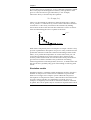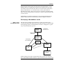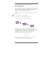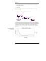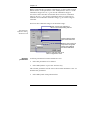
1
ModelMaker User Manual Cherwell Scientific Limited The Magdalen Centre Oxford Science Park Oxford OX4 4GA United Kingdom 04/00 End User License End User License Agreement 1. LICENSE 1.1. Cherwell Scientific Limited of The Magdalen Centre, Oxford Science Park, Oxford OX4 4GA (“Cherwell”) hereby grants you a non-exclusive license (“License”) to use the software accompanying this license (“Software”) and the accompanying documentation on the following terms. 1.2. The copyright and all other rights in the Software and the accompanying documentation remain with Cherwell. 2. ACCEPTANCE 2.1. You are deemed to accept the terms of this License if you install the Software on a computer. 2.2. If you do not wish to accept these terms, you must within 30 days of purchase erase any installation file, and any copy of the Software and documentation you have downloaded or stored on any medium and return any copies of the CD, manuals and packaging to Cherwell together with proof of purchase for a full refund. 3. SCOPE OF LICENSE 3.1. This License permits you to: 3.1.1. use the Software on a single computer or on a networked computer drive; 3.1.2. transfer the Software to someone else, provided that you assign all of your rights and obligations under this License to such other person, you erase all copies of the Software under your control and stored on any medium (including the hard disk copy and any backup copy), and the other person agrees to the terms of this License; 3.1.3. make one copy of the Software for back-up purposes only, which copy must reproduce and include this License in full. 3.2. You shall not: 3.2.1. use or copy the Software other than as permitted by this License; 3.2.2. at any time allow more users than stated in your sales invoice to access or use the Software concurrently; 3.2.3. modify, adapt, merge, translate, decompile, disassemble, or reverse engineer the Software, except as permitted by law; 3.2.4. use, sell, assign, rent, sub-license, loan, mortgage, charge or otherwise deal in any way in the Software or the accompanying documentation or any interest in them or under this License except as expressly provided in this License. ModelMaker iii End User License 4. TERM 4.1. Unless terminated under clause 4.2 this License shall last for as long as you continue to use the Software. 4.2. This License shall terminate automatically if you fail to abide by any of its terms. 4.3. Upon termination of this License you shall destroy the Software and its accompanying documentation and shall erase all copies of the Software under your control and stored on any medium (including the hard disk copy and any backup copy). 5. WARRANTIES AND REMEDIES 5.1. Cherwell warrants that the storage media on which the Software is supplied will be free from defects in materials and workmanship under normal use for a period of 90 days after the date of original purchase. If a defect in any disk occurs during such period you may return it with proof of purchase to Cherwell who will replace it free of charge. 5.2. Cherwell warrants that the Software will perform substantially in accordance with its accompanying documentation (provided that the Software is properly used on the computer and with the operating system for which it was designed) and that the documentation correctly describes the operation of the Software in all material respects. If Cherwell is notified of any material error in the Software during the period of 90 days after the date of original purchase it will correct any such error within a reasonable time or (at its option) refund the price of the Software (against return of the Software and its documentation). 5.3. The warranties set out in clauses 5.1 and 5.2 are your sole warranties and are in place of all warranties conditions or other terms expressed or implied by statute or otherwise, all of which are hereby excluded to the fullest extent permitted by law. Clauses 5.1 and 5.2 also set out your sole remedies for any breach of Cherwell's warranties. 5.4. In particular Cherwell does not warrant that the Software will meet your requirements or that the operation of the Software will be uninterrupted or error free or that all errors in the Software can be corrected. You load and use the Software at your own risk and in no event will Cherwell be liable to you for loss or damage of any kind (except personal injury or death resulting from Cherwell's negligence), including lost profits, consequential or other loss arising from the use of or inability to use the Software or from errors or deficiencies in it whether caused by negligence or otherwise, in excess of 125% of the price paid for the Software, except as expressly provided in this License. iv ModelMaker End User License 5.5. If you deal as a consumer as defined in the Unfair Contract Terms Act 1977, your statutory rights remain unaffected. 6. SUPPORT Cherwell’s technical support staff will endeavour to answer any queries you may have about the Software. Support contact details are given in the Schedule. 7. LAW This License constitutes the entire agreement between you and Cherwell relating to the Software and is governed by and construed in accordance with the laws of England. The courts of England shall have exclusive jurisdiction. SCHEDULE Technical support is available directly from the ModelKinetix web site at http://www.modelkinetix.com/support. Our web support database is constantly updated and we strongly urge you to explore the support options here before calling us. In the unlikely event that you cannot find your answer on our web support database, please call our UK office directly on +44 (0)1865 784800 between the hours of 9.30 and 17.30 UK time Monday to Friday inclusive (excluding UK public holidays). Telephone calls will be logged in our support system and you will be contacted by e-mail, fax, or telephone with a solution or a request for more information. E-mail support queries should be sent to [email protected]. ModelMaker v Copyright and Technical Support Copyright © 2000 Cherwell Scientific Limited. All rights reserved. No part of this publication or the program ModelMaker may be reproduced, transmitted, transcribed, stored in a retrieval system, or translated into any language or computer language in any form or by any means electronic, mechanical, magnetic, optical, chemical, manual, biological or otherwise, without prior written permission of the publisher. Publisher ModelMaker is published by: Cherwell Scientific Limited The Magdalen Centre Oxford Science Park, Oxford OX4 4GA Disclaimer Trademarks ModelKinetix.com web site Cherwell Scientific make no representations or warranties with respect to the contents hereof and specifically disclaims any implied warranties of merchantability or fitness for any particular purpose. All trademarks and registered trademarks are the property of their respective companies For technical support, Frequently Asked Questions (FAQs) or product information, please visit our web site at: http://www.modelkinetix.com Technical Support Technical support is available directly from the ModelKinetix.com web site at http://www.modelkinetix.com - simply follow the links to Support. Our Web support database is constantly updated and we strongly urge you to explore the support options here before calling us. In the unlikely event that you cannot find your answer, then please e-mail us ([email protected]) or call our UK office on +44 (0)1865 784800 during normal office hours. Telephone calls will be logged in our support system and you will be contacted subsequently with a solution or request for more information by e-mail, fax, or phone. ModelMaker vii Contents Contents INSTALLATION AND LICENSING....................................................1 DESKTOP INSTALLATION .........................................................................1 NETWORK INSTALLATION .......................................................................3 ABOUT THIS MANUAL........................................................................5 CONVENTIONS USED IN THIS MANUAL ....................................................5 1. INTRODUCTION ...............................................................................7 EMPIRICAL MODELS ................................................................................7 SIMULATION MODELS .............................................................................8 DEVELOPING A MODELMAKER MODEL ...................................................9 2. MODELMAKER TUTORIAL .......................................................... 13 STEP 1: PLANNING YOUR MODEL .......................................................... 13 STEP 2: ADDING COMPARTMENTS ......................................................... 14 STEP 3: ADDING FLOWS ........................................................................ 15 STEP 4: ADDING PARAMETERS .............................................................. 16 STEP 5: RUNNING YOUR MODEL ............................................................ 17 STEP 6: DISPLAYING TABLES .................................................................. 17 STEP 7: DISPLAYING GRAPHS ................................................................ 18 STEP 8: ADDING VARIABLES .................................................................. 19 STEP 9: ADDING INFLUENCES................................................................ 20 STEP 10: DEFINING CONDITIONAL COMPONENTS .................................. 21 STEP 11: ADDING DEFINED VALUES AND INDEPENDENT EVENTS ........... 23 STEP 12: ADDING COMPONENT EVENTS ................................................ 25 STEP 13: LOOKUP TABLES ...................................................................... 27 STEP 14: RUNNING SENSITIVITY ANALYSIS ............................................ 29 STEP 15: COMPARING THE MODEL WITH OBSERVED DATA..................... 31 STEP 16: OPTIMIZATION........................................................................ 33 STEP 17: MINIMIZATION ....................................................................... 35 STEP 18: MONTE CARLO ANALYSIS ....................................................... 37 3. VIEWS AND TOOLBARS................................................................ 41 THE MODEL EXPLORER ......................................................................... 41 VIEWS ................................................................................................... 41 TOOLBARS............................................................................................. 44 4. BASICS............................................................................................... 47 STARTING MODELMAKER..................................................................... 47 CLOSING MODELMAKER ...................................................................... 47 ModelMaker ix Contents OPENING A MODEL ............................................................................... 48 CLOSING A MODEL ................................................................................ 48 SAVING A MODEL .................................................................................. 49 SENDING A MODEL AS AN E-MAIL ......................................................... 49 PASSWORD PROTECTION ....................................................................... 50 PRINTING FROM MODELMAKER ........................................................... 50 ARRANGING WINDOWS......................................................................... 51 MODELMAKER HELP ............................................................................ 51 MODELMAKER ON THE WEB ................................................................ 52 MODELMAKER USER GROUP ................................................................ 52 5. WORKING WITH MODELS ........................................................... 53 ADDING COMPONENTS ......................................................................... 53 DEFINING COMPONENTS ....................................................................... 55 FINDING COMPONENTS ......................................................................... 55 SYMBOL SCOPE ...................................................................................... 56 CONFIGURING RUN SYMBOLS ................................................................ 57 COMPONENT DESCRIPTION ................................................................... 57 COMPONENT INFORMATION ................................................................. 58 COMPONENT BITMAP IMAGE ................................................................. 58 COMPONENT SHADING ......................................................................... 59 TEXT BOXES ........................................................................................... 59 SELECTING COMPONENTS ..................................................................... 60 MOVING COMPONENTS......................................................................... 61 FORMATTING COMPONENTS ................................................................. 61 USING THE CLIPBOARD ......................................................................... 62 SCROLLING AND ZOOMING THE MODEL DIAGRAM ................................ 63 SETTING USER PREFERENCES ................................................................. 63 6. COMPONENTS – COMPARTMENTS, FLOWS, VARIABLES AND DEFINED VALUES .................................................................... 65 COMPARTMENTS ................................................................................... 65 FLOWS .................................................................................................. 65 VARIABLES ............................................................................................ 66 DEFINED VALUES .................................................................................. 66 DEFINING UNCONDITIONAL AND CONDITIONAL COMPONENTS............ 67 DEFINING ARRAYS OF COMPONENT ELEMENTS ..................................... 69 7. COMPONENTS – LOOKUP TABLES AND LOOKUP FILES..... 73 LOOKUP SERIES ..................................................................................... 73 CONFIGURING LOOKUP FILES ................................................................ 74 CONFIGURING LOOKUP TABLES............................................................. 76 USING THE LOOKUP TABLE VIEW .......................................................... 77 x ModelMaker Contents CHANGING A LOOKUP DATA SOURCE ................................................... 78 8. COMPONENTS – INDEPENDENT AND COMPONENT EVENTS.................................................................................................. 81 EVENT TRIGGERS ................................................................................... 81 EVENT ACTIONS .................................................................................... 81 EVENT CALCULATION ORDER................................................................ 82 DEFINING EVENTS ................................................................................. 83 9. COMPONENTS – SUB-MODELS, DELAYS AND DLL FUNCTIONS.......................................................................................... 93 SUB-MODELS ......................................................................................... 93 DELAYS ................................................................................................. 97 DLL FUNCTIONS ................................................................................... 98 DLL EVALUATION ORDER ................................................................... 101 10. PARAMETERS .............................................................................. 103 USING THE PARAMETER VIEW ............................................................. 103 DEFINING PARAMETERS ...................................................................... 104 ARRAYS OF PARAMETERS .................................................................... 107 11. RUNNING A MODEL .................................................................. 109 CONFIGURING RUN OPTIONS .............................................................. 109 CONFIGURING THE INTEGRATION METHOD ........................................ 110 CONFIGURING A REPEATED RUN ......................................................... 112 CONFIGURING SENSITIVITY ANALYSIS ................................................. 113 RETAINED SERIES ................................................................................ 114 12. GRAPHS......................................................................................... 117 CREATING GRAPHS ............................................................................. 117 CUSTOMIZING GRAPHS ....................................................................... 118 GRAPH CROSS-HAIRS .......................................................................... 124 ARCHIVING GRAPHS ........................................................................... 125 SAVING A GRAPH AS A TEXT FILE ......................................................... 125 RENAMING GRAPH SUB-VIEWS ............................................................ 126 13. TABLES .......................................................................................... 127 CREATING TABLES............................................................................... 127 CUSTOMIZING TABLES......................................................................... 128 ARCHIVING TABLES ............................................................................ 129 SAVING A TABLE AS A TEXT FILE .......................................................... 130 RENAMING TABLE SUB-VIEWS ............................................................. 130 ModelMaker xi Contents 14. OPTIMIZATION........................................................................... 131 USING THE MODEL DATA VIEW .......................................................... 131 CONFIGURING OPTIMIZATION ............................................................ 133 OPTIMIZATION SETTINGS .................................................................... 134 ADVANCED OPTIMIZATION SETTINGS ................................................. 135 OPTIMIZATION RESULTS ...................................................................... 138 15. MINIMIZATION .......................................................................... 141 USING THE SAMPLE POINTS VIEW ....................................................... 141 CONFIGURING MINIMIZATION ............................................................ 142 THE PARAMETER RESULTS VIEW ......................................................... 143 ARCHIVING RESULTS ........................................................................... 143 ADVANCED MINIMIZATION CONFIGURATION ..................................... 144 16. MONTE CARLO ANALYSIS....................................................... 145 CONFIGURING MONTE CARLO ANALYSIS ........................................... 145 CREATING HISTOGRAMS ..................................................................... 147 MONTE CARLO STATISTICS ................................................................. 148 INDEX .................................................................................................. 151 xii ModelMaker Installation and licensing Installation and Licensing ModelMaker can be installed as a ‘desktop’or a ‘network’version. The desktop version is standard and should be chosen by most users. The network version is for installations where multiple linked workstations will be accessing the same data, and requires the purchase of more than one license. Desktop installation Installing ModelMaker • Insert the ModelMaker CD into your CD-ROM drive The installation routine should run automatically. If it does not, you must locate and run autorun.exe: • Open Windows Explorer or My Computer • Navigate to D:\ (where D is the name of your CD drive) • Locate and double click autorun.exe to run the installation The ModelKinetix CD menu will open. • Select Install ModelMaker 4 You will then be given 2 installation choices: 1. Install ModelMaker on your desktop 2. Install ModelMaker on your network • Select option 1 and follow the on-screen instructions. You must run the desktop version of ModelMaker from your local drive, e.g. C:\. By default, the installer suggests the directory: C:\Program Files\Cherwell Scientific\ModelMaker 4 Registering and licensing ModelMaker When ModelMaker is first run following installation, it runs as a fully functioning demo that will expire after 30 days. You must register your copy of ModelMaker with Cherwell Scientific in order to ModelMaker 1 Installation and licensing continue using it after 30 days. ModelMaker can be registered at any time during the demo or even after the demo has expired. • Select Help|About ModelMaker to open the About ModelMaker dialog box • Click User Details to open the User Details dialog • Enter your User Name, Organization name and your ModelMaker Serial Number Note that if you do not have a ModelMaker Serial Number this entry can be left blank. • Click OK • Click Licensing to open the Licensing dialog and note the settings in the following table: Serial Number User Name Organization User Code 1 User Code 2 To complete your license registration, you must contact Cherwell Scientific to obtain your Activation Codes: • Open the modelkinetix.com web site: http://www.modelkinetix.com • Navigate to Support and follow the on-line instructions Alternatively, you can e-mail us ([email protected]) or, if you don’t have internet access, telephone our UK office. When you have obtained your Activation Codes: 2 ModelMaker Installation and licensing • Enter the 2 Activation Codes in the License Control dialog box • Click OK Your copy of ModelMaker will now be fully licensed. Network installation This installation should only be attempted by network administrators. Both the server and client installations require administrator privileges. It is important to follow the correct installation sequence: A. Install ModelMaker on your server B. Install ModelMaker on your client workstations C. Run ModelMaker from one of the client workstations (NOT the server) and activate licensing Installing ModelMaker • Insert the ModelMaker CD and run autorun.exe as described for a desktop version • Select Install ModelMaker 4 You will be given 2 installation choices: 1. Install ModelMaker on your desktop 2. Install ModelMaker on your network • Select option 2 to install the network version of ModelMaker You will be given 2 further choices: 1. Install ModelMaker on your network server 2. Install ModelMaker shortcuts and drivers on a network workstation • Select option 1 to install ModelMaker to your desired network directory ModelMaker 3 Installation and licensing • Run option 2 on every client workstation that will run ModelMaker over the network When ModelMaker is first run following installation, it must be run from a client workstation. It will detect that it is being invoked from a network client and set itself up as a network version. The network license is then enabled which allows ModelMaker to be run from any workstation on your network. Note that the installation will fail if ModelMaker is first run from the server. Registering and licensing ModelMaker • Register and license your network copy of ModelMaker as described for a desktop version This information will be stored in the network license file and will be retrieved by whichever workstation is running the application. Extra licenses can be bought at any stage for additional client workstations. 4 ModelMaker About this manual About this Manual This manual will guide you through ModelMaker’s comprehensive range of features. The accompanying Reference Manual contains mathematical theory and additional reference information. Chapter 1 is a brief introduction to model design and will be of interest to users with little or no previous experience of creating and using models. Chapter 2 is a tutorial, for users who are new to ModelMaker. In this chapter, we describe the layout of the interface, the construction of a simple model and some basic ModelMaker functions. Chapters 3 to 16 make up the bulk of the manual and explain how ModelMaker’s tools and features work – running the application, using the interface, model building and running, graphs, tables and analysis techniques. Conventions used in this manual • Program menu commands are referred to as File|Open, for example, meaning select Open from the File menu. • Angled brackets are used to refer to keyboard characters. For example, <Esc> means press the Escape key, <Ctrl+C> means hold down the Control key whilst pressing C, <Alt, F,O> means press the Alt key followed by F then O. • LMB refers to the Left Mouse Button and RMB refers to the Right Mouse Button menu. For example, RMB|Parameters means click the right mouse button within the Model Viewer panel and select Parameters from the menu. In ModelMaker, there are typically several ways to access dialog boxes and features. These methods include toolbars, program menus, the Right Mouse Button (shortcut) menu and keyboard shortcuts. In general, only toolbar icons and program menus have been documented in this manual. However, the shortcut menu will also access many ModelMaker functions. Note that the appearance of the shortcut menu depends on the area or component that is clicked. See the ModelMaker Reference Manual for a list of keyboard shortcuts. ModelMaker 5 Chapter 1 1. Introduction A model is a quantitative description of a real-life process or system, and is typically composed of mathematical equations which give numerical answers. These answers can be substantiated against factual data to test the accuracy of a model. If a model is accurate, it can be used to make predictions. In the next section, some of the important differences between empirical models and mechanistic or simulation models are discussed. Empirical models If you have some observed data for an event which shows how it varies in relation to another factor, then it is often possible to develop an empirical model which describes this variation. For example, in the temperate zone of the northern hemisphere, the mean monthly temperature varies during the year in a manner similar to that shown in the graph below: Celcius 15 Temperature 10 5 0 0 3 6 Months 9 12 The points on this graph provide some useful information, graphically summarizing the annual fluctuations. The data can be described further by ‘fitting’a mathematical function using statistical methods, as shown in this case with a sine function. The parameters of the sine function are estimated by minimizing the deviations of the curve from the data points. This is often a useful exercise, as the resulting fitted equation can provide a useful summary of the data, although in many cases the nature of the equation has no physical meaning. In other words, the choice of function is quite arbitrary; we simply choose something of the right general shape. However, this is not always the case; sometimes the function used is dictated by some underlying theory whose parameters are unknown. In such cases, the fitting Introduction 7 Chapter 1 process takes on new meaning as we are estimating parameters which have some physical meaning based on theory. The ‘goodness of fit’ gives us some idea of how good the theory is. For example, radioactive decay is described by the equation: N = N 0 exp(− λt ) where N is the amount of radioactive material left at time t, if there was N0 at time t = 0 and the decay constant of the radioactive material concerned is λ. This decay constant can be estimated by making observations of the count rate from the radioactive source at various times and then fitting the above equation to the data. Count Rate 100 Sample 1 80 60 40 20 0 0 20 40 60 80 100 Days Both of these empirically derived examples are simple ‘models’. They provide a quantitative description of a process. They could be used to predict the amount of radioactive material remaining at times in the future, or to predict the temperature at various times next year. Of course the predictions may not be perfect as they depend on the accuracy of the model. In the case of radioactive decay, the model is good and we could be confident of its predictions. Predicting meteorological factors like temperature, however, is much harder and the sine model is probably only good at describing overall long term trends. Simulation models Simulation models, sometimes called mechanistic models, describe a number of sub-processes which can be combined to represent the behavior of a larger more complex system. Often the sub-process descriptions are empirical in nature, rather like those described in the previous section, but they are combined in a realistic way. For example, we might try to model how radioactive fallout is adsorbed by plants. The rate of uptake may be assumed to depend on the rate of 8 Introduction Chapter 1 plant growth, which in turn will depend upon temperature, so the model will have a temperature sub-process similar to the previous sine model. Our model will also have to account for the radioactive decay of the fallout, so we will also have a decay sub-model as described previously. These sub-processes would be combined with other relevant considerations to produce a model which simulates the overall system. ModelMaker is intended primarily for developing simulation-type models rather than more statistically oriented empirical models. Developing a ModelMaker model Step 1: Your conceptual model The first step in model development is to plan your model. Let’s consider the important stages involved in the transfer of radiocaesium from grazing systems to the human food chain. A diagram is a good way to understand this process: Nuclear Release BOMB TEST CHERNOBYL ETC ATMOSPHERIC TRANSPORT Deposited on vegetation surface WEATHERING LEAF TURNOVER Absorbed by plants ROOT UPTAKE Grazing Animals Soil Humans In this example, the major components of the system are shown as boxes and radiocaesium transfer is represented by arrows. In fact each Introduction 9 Chapter 1 of the boxes represents a complex system in its own right and it may be appropriate to further divide some of them into sub-components. The next step is to identify the real-life processes at work. For example, radiocaesium deposited on the leaves of vegetation will be transferred to the soil via two real-life processes – weathering where radiocaesium is washed off by rain, and leaf turnover where leaves die and fall to the ground. Step 2: Developing mathematical relationships Each component will require an equation in terms of other components within the model, or externally input data and parameters. The equations needn’t be very complicated, but generally require some consideration of the physical processes at work. Consider the example of radiocaesium weathering from a leaf surface, a process that must be dependent on rainfall. A simple first assumption might be that it is proportional to rainfall: weathering ∝ rainfall As such, this equation can’t be implemented in ModelMaker, so a weathering coefficient could be introduced to turn the proportionality into an equation: weathering = W ×rainfall The value of W can be estimated from our knowledge of the weathering process, and adjusted in relation to observed data. It may also be appropriate to undertake experimental work to estimate W directly. In developing this relationship, two new factors have been introduced to the model - the parameter W and rainfall. Rainfall may be calculated in the model but is more likely to be input from external data. It is often the case that new relationships can only be added to the model if new components are also introduced. The implementation of mathematical relationships is a very thorough process in which every system in your model must be quantified. In some cases the relationships may be well established, and come straight from a textbook. Often, as in the example used here, the processes are only poorly understood meaning that highly empirical relationships have to be used. 10 Introduction Chapter 1 Step 3: Implementing your model ModelMaker is designed to mimic the process of conceptual model development as much as possible. The first step involves constructing a diagram on the screen which represents the various model parts. This diagram is composed of a series of ModelMaker components, each of which is intended for a different type of mathematical operation. Each component has a definition which can be edited to insert its equation and any other appropriate information. The next steps Once your model has been implemented, it can be run; the equations are solved, generating results that can be interpreted in graphs or tables. Validation of your model may involve checking the model results against observed data to test its predictive power. ModelMaker provides a series of facilities to make this as straightforward as possible. In practice model development is often very iterative. Having tested the model you are likely to find that some changes are required. Introduction 11 Chapter 2 2. ModelMaker Tutorial This tutorial will introduce you to ModelMaker’s interface and to many of its main features. The step-by-step instructions will take you through the construction of a simple illustrative example – the flow of chemical contaminants through a water system. ModelMaker opens with an empty model window called noname00.mod. ModelMaker’s interface is divided into two panels – the Model Explorer on the left and the Model View on the right. The Model Explorer presents a tree view of the many views that make up a model, and provides an easy way to navigate your model. noname00.mod opens with only one active view – the Diagram view (Main) where models are created and defined. More views are added to the Model Explorer as a model is built and analyzed. Step 1: Planning your model We are going to construct a model that represents the flow of pollutants through a simple water system that consists of two lakes connected to the sea by a river and an estuary. Lake 1 River Lake 2 Estuary Sea We shall make the following assumptions: 1. The water level in the lakes is at equilibrium, so the effects of pollutant dilution can be ignored. 2. The amount of pollutant flowing through the river and the estuary is proportional to the amount of pollutant in the lake at their source: ModelMaker tutorial 13 Chapter 2 • The flow of pollutant in the river = 0.1 × the amount of pollutant in the top lake. • The flow of pollutant in the estuary = 0.05 × the amount of pollutant in the bottom lake. 3. 1000 units of pollutant are dumped in the top lake at time (t) = 0. Step 2: Adding compartments We shall start the model by adding compartments to the Diagram view (Main). A compartment is a container in a model and is defined in terms of what is entering and leaving it. See Chapter 6: Components – Compartments, Flows, Variables and Defined Values. Compartments appear in model diagrams as rectangular boxes. • Click the Compartment icon on the toolbar • Add a compartment (C1) by moving the cursor to the desired location in the model diagram and clicking with the Left Mouse Button (LMB) • Repeat the above steps to add two more compartments (C2 and C3) The three compartments are filled with blue lines, indicating that the compartment equations are undefined. The properties of a model component are defined in its component definition dialog box. • Double click C1 with the LMB to open its definition dialog box • Enter Lake1 in the Symbol edit box and 1000 in the Initial Value edit box • Click OK to close the dialog • Double click C2 • Enter Lake2 in the Symbol edit box • Click OK 14 ModelMaker tutorial Chapter 2 • Repeat for C3, entering Sea in the Symbol edit box Step 3: Adding flows Flows represent the transport of a quantity from one compartment to another, and are used in conjunction with compartments to build up systems of differential equations. See Chapter 6: Components – Compartments, Flows, Variables and Defined Values. We shall add two flows to our model to represent the river and the estuary. • Click the Flow icon on the toolbar • Click Lake1 with the LMB followed by Lake2 • Repeat to create a flow between Lake2 and Sea Lake1 F1 Lake2 F2 Sea The equations of the compartments are automatically updated to reflect the presence of the flow. Thus, the blue shading of the compartments is removed, but now the flow is shaded red to indicate an equation error. This is because flow is defined as being proportional to the value of its source compartment: F1 = ? * Lake1 F2 = ? * Lake2 ? represents an as yet unknown value. We shall define ? as a parameter and then complete the flow definition. ModelMaker tutorial 15 Chapter 2 Step 4: Adding parameters Parameters represent constant values within a model. Their values cannot be changed from within a model but can be adjusted during certain model analysis procedures. See Chapter 10: Parameters. Parameters are added to a model from the Parameters view. • Click the Parameters icon The Parameters view is created and activated. This view is divided into six columns – Name, Value, Optimize, Minimize, Monte Carlo and Dist Type. • Click the Parameter icon on the Parameters toolbar A new parameter, p1, is added to the Parameters view. • Repeat to add a second parameter, p2 • Double click p1 to open its definition dialog • Enter river_rate in the Symbol edit box and 0.1 in the Value edit box • Click OK • Repeat for p2, entering estuary_rate and 0.05 in the Symbol and Value edit boxes Now we can complete the flow definition: • Activate the Diagram view (Main) by selecting it in the Model Explorer • Double click F1 to open its definition dialog box • Enter River in the Symbol edit box and river_rate * Lake1 in the Equation edit box (i.e. select ? and double click river_rate in the Available Components list box) • Click OK 16 ModelMaker tutorial Chapter 2 • Repeat for F2, entering Estuary in the Symbol edit box and estuary_rate * Lake2 in the Equation edit box Once the flows have been updated, the model diagram should not contain any blue or red shading, indicating that ModelMaker can find no errors in the model definition and that the model is ready to run. Step 5: Running your model The model is now ready to run. This is the process of solving the equations over the desired range of the model’s independent variable. See Chapter 11: Running Models. By default, ModelMaker’s independent variable is time, t. All equations are solved over a range of values for t, and all equations are written with respect to t. • Click the Integrate icon The Run dialog box opens. ModelMaker runs a model from t = 0 to t = 100 by default, and calculates values 100 times during the model run. • Click OK The model is run with the default options. When the calculations are complete a message appears stating how long the calculation has taken. This simple model should only take a fraction of a second. Click OK to dismiss this dialog. Step 6: Displaying tables Tables provide access to the values calculated by ModelMaker during a model run. See Chapter 13: Tables. We shall create a table of Lake1 and Lake2 against time. • Click the Table icon The Table Selection dialog box opens. • Select Lake1 and Lake2 in the Components list box (i.e. use <Ctrl> or <Shift> to make multiple component selections) • Click >> to move Lake1 and Lake2 into the Selected list box The independent variable, t, is selected by default. ModelMaker tutorial 17 Chapter 2 • Click OK The Results view is created and activated with a sub-view Table1 which contains your model’s data. Tables can be customized using the Table Series dialog box. To open this dialog: • Click the Series icon on the Tables toolbar This dialog is used to change column titles and apply different numeric formats. Click OK to close the dialog. Step 7: Displaying graphs Graphs represent a useful way of examining data trends. See Chapter 12: Graphs. We shall plot a graph of Lake1 and Lake2 against time. • Click the Graph icon The Graph Selection dialog box opens. • Select Lake1 and Lake2 in the Components list box • Click >> to move Lake1 and Lake2 into the Vertical Axis list box By default, ModelMaker plots the graph against the independent variable. • Click OK The completed model up to this point is “tutor1.mod” A new graph is added to the Results view as Graph1. Many of the graph’s properties can be customized in the Graph Series Options, 18 ModelMaker tutorial Chapter 2 Graph Attributes Configuration, X-Axis Configuration and Y-Axis Configuration dialog boxes. These dialogs can all be accessed from the Graph toolbar by clicking the Series, Attributes, X-Axis and Y-Axis icons respectively. Step 8: Adding variables We shall now assume that there is a continuous discharge of pollutant into Lake1 in addition to the initial dumping incident. We will define the discharge as a variable component, where: t ×π Discharge = 25 ×sin 365 A variable is a value which is calculated as the model is run, according to its equation. See Chapter 6: Components – Compartments, Flows, Variables and Defined Values. Before adding the variable, we will add a new parameter, π(pi), to our model. To follow this example load the model “tutor1.mod” • Activate the Parameters view by selecting it in the Model Explorer • Add a new parameter with the symbol pi and the approximate value 3.1415927 Now we can define the variable, Discharge: • Activate the Diagram view (Main) by selecting it in the Model Explorer • Add a variable, V1, to your model • Double click the variable to open the Variable Definition dialog box • Enter Discharge in the Symbol edit box and 25*sin(t*pi/365) in the Equation edit box • Click OK The next step in our model definition is to tell ModelMaker that Lake1 will use the value of the Discharge variable. This is done by using an influence. ModelMaker tutorial 19 Chapter 2 Step 9: Adding influences • Select the Influence icon • Click Discharge followed by Lake1 The influence is inserted between the two components. Lake1 River Lake2 Estuary Discharge Sea Next we must update the equation of the Lake1 compartment to take account of the Discharge variable. • Double click Lake1 to open its definition dialog box • Update the Equation edit box to read Discharge – River Select the graph of Lake1 and Lake2 and re-run the model. The amount of pollutant now increases towards the end of the run, as the pollutant discharge increases. The completed model up to this point is “tutor2.mod” 20 ModelMaker tutorial Chapter 2 Step 10: Defining conditional components Up to this point, all the components we have created have had only one equation, which has been evaluated throughout the model run. This is fine for most continuous models, but often things change as the model progresses. For our model, for example, let’s assume that when the level of pollutant in Lake2 reaches 250 units, the discharge in the lake is reduced to a value given by the following equation: t ×π Discharge = 10 ×sin 365 To deal with this, we can make Discharge a conditional component. (See Chapter 6: Components – Compartments, Flows, Variables and Defined Values). Instead of having a single equation, a conditional component has a list of conditions with associated equations. ModelMaker evaluates each condition in turn until it finds a condition which is true and uses the associated equation to evaluate the component. To follow this example load the model “tutor2.mod” In our new model, the value of Discharge will be influenced by the value of Lake2, so we must insert a new influence between Lake2 and Discharge. • Add an influence from Lake2 to Discharge Now we can define Discharge as a conditional component. • Double click Discharge to open its definition dialog box • Click Conditional… The Conditional Variable Definition dialog box opens. Initially, the conditional component is defined with a single default condition. Default or empty conditions are always defined as true. • Click New The Conditional Equation dialog box opens. ModelMaker tutorial 21 Chapter 2 • Enter Lake2>250 in the Condition edit box and 10*sin(t*pi/365) in the Equation edit box • Click OK The new conditional equation is inserted into the Condition and Equation list boxes. • Click OK to close the definition dialog box Lake1 River Lake2 Discharge Estuary Sea Select the graph of Lake1 and Lake2 and re-run the model. The graph now shows the effect of switching the rate of discharge as the amount of pollutant in Lake2 changes. Create a new graph of the value of Discharge to see how the conditional component changes during the model run. The completed model up to this point is “tutor3.mod” 22 ModelMaker tutorial Chapter 2 Step 11: Adding defined values and independent events A defined value is calculated only at the start of a model run, or in response to the actions of an event. This means that they are very useful for holding values which do not change very often, or which change only in a discontinuous manner. See Chapter 6: Components – Compartments, Flows, Variables and Defined Values. We shall use a defined value to hold the discharge level which is changed by an event. ModelMaker provides two types of event to cater for discontinuous models – independent and component events; events can adjust model component values. See Chapter 8 – Independent and Component Events. Let’s assume that the pollutant discharge rate in our model follows a regular pattern: every week it switches between 25 kgd-1 and 10 kgd-1. To model this behavior we will replace the variable Discharge with a defined value (also called Discharge) and an independent event. To follow this example load the model “tutor3.mod” • Select the Discharge variable and press <Delete> Discharge and the influences connecting it to Lake1 and Lake2 are deleted. • Add a defined value, D1 • Double click D1 to open its definition dialog box • Enter Discharge in the Symbol edit box and 25 in the Equation edit box • Click OK • Add an independent event, E1 • Insert three new influences between Discharge and Lake1, Discharge and E1, and E1 and Discharge ModelMaker tutorial 23 Chapter 2 Independent events are triggered at pre-determined values of the independent variable. Such triggers can be periodic or non-periodic. • Double click E1 to open its definition dialog box • In the Definition tab, enter Switch in the Symbol edit box, set Initial Status to Active and set Event Class to Reactivate • Select the Triggers tab The Triggers tab defines when the event will be triggered. • Select Periodic Trigger • Enter 7 in the Period edit box and 7 in the Starting At edit box • Select the Actions tab The Actions tab defines what will happen when the event is triggered. We want to say: If the value of Discharge is 25 Set Discharge to 10 Otherwise Set Discharge to 25 To define this action, we can use the if… else statement. • Define the action as shown below: Everything to the right of a double slash ‘//’is a comment and is ignored by ModelMaker. • Click OK to close the dialog 24 ModelMaker tutorial Chapter 2 Lake1 River Lake2 Estuary Discharge Sea Switch This completes the definition of the independent event. Re-running the model results in a zigzag pattern of pollutant discharge as the initial dumping fades away. The completed model up to this point is “tutor4.mod” Step 12: Adding component events Component events and independent events differ only in the way they are triggered. Component events are triggered when a defined condition becomes true. ModelMaker uses a tolerance value to ensure that component events are triggered correctly. See Chapter 8 – Independent and Component Events. We shall now assume that when the pollutant level in our model reaches 400 kg, a chemical treatment is applied to the lake which removes 150 kg of pollutant from the water. This event will be triggered within one hour of the pollutant level becoming too high. The tolerance will therefore be set to 1/24 = 0.042. ModelMaker tutorial 25 Chapter 2 To follow this example load the model “tutor4.mod” The next stage in developing the model is to insert a new component event. The model also requires two new influences between Lake2 and the event because the event both tests and adjusts the value of Lake2. • Add a component event, E1 • Add two influences between Lake2 and E1, and E1 and Lake2 Lake1 Treatment River Lake2 Estuary Discharge Sea Switch • Double click E1 to open its definition dialog box • In the Definition tab, enter Treatment in the Symbol edit box • Select the Trigger tab • Enter Lake2>400 in the Condition edit box and 0.042 in the Tolerance edit box • Select the Actions tab • Enter Lake2 = Lake2 – 150; in the edit box Re-run the model. The graph of Lake2 shows the zigzag trace of the pollutant treatments. 26 ModelMaker tutorial Chapter 2 The completed model up to this point is “tutor5.mod” Step 13: Lookup tables Suppose that somebody has actually gone out to Lake1 and measured the pollutant discharge rate on the first day of each week. Instead of using the regular pattern of discharge assumed so far, we can use this new information to get a more accurate picture of what is going on. We will use a lookup table component (Chapter 7: Components – Lookup Tables and Lookup Files) to add the following table of data to our model: To follow this example load the model “tutor5.mod” Time (days) 0 7 14 21 28 35 42 49 56 63 70 77 84 91 98 105 Discharge rate (kgd-1) 25 12 30 20 50 4 65 15 20 3 45 17 21 10 8 2 • Delete the Switch event and the Discharge defined value ModelMaker tutorial 27 Chapter 2 • Add a lookup table, T1 • Add an influence between T1 and Lake1 • Double click T1 to open its definition dialog box • In the Table tab, enter Data in the Symbol edit box • Select the Series tab Treatment Lake1 River Lake2 Data Estuary Sea We must create a lookup series for every column of data in the table so that ModelMaker knows what the data represents. The first column of data contains observation times. We will define this column as a ‘control’series because ModelMaker uses this column to control which value is drawn from the discharge rate column. We will define the second column as ‘controlled’because it is controlled by time. • Select Series1 in the Lookup Series list box and enter t in the Series Symbol edit box ModelMaker assumes that the first column is a control series. • Click Define to complete the definition of the first series • Select Series2 in the Lookup Series list box and enter Discharge in the Series Symbol edit box ModelMaker assumes that the second column is controlled by t. 28 ModelMaker tutorial Chapter 2 There is not a data point for every day of the year, so if we want to know what the discharge rate is on day 65, for example, we must use interpolation. The default method is linear interpolation where the data takes a straight line between data points. In our model, we will assume that the discharge rate on day 65 is the same as on day 63, i.e. we will use start value interpolation. • Select the Interval Start interpolation method • Click Define to complete the definition of the second series • Click the View Data button The Lookup Tables view is created and activated with the sub-view Data. Data contains an empty sheet called Page 1 with the column headers t and Discharge. This is where the lookup table data are entered. • Enter the lookup table data We can now re-run the model. The new graph of Lake2 shows that there is actually more pollutant reaching the bottom lake than we had assumed, and that the chemical treatment is being applied much more often. The completed model up to this point is “tutor6.mod” Step 14: Running sensitivity analysis When developing or analyzing a model it is often useful to investigate the effect of altering aspects of the model. Sensitivity analysis allows the effect of systematic parameter adjustment on the values of selected components to be investigated. See Chapter 11: Running Models. In our ModelMaker tutorial 29 Chapter 2 model, we shall investigate the effect of adjusting river_rate from 0.05 to 0.09. To follow this example load the model “tutor6.mod” Sensitivity analysis is configured in the Run Options dialog box. • Click the Integrate icon The Run dialog box opens. • Click the Advanced… button The Run Options dialog box opens. • Select the Repeated Run tab • Enter 4 in the Number of runs edit box • Double click Lake1 in the Components to include list box Lake1 is moved into the opposite list box. The values of Lake1 will be saved as retained series. • Select the Repeated Run Settings tab • Select the Sensitivity analysis option • Select river_rate as the Sensitivity Parameter • Enter 0.05 and 0.09 in the Start Value and Stop Value edit boxes • Click OK in the Run Options dialog box • Select Repeated Run in the Run dialog box • Click OK in the Run dialog box The model is run five times at river_rate values 0.05, 0.06, 0.07, 0.08 and 0.09. The resulting values of Lake1 are saved as retained series which can be presented as a graph or table by accessing the Graph Selection or Table Selection dialog boxes. We will replace the graph of Lake1 and Lake2 (Graph1) with a graph of the retained series. 30 ModelMaker tutorial Chapter 2 • Activate Graph1 by selecting it in the Model Explorer • Click the Selection icon on the Graph toolbar The Graph Selection dialog box opens. • Select Lake1 and Lake2 in the Vertical Axis list box • Click << to move them into the Components list box • Select Lake1:river_rate=0.05, Lake1:river_rate=0.06, Lake1:river_rate=0.07, Lake1:river_rate=0.08, Lake1:river_rate=0.09 in the Components list box • Click >> to move them into the Vertical Axis list box • Click OK to plot the graph The completed model up to this point is “tutor7.mod” Step 15: Comparing the model with observed data When a model of a ‘real’system has been developed it is important to assess how well it is working by comparing the model’s predictions with experimental data. We shall overlay some experimental data to a graph of our model’s predictions. For this example, we will reload tutor2.mod. ModelMaker tutorial 31 Chapter 2 To follow this example load the model “tutor2.mod” Experimental data is configured in the Model Data view. • Select View|Model Data The Model Data view is created and activated with an empty sheet (Page 1). You need to enter the data. • Enter the following experimental data: Time (days) 10 20 30 40 50 60 70 80 90 100 Pollutant Levels (kg) Lake1 Lake2 300 530 230 540 140 495 115 340 120 280 130 190 150 290 170 300 195 310 215 320 Each column of data must be configured and associated with a model component. One column must represent the independent variable (t) – this is assumed to be the first column by default. • Click the Series icon on the Model Data toolbar The Model Data Series Definition dialog box opens. • Select the second series in the Series list box • Change the series type to Data Value and select Lake1 in the Available Components list box • Click Define to complete the series definition • Select the third series in the Series list box • Change the series type to Data Value and select Lake2 in the Available Components list box 32 ModelMaker tutorial Chapter 2 • Click OK to complete the series definition and close the dialog The model data values we have just configured are automatically added to the graph of Lake1 and Lake2 (unless otherwise configured in the Graph Series dialog box). Error bars have also been calculated for the model data, based on the default optimization error which is configured in the Weighting tab of the Optimization Settings dialog box. We shall change the default error value to a more appropriate fractional error value of 0.25: • Select Model|Configure>Optimization The Optimization Settings dialog box opens. • Select the Weighting tab • Check that Fractional is selected as the Data Error and enter 0.25 in the edit box • Click OK The graph of Lake1 and Lake2 is updated to reflect the new default error settings. The completed model up to this point is “tutor8.mod” Step 16: Optimization Once experimental data have been associated with a model, it is possible to improve the model so that it fits the experimental data more accurately. This is achieved by optimization, where selected model parameters are systematically adjusted to reduce the deviation ModelMaker tutorial 33 Chapter 2 between the model and experimental data. See Chapter 14: Optimization. To follow this example load the model “tutor8.mod” We are now in a position to optimize our example model with respect to the configured experimental data. We shall optimize the parameters river_rate and estuary_rate using the default optimization settings of Marquardt optimization and Ordinary least squares weighting. • Activate the Parameters view by selecting it in the Model Explorer • Select the Optimize check boxes for river_rate and estuary_rate Optimization is now enabled. • Click the Integrate icon arrow drop-down menu and select Optimize from the The Optimization Run dialog box opens. Use this dialog to confirm the optimization method and parameter selection, and start the calculation. • Click OK to run the optimization The optimization eventually converges on the new parameter values of river_rate = 0.0968 and estuary_rate = 0.0431. The new parameter values are shown in the Parameter Results view which is a sub-view of Results. The Marquardt default optimization method also produces an estimate of the standard error associated with each optimized parameter value. A summary of the optimization statistics is written to the Optimization Statistics view, which is also a sub-view of Results. The optimization process produces an excellent fit between the model and the experimental data, with an r2 value of almost 0.9. Updating the parameters Now we can update the model with the optimized values of river_rate and estuary_rate: • Activate the Parameter Results view • Select river_rate and select RMB|Update parameter 34 ModelMaker tutorial Chapter 2 • Repeat for estuary_rate Now re-run the model with the optimized parameters to inspect the improved fit of the model to the experimental data. The completed model up to this point is “tutor9.mod” Step 17: Minimization During minimization, the parameter values used in the model are systematically adjusted to find the smallest value of a particular component at a selected point in the model run. See Chapter 15: Minimization. However, by choosing the way in which the model component is defined, minimization can also be used to maximize another component value, or make it converge on a desired value. In our model, let’s assume that we want to force the amount of pollutant in Lake2 to be 500 kg on day 20 of the model run. To do this, we shall add a new variable to the model. For this example, we will reload tutor2.mod. To follow this example load the model “tutor2.mod” • Add a variable, V1 • Add an influence between Lake2 and V1 • Double click V1 to open its definition dialog box • Enter Minimum in the Symbol edit box and abs(Lake2 – 500) in the Equation edit box (abs is an absolute value) • Click OK to close the dialog ModelMaker tutorial 35 Chapter 2 Minimum Lake1 River Lake2 Discharge Estuary Sea Now the model definition is completed, we can set up the minimization options. • Activate the Parameters view • Select the Minimize check boxes for river_rate and estuary_rate ModelMaker uses sample points to test the values of selected components at selected moments in time. Sample points are configured for minimization and Monte Carlo analysis in the Sample Points view. • Click the Sample Points icon The Sample Points view is created and activated. This view is divided into five columns – Name, Component, Time Point, Monte Carlo and Minimize. • Click the Sample Point icon on the Sample Points toolbar A new sample point, SP1, is created. • Double click SP1 to open the Sample Point Definition dialog box • Enter 20 in the Time Point edit box and select Minimum in the Component list box • Click OK to close the dialog • Select the Minimize option button in the Sample Points view for SP1 36 ModelMaker tutorial Chapter 2 The model is now ready to minimize. • Click the Integrate icon arrow and select Minimize from the dropdown menu The Start Minimization dialog box opens. This dialog summarizes the component, time point and parameter selection, and starts the calculation. • Click Advanced The Minimization Configuration dialog box opens. • Enter 1 in the Convergence Change edit box and 25 in the Convergence Steps edit box • Click OK to close the dialog • Click OK to close the Start Minimization dialog and run the minimization The completed model up to this point is “tutor10.mod” ModelMaker runs the model many times, adjusting the values of river_rate and estuary_rate. When the process finishes, the new parameter values are displayed in the sub-view Parameter Results river_rate = 0.1048 and estuary_rate = 0.0471. Use the update command to adopt the minimize values in the model. Re-run the model and check a table of Lake2 values to confirm that it contains 500 kg of pollutant on day 20. Step 18: Monte Carlo analysis Monte Carlo analysis enables model parameters to be specified as random distributions. A model is run for a specified number of times, and during each run the value of the parameter is taken from a specified probability distribution. In this way, the effect of varying parameters on a component value can be investigated. See Chapter 16: Monte Carlo Analysis. In our model, we shall investigate what effect varying estuary_rate has on the value of Lake2 on day 50 of the model run. We will specify that estuary_rate follows a normal distribution. For this example, we will reload tutor6.mod. ModelMaker tutorial 37 Chapter 2 To follow this example load the model “tutor6.mod” • Activate the Parameters view • Select the Monte Carlo check box for estuary_rate • Click the … button in the in the Dist Type field for estuary_rate The Distribution dialog box opens. • Select Normal from the Distribution drop-down list • Enter 0.05 in the Mean edit box and 0.02 in the Standard deviation edit box • Click OK • Click the Sample Points icon to activate the Sample Points view As with minimization, Monte Carlo analysis uses sample points to test the values of selected components at selected moments in time. • Add a sample point, SP1 • Double click SP1 to open its definition dialog box • Enter 50 in the Time Point edit box and select Lake2 in the Component list box • Click OK • Select the Monte Carlo button in the Sample Points view for SP1 The Monte Carlo configuration is now complete and is ready to run. • Click the Integrate icon arrow and select Monte Carlo from the drop-down menu The Monte Carlo Run dialog box opens. This dialog summarizes the parameter and sample point configuration. We shall keep the default value of 100 trial runs. • Click OK to run the analysis Next we will display the Monte Carlo results as a histogram. 38 ModelMaker tutorial Chapter 2 Histograms • Click the Histogram icon The Histogram Selection dialog box opens. • Enter 15 in the Number of Bins edit box The x-axis will be divided into 15 columns. • Select SP1 in the Sample Points list box and click >> to move it into the Selected list box • Click OK The histogram is added to the Results view as Histo2. The graph shows the frequency distribution of Lake2 values (in 100 trials) if the estuary_rate fluctuates by a standard deviation of 0.02 around a normal distribution. Like graphs, histograms can be customized in the Series, Attributes, X-axis and Y-axis dialogs which can be accessed from the Graph toolbar. Try adjusting the axis scaling until you are happy with the distribution. Monte Carlo statistics To view the statistics from the Monte Carlo analysis: • Click the Series icon on the Graph toolbar The Graph Series Options dialog box opens. ModelMaker tutorial 39 Chapter 2 • Click Series Statistics The completed model up to this point is “tutor11.mod” The Global Sensitivity Results dialog box opens. This dialog summarizes the statistics for SP1. In our distribution, Lake2 varies from 250.9 to 399.5 kg with a mean value of 317.2 kg. 40 ModelMaker tutorial Chapter 3 3. Views and Toolbars The Model Explorer ModelMaker’s interface is divided into two panels – the Model Explorer on the left and the Model View on the right. The Model Explorer organizes the many views that make up a model into a tree structure, with each branch representing a different view, and provides a simple way to navigate your model. Click a view in the Model Explorer to display its contents in the Model View. Expand and collapse branches by clicking the plus and minus icons. When a new model is opened, only the Diagram view is represented in the Model Explorer. Additional views are added to the Model Explorer as a model grows in complexity. Views The Diagram view The Diagram view contains the model diagram and is where models are created and defined. This view is displayed when a new model is opened and has the default name Main. Sub-models are stored under the Diagram view as sub-views called Sub1, Sub2 etc. The Diagram toolbar, plus specific View menu, Component menu and RMB commands are active in the Diagram view. Components and model building are discussed in more detail in Chapters 5, 6, 7, 8 and 9. Views and toolbars 41 Chapter 3 The Definition view The Definition view shows the definition of all model components. It provides a tree view of the structure of a model, with each branch representing a sub-model or set of component array elements. To create the Definition view: • Select View|Definition If the Definition view already exists, it becomes the active view. The Model Definition view is an alphabetical text listing of the components of a model. When used in combination with the model diagram, it can speed the process of model development and debugging. Double click a component to open its definition dialog box directly from the Definition view. The Parameter view The Parameter view is used to create, view and manipulate parameters. It provides a tree view of a model’s structure, with each branch representing a sub-model or parameter array range. To create the Parameter view: • Click the Parameters icon If the Parameter view already exists, it becomes the active view. The Parameter toolbar, plus specific Component menu and RMB commands, are active in the Parameter view. Parameters and the Parameter view are discussed in more detail in Chapter 10: Parameters. The Model Data view The Model Data view is used to configure experimental data for optimization, when the fit between the model predictions and the configured data is improved. To create the Model Data view: • Select View|Model Data If the Model Data view already exists, it becomes the active view. The Model Data toolbar, plus specific View menu and RMB commands are active in the Model Data view. The Model Data view is discussed in more detail in Chapter 14: Optimization. The Results view The Results view contains a set of working results where graphs, tables, minimization results and optimization results are stored as sub-views. The Results view is created when a graph or table is 42 Views and toolbars Chapter 3 defined, or results are generated during an optimization or minimization calculation. Graphs and histograms are stored under the Results view as Graph1, Graph2 or Histo1, Histo2 etc. The Graph toolbar, plus specific View menu and RMB commands are available in the graph sub-views. Graphs and histograms are discussed in more detail in Chapter 12: Graphs and Chapter 16: Monte Carlo Analysis. Tables are stored under the Results view as Table1, Table2 etc. The Table toolbar, plus specific View menu and RMB commands are available in the table sub-views. Tables are discussed in more detail in Chapter 13: Tables. The optimization and minimization parameter results are stored in the Parameter Results sub-view, and the statistics from the optimization calculation are stored in the Optimization Statistics subview. See Chapter 14: Optimization and Chapter 15: Minimization. The Results view can be archived to a new view which is not updated as your model is changed. To archive the Results view: • Click the Results view in the Model Explorer • Select RMB|Archive The Results view and a copy of the Definition view are archived to a view called Archive1. Additional results sets are archived as Archive2, Archive3 etc. The Sample Points view The Sample Points view is used to create sample points for minimization and Monte Carlo analysis. A sample point represents the value of a component at a particular moment in time. To create the Sample Points view: • Click the Sample Points icon If the Sample Points view already exists it becomes the active view. Sample points are discussed in more detail in Chapter 15: Minimization and Chapter 16: Monte Carlo Analysis. Views and toolbars 43 Chapter 3 The Lookup Tables view Deleting and renaming views The Lookup Tables view is created when a lookup table component is configured. All lookup table data are stored under this view. See Chapter 7: Components – Lookup Tables and Lookup Files. To delete a view: • Click the view to be deleted in the Model Explorer • Select RMB|Delete View To rename a view: • Click the view to be renamed in the Model Explorer • Select RMB|Rename View The View Name dialog box opens. • Enter a name in the View Name edit box and click OK Toolbars By default ModelMaker displays two toolbars – the Main toolbar and the View toolbar. Pass the mouse cursor over an icon to display its ToolTip. The Main toolbar cannot be customized and is always displayed. It displays the New, Open, Save, Cut, Copy, Paste, Undo, Redo, Print, Print Preview, Find Component, Integrate, Graph, Histogram, Table, Parameters, Sample Points, Contents and What’s This? icons. The Main toolbar The View toolbar icon selection varies with each ModelMaker view. It ensures that the dialog boxes and features most relevant to a particular view are readily available. For example, the Diagram toolbar is displayed when the Diagram view (Main) is active. It displays the Select, Compartment, Variable, Defined Value, Flow, Influence, Delay, DLL Function, Sub-model, Input, Output, Lookup Table, Lookup File, Independent Event, Component Event and Text Box icons. 44 Views and toolbars Chapter 3 The Diagram toolbar To turn the View toolbar off or on: • Select View|Toolbar>Display To customize the View toolbar: • Select View|Toolbar>Customize… The Toolbar Customization dialog box opens. Select the view toolbar to be customized in the View drop-down list. The toolbar icons available for selection are listed on the left-hand side of the dialog box, and the currently selected icons are listed on the right. Use >> and << to add or remove icons from the toolbar. The order in which the chosen icons are listed corresponds to the order in which they appear on the toolbar. Use Up and Down to alter the relative position of icons. Use the Separator button to group icons together (through the addition of separators). See the ModelMaker Reference Manual for a list of ModelMaker’s toolbar icons. Views and toolbars 45 Chapter 4 4. Basics This chapter deals with ModelMaker’s utility commands. Starting ModelMaker There are several ways to start ModelMaker. From the Start menu A ModelMaker program item is automatically created during installation. • Select Start|Programs|ModelMaker 4|ModelMaker 4 from the Windows Taskbar Start Menu From Windows Explorer • Access Windows Explorer or My Computer The default ModelMaker installation is to C:\Program Files\Cherwell Scientific\ModelMaker 4\mm.exe • Locate and double click the file mm.exe From a shortcut You can create a shortcut to ModelMaker on your Windows desktop: • Select the mm.exe file in Windows Explorer • Select RMB|Create Shortcut • Drag the new shortcut onto your desktop To start ModelMaker from the shortcut: • Double click the desktop icon Closing ModelMaker To close ModelMaker: • Select File|Exit, or: • Click the Close button (x) in the upper right hand corner of the ModelMaker window Basics 47 Chapter 4 You will be prompted to save any changes to models you have been working on. Opening a model To open a model in ModelMaker: • Click the Open icon, or: • Select File|Open The Open dialog box opens. • Use the Look in drop-down list to locate your model • Click Open To open a new model: • Click the New icon, or: • Select File|New Alternatively, you can open a model from the recent models list: • Select File|’recent model.mod’ Closing a model To close a model: • Select File|Close • Click the close icon (x) in the top right hand corner of the model window You will be prompted to save any changes. To close all open models: • Select Window|Close All 48 Basics Chapter 4 Saving a model ModelMaker saves models with the extension ‘mod’. To save a model: • Click the Save icon, or: • Select File|Save To save a model with a new name: • Select File|Save As The Save As dialog box opens: • Use the Save in drop-down list to locate your desired drive and folder • Enter the model name in the File name edit box • Select Model files (*.mod) from the Save as type drop-down list • Click OK ModelMaker creates two other types of file when saving models: 1. Model backup files with the extension ‘mbk’. When a model is saved to file, a backup copy is made if a previous version already exists. 2. Model save files with the extension ‘sav’. As the model is run, ModelMaker saves the calculated values of the model components to file. Sending a model as an e-mail To send a model as an e-mail: • Select File|Send… A new e-mail message dialog opens with your model attached as a file. Basics 49 Chapter 4 Password protection To protect a model with a password: • Select File|Password Protection… The Add Password Protection dialog box opens. • Enter a password in the Password and Verify edit boxes You will be prompted for the password next time you open the model. Printing from ModelMaker Any of the ModelMaker views can be printed: • Click the Print icon, or: • Select File|Print The Print dialog opens. • Check that the printer details are correct and click OK Use Print Preview to check what a printed document will look like. To access Print Preview: • Click the Print Preview icon, or: • Select File|Print Preview From Print Preview you can: 1. Print the document by clicking on the Print icon 2. Scroll through the document pages with the left and right arrows 3. Close the preview by clicking the Close icon Open the Page Setup dialog box to customize your page and printer settings: • Select File|Page Setup 50 Basics Chapter 4 • Check the settings and click OK Arranging windows The names of all open models are listed at the foot of the Window menu. Click a model with the LMB to make it the active model. Use the Window menu options to arrange open model windows. To display model windows in a cascading style: • Select Window|Cascade To display model windows vertically across the width of the ModelMaker window: • Select Window|Tile Vertically To display model windows in horizontally down the length of the ModelMaker window: • Select Window|Tile Horizontally To arrange the icons of minimized model windows: • Select Window|Arrange Icons ModelMaker Help On-line help Select Help|Contents or Help|Index to launch the on-line Microsoft Windows Help system. Select Help|Using help for help on using and customizing the help system. Context sensitive help Context sensitive help takes the form of a question mark (?) located in the top right hand corner of dialog boxes. To use context sensitive help: • Click ? with the LMB The cursor changes to indicate context sensitive help is active inside the dialog box. • Click the dialog text for which you would like more information Basics 51 Chapter 4 A popup window opens. Close this window by clicking the screen with the LMB. Alternatively, use What’s This: • Click the What’s This icon, or: • Select Help|What’s This? The cursor changes to indicate context sensitive help is active inside the ModelMaker window. Tip of the Day To read ModelMaker’s Tip of the Day: • Select Help|Tip of the Day About ModelMaker Information about your version of ModelMaker, including licensing codes, is available under About ModelMaker… Select Help|About ModelMaker… ModelMaker on the Web The ModelKinetix.com Home Page and the ModelMaker support site can be accessed directly from ModelMaker: • Select Help|ModelMaker on the Web| o ModelMaker Home Page o ModelMaker Support ModelMaker User Group To e-mail the ModelMaker User Group: • Select Help|E-mail ModelKinetix.com|ModelMaker User Group| 52 o Send a message o Subscribe Basics Chapter 5 5. Working with Models When a new model is opened, only the Diagram view is represented in the Model Explorer. Model diagrams are built in the Diagram view from the range of components displayed on the toolbar. ModelMaker has 16 types of component which are discussed in more detail in Chapters 6 to 10. Each type of component (excluding parameters) is represented by a unique diagram representation and falls into one of the following categories: 1. Component boxes - compartments, variables, defined values, delays, lookup tables, lookup files, independent events, component events, DLL functions and text boxes 2. Component lines – flows and influences 3. Sub-model references – input and output references Parameters are added to the model via the Parameter View (see Chapter 10: Parameters). Adding components Each component is represented by a unique diagram representation. Place the mouse cursor over a toolbar icon to display a ToolTip. To select a component: • Click the component icon on the toolbar, or: • Select Component|component type The cursor changes to a cross-hair to reflect the type of component selected. Adding component boxes To add a single component box to the model diagram: • Select the component box icon from the Diagram toolbar • Move the cursor to the position in the model diagram where you want the component to appear Working with models 53 Chapter 5 • Click the LMB The component box is added to the model diagram at the cursor position or at the nearest grid point if snap to grid is enabled. The cursor returns to its normal pointer shape. To indicate that the newly added component box is in its uninitialized or empty state, it appears shaded in blue. Adding component lines Component lines require a source component and a target component. For flows, the source and target boxes must both be compartments. To add a component line to the model diagram: Select the component line icon from the Diagram toolbar • Click the source component • Click the target component The component line is added between the two selected components. A newly added flow has an invalid equation and therefore appears shaded in red. If a component line is selected for addition to the diagram and the left mouse button is clicked at an invalid position in the model diagram, ModelMaker beeps to indicate the invalid mouse selection and the cursor returns to its normal pointer shape. Adding submodel references Sub-model references allow communication between parent models and sub-models. To add a sub-model reference: • Select the sub-model in the model diagram • Select the sub-model reference icon from the Diagram toolbar • Click in the model diagram The sub-model reference is added to the model diagram. A matching reference is added to the diagram of the selected sub-model. 54 Working with models Chapter 5 Adding multiple components Canceling a component selection Multiple component boxes, lines or references can be added to the model diagram by holding down the <Ctrl> key as the components are added. The cursor remains as a cross-hair, representing the selected component. If you select a component to add to the diagram and then change your mind, press <Esc> or click the Select icon on the Diagram toolbar to cancel your selection. The cursor returns to its normal pointer shape. Defining components The characteristics of each model component are defined in its component definition dialog box. To access this dialog: • Double click the component with the LMB, or: • Select the component and press <Enter> Alternatively, a number of components can be defined in turn by selecting them together and double-clicking within the selection area. The definition dialog for each of the selected components is accessed in turn. Click the Cancel button in any of the dialogs to stop the process. Component filter buttons Most of the component definition dialog boxes (and many other ModelMaker dialogs) contain list boxes which display Available Components. Use the component filter buttons to select the types of component that are displayed. Passing the mouse cursor over each filter will display a ToolTip explaining which components will be filtered. The functions filter buttons work in the same way. Finding components Use the Find Component dialog box to find a component’s model diagram representation or definition within the model. To open the Working with models 55 Chapter 5 Find Component dialog box: • Click the Find Component icon, or: • Select Edit|Find Component… The model’s components will be shown in the Components list box. • Select the component you want to find • Press Show to view the selected component which will be centered within the Diagram view, or: • Press Edit to view the definition dialog box for the selected component Symbol scope ModelMaker models can be created as hierarchical structures containing nested sub-models. With the exception of universal components considered below, sub-models are treated as separate models. This means that no two components in the same sub-model can have the same symbol, but components in two different submodels can have the same symbol. Influences and flows In general, if one component references another then they must be connected by an influence or flow. For example, if V1 = V2 * 3 then V2 can be said to influence the value of V1 and an influence must be inserted between V2 and V1. This rule ensures that the diagram represents the structure of the model, with influences and flows showing the way in which different components are interrelated. However, it is not always possible or practicable to construct models in this manner so ModelMaker defines two exceptions to the rule global and universal components. Global components Global components can be referenced by any other component in the same sub-model or in a lower sub-model. For example, a model component that is used by many components in a sub-model can be defined as global to avoid inserting many influences. Parameters do not have a diagram representation and are therefore considered to be global in scope by default. 56 Working with models Chapter 5 Universal components Universal components can be referenced by any other component in the entire model. For example, a model component that is referenced by many components in different sub-models can be defined as universal to avoid creating many sub-model references. Since a universal component can be referenced from anywhere within a model, its symbol must be unique. Whenever you attempt to change the symbol or the universal status of a model component, ModelMaker will alert you to any symbol clashes. Configuring run symbols In addition to the symbols defined by the components of the model, ModelMaker requires four further symbols: • The independent variable. This must be a unique valid symbol. By default, the independent variable is time, represented by the symbol t. • Three array iterator symbols - these must be unique valid symbols. They are used to iterate over the x, y, and z coordinates of array components. By default they are given the symbols i, j and k. The run symbols for a model are defined using the Symbols tab of the Model Options dialog box, accessed by selecting Options from the Model menu. The Model Options dialog Symbols tab Component description Each model component can have a single line of descriptive text associated with it to make the model easier to understand. The Working with models 57 Chapter 5 description can be displayed with the model component in the Model Diagram view, Parameter view or Definition view. To display a description: • Open the component definition dialog box • Enter your text in the Description edit box of the Definition tab • Select Show Description Component information A component can also have a longer section of free form information associated with it, in addition to the single line description. This might be used, for example, to give references or provide a more detailed description of the role of the component in the model. To add information about a component: • Open the Component Definition dialog box • Enter your text in the Information tab The information text is never displayed by ModelMaker but an information indicator can be displayed to show that a component has some information text defined: • Select Show Information Icons on the General tab of the User Preferences dialog box (Edit menu) Component bitmap image Model components can be represented as bitmap images in the model diagram. • Open the Component Definition dialog box • Enter a name in the Bitmap File Name edit box or invoke the Open dialog to locate your bitmap file • Select a Bitmap sizing option 58 Working with models Chapter 5 Scale component to bitmap will increase the component size to match the bitmap’s size (if it is smaller than the bitmap). Tile bitmap within component will tile the bitmap to fill the component. Scale bitmap to component will stretch or squash the bitmap to fill the component. Component shading ModelMaker uses shading to provide information about the status of model components. Component lines are outlined or completely filled with color, whereas component boxes are shaded with color. Blue diagonal lines Green outline or green diagonal lines Green or green cross-hatching Red or red crosshatching The component is empty, i.e. has no equation, event condition, event action, or lookup file name defined. Models containing empty components cannot be run. The component is global, i.e. its symbol can be referenced by other model components in the same sub-model, or a lower sub-model, without a direct influence or flow connection. The component is universal, i.e. its symbol can be referenced by other model components in the whole model without a direct influence or flow connection. The component is in error. Models containing components in error cannot be run. Text boxes Text boxes are components that allow the model developer to add informative text to a model; they take no part in model calculations. To add a text box to a model: • Select the Text Box icon from the toolbar • Click in the model diagram with the LMB Text box definition To access the Text Box Definition dialog box: • Double click the text box component with the LMB Working with models 59 Chapter 5 By default the complete text within a text box is displayed in the model diagram. For some models which contain large amounts of descriptive text, it may be more convenient (and less cluttered) to hide the text until the user wishes to read it. In this case the text box can be displayed as an information icon until opened by the user. The Text Box Definition dialog box Enter text Select border type Check to display text box as an icon By default, double-clicking the left mouse button on a text box will access its definition dialog in the normal manner. When model development is complete, this can be changed so that double-clicking the left mouse button will open or close the text box icon by selecting the ‘Double-click opens and closes text box components’check box in the General tab of the User Preferences dialog box (select Edit|User Preferences). Selecting components Components must be selected before they can be moved or resized etc. To select a Component box: • Click inside the box with the LMB To select a Component line: • Click the arrow with the LMB 60 Working with models Chapter 5 Moving components Components can be moved either singly or in groups. Select the component or components you want to move, hold the left mouse button down within the selection area and drag the components to their new position. Formatting components The way in which a model component is drawn can be changed by using the Component Format dialog box. This allows you to change the line thickness, line color, font and font color used to draw the component. For component boxes you can also define how the text within the component is formatted. Formatting a single component To format an individual component: • Select the component to be formatted • Select Component|Format to open the Component Format dialog box The Component Format dialog box is divided into two tabs – Diagram and Font. Use the Diagram tab to select line characteristics and text formatting options. Use the Font tab to specify font name, style, size and effects. Formatting all model components A model can be formatted in the Model Options dialog box: • Select Model|Options The Model Options dialog box is split into three tabs – Symbols (see Configuring run symbols), Diagram and Font. Use the Diagram tab to specify line characteristics and set grid options for the model. Use the Font tab to specify font name, style, size and effects. Sizing components The size of a component box can be changed by selecting it and dragging the appropriate sizing handle to attain the desired dimensions. ModelMaker automatically reformats the text within the component. The sizing functions of the align menu can also be used to resize component boxes. Components can be resized to match the widest, narrowest, tallest or shortest component in the model: Working with models 61 Chapter 5 • Select the component or components to be resized and the component whose size will be copied • Select Component|Align and the appropriate alignment function: o Widest, Narrowest, Tallest, Shortest ModelMaker resizes the selected components. Aligning components Model diagrams are entirely free-format; ModelMaker draws no functional inferences from the relative positions of model components. However, in order to improve the appearance of a model it is possible to align components. Flows and influences cannot be aligned because their position depends on the positions of their source and target components. To align a group of components carry out the following steps: • Select the components to be aligned • Select Component|Align and the appropriate alignment function: o Left, Center Vertically, Right, Top, Center Horizontally, Bottom ModelMaker aligns the selected components as requested. The Snap to Grid option in Model|Options can also be used to align model components as they are added, moved and resized. Using the clipboard Use the clipboard to move or copy components within or between models. Select the component that you wish to copy or move and click the Copy or Cut icons from the Main toolbar. If components are available in the clipboard they can be pasted into a model using the Paste button. If component symbols clash you are prompted to supply alternative symbols. 62 Working with models Chapter 5 Scrolling and zooming the model diagram Use the scroll bars to move around the model diagram. To zoom the model diagram out i.e. to view a greater area of the model diagram: • Select View|Zoom Out The model diagram will be re-drawn at a smaller scale. It is possible to zoom the model diagram out successively six times. To zoom into the model diagram i.e. to view a smaller area of the model diagram: • Select View|Zoom In The cursor changes to the zoom in magnifying glass. • Move the cursor to the position of interest and click the LMB The model diagram is re-drawn at a larger scale centered on the cursor position. If the model cannot be zoomed in or out, the Zoom In or Zoom Out menu items are grayed out. Setting user preferences In the User Preferences dialog box, you can set a variety of model editing, model running and output properties. The properties set are saved with a model, but the default settings that ModelMaker applies to a new model can also be changed. To open the User Preferences dialog box: • Select Edit|User Preferences The User Preferences dialog box is divided into two tabs – General and Output. Use the General tab to: 1. Select or deselect quiet editing mode 2. Request that equations are updated when flows are added or removed Working with models 63 Chapter 5 3. Show information icons 4. Set double click to open and close text box icons 5. Set the Maximum Undo Level – set to 20 by default 6. Warn when all components are initially zero 7. Collect debug information This will enable the Debug Information dialog box once a model has been run. Select Model|Debug Information to open the debugger. 8. Save selected component values 9. Update graphs during a model run 10. Display a final elapsed time message Use the Output tab to: 1. Specify the name of a report file and choose to overwrite existing files 2. Enable tracing, specify a trace file name and choose to overwrite existing files Several of the actions which an event can trigger control the output of trace messages, which can be of assistance when debugging a model. The TraceMessage event action is used to output a message to the trace file, and the message can be labeled by assigning it to one of nine trace levels. The TraceOn and TraceOff event actions are used within a model to switch tracing on or off. The Enable Tracing check box acts as a master switch for controlling whether ModelMaker processes event actions to do with tracing. The Active Levels check boxes determine which trace messages are written to the trace file. For example, if only the Level 1 check box is selected then only messages output by the TraceMessage action as level 1 messages will be written to file. See Chapter 8: Components – Independent and Component Events for more information on using events. 64 Working with models Chapter 6 6. Components – Compartments, Flows, Variables and Defined Values Compartments, flows, variables and defined values share two important characteristics – they can all be defined as: 1. Conditional or unconditional components 2. Arrays of component elements Compartments Compartments represent integrators in a model. The value of a compartment represents the quantity held within it, and is calculated using a differential equation which gives the rate of change of the value: d Compartment = f( ) dt where f( ) is a function of the values of components defined in the model, and t is the independent variable of the model, usually time. A compartment must also have an initial value which is used to define its value at the start of the model run. The initial value may be zero, but if all compartments have an initial value of zero a warning dialog will show when the model is run. The initial value equation is of the form: Initial value = g ( ) where g( ) is a function of defined values and model parameters. The value of a compartment may also be set by the actions of an independent or component event. Flows Flows represent the movement of something from one compartment to another, i.e. some quantity is subtracted from the source Components - compartments, flows, variables and defined values 65 Chapter 6 compartment and added to the destination compartment. The value of this flow is expressed as an equation of the form: Flow = f ( ) where f( ) is a function of the values of components defined in the model— often a proportion of the value of the flow's source compartment. By default, when a flow is added to the model diagram, the equations of its source and target compartments are updated to reflect its presence. The process is reversed if the flow is removed. In some models this may be inappropriate, in which case the updating of the compartment equations can be switched on or off by selecting the appropriate check box on the General tab of the User Preferences dialog box (Edit menu). Influences Influences show where the value of one component affects the value of another. Influences do not have a symbol or a definition dialog box. Variables Variables have values which are calculated as the model is run. The value of a variable is expressed as an equation of the form: Variable = f ( ) where f( ) is a function of components defined in the model. Defined values Defined values are constant values calculated at the start of a model run. The value of a defined value is expressed as an equation of the form: Defined value = g ( ) where g( ) is a function of defined values and model parameters. The value of a defined value may also be set by the actions of an independent or component event. 66 Components – compartments, flows, variables and defined values Chapter 6 Defining unconditional and conditional components Unconditional components Conditional components The value of an unconditional component is defined using a single equation which is always used when evaluating the component. This is the default state for new components. The value of a conditional component is defined using a list of conditions which have associated equations. When the component is to be evaluated ModelMaker works down the list of conditions until it finds one which is true. It then uses the associated equation to work out the value of the component. If no true condition is found, an error is generated. The Unconditional and Conditional Definition dialog boxes for compartments, flows, variables and defined values are very similar. Defining unconditional components Open the unconditional definition dialog box: • Double click the component to be defined with the LMB • Specify the component characteristics • Click OK Enter a unique symbol or an array element range expression The Unconditional Component Definition dialog Definition tab Enter a mathematical expression defining the component value Enter a mathematical expression defining the initial value (compartments only) Enter a description for the component (optional) Make the component conditional Components - compartments, flows, variables and defined values 67 Chapter 6 Defining conditional components Open the Conditional Component dialog box: • Click the Conditional button in the Unconditional Component Definition dialog box The Conditional Definition dialog box is invoked with the currently entered equation as the default equation. Enter a unique symbol or an array element range expression The Conditional Component Definition dialog Definition tab Create a new conditional expression Edit the currently selected expression Delete the currently selected expression Change the evaluation order Enter a mathematical expression defining the initial value (compartments only) Make the component unconditional Enter a description for the component (optional) • Use the New, Change, Remove, Up and Down buttons to manage the conditional equations Selecting New or Change opens the Conditional Equation Definition dialog box. • Enter values in the Condition and Equation edit boxes • Click OK 68 Components – compartments, flows, variables and defined values Chapter 6 Enter a conditional expression or leave blank for default The Conditional Equation Definition dialog box Enter a mathematical expression defining the component value Default equations If the Condition field of the Conditional Equation Definition dialog box is left blank or contains the word ‘Default’, ModelMaker will always evaluate the condition as being true. Thus any conditional equations which appear below a default equation in the equation list of a component will never be evaluated. If, when evaluating a conditional component, ModelMaker reaches the end of an equation list without finding a condition which is true, it is unable to evaluate the component and terminates the model run with an appropriate error message. Thus, using a default equation at the end of an equation list prevents accidental conditional evaluation errors. Defining arrays of component elements Component array symbols A single compartment, flow, variable or defined value component can represent an array or part of an array of component elements in up to three dimensions. A component is defined as an array of elements by adding an array range expression after the component symbol in the Symbol field of the appropriate definition dialog box. For example, a compartment with the symbol C1[0..1, 0..1] represents a 2 × 2 array of compartment elements. Components - compartments, flows, variables and defined values 69 Chapter 6 Component element definition The component elements defined by an array component are evaluated using the same equation (or set of conditional equations). ModelMaker defines three iterator symbols (i, j, and k by default) to allow the definition of component elements to reflect their position within an array. These iterator symbols are defined in the Symbols tab of the Model Options dialog box: • Select Model|Options Thus a one-dimensional array (vector) of elements can be defined in terms of i, a two-dimensional array of elements in terms of i and j and a three-dimensional array of element in terms of i, j and k. For example, if a defined value were defined as: D1[0..1, 0..1] = i + (j+1) * 10 then its elements would take the following values: D1[0,0] = 0 + (0 + 1) * 10 = 10 D1[0,1] = 0 + (1 + 1) * 10 = 20 D1[1,0] = 1 + (0 + 1) * 10 = 11 D1[1,1] = 1 + (1 + 1) * 10 = 21 Array elements may also refer to other elements in the same array (and in other arrays) using iterator expressions. For example, given two 2 × 2 arrays, one may be defined like this: V1[0..1, 0..1] = C1[i, j] In this case the values of the elements of C1 will be copied to the elements of V1. Component array sections When not all the elements within an array of component elements can be defined by the same equation (or set of conditional equations) they can be defined in more than one section. This commonly arises when modeling the edge effects of an area or volume. In this case two model components are given the same symbol but different array element ranges. For example, a 2 × 2 defined value could be defined in two sections as follows: 70 Components – compartments, flows, variables and defined values Chapter 6 D3[0..1, 0] = i * 10 D3[0..1, 1] = i * 100 + j Its elements would then take the following values: D3[0,0] = 0 * 10 = 0 D3[0,1] = 0 * 100 + 1 = 1 D3[1,0] = 1 * 10 = 10 D3[1,1] = 1 * 100 + 1 = 101 When taken together the sections of an array must define a complete, contiguous array of elements with no elements missing. For example, a defined value array with sections D3[0..1] and D3[3..4] is illegal because there is no definition for element D3[2]. Components - compartments, flows, variables and defined values 71 Chapter 7 7. Components – Lookup Tables and Lookup Files Lookup files and lookup tables provide a mechanism for linking models with external numerical data. With lookup files, the data are held in a text file which is attached to a model component. Lookup tables hold their data in a lookup view which allows direct entry of data into the model. Lookup series A lookup table or file can have many lookup series associated with it, where each series symbol represents a column of data within the Table view or attached file. Lookup series work in the same way for tables and files. There are four types of series. Control series A control series is assigned to a column of data which contains values of an existing model component. Thus a control series does not have a value or symbol of its own but uses the value of the model component to determine which data points are to be used to calculate the value of a controlled series. Controlled series A controlled series is assigned to a column of data which contains the data from which the value of the series is to be evaluated. A controlled series has its own unique symbol which is used by other model components to refer to its value. A controlled series must also be assigned a control series which determines which data points are to be used to calculate its value. Once the required data points have been identified the values of the series are calculated by interpolation. Interpolation can be constant, linear, polynomial or rational. See the ModelMaker Reference Manual for more information about interpolation. Data series A data series is assigned to a column of data from which single values can be picked. A data series has its own unique symbol but can only be evaluated using the lookup function. Data series are used to extract a data value from a specific index in a column of data. Data series are not assigned a control series and cannot be interpolated. Components – lookup tables and lookup files 73 Chapter 7 Unused series An unused series is assigned as a place holder to a column of data that is not used by the model. Configuring lookup files Lookup files are configured in the Lookup File Definition dialog box. To open the Lookup File Definition dialog box: • Double click the lookup file (from either the model diagram or Definition view) The Lookup File Definition dialog box is divided into four tabs – File, Series, Bitmap and Information. See Chapter 5: Working with Models for more details on using the Bitmap and Information tabs. Configuring the File tab • In the File tab, enter text in the Symbol and Lookup File Name edit boxes Enter a unique symbol The Lookup File Definition dialog File tab Enter a valid file name Access the Find File dialog box Configure the format of the lookup file View the lookup file Enter a description of the file (optional) Configuring the Series tab • Select the Series tab • Select the lookup series to be configured and configure its type, symbol and characteristics For a Control series: • Select a component from the Available Components drop-down list For a Controlled series: 74 Components – lookup tables and lookup files Chapter 7 • Enter a unique symbol (global or universal) in the Series Symbol edit box • Select a controlling series • If required, define the series as repeated • Select an interpolation method For a Data series: • Enter a unique symbol (global or universal) in the Series Symbol edit box • If required, define the series as repeated For an Unused series: • No other selections are required • Click OK Select the lookup series to configure The Lookup File Definition dialog Series tab Enter a symbol for the series Add a new lookup series Remove the selected lookup series View series Select the lookup series type Check to repeat data beyond available data. Repeat series can extend infinitely above and below the available data Use Up and Down to change the series order Components – lookup tables and lookup files Select the interpolation method to use 75 Chapter 7 Configuring lookup tables Lookup tables are configured in the Lookup Table Definition dialog box. To open the Lookup Table Definition dialog box: • Double click the Lookup Table (from either the model diagram or the Definition view) The Lookup Table Definition dialog box is divided into four tabs – Table, Series, Bitmap and Information. See Chapter 5: Working with Models for more details on using the Bitmap and Information tabs. Configuring the Table tab • In the Table tab, enter text in the Symbol edit box Enter a unique symbol The Lookup Table Definition dialog Table tab Select the data page to be active at the start of the model run Enter a description of the table (optional) Activate the Lookup Table view Configuring the Series tab • Select the Series tab The Lookup Table Definition dialog Series tab works in the same way as the Lookup File Definition dialog Series tab. To configure the Series tab, refer to the section Configuring the Series tab described under Configuring Lookup Files. 76 Components – lookup tables and lookup files Chapter 7 Entering lookup table data Once the form of the lookup table has been defined, the data values can be entered in the Lookup Table view. To access the Lookup Table view: • Click View Data at the bottom of the definition dialog This activates the Lookup Table view where data values can be defined. The Lookup Table view is discussed in more detail below. • Enter your data into the table Select File|Import File to import a text file into the active lookup table. The Import File dialog box opens. Select Format to configure the file format options. Using the Lookup Table view Creating the Lookup Table view To create the Lookup Table view: • Select the lookup table in the model diagram and select RMB|Lookup Table Data If the Lookup Table view already exists, it becomes the active view. The view is created with an empty sheet (Page 1) under the sub-view T1 (or the Lookup Table Symbol name if it has been defined). Further sheets can be added to T1 as Page 2, Page 3 etc. Further Lookup Tables can be added to the Lookup Table view as T2, T3 etc. Selecting the active page • Select the lookup table sub-view e.g. T1, T2 etc • Select the option that corresponds to your desired active page Adding pages To add a new page to the Lookup Table view: • Select View|Add Page Copying pages To copy the currently active data page: • Select View|Copy Page Changing pages To change the name of the currently active data page: • Select View|Change Page Components – lookup tables and lookup files 77 Chapter 7 Deleting pages To remove the currently active page of data from the table: • Select View|Delete Page Inserting columns and rows Configuring the lookup table Use the Lookup Table view toolbar icons to insert or delete rows and columns. Use the options under the View menu to insert or delete cells. The Lookup Table Definition dialog box can be accessed directly from the Lookup Table view: • Click the Series icon Alternatively, selected lookup series may be configured individually. From the Lookup Table view: • Double click in the column header of the series to be configured The Lookup Table Series Definition dialog box opens for the selected series. Changing a lookup data source ModelMaker allows the data source of a lookup table or lookup file to be changed during a model run. For lookup tables this involves changing the active page of the lookup view and for lookup files it means changing the configured lookup file. Changing the active lookup table page The Lookup view associated with a lookup table can have more than one page of data, each with the same lookup series configuration and a unique identifying number. At the start of a model run, ModelMaker calculates the values of its configured lookup series from the data contained on the active page. It is possible to change the active page during the model run by using the following event actions: • SetPage(lookup_table, page_number) This attempts to set the active page of the lookup table with the symbol lookup_table to the page with the identifier page_number. If the lookup table does not have a page with the given identifier, an error message is displayed and the model run is terminated. 78 Components – lookup tables and lookup files Chapter 7 For example, the action SetPage(MetData, 1) sets the active page of the lookup table MetData to the page with the identifier 1. • GetPage(Message, Title, lookup_table) This displays a dialog box with the given message and title prompting the user to enter the identifier of the page which is to be made the active page of the lookup table with the symbol lookup_table. The currently active page identifier is used as the default value. If the lookup table does not have a page with the entered identifier, an error message is displayed and the user is prompted to enter another value. If the user clicks Cancel the model run is terminated. For example, the action GetPage(“Please enter the new rainfall page”, “New Rainfall Data”, MetData) displays the following dialog box and sets the active page of the lookup table Rainfall to the page with the entered identifier. The event action QueryLookupPage can also be used to return the identifier of the currently active page for a lookup table. Changing the configured lookup file It is often appropriate to arrange datasets into several different files, e.g. a separate file for each year of observed sunshine hours or for the sunshine hours observed at several different meteorological stations. At the start of a model run ModelMaker loads the configured file and calculates the values of its configured lookup series from the loaded Components – lookup tables and lookup files 79 Chapter 7 data. It is possible to change the loaded file during the model run by using the following event actions: • SetFileName(lookup_file, file_name) This attempts to set the active page of the lookup file with the symbol lookup_file to the page with the identifier page_number. If the new file does not exist or cannot be loaded, an error message is displayed and the model run is terminated. For example, the action SetFileName(Sunshine, “sun2.dat”) loads the file sun2.dat from the current directory into the lookup file Sunshine. • (Message, Title, lookup_file) This displays a dialog box with the given message and title and prompting the user to enter the name of a file to load into the lookup file which has the symbol lookup_file. The name of the currently loaded file is used as the default file name. If the new file does not exist or cannot be loaded, an error message is displayed and the user is prompted to enter another file name. If the user clicks Cancel the model run will be terminated. For example, the action GetFileName(“Please enter the new sunshine file”, “New Sunshine File”, Sunshine) displays the following dialog box and loads the file with the entered name into lookup file Sunshine. 80 Components – lookup tables and lookup files Chapter 8 8. Components – Independent and Component Events ModelMaker provides two types of event component to accommodate discontinuous models – independent and component events. Events exploit the fact that ModelMaker uses initial value integration methods. ModelMaker starts every integration step as though it was the first, treating current component values as initial values and discounting what has gone before. Consequently, an event can adjust model component values at the end of an integration step without affecting the accuracy of the integration. Event triggers Independent and component events differ only in the way in which they are triggered. Independent events Independent events are triggered at user-defined values of the independent variable as the model is run. They can be periodic (e.g. trigger every 5 days starting on day 10) or non-periodic (e.g. trigger on the first Tuesday of the month) or a combination of the two (e.g. trigger on weekends and every first Tuesday). Component events Component events are triggered when a user-defined condition becomes true. This condition can be defined in terms of any other component value (e.g. when the lake is full, open the sluice gates). Event active status The active status of an event can be: 1. Configured to be active or inactive at the start of a model run 2. Configured to be re-activated or de-activated after having been triggered 3. Activated or de-activated by the actions of other events Event actions When an event is triggered a list of user-defined actions is performed. There is no difference in the way in which independent and Components – independent and component events 81 Chapter 8 component events behave once they have been triggered. In addition to simply changing the component values, events can: 1. Re-initialize selected components or the whole of the model 2. Display messages 3. Ask the model user for a Yes/No answer or a new value for a compartment or defined value 4. Change the data source for lookup tables and files 5. Control other events 6. Evaluate DLL functions 7. End the model run Events can also include loops and conditional statements in their list of actions. Event calculation order The calculation order of events can be defined by the model designer. For all other components, except DLL functions, ModelMaker calculates their values in the order which is implicit in their definition, i.e. if component A uses the value of component B, component B will be evaluated first. Since events have such freedom to change the state of the model, ModelMaker has no way of defining exactly how events should be ordered and must leave the job to the user. This only becomes important for models with many interacting events. Use the Component Order dialog box to determine the order in which events and DLL functions will be evaluated. To open the Component Order dialog box: • Select Component|Evaluation Order Use the Up and Down buttons to change the evaluation order. 82 Components – independent and component events Chapter 8 Defining events Events are configured in the Event Definition dialog box. To open the Event Definition dialog box: • Double click the event in the model diagram The Event Definition dialog box is divided into five tabs – Definition, Trigger, Actions, Bitmap, Information. Configuring event definition Independent and Component Events use the same configuration process in the Definition tab to define the symbol and type. • In the Definition tab, enter text in the Symbol edit box • Select Initial Status and Event Class options The Event Definition dialog Definition tab Enter a unique symbol Enter a description of the event (optional) Define whether the event is re-activated once triggered . Define whether the event is initially active Configuring component event triggers The component event trigger condition and tolerance are configured in the Trigger tab of the Component Event Definition dialog box. • Select the Trigger tab • Enter a Boolean expression in the Condition edit box This may contain references to any model value in order to decide whether the event should be triggered. • Enter a value in the Tolerance edit box When a component event whose condition is true is encountered, the step length of the model integration method is adjusted in order to trigger the event within the defined tolerance value. Components – independent and component events 83 Chapter 8 Enter the conditional trigger expression The Component Event Definition Trigger tab Enter the trigger tolerance value Configuring independent event triggers Independent events are triggered at user-defined values of the independent variable in the Triggers tab of the Independent Event Definition dialog box. To define a periodic trigger: • Select Periodic Trigger • Enter values in the Period and Starting At edit boxes To define a non-periodic trigger: • Select Non-periodic Triggers • Use the New, Change and Remove buttons to add, edit and delete non-periodic triggers ModelMaker must be able to evaluate periodic and non-periodic triggers at the start of the model run. As a result they must be defined in terms of model parameters, defined values and numeric expressions. The Independent Event Definition dialog Triggers tab Enter the trigger period expression Enter the trigger start value expression 84 Components – independent and component events Chapter 8 Defined non-periodic triggers Create a new nonperiodic trigger Edit the selected non-periodic trigger Delete the selected non-periodic trigger Configuring event actions The Actions tab of the Independent and Component Event Definition dialog boxes is used to define the actions which an event will perform when it is triggered. The Event Definition dialog Actions tab Defined event actions Event actions consist of a list of action statements, each separated by a semi-colon. The actions of an event may: Comments 1. Assign new values to certain model components 2. Call actions 3. Use conditional statements to execute different groups of actions based on the condition of the model To make the actions of an event easier to understand comments can be added. Any text on a line to the right of a double slash ‘//’is ignored by ModelMaker. For example: Components – independent and component events 85 Chapter 8 // Change the state of the model // Reset the year counter Year = 0 Assigning model component values Event actions can assign new values to compartments and defined values. The iterator symbols (i, j and k by default) are also available and can be assigned integer values. For example: C1 = 10; D1 = C1 * 2.5536; D2= D1 * cos(t/2); i = j + 1; To allow the assignment of new values to arrays of compartments and defined values ModelMaker makes use of the iterator symbols to define a shorthand syntax as follows: component[range_specification] = iterated_expression where range_specification defines a valid range of the elements of the component and iterated_expression is a mathematical expression in which the iterator symbols appropriate to the dimension of the component iterate over the defined range. Thus if the component is a one-dimensional array, the first iterator symbol (i by default) will iterate over the range and if it is a two-dimensional array the first and second iterator symbols will be available (i and j by default). For example, given a 2 × 2 array of compartments C1[0..1, 0..1], the expression C1[0..1, 0..1] = (i + 1) + (j * 10); assigns values to the elements of C1 as follows: C1[0,0] = (0 + 1) + (0 * 10) = 1 C1[0,1] = (0 + 1) + (1 * 10) = 11 C1[1,0] = (1 + 1) + (0 * 10) = 2 C1[1,1] = (1 + 1) + (1 * 10) = 12 86 Components – independent and component events Chapter 8 The following expression the value 10 to array elements C2[a,0] and C2[a+1,0],where a is another component value: C2[a .. a + 1, 0] = 10; The next expression copies the reflection of the array D2 about its main diagonal into D1: D1[0..10, 0..10] = D2[ j, i ]; Calling actions ModelMaker provides a wide range of actions for communicating with the model user and adjusting the state of the model. A complete list of event actions can be found in the ModelMaker Reference Manual. Event actions can be divided into two types: 1. Those which return a value (e.g. GetChoice(...), QueryPage(...)) 2. Those which do not return a value (e.g. Message(...), SetPage(...)) Actions which return a value can be used to assign values to model components, e.g. D1 = GetChoice(“Do you want to model water flow?”, “Model Configuration”); D2 = QueryPage(T1); // Get the chosen lookup table data page Actions which do not return a value must be used on their own, e.g. InitializeAll; GetValue(“Which Year ?”, “Question”, D1, D1 > 90 and D1 <= 99); Control statements if and if-else statements ModelMaker provides a set of control statements for conditionally controlling which actions are executed when the event is triggered. The if and if-else statements allow the conditional execution of actions. The syntax of the if statement is as follows: if (expression is true) execute action or group of actions; Components – independent and component events 87 Chapter 8 Thus if the bracketed expression is true, the action or group of actions which follows it is evaluated. If the expression is false, the specified action or group of actions is ignored and execution passes on to the next statement. For example: if (D1 > 10) D1 = 10; // If D1 is too big // Set D1 to its upper limit Actions can be grouped together using braces (curly brackets) ‘{’and ‘}’. All of the actions within the braces are executed when the if statement expression is true. if (year = 0) {// If the first time D1 = 0; // Initialize components. D2 = 10; // Note: semi-colon must still be used to } // separate the actions within the braces. The if statement can be extended by using the if-else form as follows: if (expression is true) execute first action or group of actions; else execute second action or group of actions; Thus if the expression in brackets is true, the first action or group of actions is executed. If the expression is false, the second action or group of action is executed instead. For example: if (D1 < 10) D1 = D1 + 1; else D1 = 0; // If not too big // increment D1 // if too big // start again Again, braces can be used to group actions to be executed. For example: if (weight > 10) { store = store + weight; weight = 0; } else { 88 // if things have got too heavy // store the product // and start again // if still spare capacity Components – independent and component events Chapter 8 } while loop weight = weight + 10; // take the load The while loop allows actions to be repeated while a specified expression is true. The syntax of the while statement is as follows: while (expression is true) execute action of group of actions; Thus for as long as the expression in the brackets is true, the action or group of actions following it is repeatedly evaluated. When the expression is false, execution passes to the next action. For example: while (D1 < 10) D1 = D1 + D2; // while D1 is small enough // add the value of D2 Braces can be used to group actions to be executed. For example: while (D2 < 100) { D2 = D3 * D4; D3 = D3 + D4; } do-while loop // while there is still room left // add the product of D3 and D4 // increment D3 The do while loop is similar to the while statement, allowing actions to be repeated while a specified expression is true. The difference lies in that the expression is evaluated at the end of the loop rather than at the beginning. The syntax of the do-while statement is as follows: do action or group of actions; while (expression is true); Thus the action or group of actions following the do statement is executed once, and then repeatedly for as long as the expression in the brackets is true. When the expression is false, execution passes on to the next action. This means that the actions or group of actions will always be executed at least once. For example: do D1 = D1 + D2; while (D1 < 10); // always increment D1 at least once // repeat until D1 is too big Braces can again be used: Components – independent and component events 89 Chapter 8 do { D2 = D3 / D4; D3 = D3 = D4; } while (D2 < 100); for loop The for loop allows actions or groups of action to be executed a specified number of times. The syntax of the for statement is as follows: for (initial assignment; condition ; increment assignment) action or group of actions; The for loop uses three expressions to control the execution of actions: 1. Initial assignment - this is evaluated before the loop is started 2. Condition - this must be true for the loop to be executed 3. Increment assignment - this is executed at the end of the loop before the condition is re-evaluated to decide whether to repeat the loop again For example: for (i = 0; i < 10; i = i + 1) // increment i from 0 to 9 Message(“D1[%i] = %f”, “info”, i, D1[i]); // display the value of each array element Braces can be used to group actions: for (D1 = 0; D1 < 10; D1 = D1 + D2) { // starting from 0 increment D1 GetValue(“How much to add?”, “Question”, D2, D2 < 10); // Get an increment from the user total = total + D2; // keep track of the total } break statement The break statement is used with while, do-while and for loops to break out of the loop and transfer execution to the next action following the loop. For example: for (i = 0; i < 10; i = i + 1) { 90 // increment i from 0 to 9 Components – independent and component events Chapter 8 } continue statement D1[i] = D1[i] + 1; if (D1[i] > 5) { break; } The continue statement is used with while, do-while and for loops to return execution to the top of the loop without executing the actions which follow the continue statement. For example: for (i = 0; i < 10; i = i + 1) { if (i = 5) { continue; } D1[i] = D1[i] + 1; } goto statement // add to the elements of D1 // if an element is too big // break from the for loop // increment i from 0 to 9 // do not add to element D1[5] // add to the elements of D1 The goto statement allows the unconditional transfer of execution to a particular action. The goto statement has the following syntax goto label; where label is a text identifier within the list of actions. A label is identified by appending a colon to it. For example: if (D1 > 10) { // if D1 is too big goto no_add; // skip the increment } D1 = D1 + 10; // increment D1 no_add: // transferred to here when D1 > 10 The goto statement can be used anywhere in the action list, although it is recommended that its use be kept to a minimum in order to maintain clarity. Components – independent and component events 91 Chapter 9 9. Components – Sub-models, Delays and DLL functions Sub-models Sub-model components are used to create hierarchical structure within a model. As a model grows in size and complexity the ease with which it can be understood and manipulated is greatly increased by dividing it into groups of components. Each group, termed a submodel, typically represents a logical section of the model. Each submodel may contain further sub-models - ModelMaker does not place a limit on how deeply sub-models can be nested. Sub-model hierarchies define the scope of the symbols of the components within them. Thus two components may have the same symbol as long as they are in separate sub-models and neither of them is universal. When a model needs to pass values in and out of the sub-models it contains, there are two options: 1. Use sub-model references This is generally the recommended method because it preserves the structure of the model. 2. Use a universal component to hold the value to be passed Making a component universal means that it can be referenced from anywhere in the model and removes the need for direct connection. The Sub-model view Sub-models are added to the Diagram view as branches of the main model diagram. By default these branches are called Sub1, Sub2 etc. To activate a sub-model view: • Double click a sub-model component in the model diagram Note, selecting View|Parent model will take you up one level into the parent model of the current sub-model. Selecting View|Top-level model will access the model diagram of the top-level model. Components – sub-models, delays and DLL functions 93 Chapter 9 Adding submodel references There are two types of sub-model reference: input and output. These are used to pass values into and out of a sub-model respectively. To add a sub-model reference to a parent model: • Select the sub-model component in the model diagram The input and output reference icons will be enabled on the toolbar. • Select a reference icon and click in the model diagram Sub-model references in the parent model SubModel Input Output Each sub-model reference is given a unique symbol to distinguish it from other references. To change the symbol of a parent model reference: • Double click the reference to be renamed • Enter a new name in the Model Reference Definition dialog box When a sub-model reference is added to a sub-model component a link is made between the sub-model and its parent. An input reference is shown in the parent model as an inward connection with a corresponding inward connection inside the sub-model. Similarly an output connection is shown as an outward connection inside the submodel, with a corresponding outward connection in the parent model. Corresponding references inside the sub-model Input Output To change the symbol or arrow position of a corresponding submodel reference: 94 Components – sub-models, delays and DLL functions Chapter 9 • Double click the reference to be customized • Select its new properties in the Model Reference Definition dialog box Input references Connecting a model component to an input reference in the parent model passes the value of the component into the sub-model, making it available to the components inside the sub-model. The connection can be made using a flow (from a compartment) or an influence. If a flow is connected to the input reference, the value of the flow is passed into the sub-model. If an influence is connected, the value of the source component of the influence is passed. Only one component may be connected to the parent end of an input reference. Value1 Input1 C1 SubModel Value2 Input2 Inside the sub-model the input reference takes the value of the connected component in the parent model. This value can be used in the normal way by using the symbol of the input reference. Value1a Input1 Value1b Value of Input1 used in Value1a and Value1b. C1 Value2a Value of Input2 used in Value2a and Value2b Value2b Input2 C2 Components – sub-models, delays and DLL functions 95 Chapter 9 Output references Connecting a model component to an output reference inside its submodel passes the value of the component out of the sub-model making it available to the components in the parent model. The connection can be made using a flow (from a compartment) or an influence. If a flow is connected to the output reference, the value of the flow is passed out of the sub-model. If an influence is connected, the value of the source component of the influence is passed. Only one component may be connected to the sub-model end of an output reference. Value1 C1 Output1 Value2 Output2 In the parent model the output reference takes the value of the connected component in sub-model. This value can be used in the normal way by using the symbol of the output reference. Value1a Output1 Value1b Value of Output1 used in Value1a and Value1b. SubModel C1 Value2a Value2b Output2 Value of Output2 used in Value2a and Value2b C2 96 Components – sub-models, delays and DLL functions Chapter 9 Delays In many systems not everything happens at once, and the consequences of certain occurrences may not be felt by the model until some period of time has passed. To accommodate this, ModelMaker provides a delay component which takes the value of another model component and delays it for a defined, but not necessarily constant, period before feeding it back into the model. A delay component is specified in terms of: 1. The component whose value is to be delayed. 2. A value or mathematical expression defining the duration of the delay. 3. An initial value. At the start of the model run ModelMaker does not know what the delayed value of the component should be, so a value or defining mathematical expression must be supplied. 4. The maximum delay. ModelMaker has to maintain a buffer of past values in order to calculate delayed values and needs to know how big to make this buffer. If the delay is variable, you should set this field to the largest value of delay you expect. If, during the model run, the delay duration exceeds this value, the run is halted with an appropriate error message ModelMaker must be able to evaluate the delay duration, initial value and maximum delay at the start of the model run, requiring that they all be defined in terms of model parameters, defined values and numeric expressions. A delay is defined using the Delay Definition dialog box which can be accessed by double clicking the delay component. Components – sub-models, delays and DLL functions 97 Chapter 9 The Delay Definition dialog box Enter a unique symbol Enter the component whose value is to be delayed Enter a mathematical expression defining the delay duration Enter a mathematical expression defining the initial value Enter a mathematical expression defining the maximum delay duration Enter a description of the delay (optional) DLL functions DLL functions allow ModelMaker models to be connected to external functions defined in Windows DLL (Dynamic Link Library) modules. Such functions may contain special calculations or dialog interfaces written for a particular purpose outside the normal scope of a ModelMaker model. Refer to the ModelMaker Reference Manual for more information on writing DLL functions. ModelMaker communicates with functions held in DLLs by passing and receiving two sets of values. The values passed or input to the functions are defined by a user-defined list of mathematical expressions. The values output by the functions are each assigned a symbol and can then be used by other model components in the normal way. DLL function evaluation A DLL function can be one of two types – normal or integration. Normal DLL functions behave in a similar way to variables and are designed to carry out straightforward calculations. In addition to the configured input value they receive the current value of the independent variable. Integration DLL functions behave in a similar way to compartments and are designed to carry out integration-type calculations over the same calculation steps as those ModelMaker uses to evaluate the rest 98 Components – sub-models, delays and DLL functions Chapter 9 of the model. In addition to the configured input values they receive the values of the independent variable at the start and at the end of the last successful integration step undertaken by ModelMaker. In addition to being normal or integration, a DLL function can be defined to be ‘event only’. By default a DLL function is evaluated (i.e. the external function is called) for every calculation step made by ModelMaker. For some external functions this is not appropriate. In such cases, event only DLL functions (which can be evaluated only by an event using the EvaluateFunction action) can be used. For example, a DLL function which uses a dialog box to ask the user for model initialization information might only be called at the start of a model run. In this case the DLL function would be made event only and would be evaluated by an event triggered at the start of the model run. DLL function definition The DLL Function Definition dialog DLL tab The DLL tab of the DLL Function Definition dialog box is used to configure the component symbol, DLL module and function. Open the DLL Function Definition dialog box by double clicking the DLL component. Enter a unique symbol Enter the name of the module containing the required function Enter the name of the function to call Find available modules Find available functions in the selected module Select the function type Enter a description of the DLL function (optional) Each DLL module may contain many functions which can be used by a DLL function component. The ModelMaker function interface allows the developer of the DLL to provide the names of the functions available in a DLL and information about their use and input and output values. If this information is available for the specified DLL, Components – sub-models, delays and DLL functions 99 Chapter 9 the Functions button will be activated. Click the Functions button to activate the DLL Functions dialog box. The DLL Functions dialog box Only display those functions which match the DLL function type Display all functions in the module Available functions Description of the selected function Description of the input values Description of the output values DLL function value definition The values input to a DLL function are specified by a list of mathematical expressions defined in terms of the other components in the model. The input values are defined using the Values tab of the DLL Function Definition dialog box. The DLL Function Definition dialog Values tab – Input Values Defined input value expressions Create a new input value Change the currently selected input value Delete the currently selected input value Use Up and Down to change the input value order Each of the output values from a DLL function is given a unique symbol so that it can be used by other components in the model. The 100 Components – sub-models, delays and DLL functions Chapter 9 output values are defined using the Values tab of the DLL Function Definition dialog box. Defined output value expressions The DLL Function Definition dialog Values tab – Output Values Enter a unique symbol for the output value Define the output value type Accept the output value definition Create a new output value Delete the currently selected output value Use Up and Down to change the output value order DLL evaluation order Use the Component Order dialog box to determine the order in which events and DLL functions will be evaluated. To open the Component Order dialog box: • Select Component|Evaluation Order Use the Up and Down buttons to change the evaluation order. Components – sub-models, delays and DLL functions 101 Chapter 10 10. Parameters Parameters store constant values within a model. They do not have a diagram representation and are considered to be global. Instead of a having a representation in the Diagram view, parameters are added, viewed and manipulated in the Parameter view. Using the Parameter view Creating the Parameter view To create the Parameter view: • Click the Parameters icon, or: • Select View|Parameters If the Parameter view already exists, it becomes the active view. The Parameter view is divided into six fields – Name, Value, Optimize, Minimize, Monte Carlo and Dist Type. The Parameter view Use the Parameter icon to add parameters to the view Use the Parameters icon to create or activate the view The Name field provides a tree view of a model’s structure with each branch representing a sub-model or parameter array range. Expand and collapse branches by double clicking the plus and minus icons. Parameters are presented in alphabetical order within each submodel. Parameters 103 Chapter 10 Use the Optimize, Minimize, Monte Carlo and Dist Type check boxes to select parameters to investigate during analysis. See Chapter 14: Optimization; Chapter 15: Minimization; Chapter 16: Monte Carlo Analysis. Adding parameters Specify which sub-model you want to add a new parameter to by clicking the appropriate sub-model entry with the LMB. To add a parameter: • Click the Parameter icon, or: • Select Component|Parameter Defining parameters Parameters are defined in the Parameter Definition dialog box. To open this dialog: • Double click with the LMB on the parameter to be defined The Parameter Definition dialog box is divided into four tabs – Definition, Constraints, Estimation and Information. See Chapter 5: Working with Models for more details about the Information tab. Configuring the Definition tab Use the Definition tab to characterize the parameter. The value of the parameter is shown in the Value field of the Parameter view. • Enter a name in the Symbol edit box • Enter a value in the Value edit box Enter a unique symbol or an array element range expression The Parameter Definition dialog Definition tab Use to define each element of the parameter array Enter a value for the parameter element Enter a description for the component (optional) 104 Parameters Chapter 10 Configuring the Constraints tab Use the Constraints tab to define parameter constraints during optimization and minimization calculations. Constraints can be defined as unconstrained, a range (multiplicative or absolute) or fixed. Unconstrained is the ModelMaker default selection and means that parameters can take any value during optimization and minimization. A constraint range provides a way to control the range of parameter values used during analysis. Select Range to set a constraint range in relation to the parameter value. For example, a range of 10 sets the multiplicative range to 0.1*value<value<10*value and the absolute range to value±10. Select Fixed to set the constraint range to lie between fixed upper and lower limits. Check for a multiplicative range and enter a value in the edit box The Parameter Definition dialog Constraints tab Check for an absolute range and enter a value in the edit box Check for fixed constraints and enter limits in the edit boxes Configuring the Estimation tab Use the Estimation tab to set limits on parameter estimation before optimization. Parameter estimation can be defined as default, none, a range (multiplicative, fractional or absolute) or fixed. Default sets parameter estimation as the default search range defined in the Optimization Settings dialog Estimation tab. None sets the parameter value to remain fixed. Parameters 105 Chapter 10 Range constrains the parameter estimation to a value within a range that is relative to the parameter value. Multiplicative allows a wide estimation range to be set, e.g. 10 sets the estimation range as 0.1*value<value<10*value. Fractional allows a narrow estimation range to be set, e.g. 0.1 sets the estimation range as value*(1±0.1). Absolute sets an absolute estimation range, e.g. 10 set the range as value±10. Fixed sets the estimation range as an absolute range. Check a range type and enter a value in the corresponding edit box The Parameter Definition dialog Estimation tab Check Fixed and enter upper and lower limits Sets the size of the grid steps when using Grid search during Range and Fixed estimation Sets the grid step sizes to be taken in logarithmic sizes Deleting parameters To delete parameters from the Parameter view: • Select the parameter to be deleted • Select Edit|Delete or press the <Delete> key The selected parameter will be removed from the Parameter view. To undelete the parameter: • Select Edit|Undo Component Delete 106 Parameters Chapter 10 Arrays of parameters To define a parameter as an array: • Double click the parameter to be defined The Parameter Definition dialog box opens. • Select the Definition tab • Enter an array range expression in the Symbol edit box Click outside the symbol field to enable the X, Y and Z spin boxes. You can now assign individual values to the array elements: • In the available X, Y or Z spin box click the up/down arrow to scroll to the appropriate array element number • Enter a number in the Value edit box • Repeat until you have defined the whole array For example, a parameter with the symbol p[0..1, 0..1] represents a 2x2 array of parameter elements, each of which can have a different value. Unlike compartments, flows, variables and defined values, parameter arrays may only be defined as a single section. This is because each parameter element must be individually defined. Note, you can also use the shortcut menu to add and define parameters i.e. select RMB|New Parameter or RMB|Edit Parameter. Parameters can be updated with optimized or minimized values – see Chapter 14: Optimization or Chapter 15: Minimization. Parameters 107 Chapter 11 11. Running a Model Once a model has been defined by inserting and configuring all the necessary model components, it can be run. This is the process of solving all the model component equations using the selected integration method, over the desired range of the model's independent variable. To run a model: • Click the Integrate icon, or: • Select Model|Integrate The Run dialog box opens. • Click OK The model is run using the default run options. The Run dialog Enter the starting value of the independent variable for the run Enter the stop value of the independent variable for the run Click to open the Run Options dialog Check to initiate repeated run options Configuring run options More advanced run options can be configured from the Run Options dialog box. To open the Run Options dialog: • Click the Advanced button in the Run dialog, or: • Select Model|Configure>Integration The Run Options dialog is divided into three tabs – Integration, Repeated Run and Repeated Run Settings. Running a model 109 Chapter 11 Configuring the integration method The integration method that is used to solve the model is selected and configured in the Integration tab. See the ModelMaker Reference Manual for more information about the available integration methods. Enter a random seed for stochastic models The Run Options dialog Integration tab Choose user defined or adaptive output points Check to use fixed step integration Enter a minimum value Enter an accuracy scaling value Enter an accuracy Select the type scaling value of error scaling to perform Random seed Integration method Output points Stochastic models require a random seed value for the pseudorandom number generator. The default value is 1. Choose from five integration methods – Euler, Mid-Point, RungeKutta, Bulirsch-Stoer and Gear. Runge-Kutta is the default method. Gear’s method has different run options which are discussed below. This is the number of output points for plotting or displaying in a table, and is used to control the amount of data generated. You can choose user defined or adaptive output points. With user defined, the number of output steps must also be entered (the default value is 100). With adaptive output points, ModelMaker will calculate the number of output points depending on the nature of the function, i.e. more output points will be calculated for curved regions of the function 110 Running a model Chapter 11 than for straight functions. Note that adaptive output points are not compatible with repeated runs. Step The step panel configures the integration step calculation. Using the default step options, the initial step length is equivalent to the full range of the integration divided by the approx no. of steps. Accuracy is used to scale the integration method’s error calculation. The smaller the accuracy value the more accurate the model calculation is but the longer the model takes to run. Minimum value is also used in the error calculation, and prevents numerical overflow when the values of model components are very small. With user defined output points, fixed step integration can be selected – select Fixed Step and enter a value in the Subdivisions edit box. Thus with this option, the total number of calculations will be equal to the number of output points multiplied by the number of subdivisions. Error scaling Configuring Gear’s method Choose how the method error is scaled. The default method sets error scaling to be proportional to a constant value of 10. If Gear is selected as the integration method, the Integration tab options change. Gear’s method is an appropriate solver for stiff simulations where processes happen on very different time scales. It automatically adjusts the size of integration steps to match the timescale on which the simulation is evolving. Note that Gear’s method may be a memory intensive calculation. If the Specify initial stepsize and Limit stepsize check boxes are left clear, ModelMaker will select values. Enter a relative error per step. E.g. An error of 0.001 ensures an error on each component in one integration step of less than 0.1%. Running a model 111 Chapter 11 Configuring a repeated run Repeated run operation provides the ability to run a model many times whilst preserving the final state of the model from one run to the next. This is particularly useful for periodic models and for stochastic models where many runs are required to assess the effect of random factors. Repeated runs are configured in the Repeated Run and Repeated Run Settings tabs of the Run Options dialog. To set up a repeated run: • Select the Repeated Run tab • Enter a value in the Number of Runs edit box • Select components in the Components to Include list box The calculated data are saved for the selected components. These retained series are available for inclusion in graphs and tables. • Click ‘>>’to move the selected components into the opposite list box • Select the Repeated Run Settings tab • Select the Repeated Run option button • Select components in the Preserved Component list box The values of these components are preserved from one run to the next. • Click ‘>>’to move the selected components into the opposite list box • Click OK in the Run Options dialog • Select Repeated Run in the Run dialog • Click OK in the Run dialog 112 Running a model Chapter 11 The Run Options dialog Repeated Run tab Enter the number of repetitions Use >> and << to select the components whose values are to be saved Pressing <Esc> will cancel the repeated run calculation. Configuring sensitivity analysis During sensitivity analysis the value of a selected parameter is systematically adjusted to obtain an indication of how sensitive the calculated values of other model components are to this change. To set up sensitivity analysis: • Select the Repeated Run tab • Select components in the Components to Include list box The calculated data are saved for the selected components. These retained series are available for inclusion in graphs and tables. • Click ‘>>’to move the selected components into the opposite list box • Enter a value in the Number of Runs edit box This is the number of runs required to reach the Stop Value. • Select the Repeated Run Settings tab • Select the Sensitivity Analysis option button • Select or clear the Logarithmic Steps check box • Select a parameter Running a model 113 Chapter 11 This parameter will be adjusted during the analysis. • Enter values in the Start Value and Stop Value edit boxes These are the initial and final values of the parameter. • Click OK in the Run Options dialog • Select Repeated Run in the Run dialog • Click OK in the Run dialog The Run Options dialog Repeated Run Settings tab Check to perform a repeated run Check to use the same random number series for each run Use >> and << to select components whose values are to be preserved Check to perform sensitivity analysis Check for logarithmic steps Select the parameter to be varied Enter parameter stop and start values Retained series During a repeated run or sensitivity analysis, ModelMaker creates a retained series of data for each selected model component for each run of the model. Each retained series is labeled with the number of the run or parameter value for which it was created. For example, a repeated run for component C1 produces retained series C1:Run1, C1:Run2 etc; sensitivity analysis of component C1 (based on the adjustment of parameter P1 at values 0.1, 0.2 etc.) produces retained series C1:P1=0.1, C1:P1=0.2. 114 Running a model Chapter 11 In most circumstances only one series of data is created for the independent variable as the component retained series are calculated for the same values of the independent variable. If, however, the run is halted, the final value in the series may be calculated at a unique value of the independent variable. In this case ModelMaker creates a retained series of data for the independent variable. The retained series created by a repeated run or sensitivity analysis are available for inclusion in tables and graphs by opening the Graph Selection or Table Selection dialog boxes. See Chapter 12: Graphs and Chapter 13: Tables for more information on graphs and tables. If, at the start of the run, retained series exist from a previous sensitivity analysis or repeated run, ModelMaker replaces the old series with the new series. Running a model 115 Chapter 12 12. Graphs Graphs provide an easy way to view both calculated and Model Data values. Graphs, like tables (see Chapter 13), can be archived and restored at a later date so that the effects of changes to the model can be examined. Graphs are stored under the Results view as Graph1, Graph2 etc. Histograms are stored under the Results view as Histo1, Histo2 etc. and are discussed in Chapter 16: Monte Carlo Analysis. The values of Compartments, Variables, Flows, Defined values and Delays can be shown on graphs. Note that component values are only available for plotting if Save Value is selected in each component definition dialog box. However, all component values are saved if Save selected component values is cleared in the User Preferences dialog box (Edit menu). Creating graphs To create a graph: • Click the Graph icon, or: • Select View|Graph The Graph Selection dialog box opens. Use this dialog to specify which component values are to be presented on the vertical and horizontal axes. • Select components in the Components list box These components will be plotted on the vertical axis • Click ‘>>’to move the selected components into the Vertical Axis list box Double clicking components also moves them from one list box to the other. • Select a component in the Horizontal Axis list box This component will be plotted on the horizontal axis. By default, the independent variable (normally time) is used for the horizontal axis Graphs 117 Chapter 12 but any other suitable component can be chosen. Now the graph is ready to plot: • Click OK Repeat the steps described above to add further graphs to the Results view. Changing the graph selection Your component selection can be changed at any time by re-opening the Graph Selection dialog box: • Click the Selection icon on the Graph toolbar, or: • Select View|Selection Use ‘>>’and ‘<<’to change your component selection. The Graph Selection dialog box Available components Components selected for the y-axis of the graph Components selected for the x-axis of the graph Use >> and << to move selected components between list boxes Use <Shift> and <Ctrl> to make multiple selections Use these filters to select the component types displayed Customizing graphs The graph series, title, axes and legend can be customized in order to present the graph in the most effective way. Customizing the graph series When a model component is selected for the vertical axis of a graph, a graph series is created to display the values associated with the 118 Graphs Chapter 12 component. A graph series can be associated with the following sets of values: 1. Model values i.e. values calculated from the model. 2. Data points i.e. data configured in the Model Data view. See Chapter 14: Optimization. 3. Error bars i.e. error calculated for the data points. Error bars are based on the default optimization error which is configured in the Weighting tab of the Optimization Settings dialog box. Error values can also be configured in the Model Data view. See Chapter 14: Optimization. The series options for a graph are defined in the Graph Series dialog box: • Click the Series icon, or: • Select View|Series The Graph Series Options dialog box opens. • Select a graph series in the Series list box and define its marker and line attributes etc. • Click Define The options for the series are saved. • Use Up and Down to change the graph series selection • Click OK to save the series options and dismiss the dialog Adding model data points If model data have been configured for the components plotted on a graph, these data can be added to the graph as data points. In the Graph Series Options dialog box: • Select Data Points for each series with model data If more than one page of data has been configured in the Model Data view, you can choose to display all model data or selected sheets only. Graphs 119 Chapter 12 • Select Show Optimization Data or Show Selected Data With Show Selected Data, you must also select the page number of one or more sheets. • Select Apply to All to apply this setting to all series See Chapter 14: Optimization for more information about configuring the Model Data view. Select the graph series to define Enter legend text Select series values to show The Graph Series Options dialog box Select the line type, line color and marker type for model values and data points Show data configured in the Model Data view (if available) Use Up and Down to change the graph series selection Select to open the Series Statistics dialog (Histograms only) Customizing graph axes When a graph is created it is given a default axis configuration depending on the value of the series. You can change the following characteristics of a graph axis: 1. Maximum and minimum values. 2. Major and minor tick intervals. 3. Crossing point. 120 Graphs Chapter 12 4. Grid lines. 5. Axis title text, position, color and font. 6. Axis label numeric format, color and font. To customize a graph axis: • Click the X-Axis or Y-Axis icon, or: • Select View|X-Axis or View|Y-Axis The appropriate Graph Axis Configuration dialog box opens. • Define the new axis characteristics • Click OK The Graph Axis Configuration dialog boxes are divided into three tabs – Format, Labels and Title. Use the Format tab to define the axis limits, tick marks, crossing point and grid lines. Clear these flags to enter a fixed value for the axis characteristic The Graph Axis Configuration dialog Format tab Select the major unit tick mark type Select the minor unit tick mark type Select the minor unit tick mark type Customize grid Graphs 121 Chapter 12 Use the Labels tab to define the font and numeric format for the axis labels. Select or enter a font name Select or enter a font style The Graph Axis Configuration dialog Labels tab Select or enter a font size Select a font effect Select a new font color Select a numerical format and enter the number of decimal places Use the Title tab to define the font, text, position and orientation of the axis title. Select or enter a font name Select or enter a font style Select or enter a font size The Graph Axis Configuration dialog Title tab Select a font effect Select a new font color Enter the axis title Select the position and text orientation (y-axis only) of the axis title 122 Graphs Chapter 12 Axis scaling during a model run Customizing the title, legend, background and frame As a model is run, the values of model components displayed on a graph may exceed the bounds of the current graph scale. You can configure the axis to expand its scale during the model run by selecting the Minimum and Maximum fields in the Format tab of the Graph Axis Configuration dialog box. If these options are selected, the axis will adjust during the model run (if necessary), and at the end of the run in order to display the best presentation of the data. The following graph attributes can be changed: 1. Title text, position, color and font. 2. Legend position, color and font. 3. Graph background color and frame properties. To customize the title and legend: • Click the Attributes icon, or: • Select View|Attributes The Graph Attributes dialog box opens. • Define the new title, legend, frame and background characteristics • Click OK The Graph Attributes dialog box is divided into three tabs – General, Title and Legend. The Graph Attributes dialog General tab Select a graph background color Check to add a frame Select frame color Use the General tab to change the background color and frame properties of the graph. Graphs 123 Chapter 12 Select or enter a font name The Graph Attributes dialog Title tab Select or enter a font style Select or enter a font size Select a font effect Select a new font color Enter a title for the graph Select the graph title position Use the Title tab to define the graph title characteristics. The Graph Attributes dialog Legend tab is similar to the Title tab but is used to configure the legend characteristics. Note that the graph dialog boxes can also be accessed from the RMB, or by double clicking with the LMB on appropriate areas of the graph. For example, double click the graph title to open the Graph Attributes Configuration dialog box. Graph cross-hairs To allow values to be read quickly and easily, cross-hairs can be displayed on the graph: • Press and hold down the LMB in the graph until the cross-hairs appear The x and y values at the current mouse position are shown on the message bar. The accuracy of the values shown depends on the size of 124 Graphs Chapter 12 the graph window. Thus, the greatest accuracy is achieved with a maximized graph window. Archiving graphs You may want to store several sets of results in order to investigate changes to your model. You can do this by archiving results: • Select the Results view in the Model Explorer • Select RMB|Archive… All views in the current Results view are archived to a new view called Archive1. The current Definition view is also copied to the archived view. Additional results sets will be archived as Archive2, Archive3 etc. The archived results will not be updated as you make changes to your model. Saving a graph as a text file To save the values from the active graph as a tab-separated text file: • Select View|Save View as Text… The Save View As Text dialog box opens with the default file specification of the model name and the extension ‘.txt’. • Enter a file name in the File name: edit box • Click OK The graph is saved in a tab-separated format with the selected file name. Copying a graph To copy the active graph to the Windows clipboard: • Select Edit|Copy or click the Copy icon The graph is copied to the Windows clipboard as tab-separated text, a Windows metafile or a bitmap image and can be used by other Windows applications. Graphs 125 Chapter 12 Renaming graph sub-views To rename a graph sub-view: • Select the graph in the Model Explorer • Select RMB|Rename View… The View Name dialog box opens. • Enter a name in the View Name edit box and click OK 126 Graphs Chapter 13 13. Tables Tables provide access to the values calculated by ModelMaker during a model run. Tables, like graphs (see Chapter 12), can be archived and restored at a later date so that the effects of changes to the model can be examined. The values of Compartments, Variables, Flows, Defined values, Delays and the independent variable can be shown on tables. Tables are stored under the Results view as Table1, Table2 etc. Creating tables To create a table: • Click the Table icon, or: • Select View|Table The Table Selection dialog box opens. Use this dialog to specify which components are to be presented in your table. • Select components in the Components list box These components will be tabulated. • Click ‘>>’to move the selected components into the Selected list box Double clicking components also moves them from one list box to the other. • Click OK Repeat the steps described above to add further tables to the Results view. Changing the table selection Your component selection can be changed at any time by re-opening the Table Selection dialog box: • Click the Selection icon on the Table toolbar, or: • Select View|Selection Tables 127 Chapter 13 Use ‘>>’and ‘<<’to change your component selection. Available components The Table Selection dialog box Components selected to be displayed in the table Use >> and << to move selected components between list boxes Use these buttons to select the component types displayed Use <Shift> and <Ctrl> to make multiple selections Customizing tables The table series, title and numerical format can all be customized in order to present tabulated values in the most effective way. Customizing the table series When a model component is selected for a table, a tables series is created to display the values associated with the component. The display of each of these sets of values is controlled using the Table Series dialog box. To define the options for a table series: • Click the Series icon, or: • Select View|Series The Table Series dialog box opens. • Select a table series in the Series list box and define its title and numerical format etc. • Click Define 128 Tables Chapter 13 The options for the series are saved. Use the Up and Down buttons to change the table series selection. Click OK to save the series options and dismiss the dialog. Select the table series to define Enter a title for the table column The Table Series dialog box Select a numeric format and number of decimal places Check to apply the numeric format to the whole table Use up and down to change the table series selection Note the table selection and series dialog boxes can also be accessed from the RMB, or by double clicking with the LMB on appropriate areas of the table. For example, click the table header to open the Table Series dialog box. Archiving tables You may want to store several sets of results in order to investigate changes to your model. You can do this by archiving sets of results: • Select the Results view in the Model Explorer • Select RMB|Archive… All views in the current Results view are archived to a new view called Archive1. The current Definition view is also copied to the archived view. Additional results sets will be archived as Archive2, Tables 129 Chapter 13 Archive3 etc. The archived results will not be updated as you make changes to your model. Saving a table as a text file To save the values from the active table as a tab-separated text file: • Select View|Save View as Text The Save View As Text dialog box opens with the default file specification of the model name and the extension ‘.txt’ • Enter a file name in the File name: edit box • Click OK The table is saved in a tab-separated format with the selected file name. Copying a table To copy a selection of the active table to the Windows clipboard: • Select the cells of the table which are to be copied • Select Edit|Copy or click the Copy icon The data are copied to the Windows clipboard as tab-separated text values which can be used by other Windows applications. Renaming table sub-views To rename a table sub-view: • Select the table in the Model Explorer • Select RMB|Rename View… The View Name dialog box opens. • Enter a new name in the View Name edit box 130 Tables Chapter 14 14. Optimization Calculated values produced by running a model can be compared with experimental data using the optimization feature. During optimization, selected model parameters are systematically adjusted to find the best agreement between the model and the experimental data. In ModelMaker, simple analytical methods such as linear regression are not generally applicable. Therefore, iterative numerical methods of optimization are used (Marquardt and Simplex). These are very powerful methods of optimization but can be very time consuming. They may not always find the ‘perfect’parameter values and may, in certain circumstances, simply not work. In ModelMaker, input experimental data are called model data and are configured in the Model Data view. Using the Model Data view Creating the Model Data view To create the Model Data view: • Select View|Model Data If the Model Data view already exists, it becomes the active view. The view is created with an empty page called Page 1; further pages of data are added as Page 2, Page 3 etc. Enter your data into the table or select File|Import File to import a text file into the active table. The Import File dialog box will open. Press Format to select the file format options. Adding pages To add a new page to the Model Data view: • Select View|Add Page Copying pages To copy the currently active data page: • Select View|Copy Page Changing pages To change the name of the currently active data page: Optimization 131 Chapter 14 • Select View|Change Page Deleting pages To remove the currently active page of data from the model data table: • Select View|Delete Page Inserting columns and rows Configuring the data series Use the Model Data toolbar icons to insert or delete rows and columns. Use the options under the View menu to insert or delete cells. Model data series are configured in the Model Data Series Definition dialog box. To open the Model Data Series Definition dialog box: • Click the Series icon, or: • Select View|Series Select the series to define The Model Data Series Definition dialog box Select the series type Use Define to complete the series definition, Insert to add a new series and Remove to delete a series Select the series model component In the Model Data view, one column must represent the independent variable; this is assumed to be the first column. The other columns can be one of four types: 1. Data values associated with a particular model component. 2. Fractional error values associated with a particular data value column. 132 Optimization Chapter 14 3. Absolute error values associated with a particular data value column. 4. Not used. The fractional and absolute errors are used to weight the contribution of the data values during optimization. To use these configured errors, select Use values from table in the Weighting tab of the Optimization Settings dialog box (see below). If error values do not exist, default values are configured. To configure a data series: • Select the series to be defined • Select a series type • Select a component in the Available Components list box The series will represent this component. • Click Define Configuring optimization Configuring the Parameter view • Activate the Parameter view Select which parameters will be optimized: • Select the appropriate boxes in the Optimize field Configuring the Model Data view • Activate the main Model Data view Assign the Model Data pages to be used in the optimization: • Select the appropriate boxes in the Include in optimize field Running optimization • Click the Integrate icon arrow and select Optimize from the dropdown menu The Optimization Run dialog box opens. • Click OK Optimization 133 Chapter 14 Your model is optimized with the default settings. During optimization, ModelMaker compiles the model and collates the selected model data pages. The optimization status is displayed on the message bar, showing the percentage of the independent variable range covered, the time elapsed, the number of convergent steps and the best value calculated. Optimization runs until either the convergence criteria are met or an error is encountered. Pressing <Esc> will cancel the optimization process. Optimization settings Use the Optimization Run dialog to confirm the optimization method and start optimization. The panel at the top of the dialog lists the parameters to be adjusted, their initial values, their optimized values and any error values (Marquardt only). The Optimization Run dialog box Click to open the Optimization Settings dialog box Optimization method Error weighting Choose between Marquardt and Simplex methods of optimization. Marquardt is the default and recommended optimization method. Simplex is only recommended for experienced users. Select Reasonable error estimates to use the error estimates indicated on the Weighting tab of the Optimization Settings dialog box. Clear this check box to choose a least squares method to calculate the scaling of the differences between the model values and the experimental data – ordinary least squares, weighted least squares or 134 Optimization Chapter 14 extended least squares (Marquardt only). Extended least squares is an option for situations where the errors in the data values are not known. Parameter estimation Select Calculate Estimate to enable initial parameter estimation using either Grid search or Simulated annealing. The Grid search and Simulated annealing options are configured in the Estimation tab of the Optimization Settings dialog box. Advanced optimization settings Click the Advanced button of the Optimization Run dialog box to open the Optimization Settings dialog box where more complex optimization options can be set. The Optimization Settings dialog box is divided into three tabs – Optimize, Weighting and Estimation. This dialog can also be opened from the Model menu: • Select Model|Configure>Optimization The Optimize tab Use the Optimize tab to configure the general settings for optimization i.e. convergence criteria, parameter settings for Marquardt optimization, and a constraint equation that limits the values of parameters. (The constraint expression can include more than one parameter). Enter the size of the convergent step The Optimization Settings dialog Optimize tab Enter the number of convergent steps before optimization terminates Enter the number of times the optimization will retry the last convergent steps Enter the initial lambda value Enter the minimum change in lambda Check to apply an additional constraint expression Enter a lower value, a condition and an upper value Optimization 135 Chapter 14 The Weighting tab Use the Weighting tab to configure weightings and error magnitude for error calculations. The data weighting options only apply to the reasonable error estimates and weighted least squares weighting schemes. Data weighting may be: 1. Mean Observed i.e. if you have a number of data points for one X value, the weighting can be taken as the mean of these values. 2. Predicted i.e. uses the predicted model values for the error weighting. 3. Individual i.e. use if you have individual data points with their own errors. Choose the magnitude from the Data Error panel. Select Overall mean for corrected WSS if you have several data sets and would like to use the mean of all the data sets for the corrected weighted sum of squares instead of the sum of the individual means. The Optimization Settings dialog Weighting tab Set the error as a fraction of the size of the data value Set the error as an absolute value Use the errors configured in the Model Data view The Estimation tab Use the Estimation tab to configure the initial parameter estimation method and settings if Calculate Estimate is selected in the Optimization Run dialog. Note that parameter estimation is only available with Marquardt optimization. The aim of optimization is to find the parameter set that corresponds to the global minimum deviation between the experimental and calculated data. For many problems however, multiple local minima may exist. These can cause problems for the Marquardt and Simplex algorithms (if you do not have a good initial parameter value) because they cannot distinguish a local minimum from a global minimum. 136 Optimization Chapter 14 Simulated annealing and grid search are methods of parameter estimation and can be used when the initial parameter value is poor. The Estimation tab is split into three panels – default search range, simulated annealing and grid search. Default search range Default search range sets the parameter estimation range (for simulated annealing and grid search) in relation to its value. For example, 10 sets the multiplicative range to 0.1*value<value<10*value, 0.1 sets the fractional range to value*(1±0.1), and 0.01 sets the absolute range to value±0.01. The Optimization Settings dialog Estimation tab Search Range panel Simulated annealing Simulated annealing is a standard way of optimizing models where several local minima exist in order to find the global minimum. See the ModelMaker Reference Manual for further information. Number of times the temperature is dropped Number of trials at each temperature The Optimization Settings dialog Estimation tab Annealing panel Number of trials accepted before the temperature is dropped. Trials are accepted or rejected by comparison to a Boltzmann or Tsallis distribution Select whether the temperature is dropped by multiplicative or exponential cooling Check to stop the annealing if the proportion of good trials falls below a specified level Optimization 137 Chapter 14 Grid search The Optimization Settings dialog Estimation tab Grid Search panel Sets the grid step sizes to be taken in logarithmic sizes Sets the size of the grid steps when using Grid search during parameter estimation Optimization results The Parameter Results view Update the model parameters The parameter results from the optimization are displayed under the Results view as a sub-view called Parameter Results. Parameter Results provides a tree view of a model’s structure, with each branch representing a sub-model. Branches can be expanded and collapsed by double clicking the plus and minus icons. The optimized parameter values are presented in fields called Optimize result and Optimize error. To update your model parameters with the optimization results: • Activate the Parameter Results view • Select the parameter to be updated • Select RMB|Update parameter The Optimization Statistics view The optimization statistics are displayed under the Results view as a sub-view called Optimization Statistics. Select the Optimization Statistics view in the Model Explorer to display a summary of the optimization statistics. The statistics presented in the summary are: 1. Degrees of freedom (DF). 2. Weighted sum of squares (WSS) i.e. the variation attributed to each component. 3. Mean square (MS) i.e. the variation per degree of freedom where MS = WSS /DF. 4. Total uncorrected sum of squares. 138 Optimization Chapter 14 5. r2 value i.e. r2 = Model WSS /Total WSS. 6. F-value i.e. the variance ratio, where F = Model MS /Residual MS. 7. P-value i.e. probability that the model explained the variation by chance (Marquardt only). 8. Q-value i.e. probability that the differences between the model and data have occurred by chance (Marquardt only). The optimized values of the parameters σ and ζ are also reported during extended least squares calculation. These values are calculated for each configured data series. See the ModelMaker Reference Manual for more information on extended least squares and other statistical background. Archiving results Optimization results can be archived together with graphs and tables: • Select the Results view in the Model Explorer • Select RMB|Archive… Optimization 139 Chapter 15 15. Minimization During minimization, the parameter values used in the model are adjusted to find the smallest value of a particular component at a selected point in the model run. ModelMaker uses the downhill simplex method of minimization. The Sample Points view is used to create sample points for both minimization runs and Monte Carlo analysis. A sample point is a result of the simulation, i.e. the value of a component at a particular moment in time. The model will be run up to this time point and no further in order to obtain the value of the component with the minimum computational effort. Using the Sample Points view Creating the Sample Points view To create the Sample Points view: • Click the Sample Points icon, or: • Select View|Sample Points If the Sample Points view already exists, it becomes the active view. The Sample Points view is divided into five fields – Name, Component, Time Point, Monte Carlo and Minimize. Adding sample points To add a sample point: • Click the Sample Point icon A sample point called SP1 will be added to the view; further sample points can be added as SP2, SP3 etc. Defining sample points Sample points are defined in the Sample Point Definition dialog box: • Double click with the LMB on the sample point to be defined The Sample Point Definition dialog box opens. • Enter values in the Time Point and Name edit boxes • Select a component in the Component list box Minimization 141 Chapter 15 • Click OK In the Sample Points view: • Select the Monte Carlo check box and/or the Minimize option button Configuring minimization Configuring the Parameter view • Activate the Parameter view Select the parameters to be adjusted: • Select the appropriate boxes in the Minimize field There is no limit to the number of parameters which ModelMaker can adjust during minimization, but the more that are selected the longer the process takes. Configuring the Sample Points view • Activate the Sample Points view • Configure a sample point for minimization • Select the Minimize option button for the configured sample point Only one Minimize option button can be selected. Running minimization Once parameters and sample points have been configured correctly, minimization is enabled. • Click the Integrate icon arrow and select Minimize from the dropdown menu The Start Minimization dialog box opens. • Click OK The minimization is run with the default settings. During minimization, ModelMaker compiles the model and displays the minimization status on the message bar, showing the percentage of the independent variable range covered, the time elapsed, the number of convergent steps and the best value calculated for the 142 Minimization Chapter 15 minimization component. Minimization runs until either the convergence criteria are met or an error is encountered. Pressing <Esc> will cancel the minimization process. The Start Minimization dialog box Click to open the Minimization Configuration dialog box The Parameter Results view The parameter results from the minimization are displayed under the Results view as a sub-view called Parameter Results. Parameter Results provides a tree view of a model’s structure, with each branch representing a sub-model. Branches can be expanded and collapsed by double clicking the plus and minus icons. The new parameters are displayed in a field called Minimize result. Update the model parameters To update your model parameters with the minimization results: • Activate the Parameter Results view • Select the parameter to be updated • Select RMB|Update parameter Archiving results Minimization results can be archived together with graphs and tables: • Select the Results view in the Model Explorer • Select RMB|Archive… Minimization 143 Chapter 15 Advanced minimization configuration Clicking the Advanced button of the Start Minimization dialog box opens the Minimization Configuration dialog box. This dialog can also be accessed from the Model menu: • Select Model|Configure>Minimization Constraint range Convergence change Fractional change The constraint range provides a way to control the range of parameter values used during the optimization process. The constraint range selected is used as the default range for all the parameters selected for the minimization process. Alternatively, parameters can be assigned their own constraint range which overrides the default (See Chapter 10: Parameters). This is the fractional change in the value of the model component being minimized which is considered to be convergent. This is the fractional change in the parameters which is used to calculate the vertices for the simplex method. For example, if a parameter has a value of 10.0 and the fractional change is 1.0E-3, the model is run with the parameter set to 10.0 + 10.0 × 1.0E-3 = 10.01 in order to calculate the vertex of the simplex. Minimum change This is the minimum absolute change in the value of a parameter which is allowed when calculating the vertices for the simplex method. For example, if a parameter has a value of 0.1, the fractional change is 1.0E-3 and the minimum change is 1.0E-2 then the model is run with the parameter set to 0.1 + 1.0E-2 = 0.11 because the fractional change in the parameter is less than the minimum change. Retry Count Retry count is the number of times minimization retries a calculation if a parameter violates its constraint range. The parameter is set to the nearest extent of its constraint range and the simplex step is repeated. The Minimization Configuration dialog box 144 Minimization Chapter 16 16. Monte Carlo Analysis Monte Carlo analysis enables model parameters to be specified as random distributions. A model is run for a specified number of times, and during each run the value of the parameter is taken from a specified probability distribution. In this way, the effect of varying parameters on a component value can be investigated. Monte Carlo output is plotted as a histogram, giving a distribution of a particular model value that is produced by the variation of the model parameters. To perform Monte Carlo analysis on a simulation, one or more sample points must be specified. A sample point is a result of the simulation, i.e. the value of a component at a particular moment in time. Sample points for Monte Carlo analysis and minimization runs are created in the Sample Points view. See Chapter 15: Minimization for more information about using the Sample Points view. Configuring Monte Carlo analysis Configuring the Parameter view • Activate the Parameter view Choose the parameters to be varied: • Select the appropriate check boxes in the Monte Carlo field This enables the … button in the Dist Type field • Click the … button The Distribution dialog box opens. Use this dialog to choose a random number distribution: • Select a Distribution Type, enter the required Characteristics and click OK Normal, Triangular, Uniform, Exponential, Weibull, Beta, Gamma, Logistic, Pareto, Extreme Value, Binomial, Poisson, Geometric and Log Normal distribution types are available. Each requires different characteristics which must be defined to suit your parameter distribution. Monte Carlo analysis 145 Chapter 16 The Distribution dialog box Configuring the Sample Points view • Activate the Sample Points view • Configure a sample point for Monte Carlo analysis • Select the Monte Carlo check box for the configured sample point You may configure and select any number of sample points. Use the RMB (click the Monte Carlo header) to select all sample points, clear the selection and toggle the selection. Running Monte Carlo Once parameters and sample points are correctly configured, Monte Carlo analysis is enabled. • Click the Integrate icon arrow and select Monte Carlo The Monte Carlo Run dialog box opens. This dialog summarizes the parameters and sample points that have been selected for Monte Carlo analysis. Use this dialog to specify the number of trial runs. • Enter a value in the Number of trials edit box • Click OK During Monte Carlo analysis, ModelMaker compiles the model and displays the analysis status on the message bar, showing the time elapsed and the current run number. Pressing <Esc> will cancel the analysis. 146 Monte Carlo analysis Chapter 16 The Monte Carlo Run dialog box Creating histograms The results of the Monte Carlo analysis can be viewed in the form of a histogram. To create a histogram: • Click the Histogram icon, or: • Select View|Histogram The Histogram Selection dialog box opens. • Select sample points to plot in the Sample Points list box • Click ‘>>’to move the selected components into the Selected list box • Enter a value in the Number of bins edit box • Click OK Histograms are stored under the Results view as Histo1, Histo2 etc. Repeat the steps described above to add additional histograms to the Results view. Monte Carlo analysis 147 Chapter 16 Changing the histogram selection Your sample point selection can be changed at any time by re-opening the Histogram Selection dialog box: • Click the Selection icon on the Graph toolbar The Histogram Selection dialog box Number of columns into which the data are divided Sample points selected to plot on the histogram Available sample points Customizing histograms Archiving histograms Saving a histogram as a text file Like graphs, the histogram series, title, axes and legend can be customized in order to present the graph in the most effective way. See Chapter 12: Graphs for more information about histogram customization. As histograms are stored under the Results view, they can be archived. See Chapter 12: Graphs for more information about archiving results. Histogram data, like other graphs and tables, can be saved as a tabseparated text file. See Chapter 12: Graphs for more information about saving data as a text file. Monte Carlo statistics The Monte Carlo statistics for each series can be viewed from the Graph Series Options dialog box: • Click the Series icon The Graph Series Options dialog box opens. 148 Monte Carlo analysis Chapter 16 • Use Up and Down to select a series • Click the Series Statistics button The Global Sensitivity Results dialog box opens. This dialog summarizes the statistics for the series, giving dataset information, average values, curve information and distribution data. The Global Sensitivity Results dialog box Monte Carlo analysis 149 Index Index A Actions ................................... 81 calling ................................. 87 comments ............................ 85 control statements................ 87 GetFileName....................... 80 GetPage .............................. 79 SetFileName ....................... 80 SetPage ............................... 78 Activation Codes ....................... 2 Adaptive output..................... 110 Archive ................................... 43 Arrange icons .......................... 51 Arrays components elements........... 69 parameter arrays ................ 107 Axis scaling .......................... 123 B Bitmap tab .............................. 58 C Cascading windows ................. 51 Clipboard ................................ 62 Closing a model ...................... 48 Closing ModelMaker............... 47 Compartments ......................... 65 lakes example...................... 14 Component arrays ................... 69 Component events ................... 81 lakes example...................... 25 Components adding ................................. 53 aligning ............................... 62 arrays .................................. 69 bitmap image....................... 58 boxes .................................. 53 conditional .......................... 67 defining............................... 55 description .......................... 57 finding ................................ 55 formatting ........................... 61 global.................................. 56 ModelMaker information.......................... 58 lines .................................... 53 moving ................................ 61 save value.......................... 117 selecting .............................. 60 shading................................ 59 sizing .................................. 61 sub-model references ........... 53 unconditional ....................... 67 universal.............................. 57 Conditional components .......... 67 default................................. 69 defining ............................... 68 lakes example...................... 21 Control statements ................... 87 break ................................... 90 continue .............................. 91 do while loop....................... 89 for loop ............................... 90 goto ..................................... 91 if-else ............................ 24, 87 while loop ........................... 89 Copying a graph as a bitmap ........................ 125 as a metafile ...................... 125 as text................................ 125 Copying a table ..................... 130 Copying components ............... 62 D Defined values ........................ 66 lakes example...................... 23 Definition view ....................... 42 Delays..................................... 97 Deleting views ........................ 44 Diagram view .......................... 41 Dist Type .............................. 145 DLL functions ......................... 98 defining ............................... 99 evaluation order ................. 101 E E-mail 151 Index sending a model .................. 49 user group ........................... 52 Empirical models ...................... 7 Error bars lakes example...................... 33 Error scaling ......................... 111 Evaluation order .............. 82, 101 Events..................................... 81 actions................................. 81 active status......................... 81 component - lakes example.. 25 control statements................ 87 defining............................... 83 evaluation order................... 82 independent - lakes example 23 triggers................................ 81 Extended least squares....135, 139 F Filter buttons........................... 55 Find components ..................... 55 Flows................................ 56, 65 lakes example...................... 15 Formatting components ........... 61 G Gear...................................... 111 Global components.................. 56 Global Sensitivity Results...... 149 Graphs .................................. 117 archiving ........................... 125 axis scaling ....................... 123 copying ............................. 125 cross-hairs ......................... 124 data points......................... 119 error bars........................... 119 graph axes ......................... 120 graph series ....................... 118 lakes example...................... 18 model values ..................... 119 renaming views ................. 126 save value ......................... 117 saving as a text file ............ 125 selecting components ......... 117 show optimization data ...... 120 show selected data............. 120 152 Grid search............................ 138 H Help about ModelMaker .............. 52 context sensitive .................. 51 on-line................................. 51 tip of the day ....................... 52 Histograms ............................ 147 archiving ........................... 148 customizing ....................... 148 lakes example...................... 39 saving as a text file ............ 148 selecting sample points ...... 147 I Import a text file .............. 77, 131 Independent events .................. 81 lakes example...................... 23 Independent variable ............... 57 Influences.......................... 56, 66 lakes example...................... 20 Informati on tab........................ 58 Installing ModelMaker .......... 1, 3 Integration method ................ 110 Interpolation ............................ 73 lakes example...................... 29 Iterator symbols ................. 57, 86 L License end user................................iii Licensing ModelMaker .......... 1, 4 LMB ......................................... 5 Lookup files ............................ 73 configuring .......................... 74 Lookup series .......................... 73 control series ....................... 73 controlled series................... 73 data series............................ 73 interpolation ........................ 73 lakes example...................... 28 repeat series......................... 75 unused series ....................... 74 Lookup tables.......................... 73 configuring .......................... 76 ModelMaker Index entering data........................ 77 lakes example...................... 27 Lookup Tables view .......... 44, 77 active page .......................... 77 adding pages ....................... 77 changing pages .................... 77 configuring .......................... 78 copying pages...................... 77 creating ............................... 77 deleting pages...................... 78 M Marquardt ............................. 134 mbk files.................................. 49 Minimization ........................ 141 advanced settings .............. 144 configuring ........................ 142 constraint range ................. 144 convergence change .......... 144 downhill simplex ............... 141 fractional change ............... 144 lakes example...................... 35 minimum change ............... 144 retry count ......................... 144 Model data series .................. 132 absolute errors..................... 133 fractional errors ................... 132 Model Data view............. 42, 131 configuring series .............. 132 lakes example...................... 32 Model Explorer ....................... 41 Model options ......................... 61 Model View ............................ 41 Monte Carlo .......................... 145 configuring ........................ 145 dist type ............................ 145 distribution........................ 145 global sensitivity results .... 149 lakes example...................... 37 running ............................. 146 statistics ............................ 148 O Opening a model ..................... 48 Optimization ......................... 131 advanced settings .............. 135 ModelMaker configuring ........................ 133 convergence criteria ........... 135 error weighting .................. 134 estimation.......................... 136 lakes example...................... 33 method .............................. 134 parameter estimation .......... 135 results................................ 138 running .............................. 133 statistics ............................ 138 weighting .......................... 136 Optimization Statistics view .. 138 Output points......................... 110 P Parameter Results view.. 138, 143 Parameter view................ 42, 103 Parameters ............................ 103 arrays ................................ 107 constraints ......................... 105 defining ............................. 104 deleting ............................. 106 estimation.......................... 105 lakes example...................... 16 updating .................... 138, 143 Parent model ........................... 93 Password protection ................ 50 Print Preview........................... 50 Printing ................................... 50 R Random seed......................... 110 Register ModelMaker................ 1 Renaming views ...................... 44 Repeat data.............................. 75 Repeated run ......................... 111 Results view............................ 42 archiving ............................. 43 Retained series ...................... 114 lakes example...................... 30 RMB......................................... 5 Run options........................... 109 advanced ........................... 109 error Scaling ...................... 111 integration method ............. 110 output points...................... 110 153 Index random seed ...................... 110 subdivisions ...................... 111 Run symbols ........................... 57 Running a model ................... 109 gear’s method .................... 111 lakes example...................... 17 S Sample points.................141, 145 Sample Points view ......... 43, 141 sav files................................... 49 Saving a m odel........................ 49 mbk files ............................. 49 mod files ............................. 49 sav files............................... 49 Sensitivity analysis ................ 113 lakes example...................... 29 Serial Number ........................... 2 Series statistics...................... 149 Simplex ................................ 134 Simulated annealing .............. 137 Simulation models..................... 8 Snap to grid....................... 54, 62 Starting ModelMaker from a shortcut .................... 47 from the start menu.............. 47 from Windows Explorer ...... 47 Step length ............................ 111 Subdivisions.......................... 111 Sub-model references .............. 94 input references ................... 95 output references ................. 96 Sub-models ............................. 93 Support technical.............................. vii T Tables ................................... 127 archiving ........................... 129 copying ............................. 130 lakes example...................... 17 renaming table views ......... 130 saving as a text file............ 130 selecting components ......... 127 table series ........................ 128 Technical support .................... vii 154 Text boxes............................... 59 Text file save a graph as .................. 125 save a table as.................... 130 Tile horizontally ...................... 51 Tile vertically .......................... 51 Toolbars.................................. 44 customizing ......................... 45 diagram ............................... 44 main .................................... 44 Top-level model ...................... 93 Tracing traceOff ............................... 64 traceOn ............................... 64 Triggers .................................. 81 non-periodic ........................ 81 periodic ............................... 81 U Unconditional components ...... 67 defining ............................... 67 Universal components ............. 57 Update parameters......... 138, 143 lakes example...................... 34 User Name ................................ 2 User preferences...................... 63 general tab........................... 63 output tab ............................ 64 selected component values. 117 V Variables................................. 66 lakes example...................... 19 Views archiving ............................. 43 Definition view.................... 42 deleting ............................... 44 Diagram view ...................... 41 Lookup Tables view ...... 44, 77 Model Data view ......... 42, 131 Optimization Statistics view ...................................... 138 Parameter Results view..... 138, 143 Parameter view ............ 42, 103 renaming ............................. 44 ModelMaker Index Results view........................ 42 Sample Points view ..... 43, 141 W Web sites ................................ 52 Weighting individual .......................... 136 ModelMaker mean observed................... 136 predicted ........................... 136 Windows metafile ................. 125 Z Zoom in .................................. 63 Zoom out ................................ 63 155