Download A Combined Fit of X-ray/Neutron Total Scattering

A Combined Fit of X-ray/Neutron Total Scattering,
EXAFS, and Electron Diffuse Scattering in RMCProfile:
User Manual
Victor Krayzman and Igor Levin
Ceramics Division, National Institute of Standards and Technology,
Gaithersburg MD 20899
1. General Info
Local-structure scattering refinements using a simultaneous fit of x-ray/neutron total
scattering, EXAFS, and diffuse scattering in electron diffraction are implemented as an
extension to the RMCProfile software Version 6. Users should refer to the main
RMCProfile manual for this version for details regarding RMC refinements using total
scattering data alone. A user is expected to have a reasonable knowledge of EXAFS
phenomena and be experienced in conventional EXAFS local-structure refinements.
Relevant
information,
including
tutorials,
can
be
found
at
http://cars9.uchicago.edu/~ravel/software/.
Likewise, a reasonable knowledge of
electron diffraction is required.
The present software enables accurate EXAFS calculations for large atomic
configurations with both single- and multiple-scattering of a photoelectron taken into
account. The number of datasets is specified in the main input *.dat file used by the
RMCProfile (asterisk refers to the stem filename). EXAFS data can be fitted either in kor in r-space; the choice should be specified in the *.dat file. EXAFS signal is calculated
for an atomic configuration described in the *.cfg file. All non-structural parameters that
enter the EXAFS equation, such as scattering amplitudes and phase shifts, are calculated
prior to refinements using the FEFF software (http://leonardo.phys.washington.edu/feff/).
We strongly recommend self-consistent calculations of the cluster potential implemented
in the FEFF8 version. The Artemis package (http://cars9.uchicago.edu/~ravel/software/)
can be used to evaluate photoelectron scattering paths and to perform preliminary fitting
of EXAFS data. A free version of FEFF included with Artemis does not support selfconsistent calculations; therefore, a user needs to import the output files from FEFF8 into
Artemis manually.
Once the EXAFS option is selected in the *.dat file, RMCProfile will calculate an
EXAFS signal for each absorber type. The calculations are carried out as a sum over
signals generated for the single- , double- and triple-scattering paths having effective path
lengths reff ≤ Rmax. During refinements, after each atomic move, EXAFS is re-calculated
for all absorbers within the distance Rmax from the moved atom. A list of absorbers
around each atom in the configuration is generated using the utility SCAT_ABS.exe. We
recommend using Rmax≤5 Å to ensure reasonable computation time.
This version of the RMCProfile software enables a simultaneous fit of electron (and/or Xray single-crystal) diffuse scattering along with x-ray/neutron total scattering and EXAFS
datasets. The importance of single-crystal diffuse scattering data, as obtained using
1
electron diffraction, in local-structure refinements is evident from the results obtained by
fitting the synthetic data simulated for a cubic perovskite KNbO3 with correlated atomic
displacements, which is presented in Appendix A4 of this manual. A number of electron
diffraction patterns that can be included in the fit is limited only by the amount of the
available computer RAM and reasonable computation times. Appendix A5 describes an
effective and robust algorithm for subtraction of incoherent scattering. The algorithm is
illustrated using the data for a metal hydride but is equally applicable to other systems
including nanoparticles.
2. EXAFS
2.1 Technical background
2.1.1 Single Scattering
Single scattering (two-leg path) contributions to EXAFS for the ith absorber and jth
scatterer are calculated according to a formula given in the FEFF manual:
χ
(1)
ij
=
S i2 ℜ(k ) F j (π , k )
krij2
sin( 2krij + 2δ i (k ) − lπ + ϕ j (π , k )) exp(− 2rij λ (k ))
(1)
where Si2 is the amplitude reduction factor, ℜ(k ) is the total central-atom loss factor,
rij
is
the
interatomic
distance,
k
is
the
photoelectron
wave
number, F j (π , k ) = F j (π , k ) exp(ϕ j (π , k )) is the complex backscattering amplitude, [2δi(k)lπ] is the total scattering phase shift for the absorbing atom, and λ(k) is the photoelectron
mean free path.
Functions Si2 , ℜ( k ) , 2δi(k)-lπ, λ(k), F j (π , k ) and ϕ j (π , k ) are calculated by FEFF. A
utility program EXAFS_INTER.exe is used to interpolate these functions to k-mesh of
the experimental data sets and store the parameters in the *.nsc1 file (see Section 5.1).
2.1.2 Double and Triple Scattering
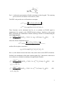
The exact equation for a double-scattering (i.e. a three-leg path, Fig. 1) contribution that
involves an absorber i and scatterers j and n is expressed as:
χ
( 2)
ijn
Here,
= Im C (ϑnij )
S i2 ℜF j (ϑijn , k ) Fn (ϑ jni , k )
reff=½(rij+rjn+rni)
krij r jn rni
exp(i (2kreff + 2δ i (k ) − lπ ) − 2reff λ (k ))
(2)
is
the
effective
scattering-path
length,
F j (ϑijn , k ) = F j (ϑijn , k ) exp(iϕi (ϑijn , k )) is the complex scattering amplitude for an atom j
and the scattering angle ϑijn , and C (ϑnij ) is the angle-dependent parameter (in the planewave approximation C (ϑnij ) = cos(ϑnij ) .
2
Fig. 1: A schematic representation of double scattering in a three-leg path. The scattering
process involves an absorber i and scatterers j and n.
The FEFF code provides two real functions as an output:
F effective (k ) =
C (ϑnij ) F j (ϑijn , k ) Fn (ϑ jni , k )
rij r jn rni
reff2
ϕ effective (k ) = arg C (ϑnij ) F j (ϑijn , k ) Fn (ϑ jni , k )
These functions can be substituted into Eq. (1) to calculate an EXAFS signal as
implemented, for example, in the IFEFFIT/Artemis software. Similarly, in the present
RMC calculations, the contribution of double scattering to EXAFS is calculated using the
approximate formula:
Si2ℜFjneff ( 2) (ϑ , k )
( 2)
( 2)
(3)
χijn =
sin(2kreff + 2δ i (k ) − lπ + ϕ eff
(ϑ , k )) exp(− 2reff λ (k )),
jn
krij rjnrni
where the effective amplitude factor is
C (ϑnij ) F j (ϑijn , k ) Fn (ϑ jni , k )
F jneff ( 2) (ϑ , k ) =
r0 ij r0 jn r0 ni ,
r02eff
and the effective phase correction is
( 2)
ϕ eff
(ϑ, k ) = arg(C (ϑnij ) F j (ϑijn , k ) Fn (ϑ jni , k )) .
jn
Here r0ij is the distance between the atoms i and j in the cluster used in FEFF calculations.
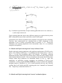
Similarly, the contributions of the triple-scattering paths (Fig. 2) that involve either one or
two scatterers are calculated according to the approximate formulae:
χijn(3) =
Si2ℜFjneff (3) (ϑijn , k )
2 2
ij jn
kr r
reff=rij+rjn (Fig. 2a)
χ
( 3)
ij
=
Si2ℜFjeff (3) (π , k )
4
ij
kr
reff=2rij, (Fig. 2b)
( 3)
sin(2kreff + 2δ i (k ) − lπ + ϕ eff
(ϑijn , k )) exp(− 2reff λ (k ))
jn
( 3)
sin(2kreff + 2δ i (k ) − lπ + ϕ eff
(π , k )) exp(− 2reff λ (k ))
j
(4a)
(4b)
3
χ
( 3)
ijn
=
S i2 ℜF jneff (3) (ϑnij , k )
krij2 rin2
reff=rij+rin (Fig. 2c)
( 3)
sin(2kreff + 2δ i (k ) − lπ + ϕ eff
(ϑnij , k )) exp(− 2reff λ (k ))
jn
(4c)
Fig. 2: Schematic representations of triple scattering paths that involve two scatterers (a,
c) and a single scatterer (b).
Triple-scattering paths that involve three different scatterers are neglected in the present
RMC refinements because of their small effect on the EXAFS signal.
Calculations of the effective amplitude factors and phase corrections are time consuming.
Therefore, these characteristics are calculated prior to RMC refinements on the
appropriate k and ϑ meshes as described below in Sections 2.2, 2.3. During the
refinements, the scattering amplitudes for the intermediate values of ϑ are calculated
using linear interpolation.
2.1.3 Double and Triple Scattering In the Nearly-Collinear Chains
Double- and triple-scattering paths that yield significant contributions to EXAFS involve
nearly (±30º) collinear chains (Figs. 1, 2) containing the intervening atom (i.e. atom j in
Figs. 1, 2) in the first coordination shell of the absorber. In principle, scattering
amplitudes and phase shifts depend on all three angles within the atomic triangle formed
by the absorber and the scatterers. However, the present code assumes that for the nearly
collinear chains these parameters are determined entirely by the ϑijn angle; this
simplifying, yet sufficiently accurate, assumption was introduced to speed up the
calculations. A utility program EXAFS_INTER.exe is used to calculate the amplitudes
and phase shifts as a function of ϑijn on a ϑ -mesh selected by the user, and write the
resulting data for all double and triple scattering paths into *.n1n2n3c2 and *.n1n2n3c3
files respectively, as detailed in Section 5.2,.
2.1.4 Double and Triple Scattering In the Nearest Coordination Spheres
4
Another important geometry for double scattering involves triangular paths with the
scatterers located in the 1st and 2nd coordinations shells around the absorber (Figs. 1b). In
this case, the effective amplitude factors and phase corrections are determined primarily
by the ϑnij angles. Again, a utility program EXAFS_INTER.exe is used to calculate the
amplitudes and phase shifts as a function of ϑnij on the ϑ -mesh selected by the user
(Section 5.3) and store the resulting data for this type of double-scattering paths in the file
*.n1n2n3s2.
The amplitude and phase parameters for the triple-scattering paths shown in Figs. 2b are
stored in the file *.nsc3. Similar tables for the triple-scattering paths shown in the Fig. 2c
are stored in the file *.n1n2n3s2.
2.2 The EXAFS files for combined PDF/EXAFS refinements
Below is a list of files required to run RMCProfile with EXAFS data included in the
refinements:
Filename
Path pictogram
File Content
photoelectron mean free path; moduli and
phases of backscattering amplitudes for the
single-scattering paths;
amplitude factors and phase corrections for the
triple-scattering paths
*.n1sc1
i
j
*.n1sc3
*.n1n2n3c2
i
*.n1n2n3c3
*.n1n2n3s2
*.n1n2n3s3
absorlist.dat
scattlist.dat
j
n
effective amplitude factors and phase
corrections for the double-scattering paths in
nearly collinear atomic chains
effective amplitude factors and phase
corrections for the triple-scattering paths in
nearly collinear atomic chains
effective amplitude factors and phase
corrections for the double-scattering paths
having both scattering atoms in the 1st and 2nd
coordination shells around the absorber
effective amplitude factors and phase
corrections for the triple-scattering paths with
the two scattering atoms located in the 1st
coordination shell around the absorber, and the
absorber atom itself acting as a scatterer
list of absorber atoms around each atom in the
configuration
list of all scattering atoms for each absorber
In the filenames, n1 stands for the type of the absorbing atom, n2 for the type of the
distant scatterer, and n3 for the type of the intervening scatterer in *.n1n2n3c2(3) files; in
the files *.n1n2n3s2(3), n2 and n3 represent types of the scattering atoms.
5
2.3 Preparation of the EXAFS Data.
Preliminary analyses of EXAFS data are needed to obtain accurate values of the energy
shifts, E0, and to subtract the background from the data, as following:
(a) Use Athena (or similar) to extract EXAFS from the absorption spectra.
(b) For each experimental EXAFS build an appropriate cluster(s) around the absorbing
atom. An average structure provides a good staring model. Examples of public
domain software that can be used to generate these clusters based on the space
group and atomic positions include Atoms/Artemis. For structures with the same
absorber species located in non-equivalent crystallographic positions, separate
clusters have to be generated for each of these sites. These non-equivalent sites
must be designated using distinct atom types in the *.cfg file. The contributions of
these clusters to the total EXAFS signal are set proportional to the respective site
occupancies.
(c) Perform self-consistent FEFF calculations of the scattering paths in a separate folder
for each cluster. In the FEFF input file, set the amplitude-reduction parameter S02 to
a value less than 0.1 to let FEFF estimate this parameter from the atomic overlap
integrals. Identify scattering paths to be used in the fit.
(d) Use Artemis (or similar) to fit the experimental EXAFS using selected scattering
paths. For all paths, set S02 (‘amp’ parameter in the GDS section) to a value
calculated by FEFF. (FEFF8.20 provides satisfactorily estimates for S02), which are
specified in the header of the chi.dat output file. The fitted value of S02 may deviate
from the theoretical due, for example, to inhomogeneous sample; significant
deviations likely indicate a problem and should be considered seriously.
If
multiple experimental EXAFS datasets are available, a simultaneous fit is
recommended. Each dataset should be assigned a single value of E0.
(e) Return to the EXAFS data-reduction software (e.g. Athena) and adjust E0 to the
fitted value to convert EXAFS oscillations from the energy- to k-space. Repeat the
fit in Artemis using these modified data and obtain a new value of E0. Repeat this
procedure iteratively until E0<0.5 eV. This process minimizes systematic errors
caused by the incorrect choice of E0.
(f) In Artemis, fit the background, if possible, and save the experimental data and the
background as chi(k).
(g) Use any spreadsheet software (e.g. Excel) to subtract the background from the
experimental data. The background subtraction option in the current version of
Artemis appears to work incorrectly.
(h) Save the background-subtracted experimental data in the following format:
1st line – number of experimental points;
2nd line – title;
Subsequent lines – k (Å-1) and chi(k) values in xy format.
2.4 Creating EXAFS files
In the following, the file structures are illustrated using perovskite-like SrAl½Nb½O3 as an
example. EXAFS data for Sr and Nb are stored in the files I_Sr-back.dat and I_Nbback.dat respectively. In the *.cfg file, the atom types are specified as 1-Sr, 2-Nb, 3-Al,
4-O.
6
Create a separate folder for each absorber type and perform FEFF calculations for all the
absorbers.
(a) Each of these folders should contain the following files/subfolders: (1)
EXAFS_INTER.exe file, (2) FEFFxxx.exe file, (3) experimental EXAFS datafile,
(4) feff.inp file generated by Artemis, (5) path.dat file generated by FEFF, and (6)
a subfolder called “store” where the output files will be stored;
(b) Rename the path.dat file created by FEFF to pathbackup.dat. An example of the
path.dat file and the description of its structure are presented in Appendix A1;
(c) Open feff.inp file and change the CONTROL card parameters to
CONTROL 0 0 0 0 1 1 for FEFF820.exe or to
CONTROL 0 0 1
1
for FEFF6l.exe
(d) Identify the paths to be included in the fit;
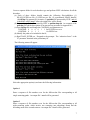
(e) Run EXAFS_INTER.exe. Respond to the prompts. The “reduction factor” is the
S02 parameter obtained in the preliminary fit.
The following menu will appear:
Select the appropriate option(s) and enter the following information:
Option 1
Enter a sequence of file numbers xxxx for the feffxxxx.dat files corresponding to all
single-scattering paths. An output file *.n1sc1 will be generated.
Option 2
Enter a sequence of file numbers xxxx for the feffxxxx.dat files corresponding to all
triple-scattering paths, which involve one scattering (not absorbing) atoms and the
absorbing atom as the second scatterer. An output file *.n1sc3 will be generated.
7
Option 3
Enter the types of the distant and intervening scatterers for a double-scattering chain-like process and
the number xxxx of the feffxxxx.dat file corresponding to this forward-scattering path. A value of
the scattering angle for the selected path will be displayed. Enter the minimum and maximum values
(in degrees) for the angular range to be sampled. An output file *.n1n2n3c2 will be generated. Enter
the number xxxx of the feffxxxx.dat file corresponding to the triple-scattering path. An output file
*.n1n2n3c3 will be generated. In order to include similar scattering processes for another set of the
distant and intervening scatterers, select option 3 again and follow the same procedure.
Option 4
Enter the types of scatterers for a double-scattering not chain-like process. Several nonequivalent
paths may exist that include the same types of scatterers. Enter the total number of these paths and,
then, the numbers xxxx of the corresponding feffxxxx.dat files in the ascending order for the internal
angle (angle θnij for a triangular path is defined in Fig. 1). As the number of the feffxxxx.dat file
corresponding to the the smallest angle is entered, a value of this angle will be displayed. Enter the
minimum and the maximum values (in degrees) for the angular range to be sampled. The procedure
will be repeated for every double-scattering path with the specified scatterers. The angle intervals
selected for different non-equivalent paths involving the same scatterers should not overlap. In order
to specify the double-scattering processes for other types of scatterers select option 4 again.
Option 5
Enter the types of scatterers for a triple-scattering not chain-like process. Several nonequivalent
paths may exist that include the same types of scatterers. Enter the total number of these paths and,
then, the numbers xxxx of the corresponding feffxxxx.dat files in the ascending order of the internal
angle (angle θnij for a triangular path is defined in Fig. 1). As the number of the feffxxxx.dat file
corresponding to the the smallest angle is entered, a value of this angle will be displayed. Enter the
minimum and the maximum values (in degrees) for the angular range to be sampled.. The procedure
will be repeated for every triple scattering path with the specified scatterers. The angle intervals
selected for different non-equivalent paths involving the same scatterers should not overlap. In order
to specify the double-scattering processes for other types of scatterers select option 5 again.
2.5 Creating lists of absorbing and scattering atoms
These lists are generated using the utility SCAT_ABS.exe and stored in the files absorlist.dat
(Appendix A2) and scattlist.dat (Appendix A3). For running SCAT_ABS.exe, copy the initial
configuration file *.cfg into a folder which contains SCAT_ABS.exe. In the same folder, create an
input file scat_input.txt. An example of the input file is shown below:
SrAlNbO3.cfg
2
1
2 4.2 0.0 4.2 0.0
1
1 4.2 0.0 4.0 0.0
! NEXAFS - number of experimental spectra
! NABS - number of types of absorbers for a given spectrum
4.2 5.0
4.2 0.0
4.2 0.0
4.2 0.0
8
The first line is a name of the configuration file. The second line is a number of the
experimental EXAFS datasets (NEXAFS). This line is followed by NEXAFS groups of
lines. The total number of these groups and their order must correspond to the order of
the EXAFS groups in the RMCProfile *.dat file.
The first line of each group specifies the number of types of absorbers for a given
EXAFS dataset (NABS). This line is followed by one line per absorber. In this line, the
first digit specifies the type of the corresponding absorbing atom. This digit is followed
by ntypes pairs of real numbers, where ntypes is the number of types of atoms in the
configuration file. The first number in the pair is the maximum distance between the
corresponding scattering atoms and the absorbing atoms to be included the list. The
second number is the maximum scattering angle to search for an intervening atom for the
chain scattering that involves these absorbing and scattering types.
3. Diffuse scattering in Electron Diffraction
3.1. Diffuse scattering calculations
The calculations of diffuse scattering were implemented according to the formalism
proposed by Butler and Welberry (B. D. Butler, T. R. Welberry, J. Appl. Cryst. 25, 391,
1992) and later adopted for RMC refinements using electron diffraction by Goodwin et
al. (A. L. Goodwin, R. L. Withers, H. B. Nguyen, J. Phys. Cond. Matter, 19(33), 335216.
2007). According to this formalism, the complex total scattering amplitude Atot(k) is
calculated in the kinematic approach as
M
Atot (k ) = ∑∑ f m (k ) exp(ik (Rn + rmn )) ,
(6)
n m =1
where k=(kx, ky, kz) is the diffraction vector, Rn=(anx, bny, cnz) is a vector that describes
the origin of the nth unit cell, rmn=(xmn, ymn, zmn) is a vector that describes the position of
the mth atom in the nth cell, fm(k) is the atomic scattering factor, a, b, and c are the lattice
parameters, Nx, Ny, and Nz specify the number of unit cells along the corresponding axes
of the the configuration box, N=NxNyNz is the total number of the unit cells in the box,
and M is the number of atoms in the unit cell, 0≤nα≤Nα-1 ( α ∈ [ x, y, z ])
The average scattering amplitude <A(k)> is calculated as
M
1
< A(k ) >= ∑∑ f m (k ) exp(ik (rmn )).
N n m =1
(7)
The amplitude of diffuse scattering AD(k) is a difference
AD (k ) = Atot (k )− < A(k ) > ψ (k ) ,
(8)
where the interference function ψ (k ) is
9
ψ (k ) = ∑ exp(ikR n ) =
n
exp(ik x aN x ) − 1 exp(ik y bN y ) − 1 exp(ik z cN z ) − 1
.
⋅
⋅
exp(ik x a ) − 1
exp(ik y b ) − 1
exp(ik z c ) − 1
(9)
The intensity of diffuse scattering is ID(k)=ln|AD(k)|2. The intensities in experimental
electron diffraction patterns are affected by multiple scattering and therefore cannot be
reproduced by calculations that rely on the kinematic approximation. Therefore, only the
locus of diffuse scattering, which reflects the topology of correlations in real space, is
fitted; the information on the magnitude of correlation parameters can be recovered only
to the extent that is encoded in the total scattering and EXAFS data. In the present fitting
procedure, the experimental (relative units) and calculated intensities are matched using
the scale factor and the offset which are adjusted after each RMC move.
Typically, the total scattering amplitude calculated for a single atomic configuration by
direct summation (6) is too noisy to be used in the fit. In the present software, the noise
is reduced using the following procedure which relies on the periodic boundary
conditions imposed in the RMC refinements. The position of an atom in the
configuration is described by a sum Rn+rmn. Therefore, the transformation of the atomic
coordinates according to the formulae
for l x ≤ nx < N x
⎧a (n − l ) + xmn
→ ⎨ x x
⎩ a (nx − l x + N x ) + xmn for 0 ≤ nx < l x
for l y ≤ n y < N y
⎧b(n y − l y ) + ymn
,
→ ⎨
⎩ b(n y − l y + N y ) + xmn for 0 ≤ n y < l y
an x + xmn
bn y + ymn
(10)
for l z ≤ nz < N z
⎧c(n − l ) + zmn
→ ⎨ z z
⎩ c(nz − l z + N z ) + zmn for 0 ≤ nz < l z
cn z + zmn
generates the atomic configuration that is equivalent to the original. The total scattering
amplitude calculated for the new configuration using Equation (6) is somewhat different
compared to that calculated for the original configuration, whereas the average scattering
amplitude remains unchanged. According the present procedure, the ID(k) calculated
after each RMC move is averaged over eight equivalent configurations with lx=0, [Nx/2];
ly=0, [Ny/2]; lz=0, [Nz/2]. The maximum number of equivalent configurations that could
be included in the averaging is N, but using so many configurations would make the
computations prohibitively expensive.
3.2 Atomic scattering factor calculations
The atomic scattering factors for electron diffraction are calculated using the traditional
parameterization according to the formula (Peng L-M, Acta Cryst., A54, 481, 1998)
5
(
)
f m (k ) = ∑ a j exp − b j k 2 +
j =1
me2
ΔZ ,
8π 2 2 k 2
(11)
10
where aj and bj are tabulated parameters (Peng L-M, Acta Cryst., A54, 481, 1998), ΔZ
me2
represents the ionic charge, the pre-factor
= 0.023934 if k is given in Å-1 and fm(k)
2 2
8π 
is in Å. The values of aj and bj are stored in the file FormfactorsTable.dat. The
FormfactorsTable.dat consists of three-line blocks for each type of atoms in the
configuration. The first line in a block is a chemical symbol for a given atom type, the
second line contains five real values of aj, and the third line contains five real values of bj.
The order of blocks in the file is not important. A user can modify this file using any text
editor. Ionic charges (valences) should be specified as real numbers in the *.dat file after
the keyword “VALENCE ::”. The valences must be listed in the same order as the atoms
in the “ATOMS ::” line.
3.3 Input and output files
The input files, each containing a distribution of diffuse intensity in a given section of
reciprocal space to be included in the fit, are produced using the ED.exe utility program
from the digitized experimental electron diffraction patterns.
The procedure for
generating these input files is detailed in Section 3.4. The first line of the input file is an
integer which specifies a number of the data lines in the file. Each following line contains
two integer numbers representing the pixel coordinates and three real numbers describing
the reciprocal-space coordinates of this point in Å-1 and the corresponding intensity value.
Two kinds of output files are produced for each diffraction pattern used in the fit. The
graphic files exper_diffus_n.bmp and calcul_diffus_n.bmp facilitate easy visual
comparison of the experimental and calculated patterns for the nth dataset. A digital
output
is
provided
in
the
files
diffuse_intensity_inputn.dat
and
diffuse_intensity_outputn.dat. The diffuse_intensity_inputn.dat file contains a
diffuse scattering pattern calculated at the start of the RMC run for the original atomic
configuration. The diffuse_intensity_outputn.dat file is saved after a user-specified run
time along with other output files (e.g. total scattering and/or EXAFS). The first three
lines in this file contain values of the residual, a scale factor, and an offset for a given
dataset. These lines are followed by a matrix describing the intensity distribution.
3.4. Input file processing
Commonly, experimental diffraction patterns containing diffuse scattering are recorded
on a film. In this case, the experimental pattern has to be digitized using a suitable
scanner or a similar device and stored in the .bmp format. The processing of the resulting
image to produce an input data file for RMCProfile involves the following steps:
a) Define the origin of the co-ordinate system for the image and determine it’s
coordinates;
b) Define two reciprocal space vectors in the image;
c) Mask all the Bragg peaks which will be excluded from the fit;
d) Choose an appropriate quarter of the diffraction pattern to be used in the fit.
11
The central spot in experimental electron diffraction patterns is saturated and, as such, is
not suitable for precise determination of the origin. Instead, the center is found from the
coordinates of several Bragg peaks located symmetrically around the central spot. The
program ED.exe prompts the user to select suitable Bragg spots using mouse clicks. The
program fits each of these peaks with a 2-D Gaussian (saturated portions of the peaks, if
encountered, are excluded by the program) to find the peak positions. The position of the
origin is calculated as an average of the Bragg peak positions.
The two reciprocal space vectors are defined (following the on-screen prompts) by using
mouse clicks to select several orders for the two independent reflection families (e.g. 111,
222, 333 and 100, 200, 300) and specifying the hkl indexes for each of these peaks. The
program automatically determines the precise positions of the selected peaks and the
length of the corresponding reciprocal space vectors in Å-1.
The RMCProfile code fits only the diffuse component of electron scattering and,
therefore, Bragg peaks must be excluded from the fitted pattern. This is accomplished by
using masks which are placed on top of all the Bragg spots in the pattern. The mask has
an ellipsoidal shape inscribed into a rectangular. The user selects the size of the mask by
defining the upper left and lower right corners of this rectangular using mouse clicks as
prompted by the program.
Once the user selects one Bragg peak, the program
automatically locates and masks its pair related by the 180° rotation around the centre.
Finally, the user selects the quarter of the diffraction pattern to be included in the fit (only
one quarter is fitted to reduce the computation time) using a mouse click in the
corresponding corner of the diffraction pattern. Once this action is completed, the
program ED.exe creates an input file for use by RMCProfile. The name of this file must
be specified in the DIFFUSE_SCATTERING :: card of the *.dat file.
4. Restraints on peak tails in partial PDFs
“DISTANCE WINDOW” and “MINIMUM DISTANCES” constraints frequently cause
unphysical spikes/discontinuities in partial PDFs at the distance limits set by these
constraints; usually, these limits and the spikes occurs in the tail portions of the PDF
peaks. This effect is most pronounced in the case of two closely overlapped partial PDFs
that exhibit opposite signs of the Faber-Ziman coefficients. In this case, the artificial
spikes in the two PDFs cancel each other so that the total PDF exhibits no discontinuities;
therefore, no driving force for “healing” these spikes exist during fitting of the total PDF.
The problem can be alleviated by imposing restraints on the peak tails in partial PDFs as
implemented in the current version of RMCProfile. These restraints can be applied to the
low-r and/or high-r tails of any peak in any partial PDF. For each restraint, a user has to
specify the rmin (left) and rmax (right) limits of the interval over which the constraint is
applied along with the tail function L(r). This function is defined as a fourth-order
polynomial with a zero constant term:
4
L(r ) = ∑ a n (r − r0 ) n
(5)
n =1
12
where r0 is set to rmin and rmax for for the low-r tail and high-r tails, respectively. The
coefficients an must be obtained by fitting L(r) to the tail of interest using any suitable
computer software. For a given partial PDF gm(r), the program checks the inequality
g (r j ) > L(r j ) for all r j ∈ [rmin , rmax ] after each RMC move.. If the condition is satisfied,
the penalty function having a user-specified weight is added to the residual.
The restraint for each low-r tail to be constrained is activated by including the following
block of keywords in the *.dat file:
LEFT_TAILS :: > START_FINISH :: here, rmin and rmax for this tail must be specified > PARTIAL :: integer corresponding to the number of a partial must be specified
> COEFFICIENTS :: 4 real numbers describing coefficients a1, a2, a3, and a4
> WEIGHT :: weight assigned to the penalty function
The restraint for each high-r tail to constrained is activated using similar keywords with
the major keyword RIGHT_TAILS ::.
5. Major keywords in the *.dat file
EXAFS :: LEFT_TAILS :: / RIGHT_TAILS :: DIFFUSE_SCATTERING :: Introduces a block of data concerning a set of EXAFS data. Text can follow the :: but will be ignored. This keyword must be followed by a block of subordinate keywords. Each EXAFS spectrum requires a separate keyword and a block of data. Do not include if no EXAFS data is fitted. Introduces a block of data concerning restraints on the tails of peaks in partial PDFs. This keyword must be followed by a block of subordinate keywords. Do not include if no restraints are used. Introduces a block of data concerning electron diffraction pattern. Text can follow the :: but will be ignored. This keyword must be followed by a block of subordinate keywords. Each diffraction pattern requires a separate keyword and a block of data. Do not include if no electron diffraction data is fitted. 6. Subordinate keywords in the *.dat file
EXAFS ::
> FILENAME ::
Filename containing the data
>FIT_SPACE ::
Acceptable values: r, k (case-insensitive).
Specifies whether a real (coordinate) space or a
wave-vector space (k) is used for the EXAFS fit.
> START_POINT_(R_SPACE) ::
Start point for a fit in the r space (Å)
13
> END_POINT_(R_SPACE) ::
End point for a fit in the r space (Å)
> R_SPACING ::
Value of the spacing used in the EXAFS fit and
the output (Å).
> LOW_R_REGION_LIMIT::
(Optional) If specified, assigns additional factor to
the lower-r part contribution to the total misfit.
This factor must be provided with the subordinate
keyword >LOW_R_WEIGHT
> LOW_R_WEIGHT ::
An additional factor for the lower-r part
contribution to the total misfit in the case of rspace fit
> START_POINT_(K_SPACE) ::
Start point of the fit in k-space (if selected in
>FIT_SPACE) or a Fourier transform for a fit in
the r space (Å-1)
> END_POINT_(K_SPACE) ::
End point of the fit in k space or a Fourier
transform for a fit in the r space (Å-1)
> K_POWER ::
Specifies the power of n in the weight-factor kn
used to multiply EXAFS signal chi(k) prior to a
Fourier transform
> WEIGHT ::
Parameter to weight the total misfit for the
EXAFS data in Monte Carlo simulation
> ENERGY_OFFSET ::
(Optional) Shift of E0 (eV) in the experimental
spectrum. If not included, E0=0
> SCALE_FACTOR ::
(Optional) Scale factor for the experimental
spectrum (optional). If not included, scale
factor=1
> NUMBER_OF_TYPES_
(Optional) Specifies the number of types of
absorbing atoms for a given EXAFS dataset. If
not included, the number of types is set to 1.
OF_ABSORBING_ATOMS::
> TYPE(S)_OF_ABSORBING
_ATOMS::
LEFT_TAILS :: (RIGHT_TAILS ::)
> START_FINISH ::
> PARTIAL ::
> COEFFICIENTS ::
> WEIGHT ::
A list of types of the absorbing atoms for a given
EXAFS dataset
rmin and rmin values (Å)
Number of partials to which the restraint is applied
Coefficients a1, a2, a3, and a4 in Equation (5)
Weight of the penalty function due to the tail
restraint
DIFFUSE_SCATTERING :: > FILENAME ::
> WEIGHT ::
Filename containing the data
Parameter to weight the total misfit for the diffuse scattering data in Monte Carlo simulation.
14
Appendix
A1. The Pathsbackup.dat file
...
Rmax 6.0000, keep limit 0.000, heap limit 0.000 Feff 6L.02 paths 3.05
Plane wave chi amplitude filter
2.50%
----------------------------------------------------------------------1 2
6.000 index, nleg, degeneracy, r= 1.9805
x
y
z
ipot label
rleg
beta
eta
0.000000 0.000000 1.980540
4 'O
'
1.9805 180.0000 0.0000
0.000000 0.000000 0.000000
0 'Nb '
1.9805 180.0000 0.0000
2
2
8.000 index, nleg, degeneracy, r= 3.3764
x
y
z
ipot label
rleg
beta
-1.949350 1.949350 -1.949350
1 'Sr '
3.3764 180.0000
0.000000 0.000000
0.000000
0 'Nb '
3.3764 180.0000
eta
0.0000
0.0000
3
3 24.000 index, nleg, degeneracy, r= 3.3810
x
y
z
ipot label
rleg
beta
1.980540 0.000000 0.000000
4
'O '
1.9805 135.0000
0.000000 -1.980540 0.000000
4
'O '
2.8009 135.0000
0.000000 0.000000 0.000000
0
'Nb '
1.9805
90.0000
eta
0.0000
0.0000
0.0000
4
2
6.000 index, nleg, degeneracy, r= 3.8987
x
y
z
ipot label
rleg
beta
0.000000 -3.898700 0.000000
3
'Al '
3.8987 180.0000
0.000000 0.000000 0.000000
0
'Nb '
3.8987 180.0000
eta
0.0000
0.0000
5
3 12.000 index, nleg, degeneracy, r= 3.8987
x
y
z
ipot label
rleg
beta
0.000000 0.000000 -3.898700
3
'Al '
3.8987 180.0000
0.000000 0.000000 -1.980540
4
'O
' 1.9182
0.0000
0.000000 0.000000 0.000000
0
'Nb ' 1.9805 180.0000
eta
0.0000
0.0000
0.0000
6
4
6.000 index, nleg, degeneracy, r= 3.8987
x
y
z
ipot label
rleg
beta
-1.980540 0.000000 0.000000
4
'O '
1.9805
0.0000
-3.898700 0.000000 0.000000
3
'Al '
1.9182 180.0000
-1.980540 0.000000 0.000000
4
'O '
1.9182
0.0000
0.000000 0.000000 0.000000
0
'Nb '
1.9805 180.0000
eta
0.0000
0.0000
0.0000
0.0000
A2. The absorlist.dat file
20480
total number of lines equal to the total number of atoms in cfg
14
maximal number of absorbers in a line
10 4097 2 4609 2 5121 2 5633 2 2049 1 2056 1 2561 1 2617 1 3073 1
3521 1
10 4098 2 4610 2 5122 2 5634 2 2049 1 2050 1 2562 1 2618 1 3074 1
3522 1
8
194 1
14 4609 2
4096 1
706 1
5057 2
1218 1
…
1730 1
…
2242 1
576 1
2754 1
1480 1
3266 1
2041 1
3778 1
2056 1
2617 1
3521 1
15
A3: The scattlist.dat file
6144 total number of lines
26 maximal number of scatterers in a line
26 2049 1 0 0
…
3073 1 0 0
20 181 1
0 0 …..6901 3 10933 4 7349 3 13493 …..
20149 4
00
A4. Example of a combined fit of neutron total PDF, Bragg profile, and electron
diffuse scattering
The cubic phase of perovskite-like KNbO3 is believed to exhibit 8-site displacive disorder
associated with random local displacements of Nb along 8 non-equivalent 〈111〉 directions.
The displacements are correlated along the -Nb-O-Nb- linear chains parallel to 〈100〉
directions. Similar 8-site disorder is encountered in perovskite BaTiO3 and AgNbO3 as well as
their solid solutions with other perovskite compounds. The correlated displacements are
manifested in three orthogonal sets of {100} sheets of diffuse intensity passing through all
fundamental reflections; the diffuse intensity is extinct through the origin of reciprocal space
because the correlated displacement components are directed parallel to the correlation
directions. In the present example we used synthetic data simulated for a large atomic
configuration that mimicked the 8-site disorder for Nb to determine whether the correct
displacement correlations can be recovered at least using error-free data. The simulated data
that was used in these analyses included neutron PDF and electron diffuse scattering.
The structure model used to simulate the data was based on the configuration cell of 64 Å × 64
Å × 64 Å, which contained 20,480 atoms located at the ideal lattice sites of the cubic
perovskite structure. The Nb atoms were shifted along 〈111〉 directions 0.1√3 Å and the O
atoms were shifted along 〈001〉 direction by 0.1 Å to generate positive Nb-Nb and negative NbO displacement correlations along the 〈001〉 -Nb-O-Nb- <001> chains; the displacements
among different chains remained uncorrelated thus yielding the desired 8-site model (Figure
A4.1). Subsequently, all atoms in the configuration were subjected to random Gaussian
displacements. The total neutron pair-distribution function (PDF) and Bragg profile were
calculated for this model configuration and used instead of experimental datasets in the RMC
fits.
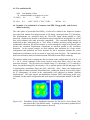
Figure A4.1: Probability density distribution functions for Nb and O viewed down 〈100〉
directions in the 8-site KNbO3 model. A splitting of the atomic positions due to
correlated atomic displacements is observed.
16
First, a combined fit of the neutron PDF and Bragg profile was performed starting from the
ideal lattice sites. The fit produced discernable negative correlations among the nearestneighbor Nb and O displacements which were evident in the doublet structure of the first peak
in the total PDF. Despite an excellent agreement between the target and calculated data, the
magnitude of the Nb-O correlations was much smaller compared to the target value. More
importantly, the refined configuration exhibited no Nb-Nb and O-O correlations but instead
featured positive K-K correlations, which were absent in the target model. No noticeable
correlations existed beyond 4 Å. Clearly, the local structure obtained using powder total
scattering data alone is grossly incorrect even though the 8-site and 2-site splitting was
reproduced to some extent for the Nb and O probability density distribution functions,
respectively. The fit also produced reasonable agreement between the calculated and target
variances <u2> for all the atomic positions. Unquestionably, without a prior knowledge of the
structural, an incorrect model would have been inferred from RMC refinements using the
neutron total scattering data.
In the second attempt, the neutron PDF and Bragg profile were complemented by the two
electron diffraction patterns containing diffuse scattering. The results of a simultaneous fit of
these four datasets are presented in Figure A4.2.
(a)
G(r)
Intensity
(b)
0
5
10
15
r (A)
(c)
20
25
30
=
10
15
20
Time of flight (msec)
25
30
(d)
Figure A4.2: Results of a simultaneous fit of the neutron PDF and Bragg profile and
electron diffuse scattering (two sections). (a, b) Experimental (blue) and
calculated (red) neutron PDF (a) and Bragg profile (b). Experimental (left)
and calculated (right) electron diffuse scattering patterns in the (130) (c) and
(114) (d) sections of reciprocal space.
17
Now, the displacement correlations were reproduced in the refined configuration,
although the correlation strengths were still significantly weaker than the target values.
In particular, positive Nb-Nb and O-O displacement correlations were recovered and the
incorrect K-K correlations, while still present, decreased considerably. Clearly, including
the information encoded in electron diffraction improved considerably a correctness of
the recovered displacement correlations.
A5. Algorithm for removal of incoherent scattering from neutron S(Q)
Strong incoherent neutron scattering that arises for example in samples containing
hydrogen (H) has to be subtracted from the data to obtain a properly normalized S(Q).
Here we implemented a robust procedure for subtracting this incoherent background from
the experimental data using RMCProfile and utility Incoh_subtr.exe.
This utility
program first calculates the difference between the experimental Sexp(Q) and the Scalc(Q)
calculated using RMCProfile for an atomic configuration representing the average
structure with random atomic displacements and, then, fits this difference using an
empirical 5-parameter analytical function f(Q)=Ae-BQQC+F/[(Q-D)2+E2], where A, B, C,
D, and E are adjustable parameters. The analytical expression was selected over a
polynomial or a B-spline (also tried) because it does not introduce any oscillations of the
kind that may arise due to real structural correlations. This fitted baseline function,
represents a contribution of incoherent scattering as well as all other additive corrections
that need to be subtracted form the data to obtain the correct shape for the sample
background function. The correction is subtracted from the experimental data (using the
external correction file option in PDFGetN) for each bank and the banks are merged.
The procedure involves the following steps:
1. Create an atomic configuration based upon atomic positions in the average
structure using utility tools supplied with RMCProfile.
2. Displace the atoms in this configuration according to random Gaussian
distributions with variances corresponding to atomic displacement parameters
(ADP) in the average structure; these ADP parameters can be either adopted from
Rietveld refinement or assigned arbitrary but sensible values. A utility such as
supplied as a part of WinNFLP suite can be used to introduce random Gaussian
displacements.
3. Obtain experimental Sexp(Q) for each detector bank using PDFGetN. Use any
suitable spreadsheet software to convert these Sexp(Q) to Fexp(Q) according to
Fexp(Q)=〈b〉2(Sexp(Q)-1), where 〈b〉 is the mean scattering length for the structure.
4. Prepare the RMCProfile *.dat file and run RMCProfile to fit Fexp(Q) (as the
experimental data) saving the results and stopping the run after a few cycles.
Note that a baseline in the calculated S(Q) represents a realistic shape of the
background for uncorrelated atomic motion.
5. Convert the output file *_SQ1.csv into the txt format and store in a folder with the
Incoh_subtr.exe utility.
6. Run Incoh_subtr.exe and follow the on-screen instructions. The output file *.fix
is the background correction file for a given bank.
7. Use any spreadsheet software to combine the individual bank*.fix files into a
single .fix file that can be plugged into PDFGetN as an “external correction file”.
18
1.4
5
(a)
(b)
1.2
4
1
0.8
S(Q)
S(Q)
3
2
0.6
0.4
0.2
1
0
0
0
5
10
15
20
25
-0.2
0
5
10
10
15
-1
20
25
Q (Ang )
-1
Q (Ang )
4
(c)
(d)
3
8
6
1
G(r)
S(Q)
2
4
0
-1
2
0
-2
0
5
10
15
-1
Q (Ang )
20
25
-3
0
5
10
r (Ang)
15
20
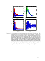
Figure A5.1: (a) Experimental (red) and calculated (blue) S(Q) for the TiZrNiD2 alloy. The
experimental data were collected using the NPDF instrument. A limited D-H
exchange reaction was sufficient to induce a significant background due to the
incoherent scattering of H in the experimental data. The calculated S(Q) was
obtained using RMCProfile for a configuration based on the Rietveld-derived
model. The baseline in the calculated S(Q) provides a background expected for
coherent scattering. (b) S(Q) for one of the detector banks having its baseline
fitted using an analytical function f(Q) described in the text. (c) S(Q) before (red)
and after (blue) subtraction of f(Q). (d) G(r) obtained from S(Q) before (red) and
after (red) subtraction of incoherent scattering. Note the changes in the low-r
range. For r>2 Å, the effect of incoherent scattering is rather insignificant.
19