Download SCOUT User`s Guide

SCOUT USER'S GUIDE
NOTICE
Although the production of this report was funded wholly by the United
States Environmental Protection Agency through contract 68-CO-0049 to
Lockheed Environmental Systems & Technologies Company, it has not been
subjected to Agency policy review, and no official endorsement should be
inferred.
TABLE OF CONTENTS
Chapter 1
Preliminaries
1.1
Introduction
1.2
Manual Organization
1.3
Installing Scout
1.4
Viewing the User's Guide
1-1
1-2
1-3
1-4
Chapter 2
Scout File Format
2.1
File Management
2.2
Reading Spreadsheet Files
2.3
Load Scout File
2.4
Save Scout File
2.5
Merge Two Files
2.6
Append Two Files
2-1
2-2
2-4
2-5
2-5
2-5
Chapter 3
Managing Data in Scout
3.1
Data Management
3.2
Scout functions and operations
3.3
Summary Statistics
3.4
Data Transformation
3.5
Print Data
3-1
3-4
3-5
3-5
3-8
Chapter 4
Classical Methods for Outlier Identification
4.1
Introduction to the Classical Methods for Outlier Identification
4.2
Select Variables
4.3
The Classical Outlier Tests
4.4
Causal Variables
4.5
Associated Causes
4.6
Remove Outlier Flags
4-1
4-2
4-2
4-3
4-4
4-4
Chapter 5
Robust Statistical Methods
5.1
Introduction to Robust Statistical Methods
5.2
Choices of robust analyses
5.3
Univariate Statistics
5.4
Robust Analysis
5.5
Confusion Matrix
5.6
Pattern Recognition
5.7
D Trend
5.8
Add Means
5.9
Causal Variables
5.10 Print Destination
iii
5-1
5-2
5-3
5-5
5-9
5-9
5-11
5-11
5-12
5-13
TABLE OF CONTENTS (con't)
Chapter 6
PCA
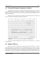
6.1
Classical Principal Components Analysis
6.2
Display Matrices
6.3
Eigenvalues
6.4
View Components
6.5
Transform Data
6-1
6-1
6-2
6-2
6-2
Chapter 7
Graphics
7.1
General Description
7.2
Modify Graph Colors and Shapes
7.3
Command Summary for 2D and 3D Graphics
7.4
2-Dimensional Graphs
7.5
Zoom Feature
7.6
3-Dimensional Graphs
7.7
Moving 3D Graphs
7.8
Change Size of 3D Graphs
7.9
Search Observation Mode
7.10 Quick 2D Graphs
7.11 Response Surfaces
7-1
7-1
7-2
7-3
7-3
7-4
7-5
7-5
7-6
7-6
7-6
Chapter 8
System information
8.1
User's Guide
8.2
Other options
8.3
Exiting Scout
8-1
8-1
8-3
Chapter 9
Scout Basics - Tutorial I
9.1
Nomenclature
9.2
Read Data Files
9.3
Examine and Save Statistics
9.4
Transformation of variables
9.5
Summary
9-1
9-2
9-3
9-4
9-5
Chapter 10 Classical Method - Tutorial II
10.1 Outlier Detection
10.2 Determining Causal Variables, and Removing Flags
10.3 Summary
iv
10-1
10-2
10-3
TABLE OF CONTENTS (con't)
Chapter 11 Robust Method - Tutorial III
11.1 Q-Q Plots
11.2 Q-Q Plots of Principal Component Analysis
11.3 PCA Sactter Plots
11.4 Statistical Intervals
11.5 Index Plots
11.6 Generalized Distance
11.7 Kurtosis
11.8 Summary
11-1
11-5
11-9
11-18
11-22
11-24
11-26
11-27
Chapter 12 Classical PCA - Tutorial IV
12.1 Display Matrices
12.2 Eigenvalues
12.3 Transform Data
12.4 Summary
12-1
12-2
12-4
12-5
Chapter 13 Graphics and System - Tutorial V
13.1 Graphics
13.2 System
13.3 Summary
13-1
13-4
13-6
Chapter 14 Statistical Procedures
14.1 Introduction to Statistical Procedures for the Identification of Multiple Outliers
14.2 General Description of Statistical Procedures in the Scout Software Package
14.3 Options Available For Robust Procedures
14.4 Robust Procedures in Scout
14.5 Normal Probability Q-Q Plots of the Original Data
and of Principal Components
14.6 Q-Q Plot of Mahalanobis Distances Using Beta Distribution
14.7 Contour Plots
14.8 Robust Principal Component Analysis
14.9 Interval Estimation
14.10 D-Trend and Add Means
14.11 Outliers in Discriminant and Classification Analysis
14-17
14-18
14-20
14-21
14-29
14-32
14-35
REFERENCES
14-39
v
14-1
14-6
14-8
14-12
Chapter 1
Preliminaries
1.1 Introduction
Scout is a univariate and multivariate data analysis tool. Several classical and robust
procedures such as outlier testing and interactive 2D/3D graphics are included in Scout,
making it a useful package for environmental and ecological applications. Straightforward
principal component, classification, and discriminant analyses are included to increase the
versatility of the software package.
(1)
(2)
(3)
(4)
(5)
(6)
(7)
Scout may be used to:
transform data
assess the normality of variables in the data set
produce histograms and Q-Q plots of raw data and principal component (PC) scores
produce scatter plots of raw data, of PCs, and of discriminant scores
identify univariate or multivariate outliers, Q-Q plots of generalized distances
perform principal component, linear, and quadratic discriminant analyses
compute and plot various statistical intervals including confidence interval for mean,
prediction interval, and simultaneous confidence interval
Scout reads ASCII data files in a specific format which is discussed later in this
manual. Files created in other software (such as WordPerfect) are not recognized by Scout,
unless they are in strict ASCII format. Scout can handle up to 22 variables, with the number
of observations limited only by the available memory of the microcomputer. Scout can save
data in a binary format. In this way, Scout can retain graph symbols and colors, and outlier
information in addition to the 22 variables. Spreadsheet data files can easily be converted into
Scout data files, as discussed in section 2.2.
Scout allows the user to view and edit a data set. Editing is limited to the existing
variables and observations. Variable fields that can be edited are name, units, format, and the
comment. Observation fields that can be edited are the label and values for the variables.
Scout is compatible with 8086, 80286, 80386, and 80486 - based microcomputers with
at least 512K of RAM and an EGA, VGA, or Hercules graphics system. A fixed disk drive is
highly recommended as Scout performs many transfers between memory and disk during
execution. Scout also uses expanded memory (if found on the system) in two ways. First, the
slow transfers between memory and disk mentioned earlier will be replaced by very fast
transfers between memory and expanded memory (needs 128K). Second, Scout will use up
to 64K of expanded memory for additional data storage. A color monitor will greatly enhance
Scout's text windows and graphics. A 20 MHz 80386 with a math coprocessor and a fixed
disk, is the minimum system recommended for Scout operation. By selecting the 'System'
heading in the main menu and then selecting 'Information', a user can display the system
Scout User's Guide
1-1
Chapter 1
Preliminaries
specification.
Scout was written by combining several subroutines and programs written for various
research projects conducted by Lockheed Environmental Systems & Technologies Company
in service of the United States Environmental Protection Agency (EPA). Thus, Scout is in the
public domain, is not copyrighted, and no license agreement is necessary. However, users
should be cautious of the source of their copy of Scout. Due to computer viruses, it is best to
obtain Scout directly from Lockheed or the EPA.
1.2 Manual Organization
The user's manual for Scout is organized into three sections: Section I (chapters 1 to 8)
is the User's guide, section II (chapters 9 to 13) includes tutorials, and section III (chapter 14)
provides technical notes, with examples, for statistically oriented users.
Users not familiar with Scout will benefit from reviewing the tutorial sections before
reading the user's guide. Various examples presented in the tutorial section are produced by
using some well known data sets.
The main menu in Scout contains seven headings. These headings are labeled as File,
Data, Classical Method, Robust Method, PCA, Graphics, and System. Each of these headings
has various options. These options can be viewed by moving the cursor in the main menu to
the appropriate area and pressing the <ENTER> button. A short description associated with
each heading or choice is displayed automatically in the window of the main Menu. The
description window associated with any heading or choice can be activated by moving the
cursor, or by using the <ARROW> key to the corresponding area. The User's guide section
and the tutorial section of the manual are organized systematically from the "File" heading to
the "System" heading.
Scout User's Guide
1-2
Chapter 1
Preliminaries
1.3 Installing Scout
Place the Scout diskette in drive A (or B) and install to hard-disk C:
1. Type 'C:' (without quotes) and press <ENTER>.
This changes the current disk drive to drive C.
2. Type 'MD \SCOUT' and press <ENTER>.
This creates a directory called SCOUT, where the program will reside.
3. Place the Scout disk in drive A (or drive B) and close the drive door.
4. Type 'COPY A:*.* C:\SCOUT' and press <ENTER>.
This copies all the files from the program disk in drive A into the SCOUT
directory on drive C.
To run Scout, enter the following commands.
1. Type 'CD \SCOUT' and press <ENTER>.
This changes the current directory to the SCOUT directory.
2. Type 'SCOUT' and press <ENTER>.
This starts the Scout program.
If you have any problems with the operation of Scout, please write to:
Scout
c/o John Nocerino or George Flatman
Characterization and Research Division
National Exposure Research Laboratory
USEPA
P.O. Box 93478
Las Vegas, NV 89193-3478
Scout User's Guide
1-3
Chapter 1
Preliminaries
1.4 Viewing the User's Guide
Scout contains an on-line User's Guide. When users are in any mode of Scout, they
can reach the on-line User's Guide for that mode by pressing the <F1> key. When a section
of text is displayed in the large window covering the lower portion of the screen, users can
move through the text using the following key commands:
HOME - Moves to the beginning of the text.
END - Moves to the end of the text.
UP ARROW - Scrolls the text up towards the beginning.
DOWN ARROW - Scrolls the text down toward the end.
PAGE UP - Scrolls the text up toward the beginning by a page.
PAGE DOWN - Scrolls the text down toward the end by a page.
ESC, ENTER - Closes the viewing window.
Scout User's Guide
1-4
Chapter 2
Scout File Format
2.1 File Management
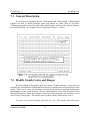
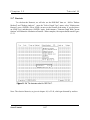
Scout reads ASCII data files in the following format. The first line of the data file is a
comment line, presumably to describe the origin or title of the data. The second line of the file
must contain the number of variables. This number, p, must be an integer greater than or
equal to one and less than or equal to 22. The next p lines contain the variable names in the
first 10 columns (1-10), and the associated units in the next ten columns (11-20). Data
formats, in FORTRAN notation, can be included after the units in columns 21-30. Finally, a
comment for each variable may be included in columns 31-80. After line p+2, the remaining
lines contain the data so that each line represents one observation. Numbers must be
separated by spaces, commas must not be used. Missing values are designated by 1E31. An
observation identifier may be placed at the end of each line. This identifier or label can be up
to ten characters long and must be in quotes. The following is an example of a file in Scout
format.
Geostatistical Environmental Data
5
Easting
feet F7.1
Northing
feet
F7.1
Arsenic
ppm G16.9
Cadmium
ppm F10.3
Lead
ppm F10.3
288.0 311.0 .850 11.5 18.25 'Sample 1'
285.6 288.0 .630 8.50 30.25 'Sample 2'
273.6 269.0 1.02 7.00 20.00 'Sample 3'
280.8 249.0 1.02 10.7 19.25 'Sample 4'
273.6 231.0 1.01 11.2 151.5 'Sample 5'
276.0 206.0 1.47 11.6 37.50 'Sample 6'
285.6 182.0 .720 7.20 80.00 'Sample 7'
288.0 164.0 .300 5.70 46.00 'Sample 8'
292.8 137.0 .360 5.20 10.00 'Sample 9'
278.4 119.0 .700 7.20 13.00 'Sample 10'
To save data in this format, select the option "Write ASCII Data File". Scout will
prompt the user to enter a file name. The user may specify an extension here that will be
used. If the file name exists, Scout will ask the user if the old file should be written over.
Scout User's Guide
2-1
Chapter 2
Scout File Format
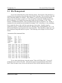
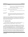
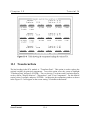
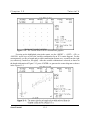
The file heading in Scout contains six headings and choices as displayed in Figure 2-1
below. These can be used to read, write, load, save, merge, and append various data sets.
2.2 Reading Spreadsheet Files
Scout cannot read Spreadsheet data directly. However, a spreadsheet file can easily be
converted into Scout data set. In order to convert a spreadsheet data file to a Scout data file,
the specific file format has to be followed. As described in Section 2.1, the format requires
including information in the file as follows:
(a)
(b)
the data set name or title (line 1)
the number of variables (line 2)
Scout User's Guide
2-2
Chapter 2
(c)
(d)
Scout File Format
the names of the variables (lines 3 through X, where X-2 is the number of variables)
the values of the variables, optionally including the labeling of each data record with a
comment in single quotes (') (lines X+1 through the end of the file)
Example spreadsheet file prepared for conversion to Scout:
Geostatistical Environmental Data
3
Arsenic
Cadmium
Lead
.850 11.5 18.25 'Sample 1'
.630 8.50 30.25 'Sample 2'
1.02 7.00 20.00 'Sample 3'
1.02 10.7 19.25 'Sample 4'
1.01 11.2 151.5 'Sample 5'
In this example, the data set name should be in spreadsheet cell A1, the number of
variables in cell A2, the variable titles in cells A3 through A5, and the values of the variables
should be in cells A6 through D10. In the spreadsheet, the column D6 to D10 contains the
name of each record, each of them must be with in single quotation marks. In some of the
spreadsheet Software, such as Excel, you may have to enter one or two space bars before the
left quotation marks for the data labels (the D column in this example). Remember, both
single quotation marks should be visible from the spreadsheet before you save the spreadsheet
file in a Space Delimited or TEXT format. One or both of these formats are built-in features
of most popular spreadsheet software.
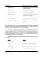
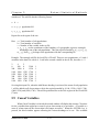
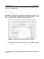
The following spreadsheet software has been tested for the ability to produce a useable
Scout file:
Software
QuattroPro 6.0 for Windows
Excel 4.0a for Windows
formats
QuattroPro 1.0 for Windows
Scout User's Guide
Result
File Format
Works
Text file
Any of 3 text file
Doesn't Work
No text or space
delimited format
available
Works
2-3
Chapter 2
Scout File Format
If the file is saved as a Space Delimited print file, use the extension *.prn. If the
spreadsheet software does not have built in Space Delimited format, then save the file with
the extension *.prn along with the following options:
(1) NO MARGIN
(2) PAGE LENGTH ONE
(3) UNFORMATTED.
After the file is saved from any spreadsheet, exit the spreadsheet Software and copy the file
into the Scout directory with extension *.dat. This newly created file in the Scout directory
can be used as a Scout file.
2.3 Load Scout File
Upon start-up of Scout, the user is placed in the "File" heading of the main menu. The
first thing the user should do is select either "Load Scout Data File" or "Read ASCII Data File'
from this pull-down menu. Both headings display a menu of possible data files from the
current directory, and any subdirectories in the current directory. The user can change the
current directory by highlighting the desired subdirectory and pressing the <ENTER> key.
All subdirectories are identified by placing the '\' symbol at the end of the name. If the user is
not in the root directory, then the first item in the menu will always be '..\', indicating the
parent directory. Choosing this item (..\) allows the user to change to the parent directory of
the current directory.
If the desired directory is not found on the current disk drive, then the user may select
a new disk drive to search. To change drives, simply press the letter of the new drive. If the
letter pressed is a valid drive from 'A' to 'N', then that drive will become the current drive.
When the user has found the desired drive and directory, a data file can then be
chosen. Use the arrow keys to highlight the desired data file, and then press <ENTER> to
select it. Sometimes there are too many file names to physically fit in the window. If the
desired data file in not displayed, then scroll through the file names by pressing and holding
the down arrow key.
Scout has the ability to search for any file name, including the use of wildcards (*).
The current search string is printed at the top of the window. This string can be changed by
pressing 'S' and then entering a new string. It is important to remember that data files saved
using the 'Save Scout File' option have the 'SCT' extension assigned by Scout automatically,
while ASCII data files may have any extension.
Scout User's Guide
2-4
Chapter 2
Scout File Format
2.4 Save Scout File
This option saves a Scout file in binary format which is intended to be used only by
Scout. Generally, other software cannot read this format. This format has the advantage of
retaining the graphics color and shape specified for each observation, and the outlier status of
each observation. To save data in this format, simply select "Save Scout Data File" from the
pull-down menu and enter a file name. Do not include an extension with the file name as
Scout will always use the '.SCT' extension. Also, do not precede the file name with a path.
New data files are always written to the current drive and directory displayed at the bottom of
the screen.
2.5 Merge Two Files
This utility allows the user to combine two data files into a new data file. The user first
selects whether to merge two ASCII files or two Scout files together. If the merge is
successful, the new data file will always be written as an ASCII file.
The merge routine assumes the variables are different in each of the input files.
Therefore the output file will contain all of the variables from both input files even if they
have the same names. The routine does however account for common observations. Two
observations taken from each of the input files that have the same label or name will be
merged into a single observation in the output file.
2.6 Append Two Files
This utility also allows the user to combine two data files into a new data file, but in a
different way than merge allowed. The user is given the option to append two ASCII files or
two Scout files together. The new data file is always written as an ASCII file. The append
routine assumes the variables are the same in each of the input files. If the two input files do
not contain the same number of variables, the routine will not allow them to be appended.
The variable names from the first input file will be used as the variables names in the new file.
All of the observations from each of the input files are written to the new file even if duplicate
record labels occur.
Scout User's Guide
2-5
Chapter 3
Managing Data in Scout
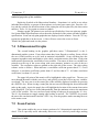
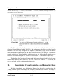
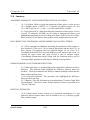
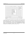
3.1 Data Management
Scout enables the user to edit, insert, or delete observations and variables currently in
memory; change the title of the data set; and change the name, units, or other attributes of the
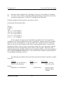
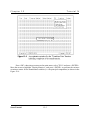
variables. Select "Data" from the main menu and "Edit Data" from the pull-down menu as
shown in Figure 3.1 below:
The data set will appear in the form of a spreadsheet. You can move about the screen
and highlight any data cell. A data cell may be a label for a given observation or a value in an
observation for a particular variable. The keys for moving about the screen are the four
<ARROW> keys, <PAGE UP>, <PAGE DOWN>, <HOME>, and <END>. Observations
that appear in red have been flagged as outliers. Press <ESC> to return to the main menu
when finished.
Editing Observations or Labels: Highlight the data cell you wish to edit by moving
about the screen with the keys mentioned above, then type the correct value or label and press
Scout User's Guide
3-1
Chapter 3
Managing Data in Scout
<ENTER>. Repeat this procedure for each cell that you wish to modify. If you are in the
process of changing a cell's value and decide that the original value was correct, you can
restore the original value by pressing the <ESC> key.
Deleting Observations or Variables: Highlight the observation or variable that you
wish to delete. Any portion of the desired observation or variable you wish to delete can be
highlighted. Press the <DELETE> key. You will be given a choice of "Observation" /
"Variable".
If you wish to delete an observation (i.e., an entire row of the spreadsheet) press the
"O" key or the <ENTER> key. A screen will then appear, asking if you are sure that you wish
to delete this specific observation. The default answer to this question is "No". If you are
sure that you wish to delete the observation, type a "Y" or move the cursor to "Yes" and press
<ENTER>. Repeat this procedure for each observation you wish to delete.
Similarly, if you wish to delete a variable (i.e., an entire column of the spreadsheet),
press the "V" key or highlight "Variable" with an <ARROW> key and press <ENTER>. A
screen will then appear, asking if you are sure that you wish to delete this specific variable.
The default answer to this question is "No." If you are sure that you wish to delete the
variable, type a "Y" or move the cursor to "Yes" with an <ARROW> key and press
<ENTER>. Repeat this procedure for each variable you wish to delete.
Inserting Observations: This heading allows the user to insert observations (i.e., rows)
to the data set. Move about the spreadsheet screen until you find the row in which you wish
to insert an observation. Press the <INSERT> key. You will then be given a choice of
"Observation" or "Variable". Select "Observation" by highlighting "Observation" with an
<ARROW> key (if necessary) and then pressing <ENTER>, or by pressing the "O" key. You
will then be given a choice of what you wish the inserted observation to be. You may choose
it to be the arithmetic mean, geometric mean, or median of all of the observations for each
variable or you may choose it to be something else (i.e., "New"). Select your choice with the
<ARROW> keys and the <ENTER> key, or press the key corresponding to the first letter of
your choice. If your choice is not "New", Scout will automatically insert the correct values
for each variable in this observation, and the label will read "Arithmetic", "Geometric", or
"Median". If, however, your choice is "New", Scout will enter a value of 1E31 for each
variable and "Obs_n" for the label (where n=the observation number). You must enter the
correct values and label manually if you select "New". Simply move about the screen with
the <ARROW> keys until you find the value or label you wish to change, type the correct
value or label, and press <ENTER>.
Scout User's Guide
3-2
Chapter 3
Managing Data in Scout
SUGGESTIONS: (1) It is recommended that means, medians, or any other
summary statistics be inserted as either the first or last observation. (2) Scout allows
insertion of only one observation at a time. If you wish to insert many observations with
additional data, it may be more time effective to exit Scout and insert the new data under a
different software (e.g., a spreadsheet).
Inserting Variables: This option allows the user to insert variables (i.e., columns) to
the data set. Move about the spreadsheet screen with the <ARROW> keys until you find the
column in which you wish to insert a variable. Press the <INSERT> key. You will then be
given a choice of "Observation" or "Variable". Select "Variable" either by highlighting
"Variable" with an <ARROW> key and then pressing <ENTER>, or by pressing the "V" key.
Scout will automatically insert a column and name the variable "Variable n", where n is the
number of the new variable. Each observation of this inserted variable is automatically
assigned the value of 1E31. To enter the desired name, units, and other information about the
inserted variable, see Editing Attributes of Variables. If the values of the inserted variable can
be calculated with a formula involving any of the other variables, see Formulas. Otherwise,
the desired values must be hand entered. Simply move about the screen with the <ARROW>
keys until you find the observation you wish to change, type the correct value, and press
<ENTER>. Repeat this procedure until each observation has the proper value.
Formulas: It is often useful to analyze variables that are functions of one or more
variables in the data set. Consider, for example, a Scout data set in which there are 4
variables, V1 through V4. It may be of interest to analyze the results of a fifth variable, V5.
Suppose that V5 = V3^^(Log(V1 + 1) * V2). Scout enables the user to overwrite the values
for a variable with values which can be calculated by a formula involving one or more of the
remaining variables in the data set. This is especially useful if the variable that you wish to
overwrite is one that has just been inserted (See Inserting Variables). Here, you would be
changing the inserted values from 1E31 to a formula involving one or more of the other
variables.
Highlight the variable that you wish to overwrite with a formula by moving about the
spreadsheet screen until you arrive at the column corresponding to the variable. Next, press
the <ALT> and the <F> keys together. You will be asked, "Replace (Variable name) with a
formula, are you sure?". Press the "Y" key for "Yes" (the default is "No"). You will then be
asked to enter the formula. Carefully enter the formula.
Scout User's Guide
3-3
Chapter 3
Scout User's Guide
Managing Data in Scout
3-4
Chapter 3
Managing Data in Scout
3.2 Scout functions and operations
Scout recognizes the following operators and functions:
+
*
/
x^^y
Abs(x)
Atan(x)
Cos(x)
Exp(x)
Ln(x)
Int(x)
Log(x)
Round(x)
Sin(x)
Sqr(x)
Sqrt(x)
addition
subtraction or opposite sign
multiplication
division
x raised to the power of y
absolute value of x
arctangent of x
cosine of x
exponential (e.g., the value of e raised to power of x)
natural logarithm
integer function (e.g., Int(7.99)=7, Int(2.000)=2)
logarithm base 10
rounding function (e.g., 7.99 becomes 8)
sine of x
x raised to the power of 2
square root of x
When you are sure that the formula is correct, press <ENTER>. Scout will
automatically do the calculations and return you to the spreadsheet.
Editing Attributes of Variables: This feature allows the user to change the name, units,
format, and any comments about the variables in the data set. Press the <ALT> and the <V>
keys together. A small screen will appear, showing the name, units, format, and comment for
the first variable in the data set. Find the variable that you wish to edit by using the
<ARROW> keys or by using the <PAGE DOWN> key. Pressing the <F1> key at this point
will reveal a screen that shows field edit commands that make editing easier (e.g., delete to
end of line). Type in the changes you wish to make. Press <ESC> to exit.
Editing the Title of the Data Set: To change the title, press the <ALT> and <T> keys
together. Type in the title of the data set. Press <ENTER> to exit.
Scout User's Guide
3-5
Chapter 3
Managing Data in Scout
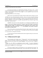
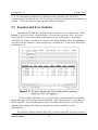
3.3 Summary Statistics
Scout will display summary statistics (such as mean, standard deviation, and variance)
for each variable when "Statistics" is chosen from the pull-down menu. The "Num" field
displays the number of valid observations that were used in the calculations for each of the
variables. The "Miss" field displays the number of missing observations for each of the
variables. The statistics can be printed by pressing <P> while the information is still on the
screen.
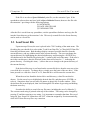
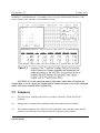
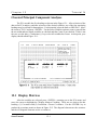
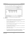
3.4 Data Transformation
The transform module in Scout allows each of the variables in memory to be tested for
normality using the Kolmogorov-Smirnov and Anderson-Darling tests.. If the variable fails
these tests you may then try various transforms on the selected variables. Each time a
transformation is tried, the resulting variable is retested for normality. You may select one or
more transformations for each variable by selecting a suitable function as displayed in the
figure 3-2. An undo feature allows you to sequentially undo each transform.
Scout User's Guide
3-6
Chapter 3
Managing Data in Scout
3.4.1 Normality Tests
Upon entering the transform module, you are given a choice between two normality
tests that can be used. These are the Kolmogorov-Smirnov test and the Anderson-Darling
test. The test selected will be used throughout the transform module.
3.4.2 Statistics Window
A window containing statistical information about each variable will appear in the
lower portion of the screen. The information displayed includes the number of observations,
mean, standard deviation, skewness, test statistic and critical value for the selected normality
test. If an asterisk character appears between the test statistic and critical value, then that
variable did not pass the normality test. You may scroll through the information in this
Scout User's Guide
3-7
Chapter 3
Managing Data in Scout
window by using any of the following keys: <UP ARROW>, <DOWN ARROW>, <PAGE
UP>, <PAGE DOWN>,
<HOME>, and <END>. This information can be printed either to a specified file or directly
to the printer by pressing the <P> key.
3.4.3 Histogram Window
Histograms may be displayed by pressing the <H> key. This key functions as a
toggle, that is, the histogram window will be active until the <H> key is pressed again. As
you scroll through the variables in the statistics window, you will notice that the histogram is
being updated to correspond to the current, highlighted variable. The two numbers near the
bottom of the histogram window are the minimum and maximum values for the current
variable. The scale for the histogram adjusts automatically as variables and transforms are
selected.
3.4.4 Transformation Menu
There are five transforms you may use. First you must highlight the variable to be
transformed and then press the <ENTER> key to bring up the transformation menu. The
menu contains five transform functions and an "undo" option. Each of these will be explained
separately in the following paragraphs.
3.4.4.1
Linear
This transform allows you to change the location and scale of a variable. The program
will prompt you to enter two constants 'a' and 'b' to be used as follows: X' = (X + a) * b where
'b' cannot be equal to zero. Once you have entered the constants, the transform will be
applied to a copy of the data. The histogram and statistics windows will be updated according
to the results of the transform. A new window in the center of the screen displays the
transform you have just selected along with any constants. This window keeps a record of all
the transforms you have chosen for each variable. If a transform does not produce the desired
results, you may "undo" that transform by selecting the undo option from the transformation
menu.
3.4.4.2
Logarithm
Transforms the data by using the natural logarithm. All of the data must be greater
Scout User's Guide
3-8
Chapter 3
Managing Data in Scout
than zero in order to use this transformation.
3.4.4.3
Power and Box-Cox
These two transformations will be explained together as they are very similar in usage.
Both of these require a nonzero constant 'a'. After entering a value for 'a', you have the option
of adjusting it. The value you entered will be displayed along with an incremental value
(delta). Pressing the <+> key will increment 'a' by delta and immediately reflect the results on
the screen. Likewise, pressing the <-> key will decrease 'a' by delta and show the results.
This gives you the ability to quickly try many values of 'a' before you decide which one to
select. You may also adjust the delta value for larger of smaller increments. Press the
<CTRL> and <-> keys at the same time to make delta smaller. Press the <CTRL> and <+>
keys at the same time to make delta larger. The range of delta is from 0.001 to 1.0. When
you find the desired value for 'a', press the <ENTER> key to accept it. If you cannot find an
acceptable value for 'a' and wish to abort this process, press the <ESC> key.
3.4.4.4
Arcsine
Transforms the data by using the Arcsine function. All of the data must be between
zero and one. This transform is typically used on data representing proportions.
3.4.4.5
Undo Option
Undesirable transforms that have been selected can be removed with the "Undo Last
Transform" choice in the menu. Transforms must be undone in the reverse order that they
were selected. This feature gives you great flexibility to try various transforms without the
risk of damaging your data. Your original data in memory is not modified until you are
finished testing and selecting the transforms for all of the variables. When you wish to exit
the transform module, the program will ask you to verify that the variables be modified with
the selected transforms.
3.4.5 Remarks on Transformation
When you have finished selecting the transforms for each of the variables and you are
Scout User's Guide
3-9
Chapter 3
Managing Data in Scout
ready to exit the transform module. Press the <ESC> key to do so and answer the question
box with the <Y> key. Another question box will appear asking you if you wish to modify
the variables in memory by doing the transforms that have been selected. Until now, your
original data has not been modified, you have only been testing the transforms. Answer the
question with <ENTER> or the <Y> key to apply the transforms to your original data. If for
some reason you wanted to abort this transform process and retain your original data, you
would answer the question with the <N> key. You should now be back in Scout's main
menu. If you have modified the variables in memory, you may wish to save them to a new
file on disk before you go on with your analysis.
CAUTION: Once you exit the transform module, your transform history is not
retained. It is advised that you log all changes for future reference. If you start the
transform module again, it is a new session and all transform lists are blank.
3.5 Print Data
This heading is used to print the data set currently in memory. Scout will ask the user
if the output is to be condensed. If the user answers no, then Scout will format the output
with up to six variables across each page. The printer should be set to 80 columns. If the user
answers yes to condensed printing, then Scout will format the output with up to ten variables
across each page. The printer should be set to 132 columns for this to work correctly.
Scout User's Guide
3-10
Chapter 4
Classical Methods for Outlier Identification
4.1 Introduction to the Classical Methods for Outlier
Identification
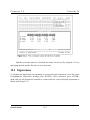
This chapter discusses the various procedures available within the "Classical Method"
menu. These procedures are used for outlier identification. Once a data file has been converted
into Scout format, Scout may be used to test for discordant observations in the data. These
discordant observations, or outliers, are highly unusual when compared to the rest of the data. For
a more thorough description of outliers and their significance, see the introduction to Chapter 14.
The Classical Method menu has two tests for discordancy: Mardia's multivariate kurtosis
and the (Mahalanobis') generalized distance. Mardia's multivariate kurtosis is also a useful test
for assessing multinormality, and is recommended when the number of outliers is unknown but
potentially substantial. The generalized distance is strictly an outlier test and is recommended
when the number of potential outliers is known to be very few. Both tests assume the data
represent a random sample from a univariate/multivariate normal population. Both of these tests
are included in the menu shown in Figure 4-1 below.
CAUTION: The removal of data values should not be based solely on their magnitudes.
Logically, one cannot truly distinguish non-normality from contamination. Discordant values
Scout User's Guide
4-1
Chapter 4
Classical Methods for Outlier Identification
should be subjected to increased scrutiny, and removal should occur only when this inspection
reveals unique or unusual problems in the measurement or recording of these values. Scout
is designed to enhance the user's ability to quickly identify such problems.
4.2 Select Variables
When searching for outliers, the user should decide which variables are to be included in
the analysis. The "Select Variables" heading will allow the user to do this. If the user skips this
step, Scout will default to testing all of the variables. Once in the variable selection screen, a
check mark next to a variable name indicates that variable will be tested. The user may place or
remove these check marks by using the <UP ARROW> and <DOWN ARROW> keys to move
the selector to a particular variable name, and then pressing the <-> key to remove the check
mark and the <+> key to place a check mark. The <-> and <+> keys move the selector to the
next variable name so that a series of variables can easily be set by holding down one of these
keys. Pressing <ENTER> or <ESC> will accept the variable selection as indicated.
4.3 The Classical Outlier Tests
The two outlier tests available in the Classical Method menu are Mardia's multivariate
kurtosis (Mardia (1970, 1974) and Schwager and Margolin (1982)) and the generalized distance
(Wilks (1963) and Barnett and Lewis (1994)), both of which have desirable properties as outlier
tests. The maximum generalized distance is a multivariate extension of a univariate test known
as Grubb's test (Grubbs 1950). This test is meant to identify a single outlier. It suffers from
masking in the presence of multiple outliers. Sequential application of this test is incorporated
in Scout.
Mardia's multivariate kurtosis is an extension of the univariate kurtosis. This test is more
powerful than the generalized distance when multiple outliers are present (Schwager and
Margolin (1982)). Mardia's multivariate kurtosis can also be used to test for deviations from
multivariate normality. However, this statistic is also not resistant to outliers, and as such, may
suffer from masking by multiple outliers.
The critical values used for the test statistic are the simulated values as given in Stapanian et al.
(1991).
This module of Scout is based on sequential application of these tests. This means that
outliers are detected sequentially: they are identified in the initial data set, removed from the data,
the statistics recomputed, and the identification, removal, and recomputing repeated until no more
outliers are found. Both tests assume the data are independent observations from a single
multivariate normal distribution. If a large proportion of the data are identified as discordant, the
user should be cautious that the problem may arise from a lack of multinormality, or the presence
Scout User's Guide
4-2
Chapter 4
Classical Methods for Outlier Identification
of multipopulations. Each observation identified as discordant is flagged as such, and the
graphics elements for those points are set to downward-pointing red triangles. The discordant
observations can then be viewed in the graphics module. Scout does not remove the discordant
observations, unless the user desires to do so.
During outlier testing, a new data set is generated. The user must decide how Scout
should handle the outliers when writing the new ASCII file. Four options available to the user
are, "Remove", "Keep", "Flag", and "Query". The "Remove" option deletes all of the outliers
from the generated file. The "Keep" option saves all outliers and the "Flag" option numerically
flags the outliers in the new file. It does this by adding a new variable called "OUTLIERS" to
the end of the variable list. The values in each observation for this new variable will be either
a '0' or a '1' where a '1' indicates this observation is an outlier. The "Query" option allows the user
to individually specify which outlier observations will be written to the new file. These features
are available only in the Classical Method menu.
CAUTION: Scout only identifies outliers for the variables selected. When viewing 2-D
or 3-D scatter plots which flag outliers, make sure that the variables in the plots were included
in the outlier test. Otherwise, the plot may include additional outliers.
4.4 Causal Variables
After an outlier test has been executed, the user may wish to identify the variables (if any)
which are responsible for each discordant observation. This is done by selecting the "Causal
Variables" choice from the pull-down menu. Scout will retest each discordant observation with
one variable excluded at a time. Thus each discordant observation is tested p times using all
subsets of p-1 of the variables. A variable is listed as causal only if absence of the variable
prevents identification of the outlier. Although this procedure is based on iterations of rigorous
tests of hypotheses, the user should consider its results only as general guidance and not as
definitive proof of the cause. Starting with an investigation of the suspected causal variable (or
group) whose removal results in the largest decrease in the value of the test statistic is
recommended. As with any quality control technique, the results of these statistical procedures
should be combined with experience and knowledge of the measurement system for proper
interpretation of the data.
The output is described as follows: The 'Outlier' column provides the observation number
and label of the discordant observation being tested. 'Test' shows the outlier test statistic, while
'Crit' gives the critical value used in the test. The test statistic and critical value are different from
those shown in the original outlier test because the dimensionality is reduced by one variable.
The 'variable' column provides the name of the identified causal variable. This is the variable
that, when present, always allows rejection of the discordant observation. The 'Observed' column
Scout User's Guide
4-3
Chapter 4
Classical Methods for Outlier Identification
displays the value in the data set for the discordant observation and causal variable. The
'Expected' column gives a prediction of the value by using multiple regression and the values
reported for the other variables in that observation. 'Low Lim' and 'Up Lim' provide the lower
and upper limits, respectively, for a prediction interval. The type I error rate (alpha) of this
interval is the same as was chosen for the outlier test.
This process is designed to identify cases where, apparently, the discordancy resulted from
substantial deviation in a single variable. This can occur when large errors in measurement are
independent, or when typographical, recording, and transcription errors cause the outlier. For
example, for the third variable in a ten dimensional data set, recording 73.56 as 37.56 or as 735.6
may cause the associated observation to be identified as an discordant. If so, executing the
Causal Variables routine will probably indicate the third variable as the cause of the discordancy.
4.5 Associated Causes
This feature allows users with sufficient understanding of their data sets to group (General
Cause) and subgroup (Specific Cause) variables which, according to their specialized knowledge,
may be causally related. The user must specify the groupings that will be sequentially excluded
from the outlier test. Any group whose exclusion results in the observation no longer being
discordant will be listed as potentially causal. This is intended to aid the user in finding and
correcting physical causes of discordancy. Thus the groupings should correspond with known
physical causes. For example, a subset of the variables may have been measured on a single
instrument. It would be natural to group these variables so that Scout can investigate the
possibility that discordancies are manifest in the entire group of variables due perhaps to faulty
operation of the instrument. Variables may be grouped according to a variety of characteristics.
The user should also run the "Causal Variable" routine and interpret the results of the associated
causes routine in light of the fact that discordancy in a single variable will cause all groups
containing that variable to appear causal.
4.6 Remove Outlier Flags
The "Remove Outlier Flags" choice provides the user with a means of unmarking any
data that has been identified as an outlier. Once a procedure has identified outliers, these outliers
are colored red in the data file. The "Remove Outlier Flags" choice turns the red data back to
white, the original color of the data.
Scout User's Guide
4-4
Chapter 5
Robust Statistical Methods
5.1 Introduction to Robust Statistical Methods
Outliers are inevitable in most applied and scientific disciplines. In a manufacturing
process, outliers (anomalies, extremes, maverick observations) typically represent some
mechanical disorder of the system, unexpected experimental conditions and results, raw material
of an inferior quality, or misrecorded values. In biological dose-response applications, outlying
observations may indicate an entirely different type of reaction (an unusual response) to a newly
developed drug. In this case, "outliers" may be more informative than the rest of the data. In
environmental and ecological applications, outliers could be indicative of highly contaminated
areas, sections of a forest in poor or degraded states, inconsistent analytical results in a typical
quality assurance and quality control (QA/QC) program, or gross typing errors.
Experimentalists, especially environmental scientists, generate and analyze large amounts
of data. Most of these practitioners, therefore, are familiar with the situations when some of their
experimental results look suspicious or significantly different from the rest of the data. In data
sets of large dimensionality, it becomes tedious to identify these anomalies. Appropriate
multivariate procedures need be used to identify multivariate anomalies. Several univariate and
multivariate procedures are incorporated in the Robust Method heading of the Scout software
package.
The successful identification of anomalous observations depends on the statistical
procedures employed. The classical Mahalanobis distance (MD) and its variants (e.g.,
multivariate kurtosis) are routinely used to identify these anomalies. These test statistics depend
upon the estimates of population location and scale. The presence of anomalous observations
usually results in distorted and unreliable maximum likelihood estimates (MLEs) and ordinary
least-squares (OLS) estimates of the population parameters. These in turn result in deflated and
distorted classical MDs and lead to masking effects. This means that the results from statistical
tests and inference based upon these classical estimates may be misleading. For example, in an
environmental monitoring application, it is possible that the classification procedure based upon
the distorted estimates may classify a contaminated sample as coming from the clean population
and a clean sample as coming from the contaminated part of the site. This in turn can lead to
incorrect remediation decisions.
It is well established among practioners that for the identification of multiple outliers, one
should use robust procedures with a high breakdown point. The estimates obtained using the
robust procedures should be in close agreement with the corresponding MLEs when no
discordant observations (from different population(s)) are present. Robust procedures for the
identification of outliers and the estimation of population parameters of location and scale
typically use an influence function. The robust module of Scout computes various statistics using
four methods. These include the classical MLE approach, the robust multivariate trimming
Scout User's Guide
5-1
Chapter 5
Robust Statistical Methods
approach (Devlin et al, 1981), the Huber influence function (Huber, 1981), and the proposed
PROP influence function (Singh, 1993). Numerous graphical procedures are incorporated in
Scout. These include the normal Q-Q plots of raw data, scatter plots, Q-Q plots and scatter plots
of principal components, Q-Q plot and index plot of the Mahalanobis distances, scatter plots of
discriminant scores, contour plots, plots of prediction interval, simultaneous confidence intervals
and more. The control-chart type quantile-quantile (Q-Q) graphical display of multivariate data
combines the effect of a formal test procedure and an informal graphical display into one
powerful multiple outlier identification procedure.
5.2 Choices of robust analyses
Several univariate and multivariate robust procedures are available in Scout which are
worked out in detail in the tutorials (Section II). There are nine options in the "Robust Method"
menu:
Select Variables
Univariate Statistics
Robust Analysis
Confusion Matrix
Pattern Recognition
D Trend
Add Mean
Causal Variables
Print Destinations
There are various screens associated with each of these options. An explanation window
associated with each of the options provides a brief description of that heading or choice.
This "Robust Method" module is independent of (cannot communicate with) "Classical
Method", "PCA", and "Graphics" headings in Scout. It can communicate with "File", "Data", and
"System" headings. For example, the Robust principal components cannot be displayed using
a 3-D graph, without first saving them in a data file and then reading in the saved data file to plot
the 3-D graph of the saved principal components.
Scout User's Guide
5-2
Chapter 5
Robust Statistical Methods
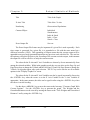
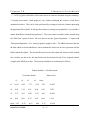
5.3 Univariate Statistics
This heading computes univariate statistics. The four methods mentioned in the
introduction to this chapter are available: (1) the classical maximum likelihood estimator (MLE),
(2) the Huber, (3) the proposed "PROP" robust method, and (4) sequential trimming. The
weights can be computed using the exact Beta distribution of generalized distances, or the Chisquare approximation.
To perform Univariate statistics, use the up and down <ARROW> key to select
"Univariate Statistics" from the menu and use the <ENTER> key. At this point, a window
entitled "Univariate Robust Statistics" will be displayed. This window can be used to set various
options for calculating Univariate statistics. This window has five main headings as follows (The
example choices used throughout this manual are those displayed by default using the IRIS.DAT
file, which is discussed in the tutorial section):
Heading
Example Choice
Compute Statistics Using . . . . . . . . . . . . . . . . . . . . . . . . . . . . . . . . . . . . . . . . Classical
Weights . . . . . . . . . . . . . . . . . . . . . . . . . . . . . . . . . . . . . . . . . . . . . . . . . . . . . . . . . . Beta
Scout User's Guide
5-3
Chapter 5
Robust Statistical Methods
Initial Estimate . . . . . . . . . . . . . . . . . . . . . . . . . . . . . . . . . . . . . . . . . . . . . . . . Classical
Right Tail Cutoff . . . . . . . . . . . . . . . . . . . . . . . . . . . . . . . . . . . . . . . . . . . . . . . . . . . 0.05
Trimming Percent . . . . . . . . . . . . . . . . . . . . . . . . . . . . . . . . . . . . . . . . . . . . . . . . . . . . . 0
Each of these headingss has various choices, which can be selected by repeated use of the
<ENTER> key when that heading is highlighted. After a selection is made, the arrow key can
be used to move the cursor to the next heading. The process can be repeated until the desired
choices have been selected. The various choices for each of the headings of the Univariate
Statistics menu are as follows:
Heading
Choices
Compute Statistics Using
Classical
Huber Influence
Proposed Influence
Multivariate Trimming
Weights
Beta
Chi-Squared
Initial Estimate
Classical
Robust
Right Tail Cutoff
A number between 0.01 and 0.8 (active only
when PROP or Huber are chosen)
Trimming percent
An integer between 0 and 100 (active only
when Multivariate Trimming is used)
The values for number choices can be typed directly on the screen after using the
<ENTER> key to highlight the corresponding heading (this applies to "Right Tail Cutoff" and
"Trimming Percent" in the previous menu). The other choices can be set by using the <ENTER>
key repeatedly. After all selections are made, move the cursor to the bottom of the third window
to indicate "Generate Statistics Using Current Options". Use the <ENTER> key to generate the
Univariate Statistics corresponding to the selected choices. At this point the result of the
univariate statistical analysis will be displayed on the screen. These statistics are also stored in
an output file of the same name with the extension ".URS". For example, statistics for IRIS.DAT
will be stored in IRIS.URS.
The statistics get appended to this file, if any information from an earlier Scout session is still in
the file, then the current statistics will be added to it.
Scout User's Guide
5-4
Chapter 5
Scout User's Guide
Robust Statistical Methods
5-5
Chapter 5
Robust Statistical Methods
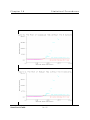
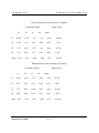
5.4 Robust Analysis
When Robust Analysis is selected, the explanation window will display the message "This
routine provides exploratory as well as confirmatory procedures for the assessment of
multinormality and detection of multivariate outliers." When <ENTER> is pressed, while
Robust Analysis is highlighted, a third menu appears listing various options. The available
headings and choices of this menu and the default choices are as follows:
Headings
Default Choices
Display Graphs For . . . . . . . . . . . . . . . . . . . . . . . . . . . . . . Q-Q Plot (Indiv: Raw Data)
Statistics Options . . . . . . . . . . . . . . . . . . . . . . . . . . . . . . . . . . . . . . . . . . . . . . Classical
Zero Lower Limit . . . . . . . . . . . . . . . . . . . . . . . . . . . . . . . . . . . . . . . . . . . . . . . . . . . No
Limit Style . . . . . . . . . . . . . . . . . . . . . . . . . . . . . . . . . . . . . . . . . . . . . . . . . . Two Sided
X Axis Variables . . . . . . . . . . . . . . . . . . . . . . . . . . . . . . . . . . . . . . . . . . . . . . . . . . . . . . 2
Y Axis Variable . . . . . . . . . . . . . . . . . . . . . . . . . . . . . . . . . . . . . . . . . . . . . . . . . . . . . . 3
Title . . . . . . . . . . . . . . . . . . . . . . . . . . . . . . . . . . . . . . . . . . . . . . . . . . . Robust Analysis
X-Axis Title . . . . . . . . . . . . . . . . . . . . . . . . . . . . . . . . . . . . . . . . . . . . . . . . . . . . . . . . . .
Numbering . . . . . . . . . . . . . . . . . . . . . . . . . . . . . . . . . . . . . . . . . . . . . . . . Observations
Contour Ellipse . . . . . . . . . . . . . . . . . . . . . . . . . . . . . . . . . . . . . . . . . . . . Indiv & Simul
Erase Output File
View Weights & Generalized Distances . . . . . . . . . . . . . . . . . . . . . . . . . . . . IRIS.WTS
Generate Graph With Current Options
Each of these headings has various choices, which can be selected by repeated use of the
<ENTER> key. After a selection is made, an arrow key can be used to move the cursor to the
next heading. The process is repeated until the desired choices for all of the headings have been
selected. For "Robust Analysis", the various choices for each of the headings are listed in a
fourth window:
The "Display Graphs For" heading offers the following list of available graphs:
Q-Q Plot (Indiv: Raw Data)
Q-Q Plot (Indiv: Standardized)
Q-Q Plot (Simul: Raw Data)
Q-Q Plot (Simul: Standardized)
Scatter Plot (Raw Data)
Q-Q Plot (PCA)
Scatter Plot (PCA)
Q-Q Plot (Generalized Dist.)
Scout User's Guide
5-6
Chapter 5
Robust Statistical Methods
Control Charts Indiv (Xi)
Control Charts Simult. (Xi)
Control Charts (Defects)
CI Limits Population Mean
Prediction Intervals
Index Plots
Multivariate Kurtosis
Use arrow keys to reach the desired procedure and then press the <ENTER> key to make
a selection from this list. The fourth window will disappear and the third window will reappear
with the selected choice listed after "Display Graph For".
CI Limits Population Mean: This choice outputs the relevant statistics and the limits for
confidence interval for mean on the screen. These limits can be graphed by pressing the letter
'Q' (or 'q'). The Prediction Intervals can be graphed similarly. The Control Charts Simult (Xi)
choice produces the graph for simultaneous confidence interval for selected settings as described
in Singh and Nocerino (1995). Multivariate Kurtosis simply computes the multivariate kurtosis
for the selected options. No graph is generated for this procedure. Some of these options are
discussed in the tutorial section.
Move the cursor to the "Statistics Options" heading. Use the <ENTER> key to display
the menu. The various choices for the "Statistical Options" headings are listed as follows:
Heading
Choices
Compute Statistics Using
Classical
Huber Influence
Proposed Influence
Multivariate Trimming
Initial Estimate
Classical
Robust
Matrix
Correlation
Covariance
Weights
Beta
Chi-Squared
X-Y Coordinate Scale Factor (%)
An integer betweeon -100 and 100
Scout User's Guide
5-7
Chapter 5
Robust Statistical Methods
Right Tail Cutoff
A number between 0.01 and 0.8 (to be used
with Huber or PROP)
Tuning Constant
A number between 0.1 and 5.0
Control Chart Limit
A number between 0.01 and 0.5
Trimming percent
An integer between 0 and 100 (to be used
with Multivariate Trimming)
Ignore Population #
A non-negative integer to represent the
population not to be considered in the analysis
Plot Ignored Population
Yes/No (The last two headings assume that
the data set has the population ID in the first
column)
NOTE: This Statistics Options menu is also shared by the three other procedures in the Robust
Analysis main menu: Confusion Matrix, Pattern Recognition, and Causal Variables. The
explanations of these headongs will refer back to this description.
For the last four headings in the fourth window (Statistics Options), given above, the
numbers for choices can be typed to the screen after using the <ENTER> key when the cursor
is on the corresponding statement. The other choices can be selected by using the <ENTER> key
repeatedly. After all selections are made, move the cursor to the bottom of the fourth window
to the "Accept New Settings." Use the <ENTER> key to accept the selected choices for the
"Statistics Options" and return to the third window.
The remaining headings and corresponding choices in the third window (Robust Analysis)
are as follows:
Heading
Choices
Zero Lower Limit
Yes/No
Limit Style
Upper Limit/Lower Limit/Two Sided
X Axis Variable
An positive integer between 1 and 22
Y Axis Variable
An positive integer between 1 and 22
Scout User's Guide
5-8
Chapter 5
Robust Statistical Methods
Title
Title of the Graph
X-Axis Title
Title of the X-Axis
Numbering
Observations/Populations
Contour Ellipse
Individual
Simultaneous
Indiv & Simul
Indiv + Class
Simul + Class
Erase Output file
See text
The Erase Output File feature may be important if a given file is used repeatedly. Each
time output is generated for a given file, it is appended to a file with the same name but a
different extension (.URS). This appending of output means that the current output will be
appended to any previously generated output from any previous work with this file. The user has
the option to erase this file prior to the recording of the current session's output, in this manner
the output file will be reflective of only the current session.
The values for the X Axis and Y Axis Variables are chosen by Scout automatically from
among the selected variables. While in the graphics mode the user can also use the Page Up and
Page Down keys to change the X-labels and the Ctrl-Page UP and Ctrl-Page Down to change the
Y-labels. New graphs appear after each selection. The 'F1' key can be used to see all available
options in the "Display Graphs For" menu.
The values for the X Axis and Y Axis Variables can also be typed in manually after using
the <ENTER> key when the cursor is on the X Axis Variable or the Y Axis Variable as
appropriate. In the same manner, the titles can be typed in after using the <ENTER> key when
the cursor is at title heading.
Use the down <ARROW> key to move the cursor to the last entry, "Generate Graph With
Current Options". Use the <ENTER> key to generate the graph. The Weights and the
Generalized distances can be viewed by moving the cursor to the "View Weights and Generalized
Distances" and by using the <ENTER> key.
Scout User's Guide
5-9
Chapter 5
Robust Statistical Methods
5.5 Confusion Matrix
This option performs linear and quadratic discriminant analysis, and expects the data to
be multivariate in nature. The first column of the data set should have the population ID (a
number between 1 and 20) and the number of variables should be at least two (2). Graphs cannot
be produced with this option.
When the Confusion (or error) Matrix heading is selected, the second window will
display the message "Robust supervised pattern recognition classification". Press the <ENTER>
key to display the third window to set various options. The available headings for this choice are
as follows:
Heading
Example Choices
Discriminant Method . . . . . . . . . . . . . . . . . . . . . . . . . . . . . . . . . . . . . . . . . . . . . Linear
Statistics Options . . . . . . . . . . . . . . . . . . . . . . . . . . . . . . . . . . . . . . . . . . . . . . Classical
The discriminant analysis method heading has two choices: Linear and Quadratic, which
can be selected by using the <ENTER> key when the cursor is at Discriminant Method in the
third window. Statistics Options presents the same menu as described in Section 5.3
Use the down <ARROW> key to move the cursor to the last selection, "Generate
Confusion Matrix With Current Options". Use the <ENTER> key to generate the Confusion
Matrix. Use the <ESCAPE> key to return to the third window if the parameters need to be
readjusted or other analyses performed.
5.6 Pattern Recognition
The pattern recognition heading performs principal component and discriminant analysis.
The data should be multivariate in nature with at least two variables. The first column should be
population ID numbers (a number from 1 to 20).
When Pattern Recognition is selected, the explanation window will display the message
"Pattern recognition using discriminant scores and principal components analyses". Pressing the
<ENTER> key displays the third window revealing various headings. The available headings
and example choices for Pattern Recognition are as follows:
Example Choices
Headings
Statistics Options . . . . . . . . . . . . . . . . . . . . . . . . . . . . . . . . . . . . . . . . . . . . . . Classical
Numbering . . . . . . . . . . . . . . . . . . . . . . . . . . . . . . . . . . . . . . . . . . . . . . . . Observations
Contour Ellipse . . . . . . . . . . . . . . . . . . . . . . . . . . . . . . . . . . . . . . . . . . . . Indiv & Simul
Scout User's Guide
5-10
Chapter 5
Robust Statistical Methods
Type of Graphs . . . . . . . . . . . . . . . . . . . . . . . . . . . . . . . . . . . . . . . Discriminant Scores
Graph Title . . . . . . . . . . . . . . . . . . . . . . . . . . . . . . . . . . . . . . . . . . . Pattern Recognition
Save Discriminant Scores . . . . . . . . . . . . . . . . . . . . . . . . . . . . . . . . . . . . . . . . . . . . . No
View Eigenvalues and Vectors . . . . . . . . . . . . . . . . . . . . . . . . . . . . . . . . . . . . . . . . Yes
View Confusion Matrix . . . . . . . . . . . . . . . . . . . . . . . . . . . . . . . . . . . . . . . . . . . . . Yes
View Covariance Matrix and Means . . . . . . . . . . . . . . . . . . . . . . . . . . . . . . . . . . . Yes
Each of these headings has various choices which can be selected by repeated use of the
<ENTER> key. After a selection is made, an arrow key can be used to move the cursor to the
next heading. The process can be repeated until each of the desired choices for the various
headings have been selected.
Statistics Options presents the same menu as described in Section 5.3. Set these options
as desired then return to the third window (as shown above). The remaining headings and
corresponding choices in the third window are as follows:
Headings
Choices
Numbering
Observations/Populations
Contour Ellipse
Individual/Simultaneous/Indiv & Simul,
Indiv + Class, Simul + Class
Type of Graphs
Discriminant Score/PCA Score/X-Y
Graph Title
Can be typed in after using the <ENTER> key
Save Discriminant Scores
Yes/No
View Eigenvalues and Eigenvectors
Yes/No
View Confusion Matrix
Yes/No
View Covariance Matrix and Means
Yes/No
The Graph titles can be typed in after using the <ENTER> key when the cursor is on the
"Graph title" option. When satisfied with all heading choices, use the down <ARROW> key to
move the cursor to the last selection: "Begin computations with selected options". Use the
<ENTER> key to generate the data pattern.
Scout User's Guide
5-11
Chapter 5
Robust Statistical Methods
The first computation in this module will be the Eigenvalues and Eigenvectors, use the
<ESC> key once to generate the Confusion (error) Matrix. Use the <ESC> key once more to
generate the scatterplots of Discriminant Scores. Various discriminant scores will be plotted
when the <PAGE UP> or <PAGE DOWN> key is used. Use the <E> key to generate the ellipse
corresponding to the various score clusters. If the Populations choice is used for the numbering
heading, graphs generated will use different colors for different populations.
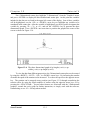
5.7 D Trend
The following two headings: D-Trend and Add means are useful to perform geostatistical
analysis. Some knowledge of geostatistical analysis such as kriging and variogram modelling
is required. Users not interested in this may like to skip this Section. These headings require the
knowledge of the geographic location (e.g., Easting, Northing coordinates) for each of the sample
observations. Ordinary kriging (OK) is a well established geostatistical technique frequently used
in site characterization studies. However, OK assumes that there are no spatial trend present, and
the mean concentration at each location is constant within the region under consideration. This
assumption is often violated by the data collected from a polluted site. Therefore, in order to use
OK to characterize the site under study, the data with spatial trend need to detrended so that the
constant mean assumption is satisfied.
Scout offers the D-Trend heading for removing trend that might be present in a
geostatistical data set obtained from a polluted site. It assumes that the data is in the same format
as for the pattern recognition option with the population IDs in the first column. Using an
appropriate multivariate technique, first the data has to be partitioned into various strata with
significantly different statistics (e.g., mean vectors). Using the geographic information of the
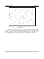
sample observations, a site map can be prepared exhibiting the actual sampling locations and the
respective population IDs. The D-trend heading when used subtracts the respective subpopulation means from each observation in the corresponding sub-population. The resulting data
thus obtained satisfy the constant mean assumption. An example is included in the tutorial
section illustrating its usage.
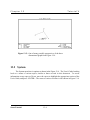
5.8 Add Means
This heading is used after OK has been performed using the detrended data and a file with
extension "grd" has been created. The means subtracted using the D-Trend option need to be
added back to the kriging estimates in the "grd' file. This can be achieved using the Add Means
heading. This option uses two input files: a statistics file with extension sts, ' Example.sts' and
a file with extension add, 'Example.add'. The sts file should follow the same format as the
statistics file generated by Scout. A separate add file (e.g., pb.add) is required for each variable
Scout User's Guide
5-12
Chapter 5
Robust Statistical Methods
considered. The add file has the following format.
a
b
c
x1 x2 y1 y2 population Id1
x1 x2 y1 y2 population Id2
Repeat for each region of the site.
Here
a = Total number of sub-populations
b = Total number of variables
c = Number of the variable in the sts file
x1 x2 y1 y2 are the coordinates of the boundary of a geographic region (a rectangle)
belonging to one of the sub-populations. Thus, the region bounded by (x1, y1), (x2, y1),
(x1, y2), and (x2, y2) belongs to the population with the corresponding ID.
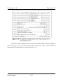
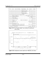
Example: The example add file for lead (Pb) is 'Pb.add'. There are two populations, a=2, and 4
variables in the data file with b=4. Lead in the second variable in the sts file, therefore c =2.
2
0
200
1100
1850
200
200
1100
4
200
3000
3000
3000
1850
1100
1850
2
0
0
1220
1700
2780
1220
1700
3500
1220
1700
3500
3500
2780
2780
1
1
1
1
1
2
2
So using this input file, when the Add Means heading is activated, the mean of sub-population
1 will be added to all observations with in the region bounded by (1100, 1220), (1100, 1700),
(3000, 1220), and (3000, 1700). This will be performed for each of the regions in the Pb.add file
(7 here) .
5.9 Causal Variables
When Causal Variables is selected, the second window will display the message "Searches
for the variables that might have caused a given observation to be an outlier. A variable is a
cause if, when removed, the observation is no longer an outlier." When the <ENTER> key is
pressed, the third window appears allowing the various headings to be set. The available
Scout User's Guide
5-13
Chapter 5
Robust Statistical Methods
headings for this choice are as follows:
Scout User's Guide
5-14
Chapter 5
Robust Statistical Methods
Headings
Example Choices
Statistics Options . . . . . . . . . . . . . . . . . . . . . . . . . . . . . . . . . . . . . . . . . . . . . . Classical
Confidence Interval . . . . . . . . . . . . . . . . . . . . . . . . . . . . . . . . . . . . . . . . . Simultaneous
Zero Lower Limit . . . . . . . . . . . . . . . . . . . . . . . . . . . . . . . . . . . . . . . . . . . . . . . . . . . No
Each of these headings has various choices, any of the choices for Confidence Interval
and for Zero Lower Limit can be selected by repeated use of the <ENTER> key. After a
selection is made, an arrow key can be used to move the cursor to the next heading. The Zero
Lower Limit option can be used when the lower limit becomes negative, and the data cannot take
negative values.
Statistics Options presents the same menu as described in Section 5.3. Set these headings
as desired and return to the third window. The remaining headings and corresponding choices
in the third window are as follows:
Headings
Choices
Confidence Interval
Simultaneous/Individual
Zero Lower Limit
No/Yes
When satisfied with all heading choices, use the down <ARROW> key to move the cursor to the
final selection, "Begin search for causal variables". Use the <ENTER> key to generate the table
for Robust Causal Variables.
5.10 Print Destination
This heading will create graphics files with an '.eps' extension. The HP LaserJet III choice
will print the screen graph to a LaserJet III printer. Typing 'F' will write the graphics screen to
a 'pcx' file.
When Print Destination is selected, the second window will display the message "Choose
print destination for graphs". When the <ENTER> key is pressed, three choices are displayed
in the third window as follows:
HP LaserJet III
QMS ColorScript 100
Encapsulated Post Script
Scout User's Guide
5-15
Chapter 5
Robust Statistical Methods
Use Encapsulated Post Script to save the graph and data output files in a format that can
be imported to a word processing software such as Word Perfect. This option will create a
graphics file with the extension ".EPS". The HP Laserjet III choice will print to the screen, or to
a Laserjet III printer. Pressing <F> can be used to write the graphics to a ".PCX" file.
Scout User's Guide
5-16
Chapter 6
PCA
6.1 Classical Principal Components Analysis
For simplicity and convenience, a separate principal component analysis (PCA) menu has
been included in Scout to perform the classical PCA. The Q-Q plots, scatterplots, and contour
ellipses for classical/robust PCA can also be produced using the "Robust Method" menu as
discussed in Chapter 5.
Using PCA, the user can look at the correlation/covariance matrix directly on the screen.
The PCA menu has five headings as displayed in Figure 6-1.
The Select Variables heading has been discussed in earlier chapters, so we omit its
description here.
6.2 Display Matrices
The user may choose to display the covariance and/or correlation matrices. To do this,
select "Display Matrices" from the PCA menu. Within this heading, users can remove outliers,
found by the Classical Method, manually. If any outliers have been identified, Scout will ask the
user if outliers are to be used or ignored. Then Scout will ask the user which matrix he is
interested in, covariance or correlation. Scout will then display the selected matrix on the screen.
Scout User's Guide
6-1
Chapter 6
PCA
If the entire matrix does not fit on the screen, then the user can press the arrow keys to scroll
through the matrix. Press <ESC> to return to the PCA menu after viewing the matrix.
6.3 Eigenvalues
This heading allows the user to view the eigenvalues. Scout will ask the user whether to
calculate the eigenvalues using the covariance or correlation matrix. After making this choice
and pressing the <ENTER> key, the eigenvalues are displayed along with their differences,
proportions, and cumulative proportions. If there are more eigenvalues than will fit in the
window, then use the <UP ARROW> and <DOWN ARROW> keys to scroll through them.
Press the <P> key to send this information either to the printer or to a file. Press the <ESC> key
to close the window and return to the menu.
6.4 View Components
This heading displays a listing of the component loadings. Scout will offer the user the
choice of performing PCA with either the covariance or correlation matrix. After making this
choice and pressing the <ENTER> key, use the <UP ARROW> and <DOWN ARROW> keys
to scroll through the information. Use the <P> key to send the information to the printer or to a
file. Press the <ESC> key to close the window and return to the menu.
6.5 Transform Data
The component scores are the product of the eigenvectors and the standardized
observation vectors. The user may wish to graph the component scores later using the Graphics
menu discussed in Chapter 7. In order to do so, these scores need to be saved. Users can save
component scores using the Transform Data heading. Before the component scores can be
graphed, Scout must be instructed to save the component scores. The component scores will
replace the original data in the memory.
CAUTION: Scout uses the same computer memory to store the component scores as that used
for the original data. The "Transform Data" heading will overwrite the original data with the
component scores. If a user generates component scores and then saves them to the same file
as the original data, the original data will be lost. Therefore, once generated, the component
scores need to be saved to a different Scout file to avoid loss of the original data. However, the
PC scores (classical or robust) can be saved in the same data file without overwriting the
original data by using the Robust Method menu where extra columns are added to the data
file.
Scout User's Guide
6-2
Chapter 6
PCA
The transformed data may consist of component scores and original variables. The user
must be careful not to misinterpret the resulting data.
Scout User's Guide
6-3
Chapter 7
Graphics
7.1 General Description
Scout features two graphics options: 2-dimensional and 3-dimensional. 2-Dimensional
graphics are used to display bivariate plots (also known as scatter plots or XY-plots).
3-Dimensional graphics are used to display three variable plots, which can be rotated to illustrate
the extra dimension. The Graphics menu is displayed in Figure 7-1 below.
7.2 Modify Graph Colors and Shapes
The first heading in the graphics pull-down menu, "Graph Parameters," allows the user
to modify the color and shape of individual observations (or points) that will be displayed on the
graphs. There are six colors and six shapes to choose from yielding 36 possible combinations
(assuming the user has a color monitor). However, choosing black as the color of an observation
has a special meaning. Black observations will not be seen on the graphs, nor will they be used
in the scaling of the graphs. The default color is yellow and the default shape is an 'x'.
To select a new color and shape, press the <F2> key. The current color will now be
Scout User's Guide
7-1
Chapter 7
Graphics
highlighted. Use the <UP> or <DOWN> arrow keys to highlight the desired color and then press
<ENTER> or the <RIGHT ARROW> key. Now the current shape will be highlighted. Again,
use the <UP> or <DOWN> arrow keys to highlight the desired shape and press <ENTER> to
complete the selection.
To change the graph symbol (color and shape) of an observation, first use the <F2> key
to change the color and shape, then use the <UP> or <DOWN> arrow keys to highlight the
observation that is to be changed and then press the <ENTER> key. The graph symbol
corresponding to the highlighted observation then changes to the selected graph symbol shown
in the right window. The highlighter is then moved automatically to the next observation. This
makes it very easy to change a continuous block of observations by holding down the <ENTER>
key.
The user can exit this screen at any time by pressing <ESC> key. All of the changes made
are retained in memory. Sometime before exiting the program, the user should save the data in
memory as a Scout file so the changes become permanent, otherwise they will be lost.
7.3 Command Summary for 2D and 3D Graphics
Scout recognizes the following field commands when either 2- or 3- dimensional plots are
displayed:
<F>
Outputs the scatter plot to a PCX file
<H>
Hides (i.e., does not display) observations that were identified as outliers (toggle).
<N>
Replaces the symbol for each observation with the observation number (toggle)
<P>
Prints the scatter plot on a printer
Outputting a graph to a PCX file: Both 2-dimensional and 3-dimensional graphics screens
may be written to a file on disk. When the user has the desired graphics image displayed,
pressing the <F> key will prompt the user for a file name. Type in a file name (including the
drive and directory, but without an extension as '.PCX' will always be used) and press <ENTER>
key. The graphics screen will be written to the file in PCX format which many other software
packages can read.
Hiding Outliers in Scatterplots: If you wish to view a scatterplot in which the outlier
observations are not displayed, press the <H> key. Press the <H> key again and the outliers will
be displayed as before. CAUTION: Hiding outliers from a scatter plot does not change the
Scout User's Guide
7-2
Chapter 7
Graphics
statistical properties of the variables.
Replacing Symbols with Observation Numbers: Sometimes it is useful to see where
individual observations, or groups of observations, are located on a scatter plot. Press the <N>
key and the symbols for the observations of the scatterplot will be replaced by the observation
numbers. Press <N> key again to return to symbols.
Printing a graph: The printer in use must be specified before Scout can print any graphs.
See System Printer Specifications to select the make and model of the printer and other graphics
specifications. Scout can only print graphs that are displayed on the monitor. Press the <P> key
to print the graph that is on the screen. A line will move across the screen as Scout
"Reads" the graph and sends it to the printer.
7.4 2-Dimensional Graphs
The second heading in the graphics pull-down menu, "2-Dimensional", is the 2dimensional graphics system. If any observations have been flagged as outliers, Scout will ask
the user if those outliers are to be used in statistical calculations. Scout will then place the
computer in graphics mode and display a color coded, correlation matrix of the data. Each point
in this matrix represents the correlation of two variables. The names of these two variables are
printed near the top of the screen along with some summary statistics on each of the two
variables. The correlation values are printed on the right side of the screen. The color coding
scheme works as follows. White indicates a correlation coefficient greater than 0.75. Green
indicates a correlation coefficient greater than 0.5 and less than 0.75. All other correlation
coefficients, less than 0.5, are red.
The upper left point of this matrix will be highlighted with a purple box. The user can
move through the matrix with the arrow keys, and quickly get an idea of how any two variables
are related. The user can view the scatter plot of the currently displayed variables by pressing
the <ENTER> key. When viewing a scatter plot, the user can scroll through the observations that
make up the graph. Again, the purple box will highlight the location of the current observation
being displayed. The axes are scaled independently from the minimum value to the maximum
value of the variable. The user can force equal scaling of both axes by pressing the <E> key.
The <E> key functions as a toggle, turning equal scaling on and off. The <ENTER> key returns
the user to the correlation matrix and the <ESC> key exits the graphics mode returning the user
to the menu screen.
7.5 Zoom Feature
This option enables the user to inspect portions of a 2-dimensional scatterplot in more
detail. This is especially useful when many data occur over a relatively small range, making
Scout User's Guide
7-3
Chapter 7
Graphics
resolution of individual observations difficult.
To use the zoom feature on a 2-dimensional scatterplot, press the <Z> key. A white
rectangle encompassing all of the observations will appear. Use the "-" (minus) key to decrease,
or the "+" key to increase, the area of the rectangle. Use the <ARROW> keys to move the
rectangle to the portion
of the scatter plot that you wish to enlarge.
When you have surrounded the observations of interest with the white rectangle, press the
<ENTER> key. Scout will automatically rescale the x- and y-axes and a scatter plot containing
only the observations of interest will appear. Press the <Z> key and Scout will return to the
original scatter plot, with the white rectangle still surrounding the observations of interest.
Pressing <ENTER> key from the "zoomed" scatter plot will cause Scout to return to the
color-coded correlation matrix.
CAUTION: You can not use the zoom feature on a scatterplot generated by the zoom
feature. If you wish to inspect an area of a "zoomed" scatter lot in detail, you must first
redefine the white rectangle. To redefine the dimensions and location of the rectangle, return
to the original scatter plot and press the "-", "+", and <ARROW> keys until the rectangle is
at the desired size and location.
If you wish to exit the zoom mode and thus eliminate the white rectangle from the original
scatter plot, press <ESC>. If you press the <Z> key again, the Scout will restore the rectangle
as it was just prior to exiting the zoom mode.
To return to the color-coded correlation matrix from the original scatter plot, exit the zoom
mode and press <ESC>.
7.6 3-Dimensional Graphs
The last heading in the Graphics menu, "3-Dimensional", is the 3-dimensional graphics
system. The user first selects a variable for each of the three axes. All of the variables will be
displayed on the screen with the first variable highlighted. The user may use the <ARROW>
keys,
<HOME> key, and <END> key to highlight any desired variable. To assign the highlighted
variable to an axis, type the letter of the desired axis 'X', 'Y', or 'Z'. When all three axes have been
selected, press <ENTER> key to view the graph.
The user has complete control over the position, size, scale, and rotation of the graph. The
user can also identify and modify individual points or observations that make up the graph. The
Scout User's Guide
7-4
Chapter 7
Graphics
next few paragraphs will cover all of these controls. Should the user forget any of these controls
while in the 3D graphics mode, pressing the <F1> key will bring up a summary of them. When
the user is finished viewing a graph, pressing the <ENTER> key will return the user to the
variable selection screen. Press <ESC> to exit 3D graphics mode and return to the main menu.
7.7 Moving 3D Graphs
The user can move the graph anywhere within its window on the screen. Pressing the 'M'
key puts the graph into movement mode. The arrow keys can now be used to move the axes to
the desired location. To exit this mode press <ESC>, <ENTER>, or <SPACEBAR>.
7.8 Change Size of 3D Graphs
The user can change the size of the graph by zooming in and out of the plot. The <+> key
zooms into the plot which makes the graph appear larger. The <-> key zooms out of the plot
which makes the graph appear smaller. Each of these keys can be used as many times as needed.
Scaling 3D Graphs: When the graph is first displayed, the three axes are scaled
independently from zero to the maximum value of each variable. The user can force equal
scaling of all axes by pressing the <E> key. The <E> key functions as a toggle, turning equal
scaling on and off. The user can also have the graph rescaled after removing an unwanted point.
This feature is explained below in the section 'Search Observation Mode'.
Rotating 3D Graphs: The four arrow keys are used to rotate the graph. The left and right
arrows rotate the graph around the Z axis. This is the blue axis which is always vertical on the
screen. The up and down arrows rotate the graph around an imaginary horizontal axis which
passes through the origin. The same arrow key can be repeatedly pressed to speed up the rotation
in that direction. The opposite arrow key can then be repeatedly pressed to slow down the
rotation, eventually stop it completely, and then begin rotating in the opposite direction.
Changing from Symbols to Pixels: This feature enables the user to inspect a
3-Dimensional graph with either symbols or pixels. The pixel and the symbol for an observation
will have the same color. Two advantages of displaying pixels instead of symbols on 3-D graphs
are (1) an increase in the speed of rotation in large data sets and (2) improved resolution of
individual observations. Disadvantages are (1) the points on the graph may be more difficult to
see, since a pixel is much smaller than a symbol and (2) information on individual observations
from coded symbols is lost. Use the <T> key to toggle from symbols to pixels, and from pixels
back to symbols.
Scout User's Guide
7-5
Chapter 7
Graphics
Stop Rotations / Restore Original Plot: The user can stop all rotations of the graph by
pressing the <SPACEBAR>. The user can also restore the original plot at any time by pressing
the <HOME> key. These features can be very helpful when the rotations get out of hand.
7.9 Search Observation Mode
The user can identify individual observations that make up the graph. This feature is
called 'Search Observation Mode' and is entered by pressing the <S> key. The user can scroll
through the observations with the up and down arrows, <PGUP>, <PGDN>, <HOME>, and
<END> keys. The user can also change the color of an observation by pressing the first letter of
the desired colors. The available colors are 'Yellow, 'W'hite, 'G'reen, 'C'yan, 'R'ed, 'B'lack. If
an observation is changed to black, that observation will be removed from the graph and the
graph will be rescaled when the user exits search observation mode. Likewise, a black
observation can be put back in the graph by changing its color. The <ESC> or <ENTER> keys
will return the user to three dimensional rotations.
7.10
Quick 2D Graphs
The user can have Scout display quick two dimensional graphs of the current three
variables. The 'X', 'Y', and 'Z' keys are used to accomplish this. Press the <Z> key to see a graph
of the X variable versus the Y variable. What Scout has really done is just rotated the graph so
that the Z axis is pointing straight out of the screen. Similarly, press the <Y> key to view the X
variable versus the Z variable, and the <X> key to view Z versus Y.
7.11
Response Surfaces
The Scout has the ability to display three dimensional surface plots. The raw data must
be in a regular grid format. The data set must be defined over a complete set of evenly-spaced
values in the X and Y variables. If a data set is not on a regular grid, then the user may wish to
modify the data set using other software so that a regular grid is achieved. The number of points
on the grid must be less than 1000, which is approximately a 30x30 grid.
To generate a surface plot from a regular grid data set, select the X and Y axes so that
these define the grid, and select the Z axis as the response variable. Press <ENTER> to display
the three dimensional scatter plot, then press the <R> key to draw the response surface. The <R>
key functions as a toggle between the scatter plot and the response surface.
Scout User's Guide
7-6
Chapter 8
System information
8.1 User's Guide
This option enables the user to view the entire Scout Manual. A menu of major headings
is provided so that the user can quickly find information about any topic in Scout. The user can
access the User's Guide for the heading that he/she is currently using by pressing the <F1> key.
8.2 Other options
The six options for the System menu are shown in Figure 8-1 below.
Information: This choice displays the Scout version and hardware configuration,
including the processor, coprocessor, graphics adapter, and the amount of RAM found and used
on the system.
Help Messages: The user can disable or enable the help windows that correspond to the
menu items. Unless the user is very familiar with Scout, disabling the help windows is not
recommended.
Printer Setup: The printer in use must be specified in order for Scout to print graphs. This
heading allows the user to select the make and model of printer for graphs. The user can also set
Scout User's Guide
8-1
Chapter 8
System information
printer specifications such as page orientation, scale, position, and port.
When this feature is selected, a screen will appear with the following headings:
Choose Printer
Page Orientation
Use Shading Patterns
Horizontal Scaling Percentage
Vertical Scaling Percentage
X Starting Location
Y Starting Location
Formfeed After Print
Specify Printer Port
Choose Printer: To select a printer, highlight "Choose a printer" from the screen
that appears, as described above. Press <ENTER> and a screen will appear,
alphabetically listing various types of printers. Find the printer you wish to use by using
the <ARROW>, <PAGE UP>, <PAGE> <DOWN>, <HOME>, or <END> keys. Press
the <ENTER> key when your printer is highlighted.
Page Orientation: The user has a choice of "Landscape" or "Portrait" mode for
printing graphs. "Landscape" is the default, and is usually the better choice for most
graphs. To change your selection, highlight "Page orientation" as described above. Press
<ENTER> to change from "Landscape" to "Portrait." Press <ENTER> again to change
back to "Landscape".
Use Shading Patterns: This option allows the user to replace the color in the
graphs with shading patterns. The choices are "Yes" and the default, "No". Select "Use
Shading Patterns" as described above. Press <ENTER> to change the use of shading
patterns to "Yes."
Horizontal and Vertical Scaling Percentage: These headings enable the user to
adjust the horizontal (width) and vertical (height) dimensions of the graph that is to be
printed. The actual size of the graph that is printed depends upon this scaling percentage,
the page orientation, and the printer in use. The larger the percent scaling, the larger will
be the printed graph. To change your selection, highlight the scaling parameter that is to
be adjusted and press <ENTER> in order to edit the scaling value. Input the desired
value.
X and Y Starting Locations: Use the X-Starting Location to set either the height
of the bottom of the graph (in pixels) from the bottom of the page. Similarly, use the
Scout User's Guide
8-2
Chapter 8
System information
Y-Starting Location to set the left margin. Highlight the location parameter to be changed
and press <ENTER> to edit the location value. Then input desired location.
Formfeed After Print: This feature causes Scout to send a form feed command to
the printer after each graph. This will cause the printer to output one graph per page. You
would not select this choice when more than one graph per page is desired. Highlight
"Formfeed After Print" and press <ENTER> to toggle from "Yes" to "No" and from "No"
to "Yes".
Specify Printer Port: This heading is used to change the printer port for output of
graphs. Scout defaults to LPT1, but the user may also select LPT2 or LPT3. Highlight
Specify Printer Port and press <ENTER> as needed to change the selection.
DOS Shell: This choice temporarily suspends Scout and runs a secondary copy
of COMMAND.COM. The user may then execute DOS commands or type EXIT to
return to Scout.
8.3 Exiting Scout
The user can exit Scout and return to DOS by selecting <Yes> with this option.
WARNING: Make sure that all of the desired graphs, data, and changes to files have been
saved before selecting this option. Unlike some software packages, Scout does not prompt the
user on whether the current file is to be saved. Scout will not automatically save data sets,
graphs, or changes made to a file with this option. See the appropriate sections of this User's
Guide for instructions on saving graphics and data in Scout.
Scout User's Guide
8-3
Chapter 9
Tutorial I
Scout Basics
9.1 Nomenclature
Scout is a statistical software package with several features. Navigating through the multiple
levels of Scout requires a standard nomenclature that can be easily followed. The following is
an explanation of the nomenclature we will use in describing Scout in these tutorials.
Menu:
A set of choices or headings.
Headings:
Those selections that will present further menus (lists of choices, and/or
headings).
Choices:
Those selections that will set a given parameter, or perform a specific
function.
Explanation
window:
Scout Tutorial
A box, appearing at any level, containing either an explanation of the
selected heading, or instructions for the performance of a Scout
9-1
Chapter 9
Tutorial I
function.
Level 1 menu:
Level 1 headings:
Level 2 menu:
Level 2 headings
and choices:
This refers to the set of headings displayed in the first window
seen upon entering Scout: File, Data, Classical Method, Robust
Method, PCA, Graphics, and System.
File, Data, Classical Method, Robust Method, PCA, Graphics, or
System, as shown in Figure 9-1 above.
This refers to any of the seven menus displayed after selection of
a Level 1 heading.
Read ASCII File, Write ASCII File, Load Scout File, Save Scout File,
Merge Two Files, and Append Two Files as shown in Figure 9-1, or any
set of headings and/or choices resulting from selection of a level 1
heading.
Additional levels of menus and headings will be found in Scout. Their description will be
consistent with the definitions described above. In this tutorial, you will learn (a) how to read
data files, (b) how to use the Statistics choice under the Data heading, (c) how to save the
statistics output obtained by using a Statistics option, and (d) how to work with the various
functions under the Transform heading.
9.2 Read Data Files
In the Scout directory, at the prompt "C:\Scout>", type "SCOUT" and use the
<ENTER> key three times. This will guide you to the screen shown in Figure 9-1. Any of
the headings can be selected by using the <RIGHT> or <LEFT> arrow keys.
Highlight (select) the "File" heading, press the <ENTER> key, and the level 2 menu
will appear. The heading: "Read ASCII File" will be highlighted, press the <ENTER> key
again and a directory will appear listing the names of files and other directories. To select a
different drive just hit the appropriate key (A, B, C, . . . etc.,) to represent the appropriate
drive. The files and directories displayed will depend on the directory content of each
individual user. The file "IRIS.DAT" should be in the Scout directory. Highlight this file and
press <ENTER>, the list of files and directories will vanish, a small explanation window will
appear stating: "Reading data, please wait", which may vanish before you can read it, and
then the Figure 9-1 screen will return. It may appear as if nothing has changed, however, in
the lower right corner of the screen is the name of the file selected, and in the lower left
corner is the path taken to get to this file. Scout has read the file and is now ready to analyze
Scout Tutorial
9-2
Chapter 9
Tutorial I
it. If you experiment with other files in other directories, remember, the ASCII files
accompanying Scout end with the ".DAT" extension, and their format matches that defined in
Chapter 2. Your own files may have any three character extension.
9.3 Examine and Save Statistics
Assuming the file IRIS.DAT has been read, use the arrow keys to move to the "Data"
heading. If you're in a level 2 menu or deeper, you may have to use the <ESC> key to get
back to the level 1 menu before the left and right arrow keys will function. Pressing the
<ENTER> key will give you the level 2 menu for the "Data" heading. Move the highlighted
cell (cursor) to the "Statistics" choice and press the <ENTER> key. Your screen should now
match Figure 9-2.
We are skipping "Edit Data", this is a potent choice with the potential to drastically
change the output we are trying to lead you through, while learning Scout we really have no
need to edit data. Keep in mind that this choice is available and will allow you to alter the
input data file, including the deletion or insertion of columns (variables) or rows
(observations).
The summary statistics describe IRIS.DAT (or whatever data file you used) in terms of
Scout Tutorial
9-3
Chapter 9
Tutorial I
(1) the number of data points in the file, (2) the number and identities of the variables used in
the file, (3) the number of missing values for any variable, (4) the minimum and maximum
values for each variable, (5) the mean of values for that variable, (6) the standard deviation
(sd), (7) the percent coefficient of variation, and (8) the variance.
Scout Tutorial
9-4
Chapter 9
Tutorial I
Should you wish to save this file (it can be incorporated in word processing software;
for example: import as ASCII (DOS) TEXT in WP6.0) press the <P> key. This option brings
forth a window asking for a file name. Fill in with an appropriate name (perhaps linking the
statistics to the data file they came from), and be sure to specify the path if different from the
default path indicated in the lower left corner. If no name is supplied, pressing the <ENTER>
key will simply print the summary statistics to the local printer.
9.4 Transformation of variables
The next option in the "Data" menu is the "Transform" heading. This option can be
used to perform variable transformation. The two headings within this menu are shown in
figure 9-3: (1) the Kolmogorov - Smirnov goodness of fit and (2) the Anderson - Darling
normality tests. Various transformation functions can be obtained by choosing one of these
two tests.
Choosing the Kolmogorov - Smirnov (Hogg and Craig, 1978) goodness of fit test and
pressing <ENTER> will give a table of variable statistics. Choosing the variable you are
interested in and pressing the <ENTER> key a second time will bring out the Transformation
Menu and a histogram of that variable as shown in Figure 9-4. Several transformations
Scout Tutorial
9-5
Chapter 9
Tutorial I
including: Z (standardization) , Logarithmic, Box-Cox type (Johnson and Wichern, 1988),
Power (square root), and more, are available in Scout.
CAUTION: Use of the transform option will produce values that will replace the
original data. Care in copying the original data to another file prior to use of the transform
option will ensure retention of the original data.
9.5 Summary
(1)
The first step in working with Scout is to read in a data file ("Read ASCII File"
heading).
(2)
Editing data is a potent Scout capability and is not needed in these tutorials.
(3)
The summary statistics for a data file can be produced easily, and the output may be
saved to a text file that can be incorporated in word-processing software.
Scout Tutorial
9-6
Chapter 9
(4)
Tutorial I
The "transform" heading offers the options of two normality tests. Transformations
can permanently alter data values, copying to another file name prior to work is
prudent.
Scout Tutorial
9-7
Chapter 10
Tutorial II
Classical Method
The level 2 "Classical Method" menu contains four headings (Select Variables,
Generalized Distance, Multivariate Kurtosis, and Associated Causes) and two choices (Causal
Variables and Remove Outlier Flags) as shown in Figure 10-1. Remember, a data file must be
read before any analysis is possible.
10.1
Outlier Detection
For outlier detection, select the IRIS.DAT data file. First, choose the "Generalized
Distance" heading from the "Classical Method" menu, set the " to either 0.1, 0.05, or 0.011, and
use the <ENTER> key to generate list of outliers in the data set. There are no outliers detected
using this method for any of the three " values. Due to masking, the classical Generalized
Distance test could not identify any outliers. Now use the Multivariate Kurtosis heading with the
same three " values, and, as shown in figure 10-2, with " set to 0.1, one outlier is detected in
the data set.
1: The limitation of only three values for " in the classical Generalized Distance test can be overcome using the
"Robust Method", selecting "Robust Analysis", setting "Display Graphs for..." to Q-Q Plot (Generalized Distance),
Scout Tutorial
10-1
Chapter 10
Tutorial II
"Compute Statistics Using..." to Classical, "Initial Estimate..." to Classical, and setting the "Right Cutoff Tail" ( ")
to any number between 0.001 and 0.8.
The "Select Variables" heading is a common option for three of the level 1 menu headings
(Classical Method, Robust Method, and PCA). In each instance, the "Select variables" option
functions in the same way: through the use of plus (+) and minus (-) signs, users can indicate
which variables they want included in, and which variables left out of, the analysis. In the above
example we didn't use "Select Variables", with this particular file, by default, all variables except
Count are selected (resulting in the "4 out of 5 variables used..." statement in Figure 10-2).
The headings for Generalized Distance and Multivariate Kurtosis both lead to the same
menu of three choices: cutoff values for " of 0.10, 0.05, or 0.01. Once an """ is selected, the
data are analyzed, and the results posted to the screen.
10.2
Determining Causal Variables, and Removing Flags
Working immediately after Multivariate Kurtosis has detected the outlier, select the
"Causal Variable" choice to determine the variable(s) that caused the outlier. A variable is
identified as a cause if, when removed from the analyses, the observations are no longer outliers.
Scout Tutorial
10-2
Chapter 10
Tutorial II
The output is sent to the screen identifying which variables displayed values outside the expected
range.
Scout Tutorial
10-3
Chapter 10
Tutorial II
The "Remove Outlier Flags" choice is merely a means of unmarking the data that has been
identified as outliers. Once Generalized Distance or Multivariate Kurtosis has identified outliers,
these outliers are colored red in the data file. The "Remove Outlier Flags" choice turns the red
data back to white, the original color of the data. After identifying the outliers with Multivariate
Kurtosis, move the cursor (highlighted rectangle) to the "Data" heading, and select "Edit Data"
(we will NOT be editing the data, merely examining it). Once the data is on the screen, use the
up and down arrow keys to examine the data and identify the red outliers. Now exit "Edit Data",
return to "Classical Method - Remove Outlier Flags", and press <ENTER>. Return to "Edit
Data", re-examine the data, and note that the previously identified outliers are now white.
10.3
Summary
•
Outlier detection on any data set can be accomplished by using one of the two
options in the Classical Method menu of Scout.
•
Each of the two outlier detection headings has three predetermined choices for ";
however, using the "Robust Method", any " between 0.001 and 0.8 can be
selected in the Generalized Distance test.
•
In addition to outlier detection, Scout can be used to identify the variable that
caused the outlier.
•
The outlier flags can be removed by using the "Remove Outlier Flags" option.
Scout Tutorial
10-4
Chapter 11
Tutorial III
Robust Method
The following tutorial is on robust analysis. Classical and Robust techniques will be
applied on some well-known data sets such as, IRIS.DAT (Fisher's (Anderson, 1984) iris data
on the Setosa species of iris), FULLIRIS.DAT (data on two other species of iris, in addition to
the Setosa), 4-METHYL.DAT (data on the recovery of 4-methyl phenol from 1993 performance
evaluation samples), and STACKLSS.DAT (Brownlee's Stack Loss data set (Daniel and Wood,
1980)). These data files can be found using the C:\Scout\Data\*.DAT path.
11.1
Q-Q Plots
Select the file IRIS.DAT using "Read ASCII File" as described in tutorial I. Use "Select
Variables" from the "Robust Method" menu, choose only one variable (e.g. sp-length) by using
the <-> (minus) key on all other checked variables. After IRIS.DAT has been selected and
properly modified, while remaining in the "Robust Method menu,choose "Robust Analysis",
press <ENTER> , and the screen should match Figure 11-1.
Select the first heading in the "Robust Analysis" menu: "Display Garphs For" and press
<ENTER>. A menu entitled: :Select Graph Type" will appear, as in Figure 11-2. Select
Scout Toturial
11-1
Chapter 11
Tutorial III
"Q-Q Plot (simul: raw data)" and press <ENTER>. The menu will disappear, and the previous
window will now indicate your graph choice opposite "Display Garphs For...".
Move the cursor to select "Generate Graph With Current Options". Press <ENTER> to
generate the graph; on the graph, notice the highlighted data point. Press <SHIFT-+> and the
identity of this data point will be revealed, use the up arrow key, press <SHIFT-+> again and the
identity of the next point will also be displayed. Using the arrow keys, move to the top three data
points, reveal their identities, and your display should now match Figure 11-3. Figures 11-3, 114, and 11-5 are obtained by using the classical statistics option. There, the mean and standard
deviation (sd) used to obtain the horizontal lines on these graphs are the classical maximum
likelihood estimator (MLE) estimates.
Scout Toturial
11-2
Chapter 11
Tutorial III
Figure 31-3: Q-Q plot of the sp-length variable with the identities of a
few data points revealed.
Press the <F> key to save the graph to disk. The generated graph will be saved as a PCX
file and you can specify its location by including the path along with the file name. The graph can
also be saved in a postscript (.EPS) format. To save the graph in a postscript format, press the
<ESC> key twice to go back to the first screen and move the cursor to "Print Destination". Press
<ENTER>, in the Print Destination window, select "Encapsulated Post Script" and use the
<ENTER> key to finish the selection. After you have selected the postscript printer, return to
"Robust Analysis", and generate the graph. Press <P> and supply the graph with a name, press
<ENTER> and the graph will be saved with the ".EPS" extension. Simply pressing <P>, when
your on-line printer is specified in "Print Destination", will result in your graph being printed.
After the graph is saved and/or printed, use the <ESC> key twice to return to the "Robust
Method" menu. Move to "Select Variables", press <ENTER>, and using both the plus (+) and
minus (-) keys, de-select the variable sp-length and select the second variable: sp-width. Perform
the same set of operations to generate the Q-Q plot, and your display will match Figure 11-4.
Scout Toturial
11-3
Chapter 11
Tutorial III
Figure 11-4: Q-Q plot of the sp-width variable with the identities of a
few data points revealed.
Figures 11-3 and 11-4 can be generated simultaneously by selecting both variables while
in the "Select Variables" option. When multiple graphs are generated they can be displayed, one
after another, by using the <PAGE DOWN> key while the graphic screen is displayed.
Return to the "Select Graph Type" menu and select "Q-Q Plot (indiv: raw data)". Press
the <ENTER> key to make the selection, move the cursor to the bottom of the window and
choose "Generate Graph with Current Options." Press the <ENTER> key to generate the Q-Q
plot using the individual setting, identify the bottom two and top two data points,and your display
will match Figure 11-5. The difference between Figures 11-4 and 11-5 is how the control limits
(horizontal lines) are computed. The horizontal lines in Figure 11-4 are obtained using the firstorder Bonferroni inequality, as given by equation (12) in chapter 14; whereas the limits in Figure
11-5 are obtained using the probability statement given by equation (13) of chapter 14.
Scout Toturial
11-4
Chapter 11
Tutorial III
Figure 11-5: Q-Q plot for individual raw data for the sp-width variable.
11.2
Q-Q Plots of Principal Component Analysis
Q-Q plots of the principal component analysis (PCA) of the IRIS.DAT data set will be
produced in this section. Accordingly, select IRIS.DAT as the data file. The initial action is to
establish that your options match those in Figure 11-6. Under "Robust Method", select "Robust
Analysis", and then select "Statistical Options". If your options do not match those in Figure 116, use the <ENTER> key (repeatedly if necessary) to change the options to one of the other preset
choices. When numerical options are called for, highlight the appropriate field and type in the
correct value. When satified, move to the bottom of this window, select "Accept New Settings",
and press <ENTER>.
Scout Toturial
11-5
Chapter 11
Tutorial III
Still in "Robust Analysis", move to "Display Graphs For..", select "Q-Q Plot (PCA)", and
press <ENTER>. Check to ensure the remaining options in the "Robust Analysis" window match
those in Figure 11-7. If necessary, use the same techniques as those explained in the last
paragraph to make them match, finishing this time with "Genrate Graph With Current Options".
Scout Toturial
11-6
Chapter 11
Tutorial III
The principal component Q-Q plot should be similar to Figure 11-8 (with the possible
exception of the eight labeled data points, which could be present by using the <SHIFT-+>
technique on the highlighted points, as described earlier). From this graph, it is clear that the
observations come from a single population (Setosa). The Q-Q plots for the other three principal
components can be obtained by using the <PAGE UP> or <PAGE DOWN> keys. Users can
press the <N> (or <n>) key, which will number all of the points on the graph. Pressing the <N>
key again will cause all numbers to disappear (Note: All keys used in generating graphics work
similarly, toggling on and off with repeated use).
Scout Toturial
11-7
Chapter 11
Tutorial III
Figure 11-8: Q-Q plot of principal component #1.
Next, we use the data file (containg all three species of iris) FULLIRIS.DAT (go to "File",
select "Read ASCII File", select FULLIRIS.DAT, and press <ENTER>). Return to "Robust
Method", select "Robust Analysis, and change "Numbering..." from "Observations" to
Populations" using the <ENTER> key. Next move to "Generate Graph With Current Options",
press <ENTER> and the three different species of iris should be distinguished on the garph as
three different sets of numbers, as shown in Figure 11-9. This figure immediately suggests that
there is more than one population. It is remarkable to see how the observations from the three
populations are grouped togeher on this graph.
Scout Toturial
11-8
Chapter 11
Tutorial III
Figure 11-9: Q-Q plot of the first principal component, three
populations (species) present.
11.3 PCA Sactter Plots
PCA Scatter Plots can be produced by selecting "Scatter Plot (PCA)" from the "Select
Graph Type" menu found under "Display Graphs For..." in the "Robust Analysis" menu.
Changing our file back to IRIS.DAT, selecting "Scatter Plot (PCA)" as described above, and
revising "Numbering" back to "Observations", we select "Generate Graph With Current Options",
and press <ENTER>. We now exercise two graphic options: (1) press <N>, and the identities
(data labels) of the data points are displayed, and (2) press <E>, and the contour ellipse is drawn
around the data (both the individual and simultaneous ellipses, if this option was not changed
since out last graph). With the exception of the title, your display should now match Figure 1110. The title can be supplied by highlighting "Title..." in the "Robust Analysis" menu, pressing
<ENTER>, typing in your title, pressing <ENTER> again, and the generating the graph.
Scout Toturial
11-9
Chapter 11
Figure 11-10:
Tutorial III
The scatter plot of principal components #1 and #2
for the Setosa data.
To draw the PCA scatter plots for data sets with multiple populations, "Pattern
Recognition" is recommended. Change the data file to FULLIRIS.DAT,and move from "Robust
Analysis" to Pattern Recognition" in the "Robust Method" menu. Press <ENTER>, view the
menu, and change any choices for the various headings to those shown in Figure 11-11.
Scout Toturial
11-10
Chapter 11
Tutorial III
Select "Begin Computations with Current Options", press <ENTER>, and the scatter plot
for the principal component scores will be drawn. Press <E> to draw the ellipses around the three
populations, and the scatter plot should match that shown in Figure 11-12.
Scout Toturial
11-11
Chapter 11
Figure 11-12:
Tutorial III
Scatter plot for the principal components of all
three species. The populations are identified by
number and defined by ellipses.
Next, use <Page Down> once to view PC Score #1 vs PC Score #3. You will notice the
largest ellipse extends past the "Y" axis, as shown in Figure 11-13.
Scout Toturial
11-12
Chapter 11
Figure 11-13:
Tutorial III
Three populations with one ellipse extending
beyond the boundaries of the graph.
Scout possesses the capability to scale this scatter plot so that the entire ellipse can be
seen. Press <ESC>, select "Statistics Options", press <ENTER>, select "X-Y Coordinates Scale
Factor (%)", press <ENTER>, type in 20, press <ENTER> again, and regenerate the scatter plot.
Figure 11-14 shows the result, all three ellipses are now entirely on the screen. The default scale
value is 10. The larger values shrink the graph.
Scout Toturial
11-13
Chapter 11
Figure 11-14:
Tutorial III
Rescaled graph.
Change the values in the "Pattern Recognition" menu to those shown in Figure 11-15, then
move to "Begin Computations with Current Options", then press <ENTER>.
Scout Toturial
11-14
Chapter 11
Tutorial III
The Eigen Values and Eigen Vectors associated with this analysis will first appear as
shown in Figure 11-16. After examination of these values, press <ESC>, and the confusion
(error) matrix will be displayed, as shown in Figure 11-17.
Scout Toturial
11-15
Chapter 11
Scout Toturial
Tutorial III
11-16
Chapter 11
Tutorial III
Press <ESC> once more, and the scatter plot of the first two discriminant scores is displayed.
Pressing <E>, will once again draw ellipses around the populations, as shown in Figure 11-18.
Pressing <Page Down> three times will produce Figure 11-19, Discriminant Score 1 vs ptlength.
Figure 11-18:
Scout Toturial
Plot of Discriminant Scores with superimposed
ellipses.
11-17
Chapter 11
Figure 11-19:
Scout Toturial
Tutorial III
Discriminant Score 1 vs pt-length.
11-18
Chapter 11
Tutorial III
11.4 Statistical Intervals
For this section, we use the data set 4-METHYL.DAT from the Scout/Data directory (use
"Read ASCII File" in the "Files" Menu, select 4-METHYL.DAT, press <ENTER>). From the
"Robust Analysis" menu, select "Display Graphs For...", press <ENTER>, select "Control Charts
Simul. (Xi)", press <ENTER>, and return to the "Robust Analysis" menu . Select "Statistics
Options", set the parameters to match those shown in Figure 11-20, move to "Accept New
Settings", press <ENTER>, and return to the "Robust Analysis" menu.
Set the other options in the "Robust Analysis" menu to match those shown in Figure 1121. Generate the simultaneous control chart for all observations, by moving to "Generate Graph
With Current Options" and pressing <ENTER>. Except for the title, and the identities of a few
data points, your display should match Figure 11-22.
Scout Toturial
11-19
Chapter 11
Scout Toturial
Tutorial III
11-20
Chapter 11
Tutorial III
Using the same data set, construct the prediction interval for future observations. Select
"Display Graphs For...", press <ENTER>, choose "Prediction Intervals", press <ENTER>, and
then model the rest of the "Robust Analysis" menu to match Figure 11-23. To generate the graph,
choose the "Generate Graph With Current Options" from the "Robust Analysis" menu and press
<ENTER>. The first output will display statistics and the prediction interval, see Figure 11-24.
Press <Q> to reveal the graph (Figure 11-25).
Scout Toturial
11-21
Chapter 11
Scout Toturial
Tutorial III
11-22
Chapter 11
Tutorial III
You can save this output by pressing <F>, and supplying the name of a file to hold the graph, or
by pressing <P>, to print the graph.
11.5 Index Plots
Select STACKLSS.DAT from the Data subdirectory of the Scout directory. Return to
"Robust Method", "Robust Analysis", and within the "Select Graph Type" menu, select "Index
Plots". Set "Statistics Options", as shown in Figure 11-26, using "Huber Influence" to detect
outliers. Accept the new settings, and then generate the graph (Figure 11-27).
This data set consists of 21 observations with four variables. Several outliers are present
in this data set. In order to unmask these outliers, a higher value of " (right-tail cutoff) must be
used (" = 0.15). The Huber procedure cannot unmask these multiple outliers, even with an " of
0.5
Scout Toturial
11-23
Chapter 11
Figure 11-27:
Tutorial III
Index plot for STACKLSS.DAT using Huber
influence.
The second Index plot is generated by exchanging "Prop Influence" for "Huber Influence"
in "Statistics Options". Using "Prop Influence" we increase our ability to unmask multiple
outliers. Accept the new settings, and then generate the graph (Figure 11-28). All of the outliers
(1, 2, 3, 4, and 21) present in this data set are well separated from the rest of the data.
Note: Typically small values of ", such as 0.001 or 0.005, correspond to classical estimates.
It is recommended to try a few different values of " on the same data set. Larger values of "
(0.15, 0.2, etc.) may be needed to unmask multiple outliers, especially in small data sets of large
Scout Toturial
11-24
Chapter 11
Tutorial III
dimensionality.
Figure 11-28:
Index plot for STACKLSS.DAT using Prop
influence.
11.6 Generalized Distance
Select IRIS.DAT from the Data subdirectory of the Scout directory. This is a fairly wellbehaved four-dimensional data set of size 50. Return to "Robust Method", "Robust Analysis",
and within the "Select Graph Type" menu, select "Q-Q Plot (Generalized Dist.)". Set "Statistics
Options", as shown in Figure 11-26 with the exception of a right-tail cutoff (")of 0.05, using
"Huber Influence" to detect outliers. Accept the new settings, and then generate the graph
(Figure 11-29). Now exchange "Prop Influence" for "Huber Influence" and regenerate the graph
(Figure 11-30), note the diferences.
Scout Toturial
11-25
Chapter 11
Figure 11-29:
Scout Toturial
Tutorial III
Generalized distance Q-Q plot using Huber
influence.
11-26
Chapter 11
Tutorial III
11.7 Kurtosis
To calculate the Kurtosis, we will also use the IRIS.DAT data set. Still in "Robust
Method" and "Robust Analysis", enter the "Select Graph Type" menu, select "Multivariate
Kurtosis", press <ENTER>, Press <END> (or move to the bottom of the menu, if you don't have
an <END> key), and then press <ENTER> again. In this instance, "Generate Graph With Current
Options" will initiate the calculation of kurtosis. When complete, the output should match Figure
11-31.
Note: The classical kurtosis, as given in chapter 10, is 25.49, which got distorted by outliers.
Scout Toturial
11-27
Chapter 11
Tutorial III
11.8 Summary
ASSESSING NORMALITY AND THE IDENTIFICATION OF OUTLIERS
•
•
(11.1) Q-Q plots: While covering the production of these plots, we also covered
(1) a graphics option (<SHIFT-+>), (2) options for graphics output (<P> and
<F>), and (3) the use of <+> and <-> to select and deselect variables.
(11.2) Q-Q plots of PCA: While describing the production of these plots, we also
covered (1) using the <ENTER> key in a menu to change preset choices, and
highlighting and typing in values for numerical fields, and (2) to the use of Page
Down (or Page Up) to display other graphics when multiple plots are present.
DATA REDUCTION TECHNIQUES AND EXAMINING DATA FOR PATTERNS
•
(11.3) PCA scatterplots: In addition to describing the production of this output we
also described: (1) the use of <N> to identify data points, and the use of <E> to
draw ellipses, (2) supplying titles for graphical output, (3) use of the "X-Y
Coordinates Scale Factor (%)" to rescale graphs to get all output on the screen, (4)
viewing the eigen values and eigen vectors as part of analysis output,
(5)examining discriminant analysis along with the confusion matrix, and (6)
viewing multiple populations with ellipses defining each population.
FORMAL/GRAPHICAL OUTLIER IDENTIFICATION
•
•
•
(11.5) Index plots: Here, we produced index plots using Huber influence and Prop
influence. The different results highlight the difference between these two
methods. The Prop method has the ability to unmask multiple outliers that the
Huber method did not detect.
(11.6) Generalized distance: This procedure also highlighted the difference
between Huber and Prop.
(11.7) Kurtosis: The value for kurtosis was calculated using "Generate Graph With
Current Options". This choice in the "Robust Analysis" menu is equivalent to an
"Execute" function.
INTERVAL ESTIMATES
•
(11.4) Control charts: In this section we (1) produced simultaneous C.I. and
prediction interval control charts, and (2) learned to use <Q> to display a graph
after a tabular output.
Scout Toturial
11-28
Chapter 12
Tutorial IV
Classical Principal Component Analyses
The PCA module has five headings as shown in the Figure 12-1. After selection of the
data set for PCA analyses, and after selection of the desired variables, any of the four remaining
headings may be selected for data analyses. For this tutorial, select the data set IRIS.DAT. Move
the cursor to "PCA" and press <ENTER>. Use the Select Variables option to assure yourself that
the two width and two length variables are checked and that Count is not checked. If this is not
the case, use the plus (+) and minus (-) keys select all variables but Count. At this point, your
display should match Figure 12-1.
12.1 Display Matrices
After the variables are selected, press <ENTER>, returning you to the PCA menu, and
move the cursor to highlight the "Display Matrices" heading. There are two choices for this
heading: (1) Covariance and (2) Correlation. Choose Covariance. Use the <ENTER> key to
produce the covariance matrix as shown in Figure 12-2. The diagonal elements are the variances
and the off-diagonal elements are the covariances.
Scout Tutorial
12-1
Chapter 12
Tutorial IV
After the covariance matrix is calculated, the matrix can be saved by using the <P> key
and typing the path and the file name to save the matrix.
12.2 Eigenvalues
To calculate the Eigenvalues corresponding to various principal components, move the cursor
to highlight the "Eigenvalue" heading, press <ENTER>, select Covariance, press <ENTER>
again, and you will generate the cumulative variance table for various principal components as
shown in the Figure 12-3.
Scout Tutorial
12-2
Chapter 12
Tutorial IV
To view the Eigenvalues, press <ESC> to return to the PCA menu, move the cursor to
highlight "View Components", select Covariance, and press <ENTER> to generate the table for
component loadings as shown in the table 12-4.
Scout Tutorial
12-3
Chapter 12
Tutorial IV
12.3 Transform Data
The last heading in the PCA module is "Transform Data". This option is used to replace the
original variables by principal components. To use this option, move the cursor to highlight
"Transform Data" and press <ENTER>. The two choices, Covariance and Correlation appear,
as they did for "Display Matrices", "Eigenvalues", and "View Components". For this tutorial
session, select Covariance, and press <ENTER>. At this point, the explanation window as shown
in the Figure 12-5 will appear on the screen stating "4-variables transformed".
Scout Tutorial
12-4
Chapter 12
Tutorial IV
Press <ESC> three times to return to the main menu, select "PCA" and press <ENTER>.
Move the cursor to highlight "Display Matrices", and press <ENTER> to generate the variance
covariance matrix for the transformed variables (i.e. the principal components) as shown in the
Figure 12-6.
Scout Tutorial
12-5
Chapter 12
Tutorial IV
12.4 Summary
•
There are six options in the PCA module in Scout, the options are displayed in the
first window when PCA is selected from the Scout's main menu.
•
The Select Variables option in this module is identical to the Select Variable
option in any other module of Scout.
•
For each heading in the PCA menu, except for "Select Variables", there are two
choices: (1) Covariance and (2) Correlation.
•
Any output from the PCA module can saved by using the <P> key and typing the
desired path followed by the file name.
•
"Display Matrices" allows users to view the variances and covariances between
any set of selected variables.
•
The cumulative variance table can be calculated using "Eigenvalues", and the
component loadings can then be viewed using "View Components".
"Transform Data" replaces the original data with principal components.
•
Scout Tutorial
12-6
Chapter 13
Tutorial V
Graphics and System
13.1 Graphics
The Graphics menu contains three headings, as shown in Figure 13-1. "Graph
Parameters" is used to select the color and shape of data points used in a graph. After selection
of a data set, and the optional selection of desired colors and shapes of data points, a 2dimensional or 3-dimensional graph can be displayed. The 3-dimensional capability of Scout
affords opportunities to view the data from many perspectives. For this tutorial, select the
FULLIRIS.DAT data set from Scout's Data directory.
The "Graphics" module always considers all the variables in a data set. Move the cursor
to highlight "2-Dimensional" and press <ENTER>. The screen will be similar to Figure 13-2.
All variables in the data set are displayed across each axis in this matrix. The upper-left to lowerright diagonal represents the correlation of a variable with itself, and therefore, always has an "r"
value of 1.00. All other points represent the correlations of the various variables with each other.
Scout Tutorial
13-1
Chapter 13
Tutorial V
Figure 13-2: The variable matrix for two dimensional graphics.
Focusing on the highlighted point in the matrix, use the <RIGHT >, <LEFT>, <UP> or
<DOWN> arrow keys to select the variable combination for an X-Y scatter diagram. For the
current tutorial, use the pt-length and pt-width combination (bottom row, second from the right
(or, reflectively, fourth row, far right)). After the variable combination is selected, as shown in
the header information of Figure 13-2, press <ENTER> to generate the scatter diagram as shown
in the Figure 13-3.
Scout Tutorial
13-2
Chapter 13
Tutorial V
For a 3-dimensional scatter plot, highlight "3-Dimensional" from the "Graphics" menu,
and press <ENTER> to display the three dimensional scatter plot. At this point the variables
included in the data set are listed in the upper left corner of the display. One of these variables
will be highlighted, use the <UP> or <DOWN> arrow keys to highlight any variable to be
considered in the scatter plot. After the variable is highlighted, use the key pad to designate that
variable by pressing <X>, <Y>, or <Z>, and use the <ENTER> key to generate the three
dimensional graph. Press <ENTER> one more time to position the graph in the center of the
screen as shown in Figure 13-4.
Figure 13-4: The three dimensional graph of sp-length (x axis) vs spwidth (y axis) vs pt-length (z axis).
To view the data from different perspectives, the 3-dimensional scatter plots can be rotated
by using the <RIGHT>, <LEFT>, <UP>, or <DOWN> arrow keys. By increasing the number
of strokes the speed of the rotation can be increased. To reduce the speed use the opposite arrow
key. The rotation can be stopped at any position (see Figure 13-5) through neutralizing the
rotation effect by using the equal numbers of strokes using the opposite arrow keys, or by
pressing the <SPACE BAR>. Several other features are associated with the 3-Dimensional
graphics, consult the user's guide for further instruction, or simply work with the software,
remembering to use <F1> for help when needed.
Scout Tutorial
13-3
Chapter 13
Tutorial V
Figure 13-5: One of many possible perspectives of the three
dimensional graph from Figure 13-4.
13.2 System
The System menu has six options as shown in the Figure 13-6. The User's Guide heading
leads to a menu of various topics, similar to those covered in this document. To access
information on any aspect of Scout, move the cursor to highlight the appropriate section of the
User's Guide, and press <ENTER>. The menu of various sections is also shown in Figure 13-6.
Scout Tutorial
13-4
Chapter 13
Tutorial V
The "Information" choice provides the Scout version number, and information about the
computer system on which Scout is loaded. The explanation windows can be toggled on or off
by using "Help Messages". The "Printer Setup" menu can be used to formate print output for
specific printers and requirements. The menu of various printer parameters is shown in the
Figure 13-7. The "DOS Shell" allows a user to execute DOS commands without leaving Scout.
And "Exit" will first ask users if they're sure they want to exit (REMEMBER THE CAUTIONS
ABOUT DATA TRANSFORMS ALTERING FILES AND SAVING DATA UNDER
APPROPRIATE FILE NAMES), and if they do, return them to DOS.
Scout Tutorial
13-5
Chapter 13
Tutorial V
13.3 Summary
•
There are three options in the "Graphics" module of the Scout, the modules are
displayed in the first window when "Graphic" module is highlighted from the
Scout's main menu.
•
A 2-Dimensional or a 3-Dimensional Graphics can be displayed by using these
options. If the number of variables in the data set exceeds the number of
dimension chosen for the graphic option, then various variable combination can
be selected for the graphic display.
•
The "System" module provides on line information of various Scout modules.
Each section of the User's guide can be displayed in the screen by selecting the
appropriate section.
•
Printer setup can be accomplished by using the "Printer Setup" option, and by
setting various parameters for the option.
Scout Tutorial
13-6
Chapter 14
Statistical Procedures
14.1 Introduction to Statistical Procedures for the Identification of Multiple Outliers
Outliers, also known as extreme, anomalous, discordant, suspect, maverick, or influential
observations, are inevitable in data sets originated from many applications. In a manufacturing
process, outliers typically represent some mechanical disorder of the system, unexpected
experimental conditions and results, raw material of an inferior quality, or misrecorded values. In
biological dose-response applications, outlying observations may indicate an entirely different type
of reaction (an unusual response) to a newly developed drug. In this case, "outliers" may be more
informative than the rest of the data. In environmental and ecological applications, outliers could
be indicative of highly contaminated areas, sections of a forest in poor or degraded states,
inconsistent analytical results in a typical quality assurance and quality control (QA/QC) program,
or gross typing errors.
Outliers, when present typically distort the classical estimates and the associated statistics,
which in turn can result in incorrect conclusions based on the statistical inference employed. It is,
therefore, important to identify and consequently down-weight the outlying observations
appropriately. Several classical and robust outlier identification procedures are incorporated in the
Scout software package. A brief description of some of the statistical procedures used in Scout is
given in this chapter. Sufficient references are included for statistically oriented users.
Scout User's Guide
14-1
Chapter 14
Statistical Procedures
Various state and federal government agencies, local communities, and industries often
need to estimate the extent of contamination at polluted sites. The entire cleanup process is
expensive and time consuming. It is, therefore, important to obtain these estimates accurately. The
presence of discordant observations can distort the entire estimation process. The use of robust and
resistant procedures is essential in the estimation phase (e.g., robust kriging rather than the classical
kriging would characterize the polluted site much more accurately). Given a sample of size n from
a polluted site, the sample may represent the mixture of several populations with varying degrees
of contamination. In this situation, the objective will be to decompose the mixture sample into the
component populations. Experimentalists, especially environmental scientists dealing with large
amounts of data, often need to identify their experimental results that are significantly different from
the rest of the data. In data sets of large dimensionality, it becomes tedious to identify these
anomalies. Appropriate multivariate procedures need be used to identify multivariate multiple
anomalies, some of which are incorporated in Scout.
The successful identification of outliers
depends on the statistical procedures employed. Most of the outlier identification procedures are
based on the Mahalanobis distances (Mds). The maximum distance, Max(Mds), is a well
documented test-statistic (e.g., see Wilks [1963], Devlin et al., [1981]) for the identification of a
single outlier. Observations with Mds greater than the "*100% critical value of the Max(Mds) are
considered as potential outliers. Singh [1993], using the first order Bonferroni inequality and
incomplete beta distribution computed the critical values of Max(Mds) for any combination of n and
p, and showed that these values are in close agreement with the available simulated values as given
Scout User's Guide
14-2
Chapter 14
Statistical Procedures
in Jennings and Young [1988], and Stapanian et al. [1991]. Computation of the critical values of
the test-statistic, Max (Mds), can be easily incorporated in a software package. A sequential outlier
detection procedure based on the test-statistic, Max(Mds) and multivariate kurtosis have been
included in the classical method menu in Scout. The robust module of Scout computes these critical
values and uses them on the Q-Q and index plots of the generalized distances, Mds, to formally
define and identify outliers.
Most outlier identification statistics, including the Max(Mds), multivariate kurtosis, and the
minimum volume ellipsoid (MVE), are functions of the Mds, which depend upon the estimates of
population location and scale. The presence of outliers usually results in distorted and unreliable
maximum likelihood estimates (MLEs) and ordinary least-squares (OLS) estimates of the population
parameters. The classical MLEs of mean and variance have a "zero" breakdown point. The
breakdown point of an estimator is the smallest possible fraction of observations that have to be
replaced to distort the estimator without any bounds (Hampel [1974]). "Zero" breakdown point of
an estimator means that the presence of even a single outlier can completely distort the statistic
under consideration. Thus, all other related statistics, including interval estimates, principal
components (PCs), and the estimates of regression parameters, get distorted by outliers. This means
that the test statistics and inference based on these classical estimates may be misleading. For
example, in an environmental monitoring application, it is quite possible that the classification
procedure based upon the distorted estimates may classify a contaminated sample as coming from
the clean population and a clean sample as coming from the contaminated part of the site. This may
Scout User's Guide
14-3
Chapter 14
Statistical Procedures
lead to incorrect remediation decisions.
The MLEs-based classical and even the robust outlier identification procedures are
vulnerable to masking and swamping effects in the presence of multiple outliers. Masking means
that the outliers are hidden, and the presence of some outliers may mask the existence of others.
Even the sequential use of the outlier identification procedures can not help unmask these multiple
outliers (e.g., see Example 1, Chapter 10). When the outliers arise in clusters, the OLS regression
model gets attracted toward the outliers resulting in deflated residuals, leading to masking of
outliers. Swamping, on the other hand, means that some of the inlying observations are identified
as outliers due to the presence of some other outliers. In the presence of multiple outliers, or for
a mixture sample from two or more populations, the generalized distances including robustified Mds
get distorted to such an extent that the cases with large Mds may not correspond to the outlying
observations. This data masking distorts the estimates of the population parameters (e.g.,
)
and the correct ordering of the Mds in an unpredictable manner and often leads to the
misidentification of outliers. The use of approximate distributions of the Mds, such as chi-square
or normal can also lead to the incorrect ordering of the Mds.
It is well known (Huber [1981], Devlin et al. [1981], Hampel et al. [1986], Rousseeuw and
Leroy [1987], Rousseeuw and van Zomeren [1990], and Barnett and Lewis [1994]) that for the
identification of multiple outliers, one should use robust and resistant procedures with a high
breakdown point. Most of the robust outlier identification procedures for the identification of
outliers and the estimation of population parameters of location and scale are iterative, requiring
Scout User's Guide
14-4
Chapter 14
Statistical Procedures
several passes through the data set. This, of course, will be impossible to achieve without a
computer software package. Several procedures and influence functions including the Biweight,
HAMPEL, HUBER, PROP, winsorization, univariate and multivariate trimming (MVT), and MVE
based robust procedures exist in the literature.
The robust procedures based on MVT, the HUBER and the PROP influence functions can
be used for univariate as well as multivariate data sets. These robust procedures, along with the
classical MLE approach to locate outliers in raw data sets, in interval estimations, and in principal
component and discriminant analyses have been incorporated in Scout. These procedures have been
tried on numerous examples, some of which are discussed in the tutorial chapters of this user's
guide. The readers are encouraged to try the procedures described here on data sets from their own
applications.
Some desirable properties of an outlier identification procedure are:
•
The procedure should be resistant to swamping and masking effects with a have high
breakdown point.
•
The procedure should be graphical and intuitively appealing to the user. There is no
substitute for a good and revealing graphical display of the data set.
•
The resulting robust and resistant estimates of location and scale and the Mds with or
without the outliers should also be in close agreement with the corresponding MLE
estimates and the Mds obtained after the removal of the outlying observations.
Scout User's Guide
14-5
Chapter 14
•
Statistical Procedures
The procedure should be able to order the Mds accurately, leading to the correct
identification of outliers.
14.2 General Description of Statistical Procedures in the Scout Software Package
All of the major menus available in Scout have been discussed in earlier chapters. Some
statistical procedures used in Scout are listed as follows.
1.
Histogram and Data Transformation: Several transformations are available including
standardization, linear and logarithmic transformations, power transformation (e.g., squareroot), Box-Cox type transformations. These have been discussed in earlier chapters.
2.
Normality Tests: Anderson-Darling test and Kolmogorov-Smirnov goodness of fit test,
graphical normal probability Q-Q plot.
3.
Classical Method Menu
This module includes the two classical sequential outlier testing procedures based upon (1)
the Max (Mds), and (2) the multivariate kurtosis. This module is given separately here for
the convenience of interested users. It should be noticed that, these procedures suffer from
severe masking in the presence of multiple outliers. Unmasking of multiple outliers requires
the use of a robust procedure with a high breakdown point. Some examples using this menu
are discussed in Chapter 10. The classical test based on Max(Mds) with graphical Q-Q and
index plots is also available in the robust module of the software package.
4.
Robust Method Menu
Scout User's Guide
14-6
Chapter 14
Statistical Procedures
The robust module of the Scout software package includes four different procedures to
compute all of the relevant statistics including the mean vector, the variance covariance (or
the correlation) matrix; the Mds, the multivariate kurtosis, and also to perform the principal
component, linear and quadratic discriminant analyses. Several examples have been
discussed in tutorial Section II, Chapter 11. The statistical procedures used for this module
are discussed in this chapter. The four outlier identification procedures in Scout are given
as follows.
a.
Classical MLE method
b.
HUBER influence function
c.
Multivariate Trimming (MVT)
d.
PROP influence function
(Wilks, 1963, based on Mahalanobis Distances)
(HUBER, 1981, Devlin et al., 1981, based on Mds)
(Devlin et al., 1981, based on Mds)
(Singh, 1993, based on Mds)
Also, numerous graphical displays are available in Scout. These include: the histogram,
normal probability Q-Q plots of raw data, scatter plots of raw data and contour plots, Q-Q
plots and scatter plots of principal components, Q-Q plot and index plot of the Mds, scatter
plots of discriminant scores, plots of prediction interval, simultaneous confidence intervals,
contour plots, and some 3-D graphics.
5.
Principal Component Analysis (PCA)
A separate PCA option is available in Scout to compute the classical dispersion and
correlation matrices, eigenvalues, eigenvectors, loadings, and principal component scores.
6.
Performs the linear and quadratic discriminant analysis (Confusion Matrix).
Scout User's Guide
14-7
Chapter 14
Statistical Procedures
The pattern recognition option can be used to (1) obtain scatter plots of raw data, (2) graph
of the PCs, and (3) compute and graph the raw discriminant scores. The corresponding
contour ellipses (5 choices are available) can also be produced on these scatter plots by
pressing the "E"/"e" key. For details see Johnson and Wichern [1988], Anderson [1984].
7.
D-Trend and Add-Means options.
These two procedures are used in geostatistical applications, especially, when the spatial data
need to be detrended, so that the constant mean assumption can be satisfied before
proceeding with ordinary kriging (OK).
14.3
Options Available For Robust Procedures
Two Options For The Initial Start Estimates
As recommended in the literature, an initial robust start in iterative robust procedures helps
in unmasking multiple outliers, and also in producing reliable estimates with a higher breakdown
point. Scout offers two options, given below, for the initial estimates to be used in the iterative
robust procedures (HUBER, PROP, and MVT).
•
Classical initial start for estimation of location and scale (e.g., simple mean vector and the
covariance matrix).
•
Robust initial start with the vector of medians, and the covariance matrix with the estimates
of standard deviations to be the corresponding MADs/0.675, where MAD represents the
median absolute deviation given in the following.
Scout User's Guide
14-8
Chapter 14
Statistical Procedures
Two Options For The Distribution of The Mahalanobis Distances
As mentioned earlier, most of the robust procedures such as MVT, MVE, HUBER use the
Mds. Under normality, the Mds are known to follow a scaled beta distribution. However, due
computational ease, a chi-square or a normal approximation is typically used for the distribution of
the individual Mds and their corresponding cut-off points, which may not lead to correct
identification of outliers, especially for large dimensional sets of small to moderate sizes. Today,
using the fast personal computers, the exact critical values based on a scaled beta distribution can
be obtained quite easily. Using Scout, the critical values of the distances, Mds, and the theoretical
quantiles used along horizontal axis in the Q-Q plot of the Mds can be obtained using one of the
following two options:
•
The Chi-square Approximation
•
The scaled beta distribution
The default option is the scaled beta distribution.
The Right Tail Probability, ", And The Confidence Coefficient
Scout allows the user to select a value for
, the right tail area (>=0.01) for the distribution
of individual Mds (default=0.05). Also, for all of the control limits (in Q-Q plots, index plot, and
interval estimates), the user can pick a confidence coefficient of his or her choice. (for example
80%, 90%, 95%, 99% etc. warning and maximum limits). The default confidence coefficient is
0.95.
Two Choices For The Scale Estimator
Scout User's Guide
14-9
Chapter 14
Statistical Procedures
For multivariate data sets, the user can obtain the relevant statistics such as the Mds, the PCs
etc., either using the variance covariance matrix or the correlation matrix. The correlation matrix
is chosen by default.
Tuning Constant and Trimming Fraction
The PROP procedure does require the use of a tuning constant. An option for selection of
a tuning constant is provided in Scout for interested users. The default value is 1.0. Also, the
trimming fraction, representing the percent of observations to be set aside, should be used for the
multivariate trimming procedure. For details see Singh [1993].
Two Choices for the Numbering of Points on a Scout Graph
The points on a graph generated by Scout can be marked either by the observation number
(numbers from 1 to n) or by the population ID (positive integer between 1 and 20). Thus a
maximum of 20 populations can be handled by the pattern recognition procedures (e.g., PCA,
Discriminant and Classification Analysis etc) in Scout. The default option is numbering by
observations. Numbering by population is used when multiple populations are present. This option
is used for pattern recognition techniques such as the PC analysis or discriminant analysis. In order
to use this option, the first column of the data file should have the population ID code (e.g., see the
Fulliris data set).
Ignoring a Population
Scout User's Guide
14-10
Chapter 14
Statistical Procedures
The user can de-select a population (the population ID should be in the first column of the
data file) which will be ignored in all subsequent computations.
For example, if enough
observations are not available or if one of the populations is significantly different from the rest of
the data, the user may wish to ignore those observations for the rest of the statistical analysis.
However, user has the choice to plot or not to plot the observations from the ignored population.
The default is to plot the data from the ignored population.
Choices of Contour Ellipses
By pressing the "E"/"e" key, several contour ellipses can be drawn on the various scatter
plots available in Scout including scatter plots of raw data, scatter plots of PCs, and those of
discriminant scores. These contours can also be erased by pressing the "E"/"e" key. The
simultaneous contour is obtained using the probability statement (7) and the individual contour is
obtained using the statement (9) given below in Section 6.0. The five contour options are:
Individual: This option simply draws the desired (classical or one of the three robust) contour
ellipse given by the statement (9) on a scatter plot by pressing the "E"/"e" key.
Simultaneous: This option plots the desired (classical or one of the three robust) simultaneous
contour ellipse given by the statement (7) by pressing the "E"/"e" key.
Indiv & Simult: This option plots the desired (classical or one of the three robust) individual as
well as simultaneous contour ellipses given by the statements (7) and (9) on a scatter plot by
pressing the "E"/"e" key.
Indiv + Class: This option plots the chosen robust (HUBER , PROP, or MVT) and the
Scout User's Guide
14-11
Chapter 14
Statistical Procedures
corresponding classical contour ellipses given by the statement (9) by pressing the "E"/"e" key.
Simult + Class: This option plots the chosen robust (HUBER , PROP, or MVT) and the classical
simultaneous contour ellipses given by the statement (7) by pressing the "E"/"e" key. Choices for
the X-Y Coordinate Scale Factor
The scale factor on both of the axes can be controlled by this option. The default value is
10. This option is really useful when drawing contour plots, especially when parts of the contours
are missing. Choosing a bigger number will shrink the graph, so that the entire contours can be seen
on the same graph.
14.4
Robust Procedures in Scout
Outliers in Univariate Data Sets
Let
represent a univariate data set of size n obtained from a normal
population with mean, µ, and sd, F.
s=
The MLEs of mean and sd are
, and
. The Grubbs test-statistic, which is equivalent to the Max(Mds) test for
univariate data sets, uses the zero breakdown point estimates and therefore, suffers from masking
effects. Dixon [1953] suggested the use of multiple hypotheses testing to identify upper and lower
outliers. Several classical procedures (e.g., Rosner's [1975], Dixon-type test-statistics) for finding
univariate multiple outliers exist in the literature, as given in Barnett and Lewis [1994]. In practice,
however, the number of outliers, k, is unknown, and it becomes quite tedious to test for multiple
hypotheses, Hk: k($1) outliers are present. Also use of a separate set of critical values is required
Scout User's Guide
14-12
Chapter 14
Statistical Procedures
for each test.
Simple robust statistics such as the sample median (M) and
estimate µ and F, respectively. The median, M and
, are sometimes used to
are computed by first arranging the data
in ascending order,
. The median, M, and the absolute deviations from the
median,
are computed next. The median of these deviations
(MAD) is computed. Next, for data sets from Gaussian populations, the statistic,
MAD/0.6745 is an unbiased estimator of the population sd, F. The use of M and
=
as the initial
start estimators in the iterative process of obtaining robust M-estimators of location and scale has
been recommended in the literature (Devlin et al. [1981]). These statistics can be obtained using
the univariate statistics option of the robust method menu in Scout.
Outliers in Univariate and Multivariate Data Sets
In order to obtain robust estimators of location and scale, a chi-square,
is typically used for the distribution of the distances,
associated
chi-square
reference
. The
value,
statement,
,
are then compared with an
satisfying
This
approximate confidence ellipsoid for individual distances,
, approximation
the
statement
probability
represents
an
. Observations with Mds larger
than the reference value are declared as outliers. However, it has also been suggested that these
cutoff points should not be used too mechanically (Cook and Hawkins [1990], Fung [1993],
Atkinson [1994]). The MVE-based robust procedures (Rousseeuw and Leroy [1987]) are also based
on similar statements with
Scout User's Guide
as the choice for the critical value,
14-13
. This statement
Chapter 14
Statistical Procedures
provides coverage to at least 50% of the observations. Small sample correction factors are typically
used to provide adequate coverage and consistency for samples from normal populations
(Rousseeuw and van Zomeren [1990]).
Let
be a random sample from a p-variate population with elliptically
contoured density function,
d
i
s
t
a
n
c
e
.
s
a
r
e
g
i
v
where
estimators of location,
,and scale,
The Mahalanobis
e
and
n
b
y
are the M-
, and are obtained by solving the following system of
equations, iteratively.
,
(1)
.
(2)
The weight functions used in (1) and (2) above are based on the PROP or the HUBER influence
functions, and are given by equations
where
and
,
represents the influence function used.
The PROP influence function used here is given as follows:
(3)
Scout User's Guide
14-14
Chapter 14
where,
is
Statistical Procedures
the
critical
value
distribution
obtained
of the distances,
from
the
. Notice that no tuning
constant, except an " value (representing the area in the right-tail of the distribution of the Mds
labelled as Right Tail Cutoff in Scout) is needed in the process. Most practitioners are familiar with
choosing a significance level "-value in their applications as all of the statistical tests typically use
some " level of significance. The M-estimates obtained using a smaller value of " (e.g.,
0.001,0.005), usually correspond to the classical estimates, whereas larger values of ", such as 0.2,
0.25 help unmask multiple outliers in small data sets of large dimensionality, or even unmasking
multiple groups of discordant observations (e.g., see the example on the four-dimensional stack loss
data set of size 21 in Chapter 11). A few values (2-4) of " may be tried on the same data set. All
of the observations within the
confidence ellipsoid (after the final iteration) can be
considered to be inlying forming the main body of the data set. Moreover, no small sample
correction factors are required to provide appropriate coverage and to achieve consistency when
samples come from normal populations. The PROP procedure described here (Singh, Singh, and
Flatman (1994)) can also be effectively used to decompose a mixture sample into component
populations.
The multivariate kurtosis statistic (Mardia [1970], and Mardia [1974]) is also available in
Scout which given by the following equation:
Scout User's Guide
14-15
Chapter 14
Statistical Procedures
(4)
where the distances,
are given above and can be obtained using one of the four procedures
(three robust, and one classical) available in Scout. The critical values of kurtosis are given in a
simulation study performed by Stapanian et al. [1991]. The classical module of Scout includes a
sequential outlier detection procedure based on multivariate kurtosis and these critical values.
The robust procedures, based on Campbell's [1980] influence function and HUBER function
as given in Devlin et al. [1981], often leave some influence of outliers on robust estimates. The
weights
associated
with
the
HUBER
and
influence
function
, otherwise, where
are
given
by
is the "*100%
critical value associated with the Mds, obtained using either a scaled beta or a chi-square
distribution. For details of the HUBER influence function and the MVT procedures in Scout, the
interested reader is referred to Devlin et al. [1981] and Singh [1993].
It is observed that the outliers have negligible influence on the estimates and Mds obtained
using the PROP function. The PROP estimates and Mds with or without outliers and the
corresponding classical MLEs and Mds based only upon the inlying observations, obtained after the
removal of outliers, are also in close agreement. This confirms that the identified (flagged)
observations indeed are all of the outliers present in the data set. In order to verify that the identified
outliers are indeed the outliers, Fung [1993] suggested the use of confirmatory analysis. This is the
reason that: (1) the MVE-based procedures are used only for the identification of outliers, since the
Scout User's Guide
14-16
Chapter 14
Statistical Procedures
MVE robust estimates differ significantly from the corresponding classical estimates after the
removal of outliers, (2) the use of a small sample correction factor is recommended, and (3) it has
been suggested not to use the approximate
chi-square values too rigorously to define large distances.
14.5
Normal Probability Q-Q Plots of the Original Data and of Principal Components
In the following, data denoted by,
represent raw/standardized values of
a variable in the data set or scores on one of the principal components. The normal probability plot
for these data can be obtained as follows.
•
Arrange the data (or PC scores) in ascending order of magnitude.
•
Compute the normal quantiles,
, using the following statement.
(5)
•
Plot the pairs,
.
If the data are from a normal population, then these pairs will be approximately linearly
related. Systematic departures from linearity and curved patterns suggest departures from normality.
Outlying observations are well-separated from the majority of the data.
The Q-Q plot of Mahalanobis distances, Mds, and an outlier test based on the Max (Mds) is
Scout User's Guide
14-17
Chapter 14
Statistical Procedures
described in the following Section.
14.6
Q-Q Plot of Mahalanobis Distances Using Beta Distribution
•
Compute
where
the
and
Mds,
for
,
are M-estimates (classical or robust) obtained appropriately using one
of the four procedures available in Scout.
•
Order the distances,
.
•
Compute the expected quantiles,
, using the beta (or a chi-square) distribution. For
example, the beta quantiles are given by the following equation:
(6)
where
theoretical quantiles,
•
,
and
. Compute the
, from the distribution of the Mds using
Finally, plot the pairs,
.
.
A Q-Q plot using the chi-square approximation can be obtained similarly. For multinormal data,
this plot resembles a straight line. A formal test-statistic,
, and its critical values to assess
multinormality are given by Singh [1993]. On this graphical display of multivariate data, points
well-separated from the main point cloud represent potential outliers.
Formal Graphical Identification of Outliers
•
Construct the Q-Q plot of the robustified Mds as described above. If assessment of
Scout User's Guide
14-18
Chapter 14
Statistical Procedures
multinormality is not of concern, the Q-Q plot can be replaced by a simpler index plot with
the sample index number running along the horizontal axis and the Mds plotted along the
vertical axis.
•
Draw a horizontal line at the
critical value,
,of Max(Mds), which is given
by the following simultaneous confidence ellipsoid:
or
(7)
equivalently, using the Bonferroni inequality is given by the statement
.
(8)
This horizontal line is labelled as "Maximum (Largest Md)" on the Q-Q (or index) plot.
•
Finally, draw a horizontal line at the
critical value,
,obtained from the
distribution,
, of the individual distances,
satisfying
(9)
This line is labelled as "Warning (Individual Md)" on the Q-Q plot (or index plot).
Observations falling above the horizontal line obtained using (8) are potential outliers, and
observations lying between the two horizontal lines given by (8) and (9) need further examination,
and points falling below the line given by (9) represent the main stream of data.
For univariate populations, the simultaneous confidence interval can be obtained by
substituting p=1 in equation (7) and is given as follows.
Scout User's Guide
14-19
Chapter 14
Statistical Procedures
.
(10)
The estimates used in statements given by equations (7) through (10) are obtained using either the
MLE or one of the robust approaches. The univariate simultaneous limits given by equation (10)
can be plotted on the single variable normal probability plots. Observations falling outside these
limits are the univariate outliers.
14.7
Contour Plots
The contour probability plots of the Mds based on classical or robust estimators of location
and scale can be used to further enhance the identification of outliers. The contour ellipsoids of the
Mds are displayed at the same two levels as the warning-point,
and the maximum-
lines on the Q-Q plot of the Mds as described above. For given values of " and n, the
point,
critical values
and
differ significantly. The associated confidence ellipsoids are given
by the following statements:
, and
.
Outlying observations stick out more clearly on the plots obtained using the robustified Mds.
Observations falling outside the outer contour are outliers, whereas the observations lying between
Scout User's Guide
14-20
Chapter 14
Statistical Procedures
the inner and the outer contours need further examination, and points falling inside the inner contour
represent the main stream of data.
14.8
Robust Principal Component Analysis
Principal component analysis (Anderson [1984], Johnson and Wichern [1988]) is one of the
well-recognized data reduction techniques. It is well known that, while the first few high-variance
principal components (PCs) represent most of the variation in the data, the last few low-variance
PCs provide useful information about the noise that might be present in the experimental results.
Graphical displays of the first few PCs are routinely used as unsupervised pattern recognition and
classification techniques. The various contour ellipses can be drawn on the scatter plots of the PCs.
The elliptical scatter of these PCs suggest normality of the data set. The normal probability Q-Q
plots and the scatter plots of PCs are also used for the detection of multivariate outliers. However,
since the MLE of the dispersion matrix gets distorted by outliers, the resulting classical PCs may
also be misleading. The robust PCs give more precise estimates of the variation and noise in the
data by assigning reduced weights to the outlying observations.
Outliers and Principal Component Analysis
Let
eigenvalues given by
represent the matrix of eigenvectors corresponding to the
, of the sample dispersion (correlation) matrix, E*
(classical or robust). The eigenvector, p1, corresponds to the largest eigenvalue,
vector, pp, corresponds to the smallest eigenvalue,
Scout User's Guide
14-21
, of E*. The equation,
, and the
, represents
Chapter 14
the p-principal components with
Statistical Procedures
representing the ith PC. The normal Q-Q plots for the
PCs can be obtained using the procedure described earlier.
Q-Q probability plots of the principal components are sometimes used to reveal suspect
observations, and also to provide checks on the normality assumption. Scatter plots of the first few
high-variance PCs reveal outliers which may inappropriately inflate variances and covariances.
Plots of the last few low-variance PCs typically identify observations that violate the correlation
structure imposed by the main stream of data but that are not necessarily discordant with respect to
any of the individual variables. An example is discussed next to illustrate these procedures.
Example: The data set of size 82, with five variables (including the octane readings (y) of gasoline
and four explanatory variables) was first considered by Daniel and Wood [1980]. Atkinson [1994]
used forward searches and stalactite plots to identify multiple outliers in this data set, which
becomes quite overwhelming for the typical user. Figure 1 is the Q-Q plot of the Mds obtained
using the MLEs. Figure 2 is the corresponding graph obtained using the PROP function ("=0.05).
This graph correctly identified the 8 outliers in a single execution. From this graph it is also clear
that observations 66 and 82 represent the border line cases. This is illustrated by the scatter plots
of some of the robust PCs as given in Figures 3 and 4, respectively.
For confirmation, the outlying observations 44, and 71-77 were deleted, and the recomputed
estimates are summarized below. Also, Figs. 5 and 6 are the classical and the PROP
Scout User's Guide
14-22
Chapter 14
Scout User's Guide
Statistical Procedures
14-23
Chapter 14
Scout User's Guide
Statistical Procedures
14-24
Chapter 14
Scout User's Guide
Statistical Procedures
14-25
Chapter 14
Statistical Procedures
("=0.05) Q-Q plots of the Mds with location and scale estimates obtained using the remaining
74 inlying observations. Both graphs are very similar confirming the existence of the above
mentioned 8 outliers. This can be easily performed by creating an extra first column representing
the population IDs with the 74 inlying observations as coming from population 1 (say) and the 8
outliers identified as coming from population 2. The extra column (variable) can be inserted using
the "Edit Data" option of Scout. The user then can use the "Ignore Population - 2" option with
"Plot Ignored Population - Yes" setting to produce graphs 5 and 6. The PROP estimates (and also
the Mds which are not included here) with or without the outliers are in close agreement with the
MLEs without the outliers. The minor differences between the robust and classical results without
the 8 outliers are due to the fact that border-line observations 66 and 82 are assigned reduced
weights in the PROP procedure. The associated statistics are summarized as follows.
Robust Statistics - All Observations
Covariance Matrix
x1
x2
x3
x1
44.35
-0.82
-7.27
x2
-0.82
1.24
x3
-7.27
x4
0.24
Octn. -3.95
Mean vector
x4
Octn.
0.24
-3.95
62.650
0.91
-0.06
-0.25
1.298
0.91
12.89
-0.35
-0.63
56.820
-0.06
-0.35
0.03
0.06
1.591
-0.25
Scout User's Guide
-0.63
0.06
0.79
14-26
91.569
Chapter 14
Statistical Procedures
Classical Statistics After Deletion of 8 outliers
Covariance Matrix
x1
x2
x1
44.24
-0.78
-7.37
x2
-0.78
1.39
x3
-7.37
x4
0.17
Octn. -4.02
x3
Mean Vector
x4
Octn.
0.17
-4.02
62.848
0.91
-0.05
-0.25
1.311
0.91
13.33
-0.3
-0.64
56.716
-0.05
-0.3
0.06
1.583
-0.25
0.03
-0.64
0.06
0.8
91.549
Robust Statistics After Deletion of 8 Outliers
Covariance Matrix
x1
x2
x1
44.35
-0.83
-7.27
x2
-0.83
1.24
x3
-7.27
x4
0.24
Octn. -3.95
x3
Mean Vector
x4
Octn.
0.24
-3.95
62.657
0.91
-0.06
-0.25
1.294
0.91
12.88
-0.35
-0.63
56.833
-0.06
-0.35
0.03
0.06
1.590
-0.25
Scout User's Guide
-0.63
0.06
0.79
14-27
91.568
Chapter 14
14.9
Statistical Procedures
Interval Estimation
Computation of several classical and robust interval estimates useful in many applications
are incorporated in the robust module of Scout. A good description of these procedures is given in
Hahn and Meeker [1991]. The following four interval estimates are available in Scout, which can
be obtained using one of the robust (HUBER, PROP, and MVT) or classical procedures.
1.
Confidence interval for the population mean, µ.
2.
Prediction interval for a single future observation, x0.
3.
Simultaneous confidence interval for all of the sample observations,
4.
Confidence interval for a single observation,
.
, in a sample.
These intervals are significantly different from each other and care must be exercised to
use them appropriately. For example, at a polluted site one of the objectives is to obtain a threshold
value estimating the background level contamination prior to any activity that polluted the site.
Here, the upper simultaneous limit, USL, and not the upper confidence limit, UCL, for the
population mean should be used. Comparing individual observations, xi, with the UCL for the
population mean, µ, and expecting an adequate coverage for the xi's, as is sometimes mistakenly
done in practice, is inappropriate. An interval estimate given by (4) above may be used if the
coverage for the individual sampled observation, xi, is desired. The prediction interval given by (2)
is used for a future and/or delayed observation, x0. Robust interval estimates are used in some of
the performance evaluation (PE) studies of the U.S. EPA (e.g., see Horn et al. [1988]). For
example, Horn et al. [1988] used the Biweight function (Kafadar [1982]) to obtain a robust
Scout User's Guide
14-28
Chapter 14
Statistical Procedures
prediction interval for a future observation, x0, using a noisy sample (with outliers) obtained from
PE studies of the U.S. EPA. Also, the robust prediction intervals based on the Biweight influence
function are used to assess the performance of the various laboratories participating in the quarterly
blind (QB) PE study of the U.S. EPA (Singh and Nocerino [1995], Singh et al. [1993]). However,
interval estimates given above by (3), by definition, are more appropriate to provide simultaneous
coverage for all of the participants in such QB PE studies. Interval Estimates
The four interval estimates obtained using the classical and robust (Huber and PROP)
approaches are given by the following probability statements, where
estimates (classical or robust) of
(a)
and
and
represent the
, respectively.
confidence interval for population mean, µ.
,
where
represents the critical value from the Student's t-distribution.
(b)
simultaneous confidence interval for all
The test statistic,
represent the
using
(11)
, is routinely used to identify a single outlier. Let
critical value for the distribution of
the Bonferroni inequality.
by
Scout User's Guide
.
, which can be obtained
The simultaneous confidence interval is given
, which is equivalent to the following probability statement.
14-29
Chapter 14
Statistical Procedures
(12)
This interval is equipped with a built-in outlier detection procedure. An observation
outside of this interval is an obvious outlier and may require further investigation.
(c)
confidence limits for the individual observations, xi, from a population with
unknown mean and sd are given by the following statement.
,
where
is the
(13)
critical value of the distribution of the robustified distances,
.
Singh et al. [1994] used this interval to resolve a mixture sample into its component populations.
The Student's t or a normal distribution is typically used to obtain the critical values used in (3),
which can result in significantly different interval estimates.
(d)
prediction interval for a future observation, x0:
.
(14)
A real data set from a QB study of the EPA is considered to demonstrate the differences
among these intervals in Chapter 11. The user can generate the graphs of these intervals by pressing
the "Q"/"q" key, which can be printed on a laserjet printer by pressing the "p" key. In summary, the
Scout User's Guide
14-30
Chapter 14
Statistical Procedures
procedure presented here: 1) identifies multiple outliers effectively, 2) uses appropriate teststatistics, 3) computes the adjusted degrees of freedom (d.f.) associated with the test-statistics by
assigning reduced weights to the outlying observations, and 4) provides more precise and accurate
estimates of the underlying population parameters and the associated intervals.
14.10
D-Trend and Add Means
These two options: D-Trend and Add means are useful to perform geostatistical analysis.
Some knowledge of geostatistical analysis such as kriging and variogram modelling is required.
Users not interested in this may prefer to skip this Section. These options require knowledge of the
geographic location (e.g., Easting, Northing coordinates) for each of the sample observations.
Ordinary kriging (OK) is a well established geostatistical technique frequently used in site
characterization studies. However, OK assumes that there are no spatial trend present, and the mean
concentration at each location is constant within the region under consideration. This assumption
is often violated by the data collected from a polluted site. Therefore, in order to use OK to
characterize the site under study, data with spatial trend need to detrended so that the constant mean
assumption is satisfied.
Scout offers the D-Trend option for removing trend that might be present in a
geostatistical data set obtained from a polluted site. It assumes that the data is in the same format
as for the pattern recognition option with the population IDs in the first column. Using an
appropriate multivariate technique, first the data has to be partitioned into various strata with
Scout User's Guide
14-31
Chapter 14
Statistical Procedures
significantly different statistics (e.g., mean vectors). Using the geographic information of the
sample observations, a site map can be prepared exhibiting the actual sampling locations and the
respective population IDs. The D-trend option subtracts the respective sub-population means from
each observation in the corresponding sub-population. The resulting data satisfy the constant mean
assumption.
Add-Means
This option is used after OK has been performed using the detrended data and a file with
extension "grd" has been created. The means subtracted using the D-Trend option need to be added
back to the kriging estimates in the "grd" file. This can be achieved using the Add Means option.
This option uses two input files: a statistics file with extension sts, ' Example.sts' and a file with
extension add, 'Example.add'. The sts file should follow the same format as the statistics file
generated by Scout. A separate add file (e.g., pb.add) is required for each variable considered. The
add file has the following format.
a
b
c
x1 x2 y1 y2 population Id1
x1 x2 y1 y2 population Id2
Repeat for each region of the site. Here
a = Total number of sub-populations
b = Total number of variables
c = Number of the variable in the sts file
Scout User's Guide
14-32
Chapter 14
Statistical Procedures
x1 x2 y1 y2 are the coordinates of the boundary of a geographic region (a rectangle) belonging
to one of the sub-populations. Thus, the region bounded by (x1, y1), (x2, y1), (x1, y2), and (x2, y2)
belongs to the population with the corresponding ID.
Example: The example add file for lead (Pb) is 'Pb.add'. There are two populations, a=2, and 4
variables in the data file with b=4. Lead in the second variable in the sts file, therefore c =2.
2 4 2
0
200
200 3000
0 3500 1
0 1220 1
1100 3000 1220 1700 1
1850 3000 1700 3500 1
200 1850 2780 3500 1
200 1100 1220 2780 2
1100 1850 1700 2780 2
So using this input file, when the add means option is activated, the mean of sub-population 1 will
be added to all observations within the region bounded by (1100, 1220), (1100, 1700), (3000, 1220),
and (3000, 1700). This will be performed for each of the 7 regions in the Pb.add file.
Scout User's Guide
14-33
Chapter 14
14.11
Statistical Procedures
Outliers in Discriminant and Classification Analysis
Discriminant and classification analyses are multivariate techniques concerned with
separating distinct groups (discriminant analysis) of observations and with allocating new
observations (classification analysis) to previously defined groups (populations). The separatory
procedure is rather exploratory. In practice, the investigator has some knowledge about the nature
and the number of groups. The study might be about k known groups, for example: k geographic
regions, k treatments, k analytical methods, k species, or k laboratories. In these cases, the
investigator knows the origin of each of the objects in a sample of size n obtained from these k
populations. However, some of these k groups may be similar in nature and can be merged together.
The objective here is to establish
significantly different groups. Let
, then
s discriminant functions can be computed for these g p-dimensional groups (Anderson [1984],
Johnson and Wichern [1988]). These functions are then used in all subsequent classifications.
However, if the investigators have no prior information about the observations and their origin, then
they have to search for natural groupings of observations (unsupervised classification). This
grouping can be done on the basis of similarities or distance measures obtained from the observed
variables or characteristics (analytes, defects, etc.).
Principal component analysis, or cluster analysis techniques, such as complete linkage,
single linkage, average linkage, and Wards minimum distance, are used to separate observations,
into various groups. Several clustering techniques should be applied on the same data set. If the
outcomes of these clustering techniques are roughly consistent with one another, then some well-
Scout User's Guide
14-34
Chapter 14
Statistical Procedures
separated groups probably exist. This separation process is often performed only once, preferably
on training sets with known group membership to investigate the differences among the various
groups. Discriminant functions are then obtained using these separated groups.
Classification procedures are less exploratory. Discriminant functions obtained in the
separatory process are used to assign current and new observations into previously defined groups.
The correct classification of the current observations with known group membership is the basis for
the validity of the discriminant functions. Scout outputs the confusion (error) matrix for the linear
and quadratic discriminant analyses.
However, outliers can distort the discriminant functions and the corresponding
discriminant scores significantly. This can result in several misclassification results. For example,
in environmental applications, it is possible that a distorted discriminant function can classify a
reasonably clean sample as coming from the contaminated population and a contaminated sample
as coming from the clean population (the background).
Fisher's Robust Method for Discriminating Among k Populations
Fisher's robust classification (Anderson [1984], Singh and Nocerino [1995]) procedure
is included in Scout. The procedure has been tried on some real environmental and historical data
sets. Fisher's iris data set has been used in Chapter 11. The population parameter, µi, and the
common covariance matrix, E, need to be estimated based upon training samples of size ni from
population, Bi, i:=1,2,...,g. These estimates can be obtained using an appropriate procedure
Scout User's Guide
14-35
Chapter 14
Statistical Procedures
(classical or the three robust procedures).
Fisher's method also provides a very convenient and effective way of graphical separation
of the p-dimensional data in terms of a few discriminant functions (# s). The graphical displays of
the first few Fisher's discriminant functions reveal possible groupings and clustering of the g
populations. It should be pointed out that the derivation of Fisher's discriminants does not require
multinormality of the distribution of the underlying g populations. Under normality and equal
covariance matrices, Fisher's discriminant functions reduce to the linear discriminant functions. The
discriminants are extracted by maximizing the between-groups variability relative to the withingroups variability, E.
The linear combinations,
, are called Fisher's discriminant
functions. Scatter plots of the pairs,
, represent valuable graphical
displays of between-group separation. The constant-distance ellipses can also be drawn individually
for each of the g groups on the scatter plots of the discriminant scores (see fulliris data example,
Chapter 11). These plots provide a formal visual separation among the various groups. The Fisher's
classification rule is: assign an observation
to
, if
(15)
Graphical displays of the discriminant functions coupled with the contour ellipses reveal
the group separation (or overlap) very effectively. Moreover, the scatter plots of the discriminants
Scout User's Guide
14-36
Chapter 14
Statistical Procedures
versus the original variables can also be used to achieve additional insight for graphically
identifying those variables that are the most significant in discriminating among the g populations
under consideration.
Scout User's Guide
14-37
Chapter 14
Statistical Procedures
REFERENCES
Anderson, T.W., (1984), Introduction to Multivariate Statistical Analysis, Second Edition, John
Wiley, New York.
Atkinson, A.C. (1994), Fast very robust methods for the detection of multiple outliers, Journal of
American Statistical Association, 89, 1329-1339.
Barnett, V., and Lewis, T. (1994), Outliers in Statistical Data, third Ed., John Wiley, UK.
Campbell, N.A. (1980), Robust procedures in multivariate analysis I: robust covariance estimation,
Applied Statistics, 29(3), 231-237.
Cook, R.D., and Hawkins, D.M. (1990), Comment on Unmasking multivariate outliers and leverage
points, by P.J. Rousseeuw and B.C. van Zomeren, Journal of American Statistical Association, 85,
640-644.
Daniel, C., and Wood, F.S. (1980), Fitting Equations to Data. John Wiley, New York.
Devlin, S.J., Gnanadesikan, R., and Kettenring, J.R. (1981), Robust estimation of dispersion
matrices and principal component, Journal of American Statistical Association, 76, 354-362.
Scout User's Guide
14-38
Chapter 14
Statistical Procedures
Dixon, W.J. (1953), Processing data for outliers, Biometrics, 9, 74-89.
Fung, W. (1993), Unmasking outliers and leverage points: A confirmation, Journal of American
Statistical Association, 88, 515-519.
Hahn, G.J., and Meeker, W.Q. (1991), Statistical Intervals, New York, John Wiley.
Hampel, F.R. (1974), The influence curve and its role in robust estimation, Journal of American
Statistical Association, 69, 383-393.
Hampel, F.R., Ronchetti, E.M., Rousseeuw, P.J., and Stahel, W.J. (1986), Robust Statistics, the
Approaches Based on Influence Functions. New York, John Wiley.
Horn, P. S., Britton, P. W., and Lewis, D. F. (1988), On the Prediction of a Single Future
Observation from a Possibly Noisy Sample, The Statistician, 37, 165-172.
Huber, P.J. (1981), Robust Statistics, John Wiley, New York.
Iglewicz, B. (1983),
Robust Scale Estimators and Confidence Intervals for Location, in
Understanding Robust and Exploratory Data Analysis, Hoaglin, D.C., Mosteller, F., and Tukey,
Scout User's Guide
14-39
Chapter 14
Statistical Procedures
J.W., eds. New York, John Wiley.
Johnson, R.A., and Wichern, D.W., (1988), Applied Multivariate Statistical Analysis, Second
Edition, Prentice Hall, New Jersey.
Jennings, L.W., and Young, D.M. (1988), Extended critical values of multivariate extreme deviate
test for detecting a single spurious observation, Communication in Statistics, Simulation and
Computation, 17, 1359-1373.
Kafadar, K. (1982), A Biweight Approach to the One-Sample Problem, Journal of the American
Statistical Association, 77, 416-424.
Mardia, K.V. (1970), Measures of multivariate skewness and kurtosis in testing normality and
robustness studies, Biometrika, 57, 519-530.
Mardia, K.V. (1974), Applications of some measures of multivariate skewness and kurtosis in
testing normality and robustness studies, Sankhya, 36, 115-128.
Rosner, B. (1975), On The Detection of Many Outliers, Technometrics, 17, 221-227.
Scout User's Guide
14-40
Chapter 14
Statistical Procedures
Rousseeuw, P. J., and Leroy, A. M. (1987), Robust Regression & Outlier Detection, John Wiley,
New York.
Rousseeuw, P. J., and van Zomeren, B. C. (1990), Unmasking multivariate outliers and leverage
points, Journal of American Statistical Association, 85, 633-639.
Schwager, S.J., and Margolin, B.H. (1982), Detection of multivariate normal outliers,
Ann. Statist., 10, 943-954.
Scout: A Data Analysis Program, Technology Support Project, U.S. EPA, EMSL-LV, Las Vegas,
NV 89193-3478.
Stapanian, M.A., Garner, F.C., Fitzgerald, K.E., Flatman, G.T., and Englund, E.J. (1991),
Properties of two tests for outliers in multivariate data. Commun. Statist. Sim., 20, 667-687.
Singh, A., and Nocerino, J.M. (1993), Robust QA/QC for Environmental Applications, Proceedings
of the Ninth International Conference on Systems Engineering, Las Vegas, Nevada, 370-374.
Singh, A. (1993), Omnibus robust procedures for assessment of multivariate normality and detection
Scout User's Guide
14-41
Chapter 14
Statistical Procedures
of multivariate outliers, Multivariate Environmental Statistics, Patil, G.P. and Rao, C.R., Editors,
Elsevier Science Publishers, Amsterdam, 445-488.
Singh, A., and Nocerino, J.M. (1995), Robust Procedures for the identification of multiple outliers,
in Handbook of Environmental Chemistry, Vol 2/G. Springer-Verlag, in press.
Singh, A., Singh, A.K., and Flatman, G.T. (1994). Estimation of background levels of contaminants,
Math. Geol., 26, 361-388.
Singh, A., F. C. Garner, Fitzgerald, Kirk, and Nocerino, J. (1993), Simultaneous Acceptance
Regions and An Alternative Statistical Scoring Algorithm to Assess the Performance of the
Laboratories Participating in the CLP Program of the USEPA. An Internal Report.
Wilks, S.S. (1963), Multivariate Statistical outliers, Sankhya, 25, 407-426.
Scout User's Guide
14-42