Download Formal Modeling and Verification of Interlocking

Downloaded from orbit.dtu.dk on: Dec 17, 2015
Formal Modeling and Verification of Interlocking Systems Featuring Sequential
Release
Vu, Linh Hong; Haxthausen, Anne Elisabeth; Peleska, Jan
Published in:
Preliminary Proceedings of the Third International Workshop on Formal Techniques for Safety-Critical Systems
(FTSCS 2014)
Publication date:
2014
Link to publication
Citation (APA):
Vu, L. H., Haxthausen, A. E., & Peleska, J. (2014). Formal Modeling and Verification of Interlocking Systems
Featuring Sequential Release. In C. Artho, & P. C. Ölveczky (Eds.), Preliminary Proceedings of the Third
International Workshop on Formal Techniques for Safety-Critical Systems (FTSCS 2014). (pp. 58-73)
General rights
Copyright and moral rights for the publications made accessible in the public portal are retained by the authors and/or other copyright owners
and it is a condition of accessing publications that users recognise and abide by the legal requirements associated with these rights.
• Users may download and print one copy of any publication from the public portal for the purpose of private study or research.
• You may not further distribute the material or use it for any profit-making activity or commercial gain
• You may freely distribute the URL identifying the publication in the public portal ?
If you believe that this document breaches copyright please contact us providing details, and we will remove access to the work immediately
and investigate your claim.
Formal Modeling and Verification of Interlocking
Systems Featuring Sequential Release
Linh H. Vu1 , Anne E. Haxthausen1 , and Jan Peleska2
1
DTU Compute, Technical University of Denmark, Kongens Lyngby, Denmark.
{lvho,aeha}@dtu.dk
2
Department of Mathematics and Computer Science
University of Bremen, Bremen, Germany.
[email protected]
Abstract. In this paper, we present a method and an associated tool
suite for formal verification of the new ETCS level 2 based Danish
railway interlocking systems. We have made a generic and reconfigurable
model of the system behavior and generic high-level safety properties.
This model accommodates sequential release – a feature in the new
Danish interlocking systems. The generic model and safety properties
can be instantiated with interlocking configuration data, resulting in a
concrete model in the form of a Kripke structure, and in high-level safety
properties expressed as state invariants. Using SMT based bounded
model checking (BMC) and inductive reasoning, we are able to verify
the properties for model instances corresponding to railway networks of
industrial size. Experiments also show that BMC is efficient for finding
bugs in the railway interlocking designs.
Keywords: Railway interlocking systems · Formal verification · Bounded
model checking · Inductive reasoning · RobustRails · Safety-critical
systems
1
Introduction
An interlocking system is responsible for guiding trains safely through a
given railway network. It is a vital part of any railway signaling system
and has the highest safety integrity level (SIL4) according to the CENELEC
50128 standard [5]. Conventionally, the development and verification process
of interlocking systems is informal and mostly manual, hence time-consuming,
costly, and error-prone. Thus, automated verification of interlocking systems is
an active research topic, investigated by several research groups, see e.g. [10,
8, 23, 15, 9, 14]. As part of the RobustRailS research project3 , our work aims at
establishing a holistic method supporting the verification of such systems. The
method should be formal and facilitate automation in order to provide a better
verification process compared to the conventional one. In Denmark, in the period
of 2009–2021, new interlocking systems that are compatible with standardized
3
http://robustrails.man.dtu.dk
European Train Control System (ETCS) Level 2 [4] will be deployed in the
entire country within the context of the Danish Signalling Programme4 . In the
context of the RobustRailS project accompanying the signalling programme on
a scientific level, the proposed method will be applied to these new systems.
The main contributions presented in this paper are as follows. (1) We
present a formal model of the behavior of ETCS Level 2 compatible interlocking
systems. (2) The model accommodates sequential release: this is a method for
incrementally releasing route portions that have been traversed by the associated
train, with the objective to increase the level of concurrency in route allocation
and, consequently, the train throughput. (3) The state space encodings allow
for high-level safety properties and state transition relations to be processed
in a highly efficient manner by SMT solvers supporting bit vector and integer
arithmetics. (4) A verification technique combining induction with bounded
model checking (BMC) using novel SMT solvers enables the verification of safety
properties for railway network instances of industrial size.
The paper is organized as follows: Section 2 gives a brief introduction to the
new Danish route-based interlocking systems. The proposed method is described
in Sect. 3. Section 4 presents the formal, generic model in the form of a Kripke
structure, while the safety properties are formalized in Sect. 5. Section 6 describes
the verification strategy. The experimental results are shown in Sect. 7. Related
work and concluding remarks are presented in Sect. 8 and Sect. 9, respectively.
2
The new Danish Route-based Interlocking Systems
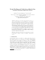
A railway network in ETCS Level 2 consists of a number of track-side elements of
different types5 : linear sections, points, marker boards. Figure 1 shows an example layout of a railway network having four linear sections (t10,t12,t14,t20),
two points (t11,t13), and eight marker boards (mb10..mb21). A linear section
is a section with up to two neighbors: one in the up end, and one in the down
end6 , e.g. the linear section t12 in Fig. 1 has t13 and t11 as neighbors at its
up end and down end, respectively. A point can have up to three neighbors: one
at the stem, one at the plus end, and one at the minus end, e.g. point t11 in
Fig. 1 has t10, t12, and t20 as neighbors at its stem, plus, and minus ends,
respectively. Linear sections and points are collectively called detection sections,
as they are used by interlocking systems to detect the presence of trains in a
railway network. A point can be switched between two positions: PLUS and
MINUS. When it is in the PLUS (MINUS) position, traffic can run from its
stem to its plus (minus) end and vice verse. A marker board is installed along a
section, and it is used as reference location for an intended travel direction that
it is facing, e.g. mb11 in Fig. 1 is installed along section t10, and it is intended
4
5
6
http://www.bane.dk/signalprogrammet
Here we only show types that are relevant for the work presented in this paper.
In Denmark, up and down denote the directions in which the distance to a reference
location is increasing and decreasing, respectively. The location is the same for both
up and down, e.g. an end of a line.
for travel direction up. Contrary to legacy systems, in ETCS Level 2, there are
no physical signals, but virtual signals associated with marker boards. A virtual
signal can be OPEN or CLOSED, respectively, allowing or disallowing traffic
to pass the associated marker board. For simplicity, the terms virtual signals,
signals, and marker boards are used interchangeably throughout this paper.
mb20
DOWN
UP
t20
mb10
mb12
t10
t11
mb11
mb14
mb21
t13
t12
mb13
t14
mb15
Fig. 1. An example railway network layout
An interlocking system monitors constantly the status of track-side elements,
and sets them to appropriate states in order to allow trains traveling safely
through the given railway network. The new Danish interlocking systems are
route-based. An interlocking table specifies the routes in the given network layout
and the conditions for setting these routes. A route is a path from a source signal
to a destination signal.
In railway signaling terminology, setting a route denotes the process of
allocating the resources – i.e. sections, points, signals – for the route, and then
locking it exclusively for only one train when the resources are allocated. The
specification of a route and conditions for setting and releasing it include the
following information: (a) a list of the detection sections in the route’s path, (b) a
list of the detection sections which are used as overlaps – buffer space in case
trains overshoot the route’s path, (c) required positions of points 7 used by the
route, (d) a set of protecting signals used for flank or front protection [19] for
the route, and (e) a set of conflicting routes which must not be set while the
current route is set.
Table 1 shows an excerpt of an interlocking table for the network shown in
Fig. 1. As can be seen, one of the routes has id 1a, goes from mb11 to mb13 via
two sections t11 and t12, and has no overlap. It requires point t11 (on its path)
to be in PLUS position and point t13 (outside its path) to be in MINUS position
(as a protecting point). The route has mb20 and mb12 as protecting signals, and
it is in conflict with routes 1b, 2a, 2b, 3, 4, 5a, 5b, 6b, 7.
Interlocking Principles. In order to prevent collision and derailment of trains,
traditional route-based interlocking systems employ a basic principle: a route is
locked exclusively for use of one train at a time. This is obtained by following
a strict procedure for setting and releasing routes based on information in their
interlocking tables. As an example, let us consider the following procedure for
route 1a specified in Table 1:
7
This includes points in the path and overlaps, and points used for flank and front
protection. For detail about flank and front protection, see [19].
Table 1. Excerpt of the interlocking table for the network layout in Fig. 1. The overlaps
column is omitted as it is empty for all of the routes. (p means PLUS, m means MINUS.)
id
1a
..
7
source
mb11
...
mb20
destination
mb13
...
mb10
points
t11:p;t13:m
...
t11:m
signals
mb12;mb20
...
mb11;mb12
path
t11;t12
...
t11;t10
conflicts
1b;2a;2b;3;4;5a;5b;6b;7
...
1a;1b;2a;2b;3;6a
(0) Initially the route is free.
(1) When a request for setting the route is received by the interlocking system,
the route is marked as requested.
(2) The interlocking system checks the status of different track-side elements in
the system to figure out whether it can start allocating resources for route
1a, e.g. sections t11 and t12 must be vacant, and conflicting routes must
not be allocated or locked. If so, the interlocking commands points and
signals to their required positions according to the route’s specification, e.g.
it commands the point t11 to switch to PLUS, t13 to switch to MINUS,
and the protecting signals mb12 and mb20 to change to CLOSED.
(3) The interlocking system constantly monitors the status of the trackside elements. When the signals and points have changed their states as
commanded in step (2), the route is locked and its source signal mb11 is set
to OPEN, allowing a train to enter the route.
(4) When the locked route is used, i.e. a train enters it, the source signal mb11
is set to CLOSED preventing other trains from entering.
(5) The route is released (set back to free) when the train has finished using it,
i.e. the train has passed mb13, or the train has come to standstill in front of
mb13.
Sequential Release. The new Danish interlocking systems employ sequential
release (also known as sectional release) [19]. This new feature results in two
major changes:
(a) With sequential release, the interlocking can release an element in a locked
route as soon as the train has passed it, instead of waiting until the train
has finished using the route and then releasing the route as a whole.
Consequently, the capacity increases.
(b) As a direct result of (a), a route may be allocated (in step (2) above) while
some of its conflicting routes are still in use by trains, instead of waiting
for all of its conflicting routes to be released as in traditional route-based
interlocking systems. For example, when a train has passed section t11
while going along route 1a, t11 will be released and then route 7 going in
the opposite direction (see Table 1) can be allocated (assuming that other
conditions for this are fulfilled).
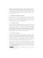
3
Verification Method
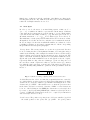
The verification process is shown in Fig. 2. The verification process begins with
Behavioral Model
DSL FOR CONFIG. DATA
DSL desc. in XML
Internal Rep.
Network
Network
Parser
Interlocking
Table
Generic
Model
Properties
Generic
Prop.
Static Checker
×
SMT Solver
and k-Induction
ITG
Interlocking
Table
Counter-examples
Model
Instance
Safety Prop.
X
Checking
Result
Fig. 2. Verification process
the configuration data of an interlocking system, consisting of a network layout
and an interlocking table. The configuration data are described in a domainspecific language [22] (DSL) having an XML representation8 . After being parsed
into an internal representation, a static checker verifies whether the configuration
data is statically well-formed according to the static semantics of the DSL.
As an option the user may not provide an interlocking table, but instead use
an interlocking table generator (ITG) to get a table created automatically.
Instantiating a generic model of the dynamic behavior of the Danish interlocking
systems with the wellformed configuration data results in a model instance in the
form of a Kripke structure. Similarly, the concrete safety-properties expressed as
state invariants are also generated from the generic safety-properties. The model
instance is then checked against the concrete properties using a combination
of BMC and inductive reasoning. If the model instance does not satisfy the
properties, counter-examples will be generated. An interface for visualizing the
counter-examples at the DSL level is under development.
The tool-chain associated with the method has been implemented using the
RT-Tester tool-box [17, 21]. The bounded model checker in RT-Tester uses the
SONOLAR SMT solver [18] to compute counter-examples for induction and
base cases. RT-Tester has been selected because (1) it is an integrated modelbased testing and BMC tool, and (2) its SMT solver also supports floating
point arithmetic. The first property is crucial for us, because our objective is to
complement the model verification with HW/SW integration tests. The second
capability is vital, because we also plan to extend the model by real-time aspects,
such as train velocity and braking curves.
4
Kripke Structure Encodings of Interlocking Systems
The dynamic behavior of an interlocking system is formalized as a Kripke
structure K = (S, s0 , R, L, AP ) with state space S, initial state s0 ∈ S, transition
relation R ⊆ S × S, and labeling function L : S → 2AP , where AP is the set
of atomic propositions and 2AP is the power set of AP . The labeling function L
maps a state s to the set L(s) of atomic propositions that hold in s. Due to the
8
A graphical representation and editor is currently under development.
limited space of this paper and the complexity of the Kripke encodings, in the
following subsections, we only outline how the state space S and the transition
relation R of a Kripke structure are encoded.
4.1
State Space
In order to encode the states of an interlocking system, a finite set V =
{v0 , . . . , vn } of variables is defined to represent the current status of different
components in the system such as a track element or a route. Each variable
v ∈ V has an associated finite domain
Dv ⊂ N0 . The state space is the set of
S
all valuation functions s : V → v∈V Dv for which s(v) ∈ Dv for all v ∈ V .
The initial state s0 is the (safe) state in which all detection sections are vacant,
all signals are closed, all routes are free, and there are no trains in the network.
In our encodings, s0 is the state in which all variables are evaluated to 0. For
readability, sometimes we use named constants instead of their corresponding
integral values in the subsequent paragraphs.
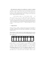
Vacancy Status. The vacancy status of a section in a given travel direction
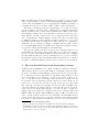
is encoded using the three least significant bits HTO of a non-negative integer
variable as shown in Fig. 3. For example, the variable l.U 2D records the vacancy
status of a linear section l in the direction from its up end to its down end. The
value 1 of the bits H, T, O indicate: (H) the head of the train is within the section,
(T) the tail of the train is within the section, and (O) the section is occupied,
respectively. This encoding offers two advantages: (a) the encoding can cover
the case where a train occupies more than one detection section (e.g., when it
is crossing the joint between two sections), and (b) the safety properties can be
expressed efficiently using arithmetic operations on integer variables as shown
in Sect. 5.
2
...
1
0
H T O
Fig. 3. A variable recording occupancy status of a detection section
Lockable Elements. In order to accommodate sequential release into our model,
we consider a linear or point section as a lockable element. The status of a lockable
element e is encoded by two variables: (1) e.MODE – indicating the mode of the
element, and (2) e.PREV – this variable is set to 1 when the previous section
in the same route has been released, otherwise e.P REV = 0. An element can
be in one of the following modes: FREE (the element is not exclusively locked
by a route, or used by any train), EXLCK (the element is exclusively locked for
a route), or USED (the element has been used, i.e., occupied, by a train after it
was exclusively locked for a route).
Point Positions. The position of a point p is encoded by two variables: (1) p.POS
– the actual position of the point, and (2) p.CMD – the point position
commanded by the interlocking. The value of p.POS can be one of the following9 :
PLUS(0), MINUS(1), or INTERMEDIATE(2) (the position where the point
is switching from one side to the other). The value of p.CMD can only be
PLUS or MINUS (as the interlocking cannot command a point to switch to
the INTERMEDIATE position).
Signal Aspects. The aspect of a signal s is encoded by two variables: (1) s.ACT
– the actual aspect of the virtual signal, its value can be OPEN or CLOSED,
and (2) s.CMD – the aspect as commanded by the interlocking, the possible
values of this variable have the same meaning as the ones of s.ACT. The s.ACT
variable represents the aspect of the signal as “seen” by the train, while s.CMD
is the aspect of the signal as seen by the interlocking. The values of these two
variables may be different because of the delay in the communication between
the interlocking system and the trains.
Routes. For each route r, a variable r.MODE is used to encode the current mode
of that route. A route can be in one of the following modes: FREE, MARKED,
ALLOCATING, LOCKED, or USED.
4.2
Transition Relation
The transition relation R ⊆ S ×S can be represented symbolically by a predicate
Φ with free variables in V ∪ V 0 , where V 0 = {v 0 | v ∈ V } is the set of next-state
variables. A pair of states (s, s0 ) ∈ R, if and only if Φ evaluates to true when
replacing every v ∈ V occuring in Φ with s(v) and every v 0 ∈ V 0 occuring in
Φ with s0 (v). In order to specify Φ, we divide the transitions in an interlocking
system into four types as in the following, each type is represented collectively
in a predicate with free variables in V ∪ V 0 .
(0) route dispatching transitions represented collectively by the predicate Φd ;
(1) interlocking transitions – e.g., setting mode of a route – represented by the
predicate Φι ;
(2) track element transitions – e.g., switching a point or a signal – represented
by the predicate Φ ; and
(3) train movement transitions represented by the predicate Φτ .
Transitions of type (0) are not prioritized, i.e., they can be chosen whenever they
are enabled, independently from other transitions. On the other hand, transitions
of types (1), (2), and (3) are prioritized in the descending order that they appear
in the list, i.e., transitions of type (1) has the highest priority and transitions of
type (3) has the lowest. Whenever two transitions of different priorities are both
enabled, the one with higher priority will be chosen. Transitions with the same
priority are chosen non-deterministically if they are enabled at the same time.
This priority of transitions is based on the intuition that in practice, the events
9
The notation name(integer-value) means that name is the name of constant having
the value integer-value.
in the interlocking control logic occur at significantly higher speed than the ones
occurring in a track element. An analogous argument applies to events related
to track elements and others related to train movements. With these types of
transitions, the transition relation of an interlocking system can be specified as
in the following
Φ ≡ Φd ∨ IT E(ι, Φι , IT E(, Φ , Φτ ))
(1)
where IT E(c, i, e) is the if-then-else function: if c holds then the value of the
function is i, otherwise it is e; ι expresses whether an interlocking transition
is enabled; and expresses whether a track element transition is enabled. The
route dispatching transition relation Φd is put outside of the IT E function in
(1) in order to allow the routes to be dispatched arbitrarily. If route dispatching
transitions were given the same or higher priority as the one of interlocking
control logic transitions, all routes which could be dispatched would have to
be dispatched before track elements or trains could make any transition. On
the other hand, if route dispatching were given lower priority than interlocking
control logic transitions, then a route could not be dispatched if another route
is processed by the interlocking.
Route Dispatching. A route can be dispatched arbitrarily whenever its mode is
FREE. This means that multiple routes can be dispatched at the same time.
Life-cycle of a Route. Figure 4 shows the “life-cycle” of a route, i.e., its different
modes and the transitions from one mode to another. This “life-cycle” reflects the
procedure for setting and sequentially releasing a route as described in Sect. 2.
The transitions labeled (1), (2), (3), (4), and (6) in Fig. 4 correspond to items
(1) – (5) in the procedure presented in Sect. 2 for setting and releasing a route.
Transition (5) models the sequential release that can take place while the route
stays in USED mode: as the train moves along the route, its elements are released
sequentially as soon as the train has passed them. Transition (2) is adapted to
sequential release: allocation is now also allowed when a conflicting route is in
the USED mode, as long as elements shared with the given route have been
sequentially released.
(1)
dispatch(r)
FREE
(2)
allocate(r)
MARKED
ALLOCATING
(6)
release(r)
(5)
seqRelease(r, e)
(3)
lock(r)
USED
(4)
use(r)
Fig. 4. A life-cycle of a route
LOCKED
Life-cycle of a Lockable Element. Figure 5 depicts the “life-cycle” of a lockable
element within the network controlled by the interlocking system. Each node
in the diagram is labeled with information about the status of the element e:
(a) whether the element is vacant, (b) its current mode, and (c) the value of
the PREV variable indicating whether the previous element prev(r, e) of e in
the route r has been released. An element e is initially in a state in which it is
vacant, in FREE mode, and its PREV variable is 0. (1) When the interlocking
system is allocating a route r that uses e, it sets the mode of the element to
EXLCK, meaning that the element is locked exclusively for r. (2) The element
becomes occupied, i.e., not vacant, as a train enters. (3) After that, e’s mode
is set to USED. (4) When the train leaves the previous element prev(r, e) of
e in the route r, prev(r, e) is released, and it informs e by setting the variable
e.P REV to 1. (5) When the train leaves e, the latter becomes vacant again, (6)
e is released and the next element next(r, e) in the same route is informed by
setting next(r, e).P REV to 1.
vacant(e)
FREE
¬PREV
(1)
allocate(r)
(6)
seqRelease(r, e) ∧
next(r, e).P REV 0 = 1
vacant(e)
USED
PREV
(5)
train leaves e
vacant(e)
EXLCK
¬PREV
(2)
train enters e
¬vacant(e)
EXLCK
¬PREV
(3)
use(r, e)
¬vacant(e)
USED
(4)
PREV
seqRelease(r, prev(r, e))
¬vacant(e)
USED
¬PREV
Fig. 5. “Life-cycle” of a lockable element e. vacant(e) is a formula over variables
encoding e’s vacancy status shown in Sect. 4.1.
Switching Points. A point p can be switched if it is requested to be switched to
a position p.CM D that is different from its current position p.P OS. The point
switching process occurs in two steps:
(1) the point moves from its current position to the intermediate position,
i.e., p.P OS 6= p.CM D ∧ p.P OS 6= IN T ERM EDIAT E ∧ p.P OS 0 =
IN T ERM EDIAT E,
(2) the point is switched from the intermediate position to the requested
position, i.e., p.P OS = IN T ERM EDIAT E ∧ p.P OS 0 = p.CM D.
Switching Signals. Whenever the actual aspect s.ACT of a signal s differs from
the commanded aspect s.CM D, the actual aspect of the signal is set to the
commanded aspect, i.e., s.ACT 6= s.CM D ∧ s.ACT 0 = s.CM D.
Train Movements. Trains are not explicitly specified in our model, in the sense
that there are no explicit train objects. Instead, train movements and other
aspects are implicitly modeled via the occupancy status of train detection
sections, inspired by the “rubber-band” model described in [1]. This implicit
model is advantageous when compared to the explicit one, because it models
arbitrary numbers of trains of arbitrary length. In the implicit model of train
movements, train length – in terms of numbers of sections that a train occupies
– may vary as trains move. This variation reflects the actual view of interlocking
systems of the train length: although trains have fixed geometric length, their
length – in terms of the number of sections that they occupy – as seen by the
interlocking systems is not fixed.
5
High-level Safety Properties
Interlocking systems must at least guarantee the high-level safety properties of
non-collision and non-derailment. These properties can be expressed as state
invariants over the vacancy status variables of linear and point sections in the
given network. Basically, an interlocking system is safe if no hazardous situations
occur on any linear or point section at any time. Thus, the high-level safety
properties can be expressed formally by the following state invariant
_
_
φ = ¬(
Hazardl ∨
Hazardp )
(2)
l:Linear
p:P oint
where Hazardl and Hazardp specify conditions for hazards to occur on a linear
section l and a point p, respectively. These propositions are conjunctions of
sub-propositions expressing hazards of different types on a section such as:
(a) head-to-head collision, (b) trains following each other collision on a section, or
(c) derailment on a point. Some examples for hazards are given in the subsequent
paragraphs.
Head-to-head collision on a linear section. A head-to-head collision occurs on
a linear section l, when two trains running in opposite directions meet. This
situation is expressed by the following formula where l.D2U (l.U 2D) is the
variable encoding the vacancy status of the section in the travel direction from
down (up) to up (down).
l.D2U ∗ l.U 2D > 0
(3)
As l.D2U ∗ l.U 2D > 0 iff l.D2U > 0 and l.U 2D > 0, the formula expresses
that the section is occupied in both down-to-up (l.D2U > 0) and up-to-down
(l.U 2D > 0) directions. Collisions of type (b) are formulated in the similar way.
Derailment on a point. A derailment occurs when a train traverses a point p
which is not locked in the correct position for the travel direction of the train.
This situation is expressed by the following formula where p.P OS is the point’s
actual position, p.S2P M , p.P 2S, and p.M 2S are variables encoding the vacancy
status of the point in the travel direction entering the point from its stem, plus,
or minus ends, respectively, & and are bit-wise and and arithmetic bit shift
right operators, respectively.
p.P OS ∗ p.P 2S + (1 − (p.P OS & 1)) ∗ p.M 2S + (p.P OS 1) ∗ p.S2P M > 0 (4)
Formula (4) captures the following cases: (a) a train is entering a point from its
plus end (p.P 2S > 0) while the point is in not in the plus position (p.P OS > 0),
(b) a train is entering a point from its minus end (p.M 2S > 0) while the point
is not in the minus position (1 − (p.P OS & 1) > 0), and (c) a train is entering
a point from its stem end (p.S2P M > 0) while the point is in the intermediate
position ((p.P OS 1) > 0).
6
Verification of Safety Properties
When a model K (see Sect. 4) and a proposition φ expressing high-level safety
properties (see Sect. 5) have been generated, the next task according to our
method is to prove the absence of hazardous situations, i.e., to prove that φ
holds in all reachable states of K. This is written K |= G(φ). The following
subsections describe our approach for verifying this.
6.1
Verification Strategy
We employ a strategy combining BMC and k-induction techniques similar to
the one in [13]. The verification procedure is performed in two steps: (i) base
case: prove that φ holds for k > 0 consecutive states10 , starting from the initial
state s0 , and (ii) induction case: prove that if φ holds for k > 0 consecutive
states, starting from an arbitrary state sn , then φ will also hold in the (k + 1)th
state. Both the base case and the induction case are transformed to problems of
finding counter-examples for their negated formulas using an SMT solver. If no
counter-examples are found, then the cases have been proved.
6.2
Invariant Strengthening
As pointed out in [3], when φ is not strong enough to be inductive, counterexamples are found for the induction case. These counter-examples are often
spurious, i.e., they start from an unreachable state and do not correspond to
any actual run of the system. In order to make φ inductive, it is strengthened
with an extra invariant ψ, i.e., one should prove φ ∧ ψ instead of φ. ψ is called
the strengthening invariant, which eliminates the spurious counter-examples. An
example of such strengthening properties is given in the following.
Train Integrity. Some states of the variables expressing the train occupancy
status of the track sections (see Sect. 4) are not feasible as they correspond to
situations that are not physically possible. An example of an infeasible state is
one in which the variables express that a section s is occupied in one direction
by a train without the head being on the section, but the next section in that
travel direction is unoccupied.
10
Two states are consecutive, if there is a transition from the first to the second
according to the model K.
The train integrity conditions can be formalized as a conjunction of formulas
over the track vacancy variables. For each travel direction (up and down), there is
a conjunct for each section s that has a next section in the given travel direction.
The pattern of such a conjunct depends on the other sections the current section
is connected to in the given travel direction. For instance, for travel direction up
and a linear section s that has a linear section s0 as neighbor in travel direction
up, the conjunct will take the following form:
(s.D2U & 0b101) = 0b001 ⇐⇒ (s0 .D2U & 0b011) = 0b001
(5)
where & is the bit-wise and operator. This formula expresses that section s
is occupied by a train in direction up (the O bit of s.D2U is 1) without the
head being on the section (the H bit of s.D2U is 0), if and only if section s0 is
occupied by a train in direction up (the O bit of s0 .D2U is 1) without a tail being
on the section (the T bit of s0 .D2U is 0). Formula (5) shows the expressiveness of
our state encodings allowing properties to be efficiently formulated in compact
formulas.
7
Experiments
We have used the tool-chain to verify the safety properties for model instances
of a number of railway networks, ranging from a trivial tiny toy network to a
large station (Køge) extracted from the early deployment line of the new Danish
signalling systems.
Table 2. Verification results for different networks using simple induction (k = 1). Toy,
cross, and mini are made-up trivial networks, while Gadstrup-Havdrup (Gt-Hd) and
Køge are extracted from the early deployment line in the Danish Signalling Programme.
(BR: branching ratio)
Case Linears Points Signals Routes BR Vars Time(sec) Memory
Toy
3
1
4
6 0.33
35
9
51 MB
Cross
4
2
8
10 0.50
56
64 127 MB
Mini
4
2
8
12 0.50
58
76 128 MB
Gt-Hd
18
5
21
30 0.28 179
1826 1171 MB
Køge
46
23
49
59 0.50 502
33627 4788 MB
In our first trials of verifying the models, we used simple induction (kinduction with k = 1), but we got spurious counter-examples. To avoid that
we tried to increase k and strengthen the invariant to be verified. It turned
out that the verification time increased significantly as k increased, making it
impossible to verify even the small networks. However, we were able to derive
strengthening properties ψ (see Sect. 6) for which the verification could be
done just using simple induction. (Not for all applications this is possible, see,
e.g., [13]). Table 2 shows the results of the final verification. Each row of the
table lists the size of a network in terms of the number of linear sections,
points, signals, and routes in the configuration, and the number of generated
variables in the corresponding model instance. The two last columns show the
approximate accumulated verification time and memory usage. All experiments
have been performed on Intel(R) Core(TM) i7-3520M CPU @ 2.90GHz, 8GB
RAM, Ubuntu 14.04 LTS, Linux 3.13.0-27-generic x86 64 kernel.
The branching ratio of a network (BR in Table 2) is defined as the ratio of
the number of points to the number of linear sections in that network. The larger
the branching ratio is, the more complex the corresponding network is in terms
of branching. The size of the formula Φ specifying the transition relation as well
as the size of the formulas φ and ψ specifying the state invariants grow as the
size of the network grows. Our experiments show that the formulas grow much
more when the network’s branching ratio also increases, than when the branching
ratio is nearly the same (as it is, e.g., the case when chaining multiple simple
stations). This is due to the fact that the interdependency between variables in
the model also increases when BR increases.
We also injected errors into models. Counter examples for these were
normally found in relatively short time. This appears to be a general trend
when dealing with interlocking systems [16]. In a few cases, it took long time to
find counter examples. Such examples usually represent very subtle errors in the
model or the configuration data, which may be easily overlooked by inspection.
8
Related Work
In recent years, the railway domain has become one of the most promising application domains of formal methods. Several research groups have investigated
how formal methods would help efficiently producing more robust railway control
systems. An overview of recent trends can be found in [7], and recommendations
and best-practices for efficient development and verification of safe railway
control systems are summarized in [12]. Re-configurable systems and automated
verification are among these recommendations that we have followed.
Model checking is a promising technique for verifying safety properties of
interlocking systems thanks to its capability to be fully automated. Unfortunately, due to the state explosion problem, the technique is only able to verify
applications of small size [8]. Several techniques have been proposed in order
to push the applicability bounds toward industrial size. Winter et al. suggest
using ordering strategies optimized for interlocking models [23]. A number of
high-level abstractions for reducing the complexity of interlocking models are
presented in [15]. In [6], Fantechi et al. suggest a distributed interlocking model
whose verification can be divided into small tasks and verified in parallel. SATbased model checking and slicing technique are used in [16]. In order to remedy
the problem with state space explosion in the global model checking approach,
we have recently for some other applications [13, 14] used BMC instead. In
the current work, a combination of SMT-based BMC with inductive reasoning
allowed us to verify safety properties without having to explore the whole state
space, hence we were able to push the bounds even further to handle larger
networks of industrial size. As an alternative to the model checking approach,
theorem proving based techniques have also shown success in the railway domain,
see, e.g., [2, 11], but are less automated.
Although sequential release has been used in some interlocking systems,
we have not found any published formal models of interlocking systems that
integrate this feature. In [20], the conditions for elements to be unlocked and
reused in sequential releases are pre-computed and specified in the interlocking
tables. In our approach, sequential release is integrated into the behavioral
model rather than into the configuration data. This reduces the complexity
of the configuration data and makes interlocking configuration data relatively
independent from the chosen interlocking approaches.
9
Conclusion and Future Work
This paper presented a fully automated, formal method and an associated tool
suite for verifying the forthcoming new ETCS Level 2 based Danish railway
interlocking systems featuring sequential release. A formal model for these
systems was outlined. A novelty in our contribution is that the system is part of
an ETCS Level 2 based signalling system in which there are no physical signals
along the tracks; instead, movement authorities are communicated via on-board
computers. By introducing the concept of virtual signals, we have been able to
handle the assignment of movement authorities in a way that is very similar
to the situations where conventional signals are used. Another novelty is that
the formal model features sequential release. As a consequence, the model is
more complex than those supporting route-based release only, because additional
variables and transitions are required. Therefore the verification becomes more
challenging. In spite of this difficulty, using a combination of SMT-based BMC
and inductive reasoning, we were able to successfully verify safety properties
for systems controlling large networks of realistic size. This was enabled by
encodings of the state space, the transition relation, and of the safety properties
that can be efficiently evaluated by SMT solvers supporting bit vector and integer
arithmetics.
In order to compare our verification approach to the approaches that use
BDD-based symbolic model checking, a translation from our model to NuSMV
– a well-known BDD-based symbolic model checker – is currently in progress. For
future work, we will benchmark how sequential release affects the complexity,
and hence verification challenges, of interlocking models. Furthermore, we
will investigate advanced techniques for automating the process of discovering
strengthening invariants, or reducing the size of the networks that need to
be modeled. For the current model there are potential overlaps between the
strengthening invariants, which should be eliminated in order to reduce the size
of the formula to be solved by the SMT solver.
Acknowledgments. The authors would like to thank Jan Bertelsen from Thales
and Ross Edwin Gammon and Nikhil Mohan Pande from Railnet Denmark for
helping us with their expertise about Danish interlocking systems and always
being helpful when we had questions; Dr.-Ing. Uwe Schulze and Florian Lapschies
from University of Bremen for their help with the implementation in the RTTester tool-chain. The first two authors’ research has been funded by the
RobustRailS project granted by the Danish Council for Strategic Research. The
third author’s work has been partially funded by ITEA2 project openETCS
under grant agreement 11025.
References
1. M. Aanæs and H. P. Thai. Modelling and Verification of Relay Interlocking
Systems. Master’s thesis, Technical University of Denmark, DTU Informatics,
E-mail: [email protected], 2012.
2. Salimeh Behnia, Amel Mammar, Jean-Marc Mota, Nicolas Breton, Paul Caspi,
and Pascal Raymond. Industrialising a Proof-based Verification Approach of
Computerised Interlocking Systems. In Eleventh International Conference on
Computer System Design and Operation in the Railway and Other Transit Systems
(COMPRAIL08). WIT Press, 2008.
3. Leonardo De Moura, Harald Rueß, and Maria Sorea. Bounded Model Checking
and Induction: From Refutation to Verification. In Computer Aided Verification,
pages 14–26. Springer, 2003.
4. ERTMS. Annex A for ETCS Baseline 3 and GSM-R Baseline 0, April 2012.
5. CENELEC European Committee for Electrotechnical Standardization.
EN
50128:2011 – Railway applications – Communications, signalling and processing
systems – Software for railway control and protection systems. 2011.
6. Alessandro Fantechi. Distributing the Challenge of Model Checking Interlocking
Control Tables. In Tiziana Margaria and Bernhard Steffen, editors, Leveraging
Applications of Formal Methods, Verification and Validation. Applications and
Case Studies, volume 7610 of Lecture Notes in Computer Science, pages 276–289.
Springer, 2012.
7. Alessandro Fantechi. Twenty-Five Years of Formal Methods and Railways: What
Next? In Steve Counsell and Manuel Núñez, editors, Software Engineering and
Formal Methods, volume 8368 of Lecture Notes in Computer Science, pages 167–
183. Springer, 2014.
8. Alessio Ferrari, Gianluca Magnani, Daniele Grasso, and Alessandro Fantechi.
Model Checking Interlocking Control Tables. In Eckehard Schnieder and Géza
Tarnai, editors, FORMS/FORMAT 2010 – Formal Methods for Automation and
Safety in Railway and Automotive Systems, pages 107–115. Springer, 2010.
9. Helle Hvid Hansen, Jeroen Ketema, Bas Luttik, Mohammad Reza Mousavi, Jaco
van de Pol, and Osmar Marchi dos Santos. Automated Verification of Executable
UML Models. In Bernhard K. Aichernig, Frank S. de Boer, and Marcello M.
Bonsangue, editors, FMCO, volume 6957 of Lecture Notes in Computer Science,
pages 225–250. Springer, 2010.
10. Anne E. Haxthausen, Marie Le Bliguet, and Andreas A. Kjær. Modelling
and Verification of Relay Interlocking Systems. In Christine Choppy and Oleg
Sokolsky, editors, 15th Monterey Workshop: Foundations of Computer Software,
Future Trends and Techniques for Development, number 6028 in Lecture Notes in
Computer Science, pages 141–153. Springer, 2010. Invited paper.
11. Anne E. Haxthausen and Jan Peleska. Formal Development and Verification
of a Distributed Railway Control Systems. In IEEE Transactions on Software
Engineering, volume 26, pages 687–701. IEEE, 2000.
12. Anne E. Haxthausen and Jan Peleska. Efficient Development and Verification of
Safe Railway Control Software. In Railways: Types, Design and Safety Issues,
pages 127–148. Nova Science Publishers, Inc., 2013.
13. Anne E. Haxthausen, Jan Peleska, and Sebastian Kinder. A Formal Approach for
the Construction and Verification of Railway Control Systems. In Formal Aspects
of Computing, volume 23, pages 191–219. Springer, 2011.
14. Anne E. Haxthausen, Jan Peleska, and Ralf Pinger. Applied Bounded Model
Checking for Interlocking System Designs. In Steve Counsell and Manuel Núñez,
editors, Software Engineering and Formal Methods, volume 8368 of Lecture Notes
in Computer Science, pages 205–220. Springer, 2014.
15. Philip James, Faron Möller, HoangNga Nguyen, Markus Roggenbach, Steve
Schneider, Helen Treharne, Matthew Trumble, and David Williams. Verification
of Scheme Plans Using CSP||B. In Steve Counsell and Manuel Núñez, editors,
Software Engineering and Formal Methods, volume 8368 of Lecture Notes in
Computer Science, pages 189–204. Springer, 2014.
16. Phillip James and Markus Roggenbach.
Automatically Verifying Railway
Interlockings Using SAT-based Model Checking. In Electronic Communications
of the EASST, volume 35. EASST, 2011.
17. Jan Peleska. Industrial-Strength Model-Based Testing - State of the Art and
Current Challenges. In Alexander K. Petrenko and Holger Schlingloff, editors,
Proceedings 8th Workshop on Model-Based Testing, Rome, Italy, volume 111
of Electronic Proceedings in Theoretical Computer Science, pages 3–28. Open
Publishing Association, 2013.
18. Jan Peleska, Elena Vorobev, and Florian Lapschies. Automated Test Case
Generation with SMT-Solving and Abstract Interpretation.
In Mihaela
Gheorghiu Bobaru et al., editor, NASA Formal Methods, volume 6617 of Lecture
Notes in Computer Science, pages 298–312. Springer, 2011.
19. Gregor Theeg, Sergeı̆ Valentinovich Vlasenko, and Enrico Anders. Railway
Signalling & Interlocking: International Compendium. Eurailpress, 2009.
20. David Tombs, Neil Robinson, and George Nikandros. Signalling Control Table
Generation and Verification. In CORE 2002: Cost Efficient Railways through
Engineering, page 415. Railway Technical Society of Australasia/Rail Track
Association of Australia, 2002.
21. Verified Systems International GmbH. RT-Tester Model-Based Test Case and Test
Data Generator - RTT-MBT - User Manual, 2013.
22. Linh Hong Vu, Anne E. Haxthausen, and Jan Peleska. A Domain-Specific Language
for Railway Interlocking Systems. In Eckehard Schnieder and Géza Tarnai, editors,
FORMS/FORMAT 2014 - 10th Symposium on Formal Methods for Automation
and Safety in Railway and Automotive Systems, pages 200–209. Institute for Traffic
Safety and Automation Engineering, Technische Universität Braunschweig, 2014.
23. Kirsten Winter. Optimising Ordering Strategies for Symbolic Model Checking
of Railway Interlockings.
In Tiziana Margaria and Bernhard Steffen,
editors, Leveraging Applications of Formal Methods, Verification and Validation.
Applications and Case Studies, volume 7610 of Lecture Notes in Computer Science,
pages 246–260. Springer, 2012.