Download Desmond Tutorial - DE Shaw Research

Desmond Tutorial
Desmond Version 3.0 / Document Version 0.6
April 2011
D. E. Shaw Research
Notice
The Desmond Tutorial and the information it contains is offered solely for educational
purposes, as a service to users. It is subject to change without notice, as is the software
it describes. D. E. Shaw Research assumes no responsibility or liability regarding the
correctness or completeness of the information provided herein, nor for damages or
loss suffered as a result of actions taken in accordance with said information.
No part of this guide may be reproduced, displayed, transmitted or otherwise copied
in any form without written authorization from D. E. Shaw Research.
The software described in this guide is copyrighted and licensed by D. E. Shaw
Research under separate agreement. This software may be used only according to the
terms and conditions of such agreement.
Copyright
© 2008-2011 by D. E. Shaw Research. All rights reserved.
Trademarks
Ethernet is a trademark of Xerox Corporation.
InfiniBand is a registered trademark of systemI/O Inc.
Intel and Pentium are trademarks of Intel Corporation in the U.S. and other countries.
Linux is the registered trademark of Linus Torvalds in the U.S. and other countries.
All other trademarks are the property of their respective owners.
April 2011
Preface
Intended Audience
This tutorial is intended for computational chemists using Desmond in setting up and
running molecular dynamics simulations. It assumes a broad familiarity with the concepts and techniques of molecular dynamics simulation and the use of the Maestro molecular modeling environment.
Prerequisites
Desmond runs on Intel™-based Linux® systems with Pentium™ 4 or more recent processors; running CentOS 3 (RHEL3) or later. Linux clusters can be networked with either
Ethernet™ or Infiniband®.
Viparr requires a recent version of Python; we recommend Version 2.5.1.
This tutorial assumes that someone has prepared the Desmond-Maestro environment for
you, either by installing the packages available from Schrödinger LLC or the Academic
release of Desmond available from D. E. Shaw Research. Where noted, the procedures
described in the tutorial make use of software that is not included in the Academic version. In those cases the software is available from Schrödinger.
April 2011
D. E. Shaw Research
i
Desmond Tutorial
About this Guide
This manual contains the following sections:
Chapter 1
describes Desmond and outlines the steps to perform a simulation on a simple protein.
Chapter 2
describes the System Builder, the tool for setting up molecular systems for simulation
using Desmond
Chapter 3
describes force field parameter assignment program Viparr and making changes to the
configuration file output by the system builder.
Chapter 4
describes how to run Desmond within the Maestro environment and from the command
line.
Chapter 5
describes Free Energy Perturbation and metadynamics simulation using Maestro workflow.
Chapter 6
describes how to view the results of Desmond simulations in Maestro.
Chapter 7
describes VMD, an alternate workflow available separately from the University of Illinois, that can also be used to setup simulation systems and to view trajectories and analyze the results of simulations.
Chapter 8
provides pointers to additional documentation on Desmond-Maestro system.
Release Notes
•
Note that Desmond 2.4 and higher internally utilizes a new binary input structure
file. These files are called Desmond Molecular System files and have the extension
.dms. The .dms file format and related information is documented in the Desmond
User’s Guide. You do not need to consider the .dms files explicitly with the sole
exception of the forceconfig.py setup tool described in “Running Simulations from
the Command Line” on page 56.
•
You will notice that the Maestro toolbars have changed from the prior release to
allow for more customization and convenience:
— The double column main toolbar in prior releases has been split into several
smaller toolbars.
— There is a new "manager" toolbar that has buttons to launch toolbars including
Project, Edit, and View. Click the buttons to show or hide the toolbars.
— You can drag toolbars to any edge of the Workspace, or even place them as freestanding toolbars outside the main window.
— You can hide toolbar buttons on any toolbar if you do not use them. Right-click
the toolbar and choose Customize.
— Each toolbar can be shown with icons only, with text labels, or text only. Rightclick the toolbar and choose the Style menu.
ii
D. E. Shaw Research
April 2011
•
Note that application and option panels pop up with a noticeable delay. However, this
only happens when you open a panel for the first time. Within the life cycle of a Maestro session subsequent opening and closing of such windows is instantaneous.
Format Conventions
Command lines appear in a monospaced font:
$SCHRODINGER/maestro
File names are bolded within text: equil.cfg
Menu selections you must make for the tutorial are bolded. For example: Select
Project > Get PDB.
Screen elements such as panel titles, option names, or button names appear in special text.
For example: Click ButtonName.
April 2011
D. E. Shaw Research
iii
Desmond Tutorial
iv
D. E. Shaw Research
April 2011
Contents
Preface . . . . . . . . . . . . . . . . . . . . . . . . . . . . . . . . . . . . . . . . . . . . . . . . . . . . . . . . . . . . . .i
Intended Audience .
Prerequisites . . . . .
About this Guide . .
Release Notes . . . .
Format Conventions
.
.
.
.
.
.
.
.
.
.
.
.
.
.
.
.
.
.
.
.
.
.
.
.
.
.
.
.
.
.
.
.
.
.
.
.
.
.
.
.
.
.
.
.
.
.
.
.
.
.
.
.
.
.
.
.
.
.
.
.
.
.
.
.
.
.
.
.
.
.
.
.
.
.
.
.
.
.
.
.
.
.
.
.
.
.
.
.
.
.
.
.
.
.
.
.
.
.
.
.
.
.
.
.
.
.
.
.
.
.
.
.
.
.
.
.
.
.
.
.
.
.
.
.
.
.
.
.
.
.
.
.
.
.
.
.
.
.
.
.
.
.
.
.
.
.
.
.
.
.
.
.
.
.
.
.
.
.
.
.
.
.
.
.
.
.
.
.
.
.
.
.
.
.
.
.
.
.
.
.
. i
. i
. ii
. ii
iii
1. Desmond Tutorial . . . . . . . . . . . . . . . . . . . . . . . . . . . . . . . . . . . . . . . . . . . . . . . . . . 1
Introducing Desmond . . . . . . . . . . . . . . . . . . . . . . . . . . . . . . . . . . . . 1
Steps to Perform Simulation on a Simple Protein . . . . . . . . . . . . . . . . . . . . . 2
Tutorial Steps . . . . . . . . . . . . . . . . . . . . . . . . . . . . . . . . . . . . . . . . . 3
2. Preparing a Desmond simulation with the System Builder . . . . . . . . . . . . . . . . 21
Overview . . . . . . . . . . . . . . . . . . . . . . . . . . . .
Selecting Solutes and Solvents. . . . . . . . . . . . . . . . .
Defining the Simulation Box . . . . . . . . . . . . . . . . . .
System Builder Output File Format. . . . . . . . . . . . . .
Adding Custom Charges. . . . . . . . . . . . . . . . . . . .
Adding Ions . . . . . . . . . . . . . . . . . . . . . . . . . . .
Generating the Solvated System. . . . . . . . . . . . . . . .
Setting Up Membrane Systems . . . . . . . . . . . . . . . .
Importing Membrane Placement from the OPM Database.
.
.
.
.
.
.
.
.
.
.
.
.
.
.
.
.
.
.
.
.
.
.
.
.
.
.
.
.
.
.
.
.
.
.
.
.
.
.
.
.
.
.
.
.
.
.
.
.
.
.
.
.
.
.
.
.
.
.
.
.
.
.
.
.
.
.
.
.
.
.
.
.
.
.
.
.
.
.
.
.
.
.
.
.
.
.
.
.
.
.
.
.
.
.
.
.
.
.
.
.
.
.
.
.
.
.
.
.
.
.
.
.
.
.
.
.
.
.
.
.
.
.
.
.
.
.
21
22
22
23
23
24
25
25
39
3. Finishing Preparations for Desmond Simulation . . . . . . . . . . . . . . . . . . . . . . . . 47
Overview . . . . . . . . . . . . . . . . . . . . . . . . . . . . . . . . . . . . . . . .
Generating Force Field Parameters with Viparr . . . . . . . . . . . . . . . . . . .
Adding Constraints . . . . . . . . . . . . . . . . . . . . . . . . . . . . . . . . . . .
Importing a Simulation System from the Amber Molecular Dynamics Package
April 2011
D. E. Shaw Research
.
.
.
.
.
.
.
.
47
47
51
51
v
Desmond Tutorial
Specifying Desmond Simulation Parameters. . . . . . . . . . . . . . . . . . . . . . . 51
Using Desmond applications in Maestro . . . . . . . . . . . . . . . . . . . . 51
Editing the Desmond Conguration File Directly . . . . . . . . . . . . . . . . 54
4. Running Desmond Simulations . . . . . . . . . . . . . . . . . . . . . . . . . . . . . . . . . . . . . . 55
Overview . . . . . . . . . . . . . . . . . . . . . . . . . . . . .
Running Simulations from the Molecular Dynamics Panel
Running Simulations from the Command Line . . . . . . .
Running MultiSim jobs from the Command Line . . . . . .
.
.
.
.
.
.
.
.
.
.
.
.
.
.
.
.
.
.
.
.
.
.
.
.
.
.
.
.
.
.
.
.
.
.
.
.
.
.
.
.
.
.
.
.
.
.
.
.
.
.
.
.
.
.
.
.
55
55
56
58
5. Preparing Free Energy Perturbation and Metadynamics . . . . . . . . . . . . . . . . . . 61
Overview . . . . . . . . . . . . . . . . . . . . . . . . . . . . . . . .
Setting Up an FEP Calculation . . . . . . . . . . . . . . . . . . . .
Using Maestro To Generate A Desmond FEP Configuration File
Running FEP Simulations from the Command Line . . . . . . .
Creating a Custom Fragment Group . . . . . . . . . . . . . . . .
Adjusting the Conformation of the Mutant . . . . . . . . . . . .
Other Types of Mutations . . . . . . . . . . . . . . . . . . . . . .
Aside: Metadynamics . . . . . . . . . . . . . . . . . . . . . . . . .
.
.
.
.
.
.
.
.
.
.
.
.
.
.
.
.
.
.
.
.
.
.
.
.
.
.
.
.
.
.
.
.
.
.
.
.
.
.
.
.
.
.
.
.
.
.
.
.
.
.
.
.
.
.
.
.
.
.
.
.
.
.
.
.
.
.
.
.
.
.
.
.
.
.
.
.
.
.
.
.
.
.
.
.
.
.
.
.
61
63
68
70
71
77
81
82
6. Visualization and Analysis using Maestro. . . . . . . . . . . . . . . . . . . . . . . . . . . . . . 87
Overview . . . . . . . . . . . . . . . . . . . .
Animating Desmond Trajectories with the
Trajectory Player . . . . . . . . . . . . . . .
Performing Simulation Quality Analysis . .
Performing Simulation Event Analysis . . .
. . . . . . . . . . . . . . . . . . . . . . . 87
. . . . . . . . . . . . . . . . . . . . . . . 87
. . . . . . . . . . . . . . . . . . . . . . . 90
. . . . . . . . . . . . . . . . . . . . . . . 92
7. System Setup and Trajectory Analysis Using VMD . . . . . . . . . . . . . . . . . . . . . . 95
Overview . . . . . . . . . . . . . . . . . . . . . . . .
The VMD Python Interface . . . . . . . . . . . . . .
Loading and Viewing Trajectories. . . . . . . . . .
Loading Files from the Command Line . .
Loading Files from the GUI. . . . . . . . .
Loading files from the scripting interface .
Getting information about snapshots . . . . . . . .
Atom selections . . . . . . . . . . . . . . .
Snapshots . . . . . . . . . . . . . . . . . . .
Centering trajectories . . . . . . . . . . . .
Writing structures and trajectories . . . . . . . . .
Analyzing whole trajectories. . . . . . . . . . . . .
.
.
.
.
.
.
.
.
.
.
.
.
.
.
.
.
.
.
.
.
.
.
.
.
.
.
.
.
.
.
.
.
.
.
.
.
.
.
.
.
.
.
.
.
.
.
.
.
.
.
.
.
.
.
.
.
.
.
.
.
.
.
.
.
.
.
.
.
.
.
.
.
.
.
.
.
.
.
.
.
.
.
.
.
.
.
.
.
.
.
.
.
.
.
.
.
.
.
.
.
.
.
.
.
.
.
.
.
.
.
.
.
.
.
.
.
.
.
.
.
.
.
.
.
.
.
.
.
.
.
.
.
.
.
.
.
.
.
.
.
.
.
.
.
.
.
.
.
.
.
.
.
.
.
.
.
.
.
.
.
.
.
.
.
.
.
.
.
.
.
.
.
.
.
.
.
.
.
.
.
.
.
.
.
.
.
.
.
.
.
.
.
.
.
.
.
.
.
.
.
.
.
.
.
.
.
.
.
.
.
.
.
.
.
.
.
. 95
. 95
. 96
. 96
. 97
104
104
105
107
108
108
108
8. Documentation Resources . . . . . . . . . . . . . . . . . . . . . . . . . . . . . . . . . . . . . . . . . 111
vi
D. E. Shaw Research
April 2011
List of Figures
Figure 1.1: Simulation process .............................................................................................. 3
Figure 1.2: Maestro main environment ............................................................................... 4
Figure 1.3: Import dialog box ................................................................................................ 4
Figure 1.4: Get PDB File dialog box ..................................................................................... 5
Figure 1.5: Imported protein structure file ......................................................................... 6
Figure 1.6: Changing from ribbon to ball-and-stick view ................................................. 7
Figure 1.7: Protein Preparation Wizard panel .................................................................... 8
Figure 1.8: Protein Preparation Wizard — Preprocessing stage ...................................... 9
Figure 1.9: Protein Preparation Wizard — Interactive H-bond optimizer ................... 10
Figure 1.10: Protein Preparation Wizard — Interactive H-bond optimizer ................. 11
Figure 1.11: Launching Desmond System Builder .......................................................... 12
Figure 1.12: Desmond System Builder panel .................................................................... 13
Figure 1.13: Solute and boundary box in the Maestro workspace ................................ 14
Figure 1.14: Ions tab in Desmond System Builder ........................................................... 15
Figure 1.15: Solvated protein structure in the workspace .............................................. 16
Figure 1.16: The Molecular Dynamics panel .................................................................... 17
Figure 1.17: The Molecular Dynamics-Start dialog box .................................................. 17
Figure 1.18: The Monitor panel ........................................................................................... 18
Figure 1.19: List of files in the Monitor panel ................................................................... 19
Figure 2.1: Launching Desmond System Builder ............................................................ 21
Figure 2.2: System Builder panel ........................................................................................ 22
Figure 2.3: Ions tab in Desmond System Builderpanel ................................................... 24
Figure 2.4: Membrane setup in the System Builder ......................................................... 26
Figure 2.5: Preprocessing the 1su4 structure .................................................................... 27
Figure 2.6: The 1su4 structure in standard orientation ................................................... 28
Figure 2.7: The Ions tab in the System Builder panel ...................................................... 29
Figure 2.8: Selecting the excluded region .......................................................................... 29
Figure 2.9: Placement of the counterions .......................................................................... 30
Figure 2.10: Visual feedback of ion placement ................................................................. 31
Figure 2.11: Set Up Membrane dialog box ........................................................................ 32
Figure 2.12: Selecting transmembrane residues ............................................................... 33
Figure 2.13: Importing the selection into the Atom Selection dialog box .................... 34
Figure 2.14: Initial automatic membrane placement for 1su4 ........................................ 35
Figure 2.15: Adjusted position of the membrane for 1su4 .............................................. 36
Figure 2.16: Final simulation system for 1su4 .................................................................. 37
Figure 2.17: Transmembrane hole in the POPC bilayer for 1su4 ................................... 38
Figure 2.18: The OPM Home page ..................................................................................... 39
Figure 2.19: Downloading the OPM pre-aligned coordinates ....................................... 40
Figure 2.20: Importing the OPM PDB file in the workspace .......................................... 41
Figure 2.21: Selecting the dummy atoms for deletion ..................................................... 42
April 2011
D. E. Shaw Research
vii
Desmond Tutorial
Figure 2.22: Set Up Membrane dialog box ....................................................................... 43
Figure 2.23: OPM pre-aligned membrane shown in the workspace ............................ 43
Figure 2.24: Full membrane simulation system for 1su4 ................................................ 44
Figure 2.25: OPM transmembrane hole in the POPC bilayer for 1su4 ......................... 45
Figure 3.1: Setting up a Desmond simulation .................................................................. 52
Figure 3.2: Advanced Options for simulation jobs .......................................................... 53
Figure 4.1: Running a Desmond simulation ..................................................................... 56
Figure 5.1: FEP Example—Ligand mutation .................................................................... 62
Figure 5.2: The ZINC-01538934 ligand structure ............................................................. 63
Figure 5.3: Ligand Functional Group Mutation by FEP panel ...................................... 64
Figure 5.4: Defining the mutation ...................................................................................... 65
Figure 5.5: Ligand Functional Group Mutation by FEP - Start dialog box .................. 66
Figure 5.6: FEP workflow control ...................................................................................... 67
Figure 5.7: Setting FEP parameters from the FEP panel ................................................. 69
Figure 5.8: Picking the attachment bond for creating a butyl side chain ..................... 72
Figure 5.9: Selecting the methyl group as the base for the butyl substitution group 73
Figure 5.10: The intermediate methyl substitution group shown in the workspace . 74
Figure 5.11: The Build panel ............................................................................................... 75
Figure 5.12: Selecting the grow bond ................................................................................ 76
Figure 5.13: The butyl substitution group shown in the workspace ............................ 77
Figure 5.14: Manual adjustment of the substitution group conformation ................... 78
Figure 5.15: Displaying the non-bonded contacts ........................................................... 79
Figure 5.16: Unfavorable contacts removed ..................................................................... 80
Figure 5.17: Butyl group superposed with original side chain ..................................... 81
Figure 5.18: Fragment library Build panel ........................................................................ 83
Figure 5.19: Metadynamics panel ...................................................................................... 84
Figure 5.20: Metadynamics Analysis panel ...................................................................... 85
Figure 6.1: Launching the Trajectory Player .................................................................... 88
Figure 6.2: The Trajectory Player ....................................................................................... 89
Figure 6.3: Workspace view for trajectory visualization ................................................ 90
Figure 6.4: Simulation Quality Analysis panel ................................................................ 91
Figure 6.5: Interactive Simulation Quality Analysis Plot ............................................... 91
Figure 6.6: Simulation Event Analyis panel ..................................................................... 92
Figure 7.1: Loading files from the GUI ............................................................................. 97
Figure 7.2: Loading the Maestro file .................................................................................. 98
Figure 7.3: Loading trajectory data .................................................................................... 98
Figure 7.4: VMD Trajectory Player .................................................................................... 98
Figure 7.5: VMD OpenGL Display .................................................................................... 99
Figure 7.6: VMD Analysis tools ......................................................................................... 99
Figure 7.7: VMD Modeling tools ...................................................................................... 100
Figure 7.8: Loading 4pti.pdb into VMD .......................................................................... 101
Figure 7.9: VMD AutoPSF window ................................................................................. 102
Figure 7.10: The solvated 4pti structure in VMD .......................................................... 103
Figure 7.11: Saving the 4pti system in Maestro format ................................................ 103
Figure 7.12: Analysis script example ............................................................................... 109
viii
D. E. Shaw Research
April 2011
1
Desmond Tutorial
Introducing Desmond
Desmond is an advanced classical molecular dynamics simulation system, which has an
intuitive graphical user interface integrated in the Maestro molecular modeling environment. Using Desmond, you can perform in silico simulations of small molecules, proteins,
nucleic acids, and membrane systems to study the interactions of complex molecular
assemblies. With Desmond, you can generate high-quality simulation trajectories of long
time scales as well as compute a variety of thermodynamic quantities. Desmond trajectories can be visualized and analyzed using numerous tools in Maestro and VMD.
This tutorial assumes a basic knowledge of molecular mechanics and molecular dynamics. For those users who have not yet used Maestro for molecular modeling, an overview
of the Maestro environment is included.
Beyond basic molecular modeling, there are a number of steps that must be performed on
a structure to make it viable for simulation with Desmond. Each of these steps mandates
an understanding of certain concepts and differing approaches that can be taken.
To enable novices and advanced users alike to process the information in this tutorial, the
organization of the tutorial includes:
•
A step-by-step example that describes, at a high level, how to perform a simulation on
a simple protein.
•
In-depth concept sections that cover the detailed information users will need in order
to perform a simulation similar to our example.
This tutorial also includes conceptual information and steps for performing free energy
perturbation (FEP) calculations. FEP is useful for performing “alchemical” ligand mutations to determine relative binding free energy differences, which is a crucial task for such
applications as computational drug design. Moreover, Desmond FEP can be used to compute the absolute solvation free energy of a large variety of solutes as well as the change in
free energy associated with protein residue mutation. Another addition to this version of
Desmond is improved support for metadynamics simulation setup and analysis.
April 2011
D. E. Shaw Research
1
Desmond Tutorial
Desmond Tutorial
Steps to Perform Simulation on a Simple Protein
While the example described in this tutorial is a basic simulation on a single protein, the
exercise is useful for learning the Maestro-Desmond environment as well as, in general,
investigating the molecular properties of different proteins.
Preparing a molecular model for simulation involves these general steps:
1.
Import a structure file into Maestro.
2.
Prepare the structure file for simulation. During this step, you remove ions and molecules which are, e.g., artifacts of crystallization, set correct bond orders, add hydrogens, detect disulfide bonds, and fill in missing side chains or whole residues as
necessary.
3.
Refine the prepared structure file. During this step, you analyze the choices made by
Maestro's Protein Preparation Wizard and manually change protonation and tautomeric states of variable residues, and (when present) of ligands and co-factors.
4.
If your system is a membrane protein, immerse the protein in the membrane.
5.
Generate a solvated system for simulation.
6.
Distribute positive or negative counter ions to neutralize the system, and introduce
additional ions to set the desired ionic strength (when necessary).
7.
Let Maestro assign OPLS-AA force field parameters to the entire molecular system;
alternatively, assign force field parameters external to Maestro with Desmond's
Viparr utility program, which provides access to a variety of widely used force fields.
8.
Configure simulation parameters using the Desmond panel in Maestro or edit the
Desmond conguration file.
9.
Run the simulation from Maestro or from the command line.
10. Analyze your results using the Trajectory Viewer and other analysis tools.
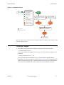
This process is illustrated in Figure 1.1.
2
D. E. Shaw Research
April 2011
Desmond Tutorial
Tutorial Steps
Figure 1.1 Simulation process
Structure Preparation
Input
Structure
File
1
2
Prepare the structure
file for simulation.
3
Refine the prepared
structure file.
4
Handle ligands or
cofactors.
5
Fill in missing residues
and side chains.
6
Setup the membrane.
7
Solvate the system.
8
Distribute counter ions.
Mae
Structure
File
9
Assign force field parameters
to the structure using Maestro
or Viparr.
10
Maeff
Structure &
Force Field File
11
Maestro tasks
Configure DESMOND
simulation parameters.
DESMOND
Configuration
File
Relax/minimize your system and
run the Desmond simulation.
DESMOND-specific tasks
DESMOND
Trajectory
File
12
Analyze results.
The rest of this section contains step-by-step procedures for building and running a simulation of a single protein.
Tutorial Steps
1.
Start Maestro from your Linux desktop by issuing the following command:
$SCHRODINGER/maestro
If you access Maestro through the network (e.g., via VNC), start the program by the
command:
$SCHRODINGER/maestro -SGL
This command will launch Maestro using a software OpenGL graphics library.
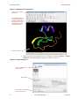
The Maestro environment appears as shown in Figure 1.2. If you are unfamiliar with
Maestro, the Schrödinger Suite or Academic Maestro distributions contain a Maestro
Tutorial and User Manual that can be consulted for more detailed information.
April 2011
D. E. Shaw Research
3
Desmond Tutorial
Desmond Tutorial
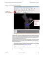
Figure 1.2 Maestro main environment
Select Project > Import
Structures
To create this layout of
the Maestro window, the
following toolbars have
been selected: Project,
Edit, Workspace, Find
and Representation.
Maestro workspace
2.
Import a protein structure file into your workspace by choosing Project > Import
Structures. The Import dialog box appears as shown in Figure 1.3.
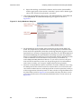
Figure 1.3 Import dialog box
Select the PDB file you
want to import.
Click Options.
Select ‘PDB’ from the ‘Files
of type’ option menu.
4
D. E. Shaw Research
April 2011
Desmond Tutorial
NOTE
Tutorial Steps
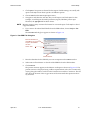
3.
Click Options. Set options as desired for the import. Default settings are usually adequate. Click Help to learn about specifics of different options.
4.
Choose PDB from the Files of type option menu.
5.
Navigate to and select the structure file you will import, and click Open. For this
example, we will import the small, proteinase (trypsin) inhibitor protein: 4pti.
Therefore, the 4pti.pdb file has been chosen.
Maestro supports many common file formats for structural input. Click Help for a list of
supported formats.
6.
If you want to download the PDB file from the PDB website, choose Project > Get
PDB.
The Get PDB File dialog box appears as shown in Figure 1.4.
Figure 1.4 Get PDB File dialog box
Enter the identifier for
the PDB file you want to
import in the ‘PDB ID’
text box.
Select ‘Auto’.
Click Download.
7.
Enter the identifier for the PDB file you want to import into the PDB ID text box.
8.
Select Auto to allow Maestro to download the PDB file from the PDB website.
9.
Click Download.
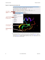
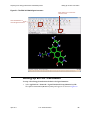
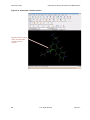
The protein structure appears in the Maestro workspace as shown in Figure 1.5. The
protein structure is displayed using a ribbon representation with colors continuously
varying along the rainbow scale from the N terminus toward the C terminus. The red
dots show the location of the oxygen atoms of the water molecules present in the Xray structure.
April 2011
D. E. Shaw Research
5
Desmond Tutorial
Desmond Tutorial
Figure 1.5 Imported protein structure file
Click ‘Ribbon’...
...and select 'Show
Ribbons'.
...then select ‘Delete
Ribbons’ to switch
to a different view.
Your protein appears
in the workspace.
Red dots represent
crystal water oxygen
atoms.
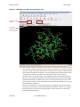
10. Switch from ribbon view to ball-and-stick view by clicking Ribbons and selecting
Delete Ribbons from the option menu that appears as shown in Figure 1.5. Next, as
shown in Figure 1.6, double-click Ball & Stick and, finally, click Color Scheme to color
the carbons in the structure green.
6
D. E. Shaw Research
April 2011
Desmond Tutorial
Tutorial Steps
Figure 1.6 Changing from ribbon to ball-and-stick view
Double-click ‘Ball
& Stick’.
Click ‘Color
Scheme’ (Custom
Carbons) Green.
Once you have arrived at this point, you are ready to prepare the structure for simulation. Just having a molecular model in the workspace is not enough to perform molecular mechanics/dynamics calculations. You must prepare the protein model so that it
corresponds as closely as possible to the biological system you are studying.
From this view, it is clear that there are no hydrogen atoms in the protein structure.
Moreover, there might be ill-defined bond orders, protonation states, formal charges,
tautomerization states, disulfide bonds, and so on. The red dots shown in the workspace represent crystal waters. All of these issues must be resolved before we can perform simulation calculations.
There are two methods of correcting these issues: using Maestro's general purpose
molecular structure editor or the Protein Preparation Wizard, which is a very useful
automated tool for protein structure preparation. For this tutorial, we will use the
Protein Preparation Wizard.
April 2011
D. E. Shaw Research
7
Desmond Tutorial
Desmond Tutorial
11. Select Workflows > Protein Preparation Wizard.
NOTE
Note the pop-up warning that Epik and Glide are not available to academic users free of
charge, but these tools are generally not necessary to setup Desmond simulation.
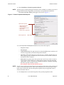
The Protein Preparation Wizard panel appears as shown in Figure 1.7.
Figure 1.7 Protein Preparation Wizard panel
Select these options:
– ‘Assign bond orders’
– ‘Add hydrogens’
– ‘Create disulfide bonds’
– ‘Cap termini’
– ‘Delete waters’ (optional)
Click ‘Preprocess’.
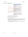
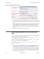
12. In the Preprocess the Workspace structure section, select these options:
— Assign bond orders
— Add hydrogens
— Create disulfide bonds. The 4pti structure has three disulfide bonds, which are all
correctly recognized by the Protein Preparation Wizard.
— Cap termini. Select this option if you want the N or C termini capped. There are
many capping groups available; the most common are ACE on the N terminus
and NMA on the C terminus.
— Delete waters. In general, select this option only if you have a reason to remove
crystal waters. Set the distance to a small value to remove all water molecules.
“Het groups” refers to atoms that are labeled HETATM in a PDB file (anything
that is not a protein residue or water).
Do not delete waters for this Tutorial exercise.
NOTE
In most cases crystal waters should not be removed from the interior of the protein molecule, or near the protein surface. These water molecules are crucial structural components of the protein and cannot be adequately reproduced by the algorithm used to
solvate the system later on.
13. Click Preprocess to execute the first phase of the protein preparation tasks.
8
D. E. Shaw Research
April 2011
Desmond Tutorial
Tutorial Steps
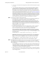
Setup takes only a few seconds to complete. The Protein Preparation Wizard displays
the chains, waters, and het groups as shown in Figure 1.8.
Figure 1.8 Protein Preparation Wizard — Preprocessing stage
The added
capping groups
are shown in
wire frame
representation.
The Display Hydrogens option in the Protein Preparation Wizard is set to Polar only in
Figure 1.7 and, therefore, aliphatic hydrogens are not shown in Figure 1.8. Also note
that the added capping groups can be seen in the circled area, shown in wire frame
representation.
14. At this point you should have a topologically correct molecular system in the workspace, which can be subjected to molecular mechanics calculations. However, since
hydrogen atoms were added by the Protein Preparation Wizard using simple geometric templates, the hydrogen bond network should be optimized.
For example, as shown in Figure 1.8 in this tutorial exercise, the Protein Preparation
Wizard reports a problem with atoms 868 and 1060 being too close (see circled area).
Hydrogen atom 868 belongs to ARG53 and hydrogen atom 1060 belongs to HOH153
(one of the crystallographic water molecules).
In general, there are two alternatives for fixing this type of problem. From the H-bond
Assignment subpanel when you click the Refine tab:
— Click Optimize to launch a comprehensive Monte Carlo search: different protonation states of ASN, GLN, and HIS residues are sampled and OH bonds are flipped
to optimize hydrogen bond geometry. As part of this procedure you can switch to
exhaustive search mode, as well as decide whether the orientation of crystal water
molecules should be sampled.
— Click Interactive Optimizer to launch an interactive tool for hydrogen bond geometry optimization. The interactive optimizer panel is shown in Figure 1.9.
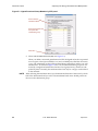
When you click Analyze Network, the Protein Preparation Wizard fills in the table with
the current protonation states of ASP, GLU, and HIS residues as well as initial OH
bond orientations. The table shown in Figure 1.9 reflects the current state after clicking Optimize in the Interactive H-bond Optimizer.
April 2011
D. E. Shaw Research
9
Desmond Tutorial
Desmond Tutorial
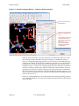
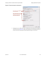
Figure 1.9 Protein Preparation Wizard — Interactive H-bond optimizer
Click
‘Interactive
Optimizer’.
Click ‘Analyze
Network’.
Click
‘Optimize’.
The table is
filled with the
current
protonation
states of ASP,
GLU, and HIS
residues as
well as initial
OH bond
orientations.
Slide the list down to the water section and click entry #69 to select HOH153. The
view in the Maestro workspace zooms in and centers on the close contact, as shown
in Figure 1.10. Click the Restore View icon next to the Optimize button to zoom out.
10
D. E. Shaw Research
April 2011
Desmond Tutorial
Tutorial Steps
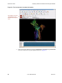
Figure 1.10 Protein Preparation Wizard — Interactive H-bond optimizer
You can set the pH for Hbond analysis.
Click the ‘Lock’ option for
a selection to preserve its
state.
The workspace is focused
on the selection. Click
and
to flip through
a number of discrete
orientations and view
changes immediately in
the workspace.
Select an item in the table to focus the workspace on the selected residue. For example, selecting item 69 in the table focuses the workspace on HOH153 as shown in
Figure 1.10. Originally, this water molecule is in close contact with the HE hydrogen
of ARG53.. By clicking
and
next to HOH153 in the table you can flip through a
pre-defined set of discrete OH orientations and immediately view the result in the
workspace. Figure 1.10 shows the workspace when the water molecule is rotated out
of the way. Similarly, residue states and OH orientations of other residues can be set
manually and, if desired, locked by selecting Lock. At this point we can confirm that
the close contact has been eliminated. Click View Problems in the Refine tab (Figure 1.9)
and you should see a popup window with the message "There are no problems to report"
as shown in Figure 1.10.
Finally, by clicking Optimize you can further optimize the hydrogen bonding network
via a computer algorithm. For further information about the Interactive H-bond Optimizer click Help.
April 2011
D. E. Shaw Research
11
Desmond Tutorial
Desmond Tutorial
15. Finally, provided that you have a Glide license from Schrödinger, the whole protein
structure in the workspace can be subjected to constrained refinement by clicking
Minimize in the Impref minimization subpanel on the Refine tab.
NOTE
The preferred refinement procedure for MD simulations is to use Desmond's own minimization/relaxation protocol (see below).
NOTE
The Protein Preparation Wizard has two options to fill in missing side chains and residues via Prime, provided that you have licensed Schrödinger’s Prime application. You
only have to select the Fill in missing side chains using Prime option or the Fill in missing loops
using Prime option (see Figure 1.7). Note that by selecting either of these options Prime
will run with default settings. Consult the Prime documentation for more advanced
options including filling in loops in the presence of a membrane bilayer.
16. The 4pti structure is now ready for preparing a Desmond simulation. Select
Applications > Desmond > System Builder as shown in Figure 1.11.
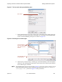
Figure 1.11 Launching Desmond System Builder
Select Applications >
Desmond > System
Builder.
This launches the Desmond System Builder panel shown in Figure 1.12. The System
Builder generates a solvated system that includes the solute (protein, protein complex, protein-ligand complex, protein immersed in a membrane bilayer, etc.) and the
solvent water molecules with counter ions.
12
D. E. Shaw Research
April 2011
Desmond Tutorial
Tutorial Steps
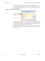
Figure 1.12 Desmond System Builder panel
Select ‘SPC’.
Select ‘Orthorombic’.
Select ‘Buffer’.
Set the distances to 10.0.
Select ‘Show boundary
box’.
Click ‘Calculate’.
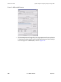
17. Select SPC from the Predefined option menu.
18. Select Orthorombic from the Box shape option menu.
19. Select Buffer from Box size calculation method.
20. Enter 10.0 in the Distances (Å) box.
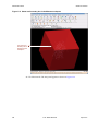
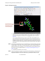
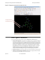
21. Select Show boundary box and click Calculate. The System Builder can also be instructed
to minimize the volume of the simulation box by aligning the principal axes of the solute along the box vectors or the diagonal. This can save computational time if the solute is not allowed to rotate in the simulation box.
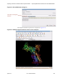
After setting all these options, the workspace displays the solute and the boundary
box as shown in Figure 1.13.
April 2011
D. E. Shaw Research
13
Desmond Tutorial
Desmond Tutorial
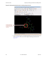
Figure 1.13 Solute and boundary box in the Maestro workspace
The solute and
boundary box is
displayed in the
workspace.
22. Click the Ions tab. The Ions panel appears as shown in Figure 1.14.
14
D. E. Shaw Research
April 2011
Desmond Tutorial
Tutorial Steps
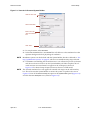
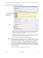
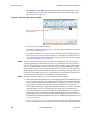
Figure 1.14 Ions tab in Desmond System Builder
Click the ‘Ions’ tab.
Select ‘Neutralize’.
Enter 0.15 in the
‘Salt concentration’
box.
Click ‘Start’.
23. For Ion placement, select Neutralize.
24. In the Salt concentration box, enter 0.150. This will add ions to the simulation box that
represent background salt at physiological conditions.
NOTE
Membrane systems can also be built with the System Builder, but this is deferred to “Setting Up Membrane Systems” on page 25, which covers membrane setup steps in detail.
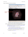
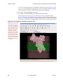
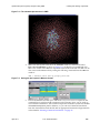
25. Click Start to start building the solvated structure. You will need to provide a job name
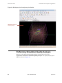
and choose a host on which to run the System Builder job. When complete, the solvated structure in its simulation box appears in the workspace as shown in
Figure 1.15. For better clarity the 4pti structure is shown as a CPK model.
NOTE
April 2011
The solvated simulation box will appear off-centered with respect to the red boundary
box. This is because the System Builder re-centers the system. To produce the view in
Figure 1.15 turn off the Show boundary box option in the System Builder panel (Figure 1.12)
and click the Fit to Workspace icon (circled in Figure 1.15).
D. E. Shaw Research
15
Desmond Tutorial
Desmond Tutorial
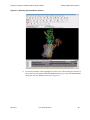
Figure 1.15 Solvated protein structure in the workspace
For clarity, the
protein structure
is shown as a
CPK model.
System Builder saves the whole simulation system in a composite model system file
with the extension .cms. Composite model system files are essentially multi-structure Maestro files that are suitable for initiating Desmond simulations.
NOTE
Maestro automatically assigns the latest OPLS-AA force field parameters available in the
Schrödinger Suite to the entire system. If you would rather apply a Desmond provided
force field (such as Amber or Charmm force fields, TIP5P water model, etc., you need to
process the .cms files using the external Viparr program (see “Generating Force Field
Parameters with Viparr” on page 47).
Now we are ready to perform the Desmond simulation.
Expert users will typically want to start a simulation from the command-line (see
“Running Simulations from the Command Line” on page 56). However, for this
tutorial we will run it from the Molecular Dynamics panel in Maestro.
26. Select Applications > Desmond > Molecular Dynamics. The Molecular Dynamics
panel appears as shown in Figure 1.16.
16
D. E. Shaw Research
April 2011
Desmond Tutorial
Tutorial Steps
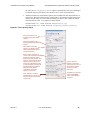
Figure 1.16 The Molecular Dynamics panel
Select ‘Load from Workspace’
and click ‘Load’.
Enter 0.12 in the
‘Simulation time’ box.
Select ‘Relax model
system before simulation’.
Click Start.
27. Import the model system into the Molecular Dynamics environment: select either
Load from Workspace or Import from file (and select a .cms file), and then click Load. The
import process may take several minutes for large systems. For this example, select
Load from Workspace.
28. In the Simulation time box, set the total simulation time to 0.12 ns.
29. Select Relax model system before simulation. This is a vital step to prepare a molecular
system for production-quality MD simulation. Maestro's default relaxation protocol
includes two stages of minimization (restrained and unrestrained) followed by four
stages of MD runs with gradually diminishing restraints. This is adequate for most
simple systems; you may also apply your own relaxation protocols by clicking Browse
and selecting a customized command script. For more details see “Running MultiSim
jobs from the Command Line” on page 58.
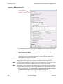
30. Click Advanced Options to set parameters for the simulation. Advanced options are
covered in “Specifying Desmond Simulation Parameters” on page 51.
31. Click Start. The Molecular Dynamics-Start dialog box appears as shown in Figure 1.17.
Figure 1.17 The Molecular Dynamics-Start dialog box
Select ‘Append new
entries’ to add results to
the current project.
Enter a name for the
simulation job.
Select the host where the
job should run; usually
localhost on a standalone
workstation
Click ‘Start’.
32. Select Append new entries from the Incorporate option menu in the Output area to indicate that results of the Desmond simulation should be added to the current Maestro
project.
April 2011
D. E. Shaw Research
17
Desmond Tutorial
Desmond Tutorial
In this example the job will run on localhost, which is typically a standalone workstation, using 4 CPUs with a domain decomposition (the number of blocks into which
the simulation box will be split in the X, Y, and Z directions) of 1x2x2. For large scale
simulations Host is usually a Linux cluster with dozens to hundreds of CPUs.
33. Click Start. The Desmond simulation process begins execution.
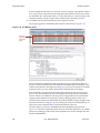
Job progress appears in the Monitor panel similar to that shown in Figure 1.18.
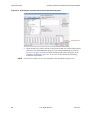
Figure 1.18 The Monitor panel
Jobs 2–8
represent the
relaxation
phase.
The job (relaxation/equilibration and the production run) will finish in about an
hour on 4 CPUs and at that point the Jobs tab in the Monitor panel will display a list
similar to that shown in the upper part of Figure 1.18. If you run the job on a smaller
number of CPUs you may want to shorten the simulation time accordingly.
Jobs numbered 2–8 represent the relaxation phase (shown in the red rectangle of
Figure 1.18). The first job in the list is the master job, and the last job is the production run. There is an additional "solvate pocket" stage (number 6) for systems that
require special treatment for explicitly solvating a binding pocket, which is not
included in the standard System Builder setup. By default this stage is skipped. The
File tab at the bottom of Figure 1.18 shows the log file of the master multisim job. It
shows the actual command that is executed and details of the run.
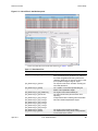
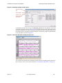
The job summary is shown in the Details tab of the Job Monitor panel shown in
Figure 1.19. The most useful information is the list of job IDs required in case a failed
job has to be debugged. The results of the simulation are saved in multiple files also
listed in the Details tab.
18
D. E. Shaw Research
April 2011
Desmond Tutorial
Tutorial Steps
Figure 1.19 List of files in the Monitor panel
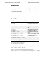
In this case the file list includes the following in Table 1.1 below.
Table 1.1 Simulation files
File
Purpose
4pti_Desmond_md_job.cfg
The Desmond conguration file, which has the simulation parameters for the production run. Note that
the actual configuration file read by Desmond is
called 4pti_Desmond_md_job-out.cfg, which is subject to postprocessing the original .cfg file.
The input structure file for simulation including the
force field parameters.
The “multisim” command script describing the
details of the equilibration stages.
The log file of the master multisim job.
The output structure file (the last frame of the
trajectory).
Compressed tar files containing all the information
about the relaxation/equilibration stages.
4pti_Desmond_md_job.cms
4pti_Desmond_md_job.msj
4pti_Desmond_md_job_multisim.log
4pti_Desmond_md_job-out.cms
4pti_Desmond_md_job_2-out.tgz
4pti_Desmond_md_job_3-out.tgz
4pti_Desmond_md_job_4-out.tgz
4pti_Desmond_md_job_5-out.tgz
4pti_Desmond_md_job_7-out.tgz
4pti_Desmond_md_job_8-out.tgz
4pti_Desmond_md_job.log
4pti_Desmond_md_job.ene
April 2011
The log file of the production simulation.
The instantaneous energy terms of the production
run are stored in the .ene file.
D. E. Shaw Research
19
Desmond Tutorial
Desmond Tutorial
Table 1.1 Simulation files
File
Purpose
4pti_Desmond_md_job_trj
The trj file is in fact a directory, which contains the
trajectory snapshots in multiple binary files. However, from an analysis point of view this directory
can be considered as a single trajectory file associated with an index file .idx and the simbox.dat file
containing data about the simulation box.
4pti_Desmond_md_job-out.idx
4pti_Desmond_md_job_simbox.dat
4pti_Desmond_md_job.cpt
Simbox information.
A checkpoint file that allows for the bitwise accurate
restart of Desmond jobs that crashed for some reason.
You can find the pertinent documentation in the Desmond User’s Guide and the
Schrödinger Desmond User Manual listed in “Documentation Resources” on page 111. Trajectory analysis is covered in “Visualization and Analysis using Maestro” on page 87
and “System Setup and Trajectory Analysis Using VMD” on page 95.
20
D. E. Shaw Research
April 2011
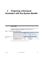
2 Preparing a Desmond
simulation with the System Builder
Overview
The System Builder is a graphical tool in Maestro that lets you generate a solvated system
for Desmond simulations. You can launch the System Builder by selecting
Applications > Desmond > System Builder as shown in Figure 2.1.
Figure 2.1 Launching Desmond System Builder
Select Applications >
Desmond > System
Builder.
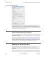
The System Builder panel appears as shown in Figure 2.2.
April 2011
D. E. Shaw Research
21
Desmond Tutorial
Preparing a Desmond simulation with the System Builder
Figure 2.2 System Builder panel
The solvated system generated by System Builder includes the solute (protein, protein
complex, protein-ligand complex, or similar systems, or, a protein immersed in a membrane bilayer), solvent, and counter ions. All structural topological information and
force field parameters for the solvated system are written to a special Maestro file that is
subsequently used for Desmond simulation.
Selecting Solutes and Solvents
The System Builder considers the current contents of the workspace to constitute the solute. Note that some parts of the structure in the workspace may not be displayed, but are
still included in the solute.
Supported solvent models in the GUI include SPC, TIP3P, TIP4P, and TIP4PEW water;
additionally, Viparr allows TIP5P (see “Generating Force Field Parameters with Viparr”
on page 47). Organic solvent boxes for DMSO, methanol, and octanol are also available
through the System Builder. Furthermore, custom models are also allowed if you can
provide the location of a pre-equilibrated box of a different solvent molecule.
Defining the Simulation Box
When defining the simulation box, the goal is to reduce the volume of solvent while
ensuring that enough solvent surrounds the solute so that the protein does not `see' a
periodic image of itself during simulation. Too much solvent will unduly lengthen the
computation.
One way to minimize solvent volume is to select a shape for the simulation box that is
similar to the protein structure. The System Builder shown on Figure 2.2 supports all
22
D. E. Shaw Research
April 2011
Preparing a Desmond simulation with the System Builder
System Builder Output File Format
standard box shapes—cubic, orthorhombic, triclinic, truncated octahedron, and so on.
Select the most appropriate shape from the Box shape option menu in the Boundary conditions section of the Solvation tab and click Calculate if you want to compute the box volume.
Besides the shape, the box size also depends on how you define the solvent buffer around
the solute:
•
Apply a buffer distance to each dimension of the simulation box. A typical buffer distance is 10 Å, which is equal to the usual real space Coulombic interaction cutoff for
long-range electrostatic calculations.
•
Or, set the absolute size of the box.
Next, by clicking Minimize Volume you can instruct the System Builder to minimize the box
volume by aligning the principal axes of the solute with the xyz or diagonal vectors of the
simulation box—essentially, you can align the protein structure so that it fits inside its
simulation box more comfortably. However, this method is only recommended if the solute is not allowed to rotate during MD simulation.
Selecting Show boundary box displays a helpful, translucent graphical representation of the
simulation box in the workspace.
NOTE
System Builder puts the center of gravity of the solute at the center of the simulation box.
As a consequence, fairly non-spherical proteins will appear to shift toward one side of the
box, leaving only a thin water buffer on that side. This may not be ideal from a visual perspective, but in terms of periodic boundary conditions, this is perfectly adequate. It is not
the distance between the outer surface of the protein and the near face of the simulation
box that matters; rather, it is the sum of two such distances with respect to the opposite
sides of the protein that is important.
System Builder Output File Format
The System Builder writes the simulation system in a composite model system file with
the extension .cms. Composite model system files are essentially multi-structure Maestro
files that are suitable for initiating Desmond simulations. Typically, the total solvated system is decomposed into five separate sections in the .cms file: protein (solute), counter
ions, positive salt ions, negative salt ions, and water molecules. The System Builder also
writes Schrödinger OPLS-AA force field parameters in the .cms file. You can find detailed
documentation of the .cms file format in the Schrödinger Desmond User Manual listed in
“Documentation Resources” on page 111. Note that Desmond 3.0 uses a different file format called a .dms file internally, but in the Desmond/Maestro environment the .dms file is
transparent to the user, there is no need for it explicitly. The .dms file format is documented in the Desmond User’s Guide.
Adding Custom Charges
In some cases you may want to have specific charges on certain molecules in a system; for
example, the ligand molecule. You can specify custom charges in the Use custom charges
section of the System Builder. First, you must identify the charge you want to use. You can
either select partial charges from a structure or you can identify the column in the Maestro
input file that is storing the custom charges. Second, you must specify the subset of atoms
April 2011
D. E. Shaw Research
23
Desmond Tutorial
Preparing a Desmond simulation with the System Builder
for which the custom charges will be applied using the Select panel. The rest of the
atoms will be assigned standard OPLS-AA charges.
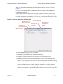
Adding Ions
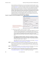
Click the Ions tab in the System Builder panel as shown in Figure 2.3 to add ions to your
system. By default the System Builder automatically neutralizes the solute. For example,
if the solute has a net charge of +N, System Builder will randomly select N residues on
the surface of the protein with a positive formal charge and, respectively, place a negative counterion in the vicinity of the selected residue. For negatively charged solutes,
positive counterions will be similarly positioned. Click Advanced ion placement to place
counterions in a more sophisticated manner; this procedure is illustrated in “Setting Up
Membrane Systems” on page 25 where membrane setup is discussed using a concrete
example. You can also define an excluded region in the Select panel where neither counter ions nor salt ions are allowed.
•
An arbitrary number of counterions can be added; for example, if there is a reason
not to neutralize the system (refer to the special note in “Setting Up Membrane Systems” on page 25). Conversely, you may choose not to place any counterions.
•
Background salt can be added to the system by specifying the salt concentration in
the Add salt section in the Ions tab. The salt ions will be randomly distributed in the
entire solvent volume of the simulation box excluding, of course, the volume occupied by the solute and if present, the lipid bilayer.
•
The type of positive or negative ions to use can be specified in the Ions tab.
Figure 2.3 Ions tab in Desmond System Builderpanel
You can choose to neutralize, add
a specific number of counterions,
or not add any counterions.
You can set the concentration of
salt to add and choose the type of
positive or negative ions.
24
D. E. Shaw Research
April 2011
Preparing a Desmond simulation with the System Builder
Generating the Solvated System
Generating the Solvated System
At this point, you can generate the solvated system by clicking Start in the System Builder
panel. After this task has completed, the solvated system will appear in the workspace
(see Figure 1.15 on page 16) and the resulting system, which is ready for Desmond simulation will be written to a .cms file (see “System Builder Output File Format” on page 23).
NOTE
System Builder automatically assigns the latest OPLS-AA force field parameters available
in the Schrödinger Suite to the entire system. If you would rather apply a Desmond provided force field (Amber or Charmm force fields, TIP5P water model, Schrödinger's PFF
polarizable force field, etc.), you need to process the .cms file using the external Viparr program (see “Generating Force Field Parameters with Viparr” on page 47).
You can also generate the solvated system from the command line. You may decide to use
this method if you want to manually edit the input file to produce an effect that cannot
directly be generated by the System Builder.
To generate the solvated system from the command line:
1.
Click Write in the System Builder panel to write the job files to disk.
There are two input files:
— my_setup.mae. The Maestro structure file of the solute, which serves as the
input for system setup.
— my_setup.csb. The command file, which can be hand-edited for custom setup
cases. For detailed documentation of the .csb file see the Schrödinger Desmond User
Manual listed in “Documentation Resources” on page 111.
And a single output file (besides a log file):
— my_setup-out.cms. The Maestro structure file of the entire simulation system
including OPLS-AA force field parameters. For details on the .cms file see the
Schrödinger Desmond User Manual listed in “Documentation Resources” on
page 111.
2.
Execute the following command at the command line:
$ $SCHRODINGER/run $SCHRODINGER/utilities/system_builder
my_setup.csb
where my_setup is the file name given to “Write”.
NOTE
Run the system_builder script with the -help command argument instead of the .csb
file to see advanced options.
Setting Up Membrane Systems
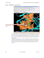
The Setup Membrane panel as shown in Figure 2.4 can be used to embed a membrane protein structure in a membrane bilayer. In this procedure a template consisting of an equilibrated membrane—including the accompanying water—is used to generate a large
enough region to encompass the protein. Using the Setup Membrane panel, you can position the protein within the membrane using a semi-automated procedure.
April 2011
D. E. Shaw Research
25
Desmond Tutorial
Preparing a Desmond simulation with the System Builder
Figure 2.4 Membrane setup in the System Builder
As a real-life example we can consider the calcium ATPase protein, 1su4. Follow the procedure below to prepare this protein for membrane simulation in Desmond.
To setup the 1su4 membrane protein system for Desmond simulation:
26
1.
Open the Protein Preparation Wizard by selecting Workflows > Protein Preparation
Wizard. Type “1su4” in the PDB box and click Import as shown in Figure 2.5.
2.
When the structure appears in the Maestro workspace, set the preprocessing options
as shown in Figure 2.5; do not delete the crystal waters as they are integral to the
protein structure. Click Preprocess. The tables will be filled in by the Protein Preparation Wizard.
3.
Click the Review and Modify tab, select the sodium ion in the Het table (the focus of
the workspace view will center and zoom on the Na ion) and then click Delete. The
sodium ion is an artifact of the crystallization process; only the Ca ions are integral
parts of the protein.
4.
You may want to experiment with H-bond assignment as described in Figure 1.10,
but it is not essential for the current membrane setup exercise. Click Close to exit
from the Protein Preparation Wizard panel.
D. E. Shaw Research
April 2011
Preparing a Desmond simulation with the System Builder
Setting Up Membrane Systems
Figure 2.5 Preprocessing the 1su4 structure
Enter ‘1su4’ in the ‘PDB’ box
and click ‘Import’.
Next, check options in this
section as shown. Do not
delete the crystal waters.
Then click ‘Preprocess’.
5.
April 2011
Change the view to ribbon view in the workspace and orient the protein similar to
what can be seen in Figure 2.6, which is the standard way of looking at membrane
proteins (with the transmembrane bundle aligned along the vertical axis).
D. E. Shaw Research
27
Desmond Tutorial
Preparing a Desmond simulation with the System Builder
Figure 2.6 The 1su4 structure in standard orientation
Click ‘Ribbon’ and select
‘Show Ribbons for All
Residues’ from the option
menu.
6.
28
Launch the System Builder by selecting Applications > Desmond > System Builder
and click the Ions tab. The panel appears as shown in Figure 2.7.
D. E. Shaw Research
April 2011
Preparing a Desmond simulation with the System Builder
Setting Up Membrane Systems
Figure 2.7 The Ions tab in the System Builder panel
Click ‘Select’.
7.
In this tutorial exercise we do not want to place counterions in the vicinity of the calcium ions. This can be achieved the following way. Click Select in the Excluded region
section. The Atom Selection panel opens as shown in Figure 2.8.
Figure 2.8 Selecting the excluded region
Click the ‘Residue’
tab, select ‘Residue
type’, and select the
CA ions.
Click ‘Proximity’ and
set the distance.
8.
NOTE
April 2011
Select the two calcium ions by “residue type” and click Proximity to select all residues
within 5 Å. The resulting ASL expression at the bottom of the selection panel defines
the excluded region. Click OK.
The Excluded region section in the Ions tab in Figure 2.7 also has an option to define a region
around the selected atoms, but the command in the ASL section (fillres within 5
((res.ptype "CA"))) shown in Figure 2.8 takes precedence.
D. E. Shaw Research
29
Desmond Tutorial
Preparing a Desmond simulation with the System Builder
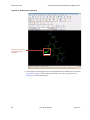
9.
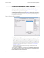
Click Advanced ion placement in the Ion placement section of the Ion tab shown in
Figure 2.7 to open the dialog box shown in Figure 2.9. Click Candidates. A list of all
negatively charged residues, which lie outside of the excluded region appear in the
table as shown in Figure 2.9.
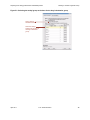
Figure 2.9 Placement of the counterions
Use Shift-Click to
select the first 23
residues.
Click ‘OK’.
Note that the 1su4 structure has a net total charge of –23 after being processed with
the Protein Preparation Wizard. The candidate residues are listed in the table in no
particular order; therefore, if you select the first 23 residues, a good spacial distribution of the positive counterions should result. Click OK.
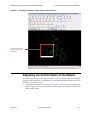
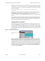
10. Temporarily turn off the ribbon view so you can see the visual feedback of candidate
selection in the workspace. The 1su4 structure should appear similar to the workspace in Figure 2.10.
30
D. E. Shaw Research
April 2011
Preparing a Desmond simulation with the System Builder
Setting Up Membrane Systems
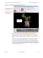
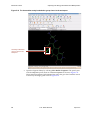
Figure 2.10 Visual feedback of ion placement
Click ‘Ribbon’ and
select ‘Delete Ribbons’
from the option menu.
Once you remove
ribbons you can
see the excluded
region (blue) and
the selected
candidate
residues (red
spheres).
The blue “blob” shows the excluded region and the selected candidate residues are
highlighted by red spheres. The positive counterions will be placed close to the red
spheres, which mark the atoms within the residues that have the largest-magnitude
partial charge. Also note that the residues that constitute the excluded region are
highlighted in blue in the sequence viewer.
In many cases, you may want to place only a few counterions at particular locations
and distribute the rest of the charges in a truly random fashion. Follow the steps
below to achieve this goal.
April 2011
a.
Set the Solvent model to None (Figure 2.2 on page 22) and instead of neutralizing,
explicitly add the number of counterions to the system that you want to place at
particular locations (Select Add in Figure 2.3 on page 24).
b.
Apply the “advanced ion placement” procedure above to place this subset of
counterions in the desired locations.
c.
Run the System Builder to generate this intermediate system with no solvent and
a remaining net total charge.
D. E. Shaw Research
31
Desmond Tutorial
Preparing a Desmond simulation with the System Builder
d. Import the resulting .cms file back to Maestro and re-run the System Builder
with the appropriate solvent and the “neutralize” option, with no further application of the “advanced ion placement” procedure.
5.
After setting the Solvation and Ions options, click Setup Membrane in the Solvation tab
of the System Builder. The Membrane Setup dialog box appears as shown in
Figure 2.11.
Figure 2.11 Set Up Membrane dialog box
Select ‘POPC’ as the
membrane model.
Click ‘Place
Automatically’.
32
6.
Set the membrane model to POPC. Other membrane models include DPPC and
POPE. The temperature in parentheses shows the temperature at which the membrane model was equilibrated. (Note that even though the panel suggests it custom
lipid models are currently not supported.) If at this point you click Set to Helices and
then Place Automatically, the System Builder will attempt to position the membrane
bilayer at a reasonable location based on the information found in the HELIX section
of the 1su4 PDB file. If such information is not present in your PDB file, try
Tools > Assign Secondary Structure in Maestro. As you will see, however, this placement will not be satisfactory in this case. By specifying the set of transmembrane
atoms more accurately, you can expect a highly improved auto placement.
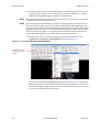
7.
Selection of transmembrane residues can be done a number of different ways using
the Select panel. In this tutorial exercise let's assume that we do not know the relevant residue numbers (that we could simply add in as an ASL expression), and try to
make an approximate selection by hand. In order to do this, change the Select tool in
the Edit toolbar (circled in Figure 2.12) to 'R' (residue selection) and select a rectangular area with the cursor around the transmembrane helices of 1su4 as shown in
Figure 2.12.
D. E. Shaw Research
April 2011
Preparing a Desmond simulation with the System Builder
Setting Up Membrane Systems
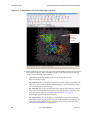
Figure 2.12 Selecting transmembrane residues
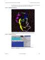
8.
April 2011
The selected residues will be highlighted in yellow color. After making the selection in
the workspace click Select in the Set Up Membrane dialog box to open the Atom Selection
dialog box and click Selection as shown in Figure 2.13.
D. E. Shaw Research
33
Desmond Tutorial
Preparing a Desmond simulation with the System Builder
Figure 2.13 Importing the selection into the Atom Selection dialog box
Click ‘Selection’.
9.
NOTE
34
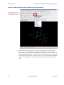
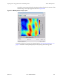
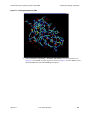
When the ASL area is filled, click OK. At this point the ASL area will be filled with the
selection in the Set Up Membrane dialog box. Click Place Automatically as shown in
Figure 2.11 on page 32 and the resulting membrane placement will appear in the
workspace as shown in Figure 2.14. As you can see, the membrane positioning
needs minor adjustment.
Switch back to ribbon view for the remainder of this membrane setup exercise.
D. E. Shaw Research
April 2011
Preparing a Desmond simulation with the System Builder
Setting Up Membrane Systems
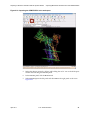
Figure 2.14 Initial automatic membrane placement for 1su4
Click ‘Transformations’
to switch between local
and global scopes.
Click ‘Ribbon’ and
select ‘Show Ribbons
from the option menu.
Initial automatic
placement for
1su4.
10. Select Adjust membrane position in the Set Up Membrane dialog box as shown in
Figure 2.11 on page 32. At this point you should be able to translate and rotate the
membrane model in the workspace, relative to the protein structure. Moving the
membrane relative to the protein structure is termed the local scope for transformations.
However, for a better view you will probably want to translate/rotate the system as a
whole as well. This is called the global scope and you can switch back and forth
between the local and the global scopes by repeatedly clicking Transformations (called
out in Figure 2.14). With only a few translations and rotations, switching between the
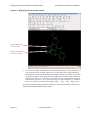
local and global scopes, you should be able to place the membrane in a suitable starting position. After applying manual transformations you should place the membrane
similar to that shown in Figure 2.15.
April 2011
D. E. Shaw Research
35
Desmond Tutorial
Preparing a Desmond simulation with the System Builder
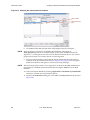
Figure 2.15 Adjusted position of the membrane for 1su4
Suitable
membrane
placement
for 1su4.
NOTE
You may want to position two or more different membrane proteins (e.g., for mutagenesis studies) in a bilayer in exactly the same way. Of course, this would be virtually
impossible to do, trying to reproduce the same manual adjustments. The Set Up Membrane dialog box in the System Builder provides a convenient way to automate this procedure. Any time you are satisfied with the membrane placement, the net translation/
rotation transformation matrix can be saved in the project entry by simply clicking Save
Membrane Position in the Set Up Membrane dialog box (see Figure 2.11 on page 32). Then,
for any subsequent protein, you can simply click Load Membrane Position to position the
entry according to the saved transformation matrix. This way, all proteins will be placed
in the membrane in exactly the same position and orientation.
11. Finally, click OK in the Set Up Membrane dialog box and click Start in the System
Builder panel to start the membrane system setup. For 1su4, the setup procedure
should take 6–8 minutes. The resulting simulation system is shown in Figure 2.16 on
page 37. For better visualization, the protein is shown as a CPK model and the lipid
bilayer is highlighted in green.
NOTE
36
The visible gap at the top and bottom of the lipid layer is the gap between the water
layer that is part of the POPC model and the extra water layer, which was added to the
system to satisfy the boundary conditions. This is expected since the system is put
D. E. Shaw Research
April 2011
Preparing a Desmond simulation with the System Builder
Setting Up Membrane Systems
together from two different, pre-equilibrated boxes of a solvated lipid bilayer and plain
solvent, respectively. The gap should go away after a relatively short equilibration period.
However, membrane systems should be equilibrated for an extended period of time to
resolve the large hole that was carved out of the lipid bilayer to accommodate the transmembrane part of the protein. The hole is shown for the 1su4 structure in Figure 2.17.
NOTE
The protein in the simulation box in Figure 2.16 is positioned so that the head of the protein is shifted to the top of the simulation box. This is the result of a visual artifact discussed in “Defining the Simulation Box” on page 22. System Builder puts the center of
gravity of the solute at the center of the simulation box. As a consequence, fairly nonspherical systems will appear to shift toward one side of the simulation box. Membrane
systems are extreme cases resulting in the view on Figure 2.16. This may not be ideal from
a visual perspective, but in terms of periodic boundary conditions, this is perfectly adequate.
Figure 2.16 Final simulation system for 1su4
Resulting
simulation
system for 1su4
protein shown
as a CPK model
for clarity.
Note that the
protein is shifted
toward the top of
the simulation
box.
Note the gaps
between the
water layers that
are associated
with the lipid
bilayer and the
added water
buffer at the top
and the bottom
of the simulation
box.
Lipid bilayer
(shown in green).
April 2011
D. E. Shaw Research
37
Desmond Tutorial
Preparing a Desmond simulation with the System Builder
Figure 2.17 Transmembrane hole in the POPC bilayer for 1su4
Note the large
hole within
which the
protein was
inserted.
12. More experienced users may want to run the System Builder job from the command
line. Instead of clicking Start, click Write to write a command script file to disk that
can be executed from the command line.
a.
Click Write in the System Builder panel to write the job files to disk.
There are two input files:
— my_setup.mae. This is the Maestro structure file of the solute (1su4 protein, calcium ions, crystal water molecules, neutralizing ions, and counterions), which
serves as the input for system setup.
— my_setup.csb. This is the command file, which can be hand-edited for custom
setup cases. For detailed documentation of the .csb file see the Schrödinger Desmond User Manual listed in “Documentation Resources” on page 111.
And a single output file (besides a log file):
— my_setup-out.cms. This is the Maestro structure file of the entire membrane
simulation system including OPLS-AA force field parameters. For detailed documentation of the .cms file see the Schrödinger Desmond User Manual listed in
“Documentation Resources” on page 111.
38
D. E. Shaw Research
April 2011
Preparing a Desmond simulation with the System Builder
b.
Importing Membrane Placement from the OPM Database
Execute the following command at the command line:
$ $SCHRODINGER/run $SCHRODINGER/utilities/system_builder
my_setup.csb
where my_setup is the file name given to “Write”.
NOTE
You can automatically perform setup of a GPCR membrane system by running this script
from the command line:
$SCHRODINGER/run mold_gpcr_membrane.py
Use the -help option for usage. mold_gpcr_membrane.py takes an input GPCR structure
in .mae format and aligns it to a pre-equilibrated protein-membrane system from a list or
a user-defined template.
Importing Membrane Placement from the OPM
Database
In many cases you can find a high-quality membrane placement already present in the
OPM (Orientations of Proteins in Membranes) database at the University of Michigan.
Using the System Builder you can import OPM placements as well as other pre-aligned
placements. In this section, we will import the OPM placement for 1su4.
To import a membrane placement from the OPM database:
1.
Search the OPM database by typing 1su4 in the Search OPM box as shown in
Figure 2.18.
Figure 2.18 The OPM Home page
2.
April 2011
Click Download Coordinates on the search result page as shown in Figure 2.19. In the
file browser, give the name 1su4_opm.pdb and save the file in your directory.
D. E. Shaw Research
39
Desmond Tutorial
Preparing a Desmond simulation with the System Builder
Figure 2.19 Downloading the OPM pre-aligned coordinates
Click ‘Download
Coordinates’.
3.
In Maestro, click Broom in the Workspace toolbar to clear the workspace.
4.
Import the 1su4_opm.pdb file by selecting Project > Import Structures.
Maestro will issue a warning, but ignore it. As you can see on Figure 2.20, the reason
for the warning message is the presence of two sets of dummy atoms in the PDB
structure shown as layers of colored disks in the workspace. These dummy atoms
designate the positions of the lipid head groups in the OPM database.
Note that the system is shown in a similar orientation that we used in the previous
exercise for better comparison, not the official OPM orientation shown in
Figure 2.19.
40
D. E. Shaw Research
April 2011
Preparing a Desmond simulation with the System Builder
Importing Membrane Placement from the OPM Database
Figure 2.20 Importing the OPM PDB file in the workspace
April 2011
5.
Delete the dummy atoms by clicking and holding the red 'X' icon in the Workspace
toolbar and launching the Selection panel.
6.
In the Selection panel click the Molecule tab.
7.
Select Molecule type in the left panel and then DUM in the right panel as shown in
Figure 2.21.
D. E. Shaw Research
41
Desmond Tutorial
Preparing a Desmond simulation with the System Builder
Figure 2.21 Selecting the dummy atoms for deletion
Select ‘DUM’.
Select ‘Molecule
type’.
8.
NOTE
These atoms are not necessary for building the membrane. The protein in
1su4_opm.pdb is placed in a coordinate system such that the membrane should be
aligned at +/- d/2 along the Z axis where d is the distance between the two sets of head
groups in the bilayer. For 1su4 the value of d is 29.6 Angstrom.
9.
NOTE
Click Add and then OK, and both disks will disappear from the workspace.
Preprocess the remaining system with the Protein Preparation Wizard exactly as
was done in the previous exercise shown in Figure 2.5 on page 27. Do not forget to
delete the sodium ion and ignore or cancel any warning messages.
The total charge of the system is -27 as opposed to -23 because the OPM database has a
few residues in a different protonation state than the original 1su4 entry in the PDB
database.
10. Launch the System Builder by selecting Applications > Desmond > System Builder
and set the solvation and ion placement options.
11. Open the Set Up Membrane dialog box. Click Place on Prealigned Structure as shown in
Figure 2.22.
42
D. E. Shaw Research
April 2011
Preparing a Desmond simulation with the System Builder
Importing Membrane Placement from the OPM Database
Figure 2.22 Set Up Membrane dialog box
Click ‘Place on Prealigned
Structure’.
The imported membrane placement is displayed in Figure 2.23.
Figure 2.23 OPM pre-aligned membrane shown in the workspace
April 2011
D. E. Shaw Research
43
Desmond Tutorial
Preparing a Desmond simulation with the System Builder
As you can see the placement is quite different from that shown in Figure 2.14 and
Figure 2.15. Note the different angle between the transmembrane helices, the plane
of the membrane, and the vertical shift between the two membranes.
12. Click OK in the Set Up Membrane dialog box.
13. Click Start in the System Builder panel to generate the membrane.
The full system is shown in Figure 2.24 and Figure 2.25 for comparison with
Figure 2.16 on page 37 and Figure 2.17 on page 38. It is clear from the comparison of
Figure 2.17 and Figure 2.25 that the OPM placement results in a much better quality
immersion of the protein in the lipid bilayer with much less void left in the channel.
Figure 2.24 Full membrane simulation system for 1su4
Note that the visual artifact
discussed with respect to
Figure 2.16 on page 37
is even more pronounced
here. The protein seems to
extend into the vacuum.
Nonetheless, because of
the periodic boundary
conditions, this is correct.
Basically, it is a periodic
image of the protruding
part of the protein at the
bottom of the simulation
box where there is plenty of
water, that is used in the
computation.
44
D. E. Shaw Research
April 2011
Preparing a Desmond simulation with the System Builder
Importing Membrane Placement from the OPM Database
Figure 2.25 OPM transmembrane hole in the POPC bilayer for 1su4
April 2011
D. E. Shaw Research
45
Desmond Tutorial
Preparing a Desmond simulation with the System Builder
This page left intentionally blank.
46
D. E. Shaw Research
April 2011
3 Finishing Preparations for
Desmond Simulation
Overview
There are a few more tasks that must take place before a simulation can be run:
•
The System Builder will always generate the latest OPLS-AA force field parameters
for the simulation system it builds and the parameters will be included in the .cms
output file. However, you may want to assign different force field parameters in case
the Schrödinger provided OPLS-AA parameters are not adequate for a particular system. You can assign alternative force field parameters for your system using a companion program to Desmond called Viparr.
•
You will also have to specify Desmond run-time simulation parameters.
These topics are addressed in the following sections along with instructions for importing
Amber Molecular Dynamics simulation input files to the Desmond environment.
Generating Force Field Parameters with Viparr
Viparr is a Python script that reads a .cms (or .mae) file and writes another .cms file, which
has all the force field parameters required to run a Desmond simulation. Viparr can assign
force field parameters from a variety of well-established force fields and water models.
Viparr force field assignment is template based. This means that unlike force field servers,
e.g., Schrödinger's OPLS-AA server that can generate parameters for various atom types
derived automatically from the molecule's topological structure, Viparr is designed to find
templates (such as an entire residue) in .cms files and assign the appropriate force field
parameters by looking at a template database associated with a particular force field. The
April 2011
D. E. Shaw Research
47
Desmond Tutorial
Finishing Preparations for Desmond Simulation
resulting parameters are guaranteed to be identical with those of the published, authentic force field.
NOTE
When Viparr begins it wipes out all previous force field information from the input .cms
file. Therefore, it is efficient to build the simulation system using System Builder, and
then perform post-processing on the .cms file with Viparr to assign the desired force field
parameters.
The Viparr script is called viparr.py and basic help on its usage can be obtained via the
command line (output for version 1.5.1):
The command line invocation of the Viparr script is
$SCHRODINGER/run -FROM desmond viparr.py
but it is referred to as viparr.py below.
$ viparr.py --help
usage:
viparr.py [options] mae_file maeff_outfile
Description:
Viparr is a force field parameter assignment program.
-f and -d are used to specify force fields; the order of force fields
is important: earlier ones take precedence over later ones.
Simple example:
viparr.py -f charmm27 -f spc mae_file maeff_outfile
More complicated example:
viparr.py -d me/myfiles/myff -f charmm27 -f spc mae_file
maeff_outfile
Available built-in force fields:
amber03
amber94
amber96
amber99
amber99SB
amber99SB-ILDN
charmm22nocmap
charmm27
charmm32
charmm36_lipids
oplsaa_impact_2001
oplsaa_impact_2005
oplsaa_ions_Jensen_2006
spc
spce
tip3p
tip3p_charmm
tip4p
tip4p2005
tip4pew
tip5p
options:
--version
show program's version number and exit
48
D. E. Shaw Research
April 2011
Finishing Preparations for Desmond Simulation
Generating Force Field Parameters with Viparr
-h, --help
-cCTNUM
show this help message and exit
run Viparr for one CT block only, e.g., for the first,
use "-c 1"
-fFFNAME
built-in force field name; several can be listed, each
preceded by its own -f
-dFORCEFIELD user-provided force field directory; several can be
listed, each preceded by its own -d
-mMERGE_DIR path to user-defined force field directory that is to be
merged with previously specified force field; several
can be listed, each preceded by its own -m
-nFFIO_NAME force field name to put into output file
-pPLUGINDIR override for plugins directory (advanced usage)
-x
do not print header info (for testing purposes)
-v
verbose output
The built-in force fields include the latest versions of Amber, CHARMM, and OPLS-AA
families of fixed-charge force fields. Viparr also provides the parameters for all SPC and
TIP families of water models. A simulation system, or chemical system, is described using a
number of structures called connection tables that reside in CT blocks in the .cms file. These
CT blocks are designated by the f_m_ct{} structure and are composed of a number of
chains, which in turn are composed of a number of residues; for our purposes, residues
may be something other than amino acids (for example, water molecules or ions). Viparr
matches residues in the chemical system to templates in the force fields.
Viparr uses atomic numbers and bond structure to match residues to templates. Thus if
there are non-standard atom or residue PDB names in the .cms file, there is no need to
modify them to match the names used in the force field. You can freely modify atom and
residue names for historic, idiosyncratic, or any other purposes. In particular, Viparr will
identify the N- and C-terminal versions of the residues correctly, as well as protonated/
deprotonated versions of a residue—even if they are not identified as such in the .cms file.
Viparr uses the atom ordering in the .cms file and does not alter this ordering when creating the output file. Residue numbering is also left unchanged, and can begin with any
integer (including negative integers); numbering does not even need to be contiguous,
which is typical to many PDB files. Residues with different chain names can have the
same residue number. To aid in diagnosing problems with the input .cms file, messages
involving residues have the form: < "chain_name", residue_number >
(residue_name) and is usually preceded by a structure number (CT number).
Viparr outputs a compressed force field representation when all the residues in a connection table are the same. For a connection table that only contains water molecules, this
means that force field parameters are output only for a single water molecule.
For the 1su4 example used in “Preparing a Desmond simulation with the System Builder”
on page 21, invocation of Viparr is very simple:
$ viparr.py -f charmm27 -f spc 1su4_desmond.cms 1su4_desmond_out.cms
where 1su4_desmond.cms is the output file from the Desmond Panel. The CHARMM-27
force field has built-in parameters for the protein, calcium, and the POPC lipid model.The
resulting 1su4_desmond_out.cms structure file along with the 1su4_desmond.cfg configuration file that can be generated using the Applications > Desmond > Molecular
Dynamics panel can now be used to run Desmond simulations (see “Specifying Desmond
Simulation Parameters” on page 51).
This simple example already shows a very useful feature of Viparr; it can be used to specify multiple force fields. In this case, each residue in the chemical system matches a temApril 2011
D. E. Shaw Research
49
Desmond Tutorial
Finishing Preparations for Desmond Simulation
plate in exactly one of the specified force fields. This means that the protein residues and
the two calcium atoms will be assigned CHARMM-27 parameters whereas the water
molecules get SPC parameters. The command line invocation for assigning the same
protein parameters, but a different water model of TIP4P, appears similar to this:
$ viparr.py -f charmm27 -f tip4p 1su4_desmond.cms 1su4_desmond_out.cms
You can also use multiple force fields to combine components of two or more force
fields. In this case, residues in the chemical system match templates in more than one of
the specified force fields. In this operation mode, all matching force fields are applied.
For example, one force field provides the angle parameters for a set of residues, while
another force field provides the dihedral parameters for the same residues. The force
field components should be disjoint so there is no conflict with the parameters that are
assigned to each component.
You may also use multiple force fields when parameters assigned to a particular residue
by one force field override parameters assigned by another force field. This situation is
similar to combining force fields; residues in the chemical system match templates in
more than one of the specified force fields and all matching force fields are applied.
However, in this case two or more force fields provide parameters for the same term; for
example, two force fields provide parameters for the angle between atoms 1, 2, and 3
causing a conflict. The conflict is resolved by allowing the first force field (that matches
the residue) to take precedence. The order is the order in which the force fields were
specified on the command line.
In all multiple force field assignment cases, Viparr prints an error message and aborts if a
bond exists between two residues that are not matched by the same force field.
The selected force fields should also have consistent van der Waals combining rules.
Otherwise, Viparr will abort with an error message.
Viparr will print the following warning and error messages when matching residues to
templates:
•
If any residue matches more than one template in a force field, then Viparr exits with
an error. (No Viparr force field should contain identical templates.)
•
If any residue name is matched to a force field template with a different name, a
message is printed. A maximum of 5 messages are printed per residue-template
name pair.
•
Viparr will check that all residues are matched by one of the selected force fields. If
there are any unmatched residues, Viparr will print all unmatched residues and exit
with an error. A maximum of 5 messages are printed per unmatched residue name.
•
If any residue is matched by more than one of the selected force fields, Viparr will
print a warning message. The user should be cautious and be responsible for any
intended use of multiple force fields with multiple matches.
Besides the -f option, there are two more basic options. The -c option allows the user to
assign parameters for a particular structure (CT block) in the input .cms file and the -n
option provides a means to include a user-defined comment in the output .cms file for
annotation purposes.
Viparr also supports user-defined, special force fields (the -d, -m, and -p options), but
that is beyond the scope of this tutorial. Please refer to the Desmond User’s Guide for
information.
50
D. E. Shaw Research
April 2011
Finishing Preparations for Desmond Simulation
Adding Constraints
Adding Constraints
NOTE
While the System Builder automatically adds all the necessary constraints to the .cms file,
Viparr does not. If you process a .mae or .cms file with Viparr you will have to add the constraints in a separate step by running the following command:
$ $SCHRODINGER/run -FROM desmond build_constraints.py input.mae output.mae
where input.mae is typically the Maestro file with Viparr parameters and output.mae will
include the constraints. The command $SCHRODINGER/run -FROM desmond
build_constraints.py -help will list more options.
Importing a Simulation System from the
Amber Molecular Dynamics Package
If you have developed simulation systems using Amber Molecular Dynamics package
(http://ambermd.org), you can import these systems into the Desmond environment. Desmond includes a command-line script for converting an Amber prmtop file and associated crd file into a Desmond cms file. The script is called amber_prm2cms and can be
launched from the command line as follows:
$SCHRODINGER/run -FROM mmshare amber_prm2cms.py -p my_amber_system.prm -c
my_amber_system.crd -o output.cms
The two input files should be standard Amber prmtop and crd files, respectively, and the
output file is the Desmond cms file. Since Desmond reads the force field parameters
directly from the cms file, it is guaranteed that Desmond will apply the exact same force
field, in one-to-one agreement with the Amber prmtop file.
Specifying Desmond Simulation Parameters
Before it can perform simulations, Desmond needs certain simulation parameters to be
set. These parameters can be set in two ways:
•
Using one of the Desmond applications in Maestro.
•
Editing the Desmond conguration file directly.
The following sections provide more details on each option.
Using Desmond applications in Maestro
There are several Desmond applications available in Maestro from the
Applications > Desmond menu. The applications include minimization, molecular
dynamics, simulated annealing, free energy perturbation (FEP), replica exchange, and
metadynamics. In this tutorial we will focus on molecular dynamics and FEP, and give a
simple example of metadynamics. Minimization is typically used in system relaxation,
which will be covered. Simulated annealing and replica exchange require very similar
April 2011
D. E. Shaw Research
51
Desmond Tutorial
Finishing Preparations for Desmond Simulation
setup to molecular dynamics and are both documented in the Desmond User's Guide and
in the Schrödinger Desmond User Manual.
The Molecular Dynamics panel appears as shown in Figure 3.1.
Figure 3.1 Setting up a Desmond simulation
Choose either ‘Load from
Workspace’ or ‘Load from file’.
Click ‘Load’.
Set simulation options.
Select ‘Relax model system
before simulation’.
Import the model system into the Molecular Dynamics panel by clicking Load: select either
Load from the Workspace or Import from file (and select a .cms file), and then click Load. The
import process may take a few seconds for large systems.
The basic settings shown in Figure 3.1 include:
•
Simulation options. Include simulation time, simulation intervals (time intervals by
which different energy terms are recorded and trajectory snapshots are saved), and
ensemble class (NVE, NVT, NPT, NPAT, and NP γ T).
•
Model relaxation. Select Relax the model system before simulation. You can either use a
default protocol (which includes a series of pre-defined minimizations and molecular dynamics executions to relax the system before the production simulation starts)
or you can import your own relaxation protocol. The stage-wise relaxation/equilibration tasks can be defined in a so-called multisim script file, which allows for running multiple simulations. The syntax of multisim .msj file is documented in the
Schrödinger Desmond User Manual.
Relaxation and equilibration of membrane systems requires extra care to prevent
water molecules from diffusing into initial voids between the membrane protein and
the lipid bilayer as shown in Figure 2.17 on page 38 and Figure 2.25 on page 45. The
Desmond/Maestro distribution includes a special script that can be used to generate
a custom relaxation protocol that you can then import to the Molecular Dynamics
panel. Run the following command from the command line to generate a suitable
relaxation protocol for the OPM-placed 1su4 system in “Importing Membrane Placement from the OPM Database” on page 39.
$SCHRODINGER/run -FROM mmshare relax_membrane.py -t 300 -i
1su4_opm_Desmond_setup-out.cms
You can directly import the resulting relax.msj file as a suitable custom protocol in
the Molecular Dynamics panel, but you can also manually edit the multisim script
beforehand to modify or introduce additional relaxation stages.
52
D. E. Shaw Research
April 2011
Finishing Preparations for Desmond Simulation
Specifying Desmond Simulation Parameters
When you click Advanced Options, the Advanced Options dialog box appears as shown in
Figure 3.2.
Options in the Integration tab for the MD task include the multiple time step (RESPA)
schedule and constraints.
Some parameters are interdependent; for example, spinboxes for setting the time step
schedule. If you set the innermost time step and hit Return the midrange and longrange
time steps are adjusted automatically. Of course, you can always manually edit the values
or use the spinbox up/down arrows to adjust the values.
Figure 3.2 Advanced Options for simulation jobs
Parameters for nonbonded interactions.
Thermostat and
barostat parameters.
Controls output files
for simulations.
Parameters for
setting harmonic
restraints.
Other parameters
such as those
defining atom
groups.
Multiple time step
parameters.
The Advanced Options dialog box has several tabs:
•
Ensemble—Contains thermostat and barostat parameters.
•
Interaction—Contains parameters for computing non-bonded interactions.
•
Restraint—Provides a table in which multiple sets of atoms can be subjected to har-
monic restraint with a user-defined force constant. Atom selection can be directly
input as an ASL expression or you can click Select to bring up the Atom Selection dialog
box.
•
Output—Includes the names of various Desmond output files, and allows you to spec-
ify how often these files are updated during the simulation. For example, different
energy terms are recorded in the energy sequence file in user-defined intervals. Snapshots of the simulation are periodically saved in the trajectory file and the entire simu-
April 2011
D. E. Shaw Research
53
Desmond Tutorial
Finishing Preparations for Desmond Simulation
lation state is also saved at user-defined intervals in a checkpoint file. Desmond
simulations can be restarted from checkpoint files with bitwise accuracy.
NOTE
The Output tab has a very useful option. If Glue close solute molecules together is set, the
Desmond trajectory file will be constructed in such a way that receptor ligand complexes, DNA strands or any other multi-molecule structures always stay together for
visualization purposes even if their primary images separate due to the periodic boundary conditions. In earlier versions of Desmond this separation (which, of course, does
not affect the simulation itself) caused unsatisfactory visual artifacts in trajectory viewing.
•
NOTE
Misc—Provides control over miscellaneous parameters, including the definition of
atom groups. Atom group definitions are documented in the Desmond User's Guide
listed in “Documentation Resources” on page 111. Atom groups include thermostat
groups, energy groups (associated with Desmond's vrun application), frozen atoms,
etc. Note that atom groups are assigned in the .cms structure file.
A `frozen' atom group means a set of atoms that move together during the entire MD
simulation as a rigid body. In Desmond, unfrozen atoms cannot be connected to frozen
atoms.
For example, an entire molecule can be frozen (during equilibration), but one cannot
freeze only the heavy atoms, or just certain residues. In that case, restraints should
be used. Also note that frozen atoms cannot be used with NPT simulations, because
the Virial will be incorrect. The other atom group termed energy is used to define
parts of the system whose interaction energies can be monitored during a simulation
by application of the "energy groups" plugin, which is documented in the Desmond
User's Guide. Atom groups can be selected the same way as restraint groups, using
ASL syntax or the Atom Selection dialog box.
The Molecular Dynamics panel is filled in automatically with default parameter values. To
set your own default values so they are automatically presented in the Molecular Dynamics panel, set the desired values in any of the tabs and save it by clicking Write. Then,
copy the resulting .cfg file to ~/.schrodinger/desmond30/desmond_default.cfg. The
new default values take effect the next time you open the Molecular Dynamics panel.
Detailed documentation of the Molecular Dynamics run-time parameter settings can be
found in the Schrödinger Desmond User Manual listed in “Documentation Resources” on
page 111.
Once you have set values for relevant parameters, you are ready to execute a simulation.
Editing the Desmond Conguration File Directly
The Desmond conguration file syntax is described in detail in the Desmond User’s Guide
(see “Documentation Resources” on page 111). You can edit the Desmond configuration
file directly. It can be useful to edit existing configuration files that were used in other
projects. You can always write out a configuration file and use it as a template by clicking Write in the Molecular Dynamics panel.
54
D. E. Shaw Research
April 2011
4 Running Desmond
Simulations
Overview
You can run a Desmond simulation from the Molecular Dynamics panel or the command
line. Before running a simulation you should select Relax the model system before simulation
in the Molecular Dynamics panel. As discussed earlier, Desmond should perform structure
relaxation to prepare a molecular system for production-quality MD simulation. Maestro's built-in relaxation protocol includes two stages of minimization (restrained and
unrestrained) followed by four stages of short MD runs with gradually diminishing
restraints and increasing temperature.
The relaxation parameters may also require edits. The relaxation protocol is written to a
.msj command file (multisim job) which can be run from the command line (see “Running
MultiSim jobs from the Command Line” on page 58). You can manually adjust the relaxation parameters by hand-editing the .msj file.
NOTE
If you decide to run the simulation from the Molecular Dynamics panel, you will be limited
to use the built-in OPLS-AA force field. You can use Viparr to generate other than OPLSAA parameters, but currently, if you run the simulation using Viparr you will need to run
it from the command line.
Running Simulations from the Molecular
Dynamics Panel
1.
April 2011
Click Start at the bottom of the Molecular Dynamics panel to launch Desmond simulation jobs directly from Maestro. The Molecular Dynamics-Start dialog box appears as
shown in Figure 4.1.
D. E. Shaw Research
55
Desmond Tutorial
Running Desmond Simulations
Figure 4.1 Running a Desmond simulation
Select ‘Append new
entries’ to add results to
the current project.
Enter a name for the
simulation job.
Select the host where the
job should run; usually
localhost on a
standalone workstation.
Set the number of CPUs
and domain
decomposition as needed.
Click Start.
2.
Select Append new entries from the Incorporate option menu in the Output area to indicate that results of the Desmond simulation should be added to the current Maestro
project.
3.
In this example, the job will run on localhost, which is typically a standalone workstation, using 4 CPUs with a domain decomposition (the number of blocks into
which the simulation box will be split in the X, Y, and Z directions) of 1x2x2. For
large scale simulations Host is usually a Linux cluster with dozens to hundreds of
CPUs.
4.
Click Start. The Desmond simulation process begins.
Running Simulations from the Command
Line
Given a valid .cms structure file and corresponding .cfg conguration file, the command
line syntax for running Desmond jobs is as follows.
$SCHRODINGER/desmond -HOST <hostname> -exec <desmond_task> -P <cpu>
-c <jobname>.cfg -in <jobname>.cms
In case a job has to be restarted from a checkpoint file, replace the -c and -in options
with -restore and the name of the checkpoint file:
$SCHRODINGER/desmond -HOST <hostname> -exec <desmond_task> -P <cpu>
-restore <jobname>.cpt
where:
56
•
<desmond task> can be either minimize to run a simple minimization, mdsim
(remd for replica exchange job) to run an MD simulation (including FEP jobs
described in “Preparing Free Energy Perturbation and Metadynamics” on page 61),
or vrun to run the vrun trajectory analysis tool (see the Desmond User's Guide for
information about vrun). Note that vrun is the engine of the Schrodinger Simulation
Event Analysis tool, which can be accessed from the Applications > Desmond menu.
•
<jobname> is the name of the job.
D. E. Shaw Research
April 2011
Running Desmond Simulations
NOTE
Running Simulations from the Command Line
•
<hostname> is the name of the compute host, which can also be the name of a queue
on a cluster.
•
<cpu> species the number of CPUs you want each Desmond simulation subjob to
use. This should be 1 for running the serial version of Desmond (for example, to
quickly test on your workstation whether your job will start at all), or a power of 2.
The number of CPUs requested for a restore job must be the same number of CPUs
used with the job that saved the checkpoint file. You can restart a Desmond MD simulation job from the Molecular Dynamics panel as well as shown in Figure 3.1 on page 52.
Select Import from file and browse to select the checkpoint file. Also note that the restore
mechanism can readily be used for continuing a completed simulation if you simply
want to extend the trajectory, but make sure to specify the total simulation time of the
extended simulation, not the additional time. For example, if you want to extend a
100 ns simulation by another 100 ns, simulation time should be set to 200 ns.
Advanced users should consider the following:
•
The Desmond driver in the Maestro environment tries automatically optimizing certain configuration parameters and, therefore, the actual .cfg file (called
your_jobname-out.cfg) that is used by Desmond itself may not be identical to the
original .cfg file that you prepared. The differences can be safely ignored most of the
time, but in some cases you may want to run Desmond with the exact parameters
given in the .cfg file. To turn off internal optimization, launch Desmond from the command line with the -noopt argument:
$SCHRODINGER/desmond -noopt ...
•
By default Desmond applications are run in single precision. Use the -dp option to
switch to double precision. This is only recommended for debugging purposes
because of the performance penalty caused from using double precision.
There is a particularly useful command-line script that can automatically generate
reasonable Desmond configuration settings to facilitate efficient force computations
including non-power-of-two Fourier grids. The script is called forceconfig and can be
launched as follows:
$SCHRODINGER/run -FROM desmond forceconfig.py <input.dms>
input.dms is a binary file that is generated automatically prior to any Desmond run
and is normally invisible to the user. However, for the purpose of using forceconfig.py one needs to generate input.dms explicitly using the following command:
$SCHRODINGER/run -FROM desmond mae2dms input.cms input.dms
where input.cms can be the output structure file of System Builder or Viparr.
NOTE
(For expert users) The .dms file format is the native format for Desmond and the only format supported in the standalone Desmond source distribution. If you have a .dms file,
there is a reverse script called dms2mae that can be used the same way to convert a .dms
file to .cms format.
The forceconfig script analyzes the system and outputs the recommended Desmond
configuration settings. The output can be copied and pasted into a custom Desmond
configuration file for use with the simulation system at hand. Run the script with the
-help option to see optional command-line arguments.
•
April 2011
While a Desmond job is running, all files related to the job are continuously updated
in a temporary directory; at job completion (or if the job crashes), files are copied back
to the working directory.
D. E. Shaw Research
57
Desmond Tutorial
Running Desmond Simulations
The location of this temporary directory is:
tmpdir/username/jobname
where:
- tmpdir is specified in the $SCHRODINGER/schrodinger.hosts file
- username is the username under which the job was submited
- jobname is the name of the Desmond job
Use the -LOCAL option to keep all job files in your working directory all the time.
Detailed documentation of several more options for running Desmond on the command
line can be found in the Schrödinger Desmond User Manual listed in “Documentation
Resources” on page 111 and the -help option gives a quick reference with examples.
NOTE
Although running Desmond from the command line as described in this section is fully
functional, the preferred way of running even single jobs is via the MultiSim utility.
Running MultiSim jobs from the Command
Line
It is often necessary to run multiple jobs, either sequentially or simultaneously, to complete a particular computational task. The two most common cases are system relaxation
and FEP simulations. System relaxation was discussed on Figure 1.16 on page 17 and
FEP simulations are introduced in “Preparing Free Energy Perturbation and Metadynamics” on page 61.
Multiple jobs are handled by the MultiSim facility. MultiSim reads a .msj command
script file and runs multiple simulations defined within it. For instance, to apply a custom relaxation protocol the following command can be used:
$SCHRODINGER/utilities/multisim -JOBNAME <jobname> -maxjob <maxjob>
-cpu <cpu> -HOST localhost -SUBHOST <hostname> -i <jobname>.cms
-m <jobname>.msj -o <jobname>-out.cms
where:
58
•
<jobname> is the name of the job.
•
<maxjob> is the maximum number of subjobs (Desmond simulation jobs of any
kind) that can be submitted to a host or a queue simultaneously. A value of zero
means that there is no limit.
•
<cpu> is the number of CPUs per subjob, which can also be specified as, e.g., "2 2 2"
(note the quotes) indicating 8 CPUs with a spatial decomposition of 2x2x2.
•
-HOST localhost means that the master job runs on your local workstation.
•
<hostname> given with the -SUBHOST option is the name of the host or queue
where the simulation jobs will be running.
•
-c <config_file> is an optional argument used to set non-default Desmond
configuration parameters.
•
-mode umbrella is the default option when a MultiSim job is run on a cluster.
MultiSim jobs include a cascade of consecutive subjobs, each of which requires a
new CPU allocation; depending on the availability of cluster resources, this can
D. E. Shaw Research
April 2011
Running Desmond Simulations
Running MultiSim jobs from the Command Line
involve a significant time lag. The -mode umbrella option instructs the cluster job
submission system to recycle allocated CPUs, thus providing better job turnaround
time.
The input files include a .cms file, which is the output file of the System Builder, and the
.msj command script file, which defines the custom relaxation protocol. The customrelaxed system will be saved in the <jobname>-out.cms file.
The .msj syntax as well as a complete list of MultiSim options can be found in the
Schrödinger Desmond User Manual listed in “Documentation Resources” on page 111 and
the -help option can be used for quick reference.
April 2011
NOTE
The MultiSim facility has a very useful restore mechanism. If a MultiSim job fails (for
example, an FEP job may involve hundreds of individual Desmond subjobs), it can be
restarted from a MultiSim checkpoint file so that only incomplete jobs (crashed or not yet
run) will be re-run.
NOTE
The MultiSim .msj file syntax provides an elegant and powerful alternative to Desmond
.cfg files. The user can fully configure Desmond, separately for each MultiSim stage,
inside the .msj script itself. The corresponding .cfg files will be generated automatically
for each subjob. Also note that configuration settings in the .msj file take precedence over
settings in .cfg file(s).
D. E. Shaw Research
59
Desmond Tutorial
Running Desmond Simulations
This page left intentionally blank.
60
D. E. Shaw Research
April 2011
5 Preparing Free Energy
Perturbation and Metadynamics
Overview
You can use Desmond to run free energy perturbation (FEP) calculations using the dual
topology approach to perform ligand and amino acid residue mutation, annihilation
(absolute free energy calculation), and single-atom mutation in a ring structure. From
Maestro, you can visually specify the fixed and variable parts of a molecule that are subjected to FEP calculations and then store the atom correspondence map (which defines
dual topologies) in the Maestro .mae file.
Ligand mutation—the most common FEP calculation—is illustrated in Figure 5.1 using a
typical scenario. The figure shows a graphical representation of the soluble form of the
human urokinase plasminogen activator receptor (sUPAR, PDB code 2fd6) and the ZINC01538934 ligand. The protein structure has been processed using the Protein Preparation
Wizard as described in “Tutorial Steps” on page 3, and the ligand was docked using
Schrödinger's Glide application as part of a virtual screening experiment on the ZINC
database (http://zinc.docking.org/). The ligand is rendered in a tube representation in the
sUPAR active site with green carbon atoms and ball-and-stick representation.
April 2011
D. E. Shaw Research
61
Desmond Tutorial
Preparing Free Energy Perturbation and Metadynamics
Figure 5.1 FEP Example—Ligand mutation
This side chain will be
mutated to replace the
NH3+ with a methyl
group.
As shown in Figure 5.1, contact residues in the active site are displayed with a matching
molecular surface to emphasize the 3D layout of the active site. One of the two –NH2+ —
CH2 — CH2 — NH3+ side chains is colored darker (see at the center of the workspace in
Figure 5.1); this is the side chain where the terminal NH3+ group will be mutated to a
methyl by FEP.
Note that the setup in Figure 5.1 is only an illustration showing a common real-life
example for FEP calculations, however, you will not need to perform any docking calculations for this tutorial exercise. Instead, just build the ligand structure using the 2D
sketcher tool (un-check convert to 3D) and then click Clean up geometry as shown in
Figure 5.2.
62
D. E. Shaw Research
April 2011
Preparing Free Energy Perturbation and Metadynamics
Setting Up an FEP Calculation
Figure 5.2 The ZINC-01538934 ligand structure
Click ‘Clean up’ to convert the
structure in 3D.
Click ‘2D Sketcher’ to
draw the ligand structure.
Setting Up an FEP Calculation
To setup a Free Energy Perturbation calculation for ligand mutation:
1.
Select Applications > Desmond > Ligand Functional Group Mutation by FEP.
The Ligand Functional Group Mutation by FEP panel appears as shown in Figure 5.3.
April 2011
D. E. Shaw Research
63
Desmond Tutorial
Preparing Free Energy Perturbation and Metadynamics
Figure 5.3 Ligand Functional Group Mutation by FEP panel
Select ‘Pick the
attachment bond’.
Select the fragment that
will replace the
substitution group.
Click Start.
2.
Select 'Pick the attachment bond' (Step 2 in Figure 5.3).
When you define a structural perturbation for FEP, the ligand molecule is separated
into two parts: a fixed part (called the core) and a variable part (called the substitution
group). The substitution group will be mutated during simulation, and the core will
remain intact. As shown in Figure 5.4, the core and the substitution groups are connected by a single bond termed the attachment bond (green arrow), which has to be
picked by hand. Currently, the attachment bond can only be a single, covalent bond
in the molecule.
NOTE
64
When selecting the attachment bond, you determine the direction of the arrow by which
half of the attachment bond you select. The attachment bond arrow should point from
the core to the substitution group.
D. E. Shaw Research
April 2011
Preparing Free Energy Perturbation and Metadynamics
Setting Up an FEP Calculation
Figure 5.4 Defining the mutation
The attachment bond is
shown as a green arrow in
the workspace. The arrow
should point from the core
to the substitution group.
3.
Define the mutation to be performed by selecting the fragment(s) that will replace the
substitution group from the Fragment Library. For this example, select the methyl row
from the list of fragments. The selected row is highlighted in yellow as shown in
Figure 5.3.
You can apply multiple mutants at a time by using CTRL-click and SHIFT-click to
select the mutants from the Fragment Library. When you select multiple fragments, the
FEP ligand mutation application creates different systems for each mutant, and runs
multiple thermodynamic cycles to compute, respectively, the binding free energy difference between the reference ligand and each of the selected mutants, with respect to
the receptor.
NOTE
The short list of substitution groups is not a limitation, it is a practical warning. Any mutation involving more than only a very few atoms is subject to very large uncertainty in the
calculated Delta G values and it is virtually impossible to achieve converged results in a
feasible simulation time. Nonetheless, you can create arbitrary groups rather than selecting mutations from the Fragment Library. See “Creating a Custom Fragment Group” on
page 71 for details.
4.
NOTE
April 2011
Click Start. FEP simulation starts execution.
Desmond uses Bennett's acceptance ratio method for FEP calculations, which means that
numerous independent simulations will be run for a single FEP calculation. Since the
independent simulations can be run simultaneously, you should be careful as to how
D. E. Shaw Research
65
Desmond Tutorial
Preparing Free Energy Perturbation and Metadynamics
many simulations can be allowed to run on your host/queue at the same time. You can
control this parameter in the Start dialog box by setting the maximum number of subjobs
as shown in Figure 5.5. The value zero means no limit. In this example the master/multisim job will run on localhost (local workstation) whereas the subjobs (the individual
Desmond FEP simulations) will run on a cluster via a submission queue called swdev,
which provides a total of 112 CPU cores. Out of the 112 only 32 cores will be used simultaneously; 4 FEP simulations running at the same time, each utilizing 8 cores. Note that
the total number of FEP simulations is 24 by default: 12 lambda windows for both
mutating the ligand in the enzime-ligand complex and mutating it in pure solvent,
respectively, moreover each FEP simulation involves an independent relaxation protocol. FEP simulations are computationally very expensive.
Figure 5.5 Ligand Functional Group Mutation by FEP - Start dialog box
Control how many simultaneous
simulations can run on your host/
queue at the same time.
5.
Alternatively, click Write. A total of four files are written:
— Two Maestro files: my-fep-job_lig.mae and my-fep-job_cmp.mae. The first file
contains the original ligand and one or multiple mutants. The second file contains the receptor and the ligand structures. Note that both files are regular Maestro files with no force field information included at this point. The only
information about the FEP setup in these files is the definition of the attachment
bond.
— Two MultiSim command script files: my-fep-job_solvent.msj and my-fepjob_complex.msj. The first script defines a series of simulations involving the
ligands in the solvent and the second script defines corresponding simulations
involving the ligand-receptor complexes.
Both .msj scripts can be run from the command line as described in “Running
MultiSim jobs from the Command Line” on page 58.
66
NOTE
Mutants do not need to be stoichiometric equivalents as in this example. Atoms that
have no match in the mutant (or vice versa) will be annihilated into, or grown out of,
dummy atoms during the course of the FEP simulation in accordance with the double
topology technique.
NOTE
For more realistic simulations, you will need to adjust the conformation of the mutant.
See “Adjusting the Conformation of the Mutant” on page 77 for details.
NOTE
This tutorial does not go into details about the configuration settings for FEP simulations, see the Desmond User’s Guide and the Schrödinger Desmond User Manual listed in
“Documentation Resources” on page 111 for a full account of this topic.
D. E. Shaw Research
April 2011
Preparing Free Energy Perturbation and Metadynamics
6.
Setting Up an FEP Calculation
There are several ways to run the FEP simulation:
— Write your own Desmond configuration file and run the FEP simulation from the
command line. See “Running FEP Simulations from the Command Line” on
page 70 for instructions to run the FEP simulation from the command line. This is
the most flexible, but least automated approach.
— Use Maestro to generate any non-default Desmond configuration file and run the
FEP simulation from the command line. See “Using Maestro To Generate A Desmond FEP Configuration File” on page 68 for instructions on using Maestro to
generate the configuration file. See “Running FEP Simulations from the Command Line” on page 70 for instructions to run the FEP simulation from the command line.
— Run the FEP simulation directly from the Ligand Functional Group Mutation by FEP
panel by clicking Start. The workflow defined in the .msj files is automatically
executed. This workflow has a short description shown under the Plan Calculation
tab shown in Figure 5.6; essentially, system setup with System Builder is automatically performed, and all required Desmond simulations (NPT or NVT) are run
with reasonable default settings, but user-defined workflows can also be
imported. This option is the least flexible, but most convenient solution.
Figure 5.6 FEP workflow control
Select ‘Use lambda
hopping to enhance
sampling’ to improve
convergence. See the
Schrödinger Desmond
User Manual for
information.
Select the FEP protocol
that will be used during
simulation.
NOTE
April 2011
Lambda hopping is a form of replica exchange in which coordinate exchanges of systems
simulated in adjacent lambda windows are attempted periodically. For mutations involving conformational flexibility, lambda hopping can improve convergence. For details see
D. E. Shaw Research
67
Desmond Tutorial
Preparing Free Energy Perturbation and Metadynamics
the the Schrödinger Desmond User Manual listed in “Documentation Resources” on
page 111.
NOTE
All of these options use the Schrödinger OPLS-AA force field server. Of course, you can
use Viparr to generate force field parameters for other force fields, however, Viparr has
limited coverage of the chemical space of organic compounds, which means that for
most ligand mutations OPLS-AA is currently the only viable force field.
7.
Compute the binding free energy difference between two different ligand molecules. Regardless of which method was used in step 6, two output .mae files have
been generated: jobname_solvent-out.mae and jobname_complex-out.mae. The difference in free energy between the ligand molecules in pure solvent (dG_solvent)
and the difference when bound to the receptor (dG_complex) are recorded, respectively, in these -out.mae files.
Import the .mae files into Maestro, open the Project Table, and locate the dG values
at the far end of the table. The relative binding free energy of ddG_binding is equal
to the difference between dG_complex and dG_solvent: dG_complex dG_solvent.
If ddG_binding is negative, the mutation resulted in better binding; otherwise if
ddG_binding is positive, the original ligand molecule had more favorable binding.
Using Maestro To Generate A Desmond FEP
Configuration File
To create a Desmond conguration file for FEP:
1.
68
Select Applications > Desmond > FEP. The FEP panel appears as shown in
Figure 5.7.
D. E. Shaw Research
April 2011
Preparing Free Energy Perturbation and Metadynamics
Using Maestro To Generate A Desmond FEP Configuration
Figure 5.7 Setting FEP parameters from the FEP panel
Select the windows that
should be included in the
simulation by clicking
the corresponding
column head.
Click Write.
The FEP panel is similar to the Molecular Dynamics panel and has the same functionality, but typically it is only used to write out a custom Desmond FEP configuration file.
If, however, you should load a structure into this panel, the structure must have
already been prepared for FEP simulations.
The Simulation section of the panel allows you to set a number of FEP related parameters. For details see the Desmond User’s Guide and the Schrödinger Desmond User Manual listed in “Documentation Resources” on page 111.
2.
NOTE
FEP simulations involve many separate calculations with different values of λ and it is
quite possible that some of them will crash at the first try. When this happens, you should
rerun the FEP simulation only for the failed λ windows. The GUI lets you select the failed
λ windows for a re-run. However, we strongly recommend that you run all FEP jobs
from their respective FEP panels (such as the Ligand Functional Group Mutation by FEP
panel), or from the command line with input files generated by these windows. Doing so
allows the FEP simulation to run via the MultiSim system which has a built-in automatic
recovery mechanism; with this recovery mechanism, you can restart a failed job from the
MultiSim checkpoint file.
3.
April 2011
Select the λ windows that should be included in FEP simulation.
Write out the Desmond conguration file by clicking Write.
D. E. Shaw Research
69
Desmond Tutorial
Preparing Free Energy Perturbation and Metadynamics
Running FEP Simulations from the Command
Line
FEP simulations can be run from the command line using a .msj command script file in
exactly the same way as described in “Running MultiSim jobs from the Command Line”
on page 58:
$SCHRODINGER/utilities/multisim -JOBNAME <jobname> -maxjob <maxjob>
-cpu <cpu> -HOST localhost -SUBHOST <hostname> -i <jobname>.mae
-m <jobname>.msj -o <jobname>-out.mae
where:
NOTE
•
<jobname> is the name of the job.
•
<maxjob> is the maximum number of subjobs that can be submitted to a host or a
queue simultaneously. A value of zero means that there is no limit.
•
<cpu> is the number of CPUs per subjob, which can also be specified as, e.g., "2 2 2"
(note the quotes) indicating 8 CPUs with a spatial decomposition of 2x2x2.
•
-HOST localhost means that the master job runs on your local workstation
whereas
•
<hostname> given with the -SUBHOST option is the name of the host or queue
where the simulation jobs will be running.
When MultiSim is used for FEP simulations, MultiSim requires special .mae files for
input instead of .cms files . These .mae files are generated by the FEP panels (ligand
mutation, protein residue mutation, ring atom mutation, and absolute/total free energy
calculation) and include the dual topology structure of the mutations. The FEP MultiSim
script will explicitly call the System Builder to prepare the solvated systems and generate the OPLS-AA force field parameters.
To apply non-default FEP λ parameters or to change the number of Lambda windows,
add the '-c config_file' option to the command syntax where config_file is a
Desmond FEP conguration file that was generated by the FEP panels as shown in
Figure 5.7 on page 69.
Note that this conguration file will be used throughout the .msj workflow to make sure
that all minimization and MD runs use the same λ settings for consistency. Also note
that FEP parameters like any other Desmond configuration setting can always be
defined directly in the MultiSim script and those values set in the .msj file take precedence. In particular, you can cut-and-paste the FEP block from the .cfg file defining the
custom lambda schedule inside the desmond{} block below in the stock .msj file that is
generated by the ligand/residue/ring-atom FEP panels.
task {
task = "desmond:auto"
set_family = {
desmond = {
checkpt.wall_interval
= 7200.0
checkpt.write_last_step = no
fep = {
lambda = {
70
D. E. Shaw Research
April 2011
Preparing Free Energy Perturbation and Metadynamics
Creating a Custom Fragment Group
...
}
}
}
}
}
For details see the Desmond User’s Guide and the Schrödinger Desmond User Manual listed in
“Documentation Resources” on page 111.
NOTE
There is a Python script available, which can be used directly to compute the free energy
difference associated with a FEP job (the script is run by default as part of an MultiSim
workflow).The following script will process the “energy” file output of the different λ
runs and compute the free energy:
$SCHRODINGER/run -FROM desmond bennett.py
Use the -help option to learn about the use of this script and consult the Desmond User's
Manual listed in “Documentation Resources” on page 111 for more details.
Creating a Custom Fragment Group
If the Fragment Library does not have the mutant structure you want to use, you can edit
any pre-defined substitution group manually using the general Build/Edit tools in Maestro.
The only caveat is that the customized substitution group will retain the name of the fragment that you modified. However, the FEP simulation will use the modified fragment.
Use caution with custom fragments. Any mutation that involves more than a few atoms is
likely subject to very large uncertainties in the free energy differences computed between
different lambda windows. Try decomposing a large mutation into several small mutations and run multiple MultiSim FEP simulations. It will take longer, but results will be
more reliable.
For this exercise let’s make a larger mutation in the ligand molecule and turn the whole
–NH2+ — CH2 — CH2 — NH3+ side chain into a butyl group. The current view of the
workspace should be similar to that shown in Figure 5.4 on page 65.
1.
April 2011
Click Pick the attachment bond in the Ligand Functional Group Mutation by FEP panel (see
Figure 5.3 on page 64) and click OK when asked to confirm that you are reselecting the
bond. This time choose the attachment bond shown in Figure 5.8. For clarity, the view
is changed to wire frame representation.
D. E. Shaw Research
71
Desmond Tutorial
Preparing Free Energy Perturbation and Metadynamics
Figure 5.8 Picking the attachment bond for creating a butyl side chain
The attachment bond
you selected is shown
as a green arrow in the
workspace.
2.
72
Select the methyl fragment on the Define Perturbation tab and select the View option as
shown in Figure 5.9. The view in the workspace will change to that shown in
Figure 5.10.
D. E. Shaw Research
April 2011
Preparing Free Energy Perturbation and Metadynamics
Creating a Custom Fragment Group
Figure 5.9 Selecting the methyl group as the base for the butyl substitution group
Select ‘Pick the
attachment bond’.
Select the methyl
fragment as the base of
the butyl substitution
group.
April 2011
D. E. Shaw Research
73
Desmond Tutorial
Preparing Free Energy Perturbation and Metadynamics
Figure 5.10 The intermediate methyl substitution group shown in the workspace
The methyl substitution
group is shown in the
workspace.
3.
74
Open the fragment library by selecting Edit > Build > Fragments. The panel opens
with the Fragments option menu set to Diverse Fragments as shown in Figure 5.11.
Select Grow, select Pick and select Bonds. Then select the grow bond with the mouse
as shown by the bright green arrow in Figure 5.12.
D. E. Shaw Research
April 2011
Preparing Free Energy Perturbation and Metadynamics
Creating a Custom Fragment Group
Figure 5.11 The Build panel
Select ‘Grow’.
Select ‘Pick’ and select
‘Bonds’.
‘Diverse Fragments’
should be selected in the
‘Fragments’ option menu.
April 2011
D. E. Shaw Research
75
Desmond Tutorial
Preparing Free Energy Perturbation and Metadynamics
Figure 5.12 Selecting the grow bond
Use the cursor to select
the grow bond in the
workspace.
4.
76
Select propyl from the fragment list in the Fragments tab of the Build panel as shown in
Figure 5.11 on page 75. The resulting side chain is a butyl group as shown in
Figure 5.13. Close the Build panel.
D. E. Shaw Research
April 2011
Preparing Free Energy Perturbation and Metadynamics
Adjusting the Conformation of the Mutant
Figure 5.13 The butyl substitution group shown in the workspace
The butyl substitution
group is shown in the
workspace.
Adjusting the Conformation of the Mutant
The initial conformation of the mutant must be as close as possible to that of the original
ligand for FEP simulations. Using Maestro, you can make manual adjustments to the conformation of small molecules.
1.
April 2011
Click Maestro's Adjust tool as shown in Figure 5.14 to turn on the manual adjustment
option. Toggle this tool to switch between manual adjustment mode and global translation/rotation mode.
D. E. Shaw Research
77
Desmond Tutorial
Preparing Free Energy Perturbation and Metadynamics
Figure 5.14 Manual adjustment of the substitution group conformation
Click ‘Adjust’ to enable
manual adjustments, such
as “quick-torsion” mode.
2.
78
Click the attachment bond (shown in green) to display the non-bonded contacts
between the butyl fragment and the ligand core. If you don't see any contacts
shown in the workspace, select Display Contacts in the Adjust tool and also make sure
that the Quick Torsion option is set. Click and hold the left mouse button to bring up
the Adjust tool's option menu. As shown in Figure 5.15, there are numerous allowed
close contacts (displayed in orange) and a few unfavorable contacts (displayed in
red).
D. E. Shaw Research
April 2011
Preparing Free Energy Perturbation and Metadynamics
Adjusting the Conformation of the Mutant
Figure 5.15 Displaying the non-bonded contacts
Unfavorable contacts
are shown in red.
Allowed close contacts
are shown in orange.
3.
To arrive at a suitable conformation of the substitution group, you must adjust the torsion angle (and often, multiple angles). You can alter the torsion angle manually by
holding down the left mouse button and moving the mouse horizontally, or by rotating the mouse wheel. Try relaxing the unfavorable contacts with rotations about different bonds in the butyl side chain. You should arrive to a conformation similar to
that shown in Figure 5.16. As you can see in Figure 5.17 the altered butyl conformation is now fairly close to that of the original –NH2+ — CH2 — CH2 — NH3+ group.
To restore the default methyl substitution group, you can click the 'Reset' column in the
Ligand Functional Group Mutation by FEP panel.
April 2011
D. E. Shaw Research
79
Desmond Tutorial
Preparing Free Energy Perturbation and Metadynamics
Figure 5.16 Unfavorable contacts removed
Only allowed close contacts
remain. The unfavorable
contacts have been
removed.
80
D. E. Shaw Research
April 2011
Preparing Free Energy Perturbation and Metadynamics
Other Types of Mutations
Figure 5.17 Butyl group superposed with original side chain
The original side chain.
The modified side chain.
Other Types of Mutations
You can also perform these mutations from the Applications > Desmond menu:
April 2011
•
Protein residue mutation can be used for two different types of calculation. With one
calculation, the difference in free energy is computed for a ligand bound to a protein
versus the same ligand bound to a mutated form of the same receptor with amino acid
residue mutations applied to the protein. With the other calculation, the difference in
free energy is computed for a protein versus a mutated protein, without a ligand.
Only single point mutations can be applied in a single FEP calculation. To consider
multiple mutations, you must run multiple FEP calculations. However, you can
always setup multiple single-point mutations in a single FEP run, for example, to
compare the effect on binding free energy of different single-point mutations.
•
Ring atom mutation can be used to replace one atom with another in a ring structure.
•
Absolute or total free energy calculation can be used to compute absolute solvation
free energies by annihilating a whole solute molecule.
D. E. Shaw Research
81
Desmond Tutorial
Preparing Free Energy Perturbation and Metadynamics
Setup for these types of mutations is straightforward and very similar to ligand mutation setup. Please consult Chapter 4 and Appendix B of the Schrödinger Desmond User
Manual listed in “Documentation Resources” on page 111 for details about FEP setup
and the syntax for programming .msj scripts, respectively.
Aside: Metadynamics
Metadynamics is a different kind of free energy perturbation method which enhances
sampling of the underlying free energy space by biasing against previously-visited values of user-specified collective variables. The biasing is achieved by periodically dropping repulsive kernels of Gaussian shape at the current location of the simulation in the
phase space of the collective variables. This history-dependent potential encourages the
system to explore new values of the collective variables, and the accumulation of potential allows the system to cross potential barriers much more quickly than would occur in
standard dynamics. Metadynamics is fully documented in the Desmond User’s Guide
listed in “Documentation Resources” on page 111.
In this Tutorial we present a simple working example to get familiarized with metadynamics. The example involves generating the well-known 2-dimensional free energy
surface of alanine dipeptide with respect to its phi and psi dihedral angles. Follow these
steps to generate and plot the free energy surface.
1.
82
Build alanine dipeptide in Maestro.
a.
Open the fragment library panel by selecting Edit > Build > Fragments.
b.
On the Fragments tab of the Build panel, select Grow, select Amino acids from the
Fragments option menu, and click ALA in the table as shown in Figure 5.18.
c.
Close the Build panel. The alanine dipeptide molecule appears in the Maestro
Workspace. (Alanine dipeptide is in fact a single alanine molecule with capping
groups ACE on the N terminus and NMA on the C terminus.)
D. E. Shaw Research
April 2011
Preparing Free Energy Perturbation and Metadynamics
Aside: Metadynamics
Figure 5.18 Fragment library Build panel
Select ‘Grow’.
Select ‘Amino acids’
from the ‘Fragments’
option menu.
Click ‘ALA’.
4.
Clean up the geometry by selecting Edit > Build > Clean Up Geometry.
5.
Build a solvated Desmond simulation box with the System Builder as described in
step 16 on page 12.
6.
Open the metadynamics panel by selecting
Applications > Desmond > Metadynamics. The Metadynamics panel appears as
shown in Figure 5.19.
Metadynamics setup is virtually identical to molecular dynamics setup except for
defining the collective variables and the height and shape of the Gaussian kernel
potential.
April 2011
D. E. Shaw Research
83
Desmond Tutorial
Preparing Free Energy Perturbation and Metadynamics
Figure 5.19 Metadynamics panel
Select ‘Load from
Workspace’ and click
‘Load’.
7.
In the Metadynamics panel, select Load from Workspace and click Load to import the
solvated system from the Workspace.
8.
Hide the water molecules by selecting Workspace > Display/UnDisplay
Atoms > Undisplay: Waters.
9.
Click Dihedral and Pick atoms and select the phi and psi angles in the Workspace by
clicking the four consecutive backbone atoms, respectively. Click Add and the
selected dihedrals appear in the table.
NOTE
You can also change the height and width of the Gaussian kernel and the frequency of
dropping the kernel in phase space; however, the default values should suffice.
NOTE
The rest of setup is identical to running a molecular dynamics job. Note, however that
this metadynamics simulation should run for 1.2 ns to achieve convergence.
NOTE
Metadynamics is also supported via MultiSim. More complicated collective variables
(via generic ASL expressions) can be set using MultiSim and command line execution.
10. When the job finishes, select Applications > Desmond > Metadynamics Analysis.
The Metadynamics Analysis panel opens. Click Browse and open the
desmond_metadynamics_job-out.cfg file (or the corresponding -out.cfg file if you
84
D. E. Shaw Research
April 2011
Preparing Free Energy Perturbation and Metadynamics
Aside: Metadynamics
provided a custom name for the job). Reading the data will take a few minutes. Then
the free energy contour plot appears as shown in Figure 5.20.
Figure 5.20 Metadynamics Analysis panel
Consult the Schrödinger Desmond User Manual listed in “Documentation Resources” on
page 111 for details on manipulating the plot and exporting the free energy data.
April 2011
D. E. Shaw Research
85
Desmond Tutorial
Preparing Free Energy Perturbation and Metadynamics
This page left intentionally blank.
86
D. E. Shaw Research
April 2011
6 Visualization and Analysis
using Maestro
Overview
Maestro provides three basic visualization and analysis tools. Maestro's Trajectory Player is
similar to the ePlayer found in the Project Table, but it is specifically designed to nicely animate Desmond trajectories much faster than the ePlayer could, and it has a number of
specific visualization options.
Maestro can also perform basic quality analysis using the Simulation Quality Analysis
panel and detailed geometric and energetic analysis of the trajectory can be carried out
using the Simulation Event Analysis tool.
The following sections cover the basics of these tools.
Animating Desmond Trajectories with the
Trajectory Player
Assuming that you have completed the first exercise in this tutorial in “Tutorial Steps” on
page 3 you should have a completed Desmond simulation of the 4pti structure in your
working directory with the base name of desmond_job by default (unless you gave it a
different name).
1.
April 2011
Select Project > Import Structures: Read in the desmond_job-out.cms file. You will
have to set the file format selector in the Import panel to Desmond to display Desmond
(.cms) files in the file browser window.
D. E. Shaw Research
87
Desmond Tutorial
Visualization and Analysis using Maestro
2.
Select Project > Show Table: Open the Project Table. The Trajectory Player can be
launched from the Project Table. Note the blue T in the Title column in the Project
Table, as shown in Figure 6.1.
Figure 6.1 Launching the Trajectory Player
Click ‘T’ to open the
Trajectory Player.
3.
Click T to open the Trajectory Player.
The Trajectory Player is shown in Figure 6.2 and the associated Maestro workspace
view can be seen in Figure 6.3.
The Trajectory Player has two sets of options for frame control and display properties; the best way to learn about these options is to experiment with them. The Trajectory Player is fully documented in the Schrödinger Desmond User Manual listed in
“Documentation Resources” on page 111.
88
NOTE
In most cases you do not want the entire system to be displayed when, for example,
visually inspecting the conformational changes of a protein molecule along the trajectory. The Trajectory Player recognizes Maestro's current display settings, which means
that you can select/deselect any set of atoms for display using the Workspace > Display
menu options and you can also render the atoms in any way you want. The Trajectory
Player will generate a smooth animation with your current display settings and you can
even save it in an MPEG movie file for incorporation in any presentation material. You
can also save selected snapshots of the trajectory in Maestro format.
NOTE
Options to center the trajectory view in the Trajectory Player include:
•
Center molecules in the Display section of the Trajectory panel (under Positioning) allows
you to post-process a trajectory such that the part of the system defined in the ASL
text box will be centered in the simulation box. This option is very useful when the
solute appears to jump in and out of the primary simulation box, which can be a
visual artifact caused by the application of periodic boundary conditions. The Center
molecules option is a post-processing option that only affects visualization and
leaves the actual trajectory intact. Note that the Center molecules option solves the
same visual artifact issues during simulation that the Glue close solute molecules
together option solves; the Glue close solute molecules together option can be found in
the Output tab of the Advanced Options dialog box for the Molecular Dynamics panel. See
Figure 3.2 on page 53.
•
mdsim.trajectory.center is an option that can also be used to center the trajectory in the simulation box; this option can be set in the Desmond .cfg configuration
D. E. Shaw Research
April 2011
Visualization and Analysis using Maestro
Animating Desmond Trajectories with the Trajectory Player
file. The mdsim.trajectory.center option is performed at run-time, resulting in
a centered trajectory file. Refer to the Desmond User’s Guide for information.
•
Additional trajectory manipulation options are available from the command line, as
shown next. The first The first utility can be used to concatenate multiple trajectories
and the second utility to extract selected frames of trajectory into a series of output
structure files. Use the -help option for more details.
SCHRODINGER/run -FROM desmond manipulate_trj.py
$SCHRODINGER/run -FROM desmond trajectory_extract_frame.py
Figure 6.2 The Trajectory Player
Control the frame for the
Trajectory Player with these
options.
Control the display of the
Trajectory Player with these
options.
Click ‘Update secondary
structure’ to display correct
ribbon rendering throughout
the trajectory movie.
Select ‘Center molecules’ to
center in the simulation box the
part of the molecular system
defined in the ASL text box. This
option is useful when the solute
appears to jump in and out of
the primary simulation box due
to a visual artifact caused by the
periodic boundary conditions.
This option only affects
visualization; the actual
trajectory is left intact.
Click ‘Structure’ to export
selected trajectory frames to the
Project Table or to an external
structure file.
April 2011
D. E. Shaw Research
Use the ‘Atoms to
display in each frame’
option to select a part of
the system to display
based on the ASL
expression.
Click ‘Movie’ to generate
a high-quality MPEG
movie of the trajectory
animation.
89
Desmond Tutorial
Visualization and Analysis using Maestro
Figure 6.3 Workspace view for trajectory visualization
Workspace view of the
Trajectory Player.
Performing Simulation Quality Analysis
Maestro can also perform basic quality analysis. Launch this tool from the
Applications > Desmond > Simulation Quality Analysis. The quality analysis panel
appears as shown in Figure 6.4.
90
D. E. Shaw Research
April 2011
Visualization and Analysis using Maestro
Performing Simulation Quality Analysis
Figure 6.4 Simulation Quality Analysis panel
Select the energy
file.
Click ‘Analyze’.
Results of the
analysis appear
in this area.
Click Browse and select the “energy” file desmond_job.ene, then click Analyze. You should
see similar output to that shown in Figure 6.4. The table displays useful information about
simulation parameters and show the statistical properties of basic thermodynamic quantities based on block averaging. Click Plot to display an interactive graphical representation
of the data table as shown in Figure 6.5.
Figure 6.5 Interactive Simulation Quality Analysis Plot
You can find more details about simulation quality analysis including plotting options in
the Schrödinger Desmond User Manual listed in “Documentation Resources” on page 111.
April 2011
D. E. Shaw Research
91
Desmond Tutorial
Visualization and Analysis using Maestro
Performing Simulation Event Analysis
The Simulation Event Analysis tool (SEA) can be accessed from the Applications > Desmond
menu. SEA is a sophisticated analysis tool described fully in Chapter 5.3 of the
Schrödinger Desmond User Manual listed in “Documentation Resources” on page 111.
Here we only intend to give a flavor of using SEA.
The Simulation Event Analysis panel is shown in Figure 6.6. When the SEA panel opens,
the Trajectory Player panel opens automatically and the Workspace view changes to only
show the solute in wireframe representation. Keep the Trajectory Player panel open for
the full duration of the analysis.
Figure 6.6 Simulation Event Analyis panel
SEA can perform two basic types of analysis based on the Desmond trajectory: energetic
analysis and geometric analysis.
•
Energetic analysis is carried out using a Desmond application called vrun. vrun
applies single point Desmond calculation on each trajectory frame separately. In the
context of SEA, vrun can be used to monitor a wide range of inter-group and intragroup energetic terms between pre-defined atom groups. A typical example is the
interaction energy between a ligand and the active site residues of an enzyme. For
details about vrun consult the Desmond User's Guide listed in “Documentation
Resources” on page 111.
•
Geometric analysis is used to monitor torsion angles, distances, and so forth,
throughout the simulation.
To begin analysis, click Browse next to Structure to select the desmond_job-out.cms file.
Then, determine the analysis to perform, and the atoms to which to apply the analysis,
from the Properties area which has multiple tabs.
92
D. E. Shaw Research
April 2011
Visualization and Analysis using Maestro
Performing Simulation Event Analysis
The tasks you can perform appear in the middle of the Simulation Event Analysis panel.
Click Analyze to run the analysis.
NOTE
When performing energetic analysis, vrun is executed and job progress is displayed in the
Job Monitor panel.
After analysis tasks have been completed, there are a number of post-processing options
listed under Data Analysis that can be performed. For example, click Export Results to export
results for further analysis in external spreadsheet programs.
In this example, a number of quantities will be monitored along the trajectory including
the total energy and torsional energy of the 4pti protein molecule, and the RMS fluctuation of the C-alpha atoms.
Trajectory analysis and sophisticated visualization and analysis tools can be applied to
Desmond trajectories utilizing the VMD visualization package, which is covered in the
next section.
April 2011
D. E. Shaw Research
93
Desmond Tutorial
Visualization and Analysis using Maestro
This page left intentionally blank.
94
D. E. Shaw Research
April 2011
7 System Setup and Trajectory
Analysis Using VMD
Overview
VMD is primarily a molecular visualization program, but it is a natural environment for
analysis with its strong support for atom selections, the ability to efficiently animate trajectories that contain thousands of snapshots, and support for Tcl and Python scripting
languages. The current release version of VMD 1.9 as well as 1.8.7 available at the VMD
website (http://www.ks.uiuc.edu/Research/vmd/) has the built-in capability of writing
Maestro files and reading Desmond trajectory files. The former is useful for preparing
your simulation system in VMD for running Desmond simulations and the latter allows
for using VMD's sophisticated tools to analyze Desmond trajectories.
This section assumes a Unix/Linux environment and basic familiarity with VMD. If you're
just getting started with VMD, a number of excellent tutorials already exist and can be
found on the VMD home page:
http://www.ks.uiuc.edu/Research/vmd/current/docs.html#tutorials
The VMD Python Interface
The Python interface can be accessed from either the console (the terminal from which
you launched VMD), or from an Idle window that runs inside of VMD (preferred). To initiate the Python interface in the console, simply type gopython at the vmd> prompt. To
launch the built-in Idle window, you'll need to set your PYTHONPATH properly as
described in the Desmond installation instructions.
The console command to launch the Idle window is
gopython -command "import vmdidle; vmdidle.start()"
April 2011
D. E. Shaw Research
95
Desmond Tutorial
System Setup and Trajectory Analysis Using VMD
You may wish to copy this command into your .vmdrc so that you open this window
every time you launch VMD. Once you have a Python prompt at either the console or
the Idle window, you're ready to start using the VMD Python interface.
In Python, classes and functions are organized into modules. Some modules are provided by the Python interpreter when you launch Python, while others are discovered at
runtime and loaded from separate files. When you access Python from within VMD, the
VMD executable provides several built-in modules for loading data into VMD, as well
as querying and modifying VMD state. The most important of these are the molecule
module, the atomsel module, and the vmdnumpy module. Use the built in help()
command to get the most up-to-date documentation for these modules.
Loading and Viewing Trajectories
Thanks to its file plugin architecture, VMD can load many different kinds of files. To
simplify the discussion, we're going to assume that you're working with only two kinds
of files:
•
Structure files: .mae or .cms files created by Maestro or Desmond. These contain
topology, mass, charge and possibly force field information about a single molecular
system, including any solvent or ions that might be present. They also contain a single snapshot of the positions of the atoms and of any virtual sites in that system, and
optional velocities.
You can read either of these files with VMD selecting the Maestro file type, mae.
•
Trajectory files: .dtr files created by Desmond. Although we will always refer to a
trajectory as a file, the on-disk representation of a dtr is in fact a directory containing
metadata files as well as frame files holding the actual snapshots. Resist the temptation to think of the frame files as being somehow independent of the rest of trajectory; they are not, and renaming or moving them around will cause issues.
There are two file types in VMD associated with Desmond trajectories. The default,
dtr, loads just the positions. A second type, dtrv, loads positions as well as velocities, if they are present in the frames.
NOTE
When referring to a Desmond trajectory file, there is a special file called clickme.dtr that
should be used. clickme.dtr resides in the same subdirectory where all the other trajectory file pieces are written.
Knowing the file type will be necessary for loading structure and trajectory files from
either the command line or the scripting interface. Both structure files and trajectory files
can be loaded in three different ways, with varying degrees of flexibility and ease of use.
Loading Files from the Command Line
If you are comfortable using the shell and the command line, loading files into VMD
using command line arguments is the easiest way to go. The syntax is:
vmd -mae structure.cms -dtr trajectory_subdir/clickme.dtr
Launching VMD in this fashion will create a new molecule, initialize its structure from
the cms file, create an initial set of coordinates from that same file, and finally append all
the snapshots from the dtr file to that molecule.
96
D. E. Shaw Research
April 2011
System Setup and Trajectory Analysis Using VMD
Loading and Viewing Trajectories
Multiple structure and trajectory files can be loaded into separate molecules using combinations of the -m and -f options. The effect of -m is to cause a new molecule to be created
for each subsequent file. The -f option causes subsequent files to be loaded into the same
molecule. For example:
vmd -m -mae mol1.mae mol2.mae -f mol3.mae -dtr trajectory_subdir/
clickme.dtr
In this example, three molecules will be created. The first molecule will take data from
mol1.mae, the second will take data from mol2.mae, and the third will take data from
both mol3.mae and the trajectory file referred to by trajectory_subdir/
clickme.dtr. Think of -m for loading multiple molecules, while -f is for loading multiple files.
Note that the command line loads all the snapshots from all the specified files before giving control back to the user. If your trajectories are so large that not all snapshots will fit
into memory, you'll need to use either the graphical user interface or the scripting interface to load a subset of snapshots into memory instead.
Loading Files from the GUI
VMD's File menu lets you load .cms and .dtr files using a graphical user interface (GUI).
Select File > New Molecule in the Main menu (Figure 7.1). Click Browse, navigate to your
structure file, and click OK or press Enter to select the file. You should now see your file in
the Filename field, and underneath the filename the file type chooser should show Maestro
File as its selected item (Figure 7.2). When the file and its type are to your satisfaction, click
Load to proceed.
Figure 7.1 Loading files from the GUI
Select FIle > New
Molecule.
Once you've loaded a molecule, you'll notice that the molecule chooser at the top of the
Molecule File Browser now points to your newly created molecule. If you create more new
molecules using different .cms files, select New Molecule from the molecule chooser and
repeat the steps above. Otherwise, to append snapshots to this molecule from a trajectory,
click Browse again and navigate to the location of the .dtr file you wish to load. Since .dtr
trajectories are stored as directories rather than ordinary files, clicking on a DTR trajectory
will take you inside of a directory (Figure 7.3). You should see a file called clickme.dtr.
Click on it, and VMD will figure out that you wanted to load the frames within the directory containing the clickme.dtr file.
April 2011
D. E. Shaw Research
97
Desmond Tutorial
System Setup and Trajectory Analysis Using VMD
Figure 7.2 Loading the Maestro file
Click Browse and select
your structure file.
'Maestro file' will appear
automatically in the file
type field. Click ‘Load’.
Figure 7.3 Loading trajectory data
Select the ‘clickme.dtr’ file
to load the frames within
the directory containing the
‘clickme’ file.
At this point, you may wish to limit the number of snapshots that are loaded from the
trajectory. In the Molecule File Browser (Figure 7.2) the file type should automatically be
reset to Desmond Trajectory and the Frames box underneath should now be active. Type in
values for the snapshots you want to load. The default First value of 0 corresponds to the
first snapshot in the trajectory; the default Last value of —1 corresponds to the last snapshot; and a Stride of 1 means load every snapshot in the selected range. Choosing a Stride
of 10 would load every 10th snapshot from the trajectory.
You also have the choice of Load in background, which is slower but keeps VMD responsive during the load and gives you the option of canceling the load before it completes,
and Load all at once, which is quite a bit faster but leaves VMD in an unresponsive state
until the load has completed. Use Load all at once whenever you're reasonably sure that
all the frames you're about to load will fit in memory.
After loading the frames, you should see similar molecular information in the VMD Main
window shown in Figure 7.4. At the bottom of the window you can see the controls of
the VMD Trajectory Player quite similar to those of the Maestro Trajectory Player in
Figure 6.2 on page 89.
Figure 7.4 VMD Trajectory Player
98
D. E. Shaw Research
April 2011
System Setup and Trajectory Analysis Using VMD
Loading and Viewing Trajectories
The trajectory movie can be seen in the VMD OpenGL Display window shown in Figure 9.5.
Note that VMD can handle much larger trajectories than Maestro.
Figure 7.5 VMD OpenGL Display
VMD provides a number of trajectory analysis tools available from the
Extensions > Analysis menu in the Main window shown in Figure 7.6.
Figure 7.6 VMD Analysis tools
You can also setup simulation systems in VMD using tools from the
Extensions > Modeling menu (Figure 7.7).
April 2011
D. E. Shaw Research
99
Desmond Tutorial
System Setup and Trajectory Analysis Using VMD
Figure 7.7 VMD Modeling tools
The general workflow of setting up a molecular system for Desmond simulation in VMD
is as follows.
1.
Load a molecule from any source that VMD can read; for example, load a protein
structure from a PDB file.
2.
Use the modeling tools in VMD shown in Figure 7.7 to generate the simulation system. The tools provide similar functionality to that of the Protein Preparation Wizard
and the Desmond System Builder in Maestro (see Figure 1.6 on page 7 and Figure 2.2
on page 22). The main building tool in VMD is the popular Automatic PSF Builder.
3.
When you are satisfied with your setup save the system in a Maestro file. Make sure
that your system is selected in the VMD Main window (click on it if it isn't highlighted
in yellow) and export a Maestro file by selecting File > Save Coordinates and choosing the mae file type.
4.
Use Viparr and the build_constraints script as described in “Finishing Preparations for Desmond Simulation” on page 47 to add force field parameters and constraints to complete the setup for running a Desmond simulation with a molecular
system generated in VMD.
As an exercise try building a simulation system with the 4pti structure that we used in
“Desmond Tutorial” on page 1 to introduce Desmond setup in Maestro.
Building a solvated protein system for Desmond simulation:
1.
100
Load the 4pti protein structure from the PDB file in your working directory using
the procedure depicted in Figure 7.1 on page 97 and Figure 7.2 on page 98, but using
the pdb file type. Alternatively, start VMD from the command line with the 'vmd
4pti' command. The structure should appear in the VMD Display window as shown
in Figure 7.8. The protein structure will be displayed in a wire frame representation;
to show the structure as depicted in Figure 7.8, change the drawing method to "licorice" in the Graphical Representations window for better picture quality.
D. E. Shaw Research
April 2011
System Setup and Trajectory Analysis Using VMD
Loading and Viewing Trajectories
Figure 7.8 Loading 4pti.pdb into VMD
2.
April 2011
Select Extensions > Modeling > Automatic PSF Builder from the menu shown in
Figure 7.7. The AutoPSF window appears as shown in Figure 7.9. Under Options, select
the Add solvation box and Add neutralizing ions options.
D. E. Shaw Research
101
Desmond Tutorial
System Setup and Trajectory Analysis Using VMD
Figure 7.9 VMD AutoPSF window
3.
102
Click I'm feeling lucky at the lower right corner of the AutoPSF window to complete the
automatic setup. Default settings in Step 1 through Step 4 should work, if you want
to change any parameter, please consult the VMD documentation. The solvated protein should appear in the VMD Display as shown in Figure 7.10.
D. E. Shaw Research
April 2011
System Setup and Trajectory Analysis Using VMD
Loading and Viewing Trajectories
Figure 7.10 The solvated 4pti structure in VMD
4.
Make sure that the last molecule in the VMD Main window is selected and select
File > Save Coordinates as shown in Figure 7.11. Set the file type to mae and click
Save. Give a name to the Maestro output file in the file browser and click OK. You can
also write out the Maestro file by issuing the following command from the VMD text
window:
vmd > animate write mae my_output_file.mae
Figure 7.11 Saving the 4pti system in Maestro format
5.
April 2011
Process the Maestro file with Viparr and the build_constraints script from the
command line to add force field parametars and constraints. Now you are ready to
run a Desmond simulation. You can either import the simulation system into the Desmond Molecular Dynamics panel in Maestro, or, you can run a Desmond simulation
from the command line with this file and an appropriate Desmond configuration file
as described in “Running a Desmond simulation” on page 56.
D. E. Shaw Research
103
Desmond Tutorial
System Setup and Trajectory Analysis Using VMD
Loading files from the scripting interface
Files can also be loaded into VMD using the Tcl or Python scripting interface. We'll confine ourselves here to the Python interface, although you may find using the Tcl interface
with VMD TkCon window more convenient for simple tasks.
Type the command gopython in the VMD text window to start the Python interface.
Load the molecule module by typing import molecule at the Python prompt (>>>).
To load a structure file and all frames of a trajectory file (henceforth we use the shorthand
trajectory.dtr as the generic name of a trajectory file instead of trajectory_subdir/
clickme.dtr), enter the following commands:
import molecule
molid = molecule.read(molid=-1, filetype='mae', filename='structure.cms')
molecule.read(molid, filetype='dtr', filename='trajectory.dtr', waitfor=-1)
The —1 argument to molecule.read indicates that a new molecule should be created
for the file. We specify filetype and filename to load the structure. Finally, we use the
molid returned by the first read command as the first argument to the second read command so that data from the trajectory gets appended to the original structure file. The
waitfor=-1 means to load all frames in the trajectory before returning from the call.
This corresponds to the ‘Load all at once’ option in the File menu.
You can also specify a range of frames to be loaded:
molecule.read(molid, 'dtr', 'trajectory.dtr',
beg=5, end=55, skip=10, waitfor=-1)
Assuming there were at least 55 snapshots in trajectory.dtr, this command would
load snapshots 5, 15, 25, 35, 45, and 55 into the molecule with the given molid.
Getting information about snapshots
Data in VMD is organized into Molecules, which represent entire molecular systems as
well any number of snapshots associated with those systems. As molecules are loaded,
they are assigned an integer key called a molid. Exactly one molecule at any given time
is tagged as the top molecule; unless you set the top molecule yourself, this will always
be the most recently loaded molecule.
Each molecule in VMD has a fixed number of atoms. To each atom, VMD associates various attributes such as name, type, mass, charge, etc. This data is usually obtained from a
structure file, but missing values not supplied by the structure file are guessed, and the
stored values can be overridden using scripting commands as described below.
The snapshots associated with each molecule are referred to as frames. Each frame holds
one set of coordinates for each atom in the molecule, as well as unit cell dimensions for
that frame. Velocities can also be stored if the trajectory file supplies them and the user
requests it using the appropriate file type. Table 7.1 summarizes the functions in the
molecule module for querying the high level structure of molecules in VMD.
In the rest of this section, we outline the Python interface provided by VMD to extract
atom and frame information from a molecule.
104
D. E. Shaw Research
April 2011
System Setup and Trajectory Analysis Using VMD
Getting information about snapshots
Atom selections
An atom selection consists of all the atoms in a particular molecule and frame that satisfy
some predicate, or set of conditions. We often refer to the predicate as the selection, but it
should be kept in mind that the set of atoms satisfying the predicate could be different for
different frames. Atom selections are used in the GUI to select which atoms to draw with
each style. The same selection language is used in the scripting interface to specify a predicate for an atom selection object.
Atom selection objects are created in the VMD Python interface using the atomsel module:
# Import the atomsel type
from atomsel import atomsel
# Create a selection corresponding to all atoms in the top molecule,
# pointing to the current frame.
all = atomsel()
Table 7.1 Summary of functions from VMD built-in molecule module
function
result
new(name)
listall()
numatoms(m)
numframes(m)
molid of newly created molecule
list of available molid values
number of atoms in molecule m
get_top()
set_top(m)
get_frame(m)
set_frame(m, frame)
molid of top molecule; -1 if none
make molecule m the top molecule
get current frame of molecule m
set current frame for molecule m to
frame
get_periodic(m=-1, frame=-1)
dictionary of periodic cell data; default
top molecule, current timestep
set_periodic(m=-1, frame=-1, )
set periodic cell keywords a, b, c,
alpha, beta, gamma
time value associated with timestep;
default top molecule, current timestep
load molecule files
number of frames (snapshots) in molecule m
get_physical_time(m=-1, frame=-1)
read(molid, filetype, filename, ...)
write(molid, filetype, filename, ...) save molecule files
# Select just the atoms named 'CA' (i.e., the alpha carbons), in the
# top molecule in the current frame
ca = atomsel(selection='name CA')
# Select the protein atoms in frame 10 of the top molecule; if the
# current frame changes, the selection will still point to the same
# frame.
pro10 = atomsel('protein', frame=10)
# Select the waters near the protein from molecules 0 and 1.
wat0 = atomsel('water and same residue as (within 5 of protein)', molid=0)
wat1 = atomsel('water and same residue as (within 5 of protein)', molid=1)
April 2011
D. E. Shaw Research
105
Desmond Tutorial
System Setup and Trajectory Analysis Using VMD
As illustrated above, the atomsel type takes three arguments, all of which are optional:
•
selection; default all. This is the selection predicate. The selection language is
described in full in the VMD User's Guide.
•
molid; default -1. The molid is the molecule associated with the selection, and
never changes. The default molid of -1 means the top molecule at the time that the
selection was created. If the top molecule happens to change after the selection is
created, for instance, when a new molecule is loaded, the molid does not change. If
a molecule gets deleted from VMD's workspace, all associated atom selections are
invalidated.
•
frame; default -1. The frame is the index of the snapshot referenced by the selection. The default value of -1 means that the selection should reference whatever the
current frame happens to be. A frame value of 0 or higher means the selection
always refers to the same frame, even if the current frame changes. If the frame referenced by selection does not exist, then the last frame in the molecule is used.
You can get and set the frame attribute in the usual Python way:
n1 = len(wat0)
f = wat0.frame
wat0.frame = 20
n2 = len(wat0)
wat0.update()
n3 = len(wat0)
#
#
#
#
#
#
number of atoms in the selection
returns -1
makes wat0 reference frame 20
will be equal to n1!
recompute the selection based on frame 20
might be different from n1
Note, however, that changing the frame does not cause the selection to be recomputed.
Only the update() method changes the set of atoms referenced by an existing selection.
However, changing the frame does change the result of calculations that depend on the
coordinates, such as center() and rmsd(). The reason things are done this way is
because one might want to select a set of atoms based on a distance criterion, such as the
wat0 selection in the example above, and then see howthe positions of those atoms
change over time. There would be no way to do this if changing the frame automatically
updated the selection.
With an atom selection object in hand, you can extract data about a molecule for the
atoms in the selection. Continuing from the first example:
# Get the number of alpha carbons
num_ca = len(ca)
# get the residue name of each alpha carbon
resnames = ca.get('resname')
# Set the 'type' attribute of all atoms to 'X'
all.set('type', 'X')
# Compute the center of mass the protein atoms in frame 10
mass = pro10.get('mass')
com = pro10.center(mass)
# Align pro10 to the corresponding atoms in frame 0, and compute
# the RMSD relative to frame 0.
pro0 = atomsel('protein', frame=0)
m = pro10.fit(pro0, weight=mass)
pro10.move(m)
106
D. E. Shaw Research
April 2011
System Setup and Trajectory Analysis Using VMD
Getting information about snapshots
rms = pro10.fit(pro0)
Snapshots
Time-varying data in VMD includes positions, velocities, and periodic cell parameters.
The atom selection interface can be used to extract positions and velocities from a given
frame in the same way as other attributes:
# get the x, y, and z coordinates for the atoms in wat1 as Python lists
x = wat1.get('x')
y = wat1.get('y')
z = wat1.get('z')
# get the z component of the velocity
vz = wat1.get('vz')
However, this method comes with significant overhead if a large number of snapshots are
to be processed, and the Python lists returned by the get() are not as efficient or convenient to work with as NumPy arrays.
For this reason, VMD implements a built-in module called vmdnumpy that returns positions and velocities as NumPy arrays, rather than lists. The syntax is
vmdnumpy.positions(molid=-1, frame=-1) # Return reference to coordinates
vmdnumpy.velocities(molid=-1, frame=-1) # Return reference to velocities
The arrays returned by positions() and velocities() are zero-copy references to
the snapshot data stored in VMD. They will be sized as N x 3 arrays, where N is the number of atoms in the molecule. The x, y, and z components of the position or velocity are
stored in columns 0, 1, and 2 of the respective arrays. If a frame holds no velocities, then
the velocities() method will return None. The molid argument defaults to the top
molecule, just like atom selections, and the frame defaults to the current frame at the time
the array is returned. Since the arrays reference snapshot data without making a copy,
they must not be used after the frame to which they refer is deleted; any attempt to do so
will probably result in a program crash. However, accessing positions with vmdnumpy is
far more efficient than extracting coordinates from atom selections. The most efficient way
to extract a subset of the coordinates corresponding to a selection is to use the atom indices as a slice argument to the positions array:
pos = vmdnumpy.positions() # all positions in top molecule's current
frame
inds = ca.get('index')
# index of all CA atoms
ca_pos = pos[inds]
# M x 3 array, where M = len(ca)
As summarized in Table 7.1, the periodic cell data is returned by molecule.get_periodic() as a dictionary whose keys are a, b, c, alpha, beta, and
gamma, corresponding to the lengths of the three unit cell shift vectors and the angle
between b and c, a and c, and a and b, respectively. To change the unit cell by hand, use
molecule.set_periodic() with the same keyword arguments as the dictionary to
change the desired attributes.
April 2011
D. E. Shaw Research
107
Desmond Tutorial
System Setup and Trajectory Analysis Using VMD
Centering trajectories
To generate a continuous trajectory view with the protein centered in the primary simulation box, load your trajectory into VMD and try either of the following commands
from VMD’s Tk console (Extensions > Tk Console):
pbc wrap -centersel protein -center com -compound res -all
pbc wrap -center bb -centersel protein -sel “not protein” -compound
res -all
You may have to superimpose all frames of the trajectory onto a selected frame in order
to center the view in the main VMD graphics window. To do so, select
VMD > Extensions > Analysis > RMSD Trajectory Tool, and select the Align option.
Note that the transformed trajectory can be written to disk for further analysis.
Writing structures and trajectories
Modified structures or trajectories can be written back out to disk for further analysis or
as input to simulation preparation. There are two distinct methods for writing out coordinates. The first method for writing coordinates and structure is the molecule.write
command:
molecule.write(molid, 'dtr', 'trajectory.dtr', waitfor=-1)
The molid, filetype, and filename are required parameters. The waitfor option indicates how many frames should be written before returning from the command; you will
almost always want to use -1. You can also specify a range of frames to be written, just
like the molecule.read command:
molecule.write(molid, 'dtr', 'trajectory.dtr', beg=100, end=-1, skip=10,
waitfor=-1)
This command would write every 10th frame starting from frame 100. Coordinates can
also be written using an atom selection:
sel = atomsel('name CA')
sel.frame = 45
sel.write('mae', 'ca45.mae')
This command would create write a Maestro file containing just the CA atoms whose
coordinates were taken from frame 45.
Analyzing whole trajectories
We can now give a nontrivial trajectory analysis example that illustrates the use of
atomsel, vmdnumpy, and molecule. The script shown in Figure 7.12 runs through all
the frames in a molecule, aligns each frame to the first frame, and computes the aligned
RMSD for each frame and the averaged position of the alpha carbons. To use this script,
it's necessary to load the reference structure and any trajectories to be processed into
VMD, using any of the methods outlined in “Loading and Viewing Trajectories” on
page 96.
108
D. E. Shaw Research
April 2011
System Setup and Trajectory Analysis Using VMD
Analyzing whole trajectories
Once that's done, you can launch the script as described in “The VMD Python Interface”
on page 95.
Figure 7.12 Analysis script example
from atomsel import atomsel
import molecule, vmdnumpy
import numpy
avg = None
# will hold averaged coordinates
all = atomsel()
# all atoms in current frame
ref = atomsel('name CA', frame=0) # reference frame is frame 0
sel = atomsel('name CA') # alpha carbons in current frame
inds = sel.get('index')
# indexes of alpha carbons don't change
mass = sel.get('mass')
# masses don't change, either
rms = [0.]
# will hold RMSD to reference frame
def processFrame():
global avg
all.move( sel.fit(ref, mass) ) # Align current frame w/ref frame
rms.append( sel.rmsd(ref, mass) ) # Append new RMSD value
# Get positions of CA atoms
pos = vmdnumpy.positions()
ca_pos = pos[inds]
# Accumulate positions into average
if avg is None: avg = ca_pos[:] # make a copy of ca_pos
else: avg += ca_pos # add this frame's contribution
# Loop over frames
n = molecule.numframes(molecule.get_top()
for i in range(1,n ):
molecule.set_frame(molecule.get_top(), i)
processFrame()
# Scale the average
avg /= n
April 2011
D. E. Shaw Research
109
Desmond Tutorial
System Setup and Trajectory Analysis Using VMD
This page left intentionally blank.
110
D. E. Shaw Research
April 2011
8
Documentation Resources
Detailed Desmond documentation can be found in the D. E. Shaw Research Desmond
User’s Guide.
The Desmond user community website provides an interactive user forum for exchanging
Desmond related information: http://groups.google.com/group/desmond-md-users/
You must register with the group, but this is done by simply applying for group membership on the site. Once you are a member, you can search the forum and post comments, as
well as browse the Desmond MD Users site, which provides additional Desmond
resources, such as FAQs, sample simulations, and information about Desmond workshops: https://sites.google.com/site/desmondmdusers/
Be sure to check the “Known Issues” file already included with the Desmond/Maestro
distribution for undocumented issues and problems with the current release.
Schrödinger also provides an extensive searchable knowledgebase with numerous Desmond-related articles: http://schrodinger.com/kb
Schrödinger's Desmond documentation includes the Quick Start Guide and the Desmond
User Manual:
$SCHRODINGER/docs/desmond/des30_quick_start.pdf
and
$SCHRODINGER/docs/desmond/des30_user_manual.pdf
The documentation is also available by choosing Help > Manuals Index in Maestro.
Maestro documentation can be found online at www.schrodinger.com and context specific online help can be brought up in any Maestro panel, which has a Help button. The
complete Maestro documentation set includes:
$SCHRODINGER/docs/maestro/mae92_command_reference.pdf,
$SCHRODINGER/docs/maestro/mae92_tutorial.pdf,
$SCHRODINGER/docs/maestro/mae92_user_manual.pdf.
The full ASL (atom specification language) documentation can be found in:
$SCHRODINGER/docs/maestro/mae92_help/misc/asl.html
April 2011
D. E. Shaw Research
111
Desmond Tutorial
Documentation Resources
The documentation of Prime can be found at:
$SCHRODINGER/docs/prime/pri30_quick_start.pdf
and
$SCHRODINGER/docs/prime/pri30_user_manual.pdf
112
D. E. Shaw Research
April 2011