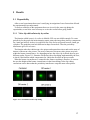
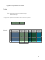
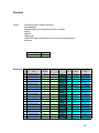
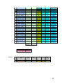
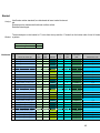
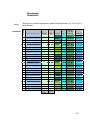
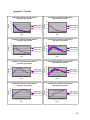
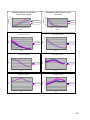
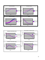
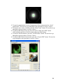
1
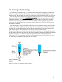
School of Innovation, Design and Engineering
BACHELOR THESIS IN
AERONAUTICAL ENGINEERING
15 CREDITS, BASIC LEVEL 300
DLE burner water rig
simulations
Authors: Peyman Mohammadi and Anders Arato
Report code: MDH.IDT.FLYG.0187.2008.GN300.15HP.E
Abstract
In today’s industrial world, there are high demands on the environmental aspects.
Siemens Industrial Turbomachinery AB (SIT AB) is a company that is keen about the
environment, and therefore spends a lot of effort in developing combustion processes in order
to reduce NOx (nitrogen oxides) emissions on their engine products. They are also researching
in optional fuels, which are more environment-friendly.
In order to provide lower emissions the SIT designed a water rig to study the flow dynamics
in a DLE (Dry Low Emission) burner.
An analyze program (GUI horizontal) was developed with new functions and the existing
functions were improved. The program’s function was to evaluate different experimental tests
of the flow dynamics in the 3rd generation DLE burners, of the SGT-800 gas turbine engine.
The aim was to ensure repeatability to enhance reliability, of the experimental test results for
further comparison, for upcoming projects concerning future DLE burners.
When repeatability was achieved, implementations of different geometrical modifications
were performed in the 3rd generation DLE burner.
The reason of the geometrical alterations was to look over if better fuel air mixture could be
obtained and accordingly (thus) to reduce hotspots in the burner and in that case reduce NOx
emissions.
II
Sammanfattning
I dagens industriella värld är kraven höga ur miljöperspektiv. Siemens Industrial
Turbomachinery AB (SIT AB) är ett företag som är väldigt mån om en god miljö och lägger
stor möda på att utveckla förbränningsprocesser i sina motorer, som i sin tur reducerar
NOx-utsläppen (kväveoxider). De forskar också mycket i alternativa bränslen, vilket är mer
miljövänligt.
I avsikt att minska emissioner konstruerade SIT en vattenrigg för att studera dynamiken på
flödet i en DLE-brännare (Dry Low Emission).
Ett analysprogram skapades för att utvärdera olika experimentella tester av flödesdynamiken
i en 3rd generation DLE-brännare, tillhörande gasturbinen SGT-800.
Målet med examensarbetet var att säkerställa repeterbarheten och därmed tillförlitligheten av
de experimentella testresultaten för fortsatt arbete, i framtida projekt kring DLE-brännare.
När repeterbarheten uppnåddes, utfördes olika geometriska ändringar i DLE-brännaren.
Detta gjordes avsiktligt, för att se om bättre bränsleluftblandning kunde uppnås för att reducera
hotspots (områden med hög koncentration av bränsle i brännaren) och därmed NOx-emissioner.
III
Abbreviations
DLE –
NOx –
SIT
–
Re
–
PLC –
GUI –
SGT –
PPM –
PDF –
MatLab –
Fps
–
Dry Low Emissions
Nitrogen Oxides
Siemens Industrial Turbo machinery
Reynolds Number
Pressure Loss Coefficient
Graphic User Interface
Siemens Gas Turbine
Parts per million
Probability Density Function
Matrix Laboratory
Frames per second
IV
1 Aim ....................................................................................1 2 Apparatus ..........................................................................2 3 Background........................................................................3 3.1 Siemens Industrial Turbomachinery AB ............................................................3 3.2 SGT-800 engine ....................................................................................................3 3.3 3rd generation DLE burner ...................................................................................4 4 Method...............................................................................6 4.1 Development of evaluation strategy ...................................................................6 4.1.1 Post processing tool – MatLab............................................................... 6 4.1.2 Test evaluation / repeatability................................................................ 6 4.1.3 DLE plastic burner experiments with geometrical alterations.................... 6 4.2 Water rig evaluation strategy...............................................................................7 4.3 Plastic burner .........................................................................................................8 4.4 Risk identification and user manual....................................................................8 4.5 Argon laser .............................................................................................................9 4.6 Tracer ....................................................................................................................10 4.7 Video capture and collection device.................................................................10 4.8 Pump .....................................................................................................................11 4.9 Calibration ............................................................................................................11 4.10 Scaling.................................................................................................................12 4.11 MatLab ................................................................................................................12 4.12 The Graphical User Interface ..........................................................................12 4.13 Mean intensity imaging.....................................................................................13 4.14 PDF......................................................................................................................13 4.15 Single pixel PDF ................................................................................................13 4.16 All pixel PDF.......................................................................................................15 4.17 3D PDF/radius ...................................................................................................15 4.18 Masscenter .........................................................................................................16 5 Results..............................................................................17 5.1 Repeatability ........................................................................................................17 5.1.1 Video clip edition/Intensity by radius ................................................... 17 5.1.2 Center search..................................................................................... 19 5.1.3 Quantity of frames ............................................................................. 19 5.1.4 Fuel flow........................................................................................... 20 5.1.5 Camera settings ................................................................................. 20 5.2 GUI vertical...........................................................................................................21 5.3 Geometrical alterations ......................................................................................22 5.3.1 Obstacle plate .................................................................................... 22 5.3.2 Obstacle cylinder ............................................................................... 23 5.3.3 Basket............................................................................................... 24 5.3.4 C-stage ............................................................................................. 26 5.3.5 Blocked film air holes ........................................................................ 27 6 Summary/Conclusions ......................................................29 7 Recommendations/Future work........................................30 V
Sources ..................................................................................31 Appendix..............................................................................32 Appendix 1: Risk identification .................................................................................32 Appendix 2: Instruktioner för handhavande av vattenrigg ...................................33 Appendix 3: Flow Sheet ............................................................................................35 Appendix 4: Scaling ...................................................................................................36 Appendix 5: Formulas................................................................................................37 Appendix 6: Experimental test schedule ................................................................38 Appendix 7: Results ...................................................................................................45 Appendix 8: User friendly manual MatLab .............................................................55 Figure 3.1.1: The water rig at SIT AB (fluid dynamics laboratory) .......................................2 Figure 3.2.1: SGT-800 engine...........................................................................................3 Figure 3.3.1: 3rd generation DLE burner............................................................................4 Figure 3.3.2: 3rd generation DLE burner............................................................................5 Figure 3.3.3: SGT-800 combustion chamber ......................................................................5 Figure 4.2.1: Water rig, combustion chamber replica...........................................................7 Figure 4.3.1: Plastic burner...............................................................................................8 Figure 4.5.1: Argon Laser.................................................................................................9 Figure 4.6.1: Fluorescein sodium salt...............................................................................10 Figure 4.7.1: Toshiba JK-L75M industrial probing camera ................................................11 Figure 4.9.1: Calculations of MASS2100 DI 6 sensor........................................................11 Figure 4.12.1: Graphic user interface window...................................................................12 Figure 4.15.1: Frame one of the movie sequence identifying one pixel ................................14 Figure 4.15.2: The intensity change per frame for one pixel ...............................................14 Figure 4.15.3: An example of how a single pixel PDF may look like...................................14 Figure 4.16.1: An example of how the user should click on the mean value picture ..............15 Figure 4.16.2: Probability Density Function for the entire radial fuel distribution (logarithmic
scale) ...........................................................................................................................15 Figure 4.17.1: An example of how a 3D PDF could look like .............................................16 Figure 4.18.1: Mass center evaluation..............................................................................16 Figure 5.1.1: Four different video clip editing..................................................................17 Figure 5.1.2: Same video clip editing with border adjustment add-in to avoid dislocation of the
burner centre.................................................................................................................18 Figure 5.1.3: Comparison of the results for the border adjustment add-in.............................18 Figure 5.1.4: Significant improvement of the repeatability due to video clip edition .............19 Figure 5.1.5: Center search performed by five users ..........................................................19 Figure 5.1.6: 25 seconds seems sufficient to obtain reliable results .....................................20 Figure 5.1.7: The shape is similar and the intensity level almost linear to the fuel mass flow .20 Figure 5.1.8: Effect of inconsistency in camera settings on the results. ................................21 Figure 5.2.1: Mean Intensity picture of the vertical application (left) and with contour add-on
(right)...........................................................................................................................21 Figure 5.3.1: The L-shaped obstacle plate ........................................................................22 VI
Figure 5.3.2: Comparison in radial fuel distribution between standard application and obstacle
plate.............................................................................................................................22 Figure 5.3.3: Comparison in PDF statistics between standard application and obstacle plate..22 Figure 5.3.4: Mass center comparison between standard (left) and obstacle plate (right) .......23 Figure 5.3.5: Obstacle cylinder .......................................................................................23 Figure 5.3.6: Comparison in radial fuel distribution between standard application and obstacle
cylinder ........................................................................................................................23 Figure 5.3.7: Comparison in PDF statistics.......................................................................24 Figure 5.3.8: Mass center comparison between standard (left) and obstacle cylinder (right)...24 Figure 5.3.9: The designed basket for the plastic burner.....................................................25 Figure 5.3.10: Similar profile for basket and standard........................................................25 Figure 5.3.11: The PDF shows that basket causes slightly less mixed areas..........................25 Figure 5.3.12: Mass center comparison between standard (left) and basket (right) ................26 Figure 5.3.13: Mass center comparison between standard (left) and basket blocked downstream
(right)...........................................................................................................................26 Figure 5.3.14: Mass center comparison between standard (left) and basket blocked upstream
(right)...........................................................................................................................26 Figure 5.3.15: C-stage fuel inlet positions ........................................................................27 Figure 5.3.16: PDF graph for C-stage ..............................................................................27 Figure 5.3.17: Blocked film air holes...............................................................................28 Figure 5.3.18: Comparison between blocked film air holes and standard .............................28 Figure 5.3.19: Summary of mass center rotation for geometrical alternations .......................28 VII
1 Aim
The purpose of the graduate project was to implement water rig testing of gas turbine burners
in order to study their flow dynamics. The results will be useful for comparison of flow
dynamics and fuel concentration between individual burners.
Water rig test procedure development to secure reliability of the water rig tests by:
Making improvements of the post processing tool in the MatLab program and to find a way
to secure repeatability of the experimental test results.
Evaluation and recommendations are also vital information for the rig improvements for
future experimental testing.
Research and find a substitute for the corresponding laser or a fluorescent tracer that is
suitable for the present laser.
Evaluate the burner performance, and study the results that geometrical
modifications/alterations may generate on the air fuel mixture, regarding:
Radial fuel distribution
Expansion shape
Flow rotation
Probability density function statistics
1
2 Apparatus
Water flow rig
2 water systems, one for air and one for fuel simulation
Argon laser ~450nm , 750mW
Toshiba JK-L75M video device camera (25fps)
D/A Video converter and a video clip editing software
PC
Fluorescein sodium salt 100ppm
MASS2100 DI 6 – mass flow measurement equipment
Figure 3.1.1: The water rig at SIT AB (fluid dynamics laboratory)
2
3 Background
3.1 Siemens Industrial Turbomachinery AB
In today’s industrial world, there are high demands on the environmental aspects.
This is something that every company has to contribute to and Siemens Industrial
Turbomachinery AB is no exception.
SIT AB is a company that is keen about the environment, and therefore spends a lot of effort
in developing combustion processes in order to reduce NOx emissions on their engine products.
They are also researching in optional fuels, which are more environment-friendly.
3.2 SGT-800 engine
The SGT-800 engine (Figure 3.2.1) was developed under the late 90’s for industrial
applications such as generate electricity, heat, propulsion and for marine purposes. It has been
a very successful and popular engine among many companies worldwide due to the good
attributes that it has. The SGT-800 has an electric power output of 45 MW and an efficiency of
37% in simple cycle. The main purpose is to use this engine in combined cycle which means
that the engines exhaust gas goes into a heat recovery steam generator for maximum efficiency
and minimal heat losses.
Figure 3.2.1: SGT-800 engine
3
3.3 3rd generation DLE burner
Due to the complex geometry of the DLE burner many parts are manufactured manually.
This implicate that the burners don’t have identical geometry and dimensions.
This can cause for example that one burner can have different NOx emissions than the other
and this can result in different NOx emissions between individual gas turbines.
Generally a swirl burner (Figure 3.3.1) injects fuel axially into airflow with a certain
tangential momentum. This contributes mainly to a more efficient air-fuel mixture and
therefore a better combustion process.
Together with the usually divergent geometry of the burner mouth it also creates
recirculation zones at the burner outlet which traps hot combustion products, that stabilizes the
flame and also acts as a permanent ignition source.
Figure 3.3.1: 3rd generation DLE burner
The 3rd generation low emission burner is an important part of the low NOx combustion
process.
1. Low NOx values are achieved when good fuel air mixture is obtained.
2. When the fuel burns at low temperatures.
A negative attribute with the low NOx emission process is the impairment of the flame
stability and combustion.
Insufficient stability in the combustion process can cause flame pulsation and vibrations that
can transmit between burners due to the acoustic nodes in the flow system that communicates
with the unstable flame.
In the middle of the space cap the lance is positioned. The main function of the lance is to
regulate the engine by changing its length and anchoring the main flame to prevent it from
pulsations. The space cap consists of four fuel injection holes (A, B, C and D see Figure 3.3.2).
The space cap provides a touch of compressed air mixed with injected fuel into the swirl cone.
4
The Swirl cone has four fuel injection cylinders. Each cylinder has 9 injection holes, with
hole 0 proximate to the space cap and hole 8 proximate to the mixing tube. The main function
of the swirl cone is to blend the compressed air with the injected fuel from the lance, space cap
and the main gas cylinders. The swirl cone is very important at the burner inlet, since it
provides the most of the air-fuel mixture as earlier mentioned.
The mixing tubes purpose is to mix all of the injected fuel with compressed air as evenly as
possible. The mixing tube also adds a slight of compressed air through the film air holes that is
positioned around it. The extra added air is to prevent the mixing tube wall from the possibility
of flame propagation backwards (flash back) along the boundary layer where the velocity is
small.
At the burner outlet the ignition of the fuel air mixture takes place and then leads to the
combustion chamber. The burner outlet is mounted to the wall that separates the compressed
air from the combustion chamber (Figure 3.3.3). The pilot holes are positioned at the burner
outlet. The pilot holes are able to inject oil as well as gas. The purpose of the pilot holes is to
add a small amount of fuel in order to retain the stability of the main flame which will result in
greater stability in the combustion chamber. The pilot influence the NOx values in a negative
way due to added unmixed fuel which contributes to higher local flame temperature.
As a result of the locally higher flame temperature the pilot holes influence the NOx values in a
negative way.
Figure 3.3.2: 3rd generation DLE burner
Figure 3.3.3: SGT-800 combustion chamber
5
4 Method
4.1 Development of evaluation strategy
4.1.1 Post processing tool – MatLab
To investigate the mixture of instant data, PDF statistics of transient fuel
concentration had to be evaluated.
Automatic search of burner circumference and burner radius in movies was
essential in order to calculate the geometry.
In order to estimate swirl, the mass center of the injected fuel into the burner has to
be calculated.
Highlight contours of the expansion shape in MatLab vertical application in order to
ease visual analyze for the user.
Secure reliability of the experimental tests by using movies.
• How long movie is required to obtain averages of sufficient accuracy?
(averages/PDF)
Evaluate statistical accuracy
• How much may the result differ if the same experiment is repeated?
(averages/PDF)
4.1.2 Test evaluation / repeatability
Research in movie-lengths. Decide the quantity of frames which is required to
obtain a secure reliability.
Determine the magnitude of fuel flow variations that may influence on the test
results.
Video clip editing. Verify the importance of the burner circumference position in
the frame.
Decide if camera settings (aperture, focus) may affect the results.
4.1.3 DLE plastic burner experiments with geometrical alterations
The purpose of all geometrical modifications was to investigate if better fuel air mixture
could be gained to reduce the NOx emissions. The different geometrical modification that has
to be implemented is the following:
Obstacle plate
Obstacle cylinder
Basket
Blocked film air holes
C-stage
6
4.2 Water rig evaluation strategy
To study the flow dynamics in a 3rd generation DLE burner and consequently evaluate why
differences in NOx is obtained from burners in the same configuration SIT designed a water
burner test rig. The advantage of a water rig is that tests can be performed with a very low cost.
The water rig at SIT replicates one real burner segment (Figure 4.2.1) of SGT 800 with the
dimensions of the outer hull 580x660x2250 mm, to get the same flow geometry as a real SIT
combustion chamber. The rig has two visualization windows and it’s made of 20 mm thick
Plexiglas. The water rig is constructed with water drainage at the top and the only way the
water can exit is through the inner test section with the dimensions 270x240x700 mm where
the burner is mounted.
The water rig has a capacity to handle a mass flow of 8 kg/s but the existing water flow that
simulates the air flow supplies maximum 3 kg/s. The water rig has two water inputs, one that
simulates the air entering the burner and one that is representing the fuel using water mixed
with fluorescent dye. The simulation of air enters the water rig at the bottom.
The pre mixed fluorescent dye is stored in a tank close to the water rig. A pump then provides
the fuel water to the water rig where the fuel allocate through a apportion cylinder to the burner
fuel hole that is in use. To be able to perform experimental tests, in the fluid dynamics
laboratory at SIT, it was necessary to make a risk identification and a flowchart for the water
rig. Later on a user manual for the water rig was created.
Figure 4.2.1: Water rig, combustion chamber replica
7
4.3 Plastic burner
The plastic burner at SIT is a model of a real DLE burner shown in Figure 4.3.1.SIT designed
the burner because they were interested to evaluate the flow field in the mixing tube.
The benefit of the opaque plastic burner is that it is possible to analyze the radial distribution of
the air fuel mixing in different sheets in the burner. The experiments were filmed horizontally
at the burner outlet and 90 mm down in the mixing tube. The plastic burner had only two
functional main gas cylinders in comparison to the real one that has four. In a real burner it is
only possible to analyze the radial distribution at the burner outlet as the burner is made of
steel. The swirl cone has as earlier mentioned four main gas cylinders. In order to study the
downstream fuel distribution that originates from each individual fuel nozzle. The fuel was
injected from one nozzle at a time. This significant procedure increases the knowledge of the
contribution of each nozzle to the total fuel distribution. However there are uncertainties in
studying the total fuel distribution using the plastic burner. If the sum of the distribution from
all individual holes is used, the error due to background light is multiplied.
If the total fuel distribution is measured, there are uncertainties of the mass flow through each
nozzle, since only the total fuel mass flow is measured.
Figure 4.3.1: Plastic burner
4.4 Risk identification and user manual
The purpose of risk identification was to eliminate and decrease the risks that could occur in
the water rig and around the rig during normal operations. The complete sheet can be found in
Appendix 1. Also a user manual was created to ensure safe operation of the water rig
(Appendix 2).
8
4.5 Argon laser
The fluid dynamics laboratory at SIT uses an argon laser (Figure 4.5.1) of 750 mW power
and a wavelength of 450 nm. The laser is used to visualize the air fuel mixture in the burner.
The laser is a class four laser and therefore one of the most powerful and dangerous lasers on
the market. The laser may damage the eyes immediately. The areas of interest was to film a
thin sheet in order to get a two dimensional environment which could be evaluated by the
MatLab program. The laser beam was positioned in two directions:
1) Horizontally when filming the radial distribution of the fuel in the mixing tube or at the
burner outlet.
2) Vertically positioned when filming the flow expansion at the burner outlet.
Figure 4.5.1: Argon Laser
9
4.6 Tracer
Fluorescent dye can be used to visualize the fluid dynamics of the particles. For example it
can be used to see the fuel air distribution in a DLE burner. A fluorescent dye that was suitable
for the argon laser (450 nm) is the Fluorescein sodium salt (C20H10Na2O5). It is an orange
powder and when it’s mixed with water it turns green (Figure 4.6.1). The mixing concentration
of the dye is 0.1 grams per 10 liters (100ppm) of water. The MatLab post processing tool as
earlier mentioned requires that the green particles have great contrast to be able to visualize the
pixels. The test section in the water rig had to be jet black to reduce the background noise and
to highlight the colors of the pixels.
Figure 4.6.1: Fluorescein sodium salt
4.7 Video capture and collection device
The camera that was used was a very sensitive powerful Toshiba JK-L75M industrial
probing camera set on a shutter speed of 25 fps (Figure 4.7.1) with a D/A Video converter.
The video clip editing software that was used to capture and store the movies called Adobe
premiere 6 with an add-on called Pinnacle studio 10. The movies were edited in Adobe
premiere 6 and it was necessary to set the properties so MatLab could read the movies. It is
very important that the user clips the area of interest of the video clip and excludes unnecessary
data since MatLab takes long time to process a large video clip. The recommended frame
resolution is 300x300 pixels. The horizontal (radial fuel distribution) experiments that was
captured and analyzed was the comparison between the left (‘V’ for left in video clip name)
and the right (‘H’ for right in video clip name) main gas cylinder. The obstacle plate, the
obstacle cylinder and the blocked film air holes were all individually compared to the standard
application using their respective gas holes. The C-stage positions were compared to the
nearest gas hole on the standard application. The vertical experiments were captured at the
burner outlet to analyze the expansion shape of the “flame”. The gas holes that were in use
during the vertical experiments were gas holes number 0 from respective gas cylinder at the
same time. The file naming system is named after <laser sheet position>, <main gas cylinder>
and <gas hole number>.
10
The translation of the video clip names is for example: H90H5_standard.avi which signifies
horizontal laser sheet, 90 mm down in the mixing tube, hole number 5 on the right main gas
cylinder and standard application.
Figure 4.7.1: Toshiba JK-L75M industrial probing camera
4.8 Pump
A relatively large electric pump was used for the fuel simulation and because of the usage of
small doses of fluorescent tracer the flow stability decreased.
With higher fuel mass flow the accuracy of the mass flow measurements were increased.
4.9 Calibration
Due to very low mass flow for the fuel simulation it was necessary to use a very sensitive
mass flow sensor. A frequent calibration was essential due to flow indicators carioles to get
reliable and sufficient test results. The mass flow indicator has an accuracy of ±0,014 g/s as
calculated in Figure 4.9.1.
Figure 4.9.1: Calculations of MASS2100 DI 6 sensor
11
4.10 Scaling
The purpose of scaling was to get comparable test result with other methods that were used in
the burner development.
The physical properties for a real burner under real engine operations had to be scaled down.
One SGT 800 burner consumes approximately 3 kg/s of air and this corresponds to 100
kg/s of water at equal Reynolds number. The Reynolds number was calculated to be
approximately 9038 in the water rig using a water flow of 3 kg/s while in a real SGT-800 it is
452000. It is a big difference (around a factor 50) in Reynolds number but sufficient enough to
have turbulent flow in the water rig. For the complete spread sheet see appendix 4.
4.11 MatLab
The MatLab program that was used was 7.3.0.267(R2006b) with a picture analysis add-on
called image post processing tool. Without this toolbox it would not be possible to analyze
movies since MatLab in its basic form is not capable to do so. MatLab use RGB system to
restore analyses of a picture. MatLab loads the movie and converts it into frames. This
implicate that one picture or one frame from a recorded movie stores in three matrices, that is
red, green and blue matrices and they have exact the same dimensions as the picture. The
matrices consist of property information of the picture and by that the intensity values of each
pixel is stored. The intensity of each pixel is described numerical between 0 and 255, where
255 is the maximum intensity. Each intensity value has a coordinate (position) in the matrices.
4.12 The Graphical User Interface
MatLab has a user friendly GUI (Graphical User Interface) shown in Figure 4.12.1, which
allows the user in a simple way to program scripts linked to functions that applies a standard
call back syntax. The good thing about the GUI is its simplicity therefore with a little effort the
user can have total control.
Figure 4.12.1: Graphic user interface window
12
4.13 Mean intensity imaging
The existing function in MatLab post processing tool called mean intensity function
calculates the mean intensity of each pixel in the entire movie sequence. Further to this, it
displays how the fuel concentration is distributed as a mean value picture of the video clip. The
script summarizes the intensity values of a specific pixel from the green matrix frame by frame
and then divides it with number of frames that the movie contains, and afterwards takes on the
next pixel for calculation and so on. All the mean pixel values are stored in a parallel created
matrix which eventually turns into a mean value picture for the entire movie. Both GUI’s use
this calculation script for the mean value evaluation.
4.14 PDF
The definition of the Probability Density Function is: “In mathematics, a probability density
function (pdf) is a function that represents a probability distribution in terms of integrals.
Formally, a probability distribution has density f if f is a non-negative Lebesgue-integrable
function
such that the probability of the interval [a, b] is given by
for any two numbers a and b. This implies that the total integral of f must be 1. Conversely,
any non-negative Lebesgue-integrable function with total integral 1 is the probability density
of a suitably defined probability distribution.
Intuitively, if a probability distribution has density f(x), then the infinitesimal interval
[x, x + dx] has probability f(x) dx. Informally, a probability density function can be seen as a
"smoothed out" version of a histogram: if one empirically samples enough values of a
continuous random variable, producing a histogram depicting relative frequencies of output
ranges, then this histogram will resemble the random variable's probability density, assuming
that the output ranges are sufficiently narrow.” 1
It is used for this project to allow the division of the area into a number of intervals.
This PDF statistics tool was to be implemented in the MatLab post processing tool.
4.15 Single pixel PDF
This function allows the user to select a point, for example where the greatest fluctuation is
situated. Subsequently the function use the chosen pixel (Figure 4.15.1), and examines the
intensity changes throughout the entire movie sequence, see Figure 4.15.2. The black line
displays the intensity change per frame and the red line shows the mean value of the intensity
throughout the whole movie. The green line indicates the mean value change per frame which
in technical term is called the dynamic mean value. Since 250 frames are used for the mean
value, the dynamic mean value is invariant with time at this number of frames. However, the
small variation in dynamic mean value indicates that 250 frames are sufficient for mean
averages.
1
http://en.wikipedia.org
13
Figure 4.15.1: Frame one of the movie sequence identifying one pixel
Single pixel PDF function was created to evaluate how long movie that is required to get
sufficient and reliable analyses (results) in MatLab.
Figure 4.15.2: The intensity change per frame for one pixel
The PDF function, seen in Figure 4.15.3, shows how many times the pixel has a certain
intensity through the entire movie sequence. The x –axis shows the intensity and the y-axis
shows number of times it hits certain intensity. The blue curve is the PDF for one pixel and the
green curve is the ideal PDF with same mean value but less high intensity hits, i.e. less spots of
high “fuel content. The oval circle indicates that there are high intensity values for this certain
pixel.
Figure 4.15.3: An example of how a single pixel PDF may look like
14
4.16 All pixel PDF
To investigate the quality of fuel air mixing in the burner and locate hot spots a function was
created to detect the fuel distribution over the entire flow field. To evaluate the areas of interest
the user has to click on three points as shown in Figure 4.16.1 nearby the burner circumference
on the mean value picture to calculate the radius and the center point of the burner. The
function investigates the intensity changes for all pixels within the radius (measured in pixel)
of the burner and then plots a curve as shown in Figure 4.16.2. The amplitude of the curve
suggests the amount of hot spots in the burner. Hot spots can occur if the fuel has less blended
zones (more high intensity points) which may increase NOx emissions.
Figure 4.16.1: An example of how the user should click on the mean value picture
Figure 4.16.2: Probability Density Function for the entire radial fuel distribution (logarithmic scale)
4.17 3D PDF/radius
To investigate the quality of fuel air mixing in the DLE burner the need for a function that
could locate unmixed areas arose. The only difference between this function and all pixel PDF
as earlier mentioned is that this function checks intensity changes for all pixels within a certain
radius interval through the whole movie sequence and then plots a 3D curve (Figure 4.17.1) for
every radius interval. The user has to go through the same procedure to find the radius of the
burner as earlier described. Any peaks that descend and rise in the 3D graph can indicate that
there is poor fuel air distribution that can result in hotspots in the DLE burner, causing
increased NOx emissions.
15
Figure 4.17.1: An example of how a 3D PDF could look like
4.18 Masscenter
The main function of the swirl cone is to define the flow rotation and initiate the fuel-air
mixing.
The center of mass is a function of the positions and masses of the particles that is included
in the system. In MatLab the mass correspond to pixel location and the amount of mass
corresponds to the intensity values of each pixel.
A function was created to evaluate how much the fuel mass center rotates between filming of
different sheets and geometrical alterations in the plastic burner or at the outlet on a real
burner. The function locates the mass center (Figure 4.18.1) of the fuel and an angle on the
mean value picture. With the information of the mass center angle and the fuel injected angle
swirl numbers can be estimated. The formulas that were in use can be found in Appendix 5.
For example it’s possible to evaluate the differences between different burners to look over
how much manufacturing variations deviate.
Figure 4.18.1: Mass center evaluation
16
5 Results
5.1 Repeatability
After several experiments that weren’t satisfying, investigation of error factors that affected
the experimental test results started.
To analyze reliability of the equipments that were in use for the water rig during the
experiments, several tests were necessary to review the results before going further.
5.1.1 Video clip edition/Intensity by radius
The function called intensity by radius in MatLab GUI was not reliable enough. To create
periodicity for the graph, the mean intensity matrix rotates the image three times to compensate
for 4 main gas holes to see how it would look like if the fuel was injected from all 4 main gas
cylinders. The graph does not look different in shape for one hole. Thus the periodicity
interference gives a level curve.
The function takes the whole mean value picture and rotates three times and not the areas of
interest of the mean value picture. The areas of interest of the mean value picture are pixels
within the burner circumference. So, depending on how the video clip is edited, the user gets
different results. Figure5.1.1 illustrates 4 different video clip editing implemented by the user,
to check if the function which compensates for 4 holes has an effect on the test results.
When the burner circumference is centered in the frame everything is flawless. As soon as
the user has displaced the burner circumference in the frame during video clip editing
conclusions can be drawn that the periodicity interference warps the mean value picture.
Figure 5.1.1: Four different video clip editing
17
Improvement of the function was necessary to obtain reliable results. Changes have been
done and now the function takes only the areas of interest of the mean value picture and then
performs the periodicity interference i.e. the mean intensity matrix is rotated around the burner
center instead of the video clip center. Figure 5.1.2 shows a comparison with the same video
clip editing between the previous function and the improved function. Figure 5.1.3 shows a
comparison of the differences in radial distribution graphs between the previous function and
the improved function.
Figure 5.1.2: Same video clip editing with border adjustment add-in to avoid dislocation of the burner
centre
Figure 5.1.3: Comparison of the results for the border adjustment add-in
18
Figure 5.1.4 illustrates a comparison of all four video clips editing with the previous function
and the new improved function.
Figure 5.1.4: Significant improvement of the repeatability due to video clip edition
5.1.2 Center search
An additional research of the center search function was performed to look over the
reliability of the manual location of the burner circumference executed by the user.
This was considered primarily that various users could cause various errors. Figure 5.1.5
demonstrates the level of influence can be disregarded when five different users performing the
center search on the same video clip.
Figure 5.1.5: Center search performed by five users
5.1.3 Quantity of frames
To improve the quality and to achieve repeatability several tests were made on three different
movie lengths: 10, 25 and 100 seconds. (25 fps)
Figure 6.1.6 shows the movie length results from main gas hole nr 3. The graph shows clear
improvement with 25 seconds or longer but regarding time and cost the amount of frames
corresponding to the sequence length of 25 seconds was considered sufficient. The 100 second
movie was also analyzed in four equal parts and compared to the full clip to investigate if any
changes occurred during the sequence.
19
Figure 5.1.6: 25 seconds seems sufficient to obtain reliable results
5.1.4 Fuel flow
Several tests with various fuel flows were performed and analyzed in the MatLab program.
The standard amount of fuel entering the main gas hole number 3 is 2g/s. The range for the
fuel simulation was set from 1.2 g/s-2.8 g/s. The effect of these deviations can be observed in
Figure 5.1.7. The shape of the fuel distribution curves are almost identical however as expected
the intensity levels are almost linear to the flow.
Figure 5.1.7: The shape is similar and the intensity level almost linear to the fuel mass flow
5.1.5 Camera settings
As earlier mentioned the camera was very light sensitive equipped with focus and aperture
set manually by the user. The main purpose of the experiment was to examine the change in
error factor when the camera settings were modified and then turned back to their original
settings and position to simulate different test occasions.
20
Figure 5.1.8 shows that major error factor was discovered during these studies since the
brightness of each pixel changes in the MatLab post processing tool.
To avoid and eliminate this error factor the user had to apply the same settings for all the
experimental tests so comparable test results could be achieved. It was necessary to adjust the
camera settings once and use exactly equal settings for upcoming experiments.
Figure 5.1.8: Effect of inconsistency in camera settings on the results.
5.2 GUI vertical
GUI Vertical is similar to GUI Horizontal but it analyzes the expansion form of the fuel
exiting at the burner outlet. Therefore the laser sheet is positioned vertically when filming.
The expansion of the fuel is very important to analyze. By filming the expansion of the fuel
at the burner outlet the user can see where the recirculation zones (created by vortices) are
located (Figure 5.2.1). By knowing the recirculation zones and the angle of the expansion
conclusions can be drawn if the stagnation point of the flame is positioned upstream or
downstream the burner outlet. For an upstream positioned flame, the larger risks there is to get
flashback. Flashback is a phenomenon that forces the flame down the burner outlet and it could
rapidly destroy the burner outlet.
The mean calculation function evaluates the mean intensity of each pixel through the entire
movie sequence. The function searches for the contrast to find the edges of the expansion
shape and therefore it is very sensitive to camera disturbance. The analyze function evaluates
the expansion angles of the fuel by using a MatLab function called “max”.
The user has to click at the most vivid point on the mean value picture to allow MatLab to find
the largest number in an array i.e. columns. MatLab then plots all the coordinates of its largest
number as the pixel that was chosen initially by the user. If there is more than one pixel in
the current column that has the same maximum, all points will be plotted to avoid loss
of data. Due to camera disturbance as earlier mentioned the function did not work properly
therefore a plot contour (Figure 5.2.1) of the mean value picture was required so the user could
easily visualize the expansion angles of the fuel. The red color shows that there are high
intensity (more fuel) values in the middle of the expansion.
Figure 5.2.1: Mean Intensity picture of the vertical application (left) and with contour add-on (right)
21
5.3 Geometrical alterations
5.3.1 Obstacle plate
Based on CFD calculations an L-shaped plate with the surface 3x3 mm was manufactured.
The main purpose of the experiment was to create local increased turbulence to investigate if
better fuel air distribution could be achieved when the L-shaped plate was fastened right in
front of the main fuel holes (Figure 5.3.1). On the fuel distribution graph, illustrated in
Figure 5.3.2, the mean value of the obstacle plate increases but the shape is similar to the
standard application. The PDF graph (Figure 5.3.3) shows that less blended zones (more high
intensity points) are achieved with the obstacle plate which may be due to of the higher mean
value in comparison to the standard application.
The obstacles are reducing the slot area which results in a higher swirl as seen in Figure 5.3.4.
Figure 5.3.1: The L-shaped obstacle plate
Figure 5.3.2: Comparison in radial fuel distribution between standard application and obstacle plate
PDF Standard vs Obstacle plate
10000000
1000000
H90H5-standard
H90H5-obstacle plate
Number
100000
10000
1000
100
10
1
1
3
5
7
9 11 13 15 17 19 21 23 25
Intensity
Figure 5.3.3: Comparison in PDF statistics between standard application and obstacle plate
22
Figure 5.3.4: Mass center comparison between standard (left) and obstacle plate (right)
5.3.2 Obstacle cylinder
A 2mm in diameter steel wire was mounted on the main fuel cylinder in front of the main
fuel holes (Figure 5.3.5) to create local turbulence and to achieve better fuel air distribution.
On the fuel distribution graph as it can be seen in Figure 5.3.6 that the obstacle cylinder has an
identical profile to the standard application. The PDF graph (Figure 5.3.7) shows that more
effective air-fuel mixture can be achieved with less high intensity points compared to the
standard application. This type of obstacle also reduces the slot area and increases the swirl.
However, the swirl increases less than for obstacle plate (Figure 5.3.8).
Figure 5.3.5: Obstacle cylinder
intensity
Standard vs Obstacle cylinder
40
35
30
25
20
15
10
5
0
H90H5-standard
H90H5-Obstacle
cylinder
1 8 15 22 29 36 43 50 57 64 71 78 85
pixel
Figure 5.3.6: Comparison in radial fuel distribution between standard application and obstacle cylinder
23
PDF Standard vs Obstacle cylinder
10000000
1000000
Number
100000
H90H5-standard
10000
H90H5-obstacle cylinder
1000
100
10
1
1
3
5
7
9 11 13 15 17 19 21 23 25
Intensity
Figure 5.3.7: Comparison in PDF statistics
Figure 5.3.8: Mass center comparison between standard (left) and obstacle cylinder (right)
5.3.3 Basket
The purpose of the basket investigation was to evaluate how much the fuel distribution is
influenced. The smaller SGT-700 engine is equipped with burners with baskets. SIT’s usage of
the basket for the SGT-800 is only for test purposes. The main purpose of the basket is to
increase the pressure drop over the burner, which stabilizes the air flow through it and reduces
the risk of Low Frequency Pulsations (LFP). The basket also changes the inflow direction
through the “swirler” which influences the swirl and fuel distribution. Also the inflow
turbulence is affected, which influences the fuel mixing. The tests were performed in order to
quantify these effects.
There was no designed basket for the plastic burner. A design of a basket with 41 rows of
holes that had the exact accurate fitting as the plastic burner was made. Earlier tests have been
performed using blocked parts of the basket on the SGT-700 engine and simulated tests have
been performed in the water rig. The test categories included basket with 17rows blocked
upstream or downstream (Figure 5.3.9).
24
Figure 5.3.9: The designed basket for the plastic burner
The tests in the water rig was captured and evaluated in the MatLab program. From the fuel
distribution graph (Figure 5.3.10) similar profile for basket and standard is obtained. The PDF
(Figure 5.3.11) shows that the basket causes slightly less mixed areas which may be due to the
changed inflow turbulence. The mass center function revealed that the basket decreases the
swirl (Figure 5.3.12) and increases when the basket is being blocked upstream (Figure 5.3.13)
which verifies the basket influence on the swirl. Basket blocked downstream (Figure 5.3.14)
decreases the swirl more than for non-blocked basket.
Figure 5.3.10: Similar profile for basket and standard.
Figure 5.3.11: The PDF shows that basket causes slightly less mixed areas.
25
Figure 5.3.12: Mass center comparison between standard (left) and basket (right)
Figure 5.3.13: Mass center comparison between standard (left) and basket blocked downstream (right)
Figure 5.3.14: Mass center comparison between standard (left) and basket blocked upstream (right)
5.3.4 C-stage
The idea was to look over if better fuel air mixture could be obtained in order to inject fuel in
different positions near the burner. Fuel hoes were mounted in to the arranged basket holes
(Figure 5.3.15). The C-stage movies were later on analyzed and compared to the proximate
burner main gas holes from the standard application. The best achievement from this study was
position F and position G as shown in Figure 5.3.16.
26
Figure 5.3.15: C-stage fuel inlet positions
Figure 5.3.16: PDF graph for C-stage
5.3.5 Blocked film air holes
As earlier mentioned the 3rd generation DLE-burner is equipped with film air holes
positioned around the mixing tube. Its main purpose is to make sure there is no fuel along the
wall and to minimize the risk of flashback that could occur at the wall.
The experimental tests were performed to see if blocking all or some of the air holes had any
impact on the radial fuel distribution.
Tests were conducted by blocking the two downstream rows, the two upstream rows and all of
the film air holes on the mixing tube (Figure 5.3.17). The conclusions of the analysis from this
experiment were:
1. The radial profiles seem to be moving outwards with blocked film air
holes.
2. By blocking all the holes the PDF curve is similar to the standard, but
the mean values are smaller.
3. Blocking upstream or downstream film air holes causes less mixed
areas.
The mass center analysis indicated that blocking the upstream film air holes increases the swirl
while blocking downstream and blocking downstream-upstream do not (Figure 5.3.18).
27
Figure 5.3.17: Blocked film air holes
Figure 5.3.18: Comparison between blocked film air holes and standard
Figure 5.3.19 shows a summary of mass center rotation for the different geometrical alterations.
It shows that the obstacle plate causes the largest swirl increase and basket blocked downstream causes the
largest decrease in swirl.
Figure 5.3.19: Summary of mass center rotation for geometrical alternations
28
6 Summary/Conclusions
Repeatability analysis
The MatLab post processing tool with its functions is a very useful aid when test repeatability
is secured. Several different error factors were investigated and eliminated in this project
regarding movie length, camera settings, clip editing, burner center search and fuel flow.
The length of the movie clips should be at least 25 seconds for the radial fuel distribution graph
and 100 second for the mass center evaluation. Identical laser, camera and rig settings with
strictly even fuel flow are absolutely essential for any comparison between tests performed at
different occasions.
The archived repeatability is now sufficient to detect flow changes due to geometrical
modifications (parameter study). Increased repeatability may be needed to detect differences
between similar burners. Some equipment requires improvements to analyze smaller
variations than performed in these parameter studies.
29
MatLab post processing tool
The existing MatLab post processing tool for concentration field measurements was further
enhanced and developed. Several PDF functions have been created for concentration field
measurements. A mass center function was added to investigate the fuel flow rotation. The
vertical expansion application was enhanced to simplify the evaluation for the user.
Geometrical alterations
As the overall goal was and still is to reduce exhaust NOx levels it was important to find ways
to obtain as even distribution of the fuel air mixture as possible. Several different geometrical
alternations on the burner were tested and analyzed. Among those modifications the obstacle
cylinder was the most promising and also relatively simple to manufacture and mount on real
burners.
The results from the basket application show that the air flow direction into the “swirler” has a
major importance for the swirl.
7 Recommendations/Future work
Water flow rig – already under construction:
Robust camera and laser mount with distinct positions to simplify for the user for
upcoming projects.
Drain hole enlargement so that emptying of water goes much faster. The now existing drain
hole for the water rig is too small and takes approximately 30 minutes to empty the water
flow rig.
Current water supply through the water rig is 3 kg/s. The water rig has a capacity to handle
mass flows around 8 kg/s of water. Increased main mass flow would obtain results closer to
reality.
Water flow rig
The valve for the fuel flow setting is very sensitive. Little changes by the user can cause
major oscillations of the fuel mass flow. The pump for delivering trace fluid is to powerful
and too big for this kind of experiments since very low mass flows are in use. Change the
current overpowered pump to a more appropriate one for example a highly mounted tank
which provides a small amount of fuel with help of the gravitation.
30
Camera with distinct aperture and focus so more repeatable studies can be obtained.
Light exclusion for the water rig to reduce the background noise and to highlight the
contrast of the pixels.
Replacement of laser optics to obtain an even laser sheet with no disturbance.
Plexiglas scratches have to be removed to avoid disturbance of the laser sheet. This
procedure will enable good movie quality and therefore increased reliability can be
achieved.
Test evaluation
The 3D PDF function requires a high performance computer to perform.
Burner performance simulations
The blocked film air holes effect on the swirl need to be further investigated.
Research of how to interpret the vertical averages with respect to the flow rotation.
Sources
1. Niklas Roos and Daniel Halling. Experimental evaluation of the flow in a
3rd generation dry low emissions burner for Siemens Industrial Turbo Machinery,
Finspong, 2006.
2. Private consultation with Daniel Lörstad, 2007.
3. Private consultation with Tomas Larsson, 2007.
4. CFD results from Daniel Lörstad, 2007.
Internet sites
http://www.powergeneration.siemens.com ,2007-06-13
31
Appendix
Appendix 1: Risk identification
32
Appendix 2: Instruktioner för handhavande av vattenrigg
1. Före/efter prov:
1.1 Vattensystem för ”bränsle” simulering
Kontrollera att
• ventilerna [AA001-AA008] är i stängt läge.
• ventilerna [AA001, AA002] eller [AA004, AA005] är i öppet läge 2 .
• pumpen [AP005] är strömlös.
1.2 Vattenriggen
Kontrollera att
• ventilerna [AA100-AA118] är i stängt läge.
1.3 Vattensystem för ”luft” simulering
Kontrollera att
• ventilerna [AA050,AA055,AA058,AA059,AA060, AA061] är i stängt läge.
2. Uppstart av vattenrigg:
2.1 Vattensystem för ”luft” simulering
Fyll vattenriggen genom att
• ställa ventilerna [AA050,AA059] i öppet läge.
• ställa ventilerna [AA055,AA058,AA060] i stängt läge.
• ställa tryckutjämningsventilen [AA061] i öppet läge.
2.2 Vattenriggen
Se punkt 1.2
2.3 Vattensystem för ”bränsle” simulering
Se punkt 1.1
2
Förhindrar att pumpen går torr vid oavsiktlig aktivering/strömsättning.
33
3. Under prov:
3.1 Vattensystem för ”luft” simulering
Kontrollera att
• ventilerna [AA050,AA059] är i öppet läge.
• ventilerna [AA055,AA058,AA060, AA061] är i stängt läge.
• Flödet indikeras på massflödes mätare [CF010].
3.2.1 Vattensystem för ”bränsle” simulering med kärl BB005
Kontrollera att
• ventilerna [AA001,AA002,AA008] är i öppet läge.
• ventilerna [AA003,A004,AA005,AA006,AA007] är i stängt läge.
• pumpen [AP005] är aktiverad.
• Alternera flödet efter behov med ventilerna [AA010 och/eller AA001].
• Flödet indikeras på massflödes mätare [CF005].
3.2.2 Vattensystem för ”bränsle” simulering med kärl BB010
Kontrollera att
• ventilerna [AA004,AA005,AA008] är i öppet läge.
• ventilerna [AA001,AA002,AA003,AA006,AA007] är i stängt läge.
• pumpen [AP005] är aktiverad.
• Alternera flödet efter behov med ventilerna [AA010 och/eller AA005].
• Flödet indikeras på massflödes mätare [CF005].
3.3 Vattenriggen
• Ventilernas [AA100-AA118] läge bestäms av provansvarig beroende på
ändamål.
4. Återställning av vattenrigg efter prov
4.1 Vattensystem för ”bränsle” simulering
Se punkt 1.1
4.2 Vattenriggen
Se punkt 1.2
4.3 Vattensystem för ”luft” simulering
• Kontrollera att ventilerna [AA050,AA055,AA059,AA060] är i stängt läge.
• Töm vattenriggen genom öppning av ventilen [AA058].
• För tryckutjämning skall ventilen [AA061] vara i öppet läge under tömning av
vattenriggen.
34
Appendix 3: Flow Sheet
35
Appendix 4: Scaling
36
Appendix 5: Formulas
1. Reynolds number Re =
ρ ⋅c ⋅l
μ
2. The mass flow formula is give by m& = ρ ⋅ c ⋅ A
3. Δp = PLC ⋅
ρ ⋅ c2
2
Pressure difference (PLC is the pressure loss coefficient)
4A
Hydraulic diameter
2(h + l )
ρ ⋅c ⋅ A
5. Momentum ratio = 1 1 1
ρ 2 ⋅ c2 ⋅ A2
4. Θ =
c= velocity
ρ = density
A = area
h = height
L, l = length
Sw = swirl number
6. Simplified velocity profiles
37
Appendix 6: Experimental test schedule
C-stage
Analys Jämföra PDF analys för att lokalisera hotspots.
Radiella fördelningen.
C-stage position 9 positions on the basket in front of one slit in 3x3 pattern
Horizontal
Check
Massflow "air"
Laser strength
Name of videoclip
Length of
clips
Nr of
clips
Section
C-stage
position
25
5
H90
1
25
5
H90
2
25
5
H90
3
25
5
H90
4
25
5
H90
5
25
5
H90
6
25
5
H90
7
25
5
H90
8
25
5
H90
9
Total nr of clips
45
Massflow
"fuel"
38
Standard
Analys
Jämförelse mellan vänster och höger
huvudgashålen.
Rotationsanalys mha masscenterfunktionen mellan
snitten.
Radiella
fördelningen.
Jämförelse mellan standardfilmer och filmerna med geometriska
ändringar.
Horizontal
3 kg/s
Max
Check
Massflow "air"
Laser strength
Name of video
clip
Length
of clip
Nr of clips
Section
Hole
nr
Hole
pos
Mass flow
"fuel"
x
H90H0_standard
25
5
H90
0
H
1 g/s
x
H90H1_standarnd
25
1
H90
1
H
2 g/s
x
H90H2_standard
25
1
H90
2
H
2 g/s
x
H90H3_standard
25
5
H90
3
H
2 g/s
x
H90H4_standard
25
1
H90
4
H
2 g/s
x
H90H5_standard
25
5
H90
5
H
2 g/s
x
H90H6_standard
25
1
H90
6
H
3 g/s
x
H90H7_standard
25
1
H90
7
H
3 g/s
x
H90H8_standard
25
5
H90
8
H
3 g/s
x
H90V0_standard
25
1
H90
0
V
1 g/s
x
H90V1_standarnd
25
1
H90
1
V
2 g/s
x
H90V2_standard
25
1
H90
2
V
2 g/s
x
H90V3_standard
25
5
H90
3
V
2 g/s
x
H90V4_standard
25
1
H90
4
V
2 g/s
x
H90V5_standard
25
5
H90
5
V
2 g/s
x
H90V6_standard
25
1
H90
6
V
3 g/s
x
H90V7_standard
25
1
H90
7
V
3 g/s
x
H90V8_standard
25
5
H90
8
V
3 g/s
39
H90navA_standard
25
1
H90
A
nav
0.8 g/s
x
H90navC_standard
25
1
H90
C
nav
0.8 g/s
x
H0H0_standard
25
5
H0
0
H
1 g/s
x
H0H1_standard
25
1
H0
1
H
2 g/s
x
H0H2_standard
25
1
H0
2
H
2 g/s
x
H0H3_standard
25
5
H0
3
H
2 g/s
x
H0H4_standard
25
1
H0
4
H
2 g/s
x
H0H5_standard
25
5
H0
5
H
2 g/s
x
H0H6_standard
25
1
H0
6
H
3 g/s
x
H0H7_standard
25
1
H0
7
H
3 g/s
x
H0H8_standard
25
5
H0
8
H
3 g/s
x
H0H0_standard
25
1
H0
0
V
1 g/s
x
H0V1_standard
25
1
H0
1
V
2 g/s
x
H0V2_standard
25
1
H0
2
V
2 g/s
x
H0V3_standard
25
1
H0
3
V
2 g/s
x
H0V4_standard
25
1
H0
4
V
2 g/s
x
H0V5_standard
25
1
H0
5
V
2 g/s
x
H0V6_standard
25
1
H0
6
V
3 g/s
x
H0V7_standard
25
1
H0
7
V
3 g/s
x
H0V8_standard
25
1
H0
8
V
3 g/s
x
H0navA_standard
25
1
H0
A
nav
0.8 g/s
x
H0navC_standard
25
1
H0
C
nav
0.8 g/s
Total nr of
clips
84
Check
Vertical
x
x
Mass flow "air"
Laser strength
3 kg/s
Max
Name of video
clips
Nr of
clips
Length of
clip
Section
Hole
nr
Mass
flow
"fuel"
Vert_rad0_standard
1
15
H0
rad0
2 g/s
40
Obstacles
Analys
Jämföra med
standard.
Jämföra PDF analys för att lokalisera
hotspots.
Radiella fördelningen.
Type1: L-bent metal plate with 3x3mm height and with placed closely in front of each
Obstacles maingashole angled towards the "airflow".
Type2 :~2mm metal tread fastened closely in front of the main gas holes 0-8
Horizontal
Extra
Check
Mass flow "air"
Laser strength
Name of video clip
Length of
clips
Nr of
clips
Section
Hole
nr
Hole
pos
Obstacles
Mass flow
"fuel"
x
H90H3_obstacles
25
5
H90
3
H
Type1
2 g/s
x
H90H5_obstacles
25
5
H90
5
H
Type1
2 g/s
x
H90H8_obstacles
25
5
H90
8
H
Type1
3 g/s
x
H90H0_Obstacles_type2
25
5
H90
0
H
Type2
1 g/s
x
H90H3_Obstacles_type2
25
5
H90
3
H
Type2
2 g/s
x
H90H5_Obstacles_type2
25
5
H90
5
H
Type2
2 g/s
x
H90H8_Obstacles_type2
25
5
H90
8
H
Type2
3 g/s
x
H90V3_obstacles
25
5
H90
3
V
Type1
2 g/s
x
H90V5_obstacles
25
5
H90
5
V
Type1
2 g/s
x
H90V8_obstacles
25
5
H90
8
V
Type1
3 g/s
x
H90V0_Obstacles_type2
25
5
H90
0
V
Type2
1 g/s
x
H90V3_Obstacles_type2
25
5
H90
3
V
Type2
2 g/s
x
H90V5_Obstacles_type2
25
5
H90
5
V
Type2
2 g/s
x
H90V8_Obstacles_type2
25
5
H90
8
V
Type2
3 g/s
Total nr of
clips
70
41
Basket
Analys
Jämförelse mellan standard,övre blockerad del samt undre blockerad
del.
Rotationen mha masscenterfunktionen mellan snitten.
Radiella fördelningen.
The blocked part on the basket is 17 holes from the top and the 17 holes from the bottom side of total 41 holes
Basket a pattern.
Horizontal
Check
Mass flow "air"
Laser strength
Name of video clip
Length
of
clips
Nr of
clips
Section
Hole
nr
Hole
pos
Blocked
part
Mass flow "fuel"
x
H90H0_Basket
25
5
H90
0
H
NA
1 g/s
x
H90H3_Basket
25
5
H90
3
H
NA
2 g/s
x
H90H5_Basket
25
5
H90
5
H
NA
2 g/s
x
H90H8_Basket
25
5
H90
8
H
NA
3 g/s
x
H0H0_Basket
25
5
H0
0
H
NA
1 g/s
x
H0H3_Basket
25
5
H0
3
H
NA
2 g/s
x
H0H5_Basket
25
5
H0
5
H
NA
2 g/s
x
H0H8_Basket
25
5
H0
8
H
NA
3 g/s
x
H90H0_Basket_blocked_lower
25
1
H90
0
H
Lower
1 g/s
x
H90H3_Basket_blocked_lower
25
1
H90
3
H
Lower
2 g/s
x
H90H5_Basket_blocked_lower
25
1
H90
5
H
Lower
2 g/s
x
H90H8_Basket_blocked_lower
25
1
H90
8
H
Lower
3 g/s
x
H0H0_Basket_blocked_lower
25
1
H0
0
H
Lower
1 g/s
x
H0H3_Basket_blocked_lower
25
1
H0
3
H
Lower
2 g/s
x
H0H5_Basket_blocked_lower
25
1
H0
5
H
Lower
2 g/s
x
H0H8_Basket_blocked_lower
25
1
H0
8
H
Lower
3 g/s
x
H90H0_Basket_blocked_upper
25
1
H90
0
H
Upper
1 g/s
x
H90H3_Basket_blocked_upper
25
1
H90
3
H
Upper
2 g/s
x
H90H5_Basket_blocked_upper
25
1
H90
5
H
Upper
2 g/s
x
H90H8_Basket_blocked_upper
25
1
H90
8
H
Upper
3 g/s
x
H0H0_Basket_blocked_upper
25
1
H0
0
H
Upper
1 g/s
x
H0H3_Basket_blocked_upper
25
1
H0
3
H
Upper
2 g/s
x
H0H5_Basket_blocked_upper
25
1
H0
5
H
Upper
2 g/s
x
H0H8_Basket_blocked_upper
25
1
H0
8
H
Upper
3 g/s
42
Total nr
of clips
56
Length
of clip
Nr of
clips
Section
Hole
nr
Blocked
part
Mass flow
"fuel"
Vertical
Check
Mass flow "air"
Laser strength
Name of video clip
x
Vertical_rad0_Basket
15
1
H0
rad0
NA
2 g/s
x
Vert_rad0_Basket_block_up
15
1
H0
rad0
Upper
2 g/s
x
Vert_rad0_Basket_block_low
15
1
H0
rad0
Lower
2 g/s
Total nr
of clips
3
43
Blockerade
filmluftshål
Horizontal
Jämförelse av radiella fördelningenm mellan blockerade filmhål 1+2, 3+4,1+2+3+4
samt standard.
Section
Hole
nr
Blocked
film air
hole row
Mass
flow "fuel"
5
H90
0
1+2
1 g/s
25
5
H90
3
1+2
2 g/s
25
5
H90
5
1+2
2 g/s
H90H8_blocked_upper
25
5
H90
8
1+2
3 g/s
x
H0H0_blocked_upper
25
5
H0
0
1+2
1 g/s
x
H0H3_blocked_upper
25
5
H0
3
1+2
2 g/s
x
H0H5_blocked_upper
25
5
H0
5
1+2
2 g/s
x
H0H8_blocked_upper
25
5
H0
8
1+2
3 g/s
x
H90H0_Blocked_lower
25
1
H90
0
3+4
1 g/s
x
H90H3_Blocked_lower
25
1
H90
3
3+4
2 g/s
x
H90H3_Blocked_lower
25
1
H90
5
3+4
2 g/s
x
H90H8_Blocked_lower
25
1
H90
8
3+4
3 g/s
x
H0H0_Blocked_lower
25
1
H0
0
3+4
1 g/s
x
H0H3_Blocked_lower
25
1
H0
3
3+4
2 g/s
x
H0H5_Blocked_lower
25
1
H0
5
3+4
2 g/s
x
H0H8_Blocked_lower
25
1
H0
8
3+4
3 g/s
x
H90H0_blocked_filmholes
25
1
H90
0
all
1 g/s
x
H90H3_blocked_filmholes
25
1
H90
3
all
2 g/s
x
H90H5_blocked_filmholes
25
1
H90
5
all
2 g/s
x
H90H8_blocked_filmholes
25
1
H90
8
all
3 g/s
x
H0H0_blocked_filmholes
25
1
H0
0
all
1 g/s
x
H0H3_blocked_filmholes
25
1
H0
3
all
2 g/s
x
H0H5_blocked_filmholes
25
1
H0
5
all
2 g/s
x
H0H8_blocked_filmholes
25
1
H0
8
all
3 g/s
Total nr
of clips
56
Check
Analys
Name of video clip
Length
of clips
Nr of
clips
x
H90H0_blocked_upper
25
x
H90H3_blocked_upper
x
H90H5_blocked_upper
x
44
Appendix 7: Results
Comparison between the left and the
right main gas cylinder
Comparison between the left and the
right main gas cylinder
150
80
60
H90H0-standard
40
H90V0-standard
Intensity
Intensity
100
100
H90H1-standard
H90V1-standard
50
20
0
0
1 8 15 22 29 36 43 50 57 64 71 78 85
1 8 15 22 29 36 43 50 57 64 71 78
Pixel
Pixel
Comparison between the left and the
right main gas cylinder
Comparison between the left and the
right main gas cylinder
80
60
H90H2-standard
40
H90V2-standard
Intensity
Intensity
100
20
0
60
50
40
30
20
10
0
1 8 15 22 29 36 43 50 57 64 71 78
Pixel
Pixel
Comparison between the left and the
right main gas cylinder
50
50
40
40
30
H90H4-standard
20
H90V4-standard
Intensity
Intensity
H90V3-standard
1 8 15 22 29 36 43 50 57 64 71 78 85
Comparison between the left and the
right main gas cylinder
30
H90H5-standard
20
H90V5-standard
10
10
0
0
1 8 15 22 29 36 43 50 57 64 71 78
1 8 15 22 29 36 43 50 57 64 71 78
Pixel
Pixel
Comparison between the left and the
right main gas cylinder
Comparison between the left and the
right main gas cylinder
40
30
H90H6-standard
20
H90V6-standard
10
0
Intensity
50
Intensity
H90H3-standard
60
50
40
30
20
10
0
H90H7-standard
H90V7-standard
1 8 15 22 29 36 43 50 57 64 71 78
1 9 17 25 33 41 49 57 65 73 81 89
Pixel
Pixel
45
Comparison between the left and the
right main gas cylinder
Comparison between nave hole A and
nave hole C
100
60
H90H8-standard
40
H90V8-standard
20
80
Intensity
Intensity
80
60
H90navA
40
H90navC
20
0
0
1 8 15 22 29 36 43 50 57 64 71 78
1 7 13 19 25 31 37 43 49 55 61 67 73 79
Pixel
Pixel
Comparison between the left and the right
main gas cylinder
Comparison between the left and the right
main gas cylinder
60
70
50
60
50
H0H0-standard
30
H0V0-standard
Intensity
Intensity
40
40
H0H1-standard
H0V1-standard
30
20
20
10
10
0
0
1
10
19
28
37
46
55
64
73
82
91
100
1
10
19
28
37
Pixel
46
55
64
73
82
91
100
Pixel
Comparison between the left and the right
main gas cylinder
Comparison between the left and the right
main gas cylinder
40
25
35
20
25
H0H2-standard
20
H0V2-standard
15
Intensity
Intensity
30
15
H0H3-standard
H0V3-standard
10
10
5
5
0
0
1
10
19
28
37
46
55
64
73
82
91
100
1
10
19
28
37
Pixel
55
64
73
82
91
100
Pixel
Comparison between the left and the right
main gas cylinder
Comparison between the left and the right
main gas cylinder
20
20
18
18
16
16
14
12
H0H4-standard
10
H0V4-standard
8
Intensity
14
Intensity
46
12
H0V5-standard
8
6
6
4
4
2
2
0
H0H5-standard
10
0
1
10
19
28
37
46
55
Pixel
64
73
82
91
100
1
10
19
28
37
46
55
64
73
82
91
100
Pixel
46
Comparison between the left and the right
main gas cylinder
Comparison between the left and the right
main gas cylinder
30
35
25
30
25
H0H6-standard
15
H0V6-standard
Intensity
Intensity
20
10
20
H0H7-standard
H0V7-standard
15
10
5
5
0
0
1
10
19
28
37
46
55
64
73
82
91
100
1
10
19
28
37
Pixel
46
55
64
73
82
91
100
Pixel
Comparison between the left and the right
main gas cylinder
Comparison between nave hole A and nave
hole C
40
50
35
45
40
30
H0H8-standard
20
H0V8-standard
15
intensity
Intensity
35
25
30
H0navA-standard
25
H0navC-standard
20
15
10
10
5
5
0
0
1
10
19
28
37
46
55
64
73
82
91
100
1
10
19
28
37
Pixel
64
73
82
91
100
PDF Standard vs Obstacle plate
10000000
80
70
60
50
40
30
20
10
0
1000000
H90H3-standard
H90H3-obstacle
plate
H90H3-standard
H90H3-obstacle plate
100000
Nu mber
Intensity
55
Pixel
Standard vs Obstacles plate
10000
1000
100
10
1
1 8 15 22 29 36 43 50 57 64 71 78
1
3
5
Pixel
7
9 11 13 15 17 19 21 23 25
Intensity
PDF Standard vs Obstacle plate
Standard vs Obstacles plate
10000000
60
1000000
50
30
H90H5-obstacle
plate
20
10
H90H5-standard
100000
H90H5-standard
40
Number
Intensity
46
H90H5-obstacle plate
10000
1000
100
10
0
1 8 15 22 29 36 43 50 57 64 71 78 85
Pixel
1
1 3
5
7 9 11 13 15 17 19 21 23 25
Intensity
47
PDF Standard vs Obstacle plate
10000000
70
60
50
40
30
1000000
H90H8-standard
H90H8-obstacle plate
100000
H90H8-standard
H90H8-obstacle plate
Number
Intensity
Standard vs Obstacle plate
20
10
10000
1000
100
10
0
1
1
9 17 25 33 41 49 57 65 73 81
1
3
5
7
9 11 13 15 17 19 21 23 25
Pixel
Intensity
PDF Standard vs Obstacles cylinder
Standard vs Obstacle cylinder
100000000
100
10000000
H90H0-standard
60
H90H0-obstacle
cylinder
40
1000000
Number
Intensity
80
H90H0-standard
100000
H90H0-obstacle
cylinder
10000
1000
20
100
0
10
1
1 9 17 25 33 41 49 57 65 73 81
1
3
5
Pixel
PDF Standard vs Obstacle cylinder
10000000
50
1000000
40
100000
H90H3-standard
30
H90H3-obstacle
cylinder
20
Number
Intensity
9 11 13 15 17 19 21 23 25
Intensity
Standard vs Obstacle cylinder
H90H3-standard
10000
H90H3-obstacle
cylinder
1000
100
10
10
0
1
1 8 15 22 29 36 43 50 57 64 71 78 85
1 3
5
7
Pixel
9 11 13 15 17 19 21 23 25
Intensity
PDF Standard vs Obstacle cylinder
Standard vs Obstacle cylinder
10000000
40
35
30
25
20
15
10
5
0
1000000
H90H5-standard
H90H5-obstacle
cylinder
100000
Number
intensity
7
H90H5-standard
H90H5-obstacle cylinder
10000
1000
100
10
1 8 15 22 29 36 43 50 57 64 71 78 85
pixel
1
1
3
5
7
9 11 13 15 17 19 21 23 25
Intensity
48
PDF Standard vs Obstacle cylinder
10000000
70
60
50
40
30
20
10
0
1000000
H90H8-obstacle
cylinder
1000
100
10
1
1
Pixel
80
70
60
50
40
30
20
10
0
3
5
7 9 11 13 15 17 19 21 23 25
Intensity
Standard vs Blocked filmholes
Standard vs Blocked filmholes
50
40
H90H0-standard
H90H0-blocked
filmholes
Intensity
Intensity
H90H8-obstacle
cylinder
10000
1 8 15 22 29 36 43 50 57 64 71 78 85
H90H3-standard
30
H90H3-blocked
filmholes
20
10
0
1 8 15 22 29 36 43 50 57 64 71 78 85
1 8 15 22 29 36 43 50 57 64 71 78 85
Pixel
Pixel
Standard vs Blocked filmholes
Standard vs Blocked filmholes
50
H90H5-standard
30
H90H5-blocked
filmholes
20
10
0
Intensity
40
Intensity
H90H8-standard
100000
H90H8-standard
Number
Intensity
Standard vs Obstacle cylinder
70
60
50
40
30
20
10
0
H90H8-standard
H90H8-blocked
filmholes
1 8 15 22 29 36 43 50 57 64 71 78 85
1 8 15 22 29 36 43 50 57 64 71 78 85
Pixel
Pixel
49
Standard VS Blocked filmholes_1+2
Standard VS Blocked filmholes_1+2
120
60
50
H90H0-standard
80
60
H90H0blocked_filmholes_
1+2
40
20
intensity
intensity
100
30
0
1 9 17 25 33 41 49 57 65 73 81
1 9 17 25 33 41 49 57 65 73 81
pixel
pixel
Standard VS Blocked filmholes_1+2
Standard VS Blocked filmholes_1+2
50
intensity
30
H90H5blocked_filmholes_
1+2
20
10
intensity
H90H5-standard
40
0
80
70
60
50
40
30
20
10
0
1 9 17 25 33 41 49 57 65 73 81
H90H8-standard
H90H8blocked_filmholes_
1+2
1 9 17 25 33 41 49 57 65 73 81
pixel
pixel
Standard VS Blocked filmholes_3+4
Standard VS Blocked filmholes 3+4
120
50
100
H90H0-standard
80
60
H90H0blocked_filmholes_
3+4
40
20
H90H3-standard
40
intensity
intensity
H90H3blocked_filmholes_
1+2
20
10
0
30
H90H3blocked_filmholes_
3+4
20
10
0
0
1 9 17 25 33 41 49 57 65 73 81
1 9 17 25 33 41 49 57 65 73 81
pixel
pixel
Standard VS Blocked_filmholes_3+4
Standard VS Blocked_filmholes_3+4
50
30
H90H5Blocked_filmholes_
3+4
20
10
0
1 9 17 25 33 41 49 57 65 73 81
pixel
intensity
H90H5-standard
40
intensity
H90H3-standard
40
70
60
50
40
30
20
10
0
H90H8-standard
H90H8blocked_filmholes_
3+4
1 9 17 25 33 41 49 57 65 73 81
pixel
50
Standard vs Basket
PDF Standard vs Basket
H90H0-standard
Intensity
120
100
H90H0-basket
80
H90H0-basket blocked
upstream
H90H0-basket blocked
downstream
60
40
20
0
H90H0-standard
100000000
10000000
1000000
100000
10000
1000
100
10
1
Number
140
H90H0-basket
H90H0-basket
blocked upstream
1
1 8 15 22 29 36 43 50 57 64 71 78 85
4
7
H90H3-standard
H90H3-basket
H90H3-basket
blocked upstream
1 9 17 25 33 41 49 57 65 73 81
Pixel
H90H3-standard
10000000
1000000
100000
10000
1000
100
10
1
H90H3-basket
1 3 5 7 9 11 13 15 17 19 21 23 25
H90H3-basket
blocked
downstream
PDF Standard vs Basket
H90H5-standard
Intensity
50
H90H5-basket
H90H5-basket
blocked upstream
20
H90H5-basket
blocked downstream
10
0
1 7 13 19 25 31 37 43 49 55 61 67 73 79
Pixel
10000000
1000000
100000
10000
1000
100
10
1
H90H5-standard
Number
60
30
H90H3-basket
blocked
upstream
H90H3-basket
blocked
downstream
Intensity
Standard vs Basket
40
H90H0-basket
blocked
downstream
PDF Standard vs Basket
Number
Intensity
Standard vs Basket
80
70
60
50
40
30
20
10
0
10 13 16 19 22 25
Intensity
Pixel
H90H5-basket
H90H5-basket
blocked upstream
H90H5-basket
blocked downstream
1
4
7
10 13 16 19 22 25
Intensity
51
Standard vs Basket
H90H8-standard
100
Intensity
80
H90H8-basket
60
40
H90H8-basket
blocked upstream
20
0
1 9 17 25 33 41 49 57 65 73 81
Pixel
H90H8-basket
blocked
downstream
52
53
54
Appendix 8: User friendly manual MatLab
1. To start access the MatLab Start menu.
<Start – toolboxes – Visualization GUI – Horizontal GUI>.
2. Set the MatLab current directory to the folder that contains the video data
3. Type the filename of the video in the “filename input” field.
4. Click the “load button” to load the file into MatLab
5. Loaded video data can be previewed using the frame slider
55
6. Choose which calculation is to be performed, more than one calculation can be chosen
at the same time.
7. Click the “Calculation execution button”
8. When a calculation is done the results appear in any of the two result windows and will
be loaded into memory for further analysis.
9. When the calculations are finished the operator can view the results again by using the
“image recall” panel. The intensities from the RMS result are often very weak, hence
the intensity enhancement box to greaten the contrasts.
Extra Hint: The “Batch button” is used to calculate an entire set of recordings. To use the
batch command, just click the check boxes of the calculations that are to be performed, and
start the calculations by clicking the “batch button”. This will automatically process all
videos in the current MatLab directory with selected calculations.
56
10. To get a correct value in the mass flow graph, use the “fuel mass flow input field“
(Object 11)
11. To start the graph analysis click the ”intensity/mass flow (compensation for 4 holes)”
graph button” (object 10)
11.1 Click on three points as near but not on the plexiglas reflections as possible on the
black & white symmetry simulated picture.
11.2 Press “any key” when the black & white symmetry simulated picture shows where the
center has been located to accept this center point, if else close the window and try again.
57
12. To start the graph analysis click the”intensity/mass flow (compensation for 1 hole)”
graph button”. The user has to go through the same procedure as in item 11 above.
13. To start the mass center evaluation, press the “Mass Center” button. The user has to go
through the same procedure as in item 11 above.
14. To start the PDF analyzes for one pixel click on the “Single pixel PDF” button.
Afterwards the user has to click on a point on the mean value picture.
15. To start the 3D PDF statistics, press the “3D PDF/radius” button. The user has to go
through the same procedure as in item 11 above.
16. To start the PDF statistics for all pixels, press the “All pixel PDF” button. The user has
to go through the same procedure as in item 11 above.
58