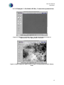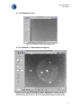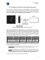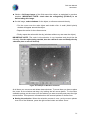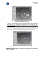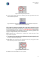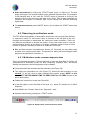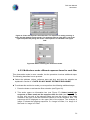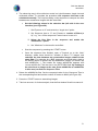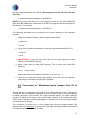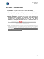
1
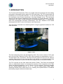
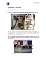
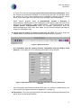
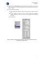
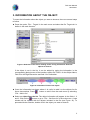
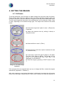
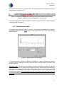
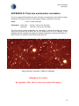
TCP USER MANUAL (TROMSØ CCD PHOTOMETER) Last modified: 2011-09-20 This version: Jorge García. Januaryl 2011 Original version by: Jose M. González. June 2007 Send comments and suggestions to Jorge García: jogarcia AT iac.es Or to the Support Astronomer Group: ttnn_a AT iac.es TCP User Manual 20/09/2011 INDEX 1. INTRODUCTION ........................................................................................................ 3 2. STARTING A SESSION ............................................................................................. 4 3. INFORMATION ABOUT THE OBJECT. .................................................................. 8 4. GETTING THE IMAGES.......................................................................................... 10 4.1. Full frame ............................................................................................................ 10 4.1.1. Ideal display mode........................................................................................ 11 4.1.2. Example 1: flat in B filter, exposure time of 5 seconds ............................... 12 4.1.3. Example 2: bias ............................................................................................ 13 4.1.4. Example 3: Astronomical objects................................................................. 13 4.2. Taking BIAS and FLATS.................................................................................... 14 4.3. Focusing .............................................................................................................. 14 4.4. ‘Windowed’ mode observations (fast photometry) ............................................. 15 4.5. Observing in multicolour mode........................................................................... 19 4.5.1. Multicolour mode: common exposure time.................................................. 19 4.5.2. Multicolour mode: different exposure times for each filter. ....................... 20 4.5.3. Sorting images by filter: “separator” ............................................................ 22 4.6. Conversion of ‘Windowed mode’ images from 1D to 2D. ................................. 23 APPENDIX I: Additional notes. .................................................................................... 26 APPENDIX II: Common problems................................................................................ 27 APPENDIX III: Pixel size and detector orientation....................................................... 29 2 TCP User Manual 20/09/2011 1. INTRODUCTION The Tromsø CCD Photometer (TCP) is a portable instrument optimized for fast reading photometry (Windowed system) based on CCD technology. The TCP incorporates the possibility of an on-line data reduction, i.e. the real time production of light curves and the calculation of the Fourier transforms of the data obtained so far. This instrument was built by the Physics Department at the University of Tromsø (Norway) –see Roy Ostensen's PhD thesis at http://whitedwarf.org/theses/ostensen.pdf– in collaboration with CUO (Copenhagen University Observatory). The TCP, installed on the IAC80 telescope since 2002, is one of its common user instruments. This document is intended as a detailed guide for using the graphical interface for TCP data acquisition. Figure 1. TCP. The TCP electronics driver was developed by CUO. The current version of TCP uses the CCD chip Site (Tektronik) 1024 x 1024, which operates at a temperature of -40 º C. The pixel size is 24 x 24 microns. The chip covers an area of 2.56 by 2.56 cm, which is a square field of about 9.2 arc minutes side in the IAC80. It is a back-illuminated chip with a high sensitivity in both the red and blue ranges thanks to its special coating. The TCP includes its own filter wheel and shutter (FASU). The FASU was designed with an unidirectional shutter to increase the accuracy of the exposures and a filter wheel that allows installation of up to 6 filters of 50 mm diameter. Currently available are the Johnson-Bessell filters U, B, V, R, I and an open position (white light). Switching between filters takes about 0.5 s, allowing the implementation of multiband photometry programs almost simultaneously. 3 TCP User Manual 20/09/2011 2. STARTING A SESSION The following paragraphs describe the follow-up sequence to properly booting and checking out of the system. ► In the dome, check that the TCP Electronic Racks are turned on (see Figure 2). Figure 2. Location of the switches of the TCP Electronic Racks. ► The TCP computer is located above the FOVIA-II monitor (see Figure 3). It is normally turned on. If not, turn it on. The computer must be connected to the network. If there are problems with the network, consult the start-up procedure of the TCP computer in Appendix II (Problem 1). The TCP computer is not used directly, but through asteroide PC. When you finish the computer booting process you will have to wait a few minutes to connect from asteroide. Figure 3. TCP computer (red) and asteroide computer (blue). 4 TCP User Manual 20/09/2011 ► Start a session in asteroide: connect as “obstcs1” (password: ask the support astronomer or the night assistant). ► Open a terminal in asteroide and type: >ssh –l observer tcp.ll.iac.es (password: ask the support astronomer or night assistant.). ► Once in tcp, open a new terminal: >xterm & ► In the new terminal, type: >download gpsold.hex This command will initialise the camera. When executing, the camera will start the process with: ‘download code to the camera *******’. If there are camera connexion errors, please contact the support astronomer (Appendix II – problem 2). ► Running the data acquisition software: >Qtcp15 ► The display will show the graphical interface of the data acquisition program (see Fig. 4) The user must check the messages appearing at the bottom-left line (marked in red) during initialisation: "Shutter initialisation" and "FASU initialisation”. If all goes well, after 2 or 3 seconds, the message "working" or "idle" should be displayed. In case of shutter and/or FASU initialising problems, a message notification will be displayed. In that case, you will need to contact the Support Astronomer to restart the system (Appendix II - Problem 3). Image 4. Graphical interface of the TCP data acquisition program. 5 TCP User Manual 20/09/2011 In Figure 4 we can see that only a part of the area of the chip is displayed. There are vertical and horizontal scrollbars to move through the chip. On the other hand, the overall size of the user interface can be changed by pressing the left mouse button in the lower-right corner and drag it by holding the left mouse button. When Qtcp15 program starts, it automatically creates a directory in home/observer, whose name is the combination of the starting date and time of the program (e.g. 2103042005 -21 March 2004 at 20:05 - ). Within this directory, Qtcp15 creates several sub-directories where the program automatically save the different image types taken: bias, flats, darks, tcp (for full-chip images) and data (for images in windowed mode). ► Check that the system is receiving data from the GPS. To do this, press the satellite button in the top right corner of the user interface (see Figure 5). Figure 5. GPS Information. It is imperative that the system receives information from the GPS to work properly. If everything is ok, the following information box is showed: Figure 6. GPS Information box. In this case the GPS is receiving data from 4 satellites. If the information box indicates that the GPS does not receive a satellite signal, you must contact the support astronomer (Appendix II, problem 4). ► Set location. Thus, the information about the observatory, telescope and instrument will be saved in the image headers. 6 TCP User Manual 20/09/2011 a) Press ‘File’ in the main menu and select ‘localisation’ (see Figure 7, left). In this option, a box with the available observatories and telescopes will be shown (see Figure 7, right). b) Select the telescope (IAC80). (1) In the ‘Observatory’ dialog box, select ‘Teide observatory’ (at the end of the list). (2) In the ‘Telescope’ dialog box, select ‘IAC80’. Observatory longitude, latitude, elevation and time zone and also the telescope focal relation will be shown. (3) Press ‘apply’. Figure 7. Selection of the information (telescope, observatory, instrument.) that will be saved in the image headers. 7 TCP User Manual 20/09/2011 3. INFORMATION ABOUT THE OBJECT. To enter the information about the object you want to observe, there are several steps to follow. ► Press the option ‘File – Targets’ in the main menu and select the file ‘Targets.lst’ or similar in the main directory. Figure 8. Selection of the file for reading and/or saving information about the objects to observe. If the object is not in the list, it can be added by typing the information in the corresponding dialog boxes of the interface utilities bar: Field 1 for the Object Name, Field 2 for the Right Ascension and field 3 for Declination. Figure 9. Information Fields of the object. ► Once the information has been written it is useful to add it to the objects list for future observations. Press button or add it from the main menu by selecting: ‘File – Add to list’. ► Select an object from the list. The object information will appear in the fields 1, 2 and 3. Click on the button or go to: ‘File – Get from list’ in the main menu. A new window will be opened with the objects included in the file (see Figure 10). To proceed with the selection, double click in the object you want to observe. 8 TCP User Manual 20/09/2011 Figure 10. Selection of the object. The user interface will also show the air mass and the hour angle of the object. 4 5 Figure 11. Information about the selected object. Field 4 shows the air mass and Field 5 the sidereal time. These data will be saved in the image headers. 9 TCP User Manual 20/09/2011 4. GETTING THE IMAGES 4.1. Full frame To do fast photometry, the first step is to obtain images from the entire chip (full frame). These images (flats, bias) are taken to help in the data reduction process, which can be done in real time, and in the selection of regions of the chip for the Windowed mode. The full frame images will be saved in the subdirectories 'tcp' (for objects), 'darks', 'flats' or 'bias', depending on the selected image type. The steps to be carried out are listed below. 1 ► Check that ‘single shot’ option in area 1 (‘Exposure’) is selected. ► Select the exposure time by writing it directly or using the arrows. 2 ► Select the filter in area 2 (‘Filter’). 3 4 ► Check that the ‘Full frame’ option is selected in area 3 (‘Transfer mode’). ► In this area, select the type of image to be taken: Flat field, Dark, Bias or Object. The images will be saved in the subdirectories flats, dark, bias o tcp depending on this selection. ► Take the image by pressing ‘START’ button in area 1. Image 12. Full frame image sequence. If the program does not respond when you try to change the filter, contact the support astronomer (Appendix II - Problem 3). After each exposure some image information is displayed by pressing the left mouse button over the image: relative position of the cursor, number of counts and distance to 10 TCP User Manual 20/09/2011 the centre of the field in arc seconds. This information appears in the bottom part of the user interface (see Figure 13). Figure 13. Information obtained by clicking the left mouse button over the image: location, number of counts and position in arc seconds In the following pages we show the different display options and some image examples –flat fields, bias and object–. 4.1.1. Ideal display mode. The default image display option is ‘min-max’, but it might be inadequate. To change the display mode press the button in the utilities menu bar. Then, the following panel is shown: Figure 14. Display mode selection panel. It is recommended to select "Histogram Equalization", which increases the relative contrast in all the regions of the chip. Once this type of image display is chosen it will be set as default. Important note: This display mode greatly increases the display contrast and set the grey scale zero level very close to the average bias value, with the idea of showing any pixel with some energy over this value. The images shown in this way may give the impression of a defective chip or that the optics is dirty, but it is in part due to the visualization algorithm. We recommend the use of this mode to be sure that there are not energy losses in the windows defined in the windowed mode when the stars are selected. 11 TCP User Manual 20/09/2011 4.1.2. Example 1: flat field in B filter, 5 seconds exposure time Figure 15. Example of full frame image: filter B flat field with 5 seconds of exposure time. The display mode is 'min-max'. Figure 16. Same image than Figure 15 but using the 'Histogram-Equalization' display mode. 12 TCP User Manual 20/09/2011 4.1.3. Example 2: bias Figure 17. Example of full frame image: bias. 4.1.4. Example 3: Astronomical objects Figure 18. Central star of the planetary nebula NGC246 using B filter and 30 s of exposure time. Image show objects below 12 magnitude. The image looks somewhat dirty due to the use of the 'Histogram-Equalization' display mode. 13 TCP User Manual 20/09/2011 4.2. Taking BIAS and FLATS ► BIAS: it is recommended to take 5-10 BIAS. The number of counts should be less than ~2,300 counts/pix. If this is not the case probably the cooler (peltier) is not properly working. In that case, please call the support astronomer. ► FLATS: the average number of counts should be between ~18,000 and ~21,000 counts/pix to be sure that they are in the linearity range of the detector. If photometric accuracy is required, it is recommended to take enough number of flats so that the total sum of counts exceeds ~ 100,000 (about 5 if the average is 20,000 in each image). Combining about 100,000 counts would roughly give s/n ratio ~ 100, which would become the photometric limit. If you take dome flats, there is a table in the control room showing the exposure times and the lights used to get images with an adequate level of counts with different filters. 4.3. Focusing ► Important: The TCP focus position is different to the CAMELOT one. In the first night some time should be spent in finding the TCP focus. As a starting point, read in the logbook the last TCP focus used. The FOVIA-II focus position is also different. Some values (used in March 2010) are: Telescope focus ~ 21,760 (Filter R); FOVIA-II focus ~ 12, T1 = 7.3. In general, the TCP focus is 2,000 units larger than the CAMELOT focus. ► To focus the TCP, not very bright objects (V<9) must be taken. Select "object" in the Exposure mode (area 4) of the selection window (see Figure 12), V filter, and an appropriate exposure time for the magnitude of the given object: the maximum amount of counts of the star used to focus should not exceed 23,000 counts. ► Image analysis will be done from asteroid using IRAF: (1) enter as "obstcs1" (2) type "iraf" in a terminal: this will run iraf in an xgterm and run ds9, (3) access to the images directory on TCP. The disc is automatically mounted in asteroide. Access to the disc by typing >cd /net/tcp/home/observer/. (4) Review the focus of the standard way: using imexam and making the star contours as circular as possible. If the image in QTCP15 (in IRAF you have to reverse “y” axis) appears: => decrease focus => increase focus ► Once the best focus is selected please annotate in the logbook the values of the telescope and FOVIA-II foci and the temperature of the mirrors. 14 TCP User Manual 20/09/2011 4.4. ‘Windowed’ mode observations (fast photometry) The main feature of the TCP electronics is the possibility of using the Windowed readout mode, which significantly reduces the CCD readout time. The observer selects a number of regions on the chip -windows- which are the only areas of the chip to be read out. The remaining pixels are discarded from the readout process. The following scheme summarizes the modus operandi of the TCP electronics. Figure 19. Example of 'Windowed' mode observations. Thus, the readout of the chip can be reduced to a 1% of the time spent in a full frame readout. The readout time in the 'Windowed mode' will depend on the number and size of the selected windows. In the case of TCP present chip (Tektronic), the full frame readout time is 23 s. However, using the 'Windowed mode' and, say, 3 windows (main star and two sky regions) and a window size of 16 x 16 pixels, the readout time would be 0.70 s. The following table shows the readout times (in seconds) in this mode for three different configurations (size and number of windows). Channels 16 x 16 32 x 32 48 x 48 64 x 64 3 0,70 1,08 1,47 1,88 5 0,95 1,58 2,23 2,92 10 1,58 2,83 4,14 5,52 Other advantages of the ‘Windowed mode’ with respect to other systems that optimize the readout speed are the following: - Available field. This mode allows the selection of the windows on the full area of the chip. This helps in areas where there are not many reference stars. - File size. The 'Windowed' system DOES NOT save the whole image, but a column of the selected windows, so that the size of each fits file is much smaller. This significantly reduces the amount of data saved, especially in fast photometric variability campaigns, where more than 1,000 frames per night can be taken. The process to observe using this mode is described below. 15 TCP User Manual 20/09/2011 ► Obtain a full frame image of the field around the object, as explained in previous sections. IMPORTANT NOTE: check that the autoguiding (FOVIA-II) is on before taking this image. ► On this image, select windows for the object, a reference star and the sky. - Put the cursor over the main object and double click. A small (64x64 pixels) window will appear around the object. - Repeat the action for the reference star. - Finally repeat the action with the sky (windows without any star near the object). IMPORTANT NOTE. The order in the selection is very important and should be the following: first the object being studied, then the reference star and finally the sky selection (one or more if desired). Figure 20. Example of Windows selection. At all times you can move and delete these windows. To move them you have to place the cursor on the window and drag it by holding the left mouse button. To view other available options put the cursor over the window you want to modify and press the right mouse button. This opens an information box with several options to choose from. ► Saving the selection. When the selection process is over, put the mouse pointer over one of the Windows, press the right mouse button and select ‘Save’. 16 TCP User Manual 20/09/2011 Figure 21. Saving the windows selection. This action sends information about the selected window to the camera electronics and creates the files 'photwins.dat' and 'photwccd.dat' in the subdirectory 'data'. These files are needed for the data acquisition program and for properly working of subsequent reduction. The borders of the windows will then go from red to blue and larger windows will cover several windows. This happens when they are very close and occupy the same reading direction. Thus, Qtcp15 further optimizes the reading process. Figure 22. Optimization of the readout windows developed by QTCP15. ► Select the Sequence time in the corresponding area (‘Sequence’) in the left side of the user interface. 17 TCP User Manual 20/09/2011 Figure 23. Selecting the sequence time. ► Put the mouse pointer again over a window, press the right Mouse button and select ‘Estimate exposure’. Figure 24. With the “Estimate exposure” option, the system optimizes the exposure time as a function of the readout time. With this option the program automatically takes a test image, computes the readout time needed and optimizes the exposure time for the selected sequence time. The process takes a few seconds. After that time, the optimized exposure time will appear in the corresponding area (area 1 in Figure 10). VERY IMPORTANT!!! Exposure time should be diminished by about 200-300 ms due to static electricity problems that introduce a slight time delay in the communications. NOTE. Sequence time = exposure time + readout time + delay time due to filters and/or shutter movements. ► The program will automatically switch to Windowed mode (section 'transfer mode' on the left side of the user interface) and sequence mode (section 'Exposure'). It will be ready to start with fast photometry. ► Write 9999 in the 'Frames' field of the 'Sequence' area. Thus, the program will take data continuously until the sequence is aborted. Figure 25. Selection of frame number.. ► Check that the selected filter is the one requested. 18 TCP User Manual 20/09/2011 ► Start observations by clicking the 'START' button (area 1 in Figure 10). The first image will begin in the closest multiple to the selected sequence time. For example, if the sampling time is 20 s and the 'START' button is pressed at 21:30:04, the exposure time of the first image will start at 21:30:20. This process simplifies the collection and analysis of complete light curves coming from different observing nights data. ► To stop the sequence press ‘ABORT’ button, placed where the 'START' button was before. 4.5. Observing in multicolour mode The TCP offers the possibility of observation sequences using a single filter (default) or multicolour mode. For this reason, there is a button on the left side of the user interface that activates or deactivates the multicolour mode (multifilter). There are two different procedures to access this option, as the user could want to use the same exposure time for all the filters or to assign a different exposure time for each of them. In general, the steps to observe in multicolour mode are: ► Bias and flats are taken as explained in Section 4.2. Of course, as many flats series as filters to be used must be taken. The process for taking full frame images is also performed as described in Section 4.1. 4.5.1. Multicolour mode: common exposure time This is the simplest procedure. Proceed similarly to how was described in Section 4.4 (observations in windowed mode) but after computing “exposure time” and before starting the sequence, the following steps must be added: ► Press the button that activates the filter selection (see Figure 26). ► This opens an information box (see Figure 27). Select the filter sequence to use (sorted). To do this, click on each selected filters (green arrow). NOTE: In this mode, SET THE EXPOSURE TIME TO ZERO FOR ALL FILTERS (boxes to the left of each button). ► Enable the “multicolour” mode (see Figure 28). ► In the filter option, set the first filter of the cycle, e.g., select “B” (number 2), for a BVI sequence. ► Write 9999 in the “Frames” field of the “Sequence” area. ► Start the sequence by pressing the ‘START’ button. Figure 26. Setup button of the multicolour mode. 19 TCP User Manual 20/09/2011 Figure 27. Filter and exposure time selection. The sequence is set by pressing, in order, the filter buttons (green arrow). The exposure time for each filter is set in the right field (red mark), using the arrows. The sequence is indicated in the upper field. Figure 28. Button enabling the multicolour mode. 4.5.2. Multicolour mode: different exposure times for each filter This observation mode is more versatile, but the procedure involves additional steps. The following describes how to proceed: ► Select the windows (object, reference stars and sky) and save the selection as explained in Section 4.4. NOTE: DO NOT MAKE "ESTIMATE EXPOSURE". ► To activate this multicolour mode you must perform the following additional steps. 1 Press the button to activate the filter selection (see Figure 26). 2 This action opens an information box (see Figure 27). Select (sorted) the sequence of filters used and the exposure time for each (see image 27). To do this, click on each of the selected filters and use the arrows on the fields located to the right of the filter selection buttons to set the exposure time. The sequence will be displayed on the upper field of the window. The example of image 27 shows the following sequence: 5 s. image in B filter, 8 s. image in V filter and 4 s. image in R Filter 20 TCP User Manual 20/09/2011 3 The observing way in this multicolour mode is a hybrid between single shot and windowed modes. To complete the procedure, the sequence time has to be calculated manually. This requires taking a test sequence to compute the time between two consecutive images with the same filter. Set the following values in the selection bar (left side in the user interface) (see Figure 28). i. Set Exposure to “0” and select the “single shot” option. ii. Set Sequence time to “0” and Frames to “number of filters (x 3)”; e.g., for a 3 filter sequence Frames has to be set to 9. iii. Select the first filter in the sequence and enable the "Multicolour" option. iv. Set “Windows” in the transfer mode field. Start the sequence by pressing the ‘START’ button. Once the sequence has finished, open a Terminal, go to the “data” directory, where there should be "number of filters x 3" images, and calculate the time between two consecutive images related to the same filter. For example, for a BVR sequence we should take a look to the starting times of w00003.fits and w00000.fits images (or w00001.fits and w00004.fits…). The header file image w00000.fits appears with >more w00000.fits. Find the time in the DATE-OBS field. By looking to the time from an image to the next (from w00000.fits to w00003.fits in this case) we find our Sequence Time. 4 Delete the w0000X.fits files. Set the computed value for the Sequence Time in the corresponding field and set the number of frames to 9999 (see Figure 28). 5 Press the ‘START’ button to start taking images. 6 Take into account, for further analysis, that the first window file will not start at 0. 21 TCP User Manual 20/09/2011 Figure 28. Parameter selection for multicolour mode observations (different exposure times). 4.5.3. Sorting images by filter: “separator” Resulting images in multicolour mode are stored as in the previous case, i.e. as consecutive images following a sequence in the data directory. For example, in the case of a sequence with three filters, "w00000.fits" will be associated with the first filter in the sequence, "w00001.fits" with the second, "w00002.fits" with the third, "w00003.fits" again with the first, and so on. To generate the light curves for the various filters is necessary to regroup the images. To do this, the "separator" program is used. This program creates directories for the different filters, copies the images associated with a particular filter and renames the files so that they have consecutive number for the same filter (required if you want to use the online reduction package RTP). The separator program is part of the collection of RTP reduction programs that complements the data acquisition program described in this manual. It is installed on the TCP computer. NOTE: This program is external to the data acquisition interface Qtcp15, and runs from the command line in any xterm opened in the TCP computer. It is recommended to run the program at the end of each night of observation to have 22 TCP User Manual 20/09/2011 the data organized before the backup! The program has to be run from the data directory. > /home/observer/bin/separator -i w00000.fits NOTE: Due to the initial test run in the multicolour mode the first file w0000X.fits WILL NOT BE w00000.fits. Remember to START the program with the first image in the directory. For example: > /home/observer/bin/separator -i w00006.fits The following describes how to proceed for the proper working of the separator program. 1. Make the reduction directory where images will be stored. > mkdir red > cd red 2. Once in the reduction subdirectory, make the filter subdirectories (B V R I). > mkdir B > cd B 3. IMPORTANT!!!: Copy the phot*.dat f files rom the data directory to each directory created with separator. 4. Make virtual links for each filter directory. This is done from each filter directory. >ln –s ../../data/1/ data Where the number correspond to the filter: 1=U, 2=B, etc… 5. Once all the virtual links have been created, every time you run separator everything is refreshed (including RTP graphics). 4.6. Conversion of ‘Windowed mode’ images from 1D to 2D. Images created in windowed mode, that is, files w00xxx.fits, have only 1 dimension. The header can be displayed in standard form, but not the image. The image appears in display programs, such as DS9, as a long horizontal streak. The online reduction program rtp waits for the data in this unusual way. However, it is possible that many users want to use other reduction packages, so first we have to convert these images to conventional 2D images. The conversion is carried out in a very simple way using the program rtcnv. This program has to be ALWAYS run at the end of the night, so the astronomer would leave the telescope with both, 1D and 2D, data. 23 TCP User Manual 20/09/2011 Below it is shown how to proceed to do the conversion. This conversion will only process the data with the BIAS subtraction using the overscan: 1. Make a new directory (at the level of data, tcp... directories). 2D images will be stored in this directory. For example: > mkdir images2D > cd images2D 2. It is convenient to copy the superflat (Flat.fits) created by rtp to this directory. If you are in this directory, the resulting 2D images will be flat-fielded. The flat reduction is better in this way, as subsequent flat-field reduction is very complicated. Keep in mind that the flats are full frame images, so you should draw exactly the region covered by the windows and create a mosaic as rtcnv generates. > cp ../red/Flats.fits . assuming that the online rtp reduction directory is red. 3. Make a virtual link to the data in the same way that when preparing data for rtp. > ln –s ../data data 4. Run the command: > rtcnv –X –S –I –n xxx where xxx is the number of images (total amount of images in the data directory -w00xxx.fits). Notes: • The final images are view00xxx.fits • These images HAVE NOT HEADER. It is very important not to delete the original data: w00xxx.fits . • If you are observing in multicolour mode you will have to create as many subdirectories as filters you have, this is, as many subdirectories as separator has created in the data directory. An example of the command line sequence would be the following (BVR sequence): > mkdir images2D > cd images2D > mkdir B > cd B > ln –s ../../data/1 data 24 TCP User Manual 20/09/2011 > cp ../../redB/Flats.fits . 1 > rtcnv –X –S –I –n xxx The same for V and R filters It has been assumed that rtp reduction for B filter images has been done in the directory redB. 1 25 TCP User Manual 20/09/2011 APPENDIX I: Additional notes ● Field of View: TCP’s field of view at IAC80 is ~9.2 x 9.2 arc minutes. ● Detector Linearity: The most energetic pixels should not exceed 30,000 counts. If the object is a very bright star and photometric accuracy is required the procedure is to defocus the telescope until the maximum number of counts is into the linear regime and then increase the size of the windows. ● Detector Temperature: The detector must be cooled by the peltier about 35 degrees below room temperature. The temperature appears at the bottom information line of the graphical interface (see Figure 29). If the detector temperature is considerably higher maybe the peltier is not working properly. In this case contact the support astronomer. Figure 29. Detector Temperature Info. ● Darks: “Normal” fast photometry programs do not need to take darks because, in windowed mode and with short exposure times (less than a minute), the readout noise dominates. However, other observations, such as imaging the entire chip for routine programs, will need to take darks if the exposure times exceed the minute (in winter), or 40 seconds (in summer). 26 TCP User Manual 20/09/2011 APPENDIX II: Common problems 1) WORKING WITHOUT NETWORK If there are communication problems between asteroide and tcp, the observations can be directly made from the tcp computer. In this case the remote used is limited to the use of a switch to control the mouse and the keyboard from the control room. In this case, the first steps of the procedure are slightly different. ► In the dome, check that the TCP electronic racks are turned on. ► Set the switches in an appropriate way to pass the keyboard and mouse control to the control room. Normally, this step is performed by the support astronomer. ► Start TCP computer session: username is ‘observer’. Support astronomer will give you the password. ► Run command: >startx ► In a terminal, run command: >download gpsold.hex From this point, proceed as described in page 5. NOTE. The image displayed on the TCP monitor is only a part of the overall image; there is a little zoom effect. The real limits are reached by moving the mouse pointer to any side of the image. 2) FAILURE TO DOWNLOAD THE CODE TO THE CAMERA This problem occurs when the next command is used: >download gpsold.hex This command will initialize the camera. When run, the camera will indicate the process 'code to download the camera *******'. The information is sent and received using an optical fiber. If you receive an error message related to the camera connection it might be because there is a bad fiber connection. The support astronomer or the night assistant (never the astronomer) should proceed disconnecting and reconnecting the fibers with special care, both in the computer electronics (dome) and in the tcp computer and/or restarting the tcp electronics (see Figure 2). Be careful with the colours of the fibers, as they should not be crossed: red to red and black to black. 3) FILTER WHEEL AND SHUTTER PROBLEMS It is possible that, when initializing the graphical interface (or even during the night), the system does not properly initialize (or refresh) the filter wheel and/or the shutter. If you have the 'working' or 'idle' message in the bottom info line, everything is ok. If 27 TCP User Manual 20/09/2011 an error message such as 'shutter calibration error' appears, please contact the support astronomer or the night assistant, who has to proceed as follows: Log off and log on from the program: >Qtcp15. If the problem stands, the system has to be reset. Resetting the system: (1) exit from the graphical interface (killing the process, if necessary); (2) go to the dome and turn off the electronic racks (see Figure 2); (3) turn back on the electronic racks; (4) run >download gpsold.hex ; (5) run back the graphical interface. Resetting the system solves the problems in 90% of cases. However, if the problems remain, the camera has to be shutdown, the telescope parked to the zenith and the telescope system reset (this has to be done by the support astronomer or the night assistant). Very rarely, the problem still persists. In this case, the serial cable that connects the TCP computer with the camera electronics can be wrong or receiving too much noise. Check the cable connections and warn MI (Instrumental Maintenance) to review the status of the cable 4) NO SATELLITES DETECTED If the information box indicates that the GPS does not receive a satellite signal, you must contact support astronomer or night assistant, who must proceed as follows: Go to the dome and check that the led located over the “gpsh” mark in the electronic rack (where the optical fibers are connected) is blinking (red light). If the light blinks, then the signal is arriving fine to the electronics, but not to the computer. Check the connections of the serie cables from the gps (yellow box) to the computer (the cable is labelled as pc at the gps side and clock at the pc side). If still does not work, reset the system (problem 3). If the light does not blink then the electronics is not receiving signal. In this case: o Log off of the graphical interface and turn off the electronic racks. Turn them on again, wait a few seconds and then see if the red light flashes. o If the light still does not blink, check the connections (serie cable) from the electronics to the yellow box (labelled as int) and from this box to the gps (labelled as gps ). 28 TCP User Manual 20/09/2011 APPENDIX III: Pixel size and detector orientation From an equatorial field with more than 150 stars, the astrometry of the field has been measured. This gives the scale of the detector and its orientation on the sky: Scale: 0.537 ± 0.002 arcsec/pix Orientation: North axis: East axis: 50º.85 ± 0.03 (0º up, 90º right) 140º.85 ± 0.03 (0º up, 90º right) The figure below shows graphically the orientation in which the images are saved (right: as you would see in DS9, left: as you would see in the TCP display). In the graphical interface display the images are rotated 90 degrees clockwise and flipped in the E-W axis (i.e. where E is the N and N where the E). a) b) Image 30. Image orientation. a) DS9. b) TCP display IMPORTANT NOTE!!! By September 2011, the FoV has been rotated 180 degrees 29