Download Manual

PDETool
Version 1.0.6
User Manual
Performance and Dependability Engineering Lab (PDE Lab)
School of Computer Engineering
Iran University of Science and Technology
http://pdel.iust.ac.ir/projects/pdetool.html
Last edit: 2009/09/17
Author: Ali Khalili (email: khalili[dot]ir[at]gmail[dot]com)
Copyright © 2008 PDE Lab. of Iran University of Science and Technology
All right reserved
PDETool user manual
Table of Content
Introduction ......................................................................................................................... 3
Introduction ......................................................................................................................... 3
The Software Architecture .............................................................................................. 3
PDETool background...................................................................................................... 4
Installation........................................................................................................................... 5
Installing SimGine and PDETool ................................................................................... 5
Modeling Background ........................................................................................................ 6
Petri Nets (PNs) .............................................................................................................. 6
Generalized Stochastic Petri Nets (GSPNs) ................................................................... 7
Stochastic Reward Nets (SRNs) ..................................................................................... 7
Stochastic Activity Networks (SANs) ............................................................................ 8
Coloured Stochastic Activity Networks (CSANs) ........................................................ 10
Overview of PDETool ...................................................................................................... 11
Constructing models ..................................................................................................... 12
Adding/editing SAN elements ...................................................................................... 13
Modifying properties of SAN elements .................................................................... 14
Adding/editing global variables ................................................................................ 17
Adding/editing CSAN elements ................................................................................... 18
Primitives of CSANs are the same with SANs in addition to the following ones: ....... 18
Adding/editing SRN primitives .................................................................................... 19
General Configuration .................................................................................................. 22
SDES Interface.............................................................................................................. 23
Specifying Reward Variables ........................................................................................... 24
GSPNs performance measures...................................................................................... 26
Model Simulation with PDETool ..................................................................................... 27
Simulation using Model Simulator ............................................................................... 28
Simulation using Model Animator................................................................................ 29
Examples ........................................................................................................................... 31
Example 1: Modeling a Queue Using SANs ................................................................ 31
Example 2: Modeling a packet generator system using CSANs .................................. 32
Example 3: SRN model of a multi processor system ................................................... 34
Appendix A: Known bugs and limitation ......................................................................... 36
Reference: ......................................................................................................................... 37
2
PDETool user manual
Introduction
PDETool is a multi-formalism modeling and simulation framework for discrete-event
models based on a unified abstract description named SDES [1]. It uses a simulation
engine for simulation of discrete-event simulation of stochastic models called SimGine.
PDETool can be easily extended to support variety of stochastic formalisms. It currently
supports SANs, CSANs, GSPNs and SRNs (which will be explained next).
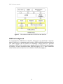
The Software Architecture
The software architecture of PDETool, shown in Figure 1, is separated to two layers: a
front-end layer and a back-end layer as follows:
• Front-End Layer (PDETool interface): This layer provides some graphical user
interfaces and a model translator. The user interfaces includes editors (model editor,
reward variables editor, global variable editor), SimGine interface, simulation and
animation GUI described in the previous subsection. Each formalism supported by
the tool has its own editor, translator and an optional graphical animator which are
responsible for communicating with the underlying layer. This layer can be viewed
as an interface between users and the back-end layer.
• Back-End Layer (SimGine engine): PDETool uses SimGine simulation engine as
the underlying layer. This back-end layer is responsible for simulation of the model
and evaluating reward variables and also provides model animation facility. As we
mentioned before, for simulating a model based on particular stochastic discreteevent formalism, a model translator prepares the input model of SimGine mapped
from the original model where these two models should be behaviorally equal. As
depicted in Figure 1, the internal architecture of SimGine includes parser, code
generator, utility library, simulator, animator and SDES simulation manager.
3
PDETool user manual
Figure 1
The software architecture of PDETool and SimGine
PDETool background
As mentioned before, PDETool uses SimGine for discrete-event simulation of stochastic
models. SimGine is a simulation engine based on SDES unified description and has its
own model structure and file format. For simulating a model based on a particular
formalism in PDETool, the model must be translated into the XML-based input language
of SimGine. For more information about SDES description, see [1]. More information
about SimGine and its manual are also available in SimGine homepage [7].
4
PDETool user manual
Installation
PDETool runs under Microsoft Windows XP/2000/Vista and needs .Net Framework
(version 2 or higher) to be installed on the system. If you do not have it installed on your
system, you must first install .Net framework.
NOTE: PDETool is not tested on Windows 95, 98, Millennium and NT. But we guess it
will work in these versions of Microsoft windows if .Net framework is installed. The last
version of .Net framework (currently version 3.5) can be freely downloaded from
http://msdn.microsoft.com/en-us/netframework/default.aspx.
Installing SimGine and PDETool
To install PDETool, download and run PDETool installation file from [8]. It installs both
PDETool and SimGine and everything needed to construct a model and simulate it.
5
PDETool user manual
Modeling Background
PDETool supports multiple formalisms, including generalized stochastic Petri nets
(GSPNs), stochastic reward nets (SRNs), stochastic activity networks (SANs) and
coloured stochastic activity networks (CSANs). In this section, we review some modeling
background about these models.
Petri Nets (PNs)
Petri nets originally were introduced by C.A. Petri in 1962 [3]. A Petri net (PN or
sometimes Place-Transition net) is a bipartite directed graph whose nodes are divided
into two disjoint sets called places and transitions. Directed arcs in the graph connect
places to transitions (called input arcs) and transitions to places (called output arcs). A
cardinality number may be associated with these arcs. A marked Petri net is obtained by
associating tokens with places. A marking of a PN is the distribution of tokens in the
places of the PN. There are several definitions for Petri nets and even more for stochastic
Petri nets. Petri net formally can be defined by a 4-tuple (P, T, A, M) where:
• P={p1,p2,…,pm} is a finite non-empty set of places,
• T={t1,t2,…,tn} is a finite non-empty set of transitions where P  T = φ ,
• A = ( P × T )  (T × P ) is the set of (input and output) arcs,
• M:P{0,1,2,…} is the marking of net which denotes the number of tokens in each
place P. Initial marking is denotes as M0.
In a graphical representation of a PN, places are represented by circles, transitions are
represented by bars and the tokens are represented by dots or integers in the places. Input
places of a transition are the set of places which are connected to the transition through
input arcs. Similarly, output places of a transition are those places to which output arcs
are drawn from the transition. A transition is considered enabled in the current marking if
the number of tokens in each input place is at least equal to the cardinality of the input arc
from that place. The firing of a transition is an atomic action in which one or more tokens
are removed from each input place of the transition and one or more tokens are added to
each output place of the transition, possibly resulting in a new marking of the PN. Upon
firing the transition, the number of tokens deposited in each of its output-places is equal
to the cardinality of the output-arc.
Each distinct marking of the PN constitutes a separate state of the PN. A marking is
reachable from another marking if there is a sequence of transition firings starting from
the original marking which results in the new marking. The reachability set (graph) of a
PN is the set (directed graph) of markings that are reachable from the other markings
(connected by the arcs labeled by the transitions whose firing causes the corresponding
change of marking). In any marking of the PN, multiple transitions may be
simultaneously enabled.
6
PDETool user manual
Generalized Stochastic Petri Nets (GSPNs)
The stochastic PNs (SPNs) [4] are obtained by associating with each transition in a PN an
exponentially distributed firing time. An SPN model can be formally defined by a five
tupple (P, T, A, M, R) where P, T, A, and M are as in simple Petri nets, and R is the set of
firing rates (possibly marking-dependent) associated with the PN transitions where
R = {rl, r2 , . . . , rm}
The underlying reachability graph of a SPN model is isomorphic to a continuous time
Markov chain (CTMC).
Generalized stochastic Petri nets (GSPNs) [5] try to extend SPNs further by introducing
immediate transitions which fire in zero time once they are enabled in addition to timed
transitions that fire after a random, exponentially distributed enabling time (like in
SPNs). Usually, timed transitions are represented by hollow rectangles while immediate
transitions are represented by thin bars.
The markings of a GSPN are classified into two types. A marking is vanishing if any
immediate transition is enabled in the marking. A marking is tangible if only timed
transitions or no transitions are enabled in the marking. If several conflicting immediate
transitions are enabled in a marking, a firing probability must be defined. The (usually
marking dependent) firing probability is specified for only timed transitions and does not
need to be specified for timed transitions.
Another type of arc exists in GSPN called inhibitor arc. An inhibitor arc connects a place
p to a transition and imposes an additional constraint on the enabling of that transition.
The transition is now enabled iff the enabling rule of ordinary Petri nets concerning the
usual arcs between places and that transition is satisfied and if the place is not marked (is
empty).
A GSPN model describes an underlying stochastic process, captured by the extended
reachability graph" (ERG) as a reachability graph with additional stochastic information
on the arcs which can be reduced to a CTMC in the state space analysis step.
Stochastic Reward Nets (SRNs)
Stochastic reward nets (SRNs) [6] are based on GSPN but extend it further. In SRNs,
every tangible marking can be associated with a reward rate. It can be shown that an SRN
can be mapped into a Markov reward model. Thus a variety of performance measures can
be specified and calculated using a very convenient formalism. SRN also allows several
other features that make specification convenient.
Each transition may have an enabling function (also called a guard), so that a transition is
enabled only if its marking dependent enabling function is true. This feature provides a
powerful means to simplify the graphical representation and to make SRNs easier to be
understood.
Marking dependent arc multiplicities are allowed. This feature can be applied when the
number of tokens to be transferred depends on the current marking. Marking dependent
firing rates are allowed. This feature allows the firing rate of the transitions to be
specified as a function of the number of tokens in any place of the Petri net,
Transitions can be assigned different priorities and a transition is enabled only if no other
transition with a higher priority is enabled,
7
PDETool user manual
Besides the traditional output measures obtained from a GSPN, such as throughput of a
transition and the mean number of tokens in a place, more complex reward function can
be defined.
Stochastic Activity Networks (SANs)
Stochastic activity networks (SANs) [10], introduced in 1984, are a stochastic extension
of Petri nets [3]. SANs are more powerful and flexible than most other stochastic
extensions of Petri nets that use graphical primitives and provide a high-level modeling
formalism with which detailed performance, dependability, and performability models
can be specified relatively easily. PDETool uses a new definition of SANs which is
introduced in [12].
Each SAN model is composed of the following elements (primitives):
- Place:
Like any extension of Petri nets, places which represent the state of the
modeled system, are represented graphically as circles. Each place contains a
certain number of tokens (an Integer value), which represents the marking of
the place. The set of all places’ marking defines the marking of the model. All
tokens in a SAN place are homogeneous, in that only the number of tokens in
a place is known; there is no identification of different kinds of tokens within
a place. Graphically, each place is represented as a circle.
- Timed activity:
Timed activities represent activities of the modeled system whose durations
impact the system's ability to perform. A timed activity has m inputs and n
outputs, where m+n>0. Each input can be a place or an input gate and each
output can also be a place or an output gate. To each timed activity is
associated an enabling rate function (i.e. a computable partial function, which
is the activity execution speed), and an n-ary computable predicate called the
reactivation predicate. Timed activities are represented graphically as thick
vertical lines.
Enabling rate functions can be generally distributed random variables. Each
distribution can depend on the marking of the network. For example, one
distribution parameter could be a constant multiplied by the marking of a
certain place.
Reactivation predicate function gives marking dependent conditions under
which an activity is reactivated. Reactivation of an activated activity means
that the activity is aborted and that a new activity time is immediately
obtained from the activity time distribution.
- Instantaneous activity:
Instantaneous activities represent system activities, which, relative to the
performance variable in question, are completed in a negligible amount of
time. These activities are represented graphically as thin vertical lines. An
instantaneous activity has m inputs and n outputs, where m+n>0.
- Input gate:
Gates are introduced to permit greater flexibility in defining enabling and
completion rules. An input gate has a finite set of inputs and one output. To
8
PDETool user manual
each such input gate is associated an n-ary computable predicate called the
enabling predicate, and a computable partial function called the input
function. An input gate is represented graphically as a triangle.
The enabling predicate is a Boolean function that controls whether the
connected activity is enabled or not and can be any function of the markings
of the input places. The input gate function defines the marking changes that
occur when the activity completes.
If a place is directly connected to an activity with an arc, it is equivalent to an
input gate with a predicate that enables the activity when ever the place has
more than zero tokens along with a function that decrements the marking of
the place by one when ever the activity fires. An input gate is represented as
follows:
-
Output gate:
An output gate which is represented by triangle has a finite set of outputs and
one input. To each such output gate is associated a computable function called
the output function which defines the marking changes that occur when the
activity completes. Like in input gates, there is also a default scenario for
output gates, i.e. if an activity is directly connected to a place, it is equivalent
to an activation in which an output gate has a function that increments the
marking of the place whenever the activity is fired. An output gate represented
as bellows:
Structurally, a SAN model is an interconnection of a finite number of primitives, subject
to the following connection rules:
• Each input of an input gate is connected to a unique place and the output of an input
gate is connected to a single activity.
• Different input gates of an activity are connected to different places.
• Each output of an output gate is connected to a unique place and the input of an
output gate is connected to a single activity.
• Different output gates of an activity are connected to different places.
• Each place and activity is connected to some input or output gates.
Note: Be aware that the order in which state updates occur in PDETool may differ from
some other tools. Input gates execute before arcs directly connect places and activities
and they execute before output gates in PDETool. Also, if there are multiple instances of
the same item, for instance multiple input gates, and the order of application of the gates
is not specified. Models must be constructed so that the gate functions are execution
order independent anytime there are multiple instances of the same type of gates
connected to an activity.
9
PDETool user manual
Coloured Stochastic Activity Networks (CSANs)
A CSAN model 13] is composed of the five primitives of a new definition of SANs,
including place, input gate, output gate, timed activity and instantaneous activity, plus a
new type of places called coloured place. A coloured place holds a list of tokens of a
user-defined token type. To differentiate the two kinds of places, we will refer to the
ordinary places of SANs as simple place. The term place is used to refer to both kinds of
places.
To each coloured place is associated a selection policy, which specifies the order of
tokens for removal by the occurrences of linked activities. Different kinds of the selection
policies are as follows:
• FIFO: In this case, tokens can be taken from the place in same order they have
been appended.
• LIFO: In this case, tokens can be taken from the place in reverse order of their
appendance.
• PRI: In this case, tokens have a priority that can be specified by a user-defined
order function.
• NSP (no-selection-policy): In this case, the list of tokens is unordered. Therefore,
a multi-set (or bag) can be used to hold tokens.
The type of the objects being held by a coloured place is defined by a token type. A token
type can be defined similar to the declaration of data types, records or structures in highlevel programming languages like C++, Java or C# (in PDETool) . Each token type has
one or more data fields, which may be an ordinal type or a user-defined type.
Both of the number of tokens inside a coloured place (i.e. the size of the token list) and
the values of its fields can be read in predicates and functions or can be read or
manipulated by functions of input/output gates.
Table 1: Graphical notation of CSAN elements
A graphical representation of the elements of CSANs is shown in Table 1. For the
coloured place, tt is the name of a token type and sp is a selection policy for the place.
10
PDETool user manual
Overview of PDETool
This section looks into the graphical user interface (GUI) of PDETool and describes
constructing, editing and simulating models by the tool.
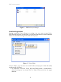
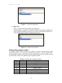
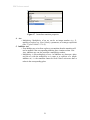
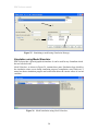
After installation, you can run the tool using Start MenuPDELabPDETool. The main
console of PDETool is shown in Figure 2.
Figure 2
Main console of the PDETool
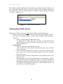
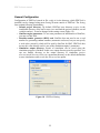
Before constructing a model, you have to create a new project or select one of existing
ones using Project Manager (ProjectsNew or ProjectsOpen) which is shown in
Figure 3.
11
PDETool user manual
Figure 3
PDETool Project Manager
Constructing models
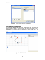
Opening a project in Project Manager or creating a new one, causes to open Project
Editor depicted in Figure 4. In this form, you can create some models or some simulation
studies to evaluate the existing models in the current project.
Figure 4
Project Editor
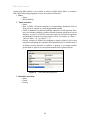
In Project Editor, you can create a new model in the current project or load and modify
existing models as follows:
• To construct a new (SAN, CSAN, SRN and GSPN) model or rename/delete a
selected existing one, use menu Model in Project Editor and select the proper
submenu.
12
PDETool user manual
•
•
To load an existing model, double click on it. It opens another form for editing and
modifying models. The type of model editor depends on type of models, e.g. in
case of SAN models, SAN Model Editor will be opened.
You can also import a model from another project into the current project
(ModelImport Model).
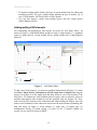
Adding/editing SAN elements
For constructing and modifying a SAN model, you must use SAN Model Editor. As
shown in Figure 6, SAN Model Editor includes 6 parts: a textual menu (1), a graphical
menu (2), model grid (3), reward variable list (4), global variable list (5) and properties
editor (6).
1
2
3
6
4
5
Figure 5
SAN Model Editor
To add a new SAN primitive, you must use graphical menu shown in Figure 6. To add a
new Place, Timed Activity, Instantaneous Activity, Input Gate or Output Gate, drag the
proper icon (Figure 6) to the model grid and drop whenever you want (location of the
new place). To connect two SAN elements (places to gates, gates to activities, places to
activities and opposite sides of them) by an Arc, push the icon Arc (Figure 6-6). Now,
(left) click the first element of the connection and while holding the button, move the
mouse to the destination of the connection and release the mouse button (Something like
drag and drop). In Figure 6, Icons include: (1) input gate, (2) output gate, (3)
instantaneous activity, (4) timed activity, (5) place, (6) arc, (7) global variable, (8)
reward, (9) save and (10) convert to SDES.
13
PDETool user manual
Figure 6
SAN Model Editor graphical menu.
Graphical and textual editors also can be used to:
• Add a global variable and reward variable (Figure 6-7 and 8): This will be
explained in detail in the following subsections.
• Save the current model: To save the current SAN model, push icon Save (Figure 69). It can be done using the textual menu too.
• Convert to SimGine input: To convert the current SAN model into the input
language of SimGine, push icon Convert to SDES in the graphical menu (Figure 610).
• Export models as an image: SAN Model Editor can export current SAN model into
an image with type JPEG. To do so, use textual menu (ModelExport as Image)
and specify destination location of the output image file.
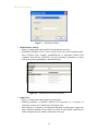
Modifying properties of SAN elements
Note that name (identifier) of each element (as an object), primitive or variable must be
unique in the model. Properties of each element in a SAN model can be accessed and
modified via Property Editor (right hand of the Model Editor as presented in Figure 6-6).
Like traditional programming languages, names (identifiers) can be defined by a string
which satisfies some constraints. Here, the lexical rules (constrains) that names must be
satisfied is as existed in .NET languages.
In the subsequent paragraphs, we will describe attributes of each element type:
1. Place:
• Name: A unique name that identifies the place. Marking of a place p (in
functions defined in a gate) can be accessed/modified by property Mark. For
example, one can write p.Mark=2.
• Initial Marking: The initial marking m of each place is an integer value equal
with or greater than zero (m≥0). Initial marking must be as an (explicit) integer
number or value of a global variable within type int.
• Position: Position of a place is a set (x,y) where x and y is horizontal and
vertical position of the place in the model editor’ grid. This property (as the
common property of all graphical elements of SAN) is not shown in Property
Editor but you can change the position of each element by dragging the
element, move it and drop it somewhere else.
14
PDETool user manual
Figure 7
Place properties
2. Timed Activity:
• Name: A unique name that identifies the timed activity.
• Distribution: It includes both a distribution function and its parameters. For
example, if execution of an activity is distributed exponentially, the mean of
distribution must be specified. Each distribution function has one or more
parameters which must be specified in Distribution Editor (Figure 9).
• Reactivation predicate: A Boolean function (an expression or a sequence of
statements written in C# that return a Boolean value) which reactivates the
activity in a state that the activity is enabled and reactivation predicate is true.
Reactivation means that a new delay will be sampled from the distribution
function, and the activity will be scheduled to fire after “delay” units of time
from the current simulation time.
Some read only properties are also shown in both instantaneous and timed activity
including input gates, output gates, input places and output places. These properties show
that which elements are connected to the activity (e.g. places that are connected as the
input places of this activity). When you change the model or modify it, these properties
change automatically.
Figure 8
Timed Activity properties
15
PDETool user manual
Figure 9
Distribution Editor
3. Instantaneous Activity:
• Name: A unique name that identifies the instantaneous activity.
• Probability (Weight): If two or more activities have the same completion time,
these activities must compete probabilistically to determine which event
completes first and the Probability is used to determine probability of firing
each activity (these probability is normalized first).
Figure 10 Instantaneous Activity properties
4. Input Gate:
• Name: A unique name that identifies the input gate.
• Enabling predicate: A Boolean function (an expression or a sequence of
statements written in C# which return a Boolean vale).
• Input function: A sequence of statements that their execution may change the
state of model (marking of some places or value of some global variables) just
before firing the activity which is connected to the gate.
16
PDETool user manual
Figure 11 Input Gate properties
5. Output Gate:
• Name: A unique name that identifies the output gate.
• Output function: A sequence of statements that their execution may change the
state of model (marking of some places or value of some global variables) just
after firing the activity which is connected to the gate.
Figure 12 Output Gate properties
Adding/editing global variables
For adding global variables (which may change or remain constant during model
execution), you have to use the global variable icon (Figure 6-7) in SAN Model Editor.
For each global variable, a unique name must be chosen and type of the variable must be
specified. Table 1 shows the available types for global variables.
Type
byte
short
ushort
Int
uint
bool
float
double
Table 1: Available type for global variables
Size (Byte)
Description
1
signed byte
2
signed short
2
unsigned short
4
signed integer
4
unsigned integer
a Boolean value
4
floating point number
8
double precision floating point number
17
PDETool user manual
After adding a global variable to the SAN model, you can change its name and type. To
do so, select the variable in Global Variable List (Figure 6-4) and change properties of
the variable in the Properties Editor (Figure 6-6). Figure 12 shows properties of variable
“Variable 1” with type “int”.
Figure 13
Global variable properties
Adding/editing CSAN elements
Primitives of CSANs are the same with SANs in addition to the following ones:
1. Color: A color is a data structure which can be used for colored tokens. To add a
new color, use the graphical menu. A color is the list of fields with the following
properties:
o Name: A unique name that identifies the color.
o An ordered list of fields. The type and name of each field must be
specified. Type of each field must be a built-in type (Table 1) or a color
that is defined before.
2. Coloured Place:
o Name: A unique name that identifies the color.
o Color: Color of the coloured place determines the type (color) of tokens
can be in the place.
o Policy: The policy determines how tokens are added or removed from the
place and can be FCFS (for queue-like places), LCLS (for stack-like
places) or Priority.
o Priority Function: The body of function that is used when the policy of the
place is Priority.
o Initial marking: To specify the initial marking of a colored place, you have
to specify the value of a colored token (values of all fields) and count of
that token which should be added to the place (for example, see Figure 14
in which the initial marking of place has 6 coloured tokens that in 5 of
them, field a is 1 and field b equals 4).
18
PDETool user manual
Figure 14
Initial Marking Editor for coloured places
Adding/editing SRN primitives
For constructing and modifying a SRN model, you have to use SRN Model Editor. As
shown in Figure 13 and like in SAN Model Editor, SRN Model Editor includes 5 parts: a
textual menu (1), a graphical menu (2), model grid (3), reward variable list (4), and
properties editor (5).
Figure 15 SRN Model Editor
19
PDETool user manual
Constructing SRN models is very similar to SANs and SRN Model Editor is somehow
alike. In the following paragraphs, we only describe the differences.
1. Place:
• Name.
• Initial Marking.
2. Timed transition:
• Name.
• Rate. In SRNs, all timed transitions are exponentially distributed. Rate of
firing can be a constant or a marking dependent number.
• Guard. In addition of traditional enabling condition of each transition, there
may exist another enabling condition named transition guard based on net
marking. A guard is a Boolean expression and can use Boolean operators
and marking of some places using property Mark, for instance (p1.Mark<=
3 && p2.Mark==2) || (p3.Mark >= 5).
• Priority. priorities is defined by assigning an integer priority level to each
transition, and adding the constraint that a transition may be enabled only if
no higher priority transition is enabled. A priority is an integer number
greater than or equal to zero and greater number shows greater priority.
Figure 16 Timed transition properties
3. Immediate transition:
• Name
• Guard
• Priority
20
PDETool user manual
Figure 17 Immediate transition properties
4. Arc:
Multiplicity: Multiplicity of an arc can be an integer number (e.g. 2),
marking of a place (e.g. place1.Mark), a parameter, or an integer expression
(like 2+(place1.Mark==1?0:2)).
5. Inhibitor Arc:
• If an inhibitor arc exists from a place to a transition, then the transition will
not be enabled if the corresponding inhibitor place contains a token. Like
Arcs, inhibitor arcs can also associate a multiplicity number.
• Multiplicity: is like multiplicity of arcs. An inhibitor arc (between a place
and an arc) with the multiplicity m is same as m replicate of a simple
inhibitor arc, i.e. the transition cannot be fired if there exist more than m
token in the corresponding place.
•
21
PDETool user manual
General Configuration
Configuration of PDETool (stored in file config.ini in the directory which PDETool is
installed) can be changed using menu Setting in main console of PDETool. The Setting
form contain following functionality:
• Default project directory: By default, PDETool uses directory project in the
installation directory of the tool to store, save and load the projects (models, reward
variables and etc.). It can be changed in the setting screen (Figure 16).
• SimGine engine parameters: To use some parameters in initialization of SimGine,
you may use this field.
• Random number generator (RNG) seed: SimGine does not need to use a seed
number for generating random numbers (automatic seed-auto) but you can specify
a seed value (manually) which will be used by SimGine for RNG. PDETool does
not use this value directly and it is one of the simulation engine’s parameters.
• Simulation output directory: Result of simulation can be saved when the
simulation progress is finished. In this case, output directory must be specified. You
can use models directory as the output directory of simulation (project
directory\model directory\Sim), set a permanent directory as the default destination
to store simulation results, or use the Always ask me option.
Figure 18 PDETool Setting
22
PDETool user manual
SDES Interface
PDETool has an interface for direct working with the SimGine. This feature is useful
when the modeler wants to simulate a SimGine file (which is based on SDES
description). In this situation, modeler can load, edit and simulate a SimGine file. A
simple model animator is also available for this purpose.
For direct simulating a SimGine model, use SimGine Tool from menu Projects
(ProjectsSimGine Tool) in main console. This opens the SDES Interface presented in
Figure 18.
Figure 19
SimGine Interface
23
PDETool user manual
Specifying Reward Variables
For evaluation of models, modeler have to specify some reward variables which define
functions that measure interested information about the system being modeled. One of
the key features of each reward is its evaluation time. There exist two main classes of
evaluation time includes transient and steady state. Transient type itself can be instance
of time, interval of time and time averaged interval. To add a new reward variable in
SAN and SRN models, use graphical icon of rewards (Figure 18) in model editor. When
you create a reward variable, it is added to the list of reward variables (Figure 5-5). Like
elements and variables, a reward variable has a unique identifier.
Figure 20
Add a reward variable within a particular type
PDETool and its simulation engine, SimGine, use performance reward variables which
introduced in [2] and include rate rewards and impulse rewards. For each reward, it can
be specified both rate function and impulse function as follows:
• A rate function is body of a function which assigns some quantity of reward when
the model is in a particular situation and must be written in code editor (Figure
19). The situation can be checked using a conditional statement that tests the state
of model (marking of places or value of global variables). Assigned quantity of
reward is the (float) return value of this rate function. When model is in a specific
state, if rate reward function returns value r, it means while model remains in that
state, reward will be accumulated with rate r.
24
PDETool user manual
Figure 21
•
Rate reward editor
An impulse function can be used to observe execution of some desired events and
specifies amount of reward earned when state of the model changes by execution
of those particular events. Name of the desired events (e.g. activities in SANs or
transitions in SRNs) must be designated and body of method that its return value
characterizes the amount of reward earned upon completion of the specified event
must be specified in the code part of the impulse reward editor (Figure 21).
Figure 22
Impulse reward editor
In addition, for all rewards, two values must be defined named confidence interval and
confidence level which determine precise of computed value of the reward and affect
duration of simulation. When simulator reaches the desired confidence interval in specific
confidence level for all reward variables, the simulation progress will be stopped.
Confidence level can be 0.95, 0.98, 0.99 or 0.999. Greater levels with smaller intervals
lead to more reliable results. For timed interval rewards (timed interval and averaged
timed interval), start and end time of the evaluation interval also should be defined (using
properties editor as in Figure 22). For example, for instance of time rewards, the moment
of evolution must be specified (Figure 23).
25
PDETool user manual
Figure 23
Properties of a reward variable with type Interval of Time
GSPNs performance measures
GSPNs have performance measures instead of rewards. These performance measures are
translated into the rewards which can be computed during simulation progress and
include following measures:
• Steady state average number of tokens in a place
• Expected number of tokens in a place at time t
• Steady state throughput of a transition
• Throughput of a transition at time t
Figure 24 GSPN performance measures
26
PDETool user manual
Model Simulation with PDETool
For simulation of a model in PDETool, modeler must first define a simulation study
using Project Editor following these steps:
• Define a simulation study in Project Editor using menu Simulation.
• Open Simulation Manager by double clicking on the defined study.
• Use Simulation manager to setup a simulation study and simulate the model.
Simulation Manager (Figure 23) has the following parts and functionality:
o Simulation Study Editor (Figure 23-1):
As mentioned before, modeler can define some global variables. A simulation
study is defined by a set of values correspond to these global variables as the
parameters of the simulation. A simulation study (parameters of simulation or
values of defined global variables) can be saved for future use.
o Simulation Parameters (Figure 23-2):
During simulation progress, graphical user interface which shows current values
of rewards is updated periodically after execution of some predefined number of
events which can be set by modeler in Event per update field. Note that low
values of this field reduce the simulation speed.
Maximum simulation time is a stop criterion, i.e. when the simulation time (model
time, not computation time) exceeds this value, the simulation will be stopped.
Minimum number of event before finish says that at least a minimum number of
events (activity) must be executed (fired) before finishing the simulation (unless
there is not any enabled activity or the model time exceeds the maximum
simulation time).
o Simulation type (Figure 23-3):
There exist two types of simulation: steady state simulation and instantaneous
simulation.
o Some buttons (Figure 23-4):
For simulating a model, you can use simulator or animator. To save the
simulation studies, push Save button. Token Play and Simulation button are used
to simulate and animate the model, correspondingly. To simulate or animate a
model, you have to choose a simulation study first.
27
PDETool user manual
2
1
4
3
Figure 25 Simulating a model using Simulation Manager
Simulation using Model Simulator
PDETool provides a general graphical simulator. It can be used for any formalism which
the tool can deal with.
Model Simulator, as shown in Figure 24, contains three parts: Simulation logs which log
the simulation events occur during simulation progress (compilation, start, finish etc), a
status bar shows simulation progress and a table that shows the current values of reward
variables.
Figure 26 Model simulation using Model Simulator
28
PDETool user manual
Simulation using Model Animator
For each model type, it may be developed an optional animator that graphically animates
the simulation progress. This facility is called token-game in Petri nets.
As shown in Figure 24, for example, SAN Animator has the following parts:
• An animator log in the right hand of the animator screen.
• A graphical animator that shows the model with the marking of each place and
emphasizes the firing of activities.
• A table that shows the current values of reward variables.
• Some graphical button in top of the animator screen that control the animation
progress which includes stop the animation, pause the animation, play (resume)
animation, and animate event-by-event (step-by-step). You can change the speed of
animation by determining interval time between events’ execution (in millisecond).
Figure 27
SAN animator in PDETool
You can also use SDES Animator (Figure 25). SDES animator has the following parts:
• An animator log which logs execution of each event in the model
• Table of state variables and their values (e.g. in SAN models: places and global
variables)
• Table of events and their scheduling time for execution (e.g. activates in SANs).
• An event log in the left hand of screen
• A table that shows the current values of reward variables
• Some graphical button to control animation progress
29
PDETool user manual
Figure 28
SDES animator in PDETool
30
PDETool user manual
Examples
Here, we bring some case studies which may be useful to understand modeling with
PDETool. More examples can be found in the tools sample models.
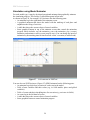
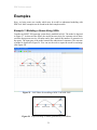
Example 1: Modeling a Queue Using SANs
Consider an M/M/3/100 queueing system that is modeled in SAN. The model is depicted
in Figure 27. As shown in the figure, the model has an activity for customer arrival, three
activities that present service execution and a place models the number of customers in
the queue. The input gate of the model controls the admission of customers. The structure
of model is depicted in Figure 26. You can use the tool to export the model as an image
(like Figure 28).
Figure 29 SAN Editor for modeling a M/M/3/100 with SAN
Figure 30 Exported image of model generated by SAN Editor
31
PDETool user manual
Table 2: Timed activities configuration of presented SAN model
Timed Activity
Distribution (rate)
Exponential (5)
Customer_Arrival
Exponential (1)
Server1
Exponential (1)
Server2
Exponential (1)
Server3
Table 2 shows the distribution and rate of all activities. The simulation results of the
model with confidence level 95% within the confidence interval 0.1 are presented in
Table 3.
Table 3: Reward variable specification and simulation results
Name
Type
Value Confidence mean
Rate{ return Place1.Mark;}
52.045
0.28
Queue length
Rate{if(Place1.Mark==100)return
1;}
0.0097
0.0009
isFull
Rate{if(Place1.Mark==0)return 1;}
0.0094
0.0009
isEmpty
Variance
850.94
0.0096
0.0093
Example 2: Modeling a packet generator system using CSANs
Consider a simple example of a packet generator system, presented in [14]. The system
generates packets with random protocol type (TCP=1, UDP=2 or RTP=3), length and
priority, and inserts them into an input buffer. An error checking (e.g. a CRC check) is
done on the generated packets. If an error is detected, the packet will be discarded;
otherwise, it will be routed to output buffers. Packets are routed probabilistically to two
output buffers with probability 0.599999 and 0.4.
The probability of detecting an error is 0.000001. The initial capacity of the system is 6
and it will stop whenever 6 packets are in error and have been discarded. The graphical
representation of the model is shown in Figure 30. Reward variables, color definitions
and global variables are also be defined in model editor. For example, in this case study,
we define a color named TPacket as follows:
TPacket={
byte Protocol;
int Len;
byte Prioriy;
}
The model is composed of a simple place (Capacity), three coloured places (InBuf,
OutBuf1 and OutBuf2), five input gates (IG1, IG2, IG3, IG4 and IG5), three output gates
(GenGate, OG1 and OG2), three timed activities (GenPacket, Send1 and Send2), and
three instantaneous activities (Route1, Route2 and ErrChk). The selection policy for
InBuf is FIFO and for OutBuf1 and OutBuf2 is Priority. The Priority function of these two
coloured places that determines the priority of sending packets from the each output
buffer and other parameters of the model are shown in Table 4 which depicts parameter
table for the definition of priority functions of coloured places and enabling predicates
and functions of input/output gates of the model.
32
PDETool user manual
The CSAN model has also a global variable tempPacket within type TPacket. In the
initial marking of the model, there are three tokens inside Capacity and two coloured
tokens inside InBuf. There is also one token inside OutBuf1 and no token inside OutBuf2.
Figure 31 CSAN model of the presented packet generator
To evaluate the constructed model, modeler must define some reward variables. After
definition of model and related reward structures, the model can be evaluated by Model
Simulator. For example, if Reward1 and Reward2 are steady state rate rewards which
denote the average number of tokens in OutBuf1 and OutBuf2 respectively, the
simulation results obtained from Model Simulator depicted in Table 5.
33
PDETool user manual
Table 3: Parameters of the presented CSAN model
Table 4: Reward variable specification and simulation results
Reward
Value
Confidence
Variance
Reward1
1.20341797
0.018929343
1.980087407
Reward2
0.60774698
0.012793362
0.904446091
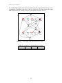
Example 3: SRN model of a multi processor system
Consider a simple multiprocessor system consisting of two dissimilar processors P1 and
P2 as in [15] which can be failed and repaired. The system is functioning as long as one
of the two processors is functioning and failures of the two processors to be independent.
While both processors work, the time to occurrence of a failure in the two processors P1
and P2 is assumed to be a random variable with the corresponding distributions being
exponential with rates λ1 and λ2, respectively. When only one processor is functioning,
the rate of failure could be correspondingly altered to reflect the fact that a single
processor shares the load of both the processors. When only P1 is functioning, we assume
its failure rate is λ’1 and when only P2 is functioning, its failure rate is λ’2. The both
processors can also fail simultaneously in exponential time λc.
Assume that the system has imperfect coverage of the failure of the processors.
Whenever a processor suffers a failure, with some probability c, called the coverage
probability, the failure is properly detected. With probability 1-c, the processor suffers an
uncovered failure, wherein the failure goes undetected. We assume that this undetected
failure results in the other normal processor also failing, causing the system failure.
34
PDETool user manual
We could consider repair of the processors where the time to repair the processors is also
exponentially distributed with rates δ1 and δ2, respectively. We also assume that when
both the processors are waiting for repair, P1 has priority for repair over P2.
Figure 32 SRN model of the multi processor system
Table 5: Availability of the multiprocessor system
C
0.1
0.8
0.9
Availability 0.5629779 0.5629779 0.56297792
35
PDETool user manual
Appendix A: Known bugs and limitation
Here is the list of known bugs:
• Exporting model as an image has bug (when the model is bigger than the screen).
• In graphical editor, multiple elements cannot be selected.
We appreciate your feedback on this tool and bugs report by sending an email to:
[email protected]. Please look at the home page of the tool for more information on how to
get in contact with the developers.
36
PDETool user manual
Reference:
1. A. Zimmermann, "Stochastic Discrete-Event Systems: Modeling, Evaluation and
Applications", Springer, 2008.
2. W.H. Sanders and J.F. Meyer: "A Unified Approach for Specifying Measures of
Performance, Dependability and Performability," Dependable Computing for Critical
Applications, Vol. 4, Springer-Verlag, pp.215-237, 1991.
3. C.A. Petri. Kommunikation mit Automaten. PhD thesis, Universit¨at Bonn, 1962.
4. RI. IC. Molloy. Performance analysis using stochastic Petri nets. IEEE Transaction on
Computers, 3 l(9) :9 13-9 17, September 1982.
5. Ajmone Marsan, M., Balbo, G., and Conte, G. A class of Generalized Stochastic Petri Nets
for the performance evaluation of multiprocessor systems. ACM Transactions on Computer
Systems. Vol.2, No.2, pp.93-122, 1984.
6. Ciardo, G. and Muppala, J.K. and Trivedi, K.S., Analyzing Concurrent and Fault-Tolerant
Software Using Stochastic Reward Nets, Journal of Parallel and Distributed Computing,
Vol.15, No.3, pp.255--269, 1992.
7. "SimGine Framework Homepage": http://pdel.iust.ac.ir/projects/simgine.html.
8. "PDETool Homepage": http://pdel.iust.ac.ir/projects/pdetool.html.
9. M. Abdollahi Azgomi, and A. Movaghar, "An Interchange Format for Stochastic Activity
Networks Based on PNML Definition", Proc. of the ICATPN'04 Satellite Workshop on the
Definition, Implementation and Application of a Standard Interchange Format for Petri Nets
(XML4PN'04), pp.1-10, Italy, 2004.
10. A. Movaghar and J.F. Meyer, "Performability Modeling with Stochastic Activity Networks",
Proc. of Real-Time Systems Symp., Austin, USA, pp.215-224, 1984.
11. Peterson, J. L.,Petri nets theory and the modeling of systems. Prentice-Hall, 1981.
12. Movaghar, A. Stochastic activity networks: A new definition and some properties. Scientia
Iranica, 8(4), pp.303-311, 2001.
13. M. Abdollahi Azgo mi and A. Movaghar, "Coloured stochastic activity networks: definitions
and behaviour," Proc. of the 20th Annual UK Performance Eng. Workshop (UKPEW'04),
Bradford, UK, July 7-8, 2004, pp. 297-308.
14. A. Jalaly Bidgoly, A. Khalili, and M. Abdollahi Azgomi, "Implementation of
Coloured Stochastic Activity Networks within the PDETool Framework," in Proc. of
3rd Asia Int'l Conf. on Modelling & Simulation (AMS09), 2009, pp. 710-715.
15. Jogesh K. Muppala, Gianfranco Ciardo, Kishor S. Trivedi, "Stochastic Reward Nets
for Reliability Prediction,"
37