Download SynDEx v7 Tutorial

SynDEx v7 Tutorial
Nicolas Dos Santos, Christophe Gensoul, Kim-Hwa Khoo
Christophe Macabiau, Quentin Quadrat, Daniel de Rauglaudre,
Yves Sorel, Cécile Stentzel
December 16, 2013
2
Contents
Introduction
1
5
Example 1: algorithm, architecture, and adequation
1.1 The main algorithm . . . . . . . . . . . . . . . . . . . . . . . . .
1.1.1 Definition of a sensor . . . . . . . . . . . . . . . . . . . .
1.1.2 Definition of an actuator . . . . . . . . . . . . . . . . . .
1.1.3 Definition of a function . . . . . . . . . . . . . . . . . . .
1.1.4 Definition of the main algorithm . . . . . . . . . . . . . .
1.2 An architecture with one operator . . . . . . . . . . . . . . . . .
1.2.1 Definition of an operator . . . . . . . . . . . . . . . . . .
1.2.2 Definition of the main architecture . . . . . . . . . . . . .
1.3 An architecture with a SAM point-to-point comunication medium
1.3.1 Definition of operators . . . . . . . . . . . . . . . . . . .
1.3.2 Definition of a medium . . . . . . . . . . . . . . . . . . .
1.3.3 Definition of the main architecture . . . . . . . . . . . . .
1.3.4 Connections between the operators and the medium . . . .
1.4 An architecture with a SAM multipoint medium . . . . . . . . . .
1.5 An architecture with a RAM medium . . . . . . . . . . . . . . .
1.6 The adequation . . . . . . . . . . . . . . . . . . . . . . . . . . .
1.6.1 Without constraint . . . . . . . . . . . . . . . . . . . . .
1.6.2 With constraints . . . . . . . . . . . . . . . . . . . . . .
.
.
.
.
.
.
.
.
.
.
.
.
.
.
.
.
.
.
8
8
8
11
11
11
14
14
16
16
16
17
17
17
18
18
19
19
19
2
Example 2: parameters and hierarchy in algorithm
2.1 Definition of the function A . . . . . . . . . . . . . . . . . . . . . . . . . . . . . . . . . . . . . .
2.2 Definition of the function B . . . . . . . . . . . . . . . . . . . . . . . . . . . . . . . . . . . . . .
2.3 Definition of the algorithm with hierarchy . . . . . . . . . . . . . . . . . . . . . . . . . . . . . .
23
23
23
25
3
Example 3: delay in algorithm
3.1 Definition of the operations input, output, and calc . . . . . . . . . . . . . . . . . . . . . . . . .
3.2 Definition of the delay . . . . . . . . . . . . . . . . . . . . . . . . . . . . . . . . . . . . . . . .
3.3 Definition of the algorithm with delay . . . . . . . . . . . . . . . . . . . . . . . . . . . . . . . .
26
26
26
26
4
Example 4: repetition and library in algorithm
4.1 An algorithm with repetition without any library . . . . . . . . . .
4.1.1 Definition of the scalar ins and the function mul on scalars
4.1.2 Definition of the vectors inv and outv . . . . . . . . . . .
4.1.3 Definition of the algorithm AlgorithmMain1 . . . . . . . .
4.2 An algorithm with repetition with the int library . . . . . . . . .
4.2.1 Inclusion of the library int . . . . . . . . . . . . . . . . .
4.2.2 Definition of the algorithm AlgorithmMain2 . . . . . . . .
4.3 An algorithm with repetition with the float library . . . . . . . .
4.3.1 Inclusion of the library float . . . . . . . . . . . . . . . .
4.3.2 Definition of the function dpacc . . . . . . . . . . . . . .
4.3.3 Definition of the function dp . . . . . . . . . . . . . . . .
28
28
28
28
29
29
30
30
31
31
31
32
3
.
.
.
.
.
.
.
.
.
.
.
.
.
.
.
.
.
.
.
.
.
.
.
.
.
.
.
.
.
.
.
.
.
.
.
.
.
.
.
.
.
.
.
.
.
.
.
.
.
.
.
.
.
.
.
.
.
.
.
.
.
.
.
.
.
.
.
.
.
.
.
.
.
.
.
.
.
.
.
.
.
.
.
.
.
.
.
.
.
.
.
.
.
.
.
.
.
.
.
.
.
.
.
.
.
.
.
.
.
.
.
.
.
.
.
.
.
.
.
.
.
.
.
.
.
.
.
.
.
.
.
.
.
.
.
.
.
.
.
.
.
.
.
.
.
.
.
.
.
.
.
.
.
.
.
.
.
.
.
.
.
.
.
.
.
.
.
.
.
.
.
.
.
.
.
.
.
.
.
.
.
.
.
.
.
.
.
.
.
.
.
.
.
.
.
.
.
.
.
.
.
.
.
.
.
.
.
.
.
.
.
.
.
.
.
.
.
.
.
.
.
.
.
.
.
.
.
.
.
.
.
.
.
.
.
.
.
.
.
.
.
.
.
.
.
.
.
.
.
.
.
.
.
.
.
.
.
.
.
.
.
.
.
.
.
.
.
.
.
.
.
.
.
.
.
.
.
.
.
.
.
.
.
.
.
.
.
.
.
.
.
.
.
.
.
.
.
.
.
.
.
.
.
.
.
.
.
.
.
.
.
.
.
.
.
.
.
.
.
.
.
.
.
.
.
.
.
.
.
.
.
.
.
.
.
.
.
.
.
.
.
.
.
.
.
.
.
.
.
.
.
.
.
.
.
.
.
.
.
.
.
.
.
.
.
.
.
.
.
.
.
.
.
.
.
.
.
.
.
.
.
.
.
.
.
.
.
.
.
.
.
.
.
.
.
.
.
.
.
.
.
.
.
.
.
.
.
.
.
.
.
.
.
.
.
.
.
.
.
.
.
.
.
.
.
.
.
.
.
.
.
.
.
.
.
.
.
.
.
.
.
.
.
.
.
.
.
.
.
.
.
.
.
.
.
.
.
.
.
.
.
.
.
.
.
.
.
.
.
.
.
.
.
.
.
4.3.4
4.3.5
5
Definition of the function prodmatvec . . . . . . . . . . . . . . . . . . . . . . . . . . . .
Definition of the algorithm AlgorithmMain3 . . . . . . . . . . . . . . . . . . . . . . . . .
.
.
.
.
.
.
.
.
35
35
35
35
35
39
39
39
39
6
Example 6: algorithm, architecture, adequation, and code generation
6.1 The main algorithm . . . . . . . . . . . . . . . . . . . . . . . . . . . . . . . . . . . . . . . . . .
6.2 The main architecture . . . . . . . . . . . . . . . . . . . . . . . . . . . . . . . . . . . . . . . . .
6.3 The adequation and the code generation . . . . . . . . . . . . . . . . . . . . . . . . . . . . . . .
41
41
41
42
7
Example 7: source code associated with an operation
7.1 Definition of the source code into the code editor window .
7.1.1 To add parameters to an already defined operation .
7.1.2 To edit the code associated with an operation . . .
7.1.3 To generate m4x files . . . . . . . . . . . . . . . .
8
9
Example 5: condition and nested condition in algorithm
5.1 An algorithm with condition . . . . . . . . . . . . .
5.1.1 Sensors x and i, actuator o . . . . . . . . . .
5.1.2 Function switch1 . . . . . . . . . . . . . . .
5.1.3 Algorithm AlgorithmMain1 . . . . . . . . . .
5.2 An algorithm with nested condition . . . . . . . . .
5.2.1 Sensors x and i, actuator o . . . . . . . . . .
5.2.2 Function switch2 . . . . . . . . . . . . . . .
5.2.3 Algorithm AlgorithmMain2 . . . . . . . . . .
33
33
.
.
.
.
.
.
.
.
.
.
.
.
.
.
.
.
.
.
.
.
.
.
.
.
.
.
.
.
.
.
.
.
.
.
.
.
.
.
.
.
.
.
.
.
.
.
.
.
.
.
.
.
.
.
.
.
.
.
.
.
.
.
.
.
.
.
.
.
.
.
.
.
.
.
.
.
.
.
.
.
.
.
.
.
.
.
.
.
.
.
.
.
.
.
.
.
.
.
.
.
.
.
.
.
.
.
.
.
.
.
.
.
.
.
.
.
.
.
.
.
.
.
.
.
.
.
.
.
.
.
.
.
.
.
.
.
.
.
.
.
.
.
.
.
.
.
.
.
.
.
.
.
.
.
.
.
.
.
.
.
.
.
.
.
.
.
.
.
.
.
.
.
.
.
.
.
.
.
.
.
.
.
.
.
.
.
.
.
.
.
.
.
.
.
.
.
.
.
.
.
.
.
.
.
.
.
.
.
.
.
.
.
.
.
.
.
.
.
.
.
.
.
.
.
.
.
.
.
.
.
.
.
.
.
.
.
.
.
.
.
.
.
.
.
45
45
45
46
49
Example 8: a complete realistic application from adequation to execution
8.1 The aim of the example . . . . . . . . . . . . . . . . . . . . . . . . . .
8.2 The model . . . . . . . . . . . . . . . . . . . . . . . . . . . . . . . . .
8.3 The controllers . . . . . . . . . . . . . . . . . . . . . . . . . . . . . .
8.3.1 Block diagrams of controllers . . . . . . . . . . . . . . . . . .
8.3.2 Source code associated with the functions . . . . . . . . . . . .
8.4 The complete model . . . . . . . . . . . . . . . . . . . . . . . . . . .
8.4.1 The car dynamics . . . . . . . . . . . . . . . . . . . . . . . . .
8.4.2 The cars and their controllers . . . . . . . . . . . . . . . . . . .
8.4.3 The main algorithm . . . . . . . . . . . . . . . . . . . . . . . .
8.4.4 Source code associated with the sensor and the actuator . . . . .
8.4.5 The example8 sdc.m4x . . . . . . . . . . . . . . . . . . . . . .
8.4.6 To handwrite the example8.m4x file . . . . . . . . . . . . . . .
8.5 Scicos simulation . . . . . . . . . . . . . . . . . . . . . . . . . . . . .
8.6 SynDEx simulation . . . . . . . . . . . . . . . . . . . . . . . . . . . .
8.6.1 In the case of a mono-processor architecture . . . . . . . . . . .
8.6.2 In the case of a bi-processor architecture . . . . . . . . . . . . .
8.6.3 In the case of a multi-processor architecture . . . . . . . . . . .
.
.
.
.
.
.
.
.
.
.
.
.
.
.
.
.
.
.
.
.
.
.
.
.
.
.
.
.
.
.
.
.
.
.
.
.
.
.
.
.
.
.
.
.
.
.
.
.
.
.
.
.
.
.
.
.
.
.
.
.
.
.
.
.
.
.
.
.
.
.
.
.
.
.
.
.
.
.
.
.
.
.
.
.
.
.
.
.
.
.
.
.
.
.
.
.
.
.
.
.
.
.
.
.
.
.
.
.
.
.
.
.
.
.
.
.
.
.
.
.
.
.
.
.
.
.
.
.
.
.
.
.
.
.
.
.
.
.
.
.
.
.
.
.
.
.
.
.
.
.
.
.
.
.
.
.
.
.
.
.
.
.
.
.
.
.
.
.
.
.
.
.
.
.
.
.
.
.
.
.
.
.
.
.
.
.
.
.
.
.
.
.
.
.
.
.
.
.
.
.
.
.
.
.
.
.
.
.
.
.
.
.
.
.
.
.
.
.
.
.
.
.
.
.
.
.
.
.
.
.
.
.
.
.
.
.
.
.
51
51
51
52
52
54
54
55
56
56
56
60
61
62
62
62
64
65
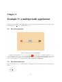
Example 9: a multiperiodic application
9.1 The main algorithm . . . . . . . . .
9.2 The main architecture . . . . . . . .
9.3 A mono-phase schedule . . . . . . .
9.3.1 Durations . . . . . . . . . .
9.3.2 Adequation . . . . . . . . .
9.4 A multi-phase schedule . . . . . . .
9.4.1 Durations . . . . . . . . . .
9.4.2 Adequation . . . . . . . . .
.
.
.
.
.
.
.
.
.
.
.
.
.
.
.
.
.
.
.
.
.
.
.
.
.
.
.
.
.
.
.
.
.
.
.
.
.
.
.
.
.
.
.
.
.
.
.
.
.
.
.
.
.
.
.
.
.
.
.
.
.
.
.
.
.
.
.
.
.
.
.
.
.
.
.
.
.
.
.
.
.
.
.
.
.
.
.
.
.
.
.
.
.
.
.
.
.
.
.
.
.
.
.
.
.
.
.
.
.
.
.
.
67
67
67
68
68
68
69
69
69
.
.
.
.
.
.
.
.
.
.
.
.
.
.
.
.
.
.
.
.
.
.
.
.
.
.
.
.
.
.
.
.
.
.
.
.
.
.
.
.
.
.
.
.
.
.
.
.
4
.
.
.
.
.
.
.
.
.
.
.
.
.
.
.
.
.
.
.
.
.
.
.
.
.
.
.
.
.
.
.
.
.
.
.
.
.
.
.
.
.
.
.
.
.
.
.
.
.
.
.
.
.
.
.
.
.
.
.
.
.
.
.
.
.
.
.
.
.
.
.
.
.
.
.
.
.
.
.
.
.
.
.
.
.
.
.
.
.
.
.
.
.
.
.
.
.
.
.
.
.
.
.
.
.
.
.
.
.
.
.
.
.
.
.
.
.
.
.
.
.
.
.
.
.
.
.
.
Introduction
This tutorial respects some writing conventions:
• menus, buttons, etc., are written in bold
(e.g. Algorithm / New Algorithm Window, OK, Definition list);
• command lines, SynDEx files, examples, etc., are written in Computer Modern
(e.g. -libs libs, examples/tutorial, ! int o);
To create an application workspace, launch SynDEx with option -libs libs. See the SynDEx v7 User Manual for more information.
The examples presented in this tutorial are located in the sub-folder examples/tutorial. Each example is located in its sub-folder. The example 7 is located in the examples/tutorial/example7, examples/tutorial/example7 mono,
and examples/tutorial/example7 bi folders.
Example 1
Algorithm, architecture, and adequation:
• we create a sensor definition, an actuator definition, and a function definition. Then, we create an algorithm
and define it as main. Finally, we create in the main algorithm two references to the sensor definition,
three references to the actuator definition, and one reference to the function definition, and we create data
dependences between these references by connecting their ports;
• we create four different architectures:
– an architecture with one operator,
– an architecture with two operators and a SAM point-to-point communication medium,
– an architecture with three operators and a SAM multipoint communication medium,
– an architecture with three operators and a RAM communication medium;
• we create constraints on the third architecture;
• we perform the adequation of the main algorithm onto the third architecture defined as main, without constraint and then with constraints.
Example 2
Hierarchy in algorithm:
• we create a function definition and a constant. Inside the function we create a reference to another function;
in that way this definition is defined by hierarchy. Then, we create a third function that references both
previous ones. Finally, we create an algorithm that references the third function and define it as main. In
that way, the main algorithm references a hierarchical function;
• we create parameters names for an operation, and assign values to these parameters.
5
Example 3
Delay in algorithm:
• we create a delay definition;
• we create a main algorithm by referencing a delay, a sensor, an actuator, and a function and by connecting
them.
Example 4
Repetition and library in algorithm:
• we create a multiplication function of a vector by a scalar by repeating a multiplication function on scalars:
– firstly without any library,
– secondly with a library;
• we create a multiplication function of a matrix by a vector by repeating a multiplication function on vectors.
Example 5
Condition and nested condition in algorithm:
• we create an algorithm conditioned by a data dependence, the value of which indicates the operation to be
executed;
• we create an algorithm conditioned by a data dependence, one operation of which is in turn conditioned
(nested condition) by the same data dependence.
Example 6
Algorithm, architecture, adequation, and code generation:
• we create a main algorithm by referencing a sensor, two actuators, three functions, and a constant and by
connecting them;
• we create an architecture with two operators of type U and a communication medium of type u/TCP;
• we perform the adequation;
• we perform the code generation, then we create manualy the example6.m4x file (for operations not defined
in libraries);
• we create manualy the example6.m4m file (to define the hostname) and the root.m4x file (for the main operator);
• we create manualy the GNUmakefile, then we execute the executives created after compilation.
Example 7
Definition of the source code into the code editor window:
• we add parameters to the conv function of Example 6;
• we modify the code associated with this function first in case of a generic processor then in case of an
architecture with heterogenous processors;
• we create manualy the example7.m4m file (to define the hostname) and the root.m4x file (for the main operator);
• we create manualy the GNUmakefile;
6
• we perform the adequation, then we perform compilation, finally we compile the executives and launch the
executables.
Definition of the source code in separate C files:
• we define the code of a new function in a .c file,
• we define the code of a new function in a .c file and we use a .h file.
Example 8
A complete realistic application from adequation to execution:
• we build the model of a complete application for two cars;
• we perform the adequation;
• we generate the code for each processor;
• we compile and execute the code associated with each processor.
Example 9
A multiperiodic application:
• we build a basic multi-periodic application
• mono-phase schedule
• multi-phase schedule
7
Chapter 1
Example 1: algorithm, architecture, and
adequation
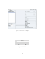
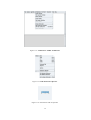
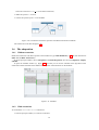
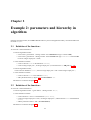
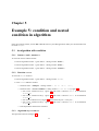
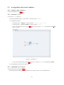
1.1 The main algorithm
Figure 1.1: Algorithm / New Algorithm Window
From the principal window, choose the File / Save as option and save your first application under a new folder
(e.g. my tutorial) with the name example1.
Choose Algorithm / New Algorithm Window (cf. figure 1.1). It opens the edition window for algorithm
definitions.
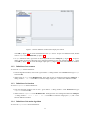
1.1.1 Definition of a sensor
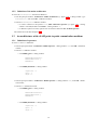
To create an input sensor definition:
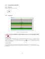
• from the algorithm window, click on the + green button. It opens a dialog window, check Sensor (cf. figure
1.2). Type the sensor name and optionally a list of parameters for the sensor. For example type input, then
8
Figure 1.2: Define Sensor
Figure 1.3: Name of the new sensor
Figure 1.4: Sensor definition window
9
Figure 1.5: Contextual menu → Add port
Figure 1.6: Create Port
10
Figure 1.7: Sensor definition window after output port created
click OK (cf. figure 1.3). It creates the definition of the input sensor. To open it in definition mode, double
click on input in the Definition list (cf. figure 1.4);
• in input definition mode, right click on the background and select Add port (cf. figure 1.5). It opens a
dialog window for the port’s direction, type, name and optionally its size. For example type ! int o, then
click OK (cf. figure 1.6). It creates the integer output port o (cf. figure 1.7) in the sensor definition window.
1.1.2 Definition of an actuator
To create an output actuator definition:
• from the algorithm window, click on the + green button → dialog window: check Actuator then type output
and click OK;
• double click on output in the Definition list. Then right click on its background and select Add port →
dialog window: ? int i. Click OK. It creates the integer input port i in the sensor definition window.
1.1.3 Definition of a function
To create a computation function definition:
• from the algorithm window, click on the + green button → dialog window: check Function then type
computation and click OK;
• double click on computation in the Definition list. Thenright click on its background and select Add port
→ dialog window: ? int a ? int b ! int o. Click OK. It creates the integer ports a, b, and o in the
function definition window.
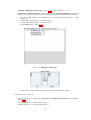
1.1.4 Definition of the main algorithm
To create an AlgorithmMain function definition:
11
Figure 1.8: Contextual menu → Set As Main Definition
Figure 1.9: Drag and drop input definition
12
Figure 1.10: Create References to input
Figure 1.11: Main algorithm after references to sensor created
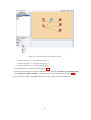
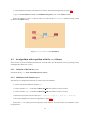
Figure 1.12: Main algorithm of the Example 1
13
• from the algorithm window, click on the + green button → dialog window: check Function then type
AlgorithmMain and click OK;
• double click on AlgorithmMain in the Definition list. Then right click on its background and select Set As
Main Definition (cf. figure 1.8);
• in its definition mode,
– to create references to the sensor input, drag and drop the sensor definition from the Definition list
to the AlgorithmMain definition window (cf. figure 1.9) → dialog window: in1 in2 (cf. figure 1.10).
The main algorithm looks like the figure 1.11,
– to create references to the actuator output, drag and drop the actuator definition from the Definition
list to the AlgorithmMain definition window → dialog window: out1 out2 out3,
– to create a reference to the function computation, drag and drop its definition → dialog window: calc,
– from the AlgorithmMain definition window, to create a data dependence between in1 and calc, point
the cursor on the output port o of the in1 operation, middle click, and drag to the input port a of the calc
operation. It draws an arrow between these target ports. After creating the other data dependences, the
main algorithm looks like the figure 1.12.
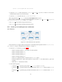
1.2 An architecture with one operator
1.2.1 Definition of an operator
Figure 1.13: Operator definition window
To create an Uinout operator definition:
• from the principal window, choose Architecture / Define Operator. It opens a dialog window, type Uinout
and click OK. It opens the operator definition window (cf. figure 1.13);
• from the Uinout definition window:
– to add a gate: click Modify gates → dialog window: gate type 1 x,
– to set the operator execution durations: click Modify durations → dialog window:
computation = 2
input = 1
output = 3
14
Figure 1.14: Architecture / Define Architecture
Figure 1.15: Edit / Reference Operator
Figure 1.16: Architecture with one operator
15
1.2.2 Definition of the main architecture
To create an ArchiOneOperator architecture definition:
• from the principal window: Architecture / Define Architecture (cf. figure 1.14) → dialog window: type
ArchiOneOperator then click OK → definition window;
• from the ArchiOneOperator definition window:
– to create a reference to the operator Uinout, Edit / Reference Operator (cf. figure 1.15) → dialog
window: click user, double click Uinout → dialog window: u1,
– to define the operator as main, right click on its reference and select Set As Main Operator.
The architecture looks like the figure 1.16.
1.3 An architecture with a SAM point-to-point comunication medium
1.3.1 Definition of operators
To create Uin and Uout definitions:
• from the principal window: Architecture / Define Operator → dialog window: Uin, click OK → definition
window;
• from the Uin definition window:
– click Modify gates → dialog window:
MediumSamPointToPoint x
MediumSamMultiPoint y
MediumRam z
– click Modify durations → dialog window:
computation = 2
input = 2
output = 5
• from the principal window: Architecture / Define Operator → dialog window: Uout, click OK → definition window;
• from the Uout definition window:
– click Modify gates → dialog window:
MediumSamPointToPoint x
MediumSamMultiPoint y
MediumRam z
– click Modify durations → dialog window:
computation = 2
input = 5
output = 3
16
1.3.2 Definition of a medium
Figure 1.17: Type of a communication medium
To create a MediumSamPointToPoint medium definition:
• from the principal window: Architecture / Define Medium → dialog window: MediumSamPointToPoint,
click OK → definition window;
• from the MediumSamPointToPoint definition window:
– click Modify type → dialog window: SAM Point to Point (cf. figure 1.17),
– click Modify durations → dialog window:
float = 2
int = 2
uchar = 1
ushort = 1
1.3.3 Definition of the main architecture
To create an ArchiSamPointToPoint architecture definition:
• from the principal window: Architecture / Define Architecture (cf. figure 1.14) → dialog window
ArchiSamPointToPoint → definition window;
• from the ArchiSamPointToPoint definition window, create references u1 and u2 to the operators Uin and
Uout;
• from the ArchiSamPointToPoint definition window: Edit / Reference Medium → dialog window: click
user, select MediumSamPointToPoint → dialog window: type medium sampp;
• define the operator u1 as main.
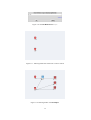
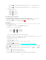
1.3.4 Connections between the operators and the medium
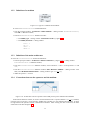
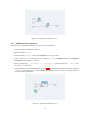
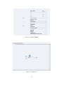
Figure 1.18: Architecture with two operators and a SAM point-to-point communication medium
In the main architecture window, to create a connection between the u1 operator and the medium sampp medium,
point the cursor on the port x of the operator, middle click, and drag it to the communication medium. It draws
an edge between the operator and the communication medium. After creating the other connection, the main
architecture looks like the figure 1.18.
17
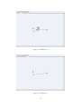
1.4 An architecture with a SAM multipoint medium
To create an ArchiSamMultiPoint architecture definition:
• from the principal window: Architecture / Define Architecture (cf. figure 1.14) → dialog window:
ArchiSamMultiPoint → ArchiSamMultiPoint definition window;
• create references u1 and u2 to the operator Uin and a reference u3 to the operator Uout, like in the previous
example;
• create a medium definition MediumSamMultiPoint of type SAM MultiPoint with durations:
float=2
int=2
uchar=1
ushort=1
• create a reference medium sammp to this medium in the main architecture window → dialog window: check
No Broadcast;
• define the operator u1 as main;
• connect the operators ports y to the medium.
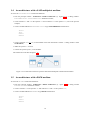
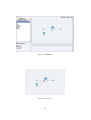
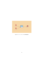
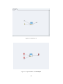
The architecture looks like the figure 1.19
Figure 1.19: Architecture with three operators and a SAM multipoint communication medium
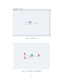
1.5 An architecture with a RAM medium
To create the ArchiRam architecture definition:
• from the principal window: Architecture / Define Architecture (cf. figure 1.14) → dialog window
ArchiRam → ArchiRam definition window;
• create a reference u1 to the operator Uin and references u2 and u3 to the operator Uout;
• create a medium definition MediumRam of type RAM with durations
float=2
int=2
uchar=1
ushort=1
18
and create a reference medium ram in the main architecture;
• define the operator u1 as main;
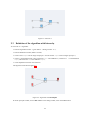
• connect the operators ports z to the medium.
Figure 1.20: Architecture with three operators and a RAM comunication medium
The architecture looks like the figure 1.20.
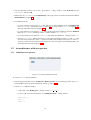
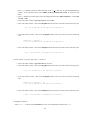
1.6 The adequation
1.6.1 Without constraint
Define the architecture with three operators and a medium of type SAM MultiPoint (cf. 1.4) as main architecture
(Edit / Set As Main Architecture).
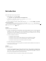
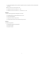
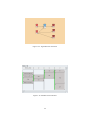
From the principal window, choose Adequation / Launch Adequation, then choose Adequation / Display
schedule.
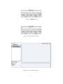
It opens the schedule window (cf. figure 1.21) in which you can see the schedule of the algorithm on the
architecture and the schedule of the different inter-operator communications on the medium.
Figure 1.21: Schedule
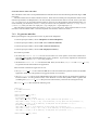
1.6.2 With constraints
To contraint the ArchiSamMultiPoint architecture:
• from the principal window, to create the constraints:
19
– Algorithm / Define Operation Group (cf. figure 1.22) → dialog window: og1 og2 og3,
– Constraints / Absolute Constraints → dialog window: select ArchiSamMultiPoint It opens a dialog
window in which you can create constraints on the different operators of the architecture selected:
∗ first click on og1, then u1, and the Create button, to constrain the operation group og1 on the
operator u1,
∗ constrain the operation group og2 on the operator u2,
∗ constrain the operation group og3 on the operator u3,
∗ click on OK button (cf. figure 1.23),
Figure 1.22: Define Operation Group
Figure 1.23: Constrain operation groups on operators of the architecture selected
• in the main mode (Main button):
– select the operation in1, click on the Group button of its Reference Properties then select og1 (cf.
figure 1.24),
– attach the operation in2 to the operation group og2,
– attach the operation out1 to the operation group og1,
20
Figure 1.24: Attach a reference to an operation group
– attach the operation out2 to the operation group og2,
– attach the operation out3 to the operation group og3,
– attach the operation calc to the operation group og3;
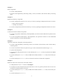
The algorithm with constraints looks like the figure 1.25.
• from the principal window, to perform the adequation with constraints: Adequation / Launch Adequation,
then Adequation / Display Schedule → schedule window. The schedule looks like the figure 1.26.
From the principal window, choose File / Close. In the dialog window, click on the Save button.
21
Figure 1.25: Algorithm with constraints
Figure 1.26: Schedule with constraints
22
Chapter 2
Example 2: parameters and hierarchy in
algorithm
From the principal window, choose File / Save as and save your second application under your tutorial folder with
the name example2.
2.1 Definition of the function A
To create the A function definition:
• from the algorithm window:
– click on the + green button → dialog window: check Function then type A and click OK,
– click on the + green button → dialog window: check Constant then type constante<X> and click OK.
Create an integer output port o inside;
• in the A definition window:
– create a reference cst<T> to the definition constante,
– create an integer input port a, an integer output port o (Contextual menu → Add port cf. 1.1.3);
• from the algorithm window,
create a function definition calcul1, with two integer input ports a and b and an integer output port o;
• in the A definition window:
– create a reference calc1 to the definition calcul1,
– add a parameter name (cf. figure 2.1): Field Parameters → T.
The function A looks like the figure 2.2.
2.2 Definition of the function B
To create the B function definition:
• from the algorithm window: + green button → dialog window: B<X;Y>;
• in the B definition window:
– create references A1 and A2 to the definition A (A1<X> A2<Y>),
– create two integer input ports a and b, one integer output port o, and the function calc1 of the definition
calcul1,
– add the parameters names X and Y (field Parameters).
The function B looks like the figure 2.3.
23
Figure 2.1: Parameters
Figure 2.2: Function A
24
Figure 2.3: Function B
2.3 Definition of the algorithm with hierarchy
To create the Main algorithm:
• from the algorithm window: + green button → dialog window: Main;
• from the definition window, define it as main;
• create a sensor input with an integer output port o and an actuator output with an integer input port i;
• in the Main algorithm window, create a reference B<1;2> to the definition B, a reference i1 i2 to the definition
input, and a reference out to the definition output;
• create dependences between the references.
The algorithm looks like the figure 2.4.
Figure 2.4: Algorithm of the Example 2
From the principal window, choose File / Close. In the dialog window, click on the Save button.
25
Chapter 3
Example 3: delay in algorithm
From the principal window, choose File / Save as and save your third application under your tutorial folder with
the name example3.
3.1 Definition of the operations input, output, and calc
Create a sensor input, an actuator output, and the function calc, like in the Examples 1 and 2. (cf. 1.1.3 and
calcul1 in 2.1)
3.2 Definition of the delay
To create the calcPrec delay:
• from the algorithm window, click on the + green button → dialog window: check Delay then type calcPrec<init;size>
and click OK; The parameter init will be used to specify the initial value of the delay, and size the number
of delays;
• in the definition window, create one input port and one output port. Enter: ? int i ! int o.
3.3 Definition of the algorithm with delay
Create an algorithm algorithmMain. Create a reference in1 to the definition input, a reference calc to the definition calc, a reference out1 to the definition output, and a reference calcPrec<0;1> to the definition calcPrec.
Create dependences between the references.
The algorithm looks like the figure 3.1.
From the principal window, choose File / Close. In the dialog window, click on the Save button.
26
Figure 3.1: Algorithm of the Example 3
27
Chapter 4
Example 4: repetition and library in
algorithm
From the principal window, choose File / Save as and save your fourth application under your tutorial folder with
the name example4.
4.1 An algorithm with repetition without any library
In this section, we create a multiplication function of a N elements vector by a scalar by repeating N times a
multiplication function on scalars.
4.1.1 Definition of the scalar ins and the function mul on scalars
In a new algorithm window:
• create a new sensor definition named ins with an integer output port o;
• create a new function definition named mul with two integer input ports a and b and an integer ouput port o).
4.1.2 Definition of the vectors inv and outv
To create the vectors:
• to create the definition inv:
– from the algorithm window, create a new sensor definition named inv,
– from the inv definition window, type N in the Parameters textfield of its Definition Properties (it has
N elements),
– create its integer output port named o with length N: ! int[N] o;
• to create the definition outv:
– from the algorithm window, create a new actuator definition outv,
– in outv definition window, type N in the Parameters textfield of its Definition Properties (it has N
elements),
– create its integer input port named i with length N: ? int[N] i.
28
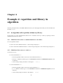
4.1.3 Definition of the algorithm AlgorithmMain1
To create the AlgorithmMain1 algorithm:
• from the algorithm window, create a new function definition named AlgorithmMain1 and from its definition
window, define it as main;
• in the AlgorithmMain1 definition mode:
– create a reference s input to the scalar ins,
– create a reference v input<N> to the vector inv,
– create a reference mul to the function mul and type N in the Repeat textfield of its Reference Properties
(it is repeated N times),
– create a reference v output<N> to the vector outv;
• create dependences between the references, in order to obtain the main algorithm (cf. figure 4.2);
• type N in the Parameters textfield of the Definition Properties of the main algorithm and 3 in the Values
textfield (cf. figure 4.1). Notice that this value is keeped as long as the algorithm remains the main one.
Figure 4.1: Parameters Values
The repetition consists in multiplying each of the 3 elements of the v input vector with the s input scalar and
placing the result in the 3 elements v output vector.
The parameter N is here the repetition factor of the mul function.
Figure 4.2: AlgorithmMain1 of the Example 4
4.2 An algorithm with repetition with the int library
In this section, we create a multiplication function of a vector by a scalar by using the int library.
29
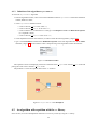
4.2.1 Inclusion of the library int
From the principal window choose File / Specify Library Directories and add the SYNDEXPATH/libs where
SYNDEXPATH is the absolute path of the SynDEx distribution.
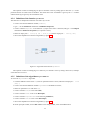
From the principal window, choose File / Included Libraries / int (cf. figure 4.3).
Figure 4.3: File / Included Libraries / int
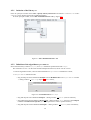
4.2.2 Definition of the algorithm AlgorithmMain2
Notice that this library contains input, mul, and output definitions parameterized with length.
We will need to set it to 1 for the scalar and the multiplication function, and to N for the vectors:
• from the algorithm window, create the function definition AlgorithmMain2 and define it as main;
• in AlgorithmMain2 definition mode:
– drag and drop the sensor definition int/input from the Definition list to the AlgorithmMain2 window
→ dialog window: s input<1> (cf. figure 4.4) (it is a scalar),
Figure 4.4: Create Reference to int/input
– drag and drop the sensor definition int/input → dialog window: v input<N> (it has N elements),
– drag and drop the function definition int/Arit mul → dialog window: mul<1> then type N in the Repeat
textfield of its Reference Properties, (it is a multiplication on scalars, repeated N times),
– drag and drop the actuator definition int/output → dialog window: v output<N> (it has N elements);
30
• create dependences between the references in order to obtain the main algorithm (cf. figure 4.5);
• type N in the Parameters textfield of the Definition Properties, and 3 in the Values textfield.
Notice the difference of the mul reference when it is seen from the AlgorithmMain2 definition mode or from
the main mode (Main button).
Figure 4.5: AlgorithmMain2 of the Example 4
4.3 An algorithm with repetition with the float library
In this section, we create a multiplication function of a N*M matrix by a M elements vector by repeating N times
a multiplication function on vectors.
4.3.1 Inclusion of the library float
Include the library float (File / Included Libraries / Float).
4.3.2 Definition of the function dpacc
This function is a multiplication function on scalars with an accumulator:
• create a new function definition named dpacc;
• create a reference mul<1> to the function float/Arit mul (the reference works on scalars);
• create a reference add<1> to the function float/Arit add (the reference works on scalars);
• add it three input ports and one output port: ? float s1 ? float s2 ? float acc ! float acc;
• then create dependences to obtain an algorithm (cf. figure 4.6).
Notice that acc is an input port and an output port of the function. It will be used as an accumulator to store
the partial sum.
31
Figure 4.6: Algorithm of the function dpacc
4.3.3 Definition of the function dp
This function is a multiplication function on vectors with an accumulator:
• create a new function definition named dp;
• add it a parameter dpaccn;
• create a reference zero<{0}> to the constant float/cst (it is the {0} scalar);
• create a reference dpacc to the function dpacc then type dpaccn in the Repeat textfield of its Reference
Properties (it is repeated dpaccn times);
• add it two input ports: ? float[dpaccn] v1 ? float[dpaccn] v2 and one output port: ! float dp (vectors have dpaccn elements);
• create dependences to obtain an algorithm (cf. figure 4.7). To build the dependence between the output port
acc of dpacc and its input port acc, choose Iterate on the dialog window (it is the connection between two
successive calls of the function).
Figure 4.7: Algorithm of the function dp
32
The repetition consists in multiplying two dpaccn elements vectors by calling dpaccn times the dpacc multiplication function on scalars with accumulator. The initial value of its accumulator is given by the zero constant
and the following are given by the accumulator itself.
4.3.4 Definition of the function prodmatvec
This function is a multiplication function of a matrix by a vector:
• create a new function definition named prodmatvec;
• type a;b in the Parameters textfield of its Definition Properties;
• create a reference dotprod<b> to the function dp (input vectors have b elements) and type a in the Repeat
textfield of its Reference Properties (it is repeated a times);
• add it two input ports: ? float[a*b] inm ? float[b] inv and one output port: ! float[a] outv;
• then create dependences to obtain an algorithm (cf. figure 4.8).
Figure 4.8: Algorithm of the function prodmatvec
The repetition consists in multiplying a a*b matrix by a b elements vector by calling a times the dp multiplication function on vectors.
4.3.5 Definition of the algorithm AlgorithmMain3
To create the AlgorithmMain3 algorithm:
• create the definition of the sensor inm, with two parameters names N and M, and with an output port: ! float
[N*M] o;
• create a new function definition named AlgorithmMain3 and define it as main;
• add it two parameters:N;M with values 3;4;
• create a reference m1<N;M> to the matrix inm;
• create a reference inv<N> to the vector float/input;
• create a reference matprodvec<N;M> to the function prodmatvec;
• create a reference outv<M> to the vector float/output;
• then create dependences to obtain an algorithm (cf. figure 4.9).
From the principal window, choose File / Close. In the dialog window, click on the Save button.
33
Figure 4.9: AlgorithmMain3 of the Example 4
34
Chapter 5
Example 5: condition and nested
condition in algorithm
From the principal window, choose File / Save as and save your fifth application under your tutorial folder with
the name example5.
5.1 An algorithm with condition
5.1.1 Sensors x and i, actuator o
To create the sensors and the actuator:
• from the algorithm window: + green button → dialog window: Sensor x;
• from the algorithm window: + green button → dialog window: Sensor i;
• from the algorithm window: + green button → dialog window: Actuator o.
5.1.2 Function switch1
To create the switch1 function:
• from the algorithm window: + green button → dialog window: switch1;
• in the switch1 definition window:
– contextual menu → Add port → dialog window: ? int x ? int i ! int o,
– contextual menu → Create Condition → dialog window: x=1 x=2 x=3 x=4 (cf. figure 5.1):
∗ click on the condition x=1 (cf. figure 5.2) and create a reference div1<1> to the definition
int/Arit div,
∗ click on the condition x=2 (cf. figure 5.3) and create a reference div2<1> to the definition
int/Arit div,
∗ click on the condition x=3 (cf. figure 5.4) and connect the port i to the port o,
∗ click on the condition x=4 (cf. figure 5.5) and create a reference mul4<1> to the definition
int/Arit mul;
– create dependences between the references.
5.1.3 Algorithm AlgorithmMain1
The algorithm looks like the figure 5.6.
35
Figure 5.1: Create Condition
Figure 5.2: Condition x=1
36
Figure 5.3: Condition x=2
Figure 5.4: Condition x=3
37
Figure 5.5: Condition x=4
Figure 5.6: AlgorithmMain1 of the Example 5
38
5.2 An algorithm with nested condition
5.2.1 Sensors x and i, actuator o
Use previous definitions (cf. 5.1.1).
5.2.2 Function switch2
To create the switch2 function:
• from the algorithm window: + green button → dialog window: switch2;
• in its definition window:
– contextual menu → Add port → dialog window: ? int x ? int y ! int o,
– contextual menu → Create Condition → dialog window: y=1 y=2,
– click on the condition y=1 (cf. figure 5.7) and create the function mul1<1> of the definition Arit mul
from int library,
Figure 5.7: Condition y=1
– click on the condition y=2 (cf. figure 5.8) and create a reference switch1 to the definition switch1;
• create dependences between the references.
5.2.3 Algorithm AlgorithmMain2
The algorithm looks like the figure 5.9.
From the principal window, choose File / Close. In the dialog window, click on the Save button.
39
Figure 5.8: Condition y=2
Figure 5.9: AlgorithmMain2 of the Example 5
40
Chapter 6
Example 6: algorithm, architecture,
adequation, and code generation
From the principal window, choose File / Save as and save your sixth application under a new folder of your
tutorial folder (e.g. my example6) with the name example6.
6.1 The main algorithm
Create the main algorithm algo (cf. figure 6.1) using the library int for the operations In<1> (input), cste2<{2}>
(cst), add<1> (Arit add), mul<1> (Arit mul), visuadd<1>, and visumul<1> (output). For the operation conv, create
a function definition conv, create a reference to this definition, and give it a duration. Create the dependences
between the references. Set it as main.
Figure 6.1: Main algorithm of the Example 6
Warning: it is necessary that the sensor “in” should be distributed onto the processor “root”, i.e. on the local
machine, in order that it operates properly.
6.2 The main architecture
To define and constraint the main architecture:
• include the library u,
41
• from the principal window, choose Architecture / Edit Architecture Definition and open the architecture
biProc,
• define it as main,
• create the operation groups og1 and og2 then create the absolute constraints on the operators: og1 on root,
og2 on P1. Attach references to operation groups: In, add, and visumul → og1, mul, and visuadd → og2.
6.3 The adequation and the code generation
To perform the adequation and to generate the code:
• before performing the code generation, you have to perform the adequation. Set the possibly missing
durations, then from the principal window: Adequation / Launch Adequation;
• from the principal window: Code / Generate Executive(s). It generates for each operator of the main
architecture the code in a file (files root.m4 and P1.m4) and an architecture description (file example6.m4).
These files are generated in the same folder as the application. The files generated for each processor may
be viewed: Code / Display Executive(s);
• the macros corresponding to the operations, included in the libraries of SynDEx, are already defined under
the folder macros (files int.m4x, U.m4x, and TCP.m4x);
• in the same folder as the SynDEx application of the Example 6, create a new file example6.m4x in which
you define the macro corresponding to the operation conv which is the only one not defined in the library,
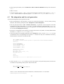
and the number of iterations. The file looks like:
dnl (c)INRIA 2001-2009
dnl SynDEx v7 executive macros specific to application tutorial/example6/example6
divert(-1)
define(‘NOTRACEDEF’)
define(‘NBITERATIONS’,3)
define(‘BINPWD’, ‘pwd’)
define(‘RSHELL’, ‘ssh’)
define(‘conv’,‘ifelse(
MGC,‘INIT’,‘dnl’,
MGC,‘LOOP’,‘$2[0] = $1[0] + 1;’,
MGC,‘END’,‘dnl’)’)
divert
divert(-1)
divert‘’dnl---------------- end of file ------------------
• create a new file example6.m4m, in which you set for each operator, except the main operator, the name of a
workstation corresponding to this operator. The file looks like:
dnl (c)INRIA 2001-2009
define(‘P1 hostname ’, HOSTNAME)dnl
where HOSTNAME is the name of the remote workstation, as indicated in the Readme file under
syndex/examples/tutorial/example6;
42
Warning: the characters ‘ and ’ are different.
Warning: if you increase the number of processors in your architecture, you must add other define statements with the corresponding “processor name”, “remote worksation name” association.
• create a new file root.m4x for the main operator including the file example6.m4m:
dnl (c)INRIA 2001-2009
include(example6.m4m)
• create a new file GNUmakefile which allows the compilation and the substitution of the macros from the code
generation by the executable code. The file looks like:
# (c)INRIA 2001-2009
A = example6
M4 = m4
export
export
export
export
SynDEx_Path = SYNDEXPATH
Algo Macros Path = $(SynDEx Path)/macros/algo libraries
Archi Macros Path = $(SynDEx Path)/macros/archi libraries
M4PATH = $(Algo Macros Path):$(Archi Macros Path)
CFLAGS = -DDEBUG
VPATH = $(M4PATH)
.PHONY: all clean
all : $(A).mk $(A).run
clean ::
$(RM) $(A).mk
$(A).mk : $(A).m4 syndex.m4m U.m4m $(A).m4m
$(M4) $< >$@
root.libs =
P1.libs =
include $(A).mk
where SYNDEXPATH is the absolute path of the SynDEx distribution.
Warning: in the previous makefile the statements $(RM) $(A).mk and $(M4) $< >$@ must begin with a tab character.
The folder of the Example 6 must contain the following files:
• example6.m4
• example6.m4m
• example6.m4x
• example6.sdc
• example6.sdx
• GNUmakefile
43
• p1.m4
• root.m4
• root.m4x
To launch the execution, type the command make in the folder of the Example 6. To delete the file created
during the compilation, type the command gmake clean.
From the principal window, choose File / Close. In the dialog window, click on the Save button.
44
Chapter 7
Example 7: source code associated with an
operation
7.1 Definition of the source code into the code editor window
In the previous Example 6, we have learnt that a m4 file, called with the name of the application plus the m4x
extension, must be manually written. It contains all the source code associated with all operations present in a
SynDEx application. For example, in the example6 application, the conv function increments of one the value of
the input and stores the result in the output. Thus example6.m4x file contains:
define(‘conv’,‘ifelse(
MGC,‘INIT’,‘dnl’,
MGC,‘LOOP’,‘$2[0] = $1[0] + 1;’,
MGC,‘END’,‘dnl’)’)
where $1 and $2 correspond respectively to the input port named i and the output port named o of the conv function.
You may read the comments written in the example6.m4x.
Handwriting this kind of code is not very easy, for several reasons:
• the port number may change by inserting or removing a port or parameter, following the SynDEx’s rule of
port numeration. For example, after inserting a parameter P in the function conv, $1 will not refer to the
input port i but it will refer to the new added parameter P. All numbers are now brought, thus we must
modify the code and replace the arguments $1 by $2 and $2 by $3;
• this task is quite repetitive when an application contains many operations;
• it is easy to make a mistake in the m4 syntax. Great knowledges in m4 syntax (two different kind of quotes,
ifelse ...) and SynDEx m4 macros (MGC) are required.
It should be more convenient to write @OUT(o)[0] = @IN(i)[0] + @PARAM(P) and let SynDEx interpret it and
generate the associated m4x file than to write the specification with the m4 syntax. SynDEx (version ≥ 7.0.0)
is able to do that thanks the code editor which is a tool integrated in the graphical user interface (GUI). In the
following example, we will show how to use this tool.
7.1.1 To add parameters to an already defined operation
In this example, we show how to modify some functions by adding parameters in order to expand parameters into
m4 arguments.
Open the example6.sdx application:
• from the principal window; choose File / Open → Open the example6.sdx file;
• save it as example7.sdx under a new folder of your tutorial folder (e.g. my example7).
45
Add parameters to the conv function:
• open the conv definition and add parameter names P;T in the Parameters field,
• open the main algorithm definition, select the conv reference, add parameters values 2;3 in the Parameters
field and modify the name reference from conv to conv ref in the Name field.
Verify that the parameters have been stored in the function
We have two solutions:
• from the algorithm window on the main algorithm: put the mouse on the conv box → Read the printed
informations in the principal window;
• or right click on the algorithm window background and select Activate Info Bubbles → Point the mouse
cursor on the conv operation box.
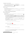
7.1.2 To edit the code associated with an operation
In the case of a generic processor
• Open the code editor
We need to launch the code editor of the selected operation. Let us consider the case of the conv ref
function. We have to do the following operations:
– in the main algorithm: double left click on the conv ref blue box. It opens the conv definition window.
In its contextual menu, select Edition of the associated source code. It opens the code editor. It looks
like a window with three push-buttons and an editable text area. Each push-button corresponds to one
specific phase of three (init, loop, and end phases). When one of the three buttons is pressed, the text
area shows the associated source code;
– in the conv definition window, right click on the background and select Edit code phases → Select
init and end → OK;
– in the code editor window: init phase → write in the text area (which is empty) the following C
language code. This code is understood as a generic code:
printf("Init phase of function $0 for default processor.\n");
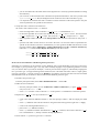
– do the same thing for the loop phase 1 :
@OUT(o)[0]=@IN(i)[0]*@PARAM(T)+@PARAM(P);
printf("Loop phase of function $0 for default processor = %i.\n", @OUT(o)[0]);
– and for the end phase:
printf("End phase of function $0 for default processor.\n");
– in the code editor window: Edit / Apply changes to all phases. It saves all buffers of all edited phases;
– in the code editor window: OK (it also saves all buffers).
Notice the following points:
1
Macros of the code editor as @IN, @OUT, @PARAM, ... are explained in the User Manual.
46
– you can not launch the code editor from a main algorithm or a read-only operation (definition coming
from libraries);
– you can write a code associated with a herarchical operation meanwhile it will not be present in the
applicationName sdc.m4x file (the background color of the text area of the code editor is grey);
– it is important to recall that the code is common to all the references of the same operator. Only the
values of parameters are specific of each instance.
• Verify that code is common to all references
We create a new reference to the conv function:
– in the main algorithm: create a reference conv ref bis<8;9> to the definition conv;
– in the main algorithm: first remove the link between the conv ref and mul boxes. Second, link the
conv ref output to the conv ref bis input. Third, link the conv ref bis output to the mul b input;
– in the algorithm window left click on the Auto-position button and write 120 in the two entry texts →
OK,
– open the code editor of this new box: the code is the same. To show that values of parameters are
specific to the reference (and not to the definition), we must generate the m4 code like shown in the
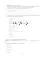
previous example (Menu Adequation / Launch Adequation then Code / Generate Executive(s))
and look in P1.m4 (Menu Code / Display Executive(s)). The file contains
conv(2,3, algo cste2 P1 o, algo conv ref o)
conv(8,9, algo conv ref o, algo conv ref bis o)
In the case of an architecture with heterogeneous processors
Sometimes it is interesting for an operation to have different source codes depending on the type of processor.
For example, a given processor type X may only offer assembly language as a programming interface. In such
case, we must be able to provide (for example) C code for processors that support it, and assembly language for
the X processor type. To support heterogeneous architecture, the code editor associates code to a triplet (phase,
processor, operation). A special processor type Default is provided for processors that have not been associated
with dedicated code. Its use allows to share a code between different processor types.
• Include a new processor type
From the principal window, choose File / Included Libraries → Select c40
• Define an new architecture:
– from the principal window, choose Architecture / Define Architecture (cf. figure 1.14) → In the
entry text, write archi2. → OK;
– in the archi2 window: create a reference root to the operator C40 and define it as the main operator.
• Replace the conv ref bis box by a reference to bar ref:
– create a new function definition named bar with one input port called in and one output port called
out;
– in the algo definition select all the references using the mouse and copy them (right click → Copy),
– create a new main algorithm named algo2;
– paste in the algo2 definition window;
– in the algo2 definition window: first delete the conv ref bis reference, then create a reference bar ref
box to the definition bar, finally create the missing dependences.
• Insert code for C40 processor type to the bar function:
47
– in the algo2 definition window: double left click on the bar ref blue box. It opens the bar definition
window. In its contextual menu, select Edition of the associated source code. It opens the code
editor;
– in the bar definition window, right click on the background and select Edit code phases → Select init
and end → OK;
– in the code editor window: Type of Processor: Select C40;
– in the code editor window: click on the init phase button and write in the text area the following code:
/* Hi, I am $0 function, in init phase for C40 processor */
– in the code editor window: click on the loop phase button and write in the text area the following
code:
@OUT(out)[0] = @IN(in)[0];
/* Hi, I am $0 function, in loop phase for C40 processor */
– in the code editor window: click on the end phase button and write in the text area the following code:
/* Bye, I am $0 function, in end phase for C40 processor */
• Insert code for U processor type to the bar function:
– in the code editor window: Type of Processor: Select U;
– in the code editor window: click on the init phase button and write in the text area the following code:
/* Hi, I am $0 function, in init phase for U processor */
– in the code editor window: click on the loop phase button and write in the text area the following
code:
@OUT(out)[0] = @IN(in)[0] * 42;
/* Hi, I am $0 function, in loop phase for U processor */
– in the code editor window: click on the end phase button and write in the text area the following code:
/* Bye, I am $0 function, in end phase for U processor */
• Modify the durations
Add c40/C40 = 1 at the end of the Durations text area for each definition referenced in algo2
48
Learn the macros of the code editor
The code editor comes with a set of predefined macros that alleviate the user from knowing the black magic of m4
processing.
The more useful ones are names translation macros. These macros translate port and parameter names to their
internal representation as m4 parameters. We have already encountered such macros in what we have just done:
@IN, @OUT and @INOUT are port name translation macros, and @PARAM is the parameter name translation macro. As
a rule of thumb, you should use @PARAM(x) when you want to refer to a parameter x and @IN(i) (resp. @OUT(o)
/ @INOUT(io)) when you refer to an input port i (resp. output port o / input-output port io).
The code editor recognizes three more macros: @NAME, @QUOTE and @TEXT. These advanced macros are not
used in this tutorial and the reader is refered to SynDEx user manual to learn more about it.
7.1.3 To generate m4x files
Before performing the code generation we have to perform the adequation:
• from the principal window, choose Adequation / Launch Adequation;
• from the principal window, choose Code: Select Generate m4x Files;
• from the principal window, choose Code / Generate Executive(s);
• from the principal window, choose Code / Display Executive(s).
Two cases are possible:
• the check box Generate m4x Files has not been checked. For each operator of the main architecture a
processor name.m4 file containing m4 macro-code is produced. As previously explained an architecture
description file (named example7.m4) is also produced;
• the check box Generate m4x Files has been checked. Then, two new files (example7.m4x and example7 sdc.m4x)
are generated in the same folder as the application.
These two files constitute the Applicative kernel:
• the MyApplication sdc.m4x file contains all m4 macro code associated with operations used in the SynDEx
application. Each time code generation is triggered, this file is overwritten;
• the MyApplication.m4x file is an user editable file whose goal is to allow the user to complete the applicative
kernel if needed. At code generation time, if this file does not exist then SynDEx creates a generic file
(including the MyApplication sdc.m4x file plus some other features), otherwise the existing file is kept.
The example7 sdc.m4x file contains the following code:
divert(-1)
# (c)INRIA 2001-2009
divert(0)
define(‘example7 bar’,‘bar’)
define(‘bar’,‘ifelse(
processorType ,‘C40’,‘ifelse(
MGC,‘INIT’, ‘‘/* Hi, I am $0 function, in init phase for C40 processor */’’,
MGC,‘LOOP’,‘‘$2[0] = $1[0]; /* Hi, I am $0 function, in loop phase for C40 processor */’’,
MGC,‘END’, ‘‘/* Bye, I am $0 function, in end phase for C40 processor */’’)’)’)
processorType ,‘U’,‘ifelse(
MGC,‘INIT’,‘‘/* Hi, I am $0 function, in init phase for U processor */’’,
MGC,‘LOOP’,‘‘$2[0] = $1[0] * 42; /* Hi, I am $0 function, in loop phase for U processor */’’,
MGC,‘END’, ‘‘/* Bye, I am $0 function, in end phase for U processor */’’)’,
define(‘example7 conv’,‘conv’)
49
define(‘conv’,‘ifelse(
processorType ,processorType ,‘ifelse(
MGC,‘INIT’,‘‘printf("Init phase of function $0 for default processor.\n");’’,
MGC,‘LOOP’,‘‘$5[0]=$3[0]*$2+$1;
printf("Loop phase of function $0 for default processor =%i.\n", $4[0]);’’,
MGC,‘END’,‘‘printf("End phase of function $0 for default processor.\n");’’)’)’)
If the example7.m4x file did not exist at code generation time then it will contain the following code:
divert(-1)
# (c)INRIA 2001-2009
divert(0)
define(‘dnldnl’,‘‘// ’’)
define(‘NOTRACEDEF’)
define(‘NBITERATIONS’,‘‘5’’)
include(‘example7 sdc.m4x’)
divert
#include <stdio.h> /* for printf */
divert(-1)
divert‘’dnl
Deeper insights about the m4 macro language can be found in SynDEx user manual and GNU M4 manual.
• See the difference between executable codes:
– create the example7.m4m file (cf. 6.3);
– create the root.m4x file (cf. 6.3);
– create the GNUmakefile (cf. 6.3), containing:
$(A).mk : $(A).m4 syndex.m4m U.m4m C40.m4m $(A).m4m
$(M4) $< >$@
– define algo2 as main algorithm;
– define archi as main architecture, perform the adequation, generate the code, and run the GNUmakefile
compilation You obtain a root.c file containing U code only (no C40 code);
– define archi2 as main architecture, perform the adequation, generate the code, and compile again.
This time, only C40 code is present in the root.c file.
Notice that:
• adequation modifies original files example7.sdx and example7.sdc;
• code generation produces these files: example7.m4, root.m4, pc1.m4 (if archi is defined as main), example7 sdc.m4x
(if Generate m4x files is set) and example7.m4x (if Generate m4x files is set and the file did not exist before);
• compilation produces these files: example7.mk, root, root.c, and root.root.o, and (if archi is defined as
main) pc1, pc1.c, and pc1.pc1.o.
From the principal window, choose File / Close. In the dialog window, click on the Save button.
50
Chapter 8
Example 8: a complete realistic
application from adequation to execution
From the principal window, choose File / Save as and save your eighth application under a new folder of yout
tutorial folder (e.g. my example8) with the name example8.
8.1 The aim of the example
In the seven previous examples we have learnt how to use SynDEx’s GUI to create architectures, algorithms,
launch adequation, obtain executive files... Now, we have sufficient knowledge to perform a simple automatic
control application that will be executed on a multiprocessor architecture.
First the application is described and the system is defined in Scicos (the block diagram editor of the Scilab
software1 ). Second the corresponding SynDEx application is created (using the Example 1 to 3 of the tutorial).
This needs the generation of some C code following the method discussed in Example 7. Finally, we compile
the application to obtain executable for several processors as it has been shown in Examples 6 and 7. SynDEx
generates the code necessary to the communication between the processors.
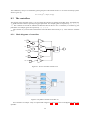
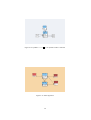
8.2 The model
We consider a system of two cars. The second car C2 follows the car C1 trying to maintain the distance l while the
acceleration and the deceleration of C1 . We call: x1 (t) the position of the first car; x2 (t) the position of the second
car plus l; x˙1 (t) and x˙2 (t) the speeds of two cars. We denote k1 and k2 the inverse of the car masses. We call r(t)
the reference speed chosen by the first driver. We suppose that we are able to observe the speed of the first car and
the distance between the cars.
We have the following fourth order (four degrees of liberty) system:
x¨1 = k1 u1
x¨2 = k2 u2
y1 = x˙1
y2 = x1 − x2
(8.1)
We will decompose the system into mono-input mono-output system S1 (u1 , y1 ) and S2 (u2, y2). Denoting by
uppercase letter the Laplace transform of the variables, we have Y1 = k1U1 /s and Y2 = (k1U1 − k2U2 )/s2 where U1
is seen as a perturbation that we want reject in the second system.
A first proportional feedback U1 = ρ1 (R−Y1 ) will insure the first car to follow the reference speed. The second
controller will be proportional derivative U2 = ρ2Y2 + ρ3 sY2 (in fact we will suppose in the following diagram that
the derivative of y2 is also observed). The coefficient ρ1 is obtained by placing the pole of the first loop:
Y1 = ρ1 k1 R/(s + ρ1k1 ).
1
http://www.scilab.org
51
The coefficient ρ2 and ρ3 are obtained by placing the pole of the transfer from U1 to Y2 in the closed loop system
which is given by:
Y2 = U1 k1 /(s2 + k2 ρ3 s + k2 ρ2 ).
8.3 The controllers
The purpose of the controller of the C1 car is to follow the reference in speed given the first driver. It stabilizes the
C1 speed around its reference speed by using pole placement. For example, gains are respectively: (0, -5, 0, 0,
-5). The controller of second car stabilizes the distance between the two cars. It stabilizes y2 around 0 by pole
placement. For example, gains are respectively: (4, 4,-4,-4).
The controler of C2 knows these informations and sends them electronically to C1 . This remark is available
for C1 .
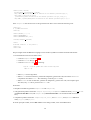
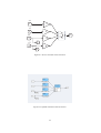
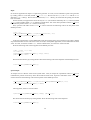
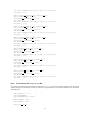
8.3.1 Block diagrams of controllers
x1
1
0
2
v1
2
−5
+
+
+
+
+
3
x2
3
0
v2
4
0
ref. vit 5
1
5
Figure 8.1: Scicos controller of the first car
Figure 8.2: SynDEx controller of the first car
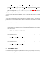
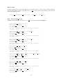
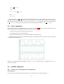
Our controllers are simple. They are represented in figures 8.1 and 8.3 in Scicos and figures 8.2 and 8.4 in
SynDEx:
52
x1
1
4
v1
2
4
x2
3
v2
4
+
+
+
+
−4
2
−4
3
Figure 8.3: Scicos controller of the second car
Figure 8.4: SynDEx controller of the second car
53
1
• create a gain def function with one input port in 1, one output port out 1 and a parameter named value.
Notice that all ports will be of type float;
• then create sommateur2 def, sommateur4 def, and sommateur5 def functions, respectively with two input
ports (in 1 and in 2), four input ports (from in 1 to in 4), and five input ports (from in 1 to in 5). Each of
these three functions is created with only one output port out 1;
• finally create both algorithms controleur1 sup and controleur2 sup (cf. figures 8.2 and 8.4), setting their
gain parameters respectively to 0, -5, 0, 0, 5 and 4, 4 ,-4 , -4.
8.3.2 Source code associated with the functions
We associate C source code to each function definition: gain and nary-sums. The code is inserted for the default
processor.
Gain
A gain is a function that multiplies its input by a coefficient given as a parameter, named GAIN. After adding this
parameter, open the code editor of the gain definition and write the following code in the loop phase of the default
processor:
@OUT(out 1)[0] = @IN(in 1)[0] * @PARAM(GAIN);
Sum
We have three different forms of sum depending of its arity: two, four or five input ports:
• open the code editor of the sum function with two input ports and write the following code in the loop phase
of the default processor:
@OUT(out 1)[0] = @IN(in 1)[0] + @IN(in 2)[0];
• open the code editor of the sum function with the four input ports and write the following code in the loop
phase of the default processor:
@OUT(out 1)[0] = @IN(in 1)[0] + @IN(in 2)[0] +
@IN(in 3)[0] + @IN(in 4)[0];
• open the code editor of the sum function with the five input ports and write the following code in the loop
phase of the default processor:
@OUT(out 1)[0] = @IN(in 1)[0] + @IN(in 2)[0] +
@IN(in 3)[0] + @IN(in 4)[0] + @IN(in 5)[0];
8.4 The complete model
In a real application, our job stops with the SynDEx’s adequation of the two controllers on their associated architectures. Nevertheless, for pedagogic reasons, we will simulate the whole system (with the dynamics of the cars)
in the aim to verify that our application does the same job that Scicos.
54
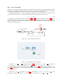
8.4.1 The car dynamics
SynDEx is only used in discrete time model (not continuous time) and is not able to manage implicit algebraic
loop. That is, in SynDEx, any loop contains at least a delay 1/z. Therefore, our application which is a continuous
time dynamic system described in Scicos, must be discretized in time to be used in SynDEx.
The differential equation ẋ = u is discretized using the simplest way: the Euler scheme. Let us denote by h the
step of the discretization and x0 an arbitrary initial value, the discretized system can be written as:
xn+1 − xn = uh
(8.2)
Finally, the system is given in Scicos in the figure 8.5 and 8.2 is given in SynDEx in the figure 8.6. Notice
that the variable h is stored in the Scicos context, and used in the input of the gain and the clock definition. In
SynDEx, h is defined as parameter in the definition of a gain and the clock definition is directly used in the source
code associated with operations.
Horloge
1
1
Pas de discretisation
u
1
h
+
+
xn
1/z
xn−1
Figure 8.5: An integral discretized in Scicos
Figure 8.6: An integral discretized in SynDEx
Create the integrale discrete sup algorithm (cf. figure 8.6). Notice that pas is of type gain def with parameter GAIN equal to 0.001, sommateur is of type sommateur2 def, and retard is of type float/delay<{0};1>.
The car dynamics are given with Scicos block diagrams in the figure 8.7 and with SynDEx operations in the
figure 8.8, where the input 1 (ref) is the acceleration of the car. The first integral gives the speed of the car and
the second its position.
Create the mecanique sup algorithm (cf. figure 8.8). Notice that puissancemoteur is of type gain def with
parameter GAIN equal to 1 whereas integrale1 and integrale2 are of type integrale discrete sup.
55
Puissance moteur
Position
1
1
1
1/s
1/s
Vitesse
2
Figure 8.7: Car dynamics with Scicos block diagrams (continous time)
Figure 8.8: Car dynamics with SynDEx operations
8.4.2 The cars and their controllers
In the following diagrams (from 8.9 to 8.12), the blocks (operations) denoted by meca are the car dynamics. Let
us get the controllers of the two cars.
Create the voiture1 sup and voiture2 sup algorithms (cf. figures 8.10 and 8.12). Notice that meca1 and
meca2 are references to mecanique sup whereas control1 (resp. control2) is a reference to controleur1 sup (resp.
controleur2 sup).
8.4.3 The main algorithm
Create the following definitions (definitionName<PARAM>):
• senseur def<POSI ARRAY> with one output port out 1,
• vitesse def<POSI ARRAY> with one input port in 1,
• scope def<POSI ARRAY> with two input ports in 1 and in 2.
Then create algomain. Create the reference speed ref vit of definition senseur def<0>, the reference vitesse
x˙1 of definition vitesse def<1>, the reference distance between the two cars of definition scope def<2>, the
reference vehicule1 of definition voiture1 sup and the reference vehicule2 of definition voiture2 sup, connect
them according to the figure 8.13.
8.4.4 Source code associated with the sensor and the actuator
We associate C source code to each function definition: input and two kinds of output.
56
1
x2
2
v2
3
Controleur1
Mecanique1
ref vit 1
1
x1
2
v1
Figure 8.9: Scicos C1 car dynamics and its controller
Figure 8.10: SynDEx voiture1 sup car dynamics and its controller
1
x1 1
v1 2
Controleur2
Mecanique2
1 x2
2
v2
Figure 8.11: Scicos C2 car dynamics and its controller
57
Figure 8.12: SynDEx voiture2 sup car dynamics and its controller
Figure 8.13: Main algorithm
58
Input
In our Scicos application an input is a square wave generator. As a rule, we will simulate a square wave generator
by reading values in a text file (named ref vitesse.txt). We will use the fopen, the fclose and the fscanf
functions (stdio.h library). We will also use assertions (assert.h library) to ensure that the opening of a file has
been successful.
For the moment, let suppose that it exists an array of FILE* (the structure returned by the fopen function) called
fd array and a variable called timer to simulate a pseudo-timer. Our sensor has a parameter called POSI ARRAY to
remember the position of the FILE* structure in the array.
Now, open the code editor of the senseur def sensor and write the following code in the init phase of the
default processor:
timer = 0;
fd array[@PARAM(POSI ARRAY)] = fopen("ref vitesse.txt", "r");
assert(fd array[@PARAM(POSI ARRAY)] != NULL);
In the Scicos application, we have defined the clock period of the square wave generator to the value 5 and the
step of discretization h to the value 0.001. Thus we need, in the SynDEx application, to send 5000 times the same
value. To count, we use the variable timer. All the 5000-th times, we read a new value in the file.
Write the following code in the loop phase of the default processor:
timer = (timer + 1) % 5000;
if (timer == 1)
fscanf(fd array[@PARAM(POSI ARRAY)], "%f\n", &data);
@OUT(out 1)[0] = data;
We need to free memory by closing the file. Write the following code in the end phase of the default processor:
fclose(fd array[@PARAM(POSI ARRAY)]);
Speed output
An output saves in a file the values of the system states. Thus, an output has a parameter called POSI ARRAY to
remember the position of the array where the stream has been saved. Open the code editor of the vitesse def
actuator and write the following code in the init phase of the default processor:
fd array[@PARAM(POSI ARRAY)] = fopen("actuator @TEXT(@PARAM(POSI ARRAY))", "w");
assert(fd array[@PARAM(POSI ARRAY)] != NULL);
The loop phase, allows to save the values:
fprintf(fd array[@PARAM(POSI ARRAY)], "%E\n", @IN(in 1)[0]);
We need to free the memory by closing the file. Write the following code in the end phase:
fclose(fd array[@PARAM(POSI ARRAY)]);
59
Distance output
Contrary to the first type of output, this output has two input ports but the init and end source codes are identical.
The loop phase differs. Open the code editor of the scope def actuator and write the following code in the init
phase of the default processor:
fprintf(fd array[@PARAM(POSI ARRAY)], "%E\n", (@IN(in 1)[0] - @IN(in 2)[0]));
8.4.5 The example8 sdc.m4x
SynDEx’s code generation will create the example8 sdc.m4x file (as explained in Example 7):
define(‘example8 algomain’,‘algomain’)
define(‘algomain’,‘ifelse(
processorType ,processorType ,‘ifelse(
MGC,‘INIT’,‘‘’’,
MGC,‘LOOP’,‘‘WARNING: empty code for macro $0 in loop phase’’,
MGC,‘END’,‘‘’’)’)’)
define(‘example8 controleur1 sup’,‘controleur1 sup’)
define(‘controleur1 sup’,‘ifelse(
processorType ,processorType ,‘ifelse(
MGC,‘INIT’,‘‘’’,
MGC,‘LOOP’,‘‘WARNING: empty code for macro $0 in loop phase’’,
MGC,‘END’,‘‘’’)’)’)
define(‘example8 controleur2 sup’,‘controleur2 sup’)
define(‘controleur2 sup’,‘ifelse(
processorType ,processorType ,‘ifelse(
MGC,‘INIT’,‘‘’’,
MGC,‘LOOP’,‘‘WARNING: empty code for macro $0 in loop phase’’,
MGC,‘END’,‘‘’’)’)’)
define(‘example8 gain def’,‘gain def’)
define(‘gain def’,‘ifelse(
processorType ,processorType ,‘ifelse(
MGC,‘INIT’,‘‘’’,
MGC,‘LOOP’,‘‘WARNING: empty code for macro $0 in loop phase’’,
MGC,‘END’,‘‘’’)’)’)
define(‘example8 integrale discrete sup’,‘integrale discrete sup’)
define(‘integrale discrete sup’,‘ifelse(
processorType ,processorType ,‘ifelse(
MGC,‘INIT’,‘‘’’,
MGC,‘LOOP’,‘‘WARNING: empty code for macro $0 in loop phase’’,
MGC,‘END’,‘‘’’)’)’)
define(‘example8 scope def’,‘scope def’)
define(‘scope def’,‘ifelse(
processorType ,processorType ,‘ifelse(
MGC,‘INIT’,‘‘’’,
MGC,‘LOOP’,‘‘WARNING: empty code for macro $0 in loop phase’’,
MGC,‘END’,‘‘’’)’)’)
define(‘example8 senseur def’,‘senseur def’)
define(‘senseur def’,‘ifelse(
processorType ,processorType ,‘ifelse(
MGC,‘INIT’,‘‘’’,
60
MGC,‘LOOP’,‘‘WARNING: empty code for macro $0 in loop phase’’,
MGC,‘END’,‘‘’’)’)’)
define(‘example8 sommateur2 def’,‘sommateur2 def’)
define(‘sommateur2 def’,‘ifelse(
processorType ,processorType ,‘ifelse(
MGC,‘INIT’,‘‘’’,
MGC,‘LOOP’,‘‘WARNING: empty code for macro $0 in loop phase’’,
MGC,‘END’,‘‘’’)’)’)
define(‘example8 sommateur4 def’,‘sommateur4 def’)
define(‘sommateur4 def’,‘ifelse(
processorType ,processorType ,‘ifelse(
MGC,‘INIT’,‘‘’’,
MGC,‘LOOP’,‘‘WARNING: empty code for macro $0 in loop phase’’,
MGC,‘END’,‘‘’’)’)’)
define(‘example8 sommateur5 def’,‘sommateur5 def’)
define(‘sommateur5 def’,‘ifelse(
processorType ,processorType ,‘ifelse(
MGC,‘INIT’,‘‘’’,
MGC,‘LOOP’,‘‘WARNING: empty code for macro $0 in loop phase’’,
MGC,‘END’,‘‘’’)’)’)
define(‘example8 vitesse def’,‘vitesse def’)
define(‘vitesse def’,‘ifelse(
processorType ,processorType ,‘ifelse(
MGC,‘INIT’,‘‘’’,
MGC,‘LOOP’,‘‘WARNING: empty code for macro $0 in loop phase’’,
MGC,‘END’,‘‘’’)’)’)
define(‘example8 voiture1 sup’,‘voiture1 sup’)
define(‘voiture1 sup’,‘ifelse(
processorType ,processorType ,‘ifelse(
MGC,‘INIT’,‘‘’’,
MGC,‘LOOP’,‘‘WARNING: empty code for macro $0 in loop phase’’,
MGC,‘END’,‘‘’’)’)’)
define(‘example8 voiture2 sup’,‘voiture2 sup’)
define(‘voiture2 sup’,‘ifelse(
processorType ,processorType ,‘ifelse(
MGC,‘INIT’,‘‘’’,
MGC,‘LOOP’,‘‘WARNING: empty code for macro $0 in loop phase’’,
MGC,‘END’,‘‘’’)’)’)
8.4.6 To handwrite the example8.m4x file
You will not can use directly the SynDEx’s generated example8.m4x generic file because both the creation of local
variable and the call of libraries is missing. After the code generation, you will must handwrite it to obtain the
following code:
define(‘dnldnl’,‘‘// ’’)
define(‘NOTRACEDEF’)
define(‘NBITERATIONS’,‘‘20000’’)
define(‘BINPWD’, ‘pwd’)
define(‘RSHELL’, ‘ssh’)
define(‘proc init ’,‘
61
FILE *fd array[10];
float data;
int timer;’)
include(‘example8 sdc.m4x’)
divert
divert(-1)
divert‘’dnl
Where the macro proc init allows the local variable declaration to be declared because it inserts its source
code between the main function and the operations initialization. Notice that the main loop of the program is
defined generically with a loop of NBITERATIONS where NBITERATIONS is initialized with the size of the input file
(ref vitesse.txt). Finally, the call of libraries is inserted after the include of the example8 sdc.m4x file.
8.5 Scicos simulation
Scicos software allows to simulate models in a window (cf. figure 8.14), where the values of three states are
plotted (ordinate axle) according to the time (abscissa axle). We have:
• the square wave generator drawn at the bottom (red);
• the speed of the first car at the top (black);
• the distance between the two cars seen in the middle of the figure (green).
Thanks the diagram, the system is stable (plots do not grow exponentially) and so it works. We do not continue
to ameliorate the controllers job.
Figure 8.14: Scope window obtained with the values 0; -5; 0; 0; -5 for gains of the C1 controller and 4; 4; -4; -4
for the C2 controller.
8.6 SynDEx simulation
8.6.1 In the case of a mono-processor architecture
The architecture
In this subsection, we suppose that the architecture is constituted of an only operator named root:
62
• create the U operator:
– set the durations with
float/delay = 1
gain def = 1
scope def = 1
senseur def = 2
sommateur2 def = 2
sommateur4 def = 1
sommateur5 def = 2
vitesse def = 1
– choose init as code generation phase in which to generate code;
• create the mono architecture:
– add one U operator named root and define it as main operator,
– define the mono architecture as main.
The adequation and the code generation
First, launch the adequation. It modifies example8.sdc and example8.sdx files.
Then, generate the executive and applicative files (setting Code / Generate m4x Files). It creates example8.m4,
example8.m4x, example8 sdc.m4x, and root.m4 files.
Finally, handwrite the example8.m4x file as explained in 8.4.6.
The compilation
First, generate manually a GNUmakefile containing:
A = example8
M4 = gm4
export ArchiMacros Path = ../../../macros/archi libraries
export AlgoMacros Path = ../../../macros/algo libraries
export M4PATH = $(ArchiMacros Path):$(AlgoMacros Path)
CFLAGS = -DDEBUG
VPATH = $(M4PATH)
.PHONY: all clean
all : $(A).mk $(A).run
clean ::
$(RM) $(A).mk *˜ *.o *.a *.c actuator *
$(A).mk : $(A).m4 syndex.m4m U.m4m
$(M4) $< >$@
root.libs =
P1.libs =
include $(A).mk
Where:
63
• A is set with the name of your application (here example8);
• the path about the generic *.m4? macro-files are stored in the exported shell variables ArchiMacros Path
and AlgoMacros Path then grouped into a new exported shell variable named M4PATH. The separator : means
that a m4 macro-file will be search first in ArchiMacros Path and then in AlgoMacros Path if is not found;
• a mix of this makefile and the informations stored in file named example8.m4m will create another makefile
called example8.mk during the compilation.
Then, copy-paste the ref vitesse.txt file from the Example 8 folder to yours.
Then, type the command gmake in a shell commands interpreter. It creates actuator 1, actuator 2, example8.mk,
root, root.c, and root.root.o files:
• the actuator 1 file contains the speed of the first car;
• the actuator 2 file contains the distance between the cars.
8.6.2 In the case of a bi-processor architecture
The architecture
In this subsection, we suppose that the architecture is constituted of two operators named root and pc1, of type U
and linked with a medium tcp1 of type TCP:
• create the TCP medium:
– set the type with SAM MultiPoint,
– set the durations with float = 1;
• modify the U operator: set the gates with TCP x and TCP y;
• create the biProc architecture:
– add one U operator named root and define it as main operator,
– add one U operator named pc1,
– add one TCP medium named tcp1 and choose the Broadcast option,
– links the medium to the x gates of the operators,
– define the biProc architecture as main.
The adequation and the code generation
First, launch the adequation. It modifies example8.sdc and example8.sdx files.
Then, generate the executive and applicative files (setting Code / Generate m4x Files). It creates example8.m4,
example8.m4x, example8 sdc.m4x, root.m4, and pc1.m4 files.
Finally, handwrite the example8.m4x file as explained in 8.4.6.
The compilation
First, generate manually the GNUmakefile, the example8.m4m, and the root.m4x files:
• the GNUmakefile has to be created as explained in 8.6.1. Upgrade it so that the line:
$(A).mk : $(A).m4 syndex.m4m U.m4m
is changed by:
64
$(A).mk : $(A).m4 syndex.m4m U.m4m $(A).m4m
• create the example8.m4m file with this line: define(‘pc1 hostname ’, HOSTNAME)dnl where HOSTNAME is substituted with the name of your remote station;
• create the root.m4x file with this line: include(example8.m4m).
Then, copy-paste the ref vitesse.txt file from the Example 8 folder to yours.
Then, type the command gmake in a shell commands interpreter. It creates actuator 1, actuator 2, example8.mk,
root, root.c, root.root.o, pc1, pc1.c, and pc1.pc1.o files:
• the actuator 1 file contains the speed of the first car;
• the actuator 2 file contains the distance between the cars.
8.6.3 In the case of a multi-processor architecture
The architecture
Figure 8.15: The architecture with 5 operators.
In this subsection, we suppose that the architecture is constituted of five operators named root,cont1, cont2,
dyna1, and dyna2, of type U and linked with a medium bus of type TCP:
• create the multi architecture (cf. figure 8.15):
– add one U operator named root and define it as main operator,
– add one U operator named cont1,
– add one U operator named cont2,
– add one U operator named dyna1,
– add one U operator named dyna2,
– add one TCP medium named bus and choose the Broadcast option,
– links the medium to the x gates of the operators, except for the root one, linked with its y gate to the
medium,
– define the multi architecture as main;
• create operation groups:
– create the og root operation group, attach ref vit, vitesse, and distance to it,
– create the og dyna1 operation group, from the main mode, in the vehicule1 reference attach meca1 to
it,
– create the og cont1 operation group, from the main mode, in the vehicule1 reference attach control1
to it,
65
– create the og dyna2 operation group, from the main mode in the vehicule2 reference attach meca2 to
it,
– create the og cont2 operation group, from the main mode, in the vehicule2 reference attach control2
to it;
• create absolute constraints:
–
–
–
–
–
constrain og
constrain og
constrain og
constrain og
constrain og
root on root,
cont1 on cont1,
cont2 on cont2,
dyna1 on dyna1,
dyna2 on dyna2.
The adequation and the code generation
First, launch the adequation. It modifies example8.sdc and example8.sdx files.
Then, generate the executive and applicative files (setting Code / Generate m4x Files). It creates example8.m4,
example8.m4x, example8 sdc.m4x, root.m4, cont1.m4, cont2.m4, dyna1.m4, and dyna2.m4 files.
Finally, handwrite the example8.m4x file as explained in 8.4.6.
The compilation
First, generate manually the Makefile.ocaml, the example8.m4m, the root.m4x, the cont1.m4x, the cont2.m4x, the
dyna1.m4x, and the dyna2.m4x files:
• copy-paste the Makefile.ocaml from the Example 8 folder to yours;
• create the example8.m4m file with these lines:
define(‘cont1
define(‘cont2
define(‘dyna1
define(‘dyna2
hostname
hostname
hostname
hostname
’,
’,
’,
’,
HOSTNAME)dnl
HOSTNAME)dnl
HOSTNAME)dnl
HOSTNAME)dnl
where HOSTNAME is substituted with the name of your remote station;
• create the root.m4x, cont1.m4x, cont2.m4x, dyna1.m4x, and dyna2.m4x files with this line: include(example8.m4m).
Then, copy-paste some files from the Example 8 folder to yours:
• copy-paste the example8.ml file.
• copy-paste the pa example8.ml file.
• copy-paste the root.sh, cont1.sh, cont2.sh, dyna1.sh, and dyna2.sh files;
• copy-paste the ref vitesse.txt file.
You will probably need to install camlp5 (see at http://pauillac.inria.fr/˜ ddr/camlp5/ ).
Then, type the command make -f Makefile.ocaml in a shell commands interpreter. It creates example8.cmi,
example8.o, pa example8.cmi, and <processor>.cmi, <processor>.cmx, <processor>.o, <processor>.opt for each
processor.
Finally, launch separatly the five script files. At the end of their execution, the actuator 1 and actuator 2 files
are created:
• the actuator 1 file contains the speed of the first car;
• the actuator 2 file contains the distance between the cars.
From the principal window, choose File / Close. In the dialog window, click on the Save button.
66
Chapter 9
Example 9: a multiperiodic application
From the principal window, choose File / Save as and save your ninth application under a new folder of yout
tutorial folder (e.g. my example9) with the name example9.
9.1 The main algorithm
Figure 9.1: Main algorithm of the Example 9
Create the main algorithm basicAlgorithm (cf. figure 9.1) using the library int for the operations input<1>
(int/input) and output<1> (int/output). For the operation compute, create a function definition compute and
create a reference to this definition. Create the dependences between the references. Set the periods to 4 for input,
8 for compute, and 8 for output by selecting each reference and filling the Period field.
9.2 The main architecture
Open the architecture monoProc from the library u. Define it as main. The durations for the U operator are by
default:
int/input = 3
Implode int = 1
compute = 1
int/output = 3
67
Implode int is an internal operation automatically generated by SynDEx to collect the different data produced
by the different occurences of the int/input operation.
In this case, the system is not schedulable.
9.3 A mono-phase schedule
9.3.1 Durations
Modify the durations for the U operator:
int/input = 1
Implode int = 1
compute = 1
int/output = 1
9.3.2 Adequation
Figure 9.2: A mono-phase schedule
Launch the adequation (Adequation / Launch Adequation). Display the schedule (Adequation / Display
Schedule) (cf. figure 9.2).
Wait operation
Notice the new operation added by SynDEx (Wait) to respect the period of the input operations.
Multiple occurrences
Notice that because of the periods, during a cycle two input operations are executed (input#1 and input#2)
whereas only one compute and one output operations are executed.
Implode operation
Notice the new operation added by SynDEx (Implode compute) to provide the data from the input operations to
the compute one.
68
9.4 A multi-phase schedule
9.4.1 Durations
Modify the durations for the U operator:
int/input = 1
Implode int = 1
compute = 2
int/output = 1
9.4.2 Adequation
Figure 9.3: A multi-phase schedule
Launch the adequation (Adequation / Launch Adequation). Display the schedule (Adequation / Display
Schedule). The computed schedule has two phases: a transitory phase (red) and a permanent phase (green) (cf.
figure 9.3).
Transitory phase
The transitory phase is executed only once. It contains the first occurrence of the input#1 operation, the first
occurrence of the input#2 operation, the first occurrence of the Implode compute operation, and the first occurrence
of the compute operation. The compute operation provide data consumed by the output operation schedule at time
9 in the permanent phase.
Permanent phase
The permanent phase is the one that is executed infinitely. It contains the second occurrence of the input#1
operation (and its following occurrences). It contains the first occurrence of the output operation (and its following
occurrences).
69