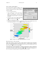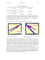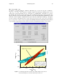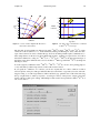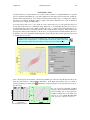
1
User's Manual for A Geochronological Toolkit for Microsoft Excel Berkeley Geochronology Center Special Publication No. 5 rev. January 30, 2012 Kenneth R. Ludw ig DISCLAIMER ISOPLOT is BGC’s Visual Basic Add-in for Microsoft’s Excel® for data analysis and graphical presentation of geochronology, earth science and other radiogenic isotope data only. BGC’s ISOPLOT is not the Isoplot® for analysis of any measuring system as described at (http://www.shainin.com/ ). BGC is not affiliated with Red X Holdings, LC. Isoplot® is a registered trademark of Red X Holdings, and is licensed to Shainin LLC. Berkeley Geochronological Center 2455 Ridge Road, Berkeley CA 94709 [email protected] Isoplot 3.75 24 February, 2012 2 Table of Contents INTRODUCTION ........................................................................................................................................ 5 ISOPLOT 3 REQUIREMENTS .......................................................................................................................... 5 EXCEL ON MACINTOSH COMPUTERS ............................................................................................................ 6 INSTALLING AND INVOKING ISOPLOT UNDER EXCEL 2003 OR EARLIER................................ 6 INSTALLING AND INVOKING ISOPLOT UNDER EXCEL 2007.......................................................... 7 THE INPUT DATA-RANGE ...................................................................................................................... 8 HEADER ROWS ............................................................................................................................................ 8 DATA IN A SINGLE, CONTIGUOUS RANGE .................................................................................................... 8 DATA IN DISCONTINUOUS ROWS ................................................................................................................. 9 DATA IN DISCONTINUOUS COLUMNS ........................................................................................................... 9 EXCLUDING DATA WITH FONTS IN STRIKETHROUGH ................................................................................... 9 USING BOLDED FONTS TO SPECIFY ADDED EMPHASIS TO PLOT-SYMBOLS.................................................. 9 SPECIFYING SYMBOL COLORS WITH FONT COLORS ................................................................................... 10 EARLY VERSUS LATE DATA SELECTION ...................................................................................................... 10 NUMERIC OUTPUT FROM ISOPLOT ................................................................................................. 10 ISOPLOT CHARTS.................................................................................................................................... 10 HIDDEN WORKSHEETS CREATED BY ISOPLOT ........................................................................................... 10 ADDING NEW DATA TO AN EXISTING CHART ............................................................................................ 10 MODIFYING CHARTS.................................................................................................................................. 11 Selecting and modifying simple data-point symbols and outline error-symbols .................................. 11 Adding Data-Point Labels.................................................................................................................... 11 Embedding charts into the data-worksheet .......................................................................................... 12 Embedding images of charts into the data-worksheet .......................................................................... 12 Superimposing charts ........................................................................................................................... 12 USING FILLED ERROR-ELLIPSES AND ERROR-BOXES ................................................................................... 12 COLOR-SCALING OF FILLED SYMBOLS ........................................................................................................ 14 EXPORTING CHARTS TO OTHER PROGRAMS ................................................................................................ 14 THE MAIN ISOPLOT DIALOG BOX .................................................................................................... 15 ISOPLOT PREFERENCES........................................................................................................................ 19 NUMERIC PREFERENCES............................................................................................................................ 19 GRAPHICS PREFERENCES ........................................................................................................................... 20 CLASSICAL ERROR-WEIGHTED X-Y REGRESSIONS AND ISOCHRONS.................................. 22 REGRESSION MODELS ............................................................................................................................... 22 Model 1................................................................................................................................................. 22 Model 2................................................................................................................................................. 22 Model 3................................................................................................................................................. 23 A WORD ABOUT 3-POINT ISOCHRONS ....................................................................................................... 23 COMMENTS ON REGRESSIONS WITH LOW PROBABILITIES-OF-FIT .............................................................. 23 EXAMINING RESIDUALS OF REGRESSIONS................................................................................... 24 ROBUST REGRESSIONS ........................................................................................................................ 25 U-PB CONCORDIA PLOTS..................................................................................................................... 26 Isoplot 3.75 24 February, 2012 3 CONVENTIONAL VERSUS TERA-WASSERBURG CONCORDIA REPRESENTATIONS ........................................ 26 Asymmetric ........................................................................................................................................... 27 Monte Carlo ......................................................................................................................................... 28 SHOWING DECAY-CONSTANT ERRORS IN THE CONCORDIA CURVE ........................................................... 29 SPECIFYING THE STYLE OF THE CONCORDIA-CURVE AGE TICKS ............................................................... 29 THE “CONCORDIA” AGE ............................................................................................................................ 30 Calculating a Concordia Age............................................................................................................... 30 Calculating a Concordia Age............................................................................................................... 31 Concordia Age MSWD’s ...................................................................................................................... 31 Concordia Age Errors .......................................................................................................................... 31 Effect of Decay-Constant Errors on Concordia Ages and Errors ........................................................ 32 THREE-DIMENSIONAL REGRESSIONS FOR U-PB CONCORDIA ..................................................................... 32 Planar Regressions............................................................................................................................... 32 Linear, Concordia-Constrained 3-D Regressions (The Total Pb/U Isochron)..................................... 33 EXTRACTING RELIABLE AGES FROM SUITES OF SINGLE-ZIRCON 238U/206PB DATES ...... 35 PB-PB ISOCHRONS AND GROWTH CURVES ................................................................................... 37 THE 230TH-234U-238U SYSTEM.................................................................................................................. 38 230 TH/U ISOCHRONS WITH VARIABLE 234U/238U......................................................................................... 38 TH/U ISOCHRONS WITH SECULAR EQUILIBRIUM 234U/238U .................................................................... 41 SINGLE-ANALYSIS 230TH/U AGES .............................................................................................................. 41 230 WEIGHTED AVERAGES OF A SINGLE VARIABLE ........................................................................ 42 ARGON-ARGON AGE SPECTRA AND PLATEAU AGES ................................................................. 43 USER-SPECIFIED PLATEAU STEPS .............................................................................................................. 44 CONNECTING LINES FOR ERROR BOXES .................................................................................................... 44 THE ARGON-ARGON PLATEAU-ISOCHRON ................................................................................... 44 CUMULATIVE PROBABILITY PLOTS AND HISTOGRAMS.......................................................... 47 PROBABILITY PLOTS ............................................................................................................................ 48 ADDING AN ALGEBRAICALLY-DEFINED CURVE TO AN EXISTING PLOT............................ 49 ADDING AN ALGEBRAICALLY-DEFINED CURVE TO AN EXISTING PLOT............................ 49 AGE LIMITS FOR A SERIES OF DATED, STRATIGRAPHICALLY-ORDERED UNITS ............ 50 STRATIGRAPHICALLY-CONSTRAINED DATES WITH CLOSE TO GAUSSIAN UNCERTAINTIES .......................... 50 STRATIGRAPHICALLY-CONSTRAINED DATES FROM 230TH/U ANALYSES..................................................... 51 DECONVOLUTION OF MULTIPLE AGE COMPONENTS USING THE SAMBRIDGECOMPSTON ALGORITHM .................................................................................................................... 52 YOUNGEST ZIRCON IN A SUITE OF DETRITAL ZIRCONS.......................................................... 53 UTILITY FUNCTIONS FOR ISOTOPIC DATA ................................................................................... 54 ACCESSING ISOPLOT’S USER FUNCTIONS .................................................................................................. 54 URANIUM-LEAD FUNCTIONS ..................................................................................................................... 56 URANIUM SERIES FUNCTIONS.................................................................................................................... 59 OTHER RADIOGENIC-ISOTOPE FUNCTIONS ................................................................................................ 60 Isoplot 3.75 24 February, 2012 4 STATISTICAL FUNCTIONS ........................................................................................................................... 60 ROUNDING FUNCTIONS .............................................................................................................................. 62 ACKNOWLEDGMENTS.......................................................................................................................... 62 REFERENCES ........................................................................................................................................... 63 APPENDIX I: TIPS ON MINIMIZING PLOT-CONSTRUCTION TIME.......................................... 65 APPENDIX II: TOOLBAR-ONLY FUNCTIONS .................................................................................. 66 APPENDIX III – ERROR CORRELATIONS ........................................................................................ 70 HOW TO CALCULATE AN ERROR CORRELATION ........................................................................................ 70 By differentiation .................................................................................................................................. 70 By observation ...................................................................................................................................... 71 INDEX ......................................................................................................................................................... 72 Isoplot 3.75 24 February, 2012 5 Introduction Isoplot (an “Add-In” program than runs under Microsoft Excel) is a flexible tool for the interpretation of radiogenic-isotope data. In addition to the plotting and calculation of the usual (Rb/Sr, Sm/Nd…) isochrons, Isoplot can: • Construct U-Pb concordia plots and calculate ages using conventional concordia intercepts, the “Concordia Age” algorithm, 3-D planar concordia intercepts, or 3-D linear (“Total U/Pb”) isochrons; • Calculate uranium-series isochron ages using 3-D or 2-D isochrons and construct 234 U/238U evolution curves and isochrons; • Construct single-stage growth-curves for plots of common-Pb data; • Construct cumulative-probability+histogram plots and linearized-probability diagrams; • Calculate and construct plots for either error-weighted or robust (nonparametric) averages of a single variable; • Calculate both conventional (analytical-error weighted) and robust (nonparametric) x-y regressions for “classical” and Pb-Pb isochrons; • Plot Ar-Ar step-heating diagrams and find the statistically-best plateau steps and age; • Combine Ar-Ar isochron with Ar-Ar step-heating diagrams to obtain the logically optimum combination of both; • Plot curves for almost any function; • Use simple Bayesian constraints Improve the estimates and error-assignments for a package of stratigraphically-constrained radiometrically-dated units whose ages overlap within errors (with a special variant for 230Th/U ages); • Deconvolute mixtures of components having Gaussian error-distributions using the SambridgeCompston approach; • Provide Monte Carlo errors as well as asymptotic (first-order) errors for most linear regressions, isochrons, and concordia-intercept solutions; • Extract reliable ages and errors from complex suites of Phanerozoic single-zircon dates; • Expand the number of Excel functions by more than 50, including many functions for radiogenicisotopes (including 16 for U/Pb and 8 for 230Th - 234U - 238U alone). 230 Th/238U- Isoplot is available without charge – contact Ken Ludwig directly ([email protected]). Iso p lo t 3 Requirement s For Windows computers, Isoplot requires an English-language version1 of Excel 97, Excel 2000, Excel 2002 or Excel 2003 Isoplot 3 is not compatible with Excel 2007 or Excel 2010. If you must use Excel 2007 or Excel 2010, request a copy Isoplot 4, which is compatible with Excel 2007/2010 only. Isoplot 4 has no more functionality than Isoplot 3.7, and somewhat less flexibility. Expect a speed penalty of up to a factor of 10 when using Excel 2007/2010. 1 For Windows systems, you must set the Control Panel's Regional and Language Options to English), and also check the Use System Separators box in the International tab of Excel's Options or Preferences sheet. Isoplot 3.75 24 February, 2012 6 Ex cel o n M a cint o sh co mput ers To run Isoplot on the Macintosh, you will need to acquire a Windows-enabling program (Fusion will work, but not Crossover nor Parallels). Despite expectations on my part, Excel 2011 is not Isoplot-compatible. When installing Excel, you must select a printer (say by printing anything from Excel) from within Excel before trying to run Isoplot. Installing and Invoking Isoplot Under Excel 2003 or Earlier →If you have been running Version 1 of Isoplot, you must first find the old Isoplot.xla file and either delete it or (preferably) rename it (e.g. IsoplotOld.xla). Start Excel, and from an open Worksheet, select Tools/Add-Ins. If Isoplot.xla is not in the list of available Add-Ins, select Browse to locate it. Isoplot will now be loaded every time you start Excel (if not wanted, uncheck Isoplot/Ex 3.00 from the add-in list before exiting Excel). To invoke Isoplot, first open the Worksheet that contains your data, and select (with the mouse or keyboard) the data-range that you want to work with (including any header-row). Then, either 1) press the Isoplot button , on Excel’s Standard toolbar (the one at the top of the screen), 2) choose Run Isoplot from the Tools menu, or 3) Press Ctrl-I. The items in the Isoplot drop-down menu can also be accessed from one of the Isoplot toolbars. To access the Isoplot toolbars, select View/Toolbars from the Standard (top) Excel toolbar and check the appropriate Isoplot item. One of the toolbars below will then appear on the screen: To see the functionality of a toolbar button, pause the mouse-cursor briefly over the button, and a text summary of its use will appear. The first 11 buttons in the Isoplot Charts & Isochrons toolbar duplicate the items in the drop-down Isoplot menu; use of the last eight, whose functions are accessible only via the toolbar, are described in Appendix II (p. 66). You can move any of Isoplot toolbar’s buttons to any of Excel’s other toolbars, so that they will always appear when you run Excel, with the following: 1) Select Tools/Customize from the Excel Standard toolbar; 2) While holding down the control key, so that the button is copied rather than permanently moved, drag and drop any button you wish from the Isoplot toolbar to any other toolbar. The changes will be permanent, until you either remove the button (by following the same procedure as above, except drag and drop the button to any area outside a toolbar) or Excel crashes. You can move the Isoplot toolbar anywhere on the worksheet, change its shape from horizontal to square or vertical (using the triangular-shaped handle at the lower right of the toolbar), or “dock” it at the top, bottom, or sides of the Excel workspace (drag and drop with the upper, stippled part of the toolbar). Avoid invoking Isoplot by double-clicking on the Isoplot.xla file’s icon, because 1) in some cases this can result in more than once copy of Excel running at the same time, and 2) the only way to unload a directlyinvoked Isoplot from Excel is to quit the Excel program. Isoplot 3.75 24 February, 2012 7 The speed of Isoplot can be greatly affected by the size of the active Excel workbook. If you have a lot of worksheets in the workbook, or a worksheet becomes very large and complex, Isoplot will slow down to a crawl, even when just displaying dialog boxes. Installing and Invoking Isoplot Under Excel 2007 Excel 2007 is a much less-capable platform for VBA add-ins such as Isoplot, requiring many compromises in coding and user interface to run Isoplot at all, and, for many uses, exacts a significant penalty in speed. Thus even if you already have a copy of Excel 2007 installeed on your computer, I urge you to find a copy of Excel 2003 and install that version on your computer as well. There is no problem in having both versions of Excel operating on the same computer at the same time. If, however, you must use Excel 2007, you will need to use Isoplot 4, compatible only with Excel 2007. To install Isoplot 4, 1. icon at the upper left of the Excel window, then click on Click on the the Excel Options button at the bottom the the resulting drop-down. 2. Click Add-Ins on the next drop-down. 3. Click Go. 4. f the correct Isoplot 4 add-in appears in the resulting Add-Ins box, select it. Otherwise, click Browse and navigate to the folder containing the latest Isoplot 4. Click OK. Isoplot 3.75 24 February, 2012 8 In Excel 2007, there are no drop-down menus for Isoplot – only Isoplot-specific toolbar buttons that appear in Excel’s Add Ins ribbon. To make the Add Ins ribbon appear, click the Add Ins in Excel’s main menu-bar. To see the function of any of the Isoplot buttons, hold the mouse-cursor briefly over the button. The Input Data-Range H ea der Ro w s If the data-range has a header-row, regardless of whether the headers lie immediately above the selected data-range or several rows above, Isoplot will try to recognize the type of plot and type of errors from it (see TestData.XLS for examples). To determine the type of plot, Isoplot looks for isotope ratios in the XY- (Z-) columns that define a supported plot type – for example, X- and Y-column headers consisting of either 147/144 143/144 or of 147Sm/144Nd 143Nd/144Nd will convince Isoplot to select an Sm-Nd isochron plot as the default plot-type. Isoplot will also try to recognize the type and sigma-level of the errors from the header rows, and offer its best guess as the default error type. Da t a in a Sing le, Co nt ig uo us Ra ng e If the cell-cursor is within a data range comprising a continuous set of cells bounded by blank rows/columns, the whole range will automatically be selected when you invoke Isoplot. The simplest data range is a contiguous rectangular block of cells comprising a header-row at the top (optional), and 2 to 9 contiguous columns containing the data, errors (optional) and error correlations (optional). For isochron or 2-dimensional concordia data, the simplest way to arrange the columns is: X X-error Y Y-error RhoXY where RhoXY is the X-Y error correlation; or as X X-error X Y. Y Y-error or as If you don’t supply columns for errors, Isoplot will ask you for values to apply to all of the data in the range. The errors can be either absolute or percent, 1σ or 2σ. Missing error correlations are assumed to be zero, except for conventional Concordia plots and “Normal” Pb-Pb plots, where you will be required to enter nonzero values. Isoplot 3.75 24 February, 2012 9 For Argon-Argon Step-Heating data, 3 columns are required: 39 Cumulative Ar-Fraction Age Age-error where the 39Ar gas-fraction can be expressed as percent if desired. For weighted averages or cumulative probability distributions, the columns must be: X X-error For 3-dimensional regressions, use any of 9, 6, or 3 columns, in the order: X X-error Y Y-error Z Z-error X X-error Y Y-error Z Z-error RhoXY RhoXZ RhoYZ or or just Y X Z Blank rows will be ignored in all cases. Da t a in Disco nt inuo us Ro w s To use only the data in certain rows, select a range with two or more discontinuous areas; for example: A3:E3,A6:E9,A12:E22 selects the 5 cells in row 3 from column A to E, then rows 6 through 9 of the same 5 columns, then rows 12 to 22. To do this with the mouse, hold down the Control key, select A3:E3, then A6:E9, then A12:E22. Da t a in Disco nt inuo us Co lumns If (and only if) your data are in contiguous rows, you can select a range with discontinuous columns to satisfy Isoplot’s requirements. For example, if your data were arranged in rows 1 through 11, with columns: A 143Nd/144Nd B C 144 147Sm/ Nd 147/144 %err D 143/144 %err your range selection would be: B1: C11,A1: A11,D1: D11 so that as interpreted by Isoplot the data would be arranged as: 147Sm/143Nd 147/144 %err 143Nd/144Nd 143/144 %err Excluding Da t a w it h F o nt s in St riket hro ug h If you don’t want to use a discontinuous-row selection to exclude certain data-rows (perhaps because you want to use discontinuous columns, or just to simplify the range-selection), you can exclude any data-row by using a font in Strikethrough mode (Format Cells Font Strikethrough) for the excluded data-cells. Using B o lded F o nt s t o Specif y Added Empha sis t o P lo t - Sy mbo ls If the font for a data-row is bolded, Isoplot will emphasize the plot-symbol by making it solid instead of open (circle, square, diamond, and triangle symbols), or by constructing the symbol with thicker lines (un- Isoplot 3.75 24 February, 2012 10 filled [outline] error ellipses and error boxes). However, no symbol-by-symbol emphasis is possible for filled error-symbols, or for the error-cross, +, or X symbols. Specif y ing Sy mbo l Co lo rs w it h F o nt Co lo rs Normally, a single color is specified for the symbols of all of the data points in a plot. You can use different colors for each data-point, though, by using the desired colors as the font color for each data-row, and specifying Font Color as the symbol color from the Isoplot dialog-box. Ea rly v ersus la t e da t a select io n Usually, you will find it easiest to select the desired data-range before invoking Isoplot. On a Windows platform, you can also select the data range with the mouse after Isoplot is invoked (provided the Range edit-box is active). Numeric Output f rom Isoplot The results of a calculation are always shown first in a popup-box such as the one at right, with or without buttons/checkboxes to select additional information or calculations. These popups are ephemeral, but all contain a checkbox labeled Show Results with Data, If Show Results with Data is checked, the information in the results-box will be transferred in a text-box to the worksheet containing the source-data (at the upper-right of the sourcedata range), and look something the box at right. These text-box results aren’t very easy to use for further spreadsheet calculations. However, in many cases, Isoplot also supplies a user-available array-function (see p. 54) that will place the results as numbers directly in worksheet cells. Isoplot Charts If the Plot checkbox of the main Isoplot dialog-box is checked, Isoplot will construct an X-Y plot (or “Chart” in Excel nomenclature) of the data on a separate sheet in the same workbook as the source-data. H idden Wo rksheet s Crea t ed by Iso p lo t The data-symbols plotted in an Isoplot chart are coupled to a hidden worksheet entitled PlotDat3 (or some other number), rather than to the worksheet containing the data that you selected for plotting. If you delete one of Isoplot’s chart-sheets, the associated hidden worksheet is no longer needed, and Isoplot will automatically remove the hidden sheet the next time it's invoked. Adding New Da t a t o a n Exist ing Cha rt You can add a second series of data points, complete with regression lines and age-results, to most Isoplot charts. To do this, 1) select the range of the new data (the new data must be in the same worksheet as the chart’s primary data); 2) switch to the Isoplot-created chart-sheet to which you want to add data; 3) select Add Data -Points from the Isoplot menu; Isoplot 3.75 24 February, 2012 11 4) specify what you want done with the new data, how to plot it, and click OK. You can also plot data along a secondary axis whose label and axis-ticks are at the right-hand side of the plot box, so that, for example, the first data-series for 207Pb/204Pb values, with y =15.4 to 15.8 are plotted as usual, and a second data-series consisting of 208Pb/204Pb values, with y =36 to 39, are plotted according to the range and axis-ticks of the right-hand axis. To do this, 1) select the range of the new data (the new data must be in the same worksheet as the chart’s primary data); 2) switch to the Isoplot-created chart-sheet to which you want to add data; 3) select Add Data -Points from the Isoplot menu; 4) select any plot symbol but an error ellipse or error box (these will not work with a secondary axis); 5) select the new data-series on the plot (you may have to scroll through the plot-elements with the up or down arrows to do this, if the data are not visible on the plot); 6) select Format/Selected data series, and click on the Axis tab; 7) specify Secondary axis; 8) double-click on the new axis to adjust its formatting and scale. M o dif y ing Cha rt s You can modify any graphical element of a chart by simply clicking on the element (say the Y-axis, or a regression line), pulling down the Format menu, and selecting the desired graphical element (usually the first one in the list, if you pre-selected an item). You can then change the foreground/background colors of the object, line colors, line styles, line widths, numeric format, font, font size, and so on. You can also add a limited range of graphical objects to the plot (arrows, textboxes, circles, polygons, curves, lines…) with the Drawing button on one of the Excel toolbars. Selecting and modifying simple data-point symbols and outline error-symbols For data plotted as a symbol without error information – that is, a circle, square, diamond, triangle, +, or X – clicking on any member of the data-series will select the whole data series, so that any formatting changes will affect the symbols for all of the members of the data series. To select an individual member of such a data series, first click on any plot-symbol within the data series, then repeatedly press the right-arrow key to step through the individual data-points. For error ellipses and boxes plotted as outlines (unfilled symbols), you can only select one data-point at a time; to step through the different data points, use the up- and downarrow keys. Adding Data-Point Labels If you’re not sure which symbol on the chart belongs to which data-row on the source-data sheet, Isoplot can attach a label to each plotted point. To do this you’ll need a column of datapoint labels somewhere on the source-data sheet (just to the left or right of the data itself would be fine). From the Chart sheet, select Label Data Points from the Isoplot menu. Select where you want the labels to appear (relative to the corresponding data points) and, if you have more than one data-series plotted, which series to label. Finally, enter the range containing the labels (must match the data-point range in both number and or- Isoplot 3.75 24 February, 2012 12 der). After plotting, the labels can be reformatted or moved as desired. Selecting individual labels: Plots with U-Pb concordia curves, U-series evolution curves, or Pb-isotope growth curves all contain labeled age-ticks on those curves. The labels will often be positioned inconveniently, so that you will want to move or delete some or all of them. To select an individual label for moving deleting, or formatting first select all of the labels by clicking on one of them. Wait a second, click on the particular label you want to change and hold down the mouse button. After about another second, the individual label will be selected. Embedding charts into the data-worksheet If you would like the chart to be part of the worksheet containing its source-data, switch to the chart-sheet and select Move Chart to data Worksheet from the Isoplot menu. The chart will be shrunk about 4 times and moved to the source-data worksheet, just to the right of the source-data range. You can further re-size the chart from the worksheet by first selecting the chart itself, then the various chart elements. Once you have done this, you can also cut/paste the chart to a blank worksheet and assemble a page of nothing but reduced-size charts (and any related commentary, such as figure legends (you may want to turn off the worksheet gridlines to improve appearance, using Tools/Options/View/Gridlines). Or, you can copy/paste the moved/shrunk chart to within an existing chart-sheet, so as to create an inset (as in the cover figure). An Embedded Chart can be edited and manipulated just like a full-sheet chart, but is less transportable to other applications. Embedding images of charts into the data-worksheet If you don't need to edit the chart once it has been embedded into the source-data worksheet, it is probably better to select Copy Chart-image to Data Worksheet. The chart will then be transferred as a picture object which can be easily pasted into other applications if desired. On Windows platforms, this object will be created at very high resolution and quality. Superimposing charts You can also superimpose charts – for example, if you need an inset showing a magnified view of a part of a chart. To do this, first have Isoplot create the master chart, in the usual way (as a separate chart-sheet), then create the chart to be inset, also in the usual way. Move/shrink the inset chart as described above, then cut/paste (or copy/paste) the resulting reduced-scale chart onto the master-chart sheet. Reformat the superimposed inset-chart as desired. Alternatively, just select one or more charts and copy/paste them to a worksheet in the usual way (note that the size of the pasted chart depends on the zoom-ratio of the destination worksheet). Shrink and superimpose the charts as required. Using f illed erro r- ellipses a nd erro r- bo xes Error ellipses and boxes will be plotted as either a simple outline or as a filled shape, depending on the status of the filled Symbols checkbox in the main Isoplot dialog-box. There are important differences in the way outline and filled error-symbols can be used, as listed below: Outline symbols are always accurately plotted, no matter how or when the plot is re-scaled or resized; Filled symbols will become slightly but noticeably mislocated whenever the magnification (zoom) of the chart is changed; Filled symbols do not respond to re-scaling or re-sizing of the chart, and so will become significantly mislocated when you change either the physical dimensions of the plot or the logical scale of either axis; The only changes that can be made to the visual appearance of outline symbols are to modify the outline color and thickness; Isoplot 3.75 24 February, 2012 13 Filled symbols can be modified in many ways, including not only their outline color/thickness and fill-color, but also the pattern, color gradient, and transparency of the fill. • Outline symbols cannot be moved, even temporarily (though they can be deleted); • Filled symbols can be temporarily or permanently moved using the usual click-and-drag (for example, to see what lies underneath a filled symbol). To rectify the location of filled symbols after any re-scaling or re-sizing action, or after any zoom-in or zoom-out, select Rescale Filled Symbols from the Isoplot menu on the Chart or Worksheet menu-bar. Any filled error-boxes or error-ellipses will then be accurately relocate and resized. You can also stack these symbols according to their size (actually, the length of their diagonal), so that smaller ellipses or boxes will lie on top of progressively larger ones, using the Sort Filled Symbols by Size menu-item. To change the order yourself, right-click a filled symbol to bring up the menu at left, select the Order item, then the desired placement with the resulting sub-menu (above left). You should always re-scale filled symbols before printing to make sure that they are accurately placed. In some cases, you may need to first zoom in to the maximum (400%) to eliminate any residual offset. Isoplot 3.75 24 February, 2012 14 Co lo r- sca ling o f f illed sy mbo ls If your data are plotted as filled error-ellipses or error boxes, you can use color scaling (or gray-scaling, if not a color plot) to represent the value of a third, z-parameter. To use color scaling: • Plot your data in the usual way; • Select a columnar range of cells to use for the color scaling—for example, a ppm Uranium column. Make sure that the number of valid cells in this range matches exactly the number of data symbols in your plot; • Select the plot again, and select Color Scale Filled Symbols from the drop-down Isoplot menu; • Re-select the scaling range if necessary; • Select how you want the colors scaled. Use Autoscale to use the lowest- and highest-values of the color-scaling range define the “lowest” (pure blue) and “highest” (pure red) colors. Figure 1: Example of color scaling to show a third, z-parameter on an x-y plot. Expo rt ing cha rt s t o o t her pro g ra ms Simply using Copy/Paste to export Excel charts to another application generally results in unacceptable quality, because of the default Windows Clipboard resolution of 1/72”. As mentioned earlier, for Windows users, Excel’s Copy Picture method (invoke the Edit menu from the chart sheet with Shift depressed) will yield excellent resolution in the exported graphic. Another method (used for the preceding figure, for example) is to import Isoplot’s charts as a bitmap using a screen-capture utility. Before capturing the screen select View/Full Screen from the chart sheet, then enlarge the plot-box as much as possible. After pasting the image into your document and shrinking it 4x or more, you should have acceptable (though not really publication quality) resolution. Isoplot 3.75 24 February, 2012 15 The Main Isoplot Dialog Box When Isoplot is invoked, the main Isoplot dialog-box will appear: If you included a header-row with the data-range that was selected when you invoked Isoplot, some of the choices will already have been correctly made; others require some thought. Your choices will include some or all of: Input Range: The range, if any, that was selected when Isoplot was invoked . You can type in any other range as well, e.g. “A10:E22”, “MyData”, “B3:F6,B8:F8, B14:F22”. On Windows platforms, you can also use the mouse to select a range after invoking Isoplot. The ranges can included discontinuous rows (so as to exclude unwanted data in a contiguous sequence), or discontinuous columns (so as to rearrange the column-order to meet Isoplot’s requirements), but not both. Rows without numeric data are ignored, as are rows whose data are shown with the Strikethrough attribute. The prompt to the right of the Input Range edit-box indicates what sort of data is assumed to be in columns (in left-to-right order) of the input range. Isoplot 3.75 24 February, 2012 16 Isochron or Plot Type: Select from the drop-down list (right): For isochrons (including U/Pb concordia), “Normal” plots yield the age from the slope of the linear regression, and initial ratios from one of the intercepts, whereas the opposite is true of “Inverse” plots. The plottypes offered by Isoplot are: U-Pb Concordia Data for a “Normal” (207Pb/235U - 206Pb/238U, or “conventional”, or “Wetherill”) Concordia plot, or for an “Inverse” (238U/206Pb - 207Pb/206Pb, or “Tera-Wasserburg”) Concordia plot. The data points can be regressed using a modified York two-error regression algorithm (York, 1969), and the resulting concordia-intercept age-errors can be calculated using either a first-derivative expansion approach or (if there is no excess scatter) a more-reliable Monte Carlo approach. If an “Inverse” Concordia plot, you can also include Z-axis (204Pb/206Pb) data for either planar 3-D or linear 3-D (“Total Pb/U Isochron”) regressions. Finally, you can select the ”Concordia Age” method to calculate ages and X-Y means for 2-D data that are both concordant and X-Y equivalent. If desired, a conventional Concordia plot can be constructed directly from Tera-Wasserburg data, or vice-versa (p. 27) Ar-Ar isochron Argon-Argon isochron data, where “Normal” is 40Ar/36Ar versus 39Ar/36Ar, and “Inverse” is 36Ar/40Ar versus 39Ar/40Ar. Rb-Sr isochron Classical 87Rb/86Sr - 87Sr/86Sr isochron (“Normal” only). Sm-Nd isochron Classical 147Sm/144Nd - 143Nd/144Nd isochron (“Normal” only). Re-Os isochron 187 Lu-Hf isochron 176 K-Ca isochron 40 Os/188Os - 187Re/188Os isochron (“Normal” only). Hf/177Hf - 176Lu/177Hf isochron (“Normal” only). Ca/42Ca - 40K/42Ca isochron (“Normal” only). 207Pb-206Pb isochron chron. 208Pb-206Pb isochron sion. 206 206 Pb/204Pb - 207Pb/204Pb (“Normal”) or 204Pb/206Pb - 207Pb/206Pb (“Inverse”) iso- Pb/204Pb - 208Pb/204Pb (“Normal”) or 208Pb/206Pb - 204Pb/206Pb (“Inverse”) regres- 238U-206Pb isochron 238 U/204Pb - 206Pb/204Pb (Normal) or 204Pb/206Pb - 238U/206Pb (Inverse) isochron. 235U-207Pb isochron 235 U/204Pb - 207Pb/204Pb (Normal) or 204Pb/207P b - 235U/207Pb (Inverse) isochron. 232Th-208Pb isochron 232 Th/204Pb - 208Pb/204Pb (Normal) or 204Pb/208Pb - 232Th/208Pb (Inverse) isochron. 230Th-234U-238U isochron For 3-D 230Th/U isochrons (required if 234U/238U cannot be assumed to be in secular equilibrium!), any combination of 232Th/238U - 230Th/238U - 234U/238U as the X-Y-Z axes. For 2-D 230 Th/U isochrons (requires all 234U/238U=1), either X=238U/232Th, Y=230Th/232Th or X= 232Th/238U, Y= 230 Th/238U. Also permitted is X = 230Th/238U, Y = 234U/238U to calculate the 230Th/U age of a single point, or to plot data for several points (in which case one or more 230Th/U evolution curves for different initial 234 U/238U can be requested). Other X-Y [-Z] plot Any other X-Y or X-Y-Z plot, X-Y isochron, or X-Y-Z regression. Weighted Average Classical inverse variance-weighted average, with two approaches for dealing with excess scatter, plus the Tukey’s Biweight robust estimator. Probability density plot Constructs the cumulative Gaussian probability curve for an assemblage of singlevalued data and errors, with or without a histogram for the data. Linearized probability plot Constructs a probability plot for a normal distribution using the selected data. Ar-Ar age spectrum Constructs the classical Ar-Ar step-heating diagram (age versus 39Ar gas-fraction), and identifies the best plateau defined by the data. Ar-ArPlateauChron Determines the isochron age of the contiguous heating steps with the largest amount of gas, which corresponds to a classical step-heating plateau age without the assumption that the trapped component 40Ar/36Ar is that of air. Isoplot 3.75 24 February, 2012 17 Graph an arbitrary function Must be invoked from an existing Isoplot chart; allows the user to algebraically define any simple or parametric x-y curve and place a graph of the curve on the plot. Ages of stacked beds Uses Bayesian statistics with a Monte Carlo approach to get the most precision out of a stratigraphically-constrained sequence of units whose dates overlap within their assigned errors. Ages of stacked U-series Similar to Age of stacked beds, but uses the radiogenic 230Th-234U-238U ratios, errors, and error correlations as input instead of the 230Th/U age directly, and includes the additional constraint of a closed system for the Th-U isotopes. Unmix ages Deconvolutes an assemblage of dates that overlap within their assigned errors but have more than one age-component, using the Sambridge and Compston approach. Zircon age extractor Implements the TuffZirc algorithm of Ludwig and Mundil (Ludwig and Mundil, 2002) for extracting reliable ages and age-errors from suites of 206Pb/238U dates on complex single-zircon populations. Youngest Detrital Zircon Determines the age and age-uncertainty of the youngest zircon in a suite of dated (single-crystal) detrital zircons, assuming only that 1) the errors assigned to the individual zircon dates are accurate and normally distributed, 2) none of the dated zircons are contaminants. Action/Plot: Check the Plot box in the Action group to obtain a plot as a separate Excel Chart-sheet. Action/Calculate: Check the Calculate box in the Action group to have Isoplot perform a regression or other calculation on the selected data. Results will be included in the plot, if one is specified. Action/Robust Regr: Instead of calculating the best-fit line, isochron, or chord using the usual 2-error regression (Yorkfit), use a robust (nonparametric) regression which makes no assumptions about the nature or distribution of the scatter about a straight line. Not available for U-Pb Concordia or 230Th-234U-238U isochrons (see p. 25). Input Errors: Specify the type and sigma-level of the errors you have assigned to your data here (if you will be regressing the data, or plotting with error-symbols). Be especially careful to correctly specify the errors as absolute or percent. The sigma-level is important for (nonrobust) regressions, as the resulting MSWD will be affected by a factor of 4. Also, if you have specified (from the Preferences/Graphics/Error Symbols dialog box) that error symbols are to be plotted at the sigma-level of the input-data, the sizes of error ellipses, error crosses, and error boxes will reflect the sigma-level you specify (see p. 20). Plotting Symbols: The available plotting symbols are shown in the Symbols dropdown: Note that error cross and error box symbols will not be enabled for plot types whose X-Y data-errors are always significantly correlated—that is, for conventional concordia Pb-Pb isochron plots. The “line connect” option constructs a line connecting the data points, in the same order that they appear in the worksheet, but without any data-point symbols. By default, the line is smoothed. Double-click on it to cancel smoothing. The “line connect” option is useful for plotting custom curves, such as non-single stage Pbisotope growth curves2. The “Spline” option constructs a classical spline curve – that is, a smoothly-joined assemblage of thirdorder polynomials forced through the data-points. 2 The age ticks could be added by plotting a data range corresponding to the age ticks as circles, then invoking Isoplot’s Label Data-Points menu-item to label the ticks. Isoplot 3.75 24 February, 2012 18 The “Akima spline” option constructs a somewhat different sort of spline curve – one that eliminates the “overshoots” that can occur with classical splines, at the expense of allowing much sharper “bends” in the curve (Akima, 1970), as shown below. Akima spline 0.70920 Sr/ Sr 0.70925 Sr/ Sr Normal spline 0.70925 87 87 86 86 0.70920 0.70915 0.70915 Age (Ma) Age (Ma) 0.70910 0.70910 0.0 0.4 0.8 1.2 1.6 2.0 2.4 0.0 0.4 0.8 1.2 1.6 2.0 2.4 Figure 2: Examples of spline curves. The "Normal" spline (left) is constructed of connected segments of cubic polynomials whose slopes are matched at each data-point. The "Akima" spline uses a different algorithm which eliminates the "overshoot" typical of Normal splines. Plot-Symbol Colors: Select the outline-color of the plot-symbols from the Symbol/Colors drop-down. You can have the symbol-outline colors vary for each datapoint by selecting Font Color, in which case the symbol color will match the color of the font used for each data-point. For non-filled symbols, the default interior color of polygonal, non-error plot-symbols is white; to use filled symbols of this type, use a bold font for the data. Other/Color: Check this box if you want the plot to use the colors specified in Options/Colors; leave unchecked for a black-and-white plot. Other/Autoscale: Check this box to have Isoplot select the X- and Y-limits of the plot-box, based on the range of the selected data. Leave unchecked to specify these limits yourself. Other/Anchored (Two-dimensional Concordia plots only): Check this box to (1) force one of the Concordia intercepts to be a specified age; (2) force the regression line to intersect the 207Pb/206Pb axis at some specified common-Pb ratio (Inverse Concordia plots only); or (3) construct a reference chord between two specified ages, using the dialog-box at right: Other/PbGrowth (207Pb - 206Pb or 208Pb - 206Pb isochrons only): Check this box to specify construction of a single-stage Pb-isotope growth curve. From the dialog-box (p. 37) that appears later, you can specify Stacey-Kramers parameters, or any other initial age, Pb-isotope ratios, and Mu for the growth curve. Other/Reject OK (Weighted-averages only): Check this box to permit outlier-rejection using a modified 2σ criterion. Isoplot 3.75 24 February, 2012 19 Isoplot Preferences Preferences are grouped into two types: Numeric and Graphics, indicated by buttons in the main Isoplot dialog box. Numeric P ref erences The Decay constants/Half lives sheet contains the relevant values for of all of Isoplot’s age calculations. When editing, values can be entered as either decay constants or half lives (see example at right). The Model age parameters sheet contains the source-region isotope ratios for Sm-Nd, Rb-Sr, Lu-Hf and Re-Os model ages. The U-Th, Ar-Ar, & statistical sheet permits editing of the U and Th decay-constant uncertainties (used in calculated U-Pb and 230Th/U age errors), as well as parameters used in the calculation of age plateaus for Ar-Ar stepheating spectra. An additional, very important parameter defined in this sheet is the “Probability of fit below which errors are expanded by Students-t × √MSWD”. Errors of weighted averages or regressions whose probability-of-fit exceeds the specified value (acceptable range = 0.05 to 0.30) will be reported with the “internal 2-sigma” error – the error propagated only from the assigned data-point errors. Errors of weighted averages or regressions having a lower probability of fit will be reported with the “95%confidence errors” calculated by multiplying the 1-sigma internal error by the Student’s-t value for the appropriate degrees of freedom, and again by the square root of the MSWD parameter for the calculation (The MSWD is the sums of squares of weighted residuals divided by the degrees of freedom of the calculation). The default value for this “minimum probability of fit” parameter is 0.15. Isoplot 3.75 24 February, 2012 20 Gra phics P ref erences Lines: Specify attributes of various lines in the Isoplot charts: Error symbols: Specify attributes of error symbols when used as data-point symbols: Resolution of error ellipses & curves: Fine yields in a large number of line-segments defining the curves and ellipses, but takes slightly more time; Coarse is the fastest, with a slight compromise on linesmoothness. Don’t judge the quality of the outline curves/ellipses at low magnification, though – to evaluate, zoom to 400% and temporarily change the line-thickness of the curve/ellipse to the thinnest available. If Clip ellipses at the plot-box boundary is checked, error ellipses will be clipped at the plotbox borders; if unchecked, they will continue beyond. Don’t use clipped ellipses if you might re-scale the plotlimits later—if you do so, the clipped ellipses will be revealed as arcs (outline ellipses) or abruptly terminated shapes (filled ellipses). Sigma-level of error symbols: You can specify that error symbols (error ellipses, error boxes, and error crosses) be plotted at 2-sigma, (regardless of the sigma-level of the input-data), or at the sigma-level of the input-data. Thus the only way of plotting 1-sigma error symbols is to have the input-data errors at 1sigma and also to specify “at sigma-level of input data” in the Error Symbols group of Options/Lines. Filled error ellipses & boxes: Check Automatically rescale to have the position of the error symbols fine-tuned before quitting plot-construction. Usually unnecessary, but may improve symbol-positioning in some cases. Check Automatically sort & stack by size to arrange the relative position of the filled symbols by size, with smaller symbols are superimposed on larger ones so that the smaller symbols are not hidden by the larger. The End-caps on error crosses box specifies whether or not error crosses will be terminated by a Isoplot 3.75 24 February, 2012 21 short, horizontal line in both the X- and Y-error directions ( versus ) Rescale shapes when done: Check this box to have the filled symbols in the plot automatically rescaled and ordered by size just before the plot is finished. Because this takes extra time, if your plots take more than a few seconds to construct you may want to leave this box unchecked (make sure to rescale the plot from the Isoplot drop-down menu before printing). Colors: Specify the default colors for the various elements of the Isoplot charts (you can always change the colors after the plot is completed). Fonts: Specify the default fonts and font-sizes for different elements of the Isoplot charts. If Superscript isotopes in axis labels is checked, number-prefixes of common geochronologic isotopes will be superscripted in the usual way (e.g. 87Sr/86Sr). Isoplot 3.75 24 February, 2012 22 Classical Error-Weighted X-Y Regressions and Isochrons Reg ressio n M o dels Unless Robust Regr. were checked (p. 25), two-dimensional (x-y) data are initially regressed using the algorithm of York (1969), with errors propagated using the (maximum-likelihood estimation) algorithm of Titterington and Halliday (1979). If the probability of fit of the regression is low, other approaches (“Models”) for weighting the data-points may be used. The 3 “Models” used by Isoplot are: Model 1 The Model 1 fit is York’s original algorithm, and assumes that the assigned errors are the only reason the data-points scatter from a straight line. The points are therefore weighted proportional to the inverse square of these errors (taking into account the error correlations). A test of the Model 1 assumption is provided by the Probability of Fit calculated by the program. If this probability is reasonably high (more than 15%), then the Model 1 assumptions are considered justified, and the regression is complete. If the probability is low (usually less than 15%, but user-definable in the range of 5% to 30%), you may choose another model. The Probability of Fit is actually the probability that, if the only reason for scatter from a straight line is the analytical errors assigned to the data points, the scatter of the data points will exceed the amount observed for your data. If you accept the Model 1 fit even though the Probability of Fit is less than 15%, Isoplot then calculates the 95%-confidence errors from the observed scatter (thus invoking the use of the Student’s-t multiplier to convert from estimated errors — equivalent to the a priori errors multiplied by the square root of the MSWD3 — to 95%-confidence errors). Note that in this case, weighting of the data points remains inversely proportional to the square of their analytical errors. Isoplot will always attempt a Model 1 fit first. In the results-box, the a priori errors are the errors in the slope and intercept calculated by propagating only your assigned errors for the points; therefore, no matter how much the points scatter, the a priori errors will not increase. The including scatter errors, however, are calculated from the actual scatter of the points from a line, and are independent of the assigned errors. These errors, given at the 1σ level, are provided mainly for comparison purposes with the output of other implementations of York’s algorithm. The only geologically useful errors for data sets with few points are the ones given as 95% Confidence-Limit errors. How the 95% confidence-limit errors are calculated depends on the probability that the assigned data-point errors can account for the observed scatter. If the probability is greater than 15%, the 95% confidence-limit errors are given as simply 1.96 (Student’s-t for an infinite number of points) times the a priori errors (the reason for this is discussed by Brooks and others, 1972). Model 2 A Model 2 fit (not supported for classical isochrons such as Rb-Sr or Sm-Nd) assigns equal weights and zero error-correlations to each point. This is seldom justified by any real mechanism, but at least avoids the mistake of weighting the points according to analytical errors (see above discussion of Model 1 regressions) when it is clear that, in fact, some other cause of scatter is involved. The 95% confidence-limit errors are 3 MSWD = Mean Square of Weighted Deviates. This does not refer to porcine perverts; it is, roughly, a measure of the ratio of the observed scatter of the points (from the best-fit line) to the expected scatter (from the assigned errors and error correlations). T h e M S W D p a r a m e t e r c a n n o t b e c o m p a r e d t o t h e c l a s s i c a l R 2 p a r a m e t e r , a n d i s n o t a m e a s u r e o f h o w h i g h l y c o r r e l a t e d t h e X - a n d Y - v a l u e s a r e . If the assigned errors are the only cause of scatter, the MSWD will tend to be near unity. MSWD values much greater than unity generally indicate either underestimated analytical errors, or the presence of non-analytical scatter. MSWD values much less than unity generally indicate either overestimated analytical errors or unrecognized error-correlations. See Wendt and Carl (1991) for a detailed discussion. Isoplot 3.75 24 February, 2012 23 calculated from tn-2 times the including scatter errors. Because this relatively know-nothing approach still makes the assumption of a normal distribution of residuals, it is arguably more realistic in most cases to choose a robust regression instead. Model 3 A Model 3 fit (for classical isochrons such as Rb-Sr or Sm-Nd) assumes that the scatter is due to a combination of the assigned errors plus an unknown but normally distributed variation in the Y-values. This model (similar to the Model 3 algorithm of McIntyre and others, 1966) may be realistic in the case of Rb-Sr or other isochron data for rocks whose initial ratios were variable. For this model, the program will solve for the unknown Y-variation (= initial-ratio variation) as well as for the best-fit line, so you can judge whether or not the solution is realistic. Remember, though, that it is physically quite possible (even likely) that the initial ratios of the samples were significantly correlated with their Rb/Sr (or other parent/daughter ratio), in which case the Model 3 assumptions are not valid. For an extended discussion of the problem, see Zheng (1989a), or Juteau and others (1984) for an excellent example. A Wo rd Abo ut 3 - P o int Iso chro ns You should be aware that the reliability of isochron ages for regression lines with only 3 or 4 data points and no resolvable “geological” scatter can be significantly less than suggested by the uncertainties calculated by most regression algorithms, including that of Isoplot. The reason is that with only 1 or 2 degrees of freedom (3 or 4 data points), the probability of getting an MSWD close to 1 even though some “geological” scatter exists in the population is significant. For such data sets, the lack of statistical resolution of this “geological” scatter can be expected to occur in a significant number of cases, and, because the use or nonuse of a very large (12.7 for N=3) Student’s-t multiplier is involved, can lead to a large underestimate of the true isochron uncertainties. Co mment s o n Reg ressio ns w it h Lo w P ro ba bilit ies- o f - F it Exactly how to quantitatively and qualitatively interpret a regression with a low probability-of-fit (sometimes referred to as an “excess scatter” regression) is a thorny issue, with no real consensus among the geochronological community. The problem centers around two points: 1) If the only reasons for scatter about a regression line are truly the errors assigned to the data points, then the only relevant regression-line uncertainties (of slope and intercept) are those propagated solely from the assigned data-point errors—in other words, the a priori regression-line errors; 2) If the probability-of-fit (that the assigned data-point errors account for the observed scatter of the data-points about the regression line) is very low, one must abandon the presumption of (1), and use the actual scatter of the data-points to estimate the regression-line uncertainty. The first point was emphasized by Williamson (1968), who unfortunately did not address the complications of the second point, which are: 1) How low should the probability-of-fit be before a priori regression-errors are abandoned? 0.01? 0.05? 0.15? 2) If the assigned errors are not the reason for (most of) the observed scatter, how should the datapoints be weighted? 3) Should one maintain the assumption of a normal error-distribution once analytical errors are shown to be inadequate to explain the scatter? 4) What is the significance of an “isochron” whose scatter arises from geologic/geochemical complications rather than analytical error? Isoplot 3.75 24 February, 2012 24 The answer to (1) above is necessarily arbitrary—Isoplot's default is 0.15, but can be specified by the user at from 0.05 to 0.30 from the Numeric/U-Th, Ar-Ar, & statistical dialog-box. In some cases, an objective weighting algorithm (for scatter clearly in excess of analytical errors) can be applied to deal with (2) above (e.g. Model 3 below), though often not. Fortunately, use of an invalid weighting algorithm should not bias the regression, but merely fail to make the most efficient use of the data, in the sense that one could have obtained a more precise regression if the true errors (and distribution) of each data-point were known. This is why (in a Gaussian world, at any rate) if the probability-of-fit of a regression is low, expansion of the a priori regression errors by the square root of the MSWD (which takes into account the actual scatter of the points) and a Student’s-t factor (which takes into account the fact that the true scatter of the data-point population is only estimated from a finite number of actual points) can be justified. The question of weighting and of intuitively-offensive probability break-points for regression-errors can be avoided by using a robust regression (sensu lato –a linear relationship between x and y is still assumed), in which no assumptions are made about why the data-points scatter from the regression line. The drawbacks of robust regressions, however, are that a) they are inefficient for the typically small data-sets of geochronology in those cases when data-point errors are adequate to explain the regression-line scatter; and b) the geological-significance question raised by point (4) above. The significance of a low probability-of-fit regression is perhaps the most difficult question of all to address, since there are no mathematical or algorithmic approaches that are really relevant. One should perhaps start with the simple statistical meaning of a correctly calculated error of such a regression – say 8 points whose regression gives an isochron age of 320 ± 8 Ma at 95% confidence – which can be stated as something like: “If one were to repeat the sampling and regression procedure an infinite number of times, the probability that the grand mean of the resulting isochron ages would fall between 312 and 328 Ma is 95%.” Notice that this statement does not say that the true age of the samples has a 95% probability of falling between 312 - 328 Ma, only that the mean of the infinitely-replicated regressions would yield an isochron age within this interval. Thus even the most robust, assumption-free regression algorithm will yield a biased isochron age if the samples comprising the isochron do not meet the basic isochron assumption of a closed system (except for the special, unlikely case of random redistribution of parent and daughter elements among the samples). The validity of the invariant initial isotope-ratio assumption is not a requirement for the isochron age to be unbiased, however, so long as the variation is not correlated with the parent-daughter ratio. For U-Pb concordia intercepts or Pb-Pb isochrons, however, it is difficult to conceive of geochemically reasonable mechanisms that would yield a very low-probability regression yet still be unbiased. In sum, I recommend treating the errors assigned by Isoplot to ages derived from a low probability-of-fit regression as a lower bound on the true errors, rather than a reliable, mathematically firmly-constrained uncertainty. I also recommend treating age uncertainties in the literature that were derived from low (say <5%) probability-of-fit regressions as geochronologic disinformation if either 1) the a priori regression errors were used, or 2) the regression comprises only a small (say <5) numbers of points and “1-sigma” regression errors were used. Examining Residuals of Regressions You can look at the weighted residuals4 of any of Isoplot’s regressions by checking the Insert WtdResiduals Column box when it appears in one of the dialog boxes. After regressing, the cells to the left of the input-data’s X-values (a new, blank column will be inserted any of these are already occupied) will then contain the weighted residuals for each of the data-points selected for the regression. In addition, Isoplot will place a small Linearized Probability Plot of the weighted residuals to the right of the input-data (see p. 48). By definition, the MSWD of an error-weighted regression will equal the sum of the squares of the weighted residuals, divided by the degrees of freedom of the regression. For York (x-y) regressions, this 4 Defined as ( yi − yˆ ) σ y i , where σy i is the value of yi predicted by the regression. Isoplot 3.75 24 February, 2012 25 will be true only for Model-1 fits; for Model-2 fits the MSWD calculated from the values in the Wtd Resids column will be meaningless, and for Model-3 fits are forced to ~unity. Robust Regressions Classical isochrons and x-y regressions assume that the residuals (observed scatter) of the data-points from a straight line have a normal (Gaussian) distribution, either because of the assigned analytical errors (Model-1 fits) or other causes. If this assumption is invalid, or even if a true, Gaussian form of the expected scatter of each data point cannot be modeled, the analyst is traditionally expected to take responsibility for whatever datatrimming is required to restore the legitimacy of the initial assumptions. When such data-trimming becomes uncomfortably arbitrary or extreme, yet the data-set is still believed to contain age-information worth extracting, the analyst may prefer instead to use a robust, nonparametric regression that makes no assumptions about the cause(s) of the observed scatter of the data from a straight line, and that requires no arbitrary5 decisions about what data should or should not be included in the regression. In such cases, Isoplot offers a robust regression option6 via the Action/Robust Regr checkbox. The robust regression algorithm used by Isoplot is either 1) The median of all pairwise slopes (Theil, 1950), with errors calculated according to Rock and Duffy (1986) after Vugrinovoch (1981); or 2) The median of the medians of all pairwise slopes taken through each successive point (Siegel , 1982), with errors generated via a bootstrap. Because of Excel constraints, the first method is used for data sets smaller than N=363, and the second for larger data-sets. 5 a priori criteria such as chemical or mineralogical characteristics are fair enough, so long as applied consistently and not specially constructed for each data-set. 6 Not offered for U-Pb Concordia data. Isoplot 3.75 24 February, 2012 26 U-Pb Concordia Plots There are three possible U-Pb concordia plots: Conventional (Wetherill, 1956), with x = 207Pb/235U y = 206Pb/238U z = 204Pb/238U , Tera-Wasserburg (Tera and Wasserburg, 1972), with x = 238U/206Pb y = 207Pb/206Pb z = 204Pb/206Pb , and its variant (Tatsumoto and others, 1972), with x = 235U/207Pb y = 206Pb/207Pb z = 204Pb/207Pb (the z coordinate is relevant to the discussion of 3-dimensional concordia, pages 32-34). Isoplot supports both Conventional and Tera-Wasserburg concordia in their 2-dimensional forms, and just Tera-Wasserburg for 3-dimensional concordia. If you intend to calculate concordia-intercept ages by regressing a suite of discordant analyses (as opposed to calculating a “Concordia Age” for a suite of concordant analyses), make sure that the ConcAge box in the main Isoplot dialog-box is unchecked. Co nv ent io na l v ersus Tera - Wa sserburg Co nco rdia Represent a t io ns 0.535 0.191 Intercepts at 1794 ± 240 & 2745 ± 13 Ma MSWD = 0.55 2720 Pb/206 Pb 2680 0.515 0.187 2720 207 206 Pb/238 U 0.525 0.183 0.505 2680 Intercepts at 1794 ± 240 and 2745 ± 14 Ma MSWD = 0.54 0.495 12.5 12.7 12.9 13.1 207 13.3 13.5 Pb/235U Figure 1: Conventional concordia plot. 13.7 13.9 0.179 1.88 1.90 1.92 1.94 238 1.96 1.98 2.00 U/206Pb Figure 2: Tera-Wasserburg concordia plat (same data as Fig. 2). Tera-Wasserburg concordia diagrams are mathematically equivalent to Conventional concordia diagrams. Tera-Wasserburg plots can have advantages in visualization, however, because the errors in their X- and Yvalues are generally much-less correlated than those of the Conventional concordia diagram, so that the relative scatter of their error ellipses is more (visually) apparent. Moreover, as long as the magnitude of the common-Pb correction is small, and the error in the 206Pb/238U ratio is significantly greater than for the 207 Pb/206Pb ratio, error correlations for Tera-Wasserburg concordia data can be satisfactorily approximated by zero, whereas a precise and accurate value for error correlations is always essential for conventional concordia-data. A disadvantage of Tera-Wasserburg concordia is that it is difficult to show data with a large range of U/Pb ages (say from 100 Ma to 2700 Ma), and impossible to show a zero-age point. Quantitative comparison of Yorkfit calculations for the two types of concordia diagrams is logical only for Model 1 fits. If you do so (being careful to use the correct errors and error-correlations in both cases), you will find that the ages and age-errors are not exactly the same for the two types of (mathematically equivalent) data. This is not due to roundoff errors in the calculations, but rather to the assumption of a normal distribution for the isotope-ratio errors (only approximately true) and the first-derivative expansion formulae used to obtain the regression-line and concordia-intercept errors. Isoplot 3.75 24 February, 2012 27 The formulae for transforming errors for conventional Concordia plots to Tera-Wasserburg Concordia plots are: S x2′ = S y2 S y′ = S x2 + S y2 - 2S x S y ρ xy S z′ = S y2 + S z2 - 2S y S z ρ yz ρ x′y ′ = S 2 - S 2 ρ ρ x′z′ = S 2 + S 2 - S 2 2S S z ′ z x′ z ′ x′ y S x xy y′ ρ y′z ′ = S S ρ − S2 + S S ρ +S S ρ 2S S ′ ′ ′ ′ ′ ′ ′ ′ ′ x x y xy x z x z y′ z ′ x z xz where S x = σ x x and ρ xy is the x-y error correlation, et cetera. Note that the corresponding equation for ρxy in Ludwig (1980) is incorrect (sorry). You can create Tera-Wasserburg concordia plots directly from conventional concordia data by checking the box labeled “plot as Tera-Wasserburg” (“Normal” specified next to the Plot-Type drop-down); or you can create conventional concordia plots directly from Tera-Wasserburg data by checking the box labeled “plot as conv. concordia” (“Inverse” specified next to the Plot-Type dropdown). Isoplot will do the necessary data, error, and errorcorrelation transformations for you, with the assumption that the measured Pb was highly radiogenic (206Pb/204Pb more than ~ 500-1000). If this assumption is invalid, you should do the data-transformation yourself with the exact equations for error propagation (e.g. Ludwig, 1980). Erro rs o f Co nco rdia - Int ercept Ag es Symmetric The simplest form of concordia-intercept age errors is obtained by propagating the variance/covariance of the regression-line slope and intercept via the usual first-derivative approximations. These age-errors are the first ones given in the results-box (above), and are of necessity symmetric — that is, the upper age-error and the lower age-error are identical, and so are given as a simple ± value. For reasonably precisely-determined ages where the uranium decay-constant errors are ignored, these symmetric age-errors are generally quite satisfactory. Age errors are shown both with [in brackets] and without incorporation of the uranium decay-constant errors( see Ludwig, in press, for method and discussion), unless the two types of age errors are almost equivalent. When decay-constant errors are acknowledged, the best possible precision for an upper concordiaintercept age is about 5 Myr (2σ, or worse if the angle of intersection of the discordia line with the concordia curve is shallow. To view or change the errors assigned to the 235U and 238U decay constants, invoke Options/Consts/Decay-Constant Errors from Isoplot. Asymmetric For imprecise concordia-intercept ages (because the regression line is either imprecise or intersects the concordia curve at a shallow angle), the true age-errors Isoplot 3.75 24 February, 2012 28 will be significantly asymmetric — that is, with different plus and minus errors (e.g. +32/-17 Ma). Asymmetric age-errors that ignore decay-constant uncertainties are given in the lower part of the Details box (above) that can be invoked from the Concordia-Intercept Ages results-box. Monte Carlo The most reliable errors for concordiaintercept ages are obtained with a Monte Carlo simulation that involves the regression procedure itself (not just the intercepts of a regression line with precalculated slope-intercept errors), and so does not rely on the usual first-derivative expansion approximations at any stage. Such Monte-Carlo age-errors are offered only if the regression-line probability-of-fit is greater than 0.05 (so that the assigned data-point errors have a reasonable likelihood of accounting for the observed scatter about the regression line). When the probability-of-fit drops below about 0.3, you will notice that the Monte Carlo errors deviate increasingly from the conventional (first-derivative expansion) errors. This discrepancy evidently arises when the assumption of dispersion from analytical errors alone is tenuous. Figure 3: Graphics for Monte Carlo solutions of concordia-intercept ages. Both are the results of 30,000 trials for the same data-set: the unconstrained distribution is shown at left, the distribution constrained to positive, finite ages at right. To take into account the uncertainties in the 235U and 238U decay constants, check Include decay-constant errors. Also, if you are convinced that the lower intercept of the discordia line with the concordia curve reflects a real geologic event, you can constrain the Monte Carlo solutions of the regression to those which have a positive lower concordia-intercept age: check the box labeled Accept Only Positive LowerIntercept Ages (equivalent to the Bayesian constraint of Davis, 1982). To visualize the distribution of the Monte Carlo solutions (which can be very non-Gaussian), you can ask Isoplot to construct a small plot (Fig. 3) next to the input data that shows a histogram of the Monte Carlo age solutions Isoplot 3.75 24 February, 2012 29 Sho w ing Deca y - Co nst a nt Erro rs in t he Co nco rdia Curv e The concordia curve can be constructed to show the effect of decay-constant errors on the position of the concordia curve. Check the Show with decay-const. errors box when it appears, and the concordia curve will be plotted as a band that reflects the 238U and 235U decay-constant errors, with error ellipses for ageticks. Note that the concordia band and ticks are always plotted at 2σ, even if the data-point errorsymbols have been specified to be 2σ. Specif y ing t he St y le o f t he Co nco rdia - Curv e Ag e Ticks Unless you request that the concordia curve be constructed as a band reflecting the decay-constant errors, you can specify that the age ticks be constructed as either small, open circles with horizontal labels, or as short lines normal to the concordia curve (Fig. 4). 0 260 238 U 00 22 2200 Pb/ 0.4 2000 206 00 18 Pb/238U 2400 00 20 0.4 206 2600 0.5 0 240 0.5 1800 0.3 0.3 0.2 0.2 4 6 8 207 10 Pb/ 235 U 12 14 4 6 8 207 10 Pb/ 235 12 14 U Figure 4: Concordia-plot age-tick styles: short lines normal to the concordia curve with coaxial labels (left), or small open circles with horizontal labels (right). Isoplot 3.75 24 February, 2012 30 The “ Co nco rdia ” Ag e In addition to the usual 206Pb/238U, 207Pb/235U 207Pb/206Pb ages, you can use any pair of 206Pb/238U 207 Pb/235U or 238U/206Pb - 207Pb/206Pb ratios to calculate a single “Concordia Age” (Ludwig, 1998). A Concordia Age is the most-probable age for a data-point (or weighted-mean data-point) on a concordia-diagram, where the true location of the data point is assumed to fall precisely on the concordia curve (Fig. 5). Because a Concordia Age makes optimal use of all of the radiogenic Pb/U and Pb/Pb ratios at the same time, it will be slightly to significantly more precise than any single U/Pb or Pb/Pb age. Though the precision advantage for Concordia Ages younger than Late Paleozoic (where most of the chronometric power resides in the 206Pb/238U ratio) is negligible, the technique still can be worth using even for analyses of geologically young material, because it yields an objective and quantitative measure of concordance. 0.532 Weighted-mean error ellipse 2720 0.524 206 Pb/ 238 U 0.528 2710 0.520 2700 Concordia Age = 2711.1 ±3.7 Ma (2σ, decay-const. errs included) MSWD = 1.13, probability=0.33 0.516 13.25 13.35 13.45 207 Pb/ 235 13.55 13.65 U Figure 5: Concordia Age plot with concordia curve (oblique band) and age ticks (labeled horizontal ellipses) constructed with decay-constant errors. Isoplot 3.75 24 February, 2012 31 Calculating a Concordia Age To calculate a Concordia Age, select a range comprising one or more data-points for either a Conventional or a Tera-Wasserburg Concordia diagram. If the range contains several data-points, they must be assumed (at least provisionally) to be equivalent, except for scatter induced by their assigned analytical errors. From the main Isoplot dialog-box, check the ConcAge box (above the Normal/Inverse buttons), select U-Pb Concordia as the Isochron or Plot Type, and specify Normal or Inverse for 206Pb/238U-207Pb/235U or 238 U/206Pb-207Pb/206Pb data, respectively. If your data-range contained more than one point, the first popup will be the results of the X-Y weighted-mean calculation. This is the 2-dimensional weighted mean of the data — that is, with their X-Y error correlations as well as their X- and Y-errors taken into account. The MSWD shown in this box refers to the goodness-of-fit of just the X-Y weighted mean – that is, how well the data fit the assumptions that the data points are repeated measurements of the same point, and that these data-points scatter only because of the assigned X-Y errors. This MSWD is for X-Y equivalence (likewise the weighted residuals, if requested). To have Isoplot plot the error ellipse of the X-Y weighted mean, check the appropriate Show/Plot At button (1σ σ - 2σ σ - 95% conf.). Concordia Age MSWD’s There are three MSWD statistics (and associated probabilities) that are relevant to the Concordia Age calculation: the MSWD for X-Y equivalence, the MSWD for concordance, and the MSWD for combined equivalence and concordance. The Concordia Age is meaningful only if the data are both equivalent and concordant, so Isoplot considers the last MSWD to be the most significant. Another way of looking at the statistics is to first require a probability of equivalence of, say, greater than 5%, then to look at the probability of concordance as a final arbiter, without further consideration of the probability of equivalence. Note that because there is only a single degree of freedom involved, the MSWD for concordance can be as high as 3.8 before the probability of concordance becomes less than 5%. Concordia Age Errors Errors for both the X-Y weighted mean and the Concordia Age are given at 3 levels. The 1σ and 2σ errors are a priori errors – that is, calculated by propagating only the assigned data-point errors, without consideration of the actual scatter of the data points from one another or from the Concordia curve. As long as the probability for X-Y equivalence and Concordance are not too low (say >.05), these errors are appropriate. The tσ√MSWD errors are the 1σ a priori errors multiplied by the square root of the MSWD (to take into account the actual scatter of the data, which for low probabilities must be the result of “geologic” error Isoplot 3.75 24 February, 2012 32 rather than analytical error) and again by a Student’s-t factor (to take into account the fact that the true σ of the data is estimated from only a few points). The tσ√MSWD errors are 95%-confidence errors, provided that the true data-point errors are Gaussian and for some reason are reasonably proportional to the assigned errors. In practical use, however, very high MSWD values must reflect a failure of the assumptions of either data-point equivalence or of concordance, in which case the concordia age has no physical significance. Thus if the probability of data-point equivalence is less than 0.001, no further calculations will be attempted. Similarly, if the probability of concordance is less than 0.001, only the word DISCORDANT will be displayed. Note for users of the SQUID add-in (for SHRIMP ion-microprobe analyses): To avoid double-counting of the Standard Calibration error, you must use SQUID's built-in Concordia-Age utility rather than Isoplot's. Effect of Decay-Constant Errors on Concordia Ages and Errors Ages calculated from 206Pb/238U, 207Pb/235U, and 207Pb/206Pb ratios are independent of errors in the uranium decay-constants, and the effects of these errors on the age errors are usually ignored. However, because the position of the Concordia curve is affected by the decay-constant errors (and so the location of the most-probable concordant age), not only is the age error affected by consideration of decay-constant errors, but also the Concordia Age itself. Equally important, the evaluation of concordance (on which the validity of a Concordia Age depends) should only be made with the decay-constant errors taken into account. Isoplot therefore offers two columns of Concordia Ages and errors — one ignoring the decay-constant errors, the other acknowledging them. As one would expect, the uncertainty in the difference between two Concordia Ages is best estimated without decay-constant errors. Three- dimensio na l Reg ressio ns f o r U- P b Co nco rdia Planar Regressions Three-dimensional planar regressions of U-Pb concordia data (pioneered by Levchenkov and Shukolyukov, 1970) can be extremely useful for suites of samples whose 206Pb/204Pb ratios are relatively low (say <1000), and whose Pb/U systematics conform to either: Radiogenic Pb/U Component (properly corrected for common Pb) Type I Type II Common Pb Component Defines a linear discordia Isotopically equivalent for all samples Only one, which is concordant Defines a line on the 206Pb/204Pb - 207Pb/204Pb plane (i.e. a secondary Pb-Pb isochron) The crucial advantage of the planar regression is that one need not know the isotopic composition of the common Pb, and in fact a crucial parameter of the common Pb – the 207Pb/204Pb at a given 206Pb/238U – is part of the regression solution itself (for detailed discussions, see Levchenkov and Shukolyukov, 1970; Neymark and Levchenkov, 1979; Wendt, 1984; and Zheng, 1989b). Another use of planar regressions is for the case when the isotopic composition of the common Pb can be assumed to be invariant, but whose ratios are only approximately known. In this case, the estimated common-Pb isotope ratios should be included as a data-point for the regression, together with its estimated errors and error correlations. Isoplot offers planar concordia-intercept solutions only for Tera-Wasserburg (= “Inverse”) concordia data, where the third, Z axis is 204Pb/206Pb. The data range for Isoplot must consist of 3 columns (X-Y-Z), 6 columns (X, X-error, Y, Y-error, Z, Z-error), or 9 columns (X, X-error, Y, Y-error, Z, Z-error, ρx,y, ρx,z, ρy,z). And, of course, both the 3-D and Planar option buttons must be on. In many cases, it is reasonable to ap- Isoplot 3.75 24 February, 2012 33 proximate the X-Y (= 238U/206Pb - 207Pb/206Pb) and X-Z (= 238U/206Pb - 204Pb/206Pb) error correlations as zero; however, if the 204Pb/206Pb errors are not much greater than the 207Pb/206Pb errors (e.g. for relatively low 206 Pb/204Pb measured on a thermal-ionization mass spectrometer), the Y-Z error correlation can be significantly nonzero and negative. The plot (if specified) will be of simply the X-Y plane of the 3-D concordia – in other words, just the usual Tera-Wasserburg concordia plot. If you request plotting of the X-Y projection of the data-points, you must also specify whether the points are to be projected parallel to the 204Pb/206Pb axis (that is, down the best-fit plane with no change in the X-values), or through some specified 204Pb/206Pb. The latter is useful if you have a pretty good idea of the 204Pb/206Pb of the common Pb, and will show you where the points would have plotted if their common Pb had each been correctly subtracted. As for a conventional 2-D discordia regression, the popup-box for the concordia-intercept ages of the planar regression will contain the upper and lower concordia-intercept ages. For 3-D planar discordia, however, two other age results are also given: the Pb-Pb isochron age defined by the intersection of the regression plane with the 204Pb/206Pb - 207Pb/206Pb plane, and the intercepts of this isochron with the Stacey-Kramers single-stage Pb-isotope growth curve (Stacey and Kramers, 1975). The latter two types of ages are relevant only for Type II data (concordant radiogenic Pb/U plus common Pb dispersed along a secondary isochron), in which case only one of the concordia-intercept ages will have a geologic meaning. As usual, the errors given in the popups will be the 2σ a priori errors if the probability of obtaining more than the observed amount of scatter of the points (from the best-fit plane) with the assigned errors is greater than 15%. For lower probabilities-of-fit, the age errors will be the 1σ a priori errors expanded by both Student’s-t for N-3 degrees of freedom and by the square root of the MSWD. In other words, the age errors for low probabilities-of-fit are calculated by expanding the analytical errors until they predict precisely the actual amount of scatter, then converting these 1σ errors to 95% confidence with the appropriate Student’s-t. Note that If the planar regression fails, it may be because the data actually define a line rather than a plane in XYZ space, so try a 3-dimensional linear regression (Total Pb/U Isochron) before giving up (see below). One interesting advantage of planar 3-D regressions of U-Pb data is that such regressions will correctly propagate the errors arising from a large common-Pb correction. For example, consider the case of a suite of, say, sphene analyses that appear to fall along a (common-Pb corrected) discordia line, where there is a reasonable, but not extremely precise idea of the common-Pb’s isotopic composition. If one simply propagates the errors assigned to the common-Pb 206Pb/204Pb and 207Pb/204Pb into the 206Pb*/238U and 207Pb*/235U ratios required for a conventional, 2-D concordia diagram, the errors for each data-point will be correct, but all of the data-points will tend to be shifted in the same direction on the concordia diagram. The result will be an artificially low MSWD for the regression (because the errors from point-to-point will be correlated, not just the X-Y errors of each point), and the concordia-intercept errors will be correspondingly elevated (this is assuming a constant common-Pb from sample to sample). The correct way to deal with this situation is to use your estimate of the common-Pb’s isotopic composition (whether from growth-curve estimates or a feldspar analysis) and errors, and include these ratios as an additional point on a 3-D planar regression. The MSWD of the regression will then correctly reflect the common-Pb uncertainty, yielding not only a more precise age, but also a more accurate one. Linear, Concordia-Constrained 3-D Regressions (The Total Pb/U Isochron) Cogenetic samples with an undisturbed U-Pb system that shares the same common-Pb isotopic composition must define a line in 238U/206Pb - 207Pb/206Pb - 204Pb/206Pb space, whose intersection with the 238U/206Pb 207 Pb/206Pb plane must fall precisely on the U-Pb concordia curve, and whose intersection with the 204 Pb/206Pb - plane is the isotopic composition of the common Pb. The 3-D linear regression that constrains the X-Y plane intercept to the concordia curve is called the Total Pb/U Isochron (Ludwig, 1998). This isochron has some unique attributes and advantages, including: 1) The regression MSWD tests for both closed-system behavior (=concordance) and the assumption of an invariant common Pb; Isoplot 3.75 24 February, 2012 34 2) All of the relevant isotope ratios are used at the same time, yielding the smallest justifiable ageerror of any possible U/Pb or Pb/Pb isochron. To invoke the Total Pb/U isochron, specify U-Pb Concordia, Inverse, 3-D, Linear. When the dialog box shown below appears, specify Constrained to intersect concordia (use Unconstrained when you don’t need quantitative age information, but just want to see where a 3-D linear regression would intersect the Concordia diagram were it not constrained to do so). If you have some idea of the isotopic composition of the common-Pb, enter its 206Pb/204Pb and 207Pb/204Pb. If not, the default values will probably be close enough to allow convergence of the solution, and yield identical results to any other nearby estimate). The Total Pb/U Isochron is the 3-D equivalent of the Concordia Age, in the same way that a planar solution (p. 32) is the 3-D equivalent of the conventional concordia-intercept age, and the data-range requirements are exactly the same as for a planar 3-D regression. The Total Pb/U isochron should be the first step in evaluating a suite of high-204Pb data. If the regression fails, or if its probability of fit is low, the next step should be a Planar regression, followed as a last resort by the classical 206Pb/204Pb - 207Pb/204Pb, 238U/204Pb 206 Pb/204Pb, or 235U/204Pb - 207Pb/204Pb isochrons. The results of the Total Pb/U Isochron are shown in two boxes — one for the Concordia-plane intercept, the other for the common-Pb plane intercept. The upper consists simply of the Total Pb/U Isochron age and error. As usual, the error is the 2σ a priori error if the probability-of-fit calculated from the MSWD is more than 15%; if less, the 1σ a priori error is expanded by the square root of the MSWD and Student’s-t for 2N3 degrees of freedom. The lower box consists of the results of the intersection of the isochron with the common-Pb plane, including the 206Pb/204Pb and 207Pb/204Pb ratios and errors, and the single-stage StaceyKramers growth-curve age and Mu (Stacey and Kramers, 1975) for those ratios. Isoplot 3.75 24 February, 2012 35 Note that, like planar regressions compared to 2-D discordia (and for the same reasons), the Total Pb/U Isochron can have a distinct advantage over a Concordia Age if the common-Pb correction required by the latter is significant. For data-sets on Phanerozoic samples, however, the main utility of the Total Pb/U Isochron is to evaluate the concordance of the U-Pb system and provide a complete estimate for the ratios and errors of the common-Pb component, not to improve the age precision, which is almost entirely provided by the 206Pb/238U system alone. Extracting Reliable Ages f rom Suites of Single-Zircon 238 U/ 2 0 6 Pb Dates U-Pb ages of zircons from Phanerozoic tuffs are invaluable for studies requiring timescale geochronology. However, modern studies show that zircon populations from such rocks are often vulnerable to both positive (from xenocrysts or cores) and negative (from Pb loss) age biases. Though biases from significantly older zircon cores and large degrees of Pb loss are easily avoided, problems arising from slightly older xenocrysts and from subtle degrees of Pb loss can be difficult to resolve, and often force the analyst into uncomfortably subjective decisions. In particular, strong trimming of data sets to obtain clusters with MSWD values close to 1 is likely to yield a biased age, with assigned errors that are erroneously small. To improve this unsatisfactory situation, Isoplot offers the TuffZirc algorithm (Ludwig and Mundil, 2002), a conceptually and mathematically simple approach that is largely insensitive to both Pb loss and inheritance, without entirely ignoring the valuable information provided by analytical errors. The 206Pb/238U ages (and errors) submitted to TuffZirc should consist of at least 10 (preferably more) analyses of internally-concordant 206Pb./238U dates on single crystal or smaller samples. If desired, these analyses can also be trimmed using any other a priori, objective criteria (e.g. anomalously high uranium or 204Pb, anomalous crystal morphology or appearance …) – though note that such pre-trimming must have been done before numerical evaluation of the data. The TuffZirc algorithm then proceeds as follows: 1) the dataset is pre-cleaned for analyses with anomalously high errors, then ranked according to 206Pb/238U age; 2) the largest cluster of the ranked analyses is found that yields a "probability-of-fit" (in the conventional geochronological sense) of >0.05; 3) the median age of the largest cluster, without regard to analytical errors (except for the initial pre-cleaning of anomalously imprecise data), is taken as the true age, with the (asymmetric) 95%-confidence errors of the median age as its uncertainty. Monte Carlo testing indicates that, as long as a reasonable fraction (say >40%) of the analyzed crystals are both cogenetic with the main eruption that produced the tuff and also free of Pb loss, both the TuffZirc age and its error are reliable – even in the presence of xenocrysts only few Myr older than the syn-eruptive tuff zircons, regardless of when the xenocrysts themselves have suffered Pb loss, and for a variety of distributions and magnitudes of Pb loss. Isoplot 3.75 24 February, 2012 186 box heights are 2σ 184 Age 182 180 178 176 174 TuffZirc Age = 182.23 +0.16 -0.67 Ma 172 (93% conf, from coherent group of 8) Figure 6: Example of TuffZirc graphics. Horizontal green band shows the inferred age and uncertainty of the syngenetic zircons; red boxes are the error bars for the arguably syngenetic zircons, blue boxes are the error bars for zircons likely to be xenocrystic or to have experienced Pb loss, white boxes indicate analyses ignored because of anomalously high errors. 36 To invoke TuffZirc, select a range of zircon 206Pb/238U dates and errors (remember, these dates must be on either single crystals or domains within single crystals), then either click on the TuffZirc toolbar button, or invoke Isoplot and choose Zircon Age Extractor from the Isochron or Plot Type dropdown menu. If TuffZirc can find a coherent (that is, statistically within analytical error) group of at least 5 analyses (or 0.3 × #analyses, whichever is larger), the age and uncertainty of the median of the coherent group is reported and, if specified, shown graphically (above). Use of TuffZirc requires that at least 30-40% of the input dates (larger sets of dates being more robust) are from crystals or crystal-domains that are: 1. Cogenetic with eruption age -- that is, neither xenocrysts, inherited from source-rocks, nor with an unusually long magma-residence time, and 2. Unaffected by Pb loss. In most cases, failure of one or the other of these assumptions will prohibit TuffZirc from calculating an age. For TuffZirc to fail (that is, report an incorrect age) requires either that xenocrystic zircons with a common age are more abundant than syn-eruptive zircons, or that a "plateau" level of Pb loss at some nonzero value exists. Though neither of these scenarios should be common, they will occur in some cases, and their likelihood should be evaluated by the geochronologist. Three appealing attributes of TuffZirc are that 1. The asymmetric uncertainties of the ages tend to expand in the direction of most complexity, 2. the degree of expansion is more or less proportional to the subtlety of the complexity (for example, while severe amounts of Pb loss result in little increase in age-uncertainty, small amounts that approach analytical error cause significant increase in age uncertainty, reflecting the difficulty of recognizing which analyses are completely uncorrupted by Pb loss), and 3. Even in the best cases, the reported age uncertainty will not be much better than the analytical error of the most-precise analyses. The third attribute accords with the concept that the real limit on accuracy for U/Pb dates is only a factor of two or so better than the analytical error of the individual analyses, rather than amenable to arbitrary improvement by increasing the number of analyses alone. This concept follows from statistical limitations on the ability to resolve complexity in the true age-structure of a suite of analyses arising from open-system behavior, presence of xenocrysts, or a variable and nonzero magma-residence-time. The Tuffzirc algorithm is not intended to be a substitute for obtaining a suite of analyses that are unaffected by Pb loss, and should never be used unless the anneal/leach method of Mattinson fails to remove all evidence of Pb loss. Isoplot 3.75 24 February, 2012 37 Pb-Pb Isochrons and Grow th Curves 16.0 800 15.6 400 0 1200 2000 15.2 2400 207 Pb/204 Pb 1600 14.8 Age = 2814 ± 57 Ma MSWD = 1.2, Probability = 0.28 Growth-curve intercepts at 269 and 2712 Ma 2800 14.4 13 15 17 206 19 21 Pb/204 Pb Figure 6: Pb-Pb isochron with growth curve. Isoplot will determine the Pb-Pb isochron age for 207Pb - 206Pb plots, which include both 206Pb/204Pb207 Pb/204Pb (“Normal”) and 204Pb/206Pb - 207Pb/206Pb (“Inverse”) types. In addition to the isochron age and age error7, the age of the intercepts (if any) of the isochron with the Stacey-Kramers growth curve will be given, as well as the 207Pb/204Pb of the isochron at the Stacey-Kramers 206Pb/204Pb for the isochron age. For plots of both 206Pb/204Pb - 207Pb/204Pb and 208Pb/204Pb - 207Pb/204Pb data, you can request construction of a single-stage Pb-isotope growth-curve by checking the PbGrowth box. The default parameters of the growth curve will be the Stacey-Kramers (1975) values, but you can specify any curve when the GrowthCurve dialog box (below) appears. 7 Isoplot will calculate the 207Pb/206Pb age-error both with and without decay-constant errors. If there is a significant difference between the “with” and “without” age-errors, both errors will be given. Isoplot 3.75 24 February, 2012 The 230 230 Th/U Iso chro ns w it h Va ria ble 38 Th- 2 3 4 U- 2 3 8 U System 234 U/ 2 3 8 U A variety of isochrons have been used to obtain 230Th/U ages. For systems with variable 234U/238U, perhaps the most common (Rosholt, 1976) are a coupled pair of isochrons, the first being 230Th/232Th versus 234 U/232Th, and the second being 234U/232Th versus 238U/232Th. The slopes of the isochrons are then used to infer the 232Th-free 230Th/234U and 234U/238U, from which a 230Th/U age can be calculated. But this representation is one of the worst possible, because: 1) The most desirable samples will have relatively little 232Th, yielding large errors for both X and Y parameters (at least when measured alpha-spectrometrically), and high X-Y error correlations for both isochrons; 2) Any spread in 238U/232Th will disperse the points along the X-axis, yielding a visually rather welldefined trend (and r2 statistic) even in the absence of geochronologically meaningful systematics; 3) Because 232Th and 234U each appear in both of the isochrons, the results of the regressions are necessarily correlated in a complex way – but these correlations are never taken into account when calculating the ages or age-errors. Isoplot 3.75 24 February, 2012 39 3.0 3.2 2.6 2.8 234 2.2 Initial U/238U U/ U 238 2.4 234 1.8 2.0 1.4 1.6 1.2 1.0 0.0 0.4 0.8 1.2 230 1.6 2.0 2.4 Th/238U Figure 7: U-series evolution diagram with labeled evolution curves and isochrons. 0 100 200 300 400 500 600 Age (ka) Figure 8: The data of Fig. 7 transformed to coordinates of Initial 234U/238U versus age. The first and second problems are addressed by using 230Th/238U versus 232Th/238U and 234U/238U versus 232 Th/238U isochrons (Osmond et al., 1970, modified by Ludwig and Titterington, 1994), where the intercepts of the isochrons are used to calculate the age; however, the third problem requires a simultaneous solution using all three of the ratios for the modified Osmond ratios, resulting in a regression for an isochron line in three dimensions. Using X = 230Th/238U, Y = 234U/238U, Z = 232Th/238U, the X-Y plane intercepts of this linear 3-D isochron define the ratios used to calculate a 230Th/U age and initial 234U/238U (Ludwig and Titterington, 1994). You can assign any combination of the 232Th/238U - 230Th/238U - 234U/238U to be X, Y, Z for plotting purposes so any of the three possible X-Y projections of the isochron can be viewed. If you specify X = 230Th/238U, Y = 234U/238U, you can also request that one or more 230Th-234U evolution curves be placed on the plot, with ages indicated either by isochron lines or age-ticks (see below, and resulting plot in Fig. 7). Isochron age-indicators will be labeled by age, parallel to the isochron line and along the top or right, inside or outside (you specify – see dialog box below) of the plot-box. Figure 7 shows the results of the above dialog-box settings, with multiple evolution curves later specified for initial 234U/238U of 3.0, 2.5, 2.0, and 1.5. Isoplot 3.75 24 February, 2012 40 Figure 8 is the mathematically equivalent plot of the same data, transformed to Age - Initial 234U/238U coordinates. This diagram, which can only be accurately created using error-propagation equations that include the error correlations (without which the tilted error ellipses of Fig. 8 would turn into rectilinear ellipses with much larger areas), is much more accessible to the non-specialist than the evolution diagram of Fig. 7. If you’ve already corrected your 230 Th/238U - 234U/238U data for detrital Th and U (or if the correction is negligible), you can specify a range of 2-dimensional data, with X = 230Th/238U, Y = 234 U/238U, and simply plot these data on the resulting 230Th-234U evolution diagram. If your data range contains only one row of data for a 2D 230Th/238U 234 U/238U plot, the 230Th/U age and initial 234U/238U will be calculated and displayed for that data-point.If the probability-offit of the isochron is greater than 0.05, you will have the option (see below) of calculating the 230 Th/U age error from either the usual first-derivative expansion (e.g. Ludwig and Titterington, 1994, p. 5033, eqn. 6-8) or by a Monte Carlo simulation. The choice is offered because age errors by usual first-derivative expansion are significantly inaccurate in cases where the age is close to the limit of the technique (say >250 ka for alpha-spectrometric analyses, >350 ka for TIMS) or the isotope-ratio errors are large. You can include the 230Th and 234U decay-constant errors in the age-error calculation. To do this correctly, you must know how the activity ratios of 230Th/238U and 234U/238U were calculated: by normalizing the measured ratios (whether alpha-spectrometric activity or mass-spectrometric atomic) to a secular-equilibrium standard, or by multiplying measured atomic ratios by the ratio of the relevant decay constants. You can also constrain the Monte Carlo solutions to those with finite ages – that is, without excess 230Th (P. Marianelli, oral comm. 2000). This Bayesian constraint requires merely that the system being analyzed have been a closed system for U-Th isotopes, which of course is the assumption built into the age equations themselves, and thus adds no assumptions that effectively have not already been made. As usual, for isochron ages the 1σ internal error is the 1σ error propagated from the assigned data-point errors and error-correlations only (the scatter from the regression line is ignored), so this error is only relevant if the probability of fit value shown is reasonably high, in which case the 95%-confidence errors shown are simply 1.96 times the 1σ internal errors. If the probability of fit is low, the 95%-confidence errors are the “1σ internal” errors multiplied by the square root of the MSWD (to take into account the fact that the data points scatter by more than can be expected from the analytical errors alone) and by Student’s-t for 2N4 degrees of freedom (to take into account that the true scatter of the points from the isochron line is estimated from a small number of data-points). It is important that the data-point error correlations greater than about 0.5 be reasonably accurate. Entering arbitrary error-correlations can result in ages and, especially, age-errors that are significantly invalid. This Isoplot 3.75 24 February, 2012 41 point, and methods for the calculation of the error correlations, are discussed in detail in Ludwig and Titterington (1994). 230 Th/U Iso chro ns w it h Secula r Equilibrium 234 U/ 2 3 8 U For volcanic rocks and minerals, one can generally assume that the 234U/238U is now, and has always been, in secular equilibrium. The 3D isochron approach is then not required, and one can simply regress either 230 Th/238U against 232Th/238U or 230Th/232Th against 238U/232Th to obtain the 232Th-free 230Th/238U from which 230 a Th/U age can be calculated. The regression algorithm is the usual X-Y error-weighted algorithm of York (1969), with errors calculated from the maximum-likelihood approach of Titterington and Halliday (1979). As always, unless the regression has a reasonably high probability-of-fit (say >0.05), the 1-sigma a priori errors have no geologic significance. X-Y error correlations for mass-spectrometric input-data of 230Th/238U -232Th/238U or 230Th/232Th U/232Th isochrons will generally be negligible (because the 230Th measurement error is typically much larger than for 238U or 232Th). For alpha-spectrometric input-data, however, these error correlations will typically be in the range of +0.2 to +0.4, which will have a noticeable (but not large) effect on the isochron’s MSWD and errors. 238 Sing le- Ana ly sis 230 Th/U Ag es If the range passed to Isoplot is a single row containing only 230Th/238U [error] 234U/238U [error] [err-correl], Isoplot will calculate a single age without correction for detrital Th and U. Generally, though, it’s probably more convenient to do this directly in the worksheet with the Th230Age or Th230AgeAnd Initial functions (p. 59), using the CorrThU function as necessary (p. 59), unless the Monte Carlo age-error option is required. Isoplot 3.75 24 February, 2012 42 Weighted Averages of a Single Variable To plot and calculate a classical error-weighted average, select a 2-column range (values and errors) and the Weighted Average plot-type. The results-popup (below) will show first the error-weighted (actually, inverse-variance weighted) mean and 2σ error propagated from the assigned errors only (=“2σ internal error”), then the “95% conf.” error. The “95% conf.” error will be 1.96 times the 1σ internal error if the probability-of-fit is more than 15%, or Student’s-t times the square root of the MSWD if the probability is less. 258 Mean = 251.30 ± 0.22 [0.089%] 95% conf. MSWD = 0.65, probability = 0.76 256 rejec ted Age (Ma) 254 252 250 248 Figure 8: Weighted average plot. If the probability of fit (of the simple error-weighted average) is low, Isoplot will also calculate a somewhat more complicated error-weighted average using the assumption that data-point scatter arises from two sources: the assigned (Gaussian) errors, plus a constant but unknown "external" (also Gaussian) error. For this calculation, the constant external error must also be solved for, in this case using a Maximum-Likelihood approach and calculating the 95%-confidence uncertainty of the weighted average using a Students-t multiplier for 2N-2 degrees of freedom. This calculation in Isoplot 3 is slightly different than in previous versions of Isoplot, and should be more accurate for small N. If the probability of fit is more than 5%, you can choose either the “2σ internal”, or “95% conf.” error to be shown on the plot. Outlier rejection (via a modified 2-sigma set of criteria) can be enabled or disabled from a checkbox in the Other section of the main Isoplot dialog-box. Isoplot 3.75 24 February, 2012 43 As an alternative to explicit, error-weighting plus outlier rejection, Isoplot also offers two robust methods: the Tukey’s Biweight” mean (Hoaglin, Mosteller, and Tukey, 1983), and the simple median. The former is best-suited to a normal distribution that is slightly “contaminated” with points not belonging to that distribution, while the latter makes no assumptions whatsoever about the distribution of the input-data (any assigned data-point errors are ignored with both methods). See Rock and Duffy (1986) for a discussion of the error-algorithm for the median. You can also place the formula and results for the Weighted Average calculation directly under a range of values and errors with Isoplot’s toolbar-button (p. 66). If an even more-robust “average” is desired, use the median function and binomial-distribution errors (Rock and others, 1987, p. 167), using Isoplot’s toolbar-button (p. 67; if you missed it, the difference between the button-images in this sentence is that the latter is in a bolded font). Argon-Argon Age Spectra and Plateau Ages box heights are 1σ 5.6 5.2 Age (Ma) 4.8 4.4 4.0 3.6 Plateau age = 4.7889 ± 0.0095 Ma Plateau age = 4.7889 Ma (1σ) (1σ, including J-error±of0.0095 .052%) MSWD = 0.27, probability=0.97 = 0.27, probability=0.97 MSWD 3.2 39 84.2% of theAr Ar Includes Includes 84.2% of the 39 2.8 0.0 0.2 0.4 Cumulative 0.6 39 0.8 1.0 To create an Argon-Argon Age Spectrum (age versus %39Ar or gas-fraction 39Ar), select Ar-Ar age spectrum as the plot type. The data range must comprise 3 columns, the first being 39Ar, either as absolute amounts (say moles 39Ar), as fraction of 39Ar in the experiment, or as percent 39Ar in the experiment. The second column must contain the calculated Ar-Ar age for that fraction, and the third the error in the Ar-Ar age. As usual, the age error can be 1σ or 2σ, percent or absolute — but must not include the propagated uncertainty in J. Isoplot will also try to pick the best statistically-justifiable plateau and plateau-age from the data, using an algorithm that selects the plateau with the largest amount of gas that meets the following criteria: Ar Fraction 1) Has three or more contiguous steps comprising more than 60% of the 39Ar (default – can be set to anywhere between 30% and 99% by the user from Options/Consts). 2) The probability-of-fit of the weighted-mean age of the steps is greater than 5%; 3) The slope of the error-weighted line through the plateau ages is not different from zero at 5% confidence; 4) The ages of the outermost 2 steps for either side of the plateau must not be significantly different (at 1.8σ) than the weighted-mean plateau age (6 or more steps only); 5) The outermost 2 steps for either side of the plateau must not have nonzero slopes (at 1.8σ) with the same sign (9 or more steps only). Criteria 2 and 3 are justified by simple statistical considerations, while criteria 1, 4 and 5 are arbitrary, and intended to reproduce one’s “visual” sense of a plateau. The plateau selection of Isoplot, while arguably at least as valid and justifiable as any of the existing ones (e.g. Dalyrmple and Lanphere, 1974; Lanphere and Dalrymple, 1978; Fleck et al., 1977; McDougall and Harrison, 1999, p. 111; Berger and York, 1970; Foland et al., 1986; Heizler and Harrison, 1988; Singer and Pringle, 1996; Snee et al., 1988; Dallmeyer and Isoplot 3.75 24 February, 2012 44 Lecorche, 1990; Berger and York, 1981) is intended primarily as a tool for data evaluation, and should not be used without contemplation. User- Specif ied P la t ea u St eps You can override Isoplot’s concept of the best plateau-steps by putting any other sequence of contiguous steps in a bolded font. Isoplot will calculate the weighted-mean age of your selection, and indicate that the plateau criteria are user-defined. If the probability-of-fit of the weighted mean is less than 5%, Isoplot will expand the a priori 1σ error by tσ√MSWD to obtain the 95%-confidence age-error. Co nnect ing Lines f o r Erro r B o xes You can specify that the boxes showing adjacent heating-steps be connected by vertical lines, according to the usual practice. Note, however, that because of an Excel limitation, if filled symbols are selected the connecting lines are vulnerable to slight mis-positions. These can be minimized by re-scaling before printing, and look worse on the screen than when printed, but are unavoidable except by canceling the filled symbols option. The Argon-Argon Plateau-Isochron If one has obtained an assemblage of isotopic analyses on argon obtained by thermally-initiated stepwise-release, the usual choice is to interpret the data via either a plateau on an Ar-Ar age spectrum, or via an argon-argon isochron constructed from the same analyses. Some workers prefer to first validate the assumption of an atmospheric composition of the trapped argon with an isochron, moving on to the plateau age only if the isochron indicates that the trapped argon cannot be statistically resolved from an atmospheric composition. However, such a procedure is fundamentally flawed in that the resulting age is both biased (because 36 the isochron-derived estimate of the trapped 40Ar/ Ar, though ignored in the age plateau calculation, is never exactly atmospheric) and less precise than claimed (because the plateau calculation ignores the uncertainty in the trapped 40Ar/36Ar). The analyst in this case cannot argue that it is obvious (from geologic, geochemical, mineralogical considerations) that the trapped Ar is precisely atmospheric, since if that were actually the case, the analyst would not have gone to the trouble of regressing the Isoplot 3.75 24 February, 2012 45 data on an isochron plot. In other words, a statistical penalty must be paid for even asking the question (via an isochron calculation) of whether or not the trapped 40Ar/36Ar is atmospheric. Figure 9: Graphics for the Argon-Argon Plateau-Isochron. The Isochron diagram shows the steps accepted for the isochron on the basis of their goodness-of-fit for both the isochron regression. The inset shows the stepwiserelease age pattern of the same data, with ages calculated using the y-intercept of the isochron to define the trapped argon 40Ar/36Ar. One solution is for the analyst to iterate from age spectrum/age plateau information (to identify likely plateau-steps) to an isochron (to determine the trapped 40Ar/36Ar and uncertainty for these steps) back to the age spectrum/age plateau and so on. However, in addition to being clumsy, the procedure is sensitive to the order in which possible plateaux are tested, as their apparent validity must change according to the assumed 40Ar/36Ar of the trapped component. A more reliable and more straightforward approach is a hybrid "Plateau-Isochron" procedure, whose algorithm is as follows: 1. Isochron regressions for all possible combinations of sequential gas steps (e.g. 4-5-6-7 or 6-7-8-9, but not 5-7-8-9-11) which comprise at least N steps and more than F fraction of the gas, are calculated. 2. For each of these isochrons and associated suites of steps, if the probability-of-fit is greater than P, the isochron steps are taken as defining a "provisionally acceptable" age plateau. 3. The suite of "provisionally acceptable" steps comprising the most gas is selected as "best". 4. Ages and age-errors are then calculated for all of the gas-release steps, using the measured Ar isotopic ratios and assuming the trapped 40Ar/36Ar indicated by the isochron of the "best" steps, without propagating the error in J (the neutron-flux parameter). The resulting ages and errors are then plotted on a conventional age-spectrum diagram. Isoplot 3.75 24 February, 2012 5. The Plateau-Isochron age and age-error is calculated from the isochron for the "best" suite of steps, this time propagating the uncertainty in J. In short, an Argon-Argon Plateau-Isochron age is the isochron age defined by the set of contiguous steps with the greatest amount of argon that defines a true isochron. Appropriate values for N, F, and P are inevitably somewhat subjective. Isoplot uses N=3, F=0.60 (default; can modified from the Preferences / Numeric / U-Th, Ar-Ar, Statistical dialog box) and P=0.05. When is the Ar-Ar Plateau-Isochron Useful? The Plateau-Isochron approach will be most useful for age spectra wherein most or all of the steps have relatively low 40Ar/36Ar (say less than ~1000) – most commonly for samples that are very young, very small, or low in K (or any combination of these). For many or even most types of age spectra, however, the Plateau-Isochron is not a useful tool – for example, age spectra for which: 1. All or most of the steps are extremely radiogenic (say with 40Ar/36Ar>5000); 2. The analytical errors are relatively small for only 2 of the steps, so that the isochron parameters are controlled by these steps and yield essentially a 2-point isochron; 3. There is reason to believe that there are multiple trapped components (though in this case, the Plateau-Isochron should still be more useful than a conventional age plateau approach assuming an atmospheric trapped component); 4. There is very little spread amongst the steps when plotted on the isochron diagram; 5. Because of any combination of (1) or (4), the 40Ar/36Ar or 36Ar/40Ar intercept of the isochron is poorly defined. 46 Isoplot 3.75 24 February, 2012 47 Cumulative Probability Plots and Histograms This plot-type shows the cumulative probability distribution obtained by summing the probability distributions of a suite of data with normally-distributed errors. The input range must comprise 2 columns — the values and their errors. You can also have a histogram of the data included in the plot by checking the Include Histogram box. You can then define the bin-width for the histogram either by checking the Auto bins box and specifying the number of bins to use (typically 20-50), or by specifying the bin width and the Bin start, which is interpreted as the lower-limit of any particular bin. In the example at left, specifying the Bin start as any number evenly divisible by 0.2 would give the same plot. 35 30 Number 25 20 15 10 5 0 248 249 250 251 252 253 Age (Ma) Figure 9: Cumulative Gaussian plus histogram plot You can add data-series to an existing Cumulative Gaussian + Histogram plot, in which case Isoplot will automatically change the colors for each new data-series. You can also choose whether to have each new set of histogram bins start at the x-axis, or to be stacked on top of existing bins as in the charts below. Figure 10: Cumulative Gaussian plus histogram plots for two data sets. In plot at left, histogram bins for the second dataset were placed on the x-axis; in plot at right, stacked on top of the bins of the first data-set. Isoplot 3.75 24 February, 2012 48 Probability Plots A useful visual way to evaluate whether or not a suite of data conforms to a normal distribution is to plot the data on a (linearized) Probability plot. On such a diagram, all of the data points from the same, normal distribution will be dispersed more or less along the same linear trend with a slope of 1 (Figure 10), whereas data from some different distribution (that is, outliers) will deviate distinctly above or below that linear trend at its lower or upper probability limits. You can plot the points as dots or as 1-sigma error bars. In the latter case, you can specify the same error for all of the points (select a 1-column input range; Figure 10), or use individual data-point errors (select a 2-column input range, the second column containing the errors). A regression line through the data is optional, and if selected can be constructed from any order-contiguous subset of the data. Data excluded from the regression will be plotted with an X, as shown above. If a regression line is included and the data are to be plotted as error bars calculated from the input data, only the data specified for the regression will be used to calculate the error-bar size. If you re-scale the Y-axis of the Probability Plot, the X-axis ticks and labels will be stranded in their original position. To put them back on the X-axis, select Rescale Filled Symbols from the Isoplot drop-down menu (or click on the Rescale toolbar-button). Once a data-range has been selected, a linearized probability plot can be invoked directly from the worksheet after data-selection, using the toolbar-button. If the input range includes only one column, a (small) probability plot will be generated immediately, and placed directly on the data-sheet next to the input-data range. For all regressions (including weighted averages), Isoplot will place a small linearized probability plot of the regression's weighted residuals next to the input -data range if you check Include Wtd Residuals in the appropriate "Results" dialog box. Isoplot-added weighted residuals Isoplot 3.75 24 February, 2012 49 Adding an Algebraically-Def ined Curve to an Existing Plot Once you’ve created a plot with Isoplot, you can easily add any curve that can be defined with Excel’s comprehensive list of mathematical functions. With the plot sheet open, select Add any curve from the Isoplot drop-down menu (or click on the add curve toolbar button). You will be asked to define the curve using the dialog box shown below and, if a parametric curve, if you want ticks and tick labels included in the plot (leave the Curve ticks edit-boxes blank if you don’t want any). If the position of the curve-tick labels isn’t what you want for every label, don’t worry – with a little practice, you can click and drag the individual tick-labels anywhere you want. The entries in the dialog box at left are just examples – they aren’t the ones used to generate the plot above. Isoplot 3.75 24 February, 2012 50 Age Limits f or a Series of Dated, Stratigraphically-Ordered Units St ra t ig ra phica lly - co nst ra ined Da t es w it h clo se t o Ga ussia n uncert a int ies The isotopic dates obtained on a sequence of geologic units in close stratigraphic proximity may overlap within their assigned errors. In such cases, there may even be apparent reversals of age with stratigraphy which are the logical result of the finite precision of the dates. Because the stratigraphic constraint of a decrease of age with stratigraphic height is an absolute one (provided the stratigraphy is unquestionable), this overlap can be used together with the analytical Elevation Ar-Ar Date errors of the dates to increase the precision of the Unit (m) (Ma) ±2σ σ dates on the individual beds, using a Monte Carlo implementation of a Bayesian approach8. A 321 17.10 ±0.26 B 325 17.22 ±0.38 For example, consider the sequence of four tuffs and C 327 17.19 ±0.42 Ar-Ar dates at right. The apparent ages of units B D 330 17.25 ±0.48 and C are reversed, but within their assigned errors. We can use the stratigraphic constraints to provide better age-estimates and tighter age uncertainties using Isoplot’s Ages of Stacked Beds utility. Enter the ages and uncertainties into a 4 × 2 (row × column) range in a worksheet, select the range, and either click on the Stacked Beds button of the Isoplot 3 Charts & Isochrons toolbar, or invoke Isoplot and select Ages of Stacked Beds from the Isochron or Plot Type drop-down menu. Check and edit the ages and errors in the resulting dialog box, and specify the type and sigma-level of the age errors. Select the number of Monte Carlo trials for the calculation (fewer trials for faster results, more for better accuracy) and click Go. The results will either appear in the original dialog box (below) or, if the Put results directly on worksheet box were checked, directly on the worksheet next to the original data. If Construct is checked, a plot showing the probability distributions for either the ages themselves or their differences will also be added to the worksheet. As in the example (below), the uncertainties of the resulting “Best ages” will generally be somewhat better than the original the analytical uncertainties on the individual dates. Note that the “Best ages” are the mode rather than the mean of the (smoothed) distribution from the Monte Carlo trials, and that it is not impossible for the “Best ages” to violate stratigraphic order if these distributions are highly skewed. The “Mean difference from overlying bed” values (the average differences in the ages for stratigraphically adjacent beds), however, will always be positive. In addition to the differences in ages between adjacent beds, Isoplot will also display (numerically, but not graphically) the age difference between the top (youngest) and bottom (oldest) beds. As for all of the other 8 See, for example, p. 440 of Bernardo and Smith (1994). For examples of archaeometric applications with. radiocarbon dating, see Buck et al. (1996). Isoplot 3.75 24 February, 2012 51 results of this calculation, the youngest-oldest age difference will be a function of all of the dates, not just those of the top and bottom beds. Figure 11: Example of worksheet with data for the Stacked Beds routine after solving for best ages with both the "Put results directly on worksheet" and "Include small plot on worksheet" boxes checked. The "Age" and "Age difference plots are both shown for illustration. St ra t ig ra phica lly - co nst ra ined Da t es f ro m 230 Th/U Ana ly ses As mentioned earlier (p. 40), uncertainties for dates by the 230Th/U method can be significantly asymmetric and non-Gaussian, especially for dates approaching the upper limit of the method (say >200 ka for alphaspectrometric analyses, or >350 ka for TIMS or ICP-MS analyses). Because of this complication, for relatively "old" suites of 230Th/U dates you should use the Ages of Stacked U-series utility instead of the Ages of Stacked Beds utility described above (you can use the Isoplot 3 Charts & Isochrons toolbar-button at left). The input data for Ages of Stacked 230 U-series are the Th/238U and 234 238 U/ U activity ratios, errors, and error correlation (see example at right). As usual, the errors can be specified as 1- or 2σ, percent or absolute. If the 230Th/238U – 234U/238U error correlation is small (e.g. for TIMS/ICP-MS data), it can be omitted from the data range. The results (both graphically and numerically) are displayed in a format similar to the Ages of Stacked Beds utility. Isoplot 3.75 24 February, 2012 52 Deconvolution of Multiple Age Components Using the Sambridge-Compston Algorithm Isoplot includes a partial implementation (Gaussian distributions only) of the Sambridge and Compston (1994) "mixture modeling" method for deconvoluting a suite of dates obtained on single-crystal (or smaller) samples that contain multiple age components. Isoplot asks the user to specify the number of components present; starting guesses as to component age and proportion can either be made by the user or left to Isoplot. In the latter case, a slightly different guess is made for each trial, so the stability of any solution can be assessed by pressing the Calculate button repeatedly. To invoke the procedure, either select Unmix Ages from Isoplot's drop-down menu, or click on the toolbar button for Unmix Ages Using Gaussian Deconvolution. You must guess at the number of age components present in the mixture (Isoplot offers the solution for 2 components as a starting point). If you're not sure, increase the number of components until adding one either yields a negligible decrease of the Relative Misfit parameter (as defined by Sambridge and Compston, 1994), or yields two components of essentially equal age. You can guess at trial components and fractions yourself (you can leave the final fraction blank, as Isoplot knows that they must sum to 1), or have Isoplot do so for you. In the latter case, each subsequent calculation starts with a randomly different set of guessedat component ages and fractions, so you test the stability of the solution is by repeatedly pressing the Calculate button. If you check the Show Chart next to Data box, Isoplot will put a small histogram and cumulative-Gaussian curve plot next to the source-data (see above). To have a text-box containing the ages, fractions, and errors placed next to the source-data on the worksheet, check the Show Numeric Results with Data box. Check the Include Error-Rho Matrix with Results to see the full matrix of 1-sigma errors and error correlations for the various ages and fractions. Note that there is no error associated with the fraction of the last component, since by definition its value is 1 minus the sum of the fractions of the other components. The Sambridge-Compston algorithm can produce surprisingly accurate and precise results, but only when: (1) the number of components can be specified a priori with reasonable confidence, and (2) the errors of the input-data are accurate and truly Gaussian. When one or both of these conditions are absent, the method is best suited for qualitative exploration and evaluation of data. Isoplot 3.75 24 February, 2012 53 Youngest Zircon in a Suite of Detrital Zircons Given a suite of (usually U-Pb) dates on a large number of zircon crystals , it is often useful to know what the youngest true age is of the suite. If one can assume that: • The errors assigned to each date are normally distributed as well as accurate, and • The analyzed crystals all come from the same sample – that is, no contamination during mineral separation or mounting has occurred, then one of the few (or perhaps only) approaches that can be statistically justified is to ;: 1. Perturb each date randomly by its (Gaussian) assigned error, 2. Select the youngest of the suite of perturbed dates, 3. Repeat steps 1-2, say, 10,000 times, 4. Sort the suite of 10,000 youngest dates, 5. From this sorted set of youngest dates, select the mode (or mean, if desired), upper limit on the mode (i.e. the date for which only 2.5% of the youngest dates are older), and the lower limit on the mode (i.e. the date for which only 2.5% of the youngest dates are younger 6. Use the mode (or mean) as the best estimate of the youngest age, with the upper/lower limits defining the uncertainties at 95% confidence. If you want to take into account the possibility of contamination by younger zircons during mineral separation, select the degree of contamination that you want to guard against using the “Change degree of “youngest” spin-button (right), then click OK again. Figure 11: The Youngest detrital zircon routine results-box. For rather large suites of analyses (say >50), you can speed up the calculation by selecting only those grains whose dates obviously cannot overlap with any reasonable credible guess at the youngest age at, say, the 4sigma error level. Thus in the example below, selecting only those grains younger than, say, 120 Ma should produce the same result as selecting all grains, with a several-fold decrease in calculation time. Age of youngest grain is 86.92 +2.3 -3.1 Ma at 95% conf. 80 82 84 86 88 90 92 Age (Ma) Age Figure 12: Left: Distribution of dates for a suite of detrital zircons. Right: Isoplot’s output for youngest detrital grain. Vertical red line shows mode, blue boxes show distribution of Monte Carlo simulations. Isoplot 3.75 24 February, 2012 54 Utility Functions f or Isotopic Data Many of the numeric routines used by Isoplot are made available to the user as a set of additional spreadsheet functions, which can be used like any other Excel function. For example, to insert the 207Pb/206Pb age of the 207Pb/206Pb ratio in cell G3 into cell H3, just enter =AgePb76(G3) into cell H3, where AgePb76 is one of the Isoplot “user-defined” functions (in this case, “user” is me, not you). Note that for functions that return errors, where the level of the input errors can be specified as either 1σ or 2σ, the default input errors are always 2σ and the default output errors are always 2σ/95%-conf. Accessing Iso plo t ’ s User F unct io ns Press the Function button on the Standard Toolbar (the button containing the fx symbol). Select User Defined from the Function Wizard’s Function Category. The list at the right will show the Isoplot functions available, with a brief description of each function at the bottom (as the cursor is moved). Select the desired function, click NEXT. A dialog box with more-detailed explanation will appear, in which you can enter the required arguments as either numeric values (e.g. 1.234), calculated values (e.g. 123.4/100) or ranges (e.g. D5). As soon as you have entered the required arguments, the result of the function will appear at the upper-right of the Function Wizard. When you click Finish, your entries will appear on the Formula line of Excel. Once you already know how the function works and the arguments it requires, you can use it like any other Excel function – for example, entering =AgePb76(0.123) 207 206 will calculate the Pb/ Pb age for the ratio 0.123. When a function requires the use of geochemical constants such as decay constants, Isoplot will use the constants defined in the Options/Consts screen. Because you won’t be able to remember the syntax of all of Isoplot’s functions, one of the best ways to invoke a function is to first type in its name in the relevant cell, e.g. =AgeErPb76 then press the fx symbol in either the formula bar or one of the toolbars. If you typed the function name in correctly, Excel will present a dialog box in which you can enter the function’s arguments, e.g. Some of the Isoplot functions are array functions, which are a bit tricky to use. The output of an array function occupies a range of cells rather than a single cell, so you need to know in advance how large a range to select before invoking the array function. For example, the worksheet output for the WtdAv function looks like: Isoplot 3.75 24 February, 2012 25.159 Wtd Mean (using ext. err) 0.029 95%-conf. err. of mean 0.051 Required external 2-sigma 1.873 MSWD 1 0.059 55 #rejected Probability of fit with the numeric output in the left column of the 6-row by 2-column range and the explanation (which is part of the function output) in the right. You could select a smaller range — for example 6 rows by 1 column — in which case the explanation column would not be shown. To enter an array function, select the output range as discussed above, type in the equals sign followed by the function name and arguments (or use the function wizard), then press Ctrl-Shift-Return instead of simply Return. If you create a workbook with Isoplot functions on one computer and open a copy of that workbook on another, the second computer’s Excel must also have Isoplot loaded. In addition, you must update the references to the Isoplot functions using the Renew Isoplot References toolbar-button. Isoplot 3.75 24 February, 2012 56 Ura nium- Lea d F unct io ns Age7corr (TotPb6U8, TotPb76, Comm76) Returns the “207-corrected age” often-used by SHRIMPsters. Variables are the total (that is, uncorrected for common Pb) 238U/206Pb and 207Pb/206Pb, and the assumed common 207Pb/206Pb. The age returned is calculated by assuming that the true radiogenic 238U/206Pb and 207Pb/206Pb ages are precisely concordant. Age8Corr (TotPb6U8, TotPb8Th2, Th2U8, CommPb68) Returns the “208-corrected age”, also mainly used by SHRIMPkins. Variables are the total (that is, uncorrected for common Pb) 238U/206Pb and 208Pb/232Th, and the assumed common 206Pb/208Pb. The age returned is calculated by assuming that the true radiogenic 238U/206Pb and 208Pb/232Th ages are precisely concordant. AgeEr7Corr (Age, TotPb6U8, TotPb6U8err, TotPb76, TotPb76err, CommPb76, CommPb76err) Returns the error in the “207-corrected age” calculated by Age7corr. Variables are the 207-corrected age, total 238U/206Pb, error, total 207Pb/206Pb, error, common-Pb 207Pb/206Pb, error. Because the sigmalevel of input errors is unspecified, the output error is at same sigma-level as the input error. AgeEr8Corr (T, TotPb6U8, TotPb6U8err, TotPb8Th2, TotPb8Th2err, Th2U8, Th2U8err, CommPb68, CommPb68err) Returns the error in the “208-corrected age” calculated by Age8corr. Variables are the 208-corrected age, total 238U/206Pb, error, total 208Pb/232Th, error, common-Pb 208Pb/206Pb, error. Because sigma-level of input errors is unspecified, output error is at same sigma-level as input error. AgeErPb76 (Pb76rad, Pb76er, Optional t2, Optional withLambdaErrs, Optional SigmaLevel, Optional PercentErrsIn) Returns the error in the 207Pb/206Pb age calculated by AgePb76 (also available via Isoplot’s toolbar button: see p. 66) Required variables are the radiogenic 207Pb/206Pb and error (absolute or percent); optional variables are: t2 The time at which Pb-isotope evolution ceased, zero if unspecified; withLambdaErrs TRUE if the 238U and 235U decay-constant errors are to be propagated in the ageerror calculation, FALSE if unspecified; SigmaLevel Relevant only if withLambdaErrs=TRUE; 2 if unspecified; must be either 1 or 2; PercentErrsIn If Pb76er is in percent, must be TRUE. Output errors are always 2σ (even if input is 1σ), absolute. AgePb6U8 (Pb6U8) Returns the 206Pb/238U age. Input is the radiogenic 206Pb/238U. Isoplot 3.75 24 February, 2012 57 AgePb76 (Pb76rad, Optional t2) Returns the classical 207Pb/206Pb age (also available via Isoplot’s toolbar button: see p. 66). Variables are the radiogenic 207Pb/206Pb and the time at which the system ceases to evolve (zero if not specified). AgePb7U5 (Pb7U5) Returns the 207Pb/235U age. Input is the radiogenic 207Pb/235U. AgePb8Th2 (Pb208Th232) Returns the 208Pb/232Th age. Input is the radiogenic 208Pb/232Th. Concordia (Pb7U5, Pb7U5err, Pb6U8, Pb6U8err, ErrCorrel, Optional withLambdaErrs, Optional PercentErrs, Optional SigmaLevel) An array function that returns the “Concordia” age for the conventional-Concordia ratios, errors, & error-correlation (see Ludwig, 1998). Input values are 206Pb*/238U, error, 207Pb*/235U, error, error-correlation, withLambdaErrs (TRUE to propagate the 235U and 238U decay-constant errors), and two optional Boolean variables (PercentErrs and SigmaLevel specifying the type of error input (default is absolute, 2σ). Output is a 2-row x 4-col range containing the Concordia Age, 2σ a priori age error, MSWD, and probability-of-concordance. The second row of cells contains captions for the values in the first row. Remember that the a priori error propagates only the assigned 206Pb/238U and 207Pb/206Pb errors, and so is invalid/irrelevant for low probabilities. For Tera-Wasserburg Concordia data, use ConcordiaTW . ConcordiaTW (U8Pb6, U8Pb6 err, Pb76, Pb76 err, Optional ErrCorrel, Optional withLambdaErrs,. Optional PercentErrs, Optional SigmaLevel) Same as the Concordia function, but with Tera-Wasserburg Concordia ratios. ConvertConc (InputRange, TeraWassIn, Optional PercentErrs) An array function that converts Tera-Wasserburg concordia ratios, errors, and error correlations to Conventional concordia ratios, errors, and error correlations — or vice-versa. The input ratios can be either 2-dimensional (X=238U/206Pb, Y=207Pb/206Pb to/from X=207Pb/235U, Y=206Pb/238U) or 3-dimensional (X=238U/206Pb, Y=207Pb/206Pb, Z=204Pb/206Pb to/from X=207Pb/235U, Y=206Pb/238U, Z=204Pb/238U). For converting Tera-Wasserburg ratios to Conventional ratios (TeraWassIn = TRUE), the input range must be structured as: X, X-error, Y, Y-error [, ρxy] for 2-dimensional data, or as X, X-error, Y, Y-error, Z, Z-error or as X, X-error, Y, Y-error, ρxy, Z, Z-error [, ρxz, ρyz] for 3-dimensional data, where ρxy is the X-Y error correlation, and the brackets indicate an optional parameter. For converting Conventional ratios to Tera-Wasserburg ratios (TeraWassIn = FALSE), the input-range must be X, X-error, Y, Y-error, ρxy for 2-dimensional data, or as X, X-error, Y, Y-error, ρxy, Z, Z-error, ρxz, ρyz for 3-dimensional data. The output range is always X, X-error, Y, Y-error, ρxy [, Z, Z-error, ρxz, ρyz] The errors can be input either as absolute (default) or percent (add TRUE as a third parameter). Output errors are the same form as input errors. Isoplot 3.75 24 February, 2012 58 DisEq68age (Pb206U238, init234238ar, init230238ar) Returns the 206Pb/238U age (in Ma) for the specified Th/238U activity ratios. 206 Pb*/238U ratio, and initial 234 U/238U and 230 DisEq68ratio (AgeMa, init234238ar, init230238ar) Returns the ratios. 206 Pb*/238U ratio for the specified age (in Ma), and initial 234 U/238U and 230 Th/238U activity DisEq75age (Pb207U235, init231235ar) Returns the 207Pb/235U age (in Ma) for the specified 207Pb*/235U ratio and initial 231Pa/235U activity ratio. DisEq75ratio (AgeMa, init231235ar) Returns the 207Pb*/235U ratio for the specified age (in Ma) and initial 231Pa/235U activity ratio. DisEq76ratio (AgeMa, init234238ar, init230238ar, init231U235ar) Returns the 207Pb*/206Pb* ratio for the specified age (in Ma) and initial 231 Pa/235U activity ratios. 234 U/238U, 230 Th/238U, and DisEqPbPbAge (R76, Init234238ar, Init230238ar, Init231235ar) Returns the 207Pb/206Pb age (in Ma) for the specified 207Pb*/206Pb* ratio and initial 234U/238U, 230Th/238U, and 231Pa/235U activity ratios. La232 ( ) Returns the 232Th decay constant, in decays per year per atom, as specified in Isoplot's Consts dialog box. La235 ( ) Returns the box. 235 U decay constant in decays per year per atom, as specified in Isoplot's Consts dialog 238 U decay constant in decays per year per atom, as specified in Isoplot's Consts dialog La238 ( ) Returns the box. Pb76 (AgeMa) Returns the radiogenic 207Pb/206Pb ratio for the specified age, assuming initial secular equilibrium of the radioactive uranium daughters. SingleStagePbMu (Pb206Pb204, Pb207Pb204) Returns the Mu-value defined by the specified 206Pb/204Pb and 207Pb/204Pb, assuming single-stage Pbisotope evolution using the Stacey and Kramers (1975) parameters. SingleStagePbR (Age, WhichRatio) Returns the 206Pb/204Pb, 207Pb/204Pb, or 208Pb/204Pb ratio (WhichRatio = 0, 1, 2, respectively) for the specified age, assuming single-stage Pb-isotope evolution using the Stacey and Kramers (1975) parameters. SingleStagePbT (Pb206Pb204, Pb207Pb04) Returns the age defined by the specified 206Pb/204Pb and 207Pb/204Pb, assuming single-stage Pb-isotope evolution using the Stacey and Kramers (1975) parameters. U238U235 ( ) Returns the present-day natural dialog box. 238 U/235U atomic ratio (e.g. 137.88) as specified in Isoplot's Consts Isoplot 3.75 24 February, 2012 59 Ura nium Series F unct io ns AlphaMS (Ratios, Optional PercentErrs) An array function that converts Osmond-type U-series isochron ratios (X=238U/232Th, Y=230Th/232Th, Z=234U/232Th) to Rosholt-type ratios (X=232Th/238U, Y=230Th/238U, Z=234U/238U). “Ratios” is a 6- or 9cell range of X, x-error, Y, y-error, Z, Z-error [, ρxy, ρxz, ρyz]. The error correlations ® are optional, but should always be included when converting from Rosholt to Osmond ratios. Errors are assumed to be in percent, unless the optional PercentErrs parameter is FALSE. Output is a 9-cell range containing the converted X, x-error, Y, y-error, Z, Z-error, ρxy, ρxz, ρyz, with the errors in the same form as the input errors. CorrThU (Detritus, Sample, Optional PercentIn, Optional PercentOut) An array function that corrects measured 230Th-232Th-234U - 238U ratios for a detrital component, using Th as an index isotope. Detritus is a 6- or 9-cell range containing 232Th/238U, err, 230Th/238U, err, 234 U/238U, err (all as activity ratios) and, optionally, the error correlations for 230Th/238U-232Th/238U, 234 U/238U-230Th/238U, and 234U/238U-230Th/238U (assumed to be zero if not specified). Sample is another 6- or 9-cell range with the same ratios, but for a measured, detritally-contaminated sample. The two optional Boolean variables specify the form of the input and output errors (default is FALSE for both). Output is a 5-cell row containing the detritus-corrected 230Th/238U, error, 234U/238U, error, error-correlation. 232 InitU234U238 (AgeKyr, U234U238ar) Returns the initial activity ratio. 234 U/238U activity ratio for the specified age (in kiloyears) and present-day 234U/238U Th230238ar (AgeKyr, InitialU234U238ar) Returns the 230Th/238U activity ratio for a closed system of AgeKyr kiloyears with an initial 234U/238U activity-ratio of InitialU234U238ar. Th230Age (Th230U238ar, U234U238ar) Returns the age in kiloyears for a closed system with present-day activity ratios for U/238U of Th230U238ar and U234U238ar. 230 Th/238U and 234 Th230AgeAndInitial (Th230U238, Th230Err, U234U238, U234Err, Optional RhoThU, Optional PercentErrs, Optional SigmaLevel, Optional WithLambdaErrs, Optional AtomRatios) An array function whose input are the 230Th/238U, error, 234U /238U, error, and error-correlation (in activity ratios) of a closed-system sample. If the error correlation is not specified, it is assumed to be zero (OK for mass-spectrometric, but not for alpha-spectrometric analyses). By default, the errors are assumed to be absolute, 2σ; use the optional, Boolean PercentErrs and SigmaLevel to specify otherwise. If withLambdaErrs is specified as TRUE, the 230Th and 234U decay-constant errors will be propagated in the age-error calculation (default is without decay-constant errors). If the activity ratios were calculated by multiplying measured atomic ratios times the decay-constant ratios, you must specify AtomRatios as TRUE to correctly propagate the decay-constant errors. U234age (U234U238ar, InitialAR) Returns the 234U/238U age, in ka, for the specified present-day and initial 234U /238U activity ratios. U234U238ar (AgeKyr, InitialU234U238ar) Returns the present-day 234U /238U activity ratio for the specified age, in ka, and initial 234U /238U activity ratio. Isoplot 3.75 24 February, 2012 60 O t her Ra dio g enic- Iso t o pe F unct io ns Lambda (RadiogenicNuclideMass) Returns the decay constant (in decays/year/atom) of the geochronologically-useful nuclide with that (integral) mass. For example, Lambda(147) returns the decay constant of 147Sm. HalfLife (RadiogenicNuclideMass) Returns the half life (in years) of the geochronologically-useful nuclide with that (integral) mass. For example, HalfLife(147) returns the half life of 147Sm. ModelAge (RockParent, RockRad, Optional Mtype, Optional Depleted, Optional SourceParent, Optional SourceRad, Optional DecayConst) Returns an Rb/Sr, Sm/Nd, Re/Os, or Lu/Hf model age (Mtype = 1 to 4, respectively; default = Sm/Nd). The two required arguments are the parent-isotope and radiogenic-isotope ratios of the rock, relative to the daughter-element normalizing-isotope (e.g. 147Sm/144Nd and 143Nd/144Nd); Mtype specifies what system (default is Sm/Nd); Depleted specifies calculation of a depleted-mantle age; SourceParent and SourceRad are the corresponding ratios for the source; DecayConst is the decay constant of the parent isotope, in decays per year. If Depleted is specified, Mtype must be 2 (=Sm/Nd), the DePaolo (1981) quadratic constants are used, and the function becomes an array function whose 1x3-cell output is the depleted-mantle age, initial ratio, and Epsilon CHUR (assuming that the Source ratios are CHUR ratios). If SourceRad, SourceParent, or DecayConst are unspecified, the stored Isoplot values are used (from the Options/Consts dialog box). St a t ist ica l F unct io ns Biweight (NumRange, Optional Tuning) An array function that returns the Tukey’s biweight robust mean, “sigma”, and 95%-conf. error in a 3row x 2-col range (the right-hand column contains captions for the 3 numbers). NumRange is the Worksheet range containing the data to be averaged; Tuning affects how robust the algorithm is against outliers, and must be either 9 (default) or 6 (more robust). The biweight mean self-weights the points according to their deviation from the (robust) mean; values more than Tuning deviations from the mean are ignored. The 95%-conf. error returned is only valid for slightly-contaminated normal distributions. ChiSquare (MSWD, DegFree As Integer) Returns the “probability of fit” for a regression. is the Mean Square of Weighted Deviates (expectation=1 if the assigned data-point errors are the only cause for scatter in the regression), DegFree is the degrees of freedom in the regression (e.g. N-1 for a 1-dimensional weighted average, N-2 for a 2dimensional linear regression…). The result is the probability that the assigned data-point errors will yield the observed amount of scatter or more. GaussCorr (X, SigmaX, Y, SigmaY, RhoXY) An array-function that generates a pair of X-Y values with random, Gaussian distributions about the specified errors, with the specified error correlation. Output is a 2-cell range in the same row. Gaussian (Mean, Sigma) Generates a random, Gaussian-distributed value with the specified mean and standard deviation. MAD(Values) Returns the Median Absolute Deviation from the Median. The MAD is a robust estimator of variability — use MAD with medians in the same way that standard deviations are used with averages. StudentsT (DegFree) The Students-t value for the specified degrees of freedom (2-tailed, 5% confidence). Isoplot 3.75 24 February, 2012 61 WtdAv (ValuesAndErrors, Optional PercentOut, Optional PercentIn, Optional SigmaLevel, Optional CanReject, Optional ConstantExternalErr) An array function that returns the error-weighted mean of a set of values and assigned errors. The required argument ValuesAndErrors must be a range that includes the measured values in the left-hand column, and their associated errors in an immediately adjacent righthand column. The errors are assumed to be 2σ, absolute unless the optional PercentIn and SigmaLevel arguments specify otherwise. Similarly, the output error will be absolute, unless the optional PercentOut variable is TRUE (output errors are always 2σ /95%-confidence). If the optional CanReject is TRUE, outliers will be identified and rejected. Weighting of the data points is by the inverse-square of their errors, unless 1) the probability-of-fit is less than 15%, and 2) the optional ConstantExternalErr is TRUE. Also invokable (in modified form) from Isoplot’s toolbar button. For ConstantExternalErr weighting, the data are assumed to scatter because of a combination of the assigned errors and some unknown but constant error. The constant (“external”) error that, together with the assigned errors, would yield an MSWD=1 is found iteratively, and the data-points appropriately reweighted. For ConstantExternalErr weighting, or if the probability-of-fit from the assigned errors is less than 10%, the error of the mean includes a Students-t factor, as well as the square root of the MSWD (since the assigned errors are unlikely to be responsible for the observed scatter). Output is a 2-column x 6-row (internal-error weighting) or 2-column x 7-row (weighting by internal+external errors) range, where the left column contains values and the right column the captions for the output. If CanReject, is TRUE, the sixth or seventh row in the output range contains the index numbers of any rejected values in the input range. xyWtdAv (XYrange, Optional PercentErrs, Optional SigmaLevel) An array function that calculates the weighted mean of a set of N measured X-Y data pairs whose errors are more or less correlated, using the algorithm given in Ludwig (1998). Input is an N-row by 5-column range containing X, X-error, Y, Y-error, Error-correlation. By default, the errors are absolute, 2σ. Use the optional PercentErrs and SigmaLevel arguments to specify otherwise. Output is either 1 or 2 rows of up to 7 columns. The first row contains: Mean X, 2σ error, Mean Y, 2σ error, Error correlation of mean X-Y pair, MSWD, Probability-of-fit. The second row contains captions for these values. Note that the output errors are a priori errors — that is, they are propagated from the input errors only, and ignore the actual scatter from a single X-Y point. Obviously, when the probability-of-fit becomes small (say less than 5%), the data-points are not equivalent, and the a priori errors are an irrelevant underestimate. YorkSlope (xyValuesAndErrs, Optional PercentErrors, Optional SigmaLevel) Returns the slope of the x-y error-weighted regression ("Yorkfit"; York, 1969 – but see also the "put Yorkfit" function described on p.68) of the xyValuesAndErrs range. This range must be a contiguous set of cells whose columns contain, in order, the x values, x errors, y values, y errors, and (optional) x-y error correlation (if the latter is omitted, it is assumed to be zero). The x-y errors are assumed to be at the 1σ level and absolute, unless the optional PercentErrors and SigmaLevel parameters specify otherwise. If specified, PercentErrors must be either True or False. YorkSloperErr95 YorkInter YorkInterErr95 YorkMSWD YorkProb All have the same input parameters as YorkSlope, and return other parameters of the same 2-error regression. The errors (YorkSloperErr95 and YorkInterErr95) are returned at the 2σ level, propagated from the x-y input-errors alone, if the probability-of-fit of the regression is greater than 15%. If the probability-offit of the regression (YorkProb) as calculated from its MSWD (YorkMSWD) is less than 15%, the slope and intercept errors are expanded by Student's-t × √MSWD and thus returned at the 95%-confidence level. Isoplot 3.75 24 February, 2012 62 Ro unding F unct io ns Drnd (Number, SigFigs As Integer) Returns Number rounded to SigFigs significant figures. Ernd (Value, PlusOrMinus, Optional Short) Returns Value whose significant figures are justified by its error, PlusOrMinus, at 3 significant figures for the latter. Specify Short = TRUE if you want only 2 significant figures. Acknow ledgments Isoplot uses several algorithms that were adapted or extended from other sources. The Model 1 Yorkfit is, of course, modified from York (1969), except that errors are calculated using the maximum-likelihood estimation algorithm of Titterington and Halliday (1979). The Model 2 Yorkfit is a modification of the “equal weight” model of McSaveney (Faure, p. 427-434). The Tukey’s Biweight algorithm is from Hoaglin and others (1983), except for the 95%-confidence error-estimator (based on Monte Carlo simulations by KRL). The planar-fit solution uses the algorithm of Kent and others (1990, with corrections for typographical errors), and the solution for unconstrained 3-D linear regressions would not have been possible without the help of Michael Titterington. Regressions for 3-D lines and Total-Pb/U Isochrons make use of a downhill simplex algorithm modified from Press and others (1987), from which the one-dimensional minimization algorithm used by the Concordia Age solution was also adapted. This material is based upon work supported in part by the National Science Foundation under Grants No. 22719 and 0125705, and also by the Ann and Gordon Getty Foundation. Any opinions, findings, and conclusions or recommendations expressed in this material are those of the author and do not necessarily reflect the views of the National Science Foundation. Isoplot 3.75 24 February, 2012 Ref erences Akima, H., 1970, A new method of interpolation and smooth curve fitting based on local procedures: J. Assoc. Computing Mach. 17, 589-602. Bernardo, J.M., and Smith, A.F., 1994, Bayesian Theory. John Wiley & Sons, 586 p. Brooks, C., Hart, S.R., and Wendt, I., 1972, Realistic use of two-error regression treatments as applied to rubidium-strontium data: Rev. Geophys. Space Phys. 10, 551-577. Buck, C.E., Cavanagh, W.G., and Litton, C.D., 1996, Bayesian Approach to Interpreting Archaeological Data. John Wiley & Sons, Chichester, 382 p. Davis, D.W., 1982, Optimum linear regression and error estimation applied to U-Pb data. Can. J. Earth Sci. 19 , 2141-149. DePaolo, D.J., 1981, Neodymium isotopes in the Colorado Plateau Front Range and implications for crust formation and mantle evolution in the Proterozoic: Nature 291, 705-708. Faure, Gunter, 1977, Principles of Isotope Geology, John Wiley and Sons, 464 p. Hoaglin, D.C., Mosteller, F., and Tukey, J.W., 1983, Understanding Robust and Exploratory Data Analysis: John Wiley and Sons, 345-349. Juteau, M., Michard, A., Zimmerman, J.-L., and Albarède, F., 1984, Isotopic heterogeneities in the granitic intrusion of Monte Capanne (Elba Island, Italy) and dating concepts: Jour. Petrol. 25, 532-545. Kent, J.T., Watson, G.S., and Onstott, T.C., 1990, Fitting straight lines and planes with an application to radiometric dating: Earth Planet. Sci. Lett. 97, 1-17. Levchenkov, O.A., and Shukolyukov, Yu. A., 1970, A New method for calculating age and time of metamorphism of minerals and rocks without correction for ordinary lead: Geochem. Internat. 1, 60-65. Ludwig, K.R., 1980, Calculation of uncertainties of U-Pb isotope data: Earth Planet. Sci. Lett. 46, 212-220. —————, 1998, On the treatment of concordant uranium-lead ages: Geochim. Cosmochim. Acta 62, 665-676. 63 ——————, 2000, Decay constant errors in UPb concordia-intercept ages: Chem. Geol., 166 315-318. ——————, and Titterington, D.M., 1994, Calculation of 230Th/U Isochrons, ages, and errors: Geochim. Cosmochim. Acta 58, 5031-5042. ——————, and Mundil, R., 2002, Extracting reliable U-Pb ages and errors from complex populations of zircons from Phanerozoic tuffs. J. Conf. Abstr. 12th Goldschmidt Conf. 2002. McIntyre, G.A., Brooks, C., Compston, W., and Turek, A., 1966, The statistical assessment of Rb-Sr isochrons: J. Geophys. Res. 71, 5459-5468 Neymark, L.A., and Levchenkov, O.A., 1979, A method of age calculation for open U-Pb isotope systems: Geochem. Internat. 5, 34-39. Powell, R., Hergt, J., and Woodhead, J., 2002, Improving isochron calculations with robust statistics and the bootstrap: Chem. Geol. 185, 191– 204. Press, W.H., Flannery, B.P., Teukolsky, S.A., and Vetterling, Q.T., 1987, Numerical Recipes, Cambridge Univ. Press, N.Y., 818 p. Rock, N.M.S., and Duffy, 1986, REGRES: A FORTRAN-77 program to calculate nonparametric and “structural” parametric solutions to bivariate regression equations: Computers and Geoscience 12, 807-818. —————, Webb, J.A., McNaughton, N.J., and Bell, G.D., 1987, Nonparametric estimation of averages and error for small data-sets in isotope geoscience: a proposal: Chem. Geol. 66, 163177. Sambridge, M.S., and Compston, W., 1994, Mixture modeling of multi-component data sets with application to ion-probe zircon ages: Earth Planet. Sci. Lett. 128, 373-390. Siegel, A.F., 1982, Robust regression using repeated medians: Biometrika 69, 242-244. Stacey, J.S., and Kramers, J.D., 1975, Approximation of terrestrial lead isotope evolution by a two-stage model: Earth Planet. Sci. Lett. 26, 207-221. Tatsumoto, M., Hedge, C.E., Doe, B.R., and Unruh, D.M., 1972, U-Th-Pb and Rb-Sr measurements on some Apollo 14 lunar samples: Proc. 3rd Lunar Sci. Conf. 2, 1531-1555. Isoplot 3.75 February 24, 2012 Tera, F., and Wasserburg, G.J., 1972, U-Th-Pb systematics in three Apollo 14 basalts and the problem of initial Pb in lunar rocks: Earth Planet. Sci. Lett. 14, 281-304. Theil, H., 1950, A rank-invariant method of linear and polynomial regression analysis, I, II, and III: Proc. Koninklijke Nederlands Akadamie van Wetenschappen 53, 386-392, 521-525, 13971412. Titterington, D.M., and Halliday, A.N., 1979, On the fitting of parallel isochrons and the method of maximum likelihood: Chem. Geol. 26 183195. Vugrinovich, R.G., 1981, A distribution-free alternative to least-squares regression and its application to Rb/Sr isochron calculations: J. Math. Geol. 13, 443-454. Wendt, I., 1984, A three-dimensional U-Pb discordia plane to evaluate samples with common lead of unknown isotopic composition: Chem. Geol. 46, 1-12. Wendt, I., and Carl, C., 1991, The statistical distribution of the mean squared weighted deviation: Chem. Geol. 86, 275-285. Wetherill, G.W., 1956, Discordant uranium-lead ages: Trans. Amer. Geophys. Union 37, 320-326. Williamson, J.H., 1968, Least-squares fitting of a straight line: Can. J.. Phys. 46, 1845-1847. York, Derek, 1969, Least-squares fitting of a straight line with correlated errors: Earth Planet. Sci. Lett. 5, 320-324. Zheng, Y.-F., 1989a, Influences on the nature of the initial Rb-Sr system on isochron validity: Chem. Geol. 80, 1-16. —————1989b, On the use of a three-dimensional method in solving the U-Pb two-stage model: Geochem. Jour. 23, 37-43. 64 Isoplot 3.75 February 24, 2012 Appendix I: Tips on Minimizing Plot-Construction Time • Use Filled Symbols instead of outline symbols for error ellipses and error boxes; • Leave Minimum Sheet Margins unchecked (Options/Lines); • Leave Superscript Isotopes In Axis Labels unchecked (Options/Fonts); • Leave Show Results With Data and Show Results With Plot unchecked; • Leave Rescale When Done unchecked (Preferences/Graphics/Lines); • Select Coarse Error Ellipses & Curves from Options/Lines (generally a small effect on speed). 65 Isoplot 3.75 February 24, 2012 Appendix II: Toolbar-Only Functions Four of the toolbar buttons in the Isoplot toolbar offer functions that can only be accessed via these buttons. All of these four buttons put results of an operation on a range immediately on the worksheet. Places the 207Pb*/206Pb* ages corresponding to the 207Pb*/206Pb* ratios of the selected range one column to the right of the selected range. The selected range can be a single cell or a columnarrange of cells. For example, if the selected input range were the result would look like Places the 207Pb*/206Pb* ages and age-errors corresponding to the 207Pb*/206Pb* ratios and ratioerrors of the selected range one column to the right of the selected range. The selected range must be two columns of cells where the left-hand column contains 207Pb*/206Pb* ratios and the right-hand columns their corresponding errors, either absolute or percent (Isoplot will recognize which). For example, an input range of: will fill the right-hand columns so the result would be as shown at right (note that in this case the errors were interpreted by Isoplot as percent). Places the weighted-average values, errors, and statistics below the selected range of values and errors. Assumes that the selected range consists of a left-hand column of cells containing the values of interest, with a right-hand column containing their errors . The errors can be either absolute or percent, 1-sigma or 2-sigma. If there is a header-cell just above the first cell in the error column, Isoplot will attempt to decide the error type based on the contents of that cell (e.g. whether it contains the word “percent” or the % character, or the characters “1-s” , “1 s”, “2-s”, or “2 s”). So an input range of 66 Isoplot 3.75 February 24, 2012 will give the output at right: Note that under the User specifies cell there are 5 parameters that you can change at any time, and which will be reflected in the output above as soon as the worksheet is recalculated (that is, upon pressing the Recalculate key (F9) or immediately if Calculation is set to Automatic). The output errors are always given at 2-sigma of 95%-confidence regardless of the input-error level. Puts the median of the values in the selected 1-column range below the selection, together with their upper and lower error-bounds. The median is an extremely robust measure of central tendency, and the error calculation (following Rock et al., 1987) makes no assumption about the distribution of the scatter of the data. The confidence limit of the errors is shown with the calculation (see right), as it is not always 95%. 67 Isoplot 3.75 68 February 24, 2012 Puts the results of a Yorkfit (2-error regression) calculation for the selected X-Y values and errors below the selection. The selected range must be contiguous, and column-wise in the column-order of X-values, X-errors, Y-values, Y-errors [,X-Y error correlation] (the fifth column is optional; if missing, error correlations are assumed to be zero). By default, the errors are assumed to be 2sigma, percent; this can be changed by including the word or symbol for percent and/or word or symbol for 2-sigma in a header-row above the selected data. Puts the results of a robust (nonparametric) x-y regression for the selected X-Y values below the selection. The algorithm used is that discussed in Rock and Duffy (1986), ultimately derived from Vugrinovich (1981). Changes the font of all isotope numbers in the selected range to superscripts. To recognize an isotope number, it must precede an element symbol. For example, selecting a range containing 87 86 87 86 Sr/ Sr Rb/ Sr. 87Sr/86Sr 87Rb/86Sr would yield Replaces appropriately-delimited, spelled-out Greek letters in the selected Worksheet cells (e.g. "alpha" or "sigma") with their corresponding symbols in a worksheet. Besides spaces and hard returns, and numbers, recognized delimiters can be any of the following characters: % ( ) ; , - ± . The Greek letter will be lower case, unless all of the characters in the spelled-out letter are uppercase (e.g. ALPHA). Updates references to Isoplot functions for workbooks that were originally saved on another computer (if not updated, imported workbooks with cells containing Isoplot functions cannot be calculated, even though they worked fine on the source computer). Plot and regress data for a conventional U-Pb concordia plot. Plot and/ regress data for a Tera-Wasserburg U-Pb concordia plot. Plot and regress data for a Total-Pb/U (concordia-constrained linear) isochron. 238 U/206Pb - 207Pb/206Pb - 204Pb/206Pb Plot and regress data for a planar fit on the 238U/206Pb - 207Pb/206Pb - 204Pb/206Pb Concordia diagram. Plot and regress data for a "Normal" Ar-Ar isochron (40Ar/36Ar versus 39 Plot and regress data for an "Inverse" Ar-Ar isochron (36Ar/40Ar versus Ar/36Ar). 39 Ar/40Ar). Plot data and extract a Plateau age for an Ar-Ar stepwise-release age spectrum. Plot and determine the "Ar-Ar PlateauChron" age for an Ar-Ar stepwise-release age spectrum. Plot and regress data for an Rb-Sr isochron. Plot and regress data for an Sm-Nd isochron. Plot and regress data for an Re-Os isochron. Plot and regress data for a "Normal" Pb-Pb isochron (207Pb/204Pb versus 206Pb/204Pb). Plot and regress data for an "Inverse" Pb-Pb isochron (207Pb/206Pb versus 204Pb/206Pb). Plot and regress data for a "Normal" 238U-206Pb isochron (206Pb/204Pb versus 238U/204Pb). Isoplot 3.75 69 February 24, 2012 Plot and regress data for an "Inverse" 238U-206Pb isochron (204Pb/206Pb versus 238U/206Pb). Plot and regress data for any type of x-y data. Construct and plot data on a 230Th/U evolution plot (234U/238U versus curves for specified initial 234U/238U). 230 Th/238U, with evolution Plot and regress data for a 230Th/U 3-D isochron (230Th/238U - 234U/238U - 232Th/238U activity ratios). Plot and calculate a weighted (and robust) average. Deconvolute ("unmix") a suite of dates or other parameters with overlapping errors, using the Sambridge-Compston algorithm. Determine best estimates of ages of dated samples in known stratigraphic order but with overlapping date-errors. Determine best estimates of ages of samples in known stratigraphic order from their tope ratios and errors. Construct a linearized probability plot for the selected data. Construct a probability density ("cumulative Gaussian") plot and related histogram. Extract the best age-estimate from a complex suite of single-zircon analyses. 230 Th/U iso- Isoplot 3.75 70 February 24, 2012 Appendix III – Error Correlations Error correlations are a statistical index of the tendency of the measurement errors of two values to be in the same direction. For example, if the error in measurements of parameter x tends to be positive (measured x higher than true x) when the simultaneous measurement error of parameter y is also positive, and vice versa (y error negative when x error negative), the x,y errors will have a positive error correlation. If the y errors tend to be negative when the x errors are positive, the x,y errors will have a negative error correlation. Error correlations can range from -1 to +1, with +1 indicating a perfect, positive correlation – that is, the x and y measurement errors will not only always have the same sign, they will also maintain precisely the same relative size. Error correlations affect how error ellipses will appear. The major and minor axes of error ellipses for data points having error correlations of zero will be parallel to the x- and y-axes. Error ellipses for data points with nonzero, positive (negative) error correlations will appear tilted, with the long axis of the ellipse having a positive (negative) slope. For error-weighted regressions (e.g. "Model 1" isochrons), the quantitative effect (on the regression line slope, intercept, errors, and MSWD) of the data-point error correlations can be as important as the datapoint errors themselves, especially for error correlations approaching +1 or -1. Note that in assessing the relative importance of an error correlation to a regression, use 1/( ρ2−1) rather than ρ itself, thus showing, for example, that although a ρ of 0.9999 seems similar to one of 0.99, the 1/( ρ2−1) values of 50 and 5,000, respectively, do not. H o w t o Ca lcula t e a n Erro r Co rrela t io n By differentiation If you know the analytical expressions from which the two (possibly correlated) parameters of interested can be calculated, you can use simple differential calculus to determine the error correlations of the two parameters, provided that each of the variables with errors in the two expressions are either uncorrelated, or whose error correlations themselves are known. Example Consider parameters x and y, which are calculated from measurements of parameters a, b, and c, such that a b x = and y = . We first determine the partial derivatives of both equations c c dx = 1 a da − 2 dc c c dy = 1 b db − 2 dc c c which can be rearranged to the more convenient dx da dc = − x a c and dy db dc = − y b c Taking the squares and the cross-products of the above equations and substituting the assigned errors for the differentials (thus obtaining a linear extrapolation of the effect of the assigned errors on the parameters of interest), we obtain σ 2x σ a2 σ c2 cov(a, c ) (1) = + −2 2 2 2 x a c ac σ 2y y2 = σb2 σ 2c cov(b, c ) + −2 2 2 b c bc σ 2 cov(a, b ) cov(a, c ) cov(b, c ) cov(x, y ) = 2c + − − xy c ab ac bc where cov(x,y) is the covariance of x and y. The error correlation, ρ, is defined as (2) (3) Isoplot 3.75 71 February 24, 2012 ρx, y ≡ so that cov( x, y ) σ xσ y σ σy cov( x, y ) = x ρ x, y xy x y Equations (1-3) can be rearranged (defining S x = σ x x , etc.) to ρ x, y = S x2 = S a2 + S c2 − 2 S a S c ρ a ,c (4) S y2 = S b2 + S c2 − 2 S b S c ρ b ,c (5) S c2 + S a S b ρ a ,b − S a S c ρ a ,c − Sb S c ρb ,c (6) SxS y If the errors of a, b, and c are all uncorrelated (that is, ρa,b = ρa,c = ρb,c = 0), equations (4-6) are simplified considerably, to S x2 = S a2 + Sc2 (7) S y2 = S b2 + S c2 (8) S c2 SxS y (9) ρ x, y = This general approach can be extended to any pair of analytical expressions, no matter how complex. By observation If the parameters x and y can't be described analytically, we can still estimate ρx,y using a series of replicate measurements of x and y, and calculating the familiar linear correlation coefficient, ρ x, y = ∑ (x − x )( y − y ) ∑ (x − x ) ∑ ( y − y ) i i 2 i 2 i where x and y are the means of x and y, respectively. If You Want to Simplify Plotting and Calculations by Avoiding Correlated Errors For x, y regressions of isotope ratios involving 3 isotopes, calculations of error correlations can often be avoided entirely by simply using different ratios of the 3 isotopes. The trick is to sequester the largest component of measurement error in just one of the axes. For example, consider the common 206Pb/204Pb 207 Pb/204Pb plot and associated isochron. If all of the data are highly radiogenic, so that both 206Pb/204Pb and 207 Pb/204Pb are always very large (say >500), the largest source of error in both ratios will arise from 204Pb measurement error, and all of the 206Pb/204Pb - 207Pb/204Pb error correlations will approach unity. The solution here (if avoiding error correlations is the goal, at any rate) is to shift 204Pb from the denominator of both axes to the numerator of only one of the axes – for example. 207Pb/206Pb versus 204Pb/206Pb, or 206Pb/207Pb versus 204Pb/207Pb. The error correlations will then be close to zero, and can comfortably be ignored. Note that this strategy is ineffective for high-precision analyses of relatively unradiogenic leads – that is, with rather low 206Pb/204Pb and 207Pb/204Pb, because in these cases (at least for unspiked or single-spiked TIMS analyses) the dominant error in all possible ratios typically arises from the mass fractionation correction, thus forcing significantly nonzero error correlations even for 207Pb/206Pb-204Pb/206Pb plots. Isoplot 3.75 February 24, 2012 Index 230Th/U ages for a single anal XE "Th-230/U ages for a single analysis" ysis ...........................................41 230Th/U dates, Bayesian constraints on ...................40 3-D linear isochrons for uranium series data .........................................38 3-D Linear isochrons applied to U-Pb systems .......................................33 3-D Planar regressions U-Pb concordia-intercept ages from.....................32 3-dimensional regressions input-data format ....................................................9 3-point isochrons ......................................................23 a priori errors ..................22, 23, 24, 31, 33, 34, 57, 61 Acknowledgments.....................................................62 Algebraically-defined curve, adding to existing plot 49 Anchored plot and regression types ..........................18 Argon step-heating plots, connecting-line mispositions ...............................................................44 Argon-Argon isochrons ............................................16 Argon-Argon Plateau/Isochron .................................44 Argon-Argon step-heating criteria for plateau.................................................43 Argon-Argon Step-Heating input-data format ....................................................9 Argon-Argon step-heating plateau ............................16 Array functions .........................................................54 Automatic re-scaling of filled symbols .....................21 Autoscale ..................................................................18 Bayesian constraints on 230Th/U dates ....................40 Bayesian constraints on ages with overlapping errors ........................................................................50, 51 Bolded fonts using to specify filled or thickened symbols...........9 Buttons, toolbar, for Isoplot........................................6 Charts...................................................... 10, See Plots Color scaling.............................................................14 Colors fonts, in input data, to specify symbol-colors .......10 of plot elements, specifying ..................................21 Columns (input data) arranging for a contiguous range ............................8 Columns, discontinuous, selecting..............................9 Common Pb, anchoring regressions to on TeraWasserburg Concordia plots.................................18 Compatibility of Isoplot with non-English versions of Excel.......................................................................5 Concordia............................................................32, 33 Concordia Ages calculating ............................................................31 errors of ................................................................31 explanation of.......................................................30 function ................................................................57 MSWD’s of ..........................................................31 user function .........................................................57 with decay-constant errors....................................32 Concordia plots (U-Pb).............................................26 auto-transforming plot-data for............................ 27 error-transformation equations............................. 27 Concordia plots, U-Pb.............................................. 16 Concordia ages for ............................................... 30 decay constant errors in ....................................... 29 Monte Carlo intercept-errors................................ 28 Concordia-intercept age errors asymmetric........................................................... 27 by Monte Carlo simulation .................................. 28 symmetric............................................................. 27 with decay-constant errors ............................. 27, 28 correlated errors .......................... See Error correlation Cumulative probability plots .............................. 16, 47 histograms in........................................................ 47 Curves, arbitrary, adding to existing plot ................. 49 Decay constant errors in U-Pb concordia................. 29 Decay constants errors for U .......................................................... 27 Decay-constant errors, effect on concordia-intercept ages ...................................................................... 27 Decimal separator, specifying for Isoplot compatibility ............................................................................... 5 Deconvolution of mixed Gaussian components ....... 52 de-selecting rows........................................................ 9 Detrital grains, youngest age of................................ 53 Dialog box, main Isoplot.......................................... 15 Discontinuous columns, selecting .............................. 9 Discontinuous rows, selecting.................................... 9 Disequilibrium U-Pb functions 206Pb*/238U ratio, specified initial 234U and 230Th .............................................................. 58 206Pb/238U age, specified initial 234U and 230Th ......................................................................... 58 207Pb*/235U ratio, specified initial 231Pa ......... 58 207Pb/235U age, specified initial 231Pa ............. 58 Emphasizing plot-symbols with bolded fonts............. 9 Error correlation assumed value when unspecified ........................... 8 discussion............................................................. 70 equations for concordia-plot transformation ........ 26 in concordia plots................................................. 26 in correction for detrital U-Th.............................. 59 in data-range .......................................................... 8 in planar concordia regressions............................ 33 in uranium-series isochrons ..................... 38, 40, 41 in X-Y weighted means ....................................... 31 in Yorkfits............................................................ 22 required when converting U-series isotope ratios 59 specifying for random X-Y user function ............ 60 Error crosses, specifying end-caps for...................... 20 Error ellipse clipping................................................................ 20 color scaling with................................................. 14 increasing plotting speed of ................................. 65 obtaining thick lines for ......................................... 9 plotting as filled objects....................................... 12 72 Isoplot 3.75 February 24, 2012 plotting for X-Y weighted mean...........................31 selecting when plotted ..........................................11 setting smoothness of ...........................................20 sigma level when plotted ................................17, 20 stacking by size.....................................................13 using for concordia-age ticks................................29 Error symbols, specifying 1- or 2-sigma ...................20 Errors specifying level of input data................................17 Evolution curves for 230Th-234U-238U data ...................................39 Excel 2007 compatibility with...................................................5 Excel 5 ........................................................................5 Excel 97 (Windows) ...................................................5 Excel compatibility for non-English versions .............5 Excess-scatter regressions.........................................23 False-color scaling ....................................................14 filled symbols auto-rescaling at plot completion .........................21 changing order of..................................................13 using .....................................................................12 Filled Symbols effect on plot speed...............................................65 Fonts specifying for plot elements..................................21 Functions ..................................................................54 Gaussian deconvolution of mixed components.........52 Graphics....................................................................10 adding data-labels to.............................................11 adding new data to an existing chart.....................10 attaching charts to worksheet data ........................12 data-point symbols available ................................17 editing...................................................................11 exporting...............................................................14 filled symbols in ...................................................18 hidden worksheets connected to ...........................10 Hidden worksheets created by Isoplot removing orphaned...............................................10 significance of ......................................................10 Histograms ................................................................47 imported workbooks, updating Isoplot references in 68 Importing Isoplot charts from other programs ..........14 including scatter errors........................................22, 23 Initial 234/238 vs Age plot .......................................40 Initial ratio variation .................................................23 Input data ....................................................................8 column arrangement for..........................................8 de-selecting with strikethrough...............................9 discontinuous-row selection ...................................9 header rows.............................................................8 range selection ......................................................15 specifying error-type for .......................................17 using bolded fonts to specify filled or thickened symbols ..............................................................9 when to select .......................................................10 Isochrons 3-point ..................................................................23 types supported.....................................................16 x-y regression models ...........................................22 Isoplot installing ................................................................ 6 invoking ................................................................. 6 main dialog box ................................................... 15 requirements of ...................................................... 5 Isoplot functions, updating references to in imported workbooks............................................................ 68 K-Ca isochrons......................................................... 16 Labels, adding to plot-symbols ................................ 11 Language option required by Isoplot.......................... 5 Lead loss in zircons.................................................. 35 Lead-Lead ages (secular equilibrium), function for ............... 57 Lead-Lead isochrons ................................................ 16 Linear 3-D isochrons applied to U-Pb systems....................................... 33 Line-connect plotting option .................................... 17 Lu-Hf isochrons ....................................................... 16 Maximizing plotting speed......................................... 7 Minimum Sheet Margins box................................... 65 MIX, Gaussian deconvolution algorithm from......... 52 MIX, implementation of Gaussian deconvolution algorithm.............................................................. 52 Model 1 regressions ................................................. 22 Model 2 regressions ................................................. 22 Model 3 regressions ................................................. 23 Model ages user function for................................................... 60 Monte Carlo U-Pb concordia-intercept errors for ..................... 28 MSWD ......... 17, 22, 23, 24, 31, 33, 34, 40, 57, 60, 61 nonparametric regressions............................ 17, 25, 68 Numeric output attached to input data in worksheet...................... 10 in popup boxes..................................................... 10 Pb loss in zircons ..................................................... 35 Pb-206/U-238 age, user-function for, specified initial 234U and 230Th .................................................. 58 Pb-207/206 ratio (radiogenic), user-function for ..... 58 Pb-207/U-235 age, user-function for, specified initial 231Pa ................................................................... 58 Pb-207/U-235 age, user-function for, specified initial 231Pa ................................................................... 58 Pb-207/U-235 age, user-function for, specified initial 231Pa ................................................................... 58 Pb-isotope growth curves, plotting custom .............. 17 Pb-Pb age (secular equilibrium), function for .......... 57 Pb-Pb ages and errors, placing on worksheet with toolbar button....................................................... 66 Pb-Pb ages, placing on worksheet with toolbar button ............................................................................. 66 Pb-Pb isochrons with growth curves............................................... 37 Pb-Pb plots growth curves for ................................................. 18 isochrons.............................................................. 16 Planar regressions U-Pb concordia-intercept ages from .................... 32 Plateau/Isochron age for Ar-Ar data......................... 44 Plot Colors of graphical elements, specifying ............. 21 Plot symbols 73 Isoplot 3.75 February 24, 2012 available types ......................................................17 using bolded font to specify filled ........................18 using data-font colors to specify color..................18 Plots ..........................................................................10 adding data-point labels........................................11 adding new data to an existing .............................10 editing data-point symbols....................................11 exporting to other programs .................................14 modifying/editing .................................................11 moving to the data-worksheet...............................12 putting more than one on the same sheet..............12 types available ......................................................16 Probability diagrams ...........................................16, 48 Rb-Sr isochrons ........................................................16 Recalculation inhibiting during dialog box displays ...................21 Reference chord, adding to Concordia plots .............18 Regional options required by Isoplot..........................5 Regression X-Y, models for....................................................22 regressions low probability, significance of ............................24 Regressions low probability, significance of ............................23 robust....................................................................24 regressions, robust ..............................................25, 68 regressions, robust (nonparametric) ..........................17 Rejection, permitting for wtd averages .....................18 Relative probability plots..........................................47 Re-Os isochrons........................................................16 Rescale Filled Symbols When Done box..................21 Rescale When Done box...........................................65 Rescaling filled symbols .....................................13, 21 Residuals of regressions, weighted, automatic plotting on a probability plot .............................................48 Residuals, examining ................................................24 Robust regressions ..................................17, 24, 25, 68 Rows, discontinuous, selecting ...................................9 Sambridge and Compston, MIX, implementation of Gaussian deconvolution algorithm .......................52 Sambridge-Compston algorithm for deconvoluting mixed ages ............................................................52 secondary axis, plotting data along ...........................11 Show Results with Data box ...............................10, 65 Sigma specifying level for input data ..............................17 Sigma-level of error-symbols, specifying .................20 Single stage Pb growth curves ..................................18 Single zircon dates, extracting reliable ages from.....35 Single-stage Pb growth curves with Pb isochrons .................................................37 Single-stage Pb-growth calculating age and mu with .................................58 Sm-Nd isochrons ......................................................16 Sorting error symbols by size....................................13 Speed of Isoplot, maximizing ...............................7, 21 Stacked beds, placing age limits on ..........................50 Stacked beds, U-series dates on ................................51 Stacking error symbols by size..................................13 Statistical user functions biweight................................................................60 Chi-square probability (from MSWD)................. 60 Gaussian correlated X-Y...................................... 60 Gaussian distribution ........................................... 60 MAD.................................................................... 60 Students-t ............................................................. 60 Weighted average................................................. 61 X-Y weighted average ......................................... 61 Statistical user-functions .......................................... 60 Stratigraphically ordered units, placing age limits on ............................................................................. 50 Stratigraphically ordered units, U-series dates on .... 51 Superimposing plots................................................. 12 Superscript Isotopes in Axis Labels box ...... 21, 65 Superscripting isotope numbers with toolbar button 68 Symbols, plot adding labels to .................................................... 11 editing styles of.................................................... 11 specifying colors using data-font colors............... 10 using bolded font to specify filled........................ 18 using data-font colors to specify color ................. 18 Symbols, plotting available types...................................................... 17 colors ................................................................... 18 Tera-Wasserburg concordia converting data for ............................................... 57 Th-230/U ages for a single analysis ......................... 41 Th-Pb isochrons ....................................................... 16 Toolbar buttons, functions of ................................... 66 Toolbars and toolbar buttons for Isoplot .................... 6 Total Pb/U Isochron defined ................................................................. 33 TuffZirc algorithm.................................................... 35 U series dates on straigraphically-ordered units....... 51 Unmixing of Gaussian components.......................... 52 U-Pb 206Pb/238U age (secular equilibrium), function for ......................................................................... 56 206Pb/238U age, specified initial 234U and 230Th, function for...................................................... 58 206Pb/238U ratio (radiogenic), specified initial 234U and 230Th, function for......................... 58 207Pb/235U age (secular equilibrium), function for ......................................................................... 57 207Pb/235U age, specified initial 231Pa, function for .................................................................... 58 207Pb/235U ratio (radiogenic), specified initial 231Pa , function for......................................... 58 ages, 207-corrected .............................................. 56 ages, 208-corrected .............................................. 56 Concordia with decay-constant errors.................. 29 concordia, data conversion for............................. 57 concordia, planar intercept ages for ..................... 32 isochrons.............................................................. 16 U-Pb user functions 206/238 age.......................................................... 57 206/238 age (secular equilibrium) ....................... 56 206/238 age, specified initial 234U and 230Th ... 58 207/206 age (secular equilibrium) ....................... 57 207/206 age-error................................................. 56 207/235 age (secular equilibrium) ....................... 57 207/235 age, specified initial 231Pa .................... 58 74 Isoplot 3.75 February 24, 2012 207/235 age, specified initial 231Pa.....................58 207/235 age, specified initial 231Pa.....................58 207-corrected age .................................................56 207-corrected age-error ........................................56 208-corrected age .................................................56 208-corrected age-error ........................................56 Concordia age.......................................................57 data-conversions for conventional/T-W concordia .........................................................................57 radiogenic 206Pb/238U age, specified initial 234U and 230Th).......................................................58 radiogenic 207Pb/206Pb ratio ..............................58 radiogenic 207Pb/235U age, specified initial 231Pa .........................................................................58 single-stage Pb, age, Mu, and ratios .....................58 Updating references to Isoplot functions in imported workbooks ............................................................68 Uranium series 230Th-234U evolution curves ...............................39 3-D isochrons for..................................................38 isochrons ..............................................................16 user functions .......................................................59 Uranium series functions 230/238 from age..................................................59 230Th/U age ..........................................................59 230Th/U age and initial 234U/238U......................59 234/238 age ..........................................................59 234/238 AR ..........................................................59 correcting for detrital Th and U ............................59 data conversion (Rosholt-Osmond) ..................... 59 initial 234/238...................................................... 59 User functions accessing .............................................................. 54 array functions ..................................................... 54 for U-Pb and Pb-Pb ............................................. 56 for Uranium series................................................ 59 other radiogenic-isotope ...................................... 60 U-series Initial 234/238 vs Age plot......................... 40 Utility functions for isotopic data accessing .............................................................. 54 Utility user functions Dround (rounded number) ................................... 62 Eround (rounding by error).................................. 62 weighted averages .................................................... 16 placing on worksheet via toolbar button .............. 66 Weighted averages permitting rejection of data .................................. 18 plotting/calculating .............................................. 43 robust ................................................................... 43 Weighted residuals of regressions, automatic plotting on a probability plot............................................. 48 Windows recommended computers ....................................... 5 X-Y [-Z] plots .......................................................... 16 Youngest age of detrital zircons ............................... 53 Zircon U-Pb dates, extracting reliable ages from ..... 35 zircons, detrital, youngest age of.............................. 53 75