Download Documentation LabII

A Virtual Femtosecond Laser
Laboratory
version 5.0
by: Thomas Feurer
c
Copyright 2000
by Thomas Feurer.
All rights reserved under International Copyright Conventions.
Published in Bern, Switzerland. (version February 19, 2009)
http://www.lab2.de
2
Contents
1 Introduction
4
2 Ultrashort Laser Pulses
2.1 General . . . . . . . . . . . . . . . . . . . . . . .
2.2 Short Pulse Propagation in the Linear Regime . .
2.3 Short Pulse Propagation in the Nonlinear Regime
2.3.1 Self-phase Modulation . . . . . . . . . . .
2.3.2 Three Wave Mixing Processes . . . . . . .
2.3.3 Optical fiber propagation . . . . . . . . . .
.
.
.
.
.
.
.
.
.
.
.
.
.
.
.
.
.
.
.
.
.
.
.
.
.
.
.
.
.
.
.
.
.
.
.
.
.
.
.
.
.
.
.
.
.
.
.
.
.
.
.
.
.
.
.
.
.
.
.
.
.
.
.
.
.
.
.
.
.
.
.
.
.
.
.
.
.
.
.
.
.
.
.
.
.
.
.
.
.
.
7
7
13
14
14
15
17
3 Lasers
18
4 Linear Elements
25
5 Nonlinear Elements
49
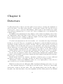
6 Detectors
62
7 Interactions
85
8 Optimizers
93
3
Chapter 1
Introduction
Modern science without lasers is like a lake without water, boring and desert-like. Over
the past decades lasers made it possible to observe motions in nature with unprecedented
temporal resolution. Let us illustrate this by one example. Everybody who has taken pictures
with dad’s analog camera knows that the little son playing hockey may only be captured in
a sharp image if the shutter time is very very short. A fraction of a millisecond is what state
of the art cameras are able to do. It is fast enough for most hockey players but it is not
fast enough to capture much more tiny hockey players in nature, such as single molecules or
atoms. Clever people have thought of an alternative way to capture images of fast moving
objects. Darken the room, leave the camera shutter open all the time, and illuminate the
object you want to image with a short flash of light. People who like clubbing know what
we mean, it’s nothing but a strobe light. Many images like this in a row make a nice movie.
The shortest strobe currently available is a (sub-)femtosecond laser. A single pulse is about
0.000000000000005 seconds long.
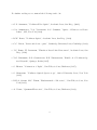
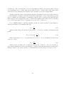
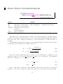
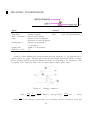
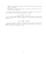
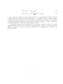
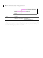
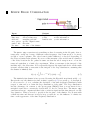
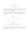
Figure 1.1: Temporal pulse width (full width at half maximum) versus spectral bandwidth
for a Ti:Sapphire laser.
Because a short burst of light must be supported by a lot of spectral components, the
4
spectrum of a femtosecond laser pulse is usually some tens or hundreds of nanometers broad.
In fig. 1.1 we show how broad the spectrum needs to be to support a laser pulse of a given
temporal duration. The lasers center wavelength is 800 nm. Obviously, a pulse width of
100 ps requires a spectral bandwidth of 0.01 nm, whereas a pulse width of 10 fs already
needs about 100 nm spectral bandwidth! Now, every optical component, such as a lens, a
window, a dielectric mirror etc., are dispersive, meaning that they influence the different
spectral components of a short laser in a different way. That, as one might guess, sometimes
has dramatic effects on the laser pulse. In other cases, well controlled dispersion is used
on purpose for intentional pulse manipulations. Another striking feature of ultrashort laser
pulses is that the peak intensity can be enormously high although the energy is at a ridiculously low level. All sorts of nonlinear material responses show up and need to be considered
when doing experiments with pulses so short. A familiar nonlinear effect is breaking the
optics whenever the laser intensity is larger than the damage threshold intensity. To circumvent damaging of optics, especially in laser amplifiers, lead to the introduction of what is now
known as chirped pulse amplification (CPA). To do such things as stretching or compressing
pulses special optical designs are required.
In the next few chapters we introduce a modular programming tool — we called it LAB
II because it was in fact in lab 2 of our institute where we spent so many nights trying to
figure out why the heck this or that stupid thing happened — that allows to simulate most
of the experimental setups in a rather intuitive way. It is almost like a virtual laboratory.
Elements are placed on a white board and connected by laser beams just as one would set
up an experiment in the lab. We have chosen to embed our package in LabView since the
graphic programming language G allows in a unique way to program something that actually
also looks like a virtual experiment.
Chapter 2 summarizes the basic math we have used for all of the programming. Chapter 3
describes the different laser sources, chapter 4 all the available linear elements, chapter 5 all
the available nonlinear elements, chapter 6 all the detectors that have been implemented,
and chapter 7 a selection of modules simulating laser matter interaction. The very last
chapter 8 introduces optimization algorithms which are commonly used in combination with
pulse shaping to reach specific goals. A couple of examples will be given.
So, enjoy reading and more importantly working with LAB II ,
Thomas
5
For further reading we recommend the following textbooks:
. G.P. Agrawal; ”Nonlinear Fiber Optics”, Academic Press, San Diego (2001)
. S.A. Akhmanov, V.A. Vysloukh, A.S. Chirkin; ”Optics of Femtosecond Laser
Pulses”, AIP, New York (1992)
. R.W. Boyd; ”Nonlinear Optics”, Academic Press, San Diego (1992)
. C.C. Davis; ”Lasers and electro-optics”, Cambridge University Press, Cambridge (1996)
. J.C. Diels, W. Rudolph; ”Ultrashort Laser Pulse Phenomena”, Academic Press, San
Diego (1996)
. V.G. Dmitriev, G.G. Gurzadyan, D.N. Nikogosyan; ”Handbook of Nonlinear Optical Crystals”, Springer, Berlin (1997)
. S. Huard; ”Polarization of Light”, John Wiley & Sons, Chichester (1997)
. S. Mukamel; ”Nonlinear Optical Spectroscopy”, Oxford University Press, New York
(1995)
. B.E.A. Saleh, M.C. Teich; ”Fundamentals of Photonics”, John Wiley & Sons, New
York (1991)
. A. Yariv; ”Quantum Electronics”, John Wiley & Sons, Chichester (1989)
6
Chapter 2
Ultrashort Laser Pulses
2.1
General
First of all we will restrict ourselves to the time dependence of the electric field and omit
the spatial part. This is equivalent to the viewpoint that a detector is located at a fixed
position and the field only varies with time. Since the electric field of the laser pulse is in
principle a measurable quantity it must be real. For most calculations, however, it is much
more convenient to use the analytic signal — a complex quantity — and in a moment we
will see why. So we start with an electric field described by
E(t) = A(t) cos [Φ(t)] = A(t)
=
1 iΦ(t)
e
+ e−iΦ(t)
2
1
A(t) eiΦ(t) + c.c.
2
(2.1)
where A(t) is time dependent amplitude and Φ(t) the time dependent phase. The Fourier
transform of the electric field is
Z∞
E(ω) = F{E(t)} =
dt E(t) e−iωt = A(ω) eiΦ(ω)
(2.2)
−∞
and the inverse Fourier transform is equivalently
E(t) = F
−1
1
{E(ω)} =
2π
Z∞
dω E(ω) eiωt .
(2.3)
−∞
One might ask, why do we consider the Fourier transformation of a time varying laser
pulse? There are many reasons to do this. The spectral analysis yields information on
the wavelengths contained in the pulse and also provides a hint whether a pulse may be
compressed in time or is as short as it can possibly get. The propagation of ultrashort laser
7
pulses through dispersive media depends strongly on the frequency and, finally, the concept
of Fourier transformation is a powerful tool for solving equations.
Since the electric field is real, i.e. E(t) = E ∗ (t), we see immediately that
∗
 ∞
Z∞
Z
dt E(t) e−iωt = E(ω).
(2.4)
E ∗ (−ω) =  dt E(t) eiωt  =
−∞
−∞
This is a useful identity for a number of the following calculations. Inspecting equation 2.1 shows that the Fourier transform has two distinct distributions which are symmetric
with respect to the origin of the frequency axis. Now, have you ever seen a spectrometer
that can measure at negative frequencies or wavelength? Certainly not, so it is sometimes
more convenient to start in the frequency domain by defining a field having only positive
frequencies. The consequence is that the electric field in the time domain becomes complex.
Again we end up with an unrealistic situation since we use complex instead of real Fourier
transformation. None of these problems would occur, would we use a real Fourier transformation, for example the cos Fourier transformation, but the mathematical efforts would
increase substantially and so nobody uses it.
1
E + (t) =
2π
Z∞
dω E(ω) eiωt
1
=
2π
Z∞
dω E + (ω) eiωt
(2.5)
−∞
0
with
+
E (ω) =
E(ω) : ω ≥ 0
0 : ω<0
(2.6)
The same holds true for the negative frequency components. They give rise to a field
E − (t). It is easy to show that the original field is reconstructed by
E(t) = E − (t) + E + (t) and E(ω) = E − (ω) + E + (ω)
(2.7)
Now we want to become somewhat more specific and adapt the formalism to laser pulses
we have to deal with in the laboratory. What are the specific features of say a Ti:sapphire
laser pulse. It’s ’central’ wavelength is around 800 nm, the pulse width is typically around
100 fs with some exceptions where pulses do get as short as 5 fs. Because the oscillation
period of the field at this wavelength is about 2.7 fs the pulses are usually longer than
one period. If we record a spectrum we see that there is a broad distribution around the
center wavelength with a width of some tens of nanometers. These experimentally observed
characteristics influence the mathematical description in the following way. Identifying a
’central’ wavelength ω0 and a width ∆ω in the spectrum satisfying the condition ∆ω/ω0 < 1
is equivalent to ∆t/T > 1. This means that the electric field of the laser pulse can be
split into a product of a slowly varying envelope ∆t and a rapid oscillation with a period
T = 2π/ω0 . The electric field in the time domain is then written
8
1
1
A(t) eiϕ(t) eiω0 t = ε(t) eiω0 t
(2.8)
2
2
where A(t) is the slowly varying amplitude, ϕ(t) the slowly varying phase, and ε(t) a
complex quantity combining the slowly varying parts. The definition of ω0 is not unique
and there are various ways to define it. A convenient one is to use the ’central’ frequency,
i.e. the frequency where the spectral amplitude has a global maximum. If the spectrum is
structured and the maximum is not easily identified it is more convenient to use the first
frequency moment. The definition of moments will appear a few times throughout the text.
The nth order moment of x is defined
R
dx xn f (x)
(n)
n
(2.9)
x = R
dx f (x)
E + (t) =
where f (x) is a distribution function. Now we have most of the basic tools and it is
time to apply the formalism developed so far to Gaussian pulses. A Gaussian pulse has a
Gaussian envelope function and we restrict ourselves to phases quadratic in time and we omit
the constant phase. If we do this many interesting effects can be calculated analytically. The
reason for choosing a Gaussian shaped envelope is simply that it allows to calculate most
things analytically with very little mathematical effort.
∆ω 2
A∆ω 2 2
∆ω
2
t cos ω0 t +
t
exp −
(2.10)
E(t) = √
4(1 + A2 )
4(1 + A2 )
2 π(1 + A2 )1/4
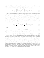
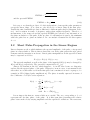
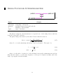
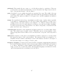
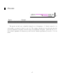
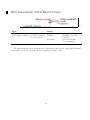
Figure 2.1 shows the electric field E(t) for a pulse with A = 0. The rapid oscillations
increase with time, reach a maximum, and decrease again. This behavior is determined by
the slowly varying envelope, i.e. the Gaussian.
The reason to choose this form is that in most cases we start with a pulse having a fixed
spectral width ∆ω and treat effects that do not change this width. The constant factor
makes the Fourier transform of this pulse relatively simple.
(ω − ω0 )2 (1 + iA)
(ω + ω0 )2 (1 − iA)
+ exp −
(2.11)
E(ω) = exp −
∆ω 2
∆ω 2
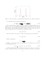
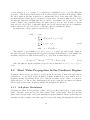
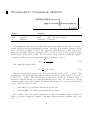
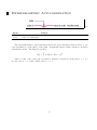
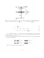
Clearly, the Fourier transform has two distinct frequency distributions around −ω0 and
ω0 (see fig. 2.2). The slowly varying envelope approximation breaks down when the two
frequency distribution start to overlap at the origin of the frequency axis. In addition, it
may be seen that a quadratic phase modulation in time leads to a quadratic phase modulation
in the frequency domain. Splitting the frequency distribution in the negative and the positive
component leads to
(ω + ω0 )2 (1 − iA)
−
E (ω) = exp −
(2.12)
∆ω 2
(ω − ω0 )2 (1 + iA)
+
E (ω) = exp −
(2.13)
∆ω 2
9
Figure 2.1: The slowly varying envelope and the rapid oscillations of a Gaussian pulse E(t)
are shown.
In the time domain we obtain
∆ω
∆ω 2
2
E (t) = √
exp −
(1 + iA)t − iω0 t
4(1 + A2 )
2 π(1 + A2 )1/4
∆ω
∆ω 2
+
2
E (t) = √
exp −
(1 − iA)t + iω0 t .
4(1 + A2 )
2 π(1 + A2 )1/4
−
(2.14)
(2.15)
After having defined the fields we have to answer the question what do we measure?
Here is where the problems start. What do we measure? First of all this question has to be
stated in a different way. If we use this specific detector what do we measure? Let’s start for
example with a pyro-electric detector. The laser pulse is absorbed in a ideally non-reflecting
layer which subsequently gets warmer and changes its electrical resistivity. This change then
is monitored on an analog display. The whole device has a time constant of a few tens of
milliseconds. So what do we measure? Not surprisingly the pulse energy. Or, what happens
if we use a photodiode with a time constant of ten femtoseconds? With this diode we will not
resolve the rapid oscillations of the laser field but we will be able to measure the temporal
evolution of the slowly varying envelope. So what we measure is mostly dependent on the
type of detector which we are using. A detector with a time constant large compared to the
rapid oscillations but fast compared to the temporal envelope will measure a quantity called
the instantaneous intensity I(t).
t+T
Z /2
1
I(t) = 0 c0 n
T
dt0 E 2 (t0 )
t−T /2
10
(2.16)
Figure 2.2: The electric field of a real Gaussian pulse E(ω) shows two distinct contributions.
For a Gaussian pulse the instantaneous intensity is
1
∆ω 2
∆ω 2
2
I(t) = 0 c0 n √
exp −
t
(2.17)
2
2(1 + A2 )
π 1 + a2
where 0 is the dielectric constant of vacuum, c0 the speed of light in vacuum, and n the
index of refraction of the transparent material the pulse is propagating in. Obviously, the
integration over one period reflects the fact that we have a detector not able to resolve the
field oscillations. The instantaneous intensity is measured in energy per unit time and per
unit area. If the finite area A of the detector is considered we obtain
Z
P (t) = dσ 0 I(t)
(2.18)
A
If the response time of the detector is even longer the pulse energy W is measured
Z∞
W =
dt P (t)
(2.19)
−∞
which for a Gaussian is
0 c0 n∆ω
√
(2.20)
2π
Making use of the slowly varying wave approximation it is relatively easy to show that
the following equalities hold
W =
1
I(t) = 0 c0 n ε(t)ε∗ (t) = 20 c0 n E + (t)E − (t)
(2.21)
2
A further useful quantity is the instantaneous frequency ω(t). Suppose you are able to
measure a spectrum of the laser, say every femtosecond, and you plot the center frequency
11
of each of these spectra as a function of time, you have a good idea of what the instantaneous frequency is. A more sophisticated definition is given by two-dimensional distribution
functions. Knowing the phase Φ(t) the instantaneous frequency is derived in the following
way
ω(t) = ∂t Φ(t) = ∂t ϕ(t) + ω0
(2.22)
For a Gaussian pulse we find
ω(t) = ω0 +
∆ω 2 A
t
2(1 + A2 )
(2.23)
Obviously, a quadratic phase leads to a linear change of the instantaneous frequency.
This is called a linear chirp. A quadratic chirp corresponds to a cubic phase and so on.
Now, suppose an ideal spectrometer is used to measure the spectrum of the pulse. Because
we operate in the frequency domain, there is no such thing as time anymore. Each infinitely
narrow frequency component corresponds to an infinitely long wave. Later we will see what
influence the finite resolution of a real spectrometer has on the measurements. We have
already noted that no spectrometer is able to measure negative frequencies, therefore, the
spectrum is
S(ω) = η(ω)2 |E + (ω)|2
(2.24)
where η(ω) contains all specific information on the spectrometer and the detection unit
used, i.e. how the response of the spectrometer (mirrors, gratings, prisms, photomultiplier,
CCD, etc.) depends on the frequency. For an ideal spectrometer η is a constant and can be
determined using Parseval’s theorem
Z∞
−∞
1
dt |E + (t)|2 =
2π
Z∞
dω |E + (ω)|2
⇒
η2 =
0 c0 n
π
(2.25)
−∞
0 c0 n
(ω − ω0 )2
exp −2
S(ω) =
π
∆ω 2
(2.26)
Integrating the spectral intensity S(ω) over ω must again yield the total pulse energy W
W =
0 c0 n∆ω
√
2π
(2.27)
There is one thing you should never forget. Once the instantaneous intensity I(t) is
known, never perform a Fourier transform in order to calculate the spectrum S(ω). Calculate
the electric field first, Fourier transform the field, and then calculate the spectral intensity.
This is the only way to obtain the correct spectrum. Try both ways and you will see that a
direct Fourier transformation leads to an erroneous result.
The last thing in this chapter is the definition of the full width at half maximum (FWHM).
For the Gaussian pulse the intensity FWHM is
12
p
8 ln 2(1 + A2 )
FWHMt =
∆ω
(2.28)
√
FWHMω = ∆ω 2 ln 2
(2.29)
and the spectral FWHM
It is easy to see that the product of both is independent of any specific pulse parameters
except the linear chirp. Note, that we only allowed for a linear chirp in the first place.
Usually the time bandwidth product is different for different pulse shapes (Gaussian, sech2 ,
etc.) and is written in terms of frequency rather than angular frequency. Therefore, a
measurement of the temporal and the spectral FWHM gives already some information on
the phase modulation of the pulse. If the product of both numbers is equal to the minimum
value the pulse has no phase modulation. In our analytic Gaussian model this requires
A = 0.
2.2
Short Pulse Propagation in the Linear Regime
Linear elements are those which influence the spectral amplitude of the pulse or its spectral
phase in a linear fashion. This is almost always the case if the pulse passes through optical
elements and the intensity is moderate. Linear pulse manipulations in the spectral domain
may be expressed as follows
Eout (ω) = Ein (ω) · H(ω) e−iΦ(ω) .
(2.30)
The spectral amplitude as well as the phase of the input field Ein (ω) may be changed by
H(ω) and Φ(ω), respectively. The generated output field is Eout (ω).
Almost all elements in the lab, which happen to be in the laser beam, are dispersive
and modify the spectral phase of the pulse. Dispersion, in most cases, is an unwanted side
effect that one would rather avoid in the first place but sometimes it is used on purpose, for
example in CPA (chirped pulse amplification). The phase is usually expressed in terms of
the coefficients of a Taylor series expansion.
∞
X
1 k
∂ω Φ(ω)ω=ω0 (ω − ω0 )k
Φ(ω) =
k!
k=0
=
∞
X
1
Φk (ω − ω0 )k
k!
k=0
with
(2.31)
Φk := ∂ωk Φ(ω)ω=ω0
Let us inspect the first two terms a little more careful. The one corresponding to k = 0
represents the absolute phase of the pulse. It is this term that determines the relative
phase between the slowly varying amplitude and the rapid field oscillations. The next term,
13
corresponding to k = 1, consists of a constant factor multiplied by (ω − ω0 ). Recalling the
properties of the Fourier transformation shows that a phase term linear in frequency, shifts
the whole pulse in the time domain by a constant time delay on the time axis. Therefore,
the first derivative with respect to frequency corresponds to the time a pulse needs to travel
through the dispersive medium and may be used to determinate the group velocity. All
terms of higher order generally change the pulse envelope in some way. It may be shown
that all even order Taylor coefficients change the slowly varying envelope in a symmetric
fashion whereas all odd order Taylor coefficients cause an asymmetric change.
In many textbooks the phase is expressed as follows
Φ(ω) = β(ω)z
∞
X
1 k
∂ω [β(ω)z]ω=ω0 (ω − ω0 )k
=
k!
k=0
∞
X
1
=
βk z (ω − ω0 )k
k!
k=0
with
(2.32)
βk := ∂ωk β(ω)ω=ω0
The number β per definition is a wave vector, or a phase per unit length. Suppose
the pulse traverses a transparent but dispersive medium with thickness d, and assume the
medium’s dispersion is fully characterized by β1 only, then we immediately see that
Eout (t) = F −1 Ein (ω)e−iβ1 d(ω−ω0 ) = Ein (t − β1 d).
(2.33)
Since the pulse propagates with the group velocity we find that β1 = 1/vg or vg = 1/β1 =
d/Φ1 .
2.3
Short Pulse Propagation in the Nonlinear Regime
Nonlinear effects involve products of electric fields in the time domain and since this is
equivalent to a convolution in the frequency domain, nonlinear processes usually lead to
frequency mixing. Depending on the order of the process there are two, three, or even more
pulses involved. So far we have implemented the most commonly encountered nonlinear
effects, such as three wave frequency mixing and self-phase modulation.
2.3.1
Self-phase Modulation
Self-phase modulation is in principle a third order (χ(3) ) effect and leads to a time varying
phase. The three waves involved are three replica of the original pulse. Just as a spectral
phase leaves the spectrum of the pulse unchanged but has dramatic effects on the temporal
intensity, a temporal phase causes the opposite, it leaves the temporal intensity the same but
14
changes the spectrum. An easy but somewhat sloppy way to express self-phase modulation
is by introducing an intensity dependent index of refraction
n(I) = n0 + n2 I
(2.34)
which in turn causes an extra phase in the time domain
ω0
ω0
n(I(t)) z =
(n0 + n2 I(t)) z
c0
c0
ω0
Φnl (t) =
n2 I(t) z
c0
Φ(t) =
so it is essentially the product of intensity I times the propagation distance z that determines the nonlinear phase contribution. In principle one would expect the same result
as one changes the material thickness z but keeps the product Iz constant by adjusting
the intensity I. This is not quite true, especially for large z, since dispersion effects tend to
broaden the pulse as it propagates which leads to a decreasing intensity I, and, consequently,
a decrease in the nonlinear phase contribution Φnl .
A frequently used expression in this context is the so called B-integral. The B-integral
is a measure of the accumulated nonlinear phase and serves as a criterion whether nonlinear
effects play a role or not. It takes into account the fact that the intensity might change as
the pulse propagates along the z-coordinate. It is defined by the following relation
ω0
B=
c0
Zd
2π
dz n2 I(z) =
λL
0
Zd
dz n2 I(z)
(2.35)
0
As a rule of thumb, self-phase modulation becomes a serious issue when the B-integral
exceeds 3 or 4, although effects of self-phase modulation may be seen much earlier.
In order to account for both dispersion and self-phase modulation, one often uses an
algorithm called ’split step Fourier transform’. This algorithm splits the material in many
slices. Each slice is again subdivided into three regions. Now, the first region takes into
account one half of the linear dispersion. Then one performs a Fourier transformation to the
time domain, accounts for the temporal phase due to self-phase modulation of the full slice
in the second region, and Fourier transforms back. The third region then takes care of the
missing half of the linear dispersion. This is done for all slices and eventually, if the number
of slices is high enough, the algorithm will converge and lead to the true output pulse.
2.3.2
Three Wave Mixing Processes
The equations that describe three wave mixing processes are coupled nonlinear differential
equations, one differential equation for each of the three fields. These equations need to
be integrated along the direction of propagation in order to simulate three wave mixing
processes in a nonlinear crystal, such as second harmonic generation, sum frequency mixing,
15
or difference frequency mixing. Energy conservation requires that ω1 + ω2 = ω3 . The
interplay between the three field Ẽj=1,2,3 is described by
Z
∂z Ẽ1 (ω1 ) = −iκ1
Z
∂z Ẽ2 (ω2 ) = −iκ2
Z
∂z Ẽ3 (ω3 ) = −iκ3
dω2 Ẽ2∗ (ω2 ) Ẽ3 (ω1 + ω2 ) ei∆k(ω1 ,ω2 )z
(2.36)
dω1 Ẽ1∗ (ω1 ) Ẽ3 (ω1 + ω2 ) ei∆k(ω1 ,ω2 )z
(2.37)
dω1 Ẽ1 (ω1 ) Ẽ2 (ω3 − ω1 ) e−i∆k(ω1 ,ω3 −ω1 )z
(2.38)
with
ωj2 deff
κj =
c20 kj
1 (2)
deff =
χ
2
(ω1 + ω2 )n3 (ω1 + ω2 ) − ω2 n2 (ω2 ) − ω1 n1 (ω1 )
∆k(ω1 , ω2 ) =
c0
(2.39)
(2.40)
(2.41)
where ωj is a frequency component corresponding to spectrum Ej and nj (ω) is the wavelength dependent index of refraction. The coupled set of three differential equations is
integrated along the direction of propagation z. The final spectral fields are obtained by
propagating the solution of the differential equations with the corresponding wave vector kj ,
which incorporates the linear dispersive effects
Ej = Ẽj e−i·kj L
(2.42)
In case the conversion efficiency is small the above set of differential equations may be
substantially simplified. This is usually the case for thin crystals and/or rather low intensities. If we assume that both fundamental input beams are not depleted by the conversion
process ∂z E1,2 ≡ 0, only one differential equation is left to solve
Z
E3 (ω3 ) = −κ
dω1 E1 (ω1 ) E2 (ω3 − ω1 ) η(ω1 , ω3 − ω1 )
ei ∆k(ω1 ,ω2 ) L − 1
∆k(ω1 , ω2 ) L
2
ω3 deff
κ =
c20 k3
η(ω1 , ω2 ) =
(2.43)
(2.44)
(2.45)
Here, E1 and E2 are the spectral fields of the incoming pulses — which are constant —
and E3 is the spectral field of the generated pulse. The constant factor κ is determined by the
center frequency ω3 , the effective nonlinearity deff (units [pm/V]) of the specified nonlinear
interaction process (which depends on the crystal orientation), the vacuum phase velocity
c0 , and the wave vector at the center frequency k3 . The phase mismatch is ∆k = k3 −k2 −k1 .
16
2.3.3
Optical fiber propagation
Another important nonlinear element is the optical fiber which is frequently used for a process
called super-continuum generation. To describe pulse propagation along an optical fiber we
need to include two more nonlinear effects, i.e. self steepening and the Raman effect, and
find
∂ξ Ẽ + (ξ; τ ) = −i
∞
X
km m +
∂ Ẽ (ξ; τ )
m m! τ
i
m=2
Z
2i
+
∂τ Ẽ (ξ; τ ) dτ1 R(τ1 )|Ẽ + (ξ; τ − τ1 )|2 , (2.46)
− iγ 1 −
ω0
where we have combined the instantaneous electronic response and the Raman response
of the medium to
R(t) = (1 − f ) δ(t) + f RR (t).
(2.47)
The relative weight is governed by the constant f which for fused silica is approximately
0.18.
17
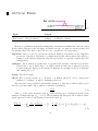
Chapter 3
Lasers
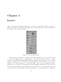
First we introduce the numerical structure of a pulse. A virtual laser pulse is a cluster of
different data types. (A cluster in G is equivalent to a structure in C or a record in Pascal).
It consists of the following elements.
Figure 3.1: Laser pulse cluster.
The first item is the number of sample points and determines how many points are used
to represent a pulse in time or frequency space. The value is always a power of 2, which
allows to use the FFT-algorithm (fast Fourier transformation). The pulse is encoded in the
frequency domain and we only consider positive frequencies. The frequency vector is stored
relative to the center frequency ω0 of the laser pulse. The vector w contains the relative
frequency vector and the corresponding spectral amplitudes and phases are stored in the
vector |E(ω)| and phi(ω). Because the energy per unit area, i.e. the fluence, is stored
separately the spectral amplitude is usually normalized to a value appropriate for numerical
18
calculations. The beam diameter is stored in diameter. First order phases (time delays)
are accumulated in t0 . Using such an encoding allows to consider large delay times with
relatively modest sampling rates which would otherwise violate the Nyquist limit.
An important flag is auto. It determines whether all simulations are done with a variable
or a fixed number of samples. Variable means that at the input of every element the program
tries to estimate the ideal number of sampling points needed to propagate the pulse through
that element, and resamples the pulse to that ideal sampling grid. Auto mode is switched
on or off by appropriate choice of parameters in all source or laser vis.
Note, LAB II assumes a uniform intensity profile across the specified beam diameter.
That is, the fluence is determined through
W
,
(3.1)
πr2
with the pulse energy W and the beam radius r = d/2. If you assume a Gaussian beam
profile
2r2
(3.2)
F (r) = F0 exp − 2 ,
w0
F0 =
with a beam waist of w0 = d/2 (measured at 13.5%, i.e. 1/e2 ), the fluence at the beam
center (r = 0) is
2W
,
(3.3)
πr2
which is twice as high as for a uniform beam profile. That is to say, if you’d like to
perform the simulations at the peak intensity of a pulse with a Gaussian spatial beam profile
having a waist of d/2, then you have to artificially increase the energy by a factor of two.
F0 =
19
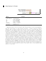
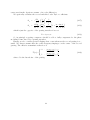
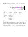
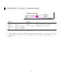
Gaussian pulse
c
TF
Input
Output
energy:
energy
pulse out:
beam diameter: beam diameter
λ0 :
center wavelength
∆λ:
spectral FWHM
∆τ :
temporal FWHM
sampling:
number of samples
resolution:
sampling mode
laser pulse
Gaussian pulse produces a laser pulse with a Gaussian shaped slowly varying amplitude.
The pulse characteristics are either specified in frequency or in time domain (two different
clusters). Only one input is required. In both cases one needs to specify the pulse energy,
the diameter of the transverse mode profile, and the center wavelength λ0 . In addition, in
frequency domain the FWHM of the laser spectrum ∆λ, and in time domain the FWHM
of the temporal intensity ∆τ are mandatory inputs. If nothing else is done, all subsequent
calculations run in auto mode, that is, fields are automatically resampled if necessary and
iterations are adjusted such that outputs converge to the percent level. In case the sampling
cluster is connected all simulations run in manual mode and sampling is determined by the
values in this cluster. The number of samples is always a power of two and there are four
options for the type of resolution. High spectral: The spectral window is such that the laser
spectrum just fits in and the spectral resolution is highest. High temporal: Here, sampling
is adjusted so that the temporal resolution is high and the full time window is only slightly
larger than the temporal FWHM of the pulse. Of course spectral resolution is very poor here.
Balanced: In this mode the sampling is such that both temporal and spectral amplitude are
sampled with a somewhat balanced resolution. Time window: Here, you can adjust the time
window to a fixed value.
20
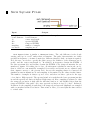
Sech Square Pulse
c
TF
Input
Output
energy:
energy
pulse out:
beam diameter: beam diameter
λ0 :
center wavelength
∆λ:
spectral FWHM
∆τ :
temporal FWHM
sampling:
number of samples
resolution:
sampling mode
laser pulse
Sech Square Pulse is similar to Gaussian Pulse. The only difference is the slowly
varying envelope is a sech2 rather than a Gaussian. The pulse characteristics are either
specified in frequency or in time domain (two different clusters). Only one input is required.
In both cases one needs to specify the pulse energy, the diameter of the transverse mode
profile, and the center wavelength λ0 . In addition, in frequency domain the FWHM of
the laser spectrum ∆λ, and in time domain the FWHM of the temporal intensity ∆τ are
mandatory inputs. If nothing else is done, all subsequent calculations run in auto mode,
that is, fields are automatically resampled if necessary and iterations are adjusted such
that outputs converge to the percent level. In case the sampling cluster is connected all
simulations run in manual mode and sampling is determined by the values in this cluster.
The number of samples is always a power of two and there are three options for the type
of resolution. High spectral: The spectral window is such that the laser spectrum just fits
in and the spectral resolution is highest. High temporal: Here, sampling is adjusted so that
the temporal resolution is high and the full time window is only slightly larger than the
temporal FWHM of the pulse. Of course spectral resolution is very poor here. Balanced:
In this mode the sampling is such that both temporal and spectral amplitude are sampled
with a somewhat balanced resolution. Time window: Here, you can adjust the time window
to a fixed value.
21
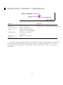
Add noise
c
TF
Input
pulse in:
noise control:
input pulse
type of noise
Output
pulse out:
output pulse
Add noise adds a certain type of noise to the input laser pulse. Presently the options
are multiply/add amplitude noise and multiply/add phase noise. Either the spectral
amplitude or the spectral phase is multiplied with a white noise of specified amplitude. An
amplitude of 0.1 for example will add ten percent noise or multiply the existing amplitude
by (1 + 0.1 · noise) depending on whether add ... or multiply ... is selected.
22
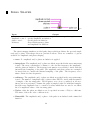
Read Pulse from File
c
GS
Input
path:
decimalpoint=’.’ ?:
path to file
set to false for ’,’ instead of ’.’
Output
pulse out:
laser pulse
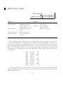
Read Pulse reads a pulse from a file. The format is as follows:
nop=. . .
auto=. . .
w0[THz]=. . .
fluence[mJ/cm2 ]=. . .
diameter[mm2 ]=. . .
t0[fs]=. . .
frq E(amp) phi(w)
... ... ... ...
number of samples
simulation mode
center frequency
energy per unit area
beam diameter
first order phase
frequency, amplitude, residual phase
23
Read Pulse from Spreadsheet
c
GS
Input
Output
path:
path to file
pulse out:
auto:
simulation mode
delimiter: tab (default), space, etc.
fluence:
fluence value
∧
2 n:
number of samples
laser pulse
Read Pulse from Spreadsheet reads a pulse from a spreadsheet file. The format is
c
equivalent to that used by the FROG program (Femtosoft).
The first column gives the
wavelength in nm, the second the spectral intensity in units of J/(m2 nm), the third column
the phase, the fourth column the real part, and the last column the imaginary part of the
spectral field in units of V/(m nm). Obviously, there is too much information here, but we
decided to simply use the format of the FROG software in order to facilitate the import of
retrieved pulses. Pulses are also correctly loaded if the last two columns are missing. If the
third column is missing the phase is assumed to be zero for all wavelengths.
If auto is true the the spectrum is automatically sampled, if false, then the number of
samples must be specified and the loaded spectrum is interpolated accordingly. If the fluence
is specified then the amplitude of the electric field is recalculated such the the fluence is equal
to the value specified.
24
Chapter 4
Linear Elements
All elements have at least one control panel that you need to connect. It allows you to
control the important parameters for the simulation and it also allows to change things and
watch in real time how the laser pulse intensity or the spectrum or whatever you are looking
at changes.
First there are a number of standard elements, such as a delay, a telescope, etc., nothing
of great importance but sometimes they come in handy. Then there are a number of linear
elements, mostly complex optical setups which are designed to stretch or compress short
pulses. In addition, all of them have a little intelligent brother that automatically adjusts
some parameters in order to optimize for maximum peak intensity at the output. Also you’ll
find most standard glass materials.
25
Ideal Beamsplitter
c
MH
Input
pulse in:
absorption:
transmission:
Output
input laser pulse
transmitted pulse:
absorption [0 . . . 1]
reflected pulse:
transmission [0 . . . 1]
transmitted laser pulse
reflected laser pulse
The ideal beamsplitter is used to split the incoming beam in two outgoing replica.
The transmission T (0 . . . 1) as well as the absorption A(0 . . . 1) are wavelength independent
and the reflectivity is R = 1 − A − T . Make sure the sum of A + T is always lower than 1.
A real beamsplitter where the transmitted beam actually passes through some dispersive
material is easily simulated by introducing a piece of dispersive material in the transmitted
beam path.
26
Beamsplitter
c
MH
Input
Output
pulse in:
input laser pulse transmitted pulse: transmitted laser pulse
beamsplitter: file name
reflected pulse:
reflected laser pulse
The beamsplitter is a more realistic version of the module ideal beamsplitter. You
may specify a file that lists the reflectivity as well as the transmission as a function of the
wavelength. This file should have the extension \*.bs and must be located in the folder
..\beamsplitters\. The files are text files and consist of three columns. The first is the
wavelength in units of meter, the second the reflectivity, and the third the transmission. If
you only specify a few values the module will interpolate in order to determine all necessary
values. The absorption is calculated from the transmission and the reflectivity values. The
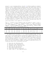
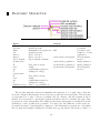
following table shows an example of a low-pass filter with a cutoff wavelength at 800 nm.
Below 800 nm it is fully transparent and above 800 nm completely opaque.
wavelength [nm]
reflectivity
transmission
2.0000E-7
3.0000E-7
4.0000E-7
5.0000E-7
6.0000E-7
7.0000E-7
7.9900E-7
8.0100E-7
9.0000E-7
1.0000E-6
1.1000E-6
0
0
0
0
0
0
0
1
1
1
1
1
1
1
1
1
1
1
0
0
0
0
27
Beamcombiner
c
TF
Input
Output
pulse A in: first incoming pulse
pulse A+B out:
pulse B in: second incoming pulse
combined pulse
The beamcombiner is designed to act as a beamsplitter that is used to combine two laser
pulses. Of course in a collinear fashion because all calculations are one-dimensional. The
two input pulses may have different center wavelengths, spectral bandwidths, or even a time
delay with respect to each other. None of the two pulses looses energy which of course is not
true for a real beamsplitter. In case the two beams have different diameters the diameter of
the second beam is adjusted to match that of the first beam, that is, when the two beams are
physically combined they end up having the same diameter. Also note that the combination
is non-interferometric, which in practice means the the two beams are not really collinear
but have a small angle.
28
Delay
c
TF
Input
pulse in:
delay [fs]:
delay stage:
incoming laser pulse
temporal delay
mimics a mechanical delay stage
Output
pulse out:
delayed pulse
The delay simulates a mechanical delay line. The delay may be specified in terms of
the time delay or in terms of the optical path the beam has to propagate. If you enter the
optical path the delay corresponds to the time it takes to travel the path back and forth just
as it is the case for a real mechanical delay.
29
Telescope
c
TF
Input
pulse in:
scale diameter:
scal area:
incoming laser pulse
relative change of diameter
relative change of pulse area
Output
pulse out:
output laser pulse
telescope simulates a telescope. It does nothing but to increase or decrease the fluence
(energy per unit area) corresponding to the magnification you choose. This you may do in
two different ways. First by specifying the magnification of the beam diameter or second of
the beam area. A value larger than one increases the beam diameter and vice versa.
30
Transparent Dispersive Element
c
TF
Input
Output
pulse in:
incoming laser pulse
pulse out: output laser pulse
dispersive element: specify the glass material phi2
second order phase
and thickness
The transparent linear medium is usually just a piece of some glass material. This
may be a vacuum window, a lens, or by combining two of those elements also an achromatic
lens or more complicated arrangements may be simulated.
The phase change introduced by just a piece of transparent but dispersive material of a
given length is
Φ(ω) =
ω
n(ω)z
c0
(4.1)
where n(ω) is the index of refraction and z the thickness of the material. The coefficients
of the Taylor series are easily calculated
i
z h k−1 ∂ωk Φω0 =
k ∂ω n ω0 + ω0 ∂ωk nω0
(4.2)
c0
To simulate such a material the index of refraction must be known. Usually it is tabulated
or given as a Sellmeier equation. In LAB II many glasses have been implemented through
the corresponding Sellmeier equation. The most prominent ones are fused silica (SQ1), BK7
and SF10 etc. You may just copy and paste any of the files under a new name (the material
you wish to add) in the folder ../chi1/ and change the parameters accordingly. It is that
easy to add a new material to the list.
31
Fabry-Perot Interferometer
c
MH
Input
Output
pulse in: incoming laser pulse
pulse reflected:
R1:
reflectivity of front surface pulse transmitted:
R2:
reflectivity of back surface
material: material between front and
back side
d:
material thickness
alpha:
angle of incidence
reflected laser pulse
transmitted laser pulse
The Fabry Perot interferometer consists of some material with two partially reflective
coatings on both sides. The material may be air or any of the transparent materials available
in the data base. The coatings are assumed to be ideal and impose no additional phase on
the pulse.
The amplitude and the phase change for the transmitted pulse Et and the reflected pulse
Er introduced by the Fabry-Perot interferometer are
Et
Er
exp(iδ/2)
= Ei t1 t2
1 − r1 r2 exp(iδ)
r1 − r2 exp(iδ)
= Ei
1 − r1 r2 exp(iδ)
(4.3)
(4.4)
where Ei is the incoming laser pulse, t1 and t2 are the transmission coefficients for the
transitions from air to the medium
and the √medium to air, respectively. The amplitude
√
reflection coefficients are r1 = R1 and r2 = R2 .
δ = 2d
sin θ =
nω
cos θ
c0
1
sin α
n
(4.5)
(4.6)
where n is the index of refraction of the medium between the two interfaces, ω is the laser
frequency, c0 the speed of light in vacuum, and θ the angle of propagation in the medium.
32
Gires-Tournois Interferometer
c
MH
Input
pulse in:
reflectivity:
material:
d:
alpha:
incoming laser pulse
reflectivity of front side
medium between front and back side
thickness of the medium
angle of incidence
Output
pulse out:
output laser pulse
The Gires Tournois interferometer is a special case of the Fabry Perot with the
back side being 100% reflective.
The phase change introduced by the Gires Tournois interferometer is
(R − 1) sin δ
Φ(ω) = arctan √
(4.7)
2 R − (R + 1) cos δ
where R = r2 is the (intensity) reflectivity of the front surface. The angle δ is
δ = 2d
sin θ =
nω
cos θ
c0
1
sin α
n
(4.8)
(4.9)
where n is the index of refraction of the medium between the semitransparent and the
fully reflective surface, ω is the laser frequency, c0 the speed of light in vacuum, and θ the
angle of propagation in the medium.
33
Prism Compressor
c
TF
Input
pulse in:
Brewster angle:
Min. deviation:
exact/approx.:
Output
incoming laser pulse
pulse out:
outgoing laser pulse
automatic alignment
phi2:
2nd order spectral phase
automatic alignment
prism angle: calculated prism angle
exact ray tracing or
angle of inc.: calculated angle of
approximate solution
incidence
prism angle:
adjust prism angle
prism base:
base size of both prisms
material:
prism material
angle of inc.:
adjust angle of incidence
distance tip-tip: distance between the
prism tips
prism-mirror:
distance prism 2 and mirror
in prism 1:
point of incidence prism 1
in prism 2:
point of incidence prism 2
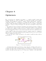
In the case of more complex optical systems the situation is somewhat more complicated.
However, in most cases the problem turns out to be a geometric one, in a sense that one
needs to find the optical path length as a function of frequency for a given optical system.
One may even use ray tracing programs to do that job.
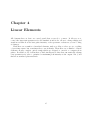
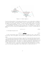
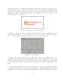
A first widely used optical system is a prism compressor. It consists of four prisms or
more frequently of two prisms and a folding mirror. Figure 4.1 shows a typical geometry of a
prism compressor. The beam impinges on the first prism, gets dispersed, passes the second
prism, is reflected at the folding mirror and goes all the way back. In order to separate the
output from the incoming beam the folding mirror is usually tilted in the vertical dimension,
such that the output beam is on top of the incoming or vice versa. Alternatively, a roof
mirror may be used. Both prisms are identical and their apex angle is α. The index of
refraction is determined by the corresponding Sellmeier equation.
Usually a prism compressor allows to adjust both positive and negative chirps depending
on the distance between the two prisms if the input pulse was bandwidth limited. That is,
34
Figure 4.1: Prism compressor.
because the glass material of the prisms itself introduces some positive phase modulation
and only if the distance between the prisms exceeds a certain threshold the overall phase
modulation becomes negative. Therefore, one may ’fine tune’ a prism compressor by moving
one of the prisms perpendicular to its base in order to introduce slightly more or less glass.
Spectral clipping occurs whenever the spectrum at the second prism is larger than the
prism itself. In other words spectral clipping happens when one of the two following equations
is true
s5 (ωmax ) < 0,
(4.10)
for the highest frequency and
s5 (ωmin ) >
B
.
2 sin(α/2)
(4.11)
for the lowest frequency, where B is the length of the prisms base and s5 is the distance
from the tip of the second prism to the point where a specific frequency enters the second
prism.
If you activate the button use Brewster angle the VI automatically adjusts the input
angle at the first prism such that the center frequency enters the first prism and also the second prism at Brewsters angle. The other choice you have is to specify use minimum deviation
which causes the apex angle of the prism to be adjusted such that the center frequency experiences minimal deviation, or in other words it passes the first prism parallel to its base.
There are two choices to calculate the compressor phase. First, through exact ray tracing
and second through an approximate solution which may be found in any textbook.
35
Intelligent Prism Compressor
c
GS
Input
pulse in:
Brewster angle:
Min. deviation:
exact/approx.:
incoming laser pulse
automatic alignment
automatic alignment
exact ray tracing or
approximate solution
prism angle:
adjust prism angle
prism base:
base size of both prisms
material:
prism material
angle of inc.:
adjust angle of incidence
distance tip-tip: distance between the
prism tips
prism-mirror:
distance prism 2 and mirror
in prism 1:
point of incidence prism 1
in prism 2:
point of incidence prism 2
Output
pulse out:
output laser pulse
optimal prism
separation:
optimized value
prism angle:
calculated prism angle
angle of inc.:
calculated angle of
incidence
The intelligent prism compressor is nothing else but a standard prism compressor
which automatically adjusts the distance between the two prisms such that the second order
phase present in the input pulse vanishes and the peak power is maximized.
36
Grating Stretcher
c
GS
Input
pulse in:
lines/mm:
angle of incidence:
focal length:
g:
grating-mirror:
grating size:
diffraction order:
incoming laser pulse
grating constant
refers to first grating
of the two mirrors or lenses
displacement (see text)
distance from grating 2
to end mirror
width of both gratings
±1
Output
pulse out: output laser pulse
phi2:
2nd order spectral phase
Grating stretchers are found in many different variations. Here we only implemented the
two most commonly used consisting of a single grating, one or two spherical mirrors, and a
flat end mirror.
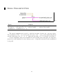
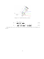
Fig. 4.2 shows the definition of the angles and when they are positive and when negative
Figure 4.2: Definition of the angles.
In the same manner we define the diffraction orders left of the zero order positive and to
the right hand side of zero order negative. The grating equation is
2πc0
β = arcsin M
− sin α
(4.12)
ωd
where M is the diffraction order and d the grating constant.
37
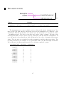
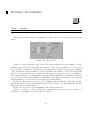
Figure 4.3: a) Stretcher geometry. b) If the setup a) is folded with respect to the plane
between the two focusing mirrors, the most commonly used stretcher geometry emerges. c)
Second, Oeffner-triplet: This setup is aberration-free and another commonly used stretcher.
R and R/2 are the radii of curvature of the two spherical mirrors.
Figure 4.3 shows the two most commonly used stretcher geometries. The overall stretching factor depends on the grating dispersion, the angle of incidence and the displacement g.
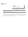
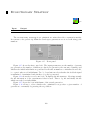
Using the more detailed graph shown in fig. 4.4 allows to calculate the phase modulation as
a function of the frequency
cos β0 − sin(β0 − β) sin α
8πg cos β0
ω
8f + 2r − 4g
+
tan β
Φ(ω) =
c0
cos β
d
(4.13)
where d is the grating constant, α the angle of incidence on the grating, β the diffraction
angle (which is negative), and β0 the diffraction angle (also negative) at the center wavelength. The diffraction order in this case is +1. The same formula may be used for the
Oeffner triplet if the focal length f is replaced by (R1 + R2 )/2 = 43 R. From the phase we
may calculate the second and third order phase term by calculating the second and third
derivative with respect to frequency
38
Figure 4.4: Detailed stretcher geometry.
Φ2
2gλL
=
πc20
Φ3 = −
3gλ2L
π 2 c30
2
λL
1
d
cos2 β0
2
λL
1
λL sin β0
1+
d
cos2 β0
d cos2 β0
(4.14)
(4.15)
Obviously, the second order dispersion is positive and that the third order dispersion is
negative.
39
Intelligent Grating Stretcher
c
GS
Input
pulse in:
lines/mm:
angle of incidence:
focal length:
g:
grating-mirror:
grating size:
diffraction order:
incoming laser pulse
grating constant
refers to first grating
of the two mirrors or lenses
displacement (see text)
distance from grating 2
to end mirror
width of both gratings
±1
Output
pulse out: output laser pulse
optimal g: optimal displacement g
The intelligent grating stretcher is nothing else but a standard grating stretcher
that adjusts automatically the displacement g such that the second order phase present in
the input pulse is minimized and the peak intensity of the out going pulse is maximal.
40
Grating Compressor
c
TF
Input
pulse in:
lines/mm:
angle of incidence:
delta:
grating-mirror:
grating size:
diffraction order:
incoming laser pulse
grating constant
refers to first grating
distance between gratings
measured at center frequency
distance from grating 2
to end mirror
width of both gratings
±1
Output
pulse out: output laser pulse
phi2:
2nd order spectral phase
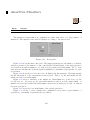
Again let’s start defining all relevant parameters as shown in fig. 4.5. We split the whole
optical path in two parts. The first represents the wavelength dependent distance between
the two gratings and the second the distance from the second grating to the end mirror. The
total phase is two times the sum of the two parts plus a relative phase term
Figure 4.5: Grating compressor.
2ω
Φ(ω) =
c0
4πD
D
+ B0 C + D(tan β − tan β0 ) sin α −
tan β
cos β
d
(4.16)
where B0 C is the distance between the second grating and the end mirror along the
41
center wavelength. Again we assume +1st order diffraction.
We again may calculate the second and third order Taylor coefficients
Φ2
DλL
= − 2
πc0
Φ3
3Dλ2L
=
2π 2 c30
2
λL
1
d
cos3 β0
2
λL
1
λL sin β0
1+
d
cos3 β0
d cos2 β0
(4.17)
(4.18)
which is just the opposite of the grating stretcher if we set
D = 2g cos β0
(4.19)
So, in principle a grating compressor should be able to fully compensate for the phase
modulation introduced by a grating stretcher.
Finally, we also consider spectral clipping that occurs whenever the second grating is too
small. We always assume that the center frequency impinges on the center of the second
grating. The effective transmission therefore is

D sin(β−β0 ) S

 0 : cos β0 cos β ≥ 2
(4.20)
T (ω) =

 1 : D sin(β−β0 ) ≤ S
cos β0 cos β
2
where S is the lateral size of the grating.
42
Intelligent Grating Compressor
c
GS
Input
pulse in:
lines/mm:
angle of incidence:
delta:
grating-mirror:
grating size:
diffraction order:
incoming laser pulse
grating constant
refers to first grating
distance between gratings
measured at center frequency
distance from grating 2
to end mirror
width of both gratings
±1
Output
pulse out:
optimal delta:
output laser pulse
optimal grating separation
The intelligent grating compressor is nothing else but a standard grating compressor
that adjusts automatically the distance between the two gratings such that the second order
phase present in the input pulse is minimized and the peak intensity of the out going pulse
is maximal.
43
Ideal Shaper
c
TF
Input
pulse in:
incoming laser pulse
amplitude control: specify amplitude modulation
phase control:
specify phase modulation
arbitrary:
array with frequency, phase
and amplitude modulation
Output
pulse out:
output laser pulse
The ideal shaper simulates an ideal pulse shaper which modulates the spectral amplitude and/or phase. This shaper shows no pixelation effects. There are a number of options
available for amplitude and phase shaping:
• none: No amplitude and/or phase modulation is applied.
• interpolate: The amplitude and/or phase modulation specified in the array arbitrary
is used. The array contains three columns, i.e. the absolute frequency, the amplitude-,
and the phase modulation. The frequency axis must not necessarily coincide with the
internally used sampling of the pulse. The amplitude and phase values are resampled
by interpolation to match the internal sampling of the pulse. The frequency vector
must contain absolute frequencies.
• arbitrary: The amplitude and/or phase modulation specified in the array arbitrary
is used. The number of amplitude and/or phase values MUST coincide with the number
of samples of the incoming pulse. The frequency vector is not considered at all as no
interpolation is performed. Assume the pulse is sampled with 256 individual samples,
then the array amplitude has to contain 256 values which then are used to modulate
the 256 amplitude values of the incoming pulse.
• Taylor: Only the phase modulation can be specified in terms of Taylor coefficients.
The units of the n-th order coefficient is fsn .
• Sinusoidal: The amplitude and/or phase of the pulse is modulated with a sinusoidal
function.
44
• Square: The amplitude and/or phase of the pulse is modulated with a periodic square
function of amplitude
• Sawtooth: The amplitude and/or phase of the pulse is modulated with a periodic
sawtooth function of amplitude
For sinusoidal, square and sawtooth the parameters are: amplitude A, offset ∆, periodicity dt and phase φ. The modulations are calculated according to
f (ω) = A sin (dt(ω − ω0 ) + φ) + ∆,
where f stands for either amplitude or phase modulation and sin may be replaced by the
square or sawtooth function. A negative amplitude is converted to a phase value keeping in
mind that −1 = eiπ .
|f (ω)|eiπ f (ω) < 0
f (ω) =
|f (ω)|
f (ω) ≥ 0
The cluster arbitrary contains three columns, the absolute frequency (with units), the
amplitude modulation (a modulation of one leaves the original frequency component unchanged), and the phase modulation in radians.
45
Pixelated Shaper
c
TF
Input
pulse in:
amplitude control:
phase control:
arbitrary:
properties:
setup:
Output
incoming laser pulse
pulse out:
output pulse
type of amplitude modulation shaper window: full spectral
type of phase modulation
window
arbitrary amplitude and phase amplitude:
applied amplitude
shaper properties
modulation
setup geometry
phase:
applied phase
modulation
This pulse shaper has been designed to simulate a real laboratory setup as realistic as
possible. The amplitude and phase modulation controls are identical to those of the ideal
shaper, except the selection arbitrary as type of amplitude or phase modulation is ignored.
Note, new here is two additional control panels, i.e. the properties and the setup control.
Setup allows to choose between two alternative experimental schemes. First, a zero dispersion compressor consisting of two gratings and two lenses (or two curved mirrors), and
second, a zero dispersion compressor where the gratings are replaced by prisms. In both
cases you need to specify the focal length of the two lenses (or the two curved mirrors).
When you pick the grating setup you need to specify the number of lines/mm, the diffraction order, and the difference between the angle of incidence and the diffraction angle at the
center wavelength. If you pick the prism setup you need to specify the prism material and
the prism angle (apex). From this information the program calculates the correspondence
between pixel and frequency. In addition to the zero dispersion compressor geometry you
need to provide information on the pixelated modulator itself. Here, the program needs to
know the number of pixels, the pixel width, and the wavelength of the center pixel.
Properties allows to switch on or off various effects connected to the pixelated nature
of the modulator device. In total there are 6 options:
46
pixelated: This switch allows to turn on or off all effects related to pixelation. This way
you may find out which experimentally observed details in the shaped waveform are
due to the pixelated nature of the modulator.
gaps: If switched on, two neighboring pixels are separated by a gap. The width of the gap
is in units of pixel width. For example 0.04 means that the gap width is 0.04 times the
pixel width. The phase modulation of all gaps is zero and the amplitude modulation
is equal to 1.
wraps: Most pixelated devices have a maximum accessible range of phase values, typically
a few times 2π. Mathematically we don’t need a phase larger than 2π, because 3π for
example leads to the same result as 3π modulus 2π = 1π. That is, whenever the phase
modulation exceeds 2π we may subtract 2π; this process is known as phase wrapping.
You may specify the wrap point in terms of 2π, that is, wraps may occur whenever the
phase exceeds 2π (1) or 4π (2) etc.
crosstalk pixel: If turned on the amplitude and phase pattern are convoluted with a Gaussian. The width is given in units of pixel. With this option you may simulate a misaligned setup where the modulator is not exactly in the focal point of the lens/curved
mirror.
diffraction: If turned on the phase and amplitude modulation pattern is convoluted with
the spatial resolution of the optical system. The system resolution is assumed to be
Gaussian and the width is determined by the beam diameter and the focal length of
the lens/curved mirror according to Fourier optics.
frequency mapping: You may select between linear frequency mapping and geometric.
If you select the first, then the relation between pixel number and frequency is assumed
to be linear. With this you may simulate what happens if you do not calibrate your
setup correctly. If you select the latter, the frequency mapping is calculated from the
optical arrangement and everything is as it should be.
47
Iterative FFT Shaper
c
TF
Input
pulse in:
incoming laser pulse
iterations: the number of iterations
Pi steps:
use π phase jumps only
target:
file name
delimiter: tab (default), space, etc.
Output
pulse out:
phase to
shaper:
plot:
output pulse
desired spectral phase
target and output pulse
The iterative FFT shaper module allows to specify target pulse shape, i.e. the temporal intensity as a function of time. It uses an iterative Fourier transform algorithm to
evaluate the phase pattern necessary to transform any input intensity as close as possible to
the desired target intensity by phase-only shaping. The number of iterations must be specified. The target intensity profile must be available as a file in the folder ../iffttargets/.
The file contains two columns separated by a delimiter. The first column is the time in
femtoseconds and the second the intensity. If the time samples do not coincide with the
time samples of the pulse the target will be resampled automatically.
48
Chapter 5
Nonlinear Elements
The nonlinear elements implemented in LAB II allow to simulate the most commonly found
nonlinear effects. There is self-phase modulation which appears in almost any material
when the intensity gets high enough and there are frequency mixing processes. Because the
spectral width of the laser pulses is very broad the pulse spectra have to be convoluted which
sometimes leads to counterintuitive results. For example, it is not always so easy to predict
what the second harmonic spectrum might look like if the fundamental pulse has some funny
shaped spectral phase. Peter Blattnig has programmed the optical fiber and most of the
demo vi’s which illustrate some important effects. Fred van Goor from the University of
Twente has used the amplifier vi to simulate a number of published multi-pass amplifier
designs. He generously agreed to let us include his results in the present manual.
49
Transparent Nonlinear Medium
c
TF
Input
Output
pulse in: incoming laser pulse pulse out: output pulse
glass:
material
phi2:
2nd order spectral phase
z:
thickness
B-integral: B integral
A transparent nonlinear medium has the same linear dispersive properties as the previously described linear transparent medium. In addition, it handles nonlinear effects
due to self-phase modulation (SPM). The numerical simulation uses a split step Fourier
transform algorithm. Whereas dispersive effects are incorporated in the spectral domain,
SPM is treated in the time domain. The integration z-step width is dynamically adjusted
so that the nonlinear phase per integration interval is always π/20, i.e.
∆z =
π
c
.
20 ωc n2 Imax
(5.1)
The output B-integral yields
Z
2π
B=
dz n2 I(z)
(5.2)
λ0
The linear material properties come from material files in the folder ../chi1/. The
transparent nonlinear medium requires nonlinear material properties and those are stored
in the folder ../chi3/. The material files in this folder provide the nonlinear index of
refraction commonly known as n2 plus the Raman response. Here, we only need n2 . As an
example we inspect fused silica (SQ1). To simulate the propagation of a short pulse through
a piece of silica we need two files:
1. ../chi1/SQ1.vi for the linear material properties and
2. ../chi3/X3_SQ1.vi for the nonlinear material properties.
If you wish to add a new material, make sure you know the nonlinear index of refraction.
Then copy the file X3_SQ1 for example to X3_SF6, edit the material constants, and you’re
done.
50
Optical Fiber
c
PB
Input
pulse in:
fiber control:
incoming laser pulse
fiber properties
Output
pulse out:
gamma:
output pulse
nonlinear constant
Even more sophisticated than the transparent nonlinear medium is the optical fiber.
Besides linear dispersion and self-phase modulation it also accounts for self-steepening and
the Raman effect. The fiber control allows you to specify the following values:
dispersion: Here you need to specify the material which is responsible for the dispersive
properties of the fiber. This may be a simple material file, such as fused silica (SQ1) or
it may be a file which contains the dispersion properties of a specific complex photonic
bandgap fiber.
nonlinear: The nonlinear properties may be specified independent of the linear properties.
This allows to use a fused silica core (SQ1) which specifies the nonlinear properties
together with any dispersion file which is dominated for example by the hole structure
surrounding the core.
length: The fiber length.
effects: Here you may switch on or off linear or nonlinear effects in order to study their
influence for example on super-continuum generation.
The integration step width is dynamically adjusted so that the nonlinear phase never
exceeds a specified limit. The nonlinear constant is calculated to
ω0 n2
(5.3)
cAeff
where ω0 is the center frequency and Aeff is the effective area, calculated from the beam
diameter d simply through Aeff = πd2 /4. The vi numerically integrates the nonlinear differential equation for the slowly varying electric field envelope
γ=
Z
∞
X
2i ∂
∂E(ξ; τ )
km ∂ m E(ξ; τ )
= −i
− iγ 1 −
E(ξ; τ ) dτ1 R(τ1 )|E(ξ; τ − τ1 )|2 ,
m m!
m
∂ξ
i
∂τ
ω
∂τ
c
m=2
(5.4)
51
where we have combined the instantaneous electronic response and the Raman response
of the medium to
R(t) = (1 − f ) δ(t) + f RR (t).
(5.5)
The relative weight is governed by the constant f which for fused silica is approximately
0.18. If you switch off dispersion then the sum (first term on the right hand side) will
be set to zero. If you switch of the Raman effect then f is set to zero. If you switch off
self steepening then ω2ic is set to zero and if you switch off SPM then γ is set to zero.
52
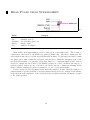
Optical Fiber Amplifier
c
TF
Input
pulse in:
fiber amplifier control:
incoming laser pulse
fiber properties
Output
pulse out: output pulse
gamma:
nonlinear constant
gain [dB] overall gain in dB
The vi optical fiber amplifier adds to the vi optical fiber the option to account
for gain. The fiber control is identical to that of the optical fiber. In addition you find
two more control clusters, where one specifies the gain medium and the other details on the
inversion profile.
Besides specifying the gain medium and the dopant concentration in weight percent, one
has the option to switch on or off gain saturation or gain dispersion effects. For each gain
medium there must exist a file containing the necessary data. If you’d like to add a new gain
medium the best thing is to copy an existing one and change the numbers appropriately.
Details on the inversion profile are first of all the longitudinal inversion profile ∆N (z).
You may select
constant: In which case the inversion profile is assumed to be constant.
exponential: The gain profile decays exponentially with the decay constant specified by α.
Fermi-Dirac: The gain profile resembles a Fermi-Dirac distribution in order to account
for saturation in the pumping process. z0 marks the position to which the gain is
roughly constant and after which it decays exponentially. Again α determines the
decay constant.
from file: This option allows to load an arbitrary inversion profile from a file which has
two columns separated by a tab. The first column is the longitudinal position scaled
by the fiber length. That is, the first column contains numbers between zero and one
which must be evenly spaced. The second column contains the upper state population
in arbitrary units.
No matter what profile you pick the absolute values are automatically adjusted so that
the overall small signal gain at the center wavelength of the pulse is as specified by the
53
control g0 [dB]. It may happen that the simulated small signal gain is smaller than the
specified one. One possible reason might be that the dopant concentration and the length
of the fiber are not large enough to allow for the desired small signal gain.
54
Ideal SHG
c
TF
Input
pulse in
input pulse
Output
pulse:
output pulse
Ideal SHG simulates an ideal second harmonic generation process. Ideal in a sense that
the phase matching condition is always perfectly fulfilled no matter how broad the input
spectrum.
ESHG (t) = EF2 (t)
(5.6)
Note that the fluence of the second harmonic field is without meaning as the ideal SHG
process assumes some fictive conversion efficiency.
55
SFM Crystal (nondepleted three wave mixing)
c
MH
Input
Output
pulse in ’e’ or ’o’: 1st pulse in
pulse out ’e’: output pulse
pulse in ’o’:
2nd pulse in
deff:
effective nonlinear
crystal:
crystal material
constant
type:
phase matching type
length:
crystal length
→
−
theta:
angle( k ,opt. ax.)
phi:
rotation angle
delay=0!:
ignore delay between input pulses
sinc2 theory?:
no group velocity effects
output array:
full, half, or every second
fast mode:
no interpolations
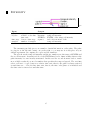
SFM Crystal (nondepleted three wave mixing) simulates a three wave mixing process in a nonlinear crystal, such as second harmonic generation, sum frequency mixing, or
difference frequency mixing. In order to save computation time we assume that both fundamental input beams are not substantially depleted by the conversion process. As shown in
an earlier chapter this leaves us with only one differential equation to solve.
Presently we have only implemented BBO, LBO, KDP, AgGaS2 , and LiIO3 . Other
crystals may be added upon request. One may choose between type I (ooe) and type II
(eoe) phase matching.
Choosing the mode delay=0 allows to ignore a possibly present time delay between the
two input pulses.
With the sinc^2 theory mode it is possible to ignore effects on the mixing process
caused by phase modulation. This is achieved by simply using the absolute value of the
phase matching term only
56
η(ω1 , ω2 )0 = |η(ω1 , ω2 )|
2 1
02
η(ω1 , ω2 ) = sinc
∆k(ω1 , ω2 ) L
2
(5.7)
(5.8)
Since this approximation is often found in textbooks, especially when dealing with the
mixing of three monochromatic fields, this mode of operation allows to compare results
of simulations with results given in the literature. In addition, the influence of a limited
spectral bandwidth acceptance may be studied without the influence of phase modulation,
for example caused by a difference in the group velocities.
The calculated output waveform has twice the number of sample points as the input
pulses, which is caused by the convolution. One may stick to that or one may reduce the
number of samples by using every second sample point or all samples in only half of the
spectral window.
57
SFM Crystal (depleted three wave mixing)
c
MH
Input
Output
pulse 1 (’e’ or ’o’): 1st pulse in
pulse 1 out:
pulse 2 (’o’):
2st pulse in
pulse 2 out:
pulse 3 (’e’ or ’o’): 3rd pulse in
pulse 3 out:
crystal:
crystal material
deff:
type:
phase matching type
length:
crystal length
evolution chart:
# of z-steps:
integration steps
→
−
theta:
angle( k ,opt. ax.)
phi:
rotation angle
delay=0!:
ignore delay between
input pulses
fast mode:
no interpolations
(recommended)
output pulse 1
output pulse 2
output pulse 3
effective nonlinear
constant
evolution of spectra
In principle SFM Crystal (depleted three wave mixing) is a very powerful tool and
is capable of handling any three wave mixing process (χ(2) -process). Dispersion effects to all
orders of Taylor coefficients are included since we use the Sellmeier equations to calculate
the index of refraction. Quite naturally, back conversion and other processes occurring as
the fields propagate through the crystal are accurately incorporated.
As mentioned earlier we assume ω3 = ω1 + ω2 which in the case of difference frequency
generation may be rearranged to ω2 = ω3 − ω1 . Note, that you need to consider this by
connecting the pulses to the right inputs of SFM Crystal (depleted three wave mixing).
58
Crystal Wizard
c
MH
Input
pulse 1
pulse 2
pulse 3
the input pulses have to
be connected such that the
crystal wizard knows the
central wavelengths
minimal SFM
essential SFM parameters,
params:
everything but angles
desired angular required precision
precision:
Output
dep. SFM
parameters out:
group velocity
indices out:
comment:
phase-matching
angle:
cluster that is compatible
to depleted SFM
ratio of c0 over the group
velocities of the pulses
information on which
angle is the phase
matching angle
calculated phasematching angle
The crystal wizard is a tool to determine the optimal angular orientation of a nonlinear
crystal for a specific sum frequency mixing situation. Therefore, it requires a control panel
similar to that of the SFM Crystal (depleted three wave mixing) crystal but without
theta or phi angles. The output is a control panel compatible to that of SFM Crystal
(depleted three wave mixing). Additional inputs are the three pulses of the three wave
mixing and an angular precision value (for example 0.05 deg). The crystal wizard determines whether theta or phi is the phase matching angle, finds the optimal phase matching
angle, and in addition optimizes the other angle for a maximal def f .
59
Amplifier
c
TF
Input
pulse in
input angle:
pump duration:
delay to 1st pulse:
pump fluence left:
pump fluence right:
% concentration:
crystal length:
medium:
effects:
input pulse
0 deg or Brewster angle
duration of pump pulse
delay between pump
and first pass
pump fluence left
pump fluence right
active ion concentration
crystal length
laser medium
switch on/off
Output
pulse out:
output pulse
The amplifier simulates a one- or two-sided longitudinally pumped laser amplifier. In
order to avoid reflection losses at the crystal, the angle of incidence may be chosen to be
equal to Brewster angle instead of normal incidence. The amplifier is characterized by its
concentration of active ions and the rod length. Both pump beams have the same duration,
but may have different energy densities, and the delay between the pump beam and the first
pass must be specified. The module accounts for saturation in the amplification process,
for dispersive effects due to the resonant amplification, and for dispersive effects of the host
material. The number of iterations is automatically determined. If one wants to simulate
a two- or other multi-pass amplifier the inversion cluster must be connected as shown in
the tutorials. We also need to specify whether the direction of the seed beam through the
amplifier crystal alternates, as in a regenerative amplifier, or does not alternate, as in a
ring-type multi-pass amplifier.
Fred van Goor from the University of Twente did simulate a number of published
Ti:sapphire amplifiers. We are very happy that he agreed to publish his results here; thank
you Fred!
’... The TiSa amplifier vi is very helpful for the design of a multi-pass Ti-sapphire
amplifier. We compared the simulation results (see table 5.1) with a number of amplifier
systems published in the literature. We selected systems reported after 1994, which were
60
designed to operate at maximum efficiency. In table 5.1 six different amplifiers are simulated.
The fluences where calculated using the published input- and output energies and beam
diameters. Also the published lengths and diameters of the TiSa rods and the number of
passes were used in the simulations. Some papers did not mention the size of the input- or
output beam or the length of the rod. In these cases we made a guess. We believe that these
guesses are reasonable because the diameter of the pump beam should be slightly larger
than that of the input- and output beam. The Titanium concentration was not given in
most papers, we guessed 0.15%. This value turns out to be not so critical. The diameter
of the output beam was not given in the papers. We have chosen it equal to the diameter
of the input beam. We also compared the peak intensities of the six systems, calculated
from the published output energies, pulse lengths of the stretched pulses, and the given
or guessed output beam diameter. It turns out that some of the systems operate close to
the damage threshold of Ti:sapphire, which is about 5GW/cm2. We are not sure about
the values resulting from reference [5], as the peak intensity is unrealistic high. Maybe the
guessed beam diameter of the output is not correct in this case.
Table 5.1: Comparison between published results and simulations. Number of passes n,
pump fluence Fpump , seed fluence Fin , amplified seed fluence Fout , pump beam diameter
dpump , seed beam diameter dseed , pump energy Wpump , seed energy Win , simulated amplified
energy Wsim , measured amplified energy Wexp , length of TiSa crystal LTiSa , diameter of TiSa
crystal dTiSa , pulse duration τ , and maximum intensity Imax .
n
4
3
4
4
4
4
4
4
Fpump
J/cm2
2.82
3.70
1.99
2.95
2.55
3.16
2.48
2.63
Fin
mJ/cm2
45.84
57.69
28.29
15.92
19.89
15.28
61.89
15.59
Fout
J/cm2
1.21
1.72
1.23
1.25
0.99
1.44
1.01
1.10
dpump
mm
6.20
8.50
6.70
5.00
5.00
5.50
12.00
4.00
din
mm
5.00
8.00
6.00
4.00
4.00
5.00
12.00
3.50
Wpump
mJ
850
2100
700
580
500
750
2800
330
Win
mJ
9
29
8
2
2.5
3
70
1.50
Wsim
mJ
237.6
864.6
347.8
157.1
124.4
282.7
1142.3
105.8
Wexp
mJ
235
790
340
160
120
280
1340
100
LTiSa
mm
13.00
12.00
20.00
10.00
7.00
18.00
10.00
15.00
dTiSa
mm
13.00
20.00
?
12.00
10.00
12.00
20.00
?
Ti
%
0.15
0.15
0.15
0.15
0.23
0.15
0.15
0.25
τ
ps
300
330
1700
950
40
800
80
80
Imax
GW/cm2
4.03
5.21
0.72
1.32
24.75
1.80
7.10
13.75
ref.
rem.
1
2
3
4
5
6
7
7
good
ok
good
good
good
good
ok
good
The simulations agree reasonably good or good with the published results. Most systems operate above the saturation fluence at the last pass yielding maximum efficiency. The
pulse lengths of the stretched pulses are such that the amplifiers operate at a safe peak
intensity well below or sometimes close to the damage threshold. The simulations have been
performed with pulse durations of about 90 ps. It was not possible to use the published
pulse lengths because the number of samples became too large when increasing the chirp.
However, we believe that this will not influence the simulation results much because we are
dealing with energies and not with intensity waveforms...’
[1]
[2]
[3]
[4]
[5]
[6]
[7]
Barty, Opt. Lett. 19 (1994), p1442
Itani, Opt. Comm. 134 (1997), p134
Yamakawa, Opt. Lett. 23 (1998), p1468
Barty, Opt. Lett. 21 (1996), p668
Zhou, Opt Lett. 20 (1995), p64
Walker, Optics Express 5 (1999), p196
Wang, J. Opt. Soc. Am. B 16 (1999), p1790
61
Chapter 6
Detectors
To fully characterize a femtosecond laser pulse it is necessary to measure the amplitude as
well as the phase of it either in the spectral or in the time domain. All electronic devices
however are too slow to come up to this challenge. And because no direct methods are applicable indirect techniques have to be used. All of those techniques rely on an instantaneous
nonlinear effect.
In LAB II we have implemented a large number of those indirect techniques, but we have
also implemented rather unrealistic devices which are extremely useful for debugging purposes. All detectors have a number of different outputs. Some may require an input, which,
if not connected, is set to a useful default value.
Correlation measurements are the most useful tools to determine the temporal intensity
in femtosecond world. They are conceptually easy and may be realized in different variations
depending on what exactly it is you want to measure. There are background free versions and
those which do have background, there are second and third order versions, depending on
what nonlinear process you are using, and there are interferometric and intensity correlation
versions, depending on whether the two beams interact in a collinear or non-collinear fashion.
Background-free versions have the great advantage that they may be used to measure
’deep’ correlations, that is, to measure the pulse intensity over many orders of magnitude.
Second order as compared to third order correlations have intrinsic time symmetry, which
prevents you from telling your lab mate whether the little bump showing up in the measurement is a pre- or a post-pulse.
Interferometric version in contrast to intensity correlations give you some additional
information on the phase of the pulse, but they are almost never background free.
All intensity correlators in LAB II have either one or two input pulses, so they allow for
auto as well as cross correlation measurements.
FROG is an abbreviation for (Frequency Resolved Optical Gating) and seems to become
one of the standard diagnostic tools in femtosecond laser science. It allows to almost fully
characterize a femtosecond laser pulse. The only missing thing is the absolute phase of
the pulse, but other than that you get the amplitude and the relative phase from a FROG
62
measurement. There is some mathematics involved in that too, because you need to process
the measured FROG trace, run an iterative algorithm, and if you have done everything as
you should you’ll get the field.
FROG in principle is conceptually easy, take any intensity correlation setup and spectrally
resolve the correlation signal. This is why there are many different types of FROG ’s out
there. The most common ones are SHG FROGs because they are easy to build and require
very little energy to operate. They have one disadvantage, however, and that is they have
no idea in which direction the time axis points. For example a SHG FROG never allows you
to distinguish between a positive and a negative phase modulation if they only differ by the
sign. The THG FROG resolves this problem but needs much more optical elements to align
and a little more energy, so does the PG FROG.
The FROG signal is a function of both the frequency and the delay time
∞
2
Z
F (ω, τ ) ∝ dt f (t, τ ) e−iωt .
(6.1)
−∞
where the function f (t) is determined by the nonlinear process you’re employing
f (t, τ ) = E1 (t) E2∗ (t − τ )
f (t, τ ) = E1 (t) E2 (t − τ )
f (t, τ ) = E12 (t) E2 (t − τ )
f (t, τ ) = E1 (t) |E(t − τ )|2
f (t, τ ) = E12 (t) E ∗ (t − τ )
f (t, τ ) = E12 (t) E ∗ (t − τ )
for
for
for
for
for
for
DFG
SFG
THG
PG
TG
SD
FROG
FROG
FROG
FROG
FROG
FROG
All FROG’s implemented here assume that the nonlinear crystal you are using has a
sufficiently broad spectral acceptance to support the full laser bandwidth. If you want to see
what happens if this is not the case you may construct a FROG by using more fundamental
LAB II modules.
63
FWHM
c
TF
Input
pulse in:
input pulse
Output
pulse out:
temporal FWHM:
spectral FWHM:
output pulse
FWHM of temporal intensity
FWHM of spectral intensity
The FWHM in time module calculates the FWHM (Full Width at Half Maximum) of the
temporal and spectral intensity distribution, no matter what kind of slowly varying envelope
the pulse has. It may lead to funny results whenever the intensity is heavily structured.
64
Intensity
c
TF
Input
pulse in:
rel/abs:
time step:
samples:
Output
input pulse
pulse out:
relative or absolute intensity:
time axis
FWHM t:
detector time step sigma t:
number of samples
output pulse
temporal intensity
FWHM of the temporal intensity
2nd order moment of the
temporal intensity
The intensity module gives you a number of useful information on the pulse. The pulse
is going in on the left and coming out on the right, so you may use it at any place in your
virtual experiment. Its outputs are a plot and two numbers.
The plot shows the temporal intensity and the two numbers are the temporal FWHM and
the second moment. As mentioned above the FWHM may lead to funny results whenever the
pulse intensity becomes heavily structured. In this case the second moment leads to much
more reliable results if you need a number that specifies the temporal spread. The rel/abs
selector allows to toggle between a relative time axis, that is, the pulse is always centered
around time zero, or an absolute time axis, that is, the first order phase t0 is included and
the time axis is centered around that time.
65
Instantaneous Frequency
c
TF
Input
pulse in:
input pulse
Output
pulse out:
instantaneous frequency
output pulse
instantaneous
frequency distribution
The instantaneous frequency module plots the relative instantaneous frequency. Relative here means relative to the laser’s center frequency. So, if the pulse has no chirp, you’d
expect the relative frequency to be zero everywhere.
66
Probe
c
TF
Input
pulse in:
input pulse
Output
pulse out
output pulse
The probe module was originally designed as a debugging tool. But it seemed to be
very useful so we made a detector out of it. The output of probe are four plots showing the
spectral amplitude and phase and the temporal amplitude and phase. probe allows you to
access these quantities at whatever position in the virtual experiment you need to look at
them.
67
Run Time Difference
c
TF
Input
pulse 1 in:
pulse 2 in:
1st pulse in
2nd pulse in
Output
time delay:
time delay between 1st and 2nd pulse
run time difference determines the delay time between two pulses by calculating the
difference of the first order phase terms. This is sometimes useful if you want to calculate
the time difference between two pulses having a different center frequency but which have
traveled through the same piece of glass and now you want to know how far are they apart
in time.
68
Save Pulse To File
c
TF
Input
pulse in:
path:
Output
input pulse
specify file name (dialog if empty)
The module save to file takes a pulse at any point in the virtual experiment and
stores it to a file. You may load it later using the corresponding read pulse module.
69
Save Pulse To Spreadsheet
c
TF
Input
pulse in:
path:
Output
input pulse
specify file name (dialog if empty)
The save pulse to spreadsheet module stores a pulse to a spreadsheet file. The
c
format is equivalent to that used by the FROG program (Femtosoft).
The first column
gives the wavelength in nm, the second the square of the absolute value (’spectral intensity’)
in units of J/(m2 nm), the third column the phase, the fourth column the real part, and
the last column the imaginary part of the spectral field in units of V/(m nm). Obviously,
there is too much information here, but we decided to simply use the format structure of
the FROG software in order to ensure compatibility.
70
Taylor Phase
c
TF
Input
pulse in:
order:
Output
input pulse
temporal phase Taylor...: Taylor coefficients of
maximum order
temporal phase
of series expansion temporal phase:
plot to check fit
spectral phase Taylor...: Taylor coefficients of
spectral phase
spectral phase:
plot to check fit
The Taylor phase module expands the spectral and the temporal phase in a Taylor
series and outputs the Taylor coefficients of both up to the order you specify. You may check
the quality of the polynomial fit by inspecting the two plots.
71
Time Bandwidth Product
c
TF
Input
pulse in:
input pulse
Output
pulse out:
bandwidth product:
output pulse
time frequency bandwidth product
The time bandwidth product module calculates for a given input pulse the product of
the temporal intensity FWHM and the spectral intensity FWHM.
FWHMI(t) FWHMS(ν)
If you prefer ∆τ ∆ω, simply multiply the result by 2π.
72
Intensity Autocorrelation
c
TF
Input
pulse in:
time step:
samples:
type:
pulse in
detector time step
number of samples
type of correlation
Output
FWHM t:
FWHM of the correlation
sigma t:
2nd moment of the correlation
autocorrelation intensity autocorrelation
The intensity autocorrelation measures the intensity autocorrelation of the incoming pulse. It can be second or third order and it can be background-free or the opposite.
73
Intensity Cross-Correlation
c
TF
Input
Output
pulse 1 in: pulse in
FWHM t:
FWHM of the correlation
pulse 2 in: pulse in
sigma t:
2nd moment of the correlation
time step: detector time step cross-correlation intensity cross correlation
samples:
number of samples
type:
type of correlation
The intensity cross-correlation measures the intensity cross correlation of the two
incoming pulses. It can be second or third order and it can be background-free or the
opposite.
74
Interferometric Autocorrelation
c
TF
Input
pulse in:
order:
input pulse
order of nonlinearity
Output
second order inter...:
2rd order interferometric correlation
The interferometric autocorrelation has the great advantage that it allows to get
some information on the phase of the pulse. In principle such a setup combines correlation
and interferometry. The signal is given by
Z
I(τ ) = dt |E(t) + E(t + τ )|2n
where n is the order of the autocorrelation. A linear correlation corresponds to n = 1, a
second order to n = 2 and a third order to n = 3.
75
2D Distribution
c
TF
Input
Output
pulse in:
input pulse
2D distribution: intensity plot
time step:
time step
t axis:
x scale information
field size:
sampling grid size
y axis:
y scale information
save option: specify output format
path to file: file name
type:
select distribution
y axis:
frequency or wavelength
The 2D distribution calculates a time-frequency distribution from the electric field of
the pulse. You may select between:
• Spectrogram
2
Z
1
0
0
0
−iωt0 S(ω, t) = √
dt E(t )E(t − t) e
2π
(6.2)
• WFFT (windowed fast Fourier transform). The function f (t) is a real Gaussian of
some appropriate width.
Z
2
0
0
0
−iωt0 S(ω, t) = dt E(t )f (t − t) e
(6.3)
• Wigner-Ville
1
S(ω, t) =
2π
Z
0
dt0 E ∗ (t − t0 /2)E(t + t0 /2) e−iωt
(6.4)
• Page
2
Zt
∂ 1
0
0
−iωt0 √
S(ω, t) =
dt
E(t
)
e
∂t 2π
(6.5)
1
e ∗ (ω) e−iωt
S(ω, t) = √ E(t)E
2π
(6.6)
−∞
• Rihaczek
76
With the time step and the field size you determine the total time window and from this
the frequency step and the frequency window are derived. The resulting intensity plot may
be saved in jpeg format to the specified file name. You can also select whether you would
like the y-axis to be frequency or wavelength.
77
FROG
c
TF
Input
Output
pulse in:
input pulse
FROG:
time step:
FROG time step
t axis:
field size:
sampling grid size
lambda axis:
save option: specify output format
path to file: file name
type:
nonlinear process
spectrogram
x scale information
y scale information
The FROG module mixes two replicas of the input pulse in a nonlinear medium and
the spectrum of the generated nonlinear signal is detected as a function of the time delay
between the two replicas. The FROG trace is displayed as a function of delay time (x-axis)
and wavelength (y-axis). Connect the scale information to a property node of the intensity
plot to get properly calibrated axis.
The FROG module requires a grid size and a time step. The larger the grid size the
longer it takes to calculate the FROG trace. Since Fourier transformation automatically
determines the frequency step size once you specify the time step there is no need to input
both. We decided to use the time step as input because in most experiments a stepper or a
dc motor driving a translation stage determines the resolution. Most spectrometer usually
measure far too many spectral samples (typically 512 to 2048 samples) and most of them
have to be thrown away in the retrieval process.
At the moment there are two save options available, namely jpeg format and retrieval
format. If you chose one of those make sure to specify a path and a filename. The color map
used for the jpeg format is equal to that used by Femtosoft, which makes it easier to compare
simulated to measured or retrieved FROG traces. If you select retrieval format an output
file will be generated that can be read directly into the FROG 3.0 software. Check the box
’use header information’ and specify ’order: delay’ and ’read in as: constant frequency’.
78
XFROG
c
TF
Input
Output
pulse 1 in:
input pulse
THG FROG: THG spectrogram
pulse 2 in:
input pulse
t axis:
x scale information
time step:
FROG time step
lambda axis: y scale information
field size:
sampling grid size
save option: specify output format
path to file: file name
XFROGS are identical to FROGs except the two pulses may be different. In addition
XFROG offers the option to use difference frequency generation as a nonlinear process, which
doesn’t make sense for FROGs.
The XFROG module requires a grid size and a time step. The larger the grid size the
longer it takes to calculate the FROG trace. Since Fourier transformation automatically
determines the frequency step size once you specify the time step there is no need to input
both. We decided to use the time step as input because in most experiments a stepper or a
dc motor driving a translation stage determines the resolution. Most spectrometer usually
measure far too many spectral samples (typically 512 to 2048 samples) and most of them
have to be thrown away in the retrieval process.
At the moment there are two save options available, namely jpeg format and retrieval
format. If you chose one of those make sure to specify a path and a filename. The color map
used for the jpeg format is equal to that used by Femtosoft, which makes it easier to compare
simulated to measured or retrieved FROG traces. If you select retrieval format an output
file will be generated that can be read directly into the FROG 3.0 software. Check the box
’use header information’ and specify ’order: delay’ and ’read in as: constant frequency’.
79
Knife Edge Correlator
c
MH
Input
pulse in:
input pulse
time step:
detector time step
field size:
sampling grid size
save option: specify output format
path to file: file name
rise time:
rise time of the shutter
Output
Page:
t axis:
lambda axis:
integral over Page function
x scale information
y scale information
The knife edge correlator is something we have been using in the lab quite often to
temporally overlap two beams of different center frequency. One beam needs to be strong
enough to create a plasma. The other beam is either diffracted or absorbed depending on
the electron density in the plasma. If you record the intensity of the weak beam as a function
of the delay between the two pulses it turns out that the whole setup is more or less the
temporal equivalent to a knife edge experiment. What you measure is the integral of the
intensity up to the delay time. If you spectrally disperse the signal and check out the math
it turns out that what you measure is the integral of the Page distribution, assuming that
the shutter is infinitely fast
Z
2
−iωτ
+
S(t, ω) ∝ dτ e
E (τ ) Θ(t − τ )
(6.7)
The infinitely fast shutter is incorporated by using the Heaviside step function Θ(t − τ ).
Even in the case the shutter rise time is finite, equation (6.7) is a pretty good description.
So all you need to do is to calculate the derivative of the time frequency distribution with
respect to time and you obtain the Page distribution of the pulse. The Page distribution
has the advantage, in contrast to the spectrogram (FROG), that you can invert it in a
straight forward way to extract the electric field. No need to iterate here. The knife edge
correlator has two outputs and that is the correlation signal and the time integral over the
Page function. What you need to specify is the rise time of the shutter. If you start with
a small rise time and increase it step by step you will also see the influence of a finite rise
time on the appearance of the time frequency distribution.
80
Spectrometer
c
TF
Input
pulse in:
input pulse
Output
center wavelength: center wavelength
sigma:
second moment of spectral intensity
FWHM:
FWHM of spectral intensity
spectrum:
spectral intensity vs. wavelength
relative spectrum: relative frequency spectrum
The ideal spectrometer has a number of useful outputs. First of all there are two
graphics, the wavelength spectrum and the relative frequency spectrum. In addition you’ll
find three numbers, the center wavelength, the spectral FWHM in units of nm, and the
second moment. The second moment is a useful quantity when the spectrum becomes
heavily structured for example due to self-phase modulation and the FWHM becomes a
somewhat meaningless number.
The spectrometer is ideal in a sense that it has no device limited spectral resolution. The
resolution is only determined by the number of samples and the full spectral window you
are using. In addition, neither the grating nor the detector have a wavelength dependent
sensitivity.
81
Spectrometer with Resolution
c
GS
Input
pulse in:
wavelength resolution:
input pulse
spectral resolution
of spectrometer
Output
center wavelength: center wavelength
FWHM:
FWHM of spectral
intensity
spectrum:
spectral intensity
vs. wavelength
The spectrometer with resolution is almost the same as the ideal spectrometer
except that you need to specify a device resolution in units of nm.
82
Energy Meter
c
TF
Input
Output
pulse in:
input pulse
fluence:
energy per unit area
laser rep rate: repetition rate ave. power: average power
energy:
pulse energy
The fluence of the laser pulse may be measured with the energy meter. The device
integrates the temporal intensity and outputs the pulse energy per unit area. If you need
you may also use the energy meter whenever you need a photo diode somewhere. Just
think of it as a calibrated photo diode. If you specify a laser repetition rate you may also
look at the average power.
83
TPC Diode
c
TF
Input
Output
pulse A in: 1st input pulse TPC signal
pulse B in: 2nd input pulse
output signal
Conventional photo diodes with a large bandgap may sometimes be used to measure the
pulse intensity. That is because the generated photo-current depends on the square of the
intensity since you need two photons to produce one electron hole pair if the bandgap is
h̄ω0 < Egap ≤ 2h̄ω0 . So the signal you’d measure in this case is
Z
S = dt I 2 (t)
(6.8)
The TPC-diode has two inputs. Usually both inputs get the same pulse, but you may
want to use two different pulses to realize something like a correlator.
84
Chapter 7
Interactions
In addition to the standard elements we have included special elements which have been
programmed by users of LAB II . You will find a resonant three level system, a n-level ladder
system, and a diatomic molecule. Both allow you to study fundamental interaction processes
between light and matter. The resonant three level system numerically solves the coupled
Maxwell-Bloch equations and has been programmed by Ralf Netz. He is also the author of
the ladder system vi. The diatomic molecule solves the time dependent Schrödinger equation
for a diatomic molecule with a ground and one excited state and has been programmed by
Tamas Rozgonyi.
85
Resonant Three Level System
c
RN
Input
pulse in:
wavelength of 13 transition:
dipole moment of 13 transition:
wavelength of 12 transition:
dipole moment of 12 transition:
cell length:
z-steps:
density:
initial values of density matrix:
ρ11 :
ρ22 :
ρ33 :
ρ31 :
ρ21 :
ρ32 :
input pulse
1st resonance
1st dipole moment
2nd resonance
2nd dipole moment
interaction length
number of
integration steps
particle density
Output
pulse out:
diagonals:
off diagonals:
output pulse
diagonal elements
of density matrix
off-diagonal
elements of
density matrix
population state 1
population state 2
population state 3
off-diagonal 31
off-diagonal 21
off-diagonal 32
The resonant three level system simulates the interaction of a short laser pulse with
a resonant three level system. The simulation is based on solving the coupled Maxwell
Bloch equations. The three level system is characterized by two resonance wavelengths, two
corresponding dipole moments, the atomic density, and the interaction length. In addition,
in manual mode the number of z integration steps has to be specified. After the calculations
the diagonal and separately the off-diagonal elements of the density matrix may be plotted
as a function of time.
With an appropriate choice of the transition wavelengths and the initial population distribution, one may either simulate a V-type, a Λ-type, or a ladder-type system.
86
Parallel Ladder System
c
RN
Input
pulse in (A):
input pulse A
pulse in (B):
input pulse B
modus of integration
slow/fast
iterations:
# of z-steps
transition wavelengths: wavelengths
of |gi → {|ki}
and |gi → |γi
dipole moments mk :
dipole moments
of transition
|gi → {|ki}
dipole moments dk :
dipole moments
of transition
{|ki} → |γi
# of states:
number of
(Min.=3)
involved states;
Tion :
lifetime of
upper state |γi
(γ = 1/Tion )
particle density:
particle density
propagation length:
propagation length
initial values
cg (t0 ), {ck (t0 )}
of amplitudes:
and cγ (t0 )
Output
pulse out (A):
pulse out (B):
ion state
intermediates
ground state
output pulse A
output pulse B
ion state population
population of
intermediate states
ground state population
The ladders parallel module calculates the space-time evolution of a multi-level quantum system (Fig. 7.1) and its driving fields. The multi-level system can be described
mathematically by the differential equations (in the rotating wave approximation, RWA)
87
Figure 7.1: Parallel connection of three-level ladder systems. The resonant transitions are
driven by the electric fields EA (t) = 21 ẼA (t) e−iωA t + c.c. and EB (t) = 12 ẼB (t) e−iωB t + c.c..
ċg = i
N
X
∗
Ωkg ck
(7.1)
k=1
∗
ċk = i(ωA − ωkg ) ck + iΩkg cg + iΩγk cγ
ċγ = i(ωA + ωB − ωγg + iγ) cγ + i
N
X
Ωγk ck .
(7.2)
(7.3)
k=1
Ωkg = µkg ẼA (t)/2h̄ and Ωγk = dγk ẼB (t)/2h̄ are the Rabi frequencies of the transitions
|gi → |ki and |ki → |γi. Since a decay process (e.g. ionization) is included in Eq. 7.3 the
atomic system is not closed for γ > 0.
The evolution in space-time of the driving fields ẼA (t) and ẼB (t) is given by the simplified
wave equation in the RWA
1 ∂
µ0
∂
+
ẼA (y, t) = i
∂y c0 ∂t
∂
1 ∂
µ0
+
ẼB (y, t) = i
∂y c0 ∂t
where P̃A (y, t) and P̃B (y, t) are calculated by
88
ωA c0
P̃A (y, t)
2
ωB c0
P̃B (y, t),
2
P̃A (y, t) = 2N
P̃B (y, t) = 2N
N
X
k=1
N
X
∗
µkg ck cg (y, t)
∗
dγk cγ ck (y, t)
k=1
and N is the particle density. This means that the system of equations combines
Maxwells wave equation with Blochs quantum-mechanical description of the field-matter
interaction and has to be solved simultaneously.
In the case of ẼA (t) = ẼB (t) = Ẽ(t) only one wave equation has to be solved with
N P
∗
∗
µkg ck cg (y, t) + dγk cγ ck (y, t) .
P̃A (y, t) = P̃B (y, t) = P̃(y, t) = 2N
k=1
To solve numerically Maxwells wave equation and the differential equations for the
probability amplitudes — in particular for fast decay processes (faster than the pulse duration) and a broad temporal window — the Predictor-Corrector-Method (slow modus) is
implemented
(0)
yn+1 = yn + h f (xn , yn )
..
..
.
.
i
h h
(ν)
(ν+1)
f (xn+1 , yn+1 ) + f (xn , yn ) ,
yn+1 = yn +
2
where ν = 0 . . . 1, resulting in
(0)
yn+1 = yn + h f (xn , yn )
i
h h
(0)
(1)
yn+1 = yn +
f (xn+1 , yn+1 ) + f (xn , yn )
2
h
i
h
(2)
(1)
yn+1 = yn +
f (xn+1 , yn+1 ) + f (xn , yn ) .
2
In the case of the fast modus the first derivative is approximated by
yn+1 − yn−1 = 2h f (xn , yn ).
(7.4)
The minimal number of involved states is 3 (one three-level ladder). To create a twolevel system only one dipole moment should be 6= 0. To examine the field-matter interaction
without propagation, e.g., the # of z-steps can be 2 (Minimum), the propagation length
0.005 mm and the particle density 1 × 1012 cm−3 .
89
Diatomic Molecule
c
TR
Input
pulse in:
grid size:
xmin:
dx:
mass 1:
mass 2:
dipole matrix:
ground state:
D:
beta:
x0:
C:
excited state:
D:
beta:
x0:
C:
simulation stop:
input pulse
spatial grid size
minimum atom separation
spatial step size
mass of atom 1
mass of atom 2
dipole matrix elements
dissociation energy
width
equilibrium separation
asymptotic energy
Output
potential surfaces:
the two Morse
potentials
diff:
resonance wavelength vs. atomic
separation
excited state wavepacket: 2D wavepacket
motion
excited state population: final population
ground state population: final population
ground state wavepacket: 2D wavepacket
motion
dissociation energy
width
equilibrium separation
asymptotic energy
time to stop simulation
The module diatomic molecule simulates the interaction of a pulse and a diatomic
molecule, which is characterized by an electronic ground and an excited state. The molecule
is represented by a pair of Morse potentials, the two masses, and the transition dipole
matrix. It is necessary to specify the spatial grid that is used to calculate the space time
propagation of the wavepackets. The initial ground state wavepacket is calculated from the
parameters of the ground state potential. You may plot the difference between the two
potentials in terms of wavelength as a function of the internuclear separation to determine
the resonant wavelengths. During the calculations a pop up window shows the evolution of
90
both wavepackets. At the end of the calculation a two dimensional plot shows the space-time
distribution of the wavepackets on both potential surfaces.
91
Spectral lines
c
TF
Input
pulse in:
min ionization:
input pulse
minimum ionization
stage; neutral = 0,
singly ionized = 1 etc.
max ionization:
maximum ionization
stage
spectral resolution: spectral resolution
list of elements:
list of elements to
include
Output
spectrum:
elements:
laser spectrum and
atomic lines
array of strings
length equal to
number of samples
The module spectral lines allows to display atomic emission spectra together with
the laser spectrum to find out what lines are within the laser bandwidth. One needs to
specify a list of elements, for example Hg and Ar for a mercury lamp with argon buffer gas,
and the minimum and maximum ionization stage. Ionization stage zero refers to the neutral
state, one to the singly ionized atom etc. The spectral resolution determines the width of the
atomic lines and is determined by the spectrometer used. The module expects the following
file structure
Rb
Rb
Rb
Rb
Rb
Rb
Rb
Rb
Rb
Rb
I
I
I
I
I
I
I
I
II
I
775.7651
300
775.9436
60
780.027 90000
792.526
5
792.554
4
794.760 45000
827.141
40
827.171
30
860.396
2000
886.8512
40
where the first line labels the ionization stage, the second the transition wavelength in
nm, and the third the relative intensity. The module can handle files downloaded from the
NIST atomic database.
92
Chapter 8
Optimizers
Here, we introduce five optimization algorithms, i.e. a simplex downhill combined with
simulated annealing, two genetic algorithms, an evolutionary algorithm, and an adaptive
algorithm. All algorithms are designed to optimize a single feedback signal, or fitness, by
continuously varying a set of parameters, for example the phase values of a spatial light
modulator. While the simplex downhill algorithm is strong for a low number of parameters
and fails to converge for a large search space, the other four are well suited for large search
spaces.
All optimizer vis call an experiment vi. Its input are the parameters (an array of numbers)
to optimize and its output is a single feedback (a dimensionless number). The experiment
vi is called by the optimizer vi whenever it needs to evaluate a new set of parameters. Its
file and path information must be entered in the appropriate field. The experiment vi may
consist of LAB II modules as shown in the following two examples. It may also communicate
with real devices control their setting through the parameters and read out a real feedback
signal, for example from a photodiode.
We first start with a virtual experiment for the simplex downhill algorithm, which is
shown in fig.8.1
Figure 8.1: The virtual experiment.
A Gaussian shaped pulse is stretched by a linear dispersive medium and the task is to
compress it through a pulse shaping apparatus. The parameters to optimize are the second
to fourth order phase terms of a Taylor expansion. Note that the zeroth (absolute phase)
and first order phase (group delay) are zero as they have no influence on the pulse width.
93
The feedback signal or the fitness is the FWHM of the signal. That is, the signal needs to
be minimized in order to achieve the desired goal. Also note that the actual experiment
needs to be located in the ’false’ part of the vi. The ’true’ section is called only once by the
optimizer algorithm and this happens at the very beginning. Here, the boundaries of the
search space have to be defined.
Figure 8.2: Definition of the search space.
Figure 8.2 shows the ’true’ case where the search space for the optimization is defined. Allowed values for second order phases are [−104 . . . 104 ] fs2 , for third order phases
[−105 . . . 105 ] fs3 , and for fourth order phases [−106 . . . 106 ] fs4 , respectively.
Figure 8.3: Front panel.
Figure 8.3 shows the front panel after optimization has been accomplished. The view
graph shows the original and the optimized pulse shape. It is recommended to always open
both the experiment vi, in order to follow the progress, and the optimizer vi. Arrange them
so that both front panels are visible and follow their progress as the optimization process
runs.
Things are quite similar for the other four optimizer vis. Again we will explain an example
vi, as shown in fig. 8.4. The task is also quite similar. A Gaussian shaped laser pulse is
stretched by a 2 cm thick piece of SF14 and compressed by a pixelated pulse shaper operated
94
in phase-only mode. The pulse shaper has 128 pixel where each pixel covers 0.75 nm giving
a full shaper window of 96 nm which is roughly four times the FWHM of the spectrum. The
center pixel coincides with the center wavelength of the laser. The pulse itself is sampled in
manual mode with 1024 samples.
Figure 8.4: Virtual experiment.
Figure 8.5 shows the ’true’ case structure where the boundaries of the search space are
fixed. Here all 128 pixels may vary between 0 and a maximum phase of 2π.
Figure 8.5: Definition of the search space.
The front panel is shown in fig 8.6. Besides the pulse spectrum we see the shaper setting,
i.e. the value of all pixel in a bar graph, and the pulse before and after the glass window
and after the shaper. As the search space is large convergence is usually reached only after
many many iterations.
Use either one of the four ’genetic’-type algorithms together with the example experiment
to see their performance. When you want to design your own experiment, use the experiment
95
Figure 8.6: Front panel.
vi that comes with LAB II , rename it, throw away everything except the input array and
the feedback indicator, and insert your own code.
96
Simplex Downhill
c
MH
Input
Output
The simplex downhill is a combination of the deterministic simplex downhill algorithm
and simulated annealing. Simulated annealing does contribute the stochastic part to the otherwise deterministic simplex downhill strategy and makes it a very powerful search algorithm
for small search spaces.
Figure 8.7: Front panel.
Figure 8.7 shows the first control tab. The input parameters control the simplex optimization. These are the annealing parameters k and α, which determine the rate with which
the annealing temperature decreases.
α
j<k
T0 1 − kj
T = Tmin +
0
j≥k
where j is the number of the actual experiment. The temperature starts at T0 and goes all
the way down to Tmin . The input T is irrelevant. The number of runs determines how many
subsequent optimizations are performed. A boolean button allows to determine whether the
feedback signal or the fitness should be minimized or maximized.
Figure 8.8 shows the second control tab. It displays the actual number of the present run,
the number of individual experiments that have been performed within this run, the final
fitness of the run, and the best fitness of all runs performed so far. It shows the temperature
97
Figure 8.8: Front panel.
and the actual parameters. The button run next allows to manually start the next run
without waiting for final convergence.
Figure 8.9: Front panel.
Figure 8.9 shows the file structure used. Most importantly the file information of the
experiment vi that is used. Then a result file may be generated that saves the final parameters
of all runs, and finally a log file that saves the results of all experiments of all runs. Optionally
one may generate a config file that saves the actual optimization parameters for later use.
If the config file load is not empty then the panel settings are overwritten by the settings of
the config file.
98
Genetic Algorithm
c
GS
Input
none
Output
none
The genetic algorithm is an optimization routine that relies on reproduction and mutation.
Figure 8.10: Front panel.
Figure 8.10 shows the first control tab. The input parameters are the number of individuals per generation, the bits/gene, the number of elite, the probability of crossover, and
the probability of mutation. The bits/gene determine the resolution of the discrete sampling
of the search space and the number of elite determines the number of the best individuals
that move on from generation to generation without experiencing any crossover or mutation.
Three buttons allow to set whether the feedback signal is minimized or maximized, whether
a log file is generated, and whether all individuals of the first generation are created from
random numbers or loaded from a previously saved individuum.
Figure 8.11 shows the second control tab. It displays the file structure. Most importantly
the file information of the experiment vi that is used. Then a log file and finally the file
which saves the best individuum.
Figure 8.12 shows the best individuum of the actual generation.
Figure 8.13 allows to select whether the optimization stops after a given number of
generations or manually by pressing the stop button.
99
Figure 8.11: Front panel.
Figure 8.12: Front panel.
Figure 8.13: Front panel.
100
Genetic Algorithm 2
c
GS
Input
none
Output
none
The genetic algorithm 2 is a identical to the genetic algorithm except that the
gens may be binned. Binning can be reduced manually as the optimization proceeds. For
example, setting binning equal to two means that always two genes have the same value and
the total number of genes reduces by a factor of 2.
Figure 8.14: Front panel.
101
Evolutionary Strategy
c
TF
Input
none
Output
none
The evolutionary strategy is an optimization routine that relies on mutation mainly.
In contrast to the genetic algorithm the search space parameters are stored as floating point
numbers.
Figure 8.15: Front panel.
Figure 8.15 shows the first control tab. The input parameters are the number of parents
per generation, the number of children produced per generation, the amount of binning, and
whether the initial individuals are generated from random numbers or initialized from a file,
i.e. a previously stored individuum. Two boolean buttons select whether the feedback signal
is minimized or maximized and whether a log file is generated.
Figure 8.16 shows the second control tab. It displays the file structure. Most importantly
the file information of the experiment vi that is used. Then a log file and finally the file
which saves the best individuum.
Figure 8.17 shows the best individuum of the actual generation.
Figure 8.18 allows to select whether the optimization stops after a given number of
generations or manually by pressing the stop button.
102
Figure 8.16: Front panel.
Figure 8.17: Front panel.
Figure 8.18: Front panel.
103
Adaptive Strategy
c
TF
Input
none
Output
none
The adaptive algorithm is an optimization routine that relies on a large number of
mutations. The mutation rate itself is adjusted according to the success rate.
Figure 8.19: Front panel.
Figure 8.19 shows the first control tab. The input parameters are the number of individuals per generation, the number of elite, and whether all individuals of the first generation
are created from random numbers or load from a previously saved individuum. Two boolean
buttons select whether the feedback signal is minimized or maximized and whether a log file
is generated.
Figure 8.20 shows the second control tab. It displays the file structure. Most importantly
the file information of the experiment vi that is used. Then a log file and finally the file
which saves the best individuum.
Figure 8.21 shows a statistics of the mutations. Individuum zero is the best, one the
second best etc. In green are the successful mutations and in red the unsuccessful. A
mutation is rated successful if the individuum can increase its rating by at least one rank in
the next generation.
Figure 8.22 shows the best individuum of the actual generation.
Figure 8.23 allows to select whether the optimization stops after a given number of
generations or manually by pressing the stop button.
104
Figure 8.20: Front panel.
Figure 8.21: Front panel.
Figure 8.22: Front panel.
105
Figure 8.23: Front panel.
106