1
Program for Solving Two-person
Zero-sum games
Dale Hogarth
Bsc (Hons) Computer Science
2006
Dissertation Title: Program for Solving Two-person Zero-sum games
Submitted by Dale Hogarth
COPYRIGHT
Attention is drawn to the fact that copyright of this dissertation rests with its author.
The Intellectual Property Rights of the products produced as part of the project belong
to the University of Bath (see http://www.bath.ac.uk/ordinances/#intelprop). This
copy of the dissertation has been supplied on condition that anyone who consults it is
understood to recognise that its copyright rests with its author and that no quotation
from the dissertation and no information derived from it may be published without the
prior written consent of the author.
Declaration
This dissertation is submitted to the University of Bath in accordance with the
requirements of the degree of Batchelor of Science in the Department of Computer
Science. No portion of the work in this dissertation has been submitted in support of
an application for any other degree or qualification of this or any other university or
institution of learning. Except where specifically acknowledged, it is the work of the
author.
Signed: ……………………………….
This dissertation may be made available for consultation within the University
Library and may be photocopied or lent to other libraries for the purposes of
consultation.
Signed: ……………………………….
1
Abstract
Game theory has played an important part in many fields of research since its
introduction in the early twentieth century. This dissertation focuses on one particular
are of game theory, that of Two-person Zero-sum finite games. Such games can be
represented with use of a data structure called a payoff matrix. The system designed in
this dissertation has the ability to take any payoff matrix and calculate the optimal
mixed strategies for both players of the game. This is done using Von Neumann’s
crucial minimax theorem and application of the Simplex method for Linear
programming problems. Another feature of the program is the programs extended
ability to take Linear programming problems in standard form and determine the
optimal solutions. The program can be used as a basic calculator to quickly solve
complex problems or as a learning aid for those wishing to improve their
understanding of Linear programming and game theory. The dissertation contains a
Literature review providing an insight into game theory features and existing
solutions to problems. Following this is a detailed requirements document and
complete design plan for the calculator. The dissertation finishes with a rigorous
testing section and a project conclusion. An appendix is attached at the back of the
dissertation containing all manner of extra documents applicable to the system
development.
2
Acknowledgements
I would like to give thanks to my project supervisor prof. Nicolai Vorobjov who has
offered his full support in the development of this project and given me important
pieces of advice throughout. I would also like to thank my head of department, Dr.
Alwyn Barry for the great help and understanding he has given to me in a year of
great difficulties. Finally I would like to acknowledge the ongoing and ever-present
support given to me by my family and my fiancée.
3
Table of Contents
Chapter
Page
1
Introduction ……………………………………………………………...
6
2
Literature Review ………………………………………………………..
7
3
2.1
Introduction ………………………………………………………...
7
2.2
Classification of a Game …………………………………………...
8
2.3
Modelling Games …………………………………………………..
9
2.4
Assumptions of Game Theory ……………………………………..
12
2.5
Two-Person Zero-Sum Games ……………………………………..
12
2.6
Pure and Mixed Strategies …………………………………………
14
2.7
Minimax Theorem ………………………………………………….
16
2.8
Optimal Mixed Strategies ………………………………………….
16
2.9
Linear Programming (LP) ………………………………………….
17
2.10 Simplex Method ……………………………………………………
18
Requirements Analysis and Specification ……………………………….
21
3.1
Introduction ………………………………………………………...
21
3.2
Product Aim ………………………………………………………..
21
3.3
Requirements Elicitation …………………………………………...
21
3.4
3.5
3.3.1
Domain Understanding ……………………………………….
22
3.3.2
Requirements Collection ……………………………………...
22
3.3.3
Classification ………………………………………………….
23
3.3.4
Conflict Resolution …………………………………………...
23
3.3.5
Prioritisation …………………………………………………..
24
3.3.6
Requirements Checking ………………………………………
24
Requirements Specification ………………………………………..
24
3.4.1
Functional Requirements ……………………………………..
24
3.4.2
Non-Functional Requirements ………………………………..
27
3.4.3
Hardware Requirements ………………………………………
29
Requirements Validation …………………………………………...
30
3.5.1
Validity Checks ……………………………………………….
30
3.5.2
Consistency Checks …………………………………………..
30
3.5.3
Completeness Checks …………………………………………
30
4
4
5
6
3.5.4
Realism Checks ……………………………………………….
31
3.5.5
Verifiability …………………………………………………...
31
Design …………………………………………………………………...
32
4.1
Introduction ………………………………………………………...
32
4.2
Flow of Control …………………………………………………….
33
4.3
Data Types …………………………………………………………
34
4.4
Saddle Point ………………………………………………………..
35
4.5
Payoff Matrix to LP Tableau ……………………………………….
36
4.6
Simplex Method ……………………………………………………
37
4.7
Interface Design ……………………………………………………
41
4.8
Error Handling ……………………………………………………..
44
4.9
Program Output …………………………………………………….
44
Detailed Design and Implementation ……………………………………
46
5.1
Introduction ………………………………………………………...
46
5.2
Pseudo-Code Solutions …………………………………………….
46
System Testing …………………………………………………………..
54
6.1
Introduction ………………………………………………………...
54
6.2
Defect Testing ……………………………………………………...
54
6.3
Integration Testing …………………………………………………
56
Conclusion ……………………………………………………………….
58
Bibliography ………………………………………………………………….
60
Website References …………………………………………………………..
61
7
Appendix A
Appendix B
Appendix C
Appendix D
5
1 Introduction
Game theory has many applications and areas of research. One particular research
area concerns two-person zero-sum games and finding optimal solutions to these
games. The term zero-sum refers in this case to the fact that if player 1 selects one of
his/her strategies and player 2 selects one of his/her strategies then the
result/gain/payment given to one player is equal to the loss of the other player. If
player 1 has m strategies to choose from and player 2 has n possible strategies then
the game can be modeled in a “payoff” matrix such that each row represent one
player’s strategies and each column represents the other player’s strategies. The
elements of the matrix are then used to represent the payoff that will occur if each
player opts to select the strategies associated with that row and column. For example,
a value of -1 in row 1 and column 2 of the matrix could represent a payoff of £1 from
player 1 to player 2.
Much investigation has gone in to being able to determine the best strategies that each
player should opt for in these situations. Prof. John Von Neumann devised his crucial
Minimax theorem in 1928 in which each player seeks to minimize his/her maximum
loss or maximize his/her minimum gain. The phenomenon of a saddle point occurs
when each player finds that the strategy they should employ to minimize their
loss/maximize their gain does in fact yield their minimum gain/maximum loss
because it is the best option for the other player as well. When such an event occurs,
neither player will benefit in changing their strategy if the other player does not
change theirs. In these cases, the optimal strategy for each player is therefore trivial as
it equates to one pure strategy for each player. Most games though are not so simple
to solve as they do not contain saddle points. The alternative solution is to create
optimal mixed strategies where each player opts to play one of their pure strategies
with a certain probability. Some of the player’s strategies will obviously be more
beneficial than others so it makes sense that these strategies should be assigned higher
probabilities. But what should these probabilities be exactly? There is a mathematical
approach that can be used to determine this and it is a branch of Linear programming
called the Simplex method.
The aim of this project is to develop a computer program that calculates the optimal
strategies of an input payoff matrix by use of the saddle point method and the Simplex
method. This dissertation contains a Literature review that explores the existing
solutions to such problems and delves into the domain of game theory to properly
understand the problem. A requirements document lists all the components and
features necessary to complete the task at hand and elicits information from the
Literature review and likely end-users to come up with a detailed specification. The
dissertation also contains a design plan for the program along with detailed design
algorithms to be incorporated into code in the final system. The testing section of the
dissertation describes the types of tests that were applied to the program before the
final system was delivered and the results of the test cases applied are also enclosed
within. The conclusion of the dissertation gives a critical appraisal of the objectives
achieved in the project, areas where the project could have been improved and how
the work done so far can be continued and expanded on. A CD is also enclosed
containing an executable version of the calculator program that has been developed.
6
2 Literature Review
2.1 Introduction
Game theory is a branch of applied mathematics that studies strategic situations where
players choose different actions in an attempt to maximize their returns. First
developed as a tool for understanding economic behaviour, game theory is now used
in many diverse academic fields ranging from biology to philosophy. Game theory
saw substantial growth during the cold war because of its application to military
strategy, most notably to the concept of mutually assured destruction. Beginning in
the 1970s game theory has been applied to animal behaviour, including species'
development by natural selection. Because of interesting games like the Prisoner's
dilemma, where mutual self interest hurts everyone, game theory has been used in
ethics and philosophy. Finally, game theory has recently drawn attention from
computer scientists because of its use in artificial intelligence and cybernetics.1
Most agree that today’s modern mathematical approach to Game theory was
pioneered by Prof. John Von Neumann and his papers published in 1928 and 1937.
French mathematician Emile Borel also published several papers on the theory of
games in the early 1920’s but he failed to expand on many of his ideas. This, along
with von Neumann’s establishment of the crucial minimax theorem is the reason why
it is von Neumann who is generally accredited as the founder of game theory.
Born in Hungary in 1903, von Neumann quickly built a reputation as a young
mathematical genius and his inspiration to investigate game theory was driven by his
admiration of poker. It was a game that he enjoyed but did not have all that much
success with. He realised that although probability plays a big part in poker, it was the
art of betting and bluffing that makes a good poker player which led to his publication
of an article in 1928 entitled “Theory of Parlor Games” where he first proved the
minimax theorem. Von Neumann knew then that game theory could play a big role in
economics and many other fields but it wasn’t until many years later when Von
Neumann teamed up with Austrian economist Oskar Morgenstern that game theory
really made an impact in the empirical sciences. The early papers by Borel and von
Neumann were written for mathematicians and confined to mathematical journals so
von Neumann and Morgenstern collaborated to write a book that could be understood
by those with limited mathematical knowledge. Their book, “Theory of Games and
Economic Behavior” first published in 1944 revolutionized the field of economics and
its influence spread into many other fields including philosophy, psychology, politics,
sociology and even warfare. In fact, Game Theory can be applied to most real life
situations where people compete for goals and payoffs by making strategic decisions.
Many books on Game Theory have since followed that of Morgenstern and von
Neumann’s and their initial theories have been expanded upon and evolved. Some of
their ideas have been challenged and proved to be flawed in certain situations but their
work was vital nonetheless in setting the cornerstone of what today is a massively
important area of research.
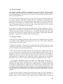
1
This excerpt was copied directly from http://en.wikipedia.org/wiki/Game_theory
7
2.2 Classification of a Game
There are a number of concepts and terms that need to be understood before it is
possible to appreciate game theory and to be able to understand what exactly is
involved in a “game”.
Firstly, the term “game” can be used to describe anything as primitive as tic-tac-toe or
as complex as international war. Many people would refute the suggestion that war is
a game but the truth is that it encapsulates the same ideologies of conflict of interest
as many other games and concepts of game theory have been used to influence the
decisions of military commanders. Definitions of the components of a game and the
types of games that exist are detailed below.
Player
Every game needs someone to play it. The participants of the game are called the
players although a player is not necessarily a single person. A football match consists
of 22 players but it is also possible to think of each football team as a single player as
each team of players is competing against the other team and working in harmony
with their own team mates. As all the players on the same side have the same
common goal (i.e. to beat the opposing team) then the only real conflict of interest
that exists is between the two teams and not the individual players.
Strategy
During a game, a player will be required to make decisions on how best to act given
the current situation they are in. A strategy is the action or sequence of actions that
describe all the possible decisions the player can make in every situation. In games
such as stone-paper-scissors the strategies are simultaneous as both players have to act
without knowing the actions of their opponent. In games such as chess the strategies
are sequential as each player is aware of the other player’s previous decisions. To
detail a complete strategy of any non-trivial game is very difficult as the total number
of situations possible is far too great to calculate.
Payoff
A player’s payoff is the result the player achieves after an action or sequence of
actions has been performed by the participating players. A player’s payoff can be
positive or negative as illustrated in the following example. Two players are playing
stone-paper-scissors with the loser in each game having to pay the winner £1, Player 1
decides to pick stone and Player two decides to pick scissors. The result of this is that
Player 1 has a payoff of +£1 and player 2 has a payoff of -£1.
Co-operative Games
In a co-operative game, the participating players are allowed to communicate freely
and bargain with one another to try and obtain the best payoff they can. One example
of a co-operative game is when somebody has a house for sale and somebody else
wants to purchase it at a lower amount than the asking price. The seller may choose to
ignore the offer and wait for a better one or bargain with the prospective buyer to get a
better price or accept the offer. If both parties co-operate and compromise then they
can both get what they ultimately want by sacrificing something, in this case the
buyer pays a little more than they would like to and the seller receives a little less
money than they would have liked.
8
Non Co-operative Games
As the name suggests, a non-cooperative game is one in which the players are not
allowed to co-operate and help one another. Unless the rules of the game allow it, the
players should not communicate any information about their own or the other player’s
options and hence work to a compromise. In games such as these, each player is
concerned only with maximizing their own payoff.
Zero-Sum Games
In a Zero-sum game the profits of all players are exactly equal to the losses of the
other players. In other words the total winnings minus the total losses for any set of
strategies chosen in the entire game must equal zero. Poker is an example of a Zerosum game as the winner of any hand will receive an amount of money exactly equal
to the sum of the losses of all the other players participating in that hand.
Constant-Sum Games
A constant-sum game is similar to that of a zero-sum game except that the total sum
of winnings minus losses between the players must add up to a constant although it is
possible for that constant to be zero as well in some cases. One example of a constant
sum game would be if a group of people are given a £100 to divide among
themselves. Each person would like to have as much of the money as possible but
none of the players will actually lose anything so the total gains minus the total losses
among the group will add up to the original £100.
Non Zero-Sum Games
In a non zero-sum game it is possible for all players to gain or suffer together.
Participants of a non zero-sum game usually have a common interest at heart whilst
still being in conflict over other issues. The earlier example of the house sale can be
thought of as a non zero-sum game in some cases. Imagine the house is worth
£200,000 but the seller lets it go for £195,000. The buyer of the house likes the house
but hates the décor and spends £10,000 on redecorating yet the house is still worth
only £200,000. The Seller has lost out on £5,000, the buyer has now overspent by
£5,000 and so it would appear that both parties have lost out in the game.
2.3 Modelling Games
In Game theory there are two different ways in which players can employ their
strategies. In some games, decisions and moves are made simultaneously (or at least
the moves are made without knowledge of what the other players plans are) whilst the
play is sequential in others. To mathematically represent these different types of
games requires two different models. Simultaneous games are represented using the
Normal form whereas sequential games are represented using the Extensive form.
From this point on, it is easier to consider the games as being played by two players
pitted against one another.
Normal Form
In a simultaneous game the strategy of each player must be determined before they
know the strategy that will be employed by the other player. In the Normal form the
9
complete strategies of each player are determined before the play begins by taking
into account the situation that each player is in. As long as the strategies of the game
are finite, that is to say there are only a limited number of moves each player can
make, then the game can be represented in an N*M matrix where one player has N
possible moves they can make and the other has M possible moves. The matrix shows
all of the possible payoffs that will occur depending on which strategies are employed
by each player. For example, Player 1 employs strategy x and Player 2 employs
strategy y, looking at the entry in column x and row y of the matrix will reveal the
payoff that will occur given this pair of strategies. A famous example of this type of
game is the Prisoner’s Dilemma which incidentally is a non zero-sum game.
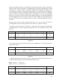
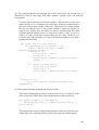
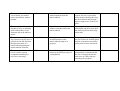
The classical prisoner's dilemma (PD) is as follows:
Two suspects A, B are arrested by the police. The police have insufficient
evidence for a conviction, and having separated both prisoners, visit each of them
and offer the same deal: if one testifies for the prosecution against the other and
the other remains silent, the silent accomplice receives the full 10-year sentence
and the betrayer goes free. If both stay silent, the police can only give both
prisoners 6 months for a minor charge. If both betray each other, they receive a 2year sentence each.
It can be summarized thus:
Prisoner A Stays Silent
Prisoner A Betrays
Prisoner
B
Stays Silent
Both serve six months
Prisoner B serves
Prisoner A goes free
ten
Prisoner A serves ten years;
Prisoner
B
Both serve two years
Prisoner B goes free
Betrays
The dilemma arises when one assumes both prisoners are selfish enough to want to
minimize their own jail term. Each prisoner has two options: to cooperate with his
accomplice and stay quiet, or to betray his accomplice and give evidence. The
outcome of each choice depends on the choice of the accomplice. However, neither
prisoner knows the choice of his accomplice. Even if they were able to talk to each
other, neither could be sure that they could trust the other.
Let's assume the protagonist prisoner is rationally working out his best move. If his
partner stays quiet, his best move is to betray as he then walks free instead of
receiving the minor sentence. If his partner betrays, his best move is still to betray, as
by doing it he receives a relatively lesser sentence than staying silent. At the same
time, the other prisoner thinking rationally would also have arrived at the same
conclusion and therefore will betray.
It would be rational then for a prisoner to decide to cooperate if only he could be sure
that the other player would not betray, and thus achieve a better result than in mutual
betrayal. However, such a co-operation is then rationally vulnerable to the treachery
of selfish individuals, which we assumed our prisoners to be. Therein lays the paradox
of the game.
If reasoned from the perspective of the optimal interest of the group (of two
prisoners), the correct outcome would be for both prisoners to cooperate with each
other, as this would reduce the total jail time served by the group to one year total.
Any other decision would be worse for the two prisoners considered together.
However by each following their individual interests, the two prisoners each receive a
lengthy sentence, which in fact hurts both the interest of the group and that of the
10
years;
individuals.2
The 2 x 2 payoff matrix in the above excerpt shows the strategies available to each
player in the game. Player A and Player B both have two options (strategies) and the
consequences that arise (the payoffs) in selecting each option are shown in the
corresponding cells of the matrix.
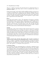
Extensive form
Unlike Normal form games, Extensive form games are dynamic in the sense that the
order of strategies employed by each player is sequential. In games such as this it is
necessary to be able to consider the strategy of each player at any point in the game
rather than just before the game begins like in the Normal form. A convenient way to
model this is to use a topological tree representation called a game tree. A game tree
consists of a number of nodes which show the exact position each player is in. The
nodes are connected by branches which represent the alternative decisions available to
each player at each node. Starting at the bottom node of the tree, it is possible to move
upward along the branches and determine exactly what situation will arise given the
order of strategies that have been followed.
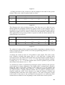
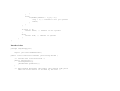
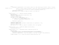
Below is an example of an extensive form game and how it can be modelled using a
game tree.
Jack and Mary are making plans for the week ahead. Jack wants to go to the cinema
one night or go the pub on one night. Mary wants to go tout for a meal on one night or
go to the ballet on one night. To save arguments they decide to take it in turns on each
night to pick where they will go. This predicament can be modelled using the game
tree shown in Figure 2.1.
Figure 2.1
This tree could continue on upwards in the same fashion if it was desirable to model
the situation that would occur if Jack and Mary continued to take turns on picking
2
The Prisoner’s Dilemma example was copied directly from
http://en.wikipedia.org/wiki/Prisoner's_dilemma
11
what they did on each night. In the above example, Jack and May are both aware of
the choices the other person makes on each turn and for this reason the branches of
Mary are illustrated to be directly attached to those of Jack’s.
In a game where each player is unaware of the other players selections the branches
are not directly attached. Instead, they are illustrated by a larger elipse or a dotted
elipse which is called an information set. In a game such as this, it is said that there is
not perfect information and although the game is actually sequential. It is often
possible to model such games in the Normal form as the result of not knowing the
other players previous moves makes it a simultaneous move game in effect. In the
famous Battle of the Bismarck Sea, the Japanese commander had to make a choice of
whether to travel north or south around New Britain to New Guinea and in turn the
allied forces commander then had to make a choice of whether to travel north or south
around New Britain to intercept the Japanese army. Because the Commanders of both
armies were unaware of the choices made by the other Commander, the game was in
effect simultaneous even though the troops of each army did not move at the same
time.
2.4 Assumptions of Game theory
When analysing games in Game theory, there are certain rules that are assumed to be
true. By taking these rules to be true, it is then possible to apply the theories that
already exist about certain types of games. It should be noted however that in real life
the following assumptions do not always hold true but for the remainder of this
project it is necessary to presume they do.
1. Each player has available to him a choice of at least two strategies to pick from, if
this were not true the game would be trivial.
2. Every combination of strategies leads to a final state, that is to say the game must
be finite.
3. There must be some sort of payoff associated with the final state of the game.
4. Each player has a full knowledge and understanding of the rules of the game and of
his opposition including the payoffs available to every player.
5. Each player will make the best rational move to ultimately yield the greatest payoff
and understands that his opponents will attempt to do the same.
2.5 Two-Person Zero-Sum Games
The aim of this thesis is to investigate Two-Person Zero-Sum Games and from this
point onward this is the only type of game that will be considered. The redeeming
characteristic of a Zero-Sum game is that there should exist a clear concept of a
solution unlike some other types of games where the preferable outcome for each
player can be hard to determine. The advantage of considering just two players in a
game is that the game can be easily modelled using a simple N*M matrix.
As was mentioned earlier, the term Zero-sum comes about due to the fact that the
12
gains of one player are exactly equal to the losses of the other player. In this sense, the
players have completely opposed interests so that if Player 1 prefers outcome x over
outcome y then Player 2 must prefer outcome y over outcome x and if Player 1 has no
preference over either outcome then neither has player 23. In a Two-Player Zero-Sum
game there is no co-operation between the players, each player acts selfishly to try
and obtain the maximum payoff he can get.
Considering a two player game in normalized form, it is possible to model such
situations in the form of a payoff matrix. Suppose each player has an initial set of
strategies to choose from as shown below.
Player 1
Player 2
S1 = {α1, α2, α3, …, αm}
S1 = {β1, β2, β3, …, βn}
The strategy chosen by each player will result in a specific payoff and this can be
illustrated using the payoff matrix discussed earlier.
3
This property of a strictly competitive game may not always hold true as some payoffs may rely on
specific odds etc. in which case the players attitudes to gambling may influence the play such that each
player’s preference is different to what may be expected.
13
β1
β2
β3
…
βn
α1
O11
O12
O13
…
O1n
α2
O21
O22
O23
…
O2n
α3
O31
O32
O33
…
O3n
…
…
…
…
…
…
αm
Om1
Om2
Om3
…
Omn
Figure 2.2
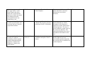
From the matrix shown in Figure 2.2 it is clear to see exactly what is going on. If
player 1 chooses strategy αi and Player 2 chooses strategy βj then the outcome
(Payoff) is represented by Oij in the matrix. If the Payoffs in the matrix were to
represent monetary values to be awarded by one player to another, then Oij would be
replaced by something like 2 or -4 for example. It is necessary in these cases to pick a
convention such that positive numbers represent a payment from player 2 to player 1
and negative numbers represent a payment from player 1 to player 2 for instance. It is
worth reiterating that this matrix representation is only applicable to games in the
Normal form where play is considered to be simultaneous.
2.6 Pure and Mixed Strategies
When playing a game in the normal form each player selects a strategy that they
believe will yield the best result. These two strategies form a pair and can be denoted
by (αi , βj). Given that neither player knows what strategy the other player is going to
pick, how do they decide upon which strategy to pick themselves to yield the greatest
payoff (or at least minimize their loss)? The example below shows how each player
may go about doing this. The convention of this example is that positive amounts
represent a payment from Player 1 to Player 2 and negative amounts represent a
payment from Player 2 to Player 1. Player 1’s possible strategies are the rows and
Players 2’s possible strategies are the columns. The rows and columns of the matrix
are called the players pure strategies.
β1
β2
β3
β4
α1
14
2
1
2
α2
-1
3
9
11
α3
4
3
4
20
α4
8
6
7
16
Figure 2.3
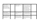
In the example shown in Figure 2.3 it looks as if Player 2 has a rough deal as the best
he can do is win £1 and that will only occur if the strategy pair (α2, β1) is selected.
Given that both players are fully aware of what possible payoffs are available for each
14
strategy they may choose, it is highly unlikely that Player 1 would pick strategy α2 as
it is the only one he can possibly lose on and the maximum he could win is £11.
Player 2 would be fully aware of this fact also. Player 1 on the other hand can win £20
if the strategy pair (α3 , β4) is chosen but again Player 2 is highly unlikely to select β4
given the amount of money he could possible lose.
The objective of Player 1 would now turn to maximising the minimum possible
amount of money he can receive by selecting a certain strategy. Selecting strategy α1
yields a minimum payment of £1, strategy α2 yields a minimum payment of -£1,
strategy α3 yields a minimum payment of £3 and strategy α4 yields a minimum
payment of £6. Taking this into account the logical move to make is to select strategy
α4 as he is assured of at least £6 and at most £16.
Conversely, Player 2 will be looking to minimize his maximum possible loss.
Selecting strategy β1 yields a maximum loss of £14, strategy β2 yields a maximum loss
of £6, strategy β3 yields a maximum loss of £7 and strategy β4 yields a maximum loss
of £20. Taking this into account the logical move to make is to select strategy β2 as the
most he can lose is £6.
Suppose now that both players make the logical decision and the strategy pair (α4, β2)
is selected. Player 1 will win his minimum amount of which he was assured and
Player 2 will lose the maximum amount that he possibly could have given the
strategies they selected. This strategy pair is called an equilibrium pair because it
would not make sense for either player to change his strategy unless the other was to
change his. In other words, even if one player told the other beforehand he was going
to pick the strategy, the best result the other player could obtain by knowing this
would still be if he stuck with his original strategy also. The property of an
equilibrium pair is that it is contains the minimum value in its row and the maximum
value in its column. The payoff associated with the equilibrium pair is called the
saddle point.
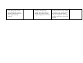
The above example illustrates a simple solution but in most cases there will not be a
saddle point as shown in Figure 2.4
β1
β2
α1
2
-2
α2
-2
2
Figure 2.4
In a case such as this, it is difficult to think of an effective strategy to employ as there
is no clear advantage to picking either strategy and the players would need to use
guesswork to try and pre-empt which strategy his opponent is likely to choose. In fact
the best way to play this game is to select the strategies completely randomly so as not
to let on to your opponent any preferences you have of one strategy over another. In
this example where the choice of pure strategies is made by taking into account the
odds, the choice is said to be a mixed strategy.
15
Suppose a player has a set of pure strategies to choose from and that no equilibrium
pair exists in the Payoff matrix.
Player 1
S1 = {α1, α2, α3, …, αm}
If there is no clear solution as to which strategy is best to pick, then the best way to
analyse the problem is to work out which strategies are better than others and allocate
each strategy a fraction x such that the sum of all the x’s add up to 1.0. The strategies
that the player definitely does not want to use will be allocated an x value of 0 so that
there is no chance that the strategy will be picked. Suppose the Player wanted to pick
strategy α1 with a probability of 50%, strategy α2 with a probability of 20%, strategy
α3 with a probability of 0% and strategy α4 with a probability of 30%. The mixed
strategy for this scenario could be represented thusly.
Player 1
X1 = {0.5α1, 0.2α2, 0α3, 0.3α4}
It may be tempting to think that the player should employ strategy α1 as it looks to be
his best option but the opposing player will also know this and can use his best
strategy to combat the player if he believes he is likely to select strategy α1. In fact the
best option the player has is to randomly pick one of the options by taking account of
the probabilities. For example, he could consult a table of random numbers from 1 to
100 and choose a strategy depending upon what number he comes across i.e. if the
number is between 1 and 50 pick strategy α1, if the number is between 51 and 70 pick
strategy α2 and if the number is between 71 and 100 pick strategy α4. By doing it in
this way, the player ensures he does not let on any personal preference of strategy he
may have for the other player to exploit.
2.7 Minimax Theorem
It is clear to see from the theories that have been so far presented, the best strategy to
employ is one that minimizes your maximum possible loss (or alternatively
maximizes your minimum reward). This phenomenon is the basic foundation of John
von Neumann’s Minimax and Maximin theorems.
The theorems basically state that for every finite two-person zero-sum game there
exists a strategy for each player such that if both players employ the strategy, they
will arrive at the same expected payoff. This means that one player will lose the
maximum of the minimum that he expected to lose and the other player will win the
minimum of maximum he could have possibly won. In other words both players are
able to employ a strategy so that Player A knows he will win an amount P at the least
and Player B knows he will lose at most an amount P resulting in an equilibrium
should both players employ the Maximin and Minimax theorems respectively.
The theorems enforce the idea that an optimal strategy exists for each player and
determining the optimal strategy is now the focus of this project.
2.8 Optimal Mixed Strategies
The idea of a mixed strategy has already been discussed with the theory behind it
16
being that each player should opt for one of their pure strategies by random selection
if a saddle point does not exist. As some of their pure strategies will yield greater
payoffs than others on average, it does not make sense to pick each strategy an equal
amount of the time. Instead, the player is better off picking their better strategies more
often and this can be done by associating a fraction to each strategy such that the sum
of fractions equal 1 and then choosing each strategy according to the odds that go with
it. For example, if strategy 1 was far better than strategy 2 then the player could
associate a value of 0.75 to strategy 1 and 0.25 to strategy 2. Then throughout the
game, the player should choose strategy 1 with a probability of 75% and strategy 2
with a probability of 25%. So how exactly are these probabilities for each strategy
calculated? This problem can be resolved by turning to an area of study called Linear
programming and employing a method called the Simplex algorithm.
2.9 Linear Programming (LP)
Linear programming is an area of mathematics that can be used to find the least
expensive results given particular constraints and resources. It is used to solve
problems in all types of business including engineering, oil refining, banking,
agriculture and many others. Linear programming can take a problem where the idea
is to maximize or minimize a particular value given certain constraints for that value.
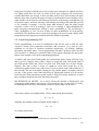
Below is an example of a Linear programming problem4.
A lumber mill saws both finish-grade and construction-grade boards from the logs
that it receives. Suppose that it takes 2 hours to rough-saw each 1000 board food of
the finish-grade boards and 5 hours to plane each 1000 board feet of these boards.
Suppose also that it takes 2 hours to rough-saw each 1000 board feet of the
construction-grade boards, but it takes only 3 hours to plane each 1000 board feet of
these boards. The saw is available 8 hours per day, and the plane is available 15 hours
per day. If the profit o each 1000 board feet of finish-grade boards is $120 and the
profit on each 1000 construction grade boards is $100, how many board feet of each
type of lumber should be sawed to maximize the profit?
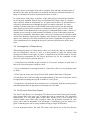
MATHEMATICAL MODEL. Let x and y denote the amount of finish-grade and
construction-grade lumber, respectively, to be sawed per day. Let the units of x and y
be thousands of board feet. The number of hours required daily for the saw is
2x + 2y
Since only 8 hours are available daily, x and y must satisfy the inequality
2x + 2y ≤ 8
Similarly, the number of hours required for the plane is
5x + 3y
So x and y must satisfy
4
Taken from Elementary Linear Programming with Applications 2nd edition, Kolman and Beck, p.46
17
5x + 3y ≤ 15
Of course, we must also have
x ≥ 0 and y ≥ 0
The profit (in dollars) to be maximized is given by
z = 120x + 100y
Thus, our mathematical model is:
Find values of x and y that will
Maximize z = 120x + 100y
Subject to the restrictions
2x + 2y ≤ 8
5x + 3y ≤ 15
x≥0
y≥0
Here, z is a value that needs to be maximized by adjusting the values of x and y.
There are a number of constraints on x and y that need to be taken into account to find
valid values of x, y and z. This is a typical Linear programming (LP) problem and it
can be solved using an algorithm called the Simplex method.
It is possible to take a payoff matrix for a two-person game and apply the method of
Linear programming shown above to it to determine the optimal probabilities to be
associated with each pure strategy to hence give a pair of optimal mixed strategies.
There are certain constraints that apply to the payoff matrix which means it is possible
to transform it into a Linear programming problem like the one above. Full details of
how this works is explained in the design section.
Given a Linear programming problem with constraints, the next step is to incorporate
it into a tableau and apply the simplex method to it.
2.10 Simplex method
The theory and method behind the Simplex algorithm is quite complex and difficult to
understand at first. It is not necessary to explain the full theory behind it here just as
long as it is understood how to set up a problem into the correct form and execute the
procedure. The first step is to take the initial problem and find a basic feasible
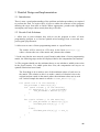
solution. The method of constructing a tableau from the initial constraints can be
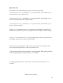
explained quite simply although the actual theory behind it is not quite so simple.
Basically, the idea is to convert the inequalities into equalities by introducing new
“slack” variables. In the previous LP example, the inequalities would be converted by
introducing some new variables thusly:
2x + 2y ≤ 8
5x + 3y ≤ 15
⇒
⇒
2x + 2y + u = 8
5x + 3y + v = 15
18
The object of the LP problem is to maximize z. The next step is to rearrange the
equation for z so that it resembles the two new equations that have just been created.
z = 120x + 100y
⇒
-120x - 100y + z = 0
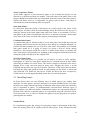
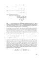
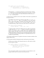
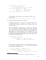
The three new equations are then put into a tableau exactly like the one shown in
Figure 2.5.
x
y
u
v
z
u
2
2
1
0
0
8
v
5
3
0
1
0
15
-120
-100
0
0
1
0
Figure 2.5
The slack variables introduced are u and v and these are called the initial basic
variables. A basic variable in a tableau has the following properties5:
1. It appears in exactly one equation and in that equation it has a coefficient of +1.
2. The column that it labels has all zeros (including the objective row entry) except
for the +1 in the row that is labelled by the basic variable.
3. The value of a basic variable is the entry in the same row in the rightmost column.
The tableau is set up to an initial basic feasible solution. In the first two rows it is
clear to see that u is 8 and v is 15 and in the last row (objective row) z is zero. The
objective is to manipulate the table to make z as large as possible by increasing the
values of x and y. To do this requires x and y to become the basic variables instead of
u and v.
At this point it should be noted that the method of setting up the initial tableau is the
same for every LP problem. In this problem there were three equations to put into the
tableau and two variables (x and y) to solve for. For every problem like this, the
coefficients for the m variables to solve for, go into the first m columns. An identity
matrix of size m * m is then inserted to take account of the newly introduced
variables before finally putting all the non-variables in the last column.
Once an initial tableau has been set up, the next step is to apply the Simplex algorithm
to it. This entails iterating through a number of steps until either an optimal solution is
found or it can be determined that an optimal solution does not exist.
The first step is to check whether the tableau is already in an optimal state. This is
done by checking the tableau against the optimality criterion.
Optimality criterion6 If the objective row of a tableau has zero entries in the columns
labelled by basic variables and no negative entries in the columns labelled by
nonbasic variables, then the solution represented by the tableau is optimal.
5
6
Taken from Elementary Linear Programming with Applications 2nd edition, Kolman and Beck, p.107
Elementary Linear Programming with Applications 2nd edition, Kolman and Beck, p.108
19
Looking at this statement it is clear to see that the tableau used in the previous
example is not in an optimal state as there are two negative entries in the objective
row. If however, the optimality criterion is satisfied, the computation can stop as an
optimal solution has been found. If the criterion is not satisfied, a procedure known as
pivoting needs to be applied before checking the tableau against the optimality
criterion again. This loop continues until either an optimal solution is found or it is
determined that no finite optimal solution exists.
The method known as pivoting essentially involves taking one of the nonbasic
variables and turning it into a basic variable by allowing it to replace one of the
current basic variables. During this process the value of the entries of the tableau are
adjusted in accordance with the constraints on the pivotal entry. Selection of the
pivotal column and the pivotal row is explained in greater detail in the design section
of this document along with an in-depth description of the entire pivoting procedure.
It is not necessary to explain at this point the whole method behind the Simplex
algorithm, it is only necessary to know that a game payoff matrix can be converted to
a LP problem and applied to the Simplex algorithm to determine optimal mixed
strategies for the game.
Some examples of existing solutions to solve Game theory and LP problems can be
found in the ‘Website References’ section of the dissertation.
20
3 Requirements Analysis and Specification
3.1 Introduction
The literature review has laid out an initial understanding of the problem that is faced
in this assignment. This section takes the knowledge gained thus far and details
exactly what is required to guarantee success in the project. The document sets out the
Functional and Non-functional requirements of the system as well as the User
requirements and Hardware requirements. The requirements will form a framework of
the system design and can be used in the testing stage to validate whether the
implementation has been successful.
3.2 Product aim
The function of the system to be designed in this project is to automatically generate
Optimal mixed strategies for two-person zero-sum finite games. The program should
be able to take any m*n payoff matrix and output Optimal mixed strategies for both
players along with the value of the game being played. In addition, the program will
be able to be applied to many other linear programming problems that can be solved
using the simplex method and provide feedback on the solutions.
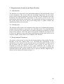
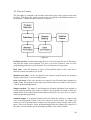
3.3 Requirements Elicitation
The purpose of this section is to take the initial understanding of the problem from the
literature review and expand upon it by considering the requirements of the
stakeholders of the system. In this particular project, the stakeholders include myself
(the developer) and any potential end-users of the system. In most cases it is
unfeasible to satisfy the desires of every single stakeholder due to things like
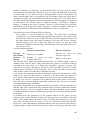
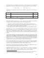
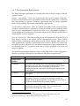
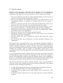
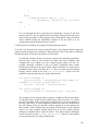
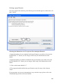
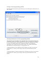
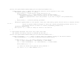
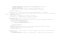
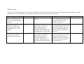
conflicting interests and resource limitations. There are several stages involved in the
elicitation process and a generic model of this is given in Software Engineering 6th
edition, by Ian Sommerville shown in Figure 3.1.
21
Figure 3.1
3.3.1 Domain Understanding
In this stage it is the job of the developer to develop their understanding of the nature
of the problem and the application domain. This is what was essentially accomplished
in the literature review although greater understanding of the domain will increase as
the elicitation process goes on. In particular, interaction with the stakeholders will
enhance the developers own knowledge of the problems involved.
3.3.2 Requirements Collection
Requirements collection involves interacting with the stakeholders to determine their
expectations of the system. In this particular project there are a few points that need to
be established before this process can begin. First of all, it is necessary to figure who
exactly are the likely end-users of such a system as without this knowledge, the only
stakeholder to influence the system development is the developer. It has already been
determined that the purpose of the system is to calculate optimal strategies for twoperson zero-sum games by use of the Minimax method or the Simplex method.
Taking this into account there are two certain groups of people that the system should
target.
People interested in game theory
People interested in Linear programming and the Simplex method
These two groups are quite broad and can be broken down into other subgroups or recategorized into occupational interests such as economists, military strategists, poker
players etc. By diversifying the project slightly to include not only the input of game
payoff matrices but also any other type of Linear programming problem, there are
more potential end-users and hence more stakeholders from which to elicit
information.
22
The most suitable method for information collection in this particular scenario is by
targeting likely end users (people with interests in the areas noted above) and either
interviewing them explicitly or by requesting them to fill in generic questionnaires
with the option to add in their own requests.
Some of the requirements gathering documentation like the questionnaires used can
be found at the back of the dissertation in Appendix A.
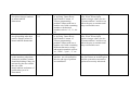
3.3.3 Classification
The information gathered in the requirements collection stage consists of unstructured
data in the form of interview transcripts and filled-in questionnaires. The
Classification stage simply involves collating this data into meaningful information to
be processed into requirements. Much of the data from the requirements collection is
written in different ways but essentially boil down to the same things and it is at this
point the developer tries to interpret exactly what the stakeholders are all asking for.
3.3.4 Conflict Resolution
Although most of the requirements gathered from the stakeholders are in agreement,
there are often contradictory views of what each stakeholder wants to see and it is
unfeasible to cater to all their desires. In this stage, compromises are made by
identifying the most rational approach.
Some of the conflicting interests encountered in this requirements elicitation are
detailed below along with the decisions taken to resolve the conflicts.
There were requests from some quarters for the program to include quite complex LP
procedures other than the Simplex method and way outside the scope of the original
aim of this project. Investigation, learning and programming of these methods
conflicted with the interest of the developer in terms of time constraints and as such
were not considered essential to the success of the project.
There was slight confusion also over what the program would be used for exactly.
People with a good understanding of the Simplex method tended to want the program
for use as a simple calculator to input and quickly solve any problems that would take
too long to solve by hand. However, a few people with a more limited knowledge of
game theory and the Simplex method asked for a program that could be used as a sort
of learning tool to guide them through the steps of the Simplex method. After some
deliberation, a decision was made to allow the user to select whether they want the
calculator to solve the problem automatically or go through the entire procedure step
by step.
Detail vs. Simplicity - The biggest conflict encountered seemed to involve the level of
complexity of the system. This included requests by some to include all kinds of
features enabling them to essentially customise and configure the system to their own
requirements. Again, these requests not only conflicted with the expectations of other
stakeholders but also of the developer who is face with timing constraints as well as
being constrained by their own programming expertise. Some of these requests were
23
hence omitted for consideration for the program after they were deemed too
complicated and time consuming to implement and nonessential to the project
success.
3.3.5 Prioritisation
Obviously there are some requirements that are more important than others. It is the
developer’s job at this stage to interact with the stakeholders and determine what is
essential for the program success and the varying degrees of importance of each
requirement. Doing this ensures the developer fully understands the task they are
faced with and enables them to gauge the success of the system during
implementation by ensuring the high priority requirements are being satisfied.
The highest priority requirements in this system were the ones concerned with
accuracy of the final results and hence the reliability of the functional computations
within the program. Less important requirements included the attractiveness of the
application layout and the implementation of “additional features” like being able to
save intermediate results to the hard drive.
3.3.6 Requirements Checking
Having compiled a set of requirements for the system, it is imperative to check the
requirements are consistent and complete. This process involves drawing up a
requirements specification which is then checked by the stakeholders to ensure it
fulfils their needs and expectations.
As shown in the diagram, the requirements elicitation is an iterative process and the
cycle continues until a complete specification is achieved. The finished specification
is given below.
3.4 Requirements Specification
From the understanding gained so far of Game theory, Linear programming and the
Simplex method as well as the purpose of the system, it is now possible to detail
exactly how the program should work. Below is the specification detailing all the
Functional and Non-Functional requirements. The tables consist of user and system
requirements
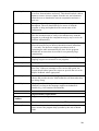
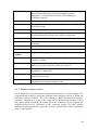
3.4.1 Functional Requirements
Requirement
Number
Requirement description
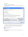
1
The program should allow the user to input any matrix/LP tableau
within the bounds of memory availability
1.1
The user should be able to select the size of the matrix/LP tableau
they wish to enter using the computer keyboard
1.1.1
The program should recognise invalid entries for the size of the
matrix/LP tableau and inform the user of the error
24
1.2
The user should be able to select an option to state whether they
want to enter a payoff matrix or a LP problem
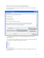
1.3
The user should be able to input matrix entries via the computer
keyboard
1.3.1
The program should recognise invalid entries for the matrix/LP
tableau and inform the user of the error
1.4
The user should be able to delete and re-input any matrix entries
that they have erroneously entered without having to restart the
entire problem
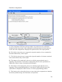
1.5
In the event that the input matrix contains errors that do not allow
the matrix to be properly processed through the program then
appropriate feedback should be displayed informing the user of
what has gone wrong
2
The program should immediately check for a saddle point if the
user entered a payoff matrix
2.1
If a saddle point exists, the program should inform the user and
output the pure strategies that are optimal for each player along
with all other details of the game
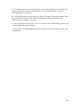
2.2
If the user entered LP problem, the program should not attempt to
find a saddle point but instead proceed straight to Functional
requirement 4
3
In the absence of a saddle point, the program should prepare the
payoff matrix so that the Simplex method can be applied
3.1
Slack variables must be added to the elements of the matrix to
ensure there are no negative entries
3.2
The payoff matrix must be converted into the larger matrix in
keeping with a linear programming problem
4
The Simplex method must be applied to the tableau
4.1
The program should be able to pick out a pivot from the matrix and
apply the pivoting procedure
4.1.2
The program should inform the user if no finite optimal solution
exists
4.2
After completion of the pivoting procedure the program should
check for optimality
4.2.1
If the optimality test is negative the program should repeat the
pivoting procedure with a new pivot
4.2.2
If the optimality test is positive the program should exit the
Simplex procedure
4.3
The user should be able to select whether they want the program to
continually provide feedback on each step of the simplex method or
proceed straight to the optimal solution if one exists
25
5
Where an optimal solution is found the user should be informed
5.1
The user should be asked whether they want the results displayed
in terms of optimal mixed strategies or as a solution to a LP
problem
The program should output the optimal results in the format the
user selected
5.2
5.3
The program should also output the value of the game or the
optimal value of the LP problem, whichever is relevant
6
The user should be provided with a continue button to advance
through each step of the computation
6.1
The program should advance to each next step of the computation
when the user activates the “Continue” button using the mouse or
the enter button on the keyboard
7
The program should contain a button to abandon the current
computation and start a new one
7.1
The program should reset all the necessary variables so values from
previous computations do not interfere with the new problem
8
The program should contain safety features to prevent the user
from making errors
8.1
The program should block out/deactivate the functions of fields and
buttons when they are not intended for use
8.1.1
The user should be informed if they are trying to operate a function
that is not allowable at that particular stage of the computation.
Alternatively it may be more applicable in some cases to simply
ignore the user’s button selection if the function they are requesting
is not applicable at that point of the computation.
9
The program should be able to easily recover from user errors
9.1
The program should be able to continue with the current
computation if the user makes a mistake and attempts to rectify it
by selecting the correct option
10
The program should be able to notice errors made by the computer
during program execution
10.1
The program should inform the user if a problem occurs and the
computation needs to be halted
26
3.4.2 Non-Functional Requirements
The Non-Functional requirements are classified into three different categories that are
explained below.7
Product requirements These are requirements that specify product behaviour.
Examples include performance requirements on how fast the system must execute and
how much memory it requires; reliability requirements that set out the acceptable
failure rate; portability requirements and usability requirements.
Organisational requirements These are derived from policies and procedures in the
customer’s and developer’s organisation. Examples include process standards which
must be used; implementation requirements such as the programming language or
design method used; and delivery requirement which specify when the product and its
documentation are to be delivered.
External requirements This broad heading covers all requirements which are derived
from factors external to the system and its development process. These include
interoperability requirements which define how the system interacts with systems in
other organisations; legislative requirements which must be followed to ensure that
the system operates within the law; and ethical requirements. Ethical requirements are
requirements placed on a system to ensure that it will be acceptable to its users and
the general public.
The Non-Functional requirements are shown in the table below. Each requirement is
labelled according to Sommerville’s breakdown of the three categories above8.
Product requirements
Requirement
Number
Requirement description
Usability 1
The layout and functionality of the application should be
familiar to the user. The vast majority of users will be used to
the functions and features of the Microsoft Windows
environment and the application should appear and run in the
same format.
The layout of the application should be neat and consistent
throughout.
Usability 2
Usability 3
The functions of the application should remain consistent
throughout. Properties, methods and meanings should not
change during program runtime to ensure the user does not get
confused or surprised by the programs actions
Usability 4
The behaviour of the system should be as clear and well
explained to the user as possible. The user should not be
surprised by the behaviour of the system.
7
8
Definitions taken directly from Software Engineering 6th edition, Ian Sommerville p.102
Software Engineering 6th edition, Ian Sommerville p.102, Figure 5.3
27
Usability 5
The system should contain recovery procedures to allow the user
to recover from mistakes and errors. This should include a delete
button to remove incorrect inputs from the user and a button to
allow the user to abandon the current computation and start a
new one.
Usability 6
The system should provide appropriate and meaningful feedback
throughout. The user should always be aware of what the
program is doing and updated on the current state of the
computation.
Usability 7
The system should be adaptable to the requirements of the user.
The user should be able to easily select whether they want the
program to go through the computation step by step or solve the
problem automatically.
Efficiency 1
Upon an average speed computer, the time for the program to
proceed from one step to the next should be almost immediate
(<1 second). For the more complex procedures such as
optimising the table automatically the time for the program
should take no more than 4 seconds for exceptionally large
computations.
Efficiency 2
The program should be no bigger than 5MB (not including
language support environment to run program).
Efficiency 3
The program should not contain excess or redundant code.
Reliability 1
The system should be as robust as possible and not fail due to
user error. If the user attempts to select an invalid option, the
system should either ignore the request or provide the user with
helpful feedback where appropriate.
Reliability 2
Upon input of the matrix, the program should not allow invalid
entries and provide the user with feedback to tell them what they
are doing wrong.
Portability 1
The program should be operable on any platform (not just
Windows) as long as the language support environment is
installed (e.g. Java runtime environment).
Organisational requirements
Requirement
Number
Requirement description
Delivery 1
The entire project must be completed by 8th May 2006.
Delivery 2
To allow adequate time for completion of the dissertation, the
aim is to have the program fully operable by the end of March
2006.
28
Delivery 3
The completed project must consist of a Literature Review,
Requirements documents, Design and Implementation
documents, Testing documents and a CD containing the
calculator program.
Implementation 1
The program will be written in the programming language Java.
Implementation 2
The program will be implemented using the Microsoft Windows
operating system.
Implementation 3
The program will be coded using the NetBeans IDE 5.0
Standards 1
The dissertation should be laid out and printed in a neat and
consistent manner and with good spelling and grammar.
Standards 2
The written document will be neatly bounded with covers.
Standards 3
The CD will be securely and neatly attached to the written
document.
External requirements
Requirement
Number
Requirement description
Ethical 1
The project should not be offensive to any particular faith,
religion or culture.
Ethical 2
Any parts of the project that were aided by the help of others or
others work will be explicitly stated and credited.
Legal 1
The project must comply with the universities rules and
regulations on plagiarism.
Legal 2
The project must at all times comply with the laws of copyright
and intellectual rights.
Legal 3
The project must comply with all international laws where the
program may be made available for use.
3.4.3 Hardware Requirements
There should be no special hardware requirements needed to run the program. The
program should be able to run on any computer with a moderate processor, RAM and
hard disk memory available. The exact amount of RAM and hard disk memory
required is impossible to gauge at this stage but any modern day computer will be
more than capable of running the system given the complexity of the program The
program should also be executable on any operating system. The only external
hardware required should be a keyboard, a mouse (or alternative cursor controlling
device) and a monitor.
29
3.5 Requirements Validation
Requirements validation is the process of checking that the Requirements document
actually meets the needs and wants of the end-users as well as finding problems with
the individual requirements. This stage is important as errors in the initial
specification will result in the creation of a program that does not provide the service
the customer wanted. This would in turn result in an inadequate program or much
reworking of the programming to try and meet the customer’s needs.
Before the design stage of the project could commence, the following checks were
made on the requirements document9.
3.5.1 Validity Checks
After consultation with the stakeholders about what they wanted from the system,
compromises were made in the generation of the requirements in an attempt to make
the system appeal to as many people as possible. Judgement calls were made to try
and resolve conflict when generating the requirements document and it was necessary
to check with the stakeholders whether the compromises made, still meant the
program met with their satisfaction.
The general consensus was that the requirements document met with the expectations
of the vast majority of the stakeholders. Very few end-users objected to any of the
requirements and the specification was drawn up with the intention of accommodating
as many of the users requests as possible.
3.5.2 Consistency Checks
It must be ensured that there are no requirements in the document that conflict or
contradict with one another. If one constraint stated that the program should execute
at a certain speed while another constraint stated that the program should be
executable on even very slow computers, it must be checked that both requirements
are achievable otherwise it may be impossible for the system to satisfy all
requirements.
Inspection and investigation of the requirements were made by cross-checking
requirements that had conflicting aims and verifying that it was possible to achieve all
contradictory statements. Another method of consistency checking is achievable via
the use of CASE tools. Given the complexity of the requirements document, this type
of analysis is not necessary for a project of the size and a simple thorough review of
the requirements was deemed sufficient.
3.5.3 Completeness Checks
The requirements specification had to be checked to ensure it defined all the functions
and constraints intended by the user. This was done by reviewing the requirements
elicitation and ensuring that nothing had been omitted from consideration. Further
checks involved collaborating with the end-users once again to see if there were any
9
Checks are described in Software Engineering 6th edition, Ian Sommerville p.137
30
requirements they thought should be added. After some deliberation and examination,
all parties were satisfied the requirements document was indeed complete.
3.5.4 Realism Checks
Having a requirements document that promises amazing things is useless if the plans
are not feasible when it comes to implementing them. In terms of technology, it was
determined that the constraints detailed in the specification were totally achievable
with the resources available today. Using knowledge of existing technology and the
characteristics of previous programs written in Java, there was no reason to believe
that any part of the program could not be accomplished in accordance with the
constraints set out in the specification.
The next thing to consider was the budget constraints. It was necessary to consider the
resources that would be required to complete the project and their costs.
Access to a PC to program the system and write up the dissertation had already
been established at zero cost.
Access to library books for research is available at zero cost from Bath university
library.
Access to the internet for research and download purposes had already been
established at zero cost.
The Runtime environment for Java is freely available for download on the
internet.
The Integrated development environment NetBeans IDE 5.0 is freely available for
download on the internet.
Having determined the majority of resources required were available at no cost, it was
determined that the project was achievable with the budget available. The only real
costs incurred as a result of the project would include printing costs, binding costs,
electricity costs, perhaps one or two books not available from the library and other
minor resources. All these minor things are well within the budget available to this
project.
The last thing to check was whether the system development could be completed
within the schedule set out. A timetable setting out time allocation to each section of
the project was drawn up with allowances for sections to overrun in case of
illness/technical difficulties/time misjudgements. After some deliberation and reworking of the timetable, the schedule set out for the project was found to be feasible.
3.5.5 Verifiability
This final section essentially involved ensuring that the requirements contained as
little ambiguity as possible so as to avoid dispute later on between the end-users and
the developers over the success of the delivered system. It was necessary to ensure
that the requirements were written in specific and concise manner so that a system of
checks could be introduced for each requirement to demonstrate whether the criteria
of every requirement had been met during the testing stages.
31
4 Design
4.1 Introduction
The purpose of the design section is to take the requirements set out in the
requirements specification and construct a design framework from which to build up a
paper prototype of the system. The paper prototype can then be put in to practice and
implemented in code.
The system will be encoded using the Java programming language and the reason for
selecting this particular language was due to several factors. Firstly it contains special
characteristics, explained later in this design document that were helpful in solving
some of the problems that the system was faced with. It is also free and easily portable
across platforms/operating systems. The main reason for choosing it was down to the
advanced graphical user interface (GUI) components that can be automatically
generated using Java’s Swing and AWT features. Creating attractive applications with
Java can be achieved with considerably more ease than most other programming
languages.
A decision was made to use an integrated development environment (IDE) to code the
program. An IDE has special useful tools and functions such as debugging features
that assist the user in coding a program. The choice of NetBeans IDE 5.0 over other
IDE’s was down to a specific feature it contains that allows the programmer to create
a GUI by setting up an initial application template which can be built up by using a
drag and drop feature to add components to the interface. This feature only controls
the layout and appearance of the interface, it has no effect on the actual functions of
the interface. For example, the programmer may be able to select where to put a
button on the interface but the programmer would have to write all the code to
determine exactly what the button does as otherwise the button would not do anything
if the user selected it.
32
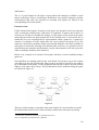
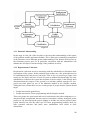
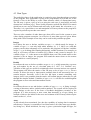
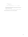
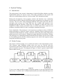
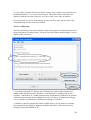
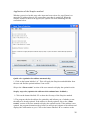
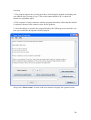
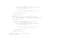
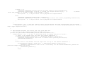
4.2 Flow of Control
The first thing to establish is the possible states and stages of the program from start
to finish. This details the options posed to the user and the individual procedures of
the program. A diagram of this is shown in Figure 4.1.
Figure 4.1
Problem selection At this initial stage the user is asked to input the size of the matrix
and state the nature of the problem. The user is given the option to enter a Linear
programming problem or a payoff matrix for a two-person zero-sum game.
Data entry Once the program is aware of the problem it has to solve, the user is
allowed to enter the matrix to be solved.
Minimax procedure In the case that the user entered a payoff matrix, the program
employs a procedure to test for saddle points.
Data conversion If the case that the user entered a payoff matrix that contained no
saddle points, the program converts the payoff matrix into a new matrix in the form of
a Linear programming problem.
Simplex method The matrix is put through the Simplex algorithm in an attempt to
find an optimal solution. This stage is reached if the program was unable to find any
saddle points in the payoff matrix and employed anyway if the user chose to enter a
Linear programming problem.
Solution output If an optimal solution has been found, the solution is output to the
user in the appropriate format. If the user entered a payoff matrix, the output will
consist of a set of optimal mixed strategies for both players along with the value of the
game. If the user entered a Linear programming problem, the output will comprise of
the value of each variable and the maximum possible value of the problem.
33
4.3 Data Types
The underlying layer of the application is required to store data throughout execution
of the program. This application is going to be programmed in Java and one of the
features of Java is the ability to create a data structure called a 2 dimensional array.
The 2D array is given a size of m by n using the code two_d_array[m][n] and each
element has a location [x][y]. These useful properties replicate the notion of a matrix
which has m rows and n columns and each entry in the matrix has a location (x, y).
Therefore, it is a good idea to use and manipulate a 2D array whenever the program is
required to perform a procedure on a matrix.
There are also a number of other data types that will be used in the system to store
values during program execution. An overview of some data types are given below
along with a short example of how they can be used in this particular program.
Integer
Java allows the user to declare variables as type int which stands for integer. A
variable of type int can only hold whole numbers (0, 1, 2, 89013 etc.) and this
property can be taken advantage of. In particular, this program will declare variables
of type int to do things like counting and storing variable locations. For example, an
entry in a 2D array will have a location [x][y] where x and y must be integers. If a
variable of type int is the answer to an equation then even if the actual answer to the
equation is not an integer, the program will round the answer down to the nearest
integer which is a useful property.
Double
Java allows the user to declare variables as type double which means they can store
any real number by the use of a decimal point (0.5, 1.837, 5.0, 2.666667 etc.).
Variables of this type are useful for calculations where accurate answers are required.
This program will allow the entries of the 2D array to be of type double for two
reasons. It allows the user to input matrix problems that do not necessarily have to
contain integers. Secondly, even if the user did input a matrix containing only
integers, there is no guarantee that the entries will remain integers when they are put
through the simplex method. Variables of type double will also be used throughout
the program to store ratios and intermediate results.
String
Java allows the user to use and declare variables of type String. A String is simply
a string of characters and/or symbols and/or numbers. The system will be required to
output Strings to the user in the form of feedback throughout execution of the
program. It is also necessary to store some data internally as of type String. An
example of this are the labels for the rows and columns of the 2D array which require
names such as x1, x2 etc.
Array
As has already been mentioned, Java has the capability of storing data in structures
called arrays. An array is essentially a list of data entries, all of the same type (double,
int, String etc.). When initialised, an array is given a particular length and type, for
34
example 10 and int respectively which means it can hold 10 values of type int. Each
entry will have an index from 0 up to 9 in the example being used here so that the
location of each value is known. Arrays are useful and necessary for this particular
program. The row and column labels need to be stored in arrays along with the game
solutions for each player.
The simple array can be extended to make it 2Dimensional. A 2D array like
example[m][n] can essentially be though of m arrays all of length n. This type of
structure is vital to this program as it is going to be used to represent the payoff
matrix, the Linear programming tableau and to also used store intermediate results.
4.4 Saddle point
The first main mathematical procedure to consider in the system is that of checking to
see whether a payoff matrix contains a saddle point. If a saddle point exists, there is
no need to employ the simplex method procedure as pure optimal strategies exist for
each player. The phenomenon of a saddle point was discussed in the literature review
and arises from von Neumann’s Minimax theorem.
The theory works thusly - Each player should choose the strategy that maximizes their
minimum payoff or alternatively minimizes their maximum loss. Given the
convention that payments from player 2 to player 1 are represented as positive
amounts and that payments from player 1 to player 2 are represented by negative
amounts, the method of locating a saddle point proceeds like this. Player 1 looks at
each of their strategies and notes the minimum amount they are guaranteed to win if
they choose to employ that particular strategy. Player 2 also looks at their strategies
and notes the maximum amount they could possibly lose by employing each strategy.
If there exists a strategy for Player 1 and a strategy for Player 2 whereby the minimum
payout guaranteed to Player 1 is equal to the maximum loss possible to player 2, then
the two strategies are said to be in equilibrium and the entry in the payoff matrix
where the strategies coincide is said to be a saddle point. Take a look at the payoff
matrix in Figure 4.2.
Figure 4.2
Player A checks to see the worst case scenario in employing each of his strategies.
Strategy 1 yields a minimum of 0 and strategy 2 yields a minimum of -5. The
maximum of these minimum wins is 0 and so it appears that player A’s best option is
to play strategy 1.
Player B checks to see the worst case scenario in employing each of his strategies.
Strategy 1 yields a maximum loss of 15, strategy 2 yields a maximum loss of 0 and
strategy 3 yields a maximum loss of 10. The minimum of these maximum losses is 0
and so it appears that player B’s best option is to play strategy 2.
From this analysis, it is evident that if Player A employs strategy 1 then Player B’s
best counter is to play strategy 2. Likewise, If player B is to play strategy 2 then
35
player A’s best option is to play strategy 1. This is the feature of a saddle point,
neither player will benefit in changing their strategy if the other player does not
change theirs. In this example, the saddle point occurs in the location (1,2) in the
matrix and has a value of 0. The value of the game is therefore said to be 0 as this is
the average amount each player will get by employing their optimal strategies.
4.5 Payoff Matrix to LP Tableau
In the case that a saddle point does not exist then the next step is to take the payoff
matrix and transform it into a Linear programming problem. The properties of a
Linear programming were explained in the literature review, namely maximising a
value subject to certain constraints. The first step in this procedure is to add a fixed
constant k to each matrix entry to ensure the matrix contains no negative entries. This
step makes no difference to the properties of the matrix as the optimal strategies
remain the same and the k value can be subtracted at the end of the computation to
find the value of the game. The reason that the matrix can contain no negative entries
is explained later.
The best way to explain this procedure is with the aid of a worked example, consider
the payoff matrix in Figure 4.3.
Figure 4.3
The value of the game v, is the amount that that will be won/lost by each player of
average if they both employ their optimal mixed strategies. Firstly, let us consider
finding an optimal strategy for the column player in the above matrix. The
probabilities associated with each of the column player’s strategies will be denoted as
a, b and c respectively. In the case that the row player selects his first strategy, it is
feasible to state that:
2a + 3b + c ≤ v
Similarly, if the row player selects his second strategy, it is also true that:
a + 2c ≤ v
There now exists a set of constraints similar to a LP problem except that the value of
v is not yet known. To get around this problem, the two equations above can be
divided throughout by v which is known to be non-negative due to the value k being
added on earlier. The equations now look like this:
2(a/v) + 3(b/v) + (c/v) ≤ v
(a/v) + 2(c/v) ≤ v
It is also known that the probabilities a, b and c add up to a total of 1, therefore:
36
a+b+c=1
Dividing throughout by v once again gives:
(a + b + c)/v = 1/v
or
(a/v) + (b/v) + (c/v) = 1/v
Replacing (a/v), (b/v), (c/v) and (1/v) with A, B, C and V for notations sake, the
payoff matrix can now be expressed as a LP problem with a set of constraints and an
objective function to maximize:
Maximize:
V=A+B+C
Subject to the constraints:
2A + 3B + C ≤ 1
A + 2C ≤ 1
A ≥ 0, B ≥ 0, C ≥ 0.
The last constraint is true since a, b, c and v are all greater than or equal to zero. A
similar method could be applied to the row player’s strategies although it is not
actually necessary to do this to solve the LP problem. The LP problem shown above
can be entered into a LP tableau as explained in the literature review and solved to
find the optimal values of A, B, C, and V. The values a, b, c and v can then in turn be
determined since v = (1/V), a = A * v, b = B * v and c = C * v. It must also be
remembered that the actual value of the game is equal to v - k since some constant
may have been added at the beginning of the computation. The value of k however
does not affect the values of a, b and c in any way.
4.6 Simplex method
If the user chooses to enter a LP tableau or if the payoff matrix contained no saddle
points, the program needs to employ the Simplex method to solve the problem. A
simple explanation of the Simplex method was given in the literature review. It
basically involves repeating a procedure known as pivoting to the LP tableau until the
table satisfies an optimality criterion.
Optimality criterion10 If the objective row of a tableau has zero entries in the columns
labelled by basic variables and no negative entries in the columns labelled by
nonbasic variables, then the solution represented by the tableau is optimal.
The Simplex procedure is best explained with the aid of a worked example. Consider
the LP tableau11 in Figure 4.4.
10
Elementary Linear Programming with Applications 2nd edition, Kolman and Beck, p.108
Example taken from Elementary Linear Programming with Applications 2nd edition, Kolman and
Beck, p.105 - p114
11
37
x
y
u
v
z
u
2
2
1
0
0
8
v
5
3
0
1
0
15
-120
-100
0
0
1
0
Figure 4.4
Checking the table against the optimality criterion, it is obvious that the table is not
yet optimal since there are negative entries in the objective row (last row). This means
that the pivoting procedure needs to be applied to the table.
The objective is to increase z as much as possible and this can be done by changing
the values of x and y. The first step of the pivoting procedure is to pick the pivotal
column and the best column to pick is the one whose value in the objective row is
smaller than all the other columns objective row values. The reason for this is that it
will have a greater impact in increasing z than the other columns. It can be seen from
the tableau above that the pivotal column should then be the ‘x’ column.
The next step is to then select the pivotal row which is a more complicated procedure
than selecting the pivotal column. The objective in this procedure is to increase x
which in turn increases z while remembering that there are certain constraints on x
allowing it to be increased only up to a certain amount. The tableau above essentially
represents
2x + 2y + u = 8
5x + 3y + v = 15
-120x - 100y + z = 0
Since y is going to be kept at zero, the first two equations can be taken and rearranged
to give:
u = 8 - 2x
v = 15 - 5x
x can only be increased until u or v become negative. Some quick mathematics shows
that:
⇒
x≤4
2x ≤ 8
5x ≤ 15
⇒
x≤3
Therefore, x cannot be increased by more than the smaller of the two values, namely
3. As x is constrained by v before u, then the row containing v must be selected for
the pivot row. This procedure may sound laborious but can be simplified to a simple
method: For each row, calculate the ratio of the entry in the final column of that row
divided by the entry in the pivotal column of that row. The row containing the
smallest ratio becomes the pivotal row.
However, there is one more point to consider. Rows that contain negative entries in
38
the pivotal column cannot be considered for the ratio procedure as they would give
negative ratios and consequently rearranging them using the method above would
show that the variable could be increased without any restriction. Similarly rows
containing zero entries in the pivotal column cannot be considered since dividing by
zero is undefined. Therefore, during selection of the pivotal row, only rows containing
positive entries in the pivotal column must be considered. If a case arose whereby
there were no positive entries in the pivotal column (objective row not included) then
the computation must stop as there exists no finite solution for that particular LP
problem. This needs to be remembered when it comes to implementing the procedure
into code.
Having selected the pivotal column and pivotal row, now comes the task of
performing the actual pivoting procedure. This involves a sequence of steps:
1. Find the value of the pivot. The pivot is entry where the pivotal row and pivotal
column intersect. From the example being used here, it can seen that the value of the
pivot is 5.
x
y
u
v
z
u
2
2
1
0
0
8
v
5
3
0
1
0
15
-120
-100
0
0
1
0
Figure 4.5
2. Next, the entries in the pivotal row need to be multiplied by 1/5 so that the value of
the pivot becomes 1.
x
y
u
v
z
u
2
2
1
0
0
8
v
1
3/5
0
1/5
0
3
-120
-100
0
0
1
0
Figure 4.6
3. Suitable multiples of the new pivotal row must then be added to all the other rows
so that all other elements in the pivotal column become zero.
Row 1 = Row 1 - 2 * (Row 2)
Row 3 = Row 3 + 120 * (Row 2)
x
y
u
v
z
u
0
4/5
1
-2/3
0
2
v
1
3/5
0
1/5
0
3
0
-28
0
24
1
360
39
Figure 4.7
4. Finally, the label of the pivotal row must be changed to the label of the pivotal
column. That is, the v label is replaced with an x label.
x
y
u
v
z
u
0
4/5
1
-2/3
0
2
x
1
3/5
0
1/5
0
3
0
-28
0
24
1
360
Figure 4.8
This illustrates the entire pivoting procedure. The idea now is to check the new
tableau against the optimality criterion once again. As there is still a negative entry in
the objective row, the tableau is not yet optimal and so the pivoting procedure must be
applied once again to the new tableau. It turns out in this particular example that one
more application of the pivoting method is required to make the tableau optimal. The
optimal tableau is given below.
x
y
u
v
z
y
0
1
5/4
-1/2
0
5/2
x
1
0
-3/4
1/2
0
3/2
0
0
35
10
1
430
Figure 4.9
The method of reading off the optimal results differs depending on whether the user
wants to display the results in terms of a linear programming problem or as a set of
optimal mixed strategies.
To display the results in terms of a LP problem is quite simple. The values of the
basic variables (variables that appear both as a row label and a column label)
correspond to the value held in end column in the row that the basic variable labels. In
the example above this equates to x = 5/2, y = 3/2. The value of the nonbasic variables
is simply zero, u = 0, v = 0 and the optimal value of the LP problem is given in the
end column of the objective row, z = 430.
To calculate the results as optimal mixed strategies requires looking at the previous
section again for a proper explanation. The column player’s strategy can be found by
taking the values of the basic variables in the same way as a LP problem and
normalising them so that their sum is equal to 1. To find the optimal strategies for the
row player requires a slightly different method. The row player’s strategies can be
found by taking the values in the objective row under the nonbasic variables and
normalising them so that their sum is again equal to 1. The value of the game is equal
to the inverse of the entry in the end column of the objective row minus any slack
constant that was added on at the beginning to make all the matrix entries positive.
40
4.7 Interface design
Decisions on the appearance and contents of the interface must be determined by
analysis of the requirements. The first task to undertake is to go through the
requirements and make a list of all the components that are needed in the interface.
The user is required to enter the size of the matrix/LP tableau, so some sort of area
where the user can input this information is required.
The user is required to select whether they want to enter a payoff matrix or a LP
programming problem. A method of selecting between the two options is
required.
The user is required to enter the values of the matrix/LP tableau they wish to solve
and some sort of area where they can enter this information is needed.
The user needs some way of selecting whether they want the calculator to solve
the problem automatically or walk them through each step of the computation.
Throughout execution of the program the user needs to be updated with feedback
on the current state of the computation.
The user needs some way of viewing the optimal solutions.
Throughout execution of the program, the user needs some way of advancing
through each step of the computation.
The user needs some way of deleting any matrix entries they have entered
erroneously.
The user needs some way of being able to reset the calculator and begin a new
computation.
Given the interface requirements above, now comes the task of finding a solution to
the problems using knowledge of the Swing and AWT components available. It
would be possible to design an interface with the minimum of components using
some sort of command line interface but this would be impractical. On the other hand,
cluttering the program with all manner of components would lead to over
complication of the GUI and go against the Non-functional usability requirements laid
down earlier.
It was decided that the interface should consist of one single layout that remains the
same throughout program execution. One alternative to this was for the program to
contain several pages that would be loaded for different sections of the computation.
However, it was felt that the latter approach detracted from the notion of the program
being a simple calculator and instead became an overcomplicated application.
The first decision taken was that the interface required a large viewing window to
overcome several of the problems posed by the interface requirements. The window
would take on the following responsibilities:
It would display instruction to the user informing them of what they need to do.
It would display the matrix as it is being entered by the user.
It would be used to update the user with feedback on the current state of the
computation.
It would be used to notify the user of errors they may have caused or that have
occurred
41
It would be used to display the optimal solutions to the user when they are found.
The most suitable component for this task is the Swing component jTextArea which
can be set to be not editable by the user. The underlying layer of the application will
decide what is displayed in the window and the user should not be able to interfere
with the display directly, only through activation of the interface controls.
The user would need a method of inputting the values of their given matrix into the
program. The best solution to this was felt to be a jTextField into which the user could
enter each element of the matrix. An actionListener could be added to the field so that
after each value entered, the user could hit the enter button on the keyboard to update
the matrix with the new value and move onto the next element.
The user requires a way of advancing through each step of the computation. It was
decided the actionListener from the jTextField could be extended so that upon each
activation of the enter key, the program would advance to the next step of the
computation. In addition though, it was felt that a button of some sorts should also be
added into the interface to give the user a choice as people less experienced with
computers often need a visual aid to help them through. A jButton component would
be implemented and labelled “Continue” so that upon activation by the user, the
program would advance to the next step or procedure. In essence, pressing the enter
button or the Continue button will have exactly the same effect.
The very first thing the user is face with when entering a problem is inputting the size
of the matrix they wish to enter. There were essentially two options available:
1. Allow the user to input the size of the matrix via the jTextField already needed.
2. Create a new separate area for the user to input the size of the matrix.
Option 1 is the easiest to implement since the jTextField already exists but it was felt,
that for the user’s sake, a new area should be added for the user to enter the matrix
size. The convention for giving the size of a matrix is:
ROWS x COLUMNS
Because of this convention, it was felt that the user may find it easier if they were
given an area resembling the diagram in Figure 4.10 to input the matrix size.
Figure 4.10
The two boxes to hold the matrix size can be attained by using two jTextField
components. They can be set to be initially editable by the user but once the
computation has begun, set to be not editable but still viewable. The advantage of this
is that the user is always able to see what the initial size of the matrix was at the start
of the computation.
The user is required to select whether they wish to solve a LP problem or Game
theory problem at the beginning of the computation. Again, a decision needed to be
42
made between two different options available.
1. Use the jRadioButton feature to allow the user to select between the two options.
2. Use two jButton components, one for each option.
At first, the radio button group option seemed most applicable as it caused less clutter
and clearly illustrated that the user could select from one of two options. However,
using the normal button option meant the interface was not filled with too many
different types of components and so retained the idea of simplicity. Another event
was then taken into consideration. Suppose the user had a game theory problem that
they had already converted into a LP problem. They would need to input the table as a
LP problem but may want to display the results as optimal mixed strategies (Game
theory results). To accommodate events similar to this, the user could be asked, once
the table had been optimised, in which format they would like the results displayed.
For this, the radio buttons or normal buttons could be used again to select between the
two options. All things considered, it was felt that introducing two normal buttons
served as a more appropriate layout as radio buttons are usually intended for specific
one-off selections whereas normal buttons are often used more than once and perform
a number of different operations although they are all actually relevant to the name
given on the button (e.g. The continue button mentioned earlier performs a number of
different functions).
The user needs a way of selecting whether they would like the program to solve the
problem given automatically or provide them with feedback as they are walked
through the entire procedure. In a similar style to the last problem, there were
essentially two options:
1. Use radio buttons to select between “provide feedback” and “solve automatically”
2. Use two normal buttons to select between the two options
The first thing to note is that the implementation of two components is not actually
necessary. The system can be set to a default whereby if the user just continually
pressed the continue button, the system would automatically provide the user with
feedback and walk them through the procedure. This would mean that if the user did
not want the feedback, they would then just need an option to turn it off. This could
be done using one radio button labelled “Solve automatically without feedback” or a
normal jButton labelled “Solve”. Either of these options is viable and both have their
own advantages so the decision on which to choose will be made during
implementation.
When the user is entering values into the matrix, it would be preferable for them to be
able to backtrack and delete any values they have entered incorrectly. A simple
“Delete” jButton can be implemented into the interface to solve this requirement.
The user needs a way of abandoning the current computation and starting a new one.
Again, a simple “Start new problem” jButton can be implemented to meet this
requirement.
43
4.8 Error handling
The system is bound to encounter problems during runtime and it is imperative that
the program contains adequate error-handling procedures to stop the system crashing
or becoming inaccurate. The main source of errors occurring will be down to bad user
input or user misadventure.
There are two main sections where the user is given free reign of what they input into
the system. These are when the user inputs the size of the matrix and when the user
puts values into the matrix. The program must ensure that it only accepts valid entries
for the size of the matrix (I.e. positive integer values) before it proceeds to the next
step. The program must also ensure that it only accepts valid entries for the elements
of the matrix (I.e. any numbers of type double).
Users who do not understand the system fully may on occasion attempt to select an
option that is not valid (e.g. pressing the solve button before the matrix has been fully
entered). Procedures must be put into place to ensure that functions will only work
when they are meant to be applied and if the user attempts to apply them when they
shouldn’t, it should cause no adverse effects to the system.
4.9 Program output
As the program advances through the various steps of the computation, the program
will output certain feedback and instructions to the user. This section details the
various stages of program output.
1. When the program is started up in its initial state, the output to the user gives
instructions to input the size of the matrix and select which type of problem they wish
to solve using the relevant fields and buttons.
2. Once the user has successfully specified the size and type of matrix they want to
enter, an empty matrix is output to the user prompting them to input the first value of
the matrix. Once the user has input the first value of the matrix, the new matrix is
updated and out put to the user with a prompt to input the next value. This continues
until the matrix is completely full. If the user entered a payoff matrix, the program
proceeds to step 3, if the user entered a LP tableau, the program proceeds to step 6.
3. The program immediately checks the matrix for saddle points and the user is
informed that the program is doing this. If one or more saddle points are found, their
locations are output to the user along with a statement that an optimal solution has
been found. If saddle points are found, the user is asked to press Continue if they wish
to continue with the Simplex procedure anyway or to press Start new problem to enter
a new problem. If no saddle points are found, the user is informed that this is the case
and asks them to press Continue if they wish to convert the payoff matrix into a LP
problem.
4. Once the user selects to continue from the previous step, the user is informed of
whether a slack variable has been added to each matrix element to ensure there are no
negative entries. The new matrix is also output to the user followed with a prompt to
44
press Continue to proceed to the next step.
5. Once the user selects to continue from the previous step, the user is informed that
the payoff matrix has be converted to a LP tableau and outputs the new LP tableau.
6. The program is now at the stage where the Simplex method needs to be applied.
This stage is reached when the user inputs an LP tableau or when a payoff matrix has
been converted to a LP tableau. The user is informed that they can press Continue to
apply the Simplex method step by step or simply press Solve to automatically
optimise the table. If the user opts to apply the Simplex method step by step, the
program proceeds to step 7. If the user opts to optimise the table automatically, the
program performs the entire Simplex method hidden from the user. If the tableau is
found to not contain any finite optimal solution the user is informed of this and the
computation halts. If the tableau is found to be optimised the user is told this and
asked how they would like to have the optimal results displayed. If the user asks for
the results to be displayed as a Game theory problem, the program proceeds to step
10, if they ask for the results to be displayed as a LP problem, the program proceeds
to step 11.
7. The user is informed of the pivotal column and pivotal row that has been selected
from the tableau and asked to press Continue to proceed to the next step.
8. The user is presented with the new matrix after the pivoting procedure has been
applied and asked to press Continue to check the new tableau for optimality.
9. If the table is not yet optimal, the user is informed that this is the case and
immediately reverts back to step 7 to reapply the pivoting method. If the table is
found to be optimal, the user is informed of this and given a choice of how they would
like the optimal results displayed. If the user asks for the results to be displayed as a
Game theory problem, the program proceeds to step 10, if they ask for the results to
be displayed as a LP problem, the program proceeds to step 11.
10. The program outputs to the user the optimal mixed strategies for the row and the
column player along with the value of the game.
11. The program outputs to the user the values of each of the variables along with the
optimal value of the LP problem.
If the user selects the “Start new problem” button at any time, the system resets itself
and reverts back to step 1.
The user manual for the program can be found in Appendix B.
45
5 Detailed Design and Implementation
5.1 Introduction
There is now a good understanding of the problem and what procedures are required
to perform the task. To begin with it is best to outline the structure of the program
showing the steps from start to finish. Where appropriate, pseudo-code algorithms
accompany each step to show exactly how they will work.
5.2 Pseudo-Code Solutions
1. Allow user to select whether they wish to use the program to solve a Linear
programming problem or to find an optimal mixed strategy from a zero-sum twoperson game payoff matrix.
2. Allow user to enter a Linear programming matrix or a payoff matrix.
The matrix will be stored in a 2D array in the form matrix[x][y]
where x denotes the row of the matrix and y denotes the column.
3. In the case that the user entered a payoff matrix rather than a Linear programming
matrix, the following steps need to be employed before the computation can continue.
3a. The program should use the minimax theory to test whether a saddle point exists
in the payoff matrix. If a saddle point does exist, the computation can stop as an
optimal solution has been found.
The first thing to do is make a note of the minimum values of each row in
the matrix. The solution to this is to make a matrix of identical size to the
original and put a mark in the matrix where the minimum values are in each
row. In this example the matrix is called minimum_matrix[x][y].
for (each row x in the matrix) {
row_minimum = matrix[x][0];
for (each column y in the matrix){
if (matrix[x][y] < row_minimum){
row_minimum = matrix[x][y];
}
}
for (each column y in the matrix){
if (row_minimum == matrix[x][y]){
minimum_matrix[x][y] = 1;
}
else{
minimum_matrix[x][y] = not_1;
}
}
}
46
There now exists a new matrix, minimum_matrix[x][y], that contains
a 1 in every position where the minimum value of each row occurs. Doing
it this way takes into account that the minimum value of each row may
occur more than once in that row. A similar procedure then needs to be
applied to create another matrix, maximum_matrix[x][y] to find the
maximum values in each column. By definition of the minimax theorem, a
saddle point exists where any element in the matrix is the minimum in its
row and the maximum in its column.
for (each row x in the matrix) {
for (each column y in the matrix){
if(minimum_matrix[x][y] and
maximum_matrix[x][y] both equal 1){
// A saddle point has been found
}
}
}
3b. Before the simplex method can be applied, it must be ensured that there are no
negative entries contained within the matrix. The program should go through the
matrix and add a constant k, to every element such that the smallest entry in the entire
matrix is zero.
The first thing to do is find the smallest entry in the entire matrix. Since this
procedure is only necessary if there are any negative entries, it is possible
to initially set the smallest value equal to 0.
smallest = 0;
for (each row x in the matrix) {
for (each column y in the matrix){
if(matrix[x][y] < smallest){
smallest = matrix[x][y];
}
}
}
slack_var = - smallest;
for (each row x in the matrix) {
for (each row y in the matrix){
matrix[x][y] = matrix[x][y] + slack_var;
}
}
3c. The matrix needs to be put into the form of a Linear programming problem. Using
the theory detailed earlier, the program should use these steps to convert the matrix to
the correct format.
The first thing to do is create a new matrix. If the original matrix is m * n
then the new matrix must be (m + 1) * (m + n + 2). Having done this, the
next step is to put the old matrix into the top left hand corner of the new
matrix.
47
for (each row x in the matrix{
for (each column y in the matrix){
new_matrix[x][y] = matrix[x][y];
}
}
Following that, a “-1” must be put in the last row under the first n columns,
a “1” must be put in the final column along the first m rows and a “0” in the
(m + 1) row. The remainder of the matrix should then be filled with a (m +
1) * (m + 1) identity matrix.
4. Labels need to be applied to the rows and columns of the matrix in preparation for
the simplex method.
The simplest way to do this is to create two new arrays row_label[a]
and column_label[b] where a is the number of rows of the matrix
minus 1 and b is the number of columns of the matrix minus 1 since it is
not necessary to label the last row and last column. This can be
accomplished using a simple iterative procedure like the one shown below.
for (the first m columns){
column_label[m] = ("x" + (m + 1));
}
A similar procedure can then be applied to the row labels except that the
variables start from (“x” + (m + 1 + “number of columns in original payoff
matrix”)). The reason for this is detailed earlier in the explanation of the
simplex method. The labels of the rows are the same as the labels of the
columns following the column where the last original payoff matrix column
lay. This allows for the pivoting procedure to be performed where the row
variables keep transforming.
4. The Simplex method needs to be applied to the matrix to determine whether a finite
optimal solution exists.
4a. The program should look through the matrix and locate the pivotal column.
The best way to do this is look along the bottom row of the matrix and find
the most negative number.
for (each column y in the matrix){
if (matrix[last row][y] < smallest){
smallest = matrix[last row][y];
pivot_column = y;
}
}
If the most negative number occurs more than once in the bottom row, the
program will take the first occurrence to be the pivotal row.
48
4b. The program should look through the matrix and locate the pivotal row or
alternatively state at this stage that finite optimal solution exists and halt the
computation.
To locate the pivotal row is a bit more complex. The pivotal row is the row
where the ratio a / b is smallest and a is the entry in the last column and b is
the entry in the pivotal column of that row. The pivotal row cannot include
the last row and the value in the pivotal column b, cannot be negative or
equal to zero. If there does not exist a row where b is greater than zero, then
no finite optimal solution exists. To keep track of this, a “flag” is set to 0,
when a ‘b’ value occurs that is greater than zero, the “flag” can be set to 1
so at the end of the procedure it is easy to determine whether or not a finite
optimal solution exists.
for (each row x in the matrix){
if (matrix[x][pivot_column] > 0){
ratio = matrix[x][last column] /
matrix[x][pivot_column];
if(flag == 0){
pivot_ratio = ratio;
pivot_row = x;
pivot_value = matrix[x][pivot_column];
flag = 1;
}
if (ratio < pivot_ratio){
pivot_ratio = ratio;
pivot_row = x;
pivot_value = matrix[x][pivot_column];
}
}
}
if (flag == 0){
// no finite optimal solution exists, halt
computation
}
4c. The program should perform the pivoting procedure.
This entails multiplying all entries in the pivotal row by 1/k where k is the
value of the entry where the pivotal column intersects the pivotal row.
for (each column y in the matrix){
matrix[pivot_row][y] = matrix[pivot_row][y] /
pivot_value;
}
The program then needs to add suitable multiples of the new pivotal row to
all the other rows such that all other entries in the pivotal column equal 0.
49
for (each row x in the matrix) {
if(x != pivot_row){
multiple = matrix[x][pivot_column] /
matrix[pivot_row][pivot_column];
for (each column y in th matrix){
matrix[x][y] = matrix[x][y] (multiple * matrix[pivot_row][y]);
}
}
}
Finally the label of the pivotal row must be replaced by the label of the
pivotal column.
row_label[pivot_row] = column_label[pivot_column];
4d. The program should check the matrix for optimality.
Optimality criterion12 If the objective row of a tableau has zero entries in
the columns labelled by basic variables and no negative entries in the
columns labelled by nonbasic variables, then the solution represented by
the tableau is optimal.
In terms of this program, the objective row is the last row of the matrix.
The basic variables are the variables that appear both in the row_label array
and the column_label array whilst the nonbasic variables are those that
appear only in the column_label array. The first step required here is to
distinguish between the basic and nonbasic variables. This can be done by
creating a new array basic_variables[] of the same size as the column_label
array and iterating through the column_label and row_label array to find all
the variables that appear in both lists.
for (each row label x){
for (each column label y){
if(row_label[x] == column_label[y]){
// A basic variable has been found
}
}
}
Knowing which of the columns are basic variables and which are not, it is
then necessary to go along the bottom row of the matrix and check each
column against the optimality criterion.
for (each column y in the matrix){
if(column belongs to basic variable){
if(matrix[bottom row][x] != 0){
// Optimality criterion has not been
met
12
Elementary Linear Programming with Applications 2nd edition, Kolman and Beck, p.108
50
}
}
else{
if(matrix[bottom row][x] < 0){
// Optimality criterion has not been
met
}
}
}
If at all through the above procedure the Optimality criterion is not met
then the matrix is not yet optimal and the program must go back and repeat
the pivoting procedure. If the program can go through the entire procedure
above without failing the Optimality criterion at all, the table is in its
optimal state and the solution can be read off.
5. Having found a solution, the program should output the answer.
5a. In the case that the user entered a payoff matrix, the program should output the
optimal mixed strategies for each player along with the value of the game to illustrate
whether the game is biased to one player over the other.
To find the solution for the row player requires the following procedure.
Read off the values in the bottom row under the slack variables (the
columns that were added on to the original payoff matrix) for the ‘m’
possible strategies available to the row player. Normalize these values
(divide each of them by the sum of their total) so that they are expressed in
probability form (their sum adds up to 1). The row players mixed optimal
strategy can be stored in an array row_solution[m] where m is the
number of strategies that the row player started with.
for (each strategy x){
row_solution[x] = matrix[bottom row][number of
columns in original payoff matrix];
row_sum = row_sum + row_solution[x];
}
for (each strategy x){
row_solution[x] = row_solution[x] / row_sum;
}
The solution for the column player requires a slightly different procedure.
Go through each variable in the column_label array up to the ‘n’ possible
strategies available to the column player and look to see if it also appears in
the row_label array. If it does appear in both arrays, take the value held in
the end column of the row that the variable appears in, as the solution for
that variable. If the variable does not appear in both arrays, let the solution
equal 0 for that variable. Having done this for all the column players
strategies, normalize these values as before. The column players strategies
can be stored in an array column_solution[n] where n is the number
of strategies that the row player started with.
51
for (each column strategy x){
int flag = 0;
for (each row y in the matrix){
if(column_label[x] == row_label[y]){
column_solution[x] = matrix[y][end
column];
column_sum = column_sum +
column_solution[x];
flag = 1;
}
}
if(flag == 0){
column_solution[x] = 0;
}
}
for (each column strategy x){
column_solution[x] = column_solution[x] /
column_sum;
}
The value of the game can be found using ‘p’, the entry in the bottom row
and end column. The value of the game is equal to (1/p) - k, where k is the
slack variable that was added on earlier to make all the matrix elements
non-negative.
game_value = (1 / matrix[bottom row][end column])
- slack_var;
Having the mixed optimal strategies for each player as well as the value of
the game it is then simply a case of displaying this information to the user
in the appropriate format.
5b. In the case that the user entered a Linear programming problem, the program
should output the values of each variable along with the maximum value of the
problem.
To find a solution to the Linear programming problem requires the
following procedure. Go through each variable in the column_label array
and look to see if it also appears in the row_label array. If it does appear in
both arrays, take the value held in the end column of the row that the
variable appears in, as the solution for that variable. If the variable does not
appear in both arrays, let the solution equal 0 for that variable.
for (each column x in the matrix){
int flag = 0;
for (each row y in the matrix){
if(column_label[x] == row_label[y]){
value = matrix[y][end column];
flag = 1;
}
52
}
if(flag == 0){
value = 0;
}
print(column_label[x] + " = " + value);
}
The maximum value of the problem is simply equal to the entry in the
bottom row and end column.
optimal_value = matrix[bottom row][end column];
The actual implemented code can be found in Appendix C.
53
6 System Testing
6.1 Introduction
The testing stage of any system is important as it basically defines whether or not the
implemented system is a success or not. The testing procedures in this section fall
under two main headings which are “Defect testing” and “Integration testing”.
During the development of the program, routines and functions were continually
checked and verified so that the individual program components were known to work
correctly. This was done using debugging methods and system print lines that the
developer used to keep up to date with how the variables and structures were
changing through the functions. Doing this was important as faults and errors were
identified in badly written procedures early on which meant there would be less
problems encountered when it came to testing the integrated prototype.
Upon completion of the prototype, it was necessary to perform a variety of different
testing procedures so that the system could be evaluated. Defect testing processes
employed included black-box testing, structural testing and path testing. Integration
testing processes used involved a bottom-up testing approach with interface testing.
The prototype was continually amended until all the test routines and test cases could
be successfully passed with the resultant program at the end of this rigorous testing
being the final delivered system.
6.2 Defect Testing
The purpose of defect testing is to try and locate defects in the implemented system.
This contrasts with Validation testing where the tests are derived from the
requirements specification and the aim is to prove the system performs correctly using
given acceptance test cases. The diagram in Figure 6.1 shows a generic model of the
defect testing process13.
Figure 6.1
To test every single possible program execution sequence is not only impractical but
unnecessary. A system can be validated and deemed successful without having to test
13
Software Engineering 6th edition, Ian Sommerville p.443, Figure 20.2
54
it with every possible set of parameters and sequences. It is the task of the developer
to anticipate where errors are likely to occur and design test cases to bring out these
errors. It is obvious that every program statement is executed at least once but there
are cases where a program statement will perform correctly with one set of
parameters but not another or a statement may work in one section of the program but
not in another.
Black-box tests are drawn from the program or component specification and their aim
is to test the functionality of the system. Essentially, black-box testing involves
constructing a set of test cases to test the functions of the program. Each test case
presents an input to the system and evaluates the corresponding output to determine
whether the function performed correctly. Where the tests produce outputs that do not
match with the expected outputs, the test has detected a fault in the system and it is
the job of the developer to rectify the fault and retest it.
Structural testing differs from black-box testing in that the tests derive from the
developers own knowledge of the implemented program. Knowing the structure of the
code, the developer can see the different routes the sequence of execution can take
and so can develop the required number of test cases to ensure every bit of the
implemented code is tested at least once.
Path testing is a type of structural testing process where the aim is to test every
possible execution path through the program. Due to its definition, this means every
piece of code will be tested at least once as otherwise not every possible path has been
tested (or redundant code exists in the program that will never be used and in which
case should be deleted). Path testing does not however test all possible combinations
of paths through the system as this is due to the program containing loops. To be able
to construct a complete path testing strategy, the first step is to draw up a program
flow graph showing the different routes and execution sequences the program can
take. The program flow graph for this system is given in Figure 6.2.
55
Figure 6.2
With the addition of the ‘Start new problem’ button, there is also a path from every
node shown above straight back to the Problem selection node. There is also a
‘Delete’ button and an option to complete the computation with or without feedback.
These also need to be considered as it is quite possible that activation of one of these
functions could cause different system effects later on in the computation.
6.3 Integration Testing
Integration testing involves taking the already tested program components and
integrating them together to test the compound functions they create. The best way to
carry out the process is to use an incremental approach to system integration and
testing. This means building up the system piece by piece and only adding the next
component once the current configuration has been completely tested and is fully
operational. Doing it using this approach helps the developer locate errors far easier.
One approach to integration testing is top-down testing where the high-level
components are integrated and tested before their implementation is finished.
Conversely, bottom-up testing involves testing the low-level components first before
the higher-level components have been created. A predominantly bottom-up testing
strategy was employed for this system as the testing could begin early in the
implementation process without having to have a complete architectural design in
place. The bottom-up approach was used throughout implementation of the system to
validate each low-level component before the next level was created.
56
Interface testing involves testing systems that have been integrated together to create a
larger system. The only place where this type of testing was required was when the
GUI had to be applied to the underlying functional layer of the program. Quite a few
faults were realised at this stage as there were some functions that did not work
properly or had to be adapted when they were applied to the buttons of the interface.
One obvious fault encountered was that the ‘Continue’ button on the interface was
responsible for initiating several different functions at different stages. To incorporate
this, a new variable was introduced to keep track of the current state of the
computation so that the program knew exactly what it had to do next.
Some of the testing documentation and results can be found in Appendix D at the
back of the dissertation.
57
7 Conclusion
There are three main points to address in the conclusion of this dissertation. Firstly,
what has been achieved in this project? Secondly, What has not been achieved in this
project or where does the project lack completeness? Lastly, How can the work
achieved so far be continued and expanded on?
The objective of this project was to create a computer program that could solve twoperson zero-sum games. The system created was able to take as an input a two-person
zero-sum payoff matrix and solve the game outputting to the user the optimal
strategies for each player along with the value of the game. The program uses Von
Neumann’s minimax theorem to check the matrix for saddle points and determine
whether optimal pure strategies exist for each player. Failing that, the program then
converts the payoff matrix into a Linear programming problem and attempts to solve
it using the Simplex method. Once the problem has been optimised, the optimal
mixed strategies for each player are output to the user along with the value of the
game. The results obtained during the testing stages prove the system works correctly
and accurately and meets it specification.
In fact, the program that was eventually developed goes far beyond the initial aim of
the project. The system was extended so that the user could use it to input not only
payoff matrices, but also Linear programming tableaux that they wish to optimise and
view the optimal results. The program also allows the user to select whether they
would like to be guided through the whole computation so that they can see what is
happening step by step or if they would like to solve the problem automatically. This
means the program doubles as a semi learning aid and a quick solve calculator. To
ensure the program had a high-level of reliability and robustness, a multitude of errorhandling procedures were implemented to result in a well explained and concise
system that is unlikely to fail due to user error. Tests were carried out on the system to
try and crash it by giving it bad data and trying to select invalid options. In none of
the tests carried out did the system stall or crash.
The delivered system could be used to aid people working with Linear programming
and/or Game theory problems by providing a way to quickly solve large computations
with the minimum of effort. Further than that, it can be used in many fields of work as
a simple calculator for people looking to work out optimal solutions to problems they
face containing certain constraints. One such example is given in the literature review
concerning maximising profit in a lumber mill. With a bit of training on how to take a
set of constrained equations and a value to optimise and convert it into a LP tableau,
even relatively unskilled workers could use the program to solve
maximisation/minimisation problems.
The program and the dissertation as a whole are by no means perfect though. There
are a few areas where the dissertation lacks some detail and completeness and areas of
the delivered system that could be improved. Much of this was due to time constraints
on the project which meant that the investigation was not as thorough as it should
have been. Greater investigation should have taken place in the requirements
elicitation process in particular it should have included the opinions of users who
would have a realistic commercial use for such an application. The design architecture
in terms of code implementation should have been planned in more detail before it
58
came to actual code implementation. Many of the low-level components of the code
had to be amended or rewritten as the higher level components were added and in
particular when it came to integrating the code into a GUI application. The result of
this was that the code lacked some efficiency and structure. There were also other
parts of the program that could be changed to improve its efficiency. The program
does not employ the method of “reduction by dominance” where strategies that are
dominated by other strategies are removed before the Minimax or Simplex method is
applied. Although the system was tested to an extreme extent, there is not enough
documentation to prove this. The project should have included written use-cases to
validate the system and although these tests were actually carried out, there is no
actual written evidence that they were.
There are several ways in which the work achieved in this project can be modified or
extended to create a new system with new applications. The program could be
extended into a full blown learning aid to help teach beginners the methods involved
in game theory and/or Linear programming. One particularly interesting area of
further research where the application could be applied is in the betting methods of
poker. Statistic calculating programs that can work out the probabilities of a particular
hand being the winning hand without any knowledge of the other player’s cards
already exist and are used by commentators in televised poker tournaments. By
interfacing such a program with the program created here could yield a very powerful
and useful tool. The system could use optimal mixed strategies to work out the best
betting and bluffing strategies. The system could include an intelligence database to
keep a record of opponent’s betting habits and patterns to improve the accuracy of the
mixed strategies that should be employed. Many poker players are able to tell when
another player is bluffing but how would they fare against a computer program that
bluffs by mathematical procedure with randomisation. The potential for such a system
is huge and there is a growing audience who believe that similar programs “poker
bots” are being used to rake in profits in on-line gambling rooms (see ‘Website
References’ section for articles on the use of optimal mixed strategies in poker and
on-line poker-bots). On a more revolutionary level, the system could be pitted against
the world’s top poker players in a similar way to when world chess champion Gary
Kasparov took on the “Deep Blue” Chess program back in 1997 and lost. If an
artificially intelligent application such as this could topple the world’s best players in
a game where human instinct is considered to be such a huge factor then it would
surely help to convince the skeptics that artificial intelligence is not such a distant
fantasy.
59
Bibliography
Aubin, Jean-Pierre (1979). ‘Mathematical methods of game and economic theory’,
North-Holland Publishing Co.
Barnes, David J (2003). ‘Objects first with Java, a practical introduction using BlueJ’,
Pearson Education Ltd.
Barry, A M (2004), ‘The Project Dissertation’, found at
‘http://www.cs.bath.ac.uk/~amb/CM30076/index.shtml’
Binmore, Ken (1992), ‘Fun and Games, a text on Game Theory’, Heath and Co.
Kolman, Bernard (1995). ‘Elementary linear programming with applications’, 2nd ed.,
Academic Press.
Osborne, Martin J (2004). ‘An introduction to Game Theory’, Oxford University
Press.
Owen, Guillermo (1982). ‘Game theory’, 2nd ed., Academic Press.
Sommerville, Ian (2001). ‘Software Engineering’, 6th ed., Pearson Education Ltd.
Vajda, S (1967). ’Theory of Games and Linear Programming’, Lowe and Brydone
(Printers) Ltd, London.
60
Website References
Garg, Rahul. ‘An Introduction to Game Theory’, lecture notes,
http://www.cse.iitd.ernet.in/~rahul/cs905/
McCain, Roger A. ‘Strategy an Conflict: An Introductory Sketch of Game Theory’,
http://william-king.www.drexel.edu/top/eco/game/game.html
Existing Linear programming and Simplex method solvers,
http://www-unix.mcs.anl.gov/otc/Guide/faq/linear-programming-faq.html#free
‘Von Neumann and the development of Game theory’,
http://cse.stanford.edu/classes/sophomore-college/projects-98/gametheory/neumann.html
Java SE and NetBeans IDE 5.0 downloads from http://java.sun.com/
Waner, Stefan. ‘Game Theory’,
http://people.hofstra.edu/faculty/Stefan_Waner/RealWorld/pdfs/GameTheory.pdf
Waner, Stefan. ‘The Simplex Method: Solving Standard Maximization Problems’,
http://people.hofstra.edu/faculty/Stefan_Waner/RealWorld/tutorialsf4/frames4_4.html
Waner, Stefan. ‘Simplex Method Tool’, An existing solution for solving Linear
programming problems,
http://people.hofstra.edu/faculty/Stefan_Waner/RealWorld/simplex.html
News Article, ‘Are poker bots raking online pots’,
http://www.msnbc.msn.com/id/6002298/
Several articles on the use of optimal mixed strategies in poker,
http://www.gametheory.net/news/news.pl?Concept=Mix&highlight=MIX
61
Appendix A
62
Questionnaire
Please answer all of the following questions as honestly as possible.
1. On a scale of 1 to 5 (1 -not familiar, 5 - very experienced)?, how familiar are you
with game theory and its applications?
2. On a scale of 1 to 5 (1 -not familiar, 5 - very experienced)?, how familiar are you
with Linear programming and its applications?
3. On a scale of 1 to 5 (1 -not familiar, 5 - very experienced)?, how familiar are you
with the Simplex method?
4. Have you ever attempted to solve a two-person zero-sum game by checking for
saddle points (equilibrium points) or by application of the Simplex method? Explain.
5. Have you ever attempted to solve Linear programming problems by application of
the Simplex method or any other method? Explain.
6. If there was a program that was able to solve two-person zero-sum games and
Linear programming problems, would you possibly use it?
7. How exactly would you like to be able to use the program? What would you like to
be able to input and what would you like to see as output?
8. If such a program did exist, what features in particular would you like to see
included?
Thank you for your time.
63
Appendix B
64
Game Theory Calculator
USER MANUAL
Program developed by Dale Hogarth
2006
65
Contents
Section 1 - Getting Started
Section 2 - Solving a payoff matrix
Section 3 - Solving a Linear programming problem
Section 4 - Application of the Simplex method
Section 5 - Show results
Section 6 - Interface components
Section 7 - Troubleshooting
66
Getting Started
System Requirements
The program is written in Java and the computer is required have an installation of a
Java runtime environment.
Installing the software
1. Insert the CD into CD drive on your computer.
2. Copy the folder named “Game theory calculator” to your computer hard drive.
Right-click on the folder with the mouse
Select “Copy” from the pop-up menu
Navigate to the folder on your hard drive where you want to save the application
Right-click on the folder with the mouse
Select “Paste” from the pop-up menu
3. Your software has been installed.
Starting up the application
1. Open the folder named “Game theory calculator”.
2. Open the folder named “dist”.
3. Double-click on the file “Simplexapp.java” with the mouse.
4. The application should start up.
67
Solving a payoff matrix
Once the program has started up, the following screen should appear (without the A, B
and C labels).
Selecting the dimensions of a Two-person Zero-sum payoff matrix
1. Input the number of rows contained in the payoff matrix you wish to solve into the
field labelled “A”. Ensure you use integer values only for the dimensions of the
matrix.
2. Input the number of columns contained in the payoff matrix you wish to solve into
the field labelled “B”. Ensure you use integer values only for the dimensions of the
matrix.
3. Click on the button labelled “C”.
4. The program should initialise the payoff matrix ready for entry of the element
values.
If you encounter any errors in attempting to carry out these steps, please refer to the
Troubleshooting section of the user manual.
68
Inputting the values of the matrix
Having successfully entered the dimensions of the payoff matrix, you should now be
presented with the following screen.
The empty matrix is displayed in the main viewing window. Where the “…..” appears
in the matrix denotes the matrix entry you are being prompted to enter. You should use
the convention that positive entries represent a payment from player 2 to player 1 and
negative entries represent a payment from player 1 to player 2.
1. Enter the value for the relevant matrix element into the field labelled “A”. Please
use real numbers only (no imaginary numbers or strings).
2. Click on the button labelled “B” or press the enter button on the keyboard to update
the matrix with the value in field “A”.
3. You should be presented with the new updated matrix in the main viewing window
and prompted to input the next value of the matrix. The convention for inputting
matrix values in this program goes from left to right then top to bottom so row 1 is
filled in first then row 2 and so on.
4. Continue the steps above until the entire matrix has been filled.
69
5. If you make a mistake and wish to delete a matrix entry you have just entered, press
the button labelled “C” to remove the last input. The matrix will be amended and
displayed with the last entry removed, you can re-enter a new value as normal.
If you encounter any errors in attempting to carry out these steps, please refer to the
Troubleshooting section of the user manual.
Test for saddle point
Once the final entry of the matrix has been input, the program will automatically check
the payoff matrix for saddle points. The main viewing window should display a screen
similar to the one below.
1. The display labelled “A” informs you of whether the input matrix contains any
saddle points and their location. Position 3,1 means there is a saddle point in row 3,
column 1 of the matrix. If a saddle point has been found then by definition, an optimal
solution has been found, in the example above the row player’s optimal pure strategy
is row 3 and the column player’s optimal pure strategy is column 1.
2. Whether or not the program has found a saddle point, you can choose to continue
the computation and apply the Simplex method to the matrix. This can be done by
clicking on the button labelled “B”.
70
3. If you have found what you need to know and want to input a new problem, click on
the button labelled “C” to reset the system.
Conversion of a payoff matrix to a Linear programming tableau
If you have opted to continue to solve the payoff matrix using the Simplex method the
following procedures will occur.
1. The program checks the matrix for negative entries. If any negative entries exist, the
program adds on a “slack variable” to every matrix element to make all the entries
greater than zero and displays the new matrix in the main viewing window. Press the
“Continue>>” button to proceed to the next step.
2. The program converts the payoff matrix into its corresponding Linear programming
tableau ready for application of the Simplex method and displays the newly created
tableau in the main viewing window. Press the “Continue>>” button to proceed to the
next step.
To see how to continue the computation and apply the Simplex method, please skip to
the “Application of the Simplex method” section of the user manual.
71
Solving a Linear programming problem
Once the program has started up, the following screen should appear (without the A, B
and C labels).
Selecting the dimensions of a Linear programming tableau
The program accepts LP tableaux in the standard format. In some book examples, the
penultimate column of the tableau representing the value to be optimised is omitted as
it is not actually required. This program however requires the column to be included.
If you have an example that does not contain this column it can be adapted by
inserting an extra column just before the final column. The column should then be
filled with zeros except for an entry of 1 in the objective row.
1. Input the number of rows contained in the LP tableau you wish to solve into the
field labelled “A”. Ensure you use integer values only for the dimensions of the
tableau.
2. Input the number of columns contained in the LP tableau you wish to solve into the
field labelled “B”. Ensure you use integer values only for the dimensions of the
tableau.
72
3. Click on the button labelled “C”.
4. The program should initialise the LP tableau ready for entry of the element values.
If you encounter any errors in attempting to carry out these steps, please refer to the
Troubleshooting section of the user manual.
Inputting the values of the tableau
Having successfully entered the dimensions of the LP tableau, you should now be
presented with the following screen.
The empty tableau is displayed in the main viewing window. Where the “…..” appears
in the representation denotes the tableau entry you are being prompted to enter.
1. Enter the value for the relevant tableau element into the field labelled “A”. Please
use real numbers only (no imaginary numbers or strings).
2. Click on the button labelled “B” or press the enter button on the keyboard to update
the tableau with the value in field “A”.
3. You should be presented with the new updated tableau in the main viewing window
and prompted to input the next value of the tableau. The convention for inputting
73
tableau values in this program goes from left to right then top to bottom so row 1 is
filled in first then row 2 and so on.
4. Continue the steps above until the entire tableau has been filled.
5. If you make a mistake and wish to delete a tableau entry you have just entered, press
the button labelled “C” to remove the last input. The tableau will be amended and
displayed with the last entry removed, you can re-enter a new value as normal.
6. The LP tableau is now ready for application of the Simplex method.
If you encounter any errors in attempting to carry out these steps, please refer to the
Troubleshooting section of the user manual.
To see how to continue the computation and apply the Simplex method, please skip to
the “Application of the Simplex method” section of the user manual.
74
Application of the Simplex method
Whether you arrived at this stage after input and conversion of a payoff matrix or
entered a LP tableau directly, the exact same procedure is employed. When the
Simplex method is about to be applied, the system will look something like the
screenshot below.
Quick solve (optimise the tableau automatically)
1. Click on the button labelled “A”. This will apply the Simplex method hidden from
the user and find the optimal tableau if one exists.
Skip to the “Show results” section of the user manual to display the optimal results.
Step by step solve (optimise the tableau with continual user feedback)
1. Click on the button labelled “B” to show the first step of the Simplex method.
2. The program checks the tableau for optimality and informs you of whether or not
the tableau is already optimal. If the tableau is already optimal, skip to the “Show
results” section of the user manual to display the optimal results. If the tableau is not
optimal, the program determines the pivotal row and pivotal column of the tableau and
displays this information to you. Click on the button labelled “B” to continue to the
75
next step.
3. The program applies the pivoting procedure of the Simplex method and displays the
new tableau after pivoting to you. Click on the button labelled “B” to check the
tableau for optimality again.
4. This sequence of steps continues until the program determines either that the tableau
is optimal or that no finite solution exists for the problem.
5. Once the tableau is optimal, the program displays the following screen and asks you
how you would like the optimal results displayed.
Skip to the “Show results” section of the user manual to display the optimal results.
76
Show Results
Display results as optimal mixed strategies
Once that table is found to be optimal, you will be presented with a screen similar to
the one shown below.
1. To display the results as optimal mixed strategies, click on the button labelled “A”.
2. You will be shown the optimal strategies for the row player and column player
along with the value of the game. An example of the display is given below.
3. The computation is now in effect complete. To begin a new problem, click on the
button labelled “B”.
77
Display results in terms of a Linear programming problem
Once that table is found to be optimal, you will be presented with a screen similar to
the one shown below.
1. To display the results in terms of a Linear programming solution, click on the
button labelled “A”.
2. You will be shown the optimal value of all the variables as well as the optimal value
of the problem. An example of the display is given below.
3. The computation is now in effect complete. To begin a new problem, click on the
button labelled “B”.
78
Interface components
A - This component is the main viewing window. It provides the user with all the
feedback on the current state of the computation and instructions on what to do next.
At the end of the computation it displays the optimal results of the input problem.
B - This field is where the user is supposed to input the number of rows contained in
the matrix/tableau they wish to input.
C - This field is where the user is supposed to input the number of columns contained
in the matrix/tableau they wish to input.
D - This button is first employed by the user to tell the program that the user is
inputting a Payoff matrix. It can also be employed by the user after optimisation to
display the results in terms of optimal mixed strategies.
E - This button is first employed by the user to tell the program that the user is
inputting a Linear programming tableau. It can also be employed by the user after
optimisation to display the results in terms of a Linear programming problem.
F - This button can be selected by the user at any point in the computation to abandon
the current problem being solved and start a new problem.
79
G - This button can be used when the values of the matrix/tableau are being input. The
button performs the operation of deleting the previous matrix/tableau entry and
allowing the user to re-enter it.
H - This field is where the user types the values to be input to the matrix/tableau. Also,
pressing the enter button on the keyboard whilst in this field performs the same
function as the “Continue>>” button.
I - Once this button becomes active, the user can select it to automatically optimise the
problem without any user feedback.
J - This button is used throughout program execution to advance to the next step of the
computation.
80
Troubleshooting
I cannot install the application files on my computer.
Check there is sufficient space to save the files on your hard drive. The program is
about 3.5MB on disk.
The application won’t run when I click on the Simplexapp.java file.
Make sure that you have an up-to-date version of a Java runtime environment properly
installed on your computer.
The files may have become corrupt, try uninstalling and re-installing the application.
I keep getting a message saying “Please input size of matrix/tableau before
pressing button”.
You are trying to state the type of problem you wish to enter before selecting the
size/dimensions of the matrix/tableau you intend to input.
Input the size of the matrix/tableau into the fields labelled B and C in the “Interface
components” section of the user manual and then click the button you clicked
initially.
I keep getting an error saying “Error: Zero is not a valid entry for the
matrix/tableau dimensions, please use positive integer values only”.
A matrix/ tableau must have at least 1 row and 1 column. Try inputting the size of the
matrix/tableau again using integer numbers greater than or equal to 1.
I keep getting an error saying “Error: Please use positive integer values for size
of matrix/tableau”.
Check that you have entered numbers into the dimension fields and not letters, strings
etc as the program will not accept these as a valid input.
Check that the size you have entered for the dimensions are greater than or equal to 1.
The dimensions of a matrix/tableau cannot be negative.
Check that the numbers you have entered are whole number values. A matrix/tableau
cannot have 2.5 rows for example.
Check that the numbers you have entered are written in integer format. For example,
the value two must be written as “2” not “2.0”.
I keep getting an error saying “Error: Not enough memory available,
matrix/tableau dimensions are too large”.
In trying to initialise the matrix/tableau, the system ran out of memory availability and
could not carry out the computation on a matrix/tableau so large.
81
I keep getting an error saying “Error: ‘ ’ is not a valid entry for the
matrix/tableau, please use real numbers only”.
You have tried to update the matrix/tableau by clicking the “Continue>>” button or
the enter button without first inputting the value you wish to add into the required
field.
Enter the value you wish to put into the matrix/tableau into the field labelled I in the
“Interface components” section of the user manual. Now press the “Continue>>”
button or the enter button to update the matrix/tableau with the new value.
I keep getting an error saying “Error: ‘ something ’ is not a valid entry for the
matrix/tableau, please use real numbers only”.
The ‘something’ you have just tried to enter is not an acceptable input for the
matrix/tableau.
Make sure you are attempting to input one value at a time.
Check that you are entering the value correctly.
The program does not accept any values containing letters or special characters. Use
real numbers only.
Examples of acceptable inputs are: 2 or -15 or 3.56554 or -42.4 or 0.0 or -4.0
I am getting a message saying “No finite solution exists for this tableau”.
The tableau that has been input does not contain any particular optimal solution
because it has been found that the variables in the table can be increased without
restriction.
The optimal solutions that the program has output do not match with the
answers I have.
Ensure you have selected the correct option to display your results. Clicking on the
“Game theory payoff matrix” button displays the results as optimal mixed strategies
along with the value of the game, clicking on the “Linear programming problem”
button displays the optimal variable values and the optimal value of the problem.
If you entered a LP tableau, you should have ensured that you added in the extra
column to take account of the ultimate value to be optimised if it was omitted from the
example you have. If you believe this may be the case, try and input the tableau again
with the following alterations Enter the size of the tableau with the extra column included
Input the tableau as before but make sure you put a zero in the penultimate column
of every row except the objective row (last row) where you should put a 1.
Look back through the program to ensure you have entered the representation
correctly.
82
Appendix C
83
Code printout
The code presented here shows all the functions and methods written by the
developer. It does not include the code automatically generated by the form editor as
this only describes the layout arrangement of the GUI components.
A quick definition of some of the interface components are given here:
jTextArea1 - The main viewing window that displays all the information to the
user.
jTextField1 - The field where the user inputs the values of the matrix/tableau
jTextField2 - The field where the user inputs the row dimension of the
matrix/tableau
jTextField3 - The field where the user inputs the column dimension of the
matrix/tableau
jButton1 - The button the user selects to declare they are inputting a Game theory
payoff matrix and also selects to display results in terms of optimal mixed
strategies with the value of the game.
jButton2 - The button the user selects to declare they are inputting a Linear
programming tableau and also selects to display results in terms of a Linear
programming problem.
jButton3 - The “Continue” button the user selects to advance to the next step.
jButton4 - The button the user selects to delete the last entry they input into the
matrix/tableau.
jButton5 - The button the user selects to abandon the current computation and
start a new problem.
jButton6 - The button the user selects to automatically solve the problem using the
Simplex method.
84
Main class
package simplexappjava;
import java.io.*;
public class Main {
/** Variable declarations */
public static int option = 0;
public static int numRows;
public static int numCols;
public static double payMat[][];
public static int currentEntry;
public static double saddleMinMat[][];
public static double saddleMaxMat[][];
public static double slackConst;
public static int newRows;
public static int newCols;
public static double newMat[][];
public static int optFlag;
public static int pivotCol;
public static int pivotRow;
public static double pivotRatio;
public static double pivotVal;
public static String rowLabel[];
public static String colLabel[];
public static int basicVarList[];
public static double colSolution[];
public static double rowSolution[];
public static double gameValue;
public static BufferedReader reader = new BufferedReader(new InputStreamReader(System.in));
public static void main (String[] args) throws IOException {
}
/** Method that checks payoff matrix for a saddle point*/
public static void saddle() {
int x;
int y;
saddleMinMat = new double[numRows][numCols];
saddleMaxMat = new double[numRows][numCols];
/**
*
*
for
Fills in a matrix identifying where the
minimum values occur in each row of the
payoff matrix */
(x = 0; x < numRows; x++) {
double rowMin = payMat[x][0];
for (y = 1; y < numCols; y++){
if (payMat[x][y] < rowMin){
rowMin = payMat[x][y];
}
}
for (int z = 0; z < numCols; z++){
if (rowMin == payMat[x][z]){
saddleMinMat[x][z] = 1;
}
else{
saddleMinMat[x][z] = 2;
}
}
}
/** Fills in a matrix identifying where the
maximum values occur in each column of the
payoff matrix */
for (x = 0; x < numCols; x++) {
double colMax = payMat[0][x];
for (y = 1; y < numRows; y++){
if (payMat[y][x] > colMax){
colMax = payMat[y][x];
}
}
for (int z = 0; z < numRows; z++){
if (colMax == payMat[z][x]){
saddleMaxMat[z][x] = 1;
}
else{
saddleMaxMat[z][x] = 3;
}
}
}
}
/** Method that takes a payoff matrix and
adds on a slack constant to each element
to ensure there are no negative entries
left in the matrix*/
public static void slacken(){
double smallest = 0;
for (int x = 0; x < numRows; x++) {
for (int y = 0; y < numCols; y++){
if(payMat[x][y] < smallest){
smallest = payMat[x][y]; // smallest is new minimum value
}
}
}
slackConst = -smallest;
/** slackConst added on to every matrix */
for (int x = 0; x < numRows; x++) {
for (int y = 0; y < numCols; y++){
payMat[x][y] = payMat[x][y] + slackConst;
}
}
}
/** This method takes a payoff matrix and
converts it into a Linear programming
tableau */
public static void convertMatrix(){
/** Sets dimensions of LP tableau and creates it */
newRows = numRows + 1;
newCols = numRows + numCols + 2;
newMat = new double[newRows][newCols];
for (int x = 0; x < numRows; x++) {
for (int y = 0; y < numCols; y++){
newMat[x][y] = payMat[x][y];
}
}
for (int x = 0; x < numCols; x++){
newMat[numRows][x] = -1;
}
for (int x = 0; x < numRows; x++){
newMat[x][newCols - 1] = 1;
}
newMat[newRows - 1][newCols - 1] = 0;
for (int x = 0; x < newRows; x++) {
for (int y = numCols; y < (newCols - 1); y++){
if(y - numCols == x){
newMat[x][y] = 1;
}
else{
newMat[x][y] = 0;
}
}
}
}
/** Method creates labels for the rows
and columns of the tableau */
public static void label(){
colLabel = new String[newCols - 1];
rowLabel = new String[numRows];
for (int x = 0; x < (newCols - 1); x++){
colLabel[x] = ("x" + (x + 1));
}
for (int x = 0; x < numRows; x++){
rowLabel[x] = ("x" + (x + numCols + 1));
}
}
/** Method determines pivotal row and
pivotal column of LP tableau */
public static void pivot1(){
double minVal = 0;
double ratio;
optFlag = 0; // Used to determine whether a finite optimal solution exists
pivotRatio = 0;
pivotVal = 0;
/** Find column with with smallest objective
row entry */
for (int x = 0; x < newCols; x++){
if (newMat[numRows][x] < minVal){
minVal = newMat[numRows][x];
pivotCol = x;
}
}
/** Find row with smallest ratio of end
column entry divided by pivotal
column entry */
for (int x = 0; x < numRows; x++){
if (newMat[x][pivotCol] > 0){
ratio = newMat[x][newCols - 1] / newMat[x][pivotCol];
if(optFlag == 0){
pivotRatio = ratio;
pivotRow = x;
pivotVal = newMat[x][pivotCol];
optFlag = 1; // A finite optimal solution may still exist
}
if (ratio < pivotRatio){
pivotRatio = ratio;
pivotRow = x;
pivotVal = newMat[x][pivotCol];
}
}
}
}
/** Method performs pivoting procedure */
public static void pivot2(){
for (int x = 0; x < newCols; x++){
newMat[pivotRow][x] = newMat[pivotRow][x] / pivotVal; // divide pivotal row by pivot value
}
/** Suitable multiples of pivotal row are
subtracted from all other rows in the
tableau */
for (int x = 0; x < newRows; x++) {
if(x != pivotRow){
double pivotMult = newMat[x][pivotCol] / newMat[pivotRow][pivotCol];
for (int y = 0; y < newCols; y++){
newMat[x][y] = newMat[x][y] - (pivotMult * newMat[pivotRow][y]);
}
}
}
/** replace label of pivotal row with that of pivotal column */
rowLabel[pivotRow] = colLabel[pivotCol];
}
/** Method that tests whether LP tableau is
in an optimal state */
public static boolean optimalityTest(){
int flag = 0;
basicVarList = new int[newCols - 1];
/** Makes a note of the location of all
basic variables */
for (int x = 0; x < numRows; x++){
for (int y = 0; y < newCols - 1; y++){
if(rowLabel[x] == colLabel[y]){
basicVarList[y] = 1;
break;
}
}
}
for (int x = 0; x < newCols - 1; x++){
if(basicVarList[x] == 1){
if(newMat[newRows - 1][x] != 0){
flag = 1; // tableau is not yet optimal
break;
}
}
else{
if(newMat[newRows - 1][x] < 0){
flag = 1; // tableau is not yet optimal
break;
}
}
}
if(flag == 1){
return false; // tableau is not optimal
}
else{
return true; // tableau is optimal
}
}
}
Interface1 class
package simplexappjava;
import java.text.NumberFormat;
public class interface1 extends javax.swing.JFrame {
/** Creates new form interface1 */
public interface1() {
initComponents();
jTextField2.grabFocus();
}
/** This method describes the events that should take place
when the solve button is clicked by the user */
private void jButton6ActionPerformed(java.awt.event.ActionEvent evt) {
if(Main.option == 8){ // Check that the solve function can be applied at this stage
while(Main.optimalityTest() == false){
Main.pivot1(); // Find pivotal column and pivotal row
if(Main.optFlag == 0){ // Check whether a finite solution exists
jTextArea1.append("No finite solution exists for this tableau\n");
jTextArea1.append("Press 'Start new problem' if you want to begin a new problem\n\n");
break;
}
Main.pivot2(); // Perform pivoting procedure
}
jTextArea1.append("Table is now optimal, Press the 'Game theory payoff matrix' button to display results
in \n" +
"terms of optimal mixed strategies or Press the 'Linear programming problem' button \n" +
"to display results in terms of a Linear programming problem.\n");
jTextArea1.append("\n");
Main.option = 9; // Table is ready for reults to be read off
}
}
/** This method describes the action that takes place when
the 'Delete last entry' button is selected by the user */
private void jButton4ActionPerformed(java.awt.event.ActionEvent evt) {
if(Main.currentEntry > 0){ // Check to ensure there are elements already in the matrix/tableau
Main.currentEntry--; // Go back to previous matrix/tableau entry
if(Main.option == 1){ // If user is editing a payoff matrix...
int s = Main.currentEntry / Main.numCols; // Row number
int t = Main.currentEntry - (s * Main.numCols); // Column number
Main.payMat[s][t] = 0;
/** Print out matrix with previous entry removed */
for (int x = 0; x < Main.numRows; x++) {
for (int y = 0; y < Main.numCols; y++){
if(((x * Main.numCols) + y) == Main.currentEntry) {
jTextArea1.append("...... ");
}
else {
jTextArea1.append(Main.payMat[x][y] + " ");
}
}
jTextArea1.append("\n");
}
jTextArea1.append("\n");
}
if(Main.option == 2){ // If user is editing a LP tableau...
int s = Main.currentEntry / Main.newCols; // Row number
int t = Main.currentEntry - (s * Main.newCols); // Column number
Main.newMat[s][t] = 0;
/** Print out tableau with previous entry removed */
for (int x = 0; x < Main.newRows; x++) {
for (int y = 0; y < Main.newCols; y++){
if(((x * Main.newCols) + y) == Main.currentEntry) {
jTextArea1.append("...... ");
}
else {
jTextArea1.append(Main.newMat[x][y] + " ");
}
}
jTextArea1.append("\n");
}
jTextArea1.append("\n");
}
}
jTextField1.setText(""); // Clear input field
jTextField1.grabFocus();
}
/** This method describes the action that takes place when the
user clicks on the 'Start new problem' button. It essentially
resets the system by changing all the necessary properties back to their
default values */
private void jButton5ActionPerformed(java.awt.event.ActionEvent evt) {
Main.option = 0;
jTextField2.setEditable(true);
jTextField3.setEditable(true);
jButton6.setEnabled(false);
jTextField2.setText("");
jTextField3.setText("");
jTextField2.grabFocus();
jTextArea1.setText("Welcome to the Game theory calculator!\nPlease enter the size of the matrix you wish to
solve in the\nboxes indicated below and then select one of the buttons \n
\"Game theory payoff matrix\"
or\n
\"Linear programming problem\"\nto select which type of matrix you wish to enter!\n\n");
}
/** This method describes the action that takes place when the
user presses the enter button in the input field */
private void jTextField1ActionPerformed(java.awt.event.ActionEvent evt) {
jButton3ActionPerformed(evt); // Perform same function as 'Continue' button
jTextField1.grabFocus();
}
/** This method describes the actions that take place when the
user clicks on the 'Continue' button */
private void jButton3ActionPerformed(java.awt.event.ActionEvent evt) {
if(Main.option == 8){ // Perform optimality test
jButton6.setEnabled(false);
if(Main.optimalityTest() == false){ // If tableau is not optimal...
jTextArea1.append("Table is not yet optimal, re-applying pivot method...\n");
jTextArea1.append("\n");
Main.option = 6; // Pivoting procedure needs to be applied again
}
else{
jTextArea1.append("Table is now optimal, Press the 'Game theory payoff matrix' button to display
results in \n" +
"terms of optimal mixed strategies or Press the 'Linear programming problem' button \n" +
"to display results in terms of a Linear programming problem.\n");
jTextArea1.append("\n");
Main.option = 9; // Table is ready for reults to be read off
}
}
if(Main.option == 7){ // Perform pivoting procedure
Main.pivot2();
jTextArea1.append("New Matrix after pivot: \n");
jTextArea1.append("\n");
/** Print out new tableau */
for (int x = 0; x < Main.newRows; x++) {
for (int y = 0; y < Main.newCols; y++){
jTextArea1.append(Main.newMat[x][y] + " ");
}
jTextArea1.append("\n");
}
jTextArea1.append("\n");
jTextArea1.append("Press Continue to check matrix for optimality...\n");
jTextArea1.append("\n");
Main.option = 8; // Table is ready for optimality test to be applied
}
if(Main.option == 2){ // Update LP tableau with new entry
displayLinearMatrix();
}
if(Main.option == 6){ // Determine pivotal column and pivotal row
Main.pivot1();
if(Main.optFlag == 0){ // No finite solution exists for the problem
jTextArea1.append("No finite solution exists for this tableau\n\n");
jTextArea1.append("Press 'Start new problem' if you want to begin a new problem\n");
}
if(Main.optFlag == 1){ // Print out pivotal column and pivotal row
jTextArea1.append("Pivotal column is column: " + (Main.pivotCol + 1) + "\n");
jTextArea1.append("Pivotal row is row: " + (Main.pivotRow + 1) + "\n");
jTextArea1.append("\n");
jTextArea1.append("Press Continue to proceed with Simplex method...\n");
Main.option = 7; // Table is ready for pivoting procedure to be applied
}
jTextArea1.append("\n");
}
if(Main.option == 10){ // Give user the option to select between feedback or no feedback
jTextArea1.append("Press Continue to apply Simplex method step by step or press Solve! to automatically
optimise \ntable\n\n");
jButton6.setEnabled(true);
Main.label(); // Label the rows and columns of the tableau
Main.option = 8; // Tableau needs to be checked for optimality
}
if(Main.option == 5){ // Convert payoff matrix into LP tableau
Main.convertMatrix();
jTextArea1.append("Payoff matrix has been converted to following Linear programming tableau:\n\n");
/** Print out newly created LP tableau */
for (int x = 0; x < Main.newRows; x++) {
for (int y = 0; y < Main.newCols; y++){
jTextArea1.append(Main.newMat[x][y] + " ");
}
jTextArea1.append("\n");
}
jTextArea1.append("\n");
Main.option = 10; // Give user option to selct between feedback mode and quick solve mode
jTextArea1.append("Press Continue to proceed...\n");
jTextArea1.append("\n");
}
if(Main.option == 4){ // Adds on variable to each matrix element so that there are no negative elements
Main.slacken();
if(Main.slackConst > 0){
jTextArea1.append("Slack variable " + Main.slackConst + " added onto every matrix element:\n");
}
else{
jTextArea1.append("All matrix elements are positive so no slack variable added\n");
}
jTextArea1.append("\n");
/** Prints out matrix with variable added on */
for (int x = 0; x < Main.numRows; x++) {
for (int y = 0; y < Main.numCols; y++){
jTextArea1.append(Main.payMat[x][y] + " ");
}
jTextArea1.append("\n");
}
jTextArea1.append("\n");
Main.option = 5; // Payoff matrix is ready to be converted into LP tableau
jTextArea1.append("Press Continue to proceed...\n");
jTextArea1.append("\n");
}
if(Main.option == 1){ // Update matrix with new value
displayPayoffMatrix();
}
if(Main.option == 3){ // Check payoff matrix for saddle points
jTextArea1.append("Testing for saddle point...\n\n");
Main.saddle();
int flag = 0;
for (int c = 0; c < Main.numRows; c++) {
for (int d = 0; d < Main.numCols; d++){
/** Check if element is minimum in its row and maximum
in its column */
if(Main.saddleMinMat[c][d] == Main.saddleMaxMat[c][d]){
flag = 1; // An optimal solution has been found
int a = c + 1;
int b = d + 1;
jTextArea1.append("There is a saddle point at position (" + a + "," + b + ") in the matrix
with a value of " + Main.payMat[c][d] + "\n\n");
}
}
}
if(flag == 1){
jTextArea1.append("An optimal solution has been found for this problem\n\n");
jTextArea1.append("Press Continue to proceed with Simplex method anyway... \n
or\nPress
'Start new problem' if you want to begin a new problem...\n\n");
Main.option = 4; // Payoff matrix can be prepared for Simplex method
}
else{
jTextArea1.append("No saddle points found\n\n");
jTextArea1.append("Press Continue to convert payoff matrix into linear programming tableau\n\n");
Main.option = 4; // Payoff matrix can be prepared for Simplex method
}
}
if(Main.option == 0){ // User has tried to press Continue before they have selected the type of problem
jTextArea1.append("Use either the 'Game theory payoff matrix' or 'Linear programming problem' button to
begin \nthe computation\n\n");
}
}
/** This method describes the actions that take place when the
user clicks on the 'Linear programming problem' button */
private void jButton2ActionPerformed(java.awt.event.ActionEvent evt) {
if(Main.option == 0){ // If user is selecting nature of problem they wish to enter...
/** Check to see whether user has input the tableau dimensions */
if(jTextField2.getText().equals("") || jTextField3.getText().equals("")){
jTextArea1.append("Please input size of tableau before pressing button\n\n");
jTextField2.grabFocus();
}
else{
/** Check to see whether user has input zero for any of the tableau dimensions */
if(jTextField2.getText().equals("0") || jTextField3.getText().equals("0")){
jTextArea1.append("Error: Zero is not a valid entry for the tableau dimensions, please use
positive integer values only\n\n");
jTextField2.grabFocus();
}
else{
try{
Main.newRows = Integer.parseInt(jTextField2.getText()); // Get number of rows
Main.newCols = Integer.parseInt(jTextField3.getText()); // Get number of columns
try{
Main.newMat = new double[Main.newRows][Main.newCols]; // Initialise tableau
Main.option = 2; // Tableau is ready for input of elements
jTextField2.setEditable(false); // Block out row dimension field
jTextField3.setEditable(false); // Block out column dimension field
jTextArea1.setText("Enter the Linear programming tableau one entry at a time\n");
jTextArea1.append("\n");
displayMatrix(Main.newRows, Main.newCols);
jTextField1.grabFocus();
}
catch(OutOfMemoryError e){ // Check that there is sufficient memory available
jTextArea1.append("Error: Not enough memory available, tableau dimensions are too
large\n\n");
}
}
catch(Exception e){ // Check the values input by the user are valid
jTextArea1.append("Error: Please input positive integer values for size of tableau\n\n");
jTextField2.grabFocus();
}
}
}
}
if(Main.option == 9){ // Output optimal results
double value = 0;
/** Sets a format so that the results can be displayed to
three decimal places */
NumberFormat r = NumberFormat.getInstance();
r.setMaximumFractionDigits(3);
/** Determines whether variales are basic or nonbasic */
for (int x = 0; x < Main.newCols - 1; x++){
int flag = 0;
for (int y = 0; y < Main.numRows; y++){
if(Main.colLabel[x] == Main.rowLabel[y]){
value = Main.newMat[y][Main.newCols - 1];
flag = 1; // Basic variable found
}
}
if(flag == 0){ // If variable is nonbasic...
value = 0;
}
jTextArea1.append(Main.colLabel[x] + " = " + r.format(value) + "\n"); // Print results
}
jTextArea1.append("\n");
double optimalValue;
optimalValue = Main.newMat[Main.numRows][Main.newCols -1]; // Calculate optimal value of problem
jTextArea1.append("Optimal value is " + r.format(optimalValue) + "\n\n"); // Print optimal value
}
}
/** This method describes the actions that take place when the
user clicks on the 'Game theory payoff matrix' button */
private void jButton1ActionPerformed(java.awt.event.ActionEvent evt) {
if(Main.option == 0){ // If user is selecting nature of problem they wish to enter...
/** Check to see whether user has input the matrix dimensions */
if(jTextField2.getText().equals("") || jTextField3.getText().equals("")){
jTextArea1.append("Please input size of matrix before pressing button\n\n");
jTextField2.grabFocus();
}
else{
/** Check to see whether user has input zero for any of the tableau dimensions */
if(jTextField2.getText().equals("0") || jTextField3.getText().equals("0")){
jTextArea1.append("Error: Zero is not a valid entry for the matrix dimensions, please use
positive integer values only\n\n");
jTextField2.grabFocus();
}
else{
try{
Main.numRows = Integer.parseInt(jTextField2.getText()); // Get number of rows
Main.numCols = Integer.parseInt(jTextField3.getText()); // Get number of columns
try{
Main.payMat = new double[Main.numRows][Main.numCols]; // Initialise matrix
Main.option = 1; // Matrix is ready for input of element values
jTextField2.setEditable(false); // Block out row dimension field
jTextField3.setEditable(false); // Block out column dimension field
jTextArea1.setText("Enter the payoff matrix one entry at a time\n");
jTextArea1.append("\n");
displayMatrix(Main.numRows, Main.numCols);
jTextField1.grabFocus();
}
catch(OutOfMemoryError e){ // Check there is sufficient memory available
jTextArea1.append("Error: Not enough memory available, matrix dimensions are too
large\n\n");
}
}
catch(Exception e){ // Check the values input by the user are valid
jTextArea1.append("Error: Please input positive integer values for size of matrix\n\n");
jTextField2.grabFocus();
}
}
}
}
if(Main.option == 9){
// show results
Main.rowSolution = new double[Main.numRows];
Main.colSolution = new double[Main.numCols];
double rowSum = 0;
double colSum = 0;
/** Sets a format so that the results can be displayed to
three decimal places */
NumberFormat r = NumberFormat.getInstance();
r.setMaximumFractionDigits(3);
/** Calculate row player's optimal strategies */
for (int x = 0; x < Main.numRows; x++){
Main.rowSolution[x] = Main.newMat[Main.numRows][x + Main.numCols];
rowSum = rowSum + Main.rowSolution[x];
}
for (int x = 0; x < Main.numRows; x++){
Main.rowSolution[x] = Main.rowSolution[x] / rowSum;
}
/** Calculate column player's optimal strategies */
for (int x = 0; x < Main.numCols; x++){
int flag = 0;
for (int y = 0; y < Main.numRows; y++){
if(Main.colLabel[x] == Main.rowLabel[y]){
Main.colSolution[x] = Main.newMat[y][Main.newCols - 1];
colSum = colSum + Main.colSolution[x];
flag = 1;
}
}
if(flag == 0){
Main.colSolution[x] = 0;
}
}
for (int x = 0; x < Main.numCols; x++){
Main.colSolution[x] = Main.colSolution[x] / colSum;
}
/** Print row player's optimal strategies */
jTextArea1.append("Row solution: [ ");
for (int x = 0; x < Main.numRows; x++){
jTextArea1.append(r.format(Main.rowSolution[x]) + "
}
jTextArea1.append("]\n");
/** Print column player's optimal strategies */
jTextArea1.append("Column solution: [ ");
for (int x = 0; x < Main.numCols; x++){
");
jTextArea1.append(r.format(Main.colSolution[x]) + "
}
jTextArea1.append("]\n\n");
");
/** Calculate value of game */
Main.gameValue = (1 / Main.newMat[Main.numRows][Main.newCols -1]) - Main.slackConst;
jTextArea1.append("Value of game:
" + r.format(Main.gameValue) + "\n\n"); // Print game value
}
}
/** This method takes the input dimension values of
the matrix/tableau and prints out the initial
emoty matrix/tableau */
private void displayMatrix(int rows, int cols) {
Main.currentEntry = 0;
/** Print out initial empty matrix/tableau with
prompt for user to input first value */
for (int x = 0; x < rows; x++) {
for (int y = 0; y < cols; y++){
if(((x * cols) + y) == Main.currentEntry) {
jTextArea1.append("...... ");
}
else {
if(Main.option == 2){
jTextArea1.append(Main.newMat[x][y] + " ");
}
if(Main.option == 1){
jTextArea1.append(Main.payMat[x][y] + " ");
}
}
}
jTextArea1.append("\n");
}
jTextArea1.append("\n");
jTextField1.grabFocus();
}
/** This method takes the input value provided by the
user, updates the matix with the new value
and prints out the new matrix */
private void displayPayoffMatrix() {
int s = Main.currentEntry / Main.numCols; // Current row entry
int t = Main.currentEntry - (s * Main.numCols); // Current column entry
try{
Main.payMat[s][t] = Double.parseDouble(jTextField1.getText()); // Read user's input value
Main.currentEntry++;
}
catch(Exception e){ // Check user has input a valid entry
jTextArea1.append("Error: ' " + jTextField1.getText() + " ' is not a valid entry for the matrix, please
use real numbers only \n\n");
}
/** Print out current state of matrix with
prompt for user to input next value */
for (int x = 0; x < Main.numRows; x++) {
for (int y = 0; y < Main.numCols; y++){
if(((x * Main.numCols) + y) == Main.currentEntry) {
jTextArea1.append("...... ");
}
else {
jTextArea1.append(Main.payMat[x][y] + " ");
}
}
jTextArea1.append("\n");
}
jTextArea1.append("\n");
jTextField1.setText("");
jTextField1.grabFocus();
if (Main.currentEntry == (Main.numRows * Main.numCols)){ // If matrix has been completely filled...
Main.option = 3; // Matrix is ready to be checked for saddle points
}
}
/** This method takes the input value provided by the
user, updates the tableau with the new value
and prints out the new tableau */
private void displayLinearMatrix() {
int s = Main.currentEntry / Main.newCols; // Current row entry
int t = Main.currentEntry - (s * Main.newCols); // Current column entry
try{
Main.newMat[s][t] = Double.parseDouble(jTextField1.getText()); // Read user's input value'
Main.currentEntry++;
}
catch(Exception e){ // Check has input a valid entry
jTextArea1.append("Error: ' " + jTextField1.getText() + " ' is not a valid entry for the tableau, please
use real numbers only \n\n");
}
/** Print out current state of tableau with
prompt for user to input next value */
for (int x = 0; x < Main.newRows; x++) {
for (int y = 0; y < Main.newCols; y++){
if(((x * Main.newCols) + y) == Main.currentEntry) {
jTextArea1.append("...... ");
}
else {
jTextArea1.append(Main.newMat[x][y] + " ");
}
}
jTextArea1.append("\n");
}
jTextArea1.append("\n");
jTextField1.setText("");
jTextField1.grabFocus();
if (Main.currentEntry == (Main.newRows * Main.newCols)){ // If tableau has been completely filled...
jTextArea1.append("Applying Simplex method...\n\n");
Main.numRows = Main.newRows - 1;
Main.numCols = Main.newCols - Main.numRows - 2;
Main.option = 10; // Give user option to select between feedback mode and quick solve mode
}
}
/** This method describes the event that takes
place when the user clicks on the exit button
on the interface */
private void exitMenuItemActionPerformed(java.awt.event.ActionEvent evt) {
System.exit(0);
}
public static void main(String args[]) {
java.awt.EventQueue.invokeLater(new Runnable() {
public void run() {
new interface1().setVisible(true);
}
});
}
Appendix D
Defect Testing
Each test case in this document does not represent a single test. Each test case describes a function/requirement of the system and it is necessary
that each test case is tested with a variety of parameters before it can be determine that it has passed.
Test description
The system should not allow
the user to edit the text in
the main viewing window at
any time
Requirements
8.1
Input
Attempt to edit text in viewing
window
Output
System sets viewing window to
not be editable by the user. All
attempts to edit text in the
window are ignored
Test Result
Pass
The system should not allow
the user to begin any
computation without first
inputting the size of the
matrix
1.1, 1.1.1, 1.2,
8.1, 9.1
Attempt to start computation
by pressing ‘Game theory
payoff matrix’ button or
‘Linear programming
problem’ button without fully
inputting the size of the matrix
System outputs message to the
user “Please input the size of the
matrix/tableau before pressing
button” and does not allow the
user to continue until they have
done this
Pass
The system should not
accept zero as a valid
matrix/tableau dimension
1.1, 1.1.1, 1.2,
9.1
Attempt to start computation
by pressing ‘Game theory
payoff matrix’ button or
‘Linear programming
problem’ button with one or
both the size fields containing
‘0’
System outputs message to the
user “Error: Zero is not a valid
entry for the tableau/matrix
dimensions” and does not allow
the user to continue until they
rectified this error
Pass
The system should not
accept non integer numbers
as matrix/tableau
dimensions
1.1, 1.1.1, 1.2,
9.1
The system should not
accept anything other than
positive integer values for
matrix/tableau dimensions
1.1, 1.1.1, 1.2,
9.1
All other buttons and fields
on the interface (other than
‘Start new problem’ button)
should do nothing if they are
activated by the user whilst
the size of the
matrix/tableau and nature of
problem has yet to be
determined
8.1, 8.1.1, 9.1
Attempt to start computation
by pressing ‘Game theory
payoff matrix’ button or
‘Linear programming
problem’ button with one or
both the size fields containing
numbers with decimal
numbers such as 2.5, 3.1, 4.0
etc.
Attempt to start computation
by pressing ‘Game theory
payoff matrix’ button or
‘Linear programming
problem’ button with one or
both the size fields containing
different characters, strings
and negative numbers such as
‘m’, ‘hello’, ‘3.plw’, ‘-3’ etc.
System outputs message to the
user “Error: Please input
positive integer values for size
of matrix/tableau” and does not
allow the user to continue until
they rectified this error
Pass
System outputs message to the
user “Error: Please input
positive integer values for size
of matrix/tableau” and does not
allow the user to continue until
they rectified this error
Pass
All buttons and fields on
interface are selected before
the size and type of problem
are established
The program does nothing when
the user selects an invalid option
and the system does not stall or
perform incorrectly afterwards
Pass
The user must be able to
input any size for the matrix
tableau within the bounds of
memory availability
1, 1.1, 1.2
Attempt to start computation
by pressing ‘Game theory
payoff matrix’ button or
‘Linear programming
problem’ button with all types
of dimension values such as
100, 200, 2, 20 etc.
The data is accepted and the
user is able to continue to input
the matrix elements.
Pass
The system must not accept
impractical dimensions for
the matrix/tableau that
would cause the computer to
run out of memory space
1, 1.1, 1.1.1, 1.2,
9.1
Attempt to start computation
by pressing ‘Game theory
payoff matrix’ button or
‘Linear programming
problem’ button with
exceptionally large dimension
values such as 10000 x 10000
System outputs message to the
user “Error: Not enough
memory available,
matrix/tableau dimensions are
too large” and does not allow
the user to continue any further
until they rectified this error
Pass
The system should not allow
the user to change the
dimensions of the
matrix/tableau once they
have been successfully input
8.1, 8.1.1
Attempt to edit dimension
fields
System locks the fields so that
they are not editable by the user
Pass
The system should not
accept anything other than
real numbers for the element
entries of the matrix/tableau
1.3, 1.3.1, 9.1
Attempt to input an invalid
entry into the matrix/tableau.
For example a String “str”
System outputs message to the
user “Error: ‘ str ’ is not a valid
entry for the matrix/tableau,
please use real numbers only”.
The user is then given the
chance to re-enter the element
value
Pass
The system should allow the
user to delete any matrix
entries should they make a
mistake
1.4
Press ‘Delete last entry’ button
with elements held in the
matrix/tableau
Previous entry is deleted by
system, the user is presented
with a matrix showing the entry
has been deleted and prompts
them to input a new value in its
place
Pass
The system should not
attempt to carry on deleting
entries when there are no
elements left in the tableau/
matrix
1.4, 8.1
Press ‘Delete last entry’ button
with no elements held in the
matrix/tableau
System ignores request to carry
on deleting and the system does
not stall or perform incorrectly
afterwards
Pass
The system should ignore
any requests from the user to
perform an invalid function
through activation of a
button when inputting the
matrix/tableau elements
8.1, 8.1.1, 9.1
Attempt to select all manner of
invalid functions while
matrix/tableau input is in
progress
The program does nothing when
the user selects an invalid option
and the system does not stall or
perform incorrectly afterwards
Pass
The system should allow the
user to exit the current
computation and begin a
new one at any stage
7, 7.1
Press ‘Start new problem’
button at all different stages of
a computation
System resets itself, the current
computation is abandoned and
the user is displayed with the
same text as if they had just
started up the program
Pass
Once the program reaches
the stage where a valid
payoff matrix has been
input, the system should
proceed to check the matrix
for saddle points and
successfully locate any
should they exist
2, 2.1
Input payoff matrices from
book examples
System correctly locates saddle
points when they exist and
informs the user of their
locations
Pass
The system should be able
to take a payoff matrix and
correctly convert it into the
required LP tableau
3, 3.1, 3.2
Input a payoff matrix and test
whether the program correctly
transforms it into a LP tableau
The program takes the payoff
matrix and adds on a slack
constant to each element (if
required) to make all the matrix
elements positive. The user is
given feedback on what value (if
any) has been added on. The
system then displays the correct
LP tableau of the matrix to the
user
Pass
The system should be able
to take a LP tableau
containing a finite optimal
solution and automatically
optimise it without user
feedback or further user
participation
4.1, 4.2, 4.2.1,
4.2.2, 4.3
Using book examples, set up
LP tableau and press ‘Solve!’
button
The program informs the user
that the tableau has been
successfully optimised and asks
the user how they would like the
results displayed
Pass
The system should be able
to take a LP tableau
containing a finite optimal
solution and advance
through each step of the
Simplex method providing
the required user feedback
until the tableau is optimised
4.1, 4.2, 4.2.1,
4.2.2, 4.3
Using book examples, set up
LP tableau and press
‘Continue’ button to advance
through each step
On the first step, the user is
informed of the pivotal column
and pivotal row being used. On
the next step, the user is shown
the new matrix after pivoting.
The last step informs the user
whether the tableau is yet
optimal. This cycle of steps
continues until the tableau has
been successfully optimised and
the user is asked how they
would like the results displayed
Pass
The system should be able
to take a LP tableau
containing NO finite optimal
solution and determine that
no finite solution exists
4.1, 4.1.2, 4.2,
4.2.1, 4.2.2, 4.3
Using book examples, set up
LP tableau and press ‘Solve!’
button or ‘Continue’ button
repeatedly
The program informs the user
that no finite optimal solution
exists in the tableau and stops
the computation from going any
further
Pass
Given that a finite solution
exists, the system must be
able to display the correct
optimal mixed strategies and
value of the game
5.1, 5.2, 5.3
Using book examples, input
payoff matrix and proceed
through steps until tableau is
optimal. Then select ‘Game
theory payoff matrix’ button
The program displays the
optimal mixed strategies of the
row and column player along
with the game value. All results
of matrices tested were correct
and accurate
Pass
Given that a finite solution
exists, the system must be
able to display the correct
optimal results in terms of a
Linear programming
problem
5.1, 5.2, 5.3
Using book examples, set up
LP tableau and proceed
through steps until tableau is
optimal. Then select ‘Linear
programming problem’ button
The program displays the
optimal results for each variable
(according to the variable labels
used) along with the optimal
value of the problem. All results
of tables tested were correct and
accurate
Pass