Download PROTAX User Manual

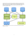
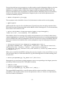
 PROTAX User Manual August 2015 Panu Somervuo Department of Biosciences University of Helsinki Finland Contents Contents ................................................................................................................................................................................ 2 Introduction ........................................................................................................................................................................ 2 How to get the software ................................................................................................................................................ 4 System requirements ...................................................................................................................................................... 4 What else is needed ......................................................................................................................................................... 4 Quick start for the impatient ....................................................................................................................................... 5 How PROTAX classification results should be interpreted ............................................................................ 5 Example 1 ....................................................................................................................................................................... 6 Example 2 ....................................................................................................................................................................... 6 Detailed examples of all functions ............................................................................................................................ 6 Preliminaries ................................................................................................................................................................. 6 Case A) PROTAX with pre-­‐computed sequence similarities ..................................................................... 7 Step 1. Generating training data ...................................................................................................................... 7 Step 2. Estimating model parameters ......................................................................................................... 11 Step 3. Classifying new sequence data ....................................................................................................... 14 Step 4. Getting node probabilities for each taxonomy level ............................................................. 15 Case B) Computing sequence similarities with online BLAST .............................................................. 16 Case C) using PROTAX with TIPP ...................................................................................................................... 17 Case D) combining BLAST and TIPP covariates .......................................................................................... 20 Integrating new covariate sources in PROTAX ................................................................................................ 21 Large taxonomy and sparse sequence data ....................................................................................................... 21 Speeding up MCMC ....................................................................................................................................................... 21 List of PROTAX functions ........................................................................................................................................... 22 Perl scripts ................................................................................................................................................................... 22 R functions ................................................................................................................................................................... 22 Introduction This documentation serves as a manual for using PROTAX (Probabilistic taxonomic classification). PROTAX is flexible for using any number of covariates in its multinomial regression model, and therefore user may use various methods for computing sequence similarities and linking sequences into taxonomical units. Obviously, the same sources of information must be available both when estimating the model parameters with training data and when using PROTAX in classification of new sequence data. Instead of integrating everything into a single monolithic system, we have implemented small Perl and R scripts to perform all necessarily steps required for model training and classification of new data. The benefit of this is that user can easily include their own sequence similaritity methods when building new models. We will explain how to use PROTAX with multiple covariate sources for DNA data and give specific code to extract the similarity information from BLAST and TIPP outputs. Since each new covariate source may give its output in a different format, we haven't prepared to all possible variations in the existing scripts, however, it is straightforward and easy to make the required changes if necessary. Also, PROTAX can be used with pre-­‐computed sequence 2 similarity files. This is useful in preliminary studies and small scale experiments if the user wants to experiment new types of sequence similarities. Detailed instructions how to use PROTAX is illustrated with four examples. The first case describes all steps in detail and the other cases focus in how to define different covariate sources BLAST, TIPP, and the combination of BLAST and TIPP. Figure 1.1, Flowchart of PROTAX. Covariate sources denote different sequence similarity computation methods. 3 How to get the software PROTAX can be downloaded from http://www.helsinki.fi/science/metapop/Software.htm All Perl scripts and R functions have been packed in a single file protax.zip. System requirements PROTAX can be run in Linux, Mac, and Windows. System requirements depend on the covariate sources of the model. For example, BLAST can be run in all three platforms. What else is needed PROTAX is written in Perl and R. In Linux and Mac, Perl is usually already installed. Windows users can obtain Perl e.g. from http://strawberryperl.com/. R can be obtained for all three platforms from http://www.r-­‐project.org/. External software is used when computing pairwise sequence similarities. The need of external software depends on the covariate sources user decides to include in the model. One of the main functions of Perl scripts is to transfer the information computed by external software to PROTAX multinomial regression model. Also the generation of the training samples, which is a crucial part of the process before training the model, is implemented in Perl. Model parameter estimation is based on Markov chain Monte Carlo (MCMC) and it is implemented in R because R provides good means for interactive visualization. Visualization is useful for making decisions concerning the quality of MCMC training, e.g. whether additional adaptation step or more MCMC iterations are needed. R functions do not require any changes when adding new covariate sources to the model. Required input data for training consists of sequences with known taxonomical classification and the tree structure of taxonomy. Sequence data is in FASTA format, taxonomy tree in a text file, and the taxonomy information of each FASTA entry is in another text file. The latter file provides the information for the location of training sequence data in the taxonomy tree. Required input data for classification consists of a file of sequences to be classified in FASTA format, a text file of PROTAX model parameters, and the same sources of information to calculate sequence similarities which were used in the model training stage. 4 Quick start for the impatient After uncompressing file ‘protax.zip’, Perl scripts and R functions will be in directory 'scripts'. Another directory 'data' contains a small example data set which can be used for checking that the software works. In this example it is assumed that the user is in the data directory. 1. get_reference_sequences_all.pl example_taxonomy.txt
example_trainseqid2taxname.txt my_rseqs.txt 2. generate_training_data.pl example_taxonomy.txt
example_trainseqid2taxname.txt my_rseqs.txt 100 1 no
my_trainsamples.txt 3. create_xdata_seqsimfile.pl my_trainsamples.txt
example_taxonomy.txt example_trainseqid2taxname.txt
my_rseqs.txt example_trainseqsim.txt my_trainxdata.txt
4. R commands for estimating model parameters > source("../scripts/amcmc.rcode.txt")
> dat=read.xdata("my_trainxdata.txt")
> pp=adaptiveMCMC(dat,9,1e4,1000,500,rseed=1,info=1)
> write.postparams(pp,"my_mcmc.txt",501:1000) 5. classify_seqsimfile.pl example_testseqids.txt
example_taxonomy.txt example_trainseqid2taxname.txt
my_rseqs.txt my_mcmc.txt map example_testseqsim.txt 1 0.01
my_testclas.txt 6. add_taxonomy_info.pl example_taxonomy.txt my_testclas.txt How PROTAX classification results should be interpreted Before going into details how to build the model and do the classification, here are two examples of PROTAX classification results with explanation how they should be interpreted. These examples are from fungal classification (not from the example data set in directory ‘data’). For each test sequence, three best classification outcomes have been listed. The taxonomy consisted of two levels under root: genus (level 1) and species (level 2). Output of classification consists of sequence id, numeric taxon id, probability, taxonomy level, and textual taxon name. It is important to know that by default, PROTAX classification outputs only the probabilities of the leaf nodes of the taxonomy. That is, the internal nodes are not present in the default output. E.g. if we are interested in the probability of a genus (which is the sum of the probabilities of all species nodes under it), it is not present in the classification output. There is a separate program for listing the top-­‐N nodes (with threshold defined by user) within each taxonomy level including both internal and leaf nodes. The programs for classification start by the name ‘classify’ and the programs for listing top-­‐N nodes within each taxonomy level start by name ‘nodeprob’. 5 Example 1 query_seqID
testseq1
testseq1
testseq1
taxID
177
175,unk
0,unk
probability
0.893021
0.068136
0.0252711
level
2
2
1
taxon_name
Perenniporia_subacida
Perenniporia,unk
root,unk
This is an example where the classification outcome with the largest probability (0.89) is species Perenniporia subacida (taxon id 177) with large margin compared to the second-­‐best classification outcome. The second-­‐best outcome with taxonomy id '175,unk' means that the sequence could belong a) to the unknown species of genus Perenniporia (taxon id 175) or b) to the known species of Perenniporia for which there are no reference sequences available in our database. In PROTAX, the probabilities of these child nodes are summed into a single value. In the same way, the third-­‐best outcome '0,unk' means that the test sequence could belong to a) unknown genus or b) the known genus in our taxonomy for which no reference sequences are available. Here the probabilities of the 2nd and 3rd best outcomes are small compared to the 1st outcome. Example 2 query_seqID
testseq2
testseq2
testseq2
taxID
19
16
13
probability
0.506796
0.179652
0.123044
level
2
2
2
taxon_name
Antrodia_serialis
Antrodia_primaeva
Antrodia_infirma
This example shows the case where the best outcome has smaller margin to the 2nd and 3rd best outcomes compared to the first example. Although the largest probability is assigned to Antrodia serialis, there is also some probability that the test sequence could belong to the other species . However, all three best outcomes belong to the same genus Antrodia. Detailed examples of all functions Preliminaries After uncompressing protax.zip, Perl scripts and R functions will be in directory 'scripts'. The content of the scripts directory must be made available to Perl. In Linux, we can define a variable which contains the path to this directory, e.g. in Bash shell using the following command where after '=' character is the path to the directory: PROTAX=~/Work/protax/scripts
After this Perl scripts can be used in the following way independently of the location of our working directory: perl $PROTAX/generate_training_data.pl
Alternatively, in Linux the scripts directory can be included in the PATH variable: PATH=${PATH}:~/Work/protax/scripts
6 and then Perl scripts can be run just typing their name generate_training_data.pl
All PROTAX related Perl scripts print their required input when running them without arguments. The expected order of input is important since there is no checking for the content of the arguments. In case the given output file already exists, it will be over-­‐written unless otherwise informed. In most scripts the last argument is optional and it is mainly used for debugging purposes. When omitted, the value of the debug_mode is zero and all scripts work silently. Value of 1 gives some information, and value of 2 may give lots of information. This extra information is written to standard output (computer screen), and what is written to an output file remains the same independently on the value of the debug_mode. We give examples how to use PROTAX in four cases A,B,C,D. They all share the first step, generation of training data, so we only explain it for case A. Also the model parameter estimation is explained in detail only for case A. All input and output files of PROTAX are ASCII text files. Case A) PROTAX with pre-­‐computed sequence similarities This is most useful for preliminary studies and small scale experiments. For large data sets, storing all pairwise sequence similarities in a file may not be practical. Step 1. Generating training data Our example taxonomy tree is in file ‘example_taxonomy.txt’ and the taxonomic information of our reference sequences is in file ‘example_trainseqid2taxoname.txt’. Taxonomy tree file is a text file consisting of four columns separated by space or tab in each line: • nodeid nodepid level taxname
where nodeid and nodepid are the numeric node identifiers. They can be in principle any integers but the nodeid of the root node must be 0. Nodepid is the parent nodeid (for root node it is the root node itself). Level is the level of the node in taxonomy (root node has level 0) and taxname is the taxonomic name. Any unique character string can be used for the taxonomic name but it should not contain any spaces or tabs (only the first part separated by space will be used as a name). The structure of the taxonomy is constructed based on the (nodeid,nodepid) pairs but the reference sequence data is linked into taxonomy based on the taxname. Taxonomy file does not have any header line so the first row contains already the first values. The file containing the taxonomic information of the reference data (example_trainseqid2taxname.txt) contains two fields separated by space or tab. The file doesn't have a header line. • seqid taxname
7 For each seqid there should be only one taxname which is the most specific taxonomic classification. Like seqid, also taxname should be unambiguous and unique. Lower level taxonomic classes (taxonomy nodes towards the root of the tree) of each sequence can be obtained based on the taxonomy tree. Step 1.1. Defining representative sequences Each node of the taxonomy is associated with the set of representative sequences. These contain a subset or all of the reference sequence data. There are three possibilities to define the representative sequences: 1. using all available reference sequences 2. selecting a random subset of reference sequences 3. using clustering with threshold for pairwise sequence similarity of reference sequences The corresponding Perl scripts are get_reference_sequences_all.pl, get_reference_sequences_random.pl, and get_reference_sequences_clustering.pl. Please note that these are the three ways to define the set of representative sequences automatically at the moment and there is no guarantee that the resulting set would be optimal. Since the classification of a new sequence is based on the representative sequences, the selection process is important. As the name ‘representative sequences’ implies, they should be selected so that they characterize the entire taxon. Here is an example of the case for limiting the number of representative sequences by using a random subset of reference sequences. Our example taxonomy has 2 levels and here we define that each node may have at most 10 representative sequences from its child nodes. This number must be specified for each level. Although in the example below we have the same number two times, it is possible to define different number for each level. The order is from the most specific node to the root. The number before the output file ‘my_rseqs.txt’, here defined to be 1, is the seed value for the random number generator. get_reference_sequences_random.pl example_taxonomy.txt 2 10 10
example_trainseqid2taxname.txt 1 my_rseqs.txt
In case the number of available reference sequences is smaller than the user defined number (like in our example data), as many representative sequences as possible are included. Output file has one line for each node and each line consists of three columns where the first one is node id, the second column lists the representative sequences of the node, and the third column contains the weights of the representative sequences • nodeid seqid1,seqid2,...,seqidN, weight1,weight2,...,weightN
The third column is optional for PROTAX, in case it is missing, each representative sequence has a default weight 1. For the first two selection processes (all and random), the weight is the inverse number of the representative sequences coming from each child of a node. This results that each child node has the same importance when computing the average of pairwise sequence similarities regardless of the differences in the number of representative sequences coming from different child nodes. So in effect, the mean similarity is the mean of means in the 8 corresponding PROTAX covariate. When the selection of representative sequences is based on clustering, the weight is the size (number of sequences) of each cluster. Step 1.2 Sampling the taxonomy to get training data In this example, we generate 100 samples representing the nodes of the taxonomy. Each node is associated with a training sequence. The details how the sampling is done can be found in the manuscript. In the present implementation, only leaf nodes of the taxonomy are sampled. The number of samples should represent the taxonomy, here we use only 100 samples because the example taxonomy and the reference data set are tiny and the purpose of the example is mainly to demonstrate the syntax of all commands. generate_training_data.pl example_taxonomy.txt
example_trainseqid2taxname.txt my_rseqs.txt 100 1 no
my_trainsamples.txt
The number 1 after the number of training samples (100) is the seed for random number generator. The next parameter is yes/no indicating whether sequences to be ignored when calculating sequence similarities from the randomly selected training sequence are included in the output file. This information can be reconstructed based on the taxonomy and the other fields of the file, so it should not be selected unless there is a reason for doing so. With large data sets, the amount of this extra information can be excessive resulting in large output files. The last argument of the command is the name of the output file. Each line of the output file consists of 6 columns • weight nodeid priprob nodeclass rnodeid trainseqid
The value for the first column weight is 1, nodeid is the randomly sampled node and priprob is the associated prior probability of this node. Nodeclass gives information of the type of the node, there are 4 classes: • nseq2 : node is a known taxon and has at least 2 reference sequences • nseq1 : node is a known taxon but has only 1 reference sequence • nseq0 : node is a known taxon but doesn't have any reference sequences • unk : node represents an unknown taxon If nodeclass is nseq2, it has been possible to pick training sequence directly from the sequences belonging to nodeid. In other cases, another node (rnodeid in 5th column) has been randomly selected among the closest neighbors of the original node (nodeid) which is at the same level and has sufficient amount of reference sequences (1 or 2 depending on the case). The details of the process can be found in our manuscript. The new node will mimick the originally sampled node. For nodeclass nseq1, additional information is needed regarding the reference sequence and this information is included in the 4th column field separated by a comma from the nodeclass, as an example nseq1,seqid. The last column is the id of the training sequence. If the 6th argument is 'yes' instead of 'no' for generate_training_data.pl, there will be 7th column in the output file which lists all sequences to be deleted when computing sequence similarities for the training sample in the present line. 9 Step 1.3. Creating X matrices In order to create input data for model estimation, we have to construct design matrices related to logistic regression for each training sample. Here the design matrix will be denoted by X. For each training sample, there will be X matrix for each level of the taxonomy starting from the parent node of training sample node and then proceeding to the root. In this example, X matrices are calculated based on sequence similarity file. By default, two values, mean similarity and max similarity are calculated based on pairwise sequence similarities. In addition, there are two other covariates, one for the case when the node does not contain any reference sequences, and another for the intercept of mean and max similarities, so altogether, there are four covariates per taxonomy level. create_xdata_seqsimfile.pl my_trainsamples.txt example_taxonomy.txt
example_trainseqid2taxname.txt my_rseqs.txt example_trainseqsim.txt
my_trainxdata.txt
The file ‘example_trainseqsim.txt’ contains pairwise sequence similarities in the sparse matrix format, each line consisting of three columns • seqid1 seqid2 sim
where sim is the similarity between seqid1 and seqid2. Not all pairwise similarities need to be listed in the file. If similarities are symmetric, only one of similarity(seqid1,seqid2) and similarity(seqid2,seqid1) needs to be present in the file. However, if for some reasons the user wants to use asymmetric similarities, then both similarities need to be present in the file in separate lines. If the similarity between two seqids is missing, there are two options, either it is ignored (considered as missing information) or it is treated as being zero. This affects to the calculation of mean similarity. At the moment, missing similarities are treated as missing and mean similarity is calculated only based on present similarities. The output file ‘my_xdata.txt’ contains one line for each training sample. The format is • priprob item1;item2;...;itemL
where priprob is the node prior probability (for details, see the manuscript) and the semicolon separated list of items in the second column contain one or more matrices. These are the design matrices of the regression model (denoted as X matrices below). The number of the items depends on the level of the training sample node, there are matrices for each level from the parent of the training sample node to the root of the taxonomy. Each item has the format • level,index,nrows,ncols,x11,x12,...,xNM
where level indicates which level of taxonomy the N-­‐by-­‐M matrix X belongs, index is the child node index where the current training sample belongs in this taxonomy level, nrows and ncols are the number of rows and columns of matrix X, respectively, and the rest nrows*ncols values are the elements of X listed row by row. The first row of each matrix which corresponds to the unknown taxon contains only zeros. Since the xdata file will be used in R software where array element indexing starts from 1 instead of 0, also here the index corresponding to the first row of matrix X is 1 instead of 0. 10 Step 2. Estimating model parameters Input to the model parameter estimation is given by xdat-­‐file. The parameter estimation is done using R. For MCMC estimation, all required functions are in the file amcmc.rcode.txt. Once R is started, we can take PROTAX related functions into use by typing source command where we define the location of the amcmc.rcode.txt file. In case the scripts directory is under the parent directory (‘../’) of our R working directory, we can type > source("../scripts/amcmc.rcode.txt")
First we read the training data. In case the xdata-­‐file is not in our R working directory, we have to include path to the file name, but the following assumes that the data is in the working directory. > dat=read.xdata("my_trainxdata.txt")
Now everything is ready for MCMC training. In our example xdata, there are 4 parameters for each level of the taxonomy and an additional parameter for mislabeling probability, so the total number of parameters is 2*4+1=9. Besides training data, we have to define variance s2 of prior distribution (zero-­‐mean Normal distribution), number of iterations, and how many of them are used for adaptation (num.burnin). Additional parameters are random seed (rseed) and info. By default, info is 0 which results in silent processing, but when it is 1, we can see the progress of the iterations. Here we apply only 1000 iterations but in practice there should be more. > num.params=9
> pp=adaptiveMCMC(dat,num.params,s2=10000, num.iterations=1000,
num.burnin=500, rseed=1, info=1)
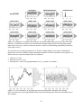
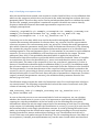
Variance of prior distribution has been set large (10000) in order not to restrict the values of parameters. However, the smaller the range of similarity values is, the larger the prior variance should be in order to allow large value for the coefficients related to sequence similarity, i.e. allowing steeper slope in the regression model. In general, all covariates should be scaled properly before using them in PROTAX. MCMC diagnostics After training, it is good practice to check trace plots. In R it is simple to plot the values of parameters during the entire MCMC history. Here we are interested in the values after burn-­‐in, so we can plot the parameter samples between iterations 501 and 1000. traceplot.all(pp,ind=501:1000,num.levels=2,title="my MCMC")
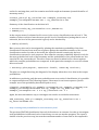
Parameter num.levels is the number of levels in our taxonomy, it helps to layout the plot so that parameters from each level are located in the same row. Values corresponding to the largest posterior probability (MAP estimate) within the given iterations are denoted by red circle. Panels next to each individual trace plot show the histograms of the parameter values. This way it is easy to see e.g. whether the MAP estimate is close to the mode of the distribution. 11 Figure 2.1. Example of traceplot.all for MCMC iterations 2000-­‐3000 (first 2000 were used for burn-­‐in). In this data set there were inconsistent sample labels (20% of the training sample labels were incorrect) which resulted in nonzero value for mislabeling probability parameter (top right corner). In case there are too many parameters to fit into a single display, trace plots of individual parameters can be visualized using command traceplot.one. Since it produces two figures, we define mfrow to split the display into two subplots. > ind=501:1000
> par(mfrow=c(1,2))
> traceplot.one(ind,pp$params[ind,3],name="Param3") Figure 2.2. Two traceplots, a) not properly mixed chain (MCMC samples show strong autocorrelation), b) converged MCMC chain. Horizontal histograms show the distributions of the samples. 12 If trace plots indicate non-­‐convergence, usually another round of adaptation helps to solve the problem. The result of MCMC adaptation can be investigated by amcmc.diagnostic.plot. In addition to acceptance ratios, it shows the adaptive step size and proposal directions. The latter are the eigenvectors of parameter covariance matrix. Parameters may be correlated by incidence due to the random initialization. Diagnostic plot reveals which parameters are correlated in MCMC proposal. > amcmc.diagnostic.plot(pp) The acceptance ratios should be close to 0.44, the numeric values can be seen by typing > pp$ac/pp$cc
pp$k contains the step size for each dimension. Typically step sizes are fairly constant when the model is properly parameterized and the Markov chain is mixing well. For documentation, these values can be saved in a file > write.table(data.frame(acr=pp$ac/pp$cc,stepsize=pp$k),
"mcmc.acr.txt", row.names=F, col.names=T)
If the Markov chain is not mixing well, usually some parameters are correlated, either due to random initialization or otherwise. The following demonstrates how to continue training from previous MCMC state with new adaptation. Here we use last value of previous MCMC chain for parameter estimates but initialize other values (adaptation step size and proposal direction vectors). > initstate=initialize.adaptation(pp$params[1000,])
> pp=adaptiveMCMC(dat, num.params, s2=10000, num.iterations=1000,
num.burnin=500, rseed=1, info=1, prev.state=initstate)
> traceplot.all(pp,ind=501:1000,num.levels=2,title="my MCMC\nafter
re-adaptation")
When we are satisfied with MCMC training, the posterior samples can be saved. Either we can save the entire chain, or values after burn-­‐in, e.g. the following writes all values starting from iteration 501: > write.postparams(pp,"my_mcmc.txt",501:1000)
Alternatively, we can choose a single parameter vector corresponding to the largest posterior probability within iterations 501-­‐1000 (MAP estimate) > ind=501:1000
> i=which.max(pp$postli[ind])
> write.postparams(pp,"my_mcmc.txt",ind[i])
The output MCMC sample file is a text file where the first value in each line is the posterior probability of the sample and the rest are the parameter values, i.e. if there are 9 parameters, each line contains 10 numbers. 13 Step 3. Classifying new sequence data After the model has been trained, new sequences can be classified. Here we use validation data which are the sequences which were not present in the model training but we know their true taxonomic labels. Therefore they can be used as an independent data set to validate the model. The first file ‘example_testseqids.txt’ contains all sequence ids which we want to classify. Sequence similarities between them and representative sequences are in ‘example_testseqsim.txt’. classify_seqsimfile.pl example_testseqids.txt example_taxonomy.txt
example_trainseqid2taxname.txt my_rseqs.txt my_mcmc.txt map
example_testseqsim.txt 1 0.01 my_testclas.txt 0 1
Taxonomy tree is the same which was used in the model training and seqid2taxname file contains the taxonomy information of reference data, ‘my_rseqs.txt’ lists the representative reference sequences for each taxonomy node, ‘my_mcmc.txt’ contains the model parameters after which comes the parameter mode (here ‘map’ for Maximum A Posteriori). The following file contains the pairwise sequence similarities between the sequences to be classified and training sequences. The next parameter (here 1) is the number of outcomes for each validation sequence, if it is set to 0 probabilities of all outcomes are included in the output. The next parameter (here 0.01) is the probability threshold which is applied in hierarchical classification. Only those nodes are proceeded which exceed the threshold. Value of 0 implies no restrictions, the closer the threshold is to 1, more strict and therefore more narrow the search becomes. The name of the output file is here ‘my_testclas.txt’, parameter 1/0 after it denotes if classification should be done in validation mode (1) or not (0). In validation mode, the reference sequence is not used if it has the same seqid as the the sequence to be classified. The last parameter 1 results that the name of the sequence being processed is printed on the screen. In case of 0, processing is silent. Last two parameters are optional, in case they are not defined, default value 0 is used for both. Since the order of parameters is important, if verbose output is wanted (last parameter nonzero), the validation mode parameter must be also defined (e.g. to be zero). Classification output contains the node id of taxonomic units. For visual inspection it helps to use textual names. The following script adds the level and the name of taxonomic node (4th column of taxonomy tree file) to the output. add_taxonomy_info.pl example_taxonomy.txt my_testclas.txt >
my_testclasname.txt
In case we have the access to true taxonomic label of each test sequence, we can calculate whether the classification is correct or not. It is important to note that by default PROTAX output gives only the probabilities of the leaf nodes so in the following the correctness information is based on only the single output leaf of the taxonomy in each line. The following script outputs 1/0 indicating whether the classification is correct (1) or not (0) in each level of the taxonomy based on the single classification outcome. It works by listing the nodes in two paths, one starting from the classification output node and proceeding to root, and another starting from the true answer node and proceeding to root. Classification in each level is correct if the two node paths intersect in that level. The file containing the true class labels of test sequences (‘example_testseqid2taxname.txt’) has the same format which was described 14 earlier for training data, each line contains two fields seqid and taxname (textual identifier of taxonomy node). correct_path.pl my_testclas.txt example_taxonomy.txt
example_testseqid2taxname.txt > my_testresults.txt
Summary of the classification can be done in R. > a=read.table(“my_testresults.txt”,header=T)
> summary(a)
In the output, mean of columns levelL.correct is the correct classification rate at level L. The number of times each level was the most specific level of classification (noting that in case of unk-­‐node, the level of the parent node is given) can be obtained by > table(a$level)
Bias-­‐accuracy plot can be investigated by plotting the cumulative probability of the best classification outcome from each test sequence against the cumulative number of the correct classification results. In order to be useful, the input file should contain only the best classification outcome for each sequence. Note that the outcome probability a$prob is only for the most probable leaf node of the taxonomy and the probabilities of its parent nodes are not saved in file ‘my_testresults.txt’. Therefore some care must be taken how to choose against which the outcome probabilities are compared. In this particular example, we can use column a$correct.level2. > accuracy.plot(a$prob, a$correct.level2, name=”my results”)
The plot is a straight line along the diagonal of the display when there is no bias in the output probabilities. In addition to producing only the most probable taxon as a result of classification, it is possible to output multiple taxa. The following outputs 2 best taxa for each test sequence (in this example we set the probability threshold equal to zero) classify_seqsimfile.pl example_testseqids.txt example_taxonomy.txt
example_trainseqid2taxname.txt my_rseqs.txt my_mcmc.txt map
example_testseqsim.txt 2 0.0 my_testclas2.txt 0 1
Again, the most informative way to investigate the results is to add the taxon name add_taxonomy_info.pl example_taxonomy.txt my_testclas2.txt >
my_testclas2name.txt
Step 4. Getting node probabilities for each taxonomy level The previous PROTAX classification lists only leaf nodes as an outcome. In order to investigate node probabilities in different levels of taxonomy, we can use another program. The input is similar as in the previous step, but now the maximum number of outcomes to be outputted is 15 the maximum number of nodes within each taxonomy level. Here we specify to get only the best node in each taxonomy level whose probability must be above 0.01 nodeprob_seqsimfile.pl example_testseqids.txt example_taxonomy.txt
example_trainseqid2taxname.txt my_rseqs.txt my_mcmc.txt map
example_testseqsim.txt 1 0.01 my_testnodeprobs.txt 0 1
The output file consists of four columns: seqid, probability, nodeid, and level. When we combine this output with the information of correct taxonomic membership, we get the classification results for each taxonomy level. The following program outputs 1/0 depending if the classification is correct/false for each taxonomy level in a separate column. The output includes also the best classification result of the query sequence (probability and taxon name) in each level. In case the previous program outputted more than one node per level, the correct one is selected, otherwise the node with the largest probability. There is only one output line for each query sequence. correct_levels.pl my_testnodeprobs.txt example_taxonomy.txt
example_testseqid2taxname.txt > my_testresults2.txt
Taxonomy level specific classification summaries can now be calculated e.g. in R using the output file ‘my_testresults2.txt’. > a=read.table(“my_testresults2.txt”,header=T)
> summary(a)
Case B) Computing sequence similarities with online BLAST Script create_xdata_BLAST.pl uses BLAST searches which are done online in the user's local computer. Standalone BLAST+ can be obtained from ftp://ftp.ncbi.nlm.nih.gov/blast/executables/blast+/LATEST/. Once it is installed, the directory where BLAST binaries are located is given as an argument to Perl script create_xdata_BLAST.pl. It utilizes two BLAST commands, makeblastdb and blastn, when constructing X matrices. create_xdata_BLAST.pl my_trainsamples.txt example_trainseq.fasta
example_taxonomy.txt example_trainseqid2taxname.txt my_rseqs.txt
~/ncbi-blast-2.2.31+/bin "-dust no –word_size 11" tmp
my_train_blast_xdata.txt 1
The first argument of create_xdata_BLAST.pl is the file containing training samples. After that comes fasta file of training sequences, then the taxonomy tree file, the file containing the taxonomic labels of training data, and the file containing the information which sequences are representative for each taxonomic node. Then comes the path to BLAST binaries. The next argument contains additional information to BLAST, e.g. as in the example, if we don't want to use low-­‐complexity filter which is by default used in BLAST, we can specify -­‐dust no to BLASTN. This information must be in double quotes. If we define many BLAST parameters, they all must be within a single pair of double quotes. One BLAST related argument which might need to be changed is the maximum number of hits which BLAST reports. By default it is 500 so for taxonomy nodes with many child nodes and large number of representative 16 sequences, this number needs to be changed by using BLAST option -max_target_seqs. User is referred to the BLAST manual for all relevant BLAST arguments. A word of warning is that by definition, BLAST finds local hits between two sequences but the pairwise sequence similarity covariate in PROTAX is defined as the number of matching nucleotides divided by the length of the “true” overlap between the two sequences. The “true” overlap length is not necessarily the alignment length of HSP given by BLAST since BLAST hits may be fragmented if long enough mismatching regions occur between the matching regions. How well BLAST finds the “true” overlap depends on the sequence data, amount of indels and mismatches. Although we have implemented also a function which uses BLAST results as anchors for rigorous dynamic programming and this way we can get the sequence similarity from the entire overlap between the two sequences, this comes with the cost of computation and reduced speed and at the moment it is not included in the current version of create_xdata_BLAST.pl. In case we don't want to give additional parameters to BLAST, we have to still specify the empty string in double quotes, i.e. "", in the Perl command. The next argument is the basename of temporary files for BLAST. The last mandatory argument is the name of the output file where all X matrices are written. The final argument is optional, the default value is 0 which results in silent processing, 1 gives some information (showing which training sample is being processed) and value 2 gives detailed information from each BLAST result. These additional information are only printed on screen and they don't affect the content of the output file. Model parameter estimation is done similarly as described in Case A. Suppose we save the MCMC parameter file as ‘my_blast_mcmc.txt’, in classification, online BLAST is again needed and the command is classify_BLAST.pl example_testseq.fasta example_taxonomy.txt
example_trainseq.fasta example_trainseqid2taxname.txt my_rseqs.txt
my_blast_mcmc.txt map ~/ncbi-blast-2.2.31+/bin "-dust no –word_size
11" tmp 1 0.01 my_test_blast_clas.txt 0 1
Case C) using PROTAX with TIPP Instead of using pairwise sequence similarities, it is possible to use the similarity between the sequence and the taxonomic node. An example of this is to use an output of another taxonomic classifier as an input to PROTAX. Here we use TIPP (Taxon Identification and Phylogenetic Profiling, Nguyen et al. 2014). The software can be obtained from http://www.cs.utexas.edu/~phylo/software/sepp/tipp-­‐submission/. The examples below are for the current version of TIPP. It is possible that future versions might have changes and require different kinds of inputs, so user is referred to TIPP manual for further details. TIPP produces probabilistic taxon membership for each input sequence. Its output is typically sparse so only few taxa get nonzero probabilities. These probabilites can be used as similarity measures in PROTAX. They are transformed using logit-­‐function in PROTAX. In order to use TIPP, we need to create a phylogeny for the training data. Since we already have taxonomic information for the training data, we utilize it when constructing the phylogenetic tree. However, in taxonomy there can be several child nodes for a single parent node (e.g. many species belonging to the same family) but phylogeny assumes only nodes with two 17 output branches. Therefore, we need to first change the multifurcation taxonomy into a bifurcating tree. The file containing the multifurcation tree of training sequences is ‘example_trainseq_mftree.txt’ below and it is in Newick format. We also need to convert both the taxonomy file and the sequence-­‐taxon mapping file suitable to TIPP (these files must be in a format suitable for pplacer, which is a piece of software TIPP utilizes internally), these are ‘example_tipptaxonomy.txt’ and ‘example_tipptxm.txt’ in the example data. Please note that taxon ids (column ‘tax_id’ in TIPP taxonomy file and first column of PROTAX taxonomy file) must be identical in order to use TIPP output with PROTAX, however, taxon names are allowed to be different in the two files. We use RAxML for creating the phylogeny for training sequences where the existing taxonomy information is used for constraining the process. Therefore, RAxML software needs to be installed. First we need to align the training sequences and the resulting multi-­‐alignment file is then used as an input to RAxML. Note that the example data here is very simplistic, there are no insertions nor deletions in the sequences so as a consequence the alignment file looks exactly like the original FASTA file, however in general this is not the case. Here we specify general time reversal Gamma model for evolution rates, --no-bfgs is for handling our small data set. raxmlHPC -p 1 -m GTRGAMMA -n train -s example_trainseq_alignment.fa
-f example_trainseq_mftree.txt --no-bfgs
For PROTAX, when computing the taxon probabilities for each training sample, the phylogeny of the reference data needs to be adjusted accordingly. Since creating a phylogeny for a large data set may take long time, it is impractical to do it separately for each training sample. Therefore, we create a single phylogeny for the entire training sequence set and then modify the resulting tree individually for each training sample. Phylogenetic tree is in Newick format. Since Newick file is a text file it is straightforward to modify it. Modification of the tree consists simply deleting those sequences from the tree which should not be present when calculating the taxon probability for a given training sample. There are many ways to do it, here we do the deleting using R-­‐package 'ape', so it needs to be installed. We are going to use the same training samples which were generated in Case A. We have to add the information which sequences should be deleted for each training sample, last argument below is the name of the output file. get_deleteseqs.pl my_trainsamples.txt example_taxonomy.txt
example_trainseqid2taxname.txt my_rseqs.txt
my_trainsamples_with_delseqs.txt
Then in R we generate a file which contains the modified Newick tree for each training sample. Newick tree file 'RAxML_bestTree.train' is the output of RAxML. Notice that here the output file will be appended, so it should be empty before running the script below, i.e., the file ‘my_trainmodtrees.txt’ should be deleted if it exists before the following commands. > library("ape")
> infile.newick = "RAxML_bestTree.train"
> infile.delseq = "my_trainsamples_with_delseqs.txt"
> outfile.newick = "my_trainmodtrees.txt"
18 >
>
>
>
ptree = read.tree(infile.newick)
a=read.table(infile.delseq,header=F)
pois=strsplit(as.character(a[,6]),',')
for (i in 1:nrow(a)) {
ptree2 = drop.tip(ptree,pois[[i]])
write.tree(ptree2,outfile.newick,append=T)
}
In output file 'my_trainmodtrees.txt', each line contains a full Newick-­‐format tree corresponding to the training sample. Now we use TIPP to get taxon probabilities for these trees. TIPP utilizes pplacer, and the output of RAxML must be adjusted to be suitable for it. For the current version of pplacer we need to make small adjustment to the content of info-­‐file produced by RAxML in order to run pplacer successfully (pplacer thinks that there are partitions although in our example data there are not). In Linux terminal, we can delete the extra line in the following way: grep -v 'Partition: 0 with name' RAxML_info.train > modRAxML_info
After this we are ready to run TIPP for each of our training samples. We use Perl script tipptrain.pl for this which is simply a wrapper for executing a loop calling run_tipp.py for each of our training samples. Most arguments for the script tipptrain.pl below are for the run_tipp.py itself. Value 0.5 is related to alignment process, the next number 0 is the threshold for probabilities, and parameters A and P (here the values 26 and 26 were used) needs to be adjusted based on the amount of training data, e.g. P could be the number of all sequences and A could be 0.1*P (for more information please look the TIPP manual). Location of tipp configuration file ‘tipp.config’ should be defined corresponding to the local system. tipptrain.pl example_trainseq.fasta my_trainsamples.txt
my_trainmodtrees.txt tmptrain example_trainseq_aligned.fasta
modRAxML_info example_tipptaxonomy.txt example_tipptxm.txt 0.5 0 26
26 ~/.sepp/tipp.config tmptipp 1 tmp my_train_tippout.txt
The output file 'my_train_tippout.txt' contains now all information what is needed to construct X matrices for PROTAX training, value 0.001 in the command below is a small constant to avoid singularities in logit-­‐transformation when converting TIPP probability into PROTAX covariate. create_xdata_TIPP.pl my_trainsamples.txt example_taxonomy.txt
example_trainseqid2taxname.txt my_rseqs.txt my_train_tippout.txt
0.001 my_train_tipp_xdata.txt
Estimating the parameters in R (small number of iterations are used in order to run the example fast, but in practice more iterations could/should be used) > source("../scripts/amcmc.rcode.txt")
> dat=read.xdata("my_train_tipp_xdata.txt")
> pp=adaptiveMCMC(dat,7,10000,1000,500,rseed=1)
> write.postparams(pp,"my_tipp_mcmc.txt",501:1000)
Now the model parameters are ready but before classifying new sequence data, we need to run TIPP for it. This gives the locations for the new sequences in the existing phylogeny and gives 19 the probabilities for these assignments which are the covariates needed for PROTAX. Again, for the explanation of TIPP parameters, user is referred to the TIPP manual. run_tipp.py -f example_testseq.fasta -t RAxML_bestTree.train -a
example_trainseq_aligned.fasta -r modRAxML_info -tx
example_tipptaxonomy.txt -txm example_tipptxm.txt -at 0.5 -pt 0 -A
27 -P 27 -c ~/.sepp/tipp.config -d my_tipptest --cpu 1 -p tmp
Then we can use PROTAX classification for the test data classify_TIPP.pl example_testseqids.txt example_taxonomy.txt
example_trainseqid2taxname.txt my_rseqs.txt my_tipp_mcmc.txt map
my_tipptest/output_classification.txt 0.001 1 0.01
my_test_tipp_clas.txt
Taxon levels and names are added to the classification results by add_taxonomy_info.pl example_taxonomy.txt my_test_tipp_clas.txt
Case D) combining BLAST and TIPP covariates When several covariate sources are combined, the corresponding X matrices of all sources are simply merged. It is important that the X matrices represent the exactly same training samples in each file in the same order. Therefore, the same trainingsample file must be used for each create_xdata_SOURCENAME.pl command. Combination can be done in R. The following is the example for merging the X matrices from two sources, BLAST and TIPP. > source("../scripts/amcmc.rcode.txt")
> blast.dat=read.xdata("my_train_blast_xdata.txt")
> tipp.dat=read.xdata("my_train_tipp_xdata.txt")
X matrices generated from both sources (BLAST and TIPP) contain the same parameters beta1 and beta2 in columns 1 and 2. We take them from the first blast-­‐related matrix with the columns 3 and 4, and from the tipp-­‐related matrix we only take the 3rd column. Merged X-­‐
matrices will have 5 columns. > dat=merge.xdata(blast.dat,c(1,2,3,4),tipp.dat,3)
Since taxonomy has two levels, there are 2*5+1=11 parameters > num.params=11
> pp=adaptiveMCMC(dat,num.params,10000,1000,500,rseed=1,info=1)
> write.postparams(pp,"my_blast_tipp_mcmc.txt",501:1000)
Although generation of xdata files could be done separately for each information source, the classification of new sequence data requires that all information sources must be available at the same time. This is because in the training phase, the single path from the most specific node to the root is known, but in the classification, the traversal in the taxonomy tree goes in 20 opposite direction and the more specific node where to proceed is known only after applying the classification for its parent node. In case there are no probability thresholds, then all nodes needs to be processed, but otherwise, only subset of them is considered. The decision which paths to continue in classification requires all covariates to be present at the same time. Although we could compute separate X matrices for each covariate sources corresponding to each node of the taxonomy, this would be waste of computing since in case of probability threshold is defined for the search process, majority of the candidate paths would be discarded at every level when proceeding to the next level. Combining TIPP output with online BLAST is done using Perl script classify_BLAST_TIPP.pl. classify_BLAST_TIPP.pl example_testseq.fasta example_taxonomy.txt
example_trainseq.fasta example_trainseqid2taxname.txt my_rseqs.txt
my_blast_tipp_mcmc.txt map ~/ncbi-blast-2.2.31+/bin "-dust no word_size 11" tmp my_tipptest/output_classification.txt 0.001 1
0.01 my_test_blasttipp_clas.txt 0 1
The syntax is the same for the program nodeprob_BLAST_TIPP.pl. Integrating new covariate sources in PROTAX If user wants to integrate their own covariate sources in PROTAX, the required changes need to be made to subroutine 'createX' in three programs: create_xdata_SOURCENAME.pl, classify_SOURCENAME.pl, and nodeprob_SOURCENAME.pl. This subroutine extracts the sequence similarity information from the output of the external software. Making the changes requires only basic knowledge of Perl language. The three existing Perl scripts create_xdata_BLAST.pl, classify_BLAST.pl, and nodeprob_BLAST.pl can be used as a template. They utilize locally installed BLAST through Perl system calls. Large taxonomy and sparse sequence data Perl script ‘compact_training_data.pl’ finds duplicated samples in the output file of ‘generate_training_data.pl’ and reduces the size of MCMC training data. The number of replicates is used as a weight of each sample which is taken into account in the MCMC parameter estimation. Speeding up MCMC In R, we have observed that the MCMC computation time reduces 40% when using the byte code compiler for the following three functions before calling adaptiveMCMC function > library(compiler)
> logprior=cmpfun(logprior)
> loglikelihood=cmpfun(loglikelihood)
> adaptiveMCMC=cmpfun(adaptiveMCMC)
21 List of PROTAX functions Perl scripts get_reference_sequences_all.pl get_reference_sequences_random.pl get_reference_sequences_clustering.pl generate_training_data.pl compact_training_data.pl get_deleteseqs.pl create_xdata_seqsimfile.pl create_xdata_BLAST.pl create_xdata_TIPP.pl tipptrain.pl classify_seqsimfile.pl classify_BLAST.pl classify_TIPP.pl classify_BLAST_TIPP.pl nodeprob_seqsimfile.pl nodeprob_BLAST.pl nodeprob_TIPP.pl nodeprob_BLAST_TIPP.pl add_taxonomy_info.pl correct_path.pl correct_levels.pl R functions read.xdata merge.xdata initialize.adaptation adaptiveMCMC write.postparams traceplot.one traceplot.all amcmc.diagnostic.plot accuracy.plot 22