Download Stat544Homeworks2012..

Stat 544 Spring 2012
Homeworks
In what follows, unless otherwise indicated, we will use the GCS&R notations/parameterizations for distributions (see their Appendix A that begins
on page 571).
If there is a con‡ict between GCS&R and OpenBUGS/WinBUGS
notations and we wish to refer to the latter, we’ll preface the distribution’s
name with the modi…er "WinBUGS-" (so, for example, N( ; 2 ) is, according to the
GCS&R convention, the normal distribution with mean and variance 2 , while
WinBUGS-N( ; 2 ) is the normal distribution with mean and variance 1= 2 (i.e.
"precision" 2 )).
Homework #1 (Due Friday January 27, 2012 5PM at the TA’s O¢ ce in Snedecor
if not turned in during class.)
1. Do problems 2.1, 2.2, 2.5, 2.8, 2.12, 2.21, 2.22 from GCS&R
2. Consider a Poisson model like the Binomial one discussed in class. That is, suppose
that conditioned on , Y1 and Y2 are independent Poisson( ) random variables.
(a) First consider the possibility of using a Gamma( ; ) prior for . Work out
analytically the posterior distribution of jY1 = y1 and (possibly only up to a
constant multiplier) the posterior predictive distribution of Y2 jY1 = y1 . For the
choices ( ; ) = (1; 1) and ( ; ) = (10; 10) plot both the prior density for
and the posterior density for jY1 = 0. For the choices ( ; ) = (1; 1) and
( ; ) = (10; 10) plot in histogram form (possibly only up to a multiplicative
constant) prior probabilities for Y2 = 0; 1; 2; 3; 4; 5; 6; 7; 8; 9; 10 and corresponding
posterior probabilities for Y2 jY1 = 0.
(b) Now consider the possibility of using a Uniform(0; 10) prior for . Work out
analytically the posterior distribution of jY1 = 0 and plot both the prior density
for and the posterior density for jY1 = 0.
(c) Use OpenBUGS/WinBUGS and get approximations for the posterior distribution
of jY1 = 3 and the posterior predictive distribution of Y2 jY1 = 3 based on
Gamma( ; ) priors for for the choices ( ; ) = (1; 1) and ( ; ) = (10; 10)
and based on the Uniform(0; 10) prior. (Use the density and stats functions
on the Sample Monitor tool to summarize these approximations. You can easily/quickly generate 100,000 or so iterations in this simple problem.)
(d) Redo part (c) using OpenBUGS/WinBUGS for the case where Y1 = 7 is observed
(instead of Y1 = 3).
In parts (c) and (d) above you will probably want to use some OpenBUGS/WinBUGS code like:
1
model {
Y1~dpois(lambda)
Y2~dpois(lambda)
lambda~dgamma(a,b)
}
list(a=1,b=1,Y1=3)
model {
Y1~dpois(lambda)
Y2~dpois(lambda)
lambda~dunif(a,b)
}
list(a=0,b=10,Y1=3)
Homework #2 (Due Monday February 13, 2012 5PM at the TA’s O¢ ce in
Snedecor.)
1. Consider the following model. Given parameters 1 ; :::; N variables X1 ; :::; :XN are
independent Poisson variables, Xi Poisson( i ): M is a parameter taking values in
f1; 2; :::; N g and if i
M; i = 1 , while if i > M; i = 2 : (M is the number of
Poisson means that are the same as that of the …rst observation.) With parameter
vector = (M; 1 ; 2 ) belonging to
= f1; 2; :::; N g (0; 1) (0; 1) we wish to
make inference about M based on X
1 ; :::; :XN in a Bayesian framework. As matters
P
of notational convenience, let Sm = m
i=1 Xi and T = SN .
(a) If, for example, a prior distribution G on is constructed by taking M uniform
on f1; 2; :::; N g independent of 1 exponential with mean 1, independent of 2
exponential with mean 1, it is possible to explicitly …nd the (marginal) posterior
of M given that X1 = x1 ; :::; XN = xN . Don’t actually bother to …nish the
somewhat messy calculations needed to do this, but show that this is possible
(indicate clearly why appropriate integrals can be evaluated explicitly).
(b) Suppose now that G is constructed by taking M uniform on f1; 2; :::; N g independent of ( 1 ; 2 ) with joint pdf g( ; ) on (0; 1) (0; 1). Describe in as much
detail as possible a SSS based method for approximating the posterior of M , given
X1 = x1 ; :::; XN = xN . (Give the necessary conditionals up to multiplicative constants, say how you’re going to use them and what you’ll do with any vectors you
produce by simulation.)
2. A curious statistician is interested in the properties of a 5-dimensional distribution on
[0; 1]5 that has pdf proportional to
h (x) = exp
(x1
x2 )2 + (x2
x3 )2 + (x3
2
x4 )2 + (x4
x5 )2 + (x5
x1 )2
This person decides to simulate from this distribution. Carefully describe a (5-variate)
rejection algorithm that could be used to produce realizations x from this distribution,
a “Gibbs Sampler”/“Successive Substitution Sampling” algorithm, a M-H-in-Gibbs
hybrid algorithm, AND a (5-variate) Metropolis-Hastings algorithm that could be used
to draw samples from this distribution. For the Gibbs sampler, give a formula for the
univariate pdf that must be sampled when replacing the ith entry of a current x
vector. This formula will involve a 1-dimensional integral that might be evaluated
numerically. For the Gibbs/M-H hybrid sampler, use univariate Metropolis-Hastings
steps in your Gibbs updates. (Note, by the way, that U = (U1 ; U2 ; : : : ; U5 ) with iid
U (0; 1) coordinates Ui has pdf p (u) = 1 on [0; 1]5 .)
3. Here is a problem related to “scale counting.” As a means of “automated” counting
of a lot of discrete objects, I might weigh the lot and try to infer the number in the
lot from the observed weight. Suppose that items have weights that are normally
distributed with mean and standard deviation 1. In a calibration phase, I weigh a
group of 50 of these items (the number being known from a “hand count”) and observe
the weight X. I subsequently weigh a large number, M , of these items and observe the
weight Y . I might model X N(50 ; 50) independent of Y N(M ; M ). Suppose
further that I use a prior distribution for ( ; M ) of independence,
N(0; (1000)2 ) and
M 1 Poisson(100). Completely describe a simulation-based way of approximating
the posterior mean of M .
4. Consider a bivariate distribution on (0; 1) (0; 1) with pdf on that space proportional
to
h (x; y) = sin2 (x) exp ( x y xy)
(Note that 0 sin2 (x) exp ( xy) 1. Note too that given a U (0; 1) random observation U , you can make an Exp( ) observation as 1 ln U .) Describe in detail several
algorithms that could be used to simulate from this bivariate distribution using only a
stream of U (0; 1) random variables. In particular, describe
(a) A rejection algorithm.
(b) A Gibbs algorithm, where for updating x you use a univariate rejection algorithm
and for updating y you use direct simulation from the conditional distribution of
Y jX = x.
(c) M-H within Gibbs algorithm, where for updating x you use a univariate MetropolisHastings step and for updating y you use direct simulation from the conditional
of Y jX = x.
(d) A M-H algorithm where the bivariate proposal distribution at any step is one of
independent Exp(1) variables.
5. (Some more practice with OpenBUGS in a fairly simple context.) A critical dimension
is measured on n = 5 consecutive metal parts produced by an automated machining
process. The resulting values (in units of :0001 in above an ideal value) are
4; 3; 3; 2; 3
3
We are going to assume that an iid N( ;
dimensions.
2
(a) Use the standard "Stat 101" t and
2
) model can be used to describe these part
interval formulas and
q give 95% two-sided
con…dence limits for and . Use the formula x ts 1 + n1 and make 95%
two-sided prediction limits for an additional value from this normal distribution.
(b) Now consider some Bayes analyses of this very small data set. There is a set of
OpenBUGS code below that can be used to analyze these data using an improper
"uniform ( 1; 1)" prior for and a U (0; 10000) prior for = 1= 2 . Run 3
chains simultaneously using this code ( and the last lists in the code as initializations of those chains), and monitor "history" plots and the "bgr diag" for all of
mu, sigma, and y from the very start of the simulation through, say 1000 iterations. Do 1000 iterations appear adequate as a burn-in for this simulation? Do
10,000 iterations appear adequate as a burn-in?. After enough updates that you
are satis…ed that burn-in has occurred, run 100,000 more iterations and based on
those 100,000 iterations look at "density" and "stats" for all of all of mu, sigma,
and y. Based on the 2:5% and 97:5% points of the posterior distributions, what
are approximately 95% posterior "credible intervals" for the mean, standard deviation, and an additional part dimension? Are these comparable to your answers
from (a)?
(c) GCS&R on page 74 suggest what they call a "non-informative prior" for ( ; 2 ).
There is a second set of code below that can be used to implement this suggestion
in OpenBUGS. Repeat part (b) using this code. Are your answers here comparable
to those in part (b)?
(d) A "di¤use" proper prior for ( ; 2 ) could (for example) be made by using a normal
prior with mean 0 and precision :0001 for and a gamma prior with mean 1 and
variance 100 for . How do inferences under such a prior compare to those for
parts (a), (b), and (c)?
model {
for (i in 1:5) {
x[i]~dnorm(mu, tau)
}
y~dnorm(mu,tau)
mu~dflat()
tau~dunif(0,10000)
sigma<-sqrt(1/tau)
}
list(x=c(4,3,3,2,3),y=NA)
list(mu=0,tau=1,y=0)
list(mu=500,tau=.0001,y=500)
list(mu=500,tau=10000,y=500)
model {
4
U~dflat()
tau<-exp(-2.0*U)
for (i in 1:5) {
x[i]~dnorm(mu, tau)
}
y~dnorm(mu,tau)
mu~dflat()
sigma<-sqrt(1/tau)
}
list(x=c(4,3,3,2,3),y=NA)
list(mu=0,U=0,y=0)
list(mu=500,U=-100,y=500)
list(mu=500,U=100,y=500)
6. What is potentially a fairly serious shortcoming of the analysis in problem 5 above
is that the data are really very "coarse"/"granular" relative to the range of the data.
That is, although strictly speaking our model says that we have realizations from a
(continuous!) normal distribution, we have only 3 distinct values in the (integer) data
set, and these have with range of only 2. A possible improvement in the analyses
of problem 5 is to think that while there are perhaps unobservable actual part measurements that are "real numbers" (with in…nite numbers of digits in their decimal
expression) what we actually observe are only "integer-rounded"/"interval-censored"
versions of these. (This kind of thinking is perhaps especially sensible in the day of
digital instruments that explicitly read to some number of decimal places.) There probably are a couple of ways of building this kind of modeling into a OpenBUGS/WinBUGS
analysis.
In "pencil and paper" terms, we would want our likelihood (for the integer xi ) to be
f (x1 ; x2 ; x3; x4 ; x5 j ; ) =
5
Y
xi + :5
xi
:5
i=1
(for the standard normal cdf) and I’m pretty sure that it’s possible to implement this
directly using the "zeros trick" (see "Tricks: Advanced Use of the BUGS Language"
in the OpenBUGS/WinBUGS user manual).
Another method is to use the OpenBUGS/WinBUGS approach to representing "censoring"
(see the "Model Speci…cation" section of the OpenBUGS/WinBUGS user manual). Some
code for this parallel to that in 5b) is below. This code treats the real measurements
as normal, but unobserved, except to the degree that we know their integer-rounded
values. Use this code and compare your inferences about the normal parameters and
an additional predicted/unobserved observation to those in 5b). (Note, by the way,
that your conclusions here should be consistent with the bit of "statistical folklore"
that says that ignoring this rounding issue will, at least for normal observations, tend
to arti…cially in‡ate one’s perception of . Note too that handling this analysis in
a non-Bayesian/frequentist fashion, i.e. coming up with con…dence and prediction
intervals, is a non-trivial matter.)
5
model {
x1~dnorm(mu,tau)I(3.5,4.5)
x2~dnorm(mu,tau)I(2.5,3.5)
x3~dnorm(mu,tau)I(2.5,3.5)
x4~dnorm(mu,tau)I(1.5,2.5)
x5~dnorm(mu,tau)I(2.5,3.5)
y~dnorm(mu,tau)
w<-round(y)
mu~dflat()
tau~dunif(0,10000)
sigma<-sqrt(1/tau)
}
list(x1=NA,x2=NA,x3=NA,x4=NA,x5=NA,y=NA)
list(mu=0,tau=1,x1=4,x2=3,x3=3,x4=2,x5=3,y=0)
list(mu=500,tau=.0001,x1=4,x2=3,x3=3,x4=2,x5=3,y=500)
list(mu=500,tau=10000,x1=4,x2=3,x3=3,x4=2,x5=3,y=500)
7. Consider again the context of Problem #1. Below are a series of 10 Poisson observations, the …rst 3 of which were generated using a mean of = 2, the last 7 of which
were generated using a mean of = 6.
1; 4; 2; 4; 7; 4; 5; 7; 6; 4
Suppose that neither the number of observations from the two di¤erent means, nor
the values of those means were known and one wished to do a Bayes analysis like that
suggested in the problem in the previous assignment to try and infer something about
those parameters. This is a "change-point problem" and the discussion of "where
the size of a set is a random quantity " in the "Model Speci…cation" section of the
OpenBUGS/WinBUGS user manual is relevant to implementing a Bayes analysis of this
problem.
(a) Below is some OpenBUGS/WinBUGS code for implementing the analysis hinted at in part
(a) of Problem #1, together with 6 di¤erent starting vectors for the MCMC. Run
this code (using 6 chains) through a million iterations, thin to every 100th or 1000th
iteration (to speed up the calculations on the output and make the plots easy to see)
and interpret the results you obtain.
(b) Change the data set under discussion to
1; 4; 2; 4; 7; 4; 50; 70; 60; 40
and rerun the code for this problem through 1 million iterations (again using 6 di¤erent
starting vectors). What indications are there that is a problematic situation for Gibbs
sampling? Look in particular at the supposed posterior for the change-point. Does
it seem sensible? Rerun the code using only the …rst 4 starting vectors. Do the
OpenBUGS/WinBUGS "answers" seem to change? Make a discussion of this simulation
in terms of "islands of probability" and the necessity of seeing many trips between
islands in order to sensibly estimate their relative importance. If you think that the
analysis in part (a) is more to be trusted than this one, how would you describe the
di¤erence between the two cases in qualitative terms?
6
(c) There is below some R code for a Metropolis-Hastings algorithm for the situation in part
(b). As far as I can tell, it is OK. Run it with several di¤erent starting vectors and
make histograms of the simulated values for each of the 3 parameters. All of the runs
I’ve made with the code seem to end up giving the same view of the posterior, namely
that with posterior probability very near 1, the change-point is at 6 (this corresponds
to one of the 2 islands of probability seen in (b)). It would seem that the second island
found in (b) is a very small one! Return to the calculus-type computations referred to
in Problem 1a, and with pencil and paper compute the ratio of the posterior probability
that M = 10 to the posterior probability that M = 6.
#Here is the OpenBUGS/WinBUGS code
model {
for (j in 1:2) {
mu[j]~dexp(1)
}
K~dcat(p[])
for (i in 1:10) {
ind[i]<- 1+step(i-K-.01) #will be 1 for all i<=K, 2 otherwise
y[i]~dpois(mu[ind[i]])
}
}
list(p=c(.1,.1,.1,.1,.1,.1,.1,.1,.1,.1),y=c(1,4,2,4,7,4,5,7,6,4))
list(K=1,mu=c(1,10))
list(K=6,mu=c(1,10))
list(K=10,mu=c(1,10))
list(K=1,mu=c(10,1))
list(K=6,mu=c(10,1))
list(K=10,mu=c(10,1))
#Here is the R code
y<-c(1,4,2,4,7,4,50,70,60,40)
sumy<-cumsum(y)
out<-matrix(0,nrow=500000,ncol=3)
cand<-matrix(0,nrow=1,ncol=3)
save<-matrix(0,nrow=500000,ncol=11)
lh<- function(M,mu1,mu2) {
sumy[M]*log(mu1)+
(sumy[10]-sumy[M])*log(mu2)((M+1)*mu1)-((10-M+1)*mu2)
}
lJ<- function(M,mu1,mu2) {
-(mu1/20)-(mu2/40)
}
7
out[1,]<-c(10,25,1)
for (i in 2:500000) {
out[i,]<-out[i-1,]
cand[1]<-sample(1:10,1)
cand[2]<-rexp(1,.05)
cand[3]<-rexp(1,.025)
accept<-lh(cand[1],cand[2],cand[3])lJ(cand[1],cand[2],cand[3])lh(out[i,1],out[i,2],out[i,3])+
lJ(out[i,1],out[i,2],out[i,3])
u<-runif(1,0,1)
if (log(u)<accept) {
out[i,1]<-cand[1]
out[i,2]<-cand[2]
out[i,3]<-cand[3]}
save[i,1]<-out[i-1,1]
save[i,2]<-out[i-1,2]
save[i,3]<-out[i-1,3]
save[i,4]<-cand[1]
save[i,5]<-cand[2]
save[i,6]<-cand[3]
save[i,7]<-exp(accept)
save[i,8]<-u
save[i,9]<-out[i,1]
save[i,10]<-out[i,2]
save[i,11]<-out[i,3]
}
save[1:20,]
Homework #3 (Due March 2, 2012 5PM at the TA’s O¢ ce in Snedecor)
1. Below are n = 10 values generated from a normal distribution.
4:90791; 4:83425; 5:19801; 6:85308; 4:07085; 4:66076; 4:16201; 5:49752; 4:15438; 3:72703
Here we consider the problem of Bayes inference for
and
based on these data.
(a) There is some R code below that can be used to make a contour plot for the loglikelihood here, ln L ( ; ). Run it and obtain a contour plot for the loglikelihood.
(b) A number of (joint) prior densities for
and
are speci…ed below. Since
g ( ; jx) _ L ( ; ) g ( ; ), it follows that what is essentially a contour plot
for log posterior density ln g ( ; jx) can be made by contour plotting ln g ( ; ) +
ln L ( ; ). For each of the priors below, make contour plots for both ln g ( ; )
AND ln g ( ; ) + ln L ( ; ). (You can modify the R code below. You will no
doubt have to change the "levels" in order to get informative plots. You may
type ?contour()in R to learn more about the contour function.) How would one
8
try to "see" from the contour plots for the log priors that priors i through iii are
ones of "independence" and the last two are not?
the product of Je¤reys improper priors, g ( ; ) = 12
a priori
N(0; 102 ) independent of 2 Inv- 2 (1; 102 )
a priori
N(0; 22 ) independent of 2 Inv- 2 (3; 22 )
the jointly conjugate prior discussed in Section 3.3 of the text, for
1; 0 = 1; 0 = 2
5. the jointly conjugate prior discussed in Section 3.3 of the text, for
10; 0 = 1; 0 = 2
1.
2.
3.
4.
0
= 0;
0
=
0
= 0;
0
=
> gsize<-101
> x<-c(4.90791,4.83425,5.19801,6.85308,4.07085,4.66076,
4.16201,5.49752,4.15438,3.72703)
> logL<- function (theta)
+ {
+ sum(log(dnorm(x,theta[1],theta[2])))
+ }
> mu<-3+seq(0,4,length=gsize)
> sigma<-.1+seq(0,2,length=gsize)
> theta<-expand.grid(mu,sigma)
> z<-apply(theta,1,logL)
> z<-matrix(z,gsize,gsize)
> plot(mu,sigma,type="n",main="LogLikelihood")
> contour(mu,sigma,z,levels=c(seq(-30,-10,1)))
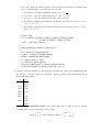
2. Consider a Bayes analysis of some bivariate normal data, under the complication that
not all of n = 10 data vectors are complete. In fact, suppose that observations are as
in the following table:
x1
3.683
7.189
5.014
4.946
3.495
4.065
4.222
-
x2
7.324
6.093
4.399
3.540
2.582
5.281
3.308
3.486
There is some OpenBUGS/WinBUGS code below that can be used to do an analysis
assuming that a priori the mean vector has
mean
0
0
and covariance matrix
9
100 0
0 100
independent of
that has
mean
4 0
0 4
and a distribution based on a fairly small number of degrees of freedom.
(a) Argue carefully that the prior used in the OpenBUGS/WinBUGS code has the properties advertised above. Then run the code and …nd 95% credible intervals for
all 5 parameters of the bivariate normal distribution (two means, two standard
deviations and a correlation) based on this prior and these data.
(b) Alter the code below as needed to make = 20 but hold the same prior mean for
. Run the code and describe how the inferences change from (a).
(c) Alter the code below as needed to make the prior covariance matrix for
the
2 2 identity. Run the code and describe how the inferences change from (a).
(d) Alter the code below as needed to make the prior mean of
4
3
3
4
Run the code and describe how the inferences change from (a).
(e) Alter the code below as needed to make the prior mean of
40 0
0 40
Run the code and describe how the inferences change from (a)
model
{
for(i in 1:10)
{
Y[i, 1:2] ~dmnorm(mu[], R[ , ])
}
mu[1:2] ~dmnorm(alpha[],Tau[ , ])
R[1:2 , 1:2] ~dwish(Lambda[ , ], nu)
D[1:2, 1:2]<-inverse(R[1:2, 1:2])
sig1<-sqrt(D[1,1])
sig2<-sqrt(D[2,2])
rho<-D[1,2]/(sig1*sig2)
}
list(nu=4, alpha=c(0,0),
Tau = structure(.Data = c(0.01, 0, 0, 0.01), .Dim = c(2, 2)),
Lambda = structure(.Data = c(4, 0, 0, 4), .Dim = c(2, 2)),
Y = structure(.Data = c(
3.683,NA, NA, 7.324,
7.189, 6.093, 5.014, 4.399,
10
4.946, 3.540, 3.495, NA,
4.065, 2.582, NA, 5.281,
4.222, 3.308, NA, 3.486), .Dim = c(10, 2)))
3. Use an OpenBUGS simulation to investigate the claim in the course outline that (say,
for the case of k = 3 dimensions and) for diagonal D, an Inverse-Wishart(k + 1; D)
distribution gives correlations that are U( 1; 1) and diagonal elements with medians
about :72= ii . (Simulate with D = diag (:1; 1; 10).)
4. What happens when you try to run the code below in OpenBUGS/WinBUGS?
model {
Y~dflat()
X~dnorm(Y,1)
}
#initial values are below
list(Y=0,X=0)
This code corresponds to a model where XjY is N(Y; 1) and Y is "uniform on <". Why is
this not a probability model for (Y; X)? If I fail to notice this issue, I might try to write
and run a Gibbs sampler for the pair. Do this (in R or some other language you like) and
run 1; 000 iterations. Make a history plot of your results. What do you conjecture is going
to happen if you keep running? (See Problem 2 on the 2008 Mid-Term Exam.)
5. Let
be the standard normal density and consider the pdf
f (x) = :9 (x) + :1 (x
10)
(the density of a mixture of standard normal and N(10; 1) distributions). Write a
Metropolis algorithm (in R or some other language you like) for sampling from this
density, where the proposal density at x is normal with mean x and standard deviation
. For sake of argument, use x0 = 0 as your starting value. Run the algorithm for
1; 000 iterations for each of = :01; :1; 1; 10; 100 and make history plots of your iterations. What message is in this problem regarding the tuning of a Metropolis jumping
distribution?
6. Consider the bivariate normal distribution with
=
0
0
and
=
1 :99
:99 1
Standard Stat 542 stu¤ says that if (X1 ; X2 )0 has this distribution, then conditioned
on X1 = x1 , X2 is normal with mean :99x1 and variance 1 (:99)2 = :0199 (and, of
course, a symmetric result holds for the other conditional).
(a) Write a Gibbs algorithm (in R or some other language you like) for sampling
this bivariate distribution. Starting at (0; 0), about how many iterations are
required to produce an empirical distribution that "looks" bivariate normal using
this method?
11
(b) Write a Gibbs algorithm (in R or some other language you like) for sampling
the bivariate normal distribution with mean vector 0 and covariance matrix I.
Starting at (0; 0), about how many iterations are required to produce an empirical
distribution that "looks" bivariate normal using this method? For pairs (z1 ; z2 )0
produced this way, what is the distribution of
!
p
p
1:99
p
p:01
z1
p 2
p2
?
1:99
:01
z2
p
p
2
2
(c) Write a Metropolis algorithm (in R or some other language you like) for sampling
from this distribution using a bivariate normal proposal distribution, where a
proposal at (x1 ; x2 )0 has mean (x1 ; x2 )0 and covariance matrix cI. Starting at
(0; 0), run this algorithm for 1; 000 iterations for each of c = :01; :1; 1; 10. What
behaviors do you see in the iterates and what message is in this exercise regarding
the tuning of a Metropolis proposal distribution?
12