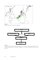
1
DROPLET to calculate concentrations at drinking water abstraction points User manual for evaluation of agricultural use of plant protection products for drinking water production from surface waters in the Netherlands Alterra Report 2020 ISSN 1566-7197 R.C. van Leerdam, P.I. Adriaanse, M.M.S. ter Horst and J.A. te Roller DROPLET to calculate concentrations at drinking water abstraction points This research project has been carried out within the Policy Supporting Research for Ministry of Agriculture, Nature and Food Quality. Theme: BO-06-010-005 Risk assessment methodologies for registration of plant protection products. Cluster: BO-06 Plant Health DROPLET to calculate concentrations at drinking water abstraction points User manual for evaluation of agricultural use of plant protection products for drinking water production from surface waters in the Netherlands R.C. van Leerdam, P.I. Adriaanse, M.M.S. ter Horst and J.A. te Roller Alterra-report 2020 Alterra Wageningen UR Wageningen, 2010 Abstract R.C. van Leerdam, P.I. Adriaanse, M.M.S. ter Horst and J.A. te Roller, 2010. DROPLET to calculate concentrations at drinking water abstraction points; User manual for evaluation of agricultural use of plant protection products for drinking water production from surface waters in the Netherlands;Wageningen, Alterra, Alterra-Rapport 2020. 78 blz.; 66 fig.; 16 tab.; 35 ref. The user-friendly shell DROPLET, acronym for DRinkwater uit OPpervlaktewater- Landbouwkundig gebruik Evaluatie Tool, assists the Dutch Board for the Authorisation of Plant Protection Products and Biocides (Ctgb) in evaluating whether pesticides may exceed the 0.1 μg/L standard in one of the Dutch surface water abstraction points for drinking water production. It operationalises the methodology developed by a Dutch expert group described in Adriaanse et al (2008). The calculation method makes use of the FOCUS D3 ditch, a 1 m wide ditch with 30 cm water in a drained, sandy soil which is one of the so-called FOCUS Surface Water Scenarios used in the registration procedure according to EU Directive 91/414 (FOCUS, 2001 and http://viso.ei.jrc.it/focus/). This manual explains how to use (i) SWASH to enter compound properties and application pattern, (ii) to run MACRO to calculate the drainage fluxes, (iii) to enter the deposition according to the Dutch Drift Table in TOXSWA, next (iv) to run TOXSWA to obtain an edge-of-field concentration in the FOCUS D3 ditch and finally (v) to run DROPLET to obtain the concentrations in the nine Dutch abstraction points plus the Bommelerwaard. DROPLET maintains a central database (in addition to the SWASH database) and combines the peak concentration of the FOCUS D3 ditch with intake area and compound specific factors, such as crop areas and compound degradation to calculate concentrations in the abstraction points. Keywords: Key words: surface water abstraction for drinking water production, pesticides, registration, DROPLET ISSN 1566-7197 The pdf file is free of charge and can be downloaded via the website www.alterra.wur.nl (go to Alterra reports). Alterra does not deliver printed versions of the Alterra reports. Printed versions can be ordered via the external distributor. For ordering have a look at www.boomblad.nl/rapportenservice. © 2010 Alterra Wageningen UR, P.O. Box 47; 6700 AA Wageningen; the Netherlands Phone: + 31 317 480700; fax: +31 317 419000; e-mail: [email protected] No part of this publication may be reproduced or published in any form or by any means, or stored in a database or retrieval system without the written permission of Alterra. Alterra assumes no liability for any losses resulting from the use of the research results or recommendations in this report. Alterra-Report 2020 Wageningen, April 2010 Contents Preface 7 Summary 9 1 Introduction 11 2 Overview of the assessment methodology for agricultural use of plant protection products for drinking water production from surface waters in the Dutch authorization procedure 13 3 Calculation of edge-of-field concentration, PECFOCUS_NL,D3 19 4 Calculation of concentrations in drinking water abstraction points, PEC_Tier1 21 5 User’s guide for calculation of PECFOCUS_NL,D3 5.1 Introduction 5.2 Installation and getting started 5.2.1 Installation of SWASH 5.2.2 Getting started with SWASH 5.2.3 Installation and getting stared with MACRO in FOCUS 5.2.4 Installation and getting started with TOXSWA 5.3 Generating FOCUS step 3 run for D3 ditch and Dutch drift deposition 5.3.1 Preparing the project for the compound and its application pattern in SWASH 5.3.2 Running FOCUS_MACRO for the D3 ditch scenario 5.3.3 Running FOCUS_TOXSWA for the D3 ditch and Dutch drift deposition 27 27 27 27 28 30 31 32 32 48 51 6 User’s guide for the command line version of DROPLET 6.1 Running the model 6.2 Description of input and output files 6.2.1 The CompoundProperties input file 6.2.2 The CropPEC input file 6.2.3 The CropArea input file 6.2.4 The Names input file 6.2.5 The Summary output file 57 57 57 57 58 59 60 62 7 User’s guide for the DROPLET Graphical User Interface 7.1 Installation 7.2 Getting started 7.3 The Main Screen - Actions 7.3.1 The wizard 7.3.2 The View Projects Screen 7.4 The Main screen – Information 7.4.1 Maps intake areas 7.4.2 Surface area of intake areas 65 65 66 67 68 71 80 80 82 7.4.3 Crop groupings 7.4.4 Map D3 scenario 8 84 86 Model parameterization 8.1 SWASH 8.2 MACRO 8.3 TOXSWA 8.3.1 Run characteristics 8.3.2 Definition of water layer and sediment 8.3.3 Hydrology of water bodies 8.3.4 Pesticide loadings 8.3.5 Substance properties 8.4 DROPLET 89 89 90 96 96 97 99 99 99 100 References 103 Appendix 1. List of abbreviations 107 Appendix 2. File specifying the default Relative Cropped Area (RCA) 109 Appendix 3. Crop groupings 111 Appendix 4. Dutch drift percentages 123 Appendix 5. The DROPLET Fortran source code 125 Appendix 6. Some error messages in DROPLET 139 Appendix 7. Example TOXSWA input file (txw file) 141 Appendix 8. Modifying the default CropArea file to obtain a new CropArea file 147 Appendix 9. Do compounds with Kom values above 10 000 L/kg reach the drinking water abstraction points? 149 Preface Commissioned by the two Dutch ministries of Spatial Planning, Housing and the Environment and of Agriculture, Nature and Food Quality a Working Group developed an assessment methodology for drinking water production from surface waters in the Netherlands from 2006 to 2008. Next, Alterra transformed the methodology into an user-friendly software instrument, called DROPLET: DRinkwater uit OPpervlaktewaterLandbouwkundig gebruik Evaluatie Tool. DROPLET allows the Dutch Board for the Authorisation of Plant Protection Products and Biocides (Ctgb) to evaluate in an easy and reproducible way whether the drinking water standard of 0.1 μg/L would be met in each of the nine abstraction points from surface water following Good Agricultural Practice. In cooperation with Robin van Leerdam and Paulien Adriaanse Mechteld ter Horst wrote the Fortran source code of DROPLET while Johnny te Roller of Alterra’s Centre for Geo Information designed the user interface. In 2008 Vincent Vulto and Wim de Winter designed the first versions of the Fortran source code and the user interface, respectively. In spring 2010 DROPLET was added to our website www.pesticidemodels.eu, from where it can be downloaded freely. While developing DROPLET it was realized that the assessment methodology of the Working Group did not result in realistic concentrations at the nine abstraction points for compounds with high sorption capacities. Therefore Alterra developed additional guidance for compounds with Kom values above 10 000 L/kg. This has been implemented in DROPLET and the guidance is underpinned in Appendix 9 of this report. Alterra-report 2020 7 8 Alterra-report 2020 Summary The software tool DROPLET has been developed to enable the Dutch Board for the Authorisation of Plant Protection Products and Biocides (Ctgb) to evaluate whether pesticides may exceed the 0.1 μg/L standard in one of the Dutch surface water abstraction points for drinking water production. It operationalises Tier 1 of the methodology developed by a Dutch expert group by order of the two Dutch ministries of Spatial Planning, Housing and the Environment and of Agriculture, Nature and Food Quality (Adriaanse et al, 2008). The methodology only considers Good Agricultural Practice as well as only contributions of Dutch agriculture, i.e. contributions from agriculture in other countries are not included in the assessment, although e.g. Germany, Belgium or France may discharge surplus water containing pesticides into the Rhine or the Meuse. The starting point for the evaluation of concentrations in drinking water abstraction points is the FOCUS D3 ditch scenario. This is a 1 m wide ditch with 30 cm water in a drained, sandy soil. It is one of the so-called FOCUS Surface Water Scenarios used in the registration procedure of active ingredients according to EU Directive 91/414 (FOCUS, 2001, and http://viso.ei.jrc.it/focus/). In the Dutch drinking water evaluation procedure the FOCUS D3 ditch is used to calculate edge-of field concentrations. All input is according to FOCUS, except the drift deposition, which follows the Dutch Drift Table of the Ctgb (www.ctgb.nl ). So, a user first enters the compound properties and its application pattern into SWASH, next MACRO is run for the FOCUS D3 ditch, and finally TOXSWA is run with drainage fluxes from MACRO and drift deposition from the Dutch Drift Table. The obtained edge-of-field peak concentrations form input for DROPLET. The edge-of-field concentrations are diluted on their way towards the abstraction points due to factors accounting for e.g. (i) the ratio of the crop area and the entire intake area, (ii) market share, reflecting that the compound is not used on the entire crop area, (iii) the difference in timing of applications and (iv) degradation and volatilization on the way from the edge-of-field watercourse to the abstraction points. Crops have been categorized in various crop groupings for the DROPLET calculations, namely (i) the Ctgb crop listing which the Ctgb considers in their registration procedure, (ii) the available crop groupings for which FOCUS Surface Water Scenarios calculations can be made and (iii) the GeoPEARL crop groupings for which the cultivated areas in the intake areas have been calculated. The main functionalities of DROPLET are: – Maintenance of a central database (in addition to the SWASH database) – Preparation of input and calculation of the concentrations at the nine abstraction points plus the Bommelerwaard – Provision of an overview of all projects and viewing their input and results. In addition, DROPLET provides information on crop areas, intake areas and crop groupings. For compounds with Kom values above 10 000 L/kg Appendix 9 underpins that concentrations in the abstraction points become more realistic if they are divided by a factor of 5. Alterra-report 2020 9 10 Alterra-report 2020 1 Introduction This software tool DROPLET has been developed for the Dutch Board for the Authorisation of Plant Protection Products and Biocides (Ctgb). It is an instrument for evaluation of pesticides use in intake areas which are connected to water courses that serve as drinking water source in the Netherlands. The software tool calculates pesticide concentrations at the protection goals, i.e. in the surface water at abstraction points for drinking water production. This tool is the lowest tier (Tier I) in a tiered approach for pesticide evaluation in view of registration in the Netherlands as described in Adriaanse et al (2008). DROPLET calculates intake area and compound specific concentrations for the nine Dutch abstraction points. A separate concentration is calculated for the Bommelerwaard polder, as this polder has an intensive agriculture and discharges into a branch of the Meuse, from which the raw surface water is abstracted for drinking water production. Using DROPLET the Ctgb can evaluate whether the drinking water standard of 0.1 μg/L is met in each of the nine Dutch drinking water abstraction points, following Good Agricultural Practice. As specified by the responsible ministries DROPLET only considers contributions of Dutch agriculture, i.e. contributions from agriculture in other countries is not included in the assessment, although e.g. Germany, Belgium or France may discharge surplus water containing pesticides into the Rhine or the Meuse. The present report provides the user manual of DROPLET. It starts with presenting briefly the developed assessment methodology (Chapter 2) and the calculation methods for the edge-of field concentration in the FOCUS D3 ditch (Chapter 3) and next at the nine abstraction points (Chapter 4). How to use the needed software is explained in the next chapters. Chapter 5 explains the use of respectively SWASH, MACRO and TOXSWA with the Dutch Drift Table to calculated the PECFOCUS_NL,D3. Chapter 6 explains the use of the command line version of DROPLET to calculate the PEC_Tier 1 in the nine abstraction points, while Chapter 7 explains how to use the User Interface to calculate the PEC_Tier1. In Chapter 8 the model parametrization is discussed. The appendices present, among others, the relationships between the various crop groupings used in DROPLET calculations, DROPLET’s Fortran source code, the Dutch Drift Table of the Ctgb and the underpinning of the factor 5 used to lower calculated PEC_Tier1 concentrations for compounds with Kom values above 10 000 L/kg. Alterra-report 2020 11 12 Alterra-report 2020 Overview of the assessment methodology for agricultural use of plant protection products for drinking water production from surface waters in the Dutch authorization procedure 2 A working group developed an assessment methodology for drinking water production from surface waters in the Netherlands to be used in the registration procedure of pesticides (Adriaanse et al., 2008). The ministries of Spatial Planning, Housing and the Environment and of Agriculture, Nature and Food Quality needed an assessment methodology to elaborate the drinking water criterion according to the Uniform Principles of EU Directive 91/414/EEC concerning placing plant protection products on the market and that also fitted within the Water Framework Directive, 2000/60/EC. Similar to the evaluation of other registration criteria, the methodology should consist of a tiered approach, with predictive modeling in lower tiers and use of measured data in higher tiers. Finally, the ministries specified that a drinking water standard of 0.1 μg/L should be evaluated, i.e. purification by drinking water companies was not to be considered. Only pesticide use according to the label, Good Agricultural Practice (GAP), should be evaluated. The Working Group strived for the development of an assessment methodology allowing on one hand the drinking water companies to have surface waters of a good quality at their disposal and on the other hand not to prohibit the registration of pesticides that do not hinder the drinking water production from surface waters. In this methodology only normal agricultural use of pesticides is assessed. At present in the Netherlands approximately 40% of all drinking water originates from surface waters. Drinking water is produced at nine locations: Heel, Brakel and Petrusplaat along the river Meuse; Nieuwegein, Amsterdam-Rijnkanaal and Scheelhoek taking in water mainly originating from the river Rhine; Twentekanaal abstracting water originating from the IJssel (branch of the Rhine); Andijk abstracting water from the inner IJsselmeer Lake and De Punt abstracting water from the Dutch river Drentsche Aa (Table 2.1, Fig. 2.1). Table 2.1 The nine locations where surface water is abstracted for producing water production in the Netherlands. # NAME LOCATION Abstraction point 1 Scheelhoek Scheelhoek Haringvliet 2 Petrusplaat Biesbosch Meuse 3 Brakel Andel Afgedamde Maas 4 Heel Heel Lateraalkanaal 5 De Punt De Punt Drentsche Aa 6 Nieuwegein Nieuwegein-Jutphaas Lekkanaal 7 Amsterdam-Rijnkanaal Nieuwersluis Amsterdam-Rijnkanaal 8 Inlaat Andijk Prinses Juliana IJsselmeer Lake 9 Twentekanaal Elsbeekweg Twentekanaal Alterra-report 2020 13 The abstraction point in the Twentekanaal has stopped its water intake since August 2003. Recently (March 2008) drinking water company Vitens decided to stop the intake of surface water for the production of drinking water definitively. However, the assessment methodology developed in this report still includes the Twentekanaal abstraction point. Figure 2.1 The nine drinking water abstraction points from surface water in the Netherlands. In each of the nine abstraction points the 0.1 μg/L standard is regularly exceeded since many years. If too high concentrations are detected, surface water abstraction may stop for several days or even weeks. 14 Alterra-report 2020 To overview the current situation all pesticides that had caused surface water intake stops in the past were identified. For these 18 pesticides all monitoring data from 2000 onwards were obtained from the drinking water companies. On January 1st 2000 the ‘Lozingenbesluit Open Teelt en Veehouderij’ was implemented. This changed considerably the GAPs, including the introduction of crop free zones along watercourses and use of drift-reducing nozzles, and therefore monitoring data from before 2000 were no more relevant. To operationalise the risk assessment methodology further the two ministries specified that they wanted to protect each individual abstraction point and that they only wanted to consider pesticide contributions originating from the Netherlands, and not from upstream located countries such as Germany or Belgium. The Working Group developed two tiers: in the first tier the concentration in each abstraction point is calculated and subsequently compared to the drinking water standard. In the second tier measured concentrations at the abstraction points are evaluated and compared to the standard. In Tier I concentrations at the abstraction points are calculated on the basis of edge-of-field concentrations for all crops in the intake area on which the pesticide can be used. Each abstraction point has its own intake area (Fig. 2.2) from where all surplus water flows towards the abstraction point. The location and size of the intake areas is based upon data of Kiwa Water Research, used in the so-called project EDG-M 'Evaluatie Duurzame Gewasbescherming' (Van der Linden et al., 2006). Alterra-report 2020 15 Figure 2.2 Intake areas and drinking water abstraction points (blue dots). Monitoring stations in the rivers Rhine at Lobith and Meuse at Eijsden (the Dutch borders) are indicated by red dots. The edge-of-field concentrations consist of concentrations in the FOCUS D3 ditch (FOCUS, 2001) caused by spray drift deposition calculated by Dutch drift values (Appendix 4) or by drainage entries calculated by the FOCUS_MACRO model (Jarvis, 1994, 1998, see Chapter 3 for a brief description). 16 Alterra-report 2020 From the edge-of-field concentration the concentration at the abstraction point is calculated by multiplying with factors accounting for e.g. (i) the relative crop area, i.e. the ratio of the area of the crop and the entire intake area, (ii) market share, reflecting that the pesticide is not used on the entire area of a crop, (iii) difference in timing of applications within the area of use, (iv) degradation and volatilisation from the edge-of-field watercourse to the abstraction point and (v) (in one case) additional dilution by a lake or incoming river. The working group agreed on the following refinement options for the Tier I calculations: – More recent crop acreages than the ones currently used – More recent delimitation of the intake areas than the current ones, which are based on a RIVM study of Van der Linden et al. (2006) – Compound specific market share factor, fmarket, instead of the default value of 0.4 – Additional dilution factor, fadd_dilution, below 1.0. A factor of 1.0 is currently used for all abstraction points except Andijk. The working group did not agree on refining the application patterns, i.e. replacing the worst case application according to the GAP sheets (which is currently used for all crops on which the compound is used) by the application pattern specified for each crop. The working group considers this to be an important conservative assumption of the proposed Tier I calculation method for compounds used in more than one crop. The Tier I calculation method assumes that the crop treatments are randomly distributed over the entire intake area and that all parts of the intake area contribute equally their surplus water to the abstraction point. For the abstraction point at Brakel in the Meuse this assumption is not true as the abstraction point is not located in the mainstream of the river but in a branch of the Meuse with a very low flow. The Bommelerwaard polder discharges its surplus water in this branch and thus treatment of crops in the Bommelerwaard heavily influences the water quality at Brakel. The Bommelerwaard polder has an intensive agriculture, partly in glasshouses and in the past, pesticides have been identified in surface waters in this polder (Kruijne, 2002). Therefore the abstraction point at Brakel needs an additional evaluation that is specific for the water draining out of the Bommelerwaard. The highest value may be selected to assess the risks for the drinking water production in Brakel in a conservative way. The concentrations of Tier I were aimed to be conservative estimations for the concentrations at the abstraction points in order to protect the abstraction points sufficiently. The working group assessed the conservativeness of the individual components of the Tier I calculation method to be neutral or neutral to conservative, and so, their combination resulted in a conservative estimate of the overall Tier I concentrations. The Tier I calculation method was tested by comparing calculated concentrations with measured ones. To do so, the Working Group defined positive and negative test cases. Positive cases were defined as substanceabstraction point combinations in which use of the substance in the Dutch part of the intake area leads to the exceedance of the drinking water standard at the abstraction point. For negative cases the drinking water standard is not exceeded. Substances of the test cases should be widely used in the intake area and at least 25 measurements should be available at the abstraction point. Additionally, for positive cases the drinking water standard should be exceeded at least three times in the period 2000-2004 and there should be a plausible relationship in time between the exceedance and the application of the pesticide. Three sound positive test cases and three sound negative cases could be identified for the 18 pesticides mentioned above, that had caused surface water intake stops in the past. The positive cases were MCPA and mecoprop at Brakel and mecoprop in the Drentsche Aa and the negative cases were dicamba, metazachlor and metribuzin at Petrusplaat. In all six cases the calculated Tier I concentration was found to be at the same side of the 0.1 μg/L standard as the monitored concentrations. An additional six negative cases were found at the abstraction point of Andijk in the IJsselmeer Lake. Tier I calculated concentrations of metoxuron, metribuzin and terbutylazin were lower than 0.1 μg/L even before applying the additional dilution factor of 6, accounting for dilution in the IJsselmeer Lake. Calculated bentazon, MCPA and mecoprop concentrations were only below Alterra-report 2020 17 0.1 μg/L after applying the dilution factor, however. The twelve test cases increased the confidence of the working group in the Tier I calculation method. In Tier II monitoring data are evaluated. The assessment of a compound moves to the monitoring data evaluation tier if the concentration in one of the nine abstraction points, calculated in the first tier (including possible refinements), has a value in the interval 0.1-Y*0.1 μg/L. The factor ‘Y’ represents a ’safety’ factor. The responsible Dutch ministries has decided that the factor ‘Y’ equals 5, so if the PEC_Tier1 in an abstraction point is smaller than 0.5 μg/L the compound remains registered but within five years monitoring has to clarify how the standard can be met in the future. For new substances not passing Tier I, the working group developed guidance for Post Registration Monitoring (PRM). In principle the registrant should procure data for all nine abstraction points. Monitoring frequency is attuned to the mean hydrological residence time in the Dutch part of the intake area, discharging to the abstraction point, which is in the order of magnitude of a few days to a couple of weeks. Monitoring should take place once to twice a week during the application period and the next two weeks, plus once a month up to one year after application or every two weeks in the three monthly period during which leaching is expected. The minimal frequency is 13 times a year. Exceeding the standard once up to no more than 0.15 μg/L was judged to be acceptable. In case of PRM, monitoring data of the entire registration period must be available, generally five years. The 90%-ile is calculated for the entire period as well as for each individual year. If the 90%-ile over the five year period exceeds 0.1 μg/L, the registration is at stake. If the 90%-ile for an individual year exceeds the 0.1 μg/L standard a problem analysis should show whether agricultural use according to GAP is the main cause and whether it is possible to adjust the GAP. 18 Alterra-report 2020 3 Calculation of edge-of-field concentration, PECFOCUS_NL,D3 The surface water and sediment calculations developed by FOCUS include three progressively refined tiers of evaluation, ranging from initial spreadsheet-based evaluations of potential aquatic concentrations to more detailed mechanistic calculations of drift, runoff, erosion and field drainage loaded into a series of small water bodies (FOCUS, 2002). For the current drinking water tool, we are only interested in the results of the tier 3 evaluation. Tier 3 calculations are performed using an overall calculation shell called SWASH (Surface WAter Scenarios Help, manual: http://www.swash.pesticidemodels.eu/pdf/UserManualSWASH21.pdf) which controls models simulating runoff and erosion (PRZM), leaching to field drains (MACRO), spray drift calculation (internally in SWASH) and finally aquatic fate in the receiving water bodies, ditches, ponds and streams (TOXSWA). The simulations provide detailed assessments of potential aquatic concentrations in a range of water body types in ten separate geographic and climatic settings. Four runoff (R1-R4) scenarios and six drainage (D1-D6) scenarios have been defined (FOCUS, 2001). A detailed description how to use SWASH in the procedure to calculate concentrations at drinking water abstraction points is given in section 5.3.1. The resulting surface water concentrations provide regulators and registrants with improved estimates of the potential aquatic concentrations of agricultural chemicals that could result from labelled product use. The Swedish model MACRO (macropore flow) is used to determine the contribution of drainage to the concentration level in surface waters. The model describes the leaching process of chemicals to lower depths in soil due to the water movement. It can take into account macropore flow as it distinguishes between different dimensions of soil particles. A detailed description how to run MACRO is given in section 5.3.2. PRZM is not used for the DROPLET tool. The Dutch model TOXSWA is used for estimating the resulting concentration in the three types of surface waters, ditch, stream and pond. TOXSWA stands for TOXic Substances in WAter and is able to deal with the combined input of the processes described above in a dynamic way. This means that the resulting concentration is calculated as a function of time. A detailed description how to run TOXSWA is given in section 5.3.3. Detailed explanations of the FOCUS Surface Water Scenario models as well as the modelling scenarios, key assumptions, required modelling inputs and model outputs are provided in the respective FOCUS modelling reports (FOCUS, 2002). The FOCUS surface water models can be freely downloaded from the FOCUS website (viso.ei.jrc.it/focus/index.htm). The working group, which developed the assessment methodology to evaluate agricultural use of plant protection products for drinking water from surface waters, decided that the D3 ditch scenario (Fig. 3.1) is the most representative scenario for the estimation of the PEC in surface water at the abstraction point for drinking water production (Adriaanse et al., 2008). The basis for the determination of PECTier1, the pesticide concentration at abstraction points in surface waters for drinking water production, is the determination of the PECFOCUS_NL,D3. The PECFOCUS_NL,D3 is the edge-of-field concentration in a FOCUS D3 ditch scenario. It is obtained by running a series of FOCUS models. First, FOCUS crops, pesticide properties, application pattern and rate have to be filled in in SWASH. Subsequently, the FOCUS drainage ditch D3 scenario has to be run with MACRO and TOXSWA. The Dutch drift deposition table (Ctgb, HTB 0.2, http://www.ctgb.nl) has to be used instead of the spray drift calculator in SWASH. Details are discussed in section 5.3.3. The output of the TOXSWA run is the input for the DROPLET tool (Fig. 3.2). Alterra-report 2020 19 Figure 3.1 Extent of FOCUS D3 drainage scenario in the European Union. FOCUS SWASH FOCUS D3 scenario Dutch Spray Drift percentages MACRO FOCUS D3 ditch+ NLdrift scenario TOXSWA Output file, used as input for DROPLET Figure 3.2 Operational structure of FOCUS Surface Water Scenarios to prepare for a DROPLET run. Instead of the FOCUS spray drift calculator the Dutch drift deposition table is used. The output of TOXSWA (PECFOCUS_NL,D3) is the input for the calculation of the PECTIER 1 with the DROPLET tool. 20 Alterra-report 2020 4 Calculation of concentrations in drinking water abstraction points, PEC_Tier1 The equation to calculate the pesticide concentration in the surface water at the abstraction points (PECTier I) reads: PECTierI crops ((PECFOCUS _ NL,D3 f corrFOCUSscen ) f use _ int ensity ) f ti min g f dissipation f add _ dilution (1) all PECTier I PECFOCUS_NL,D3 fcorrFOCUSscen fuse_intensity ftiming fdissipation fadd_dilution PEC in surface water at location where it is abstracted for drinking water preparation (μg/L) global maximum PEC edge-of-field for the FOCUS D3 scenario based upon Dutch drift deposition data (μg/L) correction factor for implicit choices concerning contributing areas made in FOCUS D3 scenario (-) factor considering the use of the pesticide (-) factor considering the difference in timing of application within the area of use (-) factor considering the dissipation from the edge-of-field watercourse to the abstraction point (-) factor considering additional dilution, e.g. by considerable water flows entering the intake area, or by lakes via which water travels to the abstraction point fcorrFOCUSscen The calculated PEC for the FOCUS D3 ditch scenario (PECFOCUS, D3) is corrected for implicit choices concerning water and pesticide contributing areas made in the FOCUS ditch scenario (fcorrFOCUSscen). The implicit choices are that the ditch neighbours a 1 ha treated field and is fed by 2 ha non-treated fields, located immediately upstream of the ditch. Spray drift deposition enters from the neighbouring field only. fuse_intensity The term PECFOCUS_NL,D3 * fcorrFOCUSscen is multiplied by the use intensity factor (fuse_intensity) and summed up for all crops on which the considered pesticide is used. The use intensity consists of an estimation of the relative cropped area, the market share and a drift or drainage factor: – The relative cropped area (RCA) factor, i.e. the ratio of the area of the crop considered and the total abstraction area. The acreage of the different crops is according to the CBS database. – The market share factor reflects that the pesticide will not be used on the total area of a crop. – The fraction of area which can contribute to the most relevant entry route. The value of this factor depends on whether drainage or spray drift is the main entry route. The use intensity factor and the relative crop area factor are defined as follows: f use _ int ensity RCA f market f relevant _ contributing _ area (2) Alterra-report 2020 21 RCA areacrop area drw _ abstraction RCA areacrop areadrw_abstraction fmarket frelevant_contributing_area (3) relative cropped area for a specific crop (-) crop area on which the pesticide is potentially used within the drinking water abstraction area (ha) total catchment area of abstraction point (ha) market share of the pesticide (-) fraction of the area contributing to the main entry route The Relative Cropped Areas are determined with the aid of the GeoPEARL 1.1.1 crop groupings (Kruijne et al., 2004) with an additional subdivision for tree nurseries and fruit culture in large and small trees (see the input file CropArea, Fig. 6.3) because of their large difference in spray drift deposition. The intake areas of the nine abstraction points are based upon data of CBS (http://statline.CBS.nl) and KIWA, used for the EDG-M study (Van der Linden et al., 2006). The crop grouping (Appendix 4) of the Dutch Board for the Authorisation of Plant Protection Products and Biocides (Ctgb) is according to the crop list in the Handbook for the Registration of Pesticides (version 1.0). This crop grouping is also used in GAP sheets. For the calculation of predicted environmental concentrations (PECs) in the FOCUS D3 ditch (PECFOCUS,D3_NL) a crop has to be categorized into a FOCUS D3 crop grouping. The D3 FOCUS surface water scenario contains only a limited number of crop groupings, namely winter and spring cereals, winter and spring oil seed rapes, sugar beets, potatoes, field beans, vegetables (root, leafy and bulb), legumes, maize, pome/stone fruit, grass/alfalfa. The crop must also be categorized into a GeoPEARL crop grouping to be able to determine the Relative Cropped Area (Appendix 2) of the crop in the intake area under concern. In GeoPEARL data are available on the crop areas in the nine intake areas, needed to calculate the Relative Cropped Areas in Equation 3. With help of Appendix 3 the user can categorize a crop in a FOCUS D3 crop grouping and in a GeoPEARL crop grouping. In principle there is no free choice: appendix 3 connects a crop to a FOCUS D3 crop grouping and a geoPEARL crop grouping. For silviculture no representative FOCUS D3 crop grouping is available in Appendix 3. Therefore, the FOCUS D3 crop grouping pome/stone fruit must be used. The possible combinations between the FOCUS D3 and GeoPEARL crop groupings are listed in Table 4.1. Crops that are not mentioned in Appendix 3 and that have small cropped areas and low application rate can be neglected for the calculation in the drinking water tool. 22 Alterra-report 2020 Table 4.1 Possible combinations between FOCUS D3 and GeoPEARL crop groupings. FOCUS D3 crops GeoPEARL crop grouping Cereals, winter Cereals / green manuring/floriculture/fallow Cereals, spring Cereals / remaining arable crops Oil seed rape, winter Leaf vegetables Oil seed rape, spring Leaf vegetables Sugar beets Sugar beets Potatoes Potatoes Field beans Legumes Vegetables, root Leaf vegetables Vegetables, leafy Strawberries / leaf vegetable / cabbage / asparagus / floriculture / remaining arable crops Vegetables, bulb Onions / flower bulbs / floriculture/ leek Legumes Legumes Maize Maize Pome/stone fruit Fruit culture / tree nurseries / silviculture Grass/alfalfa Grass Summing up (PECFOCUS, D3 * fcorrFOCUSscen )* fuse_intensity over all crops (Table 4.2) assumes that for the pesticide considered the calculated edge-of-field PECs all arrive at the same moment at the abstraction point, i.e. all PECs have the same travel time from the edge-of-field water to the abstraction point. This results in a conservative estimate of the PECTier I. Table 4.2 Example of crops with corresponding PECFOCUS, D3, FOCUS correction factors, use intensity factors and the time of occurrence of the PECs. Crops A, B and C require the same pesticide Crop Crop A Crop B Crop C Σ all crops PECFOCUS, D3 (μg/L) 6.3 3.0 2.7 PEC * fcorrFOCUSscen *fuse_intensity (μg/L) 0.013 0.06 0.012 0.085 Time of occurrence 1 May 15 May 1 September ftiming In reality the pesticide is not applied on the same day on the entire area of crops concerned, but the application is distributed in time during an estimated realistic length of the registered application period. So, there is a dilution of the edge-of-field concentration on its way to the drinking water abstraction point, due to a difference in timing of application. Alterra-report 2020 23 Figure 4.1 Illustration of Tier I calculation procedure demonstrating that edge-of-field concentration peaks do not arrive at the same moment in the abstraction point. A dilution factor of 2 from the edge-of-field concentration to the abstraction point is used, ftiming = 0.5. fdissipation During the travel time from use area to the abstraction point the pesticide concentration lowers due to degradation and volatilisation. The dissipation rate constant is the sum of the volatilisation rate constant of the pesticide from surface water and the degradation rate constant of the pesticide in surface water: k dis k vol k kdis kvol k k vol ( kl kg KH Ox A (4) dissipation rate constant of the pesticide in surface water (d-1) volatilisation rate constant of the pesticide from surface water (d-1) degradation rate constant of the pesticide in surface water (d-1) 1 1 1 O x ) (Adriaanse et al., 1997) kl K H k g A (5) transport coefficient of the compound in the liquid phase (md-1) transport coefficient of the compound in the gas phase (md-1) Henry coefficient (-) width of water surface of the FOCUS D3 ditch (m) cross sectional area of flow (m2) For rectangular cross-sections Ox/A equals 1/d, the water depth. We consider the most relevant water depth, i.e. the water depth of the watercourses where the pesticide has the longest hydraulic residence times. These are the edge-of-field ditches and next level of watercourses and not the larger watercourses near the abstraction points (Adriaanse et al., 2008). 24 Alterra-report 2020 The degradation rate constant of the pesticide in surface water depends on the temperature and can be derived from the Arrhenius equation: k (T ) k (Tref ) exp[ R T Tref E E (T Tref )] R Tref T (6) universal gas constant (J K-1 mol-1) temperature (K) reference temperature (K) molar Arrhenius activation energy (J mol-1) The first order degradation rate constant can be calculated according to: k (Tref) = ln(2)/DegT50 (7) DegT50 = half life transformation time in water (d) The remaining pesticide fraction in the surface water as a result of dissipation can be calculated as follows: f dissipation e kdiss t fdissipation t (8) factor accounting for the dissipation of the pesticide in the surface water by degradation and volatilization (-) residence time of the pesticide in the water between application and arrival at the abstraction point (d) According to Liss and Slater (1974) (in Beltman et al., 1996, User manual TOXSWA 1.1) the mass transfer coefficient of the pesticide in the liquid phase and gas phase can be estimated as follows: k l k l ,CO2 k g k g , H 2O kl,CO2 Mx kg,H2O M CO2 (9) M subs tan ce M H 2O (10) M subs tan ce transport coefficient of CO2 in the liquid phase (md-1) molecular weight of substance x transport coefficient of H2O in the vapour phase The dimensionless Henry coefficient (KH) is estimated from the quotient of mass concentration of saturated vapour of the substance (via vapour pressure) and the solubility of the substance in water: KH Psat M subs tan ce 1 R T c sol (11) Alterra-report 2020 25 Psat Msubstance T csol saturated vapour pressure of substance (Pa) molecular mass of substance (g mol-1) temperature at which the saturated vapour pressure, the solubility and the transport coefficients in the liquid and gas phases are defined (K) solubility of substance in water (g m-3) The saturated vapour pressure at temperature T is derived from the Van ‘t Hoff equation (Van den Berg and Boesten, 1998, in Beltman and Adriaanse, 1999): Psat (T ) P(Tref ) exp[ ΔHp H p R ( 1 1 )] T Tref (12) enthalpy of vaporization (J mol-1) The effect of the temperature on the water solubility is derived from the Van ‘t Hoff equation (Van den Berg and Boesten, 1998) via: c sol (T ) c sol (Tref ) exp[ ΔHsol H sol 1 1 ( )] R T Tref (13) enthalpy of dissolution (J mol-1) fadd_dilution The factor fadd_dilution accounts for additional dilution of the surplus water gathered in the intake area that travels to the abstraction point. Additional dilution may be caused by river water that enters the intake area from upstream and that does not contain the considered pesticide. It may also be caused by a large lake, via which the surplus water from the intake area travels to the abstraction point. For Andijk, abstracting its water from the IJsselmeer the factor is 0.17, i.e. there is an additional dilution by a factor of 6. 26 Alterra-report 2020 5 User’s guide for calculation of PECFOCUS_NL,D3 5.1 Introduction In this chapter the installation procedure of SWASH, MACRO and TOXSWA is described. Subsequently, the screens of the Graphical User Interfaces of SWASH, MACRO and TOXSWA are described which have to be gone through to generate a FOCUS step 3 run with Dutch drift deposition for a FOCUS D3 ditch. This results in a PECFOCUS_NL,D3, the main input for DROPLET. 5.2 Installation and getting started 5.2.1 Installation of SWASH The SWASH software package can be downloaded from the FOCUS web site: http://viso.ei.jrc.it/focus/sw/index.html. The installation procedure results in the installation of SWASH_2.1. The installation directory is C:\SWASH by default. The MACRO and TOXSWA software packages compatible with SWASH_2.1 should be installed in the same directory, i.e. C:\SWASH\MACRO and C:\SWASH\TOXSWA. SWASH works only correctly if it is installed in the root of a harddrive. The drive may also be another drive than C:\. FOCUS_SWASH_2.1 has been tested on Win2000, WinNT, WinXP and Vista. For WinNT a MS Office package is needed. SWASH is likely to run on previous versions, however, this has not been tested. On WinNT, Win2000, WinXP and Vista machines it is necessary to have Administrator rights. SWASH requires 12.5 Mb for installation. A monitor with at least a screen resolution of 800x600 is required, using 256 colours. Preferably, select ‘small fonts’ as display setting. The faster the processor the better. The installation procedure for FOCUS_SWASH_2.1 depends on whether FOCUS_SWASH_1.1 has already been installed or not. The Read_me_first file that is supplied with the installation package contains the information for installation of FOCUS_SWASH_2.1. It should be noted that if FOCUS_SWASH_1.1 has already been installed then the user has the option to save the SWASH database and restore it when completing the installation of FOCUS_SWASH_2.1 (see Figure 3.1). Please note that the structure of the database in FOCUS_SWASH_2.1 is the same as that of FOCUS_SWASH_1.1. If the option ‘save and restore database’ has been selected in the installation procedure, all user defined substances and projects will be saved. Alterra-report 2020 27 Figure 5.1 Installation options for previous installed FOCUS_SWASH. 5.2.2 Getting started with SWASH The first step to perform a FOCUS Surface Water run consists of editing the properties of a substance that is already present in the SWASH database or the creation of a new substance. Once the substance is included in the database, the User-defined wizard can be used to create the runs required in the assessment of the fate of the substance in the surface water. Using the User-defined wizard, the user can select one or more crops, one or more (up to 3) water body types and one or more (up to 10) scenarios. After creation of the project with the User-defined wizard, the user has to enter the correct application data on the ‘Applications’ form. Once the application data have been entered for the runs created in the new project, the user has to export the data to the MACRO and TOXSWA shells. This sequence of steps is depicted in Figure 5.2 Add or Edit a substance Create a project Edit the application data for the runs in the project Export input to MACRO and TOXSWA View and Print Report Figure 5.2 Scheme for preparing input to run FOCUS Surface Water Scenarios using SWASH. 28 Alterra-report 2020 Next, runs have to be started in the sequence MACRO, TOXSWA. For a drainage scenario first a run with MACRO has to be executed before running TOXSWA. After starting the MACRO shell using the ‘MACRO’ button on the main screen of SWASH, the user has to specify in the MACRO shell the run that has already been created in SWASH. The report of the SWASH project can assist the user in specifying the correct scenario, crop, parent compound and application data. In particular it is important to select the application data for the relevant run. Each application scheme has a unique ID (the runID), and the application scheme with the same runID as that for the corresponding run as defined in SWASH should be taken. After running MACRO the user has to process the output using the FOCUS_MACRO shell to create the m2t file containing the input of the drainage and pesticide fluxes for TOXSWA. The sequence of steps to specify and execute a drainage scenario for MACRO is also shown briefly in Figure 5.3. Start MACRO shell Specify crop(s) and location(s) Select substance (already defined in SWASH) Select Application scheme (already defined in SWASH) Execute MACRO Run Create m2t output file for TOXSWA Exit MACRO shell Figure 5.3 Scheme for executing a run with MACRO for a drainage scenario. The last part of execution of a run for FOCUS Surface Water scenario is to run TOXSWA. The TOXSWA shell can be started after clicking of the ‘TOXSWA’ button on the Main screen of SWASH. The steps to be followed are shown in Figure 5.4. The drain water fluxes and pesticide loadings are read from the m2t file. Once the TOXSWA runs in the project have been completed, the user has the target data on the exposure concentrations. Notice that for DROPLET the selected project needs to be copied first in order to become a false Alterra-report 2020 29 SWASH project, in which the Dutch drift deposition can be entered. In true SWASH projects all FOCUS assumptions cannot be changed by the user. It should be noted that the highest areic deposition resulting from spray drift at any time occurs for a single application. For multiple applications, the areic deposition rate per event is smaller (Ganzelmeier et al., 1995). Therefore, it is recommended to do always an exposure assessment with TOXSWA for a single application with the highest application rate. More detailed information on the TOXSWA model and guidance how to use FOCUS_TOXSWA is given in the User’s manual of FOCUS_TOXSWA_2.2.1 (Beltman et al., 2006). Support for SWASH can be requested by sending an email to [email protected]. Figure 5.4 Scheme for executing a run with TOXSWA scenario. 5.2.3 Installation and getting stared with MACRO in FOCUS MACRO in FOCUS is a program selected to run the EU FOCUS pesticide exposure assessment scenarios for surface waters using the simulation model MACRO. It can be downloaded from http://viso.ei.jrc.it/focus/sw/index.html. The surface water scenarios can only be run in connection with the SWASH program (‘Surface WAter Scenarios Help’), which is used for defining the scenario simulations to be performed, especially with respect to application patterns and doses. The MACRO surface water scenarios have to be run as a preparation for the TOXSWA en DROPLET runs. Model version The software tool MACRO in FOCUS (version 4.4.2) runs version 4.3b of the MACRO model. A technical description of MACRO can be downloaded from the web address: http://www.mv.slu.se/bgf/macrohtm/macro.htm 30 Alterra-report 2020 Installation and system files The package consists of a Windows executable (macro_focus.exe), together with the DOS program files for MACRO, Windows system files, binary-formatted weather data files, and three Microsoft Access formatted databases, one containing soil data, another containing crop data, and the third containing information on pesticide properties. Important: The system only works properly if ‘Regional Settings’ (under ‘Control Panel’ on ‘My computer’) are set to a default national setting, without making changes i.e. do not select ‘Swedish’, and then change the number format to decimal point from the default comma. All program files must be installed in a sub-directory MACRO under SWASH if the system is to work properly for surface water scenarios e.g. under the directory C:\SWASH\MACRO if you installed to the C: drive. If you have previously installed an earlier version of this software tool (3.3.1. and earlier) that was released for groundwater FOCUS scenarios, then you should uninstall any older versions prior to installation of MACRO in FOCUS v4.4.2.Unfortunately, the information on substance properties that you may have saved in the database (pest_focus.mdb) is not automatically transferable to the new version, and the format of this database has also changed significantly. Therefore, you will have to manually re-enter the substance properties into the database for MACRO in FOCUS v4.4.2. This can be done interactively either in MACRO in FOCUS v4.4.2 or in the SWASH program. If you open the MACRO in FOCUS databases using ACCESS, do not attempt to update them to the latest version of ACCESS, as the SWASH connection to MACRO in FOCUS will then not work. If during installation you get a message saying that you have newer versions of system files already on your PC, keep these. Do not overwrite them with the older versions contained in the installation package for MACRO in FOCUS. Running the system For surface water scenarios, application patterns and doses can only be defined in SWASH. Substance properties can also be defined in SWASH, as well as in MACRO in FOCUS. There is communication between SWASH and MACRO in FOCUS such that substance property information is updated in the database when it is modified in either of the tools. MACRO in FOCUS can be started either from SWASH or as a stand-alone program by clicking twice on the icon on your desktop (create the icon by drawing out macro_focus.exe to your desktop). From the start-up screen in MACRO in FOCUS, you can either define a scenario to run or view the results of earlier simulations with ‘Plot’. 5.2.4 Installation and getting started with TOXSWA Official FOCUS_TOXSWA versions can be downloaded from the website of the Joint Research Centre in Ispra, Italy (http://viso.ei.jrc.it/focus/). Notice that the installation of TOXSWA is the third step of the complete installation of the FOCUS surface water software package. Installation of SWASH and TOXSWA is explained in the read_me_first and read_me_TOXSWA text files (Beltman et al., 2006, Appendix 3). Installing comes down to first installing SWASH and next installing TOXSWA. If you encounter problems in installation of TOXSWA, contact us at: [email protected]. FOCUS_SWASH, the shell that prepares the input files for the TOXSWA model, performs all runs of a specific project and presents the main output. All input and output files of TOXSWA are located at Alterra-report 2020 31 C:\SWASHProjects\projectname\TOXSWA, except the lateral entries input files. The lateral entries files *.m2t made by MACRO are located at C:\SWASHProjects\projectname\MACRO\cropname. Users of FOCUS models can register at the JRC website in Italy. When you have registered there, you are not yet registered as a TOXSWA user. We recommend you to register as a TOXSWA at our website. Registered users have some benefits over non-registered users: – You will be put on the TOXSWA mailing lists. Through the mailing list, we will inform you about updates, bugs and reports. – You can obtain the source code upon request. Registration as a TOXSWA user is possible via: www.pesticidemodels.eu 5.3 Generating FOCUS step 3 run for D3 ditch and Dutch drift deposition 5.3.1 Preparing the project for the compound and its application pattern in SWASH In this section it is explained how a FOCUS step 3 run in SWASH can be created as a preparation for a MACRO run with a FOCUS D3 ditch. This information is described in Van den Berg et al. (2008) and more details can be found there. 5.3.1.1 The Main Screen - Actions The main screen consists of two parts, namely Actions and Information. In the Actions part the user undertakes activities with concrete results, i.e. the SWASH database is updated or projects and runs are created. The first part - ‘Actions’ - is displayed after clicking on the ‘Actions’ tab and this is shown in Figure 5.5. Figure 5.5 The main screen of the SWASH interface with the ‘Actions’ tab displayed. 32 Alterra-report 2020 The ‘Actions’ page contains six buttons and the function of the buttons will be briefly described here, but in more detail in the corresponding section of this chapter. The button ‘Create, View and Edit Substances’ gives access to the substance form, where the user can enter new substances or modify the properties of substances already present in the database. The test substances as defined by the FOCUS Surface Water Group are available in the database upon installation. However, the properties of these substances are fixed and they cannot be modified. The button ‘FOCUS wizard’ gives the user the possibility to easily create and execute FOCUS runs for a specific substance - crop combination. An overview as well as a report will be created for all those runs. The runs are organised in projects; for each substance - crop combination a separate project will be created. This wizard provides the user with all standard Step 3 runs for a specific substance-crop combination. The button ‘User-defined wizard’ gives the user more freedom in selecting scenarios and crops for which runs are to be created. Using this wizard all possible FOCUS runs for a selected substance, one run for each scenario - crop - water body type combination, can be created and put into a single project. The button ‘View Projects and Define Applications’ presents the user overviews of the runs in all projects and allows the user to define or modify the application pattern for each run. For the runs in each project, the user can decide if project output has to be created. The project output consists of the creation of input for MACRO and TOXSWA for the runs selected by the user. The user can also print a text report of the specifications of the runs in a project. The button ‘Write substance data’ will update the MACRO substance database for any changes in the substance database of SWASH. For TOXSWA this is done automatically, because TOXSWA uses the same database as SWASH. Using the ‘Exit’ button, the user can end a SWASH session. When exiting the MACRO substance database will be updated. The buttons on the upper right corner of the screen, i.e. ‘Drift’, ‘MACRO’ and ‘TOXSWA’ give the user a direct link to the Drift calculator and to the shells of the FOCUS surface water models. In the Information part of the main screen of SWASH the user is only informed about certain aspects of Step 3 exposure assessment, but no changes are made in the database, or input prepared for the other models. 5.3.1.2 The Substance Screen The substance screen gives access to the pesticide database of SWASH. On the substance screen the user can enter new substances or modify the properties of substances already present in the database. Substances entered here, will be transferred to the MACRO substance database. Substances that were entered into the MACRO database independently from SWASH will be included in the SWASH substance database when exiting the MACRO shell or starting SWASH. TOXSWA makes direct use from the SWASH database. Guidance for defining the substance properties is given in FOCUS (2001), sections 7.3 and 7.4 and below. In Figure 5.6 the ‘General’ tab of the substance screen is shown. The upper part consists of a ‘browse’ part in which the user can browse the list of substances using the scroll bar on the right. In the lower part there are four tabs. Alterra-report 2020 33 Figure 5.6 The substance form of SWASH - The general section. On the ‘General’ tab the user has to specify the general physico-chemical properties of the substance. It should be noted that the units for these properties are the units as used in SWASH. The units of the same properties in the MACRO shell are in many cases different. However, when transferring substance data between SWASH and MACRO the values as entered in SWASH will be converted to the correct values for MACRO. The code refers to the unique code that the user has to attribute to the substance, which is used in the SWASH database to identify this substance. The name field refers to the name (not necessarily unique) the user has to give to the substance. A useful functionality on the ‘Substance’ screen is that it is easy to make a copy of a substance. After clicking on ‘Copy’, a copy will be made of the substance selected, except that the substance code and the substance name will be different. Then, the user has to adjust the code and the name of the substance. Next the user has only to modify those values that are different from the values for the original substance. Other buttons on this form are the ‘New’ button in order to add a new substance to the database, and a ‘Remove’ button to remove a substance from the database. 34 Alterra-report 2020 The test substances as defined by the FOCUS Surface Water Group are available in the database upon installation. The properties of these substances are fixed and cannot be modified. To specify a new or to edit an existing transformation scheme, the user should go to the ‘Metabolite scheme’ form by clicking on the button ‘set Metabolites’. More details about metabolite schemes can be found in the SWASH manual (Van den Berg et al., 2008). In the drinking water tool DROPLET, no metabolites are used, thus if SWASH is used to prepare for DROPLET, the metabolite schemes can be ignored. The sorption section of the ‘Substance’ form is shown in Figure 5.7. In this section the user can select between the sorption options ‘General’ and ‘Detailed’. If the ‘General’ option is selected, then the user has only to enter either the Koc value or the Kom value. The value of the Kom will be automatically calculated from the Koc and vice versa. FOCUS recommends a conversion factor of 1.724: Koc = 1.724 · Kom (FOCUS, 2000). This conversion factor is used in SWASH. The Koc or Kom value will be used as the value for the sorption coefficient in all solids, i.e. soil, suspended solids and sediment. Figure 5.7 The substance form of SWASH - The sorption section. Alterra-report 2020 35 If the ‘Detailed’ sorption option is selected, then the user has to enter separate Koc or Kom values for soil, suspended solids and sediment. The user can choose the sorption isotherm using the value for the Freundlich exponent. If this exponent is set to 1, then a linear sorption isotherm is used. If the exponent is not equal to 1, the sorption is described with the Freundlich equation. The reference concentration is introduced into the Freundlich equation to obtain a Freundlich coefficient independent of the value of the exponent. The value of the reference concentration should be within the range of concentrations in the measurements on which the Freundlich sorption coefficient is based. In most studies, the value of this concentration is set to be 1.0 10-3 kg m-3 (1.0 mg dm–3). The uptake and wash-off section of the ‘Substance’ form is shown in Figure 5.8. In this section the user has to specify the factor for the uptake of the substance by the plant roots in the soil and the factor for the wash-off of the substance from the plant leaves. The coefficient for the uptake by plant roots is also described as the transpiration stream concentration factor, F. For non-ionic pesticides, this factor can be estimated from the octanol-water partitioning coefficient as described by Briggs et al. (1982). For these pesticides this factor will always be between 0.0 and 1.0. For ionic pesticides no reliable estimation methods are available and the factor may be greater than 1.0. Shone and Wood (1974) reported a value of 3 for the anion of 2,4-D. Figure 5.8 The substance form of SWASH - The uptake and wash-off section. 36 Alterra-report 2020 The user has to enter different values for the foliar wash-off factor to be used in PRZM or MACRO. The default value is 0.05/mm for MACRO. The default value is appropriate for moderately to highly soluble pesticides. If the solubility is lower than about 8000 mg L-1 then the value for the wash-off coefficient should be recalculated using the empirical equation of Wauchope et al. (1997) as explained in FOCUS (2001). The transformation section of the ‘Substance’ form is shown in Figure 5.9. In this section the user has to specify the half-lives of the substance in all the compartments considered, i.e. the water layer of the water body, the soil system, the sediment system in the water body and the crop on the field next to the water body. For the first three compartments the temperature at which the half-life has been obtained must be specified. The half-life of transformation depends strongly on the pesticide and the environmental and soil conditions. Water-sediment studies can be used to obtain data on the transformation half-life in water and sediment. Key elements for such studies as well as guidance on the procedure to derive the DT50 for the water layer and the sediment are given by FOCUS (2001). Figure 5.9 The substance form of SWASH - The transformation section. Alterra-report 2020 37 For the half-life on the crop the temperature is not needed, because there is not enough knowledge how to describe the temperature dependency of the half-life of the substance on the crop. After clicking on the ‘Specifications on transformation in soil …’ button, a screen appears on which additional data has to be entered related to the transformation in soil. The content of this form is presented in Figure 5.10. The effect of the moisture content on the rate coefficient of transformation can be described with an equation based on Walker (1974). For the FOCUS surface water scenarios this parameter is set to 0.7. For MACRO, the moisture content of the soil in the transformation experiment has to be entered as a pF value. Figure 5.10 The substance form of SWASH - Specification on the transformation in soi. 5.3.1.3 The User-Defined wizard After clicking on the button ‘User-defined Wizard’ on the main screen, the first form of the Wizard is displayed on the screen. On this form, shown in Figure 5.11, the user has to select the substance for which he wants to do FOCUS runs. The user can select a substance from the list of substances present in the database by clicking on the arrow on the right-hand side of the ‘Substance’ field. 38 Alterra-report 2020 Figure 5.11 The User-Defined Wizard – Substance. After selection of the substance, the user has to click on the ‘Next’ button. Then the form presented in Figure 5.12 is shown on the screen. In the example, the user has selected 5 crops: spring oil seed rape, maize, legumes, hops and grass/alfalfa. The user can add or delete crops from the list by clicking on the ‘>’ button or the ‘<’ button. It is also possible to put all crops in the list of selected crops by clicking on ‘>>’. Removing all crops from the list of selected crops can be done by clicking on ‘<<’. Alterra-report 2020 39 Figure 5.12 The User-Defined Wizard – Crops. After the crops have been selected, the user continues the wizard procedure by clicking on ‘Next’. Then the form with the possible water body types is shown on the screen and this form is shown in Figure 5.13. 40 Alterra-report 2020 Figure 5.13 The User-Defined Wizard - Water bodies. On this form the user can specify for which water body types runs need to be created. The user can select or deselect a water body type by marking the check boxes on the left of the water body type name. For the purpose of preparing a DROPLET run, the user must only select the Ditch waterbody type. After the selection of the water body types the user continues by clicking on ‘Next’. The next wizard form shows the list of available FOCUS surface water scenarios. Only scenarios for which the crop - water body type combinations have been defined are included in this list. In the example shown in Figure 5.14, the scenarios D1, D2, D3 and D6 are selected. For the purpose of preparing a DROPLET run, the user must only select the D3 scenario. It can be added or deleted from the list by clicking on the ‘>’ button or the ‘<’ button. The user can select all or deselect all scenarios by clicking on ‘>>’ or ‘<<’, respectively. Alterra-report 2020 41 Figure 5.14 The User-Defined Wizard – Scenarios. After the selection of the scenarios of interest, the user continues by clicking on ‘Next’. Then the last form of the wizard is shown on the screen (Fig. 5.15). On this form the user has to specify the name of the project and the description of the project. All SWASH output is put in a subdirectory of C:\SwashProjects. The SWASH output path can be changed by clicking on the button on the right-hand side of the ‘path’ field. Using the UserDefined wizard, the project name is set by default to [project_SubstanceName], but this can be modified by the user. The directory for the output of a SWASH project is set to C:\SwashProjects\[project_name]. For the example shown in this section the path is C:\SwashProjects\voorbeeld_DROPLET. The output for MACRO and TOXSWA are put into subdirectories \MACRO and \TOXSWA, respectively. 42 Alterra-report 2020 Figure 5.15 The User-Defined Wizard - Project Name and description. After clicking on ‘Finish’ the runs are generated and the user gets a message on the number of runs created. After clicking on ‘OK’ the user returns to the main screen of SWASH. 5.3.1.4 View Projects and Define Applications After clicking on the button ‘View Projects and Define Applications’ on the main screen, the form shown in Figure 5.16 is displayed on the screen (the example project from Section 5.3.1.3.). The upper part is a browse part, where the user can browse through the list of available projects using the scroll bar on the right. For each project the most important elements are: – The name of the project. – The description of the project. – The name of the substance. In the lower part of the form the runs within the project selected are shown. The run information consists of the following: – The runID: this a unique number; as MACRO output can be used by TOXSWA for different water body types, an additional character is used to distinguish between the TOXSWA runs: p for Ponds, d for Ditch and s for Alterra-report 2020 43 – – – – – – Streams. For the DROPLET tool only the ditch is relevant. The last three characters can be ‘_pa’, ‘_m1’ or ‘_m2, and these characters specify whether the fate of the parent compound is simulated in the run or metabolite 1 or metabolite 2. For DROPLET only parent compounds are considered. The crop. The number of the crop within the season (the first or the second crop in the season). The scenario. The water body type. The number of applications. Yes/No selected for report - by default set to Yes. If set to ‘Yes’ then the characteristics of the run are exported to the pesticide database of MACRO. The user can select or unselect all runs for the report by clicking on the checkbox at the top right corner of the ‘Runs’ section of the ‘Overview’ form. For a specific selection, you can sort any column to get the right projects. Figure 5.16 Overview of the ‘voorbeeld_DROPLET’ project created by the FOCUS wizard. Useful functionalities on the ‘Overview of composed projects’ screen are the buttons ‘Copy project’, ‘View Report’ and ‘Remove run’. After clicking on ‘Copy project’ a copy will be made of the selected project, except that the project name and description are different. The user has to adjust those and then to edit the run specifications in the created project. Note that the values in the yellow boxes are fixed, so only the value for ‘Selected for report’ can be modified. After clicking on the ‘Remove run’ button a run is deleted. Note that a deleted runID number will not be used again in the SWASH database. 44 Alterra-report 2020 The ‘Overview of composed projects’ screen also contains a button ‘View report’. By clicking this button an overview report is composed by SWASH, which lists all the FOCUS runs the user needs to do. It is useful to print this report to keep track of the runs to be done in the various model shells. After clicking on the button ‘View and Edit Applications’ on the ‘Overview of composed projects’ screen, the form shown in Figure 5.17 is displayed on the screen. On this form the scenario, crop, number of crop in season and water body type for each run are fixed and these are highlighted in yellow. The user can edit the application input data for the FOCUS runs: – The application method; first select a run then click on the cell in the ‘Application method’ column for this run: a list is shown of available options. – The number of applications. – The first possible day of application (entered as day-in-year number; SWASH converts this in day-month value). – The last possible day of application (entered as day-in-year number; SWASH converts this in day-month value). – The minimum time interval (in days) between two consecutive applications – The dosage (in kg ha-1). Default values used by SWASH are two weeks before emergence for the first possible day of application and 16 days after emergence for the last possible day of application. Thus, the period between the first and last possible day of application is 30 days. Figure 5.17 Application data for the runs in a project; a run for a Drainage scenario is selected. Alterra-report 2020 45 Before increasing the number of applications, the user has to widen the time window between the first possible day of application and the last possible day of application. The minimum time window that can be used is given by the following equation (FOCUS, 2001): Window 30 ( n 1) int In which: n = number of applications int = minimum interval between two consecutive applications (days) The ‘Copy’ button in the ‘Application pattern’ section allows the user to copy the application method, the number of applications, the application rates and the minimum interval between two consecutive applications to all runs in the same project. Please note that the period between the first and last possible days should be wide enough to allow the application pattern to be copied. If this is not the case, SWASH will give a message that the time window is not large enough and should be adjusted. The application pattern defines the method, time period, minimum time interval, number of applications and the rates. From these data the Pesticide Application Timer (PAT, see FOCUS, 2001) determines the exact dates of application using a standard procedure. PAT has been included in the MACRO model to minimise the influence of the user to choose the application date, as subsurface macropore flow is ‘event-driven’ and strongly depends on the rainfall pattern immediately after application. For applications in pome/stone fruit, a differentiation between early and late applications is made. This distinction in the Dutch drift table (Appendix 4) is made because of the different drift levels at early and late growth stages for these crops and because plant protection products exist which are only used either in early or in late growth stages. On the ‘Applications’ screen, the user can enter default application patterns for a substance, that differ from the default SWASH defines. The form with data on the default applications is shown in Figure 5.18. The name of the substance the user has selected is displayed in the field at the top of the form. On this form the user can enter default values for a substance. The entries are: – Crop. – Number of the crop within the year, i.e. is it the first or the second crop in the year. – Scenario. – Application method. – Number of applications. – First day-in-year of application (Julian day number). – Last day-in-year of application (Julian day number). – minimum time interval between two consecutive applications. 46 Alterra-report 2020 Figure 5.18 The substance form of SWASH - The default application pattern. The user should be aware that there is no check whether the application is within the crop period. If the period between the first day-in-year and the last day-in-year for the application is outside the cropping period, then the pesticide is applied to bare soil. Once all input data have been entered correctly, the user returns to the ‘Overview of composed projects’ form by clicking on ‘OK’. Now the user can click on the button ‘Export FOCUS input to MACRO, PRZM and TOXSWA’ to prepare the input for the runs for MACRO and TOXSWA. The options on the ‘Create project files’ form are shown in Figure 5.19. The user can select one or more options. After the appropriate options have been selected the user clicks on ‘OK’. Now all input data have been prepared to run the individual FOCUS models MACRO and TOXSWA. The user can start MACRO runs by going to the main screen of SWASH and click on the MACRO button to start up MACRO shell and select and execute the runs required. These runs must be executed first to create the m2t files before TOXSWA can be run. It is not possible to run FOCUS Surface Water models concurrently in SWASH. It is strongly recommended to start runs for all FOCUS models via SWASH to obtain consistent runs for the consecutive model calculations. Alterra-report 2020 47 Figure 5.19 Create project files – Options. 5.3.2 Running FOCUS_MACRO for the D3 ditch scenario After exporting the data of a project to the MACRO database, the user can start the MACRO shell by clicking on the ‘MACRO’ button on the main screen of SWASH. In this section a short introduction on running the FOCUS MACRO model is given. A more detailed description is given by Van den Berg et al. (2008) and in FOCUS (2001, Appendix J). The main screen of the MACRO in FOCUS shell is shown in Fig. 5.20. 48 Alterra-report 2020 Figure 5.20 Main screen of MACRO in FOCUS. To perform a run of the project the following steps have to be done: – Select from the Menu bar at the top of the MACRO main screen ‘Define scenario’ and then select ‘Surface Water’. – Select the crop for the run to be executed using the pull-down menu showing the crop list. – Select the drainage scenario for the run to be executed using the pull-down menu showing the valid scenarios for the crop selected – Select from the Menu bar at the top of the main screen ‘Define’ and then select ‘parent compound’. The substance form is now shown (Fig. 5.21). Alterra-report 2020 49 Figure 5.21 Substance form of MACRO in FOCUS. – – – – Select the substance for the run to be executed and confirm this by clicking on the button ‘Select’; MACRO will return the message ‘pesticide properties read from database’. Next click on ‘OK’. Select from the Menu bar at the top of the screen ‘Define’ and select ‘Application’. Now the form presented in Fig. 5.22 will be shown. Select the runID for the run to be executed; this runID is the same as the runID of the corresponding run in SWASH. Next click on the button ‘Run’. The PAT will give the message ‘Solution found’. Then click on ‘OK’ and repeat this twice. The MACRO run is now fully defined: click on ‘OK’. Figure 5.22 Application form of MACRO in FOCUS. 50 Alterra-report 2020 – – Select in the Menu bar ‘Execute’ and select ‘current run’. The MACRO run will now start. After completion of the simulation run, the .m2t output file has to be created. This file contains the TOXSWA input data on the drainage and the pesticide fluxes that enter the surface water. The m2t file can be created by selecting ‘Plot’ in the menu of the main screen of MACRO. Now the form presented in Figure 5.23 will be shown. Figure 5.23 Creation of the MACRO output file with input to be read by TOXSWA. – – Select the log file corresponding to the run completed; the specifications of the run, e.g. the substance, the scenario, the crop and the runid are listed in the text box in the ‘scenario’ section of the form. Click on ‘write TOXSWA file’ and MACRO starts to process the output data to create the m2t file that contains the input for TOXSWA. Once the m2t file has been created MACRO writes a message to the screen specifying the directory where this file has been put as well as the file name. Click on OK to return to the main screen of MACRO. After clicking on Quit, the user returns to the main screen of SWASH. 5.3.3 Running FOCUS_TOXSWA for the D3 ditch and Dutch drift deposition The user can start the TOXSWA shell by clicking on the ‘TOXSWA’ button on the main screen of SWASH. An updated version of the User’s Manual for FOCUS TOXSWA has been published (Beltman et al., 2006). In the following section only a short description on running FOCUS_TOXSWA_2_2_1 is given. The adjustment of the spray drift application is described in more detail here, as this is a necessary preparation step for the drinking water tool DROPLET. The TOXSWA GUI extracts all information from the same database as SWASH, so there is no separate data exchange module needed like for MACRO. Alterra-report 2020 51 The following steps have to be done to run TOXSWA as a preparation for DROPLET: – Select the project containing the runs to be executed from the main screen of the TOXSWA GUI (Fig. 5.24) and copy this project. In the column ‘SWASH Project?’ the text ‘False’ appears. The spray drift application can only be changed in a non-SWASH project. Figure 5.24 Project screen of FOCUS_TOXSWA before copying the FOCUS_Test1 project. – 52 Open the copied project by clicking on ‘OK’. For the calculation of the spray drift on surface water the Dutch drift deposition table is used (Ctgb, HTB 0.2, www.ctgb.nl, see also Appendix 4)) and not the spray drift calculator in SWASH. The application scheme has to be adjusted. It can be accessed by pressing the button behind the pick list of the option field ‘Application scheme’ (Fig. 5.25). Alterra-report 2020 Figure 5.25 Project screen of FOCUS_TOXSWA, specifying the runs of the selected project. – In the Application Scheme form information about the applications and the various entry routes into the water body need to be specified (Fig. 5.26). In the upper part of the form, a Browse box with various applications schemes is shown. To be able to adjust or set the spray drift according to the Dutch drift deposition table an application scheme has to be added with the + button of the navigator or an existing application scheme has to be copied. Application schemes are given a unique code by the GUI. A unique name has to be entered. Now, use the ‘Spray drift Edit/View’ button to define the individual spray drift events for the selected application scheme. Alterra-report 2020 53 Figure 5.26 The Application scheme form. – 54 Figure 5.27 shows the Spray drift events form. A new event can be added with the + button of the navigator or an existing event can be copied. In the lower half of the screen, the event has to be further defined. The date (chatldsd), the dosage (applot), and the drift deposition (mldsd) or the drift percentage needs to be entered. The option field of the drift deposition and the drift percentage are connected. Changing a value in one box automatically changes the other. For the drinking water tool the drift percentages according to the Dutch drift deposition table have to be used, i.e. 17% for fruit crops (tall fruit) without leaves, 7% for fruit crops (tall fruit) with leaves, 1% for field crops (including small fruit) and 1% for bush and hedge shrubbery (Appendix 4). The user has to enter the value for the drift percentage manually in the option field, in contrast to a FOCUS Step 3 scenario, where the complete Application scheme form and Spray drift events form is automatically filled in, because applications are defined in SWASH. When the application scheme is a copy of a defined application scheme by SWASH (FOCUS Step 3 run), the date fields are empty. TOXSWA receives the application dates from the header of the MACRO *.m2t file. The TOXSWA model checks that the input specified in the TOXSWA GUI with respect to number of applications and dosage corresponds to those mentioned in the header of the *.m2t file. When no drainage input is used, the dates of application cannot be read from the MACRO output files, so they have to be entered in the TOXSWA GUI. Alterra-report 2020 Figure 5.27 The Spray drift events form. – When the spray drift has been defined, the user can go back to the project screen of FOCUS_TOXSWA (Fig. 5.24) and select the just created application scheme from the list. – Subsequently, select the runs within the project by clicking on the field in the column ‘Selected’ to set the option at ‘Yes’ (Fig. 5.24). – Click on the button ‘Calculation’. Now, the TOXSWA GUI creates the TOXSWA input file (*.txw) and the selected runs will be executed one after another. – Click on ‘Report’ for each run executed to obtain the target data for the exposure assessment. The report contains amongst others: 1. An overview of the applications and pesticide entries via the two entry routes: spray drift and drainage. 2. The Global Maximum Concentration in water and in sediment. 3. TWAEC’s: Time Weighted Average Exposure Concentrations in water and in sediment over pre-defined periods. In the table 'Actual concentration in water layer' of the report the global maximum concentration in the water layer of the D3 ditch can be found. This value has to be filled in in the DROPLET GUI. If the global maximum concentration occurs exactly at the same date and time as one of the applications, then spray drift is the main entry route, otherwise drainage is the main entry route. The entry route is an important input parameter in DROPLET. Now the PECFOCUS_NL,D3 has been obtained, and the user has to proceed with DROPLET, to calculate the PEC_Tier1, the concentrations in the surface water abstraction points for drinking water production. Alterra-report 2020 55 56 Alterra-report 2020 6 User’s guide for the command line version of DROPLET This chapter describes the command-line version of DROPLET. The use of the command-line version is interesting for those who want to use DROPLET without using the shell. 6.1 Running the model After installing the DROPLET model with the setup.exe the DROPLET_CalcPEC.exe is available on a directory chosen by the user a subdirectory called ‘PEC’, for example at D:\DROPLET\PEC. By default the directory is C:\Program Files\Alterra\DROPLET\PEC. After running a DROPLET project, copies of the input files and output file are available on the PEC subdirectory. The input files can be copied to a working directory. Do not edit original files, so they can serve as a back-up. The following input files are needed: – names.inp – CompoundProperties.inp – CropArea.inp – CropPEC.inp The names of the input files can be changed, but the extensions are fixed. Assuming that the DROPLET executable has been installed in the directory D:\DROPLET\PEC, the model can be started by typing D:\DROPLET\PEC\DROPLET_CalcPEC in a bat file, e.g. called DROPLET.bat. If the batch file has been put in the working directory, the model can be run by typing only ‘DROPLET_Calc_PEC’ in the bat-file. Obviously, simulations with MACRO and TOXSWA have to be performed before the DROPLET simulation can be carried out. 6.2 Description of input and output files In this section the input files mentioned in Section 6.1 and the output file ‘summary.out’ are discussed. 6.2.1 The CompoundProperties input file The input file CompoundProperties contains the compound properties that DROPLET needs to execute its program (DROPLET_CalcPEC.exe). It is only a part of the properties imported in SWASH. These are: DT50 in water and its corresponding temperature, the solubility of the substance and its corresponding temperature, the molar mass of the substance, the saturated vapour pressure and its corresponding temperature and the activation energy (Fig. 6.1). The properties can be changed in this input file when using the command line version of DROPLET and with the button ‘Edit substance’ when using the DROPLET GUI. The general Kom value is also depicted in the CompoundProperties input file. When detailed Kom values are available in SWASH, the Kom in the sediment is depicted. The Kom value is not used in the DROPLET calculation. However, it is used to check whether calculated PECTier1 values at abstraction points are realistic. If the Kom is higher or equal to 10000 L/kg, the PECTier1 is always considered < ‘calculated value’ µg/L, because strong sorption lowers the pesticide mass travelling all the way from the place of application to the abstraction point. Alterra-report 2020 57 In the current PEC_Tier1 calculation sorption from mass entered by spray drift has not been taken into account. For more details see Appendix 9. Figure 6.1 Example of the input file CompoundProperties. 6.2.2 The CropPEC input file * Relevant crops and PEC values for Dummy compound D_sw compound, market share and additional dilution factors * * Project name : test2 * Created at : 11-12-2008 14:55:10 * Version DROPLET GUI : 0.95 * * This file contains crop & PEC data and the market share for the substance used in the DROPLET project * and it contains additional dilution factors for abstraction points * PEC_FOCUS_NL,D3 = Global maximum concentration [ug/L] for step 3 FOCUS D3 run (TOXSWA output) * PEC_code = Code indicating main contributer to global maximum concentration; (SPRAY DRIFT = 1; DRAINAGE = 2) * fmarket = market share of the pesticide [-]; DEFAULT = 0.4 * codeID = GeoPEARL code for crop groupings; values must correspond with codes in CropArea.inp file; * NB: >> GeoPEARL crops groupings may not be used more than once in a simulation << * GP_crop = name of GeoPEARL crop grouping * D3_FOCUS_crop = name of the crop grouping in the FOCUS SW D3 scenario that corresponds with used GeoPEARL crop groupings * 2 total number of crops with different GeoPEARL crop grouping codeIDs 2 total number of crops in FOCUS-SW D3 project 2 total number of applications for all FOCUS-SW D3 crops * * |--FOCUS D3 crop---| |---Number of applications---| |--application rate (kg/ha)--| |---application date---| Sugar_beets 1 1.000 10-Apr-1992 Potatoes 1 1.000 4-May-1992 * * * |------------------D3------------------| |----------GeoPEARL-crops----------| |-----------FOCUS-SW D3-crops-----------| * PEC_FOCUS_NL,D3 date peak PEC_code codeID GP_crop FOCUS-SW D3-crop used in calculation * [ug/L] [dd-mm-yyyy] [-] [-] 7.119 10-apr-1992 1 004 sugar_beets Sugar_beets YES 7.270 04-may-1992 1 001 potatoes Potatoes YES * * In case two or more FOCUS-SW D3-crop are connected to the same GeoPEARL crop grouping, only the FOCUS-SW D3-crop with the highest PEC_FOCUS_NL,D3 * will be used for the calculation of the PEC_Tier I at the abstraction points. * In case of NO the PEC_FOCUS_NL,D3 of this FOCUS-SW D3-crop is lower than the PEC_FOCUS_NL,D3 of the crop connected to the same * GeoPEARL crop grouping and therefore there this FOCUS-SW D3-crop will NOT be used for the calculation of the PEC_Tier I at the abstraction points. * * ID abstraction point 1 2 3 4 5 6 7 8 9 6b * Name abstraction point (KIWA) DE_PUNT ANDIJK N'GEIN HEEL A'DAM BRAKEL PETRUS TWENTE SCHEELH BOMMELERW * Additional pesticide dilution factor 1.00 0.17 1.00 1.00 1.00 1.00 1.00 1.00 1.00 1.00 * * fmarket [-] per GP_crop and abstraction point 004 sugar_beets 0.40 0.40 0.40 0.40 0.40 0.40 0.40 0.40 0.40 0.40 001 potatoes 0.40 0.40 0.40 0.40 0.40 0.40 0.40 0.00 0.40 0.40 Figure 6.2 The CropPEC input file. 58 Alterra-report 2020 The CropPEC input file (Fig. 6.2) repeats some information from the corresponding SWASH project of the DROPLET project, it shows the PECFOCUS_NL,D3 for all crops in the DROPLET project and it shows the values of the additional dilution factor and of the market factors per abstraction point. The number in line 17 represents the amount of different GeoPEARL crops in the DROPLET project, while the number in line 18 represents the total amount of FOCUS D3 crops. Some FOCUS D3 crops are connected to the same GeoPEARL crop (Appendix 3), so the number in line 18 can be higher than the number in line 17. The number in line 19 represents the total number of applications for all FOCUS D3 crops in the project. The numbers in line 17 to 19 can be deduced from the two tables below, in this case on lines 21-23 and 26-30. The table on lines 26-30 contains information on the PECFOCUS_NL,D3 and the date of occurrence, the GeoPEARL and FOCUS D3 crop. The user has introduced this information in the wizard of the DROPLET GUI and can change this here when using the command line version of DROPLET. In the last column it is indicated by ‘YES’ or ‘NO’ whether a PEC_FOCUS_NL,D3 is used in the calculation or not. ‘NO’ indicates that the same GeoPEARL crop is present in the table more than once and that this GeoPEARL crop has a higher PEC_FOCUS_NL,D3 at an other place in the table. The latter is not the case in the example of Figure 6.2. In the lowest part of the CropPEC input file the values for the additional dilution factor (between 0 and 1) per abstraction point and the values for the market factor (between 0 and 1) per abstraction point and per GeoPEARL crop are shown. 6.2.3 The CropArea input file Figure 6.3 shows the input file CropArea. This input file contains the total surface areas of the intake areas belonging to the nine abstraction points plus the Bommelerwaard. The areas per GeoPEARL crop grouping are according to data of Kiwa Water Research for the EDG-M study (Van der Linden et al, 2006), which are based on the provisional relation between CBS crops (CBS, 2004) and GeoPEARL crops (GeoPEARL 1.1.1). The area of tree_nurseries has been subdivided into tall_trees (009) and other_trees (010) and the area of fruit_culture has been subdivided into tall_fruit_culture (012) and small fruits (013) to be able to account for different spray drift deposition values (17 or 7% or 1%), see Appendix 4. With the surface areas in this input file the relative cropped areas (RCA’s) are calculated (see Chapter 4), which is input for the PECTier1 calculation. Alterra-report 2020 59 * Project name : test2 * Created at : 11-12-2008 14:55:10 * Version DROPLET GUI : 0.95 * * Roel Kruijne, Alterra, 15 June 2006 * - Area per GeoPEARL crop [ha] * Paulien Adriaanse, August 2006 * - Subdivision of crop groupings Tree_nurseries (009 & 010) and Fruit_cultures (012 & 013) * Addition 22 April 2008 * The intake area of abstraction point 6b (Bommelerwaard) is a subarea within abstraction point 6 (Brakel) * * ID# = crop ID; cropID in CompoundCropPEC-files must correspond with this ID#; * * #CBScrp = number of CBS crops in GeoPEARL group * * Area per GeoPEARL crop in the 9 extraction points (according to KIWA, used in EDG-M) and in the Bommelerwaard (6b)" * Based on the provisional relation between CBS crops (CBS, 2004) and GeoPEARL crops (GeoPEARL 1.1.1)" * * ID abstraction point 1 2 3 4 5 6 7 * Name abstraction point (KIWA) DE_PUNTANDIJK N'GEIN HEEL A'DAM BRAKEL PETRUS * Intake area of abstraction point [ha] 56300 1185300 127900 95200 172100 565200 614700 * ID# GP_name (Dutch) #CBScrp GP_name [ha] [ha] [ha] [ha] [ha] [ha] [ha] 001 aardappelen 5 potatoes 5511 51010 954 2640 994 16013 16638 002 aardbeien 1 strawberries 0 105 63 39 63 1065 1196 003 asperges 2 asparagus 1 81 5 244 8 2018 2060 004 bieten 4 sugar_beets 2007 24687 1488 5427 1492 16708 17478 005 bladgroenten 3 leaf_vegetables 40 439 27 345 73 1207 1416 006 handelsgewassen 4 plnts_com._purp 10 672 8 22 8 210 225 007 bloemisterij 7 floriculture 23 615 153 26 173 1328 1410 008 bol 8 flower_bulbs 0 4622 0 70 0 1370 1370 009 _grote_bomen 7 tall_trees 16 327 1036 25 1047 1704 1798 010 _overige_bomen 7 other_trees 35 1532 271 90 299 3165 3269 011 braak 2 fallow 28 548 163 68 187 746 787 012 _grote_bomen 8 tall_fruit_cult 0 1693 4014 1234 4169 2600 2711 013 _overige_fruitteelt 8 small_fruits 4 76 115 155 115 494 505 014 granen 11 cereals 3969 43231 5026 8466 5459 19201 20512 015 gras 2 grass 14240 402609 40038 13779 51067 104909 116846 016 graszaad 1 grass-seed 106 2796 213 160 255 1597 1782 017 groenbemesting 4 green-manuring 16 2695 387 189 457 1187 1322 018 groentegewassen 12 vegetables 14 5426 111 279 118 5173 5377 019 hennep 1 cannabis 0 1 2 0 2 0 0 020 houtteelt 0 silviculture 0 0 0 0 0 0 0 021 koolsoorten 5 cabbage 1 567 56 133 57 638 786 022 mais 4 maize 2709 111712 7346 6828 8170 78464 86410 023 overige_akkerbouw 8 rem._agr._crp. 39 1640 119 220 119 2118 2303 024 peulvruchten 9 legumes 49 3253 183 479 193 3854 4390 025 prei 1 leek 10 102 5 214 5 2230 2334 026 uien 3 onions 0 9985 79 153 79 668 707 000 Total_GeoPEARL 112 _ 28831 670425 61859 41288 74608 268670 293631 -----------------------------------------------------------------------------------------------------------------------------------000 not_in_GeoPEARL 48 _ 643 5269 1063 574 1138 4776 5110 000 Total 160 _ 29474 675693 62922 41862 75746 273446 298741 8 9 6b TWENTE SCHEELH BOMMELERW 20100 842300 16200 [ha] [ha] [ha] 28 23542 122 1 1255 34 0 2065 0 0 23526 35 0 1994 5 3 608 0 15 1637 92 0 1384 1 4 2836 0 23 3628 11 16 1049 34 1 8140 437 0 643 6 220 37109 258 4421 178942 6517 0 3802 15 1 2103 39 3 6027 30 0 2 0 0 0 0 1 1992 22 1700 96776 1157 0 2657 16 1 5818 4 1 2346 2 0 2053 8 6437 411932 8848 121 6558 7068 419000 349 9197 27 1 6464 8784 11 445 * The area of tree_nurseries has been subdivided into tall_trees (009) and other_trees (010) * and the area of fruit_culture has been subdivided into tall_fruit_culture (012) and small fruits (013) * to be able to account for different spray drift deposition values (17% or 1%). 000 000 boomkwekerij fruitteelt 7 8 tree_nurseries fruit_culture 51 4 1859 1769 1307 4129 114 1390 1346 4283 4870 3095 5067 3216 Figure 6.3 Input file CropArea. 6.2.4 The Names input file The content of the Names input file (Fig 6.4) is fixed. The same file is used in every DROPLET project. It contains the names of the nine abstraction points plus the Bommelerwaard and the names of the 26 GeoPEARL crops. It is read by the DROPLET_CalcPEC executable and relevant parts are written in the summary output file. 60 Alterra-report 2020 DE PUNT ANDIJK NIEUWEGEIN HEEL A'DAM-RIJNKANAAL BRAKEL PETRUSPLAAT TWENTEKANAAL SCHEELHOEK BOMMELERWAARD potatoes strawberries asparagus sugar_beets leaf_vegetables plnts_com._purp floriculture flower_bulbs tall_trees other_trees fallow tall_fruit_cult small_fruits cereals grass grass-seed green-manuring vegetables cannabis silviculture cabbage maize rem._agr._crp. legumes leek onions Figure 6.4 The Names input file. Alterra-report 2020 61 6.2.5 The Summary output file The summary output file (Fig. 6.5.) consists of three parts. In the part ‘Main input data’ the relevant pesticide properties for DROPLET are summarized, relevant information from SWASH is repeated and the PECFOCUS_NL,D3 and the main entry route are shown. In the part ‘Data for calculation of PECTier1’ all factors needed to calculate the PECTier1 are listed. The ‘Output’ part contains the main result, a list of the PECTier1 per abstraction point. * * project name : test2 * Calculated PEC abstraction in Tier I for Dummy_compound_D_sw * summary file generated on : 15/12/2008 at 14:58 * * executable name: DROPLET_CalcPEC * model version: 1.1 * model date: 15 December 2008 * compiler name: visual_fortran v6.6.0. * Working directory: D:\USERDATA\Drinkwater\DROPLET095\PEC * * * **** MAIN INPUT DATA ***** * * Relevant physical chemical properties for DROPLET tool of substance: Dummy_compound_D_sw * Molar mass = 300.0 g/mol * DT50-w = 10.0 days at 293.0 K * Psat = .10E-06 Pa at 293.0 K * Solub = .10E+01 g/L at 293.0 K * E_arrh = .54E+05 J/mol * * * FOCUS D3 crop Number of applications application rate (kg/ha) application date * ---------------------------------------------------------------------------------------------------------------------* Sugar_beets 1 1.000 10-Apr-1992 * Potatoes 1 1.000 4-May-1992 * ---------------------------------------------------------------------------------------------------------------------* * * GeoPEARL crop FOCUS D3 crop Date PEC_FOCUS_NL,D3 Main * PEC_FOCUS_NL,D3 (µg/L) entry route *-------------------------------------------------------------------------------------------------------------------------------* sugar_beets Sugar_beets 10-apr-1992 7.119 spray drift * potatoes Potatoes 04-may-1992 7.270 spray drift *-------------------------------------------------------------------------------------------------------------------------------* * In case two or more FOCUS-SW D3-crops are connected to the same GeoPEARL crop grouping, only the FOCUS-SW D3-crop * with the highest PEC_FOCUS_NL,D3 will be used for the calculation of the PEC_Tier I at the abstraction points. * * **** DATA FOR CALCULATION OF PEC_TIER1 ***** * * PEC_Tier1 = SUM_all_crops((PEC_FOCUS_NL,D3 * f_corrFOCUSscen) *f_use_int) * f_timing * f_dissipation * f_add_dil * * f_use_int = RCA * f_market * f_relevant_contributing_area * * f_corrFOCUSscen: 3 for peaks caused by drainage, 1 for peaks caused by spray drift * f_relevant_contributing_area: 1 for drainage, 0.5 for spray drift * f_timing: 0.5 * f_dissipation: 0.753472 * f_dissipation Bommelerwaard: 1.00 * Assumed surface water temp.: 288.0 K * 62 Alterra-report 2020 * Abstraction point FOCUS f_use_int RCA f_market f_add_dil * D3 crop (-) (-) (-) (-) * ----------------------------------------------------------------------------------------------------------------------* DE PUNT Sugar_beets 0.007130 0.035648 0.40 1.00 * DE PUNT Potatoes 0.019577 0.097886 0.40 1.00 * ANDIJK Sugar_beets 0.004166 0.020828 0.40 0.17 * ANDIJK Potatoes 0.008607 0.043036 0.40 0.17 * NIEUWEGEIN Sugar_beets 0.002327 0.011634 0.40 1.00 * NIEUWEGEIN Potatoes 0.001492 0.007459 0.40 1.00 * HEEL Sugar_beets 0.011401 0.057006 0.40 1.00 * HEEL Potatoes 0.005546 0.027731 0.40 1.00 * A'DAM-RIJNKANAAL Sugar_beets 0.001734 0.008669 0.40 1.00 * A'DAM-RIJNKANAAL Potatoes 0.001155 0.005776 0.40 1.00 * BRAKEL Sugar_beets 0.005912 0.029561 0.40 1.00 * BRAKEL Potatoes 0.005666 0.028332 0.40 1.00 * PETRUSPLAAT Sugar_beets 0.005687 0.028433 0.40 1.00 * PETRUSPLAAT Potatoes 0.005413 0.027067 0.40 1.00 * TWENTEKANAAL Potatoes 0.000279 0.001393 0.40 1.00 * SCHEELHOEK Sugar_beets 0.005586 0.027931 0.40 1.00 * SCHEELHOEK Potatoes 0.005590 0.027950 0.40 1.00 * * BOMMELERWAARD Sugar_beets 0.000432 0.002160 0.40 1.00 * BOMMELERWAARD Potatoes 0.001506 0.007531 0.40 1.00 * ----------------------------------------------------------------------------------------------------------------* (Bommelerwaard is a subarea of Brakel) * * * **** OUTPUT ***** * * * PEC_Tier1 [µg/L] * DE PUNT 0.073 * ANDIJK 0.006 * NIEUWEGEIN 0.010 * HEEL 0.046 * A'DAM-RIJNKANAAL 0.008 * BRAKEL 0.031 * PETRUSPLAAT 0.030 * TWENTEKANAAL 0.001 * SCHEELHOEK 0.030 * BOMMELERWAARD 0.007 Figure 6.5 The summary output file. Alterra-report 2020 63 DROPLET does not take into account the pesticide sorption during its travel from the FOCUS D3 ditch to the abstraction point. For compounds with high sorption capacities, in DROPLET defined as compounds with Kom values above 10000 L/kg this assumption is too conservative and it results in unrealistically high concentrations at the abstraction points. Therefore calculated concentrations are preceded by the “<”( smaller than) sign in the OUTPUT section (Fig. 6.6) and it is suggested to divide the calculated PEC_Tier1 concentrations by a factor of 5 (see Appendix 9). This is shown in the example of Figure 6.6. * * * * * * * * * * * * * * * * * * * * * * * * * * * * * **** OUTPUT ***** Kom value of the substance is higher than 10000 L/kg! DE PUNT ANDIJK NIEUWEGEIN HEEL A'DAM-RIJNKANAAL BRAKEL PETRUSPLAAT TWENTEKANAAL SCHEELHOEK BOMMELERWAARD PEC_Tier1# [µg/L] <0.119 <0.027 <0.147 <0.070 <0.139 <0.090 <0.092 <0.103 <0.102 <0.250 # For this project the current Tier1 calculation method does not result in realistic PEC-Tier1 values. Therefore they have been replaced by "< calculated value µg/L". The Tier1 calculation method does not account for sorption of mass entered by spray drift deposition. For the current substance with a KOM greater than 10000 L/kg this artefact results in unrealistically high values of the calculated PEC-Tier1. Based upon calculations reported in an appendix of the DROPLET user manual (Van Leerdam et al., 2010), we suggest to divide the calculated values by a factor of 5. Figure 6.6 The OUTPUT part of the summary file when the Kom > 10000 L/kg. 64 Alterra-report 2020 7 User’s guide for the DROPLET Graphical User Interface 7.1 Installation The DROPLET software package can be downloaded from the website www.pesticidemodels.eu. The installation procedure results in the installation of DROPLET_1.0 Double click on setup.exe file. Click Next in the DROPLET InstallShield Wizard and select the installation directory. The user is free to choose where to install the program, e.g. on D:\DROPLET. The default directory is C:\program Files\Alterra\DROPLET. Click Next and Install and finally click Finish. A shortcut DROPLET 1.0 is automatically created on the desktop. DROPLET has been tested on Windows XP and Vista. DROPLET is likely to run on other Windows systems, however, this has not yet been tested. To install DROPLET it is necessary to have administrator rights. To use DROPLET it is necessary to have read/write access on the directory where DROPLET is installed. No preinstalled software is required. DROPLET requires 6.5 Mb hard disk memory for installation. A monitor with at least a screen resolution of 800x600 is required using 256 colors. Preferably, select ‘small fonts’ as display setting. The faster the processor the better. On the main directory, e.g. D:\DROPLET, the DROPLET.exe (to start up the GUI), and droplet.ini are stored. Also three subdirectories are placed here: Data, PEC and Projects. The Data subdirectory contains the DROPLET database DROPLET.mdb and the subdirectories CropArea and Resources. The subdirectory Resources contains the maps that can be viewed in the Information tab of the DROPLET GUI. The subdirectory CropArea contains the file Default.CropArea, the default surface areas of the intake areas and the default areas of the crops within an intake area. The subdirectory PEC contains the latest created input files and output file, the ‘Names’ input file and the executable DROPLET_CalcPEC.exe. The ‘Names’ input file is a fixed file and contains the names of the nine abstraction points plus the Bommelerwaard and the names of the 26 GeoPEARL crops (see section 6.2.4). The Projects subdirectory contains a list of all DROPLET projects created with the DROPLET wizard in the GUI. Each project contains the input files CompoundProperties, CropPEC and CropArea when the input files have been created in the GUI. When the calculation has been done the project subdirectory also contains the Summary output file. The SWASH database, swash_db.mdb, which is normally stored at C:\ SWASH\Data or D:\ SWASH\Data contains information about hydrology, locations, meteo stations, created SWASH projects, created runs, substances, water bodies, etcetera of FOCUS surface water scenarios. Part of it is introduced by the user when creating a new SWASH project. Most of the information is fixed, indicated by the field ‘locked’ in the database and partly mentioned as ‘FOCUS definition’ in Appendix E of FOCUS (2001). The DROPLET database, DROPLET.mdb, contains information about: – Intake areas – GeoPEARL crops – Project parameters – DROPLET Projects Alterra-report 2020 65 – – DROPLET runs Substances The substance properties from the SWASH database are copied into the DROPLET database. In the DROPLET GUI it is possible to change some of the substance parameters. These modified properties are stored in the DROPLET database, but are not transferred back to the SWASH database. 7.2 Getting started Before using the DROPLET tool, the user has to make sure that a FOCUS D3 surface water (ditch) scenario project has been run with MACRO and TOXSWA and stored on the SWASH database. How to do this has been described in sections 5.2 and 5.3. When DROPLET is opened for the first time, the registry of programs is searched to locate the SWASH database and the first location found is put into the file Droplet.ini, created at the directory DROPLET. If the user has more than one copy of the SWASH database on its computer the first location found may not be the one with the wished SWASHprojects for DROPLET and so, these projects are not shown in the drop-down box of the DROPLET Wizard page 1/4. In case no FOCUS D3 projects are present in the SWASH database found while opening DROPLET for the first time, the drop-down box of the DROPLET Wizard page 1/4 remains empty. In these cases the user has to correct manually the path in the Droplet.ini file. Next, the Wizard in the DROPLET GUI can be used to create a DROPLET project. In the project overview substances, refinements and the PEC peak (TOXSWA result) can be edited, but this is only optional. Finally, the PECTier1, the concentration at the abstraction points, can be calculated. The sequence of steps is depicted in Figure 7.1. Some possible error messages which can occur in the DROPLET GUI are listed in Appendix 6. Start DROPLET shell Generate a DROPLET project with aid of wizard Enter PECFOCUS_NL,D3, date peak and main cause peak Create input files and run DROPLET View (input and) output Figure 7.1 Scheme for executing a run with DROPLET. 66 Alterra-report 2020 7.3 The Main Screen - Actions Figure 7.2 The main screen of DROPLET. The main screen consists of two parts, namely the Actions and Information tab (Fig. 7.2). In the action part the user undertakes activities, i.e. the DROPLET database is updated with Drinking water projects and runs are created. The ‘Actions’ page contains three buttons. With the button ‘Wizard’ the user can generate new drinking water projects. With the button ‘View Project, the drinking water projects, created with the wizard, can be run and the results can be viewed. More details can be found in the corresponding section of this chapter. With the ‘Exit’ button the user can end the Drinking water tool session. Alterra-report 2020 67 7.3.1 The wizard Figure 7.3 The starting screen of the wizard. After clicking on the button ‘wizard’ in the main screen, the starting screen of the wizard is displayed (Fig. 7.3). The user can select a SWASH project from the drop down menu by clicking on the arrow. The drop down menu contains the SWASH projects of the current SWASH database, stored under C:\ or D:\SWASH\Data\SWASH_db.mdb. The drop down menu contains only FOCUS SWASH D3 projects. After selection of the SWASH project, click on the ‘Next’ button. Then, the screen of Figure 7.4 is depicted. 68 Alterra-report 2020 Figure 7.4 The View application screen of the wizard. In Figure 7.4 information about the selected FOCUS D3 SWASH project is given. Here, the user can select the relevant GeoPEARL crop if the FOCUS D3 crop is connected to more than one GeoPEARL crop. All possible connections between FOCUS D3 crop and GeoPEARL crops are listed in Table 4.1. These are based on the list in Appendix 3. After clicking on the ‘Next’ button the screen of Figure 7.5 is depicted. Figure 7.5 The Enter Peak screen of the wizard. Alterra-report 2020 69 In the screen of Figure 7.5 the user has to fill in the PECFOCUS_NL,D3 in µg/L, the date of the peak (dd-mon-yyyy, e.g. 12-apr-1992) and select the main entry route for the peak concentration: drift or drainage. This information can be obtained from the TOXSWA summary file or from the report in the TOXSWA GUI. If the PECFOCUS_NL,D3 occurs at the same day and time as the pesticide application, it is caused by spray drift. Otherwise it is caused by drainage. Check that PECFOCUS_NL,D3 has been calculated with the correct compound properties. Values currently stored in the SWASH database (which might be different from the ones you used in an earlier stage to calculate PECFOCUS,NL,D3) will be imported in the DROPLET database. If two or more FOCUS FOCUS D3 crops are connected to the same GeoPEARL crop grouping (e.g. in Figure 7.5 both field beans and legumes are connected to the GeoPEARL crop grouping legumes) only the FOCUS D3 crop with the highest PECFOCUS_NL,D3 will be used for the calculation of the PECTier1 at the abstraction point. After clicking ‘Next’ the last screen of the Wizard is shown (Fig. 7.6). Figure 7.6 DROPLET project name and description. In the screen depicted in Figure 7.6 the user has to specify a unique name for the drinking water project and the description of the drinking water project. The characters <space> / \ ( ) > < * : ‘ ” , . + = ? can not be used. After clicking ‘Finish’ the runs are generated and the project is stored in the database at C:\ or D:\.Droplet\Data\DROPLET.mdb. The user is directed to the Overview of DROPLET projects screen (Fig. 7.7). 70 Alterra-report 2020 7.3.2 The View Projects Screen In the main screen, the user can click on ‘View Projects’ to go to the screen with an overview of the created DROPLET projects (Fig. 7.7). In the upper part the user can scroll through the list of available DROPLET projects. A DROPLET project can be copied with the Copy project button. In the middle left part of the screen the details of the selected DROPLET project are depicted and in the middle right part of the screen, some details of the original SWASH project are indicated. In the lower part of the screen, six buttons are available: Edit substance, Edit Refinements, Edit PEC peak, Create and View input files, Create input files and calculate, and View results, which will be discussed in the following sections. Figure 7.7 Overview of DROPLET projects. 7.3.2.1 The Edit substance screens After clicking on the button ‘Edit substance’ in the starting screen of View Projects (Fig. 7.7), the screen of Figure 7.8 is depicted. The substance of the corresponding SWASH projects is shown with its properties. This substance can be copied and partly modified. After clicking on the ‘Copy’ button, the following warning appears: “Warning! If you change properties of this compound and next, continue your calculations, you will obtain inconsistent results: You will obtain a PECTierI based upon different compound properties as your PECFOCUS,NL,D3. Do you want to continue?” After clicking on the yes button, only the properties that influence the outcome of the DROPLET calculation (white fields) can be modified in the four tabs. The Sorption tab (Fig. 7.9 and 7.10) and the Uptake and Wash-off tab (Fig. 7.11) only show information. These properties are not used in the calculation. If the SWASH database contains detailed information about the sorption of a substance, this is also shown in the DROPLET GUI. Otherwise, only general sorption is shown. In the Transformation tab (Fig. 7.12), the half life time and the activation energy can be changed. With the button ‘Reset to SWASH values’ the user can restore the properties to the actual values in the SWASH database. Alterra-report 2020 71 Figure 7.8 The Edit Substance screen – general. Figure7.9 The Edit Substance screen - general sorption. 72 Alterra-report 2020 Figure7.10 The Edit Substance screen - detailed sorption. Figure 7.11 The Edit Substance screen - Uptake and Wash-off. Alterra-report 2020 73 Figure 7.12 The Edit Substance screen – transformation. 7.3.2.2 The Edit Refinements screens After clicking on the ‘Edit Refinements’ button in Figure 7.7 the screen of Figure 7.13 is depicted. The table shows the surface areas of the ten intake areas and the specific crop acreages per crop. By selecting the radio button ‘file’ a new table can be selected with the browser to replace the default table. This table can be saved by clicking on the ‘save and close’ button. A new table can be easily prepared by copying the default file and changing the values. 74 Alterra-report 2020 Figure 7.13 Refinements screen - Crop Acreage tab. In the tab 'Additional dilution factors' (Fig. 7.14) the default values for the Additional dilution factors can be changed for every abstraction point. Figure 7.14 Refinements screen - Additional Dilution Factors tab. Alterra-report 2020 75 The tab 'Other refinements' (Fig. 7.15) shows the market share and the Relative Cropped Area (RCA) for all Abstraction Point - GeoPEARL crop combinations. The default values for the market share (0.4) can be changed here. The RCA changes automatically when a new Crop Acreage table is selected in the tab Crop Acreage. Figure 7.15 Refinements screen - Other refinements tab. 7.3.2.3 The Edit PEC-peak screen After clicking on the Edit PEC peak screen of the projects overview screen (Fig. 7.7) the screen of Figure 7.16 is depicted. Here, the user can modify the value of the PEC_FOCUS_NL,D3, the date of the peak and the entry route, which were filled in in the wizard. 76 Alterra-report 2020 Figure 7.16 The Edit PEC peak screen. 7.3.2.4 Create input files, calculate and results After clicking on ‘Create and view input files’ in the projects overview screen (Fig. 7.7), DROPLET creates three input files (Fig. 7.17). In the CropPEC tab the PECFOCUS_NL,D3, which the user has filled in in the wizard, is depicted for all FOCUS D3 crops. Further more the values for the additional dilution factor and market share factor per abstraction point are shown here. Figure 7.17 The View Input files screen. Alterra-report 2020 77 Under the tab CompoundProperties, the compound properties are shown, which are used by the DROPLET tool. These are: DT50 in water, solubility, molecular mass, saturation pressure and Kom. The tab CropArea contains the default or newly selected table of the surface areas of the ten intake areas and the specific crop acreages per crop. A detailed description of the input files has been given in section 5.3. A second option to create the input files is clicking on the button ‘Create input files and calculate’ in the project overview. The input files are created and the pesticide concentrations at the abstraction points (PECTier1) are calculated immediately. Click ‘yes’ if you want to see the result. A small screen is opened containing the PECTier1 at all abstraction points plus the Bommelerwaard (Fig 7.18). The complete output file can be viewed by clicking on ‘Show report’. The content of this output file has been discussed in section 5.3. Figure 7.18 The Summary results screen for a substance with Kom < 10000 L/kg. If the Kom exceeds 10000 L/kg the Summary results screen contains the calculated PEC_tier1 concentrations preceded by the '<' sign (Fig. 7.19). The reason is that the PEC_Tier1 calculation method does not take sorption of pesticide mass into account that entered the D3 ditch by spray drift deposition. Therefore 78 Alterra-report 2020 calculated concentrations are too high and it is suggested to divide the calculated values by a factor of 5. For more details see sections 6.2.1, 6.2.5 and Appendix 9. Figure 7.19 The Summary results screen for a substance with Kom > 10000 L/kg. The button ‘View results’ in the project overview (Fig. 7.7) is grey/inactive until the button 'Create input file and calculate' is used. The ‘View results’ button can be used to show Figure 7.18 or 7.19 at once. Alterra-report 2020 79 7.4 The Main screen – Information Figure 7.20 The main screen of the DROPLET interface with the Information tab displayed. In the second tab of the main screen, ‘Information’ (Fig. 7.20), the user is informed about certain aspects of the DROPLET. No actions are executed here, i.e. no changes take place in the database, no input is prepared and no projects are created, etcetera. The ‘Information’ page of the main screen of DROPLET contains four buttons. Behind the button ‘Maps intake areas’ maps of abstraction points for drinking water preparation in The Netherlands and their intake areas are shown. Behind the button ‘Surface areas of intake areas’ a table is available with the default surface areas of the ten intake areas. With the button ‘Crop groupings’ the available crops in the FOCUS D3 scenario can be viewed, and the surface areas of crops within intake areas. After clicking on the button ‘Map D3 Scenario’ the extent of the FOCUS D3 scenario in Europe is shown. Detailed information about the pages behind these buttons can be found in the following paragraphs. With the ‘help’ function the user can download the DROPLET User’s Manual, send an email to the user support and find links to the SWASH and FOCUS websites. Here, the user can also find the version number of the DROPLET tool. 7.4.1 Maps intake areas After clicking on ‘Maps intake areas’ in Figure 7.21 a map appears with the nine abstraction points in The Netherlands for the production of drinking water. 80 Alterra-report 2020 Figure 7.21 Maps intake areas - tab Abstraction points. The second tab ‘Intake areas’ shows maps with the intake areas for the nine abstraction points (Fig. 7.22). The intake area of an abstraction point represents the area from where all surplus water is gathered into surface waters flowing towards the considered abstraction point. The map can be viewed into more detail by clicking on the map surface. The location and size of the intake areas is based upon data of Kiwa Water Research, used in the so-called project EDG-M 'Evaluatie Duurzame Gewasbescherming' (Van de Linden et al, 2006). An intake area can be selected from the drop down menu by clicking on the arrow (▼). The nine locations where surface water is abstracted are Heel, Brakel and Petrusplaat along the river Meuse, Nieuwegein, Amsterdam-Rijnkanaal and Scheelhoek taking in water mainly originating from the river Rhine, Twentekanaal abstracting water originating from the IJssel (branch of the Rhine), Andijk abstracting water from the large inner IJsselmeer Lake and De Punt abstracting water from the little Dutch river Drentsche Aa. Alterra-report 2020 81 Figure 7.22 Intake areas and drinking water abstraction points (blue dots). Monitoring stations in the rivers Rhine at Lobith and Meuse at Eijsden (the Dutch borders) are indicated by red dots. 7.4.2 Surface area of intake areas After clicking on the button ‘Surface area of intake areas’ the surface areas of the nine intake areas are shown (Fig. 7.23). The intake area of abstraction point Bommelerwaard is part of the intake area of Brakel. After clicking on ‘Details Brakel’ the surface area of intake area Bommelerwaard is shown (Fig. 7.24). 82 Alterra-report 2020 Figure 7.23 Surface areas of intake areas. Alterra-report 2020 83 Figure 7.24 Surface area in intake area Bommelerwaard. 7.4.3 Crop groupings For the calculation of predicted environmental concentrations (PECs) in the FOCUS ditch (PECFOCUS_NL,D3) a FOCUS crop has to be selected from the D3 scenario. The FOCUS D3 surface water scenario contains only a limited number of crop groupings (Fig. 7.25). In GeoPEARL, data are available on the crop areas in the nine intake areas, needed to calculate the Relative Cropped Areas and subsequently the PECTier1. Therefore all crops in a certain intake area must be categorized in GeoPEARL crop groupings and those must be connected to FOCUS D3 surface water crop groupings in order to be able to calculate a PECTier1 (for more details see Chapter 4). 84 Alterra-report 2020 Figure 7.25 List of available crops in the FOCUS D3 drainage scenario and the corresponding GeoPEARL crop grouping. Behind the tab ‘Crop acreage’ the default surface areas of the intake areas are depicted and the default surface areas of all GeoPEARL crops within an intake area (Fig. 7.26). Alterra-report 2020 85 Figure 7.26 Crop areas of the intake areas. The areas correspond to the GeoPEARL crop groupings and are based upon data of Kiwa Water Research (Van der Linden et al, 2006). 7.4.4 Map D3 scenario After clicking on the button ‘Map D3 scenario’ a map with the extent of the FOCUS D3 scenario in Europe is shown (Fig. 7.27). 86 Alterra-report 2020 Figure 7.27 Extent of FOCUS D3 drainage scenario in the European Union. Alterra-report 2020 87 88 Alterra-report 2020 8 Model parameterization 8.1 SWASH The substance screen in SWASH gives access to the pesticide database of SWASH. On this screen the user can enter new substances or modify the properties of substances already present in the database. Substances entered here, will be transferred to the MACRO substance database. Substances that were entered into the MACRO database independently from SWASH will be included in the SWASH substance database when exiting the MACRO shell or starting SWASH. TOXSWA makes direct use from the SWASH database. Guidance for defining the substance properties is given in FOCUS (2001), sections 7.3 and 7.4. The relevant properties are also discussed below. Substances - general The saturated vapour pressure must be specified in Pa and the temperature at which this value was obtained should be given in degrees Celsius. The range in the saturated vapour pressure for pesticides is very wide. Therefore, for each substance the value should be looked up in a Handbook on chemical properties of pesticides (e.g. Tomlin, 2003, Hornsby et al., 1996). The saturated vapour pressure depends on the temperature, its dependency is described on the basis of the Van 't Hoff equation for equilibrium reactions. Therefore, a value for the enthalpy of vaporisation must be given in J mol-1. In a literature study, Smit et al. (1997) reported the enthalpy of vaporisation to range from 58000 to 146000 J mol-1 using data for 16 pesticides. The FOCUS Surface Water group has adopted a default value of 95000 J mol-1. The water solubility must be given in mg L-1 and the temperature at which this value was obtained must be given in degrees Celsius. Values for the water solubility are reported in Tomlin (2003) and Hornsby et al. (1996). As the water solubility is affected substantially by the temperature, its dependency on this factor is described on the basis of the Van 't Hoff equation for equilibrium reactions. Therefore, a value for the enthalpy of dissolution must be given. The FOCUS Surface Water group has adopted a default value of 27000 J mol-1. The diffusion coefficients of the substance in water and air must be given in m2 d-1. The default values adopted by the FOCUS Surface Water group are 0.43 10-4 and 0.43 m2 d-1, respectively (FOCUS, 2001). A more accurate value for these coefficients can be made using an estimation method described by Reid and Sherwood (1966). Substances - Sorption If the ‘General’ option is selected, then the user has only to enter either the Koc value or the Kom value. The value of the Kom will be automatically calculated from the Koc and vice versa. FOCUS recommends a conversion factor of 1.724: Koc = 1.724 · Kom (FOCUS, 2000). This conversion factor is used in SWASH. The Koc or Kom value will be used as the value for the sorption coefficient in all solids, i.e. soil, suspended solids and sediment. If the ‘Detailed’ sorption option is selected, then the user has to enter separate Koc or Kom values for soil, suspended solids and sediment. The user can choose the sorption isotherm using the value for the Freundlich exponent. If this exponent is set to 1, then a linear sorption isotherm is used. If the exponent is not equal to 1, the sorption is described with the Freundlich equation. The reference concentration is introduced into the Freundlich equation to obtain a Freundlich coefficient independent of the value of the exponent. The value of Alterra-report 2020 89 the reference concentration should be within the range of concentrations in the measurements on which the Freundlich sorption coefficient is based. In most studies, the value of this concentration is set to be 1.0 10-3 kg m-3 (1.0 mg dm–3). Substance – uptake and wash-off The user has to specify the factor for the uptake of the substance by the plant roots in the soil and the factor for the wash-off of the substance from the plant leaves. The coefficient for the uptake by plant roots is also described as the transpiration stream concentration factor, F. For non-ionic pesticides, this factor can be estimated from the octanol-water partitioning coefficient as described by Briggs et al. (1982). For these pesticides this factor will always be between 0.0 and 1.0. For ionic pesticides no reliable estimation methods are available and the factor may be greater than 1.0. Shone and Wood (1974) reported a value of 3 for the anion of 2,4-D. The user has to specify a value for the foliar wash-off factor in MACRO. The default value is 0.05/mm for MACRO. The default value is appropriate for moderately to highly soluble pesticides. If the solubility is lower than about 8000 mg L-1 then the value for the wash-off coefficient should be recalculated using the empirical equation of Wauchope et al. (1997) as explained in FOCUS (2001). Please note that the wash-off factor for a metabolite is not relevant, because it is disabled in SWASH. Substance – transformation The user has to specify the half-lives of the substance in all the compartments considered, i.e. the water layer of the water body, the soil system, the sediment system in the water body and the crop on the field next to the water body. For the first three compartments the temperature at which the half-life has been obtained must be specified. The half-life of transformation depends strongly on the pesticide and the environmental and soil conditions. Water-sediment studies can be used to obtain data on the transformation half-life in water and sediment. Key elements for such studies as well as guidance on the procedure to derive the DT50 for the water layer and the sediment are given by FOCUS (2001). For the half-life on the crop the temperature is not needed, because there is not enough knowledge how to describe the temperature dependency of the half-life of the substance on the crop. A recent EU guidance document on bird and mammal risk assessment (SANCO/4145/2000, 2002) recommends that a default value of 10 days be used as a reasonable default value for foliar half-life. To maintain harmonisation between guidelines, a default foliar half-life value of 10 days is also recommended for use in FOCUS surface water modelling. If appropriate experimental data is available to support a significantly different foliar dissipation rate, this value can be substituted for the default value. Please note that the half-life for a metabolite on the crop is not relevant, because it is disabled in SWASH. The effect of the moisture content on the rate coefficient of transformation can be described with an equation based on Walker (1974). For the FOCUS surface water scenarios this parameter is set to 0.7. For MACRO, the moisture content of the soil in the transformation experiment has to be entered as a pF value. 8.2 MACRO The complete Parameterisation of drainage input can be found in appendix C of FOCUS (2001) and can be downloaded from the FOCUS website: http://viso.ei.jrc.it/focus/sw/index.html. The MACRO model has been parameterised to calculate drainage inputs to surface water bodies for the six drainage scenarios, D1 to D6. Parameters in the model are listed in the following tables, sub-divided into sections on crop parameters, and soil and site parameters. The actual parameter names used in the model are given in parentheses. 90 Alterra-report 2020 Crop parameters Some cropping parameters are considered as crop-specific and not site-specific, and are therefore given a common value for all drainage scenarios where the particular crop is grown (FOCUS, 2001, Table 4.2.1-1). The remaining parameters, mostly concerning root depth and the crop development phases, are considered as site-specific and are therefore given different values for each scenario. Table C.1 Crop-specific MACRO parameters for all drainage scenarios: perennial crops. (Table coding according to Appendix C of Focus, 2001) Crop/crop grouping Input parameter Leaf area index (LAIC) a Root distribution Crop height (m) (HCROP) b Drought tolerance Grass+ Alfalfa Citrus 5 5 Olives 3 Medium Deep Deep 0.2 3.0 3.0 Medium Medium Medium Max. Interception capacity (mm) (CANCAP) 2.0 2.0 1.0 Ratio evaporation of intercepted water to transpiration (ZALP) 1.0 2.0 2.0 Radiation attenuation factor (ATTEN) 0.6 0.45 0.3 Stomatal resistance (s m-1) (RSURF) 50 150 200 a b % roots in top 25% of root depth (RPIN): shallow = 75%, medium = 67%, deep = 60% transpiration adaptability factor (BETA): low = 0.5, medium = 0.2, high = 0.1; critical tension for transpiration reduction (WATEN) is calculated from the known soil properties together with the % of available water exhausted before reduction in transpiration occurs: low = 50%, medium = 65%, high = 80% Alterra-report 2020 91 Table C.2 Crop-specific MACRO parameters for all drainage scenarios: annual crops. (Table coding according to Appendix C of Focus, 2001) Crop /crop grouping Input parameter Cereals, winter Cereals, spring Oilseed rape, Oilseed rape, winter spring Sugar beets Potatoes Field beans Veg., root Veg., leafy Veg., bulb Maximum leaf area index (LAIMAX) 6 4 5 4 5 4 4 3 3 3 Green leaf area index at harvest (LAIHARV) 2 2 2 2 5 2 3 3 3 3 Deep Deep Deep Deep Medium Shallow Medium Shallow Shallow Shallow 0.8 0.8 0.7 0.7 0.6 0.6 0.6 0.3 0.3 0.3 High Medium High High Medium Low Low Low Low Low a Root distribution Max. Crop height (m) (HMAX) b Drought tolerance Leaf development factor, growth (CFORM) 2.0 2.0 2.0 1.7 1.7 1.7 1.7 1.5 1.5 1.5 Leaf development factor, senescence 0.2 0.3 0.2 0.2 1.0 0.3 0.3 1.0 1.0 1.0 (DFORM) Leaf area index on specified dayd (LAIMIN) 1.0 0.01 1.0 0.01 0.01 0.01 e 1.0/0.01 0.01 0.01 c 0.01 Crop height on specified dayd (m) (ZHMIN) 0.2 0.01 0.2 0.01 0.01 0.01 e 0.1/0.01 0.01 0.01 c 0.01 Root depth on specified dayd (m) 0.2 0.01 0.2 0.01 0.01 0.01 e 0.1/0.01 0.01 0.01 c 0.01 (ROOTINIT) Max. Interception capacity (mm) (CANCAP) 3 2 3 2 2 2 2 2 2 2 1.0 1.0 1.0 1.0 1.0 1.0 1.0 1.0 1.0 1.0 Radiation attenuation factor (ATTEN) 0.6 0.6 0.6 0.6 0.6 0.6 0.6 0.6 0.6 0.6 Min. stomatal resistance (s m-1) (RSMIN) 50 50 40 40 40 40 40 40 40 40 Ratio evaporation of intercepted water to transpiration (ZALP) a b c d e 92 % roots in top 25% of root depth (RPIN): shallow = 75%, medium = 67%, deep = 60% transpiration adaptability factor (BETA): low = 0.5, medium = 0.2, high = 0.1; critical tension for transpiration reduction (WATEN) is calculated from the known soil properties together with the % of extractable micropore water exhausted before reduction in transpiration occurs: low = 50%, medium = 65%, high = 80% except scenario D6, 2nd bulb vegetable crop: LAIMIN = 0.5, ZHMIN = 0.1, ROOTINIT = 0.1 ZDATEMIN (see Tables C3 to C8) autumn sown/spring sown Alterra-report 2020 Table C.2 (continued) Crop-specific MACRO parameters for all drainage scenarios: annual crops. (Table coding according to Appendix C of Focus, 2001) Crop /crop grouping Input parameter Legumes Veg., fruiting Maize Vines Pome/ stone fruit Sunflowers Cotton Maximum leaf area index (LAIMAX) 4 3 5 5 4 4 5 Green leaf area index at harvest (LAIHARV) 2 3 2 0.01 0.01 1 3 Medium a Medium Shallow Medium Deep Deep Deep Max. Crop height (m) (HMAX) Root distribution 0.6 0.6 1.8 1.8 5.0 1.8 1.2 b Low Low Medium Medium Medium Medium Medium Drought tolerance Leaf development factor, growth (CFORM) 2.0 1.5 1.7 1.5 1.5 1.7 1.7 Leaf development factor, senescence (DFORM) 0.3 1.0 0.3 0.7 0.7 0.3 0.3 Leaf area index on specified dayc (LAIMIN) 0.01 0.01 0.01 0.01 0.01 0.01 0.01 Crop height on specified dayc (m) (ZHMIN) 0.01 0.01 0.01 1.79 4.99 0.01 0.01 Root depth on specified dayc (m) (ROOTINIT) 0.01 0.01 0.01 0.99 0.79 0.01 0.01 2 2 3 3 2 2 2 1.0 1.0 1.5 1.5 2.0 1.5 1.0 Radiation attenuation factor (ATTEN) 0.6 0.6 0.6 0.45 0.45 0.6 0.6 Min. stomatal resistance (s m-1) (RSMIN) 40 40 60 80 80 60 60 Max. Interception capacity (mm) (CANCAP) Ratio evaporation of intercepted water to transpiration (ZALP) a b c % roots in top 25% of root depth (RPIN): shallow = 75%, medium = 67%, deep = 60% transpiration adaptability factor (BETA): low = 0.5, medium = 0.2, high = 0.1 ; critical tension for transpiration reduction (WATEN) is calculated from the known soil properties together with the % of extractable micropore water exhausted before reduction in transpiration occurs: low = 50%, medium = 65%, high = 80% ZDATEMIN (see Tables C3 to C8) Alterra-report 2020 93 Table C.5 MACRO scenario-specific crop input parameters for Scenario D3. (Table coding according to Appendix C of Focus, 2001) Crop /crop grouping Input variable Grass + Cereals, Cereals, Oilseed Oilseed Sugar alfalfa winter spring rape, rape, beets winter spring Root depth (m) (ROOTMAX/ROOTDEPb) Potatoes Field Veg., Veg.,a beans root leafy Intermediate crop development (ZDATEMIN) Pome/stone fruit 0.6 0.6 0.6 0.6 0.4 0.6 0.4 0.4 0.4 0.6 0.6 0.8 21/11 1/4 2/9 10/4 25/4 10/5 30/4 25/4 25/4 25/4 15/4 5/5 15/4 26/4 16/4 6/5 16/4 30/6 15/6 10/8 1/7 1/9 10/8 20/9 30/10 5/8 16/4 2/4 21/2 11/4 26/4 11/5 1/5 26/4 - Max. leaf area development (IDMAX) 24/7 5/6 25/5 15/6 25/7 20/7 15/7 30/6 - 2 crops per season for grass + alfalfa (perennial crop) Alterra-report 2020 5/6 10/9 15/8 (IHARV) 26/4 6/8 - Harvest 94 Maize 0.6 - b Legumes 0.6 Emergence (IDSTART) a Veg., bulb 20/8 20/7 25/8 18/10 15/9 10/9 15/8 20/7 20/10 Soil and site parameters As with crop parameters, some soil and site parameters in MACRO have been set to the same value for all scenarios (e.g. dispersion length), while others are specific to each scenario (e.g. water retention curve parameters). In the scenario-specific parameter tables, each MACRO parameter is classified into one of four groups depending on how the value was obtained (known or based on measured data, calibrated against field data, default or assumed value, estimated from pedo-transfer functions). MACRO parameter names are given in parentheses. Table C.9 MACRO soil parameters assumed constant for all scenarios. (Table coding according to Appendix C of Focus, 2001) Dispersivity (cm) (DV) 5 Mixing depth (mm) (ZMIX) 0.1 * Slope of shrinkage characteristic (ZP) 0 Geometry factor (ZA) 1 Fraction of sorption sites in macropores (FRACMAC) 0.02 Initial soil temperature (oC) (TEMPINI) 10 Initial pesticide concentration (mg m-3) (SOLINIT) 0 Pesticide concentration at bottom boundary (mg m-3) (CONCIN) 0 Critical air content for transpiration reduction (m3 m-3) (CRITAIR) 0.05 Excluded pore volume (m3 m-3) (AEXC) 0 * Except for soil incorporation, where ZMIX = 0. Table C.10 MACRO site parameters assumed constant for all scenarios. (Table coding according to Appendix C of Focus, 2001) Parameter Value Pesticide concentration in rainfall (mg m-3) (CONC) 0 Rainfall correction factor (RAINCO) 1 Snowfall correction factor (SNOWCO) 1 Rainfall intensity (mm h-1) (RINTEN) 2 Snowmelt factor (mm oC d-1) (SNOWMF) 4.5 Albedo (ALBEDO) 0.25 Alterra-report 2020 95 Table C.13 Scenario-specific soil and site parameters for D3. (Table coding according to Appendix C of Focus, 2001) Horizon designation (FAO, 1990) Depth (cm) Ap Bw C 0-30 30-50 50-175 BASIC PROPERTIES Sand (%) 91 93 96 Silt (%) 6 4 2 Clay (%) 3 3 2 sand sand Sand Texture (FAO, 1990; USDA, 1999) Organic carbon (%) 2.3 0.5 0.1 Bulk density (g/cm3) (GAMMA) 1.35 a 1.46 a 1.67 a PH 5.3 Soil structure (FAO, 1990) 5.1 4.7 single grain single grain single grain 48 a 44 a 36 a Wilting point (%) (WILT) 6a 6a 6a Residual water content (%) 3a 3a 3a HYDRAULIC PROPERTIES Saturated water content (%) (TPORV) (RESID) Water content at macro/micropore boundary (%) (XMPOR) 37 a 29 a 29 a Water tension at macro/micropore boundary (cm) (CTEN) 39 a 45 a 45 a Pore-size distribution index (ZLAMB) 0.847 a 1.958 a Tortuosity factor micropores (ZM) 0.5 a 0.5 a 1.958 a 0.5 a Tortuosity factor macropores (ZN) 4c 4c 4c Effective diffusion pathlength (mm) (ASCALE) 20 c 1c 1c Saturated hydraulic conductivity (mm/hr) (KSATMIN) 70 a 110 a 110 a Conductivity at macro/micropore boundary (mm/hr) (KSM) 0.54 a 1.9 a 1.9 a FIELD DRAINAGE 1.75 a Drain depth (m) (DRAINDEP) 76.0 a Drain spacing (m) (SPACE) -1 Transmission coefficient at bottom boundary (h ) (BGRAD) a c 0.0 c derived from measured values or known default or assumed value 8.3 TOXSWA The TOXSWA parameters are discussed in the same order as presented in the *.txw file (the TOXSWA input file, appendix 7). This file is divided in five sections. Each of the sections is discussed separately in the next report sections. More details can be found in the chapters 3.3 and 5 of Beltman et al. (2006). 8.3.1 Run characteristics The run characteristics concern general information, names and paths of TOXSWA input files, simulation settings and output options for TOXSWA. Only for the calculation time step for sediment some guidance is given. 96 Alterra-report 2020 deltwb: calculation time step for sediment The time step for the sediment (deltwb) is default set at 600 seconds. Using 600 seconds for deltwb usually results in a stable and positive solution of the differential equations for mass conservation at all concentration levels. The TOXSWA program verifies whether the selected time step is sufficiently small to fulfil the positivity conditions i.e. to result in a positive solution of the mass conservation equations for the sediment, implying a positive concentration. If deltwb is too large the program stops with an error message on screen and repeated in the *.err file, the user should decrease the time step for the sediment. The time step can be halved until it fulfils the requirements of a positive solution of the mass conservation equations for the sediment. 8.3.2 Definition of water layer and sediment The definition of the water layer and the sediment concerns the dimensions and the composition of the water and the sediment layers. xdit: the length of the water body The length of the water body (xdit) is in general equal to the length of the adjacent field, because the pesticide inputs at the field on a certain crop need to be simulated. For the FOCUS D3 ditch xdit equals 100 m nxnodit: number of segments in water body For watercourses, in general, the segments are distributed uniformly over the total length of the water body. Hence, the number of segments (nxnodit) is the length of the water body (xdit) divided by the segment length (lesedit). See the item lesedit below, for guidance on the segment length with its restrictions. When the segments are not distributed uniformly, nxnodit is the number of segment lengths defined within the length of the watercourse (lesedit). lesedit: length of segments in water body For watercourses, the segment length that can be used is restricted by the numerical solution of the model, i.e. the mass conservation equations need to result in a positive and convergent solution. For the FOCUS D3 ditch the segment length is set at 10 m. coss: concentration of suspended solids The constant concentration of suspended solids (coss) in the water layer depends much on the flow regime in the water body and influence of the wind. A concentration of 15 mg/L has been selected for the FOCUS D3 ditch. raomss: mass ratio of organic matter The organic matter content of suspended solids (raomss), if not measured, can be estimated by taking the organic matter content of the top layer of the sediment (raomwb). For the sediment of the FOCUS D3 ditch a value of 0.09 was selected. dwmp: dry weight of macrophyte biomass per m2 bottom FOCUS Surface Water Scenarios do not contain macrophytes. zwb: depth sediment The total thickness of the sediment layer has to be large enough to keep the pesticide mass in the sediment during the simulated period, i.e. diffusion into and out of the sediment layer is fully taken into account. When the sediment layer is too thin, the pesticide may ‘bounce’ against the lower boundary of the sediment layer, because downward diffusion out of the sediment layer is not possible. In general, in simulations taking into account realistic application schemes over the years, a sediment layer of 5 cm is enough to simulate diffusion Alterra-report 2020 97 into and out of the sediment in a realistic way. In the FOCUS scenarios the sediment thickness has been set at 10 cm. When during the simulation substance mass leaves the lower boundary of the sediment, TOXSWA gives a warning. nznowb: number of segments in sediment lesewb: thickness of each segment in sediment The segments have to be distributed over the total thickness of the sediment (zwb). The upper segments, which are close to the water layer, have to be relatively thin, because diffusion of the substance into the sediment may cause very sharp concentration profiles. To be able to simulate the very sharp concentration profiles correctly, the upper segments need to be about 1 mm thick, or even less. The segment thickness may increase gradually with depth to about 2 to 5 cm. For substances with a Koc < 30 000 L kg-1 this leads to a stable and converging numerical solution of the mass conservation equations, so to correct exposure concentrations in water and sediment. For substances with a Koc > 30 000 L kg-1, e.g. pyrethroids, the numerical solution does not converge for 1 mm thicknesses of the upper segments of the sediment, i.e. the calculated concentration in the sediment and in the water layer depend on the size of the segments in the sediment. Therefore, we recommend using thinner segments at the top, starting with segment thicknesses of 0.01 mm. It is the responsibility of the user to check that he/she has obtained a converging solution with the segmentation used. bdwb: bulk density of dry sediment material por: porosity raomwb: mass ratio organic matter of dry sediment material (as a function of depth) Little information on sediment properties as a function of depth is available. Bulk density ρb (bdwb), porosity ε (por) and organic carbon numbers raomwb given in Table 5.1 are average values for the FOCUS D3 ditch, located in a sandy soil. They are based on bulk densities and porosities measured in the experimental ditches of Alterra that are representative for ditches in a sandy area. Table 5.1 Sediment properties as a function of depth in the FOCUS D3 ditch. (Table coding according to Appendix C of Focus, 2001) Layer Organic carbon Dry bulk density Porosity (cm) (%) (kg dm-3) (m3 m-3) 0-10 9 0.800 0.60 tor: tortuosity Tortuosity is the effect of traversing a tortuous pathway through sediment. The FOCUS scenarios use the table compiled by Leistra (1978) to estimate the tortuosity as a function of porosity for soils. ldis: dispersion length The dispersion length (ldis) in the sediment is a measure of the length over which mixing takes place along with advection flow in porous media. Van Ommen et al. (1989) indicated that the dispersion length for solute movement in field soils under natural conditions generally varies between 3 and 100 mm. Without advection flow, so no seepage flux through the sediment layer, the dispersion length is a dummy value. In the FOCUS scenarios there is no seepage flux through the sediment, so the value of 15 mm is a dummy value. 98 Alterra-report 2020 8.3.3 Hydrology of water bodies When the water body is a watercourse, the hydrology of water bodies concerns the characteristics of the watercourse including its contributing representative channel. For both types of water bodies, the description of the hydrology includes parameters describing the catchments. A full description of concepts and mathematical description of the hydrology in the FOCUS Surface Water Scenarios has been given in Adriaanse and Beltman (2009). The parameterization of the hydrology of a scenario is complex because it is partly also calibration using simulated drainage or runoff water fluxes. The parameterization of the FOCUS scenarios has been reported into detail in Sections 4.3.3 and 4.4.3 of FOCUS (2001). 8.3.4 Pesticide loadings The pesticide loadings concern loadings via the entry routes spray drift, and drainage. mldsd: pesticide mass per square metre, deposited onto the water surface The mass deposited per square metre area of water (g m-2) from e.g. a spray drift event can be calculated by multiplying the field dose (g m-2) with the drift fraction (-). Note that for this calculation the doses in e.g. kg ha-1 and the drift percentage in percentage have to be adapted to the proper dimensions. stxldsd: start of stretch of water body onto which spray drift is deposited enxldsd: end of stretch of water body onto which spray drift is deposited These two distances define the begin and end distance of a section of the watercourse onto which residues of a spray drift event deposit. It may be the whole length of the watercourse, or only a section of the watercourse. A point source release into the water body can be simulated by allowing the pesticide mass to enter one (small) water body segment, defined by its initial distance (stxldsd) and its end distance (enxldsd) stxlddr: start of stretch of watercourse into which drainage enters; enxlddr: end of stretch of watercourse into which drainage enters Drainage water fluxes always enter the whole length of the water body. Stxlddr and enxlddr refer to pesticide mass drainage fluxes and they define the begin and end distance of the loaded section of the watercourse. A point source release by drainage of pesticide into the water body can be simulated by allowing the pesticide mass to enter one (small) water body segment. 8.3.5 Substance properties Most substance properties are already discussed in section 8.1. SWASH. Here, only some additional properties are discussed. mesol: molar enthalpy of dissolution The enthalpy of dissolution depends on the substance. For most pesticides an enthalpy of dissolution of 27 kJ mol-1 can be taken as default value (see Bowman and Sands, 1985; range was –17 to 156 kJ mol-1). kdomssdit: slope sorption isotherm based at organic matter content of suspended solids, (distribution coefficient) kdomwb1: slope sorption isotherm based at organic matter content of sediment material, K_om,wb, (distribution coefficient) Alterra-report 2020 99 The sorption coefficient for soil, sediment or suspended solids based on the organic matter content Kom can be derived from the sorption coefficient based on the organic carbon content Koc by dividing the Koc by a factor 1.724 or 1.97 (see explanation under raomwb: mass ratio organic matter of dry sediment material in Section 8.3.2.). When no sorption coefficient is available for suspended solids or sediment organic matter, the sorption coefficient based on soil organic matter studies can be used. A compilation of 243 Kom values has been reported by Linders et al. (1994). kdfw: diffusion coefficient pesticide in water The diffusion coefficient in water Dw (kdfw) may be estimated from the molecular structure of the pesticide using the Hayduk and Laudy method described by Lyman et al. (1982). The value of Dw for molecules with a molecular mass of about 200 at 20 ºC in water is approximately 43 mm2 d-1 (Jury et al., 1983). Usually the output of TOXSWA is not sensitive to the diffusion coefficient, so estimation for the specific substance is not crucial. The value of the diffusion coefficient is temperature dependent, mainly because the viscosity of water depends on the temperature. When a calculation is done at a constant temperature that is not 20 ºC and the diffusion coefficient is a sensitive parameter for the simulated situation, one may consider taking the effect of temperature into account for the diffusion coefficient entered. The diffusion coefficient for a specific temperature can be calculated with the Einstein equation derived by Stokes (Tucker and Nelken, 1982; Leistra et al., 2001). This equation can be approximated with: D w (1 0 .02571 (T Tr ) D w , r where: Dwr T Tr Dw,r 8.4 = = = = diffusion coefficient of the substance in water at temperature T (m2 d-1) temperature (K) reference temperature (K) diffusion coefficient of the substance in water at reference temperature (m2 d-1). DROPLET In this section the parametersation of the factors used in DROPLET are discussed. Corresponding FOCUS scenario factor (fcorrFOCUSscen) fcorrFOCUSscen = 3 if peak is mainly caused by drainage entries and = 1 if peak is mainly caused by spray drift entries. fcorrFOCUSscen If the peak occurs at the same day as the application day, the peak is mainly caused by spray drift entries. RCA The default values of the relative cropped areas (RCA) are given in Appendix 2. Market share factor (fmarket) For the market share factor a default value of 0.4 is used. Deviation of this value is possible with valid argumentation. 100 Alterra-report 2020 Relevant contributing area factor (frelevant_contributing_area) In case of drift deposition a factor of 0.5 can be used, in case of drainage the factor is 1.0. The factor of 0.5 for drift is based on the assumption that loading of a ditch at a certain point in time (assuming the application date is the same in the entire area) cannot take place concurrently from areas located left and right from the ditch due to wind blowing from a certain direction. The factor of 1.0 is based upon the assumption that drainage fluxes originate from the entire abstraction area. Timing factor (ftiming) A dilution factor of 2 is proposed, i.e. ftiming = 0.5 Dissipation factor (fdissipation) The dissipation rate is calculated with Equation 8 (Chapter 4) and depends on the temperature of the surface water. In the drinking water report (Adriaanse et al., 2008) an average water temperature of 15 °C was assumed to be representative during the application season. Activation energy The activation energy = 65,4 kJ mol-1 (default value since 2009). Dimension FOCUS D3 ditch Water depth ditch, d = 0.30 m (default value) Width of water course, Ox = 1 m Cross sectional area of ditch, A = 0.30 m2 Travel time An average travel time from use area to abstraction point is estimated at 6 days, based on a study in the Drentsche Aa (Smidt et al., 2001) for the most downstream part of the Drentsche Aa abstraction area. This is an average value based on the assumption that application only affects the tertiary (smallest) waterways. Application along the major stream close to the abstraction area will obviously result in shorter travel times; application further upstream in longer travel times. Because in intake area Bommelerwaard (subarea of Brakel) the travel time is negligible, the dissipation factor, fdissipation = 1.0. Mass transfer coefficients en molecular weights mass transfer coefficient of CO2 in the liquid phase = 4.8 md-1 kl,CO2 kg,H2O mass transfer coefficient of H2O in the vapour phase = 720 md-1 Mx molecular weight of substance x (CO2 44 g mol-1, H2O 18 g mol-1) Enthalpy of vaporization (ΔHp) Smit et al. (1997), in User’s manual Toxswa 1.2 (Beltman & Adriaanse 1999) estimated an average enthalpy of vaporization of 95 kJ mol-1 from literature data of 16 pesticides. This value is used as default value, like in SWASH (section 8.1). Enthalpy of dissolution (ΔHsol) The enthalpy of dissolution depends on the substance. 27 kJ mol-1 is used as default value, like in SWASH (section 8.1). Additional dilution factor (fadd_dilution) The default value of this factor is 1, i.e. no additional dilution occurs. For the abstraction point in Andijk, that abstracts water from the IJsselmeer the Working Group proposes a value of 1/6, which means a 6 times dilution (Adriaanse et al., 2008). Alterra-report 2020 101 Agreed refinements for Tier I calculations The working group agreed on the following refinement options for the Tier I calculations: – More recent crop acreages than the ones currently used (See Appendix 8 for how to create a new CropArea file). This means the values of RCA and fuse intensity might change (default values of RCA are presented in Appendix 2); – More recent delimitation of the intake areas than the current ones, which are based on a RIVM study of Van der Linden et al. (2006). Again, the values of RCA and fuse intensity might change; – Compound specific market share factor, fmarket. Instead of the default value of 0.4 other values can be used. Consequently, the value of fuse intensity will also change. – Additional dilution factor, fadd_dilution, smaller than the value of 1.0, currently used for all abstraction points except Andijk. 102 Alterra-report 2020 References Adriaanse, P.I., 1996. Fate of pesticides in field ditches: the TOXSWA simulation model. DLO Winand Staring Centre, Report 90 Wageningen. Adriaanse, P.I. and W.H.J. Beltman, 2009. Transient water flow in the TOXSWA model (FOCUS versions): concepts and mathematical description. WOt-Report 101. Alterra, Wageningen. Adriaanse, P.I., W.H.J. Beltman, E. Westein, W.W.M. Brouwer and S. van Nierop, 1997. A proposed policy for differentiated hazard evaluation of pesticides in surface waters. Exposure concentrations simulated by TOXSWA and ecotoxicological hazards of pesticides in field ditches and main watercourses. DLO Winand Staring Centre for Integrated Land, Soil and Water Research. Adriaanse, P.I., J.P.M. Vink, W.W.M. Brouwer, M. Leistra. J.W. Tas, J.B.H.J. Linders and J.W. Pol, 2002. Estimating transformation rates of pesticides to be used in the TOXSWA model, from water-sediment studies. Wageningen, Alterra, Green World Research. Alterra-rapport 023. Adriaanse, PI, J.B.H.J. Linders, G.A. van den Berg, J.J.T.I. Boesten, M.W.P. van der Bruggen, K. Jilderda, R. Luttik, W.S.W. Merkens, Y.J. Stienstra and R.J.M. Teunissen. 2008. Development of an assessment methodology to evaluate agricultural use of plant protection products for drinking water production from surface waters - a proposal for the registration procedure in the Netherlands. Wageningen, Alterra report 1635. Beltman, W.H.J. and P.I. Adriaanse, 1999. User’s manual TOXSWA 1.2. Simulation of pesticide fate in small surface waters. SC-DLO Technical Document 54, Wageningen, the Netherlands. Beltman, W.H.J, M.M.S. ter Horst, P.I. Adriaanse and A. de Jong, 2006. Manual of FOCUS_TOXSWA v2.2.1. Alterra-rapport 586. Wageningen, the Netherlands. Briggs, G.G., R.H. Bromilow and A.A. Evans, 1982. Relationships between lipophilicity and root uptake and translocation of nonionised chemicals by barley. Pesticide Science 13: 495-504. Crum, S.J.H., A.M.M. van Kammen-Polman and M. Leistra, 1999. Sorption of nine pesticides to three aquatic macrophytes. Arch. Envirn. Contam. Toxicol., Vol 37, no 3 p 310-317. FOCUS, 2000. FOCUS groundwater scenarios in the EU review of active substances. Report of the FOCUS Groundwater Scenarios Workgroup, EC Document Reference SANCO/321/2000 rev.2, 202 pp. FOCUS, 2001. FOCUS Surface Water Scenarios in the EU Evaluation Process under 91/414/EEC. Report of the FOCUS Working Group on Surface Water Scenarios, EC Document Reference SANCO/4802/2001, rev.2, 245 pp. http://viso.ei.jrc.it/focus/sw/index.html. Ganzelmeier, H.; D. Rautmann, R. Spangenberg, M. Streloke, M. Herrmann, H.J. Wenzelburger and H.F. Walter, (1995). Untersuchungen zur Abtrift von Pflanzenschutzmitteln. Mitteilungen aus der Biologischen Bundesanstalt für Land- und Forstwirtschaft Berlin-Dahlem, 304. Alterra-report 2020 103 Hornsby, G.H., R.D. Wauchope and A.E. Herner. 1996. Pesticide properties in the Environment. Springer Verlag, New York. Jarvis, N.J., 1994. The MACRO model (Version 3.1). Technical Description and sample simulations. Reports and Dissertations, 19, Department of Soil Sciences, Swedish University of Agricultural Sciences, Uppsala, Sweden, 51 pp. Jarvis, N.J. and M.H. Larsson, 1998. The MACRO model (version 4.1). Technical description. http://bgf.mv.slu.se/ShowPage.cfm?OrgenhetSida_ID=5658 Jury, W.A., W.F. Spencer and W.J. Farmer, 1983. Behaviour assessment model for trace organics in soil. I Model description. J. Environ. Qual. 12: 558-564. Leistra, M, 1978. Computed redistribution of pesticides in the root zone of an arable crop. Plant Soil 49: 569-580. Leistra, M., A.M.A. van der Linden, J.J.T.I. Boesten, A. Tiktak and F. van den Berg, 2001. PEARL model for pesticide behaviour and emissions in soil-plant systems; Descriptions of the processes in FOCUS PEARL v 1.1.1. Alterra Report 013, Wageningen. Liss, P.S. and P.G. Slater, 1974. Flux of gases across the air-sea interface. Nature 24: 181-184. Kruijne, R., 2002. Belasting van de afgedamde Maas door bestrijdingsmiddelen. Een schatting van de relatieve bijdrage vanuit de uiterwaarden van de Afgedamde Maas en de polders van de Bommelerwaard. Alterrarapport 395. Alterra, Wageningen, the Netherlands. Kruijne, R., A. Tiktak, D. van Kraalingen, J.J.T.I. Boesten and A.M.A. van der Linden, 2004. Pesticide leaching to the groundwater in drinking water abstraction areas - Analysis with the GeoPEARL model. Wageningen, Alterra, Alterra-Report 1041. Linders, J.B.H.J., J.W. Jansma, B.J.W.G. Mensink and K. Otermann, 1994. Pesticides: Benefaction or Pandora’s box? A synopsis of the environmental aspects of 243 pesticides. RIVM, Report no. 679101014, Bilthoven. Lyman, W.J., W.F. Reehl and D.H. Rosenblatt, 1982. Handbook of chemical property estimation methods. McGraw-Hill, New York. OECD, 2001. Aerobic and anaerobic degradation in water/sediment systems. Test Guideline 308 (Adopted 21 April 2002). Reid, R.S. and T.K. Sherwood, 1966. The Properties of gases and liquids. (p. 550). McGraw-Hill, London, 646 pp. SANCO, 2000. Working Document SANCO/4145/2000, 25-Sep-2002, Guidance on Risk Assessment for Birds and Mammals Under Council Directive 91/414, European Commission, Health & Consumer Protection Directorate - General, Directorate E - Food Safety: plant health and welfare, international questions, E1 - Plant Health. 104 Alterra-report 2020 Shone, M.G.T. and A.V. Wood, 1974. A comparison of the uptake and translocation of some organic herbicides and a systemic fungicide by barley. I. Absorption in relation to physicochemical properties. J. Exp. Bot. 25: 390400. Smit, A.A.M.F.R., F. van den Berg and M. Leistra, 1997. Estimation method for the volatilization of pesticides from fallow soil. Environmental Planning Bureau Series 2, Agricultural Research Department, Wageningen, The Netherlands, 108 pp. Tomlin, C.D.S., 2003. The pesticide manual. A world compendium. 13th edition. British Crop Protection Council, UK, pp 421-422. Alton, Hampshire, UK. Tucker, W.A. and L.H. Nelken, 1982. Diffusion coefficients in air and water. In: Handbook of chemical property estimation methods. Environmental behavior of organic compounds. Van den Berg, F. , P.I. Adriaanse, J.A. te Roller, V.C. Vulto and J.G. Groenwold, 2008. SWASH Manual 2.1; User’s Guide version 2. Van den Berg, F. and J.J.T.I. Boesten, 1998. PESTLA 3.3: Description and user’s guide. DLO Winand Staring Centre, Technical Document 43, Wageningen (draft 29 June 1998). Van der Linden, A.M.A., P. van Beelen, G.A. van den Berg, M. de Boer, D.J. van der Gaag, J.G. Groenwold, J.F.M. Huijsmans, D.F. Kalf, S.A.M. de Kool, R. Kruijne, R.C.M. Merkelbach, G.R. de Snoo, R.A.N. Vijftigschild, M.G. Vijver and A.J. van der Wal, 2006. Evaluatie duurzame gewasbescherming 2006: milieu.(Abstract in English included). RIVM, Bilthoven, Rapport 607016001. Walker, A., 1974. A simulation model for prediction of herbicide persistence. J. Environ. Qual. 3, pp 396-401. Wauchope, R.D., R.G. Nash, L.R. Ahuja, K.W. Rojas, G.H. Willis, L.L. McDowell, T.B. Moorman and Q.L. Ma, 1997. RZWQM Technical Documentation, Chapter 6: Pesticide Dissipation Processes. Alterra-report 2020 105 106 Alterra-report 2020 Appendix 1. List of abbreviations Abbreviation Meaning PEC DAR CBS FOCUS SWASH MACRO TOXSWA GAP PRM RCA RIVM Ctgb Predicted Environmental Concentration Draft Assessments Report Central Bureau of Statistics (the Netherlands) Forum for the coordination of pesticide fate models and their use Surface Water Scenario Help (interface around FOCUS scenarios) Macropore flow model (model to calculate drainage contribution) TOXic Substances in WAter (calculation model for PECs) Good Agricultural Practice Post Registration Monitoring Relative Cropped Area National Institute for Public Health and the environment (the Netherlands) Board for the Autorisation of Plant Protection Products and Biocides (the Netherlands) Alterra-report 2020 107 108 Alterra-report 2020 Appendix 2. File specifying the default Relative Cropped Area (RCA) The crop groupings correspond to those defined for GeoPEARL. (Note that a value of 0.000000 may indicate that the factor is smaller than 0.0000005 or that the factor is truly zero.) Alterra-report 2020 109 1 GP_name 2 3 4 5 6 7 8 9 DE_PUNT ANDIJK N'GEIN HEEL A'DAM BRAKEL PETRUS TWENTE SCHEELHOEK [-] [-] [-] [-] [-] [-] [-] [-] [-] 6b BOMMELERWAARD potatoes strawberries 0.097886 0.000000 0.043036 0.000089 0.007459 0.000493 0.027731 0.000410 0.005776 0.000366 0.028332 0.001884 0.027067 0.001946 0.001393 0.000050 0.027950 0.001490 0.007531 asparagus 0.000018 0.000068 0.000039 0.002563 0.000046 0.003570 0.003351 0.000000 0.002452 0.000000 sugar_beets 0.035648 0.020828 0.011634 0.057006 0.008669 0.029561 0.028433 0.000000 0.027931 0.002160 leaf_vegetables 0.000710 0.000370 0.000211 0.003624 0.000424 0.002136 0.002304 0.000000 0.002367 0.000309 plnts_com._purp 0.000178 0.000567 0.000063 0.000231 0.000046 0.000372 0.000366 0.000149 0.000722 0.000000 floriculture 0.000409 0.000519 0.001196 0.000273 0.001005 0.002350 0.002294 0.000746 0.001943 0.005679 flower_bulbs 0.000000 0.003899 0.000000 0.000735 0.000000 0.002424 0.002229 0.000000 0.001643 0.000062 tall_trees 0.000284 0.000276 0.008100 0.000263 0.006084 0.003015 0.002925 0.000199 0.003367 0.000000 other_trees 0.000622 0.001292 0.002119 0.000945 0.001737 0.005600 0.005318 0.001144 0.004307 0.000679 fallow 0.000497 0.000462 0.001274 0.000714 0.001087 0.001320 0.001280 0.000796 0.001245 0.002099 tall_fruit_cult 0.000000 0.001428 0.031384 0.012962 0.024224 0.004600 0.004410 0.000050 0.009664 0.026975 small_fruits 0.000071 0.000064 0.000899 0.001628 0.000668 0.000874 0.000822 0.000000 0.000763 0.000370 cereals 0.070497 0.036473 0.039296 0.088929 0.031720 0.033972 0.033369 0.010945 0.044057 0.015926 grass 0.252931 0.339668 0.313041 0.144737 0.296729 0.185614 0.190086 0.219950 0.212444 0.402284 grass-seed 0.001883 0.002359 0.001665 0.001681 0.001482 0.002826 0.002899 0.000000 0.004514 0.000926 green-manuring 0.000284 0.002274 0.003026 0.001985 0.002655 0.002100 0.002151 0.000050 0.002497 0.002407 0.002099 vegetables 0.000249 0.004578 0.000868 0.002931 0.000686 0.009153 0.008747 0.000149 0.007155 0.001852 cannabis 0.000000 0.000001 0.000016 0.000000 0.000012 0.000000 0.000000 0.000000 0.000002 0.000000 silviculture 0.000000 0.000000 0.000000 0.000000 0.000000 0.000000 0.000000 0.000000 0.000000 0.000000 cabbage 0.000018 0.000478 0.000438 0.001397 0.000331 0.001129 0.001279 0.000050 0.002365 0.001358 maize 0.048117 0.094248 0.057435 0.071723 0.047472 0.138825 0.140573 0.084577 0.114895 0.071420 rem._agr._crp. 0.000693 0.001384 0.000930 0.002311 0.000691 0.003747 0.003747 0.000000 0.003154 0.000988 legumes 0.000870 0.002744 0.001431 0.005032 0.001121 0.006819 0.007142 0.000050 0.006907 0.000247 leek 0.000178 0.000086 0.000039 0.002248 0.000029 0.003946 0.003797 0.000050 0.002785 0.000123 onions 0.000000 0.008424 0.000618 0.001607 0.000459 0.001182 0.001150 0.000000 0.002437 0.000494 110 Alterra-report 2020 Appendix 3. Crop groupings Overview of the representative crop grouping for the Ctgb crops for which registration can be applied. The mentioned crop groupings (GeoPEARL, FOCUS Surface water scenario D3 crop groupings) are needed in the proposed Tier I calculation method. The D3 FOCUS surface water scenarios contain only a limited number of crop groupings, so all crops mentioned in the GAP sheets must be categorized into these FOCUS surface water crops groupings in order to be able to calculate concentrations for the crops mentioned in the GAP sheets. Furthermore the crops of the GAP sheets must be categorized into the geoPEARL crop groupings to be able to calculate their relative crop areas with the geographical information on crop areas presented in Appendix 3. Alterra-report 2020 111 Ctgb-gewassenlijst HTB 1.0 Representatief GEOPEARL gewas Representatief D3 Potatoes potatoes Volgorde van gewassen 1. Akkerbouwgewassen 1.1. Aardappelen 1.1.1. Pootaardappelen 1.1.2. Consumptieaardappelen 1.1.3. Fabrieksaardappelen idem 1.1.4. Overige aardappelen idem idem 1.2. Bieten 1.2.1. Suikerbieten Sugar beets Sugar beets 1.2.2. Voederbieten Idem idem 1.2.3. Overige bieten Idem idem 1.3.1. Wintertarwe cereals cereals, winter 1.3.2. Zomertarwe idem cereals, spring 1.3.3. Wintergerst idem cereals, winter 1.3.4. Zomergerst idem cereals, spring 1.3.5. Winterrogge idem cereals, winter 1.3.6. Zomerrogge idem cereals, spring 1.3. Granen 1.3.7. Haver idem cereals, spring 1.3.8. Triticale idem ? 1.3.9. Overige granen idem ? maize 1.4. Maïs 1.4.1. Snijmaïs maize 1.4.2. Korrelmaïs idem idem 1.4.3. Suikermaïs idem idem 1.4.4. Overig maïs idem idem legumes 1.5. Landbouwerwten 1.5.1. Kapucijner legumes 1.5.2. Gele erwt idem idem 1.5.3. Grauwe erwt idem idem 1.5.4. Groene erwt idem idem 1.5.5. Linze idem idem 1.5.6. Rozijnenerwt idem idem 1.5.7. Schokker idem idem 1.5.8. Suikererwt idem idem 1.5.9. Overige landbouwerwten idem idem 1.6. Landbouwstambonen 1.6.1. Bruine boon legumes legumes 1.6.2. Gele boon idem idem 1.6.3. Kievitsboon idem idem 1.6.4. Witte boon idem idem 1.6.5. Overige landbouwstambonen idem idem 112 Alterra-report 2020 Ctgb-gewassenlijst HTB 1.0 Representatief GEOPEARL gewas Representatief D3 1.7. Veldbonen 1.7.1. Veldbonen voor ernstige doeleinden legumes field beans 1.7.2. Overige veldbonen idem idem 1.8. Graszaadteelt 1.9. Oliehoudende zaden, vezelgewassen 1.9.1. Blauwmaanzaad leaf vegetables oil seed rape, spring 1.9.2. Karwij (= Kummel) idem idem 1.9.3. Lijnzaad idem idem 1.9.4. Mosterd (gele- en bruine-) idem idem 1.9.5. Raapzaad idem idem 1.9.6. Winterkoolzaad idem oil seed rape, winter 1.9.7. Zomerkoolzaad idem idem 1.9.8. Teunisbloem idem idem 1.9.9. Zonnebloem idem idem 1.9.10. Hennep idem idem 1.9.11. Vezelvlas idem idem 1.9.12. Overige oliehoudende zaden en idem idem green manuring cereals, winter idem vezelgewassen 1.10. Voeder- en groenbemestingsgewassen, stuifdekgewassen 1.10.1. Alexandrijnse en Perzische klaver (rode- en witte-) 1.10.2. Lupine idem 1.10.3. Serradelle idem idem idem idem 1.10.4. Luzerne 1.10.5. Voederwikke idem idem 1.10.6. Bladkool idem idem 1.10.7. Bladrammenas idem idem 1.10.8. Gele mosterd idem idem idem idem 1.10.9. Phacelia 1.10.10. Spurrie idem idem 1.10.11. Mergkool idem idem 1.10.12. Winterrogge idem idem 1.10.13. Grasgroenbemester idem idem 1.10.14. Stoppelknol idem idem idem idem 1.10.15. Overige voeder- en groenbemestingsgewassen, stuifdekgewassen 1.11. Overige akkerbouwgewassen 1.11.1. Boekweit remaining arable crops cereals, spring 1.11.2. Aardpeer (= Topinamboer) idem idem 1.11.3. Hop idem idem grass grass/alfalfa 2. Cultuurgrasland Alterra-report 2020 113 Ctgb-gewassenlijst HTB 1.0 Representatief GEOPEARL gewas Representatief D3 3. Fruitgewassen 3.1. Pitvruchten 3.1.1. Appel fruit culture Pome/stone fruit, early or late 3.1.2. Peer idem idem 3.1.3. Kweepeer idem idem 3.1.4. Mispel idem idem 3.1.5. Overige pitvruchten idem idem Pome/stone fruit, early or late applns 3.2. Steenvruchten 3.2.1. Kers fruit culture 3.2.2. Pruim idem idem 3.2.3. Abrikoos idem idem 3.2.4. Nectarine idem idem 3.2.5. Perzik idem idem 3.2.6. Overige steenvruchten idem idem 3.3.1. Rode bes fruit culture appl (hand, crop >50 cm) 3.3.2. Witte bes idem idem 3.3.3. Zwarte bes idem idem 3.3.4. Kruisbes idem idem 3.3.5. Blauwe bes idem idem 3.3.6. Bosbes (incl. vossebes en veenbes) idem idem 3.3.7. Cranberry idem idem 3.3.8. Vlierbes idem idem 3.3.9. Druif idem idem 3.3.10. Overige bessen idem idem strawberries vegetables, leafy applns 3.3. Bessen 3.4. Aardbei 3.5. Houtig klein fruit 3.5.1. Braam fruit culture appl (hand, crop >50 cm) 3.5.2. Framboos idem idem 3.5.3. Logan bes idem idem 3.5.4. Moerbei idem idem 3.5.5. Rozenbottel idem idem 3.5.6. Overig houtig kleinfruit idem idem 3.6.1. Hazelnoot fruit culture Pome/stone fruit, early or late 3.6.2. Kastanje idem idem 3.6.3. Walnoot (= okkernoot, incl. hickorynoot) idem idem 3.6.4. Overige noten idem idem 3.6. Noten applns idem 3.7. Overige fruitgewassen 114 Alterra-report 2020 fruit culture idem Ctgb-gewassenlijst HTB 1.0 Representatief GEOPEARL gewas Representatief D3 4. Groenteteelt 4.1. Bladgroenten 4.1.1. Bladmosterd (= amsoi) leaf vegetable vegetables, leafy 4.1.2. Boerenkool (incl. maaiboerenkool) idem idem 4.1.3. Choisum idem idem 4.1.4. Losbladige Chinese kool (paksoi) idem idem 4.1.5. Comatsuna idem idem 4.1.6. Raapstelen (incl. rucola) idem idem 4.1.7. Chinese broccoli idem idem 4.1.8. Krulsla idem idem 4.1.9. Snijsla idem idem 4.1.10. Pluksla idem idem 4.1.11. Eikebladsla idem idem 4.1.12. Lollo rossa idem idem 4.1.13. Kropsla (incl. rode kropsla) idem idem 4.1.14. IJs(berg)sla idem idem 4.1.15. Bindsla idem idem idem 4.1.16. Kropandijvie idem 4.1.17. Krulandijvie idem idem 4.1.18. Witloftrekteelt idem idem 4.1.19. Roodlof (Radicchio Rosso) idem idem 4.1.20. Maaiandijvie idem idem 4.1.21. Groenlof idem idem 4.1.22. Spinazie idem idem 4.1.23. Nieuw-Zeelandse spinazie idem idem 4.1.24. Snijbiet idem idem 4.1.25. Tuinmelde idem idem 4.1.26. Tuinkers idem idem 4.1.27. Postelein (incl. winterpostelein) idem idem 4.1.28. Veldsla idem idem 4.1.29. Zuring idem idem 4.1.30. Overige bladgroenten idem idem 4.2. Peulvruchten 4.2.1. Stamslaboon (= sperzieboon) legumes field beans 4.2.2. Stamsnijboon idem idem 4.2.3. Boterboon (= wasboon) idem idem 4.2.4. Flageolet idem idem 4.2.5. Stokslaboon (= sperzieboon) idem idem 4.2.6. Stoksnijboon idem idem 4.2.7. Spekboon idem idem 4.2.8. Pronkboon idem idem 4.2.9. Asperge-erwt idem idem 4.2.10. Peul (stam- en rijs-) idem legumes 4.2.11. Doperwt (= conservenerwt) idem idem 4.2.12. Kapucijner (= blauwschokker) idem idem 4.2.13. Suikererwt idem idem 4.2.14. Kouseband idem idem 4.2.15. Tuinboon idem idem Alterra-report 2020 115 Ctgb-gewassenlijst HTB 1.0 Representatief GEOPEARL gewas Representatief D3 4.2.16. Sojaboon idem idem 4.2.17. Limaboon idem idem 4.2.18. Cowpea (= korte kouseband) idem idem 4.2.19. Overige peulvruchten idem idem idem 4.3. Vruchtgroenten 4.3.1. Aubergine remaining arable crops appl (hand, crop >50 cm) 4.3.2. Augurk idem idem 4.3.3. Courgette idem idem 4.3.4. Komkommer idem idem 4.3.5. Tomaat idem idem 4.3.6. Paprika (incl. scherpe = Spaanse peper) idem idem 4.3.7. Meloen idem idem 4.3.8. Okra idem idem 4.3.9. Pattison idem idem 4.3.10. Pompoen idem idem 4.3.11. Spaghettigroenten idem idem 4.3.12. Overige vruchtgroentegewassen idem idem 4.4. Koolgewassen 4.4.1. Rode kool cabbage vegetables, leafy 4.4.2. Savooie kool (gele- en groene-) idem idem 4.4.3. Spitskool idem idem 4.4.4. Witte kool idem idem 4.4.5. Chinese kool idem idem 4.4.6. Bloemkool (witte, groene, paarse en idem idem Romanesco) 4.4.7. Broccoli idem idem 4.4.8. Spruitkool idem idem 4.4.9. Koolrabi idem idem 4.4.10. Overige koolgewassen idem idem leaf vegetables vegetables, root 4.5. Knol- en wortelgroenten 4.5.1. Knolraap (= consumptieknol = consumptieraap) 4.5.2. Koolraap idem idem 4.5.3. Radijs idem idem 4.5.4. Rammenas idem idem 4.5.5. Knolselderij idem idem 4.5.6. Wortelpeterselie idem idem 4.5.7. Bospeen idem idem 4.5.8. Waspeen idem idem 4.5.9. Winterwortel idem idem 4.5.10. Rode biet (= kroot) idem idem 4.5.11. Pastinaak idem idem 4.5.12. Schorseneer (incl. haverwortel = salsifis) idem idem 4.5.13. Witlof pennenteelt idem idem 4.5.14. Cichorei pennenteelt idem idem 4.5.15. Overige knol- en wortelgroenten idem idem 116 Alterra-report 2020 Ctgb-gewassenlijst HTB 1.0 Representatief GEOPEARL gewas Representatief D3 4.6. Alliums 4.6.1. Zaaiui (incl. picklers) onions vegetables, bulb 4.6.2. Eerstejaars plantui idem idem 4.6.3. Tweedejaars plantui idem idem 4.6.4. Bosui idem idem 4.6.5. Stengelui idem idem 4.6.6. Prei leek idem 4.6.7. Bieslook onions idem 4.6.8. Zilverui idem idem 4.6.9. Tweedejaars plantui idem idem dubbel met 4.6.3? 4.6.10. Picklers idem idem 4.6.11. Knoflook Idem idem 4.6.12. Zaaisjalot idem idem 4.6.13. Plantsjalot idem idem 4.6.14. Overige alliums idem idem 4.7. Steel- en stengelgroenten 4.7.1. Asperge (witte- / groene-) asparagus vegetables, leafy 4.7.2. Bleek-/groenselderij leaf vegetables idem 4.7.3. Snij- en bladselderij idem idem 4.7.4. Kardoen idem idem 4.7.5. Rabarber idem idem 4.7.6. Stengelsla idem idem 4.7.7. Overige steel- en stengelgroenten idem idem remaining arable crops vegetables, leafy 4.8. Overige groententeelt 4.8.1. Knolvenkel 4.8.2. Artisjok idem idem 4.8.3. Peterselie idem idem 4.8.4. Maggi idem idem 4.8.5. Overige idem idem 5. Kruidenteelt 5.1. Tuinkruidenteelt 5.1.1. Alsem remaining arable crops cereals, spring? 5.1.2. Basilicum idem idem 5.1.3. Bazielkruid idem idem 5.1.4. Bernagie idem idem 5.1.5. Bonenkruid idem idem 5.1.6. Citroenkruid idem idem 5.1.7. Citroenmelisse idem idem 5.1.8. Dille idem idem 5.1.9. Dragon idem idem 5.1.10. Engelwortel idem idem 5.1.11. Husop idem idem 5.1.12. Kervel idem idem 5.1.13. Knoflookbieslook idem idem Alterra-report 2020 117 Ctgb-gewassenlijst HTB 1.0 Representatief GEOPEARL gewas Representatief D3 5.1.14. Koreander idem idem 5.1.15. Krulpeterselie idem idem 5.1.16. Lavendel idem idem 5.1.17. Maggikruid (= lavas) idem idem 5.1.18. Majoraan (= marjolein) idem idem 5.1.19. Mierikswortel idem idem 5.1.20. Munt idem idem 5.1.21. Oregano idem idem 5.1.22. Peterselie idem idem 5.1.23. Pimpernel idem idem 5.1.24. Rozemarijn idem idem 5.1.25. Salie idem idem 5.1.26. Tijm idem idem 5.1.27. Venkel idem idem 5.1.28. Overige tuinkruiden idem idem 5.2. Medicinale tuinkruiden remaining arable crops cereals, spring? 5.2.1. Aartsengelwortel idem idem 5.2.2. Gifsla idem idem 5.2.3. Mariadistel idem idem 5.2.4. Opgeblazen Lobelia idem idem 5.2.5. Valeriaan idem idem 5.2.6. Wollig vingerhoedskruid idem idem 5.2.7. Overige medicinale kruiden remaining arable crops cereals, spring? no drift 5.3. Overige kruidenteelt 5.3.1. Driekleurig viooltje 6. Paddestoelenteelt 6.1. Champignon not relevant 6.2. Cantharel idem idem 6.3. Oesterzwam idem idem 6.4. Truffel idem idem 6.5. Overige paddestoelen idem idem 7. Sierteeltgewassen 7.1. Bloembollen- en bolbloementeelt 7.1.1. Amaryllis flower bulbs vegetables, bulb 7.1.2. Gladiool idem idem 7.1.3. Hyacint idem idem 7.1.4. Lelie idem idem 7.1.5. Narcis idem idem 7.1.6. Tulp idem idem 7.1.7. Iris idem idem 7.1.8. Krokus idem idem 7.1.9. Bijgoed idem idem 7.1.10. Overige bloembollen en bolbloemen idem idem 118 Alterra-report 2020 Ctgb-gewassenlijst HTB 1.0 Representatief GEOPEARL gewas Representatief D3 vegetables, leafy 7.2. Bloemisterijgewassen 7.2.1. Potplanten floriculture 7.2.2. Snijbloemen onder glas idem idem 7.2.3. Buitenbloemen (incl. zomerbloemen en idem idem 7.2.4. Perkplanten idem idem 7.2.5. Trekheesters idem idem 7.2.6. Snijgroen idem idem 7.2.7. Overige bloemisterijgewassen idem idem droogbloemen) 7.3. Boomkwekerijgewassen 7.3.1. Laanbomen tree nurseries Pome/stone fruit, early or late 7.3.2. Klimplanten idem idem 7.3.3. Rozeonderstammen- en buitenrozen idem idem 7.3.4. Coniferen idem idem 7.3.5. Sierheesters idem idem 7.3.6. Kerstsparren idem idem 7.3.7. Heide soorten idem idem 7.3.8. Vruchtboomonderstammen idem idem applns 7.3.9. Vruchtbomen en -struiken idem idem 7.1.1. Overige boomkwekerijgewassen idem idem floriculture cereals, winter vegetables, leafy 7.4. Vaste planten 7.5. Overige sierteelt 7.5.1. Bloemenzaadteelt/pootgoedteelt floriculture 7.5.2. Potgrond voorbehandeling idem idem 7.5.3. Particuliere tuinen idem idem 7.5.4. Kamerplanten idem idem 7.5.5. Balkonplanten idem idem 7.5.6. Borders idem idem 7.5.7. Moestuinen idem idem 7.5.8. Snijteen (vochtig) idem idem 7.5.9. Snijteen (droog) idem idem 7.5.10. Rietteelt idem idem 7.5.11. Stekmateriaal idem idem 7.5.12. Moeras- en waterplanten idem appl, aerial 7.5.13. Overige sierteelt idem vegetables, leafy grass/alfalfa 8. Openbaar groen 8.1. Openbare grasvegetatie 8.1.1. Gazon grass 8.1.2. Speelweide idem idem 8.1.3. Sportveld, golfgreens idem idem 8.1.4. Grasbermen idem idem 8.1.5. Overige openbare grasvegetatie idem idem Alterra-report 2020 119 Ctgb-gewassenlijst HTB 1.0 Representatief GEOPEARL gewas Representatief D3 tree nurseries appl, aerial silviculture appl, aerial 8.2. Openbare aanplant 8.2.1. Laan- en perkbomen 8.2.2. Windsingels 8.2.3. Wegbeplanting (bosplantsoen) 8.2.4. Plantsoenbeplanting 8.2.5. Rozenperken 8.2.6. Perkplanten floriculture 8.2.7. Vaste planten floriculture 8.2.8. Overige openbare aanplant floriculture 8.3. Bosbouw 8.3.1. Kaalslagterrein silviculture appl, aerial 8.3.2. Loofhout idem idem 8.3.3. Naaldhout idem idem 8.3.4. Gemengd bos idem idem 8.3.5. Stobben idem idem 8.3.6. Houtige opslag idem idem 8.3.7. Overige bosbouw idem idem fallow cereals, winter 8.4. Overig openbaar groen 9. Onbeteeld terrein 9.1. Tijdelijk onbeteeld terrein 9.1.1. Land dat voor zaaien of planten geschikt wordt gemaakt 9.1.2. Leeg bloembollenland idem idem 9.1.3. Op wintervoor geploegd land idem idem 9.1.4. Stoppelland idem idem 9.1.5. Braak idem idem 9.1.6. Akkerrand idem idem 9.1.7. Overig tijdelijk onbeteeld terrein idem idem 9.2. Permanent onbeteeld terrein 9.2.1. Verharde wegen en paden not relevant aminity use (USES 2.0) 9.2.2. Onverharde wegen en paden idem idem 9.2.3. Trottoirs, straatgoten idem idem 9.2.4. Spoor- en trambanen idem idem 9.2.5. Parkeerterreinen, (bij) benzinestations idem idem 9.2.6. Grensstrook van wegen en paden met de 9.2.7. Fabrieksterreinen 9.2.8. Opslagterreinen 9.2.9. Laad- en losplaatsen bermen 9.2.10. Onder hekwerken en afrasteringen 9.2.11. Onder vangrails 120 Alterra-report 2020 Ctgb-gewassenlijst HTB 1.0 9.2.12. Representatief GEOPEARL gewas Representatief D3 idem Rondom wegmeubilair (verkeersborden, bermpalen) 9.2.13. Op (rieten) daken en muren 9.2.14. Op terrassen idem 9.2.15. Op flagstones, grafzerken idem idem 9.2.16. Op tennisbanen (niet gras) en atletiekbanen idem idem Kunststof buitenbanen, kunststof idem idem idem idem 9.2.17. sportvelden 9.2.18. Overig permanent onbeteeld terrein 9.3. Overig onbeteeld terrein 10. Watergangen 10.1. (droog) Talud remaining arable crops appl. aerial 10.2. Droge slootbodems idem idem 10.3. Waterhoudende watergangen idem idem 10.4. Onderhoudspaden van watergangen idem idem 10.5. Vijvers idem idem 10.6. Overige watergangen idem idem 11. Afvalhopen 12. Bewaarplaatsen, fust, gereedschap 12.1. Bloembollenschuren 12.2. Pootgoedbewaarplaatsen 12.3. Stenen en plastic potten 12.4. Teelttafels 12.5. Kassen, glas 12.6. Gereedschappen 12.7. Overig 13. Bijenteelt 14. Overige Alterra-report 2020 121 Appendix 4. Dutch drift percentages The Dutch drift percentates are set by the Ctgb. More information can be found at the website www.ctgb.nl. Application Subdivision Drift % Fruit crops (tall fruit) without leaves 17 Lane trees with leaves 7 'spillen' 0.8 Comments (closely spaced) 'opzetters' (widely spaced) 2.8 Field crops (incl. small fruit) 1 Bush and hedge shrubbery 1 Bulb growing 1 Greenhouse applications 0.1 Special applications -airplane 5 -mud-bank 100 -dry ditch 100 including spray-free zone of 14 metres Alterra-report 2020 123 124 Alterra-report 2020 Appendix 5. The DROPLET Fortran source code ! Robin van Leerdam/Mechteld ter Horst ! Goal: Calculation of tier I PEC at ten abstraction points for drinking water ! from surface water for a selected pesticide ! ! version 22 March 2010 ! program PEC_Tier1_calculation implicit none real fdiss, sum, PECabstr, ftiming, CA(27, 10), waterdepth, RCA real PEC_Tier1(10), CP(9), tdiss, T, Add_dil(10) real, allocatable :: CCP(:,:), testCCP(:,:), f_use_int(:,:), fmarket(:,:) integer i, ii, j, k, n, ncrops_GAP_NL, u_input, u_output, curcomp, codeGP, values(9), number_appl integer ncrops_FOCUS_SW character(len = 11) buffer character(len = 56) buffer_long character(len = 110),allocatable :: buffer_extralong(:) character(len = 30) file_name character(len = 19) catchment(10) character(len = 27) crop_name(26) character(len = 22) compound_name character(len = 40) project_name character(len = 20) executable_name, model_version, model_date character(len = 25) compiler_name character(len=80) workdir, getCwd character(len = 30), allocatable :: FOCUS_D3_Crop(:) character(len = 30), allocatable :: testFOCUS_D3_Crop(:),testGP_Crop(:) character(len = 17), allocatable :: Date_PEC_FOCUS_NL_D3(:) character(len = 17), allocatable :: testDate_PEC_FOCUS_NL_D3(:) character(len = 3), allocatable :: CropUsed(:), testCropUsed(:) character(len = 10) date, time, zone, date_input(3) logical writebommelerwaard, error character dummy ! fdiss = factor accounting for the dissipation of the pesticide in the water ! f_use_int = factor considering the use of the pesticide ! fmarket = factor considering the marketshare of the pesticide; default = 0.4 ! ftiming = factor considering the diference in timing of application in an area ! CA = array containing data on crop area per abstraction area ! CP = array containing compound properties Alterra-report 2020 125 ! CCP = array containing 1: PEC, 2: PEC code, 3: Geopearl crop code per crop per compound ! CCP(i,1) = PEC value (real) ! CCP(i,2) = PEC Code; 1 = spray drift; 2 = drainage (integer, declared as real) ! CCP(i,3) = CODE ID = geopearl crop code (integer, declared as real) !T = the assumed surfacewater temperature; default = 288 K or 15 °C ! ncrops_GAP_NL = the number of crops in a GAP (per compound), read from CompoundCropProperties.0xx (ASCIIfile) ! compound = compound number corresponding with compound description in CompoundProperties.inp (ASCIIfile) ! codeGP = crop code corresponding with crops in CropArea.inp & CompoundCropProperties.0xx (ASCII-files) parameter (ftiming = 0.5, T = 288, waterdepth = 0.35, tdiss = 6.0) u_input = 10 u_output = 20 writebommelerwaard = .false. j=1 n=0 error = .false. ! release information executable_name="DROPLET_CalcPEC" model_version="1.1" model_date="15 December 2008" compiler_name="visual_fortran v6.6.0." call DATE_AND_TIME(date, time, zone, values) workdir=getCwd() ! BEGINNING OF INPUT ! -- Names.inp open(unit = u_input, file='Names.inp', status = 'old', action = 'read') do i = 1, 10 ! Read names of catchments read(u_input, '(a)') catchment(i) end do do i = 1, 26 ! read names of crops read(u_input, '(a)') crop_name(i) end do close(u_input) ! -- CropArea.inp open(unit = u_input, file='CropArea.inp', status = 'old', action = 'read') read(u_input, '(15x,a)') project_name 126 Alterra-report 2020 do i = 1, 19 read(u_input, '(a)') buffer end do ! MtH 15dec09 geformateerd inlezen r 21 CropArea.inp vervangen door ongeformateerd inlezen r 21 ! read(u_input, '(a, 10f8.0)') buffer_long, (CA(27, ii), ii = 1, 10) read(u_input, *) dummy,dummy,dummy,dummy,dummy,dummy,dummy, (CA(27, ii), ii = 1, 10) read(u_input, *) buffer do i = 1, 26 read(u_input, *) k, buffer, k, buffer, (CA(i, ii), ii = 1, 10) end do close(u_input) ! -- CropPEC.inp open(unit = u_input, file='CropPEC.inp', status = 'old', action = 'read') ! read(u_input, *) buffer ! read(u_input, '(a, a)') buffer, date_input(2) do i = 1, 16 read(u_input, *) buffer end do read(u_input, *) ncrops_GAP_NL read(u_input, *) ncrops_FOCUS_SW ! check if two or more the same geopearl crops exist in CropPec.inp ! if so, then ncrops_GAP_NL is not equal to ncrops_FOCUS_SW ! if (ncrops_GAP_NL .ne. ncrops_FOCUS_SW) then ! error2 = .true. ! end if read(u_input, *) number_appl allocate(buffer_extralong(number_appl)) do i = 1, 2 read(u_input, *) buffer end do do ii = 1, number_appl read(u_input, '(a)') buffer_extralong(ii) end do Alterra-report 2020 127 do i = 1, 5 read(u_input, *) buffer end do ! CCP(i,1) = PEC waarde (real) ! CCP(i,2) = PEC Code; 1 = spray drift; 2 = drainage (integer, gedeclareerd als real) ! CCP(i,3) = CODE ID = geopearl crop code (integer, gedeclareerd als real) allocate(testCCP(ncrops_FOCUS_SW,3)) allocate(testDate_PEC_FOCUS_NL_D3(ncrops_FOCUS_SW)) allocate(testGP_Crop(ncrops_FOCUS_SW)) allocate(testFOCUS_D3_Crop(ncrops_FOCUS_SW)) allocate(testCropUsed(ncrops_FOCUS_SW)) do i = 1, ncrops_FOCUS_SW read(u_input, *) testCCP(i,1), testDate_PEC_FOCUS_NL_D3(i), (testCCP(i, ii), ii = 2, 3),& testGP_Crop(i),testFOCUS_D3_Crop(i), testCropUsed(i) if (testCropUsed(i) .eq. 'YES' .or. testCropUsed(i) .eq. 'yes'.or. testCropUsed(i) .eq. 'Yes' .or. & testCropUsed(i) .eq. 'NO' .or. testCropUsed(i) .eq. 'no' .or. testCropUsed(i) .eq. 'No') then else print *, 'The input is not correct. Please check the input file CropPEC.inp' print *, 'spaces are not allowed in the name of the FOCUS-SW D3-crop.' stop end if end do allocate(CCP(ncrops_GAP_NL,3)) allocate(Date_PEC_FOCUS_NL_D3(ncrops_GAP_NL)) allocate(FOCUS_D3_Crop(ncrops_GAP_NL)) allocate(CropUsed(ncrops_GAP_NL)) do i = 1, ncrops_FOCUS_SW if (testCropUsed(i) .eq. 'YES' .or. testCropUsed(i) .eq. 'yes'.or. testCropUsed(i) .eq. 'Yes') then CCP(j,1) = testCCP(i,1) Date_PEC_FOCUS_NL_D3(j) = testDate_PEC_FOCUS_NL_D3(i) CCP(j,2) = testCCP(i,2) CCP(j,3) = testCCP(i,3) FOCUS_D3_Crop(j) = testFOCUS_D3_Crop(i) CropUsed(j) = testCropUsed(i) j=j+1 end if end do allocate(f_use_int(10,ncrops_GAP_NL)) allocate(fmarket(10,ncrops_GAP_NL)) do i = 1, 8 read(u_input, *) buffer end do 128 Alterra-report 2020 read(u_input, '(a)') buffer read(u_input, *) (Add_dil(i), i = 1, 10) read(u_input, *) buffer read(u_input, *) buffer do ii = 1, ncrops_GAP_NL read(u_input, *) k, buffer, (fmarket(i,ii), i = 1,10) end do close(u_input) ! -- CompoundProperties.inp open(unit = u_input, file='CompoundProperties.inp', status = 'old', action = 'read') do i = 1, 15 read(u_input, '(a)') buffer end do read(u_input, *) compound_name, (CP(ii), ii = 1, 9) close(u_input) ! END OF INPUT call f_diss(waterdepth, fdiss, tdiss, CP, T) do i = 1, 10 ! loop for 10 abstraction areas do k = 1, ncrops_GAP_NL ! loop for number of crops on which pesticide is used if (k.eq.1) sum = 0.0 call f_user_intensity(CA,CCP(k,:),i,fmarket(i,k),f_use_int(i,k)) sum = sum + CCP(k,1)*f_use_int(i,k) end do PECabstr = sum * ftiming * fdiss * Add_dil(i) if (i .le.9) then PEC_Tier1(i) = PECabstr else PEC_Tier1(i) = PECabstr/fdiss ! Voor Bommelerwaard geldt: fdiss = 1 end if end do ! BEGINNING OF OUTPUT ! Summary.out ! contains PEC_Tier1 values per abstraction point and main input data write(file_name, '(a)') 'Summary.out' ! write output file open(unit = u_output, file=file_name, action='write') Alterra-report 2020 129 ! >> Header write(u_output, '(a)') ' * ' write(u_output, '(a,a)') ' * project name ', project_name write(u_output, '(a, a)')' * Calculated PEC abstraction in Tier I for ',& compound_name write(u_output, '(a, i2.2, a, i2.2, a, i4.4, a, i2.2, a, i2.2)') ' * summary file generated on values(3), '/', values(2), '/', values(1), ' at ', values(5), ':', values(6) write(u_output, '(a)') ' * ' write(u_output, '(a,a)') write(u_output, '(a,a)') write(u_output, '(a,a)') write(u_output, '(a,a)') : ',& ' * executable name: ', executable_name ' * model version: ', model_version ' * model date: ', model_date ' * compiler name: ', compiler_name write(u_output, '(a,a)') ' * Working directory: ', WorkDir write(u_output, '(a)') ' * ' write(u_output, '(a)') ' * ' write(u_output, '(a)') ' * **** MAIN INPUT DATA *****' write(u_output, '(a)') ' * ' write(u_output, '(a,a)') ' * Relevant physical chemical properties for DROPLET tool of substance: ',& compound_name write(u_output, '(a,f5.1,a)') ' * Molar mass = ',CP(5),' g/mol' write(u_output, '(a,f8.1,a, f5.1,a)') ' * DT50-w = ',CP(1), ' days at ',CP(2),' K' write(u_output, '(a,e7.2e2,a, f5.1,a)') ' * Psat = ',CP(6), ' Pa at ', CP(7), ' K' write(u_output, '(a,e7.2e2,a, f5.1,a)') ' * Solub = ',CP(3), ' g/L at ', CP(4), ' K' write(u_output, '(a,e7.2e2,a, f5.1,a)') ' * E_arrh = ',CP(9), ' J/mol' write(u_output, '(a)') ' * ' write(u_output, '(a)') ' * ' Call range_check(CP,u_output) write(u_output, '(2a)') ' * FOCUS D3 crop Number of applications application rate (kg/ha) application date' write(u_output, '(2a)') ' * -----------------------------------------------------------','& ---------------------------------------------' ','& do ii = 1, number_appl write(u_output, '(a,a)') ' * ', buffer_extralong(ii) end do write(u_output, '(2a)')' * --------------------------------------------------------------','& -------------------------------------------' write(u_output, '(a)')' * ' write(u_output, '(a)')' * ' write(u_output, '(2a)')' * GeoPEARL crop PEC_FOCUS_NL,D3 Main 130 Alterra-report 2020 FOCUS D3 crop ' Date ','& write(u_output, '(2a)')' * PEC_FOCUS_NL,D3 (µg/L) entry route ' write(u_output, '(2a)')' *---------------------------------------------------------------------------------','& -------------------------------' ','& do i = 1, ncrops_GAP_NL if (CCP(i,2) .eq. 2) then write(u_output, '(a, a, a, a, f12.3, a)')' * ',crop_name(int(CCP(i,3))),FOCUS_D3_Crop(i),Date_PEC_FOCUS_NL_D3(i),& CCP(i,1),' drainage' else if (CCP(i,2) .eq. 1) then write(u_output, '(a, a, a, a, f12.3, a)')' * ',crop_name(int(CCP(i,3))),FOCUS_D3_Crop(i),Date_PEC_FOCUS_NL_D3(i),& CCP(i,1),' spray drift' else write(u_output, '(a,a,a,a)')' * ',crop_name(int(CCP(i,3))),FOCUS_D3_Crop(i),& 'error: PEC_code in CropPEC.inp must be 1 (spray drift) or 2 (drainage)' end if end do write(u_output, '(2a)') ' *----------------------------------------------------------------------------------','& ------------------------------ ' write(u_output, '(a)') ' * ' write(u_output, '(2a)') ' * In case two or more FOCUS-SW D3-crops are connected to the same GeoPEARL crop ','& grouping, only the FOCUS-SW D3-crop ' write(u_output, '(2a)') ' * with the highest PEC_FOCUS_NL,D3 will be used for the calculation of the PEC_Tier I ','& at the abstraction points. ' write(u_output, '(a)') ' * ' write(u_output, '(a)') ' * **** DATA FOR CALCULATION OF PEC_TIER1 *****' write(u_output, '(a)') ' * ' write(u_output, '(2a)') ' * PEC_Tier1 = SUM_all_crops((PEC_FOCUS_NL,D3 * f_corrFOCUSscen) *','& f_use_int) * f_timing * f_dissipation * f_add_dil' write(u_output, '(a)') ' * ' write(u_output, '(a)') ' * f_use_int = RCA * f_market * f_relevant_contributing_area' write(u_output, '(a)') ' * ' write(u_output, '(a)') ' * f_corrFOCUSscen: 3 for peaks caused by drainage, 1 for peaks caused by spray drift' write(u_output, '(a)') ' * f_relevant_contributing_area: 1 for drainage, 0.5 for spray drift' write(u_output, '(a)') ' * f_timing: 0.5' write(u_output, '(a, f12.6)') ' * f_dissipation: ', fdiss write(u_output, '(a, f12.6)') ' * f_dissipation Bommelerwaard: 1.00' write(u_output, '(a, f5.1, a)') ' * Assumed surface water temp.: ', T, ' K' write(u_output, '(a)') ' * ' Alterra-report 2020 131 write(u_output, '(a)') ' * Abstraction point FOCUS f_use_int RCA write(u_output, '(a)') ' * D3 crop (-) (-) (-) (-) write(u_output, '(a)') ' * ---------------------------------------------------------------------------------------------' ! range change for additional dilution factor and market share call range_check_F (Add_dil,ncrops_GAP_NL,fmarket,catchment,crop_name,u_output) do i = 1, 9 ! loop over abstraction points do ii = 1, ncrops_GAP_NL if (CA(int(CCP(ii,3)),i) .gt. 0.01) then RCA=CA(int(CCP(ii,3)), i) / CA(27, i) write(u_output, '(a, a, a, f8.6, 5x, f8.6, 3x, f4.2, 5x, f4.2)') ' * ', catchment(i),& FOCUS_D3_Crop(ii),f_use_int(i, ii), RCA, fmarket(i,ii), Add_dil(i) endif end do end do write(u_output, '(a)') ' * ' do ii = 1, ncrops_GAP_NL if (CA(int(CCP(ii,3)),i) .gt. 0.01) then RCA=CA(int(CCP(ii,3)), i) / CA(27, i) write(u_output, '(a, a, a, f8.6, 5x, f8.6, 3x, f4.2, 5x, f4.2)') ' * ', catchment(i),& FOCUS_D3_Crop(ii), f_use_int(i, ii),RCA, fmarket(i,ii), Add_dil(i) writebommelerwaard = .true. endif end do write(u_output, '(a)') ' * ---------------------------------------------------------------------------------------------' if (writebommelerwaard) then write(u_output, '(a)') ' * (Bommelerwaard is a subarea of Brakel)' end if write(u_output, '(a)') ' * ' write(u_output, '(a)') ' * ' write(u_output, '(a)') ' * **** OUTPUT *****' write(u_output, '(a)') ' * ' write(u_output, '(a)') ' * ' if (CP(8).le.10000) then write (u_output, '(a)') ' * PEC_Tier1 [µg/L]' do i = 1, 10 !loop over abstraction points write(u_output, '(a, a, f12.3)') ' * ', catchment(i), PEC_Tier1(i) end do else if (CP(8).gt.10000) then write (u_output, '(a)') ' * Kom value of the substance is higher than 10000 L/kg!' write (u_output, '(a)') ' *' 132 Alterra-report 2020 f_market f_add_dil ' ' write(u_output, '(a)') ' * PEC_Tier1# [µg/L]' do i = 1, 10 ! loop over abstraction points if (PEC_Tier1(i) .lt. 10.0) then write (u_output, '(a, a, a, f5.3)') ' * ', catchment(i), ' <',PEC_Tier1(i) else if (PEC_Tier1(i) .ge. 10.0 .and. PEC_Tier1(i).lt. 100.0) then write (u_output, '(a, a, a, f6.3)') ' * ', catchment(i), ' <',PEC_Tier1(i) else if (PEC_Tier1(i) .ge. 100.0 .and. PEC_Tier1(i).lt. 1000.0) then write (u_output, '(a, a, a, f7.3)') ' * ', catchment(i), ' <',PEC_Tier1(i) else if (PEC_Tier1(i) .ge. 1000.0 .and. PEC_Tier1(i).lt. 10000.0) then write (u_output, '(a, a, a, f8.3)') ' * ', catchment(i), ' <',PEC_Tier1(i) else if (PEC_Tier1(i) .ge. 10000.0 .and. PEC_Tier1(i).lt. 100000.0) then write (u_output, '(a, a, a, f9.3)') ' * ', catchment(i), ' <',PEC_Tier1(i) else if (PEC_Tier1(i) .ge. 10000.0 .and. PEC_Tier1(i).lt. 1000000.0) then write (u_output, '(a, a, a, f10.3)') ' * ', catchment(i), ' <',PEC_Tier1(i) end if end do write (u_output,'(a)')' *' write (u_output,'(a)')' * # For this project the current Tier1 calculation method' write (u_output,'(a)')' * does not result in realistic PEC-Tier1 values.' write (u_output,'(a)')' * Therefore they have been replaced by "< calculated value µg/L".' write (u_output,'(a)')' * The Tier1 calculation method does not account for sorption of mass' write (u_output,'(a)')' * entered by spray drift deposition.' write (u_output,'(a)')' * For the current substance with a KOM greater than 10000 L/kg' write (u_output,'(a)')' * this artefact results in unrealistically high values of the' write (u_output,'(a)')' * calculated PEC-Tier1. Based upon calculations reported in an' write (u_output,'(a)')' * appendix of the DROPLET user manual (Van Leerdam et al, 2010),' write (u_output,'(a)')' * we suggest to divide the calculated values by a factor of 5.' write (u_output,'(a)')' *' end if close(u_output) end program !-------------------------------------------------------------------------subroutine f_diss(waterdepth, fdiss, tdiss, CP, T) implicit none real CP(9), kexliq, kdegr, kdiss, fdiss, kvol, waterdepth, tdiss real csol, Molm, Psat, R, Tref_v, mCO2, kexCO2, Psatref, Tref_s, Tref_d, enth_vap real mH2O, kexH2O, kdegrref, E_arrh, csolref, kexgass, KHenry, enth_diss, T parameter (R = 8.314472) ! [J/(mol.K)] csolref = CP(3) Molm = CP(5) Psatref = CP(6) Tref_v = CP(7) ! [g/m3] solubility (mg/L = g/m3) ! [g/mol] molar mass ! [Pa] measured saturated vapour pressure ! [K] Temp. at which the saturated vapour pressure is measured Alterra-report 2020 133 Tref_s = CP(4) ! [K] Temp. at which the solubility is measured Tref_d = CP(2) ! [K] Temp. at which DT50 water is measured enth_vap = 95.e3 ! [J/mol] cf. TOXSWA manual 2.2.1 E_arrh = CP(9) ! [J/mol] cf. TOXSWA manual 2.2.1 kdegrref = alog(2.0)/CP(1) ! [d-1] degradation rate in the water mCO2 = 44.0 ! [g/mol] molar mass of CO2 kexCO2 = 4.8 ! [m/d] cf. TOXSWA manual 1.2 mH2O = 18.0 ! [g/mol] molar mass of H2O kexH2O = 720.0 ! [m/d] cf. TOXSWA manual 1.2 enth_diss = 27.e3 ! [J/mol] cf. TOWXSA manual 2.2.1 ! Calculates transport coefficient of compound in the liquid phase (m.d-1) kexliq = kexCO2 * (SQRT(mCO2) / SQRT(Molm)) ! Calculates transport coefficient of compound in the gass phase (m.d-1) kexgass = kexH2O * (SQRT(mH2O) / SQRT(Molm)) ! Calculation of saturated vapour pressure at wished temperature ! on the basis of the Van 't Hoff equation Psat = Psatref * exp((-enth_vap/R) * ((1/T) - (1/Tref_v))) ! Calculates solubility at wished temperature ! on the basis of the Van 't Hoff equation csol = csolref * exp((-enth_diss/R) * ((1/T) - (1/Tref_s))) ! Calculates dimensionless Henry coefficient ! See Report 90 (Adriaanse 1996), p 33 for more details KHenry = (Psat * Molm) / (R * T * csol) ! Calculation of degradation rate in water at the wished temperature ! on the basis of the Arrhenius equation kdegr = kdegrref * exp((E_arrh/(R * T * Tref_d)) * (T - Tref_d)) ! Calculation of dissipation rate of pesticide out of the watercourse, ! see Adriaanse et al 1997, NW4 study kvol = (1/(waterdepth)) * (1/((1/kexliq) + (1/(KHenry * kexgass)))) kdiss = kvol + kdegr fdiss = 1.0 * exp(-kdiss * tdiss) end !-------------------------------------------------------------------------subroutine f_user_intensity(CA, CCP, abstr_area, fmarket, f_use) ! Calculation of the use intensity factor implicit none real CCP(3), f_use real fcorrFOCUSscen, frelcontarea, fmarket, RCA, CA(27,10) integer ii, column_code_MC, abstr_area, codeID 134 Alterra-report 2020 codeID = CCP(3) if (CA(27, abstr_area) .ne. 0) RCA = CA(codeID, abstr_area) / CA(27, abstr_area) column_code_MC = 2 if (CCP(column_code_MC) .eq. 1) then fcorrFOCUSscen = 1.0 !1=spray drift frelcontarea = 0.5 else fcorrFOCUSscen = 3.0 !2=drainage frelcontarea = 1.0 end if f_use = RCA * fcorrFOCUSscen * fmarket * frelcontarea end !-------------------------------------------------------------------------subroutine range_check (CP, u_output) implicit none real CP(9) integer u_output if (CP(1) .lt. 0.1 .or. CP(1).gt.1000.0) then write(*, '(f8.1,a)') CP(1), ' is not a valid value for field "Half life time in water".' write(*, '(a)') 'The allowed range is 0.1 to 1000.' write(u_output,'(f8.1,a)') CP(1), ' is not a valid value for field "Half life time in water".' write(u_output,'(a)') 'The allowed range is 0.1 to 1000.' end if if (CP(2) .lt. 273.15 .or. CP(2).gt.313.15) then write(*, '(f8.1,a)') CP(2), ' is not a valid value for field "Temperature".' write(*, '(a)') 'The allowed range is 273.15 to 313.15.' write(u_output,'(f8.1,a)') CP(2), ' is not a valid value for field "Temperature".' write(u_output,'(a)') 'The allowed range is 273.15 to 313.15.' end if if (CP(3) .lt. 1.0e-6 .or. CP(3).gt. 2.0e6) then write(*, '(f8.1,a)') CP(3), ' is not a valid value for field "Solubility".' write(*, '(a)') 'The allowed range is 1.0e-6 to 2.0e6.' write(u_output,'(f8.1,a)') CP(3), ' is not a valid value for field "Solubility".' write(u_output,'(a)') 'The allowed range is 1.0e-6 to 2.0e6.' end if if (CP(4) .lt. 273.15 .or. CP(4).gt.313.15) then write(*, '(f8.1,a)') CP(4), ' is not a valid value for field "Temperature".' write(*, '(a)') 'The allowed range is 273.15 to 313.15.' write(u_output,'(f8.1,a)') CP(4), ' is not a valid value for field "Temperature".' Alterra-report 2020 135 write(u_output,'(a)') 'The allowed range is 273.15 to 313.15.' end if if (CP(5) .lt. 10 .or. CP(5).gt.9999.99) then write(*, '(f8.1,a)') CP(5), ' is not a valid value for field "Molar Mass".' write(*, '(a)') 'The allowed range is 10 to 9999.99.' write(u_output,'(f8.1,a)') CP(5), ' is not a valid value for field "Molar Mass".' write(u_output,'(a)') 'The allowed range is 10 to 9999.99.' end if if (CP(6) .lt. 0.0 .or. CP(6).gt.0.25e6) then write(*, '(f8.1,a)') CP(6), ' is not a valid value for field "Saturated vapour pressure".' write(*, '(a)') 'The allowed range is 0.0 to 0.25e6.' write(u_output,'(f8.1,a)') CP(6), ' is not a valid value for field "Saturated vapour pressure".' write(u_output,'(a)') 'The allowed range is 0.0 to 0.25e6.' end if if (CP(7) .lt. 273.15 .or. CP(7).gt.313.15) then write(*, '(f8.1,a)') CP(7), ' is not a valid value for field "Temperature".' write(*, '(a)') 'The allowed range is 273.15 to 313.15.' write(u_output,'(f8.1,a)') CP(7), ' is not a valid value for field "Temperature".' write(u_output,'(a)')'The allowed range is 273.15 to 313.15.' end if if (CP(8) .lt. 0.0 .or. CP(8).gt.10000000) then write(*, '(f12.1,a)') CP(8), ' is not a valid value for field "Kom".' write(*, '(a)') 'The allowed range is 0 to 10000000.' write(u_output,'(f12.1,a)') CP(8), ' is not a valid value for field "Kom".' write(u_output,'(a)')'The allowed range is 0 to 10000000' end if if (CP(9) .lt. 0.0 .or. CP(9).gt.1000000) then write(*, '(f12.1,a)') CP(9), ' is not a valid value for field "Activation energy".' write(*, '(a)') 'The allowed range is 0 to 10000000.' write(u_output,'(f12.1,a)') CP(9), ' is not a valid value for field "Activation energy".' write(u_output,'(a)')'The allowed range is 0 to 1000000' end if if (CP(1) .lt. 0.1 .or. CP(1).gt.1000.0 .or. CP(2) .lt. 273.15 .or. CP(2).gt.313.15 .or. CP(3) .lt. 1.0e-6 & .or. CP(3).gt. 2.0e6 .or. CP(4) .lt. 273.15 .or. CP(4).gt.313.15 .or. CP(5) .lt. 10 .or. CP(5).gt.9999.99 & .or. CP(6) .lt. 0.0 .or. CP(6).gt.0.25e6 .or. CP(7) .lt. 273.15 .or. CP(7).gt.313.15 & .or. CP(8) .lt. 0.0 .or. CP(8).gt.10000000 .or. CP(9) .lt. 0.0 .or. CP(9).gt.1000000) then close(u_output) stop end if end !---------------------------------------------------------------------------subroutine range_check_F (Add_dil,ncrops_GAP_NL,fmarket,catchment,crop_name,u_output) implicit none 136 Alterra-report 2020 real Add_dil(10),fmarket(10,26) integer u_output,i, ii,ncrops_GAP_NL character(len = 17) catchment(10), crop_name(26) do i = 1, 10 if (Add_dil(i) .lt. 0.0 .or. Add_dil(i) .gt.1.0) then write(*, '(f5.2,a,/,2a)') Add_dil(i), ' is not a valid value for field "Additional Dilution Factor" ','& for abstraction point: ', catchment(i) write(*, '(a)') 'The allowed range is 0.0 to 1.0.' write(u_output,'(a,/,f5.2,3a)') '*',Add_dil(i), ' is not a valid value for field "Additional Dilution Factor" ','& for abstraction point: ', catchment(i) write(u_output,'(a)')'The allowed range is 0.0 to 1.0.' end if do ii = 1, ncrops_GAP_NL if (fmarket(i,ii) .lt. 0.0 .or. fmarket(i,ii) .gt.1.0) then write(*, '(f5.2,a,/,2a,/,2a)') fmarket(i,ii), ' is not a valid value for field "Market Share" ','& for abstraction point: ', catchment(i), 'in combination with GeoPearl crop: ', crop_name(ii) write(*, '(a)') 'The allowed range is 0.0 to 1.0.' write(u_output,'(a,/,f5.2,3a,/,2a)') '*',fmarket(i,ii), ' is not a valid value for field "Market Share" ','& for abstraction point: ', catchment(i), 'in combination with GeoPearl crop: ', crop_name(ii) write(u_output,'(a)')'The allowed range is 0.0 to 1.0.' end if end do end do do i = 1, 10 do ii = 1, ncrops_GAP_NL if (Add_dil(i) .lt. 0.0 .or. Add_dil(i) .gt.1.0 .or. fmarket(i,ii) .lt. 0.0 .or. fmarket(i,ii) .gt.1.0) then close(u_output) stop end if end do end do end Alterra-report 2020 137 138 Alterra-report 2020 Appendix 6. Some error messages in DROPLET Main screen DROPLET - Wizard button No FOCUS SWASH D3 projects (including MACRO and TOXSWA runs) are available at the path indicated by the SWASH database (projects - path). This is normally C:\ of D:\ SWASHprojects. This means that the DROPLET wizard cannot be used. The path is specified in the Droplet.ini file located at C:\program Files\Alterra\DROPLET. This path has been found during the installation of DROPLET by searching in the registry of installed programs or by searching on the available disks. If the path is not correct (e.g. because two versions of SWASH have been installed) you may correct the path in the Droplet.ini file manually. Wizard 3/4 and Overview of DROPLET projects - Edit PEC Peak In one or more field no values has been entered: Alterra-report 2020 139 The date of the PECFOCUS_NL,D3 is not in the form of dd-mon-yyy, e.g. 01-apr-1992: Wizard 4/4 and Overview of DROPLET projects - copy project It is not allowed to use the following characters in the name of the DROPLET project: <space> = / \ ( ) > < * : “ , . + ? Refinements - Additional dilution factor/Other refinements The values of the Additional dilution factor and of the Market Share must be 0 or 1 or a value in between: 140 Alterra-report 2020 Appendix 7. Example TOXSWA input file (txw file) * * TOXSWA input file * for TOXSWA model version : TOXSWA 2.1.2.F2 * made by TOXSWA GUI version : TOXSWA GUI 2.5 * * File name : C:\SwashProjects\Droplet_test2\toxswa\00013d_pa.txw * Contents : Input for TOXSWA 2.1.2.F2 simulation * Creation : 06-Nov-2008, 14:19 * * Characteristics of run * Run id : 00013d_pa * Substance : Dummy compound D_sw * Crop : Potatoes * Water body type : focus_ditch * Application method : ground spray * Application rate of first application : 1.0000 kg/ha * Number of applications :1 * Remarks : * * * *-----------------------------------------------------------------------------* * Section 1: Run characteristics *-----------------------------------------------------------------------------* prname = 'Droplet_test2' ! Name of project (max 25 pos) locname = 'D3 (Meteo station: Vredep' ! Name of location (max 35 pos) runcom = 'FOCUS Run' ! Comments for run (max 35 pos) op_hyd = 0 ! Hydrology simulation control option met = 'Vredepeel.met' rodr = 'c:\swashprojects\droplet_test2\macro\potatoes\macro00013_p.m2t' stdate = '01-Jan-1992' endate = '30-Apr-1993' ! unit: ! unit: - chastdatemet = 'Jan-1975' chaendatemet = 'Dec-1994' deltwb deltouth = 600. =1 ! unit: s ! unit: h Alterra-report 2020 141 nwbsy =1 ! unit: iwbsy = 10 ! unit: ktop = 12 ! unit: ntcurve = 1 ! unit: tcurvedate = '01-Jan-1992-04' ! unit: op_hyb = 0 op_mfl = 0 op_rc1 = 0 op_rc2 = 0 op_cwa = 0 op_cs1 = 0 op_mwa = 0 op_mw1 = 0 op_msa = 0 op_ms1 = 0 op_dba = 0 op_db1 = 0 op_mob = 0 ! 00013d_pa.hyb (water balance) ! 00013d_pa.mfl (echo of drainage or runoff entries) ! 00013d_pa.rc1 (basic information on repr. channel) ! 00013d_pa.rc2 (additional information on repr. channel) ! 00013d_pa.cwa (concentrations water layer) ! 00013d_pa.cs1 (concentrations sediment sub-system) ! 00013d_pa.mwa (mass balance water layer) ! 00013d_pa.mw1 (mass balance segment water layer) ! 00013d_pa.msa (mass balance all sediment sub-systems) ! 00013d_pa.ms1 (mass balance sediment sub-system) ! 00013d_pa.dba (distribution substance in total water body) ! 00013d_pa.db1 (distribution substance segment nr wl) ! 00013d_pa.mob (monthly water and mass balances) * *-----------------------------------------------------------------------------* * Section 2: Definition of water layer and sediment *-----------------------------------------------------------------------------* xdit = 100.00 ! unit: m xfb = 0. ! unit: m xeb = 0. ! unit: m nxnodit = 10 ! unit: lesedit = 10.00 ! unit: m 10.00 10.00 10.00 10.00 10.00 10.00 10.00 10.00 10.00 wibot = 1.00 ! unit: m sisl = 1.0E-05 ! unit: wdhfl = 0.01 ! unit: m coss = 15. ! unit: g/m3 raomss = 0.09 ! unit: dwmp = 0. ! unit: g/m^2 castwl = 0.0000 ! unit: g/m^3 0.0000 0.0000 0.0000 0.0000 142 Alterra-report 2020 0.0000 0.0000 0.0000 0.0000 0.0000 coair = 0. zwb = 0.10000 zebb = 0. nznowb = 14 lesewb = 0.00100 0.00100 0.00100 0.00100 0.00200 0.00200 0.00200 0.00500 0.00500 0.01000 ! unit: g/m^3 ! unit: m ! unit: m ! unit: ! unit: m 0.01000 0.01000 0.02000 0.03000 bdwb por 800.0 0.60 800.0 0.60 800.0 0.60 800.0 0.60 800.0 0.60 800.0 0.60 800.0 0.60 800.0 0.60 800.0 0.60 800.0 0.60 800.0 0.60 800.0 0.60 800.0 0.60 800.0 0.60 * unit: kg/m^3 ldis = 0.0150 castwb = 0.0000 0.0000 0.0000 0.0000 0.0000 0.0000 0.0000 0.0000 0.0000 tor 0.60 0.60 0.60 0.60 0.60 0.60 0.60 0.60 0.60 0.60 0.60 0.60 0.60 0.60 ! unit: m ! unit: g/m^3 raomwb 0.090 0.090 0.090 0.090 0.090 0.090 0.090 0.090 0.090 0.090 0.090 0.090 0.090 0.090 - Alterra-report 2020 143 0.0000 0.0000 0.0000 0.0000 0.0000 * *-----------------------------------------------------------------------------* * Section 3: Hydrology of water bodies *-----------------------------------------------------------------------------* qseif = 0. ! unit: m^3/m^2.d colot = 0. ! unit: g/m^3 op_vafl = 1 ! unit: op_hd = 0 ! unit: delthy = 600. ! unit: s wdh = 0.500 ! unit: m op_powc = 1 ! unit: lerc = 1000. ! unit: m botslrc = 0.0001 ! unit: wibotrc = 1.0 ! unit: m sislrc = 1.0E-05 ! unit: Qbaserc = 0.210 ! unit: m^3/d arrc = 2. ! unit: ha crestbodyrc = 0.40 ! unit: m wicrestrc = 0.5 ! unit: m kMan1m = 25.0 ! unit: m^(1/3)/s alphaen = 1.2 ! unit: Qbasewc = 0.210 ! unit: m^3/d arupwc = 2. ! unit: ha leplot = 100. ! unit: m leerwc = 20. ! unit: m * *-----------------------------------------------------------------------------* * Section 4: Pesticide loadings *-----------------------------------------------------------------------------* op_ldsd = 1 ! unit: op_lddr = 1 ! unit: op_ldro = 0 ! unit: ntldsd = 1 ! unit: chatldsd applot mldsd '30-Dec-1899-00' 1000.0 1.594 * unit: g/ha mg/m^2 stxldsd = 0.00 enxldsd = 100.00 op1_lddr = 2 op_lddrhd = 0 144 ! unit: m ! unit: m ! unit: ! unit: - Alterra-report 2020 stxlddr = 0.00 enxlddr = 100.00 op_ldupbound = 0 rasuupbound = 0.00 ! unit: m ! unit: m ! unit: ! unit: - * *-----------------------------------------------------------------------------* * Section 5: Substance properties *-----------------------------------------------------------------------------* suname = 'D_sw' mamol = 300.00 ! unit: g/mol psat = 1.000E-07 ! unit: Pa tepsat = 293.15 ! unit: K mepsat = 95000.0 ! unit: J/mol cosol = 1.000E+00 ! unit: g/m^3 tesol = 293.15 ! unit: K mesol = 27000.0 ! unit: J/mol kdmpdit = 0.00000 ! unit: m^3/kg kdomssdit = 0.00580 ! unit: m^3/kg coobkomss = 1.00E-03 ! unit: kg/m^3 exfrss = 1.00 ! unit: kdomwb1 = 0.00580 ! unit: m^3/kg coobkomwb = 1.00E-03 ! unit: kg/m^3 exfrwb = 1.00 ! unit: dt50wl = 10.00 ! unit: d tedt50wl = 293.15 ! unit: K aetf = 54000.0 ! unit: J/mol dt50wb = 30.00 ! unit: d tedt50wb = 293.15 ! unit: K kdfw = 43.0 ! unit: mm^2/d * *----END OF FILE--------------------------------------------------------------- Alterra-report 2020 145 146 Alterra-report 2020 Appendix 8. Modifying the default CropArea file to obtain a new CropArea file The DROPLET source reads the default CropArea file as an unformatted file. From line 45 onwards the information is not needed by DROPLET, so DROPLET does not read the file from line 45 onwards. The method for modifying the default CropArea (input file for Droplet) is described step by step. Step 1 Copy the default CropArea file (Default.CropArea) from the location C:\Program Files\Alterra\Droplet\Data\CropArea (standard path, if chosen an other path during installation, go to ..\ Data\CropArea) Step 2 Paste the file in the folder C:\Program Files\Alterra\Droplet\Projects Step 3 Rename Default.CropArea Step 4 Open the CropArea file in a text editor program (for instance Notepad) Step 5 You can modify the numbers given on line 17. – Do not modify the text “* Intake area of abstraction point [ha]” – Make sure that you use tabs or spaces between the numbers – Make sure that there are exactly 10 numbers on line 21 (one number for each abstraction point) – Make sure that there are 16 comment lines above line 17 Step 6 You can modify the numbers (ha per abstraction point) given on lines 19 – 44 – Do not modify the text “* Intake area of abstraction point [ha]” – Make sure that you use tabs or spaces between the numbers – Make sure that there are exactly 10 numbers on line 21 (one number for each abstraction point) – Make sure that line 18 is a comment line – Make sure that you have 4 separate charactersets (within a set characters cannot be separated by space or tab) in front of the 10 numbers specifying the number of ha per abstraction point. – If you want to change the figures or names of “ID” ,”GP_name” “CBScrp” or “GP_name” do use tabs or spaces to separate the character sets, but do not use tabs of spaces within the character set. – Droplet reads information of 26 lines only. So if you want to add a new line do realize that only the information on lines 19 – 44 is read by the model. Step 7 Save the file Step 8 You can upload the new CropArea file in the Droplet User Interface (screen “Overview of Droplet project”, button “Edit Refinements”, tab “CropAcreage” Alterra-report 2020 147 148 Alterra-report 2020 Appendix 9. Do compounds with Kom values above 10 000 L/kg reach the drinking water abstraction points? Introduction Adriaanse et al. (2008) developed a method to estimate pesticide concentrations at the nine Dutch locations where surface water is used for drinking water production. The calculation method is based upon Good Agricultural Practice; compounds are applied on agricultural fields from where they may partly drift or leach into adjacent small surface waters. Next, they travel towards the abstraction points. During this journey the edge-of-field concentrations lower due to degradation and volatilization as well as by dilution with noncontaminated water from elsewhere within the intake area (for more details see Adriaanse et al, 2008). The calculation method does not consider sorption of pesticide to sediment in the surface water systems between the edge-of-field ditch and the abstraction points. For compounds with high sorption capacities this assumption is too conservative and it results in unrealistically high concentrations at the abstraction points. Therefore the calculation is inadequate. During the development of the software tool DROPLET this was recognized and therefore, calculated concentrations of compounds with Kom values above 10 000 L/kg are replaced by the message 'PEC_Tier1 < calculated value μg/L' in the abstraction points and it is suggested to divide the calculated values by a factor of 5. In this appendix we underpin the message and suggested factor of 5 by additional calculations demonstrating that sorption onto sediment lowers the initial edge-of-field concentrations substantially. This results in concentrations at the abstraction points that are lower than the required 0.1 μg/L standard concentration in practically all evaluated cases. Method In Adriaanse et al (2008) concentrations at the abstraction points, PEC_Tier1, are calculated with the aid of the FOCUS Surface Water D3 ditch scenario. In the D3 ditch scenario concentrations are caused by spray drift deposition on the water surface and by drainage entries. The drainage entries are calculated by the FOCUS_MACRO model. In the FOCUS scenarios the drift deposition is calculated with the aid of the FOCUS Drift Calculator, but in this study the Dutch drift table is used to calculate the drift deposition. The resulting edge-of-field peak concentration PECFOCUS_NL,D3 forms the basis for the calculation of the PEC_Tier1. In the calculations of the PEC_Tier1 of Adriaanse et al (2008) the peak concentration at the end of the 100 m ditch is used. Here we extended the ditch from 100 m up to 500 m and used the concentrations at the end of the ditch. The sorption onto the sediment from 100 to 500 m mimics the sorption of pesticides travelling from the edge-of-field up to the abstraction point in a conservative way. As these concentrations apply to a single ditch without lateral inflow, they still need correction factors to represent the concentrations at the abstraction points. So, the PECTier1 equation of Adriaanse et al (2008) was maintained, but the PECFOCUS_NL,D3 has been calculated at 495 m in the extended ditch. Alterra-report 2020 149 The equation to calculate the PECTier1 now reads: PEC TierI crops (( PEC FOCUS _ NL , D 3, 495 m f corrFOCUSscen ) f use int ensity ) f ti min g f dissipatio n f add _ dilution all eq. 1 in which: PECTier I = PEC in surface water at location where it is abstracted for drinking water production (μg/L) PECFOCUS_NL, D3,495m = global maximum PEC edge-of-field for the FOCUS D3 scenario with drift deposition according to the Dutch drift tables at 495 m (μg/L) = correction factor for implicit choices concerning contributing areas made in FOCUS D3 scenario (-) = factor considering the use of the pesticide (-) = factor considering the difference in timing of application within the area of use (-) = factor considering the dissipation from the edge-of-field watercourse to the abstraction point (-) = factor considering additional dilution, e.g. by considerable water flows entering the intake area, or by lakes via which water travels to the abstraction point. fcorrFOCUSscen fuse_intensity ftiming fdissipation fadd_dilution The use intensity factor was defined (Adriaanse et al, 2008) f use _ int ensity RCA f market f relevant _ contributing _ area eq. 2 in which: RCA areacrop area drw _ abstraction with RCA Areacrop Areadrw_abstraction fmarket frelevant_contributing_area = relative cropped area for a specific crop (-) = crop area on which the pesticide is potentially used within the drinking water intake area (ha) = total intake area of abstraction point (ha) = market share of the pesticide (-) = fraction of the area contributing to the main entry route (-) Furthermore fcorrFOCUSscen ftiming fmarket frelevant_contributing_area = = = = 1 or 3 (for peak concentrations caused by spray drift and drainage, respectively) 0.5 0.4 0.5 or 1 (for maximum concentrations caused by spray drift and drainage, respectively) The RCA is the ratio of the crop area (e.g. potatoes or legumes) and the total surface area of the intake area of an abstraction point. We calculated Table 8.1 to obtain an overview of the approximate range of the RCA and dilution factors for the major crops in the Netherlands. The dilution factors are calculated as RCA-1. 150 Alterra-report 2020 Table 8.1 Range of RCA factors and corresponding dilution factors based upon the crop area of the major crops in the nine intake areas. Crop Range RCA factor Range dilution Grass 0.14 - 0.40 Maize 0.048 - 0.14 7 - 21 Potatoes 0.014 - 0.10 10 - 72 Sugarbeets 0.022 - 0.057 17 - 45 Cereals 0.011 - 0.089 11 - 91 2.5 - 7 Table 8.1 shows that the PECFOCUS_NL,D3 is diluted by approximately at least a factor of 7 to 10 times for the major crops (excluding grass) in all abstraction points; for minor crops the dilution is even more. Combining Table 8.1 with eqs 1 and 2 results in the following simplified equation for the peak concentration at the abstraction points, PEC_Tier1, caused by spray drift depositions: PEC_TierI = 0.1 * RCA * PEC_FOCUS_NL,D3 eq. 3 and by drainage entries: PEC_TierI = 0.6 * RCA * PEC_FOCUS_NL,D3 with RCA eq. 4 = 0.011 to 0.14 for the major crops, excluding grass. So, spray drift caused peak concentrations are diluted by a factor of approximately 70 to 910 times and drainage caused peak concentrations by a factor of approximately 12 to 150 times. Notice that these numbers are valid for compounds used on only one crop. If the compound is used on more than one crop the RCA factors are added up and the dilution becomes smaller. Next we calculated the PECFOCUS_NL,D3,495m for a default run with conservative inputs (application pattern, physicochemical properties) and we demonstrated that the PEC_Tier1 is lower than 0.1 μg/L (as will be shown later). We assumed that the dissipation and the additional dilution are negligible, so, fdissipation = fadd-dilution = 1. We furthermore calculated the PECFOCUS_NL,D3,495m as a function of Kom values ranging from 0 to 500 000 L/kg. We compared the calculated PEC values at 495 m with those at 95 m and demonstrated that the ratio of PEC95m and PEC495m increases with increasing Kom values demonstrating that the concentration lowers due to increased sorption onto the sediment. Next, we constructed other plausible situations by changing one of the input parameters of the default run, e.g. application pattern, other deposition length or relevant compound properties. We evaluated whether the PEC_Tier1 concentration is below the 0.1 μg/L standard in these situations. The default run consisted of: – 500 m long ditch of which the first 100 m receives spray drift deposition and drainage flow – 5 applications of 1 kg/ha in autumn with a one week application interval – Spray drift deposition of 1% Alterra-report 2020 151 – – PEC at 495 m for dissolved fraction as well as dissolved plus sorbed to suspended matter fractions Fictitious compound with Kom = 10 000 L/kg, DT50, water=DT50, sed = 1000 d at 20˚C, saturated vapour pressure Psat = 1.0.10-5 Pa at 20˚C and solubility S = 6.0 mg/L at 20˚C. This compound has worst case properties in this context, because it has no degradation and volatilization – Suspended solids concentration is 15 mg/L with 5% organic carbon (i.e. 8.6% organic matter) – All other input according to the FOCUS D3 ditch scenario The other plausible situations comprised: – Kom values of 50 000, 100 000 and 500 000 L/kg (instead of 10 000 L/kg) – Spray drift deposition of 5 and 15% (instead of 1%) – Application rates of 2 and 0.1 kg/ha (instead of 1 kg/ha) – 1 and 10 applications with a one week interval (instead of 5 applications) – 10 and 200 m spray drift and drainage entries (instead of 100 m) – DT50, water=DT50, sed of 500 and 100 d (instead of 1000 d) – Suspended solids concentrations of 30 and 5 mg/L (instead of 15 mg/L) Results Table 8.2 PECFOCUS_NL,D3 (μg/L, dissolved fraction) as a function of Kom value at 95 and 495 m in the D3 ditch. Concentration dissolved + sorbed to 15 mg/L suspended solids in brackets. Kom (L/kg) PECFOCUS_NL,D3 (μg/L) 95 m 0 402.4 (402.4) 100 76.02 (76.03) 500 3.37 PEC95m/PEC495m 495 m 172.4 32.55 (172.4) 2.3 (32.56) 2.3 (3.37) 0.730 (0.730) 4.6 4.8 1000 3.28 (3.28) 0.677 (0.678) 10 000 3.24 (3.28) 0.655 (0.664) 4.9 50 000 3.09 (3.30) 0.205 (0.219) 15.1 100 000 2.91 (3.31) 0.163 (0.184) 17.9 500 000 1.98 (3.32) 0.137 (0.229) 14.5 Table 8.2 presents the calculated concentrations at 95 and 495 m in the ditch as a function of Kom value. Both concentrations decrease with increasing Kom values, but the concentrations at the end of the ditch, at 495 m, decrease faster than those at 95 m. This is because more sorption to sediment can take place, while the pesticide mass flows towards the end of the ditch. The last column presents the ratio of concentrations at 95 and 495 m. This ratio increases with increasing Kom values and it is above approximately a factor of 5 from Kom values of 10 000 L/kg and higher. As explained in more detail for Table8.3 the concentrations dissolved plus sorbed to 15 mg/L suspended solids first decrease with increasing Kom values, but later increase again. So, there is a minimum concentration, at 95 m for a Kom of approximately 1000 to 10 000 L/kg, and at 495 m for a Kom of approximately 100 000 L/kg. Table 8.3 summarizes the peak PECFOCUS_NL,D3 values at 495 m in the ditch. For the default run the concentration at the abstraction point is 0.655 μg/L (dissolved) and 0.664 μg/L (dissolved plus sorbed at 15 mg/L suspended solids). The concentrations (dissolved) lower when the Kom value becomes greater, as shown by the next three runs with Kom values of 50 000, 100 000 and 500 000 L/kg. Sorption to the suspended 152 Alterra-report 2020 solids increases for increasing Kom values. The concentration sorbed to the suspended solids is 0.009, 0.014, 0.021 and 0.092 μg/L for Kom values of 10 000, 50 000, 100 000 and 500 000 L/kg. The sorption to the suspended solids is instantaneous, thus decreasing immediately the initial concentration. For increasing Kom values the sum of the dissolved and sorbed concentration first decreases, from 0.664 to 0.184 μg/L, but next increases to 0.229 μg/L. Contrary to the sorption to suspended solids, sorption to sediment decreased for increasing Kom values. The sediment concentrations (averaged over top 5 cm, not shown in Table 8.3) are 1.972, 0.198, 0.154 and 0.120 μg/L for the increasing Kom values. The reason is that the concentration dissolved in the water column decreases instantaneously by sorption onto the suspended solids and the first sediment segment used in the numerical solution of the sediment conservation equation, which is only 0.08 mm thick. Sorption to the rest of the 5 cm sediment is preceded by diffusion into the sediment which is a relatively slow process. With increasing Kom values the diffusion process is even more slowed down, because its driving force (the concentration dissolved in the water column) has been stronger instantaneously decreased. The concentrations for the drift depositions of 5 and 15%, 3.276 and 9.828 μg/L (dissolved) show that concentrations increase linearly with spray drift depositions. The same holds for the application rate, as shown by the concentrations of 1.319 and 0.0655 μg/L (dissolved) for the 2 and 0.1 kg/ha applications rates. The concentrations for 1 and 10 applications instead of the 5 applications in the default run show that the concentration peaks in water do hardly pile up. The reason is that the pesticide mass accumulates in the sediment, where the peak concentrations (not shown in Table 8.3) are 0.59, 2.0 and 4.6 μg/L for 1, 5 and 10 applications, respectively. Concentrations for spray entries in the ditch over a length of 10 or 200 m instead of the default 100 m demonstrate that concentrations are approximately a linear function of the loaded stretch length. The concentrations for degradation rates of 500 and 100 d instead of the rate of 1000 d in the default run show that their influence is negligible. The reason is that the travel time in the ditch is short compared to the degradation half-lives. Finally, the concentrations of 0.648 and 0.660 μg/L (dissolved) for 30 and 5 mg/L suspended solids show that sorption to suspended solids is limited for the default Kom of 10 000 L/kg and 5% organic carbon content of the suspended solids. All concentrations in Table 8.3 are caused by spray drift deposition, and so not by the drain pipe flows. This is as expected, because the FOCUS D3 scenario has sandy soils with only matrix flow (and no macropore flow), which means that most compound mass has sorbed to the soil matrix and does not run rapidly into the drain pipes. So, eq. 3 applies to calculate PEC_Tier1, i.e. the PECFOCUS_NL,D3,495m is multiplied by a factor of 0.0011 to 0.014. Alterra-report 2020 153 Table 8.3 Peak concentrations PECFOCUS_NL,D3,495m in μg/L (dissolved and dissolved+sorbed to 15 mg/L suspended solids) at 495 m in the ditch. The run descriptions have been explained into more detail above. Run description Concentration (μg/L) at 495 m Dissolved Dissolved+sorbed (sorbed only) Default 0.655 0.664 (0.009) Kom = 50 000 L/kg 0.205 0.219 (0.014) Kom = 100 000 L/kg 0.163 0.184 (0.021) Kom = 500 000 L/kg 0.137 0.229 (0.092) Drift deposition 5% 3.276 3.320 Drift deposition 15% 9.828 9.961 Appln rate 2 kg/ha 1.310 1.328 Appln rate 0.1 kg/ha 0.0655 0.0664 Number of applications: 1 0.642 0.651 Number of applications: 10 0.894 0.906 Loaded reach: 10 m 0.0649 0.0657 Loaded reach: 200 m 1.177 1.193 DT50, water=DT50, sed= 500 d 0.655 0.664 DT50, water=DT50, sed= 100 d 0.652 0.661 Suspended solids: 30 mg/L 0.648 0.666 Suspended solids: 5 mg/L 0.660 0.663 For the default run the concentration PECFOCUS_NL,D3,495m is 0.655 μg/L (dissolved) and 0.664 μg/L (dissolved+sorbed to 15 mg/L suspended solids). This means that the PEC_Tier1 is around 0.009 μg/L or lower, so clearly below the 0.1 μg/L drinking water standard. The highest values for the PECFOCUS_NL,D3,495m in the ditch are found in case of 5 or 15% spray drift deposition, around 3.3 and 9.9 μg/L. So, the PEC_Tier1 values will be around 0.05 or 0.14 μg/L or lower. These results indicate that for compounds with high sorption capacities concentrations at abstraction points may approximate the 0.1 μg/L standard if (i) they are applied on crops covering large areas within the intake area, such as cereals, maize or sugarbeets or a combination of crops, and (ii) spray drift deposition on the edge-of-field ditch is higher than 10%. 154 Alterra-report 2020 Conclusion For compounds with Kom values above 10 000 L/kg the PEC_Tier1 concentrations calculated according to Adriaanse et al (2008) are at least a factor of 5 higher than concentrations one may expect to find at the surface water abstraction points. Moreover, generally speaking, compounds with Kom values above 10 000 L/kg are not expected to reach the Dutch surface water abstraction points for drinking water production in concentrations above the required 0.1 μg/L standard. An exception may be compounds being used on crops grown extensively within the intake area and with high spray drift deposition numbers, or compounds being used on more than one crop grouping, thus covering large areas within the intake area. Alterra-report 2020 155 156 Alterra-report 2020