Download Dynamic Programming User Manual v1.0 Anton E. Weisstein

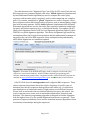
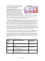
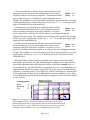
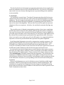
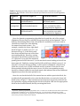
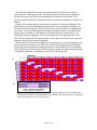
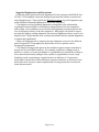
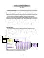
 Dynamic Programming User Manual v1.0 Anton E. Weisstein, Truman State University Aug. 19, 2014 Dynamic programming is a group of mathematical methods used to sequentially split a complicated problem into simpler sub-­‐problems. The overall solution is then generated by appropriately combining solutions to each sub-­‐problem. In bioinformatics, dynamic programming is mainly used to align nucleotide and amino acid sequences, and to predict RNA and protein folding from primary sequence data. The Excel workbook “Dynamic Programming” demonstrates this method’s application to the problem of nucleotide sequence alignment. Once the user selects an alignment type (global, semiglobal, or local), sets scoring parameters, and enters two short DNA sequences, the workbook then computes a matrix of scores from which it determines the optimal alignment. By adjusting the scoring system and switching among different types of alignment, the user can explore how these changes affect the inferred alignment. The workbook is designed to permit manual computation at key steps, and to automatically check the user’s work. 1. Scoring Matrix The first sheet in the workbook, named “Scoring Matrix”, demonstrates the calculations needed to fill in the dynamic programming (DP) matrix and calculate the optimal alignment score (Figure 1). First, the user enters two short DNA sequences (the query and the subject sequence) and defines a scoring system. The workbook uses this information to fill in the first few cells of the DP matrix: the user then manually completes the rest of the matrix. The workbook automatically flags any errors by highlighting them in red. Choice of alignment type Scoring system DNA sequences Dynamic programming matrix Figure 1 . Screenshot of the Scoring Matrix sheet, indicating user-­‐
controlled parameters. See accompanying text for details. Page 1 of 9 The radio buttons in the “Alignment Type” box (Cells A2–B7) control how the two DNA sequences are compared against each other. Global alignments (implemented by the Needleman-­‐Wunsch algorithm) are used to compare the entire query sequence with the entire subject sequence, such as when comparing two complete genes. By contrast, semiglobal or “glocal” alignments are used to compare a short query sequence with a much longer subject sequence, such as when aligning a single gene with an entire genome. Finally, local alignments (implemented by the Smith-­‐
Waterman algorithm) are used to search for short regions of similarity within both the query and subject sequences (e.g., to find shared motifs). For example, BLAST (Basic Local Alignment Search Tool) is a local alignment algorithm (Figure 2) while CLUSTAL is a global alignment algorithm. The choice of alignment type entails key assumptions about the biological interpretation and the mathematical treatment of any gaps at the end of the DNA sequences: these assumptions may substantially affect which alignments are considered optimal. Figure 2 . Screenshot of the NCBI BLASTN page, used to compare a nucleotide query sequence to a nucleotide database. BLAST combines dynamic programming with heuristic methods that greatly reduce computational time. Different BLAST programs are available at http://blast.ncbi.nlm.nih.gov/Blast.cgi for nucleotide and protein searches. Cells B13–B16 show the scoring system used to align the DNA sequences. These values represent a hypothesis about the relative frequency of specific types of mutation since the two sequences diverged from each other (e.g., via speciation, gene duplication, or horizontal transfer). High positive scores indicate frequent events, such as nucleotides that are identical between the query and subject; low scores represent rarer events, such as nucleotide substitutions, insertions, and deletions. The dynamic programming algorithm is designed to find the alignment with the highest score (i.e., the optimal alignment between two sequences). These patterns of sequence similarity can be used to formulate tentative hypotheses about evolutionary relationships among the sequences. Page 2 of 9 Cells L9–AH9 and G13–G29 contain the two DNA sequences to be analyzed. These cells also bound the dynamic programming matrix (Cells I10–AH29) used to compute the score of each potential alignment. To understand this matrix, focus first on the 2×2 blocks separated by Figure 3 . A portion of the dynamic thick black lines. Each block represents the programming matrix. hypothesis that a nucleotide from one DNA sequence aligns with a specific nucleotide from the other sequence. For example, Figure 3 shows a block that proposes aligning an A in the subject sequence (top row) with a C in the query sequence (left-­‐hand column). The DP matrix is initialized by assigning a score to each block in the top row and the left-­‐hand column: these blocks represent initial gaps in the subject and query sequences, respectively. Each block’s score is printed in the colored cell in the block’s lower right-­‐hand corner. In a global alignment, blocks in the initial row and column receive scores that are multiples of the gap penalty assigned in Cell B16 (e.g., 0, -­‐6, -­‐12, -­‐18, etc.). In local alignments, initial gaps are not penalized, so each of these blocks instead receives a score of zero. Finally, glocal alignments penalize initial gaps only in the query sequence: the left-­‐hand column thus receives multiples of the gap penalty, while the cells in the top row all have a score of zero. The white cells within the remaining blocks display that block’s candidate scores. For each block, the candidate scores represent the different ways in which a particular alignment can be reached by adding one nucleotide or a gap to the end of the existing alignment. In other words, each candidate score represents a step to one block from an adjacent block. Three possibilities must be considered (Table 1; Figure 4): Table 1. Summary of alignment procedure. Score’s position in block Upper left-­‐
hand cell Upper right-­‐
hand cell Lower left-­‐
hand cell Alignment interpretation Calculation of candidate score Add one nucleotide to the end of sequence in the previous alignment (no gaps) Add one nucleotide to the end of the query sequence, and a gap to the end of the subject sequence Add one nucleotide to the end of the subject sequence, and a gap to the end of the query sequence Add match bonus or mismatch penalty Page 3 of 9 Add gap penalty Add gap penalty • The indicated block could have been reached from the block Subject: GA
diagonally above it and to the left, aligning the G in the subject sequence with the A in the query sequence. This would not add a Query: AC
gap to either sequence, resulting in the partial alignment shown at right. The candidate score for this path is given by the previous block’s score plus either a match bonus or a mismatch penalty: in this case, -­‐2 – 2 = -­‐4, as shown in the upper left-­‐hand cell of the indicated block. • Alternatively, the indicated block could have been reached Subject: A–
from the block immediately above it, which aligns the A in the Query: AC
subject sequence with the A in the query sequence. For this to occur, a gap must be added in the subject sequence, resulting in the partial alignment shown at right. The candidate score for this path is given by the previous block’s score plus a gap penalty: in this case, -­‐1 – 6 = -­‐7, as shown in the upper right-­‐
hand cell of the indicated block. • Finally, the indicated block could have been reached from the Subject: GA
block immediately to its left, which aligns the G in the subject Query: C–
sequence with the C in the query sequence. For this to occur, a gap must be added in the query sequence, resulting in the partial alignment shown at right. The candidate score for this path is given by the previous block’s score plus a gap penalty: in this case, -­‐8 –6 = -­‐14, as shown in the lower left-­‐hand cell of the indicated block. Although all three of these paths are possible, one of these paths is more likely than others. In particular, the path with the highest candidate score represents the most likely alignment path and is therefore chosen as the block’s actual score. In the example above, the indicated block is assigned a score of -­‐4, corresponding to an alignment that matches the subject sequence’s G with the query’s A, and the subject sequence’s A with the query’s C (see Figure 4). A block’s actual score is shown in the lower right-­‐hand cell, and colored to distinguish it from the candidate scores. (Note: in local alignments, any block that would receive a negative score is instead assigned a score of zero.) Scoring system Match 5 Mismatch –2 Gap –6
Figure 4 . Calculation of candidate and actual scores. Red arrows indicate the three candidate scores, computed by adding a match bonus or mismatch penalty (diagonal arrow) or a gap penalty (vertical and horizontal arrows) to the previous block’s score. The blue arrow shows the actual score, given by maximum of the candidate scores. See accompanying text for details. Page 4 of 9 The first few blocks in the dynamic programming matrix have been completed to show the candidate scores as well as actual block scores. For the rest of the matrix, only actual scores are shown, allowing the user to practice filling in the candidate scores manually. 2. Traceback The workbook’s second sheet, “Traceback”, demonstrates how the block scores computed on the previous sheet are used to infer the optimum (highest-­‐scoring) alignment. The user begins by identifying the last block in the alignment path, and then works backwards through the dynamic programming matrix one block at a time to the start of the alignment. The user then converts this path into an actual alignment of the two sequences. As before, the workbook automatically flags any errors. The overall process of dynamic programming consists of two steps: completing the DP matrix and tracing back the optimal path through that matrix. During the first step, block scores were entered in the forward direction, from the alignment’s start (the upper left-­‐hand corner of the matrix) to its end (lower right-­‐hand corner). By contrast, the traceback step is performed in the opposite direction. Moreover, there is no need to trace back every cell in the DP matrix: it is computationally less expensive to focus only on the blocks that represent the optimal alignment. Recall that global alignments are used to compare two complete sequences. An optimal global alignment thus always begins with block in the DP matrix’s upper left-­‐hand corner, and ends with the block in the lower right-­‐hand corner. As a result, the traceback procedure starts at the block in the lower right-­‐hand corner of the DP matrix, and terminates at the block in the upper left-­‐hand corner. In contrast, because glocal alignments are used to match a short query sequence with part of a longer subject sequence, either or both sides of the subject sequence may extend past the aligned region. These portions of the subject sequence, often called terminal gaps, should be omitted from the alignment. The traceback for an optimal glocal alignment therefore begins at the highest-­‐scoring block in the last row (the query sequence’s last nucleotide), and terminates upon reaching any block in the DP matrix’s second row (corresponding to the first nucleotide in the query sequence). Finally, local alignments are used to find short areas of similarity within longer sequences. Either or both sequences may therefore contain terminal gaps. The traceback for an optimal local alignment therefore begins at the highest-­‐scoring block within the DP matrix, and terminates at the last block to have a positive score. Table 2 summarizes these rules. Page 5 of 9 Table 2 : Beginning and end points for the traceback procedure for different types of alignment. Note that the start of the traceback represents the end of the actual alignment, and vice versa.
Alignment type Global Glocal (semiglobal) Local Traceback begins at… Traceback ends at… Lower right-­‐hand corner of the traceback matrix Highest-­‐scoring block in last row of traceback matrix Upper left-­‐hand corner of traceback matrix Whichever block in the 2nd row is reached first when tracing back the alignment Highest-­‐scoring block in entire Whichever block is the last to traceback matrix have a positive score when tracing back the alignment Once the dynamic programming algorithm has located the end of the optimal alignment, the next step is to identify the previous block in the alignment. This is done by determining which of the current block’s candidate scores were used to calculate its actual score, then deleting the unused traceback arrows1. For example, consider the lower right-­‐hand block in Figure 5, with a score of -­‐1. As discussed on pp. 2–3, this block could have been reached from any of the three surrounding blocks. However, coming from block P would have yielded a score Figure 5. A portion of the traceback m atrix. of -­‐4 (block P’s score plus the mismatch penalty) instead of the observed -­‐1, so the traceback arrow leading to block P has been removed. Similarly, coming from block R would have yielded a score of -­‐14 (block R’s score plus the gap penalty), so this option is eliminated. Only block Q yields the correct score, so this traceback arrow is retained. Note that in cases where multiple blocks yield the correct score, all of the corresponding arrows should be retained within the traceback matrix: this indicates that several different alignments produce the same optimal score. Once the user has deleted all of the unused arrows within a particular block, the workbook will automatically color-­‐code that block white, as seen in the lower left-­‐
hand corner of Figure 5. Any traceback arrows that were incorrectly removed can be replaced by copying and pasting the block in Cells AA4–AB5 into the appropriate block in the traceback matrix, thereby resetting that block. P R 1
Q In practice, dynamic programming algorithms store or “memo-ize” the direction from which each block is
reached when calculating scores in the forward pass (pp. 3–4), then use that information to quickly
determine the traceback path. This approach is computationally more efficient, while yielding the same
result as the procedure outlined in this manual.
Page 6 of 9 Now that the alignment has been traced backward one step, the procedure is repeated for the subsequent steps. If multiple traceback arrows were retained at the previous step, each of the corresponding blocks must be traced back. This process continues until the traceback reaches a termination condition as specified in Table 2. Finally, the traceback path is converted into a pairwise sequence alignment. The first block in the optimal alignment corresponds to one nucleotide in sequence #1 (Cell L9) and one in sequence #2 (Cell G13): these two nucleotides are aligned with each other. As the traceback path is followed through the matrix, new nucleotides and/or gaps are added to each sequence following the rules stated in Table 1 to obtain the sequence alignment. The user can then enter this alignment into Cells C28–C29: the workbook will automatically recolor these cells if the user’s proposed alignment matches the optimal alignment. In cases where ties occurred during the traceback process, several alignments will produce the same optimal score. While this scenario is biologically quite plausible (especially given the simple scoring system that we have defined), it is not handled correctly by the current version of this workbook. In this case, the warning message “>1 Optimal Alignment” will display in Cells A31–D32 (Figure 5b). a. b. Figure 5 . (a) A completed traceback matrix for global alignment. The traceback path, consisting of the blocks containing white cells, identifies the optimal pairwise alignment between sequences 1 and 2, as given in (b). Page 7 of 9 Suggested Explorations and Discussions • Generate global, glocal, and local alignments for the sequences AACGCAGT and CTCATG. Give examples of specific biological questions for which you would use each alignment type. Then explain the biological reasons why each alignment type yields a different optimal alignment for these two sequences. • The highest-­‐scoring (optimal) alignment corresponds to the relationship requiring the least amount of evolutionary change between the two sequences under study. How confident can you be that this alignment accurately reflects the true evolutionary history of the two sequences? Why might it be useful to report not only the highest-­‐scoring alignment, but also any alignments whose score is just slightly lower? (Equivalently, how could you determine that the optimal alignment is statistically significant?) • Why is it inappropriate to compare the raw alignment scores for two different pairs of sequences? How might you adjust these scores to permit a more meaningful comparison? • The simple scoring system given in the worksheet ignores many evolutionary properties of actual DNA sequences. For example, transitions (changes from a purine to a purine, or from a pyrimidine to a pyrimidine) are usually more likely to occur than transversions (changes from a purine to a pyrimidine or vice versa). Similarly, based on parsimony, a single insertion or deletion of 3 consecutive nucleotides is much more likely than three separate insertions or deletions of one nucleotide each. Propose a more sophisticated scoring system that accounts for these characteristics. Page 8 of 9 3. Terms and Conditions You may use, reproduce, and distribute this module, consisting of both the software and this associated documentation, freely for all nonprofit educational purposes. You may also make any modifications to the module and distribute the modified version. If you do, you must: • Give the modified version a title distinct from that of the existing document, and from all previous versions listed in the "History" section. • In the line immediately below the title, replace the existing text (if any) with the text "© YEAR NAME", where YEAR is the year of the modification and NAME is your name. If you would prefer not to copyright your version, then simply leave that line blank. • Immediately below the new copyright line (even if you left it blank), add or retain the lines: Original version: Dynamic Programming 1.0 © 2014 Anton E. Weisstein See end of document for full modification history • Retain this "Terms and Conditions" section unchanged. • Add to the "History" section an item that includes at least the date, title, author(s), and a description of the modifications, while retaining all previous entries in that section. These terms and conditions form a kind of "copyleft," a type of license designed for free materials and software. Note that because this section is to be retained, all modified versions and derivative materials must also be made freely available in the same way. This text is based on the GNU Free Documentation License v1.2, available from the Free Software Foundation at http://www.gnu.org/copyleft/. History Date: Aug. 19, 2014 Title: Dynamic Programming Manual v1.0 Name: Anton E. Weisstein Institutions: Washington University and Truman State University Acknowledgements: This work was supported by a Freiburg Visiting Scholarship provided by Washington University in St. Louis. Modifications: None (original version). Page 9 of 9