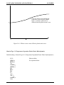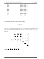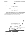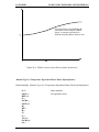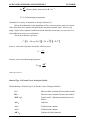
1
LS-INGRID: A Pre-Processor And Three-Dimensional Mesh Generator For The Programs LS-DYNA, LS-NIKE3D And TOPAZ3D Version 3.5 Livermore Software Technology Corporation 2876 Waverley Way Livermore, CA 94550 August 1998 Mailing Address: Livermore Software Technology Coporation 2876 Waverley Way Livermore, California 94550-1740 Support Address: Livermore Software Technology Corporation 97 Rickenbacker Circle Livermore, California 94550-7612 FAX: 510-449-2507 TEL: 510-449-2500 EMAIL: [email protected] Copyright 1989-1998 by Livermore Software Technology Corporation All Rights Reserved LS-INGRID TABLE OF CONTENTS TABLE OF CONTENTS ABSTRACT .............................................................................................................................................. I.1 PREFACE.................................................................................................................................................. I.1 1. LS-INGRID BASICS ........................................................................................................................... 1.1 1.1 The Parser............................................................................................................................. 1.1 1.2 Command File Format.......................................................................................................... 1.2 1.3 The Calculator ...................................................................................................................... 1.2 1.4 Built in Variables ................................................................................................................. 1.3 1.5 Basic Arithmetic Options ..................................................................................................... 1.4 1.6 Logical Operations ............................................................................................................... 1.4 1.7 Functions .............................................................................................................................. 1.4 1.8 Options ................................................................................................................................. 1.5 1.9 Directives ............................................................................................................................. 1.6 2. Control Commands............................................................................................................................... 2.1 3. IDEAS Part........................................................................................................................................... 3.1 3.1 Options and Functions.......................................................................................................... 3.1 4. PATRAN Part....................................................................................................................................... 4.1 4.1 Options and Functions.......................................................................................................... 4.1 5. NASTRAN Part..................................................................................................................................... 5.1 5.1 Options and Functions.......................................................................................................... 5.1 6. Standard Part ........................................................................................................................................ 6.1 6.1 DEFINITIONS ..................................................................................................................... 6.1 6.2 Index Progression ................................................................................................................. 6.10 6.3 Part Commands and Functions............................................................................................. 6.11 7. Beam Part .............................................................................................................................................. 7.1 7.1 Options and Functions.......................................................................................................... 7.3 8. Old Data Part ........................................................................................................................................ 8.1 8.1 Options and Functions.......................................................................................................... 8.5 9. MAZE Part ........................................................................................................................................... 9.1 9.1 Required Part Data ............................................................................................................... 9.1 9.2 Options and Functions.......................................................................................................... 9.3 9.3 Functions .............................................................................................................................. 9.5 10. EDIT Part............................................................................................................................................ 10.1 10.1 Options and Functions........................................................................................................ 10.1 11. DYNA3D Part .................................................................................................................................... 11.1 11.1 Options and Functions......................................................................................................... 11.1 12. Loads and Boundary Conditions......................................................................................................... 12.1 iii TABLE OF CONTENTS LS-INGRID 13. Interactive Commands ........................................................................................................................ 13.1 13.1 Exploded View Commands ................................................................................................ 13.10 13.2 TAURUS/Post-Processing Commands............................................................................... 13.11 14. Two-Dimensional Line Definitions .................................................................................................... 14.1 15. Three-Dimensional Line Definitions .................................................................................................. 15.1 16. Surface Definitions ............................................................................................................................. 16.1 17. Volume Definitions............................................................................................................................. 17.1 18. Coordinate Transformations ............................................................................................................... 18.1 19. LS-DYNA2D Commands and Materials ............................................................................................ 19.1 19.1 LS-DYNA2D Material Input.............................................................................................. 19.4 19.2 General Material Options ................................................................................................... 19.4 20. LS-DYNA3D Commands and Materials ............................................................................................ 20.1 20.1 LS-DYNA3D Material Input.............................................................................................. 20.13 20.2 General Material Options ................................................................................................... 20.13 21. Equations-of-State............................................................................................................................... 21.1 22. LS-NIKE2D Commands and Materials .............................................................................................. 22.1 22.1 LS-NIKE2D Material Input................................................................................................ 22.4 23. LS-NIKE3D Commands and Materials .............................................................................................. 23.1 23.1 LS-NIKE3D Material Input................................................................................................ 23.4 24. TOPAZ Commands and Materials....................................................................................................... 24.1 24.1 TOPAZ Material Input ....................................................................................................... 24.3 ACKNOWLEDGMENTS ......................................................................................................................... ACK.1 REFERENCES .......................................................................................................................................... REF.1 iv LS-INGRID INTRODUCTION LS-INGRID: A Pre-Processor and Three Dimensional Mesh Generator for the Programs LS-DYNA, LS-NIKE3D and TOPAZ3D. ABSTRACT LS-INGRID is a general purpose pre-processor for the programs, LS-NIKE2D[1], LS-NIKE3D[2], LS-DYNA2D[3], LS-DYNA3D[4], TOPAZ2D[5] and TOPAZ3D[6]. It can be used as a simple translator to convert various databases to these programs. In addition, it is a general purpose three-dimensional mesh generator with considerable capability to deal with complex geometries and allows for parametric geometric modeling. PREFACE LS-INGRID is an alternative mesh generator for finite element modeling which is principally intended as "research" program or one that focuses on various capabilities and techniques which are not addressed by commercial mesh generators. As a general purpose mesh generator, the capabilities are fairly complete with a wide range of geometric capabilities. An extensive parametric modeling capability is also support. LS-INGRID is most effective in combination with NIKExx and DYNAxx. A considerable amount of effort has gone into making LS-INGRID support virtually every feature of these programs (an almost impossible task given the rate that LS-DYNA3D improves). Although the usage of LS-INGRID can seem somewhat combersome relative to more traditional mesh generation schemes, the productivity of users performing parametric modeling tasks with LS-INGRID can much higher in some cases. Unlike most general purpose mesh generators, LS-INGRID was developed by the Author for the sole purpose of aiding them in their routine analysis tasks. The original code was developed to assist in the preparation of SAP5 models at the University of Tennessee beginning in 1978. The 1978 program was loosely based on index space ideas obtained from the INGEN[7] program which was developed at Los Alamost National Laboratory. In 1981, the author moved to Lawrence Livermore National Laboratory. INGRID developments continued at LLNL on the side because LLNL was committed to the development of MAZE3D, but did not have any supported three-dimensional mesh generator. In 1985, the MAZE3D effort was finally abandoned and INGRID became the principal mesh generator of LLNL by default. At this time, the program was merged with the MAZE[8] program to produce a version similar to the current LS-INGRID. After 1985, development work continued at SPARTA with a steady evolution and the I.1 INTRODUCTION LS-INGRID addition of the parametric modeling capabilities. LS-INGRID is the latest version supported by LSTC. Development on LS-INGRID is continuing in the directions which proved most popular in the past. The emphasis will continue to be providing a general purpose capability focused on NIKExx and DYNAxx with much work being done to support advanced modeling capabilities which are not found in any other program. I.2 LS-INGRID LS-INGRID BASICS 1. LS-INGRID BASICS The LS-INGRID input file is an ASCII datafile which contains a complete description of the analysis. The commands are input using a parser which is simple and efficient, but also has a considerable amount of flexibility for dealing with complex situation. 1.1 THE PARSER The parser basically takes a stream of blank delimited character strings and number and decodes them for the program. The character strings are for commands or parameters and are arbitrary in length. Normally, only the first four characters are significant. Deviations from this rule are described in the documentation. Numbers can be input in a variety of formats ranging from simple integers to floating point numbers specified with an "E" format. If an error is detected in the decoding of a number, the user will be notified. All character input for commands or numbers is automatically converted to lower case for processing. Thus case selection can be performed strictly for the purpose of enhancing readability. Any number of commands and numbers can be placed on a single line of input with the only constraint being the 80 character input line limit. In the commands description, upper case characters or characters enclosed within quotes are commands which are to be typed exactly as lower (ignoring case). Lower case items represent variables which require input. Comments may be included by using a "c" anywhere in the input followed by a blank and the comment. If the comment does not begin in column 1, then the "c" must be preceded by a blank. Blocks of input lines can be commented by preceding the block with the character "{" and ending it with "}". Although items are normally blank delimited, commas can also be used to separate items. Two commas which are separated by blanks are treated as having the number 0 between them. Lists of numbers or character strings are input and terminated normally by a ";". This ";" does not necessarily need a blank between it and the last item. If the list is a list of numbers, then the list can be terminated by simply beginning the next command and eliminating the semicolon. A function calculator is also built into the parser to permit advanced programming techniques to be used. This calculator is invoked by placing the calculator command within two square brackets. If the parser is expecting a character string, then the function will be processed without any other effect on the command stream. If a number is expected, then the calculator will send whatever value it calculates to the program. See Section 1.3 for a detailed description of the calculator functions. 1.1 LS-INGRID BASICS LS-INGRID 1.2 COMMAND FILE FORMAT The LS-INGRID input file "ingridi" has a relatively free flowing input format with few restrictions, some of which are: - Define an item before using it; e.g. a line definition must occur before applying it to a part. Materials data and code execution options cannot be input until a code output option has been selected. Some commands have order dependent effects, e.g. rotating local coordinate systems successively about different axes. Many items which have names in LS-INGRID are assigned numbers for the analysis program. These numbers are assigned sequentially starting from one based on the order of first occurrence of names. The form of ingridi is as follows: Title line Control commands Part definition Control commands Part definition (format is 80al) (Section 2) (Section 3 - 8) . . . END 1.3 The Calculator The calculator is used to insert expressions into LS-INGRID input descriptions and is particularly useful for developing parametric models. When used in conjunction with the "include" command, it is possible to write programs for individual parts which can then be assembled into larger models. The calculator capabilities are invoked by inserting an expression anywhere in the input between two square brackets (e.g. [5*sin(30)]). If at that point in the input, LS-INGRID is expecting an integer or a floating point number, then the expression is evaluated and the results passed to LS-INGRID as either the nearest integer or floating point number. If a character string is expected, then the expression is evaluated and skipped over as if it were just a comment. 1.2 LS-INGRID LS-INGRID BASICS Within the calculator variables may be created and they will remain in effect until the program completes. Thus the expression [length=5*5] would store 25.0 into a variable named "length" and return 25.0 to LS-INGRID if a number is expected. This variable could be recalled later by [length]. Separate from the variable capability is a function capability. The function capability stores an expression which may consist of variables and other functions into a particular name for future evaluations. An example follows: [a=1] [b=2] [c=1] Set some variables so this won't evaluate improperly. [def root1(a,b,c)=(-b+sqrt(b*b-4*a*c))/2*a] [root1(2,1,0)] Define the function. Evaluate the function. The general form of the calculator's capabilities is as follows: [option name = expression] Following is a summary of the calculator capabilities: 1.4 BUILT IN VARIABLES Variable Value pi e # p e Result of last operation nnode The current node number is set to nnode when outside of a part. Until the first part is complete, nnode is zero. nbeam The current beam element number is set to nbeam outside of a part. Until the first part is complete, nbeam is zero. nbrick The current brick element number is set to nbrick outside of a part. Until the first part is complete, nbrick is zero. nbrick includes both regular bricks and 8-node shell elements. nshell The current shell element number is set to nshell outside of a part. Until the first part is complete, nshell is zero. npart This variable is set inside parts and is set to the current part number. 1.3 LS-INGRID BASICS LS-INGRID 1.5 BASIC ARITHMETIC OPTIONS Operator + * / ^ % Purpose Example Addition Subtraction Multiplication Division Exponentiation Modulo arithmetic 3+4 4-1 5.5*7.6 7.5/length 10^3 5%2 1.6 LOGICAL OPERATIONS The result of a logical operator is 1.0 if true and 0.0 if false. These may be used either as expressions or as part of "if-then-else-endif" constructs. Function == != < <= > >= && || ! Purpose Equal to Not equal to Less than Less than or equal to Greater than Greater than or equal to Logical and Logical or Negation 1.7 FUNCTIONS The angles in the following trigonometric functions are all in radians by default. This can be controlled by the "deg" and "rad" options listed in the "options" section below. Function Purpose sin(angle) cos(angle) tan(angle) asin(x) acos(x) atan(x) atan2(y,x) sinh(x) cosh(x) tanh(x) exp(x) Trigonometric sine. Trigonometric cosine. Trigonometric tangent. Inverse trigonometric sine. Inverse of trigonometric cosine. Inverse of trigonometric tangent. Two argument inverse tangent. Hyperbolic sine. Hyperbolic cosine. Hyperbolic tangent. Exponential. 1.4 LS-INGRID LS-INGRID BASICS ln(x) Natural logarithm. ln2(x) Logarithm base 2. log(x) Logarithm base 10. min(x1,x2, . . .) Minimum of arbitrary number of parameters. Maximum of arbitrary number of parameters. max(x1,x2, . . .) gcd(x1,x2, . . .) Greatest common denominator. lcm(x1,x2, . . .) Least common multiple. asa(angle,side,angle) Evaluate the triangle and return largest angle. ass(angle,side,side) Evaluate the triangle and return largest angle. sas(side,angle,side) Evaluate the triangle and return largest angle. sss(side,side,side) Evaluate the triangle and return largest angle. rnd Return a random number. rnd2 Return a random number but do not update the seed. 1.8 OPTIONS Function Purpose help help subject def name=expression Print the help message. Print help for any of the calculator functions or options. Define a function "name". Any time name is encountered in future expressions, it will be recursively evaluated. save filename Save all variables to file "filename". load filename Load variables from file "filename". quit Exit calculator (this will shut down LS-INGRID). rad All angles for trigonometric functions are assumed to be defined in radians (default). deg All angles for trigonometric functions are assumed to be defined in degrees. list List current active variables. flist List current definitions of functions. Determine the roots of the nth degree polynomial with root(cn, . . .,c1,c0) coefficients c0 through cn. factor(x) Factor x into prime coefficients. integral(e1,e2,f,v) Determine the integral of the function f with respect to the variable v. The limits are from e1 to e2 which may be expressions. A Romberg integration rule is used. degree n The degree of Romberg integration for the "integral" command is n (default=4). Simpson's rule corresponds to n=1 and the trapezoidal rule is n=0. solve (f1,f2, . . .,fn) for (x1=v1+d1, . . . xn=vn+dn) Solve a system of nonlinear equations. The equations are previously defined functions, f1 through fn. Variables x1 through xn must be listed and the calculator will attempt to determine them. Optional inputs include vi and di. The initial starting guess is vi and the initial increments for iterations are di. 1.5 LS-INGRID BASICS maxits n tol t display LS-INGRID Set the maximum number of iterations for the "solve" command to n (default=30). Set the convergence tolerance for the "solve" command to t (default=1e-6). The display command is a brute force method for improving results of a divergent solve command. Results are displayed after every iteration. if expr1 then expr2 else expr3 endif If expression 1 is true than evaluate expression 2. Otherwise, evaluate expression 3. 1.6 LS-INGRID LS-INGRID BASICS 1.9 DIRECTIVES LS-INGRID provides directives to control the flow of logic in command file descriptions. Directives begin in the first column of a line and no other commands are allowed on the same line as the directive. This capability is patterned similar to the preprocessor used in the C-programming language. DIRECTIVE FUNCTION #ELSE This is for #IF - #ELSE - #ENDIF constructs. #ELSEIF expression Perform conditional execution of the following input lines as part of an #IF - #ELSEIF #ENDIF construct.The results of expression should be either true (1) or false (0). #ENDIF This signifies the end of an #IF - #ENDIF block. #ENDMACRO End definition of macro initiated by #MACRO. #IF expression Conditionally execute the following lines of input. The results of expression should be either true (1) or false (0). #INCLUDE name Begin execution of commands in file name. When a #RETURN or an end-of-file is encountered, control is returned to the original file. #MACRO name Begin definition of macro name. The definition ends when an #ENDMACRO is encountered. #RETURN Cease reading input from the current input file and return control back to the next higher level file. See also #INCLUDE. 1.7 LS-INGRID CONTROL COMMANDS 2. Control Commands Control commands are optional and can be input in any order. They must not be placed inside a part. The following control commands are available: ARRI lc Generate arrival times for pressure surfaces associated with load curve lc. Arrival times are generated by assuming that the loads are caused by a wave. This wave starts from a threedimensional point, line, or surface and travels with a velocity. The arrival time is the time required for the wave to travel from the source to an individual pressure segment. Options: CG p CL p COSINE DECAY d type [a] LINE px py pz vx vy vz PLANE px py pz vx vy vz POINT px py pz TOFF dt VELO vel ; Pressure cannot exceed p. Pressure cannot be less than p. (This option is selected with p=0.0 when "COSI" is executed). The pressure varies as a function of the angle between the pressure segments normal and the direction of the wave from the source. The pressure wave decays as a function of the distance from the source. The distance at which the scale factor for the input pressure equals 1.0 is d. The type of decay is specified by type. type = "R": relationship is 1.0/R = "R2": relationship is 1.0/R2 = "R3": relationship is 1.0/R3 = "CONSTANT": no decay = "EXP": relationship is 1.0/Ra The source is a line. (px py,pz) is any point on the line and (vx,vy,vz) is any vector along the line. The source is a plane. (px,py,pz) is any point on the plane and (vx,vy,vz) is any vector normal to the plane. The source is a point located at (px py,pz). Add dt to the arrival time. The wave travels with velocity vel. Terminate this command. 2.1 CONTROL COMMANDS LS-INGRID BATCH LS-INGRID is to operate in batch mode. The interactive commands are placed at the end of the LS-INGRID model description so that they can be read automatically. A graphics device will still be requested since one of the batch output devices may be desired. If no graphics are needed use the NOPL command. BELT This section defines the properties of seat belt systems, but possibly has other applications. The seat belt capability is supported in LS-920 and later. A detailed description is included in the LS-920 manual. SLIPRING name Define a slipring. Slip rings provide for a contiuous feeding of material through a pully. One node for the slip ring is fixed to a support structure. The slip ring logic works with seatbelt elements. Two seatbelt elements must also be identified which touch the slip ring. The friction coefficient, f, determines the resisting force to the belt being pulled through the slipring. FRIC fFriction coefficient for material sliding through the slip ring. ; End of slipring definition. RETRACTOR name Define a retractor. Retractor elements simulate the normal function of retrator systems for seat belts within an automobile. DELAY dt FEDL feed_length LCL lcl LCU lcu PULL pullout SENSOR name ; PRETENSIONER name Time delay for retractor operation. Load curve for loading. Load curve for unloading. Amount of pull-out between time delay ending and retractor locking. Sensor for trigering retractor. At least one must be specified and no more than four. End of retractor definition. Define pretensioner. During an automobile accident, pretensioners are frequently employed to automatically increase the tension on a seatbelt. Both pyrotechnic and spring type systems are supported. Usually, a sensor triggers the event. PYROTECHNIC LCP lcp RETR name TIME t Use a pyrotechnic pretensioner. Load curve for pretensioner. Retractor name effected. Time between sensor triggering and pretensioner acting. 2.2 LS-INGRID CONTROL COMMANDS PRELOAD DELAY dt SPRING ispd LOCK DELAY dt SPRING ispd The pretensioner consists of a preloaded spring. Time between sensor triggering and pretensioner acting. Spring element number. The pretensioner consists of a lock spring which is removed. Time between sensor triggering and pretensioner acting. Spring element number. DISTANCE The distance between nodes is locked. SENSOR name Pretensioner is activated by one to four sensors. ; End of pretensioner definition. SENSOR name Define sensor. A variety of sensor systems are incorporated into automobiles to sense the onset of a crash. The accelerometers are simply used for saving output to an ASCII file. The other sensors are used to initiate the retractors and pretensioners. ACCE a X Y Z TIME dt The sensor is an accelerometer. The acceleration is measured in the x-direction. The acceleration is measured in the y-direction. The acceleration is measured in the z-direction. The sensor is triggered if a is exceeded for duration dt. RETR The sensor triggers based on the retractor pullout rate. Retractor name. Pullout rate. Time over which rate of pull-out must be exceeded. RETR name RATE r TIME t TIME t The sensor triggers after time t. DIST The sensor triggers based on the distance between two nodes. Maximum distance. Minimum distance. DMAX dmax DMIN dmin ; ; CNV n End of Sensor definition. End of BELT command. Define control volume n. (MVMA/DYNA3D, LS-910 and later.) Options: 2.3 CONTROL COMMANDS DAMP d MATE m1 . . . mn ; PSCA psca REVERSE TYPE m VINI vini VSCA vsca LS-INGRID Set airbag damping constant to d. The airbag consists of material subset m1 . . . mn. Pressure scale factor used for converting pressures calculated by the thermodynamic control volume to pressures which will be applied to the finite element model. (default=1.0) Reverse normals. Control volume is of type m. Input for type m control volume begins immediately. Initial filled volume. (default = 0.0) Scale factor for converting calculated volume to volume used for thermodynamic calculations. (default = 1.0) Type 1: The pressure-volume relationship is of the form: Pressure = p0 * s/Relative volume P0 p0 SCAL s ; Initial pressure. Scale factor. Terminate control volume input. Type 3: The pressure-volume relationship is of the form: (γ +1 ) 2 γ γ γ Ýout = A 2 pρµ m Q − Q γ − 1 where Q = \f(pe,p) γ = \f(cp,cv) p = \f((γ – 1)E,V) Options: CV cv CP cp TIN t LCM lcm MU m Heat capacity at constant volume. Heat capacity at constant pressure. Input gas temperature. Load curve defining input mass flow rate. Shape factor for exit area. If m is negative, then |m| is the number of a load curve which defines the shape factor as a function of pressure. 2.4 LS-INGRID Aa PE pe RHO r GRAV g ; CONTROL COMMANDS Exit Area. If a is less than zero, then |a| is the number of a load curve which defines the area as a function of pressure. Ambient pressure. Ambient density. Gravitational constant. If the ambient density is defined in units of weight per volume, then the actual gravitational constant must be used. Otherwise, g is set to 1. Terminate control volume input. Type 4: Type 4 applies a constant internal pressure scaled by s until a point in time. A load curve is used to cause a change in behavior at some point in time. When the change occurs, the volume of the control volume is first calculated and used to initialize an adiabatic gas relationship. PINT pint LC lc SCAL s PE pe RHO r GAMM g ; Type 5: Interior pressure. Load curve. Scale factor for pressure. Ambient pressure. Density of gas when initialized. Ratio of specific heats. Terminate control volume input. Type 5 is an implementation of the Wang-Nefske airbag model. CV cv CP cp TIN t LCM lcm C23 c23 A23 a23 CP23 c23¢ AP23 a23¢ PEXT pe RHO r GRAV g VOLT v LCOUT lc PINI p0 PPOP ppop ; COOR nc data Heat capacity at constant volume. Heat capacity at constant pressure. Input gas temperature. Load curve defining input mass flow rate. Shape factor for exit hole. Exit hole area. Shape factor for exit porisity. Exit hole porosity. Ambient pressure. Ambient density. Gravitational constant. Optional tank volume. Optional load curve specifying exit flow as a function of pressure. Optional initial overpressure (gauge). Optional pressure where a plug is assumed to pop and venting begins. Terminate control volume input. Input nc global coordinate systems. Global coordinate systems remain in effect until reset using this command. Coordinate system data is 2.5 CONTROL COMMANDS LS-INGRID described in detail in the section on Coordinate Transformations. CSCA s Scale all nodal coordinates by s. CSYM Define cyclic symmetry interface. Options: AXIS px py pz The vector which orients the axis for rotational cyclic symmetry is (px,py,pz). ; Terminate the CSYM command. DEFAULT dir The default directory for finding include files is dir. Currently, this is only supported on CONVEX computers. DETP mat Define detonation point for material mat. If mat is zero then all materials are detonated. Options: LNPT px py pz qx qy qz n Generate n equals spaced detonation points on the line from (px,py,pz) to (qx,qy,qz). POINT px py pz Detonate the point (px,py,pz). TIME t Lighting time for detonation point. ; Terminate this command. DN2D i j Output generated is compatible with LSDYNA2D i and j flags specifying which 3-D coordinates correspond to the LS-DYNA2D r and z coordinates. i and j can have values "x", "y", or "z". This activates additional commands which are described in LS-DYNA2D Options and Materials. DN3D Output is generated for LS-DYNA3D. This activates additional control commands which are described in LS-DYNA3D Options and Materials. DS n Input digitized 3-D surface number n. Digitized surfaces consist of a surface defined by triangles. This is not smooth for coarse meshes; however, 10,000 and more triangles are common in defining surfaces to achieve 2.6 LS-INGRID CONTROL COMMANDS reasonably accurate definitions. This command consist of "DS n" optionally followed by a coordinate transformation and then one of the digitized surface types is input to complete the command. Option: MOVE data Move the surface definition by data. data is described in the section on Coordinate Transformations. Type 1: GRID ni nj The surface is defined by a logically regular set of points in three dimensions. ni*nj points must be input in the following order. x11 y11 z11 ... xil yi1 zi1 ... xij yij zij. Type 2: FEM m n The surface is a grid of finite element quadrilaterals. It has m nodes and n elements. x1 y1 z1 x2 y2 z2 ... i1 j1 k1 l1 i2 j2 k2 l2 ... Type 3: CONT ncont Input m nodal points. Input n four node elements. The surface is defined by ncont contours that each have an arbitrary number of points. Options: XLE x YLE y ZLE z CHORD scal FNU nu FNL n1 XF xf YF yf ZF zf L3D l L3E l n ; Data: n x1 y1 z1 ... xn yn zn X-coordinate of leading edge. Y-coordinate of leading edge. Z-coordinate of leading edge. Scale factor for the chord length. The contour is defined by nu points on the upper surface followed by n1 points on the lower surface. Contour points are in the plane X=xf. Contour points are in the plane Y=yf. Contour points are in the plane Z=zf. Use three-dimensional line definition l. The number of points on the contour is the number of points used to define the line definition. Use three-dimensional line definition l with n equal spaced points. Terminate option and read required data. Skip this section if L3D or L3E is requested. Number of points on contour. (Input only if nu=n1=0). Contour coordinates. If XF was used, do not input any X coordinates, and similarly for YF and ZF. 2.7 CONTROL COMMANDS LS-INGRID Type 4: FUNC ns nt x y z Define a parametric surface using parameters s and t. The number of points for making a grid in the s direction is ns and the number of points in the t direction is nt. s and t are assumed to range from 0 to 1. x, y and z are input as functions of s and t. Type 5: PROJ m offset The current digitized surface is formed by taking digitized surface m and projecting m a distance "offset" in the normal direction. Options: XSYM xsym xtol Digitized surface m is symmetric about X=xsym. This forces normal components of points within xtol of the symmetry plane to be in the Y-Z plane only. YSYM ysym ytol Digitized surface m is symmetric about Y=ysym. This forces normal components of points within ytol of the symmetry plane to be in the X-Z plane only. ZSYM zsym ztol Digitized surface m is symmetric about Z=zsym. This forces normal components of points within ztol of the symmetry plane to be in the X-Y plane only. ; End digitized surface definition. END Terminate the model description. FDEF n v1 v2 v3 v4 v5 v6 v7 v8 v9 Define fold plane number n. Fold planes are used later in the interactive phase to generate folded models of meshes such as airbags. The nine parameters have the following meanings: v1 = x or y position of fold relative to the unfolded mesh. v2 = x or y position of fold relative to the folded mesh. v3 = postive / negative fold flag. If v3=+1, then the folded portion lies along the positive coordinate. If v3=-1, then the folded portion lies along the negative coordinate. v4 = fold thickness desired. 2.8 LS-INGRID CONTROL COMMANDS v5 = Up / down flag. If v5=+1, then the material is folded onto the top of the mesh. If v5=-1, then the material is folded under the mesh. v6 = Direction. The fold plane is normal to the X-axis if v6=0 and normal to the Y-axis if v6=1. v7 = Fold logic flag. The thin fold logic is used if v7 = 0 and the thick fold logic is used if v7=1. v8 = Scale factor. This can be used to scale the normal thickness offsets at the fold point. This will increase the separation between layers, but possibly cause unacceptable mesh distortion. v9 = Fold radius. This will take precedence over the internally computed fold radius. See also FOLD and PFOLD under Interactive Commands. FIGN f expr When performing fold definition f, ignore nodes with undeformed coordinates that result in expr being true. (e.g. fign 6 [y<=0]). FLEX name Begin definition of flexure-torsion or cardan joints (LS-920 and later.) Options: CARDAN This joint is a cardan joint. FLEXION This joint is a flexion-torsion joint. LC1 lc1 First torque-twist load curve. LC2 lc2 Second torque-twist load curve. LC3 lc3 Third torque-twist load curve. LC4 lc4 Fourth torque-twist load curve. LC5 lc5 Fifth torque-twist load curve. LC6 lc6 Sixth torque-twist load curve. MATM m Define master material. MATS m Define slave material. MSYS s Define master side local system. 2.9 CONTROL COMMANDS LS-INGRID PHIF s First angle friction. PHIS s First angle stiffness. PSIF s Third angle friction. PSIS s Third angle stiffness. SSYS s Define slave side local system. STOPA- s Negative stop for first angle. STOPA+ s Positive stop for first angle. STOPB- s Negative stop for second angle. STOPB+ s Positive stop for second angle. STOPC- s Negative stop for third angle. STOPC+ s Positive stop for third angle. THEF s Second angle friction. THES s Second angle stiffness. FMOV f data After performing fold definition f, affected nodes are moved by the transformation described in data (see Coordinate Transformations). FOPT f options Input additional parameters for airbag folding. . Options: L3D Fold abour 3-D line denfinition ldnum. ANGLEθ Fold the material θ degrees. SCALE scale The folded section will become thicker by the factor scale. ; End of FOPT command. FSYM m x y z nx ny nz sf Define failing symmetry plane m. (x,y,z) is any point on the plane and (nx,ny,nz) is any normal vector. Solid element faces are slaved to the symmetry plane and failure occurs when the normal stress exceeds sf . GEOC igeo mat Geometric contact entity definition. A geometric contact entity is an analytical surface type which can be attached to a rigid body of 2.10 LS-INGRID CONTROL COMMANDS material mat. (MVMA/DYNA3D, LS-910 and later.) Options: COUPLE type n FRIC f INSIDE MATE m1 . . . mn ; MOVE n OUTSIDE PNLT p QUAD q SD n ; The contact is between a CAL3D/MADYMO coupled rigid body and a deformable body. The rigid body type is either "ELLIPSE" or "PLANE" and n is the number of the shape in either CAL3D or MADYMO. Set friction coefficient to f. The slaved mesh is the material subset m1 . . . mn. Move the entity using the global transformation number n. Penalty p. Quadrature rule. q=0: Nodes only. q=1: Element centers. q=2: 2«2 quadrature on segments. Use surface definition n. Valid surface types include planes, ellipsoids and spheres. Terminate this command. GMI n Increment the default material number by n for each global copy of a part. This number is initially set to zero. INCLUDE fname Include the information in file fname in the command stream. The INCLUDE command can perform to 20 levels deep. JD j Begin joint definition for joint j. Diagrams of the types of joints are shown in Figure 2-1. Nodes are assigned to joint definitions within parts. Options: SJ RJ CJ PJ UJ TJ PNLT p NC icode Spherical joint. Revolute joint. Cylindrical joint. Planar joint. Universal joint. Translational joint. Joint penalty. This joint is a simple nodal constraint. The common translational degrees of freedom are specified by icode: =-1: Rigid Massless Beam (LS-902 and later) 2.11 CONTROL COMMANDS RC icode REPE n ; LS-INGRID = 0: Rigid Massless Truss (LS-902 and later) =1: X =2: Y =3: Z =4: X and Y =5: Y and Z =6: Z and X =7: X, Y, and Z This joint is a simple nodal constraint. The common rotational degrees of freedom are specified by icode: =0: none =1: X =2: Y =3: Z =4: X and Y =5: Y and Z =6: Z and X =7: X, Y, and Z Repeat the current joint definition for a total of n joints. Terminate this command. 2.12 LS-INGRID CONTROL COMMANDS Spherical joint Revolute joint Cylindrical joint Planar joint Universal joint Translational joint Figure 2-1. Joint definitions. 2.13 CONTROL COMMANDS LS-INGRID L3D n data Begin definition of three-dimensional line n. If line n has been previously defined, this command has the effect of destroying the old definition. See Three Dimensional Line Definitions for a description of the data for this command. LABELS Define offsets for node, element and other item numbering. This applies to meshes which are imported after this command. Options: ELEMENT m Offset element labels by m. MAT m Offset material labels by m. NODE m Offset node labels by m. ; End of LABELS command. LCD n m t1 f1 ... tm fm Define load curve n with m pairs of time function points. LCDF n m f t1 tn Define load curve n with m pairs of time function points. f is input as an analytical function of variable t which ranges from t1 to tn. Thus to input one period of a sine wave with 100 points: LCDF 1 100 [sin(t)] [0] [2*pi] LD n data Begin definition of two-dimensional line n. If line n has been previously defined, this command has the effect of destroying the old definition. See Two Dimensional Line Definitions for a description of the data for this command. LEV n Define part transformation sequence n. This defines a series of operations which can be performed on groups of parts. Options: ADD m Add the list of transformations in sequence number m to the current sequence. COOR n data Add n coordinate transformations to the current sequence. The data for this command is described in the section, Coordinate Transformations. 2.14 LS-INGRID CONTROL COMMANDS CYLI Perform a cylindrical coordinate transformation. PROD i j Form the product of sequence i with sequence j. If sequence i has 1 transformations, and sequence j has m transformations,then this option produces 1*m transformations and adds them to the current sequence. REPE l1 l2 ...; Copy parts in global coordinate systems l1, l2, ... SPHE Perform a spherical coordinate transformation. ; Terminate this command. LMI n Increment the default material number by n for each local copy of a part. This number is initially set to zero. LSYS name Define local system name for single point constraints, etc. Options: PLANE px py pz rx ry rz The local X-axis is parallel to (px,py,pz) and (rx,ry,rz) is a vector in the XY-plane. 2 cx cy cz px py pz rx ry rz The center of the local system is (cx,cy,cz). (px,py,pz) is a point along the local X-axis and (rx,ry,rz) is a point in the XY-plane. NODE n1 n2 n3 The center of the local system is node n1. Node n2 is a point along the local X-axis and node n3 is a point in the XY-plane. ; Terminate LSYS command. MAT n data Code-dependent material data can be input. See the chapter on the specific computer program for input related to the MAT command. MATE m The default material name for the following parts is set to m. This name is initially set to 1. MAZT tol Set the MAZE tolerance to tol. This is used for a variety of two-dimensional line definitions and the MAZE parts. MDBC m lc amp fx fy fz Material displacment boundary condition. This command is used only for rigid body materials in DYNA3D. The load curve number is lc, amp is the scale factor and (fx,fy,fz) is in the load direction. 2.15 CONTROL COMMANDS LS-INGRID MKDS Make a binary database of digitized 3-D surfaces. Digitized surfaces are generated using the DS command and they are read back in using the RDDS command. This command is primarily intended to allow fast reinitialization during restarts of LS-INGRID. MFBC mat lc amp fx fy fz Apply force to rigid body material mat. The force is scale by load curve lc and factor amp and is in direction (fx,fy,fz).. MVBC m lc amp fx fy fz Material velocity boundary condition. This command is used only for rigid body materials in DYNA3D. The load curve number is lc, amp is the scale factor and (fx,fy,fz) is in the load direction. NFG name Define nodal force group name. Options: LSYS name The nodal force group is defined relative to local system name. (default=global) ; End of nodal force groups. NIP m1 m2 Non-interacting pairs of materials. This is used to determine lists of noninteracting segments for use by FACET to determine radiation view factors. NK2D i j Output generated is compatible with LSNIKE2D i and j flags specifying which 3-D coordinates correspond to the LS-NIKE2D r and z coordinates. i and j can have values "x", "y", or "z". This command activates additional control commands which are described in LSNIKE2D Options and Materials. NK3D Output is generated for LS-NIKE3D. This command activates additional control commands which are described in LS-NIKE3D Options and Materials. NOPL Do not perform plotting. This command suppresses the normal prompting for a graphics device and is useful in combination with the BATCH command. NOTE Input a not eto be included into the output file. Example: 2.16 LS-INGRID CONTROL COMMANDS NOTE "Copyright 1985" NSMOOTH n Perform n smoothing operations on surfaces when using the standard part. The default is zero since this can be costly and is usually necessary only for complex free form surfaces. ORV n {options} Input orientation vector n. Options: PLANE vx vy vz The sping/damper distances are measured in the plane defined by normal vector (vx,vy,vz). VECTOR vx vy vz The spring/damper distances are measured along the vector defined by (vx,vy,vz). ; End the ORV command. PAUSE Execute a FORTRAN pause statement. PLANE nplane Input nplane plane definition. These planes are for applying boundary conditions only. Do not try to use this command more than once in the same input file. Repeat the following information for each plane: px py pz Global coordinates of any point on the plane. qx qy qz Any vector normal to the plane. Tolerance All nodes within a distance less than tolerance from the plane are included in the definition. If the tolerance is negative, no nodes will be found. The "SW" command in the standard part can also be used to include nodes in the definition. Options: CYLI radius len FRIC m LCD lc vx vy vz The stonewall is a cylindrical surface. The radius is radius and the length is len. If len=0, then an infinite cylinder is assumed. (LS-910 and later). Specify stonewall friction properties. m=0: Frictionless sliding occurs. 0<m<1: m is colomb friction coefficient (LS-910 and later). m=1: No tangential motion allowed during contact. Load curve lc specifies the displacement history of the stone wall in the direction (vx,vy,vz). 2.17 CONTROL COMMANDS LCV lc vx vy vz MASS mass OVERRIDE i PLANE ax ay az alen blen PRISM ax ay az alen blen clen SPHE radius VELOCITY v LS-INGRID Load curve lc specifies the velocity history of the stone wall in the direction (vx,vy,vz). The stonewall has mass mass. (LS-910 and later). If a node is also on plane i, then this plane takes precedence. The stonewall is a finite plane. (ax,ay,az) is a vector which specifies an in-plane a-axis. The b-axis is determined from the cross-product of the a-axis with the normal vector. alen is the extent of the plane along the a-axis and blen is the extent along the b-axis. (LS-910 and later). The stonewall is a prism. (ax,ay,az) is a vector which specifies an in-plane a-axis. The b-axis is determined from the cross-product of the a-axis with the normal vector. alen is the extent of the plane along the a-axis and blen is the extent along the b-axis. c-len is the extent along the normal axis. (LS-910 and later). The stonewall is a spherical surface. The radius is radius. (LS-910 and later). The stonewall has a initial velocity v normal to the surface. (LS-910 and later). One of the following three options is required to terminate the plane definition: ASYM STONE or SW SYMM Asymmetric boundary conditions are applied to the nodes. The boundary condition is a stonewall. Symmetric boundary conditions are applied to the nodes. PPLV Eliminate the part transformation sequence at the top of the stack. See also "PPLV" and "LEV" in this section. PRINT v Echo the value of v to the terminal. This is primarily used with the calculator functions to verify calculations. PSCALE m1 m2 Scale properties. Materials from m1 to m2 are treated by this command. If m1 and m2 are numbers, than standard numeric comparisons are used to determine if materials are within the range. Otherwise, string comparisons are used. SECTION scale Scale all section properties by scale. This allows for a general unit conversion on section 2.18 LS-INGRID CONTROL COMMANDS properties. ; Terminate PSCALE command. PSLV n Begin performing part transformation sequence n on all following parts. This remains in effect until a PPLV command is given. A stack is used for performing transformation sequences. PSLV adds a transformation sequence to the top of the stack and PPLV eliminates the top sequence on the stack. QUAD Turn on generation of elements with quadratic shape functions in standard part. This causes 8node shells and 20-node bricks to be generated. RBMG m1 m2 Merge rigid body m1 to rigid body m2. m1 is the master and m2 is the slave. For a group of merged rigid bodies, there can be only one master. (DYNA3D only.) READ Read external database. Options: NDIV n Number of subdivisions for internal NURB surface processing. (Default=1) Setting this to 2 or 3 can improve the reliability of intersections calculated from NURB surfaces, however, costs and memory requirements will increase roughly proportional to the square of this number. NURB name Read a NURB surface database in file name. This ends the READ command. SC03 name Read a SC03 database in file name. This ends the READ command. ROTATION px py pz vx vy vz w Assign an initial rigid body rotation to all parts defined after this command. (px, py, pz) is any point on the axis of rotation and (vx, vy, vz) defines the axis direction. The angular velocity is w. RVBC m lc idof amp fx fy fz Rigid body velocity boundary condition. This command is used only for rigid body materials in DYNA3D. The load curve number is lc, amp is the scale factor and (fx,fy,fz) is in the load direction. idof can be: =1: X-translational degree-of-freedom =2: Y-translational degree-of-freedom =3: Z-translational degree-of-freedom 2.19 CONTROL COMMANDS LS-INGRID =.4: translational velocity in direction of vector (fx,fy,fz). =5: X-rotational degree-of-freedom =6: Y-rotational degree-of-freedom =7: Z-rotational degree-of-freedom =8: rotational velocity in direction of vector (fx,fy,fz). =9: Y and Z degrees-of-freedom for node rotating about the global X-axis =10: Z and X degrees-of-freedom for node rotating about the global Y-axis =11: X and Y degrees-of-freedom for node rotating about the global Z-axis SD n data Begin definition of surface n. If surface n has been previously defined, this command has the effect of destroying the old definition. See Surface Definitions for a description of the additional input for this command. SDMV s1 s2 data Move surface definitions s1 through s2. data is described in the section on Coordinate Transformations. SI islide Define sliding interface islide. These options apply to both slide surfaces and slide lines. Options: A3 Select contact interface type a3 (LS-920). Contact type a3 is insensitive to orientation of the contact segments. A5 Select contact interface type a5 (LS-920). Contact type a5 is insensitive to orientation of the contact segments. A13 Select contact interface type a13 (LS-920). This model is a single surface method which is principally used for inflating folded airbags. BIRTH t Birth time for interface (LS-910). BOND t GA slideline option: Bond shear modulus. BOXM xm xx ym yx zm zx Define box for master side of sliding interfaces (LS-910, VECDYNA). BOXS xm xx ym yx zm zx Define box for slave side of sliding interfaces. (LS-910, VECDYNA) COMP t GA slideline option: compressive strength of concrete. 2.20 LS-INGRID CONTROL COMMANDS DAMP d Damping coefficient (percent of critical) (LS910). DEATH t Death time for interface (LS-910). DNIS Discrete nodes impacting surface. DNTS Discrete nodes tied to surface. DUMMY Dummy slide surface. This option can be used to allow distinct but coincident nodes. FAIL e Tied slide surface with failure when volume weighted strain exceeds e (LS-DYNA3D). FD fd Dynamic friction coefficient. FE d Exponential decay coefficient. FFN f Normal failure force. FFNE f Normal failure exponent. FFS f Shear failure force. FFSE f Shear failure exponent. FRIC f Set static and dynamic friction to f. (default=0) FS fs Static friction coefficient. GA Select General Atomic's 1-D rebar slideline. HDMG t GA slideline option: Exponent in damage curve. LCV Load curve for force-penetration in types 19 and 20 contact. (LS-920 and later). LS Turn on limited search flag. (Default is off). MATERIAL MAST m1 m2 ... ; The master side of the interface consists of material subset m1, m2, ... (VEC/DYNA3D, LS920 and later). MATERIAL SLAV m1 m2 ... ; The slave side of the interface consists of material subset m1, m2, ... (VEC/DYNA3D, LS920 and later). MAXS t GA slideline option: maximum shear displacement. MERGE Coincident nodes are merged. 2.21 CONTROL COMMANDS LS-INGRID MSCA s Scale factor for master thicknesses. (LS-910 and later). MTHI t Master side thickness. (LS-910 and later). NFAIL fs Normal failure stress. NOMERGE Coincident nodes are not merged. NSWS Nodes spot welded to surface. PNLM p Change master side penalty to p. PNLS p Change slave side penalty to p. PNLT p Change penalty to p. RADIUS t GA slideline option: Radius of rebar. SETS Shell edge tied to shell surface. SFAIL fs Shear failure stress. SINGLE Single sided slide surface. SL Sliding only. SSCA s Scale factor for slave thicknesses. (LS-910 and later). STHI t Slave side thickness. (LS-910 and later). SV Sliding with voids (default). T10 Type 10 interface. T11 Type 11 interface. This is the box/material limited automatic contact for shells in LS-910 and later. It is the single surface airbag contact for MVMA/DYNA3D. T12 Type 12 interface. Automatic contact for shells. (LS-910 and later). T13 Type 13 interface. (LS-920 and later. Converts to the similar type 11 in MVMA/DYNA3D). T14 Type 14 interface. Surface to surface eroding contact. (LS-920 and later). T15 Type 15 interface. Node to surface eroding contact. (LS-920 and later). T16 Type 16 interface. Single surface eroding 2.22 LS-INGRID CONTROL COMMANDS contact. (LS-920 and later). T17 Type 17 interface. Surface to surface symmetric/asymetric constraint method. (LS920 and later). T18 Type 18 interface. Taylor and Flanagan contact force calculation technique from PRONTO3D. (LS-920 and later). T19 Type 19 interface. Rigid body to rigid body with specified force deflection curve. (LS-920 and later.) T20 Type 20 interface. Node to rigid body with specified force deflection curve. (LS-920 and later.) TBI Tie-break interface. TCRS r Thermal contact resistance is r. TIED Tied slide surface VFRI v ; Viscous friction coefficient is v. Terminate this slide surface definition. SPD n Input definition for spring/damper. Options: ROTA The spring/damper is rotary and not translational. Options (the following options end the SPD command): LE e Define a linear elastic spring with stiffness e. (force/displacement). LV d Define a linear damper with damping constant d. (force/velocity). IEP e t y Define an elastic-plastic spring with stiffness e (force/displacement), tangent stiffness t (force/displacement), and yield y (force). NE l Define a nonlinear spring using load curve l. l represents force versus displacement. NV l Define a nonlinear damper using load curve l. l represents force versus velocity. 2.23 CONTROL COMMANDS LS-INGRID GN ll lul b Yt Yc Define a general nonlinear spring. The spring loads along load curve ll and unloads along lul with hardening parameter b. The initial yield in tension is Yt and Yc for compression. (LS-910 and later). VE K0 Ki b Tc Fc iopt Three-parameter Maxwell viscoelastic spring. K0 is the short time stiffness, Ki is the long time stiffness with decay parameter b. Tc is a cutoff time and Fc is the force after cutoff. iopt is zero for an incremental treatment and nonzero for a continuous treatment. (LS-910 and later). TCO l Kul flag Inelastic tension or compression only. The spring loads along load curve l. Kul is an optional unloading stiffness and flag is -1.0 for tension only and +1.0 for compression only. (LS-910 and later). SLVM m1 m2 This command applies to the DYNA3D coupling with CAL3D or MADYMO3D. Deformable materials can be identified as being slaved to rigid bodies which are coupled to CAL3D or MADYMO3D. During the DYNA3D initialization, the deformable materials will be repositioned to reflect the shifting to global coordinates performed by CAL3D or MADYMO3D. The master rigid body is material m1 and the slaved deformable material is m2. (LS-920 and later.) STOL t Set the tolerance for surface intersections to t. (Default=1.0e-6.) STOP Execute a FORTRAN stop statement. SYNTAX Command for redefining the syntax of various part options. Options: REGION Set syntax for <Region> in part definitions. Options: STANDARD Set syntax for <Region> in standard part. Options: STANDARD Use the standard syntax for <Region> in the 2.24 LS-INGRID CONTROL COMMANDS standard part. ; Terminate SYNTAX command. MAZE Set syntax for <Region> in the MAZE part. Options: STANDARD The syntax for the <MRegion> is according to this manual and the 1985 INGRID manual from LLNL. PD The syntax for the <MRegion> has 6 indices according to the modification to INGRID by LLNL after 1986. ; Terminate SYNTAX command. OLD Set syntax for <Region> in the OLD, BEAM and other low level input parts. Options: STANDARD Use the standard definition of <Region>. This assumes <Region> = imin imax, unless the first item encountered is an expression in brackets. For an expression, it will only read one parameter. 1 Use a one paramter definition of <Region>. <Region> = imin=imax normally identifies single nodes and elements only, but can also identify a range with an expression. 2 Use a two parameter definition of <Region>. This does not allow an expression to specify the range, but is necessary for the following: B [nodebeg] [nodeend] 111000. This is because the standard method would see [nodebeg] and convert to a one parameter method. ; Terminate SYNTAX command. SYSEND Terminate existing subsystem definition. SYSTEM name Begin definition of subsystem name. This remains in effect until a SYSEND or another SYSTEM command is encountered or another 2.25 CONTROL COMMANDS LS-INGRID SYSTEM. T12 This command must be typed just prior to the use of the MAZE part. The third side, L3, of the next part will have exactly two times as many elements as side L1. The transition is accomplished with quadrilateral elements. This command does not apply to triangular parts. T13 This command must be typed just prior to the use of the MAZE part. The third side, L3, of the next part will have exactly three times as many elements as side L1. The transition is accomplished with quadrilateral elements. This command does not apply to triangular parts. TEMP t All parts defined after this command have initial temperature t. This remains in effect until reset with another "Temp" command. This can be overridden with an individual part. t can be a single number or it can be an expression of the form t(x,y,z). This allows nodes to be assigned temperatures based on an analytical expression of a temperature distribution based on the nodal coordinates. THIC t The default thickness for shells is t. TIND mat Ixx Ixy Ixz Iyy Iyz Izz Specify inertia tensor. TINE mat Ixx Iyy Izz Ixy Iyz Izx Specify inertia tensor. TIVE mat vx vy vx wx wy wz Initial velocities (global), translational and rotational TMCG mat cx cy cz Specify center of gravity. TMM n t The total mass of material n is t. The density of the material is determined by dividing the total mass of the material by the calculated volume. TMSM m s1 s2 ... ; The inertial properties which are input for material m include the masses of deformable materials s1, s2, .... The properties of m are computed such that the total mass properties of m, s1, s2 ... is equal to the input values. TMVP mat (transformation) Move center of gravity and inertias. Transformation refers to the section, Coordinate Transformations. TRACER Define tracer particles for material. 2.26 LS-INGRID CONTROL COMMANDS Options: LNPT px py pz qx qy qz n Generate n equals spaced tracer particles on the line from (px,py,pz) to (qx,qy,qz). MATERIAL t The tracer particle is fixed to a material point. POINT px py pz Define a tracer particle starting at point (px,py,pz). SPACE t The tracer particle is fixed in space. TIME t Activation time for tracer particle. ; Terminate this command. TRANS This command must be typed just prior to a MAZE part and changes the command such that k+m elements are generated along sides L1 and L2 and m elements are generated along sides L3 and L4. This command does not apply to triangular parts or parts with variable zoning. TZ2D i j Output generated is compatible with TOPAZ2D. i and j flags specifying which 3-D coordinates correspond to the TOPAZ2D r and z coordinates. i and j can have values "x", "y", or "z". This command activates additional control commands which are described in TOPAZ Options and Materials. TZ3D Output is generated for TOPAZ3D. A FACET input deck will also be created if necessary. This command activates additional control commands which are described in TOPAZ Options and Materials. WRITE format v1 v2 . . ; Issue a Fortran write statement. variables v1, v2, ... are written to standard out and format is the Fortran format statement. Example: WRITE "('I =',e13.5)" [i] ; XOFF dx Global X-offset. XSCA s Scale all X-coordinates. VD n data Begin definition of volume n. If volume n has been previously defined, this command has the effect of destroying the old definition. Volume Definitions describes the data for this command. 2.27 CONTROL COMMANDS LS-INGRID YOFF dy Global Y-offset. YSCA s Scale all Y-coordinates. VELOCITY vx vy vz Assign initial rigid body velocity (vx, vy, vz) to all parts defined after this command. vx, vy and vz can be functions of (x,y,z) to allow initial velocity distributions. ZOFF dz Global Z-offset. ZSCA s Scale all Z-coordinates. 2.28 LS-INGRID IDEAS PART 3. IDEAS Part The IDEAS part provides for importing SDRC/IDEAS neutral files into LS-INGRID. The form of the part is as follows: IDEA filename <optional functions> END filename is the name of the IDEAS neutral file. 3.1 OPTIONS AND FUNCTIONS Functions require the ability to identify groups of nodes and elements in a part and assign various properties. These have the general form of: Keyword <region> function data Where <region> is a part specific description of where the function is to be applied. For the current part, the nodes or elements through either node or element numbers or through analytical expressions. As an example: SI [mat==2] 1 M C Elements of material 2 are assigned to C the master side of contact interface 1. Variables available for function application are as follows: Variable xyz xg yg zg Description Part local coordinates of node or element center. Global coordinates of node or element node mat elem Node number. Material number. Element number. center. The following options are allowed in any order. Additional functions can be applied and are described in the section on Loads and Boundary Conditions. COOR nc data Input nc local coordinate systems. Coordinate system data is described in detail in the section on Coordinate Transformations. CYLI Nodes are converted from cylindrical to rectangular coordinates. The equations for this transformation are: X = R cos θ Y = R sin θ 3.1 IDEAS PART LS-INGRID LREP l1 l2 ... ln Repeat command. This command makes copies of the part in each of the local coordinate systems l1 to ln. If the coordinate system number is zero, the part is repeated with no transformation. MATE matnum The part has material number matnum. REPE l1 l2 ... ln Repeat command. This command makes copies of the part in each of the global coordinate systems l1 to ln. If the coordinate system number is zero, the part is repeated with no transformation. ROTA px py pz vx vy vz w Assign an initial rigid body rotation to the part. (px, py, pz) is any point on the axis of rotation and (vx, vy, vz) defines the axis direction. The angular velocity is w in radians per second. SPHE Nodes are converted from spherical to rectangular coordinates. The equations for this transformation are: X = R cos θ sin ϕ Y = R sin θ sin ϕ Z = R cos ϕ TEMP t The initial temperature of this part is t and it can be expressed as a function of x, y, z coordinates. THIC thic Plates have the thickness thic for this part. VELO vx vy vz Assign initial rigid body velocity to all nodes within this parts. (Vx, Vy, Vz) is the global velocity vector. (Vx, Vy, Vz) can be expressed as a function of x, y, z coordinates. 3.2 LS-INGRID PATRAN PART 4. PATRAN Part The PATRAN part provides for importing PATRAN neutral files into LS-INGRID. The form of the part is as follows: PATRAN filename <optional functions> END filename is the name of the PATRAN neutral file. 4.1 OPTIONS AND FUNCTIONS Functions require the ability to identify groups of nodes and elements in a part and assign various properties. These have the general form of Keyword <region> function data Where <region> is a part specific description of where the function is to be applied. For the current part, the nodes or elements through either node or element numbers or through analytical expressions. As an example: SI [mat==2] 1 M C Elements of material 2 are assigned to C the master side of contact interface 1. Variables available for function application are as follows: Variable xyz xg yg zg Description Part local coordinates of node or element center. Global coordinates of node or element node mat elem Node number. Material number. Element number. center. The following options are allowed in any order. Additional functions can be applied and are described in the section on Loads and Boundary Conditions. COOR nc data Input nc local coordinate systems. Coordinate system data is described in detail in the section on Coordinate Transformations. CYLI Nodes are converted from cylindrical to rectangular coordinates. The equations for this transformation are: X = R cos θ Y = R sin θ 4.1 PATRAN PART LS-INGRID LREP l1 l2 ... ln Repeat command. This command makes copies of the part in each of the local coordinate systems l1 to ln. If the coordinate system number is zero, the part is repeated with no transformation. MATE matnum The part has material number matnum. REPE l1 l2 ... ln Repeat command. This command makes copies of the part in each of the global coordinate systems l1 to ln. If the coordinate system number is zero, the part is repeated with no transformation. ROTA px py pz vx vy vz w Assign an initial rigid body rotation to the part. (px, py, pz) is any point on the axis of rotation and (vx, vy, vz) defines the axis direction. The angular velocity is w in radians per second. SPHE Nodes are converted from spherical to rectangular coordinates. The equations for this transformation are: X = R cos θ sin ϕ Y = R sin θ sin ϕ Z = R cos ϕ TEMP t The initial temperature of this part is t and it can be expressed as a function of x, y, z coordinates. THIC thic Plates have the thickness thic for this part. VELO vx vy vz Assign initial rigid body velocity to all nodes within this parts. (Vx, Vy, Vz) is the global velocity vector. (Vx, Vy, Vz) can be expressed as a function of x, y, z coordinates. 4.2 LS-INGRID NASTRAN PART 5. NASTRAN Part The NASTRAN part provides for importing NASTRAN input files into LS-INGRID. The form of the part is as follows: NASTRAN filename <optional functions> END filename is the name of the NASTRAN input file. 5.1 OPTIONS AND FUNCTIONS Functions require the ability to identify groups of nodes and elements in a part and assign various properties. These have the general form of: Keyword <region> function data Where <region> is a part specific description of where the function is to be applied. For the current part, the nodes or elements through either node or element numbers or through analytical expressions. As an example: SI [mat==2] 1 M C Elements of material 2 are assigned to C the master side of contact interface 1. Variables available for function application are as follows: Variable xyz xg yg zg Description Part local coordinates of node or element center. Global coordinates of node or element node mat elem Node number. Material number. Element number. center. The following options are allowed in any order. Additional functions can be applied and are described in the section on Loads and Boundary Conditions. COOR nc data Input nc local coordinate systems. Coordinate system data is described in detail in the section on Coordinate Transformations. 5.1 NASTRAN PART LS-INGRID CYLI Nodes are converted from cylindrical to rectangular coordinates. The equations for this transformation are: X = R cos θ Y = R sin θ LREP l1 l2 ... ln Repeat command. This command makes copies of the part in each of the local coordinate systems l1 to ln. If the coordinate system number is zero, the part is repeated with no transformation. MATE matnum The part has material number matnum. REPE l1 l2 ... ln Repeat command. This command makes copies of the part in each of the global coordinate systems l1 to ln If the coordinate system number is zero, the part is repeated with no transformation. ROTA px py pz vx vy vz w Assign an initial rigid body rotation to the part. (px, py, pz) is any point on the axis of rotation and (vx, vy, vz) defines the axis direction. The angular velocity is w in radians per second. SPHE Nodes are converted from spherical to rectangular coordinates. The equations for this transformation are: X = R cos θ sin ϕ Y = R sin θ sin ϕ Z = R cos ϕ TEMP t The initial temperature of this part is t and it can be expressed as a function of x, y, z coordinates. THIC thic Plates have the thickness thic for this part. VELO vx vy vz Assign initial rigid body velocity to all nodes within this parts. (Vx, Vy, Vz) is the global velocity vector. (Vx, Vy, Vz) can be expressed as a function of x, y, z coordinates. 5.2 LS-INGRID NASTRAN PART Notes: 1. The following NASTRAN keywords are supported: CBAR CELAS2 CONM2 CORD1S CORD2S CTETRA GRAV MPC PLOAD2 PSOLID SPC1 CBEAM CHEXA CORD1C CORD2C CPENTA CTRIA3 GRID PBAR PLOAD4 RBE2 CDAMP CMASS2 CORD1R CORD2R CQUAD4 FORCE MAT1 PBEAM PSHELL SPC 2. The following keywords from MSC/DYNA are also supported: DYMAT24 MATRIG 3. To preserve the arbitrary node, element and material numbering of NASTRAN input files, use the ARBITRARY command. (See LS-DYNA3D Commands and Materials.) 4. The material properties from the NASTRAN input are generally not used for LSDYNAxx calculations. To assign properties from LS-INGRID, the materials may be defined either before or after the NASTRAN part. The LS-INGRID material ID's are input the same as those of the NASTRAN input. If the LS-INGRID materials are defined prior to the NASTAN model input, but the sections are not input, then LS-INGRID will try to use the section property data from the NASTRAN input. Section properties may be scaled using the global command: PSCALE. 5. Node, element and material ID's can be shifted using the global command, LABELS. 5.3 LS-INGRID STANDARD PART 6. Standard Part 6.1 DEFINITIONS Index Space: An index space is a three-dimensional discrete coordinate system with integer values greater than or equal to 1 in each of the three directions. The three discrete coordinates are labeled, I, J, and K axes respectively. Each point in the index space (i, j, k), represents a nodal point. Elements are defined as groups of adjacent nodes in the index space. Region: A region is any rectangular or cubic block of nodes. A region is usually defined by a block in an index space. Part: A part is a collection of regions which can be grouped and generated conveniently in an index space. Beginning users will typically use one region per part while more experienced users will be able to group numerous regions together into complex parts. Model: The final model is a collection of parts. Each part has its own index space and is independent of other parts. Parts are connected together either by global coincident node removal, slide surfaces, or other constraints. The standard part in LS-INGRID is based on a three-dimensional index space which is commonly used for finite difference mesh generation. Although this can be somewhat awkward for finite element meshes, proper usage technique and some enhancements have made this quite effective for certain geometries including some that are difficult for standard finite element mesh generators. The principal enhancement to the three-dimensional index space is an additional type of index notion, the "Index Progression". Index progressions provide a concise and simple method for describing complex structures, and are used to input data to LS-INGRID. The following is a detailed description of the index space notion and the index progression. This information provides the user with the concepts necessary to use LS-INGRID effectively. Index Space Node generation in LS-INGRID is done by a mapping from Index space onto the object of interest as is shown in Figure 6-1. Each region of the object is referenced by a set of six indices; (IMIN, JMIN, KMIN) specify the minimum indices for a region in the index space and (IMAX, JMAX, KMAX) specify the maximum indices. For a solid region, all eight corner nodes are defined by combinations of minimum and maximum indices. Table 61 lists the indices of the vertices in the example of Figure 6-1. We assume that any set of three indices, (I, J, K), defines a region in space. If KMIN is set equal to KMAX, the resulting region is a plane of constant K as shown 6.1 STANDARD PART LS-INGRID in Figure 6-2a. Similarly, a plane of constant I is defined when IMIN is set equal to IMAX and a plane of constant J for JMIN equal to JMAX. A line in the index space is defined by holding two indices constant while the third index varies as shown in Figure 6-2b. K J G H E C F D A I B G Z H F C D Y B A X Figure 6-1. Mapping from index space to object space. 6.2 LS-INGRID STANDARD PART K J C (1, 5, 2) D (5, 5, 2) A (1, 1, 2) B (5, 1, 2) I Figure 6-2a. Planes in index space. K J (3, 5, 2) (3, 1, 2) I Figure 6-2b. Lines in index space. 6.3 STANDARD PART LS-INGRID TABLE 6-1. Indices associated with the vertices of a region. Node A B KMAX) C D KMAX) E F KMAX) G H KMAX) Indices (1, 1, 1) (5, 1, 1) Position (IMIN, JMIN, KMIN) (IMAX, JMAX, (1, 1, 2) (5, 1, 2) (IMIN, JMIN, KMIN) (IMAX, JMAX, (1, 5, 1) (5, 5, 1) (IMIN, JMIN, KMIN) (IMAX, JMAX, (1, 5, 2) (5, 5, 1) (IMIN, JMIN, KMIN) (IMAX, JMAX, An index space is defined as the set of all possible indices < <IMAX, < <JMAX, 1 < <KMAX. If an index is zero, then it varies over all possible indices. Thus, the indices (3, 0, 2) defines a line which extends across the index space, and (0, 0, 2) defines a plane which divides the index space into two regions. (0, 0, 0) defines the entire index space. Index Progressions Index progressions were developed to facilitate the defining of multiple regions in index space. Rather than specifying the minimum and maximum indices for a region, one simply specifies the progression in indices along the I, J, and K directions respectively. For example, the region (2, 7, 6, 8, 9, 10) is represented as the progression (2, 8); (7, 9); (6, 10). If there is a region adjacent to (2, 7, 6, 8, 9, 20) such as (2, 7, 2, 8, 9, 6), the two regions are defined together by a new progression (2, 8); (7, 9); (2, 6, 10). To define the four solids regions shown in Figure 6-3a requires the progression (3, 5, 7); (2, 4, 6); (1, 4). Index progressions for planes are defined in a similar manner. The index which remains constant throughout a plane is indicated by a negative sign so the plane (2, 5, 5, 2, 7, 8) is represented as (-2); (5, 7); (5, 8). In Figure 6-3b there are eight planes which can be represented by the progression (3, 5, 7); (2, 4, 6); (-1, -4). The savings by this notation is apparent since specifying separately the eight regions in Figure 6-3b requires 49 number where as the index progression requires only 8 numbers. 6.4 LS-INGRID STANDARD PART (7, 6, 4) (3, 2, 1) (a) Index Space (7, 6, 4) (3, 2, 4) (7, 6, 1) (3, 2, 1) (b) Object Space Figure 6-3. Index progressions for planes and solids. 6.5 STANDARD PART LS-INGRID Another addition to the index progression notation is the zero index. The two solids regions shown in Figure 6-4 could be represented as an index progression except that they are not connected. In this case, a zero index is used along the I direction to indicate that the structure is discontinuous. This gives the progression (2, 4, 0, 6, 8); (3, 7); ( 4, 5). Plane regions can be separated by the zero index in a manner similar to solid regions. More complicated regions can be represented by combining index progressions. An example of this is in Figure 6-5. The open box could be represented by two index progressions (-2, -5); (1, 7); (3, 5); and (2, 5); (1, 7); (-3, -5), but they can also be combined to give (-2, -5); (1, 7); (-3, -5). Figure 6-6 shows several more structures and their index progression representation. LS-INGRID uses the index progression notation to set up regions in the index space which are to be mapped onto the object of interest. This notation has the advantage that it requires little input data and with less than 20 indices can represent thousands of configurations in index space. In practice, not all configurations in index space can be defined by an index progression so a command is added to allow deletion of regions in the index space. The delete command along with the index progression is enough to produce almost any conceivable region in the index space and is used as the central part of LSINGRID's mesh generation. 6.6 LS-INGRID STANDARD PART Figure 6-4. Separated solid regions. Figure 6-5. Open Box. 6.7 STANDARD PART LS-INGRID (c) Cube in a Box ((-2, 4, 6, -8); (-2, 4, 6, -8); (3, 5)) (a) Intersecting Plates ((2, -4, 6); (2, -4, 6); (-3, -7)) (c) Examples of Region Deletion ((-2, -6, -10); (3, 7); (-2, -4)) Deleted Regions: (2, 3, 2, 6, 7, 2) and (6, 3, 4, 10, 7, 4) (d) Planes and Solids with Gaps ((2, 4, 0, 6, -8); (2, 4, 0, 6, 8); (-2, 4, 6, -8)) Figure 6-6. Examples of index progressions. 6.8 LS-INGRID STANDARD PART Each part definition consists of the following data: START Index progression Part control commands and functions Loads and Boundary Conditions END "START" signifies the beginning of a part definition and is require as the first card in each part. Part control commands affect properties of the mesh. Following is a list of the default properties for a part. 4 node plate elements 8 node solid element rectangular coordinates material property = 1 plate thickness = 0.0 The dimension of the index space along with all plane and solid regions are defined by the index progression. Function cards manipulate the mesh defined by the index progression and an "END" signifies the end of a part. Following are some important definitions in addition to those previously given. Index Space The set of all indices defined by an index progression. For example, the progression (2, 3, -5, 10), (4, 5), (2, 6) defines the index space 2^|I|^10, 4^|J|^5, 2^|K|^6. Reduced Index Space The reduced index space references positions in an index progression. The point, I, J, K in the reduced index space refers to the point in the index progression defined by the Ith integer in the I-progression, the Jth integer in the J-progression and the Kth integer in the Kprogression. For the progression (2, 3, -5, 10), (4, 5), (2, 6) the relationship between the reduced index space and the index space is shown in Table 6-3. Unless otherwise noted, all points and regions are defined in the reduced index space. Since the reduced index space is independent of the actual values of the index progression, the mesh can be refined or contracted only by changing the index progression. 6.9 STANDARD PART LS-INGRID Table 6-3. Comparison of the Reduced Index Space and the Index Space for the Index Progression (2, 3, -5, 10), (4, 5), (2, 6) Reduced Index Space 1, 1, 1 1, 1, 2 1, 2, 1 2, 2, 2 3, 1, 2 4, 1, 1 Index Space 2, 4, 2 2, 4, 6 2, 5, 2 3, 5, 6 5, 4, 6 10, 4, 2 6.2 Index Progression Each part must have an index progression. The following input is required. i1 i2 ... ii j1 j2 ... ji ; k1 k2 ... ki x1 x2 ... xi y1 y2 ... yi z1 z2 ... zi Progression in I direction Progression in J direction Progression in K direction Initial X-coordinates Initial Y-coordinates Initial Z-coordinates 6.10 LS-INGRID STANDARD PART 6.3 Part Commands and Functions All functions have the following form: Keyword - index specification - parameters Index specifications have three types which are abbreviated as <Point> , <Region>, or <Index Progression>. All index specifications are applied in the reduced index space. The input is defined as follows: <Point> Input for <point> consists only of the three indices (i,j,k). If any index is input as zero, then the index varies from the smallest to the largest possible value. <Region> The function locates the region defined by (im,jm,km,ix,jx,kx). If im, jm, or km is input as zero, the zero index is given the minimum possible value. If ix, jx, or kx is input as zero, the zero index is set to the maximum possible value. <Index Progression> This is used to define multiple regions according to the rules for index progression. If no indices are found for a list in a direction, then the function is assumed to go all the way through the index space in that direction. i1 i2 i3... ; j1 j2... ; k1 k2... ; Functions which use <Region> or <Index Progression> for index specification can be repeated and shifted to other parts of the index space. The general form of these commands is as follows: Keyword - <Region> or <Index Progression> parameters - first offset - parameters - second offset - parameters. The offset information is as follows: + -or- +o Either a "+" or a "+o" is required as the first information for the offset. If "+" is used then the offset occurs from the region defined by the last offset. If "+O" is used then the offset is relative to the region defined by <Region> or <Index Progression>. One and only one of the following commands must be input following "+" or "+o". 6.11 STANDARD PART LS-INGRID I di Increment I indices by di. J dj Increment J indices by dj. K dk Increment K indices by dk. IJ di dj Increment I and J indices by di and dj. JK dj dk Increment J and K indices by dj and dk. KI dk di Increment K and I indices by dk and di.` IJK di dj dk Increment I, J, and K indices by di, dj, and dk. SIJ Switch I indices with J indices. SJK Switch J indices with K indices. SKI Switch K indices with I indices. A <Region> Form a curved edge between nodes A and B. The region is a line in the reduced index space. ityp Flag specifying type of curve. =1: A parabola through point P1 (See Figure 6-7). =2: A circular arc through point P1. =3: A circular arc with center P2. x X-coordinate of point P1 or P2 y Y-coordinate of point P1 or P2 z Z-coordinate of point P1 or P2 r Radius If the radius is non-zero for a circular arc with center P2, then nodes A and B (See Figure 6-7) are moved radially from P2 until they are a distance equal to the radius from P2. An arc is formed through the nodes at their final location. 6.12 LS-INGRID STANDARD PART B P1 R A R P2 Figure 6-7. Curved boundaries. A, AE <Region> Arc keyword. The region is a plane or a solid in the reduced index space with an arbitrary length. idir Flag specifying axis of rotation in the index space. ="I": I-axis is axis of rotation ="J": J-axis is axis of rotation ="K": K-axis is axis of rotation r Radius For any plane normal to the axis of rotation such as ABCD in Figure 6-8, a point 0 on the axis of rotation is located in the center of the plane. If the radius of the cylinder is not zero, then the points A, B, C and D are moved radially from 0 until they are a distance, R, from point 0. Curved boundaries are then formed for the segments AB, BD, AC and CD using center.0. This is done for each plane normal to the axis of rotation in the reduced index space. 6.13 STANDARD PART LS-INGRID (IMAX, JMAX, KMAX) R A B R 0 C D (IMIN, JMIN, KMIN) Figure 6-8. Cylindrical region. AC, ACE <Region> <Region> is a surface in the index space. idir Flag specifying axis of rotation in the index space. ="I": I-axis is axis of rotation ="J": J-axis is axis of rotation ="K": K-axis is axis of rotation px py pz Any point on axis of cylinder (See Figure 6-9). r Radius of the cylinder. qx qy qz Any vector parallel to the axis of the cylinder. 6.14 LS-INGRID STANDARD PART u u′ Z Q r r v′ P v Y X Figure 6-9. Cylindrical surface. AUTO Perform automatic smoothing of edges and surfaces which represent continuous surface definitions.. BG Beam generation command. The BG command permits beam elements to be defined within parts defined using an index space. If only beam elements are desired for the part, then all of the shell and solid elements can be deleted. Options: MT m SC n NGEN n N1 <Point> P1 px py pz N2 <Point> P2 px py pz B1 n Beams have material number m. Beams have section number n. Generate n beams from point 1 to point 2. Point 1 is located at <Point> Point 1 is located at (px, py, pz) Point 2 is located at <Point> Point 2 is located at (px, py, pz). Set boundary code for point 1. n is a six digit binary number which specifies degrees of freedom which are to be constrained. Numbering the digits from left to right, they affect the following degree-of-freedom. 6.15 STANDARD PART V2 vx vy vz B2 n NO <Point> PO px py pz VOvx v y vz CO px, py, pz SO px, py, pz ; LS-INGRID 1st digit: x-displacement =0: free =1: fixed 2nd digit: y-displacement 3rd digit: z-displacement 4th digit: x-rotation 5th digit: y-rotation 6th digit: z-rotation Point 2 is offset from point 1 by the vector (vx, vy, vz). Set boundary code for point 2. n is has the same meaning as for the "B1" option in this command. The point defining the orientation of the local 2axis is located at <Point>. The point defining the orientation of the local 2axis is located at (px py pz). The local 2-axis is defined by vector (vx, vy, vz). Same as "PO" except the point is in cylindrical coordinates. Same as "PO" except the point is in spherical coordinates. Terminate this command. BIAS x0 y0 z0 vx vy vz r0 r1 f Bias mesh. This command is experimental. (x0,y0,z0,vx,vy,vz) represents a line towards which the elements are biased. A transition distance is defined beginning at r0 and ending at r1 and f is a factor for adjacent element scaling. COOR nc data Input nc local coordinate systems. Coordinate system data is described in detail in the section on Coordinate Transformations. CPL <Region> Center points along line. If <Region> is a line, then this command forces elements to be equally spaced from the beginning point to the ending point. If <Region> is a surface or a volume then the command is subdivided into lines in the direction specified by the direction flag. dir CYLI Direction flag (do not input if <Region> is a line). ="I": Equal space along I-index ="J": Equal space along J-index ="K": Equal space along K-index Nodes are converted from cylindrical to rectangular coordinates. The equations for this 6.16 LS-INGRID STANDARD PART transformation are: X = R cos θ Y = R sin θ D <Region> or Region deletion keyword. DI <Index Progression> EQSP Equal space along arc. This applies to the "AC" and "A" functions. FIND <Point> exp1 exp2 exp3 exp4 The FIND command places the generated coordinates of <Point> into the variables [cenx] [ceny] [cenz] and the node number into [node]. Four expressions must be input as part of this command. Example: FIND 1 2 1 [bp3x=cenx] [bp3y=ceny] [bp3z=cenz] [bp3n=node] I, J or K <Point> Specify independent variable for the function. ="I": coordinates vary as a function of the I-index. =J": coordinates vary as a function of the J-index. ="K": coordinates vary as a function of the K-index. dir2 Flag specifying which coordinate is modified. ="X": X-coordinate is modified. ="Y": Y-coordinate is modified. ="Z": Z-coordinate is modified. c1 c2 c3 ... New progression of coordinates along index dir1. INT <Region> s1 s2 Nodes within <Region> lie on the intersection of surface s1 and s2. Surfaces are defined using the "SD" command in the control section. These commands will be generated automatically if two "SF" commands result in an intersection surface in the index space. LORI vx vy vz Specify local axis for orthotropic shell elements. The vector in the local part system is (vx,vy,vz). The vector (vx,vy,vz) may be specified as a function of the local x,y,z coordinates. For example: 6.17 STANDARD PART LS-INGRID LORI [-y] [x] 0 LREP l1 l2 ... ln Repeat part command. This command makes copies of the part in each of the local coordinate systems l1 to ln. If the coordinate system number is zero, the part is repeated with no transformation. MA or MB Point functions. These commands are used to modify 1, 2, or 3 coordinates of groups of nodes. <POINT> For "MA" only. <REGION> For "MB" only. n Flag indicating which coordinates to change. ="X": x coordinate is changed ="Y": y coordinate ="Z": z coordinate ="XY": x and y coordinates ="XZ": x and z coordinates ="YZ": y and z coordinates ="XYZ": x, y, and z coordinates dx dy dz New coordinates. Only the coordinates required by flag n need to be input. The new coordinates are added to the old coordinates. MATE m The part has material number m. MS <Region> Apply multiple surface equations to <Region>. This command permits the identification of parallel index planes for the purpose of applying surface equations. The function of this command is similar to the "SF" command; however, this command can result in considerable reduction in input for many common cases. idir <Region> is divided into a series of parallel planes normal to the axis in index space specified by idir. ="I": I-axis ="J": J-axis ="K": K-axis Next, one surface equation must be input for each of the index planes in <Region> normal to the specified axis. One of the following options may be used. 6.18 LS-INGRID STANDARD PART Option 1: sf1 sf2 . . . Data for first surface equation (See Surface Definitions). Data for second surface equation. Option 2: PPX, PPY, or PPZ Parallel planes normal to x, y, or z axes respectively. u1 u2 u3 ... The point along the specified axis where the planes intercept. One value must be input for each plane. Option 3: CNSP px py pz Center of the spheres. r1 r2 r3 ... Radii. Option 4: CNCY px py pz Any point on the axis of the cylinder. vx vy vz Any vector parallel to the axis. r1 r2 r3 ... Radii. Option 5: PON, POX, POY, POZ Planes offset normal or in the x, y, or z direction, respectively. px py pz Any point on the plane. qx qy qz Any vector normal to the plane. o1 o2 o3 ... Offsets in the requested direction. MT <Region> or MTI <Index Progression> mat MTV m n Signifies material command. Material number. All elements contained within volume definition 6.19 STANDARD PART LS-INGRID m are assigned material number n. OR <Region> Specify orientation of local axes relative to the index space. This is necessary when orthotropic materials are used and/or if 8-node shells are requested. l1 Local r axis. ="I": I-axis ="J": J-axis ="K": K-axis l2 Local s axis. ="I": I-axis ="J": J-axis ="K": K-axis ORDER d1 d2 d3 Order of writing nodes in index space (d = "I", "J", or "K"). PA.i.Commands:PA; or PB.i.Commands:PB; Point functions. These commands are used to modify 1, 2, or 3 coordinates of groups of nodes. <POINT> For "PA" only. <REGION> For "PB" only. n Flag indicating which coordinates to change. ="X": x coordinate is changed ="Y": y coordinate ="Z": z coordinate ="XY": x and y coordinates ="XZ": x and z coordinates ="YZ": y and z coordinates ="XYZ": x, y, and z coordinates dx dy dz New coordinates. Only the coordinates required by flag n need to be input. The old coordinates are replaced by the new coordinates. REPE l1 l2 ...ln Repeat command. This command makes copies of the part in each of the global coordinate systems l1 to ln. If the coordinate system number is zero, the part is repeated with no transformation. RES <Region> Use unequal element spacing. idir Direction of sides to be operated on in <Region>. ="I": I-direction 6.20 LS-INGRID STANDARD PART ="J": J-direction ="K": K-direction r The ratio of the length of one element side to the next element side as the I, J, or K index increases is r. REST name Restore the nodal coordinates of the existing standard part from file "name". For complicated parts, this can save considerable amounts of computing. See also the SAVE command. ROTATION px py pz vx vy vz w Assign an initial rigid body rotation to all parts defined after this command. (px, py, pz) is any point on the axis of rotation and (vx, vy, vz) defines the axis direction. The angular velocity is w in radians per time unit. RR <Region> Rotate region. data Data for this command is described in the section on Coordinate Transformations. SAVE name Save the nodal coordinates of the existing standard part to file "name". For complicated parts, this can save considerable amounts of computing by using the REST command. SF <Region> ityp -or- Surface command. This command allows for the exact equation specification for 3-D surfaces. The command operates by moving nodes from an initial location to the closest point on the surface. Intersections of surfaces in the index space are detected and calculated. Since intersections are rarely unique the user must define initial coordinates which are near the final configuration using the initial coordinates and/or point functions. This is often necessary for LS-INGRID to converge to the correct geometry. SFI <Index Progression> ityp If a part is generated in cylindrical coordinates the surfaces are still assumed to be in rectangular coordinates. This permits nonaxisymmetric surfaces to be generated on primarily axisymmetric parts. ityp= "SD n". If itype = "SD" then the surface is defined using the command "SD" in the control section. The surface name must be input to complete this option. 6.21 STANDARD PART LS-INGRID ityp\o(=,/) "SD". ityp refers to an option in Surface Definitions. See Surface Definitions for the remaining input. SFE <Region> dir ityp -orSFEI <Index Progression> dir ityp Surface command. These commands are similar to the and SFI commands. The primary difference is that only edges of blocks oriented in direction dir (dir = "I", "J" or "K") are projected onto the surface rather than all nodes within the region. ityp= "SD n". If itype = "SD" then the surface is defined using the command "SD" in the control section. The surface name must be input to complete this option. ityp\o(=,/) "SD". ityp refers to an option in Surface Definitions. See Surface Definitions for the remaining input. SFV <Region> -orSFVI <Index Progression> Surface command. These commands are similar to the SF and SFI commands. The primary difference is that only vertices of blocks are projected to the nearest point on a surface rather than all nodes within a region. ityp= "SD n". If itype = "SD" then the surface is defined using the command "SD" in the control section. The surface name must be input to complete this option. ityp\o(=,/) "SD". ityp refers to an option in Surface Definitions. See Surface Definitions for the remaining input. SPHE Nodes are converted from spherical to rectangular coordinates. The equations for this transformation are: X = R cos θ sin ϕ Y = R sin θ sin ϕ Z = R cos ϕ TEMP t The initial temperature of this part is t and it can be expressed as a function of x, y, z coordinates. THIC t Plates have the thickness t for this part. The thickness, t, may be specified as a function of the part local coordinates to permit thickness distributions. 6.22 LS-INGRID STANDARD PART TRI2 t All quadrilateral shell elements in this part will be converted to triangular shells. The attached pressure segments, contact segments, etc. will remain as quadrilaterals. TRIA t All quadrilateral shell elements in this part will be converted to triangular shells. The attached pressure segments, contact segments, etc. will also be converted to triangles. VELOCITY vx vy vz Assign initial rigid body velocity (Vx, Vy, Vz) to all parts defined after this command. (Vx, Vy, Vz) can be expressed as a function of x, y, z coordinates to allow for velocity distributions. VTSP Equal space along chord. This applies to the "AC" and "A" functions. 6.23 STANDARD PART LS-INGRID 6.24 LS-INGRID BEAM PART 7. Beam Part Beam generation in LS-INGRID is performed by a special part. The data in the part is as follows: BEAM Local nodal point input. 0 (zero) Element generation commands 0 (zero) Optional functions END Local Node Point Input Important vertices are listed in this section. All points in this section are assigned node numbers in the global system and output even if there are no elements connected. Nodes are input sequentially and assigned local node numbers starting from one. These numbers are used later for generating elements. ctype Coordinate transformation to be performed on nodal coordinates. ="RT": rectangular coordinates (no transformation) ="CY": cylindrical coordinates ="SP": spherical coordinates n n is a six digit binary number which specifies degrees of freedom to be constrained. Numbering the digits from left to right they affect the following degrees of freedom. 1st digit: x-displacement =0 free =1 fixed 2nd digit: y-displacement 3rd digit: z-displacement 4th digit: x-rotation 5th digit: y-rotation 6th digit: z-rotation x1 y1 z1 Nodal coordinates. 7.1 BEAM PART LS-INGRID Element Generation Commands is First local node number in a beam sequence. if Last local node number in a beam sequence. nel Number of elements to be generated from is to if. mat Material number for the beams. isect Section property number for the beams. normal Third local node for defining the orientation of the beams. Note: this node can be moved by the "REPEAT" command and is not necessarily in global coordinates. 7.1 OPTIONS AND FUNCTIONS Functions require the ability to identify groups of nodes and elements in a part and assign various properties. These have the general form of Keyword <region> function data Where <region> is a part specific description of where the function is to be applied. For the current part, the nodes or elements through either node or element numbers or through analytical expressions. As an example: SI [mat==2] 1 M C Elements of material 2 are assigned to C the master side of contact interface 1. Variables available for function application are as follows: Variable xyz Description Part local coordinates of node or element xg yg zg Global coordinates of node or element node mat elem Node number. Material number. Element number. center. center. The following options are allowed in any order. Additional functions can be applied and are described in the section on Loads and Boundary Conditions. COOR nc data Input nc global coordinate systems. Coordinate system data is described in detail in the section on Coordinate Transformations. 7.2 LS-INGRID BEAM PART CYLI Nodes are converted from cylindrical to rectangular coordinates. The equations for this transformation are: X = R cos θ Y = R sin θ LREP l1 l2 ... ln Repeat command. This command makes copies of the part in each of the local coordinate systems l1 to ln. If the coordinate system number is zero, the part is repeated with no transformation. REPE l1 l2 ...ln Repeat command. This command makes copies of the part in each of the global coordinate systems l1 to ln. If the coordinate system number is zero, the part is repeated with no transformation. ROTA px py pz vx vy vz w Assign an initial rigid body rotation to the part. (px, py, pz) is any point on the axis of rotation and (vx, vy, vz) defines the axis direction. The angular velocity is w in radians per time unit. SPHE Nodes are converted from spherical to rectangular coordinates. The equations for this transformation are: X = R cos θ sin ϕ Y = R sin θ sin ϕ Z = R cos ϕ TEMP t The initial temperature of this part is t and it can be expressed as a function of x, y, z coordinates. VELO vx vy vz Assign an initial rigid body velocity to all nodeswithin this part. Vx, Vy, Vz is the global velocity vector and it can be expressed as a function of x, y, z coordinates. 7.3 BEAM PART LS-INGRID 7.4 LS-INGRID OLD DATA PART 8. Old Data Part This part permits the user to input and manipulate models which were generated by other mesh generators. It can also be used to take old finite element models and update them The data in the part is as follows: OLD Commands END The "commands" include the input nodes and elements in the form of tables. These tables may be either in free format or formatted. Before a table is input, a list of keywords is input which tells what the columns correspond to. After the data is input, the part may then be moved or otherwise modified before inclusion with the rest of the LS-INGRID model. NODES n n nodal points are input. Options: BCND LS-NIKE3D displacement boundary codes are input. BCNR LS-NIKE3D rotational boundary codes are input. BCSP SAP boundary codes are input. DUMMY Read and ignore this item. (Must be a number). FORM f Nodal points are read using format f. f is a character string up to 80 characters long which has the correct FORTRAN format. All items must be read in floating point format. No more than one node point can be specified on a card. If this option is not used then nodal point data is input free format. INCLUDE Nodes are read from file. This option terminates the NODES command and reads the nodes. K Node point increment k is input. NUMBER Node numbers are to be read. If this option is not used, then node numbers are assigned sequentially. T Temperature. 8.1 OLD DATA PART LS-INGRID X X-coordinate. Y Y-coordinate. Z Z-coordinate. ; Terminate options and read the nodal points. This is done automatically if an include file is specified. BEAMS n n beam elements are input. Options: FORM f Beam elements are read using format f. f is a character string up to 80 characters long which has the correct FORTRAN format. All items must be read in floating point format. No more than one element can be specified on a card. If this option is not used then nodal point data is input free format. NUMBER Element numbers are to be read. If this option is not used, then element numbers are assigned sequentially. K Element increment K is input. MATERIAL Material numbers are input. SECTION Section property numbers are input. INCLUDE Beam elements are read from file. This option terminates the BEAMS command and reads the beam elements. NODES Three nodes are input (first node, second node, and node defining local two axis). N1 First node. N2 Second node. N3 Node defining local two axis. DUMMY Read and ignore this item. (Must be a number). ; Terminate options and read the element data. SHELLS n n shell elements are input. Options: FORM f Elements are read using format f. f is a 8.2 LS-INGRID OLD DATA PART character string up to 80 characters long which has the correct FORTRAN format. All items must be read in floating point format. No more than one element can be specified on a card. If this option is not used then nodal point data is input free format. NUMBER Element numbers are to be read. If this option is not used, then element numbers are assigned sequentially. K Element increment K is input. MATERIAL Material numbers are input. THICKNESS Thickness of element. INCLUDE Shell elements are read from file. This option terminates the SHELLS command and reads the shells. NODES Four nodes are input. N1 Node 1. N2 Node 2. N3 Node 3. N4 Node 4. DUMMY Read and ignore this item. ; Terminate options and read the element data. BRICKS n n brick elements are input. Options: FORM f Elements are read using format f. f is a character string up to 80 characters long which has the correct FORTRAN format. All items must be read in floating point format. No more than one element can be specified on a card. If this option is not used then nodal point data is input free format. NUMBER Element numbers are to be read. If this option is not used, then element numbers are assigned sequentially. K Element increment K is input. MATERIAL Material numbers are input. 8.3 OLD DATA PART LS-INGRID INCLUDE Brick elements are read from file. This option terminates the BRICKS command and reads the brick elements. NODES Input 8 node numbers. N1 Node 1. N2 Node 2. N3 Node 3. N4 Node 4. N5 Node 5. N6 Node 6. N7 Node 7. N8 Node 8. DUMMY Read and ignore this item. ; Terminate option and read the element data. 8.4 LS-INGRID OLD DATA PART 8.1 OPTIONS AND FUNCTIONS Functions require the ability to identify groups of nodes and elements in a part and assign various properties. These have the general form of Keyword <region> function data Where <region> is a part specific description of where the function is to be applied. For the current part, the nodes or elements through either node or element numbers or through analytical expressions. As an example: SI [mat==2] 1 M C Elements of material 2 are assigned to C the master side of contact interface 1. Variables available for function application are as follows: Variable xyz xg yg zg node mat elem Description Part local coordinates of node or element center. Global coordinates of node or element center. Node number. Material number. Element number. The following options are allowed in any order. Additional functions can be applied and are described in the section on Loads and Boundary Conditions. COOR nc data Input nc local coordinate systems. Coordinate system data is described in detail in the section on Coordinate Transformations. CYLI Nodes are converted from cylindrical to rectangular coordinates. The equations are: X = R cos θ Y = R sin θ LREP l1 l2 ... ln ; Repeat command. This command makes copies of the part in each of the local coordinate systems l1 to ln. If the coordinate system number is zero, the part is repeated with no transformation. MATE matnum The part has material number matnum. REDUCE Eliminate unattached nodes which are input in this part. 8.5 OLD DATA PART LS-INGRID REPE l1 l2 ... ln Repeat command. This command makes copies of the part in each of the global coordinate systems l1 to ln. If the coordinate system number is zero, the part is repeated with no transformation. ROTA px py pz vx vy vz w Assign an initial rigid body rotation to the part. (px, py, pz) is any point on the axis of rotation and (vx, vy, vz) defines the axis direction. The angular velocity is w in radians per second. SPHE Nodes are converted from spherical to rectangular coordinates. The equations are: X = R cos θ sin ϕ Y = R sin θ sin ϕ Z = R cos ϕ TEMP t The initial temperature of this part is t and it can be expressed as a function of x, y, z coordinates. THIC thic Plates have the thickness thic for this part. VELO vx vy vz Assign initial rigid body velocity to all nodes withinthis parts. (Vx, Vy, Vz) is the global velocity vector. (Vx, Vy, Vz) can be expressed as a function of x, y, z coordinates. 8.6 LS-INGRID MAZE PART 9. MAZE Part MAZE parts provide simple methods for generating two dimensional cross sections. These sections can then be used as shell elements or as 3-D solids using drag mesh operations. The data in the part is as follows: PART Required part data (9.1) Optional part control commands (9.2) Optional functions (9.3) END 9.1 Required Part Data Each MAZE part requires a set of line definitions followed by a material number and mesh density information. There are many possible methods for describing MAZE parts as: L1 L2 L3 L4 mt k m Define four sided region edges consisting of the intersection lines L1, L2, L3,and L4. This region will have material name mt and will be subdivided in a k x m element mesh with k elements lying along edges L1 and L3 and m elements lying along edges L2 and L4. Edges must be listed in a counterclockwise order. If k or m are zero, the number of elements are assumed to be one less than the number of points in lines L1 or L2, respectively. Points defining the lines then become nodal coordinates. L1 L2 L3 L3 mt k m Define three sided region having edges consisting of the intersecting lines L1, L2, and L3. This region will have material name mt and will be subdivided into m x (2k+m) elements with k+m elements along edges L1 and L2 and 2m elements along edge L3. Edges must be listed in a counterclockwise order. L1 L2 L3 0 mt k m Define three sided region having edges consisting of the intersecting lines L1, L2, and L3. This region will have material name mt and will be subdivided into m x (2k+m) elements with k+m elements along edges L1 and L2 and 2m elements along edge L3. Edges must be listed in a counterclockwise order. 9.1 MAZE PART L1 L2 L3 L4 mt -k-m r1 r2 -orL1 L2 L3 L4 mt -k m r1 L1 L2 L3 L4 mt k-m r2 LS-INGRID Define four sided region as described above but with variable zoning. Parameters r1 and r2 are the ratios of the first segment length to the last segment length along edges 1,3, and 2,4 respectively. L1 L2 L3 L4 -mt k m r1 r2 r3 r4 Define four sided region as described above but with variable zoning. Parameters r1 to r4 are the ratios of the first segment length to the last segment length along edges 1 to 4, respectively. -L1 L2 L3 L4 mt k m L1 L2 L3 L4 mt k m Define four sided region as described above but with a specified number of elements between consecutive points defining the lines whose line numbers are proceeded by a minus sign. For this option to work properly, the first intersection point must lie either on the first and second point of the line being subdivided. The total number of points used to define the line is equal to p. If desired, not all subdivisions need to be defined. For example, if it is desired to specify the number of subdivisions between the first three points of the first line type. The other segments are equally spaced over the balance of the line. . . . etc. 9.2 LS-INGRID MAZE PART 9.2 OPTIONS AND FUNCTIONS The following part control commands are allowed. COOR nc data Input nc local coordinate systems. Coordinate system data is described in detail in the section on Coordinate Transformations. DRAG Perform a drag mesh operation to make solid elements from plane elements. Options: MOVE n data Form n layers of solid elements by moving the original plane elements to the new location specified by data. Data is described in detail in Coordinate Transformations. ROTA n px py pz qx qy qz α Form n layers of solid elements by rotating the original plane elements about an axis. (px, py, pz) is any point on the axis of rotation and (qx, qy, qz) is a vector parallel to the axis. The angle of rotation in degrees is α. RES r The ratio of one element length to the next is r. This applies only to the previous drag operation. ; Terminate this command. LREP l1 l2 ... ln Repeat command. This command makes copies of the part in each of the local coordinate systems l1 to ln. If the coordinate system number is zero, the part is repeated with no transformation. REPE l1 l2 ... ln Repeat command. This command makes copies of the part in each of the global coordinate systems l1 to ln. If the coordinate system number is zero, the part is repeated with no transformation. ROTA px py pz wx wy wz Assign an initial rigid body rotation to the part. (px, py, pz) is any point on the axis of rotation and (wx, wy, wz) is the rotation vector in radians per second. SPIN n θ Perform spin operation. The number of layers of nodes is n and the total angle of the part is q in degrees. 9.3 MAZE PART LS-INGRID STACK n q Perform stack operation. The number of layers of nodes is n and the total length of the part is θ. TEMP t The initial temperature of this part is t and it can be expressed as a function of x, y, z coordinates. THICK t Plates have the thickness t for this part. TRI2 t All quadrilateral shell elements in this part will be converted to triangular shells. The attached pressure segments, contact segments, etc. will remain as quadrilaterals. TRIA t All quadrilateral shell elements in this part will be converted to triangular shells. The attached pressure segments, contact segments, etc. will also be converted to triangles. VELO vx vy vz Assign initial rigid body velocity to all nodes within this part. (Vx, Vy, Vz) is the global velocity vector and it can be expressed as a function of x, y, z coordinates. 9.4 LS-INGRID MAZE PART 9.3 FUNCTIONS All MAZE part functions have the following form: Keyword - index specification - parameters MAZE parts have one type of index specification which is abbreviated as <Mregion>. The input for this index specification is as follows: c1 c2 p1 p2 Four indices can identify any vertex, edge, or surface in the MAZE part. Each MAZE part has either 3 or 4 corners. The first corner is the intersection of the first line and the last line that makes up the part. The second corner is the intersection of the first and second lines. Further corners are defined similarly around the part. The part also has several planes including the original cross section and one more plane for each drag operation. The first corner node reference by <Mregion> is c1 and the last corner is c2. The first plane is p1 and the last plane is p2. If c1 or c2 is zero, they take on the minimum and maximum corner numbers respectively. Similarly, if p1 or p2 is zero, they are assigned the minimum and maximum plane numbers, respectively. 9.5 MAZE PART LS-INGRID 9.6 LS-INGRID EDIT PART 10. EDIT Part The EDIT part allows loads and boundary conditions to be applied to previously defined parts. It also provides for the performing of system assembly operation from subsystems using system joint commands. The general for of this part is: EDIT filename <optional functions> END 10.1 OPTIONS AND FUNCTIONS Functions require the ability to identify groups of nodes and elements in a part and assign various properties. These have the general form of Keyword <region> function data Where <region> is a part specific description of where the function is to be applied. For the current part, the nodes or elements through either node or element numbers or through analytical expressions. As an example: SI [mat==2] 1 M C Elements of material 2 are assigned to C the master side of contact interface 1. Variables available for function application are as follows: Variable xyz Description Part local coordinates of node or element xg yg zg Global coordinates of node or element node mat elem Node number. Material number. Element number. center. center. The following options are allowed in any order. Additional functions can be applied and are described in the section on Loads and Boundary Conditions. COOR nc data Input nc local coordinate systems. Coordinate system data is described in detail in the section on Coordinate Transformations. CYLI Nodes are converted from cylindrical to 10.1 EDIT PART LS-INGRID rectangular coordinates. The equations for this transformation are: X = R cos θ Y = R sin θ LREP l1 l2 ... ln Repeat command. This command makes copies of the part in each of the local coordinate systems l1 to ln. If the coordinate system number is zero, the part is repeated with no transformation. MATE matnum The part has material number matnum. REPE l1 l2 ... ln Repeat command. This command makes copies of the part in each of the global coordinate systems l1 to ln. If the coordinate system number is zero, the part is repeated with no transformation. ROTA px py pz vx vy vz w Assign an initial rigid body rotation to the part. (px, py, pz) is any point on the axis of rotation and (vx, vy, vz) defines the axis direction. The angular velocity is w in radians per second. SPHE Nodes are converted from be to rectangular coordinates. The equations for these transformation are: X = R cos θ sin ϕ Y = R sin θ sin ϕ Z = R cos ϕ TEMP t The initial temperature of this part is t and it can be expressed as a function of x, y, z coordinates. THIC thic Plates have the thickness thic for this part. VELO vx vy vz Assign initial rigid body velocity to all nodes within this parts. (Vx, Vy, Vz) is the global velocity vector. (Vx, Vy, Vz) can be expressed as a function of x, y, z coordinates. 10.2 LS-INGRID DYNA3D PART 11. DYNA3D Part The DYNA3D part provides for importing existing DYNA3D input files into LSINGRID. The form of the part is as follows: For DYNA3D or LS-DYNA3D input files, use: DYNA3D filename <optional functions> END For VEC-DYNA3D input files, use: VECDYNA filename <optional functions> END filename is the name of the DYNA3D input file. 11.1 OPTIONS AND FUNCTIONS Functions require the ability to identify groups of nodes and elements in a part and assign various properties. These have the general form of Keyword <region> function data Where <region> is a part specific description of where the function is to be applied. For the current part, the nodes or elements through either node or element numbers or through analytical expressions. As an example: SI [mat==2] 1 M C Elements of material 2 are assigned to C the master side of contact interface 1. Variables available for function application are as follows: Variable xyz xg yg zg Description Part local coordinates of node or element center. Global coordinates of node or element node mat elem Node number. Material number. Element number. center. The following options are allowed in any order. Additional functions can be applied and are described in the section on Loads and Boundary Conditions. COOR nc data Input nc local coordinate systems. Coordinate 11.1 DYNA3D PART LS-INGRID system data is described in detail in the section on Coordinate Transformations. CYLI Nodes are converted from cylindrical to rectangular coordinates. The equations for this transformation are: X = R cos θ Y = R sin θ LREP l1 l2 ... ln Repeat command. This command makes copies of the part in each of the local coordinate systems l1 to ln. If the coordinate system number is zero, the part is repeated with no transformation. MATE matnum The part has material number matnum. REPE l1 l2 ... ln Repeat command. This command makes copies of the part in each of the global coordinate systems l1 to ln. If the coordinate system number is zero, the part is repeated with no transformation. ROTA px py pz vx vy vz w Assign an initial rigid body rotation to the part. (px, py, pz) is any point on the axis of rotation and (vx, vy, vz) defines the axis direction. The angular velocity is w in radians per second. SPHE Nodes are converted from spherical to rectangular coordinates. The equations for this transformation are: X = R cos θ sin ϕ Y = R sin θ sin ϕ Z = R cos ϕ TEMP t The initial temperature of this part is t and it can be expressed as a function of x, y, z coordinates. THIC thic Plates have the thickness thic for this part. VELO vx vy vz Assign initial rigid body velocity to all nodes within this parts. (Vx, Vy, Vz) is the global velocity vector. (Vx, Vy, Vz) can be expressed as a function of x, y, z coordinates. 11.2 LS-INGRID LOADS AND BOUNDARY CONDITIONS 12. Loads and Boundary Conditions Loads and boundary can be applied as optional functions within any of the previously describe parts. The syntax of <Region> can be slightly different depending on which part it is applied in. Refer to the appropriate part for a description of the meaning of <Region>. Alternately, <Region> may be an expression. The local part coordinates for a node are stored as internal variables, x, y and z. The current global coordinates of the same node are xg, yg and zg. The node number is stored as variable node. Thus, to create slave nodes for sliding interface 6, the following command may be used: SFC [(node<=55)$$(x>5.0)] 6 ACC <Region> lc amp fx fy fz -or- ACCI <Index Progression> lc amp fx fy fz ACCE acc_name local_node Acceleration boundary condition. The load curve number is lc. amp is a scale factor and (fx,fy,fz) indicates the load direction. Definition of accelerometer acc_name. The local node numbers are 1 through 3. Options: N <Point> The local node is defined by <Point>. P px py pz m The local node is at point (px,py,pz) in the local coordinate system. m is the rigid body number which is attached to the node. Bn The local joint node has boundary constraint n. n is a six digit binary number which specifies degrees of freedom to be constrained. Numbering digits from left to right they affect the following degrees of freedom. 1st digit: x-displacement =0 free =1 fixed 2nd digit: y-displacement 3rd digit: z-displacement 4th digit: x-rotation 5th digit: y-rotation 6th digit: z-rotation ; Terminate ACCE command. B <Region> code Boundary condition keyword. Code is a six digit binary number which specifies degrees of freedom to be constrained. Numbering the digits from left to right they affect the following 12.1 LOADS AND BOUNDARY CONDITIONS LS-INGRID degrees of freedom 1st digit: x-displacement =0: free =1: fixed 2nd digit: y-displacement 3rd digit: z-displacement 4th digit: x-rotation 5th digit: y-rotation 6th digit: z-rotation BELT type belt_name local_node Options: N <Point> Seat belt definition. This command identifies local node number local_node for item belt_name. Values for type are as follows: =RETRACTOR: Retractor definition. =SENSOR: Sensor definition. =SLIPRING: Slipring definition. The local node is defined by <Point>. P px py pz m The local node is at point (px,py,pz) in the local coordinate system. m is the rigid body number which is attached to the node. Bn The local node has boundary constraint n. n is a six digit binary number which specifies degrees of freedom to be constrained. Numbering digits from left to right they affect the following degrees of freedom. 1st digit: x-displacement =0: free =1: fixed 2nd digit: y-displacement 3rd digit: z-displacement 4th digit: x-rotation 5th digit: y-rotation 6th digit: z-rotation ; Terminate BELT command. CNV <Region> icv px py pz -orCNVI <Index Progression> icv px py pz Control volume. This command defines segments for control volume number icv. The segments are facing towards point (px,py,pz). (MVMA/DYNA3D, LS-910 and later). CSE <Point> n Identify elements for LS-DYNA3D crosssection resultant force calculations on interface n. PO i j k Use the element offset from <Point> by (i,j,k). RA <Region> Ignore <Point> and grab the elements identified 12.2 LS-INGRID LOADS AND BOUNDARY CONDITIONS by <Region>. RO im jm km ix jx kx ; Use the block of elements offset from <Point>. Terminate this command. CSN <Region> n Identify nodes for LS-DYNA3D cross-section resultant force calculations on interface n. CSY <Region> side -orCSYI <Index Progression> side Cyclic symmetry interface nodes. side can be MASTER or SLAVE. (VEC/DYNA3D, LS920 and later). CV <Region> lc1 h lc2 Tinf a -orCVI <Index Progression> lc1 h lc2 Tinf a Convection boundary condition for surface segments. lc1 is the load curve for the convection coefficient with scale factor h. lc2 is the load curve for the ambient temperature with scale factor Tin . a is the exponent in the equation q=h(T-T )a. inf CVL <Region> lc1 h lc2 Tinf a Convection boundary condition for edge segments. EDR i j k n Identify elements for deletion during restart number n. (i,j,k) are the minimum indices of the region in which elements are to be deleted. Options: RO im jm km ix jx kx The elements to be deleted are the absolute indices im<i<ix,jm<j<jx, km<k<kx, but offset by (i,j,k). ; Terminates this function. EPB <Point> Element Print Blocks. PO i j k Use the element offset from <Point> by (i,j,k). RO im jm km ix jx kx Use the block of elements offset from <Point>. ; Terminate this command. FC <Region> lc amp fx fy fz -orFCI <Index Progression> lc amp fx fy fz FD <Region> lc amp fx fy fz -or- FDI <Index Progression> lc amp fx fy fz Point force. The load curve number is lc. amp is a scale factor and (fx,fy,fz) indicates the load direction. Displacement boundary condition. The load curve number is lc. amp is a scale factor and (fx,fy,fz) indicates the load direction. 12.3 LOADS AND BOUNDARY CONDITIONS FIND <Point> expr1 expr2 expr3 expr4 LS-INGRID The FIND command places the generated coordinates of <Point> into the variables [cenx] [ceny] [cenz] and the node number into [node]. Example: FIND 1 2 1 [bp3x=cenx] [bp3y=ceny] [bp3z=cenz] [bp3n=node] FL <Region> lc scal -orFLI <Index Progression> lc scal Flux boundary condition. FN <Region> efail All nodes within <Region> are failure nodes and will fail at strain efail. Additional nodes are created, shell elements, pressure surfaces, and slide surfaces are renumbered to permit independent motion of adjacent elements (LSDYNA3D). Failure nodes are a simple method for allowing fracture. Each adjacent element has completely independent nodes. Groups of nodes are initially constrained to move together. When the average strain of adjacent elements reaches the failure strain, the constraint is eliminated and the elements separate. FRV <Region> lc amp vx vy vz Set rotational velocity boundary conditions. FT <Region> lc T -orFTI <Index Progression> lc T Set temperature boundary condition to T and scaleby load curve lc. FTB <Region> lc T Tbase -orFTBI <Index Progression> lc T Tbase Set temperature boundary condition to T and scale by load curve lc. The scaling is: (T-Tbase)*f(lc,time). FV <Region> lc amp fx fy fz FVI <Region> lc amp fx fy fz Velocity boundary condition. The load curve number is lc. amp is a scale factor and (fx,fy,fz) indicates the load direction. -or- GEOC <Region> igeo Geometric contact slave nodes. All identified nodes are slaved to geometric contact entity igeo. (LS-910 and later.) IN <Region> name -orINI <Index Progression> name Define nodes associated with component interface name. (LS-920 and later.) IS <Region> name -orISI <Index Progression> name Define segments associated with component interface name. (LS-920 and later.) JOY <Region> -or- Identify JOY interface nodes. (JOY is an 12.4 LS-INGRID LOADS AND BOUNDARY CONDITIONS JOYI <Index Progression> Eulerian hydrocode which exists only at Lawrence Livermore National Laboratory). JT Joint command. jn Joint definition number. l Local node number (See Figure 2-1). Options: N <Point> The local joint node, l, is defined by <Point> in the index space. P px py pz m The local joint node, l, is at point (px,py,pz) in the local coordinate system. m is the rigid body number which is attached to the node. INC i Increment jn by i for each copy of the part. (default = 1). Bn The local joint node has boundary constraint n. n is a six digit binary number which specifies degrees of freedom to be constrained. Numbering digits from left to right they affect the following degrees of freedom. 1st digit: x-displacement =0: free =1: fixed 2nd digit: y-displacement 3rd digit: z-displacement 4th digit: x-rotation 5th digit: y-rotation 6th digit: z-rotation ; Terminate joint command. MKI, MKI+, MKI<Index Progression> m px py pz -orMK, MK+, MK- <Region> m px py pz Surfaces in <Region> or <Index Progression> are assigned marked surface number m. For MK+ and MKI+ the surface points toward this point. For MK- and MKI- the surface points away from this point. Do not input (px, py, pz) for MK or MKI. MKL <Region> m Identify marked line number m. N+ <Region> px py pz -orNI+ <Region> px py pz Shell normal orientation command. (px,py,pz) is a vector along the element normal vector. N- <Region> px py pz -orNI- <Region> px py pz Shell normal orientation command. (px,py,pz) is a vector reverse to the element normal vector. 12.5 LOADS AND BOUNDARY CONDITIONS NPB <Point> LS-INGRID Nodal Print Block. Options: PO i j k Use the node offset from <Point> by (i,j,k). RO im jm km ix jx kx Use the block of nodes offset for <Point>. ; Terminate this command. NFG <Region> name -orNFGI <Index Progression> name Identify nodal force group name. NRB <Region> -orNRBI <Index Progression> Identify non-reflecting boundaries. ORV Define orientation vectors. The orientation vectors are used to specify which axis is to be used for determining the effects of springs and dampers. This particular option is used when two nodes are required for specifying an axis slaved to a body. jn l Orientation vector number. Local node number (either 1 or 2). Options: N <Point> The local orientation vector node, l, is defined by <Point> in the index space. P px py pz m The local orientation vector node, l, is at point (px,py,pz) in the local coordinate system. m is the rigid body number which is attached to the node. INC i Increment jn by i for each copy of the part. (default = 1). Bn The local orientation vector node has boundary constraint n. n is a six digit binary number which specifies degree of freedom to be constrained. Numbering digits from left to right they affect the following degrees of freedom. 1st digit: x-displacement =0: free =1: fixed 2nd digit: y-displacement 3rd digit: z-displacement 4th digit: x-rotation 5th digit: y-rotation 6th digit: z-rotation ; Terminate ORV command. 12.6 LS-INGRID LOADS AND BOUNDARY CONDITIONS PM <Region> m All nodes within <Region> have mass m attached to them. PR <Region> -or- Signifies pressure load command for surface PRI <Index Progression> segments. lc Load curve or load curve number. p Pressure magnitude. Spatial variations may be obtained by inputting p as a function of global coordinates (x,y,z). ax ay az (ax,ay,az) is a point in the local coordinate system toward which the pressure acts. By specifying (ax,ay,az) LS-INGRID knows in which direction the pressure is acting and numbers the pressure card node accordingly. PRL <Region> Signifies pressure load command for edge segments. lc Load curve or load curve number. p Pressure magnitude. ax ay az (ax,ay,az) is a point in the local coordinate system toward which the pressure acts. By specifying (ax,ay,az) LS-INGRID knows in which direction the pressure is acting and numbers the pressure card node accordingly. RB <Region> lc1 f lc2 tinf -orRBI <Index Progression> lc1 f lc2 tinf Radiation boundary condition. RBN <Region> set_name Assign nodes to rigid body node set set_name. RE <Region> lc1 T flag -or- Define a radiation enclosure. lc1 is a load curve for emissivity. The temperature of the segment is T if lc1=0. flag is "YES" if this surface is to be included in obstructing surface calculations and "NO" otherwise. Note: If this option is used, segments are oriented so that they face outward from the adjacent conduction elements. An error occurs if radiation segments defined by this command are not adjacent to a conduction element because the outward normal would be indeterminate. RE+ <Region> lc1 T flag px py pz -orRE- <Region> lc1 T flag px py pz Define a radiation enclosure. lc1 is a load curve for emissivity. The temperature of the segment is T if lc1=0. flag is "YES" if this surface is to be included in obstructing surface calculations 12.7 LOADS AND BOUNDARY CONDITIONS LS-INGRID and "NO" otherwise. (px,py,pz) is a point in the local coordinate system toward which the radiation occurs (RE+), or facing the opposite direction (RE-). RXN <Region> mat -orRXNI <Index Progression> mat SBI <Region> Extra nodes for rigid body of material mat. Define a shell/brick interface. <Region> must be a point or a line in the index space.side ="b": We are identifying nodes on the brick side of the interface. ="s": We are identifying nodes on the shell side of the interface. idir Nodes on an interface are in a line parallel to axis idir. =I: I-axis =J: J-axis =K: K-axis ioff1 ioff2 Increments for determining the nodes to be selected along direction dir. SC <Region> idir{options} ALE smoothing constraints. idir Smoothing constraints are generated along the line defined by axis idir. =I: I-axis =J: J-axis =K: K-axis Options: 1A i j k The first point of the smoothing constraint is located at absolute indices (i,j,k). 1R i j k The first point of the smoothing constraint is located at absolute indices (i,j,k). 2A i j k The last point of the smoothing constraint is located at absolute indices (i,j,k). 2R i j k The last point of the smoothing constraint is located at absolute indices (i,j,k). PRE Constraints are applied before ALE iterative smoothing is done. (The default requires that the constraints be performed after the smoothing is done.) ; Terminate smoothing constraint command. 12.8 LS-INGRID LOADS AND BOUNDARY CONDITIONS SFC <Region> n Identify slave nodes for sliding interface n. This is used for interfaces which involve nodes impacting surfaces or to make more precise distinctions between master and slave sides for the merging algorithms. SI <Region> -orSII <Index Progression> Identify sliding interfaces. islid Sliding interface number mslid Master/slave flag ="M": master surface ="S": slave surface SI+ <Region> -orSII+ <Index Progression> Identify sliding interface. islid1 Sliding interface number mslid Master/slave flag. ="M": master surface. ="S": slave surface. px py pz A point in the local coordinate system toward which the sliding interface faces. SI- <Region> -orSII- <Index Progression> Signifies sliding interface command. islid1 Sliding interface number. mslid Master/slave flag. ="M": master surface. ="S": slave surface. px py pz A point in the local coordinate system which the sliding interface faces away from. SL <Region> n isid SPC <Region> name xyzxyz Define nodes on slide line n. <Region> should be a line in the index space. isid is either "master" or "slave". This command is sometimes useful in conjunction with SI to fix node tolerance problems. -or- SPCI <Index Progression> name xyzxyz SPDP <Region> {options} n1 isid Single point constraints to plane name. xyzxyz is a binary number which is zero for an unconstrained degree-of-freedom and 1 for a constrained degree-of-freedom. The left three digits are for the translational dof's and the right three are for the rotational. Define springs or dampers on all nodes within 12.9 LOADS AND BOUNDARY CONDITIONS LS-INGRID <Region>. They behave according to spring/damper definition n. isid is used to force nodes to be on opposite side of the definition. isid="m" for the master side and "s" for the slave side. {options} are as follows: ORV n This spring/damper acts along orientation vector n. POFF Turn element printing off (default). PON Turn element printing on. SCAL s The spring/damper force is scaled by s. SW <Region> n -orSWI <Index Progression> n Slave nodes to stonewall number n. SYSJ Joint command. jn Joint definition name. l Local node number. Nodes 1 through 3 define the local system for the master side of a joint. Nodes 4 through 6 define the slave side of a joint. Options: INC i Increment jn by i for each copy of the part. (default = 1). Bn The local joint node has boundary constraint n. n is a six digit binary number which specifies degrees of freedom to be constrained. Numbering digits from left to right they affect the following degrees of freedom. 1st digit: x-displacement =0: free =1: fixed 2nd digit: y-displacement 3rd digit: z-displacement 4th digit: x-rotation 5th digit: y-rotation 6th digit: z-rotation N <Point> The local joint node, l, is defined by <Point> in the index space. P px py pz m The local joint node, l, is at point (px,py,pz) in the local coordinate system. m is the rigid body number which is attached to the node. 12.10 LS-INGRID LOADS AND BOUNDARY CONDITIONS SYSTEM name The local joint node, l, is defined for system name. (Default is the current active system.) ; Terminate joint command. TH <Region> -orTHI <Index Progression> thick Specify thickness command. Thickness of plates within the region. TM <Region> t -orTMI <Index Progression> t Set initial temperature (TOPAZ) or steady State temperature (DYNA/NIKE) to t. TN <Region> n -orTNI <Index Progression> n Set thickness number to n. VE <Region> Set edge visibility on for outline and phantom edge plotting. <Region> must be a line in the reduced index space. 12.11 LOADS AND BOUNDARY CONDITIONS 12.12 LS-INGRID LS-INGRID INTERACTIVE COMMANDS 13. Interactive Commands After the model is generated, LS-INGRID enters the interactive graphics phase of the program. The x-axis in screen coordinates is fixed relative to the screen and extends horizontally to the viewers right. The y-axis is positive up. The z-axis extends out of the screen towards the viewer. The following commands are allowed in this phase. AJNP px py pz Print the nodal point which is nearest to point (px,py,pz). AM m1 m2..., Add materials m1, m2,... (by number) to the active list. AMN m1 m2..., Add materials m1, m2,... (by name) to the active list. AP p1 p2 ...; Add parts p1, p2, ... to the active list. ARROW Toggle arrow plotting on or off. This allows the direction of the tool path to be visualized. ASCII Read ASCII tracer particle file. BPTOL p1 p2 t The tolerance to be used when merging part p1 to p2 is t. CCEN Select the center of the picture using the mouse. CCOL i r g b Change the (red,green,blue) values of color number i to (r,g,b). CENT Moments and products of inertia are determined relative to the centroid and global axes (default). CHUE m h Change hue of material m to h. CONT Finish model generation and format the output file. CSAT m s Change saturation of material m to s. Dx Move down distance x relative to the structure. DI ACCE Display accelerometers. DI BELT Display seat belts. 13.1 INTERACTIVE COMMANDS LS-INGRID DI CNV n Display DYNA3D control volume n. DI CSEC n Display DYNA3D force output cross section n. DI CSYM n Display cyclic symmetry boundary conditions. DI CV Display convection boundary condition. (surface segments). DI CVL Display convection boundary condition. (edge segments). DI D lc Display forced displacements associated with load case (or load curve) lc. DI DETP Display detonation points. DI DS n1 n2... ; Display digitized surface definitions n1, n2... DI DSAD n1 n2... ; Display digitized surfaces and add definitions n1, n2 ... to the display list. DI DSRM n1 n2 ... ; Display digitized surfaces and remove definitions n1, n2 ... from the display list. DI DX Display X-translational boundary conditions. DI DY Display Y-translational boundary conditions. DI DZ Display Z-translational boundary conditions.. DI EDR n Display elements to be deleted on restart n. DI EPB Display element print blocks. DI F lc Display point loads associated with load case (or load curve) lc. DI FL Display flux boundary conditions; (edge segments). DI FLUX Display flux boundary condition; (surface segments). DI FSYM Display failing symmetry planes. DI INTF name Display component substructure name. DI JOY Display joy interface nodes. DI JTS Display joints. DI L3D Display three-dimensional line definitions. 13.2 LS-INGRID DI LAX code INTERACTIVE COMMANDS Display local axes. code = "R": code = "S": code = "T": code = "RS": code = "ST": code = "TR": code = "RST": code = "CORI": local R-axis local S-axis local T-axis local RS-axes local ST-axes local TR-axes local RST-axes local composite angles DI M m1 m2 ... ; Materials m1, m2, ... are to be highlighted during plotting. DI MCG m Display mass properties of individual materials. DI MK m Display marked surface m. DI NCV Display NURB curves. DI NFG Display nodal force groups. DI NRB Display non-reflecting boundaries. DI NPB Display nodal print blocks. DI NSF Display NURB surfaces. DI NV Display shell element normal vectors. DI ORV Display orientation vectors. DI OUTL Display free edges of shells. DI P p1 p2 ... ; Parts p1, p2, ... are to be highlighted during plotting. DI PL lc Display pressure surfaces associated with load case (or load curve) lc; (edge segments). DI PM Display point masses. DI PR lc Display pressure surfaces associated with load case (or load curve) lc; (surface segments). DI PV n Display tool path n. DI RB Display radiation boundary conditions. (surface segments). DI RBL Display radiation boundary conditions; (edge segments). DI RBN Display nodal rigid bodies. (LS-910 and later). 13.3 INTERACTIVE COMMANDS LS-INGRID DI RE Display radiation enclosure; (surface segments). DI REL Display radiation enclosure. (edge segments) DI RX Display X-rotational boundary conditions. DI RXN m Display extra nodes slaved to rigid body material m. DI RY Display Y-rotational boundary conditions. DI RZ Display Z-rotational boundary conditions. DI SBI Display shell/brick interfaces. DI SFC islid mslid Display nodes which are part of sliding interface definition islid. mslid = "M": display master side. mslid = "S": display slave side. mslid = "B": display both sides. DI SI islid mslid Display slide surface islid; (surface segments). mslid = "M": display master side mslid = "S": display slave side mslid = "B": display both sides DI SL n isid Display slide line n; (edge segments). mslid = "M": display master side. mslid = "S": display slave side. mslid = "B": display both sides. DI SPC Display single point constraints. DI SPD Display springs and dampers. DI SW s Display stonewall s. DI SY isym Display symmetry plane isym. DI SYSJ isym Display symmetry plane isym. DI TB Display temperature boundary conditions. DI TI Display temperature initial conditions. DI TRACER Display tracer particles. DI VB lc Display velocity boundary conditions associated with load curve lc. DI VECT c Display vectors of component c. c = IV: initial velocity c = IR: initial rotational velocity c = IDV: initial distortional velocity 13.4 LS-INGRID INTERACTIVE COMMANDS c = IRB: initial rigid body velocity c = V: current velocity c = DV: current distortional velocity c = RB: current rigid body velocity c = A: current acceleration DI WARP ang Display shells with warp angles that exceed ang. DIAD This can be used in any of the above commands instead of DI. If this is used, then the display request is in addition to the previous ones rather than replacing them. DICOL l Following DI and DIAD options are to be performed using color number l. Valid numbers for l are 1 through 7. DIOFF Turn off display options. DM m1 m2..., Delete materials m1, m2, ... (by number) from active display list. DMN m1 m2..., Delete materials m1, m2, ... (by name) from active display list. DMEM Dump memory allocations statistics. DRAW Draw the mesh. All mesh lines are plotted. DSV View three-dimensional digitized surfaces. DSVS d1, d2, ...dn ; View digitized surfaces d1, d2 ... DSAD d1, d2, ...dn ; Add digitized surfaces d1, d2 ... to the active display list. DSRM d1, d2, ...dn ; Remove digitized surfaces d1, d2 ... from the active display list. ELPLT on/off Turn element number plotting on or off. The default is off. EXIT Exit LS-INGRID now. FOLD n d Airbag folding. All nodes of the model are included in the fold operation. Fold definitions 1 through n are applied in ascending order. d is an optional thickness which can be used to increase the fold thicknesses. The maximum of d and the fold definition specified thickness is used. FRAME Reference frame with tick marks plotted 13.5 INTERACTIVE COMMANDS LS-INGRID (default). GRID Displays will be overlaid by a grid of orthogonal lines. (Two dimensional plots only). INFO Print information on the mesh size. Lx Move left a distance x relative to the structure. L3V View three dimensional digitized surfaces. L3VS l1, l2, ...ln ; View all three-dimensional lines l1, l2, ... LCV n View load curve n. LIGHT px py pz Locate the light source for continuous color plots at (px,py,pz). LMIN l Set minimum luminosity for continuous color plots to l. LSIZE On/off switch for printing extent of active threedimensional line definitions during plotting. LV Display all two-dimensional line definitions. LVI m n Display lines m to n. LVS l1, l2, ... ln ; Display lines l1, l2, ... M m1 m2 ..., Display materials m1, m2, ... (by number). MCOL Color plots based on element materials. (See also PCOL). MMASS This is the same as TMASS except that the calculation is only performed for the active materials. MN m1 m2 ..., Display materials m1, m2, ... (by name). MPLT Plot mass properties on screen. MSIZ Print the extent of the current active material subset. NCV ; View all NURB curves. NCV d1, d2, ... dn ; View NURB curves d1, d2 ... NCAD d1, d2, ... dn ; Add NURB curves d1, d2 ... to the active display list. 13.6 LS-INGRID INTERACTIVE COMMANDS NCRM d1, d2, ... dn ; Remove NURB curves d1, d2 ... from the active display list. NDPLT on/off Turn node number plotting on or off. The default is off. NOFRAME No reference frame is plotted. NOGRID Displays will not be overlaid by a grid of orthogonal lines. (Default). NSET n x y z Set the coordinates of node n to (x,y,z). NSV ; View all NURB surfaces. NSV d1, d2, ...dn ; View NURB surfaces d1, d2 ... NSAD d1, d2, ... dn ; Add NURB surfaces d1, d2 ... to the active display list. NSRM d1, d2, ... dn ; Remove NURB surfaces d1, d2 ... from the active display list. OVERLAY n x y z Stop screen erasing of previous picture so that the next picture is overlaid. P p1 p2 ... ; Display parts p1, p2, ... To display all parts simply type "P ;". The ";" is also optional so that the command "P 1 VIEW" would show part one on the screen. PCHK Turn on checking of penetrations in the single surface contact algorithms. Currently, this is only designed to work with the airbag folding capability. Repeating this command will turn the option off. Penetrations are graphically displayed. PCOL Color plots based on element parts. This is the default. (See also MCOL). PFOLD n d p1 p2 This is the same as the FOLD command except that only parts p1 through p2 are treated rather than the entire mesh. PINF Print information on each part. PMASS This is the same as TMASS except that the calculation is only performed for the active parts. POOR Poor man's hidden line algorithm. 13.7 INTERACTIVE COMMANDS LS-INGRID PRINT v Echo the value of v back to the terminal. This is most frequently used with the calculator program. (e.g. "PRINT [SQRT(27)*24.3]" ) PSRGB Create a RGB Postscript file. PTOL n t Set the tolerance for part n to t. See also "T" and "TP". PV View tool paths. PVS p1 p2 ... pn ; View tool paths p1, p2, ... QUIT Quit LS-INGRID now. Rx Move right a distance x relative to the structure. REDUCE Eliminate exterior faces which have become interior faces due to the tolerance command. REFP rx ry rz Moments and products of inertia are determined relative to the point (rx,ry,rz) and global axes. RESO ires Set the Z-buffer resolution to ires for the VIEW command. ires is limited to one of 256, 512, 1024, 2048, 4096, 8192. (The default is 1024). REST Restore all rotations to their initial settings. Note: The local coordinates are fixed to the model and rotate as the model rotates. RLX θ Rotate the body θ degrees about the local x-axis. RLY θ Rotate the body θ degrees about the local y-axis. RLZ θ Rotate the body θ degrees about the local z-axis. RM m1 m2 ... , Remove materials m1, m2, ... (by number) from the active list. RMN m1 m2 ... , Remove materials m1, m2, ... (by name) from the active list. RP p1 p2 ... ; Remove parts p1, p2, ... from the active list. RX θ Rotate body θ degrees about the x-axis in the screen coordinates. A positive rotation is counterclockwise. RY θ Rotate body θ degrees about the y-axis in the screen coordinates. A positive rotation is counterclockwise. 13.8 LS-INGRID INTERACTIVE COMMANDS RZ θ Rotate body θ degrees about the z-axis in the screen coordinates. A positive rotation is counterclockwise. SCALE s Multiply the mesh size by s. Default is 1.0. SCOL Color plots based on system name; (see also MCOL and PCOL). SEAL name Seal airbag edges which are marked with name. SEAL CIRCLE Seal the airbag periphery. The airbag mesh is assumed to be circular in the x-y plane and centered along the z-axis at z=0; (default). SEAL OFF Turn off airbag sealing options. SEAL OUTLINE Seal the free edges of an airbag. SHRINK s Shrink individual elements by s when plotting. This is used to see if there are any holes in the mesh. SIZE Print the range of coordinates in the current active part list. STOP Exit the program immediately. T tol Remove duplicate nodes within a distance tol. This command will not eliminate coincident nodes on opposite sides of slide surfaces or joints. TMASS Calculate the total mass of the model. Mass densities must be input using the MAT command. This command also calculates kinetic energy, linear momentum, volume, moments of inertia, and the centroid. TP tol Remove duplicate nodes within a distance tol and print the number of nodes merged between any two parts. TRIAD on/off Show the coordinate system triad on the screen when doing three-dimensional plots. The default is on. TRPT On/off flag for printing timing statistics from plot commands. TTIME Plot time histories of tracer particles. (See also ASCII TRACER.) comp is one of the following components: = SX --> σxx 13.9 INTERACTIVE COMMANDS LS-INGRID = SY = SZ = SXY = SYZ = SZX =P = EFP = RHO = RVOL --> --> --> --> --> --> --> --> --> σyy σzz σxy σyz σzx Pressure Effective Plastic Strain ρ Relative Volume TV n Select graphics device n. Available graphics devices are dependent on the installation. When typing this option, LS-INGRID will prompt the user for the correct device and provide a list of available devices. Ux Move up a distance x relative to the structure. UPDATE Re-read the LS-INGRID input deck and return to the interactive phase for continued plotting. VEOS n V1 V2 View equation of state for material n from relative volume V1 to relative volume V2. VIEW or G View the mesh. An algorithm based on a zbuffer method is used for hidden line processing. WBGR Write the boundary grid into the LS-INGRID output file. For a solid grid, all internal polygons are removed and the external polygons are written out. WBIF Write the boundary information file, grfinfo for use by POST. WRDB Write reduced TAURUS database. This option only writes out surface polygons. WTDB Write TAURUS database. ZIN Zoom in on the picture by selecting the upper and lower corners with the mouse. ZOUT Zoom out on the picture by selecting the upper and lower corners with the mouse. 13.10 LS-INGRID INTERACTIVE COMMANDS 13.1 Exploded View Commands Exploded view commands permit collections of parts or materials to be moved from their generated locations. Exploding a model will affect the graphics and mass property calculations, but will not affect the output computational model. Exploding a model with respect to parts will only affect the TMASS and PMASS commands, while exploding with respect to materials will only affect the MMASS command. MEXP Exploded views are performed with respect to materials. This command is automatically invoked by all other material explode commands. MLOC data Set position of material subset to the position specified in data. Data is described in the section on Coordinate Transformations. MMOV data Shift the position of material subset by the transformation specified in data. Data is described in the section on Coordinate Transformations. Select material subset m1, m2, ... ; for explode operations. MSEL m1 m2 ... ; NEXP Turn off exploded view option. PEXP Exploded views are performed with respect to parts. This command is automatically invoked by all other part explode commands. PLOC data Set position of part subset to the position specified in data. Data is described in the section on Coordinate Transformations. PMOV data Shift the position of part subset by the transformation specified in data. Data is described in the section on Coordinate Transformations. PSEL p1, p2, ... ; Select part subset p1, p2, ... ; for explode operations. 13.11 INTERACTIVE COMMANDS LS-INGRID 13.2 TAURUS/Post-Processing Commands The post-processing phase of LS-INGRID allows for the generated models to be displayed in their deformed configurations with a variety of boundary conditions or other graphical information superimposed. Some time history facilities are also included. TAURUS file Read TAURUS database file. ALAB label Set abscissa label. ALAB OFF Use default abscissa label. ASCL scale Set abscissa scale factor. ASET min max Set abscissa range. DSF d Set displacement scale factor to d; (default=1.0). DTS s1 s2 Delete states s1 through s2. GTIME comp ; Plot global component comp. Components are defined in table 13.2.1. LS Last state. LTS List time states. NTIME comp n1 n2 ... ; Plot nodal component comp for nodes n1, n2, ... Components are defined in table 13.2.2. NTIME comp ; Plot nodal component comp for the previously used nodal list. Components are defined in table 13.2.2. OLAB label Set ordinate label. OLAB OFF Use default ordinate label. OSCL scale Set ordinate scale factor. OSET min max Set ordinate range. REP s1 s2 k Execute the next plot command from states s1 to s2 by increment state increment k. Sn Select state number n. S0 Plot the generated geometry. SI n Increment the state number by n. 13.12 LS-INGRID UDEF n INTERACTIVE COMMANDS The undeformed state is number n; (default=1). 13.13 INTERACTIVE COMMANDS LS-INGRID TABLE 13.2.1 GLOBAL TIME HISTORY COMPONENTS ENERGY Plot the total, kinetic and internal enegy. MOMENTUM Plot the momentum vector. XVEL X-momentum/total mass. YVEL Y-momentum/total mass. ZVEL Z-momentum/total mass. INTERNAL Internal enegy. KINETIC Kinetic enegy. TOTAL Total enegy. TABLE 13.2.2 VECTOR PLOT COMPONENTS A Current acceleration. DV Current distortional velocity. IDV Initial distortional velocity. IR Initial rotational velocity. IRB Initial rigid body velocity. IV Initial velocity. RB Current rigid body velocity. V Current velocity. 13.14 LS-INGRID INTERACTIVE COMMANDS TABLE 13.2.3 NODAL TIME HISTORY COMPONENTS Rectangular coordinates: X Y Z AX AY AZ DX DY DZ VX VY VZ Cylindrical coordinates: CR CT CZ CAR CAT CAZ CDR CDT CDZ CVR CVT CVZ Spherical coordinates: SR ST SP SAR SAT SAP SDR SDT SDP SVR SVT SVP Special components: TEMP TIME TOTP TOTA TOTD TOTV X-position Y-position Z-position X-acceleration Y-acceleration Z-acceleration X-displacement Y-displacement Z-displacement X-velocity Y-velocity Z-velocity Radial-position Circumfirential-position Axial-position. Radial-acceleration Circumfirential-acceleration Axial-acceleration Radial-displacement Circumfirential-displacement Axial-displacement Radial-velocity Circumfirential-velocity Axial-velocity Radial-position Theta-position Phi-position Radial-acceleration Theta-acceleration Phi-acceleration Radial-displacement Theta-displacement Phi-displacement Radial-velocity Theta-velocity Phi-velocity Temperature Time Total position Total acceleration Total displacement Total velocity 13.15 INTERACTIVE COMMANDS LS-INGRID 13.16 LS-INRID TWO-DIMENSIONAL LINE DEFINITIONS 14. Two-Dimensional Line Definitions Two-dimensional line definitions are lists of r,z (x,y) points which form a piecewise linear curve. Each line definitions has a number. LAD rc zc t Define a circular arc centered at point (rc,zc), beginning at the last point defined and sweeping through t degrees. Positive t is assumed to be counterclockwise. LADD l1 sl2 t Define line definition l as a linear combination of line definitions l1 and l2. l = s* l1 + t *l2. LADV ldr dz Add vector (dr,dz) to line definition l. LAP r1 z1 rc zc Define a circular arc by specifying points. The arc is assumed to begin at the last point defined and to end at (r1,z1). Point (rc,zc) lies at the center of the arc. LAR r1 z1 R Define a circular arc by specifying radius. An arc of radius R is assumed to begin at the last point defined and to end at (r1,z1). If R is positive, the center of the arc lies to the left as one moves from the last point defined to (r1,z1). If R is negative, the center of the arc will be to the right. LAT r1 z1 r2 z2 R Define a circular arc of radius R tangent to the last line segment and a line segment joining point (r1,z1) to point (r2,z2). These line segments will be automatically extended or truncated at the tangency point. LCC n rc zc t1 t2 r1 ... rn Define n lines consisting of circular arcs centered at point ( rc,zc) that sweep from angle t1 to t2. r1 r2, ... rn are the radii of the next n lines. Line numbers are assigned by LSINGRID beginning with the next available number. LD n Begin line definition n. 14.1 TWO-DIMENSIONAL LINE DEFINITIONS LS-INGRID LEP a b rc zc t1 t2 p Define an elliptical arc by the semi-major and semi-minor axes, a and b respectively, the center point (rc,zc), and a sweep from angle t1 to angle t2 as measured from the major axis. Angle p is the angle between the major axis and the r-axis. A circular arc is generated by setting a=b. Positive angles represent counterclockwise rotations. LEXP r(s) z(s) n Define a line definition using expression r(s) and z(s) where 0 <s< 1. The number of points to be used is n. LINT l1 l2 s The current line definition is formed by interpolation between line definition l1 and line definition l2. The equation is l = s*l1 + (1-s) * l2 . LO m r1 z1 r2 z2 Define a line segment for line n by offsetting a segment of line m such that the first point of the new segment begins at (r1,z1) and the last point terminates at (r2,z2). LOD m d Define a line segment for line n by offsetting the entire line m a distance d. Positive d offsets the line segments to the left as one moves along line m in the direction that was originally defined. Negative d offsets the segment to the right. LP n r1 z1 ... rn zn The line definition consist of n points. LPIL l1 l2 Define point for line n at the intersection point of lines l1 and l2. LPT r1 z1 r2 z2 R Define a circular arc of radius R beginning at the last point defined and tangent to a line segment joining point (r1,z1) to point (r2,z2). This line segment will be extended or truncated to begin at the tangency point. LPTA rc zc R Define a line segment beginning at the last point defined and terminating at the tangency point on an arc of radius R centered at (rc,zc). The first tangency point encountered as the arc is generated by a counterclockwise rotation from the r-axis will become the end point. If R is given as a negative number, a clockwise rotation from the r-axis will determine the first tangency point. 14.2 LS-INRID TWO-DIMENSIONAL LINE DEFINITIONS LRL n rc zc L t1 ... tn Define n lines consisting of radial lines of length L originating at point (rc,zc) and oriented at angles t1 ... tn. Positive angles are measured counterclockwise from r-axis. LROT l t Rotate line definition l about the origin t degrees. LSCA l s Scale line definition l by s. LSCR l s Scale r-coordinates of line definition l by s. LSCZ l s Scale z-coordinates of line definition l by s. LSTL m dr dz Define a line segment for line n by translating line m an increment (dr,dz). LT n dr dz Translate line n by the increment (dr,dz). LTAS r1 z1 rot r2 z2 R Define a line segment tangent to a circular arc centered at point (r1,z1), beginning at the last point defined, and sweeping counterclockwise if rot=1 and clockwise if rot =-1. The line segment terminates at its tangency point on a second arc of radius R centered at (r2,z2). The first tangency point encountered as the second arc is generated by a counterclockwise rotation from the r-axis will become the end point. If R is given as a negative number; a clockwise rotation from the r-axis will determine the tangency point. LTBC m t dt s r1 r2 ... rm Define a line segment for line n with tab cell data. Tab cell data is often used in drafting programs, and consist of m radii each dt degrees apart starting at angle t. Each radius is scaled by s. Positive angles represent counterclockwise rotations. LTBO m1 d1 m2 d2 ... mm dm Define a line segment for line n by offsetting last line defined with the "LTBC" or "LTBO" command. The radii of the first m1 points are offset d1, the next m2 by d2, and so on. Note that m=m1 + m2 + ... mm where m comes from the last "LTBC" command. LTP r z R Define a circular arc of radius R tangent to the last line segment and terminating at point (r,z). The last line segment will be automatically extended or truncated to the tangency point. LVC t l Define a line segment vector of length l, 14.3 TWO-DIMENSIONAL LINE DEFINITIONS or LVC r1 z1 t l LVC r2 z2 t -l LS-INGRID oriented at t degrees (positive counterclockwise from the r-axis). If this is the first command in a new line, the origin (r,z) must be given (second or third forms). A negative l indicates that the second point is defined, i.e., that the vector points towards the first point. RLN Read next line definition in operational input file and assign the next available line number. RLNS Read all line definitions in operational input file and assign the next available line numbers. 14.4 LS-INGRID THREE-DIMENSIONAL LINE DEFINITIONS 15. Three-Dimensional Line Definitions Three-dimensional line definitions are lists of x,y,z points which form a piecewise linear curve. Each line definition has a name which is a character string with up to eight characters. AVGN l1 l2...ln ; Average n line definitions. BLEN s1 s2 s3 s4 s5 p Determine a line interpolated between surface definition s1 and s2 by a ratio p. s3 and s4 determine the end points of the line and the line lies on s5. Convergence can be improved by using the following: PO for (s1,s3,s5), P1 for (s1,s4,s5), P2 for (s2,s4,s5), P3 for (s2,s3,s5). Refer to Figure 14-1. COMP l1 l2...ln ; Form a single line definition by placing line definitions l1 l2 ... ln end-to-end. COPY n data Move line definition n using the transformation defined by data. Input for data is described in the section on Coordinate Transformations. L2D n data Turn two-dimensional line definition n into a three dimensional line definition. The line definition is initially assumed to lie in the x-y plane and can be moved anywhere in space using data which is described in Coordinate Transformations. L3D n Begin line definition n. LAD xc yc a Form an arc about a z-vector located at (xc,yc) beginning at the last point defined and sweeping through a degrees. LADD l1 s1 l2 s2 Make a linear combination: lnew=l1*s1+l2*s2. LBCX l r f Ball-correct line definition l with a cylinder parallel to the x-axis with radius r. If the correction is to the left then f is 'left', otherwise f is 'right'. LBCY l r f Ball-correct line definition l with a cylinder parallel to the y-axis with radius r. If the correction is to the left then f is 'left', otherwise f is 'right'. LBCZ l r f Ball-correct line definition l with a cylinder 15.1 THREE-DIMENSIONAL LINE DEFINITIONS LS-INGRID parallel to the z-axis with radius r. If the correction is to the left then f is 'left', otherwise f is 'right'. LBCV l r vx vy vz Ball-correct line definition l with a cylinder parallel to the vector, (vx,vy,vz), with radius r. If the correction is to the left then f is 'left', otherwise f is 'right'. LCUT l opt dist Cut line definition l with a plane normal to axis opt (opt = X, Y or Z) at a distance of dist from the origin. The results are stored into calculator variables (l3cenx, l3ceny, l3cenz). They may then be accessed and used as necessary. LEXP x(s) y(s) z(s) n Define a line definition using expression x(s), y(s) and z(s) where 0 <s< 1. The number of points to be used is n. LFOR l opt vd sd dir Form line definition l. If a point on l is inside (opt=IN) or outside (opt=OUT) of surface definition vd, then it is projected onto surface definition sd. The projection is constrained by dir: dir=0: project to nearest point. dir=1: project along X-axis dir=2: project along Y-axis dir=3: project along Z-axis LINT l1 l2 s Form a line by linear interpolation between l1 and l2 with parameter s. LLCM l1 s1 ... ln sn ; Form a linear combination of n lines where lnew(r)=l1(r)*s1+ ... +ln(r)*sn. LP n x1 y1 z1 ... xn yn zn The line definition consists of n points. LPN n px py pz The next point on the line definition is at (px,py,pz) but n equal spaced points in a straight line are added to make up this segment. LPRJ l s Project line definition l onto surface definition s. LREV Reverse the direction of the line. Additions to the line definition will occur at the beginning of the line rather than the end of the line. LRNX l r Sharp corners on line definitions l are rounded by a cylinder parallel to the x-axis with radius r. The coordinates of the center of rotation of the last round are returned to calculator variables (l3cenx,l3ceny,l3cenz) and the last angle of sweep 15.2 LS-INGRID THREE-DIMENSIONAL LINE DEFINITIONS is returned to l3angle. LRNY l r Sharp corners on line definitions l are rounded by a cylinder parallel to the y-axis with radius r. The coordinates of the center of rotation of the last round are returned to calculator variables (l3cenx,l3ceny,l3cenz) and the last angle of sweep is returned to l3angle. LRNZ l r Sharp corners on line definitions l are rounded by a cylinder parallel to the z-axis with radius r. The coordinates of the center of rotation of the last round are returned to calculator variables (l3cenx,l3ceny,l3cenz) and the last angle of sweep is returned to l3angle. LRNV l r vx vy vz Sharp corners on line definition l are rounded by a cylinder parallel to the vector, (vx ,vy,vz), with radius r. The coordinates of the center of rotation of the last round are returned to calculator variables (l3cenx,l3ceny,l3cenz) and the last angle of sweep is returned to l3angle. LROT px py pz vx vy vz w Form an arc by taking the last point and rotating it an angle w (in degrees) about the axis defined by point (px,py,pz) and orientation vector (vx,vy,vz). LVT d Add a vector tangent to the last line segment with length d. LVTB d Add a vector tangent to the first line segment with length d. P0 x0 y0 z0 Set point P0 for intersection. P1 x1 y1 z1 Set point P1 for intersection determination on the next command. P2 x2 y2 z2 Set point P2 for intersection determination on the next command. P3 x3 y3 z3 Set point P3 for intersection determination on the next command. PINT s1 s2 s3 The next point on the line is at the intersection of s1, s2 and s3. P0 can be used to improve convergence. The results of the projection are returned to the calculator variables (l3cenx,l3ceny,l3cenz). PPRJ px py pz surf The next point on the line definition is formed 15.3 THREE-DIMENSIONAL LINE DEFINITIONS LS-INGRID by projecting (px,py,pz) to the nearest point on surface surf. SINT s1 s2 s3 s4 Determine the curve formed by the intersection of s1 and s2 beginning at s3 and terminating at s4. If this is not the first point on the line, then s3 is not input and LS-INGRID assumes that the last point defined lies on the intersection of s1 and s2. The convergence can be improved by using P0 for (s1,s2,s3) and P1 for (s2,s3,s4). 15.4 LS-INGRID SURFACE DEFINITIONS 16. Surface Definitions This section describes options for defining three-dimensional curved surfaces. Analytical representations of the surfaces are stored, if possible, so that exact projections can be made. BLND d1 l1 d2 l2 The surface is blended between line definition l1 and line definition l2. Initially the line definitions are in the x-z plane at y=0. Line definitions are moved by d1 and d2 which are described in Coordinate Transformations. CN2P px py pz vx vy vz r1 z1 r2 z2 Define a conical surface by specifying the axis and two points. (px,py,pz) is a point on the axis and (vx,vy,vz) is a vector which orients the axis. radial and axial positions relative to the center point are (r1,z1) and (r2,z2). CONE px py pz vx vy vz r θ Define a conical surface by specifying an axis, a radius and an angle. (px,py,pz) is a point on the axis where the cone has radius r and (vx,vy,vz) is a vector along the axis. The angle of the cone relative to the positive axis is θ. CP data l Form an infinite surface from line definition l. Initially the r-coordinate of the line definition is the x-coordinate of the part and the z-coordinate of the line definition is the y-coordinate of the part. The surface is the same curve in any x-y plane along the part's z-axis. Coordinate Transformations describes data which can be used to move the surface anywhere in space. CR px py pz vx vy vz l Spin two-dimensional line definition, l, about an axis to form a line. (px,py,pz) is the center point on the axis and (vx,vy,vz) is a vector which orients the axis. CRX, CRY, or CRZ l Spin two-dimensional line definition, l, about the X, Y, or Z axes, respectively. CYLI px py pz vx vy vz r Define a cylindrical surface with a point on the axis at (px,py,pz), an orientation vector (vx,vy,vz), and radius r. ER px py pz vx vy vz r1 r2 Define an elliptical surface revolved about an 16.1 SURFACE DEFINITIONS LS-INGRID axis. (px,py,pz) is the center point, (vx,vy,vz) is a vector which orients the ellipse. The radius in the plane normal to the axis of rotation is r1 and the intercept along the axis of rotation is at +/r2 . GELN a b c n data Define a general ellipsoid with the equation: (x/a)n+(y/b)n+(z/c)n=1 The ellipsoid can be positioned anywhere in space with data which is described in the section on Coordinate Transformations. GELS a b c data Define an ellipsoid with the equation: (x/a)2+(y/b)2+(z/c)2=1 The ellipsoid can be positioned anywhere in space with data which is described in the section on Coordinate Transformations. GS n Use general 3-D digitized surface number n. GS1 n Use lower side of general 3-D surface. GS2 n Use upper side of general 3-D surface. GSM data n Digitized surface n is moved by data which is described in Coordinate Transformations. GSN offset n Use digitized surface n but offset the surface by offset in the normal direction. L3 l The surface is actually just three-dimensional line definition l. L3P l vx vy vz Three-dimensional line definition l is projected along (vx,vy,vz) to form a surface. L3R l r The surface is a circular tube of radius r about three-dimensional line definition l. L3S px py pz vx vy vz l Spin three-dimensional line definition l about the axis defined by point (px,py,pz) and orientation vector (vx,vy,vz). NCV data n NURB curve defined by entity number n in the NURB geometry database is used. This curve is moved by data which is described in Coordinate Transformations. NSF data n NURB surface defined by entity number n in the NURB geometry database is used. This surface 16.2 LS-INGRID SURFACE DEFINITIONS is moved by data which is described in Coordinate Transformations. NSFN data n NURB surface defined by entity name n in the SC03 geometry database is used. This surface is moved by data which is described in Coordinate Transformations. PL3 f1 p1x p1y p1z f2 p2x p2y p2z f3 p3x p3y p3z offset Plane Defined by three points. f1, f2 and f3 specify the coordinate system which is RT for rectangular, CY for cylindrical, or SP for spherical. P1, P2, and P3 must be three noncollinear points in the plane. f2 and f3 can also be V to indicate that the input points are vectors relative to P1. The surface definition is offset from the three points by the distance offset. PLAN px py pz vx vy vz Define a plane. (px,py,pz) is any point on the plane and (vx,vy,vz) is a normal vector. POLY px py pz vx vy vz n a0 a1 ... an Define a surface as a planar polynomial which is then spun about an axis. (px,py,pz) is a point on the axis of rotation and (vx,vy,vz) is a vector which orients the axis of rotation. The polynomial is of degree n with coefficients a0, a1, ... an. PR px py pz vx vy vz r1 t1 r2 t2 r3 t3 Parabolic surface of revolution. (px,py,pz) is a point on the axis of revolution and (vx,vy,vz) is a vector orienting the axis of revolution. (r1,t1), (r2,t2) and (r3,t3) are radial and axial positions of three points which are fit with a parabola. SP px py pz r Define a sphere with center (px,py,pz) and radius r. T1 l1 l2 l3 l4 l5 This is a special purpose surface. l1, l2, l3, l4 and l5 refer to two-dimensional line definitions. The surface is axisymmetric about the Z-axis and performs Z-projections only. The equation for the surface is as follows: z = l3(r)+(l2(r)-l1(r))*(1+l4(q)*l5(r))+l1(r) T2 n opt Project along an axis onto digitized surface definition n. Values for opt are as follows: =MINX: project along the X-axis to the minimum X- intercept. =MAXX: project along the X-axis to the maximum X- intercept. =MINY: project along the Y-axis to the minimum Y- intercept. 16.3 SURFACE DEFINITIONS LS-INGRID =MAXY: project along the Y-axis to the maximum Y- intercept. =MINZ: project along the Z-axis to the minimum Z- intercept. =MAXZ: project along the Z-axis to the maximum Z- intercept. TS px py pz qx qy qz r1 t1 r2 Define a torus. (px,py,pz) is a point on the primary axis of rotation and (vx,vy,vz) is a vector which orients this axis. r1 is the radius to the secondary axis, t1 is an axial offset relative to (px,py,pz) and r2 is the radius from the secondary axis to the torus surface. TS2P px py pz vx vy vz r1 z1 r2 z2 r3 Define a torus with two points on the surface. (px,py,pz) is a point on the primary axis of rotation and (vx,vy,vz) is a vector which orients this axis. r3 is the radius of the surface from the secondary axis. If r3 > 0 then the secondary axis lies to the left as one moves from (r1, z1) to (r2, z2). Otherwise, the axis is to the right. 16.4 LS-INGRID VOLUME DEFINITIONS 17. Volume Definitions This section documents the available solid geometric objects. Solid objects are used by the "VD" command in the control section. The following types are available. CR px py pz vx vy vz l Form a solid by spinning two-dimensional line definition l about the axis defined by point (px,py,pz) and orientation vector (vx,vy,vz). CYF px py pz vx vy vz r tmin tmax Define a cylinder of radius r and axis defined by point (px,py,pz) and orientation vector (vx,vy,vz). The cylinder extends along the axis from tmin to tmax. CYLI px py pz vx vy vz r Define a cylinder of radius r and axis defined by point (px,py,pz) and orientation vector (vx,vy,vz). The cylinder has infinite length. DS n Digitized surface n is a closed surface which defines a volume. RECT n xmin xmax ymin ymax zmin zmax Define a rectangular solid with xmin<x<xmax, ymin<y<ymax and zmin<z<zmax. This can be positioned anywhere in space using global coordinate transformation number n. SD n t The surface is defined by surface definition n and thickness t. SPHE px py pz r Define a sphere of radius r and centered at (px,py,pz). TRIA n x1 y1 x2 y2 x3 y3 zmin zmax The solid is a triangular section in the X-Y plane which runs from zmin to zmax in the Z-direction. (x1,y1), (x2,y2), and (x3,y3) are the three corner points. This can be moved anywhere in space using global coordinate transformation n. 17.1 VOLUME DEFINITIONS LS-INGRID 17.2 LS-INGRID COORDINATE TRANSFORMATIONS 18. Coordinate Transformations Option 1: For Option 1, three nodal points must be input. Figure 18-1 shows the orientation of the local coordinate system defined by the three points. f1 Flag describing coordinate type for point 1 ="RT": rectangular coordinates ="CY": cylindrical coordinates (R, θ, Z). ="SP": spherical coordinates (R, θ, ψ) p1x p1y p1z Coordinates for point 1. f2 Flag describing coordinate type for point 2. ="RT": rectangular coordinates ="CY": cylindrical coordinates (R, θ, Z). ="SP": spherical coordinates (R, θ, ψ) ="V": point 2 is offset from point 1 by the vector. p2x p2y p2z Coordinates or vector for point 2 f3 Flag describing coordinate type for point 3. ="RT": rectangular coordinates ="CY": cylindrical coordinates (R, θ, Z). ="SP": spherical coordinates (R, θ, ψ) ="V": point 3 is offset from point 1 by the vector. p3x p3y p3z Coordinates or vector for point 3. 18.1 COORDINATE TRANSFORMATIONS LS-INGRID Z′ Z P1 Y′ P3 P2 Local axes X′ Y X′ Global axes Figure 18-1. Coordinate Transformations. 18.2 LS-INGRID COORDINATE TRANSFORMATIONS Option 2: Option 2 allows the following commands in any order. CSCA s D1 Scale coordinates by s. Save the current offset position and perform rotations relative to this point. D2 Restore the offset position. L Copy the previous transformation and begin defining the next system. MATRIX a11 a21 a31 a12 a22 a23 a31 a32 a33 Set the transformation to the input 3«3 matrix. MX ∆x Move ∆x in the x-direction. MY ∆y Move ∆y in the y-direction. MZ ∆z Move ∆z in the z-direction. REPE n Repeat the current transformation n times. RX θ Rotate θ degrees about the X-axis. RY θ Rotate θ degrees about the Y-axis. RZ θ Rotate θ degrees about the Z-axis. RXY Reflect about the XY plane. RYZ Reflect about the YZ plane. RZX Reflect about the ZX plane. SAVE n The sequence of coordinate transformations is generated starting from coordinate system n when using the "REPE" command. SCALE s Scale coordinates by s. V ∆x ∆y ∆z Move ∆x, ∆y, and ∆z. XSCA s Scale X-coordinates. YSCA s Scale Y-coordinates. ZSCA s Scale Z-coordinates. ; Terminate Option 2. 18.3 COORDINATE TRANSFORMATIONS LS-INGRID 18.4 LS-INGRID LS-DYNA2D COMMANDS AND MATERIALS 19. LS-DYNA2D Commands and Materials Analysis options are code dependent. They can be set either in the control section of the LS-INGRID input file or in the graphics phase. These commands become active when LS-DYNA2D output is selected with the DN2D command (see Control Commands). BRODE Define Brode function parameters. Options: YLD HEIGHT XBO yld h x YBO ZBO TBO CL y z t cl CT ct CP cp ; Yield (Ktons) Height of burst Coordinates of Brode origin (space, time) in LS-INGRID units. Conversion factor - ft. to DYNA length units (default = meters). Conversion factor - ms to DYNA time units (default - seconds). Conversion factor - psi to DYNA pressure units (default = Pascals). Terminate Brode function input. Note: If "RANG" "COEF", and "GFUN" are specified, a "modified" Brode function will be used in DYNA; otherwise, straight Brode is used. RANG COEF GFUN r1 ... r5 c1 ... c8 g1 ... g7 Range values for Brode function. Coefficient values for Brode function. GFUNC values for Brode Function. The Brode function is applied to pressure surfaces with load curve number -1. DBQT i Change default bulk viscosity type from 1 to i: =1: standard LS-DYNA2D =2: Richards-Wilkins DHGQ Qh Change default hourglass viscosity from .10 to Qh. DHQT i Change default hourglass viscosity type from 1 to i: 20.1 LS-DYNA2D COMMANDS AND MATERIALS =1: =2: =3: =4: LS-INGRID standard LS-DYNA2D rotational Flanagan-Belytschko viscous form. Hancock DQL Ql Change default linear bulk viscosity from .06 to Ql. DQQ Qq Change default quadratic bulk viscosity from 1.5 to Qq. GEOM Select geometry type. =AXIS: axisymmetric (default) =PLAN: plane strain GRAV gx gy gz Gravity acceleration vector. ITSS to Initial time step size. This is optional input for LS-DYNA3D. If to is zero, LS-DYNA3D picks the initial time step size. PLTI Dt Node and element data dump interval for TAURUS post-processing. PRTI Dt Node and element data dump interval for high speed printer. RDMT m Delete material m. This applies to the restart number selected by the RNUM command. RDSI s Delete sliding interface s. This applies to the restart number selected by the RNUM command. REST name Set the family name for restart input file generation to name. REZO t1 t2 DtPeriodic rezones begin at time t1 and end at time t2. Rezones are performed after every time interval of Dt. RHVC h The default hourglass viscosity for restart is set to h. This applies to the restart number selected by the RNUM command. RLBV l The default linear bulk viscosity for restart is set to l. This applies to the restart number selected by the RNUM command. RNUM n Restart commands apply to restart number n. RPLT t The plot interval for restart is set to t. This applies to the restart number selected by the RNUM command. 20.2 LS-INGRID LS-DYNA2D COMMANDS AND MATERIALS RPRT t The print interval for restart is set to t. This applies to the restart number selected by the RNUM command. RQBV q The default quadratic bulk viscosity for restart is set to q. This applies to the restart number selected by the RNUM command. RTERM t The termination time for this restart is t. This applies to the restart number selected by the RNUM command. RTSF s The time step scale factor for restart is set to s. This applies to the restart number selected by the RNUM command. SBRF n Number of time steps between restart dumps is n. SFSI s Sliding interface scale factor (default = 1.0). TEO i Thermal effects option =0: no thermal effects. =N: nodal temperatures are defined in input and are scaled according to a time function. N is the load curve number. =-1: each time step a new temperature state is read from a disk file. The time word at the beginning of each temperature state is ignored. =-2: each time step a temperature state is interpolated from the temperature state in a disk file. Therefore the time words at the beginning of each temperature state are used. =-3: the disk file containing temperatures has only one state. The initial state is assumed to be zero. TERM t Terminate dynamic time integration at time t. TINV n Number of time steps between dumps of reaction history blocks. TSSF s Scale factor on time step size. 20.3 LS-DYNA2D COMMANDS AND MATERIALS LS-INGRID 19.1 LS-DYNA2D MATERIAL INPUT LS-DYNA2D material input is possible after the DN2D command is input (see Control Commands). The form of this input is: MAT n TYPE m {options specific to material type m} {general material options} ENDMAT. n is a material name which is assigned an input number. Therefore, the materials should be defined in order before any additional use of materials is made. 19.2 GENERAL MATERIAL OPTIONS BQL Ql Change linear bulk viscosity for .06 to Ql. BQQ Qq Change quadratic bulk viscosity from 1.5 to Qq. BQT i Change bulk viscosity type from 1 to i: =1: standard LS-DYNA2D =2: Richards-Wilkins EOS eost Begin defining equation-of-state type eost for the current material definition. Each equationof-state is terminated by the ENDEOS command. HEAD Replace default heading (typed on the next line). HGQ Qh Change value of hourglass viscosity from .10 to Qh. HGQT Change value of hourglass viscosity type from 1 to i: =1: standard LS-DYNA2D =2: rotational =3: Flanagan-Belytschko viscous form =4: Hancock IMGL Initialize material for gravity loads. MAT m Begin material definition m. Each material definition is terminated by the ENDMAT command. RO m Density (required - no default). TYPE n The current material is of type n. 20.4 LS-INGRID LS-DYNA2D COMMANDS AND MATERIALS Material Type 1 (Elastic) Default heading: Material Type #1 (Elastic) Input any two of the following. BULK K EE GG PR ν Bulk modulus Young's modulus Shear modulus Poisson's ratio 20.5 LS-DYNA2D COMMANDS AND MATERIALS LS-INGRID Material Type 2 (Orthotropic Elastic) EA Ea EB Eb EC Ec PRBA υba PRCA υχa PRCB υcb GAB Gab AOPT aopt See constitutive matrix below Material axes option (Figure 19-1). =0.0: locally orthotropic with materials axes by j value specified on each element card and element nodes n1 and n2. (see Figure 19-1). =1.0: locally orthotropic with materials axes by a point in space and global location of element center. =2.0: globally orthotropic with materials axes determined by jG. Define for AOPT = 1. Define for AOPT = 1. Define for AOPT = 2. RP rp ZP zp PSIG jG The material law that relates stresses to strains is defined as: C = T T CLT , ~ ~ ~ ~ Where \o(T, ) is a transformation matrix and\o(C, )L is the constitutive matrix defined in ~ ~ terms of the material constants of the orthogonal material axes, a, b, and c. The inverse of \o(C, )L is defined as ~ v v 1 0 0 − ba − ca 0 Eb Ec Ea v v 1 − ab 0 0 − cb 0 E E E a b c vac vbc 1 − 0 0 0 − Eb Ec −1 E a C = 1 ~L 0 0 0 0 0 Gab 1 0 0 0 0 0 Gbc 1 0 0 0 0 0 Gca 20.6 LS-INGRID LS-DYNA2D COMMANDS AND MATERIALS v v v v v v Note that ab = ba, ca = ac, cb = bc. Eb Ec Ea Ec Eb Ea 20.7 LS-DYNA2D COMMANDS AND MATERIALS LS-INGRID c d (a) b (c) c n4 n3 n1 n d a a 2 AOPT=0.0 default d b AOPT=2.0 define a and d a (b) b c z v (d) vxn y n x x p,y p, z p AOPT=1.0 d is parallel to the z-axis shell element AOPT=3.0 Figure 19-1. Options for determining principal materials axes: (a) AOPT = 0.0, (b) AOPT = 1.0, and (c) AOPT = 2.0. 20.8 LS-INGRID LS-DYNA2D COMMANDS AND MATERIALS Material Type 3 (Kinematic/Isotropic Elastic/Plastic) Default heading: Material Type #3 (Elastic-Plastic) Input any two of the following: BULK K EE GG PR ν Bulk modulus Young's modulus Shear modulus Poisson's ratio Additional Options: SIGY σy ETAN Et Yield stress Hardening modulus BETA β' Hardening parameter, 0 < β' < 1 Isotropic, kinematic, or a combination of isotropic and kinematic hardening may be specified by varying β' between 0 and 1. For β' equal to 0 and 1, respectively kinematic and isotropic hardening are obtained as shown in Figure 19-2. Effective stress is defined in terms of the deviatoric stress tensor, sij as: 3 σ = Sij Sij 2 1 2 where, 1 Sij = σ ij − σ kkδij 3 and effective plastic strain by: εp= t ∫0 dε p where t denotes time and 2 p p dε = dε ij dεij 3 p 20.9 1 2 LS-DYNA2D COMMANDS AND MATERIALS LS-INGRID yield stress Et E ln ( ll)0 β=0 kinematic hardening β=1 isotropic hardening Figure 19-2. Elastic-plastic behavior with isotropic and kinematic hardening where l0 and l are undeformed and deformed length of uniaxial tension specimen. 20.10 LS-INGRID LS-DYNA2D COMMANDS AND MATERIALS Material Type 4 (Thermo-Elastic-Plastic) Default heading: Material Type 4 (Thermo-Elastic-Plastic) NPTS n Number of temperature values for which material constants are defined. Temperatures Young's moduli Poisson's ratios Coefficients of thermal expansion. Yield stresses Tangent moduli TEMP T1 T2...Tn E E1 E2...En PR υ1 υ2...υn ALPHA α1 α2...αn SIGY σy1 σy2...σyn ETAN Et1 Et2...Etn Material Type 5 (Soil and Crushable Foam) Default heading: Material Type 5 (Soil and Crushable Foam) Input any two of the following: BULK K EE GG PR ν Bulk modulus Young's modulus Shear modulus Poisson's ratio Additional Options: AO a0 A1 a1 A2 a2 PC Pc NPTS n Yield function constant. Yield function constant. Yield function constant. Pressure cutoff for tensile fracture. Number of points in volumetric strain versus pressure curve (n£10). Volumetric strain values. Pressures corresponding to volumetric strain values. VS εv1 εv2 ... εvn P p1 p2...pn The deviatoric yield function, φ, is described in terms of the second invariant J2. J2 = 1 s s 2 ij ij 20.11 LS-DYNA2D COMMANDS AND MATERIALS Pressure, p, LS-INGRID and constants a0, a1, and a2 as: [ ] φ = J2 − a0 + a1 p+ a2 p2 . On the yield surface, J2=1/3(σy)1/2, where σy is the yield stress, i.e., [( σ y = 3 a0 + a1 p + a2 p2 )] 2 1 For elastic-perfectly plastic behavior a1=a2=0, and (3a0)1/2 defines the yield strength. The volumetric strain is given by the natural logarithm of the relative volume V. If the pressure drops below the cutoff value, PC, then it is reset to that value. pressure Loading and unloading follows the input curve if the volumetric crushing option is off (Card 3, col. 61-70) The bulk unloading modulus is used if the volumetric crushing option is on (Card 3, col. 61-70) hysteretic behavior for option 2 tension cutoff Volumetric strain Figure 19-3. Volumetric strain versus pressure curve for soil and crushable foam model. 20.12 LS-INGRID LS-DYNA2D COMMANDS AND MATERIALS Material Type 6 (Viscoelastic) G G0 GI G´ Short term shear modulus. Long term shear modulus. KK BETA β Bulk modulus. Decay constant. The shear relaxation behavior is described by: G(t) = G + (G0 – G ) e-β t A Jaumann rate formulation is used: ∇ σ ij′ = 2 t ∫0 G(t − τ ) Dij′ (τ )dt ∇ where the prime denotes the deviatoric part of the stress rate, σ , and the strain rate DIJ. ij Material Type 7 (Blatz-Ko Rubber) Default heading: Material Type #7 (Rubber) Gm Shear modulus The second Piola-Kirchhoff stress is computed as −1 1 1−2 υδ Sij = µ − V C ij ij V where V is the relative volume, Cij is the right Cauchy-Green strain tensor, and ν is the Poisson's ratio which is set to .463 internally. This stress measure is transformed to the Cauchy stress, σij, according to the relationship σij = V-1 Fik Fjl Slk where Fij is the deformation gradient tensor. Material Type 8 (High Explosive Burn) 20.13 LS-DYNA2D COMMANDS AND MATERIALS LS-INGRID Default heading: Material Type #8 (High Explosive Burn) DD PCJ PCJ Detonation velocity. Chapman-Jouget pressure. This material model requires an equation-of-state. Material Type 9 (Null Material) Default heading: Material Type #9 (Null Material) PC pc MU µ Pressure cutoff. Viscosity. The null material must be used with an equation-of-state. Pressure cutoff is negative in tension. A viscous stress of the form σ ij = µεÝij′ is computed for nonzero µ where εÝ′ij is the deviatoric strain rate. Material Type 10 (Isotropic-Elastic-Plastic-Hydrodynamic) Default heading: Material Type #10 (Isotropic-Elastic-Plastic-Hydrodynamic) GG SIGY σy EH Eh PC pc or -sf ES σy1 σy2 ... σyn EPS εp1 εp2 ... εpn P p1 p2...pn Shear modulus Yield strength Plastic hardening modulus Pressure cutoff = 0: cutoff of -´ is assumed Yield function constant Yield function constant Number of points in yield stress-effective plastic strain curve or yield stress-pressure curve. Yield stress Effective plastic strain Pressure FS s Failure strain A1 a1 A2 a2 NPTS n 20.14 LS-INGRID LS-DYNA2D COMMANDS AND MATERIALS If the yield stress-plastic strain curve is not defined and if a1 = a2 = 0, the bilinear stress-strain curve shown in Figure 19-2 is obtained with b =1. The yield strength is calculated as σ y = σ0 + E h ε p The quantity Eh is the plastic hardening modulus defined in terms of Young’s modulus, E, and the tangent modulus, Et , as follows Eh = Et E E −Et If Cards 5-8 are used, a curve like that shown in Figure 3.4 may be defined. Effective stress is defined in terms of the deviatoric stress tensor, sij, as: 1 3 σ = sij sij 2 (1) 2 and effective plastic strain by: ∫ t 2 p p Dij Dij ε = 0 3 p 1 2 (2) dt, where t denotes time and Dijp is the plastic component of the rate of deformation tensor. In this case the plastic hardening modulus on Card 3 is ignored and the yield stress is given as ( ) σy = f ε p , ( p) is found by interpolation from the data curve. where the value for f ε 20.15 LS-DYNA2D COMMANDS AND MATERIALS LS-INGRID Piecewise linear curve defining the yield stress versus effective plastic strain. A nonzero yield stress is defined when the plastic strain is zero. σ y e p 0 Figure 19-4. Effective stress versus effective plastic strain curve. Material Type 11 (Temperature Dependent Elastic-Plastic Hydrodynamic) Default heading: Material Type #11 (Temperature Dependent Elastic-Plastic Hydrodynamic) G G0 SIGO σo BETA β Nn GAMA gi SIGM σm Bb BP b' Hh Ff AA TO Tmo GAMO γ0 SA a Shear modulus. See equations below. 20.16 LS-INGRID LS-DYNA2D COMMANDS AND MATERIALS PC pmin or -sf ECO EC0 EC1 EC1 EC2 EC2 EC3 EC3 EC4 EC4 EC5 EC5 EC6 EC6 EC7 EC7 EC8 EC8 EC9 EC9 Cold compression energy coefficients (optional) If cold compression energy coefficients are not input, then LS-DYNA2D will calculate them based on the equation-of-state. SPALL type Spall type =0: default set to "2.0" =1: p 3 pmin =2: if σmax > σf element spalls and tension p < 0, is never allowed; σmax = maximum principal stress. =3: if p < pmin element spalls and tension p<0, is never allowed. =4: failure strain Users who have an interest in this mode are encouraged to study the paper by Steinberg and Guinan [9] which provides the theoretical basis. Another useful reference is the KOVEC user's manual [10]. In terms of the foregoing input parameters, we define the shear modulus, G, before the material melts as: 1 E i − Ec − G = G0 1 + bpV 3 − h − 300 e 3 R′ where p fE i Em −Ei is the pressure, V is the relative volume, Ec is the cold compression energy: ε p = ∫ 2 D ijp D ijp 0 3 t 1 2 dt, x=1-V and Em is the melting energy: Em (x) = Ec (x) + 3R′Tm (x) 20.17 LS-DYNA2D COMMANDS AND MATERIALS LS-INGRID which is in terms of the melting temperature Tm(x): T exp (2ax) Tm ( x) = mo 2 (γ o− a− 13 ) V and the melting temperature at r = r0, Tmo. In the above equation, R' is defined by R′ = Rρ A where R is the gas constant and A is the atomic weight. If R' is not defined, LS-DYNA2D computes it with R in the cm-gram-microsecond system of units. The yield strength σy is given by: fE i 1 E i − E c − E m − Ei 3 σ y = σ′0 1 + b′pV − h − 300 e 3R ′ if Em exceeds Ei. Here, σ0' is given by: [ ( σ y = σ′0 1 + β γ i + ε − p )] n where εi is the initial plastic strain. Whenever σ0' exceeds σm, σ0' is set equal to σm. After the material melts, σy and G are set to zero. If the coefficients ECO,...EC9 are not defined above, LS-DYNA2D will fit the cold compression energy to the ten term polynomial expansion: 9 Ec = ∑ ECi η i i =0 where ECi is the ith coefficient and η=ρ/ρ0-1. The least square method is used to perform the fit. Material Type 12 (Johnson/Cook Plasticity Model) GG AA BB Nn Rr Shear modulus. See equation (1). See equation (1). See equation (1). See equation (1). 20.18 LS-INGRID LS-DYNA2D COMMANDS AND MATERIALS Mm TM Tmelt See equation (1). Melt temperature TO To EPSO Eo HCP c PC pc D1 d1 D2 d2 D3 d3 D4 d4 D5 d5 Room temperature. Effective plastic strain rate. Specific heat. Pressure cutoff (pc < 0.0). See equation (2). See equation (2). See equation (2). See equation (2). See equation (2). IT i Iteration options: =0: no iterations. =1: LS-DYNA2D iterates to determine a more accurate point on the stress-strain curve. The Johnson/Cook model is described in reference [11]. This includes strain rate hardening, thermal softening, and a complex damage model. The equations describing the flow stress versus effective plastic strain and failure strain are as follows: ( )( ) n σ y = A+ B ε p 1 + c ln εÝ* 1 − T ∗m where A, B, C, n, and m are input constants, ε p effective plastic strain εÝp −1 εÝ∗= effective plastic strain rate for εÝ0 = 1 s Ý ε0 T*=Tr/Tm=homologous temperature Constants for a variety of materials are also provided in [11]. Due to the nonlinearity in the dependence of flow stress on plastic strain, an accurate value of the flow stress requires iteration for the increment in plastic strain. However, by using a Taylor series expansion with linearization about the current time, we can solve for σy with sufficient accuracy to avoid iteration. The strain at fracture is given by [ ][ ][ ] ε f = D1 + D2 exp D3 σ∗ 1 + D4 ln Ý ε∗ 1 + D5 T ∗ where σ* is the ratio of pressure divided by effective stress: 20.19 LS-DYNA2D COMMANDS AND MATERIALS LS-INGRID p ∗ σ = σ eff Fracture occurs when the damage parameter D= ∑ ∆ε p f ε reaches the value of 1. Material Type 13 (Power Law Plasticity) Input any two of the following: BULK K EE Bulk modulus. Young's modulus. Shear modulus. Poisson's ratio. GG PR ν Additional Options: Kk Mm See equation below. See equation below. Elastoplastic behavior with isotropic hardening is provided by this model. The yield stress, σy, is a function of plastic strain and obeys the equation: ( )n σy = k εe + ε p εe is the elastic strain to yield and where ε p is the effective plastic strain. ***missing*** .***missing*** Material Type 16 (Pseudo Tensor Geological Model) Default heading: Material Type #16 (Pseudo Tensor Geological Model) GG Shear modulus (constant Shear modulus model). 20.20 LS-INGRID LS-DYNA2D COMMANDS AND MATERIALS PR ν Poisson's ratio (constant Poisson's ratio model). SIGF sigf Tensile cutoff. (Maximum principal stress for failure.) A0 a0 Cohesion. A1 a1 Yield function constant. A2 a2 Yield function constant. A0F a0f Cohesion for failed material. A1F a1f Pressure hardening coefficient for failed material. B1 b1 Damage scaling factor. PER p Percent reinforcement. ER Er Elastic modulus for reinforcement. PR νr Poisson's ratio for reinforcement. SIGY σy Initial yield strength. ETAN Et Tangent modulus. LCP lc1 Load curve giving rate sensitivity for principal material. LCR lc2 Load curve giving rate sensitivity for reinforcement. NPTS n Number of points in yield stress-effective plastic strain curve or yield stress-pressure curve; (n£16). ES σ1 σ2 ... σn Yield stress. EPS εp1 εp2 ... εp3 Effective plastic strain. P p1 p2 ... pn Pressure. See the LS-DYNA2D manual for a description of this model. Material Type 25 (Inviscid Two Invariant Geologic Cap Model) GG KK ALPHA α BETA β GAMMA γ THETA θ Shear Modulus. Bulk Modulus. α. β. γ. θ. 20.21 LS-DYNA2D COMMANDS AND MATERIALS RR DD X0 X0 R. D. X0. CC C TT NPLOT nplot C. LS-INGRID Tension cutoff. Save the following variable for plotting in ORION: =1: k =2: X =3: evp =4: J1 =5: (J2)1/2 =6: (J2|L)1/2 =7: (J2|tr)1/2 =8: MTYPE =9: number of iterations LTYPE ltype Variable ltype. =1: soil/concrete (cap contracts) =2: rock (cap doesn't contract) Singular corner region S Failure S =F e Corner S =F e Cap Cutoff Elastic region j -T O L(κ) X(κ) l Figure 19-5. The yield surface of the two-invariant cap model in pressure/J2-deviator space. f1 = 0, f2 = 0, and f3 = 0, denote the failure envelope, the hardening cap surface, and the tension cut-off surface, respectively. The shaded area in Figure 19-5 is the “compressive corner regions”. 20.22 LS-INGRID LS-DYNA2D COMMANDS AND MATERIALS ( ) f1 σ : = s − Fe J 1 ~ ~ ( for −T ≤ J 1 < κ f2 σ,κ : = s − Fc J 1, κ ~ ~ ) for κ ≤ J1 < X (κ ) f3 σ : = −T − J 1 ~ where J1 : = tr σ , ~ for −T ≤ J 1 < (κ ) , s : = s : s , with s : = σ − ~ ~~ ~ ~ 1 tr σ 1 . 3 ~ ~ In addition, T > 0 is an material constant referred to as the tension cutoff. Note that the following standard conventions in soil mechanics, we have assumed compression and compaction positive. Functional forms for Fe and Fc used are: ( ) [ ( ] ) Fe J1 : = α − λ exp −β J1 + θ J 1 Fc (J1 , κ ): = Fe2 (κ ) − [J1 −κ]2 2 R , where a > 0, λ > 0, β > 0, θ > 0, and R > 0 are material parameters. In addition, X(κ) is a function of the hardening parameter κ defined as X (κ ) : = κ + R Fe (κ ) . Ý 0 if trÝ ε p < 0, J1 = κ and fÝ 1 = f2 = 0 ds dt if J1 = κ , Ý κÝ= max h′ (κ ) tr εÝp ; f1 = 0, and fÝ 2 <0 ( κ ) F e εp h′ (κ ) tr Ý otherwise { } h(κ ) : = W 1 − exp [−D (X (κ ) − Xo)] 20.23 LS-DYNA2D COMMANDS AND MATERIALS 20.24 LS-INGRID LS-INGRID LS-DYNA3D COMMANDS AND MATERIALS 20. LS-DYNA3D Commands and Materials Analysis options are code dependent. They can be set either in the control section of the LS-INGRID input file or in the graphics phase. These commands become active when LS-DYNA3D output is selected with the DN3D command (see Control Commands). ARBITRARY Node and element numbering is arbitrary. (LS902 and later). BRODE Define Brode function parameters. Options: YLD yld HEIGHT h XBO x YBO y ZBO z TBO t CL cl CT ct CP cp ; Yield (Ktons) Height of burst Coordinates of Brode origin (space, time) in LS-INGRID units. Conversion factor - ft. to DYNA length units (default = meters). Conversion factor - ms to DYNA time units (default - seconds). Conversion factor - psi to DYNA pressure units (default = Pascals). Terminate Brode function input. Note: If "RANG" "COEF", and "GFUN" are specified, a "modified" Brode function will be used in DYNA; otherwise, straight Brode is used. RANG r1 ... r5 COEF c1 ... c8 GFUN g1 ... g7 Range values for Brode function. Coefficient values for Brode function. GFUNC values for Brode Function. The Brode function is applied to pressure surfaces with load curve number -1. BRUL n Begin definition of user specified integration rule for beams number n. 20.1 LS-DYNA3D COMMANDS AND MATERIALS LS-INGRID Options: NPTS n s1 t1 w1 <m1> ... sn tn wn <mn> Input n integration points with the parametric coordinate, (s,t) and the weight, w. This terminates the rule. BUPD opt Flag for updating coordinates of reference node for beam elements. Values of opt are "on" or "off". (LS-910 and later). CUNI length time force Unit conversion factors for coupling between LS-DYNA3D and CAL3D or MADYMO3D. (LS-910 and later). D2R m1 m2 Convert material m1 from deformable to rigid. If m2 is 0, then this is an independent rigid body. Otherwise, m2 is the master rigid body material. If a restart file definition has been initiated, then this command applies to the restart. Otherwise, it applies to the main DYNA3D input. (LS-920 and later.) D3HSP Additional output options for the D3HSP and message files. Options: DEBUG opt Option for producing debug output on calculation progress in the message file. Values for opt are either "on" or "off". (LS-910 and later). ECHO opt Additional suppression options for printout. (LS-910 and later). =0: all data is printed. =1: nodal printing is suppressed. =2: element printing is suppressed. =3: both node and element printing are suppressed. IKEDIT n Number of time steps between writing global statistics data to D3HSP file. (Default = 1000.) SUPP opt Performs suppression of output echo. Values for opt are either "on" or "off". (LS-910 and later). TSTEP opt Print flag for element time step sizes on first cycle. Values for opt are either "on" or "off". (LS-910 and later). ; Terminate the D3HSP command. 20.2 LS-INGRID LS-DYNA3D COMMANDS AND MATERIALS DBQT i Change default bulk viscosity type from 1 to i: =1: standard LS-DYNA3D DELT ∆t Set time step for mass scaled calculations to ∆t. Note that this is an advanced option. Normally LS-DYNA3D sets the time step. Study the mass scaling option in LS-DYNA3D before using this option. (LS-910 and later). DHGQ Qh Set default hourglass viscosity from .10 to Qh. DHQT i Set default hourglass viscosity type from 1 to i: =1: standard LS-DYNA3D =2: Flanagan-Belytschko viscous form =3: Flanagan-Belytschko viscous form with exact volume integration. =4: Flanagan-Belytschko stiffness form =5: full Flanagan-Belytschko stiffness form with exact volume integration. DQL Ql Set default linear bulk viscosity for .06 to Ql. DQQ Qq Set default quadratic bulk viscosity from 1.5 to Qq. DROPTS Select dynamic relaxation options. There are three separate methods in LS-910 and later for performing dynamic relaxation. The first uses the SYSD or LCDAMP commands and is designated "Method A". This is the recommended method. The second is designated "Method B" and requires the options below which must be set with care. The third is a method due to Papadrakakis and is designated "Method C". Only one method should be used at a time to avoid confusion. Options: DRFCTR d Damping factor expressed as Vn+1=d*Vn. This should be set with care based on the formulas in the DYNA3D Course Notes. (Method B) DRTOL tol Tolerance on distortional kinetic energy for determining convergence. (Method B) NRCYCK n Number of time steps between convergence checks. (Method B) TSSFDR tssfdr Time step scale factor during dynamic relaxation. (Method B) DRTERM t Termination time for dynamic relaxation simulation should convergence not be obtained. 20.3 LS-DYNA3D COMMANDS AND MATERIALS LS-INGRID (default = infinity). (LS-910 and later). (Method B) ; FLUID End of dynamic relaxation options. Set ALE and Eulerian options. (VECALE, LS930 and later.) Options: ADVECTION opt Set the advection formulation. opt = 1: first order. (SALE Method) opt = 2: second order. (Benson HIS) opt = 3: second order. (Van-Leer) ALE The element formulation is Arbitrary LagrangianEulerian. EULERIAN The element formulation is Eulerian. LAGRANGIAN The element formulation is Lagrangian (default). MAT m These options apply to material m. (The default is that the specified fluid options apply globally to the model.) NCYCLES n The number of cycles between smoothing and advection (ALE) or smoothing (Eulerian) is n. RELAX1 r1 Weight for simple average relaxation method. RELAX2 r2 Weight for Kikuchi relaxation method. RELAX3 r3 Weight for isoparametric relaxation method. RELAX4 r4 Weight for equipotential relaxation method. START ts Start time for ALE. STOP te Stop time for ALE. ; End of dynamic relaxation options. FRES m1 m2 ... ; Perform a full restart. Materials m1, m2, ... are to be remapped. If "FRES ;" is input, then all materials will be remapped. 20.4 LS-INGRID GMPRT LS-DYNA3D COMMANDS AND MATERIALS Input general printing option intervals. (LS-910 and later). Options: ABSTAT t AVSFLT t BCOUT t BELT t DEFGEO t DEFORC t ELOUT t GEFORC t GLSTAT t JOINTS t MATSUM t MOVIE t MPGS t NCFORCE t NFG t NODOUT t RBOUT t RCFORC t RWFORC t SECFORCE t SIDB t SPCFORC t SWFORC t TRACER VARIABLE typ icomp ; Airbag statistics. AVS filter. Boundary condition forces. Seat belt output file. Smug animator file. Discrete element. Element data. Geometric entity resultants. Global data. Joint file. Material energies. Movie-BYU output file. MPGS output. Nodal interface forces. Nodel force groups. Nodal point data. Rigid body acceleration output. Resultant interface forces. Rigid wall forces. Section forces. Sliding interface database. SPC reaction forces. Nodal constant resultants. Components for ASCII state output. typ can be AVS, MOVIE or MPGS. The component number is icomp. Terminate this command. GRAV gx gy gz Gravity acceleration vector. HGENERGY on/off Option for computing hourglass energy dissipation. (Default=Off.) (LS-910 and later). IARB on/off Selection for material input method. If on, then the material input is broken into separate constitutive model, equation-of-state and section property sections. LS-INGRID can convert from one method to another during generation. The last method selected applies to the output file. (Default=Off.) (LS-910 and later). IRDMS on/off Turn on deformable to rigid switching. (LS-920 and later.) ITSS to Initial time step size. This is optional input for LS-DYNA3D. If to is zero, LS-DYNA3D picks the initial time step size. 20.5 LS-DYNA3D COMMANDS AND MATERIALS LS-INGRID LCDAMP lc System damping is specified by load curve lc. (LS-902 and later). LCGX lcgx Load curve number for X-body load. (default=1). LCGY lcgy Load curve number for Y-body load. (default=1). LCGZ lcgz Load curve number for Z-body load. (default=1). LCRX lcrx Load curve number for X-centrifugal load. (default=1). LCRY lcry Load curve number for Y-centrifugal load. (default=1). LCRZ lcrz Load curve number for Z-centrifugal load. (default=1). LCMAX lc lc is a load curve which specifies the maximum time step as a function of time. MVMA Output is generated which is compatible with MVMA-DYNA3D. NCPU n Use n CPU's for parallel processing. (LS-920 and later.) NEWC Use new contact formulations. (LS-902, VEC/DYNA3D). This turns on the eroding contact in VEC/DYNA3D. NSTEP n The number of time steps for mass scaled calculations is n. Note that this is an advanced option and normally LS-DYNA3D sets the time step. Study the mass scaling option in LSDYNA3D before using this option. (LS-910 and later). OPIFS n Output interval for interface file. PASS opt Option for sorting parallel assembly of the right hand side. Values for opt are "on" or "off". (LS-920 and later). PERCENT n Maximum allowable change in total energy in percent. PLTI ∆t Node and element data dump interval for TAURUS post-processing. PRTI ∆t Node and element data dump interval for high 20.6 LS-INGRID LS-DYNA3D COMMANDS AND MATERIALS speed printer. PSPO iopt Plane stress iteration flag. =1: iterative plasticity with 3 secant iterations (default). =2: full iterative plasticity. =3: radial return non-iterative plasticity. (quick and very dirty.) R2D m1 m2 Convert material m1 from rigid to deformable. If a restart file definition has been initiated, then this command applies to the restart. Otherwise, it applies to the main DYNA3D input. (LS-920 and later.) RDENERGY on/off Option for computing stone wall energy dissipation. (Default=Off.) (LS-910 and later). RDMT m Delete material m. This applies to the restart number selected by the RNUM command. RDSI s Delete sliding interface s. This applies to the restart number selected by the RNUM command. REIN i Hughes-Liu shell normal initialization count. i = -2: unique nodal fibers per Hughes-Liu =-1: compute normals each cycle (default). =1: compute on restart. =n: compute on restart and every nth cycle. REST name Set the family name for restart input file generation to name. RHVC h The default hourglass viscosity for restart is set to h. This applies to the restart number selected by the RNUM command. RIRDMS on/off Turn on rigid to deformable switching. (LS-920 and later.) RLBV l The default linear bulk viscosity for restart is set to l. This applies to the restart number selected by the RNUM command. RNUM n Restart commands apply to restart number n. RPLT t The plot interval for restart is set to t. This applies to the restart number selected by the RNUM command. RPRT t The print interval for restart is set to t. This applies to the restart number selected by the RNUM command. 20.7 LS-DYNA3D COMMANDS AND MATERIALS LS-INGRID RQBV q The default quadratic bulk viscosity for restart is set to q. This applies to the restart number selected by the RNUM command. RTERM t The termination time for this restart is t. This applies to the restart number selected by the RNUM command. RTSF s The time step scale factor for restart is set to s. This applies to the restart number selected by the RNUM command. RWPNAL p Scale factor for rigid body nodes impacting rigid walls. If p=0.0, then this capability is ignored. SBRF n Number of time steps between restart dumps is n. SEQUENTIAL Use sequential node, element and material numbering. (Default) SFSI s Sliding interface scale factor (default = 0.1). SIOPT Additional sliding interface options. (LS-910 and later). Options: ENER opt Option for determining sliding interface energy dissipation. Values for opt are "on" and "off". CHECK opt Option for performing initial penetration checks on contact interfaces. Values for opt are "on" and "off". OFFSET n Set shell thickness offset option to n: =0: thickness is not considered in two surface contacts. =1: thickness is considered but rigid bodies are excluded. =2: thickness is considered including rigid bodies. ORIE opt Option for automatically reorienting normals of shell contact segments during initialization. Values for opt are "on" and "off". PSOPT n Penalty stiffness option: =1: use minimum of master segment and slave node (default). =2: use master segment stiffness (old way). =3: use slave node value. =4: use slave node value area or mass 20.8 LS-INGRID THIN opt ; SRUL n LS-DYNA3D COMMANDS AND MATERIALS weighted. =5: same as 4 but inversly proportional to the shell thickness. Option for including thinning of shells in thickness offsets. Values for opt are "on" and "off". Terminate SIOPT command. Begin definition of user specified integration rule for shell number n. Options: MATE NPTS n t1 w1 <m1> ... tn wn <mn> Include optional material selection. (default=off) Input n integration points with the parametric coordinate, t, the weight, w and the optional material number, m. This terminates the rule. STYP s Default shell formulation type s = HUGHES: use Hughes-Liu shell formulation (default). = BELYTSCHKO: use Belytschko-LinTsay shell theory. SWENERGY on/off Option for computing stone wall energy dissipation. (Default=Off.) (LS-910 and later). SYSD d System damping constant d. (MVMA/DYNA3D, VEC/DYNA3D, LS-902 and later.) TAURUS Additional ouput options for the D3PLOT, D3IFF and D3THDT files. Options: AVER opt Output averaged accelerations from velocities in file "nodout" and the time history database file, "d3thdt". (LS-910 and later). CMSO opt Composite material stress output option. Values for opt are "global" and "local". (LS-910 and later). DRDB opt Produce a separate TAURUS database for the dynamic relaxation option. Values for opt are "on" or "off". (LS-910 and later). IFDT Dt Output interval for interface force database. If zero, the default is the same as for complete state dumps. 20.9 LS-DYNA3D COMMANDS AND MATERIALS LS-INGRID INT4 n Number of additional integration point history variables written to the TAURUS database for shell elements. INT8 n Number of additional integration point history variables written to the TAURUS database for solid elements. SEPARATE opt Option for separating D3PLOT file into one state per family output member. Values for opt are "on" or "off". (LS-910 and later). TINT n Number of through thickness integration points written to TAURUS database. (default=3). ; Terminate TAURUS command options. TCYCLE n The termination cycle is n. (LS-910 and later). TEO i Thermal effects option =0: no thermal effects. =N: nodal temperatures are defined in input and are scaled according to a time function. N is the load curve number. =-1: each time step a new temperature state is read from a disk file. The time word at the beginning of each temperature state is ignored. = -2: at each time step a temperature state is interpolated from the temperature state in a disk file. Therefore the time words at the beginning of each temperature state is used. =-3: the disk file containing temperatures has only one state. The initial state is assumed to be zero. TERM t Terminate dynamic time integration at time t. TINV n Number of time steps between dumps of reaction history blocks. TSLIMIT ∆t The minimum time step for shell elements of type 3, 18, 19 and 24 cannot go below ∆t. To enforce this condition, the element stiffness is artificially softened. This is useful when pretty pictures are more important than good results. TSORT opt Sort triangular elements to treat degenerate quadrilateral elements with the C0 triangular shell formulation. Values for opt are "on" or "off". (LS910 and later). 20.10 LS-INGRID LS-DYNA3D COMMANDS AND MATERIALS TSSF s Scale factor on time step size. TUPD Modify shell thickness based on membrane strains (default doe not modify shell thickness). V90 Output is compatible with LS-DYNA3D version 902. V91 Output is compatible with LS-DYNA3D version 910. V92 Output is compatible with LS-DYNA3D version 920. V93 Output is compatible with LS-DYNA3D version 930. This produces the LS-DYNA3D keyword based input. VEC Output is compatible with VEC-DYNA3D. VEC92 Output is compatible with VECALE. WARP ang Shell element warpage angle in degrees. If a warpage greater than this angle is found, a warning message is printed. (default=20.0) (LS-902 and later). WEDGE Normally, LS-INGRID does not allow the generation of wedge elements. This command turns on the support for 6-node and 4-node solid elements. 20.1 LS-DYNA3D MATERIAL INPUT LS-DYNA3D material input is possible after the DN3D command is input (see Control Commands). The form of this input is: MAT n TYPE m {options specific to material type m} {general material options} ENDMAT. n is a material name which is assigned a number as input. Therefore, the materials should be defined in order before any additional use of materials is made. 20.2 GENERAL MATERIAL OPTIONS ANGLES β1 β2 ... βn Input angles for laminated materials. n is the number of integration points; thus, this command cannot be used until after the QUAD command has been used to specify the number of integration points for the current material. 20.11 LS-DYNA3D COMMANDS AND MATERIALS LS-INGRID BEAM This material is defined for two node beam elements only. BFORM s Beam formulation type s = "HUGH": Hughes-Liu s = "BELY": Belytschko-Schwer s = "TRUS": Truss BQL Ql Change linear bulk viscosity for .06 to Ql. BQQ Qq Change quadratic bulk viscosity from 1.5 to Qq. BRFORM s Brick element formulation type (LS-920 and later): s = 1: standard single point brick s = 2: fully integrated brick element BQT i Change bulk viscosity type from 1 to i: =1: standard LS-DYNA3D (not much choice) CAREH a Cross sectional area for Belytscko-Schwer beam. EOS eost Begin defining equation-of-state type eost for the current material definition. Each equationof-state is terminated by the ENDEOS command. HEAD Replace default heading (typed on the next line). HGQ Qh Change hourglass viscosity from .10 to Qh. HGQT i Change type of hourglass viscosity from 1 to i: =1: standard LS-DYNA3D =2: Flanagan-Belytschko viscous form =3: Flanagan-Belytschko viscous form with exact volume integration. =4: Flanagan-Belytschko stiffness form =5: full Flanagan-Belytschko stiffness form with exact volume integration. IMGL Initialize material for gravity loads. IRR Irr Moment of area along r-axis for BelytschkoSchwer beam. IRULE GAUSS Use gauss quadrature (default). IRULE TRAPEZOIDAL Use trapezoidal integration. IRULE USER n Use user defined integration rule n. ISS Iss Area moment of inertia along s-axis for 20.12 LS-INGRID LS-DYNA3D COMMANDS AND MATERIALS Belytschko-Schwer beam. ITT Itt Area moment of inertia along t-axis for Belytschko-Schwer beam. LTMN The local t-axis for thick shell elements of this material is the shortest direction through the brick. LTMX The local t-axis for thick shell elements of this material is the longest direction through the brick. MAT m Begin material definition m. Each material definition is terminated by the ENDMAT command. MDMP lc scale Apply mass weighted damping to material mat. The magnitude is scale which is multiplied by load curve lc. (LS-920 and later.) QUADRATURE i Select quadrature rule i. For beams the rules are: i = 1: truss element i = 2: 2 X 2 Gauss (default) i = 3: 3 X 3 Gauss i = 4: 3 X 3 Lobatto i = 5: 4 X 4 Gauss For four node shells the rules are: i = 1: membrane element i = 2: 2 point Gauss (default) i = 3: 3 point Gauss i = 4: 4 point Gauss i = 5: 5 point Gauss For eight node thick shells the rules are: i = 1: membrane element i = 2: 2 point Gauss (default) i = 3: 3 point Gauss i = 4: 4 point Gauss i = 5: 5 point Gauss RAYD b Rayleigh (stiffness proportional) damping coefficient. (LS-920 and later.) REPOSITION Reposition deformable materials which are positioned relative to CAL3D/MADYMO3D bodies at initialization time. (LS-920 and later) Options: ELLIPSE n Slave to MADYMO3D ellipse n. 20.13 LS-DYNA3D COMMANDS AND MATERIALS PLANE n Slave to MADYMO3D plane n. SEGMENT n Slave to CAL3D segment n. SYSTEM n Slave to MADYMO3D system n. LS-INGRID RO m Density (required - no default). SAREA a Shear area for Belytschko-Schwer beam. SFORM s Shell formulation type s = "HUGH": Hughes-Liu. s = "BELY": Belytschko-Lin-Tsay s = "BCZ": BCIZ triangular shell s = "C0T": C0 triangular shell. s = "MEMB": B-L-T membrane. s = "SRHL": S/R Hughes-Liu s = "CRHL": Corotational Hughes-Liu. s = "YASE": Engelmann-Whirley's "YASE" shell. (Not recommended.) SHELL This material is defined for four node shell elements only. SLOC s Factor specifying offset of the local s axis. =-1: reference surface is at bottom plane of shell. =0: reference surface is at center plane of shell =1: reference surface is at upper plane of shell STHICK thick The default thickness along the element local s axis is thick (beams and shell). TLOC t Factor specifying offset of the local t axis. =-1: reference surface is at bottom plane of shell =0: reference surface is at center plane of shell. =1: reference surface is at upper plane of shell. TSHELL This material is defined for thick (8-node solid) shell elements only. TTHICK thick The default thickness along the element local t axis is thick (beams only). TYPE n The current material is of type n. 20.14 LS-INGRID LS-DYNA3D COMMANDS AND MATERIALS Material Type 1 (Elastic) Default heading: Material Type #1 (Elastic) Input any two of the following. BULK K EE GG PR ν Bulk modulus. Young's modulus. Shear modulus. Poisson's ratio. Material Type 2 (Orthotropic Elastic) EA Ea EB Eb EC Ec PRBA υba PRCA υca PRCB υcb GAB Gab GBC Gbc GCA Gca See constitutive matrix below. AOPT aopt Material axes option (Figure 20-1). =0.0: locally orthotropic with materials axes by element nodes n1, n2, and n4, (see Figure 20-1). =1.0: locally orthotropic with materials axes by a point in space and global location of element center. =2.0: globally orthotropic with materials axes determined by vectors defined below. XP xp YP yp =3.0: SHELL ELEMENTS ONLY: The material axis is locally orthotropic with material axes determined by a vector in the plane of the shell and the shell normal. Define for AOPT = 1. Define for AOPT = 1. 20.15 LS-DYNA3D COMMANDS AND MATERIALS ZP zp LS-INGRID Define for AOPT = 1. Define for AOPT = 2. Define for AOPT = 2. Define for AOPT = 2. Define for AOPT = 2. Define for AOPT = 2. Define for AOPT = 2. Define for AOPT = 3. Define for AOPT = 3. Define for AOPT = 3. A1 a1 A2 a2 A3 a3 D1 d1 D2 d2 D3 d3 V1 v1 V2 v2 V3 v3 The material law that relates stresses to strains is defined as: C = T T CL T , ~ ~ ~ ~ where \o(T, ) is a transformation matrix, and \o(C, )L is the constitutive matrix defined in terms ~ ~ of the material constants of the orthogonal material axes, a, b, and c. The inverse of \o(C, )L is ~ defined as v v 1 0 0 − ba − ca 0 Eb Ec Ea 1 v v − ab 0 0 − cb 0 E E E a b c 1 v v ac bc − 0 0 0 − Eb Ec −1 E a C = 1 ~L 0 0 0 0 0 Gab 1 0 0 0 0 0 Gbc 1 0 0 0 0 0 Gca v v v v v v Note that ab = ba, ca = ac, cb = bc. Eb Ec Ea Ec Eb Ea 20.16 LS-INGRID LS-DYNA3D COMMANDS AND MATERIALS c d (a) b (c) c n4 n3 n1 n2 d a a AOPT=0.0 default d b AOPT=2.0 define a and d a (b) b c z v (d) vxn y n x x p,y p, z p AOPT=1.0 d is parallel to the z-axis shell element AOPT=3.0 Figure 20-1. Options for determining principal materials axes: (a) AOPT = 0.0, (b) AOPT = 1.0, and (c) AOPT = 2.0, (d) AOPT = 3.0. 20.17 LS-DYNA3D COMMANDS AND MATERIALS LS-INGRID Material Type 3 (Kinematic/Isotropic Elastic/Plastic) Default heading: Material Type #3 (Elastic-Plastic) Input any two of the following: BULK K EE GG PR ν Bulk modulus. Young's modulus. Shear modulus. Poisson's ratio. Additional Options: SIGY σy ETAN Et Yield stress Hardening modulus BETA β' SC c SP p Hardening parameter, 0 < β' < 1 Strain rate parameter, C Strain rate parameter, p Strain rate is accounted for using the Cowper and Symonds model which scales the yield stress with the factor 1 εÝ p 1+ C where εÝis the strain rate. Isotropic, kinematic, or a combination of isotropic and kinematic hardening may be specified by varying β' between 0 and 1. For β' equal to 0 and 1, respectively kinematic and isotropic hardening are obtained as shown in Figure 20-2. Effective stress is defined in terms of the deviatoric stress tensor, Sij as: 3 σ = Sij Sij 2 1 2 where, 1 Sij = σ ij − σ kkδij 3 and effective plastic strain by: εp= t ∫0 dε where t denotes time and 20.18 p LS-INGRID LS-DYNA3D COMMANDS AND MATERIALS 2 p p dε = dε ij dεij 3 p 1 2 For isotropic hardening (β' = 1) material model 12 requires less storage and is more efficient. yield stress Et E ln ( ll)0 β=0 kinematic hardening β=1 isotropic hardening Figure 20-2. Elastic-plastic behavior with isotropic and kinematic hardening where l0 and l are undeformed and deformed length of uniaxial tension specimen. 20.19 LS-DYNA3D COMMANDS AND MATERIALS LS-INGRID Material Type 4 (Thermo-Elastic-Plastic) Default heading: Material Type 4 (Thermo-Elastic-Plastic) NPTS n TEMP T1 T2...Tn E E1 E2...En PR υ1 υ2...υn ALPHA α1 α2...αn SIGY σy1 σy2...σyn ETAN Et1 Et2...Etn Number of temperature values for which material constants are defined. Temperatures. Young's moduli. Poisson's ratios. Coefficients of thermal expansion. Yield stresses. Tangent moduli. Material Type 5 (Soil and Crushable Foam) Default heading: Material Type 5 (Soil and Crushable Foam) Input any two of the following: BULK K EE GG PR ν Bulk modulus. Young's modulus. Shear modulus. Poisson's ratio. Additional Options: AO a0 A1 a1 A2 a2 PC Pc UL uopt ULD d NPTS n VS εv1 εv2 ... εvn P p1 p2...pn Yield function constant Yield function constant Yield function constant Pressure cutoff for tensile fracture Unloading option =0: volumetric crushing =1: loading and unloading are the same. =2: hysteretic behavior. Unloading distance for option 2 above. Number of points in volumetric strain versus pressure curve (n£10). Volumetric strain values Pressures corresponding to volumetric strain values The deviatoric, perfectly yield function, φ, is described in terms of the second invariant J2. 20.20 LS-INGRID LS-DYNA3D COMMANDS AND MATERIALS J2 = Pressure, p, 1 s s 2 ij ij and constants a0, a1, and a2 as: [ ] φ = J2 − a0 + a1 p+ a2 p2 . On the yield surface, J2 = 1 2 σ y , where sy is the yield stress, i.e., 3 [( σ y = 3 a0 + a1 p + a2 p2 )] 2 1 For elastic-perfectly plastic behavior a1=a2=0, and (3a0)1/2 defines the yield strength. The volumetric strain is given by the natural logarithm of the relative volume V. If the pressure drops below the cutoff value, PC, then it is reset to that value. pressure Loading and unloading follows the input curve if the volumetric crushing option is off (Card 3, col. 61-70) The bulk unloading modulus is used if the volumetric crushing option is on (Card 3, col. 61-70) hysteretic behavior for option 2 tension cutoff Volumetric strain Figure 20-3. Volumetric strain versus pressure curve for soil and crushable foam model. 20.21 LS-DYNA3D COMMANDS AND MATERIALS LS-INGRID Material Type 6 (Viscoelastic) G G0 GI G´ Short term shear modulus. Long term shear modulus. KK BETA β Bulk modulus. Decay constant. The shear relaxation behavior is described by: G(t) = G + (G0 – G ) e-β t A Jaumann rate formulation is used: ∇ σ ij′ = 2 t ∫0 G(t − τ ) Dij′ (τ )dt ∇ where the prime denotes the deviatoric part of the stress rate, σ , and the strain rate DIJ. ij Material Type 7 (Blatz-Ko Rubber) Default heading: Material Type #7 (Rubber) GG Shear modulus. The second Piola-Kirchhoff stress is computed as −1 1 1−2 υδ Sij = µ − C V ij ij V where V is the relative volume, Cij is the right Cauchy-Green strain tensor, and n is the Poisson's ratio which is set to .463 internally. This stress measure is transformed to the Cauchy stress, sij, according to the relationship σij = V-1 Fik Fjl Slk where Fij is the deformation gradient tensor. 20.22 LS-INGRID LS-DYNA3D COMMANDS AND MATERIALS Material Type 8 (High Explosive Burn) Default heading: Material Type #8 (High Explosive Burn) DD PCJ PCJ Detonation velocity. Chapman-Jouget pressure. This material model requires an equation-of-state. Material Type 9 (Null Material) Default heading: Material Type #9 (Null Material) PC pc MU µ Pressure cutoff. µ. The null material must be used with an equation-of-state. Pressure cutoff is negative in tension. A viscous stress of the form σ ij = µεÝ′ij ′ is computed for nonzero m where εÝij is the deviatoric strain rate. Material Type 10 (Isotropic-Elastic-Plastic-Hydrodynamic) Default heading: Material Type #10 (Isotropic-Elastic-Plastic-Hydrodynamic) GG SIGY σy EH Eh PC pc or -σf A1 a1 A2 a2 NPTS n ES σy1 σy2 ... σyn Shear modulus Yield strength Plastic hardening modulus Pressure cutoff = 0: cutoff of -´ is assumed Yield function constant Yield function constant Number of points in yield stress-effective plastic strain curve or yield stress-pressure curve. Yield stress 20.23 LS-DYNA3D COMMANDS AND MATERIALS EPS εp1 εp2 ... εpn P p1 p2 ... pn FS εf LS-INGRID Effective plastic strain Pressure Failure strain If the yield stress-plastic strain curve is not defined and if a1 = a2 = 0, the bilinear stress-strain curve shown in Figure 20-2 is obtained with b =1. The yield strength is calculated as p σ y = σ0 + E h ε where p is the pressure. The quantity Eh is the plastic hardening modulus defined in terms of Young's modulus, E, and the tangent modulus, Et, as follows Eh = Et E E −Et If the yield stress-plastic strain (pressure) curve is defined, a curve like that shown in Figure 20-4 may and a2 are ignored. Effective stress is defined in terms of the deviatoric stress tensor, sij, as: be defined. In this latter case, the yield stress and plastic hardening modulus, a1 3 σ = sij sij 2 1 (1) 2 and effective plastic strain by: t 2 p p Dij Dij ε = 0 3 p where t ∫ 1 2 (2) dt, denotes time and Dijp is the plastic component of the rate of deformation tensor. Yield stress may be defined as a function of plastic strain or pressure but not both. 20.24 LS-INGRID LS-DYNA3D COMMANDS AND MATERIALS Piecewise linear curve defining the yield stress versus effective plastic strain. A nonzero yield stress is defined when the plastic strain is zero. σ y e p 0 Figure 20-4. Effective stress versus effective plastic strain curve. Material Type 11 (Temperature Dependent Elastic-Plastic Hydrodynamic) Default heading: Material Type #11 (Temperature Dependent Elastic-Plastic Hydrodynamic) G G0 SIGO σo BETA β Nn GAMA γi SIGM σm Bb BP b' Hh Ff Aa TO Tmo GAMO g0 SA a Shear modulus. See equations below. 20.25 LS-DYNA3D COMMANDS AND MATERIALS PC pmin or -sf ECO EC0 EC1 EC1 EC2 EC2 EC3 EC3 EC4 EC4 EC5 EC5 EC6 EC6 EC7 EC7 EC8 EC8 EC9 EC9 LS-INGRID Cold compression energy coefficients (optional) If cold compression energy coefficients are not input, then LS-DYNA3D will calculate them based on the equation-of-state. SPALL type Spall type =0: default set to "2.0" =1: p 3 pmin =2: if smax > sf element spalls and tension p < 0, is never allowed; smax = maximum principal stress. =3: if p < pmin element spalls and tension p<0, is never allowed. =4: failure strain Users who have an interest in this mode are encouraged to study the paper by Steinberg and Guinan [9] which provides the theoretical basis. Another useful reference is the KOVEC user's manual [10]. In terms of the foregoing input parameters, we define the shear modulus, G, before the material melts as: 1 E i − Ec − G = G0 1 + bpV 3 − h − 300 e 3 R′ where p fE i Em −Ei is the pressure, V is the relative volume, Ec is the cold compression energy: ε p = ∫ t 2 p p D ij D ij 0 3 1 2 dt, x=1-V and Em is the melting energy: Em (x) = Ec (x) + 3R′Tm (x) 20.26 LS-INGRID LS-DYNA3D COMMANDS AND MATERIALS which is in terms of the melting temperature Tm(x): T exp (2ax) Tm ( x) = mo 2 (γ o− a− 13 ) V and the melting temperature at r = r0, Tmo. In the above equation, R' is defined by R′ = Rρ A where R is the gas constant and A is the atomic weight. If R' is not defined, LS-DYNA3D computes it with R in the cm-gram-microsecond system of units. The yield strength σy is given by: fE i 1 E i − E c − E m − Ei 3 σ y = σ′0 1 + b′pV − h − 300 e 3R ′ if Em exceeds Ei. Here, σ0' is given by: [ ( σ y = σ0′ 1 + β γ i + ε − p )] n where εi is the initial plastic strain. Whenever σ0' exceeds σm, σ0' is set equal to σm. After the material melts, σy and G are set to zero. If the coefficients ECO,...EC9 are not defined above, LS-DYNA3D will fit the cold compression energy to the ten term polynomial expansion: 9 Ec = ∑ ECi η i i =0 where ECi is the ith coefficient and h=r/r0-1. A least square method is used to perform the fit. Material Type 12 (Isotropic-Elastic-Plastic) Default heading: Material Type #12 (Isotropic-Elastic-Plastic) Input any two of the following: BULK K EE GG Bulk modulus. Young's modulus. Shear modulus. 20.27 LS-DYNA3D COMMANDS AND MATERIALS PR ν LS-INGRID Poisson's ratio. Additional Options: SIGY σy EH Eh Yield strength. Hardening modulus. Pressure is integrated in time Ý= − K p VÝ V This model is recommended for brick elements but not for shell elements since it is not too accurate. where V is the relative volume. Material Type 13 (Elastic-Plastic with Failure Model) Input any two of the following: BULK K EE GG PR ν Bulk modulus. Young's modulus. Shear modulus. Poisson's ratio. Additional Options: SIGY σy EH Eh FS εf FP pf Yield strength. Hardening modulus. Failure strain. Failure pressure (£0.0). When the effective plastic strain reaches the failure strain or when the pressure reaches the failure pressure, the material loses its ability to carry tension and the deviatoric stresses are set to zero, i.e., the material behaves like a fluid. 20.28 LS-INGRID LS-DYNA3D COMMANDS AND MATERIALS Material Type 14 (Soil and Crushable Foam with Failure Model) The input for this model is the same as for material type 5; however, when the pressure reaches the failure pressure, the element loses its ability to carry tension. Material Type 15 (Johnson/Cook Plasticity Model) GG AA BB Nn Rr Mm TM Tmelt Shear modulus. See equation (1). See equation (1). See equation (1). See equation (1). See equation (1). Melt temperature TO To EPSO Eo HCP c PC pc D1 d1 D2 d2 D3 d3 D4 d4 D5 d5 Room temperature. Effective plastic strain rate. Specific heat. Pressure cutoff (pc < 0.0). See equation (2). See equation (2). See equation (2). See equation (2). See equation (2). IT i Iteration options: =0: no iterations. =1: LS-DYNA3D iterates to determine a more accurate point on the stress-strain curve. The Johnson/Cook model is described in reference [11]. This model includes strain rate hardening, thermal softening, and has a complex damage model. The equations describing the flow stress vs. effective plastic strain and failure strain are as follows: ( )( ) n σ y = A+ B ε p 1 + c ln εÝ* 1 − T ∗m where A, B, C, n, and m are input constants, ε p effective plastic strain 20.29 LS-DYNA3D COMMANDS AND MATERIALS εÝ∗= LS-INGRID εÝp −1 effective plastic strain rate for εÝ0 = 1 s εÝ0 T*=Tr/Tm=homologous temperature Constants for a variety of materials are also provided in [11]. Due to the nonlinearity in the dependence of flow stress on plastic strain, an accurate value of the flow stress requires iteration for the increment in plastic strain. However, by using a Taylor series expansion with linearization about the current time, we can solve for s y with sufficient accuracy to avoid iteration. The strain at fracture is given by [ ][ ][ ] ε f = D1 + D2 exp D3 σ∗ 1 + D4 ln Ý ε∗ 1 + D5 T ∗ where s* is the ratio of pressure divided by effective stress: p ∗ σ = σ eff Fracture occurs when the damage parameter D= ∑ ∆ε p f ε reaches the value of 1. Material Type 16 (Pseudo Tensor Geological Model) Default heading: Material Type #16 (Pseudo Tensor Geological Model) GG Shear modulus (constant Shear modulus model). PR ν Poisson's ratio (constant Poisson's ratio model). SIGF sigf Tensile cutoff. (Maximum principal stress for failure.) A0 a0 Cohesion. A1 a1 Yield function constant. A2 a2 Yield function constant. A0F a0f Cohesion for failed material. 20.30 LS-INGRID LS-DYNA3D COMMANDS AND MATERIALS A1F a1f Pressure hardening coefficient for failed material. B1 b1 Damage scaling factor. PER p Percent reinforcement. ER Er Elastic modulus for reinforcement. PR νr Poisson's ratio for reinforcement. SIGY σy Initial yield strength. ETAN Et Tangent modulus. LCP lc1 Load curve giving rate sensitivity for principal material. LCR lc2 Load curve giving rate sensitivity for reinforcement. NPTS n Number of points in yield stress-effective plastic strain curve or yield stress-pressure curve; (n£16). ES σ1 σ2 ... σn Yield stress. EPS εp1 εp2 ... εp3 Effective plastic strain. P p1 p2 ... pn Pressure. See the LS-DYNA3D manual for a description of this model. Material Type 17 (Elastic Plastic with Failure Model) Input any two of the following: BULK K EE GG PR ν Bulk modulus. Young's modulus. Shear modulus. Poisson's ratio. Additional Options: SIGY σy EH Eh FS εf Yield strength. Plastic hardening modulus. Failure stress. Model 17 can fail in two ways. In hydrostatic tension, the element will fail when the failure stress is exceeded. The element will then allow hydrostatic compressive loads only. 20.31 LS-DYNA3D COMMANDS AND MATERIALS LS-INGRID If the effective stress exceeds the failure stress, the element will form a fracture plane and retain part of its strength. Material Type 18 (Power Law Plasticity) Input any two of the following: BULK K EE GG PR ν Bulk modulus. Young's modulus. Shear modulus. Poisson's ratio. Additional Options: Kk Mm SC c SP p See equation below See equation below. Strain rate parameter, C. Strain rate parameter, p. ***missing*** Elastoplastic behavior with isotropic hardening is provided by this model. The yield stress, σy, is a function of plastic strain and obeys the equation: ( σy = k εe + ε ) pn εe is the elastic strain to yield and where ε p is the effective plastic strain. The strain-rate parameters are defined in material type 3. Material Type 19 (Strain Rate Sensitive Plasticity) Input any two of the following: BULK K EE GG PR ν Bulk modulus. Young's modulus. Shear modulus. Poisson's ratio. Additional Options: 20.32 LS-INGRID LS-DYNA3D COMMANDS AND MATERIALS ECRV lc Load curve describing Young's modulus as a function of strain rate. Tangent hardening modulus. Load curve describing failure stress as a function of strain rate. Load curve describing yield as a function of strain rate. Load curve describing tangent modulus as a function of strain rate. Minimum time step. (This is for element deletion). ETAN etan FCRV lc SIGY lc TCRV lc TDEL Dt In this model, a load curve is used to describe the yield strength, s0, as a function of effective strain rate, 2 εÝ= εÝij′ εÝ′ij 3 1 2 and the prime denotes the deviatoric component. The yield stress is defined as σ y = σ0 (εÝ)+ E h ε p where ε p is the effective plastic strain and Eh is given by Eh = E Et . E − Et Material Type 20 (Rigid Body) All elements with the same material number become a single rigid body if the material is type 20 whether the elements are connected or not. Density and two independent material strength constants are required to establish penalties for contact surfaces and joints. Input any two of the following: BULK K EE GG PR ν Bulk modulus. Young's modulus. Shear modulus. Poisson's ratio. Additional Options: DEFG The rigid body is defined in the global system used by CAL3D/MADYMO3D. (LS-920) 20.33 LS-DYNA3D COMMANDS AND MATERIALS LS-INGRID DEFL The rigid body is defined in the local system used by CAL3D/MADYMO3D. (LS-920) ELLIPSE m The rigid body is slaved to MADYMO3D ellipsoid m. (LS-920) MESH Generate a mesh for the CAL3D/MADYMO3D coupled rigid body. (LS-920) MSLAV m The rigid body is slaved to CAL3D rigid body number m. (LS-920) PLANE m The rigid body is slaved to MADYMO3D plane m. (LS-920) SYSTEM n The rigid body is slaved to MADYMO3D system n. (LS-920) VDA The rigid body is characterized by a VDA surface geometry. (LS-920) AVEC ax ay az Define the vector a for the rigid body local system. VVEC vx vy vz Define the vector v for the rigid body local system. Material Type 21 (Thermal Orthotropic) EA Ea EB Eb EC Ec PRBA υba PRCA υca PRCB υcb GAB Gab GBC Gbc GCA Gca AA αa AB αb AC αc AOPT aopt See constitutive matrix for material 2. αa. αb. αc. Material axes option (Figure 20-1). =0.0: locally orthotropic with materials axes determined by element nodes n1, n2, and n4, (see Figure 20-1). =1.0: locally orthotropic with materials axes 20.34 LS-INGRID LS-DYNA3D COMMANDS AND MATERIALS determined by a point in space and global location of element center. =2.0: globally orthotropic with materials axes determined by vectors defined below. XP xp YP yp ZP zp A1 a1 A2 a2 A3 a3 D1 d1 D2 d2 D3 d3 V1 v1 V2 v2 V3 v3 =3.0: SHELL ELEMENTS ONLY: The material axis is locally orthotropic with material axes determined by a vector in the plane of the shell and the shell normal. Define for AOPT = 1. Define for AOPT = 1. Define for AOPT = 1. Define for AOPT = 2. Define for AOPT = 2. Define for AOPT = 2. Define for AOPT = 2. Define for AOPT = 2. Define for AOPT = 2. Define for AOPT = 3. Define for AOPT = 3. Define for AOPT = 3. Material Type 22 (Orthotropic Damage Model) EA Ea EB Eb EC Ec PRBA υba PRCA υca PRCB υcb GAB Gab GBC Gbc GCA Gca K Kf SC Sc XT xt YT yt YC yc ALPH α See constitutive matrix below. Bulk modulus of failed material. Shear strength, ab plane. Longitudinal tensile strength, a-axis. Transverse tensile strength, b-axis. Transverse compressive strength. Non-linear shear stress parameter. 20.35 LS-DYNA3D COMMANDS AND MATERIALS LS-INGRID AOPT aopt Ma terial axes option (Figure 20-1). =0.0: locally orthotropic with materials axes determined by element nodes n1, n2, and n4, (see Figure 20-1). =1.0: locally orthotropic with materials axes determined by a point in space and global location of element center. =2.0: globally orthotropic with materials axes determined by vectors defined below. XP xp YP yp ZP zp A1 a1 A2 a2 A3 a3 D1 d1 D2 d2 D3 d3 V1 v1 V2 v2 V3 v3 =3.0: SHELL ELEMENTS ONLY: The material axis is locally orthotropic with material axes determined by a vector in the plane of the shell and the shell normal. Define for AOPT = 1. Define for AOPT = 1. Define for AOPT = 1. Define for AOPT = 2. Define for AOPT = 2. Define for AOPT = 2. Define for AOPT = 2. Define for AOPT = 2. Define for AOPT = 2. Define for AOPT = 3. Define for AOPT = 3. Define for AOPT = 3. Material Type 23 (Thermal Orthotropic with Curves) NPTS npts EA (Ea)1 ... (Ea)n EB (Eb)1 ... (Eb)n EC (Ec)1 ... (Ec)n PRBA (νba)1 ... (νba)n PRCA (νca)1 ... (νca)n PRCB (νcb)1 ... (νcb)n AA (αa)1 ... (αa)n AB (αb)1 ... (αb)n AC (αc)1 ... (αc)n Number of points. (1<NPTS<50). 20.36 LS-INGRID LS-DYNA3D COMMANDS AND MATERIALS GAB (Gab)1 ... (Gab)n GBC (Gbc)1 ... (Gbc)n GCA (Gca)1 ... (Gca)n AOPT aopt Material axes option (Figure 20-1). =0.0: locally orthotropic with materials axes determined by element nodes n1, n2, and n4, (see Figure 20-1). =1.0: locally orthotropic with materials axes determined by a point in space and global location of element center. =2.0: globally orthotropic with materials axes determined by vectors defined below. =3.0: SHELL ELEMENTS ONLY: The material axis is locally orthotropic with material axes determined by a vector in the plane of the shell and the shell normal. XP xp YP yp ZP zp A1 a1 A2 a2 A3 a3 D1 d1 D2 d2 D3 d3 V1 v1 V2 v2 V3 v3 Define for AOPT = 1. Define for AOPT = 1. Define for AOPT = 1. Define for AOPT = 2. Define for AOPT = 2. Define for AOPT = 2. Define for AOPT = 2. Define for AOPT = 2. Define for AOPT = 2. Define for AOPT = 3. Define for AOPT = 3. Define for AOPT = 3. Material Type 24 (Elastic Plastic with Failure) Input any two of the following: BULK K EE GG PR ν Bulk modulus. Young's modulus. Shear modulus. Poisson's ratio. 20.37 LS-DYNA3D COMMANDS AND MATERIALS LS-INGRID Additional Options: SIGY sy Yield strength. Hardening modulus Number of points in effective stress-effective plastic strain curve. Note that the first point on this curve must be e1 = 0.0 and s1 = yield stress. ETAN Et NPTS n ES σ1 σ2 ... σn EPS ε1 ε2 ... εn TDEL ∆t FAIL εf Effective stress. Effective plastic strain. Minimum time step. (This is for automatic element deletion). Failure strain CSR lc Load curve which describes strain-rate effects. Strain rate is accounted for using the Cowper and Symonds model which scales the yield stress with the factor 1+ εÝ C 1 p where εÝis the strain rate. For complete generality a load curve may be input instead. This latter option is quite expensive. A curve similar to that shown in Figure 3.4 is expected. A load curve may be used with an arbitrary number of points if eight is not sufficient. The cost is roughly the same for either approach. Material Type 25 (Inviscid Two Invariant Geologic Cap Model) GG KK ALPHA α BETA β GAMMA γ THETA θ RR DD X0 X0 Shear Modulus. Bulk Modulus. α. β. γ. θ. R. D. X0. CC C TT NPLOT nplot C. Tension cutoff. Save the following variable for plotting in TAURUS: =1: k =2: X 20.38 LS-INGRID LS-DYNA3D COMMANDS AND MATERIALS =3: evp =.4: J1 =5: (J2)1/2 =6: (J2|L)1/2 =7: (J2|tr)1/2 =8: MTYPE =9: number of iterations LTYPE ltype Variable ltype. =1: soil/concrete (cap contracts) =2: rock (cap doesn't contract) For details of this model, please refer to the LS-DYNA3D User's Manual. Material Type 26 (Metallic Honeycomb) Model 26 provides a method for modeling the crushing of an anisotropic material which eventually compresses to a solid, isotropic mass. This model is valid for brick elements only. For more details, see the LS-DYNA3D manual. EE PR ν SIGY σy VF Vf LCA lca LCB lcb LCC lcc LCS lcs EAAU Eaau EBBU Ebbu ECCU Eccu GABU Gabu GBCU Gbcu GCAU Gcau LCAB lcab Young's modulus for fully compressed state. Poisson's ratio for fully compressed state. Yield stress for fully compressed state. Relative volume at which the material is fully compacted. Load curve for sigma-aa versus either relative volume or volumetric strain. Load curve for sigma-bb versus either relative volume or volumetric strain. Load curve for sigma-cc versus either relative volume or volumetric strain. Load curve for shear stress versus either relative volume or volumetric strain. Elastic modulus Eaau in uncompressed configuration. Elastic modulus Ebbu in uncompressed configuration. Elastic modulus Eccu in uncompressed configuration. Elastic shear modulus Gabu in uncompressed configuration. Elastic shear modulus Gbcu in uncompressed configuration. Elastic shear modulus Gcau in uncompressed configuration. Load curve number for sab versus either relative 20.39 LS-DYNA3D COMMANDS AND MATERIALS LCBC lcbc LCCA lcca AOPT aopt LS-INGRID volume or volumetric strain. (default: lcab=lcs) Load curve number for sbc versus either relative volume or volumetric strain. (default: lcbc=lcs) Load curve number for sca versus either relative volume or volumetric strain. (default: lcca=lcs) Material axes option (Figure 20-1). =0.0: locally orthotropic with materials axes by determined element nodes n1, n2, and n4, (see Figure 20-1). =1.0: locally orthotropic with materials axes determined by a point in space and global location of element center. XP xp YP yp ZP zp A1 a1 A2 a2 A3 a3 D1 d1 D2 d2 D3 d3 =2.0: globally orthotropic with materials axes determined by vectors defined below. Define for AOPT = 1. Define for AOPT = 1. Define for AOPT = 1. Define for AOPT = 2. Define for AOPT = 2. Define for AOPT = 2. Define for AOPT = 2. Define for AOPT = 2. Define for AOPT = 2. Material Type 27 (Compressible Mooney-Rivlin Rubber) This material model provides an alternative to the Blatz-Ko rubber model. The implementation is due to Maker [12]. AA BB PR ν Constant A. Constant B. Poisson's ratio. The strain energy density function is defined as: W=A(I-3)+B(II-3)+C(III-2-1)+D(III-1)2 where 20.40 LS-INGRID LS-DYNA3D COMMANDS AND MATERIALS C=0.5A+B. D= A(5υ − 2 ) + B(11υ − 5) 2(1 − 2 υ) ν=Poisson's ratio. 2(A+B)=G=shear modulus of linear elasticity. I, II, III are invariants of the right Cauchy-Green Tensor C . ~ Material Type 28 (Resultant Plasticity) Default heading: Material Type #28 (Resultant Plasticity) This model is available for the Belytschko-Schwer beam and the Belytschko-Tsay shell and is still under development. For beams the treatment is elastic-perfectly plastic, but for shell elements isotropic hardening is approximately modeled. Input any two of the following: BULK K EE GG PR ν Bulk modulus. Young's modulus. Shear modulus. Poisson's ratio. Additional Options: SIGY σy ET Et Yield strength. Hardening modulus (shells only). Material Type 29 (Force Limited Resultant Formulation) This model is valid for the Belytschko beam element only. Experimentally obtained force-deflection curves may be used to model buckling and plastic behavior. See the LSDYNA3D manual for more details. Input any two of the following: 20.41 LS-DYNA3D COMMANDS AND MATERIALS BULK K EE GG PR ν LS-INGRID Bulk modulus. Young's modulus. Shear modulus. Poisson's ratio. Additional Options: R R1 lc1... Rn lcn ; Applied moments for force deflection curves. n£8. LPS1 lps1 Load curve for plastic moment versus rotation at node 1 in s-direction. SFS1 sfs1 Scale factor for plastic moment versus rotation curve at node 1 in s-direction. LPS2 lps2 Load curve for plastic moment versus rotation at node 2 in s-direction. SFS2 sfs2 Scale factor for plastic moment versus rotation curve at node 2 in s-direction. LPT1 lpt1 Load curve for plastic moment versus rotation at node 1 in t-direction. SFT1 sft1 Scale factor for plastic moment versus rotation curve at node 1 in t-direction. LPT2 lpt2 Load curve for plastic moment versus rotation at node 2 in t-direction. SFT2 sft2 Scale factor for plastic moment versus rotation curve at node 2 in t-direction. Material Type 30 (Closed-Form Update Shell Plasticity) Default heading: Material Type #30 (Closed-Form Update Shell Plasticity) Input any two of the following: BULK K EE GG PR ν Bulk modulus. Young's modulus. Shear modulus. Poisson's ratio. 20.42 LS-INGRID LS-DYNA3D COMMANDS AND MATERIALS Additional Options: SIGY σy ET Et Yield strength. Hardening modulus. This model is available for the Belytschko-Schwer beam and the Belytschko-Tsay shell and is still under development. For beams, the treatment is elastic-perfectly plastic, but for shell elements, isotropic harening is approximately modeled. Material Type 31 (Frazer-Nash Rubber Model) This model implements a hyperelastic constitutive law described in [13]. C001 C001 C010 C010 C020 C020 C100 C100 C101 C101 C110 C110 C200 C200 C210 C210 C300 C300 C400 C400 LIMIT l Limit option =0.0: stop if strain limits are exceeded. 10.0: continue if strain limits are exceeded. Maximum strain limit. Minimum strain limit. EMAX εmax EMIN εmin The strain energy function, U, is defined in terms of the input constants as: 2 3 4 U = C 100 I 1 + C 200 I 1 + C 300 I 1 + C 400 I 1 + C 010 I 2 + 2 2 C 020I 2 + C 110I 1I 2 + C 210I 1 I 2 + C 001I 3 + C 101I 1I 3 The derivative of U with respect to a component of strain gives the corresponding component of stress: 20.43 LS-DYNA3D COMMANDS AND MATERIALS S where Sij, ij = ∂U ∂E =2 ij LS-INGRID ∂U ∂C ij Eij, and Cij are the second Piola-Kirchhoff stress tensor, the Green-St. Venant strain tensor, and the right Cauchy-Green deformation tensor, respectively. Material Type 32 (Laminated Glass Model) EG Eg PRG νg SYG (σy)g ETG (Et)g FSG (εf)g EP Ep PRP νp SYP (σy)p ETP (Et)p IOPT f1 ... fn ; Young's modulus for glass. Poisson's ratio for glass. Yield stress for glass. Hardening modulus for glass. Failure strain. Young's modulus for polymer. Poisson's ratio for polymer. Yield stress for polymer. Hardening modulus for polymer. Integration point options. fi=0: glass. fi=1: polymer. Isotropic hardening is assumed. The material to which the glass is bonded is assumed to stretch plastically without failure. A user defined integration rule is required which specifies the thickness of the layers making up the glass. There must be the same number of parameters for the IOPT command as integration points. Material Type 34 (Fabric) The fabric material is similar to the orthotropic composite model (22). It is designed to allow a fabric to be modeled as layers of orthotropic material. The principal characteristic of a fabric material is that it does not support compressive stresses. This is because it is usually modeled with elements that are at least an order-of-magnitude wider than the thickness of the material. This model is still somewhat experimental and model 22 is frequently substituted. EA Ea EB Eb See constitutive matrix below. 20.44 LS-INGRID LS-DYNA3D COMMANDS AND MATERIALS EC Ec PRBA υba PRCA υca PRCB υcb GAB Gab GBC Gbc GCA Gca CSF csf TSF tsf EXP exp CSEF f Compressive modulus scale factor. Tensile modulus scale factor. Exponent. Compressive stress elimination flag. =0: use the variable modulus method. =1: truncate stresses (recommended). The material law that relates stresses to strains is defined as: C = T T CL T , ~ ~ ~ ~ where \o(T, ) is a transformation matrix, and \o(C, )L is the constitutive matrix defined in terms ~ ~ of the material constants of the orthogonal material axes, a, b, and c. The inverse of \o(C, )L is ~ defined as v v 1 0 0 − ba − ca 0 E E E a b c v v 1 ab cb − 0 0 0 − E E E a b c vbc vac 1 − 0 0 0 − Eb Ec −1 E a C = 1 ~L 0 0 0 0 0 Gab 1 0 0 0 0 0 Gbc 1 0 0 0 0 0 Gca v v v v v v Note that ab = ba, ca = ac, cb = bc. Eb Ec Ea Ec Eb Ea 20.45 LS-DYNA3D COMMANDS AND MATERIALS AOPT aopt LS-INGRID Material axes option (Figure 20-1). =0.0: locally orthotropic with materials axes determined by element nodes n1, n2, and n4, (see Figure 20-1). =1.0: locally orthotropic with materials axes determined by a point in space and global location of element center. =2.0: globally orthotropic with materials axes determined by vectors defined below. XP xp YP yp ZP zp A1 a1 A2 a2 A3 a3 D1 d1 D2 d2 D3 d3 V1 v1 V2 v2 V3 v3 =3.0: SHELL ELEMENTS ONLY: The material axis is locally orthotropic with material axes determined by a vector in the plane of the shell and the shell normal. Define for AOPT = 1. Define for AOPT = 1. Define for AOPT = 1. Define for AOPT = 2. Define for AOPT = 2. Define for AOPT = 2. Define for AOPT = 2. Define for AOPT = 2. Define for AOPT = 2. Define for AOPT = 3. Define for AOPT = 3. Define for AOPT = 3. Material Type 35 (Kinematic/Isotropic Elastic-Plastic Green-Naghdi Rate) Default heading: Material Type #35 (Green-Naghdi Rate Plasticity) Input any two of the following: BULK K EE GG PR ν Bulk modulus. Young's modulus. Shear modulus. Poisson's ratio. Additional Options: SIGY σy Yield strength ET Et Hardening modulus 20.46 LS-INGRID LS-DYNA3D COMMANDS AND MATERIALS BETA β' Hardening parameter, 0 < β' < 1 SC c Strain rate parameter, C SP p Strain rate parameter, p This model is available only for brick elements and is similar to model 3 but uses the Green-Naghdi Rate formulation rather than the Jaumann rate. Material Type #37 (Transversely Anisotropic Elastic-Plastic) Default heading: Material Type #37 (Transversely Anisotropic Elastic-Plastic) Input any two of the following: BULK K EE GG PR ν Bulk modulus. Young's modulus. Shear modulus. Poisson's ratio. Additional Options: ET Et Hardening modulus LCSS lc RR Load curve number for stress-strain curve. Anisotropic hardening parameter, R. SIGY σy Yield strength This model is only available for shell elements and is intended for modeling sheet metal forming processes. This is a degenerate form of Hill's model which assumes similar in-plane flow characteristics in all directions but different through-thickness effects. See the LS-DYNA3D manual for more details. Material Type 41-50 (User Defined Material Models) NPTS npts PARAM parameter 1 ... parameter AOPT aopt Number of material parameters. Material parameters. Material axes option (Figure 20-1). 20.47 LS-DYNA3D COMMANDS AND MATERIALS LS-INGRID =0.0: locally orthotropic with materials axes determined by element nodes n1, n2, and n4, (see Figure 20-1). =1.0: locally orthotropic with materials axes determined by a point in space and global location of element center. =2.0: globally orthotropic with materials axes determined by vectors defined below. XP xp YP yp ZP zp A1 a1 A2 a2 A3 a3 D1 d1 D2 d2 D3 d3 V1 v1 V2 v2 V3 v3 =3.0: SHELL ELEMENTS ONLY: The material axis is locally orthotropic with material axes determined by a vector in the plane of the shell and the shell normal. Define for AOPT = 1. Define for AOPT = 1. Define for AOPT = 1. Define for AOPT = 2. Define for AOPT = 2. Define for AOPT = 2. Define for AOPT = 2. Define for AOPT = 2. Define for AOPT = 2. Define for AOPT = 3. Define for AOPT = 3. Define for AOPT = 3. Material Type 51 (Temperature and Rate Dependent Plasticity) Input any two of the following: BULK K EE GG PR ν Bulk modulus. Young's modulus. Shear modulus. Poisson's ratio. Additional Options: TT HC HC COEF C1 ... C18 ALPHA α1 α2 α4 α5 α6 Initial Temperature. Heat generation coefficient. Model Coefficients. Initial value of internal state variables. 20.48 LS-INGRID KAPPA κ LS-DYNA3D COMMANDS AND MATERIALS κ. See the LS-DYNA3D manual for a description of this model. Material Type 52 (Sandia's Damage Model) Input any two of the following: BULK K EE GG PR ν Bulk modulus. Young's modulus. Shear modulus. Poisson's ratio. Additional Options: TT HC HC COEF C1 ... C18 ALPHA α1 α2 α4 α5 α6 Initial Temperature. Heat generation coefficient. Model Coefficients. Initial value of internal state variables. NEXP n D0 D0 Exponent in damage evolution Initial damage (porosity). See the LS-DYNA3D manual for a description of this model. Material Type 53 (Low Density Closed Cell Polyurethane Foam) Options: EE GAM0 γ0 P0 p0 Young's modulus. Initial volumetric strain. Initial foam pressure. PA a PB b PC c PHI φ a. b. c. Ratio of foam to polymer density. 20.49 LS-DYNA3D COMMANDS AND MATERIALS LS-INGRID See the LS-DYNA3D manual for a description of this model. Material Type 54 and 55 (Composite Damage Model) Material 54 uses the Chang matrix failure criterion (the same as model 22). Material 55 uses the Tsay-Wu criterion. These models are for LS-920 and later. EA Ea EB Eb EC Ec PRBA υba PRCA υca PRCB υcb GAB Gab GBC Gbc GCA Gca FBRT fbrt SOFT soft K Kf SC Sc XT xt YT yt YC yc ALPH α TFAIL tf AOPT aopt See constitutive matrix below. Softening for fiber tensile strength =0.0: fiber rupture with tension cutoff. >0.0: stress=fbrt, Xc after failure. Softening reduction factor for material strength in crashfront elements (default=1.0) Bulk modulus of failed material. Shear strength, ab plane. Longitudinal tensile strength, a-axis. Transverse tensile strength, b-axis. Transverse compressive strength. Non-linear shear stress parameter. Time step for automatic element deletion. Material axes option (Figure 20-1). =0.0: locally orthotropic with materials axes determined by element nodes n1, n2, and n4, (see Figure 20-1). =1.0: locally orthotropic with materials axes determined by a point in space and global location of element center. =2.0: globally orthotropic with materials axes determined by vectors defined below. =3.0: SHELL ELEMENTS ONLY: The material axis is locally orthotropic with material axes determined by a vector in the plane of the shell and the shell normal. 20.50 LS-INGRID XP xp YP yp ZP zp A1 a1 A2 a2 A3 a3 D1 d1 D2 d2 D3 d3 V1 v1 V2 v2 V3 v3 LS-DYNA3D COMMANDS AND MATERIALS Define for AOPT = 1. Define for AOPT = 1. Define for AOPT = 1. Define for AOPT = 2. Define for AOPT = 2. Define for AOPT = 2. Define for AOPT = 2. Define for AOPT = 2. Define for AOPT = 2. Define for AOPT = 3. Define for AOPT = 3. Define for AOPT = 3. Material Type 57 (Low Density Urethane Foam) This model is for LS-920 and later. Options: BETA β Decay constant. EE Young's modulus. LC l Load curve number of nominal stress versus strain. TENSION t Tension cut-off stress. UNLOAD d Hysteretic unloading factor between 0 and 1 (Default=1, i.e. no energy dissipation). See the LS-DYNA3D manual for a description of this model. Material Type 59 (Composite Failure Model - Plasticity Based) This model is for LS-920 and later. EA Ea EB Eb EC Ec PRBA υba PRCA υca PRCB υcb GAB Gab See constitutive matrix below. 20.51 LS-DYNA3D COMMANDS AND MATERIALS GBC Gbc GCA Gca FBRT fbrt SOFT soft SF sf SR sr K Kf SC Sc XT xt YT yt YC yc ALPH α TFAIL tf AOPT aopt LS-INGRID Softening for fiber tensile strength =0.0: fiber rupture with tension cutoff. >0.0: stress=fbrt, Xc after failure. Softening reduction factor for material strength in crashfront elements (default=1.0) Softening factor. (default=0.0). Reduction factor. (default=0.447). Bulk modulus of failed material. Shear strength, ab plane. Longitudinal tensile strength, a-axis. Transverse tensile strength, b-axis. Transverse compressive strength. Non-linear shear stress parameter. Time step for automatic element deletion. Material axes option (Figure 20-1). =0.0: locally orthotropic with materials axes determined by element nodes n1, n2, and n4, (see Figure 20-1). =1.0: locally orthotropic with materials axes determined by a point in space and global location of element center. =2.0: globally orthotropic with materials axes determined by vectors defined below. XP xp YP yp ZP zp A1 a1 A2 a2 A3 a3 D1 d1 D2 d2 D3 d3 V1 v1 V2 v2 V3 v3 =3.0: SHELL ELEMENTS ONLY: The material axis is locally orthotropic with material axes determined by a vector in the plane of the shell and the shell normal. Define for AOPT = 1. Define for AOPT = 1. Define for AOPT = 1. Define for AOPT = 2. Define for AOPT = 2. Define for AOPT = 2. Define for AOPT = 2. Define for AOPT = 2. Define for AOPT = 2. Define for AOPT = 3. Define for AOPT = 3. Define for AOPT = 3. 20.52 LS-INGRID LS-DYNA3D COMMANDS AND MATERIALS Material Type 60 (Elastic with Viscosity) This model is for LS-910 and later. Input any two of the following: BULK K EE GG PR ν Bulk modulus. Young's modulus. Shear modulus. Poisson's ratio. Additional Options: NPTS npts T T1 ... Tn VC ν1 ... νn Number of points. (npts£8). (Default=1). Temperatures. (input only if npts>1.) Viscosity coefficients (at least one is input.) Material Type 64 (Simple Creep Model) This model is for LS-930 and later. Input any two of the following: BULK K EE GG PR ν Bulk modulus. Young's modulus. Shear modulus. Poisson's ratio. Additional Options: EI ei Kk LCK lck LCM lcm Mm Nn Value for ei. Value for k. Load curve for k. Load curve for m. Value for m. Value for n. 20.53 LS-DYNA3D COMMANDS AND MATERIALS LS-INGRID Material Type Belt This is a special material which applies to beam elements only. When material type belt is specified, beams are converted to the special seat belt element in LS-920 and later. Dummy beam elements are output to LS-DYNA3D also for viewing as null materials. LCL lcl Load curve for loading. LCU lcu Load curve for unloading. RO r Mass per unit length. MINIMUM l Minimum allowable length. (This is used to determine the minimum element size before an element is passed through a slip ring.) Example: MAT 56 TYPE BELT LCL 24 LCU 24 RO [0.100/386.4] MINIMUM 0.2 BEAM ENDMAT 20.54 LS-INGRID LS-DYNA3D COMMANDS AND MATERIALS 20.55 LS-INGRID EQUATIONS-OF-STATE 21. Equations-of-State Equations-of-state are required by certain LS-DYNA2D and LS-DYNA3D material models. They provide a relationship between pressure, relative volume, and temperature (or internal energy) which is used in place of a bulk modulus. Equations-of-state are needed when significant volume changes occur during a deformation process. They are attached to a material model and the general form of the input is: MAT i TYPE j {material options} ENDMAT EOS k {equation-of-state options} ENDEOS This will define material i as being of type j and having equation-of-state characteristics of type k. Equation-of-State Form 1 (Linear Polynomial) Default heading: Equation-of-State Form 1 (Linear Polynomial) CO C0 C1 C1 C2 C2 C3 C3 C4 C4 C5 C5 C6 C6 E0 E0 V0 V0 See equation below ENDEOS End equation-of-state definition. Initial internal energy Initial relative volume The linear polynomial equation-of-state is linear in internal energy. The pressure is given by: ( ) 2 3 2 P = C0 + C1µ + C2 µ + C3 µ + C4 + C5 µ + C6 µ E . where terms C2µ2 and C6µ2 are set to zero if µ<0, µ=ρ/ρ0-1 and ρ/ρ0, is the ratio of current density to the initial density. 21.1 EQUATIONS-OF-STATE LS-INGRID Equation-of-State Form 2 (JWL) Default heading: Equation-of-State Form 2 (JWL High Explosive) AA BB R1 R1 R2 R2 See equation below. OMEGA ω E0 E0 V0 V0 Initial internal energy Initial relative volume ENDEOS End equation-of-state definition. The JWL equation-of-state defines the pressure as −R V −R V ω ω ωE 2 p = A 1 − R V e 1 + B 1 − R V e + V , 1 2 and is usually used for detonation products of high explosives. Equation-of-State Form 3 (Sack) Default heading: Equation-of-State Form 3 (Sack Tuesday High Explosive) A1 A1 A2 A2 A3 A3 B1 B1 B2 B2 E0 E0 V0 V0 See equation below ENDEOS End equation-of-state definition. Initial internal energy Initial relative volume The Sack equation-of-state defines the pressure as A3 p = V A e 1 −A V 2 B B 1 − 1 + 2 E V V 21.2 LS-INGRID EQUATIONS-OF-STATE and is used for detonation products of high explosives. Equation-of-State Form 4 (Gruneisen) Default heading: Equation-of-State Form 4 (Gruneisen) SP C S1 S1 S2 S2 S3 S3 GAMMA g0 See equation below. SA a E0 E0 V0 V0 Initial internal energy. Initial relative volume. ENDEOS End equation-of-state definition. The Gruneisen equation-of-state with cubic shock velocity-particle velocity defines pressure for compressed materials as p = ρ0 C 2 γ a µ 1 + 1 − 20 µ − 2 µ 2 µ µ 1 − ( S − 1) µ − S S µ +1 µ 1 2 3 ( +1) 2 3 2 + (γ + a µ 0 )E . and for expanded materials as p = ρ0C 2 µ+ (γ 0 + aµ)E . where C is the intercept of the us-up curve, S1, S2, and S3 are the coefficients of the slope of the us-up curve, γ0 is the Gruneisen gamma; and a is the first order volume correction to γ0 ρ and µ = − 1. ρ0 21.3 EQUATIONS-OF-STATE LS-INGRID Equation-of-State Form 5 (Ratio of Polynomials) Default heading: Equation-of-State Form 5 (Ratio of Polynomials) A10 A10 A11 A11 A12 A12 A13 A13 A20 A20 A21 A21 A22 A22 A23 A23 A30 A30 A31 A31 A32 A32 A33 A33 A40 A40 A41 A41 A42 A42 A43 A43 A50 A50 A51 A51 A52 A52 A53 A53 A60 A60 A61 A61 A62 A62 A63 A63 A70 A70 A71 A71 A72 A72 A73 A73 ALPHA a BETA b A14 A14 A24 A24 COEF A10..A24 E0 E0 V0 V0 ENDEOS List the 32 above coefficients in the same order as they appear. Initial internal energy Initial relative volume End equation-of-state definition. 21.4 LS-INGRID EQUATIONS-OF-STATE The ratio of polynomials equation-of-state defines the pressure as 2 F1 + F 2E + F 3E + F 4E p = 2 F 5 + F 6E + F 7 E 3 (1 + α µ ) where n F = i ∑ A j =0 ij µ j ρ µ = ρ −1 0 n = 4 if i < 3 n = 3 if i • 3 is replaced by F′1 = F1 + β µ 2. By setting coefficient A10 = 1.0, the delta-phase pressure modeling for this material will be initiated. The code will reset it to 0.0 after setting flags. In expanded zones F1 Equation-of-State Form 6 (Linear Polynomial With Energy Leak) Default heading: Equation-of-State Form 6 (Linear Polynomial with Energy Leak) C1 C1 See Equation-of-State Form 1. C2 C2 C3 C3 C4 C4 C5 C5 C6 C6 E0 E0 Initial internal energy. V0 V0 Initial relative volume. CN cn Curve number of time history that gives energy deposition rate. ENDEOS End equation-of-state definition. 21.5 EQUATIONS-OF-STATE LS-INGRID Equation-of-State Form 7 (Ignition and Growth of Reaction in HE) Default heading: Equation-of-State Form 7 (Ignition and Growth of Reaction in High Explosive) AP Ap BP Bp R1P R1p R2P R2p GG WPCP wpCp AE Ae BE Be WECE weCe R1E R1e R2E R2e FCRIT FCRIT II HH Zz Xx YY CP Cp CE Ce Mm T0 T0 E0 E0 ENDEOS See equations below See equations below See equations below See equations below Second ignition coefficient See equations below See equations below See equations below See equations below See equations below See equations below Critical fraction reached First ignition coefficient Growth coefficient Pressure exponent See equations below See equations below Heat capacity of reaction products Heat capacity of unreacted HE (generally = 0) Initial temperature (oK) Initial internal energy End equation-of-state definition. A JWL equation-of-state defines the pressure in the unreacted HE as ω e ω e − R2 eVe e − R1eVe + Be 1− e Pe = Ae 1 − R1eVe R2eVe + ω Ee Ve where Ve is the relative volume, Ee is the internal energy, and the constants Ae, Be, we, R1e, and R2e are input constants. Similarly the pressure in the reaction products is defined by another JWL form ω p −R1 pVp ω p − R2 pVp ω E p e e Pp = Ap 1 − + Be 1− + R1 pVp R2 pVp Vp The mixture of unreacted explosive and reaction products is defined by the fraction reacted F (F=0) ¨ no reaction, (F=1) ¨ complete conversion from explosive to products. The pressures and temperatures are assumed to be in equilibrium and the volumes are assumed to be additive. 21.6 LS-INGRID EQUATIONS-OF-STATE V = (1-F)Ve + FVp The rate of reaction is )[ ( )] z (V −1p − 1)m 3 ∂F y −1 −1 = I (FCRIT−F ) V e − 1 1+ G V e − 1 + t ∂ ( H (1 − F )y F x P where I, G, H, x, y, z, and m (generally m=0) are input constants. The JWL equations of state and the reaction rates have been fitted to one- and twodimensional shock initiation and detonation data for four explosives: PBX-9404, RX-03-BB, PETN, and cast TNT. The details of the calculational method are described by Cochran and Chan [14]. The detailed one-dimensional calculations and parameters for the four explosives are given by Lee and Tarver [15]. Equation-of-State Form 8 ( Tabulated-Compaction) Default heading: Equation-of-State Form 8(Tabulated-Compaction) NPTS n LNV eV1 eV2 eVn Number of points in tabulated curves. Volumetric strain points, eVi = ln(Vi). PC C1 C2...Cn PT T1 T2...Tn KU K1 K2...Kn Points on the curve for C(eV). Points on the curve for T(eV). Points on the curve for the unloading bulk GAMMA γ E0 E0 V0 V0 modulus. See equation below. Initial internal energy. Initial relative volume. ENDEOS End equation-of-state definition. The tabulated compaction model is linear in internal energy. Pressure is defined by p= C(εV ) + γT (εV ) E in the loading phase. The volumetric strain eV, is given by the natural logarithm of the relative volume. Unloading occurs along the unloading bulk modulus to the pressure cutoff. Reloading always follows the unloading path to the point where unloading began, and continues on the loading path. See Figure 21-1. Up to 10 points and as few as 2 may be used when defining the tabulated function, LS-DYNA2D/3D will extrapolate to find the pressure 21.7 EQUATIONS-OF-STATE LS-INGRID if necessary. pressure The bulk unloading modulus is a function of volumetic strain Volumetric strain tension cutoff Figure 21-1. Pressure versues volumetric strain curve for equation-of-state form 8 with compaction. In the compacted states the bulk unloading modulus depend on the peak volumetric strain. Equation-of-State Form 9 (Tabulated) Default heading: Equation-of-State Form 9 (Tabulated) NPTS n LNV eV1 eV2 eVn Number of points in tabulated curves. Volumetric strain points, eVi = ln(Vi). PC C1 C2...Cn PT T1 T2...Tn Points on the curve for C(eV). Points on the curve for T(eV). GAMMA g See equation below. 21.8 LS-INGRID EQUATIONS-OF-STATE E0 E0 V0 V0 Initial internal energy. Initial relative volume. ENDEOS End equation-of-state definition. The tabulated compaction model is linear in internal energy. Pressure is defined by P = C (εV) + γT (εV)E in the loading phase. The volumetric strain eV, is given by the natural logarithm of the relative volume. Unloading occurs along the unloading bulk modulus to the pressure cutoff. Reloading always follows the unloading path to the point where unloading began, and continues on the loading path. See Figure 21-1. Up to 10 points and as few as 2 may be used when defining the tabulated function, LS-DYNA2D/3D will extrapolate to find the pressure if necessary. 21.9 EQUATIONS-OF-STATE LS-INGRID 21.10 LS-INGRID LS-NIKE2D COMMANDS AND MATERIALS 22. LS-NIKE2D Commands and Materials Analysis options are code dependent. They can be set either in the control section of the LS-INGRID input file or in the graphics phase. These commands become active when LS-NIKE2D output is selected with the NK2D command. ANAL n Analysis type ="STAT": static analysis (default). ="DYN": direct time integration. ="DYNS": direct time integration with static initialization. ="EIGE": eigenvalue extraction. BWMO n Bandwidth minimization option. ="ON": perform minimization in analysis code (default). ="OFF": don't minimize bandwidth. DCTOL tol Convergence tolerance on displacements. LSNIKE2D defaults to 0.001. DELT Dt Time step size for LS-NIKE2D. DTMAX D Maximum step size permitted. If SSO = "AUTO" the default is set by LS-NIKE2D. DTMN d Minimum step size permitted. If SSO = "AUTO" the default is set by LS-NIKE2D. ECTOL tol Convergence tolerance on energy. LS-NIKE2D defaults to 0.01. GEOM sn Node and element data dump interval for high speed printer. "PLAN" Plane strain "STRE" Plane stress "AXIS" Axisymmetric GRAV gx gy gz Gravity acceleration vector. The gravitational field is scaled in time by load curve one. GSTIF on/off Geometric stiffness option. The default is off and generally gives the best results. IPLT n Node and element data dump interval for TAURUS post-processing. LST tol Line search tolerance. 22.1 LS-NIKE2D COMMANDS AND MATERIALS LS-INGRID MSRF n Maximum number of stiffness reformations per time step. LS-NIKE2D defaults to the recommended value of 15. NBEI n The number of time steps between equilibrium iterations. NBSR n The number of time steps between stiffness matrix reformation. NEIG n Number of eigenvectors. This option turns on the subspace iteration eigenvalue/eigenvector solution method and overrides all other solution options. Eigenvectors are mass normalized and written into the graphics database. The time word corresponds to the frequency in radians/units of time. NIBSR n Maximum number of equilibrium iterations permitted between stiffness matrix reformations. LS-NIKE2D defaults to the recommended value of 10. NIP1 s First Newmark integration parameter. NIP2 s Second Newmark integration parameter. NSMD n Nonlinear solution method. ="BFGS": BFGS (default) ="BROY": Broyden's ="MODN": modified Newton To obtain a linear elastic solution, NBSR and NBEI should be larger than the number of time steps in the problem. The default parameters for nonlinear solution methods are near optimal. If a problem is having trouble converging the fixes include decreasing the time step, adding dynamic effects, or trying to eliminate some of the nonlinearities. NSTEP n Number of desired time steps. RFTS r Reduction factor for tangential stiffness. This is used for modeling the stick condition due to friction in the penalty formulation of contact. SBRF n Number of time steps between restart file generations. If zero, LS-NIKE2D writes a restart file as it terminates. SHIFT w Shift frequency in hertz. This option works with 22.2 LS-INGRID LS-NIKE2D COMMANDS AND MATERIALS the eigenvalue/eigenvector solution method. Using this option, LS-NIKE2D will find the NEIG eigenvalues nearest to w. If the model has rigid body modes, a negative value for w should be used to make the run stable. If w is exactly the same value as an eigenvalue the system becomes singular. SSIT s Slide surface insertion tolerance. SSO u Step size option. "AUTO" "MANUAL" SSOO n Optimal number of iterations per step. TEO i Thermal effects option =0: no thermal effects. =N: nodal temperatures are defined in input and are scaled according to a time function. N is the load curve number. =-1: each time step a new temperature state is read from a disk file. The time word at the beginning of each temperature state is ignored. =-2: each time step a temperature state is interpolated from the temperature state in a disk file. Therefore the time words at the beginning of each temperature state are used. =-3: the disk file containing temperatures has only one state. The initial state is assumed to be zero. TERM t Terminate dynamic time integration at time t. The dynamic time step size will be computed if this command is used instead of the "DELT" command. 22.3 LS-NIKE2D COMMANDS AND MATERIALS LS-INGRID 22.1 LS-NIKE2D MATERIAL INPUT LS-NIKE2D material input is possible after the NK2D command has been input (see Control Commands). The form of this input is: MAT n TYPE m {options specific to material type m} {general material options} ENDMAT. n is a material name which is assigned a number in the order that they occur in the input. Therefore, the materials should be defined in order before any additional use of materials is made. Material Type 1 (Elastic) Default heading: Material Type #1 (Elastic) Input any two of the following. BULK K EE GG PR n Bulk modulus. Young's modulus. Shear modulus. Poisson's ratio. Material Type 2 (Orthotropic Elastic) EA Ea EB Eb EC Ec PRBA uba PRCA uca PRCB ucb GAB Gab AOPT aopt See constitutive matrix below. Material axes option (Figure 22-1). =0.0: locally orthotropic with materials axes by y value specified on each element card and element nodes n1 and n2, (see Figure 22-1). =1.0: locally orthotropic with materials axes by a point in space and global location of element center. RP rp ZP zp PSIG yG =2.0: globally orthotropic with materials axes determined by yG. Define for AOPT = 1. Define for AOPT = 1. Define for AOPT = 2. 22.4 LS-INGRID LS-NIKE2D COMMANDS AND MATERIALS The material law that relates stresses to strains is defined as: C = T T CL T , ~ ~ ~ ~ Where \o(T, ) is a transformation matrix, and \o(C, )L is the constitutive matrix defined in ~ ~ terms of the material constants of the orthogonal material axes, a, b, and c. The inverse of \o(C, )L is defined as ~ v v 1 − ba − ca 0 0 0 E E E a b c v v 1 − ab − cb 0 0 0 E E E a b c v v 1 ac bc − − 0 0 0 Eb Ec −1 E a C = 1 ~L 0 0 0 0 0 Gab 1 0 0 0 0 0 Gbc 1 0 0 0 0 0 Gca vba vca vac vcb vbc v , , . Note that ab = = = Eb Ec Ea Ec Eb Ea 22.5 LS-NIKE2D COMMANDS AND MATERIALS LS-INGRID c d (a) b (c) c n4 n3 n1 n2 d a a AOPT=0.0 default d b AOPT=2.0 define a and d a (b) b c z v (d) vxn y n x x p,y p, z p AOPT=1.0 d is parallel to the z-axis shell element AOPT=3.0 Figure 22-1. Options for determining principal materials axes: (a) AOPT = 0.0, (b) AOPT = 1.0, and (c) AOPT = 2.0. 22.6 LS-INGRID LS-NIKE2D COMMANDS AND MATERIALS Material Type 3 (Kinematic/Isotropic Elastic/Plastic) Default heading: Material Type #3 (Elastic-Plastic) Input any two of the following: BULK K EE GG PR n Bulk modulus. Young's modulus. Shear modulus. Poisson's ratio. Additional Options SIGY sy Yield strength. ETAN Et Hardening modulus. BETA b' Hardening parameter, 0 < b' < 1 NPTS n Number of points on stress-effective plastic strain curve. ES sy1 sy2 ... syn Effective stress. EPS ep1 ep2 ... epn Effective plastic strain. Isotropic, kinematic, or a combination of isotropic and kinematic hardening may be specified by varying b' between 0 and 1. For b' equal to 0 and 1, respectively, kinematic and isotropic hardening are obtained as shown in Figure 22-2. Effective stress is defined in terms of the deviatoric stress tensor, sij as: 3 2 σ = ( Sij Sij ) where, 1 2 1 Sij = σij − σkkδij 3 and effective plastic strain by: p ε = t ∫0 dε p where t denotes time and 1 2 dε p = ( dεijpdεijp ) 2 3 22.7 LS-NIKE2D COMMANDS AND MATERIALS LS-INGRID yield stress Et E ln ( ll)0 β=0 kinematic hardening β=1 isotropic hardening Figure 22-2. Elastic-plastic behavior with isotropic and kinematic hardening where l0 and l are undeformed and deformed length of uniaxial tensions specimen. 22.8 LS-INGRID LS-NIKE2D COMMANDS AND MATERIALS Material Type 4 (Thermo-Elastic-Plastic) Default heading: Material Type 4 (Thermo-Elastic-Plastic) NPTS n Number of temperature values for which material constants are defined. Temperatures. Young's moduli. Poisson's ratios. Coefficients of thermal expansion. Yield stresses. Tangent moduli. TEMP T1 T2...Tn E E1 E2...En PR u1 u2...un ALPHA a1 a2...an SIGY σy1 σy2...σyn ETAN Et1 Et2...Etn Material Type 5 (Soil and Crushable Foam) Default heading: Material Type 5 (Soil and Crushable Foam) Input any two of the following: BULK K EE GG PR ν Bulk modulus. Young's modulus. Shear modulus. Poisson's ratio. Additional Options: AO n A1 a1 A2 a2 PC Pc UL uopt Yield function constant Yield function constant Yield function constant Pressure cutoff for tensile fracture Unloading option =0: volumetric crushing =1: no volumetric crushing Number of points in volumetric strain versus pressure curve (n£10). Volumetric strain values Pressures corresponding to volumetric strain values NPTS n VS ev1 ev2 ... evn P p1 p2 ... pn The deviatoric yield function, φ, is described in terms of the second invariant J2. J2 = 1 sij s ij 2 22.9 LS-NIKE2D COMMANDS AND MATERIALS Pressure, p, LS-INGRID and constants a0, a1, and a2 as: [ ] φ = J2 − a0 + a1 p+ a2 p2 . On the yield surface, J2=1/3(sy)1/2, where σy is the yield stress, i.e., [( 2 σ y = 3 a0 + a1 p + a2 p For elastic-perfectly plastic behavior a1=a2=0, )] 2 1 and (3a0)1/2 defines the yield strength. The volumetric strain is given by the natural logarithm of the relative volume V. If the pressure drops below the cutoff value, PC, then it is reset to that value. pressure Loading and unloading follows the input curve if the volumetric crushing option is off (Card 3, col. 61-70) The bulk unloading modulus is used if the volumetric crushing option is on (Card 3, col. 61-70) hysteretic behavior for option 2 tension cutoff Volumetric strain Figure 22-3. Volumetric strain versus pressure curve for soil and crushable foam model. 22.10 LS-INGRID LS-NIKE2D COMMANDS AND MATERIALS Material Type 6 (Viscoelastic) G G0 GI G´ Short term shear modulus. Long term shear modulus. KK BETA b Bulk modulus. Decay constant. The shear relaxation behavior is described by: G(t) = G + (G0 – G ) e-β t A Jaumann rate formulation is used: ∇ σ ′ij = 2 t ∫0 G(t − τ ) Dij′ (τ )dt ∇ where the prime denotes the deviatoric part of the stress rate, σ , and the strain rate DIJ. ij Material Type 7 (Thermal Orthotropic Elastic) Default heading: Material Type #7 (Thermal Orthotropic Elastic) EA Ea See constitutive matrix below. EB Eb EC Ec PRBA uba PRCA uca PRCB ucb ALPA aa ALPB ab ALPC ac GAB Gab AOPT aopt Thermal expansion coefficient along axis a. Thermal expansion coefficient along axis b. Thermal expansion coefficient along axis c. Material axes option (Figure 22-1). =0.0: locally orthotropic with materials axes determined by element nodes n1, n2, and n4, (see Figure 22-1). =1.0: locally orthotropic with materials axes determined by a point in space and global location of element center. 22.11 LS-NIKE2D COMMANDS AND MATERIALS LS-INGRID =2.0: globally orthotropic with materials axes determined by yG. RP rp ZP zp PSIG yG Define for AOPT = 1. Define for AOPT = 1. In radians, define for AOPT = 2. Material Type 8 (Thermo-Elastic-Creep) Default heading: Material Type #8 (Thermo-Elastic-Creep) NPTS n Number of temperature values for which material constants are defined. Temperatures Shear moduli. Bulk moduli. Coefficients of thermal expansion. Creep parameters. Creep parameters. TEMP T1 T2...Tn G G1 G2...Gn K K1 K2...Kn ALPHA a1 a2...an A a1 a2...an B b1 b2...bn In this model, G, is the shear modulus and the instantaneous creep is given by a power law of the form where a and b are functions of temperature. This model was developed and provided for LSNIKE2D by R. D. Krieg of Sandia National Laboratories. Material Type 9 (Blatz-Ko Rubber) Default heading: Material Type #9 (Rubber) Gm Shear modulus The second Piola-Kirchhoff stress is computed as −1 1 Cij − V 1 −2 υδij Sij = µ V where V is the relative volume, Cij is the right Cauchy-Green strain tensor, and n is the 22.12 LS-INGRID LS-NIKE2D COMMANDS AND MATERIALS Poisson's ratio which is set to .463 internally. This stress measure is transformed to the Cauchy stress, sij, according to the relationship σij = V-1 Fik Fjl Slk where Fij is the deformation gradient tensor. Material Type 10 (Power Law Plasticity) Input any two of the following: BULK K EE GG PR n Bulk modulus Young's modulus Shear modulus Poisson's ratio Additional Options: Kk Mm FC f MPS smax MSS tmax See equation below See equation below Failure criteria. =1: Mohr-Coulomb. =2: Drucker-Prager =3: check both Maximum pricipal stress (optional). Maximum shear stress (optional). LC lc Optional failure curve number. The stress-strain curve for this model is based on the following equation: σy = k(εe + ε p )n 22.13 LS-NIKE2D COMMANDS AND MATERIALS LS-INGRID Material Type 12 (Power Law Thermo Plasticity) NPTS n T T1 T2...Tn E E1 E2...En PR u1 u2...un K k1...kn M m1...mn Number of temperature points (£8). Temperatures Young's moduli Poisson's ratios See equation below See equation below The stress-strain curve for this model is based on the following equation: σy = k(εe + ε p )n Material Type 22 (Frazer-Nash Rubber Model) This model implements a hyperelastic constitutive law described in [13]. C001 C001 C010 C010 C020 C020 C100 C100 C101 C101 C110 C110 C200 C200 C210 C210 C300 C300 C400 C400 The strain energy function, U, is defined in terms of the input constants as: 2 3 4 U = C 100 I 1 + C 200 I 1 + C 300 I 1 + C 400 I 1 + C 010 I 2 + 2 2 C 020I 2 + C 110I 1I 2 + C 210I 1 I 2 + C 001I 3 + C 101I 1I 3 The derivative of U with respect to a component of strain gives the corresponding component of stress: S ij = ∂U ∂E =2 ij 22.14 ∂U ∂C ij LS-INGRID where, Sij, LS-NIKE2D COMMANDS AND MATERIALS Eij and Cij are the second Piola-Kirchhoff stress tensor, the Green-St. Venant strain tensor, and the right Cauchy-Green deformation tensor, respectively. 22.15 LS-NIKE2D COMMANDS AND MATERIALS 22.16 LS-INGRID LS-INGRID LS-NIKE3D COMMANDS AND MATERIALS 23. LS-NIKE3D Commands and Materials Analysis options are code dependent. They can be set either in the control section of the LS-INGRID input file or in the graphics phase. These commands become active when LS-NIKE3D output is selected with the NK3D command. ANAL n Analysis type ="STAT": static analysis (default) ="DYN": direct time integration ="DYNS": direct time integration with tatic initialization. ="EIGE": eigenvalue extraction. BWMO n Bandwidth minimization option. ="ON": perform minimization in analysis code (default). ="OFF": don't minimize bandwidth. DCTOL tol Convergence tolerance on displacements. LSNIKE3D defaults to 0.001. DELT Dt Time step size for LS-NIKE3D. DTMAX D Maximum step size permitted. If SSO = "AUTO" the default is set by LS-NIKE3D. DTMN d Minimum step size permitted. If SSO = "AUTO" the default is set by LS-NIKE3D. ECTOL tol Convergence tolerance on energy. LS-NIKE3D defaults to 0.01. GRAV gx gy gz Gravity acceleration vector. The gravitational field is scaled in time by load curve one. GSTIF on/off Geometric stiffness option. The default is off and generally gives the best results. IPLT n Node and element data dump interval for TAURUS post-processing. LST tol Line search tolerance. MSRF n Maximum number of stiffness reformations per time step. LS-NIKE3D defaults to the recommended value of 15. NBEI n The number of time steps between equilibrium iterations. 23.1 LS-NIKE3D COMMANDS AND MATERIALS LS-INGRID NBSR n The number of time steps between stiffness matrix reformation. NEIG n Number of eigenvectors. This option turns on the subspace iteration eigenvalue/eigenvector solution method and overrides all other solution options. Eigenvectors are mass normalized and written into the graphics database. The time word corresponds to the frequency in radians/units of time. NIBSR n Maximum number of equilibrium iterations permitted between stiffness matrix reformation. LS-NIKE3D defaults to the recommended value of 10. NIP1 s First Newmark integration parameter. NIP2 s Second Newmark integration parameter. NSMD n Nonlinear solution method. = "BFGS": BFGS (default) ="BROY": Broyden's ="MODN": modified Newton To obtain a linear elastic solution, NBSR and NBEI should be larger than the number of time steps in the problem. The default parameters for nonlinear solution methods are near optimal. If a problem is having trouble converging the fixes include decreasing the time step, adding dynamic effects, or trying to eliminate some of the nonlinearities. NSTEP n Number of desired time steps. RFTS r Reduction factor for tangential stiffness. This is used for modeling the stick condition due to friction in the penalty formulation of contact. SBRF n Number of time steps between restart file generation. If zero, LS-NIKE3D writes a restart file as it terminates. SHIFT w Shift frequency in hertz. This option works with the eigenvalue/eigenvector solution method. Using this option, NIKE will find the NEIG eigenvalues nearest to w. If the model has rigid body modes, a negative value for w should be used to make the run stable. If w is exactly the same value as an eigenvalue the system becomes singular. 23.2 LS-INGRID LS-NIKE3D COMMANDS AND MATERIALS SSIT s Slide surface insertion tolerance SSO u Step size option. "AUTO" "MANUAL" SSOO n Optimal number of iterations per step. TEO i Thermal effects option = 0: no thermal effects. =N: nodal temperatures are defined in input and are scaled according to a time function. N is the load curve number. =-1: at each time step a new temperature state is read from a disk file. The time word at the beginning of each temperature state is ignored. =-2: at each time step a temperature state is interpolated from the temperature state in a disk file. Therefore the time words at the beginning of each temperature state is used. = -3: the disk file containing temperatures has only one state. The initial state is assumed to be zero. TERM t Terminate dynamic time integration at time t. The dynamic time step size will be computed if this command is used instead of the "DELT" command. 23.1 LS-NIKE3D MATERIAL INPUT LS-NIKE3D material input is possible after the NK3D command has been input (see Control Commands). The form of this input is: MAT n TYPE m {options specific to material type m} {general material options} ENDMAT. n is a material name which is assigned a number in the order that they occur in the input. Therefore, the materials should be defined in order before any additional use of materials is made. 23.3 LS-NIKE3D COMMANDS AND MATERIALS LS-INGRID Material Type 1 (Elastic) Default heading: Material Type #1 (Elastic) Input any two of the following. BULK K EE GG PR n Bulk modulus. Young's modulus. Shear modulus. Poisson's ratio. Material Type 2 (Orthotropic Elastic) EA Ea EB Eb EC Ec PRBA uba PRCA uca PRCB ucb GAB Gab GBC Gbc GCA Gca AOPT aopt See constitutive matrix below. Material axes option (Figure 23-1). =0.0: locally orthotropic with materials axes by element nodes n1, n2, and n4, (see Figure 23-1). =1.0: locally orthotropic with materials axes by a point in space and global location of element center. =2.0: globally orthotropic with materials axes determined by vectors defined below. XP xp YP yp ZP zp A1 a1 A2 a2 A3 a3 D1 d1 =3.0: SHELL ELEMENTS ONLY: The material axis is locally orthotropic with material axes determined by a vector in the plane of the shell and the shell normal. Define for AOPT = 1. Define for AOPT = 1. Define for AOPT = 1. Define for AOPT = 2. Define for AOPT = 2. Define for AOPT = 2. Define for AOPT = 2. 23.4 LS-INGRID LS-NIKE3D COMMANDS AND MATERIALS D2 d2 D3 d3 V1 v1 V2 v2 V3 v3 Define for AOPT = 2. Define for AOPT = 2. Define for AOPT = 3. Define for AOPT = 3. Define for AOPT = 3. The material law that relates stresses to strains is defined as: C = T T CL T , ~ ~ ~ ~ Where \o(T, ) is a transformation matrix, and \o(C, )L is the constitutive matrix defined in ~ ~ terms of the material constants of the orthogonal material axes, a, b, and c. The inverse of \o(C, )L is defined as ~ v v 1 − ba − ca 0 Eb Ec Ea 1 v v − ab − cb 0 Eb Ec Ea 1 v v − ac − bc 0 Eb Ec −1 E a C = 1 ~L 0 0 0 Gab 0 0 0 0 0 v Note that ab Ea 0 0 0 0 0 0 0 0 0 0 1 0 Gbc 1 0 G 0 ca v v v v v = ba, ca = ac, cb = bc. Eb Ec Ea Ec Eb 23.5 LS-NIKE3D COMMANDS AND MATERIALS LS-INGRID c d (a) b (c) c n4 n3 n1 n d a a 2 AOPT=0.0 default d b AOPT=2.0 define a and d a (b) b c z v (d) vxn y n x x p,y p, z p AOPT=1.0 d is parallel to the z-axis shell element AOPT=3.0 Figure 23-1. Options for determining principal materials axes: (a) AOPT = 0.0, (b) AOPT = 1.0, and (c) AOPT = 2.0. 23.6 LS-INGRID LS-NIKE3D COMMANDS AND MATERIALS Material Type 3 (Kinematic/Isotropic Elastic/Plastic) Default heading: Material Type #3 (Elastic-Plastic) Input any two of the following: BULK K EE GG PR n Bulk modulus Young's modulus Shear modulus Poisson's ratio Additional Options: SIGY sy ETAN Et Yield stress Hardening modulus BETA b' NPTS n Hardening parameter, 0 < b' < 1 Number of points on stress-effective plastic strain curve. Effective stress. Effective plastic strain. ES sy1 sy2 ... syn EPS ep1 ep2 ... epn Isotropic, kinematic, or a combination of isotropic and kinematic hardening may be specified by varying b' between 0 and 1. For b' equal to 0 and 1, respectively kinematic and isotropic hardening are obtained as shown in Figure 23-2. Effective stress is defined in terms of the deviatoric stress tensor, Sij as: 3 2 σ = ( Sij Sij ) where, 1 2 1 Sij = σij − σkkδij 3 and effective plastic strain by: p ε = t ∫0 dε p where t denotes time and 1 2 dε p = ( dεijpdεijp ) 2 3 23.7 LS-NIKE3D COMMANDS AND MATERIALS LS-INGRID yield stress Et E ln ( ll)0 β=0 kinematic hardening β=1 isotropic hardening Figure 23-2. Elastic-plastic behavior with isotropic and kinematic hardening where l0 and l are undeformed and deformed length of uniaxial tension specimen. 23.8 LS-INGRID LS-NIKE3D COMMANDS AND MATERIALS Material Type 4 (Thermo-Elastic-Plastic) Default heading: Material Type 4 (Thermo-Elastic-Plastic) NPTS n TEMP T1 T2...Tn E E1 E2...En PR u1 u2...un ALPHA a1 a2...an SIGY sy1 sy2...syn ETAN Et1 Et2...Etn Number of temperature values for which material constants are defined. Temperatures Young's moduli Poisson's ratios Coefficients of thermal expansion. Yield stresses Tangent moduli Material Type 5 (Soil and Crushable Foam) Default heading: Material Type 5 (Soil and Crushable Foam) Input any two of the following: BULK K EE GG PR n Bulk modulus Young's modulus Shear modulus Poisson's ratio Additional Options: AO a0 A1 a1 A2 a2 PC Pc UL uopt NPTS n VS ev1 ev2 ... evn P p1 p2...pn Yield function constant. Yield function constant Yield function constant Pressure cutoff for tensile fracture Unloading option =0: volumetric crushing =1: loading and unloading are the same. Number of points in volumetric strain versus pressure curve (n£10). Volumetric strain values Pressures corresponding to volumetric strain values The deviatoric yield function, φ, is described in terms of the second invariant J2. 23.9 LS-NIKE3D COMMANDS AND MATERIALS J2 = Pressure, p, LS-INGRID 1 sij s ij 2 and constants a0, a1, and a2 as: [ ] φ = J2 − a0 + a1 p+ a2 p2 . On the yield surface, J2=1/3(sy)1/2, where sy is the yield stress, i.e., [( σ y = 3 a0 + a1 p + a2 p2 For elastic-perfectly plastic behavior a1=a2=0, )] 2 1 and (3a0)1/2 defines the yield strength. The volumetric strain is given by the natural logarithm of the relative volume V. If the pressure drops below the cutoff value, PC, then it is reset to that value. pressure Loading and unloading follows the input curve if the volumetric crushing option is off (Card 3, col. 61-70) The bulk unloading modulus is used if the volumetric crushing option is on (Card 3, col. 61-70) hysteretic behavior for option 2 tension cutoff Volumetric strain Figure 23-3. Volumetric strain versus pressure curve for soil and crushable foam model. 23.10 LS-INGRID LS-NIKE3D COMMANDS AND MATERIALS Material Type 6 (Viscoelastic) G G0 GI G´ Short term shear modulus. Long term shear modulus. KK BETA b Bulk modulus. Decay constant. The shear relaxation behavior is described by: G(t) = G + (G0 – G ) e-β t A Jaumann rate formulation is used: ∇ σ ij′ = 2 t ∫0 G(t − τ ) Dij′ (τ )dt ∇ where the prime denotes the deviatoric part of the stress rate, σ , and the strain rate DIJ. ij Material Type 7 (Thermal Orthotropic Elastic) Default heading: Material Type #7 (Thermal Orthotropic Elastic) EA Ea EB Eb EC Ec PRBA υba PRCA υca PRCB υcb ALPA αa See constitutive matrix below. Thermal expansion coefficient along material axis ALPB αb a. Thermal expansion coefficient along material axis ALPC αc b. Thermal expansion coefficient along material axis c. GAB Gab AOPT aopt Material axes option (Figure 22-1). =0.0: locally orthotropic with materials axes determined by element nodes n1, n2, and n4, (see Figure 22-1). 23.11 LS-NIKE3D COMMANDS AND MATERIALS LS-INGRID =1.0: locally orthotropic with materials axes determined by a point in space and global location of element center. =2.0: globally orthotropic with materials axes determined by ψG. Define for AOPT = 1. Define for AOPT = 1. In radians, define for AOPT = 2. RP rp ZP zp PSIG ψG Material Type 8 (Thermo-Elastic-Creep) Default heading: Material Type #8 (Thermo-Elastic-Creep) NPTS n Number of temperature values for which material constants are defined. Temperatures Shear moduli Bulk moduli Coefficients of thermal expansion Creep parameters Creep parameters TEMP T1 T2...Tn G G1 G2...Gn K K1 K2...Kn ALPHA a1 a2...an A a1 a2...an B b1 b2...bn In this model, G, is the shear modulus and the instantaneous creep is given by a power law of the form where a and b are functions of temperature. This model was developed and provided for LSNIKE3D by R. D. Krieg of Sandia National Laboratories. Material Type 9 (Blatz-Ko Rubber) Default heading: Material Type #9 (Rubber) Gµ Shear modulus 23.12 LS-INGRID LS-NIKE3D COMMANDS AND MATERIALS The second Piola-Kirchhoff stress is computed as where V is the relative volume, Cij is the right Cauchy-Green strain tensor, and n is the Poisson's ratio which is set to .463 internally. This stress measure is transformed to the Cauchy stress, sij, according to the relationship σij = V−1Fik FjlSkl where Fij is the deformation gradient tensor. Material Type 10 (Power Law Thermo Plasticity) NPTS n T T1 T2...Tn E E1 E2...En PR u1 u2...un K k1...kn M m1...mn Number of temperature points (£8). Temperatures Young's moduli Poisson's ratios See equation below See equation below The stress-strain curve for this model is based on the following equation: σy = k(εe + ε p )n Material Type 11 (Compressible Mooney-Rivlin Rubber) This material model provides an alternative to the Blatz-Ko rubber model. The implementation is due to Maker [12]. AA BB PR n Constant A. Constant B. Poisson's ratio. The strain energy density function is defined as: W=A(I-3)+B(II-3)+C(III-2-1)+D(III-1)2 23.13 LS-NIKE3D COMMANDS AND MATERIALS LS-INGRID where C=0.5A+B. D= A(5ν −2) + B(11ν − 5) 2(1− 2ν) n=Poisson's ratio. 2(A+B)=G=shear modulus of linear elasticity. I, II, III are invariants of the right Cauchy-Green Tensor. Material Type 20 (Rigid Body) All elements with the same material number become a single rigid body if the material is type 20 whether the elements are connected or not. Density and two independent material strength constants are required to establish penalties for contact surfaces and joints. Input any two of the following: BULK K EE GG PR n Bulk modulus. Young's modulus. Shear modulus. Poisson's ratio. Additional Options: LC lc SCALE scale VVEC vx vy vz Load curve number for displacement control. Scale factor. Define the vector v for the direction cosines. Material Type 23 (Thermal Orthotropic with Curves) NPTS npts EA (Ea)1 ... (Ea)n EB (Eb)1 ... (Eb)n EC (Ec)1 ... (Ec)n PRBA (nba)1 ... (nba)n PRCA (nca)1 ... (nca)n Number of points (1<NPTS<50). 23.14 LS-INGRID LS-NIKE3D COMMANDS AND MATERIALS PRCB (ncb)1 ... (ncb)n AA (aa)1 ... (aa)n AB (ab)1 ... (ab)n AC (ac)1 ... (ac)n GAB (Gab)1 ... (Gab)n GBC (Gbc)1 ... (Gbc)n GCA (Gca)1 ... (Gca)n AOPT aopt Material axes option (Figure 23-1). =0.0: locally orthotropic with materials axes determined by element nodes n1, n2, and n4, (see Figure 23-1). =1.0: locally orthotropic with materials axes determined by a point in space and global location of element center. =2.0: globally orthotropic with materials axes determined by vectors defined below. =3.0: SHELL ELEMENTS ONLY: The material axis is locally orthotropic with material axes determined by a vector in the plane of the shell and the shell normal. XP xp YP yp ZP zp A1 a1 A2 a2 A3 a3 D1 d1 D2 d2 D3 d3 V1 v1 V2 v2 V3 v3 Define for AOPT = 1. Define for AOPT = 1. Define for AOPT = 1. Define for AOPT = 2. Define for AOPT = 2. Define for AOPT = 2. Define for AOPT = 2. Define for AOPT = 2. Define for AOPT = 2. Define for AOPT = 3. Define for AOPT = 3. Define for AOPT = 3. 23.15 LS-NIKE3D COMMANDS AND MATERIALS 23.16 LS-INGRID LS-INGRID TOPAZ COMMANDS AND MATERIALS 24. TOPAZ Commands and Materials Analysis options are code dependent. They can be set either in the control section of the LS-INGRID input file or in the interactive phase. These commands become active when TOPAZ2D or TOPAZ3D output is selected with the TZ2D or TZ3D commands respectively. BWMO n Bandwidth minimization option. ="ON": minimize bandwidth (default). ="OFF": don't minimize bandwidth. DCMX dt Desired maximum temperature change in each time step above which the time step will decrease. DCTOL tol Convergence tolerance for equilibrium iterations (default = 0.0001). DELT Dt Time step size for fixed time step and initial time step for variable time step. DTMAX Dtmax Maximum time step size. DTMIN Dtmin Minimum time step size. FLUX n Nodal heat flux calculations ="ON": perform calculations ="OFF": don't perform calculations (default). IPLT n Number of time steps between output of graphics database. IPRT n Number of time steps between output printouts. IUNIT n Temperature units ="DIME": dimensionless ="CENT": centigrade ="FAHR": fahrenheit ="KELV": Kelvin =."RANK": Rankine LINEAR Problem is linear. MFTS t Modification factor for increasing/decreasing time step. MRDI m Maximum number of radiosity iterations. MSRF n Maximum number of conductance matrix reformations per time step (default = 10). 24.1 TOPAZ COMMANDS AND MATERIALS LS-INGRID NBEI n The number of time steps between equilibrium iterations (default =1). NBSR n The number of time steps between conductance matrix reformation (default = 1). NIBSR n Maximum number of equilibrium iterations permitted per conductance matrix reformation. NIP1 x First Newmark integration parameter. (default = 0.5). =1.0: fully implicit NONLINEAR Problem is non-linear. NSSD n Number of surface subdivision for radiation view factor calculation (default = 5). PHASE n Phase charge flag = "ON": perform phase change calculation = "OFF": no phase change calculation (default). RADI n Radiation calculation type = "VIEW": view factors = "EXCH": exchange factors RBAND mn Radiation bands. The number of wavelength break points is m and the number of curves is n. l1 l2...lm Wavelength breakpoints (E1)l (E2)l ...(Em)l Emissivities for curve l (E1)n (E2)n ...(Em)n Emissivities for curve n RCTOL s Radiosity convergence tolerance. RELAX r Relaxation parameter (default =1). SBC s Stefan-Boltzmann constant. SBRF n Number of time steps between restart dumps. SOLUTION STEADY Analysis is steady state. SOLUTION TRANSIENT Analysis is transient. STEP n Time step code ="FIXE": fixed time step ="VARI": variable time step. TERM t Final problem time. 24.2 LS-INGRID TIMIN TOPAZ COMMANDS AND MATERIALS t Initial problem time. 24.1 TOPAZ MATERIAL INPUT TOPAZ material input is possible after the TZ2D or TZ3D command has been input (see Control Commands). The form of this input is: MAT n TYPE m {options specific to material type m} {general material options} ENDMAT. n is a material name which is assigned a number in the order that they occur in the input. Therefore, the materials should be defined in order before any additional use of materials is made. Material Type #1 (Isotropic) RO r Density TLHA t Temperature at which latent heat is absorbed or released. LH h Latent heat. TGC lc Thermal generation rate curve number. TGM r Thermal generation rate multiplier. HCP c Heat capacity. Kk Thermal conductivity ENDMAT End this material model. Material Type 2 (Orthotropic) RO r Density TLHA t Temperature at which latent heat is absorbed or released. LH h Latent heat. TGC lc Thermal generation rate curve number. TGM r Thermal generation rate multiplier. HCP c Heat capacity. K1 k1 Thermal conductivity in local 1 direction. K2 k2 Thermal conductivity in local 2 direction. K3 k3 Thermal conductivity in local 3 direction. ENDMAT End this material model. 24.3 TOPAZ COMMANDS AND MATERIALS LS-INGRID Material Type 3 (Isotropic Temperature Dependent) RO r Density TLHA t Temperature at which latent heat is absorbed or released. LH h Latent heat. TGC lc Thermal generation rate curve number. TGM r Thermal generation rate multiplier. NPTS n Number of temperature points. TEMP T1 T2...Tn Temperatures. CP C1 C2...Cn Heat capacities K K1 K2...Kn Thermal conductivities. ENDMAT End this material model. Material Type 4 (Orthotropic Temperature Dependent) RO r Density TLHA t Temperature at which latent heat is absorbed or released. LH h Latent heat. TGC lc Thermal generation rate curve number. TGM r Thermal generation rate multiplier. NPTS n Number of temperature points. TEMP T1 T2...Tn Temperatures. CP C1 C2...Cn Heat capacities K1 (K1)1 (K1)2...(K1)n Thermal conductivities in local 1 direction. K2 (K2)1 (K2)2...(K2)n Thermal conductivities in local 2 direction K3 (K3)1 (K3)2...(K3)n Thermal conductivities in local 3 direction. ENDMAT End this material model. 24.4 LS-INGRID ACKNOWLEDGMENTS ACKNOWLEDGMENTS Any work of this magnitude obviously was influenced by a large number of people who cannot possibly be given proper credit. The authors very much appreciate the all of the inputs whether positive or hostile which have aided in this work. The original work of Bill Cook on INGEN influenced LS-INGRID considerably. Special thanks must be given to Russ Rosinsky for his patience in finding bugs, recommending new capabilities and proof reading this manual. Steve Sackett, Greg Kay, and Tracy Glover also helped in providing sample problems, new ideas, and uncovering bugs. Developments at SPARTA benefited from David Lichtblau's and Brian Wainscott's work on the calculator program. Sophie Tsui and Dawn Greayer made contributions to the materials processing portion and Bill Campbell provided some useful ideas for surface intersection algorithms. Sharon Kiefer made some important contributions in debugging and improving the manufacturing capabilities. The NURB curve and surface algorithms were developed by Alan Winslow. Eunice Hinkle, Nikki Falco, Valli A. James and Debbie Aiken all suffered through the preparation of various versions of this manual. The University of Tennessee, Lawrence Livermore National Laboratory and SPARTA, Inc. all generously provided computer resources to allow LS-INGRID to be developed. ACK.1 ACKNOWLEDGMENTS LS-INGRID ACK.2 LS-INGRID REFERENCES REFERENCES [1] [2] Hallquist, John O., "LS-NIKE2D User's Manual", LSTC Report 1006, 1990 Hallquist, John O., "NIKE3D: An implicit, finite-deformation, finite element code for analyzing the static and dynamic response of three-dimensional solids", University of California, Lawrence Livermore National Laboratory, UCID-18822, 1984. [3] Hallquist, John O., "LS-DYNA2D User's Manual", LSTC Report 1004, 1990 [4] Hallquist, John O., "LS-DYNA3D User's Manual", LSTC Report 1007, 1990 [5] Shapiro, Arthur B., "TOPAZ2D - A three-dimensional finite element heat transfer code", University of California, Lawrence Livermore National Laboratory, Rept. UCID20484 (1985). [6] Shapiro, Arthur B., "TOPAZ3D - A three-dimensional finite element heat transfer code", University of California, Lawrence Livermore National Laboratory, Rept. UCID20484 (1985). [7] Cook, William A., "INGEN: A General Purpose Mesh Generator for Finite Element Codes," Los Alamos Scientific Laboratory, Rept. LA-7135-MS (1978). [8] Hallquist, John O., "LS-MAZE: An Input Generator for NIKE2D, DYNA2D, and TOPAZ2D", LSTC Report 1005, 1990. [9] Steinberg, D.J. and M.W. Guinan, "A High-Strain-Rate Constitutive Model for Metals," University of California, Lawrence Livermore National Laboratory, Rept. UCRL-80465 (1978). [10] Woodruff, J.P. "KOVEC User's Manual," University of California, Lawrence Livermore National Laboratory, Rept. UCRL-51079 (1973). [11] Johnson, G.R. and W.H. Cook, "A Constitutive Model and Data for Metals Subjected to Large Strains, High Strain Rates and High Temperatures." Presented at the Seventh International Symposium on Ballistics, The Hague, Netherlands, April 1983. [12] Maker, B.N., Private communication, Lawrence Livermore National Laboratory. [13] Kenchington, G.J.,"A Non-Linear Elastic Material Model for DYNA3D, "Proceedings of the DYNA3D User's Group Conference, September 1988, published by Boeing Computer Services (Europe) Limited. [14] Cochran, S.G., and J. Chan, "Shock Initiation and Detonation Models in One and Two Dimensions," University of California, Lawrence Livermore National Laboratory, Rept. UCID-18024 (1979). [15] Lee, E.L., and C.M. Tarver, "A Phenomenological Model of Shock Initiation in Heterogenous Explosives," University of California, Lawrence Livermore National Laboratory, Rept. UCRL-83618 (1979). REF.1 REFERENCES LS-INGRID REF.2 LS-INGRID Index Acceleration Boundary Condition Applying 95 Accelerometer 13 Defining 95 Displaying 107 Advection Formulation DYNA3D 169 Airbag DYNA3D Ouput 170 Folding 18, 20, 111, 113 Inflator Model 13 Pentration Check 113 Sealing 114 Single Surface Contact Algorithm 31 ALE Formulation DYNA3D 170 ALE Smoothing Applying 101 Analytical Contact 20 Angular Velocity Initial 29, 68 Anisotropic Plasticity 226 Arbitrary Numbering DYNA3D 167 Arrival Time Pressure Load 11 Automatic Time Step NIKE2D 255 TOPAZ 295 AVS DYNA3D 170 Axisymmetry NIKE2D 253 Bandwidth Minimization NIKE2D 253 NIKE3D 273 TOPAZ 294 Batch Operation 12, 26 BCIZ Shell DYNA3D 179 Beam Area 177 Element Generation 63 Formulation 177 Moment of Area 178 Quadrature 178 Thickness 179 Belytschko-Lin-Tsay Shell DYNA3D 179 Belytschko-Schwer Beam DYNA3D 177, 179 Blatz-Ko Rubber DYNA3D 191 NIKE2D 267 Boltzmann Constant TOPAZ 295 Boundary Condition Constraining 95 INDEX Displaying 109 Brick Formulation DYNA3D 177 Brode Function DYNA3D 167 Bulk Viscosity DYNA3D 177 C0 Triangle DYNA3D 179 CAL3D 20, 179 Repositioning Materials 35 Unit Conversions In Coupling 168 Cap Model 214 Cardan Joint Defining 19 Circular Arc Standard Part 60, 61, 62 Coincident Node Removal 107 Commands 1 36 1A 101 1R 101 2 24, 36 2A 101 2R 102 A 14, 61, 157, 159, 196, 201, 217, 242, 266, 287, 290 A0 162, 203 A0F 162, 203 A1 149, 155, 162, 182, 188, 194, 203, 208, 210, 212, 216, 224, 227, 232, 235, 243, 262, 278, 284, 293 A10 245 A11 245 A12 245 A13 31, 245 A14 245 A1F 162, 203 A2 149, 155, 162, 182, 188, 194, 203, 208, 210, 212, 216, 224, 227, 232, 235, 243, 262, 278, 284, 293 A20 245 A21 245 A22 245 A23 15, 245 A24 245 A3 31, 182, 208, 210, 212, 216, 224, 227, 232, 235, 243, 278, 293 A30 245 A31 245 A32 245 A33 245 A40 245 A41 245 A42 245 A43 245 IND.1 A5 31 A50 245 A51 245 A52 245 A53 245 A60 245 A61 245 A62 245 A63 245 A70 245 A71 245 A72 245 A73 245 AA 208, 211, 292 AB 208, 211, 292 ABSTAT 170 AC 62, 208, 211, 292 ACC 95 ACCE 13, 95 ACCI 95 ACE 62 acos 8 ADD 24 ADVECTION 169 AE 61, 248 AJNP 107 ALAB 117 ALE 170 ALPA 265 ALPB 265 ALPC 265 ALPH 209, 231, 234 ALPHA 148, 163, 187, 214, 228, 229, 245, 261, 266, 283, 287 AM 107 AMN 107 ANAL 253, 273 ANGL 20 ANGLES 177 AO 149, 188, 262, 284 AOPT 144, 182, 208, 210, 212, 216, 224, 227, 232, 235, 257, 265, 278, 293 AP 107, 248 AP23 15 ARBITRARY 167 ARRI 11 ARROW 107 asa 8 ASCII 107 ASCL 117 ASET 117 asin 8 ass 8 ASYM 28 atan 8 atan2 8 AUTO 63 AVEC 207 AVER 174 AVGN 125 AVSFLT 170 AXIS 16 INDEX B 95, 96, 98, 100, 103, 157, 159, 196, 201, 217, 242, 266, 287, 290 B1 63, 162, 203, 243 B2 64, 243 BATCH 12 BCND 78 BCNR 78 BCOUT 170 BCSP 78 BE 248 BEAM 73, 177 BEAMS 79 BELT 12, 96, 170 BETA 146, 151, 157, 163, 185, 190, 196, 214, 225, 233, 245, 259, 264, 281, 286 BFORM 177 BG 63 BIAS 64 BIRTH 31 BLEN 125 BLND 129 BOND 31 BOXM 31 BOXS 31 BP 157, 196, 248 BPTOL 107 BQL 142, 177 BQQ 142, 177 BQT 142, 177 BRFORM 177 BRICKS 81 BRODE 139, 167 BRUL 167 BULK 143, 146, 149, 161, 181, 185, 188, 198, 199, 204, 205, 206, 207, 213, 218, 219, 220, 225, 226, 228, 229, 236, 237, 256, 259, 262, 268, 277, 281, 284, 288, 291 BUPD 168 BWMO 253, 273, 294 C001 221, 270 C010 221, 270 C020 221, 270 C1 241, 247 C100 221, 270 C101 221, 270 C110 221, 270 C2 241, 247 C200 221, 270 C210 221, 270 C23 15 C3 241, 247 C300 221, 270 C4 241, 247 C400 221, 270 C5 241, 247 C6 241, 247 CARDAN 19 CAREH 177 LS-INGRID CC 163, 214 CCEN 107 CCOL 107 CE 248 CENT 107 CG 11 CHECK 173 CHORD 17 CHUE 107 CJ 21 CL 11, 139, 167 CMSO 174 CN 247 CN2P 129 CNV 13, 96 CNVI 96 CO 64, 241 COEF 139, 167, 228, 229, 245 COMP 31, 125 CONE 129 CONT 17, 107 COOR 16, 24, 41, 43, 45, 64, 75, 82, 87, 91, 93 COPY 125 cos 8 cosh 8 COSINE 11 COUPLE 20 CP 14, 15, 129, 139, 167, 248, 299, 300 CP23 15 CPL 64 CR 129, 133 CRX 129 CRY 129 CRZ 129 CSAT 107 CSCA 16, 137 CSE 96 CSEF 223 CSF 223 CSN 96 CSR 213 CSY 96 CSYI 96 CSYM 16 CT 139, 167 CUNI 168 CV 14, 15, 97 CVI 97 CVL 97 CYF 133 CYLI 24, 27, 41, 43, 45, 64, 75, 82, 91, 94, 129, 133 D 65, 107, 153, 163, 192, 214 D0 229 D1 137, 159, 182, 201, 208, 210, 212, 216, 224, 227, 232, 235, 278, 293 D2 137, 159, 182, 201, 208, 210, 212, 216, 224, IND.2 227, 232, 235, 278, 293 D2R 168 D3 159, 182, 201, 208, 278, 293 D3HSP 168 D4 159, 201 D5 159, 201 DAMP 13, 31 DBQT 139, 168 DCMX 294 DCTOL 253, 273, 294 DEATH 31 DEBUG 168 DECAY 11 DEFAULT 16 DEFG 207 DEFGEO 170 DEFL 207 DEFORO 170 DELAY 12, 13 DELT 168, 253, 273, 294 DETP 16 DHGQ 139, 169 DHQT 139, 169 DI 65 DI ACCE 107 DI BELT 107 DI CNV 107 DI CSEC 107 DI CSYM 107 DI CV 108 DI CVL 108 DI D 108 DI DETP 108 DI DS 108 DI DSRM 108 DI DX 108 DI DY 108 DI DZ 108 DI EDR 108 DI EPB 108 DI F 108 DI FL 108 DI FLUX 108 DI FSYM 108 DI INTF 108 DI JOY 108 DI JTS 108 DI L3D 108 DI LAX 108 DI M 108 DI MCG 109 DI MK 109 DI NCV 109 DI NFG 109 DI NPB 109 DI NRB 109 DI NSF 109 DI NV 109 DI ORV 109 DI OUTL 109 DI P 109 DI PL 109 DI PM 109 LS-INGRID DI PR 109 DI PV 109 DI RB 109 DI RBL 109 DI RBN 109 DI RE 109 DI REL 109 DI RX 109 DI RXN 109 DI RY 109 DI RZ 109 DI SBI 109 DI SFC 109 DI SI 110 DI SL 110 DI SPC 110 DI SPD 110 DI SW 110 DI SY 110 DI SYSJ 110 DI TB 110 DI TI 110 DI TRACER 110 DI VB 110 DI VECT 110 DI WARP 110 DIAD 110 DICOL 110 DIOFF 110 DIST 13 DISTANCE 13 DM 110 DMAX 13 DMEM 111 DMIN 13 DMN 111 DN2D 16 DN3D 16 DNIS 31 DNTS 31 DQL 140, 169 DQQ 140, 169 DRAG 87 DRAW 111 DRDB 174 DRFCTR 169 DROPTS 169 DRTERM 169 DRTOL 169 DS 16, 133 DSAD 111 DSF 117 DSRM 111 DSV 111 DSVS 111 DTMAX 253, 273, 294 DTMIN 294 DTMN 253, 273 DTS 117 DUMMY 31, 78, 79, 80, 81 DYNA3D 93 E 143, 146, 148, 149, 161, 181, 185, 187, 188, 198, INDEX 199, 204, 205, 206, 207, 213, 215, 218, 219, 220, 222, 225, 226, 228, 229, 230, 233, 236, 237, 256, 259, 261, 262, 268, 269, 277, 281, 283, 284, 288, 289, 291 E0 241, 242, 243, 244, 245, 247, 248, 250, 252 EA 144, 182, 208, 209, 211, 223, 231, 234, 257, 265, 278, 292 EAAU 215 EB 144, 182, 208, 209, 211, 223, 231, 234, 257, 265, 278, 292 EBBU 215 EC 144, 182, 208, 209, 211, 223, 231, 234, 257, 265, 278, 292 EC1 157, 196 EC2 157, 196 EC3 157, 196 EC4 157, 196 EC5 157, 196 EC6 157, 196 EC7 157, 196 EC8 157, 196 EC9 157, 196 ECCU 215 ECHO 168 ECO 157, 196 ECRV 206 ECTOL 253, 273 EDR 97 EH 155, 194, 198, 199, 204 EI 237 ELEMENT 23 ELLIPSE 179, 207 ELOUT 170 ELPLT 111 EMAX 221 EMIN 221 END 18, 41, 43, 45 ENDEOS 241, 242, 243, 244, 245, 247, 248, 250, 252 ENDMAT 297, 298, 299, 300 ENER 173 ENERGY 118 EOS 142, 177 EPB 97 EPS 155, 162, 194, 203, 213, 259, 281 EPSO 159, 201 EQSP 65 ER 129, 162, 203 ES 155, 162, 194, 203, 213, 259, 281 ET 218, 220, 225, 226 ETAN 146, 148, 162, 185, 187, 203, 206, 213, 259, IND.3 261, 281, 283 ETG 222 EULERIAN 170 EXIT 111 exp 8, 223 F 157, 196 FAIL 31, 213 FBRT 231, 234 FC 97, 268 FCI 97 FCRIT 248 FCRV 206 FD 31, 97 FDEF 18 FDI 97 FE 31 FEDL 12 FEM 17 FFN 31 FFNE 31 FFS 31 FFSE 31 FIGN 19 FIND 65, 97 FL 97 FLEX 19 FLEXION 19 FLI 97 FLUID 169 FLUX 294 FMOV 20 FN 97 FNL 17 FNU 17 FOLD 111 FOPT 20 FORM 78, 79, 80, 81 FP 199 FRAME 111 FRES 170 FRIC 12, 20, 27, 31 FRV 98 FS 32, 155, 194, 199, 204 FSG 222 FSYM 20 FT 98 FTB 98 FTBI 98 FTI 98 FUNC 17 FV 98 FVI 98 G 115, 143, 146, 149, 151, 152, 155, 157, 159, 161, 162, 163, 181, 185, 188, 190, 191, 194, 196, 198, 199, 201, 203, 204, 205, 206, 207, 213, 214, 218, 219, 220, 225, 226, 228, 229, 236, 237, 248, 256, 259, 262, 264, 266, 267, 268, 277, 281, 284, 286, 287, 288, 291 GA 32 INDEX GAB 144, 182, 208, 209, 211, 223, 231, 234, 257, 265, 278, 292 GABU 215 GAM0 230 GAMA 157, 196 GAMM 15 GAMMA 163, 214, 244, 250, 252 GAMO 157, 196 GBC 182, 208, 209, 211, 223, 231, 234, 278, 292 GBCU 215 GCA 182, 208, 209, 211, 223, 231, 234, 278, 292 GCAU 215 gcd 8 GEFORO 170 GELN 129 GELS 130 GEOC 20, 98 GEOM 140, 253 GFUN 139, 167 GI 151, 190, 264, 286 GLSTAT 170 GMI 21 GMPRT 170 GN 34 GRAV 14, 15, 140, 171, 253, 273 GRID 17, 111 GS 130 GS1 130 GS2 130 GSM 130 GSN 130 GSTIF 253, 273 GTIME 117 H 157, 196, 248 HC 228, 229 HCP 159, 201, 297, 298 HDMG 32 HEAD 142, 177 HEIGHT 139, 167 HGENERGY 171 HGQ 142, 177 HGQT 142, 177 I 59, 65, 248 IARB 171 IDEA 41 IEP 34 IFDT 174 IJ 60 IJK 60 IKEDIT 168 IMGL 142, 178 IN 98 INC 98, 100, 103 INCLUDE 21, 78, 79, 80, 81 INFO 111 INI 98 INSIDE 20 INT 65 LS-INGRID INT4 175 INT8 175 INTERNAL 118 IOPT 222 IPLT 253, 273, 294 IPRT 294 IRDMS 171 IRR 178 IRULE-TRAPEZOIDAL 178 IRULE-USER 178 IRULE.GAUSS 178 IS 98 ISI 98 ISS 178 IT 159, 201 ITSS 140, 171 ITT 178 IUNIT 294 J 59, 65 JD 21 JK 60 JOINTS 170 JOY 98 JOYI 98 JT 98 K 60, 65, 78, 79, 80, 81, 151, 161, 163, 190, 205, 209, 214, 231, 234, 237, 264, 266, 268, 269, 286, 287, 288, 289, 297, 299 K1 298, 300 K2 298, 300 K3 298, 300 KAPPA 228 KI 60 KINETIC 118 KU 250 L 111, 137 L2D 125 L3 130 L3D 17, 20, 23, 125 L3E 17 L3P 130 L3R 130 L3S 130 L3V 111 L3VS 111 LABELS 23 LAD 121, 125 LADD 121, 125 LADV 121 LAGRANGIAN 170 LAP 121 LAR 121 LAT 121 LBCV 125 LBCX 125 LBCY 125 LBCZ 125 LC 15, 233, 268, 291 LC1 19, 20 LC2 19 LC3 19 IND.4 LC4 19 LC5 19 LC6 19 LCA 215 LCAB 215 LCB 215 LCBC 215 LCC 121, 215 LCCA 215 LCD 23, 27 LCDAMP 171 LCDF 23 LCGX 171 LCGY 171 LCGZ 171 LCK 237 LCL 12, 238 lcm 8, 14, 15, 237 LCMAX 171 LCOUTF 15 LCP 12, 162, 203 LCR 162, 203 LCRX 171 LCRY 171 LCRZ 171 LCSS 226 LCU 12, 238 LCUT 126 LCV 27, 32, 111 LD 23, 121 LE 34 LEP 122 LEV 24 LEXP 122, 126 LFOR 126 LH 297, 298, 299, 300 LIGHT 111 LIMIT 221 LINE 11 LINEAR 294 LINT 122, 126 LLCM 126 LMI 24 LMIN 111 ln 8 ln10 8 ln2 8 LNPT 16, 38 LNV 250, 252 LO 122 LOCK 13 LOD 122 LORI 65 LP 122, 126 LPIL 122 LPN 126 LPRJ 126 LPS1 219 LPS2 219 LPT 122 LPT1 219 LPT2 219 LPTA 122 LREP 41, 43, 46, 65, 75, LS-INGRID 82, 87, 92, 94 LREV 126 LRL 122 LRNV 127 LRNX 126 LRNY 126 LRNZ 126 LROT 122, 127 LS 32, 117 LSCA 122 LSCR 123 LSCZ 123 LSIZE 111 LST 253, 273 LSTL 123 LSYS 24, 25 LT 123 LTAS 123 LTBC 123 LTBO 123 LTMN 178 LTMX 178 LTP 123 LTS 117 LTYPE 163, 214 LV 34, 111 LVC 123 LVI 111 LVS 111 LVT 127 LVTB 127 M 112, 159, 161, 201, 205, 237, 248, 268, 269, 288, 289 MA 66 MASS 27 MAT 23, 25, 142, 170, 178 MATE 13, 20, 25, 42, 44, 46, 66, 82, 92, 94, 174 MATERIAL 38, 79, 80, 81 MATERIAL MAST 32 MATERIAL SLAV 32 MATM 19 MATRIX 137 MATS 19 MATSUM 170 max 8 MAXS 32 MAZE 36 MAZT 25 MB 66 MCOL 112 MDBC 25 MDMP 178 MERGE 32 MESH 207 MEXP 116 MFBC 25 MFTS 294 min 8 MINIMUM 238 MK 99 INDEX MK+ 99 MK- 99 MKDS 25 MKI 99 MKI+ 99 MKL 99 MLOC 116 MMASS 112 MMOV 116 MN 112 MOMENTUM 118 MOVE 17, 20, 87 MOVIE 170 MPGS 170 MPLT 112 MPS 268 MRDI 294 MS 66 MSCA 32 MSEL 116 MSIZ 112 MSLAV 207 MSRF 253, 273, 294 MSS 268 MSYS 19 MT 63, 67 MTHI 32 MTI 67 MTV 67 MU 14, 154, 193 MVBC 25 MVMA 171 MX 137 MY 137 MZ 137 N 95, 96, 98, 99, 103, 157, 159, 196, 201, 237 N+ 99 N- 99 N1 63, 79, 80, 81 N2 63, 79, 80, 81 N3 79, 80, 81 N4 80, 81 N5 81 N6 81 N7 81 N8 81 NASTRAN 45 NBEI 254, 273, 294 NBSR 254, 273, 295 NC 21 NCAD 112 NCFORCE 170 NCPU 171 NCRM 112 NCV 112, 130 NCYCLES 170 NDIV 29 NDPLT 112 NE 34 NEIG 254, 274 NEWC 171 NEXP 116, 229 NFAIL 32 IND.5 NFG 25, 99, 170 NFGI 99 NGEN 63 NI+ 99 NI- 99 NIBSR 254, 274, 295 NIP 25 NIP1 254, 274, 295 NIP2 254, 274 NK2D 25 NK3D 26 NO 64 NODE 23, 24 NODES 78, 79, 80, 81 NODOUT 170 NOFRAME 112 NOGRID 112 NOMERGE 32 NONLINEAR 295 NOPL 26 NOTE 26 NPB 99 NPLOT 163, 214 NPTS 148, 149, 155, 162, 168, 174, 187, 188, 194, 203, 211, 213, 227, 236, 250, 252, 259, 261, 262, 266, 269, 281, 283, 284, 287, 289, 292, 299, 300 NRB 99 NRBI 99 NRCYCK 169 NSAD 112 NSET 112 NSF 130 NSFN 130 NSMD 254, 274 NSMO 26 NSRM 112 NSSD 295 NSTEP 172, 254, 274 NSV 112 NSWS 32 NTIME 117 NUMBER 78, 79, 80, 81 NURB 29 NV 34 OFFSET 173 OLAB 117 OLD 36, 77 OMEGA 242 OPIFS 172 OR 67 ORDER 67 ORIE 173 ORV 26, 99, 103 OSCL 117 OSET 117 OUTSIDE 20 OVERLAY 112 OVERRIDE 27 P 95, 96, 98, 100, 103, 112, 149, 155, 162, 188, 194, 203, 284 INDEX P0 14, 230 P1 63, 127 P2 63, 127 P3 127 PA 68, 230 PARAM 227 PART 85 PASS 172 PATRAN 43 PAUSE 26 PB 68, 230 PC 149, 154, 155, 157, 159, 188, 193, 194, 196, 201, 230, 250, 252, 262, 284 PCHK 112 PCJ 153, 192 PCOL 113 PD 36 PE 14, 15 PER 162, 203 PERCENT 172 PEXP 116 PEXT 15 PFOLD 113 PHASE 295 PHI 230 PHIF 19 PHIS 19 PINF 113 PINI 15 PINT 15, 127 PJ 21 PL3 130 PLAN 131 PLANE 11, 24, 26, 27, 179, 207 PLOC 116 PLTI 140, 172 PM 100 PMASS 113 PMOV 116 PNLM 32 PNLS 32 PNLT 20, 21, 32 PO 64, 96, 97, 99, 127 POFF 103 POINT 16, 38 POLY 131 PON 103 POOR 113 PPLV 28 PPOP 16 PPRJ 127 PR 100, 131, 143, 146, 148, 149, 161, 162, 181, 185, 187, 188, 198, 199, 203, 204, 205, 206, 207, 213, 215, 217, 218, 219, 220, 222, 225, 226, 228, 229, 236, 237, 256, 259, 261, 262, 268, 269, 277, 281, 283, 284, 288, 289, 290, 291 LS-INGRID PRBA 144, 182, 208, 209, 211, 223, 231, 234, 257, 265, 278, 292 PRCA 144, 182, 208, 209, 211, 223, 231, 234, 257, 265, 278, 292 PRCB 144, 182, 208, 209, 211, 223, 231, 234, 257, 265, 278, 292 PRE 102 PRELOAD 12 PRETENSIONER 12 PRI 100 PRINT 28, 113 PRISM 27 PRL 100 PROD 24 PROJ 18 PRTI 140, 172 PSCA 13 PSCALE 28 PSEL 116 PSIF 19 PSIG 144, 257, 265 PSIS 19 PSLV 28 PSOPT 174 PSPO 172 PSRGB 113 PT 250, 252 PTOL 113 PULL 12 PV 113 PVS 113 PYROTECHNIC 12 QUAD 20, 28 QUADRATURE 178 QUIT 113 R 113, 159, 163, 201, 214, 219, 226 R1 242 R1E 248 R1P 248 R2 242 R2D 172 R2E 248 R2P 248 RA 96 RADI 295 RADIUS 32 RANG 139, 167 RATE 13 RAYD 178 RB 100 RBAND 295 RBI 100 RBMG 28 RBN 101 RBOUT 170 RC 21 RCFORC 170 RCTOL 295 RDENERGY 172 RDMT 140, 172 IND.6 RDSI 140, 172 RE 101 RE+ 101 RE- 101 READ 29 RECT 133 REDUCE 82, 113 REFP 113 REGION 36 REIN 172 RELAX 295 RELAX1 170 RELAX2 170 RELAX3 170 RELAX4 170 REP 117 REPE 21, 24, 42, 44, 46, 68, 75, 82, 87, 92, 94, 137 REPO 179 RES 68, 87 RESO 113 REST 68, 113, 140, 172 RETR 12, 13 RETRACTOR 12 REVERSE 13 REZO 140 RFTS 254, 274 RHO 14, 15 RHVC 140, 172 RIRDMS 172 RJ 21 RLBV 140, 173 RLN 123 RLNS 123 RLX 113 RLY 113 RLZ 113 RM 113 RMN 113 rnd 8 rnd2 8 RNUM 140, 173 RO 96, 97, 99, 142, 179, 238, 297, 298, 299, 300 ROTA 34, 42, 44, 46, 75, 82, 87, 92, 94 ROTATION 29, 68 RP 114, 144, 257, 265 RPLT 140, 173 RPRT 140, 173 RQBV 140, 173 RR 68 RTERM 141, 173 RTSF 141, 173 RVBC 29 RWFORC 170 RWPNAL 173 RX 114, 137 RXN 101 RXNI 101 RXY 137 RY 114, 137 RYZ 137 RZ 114, 137 LS-INGRID RZX 137 S 117 S1 244 S2 244 S3 244 SA 157, 196, 244 SAREA 179 sas 8 SAVE 68, 137 SBC 295 SBI 101 SBRF 141, 173, 254, 274, 295 SC 63, 101, 185, 205, 209, 225, 231, 234 SC03 29 SCAL 14, 15, 103 SCALE 114, 137, 291 SCOL 114 SD 20, 30, 133 SDMV 30 SEAL 114 SEAL CIRCLE 114 SEAL OFF 114 SEAL OUTLINE 114 SECFORCE 170 SECTION 28, 79 SEGMENT 179 SENSOR 12, 13 SEPARATE 175 SEQUENTIAL 173 SETS 32 SF 69, 234 SFAIL 32 SFC 102 SFE 69 SFEI 69 SFI 69 SFORM 179 SFS1 219 SFS2 219 SFSI 141, 173 SFT1 219 SFT2 219 SFV 69 SFVI 69 SHELL 179 SHELLS 80 SHIFT 254, 274 SHRINK 114 SI 31, 102, 117 SI+ 102 SI- 102 SIDB 170 SIGF 162, 203 SIGM 157, 196 SIGO 157, 196 SIGY 146, 148, 155, 162, 185, 187, 194, 198, 199, 203, 204, 206, 213, 215, 218, 220, 225, 226, 259, 261, 281, 283 SII 102 SII+ 102 INDEX SII- 102 SIJ 60 sin 8 SINGLE 32 sinh 8 SINT 127 SIOPT 173 SIZE 114 SJ 21 SJK 60 SKI 60 SL 32, 102 SLIPRING 12 SLOC 179 SLVM 35 SO 64 SOFT 231, 234 SOLUTION STEADY 295 SOLUTION TRANSIENT 295 SP 131, 185, 205, 225, 244 SPACE 38 SPALL 157, 196 SPC 102 SPCFORC 170 SPCI 102 SPD 34 SPDP 103 SPHE 24, 27, 42, 44, 46, 70, 75, 83, 92, 94, 133 SPIN 87 SPRING 12, 13 SR 234 SRUL 174 SSCA 32 SSIT 254, 274 SSO 255, 274 SSOO 255, 274 sss 8 SSYS 19 STACK 87 STANDARD 36 START 56, 170 STEP 295 STHI 32 STHICK 179 STOL 35 STONE 28 STOP 35, 114, 170 STOPA+ 19 STOPA- 19 STOPB+ 19 STOPB- 19 STOPC+ 20 STOPC- 20 STYP 174 SUPP 168 SV 32 SW 103 SWENERGY 174 SWFORC 171 SWI 103 IND.7 SYG 222 SYMM 28 SYNTAX 36 SYSD 174 SYSEND 37 SYSJ 103 SYSTEM 37, 104, 179, 207 T 78, 114, 163, 214, 228, 229, 269, 289 T0 248 T1 131 T10 32 T11 33 T12 33, 37 T13 33, 37 T14 33 T15 33 T16 33 T17 33 T18 33 T19 33 T2 131 T20 33 tan 8 tanh 8 TAURUS 117, 174 TBI 33 TBO 139, 167 TCO 34 TCRS 33 TCRV 206 TCYCLE 175 TDEL 206, 213 TEMP 37, 42, 44, 46, 70, 76, 83, 87, 92, 94, 148, 187, 261, 266, 283, 287, 299, 300 TENSION 233 TEO 141, 175, 255 TERM 141, 175, 255, 275, 295 TFAIL 231, 234 TGC 297, 298, 299, 300 TGM 297, 298, 299, 300 TH 104 THEF 20 THES 20 THETA 163, 214 THI 104 THIC 37, 42, 44, 46, 70, 83, 92, 94 THICK 87 THICKNESS 80 THIN 174 TIED 33 TIME 12, 13, 16, 38 TIMIN 295 TIN 14, 15 TIND 37 TINE 37 TINT 175 TINV 141, 175 TIVE 37 INDEX TJ 21 TLHA 297, 298, 299, 300 TLOC 179 TM 104, 159, 201 TMASS 114 TMCG 37 TMI 104 TMM 37 TMSM 37 TMVP 38 TN 104 TNI 104 TO 157, 159, 196, 201 TOFF 11 TOTAL 118 TP 114 TRACER 38 TRACER t Tracer particle file..i.Tracer Particles 171 TRANS 38 TRI2 70, 87 TRIA 70, 88, 133 TRIAD 114 TRPT 114 TS 131 TS2P 131 TSF 223 TSHELL 179 TSLIMIT 175 TSORT 175 TSSF 175 TSSFDR 169 TSTEP 168 TTHICK 179 TTIME 115 TUPD 175 TV 115 TYPE 13, 142, 180 TZ2D 38 TZ3D 38 U 115 UDEF 117 UJ 21 UL 188, 262, 284 ULD 188 UNLOAD 233 UPDATE 115 V 137 V0 241, 242, 243, 244, 245, 247, 250, 252 V1 182, 208, 210, 212, 224, 227, 232, 235, 278, 293 V2 64, 182, 208, 210, 212, 224, 227, 232, 235, 278, 293 V3 182, 208, 210, 212, 224, 227, 232, 235, 278, 293 V90 176 V91 176 V92 176 V93 176 LS-INGRID VARIABLE 171 VC 236 VD 38 VDA 207 VE 34, 104 VEC 176 VEC92 176 VECDYNA 93 VECTOR 26 VELO 11, 42, 44, 46, 76, 83, 88, 92, 94 VELOCITY 27, 39, 70 VEOS 115 VF 215 VFRI 33 VIEW 115 VINI 14 VO 64 VOLT 15 VS 149, 188, 262, 284 VSCA 14 VTSP 70 VVEC 207, 291 WARP 176 WBGR 115 WBIF 115 WECE 248 WEDGE 176 WPCP 248 WRDB 115 WRITE 38 WTDB 115 X 13, 78, 248 X0 163, 214 XBO 139, 167 XF 17 XLE 17 XOFF 38 XP 182, 208, 210, 212, 216, 224, 227, 232, 235, 278, 293 XSCA 38, 137 XSYM 18 XT 209, 231, 234 XVEL 118 Y 13, 78, 248 YBO 139, 167 YC 209, 231, 234 YF 17 YLD 139, 167 YLE 17 YOFF 39 YP 182, 208, 210, 212, 216, 224, 227, 232, 235, 278, 293 YSCA 39, 137 YSYM 18 YT 209, 231, 234 YVEL 118 Z 13, 78, 248 ZBO 139, 167 ZF 17 ZIN 115 ZLE 17 IND.8 ZOFF 39 ZOUT 115 ZP 144, 182, 208, 210, 212, 216, 224, 227, 232, 235, 257, 265, 278, 293 ZSCA 39, 137 ZSYM 18 ZVEL 118 Component Interface Defining 98 Composite Angles 177 Damage Model 231 Plasticity Based Damage 234 Contact Interface Defining 31 Displaying 110 DYNA3D Options 173 Eroding 33, 171 Geometric 20 Rigid Wall 27 Segment Selection 102 Slave Nodes 102 Control Volume Defining 96 Definition 13 Displaying 107 Convection Boundary Condition Applying 97 Displaying 108 Convergence Tolerance TOPAZ 294 Coordinate transformations 16 Copying Part 24 Creep DYNA3D 237 NIKE2D 266 NIKE3D 287 Cross Section Displaying 107 Crushable Foam DYNA3D 188, 200 NIKE2D 262 NIKE3D 284 Cyclic Symmetry Defining 16, 96 Displaying 107 Cylindrical Joint 21 Damper 34 Defining 103 Displaying 110 Damping Material 178 Density DYNA3D 179 Detonation Point 16 Displaying 108 Digitized Surface Defining 17 Displaying 111 Saving 25 Directives 9 LS-INGRID Discrete Mass Defining 100 Displacement Boundary Condition Applying 97 Displaying 108 Rigid Body 25 Displacement Convergence Tolerance NIKE2D 253 NIKE3D 273 Display Options Color Selection 110 Overlaying 110 Removal 110 Duplicate Node Removal 113, 114 DYNA3D Airbag Statistics 170 ASCII Output Files 170 Beam Integration Rule 167 Brode Function 167 Bulk Viscosity 168, 169 CAL3D Coupling 168 Centrifugal Load 171 Comments 26 Contact Penalty 173 D3HSP 168 Damping 174 Dynamic Relaxation 169 Full Restart 170 Gravity Load 171 Hourglass Control 169 Hourglass Energy 171 Importing Files 93 Initial Time Step 171 MADYMO Coupling 168 Mass Scaling 169, 172 Maximum Time Step 171 Minimum Time Step 175 Output Control 168 Parallel Processing 172 Plane Stress Plasticity Option 172 Rayleigh Damping 179 Rayleigh Damping Energy Dissipation 172 Restart 173 Rigid Wall Penalty 173 Shell Formulation 174 Shell Integration Rule 174 Shell Thickness Updates 175 Stone Wall Energy Dissipation 174 System Damping 171 TAURUS Database Save Interval 172 Termination Cycle 175 Termination Time 175 Time Step 169 Time Step Scale Factor 175 INDEX Eigenvalue Extraction NIKE2D 254 NIKE3D 274 Elastic Material DYNA3D 181 Elasticity NIKE2D 256 Element Delete on Restart Displaying 108 Element Number Displaying 111 Shifting 23 Element Print Block Defining 97 Displaying 108 Element Shrink Plots 114 Emmisivity Curves TOPAZ 295 Energy Convergence Tolerance NIKE2D 253 NIKE3D 273 Equation-of-State Gruneisen 244 Ignition and Growth of Reaction 248 JWL 242 Linear Polynomial 241 Linear Polynomial with Energy Leak 247 Ratio of Polynomials 245 Sack Tuesday High Explosive 243 Tabulated 252 Tabulated Compaction 250 Equipotential Relaxation 170 Eulerian Formulation DYNA3D 170 Explosive JWL Burn Model 242 Material 192 Reactive Burn Model 249 Sack Burn Model 243 Failing Symmetry Plane Defining 20 Displaying 108 Failure Tied Nodal Group 97 Fixed Nodes Displaying 108 Flexion-Torsion Joint Defining 19 Fluid DYNA3D 169 Flux Boundary Condition Applying 97 Displaying 108 Foam 233 Folding 20 Force Load Applying 97 Displaying 108 Frazer-Nash Rubber IND.9 NIKE2D 270 Free-Form Surface 17 Friction Reduction Factor NIKE2D 254 Geological Cap Model 214 Geological Material DYNA3D 203 Geometric Contact 20 Identifying Slave Nodes 98 Geometric Stiffness NIKE2D 253 NIKE3D 273 Graphics Device Selection 115 Gravity Load DYNA2D 140 DYNA3D 171, 178 NIKE2D 253 NIKE3D 273 Heat Conduction TOPAZ 297, 299 Heat Flux TOPAZ 294 Hourglass Energy 171 Hourglass Control DYNA3D 177 Hughes-Liu Beam DYNA3D 177 Hughes-Liu Shell DYNA3D 179 Importing DYNA3D Files 93 NASTRAN Files 45 PATRAN Files 43 SDRC Files 41 Include File 21 Directory 16 Initial Time Step TOPAZ 295 Interactive Model Updates 115 Intrinsic functions 8 Isoparametric Relaxation 170 Johnson/Cook Material DYNA3D 201 Joint Defining 21, 98 Displaying 108 Joints 170 JOY Interface Node Defining 98 Displaying 108 Kikuchi Relaxation 170 Line Definition Displaying 111 Three-dimensional 23 Two-dimensional 23 Line Search Tolerance NIKE2D 253 NIKE3D 273 LLNL-INGRID Compatibility 36 Load Curve 23 INDEX Displaying 111 Local Axes Displaying 108 Specifying 67 Local System Defining 24 LS-DYNA2D 16 LS-DYNA3D 16 LS-DYNA3D Version 902 176 LS-DYNA3D Version 910 176 LS-DYNA3D Version 920 176 LS-DYNA3D Version 930 176 LS-NIKE3D 26 MADYMO3D 20, 179 Repositioning Materials 35 Unit Conversions In Coupling 168 Marked Surface Defining 99 Displaying 109 Mass Property Displaying 109, 112 Input 37 Material Subset 112 Part Subset 113 Total 114 Mass Scaling DYNA3D 172 Masses 109 Material Data Input 25 Display 107 Displaying 110, 112, 113 Heading 177 Highlighting 109 Increments 21 Label Increment 24 Maximum Time Step NIKE2D 253 TOPAZ 294 Maze Part Tolerance 25 Membrane DYNA3D 179 Metallic Honeycomb 215 Minimum Time Step NIKE2D 253 TOPAZ 294 Mooney-Rivlin Rubber NIKE3D 290 MOVIE.BYU DYNA3D 170 MPGS DYNA3D 170 MVMA-DYNA3D 171 NASTRAN Importing Files 45 Newmark Integration Parameters NIKE2D 254 NIKE3D 274 TOPAZ 295 NIKE2D 25 LS-INGRID NIKE3D 273 Nodal Constraint 21 Defining 98 Nodal Force Group Defining 25 Displaying 109 Specifying 99 Nodal Print Block Defining 99 Displaying 109 Nodal Rigid Body Defining 101 Displaying 109 Node Number Displaying 112 Shifting 23 Nodes Slave To Rigid Body Displaying 109 Non-Reflecting Boundary Condition Displaying 109 Specifying 99 Null Material DYNA3D 193 Number of Time Steps NIKE2D 254 NURB Curve Displaying 109, 112 NURB Surface 29 Displaying 109, 112 Orientation Arrow Display 107 Orientation Vector Displaying 109 Specifying 99 Orientation Vectors 26 Orthotropic Elastic NIKE2D 257, 265 NIKE3D 278 Orthotropic Elastic Material DYNA3D 182 Orthotropic Heat Conduction TOPAZ 298, 300 Orthotropic Shell Local Axes 65 Parallel Processing DYNA3D 171, 172 Parametric surface 18 Part Copying 24 Displaying 114 Highlighting 109 PATRAN Importing Files 43 Pause Operation 26 Phase Change TOPAZ 295 Planar Joint 21 Plane Strain NIKE2D 253 Plane Stress NIKE2D 253 Plastic Hydrodynamic Material 194 IND.10 Plastic Material DYNA3D 185, 198, 199, 204, 205 Plasticity NIKE2D 259 NIKE3D 281 Plot Interval NIKE2D 253 NIKE3D 273 TOPAZ 294 Power Law Plasticity NIKE2D 268 NIKE3D 288 Pressure Load Applying 100 Arrival Time 11 Displaying 109 Pretensioner 12 Print Interval TOPAZ 294 Printing Calculator Result 28 Quadratic Element 28 Radiation TOPAZ 295 Radiation Boundary Condition Applying 100 Displaying 109 Radiation Enclosure Defining 101 Displaying 109 Radiosity Convergence Tolerance TOPAZ 295 Rayleigh Damping DYNA3D 179 Energy Dissipation 172 Reaction Force DYNA3D 170 Reinforced Concrete 32 Restart DYNA3D 170, 172, 173 Element Deletion 97 NIKE2D 254 TOPAZ 295 Resultant Force Cross Section Defining 96 Retractor 12 Defining 96 Revolute Joint 21 Rigid Body Center Of Gravity 37 Displacement Boundary Condition 25 Extra Node 101 Inertia 37 Initial Velocity 37 Merging 28 Moving Properties 38 NIKE3D 291 Total Mass 37 Velocity Boundary Condition 25, 29 Rigid Material LS-INGRID DYNA3D 207 Rigid Wall 27 Rotational Velocity Initial 75, 83, 87 Rubber DYNA3D 191 SALE Advection 169 Scaling coordinates 16 Screen Movement Left 107, 111 Restoring Original View 113 Right 113 Rotation 113, 114 Scaling 114 SDRC Ideas 41 Seat Belt 12 Defining 96 Displaying 107 Seat Belts 170 Section Property Scaling 28 Sensor 12 Defining 96 Shell Displaying Free Edge 109 Displaying Normal Vectors 109 Displaying Warpage 110 Formulation 179 Integration Rule 178 Orientation 99 Property Numbers 104 Quadrature 178 Reference Fiber 179 Thicknesses 70, 104 Triangular 70, 88 User Integration Rule 178 Shell/Brick Interface Displaying 109 Shift Frequency NIKE2D 254 Single Point Constraint Applying 95, 103 Displaying 110 Slide Line Applying 102 Displaying 110 Sliding Interface Applying 102 Defining 31 Displaying 110 DYNA3D Options 173 Insertion Tolerance 254, 274 Slipring 12 Defining 96 SMUG 170 Soil NIKE2D 262 NIKE3D 284 Solution Method NIKE2D 253 INDEX Spherical Joint 21 Spotweld 21 Spring 34 Defining 103 Displaying 110 Standard Part Mesh Smoothing 63 Steady State Solution TOPAZ 295 Steinberg Material DYNA3D 196 Stone Wall 27 Displaying 110 Energy Dissipation 174 Identifying Slave Nodes 103 Substructure Interface Displaying 108 Surface Applying To Mesh 69 Definition 30 Digitized 17 NURB 29 Smoothing 26 Symmetry Plane 27 Displaying 110 Failing 20 System Assembly Joint Definition 103 System Name 37 Viewing Assembly Points 110 Viewing Systems 114 System Damping Control volume 13 DYNA3D 171, 174 TAURUS Creating Database From INGRID 115 Temperature Boundary Condition Applying 98 Displaying 110 Temperature Initial Condition 37, 42, 44, 46, 70, 76, 83, 87, 92, 94 Displaying 110 Termination Time NIKE2D 255 TOPAZ 295 Thermal Effect DYNA2D 141 DYNA3D 175 NIKE2D 255 NIKE3D 275 Thermo-Plastic Material DYNA3D 187 Thermo-Plasticity NIKE2D 261, 269 NIKE3D 283, 289 Thick Shell DYNA3D 179 Local-t 178 IND.11 Thickness Shell 37 Three-Dimensional Line Definition Displaying 108 Time Step NIKE2D 253 NIKE3D 273 TOPAZ 294 Tolerance MAZE Part 25 Surface Intersections 35 Tool Path Displaying 109 TOPAZ Materials Isotropic 297 Isotropic Temperature Dependent 299 Orthotropic 298 Orthotropic Temperature Dependent 300 TOPAZ2D 38, 294 TOPAZ3D 38, 294 Tracer Particles 38, 107 Tracer ParticlesDisplaying 110 Transient Solution TOPAZ 295 Translational Joint 21 Triad Plotting 114 Truss Element DYNA3D 177 Unit Systems TOPAZ 294 Universal Joint 21 Van Leer Advection 169 VEC-DYNA3D 176 Vector Displaying 110 Velocity Initial 39, 42, 44, 46, 70, 76, 88, 92, 94 Velocity Boundary Condition Applying 98 Displaying 110 Rigid Body 25, 29 View Factor Non-interacting Materials 25 Visco-Plastic Material DYNA3D 206 Viscoelasticity DYNA3D 190, 236 NIKE3D 286 Volume Definition 39 Wang-Nefske Inflator Model 14 Warpage of Shell Displaying 110 YASE Shell DYNA3D 179