Download LUCI User`s Manual

LUCIFER
User Manual
Document Name:
LUCIFER UM 1.3.pdf
Document Number:
LBT-LUCIFER-MAN-015
Issue Number:
1.3
Issue Date:
May 3, 2010
Prepared by:
LUCIFER commissioning team
2
Issue 1.3
LUCIFER User Manual
Distribution List
Recipient
Institute / Company
No. of Copies
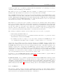
Document Change Record
Issue
Date
0.1
0.2
0.3
0.31
1.0
1.1
11/26/07
01/11/08
03/28/08
01/29/09
11/20/09
12/24/09
1.2
08/03/10
1.3
03/05/10
Sect./Paragr. affected
all
all
3.1.9, Appendix B
Appendix B
All
Tab. 8
Tab. 12
6.6.2, 7.2.2, 7.3
6.6.2
7.2
7.5.2.
all
7.3.3, 7.4
all
Reasons / Remarks
new document
minor changes
added/changed filter curves
added filter curves
Update before release
Corrected full well
Corrected Ks ZP
Updated with more information
New paragraph about tellurics for MOS masks
New section included
Description of MOS acquisition procedure added
minor changes (typos, ...)
Added information about archive parameters
Clean tables and figures caption for the table of content
Note: Chapter 5 fully related to LBT issues has been written by Dave Thompson from LBTO.
LUCIFER User Manual
Issue 1.3
3
Contents
List of Figures
6
List of Tables
8
1 Acronyms
9
2 Introduction
10
3 LUCIFER
10
3.1
Instrument description . . . . . . . . . . . . . . . . . . . . . . . . . . . . . . . . . . . .
10
3.1.1
Entrance window
. . . . . . . . . . . . . . . . . . . . . . . . . . . . . . . . . .
11
3.1.2
Focal Plane & Slit Masks . . . . . . . . . . . . . . . . . . . . . . . . . . . . . .
11
3.1.3
Collimator
. . . . . . . . . . . . . . . . . . . . . . . . . . . . . . . . . . . . . .
12
3.1.4
Gratings . . . . . . . . . . . . . . . . . . . . . . . . . . . . . . . . . . . . . . . .
13
3.1.5
Pupil Viewer . . . . . . . . . . . . . . . . . . . . . . . . . . . . . . . . . . . . .
14
3.1.6
Cameras . . . . . . . . . . . . . . . . . . . . . . . . . . . . . . . . . . . . . . . .
14
3.1.7
Filters . . . . . . . . . . . . . . . . . . . . . . . . . . . . . . . . . . . . . . . . .
15
3.2
Detector and Acquisition System . . . . . . . . . . . . . . . . . . . . . . . . . . . . . .
15
3.3
Calibration Unit . . . . . . . . . . . . . . . . . . . . . . . . . . . . . . . . . . . . . . .
17
4 Observing in the NIR
20
4.1
Atmospheric Transmittance . . . . . . . . . . . . . . . . . . . . . . . . . . . . . . . . .
20
4.2
Background Emission . . . . . . . . . . . . . . . . . . . . . . . . . . . . . . . . . . . .
20
4.3
Imaging . . . . . . . . . . . . . . . . . . . . . . . . . . . . . . . . . . . . . . . . . . . .
20
4.4
Spectroscopy . . . . . . . . . . . . . . . . . . . . . . . . . . . . . . . . . . . . . . . . .
20
4.5
Influence of the Moon . . . . . . . . . . . . . . . . . . . . . . . . . . . . . . . . . . . .
21
5 Observing at the LBT
21
5.1
Introduction . . . . . . . . . . . . . . . . . . . . . . . . . . . . . . . . . . . . . . . . . .
21
5.2
Pointing & Collimation . . . . . . . . . . . . . . . . . . . . . . . . . . . . . . . . . . .
22
5.3
Guiding . . . . . . . . . . . . . . . . . . . . . . . . . . . . . . . . . . . . . . . . . . . .
24
5.4
Open-loop tracking stability . . . . . . . . . . . . . . . . . . . . . . . . . . . . . . . . .
25
4
Issue 1.3
LUCIFER User Manual
6 Preparing observations with LUCIFER
6.1
27
Available tools . . . . . . . . . . . . . . . . . . . . . . . . . . . . . . . . . . . . . . . .
27
6.1.1
Exposure Time Calculator (ETC) . . . . . . . . . . . . . . . . . . . . . . . . .
27
6.1.2
LUCIFER Mask Simulator (LMS) . . . . . . . . . . . . . . . . . . . . . . . . .
27
6.2
Offset and position angle definition . . . . . . . . . . . . . . . . . . . . . . . . . . . . .
29
6.3
Overhead Calculations . . . . . . . . . . . . . . . . . . . . . . . . . . . . . . . . . . . .
29
6.4
Limiting magnitude & recommended integration times . . . . . . . . . . . . . . . . . .
30
6.5
Sky emissivity . . . . . . . . . . . . . . . . . . . . . . . . . . . . . . . . . . . . . . . . .
30
6.5.1
Imaging . . . . . . . . . . . . . . . . . . . . . . . . . . . . . . . . . . . . . . . .
31
6.5.2
Spectroscopy . . . . . . . . . . . . . . . . . . . . . . . . . . . . . . . . . . . . .
32
6.6
Calibrations
. . . . . . . . . . . . . . . . . . . . . . . . . . . . . . . . . . . . . . . . .
35
6.6.1
Sky flats . . . . . . . . . . . . . . . . . . . . . . . . . . . . . . . . . . . . . . . .
35
6.6.2
Night calibrations . . . . . . . . . . . . . . . . . . . . . . . . . . . . . . . . . .
35
6.6.3
Calibration Plan . . . . . . . . . . . . . . . . . . . . . . . . . . . . . . . . . . .
41
7 Observing with LUCIFER
43
7.1
Login and Software Start . . . . . . . . . . . . . . . . . . . . . . . . . . . . . . . . . .
43
7.2
Start and end of night procedures . . . . . . . . . . . . . . . . . . . . . . . . . . . . . .
43
7.2.1
Start of night . . . . . . . . . . . . . . . . . . . . . . . . . . . . . . . . . . . . .
43
7.2.2
End of the night . . . . . . . . . . . . . . . . . . . . . . . . . . . . . . . . . . .
43
7.3
Interactive Observing
. . . . . . . . . . . . . . . . . . . . . . . . . . . . . . . . . . . .
44
7.3.1
The Instrument Control GUI . . . . . . . . . . . . . . . . . . . . . . . . . . . .
44
7.3.2
The Telescope Control GUI . . . . . . . . . . . . . . . . . . . . . . . . . . . . .
47
7.3.3
The Detector Read Out GUI . . . . . . . . . . . . . . . . . . . . . . . . . . . .
49
7.4
Script Observing . . . . . . . . . . . . . . . . . . . . . . . . . . . . . . . . . . . . . . .
52
7.5
Target Acquisition . . . . . . . . . . . . . . . . . . . . . . . . . . . . . . . . . . . . . .
55
7.5.1
Imaging . . . . . . . . . . . . . . . . . . . . . . . . . . . . . . . . . . . . . . . .
56
7.5.2
Spectroscopy . . . . . . . . . . . . . . . . . . . . . . . . . . . . . . . . . . . . .
56
References
62
A Example of fits header
63
B Grating Efficiencies
67
C Additional filter information
68
LUCIFER User Manual
Issue 1.3
5
C.1 Filter Curves . . . . . . . . . . . . . . . . . . . . . . . . . . . . . . . . . . . . . . . . .
68
C.1.1 Broad Band . . . . . . . . . . . . . . . . . . . . . . . . . . . . . . . . . . . . . .
68
C.1.2 Narrow Band . . . . . . . . . . . . . . . . . . . . . . . . . . . . . . . . . . . . .
70
D Example of Scripts
72
6
Issue 1.3
LUCIFER User Manual
List of Figures
1
LUCIFER optical layout . . . . . . . . . . . . . . . . . . . . . . . . . . . . . . . . . . .
10
2
Transmission curve of the LUCIFER#1 entrance window . . . . . . . . . . . . . . . .
11
3
Pupil image . . . . . . . . . . . . . . . . . . . . . . . . . . . . . . . . . . . . . . . . . .
15
4
Detector Layout . . . . . . . . . . . . . . . . . . . . . . . . . . . . . . . . . . . . . . .
17
5
Illustration of how the LUCIFER readout modes works . . . . . . . . . . . . . . . . .
18
6
Part of a LUCIFER image showing bad pixels . . . . . . . . . . . . . . . . . . . . . . .
18
7
Transmittance of the atmosphere for two different locations . . . . . . . . . . . . . . .
20
8
Sky background . . . . . . . . . . . . . . . . . . . . . . . . . . . . . . . . . . . . . . . .
21
9
Pointing Correction . . . . . . . . . . . . . . . . . . . . . . . . . . . . . . . . . . . . . .
24
10
The AGw patrol field . . . . . . . . . . . . . . . . . . . . . . . . . . . . . . . . . . . . .
26
11
LMS-SW . . . . . . . . . . . . . . . . . . . . . . . . . . . . . . . . . . . . . . . . . . .
28
12
Offsets definition . . . . . . . . . . . . . . . . . . . . . . . . . . . . . . . . . . . . . . .
29
13
LUCIFER broad band filters over atmospheric spectrum . . . . . . . . . . . . . . . . .
33
14
Spectroscopic count rates . . . . . . . . . . . . . . . . . . . . . . . . . . . . . . . . . .
34
15
OH spectrum in K band . . . . . . . . . . . . . . . . . . . . . . . . . . . . . . . . . . .
35
16
Normalised sky spectrum in K band . . . . . . . . . . . . . . . . . . . . . . . . . . . .
37
17
Calibration lines measured with the 150 Ks and 200 H+K gratings . . . . . . . . . . .
41
18
Calibration lines measured with the LS150 slit and the 210 zJHK grating . . . . . . .
42
19
The LUCIFER Instrument Control GUI . . . . . . . . . . . . . . . . . . . . . . . . . .
44
20
The LUCIFER calibration unit GUI . . . . . . . . . . . . . . . . . . . . . . . . . . . .
46
21
The LUCIFER Telescope Control GUI . . . . . . . . . . . . . . . . . . . . . . . . . . .
47
22
The LUCIFER Read Out Manager GUI . . . . . . . . . . . . . . . . . . . . . . . . . .
49
23
The LUCIFER GEIRS GUI . . . . . . . . . . . . . . . . . . . . . . . . . . . . . . . . .
51
24
The archive information editing window . . . . . . . . . . . . . . . . . . . . . . . . . .
52
25
Extract of the Read Out Manager GUI showing updated archive information . . . . .
52
26
Archive info in the ReadoutManager GUI when a script is running . . . . . . . . . . .
54
27
The LUCIFER MOS Acquisition GUI . . . . . . . . . . . . . . . . . . . . . . . . . . .
58
28
Through mask image . . . . . . . . . . . . . . . . . . . . . . . . . . . . . . . . . . . . .
59
29
MOS Acquisition pop-up window 1 . . . . . . . . . . . . . . . . . . . . . . . . . . . . .
59
LUCIFER User Manual
Issue 1.3
7
30
MOS Acquisition pop-up window 2 . . . . . . . . . . . . . . . . . . . . . . . . . . . . .
59
31
MOS Acquisition ”last” pop-up window . . . . . . . . . . . . . . . . . . . . . . . . . .
59
32
The LUCIFER MOS Acquisition GUI . . . . . . . . . . . . . . . . . . . . . . . . . . .
60
33
MOS Acquisition: Retry pop-up . . . . . . . . . . . . . . . . . . . . . . . . . . . . . .
61
34
Wavelength dependencies of the efficiency for the 210 zJHK grating
. . . . . . . . . .
67
35
Wavelength dependencies of the efficiency for the 200 H+K grating . . . . . . . . . . .
67
36
Broad band filter transmission curves . . . . . . . . . . . . . . . . . . . . . . . . . . . .
69
37
Narrow band filter transmission curves - 1 . . . . . . . . . . . . . . . . . . . . . . . . .
70
38
Narrow band filter transmission curves - 2 . . . . . . . . . . . . . . . . . . . . . . . . .
71
8
Issue 1.3
LUCIFER User Manual
List of Tables
1
LUCIFER imaging modes . . . . . . . . . . . . . . . . . . . . . . . . . . . . . . . . . .
11
2
LUCIFER spectroscopic modes . . . . . . . . . . . . . . . . . . . . . . . . . . . . . . .
11
3
Permanently installed masks
. . . . . . . . . . . . . . . . . . . . . . . . . . . . . . . .
13
4
Characteristics of the gratings . . . . . . . . . . . . . . . . . . . . . . . . . . . . . . . .
13
5
Gratings wavelength coverage with the N1.80 camera . . . . . . . . . . . . . . . . . . .
14
6
Wavelengths which can set at the center of the detector . . . . . . . . . . . . . . . . .
14
7
Characteristics of the LUCIFER#1 filters . . . . . . . . . . . . . . . . . . . . . . . . .
16
8
Characteristics of the detector . . . . . . . . . . . . . . . . . . . . . . . . . . . . . . . .
16
9
Basic characteristics of the LBT . . . . . . . . . . . . . . . . . . . . . . . . . . . . . .
22
10
Overview of all overheads times
. . . . . . . . . . . . . . . . . . . . . . . . . . . . . .
31
11
Measured sky emissivity . . . . . . . . . . . . . . . . . . . . . . . . . . . . . . . . . . .
31
12
LUCIFER’s imaging zero points (defined as 1 ADU/SEC). . . . . . . . . . . . . . . . .
32
13
Imaging limiting magnitude . . . . . . . . . . . . . . . . . . . . . . . . . . . . . . . . .
32
14
Typical sky count rate (between OH lines) . . . . . . . . . . . . . . . . . . . . . . . . .
33
15
Count rates (ADU/s) for internal flat fields with N3.75 camera.
36
16
Spectroscopic flat field count rate per second, for different slit width.
. . . . . . . . .
38
17
Arc lines count rate (sec) . . . . . . . . . . . . . . . . . . . . . . . . . . . . . . . . . .
39
18
Definition of the lamps in the calibration unit. . . . . . . . . . . . . . . . . . . . . . .
45
19
Specifications for the filters. . . . . . . . . . . . . . . . . . . . . . . . . . . . . . . . . .
68
20
Characteristics of the current LUCIFER#2 filters. . . . . . . . . . . . . . . . . . . .
68
. . . . . . . . . . . .
LUCIFER User Manual
1
Issue 1.3
Acronyms
AO
ADC
AGw
DARK
DIT
NDIT
FIMS
FOV
FPU
LBT
LMS
LUCIFER
RON
wfs
adaptive optics
atmospheric dispersion corrector
acquisition, guiding & wavefront sensing system
dark current
detector integration time
number of detector integration time
FORS Instrument Mask Simulator
Field of View
Focal Plane Unit
Large Binocular Telescope
LUCIFER Mask preparation Software
LBT NIR Spectroscopic Utility with Camera and Integral
Field Unit for Extragalactic Research
readout noise
wavefront sensor
9
10
2
Issue 1.3
LUCIFER User Manual
Introduction
LUCIFER (LBT NIR Spectrograph Utility with Camera and Integral-Field Unit for Extragalactic
Research) is a NIR spectrograph and imager for the Large Binocular Telescope (LBT) working in the
wavelength range from 0.85 µm to 2.5 µm. Currently only one LUCIFER instrument is available at
the LBT. It is mounted on the bent Gregorian focus of the SX mirror. In 2011 an identical instrument
will be mounted on the bent Gregorian focus of the DX mirror (i.e. other side of the telescope). The
observing modes currently available are
• seeing-limited imaging over a 40 field of view (FOV)
• seeing-limited longslit spectroscopy
• seeing-limited multi object spectroscopy with slit masks
As soon as the adaptive secondary will be operational at the LBT, following additional observing
modes will exist:
• diffraction-limited imaging over a 0.50 FOV
• diffraction-limited longslit spectroscopy
Spectroscopic observations can be carried out with a resolution of up to 17,000 (seeing limited) and
40,000 (TBC - diffraction limited). The instruments are equipped with Rockwell HAWAII-2 HdCdTe
2048 × 2048 px2 array.
3
3.1
LUCIFER
Instrument description
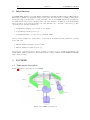
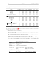
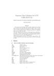
Figure 1 shows the optical layout of LUCIFER.
Figure 1: LUCIFER optical layout
view3.JPG
LUCIFER User Manual
Issue 1.3
11
The wavelength bands covered by the LUCIFER optics include z, J, H and K, i.e. the range from
0.85 to 2.5 µm. In practice however the observing range is limited on the blue side by the cut-off
wavelength of the entrance window (0.87µm, section 3.1.1) and on the red side by the cut-off of the
atmospheric window after 2.4µm.
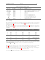
The main observing modes are summarized in Tab. 1 and Tab. 2.
Table 1: LUCIFER’s imaging modes
Camera
00
Scale ( / pixel)
FOV (arcminute)
Comments
N1.8
N3.75
N30 (non available yet)
0.25
4×4
0.12
4×4
0.015
0.5 × 0.5
FOV limited by isoplanatism
Table 2: LUCIFER’s spectroscopic modes. LSS stands for Long Slit Spectroscopy and MOS for
Multi-Object Spectroscopy.
Camera
N1.8
N3.75
N30 (non available yet)
Scale (00 / pixel)
FOV (arcminute)
Resolution (2pix)
Comments
0.25
4 × 2.8
1900 . . . 8500
LSS & MOS
full coverage zJHK
0.12
4 × 2.8
3800 . . . 17000
LSS & MOS
0.015
0.5 × 0.5
10000 . . . 40000
LSS
3.1.1
Entrance window
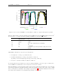
The instrument entrance window is tilted by 15◦ in order to reflect the visible light to the on-axis
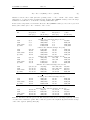
wavefront sensor (for adaptive optics). The current entrance window has a blue cut-off wavelength at
0.87 µm, as illustrated in Fig. 2.
Transmission Entrance Window #1
Transmission Entrance Window #1
100.0
100.0
90.0
99.0
98.0
70.0
Transmission
Transmission [%]
Transmission [%]
80.0
60.0
50.0
40.0
30.0
20.0
97.0
96.0
95.0
Transmission
94.0
93.0
92.0
91.0
10.0
90.0
0.0
400
600
800
1000
1200
1400 1600 1800
Wavelength [nm]
2000
2200
2400
800
2600
!
1000
1200
1400
1600
1800
2000
Wavelength [nm]
2200
2400
2600
!
Figure 2: Transmission curve of the LUCIFER #1 entrance window. The plot left shows the overall
transmission (inclusive the “leak” around 400nm), while on the right a zoom over the NIR range is
presented.
3.1.2
Focal Plane & Slit Masks
The useful unvignetted field of the telescope is ∼ 70 . The layout of the optics for the seeing limited
case covers a field of 40 × 40 (144 mm × 144 mm). The focal plane, commonly refered to the FPU
(Focal Plane Unit), can be equipped with masks for long-slit and multi-object spectroscopy as well
12
Issue 1.3
LUCIFER User Manual
as field stop mask. Up to 33 masks are available inside the instrument, out of which up to 23 can be
exchanged, without warming up the instrument.
The multi-object mode of LUCIFER offers the possibility of obtaining spectra of several objects
simultaneously. The masks used for this mode are custom made laser cut masks.
The LUCIFER multi-slit masks are made from 125 µm thick stainless steel from ThyssenKrupp, chemically blackened on one side. The coating has been tested at LN2 temperature and in a laser cutting
machine. MPE supplies this material for the mask cutting machine at LBT. The sheet thickness has
been optimized for the LUCIFER mask frames. No other material should be used to avoid problems
with stability and warping of the masks during cooldown.
The masks do not exactly follow the focal surface because they are cylindrical. The cylinder radius is
that of the focal surface (1033 mm), and the shape is defined by the mask frames. the cylinder axis
is in dispersion direction, therefore, the defocus is constant along a standard (not inclined) slit. The
defocus can be limited to ±0.5 mm for the central area of 4 armin height and 2.5 arcmin width in
dispersion direction. The limitation to this central area is sensible, because spectral clipping by the
detector array increases with increasing distance of the slit from the field center.
The exchange of masks is a daytime operation that needs about one week to be prepared:
• mask cutting (at LBTO in Tucson)
• the newly cut masks sheets have to be installed in frames, that have to be put in the cabinet
that will then be inserted in LUCIFER.
• the auxiliary cryostats one empty to receive the cabinet currently in LUCIFER and the other
one containing the newly filled cabinet of masks to be inserted, have to be cooled down
On the day of the exchange, the empty cryostat is attached to LUCIFER. A bridge vacuum seal is
pumped, the exchange gate is then opened and the currently used cabinet of masks is moved out of
LUCIFER. Thereafter the gate is closed, the vacuum bridge put back to atmospheric pressure so the
auxiliary cryostat can be detached from LUCIFER. The operation is then repeated with the other
auxiliary cryostat, the one containing the new set of masks. After the exchange, at least one auxiliary
cryostat has to be warmed up to remove the cabinet it contains and receive new masks. There is thus
a minimum of a week between 2 cabinet exchanges. At the moment, cabinet exchange are foreseen
once per month with the goal before each new block of science runs.
A software tool, the LUCIFER Mask Simulator (LMS), has been made available to prepare masks for
multi-objects spectroscopy and is presented in section 6.1.2.
Permanent masks A set of masks is permanently installed in LUCIFER. These masks are meant
either for instrumental calibration or long slit spectroscopy. These include some sieve masks used
essentially to measure flexures and internal field distortion, a blind mask to take dark frames, a set of
long slits and a mask thought for spectrophotometric calibrations. These masks all have a fix mask-ID,
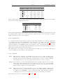
which is indicated in the Table 3 as well as the current position of these masks in the mask’s cabinet.
3.1.3
Collimator
The refractive collimator with a focal length of 1500 mm is used in all modes. The resulting collimated
beam size is 102 mm. The collimator includes 4 flat folding mirrors. The last of those mirrors is motordriven and used for the instrument internal flexure compensation.
LUCIFER User Manual
Issue 1.3
13
Table 3: Permanently installed masks
Mask Name
Mask-Number
ID
Position in cabinet
NB
Optic Sieve
Spectro Sieve
Closed/Blind
LS 600
LS 450
LS300Nblack
LS 150
3 slit
990063
990001
990031
990034
990029
990078
990065
995623
0
1
3
4
5
6
7
8
LS 300
990032
9
3.1.4
Remarks
Reference for scripts
array of pinholes (for imaging & N3.75 camera)
pinhole array for spectroscopic calibrations
used for darks measurements
00
1.00 slit
00
0.75 slit
00
0.50 slit - sampling limit N1.8
00
0.25 slit - sampling limit N3.75
00
00
3 centered vertical slits of 10 ×30
for spectrophotometric standards
Currently not usable
Gratings
The grating unit holds one mirror (for the imaging mode) and 3 gratings. The (laboratory) measured
efficiencies of the gratings are presented in Appendix B. Additionally, the main characteristics are
summarized in Tab. 4.
The difference in peak efficiency between the diagrams in Appendix B (manufacturer data) and the
values given in Table 4 is due to the fact that the gratings are used in non-Littrow configuration in
LUCIFER.
Order
λpeak [µm]
Max. Efficiency [%]
50 % Cut on [µm]
50 % Cut off [µm]
Resolution
High resolution grating with 210 lines/mm
2.
3.
4.
5.
2.44
1.64
1.24
1.00
68
77
76
72
2.02
1.41
1.09
0.89
3.18
1.90
1.41
1.11
6687
7838
8460
6877
>2.40(1)
1881 (H)/ 2573 (K)
H+K grating with 200 lines/mm
1.
1.87
83
1.38
Ks grating with 150 lines/mm
2.
2.13
78
1.81
>2.40(1)
4150
Table 4: Characteristics of the gratings. The resolution is given for the N1.80 with 2pixel sampling
at the peak wavelength.
(1)
: The 200 H+K and 150 Ks grating do not have a cut-off within our wavelength range.
The gratings can be tilted in order to center a selected wavelength at the position of the long slits.
Table 5 defines the wavelength range covered for the tilt at the nominal central wavelength.
The gratings can individually be tilted by up to ±2.5 degrees. This allows a range of wavelengths to
be centered on the detector as given in Table 6 for the N1.80 camera.
Note: the 150 Ks grating can presently not be tilted and is fixed at λcen = 2.15µm.
14
Issue 1.3
Grating
210
210
210
210
Band
λmin
λcen
λmax
∆λ
K
H
J
z
2.025
1.541
1.169
0.893
2.200
1.650
1.250
0.960
2.353
1.743
1.319
1.017
0.328
0.202
0.150
0.124
H+K
1.475
1.930
2.355
0.880
Ks
1.890
2.170
2.423
0.533
zJHK
zJHK
zJHK
zJHK
200 H+K
150 Ks
LUCIFER User Manual
Table 5: Wavelength coverage for the gratings with the N1.80 camera at the nominal center wavelength.
For the N3.75 camera multiply ∆λ by 0.48.
Grating
Band
210
210
210
210
z
J
H
K
0.87 ...
1.05 ...
1.40 ...
2.10 ...
OrderSep
1.49 ... >2.4
zJHK
zJHK
zJHK
zJHK
200 H+K
λrange (µ)
1.02
1.28
1.70
>2.4
Table 6: Wavelengths which can set at the center of the detector. Careful: the ranges given represent
the physical limits of what can be achieved with the grating tilt and does not take into account the
limits of the filters used for order separation.
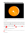
3.1.5
Pupil Viewer
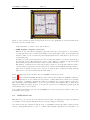
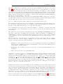
In combination with the N1.8 camera, a pupil viewer is realized which allows to check the pupil image
for vignetting and inhomogenous illumination. Two lenses have to be added to the beam: one in front
of the camera, the other one is placed in one of the positions of filter wheel #1. (Fig. 3) presents a
current pupil image of LUCIFER. Because of the structure of the one-armed swingarm support, the
diffraction spikes are not standard. The LBT PSF has an asymmetric 10-armed diffraction pattern,
rather than the usual 4-arm from typical spiders.
The displacement of the pupil to its stop causes presently a light loss of about 17%. This will be
corrected during the next warm-up of the instrument.
3.1.6
N1.8
Cameras
This camera is designed for seeing-limited spectroscopy for covering one single broad
band (z, J, H or K). The image scale of this camera is 0.25 00 /pixel. The maximum
distortion is less than 0.1 % within the 4 arcmin field. It can also be used for imaging
in seeing limited mode, but bear in mind that the lateral color is not corrected.
N3.75 It is dedicated for both seeing-limited imaging and seeing-limited slit spectroscopy. The
image scale of this camera is 0.12 00 /pixel. In spectroscopic mode it covers about half
of the zJHK bands wavelength range at higher resolution (for an equivalent slit width
defined in pixel compared to the N1.80 camera).
N30
This camera (0.015 00 /pixel) is intended to be used for diffraction-limited imaging and
longslit spectroscopy, together with the adaptive optics. The sampling of this camera
is optimal for the FWHMAiry of the J band (2.0 pixel). The H and K bands are
oversampled (2.73 pixel and 3.73 pixel respectively). It is currently not available.
The available modes are also given in Tab. 1 and Tab. 2.
LUCIFER User Manual
Issue 1.3
15
Figure 3: LUCIFER pupil image in K band. On this image the swing arm sustaining the secondary
mirror is visible (PA=160deg), as well as the displacement due to an internal pupil mis-alignment.
3.1.7
Filters
Two filter wheels are placed in the convergent beam in front of the detector. A total of up to 27
filters can be mounted. The first filter wheel contains the narrow and medium band filters as well as
a pupil viewer, while the second wheel contains all broad band filters and the order separation filter
(for spectroscopy with the 200 H+K grating). Both filter wheels contain a blind filter. Filter wheel
#1 is always set before filter wheel #2 starts moving. This is important to remember when wishing
to avoid saturation e.g. before long spectroscopic integrations. The characteristics of the currently
available filters in LUCIFER #1 are given in Tab. 7.
Appendix C contains details about the manufacturing specifications of the filters (Tab. 19), an equivalent of Tab. 7 with the filters for LUCIFER#2 ( Tab. 20) as well as all the transmittance curves
(section C.1).
3.2
Detector and Acquisition System
Characteristics
The detector is a HAWAII-2 HdCdTe detector, whose main characteristics are summarised in Tab.
8.
Readout Modes
16
Issue 1.3
LUCIFER User Manual
Table 7: Characteristics of the filters installed in LUCIFER #1.. The position indicates in which filter
wheel (FW) the filter is installed.
Name
LUCIFER
Position
λC /µm
FWHM/µm
τpeak
τaverage
z [3002]
J [0403]
H [4302]
K [3902]
Ks [3902]
Order Separation [ED763-1]
1
1
1
1
1
1
FW2
FW2
FW2
FW2
FW2
FW2
0.957
1.247
1.653
2.194
2.163
1.950
0.195
0.305
0.301
0.408
0.270
0.981
98.4 %
91.2 %
95.0 %
90.1 %
90.7 %
95.0 %
94.3 %
83.2 %
90.5 %
85.7 %
86.8 %
86.3 %
Br gam [Brackett-γ (ED477-1)]
FeII [(ED468-1)]
H2 [(ED469-1)]
HeI [(1085-15)]
J-high
J-low
OH 1060
OH 1190
P beta [Paschen-β (ED476-1)]
P gam [Paschen-γ (ED467-2)]
Y1
Y2
1
1
1
1
1
1
1
1
1
1
1
1
FW1
FW1
FW1
FW1
FW1
FW1
FW1
FW1
FW1
FW1
FW1
FW1
2.170
1.646
2.124
1.088
1.303
1.199
1.065
1.193
1.283
1.097
1.007
1.074
0.024
0.018
0.023
0.015
0.108
0.112
0.009
0.010
0.012
0.010
0.069
0.065
79.4 %
91.2 %
87.9 %
65.2 %
95.9 %
95.4 %
68.6 %
80.4 %
86.1 %
81.1 %
67.3 %
94.2 %
76.5 %
89.5 %
84.9 %
64.6 %
93.3 %
93.3 %
66.8 %
78.0 %
85.5 %
80.0 %
64.2 %
89.5 %
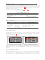
The channel layout is shown in Fig. 4. Channels are numbered along the fast direction, starting with
quadrant I. The read-modes offered are:
• DCR (double correlated read mode):
This mode is the default in high background applications, where background limited performances are reached easily.
The detector is first reset then read-out. Reading of the detector is always non-destructive.
After the selected integration time, the chip is read-out again.
The difference of the two read-out frames removes detector, channel and pixel specific properties
which are present in both frames, and preserves the integration charge value.
The ’o2’ of the o2dcr mode stands for some additional line clocking after the frame reset, which
were necessary for most HAWAII-2 detectors tested for Omega2000, to get rid of strange ramps
Table 8: Characteristics of the detector
Pixelsize
Number of pixels
Fullwell
Linearity
Quantum efficiency
18.0 µm2
2048 × 2048 pixel2
∼ 260000 e−
better than 5% at 80% full well
z=0.25, J=0.33, H=0.74, K=0.73
Readout mode
Double-Correlated Reads
(DCR)
2sec
4.083 e− /ADU
< 12 e−
0.06 e− /s/pix
Min Exposure time
Gain
RON
DC
Multiple-Endpoint Reads
(MER - fixed at 10 samples)
10 sec
3.93 e− /ADU
< 5 e−
(0.06 e− /s/pix), to be confirmed
LUCIFER User Manual
Issue 1.3
17
Figure 4: Detector Layout. The arrows indicate how the four quadrants are read and which is the
direction of the slow & fast reads.
in the first frame, to enable correct data reduction.
• MER (multiple endpoint read mode):
This mode, also called Fowler sampling, reduces the read noise by the square root of the number
of reads and has a better cosmetic than DCR for a given integration time. It is particular well
suited for faint objects observations (either imaging with narrow band filters or spectroscopic
long integrations).
A number of reads is performed after the reset, and the same number of reads is performed after
the integration time. The signal is the average of the difference of always 2 endpoint samples
(Fowler-pair), all pairs have the same double-correlated integration time.
The number of samples for the offered mode has been fixed to 10 endpoints, which is equal to
5 Fowler pairs (compromise between reduced noise and increased minimum integration time).
(mer mode of Lucifer is based on the o2dcr mode with the same additional clocking after the
frame reset to prevent problems with the first frame.)
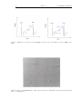
Figure 5 illustrates how the currently offered LUCIFER readout modes work.
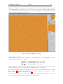
Figure 6 shows a typical LUCIFER dark frame, where some known artefacts are highlighted. The two
main nasty features are a bad column at x=[783,784] for y=[1025,2048] and a bad line at y=[859,861]
over the x range of [670,1025]. As much as possible avoid putting any of your spectrum over the area.
The central line/column (1024,1024) of “dots” are some features of the DCR readmode. They nicely
disappear in difference images, however do not put an object in view of taking its spectrum perfectly
in the middle of the detector (in Y).
Note: Unlike most infrared detectors, the LUCIFER detector is read only upon request = there is no
permanent reads on-going.
3.3
Calibration Unit
This unit can be moved in front of the entrance window. Three arc lamps (Neon, Argon and Xenon)
are available for wavelength calibration and three halogen lamps for flat fields.
Note that moving the calibration unit in front of LUCIFER obstructs the light coming from the
telescope, thus guiding will not be able to continue while internal calibrations are being taken over
18
Issue 1.3
LUCIFER User Manual
Figure 5: Illustration of the way the LUCIFER readout modes work: DCR to the left, MER to the
right.
Figure 6: Part of a LUCIFER image, where few features (bad column/line and few bad pixel clusters)
have been highlighted.
LUCIFER User Manual
Issue 1.3
19
night. In this case, ask the telescope operator to pause guiding and active optics corrections for you,
before the calibration unit is moved in the light path.
20
4
Issue 1.3
LUCIFER User Manual
Observing in the NIR
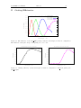
4.1
Atmospheric Transmittance
1.0
1.0
0.8
0.8
Air Transmittance
Air transmittance
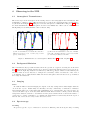
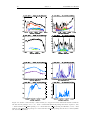
The water vapor in the atmosphere is the leading cause for absorbing light in the near-infrared. The
transmission of light for three different water-vapor levels in the wavelength range from 0.9 µm to
2.5 µm is shown in Figure 7(a). This plot is a model atmosphere for Mauna Kea. The plot 7(b) shows
the mean transmittance of an atmospheric model for the 2MASS site. The location of 2MASS is on
Mt Hopkins (about 60 km/40 miles south of Tucson, AZ).
0.6
0.4
0.2
0.6
0.4
0.2
0.0
0.0
1.0
1.2
1.4
1.6
1.8
2.0
2.2
2.4
Wavelength/µm
(a) The air transmittance for Mauna Kea and three
different water-vapor levels: 1.0 mm (red), 1.6 mm
(green), 3.0 mm (blue)
1.0
1.2
1.4
1.6
1.8
2.0
2.2
2.4
Wavelength / µm
(b) The mean air transmittance for the site of 2MASS
north (Mt. Hopkins) which is located about 150 km
(ca. 100 miles) southwest of the LBT.
Figure 7: Transmittance vs. wavelength for Mauna Kea (a) and Mt. Hopkins (b).
4.2
Background Emission
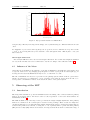
The near-infrared sky spectrum measured from the ground at a typical observing site is shown in
Fig. 8. These lines are well known and can be used for wavelength calibration in spectroscopic mode.
Below 2 µm the night sky emission is dominated by OH and O2 airglow emission. Unfortunately, the
intensity varies about 5% - 10% due to changes in local density of OH, over timescale of the order of
5 - 15 minutes. Above 2 µm thermal emission from the atmosphere and from the telescope dominates
the background radiation.
4.3
Imaging
Jitter
In classical NIR broad-band imaging the signal of the sky background is much higher than the
one from the objects. Additionally, it’s intensity can vary considerably on timescales of minutes.
Jitter imaging takes care of that issue with a minimum loss of observing time. For each exposure one
observes the same region on the sky with different small offsets around a central position. The sky
background emission can then be determined from the jittered frames if the local field is neither too
crowded nor too dusty or will have to be estimated from sky frames obtained away from the region of
interest and observed before and/or after the science field.
4.4
Spectroscopy
Nodding
In spectroscopy the object of interest is observed at different positions along the slit (=nodding
LUCIFER User Manual
Issue 1.3
21
600
500
2
Photons/sec/nm/arcsec /m
2
1.6 mm H2O, Airmass=1.5
400
300
200
100
0
0.8
1
1.2
1.4
1.6
1.8
2
2.2
2.4
Wavelength/µm
Figure 8: Sky spectrum measured at Mauna Kea
along the slit). The sky removing is then simply done by substracting two different frames from each
other.
For small size objects observed in long slit spectroscopy mode, it is recommended to keep the nod size
≤ ±3000 to avoid being affected by the curvature of the atmospheric lines. This is just to ease your
data reduction.
Wavelength Calibration
Below 2.2 µm OH lines can be used for wavelength calibration. Above that wavelength the OH lines
are very weak. In that case it is recommended to use the arc lamps of the calibration unit (3.3).
4.5
Influence of the Moon
Observing the near-infrared, the influence of the Moon illumination is small and can in many cases
be ignored. However for deep imaging (long integration of faint objects) at short wavelengths (e.g. in
z band), the increased sky illumination may need to be taken into account.
The Moon illumination is however a problem for the guiding system, which works at optical wavelength. It is therefore recommanded to avoid observing closer than 30 degrees from the Moon, to
avoid possible contamination effects on the wavefront sensor of the guider system.
5
5.1
Observing at the LBT
Introduction
The Large Binocular Telescope uses an azimuth-elevation mounting. Two 8.4 meter diameter primary
mirrors are mounted with a 14.4 meter center-to-center separation. Some basic characteristics are
summarized in Table 9.
The LBT is unlike every other major telescope in that the design is highly asymmetric. The primary
mirrors are cantilevered off a central pair of elevation C ring bearings. These elevation C rings have
extensions that support one-armed A-framed swing arms that allow the secondary and tertiary mirrors,
as well as the prime-focus cameras, to swing into or out of primary mirror optical axis. The primary
(M1) and secondary (M2) mirrors are mounted on hexapods that allows them a considerable range of
22
Issue 1.3
LUCIFER User Manual
motion (±3 mm for M1, ±10 mm for M2) in six axes. The tertiary (M3) has a smaller range (±1 mm)
and only four degrees of freedom. It is this adjustability that will allow the LBT to operate efficiently
as a fully binocular telescope.
Table 9: Basic characteristics of the LBT
effective primary aperture DTel
focal length fTel
effective system focal ratio NTel
primary spacing
image scale
FOV
field curvature rTel
AO System
8251 mm
123421.4 mm
15.0
14417 mm center-to-center
0.59836 mm/arcsec
70
1043 mm
Secondary Mirror
The effective primary aperture of 8.251 meters in the table above is the area on the primary seen from
the instrument because the slightly undersized secondary mirror is the pupil stop of the telescope
optics. The telescope focal length and image scale were determined by tying astrometric solutions on
sky (arcsec/pixel) to the scale of the precision sieve mask (mm/pixel) in LUCIFER.
There is currently a rigid secondary mirror installed on the SX side, used for seeing-limited observations. The first adaptive secondary mirror, to be installed on the DX side, is scheduled to enter
operation in late 2010.
5.2
Pointing & Collimation
The LBTO maintains models for both the pointing and collimation of the telescope, the goal of which
is to deliver to the wavefront sensor (wfs) a sufficiently collimated image that it can converge to a wellcollimated system in a few cycles. The pointing model corrects for deviations of the real telescope from
a “perfect” mechanical model, such as a tilt of the azimuth axis off zenith or flexure of the telescope
“tube” as a function of the elevation. The collimation model corrects low-order optical aberrations
(e.g. coma, focus, and astigmatism) as a function of elevation and temperature.
However, the pointing and collimation models are strongly coupled by temperature effects on this
asymmetric telescope. As of writing (Nov 2009) this is understood as unmodeled physical offsets of
the optics induced by changes in temperature or temperature gradients. These offsets in the position
of the telescope optics generate offsets to both the pointing and the collimation of the telescope. Since
collimation corrections from the wavefront sensor are applied in a pointing-free manner, we are left
with a net change in the pointing. These thermal effects are under active investigation at the LBTO.
Until this is completed, there are some steps that must be manually executed to achieve the overall
initial collimation and pointing of the telescope, and maintain it throughout the night.
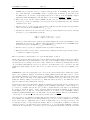
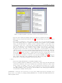
Pointing correction
Note: At the start of the observing night, a check of the pointing is always necessary.
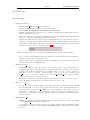
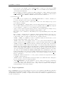
How to check and correct the pointing if necessary (Fig. 9):
1. Be sure to have the telescope operator reset the mount encoders each day before the beginning
of the night.
2. Set up LUCIFER for imaging through a narrowband filter since the pointing stars are quite
bright (R 7.5 mag). We usually use the N3.75 camera and the Brackett gamma filter
3. Point to a pointing star (accurate positions and proper motions) in open-loop TRACK mode,
the rotator mode set to PARALLACTIC, and with an angle of zero. This aligns the LU-
LUCIFER User Manual
Issue 1.3
23
CIFER detector with the telescope elevation axis (up-down on LUCIFER) and perpendicular to this (left-right on LUCIFER). A list of pointing stars is available at the telescope in
the IRTC notebook, and the corresponding stars are in a catalog on the LUCIFER computer
TargetsCoord/PointingStars.tab. The stars to use are named WT10 * or ACT*
4. Take a 2.0 second exposure with LUCIFER. At this point you can iterate this step, allowing
the telescope operator to manually correct any gross focus errors until that is not the dominant
collimation error, then
5. Ask the telescope operator for the current values of IE and CA. Also measure the approximate
centroid of star on the LUCIFER image (xstar , ystar )
6. Calculate the offset needed to move the star to the projected mechanical rotator center, currently
at pixel (xref , yref )=(1014,1043) as follows:
CAnew = CAold + 0.12 × (xref − xstar )
IEnew = IEold + 0.12 × (yref − ystar )
Please note that this reference position may change slightly after each new installation of the
instrument at the telescope. Current values will always be available in the LUCIFER image
headers in the keywords CRPIX1 (xref ) and CRPIX2 (yref )
7. Ask the telescope operator to implement these new values of IE and CA
8. Take another 2.0 second exposure to verify that the pointing star is indeed placed at the reference
coordinates to within a few pixels
There is currently no user-friendly tool to perform this simple operation.
Monitor the guide star offset from the wfs on the acquisition images during subsequent presets. Whenever the guide star is more than halfway to the edge of the acquisition image you should consider
repeating the above pointing correction procedure outlined above. Please keep in mind that the more
out of thermal equilibrium the telescope is, the more often this will need to be repeated. On wellequilibrated stable nights you may only need to do this correction once after the beginning of the
night.
Collimation Once the pointing has been corrected, the guide stars should be within the capture
range of the acquisition, guiding, and wavefront sensing (AGw) system that will be used to correct
any remaining collimation errors in the telescope and maintain collimation throughout the night. Any
large focus offset at the start of the night should be manually removed by the telescope operator
during the initial pointing correction (above). This will deliver an image to the AGw that can be
guided on while the wfs collimates the telescope.
You may select any star for this initial collimation, including an off-axis guide star at your first science
target. If the telescope is far out of collimation at the beginning of the night, or the seeing is poor
(> 2 arcsec), a brighter star (R 10 − 12m ) would be useful until the point where it is saturating
the guider or wavefront sensor. A list of Persson infrared standards is available at the telescope
in the IRTC notebook, and the corresponding stars are in a catalog on the LUCIFER computer
TargetsCoord/PerssonStds 2010.cat. The stars to use are named BS91*. These are well-distributed
over the sky, so one should be reasonably near your first science target.
Once the telescope is collimated, meaning that the rms wavefront error has converged to something
below 400nm, the collimation model will normally keep you close to decent collimation even on large
slews of the telescope. Difficulties can be found on nights with very poor seeing (>3 arcsec), very
low winds (<2 m/s), or large temperature swings. The poor seeing affects collimation because the
entrance aperture to the wfs is three arcsec in diameter, so poor seeing makes it difficult to find the
centroids in each subaperture. Conversely, very good seeing should yield rms wavefront errors well
24
Issue 1.3
Current
IE
&
CA
at
poin0ng
IE
=
12.3,
CA
=
‐27.8
Star
centered
at
1054,
927
Offset
correc0on
‐4.8”
(x),
+13.92”
(y)
LUCIFER User Manual
Final
IE
&
CA
values
IE
=
26.2,
CA
=
‐32.6
Star
centered
within
few
pixels
on
center
of
rota0on
(1014,
1043)
IE
+
CA
+
LUCIFER
image
LUCIFER
image
Figure 9: Illustration of the pointing correction method.
below 400nm. Low wind speeds do not flush out the dome air, so you can get “dome seeing” effects.
(Effect of large temperature changes have already been discussed.)
Low order collimation corrections are applied by physically moving the optics of the telescope. In
some conditions M1 can hit one of its (software) travel limits. If this occurs, you must stop observing
and ask the telescope operator to recover from this.
Please keep in mind that with its very fast primary mirror (f/1.14) the LBT is very sensitive to changes
in the positions of the optics, so open-loop collimation noticeably degrades in a few minutes. It is
thus far more desireable to operate in closed-loop, which is defined as ACTIVE mode. The standard
collimation cycle takes a 30 second exposure on the reference star to average over atmospheric effects.
The whole cycle (integration, readout, processing, application of wfs corrections) currently takes ∼45
seconds. Because the wfs integration cannot be interrupted, we recommend that observers set up their
observations to have a dwell time at each dither position of 60 seconds to ensure that a collimation
update is applied frequently. With dwell times under 60 seconds you can fall into a mode where
the dithers are out of sync with the wfs cycles and you do not get collimation updates. The main
caveat here is that with faint guide stars and/or poor seeing the wfs may have to use longer exposure
times to have sufficient signal to collimate. In such cases, the dwell times will need to be increased
correspondingly.
5.3
Guiding
Because of the way the telescope software interface was built, it is necessary for observers to come
prepared with pre-selected guide stars suitable for their intended science targets. Thus, it is important
to provide a guide star suitable for both guiding and wavefront sensing. This is a function of the seeing
and transparency, of course, but the nominal range for guide star R-band magnitudes is 12m .0−−16m .0
. The USNO-B1 catalog is a useful resource for locating guide stars and can be found at this URL:
http://www.nofs.navy.mil/data/FchPix/cfra.html
LUCIFER User Manual
Issue 1.3
25
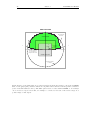
Because LUCIFER is bolted to the Auto-Guiding and (slow) Wavefront sensing (AGw) unit, they
co-rotate to follow the sky, so the AGw has a fixed patrol field (Fig. 10) with respect to the LUCIFER
field of view. Also, the (AGw) unit is built onto an R-theta stage, which affects the layout of the guide
star patrol field with respect to LUCIFER and therefore the position angles for your observations.
There are a few basic constraints to keep in mind:
1.
2.
3.
4.
5.
The guide probe can move on axis, but not past it
The guide probe theta stage limits the X motion of the probe
The focal plane is blocked at >330 arcsec radius
There is vignetting from M3 at field angles above ∼3.5 arcmin off axis
To avoid vignetting LUCIFER, keep the probe > 1 arcmin from the field edges
Some details:
1. The probe always appears to come down from above the LUCIFER field of view, independent of
position angle on sky, because LUCIFER and the AGw are bolted together.
2. The R-theta stage pivot point is 612 mm above the center of the LUCIFER field. Limits at ±18
degrees restricts the motion to just inside the usable focal plane at the left-front bent Gregorian focus.
So you need to be careful when using guide stars at high field angles and position angles that put
them near these limits.
3. The focal plane delivered by the telescope is blocked by parts of the AGw at field angles of more
than 330 arcsec radius.
4. The tertiary mirror is a bit undersized and there is some vignetting visible in the wavefront sensor
at high field angles (>3.5 arcmin). While the wavefront sensor algorithms have been adjusted to
account for this, selecting guide stars inside a radius of 240 arcsec from the science target would be
better than those outside.
5. The probe emits thermal radiation and appears bright in the K band, and at all wavelengths it
shadows the LUCIFER entrance aperture when close to on axis. The apparent size of the probe is 2
arcmin across, or about half the LUCIFER field of view. If this will cause problems for your project,
you need to be careful in the selection of your guide star and the orientation of the field for your
observations. Odd shadows or emission on LUCIFER are likely from the guide probe.
Under fully closed-loop operations (ACTIVE mode) where the same guide star is used at two offset
positions in the patrol field, the positioning accuracy of the source in the LUCIFER field of view is
completely governed by the guide stage accuracy of motion. In repeated tests, we achieve ∼50 mas
rms in the X direction on LUCIFER and ∼30 mas in Y.
5.4
Open-loop tracking stability
Please keep in mind that the telescope will deliver the best image quality under closed-loop ACTIVE
mode operations. It is in your best interest to set up your observations with an appropriate off-axis
guide star. The additional overheads of starting up the ACTIVE mode observations are small (a
few seconds) compared to TRACK mode. However it is possible, and may be desireable, to perform
rapid observations in TRACK mode, such as obtaining spectra of telluric standards where neither the
precise positioning nor collimation is strictly necessary. These objects are typically bright and only
a few minutes are needed to take a pair of spectra. In TRACK mode, you are fully subject to any
thermally-induced drifts in the pointing, so it is likely that you will need to at least make one coarse
correction of the telescope position to place your target at the required location on the LUCIFER
detector.
26
Issue 1.3
LUCIFER User Manual
AGw Patrol Field
AGw r-theta stage
theta limits.
The AGw patrol field.
N
60” vignetting
avoidance
At PA=0
E
AGw r-theta stage radial limit.
The center of rotation is
612.5 mm above the
Gregorian rotator center.
LUCIFER 4ʼ Field of View
Gregorian Focal Plane
11ʼ diameter
Figure 10: Plot of the AGw guide probe patrol field (green) is shown, relative to the 4’x4’ LUCIFER
field of view (gray square) and the delivered focal plane at the left-front bent Gregorian focal station
(outer 11 arcmin diameter circle). The AGw patrol field co-rotates with LUCIFER, so it is always
’above’ in detector space but would, for example, be oriented to the west of the science target at a
position angle of 270 degrees.
LUCIFER User Manual
6
Issue 1.3
27
Preparing observations with LUCIFER
6.1
6.1.1
Available tools
Exposure Time Calculator (ETC)
A LUCIFER exposure time calculator has been made available and can be reached at:
http://www.lsw.uni-heidelberg.de/lucifer-cgi/calculator/calculator.py
It should be used to prepare your observations and estimate the needed integration time for your
purpose.
6.1.2
LUCIFER Mask Simulator (LMS)
LMS is an observer support tool for the preparation of LUCIFER MOS mode observations.
The following is a short overview, and by no means sufficient to run LMS. Before using the program,
please read the LMS user manual carefully.
This software tool is used to:
1. set the instrument configuration (camera, grating, filter),
2. set the default slit parameters (slit type, width, length),
3. select reference stars (for telescope pointing and rotator angle offset correction),
4. select guide stars (for telescope guiding in one or more pointings),
5. position MOS slits (manually on a source image, on the source centroid using a centering routine,
automatically on a target list)
LMS requires two input files:
• The ISF (instrument summary file) containing the relevant telescope and instrument parameters.
This file is part of the LMS package.
• A FITS image or source catalog. The image can be taken with LUCIFER or any other instrument. Within LMS images and catalogs can be downloaded from several servers.
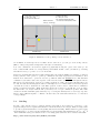
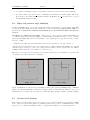
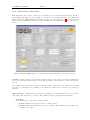
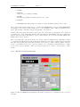
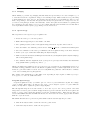
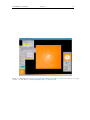
LMS displays the following items, as illustrated in Fig. 11:
1. FITS image or catalog positions projected on the LBT image plane,
2. when the mask “mode” is initialized:
(a) the LUCIFER field (white square),
(b) the back projection of the detector on the LBT image plane (blue square),
(c) central field of low defocus (inner white lines),
(d) field of unclipped spectra (inner blue lines),
(e) area of the reference slits (red rectangle close to the northern edge of the mask)
3. when the mask is initialized and labeling is on (default) in addition:
28
Issue 1.3
LUCIFER User Manual
(a) rotation angle and telescope pointing in the upper left corner,
(b) position of the six reference slits
(c) calculated wavelengths limits on the array at the two southern corners
(d) central wavelength at the northern edges of the unclipped area
4. when adding guide stars: the guider patrol field.
Figure 11: Typical display of the LMS tool.
To make sure that the slits are on the sources when observing, the following rules have to be obeyed:
1. The FITS image must be distortion corrected with high accuracy and the plate scale has to be
known with high accuracy, catalog positions must have high astrometric accuracy.
2. Science sources and reference stars have to be taken from the same image or catalog. Their
relative positions have to be known to better than 1/6 of the slit width; otherwise slit losses
occur.
3. At least two reference stars have to be defined within the LUCIFER field to compensate for
pointing and image rotation offsets. Five reference stars are recommended for higher accuracy.
The maximum number of reference stars has been set to ten.
4. It is strongly recommended to limit yourself to a maximum of 40 slits per mask.
Slits are generated with the default settings for type, length and width. Changing the default settings
will affect newly created slits as well as already existing ones. Slits can be modified and deleted
individually by clicking on their number and width labels. When all slits have been positioned, the
setup can be saved. During this process, four files are generated:
1. a *.lms file containing the instrument parameters, all slit, reference star, and guide star positions
as well as all slit parameters. This file can be loaded again to restore the session,
LUCIFER User Manual
Issue 1.3
29
2. a *.epsf file containing a picture of the mask for direct view (does not show the mask ID),
3. two Gerber files, *.grb, and * v2.grb cointaining the information for mask cutting. The *.grb
file is used for the mask cutting machine available in Munich, the * v2.grb file can be read by
the LBT mask cutting machine.
6.2
Offset and position angle definition
On the LUCIFER images, for a position angle null, North is towards the top of the image, while East
is towards the right, unlike the typical orientation of astronomical images. The position angle you
give is however defined the classical astronomical way = from North to East and given in
degrees.
All offsets are defined in arcseconds. The telescope can be offsetted either in RA/DEC, the
coordinate system is then defined as RADEC), or along the lines/columns of the detector, the coordinate
system is then DETXY. The latter is very useful for e.g. long slit spectroscopy. One also has to define
the type of offset:
- cumulative, the offset type is then relative and one moves relative to the last position, or
- absolute, where all offsets refer to the original position. When offsetting the RADEC, one basically
tells the telescope where to go; the object on the detector will move in the opposite direction. Offsets
in DETXY defines where the object will move on the detector.
The active optics duty cycle is typically of 45 seconds, it is therefore recommended to spend at least
one minute per position after/before offsetting.
'"
2"3"
$"
#"
!"
#"
("
2"4"
&"
!"
&"
!"
%"
!"
)*+(,"-".*"/"&"
$"
%"
'()*+","-.."/01"
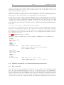
Figure 12: Illustration of the star motion defining a relative offset pattern in RADEC (left) or DETXY
(right). For offsets in DETXY coordinates, the position angle does not make any difference, the object
will always move the same way on the detector. Offset list: (0,0) - (60,60) - (-120,0) - (0,-120) - (120,0).
6.3
Overhead Calculations
Each read is associated with a given readout time, it is 2 seconds in DCR mode and 10 sec in MER
mode. Please note that an integration of 1 minute defined as 2 seconds × 30 NDIT will have a 50%
duty cycle, i.e. it will use 2 minutes of time to complete this 1 minute of on-source integration.
30
Issue 1.3
LUCIFER User Manual
Under good and smooth observing conditions, it has been calculated that offsets in active mode
(guiding and sending active optics correction) take in average ∼ 18 seconds, while only 4 seconds
when performing them in track mode.
Furthermore you have to add the time to create/save the fits file. This time is strongly related to the
number of integrations requested and the mode in which data are to be saved. The average time for
this process is ∼ 12 seconds ( between 5 - for single frames - and 20 in practice).
To those times, one has to add the preset time. This time can be only the slewing time, if one uses the
track mode. However most observations will be performed in guided mode with active optics correction
on. Therefore the guider acquisition and collimation times must be added. Over the Sept.-Oct. 2009
commissioning, over 214 succesful preset (mixed of telescope modes track & active), the average
preset time was of 70seconds. The mean time needed for collimation requests (90 measurements) was
135seconds.
A correction of the telescope pointing takes in average 7 minutes.
For spectroscopic observations one has to add the time needed to move the mask in/out of the focal
plane. To move a mask from its cabinet storage position to the focal plane, it typical takes 2.5 minutes.
Since however it is recommended to move the mask in the ‘focal plane’ position while presetting,
the overhead quoted here represents only the time to move the mask from the turnout position to
the focal plane = 45seconds.
Table 10 summarizes all types of overheads.
Example of overhead calculation (based on true examples) - without preset or acquisition time:
Imaging
Detector mode: DCR
DIT = 20 sec
NDIT = 3
NEXPO = 1
20 offsets
Total time needed
Spectroscopy
Detector mode: MER
DIT = 600 sec
NDIT = 1
NEXPO = 1
5 offsets
Total time needed
= (20.+ 2.)*3.*20. + 20.* 18. + 20. * 12.
= 1920 seconds for 1200 seconds of on-source integration
= 62.5% of shutter open time
= (600. + 10.) * 5. + 5. * 18. + 5. * 12.
= 3200 seconds for 3000 seconds of on-source integration
= 93.7% of shutter open time
6.4
Limiting magnitude & recommended integration times
6.5
Sky emissivity
Sky emissivity is an important parameter setting absolute upper limit for useable DITs in imaging
mode. Of course sky emissivity fluctuates a lot in case of clouds and is related to Moon illumination.
The bluer a filter, the stronger is the influence of the Moon in the sky background. H band sky emission
is pretty independant of the Moon illumination but however strongly affected by variable atmospheric
OH lines. Under clear weather and comparable Moon illumination, its value can fluctuate by a factor 2
on short time scale (few tens of minutes). The Mount Graham sky emissivity has been measured at
LUCIFER User Manual
Issue 1.3
31
Table 10: Overview of all overheads times
Action type
Time (sec)
Pointing correction
420
Pure preset
Collimation of active optics
70
135
Offset time
Track mode
Guided mode + active optics on
4
18
Motion of mask (turnout to FPU)
45
Read out time
DCR mode
MER mode
2
10
Time to write a file
12
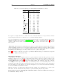
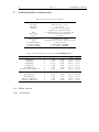
different occasions with LUCIFER, under clear weather conditions, using the N3.75 camera. Table 11
presents some typical results, where the limiting integration time has been rounded.
Filter
Sky flux
(e− /sec)
No Moon
DIT lin
(sec)
BLIP
(sec)
z
J
H
K
Ks
47
290
1315
3250
1640
3900
600
140
50
110
6
<
<
<
<
H2
Br gam
FeII
P beta
P gam
115
125
97
42
18
1600
1400
1800
4300
10000
2.5
2.3
3
7
16
minDIT
minDIT
minDIT
minDIT
70% Moon illumination
Sky flux
DIT lin
BLIP
(e− /sec)
(sec)
(sec)
120
1400
2.5
2400
4300
75
40
< minDIT
< minDIT
Table 11: Measured (N3.75 camera) sky emissivity and corresponding integration time to have the sky
background reaching the linearity limit (determined as two third of the full well) and to be background
limited.
The background-limited performance (BLIP) is defined as : t BLIP = 2×RN2 / Skyflux. It determines
the minimum DIT needed to be background limited, defined here for imaging observations in DCR
mode (minDIT ∼ 2sec) with the N3.75 camera.
6.5.1
Imaging
During clear nights, photometric standard stars have been observed in imaging mode with the N3.75
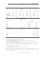
camera and all available filters. Table 12 presents the derived zero points for all filters.
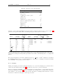
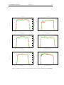
Please note that the LUCIFER1 z & J broad band filters are wider than the corresponding atmopheric
windows (as illustrated in Fig. 13). As a consequence the measured zero points in these bands are
quite sensitive to the amount of water vapor in the atmosphere, resulting in flux variations of 3% in
z and 6% in J when the atmospheric water vapor doubles.
32
Issue 1.3
LUCIFER User Manual
Table 12: LUCIFER’s imaging zero points (defined as 1 ADU/SEC).
Filter
ZP
err(ZP)
Br gam
FeII
H2
HeI
P beta
P gam
Y1
Y2
OH 1060
OH 1190
J low
J high
21.4
21.6
21.45
21.9
21.47
21.43
23.5
23.46
21.5
21.47
24.15
23.85
0.02
0.03
0.02
0.03
0.03
0.03
0.03
0.03
0.03
0.03
0.03
0.03
z
J
H
K
Ks
24.5
24.85
24.7
24.45
24.02
0.03
0.03
0.02
0.03
0.03
Table 13 presents some 3 sigma limiting magnitudes derived assuming a seeing of 0.800 , an airmass of
1.5 and 3mm of water vapor, using a DIT of 10 sec and NDIT=360, to obtain one hour on source
integration.
Table 13: Imaging limiting magnitude for a SNR=3 in one hour integration
6.5.2
Filter
Sky mag.
Limiting mag.
z
J
H
Ks
17.5
16.0
14.0
13.0
24.4
23.9
22.9
22.1
Spectroscopy
During clear nights, spectrophotometric standard stars have been observed with the 1000 wide slit,
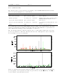
with the N1.8 camera and all the gratings .
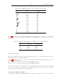
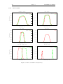
Figure 14 presents typical spectra obtained on spectrophotometric standard stars for all spectroscopic
modes. Two stars were used:
FS6: z=13.06, J=13.271, H=13.321, K=13.404 (UKIRT magnitudes)
FS29: z = 12.98, J=13.215, H=13.255, K=13.33 (UKIRT magnitudes)
In z band, one is readout noise dominated, in J band depending on the water vapor in the atmosphere
one goes from readout noise dominated to sky background dominated. For H & K, spectra are sky
background dominated irrespective of the grating used.
Recommended DITs and NDITs
To avoid unnecessarily long calibrations in the morning, it is recommended to use one of the following
LUCIFER User Manual
Issue 1.3
33
Transmission / %
100
80
60
40
20
0
0.80
1.20
1.60
2.00
Wavelength / µm
Atmosphere
z
J
H
K
J-high
2.40
J-high
Figure 13: Plot of the LUCIFER broad band filters overlaid on a typical atmospheric spectrum.
Table 14: Typical sky count rate measured between OH lines for the 210 zJHK grating with the 1000
slit and time to be background limited (BLIP) in MER mode with the N1.8 camera.
Filter
Count rate
ADU/sec/pix
BLIP
sec
z
J
J
H
K
≤ 0.1
≤ 0.2
0.5
0.8
3
16
≥ 125
≥ 62
for 100 slit - Illustrates the variability
16
< minDIT
red part of spectrum (thermal background dominated)
DIT/NDIT combination for spectroscopic integrations:
• for bright (4.5 < Vmag < 6) tellurics 2sec*15,
• for fainter standards (6 < Vmag < 10) 30sec*2 or 60sec*1,
depending on the wavelength (spectral type and seeing conditions),
• for science observations 120sec*1, 300sec*1, 600sec*1.
For all integrations longer than 60 seconds, it is always (imaging or spectroscopy) recommended to
use the MER mode which has a lower readout noise and better cosmetic.
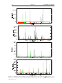
The main limitation for the integration time is given for sky background dominated modes by the sky
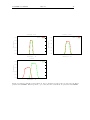
itself and specifically the OH line intensities. In K band with the 100 slit, peak counts of up to 12000
have been measured on OH lines. An example is given in Fig. 15, which also illustrates the fact that
these lines varies with time but essentially independently of the airmass.
34
Issue 1.3
LUCIFER User Manual
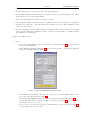
Figure 14: Stellar counts and sky counts in ADU/second/pixel for FS6 and FS29 measured with the
1000 slit and all gratings. Color code: black = FS29 with 200 H+K grating and Order Separator, blue
= FS29 with the 210 zJHK grating, red = FS29 with the 150 Ks grating and Ks filter, violet = FS6
with the 210 zJHK grating and green = FS6 with the 210 zJHK grating and the N3.75 camera (unlike
all other measurements.
LUCIFER User Manual
Issue 1.3
35
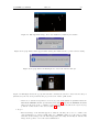
Figure 15: Sky line spectrum measured with the 100 slit, the 210 zJHK grating and the N1.8 camera
at different airmass.
6.6
6.6.1
Calibrations
Sky flats
Sky flats are taken around sunset(/sunrise) with the telescope pointing at zenith, the ventilation doors
closed and the observing doors facing away from the sun. The instrument is at nominal rotator angle
of 341 degrees and the guide probe parked. You fix your integration time and let the sky luminosity
variation do its jobs. Good flats are taken of course only under clear sky conditions. A minimum of 5
frames taken over a range of [3000,17000] ADUs provides a good minimal set of data to derive a flat
field.
Because of the relatively small pixel scale of LUCIFER, sky flats in narrow bands have to be started
before sunset. Start integrating in K narrow band filters (Br gam & H2) 35 minutes before sunset.
After that FeII can be started, followed by P gam & P beta. Once this is finished, you enter the very
short time scale period where all broad band filters can be taken, starting with the red filters (K, Ks)
and ending with the blue ones (z). When taking morning twilight flats, the order of the filters to be
used is of course reversed (short wavelength first, long wavelength (2µm) last).
It is impossible to take all flats in one sunset, you thus have to prioritise your needs. Should no
flatfield be available at all, so can you use the internal calibration unit to take imaging flats. Note
however that these are representative of true sky flats to within ±10% and thus do not allow for good
photometric data reduction.
Table 15 presents the count rate for imaging flatfields with the N3.75 camera. When setting your
calibrations’ script aim at a level of ∼15000 counts (20000 max).
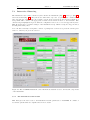
6.6.2
Night calibrations
In principle there is no need to take any night calibration as the flexure compensation is active. To be
on the safe side however, for spectroscopy short wavelength calibration and flat field might be useful
to be taken overnight. We provide here indication about counts rate per second for these calibrations.
36
Issue 1.3
LUCIFER User Manual
Table 15: Count rates (ADU/s) for internal flat fields with N3.75 camera.
Filter
Halo1
Halo2
Halo3
z
J
H
Ks
K
na
na
na
na
na
na
na
na
na
na
1450
5500
7100
3500
4550
J low
J high
Y1
Y2
OH 1060
OH 1190
HeI
P gam
P beta
FeII
H2
Br gam
na
na
na
na
na
na
na
na
na
na
na
na
na
na
na
na
2700
4450
2150
3600
6200
11000
8800
8300
2150
2150
620
750
110
190
180
150
na
480
350
3200
For a quick over night calibration, counts of the order of 200-300 ADUs are enough. Calibrations with
longer integration time are recommended to be performed during daytime.
Note: For long slit spectroscopy most wavelengths calibrations can be performed using the atmospheric
OH lines present in the spectra (see [Rousselot et al.] for a catalog of these lines). Fig. 16 shows an
example of OH lines spectrum obtained with the 210 zJHK grating, the K filter, the 100 slit and the
N1.8 camera.
Flat fields Knowing the necessary integration time for a given calibration with the N1.8 (/N3.75)
camera, multiply (/divide) it by 4 to find the required integration time for the N3.75 (/N1.8) camera
for an equivalent signal to noise. Some flatfield images may present a small ripple effect non exisiting
in night sky data. This ripple can easily be filtered out in e.g. the Fourier plane.
Table 16 present the count rate for spectroscopic flatfields. When setting your calibrations’ script aim
at a level of ∼10000 counts (15000 max).
Wavelength calibration
Knowing the necessary integration time for a given calibration with the N1.8 (/N3.75) camera,
multiply (/divide) it by 4 to find the required integration time for the N3.75 (/N1.8) camera for an
equivalent signal to noise. Table 17 present the count rate for calibration lamp lines as measured with
the 210 zJHK grating in all 4 used orders and for different slits. Two values are given: the count rate
of the brightest lines. Especially over night, you definitively want to avoid saturating them to avoid
remanents effects. The other value represents the average count rate as measured over the typical lines
(not the brightest, not the faintest). To increase the signal to noise on these lines without saturating,
you increase NDIT, keeping DIT constant.
With the exception of z Band, where Argon and Xenon lamps are recommended to be used at the
same time, all other calibrations can perfectly be performed using only the Argon lines.
Do not forget to move manually the calibration unit in and out of the field of view (via
the Instrument Manager Panel).
LUCIFER User Manual
Issue 1.3
37
Figure 16: Normalised spectrum of the K band night sky (210 zJHK grating + N1.8 camera), where
the OH lines are identified
38
Issue 1.3
LUCIFER User Manual
Table 16: Spectroscopic flat field count rate per second, for different slit width.
210 zJHK grating
Rec. Lamp
Slit
S150
S300
S450
S600
(0.2500 )
(0.5000 )
(0.7500 )
(1.0000 )
3-Slit
(only)
halo1 + halo2
halo1 + halo2
halo1
halo1 + halo2
z
J
H
K
N1.8
N3.75
N1.8
N3.75
N1.8
N3.75
N1.8
N3.75
————————————————————————————————————
(105)
25
(250)
60
(400)
100
(350)
90
350
90
850
200
1300
350
1100
300
500
125
1300
350
1900
500
1700
450
700
180
1700
450
2600
650
2200
550
700
180
(halo2!)
1700
450
(halo2!)
3100
800
(halo2!)
2200
550
(halo2!)
200 H+K grating
Recommended Lamp
Slit
S150
S300
S450
S600
SpecPhot
halo2
OrderSep
N1.8 camera
N3.75 camera
————————————————————————————————————
400
100
1300
350
2000
500
2600
700
2600
700
150 Ks grating
Recommended Lamp
Slit
S150
S300
S450
S600
SpecPhot
halo2
Ks
N1.8
N3.75
————————————————————————————————————
200
50
550
140
800
200
1100
280
1100
280
Telluric standard observations for MOS masks
- Move the MOS mask to the turnout position during the preset to the telluric star.
- Center the star to pixel (1024,1024).
- Let the acquisition finish with a blind offset that centers the star within one of the desired slitlets.
- Run the “science” script to offset the telluric star from one slitlet to another.
- (Select slitlets at the “right” and the “left” sides of the mask to cover the entire spectral range)
How to calculate the needed offsets
Use the information in the lms file associated with your mask.
From the lms example below, using the formulae below, one can calculate the separation between the
center of field, defined at position (1024,1024) for the mask creation and the first slit where on wishes
to put the telluric standard.
∆x = ∆α × cos(ROT ) − ∆δ × sin(ROT )
(1)
LUCIFER User Manual
Issue 1.3
39
∆y = ∆α × sin(ROT ) + ∆δ × cos(ROT )
(2)
Distance between center of slit #12 and “pointing center” = ∆α = 70.311”, ∆δ= 8.469”. These
values have to be entered in the acquisition script as blind offset (DETXY relative). Once the script
is finished, it is still time to re-check the centering within slitlet #12.
In the science script itself, one then introduces the offset (DETXY relative) to move the object from
slitlet #12 to slitlet #13 = ∆α = -120.265”, ∆δ= -5.435”
Slit
N1.80 camera
Integration
counts
time (sec)
(B./T. line)
N3.75 camera
Integration
counts
time (sec)
(B./T. line)
210 zJHK grating
S150
S300
S450+S600
SpecPhot
(2+2
2+2
2+2
2+2
S150
S300
S450+S600
SpecPhot
(10+10
10+10
10+10
10+10
S150
S300
S450+S600
SpecPhot
(30+30
30+30
30+30
30+30
S150
S300
S450+S600
SpecPhot
(30+30+30
30+30+30
30+30+30
30+30+30
z Band - Recommended lamps: Ar+Xe
3000/1500)
2+2
750/400
4000/2000
2+2
1000/500
12000/6000
2+2
3000/1500
15000/7500
2+2
3500/1800
J Band - Recommended lamps: Ar (+Ne)
1500/300)
30+30
1200/250
2000/400
30+30
1500/300
6000/1200
10+10
1500/300
7000/1400
10+10
1700/350
H Band - Recommended lamps: Ar+Xe
4000/200)
120+120
4000/200
5000/250
120+120
5000/250
15000/750
30+30
3500/200
17000/800
30+30
4000/200
K Band - Recommended lamps: Ar+Ne+Xe
500/200)
120+120+120
500/200
600/250
120+120+120
600/250
1800/700
60+60+60
900/350
2000/800
60+60+60
1000/400
200 H+K grating
S150
S300
S450+S600
SpecPhot
10+10
10+10
10+10
10+10
OrderSep - Recommended lamps: Ar+Xe
2000/300
20+20
1000/150
3000/400
20+20
1500/200
9000/1200
20+20
4500/600
10000/1300
20+20
5000/700
150 Ks grating
S150
S300
S450+S600
SpecPhot
10+10+10
10+10+10
10+10+10
10+10+10
Ks Filter - Recommended lamps: Ar+Xe+Ne
800/150
30+30+30
600/100
1000/200
30+30+30
750/150
3000/600
30+30+30
2300/600
4000/700
30+30+30
2500/650
Table 17: Arc lines count rate per second. The integration time are for each lamp separately, but they
of course can be switched together. The counts are given for the brightest (B.) lines and the average
of the other “typical” (fainter) lines (T.).
40
Issue 1.3
LUCIFER User Manual
lms input information
Comments
# created by SKYCAT-TOOL -- LMS-plugin V1.13
# INS.MASK.ID : 910509
# --------------------------------------------
Extracts of a lms file:
TEL.TARG.ALPHA
TEL.TARG.DELTA
TEL.ROT.OFFANGLE
TEL.TARG.EQUINOX
TEL.TARG.TYPE
022539.027
+620530.480
-30.000
2000.0
COORDINATE
Pointing information
Position at (1024,1024)
INS.SLIT.NUMBER
25
Number of slits in the mask
INS.TARG103.NAME
INS.SLIT3.REF
INS.TARG103.SHAPE
INS.TARG103.WID
INS.TARG103.LEN
INS.TARG103.ROT
INS.TARG103.WIDMM
INS.TARG103.LENMM
INS.TARG103.XMM
INS.TARG103.YMM
refslit
103
STRAIGHT
0.5
0.5
0.0
0.300
0.300
-13.000
-70.000
Information about ref. slit #3
used for MOS alignment
INS.TARG112.NAME
INS.TARG112.SHAPE
INS.TARG112.WID
INS.TARG112.LEN
INS.TARG112.ROT
INS.TARG112.ALPHA
INS.TARG112.DELTA
INS.TARG112.WIDMM
INS.TARG112.LENMM
INS.TARG112.XMM
INS.TARG112.YMM
NN
STRAIGHT
1.0
4.0
0.0
022547.099
+620612.970
0.600
2.400
-42.184
-5.106
Information about a “science” slit
selected because on the right side of field
INS.TARG113.NAME
INS.TARG113.SHAPE
INS.TARG113.WID
INS.TARG113.LEN
INS.TARG113.ROT
INS.TARG113.ALPHA
INS.TARG113.DELTA
INS.TARG113.WIDMM
INS.TARG113.LENMM
INS.TARG113.XMM
INS.TARG113.YMM
NN
STRAIGHT
1.0
4.0
0.0
022532.650
+620508.130
0.600
2.400
29.968
-1.814
“science” slit
selected because on the left side of field
INS.TARG30.ALPHA
INS.TARG30.DELTA
022535.734
+620540.850
Information about first reference star
#1 in MOS acquisition
INS.TARG39.ALPHA
INS.TARG39.DELTA
022540.637
+620419.340
Information about last reference star
#10 in MOS acquisition
INS.TARG40.ALPHA
INS.TARG40.DELTA
022517.549
+620757.250
Information about the guide star selected
INS.RSTAR.NUMBER
10
Number of reference stars selected
LUCIFER User Manual
6.6.3
Issue 1.3
41
Calibration Plan
The calibration plan on a long term is the responsability of the LUCIFER LBTO instrument scientist.
We however shortly highlight our recommendations.
Topic
Flat fields
Photometric standards
Frequency
upon observer’s request
upon observer’s request
Comment
to be taken on sky
clear conditions
Telluric standards
for each spectro. observation
Spectrophotometric standards
upon observer’s request
within 2 hours of the observation and a
maximum airmass difference of 0.2
same as above
Spectroscopic arcs & flat fields
for each spectro. observation
Darks
daily
to be taken the morning after the observations
for the readout modes used
Note: Darks with exposure time (DIT×NDIT) less than 1 minute can be taken with the dome dark
and the two blind filters. For higher exposure time darks, the blind mask has to be put in the focal
plane. This has the advantage to allow dome lights to be turned on.
The only internal calibration, which absolutely needs to be taken with no light in the dome is the
spectroscopic flatfield, for which the calibration unit is needed. Although arcs could be taken with
the dome lights on, it is not recommended.
Figure 17: Calibration lines measured with the LS300 (0.500 ) slit for the 150 Ks (top) and 200 H+K
(bottom) grating. Ar is represented in black, Xe green and Ne red (when available). From top t
bottom: z Band, J band, H band & K band.
42
Issue 1.3
LUCIFER User Manual
Figure 18: Calibration lines measured with the LS150 (0.2500 ) slit for the 210 zJHK grating. Ar is
represented in black, Xe green and Ne red (when available). From top t bottom: z Band, J band, H
band & K band.
LUCIFER User Manual
7
Issue 1.3
43
Observing with LUCIFER
The normal observing operation with LUCIFER is entirely performed through scripts (Sect. 7.4).
The interactive observing mode (Sect. 7.3) is described in detail here since it allows to introduce the
definition of all parameters needed for scripts.
7.1
Login and Software Start
Usually, the Lucifer control software (LCSP) is running continuously on the SUN V880 workstation.
That means the observer has only to start the necessary GUIs. Therefore he/she has to use the
dedicated LBTO linux machine and open a NXClient connection with the following parameters:
• User name: observer
• Password: provided at the LBT
• host: sun-luci
After being connected to the SUN X environment, double click on the Start LUCIFER icon on the
desktop. This will open all the necessary GUIs for the observations.
The readout software initial panel requests you to press on OK. With the exception of the observer
name that you can specify there, to see it updated in the FITs header, do not change any other of the
settings. Also Do NOT close any of the terminal window that opens automatically.
7.2
7.2.1
Start and end of night procedures
Start of night
• Set a new directory (path file) in the Readout Manager GUI (Fig. 22)
• Set a new filename (change the date) in the Readout Manager GUI (Fig. 22)
• Save a dummy image to stop the archive complaining it has nothing to archive
• If the sky is clear, go on with taking twilight sky flats (at zenith before sunset); see section 6.6.1
• Then move on with the pointing correction procedure; see paragraph 5.2
7.2.2
End of the night
• Put the two blind filters and the N1.8 camera in position and set the detector to DCR mode
with DIT=2sec (manual saving) while the operator is closing the telescope
• Start the flush detector.txt script
• Prepare your scripts to take the dark calibrations
• Once the dome is closed and dark (no light), the telescope at zenith, rotator angle = 341 and
the guide probe has been parked, you can take the needed calibrations with the calibration unit
• When done with the calibration unit, set again the two blind filters and run the flush detector.txt
script again
• Put the BLIND mask in FPU and start your dark calibration script
44
7.3
Issue 1.3
LUCIFER User Manual
Interactive Observing
The instrument can be fully controlled by three GUIs: the instrument- (Fig. 19), telescope- (Fig. 21)
and readout-GUI (Fig. 22). They all use the same kind of process: by pressing the commit button
after selecting the desired setup, the software collects all properties from the GUI and builds up a
setup which will be send to the appropriate software service and from there to the hardware. The
current setup is highlighted in green, while the configuration selected to be set next appears in yellow.
This allows the user to track the changes of the instrument set-up. When a set-up is being performed,
the full panel turns yellow.
Note: Should accidently a wrong filter, camera or grating have been selected, press the current green
button to discard your previous selection.
Figure 19: The LUCIFER instrument control GUI allows classical access to all relevant components
of the instrument.
7.3.1
The Instrument Control GUI
This GUI gives the user access to all instrument relevant parameters of LUCIFER. It consists of
several sub panels which are explained here in more detail.
LUCIFER User Manual
Issue 1.3
45
MOS Panel The use of masks in the focal plane is controlled from the left part of the GUI (see fig.
19). The current state of the unit is shown in the text fields Mos state and Mask In Use. During
the movement process a moving bar is visible.
Note: In the case that the Mos State changes to unknown (which will be color coded in red) the
instrument scientist has to be contacted immediately. STOP doing anything with LUCIFER
when this has happened!!
The MOS state can be changed by using the two drop down menu, one for the mask state (Mask To
Position) and the one with the mask number to use (Mask To Use). The latter one shows the names
and numbers of the current masks in the cabinet. It is updated after each cabinet exchange by the
responsible technician or the instrument scientist in charge. Three “mask states” can be selected from
the pull down menu:
1. No Mask In Use = all masks are in storage position. This is the default configuration (used
for imaging)
2. Mask To FPU = moves the mask that has been selected from the drop down menu Mask to
Use into the focal plan. This is the default set-up for spectroscopic observations.
3. Mask To Turnout = moves the mask out of the focal plane but not back to the storage
position to save time. This is needed for spectroscopic acquisition (section 7.5.2).
Calibration Panel The next panel in this GUI lets the user control the calibration unit. It can be
moved in and out from here and the current lamp status is shown. To switch on the lamps an extra
GUI (Fig. 20) can be accessed via the Open GUI button. There all lamps can be selected at once.
Note: When asking to move the calibration unit in, it sometimes happens that on the first click on ”IN”
following illegal error appears: Problems with Calibration Unit device (WebIO): java.lang.IllegalMonitorStateException
Do not worry. Just try again. Should the problem persists so ask your LBTO support astronomer to
move the calibration unit in position from the corresponding engineering panel, to which you do not
have access as user.
Table 18: Definition of the lamps in the calibration unit.
#2
Name of the lamps in the Telescope Control GUI
#3
#4
#5
#6
Position
#1
Name
Comment
Name of the lamps in the Calibration Unit GUI
Ne
Ar
Xe
halo1
halo2
halo3
Arc lamps for wavelength calibration
Halogen lamps for flat fields
The lamp intensity decreases from #1 to #3
Flexure Compensation panel In the flexure compensation panel the current flexure mode of
the instrument is shown and can be changed via the ON/OFF drop down menu. When flexure
compensation is turned ON using the GUI, it is not switched off by running scripts, even if they have
the flexure compensation flag set to OFF. Conversely, when the flexure compensation is turned OFF
using the GUI, scripts can actively switch the flexure compensation on or off (depending on the status
of the flag). Note that at the end of script the flexure compensation is then switched off.
Camera Panel The camera wheel panel allows the camera selection. The N3.75 camera is for
imaging and the N1.8 meant for spectroscopy.
Note: the N30 camera has been designed for observations together with adaptive optics and is currently
not installed.
46
Issue 1.3
LUCIFER User Manual
Figure 20: The LUCIFER Calibration Unit GUI.
Note: If moving from one camera to the other, you notice the field is not centered again, it is most
probably because the camera wheel did not reach its position properly. In this case simply move to
another camera and then back. If needed, ask your LBTO support astronomer to re-initialise the
camera wheel, from the corresponding engineering panel, to which you do not have access as user.
Grating Panel From the grating unit panel the mirror position (for imaging) and three different
gratings can be chosen. Furthermore the current wavelength is shown and the text field Desired
Wavelength allows user input for new wavelength. The unit is in microns and the maximum meaningful
precision is 0.1nm. The desired grating has to be specified before the wavelength is typed in, since
the wavelength value is cleared when a new grating unit position is selected. After typing in a new
wavelength the user has to click the Set Wavelength button and of course the Commit button to
execute the setup change. When no wavelength i given, the selected grating is moved into position
but it will not be tilted to a defined angle. Use this option only when the desired grating is fixed,
machenically, to a nominal angle; as is currently the case for the 150 Ks grating.
Pupil Viewer Panel This is mostly needed for optical calibrational work and not necessary for the
normal observing mode.
Filter Wheels Here the user can choose the filters to observe with. When both filter wheels need
to be moved, filter wheel #1 is moved first before filter wheel #2 is moved. Keep this in mind when
making a manual set up to avoid going through 2 open (clear) positions.
Note: All combinations are possible but some might not meaningful, so please be alert.
Commit The Commit button is located on the upper right side of the GUI. Here the new setup
can be executed. As long as a component inside LUCIFER is still moving from a former setup, the
Commit button is blocked. The Initialize button is located left from the Commit button . After a
software restart this button has to be pressed to re-initialise all instrument functions. During normal
operations there is not need to use this button.
Alarm Status Panel Here the overall status of the environmental systems of LUCIFER is indicated.
A change in temperature or pressure will be indicated by a warning or an alarm, which is color coded
red. The latter one is very critical and requires an urgent system check by an instrument (engineer)
expert.
LUCIFER User Manual
7.3.2
Issue 1.3
47
The Telescope Control GUI
This GUI uses a direct service connection to the Telescope Control Server (TCS) interface. An error
when starting the Telescope Service might be caused by a non running interface on the TCS side.
Please inform the LBTO instrument scientist for support. The GUI (Fig. 21) follows the same
philosophy as the Instrument Control GUI, the Commit button sends the new setup to the telescope
service.
Figure 21: The LUCIFER Telescope Control GUI provides all features to set up the telescope.
Pointing On the left side of the GUI the current position of the telescope is shown, including the
rotator, position and parallactic angle. It is updated regularly so the user is able to follow the telescope
motion.
Note: When these text fields are empty, it indicates that a connection to the TCS is not working
properly or a subsystem is not running on the TCS side. This can be checked by the Telescope
Operator.
Offset Telescope This panel is necessary for the acquisition process. The user can choose a position
angle (PA) offset and telescope position offsets. There are three pull down menues available:
• CoordSys
Lets the user choose the valid coordinate system.
1. RADEC Offsets are interpreted as sky coordinate offsets.
2. DETXY Offsets are interpreted as detector coordinate offsets. This option is useful for the
acquisition procedures.
48
Issue 1.3
LUCIFER User Manual
• Side
This describes which mirror is in use: Left (LUCIFER1), Right (LUCIFER 2) (not available
yet)
• Movetype
Describes the type of offset: relative or absolute.
Underneath these pull down menues buttons in a star pattern for 4 sky orientations are located,
allowing an offset in these direction. The offset value in arcsec has to be typed into the appropriate
text field in the middle of the pattern. Pressing one of the orange orientation buttons will directly
lead to a movement of the telescope. Furthermore x and y offsets in arcsec can be typed into the
bottom text field, divided by a comma to move the telescope directly in two directions. The small
Commit button will also directly lead to a movement of the telescope.
Current Setup Information There are three sub panels describing the current values of the target,
guide star and telescope. The current target and guide star information is stored locally since the
telescope does not provide this. This means that after a new start of the LUCIFER control software
no information will be present.
Setting Up The Telescope To set a new target the user can use the text fields for target and
guide star or a ASCII list which can be loaded via the Load Catalogue button in the Next Target
sub panel.
The Input syntax for RA and DEC has to be in sexagesimal format like
RA 06 09 07.836 and DEC 24 22 32.35 for example. The coordinates have to be in J2000.
The ASCII catalogue for target and guide stars has to be formatted as follows using a pipe (|) as the
delimiter.
TARGETNAME|RA|DEC|GUIDE* NAME|GUIDE* RA|GUIDE* DEC|PA|RA_PPM|DEC_PPM
For example:
FS29
|21 52 25.3835|+02 23 19.556|GS_r14.3_d3.77_pos047.362|21 52 36.538|+02 25 52.21|45|23.00|-302.98
For each target an appropriate guide star has to be defined by the observer. As the telecope SW
does NOT provide automatic guide star selection, the user has to select the guide star(s) in advance.
It is possible to open several catalogues at a time. By clicking on the desired line in the catalogue
and using from the menu Commit->Commit Star sends the selection to the telescope GUI but not
the telescope yet.
After the next target and guide star have been set, additional telescope specific parameters can be
changed. The typical oberving setup is POSITION ACTIVE.
• ROT MODE
Here the rotator mode can be set.
1. POSITION
2. PARALLACTIC
• TEL-MODE
Here the telescope mode can be set to
LUCIFER User Manual
Issue 1.3
49
1. STATIC
2. TRACK
Only telescope tracking is running.
3. GUIDE
Tracking and guiding is running without active optics.
4. ACTIVE
5. ADAPTIVE The full package for normal observing: Tracking+guiding+active optics
The position angle is defined with respect to North when ROTMODE is ’position’. When ROTMODE
is ’parallactic’, the angle is defined with respect to the parallactic angle. Thus, a parallactic mode
preset with an angle of 90 will orient the slit parallel to the horizon.
All three input sub panels (Next Target, Next Guide Star, Next Telescope Setup) have to be activated
by clicking the corresponding Set Target, Set Guide Star, Set Telescope button. When the
input is okay the button will change to green. After all three are green the Commit Telescope
Setup button can be pressed.
The bottom right part of the panel allows you to set the “wait for collimation flag”. This has to always
be on then scripts will start integrations after the collimation is successful; otherwise integrations may
start just after guiding started and independantly of the telescope delivered image quality. Should a
preset be successful but the active optics not starting or not collimating, change this flag to “OFF”
so the telescope preset “finishes”. Then you can preset again (do not forget to reset the flag to “ON”
again).
7.3.3
The Detector Read Out GUI
Figure 22: The LUCIFER Read Out Manager GUI. All necessary detector parameters can be set from
this GUI.
50
Issue 1.3
LUCIFER User Manual
The third control GUI for interactive observations with LUCIFER is the Readout Control GUI
(Fig. 22). The left region of the GUI shows the current detector set-up values like e.g. the readout mode in use, the integration time, the last and next file names of the images, etc. The countdown
clock located in the upper left corner indicates whether an integration is currently on-going. A static
time value on a black background (as shown in the figure) indicates that the detector is currently idle.
When a readout is started the clock changes to a yellow background and the remaining integration
time (for one exposure) starts to count down.
The right part of the GUI allows to set new readout (DIT, NDIT, NEXPO) values and to start/stop
exposures. The “Start Read” button starts an integration with the current settings displayed in the
left part. The “Abort” button can be used to stop the on-going integration.
Note: no confirmation window will be displayed before the integration is stopped!
To determine that images should be saved manually or automatically the pull-down menu next to
the “Save image” button is used. The color of this button also indicates whether the last image has
already been saved (the button is green) or not (the button is orange).
Note: Changing the selected save mode value from “manual” to “automatic” would save data if that
action takes place before an integration or a read, but does not save the last frame already read
automatically.
The “Frame type” pull down menu determines the value of the OBJECT and DATATYPE keywords
that will be written into the FITS header of the image. When the datatype is “SCIENCE”, the
OBJECT keyword value for the fitsheader will be read from the telescope service at the beginning
of the integration. For any other selection the OBJECT keyword in the fitsheader will be set to
“undefined”.
The lower right area of the GUI allows to set the values for a new readout set-up. The two available
readout modes can be selected with the “ROEMode” pull down menu. There are three different
options to save files (“Savemode” pull down menu):
1. normal: for each exposure, the detector is read out NDIT times for DIT seconds. When the
images are saved, NDIT files are written, each with DIT seconds exposure time. This is repeated
for the number of frames required.
2. integrated: only one frame is saved. It corresponds to the sum of the DIT×NDIT seconds of
integration.
3. cube: data are saved in a cube with NDIT planes.
“Filename root” allows to set the root of filenames that should be written. If the last character of this
string is not a digit, the GEIRS read out software will append four digits to this root automatically
and write files with ascending numbers. A proven practice is to end the root of the file names with
an underscore “ ” character. Typically frames are called “luci YYYYMMDD ”. The “Save Path”
text field can be used to determine a new saving directory. This can be done by typing the new path
directly into the text field or by using a file chooser which is opened when the “...” button is pressed.
If the new save directory does not exist, a message window appears after clicking the “Set new values”
button, to ask you to create this new directory.
Sending the new setup to the readout manager is done by clicking the “Set new values” button located
directly below new readout setup area. If this button is orange, changes in the readout setup have not
yet been sent since the last time the button was pressed. Like the “Save image” button this button
changes to “green” when the changes have been sent successfully. At this point the information on
the right and left side of the panel should be identical. To be able to sent a new readout setup, all
values have to be set to sensible (i.e., non negative) values. The “Filename root” and “Save Path”
fields can be left blank, however. In this case, the current values will be left unchanged.
After a read the newly observed image is displayed on the LUCIFER display (Fig 23). This display
does not offer as many options as a typical SkyCat. but allows to have a quick check at the data taken
LUCIFER User Manual
Issue 1.3
51
(sky/object counts & centering). On the top right part of the panel few statistics vaues, calculated
over the small window represented above it, are provided. For a quick look image analysis as well as
for the acquisition procedure, the image has to be saved. This triggers an automatic uploading of the
frame in the SkyCat display on same desktop.
Figure 23: The LUCIFER image display.
Archiving information
It is possible to write archiving information to the FITS header of the LUCIFER files. Three
different archiving keywords are written:
PARTNER = ’NOPARTNER’/ name of partner(s)
PI NAME = ’NOTSPECIFIED’/ name of the PI(s)
PROP ID = ’NOTSPECIFIED’/ proposal ID
In this example the default values that will be used if no other information is available are shown.
Archiving information can be set using the ReadoutManager GUI or via scripts.
The current archiving information is displayed above the readout setup information, in the “Archive
Info” box (Fig. 22).To change the current archiving information use the Set archive info... button.
This opens the dialog window presented in Fig. 24.
The three different entries can be edited as necessary. The PI Name and the Proposal ID entries can
be chosen freely, for the Partner information some rules are applied:
52
Issue 1.3
LUCIFER User Manual
Figure 24: The archive information editing window.
1. Only the following partner names are valid:
AZ,COMMISSIONING,INAF,LBTB,LBTO,LBTSDT,OSURC
2. Multiple valid partner names can be specified, if more than one name is used, the names must be
separated by a comma (,). No comma is allowed after the last partner name. Spaces ( ) are allowed
before or after the partner name but will be removed in the FITS header entry.
3. If no partner name is given (i.e., the text field is empty) the default name NOPARTNER is used.
4. If an invalid partner name is given, an error message is displayed and the preceding partner information is restored.
After entering the new values by clicking Ok, the new information is displayed in the ReadoutManager
GUI (Fig. 25) and used for all files that are saved from now on, using the GUI.
Figure 25: Extract of the LUCIFER Read Out Manager GUI showing the updated archive information.
7.4
Script Observing
Usually, observations with LUCIFER will be performed by means of ASCII scripts. These scripts
allow the setting of all relevant instrument parameters as well as the control of the telescope. Scripts
are very convenient and help significantely to maximize observing efficiency.
The scripts are structured to clearly outline which part of the set-up corresponds to the different subsystem telescope, instrument, detector and parameters specifics for the archive system. For example
all parameters relevant for the instrument set-up have to be set within the [* INSTRUMENT SETUP]
section. Any parameters not needed to be set can be commented out with a “#” at the beginning of
the line. Should you wish to use a pre-prepared script which contains a telescope set-up but actually
do not need it, so can you comment the entire setion out by adding the “#” symbol before the
[START TELESCOPE SETUP] and [END TELESCOPE SETUP].
Note: Altough the save path and filenames for the images can be specified within the scripts, it is
often more convenient to leave these two parameters out of the scripts, or just comment them out.
In this case the values that are currently set, through the READOUT GUI, are used for the images
name.
All reads made from a script will be automatically saved, with the exception of the one taken during
the ACQUISITION option in the OBSERVING SETUP part of the script.
For the observer’s convenience dedicated templates for NIR observations are made available and example scripts (presented in Appendix D) can be found in TemplateScripts/Examples on the LUCIFER
workstation.
The scripts are started by using the shell script executeLUCIScript.sh available at the prompt on
any observer terminal. Scripts can be tested, as observer on the LUCIFER workstation, for correct
syntax and structure whithout executing them, using the “–test” option =
LUCIFER User Manual
Issue 1.3
53
executeLUCIScript.sh --test <scriptname>
The list below shows all possible parameters that can be used for a script. Comments to all possible
entries are provided on the right handside. All parameters presented in the [* OBSERVING SETUP] can
of course not be used all in one single script, especially since some are meant for “science” observations
and others for calibration purposes.
[START_ARCHIVE_INFORMATION]
PARTNER
=NOPARTNER
PI_NAME
=NOTSPECIFIED
PROP_ID
=NOTSPECIFIED
[END_ARCHIVE_INFORMATION]
[START_INSTRUMENT_SETUP]
CAMERA
=N3.75
FILTER
=Ks Br_gam
GRATING_UNIT
=mirror
CENTRAL_WAVELENGTH
=
MASK
=
#AZ,COMMISSIONING,INAF,
#LBTB,LBTO,LBTSDT,OSURC
#name of PI
#proposal ID string
=no_mask_in_use
=on
#
#
#
#
#
#
#
#
#
N1.8|N3.75|N30
name of one or two filters
mirror|210_zJHK|200_H+K|150_Ks
value or leave blank
IDxxx = mask id
NBxx = cabinet position
leave blank for no mask
mask_in_fpu|mask_in_turnout|no_mask_in_use
enable flexure compensation
[START_TELESCOPE_SETUP]
TARGET_NAME
TARGET_COORD
GUIDE_NAME
GUIDE_COORD
ROT_ANG
ROT_MODE
TELESCOPE_MODE
[END_TELESCOPE_SETUP]
=test star
=05 02 50 20 40 50
=
=05 03 00 20 40 30
=50
=position
=active
#
#
#
#
#
#
#
any name or leave blank
hh mm ss dd mm ss
any name or leave blank
hh mm ss dd mm ss
in degrees
position|parallactic|idle
active|guide|track
[START_READOUT_SETUP]
DIT
NDIT
NEXPO
ROE_MODE
SAVE_MODE
SAVE_PATH
FILENAME
[END_READOUT_SETUP]
=10
=2
=2
=mer
=INTEGRATED
=/data/luci/20080911
=script_
#
#
#
#
#
#
#
any positive value, no blanks allowed
any positive value, no blanks allowed
as NDIT
o2dcr|o2scr|msr|mer (#reads)|lir
integrated|cube|normal
absolute save path
root of the filenames
MASK_POSITION
FLEXURE_COMP
[END_INSTRUMENT_SETUP]
[START_OBSERVING_SETUP]
OFFSET_TYPE
COORD_SYS
ACQUISITION
JITTER
OFFSET
OFFSET
POINTING
=absolute
=DETXY
=20 20
=10 40.0
#
#
#
#
#
=10 00
#
=10 00 45.6
#
=06 40 40 21 23 30 06 40 59 21
relative|absolute
DETXY|RADEC
wait after offset
jitter pattern with 10 exposures
a maximum offset distance of 40.0 arcsecs
offset from TARGET_COORD
same as above with a rot angle offset of 45.6
24 00
# new pointing coords
FLAT
FLAT
FLAT
LAMP
LAMP
=mer 10.0 5 10
# readout with DIT=3.0, NDIT=5, NEXPO=10
=mer 10.0 1 10 Ks clear N1.8 # specify additional instrument setup
# readout using last readout setup
=Xe 10
# turns on the Xe lamp for 10 secs
=Xe
# as above but with automatic calculation
# of the lamp activation time
DARK
FLUSH_DETECTOR
=o2dcr 60.0 5 10
# indicate DARK instead of FLAT
# executes a flush readout of the detector
# no parameters, no images are saved
54
Issue 1.3
LUCIFER User Manual
[END_OBSERVING_SETUP]
Notes on script
• Archive information
– Entries for PI NAME & PROP ID are entirely free
– Entries for PARTNER are restricted to the following list:
AZ,COMMISSIONING,INAF,LBTB,LBTO,LBTSDT,OSURC
Multiple partners must be separated by a comma (,). Invalid partner names will cause the
script to fail when it is read.
– When any of the three parameters is missing in a script, the default value (as indicated in
the above example) for this missing parameter is used.
– Archive information set in scripts is used for all frames that are taken while the script is
running, overriding any information that is set from the ReadoutManager GUI. While a
script that contains archive information is running, the ReadoutManager GUI shows this
information in red text color, as shown in Fig. 26.
Figure 26: Archive info section in the ReadoutManager GUI when a script is running
– As soon as the script is finished the old information set in the GUI is used (and displayed)
again for files that are saved from the GUI.
– When a script without archiving information is running, the current values set from the
GUI are written into the FITS headers.
• Instrument set up
– In the filter parameter, two filters can be set. Use this option to put crossed filters for
acquisition on bright objects. Two filters from the same filter wheel cannot be set together!
Possible crossed filters combinations for acquisition: HeI + z for a ∼ 7 mag. extinction,
OH 1060 + z for a ∼ 3.9 mag. extinction, HeI + J for a ∼ 2.35 mag. extinction and
P gam + J for a ∼ 0.8 mag. extinction. Of course set up like Br gam + Ks are possible
but provide a much lower extinction factor.
– The flexure compensation flag should in principle always be set to ”on”. For short photometric standard or telluric stars observations, this can be left to off.
• Telescope set up
– Presets in active mode request that you provide a guide star, otherwise the preset will fail
– Presets in track mode do not require a guide star but for the case no guide star information
is present in the telescope set up buffer (e.g. at the beginning of the night), provide as
guide star coordinates the coord. of your target. A track mode preset will park the probe
but the telescope software is anyway awaiting a full list of parameters - including the guide
star information.
• READOUT set up
– NDIT is the number of reads (DIT) that will be performed at a given position. For NDIT
> 1 the ”SAVE MODE” must be integrated.
– If you want to save more than one image per position, then set this with NEXPO, which
is the number of exposures of integration DIT×NDIT that wil be performed at the current
position.
LUCIFER User Manual
Issue 1.3
55
– If you decide to have NDIT >1 and ”SAVE MODE”= normal, note that all your NDIT
images will be saved individually but only at the end of the NDIT reads and will all have
one and the same fitsheader.
– The total number of frames you will get is defined as (Number of offsets defined in Observing
set up) * NEXPO is you are in integrated mode with NDIT> 1 or (Number of offsets defined
in Observing set up) * NEXPO * NDIT if data are saved in normal mode.
• Observing set up
– After a spectroscopic acquisition, the ”OFFSET TYPE” has to be relative, otherwise you
loose the centering of your object behind the mask.
– There is not automatic return to origin position at the end of the scripts (except you set
your offsets accordingly)
– The ”ACQUISITION” command makes a read (as defined in Readout set up) but does not
save it. This command is useful for spectroscopic acquisition since it pauses the script till
you are satisfied to continue (= you are finished with your alignment).
– ”jitter” creates a random generated jitter pattern to take (as defined in the example before)
10 images (=10 offsets), within a maximum (radial) distance of 4000 .
– The syntax of the command is: ∆X/∆RA (arcseconds) ∆Y/∆DEC (arcseconds) ∆PA
(degree)
– The ”pointing” command allows to make huge offsets but still remain in closed active loop
since you have to provide the coordinates of a new guide star. Note however that the
position angle cannot be changed between the two pointing positions.
– ”FLAT”, ”LAMP” & ”DARK” are used for calibration purposes and should be set in
separate scripts independant of the ’science’ script.
– ”FLAT” is used only to take skyflats. It has to be set together with an instrument set up
and a readout mode set up. NEXPO is used to define how many frames will be saved.
– ”LAMP” is used to take calibrations with the calibration unit. The script automatically
takes frames with the lamp off first then the lamp on. If only the lamp name is given (e.g.
LAMP =Xe), the activation time for the lamp will be calculated automatically from the
readout setup (DIT, NDIT, NEXPO). Alternatively, the time the lamp should remain on
can be set explicitly by specifying it as a second parameter (LAMP =Xe 10.0). To calculate
the ”lamp on” time manually use NEXPO*[NDIT*(DIT+2sec)+(NDIT-1)*5], where 2 sec
is the readout time for the o2dcr mode (lamp calibrations in mer mode are rare since the
integration time has to be short) and 5 the time to save a fitsfile. If NDIT>1, the save mode
has to be integrated.
NOTE: The calibration unit has to be ”IN” position, otherwise the script will abort when
a ”LAMP” script is started.
– ”DARK” is used to take dark frames. Should you wish to save darks in Normal or Integrated
mode, so should you set two scripts separately.
– ”FLUSH DETECTOR” performs 11 minutes of detector (short) reads. It is recommended
to use this between your dark scripts to ”clean” the detector. Similarly at the end
of your dark script, please run the ”clean” script, which is available in the TemplateScripts/Examples on the lucifer machine.
7.5
Target Acquisition
Target acquisition is needed mostly uniquely for spectroscopic acquisitions and has to be set in a
script separately from the science script. Under given special circumstances, in imaging mode,
one may wish to refine the ”pointing” on a given science field; but normally no acquisition is needed
for this observing mode.
56
7.5.1
Issue 1.3
LUCIFER User Manual
Imaging
When wishing to perform deep imaging and thus many new presets may be needed, it might be good
to check the field on the ”acquisition” image before starting a script. This is easily done by performing
a quick manual read of the detector. It sometimes directly shows an obvious shift in position of your
field corresponding to the fact that the guide star found by the guider did not correspond to the one
you selected. In principle, if that ”automatically” found other guide star is suitable for guiding and
the centering is not important for you, you can continue like this. Bear in mind however that this is
a strong indication that a (telescope) pointing correction is needed.
7.5.2
Spectroscopy
The steps involved in a spectroscopic acquisition are:
• Preset the telescope to the new position
• While this is happening move the mask to the FPU
• Once guiding is started, take a through slit image with short exposure time & save it
• Move the mask to the turnout position via the ”Mask to turnout” command in the MOS panel
• Once the collimation of the telescope is finished, take an acquisition image of the field of interest
• Center your object behind the mask using the SkyCat display
• Make a read from the Readout Manager GUI and check your alignment (in the SkyCat display),
take a through slit image
• Once satisfied with the alignment, start your spectroscopic script that includes the instrument
setup (mask in FPU, grating in position, ...)
When performing an acquisition before deep spectroscopic observations, avoid saturating the detector
and thus creating persistance effects. Should the acquisition image contain bright stars, it is recommended to perform a number of short detector reads (DIT=2sec) with the ’blind’ filters for a minute
or two before starting the long integrations.
The details of the alignment procedure differ a bit depending if only long slit or multi-object spectroscopy is to be done, as detailed hereafter.
Long Slit Spectroscopy
Long slit acquisition is easy: you wish to put one or more objects behind the long slit. For a single
object, a simple offset will be enough, in case of two or more aligned objects to be put behind the
mask, you may wish to adjust the position angle slightly.
The through slit image is needed as reference to move the object to the correct position. Once this
image has been saved, put it as Bias image in skycat (option reacheable from the File pull down
menu - top left of the panel) and subtract it from the acquisition image. Then use the Telescope
Control GUI Shift image & rotate image buttons. If a rotation is needed, apply it first and then
shift the object as needed.
The Shift Image button opens a new panel which leads the user through the procedure:
1. Click in the Skycat GUI to define the reference position and
2. click in the Skycat GUI to define the new position.
LUCIFER User Manual
Issue 1.3
57
In detail: First of all, the image on which you want to do the measurements has to be opened in
Skycat. Then click ”yes” in the option panel. Now choose the reference object (star) in Skycat, click
on it (pick object) and wait for a second or two. Skycat performs a 2D-Gauss fitting on the object.
Once finished, click on the position where the reference point should be moved to (center of slit).
Again, Skycat will make a fit and the calculated offset needed will appear on the Telescope Control
GUI under the Offset Telescope area in the X,Y textfield within few seconds. Pressing the small
Commit button located below will trigger the telescope offsetting.
The Rotate Image button opens a similar pop-up window as in the case of Shift Image. The
steps to follow are actually the same, except that a rotation offset will then be provided instead of a
displacement offset.
Careful: If a non-zero rotation offset angle exists in the PA entry of the ”Offset Telescope” area of the
Telescope Control GUI, this will always be applied! Thus when offsetting after a rotation correction,
make sure to set this value to zero before commiting your set-up.
Blind offset acquisition is feasible via scripts. The acquisition procedure is the same as described
above but on a nearby ”bright” star. At the end of the alignment procedure, the offset onto your
science target will be performed ==> you preset onto the reference star and provide the offset to
move from the reference star to the faint target. An example of script on how to do this is given
here. The Acquisition option, allows to have a read of the telescope automatically performed (but
no image saved from the script) once the collimation of the telescope has been reached. Then the
script pauses as long as you do not explicitly tells it to continue. This ”paused” time is then used to
perform the alignment on the reference star. Once this is finished, let the script continue (& finish):
it performs the blind offset and takes an image.
[START_INSTRUMENT_SETUP]
CAMERA
=N3.75
FILTER
=blind K
GRATING_UNIT
=mirror
MASK
=NB4
MASK_POSITION
=mask_in_fpu
FLEXURE_COMP
=off
[END_INSTRUMENT_SETUP]
[START_TELESCOPE_SETUP]
TARGET_NAME
TARGET_COORD
GUIDE_NAME
GUIDE_COORD
ROT_ANG
ROT_MODE
TELESCOPE_MODE
[END_TELESCOPE_SETUP]
=MyTarget
=11 22 33 +44 55 00.7
=GSC
=11 22 32.9 +44 55 01.2
=12.5
=position
=active
[START_READOUT_SETUP]
DIT
NDIT
NEXPO
ROE_MODE
SAVE_MODE
[END_READOUT_SETUP]
=0
=30
=1
=o2dcr
=NORMAL
[START_OBSERVING_SETUP]
OFFSET_TYPE
=relative
COORD_SYS=RADEC
ACQUISITION
= 0 0
OFFSET
=-26.61 98.34
[END_OBSERVING_SETUP]
# The offset to get centered on your faint source
Multi-object Spectroscopy
The acquisition on custom made MOS mask happens as follow:
58
Issue 1.3
LUCIFER User Manual
1. Put the mask in the focal plane and take a through mask image
2. Use the MOS Acquisition GUI and skycat to identify a reference point (small pinhole ’slit’ which
is present at the top of in any MOS mask)
3. Move the mask in Turnout and take an image of the field
4. Use the MOS Acquisition GUI and skycat to identify the reference stars used for the alignment
5. Calculate the transform to align the mask and commit the needed offsets (translation and
rotation) to the telescope
6. Check the alignment was successful (either by repeating the last 3 steps or directly by checking
in the through mask image, assuming ”bright” enough objects are easily recognisable through
the mask in 1 or 2 minute(s)).
Details of the different steps:
• Step 2
– Press on the MOS ACQU button on the Telescope Control GUI (Fig. 21) to open the GUI
needed for the alignment.
– In the MOS Acquisition GUI (Fig. 27), select the camera used to take the through mask
and press use LMS file for Ref. Stars
Figure 27: The LUCIFER MOS Acquisition GUI.
– Check that the mask number that appears corresponds to the the Mask ID that can be
read on the through mask image (Fig. 28)
– Press Set mask reference slit #3. This opens a first informative GUI (Fig. 29)
– the through mask image is displayed in skycat, another pop-up (Fig. 30) provides further
information on how to proceed
– Once a ”pick object” has been performed on the fits image, a new pop-up window (Fig. 31)
conclude that part of the procedure.
LUCIFER User Manual
Issue 1.3
59
Figure 28: Through mask image, where the mask ID (or number) is readable.
Figure 29: Pop-up window that appears when setting the mask reference (or the reference stars).
Figure 30: Pop-up window indicating how to select the reference slit #3.
Figure 31: This figure shows the pop-up window that concludes the selection of the reference slit # 3
(indicated by the red circle) as well as the proper selection of that ”pinhole slit”.
– If the above described steps have been done properly, in the MOS Acquisition GUI, the
Set Mask reference slit #3 will turn yellow (Fig. 32 left) and the Reference Stars
subsection shows now the coordinates of the reference stars as well as the expected (x,y)
positions of these stars on the detector (Fig. 32 right).
• Step 4
– The saved image of the field has appeared on skycat. Should your obect be too faint for an
easy identification, so apply a small offset (e.g. DETXY relative (5,5) in telescope GUI)
and take another image. Use the first image taken as background in skycat and the last
image as the positive one for the stars identification.
60
Issue 1.3
LUCIFER User Manual
Figure 32: MOS Acquisition panel after selection of the reference slit #3.
– Press the button Set Alignment Stars in the MOS Acquisition GUI (Fig. 27)
– This opens a pop-up window identical to Fig. 29. Once the images are properly displayed,
press YES.
– After that the identification of the reference stars start. A pop-up appears with the number of the reference star, its coordinates and estimated (x,y) position on the LUCIFER
image. Use this information to identify your star. Careful, you have to press ”OK” before
performing a ”pick object” on the star. After pressing OK the expected region where the
reference star should be located is marked with a rectangle. Now you have to perform the
pick object on the star. A good idea is to press ”return” on the pop-up window while
keeping the mouse on the star to be selected. Make sure to properly pick the object (well
centered), use the ”Z” or ”z” buttons in the pick-up window to zoom in/out. After the
pick object has been performed by the software (this can take a few seconds) a pop-up
window (Fig. 33) asks if you want to continue with the next star or try the pick object on
the currently selected reference star again in case you are not happy with the fit.
– Once all reference stars have been selected, a pop-up window similar to Fig. 31 will appear
and conclude that part of the acquisition process. The corresponding Set Aligment
Stars button of the MOS Acquisition panel will turn yellow.
• Step 5
– Press Calculate Transform on the MOS Acquisition GUI
– If you are satisfied with the identification of the reference stars, then press OK. That will
perform the calculation of the needed offsets based on all stars. If however, either a star
was not found or you wish to remove one or more stars from your selection (e.g. because
too faint), then give the number of that reference star in the pop-up panel before pressing
OK. This calculation can be repeated as often as wished. For a well prepared mask the
errors should be smaller tehn 0.5 pixels.
NOTE: Three ”selections” are needed before you can ”cancel” further star selection and thus ”abort
the process to e.g. restart it, by simply pressing CLEAR next to the Set Alignment Stars in the
MOS Acquisition GUI.
LUCIFER User Manual
Issue 1.3
61
Figure 33: This figure shows the pop-up window asking if you wish to reselect the reference you just
”picked”, as well as the rectangle indicating where to find the star.
62
Issue 1.3
References
[TRANSA] http://unagi.gps.caltech.edu/notes/bfats2002/
[Rousselot et al.] 1999, A&A 354, p 1134
LUCIFER User Manual
LUCIFER User Manual
A
Issue 1.3
63
Example of fits header
General fits header information
SIMPLE
BITPIX
NAXIS
NAXIS1
NAXIS2
COMMENT
BSCALE
BZERO
COMMENT
COMMENT
COMMENT
COMMENT
=
=
=
=
=
=
=
=
=
=
=
=
T
32
2
2048
2048
1.0
0.0
Time information
MJD-OBS =
55137.05830264 / Modified julian date ’days’ of observation end
DATE-OBS= ’2009-11-02T01:23:57.3480’/ UT-date of observation end
DATE
= ’2009-11-02T01:23:58.1050’/ UT-date of file creation
UT
=
5037.3480 / ’01:23:57.3480’ UTC (sec) at EOread
LST
=
75016.640000 / local siderial time: 20:50:16 (EOread)
ORIGIN =
OBSERVER=
TELESCOP=
FRATIO =
INSTRUME=
OPTIC
=
’Mount Graham, MGIO, Arizona’
’master’
’LBT’
’F/15’
’Lucifer’
’high res.’
Detector related information
ELECGAIN=
ENOISE =
ELECTRON=
STRT-INT=
STOP-INT=
OBJECT =
EXPO_NO =
FILENAME=
TPLNAME =
TIMER0 =
TIMER1 =
TIMER2 =
PTIME
=
READMODE=
IDLEMODE=
SAVEMODE=
CPAR1
=
ITIME
=
CTIME
=
4.100000 / electrons/DN
12.000000 / electrons/read
’MPIA IR-ROelectronics Vers. 2’
4934.6013 / ’01:22:14.6013’ start integration (sec) (UT)
5037.3432 / ’01:23:57.3432’ stop integration (sec) (UT)
’FS29’
2192 / exposure/read counter
’luci_20091101_0001.fits’
’’
/ macro/template name
1984 / milliseconds
3000 / milliseconds
1016029 / microseconds
2 / pixel-time-base index
’o2.double.corr.read’/ read cycle-type
’break’
/ idle to read transition
’o2.double.corr.read’/ save cycle-type
1 / cycle type parameter
3.000000 / (on chip) integration time [secs]
5.105992 / read-mode cycle time [secs]
64
CRATE
=
HCOADDS =
PCOADDS =
SCOADDS =
NCOADDS =
EXPTIME =
FRAMENUM=
SKYFRAME=
SAVEAREA=
SOFTWARE=
COMMENT =
Issue 1.3
0.195848
1
1
20
20
60.000000
1
/
/
/
/
/
/
/
LUCIFER User Manual
read-mode cycle rate [Hz]
# of hardware coadds
# of coadded plateaus/periods
# of software coadds
effective coadds (total)
total integ. time [secs]
INTEGRAL OF 20
’unknown’
’[1:2048,1:2048]’
’GEIRS Vers. hwplx-r251.sv9b-xO4 (Sep 17 2008, 22:35:45)’
’your comment’
WCS information
CRVAL1 =
CRVAL2 =
RA
=
DEC
=
RADECSYS=
CRPIX1 =
CRPIX2 =
SECPIX1 =
SECPIX2 =
CDELT1 =
CDELT2 =
CTYPE1 =
CTYPE2 =
CROTA1 =
CROTA2 =
CD1_1
=
CD1_2
=
CD2_1
=
CD2_2
=
328.08217135 /
2.38875000 /
’21:52:19.721123281’/ RA at MJD-OBS
’+02:23:19.542202486’/ DEC at MJD-OBS
’FK5’/
1014.060000 /
1043.510000 /
-0.120000 /
0.120000 /
0.00003333 /
0.00003333 /
’RA---TAN’/
’DEC--TAN’/
315.000000 /
315.000000 /
0.00002357 /
0.00002357 /
-0.00002357 /
0.00002357 /
Telescope information
OBJRA
=
OBJDEC =
TELALT =
TELAZ
=
PARANGLE=
POSANGLE=
ROTANGLE=
M1-X
=
M1-Y
=
M1-Z
=
M1RX
=
M1RY
=
M1RZ
=
M1CTEMP =
M2-X
=
M2-Y
=
M2-Z
=
M2RX
=
M2RY
=
M2RZ
=
’21 52 25.3835’/
’+02 23 19.556’/
56.203419 /
150.097107 /
-24.5389 /
45.0000 /
437.4367 /
-0.272624 /
-1.975723 /
1.568008 /
51.267850 /
-13.041830 /
0.000000 /
8.549333 /
-7.010000 /
-3.879000 /
0.000000 /
148.650000 /
181.800000 /
0.000000 /
RA requested
DEC requested
LBT mount altitude at MJD-OBS
LBT mount azimuth at MJD-OBS
Parallactic angle at start (deg)
position angle at start (deg)
rotator angle at start (deg)
X pos of PM
Y pos of PM
Z pos of PM
X rot of PM
Y rot of PM
Z roy of PM
temp of PM
X pos od SM
Y pos of SM
Z pos of SM
X rot of SM
Y rot of SM
Z rot of SM
LUCIFER User Manual
M2CTEMP =
M3TIP
=
M3TILT =
M3PSTN =
M3ZROT =
M3CTEMP =
TTEMP201=
TTEMP202=
TTEMP203=
TTEMP204=
TTEMP205=
TTEMP206=
TTEMP207=
TTEMP208=
TTEMP209=
TTEMP210=
TTEMP301=
TTEMP302=
TTEMP303=
TTEMP304=
TTEMP305=
TTEMP306=
TTEMP307=
TTEMP308=
TTEMP309=
TTEMP310=
SMTTEMP =
SMTPRES =
SMTHUM =
SMTDWPT =
LBTTEMP =
LBTPRES =
LBTHUM =
LBTDWPT =
GUIRA
=
GUIDEC =
Issue 1.3
8.549333 /
0.000000 /
0.000000 /
0.000000 /
0.000000 /
8.533334 /
8.291000 /
8.711000 /
8.845000 /
8.514000 /
8.765000 /
8.911000 /
8.722000 /
8.428000 /
8.889000 /
8.628000 /
8.896000 /
7.168000 /
8.686000 /
7.555000 /
8.238000 /
6.566000 /
8.711000 /
7.188000 /
8.645000 /
6.682000 /
6.100000 /
693.559900 /
23.300000 /
-13.350290 /
0.000000 /
0.000000 /
0.000000 /
0.000000 /
’21 52 36.538’/
’+02 25 52.21’/
65
temp of SM
tip of TM
tilt of TM
position of TM
Z rot of TM
temp of TM
telescope temp at sensor 201
telescope temp at sensor 202
telescope temp at sensor 203
telescope temp at sensor 204
telescope temp at sensor 205
telescope temp at sensor 206
telescope temp at sensor 207
telescope temp at sensor 208
telescope temp at sensor 209
telescope temp at sensor 210
telescope temp at sensor 301
telescope temp at sensor 302
telescope temp at sensor 303
telescope temp at sensor 304
telescope temp at sensor 305
telescope temp at sensor 306
telescope temp at sensor 307
telescope temp at sensor 308
telescope temp at sensor 309
telescope temp at sensor 310
ambient temp SMT weather station
pressure at SMT weather station
humidity at SMT weather station
dewpoint at SMT weather station
ambient temp at LBT weather station
pressure at LBT weather station
humidity LBT weather station
dewpoint LBT weather station
RA of guide object
DECS of guide object
Information about the status of the calibration lamps
STATLMP1=
STATLMP2=
STATLMP3=
STATLMP4=
STATLMP5=
STATLMP6=
’OFF’/
’OFF’/
’OFF’/
’OFF’/
’OFF’/
’OFF’/
Ne
Ar
Xe
HALO1
HALO2
HALO3
Temperature of electronics racks
RACKTEM1=
RACKLVL1=
RACKTEM2=
RACKLVL2=
RACKTEM3=
RACKLVL3=
RACKTEM4=
RACKLVL4=
292.82
100.0
293.82
100.0
287.83
100.0
284.06
200004.0
/
/
/
/
/
/
/
/
rack sensor 1 (I-Rack)
output level channel 1
rack sensor 2 (motion control electron
output level channel 2
rack sensor 3 (readout electronics)
output level channel 3
rack sensor 4 (ambient)
unused
66
Issue 1.3
RACKCLG =
LUCIFER User Manual
’ON’/ cooling of the electronics rack
Pressure and temperature of instrument
PRESSUR1=
PRESSUR2=
DETTEMP1=
DETTEMP2=
INSTEMP1=
INSTEMP2=
INSTEMP3=
INSTEMP4=
INSTEMP5=
INSTEMP6=
INSTEMP7=
INSTEMP8=
3.1200E-7
2.2300E-5
77.00
60.04
67.15
72.35
69.98
70.19
67.91
81.66
74.86
505.00
/
/
/
/
/
/
/
/
/
/
/
/
mbar
mbar
input channel A (detector)
input channel B (cold bench)
sensor 1 (structure bottom)
sensor 2 (focal plane unit)
sensor 3 (getter unit)
sensor 4 (structure top)
sensor 5 (camera unit)
sensor 6 (grating unit)
sensor 7 (MOS unit)
sensor 8 (MOS unit)
Instrument set-up
M4M1POS =
M4M2POS =
CAMPOS =
CAMNAME =
PIXSCALE=
INSFOCUS=
FILTPOS1=
FILTER1 =
FILTPOS2=
FILTER2 =
GRATPOS =
GRATNAME=
GRATVOLT=
GRATWLEN=
GRATORDE=
GRATLOOP=
MOSPOS =
MASKSLOT=
MASKID =
MASKNAME=
PVSTATUS=
LMS_INFO=
DATATYPE=
END
-1313 /
367 /
2 /
’N3.75 Camera’/
0.12000 /
-165 /
3 /
’clear’/
14 /
’K’/
2 /
’mirror’/
-3.85069 /
’not used’/
’not used’/
’OPEN’/
’no mask in use’/
’unknown’/
’unknown’/
’unknown’/
’PUPIL_VIEWER_OUT’/
’No LMS information’/
’SCIENCE’/
position of mirror 4 motor 1
position of mirror 4 motor 2
position of camera unit
camera name
arcsec/pixel
detector focus (steps from reference)
position of FW1
name of filter in FW1
position of FW2
name of filter in FW2
position of the grating unit
name of the grating unit element
tilt voltage
central wavelength (microns)
used grating diffraction order
regulation loop status
position of the MOS unit
number of the used mask
ID of the used mask
description of the used mask
position of pupil viewer
LUCIFER User Manual
B
Issue 1.3
67
Grating Efficiencies
0.9
5th
4th
3rd
2nd
0.8
Order
Order
Order
Order
0.7
Efficiency
0.6
0.5
0.4
0.3
0.2
0.1
0
0.8
1
1.2
1.4
1.6
1.8
2
2.2
2.4
Wavelength / µm
Figure 34: The efficiency of the 210 zJHK grating versus the wavelength, in Littrow configuration.
The different orders (5th - 2nd) of the grating are color coded.
H+K-grating with 200 lines/mm
Ks-grating with 150 lines/mm
0.9
0.9
2nd Order
0.8
0.7
0.7
0.6
0.6
Efficiency
Efficiency
1st Order
0.8
0.5
0.4
0.3
0.5
0.4
0.3
0.2
0.2
0.1
0.1
0.0
0.0
0.8
1.0
1.2
1.4
1.6
1.8
Wavelength / µm
2.0
2.2
2.4
0.8
1.0
1.2
1.4
1.6
1.8
2.0
2.2
Wavelength / µm
Figure 35: Grating efficiency versus wavelength, in Littrow configuration: 200 H+K grating left,
150 Ks right.
2.4
68
C
Issue 1.3
LUCIFER User Manual
Additional filter information
Table 19: Specifications for the filters.
AOI
AR Coating
Wedge
60 K, i.e. −213◦ C
OD4 from 0.8 to 3.0,µ
7.0 ± 0.5 mm
λ/2 per inch, image quality
suppression of internal ghosts
normal incidence (0◦ ), in parallel beam
on outer surface(s) if applicable
≤ 30 arcsec
Clear Aperture
Size
Peak Transmission
Tolerance CWL
Tolerance FWHM
66 x 80 mm (62 x 62 mm)
71 x 85 mm, (67 x 67 mm) +0.0 mm -0.2 mm
≥ 80%, (≥ 65%)
± 10% (10%) of FWHM
± 5% (10%) of FWHM
Operating Temperature
Blocking
Thickness
Quality
Table 20: Characteristics of the current LUCIFER#2 filters.
C.1
C.1.1
Name
LUCIFER
λC /µm
FWHM/µm
τpeak
τaverage
z (ED034-2)
J (ED044)
H (ED024)
K (ED059)
Ks (ED046-1)
Order Separation ED763-2
2
2
2
2
2
2
0.965
1.250
1.651
2.199
2.161
1.953
0.196
0.301
0.291
0.408
0.270
0.998
93.8 %
90.9 %
92.1 %
92.1 %
91.7 %
95.7 %
89.9 %
87.1 %
85.4 %
84.5 %
85.9 %
88.3 %
Brackett-γ (ED477-2)
FeII (ED468-2)
H2 (ED469-2)
Paschen-β (ED476-3)
Paschen-γ (ED467-4)
2
2
2
2
2
2.171
1.645
2.127
1.284
1.096
0.023
0.018
0.023
0.013
0.010
83.1 %
91.1 %
83.9 %
85.8 %
70.4 %
82.0 %
88.0 %
82.0 %
85.2 %
68.9 %
Filter Curves
Broad Band
LUCIFER User Manual
Issue 1.3
69
z filter
J filter
#3002
ED034-2
1
0.8
Transmission
Transmission
0.8
0.6
0.4
0.2
0.4
0
0.8
0.85
0.9
0.95
1
1.05
1.1
1
1.1
1.2
1.3
1.4
Wavelength / µm
Wavelength / µm
H filter
K filter
#4302
ED024
1
1.5
#3902
ED059
1
0.8
Transmission
0.8
Transmission
0.6
0.2
0
0.6
0.4
0.2
0.6
0.4
0.2
0
0
1.4
1.5
1.6
1.7
1.8
1.9
1.9
2
2.1
2.2
2.3
2.4
Wavelength / µm
Wavelength / µm
Ks filter
Order-Seperation Filter
#3902
ED046-1
1
2.5
ED763-1
ED763-2
1.00
0.80
Transmission
0.8
Transmission
#0403
ED044
1
0.6
0.4
0.2
0.60
0.40
0.20
0
1.9
2
2.1
2.2
Wavelength / µm
2.3
2.4
0.00
1.20
1.40
1.60
1.80
2.00
2.20
2.40
Wavelength / µm
Figure 36: Filter curves for broad-band filters. (Red = filters installed in LUCIFER1)
2.60
2.80
70
C.1.2
Issue 1.3
LUCIFER User Manual
Narrow Band
Brackett-γ filter
FeII filter
ED477-1
ED477-2
1.00
0.80
Transmission
Transmission
0.80
0.60
0.40
0.20
0.00
2.14
ED468-1
ED468-2
1.00
0.60
0.40
0.20
0.00
2.15
2.16
2.17
2.18
2.19
2.20
1.62
1.63
Wavelength / µm
1.64
H2 filter
HeI 1085-15
Transmission
Transmission
0.80
0.60
0.40
0.20
0.60
0.40
0.20
0.00
2.08
2.10
2.12
2.14
2.16
0.00
1.05
2.18
1.06
1.07
1.08
1.09
Wavelength / µm
Wavelength / µm
J-low and J-high filter
OH-hole filter
J-low
J-high
1.00
1.10
1.11
OH-hole 1
OH-hole 2
1.00
0.80
Transmission
0.80
Transmission
1.67
1.00
0.80
0.60
0.40
0.20
0.00
1.00
1.66
HeI filter
ED469-1
ED469-2
1.00
1.65
Wavelength / µm
0.60
0.40
0.20
1.10
1.20
1.30
1.40
1.50
0.00
1.00
1.05
Wavelength / µm
Figure 37: Narrow band filter curves (Part 1).
1.10
1.15
Wavelength / µm
1.20
1.25
LUCIFER User Manual
Issue 1.3
71
Paschen-β filter
Paschen-γ filter
ED476-1
ED476-3
1.00
0.80
Transmission
0.80
Transmission
ED467-2
ED467-4
1.00
0.60
0.40
0.20
0.60
0.40
0.20
0.00
0.00
1.24
1.26
1.28
1.30
1.32
1.34
Wavelength / µm
1.07
1.08
1.09
1.10
1.11
1.12
Wavelength / µm
Y filter
Y1
Y2
1.00
Transmission
0.80
0.60
0.40
0.20
0.00
0.90
0.95
1.00
1.05
1.10
1.15
1.20
Wavelength / µm
Figure 38: Narrow band filter curves (Part 2). If not otherwise specified, the red curves are the filters
present in LUCIFER1. When specified, e.g. for Y1/Y2, then both filters are present in LUCIFER1.
72
D
Issue 1.3
LUCIFER User Manual
Example of Scripts
Template used for taking photometric standards
Note: the mask parameters were set from a previous use of this template and are simply commented
out.
[START_TELESCOPE_SETUP]
TARGET_NAME
=FS 106
TARGET_COORD
=01 49 46.95 +48 37 53.4
GUIDE_NAME
=GS_R13.91_d4.31_pos230.96
GUIDE_COORD
=01 50 07.139 +48 40 37.50
ROT_ANG
= 45
ROT_MODE
=position
TELESCOPE_MODE =active
[END_TELESCOPE_SETUP]
[START_INSTRUMENT_SETUP]
CAMERA
=N3.75
FILTER
=K
GRATING_UNIT
=mirror
CENTRAL_WAVELENGTH
=
#MASK
=NB4
#MASK_POSITION
=mask_in_turnout
FLEXURE_COMP
=OFF
[END_INSTRUMENT_SETUP]
[START_READOUT_SETUP]
DIT
NDIT
NEXPO
ROE_MODE
SAVE_MODE
#SAVE_PATH
FILENAME
[END_READOUT_SETUP]
=2
=30
=1
=o2dcr
=integrated
=/data/luci/YYYYMMDD/
=luci_YYYYMMDD_Std_
[START_OBSERVING_SETUP]
COORD_SYS
OFFSET_TYPE
OFFSET
OFFSET
OFFSET
OFFSET
OFFSET
[END_OBSERVING_SETUP]
= DETXY
= relative
=45 45
=00 -90
=-90 0
=00 90
=45 -45
Example of Jitter imaging template taking3 images per position (NEXPO), performing
10 offsets with a maximum offset size of 9000 between positions
[START_INSTRUMENT_SETUP]
CAMERA
=N3.75
FILTER
=Ks
GRATING_UNIT
=mirror
MASK_POSITION
=no_mask_in_use
[END_INSTRUMENT_SETUP]
LUCIFER User Manual
Issue 1.3
[START_TELESCOPE_SETUP]
TARGET_NAME
TARGET_COORD
GUIDE_NAME
GUIDE_COORD
ROT_ANG
ROT_MODE
TELESCOPE_MODE
[END_TELESCOPE_SETUP]
=YourFavorite
=00 11 22.33 33 44 55.66
=SelectedGS
=00 11 20.7 33 44 06.77
=88
=position
=active
[START_READOUT_SETUP]
DIT
NDIT
NEXPO
ROE_MODE
SAVE_MODE
[END_READOUT_SETUP]
=10
=1
=6
=o2dcr
=NORMAL
[START_OBSERVING_SETUP]
OFFSET_TYPE
=absolute
COORD_SYS
=DETXY
JITTER
=10 90.0
[END_OBSERVING_SETUP]
Example of spectroscopic scripts
Acquisition template including blind offset
[START_INSTRUMENT_SETUP]
CAMERA
=N3.75
FILTER
=Br_gam K
GRATING_UNIT
=mirror
MASK
=NB4
MASK_POSITION
=mask_in_turnout
FLEXURE_COMP
=off
[END_INSTRUMENT_SETUP]
[START_TELESCOPE_SETUP]
TARGET_NAME
TARGET_COORD
GUIDE_NAME
GUIDE_COORD
ROT_ANG
ROT_MODE
TELESCOPE_MODE
[END_TELESCOPE_SETUP]
=MyTarget
=11 22 33 +44 55 00.7
=GSC
=11 22 32.9 +44 55 01.2
=12.5
=position
=active
[START_READOUT_SETUP]
DIT
NDIT
NEXPO
ROE_MODE
SAVE_MODE
[END_READOUT_SETUP]
=0
=30
=1
=o2dcr
=NORMAL
73
74
[START_OBSERVING_SETUP]
OFFSET_TYPE
COORD_SYS
ACQUISITION
OFFSET
[END_OBSERVING_SETUP]
Issue 1.3
=relative
=RADEC
= 0 0
=-26.61 98.34
Spectroscopic ”science” template with nodding along the slit
[START_INSTRUMENT_SETUP]
CAMERA
=N1.8
FILTER
=OrderSep
GRATING_UNIT
=200_H+K
CENTRAL_WAVELENGTH
=2.106
MASK
=NB4
MASK_POSITION
=mask_in_fpu
FLEXURE_COMP
=on
[END_INSTRUMENT_SETUP]
[START_READOUT_SETUP]
DIT
NDIT
NEXPO
ROE_MODE
SAVE_MODE
[END_READOUT_SETUP]
=100
=3
=1
=mer
=INTEGRATED
[START_OBSERVING_SETUP]
OFFSET_TYPE
COORD_SYS
OFFSET
OFFSET
OFFSET
[END_OBSERVING_SETUP]
=relative
=DETXY
=00 00
=00 30
=00 -60
Spectroscopic lamp calibration using the calibration unit.
[START_INSTRUMENT_SETUP]
CAMERA
=N1.8
FILTER
=K
GRATING_UNIT
=210_zJHK
CENTRAL_WAVELENGTH
=2.106
MASK
=NB4
MASK_POSITION
=mask_in_fpu
FLEXURE_COMP
=off
[END_INSTRUMENT_SETUP]
[START_READOUT_SETUP]
DIT
NDIT
NEXPO
ROE_MODE
SAVE_MODE
=5
=1
=1
=o2dcr
=normal
LUCIFER User Manual
LUCIFER User Manual
FILENAME
[END_READOUT_SETUP]
Issue 1.3
=luci_YYYYMMDD_Calib_
[START_OBSERVING_SETUP]
LAMP
=Ar 10
LAMP
=Xe 10
LAMP
=HALO2 10
[END_OBSERVING_SETUP]
Example of sky flat script
[START_INSTRUMENT_SETUP]
CAMERA
=N3.75
FILTER
=HeI
GRATING_UNIT
=mirror
CENTRAL_WAVELENGTH
=
MASK
=
MASK_POSITION
=no_mask_in_use
FLEXURE_COMP
=off
[END_INSTRUMENT_SETUP]
[START_READOUT_SETUP]
DIT
NDIT
NEXPO
ROE_MODE
SAVE_MODE
SAVE_PATH
FILENAME
[END_READOUT_SETUP]
=4
=1
=5
=o2dcr
=normal
=/data/luci/YYYYMMDD
=luci_YYYYMMDD_Flat_
[START_OBSERVING_SETUP]
FLAT
[END_OBSERVING_SETUP]
Examples of script to take dark calibrations in the morning
[START_READOUT_SETUP]
DIT
NDIT
NEXPO
ROE_MODE
SAVE_MODE
SAVE_PATH
FILENAME
[END_READOUT_SETUP]
=2
=1
=5
=o2dcr
=normal
=/data/luci/20091104
=luci_YYYYMMDD_Dark_
[START_OBSERVING_SETUP]
DARK
DARK
=o2dcr
DARK
=o2dcr
DARK
=o2dcr
DARK
=o2dcr
DARK
=o2dcr
3 1 5
6 1 5
15 1 5
60 1 5
120 1 5
75
76
DARK
FLUSH_DETECTOR
DARK
FLUSH_DETECTOR
[END_OBSERVING_SETUP]
[START_READOUT_SETUP]
DIT
NDIT
NEXPO
ROE_MODE
SAVE_MODE
SAVE_PATH
FILENAME
[END_READOUT_SETUP]
Issue 1.3
=o2dcr 600 1 3
=mer 600 1 2
=2
=30
=3
=o2dcr
=integrated
=/data/luci/YYYYMMDD
=luci_YYYYMMDD_Dark_
[START_OBSERVING_SETUP]
DARK
DARK
=o2dcr 3 20 3
DARK
=o2dcr 4 15 3
DARK
=o2dcr 5 3 5
DARK
=o2dcr 10 3 5
DARK
=o2dcr 20 3 3
DARK
=o2dcr 30 4 3
FLUSH_DETECTOR
DARK
=mer 300 2 3
[END_OBSERVING_SETUP]
LUCIFER User Manual