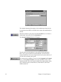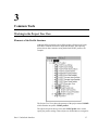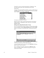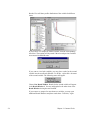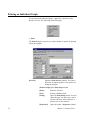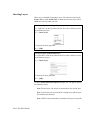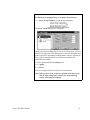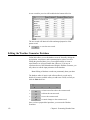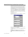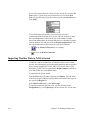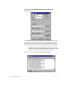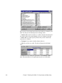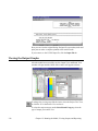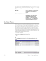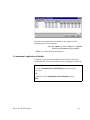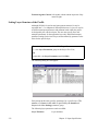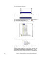
1
User’s Manual
for
WHI UnSat Suite
(includes Visual HELP)
The intuitive unsaturated zone analysis package
Developed by: Waterloo Hydrogeologic, Inc.
i
ii
November 2004
License Agreement
Waterloo Hydrogeologic Inc. retains the ownership of this copy of the software. This copy is licensed to you for use under the
following conditions:
I. Copyright Notice
This software is protected by both Canadian copyright law and international treaty provisions. Therefore, you must treat
this software JUST LIKE A BOOK, with the following single exception. Waterloo Hydrogeologic Inc. authorizes you to make
archive copies of the software for the sole purpose of backing-up our software and protecting your investment from loss.
By saying "JUST LIKE A BOOK", Waterloo Hydrogeologic Inc. means, for example, that this software may be used by
any number of people within the organization that purchased the software, and it may be freely moved from one computer location
within the licensed organization to another, so long as there is NO POSSIBILITY of it being used at one location while it is being
used at another. Just like a book can’t be read by two different people in two different places at the same time.
Specifically, you may not distribute, rent, sub-license, or lease the software or documentation; alter, modify, or adapt the
software or documentation, including, but not limited to, translating, decompiling, disassembling, or creating derivative works
without the prior written consent of Waterloo Hydrogeologic Inc. The provided software and documentation contain trade secrets
and it is agreed by the licensee that these trade secrets will not be disclosed to non-licensed persons without written consent of
Waterloo Hydrogeologic Inc.
II. Warranty
Waterloo Hydrogeologic Inc. warrants that, under normal use, the material of the magnetic diskettes and the documentation
will be free of defects in materials and workmanship for a period of 30 days from the date of purchase. In the event of notification
of defects in material or workmanship, Waterloo Hydrogeologic Inc. will replace the defective diskettes or documentation.
The remedy for breach of this warranty shall be limited to replacement and shall not encompass any other damages,
including but not limited to loss of profit, and special, incidental, consequential, or other similar claims.
III. Disclaimer
Except as specifically provided above, neither the developer(s) of this software nor any person or organization acting on
behalf of him (them) makes any warranty, express or implied, with respect to this software. In no event will Waterloo
Hydrogeologic Inc. assume any liabilities with respect to the use, or misuse, of this software, or the interpretation, or
misinterpretation, of any results obtained from this software, or for direct, indirect, special, incidental, or consequential damages
resulting from the use of this software.
Specifically, Waterloo Hydrogeologic Inc. is not responsible for any costs including, but not limited to, those incurred as a
result of lost profits or revenue, loss of use of the computer program, loss of data, the costs of recovering such programs or data,
the cost of any substitute program, claims by third parties, or for other similar costs. In no case shall Waterloo Hydrogeologic Inc.’s
liability exceed the amount of the license fee.
IV. Infringement Protection
Waterloo Hydrogeologic Inc. is the sole owner of this software. Waterloo Hydrogeologic Inc. warrants that neither the
software and documentation nor any component, including elements provided by others and incorporated into the software and
documentation, infringes upon or violates any patent, trademark, copyright, trade secret, or other proprietary right.
Royalties or other charges for any patent, trademark, copyright, trade secret or other proprietary information to be used in
the software and documentation shall be considered as included in the contract price.
V. Governing Law
This license agreement shall be construed, interpreted, and governed by the laws of the Province of Ontario, Canada, and
the United States. Any terms or conditions of this agreement found to be unenforceable, illegal, or contrary to public policy in any
jurisdiction will be deleted, but will not affect the remaining terms and conditions of the agreement.
VI. Entire Agreement
This agreement constitutes the entire agreement between you and Waterloo Hydrogeologic Inc.
License Agreement
iii
iv
November 2004
Table of Contents
UnSat Suite Interface.............................................................1
Introduction. . . . . . . . . . . . . . . . . . . . . . . . . . . . . . . . . . . . . . . . . . . . . . . . . . . . . . . . . . . . . . . . . . . .3
WHI UnSat Suite Models . . . . . . . . . . . . . . . . . . . . . . . . . . . . . . . . . . . . . . . . . . . . . . . . . . . . . . . . .3
History . . . . . . . . . . . . . . . . . . . . . . . . . . . . . . . . . . . . . . . . . . . . . . . . . . . . . . . . . . . . . . . . . . . . . . .4
New Features of WHI UnSat Suite 2.2. . . . . . . . . . . . . . . . . . . . . . . . . . . . . . . . . . . . . . . . . . . . . . .4
The WHI UnSat Suite Concept. . . . . . . . . . . . . . . . . . . . . . . . . . . . . . . . . . . . . . . . . . . . . . . . . . . . .5
How to Contact WHI . . . . . . . . . . . . . . . . . . . . . . . . . . . . . . . . . . . . . . . . . . . . . . . . . . . . . . . . . . . .6
Software Maintenance and Technical Support. . . . . . . . . . . . . . . . . . . . . . . . . . . . . . . . . . . . . .7
Other Products by WHI . . . . . . . . . . . . . . . . . . . . . . . . . . . . . . . . . . . . . . . . . . . . . . . . . . . . . . . . . .7
Waterloo Hydrogeologic Inc. Training and Consulting . . . . . . . . . . . . . . . . . . . . . . . . . . . . . . . . . .8
Acknowledgments . . . . . . . . . . . . . . . . . . . . . . . . . . . . . . . . . . . . . . . . . . . . . . . . . . . . . . . . . . . . . .8
1. Installation and Start-Up . . . . . . . . . . . . . . . . . . . . . . . . . . . . . . . . . . . . . . . . . . . 11
System Requirements . . . . . . . . . . . . . . . . . . . . . . . . . . . . . . . . . . . . . . . . . . . . . . . . . . . . . . . . . . .11
Installing WHI UnSat Suite 2.2 from the CD-Rom . . . . . . . . . . . . . . . . . . . . . . . . . . . . . . . . . . . .11
Starting WHI UnSat Suite. . . . . . . . . . . . . . . . . . . . . . . . . . . . . . . . . . . . . . . . . . . . . . . . . . . . . . . .12
2. General Features . . . . . . . . . . . . . . . . . . . . . . . . . . . . . . . . . . . . . . . . . . . . . . . . . . 13
Terms and Notation . . . . . . . . . . . . . . . . . . . . . . . . . . . . . . . . . . . . . . . . . . . . . . . . . . . . . . . . . . . .13
Getting Around the Interface . . . . . . . . . . . . . . . . . . . . . . . . . . . . . . . . . . . . . . . . . . . . . . . . . . . . .13
Main Menu . . . . . . . . . . . . . . . . . . . . . . . . . . . . . . . . . . . . . . . . . . . . . . . . . . . . . . . . . . . . . . . .14
Operational Icons . . . . . . . . . . . . . . . . . . . . . . . . . . . . . . . . . . . . . . . . . . . . . . . . . . . . . . . . . . .15
Profile Icons . . . . . . . . . . . . . . . . . . . . . . . . . . . . . . . . . . . . . . . . . . . . . . . . . . . . . . . . . . . . . . .16
Project Tree View. . . . . . . . . . . . . . . . . . . . . . . . . . . . . . . . . . . . . . . . . . . . . . . . . . . . . . . . . . .17
Profile View . . . . . . . . . . . . . . . . . . . . . . . . . . . . . . . . . . . . . . . . . . . . . . . . . . . . . . . . . . . . . . .17
Output View . . . . . . . . . . . . . . . . . . . . . . . . . . . . . . . . . . . . . . . . . . . . . . . . . . . . . . . . . . . . . . .17
Results View . . . . . . . . . . . . . . . . . . . . . . . . . . . . . . . . . . . . . . . . . . . . . . . . . . . . . . . . . . . . . .17
Starting a New Project . . . . . . . . . . . . . . . . . . . . . . . . . . . . . . . . . . . . . . . . . . . . . . . . . . . . . . . . . .17
General Project Information. . . . . . . . . . . . . . . . . . . . . . . . . . . . . . . . . . . . . . . . . . . . . . . . . . .18
Selecting a Problem and Model . . . . . . . . . . . . . . . . . . . . . . . . . . . . . . . . . . . . . . . . . . . . . . . .18
Location . . . . . . . . . . . . . . . . . . . . . . . . . . . . . . . . . . . . . . . . . . . . . . . . . . . . . . . . . . . . . . . . . .19
Units . . . . . . . . . . . . . . . . . . . . . . . . . . . . . . . . . . . . . . . . . . . . . . . . . . . . . . . . . . . . . . . . . . . . .23
Authors and Clients . . . . . . . . . . . . . . . . . . . . . . . . . . . . . . . . . . . . . . . . . . . . . . . . . . . . . . . . .26
Loading an Existing Project . . . . . . . . . . . . . . . . . . . . . . . . . . . . . . . . . . . . . . . . . . . . . . . . . . . . . .28
Profiles in UnSat Suite . . . . . . . . . . . . . . . . . . . . . . . . . . . . . . . . . . . . . . . . . . . . . . . . . . . . . . . . . .28
Creating a New Profile Using a Profile Template . . . . . . . . . . . . . . . . . . . . . . . . . . . . . . . . . . . . .30
Creating a New Profile . . . . . . . . . . . . . . . . . . . . . . . . . . . . . . . . . . . . . . . . . . . . . . . . . . . . . . . . . .30
Creating a New Profile Template . . . . . . . . . . . . . . . . . . . . . . . . . . . . . . . . . . . . . . . . . . . . . . . . . .32
Starting the Simulation . . . . . . . . . . . . . . . . . . . . . . . . . . . . . . . . . . . . . . . . . . . . . . . . . . . . . . . . . .32
Using the Material Designer . . . . . . . . . . . . . . . . . . . . . . . . . . . . . . . . . . . . . . . . . . . . . . . . . . . . . .32
Adding new contaminant to the database. . . . . . . . . . . . . . . . . . . . . . . . . . . . . . . . . . . . . . . . .35
Contents
1
Modifying and Deleting Materials . . . . . . . . . . . . . . . . . . . . . . . . . . . . . . . . . . . . . . . . . . . . . 35
3. Common Tools . . . . . . . . . . . . . . . . . . . . . . . . . . . . . . . . . . . . . . . . . . . . . . . . . . . . 37
Working in the Project Tree View . . . . . . . . . . . . . . . . . . . . . . . . . . . . . . . . . . . . . . . . . . . . . . . .
Elements of the Profile Structure . . . . . . . . . . . . . . . . . . . . . . . . . . . . . . . . . . . . . . . . . . . . . .
Indicators of the Object’s Status. . . . . . . . . . . . . . . . . . . . . . . . . . . . . . . . . . . . . . . . . . . . . . .
Accessing and Editing Objects of Profile Structure . . . . . . . . . . . . . . . . . . . . . . . . . . . . . . . .
Working in the Profile View . . . . . . . . . . . . . . . . . . . . . . . . . . . . . . . . . . . . . . . . . . . . . . . . . . . . .
Merging Layers. . . . . . . . . . . . . . . . . . . . . . . . . . . . . . . . . . . . . . . . . . . . . . . . . . . . . . . . . . . .
Restoring a Layer . . . . . . . . . . . . . . . . . . . . . . . . . . . . . . . . . . . . . . . . . . . . . . . . . . . . . . . . . .
Splitting a Layer . . . . . . . . . . . . . . . . . . . . . . . . . . . . . . . . . . . . . . . . . . . . . . . . . . . . . . . . . . .
Resizing the Layer . . . . . . . . . . . . . . . . . . . . . . . . . . . . . . . . . . . . . . . . . . . . . . . . . . . . . . . . .
Working with Multiple Profiles . . . . . . . . . . . . . . . . . . . . . . . . . . . . . . . . . . . . . . . . . . . . . . . . . .
Running the Model . . . . . . . . . . . . . . . . . . . . . . . . . . . . . . . . . . . . . . . . . . . . . . . . . . . . . . . . . . . .
Viewing the Output . . . . . . . . . . . . . . . . . . . . . . . . . . . . . . . . . . . . . . . . . . . . . . . . . . . . . . . . . . . .
Viewing the Output Graphs. . . . . . . . . . . . . . . . . . . . . . . . . . . . . . . . . . . . . . . . . . . . . . . . . . . . . .
Viewing Tables . . . . . . . . . . . . . . . . . . . . . . . . . . . . . . . . . . . . . . . . . . . . . . . . . . . . . . . . . . . . . . .
Editing Graphs. . . . . . . . . . . . . . . . . . . . . . . . . . . . . . . . . . . . . . . . . . . . . . . . . . . . . . . . . . . . . . . .
Printing an Individual Graph. . . . . . . . . . . . . . . . . . . . . . . . . . . . . . . . . . . . . . . . . . . . . . . . . . . . .
Preparing a Report. . . . . . . . . . . . . . . . . . . . . . . . . . . . . . . . . . . . . . . . . . . . . . . . . . . . . . . . . . . . .
37
37
39
39
44
45
47
47
49
49
50
50
51
55
56
58
59
4. Working with Project Sets . . . . . . . . . . . . . . . . . . . . . . . . . . . . . . . . . . . . . . . . . . 61
Definition of the Project Set . . . . . . . . . . . . . . . . . . . . . . . . . . . . . . . . . . . . . . . . . . . . . . . . . . . . .
Using the Project Set Manager . . . . . . . . . . . . . . . . . . . . . . . . . . . . . . . . . . . . . . . . . . . . . . . . . . .
Deleting Alias . . . . . . . . . . . . . . . . . . . . . . . . . . . . . . . . . . . . . . . . . . . . . . . . . . . . . . . . . . . . .
Archiving and Copying Project Sets. . . . . . . . . . . . . . . . . . . . . . . . . . . . . . . . . . . . . . . . . . . .
Returning to the Default Project Set. . . . . . . . . . . . . . . . . . . . . . . . . . . . . . . . . . . . . . . . . . . .
Deleting Projects from the Default Project Set. . . . . . . . . . . . . . . . . . . . . . . . . . . . . . . . . . . .
Opening an Archive Project Set . . . . . . . . . . . . . . . . . . . . . . . . . . . . . . . . . . . . . . . . . . . . . . .
Opening a Local Project Set . . . . . . . . . . . . . . . . . . . . . . . . . . . . . . . . . . . . . . . . . . . . . . . . . .
Working over a Local Area Network . . . . . . . . . . . . . . . . . . . . . . . . . . . . . . . . . . . . . . . . . . .
Copying a Project From One Project Set to Another . . . . . . . . . . . . . . . . . . . . . . . . . . . . . . .
Repairing the Project Set. . . . . . . . . . . . . . . . . . . . . . . . . . . . . . . . . . . . . . . . . . . . . . . . . . . . . . . .
61
61
63
63
64
64
65
65
65
67
68
The HELP Model .................................................................69
Introduction . . . . . . . . . . . . . . . . . . . . . . . . . . . . . . . . . . . . . . . . . . . . . . . . . . . . . . . . . . . . . . . . . .
History. . . . . . . . . . . . . . . . . . . . . . . . . . . . . . . . . . . . . . . . . . . . . . . . . . . . . . . . . . . . . . . . . . . . . .
New Features of Visual HELP 2.1 . . . . . . . . . . . . . . . . . . . . . . . . . . . . . . . . . . . . . . . . . . . . . . . .
New Features of Visual HELP 2.2 . . . . . . . . . . . . . . . . . . . . . . . . . . . . . . . . . . . . . . . . . . . . . . . .
Importing a Visual Help 1.1 model into Visual Help 2.2. . . . . . . . . . . . . . . . . . . . . . . . . . . .
71
71
72
72
72
5. Designing the Landfill Profile. . . . . . . . . . . . . . . . . . . . . . . . . . . . . . . . . . . . . . . . 75
Profiles in Visual HELP . . . . . . . . . . . . . . . . . . . . . . . . . . . . . . . . . . . . . . . . . . . . . . . . . . . . . . . . 75
Subprofiles . . . . . . . . . . . . . . . . . . . . . . . . . . . . . . . . . . . . . . . . . . . . . . . . . . . . . . . . . . . . . . . 77
2
Contents
Layering Rules . . . . . . . . . . . . . . . . . . . . . . . . . . . . . . . . . . . . . . . . . . . . . . . . . . . . . . . . . . . . . . . .78
Profile Properties . . . . . . . . . . . . . . . . . . . . . . . . . . . . . . . . . . . . . . . . . . . . . . . . . . . . . . . . . . . . . .78
Case Settings. . . . . . . . . . . . . . . . . . . . . . . . . . . . . . . . . . . . . . . . . . . . . . . . . . . . . . . . . . . . . . . . . .79
Editing Case Settings . . . . . . . . . . . . . . . . . . . . . . . . . . . . . . . . . . . . . . . . . . . . . . . . . . . . . . . .80
Runoff Method . . . . . . . . . . . . . . . . . . . . . . . . . . . . . . . . . . . . . . . . . . . . . . . . . . . . . . . . . . . . .80
Initial Moisture Settings . . . . . . . . . . . . . . . . . . . . . . . . . . . . . . . . . . . . . . . . . . . . . . . . . . . . . .81
Editing the Surface Water Settings . . . . . . . . . . . . . . . . . . . . . . . . . . . . . . . . . . . . . . . . . . . . . . . . .82
Editing Landfill Layers and Modifying the Profile . . . . . . . . . . . . . . . . . . . . . . . . . . . . . . . . . . . .82
Layer Properties . . . . . . . . . . . . . . . . . . . . . . . . . . . . . . . . . . . . . . . . . . . . . . . . . . . . . . . . . . . .83
Editing Layer Properties. . . . . . . . . . . . . . . . . . . . . . . . . . . . . . . . . . . . . . . . . . . . . . . . . . . . . .85
Resizing Layers . . . . . . . . . . . . . . . . . . . . . . . . . . . . . . . . . . . . . . . . . . . . . . . . . . . . . . . . . . . .87
Inserting Layers . . . . . . . . . . . . . . . . . . . . . . . . . . . . . . . . . . . . . . . . . . . . . . . . . . . . . . . . . . . .89
Deleting Layers . . . . . . . . . . . . . . . . . . . . . . . . . . . . . . . . . . . . . . . . . . . . . . . . . . . . . . . . . . . .91
Restoring Layers . . . . . . . . . . . . . . . . . . . . . . . . . . . . . . . . . . . . . . . . . . . . . . . . . . . . . . . . . . .93
Splitting Layers . . . . . . . . . . . . . . . . . . . . . . . . . . . . . . . . . . . . . . . . . . . . . . . . . . . . . . . . . . . .94
Layer Groups . . . . . . . . . . . . . . . . . . . . . . . . . . . . . . . . . . . . . . . . . . . . . . . . . . . . . . . . . . . . . .96
6. Generating Weather Data . . . . . . . . . . . . . . . . . . . . . . . . . . . . . . . . . . . . . . . . . . . 99
Introduction. . . . . . . . . . . . . . . . . . . . . . . . . . . . . . . . . . . . . . . . . . . . . . . . . . . . . . . . . . . . . . . . . . .99
World Weather Generator Database . . . . . . . . . . . . . . . . . . . . . . . . . . . . . . . . . . . . . . . . . . . . . . .100
Starting the Weather Generator . . . . . . . . . . . . . . . . . . . . . . . . . . . . . . . . . . . . . . . . . . . . . . . . . .101
Getting Around. . . . . . . . . . . . . . . . . . . . . . . . . . . . . . . . . . . . . . . . . . . . . . . . . . . . . . . . . . . .102
Precipitation and Temperature . . . . . . . . . . . . . . . . . . . . . . . . . . . . . . . . . . . . . . . . . . . . . . . . . . .111
Evapotranspiration . . . . . . . . . . . . . . . . . . . . . . . . . . . . . . . . . . . . . . . . . . . . . . . . . . . . . . . . . . . .112
Generating Weather Data . . . . . . . . . . . . . . . . . . . . . . . . . . . . . . . . . . . . . . . . . . . . . . . . . . . . . . .114
Viewing Generated Weather Data . . . . . . . . . . . . . . . . . . . . . . . . . . . . . . . . . . . . . . . . . . . . . . . .115
Editing Generated Data. . . . . . . . . . . . . . . . . . . . . . . . . . . . . . . . . . . . . . . . . . . . . . . . . . . . . . . . .118
Viewing the Weather Generator Database . . . . . . . . . . . . . . . . . . . . . . . . . . . . . . . . . . . . . . . . . .120
Adding a Record to the Weather Generator Database . . . . . . . . . . . . . . . . . . . . . . . . . . . . . . . . .121
Editing the Weather Generator Database . . . . . . . . . . . . . . . . . . . . . . . . . . . . . . . . . . . . . . . . . . .122
Importing Weather Data in Canadian Climate Centre Format . . . . . . . . . . . . . . . . . . . . . . . . . . .123
Importing Weather Data in NOAA format . . . . . . . . . . . . . . . . . . . . . . . . . . . . . . . . . . . . . . . . . .124
Customizing Weather Data . . . . . . . . . . . . . . . . . . . . . . . . . . . . . . . . . . . . . . . . . . . . . . . . . . . . . .127
7. Running the Model, Viewing Output, and Reporting . . . . . . . . . . . . . . . . . . . 133
Setting the Simulation Time with the Weather Generator . . . . . . . . . . . . . . . . . . . . . . . . . . . . . .133
Running the Visual HELP Model . . . . . . . . . . . . . . . . . . . . . . . . . . . . . . . . . . . . . . . . . . . . . . . . .134
Interpreting the Output and Preparing a Report . . . . . . . . . . . . . . . . . . . . . . . . . . . . . . . . . . . . . .134
Original DOS HELP Output . . . . . . . . . . . . . . . . . . . . . . . . . . . . . . . . . . . . . . . . . . . . . . . . .134
Viewing the Output Graphs . . . . . . . . . . . . . . . . . . . . . . . . . . . . . . . . . . . . . . . . . . . . . . . . . .135
Viewing HELP Tables . . . . . . . . . . . . . . . . . . . . . . . . . . . . . . . . . . . . . . . . . . . . . . . . . . . . . .139
Explanation of Variables . . . . . . . . . . . . . . . . . . . . . . . . . . . . . . . . . . . . . . . . . . . . . . . . . . . .141
Creating a Report . . . . . . . . . . . . . . . . . . . . . . . . . . . . . . . . . . . . . . . . . . . . . . . . . . . . . . . . . .142
The PESTAN Model ..........................................................145
Contents
3
Introduction . . . . . . . . . . . . . . . . . . . . . . . . . . . . . . . . . . . . . . . . . . . . . . . . . . . . . . . . . . . . . . . . . 147
8. Input Specification. . . . . . . . . . . . . . . . . . . . . . . . . . . . . . . . . . . . . . . . . . . . . . . . 149
The Case Settings . . . . . . . . . . . . . . . . . . . . . . . . . . . . . . . . . . . . . . . . . . . . . . . . . . . . . . . . . . . .
Editing Sorption Constant. . . . . . . . . . . . . . . . . . . . . . . . . . . . . . . . . . . . . . . . . . . . . . . . . . .
Time Dependent Groups . . . . . . . . . . . . . . . . . . . . . . . . . . . . . . . . . . . . . . . . . . . . . . . . . . . . . . .
Waste Application Schedule. . . . . . . . . . . . . . . . . . . . . . . . . . . . . . . . . . . . . . . . . . . . . . . . .
Observation Times . . . . . . . . . . . . . . . . . . . . . . . . . . . . . . . . . . . . . . . . . . . . . . . . . . . . . . . .
Specifying the Pesticides. . . . . . . . . . . . . . . . . . . . . . . . . . . . . . . . . . . . . . . . . . . . . . . . . . . . . . .
Substituting the Pesticide . . . . . . . . . . . . . . . . . . . . . . . . . . . . . . . . . . . . . . . . . . . . . . . . . . .
Editing Pesticide Properties . . . . . . . . . . . . . . . . . . . . . . . . . . . . . . . . . . . . . . . . . . . . . . . . .
Modifying the Profile . . . . . . . . . . . . . . . . . . . . . . . . . . . . . . . . . . . . . . . . . . . . . . . . . . . . . . . . .
Profile Properties . . . . . . . . . . . . . . . . . . . . . . . . . . . . . . . . . . . . . . . . . . . . . . . . . . . . . . . . .
Resizing the Layer . . . . . . . . . . . . . . . . . . . . . . . . . . . . . . . . . . . . . . . . . . . . . . . . . . . . . . . .
Substituting the Layer. . . . . . . . . . . . . . . . . . . . . . . . . . . . . . . . . . . . . . . . . . . . . . . . . . . . . .
Editing Soil Properties . . . . . . . . . . . . . . . . . . . . . . . . . . . . . . . . . . . . . . . . . . . . . . . . . . . . .
Observation Point . . . . . . . . . . . . . . . . . . . . . . . . . . . . . . . . . . . . . . . . . . . . . . . . . . . . . . . . . . . .
Adding Observation Points. . . . . . . . . . . . . . . . . . . . . . . . . . . . . . . . . . . . . . . . . . . . . . . . . .
Observation Point Properties . . . . . . . . . . . . . . . . . . . . . . . . . . . . . . . . . . . . . . . . . . . . . . . .
Deleting an Observation Point . . . . . . . . . . . . . . . . . . . . . . . . . . . . . . . . . . . . . . . . . . . . . . .
Restoring an Observation Point . . . . . . . . . . . . . . . . . . . . . . . . . . . . . . . . . . . . . . . . . . . . . .
149
150
150
151
152
153
153
154
155
155
155
156
157
159
159
160
161
161
9. Viewing Output and Reporting . . . . . . . . . . . . . . . . . . . . . . . . . . . . . . . . . . . . . 163
Original DOS PESTAN Output . . . . . . . . . . . . . . . . . . . . . . . . . . . . . . . . . . . . . . . . . . . . . . . . .
Viewing the Output Graphs. . . . . . . . . . . . . . . . . . . . . . . . . . . . . . . . . . . . . . . . . . . . . . . . . . . . .
Specified Time and Depth . . . . . . . . . . . . . . . . . . . . . . . . . . . . . . . . . . . . . . . . . . . . . . . . . .
Observation Point . . . . . . . . . . . . . . . . . . . . . . . . . . . . . . . . . . . . . . . . . . . . . . . . . . . . . . . . .
Balance . . . . . . . . . . . . . . . . . . . . . . . . . . . . . . . . . . . . . . . . . . . . . . . . . . . . . . . . . . . . . . . . .
Viewing Tables . . . . . . . . . . . . . . . . . . . . . . . . . . . . . . . . . . . . . . . . . . . . . . . . . . . . . . . . . . . . . .
Creating a Report . . . . . . . . . . . . . . . . . . . . . . . . . . . . . . . . . . . . . . . . . . . . . . . . . . . . . . . . . . . .
163
163
164
167
167
168
169
The VS2DT Model .............................................................171
10. Introduction . . . . . . . . . . . . . . . . . . . . . . . . . . . . . . . . . . . . . . . . . . . . . . . . . . . . 173
11. Case Specifications. . . . . . . . . . . . . . . . . . . . . . . . . . . . . . . . . . . . . . . . . . . . . . . 175
Case Settings . . . . . . . . . . . . . . . . . . . . . . . . . . . . . . . . . . . . . . . . . . . . . . . . . . . . . . . . . . . . . . . .
Transport Simulation . . . . . . . . . . . . . . . . . . . . . . . . . . . . . . . . . . . . . . . . . . . . . . . . . . . . . .
Soil Hydraulic Function . . . . . . . . . . . . . . . . . . . . . . . . . . . . . . . . . . . . . . . . . . . . . . . . . . . .
Initial Conditions . . . . . . . . . . . . . . . . . . . . . . . . . . . . . . . . . . . . . . . . . . . . . . . . . . . . . . . . .
Maximum Simulation Time . . . . . . . . . . . . . . . . . . . . . . . . . . . . . . . . . . . . . . . . . . . . . . . . .
Evapotranspiration . . . . . . . . . . . . . . . . . . . . . . . . . . . . . . . . . . . . . . . . . . . . . . . . . . . . . . . .
Solver Settings. . . . . . . . . . . . . . . . . . . . . . . . . . . . . . . . . . . . . . . . . . . . . . . . . . . . . . . . . . . . . . .
4
175
176
178
179
180
180
181
Contents
Editing the Solver Settings . . . . . . . . . . . . . . . . . . . . . . . . . . . . . . . . . . . . . . . . . . . . . . . . . . .181
Evapotranspiration Parameters . . . . . . . . . . . . . . . . . . . . . . . . . . . . . . . . . . . . . . . . . . . . . . . . . . .183
Editing the Evapotranspiration Parameters . . . . . . . . . . . . . . . . . . . . . . . . . . . . . . . . . . . . . .184
Boundary Conditions . . . . . . . . . . . . . . . . . . . . . . . . . . . . . . . . . . . . . . . . . . . . . . . . . . . . . . . . . .186
Boundary Rules . . . . . . . . . . . . . . . . . . . . . . . . . . . . . . . . . . . . . . . . . . . . . . . . . . . . . . . . . . .188
Flow Boundaries . . . . . . . . . . . . . . . . . . . . . . . . . . . . . . . . . . . . . . . . . . . . . . . . . . . . . . . . . .188
Transport Boundaries . . . . . . . . . . . . . . . . . . . . . . . . . . . . . . . . . . . . . . . . . . . . . . . . . . . . . . .190
Stress Period Defaults . . . . . . . . . . . . . . . . . . . . . . . . . . . . . . . . . . . . . . . . . . . . . . . . . . . . . . . . . .192
Specifying the Stress Period Defaults . . . . . . . . . . . . . . . . . . . . . . . . . . . . . . . . . . . . . . . . . .192
Setting Output Times . . . . . . . . . . . . . . . . . . . . . . . . . . . . . . . . . . . . . . . . . . . . . . . . . . . . . . . . . .193
Observation Times . . . . . . . . . . . . . . . . . . . . . . . . . . . . . . . . . . . . . . . . . . . . . . . . . . . . . . . . .193
The Finite Difference Grid . . . . . . . . . . . . . . . . . . . . . . . . . . . . . . . . . . . . . . . . . . . . . . . . . . . . . .195
Customizing the Finite Difference Grid. . . . . . . . . . . . . . . . . . . . . . . . . . . . . . . . . . . . . . . . .196
Observation Points . . . . . . . . . . . . . . . . . . . . . . . . . . . . . . . . . . . . . . . . . . . . . . . . . . . . . . . . . . . .197
Adding Observation Points . . . . . . . . . . . . . . . . . . . . . . . . . . . . . . . . . . . . . . . . . . . . . . . . . .197
Observation Point Properties . . . . . . . . . . . . . . . . . . . . . . . . . . . . . . . . . . . . . . . . . . . . . . . . .199
Deleting an Observation Point . . . . . . . . . . . . . . . . . . . . . . . . . . . . . . . . . . . . . . . . . . . . . . . .199
Restoring an Observation Point . . . . . . . . . . . . . . . . . . . . . . . . . . . . . . . . . . . . . . . . . . . . . . .200
Setting the Initial Conditions . . . . . . . . . . . . . . . . . . . . . . . . . . . . . . . . . . . . . . . . . . . . . . . . . . . .200
Selecting the Type of Initial Condition . . . . . . . . . . . . . . . . . . . . . . . . . . . . . . . . . . . . . . . . .200
Editing the Initial Conditions for a Layer . . . . . . . . . . . . . . . . . . . . . . . . . . . . . . . . . . . . . . .201
12. Modifying the Profile . . . . . . . . . . . . . . . . . . . . . . . . . . . . . . . . . . . . . . . . . . . . . 203
Profile Properties . . . . . . . . . . . . . . . . . . . . . . . . . . . . . . . . . . . . . . . . . . . . . . . . . . . . . . . . . . . . .203
Changing the Soil Profile Layer Structure . . . . . . . . . . . . . . . . . . . . . . . . . . . . . . . . . . . . . . . . . .204
Merging Layers and Erasing Layer Boundaries. . . . . . . . . . . . . . . . . . . . . . . . . . . . . . . . . . .205
Restoring a Layer . . . . . . . . . . . . . . . . . . . . . . . . . . . . . . . . . . . . . . . . . . . . . . . . . . . . . . . . . .206
Splitting a Layer . . . . . . . . . . . . . . . . . . . . . . . . . . . . . . . . . . . . . . . . . . . . . . . . . . . . . . . . . . .207
Resizing a Layer. . . . . . . . . . . . . . . . . . . . . . . . . . . . . . . . . . . . . . . . . . . . . . . . . . . . . . . . . . .208
Changing Properties of a Layer . . . . . . . . . . . . . . . . . . . . . . . . . . . . . . . . . . . . . . . . . . . . . . .209
Substituting Material in a Layer. . . . . . . . . . . . . . . . . . . . . . . . . . . . . . . . . . . . . . . . . . . . . . .210
Editing Soil Hydrologic Properties. . . . . . . . . . . . . . . . . . . . . . . . . . . . . . . . . . . . . . . . . . . . . . . .210
Editing the Soil Parameters . . . . . . . . . . . . . . . . . . . . . . . . . . . . . . . . . . . . . . . . . . . . . . . . . . 210
Permanent Soil Hydrologic Parameters . . . . . . . . . . . . . . . . . . . . . . . . . . . . . . . . . . . . . . . . .211
Dependent Soil Parameters . . . . . . . . . . . . . . . . . . . . . . . . . . . . . . . . . . . . . . . . . . . . . . . . . .212
Transport Parameters . . . . . . . . . . . . . . . . . . . . . . . . . . . . . . . . . . . . . . . . . . . . . . . . . . . . . . . . . .212
Editing Transport Parameters. . . . . . . . . . . . . . . . . . . . . . . . . . . . . . . . . . . . . . . . . . . . . . . . .213
Permanent Soil Hydrologic Parameters . . . . . . . . . . . . . . . . . . . . . . . . . . . . . . . . . . . . . . . . .215
Dependent Transport Parameters . . . . . . . . . . . . . . . . . . . . . . . . . . . . . . . . . . . . . . . . . . . . . .215
13. Running the Model, Viewing Output, and Reporting . . . . . . . . . . . . . . . . . . 217
Running the VS2DT Model . . . . . . . . . . . . . . . . . . . . . . . . . . . . . . . . . . . . . . . . . . . . . . . . . . . . .217
Viewing the Original VS2DT Input and Output Files . . . . . . . . . . . . . . . . . . . . . . . . . . . . . . . . .217
Viewing the Output Graphs . . . . . . . . . . . . . . . . . . . . . . . . . . . . . . . . . . . . . . . . . . . . . . . . . . . . .218
Specified Time and Depth . . . . . . . . . . . . . . . . . . . . . . . . . . . . . . . . . . . . . . . . . . . . . . . . . . .219
Balance, Accumulated Balance and Rate. . . . . . . . . . . . . . . . . . . . . . . . . . . . . . . . . . . . . . . .222
Contents
5
Viewing Tables . . . . . . . . . . . . . . . . . . . . . . . . . . . . . . . . . . . . . . . . . . . . . . . . . . . . . . . . . . . . . . 223
Creating a Report . . . . . . . . . . . . . . . . . . . . . . . . . . . . . . . . . . . . . . . . . . . . . . . . . . . . . . . . . . . . 224
Editing Model Stress Periods . . . . . . . . . . . . . . . . . . . . . . . . . . . . . . . . . . . . . . . . . . . . . . . . . . . 225
The VLEACH Model.........................................................227
14. Introduction . . . . . . . . . . . . . . . . . . . . . . . . . . . . . . . . . . . . . . . . . . . . . . . . . . . . 229
15. Input Specification. . . . . . . . . . . . . . . . . . . . . . . . . . . . . . . . . . . . . . . . . . . . . . . 231
Specifying the Case Settings . . . . . . . . . . . . . . . . . . . . . . . . . . . . . . . . . . . . . . . . . . . . . . . . . . . .
Specifying the Contaminant . . . . . . . . . . . . . . . . . . . . . . . . . . . . . . . . . . . . . . . . . . . . . . . . . . . .
Setting Initial Conditions . . . . . . . . . . . . . . . . . . . . . . . . . . . . . . . . . . . . . . . . . . . . . . . . . . .
Substituting the Contaminant . . . . . . . . . . . . . . . . . . . . . . . . . . . . . . . . . . . . . . . . . . . . . . . .
Editing Contaminant Properties . . . . . . . . . . . . . . . . . . . . . . . . . . . . . . . . . . . . . . . . . . . . . .
Modifying the Profile . . . . . . . . . . . . . . . . . . . . . . . . . . . . . . . . . . . . . . . . . . . . . . . . . . . . . . . . .
Profile Properties . . . . . . . . . . . . . . . . . . . . . . . . . . . . . . . . . . . . . . . . . . . . . . . . . . . . . . . . .
Resizing the Layer . . . . . . . . . . . . . . . . . . . . . . . . . . . . . . . . . . . . . . . . . . . . . . . . . . . . . . . .
Substituting the Layer. . . . . . . . . . . . . . . . . . . . . . . . . . . . . . . . . . . . . . . . . . . . . . . . . . . . . .
Editing Soil Properties . . . . . . . . . . . . . . . . . . . . . . . . . . . . . . . . . . . . . . . . . . . . . . . . . . . . .
231
232
232
234
235
235
235
237
237
238
16. Viewing Output and Reporting . . . . . . . . . . . . . . . . . . . . . . . . . . . . . . . . . . . . 241
Original DOS VLEACH Output . . . . . . . . . . . . . . . . . . . . . . . . . . . . . . . . . . . . . . . . . . . . . . . . .
Viewing the Output Graphs. . . . . . . . . . . . . . . . . . . . . . . . . . . . . . . . . . . . . . . . . . . . . . . . . . . . .
Specified Time and Depth . . . . . . . . . . . . . . . . . . . . . . . . . . . . . . . . . . . . . . . . . . . . . . . . . .
Balance . . . . . . . . . . . . . . . . . . . . . . . . . . . . . . . . . . . . . . . . . . . . . . . . . . . . . . . . . . . . . . . . .
Viewing Tables . . . . . . . . . . . . . . . . . . . . . . . . . . . . . . . . . . . . . . . . . . . . . . . . . . . . . . . . . . . . . .
Preparing a Report. . . . . . . . . . . . . . . . . . . . . . . . . . . . . . . . . . . . . . . . . . . . . . . . . . . . . . . . . . . .
241
242
242
245
246
248
The SESOIL Model ...........................................................251
17. Introduction . . . . . . . . . . . . . . . . . . . . . . . . . . . . . . . . . . . . . . . . . . . . . . . . . . . . 253
18. Input Specification. . . . . . . . . . . . . . . . . . . . . . . . . . . . . . . . . . . . . . . . . . . . . . . 255
Profiles in SESOIL . . . . . . . . . . . . . . . . . . . . . . . . . . . . . . . . . . . . . . . . . . . . . . . . . . . . . . . . . . . 255
Editing General Profile Properties . . . . . . . . . . . . . . . . . . . . . . . . . . . . . . . . . . . . . . . . . . . . . . . 256
Specifying the Case Settings . . . . . . . . . . . . . . . . . . . . . . . . . . . . . . . . . . . . . . . . . . . . . . . . . . . . 256
Specifying Climate . . . . . . . . . . . . . . . . . . . . . . . . . . . . . . . . . . . . . . . . . . . . . . . . . . . . . . . . . . . 258
Inputting climate data manually . . . . . . . . . . . . . . . . . . . . . . . . . . . . . . . . . . . . . . . . . . . . . . 260
Input climate data from the Weather Generator database . . . . . . . . . . . . . . . . . . . . . . . . . . 262
Input weather data synthetically generated in SESOIL . . . . . . . . . . . . . . . . . . . . . . . . . . . . 262
Import synthetically generated weather data and evapotranspiration from the HELP model263
6
Contents
Specifying Soil Erosion and Contaminant Washload. . . . . . . . . . . . . . . . . . . . . . . . . . . . . . . . . .265
Specifying Washload Settings . . . . . . . . . . . . . . . . . . . . . . . . . . . . . . . . . . . . . . . . . . . . . . . .265
Specifying Washload Schedule . . . . . . . . . . . . . . . . . . . . . . . . . . . . . . . . . . . . . . . . . . . . . . .266
Specifying the Contaminant . . . . . . . . . . . . . . . . . . . . . . . . . . . . . . . . . . . . . . . . . . . . . . . . . . . . .267
Defining the Contaminant . . . . . . . . . . . . . . . . . . . . . . . . . . . . . . . . . . . . . . . . . . . . . . . . . . .267
Editing Chemical Properties. . . . . . . . . . . . . . . . . . . . . . . . . . . . . . . . . . . . . . . . . . . . . . . . . .268
Setting Initial Conditions . . . . . . . . . . . . . . . . . . . . . . . . . . . . . . . . . . . . . . . . . . . . . . . . . . . .270
Contaminant Application Schedule . . . . . . . . . . . . . . . . . . . . . . . . . . . . . . . . . . . . . . . . . . . .271
Modifying the Profile . . . . . . . . . . . . . . . . . . . . . . . . . . . . . . . . . . . . . . . . . . . . . . . . . . . . . . . . . .273
Profile Properties . . . . . . . . . . . . . . . . . . . . . . . . . . . . . . . . . . . . . . . . . . . . . . . . . . . . . . . . . .273
Setting the Profile Material . . . . . . . . . . . . . . . . . . . . . . . . . . . . . . . . . . . . . . . . . . . . . . . . . .274
Setting Layer Structure of the Profile . . . . . . . . . . . . . . . . . . . . . . . . . . . . . . . . . . . . . . . . . .276
Setting Groundwater Parameters . . . . . . . . . . . . . . . . . . . . . . . . . . . . . . . . . . . . . . . . . . . . . .277
19. Running the Model, Viewing Output and Reporting . . . . . . . . . . . . . . . . . . . 279
Running the SESOIL Model. . . . . . . . . . . . . . . . . . . . . . . . . . . . . . . . . . . . . . . . . . . . . . . . . . . . .279
Viewing Original DOS SESOIL Output. . . . . . . . . . . . . . . . . . . . . . . . . . . . . . . . . . . . . . . . . . . .279
Viewing the Output Graphs . . . . . . . . . . . . . . . . . . . . . . . . . . . . . . . . . . . . . . . . . . . . . . . . . . . . .281
Specified Depth (Annual Summary) . . . . . . . . . . . . . . . . . . . . . . . . . . . . . . . . . . . . . . . . . . .282
Viewing Specified Depth (Monthly Output) . . . . . . . . . . . . . . . . . . . . . . . . . . . . . . . . . . . . .289
Specified Time (Concentration) . . . . . . . . . . . . . . . . . . . . . . . . . . . . . . . . . . . . . . . . . . . . . . .291
Preparing a Report . . . . . . . . . . . . . . . . . . . . . . . . . . . . . . . . . . . . . . . . . . . . . . . . . . . . . . . . . . . .294
Export and Internal Transfer of Simulation Results .....297
20. Export , Internal Transfer, and Import of Simulation Results . . . . . . . . . . . 299
Internal Data Transfer between WHI UnSat Suite Models . . . . . . . . . . . . . . . . . . . . . . . . . . . . .299
Export from WHI UnSat Suite . . . . . . . . . . . . . . . . . . . . . . . . . . . . . . . . . . . . . . . . . . . . . . . . . . .309
Export of Visual HELP data to Visual MODFLOW . . . . . . . . . . . . . . . . . . . . . . . . . . . . . . .309
Export of SESOIL data to Visual MODFLOW . . . . . . . . . . . . . . . . . . . . . . . . . . . . . . . . . . .315
Export of VS2DT data to Visual MODFLOW . . . . . . . . . . . . . . . . . . . . . . . . . . . . . . . . . . .327
Export of VS2DT data to Visual MODFLOW for multiple species . . . . . . . . . . . . . . . . . . .329
Contents
7
8
Contents
Part 1:
UnSat Suite Interface
1
2
Introduction
The WHI UnSat Suite combines models HELP, PESTAN, SESOIL,
VLEACH and VS2DT in powerful new graphical environment
specifically designed for simulating one-dimensional groundwater flow
and contaminant transport through the unsaturated zone. All five of these
popular models are seamlessly integrated with the WHI UnSat Suite and
each one is compiled and optimized to run as a 32-Bit, native Windows
application.
WHI UnSat Suite Models
HELP is a versatile U.S. EPA model for predicting landfill hydrologic
processes and testing the effectiveness of landfill designs, enabling the
prediction of landfill design feasibility. HELP has become a requirement
for obtaining landfill operation permits in the U.S.A. HELP is also
effective in estimating of groundwater recharge rates.
PESTAN. The PESTAN (PESTticide ANalytical) model uses an
analytical solution to predict the transport of organic solutes through the
unsaturated zone to the groundwater table. The model is commonly used
for initial screening assessments to evaluate the potential for groundwater
contamination by pesticides used in agricultural applications. However, it
is also quite useful for determining potential groundwater impacts from
any organic solutes migrating through the unsaturated zone.
SESOIL is a popular US EPA model which is capable to simultaneously
model water transport, sediment transport and pollutant fate. SESOIL is
widely used by consultants and state regulatory agencies as a screening
tool to assess contaminant fate and transport for regulatory
requirements.The ability of the model to account for contaminant
washload, volatilization and air diffusion of the volatile organic
contaminants, as well as for sorption, volatilization, degradation, cation
exchange, hydrolysis and metal complexation makes it a unique tool
which only can be applied in many practical cases.
VS2DT is a finite difference numerical model for simulating steady-state
or transient, Variably-Saturated 2-D groundwater flow and solute Transport. Typical applications of the VS2DT model include determining the
fate of agricultural chemicals, landfill leachate, UST leaks, and accidental
chemical spills as they migrate through the unsaturated zone towards the
water table.
VLEACH is a one-dimensional finite difference Vadose zone LEACHing
model for predicting the vertical mobilization and migration of organic
contaminants in the vadose zone. This model is commonly used to
evaluate groundwater impacts due to vertical migration of organic
Part 1: UnSat Suite Interface
3
contaminants through the unsaturated zone, and to predict subsurface
volatilization of VOCs.
History
WHI has developed a Windows interface for the version 3.08 of the
HELP model which was released in May 1998 under the name Visual
HELP version 1.101. This software was presented at the trade show at
SWANA’s WASTECON 1998 and ISWA World Congress 1998 in
Charlotte, North Carolina.
WHI UnSat Suite was released in May 1999. The product combined
models HELP, PESTAN, VLEACH and VS2DT in a powerful new
graphical environment specifically designed for simulating onedimensional groundwater flow and contaminant transport through the
unsaturated zone. The ideas and approaches tested in Visual HELP
version 1.101 have been advanced. The product has been sold to our
clients in three versions:
Visual HELP 2.1 which included the HELP model,
WHI UnSat Suite 2.1 which included PESTAN,
VLEACH and VS2DT, and
WHI UnSat Suite Plus 2.1 which included HELP,
PESTAN, VLEACH and VS2DT.
Currently, more than 400 copies of this product are being used by
consulting companies, government regulator bodies and Universities in
U.S.A., Canada, U.K., Germany, Australia, Sweden, Mexico, France,
Slovenia, Slovakia and Hungary.
New Features of WHI UnSat Suite 2.2
The SESOIL Model has been added
SESOIL, a popular US EPA model which is capable to simultaneously
model water transport, pollutant washload, sediment transport and
pollutant fate has been added to the modelling suite.
The Pollutant Parameter Database has been expanded
The database of pollutant parameters for PESTAN model has been
expanded. The new pollutant database for SESOIL contains all necessary
parameters for 24 common industrial and agricultural pollutants.
4
Introduction
Internal Data Transfer and Output Export become available
The data transfer between the WHI UnSat Suite models, as well as export
model data for use with other applications or processing with spreadsheet
programs (e.g. MS EXCEL) become available.
The WHI UnSat Suite Concept
The WHI UnSat Suite utilizes a unique interface design that accommodates the specialized features and analysis capabilities of each model,
while maintaining a consistent look and feel for each data set. This allows
you to easily switch from one model to another without having to go
through the painful steps of learning a different interface and data structure for each new model.
The familiar design and functionality of the interface is extremely easy to
learn and facilitates quick and easy access for conveniently modifying
any of the model input parameters. The many interactive graphical tools
allow you to quickly and easily create a model profile, modify the layer
design, and customize the model properties and boundary conditions.
The project-oriented data management system allows you to easily
manage multiple models, and different model types, within the same
project database file. This project-oriented approach lets you conveniently
navigate between different models and easily compare model input data
and simulation results. In addition, the WHI UnSat Suite supports a
teamwork environment where project files can be loaded, modified and
run over a networked system.
There are seven key benefits that make UnSat Suite 2.1 the software
package of choice for simulating unsaturated zone processes:
[1]
Organizing Information is Easy
Information is organized into projects. Each project is associated
with a name, an author, a client, and a location. This simple method
of distinguishing projects makes project management easier.
[2]
Specifying Site Conditions is Intuitive
All specific site data are organized in profiles which represent a
unique combination of unsaturated zone structure and properties.
Graphical tools available in the Project Tree and Project Profile
View make visualizing and modifying of profiles simple.
[3]
Describing a Problem is Easy
Soil and chemical properties are easy to edit and manage. The
interface tools allow you to easily specify initial and time-varying
boundary conditions of the site.
[4]
Part 1: UnSat Suite Interface
Obtaining Accurate Weather Data is Simple
5
You can easily create a database of accurate weather information for
your area of concern. WHI UnSat Suite allows you to select from
over 3000 weather stations around the world to create statistically
reliable weather data for practically anywhere on the globe.
[5]
Model Output is Comprehensive
UnSat Suite 2.1 output allows you to view information in a broad,
qualitative manner, as well as a detailed, quantitative form. You can
quickly see the effects of different properties, designs, or situations
as you adjust the parameters of your project.
[6]
Presentation of Results is Easy
You can use the Report Generator to easily create and print
your own report, which includes input information and
selected output graphs and tables.
[7]
Output Results May be Used by another Model or Exported
You may easily transfer data between the WHI UnSat Suite models,
as well as export model data for use with other applications (e.g.
export groundwater recharge assessed by Visual HELP to Visual
MODFLOW).
[8]
File Management is Flexible
Files are grouped in project sets and can be stored as well as edited
or viewed by other users through a network connection.
How to Contact WHI
If, after reading this manual and using your software, you would like to
contact Waterloo Hydrogeologic Inc. with comments, suggestions, or if
you need technical assistance with your software installation, you can
reach us at:
Waterloo Hydrogeologic Inc.
460 Phillip Street - Suite 101
Waterloo, Ontario, CANADA, N2L 5J2
Phone +1 (519) 746 1798
Fax +1 (519) 885 5262
Email: [email protected]
Web: www.waterloohydrogeologic.com
6
Introduction
Software Maintenance and Technical Support
Waterloo Hydrogeologic’s Annual Maintenance Contracts are designed
to reduce the amount of time and effort required to keep your
modeling software up-to-date. With automatic reminders of updates
and upgrades, users will never have to wonder if their software is
out-dated. Additionally, with unlimited technical support available
during the term of the Maintenance Contract, software users can
obtain rapid resolution to all of their software issues.
Annual Maintenance Benefits
• Free Major Software upgrades, and version updates
• Unlimited Telephone Support
• Unlimited email Support
• Priority Response to Error Reports
• Direct Bug Fix Updates
• Documentation Updates
• On-Demand FTP Downloads
• Showcase Your Projects in WHI E-News
• Option to Beta Test New Products
• Annual Reminder for Contract Renewal
For more information about Maintenance Contracts, please contact
our Sales department via phone at +1 (519) 746-1798, or via email
at [email protected]
Other Products by WHI
Visual MODFLOW
A pre- and post processor for MODFLOW, MODPATH, and MT3D. A
complete package for the visualization of model input and simulation
results. The largest time-saving breakthrough for rigorous threedimensional groundwater modeling since the release of MODFLOW.
FLOWPATH II
The most complete two dimensional, steady-state, groundwater flow and
pathline model. It computes hydraulic heads, pathlines, travel times,
velocities and water balances (verified against the USGS MODFLOW,
approved by the U.S. EPA, and recommended by the IGWMC).
FLOWPATH II has been radically improved from its predecessor to
include many new features and an enhanced graphical display to give you
more power, flexibility and control than ever before. Also, FLOWPATH
II now includes contaminant transport simulation capabilities.
FLONET/TRANS
A powerful yet easy-to-use two dimensional, steady-state groundwater
flow and transient contaminant transport model. Calculates and displays
Part 1: UnSat Suite Interface
7
equipotential distribution, streamlines, flow nets, velocity vectors, and
temporal graphs of concentration at multiple observation points.
AIRFLOW/SVE
The only comprehensive soil-vapour extraction model to simulate the
coupled process of soil-vapour flow and multi-component vapour
transport in the unsaturated zone.
PRINCE
A compilation of the ten Princeton Analytical Models which includes
seven mass transport models (one-, two-, and three-dimensional) and 3
two-dimensional flow models.
AquiferTest
An easy-to-use graphically oriented package for estimating
transmissivity, hydraulic conductivity and storage properties for a variety
of aquifer types. The program contains analytical solutions for pumping
tests and slug tests for confined, unconfined, and leaky confined aquifers.
Visual Groundwater
The first software package to combine state-of-the-art graphical
technology for 3-D visualization and animation capabilities with an easyto-use graphical interface designed specifically for environmental project
applications.
Waterloo Hydrogeologic Inc. Training and Consulting
Waterloo Hydrogeologic Inc. offers individual tailored training courses
on groundwater modeling. Our modeling courses emphasize on how to
set up a proper groundwater model (grid design, boundary conditions,
etc.), the interpretation of results (calibration, prediction, etc.), and
extensive coverage on the mechanics of using groundwater models.
Courses can be arranged by contacting Waterloo Hydrogeologic Inc.
Waterloo Hydrogeologic Inc. also offers expert consulting and peer
review services for all numerical modeling problems concerning
groundwater flow and mass transport. For further information contact
Waterloo Hydrogeologic, Inc.
Acknowledgments
The development of UnSat Suite was directed by Dr. Mikhail Gogolev
who designed the interface, tested the product and wrote the manual. Dr.
Dmitri Eidenzon co-designed the interface and was responsible for
8
Introduction
programming. Konstantin Choumak took responsibility for programming
of version 2.2. Other members of the development team include Igor
Evsikov, who developed the interface for the Weather Generator,
Alexander Sapozhnikov, who converted the original FORTRAN codes to
DLLs, Karin Nova, who developed sections of the database, and coop
students Diane Cameron, Livia De Vellis and Bruce Davison, who
prepared the new WGEN world database and took part in testing the
interface and preparing the manual and on-line help. Dr. Serguei
Shmakov, Douglas Graham, Gary Moore and Paul Martin provided
support, as well as Dr. Nilson Guiguer and Patrick Delaney, who are
responsible for overall software development at Waterloo Hydrogeologic,
Inc.
The software research and development was supported financially by the
National Research Council of Canada through the Industrial Research
Adaptation Program (#28557U), which is greatly appreciated. In
particular, the development team wishes to thank the Industrial
Technology Advisor, Dr. Ernie Davison for his support.
Part 1: UnSat Suite Interface
9
10
Introduction
Installation and Start-Up
System Requirements
To run WHI UnSat Suite, you will need the following minimum system
configuration:
•
•
•
•
•
Pentium II based computer;
32 MB RAM (128 MB recommended);
CD-ROM drive for software installation;
A hard drive with at least60 Mb of free space;
Windows 98/Windows NT (SP4)/Windows 2000/Windows
XP.
The following fonts should be installed on your computer: MS Sans Serif,
Arial, Times New Roman, and Courier New.
Installing WHI UnSat Suite 2.2 from the CD-Rom
A PDF file of the WHI UnSat Suite Users Manual, and extracts from the
original tutorial guides for the WHI UnSat Suite models, are included on
the Installation CD ROM in the Manual subfolder. If you do not already
have Acrobat Reader, simply select the Get Acrobat Reader link found
in the opening screen.
Please follow the steps below to install your software from the CD-ROM.
Part 1: UnSat Suite Interface
[1]
If applicable, log in as the Local Administrator of your computer, or
as a user with Local Power User rights.
[2]
Insert the program CD into your CD-ROM drive to initiate the CD
Navigator. If the navigator does not automatically open the Product
Installation screen, explore the CD-ROM drive and double click on
the Install32.exe file.
11
[3]
To begin installing your software to your hard disk, click on “WHI
UnSat Suite Plus Installation”
[4]
The Welcome window will appear. Click [Next>] to continue, and
follow the Installation Wizard to enter your product Serial Number
(please remember to use CAPITAL letters), select your installation
directory, and select the components to install.
Starting WHI UnSat Suite
After installing WHI UnSat Suite, click Start on the Windows Taskbar,
choose Programs, go to the program file where WHI UnSat Suite is
located, and click UnSat22 to open the product.
The installation program will also place an icon on your
desktop, which you can also click to start WHI UnSat Suite.
12
Chapter 1: Installation and Start-Up
2
General Features
Terms and Notation
The following terms and notations will be used throughout the manual:
type
Type in the given word or value
select
Click the left mouse button where indicated
↵
Press the <Enter> key
)
Click the left mouse button where indicated
))
Double-click the left mouse button where indicated
The bold faced type indicates menu or window items to click, or values
to type.
[...]
denotes a button to click.
...\...\...
denotes a menu selection.
Getting Around the Interface
Below is an example of the WHI UnSat Suite windows interface using the
HELP model:
Part 1: UnSat Suite Interface
13
Main Menu
Project Tree
View
Profile View
Operational
Icons
Output View
Profile
Icons
Results View
After starting and loading WHI UnSat Suite, a window will appear on
your screen. The window will be blank except for the project tree view, as
you have not chosen a problem or a model, or generated any output. The
previous window illustrates all of the display features of UnSat Suite
available after a model has been run. The Main Menu items are at the top,
Operational Icons are just below, and the Profile Icons are just above the
Profile View. The Project Tree View is to the left of the main window, the
Profile View is in the middle, and the chart and Table Output Views are
on the right. The menu items, icons, and views are described below.
Main Menu
The top menu bar contains the following menu options:
14
File
Create a project, open/close/save/delete a project, or exit
UnSat Suite. You may also open previously saved sets of
projects, archive current projects and run projects stored
on other machines through the local area network.
View
View/close Project Tree, Profile View, Output Structure,
and Results View.
Project
View project properties, create a new profile, or delete a
profile.
Chapter 2: General Features
Profile
View profile properties, view layer group geometry for
HELP, view/edit stress periods for VS2DT.
Run
Run the selected model or run the Weather Generator
(HELP) or view and edit stress period parameters
(VS2DT).
Output
View simulation results and input file or clear the Results
View.
Window
Arrange the windows that present information about
different profiles.
Settings
Create, edit, or delete profile templates, materials,
authors, clients, locations, and unit templates. You can
also restore corrupted project clicking the Repair button.
Help
Go to the Help window and general information on
UnSat Suite.
Operational Icons
The operational icons provide you with quick access to functions related
to projects.
Create New Project Click this icon to begin a new project.
Save Project
Click this icon to save a project with its current
settings.
Open/Close the Project Tree View Click this icon to open and close
the Project Tree View if you need more space
for the graphs.
Create New Profile
Choose this icon to create a new profile in the
open project.
View Profile
Choose this icon to view the profile that is
highlighted in the Project Tree View.
Run Weather Generator (HELP only)
Choose this icon to run the Weather Generator.
Run the current model for all profiles
Choose this icon to run the model simulation
for all profiles in the open project.
Part 1: UnSat Suite Interface
15
Prepare a Report
Choose this icon to prepare a report after you
have run the simulation
Remote Data Access Choose this icon to open the archived project
set or to open the project stored on the other
machine through the LAN. This icon is visible
only when all projects are closed.
Copy Holder
Use this icon to temporary store your projects
while you are switching from one project set to
another. To save a copy of the project in the
Copy Holder simply drag and drop the project
from the Project Tree. This icon is visible only
when all projects are closed
Mail To...
Click this icon to mail to the WHI’s technical
support group.
Help Topics
Click this icon for on-line help.
Exit
Click this icon to exit UnSat Suite.
Profile Icons
The profile icons provide you with quick access to functions related to
profiles.
16
View...
Click this icon to switch from zooming mode to
view mode.
Zoom In
Click this icon to zoom in on the profile.
Zoom Out
Click this icon to zoom the profile out.
Delete Layer(s)
Choose this icon to delete selected layers in the
profile view (HELP).
Restore...
Choose this icon to restore any layers that have
been deleted since the last time you saved the
project (HELP).
Chapter 2: General Features
Profile Properties
Choose this icon to view the profile properties.
Run Model For Profile
Choose this icon to run the HELP model for the
active profile in the open project.
Print Preview
Click this icon to preview and print the profile
picture.
Project Tree View
Organize your projects and profiles in the Project Tree View.
Profile View
View the profile cross-section in the profile view.
Output View
Output is organized into labeled information folders.
Results View
The Results View has three tabs. Each tab presents the data in a different
format.
Time...
The Time... tab shows a plot of the selected output.
Depth...
The Depth... tab shows a plot of the selected output vs.
the depth of the profile.
Table...
The Table... tab shows a table of the selected output.
Starting a New Project
WHI UnSat Suite makes it easy for you to organize your activities into
projects. Projects are identified by a unique project name, and are
associated with:
• a problem and a model,
• an author (or a person in charge of the project),
• a client,
Part 1: UnSat Suite Interface
17
• and a project location (for the HELP model).
To create a new project:
From the File menu, ) New Project.
OR
)
on the toolbar.
The New Project dialog box will appear:
The new project wizard will guide you through the steps required to begin
a new project.
General Project Information
Click in the Name box, and type a concise name for your project
(maximum 35 characters).
In the Description box, you can type comments about your project. If you
type a full name for your project here, you will be able to use it on the title
page of your UnSat Suite report.
)[Next>]
Selecting a Problem and Model
Using the chart below determine the model which is most appropriate for
your scenario:
18
Chapter 2: General Features
MODEL
PROBLEM
HELP
Landfill Hydrology
PESTAN
VS2DT
VLEACH
SESOIL
MODEL DESCRIPTION
A versatile US EPA model for predicting landfill
hydrologic processes and testing of effectiveness
of landfill designs.
Pesticide Contamination
A popular US EPA model for making assessments of contamination of soil and groundwater
with pesticides.
Unsaturated Flow and Transport A US Geological Survey model for describing
the transport of contaminants with unsaturated
water flow and its transformation in vadose
zone.
Hydrocarbons and VOUCH’s A popular US EPA model for making assessments of contamination of soil and groundwater
with volatile organic contaminants.
Seasonal Flow and Transport A popular US EPA model for long-term simulations of chemical transport and transformations
in soil.
From the Problem list choose the appropriate problem.
The Model list will automatically display the correct model to use.
)[Next>]
Location
If you selected the HELP or SESOIL models, the wizard will prompt you
for the location of your site:
Part 1: UnSat Suite Interface
19
The location determines the amount of solar radiation at the project site.
If you did not select HELP or SESOIL, this section will automatically be
omitted.
Select the location of your project from the Location list, or to choose a
location that is not on the list, click [Locations...].
The Location Settings dialog box will appear:
Type the name and a description of your problem in the appropriate
boxes. Also, type the surface area in the Area box. The area will be
measured in hectares if you are using the metric unit system, and acres if
you chose the customary unit system.
You can type the co-ordinates of your site in the Longitude and Latitude
boxes, or click [Select Location...] to use the GIS Map. Choose a GIS
map from the list. There are 8 maps available.These maps include Africa,
Asia, Australia, Europe, North America, South America, the Former
USSR, and the US.
20
Chapter 2: General Features
)
Click and drag a zoom rectangle around your site.
Repeat until you see cities near your site.
)
to activate the cross-hairs.
Click your site with the crosshairs.
Part 1: UnSat Suite Interface
21
The Location Settings dialog box will reappear:
Select one of the stations that best represents your climate conditions and
click OK.
You will return back to the Location Settings dialog box. Notice that the
longitude and latitude have been updated to your site.
Note: For this GIS searcher, a longitudinal value that is negative indicates west, while a positive value indicates east relative to the prime
meridian. Similarly, a negative value for latitude is south, while a
positive value is north relative to the equator.
)[Add] to save the current location to the locations database. You may
edit the location name first.
)[Modify] to save the changes to the current location.
)[Delete] to delete the current location from the list.
)[Close] to return to the New Project dialog box.
Back in the New Project dialog box:
)the locations drop-down list. Your recent selected location will be
placed in the list in alphabetical order. Click it to make it active for the
project.
)[Next>]
22
Chapter 2: General Features
Units
UnSat Suite allows you to specify the units that you will use for your
input, and the units for your results. The input and output unit templates
can differ which provides the user with more flexibility (e.g. you may
input layer thicknesses, pressure heads and other parameters which have
units of length in inches and view the results in meters).
You can also change units for all input parameters throughout the design
process.
To change the units for any input parameter:
1) )Unit field beside the Value for the appropriate parameter.
The drop-down list will show all units available for the parameter.
2) )the convenient unit.
3) input the parameter value in this unit without any conversions
4) )OK
UnSat Suite will convert the value into the units used by the model
automatically.
Select the input unit system from the Select Input/Output Unit
Templates drop-down list. Select the output units from the Select
Output Unit System drop-down list. If you are using the HELP model,
you may select the unit system for the HELP’s original listing. You are
limited to Metric and Customary units here.
To view the Unit Templates dialog box, click [Units].
Part 1: UnSat Suite Interface
23
Click the drop-down arrow in the right part of the Name text box to view
the list of available Unit Templates.
Select the desired template from the list and click the Units tab.
The Unit Template dialog box will appear for selected template.
24
Chapter 2: General Features
In unit templates, all units used in UnSat Suite are grouped into Unit
Types. One unit type may include units for several types of parameters.
For instance, parameters Flux (VS2DT), Recharge Rate (PESTAN,
LEACH), Hydraulic Conductivity (all models), and Subsurface Inflow
(HELP) all use the same units: length divided by time. All these
parameter’s units are grouped into the category Flow Velocity.
To view available units for specific unit type, click in the Unit field next
to the Unit Type. The drop-down list will appear. Below you can see
available units for the Flow Velocity unit type.
To create a new Unit Template:
1) )
to open an existing template
or from the File menu click Settings and then Units
2) Type a unique name in the Name box.
3) Type a description in the Description box.
4) )Units tab
5) To edit units, click the units from the appropriate list.
6) )[Add]
Now you can select the newly added unit template for the input or output.
The output template can also be changed after the project is complete if
you want to view the output in different units.
To view the output in different units after the project is set:
1) From the Project menu click Properties
2) )Unit tab.
3) select the appropriate output template from the list
4) )OK
6) run the model again
Part 1: UnSat Suite Interface
25
You can modify a template’s default units. To modify a template, select
the template from the list. Then, make the necessary changes.
)[Modify] to save the changes.
To delete a template, select the template from the list. Then, ) [Delete]
to delete the template. However, you are not able to delete default Metric
and Customary templates.
)
to exit Unit Templates.
)[Next>]
Authors and Clients
Click an existing author from the list, or create a new author by clicking
[Authors].
The Authors dialog box will appear:
Each author is associated with a company.
Company/Group
In this area, you can add, modify, or delete companies and groups. To add
a new company, edit the information in the Name box and the
26
Chapter 2: General Features
Description box, and click [Add]. To update an old company with
current information, edit the name and description, and click [Modify].
To delete a company, select the company or group from the list, and click
[Delete].
Author
In this area, you can add, modify, or delete authors from companies. To
add a new author, edit the information in the Name box, Title box, and
Description box, and click [Add]. To update the information about an
author, edit the information, and click [Modify]. To delete an author,
select the author from the list, and click [Delete].
)[Close] to return to the New Project dialog box.
Click an existing client from the list, or create a new client by clicking
[Clients].
The Clients dialog box will appear
Each contact is associated with a company or organization.
Company/Organization
In this section you can add, modify, or delete companies and
organizations. To add a new company, edit the information in the Name
box and Description box, and click [Add]. To update an old company
with current information, edit the information, and click [Modify]. To
delete a company, select the company from the list, and click [Delete].
Key Contact Person
In this area you can add, modify, or delete contacts from companies. To
add a new contact, edit the information in the Name box, Title box, and
Description box, and click [Add]. To update the information about a
client, edit the information, and click [Modify]. To delete a client, select
the client from the list, and click [Delete].
)[Close] to return to the New Project dialog box.
)[Next>]
Part 1: UnSat Suite Interface
27
The final step to create a new project is determining if the parameters are
correct.
If the information presented is correct )[Finish]. You can go back and
edit any step in the wizard by )[<Back]. You can cancel the new project
at any time by )[Cancel].
After the project is started, the New Profile Wizard dialog box will open.
The wizard will take you step by step through the process of selecting a
new profile. For complete instructions on choosing an existing template
or creating a new template, refer to the later sections of this chapter.
Loading an Existing Project
All existing projects are displayed in the Project Tree. To open a project,
double click on the project in the Project Tree.
OR
To open the project, <right click> on the project in the Project Tree. Click
Open.
OR
To open the project, highlight the project and from the File menu click
Open Project.
Profiles in UnSat Suite
All information about the natural conditions of the project site,
unsaturated zone layering, soil parameters and parameters of the
engineering systems installed in profile, as well as information about the
contaminant loads is stored in the UnSat Suite profiles. The UnSat Suite
models perform simulations only for information arranged in profile sets.
Consequently, profile is a main category of data arrangement in UnSat
28
Chapter 2: General Features
Suite. The profile is associated with the area which it represents. Actual
project sites will rarely be uniform. In this case the whole area of the site
has to be split into a number of sub-areas with unique profile
construction, material parameters and boundary conditions.
Two different types of profiles exist in WHI UnSat Suite which originate
from the models included in the package.
Designing profile. The first type of profile is a designing type. This type
of profile is simulated with the HELP model. Civil engineers use this
model to try different landfill designs and try the optimal combination of
the landfill performance and cost. The thickness of individual layers and
the total profile depth are the terms of the optimization equations and can
be edited by the user at any time.
Using the HELP model, WHI UnSat Suite allows the user to fix the top
elevation or the bottom elevation of the designing profile. The top
elevation can be fixed when there is a constraint on the appearance of the
landfill. The bottom elevation can be fixed when there is a constraint on
the depth of the landfill (e.g. the bottom of the landfill should be above
the highest groundwater level). When the user edits the thickness of a
layer, the profile will change differently, depending on whether the top or
bottom elevation was fixed in the Profile Properties dialog box. If the
profile top was fixed and the user increased the thickness of a layer, the
profile will grow downwards. If the profile bottom was fixed and the user
increased the thickness of a layer, the profile will grow upwards.
Natural Profile. VS2DT is a model for simulation of pollutant flow,
transport and transformation within the natural profiles of the vadose
zone. Working with these profiles, the user usually knows only the depth
of the unsaturated zone, while the exact layer structure is commonly
unknown.
Applying VS2DT, the user can set the top and bottom elevation of the
profile and edit them at any time during the input data preparation.
However, editing of the layer thickness by correcting the thickness value
is not allowed. To manipulate the soil layer structure within the fixed
profile depth, the user has a set of graphical tools with which he/she can
move the layer boundary, split and merge layers, and change the soil type
within the layer. When the user moves the upper profile boundary
graphically or changes the top profile elevation, the introduced changes
will impact only the thickness of the upper layer. Similarly, a move of the
upper profile boundary or changes to the bottom profile elevation, will
change only the thickness of the lower layer.
PESTAN and VLEACH are also models which simulate the natural
profiles. However, they can simulate only a single-layer profile.
Part 1: UnSat Suite Interface
29
Creating a New Profile Using a Profile Template
To use the profile template for creating of a new profile, you must have a
project loaded. Once the project is loaded, click New Profile from the
Project menu. You may also click the following icon from the
Operational Toolbar:
The New Profile Wizard dialog box will open.
)[Next>].
Choose the template you wish to open from the Available templates list.
)[Next>].
If the information presented is correct )[Finish]. You can go back and
edit any step in the wizard by )[<Back]. You can cancel the new profile
at any time by )[Cancel].
Creating a New Profile
To create a new profile, you must have a project loaded. Once the project
is loaded, click New Profile from the Project menu. You may also click
the following icon from the Operational Toolbar:
The New Profile Wizard dialog box will open.
30
Chapter 2: General Features
Click create new profile.
)[Next>].
Type in the values for the elevation parameters: Top, and Bottom.
Thickness will be the difference between Top and Bottom.
Select a material category from the Material Category list. Then, select a
material from the Material list. The choices for materials and categories
will vary depending on the model.
Note: The New Profile Wizard only allows you to input one layer.
Additional layers for VS2DT and HELP can be added once the
project is open.
) [Next>].
If the information presented is correct ) [Finish]. You can go back and
edit any step in the wizard by ) [<Back]. You can cancel the new profile
at any time by ) [Cancel].
From the File menu, ) Save Project.
Part 1: UnSat Suite Interface
31
Creating a New Profile Template
In addition to using one of the distribution templates, you can create your
own template to use in your projects.
Create a new profile using an existing template or create a new
template, and edit it until you are satisfied that it will suit your needs.
To create a new template:
1) From the File menu, ) Save Project. (this is necessary to save the
template)
2) <right click> on the profile in the Project Tree
3) ) Save As Template
4) ) [Yes]
5) Type a unique name for this profile template in the Confirm Name
dialog box.
6) ) [OK] to save a template.
Starting the Simulation
To run the simulation, from the Run menu click the name of the model.
Once the simulation is complete, you can view the output.
Using the Material Designer
The Material Designer lets the user maintain and edit the material
database of UnSat Suite. Both the materials comprising the profile and the
pesticides/contaminants leaching through the soil are stored in the
material database.
You can create new materials for each model with the Material Designer.
To begin, open the dialog box.
To open the dialog box:
1) From the File menu click Settings
2) click Material Designer.
Materials are stored separately for every model. To use the Material
Designer, select the name of the model from the Model list. Then, select
the layer type from the Material Category list. Finally, select the
material from the Material list.
32
Chapter 2: General Features
For VS2DT, PESTAN and VLEACH in the Material Designer all soils
are structured according to the widely used USDA-SCS classification
scheme into the material groups (categories). For the HELP model all
materials are grouped according to the functional categories of landfill
materials. Within each category the user may add an unlimited number of
soil records.
The following chart illustrates the components of the 12 main material
categories for the VS2DT, SESOIL, PESTAN and VLEACH models.
yellow color
Sand
Between 85-100% sand, under
10% clay, under 15% silt.
Loamy Sand
Between 70-90% sand, under 15%
clay, under 30% silt.
Sandy Loam
Between 42-85% sand, under 20%
clay, under 50% silt.
yellow color
turquoise color
turquoise color
Part 1: UnSat Suite Interface
Between 45-80% sand, between
Sandy Clay Loam 20-35% clay, under 27% silt.
33
green color
Silt
Under 20% sand, under 10% clay,
between 80-100% silt.
Silt Loam
Under 50% sand, under 28% clay,
between 50-90% silt.
Clay Loam
Between 20-45% sand, between
28-40% clay, between 15-52% silt.
Loam
Between 22-53% sand, between 928% clay, between 27-50% silt.
Silty Clay Loam
Under 20% sand, between 28-40%
clay, between 40-72% silt.
Sandy Clay
Between 45-65% sand, between
35-55% clay, under 20% silt.
Silty Clay
Under 20% sand, between 40-60%
clay, between 40-60% silt.
Clay
Under 45% sand, between 40100% clay, under 40% silt.
turquoise color
turquoise color
turquoise color
turquoise color
grey color
grey color
grey color
The soils were composed of silt (2-50 µm), clay (<2 µm), and sand (>50
µm).
The view of the Material Designer dialog box differs for the HELP
model. The Design Layer Permissions frame, which does not show up
for the rest of the models, displays features which pertain to specific
HELP material categories.
The custom thickness refers to the thickness of the layer and can be
edited directly in the Material Designer or can be edited through Layer
Properties. Manufactured materials, such as geomembrane liners, have
set thicknesses which can not be altered. The interface allows setting
Drainage parameters for Lateral Drainage and Geotextiles and
Geonets layers in HELP. The specific drainage parameters of the layer
can be specified in layer properties while running the project. Also in
HELP, the user can specify the initial moisture content of some layer
categories. If custom initial moisture content for the layer is checked,
the user can specify this parameter through the layer properties.
To add new material to the Material Designer, use one of the existing
material records. In the Material Properties frame, change the existing
34
Chapter 2: General Features
name to a unique name for the new material in the Name box. Then,
enter a description of your new material in the Description box.
In the Material number box you can enter an index number. For the
HELP model, material numbers 1 - 42 are used by the default materials.
New materials for the HELP model should begin at 43. For the remaining
models, numbering can begin at one. This number is for filing purposes
only and does not change the properties of the material. It is important,
however, to make sure that the model numbers do not repeat. Each new
material, within a model, should have a new number.
In the Thickness box you can enter the default thickness of the material.
Every time you enter the material into a profile, it will be entered at this
thickness. Click the accompanying units for the thickness in the
Thickness units box.
The Soil Parameters tab will display all the editable properties of the
soil. You can specify the materials default property values in the
appropriate boxes in the Value column. You can also click the
accompanying units from the Units column.
If you are designing or modeling for the VS2DT model, there will be
additional tabs for Transport Parameters and Initial Conditions. To
edit these parameters click the appropriate tab. Type in the new value in
the appropriate boxes in the Value column. You can click and select other
units from the Units column if you have your data in different units.
When you have completed specifying the properties of the new material,
) [Add].
Adding new contaminant to the database
In addition to adding new soil materials to the database, you can add new
contaminants. Pesticide and contaminant categories present in each model
are listed in the Material Category list along with the various soil
categories. New pesticides/contaminants can be added using the same
procedure outlined above.
Modifying and Deleting Materials
You can modify a material’s default properties. To modify a material,
select the material from the appropriate lists. Then, make the necessary
changes to the material’s properties. ) [Modify] to save the changes.
To delete a material, select the material from the appropriate lists. Then,
) [Delete] to delete the material.
To close the Material Designer dialog box, ) [Close].
Part 1: UnSat Suite Interface
35
36
Chapter 2: General Features
3
Common Tools
Working in the Project Tree View
Elements of the Profile Structure
Although different models require different data, all projects in UnSat
Suite have common structures to input and edit data. The following
picture shows these structures using the default VS2DT profile as an
example.
The Project Tree View shows the structure of the project named VS2DTc
which contains one profile VS2DT profile 1.
The objects shown in the tree below the VS2DT profile 1 are used to
specify the profile settings. These objects are divided into two categories:
Part 1: UnSat Suite Interface
37
• pertaining to a profile
• pertaining to a specific layer within the profile
The objects starting from the [VS2DT] Case Settings to the [VS2DT]
Observation Times are the profile parameter groups. They contain
parameters pertaining to the whole profile.
The objects starting from the Guelph Sand to the Guelph Loamy Sand
are profile layers. Layers have one or more layer parameter groups. In the
picture the layer Guelph Sandy Loam is opened and the Soil
Parameters and Transport Parameters layer parameter groups are
shown.
3URILOH3DUDPHWHU*URXSV
There are three categories of the profile parameter groups which perform
different functions and are marked with different icons:
Case Settings - parameters from this group are used to set the major
functions of the model and characteristics of the simulated case.Choises
made by the user here may determine content of some other profile and
layer parameter groups or even make them to appear or disappear.
Regular Parameter Group - this category of parameter groups is used to
specify the values of single-value parameters. The value may not be a
number, parameter may be a qualitative. In the last case the user has a list
of qualitative values to choose from.
Time Dependent Parameter Group - this category of parameter groups
is used to input time dependent parameters (e.g. types and values of
boundary conditions, observation times).
0DWHULDOVLQ3URILOH
Two types of materials can exist in a profile:
Chemical - in PESTAN and VLEACH this is a specific agricultural or
industrial pollutant distributed within the profile and characterized with
its specific transport parameters.
Layer Material - this can be a natural soil or rock (all models) or
artificial materials in HELP (e.g. geomembranes, geonets). Layer
materials has specified location within the profile and are characterized
with top/bottom elevation, thickness and specific material parameters.
2EVHUYDWLRQ3RLQWV
Observation Point - this is a depth at which a detail output is required. In
future releases of UnSat Suite the observation points will have an
interface to compare observed and simulated variables to calibrate the
model.
38
Chapter 3: Common Tools
Indicators of the Object’s Status
UnSat Suite has symbols used throughout the program to denote changes
in the profiles. The picture below illustrates these symbols:
In the above diagram, a parameter or parameters of the Silty Clay layer
and the Surface Water Settings group were edited. The red triangles
indicate the changes. The green dots are all the unaffected layers or
groups. EPA Profile 1, and the project HELP are marked with the red
triangle to show that they were somehow changed by the edit.
The Sandy Clay Loam layer was deleted. The delete is shown by a red
’x’. The red ’x’ lets the user know that the object has been deleted, but can
be restored. If the object is restored it will have a red triangle to show that
it was altered.
An object cannot be restored once the project has been saved. After
saving, the changes are permanent. The only way to go back to a previous
project is to recreate it. To show that the project has been saved, the red
triangles become green dots and the red ’x’s with the names of the deleted
objects disappear.
Accessing and Editing Objects of Profile Structure
2SHUDWLRQVZLWKWKH2EMHFWVRI3URILOH6WUXFWXUH
Different operations are allowed for the different objects of the profile
structure. While the parameter groups may be only edited, the chemicals
may be edited or substituted with other chemical. The observation points
can be edited or deleted.
Part 1: UnSat Suite Interface
39
All layer materials may be edited or substituted with other material. In
addition, the layer structure in HELP and VS2DT can be altered to allow
the user to create the specific profile structure. The way of altering profile
structure depends on the model and type of profiles as it is described in
Chapter 3.
Using the HELP model the user works with designing profiles. In
HELP interface which is developed to make the landfill designing easy,
the user may:
•
•
•
•
•
•
•
resize any layer editing its thickness or graphically,
edit parameters of the layer’s slope,
substitute material in the layer,
delete the layer,
split the layer,
insert a layer above the current,
resize the adjacent layers graphically by moving the layer’s
boundary,
• and insert a layer inside the current after using the split layer
function.
The total profile thickness may change in result of layers editing. The
elevation of profile will change depending on either the fixed top or the
fixed bottom condition was chosen.
Using the VS2DT model the user works with natural profiles. In
VS2DT interface which is developed to make multiple simulation of
natural profiles easy, the user may:
•
•
•
•
•
edit profile’s top and bottom elevation,
substitute material in the layer,
split the layer,
merge adjacent layers,
resize the adjacent layers graphically by moving the layer’s
boundary.
The total profile thickness and elevation usually remain unchanged in
result of layers editing. It will change only if the user changes top and
bottom elevation. This action will cause resizing of the top or bottom
layers.
$FFHVVLQJ2EMHFWV
There are two general ways of accessing the objects of profile structure in
UnSat Suite. You may either:
• double click the name of the object with the left mouse button
• or click the name of the object with the right mouse button and
then click the desired function with the right mouse button
40
Chapter 3: Common Tools
&XVWRPL]LQJWKH&DVH6HWWLQJVDQGD5HJXODU3DUDPHWHU*URXS
Case Settings group is used to set the major functions of the model and
characteristics of the simulated case. Choices made by the user here may
determine content of some other profile and layer parameter groups or
even make them to appear or disappear.
The way to customize the case settings is shown using this group for the
default VS2DT profile:
The Case Settings dialog box contains four fields: Parameters, Value,
Units and Comment. From the six parameters shown, five have
qualitative values and only Max. Simulation Time has a quantitative
value. However, the value for all parameters can be edited or altered.
) the Value field to the right of the Max. Simulation Time to edit the
value of this parameter. The cell will get highlighted as it is shown in the
picture. If you click the left mouse button one more time the current value
would get highlighted:
If now you type your value in the cell, it will replace the previous one. If,
instead, you place the cursor at the certain position within the highlighted
number and click again, the position of the cursor will become the
insertion point from which you can start editing the value.
As mentioned previously, UnSat Suite allows you to change units at any
time within the data preparation process. To change units for the Max.
Simulation Time, click the Units cell beside the Value cell. The list of
allowable units will appear:
Part 1: UnSat Suite Interface
41
From the list you may select the desired units by clicking them. Your
previously entered value will be recalculated for the new units
automatically.
To alter the value of the qualitative parameter, you have to double click in
the Value field beside its name. The following list will open if you double
click the Value cell for Transport Simulation:
To select one of the options, click on it.
Regular Parameter Groups contain generally parameters with numeric
values but the way of editing these values is the same as for the Max.
Simulation Time.
(GLWLQJD7LPH'HSHQGHQW3DUDPHWHU*URXS
The way to edit parameters from this category of parameter groups will be
shown on example of the Flow Upper Boundary group from the VS2DT
interface. The first time you open this group, it will look the following
way:
Let suggest that you have to input time dependent values for three periods
10 days long each and two periods 30 days long each.
To enter the length of the first period, click in the End Time cell and type
10 (the end time of the first period).
Now, to multiply the time period, click twice the Add button at the
bottom of the dialog window. By default, the program will copy the
current line of the table.
42
Chapter 3: Common Tools
To change the period length, type value 60 in the End Time cell for the
fourth period. Click the Add button to duplicate the 30 day period. The
dialog window will look the following way:
Now you may select the Boundary type and related units and edit the
values of boundary conditions for each time period separately. The way to
do it is quiet similar to that used for the Case Settings parameter group.
The only difference is that units for specific type of boundary condition
has to be uniform through the whole table (e.g. pressure heads for all
periods has to be measured only in m or feet or cm).
The interface allows you to delete the wrongly set line or insert the line
before the current. These operations can be done with Insert and Delete
buttons.
6XEVWLWXWLQJ/D\HU0DWHULDOVDQG&KHPLFDOV
To substitute a layer or chemical and edit its parameters, you have to open
Profile Material Properties dialog box.
)) the name Guelph Loamy Sand from the example VS2DT profile
tree structure. The following dialog box will appear:
To edit a specific group of parameters, click the appropriate tab.
In case you want to substitute the layer material, you have to select the
appropriate Material Category and Material.
Part 1: UnSat Suite Interface
43
) the drop-down arrow of the Material Category text box. The list of
available categories will appear:
Select a desired category and click it. Now you can open the list of
materials available within the newly selected category and choose one of
them.
After you have selected the material, you may edit its parameters to make
them completely matching your case.
These are the main common tools used to customize and edit profile
objects in the Project Tree View. There are some other tools associated
with specific models. These tools are described in the corresponding
sections of the manual.
Working in the Profile View
The Profile View is a part of the interface where the profile is presented
graphically and where its geometry and parameters may be edited.
A profile view of the default VS2DT profile is used to demonstrate
common tools used in the Profile View window:
44
Chapter 3: Common Tools
If you click anywhere within the profile picture, a menu will appear:
Through this menu you may perform operations with layer, view and edit
profile properties, save this profile as a template for your future projects
and print the profile picture.
You may use a number of graphical tools to modify profile structure to
correspond with a desired or observed soil profile.
Because of the differences in nature of the simulated profiles, the sets of
tools for profile editing in HELP and VS2DT differ and will be described
in corresponding chapters. In this chapter the commonly used tools are
explained. In both models the layering structure may be revised by either
merging, splitting layers and/or resizing a layer. Merging layers
essentially deletes one layer and expands the other layer into the space
occupied by the deleted layer. Splitting layers divides a single layer into
two layers. The properties for either layers may be changed to reflect the
new desired profile.
Merging Layers
Layers can be merged by erasing their boundary. When you erase a layer
boundary the layer that shares the boundary takes over the span of the
area formerly occupied by the erased layer.
Part 1: UnSat Suite Interface
45
To erase layer boundary:
1) Move the mouse arrow between two layers. The cursor symbol will
change:
New Cursor
Symbol
2) <right click>
3) Click Merge Layers from the appeared menu.
The Erase Boundary dialog box will appear:
4) Select the option button for the layer you wish to erase.
5) Click [OK].
46
Chapter 3: Common Tools
6) The remaining layer will span the area once occupied by the deleted
layer.
Restoring a Layer
You may restore the erased layer if you have not saved changes yet.
To restore a layer:
<right click> the layer’s name in the Project Tree View.
2) Click Restore
3) )
Splitting a Layer
You can split a layer up into multiple sections and substitute material for
each section or assign for each section different values for each
parameter.
To split a layer:
1) <right click> on the layer in the Profile View.
2) )Layer/Split
A line will appear through the layer at cursor position and a new layer
will appear in the project tree.
Part 1: UnSat Suite Interface
47
Line splitting the
layer in two.
Now each part of the layer can be edited separately with each section
having its own unique properties. You may also substitute a material in
the new layer.
The two
distinct
sections
of the
layer.
48
Chapter 3: Common Tools
Resizing the Layer
To resize a layer:
1) Move the mouse arrow between two layers. The cursor symbol will
change.
New Cursor
Symbol
2) Click and drag the boundary to its new location.
3) Either accept the new elevation or type the correct elevation in the
Confirm Value dialog box.
4) Click [OK].
Working with Multiple Profiles
To perform multi-variant simulations, UnSat Suite allows you to work
with multiple profiles within a project. To get a new profile in a project,
you may either open a default profile or copy one of already existing.
To open a default profile, click the Create New Profile icon in the
Operational toolbar.
Part 1: UnSat Suite Interface
49
To copy an existing profile, <right click> the profile name. The following
menu will appear:
Click Copy. A copy of the profile will appear in the Project Tree View
and the picture of the new profile will replace the picture of the original
profile in the Profile View. Now you may modify the newly added
profile.
Running the Model
To run the model for a single profile click the profile icon above the
Profile View.
To run the model for multiple profiles or for one profile if it is single in
the project, click the same icon in the Operational toolbar above the
Project Tree View or ) Run in the main menu and then click the model
name.
A progress bar will appear to indicate the computation progress:
Viewing the Output
To view the original model output:
) Output in the main menu, and then
) View Original Listing
50
Chapter 3: Common Tools
The following window will appear in case you are using the VS2DT
model:
Here you can scroll and view the original listing, find specific
expressions, mark and print parts of it or make a whole printout of the
model results.
If you want to see the model’s input file, click the Input File tab.
Viewing the Output Graphs
After the model has successfully run, the Output View and Result View
windows will open and the UnSat Suite window will look the following
way:
To enlarge the viewing area of the Result Window you may click the icon
to close the Project Tree View or click the ‘X’ in the Profile View to close
it.
Part 1: UnSat Suite Interface
51
To select the output category, click the arrow in the Select Result
Category drop-down list box. The following list will appear in case you
are using the VS2DT model:
Click the category you wish to view.
The first possible result group will appear in the list box below. To view
all available result groups, click the arrow in the lower drop-down list box
(Select ‘Name of Category’ Result at...).
The list of all arguments will appear drop-down in the list box. The
picture below shows the case when Specified Time was chosen in the
Select Result Category box:
Use the slider to reach the time of your interest and click it. The selected
time will appear in the drop-down box:
To view all results available for this specific time, click the icon to the
right of the Select Specified Time Result at... box.
52
Chapter 3: Common Tools
The list of available results will open in the Result Tree:
Click the check box beside the type of variable which you wish to view.
The graph of the variable will appear in the Result View window:
To add the graph for another time to the same window, select a new time
from the Select Specified Time Result at... box and check the same
variables (you will get a warning if you choose different variables). The
Part 1: UnSat Suite Interface
53
Results View will show profile distribution of the variable for different
times:
If you wish to view output for another variable, click the corresponding
check box. The warning will be posted if the new and previous variables
are measured in different units:
If you want to view both variables, you may place results for the second
variable into the new Result Window. To do this, <right click> the name
of the second variable. The following menu will appear:
Choose New Result Window. Results for the second variable will appear
in the Result Window 1. You may add graphs for the other times to the
Result Window 1 using the same method.
If you want to see outputs for more than two variables, you may open
additional Result Windows and place results there. To do this, <right
54
Chapter 3: Common Tools
click> the name of the additional variable. The following menu will
appear:
Choose New Result Window. Results for the second variable will appear
in the Result Window 2. You may repeat these steps until you see
everything you are interested in.
You may change units for your output variable without rerunning the
model. From Main Menu select Project/Properties and than Units tab.
In Units dialog box, select the proper Unit template and
) OK.
Next time when you open your output graph, it will appear with the new
units.
Viewing Tables
UnSat Suite allows you to view and edit output balance tables.
To access the desired table, click the arrow in the Select Result Category
drop-down list box and click Tables. If you click the arrow in the lower
drop-down box, you will get types of tables to select (the VS2DT model
is used as an example):
Select the table from the list and click the icon to the right of the Select
Tables Result at... box. The table will appear in the Output Tree. Click
Part 1: UnSat Suite Interface
55
the check box beside the table in the Output Tree to view all results
available for this specific table. The following dialog box will appear:
Here you may select desired output times and variables to customize your
table. You may use the following tools for editing a table:
) Unselect All to unselect all times or variables and then click desired if
you want to show only a small number of rows or columns in the table.
) Select All if you wish to specify all list after you unselected some
times or variables.
) Transpose if you want to switch columns and rows.
) OK after you have set a table.
The table will appear in the Result View.
Editing Graphs
In the Results View you can plot the results of the simulation versus either
the time of simulation or the depth of the profile. Once you have created a
graph, you can edit it and save it as a bitmap in a separate file to include in
reports and layouts.
UnSat Suite provides you with the flexibility to edit the layout of your
graph directly in the Results View window. To edit your graph use the
following method:
<right click> on the graph in the main window.
56
Chapter 3: Common Tools
) Properties
Above is the Properties window. This window has various features that
allow you to customize your Unsat Suite Graphs. Below is a list of the
tabs contained within the Properties window and the functions they
perform.
Part 1: UnSat Suite Interface
Series Tab
Add or delete variables from the graph,
position the variables on the graph, and
change the style of the plot.
General Tab
Change the overall look of your chart by
making it three dimensional, setting zoom
preferences, initiating animation, adding a
gradient to the plot, and enabling clip
markers. You can also save the graph as a
bitmap.
Axis Tab
Change the characteristics of the axes. You
can show all, none, or some of the ’x’ and ’y’
axes. You can change the scales to
logarithmic or inverted scales. You can also
change the minimum and maximum values
of the domain and range and add or edit
titles, labels, and tick marks on the axis.
Titles Tab
Change the graph title, and its
characteristics. Add a footer to the graph.
Legend Tab
Change the position, framing, and style of
the legend.
57
Printing an Individual Graph
To edit and print an individual graph, <right click> anywhere in the
Result View area. The following menu will appear:
) Print.
The Print dialog box provides you with a number of options for printing
UnSat Suite graphs.
[Preview]
Opens the Print Preview window. You can use
the mouse to drag the graph to a new position or
change the margins.
[Printer Setup]Opens Print Setup window.
58
[Print]
Prints the selection.
[Exit]
Returns to Print window.
[Setup]
Opens the Print Setup window. You can
adjust the paper size and source, choose
a printer, and click either landscape or
portrait style. In this window:
[Properties]
Opens the printer’s Properties window.
Chapter 3: Common Tools
[OK]
Saves changes and returns to Print
window.
[Cancel]
Discards changes and returns to Print
window.
Include in Print
Click to include the project title and/or the
company logo on the graph.
[Design]
Opens the Title and Logo Dialog window.
Choose to design the project title or the company
logo.
Font
Choose font, style and size.
Text
Type text that will appear on logo or
title.
Bitmap
Enter the bitmap you wish to open.
[Delete]
Delete the selected graphic.
[Browse]
Choose a graphic from file.
[Save]
Saves design and returns to Print
window.
[Cancel]
Discards changes and returns to Print
window.
Margin
Change the page margins.
Margins Units
Choose to set the margins in mm or in.
Description
Type in an appropriate comment.
[Print]
Print the selected output.
[Cancel]
Close the Print window without saving the
settings.
[Help]
Shortcut to On-Line Help.
Preparing a Report
To present results of your VS2DT simulation to your clients you may use
the UnSat Suite Report Generator.
Part 1: UnSat Suite Interface
59
To create a report and add the project input data to it, click the icon from
the Operational Icons toolbar. The report will appear in a separate
window:
In this window you may edit the report, input your own text and add any
types of graphic or table output produced by UnSat Suite.
Note: the graphs and tables will be placed at insertion point.
To add a graph or a table to the report:
[1]
In the Report window place the cursor to position where you want
your graph or table to appear in the report
[2]
Create a graph or table using one of the methods described above
and
[3]
<right click> in the Result View. The following menu will appear:
[4]
) Insert To Report. The graph or table will appear in the report.
The graph may appear smaller than the original. To get the graph of
desired size, click it in the Report window and stretch it until it will reach
the proper size.
60
Chapter 3: Common Tools
4
Working with Project Sets
Definition of the Project Set
When UnSat Suite is opened, it reveals a Default Project Set in the Project
Tree which is a collection of WHI UnSat Suite projects. In addition to the
default project set, you can archive completed project sets or open and use
project sets stored on your machine or other machines within the local
area network.
An example of Default Project Set is shown below:
The Default Project Set is located on the user’s computer and shows a
computer icon next to the title. Next to each project is a project folder
icon. This icon has a green light (light grey circle in the black and white
caption above) in the center to indicate the file is not open and is
accessible.
Using the Project Set Manager
In the Project Set Manager, all project sets are clearly displayed with their
paths and alias name. All archived project sets will also appear in this
window.
To open the Project Set Manager:
Part 1: UnSat Suite Interface
61
From the File menu ) Project Set Manager. The following dialogue
box will appear:
The main menu contains the following components:
File
Create a new alias, delete selected aliases, close the
dialogue box, or select all of the aliases.
Help
Open UnSat Suite on-line help.
The following icons form the toolbar of the Project Set Manager.
62
Create New
Alias
Map onto a remote project set through a network
connection.
Select All
Select all aliases. Selected aliases show a
checkmark in the box adjacent to their name.
Delete
Delete all selected aliases.
Help
Open on-line help.
Close Dialogue
Box
Close the dialogue box.
Chapter 4: Working with Project Sets
Deleting Alias
When you delete in Project Set Manager you do not delete the project set,
you only delete the mapped connection to the project set. The deleted path
to the project can be mapped again if needed.
To delete a project path:
1) ) on the check box for the project(s) you wish to delete.
2) )
To delete all project paths:
1) )
2) )
Archiving and Copying Project Sets
Once you have completed a set of projects in your default project set, you
can archive the completed set. The archived set can still be opened and
edited at any time, but the files will not appear in the default project set.
Therefore, authors can organize their projects without having a cluttered
work space.
To archive or copy a project set:
1) Close all projects and return to the Project Manager.
2) From the File menu ) Copy Project Set.
3) The Copy Project Set: Select Folder dialogue box will open.
Part 1: UnSat Suite Interface
63
4) Select the folder where you would like to save your completed
project set.
5) In the File name box, type the name of the project set you are about
to store. Make sure it is a unique name or it will automatically override
an existing file with the same name.) [Open].
6) You will be prompted to create the new file. ) [Yes].
7) The Confirm Database Alias dialogue box will open. In the Alias
box, type the name of the project set. This is the name you will use to
open the project set in UnSat Suite.
8) ) [OK]. The stored project set will become the current project set
in the Project Tree.
Returning to the Default Project Set
To return to the Default Project Set:
1) From the File menu ) Reopen Project Set.
2) ) Default.
OR
1) )
2) )Default.
Deleting Projects from the Default Project Set
Once you have returned to the Default Project Set you can delete the
projects that you have just archived.
To delete a project:
1) <right click> on the project in the Project Tree.
2) ) Delete.
To delete all the projects:
1) <right click> [Default] Project Set.
2) ) Delete All Projects.
After the projects are deleted you can create new projects in your empty
project set.
64
Chapter 4: Working with Project Sets
Opening an Archive Project Set
The Archive Project Set can be opened and edited at anytime.
To open an archived project set:
1) From the File menu ) Reopen Project Set.
2) ) the project set name.
Opening a Local Project Set
Project sets can be opened in one of two ways:
To open a project set:
1) From the File menu ) Reopen Project Set.
2) ) the project set name.
Or
To open a project set:
1) )
2) ) the project set name.
Working over a Local Area Network
In addition to opening stored project sets, you can map onto a project set
through a network connection. This allows you to conveniently view and
edit a colleague’s work.
To access a project set through the local area network, use one of
the following methods:
1) )
2) ) Open
Or
1) From the Settings menu ) Project Set Manager. The Remote
Data Alias Manager dialogue box will appear.
2) From the File menu ) New Alias.
Part 1: UnSat Suite Interface
65
Or
From the File menu ) Open Project Set.
The Open dialogue box will appear:
From here you may access the remote project set:
1) Navigate to My Computer\Desktop.
2) Select Network Neighborhood.
3) Select the computer on which the desired project set is located.
To map onto a network project set:
1) Locate the project set you wish to map.
2) ) [Open]. The Confirm Database Alias dialogue box will open:
3) Type the name of the project set in the Alias box.
4) ) [OK].
The project set can now be edited and viewed on your computer.
66
Chapter 4: Working with Project Sets
Copying a Project From One Project Set to Another
You can copy a project contained in one project set over to another
project set even if that project is on another machine. You can copy a
project from one project set to another with one of the following methods:
To copy a project from one project set to another:
1) From the File menu ) Reopen Project Set.
2) ) the project set which contains the original project. The project set
will open.
3) Click on the project to copy in the Project Tree and drag the project
to the storage trunk icon:
4) The copy holder icon will change its view.
This indicates
that the copy holder is holding the project.
5) From the File menu ) Reopen Project Set.
6) ) the project set you want to copy the file to.
7) )
8) )the project name that you wish to paste in the current project set.
9) Enter or confirm the name of the project and click [OK],
Or
To copy a project from one project set to another:
1) From the File menu ) Reopen Project Set.
2) ) the project set which contains the original project.
3) <right click> on the project in the Project Tree.
4) ) Copy...
Note: If you choose Make Copy, the file will be copied to the current
project set and you will be prompted to give it a distinguishing
name.
5) From the File menu ) Reopen Project Set.
6) ) the project set you want to copy the file to.
7) )
8) )the project name that you wish to paste in the current project set.
9) Click [OK]. The project will appear in the new project set.
Part 1: UnSat Suite Interface
67
Note: You can copy more than one project at a time. Use Paste All in
the copy holder to paste all the copied projects into the current
project set.
Repairing the Project Set
Because of data overflow or system failures the crashes of the WHI UnSat
Suite projects may happen at times. When you open the WHI UnSat Suite
project set again, the damaged project will be marked with the red bullet
in the Project Tree View.
To repair the project set:
1) Select the project set name in the Project Tree View.
2) In Main menu open Settings, and
3) ) Repair. The red bullet will turn green. You may continue working
with your project after performing this operation.
68
Chapter 4: Working with Project Sets
Part 2:
The HELP Model
69
70
Introduction
HELP is a versatile model for predicting landfill hydrologic processes and
testing the effectiveness of landfill designs, therefore, enabling the
prediction of landfill design failure resulting in groundwater
contamination. HELP has become a requirement for obtaining landfill
operation permits in the U.S. HELP is also effective in assessment of
groundwater recharge rates.
The quasi-two-dimensional hydrologic model accepts the following input
data:
• Weather (precipitation, solar radiation, temperature,
evapotranspiration parameters)
• Soil (porosity, field capacity, wilting point, and hydraulic
conductivity)
• Engineering design data (liners, leachate and runoff collection
systems, surface slope)
The profile structure can be multi-layered, consisting of a combination of
natural (soil) and artificial materials (waste, geomembranes) with an
option to install horizontal drainage, and change the slope of profile parts
(e.g. landfill cap, leachate collection and removal systems).
HELP uses numerical solution techniques that account for the effects of
surface storage, snowmelt, runoff, infiltration, evapotranspiration,
vegetative growth, soil moisture storage, lateral subsurface drainage,
leachate recirculation, unsaturated vertical drainage, or leakage through
soil, geomembrane, or composite liners.
Built-in Databases and tools:
• Weather Generator, a tool for synthetic generation for up to 100
years of daily values of precipitation, air temperature and solar
radiation.
• Soil, waste and geomembrane database which contains
parameters for 42 materials.
History
WHI has developed a Windows 95/98/NT interface for the version 3.08
of the HELP model which was released in May 1998 under the name
Visual HELP version 1.101. This software was presented at the trade
show at SWANA’s WASTECON 1998 and ISWA World Congress 1998
in Charlotte, North Carolina. Currently, more than 300 copies of this
product are being used by consulting companies, government regulator
bodies and Universities in U.S.A., Canada, U.K., Germany, Australia,
Sweden, Mexico, France, Slovenia, Slovakia and Hungary.
Part 2: The HELP Model
71
New Features of Visual HELP 2.1
Profile Viewing and Editing:
• A layer now can be split into two separate layers
• Numbers of the layers appear in the Project Tree, which
simplifies interpretation of results
Weather Generating:
• New databases and GIS searching tools have been developed for
the major regions of the world (more than 3000 weather stations)
• Data in NOAA format now can be imported automatically
• Diagnostics is provided to detect missing records in NOAA files
Output Presentation:
• Output units can be changed now without restarting the project
• Water Balance Tables have been added
• New tree-like interface structure allows selecting results for
displaying more efficiently
• Report Generator (a new feature of Visual HELP) allows you to
display, print and export to Microsoft Word project input
parameters and settings and output graphs and tables.
New Features of Visual HELP 2.2
Visual HELP version 2.2 allows you to easily transfer data between the
WHI UnSat Suite models, as well as export model data for use with other
applications (e.g. export groundwater recharge assessed by Visual HELP
to Visual MODFLOW).
Some users might wish to export Visual HELP simulation results and
import them into post-processing spreadsheet programs (e.g. MS
EXCEL). Version 2.2 is also capable to perform this operation.
Importing a Visual Help 1.1 model into Visual Help 2.2
To import a Visual HELP 1.1 project, click on File/Import Help 1.1 from
the Main Menu. The Import Visual Help 1.1 Projects window will open,
and shown in the following figure:
72
Introduction
Click the Browse button to locate your Visual HELP 1.1 project, and use
the checkboxes to select the appropriate options.
Known Limitations:
Some models may import without the Drainage Setting for Drainage Type
Layers. Please manually verify that this is set using the Layer Properties
Dialog of Visual HELP.
Part 2: The HELP Model
73
74
Introduction
5
Designing the Landfill Profile
Profiles in Visual HELP
For the purpose of hydrological simulation, a profile represents a part of a
landfill that is assumed to have the same cross-section throughout. The
profile contains all of the layers of the landfill that it represents. It may
also contain details of engineering components, such as subsurface
drainage, leachate recirculation systems, geomembranes, geonets, and
composite liners. The surface of the profile can be sloped, which is typical
for the peripheral parts of the landfill, or flat, which is typical for the
central part of the landfill. The slope of the landfill usually mimics the
shape of the waste body. At the time of landfill closure, the waste layer at
the periphery of the landfill is usually sloped and the entire landfill site is
capped by several layers, which form the landfill cap. Although drainage
pipes are not usually installed in the landfill cap, permeable sand layers in
the cap can transport water to the bottom drain or sump that surrounds the
landfill. This process can be simulated by UnSat Suite.
A typical landfill can be represented as a set of profiles. This is done by
creating several profiles in one project. This is useful because it allows
you to use one profile to simulate the middle of the landfill, and several
other profiles to simulate the edges, where the cross-section is tapering.
Since the size of a landfill is much smaller than the distance at which
weather changes, the same set of weather data is used for all of the
profiles in a project.
In the current version, the landfill water balance is calculated separately
for each sub-area, which is represented by a single profile, but future
releases of UnSat Suite will allow you to integrate the water balance
across the entire landfill by calculating the water balance for the entire
project.
The natural water balance components that UnSat Suite simulates are
precipitation, interception of rain water by leaves, evaporation from
leaves, surface runoff, evaporation from soil, plant transpiration, snow
accumulation and melting, and percolation of water through the profile.
Data, representing meteorological conditions, can be imported from a file
or synthetically simulated with the Weather Generator.
Part 2: The HELP Model
75
Before running the simulation, the initial water content of different
landfill layers should be specified. As with the original DOS HELP,
UnSat Suite gives you the option to have the initial water content values
specified by you or computed by the model (as nearly steady-state
values). With the latter, which is the default, UnSat Suite will assign
realistic values for the initial moisture storage of layers and simulate one
year of landfill hydrology. The values of moisture storage obtained from
this simulation will then be used as initial values, and the simulation will
start again from the beginning of year 1.
The HELP model is typically used to simulate the failure of a waste
contaminant design. Civil engineers use this model to try different landfill
designs and find the optimal combination of the landfill performance and
cost. The thickness of individual layers and the total profile depth are the
terms of the optimization equations and can be edited by the user at any
time.
Using the HELP model, UnSat Suite allows the user to fix the top
elevation or the bottom elevation of the designing profile. The top
elevation can be fixed when there is a constraint on the appearance of the
landfill. The bottom elevation can be fixed when there is a constraint on
the depth of the landfill (e.g. the bottom of the landfill should be above
the highest groundwater level). When the user edits the thickness of a
layer, the profile will change differently, depending on whether the top or
bottom elevation was fixed in the Profile Properties dialog box. If the
profile top was fixed and the user increase thickness of a layer, the profile
will grow downwards. If the profile bottom was fixed and the user
increase the thickness of a layer, the profile will grow upwards.
Default HELP Profile
Top elevation
Bottom elevation
Layers in the HELP model are organized by the hydraulic function that
they perform. Four types of layers were available in the original DOS
76
Chapter 5: Designing the Landfill Profile
HELP: vertical percolation layers, lateral drainage layers, barrier soil
liners, and geomembrane liners. Topsoil and waste layers are generally
vertical percolation layers. Sand layers above liners are typically lateral
drainage layers. Compacted clay layers are typically barrier soil liners.
Geomembranes form the group of geomembrane liners. Composite
liners can be modeled as two layers: a barrier soil layer, and a
geomembrane. In the original DOS HELP, geotextiles were not
considered as layers unless they performed a unique hydraulic function.
In UnSat Suite, geotextiles and geonets, which are a class of landfill
material that is growing extensively, are recognized as a separate type of
layer.
The graphical representation of each type of layer in a profile is as
follows:
Vertical Percolation Layer
Lateral Drainage Layer
Barrier Soil Liner
Geomembrane Liner
Geotextiles and Geonets
The symbol for each layer is the same in the Project Tree as it is in the
Profile View, except for the Geomembrane Liner and the Geotextiles and
Geonets. These two layers appear as follows:
Geomembrane Liner
Geotextiles and Geonets
Subprofiles
The HELP model calculates water flow by subprofiles. A subprofile is a
set of layers that has a barrier soil or a geomembrane liner at the bottom.
At times, a real world profile which you wish to simulate may have a
highly permeable material of Vertical Percolation or Lateral Drainage
material category at the bottom. In this case, we recommend you to split
the bottom layer into two and do a formal change with the lower part (510 cm thick): specify it as a Barrier Soil Liner remaining parameters the
same as for the upper part. From hydraulic point of view, the new profile
is the same as the original one. However, the formal rule of HELP code
will be satisfied and result of simulation will be more accurate.
Part 2: The HELP Model
77
Layering Rules
Although UnSat Suite allows a wide range of layer combinations, there
are some basic rules for arranging layers in profiles. These rules are
summarized in the following table:
Forbidden combinations
Layer Type
Above it
Below it
Between
Maximum
number of Can it be a
layers in top layer?
profile
I. Vertical Percolation II and V cannot
Layer
II. Lateral Drainage
Layer
III. Barrier Soil
Layer
IV. Geomembrane
Liner
V. Geotextiles and
Geonets
Yes
be above I
I cannot be
below II
Yes
III cannot be III cannot be III cannot be
above another below another between a IV
III
III
and another IV
IV cannot be IV cannot be IV cannot be
above another below another between a III
IV
IV
and another III
I cannot be
below V
5
No
5
No
Yes
Visual HELP will warn you if you try to delete or insert a layer
incorrectly.
Note: If two Lateral Drainage or Geomembrane layers
are adjacent, the drainage parameters for the
lower layer only will be used for calculation.
Profile Properties
Profiles contain more information than simply the number and types of
layers contained in the profile.
To change the profile properties, <right click> the profile in the Profile
View, and click Profile Properties
Or
)) the profile name in the Project Tree View,
Or
<right click> the profile name in the Project Tree View, and click
Properties.
78
Chapter 5: Designing the Landfill Profile
The Profile Properties dialogue box will appear:
Name
Type the name of the profile in this box.
Description
Type a description of the profile here.
Elevation
If the Top fixed check-box is selected, you
can set the maximum height of the profile.
Any editing of the profile’s thickness will
result in the bottom elevation to change.
If the Bottom fixed check-box is selected,
you can set the maximum depth of the
profile. Any editing of the profile’s thickness
will cause the top elevation to change.
Area
Type the land area represented by the profile
in this box.
Case Settings
The Case Settings parameter group of the profile contains parameters
which affect the entire landfill. The factors found in Case Settings
determine how the model calculates the amount of water runoff from the
landfill and how much water is initially present in the landfill. Depending
on the selection made, runoff Curve Number can be calculated by the
model, which requires no additional input by the user, or the runoff Curve
Number can be specified or calculated by the user. In both of the latter
cases, the user must input the runoff area and the runoff curve number.
Part 2: The HELP Model
79
When determining a calculation method for the initial moisture settings,
the user can specify not only whether or not the model will calculate the
value, but whether or not the landfill will have a uniform moisture
throughout. Each individual layer can have a different amount of initial
moisture storage. This is specified in the Profile Properties dialogue box.
In Case Settings, the user only indicates how the model is to calculate the
storage amount. Indicating user specified allows the user to select
uniform or non-uniform concentrations of initial water storage later on.
Editing Case Settings
Editing Case Settings can cause changes in other parameters depending
on the selection made in the Case Settings.
To edit case settings:
1) <right click> on Case Settings.
2) Click Edit. The Edit Parameters dialogue box will open,
Or
)) the Case Settings.
3) From the Value list click your selection.
4) Click [OK].
Runoff Method
As with the original DOS HELP, the rainfall-runoff processes in UnSat
Suite are modeled using the USDA Soil Conservation Service curvenumber method, which is widely accepted and allows you to adjust the
runoff calculation to a variety of soil types and land management
practices. The curve-number method was developed using rainfall-runoff
data for intensive storms on small watersheds.
The curve number (CN) is defined with respect to the runoff retention
parameter (S), which is a measure of the maximum retention of rainwater
after runoff starts (in inches).
CN = 1000 / (S + 10)
The maximum value of CN, which is 100, occurs when there is no
infiltration. The smaller CN is, the more rainwater will infiltrate into soil.
The minimum realistic value for CN can be assumed to be approximately
equal to 50. UnSat Suite uses different procedures to adjust the value of
CN to surface slope, soil texture, and vegetation class.
The model will calculate the CN for all runoff selections except for User
Specified and User Modified. Selecting one of these allows you to enter
your own CN number.
80
Chapter 5: Designing the Landfill Profile
There are three options available: Model Calculated (which is the
default), User Specified, and User Modified. Clicking anyone of these
will determine what parameters will need to be specified further. The
following chart summarizes the parameters that become active after
clicking an option:
Selection Location of New
New Parameter
Parameter
Surface Water Runoff Area = Percentage of surface area with runoff.
Model
Calculated
Settings
Vegetation Class = Class of vegetation cover.
User
Surface Water Runoff Area = Percentage of surface area with runoff.
Specified
Settings
Runoff Curve Number = USDA SCS CN method.
User
Surface Water Runoff Area = Percentage of surface area with runoff.
Modified
Settings
Runoff Curve Number = USDA SCS CN method.
Initial Moisture Settings
As with the original DOS HELP model, UnSat Suite allows two
possibilities for setting the initial moisture storage. You can select either
Model Calculated (which is the default), or User Specified. If you select
Model Calculated, HELP will assign realistic values for initial moisture
storage and then simulate one year of landfill activity. The values of
moisture storage obtained from this simulation will be used as the initial
values. The following chart shows the new parameters which become
introduced by either selection:
Selection
Location of New
Parameter
Surface Water Settings
New Parameter
Model
none
Calculated
User
Surface Water Settings Initial Surface Water = Initial amount of water
Specified
at the soil surface (snow0.
Lateral Drainage Layer, Initial Moisture Content = Initial moisture
Vertical Percolation
content for the layer.
Layers, and Geotextiles
and Geonets
Part 2: The HELP Model
81
Editing the Surface Water Settings
Surface Water Settings can be edited using the following method:
To edit the Surface Water Settings:
1) <right click> on Surface Water Settings.
2) Click Edit. The Edit Parameters dialogue box will open,
Or
)) the Surface Water Settings.
3) In the Value box type the new value.
4) Click the units from the Units list.
5) Click [OK].
Runoff Area
You are always able to change the percentage of the profile’s surface area
that has runoff.
Vegetation Class
Choose the surface vegetation from this list. Vegetation has a significant
effect on the runoff pattern. You can click one of the following:
•
•
•
•
•
Bare Soil
Poor Stand of Grass
Fair Stand of Grass
Good Stand of Grass
Excellent Stand of Grass
Initial Surface Water
Initial amount of water at the soil surface in form of snow or ice.
Editing Landfill Layers and Modifying the Profile
As it was described at the beginning of the chapter, all layers in Visual
HELP are identified by the hydraulic function that they perform. The
following design layer categories are available:
Vertical Percolation Layer
Usually this is a topsoil, suitable for vegetative growth, or a waste layer.
The primary purpose of a vertical percolation layer is to provide
moisture storage.
82
Chapter 5: Designing the Landfill Profile
Lateral Drainage Layer
Usually this is a material with moderate to high permeability (e.g. sand
or gravel) that is underlaid by a liner with a lateral drainage collection
and removal system. The primary purpose of a lateral drainage layer is to
transport water towards the drainage pipe.
Barrier Soil Liner
Usually this is a soil with low permeability (e.g. loam or clay), often
compacted, which is designed to limit percolation and leakage.
Geomembrane Liner
This is a synthetic flexible membrane designed to restrict vertical
drainage, and limit leakage.
Geotextiles and Geonets
This is a new type of layer that was not available in the original DOS
HELP.
It is a synthetic material designed to drain water laterally. Geotextiles
and geonets are produced industrially and have specific thicknesses,
which are determined by the limitations of industriously technologies.
Whereas the thickness of lateral drainage layers can be specified by the
user in UnSat Suite. Geotextiles and geonets are not resizable in UnSat
Suite.
Layer Properties
All of the layers have the same parameters, except for the Geomembrane
Liner. The common parameters are described below:
Total Porosity
Average ratio of empty space to material.
Field Capacity
Moisture storage after a prolonged period of
gravity drainage, corresponding to a suction
of 1/3 bar.
Wilting Point
The lowest moisture storage that can be
achieved by plant transpiration or air drying,
corresponding to a suction of 15 bars.
Saturated Hydraulic ConductivityPermeability of saturated material
under a unit pressure gradient. A unit
pressure gradient refers to a unit change in
head (measured in units of length) per unit
change in distance downstream (in the same
units of length), in saturated 1-D flow. Note
that a Geomembrane is considered to have
Isotropic Saturated Hydraulic Conductivity,
Part 2: The HELP Model
83
therefore only 1 value is required for both
lateral and vertical Hydraulic Conductivity.
Subsurface Inflow
Inflow from an external source into the layer.
If subsurface inflow is assigned to the
bottom layer, no leakage through the bottom
layer will be simulated.
Initial Moisture Content
Initial moisture content for the layer. This is
only present when the initial moisture setting
is specified.
Geomembrane Liners have saturated hydraulic conductivity, as well
as a number of other special parameters, which are described below:
84
Pinhole Density
The number of defects per unit area resulting
from manufacturing flaws. It is assumed that
the diameter of the hole is equal to, or
smaller than, the geomembrane thickness.
Holes are estimated to be one millimeter in
diameter.
Installation Defects
The number of defects per unit area as a
result of the installation. It is assumed that
the diameter of each hole is larger than the
geomembrane thickness. Holes are estimated
to be one square centimeter in area.
Placement Quality
Quality of contact between the
geomembrane liner and the undersoil. This
parameter can take on the following values:
1. Perfect:
Perfect contact between geomembrane and
adjacent soil.
2. Excellent:
Exceptional contact between geomembrane
and adjacent soil, which limits drainage rate
(achieved only in laboratory or field
experiments).
3. Good:
Good field installation with smooth soil
surface and geomembrane wrinkle control.
4. Poor:
Poor field installation with a less wellprepared soil surface and/or geomembrane
wrinkling, which provides poor contact
between the geomembrane and the adjacent
soil, resulting in a large gap for spreading
and greater leakage.
5. Worst Case:
Contact between geomembrane and adjacent
soil does not limit drainage rate; leakage rate
is controlled only by the hole.
Chapter 5: Designing the Landfill Profile
6. Geotextile separates geomembrane and drainage limiting soil:
Leakage rate is controlled by the in-plane
transmissivity of the geotextile.
Geotextile Transmissivity The product of the saturated hydraulic
conductivity and the thickness of the
geotextile. This parameter should be
specified only when the placement quality is
six.
Editing Layer Properties
You can edit the properties of a layer that already exists in the profile.
Open the Edit Properties dialogue box, by using one of the following
methods:
)) the layer in the Profile View,
Or
)) the layer in the Project Tree View,
Or
<right click> the layer in the Project Tree View, and click Properties,
Or
<right click> the layer in the Profile View, and click Layer Properties.
The Edit Properties dialogue box is shown below:
General Tab
Under the General tab, you can edit properties of the layer. These include
Design Layer Category and Material, Slope and Drainage, and several
other layer parameters. Drainage and Sloped [Drained] are available
only for Lateral Drainage Layers, and Geotextiles and Geonets.
Part 2: The HELP Model
85
To change the Design Layer Category or Material, click the list and
click on your selection. Click [OK]. If you change the Design Layer
Category, you will also need to specify a new Material.
Note: Changes to Design Layer Category are limited to layers that are
allowed at the insertion point.
To change the slope and drainage properties of the layer, click one of the
available buttons: No Slope, Slope (Drained), or Drainage. Click [OK]
to save your changes. The Drainage button applies in cases where
drainage pipes exist. If there are no pipes, then click either the No Slope
button or the Slope button. If the layer is sloped, you can also specify
whether the layer is Drained. If there are drainage pipes or sumps
installed around the periphery of the landfill, then a sloped layer will
function as a lateral drainage layer. The Drained feature is a new feature
offered in UnSat Suite.
You can edit all of the parameter values in the Value column. The Top
Elevation or Bottom Elevation will become active depending on fixed
top or bottom condition is applied to profile. To edit any of the available
parameters, click in the Value box and type your changes. Click [OK] to
save your changes.
You can edit the unit of thickness from this dialogue box as well. To
change the units of thickness, click in the right box of the Thickness row,
and click the new units from the list. You cannot edit any other units in
this way.
Note: When you edit the thickness of a layer, the profile will
differentiate, depending on whether the top or bottom elevation was
fixed in the Profile Properties dialogue box.
Note: If you change the slope of a layer, it will change the bottom
slope of the upper layer and the top slope of the lower layer.
Layer Parameters Tab
Under the Layer tab, you can edit the properties of the material that
comprises the layer.
To edit the values of these properties, click in the boxes and type your
changes. Edit comments in the same way. The changes will be saved
when you click [OK].
Edit the units of the parameters by clicking in the boxes and clicking the
new units from the list.
86
Chapter 5: Designing the Landfill Profile
Resizing Layers
Resizable Layers
Layers built from soil and waste, including Vertical Percolation layers,
Lateral Drainage layers, or Barrier Soil layers, are resizable.
Non-Resizable Layers
Layers built from industry-produced materials with fixed thickness,
including Geomembrane Liner, Geotextile and Geonet categories, are not
resizable.
Note: The thickness of non-resizable layers can only be changed by
editing the layer parameters. The thickness of resizable layers can be
changed graphically or by editing layer parameters.
Part 2: The HELP Model
87
To resize layers:
1) Move the mouse arrow between two layers. The cursor symbol will
change:
New Cursor
Symbol
2) Click and drag the boundary to its new location.
3) Type the correct elevation of the boundary in the Confirm Value
dialogue box.
Note: This option changes the thickness of both layers; above and
below the boundary. Other thicknesses are unchanged. The
result will not change the top or bottom elevation of the
profile.
88
Chapter 5: Designing the Landfill Profile
Inserting Layers
There are two methods of inserting a layer. You can insert a layer in the
Project Tree or in the Profile View. In both cases, the new layer will be
added above the layer that you click.
To insert a layer in the Project Tree:
1) <right click> on the layer in the Project Tree, above which you want
to insert the new layer.
2) ) Insert Layer.
3) Specify the layer properties.
4) ) [OK].
To Insert a layer in the Profile View:
1) <right click> on the layer in the Profile View, above which you want
to insert the new layer.
2) ) Insert Layer.
3) Specify the layer properties.
4) ) [OK].
An empty Profile Material Properties dialogue box will appear. Specify
the material to insert.
Note: The new layer will always be inserted above the current layer.
Note: To insert the new layer inside the existing layer, split the layer
first with the split function.
Note: VHELP can accommodate a maximum of 20 layers in a profile.
Part 2: The HELP Model
89
Material Category
Click a category from the list. The list will be
limited to those categories that are allowed at
the insertion point.
Material (Texture #)
Click the appropriate material from the list.
Each layer category is associated with
several textures that can be used in the
design of the layer. The texture number in
UnSat Suite corresponds directly to the
texture number in the original DOS HELP.
As far as material is selected, the top and bottom settings are activated.
Name
Type a unique name for material in this text
box.
Description
Edit the comments in this column.
No Slope
If the No Slope button is clicked, the layer
will be inserted with zero slope.
Slope
If the Slope button is clicked, you must
specify Slope and Slope length. Slope must
be expressed in percent. The slope length is
measured in the cross-sectional view. It is
recommended that you set up your profile so
that the slope seen in the cross-section is
equal to your maximum gradient in the subarea of your landfill.
Drained
Only Lateral Drainage layers and
Geotextiles and Geonets can be drained.
You can edit Leachate Recirculation and
To layer..., which allows you to decide if the
leachate will recirculate through the landfill,
and, if so, to which layer it will recirculate.
Drainage
Only Lateral Drainage layers and
Geotextiles and Geonets can be drained.
You can edit the Drainage Slope, Drainage
Length, Leachate Circulation, and To
layer..., which allows you to decide if the
leachate will recirculate through the landfill,
and, if so, to which layer it will recirculate.
Drainage Length refers to the spacing
between drainage pipes.
Top/Bottom Elevation
Type the top or bottom (the one allowed for
the profile) elevation of the layer in this box.
Layer Parameters Tab
Click the Specific tab to edit the properties of the layer material:
90
Chapter 5: Designing the Landfill Profile
Parameter
Displayed in this column, are the parameters
of the material.
Value
Edit the values of the parameters in this
column.
Units
You can change the units in this column.
Comment
Edit the comments about the parameters in
this column.
Deleting Layers
There are three ways to delete a layer. You can delete a layer from the
Profile View, Project Tree View, or the Tool bar.
To delete a layer from the Profile View:
1) <right click> the layer.
2) ) Delete.
Part 2: The HELP Model
91
To delete a layer from the Project Tree:
1) <right click> the layer.
Municipal
Waste
Layer
Project Tree
2) ) Delete
92
Chapter 5: Designing the Landfill Profile
To delete a layer from the tool bar:
1) ) the layer in the Profile View (the layer will be highlighted).
Tool bar
Profile
2) )
on the toolbar.
Note: UnSat Suite allows only certain materials in the top layer. If
deleting a layer would result in an inappropriate top layer, a warning
will appear, and the layer will not be deleted.
Restoring Layers
If you have deleted one or more layers, the garbage can icon on the
toolbar will appear to bulge.
At this time, you can restore one or more of the deleted layers. )
and ) Restore All or click a layer from the list.
Part 2: The HELP Model
,
93
Splitting Layers
You can split a layer up into multiple sections and assign each section of
the layer different values for each parameter.
To split a layer:
1) <right click> on the layer in the Profile View.
2) ) Layer/Split.
A line will appear through the layer and the layer will be split into two
sections in the Project Tree.
Now the layer can be edited as two separate layers with unique properties
in the Profile View and the Project Tree View.
Line splitting the
layer in two.
94
Chapter 5: Designing the Landfill Profile
The two
distinct
sections
of the
layer.
You can substitute material of each section with the following method:
To change the properties of a layer:
1) <right click> on the layer.
2) Click Layer/Properties.
3) Click a new material from the Material Category list. The
appropriate Material (texture#) will appear.
4) Give the new layer a unique name and write a descriptive comment.
5) Enter the new layer thickness and name in the appropriate box.
6) Click the *[Help]... Layer Parameters tab. Edit the parameters.
7) Click [OK].
Part 2: The HELP Model
95
Layer Groups
In landfill design, groups of layers can perform a specific function such as
landfill capping or leachate collection and removal. UnSat Suite contains
a special feature to set the properties of such layer groups.
To select a layer group:
1) Move the cursor arrow onto the Project Tree, for example, to the
left of the Fine Sandy Loam icon (as shown below):
2) Click and drag a rectangle around the layers in the group. The layers
will be highlighted in the Project Tree and in the Profile View.
To edit the layer group geometry or to delete selected layers:
1) Move the mouse onto the highlighted area in the Project Tree and
click the right mouse button.
2) ) Delete Selected Layers to delete the group.
Note: UnSat Suite allows only certain materials for the top layer. A
warning will appear and the group will not be deleted if the
result is an inappropriate top layer.
96
Chapter 5: Designing the Landfill Profile
OR
To edit the layer group geometry or to delete selected layers:
1) ) Layer Group Geometry to edit the group geometry.
The Layer Group dialogue box will appear:
On the left side of the dialogue box, you can see all the layers you have
selected. The right side of the dialogue box is used for setting the layer
group’s properties. Depending on which buttons you have selected (no
slope, slope or drainage) the boxes will become available and
unavailable accordingly.
2) Click a button and edit the Settings boxes.
3) ) [Apply].
4) ) [Close].
Your new settings will now be used for your calculations.
Note: If the top layer of the profile was included in the layer group
and the slope settings have changed, the Surface Runoff
settings will change accordingly.
Part 2: The HELP Model
97
98
Chapter 5: Designing the Landfill Profile
6
Generating Weather Data
Introduction
HELP requires three different types of meteorological data that must be
provided as daily values:
• Precipitation (rain or snow),
• Solar radiation, and
• Mean air temperature.
In addition, HELP requires a set of parameters to simulate
evapotranspiration that are constants for the duration of the simulation.
HELP will then use this data to:
• Calculate the volume of water flowing into the landfill, and
simulate surface runoff, evaporation, vegetation growth and
transpiration, and infiltration during warm periods; and
• simulate surface storage, snowmelt, runoff and infiltration during
cold periods.
The daily data can be imported from a weather data file, for a particular
meteorological station, or synthetically generated from the Weather
Generator.
For synthetic generation of daily values of precipitation, mean
temperature, and solar radiation DOS HELP and Visual HELP version 1
included a Weather Generator developed by the Agricultural Research
Service of the USDA (U.S. Department of Agriculture), as well as
parameters for generating synthetic data for 139 U.S. cities. These
parameters for local probability processes were assessed using results of
at least 20-year precipitation and 10-year temperature and radiation
observations. Daily precipitation is generated using a model that is based
on the Markov Chain model and the Two-parameter Gamma distribution
model. The occurrence of rain on a given day has a major influence on the
values of temperature and solar radiation for the day. The Weather
Generator generates precipitation independently of the other variables and
then generates temperature and solar radiation according to whether the
day is wet or dry.
Part 2: The HELP Model
99
World Weather Generator Database
After Visual HELP 1.01 was released, WHI got a lot of requests from our
clients worldwide to expand the area of Weather Generator application to
other regions of the world.
Trying to meet these requests, WHI has developed a global database that
includes more than 3000 stations and a GIS feature for searching the
nearest stations globally. As a source of raw weather data the NOAA
(National Oceanic and Atmospheric Administration) GDS (Global Daily
Summary) database, which contains 14 years of daily precipitation and
temperature data (1977-1991) for nearly 10,000 stations across the world,
was used. It took a great deal of research and programming to decode the
database files and develop filters to delete records with missing data.
Finally, selected good records were mathematically processed and
coefficients for weather generation at more than 3000 locations were
estimated. These coefficients were stored in regional databases for
Australia, Africa, Europe, Asia, North America, South America, and the
former Soviet Union.
To verify the reliability of obtained coefficients, two series of tests were
performed. In the first series of tests the generated daily precipitation and
temperature were compared to observe six U.S.cities for which
Dr.Clarence Richardson, the developer of the original Weather Generator
database, performed his comparison in 1984. Results of the tests proved
that errors between statistics for generated and observed data were in the
range or less than when Dr. Richardson performed his tests using another
set of observed data and coefficients obtained from it.
During the second series of tests, synthetic weather data was generated,
using new weather coefficient databases, were compared with observed
weather data for twelve sites around the world. The analysis revealed that
the new weather databases could be successfully used to synthesize
reliable weather data. Mean monthly temperature was consistently
accurate within 3 degrees Fahrenheit. Mean monthly precipitation was
consistently accurate within 0.3 inches.
For successful use of the HELP model, solar radiation coefficients and
evapotranspiration parameters are required. This data was not available
from the NOAA GDS disk. To fill this information gap, parameters were
extracted from different sources (The World Survey of Climatology, U.N.
Food and Agriculture Organization Agroclimatological Data Series) or
extrapolated from the US territory using the Koppen world climate zoning
scheme for determining regions with similar climate. The values of
evapotranspiration parameters were specified for all weather stations
stored in the global Weather Generator database.
If your landfill site is not located in our database, we recommend that you
choose the closest city to your site and use the generated data for that
100
Chapter 6: Generating Weather Data
location for your simulations. UnSat Suite will search for the closest
location of a given set of co-ordinates. This co-ordinate set can be entered
as actual values or interactively with a map.
If you are not simulating a landfill found in the database, you can easily
import your own set of real weather data. You must modify the format of
your data so that it meets the standards of UnSat Suite. The required
format is described further in this chapter. If you are in Canada, you can
automatically import data in the format of the Canadian Climate Centre.
In addition, our customers from the U.S.A. may automatically import data
in the NOAA format. UnSat Suite checks NOAA files for missing daily
and monthly records and informs you about the times, for which data are
missing to make the correction process easy.
Starting the Weather Generator
To start the Weather Generator, click the icon from the Operational Tool
bar, or from the Run menu click Weather Generator.
After an introductory splash screen is displayed, the Weather Generator
dialogue box will appear:
Part 2: The HELP Model
101
In this dialogue box, you can input and edit data that will be used to
generate the daily weather values. You can also view and edit the
Weather Generator database, and import weather files in several common
formats.
Getting Around
Input Features
The top menu bar contains the following menu options:
File
Import weather data files in different formats, open
GIS, or save generated files and exit.
Run
Run the Weather Generator for selected location and
weather parameters.
View
View synthesized data files.
Help
Access the Help dialogue box and general
information on the Weather Generator.
Tool Bar Buttons
The following icons provide you with quick access to functions dealing
with weather data.
Select from Map
Click this icon to activate GIS, click your project
site location and find nearest location for which
weather generating is possible.
Save to file
Click this icon to save synthesized weather
data.
Run
Click this icon to run the Weather Generator.
Output
Click this icon to view generated weather
data.
Quit
Click this icon to quit the Weather
Generator.
Help
Click this icon to get help from the Weather
Generator.
Project Tab
Under this tab, you can search for the cities for which weather generation
is possible, click the source of precipitation data (synthetic or default) for
102
Chapter 6: Generating Weather Data
several cities, and input the number of years to be modeled. You can also
input a new record to the Weather Generator database.
Precipitation/Temperature Tab
Under this tab, you can edit the mean monthly precipitations and
temperatures for the selected database city to adjust the values for your
project site. Monthly precipitations and temperatures are the input
parameters for weather generation.
Note: If you edit parameters here, your changes will
be effective for only one run of Weather
Generator. If you wish your changes to
become permanent, add the edited weather
station to the database with a new name. See
“Adding a Record to the Weather Generator
Database” on page 121 for details.
Evapotranspiration Tab
Under this tab, you can edit default evapotranspiration parameters for the
selected database city to adjust the values to your project site. These
values are not the input for the Weather Generator but they are used by
the HELP model for calculating daily evaporation from leaves,
transpiration and evaporation from soil.
Database Tab
Under this tab, you can view and edit the Weather Generator database
containing parameters for synthetic weather generation.
Selecting the Nearest Location to Generate Weather Data
There are over 7000 locations for synthetic weather generation data which
are stored in the regional databases. Within the project you may work
with only one regional database. The weather stations are listed, in
alphabetical order, in the listbox in the bottom left corner of the Weather
Generator dialog box.
With the original HELP database (US and Canada), synthetic weather
data can be generated for some of the locations, while others have actual
historical data associated with them. There are a few locations for which
the Weather Generator can generate synthetic data that also have
historical data.
With the US and Canada database the Weather Generator will generate
synthetic data (precipitation, temperature, and solar radiation) for 139
U.S. cities. When parameters for the synthetic generation are available,
the Synthetic option button will be selected.
This list also contains names of 102 U.S.cities for which the database
contains five years of historical precipitation data. You can use the
historical precipitation data to simulate five years of temperature and
Part 2: The HELP Model
103
solar radiation. When only five years of historical precipitation data are
available, the Historical option button will be selected.
For some cities, both options are possible. In this case, both the Synthetic
and Default option buttons will be available and you can choose either to
synthesize up to 100 years of precipitation data using Weather Generator
or to use default historical data.
There are two ways to select a location that is in the database. You can do
a text search for the location, or you can use the GIS feature.
Text Search
Text searches allow you to search the database by location or by region. If
you know the name of location, search the database by city.
To search the database by location, click in the By Location box in the
Search Database frame and type the first two letters of the location
name. The indicator in the Location column will show the location that
matches your selection.
You may, however, want to see all database locations for the region
(country) where your project site is located. In this case, search the
database by region.
To search the database by region, click in the By Region box and type the
first two letters of the region’s abbreviated name. All locations from the
region will be displayed in alphabetical order.
The following is a list of the regions and their database abbreviations. The
list is alphabetical for each map. There are eight maps including: U.S.A.
and Canada, Africa, Asia, Australia, Europe, North America, South
America, and the Former USSR.
The U.S.A. and Canada map contains only stations in the United States.
The stations are abbreviated by state.
U.S.A and Canada
104
Abbreviation
AK
AL
AR
AZ
CA
CO
CT
DC
DE
FL
GA
HI
IA
ID
Region (State)
Alaska
Alabama
Arkansas
Arizona
California
Colorado
Connecticut
District of Columbia
Delaware
Florida
Georgia
Hawaii
Iowa
Idaho
Chapter 6: Generating Weather Data
IL
IN
KS
KY
LA
MA
MD
ME
MI
MN
MO
MS
MT
NC
ND
NE
NH
NJ
NM
NV
NY
OH
OK
OR
PA
RI
SC
SD
TN
TX
UT
VA
VT
WA
WI
WV
WY
Illinois
Indiana
Kansas
Kentucky
Louisiana
Massachusetts
Maryland
Maine
Michigan
Minnesota
Missouri
Mississippi
Montana
North Carolina
North Dakota
Nebraska
New Hampshire
New Jersey
New Mexico
Nevada
New York
Ohio
Oklahoma
Oregon
Pennsylvania
Rhode Island
South Carolina
South Dakota
Tennessee
Texas
Utah
Virginia
Vermont
Washington
Wisconsin
West Virginia
Wyoming
The remaining maps are separated into seven world regions including:
Africa, Asia, Australia, Europe, North America, South America, and the
former Soviet Union. The stations are abbreviated by countries. Please
note that some stations in different world regions share the same country
abbreviation. Therefore, note which world region you are in before
selecting a country. These discrepancies are outlined at the end of the
table.
Africa
Part 2: The HELP Model
Abbreviation Region (Country)
ALGE
Algeria
105
Asia
Australia
Europe
106
ATLA
BENI
BURK
CANA
CAPE
COMO
KENY
MALI
MAUR
MORO
NAMB
NIGE
SENE
SOUT
TUNI
ZIMB
CARO
CHIN
COOK
DETA
FREN
HONG
INDI
JAPA
KIRI
KORE
MALA
MARI
MARS
PAKI
PHIL
SAMO
SYRI
TAIW
THAI
TURK
TUVA
VANU
VIET
AUST
AUST
AZOR
BELG
BULG
CYPR
CZEC
DENM
Atlantic Ocean Islands
Benin
Burkina Faso
Canary Islands/W Sahara
Cape Verde
Comoros
Kenya
Mali
Mauritania
Morocco
Namibia
Nigeria
Senegal
South Africa
Tunisia
Zimbabwe
Caroline Islands
China
Cook Islands
Detached Islands
French Polynesia
Hong Kong
India/w Indian Ocean Islands
Japan
Kiribati
North/South Korea
Malaysia
Marianna Islands
Marshall Islands
Pakistan
Philippines
Samoa
Syria
Taiwan
Thailand
Turkey
Tuvalu
Vanuatu
Vietnam
Australia
Austria
Azores
Belgium
Bulgaria
Cyprus
Czechoslovakia
Denmark
Chapter 6: Generating Weather Data
North America
South America
Former USSR
ESTO
FARO
FRAN
FORM
GERM
GREE
HUNG
ICEL
IREL
ITAL
LATV
LITH
MADE
NETH
NORW
POLA
PORT
ROMA
SPAI
SWED
SWIT
UNIT
CANA
GREE
MEXI
UNIT
ARGE
BOLI
BRAZ
CARI
CHIL
CUBA
JAMA
PANA
PARA
PERU
PUER
URUG
FORM
Estonia
Faroe Islands
France
Former Yugoslavia
Germany
Greece
Hungary
Iceland
Ireland
Italy
Latvia
Lithuania
Madeira
Netherlands
Norway
Poland
Portugal
Romania
Spain
Sweden
Switzerland
United Kingdom
Canada
Greenland
Mexico
United States
Argentina
Bolivia
Brazil
Caribbean Islands
Chile
Cuba
Jamaica
Panama
Paraguay
Peru
Puerto Rico
Uruguay
Former Soviet Union
The following table outlines the repetitive discrepancies in the
abbreviations of world regions and corresponding country:
Abbreviation
Region and Country 1
AUST
Australia, Australia
CANA
Canary Islands/w Sahara,
Africa
Part 2: The HELP Model
Region and Country 2
Austria, Europe
Canada, North America
107
FORM
Former Yugoslavia, Europe
Former Soviet Union, Former USSR
The GIS Map
The second way to select a city is to use the GIS map. This is especially
useful if you do not know which neighbouring locations can be used to
generate weather data.
To open the GIS map:
From the File menu click Map, or click
For example, that your project site is located in the western outskirts of
Wageningen, The Netherlands. The map of Europe will appear on your
display, as shown below:
To zoom into the correct location in the GIS searcher:
)
1) Left click on an area north-west of your site,
2) drag a zoom rectangle around your site, and
3) release the left mouse button.
Repeat these steps, until you can see your site.
To select the correct location of your site in the GIS searcher:
)
to activate the crosshairs.
) your site.
108
Chapter 6: Generating Weather Data
The window below illustrates what will appear if you zoom in on
Wageningen, The Netherlands.
Move the crosshairs to the spot on the map where your site is located and
select.
Part 2: The HELP Model
109
The search results will appear:
The Select Nearest Meteo Station dialogue box displays the latitude and
longitude of the point that you clicked, as well as the closest cities that are
in the database, and the distance from your site in kilometers. The closest
weather station does not always best represent local weather conditions.
Water bodies and mountain ridges can cause a city that is farther away to
be more representative. Using your knowledge of local geography, select
the most representative city. Parameters for this city will appear in the
boxes throughout the Weather Generator.
Note: For this GIS searcher, a longitudinal value that is negative
indicates west, while a positive value indicates east. Similarly, a
negative value for latitude is south, while a positive value is north.
After clicking the nearby database city, two sets of co-ordinates will
appear under the Project tab of the Weather Generator.
Under Project Location, you will see the co-ordinates of your project
site.
Under Representative Meteo Station, you will see the co-ordinates of
the most representative meteo station, which was selected from the
database:
110
Chapter 6: Generating Weather Data
:
Now you can generate weather data for your project.
During the calculation, the Weather Generator will use all of the
parameters of the selected database weather station except the latitude and
longitude. The latitude and longitude of your project site will be used.
This correction allows you to generate more accurate values of solar
radiation. However, you may want to edit the input coefficients to suit
them to your local conditions.
Precipitation and Temperature
UnSat Suite allows you to edit commonly available data which is used as
input parameters for weather generation.
Part 2: The HELP Model
111
To edit the monthly average precipitation and temperature values used for
synthetic weather generation, click the Precipitation/Temperature tab:
)
under Default.
The default values will be copied to the User column, where they can be
edited.
Click the [Clear] button to erase the values in the User column.
Values in the User column will be used for calculations. If a value is
missing from the User column, the default values will be used.
Note: If you edit parameters here, your changes will be effective for
only one run of Weather Generator. If you wish your changes become
permanent, add the edited weather station to the database with a new
name.
Evapotranspiration
The HELP model uses a complicated multilevel procedure to calculate
different types of evaporation and evapotranspiration. The subroutines of
this model allow calculation of evaporation from snow, soil, and leaves.
In addition, the model calculates vegetation growth and transpiration. In
total, around 70 equations describe these processes. Fortunately, the
112
Chapter 6: Generating Weather Data
number of parameters which require the user’s input are much less than
the number of equations.
These parameters are:
•
•
•
•
•
Evaporative zone depth
Maximum leaf area index
Growing season start and end day
Average wind speed
Quarterly relative humidity
To see and edit the parameters used for simulating evaporation from soil
and leaves and plant transpiration, click the Evapotranspiration tab.
Edit the parameters accordingly.
Evaporative zone depth
This is the maximum depth from which the water can be removed by
evapotranspiration. The program does not allow the evaporative zone
depth to exceed the depth to the uppermost geomembrane liner or a
barrier soil layer. You can find three values of this parameter in the
Evaporative zone depth box for the specified location. These values are
characteristic for grassy vegetation on a thick layer of loamy soil. Three
values correspond, in growing order, to bare soil, fair and excellent stand
of grass. The evaporative zone depth can be 2-3 times more shallow for
sandy soil and 2-5 times deeper for clay soil.
Part 2: The HELP Model
113
Maximum leaf area index
The leaf area index is the ratio of the leaf area of actively transpiring
vegetation to the surface area on which the vegetation is growing. UnSat
Suite provides you with the value typical of the selected location. The
maximum value for bare soil is 0. For a poor stand of grass the typical
value is 1; for a fair stand of grass, 2; for a good stand of grass, 3.5; and
for an excellent stand of grass, 5.
Growing season start and end days
The start and end of the growing season are determined, generally, by air
temperature. In North America the growing season starts when the mean
daily temperature rises above 10-12 °C (50 - 55 °F).
Average wind speed
This is the average annual wind speed.
Quarterly relative humidity
These are the average quarterly values of relative humidity.
Generating Weather Data
The majority of the database locations allow you to synthetically generate
precipitation. In this case, you must specify the number of years to be
simulated. If the database city you have selected has historical
precipitation data, and you have chosen to use this data, then the
simulation will run for five years, by default. For these cities, the number
of years for the simulation of temperature and solar radiation data will
also be restricted to five years.
To specify the number of years to be simulated, click in the Number of
Years box under the Project tab and type the number of years (maximum
100).
To run the Weather Generator:
)
on the Weather Generator tool bar.
Or
) Run\All.
When the computations are complete,
)
114
to save the weather data.
Chapter 6: Generating Weather Data
Viewing Generated Weather Data
To view the results of meteorological simulation:
)
on the tool bar
Or
) View.
Click the appropriate option from the Output dialogue box that
appears.
The Output window will appear:
Menu
The following menu items can be used in the Output window:
Part 2: The HELP Model
File
Save and print generated data, and exit the Output
dialogue box.
View
View different types of generated data, activate and
disactivate the zooming feature.
Options
Switch between different time scales and activate the
data editor (this function is available only for daily
data).
115
Tool Bar Buttons
Precipitation
Use this icon to view precipitation
data.
Solar Radiation
Use this icon to view solar radiation
data.
Temperature
Use this icon to view temperature
data.
Zoom In
Use this icon to zoom in on the
graph.
Zoom Out
Use this icon to zoom out of the
graph.
3D-View
Use this icon to view graph in 3D
(recommended if the number of
simulated years is less than five).
View/Edit Data
Use this icon to view and edit
generated weather data (this option
is available only for daily values).
Graph Properties
Use this icon to change graph
properties.
Help
Use this button to open the Help
dialogue box.
In the Select frame, below the tool bar, you can choose the time scale that
you would like to view the generated data with. The By Years button is
the default.
116
Chapter 6: Generating Weather Data
To view a specific graph, click the type of weather variable from the tool
bar or from the View menu and click the desired button in the Select
frame or from the Options menu.
Note: The y-axis on the graph is scaled between maximum and
minimum values.
If the length of the simulated period exceeds five years and the By days or
By months time scale is selected, values for the first five years will be
graphed by default.
For each day or month, the data for displayed years will be portrayed in
ascending order from left to right. Values for different years will be
coloured in different colors, the correspondence between colors and years
can be seen in the upper right corner of the dialogue box.
If you choose to graph By days or By month, you may specify the years
you want to plot in the list, and the format you wish to use in the
Selection Type frame.
Your first option is Custom, and click the relevant years from the list.
The Group of N elements button allows you to plot data corresponding
to any number of consecutive years. Specify the number of years in the
Number of Years spin box, and click [Select Next Group] to cycle
through your data.
Click the Each N-th button to graph data for the first year, and years
(1+N), (1+2N), (1+3N), etc. Specify the number in the Each N-th box.
Click the Select All button to plot data for all years. Click the Unselect
All button to clear your graph.
Part 2: The HELP Model
117
If you click Print from the File menu, the TeeChart Print Preview
dialogue box will appear:
From this dialogue box you can set up printing characteristics and print
the graph.
You can also save a graph as a bitmap by clicking Save As from the File
menu.
Editing Generated Data
You may wish to see generated weather data in table format.
To view the generated weather data in table format:
)
Or
from the Options menu ) View/Edit.
118
Chapter 6: Generating Weather Data
The following table will appear if you select the By months option in the
Output dialogue box:
To find specific value in the hidden part of the table, use the scroll bars.
You cannot edit data generated with the monthly and annual time scales.
However, you can edit data generated as daily values, which is
particularly useful if you would like to test the landfill performance under
the extreme conditions, e.g. 50 year storm. If you choose By day, the Edit
option in the bottom of the table will become selected:
Note: In the table of daily values each row represents a month of
generated weather data.
Part 2: The HELP Model
119
Viewing the Weather Generator Database
Click the Database tab to see the Weather Generator database.
The database contains all of the parameters necessary to synthetically
generate daily precipitation, air temperature, and solar radiation. In
addition to those parameters, the database contains a number of specific
statistical parameters necessary for generating weather data.
The lower part of the Database tab contains the Unit Converter for
converting between customary and metric unit systems.
To convert temperature from Fahrenheit to Celsius:
Click in the box to the right of the °F and type the number.
)
The converted value will appear in the box to the left of °C.
120
Chapter 6: Generating Weather Data
To convert temperature from Celsius to Fahrenheit:
Click in the box to the left of the °C and type the number.
)
The converted value will appear in the box to the right of °F.
The same procedure is used to convert the depth of precipitation (mm to
in) and wind speed (km/h to mph).
Adding a Record to the Weather Generator Database
In addition to being able to get more information about the selected
weather station, Visual HELP allows you to save your specific set of
coefficients for future use by adding a new record to the database.
To add a new record to the database:
1) Click a representative meteo station from the database.
2) Use the
button in each Tab to copy the default values
from the representative station. Then, Edit the input coefficients
for your project location under the Project, Precipitation/
Temperature, and Evapotranspiration tabs.
3) Click the Projects tab, and Type the city name in the City
box.
4) Type the region abbreviation in the Region box.
5) ) [Add to Database]
Part 2: The HELP Model
121
A new record for your site will be added to the bottom of the list:
The new record will inherit all of the unchanged properties of the
parent record.
K
to save the new record.
Editing the Weather Generator Database
UnSat Suite allows you to edit database records. Normally, editing the
precipitation, temperature, and evapotranspiration values, as well as
editing the generated data, gives you enough flexibility to create a
representative set of input weather data. However, if you are an
experienced user of the Richardson and Wright’s Weather Generator, you
may choose to edit the input parameters in the database.
Note: Editing of database records can permanently harm your data.
The database editor is inactive (the editor toolbar is greyed out) by
default. It becomes available when you add a new record, or when you
click the Edit check box.
)
to insert a new line above the current record.
)
to delete the current record.
)
to save the current record.
)
to cancel changes to the current record.
Once you have prepared the input data, you can run the Weather
Generator.
122
Chapter 6: Generating Weather Data
Importing Weather Data in Canadian Climate Centre Format
In addition to generating weather data or using the default five year sets of
precipitation for the selected years, UnSat Suite allows you to import files
containing weather data in the format used by the Canadian Climate
Centre. Sample files are provided with the installation and will appear in
the Weather Import subfolder of your WHI UnSat Site/Visual HELP
folder. This folder contains two years of Canadian weather data in proper
format. The files are: CanPrec.dat for precipitation, CanTemp.dat for
temperature, and CanSRar.dat for solar radiation. Please NOTE that if
you want to import more than 2 years of data, we recommend that you
split up your data into multiple files each containing 2 years, and import
them separately.
To import data in this format:
From the File menu of Weather Generator click Import. The following
dialogue box will appear:
Type the name of the location in the City box, and the abbreviated name
of the region or province in the Region box.
In the Input Format frame, you can see that the Canadian option button
is selected.
To import precipitation data from a file, type the file name in the
Precipitation box, or click [Browse] to browse for the file. Use the same
procedure to import solar radiation data, and temperature data. Click
[OK].
Part 2: The HELP Model
123
If you wish to import data for a subset of years in your file, clear the All
Years option. Type the start year for desired set of years in the Start
Year box.Type the end year for desired set of years in the End Year box.
Click [OK].
To run UnSat Suite successfully, you also need to specify the
evapotranspiration coefficients for your site. This can be done by using
the evapotranspiration coefficients for one of the database weather
stations and editing them. In the main dialogue box of Weather Generator,
click the database city and proceed to the Evapotranspiration tab. Edit
the evapotranspiration coefficients to suit your local conditions.
)
)
in the Weather Generator to save changes.
to close the Weather Generator.
Importing Weather Data in NOAA format
In addition to import weather files in Canadian Climate Centre format,
you may check and import precipitation and temperature data in common
NOAA format. Sample files NOAA_PRC.TXT, NOAA_TMAX.TXT
and NOAA_TMIN.TXT are located in the Weather Import subfolder in
your WHI UnSat Site/Visual HELP folder.
To import data in NOAA format:
From the File menu of Weather Generator click Import. Type the name
of the location in the City box, and the abbreviated name of the region or
province in the Region box.
In the Input Format frame, select NOAA tape.
To import precipitation data from a file, type the file name in the
Precipitation box, or click [Browse] to browse for the file. Use the same
124
Chapter 6: Generating Weather Data
procedure to import Minimum Temperature and Maximum
Temperature data.
Click [OK]. UnSat Suite/Visual HELP will start checking input files. The
users who have been using NOAA files for a long time report multiple
missing daily records and, sometimes, missing monthly records. UnSat
Suite/Visual HELP will correct missing daily records the following way:
• missing daily precipitation records will be filled with 0 values,
• missing minimum or maximum temperature records will be filled
with the average value for the previous and next day.
All corrections will be documented in the Import log file:
Part 2: The HELP Model
125
You may print this file and make your own corrections of missing daily
records.
If the source files contain missing monthly records, UnSat Suite/Visual
HELP will stop checking procedure and put a message at the end of the
Import log file:
Missing monthly records have to be corrected or the whole year with a
missing record has to be deleted by the user from the original file.
Note: If you are going to delete a year with a missing monthly record,
to prevent a consistency of weather data, you have to delete
corresponding annual records from the rest of the files. E.g., if year
1964 of the sample precipitation file contains a missing monthly
record, all records for this year has to be deleted from the
precipitation, minimum temperature and maximum temperature files.
After you deleted years with missing monthly records, run the import
feature again. Scroll the precipitation Import log file to the end and if no
missing monthly records were reported, click OK. The program will start
checking for the minimum and maximum temperature files. Scroll the
temperature Import log file to the end and if no missing monthly records
were reported, click OK. The following message will inform you about
results of the import procedure:
Click OK.
The recently imported Precipitation and Temperature files as well as the
parameters for the weather station noted in the Representative Meteo
Station text box will be used to generate a Solar Radiation file. If, by
your opinion, this station does not represent your site adequately, select
another station. The evapotranspiration coefficients for this station will be
also used for the HELP simulation.
To generate a Solar Radiation file, under Run menu of the Weather
Generator window select Solar Radiation.
)
126
in the Weather Generator to save changes.
Chapter 6: Generating Weather Data
)
to close the Weather Generator.
Customizing Weather Data
There are two ways to customize weather data in UnSat Suite.
If you have your own daily data for precipitation, mean temperature, and
solar radiation, you may convert them into the UnSat Suite format and run
your model.
To locate your project in your machine:
1) Run the project with data generated for one of the available
locations by Weather Generator.
2) ) Output
3) ) Original Listing
The standard listing used by the DOS version of the HELP model will
open. Just below the title block will be a list of weather files. They will be
described by drive, folder(s), and project name. They will end in one of
the four following subscripts:
_weather1.dat - Daily Precipitation,
_weather2.dat - Mean Daily Temperature,
_weather3.dat - Daily Solar Radiation, and
_weather4.dat - Evapotranspiration Parameters.
You have to format your data the same way as these files are formatted
and replace the existing files.
Formatting the first three files is very simple: 10 numbers in a row, 37
rows for a year. In summary, convert your data into this format using any
data editor. Direct your files into the project directory and run UnSat
Suite.
Part 2: The HELP Model
127
Here are parts of the Precipitation and Temperature files for Cheyenne,
WY:
PRECIPITATION
2
1
Cheyenne
WY
0.41 0.40 0.97 1.24 2.39 2.00 1.87 1.39 1.06 0.68 0.53 0.37
1 0.00 0.00 0.00 0.00 0.00 0.00 0.00 0.00 0.00 0.00
1
1 0.00 0.00 0.00 0.00 0.00 0.00 0.00 0.01 0.00 0.00
2
1 0.00 0.00 0.00 0.00 0.00 0.00 0.00 0.00 0.07 0.00
3
1 0.00 0.00 0.00 0.00 0.00 0.00 0.00 0.00 0.00 0.00
4
1 0.00 0.00 0.00 0.00 0.00 0.00 0.00 0.00 0.01 0.00
5
TEMPERATURE
2
1
Cheyenne
WY
26.1 29.3 32.1 41.8 52.2 62.0 68.9 66.8 57.9 47.5 34.8 29.3
1 27.9 23.7 23.0 16.6 23.7 35.3 26.3 27.4 29.7 19.9
1
1 26.3 19.0 19.2 15.7 9.1 15.4 22.6 21.6 42.1 47.7
2
1 53.6 41.9 51.9 53.9 42.6 36.6 37.8 36.5 28.8 43.3
3
1 37.8 28.5 25.4 32.6 21.7 22.4 27.5 41.4 42.5 39.1
4
1 48.3 45.2 45.5 50.8 44.4 43.4 41.1 41.8 36.4 34.2
5
1 42.0 31.9 30.0 26.1 32.9 26.3 25.5 38.0 39.7 29.9
6
The first number (2) indicates the source of data, you may leave it
unchanged. The second number (1) indicates the unit system, which
should be in accordance with the Output Units setting of the Project. In
this case, units are customary (1 - customary, 2 - metric). The third line
contains location. The fourth line contains precipitation monthly totals
and temperature averages and the remaining lines contain daily values.
The first number in a row is a relative year #, the next ten are daily values,
the last number in a row is a number of the row within a year (37 rows for
a year).
128
Chapter 6: Generating Weather Data
A characteristic part of the Solar Radiation file is presented below.
SOLAR RADIATION
2
1
Cheyenne
WY
41.15
1 212.9
221.2
250.5
128.6
183.6
178.2
226.3
202.7
242.2
170.4 1
1 175.6
188.0
86.0
239.2
229.9
170.7
118.1
55.7
181.1
268.6 2
1 252.7
189.0
229.9 171.0
276.8
273.3
303.8
307.0
162.6
188.6 3
1 148.7
227.3
260.5
246.0
197.4
243.6
310.8
342.6
270.0
193.0 4
1 288.5
358.6
347.4 285.6
364.6
336.4
224.9
271.8
159.8
343.6 5
The only difference here is that in row four there is a latitude of the site
instead of precipitation monthly totals or temperature averages.
In addition, the following is a file containing evapotranspiration
parameters:
EVAPOTRANSPIRATION
1
Cheyenne
WY
41.15 138 273 2.5 12 12.9 52 54 50 51
The first two lines provide information about the unit system and
location. The third line contains numbers for:
Site latitude, growing season start day, growing season end day,
maximum leaf area index, maximum evaporative zone depth (in), average
annual wind speed (mi/hour), and average relative humidity for the four
quarters of a year.
Part 2: The HELP Model
129
This is the way you should format your data. Note that in HELP you may
use only daily data for full years.
To be able to run the model using the new data:
1) Run the Weather Generator with parameters of one of the
database weather stations. Set the number of years for simulation
equal to the number of full years of real data you have converted
into HELP format.
2) Import your data into the project directory with the names
(replace existing files for the dummy weather station):
_weather1.dat
_weather2.dat
_weather3.dat
_weather4.dat
3) Run the HELP Model again.
You can import and effectively use your own weather data. However, this
option is not very effective if you do not have a full set of data. Say, you
have only precipitation and temperature but don’t have solar radiation. For
the latter case you should use the precipitation and temperature correction
option of Weather Generator.
Note:
130
You
cannot
utilize
both,
the
PRECIPITATION/TEMPERATURE
tab
and the EVAPOTRANSPIRATION tab, for
this purpose (corrections made with these
tabs work for a single run only).
Chapter 6: Generating Weather Data
To use the precipitation, temperature, or evapotranspiration
correction option:
1) Choose a weather station from the database nearest your
conditions and add it to the database with a new name (type your
project location and region under the Project Location of the
Project tab of Weather Generator and click Add to Database
button. The Database tab will activate and the asterisk will
show the newly added record with the name which you have
input).
2) Scroll the bottom bar until the Default normal mean
monthly temperature T1(Jan)[F] column appears in the
dialogue box. Input the average value for January (degrees
Fahrenheit) for your location, scroll the bar further and edit the
rest of the mean monthly values for temperature.
3) Just after mean monthly temperatures you will find the
Default normal mean monthly rainfall R1(Jan)[IN] column
which contains mean monthly total precipitation for January.
Input the average value for January (in) for your location, scroll
the bar further and edit the rest of the mean monthly precipitation
totals.
4) Scroll the bottom bar to the left and find Growing season
start day, Growing season end day, Default maximum leaf
area index, and three values of Evaporative zone depth for
different types of vegetation cover. Edit these values if required.
5) Scroll the bottom bar to the right and find Mean annual wind
speed [mph]. Edit these values if required.
6) Scroll the bottom bar to the far right and find four values of
the Quarterly mean relative humidity (RHUM) for the four
quarters of a year. Edit these values if required.
7) Click the Save icon (checkmark symbol) above.
8) Now you can use this database record as a project weather
station (customized to your local conditions) with the whole set
of features associated with the Weather Generator.
Part 2: The HELP Model
131
132
Chapter 6: Generating Weather Data
7
Running the Model, Viewing Output, and Reporting
Setting the Simulation Time with the Weather Generator
The simulation time is limited by the amount of weather data prepared.
The model will run for a length of time that weather data is available.
Likewise, when you use the Weather Generator to create statistically
reliable data, you must type the simulation time in the Number of Years
box, which is located in the Simulation Length frame on the Weather
Generator dialogue box shown below:
Simulation
Length text
box - enter
simulation
length in
years.
Part 2: The HELP Model
133
The default simulation time is zero years. You must type in a positive
integer value to use the Weather Generator. The maximum number of
simulation years is 100. The minimum number of years is one.
To run the Weather Generator and set the simulation time:
From the Run menu ) Weather Generator, or )
The Weather Generator dialogue box will appear.
Type the simulation time in the Number of Years box, which is found in
the Simulation Length frame.
Specify the other parameters for your landfill site in the Weather
Generator dialog box.
) Run to generate weather data, or )
Click File, and ) Save to save your data, or )
Click File, and ) Exit to close the Weather Generator, or )
Statistically reliable weather data has been generated, and the simulation
length has been set.
Running the Visual HELP Model
To run the model for a single profile click the profile icon above the
Profile View.
To run the model for multiple profiles or for one profile if it is a single
project:
• Click the same icon from the Operational toolbar above the
Project Tree View
or
• ) Run (in the main menu). ) HELP model
The program will collect input files and run the model. A box with a
progress bar will appear.
Interpreting the Output and Preparing a Report
Original DOS HELP Output
UnSat Suite allows you to view and print the original DOS HELP report.
If you are familiar with original HELP output, you may choose to use
these results.
To view and print original HELP output:
134
Chapter 7: Running the Model, Viewing Output, and Reporting
) Output from the main menu.
) Original Listing.
The Original Model Listing dialogue box will appear. Here you can
view the original listing, find specific expressions, mark and print parts or
make a printout of the model results.
If you want to see the HELP input file, click the Input File tab.
To print the file or the marked part of a file:
) Print from the File menu.
Specify the print properties, and click [OK] to print.
Viewing the Output Graphs
After the model has successfully ran, the Output View and Result View
windows will open and the UnSat Suite window will look the following
way:
To enlarge the graphs viewing area you may:
Click the icon to close the Project Tree View, or click the ‘X’ in the
Profile View to close it.
To select the output category, click the arrow in the Select Result
Category drop-down listbox. The following list will appear:
Click the category you wish to view.
Part 2: The HELP Model
135
The first possible result group will appear in the listbox below. To view
all available result groups, click the arrow in the Select ‘Name of
Category’ Result at... drop-down listbox.
Annual Total and Accumulated Annual Balance
UnSat Suite offers a wide range of methods of viewing results. We
recommend that you begin by viewing your results with an Annual Total
time scale.
The option to graph Accumulated Volumes is a new feature, offered
only in UnSat Suite. This plot will show you the total volumes of water
that flowed or were drained during a period of time. This allows you to
examine the total volume of leachate to percolate through the landfill
bottom during a specified period of time and assess total volumes of other
water balance constituents.
The list of available types of balance will appear in the lower listbox if
you have selected Annual Total or Accumulated in the upper Select
Result Category drop-down listbox: rate, volume, and percent (Annual
Total).
Here rate means annual rate of the balance constituent, volume means
volume for the area represented by the profile and percent means percent
of the ongoing volume of water which is precipitation.
Select rate.
To view all results available for this specific type of balance, click the
icon to the right of the Select Annual Total Result at... box.
136
Chapter 7: Running the Model, Viewing Output, and Reporting
The list of available balance constituents will open in the Result Tree:
Click the check boxes beside the types of variable you wish to view. The
graph of the variable will appear in the Result View window:
To erase a variable from the Result View window, deselect the
corresponding check box in the Result Tree.
If you wish to clear the Result View window:
) Output from the main menu.
) Clear Display Results.
Part 2: The HELP Model
137
To view many variables, you may place results for some variables into a
new Result Window. <right click> the name of the variable you wish to
put into a new window. The following menu will appear:
Choose New Result Window. Results for the variable will appear in the
Result Window 1. You may add graphs for the other variables to the
Result Window 1 using the same method.
To see outputs for many variables, open additional Result Windows and
place results there. <right click> the name of the additional variable. The
following menu will appear:
1. Choose New Result Window. Results for the additional variable will
appear in the Result Window 2. You may repeat these steps.
All viewing methods described above may be applied to study
Accumulated annual water balance constituents.
Daily and Monthly Output
If, from the Select Result Category you select Daily Output or Monthly
Output, you will be prompted to select the year for which you would like
to have results to be displayed from the lower listbox:
Scroll the list of years, if necessary, and select the desired year.To view
all results available for this specific type of balance, click the Add to
Output Tree icon to the right of the lower output listbox.
138
Chapter 7: Running the Model, Viewing Output, and Reporting
Select the desired types of balance variables the same way it was done for
the Annual Total category and view results:
All viewing methods described above for Annual Total balance
constituents may be applied to study Daily and Monthly output
categories.
Viewing HELP Tables
In addition to UnSat Suite’s useful graphing capabilities, you can also
obtain information from Annual Total, Accumulated balance and Peak
daily values of different water balance constituents in table format.
To view HELP tables:
) Tables from the Select Result Category drop-down listbox.
) the type of table you wish to view from the lower listbox and click
the Add to Output Tree icon to the right of the lower output listbox.
The table will appear in the Output Tree. Click the check box to the left
of the table’s name to open the list of available rows and columns.
Part 2: The HELP Model
139
Here you may select desired output times and variables to customize your
table. You may use the following tools for editing a table:
) Unselect All to unselect all times or variables and then click desired if
you want to show only a small number of rows or columns in the table.
) Select All if you wish to specify all lists after you have unselected
some times or variables.
) Transpose if you want to switch columns and rows.
) OK after you have set a table. The table will appear in the Result
View:
All methods of table editing are applicable to the Peak daily values
table: This table differs in its components from the rest of the tables.
140
Chapter 7: Running the Model, Viewing Output, and Reporting
However, the data it contains allows you to focus at the extreme
hydrologic events.
Note that the Rate indicated is a unit rate based on the layer (i.e. in the
above example, 2.45 inches of precipitation fell everywhere in the
model). To determine the volumetric rate, multiply this value by the area
you are interested in.
Explanation of Variables
The variables that can be graphed in Visual HELP are explained below:
Precipitation
Inflow in the form of rain or snow.
Runoff
Water from precipitation that does not
infiltrate into the landfill, and flows off at the
surface.
Evapotranspiration
Evaporation from the leaves and soil surface,
as well as transpiration by plants.
Evaporative zone water
Water storage that can be extracted by
evapotranspiration. The evaporative zone
depth is specified in the Weather Generator.
Change in water storage
Total change in the amount of water stored in
the profile.
Annual water budget balance Inflow water minus outflow water minus
the change in water storage.
Soil water
The amount of soil water at the end of the
year.
Snow water
The amount of snow water at the end of the
year.
Lateral drainage from layer ‘x’ The amount of water drained, by pipe
or slope drainage, from the lateral drainage
layer ‘x’.
Part 2: The HELP Model
141
Percolation or leakage through layer ‘x’ The amount of water
percolated through the barrier soil liner ‘x’,
or through a geomembrane liner if it is not
underlaid by a barrier soil liner.
Average head on top of layer ‘x’ The mean head on top of a liner.
Deviation of head on top of layer ‘x’ The standard deviation of the head
on top of a liner.
Note: For Daily and Monthly time scales, the only available output
units are millimeters (metric system) and inches (customary system)
or other length units which you may set with your Units template.
These units measure the water balance constituent as a head per unit
area of the landfill. For the Annual Total and Accumulated Volumes,
you can also view the results in cubic meters or cubic feet. These
units measure the water balance constituent as a volume of water in
the part of the landfill represented by profile. For the Annual Total,
you can also plot the results as a percentage of the total inflow of
water.
Creating a Report
To present results of your Visual HELP simulation to your clients, use the
UnSat Suite Report Generator.
142
Chapter 7: Running the Model, Viewing Output, and Reporting
To create a report and add the project input data to it, click the icon from
the Operational Icons toolbar. The report will appear in a separate
window:
By default, the Report Generator lists all input data for your project.
In the Report window you may edit the report, input your own text and
add any type of graphics or table outputs produced by UnSat Suite.
Note: The graphs and tables will be placed at insertion point.
To add a graph or table to the report:
Part 2: The HELP Model
[1]
In the Report window place the cursor to the position you want
your graph or table to appear in the report.
[2]
Create a graph or table using one of the methods described above.
[3]
<right click> in the Result View. The following menu will appear:
[4]
) Insert To Report. The graph or table will appear in the report.
143
A graph may appear a size smaller than the original. To view the graph of
desired size, click the graph in the Report window and stretch it until it
reaches proper size.
A table may be longer than the Report window allows. In this case the
table will be automatically wrapped.
Add necessary graphs and tables in the report and write your comments.
You may insert a header and footer into your report. Apply different fonts
and styles while working in the Report window. To utilize these and
other options, make corresponding selections from the top menu. After
you are done, you may print the report or save it.
144
Chapter 7: Running the Model, Viewing Output, and Reporting
Part 3:
The PESTAN Model
145
146
Introduction
PESTAN is a popular US EPA model for evaluating the environmental
impacts of potential non-point agricultural sources of groundwater
contamination. It simulates the 1-D vertical transport of organic
pollutants, commonly pesticides, through homogeneous soil to
groundwater. The model is based on a close-form analytical solution of
the advection-dispersive-reactive transport equation.
The model was developed for initial screening assessments to evaluate the
potential for groundwater contamination of already registered pesticides
and those submitted for registration. The model has been tested under
field and laboratory conditions (see extracts from the original PESTAN
manual in Appendices).
Allowed profile structure: One-layer homogeneous profile.
Simulated processes:
Surface: Constant recharge rate, agricultural application of pesticides.
Subsurface: Flow and transport of pesticides through the soil with
constant velocity, sorption and decay of pesticide, leaking of pesticide to
groundwater.
The vertical transport of dissolved pollutant through the vadose zone is
simulated in PESTAN as a ’slug’ of contaminated water that migrates in
homogeneous partly saturated soil. The concentration of the chemical
slug equals to the solubility of the pollutant in water.
A maximum of ten applications of the active ingredients can be applied in
a single calculation and for each application, the time of application prior
to recharge needs to be provided.
The slug begins to enter the soil at the first precipitation and irrigation
event at a rate equal to the pore water velocity. The pollutants stored at
the soil surface before the recharge is subject for solid-phase decay. Once
the recharge starts, the remaining pollutant is considered dissolved and
starts to enter the soil. In the soil the pollutant is influenced by liquidphase decay, sorption and dispersion. The flow of the pollutant slug
occurs with the constant velocity. The hydraulic conductivity of the soil
accounts for partly saturated conditions using the Campbell’s equation.
These are the basics of PESTAN conceptualization and assumptions. For
more information on the model’s theory, see extracts from the original
PESTAN manual in Appendices.
Assumptions incorporated in PESTAN do not allow it to simulate such
sophisticated cases as VS2DT allows. However, this model proved to be a
very efficient tool for preliminary estimates of environmental impacts of
potential non-point agricultural sources of groundwater contamination.
The potential of this model is satisfactory in a wide range of
Part 3: The PESTAN Model
147
environmental expertise and it has a lot of advantages to be used as a base
model for risk assessment studies which require multivariant simulations.
UnSat Suite allows you to quickly prepare, run and interpret PESTAN
simulation by the use of graphical tools. PESTAN is also equipped with a
limited database of soil materials and pesticides. It is planned that in the
next release of the UnSat Suite the database for several hundred of
existing pesticides will become available.
148
Introduction
8
Input Specification
The Case Settings
The following parameters are editable under the Case Settings group in
PESTAN:
• Recharge rate
• Simulation length
• Sorption Constant
To edit the case settings:
1) ) ) the Case Settings,
2) Or <right click> the Case Settings.
3) Click Edit.
4) Type in the new value for the appropriate characteristic in its Value
box.
5) Adjust the units in the Units list.
6) Click [OK].
The following parameters can be edited using the methods discussed
above:
Part 3: The PESTAN Model
Recharge
Infiltration rate of water entering the soil.
Simulation Length
The total time length of simulation.
149
Editing Sorption Constant
Sorption Constant is a qualitative parameter. The selection made for this
parameter affects data requirements of other parameter groups.
The sorption constant is the linear partition coefficient which describes
the relative distribution of the pollutant between the solid phase and the
dissolved phase in water. It is a function of the fraction of organic content
of the soil and can be estimated as the product of the fraction organic
content (characteristic of soil) and the organic carbon partition coefficient
of the pollutant (characteristic of pollutant). The faction organic content
and the organic carbon partition coefficient of the pollutant are much
more accessible parameters than the sorption constant. However,
PESTAN requires just the value of the sorption constant. The UnSat Suite
allows the user to input this value either directly or to input values for its
more available components.
To select the way of inputting the sorption constant, in Case Settings
click in the Value column beside it.
Click either Calculate or Input Directly.
Click [OK].
The following chart shows how the choice made in the Case Settings can
affect the other parameters:
Selection
Location of
New
Parameter
New Parameter
Calculate
Soil
Parameters
Fraction Organic Content = Fraction of organic content in the soil.
Calculate
Pesticide
Parameters
Organic Carbon Partition Coefficient = Chemical characteristic of the
chemical.
Input
Directly
Soil
Parameters
Sorption Constant = The linear partition coefficient describing
distribution of the pollutant between the solid phase of soil and pore
solution.
The new parameters are all numeric values and can be edited directly at
their respective locations.
Time Dependent Groups
There are two time dependent groups of parameters in PESTAN:
150
Chapter 8: Input Specification
Waste Application ScheduleTimes and rates of chemical applications
prior to recharge start. The pesticide is a
subject to the solid phase decay during the
storage time.
Observation Times
The desired times for output.
To open the time dependent parameter groups:
[1]
)) the group name,
[2]
Or <right click> the group name.
[3]
Click Edit.
Waste Application Schedule
To add times of pesticide application ) [Add].
Alter the values for Time and Waste Application Rate in the appropriate
boxes. Click Add, the value of Waste Application Rate will be copied
and the value of Time will grow by the value of the previous time step
(the difference between two previous application times). If you wish to
input pesticide application schedule with variable time steps and rates,
edit appropriate cells. To edit the pesticide application schedule you may
use the following tools:
To insert a time step between two existing time steps:
1) Click the boxes above where your new step will be inserted.
2) ) [Insert].
3) Change the time and rate.
As easy as time steps can be added, they can also be deleted.
To delete a time step:
1) Click the box for the step you wish to delete.
2) ) [Delete].
All the time steps can be deleted by ) [Delete All].
) [OK] after you are done with the input.
An example of a pesticide application schedule is shown below:
Part 3: The PESTAN Model
151
Observation Times
All methods of inputting and editing of the Waste Application Schedule
are applicable for Observation Times. The default value in the Is
Output Desired? field is yes. If you do not want output to be recorded for
specific time this run, click in the appropriate cell and deselect the check
box. The cell value will turn to no.
152
Chapter 8: Input Specification
Specifying the Pesticides
Substituting the Pesticide
To substitute a chemical, open Profile Material Properties dialogue box.
To open Profile Material Properties dialogue box:
1) ) )the name of the pesticide
Or
2) )the name of the pesticide and click Edit.
) the drop-down arrow of the Material listbox. The list of available
pesticides will appear:
Select a desired pesticide and click it. After you have selected the
pesticide, you may edit its parameters to make them completely match
your case.
In the UnSat Suite version 2.2.02 the list contains only 15 sample
pesticides. It is planned to add several hundred common pesticides to the
database for the next version of UnSat Suite.
Part 3: The PESTAN Model
153
Editing Pesticide Properties
You can access the properties of a pesticide in two ways:
To access pesticide properties:
1) ) )the name of the pesticide
) Pesticide Parameters tab
Or
2) )the name of the pesticide and click Edit
)Pesticide Parameters tab
The following is a list of changeable pesticide characteristics and a brief
description of each:
Water solubility
The solubility of the chemical in water
under the standard conditions.
Organic carbon partition coefficientCharacteristic organic carbon
content of the soil.
Solid-phase degradation rate constantDecay of the pollutant at the
surface occurs prior to the infiltration
into the soil starts. Decay is defined as
the rate of loss per hour.
Liquid-phase degradation rate constant Liquid-phase decay describes
the process where mass is lost within
the soil system. Degradation occurs
primarily by soil microorganisms and
may vary depending upon soil
temperature and moisture.
154
Chapter 8: Input Specification
Modifying the Profile
Profile Properties
To view or edit the profile properties:
<right click> the profile picture, and click Profile Properties
Or
)) the profile name
Or
<right click> the profile name and click Profile Properties
The Profile Properties dialogue box will appear:
The following data are available in the Profile Properties dialogue box:
Name
Name of the profile.
Description
Description of the profile.
Elevation
You may specify the elevation of the profile top or
bottom in this part of the dialogue box.
Area
Type the land area represented by this profile in this
box.
Resizing the Layer
You may resize the layer either through the Profile Properties dialogue
box by changing its top and bottom elevation or graphically in the Profile
View.
Part 3: The PESTAN Model
155
To resize a layer graphically:
1) Move the mouse pointer to the layer’s boundary. The pointer symbol
will change.
New Cursor
Symbol
2) Click and drag the boundary to its new location.
3) Type the correct elevation in the Confirm Value dialogue box.
4) Click [OK].
Substituting the Layer
To access a layer:
1) <right click> on the soil in the Profile View.
2) Click Layer/Properties. The Profile Material Properties dialogue
box for the soil will open,
or
)) the layer name in the Project Tree View,
or
<right click> the layer name and click Properties.
156
Chapter 8: Input Specification
To substitute a layer:
1) Select a new material category from the Material Category list.
The available soils will appear in the Material drop-down listbox.
2) Select a new soil (material) from the Material list.
3) Give the new layer a unique name and write a descriptive comment.
4) Click the Soil Parameters tab and edit the values for soil
parameters if necessary.
5) Click [OK].
Editing Soil Properties
Open the Profile Material Properties dialogue box using one of the
methods described in the previous section.
) the Soil Parameters tab.
Part 3: The PESTAN Model
157
Under the Soil Parameters tab, you can edit the properties of the layer
material.
To edit a value of a property, select units (if necessary), click in the Value
box and type your changes. The changes will be saved when you click
[OK].
The following is a list of changeable soil characteristics and a brief
description of each:
Bulk Density
The mass of dry soil relative to the bulk
volume of soil.
Saturated Water Content
The saturated water content of the soil is
the volume of water at saturation relative
to the volume of soil. This parameter is
equal or slightly less (because of
entrapped air), than the soil’s porosity.
Characteristic Curve Coefficient The parameter of the dependency of
the relative conductivity of the soil to the
relative saturation under steady-state
conditions in Campbell’s equation. May
vary from 4 for sand to 12 for clay.
Saturated Hydraulic ConductivityPermeability of saturated soil under a
unit pressure gradient.
Dispersion Coefficient
Coefficient of hydrodynamic dispersion.
Sorption Constant
Describes the ratio of the pollutant that is
sorbed to the solid phase to the portion
that is dissolved in water. The higher the
value of the partition coefficient the
greater the sorption to the solid phase.
Fraction Organic Content
Fraction of organic content in the soil
expressed as a percent.
Note: Depending on your selections in the Case Settings group, either
158
Chapter 8: Input Specification
Sorption Constant or Fraction Organic Content will appear in Soil
Parameters group.
For more explanation on soil parameters, see PESTAN original manual
extract in the appendices.
Observation Point
UnSat Suite allows you to view output at 100 different depths with a
constant depth step within the profile. However, you may want to view
results at a specific depth which may not coincide with one of the default
depths. This need particularly increases when you are using data obtained
from a probe set at specific depth for site model calibration. For this
purpose you may set an observation point to measure the pesticide
concentration at any depth in the profile. Only one observation point is
allowed in PESTAN.
Adding Observation Points
Please NOTE: At present, this feature is not enabled in PESTAN. The
information contained below has been included as a reference for future
releases of UnSat Suite.
To select the position of observation points:
<right click> on the Observation Points Column to the right of the profile
picture in the Profile View.
) Add
Or
<right click> on the Profile Name in the Project Tree View.
) Add Observation Point
Part 3: The PESTAN Model
159
The following dialogue box will appear:
Enter the name in the Name text box and the depth, where you wish to
place your observation point, in the Elevation box.
) [OK]
The observation point will appear in the Profile View and in the Project
Tree View.
Observation Point Properties
To change the properties of an observation point:
<double click> on the observation point in the Profile View.
Or <right click> on the observation point name in the Project Tree View
and select Properties.
The following dialogue box will appear:
Edit properties of the observation point and ) [OK].
160
Chapter 8: Input Specification
Deleting an Observation Point
To delete an observation point:
<right click> on the observation point in the Project Tree View.
) Delete
Restoring an Observation Point
To restore an observation point:
<right click> on the observation point in the Project Tree View.
) Undo Delete
The observation point will appear in the Profile View and in the Project
Tree.
Part 3: The PESTAN Model
161
162
Chapter 8: Input Specification
9
Viewing Output and Reporting
Original DOS PESTAN Output
UnSat Suite allows you to view and print the original DOS PESTAN
output. If you are familiar with original PESTAN output, you may choose
to use these results.
To view and print original output:
) Output from the main menu.
) Original Listing.
The Original Model Listing dialogue box will appear. Here you can
view the original listing, find specific expressions, mark and print
sections or make a full printout of the model results.
If you want to see the PESTAN input file, click the Input File tab.
To print the file or the selected part of a file:
) Print from the File menu.
Specify the print properties, and click [OK] to print.
Viewing the Output Graphs
After the model has successfully ran, the Output View and Result View
windows will open and the UnSat Suite window will look the following
way:
Part 3: The PESTAN Model
163
To enlarge the graph viewing area you may:
Click the icon to close the Project Tree View, or click the ‘X’ in the
Profile View to close it.
To select the output category, click the arrow in the Select Result
Category drop-down listbox. The following list will appear:
Click the category to view.
The first available result group for this category will appear in the listbox
below. To view all available result groups, click the arrow in the Select
‘Name of Category’ Result at... drop-down listbox.
Specified Time and Depth
The list of all times, including the observation times, will appear if you
selected Specified Time in the Select Result Category drop-down
listbox:
Use the slider to reach the time of your interest and click it. The selected
time will appear in the drop-down box:
To view all results available for this specific time, click the icon to the
right of the Select Specified Time Result at... box.
164
Chapter 9: Viewing Output and Reporting
The list of available results will open in the Result Tree:
Click the check box beside the type of variable you wish to view. The
graph of the variable will appear in the Result View window.
To add the graph for another times to the same window, select a new
times from the Select Specified Time Result at... box and check the
same variables (you will get a warning if you choose different variables).
The Results View will show profile distribution of the variable for
different times:
To erase an output for specific time from the Result View window,
deselect the corresponding check box in the Result Tree.
If you wish to clear the Result View window:
) Output from the main menu.
) Clear Display Results.
Part 3: The PESTAN Model
165
To view output for other variables, click the corresponding check box. A
warning will be posted if the new and previous variables are measured in
different units:
To view both variables, which are measured in different units, you may
place results for the second variable into the new Result Window. To do
this, <right click> the name of the second variable. The following menu
will appear:
Choose New Result Window. Results for the second variable will appear
in the Result Window 1. You may add graphs for the other times to the
Result Window 1 using the same method.
To see outputs for more than two variables, you may open additional
Result Windows and place results there. To do this, <right click> the
name of the additional variable. The following menu will appear:
Choose New Result Window. Results for the second variable will appear
in the Result Window 2.
All the methods described for the Specified Time output viewing, are
applicable to the Specified Depth category. The graphs of this category
will present time changes of the variable occurred at a specific depth.
Points of the profile depth are restricted to 100 nodes. The list of all nodes
will appear if you selected Specified Depth category in the Select Result
Category drop-down listbox and click the drop-down arrow of the Select
Specified Depth Result at... box:
Select desired depth from this list, open the list of available variables and
select variables to view using the same tools which were described earlier
for the Specified Time output category.
166
Chapter 9: Viewing Output and Reporting
Observation Point
To view the graph of the pesticide concentration at observation point,
select Observation Point from the Select Result Category drop-down
listbox.
Click the icon to the right of the Select Specified Time Result at... box to
add the output to the Output Tree.
Select the check box beside the variables name and view the results:
Balance
The PESTAN model allows you to compute the balance of the profile. In
UnSat suite you may view the balance graphs and add them to a report.
Select Balance in the Select Result Category drop-down listbox.
To view all results available for this specific type of output, click the icon
to the right of the Select Balance Result at... box.
The list of available variables will appear:
Part 3: The PESTAN Model
167
Select the desired variables and view them by using all tools described
earlier.
Viewing Tables
UnSat Suite allows you to view and edit PESTAN balance tables and add
them to a report.
To access the desired table, click the arrow in the Select Result Category
drop-down listbox and click Tables. In the lower Select Tables Result
at... box you will get: Balance.
Click the icon to the right of the Select Tables Result at... box to add the
output to the Output Tree.
In the Output Tree select the check box beside the Balance in the Output
Tree to view all results available for this specific table. The following
dialogue box will appear:
Here you may select desired output times and variables to customize your
table. You may use the following tools for editing a table:
168
Chapter 9: Viewing Output and Reporting
) Unselect All to unselect all times or variables and then click desired if
you want to show only a small number of rows or columns in the table.
) Select All if you wish to specify all lists after you unselect some times
or variables.
) Transpose if you want to switch columns and rows.
) OK after you have set a table.
The table will appear in the Result View:
You may change the size of the table fields by dragging boundaries of the
field names and use the scroll-bar at the bottom of the table to view all
results.
Creating a Report
To present results of your PESTAN simulation to your clients, you may
use the UnSat Suite Report Generator.
To create a report and add the project input data, click the icon from the
Operational Icons tool bar. The report will appear in a separate window.
By default, the Report Generator lists all input data for your project.
Part 3: The PESTAN Model
169
In the Report window you may edit the report, input your own text and
add any type of graphics or table outputs produced by UnSat Suite.
Note: The graphs and tables will be placed at the insertion point.
To add a graph or table to the report:
[1]
In the Report window place the cursor in position where you would
like your graph or table to appear in the report.
[2]
Create a graph or table using one of the methods described above
and
[3]
<right click> in the Result View. The following menu will appear:
[4]
) Insert To Report. The graph or table will appear in the report.
The graph may appear a size smaller than the original. To view the graph
of desired size, click the graph in the Report window and stretch it until it
reaches proper size.
A table may be longer than the Report window allows. In this case the
table will be automatically wrapped.
Add necessary graphs and tables into the report and write your comments.
You may insert a header and footer in your report, apply different fonts
and styles while working in the Report window. To utilize these and
other options, make corresponding selections from the top menu. After
you are done, you may print the report or save it in your machine.
170
Chapter 9: Viewing Output and Reporting
Part 4:
The VS2DT Model
171
172
Introduction
VS2DT (Variably Saturated 2-D Flow and Transport Model), is a well
tested U.S. Geological Survey (USGS), finite difference model for crosssectional, variably saturated flow and transport in porous media.
As part of UnSatSuite, VS2DT is a comprehensive 1-D unsaturated zone
model based on the solution of Richard’s equation. This model describes
the transport of different types of contaminants (agricultural, industrial,
(including radioactive)) with unsaturated water flow and its
transformation in the soil and vadose zone and leaching of contaminant to
groundwater.
Allowed profile structure: multilayer heterogeneous profile with an
option to simulate hydraulic anisotropy.
Simulated processes:
Surface: surface storage (constant head), infiltration (constant flux),
seasonal soil evaporation and plant transpiration, and vegetative growth.
Subsurface: unsaturated vertical flow (van Genuchten, Brooks and Corey
and Haverkamp functions); pollutant transport with hydraulic dispersion,
pollutant decay, pollutant adsorption (Freundlich and Langmuir
isotherms), ion exchange (monovalent-monovalent, divalent-divalent,
monovalent-divalent, divalent-monovalent).
Initial conditions may be inputted as moisture content or as pressure
head for water and as concentration for chemical uniformly throughout
the profile or by individual layers. An equilibrium profile may be
specified above a user defined free water surface.
VS2DT is a most sophisticated unsaturated zone model that can serve as a
primary standard for a solution of the most complicated practical
problems. This model was used in different applications for solution of
some important cases (e.g. wetland model). Until now it was not easy to
use Windows interface in which you were able to utilize all potential
capabilities of this powerful code.
UnSat Suite allows you to quickly prepare, run and interpret VS2D/T
simulation by the use of graphical tools. The structure of the UnSat Suite
interface allows you to decrease the number of input parameters by 2.5
times compared to the DOS version of the program.
VS2DT is equipped with a limited database of soil materials. In the next
release of UnSat Suite, the database for several hundred soil types will be
available.
Part 4: The VS2DT Model
173
174
Introduction
10
Case Specifications
Case Settings
Constructing the profile requires the user to make several decisions
regarding initial conditions and which types of processes will be
simulated. These model options may be edited in the project parameter
group labeled Case Settings. The various model options include:
•
•
•
•
•
•
Transport Simulation Type;
Soil Hydraulics;
Initial Water Conditions;
Initial Chemical Conditions;
Simulation Time; and
Evapotranspiration.
The following sections outline the various methods used for editing the
case settings. Most case settings on selection introduce additional
parameters. There are tables which outline the various selections possible
for each case setting, the new location of each parameter that requires
inputting after the selection was made, and the name of the new
parameters that will become available with a one line description of the
input parameter.
To edit all case settings:
1)
a) <right click> on Case Settings.
b) Click Edit. The Edit Parameters window will open.
or
2) Double Click ())) on Case Settings.
3) Click an option for the appropriate parameter in its Value list.
4) The units are not editable. The default value none will remain.
5) Click [OK].
Part 4: The VS2DT Model
175
Transport Simulation
Transport Simulation is a logical variable that determines whether or
not solute transport is simulated. Choices include: No transport
simulation, No Adsorption or Ion Exchange, Linear Adsorption,
Freundlich Adsorption, Langmuir Adsorption, MonovalentMonovalent, Divalent-Divalent, Monovalent-Divalent, and DivalentMonovalent.
The following chart contains the respective parameters that will become
changeable in the Transport Parameters section for each soil depending
on the chosen Transport Simulation method.
Selection
Location of
Active
Parameter
No transport Each Soil’s
simulation
Transport
Parameters
Solver Settings
No adsorption Each Soil’s
or ion
Transport
exchange
Parameters
Solver Settings
Linear
Adsorption
176
Each Soil’s
Transport
Parameters
Active Parameter
none
none
Default Parameters
Transport Equation Closure = Closure criteria for iterative solution of
transport equation.
Default Parameters
Kd (Linear Adsorption) = Equilibrium distribution coefficient.
Chapter 10: Case Specifications
Solver Settings
Freundlich
Adsorption
Each Soil’s
Transport
Parameters
Solver Settings
Langmuir
Adsorption
Each Soil’s
Transport
Parameters
Solver Settings
MonovalentMonovalent
Each Soil’s
Transport
Parameters
Transport Equation Closure = Closure criteria for iterative solution of
transport equation.
Default Parameters
Kf (Freundlich Isotherm) = Freundlich adsorption constant.
n (Freundlich Isotherm) = Freundlich exponent.
Transport Equation Closure = Closure criteria for iterative solution of
transport equation.
Default Parameters
K1 (Langmuir Isotherm) = Langmuir adsorption constant.
Q (Langmuir Isotherm) = Maximum number of adsorption sites.
Transport Equation Closure = Closure criteria for iterative solution of
transport equation.
Default Parameters
Km (Ion exchange) = Ion exchange selectivity coefficient.
Qi (Ion exchange) = Ion exchange capacity of material.
Solver Settings
DivalentDivalent
Each Soil’s
Transport
Parameters
Co (Ion exchange) = Total solution concentration for a pair of ions
involved in the ion exchange process.
Transport Equation Closure = Closure criteria for iterative solution of
transport equation.
Default Parameters
Km (Ion exchange) = Ion exchange selectivity coefficient.
Qi (Ion exchange) = Ion exchange capacity of material.
Solver Settings
MonovalentDivalent
Each Soil’s
Transport
Parameters
Co (Ion exchange) = Total solution concentration for a pair of ions
involved in the ion exchange process.
Transport Equation Closure = Closure criteria for iterative solution of
transport equation.
Default Parameters
Km (Ion exchange) = Ion exchange selectivity coefficient.
Qi (Ion exchange) = Ion exchange capacity of material.
Solver Settings
Part 4: The VS2DT Model
Co (Ion exchange) = Total solution concentration for a pair of ions
involved in the ion exchange process.
Transport Equation Closure = Closure criteria for iterative solution of
transport equation.
177
DivalentMonovalent
Each Soil’s
Transport
Parameters
Default Parameters
Km (Ion exchange) = Ion exchange selectivity coefficient.
Qi (Ion exchange) = Ion exchange capacity of material.
Solver Settings
Co (Ion exchange) = Total solution concentration for a pair of ions
involved in the ion exchange process.
Transport Equation Closure = Closure criteria for iterative solution of
transport equation.
The transport parameters section always contains the default parameters
except when there is no transport simulation. The default parameters
include:
Alpha L
Longitudinal dispersivity of the porous
medium (can vary between 10cm - 300 cm
for field site applications).
Alpha T
Transverse dispersivity of the porous
medium.
Dm (Molecular Diffusion) Molecular diffusion coefficient.
Decay Constant
Decay constant.
Dry Bulk Density
Dry Bulk density of solid phase.
Soil Hydraulic Function
Soil Hydraulic Function is a logical variable that defines the specific soil
hydraulic function used for the simulation. Options include: Brooks and
Corey, van Genuchten, and Haverkamp.
The following chart lists the active parameters found under Soil
Parameters for each soil with their respective selection.
Selection
Brooks and Corey
Active Parameters Under Each Soil’s Soil Parameters
Hb (Brooks and Corey) = Bubbling or air-entry pressure potential.
van Genuchten
Lambda (Brooks and Corey) = Pore size distribution index.
Alpha’ (van Genuchten) = van Genuchten's parameter for the pressure headmoisture content curve. Must be negative.
Beta’ (van Genuchten) = Exponent in van Genuchten's function for the pressure
head-moisture content curve.
178
Chapter 10: Case Specifications
Haverkamp
A’ (Haverkamp) = Pressure potential where relative hydraulic conductivity = 0.5.
B’ (Haverkamp) = Haverkamp's constant equal to the slope of the log-log plot of
(1/Kr-1) versus the pressure potential.
Alpha (Haverkamp) = Haverkamp's parameter for the pressure head-moisture
content curve. Must be negative.
Beta (Haverkamp) = Haverkamp's parameter for the pressure head-moisture
content curve. Must be negative. Equal to slope of log-log plot of (1/Se - 1) vs. h.
Initial Conditions
The initial water and chemical distributions may be set in the soil profile.
Either as a uniform profile where all layers have the same conditions or
non-uniformly where each layer may have a unique value. Depending on
the selections made, the initial condition value must be entered under soil
parameters or under profile initial conditions.
Initial Conditions: Water
Initial Conditions: Water indicates if initial conditions are read as
pressure heads or moisture contents. Options include: Uniform Moisture
Content, Uniform Pressure Head, Equilibrium Profile, Nonuniform
Moisture Content, and Nonuniform Pressure Head.
The following chart lists the active parameters associated with each
selection and where the active parameter(s) are located.
Selection
Location of New
Parameter
Profile Initial Conditions
Uniform Moisture
Content
Uniform Pressure Profile Initial Conditions
Head
Equilibrium Profile Profile Initial Conditions
Nonuniform
Moisture Content
Nonuniform
Pressure Head
New Parameter
Value of Moisture Content = Value of initial uniform
moisture content.
Value of Pressure Head = Value of initial uniform
pressure head.
Minimum Head for Equilibrium Profile = Value of
initial minimum pressure head for equilibrium profile.
Groundwater Depth = Value of initial depth to ground
water surface.
Under each soil’s Initial Value of Moisture Content = Value of moisture content
Conditions Parameters.
for the layer at the beginning of simulation.
Under each soil’s Initial Value of Pressure Head = Value of pressure head for
Conditions Parameters.
the layer at the beginning of simulation.
Initial Conditions: Chemical
Initial Conditions: Chemical is the chemical concentration at the
beginning of the simulation. Options include: Uniform Concentration,
Nonuniform Concentration.
Part 4: The VS2DT Model
179
The following chart lists the active parameters associated with each
selection and where the active parameter(s) are located.
Selection
Uniform
Concentration
Nonuniform
Concentration
Location of Active
Parameter
Profile Initial Conditions
Active Parameter
Value of Initial Concentration = Value of initial uniform
concentration through profile.
Under each soil’s Initial Value of Concentration = Value of chemical concentration
Conditions Parameters.
for the layer at the beginning of simulation.
Maximum Simulation Time
The maximum simulation time determines the length of simulation, but
does not activate any additional parameters regardless of the value
inputted.
Max. Simulation Time
Maximum length of simulation.
Evapotranspiration
The number of parameters required to be inputted by the user is
dependent on the selected evapotranspiration setting. In addition, the
parameters can be altered at different time steps to simulate different rates
of evapotranspiration during different states in the simulation.
Evapotranspiration settings are very flexible. The user can choose to
simulate either evaporation or transpiration, or both.
The following chart lists the active parameters associated with each
selection and the location of the new parameter(s).
Selection
Evaporation
and
transpiration
Location of Active
Parameter
Active Parameter
Evapotranspiration
Potential Evaporation Rate
Surface Resistance to Evaporation
Atmospheric Pressure Potential
Potential Evapotranspiration Rate
Root Depth
Root Activity at Base
Root Activity at Top
Evaporation
only
Evapotranspiration
Root Pressure
Potential Evaporation Rate
Surface Resistance to Evaporation
Atmospheric Pressure Potential
180
Chapter 10: Case Specifications
Selection
Transpiration
only
Location of Active
Parameter
Active Parameter
Evapotranspiration
Potential Evapotranspiration Rate
Root Depth
Root Activity at Base
Root Activity at Top
Root Pressure
No evaporation Evapotranspiration
Solver Settings
Solver settings allow the user to specify how the flow and transport
equations are to be solved for each time step. The parameters that can be
altered are:
• Maximum and minimum number of iterations per time step;
• Maximum number of time steps for the whole simulation;
• Relaxation parameter for how aggressive the solver converges on
the solution;
• The equation solution accuracy or closure criteria;
• Calculation method for achieving the weighted hydraulic
conductivity between cells (for all but a few cases, the geometric
mean provides the most accurate values); and
• Space Differencing
• Time Differencing
• Display or not display Profile Balance after Every Time Step
These functions are pre-set to the most appropriate values and do not have
to be mandatory specified for every new projects. However, if numeric
solution will be unstable and the output variables will oscillate, correction
of these functions is the only way to get a reliable result.
Editing the Solver Settings
You can edit the solver settings in two ways:
Part 4: The VS2DT Model
181
List
To edit the solver settings:
1) <right click> on Solver Settings.
2) Click Edit. The Edit Parameters window will open.
or )) Solver Settings
3) Type in the new value for the appropriate characteristic in its text
box or click your selection from the Value list box.
4) Adjust the units in the Units list box.
5) Click [OK].
Note: The Weighting Hydr. Cond., Space Differencing, and Time
Differencing parameters Value boxes are drop-down lists. Select
from the Value list to edit the parameter.
Note: The only parameters with changeable units are Flow Equation
Closure and Transport Equation Closure.
The following parameters can be edited using the methods discussed
above:
182
Flow Equation Closure
Closure criteria for the iterative solution
of the flow equation (units used for
head). A higher value will decrease the
number of iterations required for head to
converge.
Relaxation
Relaxation parameter for the iterative
solving process. The relaxation
Chapter 10: Case Specifications
parameter directly influences the time
for convergence.
Transport Equation Closure
Closure criteria for the iterative solution
of the transport equation (units used for
concentration). Active only if Transport
Simulation (Case Settings Group) is set
not to No Transport Simulation. A
higher value of this parameter will
decrease the number of iterations
required for concentration to converge.
Weighting Hydr. Cond.
Weighting option for inter-cell relative
hydraulic conductivity. Should be 1 for
full upstream weighting, 0.5 for
arithmetic mean, 0.0 for geometric
mean.
Min. Iterations
Minimum number of iterations per time
step.
Max. Iterations
Maximum number of iterations per time
step.
Space Differencing
Closure criteria for the iterative solution
of the flow equation, units used for head.
Choices include Center-in-Space or
Backward-in-Space.
Time Differencing
Closure criteria for the iterative solution
of the flow equation, units used for head.
Choices include Center-in-Time or
Backward-in-Time. We recommend to
set this parameter to Backward-in-Time
to avoid numeric oscillations. However,
the solution will be less accurate than if
Center-in-Time is used.
Max. Number of Time Steps
Maximum allowed number of time steps
for the simulation.
For further explanations of the parameters, see the attached manual
extract for the original VS2D/T model in the appendices of this manual.
Evapotranspiration Parameters
Evapotranspiration (ET) is the combination of evaporation and
transpiration. There are four possibilities for simulating
evapotranspiration. The user can select No evapotranspiration,
Evaporation and transpiration, Evaporation only or Transpiration
Part 4: The VS2DT Model
183
only. With the No evapotranspiration option, no parameters need to be
set in the evapotranspiration section.
Both evaporation and evapotranspiration are two stage processes. The
first stage of the evaporation process begins with a wet soil surface.
Liquid is leaving the soil system at a rate which is equal to the evaporative
demand of the atmosphere. This continues until stage two. In stage two
the water supply to the surface is insufficient to satisfy the demand of the
atmosphere and the surface dries out. The Potential Evaporation Rate,
the Surface Resistance to Evaporation, and the Atmospheric Potential
all have to be inputted to simulate the evaporation process.
If the user chooses to model both transpiration and evaporation, the
process is similar to evaporation. However, in evapotranspiration the soil
surface supports vegetative growth. Therefore, the water supply from the
soil is being evaporated into the atmosphere and it is also being extracted
by roots growing in the soil to supply the water demands of the plants.
The user must then input not only the evaporation parameters, but the
evapotranspiration parameters as well. Such parameters include: the
Potential Evapotranspiration, Root Depth, Root Activity at the base
and top of the root zone, and the Root Pressure.
Editing the Evapotranspiration Parameters
The Evapotranspiration parameters are subject to time steps with
constant length. This allows you to accurately simulate effects due to
climate changes over a long simulation time period.
By default the time steps are set at zero. You can add and delete time
steps to suit the project needs.
To edit the Evapotranspiration parameters:
1) <right click> on Evapotranspiration.
2) Click Edit. The Edit Parameters window will open.
or )) Evapotranspiration group name.
The Edit Parameters dialog box for evapotranspiration is shown below:
184
Chapter 10: Case Specifications
Time Steps
The length of the period to simulate the evapotranspiration is specified by
the value entered by the user in the Period box. The Start Time and End
Time fields show numbers for time steps but are not editable. The only
value allowed to be edited in these fields is the start time of the first time
step. Also for reference only, the grayed Parameters box displays the
time step number and duration.
Time steps can be added by pressing [Add]. With each time step addition,
the appropriate parameters may be altered.
As easy as time steps can be added, they can also be deleted.
To delete a time step:
1) Select the time step you wish to delete.
2) ) [Delete].
All the time steps can be deleted by selecting [Delete All].
The simulation of the Evapotranspiration runs independently of the upper
boundary condition for flow. However, it can be turned on or off by
selecting the appropriate Boundary Type in the Flow Upper Boundary
parameter group. This allows input of the evapotranspiration parameters
according to the natural cycles of this process. The simulation of the
Evapotranspiration runs at the background of the main simulation as a
loop. After the last period of Evapotranspiration has been simulated, the
first period starts again. This way of simulation reflects the cyclic nature
of the evapotranspiration processes. For example, if the length of the
simulation process is set to 30.4 days and the cycle includes 12 sets of
values, the described subroutine will simulate the annual cycle of
evapotranspiration.
Part 4: The VS2DT Model
185
Evapotranspiration Parameters
Potential Evaporation Rate
Estimated evaporative demand of the
atmosphere on the soil moisture.
Surface Resistance to EvaporationFor a uniform soil it is equal to the
reciprocal of the distance from the top
active node to land surface.
Atmospheric Pressure PotentialDepends on air temperature and air
humidity, and under normal conditions
varies between -100m and -2000m.
Potential Evapotranspiration RateThe estimated combined effects of
evaporation (see above) and loss of
moisture through plant uptake and
subsequent release to the atmosphere
(transpiration).
Root Depth
Root depth at beginning of the ET
period.
Root Activity at Base
Root activity at base of root zone.
Estimated as the length of roots in one
unit volume of soil. Under normal
conditions will vary between 0 and 3.0
(1/cm2).
Root Activity at Top
Root activity at top of root zone.
Estimated as the length of roots in one
unit volume of soil. Under normal
conditions will vary between 0 and 3.0
(1/cm2).
Root Pressure
Pressure head in root at beginning of ET
periods. Usually set to the permanent
wilting point which is -150m for most
agricultural crops.
See original VS2DT manual extracts for more explanation about
parameters.
Boundary Conditions
Simulations with the VS2DT model require boundary conditions to be
specified.
In VS2DT the upper boundary is always set at the soil surface while the
location of the lower boundary may be specified at any point within the
profile including points below the phreatic surface.
186
Chapter 10: Case Specifications
Two sets of parameters need to be specified at the upper and lower profile
boundaries:
• flow conditions
• transport conditions
The following types of conditions are allowed at the profile Flow Upper
Boundary which reflects interaction between the soil profile and the
atmosphere:
•
•
•
•
•
•
•
specified pressure head,
specified flux,
specified total head,
evaporation,
transpiration,
evaporation and transpiration,
and no specified boundary (impermeable boundary)
The following types of conditions are allowed for the profile Flow Lower
Boundary which reflects interaction between the soil profile and the
surrounding soil:
•
•
•
•
specified pressure head,
specified flux,
specified total head,
and no specified boundary (impermeable boundary)
The Upper and Lower Transport Boundaries do not differ in the type
of condition they are able to simulate. For both boundaries the following
types of conditions are allowed:
• specified concentration,
• specified mass flux,
• and no specified boundary
In VS2DT boundary conditions are time dependent. They have to be
specified for the stress periods of variable length within which your
knowledge of boundary processes allows you to presume uniformity. The
length of stress periods is determined by the user. By managing types of
boundary conditions and length of stress periods you may approximate
any situation occurring at the upper and lower boundaries of the
simulation domain. For recommendations on which type of boundary
condition needs to be used to simulate specific practical case, look in the
original VS2DT manual extract in the Manual folder of your installation
CD-Rom.
The original DOS VS2DT model required the stress period to be of the
same length for all boundary conditions. For example, if the Upper Flow
Boundary is used to simulate daily changes in pressure head, all other
boundary conditions must use the same stress periods. However, flow and
transport processes at the boundary are independent by its nature. In
UnSat Suite the length of stress periods for all four boundary conditions
Part 4: The VS2DT Model
187
may be specified independently which makes the data input process more
efficient and the simulation of boundary processes more flexible.
Boundary Rules
Although the VS2DT model allows very flexible approximation of the
boundary processes, not all combinations of flow and transport boundary
conditions are allowed. The following chart is a summary of the
permissible combinations for selecting boundary conditions.
Transport Boundary Conditions
Flow Boundary
Fixed
Fixed mass
Conditions
concentrations
flux
Fixed head, flow into
Permitted
Not Allowed
domain
Fixed head, flowhead out Not Allowed
Not Allowed
of domain
Fixed flux into domain
Permitted
Not Allowed
Fixed flux out of domain
Not Allowed
Not Allowed
No specified boundary
Permitted
Permitted
Evaporation
Not Allowed
Not Allowed
Plant transpiration
Not Allowed
Not Allowed
Evaporation and transpi- Not Allowed
Not Allowed
ration
No specified Specified concentration
boundary
of inflow
Permitted
Has to be Specified
Permitted
Has to be Specified
Permitted
Permitted
Permitted
Permitted
Permitted
Permitted
Has to be Specified
Has to be Specified
Not Required
Not Required
Not Required
Not Required
The execution of the boundary rules applies some restrictions on the
combinations of the flow and transport boundaries. Under conditions
when all boundaries are specified independently, it is hard to prevent the
appearance of the forbidden combination during the user’s input. The
program allows the user to input any boundary type at any time. At a later
stage the program recalculates the user-inputted stress periods into the
model stress periods and checks the compatibility of boundary conditions.
If a forbidden combination is detected, it will be replaced with the one
allowed for the selected type of flow boundary. Fortunately, the most of
forbidden combinations simulate very rare cases and the combinations
which substitute them do not deteriorate the accuracy of results
substantially.
Flow Boundaries
VS2DT Conventions
Pressure head is equal to zero at the phreatic surface or negative if the
flow boundary simulates the unsaturated soil. Pressure head grows
positively with a unit gradient below the phreatic surface.
188
Chapter 10: Case Specifications
Total head equals the sum of the pressure head and the elevation
potential. The elevation potential is always negative within the profile
because the datum is taken at the soil surface and the elevation is counted
negatively downwards.
The flux into domain is counted positively and out of domain negatively.
Setting Flow Boundaries
To edit flow boundaries, open the appropriate parameter group.
To open the Flow Boundary parameter group:
1) <right click> on the boundary you wish to edit.
2) Click Edit. The Upper or Lower Flow Boundary dialog box will
open.
or )) the name of the group.
The Edit Parameters dialog box is shown below:
You can add time steps by ) [Add].
For each time step you can specify the Start Time and End Time in the
appropriate boxes. The duration of the time step appears in brackets next
to the time step number. Select the boundary condition for the time step
from the Boundary Type list box. In the Value box, type the value of the
flow, and select the appropriate units from the Units list box.
Ponding of water occurs when the rate of precipitation is greater than the
rate of infiltration.The infiltration rate may be high at the beginning of the
stress period, when the pressure head gradient in the soil is high but at a
certain point the ability of soil to infiltrate water may get smaller than the
intensity of flow at the boundary. As a result, the water accumulates
above the surface of the profile. Therefore, ponding only occurs at the
upper flow boundary, and is given as a height of water. The height is
Part 4: The VS2DT Model
189
assumed to be constant at all points on a flat surface. Any water that
accumulates above this height is assumed to runoff/discharge to other
areas and is not recharged into the profile. The units for ponding can be
specified by selecting the appropriate units for the list box below the title
column for Ponding. The value for ponding for each time step can be
typed in the appropriate text boxes.
Time steps do not have to be added at the end. They can be added
anywhere in the time period.
To insert a time step between two existing time steps:
1) Click the box below where your new step will be inserted.
2) ) [Insert].
As easy as time steps can be added, they can also be deleted.
To delete a time step:
1) Click the box for the step you wish to delete.
2) ) [Delete].
All the time steps can be deleted by ) [Delete All].
Transport Boundaries
Transport boundaries can be set as either a specified concentration or as a
fixed mass flux, or as no specified boundary. The specified concentration
is the most commonly used type of transport boundary condition. For the
boundary where flow is into the profile, the mass flux rate is calculated as
the sum of influx rate times concentration of inflow plus the rate of
dispersive flux from the boundary node.
The specified mass flux is used to represent a strictly diffusive flux and
can only be combined with the impermeable flow boundary.
If No Specified Boundary condition is chosen for the boundary where
flow is into domain, the mass flux rate is calculated as the sum of influx
rate times concentration of inflow.
For stress periods or parts of stress periods when flow leaves the domain,
no transport boundary conditions will be specified (See Boundary Rules).
Under this condition the rate of solute flux out of the domain is equal to
the rate of water flux times the concentration at the boundary node.
Diffusive flux out of the domain is not allowed.
The evapotranspiration boundary condition assumes the water to be solute
free.
190
Chapter 10: Case Specifications
Setting Transport Boundaries
The boundary condition can be altered at each time step to accurately
represent the chemical’s loading history at the boundary over a specified
period of time.
To edit the flow boundaries, open the appropriate parameter group.
To open the Transport Boundary parameter group:
1) <right click> on the boundary you wish to edit.
2) Click Edit. The Upper or Lower Transport Boundary dialog box
will open.
or )) the name of the group.
The Transport Boundary dialog box is shown below:
You can add time steps by ) [Add].
For each time step you can specify the Start Time and End Time in the
appropriate boxes. The duration of the time step appears in brackets next
to the time step number. Then, select the boundary type for the stress
period from the Boundary Type list. Then, click the appropriate units
from the Units list and type the desired value in the Value box. Input the
value of Inflow Concentration, which will be used during the stress
periods or parts of the stress periods when water enters the domain.
Time steps do not have to be added at the end. They can be added
anywhere in the time period.
To insert a time step between two existing time steps:
1) Click the box below where your new step will be inserted.
2) ) [Insert].
Part 4: The VS2DT Model
191
As easy as time steps can be added, they can also be deleted.
To delete a time step:
1) Click the box for the step you wish to delete.
2) ) [Delete].
All the time steps can be deleted by ) [Delete All].
Stress Period Defaults
Stress period defaults are default parameters used to set simulation for
stress periods. In the stress period defaults section, you can specify the
factors associated with time steps.
The length of the initial time step can be edited along with the maximum
and minimum length of time steps to follow. You can also specify a
multiplier for the initial time step length. Therefore, time steps will get
larger or smaller depending on the nature of the simulation.
However, complications may arise during simulation. If convergence can
not be achieved during a time step, a factor for time step reduction can be
modified.
Specifying the Stress Period Defaults
The stress period default parameters can be edited using the following
steps:
To access stress period default parameters:
1) <right click> on Stress Period Defaults.
2) Click Edit. The Edit Parameters dialog box will open.
or )) Stress Period Defaults
The following dialog box will appear:
192
Chapter 10: Case Specifications
To edit stress period default parameters:
1) Select the appropriate units from the Units list where possible.
2) Edit the Value box.
3) Click [OK].
The following stress period default parameters can be edited with the
method mentioned above.
Initial Time Step
Length of an initial time step for the stress
period.
Time Step Multiplier
Multiplier for the length of the time step for
the stress period.
Maximum Time Step
Maximum length of time step for the stress
period.
Minimum Time Step
Minimum length of time step for the stress
period.
Reduction Factor
Factor by which time step length is reduced
if convergence is not achieved.
Maximum Head Change Maximum allowed change in head per time
step.
Head Criterion
Steady-state head criterion to finish the
iteration process for the time step. When the
change in head between successive time
steps is less than this value, it is assumed that
steady state has been reached.
Setting Output Times
UnSat Suite allows the user to view model results for time steps.
However, your desired output times may not coincide with the default
time steps. In this case, you can specify your own output time.
Observation Times
In the Observation Times dialogue box you have to input times to
display results and choose if you are going to see results this model run. If
the Balance Summary check box is set to yes, the balance summary for
the selected time will be printed for the run. By default no time steps are
set. You can add and delete time steps to suit your needs.
Part 4: The VS2DT Model
193
To open the Observation Times dialogue box, use one of the two
following methods:
To open the Edit Parameters dialogue box:
1) <right click> on Output Settings.
2) Click Edit. The Edit Parameters dialogue box will open.
3) or <double click> on the Observation Times. The Edit
Parameters dialogue box will open.
The Observation Times dialogue box is shown below:
To add observation times ) [Add]. When you click Add for the first
time, the first line will be copied. Edit the value in the Time cell. Click
Add and the new times will be added with the step equal to the difference
between the first and second output times. If you want to change the time
step for output times, edit the value of the last added time to bring the
difference between the last two observation times to the desired value.
When you click Add, the new times will be added with the new time step.
By default the value in the Balance Summary column is set to yes. If you
do not need the output to be displayed at this time for the current run,
click the cell and then click the appeared check box. The value will
194
Chapter 10: Case Specifications
change to no. Time steps do not have to be added at the end. They can be
added anywhere in the time period.
To insert a time step between two existing time steps:
1) Click the boxes below where your new step will be inserted.
2) ) [Insert].
3) Change the time and rate.
As easy as time steps can be added, they can also be deleted.
To delete a time step:
1) Click the box for the step you wish to delete.
2) ) [Delete].
All the time steps can be deleted by ) [Delete All].
The Finite Difference Grid
VS2D/T uses the finite difference method to approximate the flow and
transport the profile. To utilize this method, each layer must be separated
into finite difference cells. The size of these cells can affect the
convergence of the set of equations being solved. Furthermore, solution
convergence is more difficult at the interface between layers in the profile
where there may be large differences in the properties of the individual
layers.
Solution convergence is improved by using reduced grid spacing near the
outer boundaries or the boundaries of the profile layers. In the middle of
the layer, the finite difference grid does not need to be as fine as at the
boundaries. The grid design of fine grid spacing near the layer boundaries
and larger grid spacing in the middle of the layer minimizes
computational time and improves solution stability and time to
convergence.
The UnSat Suite interface allows the user to set the grid quickly and
effectively. Built in functions allow the user to customize parameters of
the finite difference grid for each individual layer. These functions
include:
Part 4: The VS2DT Model
Minimum Step length
Set the minimum grid spacing.
Maximum Step length
Set the maximum grid spacing.
195
Multiplier
Increases the step interval by a constant
multiplier through the layer until it reaches
the Maximum Step length.
Symmetric
Creates a symmetric grid spacing where the
grid is widest in the middle of the layer and
narrowest at the boundaries.
Start at Bottom
Starts the finest grid spacing at the bottom of
the layer.
Customizing the Finite Difference Grid
To set the grid characteristics:
<right click> on the layer to be edited in the Project Tree View and select
Mesh Settings
or <right click> on the layer in the Profile View and select
Layer\Meshing Settings.
Mesh Settings
Profile View
The following dialog box will appear:
196
Chapter 10: Case Specifications
By default the following settings will be used for all profile layers:
Minimum Step length
1/20 of the layer thickness
Maximum Step length
1/4 of the layer thickness
Multiplier
1.2
If you clear the Start At Bottom button, the grid will start at the top with
the coarsest grid spacing and gradually decrease in grid spacing down the
layer. If you click the Symmetric button, the grid will be symmetric
about the middle of the layer.
After you have edited the properties of the grid, click [OK] to save the
changes.
Observation Points
Model output may be saved separately at different cells along the soil
profile by including observation points. Currently, observation points are
restricted to the nodal values located at the centre of the finite difference
cells. Any observation point depth may be entered into the profile;
however, the observation point value will be obtained from the nearest
node. Refining the grid spacing and dividing layers will allow greater
flexibility in observation point locations. In future releases of UnSat
Suite, a special interface will be developed to allow comparison of field
observations to values calculated by the model for calibration.
Adding Observation Points
Please NOTE: At present, this feature is not enabled in VS2DT. The
information contained below has been included as a reference for future
releases of UnSat Suite.
Part 4: The VS2DT Model
197
To select the position of observation points:
<right click> on the Observation Points Column in Profile View.
Observation Points Column
) Add
OR
<right click> on the profile name in the Project Tree View.
) Add Observation Point
The following dialog box will appear.
Enter the name in the Name text box and the depth where you wish to
place your observation point, in the Elevation text box.
) [OK]
198
Chapter 10: Case Specifications
The observation point will appear in the Profile View and in the Project
Tree View.
Observation Point Properties
To change the properties of an observation point:
<double click> on the observation point in the Profile View.
Or <right click> on the observation point name in the Project Tree View
and select Properties.
The following dialog box will appear.
Edit properties of the observation point and ) [OK]
Deleting an Observation Point
To delete an observation point:
Part 4: The VS2DT Model
199
<right click> on the observation point in the Project Tree View.
) Delete
Restoring an Observation Point
To restore an observation point:
<right click> on the observation point in the Project Tree View.
) Undo Delete
Setting the Initial Conditions
When using VS2DT you must specify initial conditions for water and
contaminant distribution. You may do it by layer or assign the values
uniformly distributed within the profile.
Selecting the Type of Initial Condition
Water
To select the type of initial condition for water:
[1]
Open the Case Settings parameter group,
[2]
) in the Value cell to the left of the Initial Condition: Water. The
following list box will appear:
Select a type of initial condition that best represents actual site conditions
and click OK.
If your choice is: Uniform Moisture Content, Uniform Pressure
Head, or Equilibrium Profile, next you must specify appropriate
parameters in the Profile Initial Conditions parameter group.
200
Chapter 10: Case Specifications
)) Profile Initial Conditions. The following dialog box will appear if
Equilibrium Profile has been selected:
Enter the values for Groundwater Depth and Minimum Head for
Equilibrium Profile here.
Concentration Distribution
To select the type of initial condition for chemical:
[1]
Open the Case Settings parameter group,
[2]
) in the Value cell to the left of the Initial Condition: Chemical,
the list box with the following choices will appear: Uniform
Concentration, Nonuniform Concentration.
Make your selection to specify your initial conditions for chemical and
click OK.
If your choice is: Uniform Concentration, next you must specify
appropriate parameters in the Profile Initial Conditions parameter group
as it was previously described.
Editing the Initial Conditions for a Layer
If in Case Settings parameter group you select Nonuniform Moisture
Content or Nonuniform Pressure Head for Water and Nonuniform
Concentration for Chemical, you must specify values for each layer
separately.
You may access layer’s initial conditions from the Project Tree View or
Profile View.
To access Initial Conditions from the Project Tree View:
1) ) the [+] on the left side of the soil you are editing.
2) )) Initial Conditions
OR
Part 4: The VS2DT Model
201
1) ) the [+] on the left side of the soil you are editing.
2) <right click> on Initial Conditions.
3) Click Edit.
OR
1) <right click> on name of the soil you wish to edit.
2) Click Properties. The Edit Properties window will open.
3) Click the Initial Conditions tab.
To access Initial Conditions from the Profile View:
1) <right click> on the layer
2) ) Layer/Properties. The Profile Material Properties window
will open.
3) Click the Initial Conditions tab.
OR
1) ))on the layer. The Profile Material Properties window will
open.
2) Click the Initial Conditions tab.
The dialog box will appear in result of the described actions:
Select units, if necessary, and enter the proper value for initial conditions
in the Value cell.
) OK to save changes.
202
Chapter 10: Case Specifications
11
Modifying the Profile
In this chapter, the tools for editing profile are explained. As was
explained in “Profiles in UnSat Suite” on page 28, VS2DT works with
natural profiles.
Applying VS2DT, the user can set the top and bottom elevation of the
profile and edit them at any time during the input data preparation.
However, editing of the layer thickness value is not allowed. To
manipulate the soil layer structure within the fixed profile depth, the user
has a set of graphical tools that can move the layer boundary, split and
merge layers, and change the soil type within the layer. When the user
moves the upper profile boundary graphically or changes the top profile
elevation, the introduced changes will affect only the thickness of the
upper layer. A move of the upper profile boundary or changes to the
bottom profile elevation, will change only the thickness of the lower
layer.
Profile Properties
The basic profile properties include:
•
•
•
•
•
Name,
Description,
Top and bottom elevation,
Area,
Units.
To edit the basic profile properties:
<right click> the profile in the Project Tree and click Properties
or <right click> in the Profile View, and click Profile Properties
or <double click> the profile name in the Project Tree View.
The Profile Properties dialog box will appear:
Part 4: The VS2DT Model
203
Name
A name of the profile.
Description
A description of the profile.
Area
A land area represented by profile (for
information purpose).
Note: All balance constituents in VS2DT are calculated for a profile
with the unit area 1 sq.cm. independently on the unit system selected.
However, balance variables measured in volumes of water or pollutant
mass are presented in the units selected by the user in the output.
Elevation: Top
The elevation of the uppermost layer of the
profile. The uppermost soil layer will either
stretch or contract depending on whether the
top elevation will increase or decrease in
result of editing. The minimum allowed top
elevation is the lower boundary of the top
soil layer.
Elevation: Bottom
The elevation of the lowermost layer of the
profile. The bottom soil layer will either
stretch or contract depending on whether the
bottom elevation will increase or decrease in
result of editing. The minimum bottom
elevation is the upper boundary of the
bottom soil layer.
Elevation: Units
Select the elevation length units from the
units listbox.
Changing the Soil Profile Layer Structure
The layer structure of the default soil profile, and customized soil profiles,
can be altered to correspond with a desired or observed soil profile. To
maintain the profile’s elevations and expedite changes, layer structure
204
Chapter 11: Modifying the Profile
may be revised by either merging or splitting layers. Merging layers
deletes one layer and expands the other layer into the space occupied by
the deleted layer. Splitting layers divides a single layer into two layers.
The properties for either layers may be changed to reflect the new desired
profile.
Merging Layers and Erasing Layer Boundaries
A layer can be deleted by erasing its boundaries. When you erase a layer
boundary the layer that shares the boundary takes over the span of the
area formerly occupied by the erased layer. Therefore, the overall depth
of the profile does not change.
To erase layer boundaries:
1) Move the mouse arrow between two layers. The cursor symbol will
change:
New Cursor
Symbol
Part 4: The VS2DT Model
205
2) <right click>
3) Click Merge Layers. The Erase Boundary dialog box will appear:
4) Select the option button for the layer you wish to erase.
5) Click [OK].
The remaining layer will span the area once occupied by the deleted layer.
Restoring a Layer
To restore a layer:
<Right click> the layer’s name in the Project Tree View.
2) Click Restore
3) )
206
Chapter 11: Modifying the Profile
Splitting a Layer
You can split a layer into multiple sections, and substitute material for
each section. And you can assign different values for each parameter.
To split a layer:
1) <right click> on the layer in the Profile View.
2) ) Layer/Split
A line will appear through the layer at the mouse pointer position and a
new layer will appear in the Project Tree.
Line splitting the
layer in two.
Now each part of the layer can be edited separately with each section
having its own unique properties. You may also substitute a material in
the new layer.
Part 4: The VS2DT Model
207
The two
distinct
sections
of the
layer.
Resizing a Layer
To resize a layer:
1) Move the mouse pointer between two layers. The pointer symbol
will change.
New Cursor
Symbol
2) Click and drag the boundary to its new location.
3) Either accept the new elevation or type the correct elevation in the
Confirm Value dialog box.
4) Click [OK].
208
Chapter 11: Modifying the Profile
Changing Properties of a Layer
There are four different groups of parameters associated with a layer in
VS2DT:
•
•
•
•
General Parameters;
Soil Parameters;
Transport Parameters
Initial Conditions.
To edit the properties of an existing layer in the profile, open the Profile
Material Properties dialog box using one of the following methods:
)) the layer in the Profile View.
or )) the layer name in the Project Tree View
or <right click> the layer in the Project Tree View, and click Properties.
or <right click> the layer in the Profile View, and click Layer\
Properties.
A Profile Material Properties dialog box will appear.
To edit the property values, click the appropriate tab to open the
parameter group that needs to be edited. Type your changes in the
corresponding text boxes located beside each parameter. Edit the units of
the parameters by selecting the appropriate unit from the associated list
box. The changes will be saved by clicking the [OK] button.
Part 4: The VS2DT Model
209
Substituting Material in a Layer
To substitute material of a layer:
1) Open the Profile Material Properties dialog box.
2) Select, if necessary, new material category from the Material
Category drop-down list box.
3) Click a new material from the Material Category list.
4) Give the new layer a unique name and write a descriptive comment.
5) Edit layer parameters or initial conditions if required.
10) Click [OK] to accept all changes.
Editing Soil Hydrologic Properties
Soil hydrologic properties determine conditions of water flow in the
unsaturated zone. The salient featureS of the unsaturated zone is that both
moisture content and the hydraulic conductivity of the material depends
on the energy characteristic - pressure head. In VS2DT these
dependencies can be approximated in three ways using the following
functions:
• Brooks and Corey
• van Genuchten
• Haverkamp
Editing the Soil Parameters
You may access the soil properties from the Project Tree or from the
Profile View.
To access soil properties from the Project Tree:
1) ) the [+] on the left side the soil parameters you are editing.
2) )) Soil Parameters
OR
210
Chapter 11: Modifying the Profile
1) ) the [+] on the left side of the soil you are editing.
2) <right click> on Soil Parameters.
3) Click Edit. The Profile Material Parameters dialogue box will
open.
OR
1) <right click> on name of the soil you wish to edit.
2) Click Properties. The Edit Properties dialogue box will open.
3) Click the Soil Parameters tab.
To access soil properties from the Profile View:
1) <right click> on the layer
2) ) Layer/Properties. The Profile Material Properties dialogue
box will open.
3) Click the Soil Parameters tab.
OR
1) )) on the layer. The Profile Material Properties dialogue box
will open.
2) Click the Soil Parameters tab.
In the dialogue box above you can edit the soil hydrologic parameters.
Some of these parameters always exist in the dialog box, some of them
appear depending on which choice was made in the Soil Hydraulic
Function list box of the Case Settings parameter group.
Permanent Soil Hydrologic Parameters
The following parameters are not dependent on selections made in the
Case Settings parameter group.
Part 4: The VS2DT Model
211
Anisotrophy
Ratio of vertical-to-horizontal
conductivity.
Horizontal Sat. Hydr. ConductivityHorizontal permeability under the
unit pressure gradient.
Specific Storage
Change in storage of the unit volume of
material under the unit change of
pressure.
Porosity
Total fraction of voids.
Qr
Residual moisture content.
Dependent Soil Parameters
The remainder of the parameters are dependent on the choice of Soil
Hydraulic Function selected. The following chart displays the options:
Selection
Parameters
Brooks and Corey
Hb (Brooks and Corey) = Bubbling or air-entry pressure potential.
van Genuchten
Lambda (Brooks and Corey) = Pore size distribution index.
Alpha’ (van Genuchten) = van Genuchten's parameter for the pressure headmoisture content curve. Must be negative.
Beta’ (van Genuchten) = Exponent in van Genuchten's function for the pressure
Haverkamp
head-moisture content curve.
A’ (Haverkamp) = Pressure potential where relative hydraulic conductivity = 0.5.
B’ (Haverkamp) = Haverkamp's constant equal to the slope of the log-log plot of
(1/Kr-1) versus the pressure potential.
Alpha (Haverkamp) = Haverkamp's parameter for the pressure head-moisture
content curve. Must be negative.
Beta (Haverkamp) = Haverkamp's parameter for the pressure head-moisture
content curve. Must be negative.
For more explanations on parameters, see VS2DT original manual extract
in the appendices.
Transport Parameters
Soil transport parameters determine conditions of chemical transport and
transformation in the unsaturated zone. In VS2DT the processes
describing chemical transport and transformation include:
212
Chapter 11: Modifying the Profile
•
•
•
•
•
Advection
Hydrodynamic Dispersion
Decay
Adsorption
and Ion Exchange
The adsorption process can be approximated in three ways using the
following empirical relationships:
• Linear Adsorption
• Freundlich Adsorption
• Langmuir Adsorption
The following processes of ion exchange can be simulated:
•
•
•
•
Monovalent-Monovalent
Divalent-Divalent
Monovalent-Divalent
and Divalent-Monovalent
Editing Transport Parameters
You may access the transport properties from the Project Tree View or
from the Profile View.
To access Transport properties from the Project Tree View:
1) ) the [+] on the left of the soil you are editing.
2) )) Transport Parameters
OR
1) ) the [+] on the left side of the soil you are editing.
2) <right click> on Transport Parameters.
3) Click Edit. The Edit Parameters/ Transport Parameters
dialogue box will open.
OR
Part 4: The VS2DT Model
213
1) <right click> on name of the soil you wish to edit.
2) Click Properties. The Edit Properties dialogue box will open.
3) Click the Transport Parameters tab.
To access Transport properties from the Profile View:
1) <right click> on the layer
2) ) Layer/Properties. The Profile Material Properties dialogue
box will open.
3) Click the Transport Parameters tab.
OR
1) )) on the layer. The Profile Material Properties dialogue box
will open.
2) Click the Transport Parameters tab.
Note: The Transport Parameters group will appear for all profile layers provided the Transport Simulation selection (in the Case Settings
group) is not set to No transport simulation.
The Edit Parameters dialogue box will appear as shown below.
Here you may edit transport parameters using the common tool of the
UnSat Suite. The appearance of the Transport Parameters dialogue box
depends on the selection made in the Transport Simulation listbox of
the Case Settings parameter group. Some of the transport parameters
always exist in the dialogue box, some of them appear depending on
which choice was made in the Transport Simulation list box of the Case
Settings parameter group.
214
Chapter 11: Modifying the Profile
Permanent Soil Hydrologic Parameters
The following parameters are not dependent on selections made in the
Case Settings parameter group.
Alpha L
Longitudinal dispersivity of the porous
media (can vary between 10cm - 300 cm for
field site applications).
Alpha T
Transverse dispersivity of the porous media.
Dm (Molecular Diffusion) Molecular diffusion coefficient.
Decay Constant
Decay constant.
Dry Bulk Density
Dry Bulk density of solid phase.
Dependent Transport Parameters
The following parameters appear depending on the selection made in the
Transport Simulation list box of the Case Settings parameter group.
Selection
made for
Transport
Simulation
Active Parameter
No
adsorption or
ion exchange
Default Parameters
Linear
Adsorption
Default Parameters
Freundlich
Adsorption
Kd (Linear Adsorption) = Equilibrium distribution
coefficient.
Default Parameters
Kf (Freundlich Isotherm) = Freundlich adsorption
constant.
n (Freundlich Isotherm) = Freundlich exponent.
Langmuir
Adsorption
Default Parameters
K1 (Langmuir Isotherm) = Langmuir adsorption
constant.
Q (Langmuir Isotherm) = Maximum number of
adsorption sites.
Part 4: The VS2DT Model
215
MonovalentMonovalent
Default Parameters
Km (Ion exchange) = Ion exchange selectivity
coefficient.
Qi (Ion exchange) = Ion exchange capacity of
material.
Co (Ion exchange) = Total solution concentration for a
pair of ions involved in the ion exchange process.
DivalentDivalent
Default Parameters
Km (Ion exchange) = Ion exchange selectivity
coefficient.
Qi (Ion exchange) = Ion exchange capacity of
material.
Co (Ion exchange) = Total solution concentration for a
pair of ions involved in the ion exchange process.
MonovalentDivalent
Default Parameters
Km (Ion exchange) = Ion exchange selectivity
coefficient.
Qi (Ion exchange) = Ion exchange capacity of
material.
Co (Ion exchange) = Total solution concentration for a
pair of ions involved in the ion exchange process.
DivalentMonovalent
Default Parameters
Km (Ion exchange) = Ion exchange selectivity
coefficient.
Qi (Ion exchange) = Ion exchange capacity of
material.
Co (Ion exchange) = Total solution concentration for a
pair of ions involved in the ion exchange process.
For more explanations on parameters, see VS2DT’s original manual
extract in the appendices.
216
Chapter 11: Modifying the Profile
12
Running the Model, Viewing Output, and Reporting
Running the VS2DT Model
To run the model for a single profile, click the profile icon above the
Profile View:
To run the model for multiple profiles or for one profile, if it is a single
project, click the operational icon above the Project Tree View or ) Run
in the main menu and then click VS2DT.
A progress bar will appear to indicate the computation progress, as shown
below:
Viewing the Original VS2DT Input and Output Files
To view the original VS2DT output:
) Output in the main menu, and then
) View Original Listing
The following window will appear.
Part 4: The VS2DT Model
217
Here you can view the original listing, find specific expressions, mark and
print parts or make a complete printout of the model results.
If you want to see the VS2DT input file, click the Input File tab.
Viewing the Output Graphs
After the model has successfully ran, the Output View and Result View
window will open and the UnSat Suite window will appear as below:
To enlarge the viewing area click the icon to close the Project Tree View,
or click the ‘X’ in the Profile View to close it.
To select the output category under Select Result Category, select the
type of output you want to view.
218
Chapter 12: Running the Model, Viewing Output, and Reporting
The first possible result group will appear in the list box below.
To view all available result groups, click the arrow in the Select ‘Name of
Category’ Result at... drop-down list box.
Specified Time and Depth
The list of observation times will appear if you select Specified Time in
the Select Result Category. Under Select Specified Time Result at...
choose the output time you wish to view.
To view all results available for this specific time, click the icon to the
right of the Select Specified Time Result at... box.
The list of available results will open in the Result Tree:
Part 4: The VS2DT Model
219
Click the check box beside the type of variable you wish to view. The
graph of the variable will appear in the Result View window:
To add the graph for another times to the same window, select a new
times from the Select Specified Time Result at... and check the same
variables (you will get a warning if you choose different variables). The
Result View will show profile distribution of the variable for different
times:
220
Chapter 12: Running the Model, Viewing Output, and Reporting
If you wish to view output for other variables, click the corresponding
check box. The warning will be posted if the new and previous variables
are measured in different units:
If you want to view both variables, you may place results for the second
variable into the new Result Window. To do this, <right click> the name
of the second variable. The following menu will appear:
Choose New Result Window. Results for the second variable will appear
in the Result Window 1. You may add graphs for the other times to the
Result Window 1 using the same method.
If you want to see outputs for more than two variables, you may open
additional Result Windows and place results there. To do this, <right
click> the name of the additional variable. The following menu will
appear:
Choose New Result Window. Results for the second variable will appear
in the Result Window 2.
All the methods described for the Specified Time output viewing are
applicable to the Specified Depth category. However, the graphs of this
category will present time changes of the variable occurred at a specific
depth.
Points of the profile depth are restricted to the nodes of the finitedifference mesh. The list of all nodes of the mesh will appear if you have
selected Specified Depth category in the Select Result Category dropdown list box and click the drop-down arrow of the Select Specified
Depth Result at... box:
Part 4: The VS2DT Model
221
Select desired depth from this list. Open the list of available variables and
select variables to view, using the same tools as described earlier, for the
Specified Time output category.
Balance, Accumulated Balance and Rate
The VS2DT model allows you to view mass of the profile balance graphs
and add them to a report.
To select the desired category, click the arrow in the Select Result
Category drop-down list box and click Balance, Accumulated Balance
or Rate. For each of the choices, you may select either Flow or Mass in
the lower drop-down box of the Result View.
To view all results available for this specific type of output, click the icon
to the right of the Select Specified Time Result at... box
The list of available variables will appear:
222
Chapter 12: Running the Model, Viewing Output, and Reporting
Select the desired variables and view them, using all tools described
earlier.
Note: All balance constituents in VS2DT are calculated for a profile
with the unit area 1 sq.cm. independently on the unit system selected.
However, balance variables measured in volumes of water or pollutant
mass are presented in the units selected by the user in the output.
Viewing Tables
UnSat Suite allows you to view and edit VS2DT balance tables and add
them to a report.
To access the desired table, click the arrow in the Select Result Category
drop-down list box and click Tables. If you click the arrow in the lower
drop-down box, you will get four types of tables to select:
Select the table from the list and click the icon to the right of the Select
Tables Result at... box. The table will appear in the Output Tree. Click
the check box beside the table in the Output Tree to view all results
available for this specific table. The following dialogue box will appear:
Here you may select desired output times and variables to customize your
table. You may use the following tools for editing a table:
) Unselect All to unselect all times and variables.
Part 4: The VS2DT Model
223
) Select All if you wish to specify all lists after you have unselected
some times or variables.
) Transpose if you want to switch columns and rows.
) OK after you have set a table.
The following table will appear in the Result View:
You may change the size of the table fields by dragging boundaries of the
field names and use the scroll bar at the bottom of the table to view all
results.
Creating a Report
To present results of your VS2DT simulation to your clients you may use
the UnSat Suite Report Generator.
To create a report and add the project input data, click the icon from the
Operational Icons tool bar. The report will appear in a separate window:
224
Chapter 12: Running the Model, Viewing Output, and Reporting
In this window you may edit the report, input your own text and add any
types of graphics or table outputs produced by UnSat Suite.
Note: The graphs and tables will be placed at the insertion point.
To add a graph or a table to the report:
[1]
In the Report window place the cursor to position where you want
your graph or table to appear in the report.
[2]
Create a graph or table using one of the methods described above.
[3]
<right click> in the Result View. The following menu will appear:
[4]
) Insert To Report. The graph or table will appear in the report.
The graph may appear smaller than the original. To view the graph of
desired size, click it in the Report window and stretch the graph until it
reaches the proper size.
Editing Model Stress Periods
The running procedure for the VS2DT model differs slightly from the rest
of the UnSat Suite models. The difference is you can review, and if
appropriate, change settings for the model stress periods.
As explained before, the original DOS VS2DT model requires the stress
period to be of the same length for all boundary conditions. However,
flow and transport processes at the boundary are independent by its
nature. In UnSat Suite the length of stress periods for all four boundary
conditions may be specified independently, which makes the simulation
of boundary processes more flexible. These stress periods are specified by
the user for each boundary condition. After the data preparation process is
finished and the user has saved the project settings, the user determined
stress periods are calculated into the model stress periods. Each of the
model stress periods is characterized by the unique combination of the
boundary conditions. In addition to calculation of the user’s defined stress
periods, the interface also fills tail time gaps in the boundary condition
schedule. If the total length of the period for which the boundary
condition is determined is less than the total simulation length, the
Part 4: The VS2DT Model
225
remaining time will be filled with the last boundary condition stress
period.
By default, all model stress periods are set with the default stress period
parameters (specified in Stress Period Defaults parameter group).
However, in many cases it may be necessary to edit these parameters for a
particular model stress period. One such case is when the pressure head at
the boundary changes rapidly and the model solution starts to oscillate. In
this case, the reduction of the initial time step permits a solution to the
problem.
To view or edit parameters of the model stress periods:
) Run in the main menu. The following list will appear.
) Stress Periods.
The Stress Period Settings dialogue box will appear:
Here you may edit parameters of the individual model stress periods. For
more information on parameters, see “Stress Period Defaults” on
page 192.
226
Chapter 12: Running the Model, Viewing Output, and Reporting
Part 5:
The VLEACH Model
227
228
Introduction
VLEACH is a popular US EPA model widely used for assessment of
potential groundwater impacts and volatilization of volatile organic
contaminants.
Allowed profile structure: one-layer homogeneous profile with initially
uneven distribution of volatile contaminant.
Simulated processes:
Surface: constant recharge rate
Subsurface: constant flow and transport of volatile contaminant through
soil, sorption, volatilization, diffusion to atmosphere and leaking of
contaminant to groundwater
VLEACH is a 1-D finite difference model. The code simulates leaching in
a soil polygon. The contaminant may be present in the soil as initial
condition and may be introduced at the top boundary as a concentration
for the recharge. A polygon is represented by a vertical stack of cells with
constant depth that reach from the land surface to the groundwater table.
The soil properties are considered to be uniform within the polygon. The
initial contaminant concentration may vary from cell to cell.
The total mass of contaminant within each cell is partitioned among three
phases: liquid (dissolved in water), vapor, and sorbed to solid surfaces.
For simulation purposes, the total simulation time is divided into userspecified discrete time steps of constant length. During each time step
there are three separate processes that take place. The contaminant in the
liquid phase is subject to downward advection, and the contaminant in the
vapor phase is subject to gas diffusion. Finally each cell is re-equilibrated
according to the distribution coefficients. Gas diffusion can take place at
the top and bottom boundaries. The mass flux in the liquid phase running
across the bottom boundary is calculated. The model assume a steadystate downward water flow. The processes of in-situ degradation or
production, and dispersion are neglected.
Assumptions incorporated in VLEACH do not allow it to simulate such
sophisticated cases as VS2DT does. However, this model proved to be a
very efficient tool for estimates of environmental impacts of industrial
sources of groundwater contamination such as leaking from underground
fuel tanks or spills from the pipelines. The ability of the model to account
for volatilization and air diffusion of the volatile organic contaminants
makes it a unique tool which only can be applied in many practical cases.
This model has also a lot of advantages to be used for risk assessment
studies which require multi-variant simulations.
UnSat Suite allows to quickly prepare, run and interpret VLEACH
simulation by use of graphical tools. VLEACH is also equipped with a
Part 5: The VLEACH Model
229
limited database of soil materials and volatile organic contaminants. It is
planned that in the next release of the UnSat Suite the database for several
hundred of existing volatile organic contaminants will become available.
It is also planned to develop a new feature which will allow running
VLEACH for multiple polygons and integrate results for assessment of
overall area-weighted groundwater impact for the entire area of the site.
230
Introduction
13
Input Specification
Specifying the Case Settings
The case settings section contains parameters which affect the entire
profile.
To open the Case Settings parameter group:
1) )) the Case Settings,
2) Or <right click> the Case Settings.
3) Click Edit.
The following parameters can be edited in the Case Settings parameter
group:
Part 5: The VLEACH Model
Simulation Length
The total time length of simulation.
Cell Number
The number of cells within the profile.
Recharge Rate
The rate at which water enters and flows
through the vadose zone.
231
Concentration in Recharge Water The contaminant concentration in
the recharge water.
Upper Boundary for Vapor
The contaminant concentration in the
atmosphere above the soil surface.
Lower Boundary for Vapor
The contaminant concentration in the
groundwater at the base of the root zone.
Output Time Step
The time step at which simulation results
are to be presented.
Simulation Time Step
The length of the simulation time step.
Smaller Simulation Time Steps allow the
model to more accurately determine the
calculated results.
Specifying the Contaminant
Setting Initial Conditions
VLEACH allows you to specify the initial pollutant concentration in the
soil within a single cell or a set of cells.
To set initial contaminant concentration:
<right click> on Initial Conditions in the Project Tree,
) Edit
Or
)) on Initial Conditions in the Project Tree.
Enter the value of the Start Depth and End Depth for the first layer with
uniform initial contaminant concentration. Change the units for Initial
Contaminant Concentration if necessary, and enter the value of
concentration for the layer.
232
Chapter 13: Input Specification
) [Add] to add additional depth increments. By default, the program will
repeat the depth step for the previous layer and copy the value of the
concentration.
Edit the start, end depths and concentration for the layers.
Although the VLEACH model requires the initial contaminant
concentration to be input by cells that have a constant depth. You may
input the initial contaminant concentration according to the observed
distribution. The program will recalculate into cell concentrations, taking
into account weights of different layers, if a cell includes more than one
layer.
As easy as depth steps can be added, they can also be deleted.
To delete a depth increment:
1) Click the box for the step you wish to delete.
2) ) [Delete].
All the depth increments can be deleted by ) [Delete All].
) [OK] after you are done.
Part 5: The VLEACH Model
233
Substituting the Contaminant
To substitute a chemical, open Profile Material Properties dialogue box
for the chemical.
To open Profile Material Properties dialog box:
1) )) the name of the pesticide,
Or
2) <right click> the name of the pesticide and click Edit.
) the drop-down arrow of the Material list box. The list of available
pesticides will appear:
Select a desired chemical and click it. After you have selected the
chemical, you may edit its parameters to make them completely matching
your case.
In UnSat Suite version 2.101 the list contains only three sample
chemicals. It is planned to add several hundred common volatile
chemicals to the database for the next version of this product.
234
Chapter 13: Input Specification
Editing Contaminant Properties
You can access the properties of a contaminant in two ways:
To access contaminant properties:
1) )) the name of the pesticide,
) Chemical Parameters tab,
Or
2) ) the name of the pesticide and click Edit,
) Chemical Parameters tab.
The following contaminant parameters are changeable in this dialogue
box:
Water Solubility
Solubility of the chemical in water under
the standard conditions.
Organic Carbon Partition Coefficient Characteristics of chemicals
describing the partitioning of the
contaminant with organic carbon.
Henry’s Law Constant
Characteristic of the liquid-gas
partitioning the contaminant.
Free Air Diffusion Coefficient Characteristic transfer of the
contaminant due to Brownian motion in
the air phase.
For more information on chemical parameters see extracts from the
official VLEACH manual in the appendices.
Modifying the Profile
Profile Properties
To view or edit the profile properties:
Part 5: The VLEACH Model
235
<right click> the profile picture, and click Profile Properties,
Or
)) the profile name,
Or
<right click> the profile name and click Profile Properties.
The Profile Properties dialogue box will appear:
The following data are available in the Profile Properties dialogue box:
236
Name
Type the name of the profile.
Description
Type a description of the profile.
Elevation
You may specify the elevation of the profile
top or bottom.
Area
Type the land area represented by this
profile.
Chapter 13: Input Specification
Resizing the Layer
You may resize the layer through the Profile Properties dialogue box by
changing its top and bottom elevation or graphically in the Profile View.
To resize a layer graphically:
1) Move the mouse arrow to the layer’s boundary. The cursor symbol
will change.
New Cursor
Symbol
2) Click and drag the boundary to its new location.
3) Type the correct elevation in the Confirm Value dialogue box.
Substituting the Layer
To access a layer:
1) <right click> on the soil in the Profile View.
2) Click Layer/Properties. The Profile Material Properties dialogue
box for the soil will open,
Or
)) the layer name in the Project Tree View,
Or
<right click> the layer name and click Properties.
Part 5: The VLEACH Model
237
To substitute a layer:
1) Select a new material category from the Material Category list.
The available soils will appear in the Material drop-down list box.
2) Select a new soil (material) from the Material list.
3) Give the new layer a unique name and write a descriptive comment.
4) Click the Soil Parameters tab and edit the values for soil
parameters if necessary.
5) Click [OK].
Editing Soil Properties
Open the Profile Material Properties dialogue box using one of the
methods described in the previous section.
) the Soil Parameters tab.
238
Chapter 13: Input Specification
The following are the changeable soil parameters:
Bulk Density
Bulk density of dry soil.
Effective Porosity
The rate of void space within the soil that is
potentially fillable with water. The effective
porosity equals total porosity minus
irreducible water content. Since Peff=Ptot WC, and Peff cannot be larger than Ptot
(obviously), therefore WC must be less than
or equal to Peff.
Water Content
The volumetric water content of the soil.
Fraction Organic Content Fraction organic content of the soil. You
have two options for entering the F.O.C. The
default units are % %, meaning that the value
you have typed is a true percentage.
Therefore, if you have 1% organics, type a
value of 1 in this field, and use the % %
units. The program will then convert this
value into a decimal value. If you use the
“part of unit” option for units, you would
enter a decimal value of 0.01to indicate 1%
organics.
Part 5: The VLEACH Model
239
240
Chapter 13: Input Specification
14
Viewing Output and Reporting
Original DOS VLEACH Output
UnSat Suite allows you to view and print the original DOS VLEACH
output.
To view and print original output:
) Output from the main menu.
) Original Listing
The Original Model Listing dialogue box will appear.
Scroll and view the original listing, find specific expressions, and print
your results.
To view the VLEACH input file, click the Input File tab.
To print the file or the selected part of the file:
) Print from the File menu.
Specify the print properties, and click [OK] to print.
Part 5: The VLEACH Model
241
Viewing the Output Graphs
After the model has successfully ran, the Output View and Result View
windows will open and the UnSat Suite window will appear shown
below:
To enlarge the graph viewing area you may:
Click the icon to close the Project Tree View, or click the ‘X’ in the
Profile View to close it.
To select the output category, click the arrow in the Select Result
Category drop-down list box. The following list will appear:
Click the category you wish to view.
The first available result group for this category will appear in the listbox
below. To view all available result groups, click the arrow in the Select
‘Name of Category’ Result at... drop-down listbox.
Specified Time and Depth
The list of output times will appear if you select Specified Time in the
Select Result Category drop-down listbox:
242
Chapter 14: Viewing Output and Reporting
Use the slider to reach the time of your interest and click it. The selected
time will appear in the drop-down box:
To view results for this specific time, click the icon to the right of the
Select Specified Time Result at... box.
The list of results will open in the Result Tree:
Click the check box beside the type of variable you wish to view. The
graph of the variable will appear in the Result View window.
To add the graph for another time to the same window, select a new time
from the Select Specified Time Result at... box and check the same
variables (a warning will display if you choose different variables). The
Part 5: The VLEACH Model
243
Result View will show profile distribution of the variable for different
times:
To erase an output for a specific time from the Result View window,
unselect the corresponding check box in the Result Tree.
To clear the Result View window:
) Output from the main menu.
) Clear Display Results
If you wish to view output for other variable, click the corresponding
check box. The warning will be posted if the new and previous variables
are measured in different units:
To view both variables which are measured in different units, you may
place results for the second variable into the new Result Window. To do
this, <right click> the name of the second variable. The following menu
will appear:
Choose New Result Window. Results for the second variable will appear
in the Result Window 1. You may add graphs for the other times to the
Result Window 1 using the same method.
244
Chapter 14: Viewing Output and Reporting
To see outputs for more than two variables, you may open additional
Result Windows and place results there. To do this, <right click> the
name of the additional variable. The following menu will appear:
Choose New Result Window. Results for the second variable will appear
in the Result Window 2.
All the methods described for the Specified Time output viewing are
applicable to the Specified Depth category. The graphs of this category
will present time changes of the variable occurred at a specific depth.
The output for specified depth is produced for all cells. The list of cells
will appear if you click the drop-down arrow of the Select Specified
Depth Result at... box:
Select desired depth from this list, open the list of available variables and
select variables to view using the same tools which were described before
for the Specified Time output category.
Balance
The VLEACH model allows you to compute the balance of the profile. In
UnSat Suite you may view the balance graphs and add them to a report.
Select Balance in the Select Result Category drop-down listbox.
To view all results available for this specific type of output, click the icon
to the right of the Select Balance Result at... box:
The list of available variables will appear:
Part 5: The VLEACH Model
245
Select the desired variables and view them using all tools described
earlier.
Viewing Tables
UnSat Suite allows you to view and edit VLEACH balance tables and add
them to a report.
To access the desired table, click the arrow in the Select Result Category
drop-down listbox and click Tables. In the lower Select Tables Result
at... box you will get: Balance and Accumulated Balance.
Click the icon to the right of the Select Tables Result at... box to add the
output to the Output Tree:
In the Output Tree select the check box beside the Balance to view all
results available for this specific table. The following dialogue box will
appear:
246
Chapter 14: Viewing Output and Reporting
Here you may select desired output times and variables to customize your
table. You may use the following tools for editing a table:
) Unselect All to unselect all times or variables and then click desired if
you want to show only a small number of rows or columns in the table.
) Select All to specify all lists after you unselected some times or
variables.
) Transpose to switch columns and rows.
) OK after you have set a table.
The table will appear in the Result View:
You may change the size of the table fields by dragging boundaries of the
field names and use the scroll-bar at the bottom of the table to view all
results.
The list of variables for the Accumulated Balance differs from that of the
Balance table:
From this list, two variables; Advection to ground water and Diffusion
to ground water will be of specific interest to hydrogeologists and
environment protection specialists.
Part 5: The VLEACH Model
247
You may apply all viewing tools described above, for the Balance table
and the Accumulated Balance table.
Preparing a Report
To present results of your VLEACH simulation to your clients you may
use the UnSat Suite Report Generator.
To create a report and to add the project input data, click the following
icon from the Operational Icons tool bar. The report will appear in a
separate window. By default, the Report Generator lists all input data for
your project:
In the Report window you may edit the report, input your own text and
add any type of graphics or table outputs produced by UnSat Suite.
Note: The graphs and tables will be placed at the insertion point.
To add a graph or a table to the report:
248
[1]
In the Report window place the cursor to position where you want
your graph or table to appear in the report
[2]
Create a graph or table using one of the methods described above.
[3]
<right click> in the Result View.
[4]
) Insert To Report. The graph or table will appear in the report.
Chapter 14: Viewing Output and Reporting
A graph may appear smaller than the original. To get the graph to the
desired size, click the graph in the Report window and stretch it until it
reaches the desired size.
A table may be longer than the Report window allows. In this case the
table will be automatically wrapped.
Add necessary graphs and tables into the report and write your comments.
You may insert a header and footer in your report, apply different fonts
and styles while working in the Report window. To utilize these and
other options, make corresponding selections from the main menu. After
you are done, you may print the report or save it.
Part 5: The VLEACH Model
249
250
Chapter 14: Viewing Output and Reporting
Part 6:
The SESOIL Model
251
252
Introduction
SESOIL is a popular US EPA model which is capable to simultaneously
model water transport, sediment transport and pollutant fate. SESOIL is
widely used by consultants and state regulatory agencies as a screening
tool to assess unsaturated zone contaminant fate and transport for
regulatory requirements.
Allowed profile structure: four-layer homogeneous regarding flow and
variable regarding transport profile with initially uneven distribution of
contaminant.
Simulated processes:
Surface: weather boundary condition, surface runoff, soil erosion,
pollutant washload
Subsurface: variable flow, as a function of the average moisture content,
and advective transport of the contaminant through soil affected by
sorption, volatilization, degradation, cation exchange, hydrolysis and
metal complexation.
SESOIL is a 1-D compartment balance model. The code simulates
leaching in a soil polygon. The contaminant may be present in the soil as
initial condition and may be introduced or removed from any layer at any
time during the simulation.
The total mass of contaminant within each cell is partitioned among three
phases: liquid (dissolved in water), vapor, and sorbed to solid surfaces.
The SESOIL model proved to be a very efficient tool for screening
assessment of potential groundwater contamination. The ability of the
model to account for contaminant washload, volatilization and air
diffusion of the volatile organic contaminants, sorption, volatilization,
degradation, cation exchange, hydrolysis and metal complexation makes
it a unique tool which only can be applied in many practical cases. This
model has also a lot of advantages to be used for risk assessment studies
which require multi-variant simulations.
UnSat Suite allows to quickly prepare, run and interpret SESOIL
simulation by use of graphical tools. SESOIL is also equipped with a
limited database of soil materials and agricultural and industrial
contaminants.
Part 5: The VLEACH Model
253
254
Introduction
15
Input Specification
This chapter describes how to setup a SESOIL project using specific
parameter groups. To learn how to open a SESOIL project, please see
Chapter 2.
Profiles in SESOIL
The SESOIL profile represents the unsaturated zone consisting of one
material with homogeneous flow properties. In the hydrologic cycle, the
whole column is treated as a single compartment extending from the soil
surface to the groundwater table.
The profile is separated into 2, 3 or 4 layers, which may have different
thicknesses. Layers are used to setup different transport parameters and
pollutant loads within the profile. As designed by the code developers, the
user has to specify flow and transport parameters for the uppermost layer
only. As stated previously, the flow properties are the same for each layer
of the model. Individual transport parameter settings for the lower layers
are determined by parameter value ratios for each specific layer.
Each layer may be separated into 10 sublayers of equal thickness within a
layer. Initial pollutant concentration may be set for each sublayer
individually. In SESOIL, flow calculations between sublayers represents
the highest level of detail. In addition, these sublayers are used to output
simulation results.
In SESOIL, complex surficial and unsaturated zone processes are grouped
into three cycles:
- Hydrologic cycle,
- Washload cycle,
- Pollutant fate cycle.
The hydrologic cycle is simulated first, followed by the washload cycle.
The results from the hydrologic cycle and the washload cycle are then
used to calculate the pollutant fate cycle. The hydrologic cycle is based on
a statistical dynamic theory of a vertical soil water budget formulated by
Eagleston (1978), which was adopted to account for variations in soil
moisture. This hydrologic cycle controls the sediment and washload
cycles. The pollutant cycle simulates contaminant transport and
Part 6: The SESOIL Model
255
transformation in three soil phases: soil-air or gas phase, soil-moisture
phase and soil-solid phase.
SESOIL requires time-variable boundary conditions and sources, and
performs calculations using constant time intervals of 30.4 days (average
month). The minimum simulation length for SESOIL is one year, which
starts in October and ends in September.
Editing General Profile Properties
To edit the general profile properties, the Profile Properties dialogue
window has to be opened.
)) the profile name in the Project Tree View. The picture resembling the following will appear:
In this window you may assign the elevation of the profile top, change
units for elevation, profile name or add a profile description.
In the Area text window you may input the area of site. The value of the
area is used to calculate the profile balance.
Specifying the Case Settings
The Case Settings section contains parameters that affect the entire
model profile. These settings are used to configure the SESOIL model.
The Case Settings can be accessed from the Project Tree on the left hand
side of the window.
256
Chapter 15: Input Specification
To open the Case Settings parameter group:
1) )) the Case Settings,
2) OR <right click> the Case Settings.
3) Click Edit.
The following dialog box will appear:
The following parameters can be edited in the Case Settings parameter
group:
Number of Layers
Total number of layers with different
transport parameters and/or initial
contaminant concentrations (minimum
2, maximum 4).
Note: Depending on number of layers you select, the number of rows in
groups Contaminant Load Schedule and Initial Concentrations will
be different.
Simulation Length
Total simulation length in years (to a
maximum of 100).
Site Latitude
Site latitude.
Washload Simulation
Toggles the subroutine simulating soil
erosion and contaminant washload On/
Off.
To activate the washload function, click in the Value field and then select
Simulate Washload Transport.
Part 6: The SESOIL Model
257
Note: If you activate the Washload function, two new parameter groups
(Washload Settings and Washload Schedule) will appear in the Project
Tree.
Spill Type
Specify contaminant loading as either
instantaneous spill or continuous
loading.
Month to load initial concentrations
Month during year 1 when initial
contaminant concentrations are
introduced. To add contaminant in
subsequent years, see “Contaminant
Application Schedule” on page 271.
Specifying Climate
SESOIL requires you to specify monthly climate parameter values for the
entire simulation length. In the original SESOIL model, the user had to
input the required data manually. However, WHI UnSat Suite provides a
direct link between SESOIL and the WHI Global Weather Generator,
allowing you to generate and import weather station data for nearly any
location in the world. Please NOTE that climate data is “generated” based
on the weather generator database, therefore the calculated data may vary
slightly from the Weather Generator values.
To set climate conditions:
<right click> on Climate in the Project Tree,
) Edit
OR
)) on Climate in the Project Tree. The following dialog box will
appear
258
Chapter 15: Input Specification
This dialog box allows you to easily input and edit the appropriate
number of annual climatic data sets.
Each annual set must contain the following parameters specified for each
month:
Mean Air Temperature
Mean monthly air temperature (Degrees C).
Mean Monthly Cloud Cover
Mean monthly fraction of cloud cover,
ranging from 0.0 to 1.0.
Mean Monthly Relative Humidity
Mean monthly fraction of relative humidity,
ranging from 0.0 to 1.0.
Short Wave Albedo
Mean monthly fraction of short wave albedo
ranging from 0.0 to 1.0.
Mean Monthly Evapotranspiration RateMean monthly fraction of the
evapotranspiration rate (cm/day).
Monthly Precipitation
Total monthly precipitation (cm).
Mean Storm Duration
Mean monthly duration of storm event
(days).
Number of Storms
Mean monthly number of storm events.
Length of Rainy Season
Length of rainy season for each month of the
year (days). For most regions this parameter
should be set to 30.4, which means that rain
may occur any day within the month.
The SESOIL model applies certain relationships between climate
parameters. The parameters, Mean Air Temperature, Mean Monthly
Cloud Cover, Mean Monthly Relative Humidity and Short Wave
Albedo, are used only to simulate Mean Monthly Evapotranspiration
Rate. This calculated rate is used by the model only if the Mean Monthly
Evapotranspiration Rate is equal to zero.
Basing on the SESOIL code requirements, WHI has developed a
technology that allows the user to easily set site specific climate data. the
The WHI UnSat Suite provides four options to input climate data in
SESOIL:
1) input data manually,
2) input data from the Weather Generator database,
3) input weather data synthetically generated in SESOIL,
4) import synthetically generated weather data and evapotranspiration from HELP.
Part 6: The SESOIL Model
259
Each option requires a series of different steps that ultimately
produces a set of climate data. Below you will find a description of the
four options.
Inputting climate data manually
Using this option, the user must know all the required climate parameter
values. To input the data, you must learn how to work with the Annual
INPUT type of table within the SESOIL Interface.
Note: Beside CLIMATE, the Annual INPUT type of table is used for
Washload Schedule and Contaminant Load Schedule parameter
groups.
260
Chapter 15: Input Specification
Working with the Annual INPUT table within the SESOIL
Interface
By default, the Annual INPUT table opens with a one year set of
climate parameters for Buffalo, NY. To input data manually, select the
appropriate cell of the table and type the new value. You may change
parameter units at any time for the appropriate parameter.
) OK after you have completed editing year 1. The Annual INPUT
table will be saved. If you run the SESOIL model, the same annual set
of climate data will be used for the number of years specified by
parameter Simulation Length from the Case Settings parameter
group.
If you want to enter data for more than one year, you may use the Add
function which allows you to duplicate complete annual data sets.
To duplicate a single annual set:
1) ) in the left field beside any parameter in the desired annual data
set. The entire annual set will be highlighted.
2) ) in the text-box beside the Add button and enter the number of
copies.
3) ) Add button. The requested number of annual data sets will
appear appended to the bottom of the table.
To duplicate several annual sets:
You may duplicate only sequential annual sets.
1) ) in the left field beside any parameter in the desired annual data
set, click the left mouse button and move the pointer over the annual
set you wish to multiply. The selected annual set will be highlighted.
2) ) in the text-box beside the Add button and enter the number of
copies.
3) ) Add button. The requested number of annual set copies will
appear appended to the bottom of the table.
Note: If the number of full annual data sets is less than the
number of years specified in the Simulation Length, the
SESOIL model will run the last annual set until the end of
the simulation.
To delete one or several annual sets:
1) select one or more sequential annual sets as described above.
2) ) Delete button.
Part 6: The SESOIL Model
261
Input climate data from the Weather Generator database
This option allows you to create an annual data set with site specific
average monthly values for Mean Air Temperature and Total Monthly
Precipitation contained in the WHI Weather Generator database. This
database contains data for more than 3000 locations around the Globe
(see chapter 6 for information on the Weather Generator).
To use this option:
1) start the Weather Generator by selecting Run/Weather Generator
from the main menu
OR
) the icon
in the main toolbar.
2) Run the Weather Generator for 1 year as described in Chapter 6.
3) Save generated weather data and close the Weather Generator.
4) Open the Climate Annual Input table as described in “Specifying
Climate” on page 258.
5) ) the drop-down arrow in the Import drop-down list box and select
Use averages from the list that appears. Monthly Mean Air
Temperature and Total Monthly Precipitation for the specified
weather station will appear in the appropriate rows of the first annual set.
Next you have to manually input monthly values for the remaining six
parameters (except Mean Monthly Evapotranspiration Rate).
Subsequently, you may multiply and edit annual data sets as described
above (see “Working with the Annual INPUT table within the
SESOIL Interface” on page 261).
) OK when completed.
Input weather data synthetically generated in SESOIL
This option allows you to synthetically generate site-specific statistically
reliable data for the entire simulation length with the Weather Generator.
This option allows you to assess values of Mean Air Temperature,
Total Monthly Precipitation and Number of Storms. The remaining
five parameters (except Mean Monthly Evapotranspiration Rate) have
to be input manually.
To use this option:
1) start the Weather Generator by selecting Run/Weather Generator
from the main menu
OR
) the icon
262
in the main toolbar.
Chapter 15: Input Specification
2) Run the Weather Generator for N+1 years, where N is the specified
simulation length.
Note: N+1 years is required as the Weather
Generator produces annual data sets that
begin in January while the SESOIL year
starts in October.
3) Save the generated weather data and close the Weather Generator.
4) Open the Climate Annual Input table.
5) ) the drop-down arrow in the Import drop-down list box and select
Use simulated values from the list that appears. Monthly Mean Air
Temperature, Total Monthly Precipitation and Number of Storms for
the specified weather station will appear in the appropriate rows of the
Climate Annual Input table.
Next, you have to manually input the five remaining monthly parameter
values (except Mean Monthly Evapotranspiration Rate).
) OK when completed.
Import synthetically generated weather data and evapotranspiration from the
HELP model
This option requires you to use an additional WHI UnSat Suite model,
HELP. However, this option will produce the most complete weather data
for the entire length of the SESOIL simulation.
To use this option:
1) Create a Visual HELP project representing the unsaturated zone profile
of your site (see Chapters 2, 5 and the Visual HELP Infiltration Lab
exercise). Create a unit template with months units for time. Select this
unit template for the model output.
2) Start the Weather Generator in the HELP model. Specify the
Evapotranspiration parameter and run the Weather Generator for N+1
years, where N is the specified SESOIL simulation length.
3) Run the HELP model for your site conditions. Open the output and
export Evapotranspiration using the internal Unsat Suite format (see
Chapter 17, Internal Data Transfer between WHI UnSat Suite
Models).
4) Open your SESOIL project and the Climate Annual Input table.
Part 6: The SESOIL Model
263
5) ) the drop-down arrow in the Import drop-down list-box and select
Import from HELP from the list that appears, as seen below:
6) If you have more than one Visual HELP project in the current project
set, ) the drop-down arrow to the right of the Import from/Projects
drop-down list box and select the appropriate project.
The name of the exported Visual HELP variable (Export:
Evapotranspiration) will appear in the Import From/Exports dropdown list box.
7) ) Import
Monthly Mean Air Temperature, Total Monthly Precipitation, Mean
Monthly Evapotranspiration Rate and Number of Storms for the
specified weather station will appear in the appropriate rows of the
Climate Annual Input table.
The only parameter you have to input manually is Mean Storm
Duration. However, this parameter does not change drastically from year
to year, thus making data input relatively simple.
8) ) OK when complete.
264
Chapter 15: Input Specification
Specifying Soil Erosion and Contaminant Washload
Two parameter groups are used to specify soil erosion and contaminant
washload settings. The Washload Settings parameter group contains soil
and landscape parameters that govern annual erosion and contaminant
washload processes.
Specifying Washload Settings
To open the Washload Settings parameter group:
1) ) ) the Washload Settings,
OR
2) <right click> the Washload Settings and Click Edit.
The following dialog box will appear:
The following parameters can be edited in the Washload Settings
parameter group:
Washload Area
Washload simulation area; must be less than or
equal to the profile area.
Silt Fraction
Silt fraction in the topsoil.
Sand Fraction
Sand fraction in the topsoil.
Clay Fraction
Clay fraction in the topsoil.
Note: The sum of the silt, sand and clay fractions
must equal 1.
Part 6: The SESOIL Model
265
Slope Length
Slope length of the representative landscape
element.
Slope
Average slope of the representative landscape
element.
Specifying Washload Schedule
To open the Washload Schedule parameter group:
1) ) ) the Washload Schedule,
OR
2)<right click> the Washload Schedule and Click Edit.
The following dialog box will appear:
The following parameters can be edited in the Washload Schedule
parameter group:
Soil Erodibility Factor
266
Universal Soil Loss Equation parameter,
typically ranges from 0.03 to 0.69 (default set
to 0.23).
Soil Loss Ratio
Universal Soil Loss Equation parameter,
typically ranges from 0.0001 (well managed soil)
to 0.94 (tilled). Default set to 0.26.
Contouring Factor
Contouring factor for agricultural land, typically
ranges from 0.1 (extensive practice) to 1.0 (no
supporting practice). Default set to 1.0.
Chapter 15: Input Specification
Manning’s Coefficient
Overland flow parameter in the Universal
Soil Loss Equation, typically ranges from
0.01 to 0.4 (default set to 0.03).
Note: For more details on simulation of erosion
and washload, see the original SESOIL
manual on the installation CD. For
information on how to edit annual data sets,
see “Working with the Annual INPUT table
within the SESOIL Interface” on page 261.
Specifying the Contaminant
This section describes how to setup initial conditions, specify
contaminant parameters and define contaminant load schedule in the
SESOIL model.
Defining the Contaminant
Each new SESOIL model profile starts with Benzene selected as the
default contaminant. To define a different chemical as a contaminant for
your model, open the Profile Material Properties dialogue box for the
chemical.
To open Profile Material Properties dialog box:
1) ) ) the name of the chemical at the bottom of the Project Tree,
OR
2) <right click> the name of the chemical and click Edit.
The following dialog box will appear:
Part 6: The SESOIL Model
267
) the drop-down arrow of the Material list box. A list of 23 sample
chemicals will appear:
Select a desired chemical, and edit the chemical parameters to match the
conditions of your site.
In addition to using the available contaminants, you may add as many
new chemicals to the database as required using the Material Designer
(see Chapter 2).
Editing Chemical Properties
You can access contaminant properties in two ways:
To access chemical properties:
1) ) ) the name of the chemical in the Project Tree,
) Chemical Parameters tab,
OR
2) ) the name of the chemical and click Edit,
) Chemical Parameters tab.
268
Chapter 15: Input Specification
The following dialog box will appear:
The following contaminant parameters can be modified in this dialogue:
Water Solubility
Solubility of the chemical in water under
standard conditions.
Free Air Diffusion Coefficient Characteristic of contaminant transfer
due to Brownian motion in the air phase.
Henry’s Law Constant
Chemical characteristic of the
contaminant describing liquid-gas
partitioning.
Organic Carbon Partition Coefficient
Chemical characteristic of the
contaminant describing organic carbon
partitioning.
Adsorption Coefficient
Equilibrium distribution coefficient in
Freundlich equation (K). Equal to Kd if
Freundlich exponent = 1.
Molecular Weight
Molecular weight of contaminant.
Valence
Valence of contaminant.
Neutral Hydrolysis Constant Neutral hydrolysis rate constant.
Part 6: The SESOIL Model
269
Base Hydrolysis Constant
Base hydrolysis rate constant.
Acid Hydrolysis Constant
Acid hydrolysis rate constant.
Liquid Phase Degradation Rate Coef.
Contaminant decay parameter in liquid
phase.
Solid Phase Degradation Rate Coef.
Contaminant decay parameter in solid
phase.
Dissociation Constant
Complexation (chelation) process
parameter. During this process, the
pollutant combines with organic
molecules (ligands) and forms stable
complexes, which is effective only for
heavy metals. Should be set to zero for
other cases.
Relative Concentration of Ligand
Number of moles of ligand per mole of
pollutant. Used only for processes of
complexation, and should be set to zero
for other cases.
Molecular Weight of Ligand
Molecular weight of ligand, which is
used only for complexation processes.
Should be set to zero for other cases.
Note: For more details on chemical properties, see
the original SESOIL manual available on
the installation CD.
Setting Initial Conditions
SESOIL allows you to specify the initial pollutant concentration in each
sublayer within the profile.
To set initial contaminant concentration:
<right click> on Initial Concentrations in the Project Tree,
) Edit
OR
)) on Initial Concentrations in the Project Tree.
270
Chapter 15: Input Specification
Enter the initial contaminant concentration in the appropriate cells,
changing the units where necessary.
Note: The number of active sublayers is regulated
by the Layer Parameters group settings.
) [OK] to save data and close the dialog box.
Contaminant Application Schedule
In SESOIL, you may input contaminant into the profile or simulate a
contaminant sink from a specified layer at any time during the simulation.
To set the Contaminant Load Schedule:
)) the Contaminant Load Schedule group in the Project
Tree View,
OR
<right click> the Contaminant Load Schedule and click
Edit.
Part 6: The SESOIL Model
271
The following SESOIL Annual Input group will appear:
In this table, you may specify contaminant sources/sinks for any layer for
each month of the simulation. By default, the input template for year 1 is
opened.
The following contaminant sources/sinks may be specified:
Pollutant Load
Monthly pollutant load in the top sublayer
(e.g. leaking storage tank, or pesticide
application to soil).The Initial Concentration
value entered previously refers to the
contaminant concentration at the start of the
simulation. If you have additional
contaminants being added to the profile after
time=0, the Pollutant Load variable can
accommodate this. Otherwise, “year 2”
initial concentration would be the output of
“year 1”.
Pollutant Transformation Monthly mass of pollutant transformed in the
layer.
272
Pollutant Removal
Monthly mass of pollutant removed from the
layer.
Ligand Input
Monthly input of ligand to the layer.
Volatilization Index
Volatilization index of the layer. VOLF=0.0
means no volatilization/diffusion from the
layer, while VOLF=1.0 means full
volatilization/diffusion from the layer.
Chapter 15: Input Specification
Runoff Index
Ratio of pollutant concentration in surface
runoff to concentration in top sublayer.
Rain Ratio
Ratio of pollutant concentration in rain to
pollutant solubility in water.
Note: For information on how to edit annual data
sets, see “Working with the Annual INPUT
table within the SESOIL Interface” on
page 261.
Modifying the Profile
Profile Properties
To view or edit the profile properties:
<right click> the profile picture, and click Profile Properties,
OR
)) the profile name,
OR
<right click> the profile name and click Profile Properties.
The Profile Properties dialogue box will appear:
The following data is available in the Profile Properties dialogue box:
Part 6: The SESOIL Model
Name
Type the profile name.
Description
Type a profile description.
273
Elevation
Specify the top elevation of the profile.
Area
Specify the land area represented by this
profile.
Setting the Profile Material
The SESOIL profile represents the unsaturated zone consisting of one
homogeneous material extending from the soil surface to the groundwater
table (i.e. the water table is the bottom of the profile).
To view the parameters of the profile material:
1) <right click> on the soil in the Profile View.
2) Click Layer/Properties. The Profile Material Properties dialogue
box for the soil will open,
OR
)) the soil name in the Project Tree View,
OR
<right click> the soil name and click Properties.
The following dialog box will appear:
This dialog box provides you with information on the profile material. To
match the soil profile to your case, you may either substitute the material
with one from the SESOIL database or edit the material parameters.
274
Chapter 15: Input Specification
Substituting the Profile Material
To substitute a material:
1) Select a new material category from the Material Category list.
The available soils will appear in the Material drop-down list box.
2) Select a new soil (material) from the Material list.
3) Assign a unique name to the new layer and enter a descriptive
comment.
4) Click the Soil Parameters tab and edit the soil parameter values if
necessary.
5) Click [OK].
Editing Soil Properties
Open the Profile Material Properties dialogue box using one of the
methods described in the previous section.
) the Soil Parameters tab. The following dialog box will appear:
The following soil parameters can be modified:
Part 6: The SESOIL Model
Dry Bulk Density
Dry bulk soil density.
Intrinsic Permeability
Intrinsic soil permeability (cm2), which can
be converted to saturated hydraulic
conductivity (cm/sec) by multiplying by 1.0
E+5.
Disconnectedness Index
Soil Disconnectedness Index.
Effective Porosity
Volume of voids minus residual saturation.
275
Fraction Organic Content Soil organic carbon content in percent of dry
matter weight.
Setting Layer Structure of the Profile
Although SESOIL is based on one homogeneous material, it may be
separated into 2, 3 or 4 layers of different thicknesses. Layers are used to
set different transport parameters and pollutant loads within the profile.
As designed by the code developers, the user must specify flow and
transport parameters for the uppermost layer only. Individual transport
parameter settings for the lower layers are determined by parameter value
ratios for the specific layer.
To set the layer structure of the SESOIL profile:
)) the Layer Parameters group in the Project Tree View,
OR
<right click> the Layer Parameters and click Edit.
The following dialog box will appear:
Each column in this table specifies parameters for a specific layer. The
number of columns in this table is specified by the Number of
Layers in the Case Settings parameter group.
The following layer parameters can be modified:
Layer Thickness
276
Layer thickness.
Chapter 15: Input Specification
Number of Sublayers
Number of sublayers used to input initial
conditions and present simulation results.
Maximum number is 10.
pH
pH of the layer.
Intrinsic Permeability
Intrinsic permeability of the layer.
Note: The values of intrinsic permeability specified
in this table are used only if this parameter is
set to zero in the Soil Parameters table.
Liquid Phase Degradation Ratio
Ratio of the liquid phase degradation
coefficient in the current layer compared to
layer 1.
Solid Phase Degradation Ratio
Ratio of the solid phase degradation
coefficient in the current layer compared to
layer 1.
Organic Carbon Ratio
Ratio of organic carbon content in the
current layer compared to layer 1.
CEC Ratio
Ratio of cation exchange capacity in the
current layer compared to layer 1.
FRN Ratio
Ratio of Freundlich exponent for the current
layer compared to layer 1.
Kd Ratio
Ratio of adsorption coefficient for the
current layer compared to layer 1. Kd is set
under Chemical Parameters as the
Adsorption Coefficient, and is mostly used
for inorganics.
Setting Groundwater Parameters
The SESOIL model allows you to set parameters of the aquifer. A
modified Summer’s model equation is used for computing the
contaminant concentration in the saturated zone.
Part 6: The SESOIL Model
277
To set the Groundwater Parameters of the SESOIL profile:
)) the Groundwater Settings group in the Project Tree
View,
OR
<right click> the Groundwater Settings and click Edit.
The following dialog box will appear:
The following groundwater parameters may be edited in this group:
Saturated Hydraulic Conductivity
Saturated hydraulic conductivity of the
saturated zone.
Hydraulic Gradient
Hydraulic gradient of the phreatic surface.
Thickness of Saturated Zone
Thickness of saturated zone.
Width of Contaminated Zone
Width of contaminated zone.
Background Concentration
Background contaminant concentration in
the groundwater.
278
Chapter 15: Input Specification
16
Running the Model, Viewing Output and Reporting
Running the SESOIL Model
To run the model for a single profile, click the profile icon above the
Profile View:
To run the model for multiple profiles or for one profile, if it is a single
profile in the project, click the operational icon above the Project Tree
View
OR
) Run in the main menu and then click SESOIL.
A progress bar will appear to indicate the computation progress, as shown
below:
Viewing Original DOS SESOIL Output
UnSat Suite allows you to view and print the original DOS SESOIL
output.
To view and print original output:
) Output from the main menu.
) Original Listing
Part 6: The SESOIL Model
279
The Original Model Listing dialogue box will appear:
Scroll and view the original listing, find specific expressions, and print
your results.
To view the SESOIL input file, click the Input File tab.
To print the file or the selected part of the file:
) Print from the File menu.
Specify the print properties, and click [OK] to print.
Click the [X] to close the window after you are finished.
280
Chapter 16: Running the Model, Viewing Output and Reporting
Viewing the Output Graphs
After the model has successfully ran, the Output View and Result View
windows will open and the UnSat Suite window will appear as shown
below:
To enlarge the graph viewing area you may:
Click the icon to close the Project Tree View, or click the ‘X’ in the
Profile View to close it.
The Output View window contains two drop-down windows:
1.
Select Result Category
(used to select general result category)
1.
Select Specified (Category Name) Result At....
specific result category)
(used to select
To select general output category, click the arrow in the Select Result
Category drop-down list box. The following list will appear:
Click the category you wish to view.
The first available result group for this category will appear in the listbox
below. To view all available result groups, click the arrow in the Select
‘Name of Category’ Result at... drop-down listbox.
Part 6: The SESOIL Model
281
Specified Depth (Annual Summary)
This output category allows you viewing annual total balances of water
and contaminant, as well as breakthrough curves at fixed depths (in
specific sublayer) within the whole period of simulation.
As this output category allows you to make a general overview of simulation results, we recommend you always start your output examination
with this option.
You may view the following sub-categories and variables as annual totals
and averages:
Hydrologic Cycle Components Components of the profile hydrologic
balance
Washload Cycle Components
Components of the profile washload
cycle (if simulated)
Pollutant Mass Input
Contaminant input into the profile presented for each layer
Pollutant Mass Distribution
Contaminant balance presented for each
layer and sub-layer
Average Pollutant ConcentrationContaminant concentration in liquid,
solid and gas phases of the soil presented for each layer and sub-layer
Maximum Pollutant Depth
Contaminant downward propagation
within the profile
Average Concentration in GroundwaterContaminant concentration in
groundwater
Next you will review some of the sub-categories.
Hydrologic Cycle Components
) Specified Depth (Annual Summary) in the Select Result Category
drop-down list box.
The drop-down list box Select Specified Depth (Annual
Summary) Result at... will show the first available sub-category
Hydrologic Cycle Components:
282
Chapter 16: Running the Model, Viewing Output and Reporting
To view results for this sub-category, click the icon
to the right of
the Select Depth (Annual Summary) Result at... box.
The list of available hydrologic variables will appear:
) the check-boxes beside the variables which you wish to view.
As far as you select check-boxes, graphs for specific variables will appear
in the Result View window. Eventually, the picture resembling the one
Part 6: The SESOIL Model
283
below will appear if you select Precipitation, Evapotranspiration, Surface
Runoff and Groundwater Recharge:
If you wish to view output for the variable which is measured in different
units (e.g. Moisture in Layer 1), click the corresponding check box. The
warning will be posted:
Select Yes if you want the previous graph to be replaced with the new
one.
To view both variables which are measured in different units, you may
place results for the second variable into the new Result Window. To do
this, <right click> the name of the second variable (e.g. Moisture in Layer
1). The following menu will appear:
) Send To, an additional window will appear:
284
Chapter 16: Running the Model, Viewing Output and Reporting
:
Choose New Result Window. Results for the second variable will appear
in the Result Window 1. You may add graphs for the other times to the
Result Window 1 using the same method.
To see outputs for more than two variables, you may open additional
Result Windows and place results there. To do this, <right click> the
name of the additional variable. The following menu will appear:
Choose New Result Window. Results for the second variable will appear
in the Result Window 2.
To clear Result window:
)
Output
(from the top menu bar)
)
Clear Display Results
(the Result View window will clear).
Contaminant Mass Distribution
) the arrow in the Select Specified Depth (Annual Summary)
Result at... drop-down listbox. The list of available sub-categories will
appear:
) Mass Distribution.
) the icon
to the right of the Select Depth (Annual
Summary) Result at... box. The list of profile layers will appear in the
window below:
Part 6: The SESOIL Model
285
Now you may study contaminant balance presented for each layer and
sub-layer. Let, for example, study the contaminant distribution close to
the groundwater level (in case you have all allowed layers and sublayers
this refers to Layer 4, Sublayer 10) and volatilization to the atmosphere
(this refers to Layer 1,Sublayer 1).
) the’+’ sign to the left of Layer 4. Ten sublayers will appear in the tree.
) the’+’ sign to the left of Sublayer 10. Available variables for this
sublayer will appear in the tree:
) the check box beside Total To Groundwater. The graph will appear
in the Result view window.
)
286
’+’ sign to the left of Layer 1
Chapter 16: Running the Model, Viewing Output and Reporting
•)
’+’ sign to the left of Sub-layer 1 (available variables will appear
in the tree)
•)
the check-boxes beside Total Volatilized
The second graph will appear in the Result view window. To highlight
the most important points at your graphs, move your mouse over the
graph, place it on the peak values for each data set (a bubble sign will
appear) and click. Values of the variable and the argument will appear in
the bubble.
Your graph should appear resembling the figure below:
Pollutant Concentration
) the arrow in the Select Specified Depth (Annual Summary)
Result at... drop-down listbox.
The list of available sub-categories will appear:
) Pollutant Concentration
Part 6: The SESOIL Model
287
) the icon
to the right of the Select Depth (Annual
Summary) Result at... box. The list of profile layers will appear in the
Output Tree below the last viewed output. You may need to use the side
slider in the Output Tree to reach this sub-category:
Now you may study contaminant concentration presented for each layer
and sub-layer. Let, for example, study the contaminant concentration
close to the groundwater level (in case you have all allowed layers and
sublayers this refers to Layer 4, Sublayer 10).
) the’+’ sign to the left of Layer 4. Sublayers of Layer 4 will appear in
the tree.
) the’+’ sign to the left of the bottom Sublayer. Available variables for
this sublayer will appear in the tree:
) the check box beside In Soil Moisture. The graph for concentration,
resembling the following, will appear in the Output View window:
288
Chapter 16: Running the Model, Viewing Output and Reporting
Viewing Specified Depth (Monthly Output)
This output category allows you viewing balances of water and
contaminant, as well as breakthrough curves at fixed depth (in specific
sublayer) within annual cycles of simulation.
All the methods of output viewing described above for the Specified
Depth (Annual Summary) are applicable to the Specified Depth
(Monthly Output) category. At the first level of output you have to select
the year to view.Within the year output branch, the structure of the output
for this general category are much the same as that for Specified Depth
(Annual Summary).
) Specified Depth (Monthly Output) in the Select Result
Category drop-down list box. The first available annual set of results
Part 6: The SESOIL Model
289
Year 1 will show up in the drop-down list box Select Specified Depth
(Monthly Output) Result at... below:
Let, for example, examine the pollutant concentration in the bottom of the
profile (in case you have all allowed layers and sublayers this refers to
Layer 4, Sublayer 10) for year 3.
) the arrow in the Select ‘Specified Depth (Monthly Output)
Result at... drop-down listbox.
The list of available annual sets will appear:
) Year 3 from the drop-down list.
) the icon
to the right of the Select Specified Depth
(Monthly Output) Result at... drop-down list box to view available
results for year 3.
The following structure will appear in the Output Tree:
290
Chapter 16: Running the Model, Viewing Output and Reporting
) the ’+’ sign to the left of Pollutant Concentration below Year 3.
The list of four profile layers will appear in the Output Tree.
) the ’+’ sign to the left of Layer 4. Ten sublayers will appear in the tree.
) the ’+’ sign to the left of Sublayer 10. Available variables for this
sublayer will appear in the tree:
) the check box beside In Soil Moisture. The graph for concentration at
Sublayer 10, Layer 4, the point closest to the groundwater surface, will
appear in the Output View window:
Specified Time (Concentration)
This output category allows you viewing vertical profiles of contaminant
concentration in liquid, gas and solid phases at any time during the
simulation period.
) Specified Time (Concentration) in the Select Result Category
drop-down list box.
) the arrow in the Select ‘Specified Time (Concentration)’ Result
at... drop-down listbox.
Part 6: The SESOIL Model
291
The list of output times will appear:
Use the slider to reach the time of your interest and click it. The selected
time will appear in the drop-down box:
To view results for this specific time, click the icon
the Select Specified Time Result at... box.
to the right of
The list of results for specified year will open in the Result Tree:
Click the add sign beside the month you wish to view results for:
Click the check box beside the type of variable you wish to view. The
graph of the variable will appear in the Result View window.
To add the graph for another time to the same window, select a new time
from the Select Specified Time (Concentration) Result at... box and
check the same variables (a warning will display if you choose different
292
Chapter 16: Running the Model, Viewing Output and Reporting
variables). The Result View will show profile distribution of the variable
for different times:
To erase an output for a specific time from the Result View window,
unselect the corresponding check box in the Result Tree.
To clear the Result View window:
) Output from the main menu.
) Clear Display Results
If you wish to view output for other type of variable (e.g. Adsorbed on
Soil), click the corresponding check box. The warning will be posted if
the new and previous variables are measured in different units:
Part 6: The SESOIL Model
293
To view both variables which are measured in different units, you may
place results for the second variable into the new Result Window. To do
this, <right click> the name of the second variable. The following menu
will appear:
Choose New Result Window. Results for the second variable will appear
in the Result Window 1. You may add graphs for the other times to the
Result Window 1 using the same method.
To see outputs for more than two variables, you may open additional
Result Windows and place results there. To do this, <right click> the
name of the additional variable. The following menu will appear:
Choose New Result Window. Results for the second variable will appear
in the Result Window 2.
Preparing a Report
To present results of your SESOIL simulation to your clients you may use
the UnSat Suite Report Generator.
To create a report and to add the project input data, click the icon from the
Operational Icons tool bar. The report will appear in a separate window.
294
Chapter 16: Running the Model, Viewing Output and Reporting
By default, the Report Generator lists all input data for your project:
In the Report window you may edit the report, input your own text and
add any type of graphic output produced by UnSat Suite.
Note: The graphs will be placed at the insertion point.
To add a graph to the report:
[1]
In the Report window place the cursor to position where you want
your graph or table to appear in the report
[2]
Create a graph using one of the methods described above.
[3]
<right click> in the Result View.
[4]
) Insert To Report. The graph or table will appear in the report.
A graph may appear smaller than the original. To get the graph to the
desired size, click the graph in the Report window and stretch it until it
reaches the desired size.
Add necessary graphs into the report and write your comments. You may
insert a header and footer in your report, apply different fonts and styles
while working in the Report window. To utilize these and other options,
Part 6: The SESOIL Model
295
make corresponding selections from the main menu. After you are done,
you may print the report or save it.
296
Chapter 16: Running the Model, Viewing Output and Reporting
Part 7:
Export and Internal Transfer of
Simulation Results
297
298
17
Export , Internal Transfer, and Import of Simulation
Results
This section describes tools that enable internal transfer of data between
models within WHI UnSat Suite, as well as the export of model data for
use with other applications.
Internal data transfer between WHI UnSat Suite models
WHI UnSat Suite combines different models that illustrate unsaturated
zone processes from different viewpoints. The advantage of allowing
different models to share the same interface is that, as a whole, the
modeling package becomes more effective. Data produced by one model,
and subsequently used as input into other model, can substantially
improve the quality of the ultimate model output.
For example, VS2DT utilizes the constant or step-wise flux or head
condition at the upper boundary. Commonly, it is hard for a practician to
schematize existing information about soil boundary events in this form
and prepare detailed input information describing transient processes.
HELP, on the other hand, has a nicely developed routine for estimating
surface and subsurface water flows, including infiltration and
groundwater recharge. Import of the infiltration/evapotranspiration values
determined by HELP, and their use as the upper flow boundary condition
in VS2DT, strongly improves the reliability of results obtained with
VS2DT.
Export from WHI UnSat Suite
Results obtained from one or more WHI UnSat Suite models can be
exported from the Suite and used by other applications. For example,
results exported from HELP, SESOIL and VS2DT models can be used as
recharge rates and surfucial pollutant loads for Visual MODFLOW
model. However, some users might wish to export WHI UnSat Suite
simulation results and import them into post-processing spreadsheet
programs (e.g. MS EXCEL). All of the functions described above are
now available with WHI UnSat Suite.
Internal Data Transfer between WHI UnSat Suite Models
HELP and VS2DT models have certain advanced features that increase
accuracy and reliability of unsaturated zone simulation results when
Part 7: Export and Import of Simulation Results
299
combined. WHI has developed a technology that combines the
advantages of each model, and allows them to work together in the most
efficient way.
During the first stage of this technology, the upper part of the unsaturated
zone (specific top layer or the root zone) is simulated with the HELP
model and Weather Generator. This simulation provides high accuracy
for assessment of water flux values at the bottom of the upper layer.
During the second stage, the VS2DT model is used to simulate
unsaturated flow and transport of a specific chemical in the major (lower)
part of the soil profile using results from the HELP simulation as an upper
boundary condition.
To illustrate the application of this technology, we will examine a
practical case to which WHI UnSat Suite was previously applied.
The case conditions are as follows:
Some innovative companies have developed processes for recycling
powerplant bottom ash, the by-product of coal combustion. The processed
ash product is used as construction fill to a depth of 2 feet at the site near
Buffalo, NY. The ash contains chlorine, which can potentially leach from
the ash and contaminate groundwater. During the first stage, HELP was
used to assess the monthly values of water percolating through the 2 feet
ash layer for a monthly intervals. The compacted aggregated ash has the
following parameters: the saturated hydraulic conductivity 0.8 m/day, the
total porosity 0.57 and field capacity 0.29. Initial conditions for soil
profiles were near steady-state provided by the standard HELP
procedure. The length of the simulation is ten years.
Note: The length of Visual HELP simulation
should be equal to the length of VS2DT
forecast.
During the second stage, the VS2DT model is used to simulate
unsaturated transport of chlorine in the zone below the ash layer. The
natural profile of the unsaturated zone below the ash layer is formed from
a 10 m thick sandy loam layer. Standard VS2DT database flow and
transport parameters are used for the sandy loam layer. The VS2DT
application uses monthly averages of percolation through the ash layer
assessed with Visual HELP as the flow upper boundary.
To conduct an internal transfer of data within the WHI UnSat Suite, the
following steps need to be executed:
i) Set output units in Visual HELP equal to
the desired units of the model-recipient
(VS2DT).
ii) Run the Visual HELP model.
300
Chapter 17: Export , Internal Transfer, and Import of Simulation Results
iii) Open the Visual HELP output with the
desired time intervals.
iv) Export data from Visual HELP.
v) Import data into the VS2DT model.
Below, you will find the description of additional functions required to
transfer data between models. To view general instructions on how to
setup the HELP project, see Chapter 2. To view general instructions on
how to run the HELP project, see Chapter 7.
Setting output units in Visual HELP equal to the desired units of
the model-recipient
Working with the WHI UnSat Suite you may select different units for the
HELP and VS2DT models. The HELP model produces recharge values
(percolation through the top layer) accumulated over a selected time
interval (day, month or year) in units of length while VS2DT requires
input in units of flux (m/day). In addition, the HELP model produces
recharge values accumulated over a selected time interval (day, month or
year) while VS2DT allows setting the time intervals for the flow upper
bundary in days only. As such, you must be careful to check the
consistency of Visual HELP and VS2DT units.
The recommended units for flow through the upper boundary (recharge
rate) in VS2DT are ‘m/day’. To set these units for export from the HELP
model, select the Metric unit template for HELP output when setting the
project properties:
The metric Unit template has unit ‘m’ for length and ‘days’ for time.
Part 7: Export and Import of Simulation Results
301
Opening Visual HELP output with desired time intervals
After you create weather files with the Weather Generator and run the
HELP model for the top ash layer, you have to open the data for
percolation through the bottom of the ash layer with monthly time
intervals.
) the drop-down arrow in the Select Result category drop-down list box
and then
) Monthly Output
) Year 3 in the Select Monthly Output Result at...drop-down list box.
) the icon to the right of the Select Monthly Output Result at...
box.
The list of available monthly variables for year 3 will open in the
Result Tree:
Now select the check-box beside the Percolation or leakance through
Layer 1 in the Output Tree, as it is used in the WHI UnSat Suite to select
variables. You will produce a graph of percolation through the bottom of
the ash layer for year 3 in the Result window.
However, the task is to export recharge data for all 10 years of simulation.
To accomplish this,
302
Chapter 17: Export , Internal Transfer, and Import of Simulation Results
click the right mouse button at the name of the variable Percolation or
leakance through Layer 1. The following dialog box will appear:
This dialog box allows you to select the data aggregation method.
If you select Combine All Preceding, the data for all preceding years and
the current year will be presented.
If you select Combine All Following, the data for the current year and all
following years will be presented.
If you select Combine All, the data for the whole simulation period will
be presented.
) Combine All
The following graph will appear in the Result Window 1:
This graph shows monthly variation of percolation through the bottom of
the ash layer over the 10-year period.
Part 7: Export and Import of Simulation Results
303
Exporting data from Visual HELP
To export data presented on the graph, place the mouse pointer at the
graph line (the bubble sign will appear) and click right mouse button. A
button named Export.. will appear.
) Export..
The Export:Percolation or leakance through Layer 1 dialog box will
appear:
3) ) Use unsat export format check box.
4) ) the Export button.
Importing data into the VS2DT model.
To learn how to create a VS2DT project, see Chapters 2 and 10. After you
create a VS2DT project representing the portion of the unsaturated profile
below the ash layer, you may import data simulated by Visual HELP for
flow through the ash layer.
In the VS2DT project tree:
304
Chapter 17: Export , Internal Transfer, and Import of Simulation Results
) ) the Flow Upper Boundary parameter group. The following dialog
box will appear:
) ) in the Boundary type field and select Flux from the list that
appears.
) the Import button at the bottom of the dialog box. The following
dialog box will appear:
) the drop-down arrow to the right of the Import to drop-down list box.
) Flux from the list that appears.
If you have more than one Visual HELP project in the current project set,
) the drop-down arrow to the right of the Import from/Projects dropdown list box and select the appropriate project.
Part 7: Export and Import of Simulation Results
305
Unselect the Check export/Value and Check export/Argument boxes.
The name of the exported Visual HELP variable will appear in the
Import From/Exports drop-down list box.:
Information about the file including the number of items, minimum and
maximum values, and units used will appear in the Information area.
Next you have to select the method of step-wise approximation.
Selecting the method of step-wise approximation
The figure on the following page illustrates different ways of step-wise
approximation for time-dependent data. In the given example, values
v1, v2, v3 and v4 have been simulated by the HELP model to occur at
times t1, t2, t3 and t4. Monthly output at times t1, t2, t3 and t4
represent the middle of months 1, 2, 3 and 4.
306
Chapter 17: Export , Internal Transfer, and Import of Simulation Results
On the graph, thick horizontal lines illustrate how the output variable
will be represented in the export file. If the options Values for
beginning of a period, Calculated values, average times and
Calculated times, average values are selected, the line format of the
output file is as follows:
time started - delimiter - time ended - delimiter - value.
If No approximation is selected, the line format of the export file is:
time simulated - delimiter - value.
Part 7: Export and Import of Simulation Results
307
After examining the previous explanations, you may finish importing data
from the HELP model:
1) ) the drop-down arrow beside the Stepwise approximation dropdown listbox and select the appropriate approximation method (e.g.
Values for beginning of a period),
2) ) Calculate intensity check-box. This will divide the monthly totals
for percolation through the ash layer by 30.4, which is the daily average
precipitation.
Note: this is requested because the HELP model
produces recharge values accumulated over
a selected time interval (day, month or year)
in units of length (‘m’ in Metric unit
template) while VS2DT requires input in
units of flux (m/day). This functions should
not be activated if the HELP output was
produced with daily intervals.
Note: If the percolation data were accumulated over
a year (Annual Output in Visual HELP) the
results will be divided by 365.25 when this
function is applied.
3) ) Import
The imported data will appear as the Flow Upper Boundary parameter
group:
308
Chapter 17: Export , Internal Transfer, and Import of Simulation Results
Now, you may specify the rest of the project settings and run the VS2DT
model with accurate data for the flow upper boundary which was created
with the HELP simulation.
Export from WHI UnSat Suite
Prior to exporting data from an WHI UnSat Suite model, ensure the
appropriate input data is used with the model. In this section, exporting
HELP and VS2DT results for use as input into Visual MODFLOW is
described. These two cases covers almost all available variants.
Export of Visual HELP data to Visual MODFLOW
An essential input variable that can be effectively assessed by Visual
HELP is groundwater recharge. Visual HELP can produce this variable
for daily, monthly, or annual intervals. To help illustrate this feature, a
sample project using the settings from the Visual HELP Infiltration Lab
can be used (refer to the included lab). To simplify matters, only 10 years
of simulated data is used, as opposed to 100 years in the lab. For
demonstrating of the data export feature, let us use monthly time intervals
to approximate recharge with recharge rate units required by Visual
MODFLOW be ‘m/day’.
Both WHI UnSat Suite and Visual MODFLOW allow the user to select
from a number of different time scales. However, the Visual MODFLOW
allows you to select the units for recharge rate separately, while the
Visual HELP uses consistent units for time and length for all output
results.In addition, the HELP model produces recharge values
(percolation through the unsaturated zone) accumulated over a selected
time interval (day, month or year) in units of length while Vusual
MODFLOW requires input in units of flux (m/day). As such, you must be
careful to choose your recharge rate in Visual MODFLOW such that the
units of length in the numerator and the units of time in the denominator
(e.g. m/day) are the same as the units of time in the Visual HELP model.
For example, if the Visual HELP model length units are ‘m’ and time
units are ‘days’, you must select units of recharge in ‘m/day’.
However, if you wish to have your recharge to be imported into the
Visual MODFLOW in specific units or the Visual HELP units does not
match with allowed Visual MODFLOW recharge units, you need to
change length and time units in the Visual HELP model.
As a result of running the Visual HELP Infiltration Lab, and subsequently
selecting the Annual Total/rate/ Percolation or leakance through
Layer 1 option in the Output tree, the following figure appears:
Part 7: Export and Import of Simulation Results
309
:
The graph in the right window shows that peak recharge occurs in year 7
of the simulation with an annual recharge rate of approximately 14.8
inches.
Next, you will learn how to convert this data into the required format and
export to Visual MODFLOW.
To export data from UnSat Suite, the following steps need to be executed:
i) Set output units in Visual HELP equal to
the desired Visual MODFLOW units.
ii) Open the Visual HELP output with the
desired time intervals
iii) Export the data.
Setting output units in Visual HELP equal to the desired Visual
MODFLOW units
Visual MODFLOW requires input in units of recharge rate (m/day)
averaged over monthly time intervals. Because the units for recharge in
the quoted Visual HELP Lab exercise are ‘in’ totalled over a year
intervals, units in HELP output have to be corrected.
To change units, in the Main menu:
) Project
) Properties
The following dialog box will appear:
310
Chapter 17: Export , Internal Transfer, and Import of Simulation Results
) Units tab
The Units selection dialog box will appear.
) the drop-down arrow beside Output and select Metric from the dropdown list:
The metric Unit template has unit ‘m’ for length and ‘days’ for time.
) OK to close the dialog box.
Note: the example above shows how to change units
in a previously created project when units
differ from the desired units. If you are
creating a new project for HELP simulation,
set appropriate units right at the project setup (see Chapter 2).
Part 7: Export and Import of Simulation Results
311
Opening the Visual HELP output with the desired time intervals
To open the recharge data with monthly time intervals,
) ) the drop-down arrow in the Select Result category drop-down list
box and then
) Monthly Output
) Year 3 in the Select Monthly Output Result at...drop-down list box.
) the icon to the right of the Select Monthly Output Result
at... box.
The list of available monthly variables for year 3 will open in the Result
Tree:
Now select the check-box beside the Percolation or leakance through
Layer 1 in the Output Tree, as it is used in the WHI UnSat Suite to select
variables. You will produce a graph of percolation through the bottom of
the unsaturated profile (the recharge rate) for year 3 in the Result
window.
However, the task is to export recharge data for all 10 years of simulation.
To do this,
click the right mouse button at the name of the variable Percolation or
leakance through Layer 1. The following dialog box will appear:
312
Chapter 17: Export , Internal Transfer, and Import of Simulation Results
This dialog box allows you to select the data aggregation method.
If you select Combine All Preceding, the data for all preceding years and
the current year will be presented.
If you select Combine All Following, the data for the current year and all
following years will be presented.
If you select Combine All, the data for the whole simulation period will
be presented.
) Combine All
The following graph will appear in the Result Window 1:
This graph shows monthly variation of recharge over the 10-year period.
Exporting data
To export data presented on the graph, place the mouse pointer at the
graph line (the bubble sign will appear) and click right mouse button. A
button named Export.. will appear.
) Export..
Part 7: Export and Import of Simulation Results
313
The Export:Percolation or leakance through Layer 1 dialog box will
appear:
This dialog box allows you to specify the following settings for data
export:
- the step-wise approximation method
- the data delimiter type
- the export file destination
To export recharge rate from the Visual HELP model:
1) Select the step-wise approximation method. To do this,
) the drop-down arrow beside the Stepwise approximation drop-down
listbox and select the appropriate method of approximation (e.g. Values
for beginning of a period).
Note: To learn about step-wise approximation
methods, see the explanation in the previous
section (p. 296).
2) ) Calculate intensity check-box. This will divide the monthly totals
for precipitation by 30.4, to calculate the average daily recharge (recharge
rate).
Note: If the percolation data were accumulated over
a year (Annual Output in Visual HELP) the
results will be divided by 365.25 when this
function is applied.
Note: this function should not be activated if the
HELP output was produced with daily
intervals and you use units ‘ft/day’ or ‘m/
314
Chapter 17: Export , Internal Transfer, and Import of Simulation Results
day’ for recharge rate in Visual
MODFLOW. The same applies to the case
when Annual Total values are used for
Recharge in HELP and ‘mm/year’ or ‘in/
year’ - for recharge rate in Visual
MODFLOW.
3) Edit the file name in the Export to file text box, if necessary.
4) ) the icon
to the right of the Export to file text box. This will
activate the browser. Navigate to the directory where you would like to
store your output file.
5) ) the Export button.
The export data file will appear in the designated directory. A sample
fragment of the recharge file is shown below.
Note: In Visual MODFLOW, the recharge data
saved in this file can be imported at the
following part of the interface: Input/
Boundaries/Recharge/Edit/Property.
Export of SESOIL data to Visual MODFLOW
The SESOIL model can be effectively used for assessment of both
groundwater recharge and contaminant inflow concentration at the
groundwater surface. As it is known, SESOIL is not the only model
within the WHI UnSat Suite which may be used for this purpose.
Particularly, Visual HELP with its well developed routine for simulation
of soil-atmospheric boundary processes may produce the most reliable
Part 7: Export and Import of Simulation Results
315
assessments of groundwater recharge. In its turn, VS2DT which utilizes
the Richard’s equation for moisture transport and enables simulating
variety of chemical processes, may produce a very reliable estimate of
contaminant inflow at the groundwater surface. However, SESOIL allows
assessment of both variables within the same model in a most efficient
and well information-balanced way. Taking into account the quality of
the input data commonly available, we would recommend using SESOIL
(in conjunction with the Weather Generator) for assessment of the
recharge and contaminant inflow at the groundwater surface in majority
of cases. In addition, the capability of SESOIL to simulate hydrolysis and
metal complexation makes it the only tool in some specific cases.
This section explains how to convert SESOIL results for groundwater
recharge and contaminant inflow concentration into the required format
and export to Visual MODFLOW or to other program. Export of other
variables, if required, may be executed in the same manner. To explain
the technology, the project case from the SESOIL Demo Lab is used.
To export data from SESOIL, the following steps need to be executed:
i) Open the SESOIL output with the desired
Visual MODFLOW time units,
ii) Select variables to export and combine
data if monthly data is desired;
iii) Export the data.
Open the SESOIL output with the desired Visual MODFLOW
time units
Both WHI UnSat Suite and Visual MODFLOW allow the user to select
from a number of different time scales. However, the Visual MODFLOW
allows you to select the units for recharge rate separately, while the WHI
Suite uses consistent units for time and length for all output results. As
such, you must be careful to choose your recharge rate in Visual
MODFLOW such that the units of length in the numerator and the units of
time in the denominator (e.g. m/day) are the same as the units of length
and time in the SESOIL model. For example, if the SESOIL model length
units are ‘m’ and time units are ‘days’, you must select in Visual
MODFLOW ‘m/day’ units for recharge.
However, if existing units of SESOIL model do not allow you to select
appropriate Visual MODFLOW recharge units, you have to change units
in the SESOIL model.
Note: There is no need to change units in SESOIL
if your project utilizes the default Customary
or Metric unit templates for the output. The
Customary template uses ‘feet’ units for
length and Metric template uses ‘m’ for
316
Chapter 17: Export , Internal Transfer, and Import of Simulation Results
length. Both templates use ‘days’ units for
time. In these cases you may use units ‘ft/
day’ or ‘m/day’ for recharge rate in Visual
MODFLOW.
To change units in the SESOIL model, in the Main menu:
) Project
) Properties
The following dialog box will appear:
) Units tab
The Units selection dialog box will appear.
) the drop-down arrow beside Output and select Customary or Metric
from the drop-down list:
) the Edit Units button to view/edit the model units. Please refer to
section 2 for a detail description of unit templates.
) OK to close the dialog box.
Part 7: Export and Import of Simulation Results
317
Select variables to export, and combine data (monthly output)
As it was explained in Chapter 15, the SESOIL model calculates
unsaturated flow and contaminant transport using monthly intervals. In
the output the variation of groundwater recharge and contaminant
concentration in recharge are presented in two time scales:
• annually in result category Specified Depth (Annual
Summary),
• monthly in result category Specified Depth (Monthly Output),
Monthly output data are presented in 12-number sets (one number per
month) and the output contains N such sets where N is the number of
years simulated. To export the monthly data for each year of simulation,
you must combine all annual data sets for selected variable.
Next you will learn how to select annual data for groundwater recharge
and contaminant concentration.
Selecting annual groundwater recharge
) Specified Depth (Annual Summary) in the Select Result Category
drop-down list box.
The lower drop-down list box Select Specified Depth (Annual
Summary) Result at... will show the first available sub-category
Hydrologic Cycle Components.
) the icon
Result at... box.
to the right of the Select Depth (Annual Summary)
The list of available hydrologic variables will appear:
) the check-boxes beside Groundwater Recharge.
318
Chapter 17: Export , Internal Transfer, and Import of Simulation Results
A graph for Groundwater Recharge will appear in the Result View
window:
Now you may examine simulated Recharge. The steps to export the
Groundwater Recharge rates are described later in the section.
Next you will learn how to create a graph of the annual contaminant
concentration in recharge.
Selecting annual contaminant concentration in recharge
) the arrow in the Select Specified Depth (Annual Summary) Result
at... window
The list of available sub-categories will appear:
) Pollutant Concentration.
) the icon
Result at... box.
Part 7: Export and Import of Simulation Results
to the right of the Select Depth (Annual Summary)
319
A list of four profile layers will appear in the Output Tree. You may need
to use the side slider in the Output Tree to display this sub-category.:
)
’+’ sign to the left of Layer 4 (10 sub-layers will appear in the tree)
)
’+’ sign to the left of Sub-layer 10 (available variables will appear
in the tree)
)
the check box beside In Soil Moisture
The graph for concentration at Sub-layer 10, Layer 4, will appear in the
Output View window. This is the point closest to the groundwater
surface:
320
Chapter 17: Export , Internal Transfer, and Import of Simulation Results
Note: If you have specified less than 4 layers within
the unsaturated profile, open the bottom
sublayer of the lowest layer in the profile to
reach contaminant concentration in
recharge.
Next you will learn how to prepare monthly groundwater recharge
summaries.
Preparing graph of the monthly groundwater recharge
) Specified Depth (Monthly Output)
Category drop-down list)
(in the Select Result
The dialogue window will display the first available annual set of results.
) the icon
to the right of the Select Specified Depth (Monthly
Output) Result at... box.
The list of available monthly variables for year 1 will open in the Result
Tree:
Part 7: Export and Import of Simulation Results
321
) the ‘+’ sign to the right of the Hydrologic Cycle Components:
Right click Groundwater Recharge. The following menu box will
appear:
This dialog box allows you to select the data aggregation method.
If you select Combine All Preceding, the data for all preceding years and
the current year will be presented.
If you select Combine All Following, the data for the current year and all
following years will be presented.
If you select Combine All, the data for the whole simulation period will
be presented.
) Combine All
After a short computation reflected with a progress bar, the following
graph will appear in the separate window:
322
Chapter 17: Export , Internal Transfer, and Import of Simulation Results
This graph presents all monthly sets of Groundwater Recharge combined
in one set.
Preparing graph of the monthly concentration of contaminant in
groundwater recharge
) Specified Depth (Monthly Output)
Category drop-down list)
(in the Select Result
The dialogue window will display the first available annual set of results.
) the icon
to the right of the Select Specified Depth (Monthly
Output) Result at... box.
Part 7: Export and Import of Simulation Results
323
The list of available monthly variables for year 1 will open in the Result
Tree:
) the ‘+’ sign to the right of the Pollutant Concentration. The list of
four profile layers will appear in the Output Tree.
) the ’+’ sign to the left of Layer 4. Ten sublayers will appear in the tree.
) the ’+’ sign to the left of Sublayer 10. Available variables for this
sublayer will appear in the tree.
Right click In Soil Moisture. The menu box will appear:
) Combine All
324
Chapter 17: Export , Internal Transfer, and Import of Simulation Results
After a short computation reflected with a progress bar, the following
graph will appear in the separate window:
The graph for concentration at Sublayer 10, Layer 4, the point closest to
the groundwater surface, will appear in the Output View window
combined for the whole simulated period.
Exporting data
To export data presented on the graph, place the mouse pointer at the
graph line (the bubble sign will appear) and click right mouse button. A
button named Export.. will appear.
) Export..
The Export: [Variable Name] dialog box will appear:
Part 7: Export and Import of Simulation Results
325
This dialog box allows you to specify the following settings for data
export:
- the step-wise approximation method
- the data delimiter type
- the export file destination
To export recharge rate from the SESOIL model:
1) Select the step-wise approximation method. To do this,
) the drop-down arrow beside the Stepwise approximation drop-down
listbox and select the appropriate method of approximation (e.g. Values
for beginning of a period).
Note: To learn about step-wise approximation
methods, see the explanation in the previous
section (p. 296).
2) ) Calculate intensity check-box. This will divide the monthly totals
for precipitation by 30.4, to calculate the daily average recharge (the
recharge rate).
3) Edit the file name in the Export to file text box, if necessary.
4) ) the icon
to the right of the Export to file text box. This will
activate the browser. Navigate to the directory where you would like to
store your output file.
5) ) the Export button.
The export data for recharge file will appear in the designated directory.
A sample fragment of the recharge file is shown below.
Note:
Note: In Visual MODFLOW, the recharge data
saved in this file can be imported at the
326
Chapter 17: Export , Internal Transfer, and Import of Simulation Results
following part of the interface: Input/
Boundaries/Recharge/Edit/Property.
The export contaminant concentration in recharge, the sequence of
actions should be similar to the previously described for recharge rate,
except the check box Calculate intensity should not be activated.
A sample fragment of the recharge concentration file is shown below.
In this file the first number in a row shows the beginning of the time
interval in days, the second number is the end of time interval in days and
the third number is concentration of contaminant in recharge in mg/l.
Export of VS2DT data to Visual MODFLOW
To export results from an unsaturated transport simulation obtained with
the VS2DT model, including the multi-species results, the same tools that
were described above should be used.
The following steps need to be executed:
i) Create the VS2DT project and set output
units equal to the desired units of the modelrecipient.
ii) Run the VS2DT model.
iii) Export data from VS2DT.
The most promising application of the VS2DT model is the possibility to
accurately assess pollutant concentrations reaching the groundwater
surface, and subsequently use this data as input for Visual MODFLOW.
Part 7: Export and Import of Simulation Results
327
This section describes tools used for VS2DT export. To learn how to
create a VS2DT project, see Chapters 2 and 10.
After you create a VS2DT project representing the unsaturated profile and
subsequently run the model, select a Specified Depth close to the
groundwater surface from the list in the Output window.
Open all available variables for this depth and select Concentration. The
breakthrough curve for concentration at the specified depth will appear in
the Result window.
To export data presented on the graph, place the mouse pointer at the
graph line (the bubble sign will appear) and click right mouse button. A
button named Export.. will appear.
) Export..
The same Export dialog box that was described above for the Visual
HELP export will appear.
This dialog box allows you to specify the following settings for data
export:
- the step-wise approximation method
- the data delimiter type
- the export file destination
In addition, you may:
- add a title to the file by selecting Add title,
- calculate the average value by selecting Average
value
328
Chapter 17: Export , Internal Transfer, and Import of Simulation Results
Note: do not activate the Calculate intensity checkbox while exporting Concentration data.
For more details about export, see previous sections of this chapter. When
you are finished setting parameters for the export,
) Export button.
Export of VS2DT data to Visual MODFLOW for multiple species
As stated in the VS2DT description (Part 4, Introduction), this model is
capable of simulating transport for only one chemical at a time. However,
you can produce an export file that will contain more than one species.
The following algorithm allows you to create such a file:
- determine the sequence of the species in the
export file,
- run the VS2DT model for the first species,
- create the export file for this species as
described in the previous section,
- set new transport boundaries and initial
chemical conditions for the second species
while retaining the flow settings,
- run the VS2DT model for the second species,
- open the Export dialog box.
In the Export dialog box:
- set export settings for the second species
similar to the settings for the first species,
- in the Export to file text box select the file
to which the first species was saved,
- select Add value to existing export file
check-box.
Part 7: Export and Import of Simulation Results
329
Concentration values for the second species will appear in the column
next to the first species.
After adding the second species, you may add as many as required by
your simulation scenario using the same algorithm.
330
Chapter 17: Export , Internal Transfer, and Import of Simulation Results
Index
copy project 67
Create New Profile icon 15
Create New Project icon 15
create report 169, 224
Creating a New Profile Using a Profile Template 30
curve number 80
customary units 23
A
Accumulated Volumes 136
acknowledgements 8
add new contaminant 35
add observation point 159
Adding new contaminant to the database 35
Africa 104
air diffusion 235
AIRFLOW/SVE 8
anisotrophy 211
ANNUAL INPUT table 261
Annual Total 136
AquiferTest 8
archive project set 63
area 155, 204, 236, 274
Asia 104
atmospheric pressure 186
Australia 104
authors 26
D
database
weather generator 120
defaults
project set 64
stress period 192
Delete Layers icon 16
delete observation point 161
delete project set 63
dependent soil parameters 212
dependent transport parameters 215
depth 164, 242, 291, 294
description 18
Design Layer Permissions 34
Designing profile 29
dispersion coefficient 158
DOS HELP Output 134
drainage layers 77, 83
drained 90
B
balance result 167, 245, 294
balance summary 194
barrier soil liners 77, 83
bottom elevation 29
boundary conditions 186
bulk density 158, 239, 275
E
edit soil properties 157, 238, 276
effective porosity 239
elevation 29, 155, 204, 236, 274
Europe 104
evaporation 99
evapotranspiration
case setting 180
parameters 183
tab 103
Exit icon 16
Export from WHI UnSat Suite 299
Export of SESOIL data 315
Export of Visual HELP data to Visual
MODFLOW 309
Export of VS2DT data to Visual MODFLOW 327
C
Canada 104
Canadian Climate Centre 101
Canadian Climate Centre format 123
case settings 79, 149, 175, 231, 255
Case Settings group 41
case specifications 175
cell number 231, 257, 261
characteristic curve coefficient 158
Chemical 38
clients 26
CN 80
company 26, 27
concentration distribution
initial condition 201
concentration in recharge water 232
consulting 8
contact person 27
contaminant
properties 235, 268
specify 232, 258
substitute 234, 273
Contaminant Load Schedule 271
Contouring Factor 266
conventions
VS2DT 188
co-ordinates 20
Copy Holder icon 16
Index
F
field capacity 83
File menu item 14
finite difference grid 195
FLONET/TRANS 7
flow boundaries 188
flow equation closure 181
FLOWPATH 7
former USSR 104
fraction organic content 158
free air diffusion 235
G
general features 13
331
generate
weather 99, 114
generator
weather 144
geomembrane liners 77, 83
geonets 77, 83
geotextiles 77, 83
GIS map 20, 108
GIS searcher 22, 108
graph
edit 56
print 58
view 51, 163, 218, 242, 281
Graphs 142
grid
finite difference 195
groundwater recharge 309, 315, 316, 318
group 26
K
key contact person 27
L
landfill profile 75
lateral drainage layers 77, 83
latitude 20, 22
layer
delete 91
group 96
initial condition 201
insert 89
merge 45, 205
properties 83, 209
resize 49, 87, 155, 208, 237, 276
restore 47, 93, 206
rules 78
split 47, 94, 207
structure 204
substitute 156, 237, 275
Layer Material 38
leaves 75
length
simulation 133, 149, 231, 257
license agreement iii
liners 77, 83
load project 28
location 19, 22
longitude 20, 22
H
hardware requirements 11
head change 192
head criterion 192
Help menu item 15
HELP model 71
run 134
HELP Output 134
Help Topics icon 16
Henry’s law 235
historical data 103
history 71
hydraulic conductivity 211
hydrologic parameters 210
I
icons
operational 15
profile 16
import weather data 123, 124
indicator of status 39
infiltration 99
initial conditions
chemical distribution 179
set 200
VLEACH 232, 265
water 179
initial moisture settings 81
initial surface water 82
initial time step 192
insert layer 89
installation 11
installation defects 84
interface 13
INTERPRETING OUTPUT 133
Intrinsic Permeability 277
introduction 3
iterations
maximum 181
minimum 181
332
M
Mail To icon 16
main menu 14
Manning’s Coefficient 267
map icon 102
map network project set 65
Markov Chain model 99
material
category 90
substitute 210
material category 31
Material Designer 32
material designer 32
Materials in Profile 38
mean air temperature 99
menu
main 14
merge layers 45, 205
Meteo station 110
meteorological station 99
metric units 23
model 18
model stress periods 225
moisture content 84
moisture settings
initial 81
multiplier 192, 195
Index
properties 78, 155, 203, 235, 273
template, new 32
view 17, 44
Profile menu item 15
Profile Properties icon 17
profile template 30
project
archive set 63
copy 67
delete set 63
information 18
load 28
new 17
set 61
tree 17, 28, 37
Project menu item 14
properties
contaminant 235, 268
layer 83, 209
observation point 160
profile 78, 155, 203, 235, 273
soil 157, 238, 276
N
name 18
Natural Profile 29
new features 4, 72
new profile 30
new profile template 32
new project 17
NOAA format 124
North America 104
notation 13
O
observation points 38, 159, 167, 197
observation times 152, 193
Open Project icon 15
operational icons 15
Operations with the Objects of Profile Structure 39
organic carbon 235, 269
organic content 239
organization 27
Original DOS HELP Output 134
original DOS PESTAN output 163
original DOS VLEACH output 241, 279
Original Listing 135, 137
original listing 163, 241, 279
output
graphs 163, 218, 242, 281
Output menu item 15
output times 193
output view 17
P
parameters
evapotranspiration 183
hydrologic 210
soil 157
transport 212
percolation 75, 82
period 185
permanent soil parameters 211
permanent transport parameters 215
pinhole density 84
placement quality 84
plants 75
porosity 83, 211
potential evaporation rate 186
potential evapotranspiration rate 186
precipitation 75, 99, 114
Prepare a Report icon 16
PRINCE 8
print graph 58
Print Preview icon 17
profile
edit 203
icons 16
landfill 75
modify 155
multiple 49
new 30
parameter groups 38
Index
R
rain 99
rate
waste application 151
recharge rate 149, 231
reduction factor 192
relaxation 181
Remote Data Access icon 16
Repairing 68
Repairing the Project Set 68
report
create 169, 224
prepare 59, 248, 294
requirements
system 11
residual moisture content 211
resize layer 49, 87, 155, 208, 237, 276
Restore icon 16
restore layer 47, 93, 206
restore observation point 161
Result Category 52
Results View 17
results view 17
root activity 186
root depth 186
root pressure 186
run current model for all profiles 15
Run menu item 15
Run Model For Profile icon 17
run VS2DT model 217
Run Weather Generator icon 15
Running the Model 50
runoff 75, 99
runoff area 82
runoff method 80
333
T
S
saturated hydraulic conductivity 83, 158
saturated water content 158
Save Project icon 15
schedule
waste application 151
search 104
select location 20
Selecting the method of step-wise approximation 306
settings
case 79, 149, 175
solver 181
Settings menu item 15
simulation
length 133, 149, 231, 257
maximum time 180
set time 144
start 32
site 20
slope 90
snow 75, 99
snowmelt 99
software requirements 11
Soil Erodibility Factor 266
soil hydraulics 178
soil hydrologic parameters 210
soil liners 77, 83
Soil Loss Ratio 266
soil parameters 32
soil properties 157, 238, 276
solar radiation 20, 99, 114
solver settings 181
sorption constant 149, 158
South America 104
space differencing 181
specific storage 211
specified time 164, 242, 291, 294
split layer 47, 94, 207
start at bottom 195
start new project 17
start simulation 32
start UnSat Suite 12
start weather generator 101
status indicator 39
step length 195
stress period defaults 192
stress periods 225
sublayers 255
substitute contaminant 234, 273
substitute layer 156, 237, 275
substitute material 210
subsurface inflow 84
surface resistance 186
surface runoff 99
surface storage 99
surface water
initial 82
settings 82
symmetric 195
synthetic weather data 103
system requirements 11
334
table
view 55, 168, 223, 246
Tables 139
temperature 114
template
units 23
terms 13
text search 104
time
output 193
simulation 144
time dependent groups 150
Time Dependent Parameter Group 42
time differencing 181
time steps
maximum 181
multiplier 192
output 232
simulation 232
top elevation 29
training 8
transmissivity 85
transpiration 99
transport boundaries 190
transport equation closure 181
transport parameters 212
transport simulation 176
tree view 37
two-parameter Gamma distribution model 99
U
unit templates 23
units 23
UnSat Suite profiles 28
US states 104
USSR (former) 104
V
vapor boundaries 232
vegetation class 82
vegetation growth 99
vertical percolation layers 77, 82
View icon 16
View menu item 14
view original files 217
View Original Listing 50
view output graphs 51, 163, 218, 242, 281
View Profile icon 15
view tables 55, 168, 223, 246
view weather data 115
Viewing Visual HELP Tables 139
Visual Groundwater 8
visual HELP model
run 134
Visual HELP Tables 139
Visual MODFLOW 7
VS2DT conventions 188
Index
W
Washload Settings 265
waste application schedule 151
water
initial condition 200
solubility 235, 269
water content
saturated 158
VLEACH 239
Waterloo Hydrogeologic Inc.
How to Contact WHI 6
weather generator 99, 144
weighted hydr. cond. 181
wilting point 83
Window menu item 15
Working over a Local Area Network 65
world weather generator database 100
Z
Zoom In icon 16
Zoom Out icon 16
Index
335