Download bioproc.

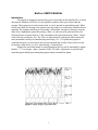
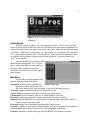
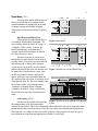
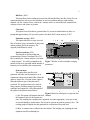
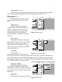
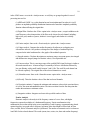
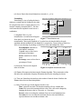
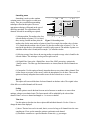
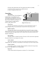
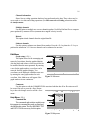
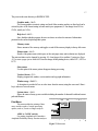
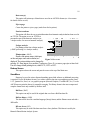
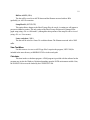
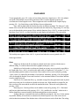
Biomechanics
Laboratory
School of Human Kinetics
University of Ottawa
BioProc User’s Manual
D. Gordon E. Robertson, Ph.D. and Sheila Purkiss, M.Sc.
Biomechanics Laboratory
Last revised: January 2001
© School of Human Kinetics, University of Ottawa
TABLE OF CONTENTS
TABLE OF CONTENTS . . . . . . . . . . . . . . . . . . . . . . . . . . . . . . . . . . . . . . . . . . . . . . . . . . ii
BioProc USER’S MANUAL . . . . . . . . . . . . . . . . . . . . . . . . . . . . . . . . . . . . . . . . . . . . . . . . . . . . . 1
Introduction . . . . . . . . . . . . . . . . . . . . . . . . . . . . . . . . . . . . . . . . . . . . . . . . . . . . . . . . . . . . . 1
Getting Started . . . . . . . . . . . . . . . . . . . . . . . . . . . . . . . . . . . . . . . . . . . . . . . . . . . . . . . . . . . 2
Main Menu . . . . . . . . . . . . . . . . . . . . . . . . . . . . . . . . . . . . . . . . . . . . . . . . . . . . . . . . . . . . . 2
Function Key Options . . . . . . . . . . . . . . . . . . . . . . . . . . . . . . . . . . . . . . . . . . . . . . . . . . . . . 3
Open Menu . . . . . . . . . . . . . . . . . . . . . . . . . . . . . . . . . . . . . . . . . . . . . . . . . . . . . . . . . . . . . 4
BioA/D menu and BioA/D ch. . . . . . . . . . . . . . . . . . . . . . . . . . . . . . . . . . . . . . . . . . 4
Ariel analog . . . . . . . . . . . . . . . . . . . . . . . . . . . . . . . . . . . . . . . . . . . . . . . . . . . . . . . 4
BioWare . . . . . . . . . . . . . . . . . . . . . . . . . . . . . . . . . . . . . . . . . . . . . . . . . . . . . . . . . 5
Clear data . . . . . . . . . . . . . . . . . . . . . . . . . . . . . . . . . . . . . . . . . . . . . . . . . . . . . . . . 5
Ensemble average . . . . . . . . . . . . . . . . . . . . . . . . . . . . . . . . . . . . . . . . . . . . . . . . . . 5
Fourier transform . . . . . . . . . . . . . . . . . . . . . . . . . . . . . . . . . . . . . . . . . . . . . . . . . . . 5
Generate data . . . . . . . . . . . . . . . . . . . . . . . . . . . . . . . . . . . . . . . . . . . . . . . . . . . . . 5
(i) All . . . . . . . . . . . . . . . . . . . . . . . . . . . . . . . . . . . . . . . . . . . . . . . . . . . . . . 5
(ii) Bias . . . . . . . . . . . . . . . . . . . . . . . . . . . . . . . . . . . . . . . . . . . . . . . . . . . . 5
(iii) Drift . . . . . . . . . . . . . . . . . . . . . . . . . . . . . . . . . . . . . . . . . . . . . . . . . . . . 6
(iv) Impulse . . . . . . . . . . . . . . . . . . . . . . . . . . . . . . . . . . . . . . . . . . . . . . . . . 6
(v) Noise . . . . . . . . . . . . . . . . . . . . . . . . . . . . . . . . . . . . . . . . . . . . . . . . . . . 6
(vi) Step . . . . . . . . . . . . . . . . . . . . . . . . . . . . . . . . . . . . . . . . . . . . . . . . . . . . 6
(vii) Square . . . . . . . . . . . . . . . . . . . . . . . . . . . . . . . . . . . . . . . . . . . . . . . . . 6
(viii) Ramp. . . . . . . . . . . . . . . . . . . . . . . . . . . . . . . . . . . . . . . . . . . . . . . . . . 6
(ix) Sine . . . . . . . . . . . . . . . . . . . . . . . . . . . . . . . . . . . . . . . . . . . . . . . . . . . . 6
(x) Triangle . . . . . . . . . . . . . . . . . . . . . . . . . . . . . . . . . . . . . . . . . . . . . . . . . 6
(xi) Sawtooth . . . . . . . . . . . . . . . . . . . . . . . . . . . . . . . . . . . . . . . . . . . . . . . . 6
(xii) Zeros . . . . . . . . . . . . . . . . . . . . . . . . . . . . . . . . . . . . . . . . . . . . . . . . . . 6
BioProc binary . . . . . . . . . . . . . . . . . . . . . . . . . . . . . . . . . . . . . . . . . . . . . . . . . . . . . 6
GlobalLab or DAFF . . . . . . . . . . . . . . . . . . . . . . . . . . . . . . . . . . . . . . . . . . . . . . . . 6
U.Mass. data . . . . . . . . . . . . . . . . . . . . . . . . . . . . . . . . . . . . . . . . . . . . . . . . . . . . . . 7
Path change . . . . . . . . . . . . . . . . . . . . . . . . . . . . . . . . . . . . . . . . . . . . . . . . . . . . . . . 7
Reload . . . . . . . . . . . . . . . . . . . . . . . . . . . . . . . . . . . . . . . . . . . . . . . . . . . . . . . . . . . 7
BioProc ASCII . . . . . . . . . . . . . . . . . . . . . . . . . . . . . . . . . . . . . . . . . . . . . . . . . . . . 7
Timeclip is On/Off . . . . . . . . . . . . . . . . . . . . . . . . . . . . . . . . . . . . . . . . . . . . . . . . . . 7
View Menu . . . . . . . . . . . . . . . . . . . . . . . . . . . . . . . . . . . . . . . . . . . . . . . . . . . . . . . . . . . . . 7
APDF and CAPDF . . . . . . . . . . . . . . . . . . . . . . . . . . . . . . . . . . . . . . . . . . . . . . . . . 7
BioA/D setup . . . . . . . . . . . . . . . . . . . . . . . . . . . . . . . . . . . . . . . . . . . . . . . . . . . . . . 7
Comments . . . . . . . . . . . . . . . . . . . . . . . . . . . . . . . . . . . . . . . . . . . . . . . . . . . . . . . . 8
Data Digitally . . . . . . . . . . . . . . . . . . . . . . . . . . . . . . . . . . . . . . . . . . . . . . . . . . . . . . 8
ii
Experiment information . . . . . . . . . . . . . . . . . . . . . . . . . . . . . . . . . . . . . . . . . . . . . . 8
Fourier analysis . . . . . . . . . . . . . . . . . . . . . . . . . . . . . . . . . . . . . . . . . . . . . . . . . . . . 8
Fatigue analysis . . . . . . . . . . . . . . . . . . . . . . . . . . . . . . . . . . . . . . . . . . . . . . . . . . . . 8
Channel information . . . . . . . . . . . . . . . . . . . . . . . . . . . . . . . . . . . . . . . . . . . . . . . . . 8
Multiple axes . . . . . . . . . . . . . . . . . . . . . . . . . . . . . . . . . . . . . . . . . . . . . . . . . . . . . . 8
Single axis . . . . . . . . . . . . . . . . . . . . . . . . . . . . . . . . . . . . . . . . . . . . . . . . . . . . . . . . 8
Graph setup . . . . . . . . . . . . . . . . . . . . . . . . . . . . . . . . . . . . . . . . . . . . . . . . . . . . . . . 8
Video/film information . . . . . . . . . . . . . . . . . . . . . . . . . . . . . . . . . . . . . . . . . . . . . . . 8
System status . . . . . . . . . . . . . . . . . . . . . . . . . . . . . . . . . . . . . . . . . . . . . . . . . . . . . . 9
Analyze Menu . . . . . . . . . . . . . . . . . . . . . . . . . . . . . . . . . . . . . . . . . . . . . . . . . . . . . . . . . . . 9
Analyze forces . . . . . . . . . . . . . . . . . . . . . . . . . . . . . . . . . . . . . . . . . . . . . . . . . . . . . 9
Bias removal . . . . . . . . . . . . . . . . . . . . . . . . . . . . . . . . . . . . . . . . . . . . . . . . . . . . . . 9
Correlation . . . . . . . . . . . . . . . . . . . . . . . . . . . . . . . . . . . . . . . . . . . . . . . . . . . . . . . . 9
Descriptive statistics . . . . . . . . . . . . . . . . . . . . . . . . . . . . . . . . . . . . . . . . . . . . . . . . . 9
EMG menu . . . . . . . . . . . . . . . . . . . . . . . . . . . . . . . . . . . . . . . . . . . . . . . . . . . . . . . 9
(i) APDF and CAPDF . . . . . . . . . . . . . . . . . . . . . . . . . . . . . . . . . . . . . . . . 10
(ii) Digital Filter . . . . . . . . . . . . . . . . . . . . . . . . . . . . . . . . . . . . . . . . . . . . . 10
(iii) Fourier analysis . . . . . . . . . . . . . . . . . . . . . . . . . . . . . . . . . . . . . . . . . . 10
(iv) Fatigue analysis . . . . . . . . . . . . . . . . . . . . . . . . . . . . . . . . . . . . . . . . . . 10
(v) Integral statistics . . . . . . . . . . . . . . . . . . . . . . . . . . . . . . . . . . . . . . . . . . 10
(vi) Linear envelope . . . . . . . . . . . . . . . . . . . . . . . . . . . . . . . . . . . . . . . . . . 10
(vii) Normalize menu . . . . . . . . . . . . . . . . . . . . . . . . . . . . . . . . . . . . . . . . . 10
(viii) Rectify . . . . . . . . . . . . . . . . . . . . . . . . . . . . . . . . . . . . . . . . . . . . . . . . 10
(ix) Descriptive statistics . . . . . . . . . . . . . . . . . . . . . . . . . . . . . . . . . . . . . . . 10
(x) Integration window . . . . . . . . . . . . . . . . . . . . . . . . . . . . . . . . . . . . . . . . 10
Fourier Analysis . . . . . . . . . . . . . . . . . . . . . . . . . . . . . . . . . . . . . . . . . . . . . . . . . . . 10
High-pass filter . . . . . . . . . . . . . . . . . . . . . . . . . . . . . . . . . . . . . . . . . . . . . . . . . . . . 11
Integration . . . . . . . . . . . . . . . . . . . . . . . . . . . . . . . . . . . . . . . . . . . . . . . . . . . . . . . 11
(i) Simpson’s . . . . . . . . . . . . . . . . . . . . . . . . . . . . . . . . . . . . . . . . . . . . . . . 11
(ii) Trapezoidal . . . . . . . . . . . . . . . . . . . . . . . . . . . . . . . . . . . . . . . . . . . . . . 11
(iii) Reimann . . . . . . . . . . . . . . . . . . . . . . . . . . . . . . . . . . . . . . . . . . . . . . . . 11
(iv) Indefinite . . . . . . . . . . . . . . . . . . . . . . . . . . . . . . . . . . . . . . . . . . . . . . . 11
(v) Cumulative function . . . . . . . . . . . . . . . . . . . . . . . . . . . . . . . . . . . . . . . . 11
(vi) Gadd Severity Index (GSI) . . . . . . . . . . . . . . . . . . . . . . . . . . . . . . . . . . 11
(vii) Head Injury Criterion (HIC). . . . . . . . . . . . . . . . . . . . . . . . . . . . . . . . . 11
(viii) Integration window . . . . . . . . . . . . . . . . . . . . . . . . . . . . . . . . . . . . . . . 12
Low-pass filter . . . . . . . . . . . . . . . . . . . . . . . . . . . . . . . . . . . . . . . . . . . . . . . . . . . . 12
Mathematics functions . . . . . . . . . . . . . . . . . . . . . . . . . . . . . . . . . . . . . . . . . . . . . . 12
(i) Absolute values . . . . . . . . . . . . . . . . . . . . . . . . . . . . . . . . . . . . . . . . . . . 12
(ii) Bias . . . . . . . . . . . . . . . . . . . . . . . . . . . . . . . . . . . . . . . . . . . . . . . . . . . 12
(iii) Cumulative function . . . . . . . . . . . . . . . . . . . . . . . . . . . . . . . . . . . . . . . 12
(iv) Differentiation . . . . . . . . . . . . . . . . . . . . . . . . . . . . . . . . . . . . . . . . . . . . 12
(v) Negate . . . . . . . . . . . . . . . . . . . . . . . . . . . . . . . . . . . . . . . . . . . . . . . . . 12
iii
(vi) Integrate . . . . . . . . . . . . . . . . . . . . . . . . . . . . . . . . . . . . . . . . . . . . . . . 12
(vii) Multiply . . . . . . . . . . . . . . . . . . . . . . . . . . . . . . . . . . . . . . . . . . . . . . . . 12
(viii) Normalize . . . . . . . . . . . . . . . . . . . . . . . . . . . . . . . . . . . . . . . . . . . . . . 12
(ix) Power function . . . . . . . . . . . . . . . . . . . . . . . . . . . . . . . . . . . . . . . . . . . 12
(x) Square root . . . . . . . . . . . . . . . . . . . . . . . . . . . . . . . . . . . . . . . . . . . . . 12
(xi) Squares . . . . . . . . . . . . . . . . . . . . . . . . . . . . . . . . . . . . . . . . . . . . . . . . 12
(xii) Invert . . . . . . . . . . . . . . . . . . . . . . . . . . . . . . . . . . . . . . . . . . . . . . . . . 13
Normalizing . . . . . . . . . . . . . . . . . . . . . . . . . . . . . . . . . . . . . . . . . . . . . . . . . . . . . . 13
(i) Amplitude . . . . . . . . . . . . . . . . . . . . . . . . . . . . . . . . . . . . . . . . . . . . . . . 13
(ii) Invert time . . . . . . . . . . . . . . . . . . . . . . . . . . . . . . . . . . . . . . . . . . . . . . . 13
(iii) Shannon . . . . . . . . . . . . . . . . . . . . . . . . . . . . . . . . . . . . . . . . . . . . . . . . 13
(iv) Time axis . . . . . . . . . . . . . . . . . . . . . . . . . . . . . . . . . . . . . . . . . . . . . . . 13
(v) Units . . . . . . . . . . . . . . . . . . . . . . . . . . . . . . . . . . . . . . . . . . . . . . . . . . . 13
Smoothing menu . . . . . . . . . . . . . . . . . . . . . . . . . . . . . . . . . . . . . . . . . . . . . . . . . . . 14
(i) Moving median . . . . . . . . . . . . . . . . . . . . . . . . . . . . . . . . . . . . . . . . . . . 14
(ii) Moving average . . . . . . . . . . . . . . . . . . . . . . . . . . . . . . . . . . . . . . . . . . 14
(iii) Digital Filter . . . . . . . . . . . . . . . . . . . . . . . . . . . . . . . . . . . . . . . . . . . . . 14
(iv) Interpolate . . . . . . . . . . . . . . . . . . . . . . . . . . . . . . . . . . . . . . . . . . . . . . 14
Rectify . . . . . . . . . . . . . . . . . . . . . . . . . . . . . . . . . . . . . . . . . . . . . . . . . . . . . . . . . . 14
Scaling . . . . . . . . . . . . . . . . . . . . . . . . . . . . . . . . . . . . . . . . . . . . . . . . . . . . . . . . . . 14
Time base . . . . . . . . . . . . . . . . . . . . . . . . . . . . . . . . . . . . . . . . . . . . . . . . . . . . . . . 14
(i) Invert. . . . . . . . . . . . . . . . . . . . . . . . . . . . . . . . . . . . . . . . . . . . . . . . . . . 14
(ii) Normalize . . . . . . . . . . . . . . . . . . . . . . . . . . . . . . . . . . . . . . . . . . . . . . . 15
(iii) Rotate . . . . . . . . . . . . . . . . . . . . . . . . . . . . . . . . . . . . . . . . . . . . . . . . . 15
(iv) Shift . . . . . . . . . . . . . . . . . . . . . . . . . . . . . . . . . . . . . . . . . . . . . . . . . . . 15
(v) Units . . . . . . . . . . . . . . . . . . . . . . . . . . . . . . . . . . . . . . . . . . . . . . . . . . . 15
Channel Menu . . . . . . . . . . . . . . . . . . . . . . . . . . . . . . . . . . . . . . . . . . . . . . . . . . . . . . . . . . 15
Add channels . . . . . . . . . . . . . . . . . . . . . . . . . . . . . . . . . . . . . . . . . . . . . . . . . . . . . 15
Clear all data . . . . . . . . . . . . . . . . . . . . . . . . . . . . . . . . . . . . . . . . . . . . . . . . . . . . . 15
Duplicate channels . . . . . . . . . . . . . . . . . . . . . . . . . . . . . . . . . . . . . . . . . . . . . . . . . 15
Erase channels . . . . . . . . . . . . . . . . . . . . . . . . . . . . . . . . . . . . . . . . . . . . . . . . . . . . 15
Fourier channels . . . . . . . . . . . . . . . . . . . . . . . . . . . . . . . . . . . . . . . . . . . . . . . . . . . 15
Generate channels . . . . . . . . . . . . . . . . . . . . . . . . . . . . . . . . . . . . . . . . . . . . . . . . . 15
Hypotenuse . . . . . . . . . . . . . . . . . . . . . . . . . . . . . . . . . . . . . . . . . . . . . . . . . . . . . . 15
Channel information . . . . . . . . . . . . . . . . . . . . . . . . . . . . . . . . . . . . . . . . . . . . . . . . 16
Multiply channels . . . . . . . . . . . . . . . . . . . . . . . . . . . . . . . . . . . . . . . . . . . . . . . . . . 16
Reload . . . . . . . . . . . . . . . . . . . . . . . . . . . . . . . . . . . . . . . . . . . . . . . . . . . . . . . . . . 16
Subtract channels . . . . . . . . . . . . . . . . . . . . . . . . . . . . . . . . . . . . . . . . . . . . . . . . . . 16
Edit Menu . . . . . . . . . . . . . . . . . . . . . . . . . . . . . . . . . . . . . . . . . . . . . . . . . . . . . . . . . . . . . 16
Graph setup . . . . . . . . . . . . . . . . . . . . . . . . . . . . . . . . . . . . . . . . . . . . . . . . . . . . . . 16
Comments . . . . . . . . . . . . . . . . . . . . . . . . . . . . . . . . . . . . . . . . . . . . . . . . . . . . . . . 16
Help Menu . . . . . . . . . . . . . . . . . . . . . . . . . . . . . . . . . . . . . . . . . . . . . . . . . . . . . . . . . . . . . 16
Command line . . . . . . . . . . . . . . . . . . . . . . . . . . . . . . . . . . . . . . . . . . . . . . . . . . . . 16
iv
Graphics mode . . . . . . . . . . . . . . . . . . . . . . . . . . . . . . . . . . . . . . . . . . . . . . . . . . . . 17
Help level . . . . . . . . . . . . . . . . . . . . . . . . . . . . . . . . . . . . . . . . . . . . . . . . . . . . . . . . 17
Memory status . . . . . . . . . . . . . . . . . . . . . . . . . . . . . . . . . . . . . . . . . . . . . . . . . . . . 17
Printer status . . . . . . . . . . . . . . . . . . . . . . . . . . . . . . . . . . . . . . . . . . . . . . . . . . . . . 17
Show mouse . . . . . . . . . . . . . . . . . . . . . . . . . . . . . . . . . . . . . . . . . . . . . . . . . . . . . 17
Version (About) . . . . . . . . . . . . . . . . . . . . . . . . . . . . . . . . . . . . . . . . . . . . . . . . . . . 17
Window usage . . . . . . . . . . . . . . . . . . . . . . . . . . . . . . . . . . . . . . . . . . . . . . . . . . . . 17
System status . . . . . . . . . . . . . . . . . . . . . . . . . . . . . . . . . . . . . . . . . . . . . . . . . . . . . 17
Print Menu . . . . . . . . . . . . . . . . . . . . . . . . . . . . . . . . . . . . . . . . . . . . . . . . . . . . . . . . . . . . . 17
APDF or CAPDF analysis . . . . . . . . . . . . . . . . . . . . . . . . . . . . . . . . . . . . . . . . . . . 17
Data array(s) . . . . . . . . . . . . . . . . . . . . . . . . . . . . . . . . . . . . . . . . . . . . . . . . . . . . . 18
Eject a page . . . . . . . . . . . . . . . . . . . . . . . . . . . . . . . . . . . . . . . . . . . . . . . . . . . . . . 18
Fourier transform . . . . . . . . . . . . . . . . . . . . . . . . . . . . . . . . . . . . . . . . . . . . . . . . . . 18
Fatigue analysis . . . . . . . . . . . . . . . . . . . . . . . . . . . . . . . . . . . . . . . . . . . . . . . . . . . 18
Printer status . . . . . . . . . . . . . . . . . . . . . . . . . . . . . . . . . . . . . . . . . . . . . . . . . . . . . 18
Redraw Screen . . . . . . . . . . . . . . . . . . . . . . . . . . . . . . . . . . . . . . . . . . . . . . . . . . . . . . . . . 18
Save Menu . . . . . . . . . . . . . . . . . . . . . . . . . . . . . . . . . . . . . . . . . . . . . . . . . . . . . . . . . . . . 18
BioWare . . . . . . . . . . . . . . . . . . . . . . . . . . . . . . . . . . . . . . . . . . . . . . . . . . . . . . . . 18
BioProc binary . . . . . . . . . . . . . . . . . . . . . . . . . . . . . . . . . . . . . . . . . . . . . . . . . . . . 18
RF raw forces . . . . . . . . . . . . . . . . . . . . . . . . . . . . . . . . . . . . . . . . . . . . . . . . . . . . 18
BioProc ASCII . . . . . . . . . . . . . . . . . . . . . . . . . . . . . . . . . . . . . . . . . . . . . . . . . . . 19
Setup BioA/D . . . . . . . . . . . . . . . . . . . . . . . . . . . . . . . . . . . . . . . . . . . . . . . . . . . . 19
Lotus worksheet . . . . . . . . . . . . . . . . . . . . . . . . . . . . . . . . . . . . . . . . . . . . . . . . . . 19
View Text Menu . . . . . . . . . . . . . . . . . . . . . . . . . . . . . . . . . . . . . . . . . . . . . . . . . . . . . . . . 19
Calculator . . . . . . . . . . . . . . . . . . . . . . . . . . . . . . . . . . . . . . . . . . . . . . . . . . . . . . . . . . . . . 19
GRAPH MODE . . . . . . . . . . . . . . . . . . . . . . . . . . . . . . . . . . . . . . . . . . . . . . . . . . . . . . . . . . . . . . 20
Axes . . . . . . . . . . . . . . . . . . . . . . . . . . . . . . . . . . . . . . . . . . . . . . . . . . . . . . . . . . . . . . . . . 20
Colours . . . . . . . . . . . . . . . . . . . . . . . . . . . . . . . . . . . . . . . . . . . . . . . . . . . . . . . . . . . . . . . 21
Cursors . . . . . . . . . . . . . . . . . . . . . . . . . . . . . . . . . . . . . . . . . . . . . . . . . . . . . . . . . . . . . . . 21
Statistics . . . . . . . . . . . . . . . . . . . . . . . . . . . . . . . . . . . . . . . . . . . . . . . . . . . . . . . . . . . . . . 22
Line type . . . . . . . . . . . . . . . . . . . . . . . . . . . . . . . . . . . . . . . . . . . . . . . . . . . . . . . . . . . . . . 22
Print . . . . . . . . . . . . . . . . . . . . . . . . . . . . . . . . . . . . . . . . . . . . . . . . . . . . . . . . . . . . . . . . . . 22
v
BioProc USER’S MANUAL
Introduction
This program is designed to perform many types of processing on data from BioA/D, or various
data properly formatted ASCII files. It is also possible to generate some types of data within the
program. This program can be used in menu mode, or can be operated in command line mode. When
used in menu mode, the choosing of an option in one menu results in a second menu of different choices
appearing. This continues until the type of processing is fully defined. An option is chosen by: using the
arrow keys to highlight the option, then pressing <Enter>; or with a mouse by point and click; or by
selecting the letter in square brackets, [], that corresponds to the option and pressing <Enter>. Menus
can be exited by pressing the <Esc> key. There are instructional cues that appear when needed, and
more information can always be obtained using on-line help (<F1>). To operate this program in
command line mode you need to know the relevant commands and switches. These can be accessed
by choosing <Help menu> (or <F6>), then choosing <Command Line>.
Program text used in this manual or text designating specific keys will be surrounded by angular
brackets “<>”. For example: <Enter> means the “Enter” key while <Open menu> means the Open
menu that appears initially upon starting the program without command line options.
Figure 1 Sample display of generated data
1
2
Figure 2 Press F11 to obtain version and author
information
Getting Started
When the program is loaded, a title screen appears (see above). After a key press the main
menu will appear on the left hand side of the screen (see below) and a list of options controlled by the
function keys will be listed at the bottom of the screen. Until data are loaded only the following options
are available: <Open menu>; <Help menu>; <F1> general help; <F2> open menu; <F6> help menu;
<F11> program title and authors; and <F12> date and time. If any of the other selections are chosen,
the computer will beep, and the following error message will appear: “No data are loaded. Press
<ESC> key to continue”.
Data can be loaded by accessing the Open
Menu, through choosing either <F2> or <Open
menu> on the screen. There are many options in
this menu, and the workings of each will be
detailed later (for details, see the section, Open
Menu Options).
Main Menu
The following are brief descriptions of the
purposes of the items in the Main Menu:
Open menu: enables the user to load different
Figure 3 Main menu
types of files and/or generate data. Also,
data in one channel can be copied to another, or files can be ensemble averaged.
View menu: graphs and information files can be selected for viewing.
Analyze menu: presents many techniques for data analysis and processing.
Channel menu: generate functions, add, copy or subtract channels, clear data
Edit menu: changes graph appearance or edits comments that are saved with the file.
Help menu: provides information on: command line mode; graphics mode; printer status; help level;
program version; and window usage.
Print menu: enables user to print data arrays and harmonic analysis results.
Save menu: enables user to save data in different formats, and can save changes to graph appearance.
View text menu: allows for the viewing of text or ASCII based data or output files.
Calculator: this loads a calculator that is provided with BioProc or the Windows calculator.
3
Function Key Options
After data have been loaded, the purposes of the function keys are the following:
<F1>:
Displays on-line help. Messages vary with the menu that you are in, giving relevant
information and instructions about the option chosen.
<F2>:
Displays <Open menu>. Same as choosing <Open menu> from the Main menu.
<F3>:
Displays <Analyze menu>. Same as choosing <Analyze menu> from the Main menu.
<F4>:
Displays setup file information of the loaded BioA/D files. The information can only be
viewed, not changed. This option is also found in <View menu>.
<F5>:
Displays comments stored with the loaded file. This option is also found in <View menu>.
A cue will appear if no comments are stored. Comments can be added to a file through the
<Edit menu>.
<F6>:
Displays <Help menu>. Same as choosing <Help menu> from the Main menu.
<F7>:
Displays <View menu>. Same as choosing <View menu> from the Main menu.
<F8>:
Displays graph setup. This option is also found in <View menu>. The title of the graph, the
axis labels and axis numbers and the graph colours can be changed, and the changes can be
saved using the <Setup> option of the <Save menu>.
<F9>:
Displays channels on a single axis graph. This option is also found in <View menu>.
<F10>:
Displays channels on a multiple axes graph. This option is also found in <View menu>.
<F11>:
Displays the program title, authors, version number and copyright information.
<F12>:
Displays time and date.
<Alt-F1>: Toggles help level from high to low and vice versa.
<Alt-G>: Displays graphics mode and settings.
<Alt-P>:
Displays printer status and settings.
<Alt-S>:
Displays status information about program settings and loaded channels.
4
Open Menu (<F2>)
The open menu enables different types of
files to be loaded, data to be generated, and
some information to be manipulated, in the form
of channel copying and ensemble averaging.
These options will be discussed below in greater
detail.
BioA/D menu and BioA/D ch.
These options are used when the files to
Figure 4 Open menu
be loaded are from the BioA/D program. The
user is initially offered the choice of <Setup> or
<Channels>. When <Setup> is chosen, the
BioA/D data directory on the hard drive is
accessed, and the files found there are listed in
the <Data directories> menu.
The arrow keys can be used to move
through this list, and a selection can be made by
pressing <Enter>. If your file is not in the BioA/D
data directory, the <Change path> option (in
<Open menu>) can be used to access it. In this
instance, the BioA/D files in the new directory will Figure 5 Windows for selecting BioAD files
be listed in the <Data directories> menu. Once
the file to be loaded is chosen, a prompt will
appear which gives some information about the
file, and directs the user on how to load some or all
of the channels in the file. The set-up channel of the
file is always loaded, even when the prompt
<Channels> is originally chosen. Selecting
<Channels> (instead of <Setup>) will load the
BioA/D file at the top of the <Data directories>
menu.
Ariel analog (.ANA)
Use this item to read data collected using Figure 6 Window to select which BioAD channels
to load
the Analog module of the Ariel Performance
Analysis System (APAS). These files hold multiple trials and therefore you may be prompted to enter
the trial number that you want to process. These files can contain force platform data that need to be
converted from raw voltages to forces and centres of pressure. The program will detect the type of
force platform can convert the data appropriately (Kistler or AMTI only).
5
BioWare (.DAT)
This item allows for the reading and conversion of Kistler BioWare data files. These files can
contain the data from one or two force platforms or one force platform and up to eight auxiliary
channels. Use the <Analyze forces> item in the <Analyze menu> to convert the force channels from
voltages to forces and centres of pressure.
Clear data
This option clears all loaded or generated data. To prevent accidental data loss, there is a
prompt that appears asking “Do you really want to clear these DATA from memory (Y/N)?”.
Ensemble average (.BPE)
This option allows the average of several
files to be taken, using a set number of data points,
and the resulting file saved separately. The
originally loaded data are erased.
Fourier transform (.FTF)
This item allows for the reading and
reconstruction of Fourier Transform Files (FTF
files) created by the <Fourier analysis> item in the
<Analyze menu>. You will be prompted for the
Figure 7 Window to select ensemble averaging
number of data to be generated and the number of parameters
harmonics to be included in the reconstruction.
Generate data
This option allow data files to be
generated, and either used by themselves or in
conjunction with previously loaded files. When this
option is chosen, the <Generate menu> appears,
listing the different types of data that can be
generated. The generated data can be used for
many purposes, including testing of processing
techniques and equipment. A brief description of
the options in the generate menu follows.
Figure 8 Menu for selecting how to generate data
(i) All. This options will generate data in all channels
the functions in this list, one function at a
time. The sampling rate, sampling time, amplitude, and where appropriate, cycles per second,
are set individually for each function. The list can be exited at any point by pressing <Esc>. The
resulting graph will display the data generated for each function on separate axes.
(ii) Bias. A constant value is added to the zero baseline. The sampling rate, sampling time and
amplitude can all be individually set.
6
(iii) Drift. A slowly increasing value is added to
the zero baseline. The sampling rate, sampling
time, and amplitude are all individually set.
(iv) Impulse. One brief signal, of a chosen
amplitude, occurs along a zero baseline. The
sampling rate and sampling time are also
selected.
(v) Noise. Random values occur within a
chosen amplitude range around the baseline.
The sampling time and rate are also selected.
Figure 9. Generated data channels using noise,
sine, triangle and sawtooth wave functions
(vi) Step. Half of the sampling time the value is at the zero the other half its at the chosen
amplitude. Sampling time and rate are also selected.
(vii) Square. Similar to the step function, except it moves from the positive amplitude value to
the negative amplitude value at the selected frequency.
(viii) Ramp. The value rises steadily from the zero baseline to the chosen amplitude, then drops
vertically back to the baseline. The number of cycles per second, the sampling rate and the
sampling time are also chosen.
(ix) Sine. A sine wave of chosen amplitude range (positive and negative), cycles per second
and sampling time and sampling rate is created.
(x) Triangle. A triangular wave varies around the baseline in a chosen amplitude range, and at a
selected number of cycles per second, sampling time and sampling rate.
(xi) Sawtooth. Similar to the ramp function, but it has both positive and negative values (drops
to the negative value of the amplitude, not to the zero baseline).
(xii) Zeros. Creates a channel of zeros.
BioProc binary (.BIN)
Use this item to read files saved using the <BioProc binary> item in the <Save menu>. The
directory path and filename can be entered directly, or the binary files in the current directory can be
listed by pressing <Insert>, then selected from the list of files.
GlobalLab or DAFF (.DAT)
This data file format is used by GlobalLab and follows the Data Acquisition File Format
specification.
7
U.Mass. data (.DAT)
Use this format to read data files created by the University of Massachusetts, Biomechanics
Laboratory. These files must have the extension, “.DAT”.
Path change
With this option the drive, root and parent directories can be changed so that files can be
accessed. The desired drive and directory path can be typed in directly, or a directory listing can be
displayed using the <Insert> key, and the appropriate options selected.
Reload
This option reloads channels from the original data file.
BioProc ASCII (.BPA)
When this option is chosen, a prompt displaying the current directory path and requesting a
new filename appears. Pressing <Insert> will list the ASCII files that are in the current directory. If the
file you need is one of these, it can be chosen using the arrow keys and <Enter> . If the file needed is in
another directory, it can be loaded immediately by typing in the appropriate directory path and
filename, or the directory path can be changed using the <Path change> option.
Timeclip is On/Off
Toggles (switches) whether time clipping is on or off. When on data can be clipped from the
front and end of the data channels. This is useful to reduce large data files or ignore parts of data files.
Currently only APAS .ANA files can be clipped.
View Menu (<F7>)
This menu gives different viewing options,
including viewing information files as well as
graphs. It can also be entered by pressing <F7>.
APDF and CAPDF
Displays the results from an Amplitude
Probability Distribution Function and Cumulative
APDF analysis. The results are displayed
digitally.
Figure 10 View menu
BioA/D setup (<F4>)
The setup portion of a BioA/D file can be viewed. If other types of data are loaded (not
BioA/D), or if data have been generated, their graph setups are displayed instead. The setup can only
be viewed, not altered. The setup can also be viewed using <F4>.
8
Comments (<F5>)
Any comments saved with the currently loaded file can be viewed. A prompt will appear if no
comments were stored with the file. Comments can also be viewed by pressing <F5>. Comments can
be added to a file using the <Edit menu>.
Data Digitally
Presents the raw data in digital form. Use
the angle brackets to increase or decrease the
number of decimal digits. Press <T> to toggle
display of the associated sample times. Use the
Figure 11 Press F4 to view BioAD channel setup
arrow keys and page keys to move through the
file. The <Home> and <End> keys move the view to the beginning and end of the data, respectively.
Experiment information
Any experiment information saved with the currently loaded file can be viewed. A message will
appear if no experiment information was stored with the file.
Fourier analysis
Displays the results from a Fourier analysis. The results are displayed digitally.
Fatigue analysis
Displays the results from fatigue analysis. The results are displayed digitally.
Channel information
Display various information about each channel, including scaling and bias factors.
Multiple axes (<F10>)
Information from each channel is displayed on a different axis of the same graph. This option
can also be chosen by pressing <F10>.
Single axis (<F9>)
Information from all channels is displayed on a single axis graph. This option can also be chosen
by pressing <F9>.
Graph setup (<F8>)
The graph setup information is displayed. The graph title, axis labels, axis number and graph
colour can be changed. This option can also be chosen by pressing <F8>. See Graph Setup on the Edit
Menu for more information.
Video/film information
Any film information (i.e., camera type, film type, etc.) that was saved with the currently loaded
file can be viewed. A message will appear if no information was saved.
9
System status (<Ctrl-S>)
Displays various system settings, including which channels are loaded, gain settings, whether
data have been changed, default path etc. Can also be displayed by pressing <Ctrl-S>.
Analyze Menu (<F3>)
This menu provides a variety of ways of
analyzing and processing loaded or generated
data.
Analyze forces
This item is provided to permit the
conversion of raw force signals from Kistler or
AMTI force platforms. Only certain types of
data files are permitted to use this item. This
function replaces the raw signals with their
reduced equivalents. The operation can only be
done once.
Figure 12 Analyze menu
Bias removal
This option will subtract a constant value
(bias) from the data. There are two ways of doing
this: by choosing <Mean> the mean value is
subtracted from selected channels; by choosing
<Term> a bias can be selected for each channel.
The original data are lost.
Correlation
Three options are
Figure 13 Bias removal menu
presented–Autocorrelate, Crosscorrelate and
Pearson product correlation. The Pearson product moment correlation (a measure of the similarity of
data sets) is found for two selected channels (designated x and y). The results are presented in table
form (standard deviation for x and y, correlation coefficient (r), coefficient of determination, standard
error of estimate, and the regression of y and x).
Descriptive statistics
This option computes the minimum,
maximum, mean, standard deviation, root mean
square (RMS), coefficient of variation and standard
error for the data in each channel, and reports them
in table form.
EMG menu
Although some of the analyzing techniques
Figure 14 EMG menu
10
in the <EMG menu> occur in the <Analyze menu> as well, they are grouped together for ease of
processing into one list.
(i) APDF and CAPDF. As yet this function has not been implemented, but when it is it will
produce an amplitude probability distribution function and a cumulative amplitude probability
function without affecting the original data.
(ii) Digital Filter. Similar to the <Filter> option in the <Analyze menu>, except in addition to the
cutoff frequency, other characteristics of the filter can be chosen for each channel, including:
high or low pass; number of passes; whether it is zero lagged; and whether it is critically
damped.
(iii) Fourier analysis. Same as the <Fourier analysis> option in the <Analyze menu>.
(iv) Fatigue analysis. Computes the median frequencies for adjacent or overlapping user
selected time intervals. Also produces a histogram of the changes of median frequency
compared to the initial median and/or a line graph of the median frequencies.
(v) Integral statistics. Calculates the minimum, maximum, range, root-mean-square, time integral
and absolute time integral (integral of absolute values). Uses trapezoidal rule.
(vi) Linear envelope. This is a moving average of the rectified EMG signal. Its shape is similar to
the muscle tension curve. A linear envelope is essentially a full wave rectification followed by
low pass filtering, with a cutoff usually between 3 and 10 Hz. The cutoff for each channel can
be selected separately. The original data of the selected channels are erased.
(vii) Normalize menu. Same as the <Normalize menu> option in the <Analyze menu>.
(viii) Rectify. Takes the absolute values of the data in selected channels.
(ix) Descriptive statistics. Computes the minimum and maximum values a their associated times,
as well as, the mean and standard deviation. The times are taken from the first data point that
reaches the maximum or minimum values.
(x) Integration window. Integrates and resets after specified number of data.
Fourier Analysis
Harmonic analysis is the analysis of the frequency content of a wave form, with higher
frequencies expressed a multiples of a fundamental frequency. Fourier transformation is the
mathematical process that results in the power (amplitude) of each frequency component being plotted
against frequency in a graph called a frequency spectrum. Most data should be filtered and, in some
cases, rectified, before a harmonic analysis is performed. The number of harmonics can be set between
1and 5000 for the selected channel. The results (mean, time, cosine, sine, hertz and median frequency)
11
are displayed numerically, then graphs of the frequency spectrum, normalized power, accumulated
power, median frequency and relative power can be plotted and printed. Afterwards the option of
saving the Fourier transform digitally appears. This file may be used to recreate the signal (see Open
menu, Fourier item).
High-pass filter
This is essentially a high pass filter. As noted in the provided cue, the filter used is a fourth
order, high, pass, critically damped, zero lag filter. The cutoff frequency can be set for each channel.
The original data for the filtered channels are erased.
Integration
Some definite integrals can not be
evaluated exactly; instead, approximate values are
found through different integration techniques.
Integration is basically finding the area under the
curve. There are many different ways of integrating
in this program, and choosing the most appropriate
depends on the type of data being used. Most data
needs to be rectified (using <Rectify> in the analyze
menu) before being integrated.
Figure 15 Integration menu
(i) Simpson’s. The area under the curve is estimated by: breaking the curve into small parabolic
segments and summing the areas of these. This type of analysis is the best for data involving
many curves and direction changes (i.e. EMG signals).
(ii) Trapezoidal. The area under the curve is estimated by summing trapezoidal segments.
(iii) Reimann. The area under the curve is estimated by summing rectangular segments.
(iv) Indefinite. As noted in the cue, trapezoidal integration is used to calculate the indefinite
integral (a definite integral is a number, an indefinite integral is a function). The original data are
erased.
(v) Cumulative function. As noted in the cue, the accumulative function of selected channels is
computed. The original data are erased.
(vi) Gadd Severity Index (GSI). A measure of the severity of positive acceleration, it is
calculated for all channels. A negative answer indicates an error resulting from negative
accelerations being present.
(vii) Head Injury Criterion (HIC). The head injury criterion is calculated for all channels. An
error results if the data are not positive accelerations.
12
(viii) Integration window. Integrates and resets after specified number of data.
Low-pass filter
Filtering is used to increase the signal-to-noise ratio of the collected data. Although noise can
never be entirely eliminated, with careful selection of the cutoff frequency it can be greatly attenuated
without significant signal distortion.. As noted in the provided cue, selected channels are filtered with a
low pass, fourth order, critically damped, zero lag filter. The cutoff frequency can be set separately for
each channel, with zero indicating no filtering.
Mathematics functions
This option enables many different mathematical processes to be performed on the data. When
each is chosen, a cue will appear giving a brief description of the process. For all of these, processing
causes the original data in the selected channels to be erased.
(i) Absolute values. The absolute values for
selected channels are calculated.
(ii) Bias. Used to subtract (or add) a
constant to channels.
(iii) Cumulative function. Cumulative
function on selected channels. Each value is
added to sum of all previous.
(iv) Differentiation. The time derivatives for Figure 16 Mathematics menu
selected channels are calculated.
(v) Negate. Data in the selected channels are multiplied by -1.
(vi) Integrate. The indefinite integrals for selected channels are calculated (see <Integration>
option of <Analyze menu> for more detailed description).
(vii) Multiply. Each channel is multiplied by a separately selected scale factor.
(viii) Normalize. Each channel is normalized (divided) by a separately selected factor (see the
<Normalize> option in the <Analyze menu> for a more detailed description).
(ix) Power function. Data in the selected channels are raised to separately chosen powers.
(x) Square root. The square roots for selected channels are calculated.
(xi) Squares. Data in selected channels are squared.
13
(xii) Invert. Data in the selected channels are inverted (i.e., y=1/x).
Normalizing
Normalizing is a way of scaling the data in
relation to a certain value (by dividing by the value)
for example body mass or weight or the force of a
maximal voluntary contraction (MVC). The data
can be normalized in amplitude or time base or a
combination.
(i) Amplitude. This is a y-axis
normalization. A second menu will appear
Figure 17 Normalization menu
from which you choose the type of
normalization. Choose peak amplitude or % peak to have the data divided by the peak
amplitude and then multiplied by one hundred (%), respectively. Choose, factor to divide by a
factor of your choosing or percentage to divide by a factor and multiplied by 100%.
Peak amplitude: normalize to
each channel’s maximum
% peak: same as above but in
percentages of maximum
Factor: normalize to a chosen
factor
Percentage: same as above but in
percentages of factor
(ii) Invert time. Reverses the temporal
order of the data.
Figure 18 Amplitude normalization menu
(iii) Shannon. Reconstructs the data using the Shannon algorithm. This reconstruction of the
data takes into consideration frequency information based on the sampling rate chosen.
(iv) Time axis. Normalizes the time base to the number of intervals chosen. Similar to the
Shannon above but uses linear interpolation.
(v) Units. Choose the type of units displayed on the x-axis:
Time: expressed in seconds. The maximum number will vary with the data.
Count: from zero to the maximum abscissa value. This value can be changed by
changing the abscissa value in <Time axis> or <User units>.
Percent: values occur along the continuum from zero to one hundred percent.
User units: the user can chose the maximum abscissa value and all data are
expressed between zero and the maximum value.
14
Smoothing menu
Smoothing is used to reduce random
variation (noise) so the signal is revealed more
clearly. There are several different smoothing
techniques offered in this option. The most
appropriate technique will depend on the type of
data being smoothed. The original data in the
channels selected for smoothing are replaced.
(i) Moving median. The median value for a
selected number of points (3-21) is found,
Figure 19 Smoothing menu
then, moving forward one data point, the
median value for the same number of points is found. For example, the median value of points
1-3 is found, then the median value of points 2-4, then the median value of points 3-5, etc. As
noted in the provided cue, this technique is useful for spike removal. The number of points over
which the median value is found (in this example: 3) is called the window.
(ii) Moving average. Same idea as the moving median, except the average value is found for the
selected window. This technique is also good for spike removal.
(iii) Digital Filter. Same as the <Digital filter> item of the <EMG processing> option in the
<Analyze menu>. The filter type and characteristics are chosen, then the selected channels are
filtered.
(iv) Interpolate. Use this option to linearly interpolate between two points within a channel. First
set the cursors to two parts of the curve(s) where the interpolation is to be done. Then use this
option two linearly interpolate between the cursors for the selected curve or curves.
Rectify
This option will convert all the data of selected channels to absolute values. The original values
of the full wave rectified channels will be erased.
Scaling
Use this option to rescale the data from one unit of measure to another or to convert from
analogue voltages to mechanical units. The factor entered will be multiplied by the selected data
channel. Enter 1 to leave a channel unchanged or -1 to reverse a channel.
Time base
Use this option to alter the time base or phase-shift individual channels. Use the <Units> to
change the times units displayed.
(i) Invert. The time base can be inverted, that is, reversed as long as all channels have the same
sampling rate. If not, use the normalize option to synchronize each channel.
(ii) Normalize. normalize to a specified number of intervals, e.g., percentages
15
(iii) Rotate. phase-shifts the data in the left or right directions without zero-padding
(iv) Shift. time shift left or right with zeros padded on the ends
(v) Units. to change the time base’s units
Channel Menu
Add channels
This allows the data of selected channels to
be added. When viewed (multiple axes), the
original channels are still displayed on their own
axes, and the summed channel is on an axis below
them. To mark a channel for summing press <Y>.
All marked channels are added together to
produce a single channel of data.
Figure 20 Channel menu
Clear all data
This option clears all loaded or generated data. To prevent accidental data loss, there is a
prompt that appears asking “Do you really want to clear these DATA from memory (Y/N)?”.
Duplicate channels
This option allows channels of previously loaded data to be selected for copying. A prompt
appears giving directions on how to select the channels for copying. When viewed, the copied channels
are in the same graph as the original channels, but in a different colour. More than one channel can be
duplicated, simultaneously.
Erase channels
This option “unloads” a channel from memory. The data are NOT erased from the original data
file unless the data file are saved using the <Save menu>.
Fourier channels
Allows for the reconstruction of a Fourier series waveform from the data stored in a Fourier
Transform File (.FTF). These files are created from the <Fourier analysis> item in the <Analyze menu>.
Generate channels
Use this option to generate a waveform. The list of possible waveforms have been previously
described under Open menu subsection Generate data.
Hypotenuse
Creates a channel which is the hypotenuse or resultant of 2 or 3 selected channels.
16
Channel information
Shows bias or scaling operations that have been performed on the data. These values may be
use to undo or view bias and scaling operations. (See Bias removal and Scaling subsections under
the Analyze menu.
Multiply channels
Use this option to multiply two or more channels together. Useful for KinCom files to computer
power produced by moment of force (moment times angular velocity in rad/s).
Reload
This option reloads channels from the original data file.
Subtract channels
Use this option to subtract one channel from another. Press the <X> key then the <Y> key to
perform the subtraction Y-X. One two channels can be subtracted at one time.
Edit Menu
Graph setup (<F8>)
This option allows for the rearranging and
removal of waveforms from the graphical display.
Also the labels and colours of each waveform can
be modified from the menu presented. By entering
a zero for the graph number a waveform can be
removed from the graphical display. Two
waveforms can be displayed within the same axes
by entering the same graph number for each
Figure 21 Edit menu
waveform. Note, blank areas will appear if the
graph numbers are not continuous.
Comments
Use this option to edit the COMMENTS file associated with the data. If no file exists one will
be created. Be sure to press the <Page Down>
key to have the changes saved or use the <Save
menu>.
Help Menu (<F6>)
Command line
The commands and switches needed to run
this program in command line mode are listed and
described in this option. The files BIOPROC.TXT
and LIST.COM are necessary for this option.
Figure 22 Help menu
17
They must in the same directory as BIOPROC.EXE.
Graphics mode <Alt-G>
The current graphics (monitor) settings are listed. Other monitor graphics are listed and can be
selected in place of the current setting to better match your equipment (i.e. can change from EGA to
SVGA, usually use VGA).
Help level <Alt-F1>
Once familiar with this program, the user can choose to reduce the amount of information
presented in the on-line help through this option.
Memory status
Shows amount of free memory and toggles on and off the memory display in the top left corner.
Printer status <Alt-P>
Details of the printer status (which port, on-line and paper status and resolution) are displayed.
The print resolution can be changed by pressing <R> from largest (0) to smallest (3) print sizes. Press
<E> to cause a page eject or form feed. Can also change default printing device, either LPT1, LPT2 or
LPT3.
Show mouse
Use this option if the mouse pointer disappears during processing.
Version (About) <F11>
Displays program title, authors, version number and copyright information.
Window usage <Shift-F1>
A description is provided of how to select items from the menus (using the cursor and <Enter>
keys) and move between menus.
System status <Alt-S>
Shows the status of many system variables including the number of channels loaded and current
path and filename.
Print Menu
This menu enables the printing of data
arrays and the results of various processing
options, such as, Fourier or fatigue analyses.
APDF or CAPDF analysis
For printing Amplitude and Cumulative
Amplitude Probability Density Function analyses.
Figure 23 Print menu
18
Data array(s)
This option will print arrays of data that are saved in an ASCII file format (see <Save menu>
for details of how to save).
Eject a page
Causes the printer to eject a page (sends form feed to printer).
Fourier transform
This option will allow the user to print information from harmonic analysis that has been saved in
an .FTF file. The option to save an .FTF file is
presented as part of the harmonic analysis (see
<Analyze menu> for more on harmonic analysis).
Fatigue analysis
For printing results from a fatigue analysis
(<EMG processing> in <Analyze menu>).
Printer status <Alt-P>
Details of the printer status (which port,
on-line and paper status and resolution) are
Figure 24 Save menu
displayed. The print resolution can be changed by
pressing <R> from largest (0) to smallest (3) print sizes. Press <E> to cause a page eject or form feed.
Can also change default printing device, either LPT1, LPT2 or LPT3.
Redraw Screen
This option redraws the screen and puts the cursor at the top of the Main men..
Save Menu
Data may be saved in various formats depending upon which software or additional processing
is required. Use the Worksheet format if you want to read the data into a spreadsheet program (Lotus
1-2-3, Quattro Pro, Excel, etc.) or graphics program (Harvard Graphics, CorelDRAW!, etc.). Use the
ASCII format to print the data or for ensemble averaging. The Binary format is the most compact and
complete format but it only readable by BioProc itself.
BioWare (.DAT)
This option can only be used if the original data were from a BioWare data file.
BioProc binary (.BIN)
The data will be saved in a machine language (binary) format, and the filename must end with a
.BIN suffix.
RF raw forces (.RF)
This option may be used if the data came from a force platform. This format is used by the
Biomech Planar Motion Analysis System.
19
BioProc ASCII (.BPA)
The data will be saved in an ASCII format and the filename must end with an .BPA
(preferably) or .ASC file extension.
Setup BioA/D (SETUP.STP)
This option allows changes to the BioA/D setup file to be saved. A warning cue will appear to
prevent accidental overwrites. The only portion of the BioA/D setup file that can be changed is the
graph setup (using <F8> or <Edit menu>), although the other portions of the setup file can be viewed
(using <F4> or <View menu>).
Lotus worksheet (.WK1)
The data will be saved in a Lotus 2.0 worksheet format. The filename must end with a .WK1
suffix.
View Text Menu
Use this menu to view text or ASCII type files. It requires the program, LIST.COM, be
included in the same directory as BIOPROC.EXE or in the search path.
Calculator
This item invokes a calculator program. A DOS program is provided with the software but the
program may invoke the Windows Calculator depending upon the PATH environment variable. Note,
the ANSI.SYS driver must be loaded by the CONFIG.SYS file.
20
GRAPH MODE
To start graph mode, press <F9> to have all waveforms plotted on a single axis or <F10> for multiple
axes mode. With multiple axes mode the placement of the waveforms depends upon how the
waveforms have been assigned to axes. These assignments can be modified in the Graph Setup by
pressing <F8>. See Graph Setup on the Edit Menu for more information.
Note, while in graph mode the function keys take on different meanings. The “help area” at the
bottom of the screen shows the functions associated with each function key. By pressing <F1> the help
area cycles through the various groups of keys and their functions. Press <Ctrl-F1> to return to the first
help menu. Press <Alt-F1> to remove the help area and display trial information. The various help
The last help menu appears when <Alt-F1> is pressed and when the screen is printed with <F5>.
menus appear below:
Axes
Single axis. In this mode all waveforms are plotted on the same axis but with the same or
different scaling. To switch to this mode while in graphics mode press <Alt-1>.
Multiple axes. In this mode waveforms are plotted on as many axes as required or specified in
the Graph setup. Press <Alt-0> to switch to this mode while in Graph mode. You can have 2, 3, 4 or
more depending upon the number of waveforms. These number of axes can be realized by pressing
<Alt-#> where # is replaced by the number of axes desired. Alternately, pressing <F10> the program
will cycle through the number of axes until it reaches 9 or the maximum number of waveforms and then
reverts to single axis mode.
Paired axes. For certain data files (e.g., ensemble average files) the graph mode starts in paired
mode where each pair of waveforms are plotted on the same axes. With ensemble averaged files, the
first waveform is the mean and the second is the standard deviation. This mode can be produced by
pressing <Alt-P>.
Removing axes. Vertical grid lines can be added or removed by pressing <F11>. Horizontal
grid lines are added and removed by pressing <F12>. <F6> modifies the “zero-line” which can be a
solid or dotted line or removed entirely if the horizontal grid lines are also removed.
Scaling of the axes is automatic but can be modified by pressing the <F8> key. Various options
are possible. Initially, all waveforms are maximized to fit their respective axes. That is, the axes are
scaled so that the maximum of the absolute values of the waveform are used to fit the data. The scaling
21
factor is displayed on the right side of the screen under the channel number and name. By pressing
<F8> once, the scaling is changed so that all waveforms are displayed with the same scale factor.
Pressing <F8> again causes scaling of +/-10 (V) and pressing a third time (or by pressing <%>) causes
percentage axes (+/-100%). Pressing <F8> again or pressing <Alt-F2> (reset) cycles back to the
original scaling factors. Note that the scaling factor displayed is affected by the number of grid lines and
the number of axes displayed.
Colours
The colours of each waveform is defined in the Graph setup. The colours are assigned by
default during loading or predefined by the program that created the data. They can be manually
assigned within the Graph Setup. The display can be changed from Black&white mode to Colour mode
by pressing the <F9> key. Black&white mode is useful for “screen grabs” or printing on black and
white printers.
Cursors
Two cursors are available to display data or to zoom in on a particular part of the waveform.
The left cursor is coloured yellow while the right is in white. The data points under these cursors are
displayed in the same colours in the channel display on the right side of the screen. One cursor may be
selected for movement by the arrow or cursor movement keys. Pressing <Enter> switches the selection
between the right and left cursor. The selected cursor is indicated in the lower right corner of the
screen. Alternately, the cursors can be moved by holding the left or right mouse buttons which control
movements of the left or right cursors, respectively.
Since more data are usually present then can be plotted on the limited number of pixels
available to the display monitor only one datum under the cursor is displayed. By pressing the left or
right arrow keys each datum may be displayed digitally. Pressing <Ctrl> and the right or left arrow keys
jumps along the data by one pixel. For example, if there 2000 data per waveform then each horizontal
pixel will represent 4 data. Pressing <Ctrl> and the right or left arrow key will jump to every 4th datum
while pressing just the arrow key will advance the cursor 1 datum.
The up and down arrows move up and down the file 1/40th of the screen while <Ctrl> and
these keys move the cursors 1/20th. The <PageUp> and <PageDown> keys move the cursors 1/10th of
the screen while holding the <Ctrl> key down moves one horizontal division left or right.
The <Home> key resets the left cursor to the extreme left of the screen; and the <End> key
resets the right cursor to the extreme right. The <F2> key resets both cursors.
To zoom in on the data, first select the area by moving the cursors keys, then press <F3>.
Once zoomed, pressing <Alt> and the right or left arrow keys pans the display right or left. When
zoomed, notice the “more” indicator at the bottom right. The symbols “<” and “>” indicate whether
there are data to the left and right, respectively. To zoom in and return to the command menus press
<Ctrl-F3>. To “unzoom” press <F3> again.
The cursors can be removed entirely by pressing <F7>. Pressing <F7> again, removes the
channel display on the right. A third press, restores the two cursors.
22
Statistics
To view statistical information press <D> for descriptive statistics, such as, maxima, minima,
means and standard deviations. The statistics presented are from the data between the two cursors.
Pressing <I> shows the ranges, integrals and absolute integrals for the displayed waveforms. These
numerical displays may be printed by pressing the <PrintScreen> key. Note, Windows may intercept
this function and place the screen image on the clipboard. To override this enter the Properties menu
when BioProc is running and click of the Misc. tab. Then make sure the “PrtSc” box is unchecked. To
view the data numerically, starting at the left cursor, press <V>.
Line type
Several line types for the waveforms are possible. If there are fewer data than the number of
pixels each datum is connected to the next by a line. By default if more data are present than there are
pixels than a “high-low” graph is used. In this case a vertical line is drawn between the highest and
lowest datum. Pressing <H> will set this line type. Pressing <L> will connect a line between the first
element in each pixel group. <M> will plot a line between the means of each pixel group while <P> will
plot a point for each datum with no connecting lines.
Print
To print the graphical waveforms press <F5>. The program will test whether the printer is online and ready before asking what type of printer is being used. If ready select either <H> for a printer
that accepts Hewlett-Packard PCL graphics, or <E> for Epson graphics or <I> for IBM Proprinter
graphics. Postscript graphics is not yet implemented. This method of printing renders the graphics as if
they were in black and white.
Alternately, pressing the <PrintScreen> key will print the screen directly to the printer but in
colour. Depending on the printer and operating system the graph may be printed appropriately. For
some operating systems, the DOS program, GRAPHICS.COM (also needed is the file
GRAPHICS.PRO) must be loaded with the appropriate printer selected. For example, to use a
Laserjet II or III, issue the command, GRAPHICS LASERJETII. Note, that the printer will shade the
lines depending upon their colours. Unfortunately, yellow curves appear invisible.