Download Untitled

LAB OF TOMORROW
GUIDE OF GOOD PRACTICE
1
Editors:
Michalis Orfanakis
Sofoklis Sotiriou
Stavros Savvas
Artwork:
Vassilis Tzanoglos
Lab of Tomorrow project is carried out within the framework of the
IST programme and is co-financed by the European Commission
Contract Number: IST-2000-25075
Copyright © 2004 by Ellinogermaniki Agogi. All rights reserved.
Reproduction or translation of any part of this work without the written permission of the copyright owner is
unlawful. Request for permission or further information should be addressed to
Ellinogermaniki Agogi, Athens, Greece.
Printed by EPINOIA S.A.
ISBN No. 960-8339-51-0
2
LAB OF TOMORROW
GUIDE OF GOOD PRACTICE
3
Contributors
Technical Engineers
Science Educators
ANCO S.A
Ellinogermaniki Agogi S.A
Vassiliki Tzagatzoni
Fotis Psomadellis
Kostas Giannakakis
Stathis Skarvelis
Sofoklis Sotiriou
Stavros Savvas
Michalis Orfanakis
Manos Apostolakis
Vassilis Tolias
Yiannis Stavrakis
Giorgos Babalis
Consorzio per la Ricerca e l’Educazione
Permanente
Emilio Perona
Luisa Viglieta
Stefano Turso
Marco Zambotto
University of Dortmund
Hans E. Fischer
Ruediger Tiemann
Dennis Draxler
National Technical University of Athens
Nikolaos Uzunoglou
Rodoula Makri
Michalis Gargalakos
Petros Tsenes
University of Birmingham
Chris Baber
Anthony Schwirtz
James Knight
4
Helene Lange Gymnasium
Udo Wlotzka
Ulrich Moellenkamp
Juergen Hillmann
Phoenix Gymnasium
Thomas Daub
Klaus Radtke
Technical Senior Secondary School
of Pininfarina
Ada Sargentie
Claudio Ferrero
BG&BRG Schwechat
Peter Eisenbarth
Markus Artner
Manfred Lohr
Michael Tichacek
Our vision for the school of tomorrow is that it will not be an island,
a self-contained campus, a counterworld. The school of tomorrow will be able
to emit and absorb along different wavelengths,
be immersed in contemporary culture, be open to the emotions,
facts and news of its time. It will be permeated by society,
but not unprotected: the relationship between school and society
will be one of osmosis, where the proposed pedagogical framework filters,
guides, and acts as a membrane and interface.
The Lab of Tomorrow partnership, 2000
5
6
Contents
For the User . . . . . . . . . . . . . . . . . . . . . . . . . . . . . . . . . . . . . . . . . . . . . . . . . . . . . . . . . . . . . . . . . . . . . . . . 9
Introduction . . . . . . . . . . . . . . . . . . . . . . . . . . . . . . . . . . . . . . . . . . . . . . . . . . . . . . . . . . . . . . . . . . . . . . . 11
Chapter 1 The Pedagogical Approach of Lab of Tomorrow project . . . . . . . . . . . . . . . . . . . . . . . . . . . . . . . 15
1.1 Concepts . . . . . . . . . . . . . . . . . . . . . . . . . . . . . . . . . . . . . . . . . . . . . . . . . . . . . . . . . . . . . . . . . . . . . . . . . . . 17
1.2 Scientific Literacy . . . . . . . . . . . . . . . . . . . . . . . . . . . . . . . . . . . . . . . . . . . . . . . . . . . . . . . . . . . . . . . . . . . . . 18
1.3 Theory of Basic Concepts . . . . . . . . . . . . . . . . . . . . . . . . . . . . . . . . . . . . . . . . . . . . . . . . . . . . . . . . . . . . . . . 20
1.4 Summary of the Basic Concepts, examples of necessary features and a possible surface structure . . . . . . . . 24
1.5 Pedagogical framework . . . . . . . . . . . . . . . . . . . . . . . . . . . . . . . . . . . . . . . . . . . . . . . . . . . . . . . . . . . . . . . . . 31
Chapter 2 Technical description of the Lab of Tomorrow system . . . . . . . . . . . . . . . . . . . . . . . . . . . . . . . . 35
2.1 Base Station . . . . . . . . . . . . . . . . . . . . . . . . . . . . . . . . . . . . . . . . . . . . . . . . . . . . . . . . . . . . . . . . . . . . . . . . . 38
2.2 Student Set . . . . . . . . . . . . . . . . . . . . . . . . . . . . . . . . . . . . . . . . . . . . . . . . . . . . . . . . . . . . . . . . . . . . . . . . . . 39
2.3 Ball module . . . . . . . . . . . . . . . . . . . . . . . . . . . . . . . . . . . . . . . . . . . . . . . . . . . . . . . . . . . . . . . . . . . . . . . . . . 43
2.4 The LPS (Local Positioning System) . . . . . . . . . . . . . . . . . . . . . . . . . . . . . . . . . . . . . . . . . . . . . . . . . . . . . . . 45
2.5 The Lab of Tomorrow User Interface . . . . . . . . . . . . . . . . . . . . . . . . . . . . . . . . . . . . . . . . . . . . . . . . . . . . . . . 48
2.6 Using the LOT User Interface . . . . . . . . . . . . . . . . . . . . . . . . . . . . . . . . . . . . . . . . . . . . . . . . . . . . . . . . . . . . . 53
7
Chapter 3 Good practice with “Lab of Tomorrow” . . . . . . . . . . . . . . . . . . . . . . . . . . . . . . . . . . . . . . . . . . . 65
3.1 Using the Lab of Tomorrow tools in real classroom conditions . . . . . . . . . . . . . . . . . . . . . . . . . . . . . . . . . . . . 66
3.2 Table of Contents and Lab of Tomorrow lesson plans. . . . . . . . . . . . . . . . . . . . . . . . . . . . . . . . . . . . . . . . . . . 67
3.3 First lessons and basic experiments. . . . . . . . . . . . . . . . . . . . . . . . . . . . . . . . . . . . . . . . . . . . . . . . . . . . . . . . 72
3.4 Sequence of preparatory lessons. . . . . . . . . . . . . . . . . . . . . . . . . . . . . . . . . . . . . . . . . . . . . . . . . . . . . . . . . . 74
3.5 School practice with Lab of Tomorrow. . . . . . . . . . . . . . . . . . . . . . . . . . . . . . . . . . . . . . . . . . . . . . . . . . . . . . 86
Chapter 4 Evaluation of Lab of Tomorrow . . . . . . . . . . . . . . . . . . . . . . . . . . . . . . . . . . . . . . . . . . . . . . . . 107
4.1 Introduction. . . . . . . . . . . . . . . . . . . . . . . . . . . . . . . . . . . . . . . . . . . . . . . . . . . . . . . . . . . . . . . . . . . . . . . . . 108
4.2 Project’s Evaluation Scheme 109
4.4 Results . . . . . . . . . . . . . . . . . . . . . . . . . . . . . . . . . . . . . . . . . . . . . . . . . . . . . . . . . . . . . . . . . . . . . . . . . . . . 119
4.5 Conclusions . . . . . . . . . . . . . . . . . . . . . . . . . . . . . . . . . . . . . . . . . . . . . . . . . . . . . . . . . . . . . . . . . . . . . . . . 145
Chapter 5 How to use the LoT Equipment- Quick Manual . . . . . . . . . . . . . . . . . . . . . . . . . . . . . . . . . . . . 147
5.1 Base Station . . . . . . . . . . . . . . . . . . . . . . . . . . . . . . . . . . . . . . . . . . . . . . . . . . . . . . . . . . . . . . . . . . . . . . . . 148
5.2 Student Set . . . . . . . . . . . . . . . . . . . . . . . . . . . . . . . . . . . . . . . . . . . . . . . . . . . . . . . . . . . . . . . . . . . . . . . . . 149
5.3 Ball Module . . . . . . . . . . . . . . . . . . . . . . . . . . . . . . . . . . . . . . . . . . . . . . . . . . . . . . . . . . . . . . . . . . . . . . . . . 155
5.4 Using the Video Grabber Software . . . . . . . . . . . . . . . . . . . . . . . . . . . . . . . . . . . . . . . . . . . . . . . . . . . . . . . . 156
Appendices . . . . . . . . . . . . . . . . . . . . . . . . . . . . . . . . . . . . . . . . . . . . . . . . . . . . . . . . . . . . . . . . . . . . . . 161
Appendix A: Leg / Arm Accelerometer Migration Procedure . . . . . . . . . . . . . . . . . . . . . . . . . . . . . . . . . . . . . . . . 162
Appendix B: Repair Instructions in case of Flexi Cable Disconnection or Misplacement . . . . . . . . . . . . . . . . . . . . 163
Appendix C: Set-up and calibration of the LPS system . . . . . . . . . . . . . . . . . . . . . . . . . . . . . . . . . . . . . . . . . . . . 166
Appendix E: Lab of Tomorrow Glossary . . . . . . . . . . . . . . . . . . . . . . . . . . . . . . . . . . . . . . . . . . . . . . . . . . . . . . . 169
References . . . . . . . . . . . . . . . . . . . . . . . . . . . . . . . . . . . . . . . . . . . . . . . . . . . . . . . . . . . . . . . . . . . . . . 171
8
For the User
The aim of the Lab of Tomorrow guide of good practice is to support the users, mainly teachers,
to effectively use the Lab of Tomorrow (LOT) systems in their teaching and learning practices. The guide provides support on how to use these systems within the framework of the normal school curriculum. Moreover,
by reading this guide one can find very valuable hints on how to utilise Lab of Tomorrow, not only in science
teaching but in gymnastics or in investigating every day activities in a more scientific manner. Thus the aim of
this document is to help, both teachers and students, to reach teaching and learning fields in which they can
make the most valuable contributions, and potentially improve the way of teaching and learning respectively.
To assure maximal usability of the new tools, optimal adaptation to the local environments and realistic evaluation of the pedagogical effects, the Lab of Tomorrow proposes the adaptation of a student-centered approach.
Lab of Tomorrow as a project included three extended periods of school-centered work. These trials involved
teachers and students to giving direction to the project and its technological and pedagogical results. This guide
summarises also, aspects of the evaluation results of the pilot implementation of the project that provide useful
information for the users.
During implementation, users are advised to experiment with the LOT axions, embedded in objects (toys, clothes)
in their everyday activities and measure a series of quantities like acceleration, forces, temperature etc. Almost
all physical phenomena and fundamental laws of Mechanics as well as aspects of in disciplines like Chemistry
9
and Biology can be studied using the data acquired by the LOT systems. The open architecture of the axions and
the user-interface allow the adoption of the new ideas in short time. The LOT partnership believes that have the
opportunity to view their involvement with Lab of Tomorrow as a craft that rewards dedication and precision but
simultaneously encourages a spirit of creativity, exuberance, humour, stylishness and personal expression. The
Lab of Tomorrow user is familiarised with the scientific method, design and conduction of scientific experiments,
collection and display data, as well as reporting of results. Students in particular, are given examples of how
scientific method can be used to solve real world problems.
Following the echo from IST’99 session “Children shaping the future” and the hope that the passionate debate
about children and how their voices can bring freshness and new meaning in the development of a better IT
world, with Lab of Tomorrow, students and teachers come together with researchers, psychologists, designers
and technologists to re-engineer the lab of the school of tomorrow. This is achieved with the introduction of a
new learning scheme based on the production of computational tools and educational material that allow high
school students to design their own scientific projects.
The document consists of four main chapters which include all the necessary information successful implementation of Lab of Tomorrow both in a secondary education class as well as in real life situations by individual
users. The first chapter is describing the basic aspects of the pedagogical approach of the project and the
basic concepts that govern the design of the Lab of Tomorrow lesson plans. The second chapter describes the
functionalities of the Lot tools in detail. It includes specific guidelines for their use and technical maintenance.
In addition it focuses on the Lab of Tomorrow User Interface and its capabilities not only for the demonstration of the collected data but also as a pedagogical tool. The third chapter presents paradigms of good Lab of
Tomorrow practice that are based on the pilot implementation of the project in five diferrent schools in Austria,
Germany, Greece and Italy during the school period 2003-2004. These good practice paradigms mainly aim to
support teachers during the implementation of LOT in their classes and should be conceived as recommendations to teachers in order to get familiarized with the use of axions and discover their functionalities. The fourth
chapter describes the evaluation methodology of the project and includes specific evaluation data referring to the
project’s pilot implementation. In addition this document includes appendices that the user can be considered as
a quick guide to the use of the systems and supporting material. All these documents are necessary not only for
the smooth implementation of Lab of Tomorrow but also for own evaluation purposes in order the make direct,
informal comparison between the proposed approach and the traditional approach in Science teaching.
This document, in parallel with the already published issue of the Lesson Plans, the Teachers Workshop Proceedings and the on-line training material, published on the project’s web site (www.laboftomorrow.org) aims to
provide help and support to the teachers of the Lab of Tomorrow.
10
Introduction
[Science, whatever be its ultimate developments,
has its origin in techniques, in arts and crafts…
Science arises in contact with things, it is dependent
on the evidence of the senses, and however far it seems
to move from them, must always come back to them.]
B. Farrington, Greek Science, 1949
There is sufficient evidence to suggest that both the persistence and the quality of learning are
highly enhanced when the student is actively participating in the learning process. This is the essential and
widely accepted message of “constructionism” (Papert, 1994 & Resnick, 1993). Juxtaposing this ideal with the
current reality of organized learning in school environments creates the impression that the school is not connected at the desirable degree with daily life experiences.
One particular and most striking example is science teaching. Throughout history science has advanced through
observation, inspection, formulation of hypotheses, testing of the hypotheses by means of experiments and collection of data, rejection or acceptance of the hypotheses, formulation of topics for further research. It seems
that in schools this process of acquisition of scientific knowledge gets reversed. Science is presented as a coherent body of knowledge, the experiment is the illustration of the phenomenon, and the questions are answered
11
even before they are asked. The result is that the student acquires short-term knowledge targeted at standardized test questions, and in many instances this “forced and inefficient” learning lacks on long term sustainability.
Possible pragmatic remedies have been proposed. Regarding to (Glasersfeld,1995) the constructivist point of
view has been very fruitful to develop science instruction. In this model knowledge acquisition is only a matter
of individual mental activities. But, constructionism (Duit, 1995) in its pure, so-called “radical” version is also
discussed controversially. The instructional component is missing in the model and therefore it is very difficult
to derive investigation methods and codings which are able to represent the instructional influence upon learning
processes. Thus, since the early 90s a pragmatic interim position was discussed, named by (Merrill, 1991) as
“instructional design of the second generation”. It is seen as integration of constructionism and cognitive theory.
It accepts learning as a process of individual cognitive construction and states the dependence of this process
on adequate learning environments (Weidenmann, 1993, Derry, 1996). Even models of situated learning (Mandl
et al., 1997, Roth, 1995) can be seen as a combination of these two approaches, taking into account the learning
situation and motivating and communicative aspects, which is an obvious weakness of radical constructionism.
As it turns out the main link missing in the learning process is that students do not learn sufficiently through
experience but through a systemic model based approach, which should be the culmination of learning efforts
and not the initiation. A particularly disturbing phenomenon that is common knowledge among educators is that
students fail to see the interconnections between closely linked phenomena in e.g. biology and chemistry, or fail
to understand the links of their knowledge to everyday applications. In most cases the physical quantities have
become abstract for the students and the experimental set-ups alien or distant to every day experience.
Students are early faced with two separate fields: “school science” and every day life’s “rules and principles”.
Such separation commonly leads to the formation of misconcepts (Nachtigal, 1991). “School science” explains
adequately “school science lab phenomena” while preconceptual or misconceptual reasoning explains daily
phenomena. Various approaches try to bridge these two fields (Nachtigal, 1992). They converge in the wide
usage of every day materials and means in the classroom, something relatively easy in primary school level. In
higher levels this becomes less effective since the phenomena and the concepts under study (like acceleration,
momentum transfer or energy conservation) are more abstract. In such cases technology is providing some help
with the supply of educational scientific instruments and software. Both the power and the problem with modern
scientific instruments used in the school laboratories are reflected in the term “black box” that is commonly
used to describe the equipment. Today’s black-box instruments are highly effective in allowing students to make
measurements and collect data - enabling even novices to perform advanced scientific experiments based in
most of the cases on advanced simulations. But at the same time, these black boxes are “opaque” as their inner
workings are often hidden and thus poorly understood by the users. Furthermore they are bland in appearance
making it difficult for students to feel a sense of personal connection with scientific activity. “To many students
a lab means manipulating equipment and not manipulating ideas” (Lunetta, 1998).
12
Electronics and computational technologies have accelerated this trend, filling science laboratories and classrooms with ever more opaque black boxes. Paradoxically, the same electronics technologies that have contributed to the black-boxing of science can also be used to reintroduce a vigorously creative and aesthetic dimension
into the design of scientific instrumentation - particularly in the context of science education.
The Lab of Tomorrow project introduces innovation both in pedagogy and technology. It aims at developing
tools that will allow for as many links of teaching of natural sciences as possible with every day life. It will allow
the student to link i.e. physics with “physis” (Greek word for nature), biology with “bios” (Greek word for life)
and so on. The Lab of Tomorrow project is developing a new learning scheme by introducing a technologically
advanced approach for teaching science through every day activities. Science deals with the study of nature
and the world around us, so teaching science cannot be separated from daily experiences resulting from student’s interaction with the physical phenomena. The connection of tangible phenomena and problems provides
students with the ability to apply science everywhere and not only in specially designed experiments under the
laboratory’s controlled conditions (Nachtigal, 1992).
In the Lab of Tomorrow project the re-engineering of the school lab of tomorrow is proposed by developing
a new learning scheme based on the production of computational tools and project materials that allow high
school students to use their every day life environment as the field where they will conduct sophisticated experiments experiencing the applicability of the theoretical background given at school. The partnership proceeded
to the development of a wearable technology, a series of “artefacts”, called axions, that allow students to derive
experimental results drawn from their everyday activities and which, in many cases, involve data collection over
extended periods of time. The axions embedded in every day objects (for example an accelerometer embedded
inside a ball) or in clothes (for example a heart pulse meter embedded in a T-shirt) are used in order to collect
data during students’ activities. Important factors of their design are ergonomics and economy, so they will not
stay on a test bench nor used by a small number of users. The data collected by the axions1 are presented with
the use of advanced programming tools compatible with graphing and analysis software components so that
students can easily investigate trends and patterns and correlate them with the theory taught at school.
The Lab of Tomorrow project adopts an activity-based design methodology. It has been recently questioned (Baber et al., 1999) whether the contemporary approach to the design of computer applications can be sustained
for future technologies. Norman suggests that a primary reason why the desktop metaphor remains in vogue is
that it allows designers and manufacturers to strive for the production of multipurpose products, i.e., products
1
The partnership has chosen this specific name for two reasons. In physics axion is a hypothetical elementary particle. Even
though the axion -- if it exists -- should have only a tiny mass, axions would have been produced abundantly in the Big Bang, and
relic axions are an excellent candidate for the dark matter in the universe. The second reason is the word game between axion
and action.
13
and applications that can be used for any job in any office. This seems to take good business sense, with most
people finding most of the functions useful. Nevertheless, it also leads to claims that the majority of the functions
offered will not be used by the majority of users (Norman, 1998).
Norman’s proposal is that future computers will offer restricted function sets, and that people will select the
function set most appropriate to their defined requirements. He calls this “activity-based computing” since
computers will be designed to support specific activities. This would mean that the wearer would have less
equipment to operate and carry, and it could also mean that interaction with the computer could be performed
via familiar objects and products.
In Lab of Tomorrow it is believed that activity-based computing extends the basic assumptions of user-centered
design and requirements engineering, because it allows considering the architecture that might be appropriate
for a specific wearable product. The approach, which has been adopted in the framework of the project, is to use
scenario-based design methods as a means of defining suitable applications of wearable technology.
14
Chapter 1
The Pedagogical Approach of Lab of Tomorrow project
Usually pre-designed experiments are used in science teaching. In the framework of the Lab of Tomorrow project students will be able to use the axions and the wearables to set up their own experiments, which
they will conduct autonomously. In this way the procedure of scientific inquiry is fully simulated: formulation
of hypothesis, experiment design, selection of axions, implementation, verification or rejection of hypothesis,
evaluation and generalisation are the steps that will allow for a deeper understanding of the science concepts.
The partnership believes that the proposed approach will act as a qualitative upgrade to everyday teaching for
several reasons:
Motivation: Students are more likely to feel a sense of personal investment in a scientific investigation as they
will actively participate in the research procedure and will add their own aesthetic touches to their intelligent toys
and cloths.
Extending the experimentation possibilities: The axions can serve as spurs to the imagination, promoting students to see all sorts of daily activities as possible subjects of scientific investigation. The proposed procedure
will be freed from the pressing time limitation of the teaching hour.
15
Developing critical capacity: Too often students accept the readings of scientific instruments without question.
When students will get involved in the proposed activities for example by measuring their physical parameters
as they are playing, they should as a result develop a healthy scepticism about the readings and a more subtle
understanding of the nature of the scientific information and knowledge.
Making connections to underlying concepts: In the framework of the project’s application to the school communities, students will be asked to design their own projects. During this procedure students will figure out
what things to measure and how to measure them. In the process they will develop a deeper understanding of
the scientific concepts underlying the investigation. If students use a wearable thermometer, for example, they
naturally encounter (and make use of) the concepts of thermal conductivity and heat capacity.
Understanding the relationship between science and technology: Students participating to the project will gain
firsthand experience in the ways that technology design can both serve and inspire scientific investigation.
16
1.1 Concepts
The pedagogical concept of the project has to represent two corresponding features: The first
refers to the general education aims of our modern societies and the results of recent research in science education, the second has to take into account the specific conditions of the project like requirements of the national
curricula and the specific background of the schools involved. The partnership proposes the following two concepts that match these requirements of Lab of Tomorrow as a modern and trend-setting European project:
•The PISA concept of scientific literacy
•The theory of basic concepts on teaching and learning
Reasoning
General discussions in science, society and politics about scientific literacy agree that it must be
based on the development of a general understanding of essential “key concepts” of physics. These concepts
should enable the students to recognize recognition scientific questions and to realize scientific processes. They
allow an autonomous reasoning and a communicative interaction in the field of physics. Accordingly, these
considerations have to be transformed to sequences of teaching and learning physics. We have to take into
account the results of the international large scale assessments TIMSS (Baumert et al., 1997), PISA of the last
five years which indicate that subject oriented planning and performing of physics lessons is not as successful
as expected.
The theory of “basic concepts about learning” of Oser & Patry (1990) and Fischer & Reyer (2002) can be used
to plan teaching and learning processes at school. This theory has two decisive advantages: it allows a reasonable planning of teaching and it is not strictly subject oriented but focussed on enabling subject related learning
processes. For example the usually applied subject related teaching aim “Newton’s laws” is transformed into
“problem solving (using Newton’s laws as an example)”, “theory development (using friction as an example)”
or “training to use force concepts to enable routines”.
17
1.2 Scientific Literacy
“(…) the ability to recognize scientific questions and
to draw scientific conclusions in order to understand
decisions and to take decisions according to the world
and to changes of the world, based on human activity.”
OECD/PISA scientific literacy 2000
The scientific literacy is clearly more than the knowledge of facts and terms. It contains an understanding of basic concepts and requires a decontextualized, global applicability. Tasks in the frame of scientific
thinking have to take into account the following levels of scientific reasoning:
• Applying scientific concepts
• Organizing scientific processes
• Communicating scientific contents
Consequently, these three levels are part of the pedagogical frameworks of the Lab of Tomorrow project. To
design a task- and learning process-orientated structure of the lesson plans the range of the sequences planned
has to ensures that scientific knowledge in its different complexities is used in as well versatile meaningful contexts as possible.
Scientific Concepts
Concepts are so far recognized experiences, which can be summarized in a category. They enable
a connection of new with already made experiences to construct a meaningful activity in the field of physics.
Scientific concepts are formulated in many different ways, from general terms until detailed lists of features. For
the Lab of Tomorrow project, concepts should satisfy the following requirements:
• Importance of the concepts and contents for everyday life
• Significance to prove scientific literacy
• Enabling student’s communication about physics
18
As a situation close to reality, OECD/PISA 2000 puts forward situations containing problems related to individuals, members of the society or citizens of the world. In addition, historical information can be integrated in order
to gain an understanding of progress of scientific knowledge.
Scientific Processes
Scientific processes are predominantly mental actions like the interpretation or the assessment
of data to organize mental, manipulative and/or social activities. Thus, they are always related to a specific
content.
Based on the notion of scientific literacy, five processes can be identified:
• Solving tasks
• Identifying scientific evidences
• Concluding from or judging scientific topics
• Organizing group communication
• Organizing scientific working (experimental and theoretical)
19
1.3 Theory of Basic Concepts
The theory of Basic Concepts of teaching and learning is based on the “Choreography of classroom learning” (Oser & P atry 1990). This project examines three criteria that characterize successful teaching.
These are the “atmosphere” during the lessons, the “content structures” and the “chronological order of the
lessons”, build up by a sequence of teaching methods, instructional tasks and learning offers. The last aspect is
the cornerstone of Oser’s theory of Basic Concepts of teaching.
Deep structure and apparent structure
Teaching and learning is guided by rules, which are not necessarily evident for the teacher or
the learner. Sometimes they are too complex to be easily expressed, or they are not explicitly known by the
teacher.
However, by an observer a single lesson can be judged as “wrong” or “right”, or decisions in different situations are more or less suitable for achieving a teaching aim. But the teacher mostly cannot say explicitly why a
decision was right or wrong - he/she acts intuitive. This intuition can be expression of a guiding concept if it is
consciously based upon a theory and the related activities are routines of pedagogical behaviour.
Consequently, in order to describe lessons in different levels, should be established a disting between a surface
structure and a deep structure. The surface structure describes the observable activities and interactions of
a lesson. For instance, the instructions of the teacher, the teaching methods or the behaviour of the students
are elements of a surface structure. The deep structure contains concepts, theories and beliefs of the teacher
concerning teaching and learning in general, but also his/her own way of teaching and his/her beliefs about
the learning processes of his/her actual students in the classroom. The teachers concepts and beliefs can be
expressed as a great variety of possible surface structures. According to Oser, these combinations can be systematically described by the following Basic Concepts of teaching relevant to students:
20
The basic Concepts of teaching
Learning by experiences
Deductive-inductive linkage
Search processes
Automatism
Transformation
Expressive affect-transformation
Problem solving
Exchange of social behaviour
Learning of facts
Identity development
Concept learning
Learning by consensus
Mediation
Meta-learning
These models of teaching make the hypotheses of different learning methods into account. They are independent of the teaching content. Each content model is based on a section of the deep structure. This part is called
Basic Concept and contains all rules and theories that are necessary for this particular teaching model.
Operation sequences and apparent structure
According to Oser the achievement of a teaching aim is determined by a chronological sequence
of different operations related to the planned learning processes. These operations are located on a level between the apparent structure and the deep structure. Related to the intended teaching aim, each Basic Concept
is consequently justified by an operation sequence as the smallest unit of “time structure” and “methodical
structure”.
For designing lessons with this model, the teacher can use different kinds of actions in the apparent structure
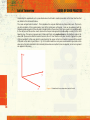
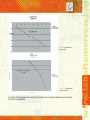
to realize a unit in the operation sequence. Figure 1.1 illustrates this aspect: Each education aim is respectively
based on a Basic Concept, and this Basic Concept can be operationalized by an operation sequence. The three
examples express operation sequences, which are consisting of five steps. Each teaching sequence can be
realized in different ways, for instance symbolized like a)-c). The single steps of an operation sequence can although be realized in many ways, expressed by the different symbols. For instance, a teacher choosing teaching
sequence (a) realizes step one by giving his students a text and ask questions.
21
Another teacher although chooses this educational aim but realizes the first step by designing an experiment
together with his/her students, and they work in small groups on this experiment or further tasks, a third teacher
uses interviews in a shopping centre to organize the learning process. There are many possibilities for the apparent structure, and they are all based on the same operation sequence.
Figure 1.1: Deep Structure and Apparent Structure, linked by Operation sequences.
Design of lessons
The operation sequences are suitable to explain the activities of the students. Planning a lesson by
means of Basic Concepts offers the possibility to concentrate on an intended learning process. The method fits
with the cognitive background of the students and allows for a more efficient way of teaching (Brouer 2001).
The following list describes the design of a lesson based on the theory of basic models. Starting with an edu-
22
cational aim is different from conventional lesson planning starting with a content and, hopefully, looking for an
educational aim related to this content.
1. Determination of the educational aim
2. Classification of the basic model
3. Classification of the operational sequence
4. Methodological design of the lesson
The educational objective is closely related to the subject matter, but starting with an educational aim is a new
way of organizing teaching and learning.
23
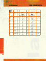
1.4 Summary of the Basic Concepts,
examples of necessary features and a possible surface structure
The theory of Oser proposes 14 Basic Concepts, based on approaches concerning a non-science research field. As a result of reviewing these models for their suitability in research on science teaching and learning the
following models remain
Basic Concept
Necessary features
Learning by own experiences
Everyday activity, integration of scientific “rediscover” of everyday phenomena
knowledge in every day knowledge
Example of a surface structure
Structure transforming learning / developing Processes of de-equilibration, new construc- Dilemma discussions like wave-particle
fostering learning
tion instead of adapting knowledge
dualism, misconceptions like energy consumption
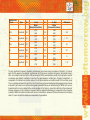
24
Problem solving
Problem solving with an information value
Determination of a new value like angular momentum or electrical resistance, construction
of a physical relation like Hook’s law
Theoretical knowledge/knowledge of theory
Isolated aspects, abstraction, analogies, Elaboration of relations like F=ma or the delimitations
cay law, perception of causalities like thermal
conductivity
Contemplate learning, meditation
Internal recapitulation of ontological, fateful, To be astonished about selected physical
religious, realities, …
phenomena like astronomical distances or
nuclear physics
Routine, skill training
Repetition and training, relieving of con- Learning of practical methods like the use of
sciousness
an oscilloscope, presentation of data or the
use of mathematical calculations
Motility
Creative elaboration of events, expressions Creative presentation of phenomena or rerelated to the fine arts
sults, e.g. as wall papers of project results,
artistic play with phenomena or conjuring
tricks
Dynamical social relationships
Pro-social acting, acting/living in groups, Cooperative learning, group work like distribudevelopment of friendships
tion of tasks during an experiment or mutual
learning support
Development of values and identities
Value constitution by participation, main Discussion of relevant topic for the society
method: scientific literacy
like pro and contra “nuclear energy”
Over all view - learning
To judge and select information, surveys
Judgement and arrangement of physical aspects of everyday activities with the help of
papers, articles, internet, literature, …
Basic Concept 1: Learning by own experiences
In a learning process at school the students should integrate their own experiences in already
existing knowledge.
These experiences are always connected to actions. According to Piaget (1977) the objectives of learning by
own an experience is an assimilation of new knowledge.
Operation sequence:
1. Internal, contextual representation of acting (preparation, design …)
2. Contextual acting (doing an experiment, categorizing, searching …)
3. First critical reflection of the acting pathway, the aim of acting and the intention of action
4. Generalisation of the results of the reflexion process
5. Transfer of the learning consequences onto larger contents, start of a symbolic representation
Main characteristics of this basic model are the everyday conceptions as starting points and implementation of
this prior knowledge into the learning process.
Basic Concept 2: Structure transforming learning / developing fostering learning
This model is based on the ideas of the conceptual change approaches. The recognition of new
knowledge elements that cannot be fit into already existing structures generates a cognitive conflict. Piaget
(1977) calls this process of integration of new concepts accommodation. Oser (1990) describes this model for
learning as an element to judge in moral situations. For teaching science, it can easily be modified for learning
scientific contents.
Operation Sequence:
1. Rattling of the learner in his way of thinking and de-equilibration of existing structures (concerning social
and/or moral and/or political values)
2. Disintegrate existing knowledge structures and recognition of important new elements, discussing advantages and disadvantages of different suggestions, seeing different ways of reasoning
25
3. Integration of the new elements, change of values and relationships, as a consequence transformation of the
structure or dismantling of old elements
4. Testing and securing the new structure by transferring to new contents
Basic Concept 3: Problem solving
In contrast to the general understanding of problem solving in science education research model
problem solving is not understood as a meta-competence, but related to the way of recognizing new elements as
necessary and to integrate them into the knowledge. It is only possible to focus on content orientated problems,
if the students have an adequate repertoire of problem solving strategies - and are able to use them.
Accordingly, problem solving as a methodological competence can only be learned in meaningful, “real” contents.
Operation Sequence:
1. Students discover a problem that is important to them «here and now”. It must originate from their
experiences.
As an alternative the teacher could present a problem, related to their experiences and interests that emphasise
a discrepancy between expectations and experience (Problem stimulation).
2. The students describe a problem based on this stimulation that consists of the conditions at the beginning
and an aspired solution. The “tools” (strategy of solving the problem) are unknown (problem description, as
accurate as possible).
3. Students suggest strategies of solving the problem (also suggestions that are judged by the teacher as not
successful).
4. Proving the suitability of the suggested strategies for a successful problem solving with the given starting
conditions (testing the ways of problems solving, selection). If there is no satisfying possibility to solve the
problem, then start again with step 3.
5. Use of the strategy for new problems of the similar categories and analysis of the possibilities for transfer or
generalisation of the strategy.
26
Basic Concept 4: Theoretical knowledge/knowledge of theory
This model is based on the assumption that knowledge is built up on a network of related concepts and can be represented with propositional maps. This basic model is a combination of two Oser-models,
generation of terms and generation of concepts. Both are determined by very similar operation sequences, so
consequently both models are combined to the model of theoretical knowledge.
Operation sequence:
1. Become directly or indirectly aware of already existing, and for the lesson necessary, theoretical knowledge
2. Presentation and elaboration of a prototypical example, which consists of all essential elements end features
of the learning concept
3. Explication: elaboration of the essential features and principles of the concept
4. Elaboration: active usage of the new concept (use, analysis, synthesis), compare/ relate/mark off with already
known concepts and examples on different representation levels
5. Linkage: connecting of new concepts with already existing ones
Basic Concept 5: Contemplate learning, meditation
Learning by mental lapsing with an objective of an internal recapitulation of ontological, fateful
or religious realities is rather emotional than cognitive. It is not based on a de-equilibration of knowledge or a
conceptual change like most of the other learning strategies. And it seems not to be suitable for science teaching. But nevertheless, to discover aspects of science as astonishing, offers possibilities and change the point of
view on effective teaching and learning also in science. Contemplate learning can be the beginning of a learning
process, as great researchers in history start their discoveries by astonishment and enthusiasm.
Operation sequence:
1. Create an internal void, leave the will, be ready for a way
2. To touch, to hear, etc. The external structure of a phenomenon, a work of art (flower, music, picture…)
3. First spontaneous interpretation of the recognized semantic
27
4. Second interpretation of the recognized semantic, but now transcendentally, religiously or aesthetically
5. Integration in life context
Basic Concept 6: Routine, skill training
The objective for becoming routine is the development of an automatism for complex cognitive
tasks. The operation sequence of this model fosters a mechanism of expectation-action-correction and matches
with results of cognitive psychology.
Operation Sequence:
1. First attempt of single action steps and presentation/elaboration of the linkage of means and aims (What is
the aim of the action?)
2. Creation of the complete actions by determination of the action range and regularities; analysing the meaning
of single elements and relations
3. Repetition of action steps, combination of action steps or complete actions and checking and control with
correction.
4. Complete evaluation of single steps. Repetition of operation 3 and 4 until automatism.
5. Discrimination of situations of application and training of discrimination
Basic Concept 7: Motility
Motility is fostering and grounding on an expressive transformation of affective states of excitements. Like contemplative learning, this model might not seem suitable for science teaching and learning. Nevertheless, also motility enriches the possibilities of different teaching methods.
Operation Sequence:
1. Explanation of ways to reach “motility”
2. Creation of anxious expectation: presentation of an object or phenomena which is suitable for creating an
anxious expectation
28
3. Cognitive restructuring of accumulate energy and inducing of a “creative” break
4. Creative transformation of this energy
5. Strengthening and transferring of these experiences by comparison with results of strange transfer processes
Basic Concept 8: Dynamical social relationships
The operation sequence maintains a reflection of spontaneous actions in social contexts. The sequence can be combined with other learning methods for fruitful outcomes, for example experimental laboratory
work.
This implies that the following operation sequences must initiate another basic model or its operation sequence,
respectively, for a “methodological situated” construction of dynamical social relationships.
Operation Sequence:
1. Holistic recognition, presentation and evaluation of social skills
2. Build up conditions for testing these skills and their suitable application
3. Reflection of these skills and explanation, legitimating or criticism of them
4. Behaviour exchange with different persons for a generalisation of the skills
Basic Concept 9: Development of values and identities
The operational sequences of this model are aimed at a classification of actions in an ethical way. Science education refers to the identity of a researcher and to his/her responsibility for an honest interpretation of the data
and for the society.
Operation Sequence:
1. Analysing already existing values (rules) concerning a current problem. Building a hierarchical structure of
rules for a discursive discussion
2. Suggestions for an integration of new rules
29
3. Participation in decision-making for the integration of the new rule in already existing ones
4. Realization of the new rule by single persons, by the society or by bodies
Basic Concept 10: Over all view - learning
The objective of this model is not to learn details or to identify gaps in the knowledge structure, but
to recognize and outline a topic “top down”. An “over all view - learning” needs a longer period of time, consisting of several learning processes that are framed by this way of learning. This matter is obviously described in
step 3 and 6 of the operation sequence.
Operation Sequence:
1. Selection of a topic
2. Over all view of the resources
3. Decision of the learning method
4. Selection of a guided or unguided way of learning
5. Feed back orientated doing of a task, reading…
6. Evaluation
30
1.5 Pedagogical framework
The described concepts of “Scientific Literacy” and “Basic Concept theory” are both necessary
for a holistic strategy to plan lessons in the context of the Lab of Tomorrow project. While scientific literacy
generates the general frame for the project, the Basic Concept theory generates the “tools” for a successful
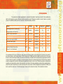
implementation of the project’s objectives as outlined in the following Table:
Table I: The basic concepts for the implementation of the Lab of Tomorrow project.
Scientific Literacy
Concepts: force, motion
energy, conservation of energy
Situations: everyday activities
physical education, sports
Processes: reconstruction of physics (science) tasks
constructivist approach
communication
Basic Concept Theory, preferred models
• Learning by own experiences
• Problem solving
• Routine, Skill training
• Theoretical knowledge
• Dynamical social relationships
• Motility
31
The design of learning processes
According to modern pedagogy teaching should be guided by a holistic planning process that
takes the students’ learning processes, the subject matter and the teaching methods into account. As a maximum of students’ orientation, it is a very important and significant variable which correlates positively with the
students’ performance. It offers the students the chance to link the teaching contents to their experiences and
their prior knowledge.
They have the chance to remark the characteristics of an active and self-guided learning process.
Consequently, learning processes must be designed on conditions that they are oriented to the student’s prior
knowledge.
For learning science this means to enable students to see connections to familiar problems relevant and important for their lives. Additionally, the situated learning fosters the ability of transferring acquired knowledge to a
variety of different situations. One of the main objectives is to acquire the ability of self-organised and self-regulated learning. Schools should generate the conditions for the development of the competence to learn and, as
a perspective, an autonomous learning. This includes the development of meta-cognitive learning competences
like e.g. elaboration strategies or learning strategies and their application and usefulness.
Learning processes in the future will be embedded in communicative situations, where teaching science offers
good conditions by fostering communication and cooperation in students’ experimental practices.
For a content orientation the planned teaching topics should be based on a broad field of knowledge and application. The teaching sequences must be build up in a way that knowledge can increase and link. Learning
processes in science are orientated to the typical increasing complexity in science. An increasing process of
finding systematic and rules, a more and more theoretical guided model building on the basis of an experimental
extraction of a part of reality are features of each scientific inquiry. The necessary systematic, long time planned
and cumulative learning contributes to a well-arranged, internal linked and in different situation flexible adaptive
knowledge.
Of course, the school is a part of the student’s life, but learning in school can only be successful, if the contents
are also relevant behind the border of school reality. There should be a guaranteed link to future learning processes. Summarizing these aspects, teaching and learning in science is successful, if it will be possible to realize
a sequence of topics that equally guarantee a systematic learning (vertical knowledge transfer) and situation
orientated learning with every day tasks and problems (horizontal knowledge transfer).
A method orientation expresses the possibility for the students to learn the necessary subject and cross subject
methods. In the learning groups there should be occasions for dialogs, at first guided by the help of a teacher,
32
but more and more autonomous and aimed at the development of scientific orientated conceptions and concepts. The students should have the possibility to describe their individual learning pathways and their individual
solutions of problems. Creativity, efforts and flexibility must be acknowledged. A teaching method contains the
teaching sequences, work-methods and the structural elements of ways of teaching and learning.
Task-oriented lesson plans
Regarding actual research in science teaching and learning the structure and the transparency of
lessons are crucial features of teaching. Both are organised by task orientation (e.g. according to the results of
SINUS).
In the Lab of Tomorrow project the lessons are organised in tasks according to two different levels of understanding, so two sequences of tasks are offered to students like to perfect pathways for conceptual growing.
For the tasks all problems are well described in literature, concerning e.g. preconceptions or problem solving
processes, so parallel to the two pathways alternatives with learning aims according to these problems are
offered. Such a structure requires small learning groups to enable individual experiences with the offered phenomena.
Moreover those tasks have to be arranged in conventional, so-called learning cycles.
33
34
Chapter 2
Technical description of the Lab of Tomorrow system
This chapter aims to help the teacher who is using the Lab of Tomorrow system during his lesson
by giving specific guidelines of the functionalities of the main components of the Lab of Tomorrow system.
The Lab of Tomorrow system consists of the following modules:
•
Base Station Set, that receives all data from the peripheral units and transmits them to the
workstation:
•
Base Station Unit with a stub antenna @ 433MHz.
•
Base Station Power Supply Pack.
•
RS-232 cross-cable.
•
Student Set, for the collection of the SensVest data and their transmission to the base station via the
radionetwork:
•
Belt Assembly.
•
Heart-Rate Measurement Belt (Polar Belt).
35
•
Temperature Sensor.
•
Leg Accelerometer Module.
•
Arm Accelerometer Module.
•
Bracelets for Leg / Arm Accelerometer Modules - 3 sizes (small, medium, large).
•
Belt Assembly and Leg-Arm Accelerometer Battery Chargers (x2).
•
Ball Module Set, which transmits the acceleration data to the base station:
•
Ball Module.
•
Ball Module Battery Charger.
•
The workstation, which collects and processes all system data.
•
The User Interface, which presents the graphical representation of the data.
Figure 2.1a: The components of the Lab of Tomorrow system
36
Figure 2.1b: The components of the Lab of Tomorrow system
Additionally an LPS (Local Positioning System) is used in order to help the students to estimate the position of
different objects during their activities.
In the following paragraphs a short description of the Lab of Tomorrow system will be given. For those teachers
who want to have a detailed description of the system they have to refer to the technological report of the project
and the relevant technical reports of each device which are also available.
37
2.1 Base Station
Power Supply
The Base Station is powered by the power-pack provided. Just plug the power-pack to the main supply and
connect it to the Base Station.
Operation
For proper operation place the Base Station on a table, at a height about one meter above the ground. The area
near it should be clear from any obstacles. The Base Station is connected to the Work Station (a PC with LOT
software installed) with the RS-232 cross-cable provided.
Figure 2.2:
Base Station
Attention: Use only the RS-232 cable provided.
The Base Station will not work with a straight, PC-to-modem cable.
38
2.2 Student Set
The Student Set consists of the following modules:
• Belt Assembly (AN-BLA-V1.0).
• Arm Accelerometer Module (AN-AAM-V1.0).
• Leg Accelerometer Module (AN-LAM-V1.0).
• Heart Rate Measurements Belt (Polar Belt).
• Temperature sensor.
• Bracelets for Leg and Arm Accelerometers (3 sizes - small, medium, large).
• Battery charger (2 items).
Belt Assembly
Power Supply
The Belt Assembly is the main
part of the student set. To switch
the module on, open (de-strap)
the belt and press the button on
the AN-STMBAN-V1.0 module for
about one (1) second, until the LED
flashes twice. Once the module is
switched-on, the LED flashes every
two seconds. To switch the module
off, press the button, until the LED
flashes twice.
Figure 2.3: Belt Assembly
39
Operation
The Belt Assembly consists of three main modules:
a. The student set radio module (AN-STMCPU-V1.0), which establishes the radio communication with the Base
Station of the network.
b. The Body Area Network radio module (AN-STMBAN-V1.0), which collects wirelessly via the BAN all data from
the Arm and Leg Accelerometer modules.
c. The Heart - Rate - Temperature - Body Accelerometer module (AN-CHTBA-V1.0), which includes the heart
rate receiver, the temperature connector and read-out circuit as well as the body accelerometer sensor.
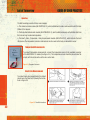
Temperature Measurements
To conduct temperature measurements, connect the temperature sensor to the available connector
at the ANCHTBA-V1.0 module (See Figure 2.4). The temperature sensor should be placed under the
armpit, with the metal surface at the skin contact side.
Figure 2.4: Temprature Connector
Heart-Rate Measurements
To conduct heart-rate measurements, the student
should wear the Polar belt, following the instructions in Figure 2.5.
Figure 2.5: Polar Belt Instructions
40
After the experiment has finished, carefully wash the belt with a mild soap and water solution, rinse it with pure
water and dry it carefully with a soft towel. The belt should be stored in a clean and dry place.
Battery Charging
The battery of the module is a state-of the - art Li-Polymer type and can be charged at any time, without affecting
battery life. To re-charge the battery, take-off the belt, switch it off and connect it to the charger provided.
The battery becomes fully charged at less than two hours and provides power for about 3.5 hours of continuous
operation.
Attention:
The module is not operational, when charging is in progress and it should not be
turned on during this process.
Leg and Arm Accelerometers
Power Supply
The Leg and Arm Accelerometers have no power switch. They are switched on and off by the Belt Assembly,
whenever an experiment starts and stops. The module will also switch itself off, if it is unable to communicate
with the Belt Assembly for a long period of time.
Figure 2.6: Leg Accelerometer
41
Operation
The student should wear the Leg Accelerometer at his/her leg and the Arm Accelerometer at his/her arm. When
the Work Station issues an experiment start command, the student wearing the belt and the accelerometers must
stand in such a way, that the y axis of both modules is vertical to the earth's surface. The student must remain in
this position until the modules LEDs are turned on and remain lit. This means, that the activation signal has been
received. After a while, the LED will switch off and start blinking. This means that the experiment has started and
the sensors are gathering data. The LED will switch off permanently, when the experiment stops.
Attention:
All the Leg/Arm accelerometers, that are located in the vicinity of the experiment area
and are not taking part in the measurements, should be placed in the horizontal
position in order not to interfere with the working system.
Battery Charging
The accelerometer modules have the same battery as the Belt Assembly. The same charger is used to recharge
these batteries. The battery becomes fully charged at less than two hours and provides power for 24 hours of
continuous operation and for months, when in idle state.
42
Attention:
The module is not operational when charging is in progress.
Attention:
When an Arm/Leg Accelerometer is in the horizontal position, it does not search for
activation signals. For this reason, place the accelerometers horizontally when you
store them for long periods, as this will extend battery life.
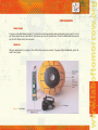
2.3 Ball module
Power Supply
To power-on the Ball Module (Figure 2.7), press the switch momentarily using a ball-point pen or a pencil. Do not
use sharp objects to press the switch. Upon power-up, the LED flashes twice. When the Ball Module is powered
up, the LED flashes every four seconds.
Operation
When an experiment is in progress, the LED flashes every two seconds. To power off the Ball Module, press the
switch once again.
Figure 2.7: Ball Module
43
Battery Charging
The battery can be re-charged with the corresponding charger provided. The battery becomes fully charged at about 3
hours and provides power for about 4 hours of continuous operation.
Attention:
44
When no experiment is executed, the Ball Module should not be left switched on, as this will
consume the battery very quickly.
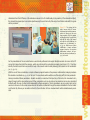
2.4 The LPS (Local Positioning System)
Based on the consideration of a reliable solution and in order to provide a short-term result the option
of using a 2- CCD camera solution was adopted for the test phase of the project's implementation. The space to be
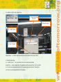
observed will be viewed with two cameras (Figure 2.8).
Figure 2.8: One of the LPS cameras as it is mounted on the wall
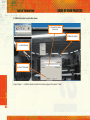
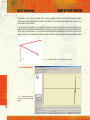
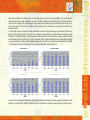
The scenes to be recorded (frames) by the two cameras will be synchronized in time and the observation in two orthogonal planes will provide the coordinates in 3D space as shown in Figure 2.9.
Figure 2.9: The basic principle of the LPS architecture
By measuring (x1, z1) and (y2, z2) coordinates the absolute coordinates (xM, yM, zM) of the ball (point M) can be obtained
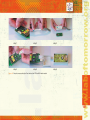
provided the positions A and B of cameras are known. In Figure 2.10 two views of the experimental area (including a
table and the Axion Ball) are presented as they were captured by the LPS.
45
Figure 2.10: Two views of the experimental
area captured by the LPS. Students have to
point the Axion Ball with the cursor on the
two frames and the coordinates of the ball
will be calculated automatically.
The minimum test area required for the whole 2-camera system would be 5mX5mX3m. This means that the
system will be able to identify and record the position of an object (ball) at least within this area.
The pixel analysis for the proposed cameras will be 768X512 pixels. The accuracy of the system for the above
field of view and the specific pixel analysis will be around 5-10 cm. Of course as the field of view increases, the
actual accuracy of the system will deteriorate because the pixel size for each camera is constant.
The indoor application of the system could be situated in closed basketball or volleyball court where the ball
game will take place. Alternatively any closed recreation ground with the above minimum dimensions could be
used for the first series of experiments. It is recommended to start the series of experiments with indoor applications and these can be justified considering the illumination requirements of the camera system. Such systems
that involve these kinds of experiments require constant illumination conditions for the field of view.
The outdoor experiments might be affected by the climatic conditions, which of course involve the illumination
parameter.
The basic architecture of the system is schematically shown in Figure 2.9. Two CCD cameras are positioned on
the x-y, x-z or y-z levels. The cameras must form a right angle between them in order to achieve the best accuracy. At least 2-3 meters between the cameras and the field of view is required for the proper focusing of the test
area. Both cameras are connected to a PC, which will be located nearby. The system will record the trajectory
of the object of interest and the relevant players during the proposed activity.
The cameras are connected to the personal computer through the parallel ports. Two frame grabber PC cards
are used. Each camera has the ability to record 50 frames/sec. The LPS system is able to capture 25 active
frames per second. This is due to the parallel frame grabber's architecture that is utilized. Since both cameras
must be synchronized and each frame must be recorded at the same time, the final capacity of the system is
46
diminished from the 50 frames of the individual camera to the 25. Additionally to the position of the observation object,
the relevant time parameter is recorded simultaneously for each frame. By this way a few minutes video with the game
will be produced.
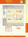
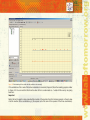
Figure 2.11: The student will be
able to recover to the PC screen
the frames from both the cameras,
which are referring to the same
time parameter. Then the student
will identify the ball in each frame
and with the help of the mouse
will mark the ball producing the
relevant set of coordinates (x1,
z1), (y2, z2). With the use of these
coordinates, a simple software
program based on the previous
mathematical analysis, will produce the absolute coordinates (xo,
yo, zo) of the ball.
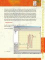
For the presentation of the recorded frames a user-friendly software tool is used. Students are able to recover to the PC
screen the frames from both the cameras, which are referring to the same time parameter (see Figure 2.11). Then they
identify the ball in each frame and with the help of the mouse mark the ball producing the relevant set of coordinates
(x1, z1), (y2, z2).
With the use of these coordinates, a simple software program based on the previous mathematical analysis produces
the absolute coordinates (x0, y0, z0) of the ball. The coordinates will be written on a file along with the time parameter.
Having recorded all these parameters, students are able to reconstruct the trajectory of the ball or the movements of a
player through out the observation period. Other parameters such as velocity and acceleration can be also calculated
indirectly with the use of other small independent software programs. These calculations are very useful and can be
used as a reference for the same measurements that will be conducted through the axions embedded in the foot anklet
and the ball. By this way an accurate method for the verification of these measurements will be simultaneously available.
47
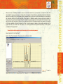
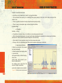
2.5 The Lab of Tomorrow User Interface
The axions give data in a format compatible with graphing and analysis software tools; so that
students can easily investigate trends and patterns in the data they collect with the wearable sensors. A database
and an advanced web based software tool have been created to process the received information. The information is retrieved and effectively classified in order to decode it and present it with the help of the graphical User
Interface in a way familiar and adjustable to the student. The main innovation of the approach is that students
are able to study the physical phenomena emerging from their own activities and everyday situations and not
only from specially designed experimental set-ups with the use of simulated data. Students through a sequence
of steps involving, data accessing, plotting data on a graph, creating a mathematical model to fit the data and
relate the graph with the motions of the axions provided by the user-interface, gain deeper understanding of the
phenomena. Necessary information may comprise diagrams of a variable versus an independent value (kinetic
energy vs. distance), mathematical models that make possible the interpretation of information within the laws of
physics (e.g. position, velocity and acceleration will be plotted and fit to see the correlation of the real data and
the kinematics equations), graphic diagrams of the changes in pulse beat or temperature as in a medical instrument with the use of statistical models, the use of thresholds and different windows to observe instantaneously
different variables etc.
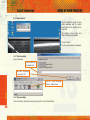
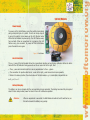
Lab of Tomorrow User Interface Guide
Quick Launch Form
Quick Launch Tab
The quick launch screen, appears at the start-up of the Lab Of Tomorrow application. It intends to provide to the
user, a collection of the most common tasks. The quick launch tab, contains the following 6 tasks, represented
by their corresponding icons
• Start A New Experiment
• Open A New Experiment
• Browse Experiments
• Import And Merge
• Help
• Courses
48
The Help, and Courses sections, are not implemented at the current version.
Each of the following sections that are functional, are described at later chapters.
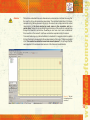
Recent Files Tab
The Recent Files tab, intends to facilitate the post processing procedure,
by providing a list of the recent files, the user has created, edited or opened. If
you double click on a file from the list (or select it and press "OK"), the application will open the corresponding experiment for post processing.
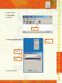
Main Form
The main form, holds all experiment forms, and contains a menu bar and a toolbar. These two elements (Menu and Tool
Bars) contain all the basic and advanced functions. If a button, or menu item is disabled, it will appear as "grayed", and
the user will not be able to use that function. In the following both these objects are described in detail.
Menu Bar
Tool Bar
49
Menu Bar
"File" Category
The "File" menu bar category, contains the following items:
• New
• New Session File (Creates a new session file)
• New From Raw Data (Creates a new file from raw data-Used only for debugging purposes.
• Open (Opens a new file)
• Save (Save the current file)
• Save Us (Saves the current file, under a new name)
• LPS Data Import (Imports or merges, LPS data, into an sensors only experiment file)
• Explorer (A windows explorer style, with usefull information about experiment files)
• Recent Files (Contains a list with the recent files , used by the application)
• Exit (Exits the Lab Of Tomorrow application)
"Edit" Category
The "Edit" menu bar category, contains the following items:
• Cut (Cuts data from the selected cells. Used only when viewing the raw data tab)
• Copy (Copies data from the selected cells. Used only when viewing the raw data tab)
• Paste (Pastes data from the clipboard. Used only when viewing the raw data tab)
"Chart" Category
The "Chart" menu bar category, contains the following items:
• Zoom
• Zoom In (Zooms in the both the vertical and horizontal axis by a percent)
50
• Zoom Out (Zooms out the both the vertical and horizontal axis by a percent)
• Zoom Fit (Zooms both the vertical and horizontal axis, so that all data are visible)
• Zoom In Horizontal (Zooms in only the horizontal axis)
• Zoom Out Horizontal (Zooms out only the horizontal axis)
• Zoom In Vertical (Zooms in only the vertical axis)
• Zoom Out Vertical (Zooms out only the vertical axis)
• Pan
• Left (Moves the charts ,left)
• Right (Moves the charts, right)
• Up (Moves the charts, up)
• Down (Moves the charts, down)
Tool Bar
The toolbar contains some useful tools. These tools are described below, ordered by their corresponding
number in the picture above.
1. New File
2. Open File
3. Save File
4. Copy Data
5. Zoom In
6. Zoom Out
7. Zoom Fit
51
8. Zoom In Horizontal
9. Zoom Out Horizontal
10. Zoom In Vertical
11. Zoom Out Ver tical
12. Pan Left
13. Pan Right
14. Pan Up
15. Pan Down
16. Help
17. Courses
18. Settings
19. Axion Ball Chart (Shows or hides the axion ball chart if the current experiment contains one)
20. Sensvest Accelerator Sensor Charts (Shows or hides the chart that contains accelerator sensor data)
21. Pulse, Temp Chart (Show or hides the chart that contains pulse and temperature data)
22. LPS Chart (Show or hides the LPS Data Chart)
52
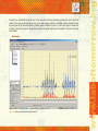
2.6 Using the LOT User Interface
Creating a new Experiment
The user can create a new experiment, by clicking the "New" button in the toolbar, or selecting
File->New->New Session File,
or by selecting the "Start New Experiment" option in the Quick Launch Form. The following form appears:
Experiment Settings Summary
Status Bar
53
Clicking on the settings, button will show the Experiment Settings form where all experiment settings are configured.
When done, the Play button, will start sampling data from the base station. At the time the sampling is over, all chart
and data manipulation functions are enabled, and the experiment can be saved as a file, for later viewing.
Attention:
Please notice that every time you start new experiment you have always to configure the
experiment settings again.
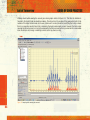
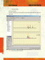
Opening An Experiment
This is very simply done, by just selecting the file
you wish to open. The Open Experiment dialog,
can be enabled by clicking the Open button in the
toolbar or by selecting
File->Open
Selecting a file, will result in the file being opened. In the next Screenshot you can see an experiment opened as a file,
and a short description for every visible section of the form.
54
Chart Area
Shows or hides the clicked
sensor data.This Tick icon
represents a visible sensor,
while the X icon represents a
non visible one.
Timeline Slider
55
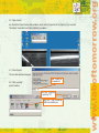
Saving an Experiment
By selecting File->Save or by clicking the Save button in the toolbar, the current experiment is saved under the name
you choose. If the current editing file, was saved before, then all changes are save under the same name. If you select
File->Save As, then the current file is saved under a new name, even if it was saved before.
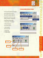
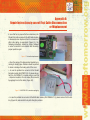
Importing LPS Data
Choose
File->Import LPS.
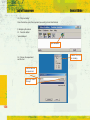
The following form appears:
This form, contains
of two discrete sections. The "LPS"
section, and the
"Sensors" section.
In order to import
or merge LPS Data,
you must click on
the Browse button
of the LPS Section.
A valid *.mdb (Microsoft Database)
file,
containing
LPS data must be
selected. If the file
contains LPS information, then the
Import LPS button
is enabled, and
at the Summary
56
frame of the LPS section, you can see a brief description of the LPS file data. For an example file the form will look like
this:
Finally, click on the Import LPS button, choose the name for the new Lab of Tomorrow file that will contain the LPS data,
and a message will inform you about the success of the function.
If you wish to merge LPS data with an existing Lab of Tomorrow file, then you must select that file, by clicking the
Browse button of the Sensors section. By doing so, the Open File dialog appears, and upon completion, the Summary
of the file's parameters and settings appears at the Summary frame of the Sensors section.
57
If the Lab Of Tomorrow File, contains
synchronization data
, then the Merge File
button , is enabled.
If clicked, then the
two files are merged
into a new one. The
application takes no
action to prevent
merging of files that
are time unrelated.
You must, choose
the correct files (the
Date And Time reports are very helpful for this manner).
Selecting unrelated
files, can have unexpected results when
viewing the file at a
later time.
For the above reasons it is suggested, that experiments containing sensor and LPS data, should be conducted in the
following manner:
First, the LoT software
starts sampling data from
the sensors. A few seconds
later, the LPS can start sampling data, but the process
must be stopped BEFORE the LoT software has stopped sampling.
58
2.7 Using the Video Grabber Software
The video grabber programme is the software
used for gathering the LPS camera
frames and for creating the database of
measurements. In order to use the video
grabber successfully it is suggested that
you will follow the following steps:
1. Start the software "Video Grabber"
2. Choose the video scale
(recommended: half size)
3. Initialize database
(erase previous data)
4. Creating videos
4.1. Button overview
open camera
close camera
start recording
stop recording
59
4.2. "Open camera"
Use this button to open the two
video windows and to control
the position of the object(s) to be
recorded.
The buttons "close video" and
"start recording" are enabled.
"Close Camera"
The two video windows disappear
4.3. "Start recording"
press the button
enter a name for
the experiment
then start recording
by pressing “OK”
only the “stop recording”
button is enabled now
4.4. "Stop recording"
Press the button, when the movement you want to record has finished
60
5. Analysing the videos
5.1. Press the button
"open database"
open database
5.2. Choose the experiment and the tool
choose the tool
for marking
enter the name of
the experiment
press the button
“Change”
The video frames will occur.
61
5.3 Mark the object in each video frame
1. Choose the frame
you need
2. Mark the object
3. ...in both frames
4. Press “Calculate”
Repeat steps 1 - 4 until the whole movement has been analysed, then press "Close"
62
6. Transferring the data
6.1. An MS-Access™ - file ("grab.mdb") has been created automatically, where the x-, y- and zcomponent of the positions and the assigned time ("tick") is stored:
6.2. There it can be merged into the LOT-software.
63
64
Chapter 3
Good practice with “Lab of Tomorrow”
65
3.1 Using the Lab of Tomorrow tools in real classroom conditions
Lab of Tomorrow aims at upgrading science teaching in secondary education. This is achieved with the introduction and utilization of advanced technologies in the teaching and learning process. This gives the opportunity
to redesign the school science laboratory expanding its experimental capabilities. The connection of science
teaching with real life is essential while special effort should be put on motivating students to be engaged with
science and exploratory learning in general. Lab of Tomorrow with the introduction of technological novelties
in the classroom is believed to achieve the above goals by bringing a new era in the school science and experimentation teaching. This unit is giving essential information that concern the introduction of the Lab of Tomorrow
tools in Science teaching and learning, the suggested initial experimental activities, useful information and hints
on how you can successfully investigate specific aspects of Kinetics and Mechanics
66
3.2 Table of Contents and Lab of Tomorrow lesson plans
The Lab of Tomorrow “Table of Contents” presented below is a list of suggestions that takes into account the
structure of the pedagogical framework as well as the advantages of the technical devices. Not all the topics of this list can be taught in school, but all taught topics should be located in this list. Within the following
paragraphs several lesson plans guided by the teaching and learning principles that were introduced above,
are presented. These lesson plans are designed to meet the needs of the implementation of the project in the
school environment. The lesson plans are based on simple experimental activities with the use of the Lab of
Tomorrow products so as for the new artefacts to be smoothly introduced in the science classroom. The lesson
plans are designed to be complementary to the conventional physics lessons. Specifically the parts of the table
of content that correspond to the project’s lesson plans are highlighted. The aim is at the future to improve the
functionalities of the axion prototypes develop more extended and sophisticated case studies and thus increase
the applications of the Lab of Tomorrow system’s components.
Table of Contents
Part I: Uniform Rectilinear Motion and Mechanical Energy
1) Units and quantities, space and time and trajectories
a) Repetition of fundamental units and quantities
g) Those simple examinations should be particularly used
to make the students acquainted with the User Interface
2) Uniform rectilinear motion
a) Further examination the prior experiment’s horizontal
component (the result should be:
b) Horizontal velocity is nearly constant)
b) Experiment: throwing of a ball (tennis ball), measure
position with LPS
c) Examination of similar but simpler, one-dimensional
movements with LPS: rolling balls, pushed boxes or toy
cars and also experiments with an air cushion rail
c) Examination of data in multiple ways, e.g. different
graphs of displacement (x, y, z) as a function
d) One result has to be that for a motion with constant
velocity the following laws are valid:
d) of time, (x, y) as a function of time, x as a function of
time, projection of motion into one plane
s=v*t, <v>=v(t), dv/dt=0
e) Derivation of velocity as the ratio of the displacement to
the time interval, average
f) Velocity and instantaneous velocity
e) Minimizing friction leads to the assumption that without
friction or other forces, every motion should “go on forever as a uniform rectilinear motion”; this leads directly
to…
67
3) Newton’s first law (also called “The Law of Inertia”):
“A free particle always moves with constant velocity.”
8) Collisions II: inelastic collisions in one dimension
4) Introduction of kinetic energy and momentum as
additional, constant quantities for describing uniform
rectilinear motion, based on the prior experiments; noticing, that the importance of these quantities will only
become clear in the further course of the experiments
c) Limitations (e.g. difficulty of changing masses and
necessity of an exactly central collision) also with axion
balls
5) Interlude: springs (specific terms, force F=k*s,
work and energy E=1/2*k*s2 ) and potential energy
(E=m*g*h)
6) Interaction of bodies in motion and springs
a) Experiments with LPS: e.g. moving body on an air
cushion rail, stopped when upsetting a spring an set into
motion again
b) First hint that energy may be conserved
b) these kinds of collisions can also be realized best with
an air cushion rail, but with
d) Result: momentum is conserved, but energy is not
9) Collisions III: collisions in two dimensions
a) LPS and axion balls can be used for this more realistic
kind of collisions
b) Validity of conservation of momentum is shown in a
more complex context
Part II: Rectilinear Motion and Heat
1) Examination of a free falling axion ball as a prototype
of a knew kind of motion
a) Examination of graphs of velocity and displacement
7) Collisions I: elastic collisions in one dimension
a) Elastic collisions can only be realized using an air
cushion rail
68
b) Introduction of the following laws: s=1/2*a*t2 ,
v=ds/dt=a*t
c) a=dv/dt as the new physical quantity acceleration
b) Experiments with colliding vehicles of different masses
and velocities (LPS)
d) Description of the motion as “uniformly accelerated”
(a=constant)
c) Result: energy and momentum are conserved
e) Introduction of the acceleration sensor
d) Reversal: conservation of momentum and energy are
sufficient for predicting velocities
f) Comparison of data collected directly by the acceleration sensor and data derived from the
e) After collision, when initial velocities and masses are
known
LPS
g) Momentum and energy are not constant
2) Re-definition of force as the changing of momentum
5) Accelerated every-day motions
a) F=dp/dt
a) Question: can they be described as uniformly accelerated?
b) As the mass m should be constant, this means
F=m*a
c) Newton’s second law: “The time rate of change of
momentum of a particle is equal to the force acting on
a particle.”
d) Considering that momentum is a conserved quantity,
you can hence Newton’s third law from his second law:
“When two particles interact, the force on one particle is
equal and opposite to the force on the other.”
e) Other important forces, e.g. gravitational force
(F=m*g with the above experiment, additionally
F(gravitation)=(G*m1*m2)/r2
3) Closer examination of energy in uniformly accelerated, rectilinear motion
a) The accelerating force F has the same direction as the
motion, hence work is done
b) Comparison of E(t=0), E(t=T) and W=F*s=m*a*s
with data from axion balls
c) Conclusion: the work done on a particle is equal to the
change of its kinetic energy; power as work done per unit
time
b) Examples of accelerated every-day motions: walking,
running, riding on a bike, a car, a motorbike, inline-blades,
hitting balls etc. (using LPS, accelerometers and sensorvest)
c) first intake to accelerated motions without constant
acceleration
6) motions with negative acceleration
a) Vertical throws of an axion ball
b) car decelerated by a spring (repetition)
7) Complex systems of particles in motion:
a) Structure of matter
b) Kinetic energy of a system of particles
c) Conservation of energy of a system of particles
d) Collisions in a system of particles
e) Velocity distribution in a system of particles
f) Temperature as a quantity related to the average kinetic
energy of the particles
g) First law of thermodynamics
4) Other motions of the same kind: car accelerated by a
spring (repetition), body gliding on inclined planes etc.,
using LPS and accelerometer
h) “New” interpretation of pressure and expansion of
gasses
i) Repetition of basic laws of thermodynamics (heat capacity etc.)
69
8) “Realistic” uniform rectilinear motion
a) Why is Newton’s first law only an idealization; in other
words: why do bodies, once set into motion, usually slow
down
b) Interpretation of the loss of momentum as an indicator
of a force opposing the motion
c) Identification of these forces as frictional forces (sliding
friction, static and kinetic
d) Coefficients of friction, fiction in fluids and gases)
Part III: Superposition of Motion and Conversion of Energy
1) Introduction of the law of conservation of energy as
an alternative to momentum and forces in describing/
predicting motions, combined with a repetition of the
basic motions already known
a) Uniform rectilinear motion
b) Free fall
c) Sliding bodies on inclined planes
e) Measurement of coefficients of friction with moving
bodies and inclined planes using LPS and accelerometer
d) Vertical throw
f) Work and frictional forces
e) Acceleration of vehicles
g) Atomistic interpretation of friction: where do momentum and energy go?
h) Law of conservation of energy: “the sum of the kinetic
energy and the internal potential
i) Energy (or the proper energy) of an isolated system of
particles remains “constant”
2) Examination of more complex motions as superposition of known motions with LPS and accelerometer; the
user-interface will help to split the complex motions
into the underlying s i m p l e components, which are
stated in brackets
b) Bouncing balls with no horizontal motion (free fall, collision, vertical throw)
9) Friction and accelerated/decelerated every-day motions
c) Horizontal throw (free fall and uniform horizontal motion)
a) Friction as a limitation of acceleration and deceleration
d) Bouncing ball with a horizontal motion (uniform
horizontal motion and bouncing balls with no horizontal
motion)
b) Examples of decelerated every-day motions: breaking
with different vehicles using LPS, accelerometers and
sensor-vest (bikes, cars, motor-bikes, toy cars) with special emphasis on questions of traffic safety
e) Projectile motion without air resistance (vertical throw
and uniform horizontal movement)
f) Projectile motion with air resistance, using for example
different kind of balls and
g) shuttlecocks (vertical throw and accelerated horizontal
movement)
70
h) Projectile motion with starting point and target on different latitude, including sport
4) every-day circular motions, examined with LPS and
accelerometers
i) Examples: long jump, putting the shot
a) (Toy) cars in curves
j) Motion of a system of particles (motion of centre of
mass and relative motion of a single particle)
b) Banking of curves
c) (motor-) bikes in curves
k) Particles
5) Motion of rolling objects
3) Uniform circular motions
a) Example: spinning around an axion ball on a string of
variable length
b) Measurements with LPS and accelerometers: angular
velocity, period, frequency, angular acceleration, centripetal force
c) Angular momentum and rotational energy as a conserved quantities
d) Centripetal and “centrifugal” forces (measuring within
an accelerated reference system, using the axion ball)
a) Examination of different cylinders rolling down inclined
planes with LPS (possibly using coloured spots)
b) Velocity and angular velocity
c) Potential, kinetic and rotational energy
d) Momentum of inertia
6) Oscillatory motion
a) Small axion ball on a spring as a prototype of a simple
harmonic oscillator, also using LPS
b) Kinematics of, force and energy in and basics equations of simple harmonic motion
c) Small axion ball on a string as a nearly harmonic oscillator (also using LPS), kinematics, force, energy and
basics equations
71
3.3 First lessons and basic experiments
Getting started with Lab of Tomorrow experiments
Lab of Tomorrow can be used by any user who wants to explore Science and Physics in a more
exploratory manner i.e. connected closer to real life conditions. However, initially, Lab of Tomorrow has been
designed to address the learning needs of students in secondary education. Thus, the analysis and the presentation of Lab of Tomorrow experiments in this chapter has been designed to meet the needs of students 15-16
years old. However, this doesn’t mean that the content of this chapter is not useful for other categories of potential Lab of Tomorrow users. This paragraph indicates a minimum of competencies that are required for the user
to possess so as to be able to use the LOT tools with success. The minimum competencies are in line with what
15-16 year old students have in science. Of course any one who has knowledge above this minimum, can very
easily make and analyse experiments with Lab of Tomorrow.
In general, Students have different background in Physics and Science subjects respective to their age and the
curriculum of the country they come from. National educational systems and curricula differ significantly from
country to country and so students don’t have the same knowledge in mathematics or physics. However some
general conclusions on what is in general considered acquired knowledge or not can be derived.
In general it is considered that students:
• don’t know how to derive functions
• don’t know how to work with an EXCEL spreadsheet
• only have basic skills in interpreting diagrams
And they are considered to:
• know how to draw diagrams when they have a table of measurements
• recognize a proportional relation between two physical quantities
• know how to make simple measurements (time with a stopwatch, length with a ruler, temperature with a
thermometer, voltage and current with a multimeter)
So the question is:
“What should students know or need to know to before they carry out experiments with the Lab-of-Tomorrow
equipment?”
72
The answer is that students should:
• have a detailed idea about how acceleration is defined and
• how position and velocity can be measured
• be able to draw correct s-t- and a v-t, a-t diagrams despite of the inaccuracy of measurement
• know the difference between average velocity and instantaneous velocity,
• be able to interpret an s-t-diagram and from this graph derive the
• average velocity as the slope of the linear graph and the
• instantaneous velocity as the slope of the tangent of the non-linear graph
• know that also the area under the graph has a special physical meaning
(esp. area under v-t-diagram _ distance)
Teachers should have a general impression of which of the above topics their students know and feel comfortable to handle in physics and science lessons. These topics are listed in national curricula and considered basic
knowledge and thus they are taught extensively in schools. However if the teacher realise that students need to
have some additional exercise and support lessons the following sequence of lessons is suggested as an introduction into basic physical methods and knowledge and familiarisation with the Lab of Tomorrow tools.
73
3.4 Sequence of preparatory lessons
In general, a sequence of preparatory lessons and experiments are proposed in order for the students or the LoT users in general, to be familiarized with the way of “thinking” and “acting” within the framework
of Lab of Tomorrow.
In case of a teacher who is about to implement Lab of Tomorrow in classroom, apart from the preparatory experiments the introduction of the Lab of Tomorrow may additionally include:
• Worksheets in “Mechanics: Introduction into Kinematics”
• Worksheets on “Interpretation of diagrams” (1 - 2 lessons / homework)
• Worksheets on “Getting practice in measuring” (2 - 4 lessons)
Choose worksheets depending on the time available and the general competence in science of the classroom.
Teams of students carry out several simple experiments and work out the results. Thus they learn about several
methods of measuring, about discussing and presenting the results and about different types of movement.
Experiments with the “Lab of Tomorrow” equipment
As it was mentioned above the aim of these experiments is to get the students accustomed with
handling the equipment and the software and with interpreting the graphs delivered by the software.
Carry out some of these tests with changing sample rates 10 - 100 Hz
Initial Experiments with the Ball
Let the ball lying on the Table
Orientate the ball in such a way, that the x- and y-axis deliver the value “0” and the z-axis delivers “1”.
Explain the reason!
How do accelerometers work?
74
Attention
The ball has embedded three one dimensional accelerometers combined in a way that
the result is a three dimensional accelerometer. The important parameter in the meas
urements is that although we are referring to the sensors as accelerometers the actual
measurement is the force exerted on each sensor in the respective axis in a
certain time. Taking into account that the inertial mass of the sensor is constant then
through the Newton’s second law F=m*a you can have one to one correlation of
force exerted on the sensor F and the a acceleration experienced by the sensor.
To avoid introducing any notional confusion to students it is suggested here to explain
to them that what is measured by the accelerometers of the Lab of Tomorrow system
is the “the reaction force that the sensor feels at each moment”. Do not forget that the
same applies to the accelerometer sensors of the Sensvest accelerometer.
Figure 3.1 The ball
is standing still on
a surface
75
Conducting the experiment as it is prescribed above it will lead to results presented on the User Interface that
are similar to the screenshot above.
The z axis will give back the value 1. This is because the only axis that feels any force is the z axis. This has to
do with orientation of the accelerometers’ axis of the ball shown on Diagram 1 and can be explained with the
following simple argument. When the ball is standing still on the surface it acts force equal to its weight B=m*g
to the surface and the surface reacts back with an equal and opposite force N=m*g according to the third
Newton’s law. The sensor measures what it feels and it feels only reaction forces so the feedback value is the
value of N. Please notice that the reaction forces in the LoT User Interface are given in units of g (see the y axis
of the screenshot). In this case what it is given back by the sensor is the force N which is equal with the weight
of the ball, but in units of g and thus is 1 g. On the other hand the x and y axis accelerometers give back a zero
value since they are orientated in the horizontal plane where no reaction forces are applied (no forces in general
are applied in this case).
Diagram 1 Orientation of the accelerometers’ axis of the ball
76
Figure 3.2 Ball standing still on a table with the positive z axis reversed.
I f the orientation of the z axis of the ball accelerometer is reversed (Diagram 2) then the resulting graph is similar
to Figure 3.2. You can note that this time the value of the z accelerometer is -1 while still the x and y are giving
back zero.
Important
Notice that on the graph is also presented the module of the reaction force that is being sensed i.e the net value
of all the reaction force coordinates x,y,z (the square root of the sum of the squares of the three coordinates).
77
The module, as it is a value of a square root, is always a positive number it is very useful for the presentation
of data since can be understood more easily by the students. This is because the module is not a vector, is just
the net value of the total force.
If we would like to study the x,y,z coordinates of the force sensed by the ball when hitting the surface we can
always select the respective components from the option area of the User Interface at the left part of the screen.
As you can see each sensor x,y or z experiences something different depending its orientation and can record
negative values as well. However the module is the sum of these components and is always a positive number.
Diagram 2 Orientation with the z accelerometer axis reversed
Hit the table with your fist.
Figure 3.3 Hitting the table, module of the total force sensed by
the ball
78
Hitting the table on which the ball is kept still will produce a graph similar to what is shown in Figure 3.3. The
ball when the hand hits the table it almost looses contact (the force N is almost 0) with the surface of the table
and thus for an instant the sensor gives us a value near zero as it is indicated with the arrow on the left. The next
moment it hits on the surface again so the sensors feel the reaction force of this hit which refers to the peak indicated by the arrow on the right. Finally after a few instants the ball (the sensor actually) regains stability on the
surface and the net value that it is given back by the system is 1 (the value of the force N). It has to be mentioned
here that what it is presented on the graph is the result of the vibration that is “diffused” to the sensor indirectly
via the surface of the table. What the sensor “feels” depend on the way we hit the surface, the material of the
surface and its characteristics and the way that this vibration moves to the sensors. It is usual that you will not
always take the same results in this experiment since there is not any force applied on the ball in a direct way.
Rolling the ball on the table
If possible, it should be orientated in such a way, that the z-acceleration is “0”.
Describe the graphs (x-, y-,).
Count the number of rotations.
Figure 3.4 Rolling the ball
79
Conducting this experiment it will result to graphs like the one of Figure 3.4. The ball before starting rolling was
roughly orientated in a way the the z axis accelerometer was horizontal and always giving back the value 0 (no
reaction force is applied on the horizontal plane) while the x, y were orientated in vertical plane in a way that the
initial values was approximately 1 for x accelerometer and approximately 0 for y axis.
As the ball starts to roll then progressively the value of x alters from 1 and becomes 0 and then -1 and so on.
Something similar applies for y accelerometer, it’s value changes from 0 to 1 and then 0 and -1 and so on. Each
time that the accelerometers show their initial values, it means that the ball has completed one cycle while rolling and this is one simple way to count the number of rolls. Notice that the way the acceleration values of the
sensors x, y, z are changing depend among others on the initial orientation of the ball.
Holding the ball
Move the ball upwards and downwards several times with alternating speed.
Explain the different heights of the peaks.
What does “module”
mean?
Figure 3.5 Holding and moving the ball with the hand
80
When someone is holding the ball the sensors record the reaction force exerted from our hand to the ball. This
means that if we are not moving our hand at all, the reaction force N that we exert with our hand to the ball is
equal to the weight of the ball. However almost always there is a light or less light trembling of our hand which
can been also noticed at the left hand side of the Figure 3.5. Moreover when we move our hands, holding the
ball, up or down, a force exerted on the ball is imposed by our moving hand and peaks like those that are presented on the right hand side of Figure 3.5 are observed. Note that the graph presents the values of the module
of the force exerted on the ball in respect of time. Thus the peaks are always in the positive value part of the
graph and each one of them can refer either to an upward or downward movement depending on the specific
conditions of the experiment.
Throw the ball vertically upwards several times and catch it in an alternating manner
How long does the free flight last?
Explain the different heights of the peaks when catching the ball.
6
1
3
5
4
2
(A) (B)
(C)
Figure 3.6 The ball is
thrown up
81
When the ball is thrown up and is moving on the air it looses contact with other objects and thus no reaction
forces are applied to it. The net force shown on the graph by the sensors is zero. Initially however, our hand threw
the ball upwards by exerting instantly a force to the ball. This reaction force is observed and refers to peaks numbered 1, 3, 5. This is the case since in the experiment presented in Figure 3.6 the ball has been thrown upwards
three times in the row. The peaks 2, 4 and 6 refer to the three times that the ball was caught again by the hands
while the letters A, B and C refer to the time slots when the ball was on the air.
Using the Sensvest
As it is mentioned elsewhere the sensvest consists of three two dimensional accelerometers, on heart pulse
meter and one body temperature sensor. There is a large variety of experiments that include LoT user’s participation in activities that can be studied with the new tools. The following paragraphs aiming at providing some
hints on what can be studied and analysed with the sensvest or what can by studied with the combined use of
the sensvest, the ball and the LPS.
Sit down and stand up.
Put on the sensvest components; wear the belt and
the arm and leg sensors.
After setting up the system and before started
taking measurements sit
on a chair.
Figure 3.7 Sitting and standing
while wearing the sensvest
82
Proceed to an experiment where the user of the sensvest is sitting and standing several times in the row. If the
motion of the leg is neglected and one focus to the body module and the arm module of the acceleration values
that are given by the sensvest, then the resulting graph is similar to Figure 3.7. Each time that you stand up or
sit down a peak is produced in the positive section of the graph referring to the modules of the arm and body
acceleration.
Walk around.
Figure 3.8 Walking around while wearing the sensvest
83
Walking around while wearing the senvest gives back graphs similar to Figure 3.8. This time the attention is
focused to the leg and body acceleration modules. The interest is in the number of the peaks which refer to the
number of the steps that are made by the user. Moreover it can be noticed that each time that a step is made
there is a respective reaction force that is sensed by the body accelerometer sensor. However the force values
recorded by the last sensor is not as high compared to the forces sensed by the leg sensor which is reasonable
since the body is not moving or vibrating so much as the leg does in a step.
Jump.
Figure 3.9 Jumping while wearing the sensvest
84
When jumping while wearing the sensvest the resulting graph is similar to Figure 3.8 qualitatively but the values
of the peaks are higher. This is something that is expected since the forces when we hit the ground are stronger
than when we walk. In Figure 3.9 we can discriminate three pairs of peaks. The first peak of each pair refers to
the force exerted on the leg and the body when jumping upwards while the second refers to the forces when
hitting the ground.
85
3.5 School practice with Lab of Tomorrow
Apart from the above initial experiments there is a variety of other experiments that can be conducted with the LoT tools. There is a series of experiments that are in accordance with national school curricula
and can be used for the verification of the basic laws of Mechanics. In this paragraph several examples of this
kind are presented and guidelines are given on how can be smoothly introduced in everyday classroom practice.
Free Fall
The following is a lesson plan providing information and material concerning the experimental
study of free fall motion with the use of the axion ball.
Specific experimental activities are presented and several questions, exercises and tasks are
proposed to assist consolidation of the acquired knowledge.
Figure 3.10a Free Fall
Duration:
i) Classroom lesson 1x45min
ii) Experimental Activities 25min
Vocabulary
free fall, linear motion, acceleration of gravity, air resistance
Tools and Materials
Axion Ball, LPS
86
Aims and Objectives
The students:
• to be able to describe acceleration as the rate of velocity.
• to report free fall as a special case of rectilinear motion with constant acceleration.
• to find out that the acceleration of gravity is the same independently of the object’s mass.
• to distinguish accelerating motion - decelerating motion ( in case of upwards vertical throw)
• to be able to describe verbally, mathematically and graphically the laws of the basic physical quantities for the
free fall motion.
Student’s usual Misconceptions
• Heavier objects reach the earth earlier than lighter ones
• Bigger objects reach the earth earlier than smaller ones
Implementation
a. Stimulation
Duration ~20min
• Presentation of selected pictures or videos of different objects falling
• Short discussion on the presented material
• Track student’s misconceptions as far as objects’ motion is concerned
• Draw up a list on the blackboard with these misconceptions without any
comments.
Figure 3.10b Free Fall with the Axion Ball
87
b. Experimental Activities
I) Ball is left to fall free by student’s hand.
The axion ball is left to fall free from student’s hands. Data are recorded by the base station and are presented
to the students with the User Interface. The LPS system can be used additionally or in parallel to record frames
that represent the motion of the ball, so as to have a two fold verification of the theoretical data.
II) Alternative-Additional Experiments
As alternative experiment the following can be proposed:
• The upwards vertical throwing of the ball to study decelerating motion as well
Figure 3.11 LPS data of a Vertical Throw experiment
The vertical throw experiment will have similar results and diagrams with the free fall experiment if one conduct it
with the axion ball. It is very interesting though to analyse this motion with the use of LPS by studying diagrams
like the one presented in Figure 3.11
88
c. Observation - Discussion
• Theory and experiment comparison
• Comparison with the ideal theoretical case of each motion case
• Examples deriving from daily activities to start a discussion on the misconceptions
d. Conclusion Drawing
• Free fall time is the same for every object regardless of mass variations
• Physical Quantities, mathematical laws, graphical representations
• Experimental calculation of the acceleration of gravity using the initial height of fall or the time of flight of the
ball
e. Consolidation
Questions, exercises and tasks aiming
at consolidation of the
acquired knowledge.
In Figure 3.12 which is a typical diagram of a free fall of the axion ball, the
area A refers to the time of flight of
the ball while the peak 1 refers to the
force that is exerted on the ball when it
hits the ground. The time of flight can
provide the height of the fall experimentally. If the height of the fall is known
then the acceleration of gravity can be
experimentally calculated by the time
of flight.
1
(A)
The rest of the peaks and time of flight
period that are shown in the same figure represent the consequent bouncing
of the ball.
Figure 3.12 The axion ball data during Free Fall
89
Horizontal Throw
This lesson plan provides information and material concerning the experimental study of horizontal
throw motion using the LPS. Specific experimental activities are presented and several questions, exercises and
tasks are proposed to assist consolidation of acquired knowledge.
Duration:
i) Classroom lesson 2x45min
ii) Experimental Activities 25min
Vocabulary
horizontal throw
Tools and Materials
Axion Ball, LPS, plane surface exalted
Aims and Objectives
The students should:
• be able to distinguish that the motion as a whole can be analyzed in other independent, separate motions
• be able to distinguish the two simple motions (free fall, rectilinear with constant velocity) that constitute horizontal throw.
• be able to describe verbally, mathematically and graphically the laws of the basic physical quantities of the
horizontal throw
Student’s usual Misconceptions
• there are difficulties for the students to comprehend that horizontal throw is a complex motion
• In horizontal throw, the applied force e.g. by a hand , continues to act on the object (e.g. on the ball) even if
the object is no longer in touch with the hand
Implementation
a. Stimulation
Duration ~20min
• Presentation of selected video of the motion
90
• Short discussion on the presented material
• Track student’s misconceptions as far as objects’ motion is concerned
• Draw up a list on the blackboard with these misconceptions without any comments.
b. Experimental Activities
Figure 3.13 Horizontal Throw
I) Horizontal Throw.
A ball is thrown horizontally from an exalted surface. Data
are recorded with the LPS
and the exact trajectory of the ball
is constructed afterwards by the User Interface.
The mathematical analysis is done by exporting
the data to an excel sheet
II) Alternative-Additional Experiments
As alternative experiment the following can be proposed:
• to repeat the activity with different initial velocities
91
Figure 3.14 Horizontal Throw, camera frames of the LPS
A characteristic dataset that can be obtained by the LPS during the Horizontal Throw experiment is shown in
Figure 3.15. The data presented have been already exported to an excel spreadsheet and have been normalised
to the initial conditions(x0, y0, z0) of the experiment.
Figure 3.15 Horizontal Throw data set
The analysis with the mathematic tools of the excel can result the following diagrams
92
Figure 3.16 Displacement in
x axis over time
Figure 3.17 Displacement
in z axis over time
The analysis of these diagrams can reveal plenty of information and can provide an alternative way of calculating
the value of g experimentally.
93
c. Observation - Discussion
Discussion of theoretical issues arising from the experimental activities.
• Theory and experiment comparison
• Comparison with the ideal theoretical case of each motion case
• Examples deriving from daily activities to start a discussion on the misconceptions
d. Conclusion Drawing
• Motion can be analysed in other separate independent motions
• the falling time of the objects in horizontal throw it is dependent only on the height and it is independent on
object’s mass and initial velocity
• Physical Quantities, mathematical laws, graphical representations
e. Consolidation
Questions, exercises and tasks aiming at consolidation of the acquired knowledge
Volleyball game
Side Throw
As an example of a more complex situation for the use of the axions, the following volleyball lesson is given
below. This Lesson plan is a proposal for a sequence of lessons in which students can apply their physical
knowledge.
It is considered that they already know
• physical quantities
• laws of uniform rectilinear motion
• laws of accelerated rectilinear motion
• superposition of motions
• evaluation of graphs and measurements
• the students know how the axions work
94
Duration
i) Conventional Lesson
2x 45 min to evaluate and to discuss the data, verify laws, find new relations between physical subjects
ii) Experimental Activities
45 min in the sports hall
Vocabulary
curvilinear motion
superposition of motions
trajectory
Tools and Materials
• Accelerometer at the player‘s wrist (part of the sensvest)
• Accelerometer in the ball
• Camera system (LPS ) for Video analysis of the ball‘s motion
Aims and Objectives
• shift physics-lessons out of the classroom into everyday-learning environment
• integrate Lab of Tomorrow Equipment
• verify Newton’s laws of motion
• let students apply their physical knowledge
• enable introduction of new principles
• allow students to develop their own experimental ideas
Student’s usual Misconceptions
As these lessons takes place, when Newton’s laws have already been derived, there should be no misconceptions concerning the laws of motion. But:
• it might be that the students have wrong ideas about the influence of air resistance
95
• students will think that the higher developed our equipment is the better should all experimental data from different tools fit together.
Implementation
a) Stimulation
For example: Movie of a volleyball match
Task: Examine, whether the physical laws of motion are useful to describe the motion of an ordinary object like
a volleyball.
Students can split up that task into several detailed questions, e.g.:
• Measure the initial velocity
• the initial angle of the volleyball by video analysis or by analysing data from the accelerometer.
• Measure the horizontal range of the ball’s flight
... in terms of the initial angle and
... in terms of the initial velocity.
• Compare those data with theoretically derived values and in that way confirm the laws of motion.
• Regard the x- and the y- component of the velocity,
… verify that the y-velocity derives from accelerated motion like a vertical throw
… and the x- velocity derives from uniform motion
• Describe the difference between theoretically and experimentally acquired data,
... estimate the influence of the air resistance.
• Calculate forces and momenta
• If possible, examine other influences, e.g. spinning of the ball.
b) Experimental Activities
students perform single volleyball
tosses like
• underhand serve
96
• overhand serve
• forearm pass
• overhand pass
wearing the sensor vest.
Other students film those activities with
a video camera.
Figure 3.18 Volleyball analysis with LoT tools
c) Observation – Discussion
Figure 3.19 Teaching strategy
97
d) Conclusion Drawing
The motion of a volleyball is nearly a parabola, so it can be described with Newton’s laws of motion; especially
• the horizontal range
• the maximum height
• the time of flight can be pre-calculated using the equations of the curvilinear motion, provided that the initial
velocity and initial angle are known.
The initial velocity
• can be taken from video analysis
• or by integrating the acceleration (ball and/or body accelerometer)
The results of the three measurements vary a lot. The superposition of motions can be confirmed when x- and
y components are regarded separately.
Evaluating the decrease of the horizontal component of velocity the influence of air resistance can be estimated.
It is rather small for a volley ball.
e) Consolidation
Questions
- how can the experiments be improved?
- is there an influence of other aspects, e.g. the spinning of a ball
Exercises
Integration with other subjects
• flight of other objects as cannon balls (see lesson plan “horizontal throw”)
• theory of air resistance
• why does the trajectory of a long-range projectile like an intercontinental ballistic missile differ from a parabola
(it is more an elliptical path)?
98
Physics in Sports
A qualitative approach with the use of sensvest
This lesson plan provides information and material concerning the experimental study of simple sport activities
utilizing the sensvest axion developed in the lab of tomorrow framework. The main aim is to reveal the basic underlying physical and biologic concepts that govern such activities. Specific experimental activities are presented
and several questions, exercises and tasks are proposed to assist consolidation of the acquired knowledge.
Duration:
i) Classroom lesson 2x45min
ii) Experimental Activities 25min
Vocabulary
Heart rate, pulse rate, step rate, temperature, acceleration, velocity
Tools and Materials
Axion Sensvest
Aims and Objectives
General Aims
The students should:
• be able to estimate the quality of physical measurements
• be able to make qualitative statements about the precision of a measurement
• to find out the qualitative relationship between physical laws and biology laws
Specific Aims
The students should:
• be able to find out experimentally that the velocity and acceleration of a person who is either moving at a constant speed or is accelerating and then is making a 180o turn, are zero at the exact moment of the turn.
• be able to find out experimentally that pulse rate increases with exercise
• be able to find out experimentally that body temperature varies slightly with exercise
• be able to recognize specific body activities (like a jump or a ball kick) in the peaks of an a-t diagram
99
Student’s usual Misconceptions
• Everything can be determined “exactly” by physical methods
• The acceleration and velocity of a constantly moving body during a 180o turn is not -at any moment of the
motion- zero.
• There is significant variation in body temperature during body activity
• There is energy consumption only in intense physical activities
Implementation
a. Stimulation
Duration ~20min
• Presentation of selected video of an athlete on a lab during ergometric tests.
• Short discussion about physics in sports and human physiological parameters in various sport activities,
discussion on what could be measured during these tests and why.
• Track student’s misconceptions arising from the previous discussion
• Draw up a list on the blackboard with these misconceptions without any comments.
b. Experimental Activities
I) Walk to one direction, turn around
and walk backwards
A student wearing the sensvest walks
in one direction
with approximately constant velocity,
after some
meters walk, turns around to continue his walk back to
his starting point. Data from the
sensvest (body acceleration,
pulse rate, tempreture) are recorded.
Figure 3.20 Walking forward and backwards
100
II) Accelerate in one direction, turn around and accelerate backwards
A student wearing the sensvest accelerates in one direction and after a several meters run, turns around to
continue running back to his starting point. Data from the sensvest (body acceleration, pulse rate, temperature)
are recorded.
III) Jumping repeatedly with different rates
A student wearing the sensvest starts jumping repeatedly on the same spot for a several seconds.
The physiological parameters of the student (pulse rate, temperature, body acceleration) as well as the jumping
rate are recorded. The experiments is repeated with different duration and jumping rate.
IV) Combined movements
A student wearing the sensvest is making more complex moves while wearing the sensvest. Figure 3.21
presents a typical diagram of its kind when the student sits and stands up, walks, runs and jumps.
Figure 3.21 Analysing combined movements with the
sensvest
V) Alternative-Additional Experiments
As alternative experiments the following can be proposed:
• Repeat the former experiments with male, female students and teachers to record possible differences
• Repeat the former experiments with different degrees of effort and speed
c. Observation - Discussion
Discussion of theoretical issues based on the experimental activities.
101
• Theory and experiment comparison
• Examples deriving from daily activities to start a discussion on the misconceptions
d. Conclusion Drawing
Students write down the conclusions from their experimental activities and the relevant discussions.
• Nothing can be determined “exactly” by physical methods
• There are significant variations in several physiological parameters during physical activities.
• There is energy consumption of human body during any physical activity.
e. Consolidation
Questions, exercises and tasks aiming at consolidation of the acquired knowledge (Refer to the relevant worksheet)
Kicking and catching the ball
A qualitative approach with the use of sensvest
This lesson plan provides information and material concerning the experimental study of simple sport activity
utilizing the sensvest and the ball axions. The main aim is to verify experimentally the validity of the third Newton’s Law. There are not many experiments in the conventional school laboratory that allow the study of the third
Newton’s Law and thus this experiment has special added value.
Duration:
i) Classroom lesson 1x45min
ii) Experimental Activities 25min
Vocabulary
Action-reaction
Tools and Materials
Axion Ball, sensvest
Aims and Objectives
The students:
102
• to be able to understand action and reaction law
• to be able to report that action and reaction do not result to a total zero
force value
• to find out that gravity is the only force that is applied on the ball when it is
on the air
Figure 3.22 Kicking and catching the ball
Student’s usual Misconceptions
• there are difficulties for the students to comprehend that kicking is a complex motion
• In kicking like horizontal throw, the applied force e.g. by the leg or the hand , continues to act on the object
(e.g. on the ball) even if the object is no longer in touch with the leg or the hand
Implementation
a. Stimulation
Duration ~20min
• Presentation of selected video of a football game or penalty kicks
• Short discussion on the presented material
• Track student’s misconceptions as far as objects’ motion is concerned
• Draw up a list on the blackboard with these misconceptions without any comments.
103
b. Experimental Activities
I) Kick and catch the ball
One student is wearing the leg accelerometer and kicks the ball towards another students who wears the arm
accelerometer.
1
2
2
1
Figure 3.23 Data of kicking and catching the ball experiment
104
Figure 3.23 is a very characteristic example of the verification of the 3rd Newton’s law and the qualitative analysis of a complex activity like kicking and catching a ball. The black line refers to the total reaction force that
is exerted on the ball while the blue and red lines are the reaction forces sensed by the leg and arm sensors
respectively. At instant 1 a peak is presented in the diagram both for the leg and the ball. The values of the peaks
are almost identical which represents the verification of the 3rd law. The peaks of the leg sensor before instant
1 represent the motion of the leg while the ball at the same time is still on the ground not moving.
The 3rd law is again verified at the instant 2 which represents the instant that the ball is being caught by the other
student’s hand. Again the two reaction force peaks of the ball and the arm have almost the same value.
The time interval between instants 1 and 2 represent the time of flight of the ball.
V) Alternative-Additional Experiments
As alternative experiments the following can be proposed:
• Repeat the former experiment with male, female students and instead of catching the ball kick it against the
wall.
c. Observation - Discussion
Discussion of theoretical issues based on the experimental activities.
• Theory and experiment comparison
• Examples deriving from daily activities to start a discussion on the misconceptions
d. Conclusion Drawing
Students write down the conclusions from their experimental activities and the relevant discussions.
• Nothing can be determined “exactly” by physical methods
• Action has its reaction
• The only universal force on earth is gravity
e. Consolidation
Questions, exercises and tasks aiming at consolidation of the acquired knowledge (Refer to the relevant worksheet)
105
106
Chapter 4
Evaluation of Lab of Tomorrow
107
4.1 Introduction
While modern technology occupies a major part in everyday life and is commonly available in
schools of today, the technology itself does not provide support of the development of scientific concepts: To
many students working in a science laboratory is limited to manipulating equipment instead of manipulating
ideas. This is because of two reasons: on the one hand modern technological equipment is seldom designed and
developed with pedagogical aspects in mind; on the other hand are pedagogical concepts seldom well-adjusted
to the special features and possibilities modern technology offers.
Therefore the basic idea of the Lab of Tomorrow project is to develop innovative pedagogical and technological
approaches and to integrate them into a specifically designed learning environment, in which the students shall
be enabled to use technical equipment to reach the level of interpretation of observed phenomena in a shorter
time and without needing mathematical competences which are beyond their capabilities.
108
4.2 Project’s Evaluation Scheme
The evaluation of the Lab of Tomorrow project is based on three aspects:
•
Evaluation of students’ learning. In assessing students’ learning, students’ engagement in
science as inquiry is going to be primarily examined. It is assumed that the activity of designing
projects and experiments provides a powerful way for students to be involved in scientific
inquiry
•
Evaluation of the pedagogical framework. The major theoretical issue underlying the project
asks whether the implementation of the technology is able to offer a qualitative upgrade of
science teaching at high school level. In such a case the introduction of technology would not
act as a substitute of the conventional teaching but rather as an addition that has to justify its
introduction in everyday school practice.
•
Ethnographic evaluation. The project will take advantage of the different school environments
across Europe and is going to investigate the attitudes of students and teachers of different
cultures to the implementation of ICT in education.
As stated above the evaluation scheme concerns three aspects. Consequently for each of the three aspects
specific research goals and methodologies have to be selected that basically represent the respective aspect.
Research targets
Regarding the evaluation of students’ learning the students’ performance after attending the Lab of
Tomorrow lessons needs to be assessed first. Another important aspect in the evaluation of students’ learning is
the actual course of the students’ learning processes. Since the learning processes in a technology based learning environment like the Lab of Tomorrow mainly depend on the students’ abilities in the usage of the technological equipment, it is important to evaluate the students’ attitude and aptitude using modern technology. Therefore
the following research targets can be formulated as to the evaluation of the Lab of Tomorrow:
•
Students’ performance before and after attending Lab of Tomorrow lessons
•
Students’ learning processes
•
Students’ attitude and aptitude regarding modern technology
•
Lesson implementation
109
The evaluation of the pedagogical framework is tightly related to the actual lesson implementation.
•
School background
To correlate different results to different ethnographical situations, background information about the respective
school is needed.
The ethnographical evaluation has to be based on the different participating schools. That is, the above characteristics of the evaluation of students’ learning and the pedagogical framework have to be compared in this
aspect.
Methodology
The evaluation of students’ performance in an international project like the Lab of Tomorrow
project requires an assessment tool that is able to cope with the different national conditions of the participating
countries; namely language, school curricula and culture. A reliable questionnaire accomplishing these qualities
has been used in the scope of TIMSS. The items of the TIMSS questionnaire are Rasch-scaled, which allows
the comparison of different topics and countries on a large scale related to students’ performance. To allow an
attribution of the actual test results to the specific Lab of Tomorrow lessons the evaluation will be organised as
a pre-post-evaluation with treatment and control groups in one country.
One method for the empirical analysis of learning processes is video documentation. Since the structure of the
project and its large extent is not suitable for a detailed analysis of learning processes, only essential key elements of the lessons are taken into account.
To assess students’ attitude and aptitude regarding modern technological equipment an ICT questionnaire is
used. An extensive literature survey concerning ICT questionnaires showed that surprisingly few studies deal
with this topic. Additionally most existing questionnaires are often used without further evaluation and are not
taken up, modified and re-evaluated by others. Also a lot of questionnaires are considerably out of date. Since it
seems inefficient to develop a wholly new instrument, the questionnaire in line with the Lab of Tomorrow evaluation will be constructed from several questionnaires thereby balancing their weaknesses. While this still allows
comparability to some degree it may also be a contribution to the development of a well-evaluated instrument
for assessing student’s attitude and aptitudes concerning ICT.
The results of the treatment group of Ellinogermaniki Agogi will be compared with a control group. The results
of the international TIMSS score may serve as an additional control group especially with a focus on students’
performance.
110
The evaluation of the pedagogical framework is strongly connected with an analysis of the implementation of the
lessons. To obtain information about major characteristics of the lesson implementation a teachers’ questionnaire will be used. Additional information like for example the lessons superficial structure, students’ time-ontask or the teachers’ actual education aims can be achieved by analysing the video documentation.
As discussed in the preceding section the ethnographical evaluation will be based on a school-wise comparative
analysis of the above results. To gain detailed information about the specific school background a questionnaire
will be prepared containing questions regarding the school situation. That questionnaire should be completed by
the headmasters of the participating schools.
The following assessment tools are selected to assess data concerning the research targets as specified:
Students performance after attending Lab of Tomorrow lessons
TIMSS Questionnaire
Students learning processes
Video Documentation
Students attitude and aptitude regarding modern technological equipment
ICT Questionnaire
Lesson characteristics
Teachers Questionnaire
Lesson implementation
Video Documentation
School background
School Background Questionnaire
TIMSS Questionnaire
The general idea and structure of the “Third International Mathematics and Science Study” (TIMSS)
was described in great detail in the fifth pedagogical report. Therefore it will not be further discussed here.
For the Lab of Tomorrow evaluation the “TIMSS population II test” will be used. It is designed for students at the
age of 15 and suitable for the Lab of Tomorrow evaluation because its content matches with the content of the
curriculum of the participating countries and the content of the project. In pre- and post-test different booklets
will be used to avoid recognition effects. Because of the TIMSS international studies’ rotation design pre- and
post-tests will still be comparable.
111
Video Documentation
The use of video documentation provides the possibility of an international comparison but also
requires a high standard for that purpose. As a consequence strict video guidelines have to be applied.
The video material is prepared by the partners. For their help two guidelines have been developed where they will
find information for high quality video shooting:
Documentation of the IST-project Lab of Tomorrow
PART I: Checklists for video-taping
Documentation of the IST-project Lab of Tomorrow
PART II: Guidelines for video-taping
The video material is digitalised and coded by the partners before they send it to the evaluation team; for that
purpose a coding seminar is offered. The video documentation thus is carried out once for every lesson. Later it
is analysed in respect to the different research targets.
ICT Questionnaire
The ICT questionnaire was constructed of two evaluated assessment tools: the „Computer Attitude
Scale“(CAS), which examines computer anxiety, computer confidence, computer liking and computer usefulness and the „Level of Computer Familiarity“ of TOEFL Examinees.
Teachers Questionnaire
The teachers’ questionnaire is supposed to provide an overview in broad outline of the lesson
implementation. It contains questions regarding the number of students, the topic of the lesson, the type of
experiments carried out, which modules of the “Lab of Tomorrow” system have been used and the estimated
learning outcome.
School Background Questionnaire
112
The school background questionnaire is most important to assess specific school characteristics.
The questionnaire consists for example of items concerning the size of the city, the schools’ educational profiles,
activities, social background, its number and distribution of teachers as well as co-operations.
4.3 Evaluation
The evaluation sample regarding the evaluation of students’ learning consists of all available students in the physics courses that were either using the Lab of Tomorrow system or were chosen as control
group. The following table gives an overview of the participating schools:
School
Bundesgymnasium und Bundes-
BGS
Realgymnasium Schwechat
Helene Lange Gymnasium
HLG
Country
Type
Age (yrs.)
Students
Austria
Treatment
15
30
Germany
Treatment
17
20
Treatment
17
25
Phönix-Gymnasium Hörde
PHX
Germany
Treatment
17
22
Ellinogermaniki Agogi
EA
Greece
Treatment
15
25
Control
15
24
Treatment
15
21
Technical Senior Secondary
School “G. B. Pininfarina”
PIN
Italy
The evaluation of the Lab of Tomorrow was planned as follows: After a preceding test run a final run should follow in two phases. Just before phase A of the final run the TIMSS pre-tests would be carried out. At the same
time ICT tests would be performed. In phase A of the final run students then would perform experiments with the
Lab of Tomorrow system according to the lesson plans. Phase A is followed by phase B in which the students
would be supposed to perform self-planned experiments based on the Lab of Tomorrow system. Both phases
would be accompanied by video documentation according to the video guidelines and teachers questionnaires,
which the teacher would have to answer directly after every lesson. After completion of phase B the TIMSS post
tests would be carried out. The following figure shows a time based overview of the evaluation scheme:
113
The following table provides the time on task at the respective schools:
School
Final Run Start
Duration of Final Run
Bundesgymnasium und Bundes-Realgymnasium
Schwechat
BGS
Mid 02/2004
1.5 months
Helene Lange Gymnasium
HLG
Mid 11/2003
4.5 months
Phönix-Gymnasium Hörde
PHX
Mid 11/2003
4.5 months
Ellinogermaniki Agogi
EA
Mid 11/2003
4.5 months
Technical Senior Secondary School “G. B. Pininfarina”
PIN
End 11/2003
2.5 months
The indicated periods of time represent only the time covered by video recordings and teacher questionnaires
sent by the schools.
Despite of that the evaluation scheme of the project has been realised as planned; that is, the TIMSS pre- and
post-tests have been carried out before respectively after the scheduled final run period. The ICT tests have
been carried out in the same period by the local teachers. Video documentation has been executed by the video
groups implemented at the schools in line with the final run. Teacher’s questionnaires were handed out to the
teachers, who were supposed to fill out one questionnaire for each lesson performed with the „Lab of Tomorrow“ system. The school background questionnaires already had been carried out before the pre-test and final
114
run phases. All performed tests have been anonymous for privacy. Details of the evaluation procedure are discussed in the following.
TIMSS Questionnaire
As already mentioned the TIMSS questionnaire has been carried out in a pre-post-design. The
following table provides information about when the pre-test (1st Run) and post-test (2nd Run) have been carried out at the participating schools. In each case the number of students that performed the test is given in
parentheses.
School
Type
1st Run (n)
2nd Run (n)
Bundesgymnasium und Bundes-Realgymnasium
Schwechat
BGS
Treatment
10/2003 (30)
4/2004 (25)
Helene Lange Gymnasium
HLG
Treatment
11/2003 (20)
4/2004 (18)
Treatment
11/2003 (25)
4/2004 (24)
Phönix-Gymnasium Hörde
PHX
Treatment
11/2003 (22)
4/2004 (17)
Ellinogermaniki Agogi
EA
Treatment
10/2003 (25)
3/2004 (22)
Control
10/2003 (24)
3/2004 (24)
Treatment
10/2003 (21)
3/2004(21)
Technical Senior Secondary School “G. B. Pininfarina”
PIN
As can be seen from the provided dates, there have been only about 6 months between the two runs. Since
this is about half of the originally planned final run duration, differences of 15 year old students’ performance
between classes may no longer be detected by the TIMSS questionnaire, but of course differences between preand post testing. According to former longitudinal studies by means of TIMSS-testing an increase of one standard deviation can be expected as result of a one year instruction. Thus TIMSS questionnaire results may show no
differences of performance increase although the Lab of Tomorrow technical and pedagogical implementation
still may have induced different learning processes. Since the development of such an evaluation instrument
requires consideration of content and time, it was not possible to respond to this problem in the short time left
after the change of schedule and the begin of the final run. Additionally different students missing in the 1st and
2nd test run and problems with making the data anonymous (for different reasons students sometimes couldn’t
apply the same procedure twice), which partially averted a connection between individual 1st and 2nd run results,
limit the data analysis.
115
Moreover the reports of the executing staff about the test procedure showed great differences concerning the
discipline of the classes while performing the tests – especially in some cases the tests were not performed
individually. Consequently a comparison between schools cannot be done in most of the cases and has to be
handled very carefully.
Video Documentation
For the video documentation video groups should have been trained at each school. These groups
were supposed to document the lessons of Lab of Tomorrow according to the two guidelines for the work of the
video groups, the “Video-Checklists” and the “Video-Rules”.
It has been decided to classify the videos available by three categories: videos documenting an introductory
lesson (Type A), videos documenting a lesson in which students perform simple experiments initiated by the
teacher (Type B) and videos documenting a lesson in which students perform complex experiments initiated by
them (Type C).
The following table lists the availability of the three video types per school; where „C“ means the video has been
recorded according to the guidelines and is comparable in this regards, „N/A“ means the video is not available
and „N/C“ means, that the video has not been recorded according to the guidelines and therefore is not comparable. Unfortunately no video of type C has been provided by PHX.
School
116
Type A
Type B
Type C
Bundesgymnasium und Bundes-Realgymnasium Schwechat
BGS
C
C
C
Helene Lange Gymnasium
HLG
C
C
N/A
N/A
C
C
Phönix-Gymnasium Hörde
PHX
C
C
-
Ellinogermaniki Agogi
EA
C
C
C
Technical Senior Secondary School “G. B. Pininfarina”
PIN
N/C
N/C
N/C
ICT Questionnaire
The ICT questionnaires as well as the TIMSS questionnaires have been completed well before the
start of the project. They have been carried out by the teams at the schools and sent back to the evaluation team.
The following table gives an overview of the numbers of the participating students:
School
Type
ICT
Bundesgymnasium und Bundes-Realgymnasium Schwechat
BGS
Treatment
30
Helene Lange Gymnasium
HLG
Treatment
20
Treatment
25
Phönix-Gymnasium Hörde
PHX
Treatment
22
Ellinogermaniki Agogi
EA
Treatment
25
Control
24
Treatment
21
Technical Senior Secondary School “G. B. Pininfarina”
PIN
Teachers Questionnaire
The teachers’ questionnaires were supposed to be answered directly after the respective lessons
in which the Lab of Tomorrow system was used. An analysis of the questionnaires leads to the assumption that
this applies only to a small number of lessons. Moreover the number of the teachers’ questionnaires differs from
class to class (see the following table) and we have some hints that some reports are not filled immediately after
the lesson but at once some time later. That means that no reliable comparison of the teachers’ questionnaires
can be established. Consequently the analysis of the pedagogical framework will be completely based on the
analysis of the video documentation.
117
School
Type
Teachers
Questionnaires
Video
Documentations
Bundesgymnasium und Bundes-Realgymnasium
Schwechat
BGS
Treatment
4
4
Helene Lange Gymnasium
HLG
Treatment
25
6
Treatment
4
4
Phönix-Gymnasium Hörde
PHX
Treatment
0
0
Ellinogermaniki Agogi
EA
Treatment
11
3
Technical Senior Secondary School “G. B.
Pininfarina”
PIN
Treatment
7
7
School Background Questionnaire
The school background questionnaires were sent to the schools’ headmasters in course of the
final run and have been received back after an appropriate time from all schools but HLG.
118
4.4 Results
This section provides a discussion of the project evaluation results.
TIMSS Questionnaire
In a first step the TIMSS questionnaires have been coded and processed according to the TIMSS
international studies coding instructions. That included in a first step a professional translation of non-German
questionnaires with respect to the items requiring free answers. In a second step the electronically processed
data has been verified by the International Association for the Evaluation of Educational Achievements Data
Processing Centre (IEA DPC) located in Hamburg. In a third step the IEA DPC computed individual scores for
mathematics and science items per student according to the TIMSS95 scoring routines. Finally the computed
scores have been Rasch-scaled to allow a comparison between the participating classes.
Math and Science Items
The following tables list the mean avarage values of the pre-test (1st run) and post-test (2nd run)
along with the differences and standard deviations per school for the math and science results; significant differences are marked with an asterisk (*).
119
Science
Results
School
Type
N
BGS
Treatment
30
HLG
Treatment
45
PHX
Treatment
22
EA
Treatment
25
Control
24
Treatment
21
PIN
120
1st Run
Mean
(Standard Deviation)
609
(64)
629
(59)
651
(66)
629
(59)
588
(71)
579
(85)
N
25
42
18
22
24
21
2nd Run
Mean
(Standard Deviation)
614
(77)
668
(61)
654
(49)
625
(60)
599
(89)
510
(66)
Difference
5
*39
3
-4
11
*-69
Math Results
School
Type
N
BGS
Treatment
30
HLG
Treatment
45
PHX
Treatment
22
EA
Treatment
25
Control
24
Treatment
21
PIN
1st Run
Mean
(Standard Deviation)
619
(66)
610
(76)
629
(85)
618
(77)
600
(62)
534
(79)
N
25
42
18
22
24
21
2nd Run
Mean
(Standard Deviation)
586
(69)
631
(70)
661
(75)
587
(74)
605
(81)
487
(58)
Difference
-33
21
32
-31
5
* -47
The only significant increase in students’ performance concerning science took place at the HLG (17 years of
age!). On the opposite the students’ performance at PIN shows a significant decrease in both math and science. According to reports from the staff executing the TIMSS questionnaires on-site, this may be the result of
a seemingly low students’ motivation to perform the questionnaires. Furthermore – though not significant – a
comparison of treatment and control group at the EA demonstrates even better results for the control group.
Thus a correlation between the use of the Lab of Tomorrow system and pedagogical framework and an increase
in students’ performance can not be stated regarding scientific literacy as measured by the TIMSS-test. As mentioned before this may be related to the shorter duration of the final run, since minor effects on the increases of
learning outcomes can not reliably be measured with the applied methodology. A comparison to the respective
countries TIMSS international achievement has been turned down, because of those achievement scores being
about 10 years old and the resulting incomparability of populations.
121
Since the students at the HLG were from a higher grade, it might as well be concluded that the Lab of Tomorrow
system could induce a higher effect when used in higher grades. But this can not be confirmed by the students’
results at the PHX. Thus it would need further evaluation.
Background Items
Background items in the TIMSS questionnaire were supposed to provide further explanation of
differences in math and science results not induced by the project implementation but different private students’
profiles. The background items have been correlated with math and science results. First, items not correlating
with both – math and science results – have been eliminated from further analysis. In a second step a one way
analysis of variance has been performed on the remaining items. Items where significant differences between
the participating classes have been found are provided in the table “TIMSS Questionnaire Background Details” in
the appendix. The table provides the items grouped by “general”, “science” and “math”. For each item only significant differences between classes are listed, while a positive value stands for a higher agreement, frequency,
et cetera.
In the group of general items it has to be noticed first, that the students’ year of birth is significantly lower at PHX
and HLG compared to all other participating schools. That would have been expected from the table on page
14 and thus indicates a valid analysis process concerning background items. Moreover has to be noticed, that
students at PIN aim for a lower education level than students at BGS, EA, HLG and PHX. That may be related to
the PIN special education focus as a technical school. An additionally interesting aspect seems to be a higher
security at BGS, EA, HLG and PHX, which is expressed by significantly lower events like stealing or anxiousness of being hurt. This indicates fundamentally different social backgrounds of the students at the participating
schools.
Concerning math and science items a demonstrative difference between EA and all other classes can be stated:
students at EA receive a significantly higher amount of extra lessons in math and science.
This peculiarity might explain why no significant math or science performance differences could have been
observed for students at EAT and EAC. Both groups had obviously the same amount of extra lessons. Other
remarkable distinctivenesses concerning math and science background items are: Students at BGS and PIN like
math significantly less than students at PHX and EA, and additionally students at BGS like science significantly
less than students at all other schools except PIN. This may account for the bad results at PIN and the missing
significant changes at BGS. Obviously computers are used more often in math lessons at PIN – in fact significantly more often than at any other participating school. This will have to be kept in mind when analysing the
ICT questionnaires in detail.
122
So basically it can be assumed that a different social and educational background holds the responsibility for
missing math and science performance increases and even performance decreases. Moreover may the results
of the ICT questionnaire provide more information about whether increases or no increases in students’ performance may be related to the students’ attitudes and aptitude regarding computer technology.
Video Documentation
The prepared videos of the lessons have – as explained above – been classified in three different categories:
•
Type A: Introductory lesson, in which the teacher explains the Lab of Tomorrow system.
•
Type B: Lesson with simple experiments, in which students perform experiments with the Lab
of Tomorrow system initiated by the teacher.
•
Type C: Lesson with complex experiments, in which students perform experiments with the
Lab of Tomorrow system initiated by themselves.
For the purpose of the analysis of the recorded lessons a set of categories has been developed by the evaluation
team and a video workshop has been held. In the course of the workshop coders from the participating countries
were trained (even though limited) in the use of the category system and subsequently coded the videos from
their respective countries.
Since the category system for the video analysis will be described in detail in the pedagogical report, only a
rough overview will be provided here: Concerning the analysis of the actual lesson implementation, e.g. teaching methods used, a set of categories regarding the superficial characteristics of lessons (Category Set A) has
been compiled from the extensive category system Reyer (2003) developed for the analysis of apparent and
deep structure of lessons. To receive information about the ICT related activities of students a set of categories
regarding computer use and learning physics has been developed (Category Set B). For the analysis concerning
educational aims and content-related actions two more category sets have been created based on the work of
Reyer (2003): Categories regarding learning physics and modelling (Category Set C) and categories regarding
application and transfer of the acquired knowledge (Category Set D). The video documented lessons at hand
have been split into coding intervals of 20 seconds. Each interval has been coded with the above mentioned
category sets. The analysis of the video documented lessons according to these category sets will be described
in the following.
This analysis is mere descriptive and exclusively related to the video documented class. By no means may
conclusions be drawn for the respective school or country.
123
Superficial characteristics of lessons
The description of superficial lesson characteristics allows the creation of profiles regarding the actual lesson
implementation in line with the “Lab of Tomorrow” project. The chosen category set contains the following
categories:
•
Teachers’ verbal action
•
Students’ verbal action
•
Teachers’ manipulative action
•
Students’ manipulative action
•
•
Teachers’ media
Interaction types
•
Students’ media
•
Activities in classroom discourse
•
Activities in students’ working phases
Each of these
categories conceives between 4 and 7 items, which provides a detailed description.
The following figure shows the teachers’ verbal action for the participating schools the video documentation
could be analysed – grouped by lesson type (Figure A1):
124
Obviously the teacher’s main activity is Lecturing – especially in course of type A lessons. The small shares of
Lecturing at PIN can be explained by the specially cut video data, which misses for example introductory phases
at the beginning of the lessons and explanations of the teacher. In addition lecturing amounts decrease from lesson type A to lesson type C. This confirms expectations, considering that lesson type A is mostly introductory
while lesson type C involves the students in an autonomous way. Interestingly the teachers at BGS and HLG in
opposite to PHX as well as EA and PIN only show small amounts of Discussing, though those amounts grow
slightly from type A to type C. The amount of Questioning seems to remain nearly constant from lesson type A to
lesson type B and to decrease to lesson type C. Again, that was to be expected, since the students do a lot more
autonomous work in lesson type C. Answering contributions are low for all schools and lesson types except EA
where Answering takes place a lot in lesson types B and C. Testing could not be observed for all schools but for
PIN, where obviously a considerable amount of testing takes place for all lesson types.
Figure A-2 shows the teacher’s manipulative actions - again for all schools grouped by lesson types.
125
Noticeable amounts of Assembling and Executing can be observed for all schools. In case of Executing mostly
in lesson type A, in case of Assembling mostly in lesson type C. Lesson type B seems to be a transition in this
regard. The shares for PIN are low in comparison, which applies for all PIN manipulative teachers’ actions. Although Assembling occurs in a considerable amount, Disassembling can not be observed besides very small
amounts in lesson type B. Orientating respectively Making Plans can be considered important only for EA lessons.
Verbal students’ actions are shown in Figure A-3.
While no noticeable amounts of Lecturing can be observed, again high amounts of Discussing are revealed at
PHX, EA and PIN for all lesson types and the smaller amounts at BGS and HLG in lesson type A still increase to
lesson type C. Large amounts of Answering and still considerable amounts of Questioning can be stated for all
schools and all lesson types. Although those do not follow a special scheme, this complements the respective
verbal teachers’ actions. Thus the observed verbal students’ actions fit well with the observed verbal teachers’
actions.
126
Figure A4 presents manipulative students actions.
While Assembling shares are quite low for lesson types A and B, they increase in lesson type C. That seems
plausible considering that in self-organised group work more Explaining and thus Drawing would be needed,
as often used in scientific explanations. The high shares of Executing for lesson type A, which decrease to lesson type B and C are irritating. They may be explainable if Executing is interpreted as a direct consequence of
a teachers’ directive. The amounts of Drawing and Writing at HLG in lesson type B and Writing at PIN in lesson
types B and C seem to indicate that special lesson implementations have been carried out.
127
Teachers and students use of media are presented in Figure A-5:
Obviously the teachers only used three out of seven media: Blackboard (or projector), Experiment (or demonstration object) and Multimedia (including computers). In all lessons of type A the blackboard is used at least
the second most. This is the same in lesson type B for BGS, HLG and EA, although the absolute amounts decrease. The large shares of Blackboard at BGS and PIN in lesson type C, which contradict the lesson type, may
be related to the teachers using a projector along with multimedia or a computer, while at HLG and EA only the
computer may have been used. This is in particular the case for the HLG which owns a mobile computer lab
containing notebooks, so that the students can follow the teacher by means of their own media. Otherwise – for
the use of experiments – no special scheme or profile can be identified. The remarkable use of experiments at
PHX and Multimedia at PIN in lesson type B again points to special lesson implementations.
128
The distribution of students’ media (Figure A6) gives a slightly different picture. Although again Blackboard, Experiment and Multimedia seem to be the most used media, other media can be observed in a noticeable amount.
Especially in lesson type B where HLG and PIN students use Notebooks or Worksheets in a sensible amount.
This may be related to the teachers’ actual methodological approach.
129
The analysis of the video documentation with respect to interaction types (Figure A9) shows large percentages
of classroom discourse for all lesson types, except for PHX and PIN. In the case of the latter this has to be
explained again by the character of the video data, which did mostly contain students’ working-phases. Still,
shares of Classroom Discourse decrease from lesson type A to C as one would have expected. Correspondingly, the amounts of group work and transition increases. For PHX the before mentioned indication of a special
lesson implementation can be confirmed here. Besides, just BGS as well as PIN show any shares of seatwork in
a lesson of type A . Obviously all other teachers did not use seatwork as a teaching method.
Since Classroom Discourse and Transition takes most part of the actual lessons, the activities in those phases
are presented in the following Figure A8.
130
High amounts are accounted for Instruction, which can be related to classroom discourse phases, and preparation for working phases, which can be related to transition phases. In comparison to PHX, EA and PIN, the BGS
and HLG schools show higher shares of instruction. At EA and PIN the missing percentages can seemingly be
accounted for a monitoring of the learning processes by the teacher – at PHX especially Introduction and Preparation are favoured. Small amounts of the exchanging or collecting of results as well as introduction or activation
can be observed for the majority of lesson types and schools. Efficiency or control tests on the other hand did
not take place.
131
Computer use and learning physics
To obtain an overview of teachers’ and students’ activities with respect to the use of ICT equipment
as well as the association between the use of ICT equipment and physics learning, two category sets have been
recently developed: students’ learning related actions while working with technical equipment (students’ timeon-task) and teachers support related to students’ actions (teachers’ learning support).
The following two figures provide an overview over the students’ time-on-task (Figure B1) and the teachers’
learning support (Figure B2) during lesson phases with use of ICT:
While for BGS and HLG the distribution of tasks over time is very differentiated, EA shows a high amount of
teachers instruction and teachers demonstration in lessons of type A and B as well as large amounts of teachers instruction concerning lesson type C. Additionally for lesson type C a considerable amount of idle time due
to technical problems could be observed. According to the teachers report this is because in the lesson of type
C at EA teacher and students actually left the classroom to perform some real life sports while using the Lab
132
of Tomorrow equipment. The total amount of students’ time-on-task in lesson type B at HLG and PHX is surprisingly low. A detailed analysis of the underlying video data revealed that in both cases special lessons took
place: simple experiments have been developed and performed by the teacher with help from the students. The
teacher handled the ICT equipment in both cases, so there were only small numbers of students working with
ICT equipment and thus respectively low amounts of students time-on-task. Overall the amounts accounted for
the different category items can be rated as sufficiently distributed, though larger amounts of tasks concerning
ICT related physics would have been desirable.
More than half of the teachers’ learning support is made up of instruction at all schools – except for PHX and
PIN, which in case of the latter may once again be related to the specific character of the video data. In lessons
of type B and C the shares of instruction decrease in favour of hints for lessons of type B and additionally observation and passivity in case of lessons of type C. For HLG and PHX the above mentioned observation of low
amounts of students’ time-on-task in the course of the lesson are affirmed by low amounts of teachers’ learning
support. This can again be traced back to a special lesson implementation.
133
Learning physics and modeling
As described in section 2.2 the Lab of Tomorrow pedagogical framework and derived lesson plans
have been developed along certain education aims, like for example learning by experience. To retrieve information about the actual education aims of the teacher in course of the accomplished lessons, the video data has
been coded into categories related to education aims considered most important: learning by experience, problem solving, constructing theory. The remaining education aims have been summarised in a category “Other”.
The following Figure C1 shows the analysis of the education aims by lesson type and school:
Obviously learning by experience and other education aims are pursued most of the time. Problem solving does
not occur in noticeable amounts at BGS, HLG or PHX at all, and for EA only in lessons of type B. It is observed in
perceptible amounts for lessons of type A and C at PIN, which can not be explained by the character of the PIN
video data since the shares of other education aims remain the same. For constructing theory higher amounts
can be observed mostly for EA and PIN in comparison to BGS and HLG for all lesson types – and for PHX in
134
lesson type B. Therefore BGS and HLG mainly pursue learning by experience and other education aims, while
EA and especially PIN prefer the education aims classified as important within the Lab of Tomorrow project. Due
to the missing data of lesson type C no scheme can be constituted for PHX.
Application and transfer
To receive information about the application and transfer of acquired knowledge so called content
operations have been coded. Content operations are noticeable characteristics of a lesson in terms of content
related learning. The content operations have been coded in great detail to provide a maximum of accuracy and
have been summarised in major categories later, as presented in the following Figure D1:
The content operation elaborating plan or goal is observable in a considerable amount for all lesson types at
all schools. At BGS, HLG and PHX it makes up the major content operation in all cases while at EA and PIN
135
repetition takes considerable amount in lessons of type A, which contradicts the findings of figure C. Obviously
the teachers’ goals are not received by the students. Admittedly the amount of elaborating plan increases for
EA from lesson type A to C, where it is accounted for almost the whole lesson. While generalizing occurs in
relatively low amounts applying can be observed in higher amounts for all schools but HLG. Formulating does
furthermore appear only at EA and PIN – and at BGS for lesson type C. Overall it seems that no special scheme
of lesson type or per school can be finally and reliably determined.
Summary
As a result of the video documentation, lesson and school profiles with respect to the use of the
Lab of Tomorrow system can be identified. Again it is to be noticed that these are individual profiles that are
exclusively related to the respective class and teacher.
The analysed lesson types were: introduction into the Lab of Tomorrow system (A), simple experiments with the
Lab of Tomorrow system (B) and self-planned experiments with the Lab of Tomorrow system (C). Therefore the
confinement of the environment by teachers’ instructions is reduced from type A to C, while students’ participation should increase.
As described, the amount of lecturing by the teacher mostly decreases from lesson type A to C, while other
amounts of verbal teachers’ activity remain the same. The overall amount of verbal students’ activity increases
on the other hand (mostly Disusing and Questioning) although no special category based profile can be found.
Regarding students’ manipulative actions a decrease of Executing seems at first surprising. On the other hand if
one assumes that Executing has been understood as a students’ manipulative action following from a teachers’
directive, the decrease seems reasonable. It includes a decrease in the use of the blackboard or projector and
multimedia or computer as teachers’ media. The distribution of interaction types shows as well a decrease of
classroom discourse phases in favour of group work and transition phases.
Concerning computer use and learning physics, learning physics and modelling and the application and transfer
of knowledge no lesson type profiles can be established. Nevertheless may lesson profiles be detected that correspond to the pedagogical framework, which is a matter of transeunt analysis.
Regarding school profiles the participating schools have been compared with each other: this reveals high
amounts of teachers’ activities in Lab of Tomorrow lessons for all schools. For example the teacher is still lecturing for about 60 percent of the lessons in all schools for all types of lessons. Moreover the teachers’ manipulative actions consist mostly of making plans or drawing or writing. The above described development of interaction types during the different lesson types can also be observed for all schools – except for PIN, which has to
be handled carefully in school-wise comparison because of the special nature of the provided video data.
136
The BGS shows the highest amounts of lecturing as teachers’ verbal activities, whereas in comparison a considerable amount of questioning could be observed, too. In comparison to EA and PIN no other teachers’ verbal
activities occur in a noticeable amount. On the other hand only low amounts of students’ verbal activities can be
stated, while students’ manipulative activities are mainly executing or performing. Together with a major amount
of instruction in classroom discourse it seems that at BGS classroom activities are mainly teachers’ activities
while in other phases students carry out activities discussed or planned in the preceding classroom discourse.
This again fits with the observation of a high amount of elaborating plan or goal as a content operation with
respect to the application and transfer of knowledge.
At EA high amounts of questioning as a students’ verbal activity could be observed. This is in accordance with
an appropriately high amount of answering as a teachers’ activity. Moreover, a relatively high amount of constructing theory can be observed as an important education aim. Obviously the interplay between the students’
questioning and the teacher answering is a teaching method intended to lead to the construction of theory at
EA. But this can not be confirmed by the results of the TIMSS questionnaire. For lesson type C a large amount
of technical problems seem to have happened because of idle times in students’ time-on-task and no observed
executing or performing as students’ activity. This reflects as a high amount of instructive teachers support. In
combination with a high amount of teachers’ instruction in students’ time-on-task and high amounts of making
plans and lecturing as a teachers’ activity this conflicts with learning by experience as the major education aim
– especially for lesson type C.
For HLG similar observations can be made as for BGS: High amounts of lecturing and questioning can be accounted for teachers’ verbal activities, but less amounts of other verbal activities. Moreover high amounts of
executing can be observed – regarding the lesson of type C as a special case with no executing. Classroom
discourse consists mostly of instructions given by the teacher, too. Therefore, the same conclusion as for BGS
can be drawn: classroom activities are mainly determined by the teachers while in other phases students carry
out activities discussed or planned in the preceding classroom discourse. Again this is confirmed by a high
amount of elaborating plan or goal as a content operation, which on the other hand decreases from lesson type
A to C. That may lead to the conclusion that at HLG students work more independently in later lesson types. This
assumption can be backed up by decreasing amounts of instruction in classroom discourse and in teachers
learning support. Additionally the increase of other education aims may be interpreted in this context as follows:
a high amount of different education aims may indicate that the learning environment is less confined. This is
because a less confined learning environment needs the teacher to be more flexible in respect to pursued education aims in a given situation.
While PHX shows a similar distribution of teachers’ manipulative actions like BGS and HLG, the teachers’ verbal
actions are in contrast formed by a large amount of Discussing in all lesson types. This is confirmed by students’
verbal actions, which also consist mostly of Discussing. Teachers’ and Students’ Media are predominantly the
137
experiment which relates to the tight connection between the amounts of teachers’ and students’ discussing.
The non profile behaviour at PHX concerning interaction types together with the above observations of similar
lessons between type A and B leads to the assumption that both lessons have been carried out by the teacher
in a very special way. This can be confirmed by the detailed analysis of the underlying video data performed in
course of the analysis of students’ time-on-task and the teacher’s reports: a very special experiment (car jumping through a loop) has been developed and performed by the teacher.
Amazingly PIN is the only school in which testing has been observed as a teachers’ verbal action. The very
same observation holds for the occurrence of seatwork as an interaction type. Also less classroom discourse
seems to take place, though this again may be related to the special nature of the provided video data. If one only
considers students’ working phases, which actually were available on the videos, a comparably less amount of
teachers’ instruction in favour of a higher amount of hints has to be stated. These observations may lead to the
conclusion that basically different teaching methods are used at PIN in comparison to the other schools.
ICT Questionnaire
The ICT Questionnaire consists of two parts: the “Computer Attitude Scale” (part one) and the
“Level of Computer Familiarity” (part two). These will be handled separately for analysis. Results will later be
merged to establish per class ICT profiles.
The first part of the questionnaire contained four different scales concerning computer attitudes: anxiety, confidence, liking and usefulness. Each scale was built of 10 items, where at a time five correlate positively and
five negatively with the respective scale. Each item could be answered on a 5 level Likert scale. For analysis the
ordinary values of 1 to 5 have been assigned to the answers of items correlating positively and the values of 5 to
1 for the items correlating negatively. That is, a value of 5 corresponds with for example a high computer anxiety.
In a next step a factor analysis has been performed for an estimation of how each item contributes to the scale.
The following table shows the number of factors for each scale and the respective reliability expressed through
Cronbachs Alpha:
Scale
Anxiety
Confidence
Liking
Usefulness
138
# Factors
2
1
1
3
α
0,8861
0,895
0,8842
0,7949
Obviously confidence and liking scales are formed by only one factor with high reliability. The anxiety scale is
formed by two factors with a reliability as high as for the confidence and liking scales. The largest number of
factors can be observed for the usefulness scale, whereas the reliability can be considered high enough to assume one scale for all ten items. Therefore all four scales can be considered as correctly represented by the
respective items.
In a final step a value per student has been calculated for each scale by summing up the values of all items contained by the respective scale. Through that an average per class has been calculated and an overall average of
all classes. The following figures show the mean values per class for the four scales: anxiety, confidence, liking
and usefulness (with a minimum of 10 and a maximum of 50). Significant differences have been determined by
a one way analysis of variances and multiple comparisons in a post hoc procedure. and marked with an asterisk
(*) followed by the token for the respective class the results differ significantly from.
As can be seen, there are no differences regarding the computer confidence and the computer usefulness values
between the classes. But significant differences can be stated for computer anxiety and liking: BGS shows a
139
significantly lower computer anxiety than treatment and control class at EA and HLG even shows a lower one
compared to EA’s control class. This corresponds with the results concerning computer liking, where classes at
BGS and HLG show higher means as the EA control class. Moreover, students at PIN show a significantly higher
rating of computer liking than both classes at EA, which corresponds to the higher use of computers in math
lessons at PIN. It may be explained by the special technological profile of PIN. Overall it can be stated as a trend
that classes at BGS, HLG and PIN show a lower anxiety and higher liking than classes at EA.
The second part of the ICT questionnaire was related to the “Level of Computer Familiarity”. It consisted of 23
different questions about availability, usage and comfort of different IT-based technological devices – especially
computers. Each question could be answered on a 4 level Likert scale. Following the above procedure the ordinary values of 1 to 4 have been assigned to the answers, whereas “1” corresponds with high and “4” with low
familiarity, frequency, etc. In a next step mean values per item have been calculated for each class. The following
table provides the list of items together with the respective mean value for each class.
140
BGS
HLG
PHX
PIN
EA T
EA C
N = 28 N = 39 N = 20 N = 6 N = 25 N = 25
Computer at home
1,0
1,1
1,2
1,0
1,4
1,1
Computer at school
1,3
2,0
2,3
1,5
2,8
2,4
Computer at work
2,9
3,1
3,7
4,0
3,5
2,2
Computer at library
2,9
2,9
2,8
3,7
3,4
3,1
Comfort w/ computer
1,6
1,7
1,7
1,5
2,0
2,1
Comfort w/ mouse
1,3
1,4
1,6
1,5
1,7
1,5
Comfort writing
1,7
1,6
1,9
1,4
1,9
2,0
Comfort test (TOEFL)
1,8
2,0
2,3
1,7
2,3
2,4
#exams on computer
2,7
2,6
3,2
2,5
2,9
3,2
Computer ability
2,2
2,4
2,5
2,0
2,3
2,2
Touch tone phone
1,9
2,6
3,4
3,0
3,5
3,2
Program VCR
3,2
2,7
3,0
2,8
2,3
2,0
Auto banking machine
3,4
2,8
2,4
3,8
3,3
2,8
Auto ticket machine
2,6
3,4
3,2
3,3
2,4
2,2
How often use computer
1,0
1,2
1,6
1,0
1,7
1,5
How often internet
1,2
1,5
1,7
2,3
1,9
2,0
How often e-mail
1,9
1,8
2,0
3,5
2,7
2,7
How often mouse
1,0
1,3
1,4
1,0
1,6
1,4
How often games
1,6
2,1
1,8
1,2
1,4
1,6
Word processing /own language
1,8
1,9
1,8
2,0
2,1
2,0
Word processing /English
2,6
2,9
2,5
3,2
2,8
2,4
Spreadsheets
2,5
2,8
2,5
2,8
2,8
2,8
Graphics
2,4
2,7
2,5
2,8
2,9
2,6
An analysis of the provided data reveals that classes at EA show a lower than average level of computer familiarity. The treatment class for example obtains only a higher than average result for programming a VCR, using an
auto ticket machine and frequency of gaming. The control class of EA provides slightly more higher than average
results, which is potentially related to the higher availability of computers (see results of the first four items).
The means of both classes are lower than BGS and HLG for almost all items. Therefore the trend that has been
identified in the questionnaires first part is confirmed by the analysis of the second part. It can be expected that
141
at least BGS and HLG perform better when handling technical equipment – especially computers – than EA.
This is presumably due to a higher than average availability of computers for students at BGS and HLG and a
lower than average availability for students at EA. This would be an explanation for the significant increase in
science performance at HLG. Still there has to be another major factor to be taken into account since there is no
significant increase in science or math performance of students at BGS; although those hold very good results
with respect to the ICT questionnaire.
School Background Questionnaire
The school background questionnaire was taken from the German SINUS project, translated into
English and sent to the headmasters of the participating schools. The returned questionnaires have been processed electronically. The data of the schools has been compared to find differences with respect to items with
special importance for the Lab of Tomorrow project. HLG did not return the questionnaire. Items selected by this
means are presented in the following table:
School Location
Number of male Students
Number of female Students
School Type
Class levels available
Percentage of 15-year olds in..
..course < 9th grade
..10th grade
..12th to 13th grade
Computers available..
..at school altogether
..accessible for 15-year-olds
..accessible for teachers only
..accessible for administration only
..with internet access
..connected to local network
..per student
142
EA
Large City
339
248
Private
7th to 12th
PIN
Town
928
38
Public1
9th to 13th
BGS
Town
345
440
Public
5th to 12th
PHX
Large City
336
331
Public
5th to 13th
0
0
100
0
59
0
78
7
15
,
,
,
70
40
10
10
70
70
0,09
250
75
25
35
250
250
0,20
40
30
5
5
40
40
0,04
28
20
4
4
20
20
0,03
Particular educational profile..
..mathematics
..biology
..chemistry
..physics
..natural science
..science
..new technologies
Activities available to students..
..mathematics/science field
..mathematics/
science field (Number)
..mathematics/
science field (Participating)
..new technologies
..new technologies (Number)
..new technologies (Participating)
Teachers
Teachers per student
Teachers teaching..
..mathematics
..biology
..chemistry
..physics
..natural science
Teachers having attended
further education
Funding school gets from private
Persons in the past year.
..parents
..private persons
Funding from school activities
no
no
no
yes
yes
yes
yes
no
no
yes
yes
no
no
yes
yes
yes
yes
yes
no
no
no
yes
no
no
yes
missing
no
yes
yes
no
yes
yes
3
0
2
3
50
0
20
30
yes
1
100
60
0,10
yes
0
0
115
0,12
yes
10
100
60
0,08
yes
2
50
31
0,05
6
2
3
5
0
13
0
4
6
3
14
4
2
14
0
10
5
3
4
0
10 %
0%
20 %
30 %
0
0
5000
0
0
0
0
0
2000
15000
5000
2000
143
Students assessed by
..standardized tests
..tests or exams developed
by teacher
..assessment by teacher
..students’ works
..homework
never
four times a
once a year
four times a
three a year
four times a
year or more
four times a
year or more
four times a
year or more
year or more
four times a
year or more
four times a
year or more
four times a
year or more
four times a
year or more
year or more
twice a year
once a year
once a year
never
once a year
four times a
year or more
twice a year
four times a
year or more
From the table above differences between the participating schools can be asserted on a general level as well
as concerning the availability of computers and educational profiles that directly relate to the Lab of Tomorrow
project. So has to be noticed that EA is the only private school while all other participating schools are public.
With few exceptions students at PIN are male students, which has to be attributed to the schools’ technical profile. That again holds responsible for the reduced amount of available class levels (9th to 13th).
Concerning the availability of computers PIN provides by far the best ratio of computers per students, followed
by EA with a 1/10 ratio. All other schools are ranked far below with a ratio of 1/20 or less. Again this fits with a
higher application of computers at PIN due to its special technological orientation.
Educational profiles also vary between the respective schools: while EA puts an emphasis on natural sciences
in general, PIN concentrates on chemistry and physics. BGS uses an educational profile that is based on mathematics and the three classical natural sciences physics, chemistry and biology. At last PHX follows kind of a
new technology approach based on a focus on mathematics, physics and new technologies.
The ratio of teachers per students does not vary widely, although PHX reveals a very low ratio with 1/20. The distribution of teachers teaching different subjects can be considered similar for all schools. Remarkable remains
the fact that teachers at BGS and PHX attend further education more often than teachers at EA and PIN.
144
4.5 Conclusions
The objectives of the Lab of Tomorrow project were based on emerging new technologies. To
foster students’ learning a set of new educational tools and learning environments – based upon a pedagogical
framework – was developed. The course of the project was accompanied by a detailed evaluation procedure to
gather valuable information about implementation details and effects. The three basic aspects to be evaluated
were from a pedagogical point of view: the students’ learning processes, the pedagogical framework, as well as
an ethnographic comparison.
As described in section 4.1 no general increase in students’ performance and thus no enhancement with regards
to students’ learning outcomes measured by an internationally validated tool could have been verified. From this
can not in the end be concluded that there was no effect – especially since the duration of the final run had to be
cut down due to technical problems with the Lab of Tomorrow system. The TIMSS questionnaire used is able to
measure Scientific Literacy on an internationally validated Rasch-scale, which allows in general comparing the
related performance of different groups on a classroom level. But to compare the effect of a certain intervention,
like the instruction in the Lab of Tomorrow classrooms has been, the increase (as effect of the intervention)
has to be measured in a pre/post design. Clearly an increase of knowledge as an effect of an intervention is
dependent on the duration of the intervention. Regarding international results, an increase of TIMSS-test results
of 1 to 1.5 standard deviations can be expected as an effect of one year instruction. The results of the tests in
the evaluation of LOT show a not significant increase of knowledge in most of the cases, but it is principally not
possible to expect different increases dependent on different treatments as an effect of 3 month instruction. The
absolute differences and the development of certain classes can be related to different social and educational
backgrounds of the schools and the classes as could be derived from the background items of the applied
TIMSS questionnaire.
As a result of the video documentation lesson profiles could be observed that clearly demonstrate that the lessons held in course of the Lab of Tomorrow project reduce the confinement of the learning environment. Thus
the Lab of Tomorrow allows a higher participation and individual development of students. Additionally quite
detailed school profiles have been established, though those could not be related to the schools’ performance
results.
An analysis of the ICT questionnaire revealed that classes at EA have a lower than average level of computer
familiarity. In contrast classes at BGS and HLG endue higher capabilities when handling ICT equipment. This
does on the other hand not generally lead to a better performance, as discussed above.
From the data assessed by the School Background Questionnaires several differences could be found between
the participating schools, for example concerning educational profiles and computer per students rating. Al-
145
though these differences could neither be related to the students’ performance results nor explain them. Still
one particular aspect revealed by the school background questionnaire seems to be important: Since it is at
least known for German schools that the regular funding (by the government) not sufficiently covers necessary
expenses, from the amounts of additional funding it can be concluded, that the Lab of Tomorrow system at its
current pricing will not be affordable for those schools. Therefore a module system should be taken into account
to enable schools to split the acquisition of the LOT equipment up into several years.
As far as the teachers that participated in LoT are concerned, giving an overview about the implementation and
testing in LoT schools, the picture has to be described as follows:
Generally the LoT tools were much valued by the teachers. The first evidence of the TIMSS evaluation analysis
shows that there is no remarkable differentiation of the performance of students in physics.
The teachers’ point of view is that this is reasonable since:
- The number of schools and students in Lab of tomorrow classes was limited.
- The duration of the Final Runs was only a few months
But clearly teachers believe that:
•
Students have high motivation to participate in the lessons
•
Students can comprehend deeper phenomena and laws referring to complex theoretical issues
(2D-3D motion, circular motion etc.)
•
Students understand better the connection of physics with real life
•
The learning by experience approach in Physics can have very positive results
The teachers are very excited to use the LoT tools, since the environment of implementation does not represent
a difficulty for them. This relates to the embedding within the curriculum, as well as the preparation of lessons
for the students. Additionally they would see no technical equipment barrier for the use of the LoT tools within
their classrooms.
Also they rate the motivational factor for the students as very high, which is an asset for their teaching. Approximately the same results were analysed with the questionnaire of the students. Still comments on the paper
by students stated that for some students it might become boring after a while. This is a very common fact for
multimedia products, but it also means that a motivational role is not taken off from the teacher.
Most of the teachers think that the LoT tools are very effective in helping the students to reach the learning goals
accordingly to the lesson plans.
146
Chapter 5
How to use the LoT Equipment
Quick Manual
147
5.1 Base Station
Power Supply.
The Base Station is powered by the power-pack provided. Just plug the power-pack into the mains supply
(230VAC) and connect it to the Base Station.
Operation.
For proper operation place the Base
Station on a table, at a height about
one meter above the ground. The
area near it should be clear from any
obstacles. The Base Station is connected to the Work Station (a PC with
LOT software installed) via the RS-232
cross-cable provided.
Figure 5.1 Base Station
Attention:
148
Use only the RS-232 cable provided. The Base Station will not work with a
straight, PC-to-modem cable.
5.2 Student Set
The Student Set consists of the following modules:
• Belt Assembly (AN-BLA-V1.0).
• Arm Accelerometer Module (AN-AAM-V1.0).
• Leg Accelerometer Module (AN-LAM-V1.0).
• Heart Rate Measurements Belt (Polar Belt).
• Temperature sensor (BLATMP V1.0).
• Bracelets for Leg and Arm Accelerometers (3 sizes - small, medium, large).
• Battery charger (2 items).
The x, y axes orientation of the Leg, Arm, Body Accelerometers follow the conventional notation and are defined
by the silk screen at the top of each device.
All accelerometer modules are factory calibrated and no additional procedure is required by the user.
149
Belt Assembly.
Power Supply.
The Belt Assembly is the main part of the student set. To switch the module on, open (de-strap) the belt and
press the button (Figure 5.2) on the AN-STMBAN-V1.0 module for about one (1) second, until the LED flashes
twice. This LED is
included in the ANCHTBA-V1.0 module (see Figure 6).
Once the module
is switched-on, the
LED flashes every
two seconds. To
switch the module
off, press the button, until the LED
flashes twice.
Figure 5.2 Belt Assembly
Operation.
The Belt Assembly consists of three main modules:
a. The Student Set radio module (AN-STMCPU-V1.0), which establishes the radio communication with the Base
Station Unit.
150
Connection to
AN-CHTBA-V1.0
Flexi Cable
Figure 5.3 AN-STMCPU-V 1.0
b. The Body Area Network radio module (AN-STMBANwhich collects wirelessly via the BAN all data from the
Leg Accelerometer modules.
V 1 . 0 ) ,
Arm Button
and
Charger
Connector
Flexi Cable
Figure 5.4 AN-STMBAN-V 1.0
Led
Temprature
Connector
Connection to
AN-STMCPU-V1.0
c. The Heart Rate - Temperature - Body Accelerometer module
(AN-CHTBA-V1.0), which
includes the heart rate
receiver, the temperature
connector and read-out
circuit as well as the body
accelerometer sensor.
Figure 5.5
module.
AN-CHTBA-V1.0
151
Temperature Measurements.
To conduct temperature measurements, connect the temperature sensor to the available connector at the ANCHTBA-V1.0 module (Figure 5.6). The temperature sensor should be placed under the armpit, with the metal
surface at the skin contact side.
To conduct heart-rate measurements, the student should wear the Polar belt, following the instructions in Figure
5.6.
Figure 5.6 Polar Belt Instructions.
152
Attention should be paid, so that the Belt Assembly is born in the upright position, no more than 30 cm away
from the Polar Belt. When an experiment with heart-rate measurements is in progress, the Belt Assembly LED
flashes in accordance with the person's heart beat.
After the experiment has finished, carefully wash the belt with a mild soap and water solution, rinse it with pure
water and dry it carefully with a soft towel. The belt should be stored in a clean and dry place.
Battery Charging.
The battery of the Belt Assembly is a state-of-the-art Li-Polymer type and can be charged at any time, without affecting battery life. To re-charge the battery, take-off the belt, switch it off and connect it to the charger
provided. The battery becomes fully charged at less than two hours and provides power for about 3.5 hours of
continuous operation.
Attention:
The module is not operational, when charging is in progress and it should not be
turned on during this process.
Leg and Arm Accelerometers.
Power Supply.
The Leg and Arm Accelerometers have no power switch. They are
switched on and off by the Belt Assembly, whenever an experiment starts and stops. The module will also switch itself off, if it is
unable to communicate with the Belt Assembly for a long period
of time.
Led
Battery - charger
socket
Figure 5.7 Leg and Arm Accelerometer.
153
Operation.
The student should wear the Leg Accelerometer at his/her leg and the Arm Accelerometer at his/her arm. When
the Work Station issues an experiment start command, the student wearing the belt and the accelerometers must
stand in such a way, that the y axis of both modules is vertical to the earth's surface. The student must remain in
this position until the modules LEDs are turned on and remain lit. This means, that the activation signal has been
received. After a while, the LED will switch off and start blinking. This means that the experiment has started and
the sensors are gathering data. The LED will switch off permanently, when the experiment stops.
Attention:
All the Leg/Arm accelerometers, that are located in the vicinity of the experiment area
and are not taking part in the measurements, should be placed in the horizontal
position in order not to interfere with the working system.
Battery Charging.
The accelerometer modules have the same battery type as the Belt Assembly. The same charger is used to recharge these batteries. The battery becomes fully charged at less than two hours and provides power for at least
45 hours of continuous operation and for months, when in idle state.
Attention:
The module is not operational when charging is in progress.
Attention: When an Arm/Leg Accelerometer is in the horizontal position, it does not search for activation signals.
For this reason, place the accelerometers horizontally when you store them for long periods, as this will extend
battery life.
154
5.3 Ball Module
Power Supply.
To power-on the Ball Module, press the switch momentarily
using a ball-point pen or a pencil. Do not use sharp objects
to press the switch. Upon power-up, the LED flashes twice.
When the Ball Module is powered up, the LED flashes every
four seconds. When an experiment is in progress, the LED
flashes every two seconds. To power off the Ball Module,
press the switch once again.
Figure 5.8 Ball Module
Axes Orientation.
The x, y, z axes of the Ball module follow the conventional notation and are factory calibrated. When the ball is
held with the LED indicator facing upwards and the air valve inlet to the right, then:
• The x, y axes are horizontal and the z axis is perpendicular to the x - y plane.
• The convention for positive direction is : x-axis to the right, y-axis forward and z-axis upwards.
• When in the above position, the actual values of the Ball module x, y, z acceleration components are:
x=0, y=0, z=+1.
Battery Charging.
The battery can be re-charged with the corresponding charger provided. The battery becomes fully charged at
about 3 hours and provides power for about 4 hours of continuous operation.
Attention:
When no experiment is executed, the Ball Module should not be left switched on, as
this will consume the battery very quickly.
155
5.4 Using the Video Grabber Software
Student's User Manual
1. Start the software "Video Grabber"
2. Choose the video scale
(recommended: half size)
3. Initialize database
(erase previous data)
start recording
4. Creating videos
open camera
4.1. Button overview
close camera
156
stop recording
4.2. "Open camera"
Use this button to open the two video windows and to control the position of the object(s) to be recorded.
The buttons "close video" and "start recording" are enabled.
4.3. "Close Camera"
The two video windows disappear
4.4. "Start recording"
enter a name for
the experiment
press the button
then start recording
by pressing “OK”
only the “stop recording”
button is enabled now
157
4.5. "Stop recording"
Press the button, when the movement you want to record has finished
5. Analysing the videos
5.1. Press the button
"open database"
open database
5.2. Choose the experiment
and the tool
enter the name of
the experiment
press the button
“Change”
158
choose the tool
for marking
5.3. Mark the object in each video frame
1. Choose the frame
you need
2. Mark the object
3. ...in both frames
4. Press “Calculate”
Repeat steps 1 - 4 until the whole movement has been analysed, then press "Close"
6. Transferring the data
6.1. An MS-Access™ - file ("grab.mdb") has been created automatically,
where the x-, y- and z-component of the positions and the assigned time ("tick") is stored:
6.2. This file can be transferred to the LOT-computer using the batch-file "Transfer.bat".
6.3. There it can be merged into the LOT-software.
159
160
Appendices
161
Appendix A:
Leg / Arm Accelerometer Migration Procedure
In case an Arm or Leg Accelerometer of a Student Set stops functioning, ANCO Axion System hardware has
the capability to allow for a replacement of the damaged device with an Arm / Leg Accelerometer from another
student set.
Before describing the replacement procedure, it is important to clarify the following: The two Student Sets function at different frequencies, namely channel 1 for the Student Set 01 and channel 2 for Student Set 02.
Thus, if there is a need to replace an Arm / Leg Accelerometer with a module from another student set, the user
then has to change the channel of the new module to the channel of the Belt Assembly used.
In order to tune the new Arm or Leg Accelerometer module to the channel of the Belt Assembly, the following
steps should be followed:
1. During the migration procedure one Belt Assembly, one Leg and one Arm Accelerometer are required, even if
only one Leg / Arm Accelerometer module has to be tuned.
2. Make sure, that the Belt Assembly is switched off and that both Accelerometer modules are in a vertical to
ground position. Also, make sure that no other Leg or Arm Accelerometer in the vicinity is active (in a vertical
position).
3. Press the Belt Assembly button steadily for 15 seconds. After this period, the Belt Assembly LED will illuminate constantly.
4. Once the tuning process has concluded successfully, the LED indicator of the Belt Assembly will switch off. In
case that, for some reason the process has failed, the LED indicator will flash twice just before switching-off.
Troubleshooting
In case the above process fails, then check that none of the following conditions exists:
1. Either the Leg or Arm Accelerometer module is not in a vertical position.
2. There is more than one Leg or Arm Accelerometer modules active in the vicinity.
3. An attempt is made to change channel to either two Leg or two Arm Accelerometers.
162
Appendix B:
Repair Instructions in case of Flexi Cable Disconnection
or Misplacement
In case that for any reason the flexi cable linking the
Student Set radio module with the BAN radio module
is disconnected or misplaced from its connector at
either side during an experiment (Figure A1), the
following instructions should be closely followed
in order to reinstall it and establish Belt Assembly
proper operation again:
Figure A1 Flexi cable misplacement
• Open the casing of the disconnected module by removing its holding tape. Attention should be paid not
to break or damage the locking nails of the cover.
• In case the problem has occurred at the Student
Set radio module (AN-STMCPU-V1.0), please disconnect the AN-CHTBA-V1.0 module using a small flat
- shaped screw driver. Do not unplug the connector
by applying force to the cables (Figure A2).
Figure A2 AN-CHTBA-V1.0 connector unplugging.
• In case the problem has occurred at the BAN radio module (AN-STMBAN-V1.0), please remove first the battery (Figure A3) and reinstall it only after fixing the problem.
163
Figure A3 Battery removal
The following steps apply to either case of radio module (STM or BAN):
• Remove the PCB from the casing and lift the lever of the flexi cable connector (Figure A4, step 1).
• Hold the edge of the flexi cable with one hand, the protective sleeve of the cable with the other. Draw backwards the protective sleeve in order to reveal the flexi cable for about 2 - 5 cm (Figure A4, step 2).
• Pass the flexi cable through the cutting of the casing for at least 4 cm (Figure A4, step 3).
• Flip over the flexi cable and push it carefully into the flexi cable connector (make sure that the lever is lifted up).
Make sure that the flexi cable has been fully inserted into the connector and then close the lever (push it down)
with your finger (Figure A4, step 4).
• Make sure, that the flexi cable has been secured straight and firmly (Figure A4, step 5).
• Place the PCB back in its casing (Figure A4, step 6).
• Put the cover and apply a piece of tape to close the casing.
164
step1
step 2
step 3
step 4
step 5
step 6
Figure A4 Steps for reconnecting the Flexi cable at the STM or BAN radio module.
165
Appendix C
Set-up and calibration of the LPS system
The LPS system consists of the following items
1. The LPS PC with the two video grabber cards, which have a BNC cable output each.
2. Two Sony cameras.
3. Two cables 25 meters long and two cables 5 meters long connecting the Sony cameras with the camera
adaptor boxes.
4. 2 BNC cables.
5. 2 camera adaptor boxes (DC-700 Sony).
The installation procedure consists of the following steps
1. First the area where the cameras will be installed permanently is chosen. There are two sets of cables, one of
which is 25 m long something that gives enough freedom for the selection of the area. It is preferable that cameras are permanently mounted on a wall and their
bodies should be horizontal to the ground.
2. Special attention should be given to the common field of view of both cameras to cover the area
that must be monitored.
3. Once the user has selected and permanently
installed the cameras then he must set a three-axis
orthogonal system like the one that is presented in
the following picture.
3-ORTHOGONAL CAMERA CALIBRATION
SYSTEM
166
Point A and B are the centres of the camera lenses that are placed on the xz and yz levels respectively. Care
should be taken to perform every measurement from the centre of the lenses and not from the point that the
camera is mounted on the wall. Lines MA and MB starting from the centres of the lenses and meeting at point
M should be vertical to each other. Failure to achieve this vertical placement of the cameras will result in a systematic measurement error.
Following this 3-axis orthogonal system four numbers should be determined: a1, b1, a2, b2 as they are set on
picture 1. Once these measurements have been performed as accurately as possible, then the user must go to
the LPS PC desktop and find the file videograbber.ini. After opening this file the user must change the following
parameters according to the measurements.
a1a=a1
b1a=b1
a2a=a2
b2b=b2
All numbers should be set in cm. No other parameter within the file should be altered. Then the file should be
saved and closed.
4. Then the camera cables must be mounted from the one end to the cameras and from the other end to each
camera adaptor box (DC-700 Sony). In the next step, from the video 1 output of each camera adaptor box, a
BNC cable must connect this box with each one of the video grabber PC cards outputs. This procedure should
be done for both cameras.
5. Finally before starting the measurement procedure, the user should check if all the cable connections of the
system are ok and then open first the power in the black camera adaptor boxes (DC-700 Sony). Then it should
open the software and the two video icons. Special attention should be given to the following point.
When the two video images are presented on the PC screen, the image that comes from the camera which is
in the yz level must appear on the left hand of the PC screen. If this is opposite, the user should just switch the
BNC cables of the video cards in the PC and the problem will be fixed. Half size windows should be used in this
step because it is easier to determine which window is left and which is right.
6. After this the user should be ready to measure. Some sample measurements from some fixed points of which
the exact (x,y,z) position is known should be taken and be compared with the ones calculated from the LPS.
If the difference between the LPS measurement and the actual measurement is less than 10 cm the system is
properly calibrated and ready to operate. If this difference lays in the region of 10-25 cm then the user should
conduct more measurements to verify whether this is a calibration error or a random error caused by the user
167
itself, during the identification of the object in the PC and its marking. If the error is greater then the user should
repeat from the beginning steps 1-6.
NOTE: If the user changes the position of the cameras the whole calibration procedure should be repeated. It is
also advisable to check periodically the accuracy of the measurements because it is easy for the cameras to be
slightly moved either by the user-students or by the force implied on the camera body by the cable that connects
it with the camera adaptor boxes. Consequently it would be advisable to give extra care to the mounting of the
cameras in order to avoid all the above problems that may produce systematic errors to the measurements.
168
Appendix E:
Lab of Tomorrow Glossary
Axions. A series of artifacts that consist of three main parts: a sensor interface, a main electronic board and a
communication system. Exambles of axions in LoT are the SensVest Module and the Axion Ball.
SensVest Module. A wearable system of sensors measuring physical parameters.
Accelerometer Module. A device that measures the magnitude of its acceleration (or the acceleration of the
body that is attached to). In LoT the accelerometer module is attached either to the user's leg or to a ball (axion
ball).
Axion Ball. A ball with a three dimensional accelerometer module stabilized inside it.
Student Transmitter Module (STM). A radio module that receives data from the SensVest Module and then
transmits them to the Base Station Module.
Base Station Module. A radio module that is responsible for the initialization of the systems (axion ball, sensvest), the collection of transmitted data from them, the proper formatting of these data and its dispatch to the
workstation.
Workstation. A PC that collects and processes all system data. Local Positioning System (LPS). A two-digital
camera system that is used to determine the position coordinates of an object in real space.
User Interface. A software interface that allows the students to manipulate the data collected by the axions.
169
170
References
171
Baber, C. et al. (1999). Contrasting paradigms for the development of wearable computers. IBM Systems Journal, vol. 38, No. 4.
Brouer, B. (2001). Forderung der Wahrnehmung von Lernprozessen durch die Anwendung Der Basismodelle des
Lernens dei der Gestaltung von Unterricht. Unterrichtswissenschaft, weinheim, 153-170.
Baumert, J., Lehmann, R., Lehrke, M., Schmitz, B., Clausen, M., Hosenfeld, I., Köller, O. & Neubrand, J. (1997).
TIMSS – Mathematisch-naturwissenschaftlicher Unterricht im internationalen Vergleich. Opladen: Leske +
Budrich.
Derry, S.J. (1996). Cognitive schema theory in the constructivist debate. Educational Psychologist, 31(3/4),
163-174.
Deutsches PISA - Kosortium (Hrsg.) PISA 2000. Basiskompetenzen von Schulerinnen und Schulern im Internationalen Vergleich. Opladen: Leske & Budrich
Farrington, B, (1949) Greek Science. Harmondsworth: Penguin.
Fischer, H. E. (1998). Scientific Literacy und Physiklernen. Zeitschrift für Didaktik der Naturwissenschaften, 4.
Jg., 2, 41-52.
Fischer, H. & Reyer, T. (2000). Instructional Process and Teaching Methods in Physics Education: Concerning
Teachers' Teaching Concepts. In: Bridging Research Methodology and Research Aims. ESERA Summerschool,
Gilleleje, Denmark
Glasersfeld, E. v. (1995). Radical Constructivism, A Way of Knowing and Learning, Washington, Farmer Press.
Knight, J., Baber, C., Schwirtz, A. and Bristow, H.W., (2002). The comfort assessment of wearable computers,
6th International Symposium on Wearable Computers, New York: IEEE Computer Society, pp. 65-74
Lab of Tomorrow Lesson Plans (2002), Lab of Tomorrow internal document.
Lab of Tomorrow Teachers' Workshop proceedings (2002), ed. Sotiriou S., Orfanakis M., EPINOIA S.A., ISBN
960-8298-90-3.
Lunetta, V.N. (1998). The school science laboratory: Historical perspectives and contexts for contemporary
teaching. In Fraser, B. J. & Tobin, K. G. (Editors): International Handbook of Science Education, Dordrecht: Kluwer, S. 249-264.
Lazarowitz, R. & Tamir, P. (1994). Research on using laboratory instruction in science. In Gabel, D. L. (Ed.):
Handbook of Research on Science Teaching and Learning. New York: Macmillan.
172
Mandl, H., Gruber, H. & Renkl, A. (1997). Situiertes Lernen in multimedialen Lernumgebungen, in: L. J. Issing &
P. Klimsa (Hrsg.), Information und Lernen mit Multimedia, Weinheim: Psychologie Verlags Union, 167-178.
Merrill, M. D. (1991). Constructivism and Instructional Design, Educational Technology, 31, May, 45-53.
Nachtigall, D. (1991). Pra - und Misskonzepte und das Lehren, Lernen und Verstehen von Physik. Seminarmaterial 1991, University of Dormund, Dortmund.
Nachtigall, D. (1992). Physikdidaktik im Aus-und Inland. Vor trage Physikertagung 1992, Deutsche Physikalishe
Gesellschaft, Fachverband Didaktik der Physik, Berlin, pp.8-33.
Nachtigall, D. (1992). Was lernen die Schuler im Physikerunterricht? Physikalische Batter. Vol.48, No.3, pp.169173
Norman, D. (1998), The Invisible Computer, The MIT Press, Cambridge
Oser, F & Patry, J. (1990). Choreografien unterrichtlichen Lernens, Basismodelle des Unterrichts. In: Berichte zur
Erziehungswissenshaft, Padagogisches Institut der Universitat Freiburg, Nr. 89.
Papert, S. (1994). The Children's Machine. New York: Basic Books
Piaget, J. (1977). The Development of Thought: Equilibration of Cognitive Structures. Translated by Arnold
Rosin. New York:Viking Press.
Reyer, T (2003). Oberflächenmerkmale und Tiefenstrukturen im Unterricht. Dissertation amFachbereich Physik
der Universität Dortmund. In preparation.
Reyer, T., Fischer, H. E., Tiemann, R., Neumann, K., Labusch, S. (2004). Coding Manual for Lesson Analyses by
Video Recordings in the „Lab of Tomorrow“.
Resnick, M. (1993). Behavior Construction Kits. Communications of the ACM, 36 (7): 64-71.
Roth, W.-M. (1995). Authentic school science: Knowing and learning in open-inquiry science laboratories. Dordrecht, Netherlands: Kluwer Academic Publishing.
Schecker, H. (1998). Integration of experimenting and modelling by advanced educational technology: Examples
from nuclear physics. In Tobin, K. & Fraser, B. (Eds.): International Handbook of Science Education. Dordrecht,
Kluwer Academic Publishers, 383-398.
Seidel, T.; Dalehefte, I.M.; Meyer, L. (2000). Videomanual zur Videostudie "Lehr-/ Lernprozesse im Physikunterricht". Kiel: Institut fur die Padagogik der Naturwissenschaften.
173
SINUS Report, http://blt.mat.uni-bayreuth.de
Stigler, J.W.; Fernandez, C. (1995). TIMSS Videotape Classroom Study / Field Test Report. IEA, USA.
Stigler, J.W.; Gonzales, P.; Kawanaka, T.; Knoll, S.; Serrano, A. (1999). The TIMSS Videotape Classroom Study:
Methods and Findings from an Exploratory Research Project on Eighth-Grade Mathematics Instruction in Germany, Japan, and the United States.
Tiemann et al., Lab of Tomorrow 5th pedagogical report (2002), Lab of Tomorrow internal document.
Weidenmann, B. (1993). Multicodierung und Multimodalitat im Lernproze?, in: L. J. Issing & P. Klimsa (Hrsg.),
Information und Lernen mit Multimedia, Weinheim: Psychologie Verlags Union, 65-84.
174
175
176