Download Complete User Manual Ver 2.16

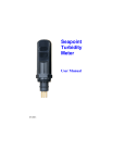
Data Bank User Manual
Rev. 2.16 December 27, 2008
Table of Contents
Chapter 1: Introduction
1.1
1.2
1.3
Front Panel
Features
Specifications
Chapter 2: Quick-Start Operation
2.1
2.2
Quick Start Data Collection
Quick Start Data Logging
Chapter 3: Button Description and Operation
3.1
3.2
3.3
3.4
3.5
Power Button
Store Button
Recall Button
Select Button
Special Combinations
Chapter 4: Windows to Data Bank - Graphical User Interface
4.1
4.2
4.3
4.4
4.5
4.6
4.7
4.8
4.9
Introduction
“SETUP OPTIONS” Tab
“Save Data Bank’s Settings to a File” frame
“SET Data Bank Settings from a File” frame
Updating the Data Bank’s Operating System
“SAVE DATA BANK RECORDS” Tab
“EQUATION GROUPS AND CALIBRATIONS” Tab
“Computer Assisted Calibration” frame
“REPORT HELPER” Tab
Chapter 5: Sensors and Cables
5.1
5.2
5.3
Typical Sensors
Endorsement
Attaching and Changing Sensor Cables
Chapter 6: Batteries, Charging & External Power
6.1
6.2
6.3
6.4
6.5
6.6
6.7
6.8
6.9
6.10
Battery Life Estimates
Low Battery
Replacing the Battery
Charging the Battery
Termination Mode
Amp/Hour Gauge
Recharging a Charged Battery
When to Charge
When it won't Charge
External Power Option
3
3
4
5
6
6
7
8
8
8
9
10
10
11
11
11
13
14
16
19
21
23
27
28
28
28
28
31
31
31
32
32
33
33
34
34
34
35
Chapter 7: GPS
36
7.1
7.2
7.3
36
36
36
Mounting
Setup
Use
Appendixes
A:
B:
C:
D:
37
Setting Up Window's HyperTerminal
Using HyperTerminal to Download Data Files
Communications via a Terminal Program
Recovering from Failed Data Bank Upgrades
Product Guarantees
37
38
40
45
46
2
Chapter 1
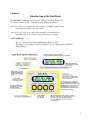
Introduction to the Data Bank
The Data Bank is intended for Interpretive Metering and Data Collection.
It is used in conjunction with a computer for setup, and record retrieval.
"Interpretive Metering" translates the sensor's output to a familiar readable display,
in the engineering units of the users choice.
"Data Collection" stores up to 9,999 records manually, or automatically at
timed intervals, for later recall or downloading to your computer.
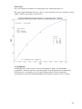
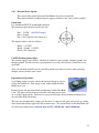
1.1 Front Panel:
Below is a reduced view of the Data Bank Quick Reference page.
This image is also available on the CD, and the web site, as a full page Adobe PDF file;
DBQuickRef.pdf.
3
1.2 Features:
• Accepts sensors from various manufacturers;
(For example: Seapoint, Turner Designs, Campbell Scientific, Wet Labs, etc.)
Software selectable sensor voltage.
Software selectable sensor warm up time.
Software selectable sensor gain.
Input selection of Voltage or Current.
• Interpretive data metering:
Sensor’s readings interpreted for you, continuously, in real time.
Readings displayed in the units of your choice.
Sixteen field selectable Parameter Groups*.
Parameter Group* titles are user defined, in plain English.
Save or restore Parameter Groups* from your PC’s hard drive.
• Auto ranging, display:
00.00 to 99999 (for negative numbers, the leftmost digit becomes “-“).
• Computer assisted calibrations:
Continuous sensor readings assist user in creating data points.
Fits an equation to collected data points. Graphs results.
View results graphically while modifying data points, order of fit, etc.
Increase low-end accuracy with our exclusive “Force thru First” feature.
Automatically programs the Data Bank to newly created formula.
• Unattended data logging:
Logging intervals from 1 second to over 4 days.
Data Bank shuts off between samples.
Internal real time clock, includes automatic handling of leap years.
• Non-volatile Data Storage:
Won’t loose your records, or settings, even with dead batteries.
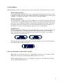
Up to 9,999 records, including GPS data.
• Selective downloads:
May retrieve records as stored, sequentially, or from a single location.
• High power rechargeable battery:
Powers Data Bank, external sensor, and optional GPS.
User replaceable. No memory effects. No safety hazards.
Built-in battery charger, with “Amp/Hour Gauge”.
Recharge from AC power or cigarette lighter.
• Display Backlight:
Manual operation or timed auto shut off.
Normal and Low-Power modes.
• Flash operating system:
Upgradeable WITHOUT opening the case or corrupting stored data.
Automatic upgrade notice, and assistance, from Windows software.
• Watertight durable polyamide enclosure:
Real pushbuttons! Sealed, low-force, snap-action.
Easy, one-handed operation, even with gloves!
* A Parameter Group: 1 of 16 groups of data that defines the calibration for a given sensor, location, sediment, etc.
It consists of the Formula, Title, Engineering Units, Sampling scheme, Gain, and Date.
4
1.3 Specifications:
Current Draw:
Computer: <=45 mA (at full charge). Sleeping <20 uA.
LCD Backlight: Full power ~ 30 mA. Low Power ~ 15 mA.
Sensor Power Available:
Output Type: Low Noise Regulated DC.
Voltage: Software selectable 3 to 12 volts.
Current: Maximum; 150 to 100 mA (for 3 to 12 V, respectively).
GPS Power:
3.3 VDC @ up to 300 mA.
Note: While Data Bank is off, GPS is self-powered.
Battery:
Type: NiMH rechargable, 4.8 volts, 4,000 mA/Hr. User replaceable.
Life: Continuous: >70 hours (Seapoint turbidity sensor, no backlight or GPS).
Charger:
Type: Internal, rapid, intelligent, switching mode, DC powered.
Charge Time: ~3 hours (for a fully discharged battery; ambient @ 25 degrees C.)
AC charging: AC to DC switching supply; Glob Tech, Inc. TR9CD1700CCP-Y
(Input 110-240 VAC @ 1.0 A max., Out 9.0 VDC @ 1.7 A max.)
DC charging: cigarette lighter cord (9-15 VDC @ ~1.4 A max., fused @ 2 A.
Charge Current: 2, 1.5, 1, & .35 A (set by battery temperature and/or voltage.)
Termination: Delta Temp/time, - Delta V, Over Temp, Over Voltage, Max. Amp/Hrs
stored (time).
Indicators: Amp Hours stored (.1 A/Hr steps) and type of termination.
Inputs:
Range: 0-5 Volts or 0-25 mA. (0-4.095 V available upon request.)
Resolution: 12 bits (1.221 mV per step; or 6.1 uA per step).
Input Type: Precision Instrumentation Amplifier
Input Selection: Switch; Differential Voltage, Differential Current, or Dual Current
(primarily for Global's turbidity sensor with dual outputs.)
Impedance: Voltage ~ 10 Meg ohm ; Current ~ 200 ohm
Sampling Rate: 1000 Hz (bursts); groups of bursts re-averaged @ 30 Hz.
Outputs:
Two, Open Drain, up to 200 mA @ 15V max.
(Used primarily for gain selection; as with Seapoint or Turner sensors.)
Serial Communications:
RS-232 (9600 baud) or USB (via optional converter). Auto-select com port 1-8.
Storage: Non-Volatile, 1280 Kb (9,999 records, and all definable parameters).
Physical:
Size:
Main body: 4.6"W x 3.2"H, x 3.4"D, Handle: 4.8" long.
Overall: 11"H (with handle, stain-relief and connector).
Weight: 1.7 lb. (.76 kg) w/o GPS;
2 lb. (.90 kg) with side-mounted Geko GPS
Watertight; case IP65, connector IP68, buttons IP64.
5
Chapter 2
Quick Start Operation
See section 1.1, “Front Panel” for a visual representation of the control panel layout.
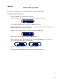
2.1 Quick Start Data Collection:
1) Press the Power button and the unit will turn on.
A few seconds may be required for the external sensor to stabilize ("warm up”).
2) To toggle backlighting: press and release the Power button again.
3) Press the Select button to choose the location / sediment being monitored by repeatedly pressing
the Select button until your choice is displayed.
4) When a value is displayed that you wish to store, press the Store button.
5) This value can be reviewed by pressing the Recall button.
6) If, for some reason, you wish to erase this record, hold the Recall button for one (1) second.
First you will receive a warning; continue holding.
7) Repeat the above process for as many reading as you wish.
8) When done, hold the Power button for a full second to turn the unit off.
6
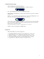
2.2 Quick Start Data Logging:
1) Press the Power button and the unit will turn on.
A few seconds may be required for the external sensor to stabilize ("warm up”).
2) To toggle backlighting: press and release the Power button again.
3) Repeatedly press the Select button to select the desired parameters for the location / sediment
being monitored.
4) When you are satisfied that the unit is displaying data as desired, hold the Store button for one
full second. After seeing “Logging Mode Entered”, release the button.
The unit will have taken a reading (on the initial press), and will now power down in the logging
mode. It will reawaken and gather new readings as defined by the previously set time interval.
Intervals are set via an external computer.
For detailed information on logging see “Logging Interval” in section 4.2.
5) When you wish to end logging press the Power button.
Logging Notes:
When the Data Bank powers up in the logging mode:
1)
2)
3)
4)
5)
The backlight will flash on during power up, but will turn off to conserve power.
While “Warming Up”, the “s” indicates the sample number about to be stored.
When the “s” changes to ‘r” the value stored is being recalled, for three seconds.
The Data Bank will then turn back off (assuming sufficient time for sleeping).
Logged data is also output via the serial port on each data collection.
7
Chapter 3
Button Description and Operation
Note that there are two distinct ways to operate each of the four buttons:
1) "Press" which is to press the button and release it within less than 1 second.
2) "Hold" which is to hold the button for a full second before releasing.
3.1 Power Button:
The power button is used to turn the unit and backlight on and off, and to end the logging mode.
Power On
When the power is off, a press of this button will turn the power on, and terminate logging.
Backlight
When the power is on, each press of this button will toggle the LCD's backlight on and off.
If the unit was logging, the first press will terminate logging, subsequent presses will then
toggle the backlight.
Power Off
Hold the power button for a full second to turn the unit off, and terminate logging.
3.2 Store Button:
The store button is used to manually store the current reading, and to initialize the logging mode.
Store
Press, and release, the store button to store the current reading. The sample number (“sXXXX”)
will increment. The “s” to the left of the number simply reminds you that you are viewing the
sample number about to be “stored” (as compared to a flashing “r” for recalled values). The
“XXXX” portion represents the current record number, to a maximum of 9,999. When memory
becomes full, the numeric storage number will be replaced by the flashing word “FULL”.
Log
Hold the store button for a full second to initialize the logging mode. The display will indicate
"Logging Mode Entered".
Release the button and the unit will shut off. It will re-awaken at the preset time interval,
store a new reading, and go back to sleep.
8
3.3 Recall Button:
The Recall button is used for recalling previously stored records and for clearing of the last record stored.
Recall Last Record Stored
Press the Recall button while the unit is in its normal display mode and the last stored record will
be displayed for three (3) seconds, after which, it will revert to normal display mode. During recall,
a flashing “r” will replace the normal “s”, just to the left of the sample number.
Recall Previous Records
Press the Recall button, while it is presently recalling a record, and it will decrement to the record
stored just before the currently displayed record. This process may be repeated until it reaches the
first record stored, at which point each press will increment through the stored data. (Decrements
through the samples until it reaches the bottom, then increments back up until it reaches the top;
then the process repeats as long as the button continues to be pressed repeatedly.)
Erasing Records
Holding the Recall button, while the unit is displaying the last stored record, will cause that record
to be erased from memory. The display will warn of the pending erasure, "Caution, About to
Clear". If the button is not released within the next second, the record will be erased, and the
display will show "Cleared Top Record".
4) Holding the button, while reviewing any record other than the top record, causes the display to
read "Only Top Record May be Cleared".
Notes regarding displayed sample numbers & GPS:
While ready to store data; the lower case “s” will change to an upper case “S” whenever a valid
GPS signal is being received, indicating that GPS data will also be stored.
While recalling data; the lower case “r” will change to an upper case “R” whenever the recalled
data also includes GPS information.
9
3.4 Select Button:
The Select button is used for reviewing and/or selecting a group of parameters. This group of parameters
includes the formula for conversion from the sensor reading to the desired display format.
Group definitions can be defined for different sensors, locations, sediments, etc. Selecting the correct group
depends on how they were defined. To simply selection, pressing the Select button gives additional group
information, as follows:
#gg eeee mmddyy (gg=group #, eeee=Eng. Units, mmddyy=date of calibration.)
-descriptive title1) Pressing the Select button, while the unit is in its normal mode, will display
the above descriptive information of your current selection.
2) Press the Select button again, while already displaying descriptive information, and it will
increment the to the next group number, displaying information on that group. Once the button is
released for a full second, the current displayed group will become the new chosen parameter
group. Note: The selection numbers will increment from one (1) to sixteen (16), then back to one
(1).
3) Holding the Select button for a full second will set the selection number back to group one (#01).
This is useful if, for example, you only have five (5) groups programmed; you can increment
through all five, then hold the button to go back to group one (#01) without having to increment
through the unused groups.
3.5 Special Combinations:
1) Reset
Pressing all 4 buttons simultaneously, then releasing, will result in a hardware reset of the Data
Bank. Simply re-power to get back to normal operation. This mode is used in the event that the
computer were to ever to lock up, which prevents normal power down.
It is also used after updating the Data Banks operating system.
2) Display Mode
The user may operate the display in one of two modes: “Title” or “Date & Time”. To toggle the
display mode in the field, press the Select button, then (within one second) press the Recall button.
Hold both buttons for one full second. The display will blank. When the buttons are released you
will have toggled between display modes. Note that the unit reverts back to the original
programmed display mode on the next power up.
3) Flash Programming Mode
Entering this mode will place the Data Bank in a programming mode for the purpose of updating its
operating system. This mode is locked out unless a serial communication connection is established,
and even then, would be next to impossible to enter accidentally. See section 4.5 “Updating the
Data Bank’s Operating System” for detailed information.
10
Chapter 4
Windows to Data Bank - Graphical User Interface
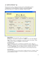
4.1 Introduction
This program runs in Microsoft Windows for communication with the Data Bank.
Proper operation of this program requires that a Data Bank be connected to the PC’s serial port.
Port settings are not required as the software will search all ports for the presence of a Data Bank.
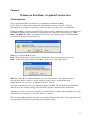
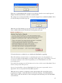
With the Data Bank powered up, when the GUI program is started, communications will be established and
Data Bank information will be displayed towards the upper left. Illustrated on the next page as “Data
Bank: S/N A0005 Ver. 1.10” (serial number and version of the operating system). If the Data Bank is
not found the following message will pop up:
Abort: Closes the Data Bank program.
Retry: Click after attaching, and powering up a Data Bank, and the program again searches ports.
Ignore: Click to run program without a Data Bank. Allows user to enter a Demo Mode:
OK: Enters Demo Mode, which has limited use, but does allow the use of the calibration features.
Once the Demo Mode is entered, you must end the program in order to end the Demo Mode.
Cancel: Returns user to previous “Communications Error” window.
Once valid communications has been established with the Data Bank, the user MAY change Data Banks
while the program is running. Settings will automatically update to match the newly attached unit.
Although the software controls were designed to be initially intuitive, additional hints and help also pops up
whenever the mouse pointer sits over words, windows, or buttons.
The following graphical examples are based on the standard “Windows XP” theme. Actual appearances will
vary depending on the Windows operating system and theme settings.
11
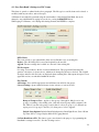
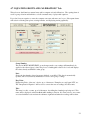
4.2 “SETUP OPTIONS” Tab
This tab is used for setting, or changing, the general operation of the Data Bank. On initial
communications, these settings will change to reflect those of the attached Data Bank.
As synchronization occurs, the background of each pull-down menu will turn light blue.
Please wait for this process to complete before attempting to change any settings.
Date and Time:
May be set to reflect the current PC’s settings, or done manually.
PC Time: PC’s date and time is displayed. Press SEND to set the Data Bank. Manual
Entry: When selected, two window boxes open for the setting of date and time. When
satisfied with the settings, press SEND to set the Data Bank.
Backlight Operation:
This choice defines the operation of the lighting for the Data Bank’s display. When set to
“Manual”, the backlight may be turned on and off manually by pressing the “POWER” button on
the Data Bank. In this mode, when on, the display will remain on indefinitely, until manually shut
off. In the “Auto Shut-Off” mode, the backlight, when turned on manually, shuts itself off
automatically after a given number of seconds. This time is selected via the pull down menu.
Back Light Power:
This choice defines the power used by the display’s backlight, and therefore, its brightness. When
power consumption is an important consideration, using Low power will reduce the backlight
power from about 27 to 14 mA.
12
Display Mode:
This choice defines the way the Data Bank displays its’ lower line reads during normal operation.
If set to “Date & Time” it will read, for example: “#01 04/06 10:32” (selection #1, April 6, 10:32
AM). If set to “Title”, it will read, for example: “Amazon River Mud” (the title of your current
selection). For a visual example, see section 1.1.
Warm Up Time:
This value is used to set a time for the external sensor to stabilize, upon power up, before any
readings are taken. Check your sensors manual for a specification defining this value. The warm
up time is set by use of the pull down menu. Note: The stated sensor warm up time specification is
often based on optimum conditions, and will likely be longer at minimum voltages and at
temperature extremes. Our recommendation: Be Generous! This is especially important when
expecting to do unattended data logging.
(Note: The pull down menu * indicates the recommended setting for Seapoint sensor; 5 Sec.)
Sensor Voltage:
This value defines the voltage applied to the external sensor on power up. To conserve energy, this
voltage should be set as low as reliable sensor operation permits (Check your sensor’s manual).
Typically, a good choice is 1 volt above the sensor’s minimum suggested operating voltage. (Note:
Menu * = recommended setting for Seapoint sensors; 8V)
Logging Interval:
This time setting only applies when the Data Bank is placed into an automatic logging mode. This
time is the interval between samplings. Entry is hh:mm:ss, from 00:00:01 to 99:59:59 (over four
days). If there is enough time between samples, the computer will completely shut off until it is
time to wake up for another sample
Save Settings to a File:
This button will open a new frame (see illustration on next page) for the purpose of saving all, or a
part of, the current Data Bank settings to a file; which can include ALL setup options, groups,
formulas, etc., or any part thereof.
13
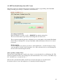
4.3 “Save Data Bank’s Settings to a File” frame
This frame is opened as outlined in the above paragraph. The file type is a text file, than can be viewed, or
modified, with any text editor, such as Notepad.
A filename is automatically generated using the serial number of the attached Data Bank, but can be
changed to any path\filename by typing in your choice or using the BROWSE button.
When typing in a filename, or modifying and existing filename, hit ENTER to complete.
If File Exists:
This section fades to gray (unavailable) if the chosen filename is not an existing file.
Replace: The old Settings file is erased and replaced by the new file.
Append: The new settings data is added on to the end of the existing file.
File Descriptor:
Is a string of text written to the file for better identification. The program will automatically
generate a descriptor (as shown above), which can be changed by the user as desired. The original
descriptor written to the file is the one displayed when searching files. Subsequent descriptors, from
appended sections, are embedded within the text file.
File Content:
All Settings: Saves ALL Setup Options and ALL data from ALL 16 data groups.
Selected Settings: Opens additional frames for the selection of various choices:
Range of Groups to Save: Applies to data groups 1 through 16; May be set for any
group(s), ascending or descending order. Only the selected groups will be written to the
file. Hint: if you wish only groups 1 and 3, then do only store group 1 (1,1). When done,
repeat process for group 3 to the file (3,3), being sure to select “Append”.
Include Setup Options: Includes Back Light Operation, Back Light Power, Sensor Warm
Up Time, Sensor Voltage, Display Mode and Logging Interval.
Set Data Bank from a File: This button opens a new frame for the purpose of programming the
Data Bank’s settings from a file. See the following section.
14
4.4 “SET Data Bank Settings from a File” frame
This frame is entered as described in the previous paragraph. It allows programming of the Data Bank
settings, including group settings, to match that of the selected file.
Get settings from this file:
Enter the filename you wish to recall, or “BROWSE” through the existing files.
The chosen file should be a previously saved Settings file (see Section 4.3).
The program automatically generates a filename based on serial number of the attached Data Bank.
If more than one Settings file is saved per Data Bank, additional filenames will need to be created
by the user.
File Description:
Is a text string previously written to the file for added identification. Use this information to help
verify that the file selected is the file intended. Note: If the selected file in not a valid Settings file,
the user will be warned using this window.
(Note regarding “Settings” Files)
The first line in each Settings file is used by the software to assure that the file is a valid Settings file. This
line must remain the first line on any Settings file, and remain unedited. It is as follows: (Data Bank Setup
File. DO NOT move or modify this line.)
This text line is automatically added to the file upon creation and requires no user intervention.
It is mentioned here for users who might choose to manually edit their Settings files.
15
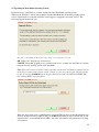
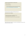
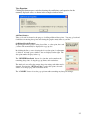
4.5 (Updating the Data Banks Operating System)
Each new release of the Windows software includes the latest Data Bank operating system.
Whenever the Windows software detects that the attached Data Bank has an internal operating system
version older than the one currently available, it will suggest you upgrade to the latest version. The
following Upgrade frame will open:
Note: The version numbers shown above may change as new software is released.
OK: Takes you to the next step, shown below.
CANCEL: Exists that Upgrade process, and allows the user to continue into the Windows software
using the current operating system of the Data Bank.
Note: If for some reason you wish to change operating systems when the Windows software has not
deemed in necessary (older version, custom versions, etc.) the user can force the following window
to open by entering NewDBOS into the Logging Interval box (under the SETUP OPTIONS Tab)
then clicking SEND, or pressing Enter.
When the above frame opens a path\filename is suggested. The user may modify this information as
desired. An Intel hex file is required (.hex). If the BROWSE feature is used to find the file, it will
expect the file to start with DB and end .HEX. Any other selected files will generate the following
error window:
16
If the user is confident that the file is indeed a correct file type, the above error may be ignored.
Simply click OK in the File Error, and OK to start the transfer.
The software also tests the selected file to be a hex file designed for use with the Data Bank. If it is
not, the following error window pops up:
When the above File Warning pops up, the user must select a different hex file.
Once a valid hex file has been selected, the following frame will open:
Follow the directions as outlined above to initialize the Data Bank for upgrading.
Hints: The hold times, mentioned above, are minimum times and are already padded by one
second. It is helpful if the Data Bank is in the Date & Time display mode as the flashing colon and
be useful for counting seconds, and will stop flashing once the Data Bank has entered the
programming mode.
If you fail the first attempt, press all four buttons, then release, which resets the Data Bank. Turn it
back on, and repeat the above process.
In case of a serious failure, where the Data Bank will no longer power up normally, refer to
Appendix D; “Recovering from Failed Data Bank Upgrades”.
When the above procedure is completed correctly, the next frame will open and the erase/reprogram process begins. At first the window box will show “Erasing… One Moment Please”.
After several seconds, the window box starts showing the actual data being sent to the Data Bank;
as shown below:
17
Once the procedure has completed, the following frame opens:
Simply follow the above instructions to restart the reset the Data Bank and return to normal
operation of the Windows software.
18
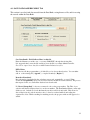
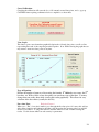
4.6 “SAVE DATA BANK RECORDS” Tab
This section is used to fetch data records from the Data Bank, saving them to a file, and for erasing
the records within the Data Bank.
Save Data Bank’s ‘Field Collected Data’ to this file:
Enter the filename you wish to use, or you may “BROWSE” through the existing files.
It is suggested that you use the file extension .txt as the file is a comma delimited text file.
Excel users: import these data files as ANSI Comma Delimited text files.
If File Exists:
This choice tells the program what to do if the file you’ve chosen already exists. You can either
add on to the existing file (“Append”), or replace it entirely (“Replace”).
Records to Download:
Records may be downloaded in; the order they were stored, sequentially, or sorted. When
downloaded Sequentially, all records stored for Selection #1 will be downloaded first. The process
then repeats for #2, etc., until all the data has been downloaded.
If ‘Selected Group Only” is chosen you must also choose the group number. The Title of you
selection will then be displayed next to your chosen number. The Data Bank will then sort through
all the records. Only those records that match your choice will be downloaded. This allows for
data collection in any order from various sites, to later be reordered while downloading into
separate files. Note: While searching for matching records, the progress window will appear to be
stalled.
19
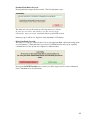
Download Data Bank’s Records:
Pressing this button begins the data transfer. The following frame opens:
The window box shows the actual records being retrieved; as follows:
Record #, Selection #, Date, Time (24 Hr.), Sensor mV, Calculated Value
followed by: Latitude, Longitude when used with an optional GPS receiver.
Numeric progress will also be displayed on the Data Bank’s LCD display.
Delete Data Bank’s Records:
This button is a request to delete all the records stored in the Data Bank, effectively freeing up the
associated memory. When this button is pressed, a CAUTION window will pop up, requiring
confirmation before the operation is completed; as illustrated here:
Pressing the CANCEL Deletion button cancels your delete request and closes the confirmation
frame. Data Bank records remain intact.
20
4.7 “EQUATION GROUPS AND CALIBRATIONS” Tab
This tab serves dual functions: manual entry and/or computer assisted calibrations. The opening frame is
used for group selection and definition, as well as manual entry of polynomial equations.
If you don’t have an equation to enter, the computer can create and enter one for you. Subsequent frames
will assist in collecting data points, creating formulas, and displaying results graphically.
Group Number:
This choice MUST BE SET FIRST, as any changes made to any settings will immediately be
applied to the selected group’s data. The process of making this selection also loads and displays
the values already established for that group.
Date:
Shows the date that the selected group was defined, or modified. This date is automatically
updated, and stored, when any modification is done to this group’s settings.
Eng. Units:
Engineering Units; of the user’s choice, up to 4 characters. Examples are: mg/l, ppm, NTU, etc.
The “Interpretation Equation” will be used to convert the sensors readings, into these units.
Title:
This entry is a title, or name, up to 16 characters, describing the formula/group being used. This
name will be displayed on the Data Bank while making a selection. It is often easiest to use a name
associated with the location where the sediment originated and where the readings will be taken.
21
Gain:
Caution: A new Gain setting requires a new formula, or calibration.
This gain setting applies only to sensors that have inputs for selecting the gain (such as Seapoint
sensors) or sensors with multiple outputs (as with Global Waters turbidity sensor). This number
should be selected at the start of a calibration and should not be changed afterwards as it affects the
output of the sensor.
If you wish to use different gain ranges at the same location you will need to define separate
equations for each. For example: #03 = ”Casco Bay 0-100”, #04 = ”Casco Bay 0-2000”.
The Gain should be selected for the highest setting possible gain that gives a “Sensor Reading” of
less than, but as close as possible to the maximum reading of 4000 mv (or 20 mA). This is done
while the sensor is immersed in a sample solution equal to the maximum concentration you will
expect to find at the location where the readings are to be taken.
Samples:
This defines the number of reading taken from the sensor for each sample stored.
A burst of readings is taken every 30th of a second. During the burst, readings are taken a one
millisecond intervals. We recommend using the maximum settings for each; 32 readings per burst
and 8 bursts per sample. The result is a running average of the last 128 readings over
approximately the last ¼ of a second.
Interpretation Equation:
This formula is used to convert the sensor’s readings into a value, in the engineering units of the
users choice. Further explanations are given for each portion of the formula when the mouse
pointer is left over the part in question.
Entries may be entered manually or created by the computer upon completion of a “computer
assisted calibration”. CAUTION: Any formula changes will affect all Data Bank’s previously
stored field collected data, for that selected group number.
This allows for post-calibrations, but caution should be applied.
mV / mA :
Selects whether the formula display will be in millivolts (for sensors that output voltage, as does
Seapoint, Cyclops-7, and OBS-3 sensors), or in milliamps (for sensors outputting current, as does
the Global Water’s turbidity sensor). This setting should reflect the choice made by the switch
inside the Data Bank’s handle that is set at the time the sensor cable was attached. Note: The mV to
mA conversion applies only to the Data Bank unit as it is based on the Data Banks internal 200 ohm
resistor (1 mV /200 = 5 uA).
Dec. / S.N. :
Decimal or Scientific Notation; Selects the numeric format used to display the Equation.
Collect Data and Create New Equation:
Clicking this button pops open a frame titled “Computer Assisted Calibration” (see next
section) which is used for the gathering data points, fitting an equation, and graphing the
results.
22
4.8 “Computer Assisted Calibration” frame
This section is entered from the “Equation Groups and Calibrations” tab, selecting a group number,
defining its parameters, and then clicking the “Collect Data and Create New Equation” button. A
frame opens, similar to the following:
Datapoint Creator:
This section is used for the generation of each data point. Typically the Data Bank sensor is used as
the source of the reading and the user enters the concentration for each data point being created.
For instance: place the sensor in a solution standard of 100 NTU’s and then let the computer know
what the sensor is reading by entering 100 into the “Concentration of Solution” window. Then
click the “Make Datapoint” button. The number following “Make Datapoint” is the number of the
data point being created.
Typically the user starts at a zero concentration, increasing the concentration with each data point,
however, the computer allows entry of data points in any order.
The more data points, the more accurate the results. The minimum is two data points for a linear
equation, 3 for a curve (2nd order), and 4 for a “S” curve (3rd order). Once two data points have
been entered, the “View Graph” button turns from gray to light blue, and the graphical view of
your progress becomes available.
Source of Readings:
Data Bank Sensor: Readings are taken continuously from the attached sensor and displayed
accordingly. Averaging is done as defined on the previous screen (Samples).
Manual Entry: The displayed reading changes to an entry box for user entry of the sensor reading.
The actual sensor attached to the Data Bank is ignored. This is useful when entering data from a
printed material, such as calibration sheets, etc.
23
Cancel Calibration:
Canceling the calibration will cause the loss of all currently created data points, and so, pops up
CAUTION frame requiring confirmation before completion; as shown here:
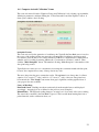
View Graph:
This button opens a new frame that graphically depicts the collected data points, as well as a line
representing the result of the computer generated equation. Note: While viewing the graph the user
may return to enter more data points at any time.
Type of Equation:
Defines the number of terms used in creating the formula. 1st Order has two terms, the 2nd
has three, etc. With as little as four data points you can choose any of the three. You may
change from one to the other while viewing the results graphically. This allows for easy
selection of the best choice (usually the best fit).
Force thru First:
Exclusive Feature !
When set to “Yes”, forces the formula to pass through the first data point. Of course, this only has
affect if the formula would otherwise miss that point. Increasing the accuracy at the low end will
decrease it elsewhere. To judge the tradeoffs, turn this function on and off while viewing the
results. Use this feature when low-end accuracy is paramount.
24
View Equation:
Clicking this button opens a window showing the coefficients, and equation, for the
currently displayed curve; as shown in the example window below:
Add Data Point(s):
Takes you back one frame for the purpose of adding additional data points. You may go back and
forth between entering data points and viewing the graph as many times as you like.
(Additional Graph Features)
By placing the mouse pointer on the plotted line, or a data point, the x and
y values will automatically be displayed in a pop up box.
By clicking the line, you are selecting the closest data point for adjustment
or deletion. A frame opens, similar to the one displayed at the right. The
data point number displays at the top.
The “DELETE Data Point” button does just that, and re-numbers the
remaining data points, closing the pop up frame, and recalculates.
The window boxes reflect the current data point settings and either may be
changed. Pressing the “SET New Value” sets the data point to the new
values, closes the pop up, and recalculates the fit.
The “CANCEL” button closes the pop up frame without making any data point changes.
25
Print Graph:
Pops open a Page Layout window for setting up the page, selecting the printer, etc.
The printed graph will include title, date, values for each of the data points, the coefficients, and the
equation; similar to the reduction shown below:
Accept Equation:
Clicking this button ends, and closes, the assisted calibration routines. The Data Bank is
programmed to match the equation as currently graphed. Both the Graph frame and Enter Data
Points frames close, returning you to the original equation frame. The new formula will
automatically be retrieved from the Data Bank and loaded into the equation boxes for display.
26
4.9 “REPORT HELPER” Tab
For Future Addition
27
Chapter 5
Sensors and Cables
5.1 Typical Sensors:
Turbidity & Suspended Solids :
Seapoint Sensors, Inc (NH, USA)
Turner Designs
(CA, USA)
Campbell Scientific
(UT, USA)
Global Water Inst. Inc. (CA, USA)
http://www.seapoint.com/stm.htm
http://www.turnerdesigns.com/t2/instruments/turbidity_c7.html
http://www.campbellsci.com/turbidity
http://www.globalw.com/catalog.html
Fluorometers:
Seapoint Sensors, Inc
Turner Designs
(NH, USA)
(CA, USA)
www.seapoint.com/products.htm
http://www.turnerdesigns.com/t2/instruments/cyclops7.html
Transmissometers:
WET Labs, Inc.
(OR, USA)
http://www.wetlabs.com/products/cstar/cstar.htm
5.2 Endorsement:
Dataron Instruments selects Seapoint Sensors as the best match for use with the Data Bank.
Their turbidity sensor uses very low current, has four selectable ranges, and optical feedback.
Further, their several fluorometers can be interchanged with the turbidity sensor without changing
cables. Each also benefits from the four gain ranges, which are selected by the Data Bank.
Of course, Turner Designs “Cyclops-7” line can’t be overlooked. They too are an excellent match.
Low power, three selectable ranges, and field interchangeable. The line offers a turbidity sensor, as
well as a wide range of fluorometers.
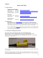
5.3 Attaching and Changing Sensor Cables:
1) Loosen the outer nut on the strain relief at the bottom of the Data Bank’s handle.
2) Remove the four screws that attach the handle to the body of the Data Bank; remove handle.
3) As the handle is removed a small bundle of wires will unplug from the Data Bank.
4) Feed the cable into the handle, which pushes the terminal strip out the open end. Continue until the
terminal strip is completely exposed.
5) Cut of the tie-wrap and disconnect all the wires by loosening the screws at each terminal. Pull the cable
out of the handle.
6) Feed the new cable through the strain relief. When our standard shielded cable is used, leave about 3/8”
exposed, tie-wrapping the shield so as to make contact with the printed circuit board. Then, trimming each
wire to length, connect to the appropriate terminals:
28
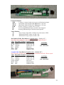
Tie-rap shielded cables so that shield contacts ground plane of circuit board (Seapoint shown).
Terminal Definitions:
GND
Common (or return) for the sensor power, and dual current inputs
CTL-A
Open Drain output #1 (Gain bit 0) 200mA max., 15V max.
CTL-B
Open Drain output #2 (Gain bit 1) 200mA max., 15V max.
PWR
Positive voltage to power the sensor (3-12V).
IN+
Non-inverting differential input, and dual current input #1
INInverting differential input, and dual current input #2
Switch Positions:
2C
“Two Current” inputs; IN+ is #1; IN- is #2; both return to GND.
dC
“Differential Current” inputs; use IN+ to INdV
“Differential Voltage” inputs; use IN+ to INOur Standard Cable; Data Bank to a Seapoint sensor: (Switch=“dV”)
Our cable color coding does not match that used by Seapoint Sensors !
Color
Black
Brown
Blue
Red
White
Green
Data Bank Terminals
1 GND
2 CTL-A
3 CTL-B
4 PWR
5 IN +
6 IN -
Seapoint Sensor
1 Power Ground
6 Gain Control B
5 Gain Control A
4 Power In
2 Signal Output
3 Signal Ground
CAUTION:
Double check
your connections!
Seapoint Cable; Data Bank to Seapoint sensor: (Switch=”dV”)
Note: Seapoint’s ½” Dia. Carol cable requires a non-standard strain relief. Please request.
Color Data Bank Terminals Seapoint Sensor
White 1 GND
1 Power Ground
CAUTION:
Red
2 CTL-A
6 Gain Control B
Double check
Green 3 CTL-B
5 Gain Control A
your connections!
Orange 4 PWR
4 Power In
Black 5 IN +
2 Signal Output
Blue 6 IN 3 Signal Ground
29
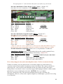
Tie-rap Seapoint’s ½” cable such that cable jacket is just off the edge of the board.
Our cable; Data Bank to a Turner Designs Cyclops-7 sensor: (Switch=”dV”)
Our cable color codes do match those of Turner Designs Cyclops-7 cables.
Color
Black
Blue
Brown
Red
White
Green
Data Bank Terminals
1 GND
2 CTL-A
3 CTL-B
4 PWR
5 IN +
6 IN -
Cyclops-7
2 Power Ground
5 X10 Gain
6 X100 Gain
1 Supply Voltage
3 Signal Out
4 Analog Ground
CAUTION:
Double check
your connections!
Our cable; Data Bank to Campbell Scientifics OBS-3+: (Switch=”dV”)
Our cable color codes do match those of Campbell’s OBS-3+ cables.
The OBS-3+ has two analog outputs, of which only one may be used at a time*.
Color Data Bank Terminals OBS-3+ Sensor
Black 1 GND
2 Power Common
CAUTION:
Red
4 PWR
1 Power (5-15V)
Double check
White* 5 IN +
4 Hi Signal (4X)
your connections!
Blue* 5 IN +
5 Low Signal (1X)
Green 6 IN 3 Signal Common
* Only one of these two sensor outputs may be connected to the standard Data Bank at any given
time. By special request, the interface board can be modified for dual mV inputs, at no charge.
For D&A Instrument’s original OBS-3 Wire as above, except that there is no Blue wire.
Global Waters’ WQ720 turbidity is supplied with a built in cable assembly (standard 25 feet).
The WQ720 uses 4-20 mA transmitters. Change switch setting!.. (Switch=”2C”)
Color Data Bank Terminals WQ720
Black 1 GND
Ground
CAUTION: Double check your connections!
Red
4 PWR
10-36V
White 5 IN +
4-20 mA high range output (1,000 NTU)
Green 6 IN 4-20 mA low range output (50 NTU)
We are always happy to assist you in connecting other sensors. Feel free to contact us for help.
7) When reassembling, leave the printed circuit board extending slightly beyond the handle body
so that the connectors may be mated. Note that the connector is polarized. The connector will slide in,
without any locks. Once connected, slide the handle towards body, which locks the board in place.
During all this, be sure that the connector stays fully engaged while aligning the handle for final assembly.
8) Install the 4 screws and tighten the strain relief. CAUTION: Do not over tighten.
The screws should just be snug. The strain relief will firmly hold the cable, even when only
hand tightened. However, you may want to tighten it slightly beyond hand-tight, to prevent it from coming
loose in the field.
30
Chapter 6
Batteries, Charging & External Power
6.1
Battery life estimates:
The power drawn from the battery, by the external sensor, is equivalent to the power used by the
sensor, divided by the efficiency of the power supply boosting the voltage.
As efficiency drops with increasing sensor voltage, it is best to use the lowest voltage that will
power the sensor reliably.
The sensors power supply will supply 150 to 100 mA (maximum) for 3-12 V output respectively
(at approximately 70% efficiency).
Calculate battery draw based on sensor power:
(Sensor V * Sensor I / Efficiency / 4.8V). For example: Seapoint Turbidity sensor, @ 8v, 4
mA, 70% (.7) will draw ~10 mA from the battery.
Add in other current draws:
Computer:
47 mA
Backlight:
30 or 15 mA (if set to “low power”)
GPS:
(eTrex)140 to 180 mA (depending on backlight)
Divide 4000 mA (battery capacity) by the total mA from the above calculations. The result
is an estimate of the hours of continuous use that the user might expect.
For example: with a Seapoint turbidity sensor (no backlight or GPS) the result would be
greater than 70 hours of continuous use. (With full power backlight, over 45 hours.)
The second consideration is the off time. All batteries exhibit self-discharge, meaning they
will go dead even when not in use. This effect is more pronounced in rechargeable
batteries. Exact calculations are difficult as the effect varies with temperature, but a good
rule of thumb is to figure 1% per day at room temperature, rising to 2% per day as
temperatures rise above 110 °F.
This self-discharge effect must be considered during unattended data logging; especially
when long sleep intervals exist between each reading.
6.2
Low Battery:
When the battery is low, the display will show:
This will display for a second, every 4 seconds until the battery is either recharged or gets too low
for continued use. When the battery is exhausted, it will simply turn the unit back off each time
you turn it on, until eventually it won't even turn on.
Note: At the first indication of a low battery, assisted GPS power is discontinued.
31
6.3
Replacing the Battery:
The battery pack is user replaceable, however, the battery must be ordered from Dataron. The part
number is: ODXDATR04. It is best to have a new battery in hand before beginning the
disassembly. If you prefer, Dataron Instruments will install your new battery for you; at no
additional cost beyond that of the battery and shipping.
To replace the battery follow these steps:
1) Loosen the strain relief around the sensor cord. Remove the handle and the terminal strip. (For a
complete explanation see the section 5.3, “Attaching and Changing Sensor Cables”.)
2) Remove the screws on the back of the Data Bank with the buttons face down in your other hand.
3) Lift away the body of the case, unplugging the harness connector as you do.
4) Unplug the battery from the printed circuit board.
5) Cut away the tie-wrap and lift the battery out.
6) Re-assembly in the reverse order. Caution! Plugging in the battery incorrectly will likely cause
damage to the Data Bank. Pay special attention to pin alignment.
6.4
Charging the Battery:
The battery may either be recharged using the AC to DC power supply or cigarette lighter cord.
Plug the serial cable into the connector on the top of the Data Bank (You will need to disconnect
the GPS cable, if in use.) Then plug the charger device, of your choice, into the serial cable. Apply
power to your charger device.
The Data Bank will turn itself on (if not already on). The microprocessor is used to monitor and
control the charging. During charging, all other internal features are disabled, including the power
switch (you can not turn off the power). However, communications with a PC will still be
available, for setup and downloading.
When charging is initialized, the display will show:
Beginning in 2006: The display format becomes:
CHARGING @ 2.0 A
AHr STORED: 0.0
Where the 0.0 is the estimated charge placed into the battery in amp/hours. Once the charge is
complete, the display will show something like:
When charging is complete, DONE will be flashing, pv is the termination mode (see "Termination
Mode" below), and the 2.6 (could be any number) is the estimated Amp/Hours received by the
battery (see section 6.6, "Amp/Hour Gauge").
32
6.5
Termination Mode:
When a charge cycle ends, the Data Bank will indicate the mode that caused the termination, as
follows:
pv
Peak Voltage: negative delta voltage. (The voltage had been rising, then dropped
slightly.) Indicates a complete charge.
tr
Temperature Rise: delta temperature/delta time. (Temperature rises faster than
expected.) Indicates a complete charge.
ot
Over Temperature: Indicates a maximum temp has been reached.
Indicates charge may or may not be complete.
oc
Over Capacity: Indicates the battery capacity is exceeded.
(Total estimated amp/hours received.)
bb
Bad Battery: Indicates that the battery did not charge normally, and that it may be
time to replace the battery. Ignore this indicator until it begins to happen regularly.
(Occurs if minimum voltage is not reached within a given time, or maximum
voltage is exceeded.)
After battery charging has terminated, the charger circuit will continue to power the Data Bank
until disconnected.
6.6
Amp/Hour Gauge:
The Amp/Hour gauge is used to help you estimate how much charge your battery has accepted.
This number allows you to estimate the percentage of battery capacity used; (% of battery
consumed = 25 x [amp hours used]).
The amp/hour gauge/counter is only an estimation of actual acceptance. A NiMH battery retains a
different percentage, of the charge dumped into it, based primarily on the rate of charge. At full
charge it may retain 85%, but at the lowest rate, only about 62%. Since the Data Bank is charging
the batteries in a confined space, the charge current must drop as the battery temperature rises, to
prevent overheating. The result is that the most efficient charge occurs during the first hour of
charging. In fact, about half of a complete charge is accomplished in that first hour.
Under normal use, with your selected sensor(s), you will begin to get a feel for how much energy is
used from the battery on a daily basis. This occurs by monitoring the amount of amp/hours
replaced during each charge. See section 6.1 for estimation formulas.
If one day, you left the Data Bank in the sun, then started charging, it would likely shut down
prematurely do to high temperature (“ot”) with less charge than expected.
It would be easy to guess that the battery could use more charging (see next section).
33
6.7
Recharging when Not Enough Charge:
Under certain circumstances you may feel that the battery did not get as much of a charge as it
should have. This is likely to occur if charging is initialized at an elevated temperature (causing
premature charge termination as the maximum internal temperature was reached - "ot"); and may
occur under other circumstances.
In this case you can continue the charge (once the batteries have cooled a while) by disconnecting
the charger, then reconnecting it.
When the charger is disconnected the Data Bank will go back to normal operation, but does not turn
itself off. It will remember the amount of charge previously placed into the battery (amp/hours)
until the Data Bank is turned off.
If charger power is reapplied without the Data Bank being switched off, it will continue adding
amp/hours to the counter from where it previously left off. This helps protect the battery from being
excessively overcharged and helps inform the user about the total charge that the battery has
received.
6.8
When to Charge:
The batteries can be safely charged, even when they are only partially discharged, because the
charger uses a rapid charging scheme. Since the charger is most efficient during the beginning
charge time, it is most efficient (time wise) to charge the battery when it is only partially
discharged.
While using it in the field, it may be good to start by charging it every day. Soon you will have a
feel of how much the battery is being used, and can adjust the charge schedule as needed.
Example: Every day the battery has been recharging about 0.4 amp/hours. Since it is rated (when
new) at 4.0 amp/hours, you can easily see that you're only using about 1/10 of the battery capacity
each day and may choose to change the charging schedule to a full charge once a week; or possibly
in the field, a quick charge every other day during lunch.
Another consideration is battery life. The battery manufacturer specifies the battery as
being good for minimum of 500 recharges. So, at once a day, that’s almost 2 years.
Normally the Data Bank will only be used seasonally, extending that life considerably.
Self-discharge must also be considered. The batteries will become exhausted even
when not in use. This effect varies with temperature. The battery manufacturer
recommends that when batteries are stored between -4 to 86°F (-20 to 30°C) that they
be recharged every 3-6 months. If batteries are allowed to completely self-discharge,
their energy storage capacity will become reduced.
6.9
When it won't Charge:
If the Data Bank has been stored for a long period of time and the battery has become
completely exhausted, attaching the charger may appear to have no effect.
Without sufficient battery power, the computer will not start up normally, however, the
battery does receive a pulse of a charge upon connection. Disconnecting, and
reconnecting, every 30 seconds will give the battery a pulse charge of 2 amps, quickly
tapering down to 0. Repeating this several times should boost the battery sufficiently for
the computer to start up normally, and begin displaying the normal “CHARGING” mode.
34
6.10
External Power Option:
This special order option allows the Data Bank to be powered externally.
This option includes an additional power supply, connector, and 3 meter cable assembly.
Connection:
Use Switchcraft EN3C3F weathertight connector.
This drawing depicts the back (solder cup) side.
Pin 1: 12 VDC (9-32 VDC range)
Pin 2: Ground
Pin 3: No Connection (for future use)
The supplied cable is wired as follows:
White: + 12 VDC
Black: Ground (-12 VDC)
Shield: No Connection
CAUTION about ground loops:
The external supply is not isolated. Grounds are common; sensor ground, computer ground, and
charging ground. For this reason it is good practice to use only one of the two connectors at any
given time.
Also, consideration should be given to possible ground loops between sensors when powering
multiple sensors from the same source.
Explanation of Operation:
A switching supply is used to convert the external voltage to a lower
voltage for internal use. This supply is only enabled while the Data
Bank power is on.
External power will not maintain the internal battery while Data Bank
is off. The battery will be boosted (if needed) each time power comes
on, as in the Logging mode. This boost is to prevent the battery from becoming discharged, but
does not fully charge the battery.
The lower the internal battery voltage gets, the more of a boost it will get at each power up, and the
more current that will be supplied by the external source. The external loads on the Data Bank will
also affect the current drawn. (Current draw at 12V: Off=0.2 mA, On=5 to 800 mA)
35
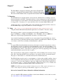
Chapter 7
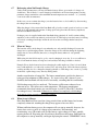
Garmin GPS
The Data Bank is designed to interface with various Garmin GPS
receivers. An optional side mounted eTrex is shown in this picture.
The cover of this manual shows an optional side mounted Geko 201.
7.1 Mounting:
The Data Bank may be purchased with a "side mount" kit, which includes everything you need to
mount and interface your GPS. Using this kit allows for clear viewing and easy removal, however,
side mounting throws off the balance of the unit and may therefore be fatiguing when held upright
for long periods. Currently, at 3.1 ounces, the Geko series is by far the lightest GPS around.
Another approach is to wear the GPS (such as using a Garmin neck lanyard) and then connect it to
the Data Bank using a longer cable (which we of course can supply).
7.2 Setup:
Note: if you received your Garmin GPS through Dataron, this setup has already been done.
Using the Garmin GPS with the Data Bank requires the use of Garmin’s “Text Out” setting.
The typical procedure to set the proper interface mode will be something like this:
Page to the Menu, go to Setup, select Interface, select "Text Out", and set to 9600 baud.
When done, just press Page repeatedly until you return to your desired screen.
A more detailed explanation is available in your owners manual. If your Data Bank was ordered
with a side mount, you will likely find that we have included your GPS Owners Manual, along with
our software, on the CD we sent with your Data Bank (in a .pdf file).
7.3 Use:
To use the GPS with the Data Bank, the interface cable must be attached between the two devices.
The GPS must be turned on separately from the Data Bank, however, when the Data Bank is on, it
may supply the power for the GPS; otherwise, the GPS is powered by its own internal batteries. If
the Data Bank senses that it’s own batteries are getting low, it will stop supplying power to the GPS
(until the Data Bank is powered off, and on, again.)
This "Assisted Power" feature applies to Garmin's Geko, eTrex and eMap series receivers (except
Geko 101). Other Garmin GPS receivers will have to rely entirely on their own internal batteries.
The purpose of this feature is to extend the relatively short Garmin battery life.
The GPS will take several seconds, to several minutes, to lock in on the available satellites. Once a
lock is established it will be displayed on the GPS, and verified on the Data Bank by changing the
lower case “s” (in front of the sample #) to upper case. When in the “Time & Date” display mode,
also displayed is a star (“*”) next to the group number. Whenever this star (or “S”) is visible, and
data is stored, Longitude and Latitude will be added to the data record.
NOTE: If the GPS keeps turning itself off, it's batteries are low. Either replace the batteries, or
remove them completely (allowing the Data Bank to supply the necessary power).
Refer to the Garmin GPS Owners Manual for additional information.
A list of compatible GPS equipment, and links to their Owners Manuals, can be found on our web
site: www.dataron.com/CompatibleGPS.html .
36
Appendixes
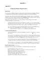
Appendix A
Setting Up Window's HyperTerminal
Quick Setup:
To assist the user of Hyper Terminal, a settings file has been included that starts Hyper Terminal
set appropriately for the Data Bank (except for the possibility of an incorrect COM port).
The Setup program will have installed the Data Bank files in the "Data Bank" directory (or the alternate
directory of your choice). There you will find a file "DataBank.ht" which is a Hyper Terminal setup file.
Double clicking this file opens Hyper Terminal setup for the Data Bank.
Right clicking on this file will allow you to change the Hyper Terminal settings associated with it.
To change the COM port, do the following:
1) HyperTerminal will start expecting to use COM1. If you wish to use a port other than COM1,
right click the file, then select "Properties”. In the "Connect To" tabbed section, pull down the menu
“Connect Using” and select the “Direct to Comx”; where x is the COM port of your choice.
2) To verify communications (with the Data Bank attached and turned on) hit ENTER, then type
“RST” (upper case), then ENTER again. You should get a response similar to:
Dataron Instruments ; Firmware Ver. 1.13 04/12/04 ; S/N: A0005 03/067/04
Creation of Desktop Shortcut:
1) In the Data Bank directory, right click "DataBank.ht", then click "Create Shortcut". A shortcut
file is created.
2) If you wish, you can change the icon of the shortcut. To do so right click the new shortcut, then
click "Properties", then click the "Change Icon" button and select your desired icon. If you want to
use the Data Bank icon, select the "DataBankGUI.exe" program, then double click on its icon.
3) If you wish, you may also change the shortcut name. We like: "DataBank HyperTerm". To do
so, simply right click the shortcut, then click "Rename", enter the new name, then hit Enter.
4) To move this icon on your desktop, you can just drag it there. Alternately, you can just send a
copy to the desktop by right clicking it, place your mouse on "Send To" and then click "Desktop".
HyperTerminal Settings: For reference
When HyperTerminal is started via “DataBank.ht”, it is initialized with the following settings:
Connected using: Direct Connect using Com1
Bits/sec: 9600, Data bits: 8, Parity: none, Stop bits: none, Flow control: hardware.
Function, arrow, and ctrl keys act as: terminal keys
Backspace key sends: Ctrl H, Emulation: Auto Detect
Telnet terminal: ANSI, Backscroll buffer lines: 250
Line delay: 100mS, Character delay: 10mS
Append line feeds, Wrap lines that exceed terminal width.
37
Appendix B
Note: We recommend using the Data Bank GUI (Graphical User Interface) for downloading.
It simplifies the download process, while also offering additional features (see section 4.6).
While the below text was written for HyperTerminal, the described process is also a typical
example for other terminal programs.
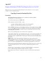
Using HyperTerminal to Download Data Files
Downloading:
1) Open HyperTerminal as previously set up for communication with the Data Bank.
(See Appendix A for setup information.)
Note: all letter entries must be in UPPER CASE.
2) The command to download is "DLD s"; where:
“s” is the sort character, 0 thru F for curves 1-16 or S for sequential.
"SPACE" (or any other character) will retrieve unsorted data.
3) Press "ENTER". The display on the Data Bank should show "Downloading" followed by "0000
of xxxx", where 0000 is the current record number, followed by xxxx, which is the total number of
records to be downloaded. (The record number will not be incrementing at this time since actual
downloading has not yet started.)
4) Now, in your terminal program, select "Transfer" then "Capture Text".
After selecting "Capture Text": enter a filename and press start. (A ".txt" extension should be used
as this will be a text file.) Once these preparations are complete, press Ctrl-Q on the keyboard to
start the flow of data. You will be able to see the progress on the screen; the record number will be
incrementing.
NOTE: During "sorted" downloads, the flow of data may stop for up to several seconds
(5mS/record skipped over; up to 45 sec./9999). This is normal (and also the reason we could not
use XMODEM, etc.). The cause is that internal nonvolatile memory is serially accessed and takes
time to read. Records, including GPS data, are downloaded at approximately 8 records/second.
During downloading the X-Off and X-On commands (Ctrl S & Ctrl Q) can be used to stop (up to 30
seconds) and start the download. Ctrl C can be used to terminate the program before it has
completed.
Watch the display on the Data Bank. It will display "DOWN-LOADING" to and reflect the
progress. When this display disappears, when the download is complete.
Once completed select "Transfer -> Capture Text -> Stop" Your file has been downloaded and
saved.
38
The data file:
Each line of information transferred will be in the following order:
Record #, Selection#, Date, Time (24 Hr.), Sensor mV, Value, Latitude, Longitude
“Sensor mV” is the raw voltage, in milli-volts, as read from the sensor.
“Value” is the result of the formula’s conversion, in the engineering units of your choice.
Of course, longitude & latitude will not be present if a GPS is not attached, or was not tracking
satellites. In this case, those fields will be blank.
Use Excel, or other spreadsheet programs for plotting the data. The file is an ASCII text file and
can also be viewed by any word processor or editor.
Repeated downloads:
You may repeat the above as many times as you like until you decide to delete the data records
inside the Data Bank. Being able to repeat the download is helpful in that you may create a
separate file for each selection number (or location).
Example: All week you've collected data from the same five locations each day. Having selected
different numbers for each location you are able to extract all the data stored for that number, while
ignoring others. You can then create a file, just for this location; then repeat the process for another
number (location) until you have created a separate file for each location.
Deleting Data Bank records:
If you do not delete records after a download, continued data collection will simply be appended to
your present data.
To erase the data memory inside the Data Bank the command "CSD" (clear stored data) is used.
This will erase all the records that you had recorded. CAUTION: once this command is given,
there is no way to recover the deleted records. Progress of the "clearing" process will be shown on
the Data Bank’s display.
39
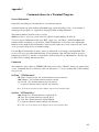
Appendix C
Communications via a Terminal Program
General Information
Setup and downloading are done with the use of an external computer.
A terminal emulator program facilitates Data Bank setup, and downloading of data. As an example of
setting up such a program, see “Appendix A: Setting Up Window's HyperTerminal”.
The terminal emulator should be set up as follows:
9600 baud, 8 bits, 1 stop bit, no parity, echo=off, add LF=on, hand-shaking= X-on/X-off.
To test for proper communication link, type "RST" (upper case), and “Enter”, and the Data Bank will
transmit serially; and display on your monitor, "Dataron Instruments", followed by text containing the
firmware version number and serial numbers. If this test fails, make sure you are connected to the correct
"com" port and re-check all of your terminal settings.
Note that Hyper-Terminal may be used to send a pre-defined file of all settings to the Data Bank. This
process is less error prone than individual entry of each parameter. Date and Time should be set before
using this procedure. Use “transfer -> send text file” then select the file (eg: DBdefault.txt). The file may
be edited, before sending, with any text editor.
Commands
All commands consist of three (3) UPPER CASE letters followed by a "SPACE", then by any required data
or text. Commands that do not return any other text will return a “*” (star) to indicate that a valid command
was processed.
Set Time: "STM hh:mm:ss"
"hh" Hours, 24 hour format. Two decimal characters must be entered.
"mm" Minutes. Two decimal characters must be entered.
"ss" Seconds. Two decimal characters must be entered.
":" A separator character must be entered; any character.
Note: Seconds are not shown on the display, but are stored with the data.
Set Date: "SDT mm/dd/yy"
"mm" Month. Two decimal characters required; 01-12.
"dd" Day. Two decimal characters required; 01-31.
"yy" Year. Two decimal characters required; 00-99.
"/" A separator character must be entered, any character.
Note: The year is not shown on the display, but is stored with the data.
40
Set Time Between Wake-Ups: "TBW hh:mm:ss"
In logging mode, this is the time between wake ups, whereupon data is again logged. After logging,
the unit will turn itself back off. Entry format is as in "Set Time". Range 00:00:01 to 99:59:59
(hh:mm:ss).
Note: If TBW is less than the time required for system and sensor warm up, logging will proceed as
programmed, but power will not shut off between sample times.
Start Logging: “LOG”, “LOG X”, “LOG hh:mm” or “LOG hh:mm X” (> Ver. 2.02)
LOG, initiates standard logging mode with power off between logging intervals.
LOG X, as above except power remains on between logging intervals.
LOG hh:mm; enters standard logging mode, to begin after the entered delay, within the
range of 1 minute to 99 hours, 99 minutes.
LOG hh:mm X, as above except power will remain on during delay, and while logging.
Clear Stored Data: "CSD"
Writes blanks ("FF hex") into each previously used data record.
A “Ctrl C” can be used to stop the process, however, all pointers will still be reset to zero so that
new data records will overwrite the old ones.
Note: Data is not cleared automatically after a download. The CSD command, must be
used, to clear out previously recorded data. The rate is ~ 140 records/second.
The Data Bank will display the progress until completed.
Caution: be sure you have downloaded all the data records that you wish to save before use of this
command. CSD is irreversible. All Data Will Be Lost
Reset System: "RST x"
"RST" = Performs a warm boot after first disabling the logging mode and saving all data. Time or
date registers are not affected, including the time between wakeups (logging).
Each of those must be set individually, if needed. The display mode is not affected.
“RST T” = Sets the Data Bank display mode to the “Title” mode.
Example: “Amazon River Mud”
“RST D” = Sets the Data Bank display mode to the “Date & Time” mode.
Example: “#01 11/03 12:32”
Download Data: "DLD s" (See Appendix B for detailed information)
“s” is the sort value. SPACE=none. 0-F (for parameter groups 1-16) will cause only the selected
records to be downloaded. If uppercase "S" is entered, the download will sort records sequentially
starting with group number 1. This character is optional.
Once initialized, the download will be paused until a X-On (Ctrl Q) is received serially, or the
Recall button is pressed on the Data Bank.
The Data Bank will display the downloading progress until completed.
Note: Downloads may be canceled with a Ctrl C or Ctrl X. Also, downloads may be paused and restarted by X-OFF and X-ON (Ctrl S and Ctrl Q). For more detailed help with downloads see
“Appendix B: Using HyperTerminal to Download Data Files”.
41
Set Warm Up Time: "WRM ttt"
"ttt", in 1/10 seconds to 255 (25.5 seconds), is the time that the external sensor is "warmed up"
before the Data Bank begins taking readings from it. Three (3) decimal characters must be entered.
Set Back Light Time: "BLT tttL"
“ttt" in seconds up to 127, is the time the backlight remains on once activated.
If set to "000" no timeout will occur; display will remain on until manually shut off. Three
characters must be entered for “ttt”.
"L" (optional) sets the backlight to low power mode (50%). Any other character will cause full
power to be applied while the backlight is on.
Set Output Voltage: "SOV xx"
“xx” in hexadecimal from FF to 00 for 3 to 12 volts for the powering of the external sensor. Use the
below formula, then convert the result to hexadecimal before entering:
value to enter = (12.3 – desired volts) * 26.6
Calibration Mode: "CAL brg" (Exit using a "CTRL C")
This mode is designed for use by Windows GUI software. It is used by the “Assisted Calibration”
routine. Once initialized, it serially transmits the sensor’s averaged readings, continuously, until
cancelled by a CTRL C. Note: CAL is not available during charging.
“b” is the number of bursts per sample, 0,1,3,7 (for 1,2,4,8); @ 30 Hz
“r” is the number of readings per burst, 0,1,3,7,F (for 1,2,4,8,16); @ 1000 Hz
“g” is optional gain setting, 0-3. Default=0.
(Note: “g” vs. Seapoint gains: 0=1x, 1=5x, 2=20x, 3=100x)
Notes regarding “Curves” “Curves” are the formula portion of the 16 parameter groups.
When done manually, the process of defining curves, and entering converted values, is a very
difficult task. The use of the “Windows / Data Bank Graphical User Interface” is recommended as
its “Assisted Calibration” has it ability to automate the process.
The following commands are for the setup of curve information.
The basic ingredient of the curve is the formula needed to generate the curve. Up to third order
polynomials can be handled by the Data Bank.
The use of “Order” numbers is illustrated in the following polynomial: (Where mV = sensor voltage):
Result = (Order 3 * mV cubed) + (Order 2 * mV squared) + (Order 1 * mV) + (Order 0)
With only Orders 0 & 1 used: the equation is a linear equation. With the addition of Order 2, the equation
defines a curve. Adding a 3rd Order, and the equation can define an "S" curve. Order 0 is always the offset
value.
The Data Bank’s internal processor works only with whole numbers, so to maintain accuracy to better than
six (6) decimal places, while maintaining internal processing speed, the decimal numbers for orders 0 and 1
are multiplied by 1,000,000 hex before they are entered. Increased accuracy is required for the next two
orders; Order 2 multiply by 100,000,000 hex, and order 3 by 10,000,000,000 hex.
42
Set Curve (Polynomial): "SCV co xxxxxxxxxx"
(See additional documentation ???)
“c” is the group number 0-F for group # 1-16.
“o” is the order number 0-3 (each order must be entered individually)
“x” is 10 hexadecimal characters (actual value times 1,000,000 Hex)
Spaces are required as illustrated above.
All three (3) orders must be entered for every curve (polynomial). Unused orders need to be set to
0000000000. The decimal range of each number is + or – 32,767.99999995.
Note: most scientific calculators will not allow conversions out to 10 hexadecimal digits. A simple workaround is to; first, take the integer portion of your number and convert it to hexadecimal. Jot down the
result, padding with leading zeros if necessary, to make exactly four (4) digits. Then take the decimal part
of your number (<1) times 16777216 (1,000,000 hex). Convert this number to hexadecimal. Jot down the
result, again padding with leading zeros, if needed, to make 6 digits. Place them to the right of your first
result. You now have your ten (10) digit hexadecimal result. For example: 123.456 * 16777216 =
007B74BC6A Hex.
(Step 1; 123 = 7B hex = 007B. Step 2; .456 * 16777216 = 7650410.496 = 74BC6A hex.)
If the number is negative be sure to use "-" for each side of the calculation. If the fraction portion of the
number is not zero (0), increment the integer portion before converting to hex. After the conversion, drop
any upper digits you don’t need. For example: -123, goes to –124 = FFFFFF84.
Needing only four digits, = FF84. Then -.456 * 16777216= FF8B4396. The result=FF848B4396.
The above works for orders 0 and 1 (with a range of +/- 32,768). For order 2, first multiply the number you
wish to convert by 256 (100 hex), then perform the above steps (the range is +/- 128). For order 3, first
multiply by 65,536 (10,000 hex), limiting its range to +/- 0.5.
Set Title (Description): "STT c eeee dddddddddddddddd"
“c” is the group number, hexadecimal digit 0-F for group # 1-16.
“e” is the engineering units. Example: “mg/l”. Must have four (4) characters.
“d” is the description, up to 16 characters. Example: “Amazon River Mud”.
Spaces are required as illustrated, and are also valid characters for “e” or “d”.
Number of samples (and Gain): "NOS cbrg"
“c” is the group number, 0-F for group # 1-16
“b” is the number of bursts to average per sample, 0,1,3,7 (for 1,2,4,8); @ 30 Hz
“r” is the number of readings per burst, 0,1,3,7,F (for 1,2,4,8,16); @ 1000 Hz
(Note: total readings averaged will be b*r , or 1 to 128)
“g” is optional gain setting, 0-3. Default=0 (Applies only to sensors so equipped).
(Note: “g” vs. Seapoint gains: 0=1x, 1=5x, 2=20x, 3=100x)
(Note: “g” vs. Cyclops-7 gains: 3=1x, 2=10x, 1=100x, 0=not valid.)
43
The Following Commands Apply to Newer Data Banks only:
In version 2.02 serial output, of currently logging data, was added for transmission via modem.
Initialize Logging Modes: “LOG hh:mm” “LOG X hh:mm” Ver. 2.03 or greater
hh:mm (hours:minutes) are optional. Sets a delay time before logging will start.
“LOG” Starts standard logging. If hh:mm is set, logging will start after that delay.
In Standard Logging, power will shut off (if possible) between logging intervals.
“LOG X” Starts special logging mode. If hh:mm is set, logging will start after that delay.
In this Special Logging mode, power will remain ON between logging intervals.
This mode is appropriate when externally powered and connected to a modem.
Note: RST command may be used to end either of the above logging modes.
Output Dual Results: “DBL ON” or “DBL OFF” Ver. 2.06 or greater
On occasion a user may want to display both turbidity and suspended solids at the same time.
During logging (via the serial port), and during downloads of the data file, if “Double” is turned on,
the calculated value of the selected group number, as well as the calculated value of the next group
number, will be displayed on the same line. In other words, two formulas are applied, and their
results displayed, for each reading of the sensor.
Notes:
1) “Double” may be turned on just before downloading, even if it was not on during logging.
2) If the selected group # is 16, then the next formula displayed will be from group #1.
3) When on, Engineering units will be shown for each of the displayed results.
44
Appendix D
Recovering from Data Bank Upgrade Errors
Normally if the Data Bank turned off, instead off entering the Upgrade mode it’s just a sign that the button
timing or sequence was not correct, and no harm was done.
If the software is still waiting for completion of the entry process (“Initialize Data Bank for Upgrade” frame
is still open) simply turn the Data Bank back on and try again. If the power is still on, press all three
buttons to perform a Reset. Turn the Data Bank back on, and try again.
In the event that the Upgrade program got cancelled, you can close the Data Bank GUI program, and then
re-start it, and it will begin the Upgrade process all over.
If something has happened that the Data Bank has had its program erased (older units only), but the
uploading of the new software failed (because of removing the cable, resetting the Data Bank, or a crashed
Windows program, etc.) may not turn off, or it’s off and you can’t make it stay on or display anything, then
the program has erased, but not successfully re-programmed. A four-button reset will work on newer units
to restore the previous program. If that doesn’t work (older units), follow the instructions below.
1,1) On your Data Bank CD you’ll find a file “Data Bank.ht”. Double click it and it should open your
Hyper-Terminal program, all set up for communications with the Data Bank, with the exception of possibly
having to change the Com port. (Or you may use the standard Hyper-Terminal program and set the settings
to 9600,N,8,1 and the appropriate com port.)
1,2) The Data Bank requires a valid RTS signal in order to open the programming lock within the Data
Bank. The Hyper-Terminal program is used to supply this signal, allowing the programming mode to be
entered. Follow the same button sequence used previously (see page 17).
1,3) If the Data Bank enters the programming mode successfully its power will remain on when the power
button is released. Hyper-Terminal will also display some text (ADI ??? ???).
If program entry fails, recheck for the proper com port, and retry button sequence until successful.
If program entry succeeded, close the Hyper-Terminal program.
2,1) On your Data Bank CD is a program “WSD_V6_7.exe” (or similar). This is Analog Devices
“Windows Serial Downloader” program. Please install this program.
2,2) Start the WSD program.
If the programs window shows (among other things) “ADuC812” or “ADuC841” then the computer chip is
recognized and all is OK. You can go on to the next step.
If it failed, click the “Configuration” button, verify settings of 9600 bps and 11.059MHz, and then try
another Com port. Afterwards, click the Reset button.). Repeat, if necessary, for other Com ports.
Also, it is assumed that the Data Bank is powered up and in the programming mode.
2,3) Once the Reset is successful, click the DOWNLOAD button, then select the hex file that you originally
intended to send. Downloading will start automatically.
2,4) When completed, click the RUN button and the Data Bank should now be running your new code.
This completes the fix. Close WSD.
45
Product Guarantees
30 Day Money Back Guarantee:
If the purchaser is dissatisfied with any of Dataron Instruments’ products the customer may return that
product (in new condition), within 30 days (ship date to ship date), for a full refund (less shipping).
In the event that the product is returned damaged, the customer’s refund will be reduced by the cost of
restoring the product to new condition. In this event, the customer will be notified regarding the cost of the
repairs before the repairs are completed.
3 Years Parts and Labor:
All products manufactured by Dataron Instruments are warranted against defects in material or
workmanship for a period of THREE years from the original date of shipment.
If it is determined that the required repairs are due to defective materials or workmanship, Dataron
Instruments will cover the costs of the repair; including parts, labor, and return shipping.
In the event that it is determined that the required repair is due to other than normal use or service, Dataron
Instruments will notify the customer of the cost of repairs and shipping before doing any repairs. Upon
customer approval the repairs will be completed.
Note: Battery life span is not guaranteed. Battery life is dependent mainly on the number of charges.
Normally our batteries should endure 500 charge cycles, however, heavy loads and excessive recharging
can shorten that life span. Of course our batteries are still covered against defects in material or
workmanship, including damage done by circuitry that has failed due to defective parts or workmanship.
Please contact Dataron Instruments prior to any returns:
Phone: 1-360-580-2220 or [email protected]
Returned products must be shipped prepaid. As Dataron Instruments accepts no responsibility for
damage during shipping, it is best to insure return shipments.
Ship to:
Dataron Instruments
92-8216 Marlin Blvd., Box 6811
Ocean View, HI 96737-6811 USA
Note: as the years go by, we might have moved. Please check our current address at our website:
http://www.dataron.com/DataronContact.html
Also, you can always find the latest software updates, or User Manual, at our website:
http://www.dataron.com/Updates.html
46