Download T - Wseas

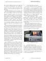
Virginia Finca, Radu Zglimbea,
Emilian Greaban, Constantin Marin
WSEAS TRANSACTIONS on SYSTEMS and CONTROL
Methods for Parameters Identification of a HVAC Installation
VIRGINIA FINCA, RADU ZGLIMBEA, EMILIAN GREABAN, CONSTANTIN MARIN
Department of Automation
University of Craiova
Bd. Decebal, no.5, Craiova
ROMANIA
[email protected]
Abstract: — This paper presents a procedure for time variant system identification based on some
experimental studies. Some of the system parameters change in time according to unknown laws. These laws
are expressed as finite degree time polynomials whose parameters are included in the set of parameters to be
identified. Mainly it is an extension of the procedure developed in [1]. The theoretical methods are now
applied on some concrete platform. Our paper presents the concretization of some experimental identification
methods on experimental workbench from Quanser. HVAC installation is a test installation for controlling
temperature in a chamber, and for parameters identification
Key-Words: - Continuous time systems, Identification, Nonlinear systems, HVAC, Quanser.
direction in continuous-time system identification is
to transform the system differential equations to an
algebraic system that reveals the unknown
parameters. By using some measures, the direct
computation of the input-output data derivatives can
be completely avoided. For linear system
identification, several methods are reported on this
direction: identification based on weighted
moments; use of the Poisson moment functional;
using the Laplace transformation and then use the
Laguerre filter; or transforming the continuous-time
system to the frequency domain. [4],[11],[12],[16]
Nonlinear identification is an increasingly active
research area. Among the various approaches that
have been developed are nonparametric methods,
which are primarily frequency-domain based. These
methods include techniques for identifying Volterra
kernels, which characterize input-output response
fey means of a sum of multi-frequency
convolutions. For time-domain simulation, however,
it is convenient to construct nonlinear state-space
realizations of these maps, which may be difficult in
practice [1]. On the other hand, parametric methods
have been developed based on structured and
1 Introduction
The analysis of time-varying or time-periodic
nonlinear systems is challenging, requiring a degree
of sophistication not needed for autonomous
nonlinear systems. Most analysis methods for timevarying nonlinear dynamical systems are coordinatebased approaches that do not utilize the power and
generality afforded to a description using the
language of differential geometry. Such an oversight
has important consequences in the area of control of
under actuated nonlinear systems due to the
increasing prevalence of geometric techniques for
the study of nonlinear control systems.
In recent years, a progress has been made in the
area of continuous-time system identification. Even
if the most physical systems are naturally
continuous, a much more attention has been paid to
parameter estimation of discrete-time systems,
mainly because they are better suited for numerical
implementations. Continuous-time identification
makes possible a more direct link to the physical
properties and operation of the underlying systems
and the direct estimation of physical parameters
which have a clear significance. One important
ISSN: 1991-8763
455
Issue 9, Volume 4, September 2009
Virginia Finca, Radu Zglimbea,
Emilian Greaban, Constantin Marin
WSEAS TRANSACTIONS on SYSTEMS and CONTROL
unstructured time-domain models. Unstructured or
black-box models [1,3] often rely on neural network
models to exploit their function approximation
properties. Structured or gray-box models [5] are
based on the interconnection of linear and nonlinear
subsystems [2].
It is essential to ‘know and understand’ a system
before it is handled, manipulated or controlled. A
system is known through modeling and
identification and understood by analysis. Modeling
and identification happen to be a conjugate pair of
activities in the process of developing knowledge
about a system. They are prerequisites to the
practice of automatic control. Modeling by itself is a
very vast area rich in a host of well-established
methods that are based on a variety of principles.
Among the many variants, modeling on the basis of
physical unified framework principles can hardly be
overemphasized, particularly for physical systems.
The key problem in system identification is to
find a suitable model structure within which a good
model is to be found. Fitting a model within a given
structure (parameter estimation) is in most cases a
lesser problem. A basic rule in estimation is not to
estimate what you already know. In other words,
one should utilize prior knowledge and physical
insight about the system when selecting the model
structure. It is customary to distinguish between
three levels of prior knowledge, which have been
‘color-coded’ as follows.
• White-box models. This is the case when a model
is perfectly known; it has been possible to construct
it entirely from prior knowledge and physical
insight.
• Gray-box models. This is the case when some
physical insight is available, but several parameters
remain to be determined from observed data. It is
useful to consider two sub cases.
1. Physical modeling. A model structure can be built
on physical grounds, which has a certain number of
parameters to be estimated from data. This could,
for example, be a state-space model of given order
and structure.
2. Semi physical modeling. Physical insight is used
to suggest certain nonlinear combinations of
ISSN: 1991-8763
measured data signal. These new signals are then
subjected to model structures of black-box character.
• Black-box models. No physical insight is available
or used, but the chosen model structure belongs to
families that are known to have good flexibility and
have been ‘successful in the past’.[3]
Obviously, a large number of dynamical systems
encountered in practice are both continuous in time
and nonlinear. Moreover, identification of
continuous-time systems from available sampled
input-output data records is desirable to enhance the
interpretation of the dynamical system behavior and
to support the controller design. Clearly, the
identification of continuous-time nonlinear systems
is a topic which has received considerable attention.
To identify a plant based on parametric models one
requires either a general or a special nonlinear
model. The former uses a general description to
represent the process while the latter considers
nonlinear models of a particular type which are
appropriate for certain classes of processes. Thus,
nonlinear systems may be investigated with the help
of a series polynomial expansions approach, such as
a Hammerstein model. The Hammerstein model is a
nonlinear model which describes a special class of
system nonlinearities, and it can be represented by
the series interconnection of a static nonlinear
element followed by a linear dynamic model.
2 Theoretical Aspects Of Continuous
Time Systems Identification
Let us consider a dynamical continuous time
system with nu inputs,
u : E → E n , t → u (t ), u ∈ Ω
u
(1)
and n y outputs,
y:E → E
n yu
, t → u (t ), u ∈ Γ
(2)
where Ω represents the set of admissible inputs and
Γ is the set of possible outputs. It can be expressed
by a differential operator,
qθ / (u , y ) = Q(u , y , θ )
(3)
whose expression depends on a vector of parameters
θ = [θ 1 ...θ i ...θ p ]
T
456
(4)
Issue 9, Volume 4, September 2009
Virginia Finca, Radu Zglimbea,
Emilian Greaban, Constantin Marin
WSEAS TRANSACTIONS on SYSTEMS and CONTROL
[
](
The operator (3), whose class can be determined,
represents a family of models with a given structure
wi (t ) = ∑ Ψi j (u (t ), y (t ))
realization of the model if the function
ν (t ) = ∑ [Ψ0j (u (t ), y (t ))]
pi
(5)
is the zero function,
qθ / (u , y ) = 0
(6)
*
*
*
*
that means,
qθ / (u
*
*
, y*
(
)
*
*
*
) (t ) = Q u (t ), y (t ), θ = 0, ∀t ∈ E
(t ) = Q(u (t ), y(t ),θ * ) = 0, ∀t ∈ i, ∀(u, y )∈ Ω × Γ
output pair (uT , yT ) ,
(9)
θˆ = θˆ(uT , yT , Q )
(17)
(10)
in a such a way that,
qθˆ / (u , y ) (t ) = 0, ∀t ∈ E
(18)
T
qθˆ / (u , y ) (t ) = 0, ∀t ∈ E , ∀(u , y ) ∈ Ω × Γ
system. As the unknown parameter θ has a finite
number p of components, then it will be enough to
represent a sum of the
choose (utilize) a finite number N of time instants,
ti , i = 1 : N based on which to create an algebraic
derivatives of some known, possible nonlinear,
functions Ψi , Ψ , with respect to the input and
j
0
(12)
equation. In the specific case of (11), this is a linear
system
(20)
Wθ = v
Where W is a N × p matrix of real numbers,
(13)
W = w(t1 ) ;...; w(ti ) ;...; w(t N )
output variables,
pi
[
](
wi = ∑ Ψi j (u , y )
ni j
)
, i = 1: p
j =1
ν = ∑ [Ψ0j (u , y )]
(n )
p0
j
0
[
j =1
Parameters
pi , nij , p0 , n0j
are
given
integer
(22)
]
v = [v(t1 ),..., v(ti ),..., v(t N )]
(23)
unique solution is obtained,
−1
θˆ = (W T W ) W T v = θ *
(24)
Let us denote r = rank (W ) . If r = p , then a
(14)
i =1
The equation (24) is of no practical interest
because it is not recommended to measure (or to
estimate) the derivatives of signals, mainly when
]
w T (t ) = w1 (t ), ..., wi (t ), ..., w p (t )
ISSN: 1991-8763
Whose i-th row ( i = 1 : N ) is,
w(ti ) = w1 (ti ),..., wk (ti ),..., w p (ti )
T
T
p
[
(21)
T
The symbol v denotes a N column real vector,
value of the function qθ / (u, y ) (t ) is a real vector
where
]
T
[
numbers. The identification problem, into condition
(11), has a unique solution. At any time instant t, for
a measured input-output pair of functions (u, y ) the
qθ / (u , y ) (t ) = ∑ wi (t )θ − ν (t ) = w T (t )θ − ν (t )
(19)
For any input-output pair (u , y ) observed to that
(11)
i =1
j
T
This condition involves,
p
Where wi and ν
respectively. If no
model structure Q , (3), and the observed input-
A special case is the model (3) expressing a
linear relation in the parameters
qθ / (u , y ) = Q(u , y ,θ ) = ∑ wiθ −ν = wT θ − ν
(16)
confusion would appear, then we may drop the
subscript T .
An identification problem means to determine the
parameter θ = θˆ , given the priori information on the
2. Uniqueness condition
qθ / (u , y ) (t ) = 0, ∀t ∈ i, (u , y ) ∈ Ω × Γ ⇒ θ = θ *
j
0
(uT , yT )
T is denoted by
(7)
or, equivalently,
/ (u , y )
(15)
Practically, it is possible to record the functions
(u, y) in the time interval T ⊂ E only, called
observation time interval or just time window. The
restriction of the functions (u, y ) to the time interval
*
*
(n )
p0
The value θ = θ * is consistent with the model (5)
if and only if the two following conditions are
accomplished:
1. Covering condition
(8)
qθ / (u , y ) = Q (u , y ,θ * ) = 0, ∀(u , y ) ∈ Ω × Γ
qθ
, i = 1: p
j =1
qθ / (u , y ) = Q (u * , y * ,θ * )
*
)
j =1
in constant parameters. A triple (u * , y * , θ * ) is a
*
nij
457
Issue 9, Volume 4, September 2009
Virginia Finca, Radu Zglimbea,
Emilian Greaban, Constantin Marin
WSEAS TRANSACTIONS on SYSTEMS and CONTROL
they are noise contamined. However, the equation
(24) has a form as in any discrete time identification
problem, where coefficients are values of the
functions u and y in different sampling time
moments.[9]
prevents the evaporation of sweat. High humidity
also decreases physical strength, which usually leads
to fatigue. An unhealthy surrounding can also affect
people’s thinking abilities. Hypothermia, heat
stroke, and hyperpyrexia, among others, are some of
the illnesses that may also occur
Heating, ventilating and air conditioning is based
on the principles of thermodynamics, fluid
mechanics, and heat transfer, and on inventions and
discoveries made by Michael Faraday, Willis
Carrier, Reuben Trane, James Joule, William
Rankine, Sadi Carnot, and many others. The
invention of the components of HVAC systems went
hand-in-hand with the industrial revolution, and new
methods of modernization, higher efficiency, and
system control are constantly introduced by
companies and inventors all over the world.
3
Technical Aspects on Taking
Experiments
In our laboratory we had elaborated some
technical procedures for parameters identification.
Our installation gave us the perfect way to analyze
the results we obtained.
HVAC (pronounced either "H-V-A-C" or "Hvak") is an initials or acronym that stands for
"heating, ventilating, and air conditioning". HVAC
is sometimes referred to as climate control and is
particularly important in the design of medium to
large industrial and office buildings such as
skyscrapers and in marine environments such as
aquariums, where humidity and temperature must all
be closely regulated while maintaining safe and
healthy conditions within. In certain regions (e.g.,
UK) the term "Building Services" is also used, but
may also include plumbing and electrical systems.
Refrigeration is sometimes added to the field's
abbreviation as HVAC&R or HVACR, or
ventilating is dropped as HACR (such as the
designation of HACR-rated circuit breakers).
The beginning of HVAC is not clear, though as
early as second century, a lot of Roman cities were
using a central heating system known as hypocaust.
This is further popularized during the Industrial
Revolution as big factories used it. Now most
modern buildings that you see have integrated
HVAC.
The HVAC system is also known as climate
control. This is because these three functions are
essential in maintaining comfort in every dwelling.
The primary use of HVAC is to regulate room
temperature, humidity, and air flow, ensuring that
such elements remain within their acceptable ranges.
Effective control of such factors minimizes healthrelated risks. A very humid atmosphere impairs the
body’s ability to regulate body temperature as it
ISSN: 1991-8763
Three Functions of HVAC
Heating is significant in maintaining adequate
room temperature especially during colder weather
conditions. There are two classifications of heating:
local and central. The latter is more commonly used
because it is more economical. Furnace or boiler,
heat pump, and radiator make up the heating system.
Ventilation, on the other hand, is associated with
air movement. There are many types of ventilation,
but they all function similarly. Ventilation is
necessary to allow carbon dioxide to go out and
oxygen to get in, making sure that people are
inhaling fresh air. Stagnant air causes the spreading
of sickness, usually airborne, and allergies. But it is
also essential to maintain an efficient ventilation
system, especially in the attics. Insufficient
ventilation usually promotes the growth of bacteria
and fungi such as molds because of high humidity. It
will also decrease the effectiveness of rafter and roof
sheathing insulation because of water vapor
condensation.
The air-conditioning system controls the heat as
well as ventilation. They often come in different
sizes. Most air conditioners have large air ducts, so
it is better to check out the building first to see if
they can be installed. Or else, you can use the split
system or remote coils. It is necessary, though, that
air ducts are properly cleaned. Pathogens thrive in
458
Issue 9, Volume 4, September 2009
Virginia Finca, Radu Zglimbea,
Emilian Greaban, Constantin Marin
WSEAS TRANSACTIONS on SYSTEMS and CONTROL
dirty air ducts. Return-air grills are also vulnerable
to chemical, microbiological, and radiological
elements. Thus, HVAC return-air grill height should
be that it is not accessible but visible for any
observation.
In modern buildings the design, installation, and
control systems of these functions are integrated into
one or more HVAC systems. For very small
buildings, contractors normally "size" and select
HVAC systems and equipment. For larger buildings
where required by law, "building services" designers
and engineers, such as mechanical, architectural, or
building services engineers analyze, design, and
specify the HVAC systems, and specialty
mechanical contractors build and commission them.
In all buildings, building permits and codecompliance inspections of the installations are the
norm.
How has technology changed in the HVAC field?
Well, using PLCs (programmable logic controllers)
in HVAC is the trend nowadays. But a great deal of
development of the HVAC system lies on the everchanging technology and continuous innovation.
Companies are adopting wireless technology after
they found out that networking HVAC controllers,
which often use sensors, can eventually cut
installation and labor costs. A lot of engineers are
also focused on further improving this technology
through the use of mesh wireless setup, which will
work for both the wireless sensor and wireless
controller networks. The only downside of this
could probably be the risk of being exposed to RF
(radio frequency) radiation.
The installation of an HVAC system is
imperative if we want to achieve maximum comfort
and be healthy in our homes, office spaces, or other
building facilities. But you also need to consider the
building size in installing an HVAC system.
Optimum efficiency and comfort level are best
achieved if the system is appropriate for the size.
After all, any ineffective system usually means more
incurred costs in the future. You should also see to it
that HVAC is carefully integrated to the overall
building design so other aspects needed for proper
operations, such as cabling, are not sacrificed.
ISSN: 1991-8763
A.
HVAC plant general presentation
The Quanser National Instruments Engineering
Trainer (QNET) is a versatile and powerful training
tool. Amongst its many capabilities, the QNET
series of trainers allows for PC based control using
the LABVIEW or Matlab programming language, a
National Instruments E-Series or M-Series data
acquisition card, and an ELVIS workstation. The
QNET allows for a scalable laboratory setup
utilizing the ELVIS workstation platform
As a quick nomenclature, Table 1, below,
provides a list of the principal elements composing
the Heating, Ventilation, and Air Conditioning
(HVAC) Trainer system. Every element is located
and identified, through a unique identification (ID)
number, on the
HVAC plant represented in Figure 1, below.
The Heating, Ventillation, and Air Conditioning
Trainer QNET module is designed to operate on the
NI-ELVIS platform. The ELVIS unit is connected to
an NI E-Series data acquisition card inside the PC.
The whole installation is presented in figure 1.
Figure 1. QNET HVAC process
B.
Workbench characteristics
The QNET-HVAC Trainer system consists of a
Plexiglas duct(chamber), equipped with a heater on
one end and a blower on the other. A thermistor is
placed in between at the location in the chamber
where the temperature is to be controlled. The heater
is made of a 12- Volt halogen lamp. The blower is a
24-Volt variable-speed fan.
459
Issue 9, Volume 4, September 2009
Virginia Finca, Radu Zglimbea,
Emilian Greaban, Constantin Marin
WSEAS TRANSACTIONS on SYSTEMS and CONTROL
Table 1, below, provides a list of the principal
elements composing the Heating, Ventilation, and
Air Conditioning (HVAC) Trainer system. Every
element is located as it is shown in figure 2, below
Figure 2. HVAC process
Figure 3. Process Response to a step voltage
TABLE 1.
HVAC COMPONENTS
Apparently the solution to all the problems witch
can appear are simply but if we study more careful
we will observe that we have some nonlinearity
given by the Temperature Sensor. Thus the block
diagram of our process it is shown in Figure 4.
No
1
2
3
4
Description
Heater/ Halogen Lamp
Blower/ Fan
Temperature Sensor
Chamber/ Duct
U [V] TEMPERATURE
SENSOR
The HVAC plant consists of two inputs, namely
the heater and blower voltages, for one output, the
chamber temperature. The system thermal resistance
and capacitance are not known. Additionally, the
heater and blower heat flow rate constants are also
unknown. Therefore, system identification is
required to model the dynamics of the plant. [7],[8]
The thermodynamics theory shows that the
behavior of chamber cooling dynamics due to air
blowing can be approximated by the following
simple-lag Laplace transfer function from blower
voltage to chamber temperature difference:
ΔT (s ) K
(1)
Gr (s ) = c = rp _ r
Vr (s ) τ r s + 1
Y0 C
Figure 4. Cooling Process Block Diagram
In our case we the Temperature Sensor it is a
thermistor with nonlinear characteristics.
A thermistor is a type of resistor whose resistance
varies with temperature. The word is a portmanteau
of thermal and resistor. Thermistors are widely used
as inrush current limiters, temperature sensors, selfresetting overcurrent protectors, and self-regulating
heating elements.
Thermistors differ from resistance temperature
detectors (RTD) in that the material used in a
thermistor is generally a ceramic or polymer, while
RTDs use pure metals. The temperature response is
also different; RTDs are useful over larger
temperature ranges, while thermistors typically
achieve a higher precision within a limited
temperature range [usually -90C to 130C].
Thermistors are special solid temperature sensors
that behave like temperature-sensitive electrical
resistors. No surprise then that their name is a
contraction of "thermal" and "resistor". There are
basically two broad types, NTC-Negative
where the difference with a constant ambient
temperature is defined as:
ΔTc = Tc − Ta
(2)
As defined in equation (1), the HVAC system
steady-state gain and time constant during cooling,
k rp _ r and τ r , can be determined experimentally by
analyzing the system open loop response to a step
input. A typical first-order temperature response to a
blower voltage step input is illustrated in Figure 3,
below. The heater voltage is held constant at zero.
ISSN: 1991-8763
COOLING
PROCESS
460
Issue 9, Volume 4, September 2009
Virginia Finca, Radu Zglimbea,
Emilian Greaban, Constantin Marin
WSEAS TRANSACTIONS on SYSTEMS and CONTROL
Temperature Coefficient, used mostly in
temperature sensing and PTC-Positive Temperature
Coefficient, used mostly in electric current control.
A thermistor is a thermally sensitive resistor that
exhibits a change in electrical resistance with a
change in its temperature. The resistance is
measured by passing a small, measured direct
current through it and measuring the voltage drop
produced.
When a current flows through a thermistor, it will
generate heat which will raise the temperature of the
thermistor above that of its environment. If the
thermistor is being used to measure the temperature
of the environment, this electrical heating may
introduce a significant error if a correction is not
made. Alternatively, this effect itself can be
exploited. It can, for example, make a sensitive airflow device employed in a sailplane rate-of-climb
instrument, the electronic variometer, or serve as a
timer for a relay as was formerly done in telephone
exchanges.
T
[ C]
Time
Figure 5. Sensor Characteristic
The parameters witch we have to identify from
this process are the gain factor k rp _ r and the time
constant τ r . Using the soft dedicated made by
Quanser we have had determined from diagrams
presented in figure below some experimental values:
Besides practical experiments we had consider
that will be useful to simulate our process and
compare the results. Thus we create his version in
Matlab Simulink and we obtained some edifying
results.Our virtual process has the form presented in
figure 6.
Figure 6. Experimental Cooling Process
The response of simulated process is shown in
what will follow in figure 7 and the evolution of the
system is quite good. We can say that the system
work properly even if due to the computer
truncation some approximations are made.
The standard reference temperature is the
thermistor body temperature at which nominal zeropower resistance is specified, usually 25°C. The
zero-power resistance is the dc resistance value of a
thermistor measured at a specified temperature with
a power dissipation by the thermistor low enough
that any further decrease in power will result in not
more than 0.1 percent change in resistance
From experiments we have established the type
on nonlinearity witch seems to describe best our
sensor. Thus we made our experiments considering
that in our process sensors characteristics it is one of
the form presented in figure 5.
ISSN: 1991-8763
Figure 7. Time response of real process – Simulink
461
Issue 9, Volume 4, September 2009
Virginia Finca, Radu Zglimbea,
Emilian Greaban, Constantin Marin
WSEAS TRANSACTIONS on SYSTEMS and CONTROL
The installation responses in the terms of
dedicated soft were obtained and looks like the ones
in figure below.
Figure 10. Time Evolution of Cooling Process with
Identified Parameters
In the next stage, after we have made the
identification we firs simulate the process. The
values of identified parameters were now
The response of HVAC installation after we have
had identified the parameters it is presented in what
will follow.
To ensure that our identification methods are
good we have made another experiment. The new
system makes o comparison between real values and
identified value. The new systems is the one from
the figure 11
⎡ deg C ⎤
K rp _ r = 2.45 ⎢
⎥, τ r = 29,18 [s ]
⎣ V ⎦
and the systems become same as in figure 8 and his
response is presented in figure 9 and figure 10
Figure 8. Experimental and Identified Process
Figure 11. Error comparisons
Figure 9. Time Evolution of Cooling Process
ISSN: 1991-8763
462
Issue 9, Volume 4, September 2009
Virginia Finca, Radu Zglimbea,
Emilian Greaban, Constantin Marin
WSEAS TRANSACTIONS on SYSTEMS and CONTROL
4 Conclusion
Through this research has been proved that it is
possible to identify all parameters of continuous
time systems even if they are related to measured
variables by rational expressions. This is possible if
the identification problem is formulated as a set of
interconnected identification problems with linear
dependences between parameters and measured
variables.
The obtained results have shown that our methods
are good and experimental tries has helped us to
refine our algorithms.
Figure 12. Temperature variation
As it is shown in figure above, we can see that
identification error produces temperature variation
with maximum 0.50C. The variation we obtained in
Simulink it reflects on real HVAC installation to as
we can see in figure 14 and figure 15.
ACKNOWLEDGEMENTS
This work was supported by the National
University Research Council - CNCSIS, Romania,
under the research projects ID 786, 2007 (PNCDI II)
References:
[1] C. Marin, System Identification Based on
Distribution Theory. Proceedings of the IASTED
International Conference Applied Simulation
and Modelling (ASM 2002), Crete, June, 2002
[2] C. Marin, System Identification by the method
of weighted moments, 12th Int. Conference on
Control Systems and Computer Science, CSCS
12, Bucharest
[3] Marin C., Marin E. D., A distribution approach
International
of
system
identification,
Symposium SINTES 10 , Craiova, Romania, May
2000.
[4] Harish J. Palanthandalam-Madapusi, Jesse B.
Hoag, Dennis S. Bernstein, Basis-Function
optimization for Subspace-Based Nonlinear
Identification of Systems with Measured-Input
Nonlinearities, Proceedings of the 2004
American
Control
Conference,
Boston,
Massachusetts, June, 2004
[5] H. Unbehauen, G.P. Rao, A review of
identification in continuous-time systems,
Annual Reviews in Control, Vol 20, 1998, pp.
145-171
Figure 14. Cooling Process with first set of
estimated parameters
Figure 15. Cooling Process with first set of
estimated parameters
ISSN: 1991-8763
463
Issue 9, Volume 4, September 2009
Virginia Finca, Radu Zglimbea,
Emilian Greaban, Constantin Marin
WSEAS TRANSACTIONS on SYSTEMS and CONTROL
[6]N. K.Sinh, G. P. Rao, “Identification of
continuous–time systems”, Dordreht: Kluwer
Academic Press
[7] Quanser NI-ELVIS Trainer, Heating,
Ventilation, and Air Conditioning User Manual
[8] N. K.Sinh, G. P. Rao, Identification of
continuous–time systems. Dordreht: Kluwer
Academic Press.
[9] C. Marin, "System Identification by the method
of weighted moments, 12th Int. Conference on
Control Systems and Computer Science, CSCS
12, Bucharest.
[10] T. Bastogne, H. Garnier, P. Sibille, "PMFbased subspace method for continuous-time
model identification deterministic study," Proc.
of 11th IFAC Symp.SYSID'97, Fukuoka, July,
1665-1670.
[11] A. E. Pearson, A. E. Lee, "On the identification
of polynomial input-output differential systems,"
IEEE Trans.Aut.Contr.,Vol. AC30, No8, 778782.
[12] A. Patra, H. Unbehauen, "Identification of a
class of nonlinear continuous time systems using
Hartley modulating functions," Int. J. Contr.
Vol.62, No.6,1431-1452.
[13] A. Ohsumi, K. Kameiama, "Subspace
identification for continuous-time systems via
distribution-based approach," Automatica, 38,
2002, 63-79.
[14] W. Kecs, P. Teodorescu, Introduction to
distribution theory with technical applications,
Editura Tehnica, Bucharest 1975.
[15] V. Barbu, Differential equations. Editura
Junimea, Iasi 1985.
[16] V. Utkin, Sliding modes in control
optimization, Springer, 1992.
ISSN: 1991-8763
464
Issue 9, Volume 4, September 2009