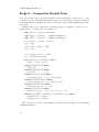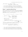
1
The Monad.Reader Issue 11
by Douglas M. Auclair [email protected]
and Kenneth Knowles [email protected]
and David F. Place [email protected]
August 25, 2008
Wouter Swierstra, editor.
Contents
Wouter Swierstra
Editorial
3
David F. Place
How to Refold a Map
5
Kenneth Knowles
First-Order Logic à la Carte
15
Douglas M. Auclair
MonadPlus: What a Super Monad!
39
2
Editorial
by Wouter Swierstra [email protected]
I’m happy to announce that the very first five issues of The Monad.Reader are
back on the Haskell wiki:
http://www.haskell.org/haskellwiki/The_Monad.Reader
Although most of the authors have agreed to the new Haskell wiki’s license, there’s
still work to be done. The new MediaWiki has slightly different formatting commands than the old MoinMoin wiki. If you decide to read any of the old articles
and can spare a few minutes to tidy up the formatting, I’d really appreciate your
help. Thanks to Gwern and Lemming for their efforts so far – but there’s still
plenty of work to go round. . .
In the meantime, enjoy this issue with three new great articles: David Place
shows how to use monoids to perform incremental computations over binary trees;
Kenn Knowles has written a series of transformations on logical formulas, using
rich type information to safely compose each individual step; Doug Auclair tops it
all off with a bit of monadic logic programming in Haskell.
How to Refold a Map
by David F. Place [email protected]
The full persistence of functional data structures is a reliable source of pleasure
when programming in Haskell. It often makes complex algorithms surprisingly easy
to code. In the following, I describe a small change to the balanced binary trees
used to implement the Data.Map module which allows incremental evaluation of
a fold over the elements of a Map. I found this to be efficacious in programming
optimization problems using local search, achieving a significant improvement in
execution time. Also, I bump into a snag and make a modest proposal.
Search Locally, Optimize Globally, Compute
Incrementally
Local Search algorithms for combinatorial optimization provide many different
strategies for coping with intractably large search spaces. An alphabet of metaphors from annealing crystals to zapping synapses [1] guide the search for a global
optimum, but all of these methods benefit from the efficient implementation of
utilities which modify a candidate solution to create its local neighbors in the
search space and evaluate an objective function to rank each new candidate.
The prototypical combinatorial optimization problem is the Traveling Salesman
Problem or TSP . (What better example problem since our topic is maps?) We
wish to construct a round trip itinerary that visits all of the cities in a list, minimizing the travel distance.
Algorithms for TSP typically create a neighbor of a candidate solution by swapping some of the city pairs. Some utilities to support this are given in Listing 1.
While this gives satisfactory logarithmic performance for creating a new neighbor,
it is disappointingly linear in computing the objective function on the new neighbor. Perhaps we can somehow take advantage of the mechanism which provides
satisfactory performance for update to improve the performance of the objective
function evaluation.
The Monad.Reader Issue 11
import qualified Data.Map as Map
type City = Int
type Distance = Int
type Tour = Map.Map (City, City) Distance
insertLeg :: City → City → Distance → Tour → Tour
insertLeg city1 city2 distance tour =
Map.insert (city1 , city2 ) distance tour
removeLeg :: City → City → Tour → Tour
removeLeg city1 city2 tour =
Map.delete (city1 , city2 ) tour
objectiveFunction :: Tour → Distance
objectiveFunction tour = Map.fold (+) 0 tour
Listing 1: Some Traveling Salesman Utilities
Some Terms of Art
Persistence
Previous versions of persistent (as opposed to ephemeral) data structures remain
available for operations after they have been updated. In the case of partially
persistent data structures, we can perform query operations on previous versions.
For fully persistent data structures, in addition to queries, further updates may be
performed on older versions, allowing a branching structure of versions to emerge.
A good example of this for the Haskell programmer is. . . pretty much any data
structure in Haskell. All functional data structures are fully persistent, because
one never actually mutates anything [2]. The amazing effort required to achieve
this property in imperative languages is well documented [3].
Incremental Evaluation
Incremental evaluation is simply a method of minimizing recomputation after some
sort of update. These methods are ubiquitous in our computing environments,
often appearing as ad hoc solutions to interactive computations. The incremental
redisplay algorithm controlling the display of emacs as I type this article must
surely be one of the most venerable examples. Some efforts have been made to
take more generalized approaches [4, 5], but many problems require specialized
solutions.
6
David F. Place: How to Refold a Map
Implementation
Taking a Hint
A quick glance at the source for the Data.Map module [6] reveals that, in addition
to the expected slots for key, value, and subtrees, the Bin data constructor of
the Map type has a slot for size which stores the number of elements in the
tree. Caching the size attribute is essential to the performance of the balancing
algorithm. Its value is maintained incrementally in precisely the same way that
we would like to compute the objective function.
When an update operation creates a new tree, much of the structure of the
old tree is shared, including the intermediate values of size which are stored in
the subtrees. The full persistence of the data structure leaves the shared part
available for all further queries and updates. Adding a slot for intermediate values
of the objective function as in Listing 2 imitates the behavior of size. The function
getValue which accesses this slot is modeled after size.
type Size = Int
data Map k a = Tip
| Bin a Size k a (Map k a) (Map k a)
size Tip = 0
size (Bin s
)=s
getValue Tip = 0
getValue (Bin x
)=x
Listing 2: Redefining Map.
We have defined our new slot using a type variable constraining it to be the same
type as the value of the (key, value) pair of the definition, but the definition of the
equation for getValue Tip is 0. Shall we limit this data structure to incrementally
evaluating Int valued functions? Any Haskell programmer knows the benefits of
laziness, but let’s not be that lazy!
Making it Classier
In Listing 3, we use the Monoid class [7] to restore the polymorphic type, which, in
spite of its scary name that sounds like an infectious hybrid of Mononucleosis and
Typhoid, provides exactly what we need. Any type we would like to store in this
data structure is required to provide a binary function (mappend :: a → a → a)
7
The Monad.Reader Issue 11
and its identity (mempty :: a). The Data.Monoid module provides many useful
instances of Monoid in addition to the Monoid class definition.
import Data.Monoid
getValue Tip = mempty
getValue (Bin x
)=x
iSum l x r = l ‘mappend ‘ x ‘mappend ‘ r
Listing 3: Using Monoid to compute incrementally.
In order to implement this change, we must do a small amount of rewriting of the
Data.Map module. The major part of this work is handled by the construction
function mkBin. In every place where the data constructor Bin is used in the
Data.Map module, we substitute mkBin.
mkBin sz k x l r = Bin x 0 sz k x l r
where x 0 = iSum (getValue l ) x (getValue r )
Listing 4: A new data constructor.
The last edit required is to change every place where Bin is used in a pattern
to ignore the additional first slot. (Of course, if Data.Map had been implemented
using records this step would not be needed.)
What a twist!
As we prepare to save the edited version, we hesitate. With horror, we realize that
we are about to commit an egregious act of copy and paste polymorphism. By
duplicating code rather than making it more abstract through refactoring and then
reusing, we are giving in to one of the very worst practices of software engineering –
in the twenty-first century! – in the world’s most advanced programming language!
How embarrassing! Perhaps we should study how it is done in the Haskell Libraries.
As we examine the source code for the Data.Set module [8] in the Haskell libraries, the truth is hard to take. Data.Map has been copied and pasted from
Data.Set. All of the balancing routines have been copied and changed to add a
slot for key to the Bin data constructor. This is terrible. Someone should do
something about it someday.
8
David F. Place: How to Refold a Map
Sharing is good
Well, there’s no time like the present. Let’s approach this problem in a way very
similar to our work in the previous section. In order to create an extensible version
of balanced binary trees, let’s have the types we want to store in the tree do all
of the work specific to each collection type; they can then share one definition of
balanced tree operations.
We’ll create a class to provide an interface to the different behaviors we expect as
in Listing 5. We name the first method synthesize in analogy with the synthesized
attributes of attribute grammars [9]. We add this code to Data.Set and edit each
occurrence of the Bin data constructor to be mkBin as we did previously. This
time, we don’t need to change the use of Bin in patterns because we are not
changing its definition. Let’s change the type and module name to BBTree. (See
Listing 10 in the Appendix for details.)
class Element a where
synthesize :: a → a → a → a
synthesize x = x
eZero :: a
eZero = ⊥
getContent :: (Element a) ⇒ BBTree a → a
getContent Tip = eZero
getContent (Bin x
)=x
mkBin :: (Element a) ⇒ Size → a → BBTree a → BBTree a → BBTree a
mkBin sz x l r = Bin sz x 0 l r
where x 0 = synthesize (getContent l ) x (getContent r )
Listing 5: The Element Class and utilities.
The trees are now constrained to hold only members of the Element class.
Listing 6 and Listing 7 offer a taste of the proposed refactoring of Data.Set and
Data.Map. The data constructor SE is used for creating set elements for insertion
into a BBTree used as a set. We’ve added a modified version of lookup to BBTree
which returns the entire object found in the subtree. The functions defined in the
Set module simply add and remove constructors to keep the types in alignment.
For Map, we construct map elements with ME . The ME type has specific
instances of classes Eq and Ord that compare only the keys. Our Map module’s
lookup wraps and unwraps the values in a way compatible with the interface of
Data.Map.
Now, let’s redefine our incremental function map in this new regime as in List-
9
The Monad.Reader Issue 11
module Set where
import qualified BBTree as BB
newtype SE a = SE a deriving (Eq, Ord )
instance BB .Element (SE a)
newtype Set a = Set (BB .BBTree (SE a))
empty :: Set a
empty = Set $ BB .empty
singleton :: a → Set a
singleton x = Set $ BB .singleton (SE x )
insert :: (Ord a) ⇒ a → Set a → Set a
insert x (Set t) = Set $ BB .insert (SE x ) t
member :: (Ord a) ⇒ a → Set a → Bool
member x (Set t) = maybe False (const True) $ BB .lookup (SE x ) t
Listing 6: Refactored Set.
module Map where
import qualified BBTree as BB
data ME k a = ME k a
instance Eq k ⇒ Eq (ME k a) where (ME x ) ≡ (ME y ) = x ≡ y
instance Ord k ⇒ Ord (ME k a) where
compare (ME x ) (ME y ) = compare x y
instance BB .Element (ME k a)
newtype Map k a = Map (BB .BBTree (ME k a))
empty :: Map k a
empty = Map $ BB .empty
singleton :: k → a → Map k a
singleton k x = Map $ BB .singleton (ME k x )
insert :: (Ord k ) ⇒ k → a → Map k a → Map k a
insert k x (Map t) = Map $ BB .insert (ME k x ) t
lookup :: (Monad m, Ord k ) ⇒ k → Map k a → m a
lookup k (Map t) = BB .lookup (ME k ⊥) t >>= λ(ME x ) → return x
Listing 7: Refactored Map.
10
David F. Place: How to Refold a Map
ing 8. The value ⊥ (that’s ”undefined” in unformatted Haskell) has great utility
here, allowing us to create instances of data types when we don’t care about some
of the components. This is also the first module to provide its own version of the
methods of the Element class which synthesize the value up the tree.
module IMap where
import qualified BBTree as BB
import Data.Monoid
data IE k a = IE k a a
instance Eq k ⇒ Eq (IE k a) where (IE x
) ≡ (IE y
)=x ≡y
instance Ord k ⇒ Ord (IE k a) where
compare (IE x
) (IE y
) = compare x y
instance Monoid a ⇒ BB .Element (IE k a) where
eZero = IE ⊥ ⊥ mempty
synthesize (IE
l ) (IE k x ) (IE
r) =
IE k x $ l ‘mappend ‘ x ‘mappend ‘ r
newtype Map k a = Map (BB .BBTree (IE k a))
empty :: Map k a
empty = Map $ BB .empty
insert :: (Ord k , Monoid a) ⇒ k → a → Map k a → Map k a
insert k x (Map t) = Map $ BB .insert (IE k x ⊥) t
delete :: (Monoid a, Ord k ) ⇒ k → Map k a → Map k a
delete k (Map t) = Map $ BB .delete (IE k ⊥ ⊥) t
getValue :: (Monoid a) ⇒ Map k a → a
getValue (Map t) = (λ(IE
x ) → x ) $ BB .getContent t
lookup :: (Monad m, Ord k ) ⇒ k → Map k a → m a
lookup k (Map t) = BB .lookup (IE k ⊥ ⊥) t >>= λ(IE x ) → return x
Listing 8: Refactored Incremental Map
Ready at Last
Everything is in place to redefine our Traveling Salesman Problem utilities in
Listing 9 with logarithmic performance when calculating the value of the objective function on neighbors. The Sum type is an instance of Monoid defined in
Data.Monoid to create the sum of members of the Num class.
11
The Monad.Reader Issue 11
import qualified IMap as IMap
import Data.Monoid
type City = Int
type Distance = Sum Int
type Tour = IMap.Map (City, City) Distance
insertLeg :: City → City → Distance → Tour → Tour
insertLeg city1 city2 distance tour =
IMap.insert (city1 , city2 ) distance tour
removeLeg :: City → City → Tour → Tour
removeLeg city1 city2 tour =
IMap.delete (city1 , city2 ) tour
objectiveFunction :: Tour → Distance
objectiveFunction tour = IMap.getValue tour
Listing 9: Improved Traveling Salesman Utilities
Results
The simplified Traveling Salesman utilities serve to introduce and motivate these
ideas, but real applications are much more complex. However, in a different application, which microtonally adjusts the pitches of harmonic adjacencies in examples
of Renaissance polyphony to realize them in Just Intonation [10, 11], I observe an
execution time speed up of 4-8x when I change to the incremental objective function.
I implemented enough of the refactored Map and Set modules to use them in
my application and found no measurable performance penalty.
Conclusions
We have made a small change to the implementation of Data.Map to increase
its utility for a whole class of applications. We took advantage of the natural
full persistence of functional data structures to easily implement an incremental
evaluation scheme. Haskell’s class system made it possible to turn a small hack
into a module with many potential uses.
We made a digression into refactoring and found it to be a pleasant experience
using Haskell’s classes. Perhaps this solution should be adopted in the Library
modules.
12
David F. Place: How to Refold a Map
About the Author
David F. Place is a composer whose music has been performed in the USA and
Europe. He is also a performer, musicologist and independent computer software
consultant specializing in embedded domain specific languages and end-user programming. He resides in Boston, MA, USA.
References
[1] Aarts and Lenstra. Introduction. In Emile Aarts and Jan Karel Lenstra (editors),
Local Search in Combinatorial Optimization. Wiley (1997).
[2] Chris Okasaki. Purely Functional Data Structures. Cambridge University Press,
Cambridge, England (1998).
[3] Driscoll, Sarnak, Sleator, and Tarjan. Making data structures persistent. JCSS:
Journal of Computer and System Sciences, 38 (1989). http://www.cs.cmu.edu/
~sleator/papers/making-data-structures-persistent.pdf.
[4] T. Reps. Generating Language-Based Environments. MIT Press, Cambridge, MA
(1984).
[5] Scott E. Hudson. Incremental attribute evaluation: A flexible algorithm for lazy
update. ACM Transactions on Programming Languages and Systems, 13(3):pages
315–341 (July 1991).
[6] http://www.haskell.org/ghc/docs/latest/html/libraries/containers/
src/Data-Map.html.
[7] http://www.haskell.org/ghc/docs/latest/html/libraries/base/src/
Data-Monoid.html.
[8] http://www.haskell.org/ghc/docs/latest/html/libraries/containers/
src/Data-Set.html.
[9] http://en.wikipedia.org/wiki/Attribute_grammar.
[10] Olivier Bettens. Renaissance Just Intonation: Attainable standard or utopian
dream? http://www.medieval.org/emfaq/zarlino/article1.html.
[11] Hieronimo Maffoni. Quam pulchri sunt gressus tui. In Knud Jeppesen (editor),
Italia Sacra Musica. Wilhelm Hansen, Copenhagen (1962). http://sneezy.cs.
nott.ac.uk/darcs/TMR/Issue11/maffoni.mp3.
13
Appendix
module BBTree where
import qualified Data.List as List
data BBTree a = Tip | Bin Size a (BBTree a) (BBTree a)
class Element a where
synthesize :: a → a → a → a
synthesize x = x
eZero :: a
eZero = ⊥
getContent :: (Element a) ⇒ BBTree a → a
getContent Tip = eZero
getContent (Bin x
)=x
mkBin :: (Element a) ⇒ Size → a → BBTree a → BBTree a → BBTree a
mkBin sz x l r = Bin sz x 0 l r
where x 0 = synthesize (getContent l ) x (getContent r )
singleton :: (Element a) ⇒ a → BBTree a
singleton x = mkBin 1 x Tip Tip
balance :: (Element a) ⇒ a → BBTree a → BBTree a → BBTree a
balance x l r
| sizeL + sizeR 6 1
= mkBin sizeX x l r
| sizeR > delta ∗ sizeL = rotateL x l r
| sizeL > delta ∗ sizeR = rotateR x l r
| otherwise
= mkBin sizeX x l r
where
sizeL = size l
sizeR = size r
sizeX = sizeL + sizeR + 1
Listing 10: Some Highlights of the BBTree Module
First-Order Logic à la Carte
by Kenneth Knowles [email protected]
Classical first-order logic has the pleasant property that a formula can be reduced
to an elegant implicative normal form through a series of syntactic simplifications. Using these transformations as a vehicle, this article demonstrates how to
use Haskell’s type system, specifically a variation on Swierstra’s “Data Types à la
Carte” method, to enforce the structural correctness property that these constructors are, in fact, eliminated by each stage of the transformation.
First-Order Logic
Consider the optimistic statement “Every person has a heart.” If we were asked
to write this formally in a logic or philosophy class, we might write the following
formula of classical first-order logic:
∀p. P erson(p) ⇒ ∃h. Heart(h) ∧ Has(p, h)
If asked to write the same property for testing by QuickCheck [1], we might
instead produce this code:
heartFact :: Person → Bool
heartFact p = has p (heart p)
where heart :: Person → Heart
...
These look rather different. Ignoring how some of the predicates moved into
our types, there are two other transformations involved. First, the universally
quantified p has been made a parameter, essentially making it a free variable of
the formula. Second, the existentially quantified h has been replaced by a function
heart that, for any person, returns their heart. How did we know to encode things
this way? We have performed first-order quantifier elimination in our heads!
The Monad.Reader Issue 11
This idea has an elegant instantiation for classical first-order logic which (along
with some other simple transformations) yields a useful normal form for any formula. This article is a tour of the normalization process, implemented in Haskell,
using a number of Haskell programming tricks. We will begin with just a couple
of formal definitions, but quickly move on to “all code, all the time.”
First, we need the primitive set of terms t, which are either variables x or function
symbols f applied to a list of terms (constants are functions of zero arguments).
t ::= x | f (t1 , · · · , tn )
Next, we add atomic predicates P over terms, and the logical constructions
to combine atomic predicates. Since we are talking about classical logic, many
constructs have duals, so they are presented side-by-side.
φ ::=
|
|
|
|
|
P (t1 , · · · , tn )
¬φ
φ1 ⇒ φ2
TT
| FF
φ1 ∧ φ2
| φ1 ∨ φ2
∀x. φ
| ∃x. φ
We will successively convert a closed (no free variables) first-order logic formula
into a series of equivalent formulae, eliminating many of the above constructs.
Eventually the result will be in implicative normal form, in which the placement
of all the logical connectives is strictly dictated, such that it does not even require a
recursive specification. Specifically, an implicative normal form is the conjunction
of a set of implications, each of which has a conjunction of terms on the left and
a disjunction of terms on the right:
^ h^
_ i∗
implicative normal form ::=
t∗ ⇒
t∗
The normal form may be very large compared to the input formula, but it is
convenient for many purposes, such as using Prolog’s resolution procedure or an
SMT (Satisfiability Modulo Theories) solver. The following process for normalizing
a formula is described by Russell and Norvig [2] in seven steps:
1. Eliminate implications.
2. Move negations inwards.
3. Standardize variable names.
4. Eliminate existential quantification, reaching Skolem normal form.
5. Eliminate universal quantification, reaching prenex formal form.
6. Distribute boolean connectives, reaching conjunctive normal form.
7. Gather negated atoms, reaching implicative normal form.
Keeping in mind the pattern of systematically simplifying the syntax of a formula, let us consider some Haskell data structures for representing first-order logic.
16
Kenneth Knowles: First-Order Logic à la Carte
A Natural Encoding
Experienced Haskellers may translate the above definitions into the following
Haskell data types immediately upon reading them:
data Term = Const String [Term ]
| Var String
We will reuse the constructor names from FOL later, though, so this is not part
of the code for the demonstration.
data FOL = Impl FOL FOL
| Atom String [Term ] | Not FOL
| TT
| FF
| Or FOL FOL
| And FOL FOL
| Exists String FOL | Forall String FOL
To make things more interesting, let us work with the formula representing the
statement “If there is a person that eats every food, then there is no food that
noone eats.”
∃p. P erson(p) ∧ ∀f. F ood(f ) ⇒ Eats(p, f )
⇒ ¬∃f. F ood(f ) ∧ ¬∃p. P erson(p) ∧ Eats(p, f )
foodFact =
(Impl
(Exists "p"
(And (Atom "Person" [Var "p"])
(Forall "f"
(Impl (Atom "Food" [Var "f"])
(Atom "Eats" [Var "p", Var "f"])))))
(Not (Exists "f"
(And (Atom "Food" [Var "f"])
(Not (Exists "p"
(And (Atom "Person" [Var "p"])
(Atom "Eats" [Var "f"]))))))))
Higher-Order Abstract Syntax
While the above encoding is natural to write down, it has drawbacks for actual
work. The first thing to notice is that we are using the String type to represent variables, and may have to carefully manage scoping. But what do variables
17
The Monad.Reader Issue 11
range over? Terms. And Haskell already has variables that range over the data
type Term, so we can re-use Haskell’s implementation; this technique is known as
higher-order abstract syntax (HOAS).
data FOL = Impl FOL FOL
| Atom String [Term ] | Not FOL
| TT
| FF
| Or FOL FOL
| And FOL FOL
| Exists (Term → FOL) | Forall (Term → FOL)
In a HOAS encoding, the binder of the object language (the quantifiers of firstorder logic) are implemented using the binders of the metalanguage (Haskell).
For example, where in the previous encoding we would represent ∃x. P (x) as
Exists "x" (Const "P" [Var "x"]) we now represent it with Exists (λx →
(Const "P" [x ])). And our example becomes:
foodFact =
(Impl
(Exists $ λp →
(And (Atom "Person" [p ])
(Forall $ λf →
(Impl (Atom "Food" [f ])
(Atom "Eats" [p, f ])))))
(Not (Exists $ λf →
(And (Atom "Food" [f ])
(Not (Exists $ λp →
(And (Atom "Person" [p ])
(Atom "Eats" [f ]))))))))
Since the variables p and f have taken the place of the String variable names,
Haskell’s binding structure now ensures that we cannot construct a first-order logic
formula with unbound variables, unless we use the Var constructor, which is still
present because we will need it later. Another important benefit is that the type
now expresses that the variables range over the Term data type, while before it
was up to us to properly interpret the String variable names.
Exercise 1. Modify the code of this article so that the Var constructor is not
introduced until it is required in stage 5.
Data Types à la Carte
But even using this improved encoding, all our transformations will be of type
FOL → FOL. Because this type does not express the structure of the computation very precisely, we must rely on human inspection to ensure that each stage is
18
Kenneth Knowles: First-Order Logic à la Carte
written correctly. More importantly, we are not making manifest the requirement
of certain stages that the prior stages’ transformations have been performed. For
example, our elimination of universal quantification is only a correct transformation when existentials have already been eliminated. A good goal for refining our
type structure is to describe our data with types that reflect which connectives
may be present.
Swierstra proposes a technique [3] whereby a variant data type is built up by
mixing and matching constructors of different functors using their coproduct (⊕),
which is the “smallest” functor containing both of its arguments.
data (f ⊕ g) a = Inl (f a) | Inr (g a)
infixr 6 ⊕
instance (Functor f , Functor g) ⇒ Functor (f ⊕ g) where
fmap f (Inl x ) = Inl (fmap f x )
fmap f (Inr x ) = Inr (fmap f x )
The ⊕ constructor is like Either but it operates on functors. This difference
is crucial – if f and g represent two constructors that we wish to combine into a
larger recursive data type, then the type parameter a represents the type of their
subformulae.
To work conveniently with coproducts, we define a type class ,→ that implements
subtyping by explicitly providing an injection from one of the constructors to the
larger coproduct data type. There are some technical aspects to making sure
current Haskell implementations can figure out the needed instances of ,→, but
in this example we need only Swierstra’s original subsumption instances, found in
Figure 2. For your own use of the technique, discussion on Phil Wadler’s blog [4]
and the Haskell-Cafe mailing list [5] may be helpful.
If the above seems a bit abstract or confusing, it will become very clear when
we put it into practice. Let us immediately do so by encoding the constructors of
first-order logic in this modular fashion.
data TT
data FF
data Atom
data Not
data Or
data And
data Impl
data Exists
data Forall
a
a
a
a
a
a
a
a
a
= TT
= FF
= Atom String [Term ]
= Not a
= Or a a
= And a a
= Impl a a
= Exists (Term → a)
= Forall (Term → a)
19
The Monad.Reader Issue 11
{-#
{-#
{-#
{-#
LANGUAGE
LANGUAGE
LANGUAGE
LANGUAGE
RankNTypes,TypeOperators,PatternSignatures #-}
UndecidableInstances,IncoherentInstances #-}
MultiParamTypeClasses,TypeSynonymInstances #-}
FlexibleContexts,FlexibleInstances #-}
import Text.PrettyPrint.HughesPJ
import Control .Monad .State
import Prelude hiding (or , and , not)
Figure 1: LANGUAGE pragma and module imports
class (Functor sub, Functor sup) ⇒ sub ,→ sup where
inj :: sub a → sup a
instance Functor f ⇒ (,→) f f where
inj = id
instance (Functor f , Functor g) ⇒ (,→) f (f ⊕ g) where
inj = Inl
instance (Functor f , Functor g, Functor h, (f ,→ g))
⇒ (,→) f (h ⊕ g) where
inj = Inr ◦ inj
Figure 2: Subsumption instances
20
Kenneth Knowles: First-Order Logic à la Carte
Each constructor is parameterized by a type a of subformulae; TT , FF , and
Atom do not have any subformulae so they ignore their parameter. Logical operations such as And have two subformulae. Correspondingly, the And constructor
takes two arguments of type a.
The compound functor Input is now the specification of which constructors may
appear in a first-order logic formula.
type Input = TT ⊕ FF ⊕ Atom
⊕ Not ⊕ Or ⊕ And ⊕ Impl
⊕ Exists ⊕ Forall
The final step is to “tie the knot” with the following Formula data type, which
generates a recursive formula over whatever constructors are present in its functor
argument f .
data Formula f = In{out :: f (Formula f )}
If you have not seen this trick before, that definition may be hard to read and
understand. Consider the types of In and out.
In :: f (Formula f ) → Formula f
out :: Formula f → f (Formula f )
Observe that In ◦ out ≡ out ◦ In ≡ id . This pair of inverses allows us to “roll” and
“unroll” one layer of a formula in order to operate on the outermost constructor.
Haskell does this same thing when you pattern-match against “normal” recursive
data types. Like Haskell, we want to hide this rolling and unrolling. To hide
the rolling, we define some helper constructors, found in Figure 3, that inject a
constructor into an arbitrary supertype, and then apply In to yield a Formula.
To hide the unrolling, we use the fact that a fixpoint of a functor comes with
a fold operation, or catamorphism, which we will use to traverse a formula’s syntax. The function foldFormula takes as a parameter an algebra of the functor
f . Intuitively, algebra tells us how to fold “one layer” of a formula, assuming all
subformulae have already been processed. The fixpoint then provides the recursive
structure of the computation once and for all.
foldFormula :: Functor f ⇒ (f a → a) → Formula f → a
foldFormula algebra = algebra ◦ fmap (foldFormula algebra) ◦ out
We are already reaping some of the benefit of our “à la carte” technique: The
boilerplate Functor instances in Figure 3 are not much larger than the code of
foldFormula would have been, and they are defined modularly! Unlike a monolithic foldFormula implementation, this one function will work no matter which
21
The Monad.Reader Issue 11
constructors are present. If the definition of foldFormula is unfamiliar, it is worth
imagining a Formula f flowing through the three stages: First, out unrolls the
formula one layer, then fmap recursively folds over all the subformulae. Finally,
the results of the recursion are combined by algebra.
Here is what our running example looks like with this encoding:
foodFact :: Formula Input
foodFact = (exists $ λp → atom "Person" [p ]
‘and ‘ (forall $ λf → atom "Food" [f ]
‘impl ‘ atom "Eats" [p, f ]))
‘impl ‘
(not (exists $ λf → atom "Food" [f ]
‘and ‘ (not (exists $ λp → atom "Person" [p ]
‘and ‘ atom "Eats" [p, f ]))))
A TeX pretty-printer is included as an appendix to this article. To make things
readable, though, I’ll doctor its output into a nice table, and remove extraneous
parentheses. But I won’t rewrite the variable names, since variables and binding
are a key aspect of managing formulae. By convention, the printer uses c for
existentially quantified variables and x for universally quantified variables.
*Main> texprint foodFact
(∃c1 . P erson(c1 ) ∧ ∀x2 . F ood(x2 ) ⇒ Eats(c1 , x2 ))
⇒ ¬∃c4 . F ood(c4 ) ∧ ¬∃c8 . Eats(c8 , c4 )
Stage 1 – Eliminate Implications
The first transformation is an easy one, in which we “desugar” φ1 ⇒ φ2 into
¬φ1 ∨ φ2 . The high-level overview is given by the type and body of elimImp.
type Stage1 = TT ⊕ FF ⊕ Atom ⊕ Not ⊕ Or ⊕ And ⊕ Exists ⊕ Forall
elimImp :: Formula Input → Formula Stage1
elimImp = foldFormula elimImpAlg
We take a formula containing all the constructors of first-order logic, and return
a formula built without use of Impl . The way that elimImp does this is by folding
the algebras elimImpAlg for each constructor over the recursive structure of a
formula.
The function elimImpAlg we provide by making each constructor an instance
of the ElimImp type class. This class specifies for a given constructor how to
22
Kenneth Knowles: First-Order Logic à la Carte
instance Functor
instance Functor
instance Functor
instance Functor
instance Functor
instance Functor
instance Functor
instance Functor
instance Functor
TT
FF
Atom
Not
Or
And
Impl
Forall
Exists
where fmap
where fmap
where fmap
where fmap
where fmap
where fmap
where fmap
where fmap
where fmap
f
f
f
f
f
f
= TT
= FF
(Atom p t̄) = Atom p t̄
(Not φ)
= Not (f φ)
(Or φ1 φ2 ) = Or (f φ1 ) (f φ2 )
(And φ1 φ2 ) = And (f φ1 ) (f φ2 )
(Impl φ1 φ2 ) = Impl (f φ1 ) (f φ2 )
(Forall φ) = Forall (f ◦ φ)
(Exists φ) = Exists (f ◦ φ)
inject :: (g ,→ f ) ⇒ g (Formula f ) → Formula f
inject = In ◦ inj
tt :: (TT ,→ f ) ⇒ Formula f
tt = inject TT
ff :: (FF ,→ f ) ⇒ Formula f
ff = inject FF
atom :: (Atom ,→ f ) ⇒ String → [Term ] → Formula f
atom p t̄ = inject (Atom p t̄)
not :: (Not ,→ f ) ⇒ Formula f → Formula f
not = inject ◦ Not
or :: (Or ,→ f ) ⇒ Formula f → Formula f → Formula f
or φ1 φ2 = inject (Or φ1 φ2 )
and :: (And ,→ f ) ⇒ Formula f → Formula f → Formula f
and φ1 φ2 = inject (And φ1 φ2 )
impl :: (Impl ,→ f ) ⇒ Formula f → Formula f → Formula f
impl φ1 φ2 = inject (Impl φ1 φ2 )
forall :: (Forall ,→ f ) ⇒ (Term → Formula f ) → Formula f
forall = inject ◦ Forall
exists :: (Exists ,→ f ) ⇒ (Term → Formula f ) → Formula f
exists = inject ◦ Exists
Figure 3: Boilerplate for First-Order Logic Constructors
23
The Monad.Reader Issue 11
eliminate implications – for most constructors this is just the identity function,
though we must rebuild an identical term to alter its type. Perhaps there is a way
to use generic programming to eliminate the uninteresting cases.
class Functor f ⇒ ElimImp f where
elimImpAlg :: f (Formula Stage1 ) → Formula Stage1
instance ElimImp Impl where elimImpAlg (Impl φ1 φ2 ) = (not φ1 ) ‘or ‘ φ2
instance ElimImp
instance ElimImp
instance ElimImp
instance ElimImp
instance ElimImp
instance ElimImp
instance ElimImp
instance ElimImp
TT
FF
Atom
Not
Or
And
Exists
Forall
where elimImpAlg
where elimImpAlg
where elimImpAlg
where elimImpAlg
where elimImpAlg
where elimImpAlg
where elimImpAlg
where elimImpAlg
TT
= tt
FF
= ff
(Atom p t̄) = atom p t̄
(Not φ)
= not φ
(Or φ1 φ2 ) = φ1 ‘or ‘ φ2
(And φ1 φ2 ) = φ1 ‘and ‘ φ2
(Exists φ) = exists φ
(Forall φ) = forall φ
We extend ElimImp in the natural way over coproducts, so that whenever all
our constructors are members of the type class, then their coproduct is as well.
instance (ElimImp f , ElimImp g) ⇒ ElimImp (f ⊕ g) where
elimImpAlg (Inr φ) = elimImpAlg φ
elimImpAlg (Inl φ) = elimImpAlg φ
Our running example is now
*Main> texprint . elimImp $ foodFact
¬(∃c1 . P erson(c1 ) ∧ ∀x2 . ¬F ood(x2 ) ∨ Eats(c1 , x2 ))
∨ ¬∃c8 . F ood(c4 ) ∧ ¬∃c8 . P erson(c8 ) ∧ Eats(c8 , c4 )
Exercise 2. Design a solution where only the Impl case of elimImpAlg needs to be
written.
Stage 2 – Move Negation Inwards
Now that implications are gone, we are left with entirely symmetrical constructions,
and can always push negations in or out using duality:
¬(¬φ)
¬(φ1 ∧ φ2 )
¬(φ1 ∨ φ2 )
¬(∃x. φ)
¬(∀x. φ)
24
⇔
⇔
⇔
⇔
⇔
φ
¬φ1 ∨ ¬φ2
¬φ1 ∧ ¬φ2
∀x. ¬φ
∃x. ¬φ
Kenneth Knowles: First-Order Logic à la Carte
Our eventual goal is to move negation all the way inward so it is only applied
to atomic predicates. To express this structure in our types, we define a new
constructor for negated atomic predicates as well as the type for the output of
Stage 2:
data NAtom a = NAtom String [Term ]
instance Functor NAtom where fmap f (NAtom p t̄) = NAtom p t̄
natom :: (NAtom ,→ f ) ⇒ String → [Term ] → Formula f
natom p t̄ = inject (NAtom p t̄)
type Stage2 = TT ⊕ FF ⊕ Atom
⊕ NAtom
⊕ Or ⊕ And
⊕ Exists ⊕ Forall
One could imagine implementing duality with a multi-parameter type class that
records exactly the dual of each constructor, as
class (Functor f , Functor g) ⇒ Dual f g where
dual :: f a → g a
Unfortunately, this leads to a situation where our subtyping must use the commutativity of coproducts, which it is incapable of doing as written. For this article,
let us just define an algebra to dualize a whole formula at a time.
dualize :: Formula Stage2 → Formula Stage2
dualize = foldFormula dualAlg
class Functor f ⇒ Dualize f where
dualAlg :: f (Formula Stage2 ) → Formula Stage2
instance Dualize
instance Dualize
instance Dualize
instance Dualize
instance Dualize
instance Dualize
instance Dualize
instance Dualize
TT
FF
Atom
NAtom
Or
And
Exists
Forall
where dualAlg
where dualAlg
where dualAlg
where dualAlg
where dualAlg
where dualAlg
where dualAlg
where dualAlg
TT
= ff
FF
= tt
(Atom p t̄) = natom p t̄
(NAtom p t̄) = atom p t̄
(Or φ1 φ2 ) = φ1 ‘and ‘ φ2
(And φ1 φ2 ) = φ1 ‘or ‘ φ2
(Exists φ) = forall φ
(Forall φ) = exists φ
instance (Dualize f , Dualize g) ⇒ Dualize (f ⊕ g) where
dualAlg (Inl φ) = dualAlg φ
dualAlg (Inr φ) = dualAlg φ
25
The Monad.Reader Issue 11
Now perhaps the pattern of these transformations is becoming clear. It is remarkably painless, involving just a little type class syntax as overhead, to write
these functor algebras. The definition of pushNotInwards is another straightforward fold, with a helper type class PushNot. I’ve separated the instance for Not
since it is the only one that does anything.
class Functor f ⇒ PushNot f where
pushNotAlg :: f (Formula Stage2 ) → Formula Stage2
instance PushNot Not
instance PushNot
instance PushNot
instance PushNot
instance PushNot
instance PushNot
instance PushNot
instance PushNot
where pushNotAlg (Not φ)
= dualize φ
TT where pushNotAlg TT
= tt
FF where pushNotAlg FF
= ff
Atom where pushNotAlg (Atom p t̄) = atom p t̄
Or
where pushNotAlg (Or φ1 φ2 ) = φ1 ‘or ‘ φ2
And where pushNotAlg (And φ1 φ2 ) = φ1 ‘and ‘ φ2
Exists where pushNotAlg (Exists φ) = exists φ
Forall where pushNotAlg (Forall φ) = forall φ
instance (PushNot f , PushNot g) ⇒ PushNot (f ⊕ g) where
pushNotAlg (Inr φ) = pushNotAlg φ
pushNotAlg (Inl φ) = pushNotAlg φ
All we have to do now is define a fold that calls pushNotAlg.
pushNotInwards :: Formula Stage1 → Formula Stage2
pushNotInwards = foldFormula pushNotAlg
Our running example now becomes:
*Main> texprint . pushNotInwards . elimImp $ foodFact
(∀x1 . ¬P erson(x1 ) ∨ ∃c2 . F ood(c2 ) ∧ ¬Eats(x1 , c2 ))
∨ (∀x4 . ¬F ood(x4 ) ∨ ∃c8 . P erson(c8 ) ∧ Eats(c8 , x4 ))
Exercise 3. Instead of the NAtom constructor, define the composition of two
functors f • g and re-write Stage2 = TT ⊕ FF ⊕ Atom ⊕ (Not • Atom) ⊕ Or ⊕
And ⊕ Exists ⊕ Forall
Exercise 4. Encode a form of subtyping that can reason using commutativity of
coproducts, and rewrite the Dualize algebra using a two-parameter Dual type class
as described above.
26
Kenneth Knowles: First-Order Logic à la Carte
Stage 3 – Standardize variable names
To “standardize” variable names means to choose nonconflicting names for all the
variables in a formula. Since we are using higher-order abstract syntax, Haskell is
handling name conflicts for now. We can immediately jump to stage 4!
Stage 4 – Skolemization
It is interesting to arrive at the definition of Skolemization via the Curry-Howard
correspondence. You may be familiar with the idea that terms of type a → b
are proofs of the proposition “a implies b”, assuming a and b are interpreted as
propositions as well. This rests on a notion that a proof of a → b must be some
process that can take a proof of a and generate a proof of b, a very computational
notion. Rephrasing the above, a function of type a → b is a guarantee that for all
elements of type a, there exists a corresponding element of type b. So a function
type expresses an alternation of a universal quantifier with an existential. We will
use this to replace all the existential quantifiers with freshly-generated functions.
We can of course, pass a unit type to a function, or a tuple of many arguments, to
have as many universal quantifiers as we like.
Suppose we have ∀x. ∀y. ∃z. P (x, y, z), then in general there may be many choices
for z, given a particular x and y. By the axiom of choice, we can create a function f that associates each hx, yi pair with a corresponding z arbitrarily, and then
rewrite the above formula as ∀x. P (x, y, f (x, y)). Technically, this formula is only
equisatisfiable, but by convention I’m assuming constants to be existentially quantified.
So we need to traverse the syntax tree gathering free variables and replacing
existentially quantified variables with functions of a fresh name. Since we are
eliminating a binding construct, we now need to reason about fresh unique names.
Today’s formulas are small, so let us use a naı̈ve and wasteful splittable unique
identifier supply. Our supply is an infinite binary tree, where moving left prepends
a 0 to the bit representation of the current counter, while moving right prepends
a 1. Hence, the left and right subtrees are both infinite, nonoverlapping supplies
of identifiers. The code for our unique identifier supplies is in Figure 4.
Launchbury and Peyton-Jones [6] have discussed how to use the ST monad to
implement a much more sophisticated and space-efficient version of the same idea.
The helper algebra for Skolemization is more complex than before because a
Formula Stage2 is not directly transformed into Formula Stage4 but into a function from its free variables to a new formula. On top of that, the final computation
takes place in the Supply monad because of the need to generate fresh names for
Skolem functions. Correspondingly, we choose the return type of the algebra to
27
The Monad.Reader Issue 11
type Unique = Int
data UniqueSupply = UniqueSupply Unique UniqueSupply UniqueSupply
initialUniqueSupply :: UniqueSupply
initialUniqueSupply = genSupply 1
where genSupply n = UniqueSupply n (genSupply (2 ∗ n))
(genSupply (2 ∗ n + 1))
splitUniqueSupply :: UniqueSupply → (UniqueSupply, UniqueSupply)
splitUniqueSupply (UniqueSupply l r ) = (l , r )
getUnique :: UniqueSupply → (Unique, UniqueSupply)
getUnique (UniqueSupply n l r ) = (n, l )
type Supply a = State UniqueSupply a
fresh :: Supply Int
fresh = do supply ← get
let (uniq, rest) = getUnique supply
put rest
return uniq
freshes :: Supply UniqueSupply
freshes = do supply ← get
let (l , r ) = splitUniqueSupply supply
put r
return l
Figure 4: Unique supplies
28
Kenneth Knowles: First-Order Logic à la Carte
be [Term ] → Supply (Formula Stage4 ). Thankfully, many instances are just
boilerplate.
type Stage4 = TT ⊕ FF ⊕ Atom ⊕ NAtom ⊕ Or ⊕ And ⊕ Forall
class Functor f ⇒ Skolem f where
skolemAlg :: f ([Term ] → Supply (Formula Stage4 ))
→ [Term ] → Supply (Formula Stage4 )
instance Skolem TT where
skolemAlg TT
xs = return
instance Skolem FF where
skolemAlg FF
xs = return
instance Skolem Atom where
skolemAlg (Atom p t̄) xs = return
instance Skolem NAtom where
skolemAlg (NAtom p t̄) xs = return
instance Skolem Or where
skolemAlg (Or φ1 φ2 ) xs = liftM2
instance Skolem And where
skolemAlg (And φ1 φ2 ) xs = liftM2
tt
ff
(atom p t̄)
(natom p t̄)
or (φ1 xs) (φ2 xs)
and (φ1 xs) (φ2 xs)
instance (Skolem f , Skolem g) ⇒ Skolem (f ⊕ g) where
skolemAlg (Inr φ) = skolemAlg φ
skolemAlg (Inl φ) = skolemAlg φ
In the case for a universal quantifier ∀x. φ, any existentials contained within
φ are parameterized by the variable x, so we add x to the list of free variables
and Skolemize the body φ. Implementing this in Haskell, the algebra instance
must be a function from Forall (Term → [Term ] → Supply (Formula Stage4 ))
to [Term ] → Supply (Forall (Term → Formula Stage4 )), which involves some
juggling of the unique supply.
instance Skolem Forall where
skolemAlg (Forall φ) xs =
do supply ← freshes
return (forall $ λx → evalState (φ x (x : xs)) supply)
From the recursive result φ, we need to construct a new body for the forall
constructor that has a pure body: It must not run in the Supply monad. Yet
the body must contain only names that do not conflict with those used in the
rest of this fold. This is why we need a moderately complex UniqueSupply data
structure: To break off a disjoint-yet-infinite supply for use by evalState in the
29
The Monad.Reader Issue 11
body of a forall , restoring purity to the body by running the Supply computation
to completion.
Finally, the key instance for existentials is actually quite simple – just generate a
fresh name and apply the Skolem function to all the arguments xs. The application
φ (Const name xs) is how we express replacement of the existentially bound term
with Const name xs with higher-order abstract syntax.
instance Skolem Exists where
skolemAlg (Exists φ) xs =
do uniq ← fresh
φ (Const ("Skol" ++ show uniq) xs) xs
After folding the Skolemization algebra over a formula, Since we are assuming
the formula is closed, we apply the result of folding skolemAlg to the empty list of
free variables. Then the resulting Supply (Formula Stage4 ) computation is run to
completion starting with the initialUniqueSupply.
skolemize :: Formula Stage2 → Formula Stage4
skolemize formula = evalState (foldResult [ ]) initialUniqueSupply
where foldResult :: [Term ] → Supply (Formula Stage4 )
foldResult = foldFormula skolemAlg formula
And the output is starting to get interesting:
*Main> texprint . skolemize . pushNotInwards . elimImp $ foodFact
(∀x1 . ¬P erson(x1 ) ∨ F ood(Skol2 (x1 )) ∧ ¬Eats(x1 , Skol2 (x1 )))
∨ (∀x2 . ¬F ood(x2 ) ∨ P erson(Skol6 (x2 )) ∧ Eats(Skol6 (x2 ), x2 ))
In the first line, Skol2 maps a person to a food they don’t eat. In the second
line, Skol6 maps a food to a person who doesn’t eat it.
Exercise 5. In the definition of skolemAlg, we use liftM2 to thread the Supply
monad through the boring cases, but the (→) [Term ] monad is managed manually.
Augment the (→) [Term ] monad to handle the Forall and Exists cases, and then
combine this monad with Supply using either StateT or the monad coproduct [7].
Stage 5 – Prenex Normal Form
Now that all the existentials have been eliminated, we can also eliminate the universally quantified variables. A formula is in prenex normal form when all the
quantifiers have been pushed to the outside of other connectives. We have already
30
Kenneth Knowles: First-Order Logic à la Carte
removed existential quantifiers, so we are dealing only with universal quantifiers.
As long as variable names don’t conflict, we can freely push them as far out as we
like and commute all binding sites. By convention, free variables are universally
quantifed, so a formula is valid if and only if the body of its prenex form is valid.
Though this may sound technical, all we have to do to eliminate universal quantification is choose fresh names for all the variables and forget about their binding
sites.
type Stage5 = TT ⊕ FF ⊕ Atom ⊕ NAtom ⊕ Or ⊕ And
prenex :: Formula Stage4 → Formula Stage5
prenex formula = evalState (foldFormula prenexAlg formula)
initialUniqueSupply
class Functor f ⇒ Prenex f where
prenexAlg :: f (Supply (Formula Stage5 )) → Supply (Formula Stage5 )
instance Prenex Forall where
prenexAlg (Forall φ) = do uniq ← fresh
φ (Var ("x" ++ show uniq))
instance Prenex TT where
prenexAlg TT
= return
instance Prenex FF where
prenexAlg FF
= return
instance Prenex Atom where
prenexAlg (Atom p t̄)
= return
instance Prenex NAtom where
prenexAlg (NAtom p t̄) = return
instance Prenex Or where
prenexAlg (Or φ1 φ2 )
= liftM2
instance Prenex And where
prenexAlg (And φ1 φ2 )
= liftM2
tt
ff
(atom p t̄)
(natom p t̄)
or φ1 φ2
and φ1 φ2
instance (Prenex f , Prenex g) ⇒ Prenex (f ⊕ g) where
prenexAlg (Inl φ) = prenexAlg φ
prenexAlg (Inr φ) = prenexAlg φ
Since prenex is just forgetting the binders, our example is mostly unchanged.
*Main> texprint . prenex . skolemize . pushNotInwards
. elimImp $ foodFact
(¬P erson(x1 ) ∨ F ood(Skol2 (x1 )) ∧ ¬Eats(x1 , Skol2 (x1 )))
∨ (¬F ood(x2 ) ∨ P erson(Skol6 (x2 )) ∧ Eats(Skol6 (x2 ), x2 ))
31
The Monad.Reader Issue 11
Stage 6 – Conjunctive Normal Form
Now all we have left is possibly-negated atomic predicates connected by ∧ and
∨. This second-to-last stage distributes these over each other to reach a canonical
form with all the conjunctions at the outer layer, and all the disjunctions in the
inner layer.
At this point, we no longer have a recursive type for formulas, so there’s not too
much point to re-using the old constructors.
type Literal = (Atom ⊕ NAtom) ()
type Clause = [Literal ] -- implicit disjunction
type CNF = [Clause ] -- implicit conjunction
(\/) :: Clause → Clause → Clause
(\/) = (+
+)
(/\) :: CNF → CNF → CNF
(/\) = (+
+)
cnf :: Formula Stage5 → CNF
cnf = foldFormula cnfAlg
class Functor f ⇒ ToCNF f where
cnfAlg :: f CNF → CNF
instance ToCNF TT where
cnfAlg TT
= []
instance ToCNF FF where
cnfAlg FF
= [[ ]]
instance ToCNF Atom where
cnfAlg (Atom p t̄) = [[inj (Atom p t̄)]]
instance ToCNF NAtom where
cnfAlg (NAtom p t̄) = [[inj (NAtom p t̄)]]
instance ToCNF And where
cnfAlg (And φ1 φ2 ) = φ1 /\ φ2
instance ToCNF Or where
cnfAlg (Or φ1 φ2 ) = [a \/ b | a ← φ1 , b ← φ2 ]
instance (ToCNF f , ToCNF g) ⇒ ToCNF (f ⊕ g) where
cnfAlg (Inl φ) = cnfAlg φ
cnfAlg (Inr φ) = cnfAlg φ
And we can now watch our formula get really large and ugly, as our running
example illustrates:
32
Kenneth Knowles: First-Order Logic à la Carte
*Main> texprint . cnf . prenex . skolemize
. pushNotInwards . elimImp $ foodFact
(¬P erson(x1) ∨ F ood(Skol2(x1)) ∨ ¬F ood(x2) ∨ P erson(Skol6(x2)))
∧ (¬P erson(x1) ∨ F ood(Skol2(x1)) ∨ ¬F ood(x2) ∨ Eats(Skol6(x2), x2))
∧ (¬P erson(x1) ∨ ¬Eats(x1, Skol2(x1)) ∨ ¬F ood(x2) ∨ P erson(Skol6(x2)))
∧ (¬P erson(x1) ∨ ¬Eats(x1, Skol2(x1)) ∨ ¬F ood(x2) ∨ Eats(Skol6(x2), x2))
Stage 7 – Implicative Normal Form
There is one more step we can take to remove all those aethetically displeasing
negations in the CNF result above, reaching the particularly elegant implicative
normal form. We just gather all negated literals and push them to left of an
implicit implication arrow, i.e. utilize this equivalence:
(¬t1 ∨ · · · ∨ ¬tm ∨ tm+1 ∨ · · · ∨ tn ) ⇔ ([t1 ∧ · · · ∧ tm ] ⇒ [tm+1 ∨ · · · ∨ tn ])
data IClause = IClause
[Atom ()]
[Atom ()]
-- implicit implication
-- implicit conjunction
-- implicit disjunction
type INF = [IClause ]
-- implicit conjuction
inf :: CNF → INF
inf formula = map toImpl formula
where toImpl disj = IClause [Atom p t̄ | Inr (NAtom p t̄) ← disj ]
[t
| Inl t@(Atom
) ← disj ]
This form is especially useful for a resolution procedure because one always
resolves a term on the left of an IClause with a term on the right.
*Main> texprint . inf . cnf . prenex . skolemize
. pushNotInwards . elimImp $ foodFact
([P erson(x1) ∧ F ood(x2)] ⇒ [F ood(Skol2(x1)) ∨ P erson(Skol6(x2))])
∧ ([P erson(x1) ∧ F ood(x2)] ⇒ [F ood(Skol2(x1)) ∨ Eats(Skol6(x2), x2)])
∧ ([P erson(x1) ∧ Eats(x1, Skol2(x1)) ∧ F ood(x2)] ⇒ [P erson(Skol6(x2))])
∧ ([P erson(x1) ∧ Eats(x1, Skol2(x1)) ∧ F ood(x2)] ⇒ [Eats(Skol6(x2), x2)])
33
The Monad.Reader Issue 11
Voilà
Our running example has already been pushed all the way through, so now we can
relax and enjoy writing normalize.
normalize :: Formula Input → INF
normalize =
inf ◦ cnf ◦ prenex ◦ skolemize ◦ pushNotInwards ◦ elimImp
Remarks
Freely manipulating coproducts is a great way to make extensible data types as well
as to express the structure of your data and computation. Though there is some
syntactic overhead, it quickly becomes routine and readable. There does appear
to be additional opportunity for scrapping boilerplate code. Ideally, we could
elminate both the cases for uninteresting constructors and all the “glue” instances
for the coproduct of two functors. Perhaps given more first-class manipulation
of type classes and instances [8] we could express that a coproduct has only one
reasonable implementation for any type class that is an implemention of a functor
algebra, and never write an algebra instance for (⊕) again.
Finally, Data Types à la Carte is not the only way to implement coproducts.
In Objective Caml, polymorphic variants [9] serve a similar purpose, allowing free
recombination of variant tags. The HList library [10] also provides an encoding of
polymorphic variants in Haskell.
About the Author
Kenneth Knowles is a graduate student at the University of California, Santa Cruz,
studying type systems, concurrency, and parallel programming. He maintains a
blog of mathematical musings in Haskell at http://kennknowles.com/blog
References
[1] Koen Claessen and John Hughes. Quickcheck: An automatic testing tool for haskell.
http://www.cs.chalmers.se/~rjmh/QuickCheck/.
[2] Stuart Russell and Peter Norvig. Artificial Intelligence: A Modern Approach.
Prentice-Hall, Englewood Cliffs, NJ, 2nd edition edition (2003).
34
Kenneth Knowles: First-Order Logic à la Carte
[3] Wouter Swierstra. Data types à la carte. Journal of Functional Programming,
18(4):pages 423 – 436 (2008). http://www.cs.nott.ac.uk/~wss/Publications/
DataTypesALaCarte.pdf.
[4] Phil Wadler. Wadler’s blog: Data types a la carte. http://wadler.blogspot.com/
2008/02/data-types-la-carte.html.
[5] Kenneth Knowles. [haskell-cafe] data types a la carte - automatic injections (help!).
http://www.haskell.org/pipermail/haskell-cafe/2008-July/045613.html.
[6] John Launchbury and Simon L. Peyton Jones. State in haskell. Lisp and Symbolic
Computation, 8(4):pages 293–341 (1995).
[7] Christoph Lüth and Neil Ghani. Combining monads using coproducts. In International Conference on Functional Programming (2002). http://www.cs.nott.ac.
uk/~nxg/papers/icfp02.ps.gz.
[8] Matthieu Sozeau and Nicolas Oury. First-class type classes. In Types and HigherOrder Logics (2008). http://sneezy.cs.nott.ac.uk/~npo/classes.pdf.
[9] Xavier Leroy, Damien Doligez, Jacques Garrigue, Didier Rémy, and Jérôme Vouillon. The objective caml system release 3.10 documentation and user’s manual
(2007). http://caml.inria.fr/pub/docs/manual-ocaml/manual006.html.
[10] Oleg Kiselyov, Ralf Lämmel, and Keean Schupke. Strongly typed heterogeneous collections. In Haskell ’04: Proceedings of the ACM SIGPLAN workshop on Haskell,
pages 96–107. ACM Press (2004). http://homepages.cwi.nl/~ralf/HList/.
Appendix – LATEXPrinting
We need to lift all the document operators into the freshness monad. I wrote all
this starting with a pretty printer, so I just reuse the combinators and spit out
TeX (which doesn’t need to actually be pretty in source form).
sepBy str = hsep ◦ punctuate (text str )
(<++>) = liftM2 (<+>)
(<−>) = liftM2 (<>)
textM = return ◦ text
parensM = liftM parens
class Functor f ⇒ TeXAlg f where
texAlg :: f (Supply Doc) → Supply Doc
instance TeXAlg Atom where
texAlg (Atom p t̄) = return ◦ tex $ Const p t̄
35
The Monad.Reader Issue 11
instance TeXAlg NAtom where
texAlg (NAtom p t̄) = textM "\\neg" <++> (return ◦ tex $ Const p t̄)
instance TeXAlg TT where
texAlg
= textM "TT"
instance TeXAlg FF where
texAlg
= textM "FF"
instance TeXAlg Not where
texAlg (Not a)
= textM "\\neg" <−> parensM a
instance TeXAlg Or where
texAlg (Or a b)
= parensM a
<++> textM "\\vee"
<++> parensM b
instance TeXAlg And where
texAlg (And a b) = parensM a
<++> textM "\\wedge"
<++> parensM b
instance TeXAlg Impl where
texAlg (Impl a b) = parensM a
<++> textM "\\Rightarrow"
<++> parensM b
instance TeXAlg Forall where
texAlg (Forall t)
= do uniq ← fresh
let name = "x_{" ++ show uniq ++ "}"
textM "\\forall"
<++> textM name
<−> textM ".\\,"
<++> parensM (t (Var name))
instance TeXAlg Exists where
texAlg (Exists t)
= do uniq ← fresh
let name = "c_{" ++ show uniq ++ "}"
textM "\\exists"
<++> textM name
<−> textM ".\\,"
<++> parensM (t (Var name))
36
instance (TeXAlg f , TeXAlg g) ⇒ TeXAlg (f ⊕ g) where
texAlg (Inl x ) = texAlg x
texAlg (Inr x ) = texAlg x
class TeX a where
tex :: a → Doc
instance TeXAlg f ⇒ TeX (Formula f ) where
tex formula = evalState
(foldFormula texAlg formula)
initialUniqueSupply
instance (Functor f , TeXAlg f ) ⇒ TeX (f ()) where
tex x = evalState
(texAlg ◦ fmap (const (textM "")) $ x )
initialUniqueSupply
instance TeX CNF where
tex formula = sepBy "\\wedge"
$ fmap (parens ◦ sepBy "\\vee" ◦ fmap tex ) formula
instance TeX IClause where
tex (IClause p q) = (brackets $ sepBy "\\wedge" $ fmap tex $ p)
<+> text "\\Rightarrow"
<+> (brackets $ sepBy "\\vee" $ fmap tex $ q)
instance TeX INF where
tex formula = sepBy "\\wedge" $ fmap (parens ◦ tex ) $ formula
instance TeX Term where
tex (Var x )
= text x
tex (Const c [ ]) = text c
tex (Const c args) = text c <> parens (sepBy "," (fmap tex args))
texprint :: TeX a ⇒ a → IO ()
texprint = putStrLn ◦ render ◦ tex
MonadPlus: What a Super Monad!
by Douglas M. Auclair [email protected]
MonadPlus types are often touted to be useful for logic programming with implementations of the amb operator being given as the demonstrative example. That’s
all well and good, but to do effective logic programming, we not only need nondeterminism, but also need the results delivered quickly. This article takes a page
from the book of lessons learned by logic programmers and applies their fruits here
to deliver a logic programming style (over a small domain) that is typeful, nondeterministic, and efficient.
MonadPlus Types
The application of category theory in Haskell has given us the concept of monad.
Before monads, expressing computations, such as input/output, or state, were a
rather awkward affair. With monads these computations are now handled much
more naturally in the purely functional domain.
It doesn’t stop there, the MonadPlus class layers on top of monad’s fail (expressed as mzero) the concept of success(es) (expressed as mplus). This new functionality can be used to model nondeterministic computation, or computations
that proceed along multiple possible paths, as we shall see.
First, let’s take a look at three monad types that can also be MonadPlus types.
Haskell comes with three kinds of monads that have been used specifically for
nondeterministic computation: the Maybe monad, the list data type and, a new
one, the Either monad.
Mabye Monad
Besides the IO monad, the Maybe monad is perhaps the first monad that Haskell
programmers encounter. This type has two constructors: Nothing and Just x
The Monad.Reader Issue 11
(where x is the specific value of the computation). The Maybe monad is illustrated
by the two dialogues below:
Waiter:
How is the pork chop, can I get you anything to go with that?
Customer: Oh, Nothing for me, thanks.
Waiter:
Wonderful, enjoy your meal.
Or alternatively:
Waiter:
How is the pork chop, can I get you anything to go with that?
Customer: Oh, Just a small bowl of applesauce, please?
Waiter:
Sure, I’ll bring that right out.
The waiter in the above two scenarios doesn’t know exactly what the customer
will want, but that waiter is pretty sure the customer will ask for Nothing or for
Just something, and these options describe the Maybe monad type.
Another example of this kind of monad is the list data type. But whereas the
Maybe monad allows two options (the answer or failure), the list data type allows
multiple answers, or even no answers at all, represented by the empty list. These
kinds of monads form a protocol called the MonadPlus class, just as the more
general monad data types form the more general protocol of the Monad class.
First, let us specify and explain what the MonadPlus protocol is. All MonadPlus
types must have the following two functions defined:
mzero :: m a
mplus :: m a → m a → m a
For the Maybe instance of the MonadPlus class the above functions are defined
as follows:
mzero = Nothing
Nothing ‘mplus‘ b = b
a ‘mplus‘ b = a
In other words, Nothing is the failure case, and mplus tries to choose a nonNothing value (roughly: ”If a is Nothing, pick b; otherwise pick a.” Here’s a
question for you: what happens when both a and b are Nothing, and for what
reason?) Note the interesting semantics of mplus – it is not at all addition, as we
expect, for:
*Main>
Just 3
40
Just 3 ‘mplus‘ Just 4
Douglas M. Auclair: MonadPlus: What a Super Monad!
If we wish to do monadic addition, we need to define such an operator . . .
madd :: (Monad m, Num a) ⇒ m a → m a → m a
madd = liftM2 (+)
. . . giving Just 3 ‘madd ‘ Just 4 = Just 7.
So, now madd is not mplus (which is not addition): it is addition for monads containing numbers, and it either heightens awareness or annoys the cause of
“MADD” (Mothers Against Drunk Driving). Got all that?
The Maybe type has a special handler, called maybe. Its type signature is:
maybe :: b → (a → b) → Maybe a → b
What does this function do? One can read the arguments from right to left,
to get the feel of an if-then-else: if the last argument is Just a, then pass a to
the second argument (which is a function that converts an a to the proper return
type); else return the first argument. A very compact and useful function when
working with Maybe types.
List Monad
The second most commonly used data type used for non-deterministic computation
is the list MonadPlus data type. It has an interesting variation from the Maybe
definition:
mzero = [ ]
mplus = (++)
In other words, the empty list ([ ]) is the base (failure) case, and mplus here
actually is addition (‘concatenation’, to be technically correct); addition, that is,
in the list-sense. But it all works out, particularly when it comes to the base cases,
for:
*Main> [3] ‘mplus‘ [4]
[3, 4]
*Main> Just 3 ‘mplus‘ Just 4
Just 3
But this difference is consistent with the different types: the list monad allows
for multiple solutions, whereas the Maybe monad allows only one.
41
The Monad.Reader Issue 11
Either Monad
The third data type that is used, albeit less frequently, for non-deterministic computation is the Either data type. It’s structure is as follows:
data Either a b = Left a | Right b
The way Either operates is that it offers a mutually-exclusive choice. For example, little Isabel sits to my Left and Elena Marie sits to my Right, so at 4 p.m. I
must choose Either one to serve tea first: Left Isabel or Right ElenaMarie.
The interesting distinction of the Either monad to MonadPlus types such as
the list data type and the Maybe monad is that both options are weighed equally.
More to the point, neither is considered to be the base case. This means that
Either qua Either is not in the MonadPlus class. With this caveat, can the Either
type be used for non-deterministic computation? Yes, absolutely! Particularly
when working with arrows, but that topic is outside the scope of this article.
Not only can the Either type be used in its basic monadic form, but it also can
be coerced into the MonadPlus class. How? It’s simple, really. By choosing one of
the branches to be the base (the Haskell library designers chose Left), the Either
type now conforms to that protocol. The convention assigns the error message (a
String) to the Left and the value sought is assigned to the Right one. This rather
reduces Either to a glorified, error-handling, Maybe, and that is how it is used in
every-day Haskell code for the most part.
The Either monad also has a special handler, either , with the type signature of:
either :: (a → c) → (b → c) → Either a b → c
This function is in the same vein as the Maybe handler, but complicated by the
fact that maybe has only one (success) type to handle, whereas this function has
two possible types it deals with – either ’s type translates as: if the answer from
the third argument (Either a b) is Left a, then feed a to the first argument (a
function that converts the input value of type a to the output of type c), but if
the answer from the third argument is of type Right b, then feed b to the second
argument (a function that converts the input value of type b to the output of type
c).
Send more money
The previous section introduced three instances of MonadPlus, here we’ll focus
on one of them (the list monad) to demonstrate declarative nondeterministic programming, highlighting the guard monadic function. We will be using the standard
42
Douglas M. Auclair: MonadPlus: What a Super Monad!
nondeterministic ”Hello, world!” problem, that is: solving a simple cryptarithmetic
problem:
SEND + MORE = MONEY
. . . that is, we must find digits between 0 and 9 to substitute for all the above letters
such that the result of the substitution yields a correct arithmetic calculation. We
will start with a simple solution, before iteratively improving its efficiency.
First up, list comprehensions are a powerfully expressive programming technique
that so naturally embodies the nondeterministic programming style that users
often don’t know they are programming nondeterministically. List comprehensions
are expressions of the form . . .
[x | qualifiers on x ]
. . . where x represent each element of the generated list, and the qualifiers either
generate or constraint values for x . Given the above definition of list comprehensions, writing the solution for our cryptarithmetic problem becomes almost as
simple as writing the problem itself:
[(s, e, n, d , m, o, r , e, m, o, n, e, y)
| s ← digit, e ← digit, n ← digit,
d ← digit, m ← digit, o ← digit,
r ← digit, y ← digit,
num [s, e, n, d ] + num [m, o, r , e ]
≡ num [m, o, n, e, y ]
where digit = [0 . . 9]
num = foldl ((+) ◦ (∗10)) 0
Here the num function converts a list of digits to the corresponding integer. For
example, num [1, 2, 3] evaluates to 123. Easy, but when run, we see that it’s not
really what we needed for the answer is . . .
[(0, 0, 0, 0, 0, 0, 0, 0, 0, 0, 0, 0, 0), (0, 0, 0, 1, 0, 0, 0, 0, 0, 0, 0, 0, 1), ...
. . . and 1153 others. No, we wish to have SEND + MORE = MONEY such that
S and M aren’t zero and that all the letters represented different digits, not, as was
in the case of the first solution, all the same digit (0). Well, whereas we humans
can take some obvious constraints by implication, software must be explicit, so we
need to code that S and M are strictly positive (meaning, ”greater than zero”)
and that all the letters are different from each other. Doing that, we arrive at the
more complicated, but correct, following solution . . .
43
The Monad.Reader Issue 11
[(s, e, n, d , m, o, r , e, m, o, n, e, y)
| s ← digit, s > 0,
e ← digit, n ← digit, d ← digit,
m ← digit, m > 0,
o ← digit, r ← digit, y ← digit,
different [s, e, n, d , m, o, r , y ],
num [s, e, n, d ] + num [m, o, r , e ]
≡ num [m, o, n, e, y ]]
where digit = [0 . . 9]
num = foldl ((+) ◦ (∗10)) 0
different (h : t) = diff 0 h t
diff 0 x [ ] = True
diff 0 x lst@(h : t) = all (6≡ x ) lst ∧ diff 0 h t
The function different, via the helper function diff 0 , checks if every element of
the argument list are (not surprisingly) different. After a prolonged period (434
seconds), this expression delivers the answer:
[(9, 5, 6, 7, 1, 0, 8, 5, 1, 0, 6, 5, 2)]
Okay! We now have the solution, so we’re done, right? Well, yes, if one has all
that time to wait for a solution and is willing to do the waiting. However, I’m of
a more impatient nature: the program can be faster; the program must be faster.
En Guard!
There are few ways to make this program run faster, and they involve providing
hints (sometimes answers) to help the program make better choices. We’ve already
done a bit of this with the constraints for both S and M to be positive and adding
the requirement that all the letters be different digits. So, presumably, the more
hints the computer has, the better and faster it will be in solving this problem.
Knowing the problem better often helps in arriving at a better solution, so let’s
study the problem again:
S E N
+ M O R
M O N E
D
E
Y
The first (highlighted) thing that strikes me is that in MONEY , the M is freestanding – its value is the carry from the addition of the S from SEND and the
M from MORE . Well, what is the greatest value for the carry? If we maximize
everything, then the values assigned are 8 and 9 to either of S and M , then we
44
Douglas M. Auclair: MonadPlus: What a Super Monad!
find the carry can at most be 1, even if there’s carry over (again, of at most 1)
from adding the other digits. That means M , since it is not 0, must be 1.
What about for S , can we narrow its value? Yes, of course. Since M is fixed
to 1, S must be of a value that carries 1 over to M . That means it is either 9 if
there’s no carry from addition of the other digits or 8 if there is. Why? Simple: O
cannot be 1 (as M has taken that value for itself), so it turns out that there’s only
one value for O to be: 0! We’ve fixed two values and limited one letter to one of
two values, 8 or 9. Let’s provide those constraints (or “hints”) to the system.
But before we do that, our list compression is growing larger with these additional constraints, so let’s unwind into an alternate representation that allows us
to view the smaller pieces individually instead of having to swallow the whole pie
of the problem in one bite. This alternative representation uses the do-notation,
with constraints defined by guard s.
A guard is of the following form:
guard :: MonadPlus m ⇒ Bool → m ()
What does that do for us? Recall that MonadPlus types have a base value
(mzero) representing failure. Now guard translates the input Bool ean constraint
into either mzero (failure) or into a success value. Since the entire monadic computation is chained by mplus, a failure of one test voids that entire branch (because
the failure propogates through the entire branch of computation).
So, now we are armed with guard , we rewrite the solution with added constraints
in the new do-notation resulting in the code in Figure 1. Besides the obvious
structural difference from the initial simple solution, we’ve introduced a few other
changes:
I
When fixing a value, we use the let-construct.
I
As we’ve grounded M and O to 1 and 0 respectively, we’ve eliminated those
options from the digit list.
I
Since the do-notation works with monads in general (it’s not restricted to
lists only), we need to make explicit our result. We do that with the return
function at the end of the block.
What do these changes buy us?
[(9, 5, 6, 7, 1, 0, 8, 5, 1, 0, 6, 5, 2)]
. . . returned in 0.4 seconds.
One thing one learns quickly when doing logic, nondeterministic, programming
is that the sooner a choice is settled correctly, the better. By fixing the values of
45
The Monad.Reader Issue 11
do let m = 1
let o = 0
s ← digit
guard (s > 7)
e ← digit
n ← digit
d ← digit
r ← digit
y ← digit
guard (different [s, e, n, d , m, o, r , y ])
guard (num [s, e, n, d ] + num [m, o, r , e ] ≡ num [m, o, n, e, y ])
return (s, e, n, d , m, o, r , e, m, o, n, e, y)
where digit = [2 . . 9]
Figure 1: Searching with the do-notation and gaurd function
M and O we entirely eliminate two lines of inquiry but also eliminate two options
from all the other following choices, and by refining the guard for S we eliminate
all but two options when generating its value.
In nondeterministic programming, elimination is good!
Adding a bit of state
So, we’re done, right? Yes, for enhancing performance, once we’re in the subsecond territory, it becomes unnecessary for further optimizations. So, in that
regard, we are done. But there is some unnecessary redundancy in the above code
from a logical perspective: once we generate a value, we know that we are not
going to be generating it again. We know this, but digit, being the amb operator
doesn’t, regenerating that value, then correcting that discrepancy only later in the
computation when it encounters the different guard.
We need the computation to work a bit more like we do, it needs to remember
what it already chose and not choose that value again. This sounds very much like
memoization for which the State monad is well-suited; so let’s incorporate that
into our generator here.
What we need is for our amb operator to select from the pool of digits, but when
it does so, it removes that selected value from the pool. In a logic programming
language, such as Prolog, this is accomplished easily enough as nondeterminism
and memoization (via difference lists) are part of the language semantics. In
46
Douglas M. Auclair: MonadPlus: What a Super Monad!
Haskell, there’s a slightly different process. Basically, what we wish to do is to
take a given list and return one of the elements and the remainder of the list. (I’d
like to thank Dirk Thierbach for giving me this insight [1]). That is, we need to
define a function split with the following type:
splits :: Eq a ⇒ [a ] → [(a, [a ])]
Given that type signature, and the knowledge that MonadPlus provides nondeterminism, the function nearly writes itself:
splits list = list >>= λx → return (x , delete x list)
. . . which reads from a list, choose an element and return it along with the
rest of the list. Now we lift this computation into the State monad transformer
(transformers are a topic covered much better elsewhere [2, 3]). . .
choose :: StateT [a ] [ ] a
choose = StateT (λs → splits s)
. . . and then replace the (forgetful) digit generator with the (memoizing) choose
(which then eliminates the need for the different guard ) . . .
sendmory 0 :: StateT [Int ] [ ] [Int ]
sendmory 0 = do let m = 1
let o = 0
s ← choose
guard (s > 7)
e ← choose
d ← choose
y ← choose
n ← choose
r ← choose
guard (num [s, e, n, d ] + num [m, o, r , e ]
≡ num [m, o, n, e, y ])
return [s, e, n, d , m, o, r , y ]
. . . called now with runStateT sendmory 0 [2 . . 9] to obtain the same result with
a slight savings of time (the result is returned in 0.04 seconds). By adding these
two new functions and lifting the nondeterminism into the State monad, we not
only saved an imperceptibly few sub-seconds (my view is optimizing performance
on sub-second computations is silly), but more importantly, we eliminated more
unnecessary branches at the nondeterministic choice-points.
47
In summary, this article has demonstrated how to program with choice using the
MonadPlus class. We started with a simple example that demonstrated (naı̈ve)
nondeterminism, then improved on that example by pruning branches and options with the guard helper function. Finally, we incorporated the technique of
memoization here that we exploited to good effect in other computational efforts to
prune away redundant selections. The end result was a program that demonstrated
declarative nondeterministic programming not only fits in the (monadic) idiom of
functional program but also provides solutions efficiently and within acceptable
performance measures.
About the author
Doug Auclair is an independent software consultant living in the metropolitan
Washington D.C. area. His areas of expertise include satellite mission planning,
image classification, and rule-based expert systems.
References
[1] Dirk Thierbach.
How to lift delete to state list monad?
http:
//groups.google.com/group/comp.lang.haskell/browse_thread/thread/
95151ab5e0326c13/2a109ee97817f42c?lnk=gst&q=splits+delete.
[2] Sheng Liang, Paul Hudak, and Mark Jones. Monad transformers and modular interpreters. In Conference record of the 22nd ACM SIGPLAN-SIGACT Symposium
on Principles of Programming Languages, pages 333–343 (1995).
[3] Martin Grabmüller. Monad transformers step by step. http://uebb.cs.tu-berlin.
de/~magr/pub/Transformers.en.html.