Download Matita Tutorial - Dipartimento di Informatica

Matita Tutorial
ANDREA ASPERTI
DISI: Dipartimento di Informatica, Università degli Studi di Bologna
and
WILMER RICCIOTTI
IRIT, Université de Toulouse
and
CLAUDIO SACERDOTI COEN
DISI: Dipartimento di Informatica, Università degli Studi di Bologna
This tutorial provides a pragmatic introduction to the main functionalities of the Matita interactive theorem prover, offering a guided tour through a set of not so trivial examples in the field of
software specification and verification.
Contents
0 Getting Started
0.1 Installing Matita . . . . . . .
0.2 Preparing a working directory
0.3 Matita interface . . . . . . . .
0.4 Browsing the library . . . . .
0.5 Live DVD . . . . . . . . . . .
0.6 Matita Web . . . . . . . . . .
.
.
.
.
.
.
.
.
.
.
.
.
.
.
.
.
.
.
.
.
.
.
.
.
.
.
.
.
.
.
.
.
.
.
.
.
.
.
.
.
.
.
.
.
.
.
.
.
.
.
.
.
.
.
.
.
.
.
.
.
.
.
.
.
.
.
.
.
.
.
.
.
.
.
.
.
.
.
.
.
.
.
.
.
.
.
.
.
.
.
94
94
95
95
96
97
98
1 Data Types, Functions and Theorems
1.1 The goat, the wolf and the cabbage . . . . .
1.2 Defining functions . . . . . . . . . . . . . .
1.3 Our first lemma . . . . . . . . . . . . . . . .
1.4 Introducing hypothesis in the context . . .
1.5 Case analysis . . . . . . . . . . . . . . . . .
1.6 Predicates . . . . . . . . . . . . . . . . . . .
1.7 Rewriting . . . . . . . . . . . . . . . . . . .
1.8 Records . . . . . . . . . . . . . . . . . . . .
1.9 Automation . . . . . . . . . . . . . . . . . .
1.10 Application . . . . . . . . . . . . . . . . . .
1.11 Focusing . . . . . . . . . . . . . . . . . . . .
1.12 Implicit arguments and partial instantiation
.
.
.
.
.
.
.
.
.
.
.
.
.
.
.
.
.
.
.
.
.
.
.
.
.
.
.
.
.
.
.
.
.
.
.
.
.
.
.
.
.
.
.
.
.
.
.
.
.
.
.
.
.
.
.
.
.
.
.
.
.
.
.
.
.
.
.
.
.
.
.
.
.
.
.
.
.
.
.
.
.
.
.
.
.
.
.
.
.
.
.
.
.
.
.
.
.
.
.
.
.
.
.
.
.
.
.
.
.
.
.
.
.
.
.
.
.
.
.
.
.
.
.
.
.
.
.
.
.
.
.
.
.
.
.
.
.
.
.
.
.
.
.
.
.
.
.
.
.
.
.
.
.
.
.
.
.
.
.
.
.
.
.
.
.
.
.
.
99
99
100
101
102
102
103
103
104
105
105
106
107
2 Induction
2.1 Elimination . . . . . . . . . . . . . . . . . . . . . . . . . . . . . . . .
2.2 Existentials . . . . . . . . . . . . . . . . . . . . . . . . . . . . . . . .
2.3 Decomposition . . . . . . . . . . . . . . . . . . . . . . . . . . . . . .
109
109
110
111
.
.
.
.
.
.
.
.
.
.
.
.
.
.
.
.
.
.
.
.
.
.
.
.
.
.
.
.
.
.
.
.
.
.
.
.
.
.
.
.
.
.
Journal of Formalized Reasoning Vol. 7, No. 2, 2014, Pages 91–199.
92
·
2.4
2.5
2.6
2.7
2.8
2.9
A. Asperti and W. Ricciotti and C. Sacerdoti Coen
Computing vs. Proving . . . . .
Destruct . . . . . . . . . . . . . .
Cut . . . . . . . . . . . . . . . .
Lapply . . . . . . . . . . . . . . .
Mixing proofs and computations
Tactic patterns . . . . . . . . . .
.
.
.
.
.
.
.
.
.
.
.
.
.
.
.
.
.
.
.
.
.
.
.
.
.
.
.
.
.
.
.
.
.
.
.
.
.
.
.
.
.
.
.
.
.
.
.
.
.
.
.
.
.
.
.
.
.
.
.
.
.
.
.
.
.
.
112
113
114
115
116
117
3 Everything is an inductive type
3.1 Conjunction . . . . . . . . . . . . . . . . . . . . . .
3.2 Disjunction, False, True, Existential Quantification
3.3 A bit of notation . . . . . . . . . . . . . . . . . . .
3.4 Leibniz Equality . . . . . . . . . . . . . . . . . . .
3.5 Equality, convertibility, inequality . . . . . . . . . .
3.6 Inversion . . . . . . . . . . . . . . . . . . . . . . . .
.
.
.
.
.
.
.
.
.
.
.
.
.
.
.
.
.
.
.
.
.
.
.
.
.
.
.
.
.
.
.
.
.
.
.
.
.
.
.
.
.
.
.
.
.
.
.
.
.
.
.
.
.
.
.
.
.
.
.
.
119
119
120
121
123
125
126
4 Propositions as Types
4.1 Cartesian Product and Disjoint Sum .
4.2 Sigma Types and dependent matching
4.3 Kolmogorov interpretation . . . . . . .
4.4 The Curry-Howard correspondence . .
4.5 Prop vs. Type . . . . . . . . . . . . .
.
.
.
.
.
.
.
.
.
.
.
.
.
.
.
.
.
.
.
.
.
.
.
.
.
.
.
.
.
.
.
.
.
.
.
.
.
.
.
.
.
.
.
.
.
.
.
.
.
.
.
.
.
.
.
.
.
.
.
.
.
.
.
.
.
.
.
.
.
.
.
.
.
.
.
.
.
.
.
.
.
.
.
.
.
128
128
130
131
132
134
5 More Data Types
5.1 Option Type . . . . . . . . . . . .
5.2 Lists . . . . . . . . . . . . . . . . .
5.3 List iterators . . . . . . . . . . . .
5.4 Naive Set Theory . . . . . . . . . .
5.5 Sets with decidable equality . . . .
5.6 Unification hints . . . . . . . . . .
5.7 Prop vs. bool . . . . . . . . . . . .
5.8 Finite Sets . . . . . . . . . . . . . .
5.9 Vectors . . . . . . . . . . . . . . .
5.10 Dependent matching . . . . . . . .
5.11 A heterogeneous notion of equality
.
.
.
.
.
.
.
.
.
.
.
.
.
.
.
.
.
.
.
.
.
.
.
.
.
.
.
.
.
.
.
.
.
.
.
.
.
.
.
.
.
.
.
.
.
.
.
.
.
.
.
.
.
.
.
.
.
.
.
.
.
.
.
.
.
.
.
.
.
.
.
.
.
.
.
.
.
.
.
.
.
.
.
.
.
.
.
.
.
.
.
.
.
.
.
.
.
.
.
.
.
.
.
.
.
.
.
.
.
.
.
.
.
.
.
.
.
.
.
.
.
.
.
.
.
.
.
.
.
.
.
.
.
.
.
.
.
.
.
.
.
.
.
.
.
.
.
.
.
.
.
.
.
.
.
.
.
.
.
.
.
.
.
.
.
.
.
.
.
.
.
.
.
.
.
.
.
.
.
.
.
.
.
.
.
.
.
137
137
137
140
141
142
143
144
145
145
146
147
6 A formalization example: regular expressions and DFA
6.1 Words and Languages . . . . . . . . . . . . . . . . . . . .
6.2 Regular Expressions . . . . . . . . . . . . . . . . . . . . .
6.3 Pointed regular expressions . . . . . . . . . . . . . . . . .
6.4 Intensional equality of PREs . . . . . . . . . . . . . . . .
6.5 Broadcasting points . . . . . . . . . . . . . . . . . . . . .
6.6 Semantics . . . . . . . . . . . . . . . . . . . . . . . . . . .
6.7 Initial state . . . . . . . . . . . . . . . . . . . . . . . . . .
6.8 Lifted operators . . . . . . . . . . . . . . . . . . . . . . . .
6.9 Moves . . . . . . . . . . . . . . . . . . . . . . . . . . . . .
6.10 Regular expression equivalence . . . . . . . . . . . . . . .
.
.
.
.
.
.
.
.
.
.
.
.
.
.
.
.
.
.
.
.
.
.
.
.
.
.
.
.
.
.
.
.
.
.
.
.
.
.
.
.
.
.
.
.
.
.
.
.
.
.
.
.
.
.
.
.
.
.
.
.
150
150
151
151
153
153
155
156
156
157
160
Journal of Formalized Reasoning Vol. 7, No. 2, 2014.
.
.
.
.
.
.
.
.
.
.
.
.
.
.
.
.
.
.
.
.
.
.
.
.
.
.
.
.
.
.
.
.
.
.
.
.
.
.
.
.
.
.
.
.
.
.
.
.
.
.
.
.
.
.
.
.
.
.
.
.
.
.
.
.
.
.
.
.
.
.
.
.
.
.
.
.
·
Matita Tutorial
93
7 Quotienting in type theory
7.1 Rewriting setoid equalities . . . . . . . . . . . . . . . . . . . . . . . .
7.2 Dependent setoids . . . . . . . . . . . . . . . . . . . . . . . . . . . .
7.3 Avoiding setoids . . . . . . . . . . . . . . . . . . . . . . . . . . . . .
162
167
170
170
8 Infinite structures and Coinductive Types
8.1 Real Numbers as Cauchy sequences . . . . . .
8.2 Traces of a program . . . . . . . . . . . . . .
8.3 Infinite data types as coinductive types . . .
8.4 Real numbers via coinductive types . . . . . .
8.5 Intermezzo: the dynamics of coinductive data
8.6 Traces of a program via coinductive types . .
8.7 How to compare coinductive types . . . . . .
8.8 Generic construction principles . . . . . . . .
172
172
174
176
178
180
181
185
188
.
.
.
.
.
.
.
.
.
.
.
.
.
.
.
.
.
.
.
.
.
.
.
.
.
.
.
.
.
.
.
.
.
.
.
.
.
.
.
.
.
.
.
.
.
.
.
.
.
.
.
.
.
.
.
.
.
.
.
.
.
.
.
.
.
.
.
.
.
.
.
.
.
.
.
.
.
.
.
.
.
.
.
.
.
.
.
.
.
.
.
.
.
.
.
.
.
.
.
.
.
.
.
.
9 Logical Restrictions
190
9.1 Positivity in inductive definitions . . . . . . . . . . . . . . . . . . . . 190
9.2 Universe Constraints . . . . . . . . . . . . . . . . . . . . . . . . . . . 192
9.3 Informative and non informative content . . . . . . . . . . . . . . . . 194
10 Further readings
197
Journal of Formalized Reasoning Vol. 7, No. 2, 2014.
·
94
0.
A. Asperti and W. Ricciotti and C. Sacerdoti Coen
GETTING STARTED
Matita [4] is a dependently-typed interactive prover under development at the Computer Science Department of the University of Bologna.
An interactive prover is a software tool aiding the development of formal proofs
by man-machine collaboration. It provides a formal language where mathematical definitions, executable algorithms and theorems coexist, and an interactive
environment keeping the current status of the proof, and updating it according to
commands (usually called tactics) issued by the user [13, 24].
This tutorial provides an introduction to the system, explicitly addressed to
absolute beginners, and does not require previous knowledge about interactive theorem proving or type theory. An executable version of the tutorial is available in
the /usr/share/matita/lib/tutorial directory after having installed Matita (see
next Section). The reader is supposed to run the executable tutorial while reading
the current document: in this document we only illustrate those code snapshots
that showcase noteworthy concepts and techniques for the first time.
The tutorial is also a companion document to the user manual of Matita, that
can be browsed from the Help menu of the application. The manual provides the
comprehensive list of commands of Matita, comprising their syntax and semantics.
0.1
Installing Matita
At present, Matita only works on Linux-based systems. Both Debian and Ubuntu
systems have packages called “matita” in the standard system repositories, but we
do not suggest to use them, since they would install an out-of-date and incompatible
version of the Matita system.
If you are running a Debian-based system with APT installed, you should first of
all install the required dependencies by issuing the following command at a terminal
window1
apt-get install ocaml ocaml-findlib libgdome2-ocaml-dev
liblablgtk2-ocaml-dev liblablgtksourceview-ocaml-dev
libsqlite3-ocaml-dev libocamlnet-ocaml-dev libzip-ocaml-dev
libhttp-ocaml-dev ocaml-ulex08 libexpat-ocaml-dev
libmysql-ocaml-dev camlp5
The next step is to prepare a directory for the Matita sources and binaries and
enter it; for instance, issue the following series of commands:
$ cd ˜
$ mkdir Matita
$ cd Matita
We shall henceforth refer to this directory as $MATITA_HOME. You should now download and unpack from the Matita download page at http://matita.cs.unibo.it/
download.shtml the most recent version of the Matita development source tarball;
at present this is matita_130312.tar.gz:
1 If
you are running the latest Ubuntu release the package liblablgtksourceview-ocaml-dev has
been superseded by liblablgtksourceview2-ocaml-dev
Journal of Formalized Reasoning Vol. 7, No. 2, 2014.
Matita Tutorial
·
95
$ wget http://matita.cs.unibo.it/sources/matita_130312.tar.gz
$ tar -xzf matita_130312.tar.gz
In $MATITA_HOME you should now be left with two further subdirectories, matita
and components, as well as numerous makefiles and auto-configuration scripts.
Build the configuration script with the following command:2
$ autoconf configure.ac > configure
$ chmod +x configure
$ ./configure
This will check that all needed tools and libraries are installed and prepare the
sources for compilation and installation. Then, type:
$ make world
All being well, the previous command will build the various Matita-related binaries
and their optimised counterparts and place them in $MATITA_HOME/matita. In
particular, check for the presence of the optimised Matita binary, matita.opt, in
this subdirectory.
0.2
Preparing a working directory
Before you start editing proof scripts you must prepare a working directory; this
can be anywhere in your file systemâĂŹs file hierarchy and does not need to be a
subdirectory of $MATITA_HOME. For example:
$ cd ˜
$ mkdir ProofScripts
$ cd ProofScripts
We shall refer to this directory as $SCRIPTS_HOME, henceforth. In $SCRIPTS_HOME
create a file called root containing the following declaration:
baseuri=cic:/matita
Congratulations, you are ready to start proving things!
0.3
Matita interface
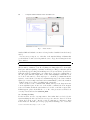
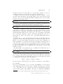
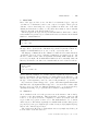
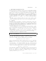
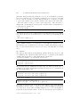
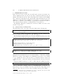
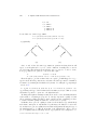
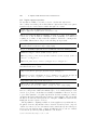
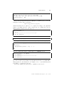
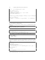
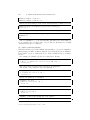
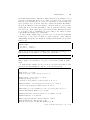
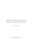
In order to check that everything is up and running, let us perform a simple experiment. Open Matita by invoking $MATITA_HOME/matita/matita.opt from a
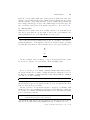
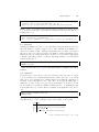
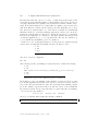
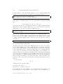
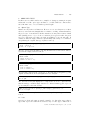
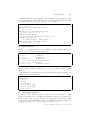
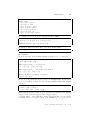
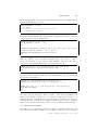
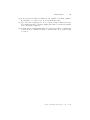
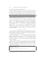
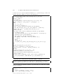
command line. A window should appear on your screen with the shape in Figure 0.3
The interface [8] is divided into three subpanes: one on the left and two stacked
vertically on the right. The pane in the top right contains, at the moment, the
Matita logo: when you are in the middle of a proof, it will be used to visualize
open goals in a sequent like fashion; the pane beneath it is a read only area meant
for error and log messages; finally, the pane on the left is an editor pane. When
you open a new file, the latter pane contains a default comment with copyright
information. Let us observe, by the way, that Matita’s style of comments follow the
2 If
autoconf is not installed in your system, you will have to install it using the command apt-get
install autoconf first
Journal of Formalized Reasoning Vol. 7, No. 2, 2014.
96
·
A. Asperti and W. Ricciotti and C. Sacerdoti Coen
Fig. 1.
Matita interface
Standard ML and OCaml convention of being bracketed with the lexical tokens (*
and *).
Let us now try to import one of the files of the standard library of Matita that
you should have downloaded along with the source. Type the following line in the
editor window
include "basics/logic.ma".
and then hit Ctrl+Alt+Page Down or press the button at the top of the Matita
window with a downarrow on it. If everything is working right, the bottom righthand pane will start printing out numerous messages, telling you that the system
is (recursively) typechecking and including basics/logic.ma and its dependencies.
When the include command has been completely processed, the command line of
the editor pane will turn a light shade of blue. Lines highlighted with this colour
are “locked” and cannot be edited any longer: to edit them, you must first ask the
system to retract them. You may use Ctrl+Alt+Page Up (or the button with an
uparrow) to retract a single statement, and Ctrl+Alt+Home (or the button with an
overlined uparrow) to retract everything in the current file.
If the execution of the command fails, Matita will report its diagnosis in the
bottom right hand pane; in the case of the include command, the most frequent
reason for a failure is that the system has not been able to find the requested file.
If this happens, please check that the “root” file of the previous section has been
correctly created and saved in $SCRIPTS_HOME.
0.4
Browsing the library
For the moment, it is not very important to know what has been loaded by the
system including the file logic.ma; however, if you are curious to have a look at its
content, the best choice is to directly open it. To this purpose, click File > Open
in the menu bar: this will open a new pop up window allowing you to browse the
Journal of Formalized Reasoning Vol. 7, No. 2, 2014.
Matita Tutorial
·
97
file system. Choose the desired file (e.g. logic.ma) and confirm your choice by
pressing the OK button: the file will open up in the editing window.
Sometimes, you are not interested in reading an entire file, but just to “check”
a specific result. For instance, after having included logic.ma as described in the
previous section, type the following line (without a fullstop) and execute it as usual,
by hitting Ctrl+Alt+Page Down
check True
a new window (called Matita Browser) should pop up with type information about
the constant True. In particular, this window should tell you that:
True : Prop
The language of Matita is strongly typed: every term of the language has a type
(including types themselves). The syntax M:T is the standard notation adopted
in type theory to express the fact that the term M has type T. So, the previous
statement informs us that True is a term of type Prop. Prop (that is a shorthand
for Proposition) is a primitive constant of the system, that stands for the type of
all propositions3 . Hence, the sentence True : Prop simply affirms that True is a
proposition.
So, this is the type of True, but what is its actual definition? The Matita Browser
(similarly to the goal window) is hypertextual: you can directly jump to the definitions of objects by just clicking on them. If you click on True you will discover
that it is an instance of an entity called inductive type. Matita is actually based on
a Dependent Type System known as the Calculus of Inductive Constructions (see
[23, 18]): in such a framework, as we shall explain in Section 3, almost everything
is defined as an inductive type (we shall also come back, in that occasion, to the
definition of True).
We claimed that every term has a type, so you might wonder what is the type of
Prop. If you check it, you will discover that
Prop : Type[0]
In the same way as Prop is the type of all propositions, Type is, in a sense, the
type of all types. But what is the meaning of the label 0? Well, the point is that,
to avoid logical paradoxes “à la Russell”, types of types (called universes) should
be organized into a hierarchy of the following kind
Type[0] : Type[1] : Type[2] : Type[3] . . .
For the moment, you may just ignore the existence of Type[i] for i larger than 0.
0.5
Live DVD
If you are not running Linux or you do not want to install Matita, you can download
a Live DVD image from the download page of Matita. The image can be burned
to a bootable DVD or it can be directly executed in a virtual machine using any
virtual machine emulator like VMWare. The image is a full Debian installation
3 We
shall give more details on Matita system of types and its logical restrictions in Section 9
Journal of Formalized Reasoning Vol. 7, No. 2, 2014.
98
·
A. Asperti and W. Ricciotti and C. Sacerdoti Coen
with a copy of Matita already installed. It is sufficient to open a terminal and type
matita to start experimenting.
0.6
Matita Web
Still another alternative is to interact with Matita on line, through our web interface
[3]. Matita is available as a multi-user web application running remotely on our
server. The web application can process the same proof scripts as the stand-alone
system, adding support for scripts containing HTML-like markup.
Every Matitaweb user has a separate space for storing definitions and proofs.
The personal copies can then be synchronized with the centralized library for collaborative developments (selected users, currently testing only).
In order to get access to Matita Web, follow the instructions at the following url:
http://matita.cs.unibo.it/matitaweb.shtml.
You will also find an on-line, executable version of this tutorial.
Journal of Formalized Reasoning Vol. 7, No. 2, 2014.
Matita Tutorial
1.
·
99
DATA TYPES, FUNCTIONS AND THEOREMS
Matita is both a programming language and a theorem proving environment: you
can define datatypes and programs, and then prove properties about them. Very
few things are built-in: not even booleans or logical connectives, but you may of
course freely include and reuse libraries, as in normal programming languages. The
main philosophy of the system is to let you define your own data-types and functions
using a powerful computational mechanism based on the declaration of inductive
types.
Let us start this tutorial with a simple example based on the following well known
problem.
1.1
The goat, the wolf and the cabbage
A farmer needs to transfer a goat, a wolf and a head of cabbage across a river, but
there is only one place available on his boat. Furthermore, the goat will eat the
cabbage if they are left alone on the same bank, and similarly the wolf will eat the
goat. The problem consists in bringing all three items safely across the river.
Let us start with including the file logic.ma that contains a few preliminary
notions not worth discussing for the moment. As a general practice, it is advisable
to always include basics/pts.ma that contains the declaration of universes, or, at
least, to include basics/core_notation.ma for some basic notations. The former
includes the latter, and every file from the standard library recursively includes
both.
include "basics/logic.ma".
Our first data type defines the two banks of the river, which will be named east
and west. It is a simple example of enumerated type, defined by explicitly declaring
all its elements. The type itself is called “bank”. Let’s have a look at the definition,
then we shall discuss its syntax.
inductive bank: Type[0] :=
| east : bank
| west : bank.
The definition starts with the keyword inductive followed by the name we want to
give to the new datatype (in this case, bank), followed by its type (a type of a type
is traditionally called a sort in type theory). A sort in Matita is either Prop or a
Type[i]. As we already said in the introduction, Prop is meant for propositions,
Type[0] for datatypes and Type[i] for large collections.
The definition proceeds with the keyword “:=” (or \def) followed by the body
of the definition. The body is just a list of constructors for the inductive type,
separated by the symbol | (vertical bar). Each constructor is a pair composed by
a name and its type. Constructors (in our case, east and west) are the canonical
inhabitants of the inductive type we are defining (in our case, bank), hence their
type must be of type bank. In general, as we shall see, constructors for an inductive
type T may have a more complex structure, and in particular can be recursive:
the general proviso is that they must always return a result of type T. Hence, the
Journal of Formalized Reasoning Vol. 7, No. 2, 2014.
100
·
A. Asperti and W. Ricciotti and C. Sacerdoti Coen
declaration of a constructor c for and inductive type T has the following typical
shape4 :
c: A1 → . . . → An → T
where A1 . . . An can be arbitrary types, comprising T itself.
As a general rule, the inductive type must be conceptually understood as the
smallest collection of terms freely generated by its constructors.
1.2
Defining functions
We can now define a simple function computing, for each bank of the river, the
opposite one.
definition opposite :=λs.
match s with
[ east ⇒ west
| west ⇒ east
].
Non-recursive functions must be defined in Matita using the keyword definition
followed by the name of the function and an optional type. The type bank → bank
is omitted in the example because it is automatically inferred by the system. The
definition proceeds with the keyword “:=” followed by the function body. The body
starts with a list of input parameters, preceded by the symbol λ (\lambda); many
TEX-like macros are automatically converted by Matita into Unicode symbols: see
View > TeX/UTF-8 table in the menu bar for a complete list.
We then proceed by pattern matching on the parameter s: if the input bank is
east we return west, and conversely if it is west we return east. Since the input
parameter s is matched against the constructors of the type bank, its type is inferred
to be bank. Since in every case the match returns a bank, the output of opposite is
inferred to be bank too.
Pattern matching is a well known feature typical of functional programming
(especially of the ML family), allowing simple access to the components of complex
data structures. A function definition most often corresponds to pattern matching
on one or more of its parameters, allowing the function to be easily defined by cases.
The syntactic structure of a match expression is the following:
match expr with
[ p1 ⇒ expr1
| p2 ⇒ expr2
:
| pn ⇒ exprn
]
The expression expr, which is supposed to be an element of an inductive type T,
is matched sequentially to the various patterns p1 , . . . , pn . A pattern pi is just a
constructor of the inductive type T possibly applied to a list of variables, bound
4 The
notion of inductive type is more general and admits other shapes. They will be discussed in
Section 3. Moreover, not every form of recursive constructor is accepted, since, in order to ensure
logical consistency, we must respect some positivity conditions that we shall discuss in Section 9.
Journal of Formalized Reasoning Vol. 7, No. 2, 2014.
Matita Tutorial
·
101
inside the corresponding branch expri . If the pattern pi matches the value expr,
then the corresponding branch expri is evaluated (after replacing in it the pattern
variables with the corresponding subterms of expr). Usually, all expressions expr
have a single, uniform type; however, since Matita supports dependent types, the
type of branches could depend on the matched expression, too (see section 5.10).
1.3
Our first lemma
Functions are live entities, and can be actually computed. To check this, let us
state the property that the opposite bank of east is west; every lemma needs a
name for further reference, so we will call this one east_to_west.
lemma east_to_west : opposite east = west.
If you enter the previous declaration and execute it, you will see a new pane replacing the matita logo on the right side of the screen: it is the goal pane, providing
a sequent-like representation of the following form, for each open goal in the proof
B1
B2
...
Bk
A
A is the conclusion of the goal and B1 , ..., Bk are the hypotheses in the context.
In our case, we only have one goal, and the context is initially empty:
opposite east = west
We proceed in the proof by issuing commands (traditionally called tactics) to
the system. In this case, we want to evaluate the function, which can be done by
invoking the “normalize” command (remember that strings within the delimiters
“(*” and “*)” are just comments):
normalize (* this command reduces the goal to the normal form *)
By executing it, you will see that the goal will change to west = west: in particular,
the subexpression opposite east has been reduced to west. You may use the retract
button to undo the step, if you wish.
The new goal west = west is trivial: it is just a consequence of reflexivity. Such
trivial steps can be closed in Matita by just typing a double slash. We complete the
proof by the qed command, that instructs the system to store the lemma performing
some book-keeping operations.
// qed. (* close the goal by invoking automation
and add the theorem to the library *)
In exactly the same way, we can prove that the opposite side of west is east. In
this case, we avoid the unnecessary simplification step: // will take care of it.
Journal of Formalized Reasoning Vol. 7, No. 2, 2014.
102
·
A. Asperti and W. Ricciotti and C. Sacerdoti Coen
lemma west_to_east : opposite west = east.
// qed.
Instead of lemma, you may also use theorem or corollary. Matita does not attempt
to make a semantic distinction between them, and their use is entirely up to the
user.
In some cases, the normalize tactic is too aggressive since the normal form of a
term can be very large and unreadable. An alternative is the whd tactic that reduce
terms only at the top level. Moreover, we will introduce patterns in Section 2.9 to
better control reduction by restricting it to chosen subterms.
1.4
Introducing hypothesis in the context
A slightly more complex problem consists in proving that opposite is idempotent
lemma idempotent_opposite : ∀x. opposite (opposite x) = x.
We start the proof by moving x from the conclusion into the context, that is a
(backward) introduction step. Matita syntax for an introduction step is simply the
sharp character “#” followed by the name of the item to be moved into the context.
This also allows us to rename the item, if needed: for instance if we wish to rename
x to b (since it is a bank), we just type #b.
#b (* introduce b into the context *)
After executing this command, the goal-pane will look like the following:
b: bank
opposite (opposite b) = b
The variable b has been added to the context, replacing x in the conclusion; moreover its implicit type “bank” has been made explicit. The foundational language of
Matita is strongly typed, hence every time you declare a variable with some binding
mechanism you are supposed to provide its type. Luckily, in many cases, this type
can be automatically inferred by the system according to the usage of variable,
sparing the user the burden to write it.
1.5
Case analysis
But how are we supposed to proceed, now? Simplification cannot help us, since b
is a variable: just try to call normalize and you will see that it has no effect. The
point is that we must proceed by case-analysis according to the possible values of b,
namely east and west. To this aim, you must invoke the cases command, followed
by the name of the hypothesis (more generally, an arbitrary expression) that must
be the object of the case analysis (in our case, b). Note that we do not need to
specify the possible cases: the system is able to compute them from the type of the
expression (that must be an inductive type).
cases b (* cases analysis on b *)
Journal of Formalized Reasoning Vol. 7, No. 2, 2014.
Matita Tutorial
·
103
This is the first example of a tactic that takes an argument. In this case the
argument is just a variable. In case of a compound expression, parentheses are
needed around it.
Executing the previous command has the effect of opening two subgoals, corresponding to the two cases b=east and b=west: you may view one or the other
by clicking on the tabs within the goal pane. Both goals can be closed by trivial
computations, so we may use // as usual. If we had to treat each subgoal in a
different way, we should have focused on each of them in turn, in a way that will
be described at the end of this section.
// qed. (* this command closes both goals *)
1.6
Predicates
Instead of working with functions, it is sometimes convenient to work with predicates. For instance, instead of defining a function computing the opposite bank,
we could declare a predicate opp stating when two banks are opposite to each
other; opp is a binary predicate on banks, that is, in curried form, an object of type
bank → bank → Prop. Only two cases are possible, leading naturally to the following
inductive definition:
inductive opp : bank → bank → Prop :=
| east_west : opp east west
| west_east : opp west east.
In precisely the same way as bank is the smallest type containing east and west, opp
is the smallest predicate containing the two sub-cases east_west and weast_east. If
you have some familiarity with Prolog, you may look at opp as the predicate defined
by the two clauses - in this case, the two facts - east_west and west_east.
Between opp and opposite, the following relation holds:
opp a b ↔ a = opposite b
Let us prove it, starting from the left to right implication, first.
lemma opp_to_opposite: ∀a,b. opp a b → a = opposite b.
We start the proof introducing a, b and the hypothesis opp a b, that we call oppab.
Next, we proceed by case-analysis on the possible proofs of opp a b (i.e. on the
possible shapes of oppab. By definition, there are only two possibilities, namely
east_west or west_east. Both resulting subcases are trivial, and can be closed by
automation. The whole proof is hence:
#a #b #oppab cases oppab // qed.
1.7
Rewriting
Let us consider the opposite direction.
lemma opposite_to_opp: ∀a,b. a = opposite b → opp a b.
Journal of Formalized Reasoning Vol. 7, No. 2, 2014.
104
·
A. Asperti and W. Ricciotti and C. Sacerdoti Coen
As usual, we start introducing a, b and the hypothesis a = opposite b, that we
call eqa. The right way to proceed, now, is by rewriting a into opposite b. We
do this by typing >eqa that instructs the system to rewrite inside the goal using
the equation named eqa oriented from left to right. If we wished to rewrite in the
opposite direction, namely opposite b into a, we would have typed <eqa. In section
2.9 we shall explain how to restrict/localize rewriting (and other operations) by
means of patterns.
After rewriting, we simply conclude the proof by case-analysis on b. Here is the
whole proof:
#a #b #eqa >eqa cases b // qed.
1.8
Records
It is time to proceed with our formalization of the farmer’s problem. A state of
the system is defined by the position of four items: the goat, the wolf, the head of
cabbage, and the boat. The simplest way to declare such a data type is to use a
record.
record state : Type[0] :={
goat_pos : bank
; wolf_pos : bank
; cabbage_pos: bank
; boat_pos : bank}.
When you define a record named foo, the system automatically defines a record
constructor named mk_foo. To create a new record you need to pass as arguments
to mk_foo the values of the record fields:
definition start :=mk_state east east east east.
definition end :=mk_state west west west west.
We must now define the possible moves. A natural way to do it is in the form of a
relation (a binary predicate) on states.
inductive move : state → state → Prop :=
| move_goat: ∀g,g1,w,c.
opp g g1 → move (mk_state g w c g) (mk_state g1 w c g1)
(* We can move the goat from a bank g to the opposite bank g1
if and only if the boat is on the same bank g as the goat
and we move the boat along with it. *)
| move_wolf: ∀g,w,w1,c.
opp w w1 → move (mk_state g w c w) (mk_state g w1 c w1)
| move_cabbage: ∀g,w,c,c1.
opp c c1 → move (mk_state g w c c) (mk_state g w c1 c1)
| move_boat: ∀g,w,c,b,b1.
opp b b1 → move (mk_state g w c b) (mk_state g w c b1).
We say that a state is safe if either the goat is on the same bank of the boat, or
both the wolf and the cabbage are on the opposite bank of the goat.
Journal of Formalized Reasoning Vol. 7, No. 2, 2014.
Matita Tutorial
·
105
inductive safe_state : state → Prop :=
| with_boat : ∀g,w,c.safe_state (mk_state g w c g)
| opposite_side : ∀g,g1,b.opp g g1 → safe_state (mk_state g g1 g1 b).
Finally, a state y is reachable from x if either there is a single move leading from x
to y, or there is a safe state z such that z is reachable from x and there is a move
leading from z to y.
inductive reachable : state → state → Prop :=
| one : ∀x,y.move x y → reachable x y
| more : ∀x,z,y. reachable x z → safe_state z → move z y → reachable x y.
1.9
Automation
Remarkably, Matita is now able to solve the farmer problem by itself, provided you
allow automation to exploit enough resources. The command /n/ is similar to //,
where n is a measure of this complexity: in particular it is a bound to the depth of
the expected proof tree (more precisely, to the number of nested applicative nodes).
In this case, there is a solution in six moves, and we need a few more applications
to handle reachability, and side conditions. The magic number to let automation
work is, in this case, 9.
lemma problem: reachable start end.
normalize /9/ qed.
The reader is referred to [9, 10] for technical information on Matita’s automation
facilities.
1.10
Application
Let us now try to derive the proof in a more interactive way. Of course, we expect
to need several moves to transfer all items from a bank to the other, so we should
start our proof by applying more. Matita syntax for invoking the application of
a lemma or theorem named foo is to write @foo. In general, the philosophy of
Matita is to describe each proof of a property P as a structured collection of objects
involved in the proof, prefixed by simple modalities (#,<,@,+. . . ) explaining the way
it is actually used (e.g. for introduction, rewriting, in an applicative step, and so
on).
lemma problem1: reachable start end.
normalize @more
After performing the previous application, we have four open subgoals (note by the
way that the type of some goals may depend on the values of other goals):
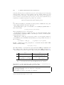
goal
X
Y
W
Z
type
state
reachable (mk state east east east east) X
safe state X
move X (mk state west west west west)
Journal of Formalized Reasoning Vol. 7, No. 2, 2014.
106
·
A. Asperti and W. Ricciotti and C. Sacerdoti Coen
namely, we must provide a state X such that (Y) it is reachable from start, (W)
it is safe, and (Z) there is a move leading from X to end. All goals are active, as
emphasized by the fact that their title in the goal pane are all bold. Any command
typed by the user is normally applied in parallel to all active goals, but clearly, in
the above case, we must proceed in a different way for each of them. The operation
of selecting a goal among the active ones is called focusing and is described in the
next section.
When applying a tactic, check that there is at least one active goal; otherwise
the command will be silently discharged.
1.11
Focusing
The general idea is that when you have multiple subgoals you should structure your
proof accordingly, using a syntax like [p1 |p2 |. . . |pn ] where you have a subproofs
pi for every active subgoal. The inner proofs can branch again when multiple goals
become active, resulting in a tree-like proof structure.
In all other provers, [p1 |p2 |. . . |pn ] is a new tactic built from the tactical [. . . |. . . |. . . ].
A tactical builds a tactic from arguments that are tactics (or proofs) themselves.
Tactics built with tacticals are executed as a monolitic step: it is not possible to
stop in the middle of execution to observe the intermediate proof states.
Matita decomposes the [. . . |. . . |. . . ] tactical into three commands “[”, “|” and
“]”, called tinycals [20], that can be executed individually. More precisely,
—the tinycal “[” opens a new focusing section for the currently active goals, and
focus on the first of them
—the tinycal “|” shifts the focus to the next goal in the current section
—the tinycal “]” closes the focusing section, falling back to the previous level and
adding to it all the remaining (not yet closed) goals.
Matita also provides other tinycals and a few tacticals that are not described in the
tutorial, but can be found in the user manual.
Let us see the effect of the “[” on our proof. We were in a state where we had
four active goals. By executing “[” the four goals get a progressive number, and
the first of them (the new intermediate state) gets the focus.
We can now proceed in several possible ways. The most straightforward way is to
explicitly supply the next intermediate state, that is (mk_state east west west east).
We can do it, by applying the term (mk_state east west west east).
This application closes the current goal; at present, no goal has the focus on. In
order to act on the next goal, we must focus on it using the “|” operator. In this
case, we would like to skip the next goal, and focus on the trivial third subgoal: a
simple way to do it, is by typing “|” again. The current goal is hence:
safe_state (mk_state east west west east)
whose proof is trivial and can be delegated to automation.
We then advance to the next goal, namely the fact that there is a move from
(mk_state east west west east)} to (mk_state west west west west)}; this is trivial too, but it requires /2/ (automation at depth two) since move_goat} opens an
Journal of Formalized Reasoning Vol. 7, No. 2, 2014.
Matita Tutorial
·
107
additional subgoal. By applying “]” we refocus on the skipped goal, going back to
a situation similar to the one we started with.
Here is this fragment of the proof:
[@(mk_state east west west east) || // | /2/ ]
Note that we had four goals, we closed three of them, hence we are left with a single
goal:
reachable (mk_state east east east east) (mk_state east west west east)
1.12
Implicit arguments and partial instantiation
Let us perform the next step, namely moving back the boat, in a slightly different
way. The more operation expects as its second argument the new intermediate state,
hence instead of applying more we can apply this term already instantiated on the
next intermediate state, that is
more ? (mk_state east west west west)
The question mark stands for an implicit argument to be inferred by the system.
The joint use of partial instantiation and implicit arguments is a very powerful
tool for reducing the length of proofs; Matita’s inference system is based on a
sophisticated bidirectional algorithm [7], exploiting both exptected and inferred
types, that is particularly convenient for the automatic management of implicit
information.
By applying the previous term, we get three independent subgoals (i.e. not
sharing any variable), all active, and two of them are trivial. We can just apply
automation to all of them in parallel, and it will close the two trivial goals. In this
case, we performed a move of the boat with the following code (note in particular
the we had no need to focus):
@(more ? (mk_state east west west west)) /2/
Let us come to the next step, that consists of moving the wolf. Suppose that
instead of specifying the next intermediate state, we prefer to specify the next move.
In the spirit of the previous example, we can do it in by simply instantiating more
with the suitable move, that is (more . . . (move_wolf . . . )). The dots stand here for
an arbitrary number of implicit arguments, to be guessed by the system, and can
be typed in Matita as \ldots .
Unfortunately, the previous move is not enough to fully instantiate the new intermediate state, and we obtain the following goals:
goal
X
Y
Z
W
type
reachable (mk_state east east east east) (mk_state east W west W)
safe_state (mk_state east W west W)
opp W west
bank
In particular, the bank towards which we move (W) remains unknown (we know
that it is the opposite of the current one (Z), but this information is still implicit).
Journal of Formalized Reasoning Vol. 7, No. 2, 2014.
108
·
A. Asperti and W. Ricciotti and C. Sacerdoti Coen
Automation cannot help here, since all goals depend from the bank W (they are in a
same cluster, in Matita terminology) and automation refuses to close some subgoals
instantiating other subgoals remaining open (the instantiation could be arbitrary).
The simplest way to proceed is to focus on the bank, that is the fourth subgoal, and
explicitly instantiate it. Instead of repeatedly using “|”, we can perform focusing
by typing “4:” as described by the following command.
[4: @east] /2/
Alternatively, we can directly instantiate the bank into the move. Let us complete
the proof in this, very readable way.
@(more . . . (move_goat west . . . )) /2/
@(more . . . (move_cabbage ?? east . . . )) /2/
@(more . . . (move_boat ??? west . . . )) /2/
@one /2/ qed.
Journal of Formalized Reasoning Vol. 7, No. 2, 2014.
Matita Tutorial
2.
·
109
INDUCTION
Most of the types we have seen so far have been enumerated types, composed
of a finite set of alternatives, and records, composed of tuples of heterogeneous
elements. A more interesting case of type definition is when some of the rules
defining its elements are recursive, i.e. they allow the formation of more elements
of the type in terms of the already defined ones.
The most typical case is provided by the natural numbers, which can be defined
as the smallest set generated by a constant 0 and a successor function from natural
numbers to natural numbers:
inductive nat : Type[0] :=
| O : nat
| S : nat → nat.
The two terms O and S are called constructors: they define the signature of
the type, whose objects are the elements freely generated by means of them. So,
examples of natural numbers are O, S O, S (S O), S (S (S O)) and so on.
The language of Matita allows the definition of well founded recursive functions
on inductive types; in order to guarantee termination of recursion you are only
allowed to make recursive calls on arguments structurally smaller than the ones
you received as input. Most mathematical functions can be naturally defined in
this way. For instance, the sum of two natural numbers can be defined as follows
let rec add n m :=
match n with
[ O ⇒m
| S a ⇒ S (add a m)
].
Observe that the definition of a recursive function requires the keyword let rec
instead of definition. The specification of formal parameters is different too. In
this case, they come before the body, and do not require a λ. If you need to specify
the type of some argument, you need to enclose it in parentheses, e.g. (n:nat).
By convention, recursion is supposed to operate on the first argument that means
that this is the only argument that is supposed to decrease in the recursive calls.
In case you need to work on a different argument, say foo, you can specify it by
explicitly mentioning “on foo” just after the declaration of all parameters.
2.1
Elimination
As we remarked at the end of the previous section, the function “add” works by
recursion on the first argument. This means that, for instance, (add O x) will
reduce to x, as expected, but the computation of (add x O) is stuck. How can
we prove that, for a generic x, add x O = x ? The mathematical tool to do this is
called induction. The induction principle for natural numbers states that, given a
property P (n) , if we prove P (O) and prove that, for any m, P (m) implies P (S m),
then we can conclude P (n) for any n.
The “elim” tactic allows us to apply induction in a very simple way. If the goal
is of the form P n, the invocation of
Journal of Formalized Reasoning Vol. 7, No. 2, 2014.
110
·
A. Asperti and W. Ricciotti and C. Sacerdoti Coen
elim n
will break it down to the two subgoals P 0 and ∀m.P m → P (S m). Let us apply it
to our case
lemma add_0: ∀a. add a O = a.
#a elim a
We generated the following goals:
goal type
G1 add O O = O
G2 ∀x. add x O = x → add (S x) O = S x
After normalization, both goals are trivial:
normalize // qed.
In a similar way, it is convenient to state a lemma about the behaviour of add when
the second argument is not zero; the proof is a simple induction on a:
lemma add_S : ∀a,b. add a (S b) = S (add a b).
#a #b elim a normalize // qed.
We are now in the position to prove the commutativity of add. We proceed by
induction on the first argument, and simplify the goals by invoking normalization:
theorem add_comm : ∀a,b. add a b = add b a.
#a elim a normalize
We are left with two sub goals:
goal type
G1 ∀b. b = add b O
G2 ∀x.(∀b. add x b = add b x) → ∀b. S (add x b) = add b (S x)
G1 is just our lemma add_O. For G2 , we could start introducing x and the induction
hypothesis IH; then, the goal would be proved by rewriting using add_S and IH.
The resulting script would be #x #IH >add_S >IH //. Instead, this easy proof can
be found automatically by Matita invoking the automation tactic //.
2.2
Existentials
We are interested in proving that for any natural number n there exists a natural
number m that is the integer half of n, defined as the result of the integer division of n
by 2. This will give us the opportunity to introduce new connectives and quantifiers
and, later on, to highlight some important aspects of proofs and computations. It is
interesting to observe that not even existential quantification is a primitive notion
in Matita: in fact, it is defined in the library file basic/logic.ma, and in order to
use it we need to include this file, or another one that recursively includes it (we
shall come back on the actual definition of the existential in section 3.2). Here is
the formal statement of the theorem we are interested in:
Journal of Formalized Reasoning Vol. 7, No. 2, 2014.
Matita Tutorial
·
111
include "basics/types.ma".
definition twice :=λn.add n n.
theorem ex_half: ∀n.∃m. n = twice m ∨ n = S (twice m).
We proceed by induction on n; after normalizing, we get the following goals:
goal type
G1 ∃m.O = add O O ∨ O = S (add m m)
G2 ∀x.(∃m. x = add m m ∨ x = S (add m m)) →
∃m. S x = add m m ∨ S x = S (add m m)
The only way we have to prove an existential goal is by exhibiting the witness,
which in the case of the first goal is O. We do it by applying the term called
ex intro instantiated by the witness. Then, it is clear that we must follow the
left branch of the disjunction. In Section 3.2 we will explain that the disjuction
connective is defined as an inductive type generated by two constructors, called
or introl and or intror. Therefore to proceed in the proof we can apply the term
or introl. However, remembering the names of constructors can be annoying: we
can invoke the application of the n-th constructor of an inductive type (inferred
from the current goal) by typing %n. At this point, we are left with the subgoal
O = add O O, that is closed by computation. It is worth to observe that invoking
automation at depth /3/ would also automatically close G1 . Here is the fragment
of the proof, up to this point:
#n elim n normalize
[@(ex_intro . . . O) %1 //
2.3
Decomposition
The case of G2 is more complex. We should start introducing x and the induction
hypothesis
IH: ∃m. x = add m m ∨ x = S (add m m)
The induction hypothesis IH asserts the existence of an m that satisfies the thesis;
to obtain such an m, we eliminate the existential at the front of the hypothesis using
the case tactic. This is motivated by the fact that the existential is just a particular
inductive type. This situation, where we introduce something into the context and
immediately eliminate it by case analysis is so frequent that Matita provides a
convenient shorthand: you can just type a single “*”. The star symbol should be
reminiscent of an explosion: the idea is that you have a structured hypothesis, and
you ask to explode it into its constituents. In the case of the existential, it allows
us to pass from a goal of the shape
(∃x.P x) → Q
to a goal of the shape
∀x.(P x → Q)
Journal of Formalized Reasoning Vol. 7, No. 2, 2014.
112
·
A. Asperti and W. Ricciotti and C. Sacerdoti Coen
At this point we are left with a new goal with the following shape
G3 : ∀m. (x = add m m ∨ x = S (add m m)) → . . .
We should introduce m, the hypothesis H: x = add m m ∨ x = S (add m m), and then
reason by cases on this hypothesis. It is the same situation as before: we must
explode the disjunctive hypothesis into its constituents. In the case of a disjunction,
the * tactic allows us to pass from a goal of the form
A ∨B →Q
to two subgoals of the form
A → Q and B → Q
In the first subgoal, we are under the assumption that x = add m m. Half of (S x) is
therefore m, and we have to prove the right branch of the disjunction. In the second
subgoal, we are under the assumption that x = S (add m m). The half of (S x) is
hence (S m), and we have to follow the left branch of the disjunction.
Here is the simple proof of G2 :
|#x * #m * #eqx
[@(ex_intro . . . m) /2/ | @(ex_intro . . . (S m)) normalize /2/
]
qed.
2.4
Computing vs. Proving
Instead of proving the existence of a number corresponding to the half of n, we
could be interested in computing it. The best way to do it is to define this division
operation together with remainder, that in our case is just a boolean value: true if
the input term is even, and false if the input term is odd. The boolean data type is
defined in basics/bool.ma: it is just an inductive type with two constructors true
and false.
Since we must return a pair, we could use a suitably defined record type, or simply
a product type nat×bool, already defined in the basic library in basics/types.ma,
together with notation for building and destructuring pairs. The product type is
just a sort of “general purpose” record, with standard fields fst and snd, called
projections. A pair of values n and m is written hn,mi. When p is a pair, the
expression let hx,yi :=p in E binds x and y in E respectively to the first and second
component of p.
We first write down the division function, and then discuss it.
let rec div2 n :=
match n with
[ O ⇒ hO,falsei
| S a ⇒
let hq,ri :=(div2 a) in
match r with
[ true ⇒ hS q,falsei
| false ⇒ hq,truei
]
].
Journal of Formalized Reasoning Vol. 7, No. 2, 2014.
Matita Tutorial
·
113
It is important to point out the substantial analogy between the algorithm for
computing div2 and the proof of ex_half. Consider ex_half which returns a proof
of the form ∃n.A n ∨ B n: the real informative content in it is the witness n and
a boolean indicating which one between the two conditions A n and B n is met.
This is precisely the quotient-remainder pair returned by div2. In both cases we
recur (respectively, by induction or by recursion) over the input argument n. In
case n = 0, we conclude the proof in ex_half by providing the witness O and a
proof of A O; this corresponds to returning the pair hO,falsei in div2. Similarly,
in the inductive case n = S a, we must exploit the inductive hypothesis for a (i.e.
the result of the recursive call), distinguishing two subcases according to the two
possibilities A a or B a (i.e. the two possible values of the remainder for a). The
reader is invited to check all the details of this correspondence.
2.5
Destruct
Let us now prove that our div2 function has the expected behaviour. We start
proving a few easy lemmas:
lemma div2SO: ∀n,q. div2 n = hq,falsei → div2 (S n) = hq,truei.
#n #q #H normalize >H normalize // qed.
lemma div2S1: ∀n,q. div2 n = hq,truei → div2 (S n) = hS q,falsei.
#n #q #H normalize >H normalize // qed.
Here is our statement, where nat_of_bool is the conversion function that maps
false to zero and true to one:
lemma div2_ok: ∀n,q,r. div2 n = hq,ri → n = add (nat_of_bool r) (twice q).
We proceed by induction on n, which produces two subgoals. The first subgoal
looks like the following:
∀q,r.div2 O = hq,ri → O = add (nat_of_bool r) (twice q)
We may introduce q,r and the hypothesis
H: div2 O = hq,ri
Note that the left hand side of this equation is not in normal form, and we would
like to reduce it. We can do it by specifying a pattern for the normalize tactic,
introduced by the “in” keyword, and delimited by a semicolon. In this case, the
pattern is just the name of the hypothesis, and we should write
normalize in H
At this point, the first subgoal looks like the following:
n:
q:
r:
H:
nat
nat
bool
hO, falsei=hq, ri
O = add (nat_of_bool r) (twice q)
Journal of Formalized Reasoning Vol. 7, No. 2, 2014.
114
·
A. Asperti and W. Ricciotti and C. Sacerdoti Coen
From the hypothesis H we expect to be able to conclude that q=O and r=false. The
tactic that provides this functionality is called destruct. The tactic decomposes
every hypothesis that is an equality between structured terms into smaller components: if an absurd situation is recognized (like an equality between O and (S n),
built from different constructors) the current goal is automatically closed; otherwise, all derived equations where one of the sides is a variable are automatically
substituted in the proof, and the remaining equations are added to the context (replacing the original equation). The tactic considers the two sides to be structured
if they are the application of constructors, and skips equalities involving at least
one function application (e.g. f n = S m), unless the other side is a variable (e.g.
f n = m, handled by substituting f n for m everywhere).
In the above case, by invoking destruct we would get the two equations q=O and
r=false; these are immediately substituted in the goal, that becomes:
n: nat
q: nat
r: bool
O = add (nat_of_bool false) (twice O)
and can be solved by computation.
2.6
Cut
The next subgoal, after performing a few introductions, looks like the following:
n: nat
a: nat
Hind: ∀q:nat.∀r:bool.div2 a=hq,ri→ a=add (nat_of_bool r) (twice q)
q: nat
r: bool
div2 (S a) = hq,ri→ S a = add (nat_of_bool r) (twice q)
We should proceed by case-analysis on the remainder of (div2 a), but before doing
it we should emphasize the fact that (div2 a)} can be expressed as a pair of its two
projections. The tactic that allows to introduce a new hypothesis, splitting complex
proofs into smaller components is called cut. The invocation of cut A transforms
the current goal G into the two subgoals A and A → G (A is called the cut formula).
In our case, the cut formula is
div2 a = hfst . . . (div2 a), snd . . . (div2 a)i
whose proof is trivial. After typing the following commands
cut (div2 a = hfst . . . (div2 a), snd . . . (div2 a)i) [//]
Journal of Formalized Reasoning Vol. 7, No. 2, 2014.
Matita Tutorial
·
115
we are left in the new state:
n: nat
a: nat
Hind: ∀q:nat.∀r:bool.div2 a=hq,ri→ a=add (nat_of_bool r) (twice q))
q:nat
r:bool
div2 a=hfst . . . (div2 a),snd . . . (div2 a)i→
div2 (S a)=hq,ri→ S a=add (nat_of_bool r) (twice q)
We now proceed by induction on (snd . . . (div2 a)); the two subgoals are respectively closed using the two lemmas div2SO and div2S1 in conjunction with the
inductive hypothesis, and do not contain additional challenges.
The whole proof of div2_ok is therefore the following:
#n elim n
[#q #r #H normalize in H; destruct //
|#a #Hind #q #r
cut (div2 a = hfst . . . (div2 a), snd . . . (div2 a)i) [//]
cases (snd . . . (div2 a)) #H
[>(div2S1 . . . H) #H1 destruct normalize @eq_f >add_S @(Hind . . . H)
|>(div2SO . . . H) #H1 destruct normalize @eq_f @(Hind . . . H)
]
qed.
2.7
Lapply
The cut rule is the main tool for “forward reasoning” in interactive provers, that is
for introducing a new intermediate proposition P between the given hypothesis and
the current goal.
If we already have in mind an explicit proof H for the proposition P, a viable
alternative to introduce P with a cut and prove it with H is to call the following
tactic:
lapply H
If the type of H is P, the effect of the tactic is to transform the current goal G into
the new goal P → G.
For instance, if n:nat, the tactic
lapply (add_S n O) S
would transform a goal G into add n (S O) = S (add n O) → G.
The name lapply stands for “left application”, where left should be understood
in sequent-like sense, that is as referring to the left side of the sequent, which is the
context. It is in fact a generalization of the left introduction rule for application in
sequent like calculi.
The advantage of lapply with respect to a cut is to avoid the explicit writing of
the cut-formula, that in the case of lapply is automatically inferred, being the type
of its argument.
Journal of Formalized Reasoning Vol. 7, No. 2, 2014.
116
·
A. Asperti and W. Ricciotti and C. Sacerdoti Coen
The lapply tactic can also be used to generalize hypotheses, e.g. before performing an elimination. If we have a goal G in a context where x:A, the execution of the
command
lapply x
will transform the goal into ∀x:A.G, generalizing the variable x in G. If x is also
used in some hypothesis H:P, the goal is usually generalized on H using lapply H
before doing the same on x, resulting in ∀x:A.P → G. After generalizing on x, the
command -x is often used to erase the old — and now useless — assumption x:A
from the context.
2.8
Mixing proofs and computations
So far we have seen how to prove the existence of the integer half of a natural
number, how to compute it by an explicit program and how to specify and prove
the correctnes of such a program.
There is still another possibility: to mix the program and its specification into a
single entity. The idea is to refine the output type of the div2 function: it should
not just be a generic pair hq,ri of natural numbers but a specific pair satisfying the
specification of the function. In other words, we need the possibility to define, for
a type A and a property P on A, the subset type {a:A|P a} of all elements a of type
A that satisfy the property P. Subset types are just a particular case of dependent
types, that are types that can depend on arguments, such as arrays of a specified
length taken as a parameter. This kind of types is quite unusual in traditional
programming languages, and their study is one of the new frontiers of the current
research on type systems.
There is nothing special in a subset type {a:A|P a}: it is just a record composed
of an element a of type A and a proof of P a. Nevertheless, it provides a language
rich enough to comprise proofs among its expressions.
record Sub (A:Type[0]) (P:A → Prop) : Type[0] :=
{witness: A; proof: P witness}.
definition qr_spec :=λn.λp.∀q,r. p=hq,ri → n=add (nat_of_bool r) (twice q).
We can now construct a function from n to {p|qr_spec n p} by composing the
objects we already have:
definition div2P: ∀n. Sub (nat×bool) (qr_spec n) :=λn.
mk_Sub ?? (div2 n) (div2_ok n).
But we can also try to directly build such an object:
definition div2Pagain : ∀n.Sub (nat×bool) (qr_spec n).
#n elim n
[@(mk_Sub . . . hO,falsei) normalize #q #r #H destruct //
|#a * #p #qrspec
cut (p = hfst . . . p, snd . . . pi) [//]
cases (snd . . . p) #H
[@(mk_Sub . . . hS (fst . . . p),falsei) #q #r #H1
Journal of Formalized Reasoning Vol. 7, No. 2, 2014.
Matita Tutorial
·
117
destruct @eq_f >add_S @(qrspec . . . H)
|@(mk_Sub . . . hfst . . . p,truei) #q #r #H1 destruct @eq_f @(qrspec . . . H)
]
qed.
The reader is invited to run the computation of the previous function on a few
examples, to see what the output looks like. The only “readable” information is,
in fact, the witness: the proof is, in general, a complex lambda term whose only
purpose is to provide a mechanically verifiable certificate that the witness satisfies
a given property. We shall come back to subset types is section 4.2.
2.9
Tactic patterns
Generally speaking, the scope of a tactic is the conclusion of the current goal (or the
current goals if many are selected at once). In section 2.5, however, we have used
normalize in H; to indicate that the tactic should take effect within hypothesis H
rather than the conclusion. This “in H;” is an instance of a more general scheme
to express paths within the current goals by means of patterns. Patterns allows us
to specify any subterm of the conclusion or of any hypothesis.
Since the purpose of a pattern is to identify a subterm within a term, its syntax
is similar to that of a term, where, in addition to the usual syntax, the symbol % is
used to specify the target position (i.e. the subterm where the tactic should act);
all the parts of the term that must not be targeted by the tactic are replaced by
? symbols in the pattern. For the purpose of matching against patterns, all user
defined notation (e.g. infix symbols, omitted terms to be inferred by the system)
is ignored. Notations will be discussed in Section 3.3.
For example, if we are given a term x = a + b + c, that, ignoring notation for
addition and equality, is
eq nat x (plus (plus a b) c)
we can specify the subterm a+b by means of the pattern (???(?%?)). The pattern
specifies that the term is an application of one term (called head of the application)
to three arguments: the head and the first two arguments are generic (this is
expressed by the ? symbol), while the last argument is itself an application with
one head and two arguments, the former of which should be the scope of a tactic
(as expressed by the % symbol). Notice that the pattern sublanguage does not
understand at all user defined notation, comprising that defined in the standard
library: therefore, a pattern in the form ?=%+? is not legal.
Patterns can be used to identify a path in either a hypothesis or in the conclusion,
by means of the following syntaxes:
normalize in `(???(?%?)); (* rewrites in the conclusion *)
normalize in H1:(???(?%?)); (* rewrites in hypothesis H1 *)
We use \vdash to insert the ` symbol (which is required when specifying a subterm
in the conclusion).
Patterns are not restricted to applicative terms, but can be used under all circumstances:
—in arrow types: in a term (x=1 → x>0), (??%? → ?) specifies the first x;
Journal of Formalized Reasoning Vol. 7, No. 2, 2014.
118
·
A. Asperti and W. Ricciotti and C. Sacerdoti Coen
—within binders: in (∀x,y:nat.P (x*y)), (∀_,_:?.?%) specifies x ∗ y (notice that in
the pattern, bound variables can be replaced by the _ “don’t care” placeholder);
—within a match: match ? with [ _ ⇒ % | _ ⇒ ?] specifies the subterm contained
in the first branch of a binary match. Notice that the names of costructors must
be replaced by underscores in the pattern.
A second kind of pattern is used to specify all the subterms that match a userspecified term u: these are expressed by the syntax “in match u;”.
For instance it is possible to match all additions in the conclusion by means of
the pattern in match (? + ?);.
Example 1. The two kinds of patterns can be combined in a single statement.
Suppose the current goal has a hypothesis H of type:
∀z:nat.z*(x+y)=z*x+z*y
Then to match only the leftmost sum, we can use the pattern
in match (?+?) in H1:(∀_:?.??%?);
This instructs Matita to match additions, but only within the left-hand side of the
equality.
Journal of Formalized Reasoning Vol. 7, No. 2, 2014.
Matita Tutorial
3.
·
119
EVERYTHING IS AN INDUCTIVE TYPE
As we have mentioned several times, very few notions are really primitive in Matita:
one of them is the notion of universal quantification (or dependent product type)
and the other one is the notion of inductive type. Even the arrow type (also called
function space) A → B is not really primitive: it can be seen as a particular case of
the dependent product ∀x:A.B in the degenerate case when B does not depends on
x. All the other familiar logical connectives - conjunction, disjunction, negation,
existential quantification, even equality - can be defined as particular inductive
types.
We shall look at those definitions in this section, since it can be useful to acquire
confidence with inductive types, and to get a better theoretical grasp on them.
3.1
Conjunction
In natural deduction, logical rules for connectives are divided in two groups: there
are introduction rules, allowing us to introduce a logical connective in the conclusion,
and there are elimination rules, describing how to deconstruct information about
a compound proposition into information about its constituents (i.e. how to use a
hypothesis having a given top-level connective).
Consider conjunction. In order to understand the introduction rule for conjunction, you should answer the question: how can we prove A∧ B ? The answer is
simple: we must prove both A and B. Hence the introduction rule for conjunction
is A → B → A∧ B.
The general idea for defining a logical connective as an inductive type is simply
to define it as the smallest proposition generated by its introduction rule(s).
For instance, in the case of conjunction, we define
inductive And (A,B:Prop) : Prop :=
conj : A → B → And A B.
The corresponding elimination rule is induced by minimality: if we have a proof of
A∧ B it may only derive from the conjunction of a proof of A and a proof of B. A
possible way to formally express the elimination rule is the following:
∀A,B,P:Prop. (A → B → P) → A∧ B → P
that is, for all A and B, and for any proposition P if we need to prove P under the
assumption A∧ B, we can reduce it to proving P under the pair of assumptions A and
B.
It is interesting to observe that the elimination rule can be easily derived from
the introduction rule in a completely syntactic way. Basically, the general structure
of the (non dependent) elimination rule for an inductive type T is the following
∀~A,P. C1 → . . . → Cn → T → P
~ is the list of parameters of the inductive type, and every Ci is derived from
where A
the type Ti of a constructor ci of T by just replacing T with P in it. For instance, in
the case of the conjunction we only have one constructor of type A → B → A∧ B and
replacing A∧ B with P we get C1 = A → B → P.
Journal of Formalized Reasoning Vol. 7, No. 2, 2014.
120
·
A. Asperti and W. Ricciotti and C. Sacerdoti Coen
Every time we declare a new inductive proposition or type T, Matita automatically declares an axiom called T_ind5 , which embodies the elimination principle for
this type. The actual shape of the elimination axiom is more complex than the one
described above, since it also takes into account the possibility that the predicate
P depends on the term of the given inductive type (and possible arguments of the
inductive type).
Actually, the elimination tactic elim for an element of type T is a straightforward
wrapper that applies the suitable elimination axiom.
3.2
Disjunction, False, True, Existential Quantification
Let us introduce now other connectives as inductive types, mimicking what we
did for conjunction and starting with disjunction. The first point is to derive the
introduction rule(s). When can we conclude A∨ B ? Clearly, we must either have a
proof of A, or a proof of B. So, we have two introduction rules, in this case:
A → A∨ B
and
B → A∨ B
that leads us to the following inductive definition of disjunction:
inductive Or (A,B:Prop) : Prop :=
or_introl : A → Or A B
| or_intror : B → Or A B.
The elimination principle, automatically generated by the system is
or_ind: ∀A,B,P:Prop. (A → P) → (B → P) → A∨ B → P
that is a traditional formulation of the elimination rule for the logical disjunction
in natural deduction: if P follows from both A and B, then it also follows from their
disjunction.
More surprisingly, we can apply the same methodology to define the constant
False. The point is that, obviously, there is no (canonical) way to conclude False:
so we have no introduction rule, and we must define an inductive type without
constructors, which is accepted by the system.
inductive False: Prop :=.
The elimination principle is in this case
False_ind: ∀P:Prop.False → P
that is the well known principle “ex falso quodlibet”.
What about True? You may always conclude True, hence corresponding inductive
definition just has one trivial constructor, traditionally named I:
inductive True: Prop := I : True.
As expected, the elimination rule is not informative in this case: the only way to
conclude P from True is to prove P :
5 In
case of inductive data types of sort Type[j] for some j, the system also generates for each
i an elimination rules towards P:Type[i], called T_rect_Typei. The rule allows us to inhabit
some type U:Type[i] by recursion on the eliminated term of type Type[j].
Journal of Formalized Reasoning Vol. 7, No. 2, 2014.
Matita Tutorial
·
121
True_ind: ∀P:Prop.P → True → P
Finally, let us consider the case of existential quantification. In order to conclude
∃x:A.Q x we need to prove Q a for some term a:A. Hence, the introduction rule for
the existential looks like the following:
∀a:A. Q a → ∃x.Q x
from which we get the following inductive definition, parametric in A and Q.
inductive ex (A:Type[0]) (Q:A → Prop) : Prop :=
ex_intro: ∀x:A. Q x → ex A Q.
In the next Section we will see how to associate the usual notation ∃x:A.Q to
ex A λx.Q.
The elimination principle automatically generated by Matita is
ex_ind: ∀A.∀Q\:A → Prop. ∀P:Prop. (∀x:A. Q x → P) → (∃x:A.Q) → P
That is, if we know that P is a consequence of Q x for any x:A, then it is enough to
know ∃x:A.Q x to conclude P. It is also worth spelling out the backward reading of
the previous principle. Suppose we need to prove P under the assumption ∃x:A.Q.
Then, eliminating the latter amounts to assuming the existence of x:A such that
Q x and proceed to prove P under these new hypotheses.
3.3
A bit of notation
Since we make frequent use of logical connectives and quantifiers, it would be nice
to have the possibility to use a more familiar-looking notation for them. Matita
offers you the possibility to associate your own notation to any notion you define.
To exploit the natural overloading of notation typical of scientific literature, its
management in Matita is split in two steps: one from presentation level to content
level, where we associate a notation to a fragment of abstract syntax, and one from
content level to term level, where we provide (possibly multiple) interpretations for
the abstract syntax.
The mapping between the presentation level (i.e. what the user writes as input
and what is displayed in the goal panes) and the content level is defined with the
notation command.
notation "hvbox(a break \land b)"
left associative with precedence 35 for @{ ’and $a $b }.
This declaration associates the infix notation a \land b (rendered as a∧ b by a builtin Unicode mapping) with an abstract syntax tree composed by the new symbol
’and applied to the result of the parsing of input argument a and b.
The presentation pattern is always enclosed in double quotes. The special keyword break indicates the line breaking point and the box schema hvbox indicates
a horizontal or vertical layout, according to the available space for the rendering
(they can be safely ignored for this tutorial).
The content pattern begins right after the for keyword and extends to the end of
the declaration. Parts of the pattern surrounded by @{. . . } denote verbatim content
fragments, those surrounded by ${. . . } denote meta-operators and references to
notational meta-variables occurring in the presentation pattern (for example $a).
Journal of Formalized Reasoning Vol. 7, No. 2, 2014.
122
·
A. Asperti and W. Ricciotti and C. Sacerdoti Coen
The declaration also informs the system that the notation is supposed to be left
associative and provides information about the syntactic precedence of the operator,
which governs the way an expression with different operators is interpreted by the
system. For instance, suppose we declare logical disjunction at a lower precedence:
notation "hvbox(a break \lor b)"
left associative with precedence 30 for @{ ’or $a $b }.
Then, an expression like A ∧ B ∨ C will be understood as (A ∧ B)∨ C and not as
A ∧ (B ∨ C).
An annoying aspect of user defined notation is that it will eventually interfere with
the primitive one, so introducing operators with suitable precedence is an important
and delicate issue. The best thing to do is to consult the file basics/core notation.ma
and, unless you cannot reuse an already existing notation overloading it (which is
the recommended solution), try to figure out the most suitable precedence for your
notation by analogy with other notations. Another possibility is to use the Terms
grammar entry of the View menu of Matita to look at all notations currently loaded,
partitioned according to their precedence level.
The next step is to associate an interpretation with content patterns, in the
following way:
interpretation "logical and" ’and x y = (And x y).
interpretation "logical or" ’or x y = (Or x y).
With these commands we are saying that a possible interpretation of the symbol
’and is the inductive type And, and a possible interpretation of the symbol ’or is
the inductive type Or. But we could e.g. define boolean functions andb and orb,
and provide an alternative interpretation of ’and and ’or on them. As a result, the
notations A∧ B and A∨ B would be overloaded, and interpreted as a proposition or a
boolean depending on the context they occur in. For details on the resolution of
overloading, see [?].
Let us conclude this section with a discussion of the notation for the existential
quantifier. In contrast to what we did previously, we use one mapping for the
notation used to pretty print terms, and a different one for parsing. The one for
parsing will be more complex to allow omission of types and packing of multiple
declarations into a more compact syntax.
notation < "hvbox(\exists ident i : ty break . p)"
right associative with precedence 20 for @{’exists (λ${ident i}: $ty. $p)}.
The < symbol after the notation keyword states that this mapping will only
be used during pretty printing. The other main novelty is the special keyword
ident that instructs the system that the variable i is expected to be an identifier.
Matita abstract syntax trees include lambda terms as primitive data types, and the
previous declaration simply maps the notation ∃x:T.P into a content term of the
form (’exists (λx:T’.P’)) where T’ and P’ are the content term obtained from T
and P.
The interpretation is then straightforward:
Journal of Formalized Reasoning Vol. 7, No. 2, 2014.
Matita Tutorial
·
123
interpretation "exists" ’exists x = (ex ? x).
Our notational language has an additional list operator for dealing with variablesized terms having a regular structure. This operator has a corresponding fold
operator, used to build up trees at the content level.
For example, in the case of quantifiers, it is customary to group multiple variable
declarations under a same quantifier, writing e.g. ∃x,y,z.P instead of ∃x.∃y.∃z.P.
This can be achieved by the following notation, used only during parsing as
specified by the > symbol:
notation > "\exists list1 ident x sep , opt (: T). term 19 Px"
with precedence 20
for ${ default
@{ ${ fold right @{$Px} rec acc @{’exists (λ${ident x}:$T.$acc)} } }
@{ ${ fold right @{$Px} rec acc @{’exists (λ${ident x}.$acc)} } }
}.
The presentational pattern matches terms starting with the existential symbol,
followed by a list of identifiers separated by commas, optionally terminated by a
type declaration, followed by a fullstop and finally by the body term. We use list1
instead of list0 since we expect to have at least one identifier: conversely, you
should use list0 when the list can possibly be empty.
The default meta operator at content level, matches the presentational opt and
has two branches, which are chosen depending on the matching of the optional
subexpression. Let us consider the first, case, where we have an explicit type. The
content term is built by folding the function
rec acc @{’exists (λ${ident x}:$T.$acc)}
(rec is the binder, acc the bound variable and the rest is the body) over the initial
content expression @{$Px}.
When a notation is not a simple infix operator, it may be the case that a different
precedence is required for its arguments. In this case we can use the term n X syntax
to declare that the term matched by the variable X needs to be parsed or prettyprinted at precedence n. For example, knowing that conjunction has precedence
35, by requiring Px to be parsed at level 19 in the notation of the existential, an
expression like ∃x.P∧ Q will be parsed as ∃x.(P∧ Q), whereas it would be parsed
as (∃x.P)∧ Q if Px was required to be at any level greater than 35. The maximal
level of precedence is 90. By asking an argument to have precedence 90, we force
the argument to be always either a single identifier or to be delimited (e.g. by
parentheses).
The user is invited to consult “basics/core_notation.ma” for more examples of
declarations of complex notations.
3.4
Leibniz Equality
Even equality is a derived notion in Matita, and a particular case of an inductive
type. The idea is to define it as the smallest relation containing reflexivity (that is,
Journal of Formalized Reasoning Vol. 7, No. 2, 2014.
124
·
A. Asperti and W. Ricciotti and C. Sacerdoti Coen
as the smallest reflexive relation on a given type)6 .
inductive eq (A:Type[0]) (x:A) : A → Prop :=
refl: eq A x x.
We can associate the standard infix notation for equality via the following declarations:
notation > "hvbox(a break = b)"
non associative with precedence 45 for @{ ’eq ? $a $b }.
interpretation "leibnitz’s equality" ’eq t x y = (eq t x y).
The induction principle eq_ind automatically generated by the system has the
following shape after removing type dependencies for clarity:
∀A:Type[0].∀x:A. ∀P:A → Prop. P x → ∀y:A. x=y → P y
This principle is usually known as “Leibniz equality”: two objects x and y are equal
if they cannot be told apart, that is for any property P, P x implies P y.
The order of the arguments in eq_ind may look a bit random but, as we shall see,
it is motivated by the underlying structure of the inductive type. Before discussing
the way eq_ind is generated, it is time to have an important discussion about the
parameters of inductive types. If you look back at the definition of equality, you
will see that the first argument x has been explicitly declared, together with A, as
a formal parameter of the inductive type, while the second argument has been left
implicit in the resulting type A→ Prop. One could wonder if this really matters, and
in particular if we could use the following alternative definitions:
inductive eq1 (A:Type[0]) (x,y:A) : Prop :=
refl1: eq1 A x x.
inductive eq2 (A:Type[0]): A → A → Prop :=
refl2: ∀x.eq2 A x x.
The first definition is wrong. If you try to write it in Matita, you would get the
following error message: “CicUnification failure: Can’t unify x with y”. The
issue is that the role of parameters is really to define a family of types uniformly
indexed over them. This means that we expect all occurrences of the inductive type
in the type of constructors to be precisely instantiated with the input parameters, in
the order they are declared. If A,x and y are parameters for eq1, then all occurrences
of this type in the type of constructors must be of the kind eq1 A x y while we have
eq1 A x x, that explains the typing error.
If you cannot express an argument as a parameter, the only alternative is to
implicitly declare it in the type of the inductive type. Henceforth, when we talk
6
The definition can only be used to equate inhabitants of small types (of type Type[0]). Matita
does not provide a way to define a property that works uniformly at every universe. Therefore,
in the rare cases when equality is needed at higher universes, the user needs to duplicate its
definition or to re-declare it to work on, say, Type[1]. Every type that inhabits a Type[i] is
also recognized to be of type Type[j] for every j > i.
Journal of Formalized Reasoning Vol. 7, No. 2, 2014.
Matita Tutorial
·
125
about “arguments” of inductive types, we shall implicitly refer to arguments which
are not parameters . Sometimes, people call them “right” and “left” parameters,
according to their position w.r.t the colon in the type declaration. In general, it is
always possible to declare everything as an argument, but it is a very good practice
to shift as many argument as possible in parameter position. As we shall see, the
induction principle generated for eq2 is harder to understand than eq_ind.
~ and a
The elimination rule for an inductive type T having a list of parameters A
~ has the following shape (still, up to dependencies):
list of arguments B
~
~ → Prop. C1 → . . . → Cn → ∀~
~
∀~a:A,P:
B
x:B.T
~a ~
x →P ~
x
where Ci is obtained from the type Ti of the constructor ci replacing in it each
occurrence of T ~a ~t with P ~t.
For instance, eq2 only has A as parameter, and two arguments. The corresponding elimination principle eq2_ind is then as follows:
∀A:Type[0]. ∀P:A → A → Prop. ∀z. P z z → ∀x,y:A. x=y → P x y
It is possible to prove that eq2_ind and eq_ind are logically equivalent (that is, they
mutually imply each other), but eq2_ind is slighty more complex and unnatural.
3.5
Equality, convertibility, inequality
Leibniz equality is a pretty syntactic (intensional) notion: two objects are equal
when they are the “same” term. There is however, an important point to understand here: the notion of sameness on terms is convertibility, the smallest equivalence relation containing reduction. When reduction is confluent, two terms are
convertible if they have the same normal form. For this reason, not only 2 = 2 but
also 1 + 1 = 2 since the normal form of 1 + 1 is 2.
Having understood the notion of equality, one could easily wonder how we can
prove that two objects are different. For instance, in Peano arithmetic, the fact
that for any x, 0 6= Sx is an independent axiom. With our inductive definition on
natural numbers of Section 2, can we prove it, or are we supposed to assume such
a property axiomatically?
In fact, in a logical system like the Calculus of Inductive Constructions it is
possible to prove it. We shall discuss the proof here, since it is both elegant and
instructive.
The crucial point is to define, by case analysis on the structure of inductive terms,
a characteristic property for the different cases.
For instance, in the case of natural numbers, we could define a property not_zero
as follows:
definition not_zero: nat → Prop :=
λn: nat. match n with [ O ⇒ False | (S p) ⇒ True ].
The possibility of defining predicates by structural recursion on terms is one of the
major characteristics of the Calculus of Inductive Constructions, known as strong
elimination.
Suppose now we want to prove the following property:
theorem not_eq_O_S : ∀n:nat. O = S n → False.
Journal of Formalized Reasoning Vol. 7, No. 2, 2014.
126
·
A. Asperti and W. Ricciotti and C. Sacerdoti Coen
After introducing n and the hypothesis H:O = S n we are left with the goal False.
Now, observe that also not_zero O is false: actually not_zero O reduces to False and
the two terms are actually convertible, that is identical. So, it should be possible
to replace False with not_zero O in the conclusion, since they are the same term.
The tactic that does the job is the change with tactic. The invocation of
change with t checks that the current goal is convertible with t, and in this case t
becomes the new current goal.
In our case, typing
change with (not_zero O);
we get the new goal not_zero O. But we know, by H, that O=S n, hence by rewriting
we get the goal not_zero (S n) that reduces to True, whose proof is trivial (use @I
or //).
Here is the complete proof
#n #H change with (not_zero O); >H // qed.
Using a similar technique you can always prove that different constructors of the
same inductive type are distinct from each other; actually, this technique is also at
the core of the destruct tactics of Section 2.5 in order to automatically close absurd
cases.
3.6
Inversion
The only type that really needs arguments is equality. In all other cases you could
conceptually get rid of them by adding, inside the type of constructors, the suitable
equalities that would allow to turn arguments into parameters.
Consider for instance our opp relation of Section 1.6:
inductive opp : bank → bank → Prop :=
| east_west : opp east west
| west_east : opp west east.
The predicate has two arguments, and since they are mixed up in the type of
constructors we cannot express them as parameters. However, we could state it in
the following alternative way:
inductive opp1 (b1,b2: bank): Prop :=
| east_west : b1 = east → b2 = west → opp1 b1 b2
| west_east : b1 = west → b2 = east → opp1 b1 b2
Or also, more elegantly:
inductive opp2 (b1,b2: bank): Prop :=
| opposite_to_opp2 : b1 = opposite b2 → opp2 b1 b2
Now, suppose we know H:opp x west, where x is a variable of type bank. From this
hypothesis we should be able to conclude x=east, but this is slightly less trivial than
one could expect. One would be naturally tempted to proceed by case-analysis on
H, but this would lead him nowhere: in fact it would generate the following two
Journal of Formalized Reasoning Vol. 7, No. 2, 2014.
Matita Tutorial
·
127
subgoals:
G1 : east=east
G2 : west=east
where the second one cannot be proved. Also induction on x does not help, since
we would get the goals
G1 : opp east west → east=east
G2 : opp west west → west=east
The first goal is trivial, but proving that opp west west is absurd has about the
same complexity of the original problem. In fact, the best approach consists of
generalizing the statement to something similar to opp_to_opposite and then prove
it as a corollary of the latter.
It is interesting to observe that we would not have the same problem with opp1
or opp2. For instance, by cases analysis on H:opp1 x west, we would obtain the two
subgoals
G1 : x=east → west=west → x=east
G2 : x=west → west=east → x=east
The first one is trivial, while the second one is easily closed using destruct.
The point is that naive pattern matching is not powerful enough to discriminate
the structure of arguments of inductive types. To this aim, however, you may
exploit an alternative tactic called inversion.
Suppose to have in the local context an expression H:T ~t, where T is some inductive type. Then, inversion H derives for each possible constructor ci of T ~t all the
necessary conditions that should hold for the instance T ~t to be proved by ci .
For instance, if the current goal is x=east, invoking inversion on the hypothesis
H:opp x west would result in the following subgoals:
G1 : x=east → west=west → x=east
G2 : x=west → west=east → x=east
that are precisely the same goals generated by case analysis on opp1.
Remark 1. Invoking inversion on inductive types without arguments does not
make any sense, and has no practical effect.
Journal of Formalized Reasoning Vol. 7, No. 2, 2014.
·
128
4.
A. Asperti and W. Ricciotti and C. Sacerdoti Coen
PROPOSITIONS AS TYPES
In the previous section, we introduced several logical connectives by means of inductive definitions in the sort Prop. Do the same constructions make any sense in
Type[i]? The answer is yes! Not only do they make sense, but they are the familiar
type constructors: Cartesian product, disjoint sum, empty and singleton types, and
“sigma types” (disjoint unions of families of types indexed over a given base type).
This is not a coincidence, but an instance of a principle known under the name of
“Propositions as Types analogy” (or Curry-Howard correspondence).
We shall first discuss the constructions, and then we shall come back on the
general correspondence.
4.1
Cartesian Product and Disjoint Sum
The Cartesian product of two types A and B is defined in the following way:
inductive Prod (A,B:Type[0]) : Type[0] :=
pair : A → B → Prod A B
Observe that the definition is identical to the definition of logical conjunction, but
for the fact that the sort Prop has been replaced by Type[0].
The following declarations allow us to use the canonical notations A×B for the
product and ha,bi for the pair of the two elements a and b.
notation "hvbox(x break ×y)" with precedence 70 for @{ ’product $x $y}.
interpretation "Cartesian product" ’product A B = (Prod A B).
notation "hvbox(hterm 19 a, break term 19 bi)"
with precedence 90 for @{ ’pair $a $b}.
interpretation "Pair construction" ’pair x y = (pair ?? x y).
We can define the two projections fst and snd as a simple case analysis on the
term:
definition fst :=λA,B.λp:A×B. match p with [pair a b ⇒ a].
definition snd :=λA,B.λp:A×B. match p with [pair a b ⇒ b].
As in the case of inductive propositions, Matita automatically generates elimination
principles for A×B. In this case, however, it is interesting to consider the possibility
that the proposition towards which we are eliminating a given pair p: A×B contains
a copy of p itself. In other words, if we have p: A×B in the current context, it is
possible that p also occurs in the current goal, that is that the current goal depends
on p7 .
A typical example is in the proof of the so called “surjective pairing” property:
lemma surjective_pair: ∀A,B.∀p:A×B. p = hfst ?? p, snd ?? pi
where p occurs in the conclusion. The proof is straightforward: we introduce A, B
and p and proceed by case-analysis on p : since p is a pair, the only possible case is
that it is of the form ha,bi for some a and b. At this point the goal looks like
7 This
is also possible when we are eliminating a proof h of a conjunction, since proofs are first
class and may occur inside other types, but it is less frequent.
Journal of Formalized Reasoning Vol. 7, No. 2, 2014.
Matita Tutorial
·
129
ha,bi=hfst ?? ha,bi,snd ?? ha,bii
and the two sides of the equation are convertible. The whole proof is hence:
#A #B #p cases p #a #b // qed. (* #p cases p can be replaced by ‘‘*’’ *)
When we call cases p we are actually applying the dependent elimination principle
for the product, so it becomes interesting to have a look at it:
∀A,B.∀P:A×B → Prop. (∀a:A,∀b:B. P ha,bi) → ∀x:A×B. P x
The previous principle has a very natural backward reading: in order to prove that
the property P x holds for any x of type A×B is is enough to prove P ha,bi for any
a:A and b:B.
By reflecting in Type[0] the definition of logical disjunction we obtain the disjoint
union (the sum) of two types:
inductive Sum (A,B:Type[0]) : Type[0] :=
inl : A → Sum A B
| inr : B → Sum A B.
notation "hvbox(a break + b)"
left associative with precedence 55 for @{ ’plus $a $b }.
interpretation "Disjoint union" ’plus A B = (Sum A B).
The two constructors are the left and right injections. The dependent elimination
principle has the following shape:
∀A,B.∀P:A+B → Prop. (∀a:A.P (inl a)) → (∀b:B.P (inr b)) → ∀x:A+B. P x
that is, in order to prove the property P x for any x:A+B it is enough to prove
P (inl a) and P (inr b) for all a:A and b:B.
The counterparts of False and True are, respectively, an empty type and a singleton type:
inductive void : Type[0] :=.
inductive unit : Type[0] := it: unit.
The elimination principle for void is simply
∀P:void → Prop. ∀x:void. P x
stating that any property is true for an element of type void (since we have no such
element).
Similarly, the elimination principle for the unit type is:
∀P:unit → Prop. P it → ∀x:unit. P x
Indeed, in order to prove that a property is true for any element of the unit type,
it is enough to prove it for the unique (canonical) inhabitant it.
As an exercise, let us prove that all inhabitants of unit are equal to each other:
lemma eq_unit: ∀a,b:unit. a = b.
Journal of Formalized Reasoning Vol. 7, No. 2, 2014.
130
·
A. Asperti and W. Ricciotti and C. Sacerdoti Coen
The idea is to proceed by case-analysis on a and b: we have only one possibility,
namely a=it and b=it, hence we end up proving it=it, that is trivial. Here is the
proof:
#a cases a #b cases b // qed. (* also: * * // qed. *).
It is interesting to observe that we get exactly the same behavior by directly applying unit_ind instead of proceeding by case-analysis. In fact, this is an alternative
proof:
@unit_ind @unit_ind // qed.
4.2
Sigma Types and dependent matching
As a final example, let us consider “type” variants of the existential quantifier; in
this case we have two interesting possibilities:
inductive Sig (A:Type[0]) (Q:A → Prop) : Type[0] :=
Sig_intro: ∀x:A. Q x → Sig A Q.
inductive DPair (A:Type[0]) (Q:A → Type[0]) : Type[0] :=
DPair_intro: ∀x:A. Q x → DPair A Q.
In the first case (traditionally called sigma type), an element of type Sig A P is a
pair Sig_intro a h (we shall use the traditional pair notation ha ,hi) where a is an
element of type A and h is a proof that the property P a holds. A suggestive reading
of of Sig A P is as the subset of A satisfying the property P, that is {a:A|P(a)}.
In the second case, an element of DPair A B is a dependent pair DProd_intro a h
(we shall use the following notation in this case: a,h ) where a is element of
type a and h maps a into an element in B a; the intuition is to look at DProd A B as
a (disjoint) family of sets B a indexed over elements a:A.
In both cases it is possible to define projections extracting the two components
of the pair. Let us discuss the case of the sigma type (the other one is analogous).
Extracting the first component (the element) is easy:
definition Sig_fst :=λA:Type[0].λP:A→ Prop.λx:Sig A P.
match x with [Sig_intro a h ⇒ a].
Getting the second component is a bit trickier. The first problem is the type of the
result: given a pair ha,hi: Sig A P the type of h is P a, that is P applied to the first
argument of the pair of which we want to extract the second component. Luckily,
in a language with dependent types, it is not a problem to write such a type:
definition Sig_snd : ∀A,P.∀x:Sig A P.P (Sig_fst A P x) :=. . .
A subtler problem occurs when we define the body. If we just write
definition Sig_snd : ∀A,P.∀x:Sig A P.P (Sig_fst A P x) :=λA,P,x.
match x with [Sig_intro a h ⇒ h].
the system will complain about the type of h. The issue is that the type of this term
depends on a, that itself depends non-trivially on the input argument x. In such a
Journal of Formalized Reasoning Vol. 7, No. 2, 2014.
Matita Tutorial
·
131
situation, the type inference algorithm of Matita requires a little help: in particular
the user is asked to explicitly provide the return type of the match expression, that
is a map uniformly expressing the type of all branches of the case as a function
of the matched expression. In our case we only have one branch and the return
type is λx.P (Sig_fst A P x); we declare such a type immediately after the match,
introduced by the keyword “return”:
definition Sig_snd : ∀A,P.∀x:Sig A P.P (Sig_fst A P x) :=λA,P,x.
match x return λx.P (Sig_fst A P x) with [Sig_intro a h ⇒ h].
Remark 2. We already did a systematic abuse of the arrow symbol: the expression A → B was sometimes interpreted as the implication between A and B and
sometimes as the function space between A and B. Actually, in a foundational system like the Calculus of Construction, they are the very same notion: we only
distinguish them according to the sort of the resulting expression. Similarly for the
dependent product Πx:A.B: if the resulting expression is of sort Prop we shall look
at it as a universal quantification (using the notation ∀x:A.B), while if it is in some
Type[i] we shall typically regard it as a generalized Cartesian product of a family
of types B indexed over a base type A.
4.3
Kolmogorov interpretation
The previous analogy between propositions and types is a consequence of a deep
philosophical interpretation of the notion of proof in terms of a constructive procedure that transforms proofs of the premises into a proof of the conclusion. This is
usually referred to as Kolmogorov interpretation, or Brouwer-Heyting-Kolmogorov
(BHK) interpretation.
The interpretation states what is intended to be a proof of a given proposition
and is specified by induction on its structure:
—a proof of P ∧ Q is a pair ha, bi where a is a proof of P and b is a proof of Q;
—a proof of P ∨ Q is a pair ha, bi where either a is 0 and b is a proof of P, or a is
1+ and b is a proof of Q;
—a proof of P→ Q is a function f which transforms a proof of P into a proof of Q
—a proof of ∃x:S. P x is a pair ha, bi where a is an element of S, and b is a proof
of P a;
—a proof of ∀x:S. P x is a function f which transforms an element a of S into a
proof of P a;
—the proposition ¬ P is defined as P → False, so a proof of it is a function f which
transforms a proof of P into a proof of False
—there is no proof of False.
For instance, a proof of the proposition P → P is a function transforming a proof of
P into a proof of P: the identity function will do.
You can explicitly exploit this idea for writing proofs in Matita. Instead of
declaring a lemma and proving it interactively, you may define your lemma as if it
were the type of an expression, and directly proceed to inhabit it with its proof:
definition trivial: ∀P:Prop.P→ P :=λP,h.h.
Journal of Formalized Reasoning Vol. 7, No. 2, 2014.
132
·
A. Asperti and W. Ricciotti and C. Sacerdoti Coen
It is interesting to observe that this is really the same proof (intensionally!) that
would be produced interactively, as testified by the following fragment of code:
lemma trivial1: ∀P:Prop.P→ P. #P #h @h qed.
lemma same_proofs: trivial = trivial1. @refl qed.
Even more interestingly, we can do the opposite, namely define functions interactively. Suppose for instance that we need to define a function with the following
type:
∀A,B,C:Type[0]. (A → B → C) → A×B → C
If we just declare the type of the function followed by a fullstop, Matita will start
an interactive session completely analogous to a proof session, and we can use the
usual tactics to “close the goal”, that is to inhabit the type.
definition uncurrying: ∀A,B,C:Type[0]. (A→ B→ C)→ A×B→ C.
#A #B #C #f * @f qed.
If you are not convinced you generated a function, or – and this is plausible – you
are not so sure about the function you generated you can check your term, or test
it, like in the following example (example is just another Matita keyword similar
to lemma or theorem; examples may be referred to in proofs, but are not used by
automation)
example uncurrying_ex: uncurrying . . . plus h2,3i = 5. @refl qed.
4.4
The Curry-Howard correspondence
The philosophical ideas contained in the BHK interpretation of a proof as constructive procedure building a proof of the conclusion from proofs of the hypothesis get a
precise syntactic systematization via the Curry-Howard correspondence, expressing
a direct relationship between computer programs and proofs. The Curry-Howard
correspondence, also known as proofs-as-programs analogy, is a generalization of a
syntactic analogy between systems of formal logic and computational calculi first
observed by Curry for Combinatory Logic and Hilbert-style deduction systems, and
later by Howard for λ-calculus and Natural Deduction: in both cases the formation
rules for well typed terms have precisely the same shape of the logical rules of introduction of the correspondent connective (as we already exploited in Sections 4.1
and 4.2).
So, the expression
M :A
really has a double possible reading:
(1) M is a term of type A
(2) M is a proof of the proposition A
In both cases, M is a witness that the object A is inhabited. A free variable x : A
is an assumption about the validity of A (we assume to have an unknown proof
Journal of Formalized Reasoning Vol. 7, No. 2, 2014.
Matita Tutorial
·
133
named x). Let us consider the cases of the introduction and elimination rule of the
implication in natural deduction, that are particularly interesting:
Γ`A→B
Γ`A
Γ, A ` B
Γ`A→B
Γ`B
The first step is to enrich the representation by decorating propositions with explicit
proof terms. In particular, propositions in the context, being assumptions, will
be decorated with (pairwise distinct) free variables, while the conclusion will be
decorated with a term whose free variables appear in the context.
Suppose Γ, x : A ` M : B: what is the expected decoration for A → B? According to the Kolmogorov interpretation, M is a procedure transforming the proof
x : A into a proof of B; the proof of A → B is hence the function that, taken x
as input, returns M , and our canonical notation for expressing such a function is
λx : A.M . Hence we get:
Γ, x : A ` M : B
Γ ` λx : A.M : A → B
that is precisely the typing rule for functions.
Similarly, let us suppose that Γ ` M : A → B and Γ ` N : A, and let us derive a
natural proof decoration for the arrow elimination rule (that is just the well known
modus ponens rule). Again, we get inspiration from Kolmogorov interpretation: a
proof M : A → B is a function transforming a proof of A into a proof of B hence,
since we have a proof N : A in order to get a proof of B it is enough to apply M to
the argument N :
Γ`M :A→B
Γ`N :A
Γ ` (M N ) : B
But this is nothing else than the typing rule for application!
There is still a point that deserves discussion: the most interesting point of programs is that they can be executed (in a functional setting, terms can be reduced
to a normal form). By the Curry-Howard correspondence, this should correspond
to a normalization procedure on proofs: does this operation make any sense at the
logical level? Again, the answer is yes: not only it makes sense, but it was independently investigated in the field of proof theory. A reducible expression corresponds
to what is traditionally called a cut: a logical “detour” typically arising by an introduction rule immediately followed by an elimination rule for the same connective,
as in a β-redex, where we have a direct interaction between an application and a λ
abstraction:
λx.M N
One of the main meta-theoretical results that is usually investigated on proof systems is if they enjoy the so called cut-elimination principle, that is if the cut-rule
is admissible: any proof that makes use of cuts can be turned into a cut-free proof.
Since cuts are redexes, a cut-free proof is a term that does not contain any redex,
that is a term in normal form. Hence, the system enjoys cut-elimination if and only
if the corresponding calculus is normalizing.
Cut-elimination is a major tool of proof theory, with important implications on
e.g. consistency, automation and interpolation.
Journal of Formalized Reasoning Vol. 7, No. 2, 2014.
134
·
A. Asperti and W. Ricciotti and C. Sacerdoti Coen
Logic
proposition
proof
cut
cut free
cut elimination
correctness verification
Fig. 2.
Programming
type
program
reducible expression (redex)
normal form
normalization
type checking
Curry-Howard Correspondence
Let us make a final remark. If a program is a proof, then what corresponds to
the act of verifying the correctness of a proof M of some proposition A? Well, M is
just an expression that is supposed to have type A, so proof verification is nothing
else than type checking!
This should also clarify that proof verification is a much easier task than proof
search. While the former corresponds to type checking, the second one corresponds
to the automatic synthesis of a program from a specification!
The main ideas behind the Curry-Howard correspondence are summarized in
Figure 2.
4.5
Prop vs. Type
In view of the Curry-Howard analogy, the reader could wonder if there is any
actual difference between the two sorts Prop and Type in a system like the Calculus
of Constructions, or if it is just a matter of flavour.
In fact, there is a subtle difference concerning the type of product types over the
given sorts. Consider for instance a higher order statement like ∀P:Prop.P. This is
just a sentence asserting that any proposition is true, and it looks natural to look
at it as an object of sort Prop. However, if this is the case, when we are quantifying
on all propositions we are also implicitly quantifying over the proposition we are in
the act of defining, that creates a strange and possibly dangerous circularity.
In mathematics, definitions of this kind, where the definition (directly or indirectly) mentions or quantifies on the entity being defined are called impredicative.
The opposite notion to impredicativity is predicativity, which essentially entails
building stratified (or ramified) theories where quantification on lower levels results
in objects of some new type.
Impredicativity can be dangerous: a well known example is Russell’s “set of all
sets” resulting in famous logical paradox. Consider in particular, the set U of “all
sets” not containing themself as an element. Does such a set contain itself as an
element? If it does then by definition it should not, and if it does not then by
definition it should.
A predicative approach would consist of distinguishing e.g. between “small” sets
and “large” sets, where the set of all small sets would result in a large set.
In fact, if we look at ∀P:Type[0].P as a dependent product, and we identify
Type[0] as a universe of (small) “sets”, it would seem strange to conclude that
quantifying on all (small) sets we could obtain another (small) set.
In Matita, ∀P:Type[0].P has in fact type Type[1] and not Type[0], where Type[1]
is also the type of Type[0].
Journal of Formalized Reasoning Vol. 7, No. 2, 2014.
Matita Tutorial
·
135
So, while Prop is impredicative, sorts of the kind Type[i] define a potentially
infinite hierarchy of predicative sorts.
The difference between predicative and impredicative sorts is in the typing rule
for the product Πx:A.B.
If the sort of B is Prop then Πx:A.B : Prop (whatever the sort of A is).
If A:Type[i] and B:Type[j], then Πx:A.B : Type[k] where Type[k] is the smallest
sort strictly larger than Type[i] and Type[j]:
Γ ` A : s Γ, x : A ` B : Prop
Q
Γ ` x : A.B : Prop
Type[k] = Type[i] t Type[j]
Γ ` A : Type[i] Γ, x : A ` B : Type[j]
Q
Γ ` x : A.B : Type[k]
It is worth observing that in Matita, the index i is just a label: constraints among
universes are declared by the user. The standard library (see basics/pts.ma) declares a few of them, with the following relations:
Type[0] < Type[1] < Type[2] < . . .
The impredicativity of Prop is not a problem from the point of view of logical
consistency, but there is a price to be paid for this: we are not allowed to eliminate
a proposition (of type Prop) when the current conclusion is a type (of type Type[i]).
In concrete terms this means that while we are allowed to build terms, types or
even propositions by structural induction on terms, the only thing we can do by
structural induction/case analysis on proofs is to build other proofs.
For instance, we know that a proof of p:A∨ B is either a proof of A or a proof of
B, and one could be tempted to define a function that returns the boolean true in
the first case and false otherwise, by performing a simple case analysis on p:
definition discriminate_to_bool :=λA,B:Prop.λp:A∨ B.
match p with
[ or_introl a ⇒ true
| or_intror b ⇒ false
].
If you type the previous definition, Matita will complain with the following error:
“TypeChecker failure: Sort elimination not allowed: Prop towards Type[0]”.
Even returning the two propositions True and False instead of two booleans would
not work:
definition discriminate_to_Prop :=λA,B:Prop.λp:A∨ B.
match p with
[ or_introl a ⇒ True
| or_intror b ⇒ False
].
The error message is the same as before: in both cases the sort of the branches (the
right hand sides of the pattern matching construct) is Type[0]. The only thing we
can do is return other proofs, like in the following example:
definition or_elim :=λA,B,C:Prop.λp:A∨ B.λf:A→ C.λg:B→ C.
match p with
Journal of Formalized Reasoning Vol. 7, No. 2, 2014.
136
·
A. Asperti and W. Ricciotti and C. Sacerdoti Coen
[ or_introl a ⇒ f a
| or_intror b ⇒ g b
].
Exercise: repeat the previous examples in interactive mode, by elimination on
the hypothesis p:A∨ B.
Journal of Formalized Reasoning Vol. 7, No. 2, 2014.
Matita Tutorial
5.
·
137
MORE DATA TYPES
In this section we shall consider more examples of datatypes, starting from quite
traditional ones, like option types and lists, to conclude with less common structures, like finite sets, or vectors with a specified length.
5.1
Option Type
Matita can only define total functions. However, we are not always in a condition
where we can return a meaningful value: for instance, working on natural numbers,
the predecessor of 0 is undefined. In these situations, we may either return a default
value (usually, pred 0 = 0), or decide to return an option type as a result. An option
type is a polymorphic type that represents encapsulation of an optional value. It
consists of either an empty constructor (traditionally called None), or a constructor
encapsulating the original data type A (written Some A):
inductive option (A:Type[0]) : Type[0] :=
None : option A
| Some : A → option A.
The type option A is isomorphic to the disjoint sum between unit and A. The two
bijections are simply defined as follows:
definition option_to_sum :=λA.λx:option A.
match x with
[ None ⇒ inl ?? it
| Some a ⇒ inr ?? a ].
definition sum_to_option :=λA.λx:unit+A.
match x with
[ inl a ⇒ None A
| inr a ⇒ Some A a ].
The fact that going from the option type to the sum and back again we get the
original element follows from a straightforward case analysis:
lemma option_bij1: ∀A,x. sum_to_option A (option_to_sum A x) = x.
#A * // qed.
The other direction is just slightly more complex, since we need to exploit the fact
that the unit type contains a single element: we could use lemma eq_unit or proceed
by case-analysis on the unit element.
lemma option_bij2: ∀A,x. option_to_sum A (sum_to_option A x) = x.
#A * // * // qed.
We shall see more examples of functions involving the option type in the next
section.
5.2
Lists
Options, products and sums are simple examples of polymorphic types, that is,
types that depend in a uniform and effective way on other types. This form of
Journal of Formalized Reasoning Vol. 7, No. 2, 2014.
138
·
A. Asperti and W. Ricciotti and C. Sacerdoti Coen
polymorphism (sometimes called parametric polymporphism to distinguish it from
ad hoc polymorphism, also known as overloading) is a major feature of modern
functional programming languages: in many interesting cases, it allows us to write
generic functions operating on inputs without depending on their type. We illustrate this with a typical polymorphic type, lists. For instance, appending two lists
is an operation that is essentially independent of the type A of the elements in the
list, and we would like to write a single append function working parametrically on
A.
The first step is to define a type for lists polimorphic on the type A of its elements:
inductive list (A:Type[0]) : Type[0] :=
| nil: list A
| cons: A → list A → list A.
The definition should be clear: a list is either empty (nil) or is obtained by prefixing
(cons) an element of type A to a given list. In other words, the type of lists is the
smallest inductive type generated by the two constructors nil and cons.
The first element of a list is called its head. If the list is empty the head is
undefined: as discussed in the previous section, we should either return a “default”
element, or decide to return an option type. We have an additional complication
in this case, since the “default” element should have type A (as the head), and we
know nothing about A (it could even be an empty type!). We have no way to guess
a canonical element, and the only possibility (along this approach) is to take it as
input. These are the two options:
definition hd :=λA.λl: list A.λd:A.
match l with [ nil ⇒ d | cons a _ ⇒ a].
definition option_hd :=
λA.λl:list A. match l with
[ nil ⇒ None ?
| cons a _ ⇒ Some ? a ].
What remains of a list after removing its head is called the tail of the list. Again,
the tail of an empty list is undefined, but in this case the result must be a list, and
we have a canonical inhabitant of lists, that is the empty list. So, it is natural to
extend the definition of tail saying that the tail of nil is nil (that is very similar to
saying that the predecessor of 0 is 0):
definition tail :=λA.λl: list A.
match l with [ nil ⇒ [] | cons hd tl ⇒ tl].
Using destruct, it is easy to prove that cons is injective in both arguments.
lemma cons_injective_l : ∀A.∀a1,a2:A.∀l1,l2.a1::l1 = a2::l2 → a1 = a2.
#A #a1 #a2 #l1 #l2 #Heq destruct // qed.
lemma cons_injective_r : ∀A.∀a1,a2:A.∀l1,l2.a1::l1 = a2::l2 → l1 = l2.
#A #a1 #a2 #l1 #l2 #Heq destruct // qed.
The append function is defined by recursion on the first list:
Journal of Formalized Reasoning Vol. 7, No. 2, 2014.
Matita Tutorial
·
139
let rec append A (l1: list A) l2 on l1 :=
match l1 with
[ nil ⇒ l2
| cons hd tl ⇒ hd :: append A tl l2 ].
We leave it to the reader to prove that append is associative, and that nil is a
neutral element for it.
Before discussing more operations over lists, it is convenient to introduce a bit of
notation; we shall write a::l for cons a l, [a1 ;a2 ,. . .,an ] for the list composed by
the elements a1 ,a2 ,. . .,an and l1 @l2 for the concatenation of l1 and l2 . This can
be obtained by means of the following declarations:
notation "hvbox(hd break :: tl)"
right associative with precedence 47 for @{’cons $hd $tl}.
notation "[ list0 term 19 x sep ; ]"
non associative with precedence 90
for ${fold right @’nil rec acc @{’cons $x $acc}}.
notation "hvbox(l1 break @ l2)"
right associative with precedence 47 for @{’append $l1 $l2}.
interpretation "nil" ’nil = (nil ?).
interpretation "cons" ’cons hd tl = (cons ? hd tl).
interpretation "append" ’append l1 l2 = (append ? l1 l2).
Note that [] is an alternative notation for the empty list, and [a] is a list containing
a singleton element a.
We conclude this section discussing another important operation over lists, namely
the reverse function, returning a list with the same elements as the original list but
in reverse order.
One could define the reverse operation as follows:
let rec rev A l1 on l1 :=
match l1 with
[ nil ⇒ nil A
| cons a tl ⇒ rev A tl @ [a]
].
However, this implementation is sligtly inefficient, since it has a quadratic complexity. A better solution consists of exploiting an accumulator, passing through the
following auxilary function:
let rec rev_append S (l1,l2:list S) on l1 :=
match l1 with
[ nil ⇒ l2
| cons a tl ⇒ rev_append S tl (a::l2)
].
definition reverse :=λS.λl.rev_append S l [].
Journal of Formalized Reasoning Vol. 7, No. 2, 2014.
140
·
A. Asperti and W. Ricciotti and C. Sacerdoti Coen
Exercise Prove the following results:
lemma reverse_cons : ∀S,a,l. reverse S (a::l) = (reverse S l)@[a].
lemma reverse_append: ∀S,l1,l2.
reverse S (l1 @ l2) = (reverse S l2)@(reverse S l1).
lemma reverse_reverse : ∀S,l. reverse S (reverse S l) = l.
For a solution, look into the file basics/lists/list.ma in the standard library.
5.3
List iterators
In general, an iterator for some data type is an object that enables us to traverse
its structure performing a given computation. There is a canonical set of iterators
on lists deriving from programming experience. In this section we shall review a
few of them, proving some of their properties.
A first, famous iterator is the map function, that applies a function f to each
element of a list [a1 ,. . . ,an ], building the list [f a1 ;. . . ;f an ].
let rec map (A,B:Type[0]) (f: A → B) (l: list A) on l: list B :=
match l with
[ nil ⇒ nil ?
| cons x tl ⇒ f x :: (map A B f tl)
].
The map function distributes over append, as can be simply proved by induction on
the first list:
lemma map_append : ∀A,B,f,l1,l2.
(map A B f l1) @ (map A B f l2) = map A B f (l1@l2).
#A #B #f #l1 elim l1
[ #l2 @refl | #h #t #IH #l2 normalize // ] qed.
The most important iterator is traditionally called fold; we shall only consider
the so called fold-right variant, that takes as input a function f:A → B → B, a
list [a1 ;. . . ;an ] of elements of type A, a base element b:B and returns the value
f a1 (f a2 (. . . (f an b) . . . )).
let rec foldr (A,B:Type[0]) (f:A → B → B) (b:B) (l:list A) on l :B :=
match l with [ nil ⇒ b | cons a l ⇒ f a (foldr A B f b l)].
Many other interesting functions can be defined in terms of foldr. A first interesting
example is the filter function, taking as input a boolean test p and a list l and
returning the sublist of all elements of l satisfying the test.
definition filter :=
λT.λp:T → bool.
foldr T (list T) (λx,l0.if p x then x::l0 else l0) (nil T).
As another example, we can generalize the map function to an operation taking
as input a binary function f:A → B → C, two lists [a1 ;. . . ;an ] and [b1 ;. . . ;bm ] and
returning the list [f a1 b1 ;. . . ;f an b1 ;. . . ;f a1 bm ; f an bm ]
Journal of Formalized Reasoning Vol. 7, No. 2, 2014.
Matita Tutorial
·
141
definition compose :=λA,B,C.λf:A→ B→ C.λl1,l2.
foldr ?? (λi,acc.(map ?? (f i) l2)@acc) [ ] l1.
The folded function λi,acc.(map ?? (f i) l2)@acc takes as input an element i and
an accumulator, and adds to the accumulator the values obtained by mapping the
partial instantiation f i on the elements of l2. This function is iterated over all
elements of the first list l1, starting with an empty accumulator.
5.4
Naive Set Theory
Given a “universe” U (an arbitrary type U:Type[i] for some i), a practical way to
deal with subsets of U is simply to identify them with their characteristic property,
i.e. as functions of type U → Prop.
For instance, the empty set is defined by the False predicate; a singleton set {x}
is defined by the property that its elements are equal to x.
definition empty_set :=λU:Type[0].λu:U.False.
definition singleton :=λU.λx,u:U.x=u.
The membership relation is trivial: an element x is in the set (defined by the
property) P if and only if it enjoys the property:
definition member :=λU:Type[0].λu:U.P→ Prop:U.P u.
The operations of union, intersection, complementation and difference are defined
in a straightforward way, in terms of logical operations:
definition union :=λU:Type[0].λP,Q:U → Prop.λa.P a ∨ Q a.
definition intersection :=λU:Type[0].λP,Q:U → Prop.λa..P a ∧ Q a.
definition complement :=λU:Type[0].λA:U → Prop.λw.¬ A w.
definition difference :=λU:Type[0].λA,B:U → Prop.λw.A w ∧ ¬ B w.
More interesting are the notions of subset and equality. Given two sets P and Q, P
is a subset of Q when any element u in P is also in Q, that is when P u implies Q u.
definition subset: ∀U:Type[0].∀P,Q:U→ Prop.Prop :=λU,P,Q.∀u:U.(P u → Q u).
Then, two sets P and Q are equal when P ⊆ Q and Q ⊆ P, or equivalently when for
any element u, P u ↔ Q u.
definition eqP :=λU:Type[0].λP,Q:U → Prop.∀u:U.P u ↔Q u.
.
We shall use the infix notation = for the previous notion of equality. It is important to observe that the eqP is different from Leibniz equality of section 3.4. As
we already observed, Leibniz equality is a pretty syntactic (or intensional) notion,
that is a notion concerning the connotation of an object and not its denotation
(the shape assumed by the object, and not the information it is supposed to convey). Intensionality stands in contrast with extensionality, referring to principles
that judge objects to be equal if they enjoy a given subset of external, observable
Journal of Formalized Reasoning Vol. 7, No. 2, 2014.
142
·
A. Asperti and W. Ricciotti and C. Sacerdoti Coen
properties (e.g. the property of having the same elements). For instance given two
.
sets A and B we can prove that A∪B = B∪ A, since they have the same elements, but
there is no way to prove A∪B = B∪A.
The main practical consequence is that, while we can always exploit a Leibniz
equality between two terms t1 and t2 for rewriting one into the other (in fact,
this is the essence of Leibniz equality), we cannot do the same for an extensional
equality (we could only rewrite inside propositions “compatible” with our external
observation of the objects).
5.5
Sets with decidable equality
We say that a property P:A → Prop over a datatype A is decidable when we have
an effective way of assessing the validity of P a for any a:A. As a consequence
of Gödel’s incompleteness theorem, not every predicate is decidable: for instance,
extensional equality of sets is not decidable, in general.
Decidability can be expressed in several possible ways. A convenient one is to
state it in terms of the computability of the characteristic function of the predicate
P, that is in terms of the existence of a function Pb: A → bool such that
P a ↔ Pb a = true
Decidability is an important issue, and since equality is an essential predicate, it is
always interesting to try to understand when a given notion of equality is decidable
or not.
In particular, Leibniz equality on inductively generated datastructures is often
decidable, since we can simply write a decision algorithm by structural induction
on the terms. For instance we can define characteristic functions for booleans and
natural numbers in the following way:
definition beqb :=λb1,b2.
match b1 with [ true ⇒ b2 | false ⇒ notb b2].
let rec neqb n m :=
match n with
[ O ⇒ match m with [ O ⇒ true | S q ⇒ false]
| S p ⇒ match m with [ O ⇒ false | S q ⇒ neqb p q]
].
It is so important to know if Leibniz equality for a given type is decidable that we
often pack this information together into a single algebraic data structure called
DeqSet:
record DeqSet : Type[1] :=
{ carr :>Type[0]
; eqb: carr → carr → bool
; eqb_true: ∀x,y. (eqb x y = true) ↔(x = y)}.
A DeqSet is simply a record composed by a carrier type carr, a boolean function
eqb: carr → carr → carr representing the decision algorithm, and a proof eqb_true
that the decision algorithm is correct.
The definition of a DeqSet is an instance of a mathematical structure in algebra,
that are often denoted simply by their carriers. For example, if G is a group, we
Journal of Formalized Reasoning Vol. 7, No. 2, 2014.
Matita Tutorial
·
143
write x ∈ G to say that x belongs to the carrier of G. The same abuse of notation is
achieved in Matita via coercions. A coercion from a type T1 to a type T2 is a function
that is silently inserted around an expression e1 :T1 to turn it into an expression of
type T2 . The :> symbol in the definition of DeqSet declares the projection carr as a
coercion from a DeqSet to its carrier type. The reader may consul the user manual
of Matita for the general syntax to declare coercions.
We use the infix notation “==” for the decidable equality eqb of the carrier.
The notations \P H and \b H are used, respectively, to convert a boolean equality
(x == y) = true into a propositional equality x = y and vice-versa, and are converted to instances of eqb_true (of course, x and y must belong to a DeqSet in order
for this notation to work).
notation "a == b" non associative with precedence 45 for @{ ’eqb $a $b }.
interpretation "eqb" ’eqb a b = (eqb ? a b).
notation "\P H" non associative with precedence 90
for @{(proj1 . . . (eqb_true ???) $H)}.
notation "\b H" non associative with precedence 90
for @{(proj2 . . . (eqb_true ???) $H)}.
Suppose we proved the following facts (do it as an exercise)
lemma beqb_true_to_eq: ∀b1,b2. beqb b1 b2 = true ↔b1 = b2.
lemma neqb_true_to_eq: ∀n,m:nat. eqb n m = true → n = m.
Then, we can build the following records:
definition DeqBool :=mk_DeqSet bool beqb beqb_true_to_eq.
definition DeqNat :=mk_DeqSet nat eqb eqbnat_true.
Note that, since we declared a coercion from the DeqSet to its carrier, the expression
O:DeqNat is well typed, and it is understood by the system as O:carr DeqNat.
5.6
Unification hints
Now, suppose we need to write an expression of the following kind:
b == false
that, after removing the notation, is equivalent to
eqb ? b false
The system knows that false is a boolean, so in order to accept the expression, it
should figure out some DeqSet having bool as carrier. This is not a trivial operation:
Matita should either try to synthesize it (which is a complex operation known as
narrowing) or look into its database of results for a possible solution.
In this situation, we may suggest the intended solution in Matita, which uses
the mechanism of unification hints [6, 19]. The concrete syntax of unification
hints is a bit involved: we strongly recommend that the user include the file
hints_declaration.ma, allowing us to write hints in a more convenient and readable
way.
Journal of Formalized Reasoning Vol. 7, No. 2, 2014.
144
·
A. Asperti and W. Ricciotti and C. Sacerdoti Coen
include "hints_declaration.ma".
The following declaration uses the aforementioned mechanism to hint that a solution
of the equation bool = carr X is X = DeqBool.
unification hint 0 := ;
?
X = DeqBool
(* ---------------------------------------- *) `
bool ≡ carr X.
Using the previous notation (we suggest the reader to cut and paste it from previous hints) the hint is expressed as an inference rule. The conclusion of the rule is
the unification problem that we intend to solve, containing one or more variables
X1 ,. . . ,Xb . The premises of the rule are the solutions we are suggesting Matita. In
general, unification hints should only be used when there exists just one “intended”
(canonical) solution for the given equation. When you declare a unification hint,
Matita verifies its correctness by instantiating the unification problem with the
hinted solution, and checking the convertibility between the two sides of the equation.
example exhint: ∀b:bool. (b == false) = true → b = false.
#b #H @(\P H).
qed.
In a similar way,
unification hint 0 := b1,b2:bool;
?
X = mk_DeqSet bool beqb beqb_true
(* ---------------------------------------- *) `
beqb b1 b2 ≡ eqb X b1 b2.
5.7
Prop vs. bool
It is probably time to have a discussion about Prop and bool, and their different
roles in the Calculus of Inductive Constructions.
Inhabitants of the sort Prop are logical propositions. In turn, logical propositions
P:Prop can be inhabitated by their proofs H:P. Since, in general, the validity of
a property P is not decidable, the role of the proof is to provide a witness of the
correctness of P that the system can automatically check.
On the other hand, bool is just an inductive datatype with two constructors true
and false: these are terms, not types, and cannot be inhabited. Logical connectives
on bool are computable functions, defined by their truth tables, using case analysis.
Prop and bool are, in a sense, complementary: the former is more suited to
abstract logical reasoning, while the latter allows, in some situations, for bruteforce proving by evaluation. Suppose for instance that we wish to prove that the
2 ≤ 3!. Starting from the definition of the factorial function and properties of the
less or equal relation, the previous proof could take several steps. Suppose however
we proved the decidability of ≤, that is the existence of a boolean function leb
reflecting ≤ in the sense that
Journal of Formalized Reasoning Vol. 7, No. 2, 2014.
Matita Tutorial
·
145
n ≤ m ↔ leb n m = true
Then, we could reduce the verification of 2 ≤ 3! to that of of leb 2 3! = true that
just requires a mere computation!
5.8
Finite Sets
A finite set is a record consisting of a DeqSet A, a list of elements of type A enumerating all the elements of the set, and the proofs that the enumeration does not
contain repetitions and is complete (memb is the membership operation on lists, defined in the obvious way, and uniqueb is the function that returns true if its third
argument is an enumeration without repetitions).
record FinSet : Type[1] :=
{ FinSetcarr:> DeqSet
; enum: list FinSetcarr
; enum_unique: uniqueb FinSetcarr enum = true
; enum_complete : ∀x:FinSetcarr. memb ? x enum = true}.
The standard library of Matita provides many operations for building new FinSets
by composing existing ones: for example, if A and B have type FinSet, then option A,
A×B, A+B are finite sets too. In all these cases, unification hints are used to suggest
the intended finite set structure associated with them, that makes their use quite
transparent to the user.
A particularly interesting case is that of the arrow type A → B. We may define
the graph of f:A → B, as the set (sigma type) of all pairs ha,bi such that f a = b.
definition graph_of :=λA,B.λf:A→ B. Σp:A×B.f (\fst p) = \snd p.
When the equality on B is decidable, we can effectively enumerate all elements of the
graph by simply filtering from pairs in A×B those satisfying the test
λp.f (\fst p) == \snd p, as expressed by the following definition:
definition graph_enum :=λA,B:FinSet.λf:A→ B.
filter ? (λp.f (\fst p) == \snd p) (enum (FinProd A B)).
The proofs that this enumeration does not contain repetitions and is complete are
straightforward.
5.9
Vectors
A vector of length n of elements of type A is simply defined in Matita as a record
composed by a list of elements of type A, plus a proof that the list has the expected
length. Vectors are a paradigmatic example of dependent type, that is of a type
whose definition depends on a term.
record Vector (A:Type[0]) (n:nat): Type[0] :=
{ vec :>list A
; len: length ? vec = n }.
Given a list l we may trivially turn it into a vector of length |l|; we just need to
prove that |l|=|l|, which follows from the reflexivity of equality.
Journal of Formalized Reasoning Vol. 7, No. 2, 2014.
146
·
A. Asperti and W. Ricciotti and C. Sacerdoti Coen
lemma Vector_of_list :=λA,l.mk_Vector A (|l|) l (refl ??).
Most functions operating on lists can be naturally extended to vectors: interesting
cases are vec_append, concatenating vectors, and vec_map, mapping a function f on
all the elements of the input vector and returning a vector of the same length as
the input one.
Since a vector is automatically coerced, if needed, to the list of its elements, we
may simply use typical functions over lists (such as nth) to extract/filter specific
components.
The function change_vec A n v a i replaces the content of the vector v at position
i with the value a.
The most frequent operation on vectors for our purposes is comparison. In this
case, we have essentially two possible approaches: we may proceed component-wise,
using the following lemma
lemma eq_vec: ∀A,n.∀v1,v2:Vector A n.∀d.
(∀i. i < n → nth i A v1 d = nth i A v2 d) → v1 = v2.
or alternatively we may manipulate vectors by exploiting commutativity or idempotency of change_vec and its interplay with other operations.
5.10
Dependent matching
We are now going to present the full syntax of the pattern matching construct, as
well as its typing rule, by means of simple examples concerning a type of strictly
balanced binary trees. In standard textbooks on data structures, a binary tree is
balanced when the heights of the left and right subtrees of every node differ by at
most 1; our definition is strictly balanced because we require the subtrees of every
node to have exactly the same height.
Concretely, we define the inductive type SBBT n of strictly balanced binary trees of
height n that store natural numbers in their leafs. The constructor leaf has as input
the natural number stored in the leaf, and builds ans SBTT of zero height. The
constructor node combines two SBBTs t1 ,t2 of the same height m into a new SBBT
of height S m. The height cannot be expressed as a parameter because different
subtrees have different heights, whereas parameters must remain constant.
inductive SBBT : nat → Type[0] :=
| leaf : nat → SBBT O
| node : ∀n.SBBT n → SBBT n → SBBT (S n).
Suppose we want to write a function subtree_left which, given a SBBT, returns
its left subtree, assuming it exists. A possible implementation uses, as the output
type of the function, an optional value, which allows us to return a None when the
input is a leaf:
definition subtree_left :
∀n.∀t:SBBT n.option (SBBT (pred n))
:=λn,t.match t with
[ leaf k ⇒ None ?
| node m t1 t2 ⇒ Some ? t1 ].
Journal of Formalized Reasoning Vol. 7, No. 2, 2014.
Matita Tutorial
·
147
This operationally correct implementation is rejected by the system, which is
unable to synthesize the return type of the match. To overcome this problem, as
we did in Section 4.2, we need to add more type annotations by means of the return
clause to the match. Since the matched type depends on an argument (the height
of the tree), which changes depending on the branch of the match, the function
expressing the return type must depend not only on the matched term, but also on
the index n of its type SBBT n. For the subtree_left function, we need to specify
that the output type is an optional SBBT whose height is the predecessor of that
of the input tree:
definition subtree_left :
∀n.∀t:SBBT n.option (SBBT (pred n))
:=λn,t.match t return (λn0,t0.option (SBBT (pred n0))) with
[ leaf k ⇒ None ?
| node m t1 t2 ⇒ Some ? t1 ].
To typecheck the match, Matita will ensure that the type of each branch corresponds to the (properly instantiated) return type. In particular:
—in the first branch the type of leaf k is SBBT O, thus Matita verifies that None ?
has type
(λn0 , t0 .option(SBBT (predn0 )))O(leaf k)
—in the second branch, the type of node m t1 t2 is SBBT (S m), thus Matita verifies
that Some ? t1 has type
(λn0 , t0 .option : (SBBT (predn0 )))(Sm)(nodemt1 t2 )
Since both checks succeed, the type of the match will be the return type instantiated
on the matched term:
(λn0 , t0 .option : (SBBT (predn0 )))nt
which reduces to option (SBBT (pred n)), that is the type declared for subtree_left.
The typing rule for dependent matching is one of the most complex rules of the
type theory implemented in Matita. A formal description of the rules can be found
in [7].
5.11
A heterogeneous notion of equality
While the SBBT n type contains strictly balanced binary trees of a given height n,
we might be interested in stating properties of SBBTs regardless of their height.
In set theoretical terms, this is achieved by stating the properties on the (disjoint)
union indexed over n of the family of sets SBBT n.
In type theory, this indexed disjoint union corresponds to the dependent pair
type DPair of Section 4.2: the “unified” type of SBBTs
USBBT := DPair nat SBBT
contains all the pairs k,t where k is a natural number and t has type SBBT k.
USBBT enables us to consider properties involving balanced trees of unknown
height. This means, of course, that we can immediately express equalities or inequalities about any pair of USBBTs. Consider for instance the following context:
Journal of Formalized Reasoning Vol. 7, No. 2, 2014.
148
·
A. Asperti and W. Ricciotti and C. Sacerdoti Coen
m,n
a,b
c,d
x
y
:
:
:
:
:
nat
SBBT
SBBT
SBBT
SBBT
m
n
(S m)
(S n)
Let us define two terms of type USBBT:
t1 := S (S m),node (S m) (node m a b) x
t2 := S (S n),node (S n) y (node n c d)
or, graphically:
•
•
•
a
x
•
y
b
c
(t1 )
(t2 )
d
Since t1 and t2 have the same type USBTT, an equation involving them is well
typed, even though m and n, a priori, could be different. Actually, since t1 and t2
are dependent pairs and DPair is an inductive type, we expect to be able to derive,
from t1 =t2 that the two pairs are component-wise equal:
e1 :
S (S m) = S (S n)
e2 : node (S m) (node m a b) x = node (S n) y (node n c d)
Even though by e1 we know that m and n are equal, e2 is still ill-typed; for e2 to
typecheck, the knowledge that its two sides have the same type must be formalized,
for instance by rewriting the left-hand side by means of e1 , using the eq_ind principle
of Section 3.4:
e2 : eq_ind ??? (node (S m) (node m a b) x) ? e1 = node (S n) y (node n c d)
eq_ind changes the type of the left-hand side from SBBT (S (S m)) to SBBT (S (S n))
and makes it possible to equate it to the right-hand side.
Working with explicit rewritings is cumbersome and becomes essentially infeasible
as the number of rewriting steps grows. To directly express the equality of terms
whose actual types differ (but may be made equal by means of rewriting), we have
to abandon Leibniz equality and switch to a heterogeneous equality.
In Matita, heterogeneous equality is defined as an inductive type which, likely
its Leibniz counterpart, is only inhabited by reflexivity; the difference between the
two is that heterogeneous equality has an additional argument allowing the type of
the right-hand side to be different from that of the left-hand side. For a concrete
proof of equality built by reflexivity, the two types (and the two terms) have to be
Journal of Formalized Reasoning Vol. 7, No. 2, 2014.
Matita Tutorial
·
149
the same, but unlike with Leibniz equality, merely stating an equality involving two
different types is still well-typed. This is the definition of heterogeneous equality,
taken from the library file basics/jmeq.ma:
inductive JMeq (A:Type[0]) (x:A) : ∀B:Type[0].B → Prop :=
refl_jmeq: JMeq A x A x.
For a heterogeneous equality JMeq A a B b equating a:A and b:B we use the notation a' b. Like every inductive type, heterogeneous equality provides an induction
principle: its shape looks quite similar to that of its Leibniz counterpart:
JMeq_ind: ∀A:Type[0].∀x:A. ∀P:∀T:Type[0].T → Prop. P A x →
∀B:Type[0].∀y:B. x' y → P B y
The difference between JMeq_ind and eq_ind is analogous to that in the definition of
the two equalities: in JMeq_ind, the scheme P is abstracted not only over the term
to be rewritten, but also over its type, which is also going to be rewritten. This is
not as nice as it sounds, because not every predicate can be made generic over the
type of its argument: when this is not possible (in practice: most of the time), all
attempts to use JMeq_ind to perform rewriting will fail.
While the above discussion may sound abstract, a very concrete example is that
the property
jmeq_to_eq : ∀T:Type[0].∀x,y:T.x' y → x=y
is not an immediate consequence of JMeq_ind – in particular, depending on certain
characteristics of the type theory in use, it may even be not provable. In Matita, it
is proved by exploiting proof irrelevance (which we will briefly discuss in Section 9.3)
and declared as a coercion, allowing heterogeneous equalities where both sides have
the same type to be used in tactics in place of Leibniz equalities.
Heterogeneous equality is integrated in Matita: after the file basics/jmeq.ma has
been included, the system will create heterogeneous versions of discrimination and
inversion principles for all the inductive types subsequently defined. In particular,
returning to our example, if we know by hypothesis that t1 ' t2 and we want to
prove that
x ' node n c d ∧ y ' node m a b
it is sufficient to destruct the hypothesis. The goal will become
node n c d ' node n c d ∧ node n a b ' node n a b
which is easily closed by reflexivity (notice that destruct has also performed unification in the context, changing the type of a and b to from SBBT (S m) to SBBT (S n)).
Journal of Formalized Reasoning Vol. 7, No. 2, 2014.
150
6.
·
A. Asperti and W. Ricciotti and C. Sacerdoti Coen
A FORMALIZATION EXAMPLE: REGULAR EXPRESSIONS AND DFA
As a first, non-trivial application of the notions we have been studying so far,
we shall investigate in this section some basic results on regular expressions and
deterministic finite automata. In particular, we shall provide a formal construction
of the deterministic finite automaton associated with a given regular expression,
and a fully verified bisimilarity algorithm to check regular expression equivalence.
Our approach is based on the notion of pointed regular expression (pre), introduced in [11, 1]. A pointed regular expression for e is just a regular expression e
internally labelled with some additional points. Intuitively, points mark the positions inside the regular expression which have been reached after reading some
prefix of the input string, or better, the positions where the processing of the remaining string has to be started. Each pointed expression for e represents a state
of the deterministic automaton associated with e; since we obviously have only a
finite number of possible labellings, the number of states of the automaton is finite.
Pointed regular expressions offer an appealing alternative to Brzozowski’s derivatives, avoiding their weakest point, namely the fact of being forced to quotient
derivatives with respect to a suitable notion of equivalence in order to get a finite
number of states (that is not essential for recognizing strings, but is crucial for
comparing regular expressions).
6.1
Words and Languages
An alphabet is an arbitrary set of elements, equipped with a decidable equality (a
DeqSet, see Section 5.5).
A string (or word) over the alphabet S is just an element of list S. The empty
string is then another notation for the empty list [].
A language L (over an alphabet S) is a set of strings in list S. As described in
Section 5.4, a traditional way to encode subsets of a given set U in type theory is
by means of predicates over a type U, which are elements of U → Prop. A language
over an alphabet S is hence an element of list S → Prop.
Languages inherit all the basic operations for sets, namely union, intersection,
complementation, difference, and so on. In addition, we may define some new
operations induced by string concatenation, and in particular the concatenation
A · B of two languages A and B, the Kleene’s star A∗ of A and the derivative of a
language A w.r.t. a given character a, which is the set of all strings w such that
aw ∈ A:
definition cat :=λS,A,B.λw:word S.
∃w1,w2.w1 @ w2 = w ∧ A w1 ∧ B w2.
definition star :=λS,A,λw:word S.
∃lw.flatten S lw = w ∧ list_forall S lw A.
definition deriv :=λS,A,a,w. A (a::w).
In the definition of star, flatten and list_forall are standard functions over lists,
mapping [l1 ,. . . ,ln ] to l1 @l2 . . . @ln and [w1 ,w2 ,. . . ,wn ] to (A w1 )∧ (A w2 ). . . ∧ (A wn ).
Two languages are equal if they are equal as sets (see the definition of eqP, in
Section 5.4), that is, if they contain the same words.
Journal of Formalized Reasoning Vol. 7, No. 2, 2014.
Matita Tutorial
·
151
The main equations between languages that we shall need for the purposes of this
tutorial (in addition to the set theoretic ones, and those expressing extensionality
of operations) are listed below; the simple proofs are omitted.
lemma epsilon_cat_r: ∀S.∀A:word S → Prop.
.
A · {} = A.
lemma epsilon_cat_l: ∀S.∀A:word S → Prop.
.
{} · A = A.
lemma distr_cat_r: ∀S.∀A,B,C:word S → Prop.
.
(A ∪ B) · C = A · C ∪ B · C.
lemma deriv_union: ∀S,A,B,a.
.
deriv S (A ∪ B) a = (deriv S A a) ∪(deriv S B a).
lemma deriv_cat: ∀S,A,B,a.
.
¬ A → deriv S (A·B) a = (deriv S A a) · B.
lemma star_fix_eps : ∀S.∀A:word S → Prop.
.
A∗ = (A - {}) · A∗ ∪ {}.
6.2
Regular Expressions
The type re of regular expressions over an alphabet S is the smallest collection of
objects generated by the following constructors:
inductive re (S: DeqSet) : Type[0] :=
z: re S
(* empty *)
| e: re S
(* epsilon *)
| s: S → re S
(* symbol *)
| c: re S → re S → re S (* concatenation *)
| o: re S → re S → re S (* plus *)
| k: re S → re S.
(* kleene’s star *)
We skip the obvious notational command that allow us to use the traditional notation for regular expressions, namely ∅,,a,e1 ·e2 ,e1 +e2 ,e∗ where a ranges over the
alphabet S.
The language sem r (notation: JrK) associated with the regular expression r is
defined by the following function:
let rec sem (S : DeqSet) (r : re S) on r : word S → Prop :=
match r with
[ z ⇒∅
| e ⇒ {}
| s x ⇒ {[x]}
| c r1 r2 ⇒ Jr1K ·Jr2K
| o r1 r2 ⇒ Jr1K ∪Jr2K
| k r1 ⇒ Jr1K∗ ].
6.3
Pointed regular expressions
A pointed item is a data type used to encode a set of positions inside a regular
expression. A simple way to formalize pointers inside a data type is by means of a
labelled version of the very same data type. For our purposes, it is enough to mark
positions preceding individual characters, so we shall have two kinds of characters
•a (pp a) and a (ps a) according to whether a is pointed or not.
Journal of Formalized Reasoning Vol. 7, No. 2, 2014.
152
·
A. Asperti and W. Ricciotti and C. Sacerdoti Coen
inductive pitem (S: DeqSet) : Type[0] :=
pz: pitem S
| pe: pitem S
| ps: S → pitem S
| pp: S → pitem S
| pc: pitem S → pitem S → pitem S
| po: pitem S → pitem S → pitem S
| pk: pitem S → pitem S.
A pointed regular expression (PRE) is just a pointed item with an additional
boolean, that must be understood as the possibility of having a trailing point at
the end of the expression. As we shall see, pointed regular expressions can be
understood as states of a DFA, and the boolean indicates if the state is final or not.
definition pre :=λS.pitem S ×bool.
The carrier |i| of an item i is the regular expression obtained from i by removing
all the points. Similarly, the carrier of a pointed regular expression is the carrier
of its item. The formal definition of this functions are straightforward, so we omit
them.
The intuitive semantics of a point is as a mark on the position where we should
start reading the regular expression. The language associated to a PRE is the union
of the languages associated with its points. Here is the straightforward definition
(the question mark is an implicit parameter):
let rec semi (S : DeqSet) (i : pitem S) on i : word S → Prop :=
match r with
[ pz ⇒ ∅
| pe ⇒ ∅
| ps _ ⇒ ∅
| pp x ⇒ {[x]}
| pc i1 i2 ⇒ ((semi ? i1) ·J|i2|K) ∪(semi ? i2)
| po i1 r2 ⇒ (semi ? i1) ∪(semi ? i2)
| pk i1 ⇒ (semi ? i1) ·J|i1|K∗ ].
definition semp :=λS : DeqSet.λp:pre S.
if (\snd p) then semi ? (\fst p) ∪{} else semi ? (\fst p).
In the sequel, we shall often use the same notation for functions defined over re,
items or PREs, leaving to the reader the simple disambiguation task. Matita is also
able to solve automatically this kind of notational overloading. We shall denote with
JeK all semantic functions sem, semi and semp.
Example 2.
(1 ) If e contains no point then JeK=∅
(2 ) J(a+•bb)∗ K = Jbb(a+bb)∗ K
Here are a few, simple, semantic properties of items
Journal of Formalized Reasoning Vol. 7, No. 2, 2014.
Matita Tutorial
·
153
lemma not_epsilon_item : ∀S:DeqSet.∀i:pitem S.
¬ (JiK ).
lemma epsilon_pre : ∀S.∀i:pre S.
(JiK ) ↔ (\snd i = true).
lemma minus_eps_item: ∀S.∀i:pitem S.
.
JiK = JiK-{}.
lemma minus_eps_pre: ∀S.∀i:pre S.
.
J\fst iK = JiK-{}.
The first property is proved by a simple induction on i; the other results are easy
corollaries.
6.4
Intensional equality of PREs
Items and PREs are a very concrete datatype: they can be effectively compared, and
enumerated. This is important, since PREs are the states of our finite automata,
and we shall need to compare states for bisimulation in Section 6.10.
We can define beqitem and beqitem_true enriching the set (pitem S) to a DeqSet.
definition DeqItem :=λS.
mk_DeqSet (pitem S) (beqitem S) (beqitem_true S).
Matita’s mechanism of unification hints [6], see Section 5.6, allows the type inference system to look at (pitem S) as the carrier of DeqSet, and at beqitem as if it
were the equality function of DeqSet.
The product of two DeqSets is clearly still a DeqSet. Via unification hints, we
may enrich a product type to the corresponding DeqSet; since moreover the type of
booleans is a DeqSet too, this means that the type of PREs automatically inherits
the structure of a DeqSet (in Section 6.10, we shall deal with pairs of PREs, and in
this case too, without having anything to declare, the type will inherit the structure
of a DeqSet).
Items and PREs can also be enumerated. In particular, it is easy to define a
function pre_enum that takes as input a regular expression and gives back the list of
all PREs having e for carrier. Completeness of pre_enum is stated by the following
lemma:
lemma pre_enum_complete : ∀S.∀e:pre S.
memb ? e (pre_enum S (|\fst e|)) = true.
6.5
Broadcasting points
Intuitively, a regular expression e must be understood as a pointed expression with
a single point in front of it. However, since we only allow points before symbols, we
must broadcast this initial point inside e traversing all nullable subexpressions (i.e.
subexpressions denoting languages that accept the empty string), which essentially
corresponds to the -closure operation on automata. We use the notation •(·) to
denote such an operation; its definition is the expected one: let us start discussing
an example.
Example 3. Let us broadcast a point inside (a+)(b∗ a+b)b. We start working
in parallel on the first occurrence of a (where the point stops), and on that gets
Journal of Formalized Reasoning Vol. 7, No. 2, 2014.
154
·
A. Asperti and W. Ricciotti and C. Sacerdoti Coen
traversed. We have hence reached the end of a+ and we must pursue broadcasting
inside (b∗ a+b)b. Again, we work in parallel on the two additive subterms b∗ a and
b; the first point is allowed to both enter the star, and to traverse it, stopping in
front of a; the second point just stops in front of b. No point reached the end of
b∗ a+b hence no further propagation is possible. In conclusion:
•((a+)(b∗ a+b)b)=h(•a+)((•b)∗ •a+•b)b,falsei
Note that broadcasting a point inside an item generates a PRE, since the point
could possibly reach the end of the expression.
Broadcasting inside a pair i1 +i2 amounts to broadcasting in parallel inside i1
and i2 . If we define
hi1 ,b1 i⊕ hi2 ,b2 i = hi1 +i2 ,b1 ∨ b2 i
then, we just have •(i1 +i2 ) = •(i1 )⊕ •(i2 ).
Concatenation is a bit more complex. In order to broadcast an item inside i1 Âůi2
we should start broadcasting it inside i1 and then proceed into i2 if and only if a
point reached the end of i1 .
This suggests to define •(i1 ·i2 ) as •(i1 ).i2 , where e . i is a general operation of
concatenation between a PRE and item (named pre_concat_l) defined by cases on
the boolean in e
hi1 ,truei.i2 = i1 /•(i_2)
hi1 ,falsei.i2 = hi1 ·i2 ,falsei
In turn, / (named pre_concat_r) says how to concatenate an item with a PRE,
which is extremely simple:
i1 /hi1 ,bi= hi1 ·i2 ,bi
The different kinds of concatenation between items and PREs are summarized in
Fig. 3, where we also depict the concatenation between two PREs of Section 6.8.
The definition of •(·) (eclose) and . (pre_concat_l) are mutually recursive. In
item
item
pre
pre
i1 ·i2
i1 /e2
i1 /hi2 ,bi := hi1 ·i2 , bi
e1 .i2
e1 e2
hi1 ,truei.i2 := i1 /•(i2 )
e1 hi2 ,bi:= let hi’,b’i:= e1 .i2
hi1 ,falsei.i2 := hi1 ·i2 ,falsei
in hi’,b∨ b’i
Fig. 3.
Concatenations between items and PREs and respective equations
this situation, a viable alternative that is usually simpler to reason about, is to
abstract one of the two functions with respect to the other.
definition pre_concat_l :=
λS. λbcast:(∀S.pitem S → pre S). λe1:pre S. λi2:pitem S.
let hi1,b1i := e1 in
if b1 then i1 / (bcast ? i2) else hi1 · i2,falsei.
Journal of Formalized Reasoning Vol. 7, No. 2, 2014.
Matita Tutorial
·
155
let rec eclose (S: DeqSet) (i: pitem S) on i : pre S :=
match i with
[ pz ⇒ hpz S, falsei
| pe ⇒ hpe S, truei
| ps x ⇒ hps S x, falsei
| pp x ⇒ hpp S x, falsei
| po i1 i2 ⇒ •i1 ⊕ •i2
| pc i1 i2 ⇒ •i1 .i2
| pk i ⇒ h(fst (•i))∗ ,truei ].
The definition of eclose can then be lifted from items to PREs:
definition lift :=λS.λf:pitem S → pre S.λe:pre S.
let hi,bi := e in h\fst (f i), \snd (f i) ∨ bi.
definition preclose :=λS. lift S (eclose S).
By induction on the item i it is easy to prove the following result:
lemma erase_bullet : ∀S.∀i:pitem S. |\fst (•i)| = |i|.
6.6
Semantics
We are now ready to state the main semantic properties of ⊕ , . , / and •(·):
lemma sem_oplus: ∀S:DeqSet.∀e1,e2:pre S.
.
Je1 ⊕ e2K = Je1K ∪ Je2K.
lemma sem_pre_concat_r : ∀S,i.∀e:pre S.
.
Ji / eK = JiK · J|fst e|K ∪ JeK.
lemma sem_pre_concat_l : ∀S.∀e1:pre S.∀i2:pitem S.
.
Je . iK = JeK · J|i|K ∪ JiK.
theorem sem_bullet: ∀S:DeqSet. ∀i:pitem S.
.
J•iK = JiK ∪ J|i|K.
The proofs of sem_oplus} and sem_pre_concat_r are straightforward. For the others,
we proceed as follow: we first prove the following auxiliary lemma, that assumes
sem_bullet
lemma sem_pre_concat_l_aux : ∀S.∀e1:pre S.∀i2:pitem S.
.
J•i2K = Ji2K ∪ J|i2|K →
.
Je1 . i2K = Je1K · J|i2|K ∪ Ji2K.
Then, using the previous result, we prove sem_bullet by induction on i. Finally,
sem_pre_concat_l_aux and sem_bullet give sem_pre_concat_l.
It is important to observe that all proofs have an algebraic flavor. Let us consider
for instance the proof of sem_pre_concat_l_aux. Assuming e1 = hi1 ,b1 i we proceed
Journal of Formalized Reasoning Vol. 7, No. 2, 2014.
156
·
A. Asperti and W. Ricciotti and C. Sacerdoti Coen
by case-analysis on b1 . If b1 is false, the result
.
Jhi1 ,truei/i2 K=Ji1 K.•(i2 )
.
=Ji1 K · J|fst •(i2 )|K∪J•(i2 )K
.
=Ji1 K · J|i2 |K∪Ji2 K∪J|i2 |K
.
=Ji1 K · J|i2 |K∪J|i2 |K∪Ji2 K
.
=(Ji1 K∪{}) · J|i2 |K∪Ji2 K
.
=Jhi1 ,trueiK·J|i2 |K∪Ji2 K
is trivial; if b1 is true, we have
by
by
by
by
by
by
def. of /
sem_pre_concat_r
erase_bullet and sem_bullet
assoc. and comm.
distr_cat_r
the semantics of pre
As another example, let us consider the proof of sem_bullet}. The proof is by
induction on i; let us consider the case of i1 ·i2 . We have:
.
J•(i1 ·i2 )K=J•(i1 )K/Ji2 K
.
=J•(i1 )K·J|i2 |K∪Ji2 K
.
=(Ji1 K∪J|i1 |K)·J|i2 |K∪Ji2 K
.
=Ji1 K · J|i2 |K∪J|i1 |K·J|i2 |K∪Ji2 K
.
=(Ji1 K · J|i2 |K∪Ji2 K)∪J|i1 ·i2 |K
.
=J(i1 ·i2 )K∪J|i1 ·i2 |K
6.7
by
by
by
by
by
by
definition of •(·)
sem_pre_concat_l
induction hypothesis
distr_cat_r
assoc. and comm.
definition of J K
Initial state
As a corollary of theorem sem_bullet, given a regular expression e, we can easily
find an item with the same semantics of e: it is enough to get an item (blank S e)
having e as carrier and no point, and then broadcast a point in it:
.
.
J•(blank S e)K= J(blank S e)K∪JeK = JeK
The definition of blank is straightforward; its main properties (both proved by an
easy induction on e) are the following:
lemma forget_blank: ∀S.∀e:re S.|blank S e| = e.
.
lemma sem_blank: ∀S.∀e:re S. Jblank S eK =∅.
.
theorem re_embedding: ∀S.∀e:re S. J•(blank S e)K =JeK.
6.8
Lifted operators
plus and eclose have been already lifted from items to PREs. We can now do a
similar job for concatenation ( ) and and Kleene’s star ).
definition lifted_cat :=λS:DeqSet.λe:pre S.lift S (pre_concat_l S eclose e).
definition lk :=λS:DeqSet.λe:pre S.
let hi1,b1i := e in if b1 then h(fst (eclose ? i1))∗ , truei else hi1∗ ,falsei.
We can easily prove the following properties:
lemma sem_odot: ∀S.∀e1,e2: pre S.
.
Je1 e2K = Je1K · J|fst e2|K∪Je2K.
theorem sem_ostar: ∀S.∀e:pre S.
.
Je K = JeK · J|fst e|K∗ .
Journal of Formalized Reasoning Vol. 7, No. 2, 2014.
Matita Tutorial
·
157
For example, let us look at the proof of the latter. Given e=hi,bi we proceed by
case-analysis on b. If b is false the result is trivial; if b is true we have:
.
Jhi,truei K=J(fst •(i))∗ K∪{}
.
=Jfst •(i)K · Jfst |•(i)|K∗ ∪{}
.
=Jfst •(i)K · J|i|K∗ ∪{}
.
=(J•(i)K-{}) · J|i|K∗ ∪{}
.
=((JiK ∪ J|i|K)-{}) · J|i|K∗ ∪{}
.
=((JiK-{})∪(J|i|K-{})) · J|i|K∗ ∪{}
.
=(JiK ∪ (J|i|K -{})) · J|i|K∗ ∪{}
.
=JiK · J|i|K∗ ∪ (J|i|K-{}) · J|i|K∗ ∪{}
.
=JiK · J|i|K∗ ∪ J|i|K∗
.
=(JiK ∪ {}) · J|i|K∗
.
=Jhi,trueiK · J|i|K∗
6.9
by
by
by
by
by
by
by
by
by
by
by
definition of definition of J K
erase_bullet
minus_eps_pre
sem_bullet
distr_minus
minus_eps_item
distr_cat_r
star_fix_eps
distr_cat_r
definition of J K
Moves
We now define the move operation, corresponding to the advancement of the state
in response to the processing of an input character a. The intuition is clear: we
have to look at points preceding the given character a, allow the point to traverse
the character, and broadcast it. All other points must be removed.
We can give a particularly elegant definition in terms of the lifted operators of
the previous section:
let rec move (S: DeqSet) (x:S) (E: pitem S) on E : pre S :=
match E with
[ pz ⇒ hpz S, falsei
| pe ⇒ hpe S, falsei
| ps y ⇒ hps S y, falsei
| pp y ⇒ hps S, x == yi(*the point is advanced if x==y, erased otherwise*)
| po e1 e2 ⇒ (move ? x e1) ⊕ (move ? x e2)
| pc e1 e2 ⇒ (move ? x e1) (move ? x e2)
| pk e ⇒ (move ? x e) ].
Example 4. Let us consider the PRE (•a+)((•b)∗ •a+•b) b and the two moves
w.r.t. the characters a and b. For a, we have two possible positions (all other
points gets erased); the innermost point stops in front of the final b, the other one
is broadcasted inside (b∗ a+b) b, so
move a ((•a+)((•b)∗ •a+•b)b) = h(a+)((•b)∗ •a+•b)•b,falsei
For b, we have two positions too. The innermost point stops in front of the final b
too, while the other point reaches the end of b∗ and must go back through b∗ a:
move b ((•a+)((•b)∗ •a+•b)b) = h(a+)((•b)∗ •a+b)•b,falsei
Obviously, a move does not change the carrier of the item, as one can easily prove
by induction on the item
Journal of Formalized Reasoning Vol. 7, No. 2, 2014.
158
·
A. Asperti and W. Ricciotti and C. Sacerdoti Coen
lemma same_carrier: ∀S:DeqSet.∀a:S.∀i:pitem S.
|fst (move a i)| = |i|.
Here is our first major result.
theorem move_ok: ∀S:DeqSet.∀a:S.∀i:pitem S.
.
Jmove a iK = deriv JiK a.
The proof is a simple induction on i. Let us see the case of concatentation:
.
Jmove a (i1 ·i2 )K=Jmove a i1 move a i2 K
.
= Jmove a i1 K·J|fst (move a i2 )|K∪Jmove a i2 K
.
= Jmove a i1 K·J|i2 |K∪Jmove a i2 K
.
=(deriv Ji1 Ka) · J|i2 |K∪(deriv Ji2 Ka)
.
=(deriv (Ji1 K·J|i2 |K) a)∪(deriv Ji2 Ka)
.
=deriv (Ji1 K·J|i2 |K∪Ji2 K) a
.
=deriv Ji1 ·i2 Ka
by
by
by
by
by
by
by
def. of move
sem_odot
same_carrier
ind. hyp.
deriv_cat
deriv_union
definition of J K
The move operation is generalized to strings in the obvious way:
let rec moves (S : DeqSet) w e on w : pre S :=
match w with
[ nil ⇒ e
| cons a tl ⇒ moves S tl (move S a (fst e))].
lemma same_carrier_moves: ∀S:DeqSet.∀w.∀e:pre S.
|fst (moves ? w e)| = |fst e|.
theorem decidable_sem: ∀S:DeqSet.∀w: word S. ∀e:pre S.
(snd (moves ? w e) = true) ↔JeK w.
The proof of decidable_sem is by induction on w. The case w= is trivial; if w=a::w1
we have
snd (moves (a::w1 ) e) = true
↔ snd (moves w1 (move a (fst e))) = true by def. of moves
↔ Jmove a (fst e)Kw1
by ind. hyp.
↔ JeK a::w1
by move_ok
It is now clear that we can build a deterministic finite automaton (DFA) De
for e by taking PREs as states, and move as transition function; the initial state is
•(e) and a state hi,bi is final if and only if b=true. The fact that states in De are
finite is obvious: in fact, their cardinality is at most 2n+1 where n is the number
of symbols in e. This is one of the advantages of pointed regular expressions w.r.t.
derivatives, whose finite nature only holds after a suitable quotient.
Example 5. Figure 4 depicts the DFA for the regular expression (ac+bc)∗ .
The graphical description of the automaton is the traditional one, with nodes for
states and labelled arcs for transitions. Unreachable states are not shown. Final
states are emphasized by a double circle: since a state he,bi is final if and only if b
is true, we may just label nodes with the item.
Journal of Formalized Reasoning Vol. 7, No. 2, 2014.
·
Matita Tutorial
159
c
00
11
00 c + b c) *
11
(a
00
11
c
00
11
11
00
( a
00
11
c
00
11
11
+00
00b
11
a|b
a
b
c) *
a|b|c
(a c + b c) *
00
11
a|b
00c) *
11
(a c + b11
00
c
Fig. 4.
DFA for (ac+bc)∗
The automaton is not minimal: it is easy to see that the two states corresponding to
the PREs (a•c +bc)∗ and (ac+b•c)∗ are equivalent. A way to prove it is to observe
that they define the same language! In fact, each state has a clear semantics given
in terms of the associated PRE e and not of the behaviour of the automaton. As a
consequence, the construction of the automaton is not only direct, but also extremely
intuitive and locally verifiable. Example 6. Starting from the regular expression (a+)(b∗ a+b)b, we obtain the
automaton in Figure 5.
1
(●a + ε)(●b*●a + ●b) b
a
b
2
3
( a + ε)(● b*● a + b) ●b
( a + ε)(● b*● a + ● b) ●b
a
b
a
b
6
5
4
a
( a + ε)( b*a + b) ●b
( a + ε)(● b*● a + b) ●b
b
( a + ε)(● b*● a + b) b
a
b
b
a
7
( a + ε)( b* a + b) b
8
a
9
a|b
( a + ε)(● b*● a + b) b
( a + ε)( b* a + b) b
b
a|b
Fig. 5.
DFA for (a+)(b∗ a+b)b
Remarkably, this DFA is minimal, testifying to the small number of states produced
by our technique (the pair of states 6 − 8 and 7 − 9 differ for the fact that 6 and 7
are final, while 8 and 9 are not). Journal of Formalized Reasoning Vol. 7, No. 2, 2014.
160
6.10
·
A. Asperti and W. Ricciotti and C. Sacerdoti Coen
Regular expression equivalence
We say that two PREs hi1 ,b1 i and hi2 ,b2 i are cofinal if and only if b1 =b2 .
As a corollary of decidable_sem, we have that two expressions e1 and e2 are equivalent iff for any word w the states reachable through w are cofinal.
theorem equiv_sem: ∀S:DeqSet.∀e1,e2:pre S.
.
Je1K = Je2K ↔ ∀w.cofinal hmoves w e1,moves w e2i.
This does not directly imply decidability: we have no bound on the length of
w; moreover, so far, we made no assumption on the cardinality of S. Instead of
requiring S to be finite, we may restrict the analysis to characters occurring in the
given PREs. This means we can prove the following, stronger result:
lemma equiv_sem_occ: ∀S.∀e1,e2:pre S.(∀w.(sublist S w (occ S e1 e2))→
.
cofinal hmoves w e1,moves w e2i) → Je1K =Je2K.
The proof essentially requires the notion of sink state and a few trivial properties:
definition sink_pre :=λS.λi.hblank S (|i|), falsei.
lemma not_occur_to_sink: ∀S,a.∀i:pitem S. memb S a (occur S (|i|)) 6=true →
move a i = sink_pre S i.
lemma moves_sink: ∀S,w,i. moves w (sink_pre S i) = sink_pre S i.
Let us say that a list of pairs of PREs is a bisimulation if it is closed w.r.t. moves,
and all its members are cofinal.
definition sons :=λS:DeqSet.λl:list S.λp:(pre S)×(pre S).
map ?? (λa.hmove a (fst (fst p)),move a (fst (snd p))i) l.
definition is_bisim :=λS:DeqSet.λl:list ?.λalpha:list S. ∀p:(pre S)×(pre S).
memb ? p l = true → cofinal ? p ∧ (sublist ? (sons ? alpha p) l).
Using lemma equiv_sem_occ it is easy to prove
lemma bisim_to_sem: ∀S:DeqSet.∀l:list ?.∀e1,e2: pre S.
.
is_bisim S l (occ S e1 e2) → memb ? he1,e2i l = true → Je1K =Je2K.
This is already an interesting result: checking if l is a bisimulation is decidable,
hence we could generate l with some untrusted piece of code and then run a (boolean
version of) is_bisim to check that it is actually a bisimulation. However, in order
to prove that equivalence of regular expressions is decidable we must prove that we
can always effectively build such a list (or find a counterexample). The idea is that
the list we are interested in is just the set of all pair of PREs reachable from the
initial pair via some sequence of moves.
The algorithm for computing reachable nodes in a graph is a very traditional one.
We split nodes in two disjoint lists: a list of visited nodes and a frontier, composed
of all nodes connected to a node in visited but not visited already. At each step we
select a node a from the frontier, compute its childrens, add a to the set of visited
nodes and the (not already visited) childrens to the frontier.
Journal of Formalized Reasoning Vol. 7, No. 2, 2014.
Matita Tutorial
·
161
Instead of first computing reachable nodes and then performing the bisimilarity
test we can directly integrate it into the algorithm: the set of visited nodes is closed
by construction w.r.t. reachability, so we just have to check cofinality for any node
we add to visited.
Here is the extremely simple algorithm
let rec bisim S l n (frontier,visited: list ?) on n :=
match n with
[ O ⇒ hfalse,visitedi (* unreachable code *)
| S m ⇒
match frontier with
[ nil ⇒ htrue,visitedi
| cons hd tl ⇒
if beqb (snd (fst hd)) (snd (snd hd)) (* cofinality *) then
bisim S l m
(unique_append ?
(filter ? (λx.notb (memb ? x (hd::visited))) (sons S l hd))
tl)
(hd::visited)
else hfalse,visitedi
]
].
The integer n is an upper bound to the number of recursive calls, equal to the
dimension of the graph. It returns a pair composed of a boolean and the set of
visited nodes; the boolean is true if and only if all visited nodes are cofinal.
The main test function is:
definition equiv :=λSig.λre1,re2:re Sig.
let e1 :=•(blank ? re1) in
let e2 :=•(blank ? re2) in
let n :=S (length ? (space_enum Sig (|fst e1|) (|fst e2|))) in
let sig :=(occ Sig e1 e2) in
(bisim ? sig n [he1,e2i] []).
We proved both correctness and completeness; so, we have
theorem equiv_sem : ∀Sig.∀e1,e2:re Sig.
.
fst (equiv ? e1 e2) = true ↔Je1K =Je2K.
For correctness, we use the invariant that at each call of bisim the two lists visited
and frontier only contain nodes reachable from he1 ,e2 i: hence it is absurd to
suppose the existence of a pair that is not cofinal. For completeness, we use the
invariant that all the nodes in visited are cofinal, and the childrens of visited are
either in visited or in the frontier; since at the end frontier is empty, visited is
therefore a bisimulation. All in all, correctness and completeness take little more
than a few hundred lines.
Journal of Formalized Reasoning Vol. 7, No. 2, 2014.
162
7.
·
A. Asperti and W. Ricciotti and C. Sacerdoti Coen
QUOTIENTING IN TYPE THEORY
One fundamental operation in set theory is quotienting: given a set S and an
equivalence relation R over S, quotienting creates a new set S/R whose elements
are equivalence classes of elements of S. The idea behind quotienting is to replace
the structural equality over S with R, therefore identifying elements up to R. The
use of equivalence classes is just a technicality.
Matita does not have the type-theoretic counterpart to quotienting, which are
quotient types. In the literature there are alternative proposals to introduce quotient types, but no consensus has been reached. Nevertheless, the notion of setoids
delivers all the features of quotient types without needing to extend the type theory. A setoid is defined as a type S coupled with an equivalence relation R, used
to compare elements of S. In place of working with equivalence classes of S up to
R, one keeps working with elements of S, but compares them using R in place of
=. Setoids over types (elements of Type[0]) can be declared in Matita as follows.
record equivalence_relation (A: Type[0]) : Type[0] :={
eqrel:> relation A
; equiv_refl: reflexive . . . eqrel
; equiv_sym: symmetric . . . eqrel
; equiv_trans: transitive . . . eqrel
}.
record setoid : Type[1] :={
carrier:> Type[0]
; eq_setoid: equivalence_relation carrier
}.
Note that carrier has been defined as a coercion so that when S is a setoid we
can write x:S in place of x: carrier S.
We use the notation ' for the equality on setoid elements.
notation "hvbox(n break ' m)"
non associative with precedence 45
for @{ ’congruent $n $m }.
interpretation "eq_setoid" ’congruent n m = (eqrel ? (eq_setoid ?) n m).
Example: integers are traditionally defined as pairs (n, m) of natural numbers
quotiented by (n1, m1) ' (n2, m2) iff n1 + m2 = m1 + n2. The integer +n is
represented by any pair (k, n + k), while the integer −n by any pair (n + k, n).
If we write
definition Z: setoid :=
mk_setoid (N ×N)
(mk_equivalence_relation . . .
(λc1,c2. \fst c1 + \snd c2 = \fst c2 + \snd c1) . . . ).
we are left with three proof obligations (i.e. three open goals), corresponding to
reflexivity, symmetry and transitivity of the given relation. We can immediately
close two of them by automation, while transitivity requires some algebraic manipulation:
Journal of Formalized Reasoning Vol. 7, No. 2, 2014.
Matita Tutorial
·
163
whd // * #x1 #x2 * #y1 #y2 * #z1 #z3 #H1 #H2
cut (x1 + y2 + y1 + z3 = y1 + x2 + z1 + y2) // #H3
cut ((y2 + y1) + (x1 + z3) = (y2 + y1) + (z1 + x2)) // #H4
@(injective_plus_r . . . H4)
qed.
The two integers (0, 1) and (1, 2) are equal up to ', written h0,1i ' h1,2i. Unfolding the notation, that corresponds to
eqrel ? (eq_setoid ?) h0,1ih1,2i
which means that the two pairs are to be compared according to the equivalence
relation of an unknown setoid ? whose carrier is N × N. A hint can be used to
always pick Z as “intended” setoid for N × N.
unification hint 0 := ;
?
X =Z
(* ---------------------------------------- *) `
N × N ≡ carrier X.
For instance, thanks to the hint, Matita accepts the following statement:
example ex1: h0,1i ' h1,2i.
Every type is a setoid when elements are compared up to Leibniz equality.
definition LEIBNIZ: Type[0] → setoid :=
λA.
mk_setoid A
(mk_equivalence_relation . . . (eq . . . ) . . . ).
//
qed.
As before, a hint can be used to enrich a type to a “LEIBNIZ” setoid:
unification hint 10 := A: Type[0];
?
X = LEIBNIZ A
(* ---------------------------------------- *) `
A ≡ carrier X.
Note that we declare the previous hint with a lower precedence level (10 vs 0,
precedence levels are in decreasing order). In this way an ad-hoc setoid hint will be
always preferred to the Leibniz one. for example, h0,1i ' h1,2i is still interpreted
in Z, while 1 ' 2 is interpreted as 1=2.
As another example, propositions up to equivalence form a setoid:
Journal of Formalized Reasoning Vol. 7, No. 2, 2014.
164
·
A. Asperti and W. Ricciotti and C. Sacerdoti Coen
definition PROP: setoid :=
mk_setoid Prop
(mk_equivalence_relation . . . (λx,y. x ↔y) . . . ).
whd [ @iff_trans | @iff_sym | /2/ ]
qed.
unification hint 0 := ;
?
X = PROP
(* ---------------------------------------- *) `
Prop ≡ carrier X.
In set theory functions and relations over a quotient S/R can be defined by lifting
a function/relation over S that respects R. Respecting R means that the relation
holds for an element x of S iff it holds for every y of S such that xRy. Similarly, a
function f respects R iff f x = f y for every x, y such that xRy.
We say that a function between two setoids is proper when it respects their
equalities.
definition proper: ∀I,O:setoid. (I → O) → Prop :=
λI,O,f. ∀x,y:I. x ' y → f x ' f y.
A proper function is called a morphism.
record morphism (I,O: setoid) : Type[0] :={
mor_carr:1> I → O
; mor_proper: proper . . . mor_carr
}.
We introduce a notation for morphisms using the symbol of an arrow followed
by a dot.
notation "hvbox(I break →· O)"
right associative with precedence 20
for @{ ’morphism $I $O }.
interpretation "morphism" ’morphism I O = (morphism I O).
By declaring mor_carr as a coercion using :1>, it is possible to write (f x) for
(mor_carr f x) in order to apply a morphism f to an argument. The 1 in :1> is
the number of arguments required to trigger the coercion.
As a simple example, let us define the negation opp of an integer number. We first
implement the function over Z and then lift it to a morphism. The proof obligation
is to prove properness.
definition opp: Z → Z :=λc.h\snd c,\fst ci.
definition OPP: Z →· Z :=mk_morphism . . . opp . . . .
normalize //
qed.
Journal of Formalized Reasoning Vol. 7, No. 2, 2014.
Matita Tutorial
·
165
When writing expressions over Z we will always use the function opp, which does
not carry additional information. The following hints will be automatically used by
the system to retrieve the morphism associated to opp when needed, i.e. to retrieve
the proof of properness of opp. This is a use of unification hints to implement
automatic proof search. The first hint is used when the function is partially applied,
the second one when it is applied to an argument.
unification hint 0 := ;
?
X = OPP
(* ---------------------------------------- *) `
opp ≡ mor_carr . . . X.
unification hint 0 := x:Z ;
?
X = OPP
(* ---------------------------------------- *) `
opp x ≡ mor_carr . . . X x.
For instance, consider the proof that opp is proper. We can prove it without
any explicit mention of OPP. In particular, when we apply the universal property
mor_proper of morphisms, Matita looks for the morphism associated to opp x and
finds it thanks to the second unification hint above, completing the proof.
example ex2: ∀x,y. x ' y → opp x ' opp y.
#x #y #EQ @mor_proper @EQ
qed.
The previous definition of proper only deals with unary functions. In type theory
n-ary functions are better handled in curried form as unary functions whose output
is a function space. When we restrict to morphisms, we do not need a notion
of properness for n-ary functions because the function space can also be seen as
a setoid quotienting functions using functional extensionality: two morphisms are
equal when they map equal elements to equal elements.
definition function_space: setoid → setoid → setoid :=
λI,O.
mk_setoid (I →· O)
(mk_equivalence_relation . . . (λf,g. ∀x,y:I. x ' y → f x ' g y) . . . ).
whd
[ #f1 #f2 #f3 #f1_f2 #f2_f3 #x #y #EQ @(equiv_trans . . . (f2 x)) /2/
| #f1 #f2 #f1_f2 #x #y #EQ @(equiv_sym . . . (f1_f2 . . . )) @equiv_sym //
| #f #x #y #EQ @mor_proper // ]
qed.
unification hint 0 := I,O: setoid;
?
X = function_space I O
(* ---------------------------------------- *) `
I →· O ≡ carrier X.
We overload the notation so that I →· O can mean both the type of morphisms
from I to O or the function space from I to O.
Journal of Formalized Reasoning Vol. 7, No. 2, 2014.
166
·
A. Asperti and W. Ricciotti and C. Sacerdoti Coen
interpretation "function_space" ’morphism I O = (function_space I O).
A binary morphism is just obtained by currying. In the following we will use
I1 →· I2 →· O directly in place of bin_morphism.
definition bin_morphism: setoid → setoid → setoid → Type[0] :=
λI1,I2,O. I1 →· I2 →· O.
Directly constructing an inhabitant of a binary morphism is annoying because
one needs to write a function that returns a morphism instead of a binary function.
Moreover, there are two proof obligations to prove. We can simplify the work by
introducing a new constructor for binary morphisms that takes in input a binary
function and opens a single proof obligation, called proper2.
definition proper2: ∀I1,I2,O: setoid. (I1 → I2 → O) → Prop :=
λI1,I2,O,f.
∀x1,x2,y1,y2. x1 ' x2 → y1 ' y2 → f x1 y1 ' f x2 y2.
definition mk_bin_morphism:
∀I1,I2,O: setoid. ∀f: I1 → I2 → O. proper2 . . . f → I1 →· I2 →· O :=
λI1,I2,O,f,proper.
mk_morphism . . . (λx. mk_morphism . . . (λy. f x y) . . . ) . . . .
normalize /2/
qed.
We can also coerce a binary morphism to a binary function and prove that proper2
holds for every binary morphism.
definition binary_function_of_binary_morphism:
∀I1,I2,O: setoid. (I1 →· I2 →· O) → (I1 → I2 → O) :=
λI1,I2,O,f,x,y. f x y.
coercion binary_function_of_binary_morphism:
∀I1,I2,O: setoid. ∀f:I1 →· I2 →· O. (I1 → I2 → O) :=
binary_function_of_binary_morphism
on _f: ? →· ? →· ? to ? → ? → ?.
theorem mor_proper2: ∀I1,I2,O: setoid. ∀f: I1 →· I2 →· O. proper2 . . . f.
#I2 #I2 #O #f #x1 #x2 #y1 #y2 #EQx #EQy @(mor_proper . . . f . . . EQx . . . EQy)
qed.
Continuing our example on integer numbers, let us define addition. As usual,
we first define it as a function and then lift it to a morphism (we overload + over
integers):
definition Zplus: Z → Z → Z :=λx,y. h\fst x + \fst y,\snd x + \snd yi.
interpretation "Zplus" ’plus x y = (Zplus x y).
definition ZPLUS: Z →· Z →· Z :=mk_bin_morphism . . . Zplus . . . .
normalize * #x1a #x1b * //
qed.
Journal of Formalized Reasoning Vol. 7, No. 2, 2014.
Matita Tutorial
·
167
The following hint allow the system to automatically retrieve the morphism ZPLUS
associated with Zplus, as needed.
unification hint 0 := x,y:Z ;
?
X = ZPLUS
(* ---------------------------------------- *) `
x + y ≡ mor_carr . . . X x y.
The identity function is a morphism and composition of morphisms is also a
morphism. This means that the identity function is always proper and a compound
context is proper if every constituent is.
definition id_morphism: ∀S: setoid. S →· S :=
λS. mk_morphism . . . (λx.x) . . . . //
qed.
definition comp_morphism: ∀S1,S2,S3. (S2 →· S3) → (S1 →· S2) → (S1 →· S3) :=
λS1,S2,S3,f1,f2. mk_morphism . . . (λx. f1 (f2 x)) . . . .
normalize #x1 #x2 #EQ @mor_proper @mor_proper //
qed.
By iterating applications of mor_proper, we can consume the context one application at a time in order to perform a rewriting. Like in ex2, the proof works on
any setoid because it does not reference OPP anywhere. The above theorem on
composition of morphisms justifies the correctness of the proofs.
example ex3: ∀x,y. x ' y → opp (opp (opp x)) ' opp (opp (opp y)).
#x #y #EQ @mor_proper @mor_proper @mor_proper @EQ
qed.
We can improve the readability of the previous proof by assigning a notation to
mor_proper and by packing together the various applications of mor_proper and EQ.
We pick the prefix symbol †.
notation "† c" with precedence 90 for @{’proper $c }.
interpretation "mor_proper" ’proper c = (mor_proper ????? c).
example ex3’: ∀x,y. x ' y → opp (opp (opp x)) ' opp (opp (opp y)).
#x #y #EQ @(†(†(†EQ)))
qed.
While the term (†(†(†EQ))) can seem puzzling at first, note that it closely matches
the term (opp (opp (opp x))). Each occurrence of the unary morphism opp is
replaced by † and the occurrence x to be rewritten to y is replaced by EQ: x ' y.
Therefore the term (†(†(†EQ))) is a compact notation to express at once where the
rewriting should be performed and what hypothesis should be used for rewriting.
In the next section we address the problem of setoid rewriting in full generality.
7.1
Rewriting setoid equalities
In set theory, once a quotient S/R has been defined, equivalence classes are compared using the standard equality =, whose main property is to allow rewriting in
Journal of Formalized Reasoning Vol. 7, No. 2, 2014.
·
168
A. Asperti and W. Ricciotti and C. Sacerdoti Coen
every context: if E1 = E2 then f E1 can be replaced with f E2 in every context f .
Note that f is applied to equivalence classes of elements of S. If we started instead
from a function f 0 defined on elements of S, first of all we would need to lift it to
work on equivalence classes, and this is possible only if f 0 is a proper context for R,
defined as an f 0 such that s1 Rs2 implies f 0 s1 = f 0 s2 .
When using setoids, we keep working with elements of S instead of forming a
new type. Therefore, we must deal with contexts f that are not proper. When
f is not proper, f E1 cannot be replaced with f E2 even if E1 ' E2. For example, h0,1i ' h1,2i but \fst h0,1i =
6 \fst h1,2i. Therefore every time we want to
rewrite E1 with E2 under the assumption that E1 ' E2 we need to prove the context
to be proper. Most of the time the context is just a composition of morphisms and,
like in ex3’, the only information that the user needs to give to the system is the
position of the occurrences of E1 to be replaced and the equations to be used for
the rewriting. As for ex3’, we can provide a simple syntax to describe contexts and
equations at the same time. The syntax is just given by a few notations to hide
applications of mor_proper, reflexivity, symmetry and transitivity.
Here is a synopsis of the syntax:
†_
to rewrite in the argument of a unary morphism
_ ‡ _ to rewrite in both arguments of a binary morphism
#
to avoid rewriting in this position
t
to rewrite from left to right in this position using the proof t.
Usually t is the name of an hypothesis in the context of type
E1 ' E2
tˆ-1
._
.=_
to rewrite from right to left in this position using the proof t.
Concretely, it applies symmetry to t, proving E2 ' E1 from
E1 ' E2.
to start rewriting when the goal P E1 is not an
equation ' , and the goal to be obtained is P E2.
Concretely, it applies the proof of P E2 → P E1 obtained by
splitting the double implication P E2 ↔ P E1, which is equivalent
to P E2 ' P E1 where ' is the equality of the PROP setoid. Thus
the argument should be a proof of P E2 ' P E1, obtained using
the previous symbols according to the shape of P.
to prove an equation G1 ' G2 by first rewriting into E1 leaving a
new goal G1’ ' G2. Concretely, it applies transitivity of ' .
notation "l ‡ r" with precedence 90 for @{’proper2 $l $r }.
interpretation "mor_proper2" ’proper2 x y =
(mor_proper ? (function_space ? ?) ?? ? x ?? y).
notation "#" with precedence 90 for @{’reflex}.
interpretation "reflexivity" ’reflex = (equiv_refl ???).
interpretation "symmetry" ’invert r = (equiv_sym ???? r).
notation ".= r" with precedence 55 for @{’trans $r}.
interpretation "transitivity" ’trans r = (equiv_trans ????? r ?).
Journal of Formalized Reasoning Vol. 7, No. 2, 2014.
Matita Tutorial
·
169
notation ". r" with precedence 55 for @{’fi $r}.
definition fi: ∀A,B:Prop. A ' B → (B → A) :=λA,B,r. proj2 ?? r.
interpretation "fi" ’fi r = (fi ?? r).
The following example shows several of the features at once:
(1) the first occurrence of x2 is turned into x1 by rewriting the hypothesis from
right to left.
(2) the first occurrence of x1 is turned into x2 by rewriting the hypothesis from left
to right.
(3) the two rewritings are performed at once.
(4) the subterm z+y does not need to be rewritten. Therefore a single # is used in
place of # ‡ #, which is also correct but produces a larger proof.
(5) we can directly start with an application of ‡ because the goal is a setoid
equality
example ex4: ∀x1,x2,y,z:Z. x1 ' x2 →
(y + x2) + (x1 + (z + y)) ' (y + x1) + (x2 + (z + y)).
#x1 #x2 #y #z #EQ @((#‡EQˆ-1)‡(EQ‡#))
qed.
The following example is just to illustrate the use of .= We prove the same
statement of ex4, but this time we perform one rewriting at a time. Note that in
an intermediate goal Matita replaces occurrences of Zplus with occurrences of (the
carrier of) ZPLUS. To recover the notation + it is sufficient to expand the declaration
of ZPLUS.
example ex5: ∀x1,x2,y,z:Z. x1 ' x2 →
(y + x2) + (x1 + (z + y)) ' (y + x1) + (x2 + (z + y)).
#x1 #x2 #y #z #EQ @(.=(#‡EQˆ-1)‡#) whd in match ZPLUS; @(#‡(EQ‡#))
qed.
Our last example involves rewriting under a predicate different from ' . We first
introduce such a predicate over integers.
definition is_zero: Z → Prop :=λc. \fst c = \snd c.
definition IS_ZERO: Z →· PROP :=mk_morphism . . . is_zero . . . .
normalize /3 by conj,injective_plus_r/
qed.
unification hint 0 := x:Z ;
?
X = IS_ZERO
(* ---------------------------------------- *) `
is_zero x ≡ mor_carr . . . X x.
We can rewrite under any predicate using “.”.
example ex6: ∀x,y:Z. x ' y → is_zero (x + y) → is_zero (x + x).
#x #y #EQ #H @(.†(#‡EQ)) @H
qed.
Journal of Formalized Reasoning Vol. 7, No. 2, 2014.
170
7.2
·
A. Asperti and W. Ricciotti and C. Sacerdoti Coen
Dependent setoids
A setoid is essentially a type equipped with its own notion of equality. In a framework with dependent types, one expects to be able to build setoids dependent on
other types and setoids. Working with families of setoids that depend on a plain
type — i.e. not another setoid — poses no additional problem. For example, we
can build a setoid out of vectors of length n assigning to it the type N → setoid. All
the machinery for setoids just introduced keeps working. On the other hand, types
that depend over a setoid require much more complex machinery and, in practice,
it is not advised to try to work with them in an intentional type theory like the one
of Matita.
To understand the issue, imagine that we have defined a family of types I dependent over integers: I: Z → Type[0]. Because h0,1i and h1,2i both represent the
same integer +1, the two types I h0,1i and I h1,2i should have exactly the same
inhabitants. However, being different types, their inhabitants are disjoint. The solution is to equip the type I with a transport function t: ∀n,m:Z. n ' m → I n → I m
that maps an element of I n to the corresponding element of I m. Starting from
this idea, the picture quickly becomes complex when one start considering all the
additional equations that the transport functions should satisfy. For example, if
p: n ' m, then t . . . p (t . . . pˆ-1 x) = x, i.e. the element in I n corresponding to
the element in I m that corresponds to x in I n should be exactly x. Moreover, for
any function f: ∀n. I n → T n for some other type T dependent on n the following
equation should hold: f . . . (t . . . p x) = t . . . p (f . . . x) (i.e. transporting and applying f should commute because f should be insensitive too up to ' to the actual
representation of the integral indexes).
Luckily enough, types dependent on setoids are rare in practice. Most examples
of dependent types are indexed over discrete objects, like natural, integers and
rationals, that admit a unique representation. By continuity, types dependent on
real numbers can also be represented as types dependent on a dense subset of the
reals, like the rational numbers.
7.3
Avoiding setoids
Quotients are used pervasively in mathematics. In many practical situations, for
example when dealing with finite objects like pairs of naturals, a unique representation can be imposed, for example by introducing a normalization procedure to be
called after every operation. For example, integer numbers can be normalized to
either h0,ni or hn,0i. Or they can be represented as either 0 or a non zero number,
with the latter being encoded by a boolean (the sign) and a natural (the predecessor
of the absolute value). For example, -3 would be represented by NonZero hfalse,2i,
+3 by NonZero htrue,2i and 0 by Zero. Rational numbers n/m can be put in normal
form by dividing both n and m by their greatest common divisor, or by picking n=0,
m=1 when n is 0.
Imposing a unique representation is not always possible. For example, picking
a canonical representative for a Cauchy sequence is not a computable operation.
Nevertheless, when possible, avoiding setoids is preferable:
(1) when Leibniz equality is used, replacing n with m knowing n=m does not require
any proof of properness;
Journal of Formalized Reasoning Vol. 7, No. 2, 2014.
Matita Tutorial
·
171
(2) at the moment automation in Matita is only available for Leibniz equalities.
By switching to setoids fewer proofs are automatically found;
(3) types dependent on plain types do not need ad-hoc transport functions because
the rewriting principle for Leibniz equality plays that role and already satisfies
for free all required equations;
(4) normal forms are usually smaller than other forms. By sticking to normal forms
both the memory consumption and the computational cost of operations may
be reduced.
Journal of Formalized Reasoning Vol. 7, No. 2, 2014.
172
8.
·
A. Asperti and W. Ricciotti and C. Sacerdoti Coen
INFINITE STRUCTURES AND COINDUCTIVE TYPES
The only primitive data types of Matita are dependent products and universes. So
far, every other user defined data type has been an inductive type. An inductive
type is declared by giving its list of constructors (or introduction rules in the case of
predicates). An inhabitant of an inductive type is obtained by composing together
a finite number of constructors and data of other types, according to the type of
the constructors. Therefore all inhabitants of inductive types are essentially finite
objects (obviously, up to the possible arguments of constructors). Natural numbers,
lists, trees, states a DFA, letters of an alphabet are all finite and can be defined
inductively.
Sometimes, however, it may be necessary to represent and manipulate infinite
structures. Typical examples are: sequences, real numbers (a special case of sequences), data streams (e.g. as read from a network interface), traces of diverging
computations of a program, etc.
In the next section we shall start discussing a few examples exploiting functions
for the representation of objects; then, we shall move on to a different encoding,
based on coinductive types.
8.1
Real Numbers as Cauchy sequences
In many cases it is possible to describe an infinite object by means of an infinite
sequence of approximations (also called observations), where the sequence can be
simply defined as a function on the domain of natural numbers.
definition seq : Type[0] → Type[0] :=λA:Type[0]. N→ A.
A well known example is the definition of Real numbers by means of Cauchy sequences. First of all, we axiomatize the relevant properties of rational numbers.
axiom Q: Type[0].
axiom Qdist: Q → Q → Q.
axiom symmetric_Qdist: ∀x,y. Qdist x y = Qdist y x.
axiom Qleq: Q → Q → Prop.
interpretation "Qleq" ’leq x y = (Qleq x y).
axiom transitive_Qleq: transitive . . . Qleq.
axiom Qplus: Q → Q → Q.
interpretation "Qplus" ’plus x y = (Qplus x y).
axiom Qleq_Qplus: ∀qa1,qb1,qa2,qb2.
qa1 ≤ qb1 → qa2 ≤ qb2 → qa1 + qa2 ≤ qb1 + qb2.
axiom Qdist_Qplus: ∀qa1,qb1,qa2,qb2.
Qdist (qa1 + qa2) (qb1 + qb2) ≤ Qdist qa1 qb1 + Qdist qa2 qb2.
axiom Qhalve: Q → Q.
axiom Qplus_Qhalve_Qhalve: ∀q. Qhalve q + Qhalve q = q.
axiom triangular_Qdist: ∀x,y,z. Qdist x z ≤ Qdist x y + Qdist y z.
Then, we can define a sequence of rationals
definition Qseq: Type[0] :=seq Q.
and state the Cauchy property.
Journal of Formalized Reasoning Vol. 7, No. 2, 2014.
Matita Tutorial
·
173
definition Cauchy: Qseq → Prop :=
λR:Qseq. ∀eps. ∃n. ∀i,j. n ≤ i → n ≤ j → Qdist (R i) (R j) ≤ eps.
A real number is an equivalence class of Cauchy sequences. In type theory we
can define R as a setoid whose carrier R_ is the type of Cauchy sequences.
record R_: Type[0] :=
{ r: Qseq
; isCauchy: Cauchy r
}.
Two sequences are equal when for every epsilon they are eventually pointwise
closer than epsilon.
definition R : setoid :=
mk_setoid R_
(mk_equivalence_relation . . .
(λr1,r2:R_. ∀eps. ∃n. ∀i. n ≤ i → Qdist (r r1 i) (r r2 i) ≤ eps) . . . ).
[ (* transitivity *) #x #y #z #H1 #H2 #eps cases (H1 (Qhalve eps)) #i -H1 #H1
cases (H2 (Qhalve eps)) #j -H2 #H2 %{(max i j)} #l #Hmax
<(Qplus_Qhalve_Qhalve eps) @transitive_Qleq
[3: @(Qleq_Qplus . . . (H1 l . . . ) (H2 l . . . )) /2 by le_maxl,le_maxr/
|2: // ]
| (* symmetry *) #x #y #H #eps cases (H eps) /3 by ex_intro/
| (* reflexivity *) #x #eps cases (isCauchy x eps) /3 by ex_intro/ ]
qed.
unification hint 0 := ;
?
X =R
(* ---------------------------------------- *) `
R_ ≡ carrier R.
The following coercion is used to write r n to extract the n-th approximation
from the real number r.
coercion R_to_fun : ∀r:R. N→ Q :=r on _r:R to ?.
We conclude this first example considering the definition of the sum operation
between real numbers. This just requires pointwise addition of the approximations.
The proof that the resulting sequence is Cauchy is the standard one: to obtain an
approximation up to it is necessary to approximate both summands up to /2.
definition Rplus_: R_ → R_ → R_ :=
λr1,r2. mk_R_ (λn. r1 n + r2 n) . . . .
#eps
cases (isCauchy r1 (Qhalve eps)) #n1 #H1
cases (isCauchy r2 (Qhalve eps)) #n2 #H2
%{(max n1 n2)} #i #j #K1 #K2 @(transitive_Qleq . . . (Qdist_Qplus . . . ))
<(Qplus_Qhalve_Qhalve eps) @Qleq_Qplus [@H1 @le_maxl | @H2 @le_maxr]
[2,6: @K1 |4,8: @K2]
qed.
Journal of Formalized Reasoning Vol. 7, No. 2, 2014.
174
·
A. Asperti and W. Ricciotti and C. Sacerdoti Coen
We lift Rplus_ to a morphism by proving that it respects equivalence of real
numbers.
We closely follow the usual mathematical proof: to compute the sum up to epsilon
it is sufficient to fetch the arguments at precision /2.
definition Rplus: R →· R →· R :=
mk_bin_morphism . . . Rplus_ . . . .
#x1 #x2 #y1 #y2 #Hx #Hy #eps
cases (Hx (Qhalve eps)) #i -Hx #Hx
cases (Hy (Qhalve eps)) #j -Hy #Hy
%{(max i j)} #l #Hmax <(Qplus_Qhalve_Qhalve eps) @transitive_Qleq
[3: @(Qleq_Qplus . . . (Hx l . . . ) (Hy l . . . )) /2 by le_maxl,le_maxr/
|2: // ]
qed.
8.2
Traces of a program
Let’s introduce a very simple programming language whose instructions can test
and set a single implicit variable.
inductive instr: Type[0] :=
p_set: N→ instr
(* sets the variable to a constant *)
| p_incr: instr
(* increments the variable *)
| p_while: list instr → instr. (* repeats until the variable is 0 *)
The states of a program are given by the current value of the variable and the
list of instructions to be executed.
definition state :=N×(list instr).
The following function defines the transition relation beteen states:
inductive next: state → state → Prop :=
n_set: ∀n,k,o. next ho,(p_set n)::ki hn,ki
| n_incr: ∀k,o. next ho,p_incr::ki hS o,ki
| n_while_exit: ∀b,k. next h0,(p_while b)::ki h0,ki
| n_while_loop: ∀b,k,o. next hS o,(p_while b)::ki hS o,b@(p_while b)::ki.
A diverging trace is a sequence of states such that the n+1-th state is obtained
executing one step from the n-th state.
record div_trace: Type[0] :=
{ div_tr: seq state
; div_well_formed: ∀n. next (div_tr n) (div_tr (S n))
}.
The previous definition of trace is not computable: we cannot write a program
that given an initial state returns its trace.
To write such a function, we first write a computable version of next, called step.
Journal of Formalized Reasoning Vol. 7, No. 2, 2014.
Matita Tutorial
·
175
definition step: state → option state :=
λs. let ho,ki :=s in
match k with
[ nil ⇒ None ?
| cons hd k ⇒
Some . . . match hd with
[ p_set n ⇒ hn,ki
| p_incr ⇒ hS o,ki
| p_while b ⇒
match o with
[ O ⇒ h0,ki
| S p ⇒ hS p,b@(p_while b)::ki ]]].
We can esasiliy prove that next o n if and only if step o = Some . . . n:
theorem step_next: ∀o,n. step o = Some . . . n → next o n.
theorem next_step: ∀o,n. next o n → step o = Some . . . n.
Termination is the archetypal undecidable problem. Therefore there is no function that given an initial state returns a diverging trace if the program diverges or
fails in case of error. The best we can do is to give an alternative definition of trace
that captures both diverging and converging computations.
record trace: Type[0] :=
{ tr: seq (option state)
; well_formed: ∀n,s. tr n = Some . . . s → tr (S n) = step s
}.
The trace is diverging if every state is not final.
definition diverging: trace → Prop :=λt. ∀n. tr t n 6=None ?.
We leave as a simple exercise for the reader to check that the two definitions of
diverging traces are equivalent, as expressed by the following statements:
theorem div_trace_to_diverging_trace:
∀d: div_trace. ∃t: trace. diverging t ∧ tr t 0 = Some . . . (div_tr d 0).
theorem diverging_trace_to_div_trace:
∀t: trace. diverging t → ∃d: div_trace. tr t 0 = Some . . . (div_tr d 0).
While we cannot decide divergence, we can always compute a trace from a given
initial state. Note that every time the n-th element of the trace is accessed, all the
elements in position ≤ n are computed too.
let rec compute_trace_seq (s:state) (n:nat) on n : option state :=
match n with
[ O ⇒ Some . . . s
| S m ⇒
match compute_trace_seq s m with
[ None ⇒ None . . .
| Some o ⇒ step o ]].
Journal of Formalized Reasoning Vol. 7, No. 2, 2014.
176
·
A. Asperti and W. Ricciotti and C. Sacerdoti Coen
We can emphasize that the initial state of the trace computed by the previous
function is s by returning a suitable sigma type:
definition compute_trace: ∀s:state. Σt:trace. tr t 0 = Some . . . s.
#s %
[ %{(compute_trace_seq s)}
#n #o elim n [ whd in `(??%? → ??%?); #EQ destruct // ]
-n #n #_ #H whd in ; whd in `(??%?); >H //
| // ]
qed.
8.3
Infinite data types as coinductive types
All the previous examples were handled very easily via sequences declared as functions. A few criticisms can be made to this approach though:
(1) the sequence allows for random access. In many situations, however, the elements of the sequence are meant to be read one after the other, in increasing
order of their position. Moreover, the elements are meant to be consumed
(read) linearly, i.e. just once. This suggests a more efficient implementation
where sequences are implemented with state machines that emit the next value
and enter a new state every time they are read. Indeed, some programming
languages like OCaml differentiate between (possibly infinite) lists, that are
immutable, from mutable streams whose only access operation yields the head
and turns the stream into its tail. Data streams read from the network are a
typical example of streams: the previously read values are not automatically
memoized and are lost if not saved when read. Files on disk are also usually
read via streams to avoid keeping all of them in main memory. Another typical case where streams are used is that of diverging computations: instead of
generating at once an infinite sequence of outputs, a function is turned into a
stream and asking the next element of the stream runs one more iteration of
the function to produce the next output (often an approximation).
(2) if a sequence computes the n-th entry by recursively calling itself on every entry
less than n, accessing the n-th entry requires re-computation of all entries in
position ≤ n, which is very inefficient.
(3) by representing an infinite object as a collection of approximations, the structure of the object is lost. This was not evident in the previous examples because
in all cases the intrinsic structure of the datatype was just that of being ordered
and sequences capture the order well. Imagine, however, that we want to represent an infinite binary tree of elements of type A with the previous technique.
We need to associate to each position in the infinite tree an element of type
A. A position in the tree is itself a path from the root to the node of interest.
Therefore the infinite tree is represented as the function (N → B) → A where
B are the booleans and the tree structure is already less clear. Suppose now
that the binary tree may not be full, i.e. some nodes can have fewer than two
children. Representing such a tree is definitely harder. We may for example
use the data type (N → B) → option A where None would be associated to the
position b1 . . . bn if a node in such position does not exist. However, we would
Journal of Formalized Reasoning Vol. 7, No. 2, 2014.
Matita Tutorial
·
177
need to add the invariant that if b1 . . . bn is undefined (i.e. assigned to None),
so are all suffixes b1 . . . bn bn+1 . . . bn+j .
The previous observations suggest the need for primitive infinite datatypes in the
language, usually called coinductive types or codata. Matita allows us to declare
coinductive types with the same syntax used for inductive types, just replacing
the keyword inductive with coinductive. Semantically, the two declarations differ
because a coinductive type also contains infinite inhabitants (or, more precisely,
finite, cyclic generators for them) that respect the typechecking rules.
As a simple example, instead of using functions, an infinite sequence of elements
of type A can be defined by the following coinductive definition:
coinductive streamseq (A: Type[0]) : Type[0] :=
sscons: A → streamseq A → streamseq A.
Note that we do not have a “base case”, so how can we inhabit the previous type?
In general, coinductive types are inhabited by infinite data obtained by means of a
special kind of coinductive definitions, introduced by the keyword let corec.
The syntax of let corec definitions is the same of let rec definitions, but for the
declarations of the recursive argument. While let rec definitions are recursive definition that are strictly decreasing on the recursive argument, let corec definitions
are productive recursive definitions. A recursive definition is productive if, when
its definiendum is fully applied to its arguments, it reduces in a finite amount of
time to (the application of) a constructor of a coinductive type. In typical cases,
the definiendum is already the application of a constructor.
Let us see some simple examples of coinductive definitions of corecursive streamseqs. The following definition defines an infinite sequence of zeros.
let corec all_zeros: streamseq nat :=sscons nat 0 all_zeros.
Note that all_zeros is not a function and does not have any argument. The
definition is clearly productive because its definiendum is the constructor sscons.
The following definition defines the sequence n, n + 1, n + 2, . . . starting from an
input value n.
let corec from_n (n:N) : streamseq nat :=sscons . . . n (from_n (S n)).
The definition essentially behaves like an automaton with state n. When the
streamseq is pattern matched, the current value n is returned as head of the streamseq and the tail of the streamseq is the automaton with state (S n).
In order to retrieve the n-th element from a streamseq we can write a function
recursive on n.
let rec streamseq_nth (A: Type[0]) (s: streamseq A) (n:N) on n : A :=
match s with [ sscons hd tl ⇒
match n with [ O ⇒ hd | S m ⇒ streamseq_nth . . . tl m ]].
Any sequence can be turned into the equivalent streamseq and the other way
around.
let corec streamseq_of_seq (A: Type[0]) (s: seq A) (n:N) : streamseq A :=
Journal of Formalized Reasoning Vol. 7, No. 2, 2014.
178
·
A. Asperti and W. Ricciotti and C. Sacerdoti Coen
sscons . . . (s n) (streamseq_of_seq A s (S n)).
lemma streamseq_of_seq_ok:
∀A:Type[0]. ∀s: seq A. ∀m,n.
streamseq_nth A (streamseq_of_seq . . . s n) m = s (m+n).
#A #s #m elim m normalize //
qed.
definition seq_of_streamseq: ∀A:Type[0]. streamseq A → seq A :=streamseq_nth.
lemma seq_of_streamseq_ok:
∀A:Type[0]. ∀s: streamseq A. ∀n. seq_of_streamseq . . . s n = streamseq_nth . . .
s n.
//
qed.
8.4
Real numbers via coinductive types
In thi section, we closely follow the content of Section 8.1, replacing sequences with
streamseqs.
definition Qstreamseq: Type[0] :=streamseq Q.
definition Qstreamseq_nth :=streamseq_nth Q.
Here is the Cauchy property
definition Cauchy’: Qstreamseq → Prop :=
λR:Qstreamseq. ∀eps. ∃n. ∀i,j. n ≤ i → n ≤ j →
Qdist (Qstreamseq_nth R i) (Qstreamseq_nth R j) ≤ eps.
and the definition of a real numbers as an equivalence class of Cauchy sequences:
record R_’: Type[0] :=
{ r’: Qstreamseq
; isCauchy’: Cauchy’ r’
}.
The following statement provides the setoid structure for reals; the proof that
Cauchy’ is an equivalence relation is identical to the proof is section 8.1, and we
skip it.
definition R’ : setoid :=
mk_setoid R_’
(mk_equivalence_relation . . .
(λr1,r2:R_’. ∀eps. ∃n. ∀i. n ≤ i →
Qdist (Qstreamseq_nth (r’ r1) i) (Qstreamseq_nth (r’ r2) i) ≤ eps) . . . ).
unification hint 0 := ;
?
X = R’
(* ---------------------------------------- *) `
R_’ ≡ carrier R’.
Journal of Formalized Reasoning Vol. 7, No. 2, 2014.
Matita Tutorial
·
179
The following coercion is used to write r n to extract the n-th approximation
from the real number r.
coercion R_to_fun’ : ∀r:R’. N→ Q :=(λr. Qstreamseq_nth (r’ r)) on _r:R’ to ?.
Pointwise addition over Qstreamseq defined by corecursion. The definition is
productive because, when Rplus_streamseq is applied to two closed values of type
Qstreamseq, it will reduce to sscons.
let corec Rplus_streamseq (x:Qstreamseq) (y:Qstreamseq) : Qstreamseq :=
match x with [ sscons hdx tlx ⇒
match y with [ sscons hdy tly ⇒
sscons . . . (hdx + hdy) (Rplus_streamseq tlx tly) ]].
The following lemma was for free using sequences. In the case of streamseqs it
must be proved by induction on the index because Qstreamseq_nth is defined by
recursion on the index.
lemma Qstreamseq_nth_Rplus_streamseq:
∀i,x,y.
Qstreamseq_nth (Rplus_streamseq x y) i
= Qstreamseq_nth x i + Qstreamseq_nth y i.
#i elim i [2: #j #IH] * #xhd #xtl * #yhd #ytl // normalize @IH
qed.
The proof that the resulting sequence is Cauchy is exactly the same we used for
sequences, up to two applications of the previous lemma.
definition Rplus_’: R_’ → R_’ → R_’ :=
λr1,r2. mk_R_’ (Rplus_streamseq (r’ r1) (r’ r2)) . . . .
#eps
cases (isCauchy’ r1 (Qhalve eps)) #n1 #H1
cases (isCauchy’ r2 (Qhalve eps)) #n2 #H2
%{(max n1 n2)} #i #j #K1 #K2
>Qstreamseq_nth_Rplus_streamseq >Qstreamseq_nth_Rplus_streamseq
@(transitive_Qleq . . . (Qdist_Qplus . . . ))
<(Qplus_Qhalve_Qhalve eps) @Qleq_Qplus [@H1 @le_maxl | @H2 @le_maxr]
[2,6: @K1 |4,8: @K2]
qed.
We lift Rplus_’ to a morphism by proving that it respects the equality for real
numbers. The script is exactly the same we used to lift Rplus_, but for two applications of Qstreamseq_nth_Rplus_streamseq.
definition Rplus’: R’ →· R’ →· R’ :=
mk_bin_morphism . . . Rplus_’ . . . .
#x1 #x2 #y1 #y2 #Hx #Hy #eps
cases (Hx (Qhalve eps)) #i -Hx #Hx
cases (Hy (Qhalve eps)) #j -Hy #Hy
%{(max i j)} #l #Hmax <(Qplus_Qhalve_Qhalve eps) @transitive_Qleq
[3: @(Qleq_Qplus . . . (Hx l . . . ) (Hy l . . . )) /2 by le_maxl,le_maxr/
|2: >Qstreamseq_nth_Rplus_streamseq >Qstreamseq_nth_Rplus_streamseq // ]
qed.
Journal of Formalized Reasoning Vol. 7, No. 2, 2014.
180
8.5
·
A. Asperti and W. Ricciotti and C. Sacerdoti Coen
Intermezzo: the dynamics of coinductive data
Corecursive definitions, like recursive ones, are a form of definition where the
definiens occurs in the definiendum. Matita compares terms up to reduction and
reduction always allows the expansion of non recursive definitions. If it also allowed
the expansion of recursive definitions, reduction could diverge and type checking
would become undecidable. For example, consider again the definition of all_zeros
let corec all_zeros: streamseq nat :=sscons nat 0 all_zeros.
If the system expanded all occurrences of all_zeros, it would expand it forever to
sscons . . . 0 (sscons . . . 0 (sscons . . . 0 . . . )).
In order to avoid divergence, recursive definitions are only expanded when a
certain condition is satisfied. In the case of a let rec defined function f that is
recursive on its n-th argument, f is only expanded when it occurs in an application (f t1 . . . tn . . . ) and tn is (the application of) a constructor. Termination is
guaranteed by the combination of this restriction and f being guarded by destructors: the application (f t1 . . . tn . . . ) can reduce to a term that contains another
application (f t1’ . . . tn’ . . . ) but the size of tn’ (roughly the number of nested
constructors) will be smaller than the size of tn eventually leading to termination.
Dual restrictions are put on let corec definitions. If f is a let rec defined term,
f is only expanded when it occurs in the scrutinee of a match expression, that is in
a situation of the kind
match f t1 . . . tn with . . .
To better understand the duality, that is not syntactically perfect, note that:
in the recursive case f destructs terms and is expanded only when applied to a
constructor; in the co-recursive case f constructs terms and is expanded only when
it becomes argument of the match destructor.
Termination is guaranteed by the combination of this restriction and f being
productive: the term match f t1 . . . tn . . . with will reduce in a finite amount of
time to a match applied to a constructor, whose reduction can expose another
application of f, but not another match f t1’ .. tn’ . . . with. Therefore, since no
new matches around f can be created by reduction, the number of destructors that
surrounds the application of f decreases at every reduction of the match, eventually
leading to termination.
Even if a coinductively defined f does not reduce in every context to its definiendum, it is possible to prove that the definiens is Leibniz equal to its definiendum.
The trick is to prove first an eta-expansion lemma for the coinductive type that
states that an inhabitant of the coinductive type is equal to the one obtained
destructing and rebuilding it via a match. The proof is done by cases on the inhabitant. Let’s see an example.
lemma eta_streamseq:
∀A:Type[0]. ∀s: streamseq A.
match s with [ sscons hd tl ⇒ sscons . . . hd tl ] = s.
#A * //
qed.
Journal of Formalized Reasoning Vol. 7, No. 2, 2014.
Matita Tutorial
·
181
In order to prove now that all_zeros is equal to its definiendum, it suffices to
rewrite it using the eta_streamseq lemma in order to insert around the definiens
the match destructor that triggers its expansion.
lemma all_zeros_expansion: all_zeros = sscons . . . 0 all_zeros.
<(eta_streamseq ? all_zeros) in `(??%?); //
qed.
Expansions lemmas as the one just presented are almost always required to
progress in non trivial proofs, as we will see in the next example. In contrast,
the equivalent expansions lemmas for let rec definitions are rarely required.
8.6
Traces of a program via coinductive types
A diverging trace is a streamseq of states such that the n+1-th state is obtained by
executing one step from the n-th state. The definition of div_well_formed’ is the
same we already used for sequences, but on streamseqs.
definition div_well_formed’ : streamseq state → Prop :=
λs: streamseq state.
∀n. next (streamseq_nth . . . s n) (streamseq_nth . . . s (S n)).
record div_trace’: Type[0] :=
{ div_tr’:> streamseq state
; div_well_formed’’: div_well_formed’ div_tr’
}.
The well formedness predicate on streamseq can also be redefined using as a
coinductive predicate. A streamseq of states is well formed if the second element
is the next of the first and the stream without the first element is recursively well
formed.
coinductive div_well_formed_co: streamseq state → Prop :=
is_next:
∀hd1:state. ∀hd2:state. ∀tl:streamseq state.
next hd1 hd2 → div_well_formed_co (sscons . . . hd2 tl) →
div_well_formed_co (sscons . . . hd1 (sscons . . . hd2 tl)).
Note that Matita automatically proves the inversion principles for every coinductive type, but no general coinduction principle. That means that the elim tactic
does not work when applied to a coinductive type. The tactics inversion and cases
are the only ways to work with coinductive hypothesis.
A proof of div_well_formed cannot be built stacking a finite number of constructors. The type can only be inhabited by a coinductive definition. As an example, we
show the equivalence between the two definitions of well formedness for streamseqs.
A div_well_formed’ stream is also div_well_formed_co. We write the proof term
explicitly, omitting the subterms that prove div_well_formed’ (sscond . . . hd2 tl)
and next hd1 hd2. Therefore we will obtain two proof obligations. The given proof
term is productive: if we apply it to a closed term of type streamseq state and a
proof that it is well formed, the two matches in head position will reduce and the
lambda-abstraction will be consumed, exposing the is_next constructor.
Journal of Formalized Reasoning Vol. 7, No. 2, 2014.
182
·
A. Asperti and W. Ricciotti and C. Sacerdoti Coen
let corec div_well_formed_to_div_well_formed_co
(s: streamseq state): div_well_formed’ s → div_well_formed_co s :=
match s with [ sscons hd1 tl1 ⇒
match tl1 with [ sscons hd2 tl ⇒
λH: div_well_formed’ (sscons . . . hd1 (sscons . . . hd2 tl)).
is_next . . .
(div_well_formed_to_div_well_formed_co (sscons . . . hd2 tl) . . . ) ]].
[ (* First proof obligation: next hd1 hd2 *)
@(H 0)
| (* Second proof obligation: div_well_formed’ (sscons . . . hd2 tl) *)
@(λn. H (S n)) ]
qed.
A div_well_formed_co stream is also div_well_formed’. This time the proof is by
induction on the index and inversion on the div_well_formed_co hypothesis.
theorem div_well_formed_co_to_div_well_formed:
∀s: streamseq state. div_well_formed_co s → div_well_formed’ s.
#s #H #n lapply H -H lapply s -s elim n [2: #m #IH]
* #hd1 * #hd2 #tl normalize #H inversion H #hd1’ #hd2’ #tl’ #Hnext #Hwf
#eq destruct /2/
qed.
Like for sequences, because of undecidability of termination there is no function
that given an initial state returns the diverging trace if the program diverges or
fails in case of error. We need a new data type to represent a possibly finite stream
of elements. Such a data type is usually called stream and can be defined elegantly
as a coinductive type.
coinductive stream (A: Type[0]) : Type[0] :=
snil: stream A
| scons: A → stream A → stream A.
The following lemma will be used to unblock blocked reductions, as previously
explained for eta_streamseq.
lemma eta_stream:
∀A:Type[0]. ∀s: stream A.
match s with [ snil ⇒ snil . . . | scons hd tl ⇒ scons . . . hd tl ] = s.
#A * //
qed.
In order to give the formal definition of a trace, we first need to (coinductively)
define the well_formedness predicate, whose definition is slightly more complex
than the previous one.
coinductive well_formed’: stream state → Prop :=
wf_snil: ∀s. step s = None . . . → well_formed’ (scons . . . s (snil . . . ))
| wf_scons:
∀hd1,hd2,tl.
step hd1 = Some . . . hd2 →
Journal of Formalized Reasoning Vol. 7, No. 2, 2014.
Matita Tutorial
·
183
well_formed’ (scons . . . hd2 tl) →
well_formed’ (scons . . . hd1 (scons . . . hd2 tl)).
Note: we could have equivalently defined well_formed’ avoiding coinduction by
defining a recursive function to retrieve the n-th element of the stream, if any. From
now on we will stick to coinductive predicates only to show more examples of usage
of coinduction. In a formalization, however, it is always better to explore several
alternatives and see which ones work best for the problem at hand.
record trace’: Type[0] :=
{ tr’:> stream state
; well_formed’’: well_formed’ tr’
}.
The trace is diverging if every state is not final. Again, this can be defined by
means of a coinductive definition.
coinductive diverging’: stream state → Prop :=
mk_diverging’: ∀hd,tl. diverging’ tl → diverging’ (scons . . . hd tl).
The two coinductive definitions of diverging traces are equivalent. To state the
two results we first need a function to retrieve the head from traces and diverging
traces.
definition head_of_streamseq: ∀A:Type[0]. streamseq A → A :=
λA,s. match s with [ sscons hd _ ⇒ hd ].
definition head_of_stream: ∀A:Type[0]. stream A → option A :=
λA,s. match s with [ snil ⇒ None . . . | scons hd _ ⇒ Some . . . hd ].
A streamseq can be extracted from a diverging stream using corecursion.
let corec mk_diverging_trace_to_div_trace’
(s: stream state) : diverging’ s → streamseq state :=
match s return λs. diverging’ s → streamseq state
with
[ snil ⇒ λabs: diverging’ (snil . . . ). ?
| scons hd tl ⇒ λH. sscons ? hd (mk_diverging_trace_to_div_trace’ tl . . . ) ].
[ cases (?:False) inversion abs #hd #tl #_ #abs’ destruct
| inversion H #hd’ #tl’ #K #eq destruct @K ]
qed.
An expansion lemma will be needed soon.
lemma mk_diverging_trace_to_div_trace_expansion:
∀hd,tl,H. ∃K.
mk_diverging_trace_to_div_trace’ (scons state hd tl) H =
sscons . . . hd (mk_diverging_trace_to_div_trace’ tl K).
#hd #tl #H cases (eta_streamseq . . . (mk_diverging_trace_to_div_trace’ ??)) /2/
qed.
To complete the proof we need a final lemma: streamseqs extracted from well
formed diverging streams are well formed too. The definition is mostly interactive
Journal of Formalized Reasoning Vol. 7, No. 2, 2014.
184
·
A. Asperti and W. Ricciotti and C. Sacerdoti Coen
because we need to use the expansion lemma above to rewrite the type of the scons
branch. Otherwise, Matita rejects the term as ill-typed.
let corec div_well_formed_co_mk_diverging_trace_to_div_trace
(t : stream state)
:∀W:well_formed’ t.
∀H:diverging’ t.
div_well_formed_co (mk_diverging_trace_to_div_trace’ t H)
:=match t return λt. well_formed’ t → diverging’ t → ?
with
[ snil ⇒ λ_.λabs. ?
| scons hd tl ⇒ λW.λH. ? ].
[ cases (?:False) inversion abs #hd #tl #_ #eq destruct
| cases (mk_diverging_trace_to_div_trace_expansion . . . H) #H’ #eq
lapply (sym_eq ??? . . . eq) #Req cases Req -Req -eq -H
cases tl in W H’;
[ #_ #abs cases (?:False) inversion abs #hd #tl #_ #eq destruct
| -tl #hd2 #tl #W #H
cases (mk_diverging_trace_to_div_trace_expansion . . . H) #K #eq >eq
inversion W [ #s #_ #abs destruct ]
#hd1’ #hd2’ #tl’ #eq1 #wf #eq2 lapply eq1
cut (hd=hd1’ ∧ hd2 = hd2’ ∧ tl=tl’) [ destruct /3/ ]
** -eq2 ***
#eq1 %
[ @step_next //
| <eq @div_well_formed_co_mk_diverging_trace_to_div_trace // ]]]
qed.
theorem diverging_trace_to_div_trace’:
∀t: trace’. diverging’ t → ∃d: div_trace’.
head_of_stream . . . t = Some . . . (head_of_streamseq . . . d).
#t #H %
[ %{(mk_diverging_trace_to_div_trace’ . . . H)}
@div_well_formed_co_to_div_well_formed
@div_well_formed_co_mk_diverging_trace_to_div_trace
@(well_formed’’ t)
| cases t in H; * normalize // #abs cases (?:False) inversion abs
[ #s #_ #eq destruct | #hd1 #hd2 #tl #_ #_ #eq destruct ]]
qed.
A stream can be extracted from a streamseq using corecursion.
let corec stream_of_streamseq (A: Type[0]) (s: streamseq A) : stream A :=
match s with [ sscons hd tl ⇒ scons . . . hd (stream_of_streamseq . . . tl) ].
We need again an expansion lemma to typecheck the proof that the resulting
stream is divergent.
lemma stream_of_streamseq_expansion:
∀A,hd,tl.
stream_of_streamseq A (sscons . . . hd tl)
= scons . . . hd (stream_of_streamseq . . . tl).
Journal of Formalized Reasoning Vol. 7, No. 2, 2014.
Matita Tutorial
·
185
#A #hd #tl <(eta_stream . . . (stream_of_streamseq . . . )) //
qed.
The proof that the resulting stream is diverging also needs corecursion.
let corec diverging_stream_of_streamseq (s: streamseq state) :
diverging’ (stream_of_streamseq . . . s) :=
match s return λs. diverging’ (stream_of_streamseq . . . s)
with [ sscons hd tl ⇒ ? ].
>stream_of_streamseq_expansion % //
qed.
let corec well_formed_stream_of_streamseq (d: streamseq state) :
div_well_formed’ . . . d → well_formed’ (stream_of_streamseq state d) :=
match d
return λd. div_well_formed’ d → ?
with [ sscons hd1 tl ⇒
match tl return λtl. div_well_formed’ (sscons . . . tl) → ?
with [ sscons hd2 tl2 ⇒ λH.? ]].
>stream_of_streamseq_expansion >stream_of_streamseq_expansion %2
[2: <stream_of_streamseq_expansion @well_formed_stream_of_streamseq
#n @(H (S n))
| @next_step @(H O) ]
qed.
theorem div_trace_to_diverging_trace’:
∀d: div_trace’. ∃t: trace’. diverging’ t ∧
head_of_stream . . . t = Some . . . (head_of_streamseq . . . d).
#d %{(mk_trace’ (stream_of_streamseq . . . d) . . . )}
[ /2/ | % // cases d * // ]
qed.
8.7
How to compare coinductive types
Inhabitants of inductive types are compared using Leibniz’s equality that, on closed
terms, coincides with convertibility. The situation is radically different in the case
of coinductive types. Because of the restrictions for the evaluation strategy (see
Section 8.5), two inhabitants of coinductive types, even if closed, may not be convertible (having distinct normal forms), but can be shown to be Leibniz equal.
For example, the following two definitions in normal form produce the same
streamseq 0,1,0,1,. . . but are not equal because the normal forms are syntactically
different.
let corec zero_one_streamseq1: streamseq N:=
sscons . . . 0 (sscons . . . 1 zero_one_streamseq1).
let corec one_zero_streamseq: streamseq N:=
sscons . . . 1 (sscons . . . 0 one_zero_streamseq).
definition zero_one_streamseq2: streamseq N:=sscons . . . 0 one_zero_streamseq.
Journal of Formalized Reasoning Vol. 7, No. 2, 2014.
186
·
A. Asperti and W. Ricciotti and C. Sacerdoti Coen
In place of Leibniz equality, the right notion to compare coinductive terms is
bisimulation. Two terms t1,t2 are bisimilar if one simulates the other and the other
way around, where t2 simulates t1 if every observation on t1 can be performed on
t2 as well, and the observed subterms are co-recursively bisimilar. In practice two
coinductive terms are bisimilar if they are the same constructor applied to bisimilar
coinductive subterms.
We define bisimilarity for streamseqs using a coinductive predicate.
coinductive ss_bisimilar (A: Type[0]) : streamseq A → streamseq A → Prop :=
sscons_bisim:
∀x,tl1,tl2.
ss_bisimilar . . . tl1 tl2 →
ss_bisimilar . . . (sscons . . . x tl1) (sscons . . . x tl2).
The two streams above can be proved to be bisimilar. By using the eta_streamseq
trick twice, we expand both definitions once so to obtain a proof obligation that
asks to show that the stream sscons . . . 0 (sscons . . . 1 zero_one_streamseq1) is
bisimilar to sscons . . . 0 (sscons . . . 1 zero_one_streamseq2). Then we apply twice
the sscons_bisim constructor to consume the leading 0 and 1, finding again the
original goal. Finally we conclude with the coinductive hypothesis. The proof is
productive because, after the two rewriting steps, it reduces to two applications of
the sscons_bisim constructor, immediately followed by the recursive call.
let corec zero_one_streamseq_eq:
ss_bisimilar . . . zero_one_streamseq1 zero_one_streamseq2 :=?.
<(eta_streamseq . . . zero_one_streamseq1) normalize
<(eta_streamseq . . . one_zero_streamseq) normalize
% % @zero_one_streamseq_eq
qed.
We can finally turn streamseqs into a setoid and lift every operation on streamseqs
to morphisms. We first prove reflexivity, symmetry and transitivity of bisimulation
because each proof must be given using let corec.
let corec reflexive_ss_bisimilar (A: Type[0]): reflexive . . . (ss_bisimilar A)
:=?.
* #hd #tl % @reflexive_ss_bisimilar
qed.
let corec symmetric_ss_bisimilar (A: Type[0]): symmetric . . . (ss_bisimilar A)
:=?.
* #hd1 #tl1 * #hd2 #tl2 * #hd #tl1’ #tl2’ #H % @symmetric_ss_bisimilar @H
qed.
In the proof of transitivity we face a technical problem. After inverting one of the
bisimilarity hypothesis we are left with an equation of the form
sscons . . . hd1 tl1 = sscons . . . hd2 tl2 and we need to infer the two equations
hd1 = hd2 and tl1 = tl2 to conclude the proof. The destruct tactic does exactly
this, but it produces a proof term that is not recognized to be productive by Matita.
Moreover, for technical reasons, checking for productivity is only performed at qed
Journal of Formalized Reasoning Vol. 7, No. 2, 2014.
Matita Tutorial
·
187
time: every step of the proof would be accepted by Matita, but the whole proof
would be rejected at qed.
The trick to preserve productivity is to cut the two equalities and to use destruct
to prove them. In this way the destruct tactic is used only in a side proof inside
which there is no recursive call, and the whole proof term is recognized to be
productive.
let corec transitive_ss_bisimilar (A: Type[0]):transitive . . . (ss_bisimilar A)
:=?.
* #hd1 #tl1 * #hd2 #tl2 * #hd3 #tl3
* #hd #tl1’ #tl2’ #H1
#H inversion H #hd’ #tl1’’ #tl2’’ -H #H #EQ1 #_
cut (hd=hd’ ∧ tl1’’=tl2’) [ destruct /2/ ]
** #EQ % @transitive_ss_bisimilar //
qed.
definition STREAMSEQ: Type[0] → setoid :=
λA.
mk_setoid (streamseq A)
(mk_equivalence_relation . . . (ss_bisimilar A) . . . ).
//
qed.
unification hint 0 := A:Type[0];
?
X = STREAMSEQ A
(* ---------------------------------------- *) `
streamseq A ≡ carrier X.
As an example, we lift streamseq_nth to a morphism.
definition STREAMSEQ_NTH:
∀A: Type[0]. STREAMSEQ A →· (LEIBNIZ N) →· (LEIBNIZ A) :=
λA. mk_bin_morphism ??? (streamseq_nth A) . . . .
#x1 #x2 #n1 #n2 #bisim *
lapply bisim -bisim lapply x2 -x2 lapply x1 -x1 -n2 elim n1
[ #x1 #x2 #H inversion H //
| #m #IH #x1 #x2 #H inversion H #hd #tl1 #tl2 #bisim #EQ1 #EQ2
destruct @IH //]
qed.
Working with setoids introduces technical complications that one would rather
avoid. The alternative encoding of streams via sequences does not solve the issue.
Sequences are functions and, to capture the mathematical meaning of equality
for sequences, functions need to be compare using functional extensionality. Two
functions are extensionally equal when they are pointiwse equal, i.e. they map
equal inputs to the same outputs. Intensional equality of functions, in contrast,
just compares the two codes.
For example, the next two enumerations 0,1,2,. . . are extensionally, but not
intensionally equal.
Journal of Formalized Reasoning Vol. 7, No. 2, 2014.
188
·
A. Asperti and W. Ricciotti and C. Sacerdoti Coen
definition enum_N1: seq N:=λi.i.
definition enum_N2: seq N:=λi.i+0.
Functional extensionality is defined in the standard library of Matita as follows.
definition exteqF: ∀A,B:Type[0].∀f,g:A→ B.Prop :=λA,B.λf,g.
∀a.f a = g a.
The proof that the two sequences above are extensionally equal is trivial.
lemma enum_N_equal: exteqF . . . enum_N1 enum_N2.
normalize //
qed.
Like for bisimulation, to work systematically with functional extensionality we
need to turn the type of sequences into a setoid. The two alternatives are actually
equivalent with respect to this issue.
8.8
Generic construction principles
When an inductive type is defined Matita automatically proves a generic elimination
principle using a recursive definition. Later the user can apply the generic eliminator
in the middle of a proof, without the need to make a lemma and prove it using a
let rec.
For example, the principle generated for a list is the following:
∀A:Type[0]. ∀P: A → Prop.
P (nil . . . ) → (∀hd:A. ∀tl: list A. P tl → P (hd::tl)) →
∀l:list A. P l
Here the predicate P is dependent on the list we are analyzing.
The useless corresponding non dependent principle is:
∀A:Type[0]. ∀P: Prop.
P → (∀hd:A. ∀tl: list A. P → P) →
∀l:list A. P l
that we can rewrite up to currying as
∀A:Type[0]. ∀P: Prop.
((unit + A ×list A × P) → P) →
list A → P
and, turning the recursor into an iterator, to the simpler form
∀A:Type[0]. ∀P: Prop.
((unit + A ×P) → P) →
list A → P
Thinking of a list as the least fixpoint of the equation
list A = unit + A ×list A
Journal of Formalized Reasoning Vol. 7, No. 2, 2014.
Matita Tutorial
·
189
the above principle says that we can prove P as soon as we can prove P for every
possible shape of the list, replacing sublists (list A) with the result P of recursive
calls of the iterator.
Streams are the greatest fixpoint of the same equation
stream A = unit + A ×stream A
Dualizing the idea of a generic destructor for list, we obtain the type of the
generic constructor for streams:
∀A:Type[0]. ∀P: Prop.
(P → (unit + A ×P)) →
P → stream A
The above principle says that we can build a stream from a proof of P as soon
as we can observe from P what shape the stream has and what P will be used to
generate the reamining of the stream. The principle is indeed easily provable in
Matita.
let corec stream_coind (A: Type[0]) (P: Prop) (H: P → Sum unit (A ×P))
(p:P) : stream A :=
match H p with
[ inl _ ⇒ snil A
| inr cpl ⇒ let hhd,p’i :=cpl in scons A hd (stream_coind A P H p’) ].
At the moment Matita does not automatically prove any generic construction
principle. One reason is that the type of the generated principles is less informative than that for elimination principles. The problem is that in the type theory
of Matita it is not possible to generalize the above type to a dependent version,
to obtain the exact dual of the elimination principle. In case of the elimination
principle, the type P depends on the value of the input, and the principle proves
the dependent product ∀l: list A. P A. In the case of the introduction principle,
the output is P → list A. To obtain a dependent version, we would need a dual of
the dependent product such that the type of the input is dependent on the value of
the output: a notion that is not even meaningful when the function is not injective.
Journal of Formalized Reasoning Vol. 7, No. 2, 2014.
·
190
9.
A. Asperti and W. Ricciotti and C. Sacerdoti Coen
LOGICAL RESTRICTIONS
In this section we shall discuss some of the logical restrictions of the logical system
required for preserving consistency. At the same time, we shall provide a more
detailed and precise exposition of the Calculus of Inductive Constructions. In order
to fully understand all nuances of the type system, the reader is invited to read the
description of the Matita kernel in [5].
9.1
Positivity in inductive definitions
Not every inductive definition is accepted by Matita. The following is a typical
example:
inductive D : Type[0] :=
lam: (D → D) → D.
which is rejected by the system with the following error message:
Error: Non positive occurence in ((D → D) → D).
The definition of D should be quite familiar: for instance, in order to build a model
for the λ-calculus, one needs a domain D that is isomorphic to its own function space
D → D (each term is also a function), and one could be tempted to simply define it
as the smallest type D for which there exists an embedding (D → D) → D.
Suppose we accept such a definition. We would then expect to be able to reason
by case-analysis on an object d:D. In particular, d must reduce to the form lam f
for some function f and we would expect to be able to extract this information out
of d by means of the usual pattern matching operation.
This is all we need to write a function that, given two terms in D, interprets
the first as a function (i.e. unboxes the embedded function) and applies it to the
second.
definition app : D → D → D :=λd,e. match d with [lam f ⇒ f e].
At this point it should be clear that what we are really doing is embedding the λcalculus into CIC. More importantly, our embedding reuses the binding structures
of CIC to express binding in the object calculus. For instance, we can easily express
the familiar duplicator term of the λ-calculus (i.e. λx.x x) as follows:
definition dup : D :=lam (λx:D. app x x).
However, our embedding goes beyond that: we can even reuse reduction in CIC
to express reduction in the object λ-calculus. Since the λ-calculus admits nonterminating terms, making the definition of D legal has surreptitiously added nonterminating computations into CIC as well. Let for example:
definition omega : D :=app dup dup.
Then,
omega = app dup dup = (λx:D.app x x) dup = app dup dup = omega
hence omega would reduce to itself, resulting in a non-terminating computation!
So, what is so dangerous with non-termination? Consider for instance the following definitions:
Journal of Formalized Reasoning Vol. 7, No. 2, 2014.
Matita Tutorial
·
191
definition F : D :=lam (λz. lam (λy.z)).
(* λz,y.z *)
definition Fxx : D :=lam (λx.app F (app x x)). (* λx.F (x x) *)
definition YF : D :=app Fxx Fxx.
(* (Fxx Fxx) == Y F *)
We used basic results about existence of fixed points in the λ-calculus to build a
non-terminating term YF that, upon reduction, produces infinite copies of the lam
constructor. Then we can define a function size whose purpose is to count the
number of constructors used in a term of type D:
definition I : D :=lam (λx.x).
let rec size d :=match d with [ lam f ⇒ S (size (f I)) ].
where the identity term I is a dummy, used to obtain from f a new term for a
recursive call to size. Then, if we try to compute the size of YF, we discover that it
is equal to S ((λy.app Fxx Fxx) I) = S (size YF), but this is simply absurd, since
no natural number can be equal to its successor! The point is that nat was supposed
to range over natural numbers, while introducing the possibility of divergence, we
are surreptitiously extending the domain adding a new “bottom” element.
In order to ensure consistency, the inductive definition must respect some “positivity” conditions concerning the occurrences of the inductive type in the types of
the arguments of constructors.
The polarity of an occurrence of a propositions A inside a propositions B is defined
in the following way. If A=B then A occurs positively in B. if B = C → D or B = ∀x:C.D,
then if A occurs positively (negatively) in D, then it occurs positively in B; conversely,
if it occurs positively (negatively) in C, then it occurs negatively (positively) in B.
For instance D occurs two times in D → D (the type of the only argument of embed);
the first occurrence is negative, while the second is positive.
As a first approximation, the strict positivity requirement for inductive definitions
imposes that for any constructor
c: A1 → . . . → An → X
the inductive type X can only occur positively in any of the Ai .
To understand the reasons for this restriction we need to make a short digression
on recursive domain equations.
When we define a (recursive) inductive type we are essentially defining a type as
a solution of a suitable equation. Consider for instance the type of natural numbers.
The type of the two constructors can be seen as two injections 0: unit → nat and
S: nat → nat; since we have no additional elements, the type of natural numbers
satisfies the equation
nat ≡ unit ⊕ nat
The reasoning can be generalized to any inductive type X. In particular X must be
isomorphic to the disjoint sum âŁŢ of the Cartesian product of the types of the
constructor’s arguments. To take another example, let us consider the type of lists
Journal of Formalized Reasoning Vol. 7, No. 2, 2014.
192
·
A. Asperti and W. Ricciotti and C. Sacerdoti Coen
on a parametric type A. In this case:
list A ≡ unit ⊕ A × list A
The delicate issue is to ensure the existence of solutions to such recursive domain
equations (see e.g. [2], for an introduction). In general, the standard approach
to solve a recursive definition is to look for a fixed point. There are a lot of
interesting fixed-point theorems in mathematics, but one that is particularly simple
and appealing is the Knaster-Tarski theorem. This theorem says that if L is a
complete lattice and f : L → L is a monotone function, then the set of fixed points
of f is also a complete lattice. In particular, there is a least fixed point µf (as well
as a greatest fixed point νf ).
A lattice is just a degenerate case of a category. Instead of having elements and a
partial order relation on them, in a category we have a collection of objects and, for
each pair of objects a, b a collection hom[a, b] of morphisms from a to b (we write
f : a → b to express that f ∈ hom[a, b]). Morphisms are supposed to be closed
under composition, generalizing the transitivity of the order relation, and we are
supposed to have identities for any object, generalizing reflexivity.
The notion of monotone function generalizes to the notion of functor. A functor
F between two categories C and D is a transformation mapping any object a
of C into an object F (a) of D, and any morphism f : a → b into a morphism
F (f ) : F (a) → F (b) in D. The functor is supposed to be well-behaved, in the sense
that it maps identities to identities (F (ida ) = idF (a) ) and it preserves composition
(F (f ◦ g) = F (f ) ◦ F (g)).
So, when we try to interpret types defined by a recursive equations of the form
X = F (X) an essential prerequisite is to be able to provide a functorial description
of the transformation F , and in particular of the action of F on morphisms (i.e.
on terms). Consider for instance the equation X = unit ⊕ X definining nat. Given
a function f : A → B, it is natural to lift it to F (f ) : unit ⊕ A → unit ⊕ B as
idunit ⊕ f . Now, suppose we have an equation of the form X = X → X; then
given f : A → B we would need to lift f to a morphism in (A → A) → (B → B)
and there is no natural way to do it (we miss a transformation from B to A).
The strict positivity condition is a syntactic criterion that guarantees that we can
always associate a functorial action with our construction. This is actually directly
exploited in the definition of the eliminators for the inductive type.
9.2
Universe Constraints
Another constraint on inductive definitions requires that the sorts of constructors
and the sort of the inductive type must be equal. Considering that each constructor
for an inductive type T must have a type of the form
A1 → . . . → An → T
there are two possibilities: either T:Prop and then any argument is accepted (but,
as we shall see, with restrictions on the elimination rules), or T:Type[j]. In this
case, for every i such that Ai :Type[ki ], we expect to have ki ≤ j.
Consider for instance the case of DeqSets:
record DeqSet : Type[1] :=
Journal of Formalized Reasoning Vol. 7, No. 2, 2014.
Matita Tutorial
·
193
{ carr :>Type[0]
; eqb: carr → carr → bool
; eqb_true: ∀x,y. (eqb x y = true) ↔(x = y)}.
As we know, this is syntactic sugar for an inductive type with a single constructor
taking as arguments the values of the record fields. So, among the arguments we
have the carrier, and since we are quantifying over generic elements in Type[0] we
shall end up with a larger type, the smallest being Type[1].
In order to understand the reasons for this restriction, we shall prove that its
omission essentially opens the way to an encoding of Russell’s paradox, as first
observed in [23].
Let us consider the following type:
inductive U : Type[1] :=c: ∀A:Type[0].(A→ Prop) → U.
You may look at c as a sort of comprehension axiom that for every property builds
the corresponding “set” as an element of the universe U. We can define
definition carrier :=λu:U.match u with [ c A P ⇒ A].
definition property :=λu:U.
match u return (λu. carrier u → Prop)
with [ c A P ⇒ P].
so, from each element u:U we can extract its characteristic property.
Given two terms u:U and a:A such that A=carrier u we say that a is a member
of u provided a satisfies the characteristic property of u. A tricky point is that
(property u) expects as input an element of type carrier u, while a:A; we know
that they are equal, but this does not imply that they are convertible!
What we can do is to use the equality between the two types A and B to define
an embedding from A to B:
lemma embed: ∀A,B:Type[0].A=B → B→ A.
#A #B #h >h // qed.
The previous embedding has very good properties; in particular, if the two types
can be proved to be identical via reflexivity, the corresponding embedding is just
the identity.
lemma embed_id: ∀A,a.embed A A (refl . . . ) a = a.
// qed.
Using the previous embedding we can now define the following membership relation:
definition member : ∀u:U.∀A:Type[0].∀a:A.carrier u = A → Prop :=
λu,A.λa:A.λh.property u (embed (carrier u) A h a).
where in particular
lemma member_to_P: ∀A,P,a.
property (c A P) (embed ?? (refl ??) a) = P a.
Journal of Formalized Reasoning Vol. 7, No. 2, 2014.
194
·
A. Asperti and W. Ricciotti and C. Sacerdoti Coen
However, suppose we accept the following definition, with U:Type[0]:
inductive U : Type[0] :=c: ∀A:Type[0].(A→ Prop) → U.
Then, we may look, inside the type U, for all those elements having U as carrier, and
for these elements it would be sound to ask if they belong to themselves or not.
definition RussellP :=λu:U.∀h:carrier u = U.¬ (member u U u h).
Then, we could form the following paradoxical element of U:
definition Russell : U :=c U RussellP
Suppose (RussellP Russell); by expanding the definition of RussellP, this is equivalent to
∀h:carrier Russell=U. ¬ (member Russell U Russell h)
In particular, we may instantiate h with reflexivity, and by member_to_P we get
¬ (RussellP Russell)
Since (RussellP Russell) implies its negation, we conclude ¬ (RussellP Russell).
To get a contradiction, we still need to prove (RussellP Russell), or equivalently,
∀h:carrier Russell=U. ¬ (member Russell U Russell h)
If we assume proof irrelevance (in fact, Streicher’s axiom of the uniqueness of identity proofs is enough) all proofs that carrier Russell = U are the same, and we
may replace h with reflexivity, getting the goal
¬ (member Russell U Russell h)
that we just proved.
9.3
Informative and non informative content
As we observed in the previous section, the following definition is not accepted by
Matita since it would be inconsistent:
inductive U : Type[0] := c: ∀A:Type[0].(A→ Prop) → U.
However, this is prefectly legal:
inductive U : Prop := c: ∀A:Prop.(A→ Prop) → U.
and one could (and should) naturally wonder how we avoid the paradox in this
case. What happens is that the definitions of carrier and property are rejected.
For instance, if we enter the following definition
definition carrier :=λu:U.match u with [c A P ⇒ A].
we would now get the error message
Sort elimination not allowed: Prop towards Type.
The intuition is that proofs (elements of sort Prop) should be merely understood
as certificates testifying that their type is inhabited, but are not supposed to carry
Journal of Formalized Reasoning Vol. 7, No. 2, 2014.
Matita Tutorial
·
195
any additional information. This can be further stressed by the principle of proof
irrelevance, asserting that all proofs of a same proposition A are provably equal
inside the logic. In this sense, proofs are non informative: no kind of inspection
can be perfomed on proofs, and no data can be extracted from them. For instance,
the previous definition of carrier is trying to extract from the proof u:U:Prop the
carrier, that is an observable information: some propositions could have carrier
True, and some others carrier False, and True is provably different from False.
So we would be able to discriminate proofs according to the extracted carrier,
contradicting the principle of proof irrelevance.
To take a simple example, suppose we have a proof of A∨ B; we know that this
is either a proof of A or a proof of B and we could be tempted to define a function
distinguishing among these two situations, returing True in the first case and False
in the second.
definition discriminate_or :=λA,B.λp:A∨ B.
match p with
[or_intror _ ⇒ True
|or_introl _ ⇒ False ].
Suppose we accept the previous definition, and consider the following proofs of
True∨ True that we can assume to be equal by proof irrelevance:
axiom eq_proofs: or_introl True True I = or_intror True True I.
But then, True would be equal to discriminate_or (or_intro_l or_True True I)
that is equal to discriminate_or (or_intro_r or_True True I) that is equal to
False!
To make another example, let us see how we can derive the paradox of the
previous section axiomatizing the existence of carrier and property.
inductive U : Prop :=c: ∀A:Prop.(A→ Prop) → U.
axiom carrier : U → Prop.
axiom carrier_def : ∀A,P. carrier (c A P) = A.
axiom property : ∀u:U. carrier u → Prop.
axiom property_def: ∀A,P,a.
property (c A P) (embed ?? (carrier_def A P) a) = P a.
definition member : ∀u:U.∀A:Prop.∀a:A.carrier u = A → Prop :=
λu,A.λa:A.λh.property u (embed (carrier u) A h a).
lemma member_to_P: ∀A,P,a.member (c A P) ? a (carrier_def A P) = P a.
#A #P #a whd in match (member ????); // qed.
definition RussellP :=λu:U.∀h:carrier u = U.¬ (member u U u h).
definition Russell :=c U RussellP.
lemma not_RussellP_Russell: RussellP Russell → False.
whd in match Russell; whd in `(%→ ?); #H
cases (H (carrier_def ??)) #H1 @H1 >member_to_P @H
Journal of Formalized Reasoning Vol. 7, No. 2, 2014.
196
·
A. Asperti and W. Ricciotti and C. Sacerdoti Coen
qed.
Moreover, assuming proof irrelevance
axiom irrel: ∀A,P.∀h1,h2: carrier (c A P) = A. h1 = h2.
lemma RussellP_Russell: RussellP Russell.
whd in match Russell; #h % cut (carrier_def ?? = h) [@irrel]
#Hcut <Hcut >member_to_P @not_RussellP_Russell
qed.
Journal of Formalized Reasoning Vol. 7, No. 2, 2014.
Matita Tutorial
10.
·
197
FURTHER READINGS
Unfortunately, there is no really good theoretical introduction to modern, dependent type theory. The best textbook probably remains old Martin-Löf’s monograph
[16] that, however, does not address any major metatheoretical issue (normalization, consistency, etc.).
For the simply typed lambda calculus, system T, and system F (i.e. the polymorphic lambda calculus) an excellent introductory text is the book by Girard et
al. [14]; in it, the reader may also find a clear explanation of the so called impredicative encoding of inductive types, that is a way for expressing inductive types
using higher order polymorphism.
For pure type systems (PTSs), i.e. various systems of typed lambda calculi
comprising types dependent on terms but not explicit inductive definitions, a very
clear (but a bit dry) reference is Barendergt’s monograph [12]. Alternatively, you
may consult the conspicuous book by Sorensen and Urzyczyn on the Curry-Howard
analogy [21].
Concrete models of the Calculus of Inductive Construction have been mostly
investigated by Miquel et al. [17]. For a categorical investigation, and the relation
between type theory and categorical logic, see Jacobs’s book [15].
Recently, a very interesting relation between Type Theory and Omotopy Theory has been discovered, giving birth to Homotopy Type Theory (HoTT). People
interested in this topic can start from [22].
References
[1] Andrea Asperti. A compact proof of decidability for regular expression equivalence. In Interactive Theorem Proving - Third International Conference, ITP
2012, Princeton, NJ, USA, August 13-15, 2012. Proceedings, volume 7406 of
Lecture Notes in Computer Science, pages 283–298. Springer, 2012.
[2] Andrea Asperti and Giuseppe Longo. Categories, Types and Structures. M.I.T.
Press, 1991.
[3] Andrea Asperti and Wilmer Ricciotti. A Web Interface for Matita. In Proceedings of Intelligent Computer Mathematics (CICM 2012), Bremen, Germany,
volume 7362 of Lecture Notes in Artificial Intelligence. Springer, 2012.
[4] Andrea Asperti, Wilmer Ricciotti, Claudio Sacerdoti Coen, and Enrico Tassi.
The Matita Interactive Theorem Prover. In Proceedings of the 23rd International Conference on Automated Deduction (CADE-2011), Wroclaw, Poland,
volume 6803 of LNCS, 2011.
[5] Andrea Asperti, Wilmer Ricciotti, Claudio Sacerdoti Coen, and Enrico Tassi.
A compact kernel for the Calculus of Inductive Constructions. Sadhana,
34(1):71–144, 2009.
[6] Andrea Asperti, Wilmer Ricciotti, Claudio Sacerdoti Coen, and Enrico Tassi.
Hints in unification. In TPHOLs 2009, volume 5674 of LNCS, pages 84–98.
Springer-Verlag, 2009.
[7] Andrea Asperti, Wilmer Ricciotti, Claudio Sacerdoti Coen, and Enrico Tassi.
A Bi-Directional Refinement Algorithm for the Calculus of (Co)Inductive Constructions. Logical Methods in Computer Science, 8(1), 2012.
Journal of Formalized Reasoning Vol. 7, No. 2, 2014.
198
·
A. Asperti and W. Ricciotti and C. Sacerdoti Coen
[8] Andrea Asperti, Claudio Sacerdoti Coen, Enrico Tassi, and Stefano Zacchiroli. User interaction with the Matita proof assistant. Journal of Automated
Reasoning, 39(2):109–139, 2007.
[9] Andrea Asperti and Enrico Tassi. Smart matching. In Intelligent Computer Mathematics, 10th International Conference, AISC 2010, 17th Symposium, Calculemus 2010, and 9th International Conference, MKM 2010, Paris,
France, July 5-10, 2010. Proceedings, volume 6167 of Lecture Notes in Computer Science, pages 263–277. Springer, 2010.
[10] Andrea Asperti and Enrico Tassi. Superposition as a logical glue. EPTCS,
53:1–15, 2011.
[11] Andrea Asperti, Enrico Tassi, and Claudio Sacerdoti Coen. Regular expressions, au point. eprint arXiv:1010.2604, 2010.
[12] Henk Barendregt. Lambda Calculi with Types. In Abramsky, Samson and
others, editor, Handbook of Logic in Computer Science, volume 2. Oxford University Press, 1992.
[13] Herman Geuvers. Proof Assistants: history, ideas and future. Sadhana,
34(1):3–25, 2009.
[14] Jean-Yves Girard, Yves Lafont, and Paul Taylor. Proofs and Types, volume 7
of Cambridge Tracts in Theoretical Computer Science. Cambridge University
Press, 1989.
[15] Burt Jacobs. Categorical Logic and Type Theory, volume 141. North-Holland,
1998.
[16] Per Martin-Löf. Intuitionistic Type Theory. Bibliopolis, 1984.
[17] Alexandre Miquel and Benjamin Werner. The not so simple proof-irrelevant
model of CC. In Herman Geuvers and Freek Wiedijk, editors, Types for Proofs
and Programs: International Workshop, TYPES 2002, volume 2646 of Lecture
Notes in Computer Science, pages 240–258. Springer-Verlag, 2003.
[18] Christine Paulin-Mohring. Définitions Inductives en Théorie des Types d’Ordre
Supérieur. Habilitation à diriger les recherches, Université Claude Bernard,
Lyon I, December 1996.
[19] Claudio Sacerdoti Coen and Enrico Tassi. Nonuniform coercions via unification
hints. volume 53 of EPTCS, pages 16–29, 2011.
[20] Claudio Sacerdoti Coen, Enrico Tassi, and Stefano Zacchiroli. Tinycals: step
by step tacticals. In Proceedings of User Interface for Theorem Provers 2006,
volume 174 of Electronic Notes in Theoretical Computer Science, pages 125–
142. Elsevier Science, 2006.
[21] Morten Heine Sorensen and Pawel Urzyczyn. Lectures on the Curry-Howard
Isomorphism, volume 149. Elsevier, 2006.
[22] The Univalent Foundations Program. Homotopy Type Theory: Univalent
Foundations of Mathematics. http://homotopytypetheory.org/book, Institute for Advanced Study, 2013.
[23] Benjamin Werner. Une Théorie des Constructions Inductives. PhD thesis,
Université Paris VII, May 1994.
[24] Freek Wiedijk. The seventeen provers of the world. LNAI, 3600, 2006.
Journal of Formalized Reasoning Vol. 7, No. 2, 2014.
Matita Tutorial
·
199
Journal of Formalized Reasoning Vol. 7, No. 2, 2014.