Download Hydraprobe manual

Stevens® Water Monitoring System, Inc.
The Hydra Probe® Soil Sensor
Comprehensive
Stevens Hydra Probe
Users Manual
92915 June 2008
1
Safety and Equipment Protection
_____________________________________________________________
WARNING!
ELECTRICAL POWER CAN RESULT IN DEATH, PERSONAL INJURY OR CAN CAUSE
DAMAGE TO EQUIPMENT. If the instrument is driven by an external power source,
disconnect the instrument from that power source before attempting any repairs.
WARNING!
BATTERIES ARE DANGEROUS. IF HANDLED IMPROPERLY, THEY CAN RESULT IN
DEATH, PERSONAL INJURY OR CAN CAUSE DAMAGE TO EQUIPMENT. Batteries can
be hazardous when misused, mishandled, or disposed of improperly. Batteries contain potential
energy, even when partially discharged.
WARNING!
ELECTRICAL SHOCK CAN RESULT IN DEATH OR PERSONAL INJURY. Use extreme
caution when handling cables, connectors, or terminals; they may yield hazardous currents if
inadvertently brought into contact with conductive materials, including water and the human
body.
CAUTION!
Be aware of protective measures against environmentally caused electric current surges. Read
the Stevens Engineering Applications Note, Surge Protection of Electronic Circuits, part
number 42147. In addition to the previous warnings and cautions, the following safety activities
should be carefully observed.
Children and Adolescents.
NEVER give batteries to young people who may not be aware of the hazards associated with
batteries and their improper use or disposal.
Jewelry, Watches, Metal Tags
To avoid severe burns, NEVER wear rings, necklaces, metal watch bands, bracelets, or metal
identification tags near exposed battery terminals.
Heat, Fire
NEVER dispose of batteries in fire or locate them in excessively heated spaces. Observe the
temperature limit listed in the instrument specifications.
Charging
NEVER charge "dry" cells or lithium batteries that are not designed to be charged.
NEVER charge rechargeable batteries at currents higher than recommended ratings.
NEVER recharge a frozen battery. Thaw it completely at room temperature before connecting
charger.
2
Safety and Equipment Protection (Continued)
Unvented Container
NEVER store or charge batteries in a gas-tight container. Doing so may lead to pressure buildup
and explosive concentrations of hydrogen.
Short Circuits
NEVER short circuit batteries. High current flow may cause internal battery heating and/or
explosion.
Damaged Batteries
Personal injury may result from contact with hazardous materials from a damaged or open
battery. NEVER attempt to open a battery enclosure. Wear appropriate protective clothing, and
handle damaged batteries carefully.
Disposal
ALWAYS dispose of batteries in a responsible manner. Observe all applicable federal, state, and
local regulations for disposal of the specific type of battery involved.
NOTICE
Stevens makes no claims as to the immunity of its equipment against lightning strikes, either
direct or nearby.
The following statement is required by the Federal Communications Commission:
WARNING
This equipment generates, uses, and can radiate radio frequency energy and, if not installed in
accordance with the instructions manual, may cause interference to radio communications. It has
been tested and found to comply with the limits for a Class A computing device pursuant to
Subpart J of Part 15 of FCC Rules, which are designed to provide reasonable protection against
such interference when operated in a commercial environment. Operation of this equipment in a
residential area is likely to cause interference in which case the user at his own expense will be
required to take whatever measures may be required to correct the interference.
USER INFORMATION
Stevens makes no warranty as to the information furnished in these instructions and the reader
assumes all risk in the use thereof. No liability is assumed for damages resulting from the use of
these instructions. We reserve the right to make changes to products and/or publications without
prior notice.
3
Comprehensive Stevens Hydra Probe II User's Manual
Table of Contents
1 Introduction
6
1.1 Applications .........................................................................................................................6
1.2 Temperature Corrections ......................................................................................................7
1.3 Calibrations ..........................................................................................................................7
1.4 Dielectric Constants .............................................................................................................7
1.5 Structural Components ........................................................................................................7
1.6 Accuracy and Precision ........................................................................................................7
2 Configurations of the Hydra Probe
8
2.1 Digital Probes .......................................................................................................................8
2.1.1 Addressing & Programming .........................................................................................9
2.1.2 Daisy Chaining Versus Home Run Wiring ..................................................................9
2.1.3 SDI-12 Hydra Probe II .................................................................................................9
2.1.3.1 Transparent Mode .................................................................................................9
2.1.4 Digital RS-485 Hydra Probe II ...................................................................................10
2.1.4.1 Addressing and Programming ............................................................................10
2.2 Analog Hydra Probe ...........................................................................................................11
2.2.1 Analog Hydra Probe Output .......................................................................................11
2.3.2 Post possessing raw voltages into the measurements of interest. ...............................12
2.2.2 Trouble Shooting the Analog Hydra Probe ................................................................13
2.3 Other Applications and Alternative Calibrations ...............................................................13
2.3.1 Frozen Soil..................................................................................................................14
3 Installation
15
3.1 Avoid Damage to the Hydra Probe: ...................................................................................15
3.1.1 Lightning ....................................................................................................................15
3.2 Wire Connections ..............................................................................................................15
3.2.1 Analog Probe Wire Connection..................................................................................15
3.2.2 SDI-12 Hydra Probe Wiring Connections .................................................................15
3.2.3 RS-485 Hydra Probe wiring Connections ..................................................................16
3.3 Soil and Topographical Considerations ............................................................................17
3.3.1 Soil Moisture Calibration ...........................................................................................17
3.3.2 Soil Classifications .....................................................................................................18
3.4 Installation of the Hydra Probe in Soil ..............................................................................19
3.4.1 Topography and Groundwater Hydrology .................................................................19
3.4.2 Installation of the Hydra Probe into Soil. ..................................................................21
3.4.3 Hydra Probe Depth Selection .....................................................................................22
3.4.4 Back Filling the Hole after the Probes are Installed. .................................................24
4 Measurements, Parameters, and Data Interpretation
26
4.1 Analog Hydra Probe Output ..............................................................................................26
4.1.1 Raw Voltages V1, V2, and V3. ................................................................................26
4.1.2 V4 ...............................................................................................................................26
4.1.3 V5 ..............................................................................................................................26
4.1.4 ADC Reading 1 through 5 .........................................................................................26
4
4.1.5 Diode Temperature .....................................................................................................26
4.2 Soil Temperature ................................................................................................................27
4.3 Soil Moisture .....................................................................................................................27
4.3.1 Soil Moisture Units.....................................................................................................27
4.3.2 Soil Moisture Measurement Considerations ..............................................................28
4.4 Soil Salinity (g/L NaCl) ....................................................................................................29
4.5 Soil Electrical Conductivity (Temperature corrected) .......................................................30
5 Theory of Operation
31
5.1 Real and Imaginary Dielectric Constants ..........................................................................31
5.2 Real Dielectric and Imaginary Constants (Temperature corrected) ..................................33
5.3 Soil Electrical Conductivity. .............................................................................................33
5.3.1 Electrical Conductivity Pathways in Soil ..................................................................34
5.3.2 Solution Chemistry .....................................................................................................35
5.3.3 Cation Exchange and Agriculture – Reclaiming Salt Infested Land ..........................36
6 Maintenance and Trouble Shooting
37
6.1 How to tell if the Hydra Probe is Defective .......................................................................37
6.1.1 SDI-12 Hydra Probe Trouble shooting commands ....................................................37
6.2 Check the Wiring ...............................................................................................................38
6.3 Logger Setup ......................................................................................................................38
6.4 Soil Hydrology ...................................................................................................................38
6.4.1 Evapotranspiration ......................................................................................................39
6.4.2 Hydrology and Soil Texture .......................................................................................39
6.4.3 Soil Bulk Density .......................................................................................................40
6.4.4 Shrink/Swell Clays .....................................................................................................40
6.4.5 Rock and Pebbles .......................................................................................................40
6.4.6 Bioturbation ................................................................................................................40
6.4.7 Salt Affected Soil .......................................................................................................41
Appendix A - SDI-12 Communication
42
Appendix B - RS-485 Communication
47
Appendix C - Stevens DOT Logger with the SDI-12 Hydra Probe
53
Appendix D - Statistics
57
Appendix E - Ordering Information
59
Appendix F - Useful links
60
Appendix G - References
61
Appendix H - WARRANTY
62
5
1
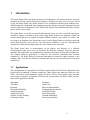
Introduction
The Steven Hydra Probe Soil Sensor measures soil temperature, soil moisture and soil electrical
conductivity and the complex dielectric permittivity. Designed for many years of service buried
in soil, the Hydra Probe uses quality material in its construction. Marine grade stainless steel,
ABS housing and a high grade epoxy potting protect the internal electrical component from the
corrosive and reactive properties of soil. Most of the Hydra Probes installed more than a decade
ago are still in service today.
The Hydra Probe is not only a practical measurement device it is also a scientific instrument.
Trusted by farmers to maximize crop yields, using Hydra Probes in an irrigation system can
prevent runoff that may be harmful to aquatic habitats, conserve water where it is scarce, and
save money on pumping costs. Researchers can rely on the Hydra Probe to provide accurate and
precise data for many years of service. The inter-sensor variability is very low, allowing direct
comparison of data from multiple probes in a soil column or in a watershed.
The Hydra Probe bases it measurements on the physics and behavior of a reflected
electromagnetic radio wave in soil to determine the dielectric constants. From the dielectric
constants, the Hydra Probe can simultaneously measure soil moisture and electrical conductivity.
The complex dielectric permittivity is related to the electrical capacitance and electrical
conductivity. The Hydra Probe uses patented algorithms to convert the signal response of the
standing radio wave into the dielectric constants and thus the soil moisture and soil electrical
conductivity.
1.1
Applications
The US Department of Agriculture Soil Climate Analysis Network (SCAN) has depended on the
Hydra Probe in hundreds of stations around the United States and Antarctica since the early
1990s. The Bureau of Reclamation's Agrimet Network, NOAA, and countless other mesonets
and research watersheds around the world trust the measurements the Hydra Probe provides.
Some of the applications include:
Agriculture
Viticulture
Research
Water Shed Modeling
Land Reclamation
Shrink/Swell Clays
Satellite Ground Truthing
Predicting Weather
Irrigation
Sports Turf
Phyto Soil Remediation
Evapotranspiration Studies
Land Slide Studies
Flood Forecasting
Wetland Delineation
Precision Agriculture
6
1.2
Temperature Corrections
The Hydra Probe’s soil moisture and electrical conductivity measurements are temperature
corrected providing temperature independent data year round.
1.3
Calibrations
The Hydra Probe has four calibrations that provide excellent performance in most mineral soils
regardless of texture or organics. The calibrations are sand, silt, clay and loam. The loam soil
calibration is the default calibration and is suitable for Silt Loams, Loam, Clay Loam, Silty Clay
Loam, Sandy Clay Loam, Sandy Loam, and some medium textured clays.
1.4
Dielectric Constants
For research studies involving andisol pumas soil, wetland histasol soils or soil with extremely
low bulk densities, the uncorrected and the temperature corrected dielectric constants are
provided for custom calibrations.
1.5
Structural Components
There are three main structural components to the Hydra Probe. The marine grade stainless steel
tine assembly is the wave guide. The tine assembly is the four metal rods that extend out of the
base plate. Each tine is 45 mm long by 3 mm wide. The base plate is 25 mm in diameter.
Electromagnetic waves at a radio frequency are transmitted and received by the center tine. The
head or body of the probe contains the circuit boards, microprocessors, and all the other
electrical components. The outer casing is ABS and the internal electronics are permanently
potted with a rock-hard epoxy resin giving the probes a rugged construction. The cable has a
direct burial casing and contains the power, ground, and data wires that are all soldered to the
internal electronics.
1.6
Accuracy and Precision
The Hydra Probe provides accurate and precise measurements. Table 1.1 below shows the
accuracy. For a detailed explanation of accuracy and precision and on the statistical evaluation of
the Hydra Probe, see Appendix D.
Parameter
Temperature (C)
Soil Moisture wfv (m3 m-3)
Soil Moisture wfv (m3 m-3)
Electrical Conductivity (S/m) TUC*
Electrical Conductivity (S/m) TC**
Real/Imaginary Dielectric Constant TUC*
Real/Imaginary Dielectric Constant TC*
Accuracy/Precision
+/- 0.6 Degrees Celsius(From -10o to 36oC)
+/- 0.03 wfv (m3 m-3) Accuracy
+/- 0.003 wfv (m3 m-3) Precision
+/- 0.0014 S/m or +/- 1%
+/- 0.0014 S/m or +/- 5%
+/- 0.5 or +/- 1%
+/- 0.5 or +/- 5%
Table 1.1 Accuracy and Precision of the Hydra Probes’ Parameters .
*TUC Temperature uncorrected full scale
**TC Temperature corrected from 0 to 35 o C
7
2
Configurations of the Hydra Probe
The Hydra Probe is available in three versions, differentiated by the manner that information is
transferred.
● SDI-12
● RS-485
● Analog
The two digital versions (SDI-12 and RS-485) incorporate a microprocessor to process the
information from the probe into useful data. This data is then transmitted digitally to a receiving
instrument. SDI-12 and RS-485 are two different methods of transmitting digital data. In both
versions there are electrical and protocol specifications that must be observed to ensure reliable
data collection.
The Analog version requires an attached instrument to measure voltages. This information must
then be processed to generate useful information. This can be done either in the attached
instrument, such as a data logger, or at a central data processing facility.
All configurations provide the same measurement parameters with the same accuracy. The under
lying physics behind how the Hydra Probe works, and the outer construction are also the same
for each configuration. Table 2.1 provides a physical description of the Hydra Probe.
Feature
Probe Length
Diameter
Sensing Volume*
(Cylindrical measurement region)
Weight
Power Requirements
Temperature Range
Storage Temperature Range
Attribute
12.4 cm (4.9 inches)
4.2 cm (1.6 inches)
Length 5.7 cm (2.2 inches)
Diameter 3.0 cm (1.2 inches)
200g
(cable 80 g/m)
7 to 20 VDC (12 VDC is ideal)
-10 to 65o C
-40 to 70o C
Table 2.1 Physical description of the Hydra Probe (All Versions)
The cylindrical measurement region or sensing volume is the soil that resides between the stainless steel tine
assembly. The tine assembly is often referred to as the wave guide and probe signal averages the soil in the sensing
volume.
2.1
Digital Probes
Digital probes offer some advantages over the Analog version. One is that post-processing of the
data is not required. Another is that the data is not affected by the length of the cable. Analog
probes, since their information is delivered as voltage, should only be used with relatively short
cables, on the order of 8 meters (25 feet). Digital cables can be much longer. SDI-12 cables can
be up to 50 meters long (150 feet), and RS-485 cables can be up to 1000 meters (3000 feet).
Digital probes can also be used with short cables without any trouble. Some installations use
cables that are less than a meter (three feet) long.
8
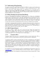
2.1.1 Addressing & Programming
The digital versions of the Hydra Probe (the SDI-12 and RS-485 versions) can be connected in
parallel so that multiple probes can be connected to a single communications port of a data
logger or other device. When multiple probes are connected this way, each probe must be
assigned a unique address before they are installed. The methods used for both probes are
similar, but unique. In addition, the user can select which processing method for the probe to use
and select which data is to be transmitted.
2.1.2 Daisy Chaining Versus Home Run Wiring
If you are contemplating the installation of multiple probes over a large area, consideration
should be given to the physical layout of the cables. Digital probes can be connected in a “Daisy
Chain” manner, where each probe is spliced onto the cable of the previous probe. This can
reduce the amount of cable required along with the corresponding cost. However, this means that
splices with have to made, and will likely need to be done in the field. Further if a cable breaks
or a splice fails, all probes beyond that point will be out of service until the break is repaired.
“Home Run” wiring means that each probe has a dedicated cable that runs all the way back to the
data collection station. The advantages here are just the reverse of “Daisy Chaining”. If there is a
break in the cable, only that probe is affected. There are no splices to fail. The disadvantage is
that the cable requirements and associated costs will be higher.
2.1.3 SDI-12 Hydra Probe II
The SDI-12 version is digital and can be used with Data Loggers that support this
communications method. SDI-12 stands for Serial Data Interface at 1200 baud. SDI-12 was
developed in cooperation with the USGS (U.S. Geological Survey) and is a standard
communication protocol for environmental sensors and data loggers.
2.1.3.1
Transparent Mode
Transparent Mode allows the user to communicate directly with the Hydra Probe. This is
necessary in order to assign an address to the probe or modify the probe's configuration.
To program an SDI-12 Version of the Hydra Probe, an SDI-12 compatible device that supports
Transparent Mode is required. Most SDI-12 data loggers support Transparent Mode. The SDI-12
protocol is not compatible with common serial data communications, so a device is needed to
convert between the two. A typical method is to connect a Personal Computer (PC) to a data
logger using a standard nine pin serial data communications cable, and then the probe is
connected to the SDI-12 port on the logger, and power is supplied. A terminal program (like
Hyper Terminal) is started on the PC. Typically the user must issue a command to the logger to
enter Transparent Mode.
See Appendix A for specific information on SDI-12 commands for the Hydra Probe. Please visit
www.SDI-12.org for more information about the SDI-12 Protocol. Table 2.2 describes the
physical specifications, wire designations, and other information about the digital SDI-12 Hydra
Probe II.
9
Power Requirements
Red Wire
Black Wire
Blue Wire
Baud Rate
Power Consumption
9 to 20 VDC (12VDC Ideal)
+Volts Power Input
Ground
SDI-12 Data Signal
1200
<1 mA Idle, 30 mA Active
Table 2.2 Digital SDI-12 Hydra Probe II Information.
2.1.4 Digital RS-485 Hydra Probe II
Like the SDI-12 Hydra Probe, the RS-485 probe is also digital. The RS-485 communication
format has 2 data wires, consumes more power when idle and has a custom communication
protocol. Being digital, the RS-485 version shares many of the benefits the SDI-12 version does.
The RS-485 sensors can be “daisy chained” or wired to a terminal assembly to simplify
installation. The RS-485 Hydra Probe has a maximum cable length of 1000 meters. The user
may have specific applications where this capability is advantageous, however, due to the cost of
the cable, it may be more cost effective to run short cables and have additional data loggers. See
appendix B for more information about commands for the RS-485 Hydra Probe.
Power Requirements
Red Wire
Black Wire
White Wire
Green Wire
Baud Rate
Power Consumption
9 to 20 VDC (12VDC Ideal)
+Volts Power Input
Ground
Data Signal A non-inverting signal
Data Signal B inverting signal
9600 8N1
<10 mA Idle 30 mA Active
Table 2.3 Digital RS-485 Hydra Probe II Information.
2.1.4.1
Addressing and Programming
RS-485 data communications ports are not commonly found on Personal Computers (PC's). To
prepare an RS-485 version of the Hydra Probe it will be necessary to program the address. One
method to talk to the probe is to connect the probe to a PC via an “RS-485 to RS-232 converter”.
These devices are available from several vendors specializing in data communications products.
Once the probe is connected and power is applied, a terminal emulation program, such as Hyper
Terminal is started on the PC. Certain settings will be need to be set to enable communications
with the probe. The following settings are for Hyper Terminal, but most terminal emulation
programs should have equivalent settings.
●
COM Port should be set to correspond with actual port on the PC where the
communications cable is plugged in. For instance COM1, COM2, etc.
●
Baud rate should be set to 9600
●
Data bits should be set to 8
●
Parity should be set to none.
●
Stop bits should be set to 1 (one).
10
●
Flow control should be set to none.
In addition, these setting will make the program easier to use. In Hyper Terminal these settings
are found under File / Properties / Settings / ASCII Setup / ACSII Sending:
●
Check “Send line ends with line feeds”. All commands sent to an RS-485
version of the Hydra Probe must end with a “Carriage Return” “Line Feed” pair.
●
Check “Echo typed characters locally”. The Hydra Probe does not echo any
commands. Checking this enables you to see what you have typed.
2.2
Analog Hydra Probe
The Analog Hydra Probe was the first version made available. The Analog version is useful for a
number of applications. Current customers of the Analog probe include users that need to replace
or add a sensor to an existing system that was specifically tailored for the analog sensors. One
advantage the Analog Hydra Probe has over the digital version is the fast measurement rate. For
example, on the beach, ocean researchers can use the analog Hydra Probe to measure the
hydrology of sands in the surf zone where they would want to take several measurements
between waves. This would entail taking measurements several times per second, something the
digital probes cannot do.
2.2.1 Analog Hydra Probe Output
The output of the Analog Hydra Probe is 4 voltages. These four voltages are the raw signal
response of the measurement and directly represent the behavior of the reflected electromagnetic
standing wave. The four voltages need to be processed by a computer program in order to obtain
the parameters of interest such as soil temperature, soil moisture, soil electrical conductivity and
the dielectric constants.
Table 2.4 below shows the wiring scheme.
Black Wire
Red Wire
Blue Wire (Output)
Brown Wire (Output)
Green Wire (Output)
White Wire (Output)
Yellow Wire
Power Draw Active
Ground
Power 7 to 30 VDC (12 VDC Ideal)
V1 (Raw Voltage 1) Range 0-2.5 volts
V2 (Raw Voltage 2) Range 0-2.5 volts
V3 (Raw Voltage 3) Range 0-2.5 volts
V4 (Raw Voltage 4) Range 0-1 volts
Reference Ground
35 to 40 mA
Table 2.4 wiring scheme for the Analog Hydra Probe.
An easy way to remember the wiring scheme is the colors of the wires are ordered
alphabetically. The black and yellow ground wires may be connected and grounded together or
grounded separately. The four voltage data wires need to be wired into four separate voltage
sensing connection points on the recording instrument. On the Stevens DOT Logger, the analog
ports are labeled A1, A2, A3, and A4. Use the logger data acquisition procedure to obtain the
raw voltages values. For more information about the Stevens Dot Logger, see appendix C.
11
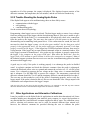
2.3.2 Post possessing raw voltages into the measurements of interest.
The output of the Analog Hydra Probe is 4 voltages, each on a separate color coded wires. V1
V2 and V3 will be between 0 and 2.5 volts DC. V4 will be between 0.1 to 0.8 volts DC. These 4
voltages need to be processed by a series of algorithms to obtain the parameters of interest.
Stevens provide two executable programs to perform these calculations:
● HYDRA.EXE
● HYD_FILE.EXE.
HYD_FILE.EXE and HYDRA.EXE as well as the instruction procedure for HYD_FILE.EXE
can be downloaded from the Stevens website at: http://www.stevenswater.com
HYD_FILE.EXE is the program used for processing tables of raw voltages collected over time.
HYDRA.EXE is the program used for a single measurement of the 4 voltages.
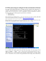
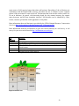
FIG. 2.1 HYDRA.EXE Input V1, V2, V3, V4 and Output Parameters.
To use HYDRA.EXE simply open the file and follow the prompts. The first prompt will ask
“Type A Probe ? (Y/N):”. Type Y. Almost all of the Analog Hydra Probes are type A.
Type A probes use a 2.5 volt reference for the temperature sensing element. A non-type A probe
uses a 5 volt reference. Next, enter the soil type and then the four voltage values. After the user
12
responds to all of the prompts, the output is displayed. The displayed output consists of the
dielectric constants, the temperature, the soil moisture, and the soil electrical conductivity.
2.2.2 Trouble Shooting the Analog Hydra Probe
If the Hydra Probe appears to be malfunctioning, there are three likely causes:
● communication with the logger
● soil hydrology
● a malfunctioning probe.
See the section about soil hydrology.
Programming a data logger is not a trivial task. The data logger needs to extract 4 raw voltages
from four analog ports on the logger with the desired timing interval. If the user is unable to get a
response from the Hydra Probe, it is recommended to first physically check wire connections
from the probe to the logger. The user may also want to cycle the power to the probe by
disconnecting and reconnecting both ground wires. If the connections are sound, the user will
next need to check the logger’s setup. Are the data ports enabled? Are the data ports scaled
properly in the appropriate units? Are the probes and logger adequately powered? Is the data
properly recorded on the logger? If the logger has GUI based operation software, there may be
a help function. If the logger only accepts terminal command scripts in a terminal window, refer
to the logger’s manual or manufacturer. Also, make sure the computer is properly connected to
the logger. Is the computer on the proper COM port? What about the Baud rate? Does the
logger need a NUL modem or optical isolator in order to be connected to a computer? Most of
the technical support questions Stevens receives are not due to malfunctioning probes but rather
an incorrect data logger setup.
A good way to verify if the probe is working properly is to submerge the probe in distilled
water* in a plastic container and check the dielectric constants. Once the probe is submerged,
connect the black and yellow wires to a ground and connect the red wire to a +12 volt DC power
source. Use a voltmeter to measure the raw voltage on the 4 data wires. A common hand held
unit is adequate. Use HYDRA.EXE to process the voltages. The temperature corrected real
dielectric constant should be 75 to 85 and the imaginary dielectric constant should be less than 5.
The user may use this method to verify if the probe is functioning properly, and to verify the
logger output. If the probe is buried in the soil, the user can obtain the 4 raw voltage outputs with
a multimeter and compare them to the logger’s output.
*The user may also use tap water for this procedure, however, it is important to note that tap water contains
dissolved material and trace contaminants that might affect the dielectric constants.
2.3
Other Applications and Alternative Calibrations
It may be possible to use the Hydra Probe for applications in media other than mineral soil. Some
examples include peat, decomposed plant material, grain, compost, ice cream/ food products or
any material that has a small dielectric constant compared to that of water. The calibration curves
used to calculate soil moisture may not be valid for material different from mineral soil;
however, the dielectric constants are provided allowing the user to calibrate the probe
13
accordingly. The calibration curves will mathematically have the appearance of equation [2.1] or
[2.2]
 = A + BEr + CEr2 +DEr3 [2.1]
 = AEr1/2 + B
[2.2]
Where  is moisture Er is the real dielectric constant and A,B,C, and D are coefficients. If the
user wishes to use the Hydra Probe to measure moisture in a matrix that is not mineral soil, the
user must empirically and experimentally solve equation [2.1] or equation [2.2]. Also, The user
should review the matrix compatibility requirements of the probe in section 3.1.
2.3.1 Frozen Soil
The Hydra Probe can also be used to determine if soil is frozen. Once ice reaches 0o Celsius, it
will begin to thaw and the real dielectric constant will increase from 5. The temperature alone
may not indicate whether or not the soil is frozen. As the soil begins to thaw, the soil moisture
and the real dielectric constant should return to values similar to what they were before the soil
froze.
14
3
Installation
The Hydra Probe is easy to install and the use of installation tools are seldom required.
3.1
Avoid Damage to the Hydra Probe:
Do not subject the probe to extreme heat over 70 degrees Celsius (160 degrees
Farenheit).
● Do not subject the probe to fluids with a pH less than 4.
● Do not subject the probe to strong oxidizers like bleach, or strong reducing agents.
● Do not subject the probe to polar solvents such as acetone.
● Do not subject the probe to chlorinated solvents such as dichloromethane.
● Do not subject the probe to strong magnetic fields.
● Do not use excessive force to drive the probe into the soil because the tines could bend. If
the probe has difficulty going into the soil due to rocks, simply relocate the probe to an
area slightly adjacent.
● Do not remove the Hydra Probe from the soil by pulling on the cable.
While the direct burial cable is very durable, it is susceptible to abrasion and cuts by shovels.
The user should use extra caution not to damage the cable or probe if the probe needs to be
excavated for relocation.
●
Do not place the probes in a places where they could get run over by tractors or other farm
equipment. The Hydra Probe may be sturdy enough to survive getting run over by a tractor if it is
buried; however, the compaction of the soil column from the weight of the vehicle will affect the
hydrology and thus the soil moisture data.
3.1.1 Lightning
Lightning strikes will cause damage or failure to the Hydra Probe or any other electrical device,
even though it is buried. In areas prone to lightning, serge protection and /or base station
grounding is recommended.
3.2
Wire Connections
3.2.1 Analog Probe Wire Connection
Table 2.4 in section 2.4.3 shows the wiring scheme for the Analog Hydra Probe. The four
voltage data wires need to be wired into four separate data ports on the logger. On the Stevens
DOT Logger, the analog ports are labeled A1, A2, A3, and A4. The red power wire should be
connected to a +12 volt power supply and the black and yellow wires should be connected to a
ground. For more information, refer to the data loggers operation manual. For DOTSET and the
Stevens DOT Logger refer to Appendix C.
3.2.2 SDI-12 Hydra Probe Wiring Connections
Table 2.2 and section 2.1 provide important information about the SDI-12 Hydra Probe. Connect
the red wire to a +12 volt DC power supply, connect the black wire to a ground, and connect the
blue wire to the SDI-12 port or the Data Logger. The SDI-12 data port on the Stevens DOT
logger is conveniently located on the right side of front face plate. The advantage of SDI-12
15
communications is that multiple probes can be connected to a single port on data logger. The
probes may be “daisy chained” together, or they may all be connected to a central terminal
assembly. The single SDI-12 data port on the DOT Logger can accommodate 150 SDI-12
Channels. To have 150 SDI-12 channels means that 50 probes set to measure soil moisture,
conductivity and temperature can all be wired together on a multiplexer with a single data wire
going into the single SDI-12 data port. For more information, refer to the data loggers operation
manual. For more information about the Stevens DOT Logger refer to Appendix C.
For more than 6 Hydra Probes, the user may find it easier to have the terminal assembly in a
separate enclosure from the logger, telemetry and power supply.
3.2.3 RS-485 Hydra Probe wiring Connections
Table 3.1 and section 2.1.4 provide important information about the RS-484 Hydra Probe.
Connect the red wire to a +12 volt DC power supply, and connect the black wire to a ground.
The green and white wires are the data wires.
Power Requirements
Red Wire
Black Wire
White Wire
Green Wire
Baud Rate
Power Consumption
Control system settings
Control system settings
Control system settings
9 to 20 VDC (12VDC Ideal)
+Volts Power Input
Ground
Data Signal A non-inverting signal
Data Signal B inverting signal
9600
<10 mA Idle 30 mA Active
8 DATA BITS
One Stop Bit
NO Parity
Table 3.1 Digital RS-485 Hydra Probe II Information.
Like SDI-12, the RS-485 communication format is also digital, therefore the probes’ data wires
can be “daisy chained” or connected together at a terminal assembly. See Appendix B for
RS-485 command structure.
16
3.3
Soil and Topographical Considerations
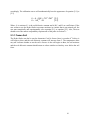
3.3.1 Soil Moisture Calibration
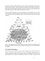
There are four calibration curves depending on the texture of the soil. The calibrations curves are
polynomials that include the real dielectric constant and several coefficients (Topp 1980,
Seyfried and Murdock 2004). The four user selectable soil texture settings are Sand, Silt, Clay,
and Loam. The texture is determined by the percentage of sand silt and clay there is in the soil.
Figure 3.1 shows the corresponding percentages to the different textures. If you are unsure of
your soil texture, determining which soil setting that is best for your soil is easy and there are a
number of different ways to make the determination (Birkeland 1999).
a)
A detailed soil survey for your area can be downloaded for free from the US Department of
Agriculture at http://soildatamart.nrcs.usda.gov/
b) Many times, it will be obvious. Sand looks different from clay.
c) Grab a baseball size portion of the soil in your hands. Wet the soil with water and work the
moist soil with your hands. The stickier it is, the more clay there is. The “soapier” the soil
feels the higher the silt content. Grittiness is indicative of sand.
Figure 3.1 Soil Texture Triangle
17
If you have a mixture of sand, silt and clay or if you are unsure what the texture of your soil is,
then use the Loam setting. The Sand, Silt and Clay settings are only suitable for soils that are
comprised almost entirely of that one material. For most mixtures the Loam setting will give
better results. The Loam setting is applicable for Loam, Clay Loam, Silty Clay Loam, Silt Loam,
Sandy Loam, Sandy Clay Loam, Sandy Clay and Silty Clay textures.
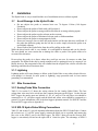
If unsure as which calibration to use, the loam calibration will accommodate most soils. The
Loam calibration is the default calibration, which means, the Hydra Probe is preset to the loam
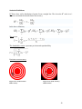
soil type setting when it leaves the factory. Figure 3.2 shows the textures where the loam setting
works best.
Figure 3.2 The shaded circle in the soil texture triangle is the region where the Loam soil calibration works
best. Most users should use the loam calibration. The Hydra Probe is preset to use the loam soil calibration
when shipped.
3.3.2 Soil Classifications
Between the four preset calibrations and the custom calibration option, the Hydra Probe can
measure soil moisture in almost any kind of soil. There are thousands of different kinds of soil
through out the world, and almost every nation has some kind of classification system. The most
wide spread and most current soil classification system is the Orders of American Soil
18
Taxonomy. In this system, all of the worlds’ soils are broken into 12 orders based on climate,
topography, biology and soil chemistry. Table 3.2 lists the orders.
The Hydra Probe can accommodate all of the soil orders. Andisols, gelisols and histosols are
soil that may have soil moistures and properties that depart from the Hydra Probe’s built in
calibration curves. If the bulk density is extremely low giving the soil an effective porosity
greater than 0.5, the user will need a custom calibration If a custom calibration is required see
Section 2.3. If the Hydra Probe needs to be switched from the default Loam calibration setting,
see the RS-485 or SDI-12 command sections in the appendix.
Soil
Order
Entisol
Inceptisol
Vertisol
Histosol
Aridisol
Mollisol
Spodosol
Alfisol
Ultisol
Oxisol
Gelisol
Andisol
Climate or Regime
Soil Characteristics
Sandy Young Soil
Silty Young Soil
Shrink/Swell Clay
Wetland Soil
Desert Soil
Grass land Soil
Needle Leaf Forest Soil
Forest Soil
Old Forest Soil
Ancient Forest Soil
Soil With Permafrost
Volcanic Ash Soil
Stream Flood Plain
Evidence of red color
Homogenized Soil
Anoxic Reduced State
Higher pH
Higher pH
Low pH
Low pH
Low pH
Red, Oxidized
Organic Rich
Low Density
Hydra Probe
Calibration
Sand
Sand or Silt
Loam or Clay
Loam or Custom
Sand
Loam or Silt
Loam or Silt
Loam or Silt
Loam
Loam
Loam or Custom
Loam or Custom
Table 3.2 The 12 Orders of Soil Taxonomy, Characteristics and Hydra Probe Calibration setting.
3.4
Installation of the Hydra Probe in Soil
3.4.1 Topography and Groundwater Hydrology
The land topography often dictates the soil hydrology. Depending on the users’ interest, the
placement of the Hydra Probe should represent what would be most useful. For example, a
watershed researcher may want to use the Hydra Probe to study a micro climate or small
hydrological anomaly. On the other hand, a farmer will want to take measurements in an area the
best represents the condition of the crops as a whole.
Other factors to consider would be tree canopy, slope, surface water bodies, and geology. Tree
canopy may affect the influx of precipitation/irrigation. Upper slopes may be better drained than
depressions. There may be a shallow water table near a creek or lake. Hill sides may have seeps
or springs.
19
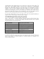
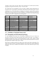
Figure 3.3 Groundwater pathways and Surface water. Taken from USGS Report 00-4008
Figure 3.4 Groundwater flow direction and surface water body. Taken from USGS report 00-4008.
Figures 3.3 and 3.4 illustrate subsurface water movement in the water table. The Hydra Probe
data is most meaningful in the unsaturated zone where soil moisture values will fluctuate. If the
water table rises to the depth of the Hydra Probe, the Hydra Probe soil moisture measurements
will be at saturation and will be indicative of the effective porosity. If the user is interested in
groundwater level measurements in wells, a water depth sensor might provide the necessary
information.
20
3.4.2 Installation of the Hydra Probe into Soil.
The most critical thing about the installation of the Hydra Probe is the soil needs to be
undisturbed and the base plate of the probe needs to be flush with the soil. To install the probe
into the soil, first select the depth (see section 3.4.3 for depth selection). A post hole digger or
spade works well to dig the hole. If a pit has been prepared for a soil survey, the Hydra Probes
can be conveniently installed into the wall of the survey pit before it is filled in. Use a paint
scraper to smooth the surface of the soil where it is to be installed. It is important to have the soil
flush with the base plate because if there is a gap, the Hydra Probe signal will average the gap
into the soil measurement and create errors.
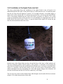
Figure 3.5 Hydra Probe Installed in undisturbed soil.
Push the tines of the Hydra Probe into the soil until the base of the tines is flush with the soil.
The tines should be parallel with the surface of the ground, i.e. horizontal. Avoid rocking the
probe back and fourth because this will disturb the soil and create a void space around the tines.
Again, it is imperative that the bulk density of the soil in the probe’s measurement volume
remain unchanged from the surrounding soil. If the bulk density changes, the volumetric soil
moisture measurement and the soil electrical conductivity will change.
The user may also want to run the Hydra Probe cable through a metal conduit like the one shown
in figure 3.6 to add extra protection to the cable.
21
3.4.3 Hydra Probe Depth Selection
Like selecting a topographical location, selecting the sensor depth depends on the interest of the
user. Farmers will be interested in the root zone depth while soil scientists may be interested in
the soil horizons.
Depending on the crop and the root zone depth, in agriculture two or three Hydra Probes may be
installed in the root zone and one Hydra Probe may be installed beneath the root zone. The
amount of water that should be maintained in the root zone can be calculated by the method
described in section 4.3. The probe beneath the root zone is important for measuring excessive
irrigation.
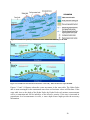
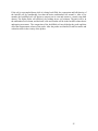
Figure 3.6 Six Hydra Probes installed into 6 distinct soil horizons.
The soil horizons often dictate the depths of the Hydra Probes’ placement. Soil scientist and
groundwater hydrologist are often interested in studying soil horizons. The Steven Hydra Probe
is an excellent instrument for this application because of the accuracy and precision of the
volumetric water fraction calibrations. Soil horizons are distinct layers of soil that form naturally
in undisturbed soil over time. The formation of soil horizons is called soil geomorphology and
the types of horizons are indicative of the soil order (see table 3.2). Like other natural processes,
the age of the horizon increases with depth. The reason why it is so useful to have a Hydra Probe
in each horizon is because different horizons have different hydrological properties. Some
horizons will have high hydraulic conductivities and thus have greater and more rapid
fluctuations in soil moisture. Some horizons will have greater bulk densities with lower effective
porosities and thus have lower saturation values. Some horizons will have clay films that will
22
retain water at field capacity longer than other soil horizons. Knowledge of the soil horizons in
combination with the Hydra Probes accuracy will allow the user to construct a more complete
picture of the movement of water in the soil. The horizons that exist near the surface can be 6 to
40 cm in thickness. In general, with increasing depth, the clay content increases, the organic
mater decreases and the base saturation increases. Soil horizons can be identified by color,
texture, structure, pH and the visible appearance of clay films.
More information about soil horizons is provided by the USDA National Resource Conservation
Service at http://soils.usda.gov/education/resources/k_12/lessons/profile/
More information about the soil horizons in your area can be found by in a soil survey. A soil
survey for your area can be found at http://soildatamart.nrcs.usda.gov/
Soil
Horizon
O
A
B
E
C
Property
Decaying plants on or near surface
Top Soil, Organic Rich
Subsoil, Most Diverse Horizon and the Horizon with the most sub
classifications
Leached Horizon (light in color)
Weathered/aged parent material
Table 3.3 Basic description of soil horizons.
Figure 3.7 Soil Horizons.
23
Figure 3.8 Illustration of soil horizons. In this frame, the soil horizons are very distinct and show the
geological history of the soil.
3.4.4 Back Filling the Hole after the Probes are Installed.
After soil is removed from the ground and piled up next to the hole, the horizons and soil
become physically homogenized. The bulk density decreases considerably because the soil
structure has been disturbed. After the probes are securely installed into the wall of the pit, the
pit needs to be backfilled with the soil that came out it. It is impossible to put the horizons back
the way they have formed naturally, but the original bulk density can be approximated by
compacting the soil. For every 24 cm (1 foot) of soil put back into the pit, the soil should be
compacted. Compaction can be done by trampling the soil with feet and body weight.
Mechanical compactors can also be used, though typically they are not required. Extra care must
be taken not to disturb the probes that have exposed heads, cables and conduits when compacting
the soil. If the probes were installed in a post hole, a piece of wood, such as a post, can be used to
pack the soil.
24
If the soil is not trampled down while it is being back filled, the compaction and bulk density of
the backfill will be considerably less than the native undisturbed soil around it. After a few
months, the backfilled soil will begin to compact on its own and return to a steady state bulk
density. The Hydra Probe will effectively be residing in two soil columns. The tines will be in
the undisturbed soil column, and the head, cable and conduit will be in the backfill column that is
undergoing movement. The compaction of the backfilled soil may dislodge the probe and thus
affect the measurement volume of the probe. After the probes are installed, avoid foot traffic and
vehicular traffic in the vicinity of the probes.
25
4
Measurements, Parameters, and Data Interpretation
4.1
Analog Hydra Probe Output
Parameters V1, V2, V3 and V4 returned by the digital probes correspond to the voltages read
from the analog probe. In almost all applications, V1, V2, V3, V4 and V5 by themselves are of
no interest to most users of the digital Hydra Probe. See section 2.2.3 for analog processing
information.
4.1.1 Raw Voltages V1, V2, and V3.
The first three voltages are the raw signal responses. The Hydra Probe is a Frequency Domain
Reflectometer in that it is measuring the behavior of a standing wave generated from the
reflection of an electromagnetic wave at a radio frequency of 50 MHz. The 50 MHz
electromagnetic wave propagates along the wave guide. The soil absorbs most of the wave. The
portion of the wave that reflects back down the wave guide encounters the emission propagation
creating a standing wave. The first three voltages represent the behavior of the standing wave
and thus the complex dielectric permittivity. The direct measurement of the complex dielectric
permittivity from the raw signal responses is the basis behind the other parameters and makes the
Hydra Probe unique among other FDR type methods (Campbell, 1990, Seyfried and Murdock,
2004).
4.1.2 V4
V4 is the raw signal response of the diode thermistor. The diode thermistor is located within the
probe housing. V4 is used to make temperature corrections to the electronics. See Diode
temperature below for more information.
4.1.3 V5
V5 is the raw signal response of the soil thermistor. The soil thermistor is located in the stainless
steel base plate between the tines. It is in close proximity to the soil providing accurate soil
temperature readings. Complex dielectric permittivity is influenced by temperature. Not only can
the Hydra Probe measure soil temperature, it can make temperature corrections to the calibration
curves based on the temperature corrections of the complex dielectric permittivity. See
temperature corrected real and imaginary dielectric constant for more information. See section
2.2.3 for analog processing information.
4.1.4 ADC Reading 1 through 5
The ADC Reading 1 through 5 are the analog to digital values at 10 bits. They are the binary
numbers that correspond to V1 through V5. They are used by Stevens for development or trouble
shooting purposes.
4.1.5 Diode Temperature
The Diode Temperature is the temperature of the electronics within the Hydra Probe housing. It
corresponds to V4. Because the electronics produces a negligible amount of heat while taking a
reading, the diode temperature is usually very close, if not the same value as soil temperature.
26
The diode temperature is used by the Hydra Probe to make algorithmic temperature correction to
the electronics.
4.2
Soil Temperature
The user can select Fahrenheit or Celsius. Diurnal (daily) temperature fluctuations between
daytime highs and nighttime lows may be observed with the Hydra Probe’s temperature data.
These fluctuations will become less pronounced with depth. Vegetation, tree canopy, and soil
moisture are factors that will effect the diurnal soil temperature fluctuations. For example, in the
American Southwest, A Hydra Probe buried at a five inch depth will have very pronounced
temperature fluctuations between the nighttime lows and the daytime highs if there is no
vegetation insulating the soil. Seasonal trends can also be observed in soil temperature data.
4.3
Soil Moisture
4.3.1 Soil Moisture Units
The Hydra Probe provides accurate soil moisture measurements in units of water fraction by
volume (wfv or m3m-3 ). That is, a percentage of water in the soil displayed in decimal form.
For example, a water content of 0.20 wfv means that a one liter soil sample contains 200 ml of
water. Full saturation (all the soil pore spaces filled with water) occurs typically between 0.30.45 wfv and is quite soil dependent.
There are a number of other units used to measure soil moisture. They include % water by
weight, % field capacity, % available (to a crop), inches of water to inches of soil, and tension
(or pressure). They are all interrelated in the sense that for a particular soil, knowledge of the
soil moisture in any one of these units allows the soil moisture level in any of the other unit
systems to be determined. It is important to remember that the conversion between units can be
highly soil dependent.
The unit of water fraction by volume (wfv) was chosen for the Hydra Probe for a number of
important reasons. First, the physics behind the soil moisture measurement dictates a response
that is most closely tied with the wfv content of the soil. Second, without specific knowledge of
the soil, one can not convert from wfv to the other unit systems. Third, the unit wfv allows for
direct comparison between readings in different soils. A 0.20 wfv clay contains the same
amount of water as a 0.20 wfv sand.
However, the same thing can not be said about the other measurement units. For example, to use
the unit common in tensiometer measurements, a one Bar sand and a one Bar clay will have
vastly different water contents. The wfv unit can also be readily used to estimate the effects of
precipitation or irrigation. For example, consider a soil that is initially 0.20 wfv, and assume a 5
cm rainfall that is distributed uniformly through the top one meter of soil. What will the
resultant soil moisture in the top one meter of soil be? 5 cm is 0.05 of one meter, so the rainfall
will increase the soil moisture by 0.05 wfv to result in a 0.25 wfv soil. For other units, this
calculation can be much less straightforward, particularly when soil moisture is measured as a
tension.
27
4.3.2 Soil Moisture Measurement Considerations
Soil moisture measurements are important for a number of applications and for a number of
different reasons. Some applications include; land slide studies, erosion, water shed studies,
climate studies, predicting weather, flood warning, crop quality and yield optimization,
irrigation, and soil remediation to name a few.
Soil moisture values are particularly important for irrigation and the health of the crop. Equations
[4.1], [4.2] and [4.3] can help determine when to irrigate. The following are terms commonly
used in soil hydrology:
●
Soil Saturation, refers to the situation where all the soil pores are filled with water. This
occurs below the water table and in the unsaturated zone above the water table after a
heavy rain or irrigation event. After the rain event, the soil moisture (above the water
table) will decrease from saturation to field capacity.
●
Field Capacity (FC in equations below) refers to the amount of water left behind in soil
after gravity drains saturated soil.
●
Permanent Wilting Point (PWP in equations below) refers to the amount of water in soil
that is unavailable to the plant.
●
The Allowable Depletion (AD in the equations below) is calculated by equation [4.1].
The allowable depletion represents the amount of soil moisture that can be removed by
the crop from the soil before the crop begins to stress.
●
Lower soil moisture Limit (LL from [4.3]) is the soil moisture value below which the
crop will become stressed because it will have insufficient water. When the lower limit is
reached, it is time to irrigate.
●
The Maximum Allowable Depletion (MAD) is the fraction of the available water that is
100% available to the crop.
●
Available Water Capacity (AWC) is the amount of water in the soil that is available to
the plant.
The lower soil moisture limit is a very important value because dropping below this value will
affect the health of the crops. Equations 4.1, 4.2, and 4.3 and the example show how to calculate
the lower soil moisture limit.
Texture
Clay
MAD
0.3
Silty
Clay
0.4
Clay
Loam
0.4
= (FC – PWP ) x MAD
AWC = FC – PWP
LL = FC – AD
Loam
0.5
Sandy
Loam
0.5
Loamy
Sand
0.5
Sand
0.6
[4.1]
[4.2]
[4.3]
Table 4.1 Maximum allowable depletions for different soil textures
28
A
D
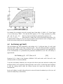
Figure 4.1 soil textures and the available water.
For example, let us suppose your soil is a sandy loam. From table 4.1, MAD = 0.5, From Figure
4.1 (or a soil surrey) PWP = 13% and the field capacity is 25%. Using equation [4.1] yields;
AD = (25-13) x 0.5 = 6% . The lower limit would then be calculated by equation [4.3].
LL = 25 - 6 = 19%.
This means for a sandy loam, if the soil moisture drops below 19%
(or Hydra Probe reading of 0.19), the crop may become stressed and it is time to irrigate. Never
let the soil moisture drop below the permanent wilting point.
4.4
Soil Salinity (g/L NaCl)
The Soil Salinity (g/L NaCl) parameter is the salinity of a 1:1 soil/water slurry. It is the “total
dissolved solids” (TDS) in the form of dissolved salts. The soil salinity parameter is primarily
used with the portable versions of Hydra Probe. The soil salinity parameter is not applicable for
in situ measurements in a permanent/semi permanent installation in soil. The soil salinity is
approximated:
Soil Salinity (g/L) ≈ EC (S/m) x 6.4
[4.4]
Equation [4.4] is found in the literature (McBride 1994) and works well if the soil is not
extremely acidic or extremely alkaline.
To use the Soil Salinity Parameter, mix one part soil with one part water and take a reading with
the Hydra Probe’s tines completely submerged in the water extract. Avoid using metal containers
to take the reading and/or make the slurries because the metal may interfere with the
measurements.
In situ soil salinity is usually inferred by the in situ soil electrical conductivity in S/m (see soil
electrical conductivity section below).
29
4.5
Soil Electrical Conductivity (Temperature corrected)
The Hydra Probe measures the in situ electrical conductivity in units of Siemens per meter. Soil
electrical conductivity is indicative of dissolved salts, dissolved solids, and fertilizers (McBride
1994). It may also be indicative of very high pH conditions. The soil electrical conductivity is
calculated from the temperature corrected imaginary dielectric constant [Ei(tc)] by the theoretical
expression:
EC = 2πf ε0 Ei(TC) [4.5]
Where EC is the electrical conductivity, f is the frequency (50 MHz for the Hydra Probe) and ε 0
is the dielectric constant of a vacuum. For more information on soil electrical conductivity
considerations, see soil electrical conductivity section below.
As the temperature increases, the molecular vibration increases (Levine, 1993). The molecular
vibration has a complex affect on both the orientation polarization and on the imaginary
dielectric constant. The temperature corrections are based on the small incremental changes of Ei
and Er with temperature.
30
5
Theory of Operation
5.1
Real and Imaginary Dielectric Constants
The Hydra Probe is a dielectric constant sensor (Seyfriend, Grant, and Humes 2005) measuring
the complex dielectric permittivity. The complex dielectric permittivity is the raw electrical
parameter that has real and imaginary components (the real dielectric constant and the imaginary
dielectric constant). These two parameters serve to fully characterize the electrical response of
soil and are measured from the response of a reflected standing electromagnetic wave at a radio
frequency of 50 MHz. Both the real and imaginary dielectric constants are dimensionless
quantities.
The Hydra Probe is different from all other soil sensors because it measures both components of
the complex dielectric permittivity of the soil. In other words, The Stevens Hydra Probe uses the
reflected properties of a radio waves to measure soil moisture and soil electrical conductivity
simultaneously.
The complex dielectric permittivity contains both real and imaginary components where the real
component is related to the capacitance (soil moisture) and the imagery component is related to
the electrical conductivity
Capacitance is the measure of electric charge that can be stored in a media. The dielectric
constant is related to capacitance by the following equation:
εoE = Cx
[5.1]
εo is the capacitance in a vacuum, E is the dielectric constant, and Cx is the measured
capacitance of the media in Farads. Every material has a dielectric constant. As the dielectric
constant increases, the capacitance of the media increases. In other words, the capacitance
increases as a factor of the dielectric constant.
In the presence of an electromagnetic wave, the dielectric constant becomes frequency
dependent. The frequency dependence of the dielectric constant is generally termed complex
dielectric permittivity because the relationship between frequency and the dielectric constant
becomes a complex modulus containing both real and imaginary components.
The real dielectric constant represents the molecular orientation polarizability. The orientation
polarization of a water molecule in the presence of an electromagnetic wave is much greater than
the polarization of dry soil, which is mostly due to electronic and atomic polarization. The real
dielectric constant of dry soil can be from 1 to 5 where the real dielectric constant for pure water
is about 80. The real dielectric constant of soil is mostly attributed to the presence of water.
Figure [5.1] illustrates the different kinds of polarization molecules can under go upon receiving
electromagnetic energy. The general equation that describes complex dielectric permittivity is:
K* ε0 = E*,
K* = Er - jEi
[5.2]
31
Where (Ei) is imaginary dielectric constant, j = -11/2 and is the imaginary number, and (Er) is the
real dielectric constant.
Figure [5.1]. Illustration of polarization. The real dielectric constant of soil is mostly due to orientation
polarization of water (Taken from Lee et al. 2003)
The imaginary dielectric constant is directly related to the conductivity of the medium, the higher
the imaginary dielectric constant, the higher the conductivity. Assuming the molecular relaxation
is negligible, the imaginary dielectric constant is a function of frequency and electrical
conductivity by the following relationship:
Ei = EC/ 2πf ε0 [5.3]
Where EC is the electrical conductivity, f is the frequency (50 MHz for the Hydra Probe) and ε0
is the dielectric constant in a vacuum. As can be shown by equation [5.3], as the frequency
increases, the Ei rapidly decreases. Conversely, if the frequency decreases or if cations are
introduced, the Ei will increase thus affecting the real dielectric constant of the matrix.
32
The Hydra Probes’ design features such as the geometry of the wave guide and the frequency at
50 MHz allows the Hydra Probe to simultaneously measure both real and imaginary dielectric
constants (Campbell, 1990).
5.2 Real
corrected)
Dielectric
and
Imaginary
Constants
(Temperature
Since both the real and imaginary dielectric constants will vary somewhat with temperature, the
user of the Hydra Probe has the option of selecting the temperature corrected values for the real
and imaginary dielectric constants. The uncorrected and the corrected dielectric values may be
of interest for some researchers. The soil moisture calibrations are based on the temperature
corrected values because the calibration curves were established at a constant temperature.
Similarly, the temperature corrected imaginary dielectric constant was used for the electric
conductivity measurement.
As the temperature increases, the molecular vibration increases (Levine, 1993). The molecular
vibration has a complex effect on both the orientation polarization and on the imaginary
dielectric constant. The temperature corrections are based on the small incremental changes of Ei
and Er with temperature.
5.3
Soil Electrical Conductivity.
The Hydra Probe measures the in situ electrical conductivity in units of Siemens per meter (S/m).
Soil electrical conductivity is indicative of dissolved salts, dissolved solids, and fertilizers
(McBride 1994). It may also be indicative of very high pH conditions. The soil electrical
conductivity is calculated from the imaginary dielectric constant [Ei]. by the theoretical
expression:
EC = 2πf ε0 Ei [5.4]
Where EC is the electrical conductivity, f is the frequency (50 MHz for the Hydra Probe) and ε0
is the dielectric constant of a vacuum.
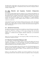
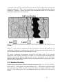
5.3.1 Electrical Conductivity Pathways in Soil
The electric conductivity of soil is complex. Figure [5.2] shows the three pathways the electrical
conductivity can propagate in soil. The bulk density, the porosity, the tortuosity, the water
content, and the dissolved ion concentration working in concert with the different pathways,
dramatically influences the electrical conductivity of a soil.
Pathway 1 is the electrical pathway that goes from water to the soil and back through the water
again. The electrical conductivity contribution of pathway 1 is a function of the conductivity of
the water and soil. As water increases, pathway 1 increases which may increase the electrical
conductivity of the soil as a whole.
Pathway 2 is the pathway that is attributed to the electrical conductivity of the soil water.
Increasing the dissolved salts will increase the conductivity of pathway 2; however, like pathway
33
1, increases in the soil water content will increase the size of the pathway thus increasing the
electrical conductivity. That is to say, that there are two factors influencing the electrical
conductivity of pathway 2, namely the dissolved salt concentration and the size of the pathway
attributed to the amount of water in the soil.
Figure 5.2 Pathway3 of electric conductivity in soil matrix. 1 water to solid, 2 soil moisture, 3 solid. Taken from Corwin
et al. (2003).
Pathway 3 is the electrical conductivity of the soil particles. Like the other pathways, the
contribution of pathway 3 in influenced by a number of factors that include bulk density, soil
type, oxidation/reduction reactions and translocation of ions.
The electric conductivity measurements provided by the Hydra Probe is the electrical
conductivity of the dynamic soil matrix as a whole. No in situ soil sensor can distinguish the
difference between the different pathways nor can any conventional in situ soil sensor
distinguish the difference between sodium chloride and any other number of solutes that all have
different electrical conductivities
5.3.2 Solution Chemistry
Salinity refers to the presence of dissolved inorganic ions such as Mg+ , Ca++, K+, Na+, Cl-, SO24-,
HCO3- and CO32- in the aqueous soil matrix (Hamed 2003) . The salinity is quantified as the
total concentration of soluble salts and is expressed in terms of electrical conductivity. There
exists no in-situ salinity probe that can distinguish between the different ions that may be
present.
34
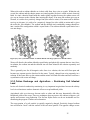
When salts such as sodium chloride are in their solid form, they exist as crystals. Within the salt
crystal, the sodium and the chorine atoms are joined together in what is called an ionic chemical
bond. An ionic chemical bond holds the atoms tightly together because the sodium atom will
give up an electron to the chlorine thus ionizing the atoms. If an atom like sodium gives up an
electron, it is said to be a positively charged ion (also called a cation). If an atom such as chlorine
receives an electron, it is said to be a negatively charged ion (also called an anion and is given
the suffix ide, like chloride). The sodium and the chloride ions comfortably arrange themselves
into a stacked like configuration called a crystal lattice. The sodium chloride crystal lattice has a
zero net charge.
Figure [5.3] The crystal lattice model of sodium chloride. The larger spheres are chloride anions.
Water will dissolve the sodium chloride crystal lattice and physically separate the two ions. Once
in solution, the sodium ion and the chloride ion will float around in the solution separately and
randomly.
This is generally true for all inorganic salts. Once in a solution, the ions will float apart and
become two separate species dissolved in the water. Typical, charged ions exist separately in a
solution. If the water dries up, the cations and the anions will find each other and fuse back into a
crystal lattice with a zero net charge.
5.3.3 Cation Exchange and Agriculture – Reclaiming Salt Infested
Land
In situ soil electrical conductivity monitoring is very important in agriculture because the salinity
levels in soil moisture can have dramatic effects on crop health and yields.
Agricultural soils over time may become sodic or saline and this may dramatically effect the
health and yields of the crops. There are techniques that can remove the sodium to improve soil
quality and increase crop production. The Stevens Hydra Probe can be an invaluable tool for
monitoring the progress of saline soil reclamation.
The outer portion of a soil particle is typically negatively charged. Positively charged sodium
ions will bind or “hook” onto the surface of the soil micro particle. The opposite charges create
35
an electronic attraction between the sodium ion and the soil. The sodium ions compete for
negatively charged sites on the soil particle surface and in doing so, disperse the aggregates of
soil. The aggregate dispersion of the soil caused by the sodium ions will decrease the porosity of
the soil. As porosity decreases, the water holding capacity of the soil decreases. Not only are
high levels of sodium ions toxic to the crops, it decreases the water that would be available to the
plants.
Ion exchange reactions are the basis behind the soil reclamation practices. Saline soil reclamation
includes the application of calcium rich material (such as lime or gypsum) onto the salt affected
land. After application of this material, the saline affected area should be irrigated (with low
saline water) to translocate the calcium down into the different horizons (layers) of soil. Once
calcium ions are introduced into the horizons of the soil, the ion exchange begins.
The calcium ion has a 2+ charge where the sodium ion has a 1+ charge. Because the calcium ion
has a greater electric charge, the soil will have a stronger affinity for the calcium ions than the
sodium ions. The sodium is then exchanged with calcium on the soil anionic sites.
Once the calcium becomes the dominant ion present, the porosity of the soil will increase. This
will be evident in the Hydra Probe soil moisture data. As the porosity increases the hydraulic
conductivity will increase. The user will notice trends in the wetting fronts such as higher soil
moisture values after irrigation, quick decreases to field capacity and shorter time intervals from
one probe to the next as the water percolates downward.
With calcium as the dominant ion present, irrigation continues, leaching the calcium out of the
soil. Calcium is less soluble than sodium, and will fall out of solution at some depth below the
root zone. The removal of the calcium will be apparent in the Hydra Probe data by the decrease
in electrical conductivity. The decrease in electrical conductivity will start at the Hydra Probe
that is the closest to the surface, as the calcium leaches downward. Once the electrical
conductivity below the root zone reaches an acceptable level, the soil can then be cultivated.
36
6
Maintenance and Trouble Shooting
If a probe appears to be malfunctioning, there are generally three main reasons that may explain
why a probe may appear to be malfunctioning. The three most common reasons why a probe
may seam to be malfunctioning are:
1) Improper logger setup or improper wiring,
2) soil hydrology may produce some unexpected results, and
3) the probe is defective.
6.1
How to tell if the Hydra Probe is Defective
The Hydra Probe goes through several tiers of quality control testing at various stages of
production; therefore, it is extremely uncommon for a user to encounter a bad probe. Also, the
probes are rugged enough to function for many years buried in soil.
The Hydra Probe is a dielectric constant sensor, therefore if the Hydra Probe is placed in material
with a know dielectric constant, the Hydra Probe’s dielectric constant measurements should
match that of the literature values. Distilled water has a dielectric constant of about 80. The
Hydra Probe when placed in distilled water should have a real dielectric constant (temperature
corrected) from 75 to 85 and the imaginary dielectric constant should be less than 5. The Hydra
Probe temperature measurement can be verified with a thermometer. Use a clean plastic
container and make sure the probe is completely submerged.
All configurations of the Hydra Probe should have a real dielectric constant of about 80 in water.
For special instructions for trouble shooting Analog probes see Section 2.2.3.
If the Hydra Probe produces a temperature corrected real dielectric constant of 80 +/-5 in
distilled water, the Hydra Probe is NOT malfunctioning.
If distilled water is not available, the user may use tap water for this procedure. It is important to
note, however, that tap water may contain trace levels of material that may affect the dielectric
constants.
6.1.1 SDI-12 Hydra Probe Trouble shooting commands
To verify that the Hydra Probe is functioning properly perform the following commands: Place
the Hydra Probe in distilled water in a plastic container. Make sure the entire probe is
submerged. In transparent mode and with the third parameter set (aM3!), type “1M3!” followed
by “1D0!” (with a probe address of 1 for this example). The typical response of a Hydra Probe
that is functioning properly should be 1+77.895+78.826+2.462. From this example, the real
dielectric constant is 77.895, the temperature corrected dielectric constant is 78.826, and the
imaginary dielectric constant is 2.462. According to factory specifications, the temperature
corrected dielectric constant should be from 75 to 85 and the imaginary dielectric constant
should be less than 5. After the probe verification, the user may wish to reset the probe back to
the default parameter set or any other parameter set.
37
6.2
Check the Wiring
If the user is unable to get a response from the Hydra Probe it is recommended to first physically
check wire connections from the probe to the logger. Check the cable for cuts and abrasions.
6.3
Logger Setup
If the connections are sound, the user will need to check the logger’s setup. Programming a data
logger is not a trivial task. The data logger needs to extract the data from data ports on the logger
with the desired timing interval. The logger is often times the power source for the probes. The
user may also want to cycle the power to the probe by disconnecting and reconnecting power.
Are the data ports enabled? Are the data ports scaled properly in the appropriate units? Are the
probes and logger adequately powered? Is the data properly reported and archived on the
logger’s firmware? If the logger has GUI based operation software, there may be a help
function. If the logger only accepts terminal command scripts in a terminal window, refer to the
logger’s manual or manufacturer. Also, make sure the computer is properly connected to the
logger. Is the computer on the proper COM port? What about the Baud rate? Does the logger
need a NUL modem or optical isolator in order to be connected to a computer? Most of the
technical support questions Stevens receives are not due to malfunctioning probes but rather an
incorrect data logger setup.
DOTSet is a Windows program used to program a Stevens DOT Logger. Please refer to
Appendix C for more information about programming DOT Loggers.
6.4
Soil Hydrology
Sometimes the soil moisture data may look incorrect when in fact the Hydra Probes are
accurately measuring the actual soil moisture gradient. Soil Hydrology is complex and can be
modeled by Darcy’s Law and Richard’s Equation. These involved theories are beyond the scope
of this manual; however, knowledge of basic soil hydrology is worth discussing.
It’s important to note that the soil that resides between the tine assembly is where the
measurements are taken. If there is a void space in the soil between the tines, this will affect the
hydrology where the Hydra Probe is taking measurements. If the void space is saturated with
water, it will increase the soil moisture measurement. If the void space is not fully saturated, the
soil will appear dryer. Figure 6.1 shows the measurement volume where the Hydra Probe takes
measurements and a void space between the tine assembly. These void spaces can occur from a
poor installation, such as rocking the probe side to side or not fully inserting the probe into the
soil.
38
Figure 6.1 Measurement volume with a void space between the tine assembly.
Void spaces between the tine assembly can also occur from changing soil conditions. Factors
such as shrink/swell clays, tree roots or pebbles may introduce a void space. The following
sections describe some of these factors.
6.4.1 Evapotranspiration
Water in the soil will be pulled downward by gravity, however during dry period or in arid
regions, the net movement of water is up toward the surface. Water will move upward in the soil
column by a phenomenon called Evapotranspiration (ET). ET is the direct evaporation out the
soil plus the amount of water being pulled out of the soil by plants. Factors such as wind,
temperature, humidity, solar radiation and soil type play a role in the rate of ET. If ET exceeds
precipitation, there will likely be a net upward movement of water in the soil.
6.4.2 Hydrology and Soil Texture
Sandy soils drain better than soils that are clay rich. In general, the smaller the soil particle size
distribution, the slower it will drain. Sometimes silt may have the same particle size distribution,
as clay but clay will retain more water for longer periods of time than silt. This can be explained
by the shape of the soil particles. Clay particles are planar where as silt particles are spherical.
Water basically gets stuck between the planar plate shaped clay particles and thus slows the flow
of water.
39
6.4.3 Soil Bulk Density
In general, the greater the soil density, the less water it will hold and the slower water will move
through it. There will often times be soil horizons that will be more dense than others giving the
soil different hydrological properties with depth. Occasionally, water will stop or slow down and
rest on a dense, less permeable layer of soil. This phenomenon is called perched water. If two
Hydra Probes 20 cm apart have very different soil moisture readings, chances are that one of the
probes is residing in perched water.
6.4.4 Shrink/Swell Clays
Shrink/swell clays belong to the soil taxonomic order vertisol and are composed of smectite
clays. These clays have a large ion exchange capacity and will shrink and swell seasonally with
water content. The seasonal expansion and contraction homogenizes the top soil and the subsoil.
As the clay shrinks during a drying period, the soil will crack open and form large crevasses or
fissures. If a fissure forms in the measurement volume of the Hydra Probe, the probe will signal
average the fissure and potentially generate biased results. If the fissure fills with water, the soil
moisture measurement will be high, if the fissure is dry, the soil moisture measurement will be
lower than expected. If the Hydra Probe measurements are being affected by shrink/swell clays,
It recommend to relocate the probe to an adjacent location.
6.4.5 Rock and Pebbles
Often times, it will be obvious if a rock is encountered during an installation. Never use
excessive force to insert the probe into the soil. Some soils will have a distribution of pebbles. If
a pebble finds its way between the probe’s tines, it will create an area in the measurement
volume that will not contain water. The probe will signal average the pebble and thus lower the
soil moisture measurement. If the pebble is an anomaly, relocating of the probe would provide
more representative soil measurements. However, if it is revealed from the soil survey that there
exists a random distribution of pebbles, a pebble between the tines may provide realistic
measurements because of the way pebbles influence soil hydrology.
6.4.6 Bioturbation
Organisms such as plants and burrowing animals can homogenize soil and dislodge soil probes.
A tree root can grow between the tines affecting the measurements and in some cases, tree roots
can bring a buried soil probe to the soil surface. Burrowing mammals and invertebrates may
decide that the Hydra Probes’ tine assembly makes an excellent home. If the Hydra Probe’s tine
assembly becomes home to some organism, the soil moisture measurements will be affected.
After the animal vacates, the soil will equilibrate and the soil measurements will return to
representative values.
The cable leading to the probe may also become a tasty treat for some animals. If communication
between the logger and the probe fails, check the cable for damage. A metal conduit like the one
shown in figure 3.7 is recommended.
40
6.4.7 Salt Affected Soil
The Hydra Probe is less affected by salts than TDR or other FDR soil sensors because of the
operational frequency of 50Mhz. While the Hydra Probe performs relatively well in salt affected
soils, salts that are dissolved in the soil water will influence both dielectric constants and thus the
measurements. The salt content will increase the imaginary dielectric constant and thus the soil
electrical conductivity. See Chapter 5. The Hydra Probe will not measure electrical conductivity
beyond 1.5 S/m
In general, if the electrical conductivity reaches 1 S/m, the soil moisture measurements will be
significantly affected. The imaginary dielectric constant will have an influence on the real
dielectric constant because dissolve cations will inhibit the orientation polarization of water.
When addressing the Hydra Probes’ performance in salt affected soil, it is useful to use the loss
tangent equation [6.1].
Tan δ = Ei/Er
[6.1]
The loss tangent (Tan δ) is simply the imaginary dielectric constant divided by the real dielectric
constant. If Tan δ become greater than 1.5 than the Hydra Probes calibration becomes unreliable.
It is interesting to note that the Hydra Probe will still provide accurate dielectric constant
measurements up to 1.5 S/m. If the salt content reaches a point where it is affecting the
calibrations, the user can use a custom calibration that will still provide realistic soil moisture
measurements in the most salt affected soils. See section 2.3 for custom calibrations.
41
Appendix A - SDI-12 Communication
SDI-12 (serial data interface at 1200 baud) communications protocol allows compatible devices
to communicate with each other. More information about SDI-12 can be found at
http://www.sdi-12.org/.
SDI-12 Wiring Information
The SDI-12 Hydra Probe has three wires. A ground wire, a +12 volt power wire and a blue data
wire. The data wires from multiple probes can be connected in parallel to a terminal assembly. A
single data wire from the terminal assembly can then be connected to the SDI-12 data port on
the logger.
Power Requirements
Red Wire
Black Wire
Blue Wire
Baud Rate
Power Consumption
9 to 20 VDC (12VDC Ideal)
+Volts Power Input
Ground
SDI-12 Data Signal
1200
<1 mA Idle 30 mA Active
Table 2.2 Digital SDI-12 Hydra Probe II Information.
Addressing an SDI-12 Sensor
Data is communicated digitally between the probe and the logger on the single data wire.
Communications over this single wire is necessarily half duplex. That is, only one device can
send data at a time. SDI-12 communications is of the master/slave variety. The logger is the
master and all of the probes are slaves. The probes must each have a unique address. This must
necessarily be set before the probes are all connected. The probes reply with information only
when they have received a valid command that is addressed to them.
It is important to note that each SDI-12 sensor must have its own unique address. If two sensors
on a logger have the same address, it will disrupt communication between the loggers and the
probes. The default address for the Hydra Probe is “0”. The user must change the address of the
probe from 0 to another letter or digit as the probes are added to the terminal assembly. The data
logger's “Transparent Mode” can be used to set this address.
Changing SDI-12 Parameter Sets
In Transparent Mode, the parameter set can be changed to an alternate parameter set or set to any
parameter set the user wants. For the example below, the address of the probe is 1.
A) Type “1M!” . the response should be 10029. This means that a sensor with an
address of 1 will take 2 seconds to return 9 parameters with one or more D
commands.
B) Type “1XM!”. The response should be 1HJFGOKMLN. This means that the sensor
with address 1 has been set to the first default Parameter set. The letters correspond to
parameters that the Hydra Probe is capable of measuring in this set. Most users are
only interested in H, J, F, and G. If the probe has another parameter set, you may
wish reset the probe to the first parameter set by typing “1M!” or the user may type
42
“1XM=GH!’ to only measure soil moisture and temperature. If the user wishes to
display only the 5 raw voltages, type “1M4!”.
Stevens Hydra Probe SDI-12 Command Specification
For Firmware Versions 2.7 and Later
The Stevens HP2 is fully compliant with the SDI-12 Version 1.2 command specification. As
such, responses to many of the standard commands are not detailed here.
A complete description of the SDI-12 Command Grammar is contained in the SDI-12 Protocol
Specification. This document is available online from the SDI-12 Support Group website:
http://www.sdi-12.org/
Measurement Commands
The HP2 can return any of 22 values, or parameters, as they are called in SDI-12 terminology. The following table
lists the values and letter used to refer to them:
SDI-12 Parameters
Selector
A
B
C
D
E
F
G
H
I
J
K
L
M
N
O
P
Q
R
S
T
U
V
Description
Voltage 1
Voltage 2
Voltage 3
Voltage 4
Voltage 5
Soil Temperature
Soil Temperature
Soil Moisture
Soil Salinity
Soil Conductivity (temp. corrected)
Real dielectric constant
Real dielectric constant (temp. corrected)
Imaginary dielectric constant
Imaginary dielectric constant (temp. corrected)
Soil Conductivity
Diode temperature
Soil Water Conductivity (temp. corrected)
ADC Reading 1
ADC Reading 2
ADC Reading 3
ADC Reading 4
ADC Reading 5
Table 1 – Parameter Selectors
Units
Volts
Volts
Volts
Volts
Volts
Celsius
Fahrenheit
Percentage
Grams NaCl / Liter
Siemens / Meter
Siemens / Meter
Celsius
Siemens / Meter
-
The HP2 responds to the start measurement command aM!, as well as 5 additional measurement commands, aM1! aM5!. Each measurement command responds with a different subset of the total parameter set. The start
measurement command, aM!, returns a set of readings that is user-configurable through the use of SDI-12 extended
commands. This feature allows any of the 22 parameters to be accessed by older SDI-12 loggers, many of which do
not support more than one measurement command. Instructions for configuring this reading set can be found in the
Extended Commands section of this appendix.
The following measurement set descriptions detail the parameters returned by each of the measurement commands.
For the aM! command, only the default reading set is listed.
43
All data transmitted using SDI-12 must be printable ASCII characters. The first character of any command or
response is the address. The lowercase 'a' at the beginning of each command represents the address character.
SDI-12 Measurement Sets
Command
aM!
aM1!
aM2!
aM3!
aM4!
aM5!
Response Parameters – Refer to Table 1
P1
P2
P3
P4
P5
P6
P7
P8
H
J
F
G
O
K
M
L
F
G
F
G
H
O
J
K
L
M
N
O
P
Q
A
B
C
D
E
R
S
T
U
V
Table 2 – Measurement Command Sets
P9
N
SDI-12 Extended Command Summary
The HP2 implements a number of SDI-12 extended commands. The following table lists all of the supported
extended commands and a brief description:
SDI-12 Extended Commands
Command
Description
aXS!
Get soil type
aXS<soil>!
Set soil type
aXP0!
Turn on the probe circuitry
aXP1!
Turn off the probe circuitry
aXM!
Get the default measure set
aXM=0!
Set the default measure set to set 0
aXM=1!
Set the default measure set to set 1
aXM=2!
Set the default measure set to set 2
aXM=3!
Set the default measure set to set 3
aXM=4!
Set the default measure set to set 4
aXM=5!
Set the default measure set to set 5
aXM=<set>!
Set custom default measure set
aXR!
Reset probe to defaults
aXY<constant>!
Get water constant
aXY<constant><float>!
Set water constant
aXW!
Get probe warmup time
aXW<warmup>!
Set probe warmup time
Table 3 – SDI-12 Extended Commands
<soil>
Single ASCII character representing the soil type. The default soil type is 4.
Values:
1
Sand
2
Silt
3
Clay
4
Loam
C
Custom 1
D
Custom 2
<set>
String of 1-9 ASCII characters that specify the measurements taken by the standard measurement
command (aM!). Valid values are any of the letters A-V. The default measurement set is
HJFGOKMLN.
<constant>
Single ASCII character specifying the water constant accessed by the command. Water constants
are used in conjunction with the Custom soil types. When a Custom soil type is selected, the
probe will use the water constants to compute the soil moisture content. Custom 1 uses all 4
44
constants, Custom 2 uses the first 2 constants only. The default constant values are the same as the
Silt soil type.
Values:
A
Constant A
B
Constant B
C
Constant C
D
Constant D
<float>
Decimal number, optionally using a form of scientific notation.
Ex: “+23.54, 0.001, -123.0E5, 45.E-3”
<warmup>
16-bit integer value between 0-65535. This is the number of milliseconds that the probe is
enabled before measurements are taken and ready. The default value is 1000.
<id-string>
Identification string containing the manufacturer, model number, version and
manufacturer specific data. In this case the specific data is the soil type and
serial number. Example:
012STEVENSW0000012.7ST4SN00000000
SDI-12 Extended Command Descriptions
aXS! – Get soil type
Returns the current soil type of the HP2.
Response:
a<soil><CR><LF>
aXS<soil>! – Set Soil Type
Sets the soil type specified by <soil>. Returns the new soil type of the HP2.
Response:
a<soil><CR><LF>
aXP0! – Turn on probe circuitry
Switches on the voltage to the HP2 RF section.
Response:
aPROBE:ENABLED<CR><LF>
aXP1! – Turn off probe circuitry
Switches off the voltage to the HP2 RF sections.
Response:
aPROBE:DISABLED<CR><LF>
aXM! – Get default measurement set
Returns the <set> specifying the readings returned by the aM! Command.
Response:
a<set><CR><LF>
aXM=0! – Set default measurement set to measurement set 0
Sets the default measurement set to HJFGOKMLN.
Response:
aHJFGOKMLN <CR><LF>
aXM=1! – Set default measurement set to measurement set 1
Sets the default measurement set to FG.
Response:
aFG<CR><LF>
aXM=2! – Set default measurement set to measurement set 2
Sets the default measurement set to FGHOJ.
Response:
aFGHOJ<CR><LF>
aXM=3! – Set default measurement set to measurement set 3
45
Sets the default measurement set to KLMNOPQ.
Response:
aKLMNOPQ<CR><LF>
aXM=4! – Set default measurement set to measurement set 4
Sets the default measurement set to ABCDE.
Response:
aABCDE<CR><LF>
aXM=5! – Set default measurement set to measurement set 5
Sets the default measurement set to RSTUV.
Response:
aRSTUV<CR><LF>
aXM=<set>! – Set custom default measurement set
Set the default measurement set to a custom <set>. Returns the new default measurement set.
Response:
a<set><CR><LF>
aXR! – Reset probe to defaults
Resets all probe settings to default.
Response:
a<id-string><CR><LF>
aXY<constant>! – Get water constant
Returns the water constant specified by <constant>.
Response:
a<float><CR><LF>
aXY<constant><float>! – Set water constant
Sets the water constant specified by <constant> with the specified <float> value. Returns the new <float>
value of the specified water constant.
Response:
a<float><CR><LF>
aXW! – Get probe warmup time
Returns the warmup time used by the HP2 before taking a measurement.
Response:
a<warmup><CR><LF>
aXW<warmup>! – Set probe warmup time
Sets the warmup time specified by <warmup>. Returns the new warmup time.
Response:
a<warmup><CR><LF>
46
Appendix B - RS-485 Communication
The RS-485 Hydra Probe is also digital and uses an RS-485 communication format. The RS-485
Hydra Probe has 4 wires: a ground wire, a +12 volt power wire and 2 data wires. The RS-485
Hydra Probe communicates through two data wires and can be wired into a RS-485 port on a
logger. They can be connected to a terminal assembly like the SDI-12 version, but with four
wires instead of three. The advantage RS-485 has over the SDI-12 version is that the RS-485
version’s cable can run over 3000 feet. The disadvantage is that it draws more power.
Power Requirements
Red Wire
Black Wire
White Wire
Green Wire
Baud Rate
Power Consumption
9 to 20 VDC (12VDC Ideal)
+Volts Power Input
Ground
Data Signal A non-inverting signal
Data Signal B inverting signal
9600 8N1
<10 mA Idle 30 mA Active
Table 2.3 Digital RS-485 Hydra Probe II Information.
Stevens Hydra Probe RS-485 Command Specification
For Use with Firmware Version 2.7 and Later
Command Format
AAACC<CR><LF>
AAACC=?<CR><LF>
AAACC=XXX…<CR><LF>
Execute
Query current setting
Assign new value
AAA:
3 byte address
ASCII characters, 0-9 A-Z a-z
Wildcard character: “/”
Broadcast address: “///”
CC:
2 byte command
XXX…:
Command data.
<CR>:
Carriage return character (ASCII 13)
<LF>:
Linefeed character (ASCII 10)
See command info for specific requirements.
Other Grammar
<d>:
Digit, ASCII „0‟ through ASCII „9‟
<a>:
ASCII „A‟ through ASCII „D‟, used for custom water constant
<serial>:
Serial number, 8 digits. <d><d><d><d><d><d><d><d>
<soil>:
Soil Type, 1 character {„1‟ | „2‟ | „3‟ | „4‟| „C‟ | „D‟}
47
<quick>:
Quick mode, 1 character {„1‟ – „6‟, „X‟}
<warmup>:
Warmup time, 1-5 digits, 0-65535
<bool>:
Boolean value, 1 character, {„0‟ | „1‟}
<firmware>: Firmware, 3 or 4 bytes, formatted like “2.7” or “R2.7” or “2s7”
<text>:
Printable ASCII text
<float>:
Decimal number, optionally using a form of scientific notation.
Ex: “+23.54, 0.001, -123.0E5, 45.E-3”
<readings>: Comma-delimited string of floats.
Ex: “+23.54,-42.532,+2342.12”
Hydra Probe Specific RS-485 Commands
Information Commands
Serial Number
Description:
Access Level:
Read Addresses:
Read Command:
Read Response:
Firmware Version
Description:
Access Level:
Read Addresses:
Read Command:
Read Response:
Returns the factory serial number.
Read only
Broadcast, Exact
<addr>SN=?<CR><LF>
<addr><serial><CR><LF>
Returns the firmware version number.
Read only
Broadcast, Exact
<addr>FV=?<CR><LF>
<addr><firmware><CR><LF>
Standard Configuration Commands
Address
Description:
Access Level:
Read Addresses:
Read Command:
Read Response:
Write Addresses:
Write Command:
Write Response:
Gets/sets the probe address.
Read/Write
Broadcast, Exact
<addr>AD=?<CR><LF>
<addr><CR><LF>
Exact
<addr>AD=<serial><new_addr><CR><LF>
<new_addr><CR><LF>
48
Soil Type
Description:
Access Level:
Read Addresses:
Read Command:
Read Response:
Write Addresses:
Write Command:
Write Response:
Gets/sets the probe soil type.
Read/Write
Broadcast, Exact
<addr>ST=?<CR><LF>
<addr><CR><LF>
Broadcast, Exact, Wildcard
<addr>ST=<soil><CR><LF>
<addr><soil><CR><LF>
(No response for wildcard address)
49
Advanced Configuration Commands
Location
Description:
Access Level:
Read Addresses:
Read Command:
Read Response:
Write Addresses:
Write Command:
Write Response:
Gets/sets the probe location.
Read/Write
Broadcast, Exact
<addr>LO=?<CR><LF>
<addr><text><CR><LF>
Exact
<addr>LO=<text><CR><LF>
<addr><text><CR><LF>
Description
Description:
Access Level:
Read Addresses:
Read Command:
Read Response:
Write Addresses:
Write Command:
Write Response:
Gets/sets the probe description.
Read/Write
Broadcast, Exact
<addr>DS=?<CR><LF>
<addr><text><CR><LF>
Exact
<addr>DS=<text><CR><LF>
<addr><text><CR><LF>
Custom Water Constants
Description: Gets/sets the custom probe water constants.
Access Level: Read/Write
Read Addresses: Broadcast, Exact
Read Command: <addr>X<a>=?<CR><LF>
Read Response: <addr><float><CR><LF>
Write Addresses: Exact
Write Command: <addr>X<a>=<float><CR><LF>
Write Response: <addr><float><CR><LF>
Quick Mode
Description:
Access Level:
Read Addresses:
Read Command:
Read Response:
Write Addresses:
Write Command:
Write Response:
Gets/sets the probe quick reading response mode.
Read/Write
Broadcast, Exact
<addr>QM=?<CR><LF>
<addr><quick><CR><LF>
Exact
<addr>QM=<quick><CR><LF>
<addr><quick><CR><LF>
50
Debug Commands
Warmup Time
Description:
Access Level:
Read Addresses:
Read Command:
Read Response:
Write Addresses:
Write Command:
Write Response:
Probe Enable
Description:
Access Level:
Read Addresses:
Read Command:
Read Response:
Write Addresses:
Write Command:
Write Response:
Gets/sets the custom probe warmup time.
Read/Write
Broadcast, Exact
<addr>WT=?<CR><LF>
<addr><warmup><CR><LF>
Exact
<addr>WT=<warmup><CR><LF>
<addr><warmup><CR><LF>
Gets/sets whether the probe circuitry is enabled.
Read/Write
Broadcast, Exact
<addr>PE=?<CR><LF>
<addr><bool><CR><LF>
Exact
<addr>PE=<bool><CR><LF>
<addr><bool><CR><LF>
Measurement Commands
Take Reading
Description:
Access Level:
Execute Addresses:
Execute Command:
Execute Response:
Transmit Reading Set
Description:
Access Level:
Execute Addresses:
Execute Command:
Execute Response:
Instructs a probe or group of probes to take a reading sample.
Execute
Broadcast, Exact, Wildcard
<addr>TR<CR><LF>
(none)
Instructs a probe to transmit a specific reading set.
Execute
Broadcast, Exact
<addr>T<set><CR><LF>
<addr><readings><CR><LF>
51
RS-485 TRANSMIT SETS
(tc) indicates values that have been temperature corrected
T0 - Transmit Set 0:
H) Moisture
J) Conductivity (tc)
F) Temp C
G) Temp F
O) Conductivity
K) Real Dielectric
M) Imag Dielectric
L) Real Dielectric (tc)
N) Imag Dielectric (tc)
T1 - Transmit Set 1:
F) Temp C
G) Temp F
T2 - Transmit Set 2:
F) Temp C
G) Temp F
H) Moisture
O) Conductivity
J) Conductivity (tc)
T3 - Transmit Set 3:
F) Temp C
G) Temp F
H) Moisture
I) Salinity
J) Soil Conductivity (tc)
K) Real Dielectric
L) Real Dielectric (tc)
M) Imag Dielectric
N) Imag Dielectric (tc)
O) Soil Conductivity
P) Diode Temperature
Q) Water Conductivity (tc)
T4 - Transmit Set 4:
A) V1 (volts)
B) V2 (volts)
C) V3 (volts)
D) V4 (volts)
E) V5 (millivolts)
T5 - Transmit
R) V1 raw
S) V2 raw
T) V3 raw
U) V4 raw
V) V5 raw
Set 5:
adc
adc
adc
adc
adc
52
Appendix C - Stevens DOT Logger with the SDI-12 Hydra Probe
The Stevens DOT Logger is the perfect companion for the Hydra Probe. The DOT logger has
100 SDI-12 channels for recording data. For example, 33 Hydra Probes each measuring 3
parameters such as EC, temperature and soil moisture, can be connected to a single DOT logger.
(100 available SDI-12 channels divided by 3 parameters per sensor = a rounded 33 sensors).
Tutorial
The following tutorial will show how to program the DOT Logger with two SDI-12 Hydra
Probes. The two Hydra Probes will need to be programmed to measure soil moisture,
temperature in Celsius and soil electrical conductivity. The DOT Logger will need to be
programmed to take measurements every hour and the user will need to store the data in a file
that can be used with Excel, a spreadsheet program from Microsoft.
Step 1 - Connect the DOT Logger to a PC
Power the DOT Logger with a +12 Volt power source and ground. Connect the DOT Logger to a
PC that has DOTset software loaded. DOTset comes with the DOT Logger or can be
downloaded for free at Stevenwater.com. Connect the DOT Logger to the PC with an RS-232
serial cable.
Step 2 - Connect one of the Hydra Probes to the Terminal assembly
Connect one of the Probes to a terminal assembly, and connect the terminal assembly data wire
into the SDI-12 Port on the DOT Logger. The +12 volt and ground connection points on the
DOT Logger can be used to power a small number of sensors.
Step 3 - Address the SDI-12 Probes
Each SDI-12 Probe needs to have its own unique address or there will be communication conflict
on the logger. All of Hydra Probes leave the factory with an address of 0. The address of one of
the probes must be changed before wiring the second probe into the terminal assembly.
A) Open the DOTset Software and click the connect button. A Green light will appear when
the logger is connected
B) Open the SDI-12 Window by clicking on SDI-12 on the left side of the DOTset window.
C) Click the Transparent Mode Box. The Transparent Mode Window should pop up and ask
for a sensor command. Have CAP LOCK enabled.
D) Type ?! in the command box that is located below the Response box in the Transparent
Mode Window. The ?! Command asks the sensor for its address.
The response from the sensor in the response box should be:
Enter Sensor Command: ?!
Response from sensor: 0
The address of this sensor is “0” and it needs to be changed before the other sensor can
be added.
E) Type: 0A1! This command changes the address from 0 to 1. The response in the
response box should be:
53
Enter Sensor Command: 0a1!
Response from sensor: 1!
If in doubt, type ?! to verify the address change.
F) While in Transparent Mode, the user may wish to confirm the parameter set.
Type 1XM! The response should be:
Enter Sensor Command: 1XM!
Response from sensor: 1HJFGOKMLN
This means that a probe with an address of 1 is set for the default parameter set. See
Table 2 in Appendix A for definitions. In this example we are only interested in HJF
which are parameters 1, 2 & 3 which correspond to soil moisture, temperature in Celsius
and soil electrical conductivity. Leave Transparant Mode. For this example we will
assume that the second probe has an address of 0 and has the same default parameter set.
G) Connect both Hydra Probes to the terminal assembly.
Figure C1 DOTset
Step 4 Setting the SDI-12 Channels
On the DOT logger, everything is recorded on a channel basis. Each parameter is recorded on its'
own channel. For every parameter that you wish to record, a channel will need to be assigned
and then configured for that use. In the SDI-12 window of DOTset, the SDI-12 channels can be
set up. In this example, we will need to set up 6 channels. Table C.1 shows the channel set up for
54
this example. Note that for compatibility with Logger XL, channel ID names must be no more
than six characters long and cannot contain any spaces. In this table “Soil Moisture” has been
abreviated “SM”, “Electrical Conductivity” has been abreviated “EC” and “Temperature” has
been abreviated “Temp”.
SDI-12 Channel
Channel l
Channel 2
Channel 3
Channel 4
Channel 5
Channel 6
Sensor
Address
0
0
0
1
1
1
Sensor
Parameter
1
2
3
1
2
3
ID
SM0
EC0
Temp0
SM1
EC1
Temp1
Logging
Interval
1 hour
1 hour
1 hour
1 hour
1 hour
1 hour
Table C.1 Tutorial SDI-12 Channel setup. Sensor parameters 1, 2 & 3 correspond to parameters HJF in
Table 2 in Appendix A.
Each channel now needs to be programmed with the information from this table. The user can
switch channels by clicking on the channel field toward the top of the DOTset window. Below
are the programmable options for each channel.
Channel:
The user can switch channels
ID:
The user can name the channel
Logging Enabled:
Check this box to enable logging
Reporting Enable:
Check this box if you have telemetry
Top of Casing:Offset for water level probes
Logging interval:
The User can select a logging interval
Reporting Interval: Reports to Radio or Modem
Offset:
Offset, added to reading.
Scale:
Multiplier.
Sensor address:
Sets Sensor address
Sensor Parameter:
Sets Sensor Parameter.
For the Hydra Probe, TOC, Offset and Scale can be left at their default settings. That is TOC
should not be checked, Offset should be zero, and Scale should be 1.
Step 5 Click “Upload to DOT” to load all of the channel configurations to the DOT Logger. The
DOT Logger is now logging. Close DOTset.
Steps 1 though 5 set up the data logger and the probes. Once logging is enabled, the system will
start taking measurements and start logging data.
Step 6 Retrieving Data.
To retrieve the data, launch “Stevens Logger XL”.
Step 7 Set up Logger XL.
● From the main window select “Define DOT logger batch”.
55
Check the “Access Dot Logger batch” box.
● Select “All channels” in the Batch list Dialog box.
Next, go to the configuration menu, data access setting and:
● check “auto create data.csv.file”
● check “append data to file”.
Under configurations, comport settings:
● select COM1,
● Echo off,
● Parity none,
● Stop bits 1,
● Data bits 8
● Flow control Xon/Xoff.
●
Step 8 Click on the black box in the upper right side of the terminal window and a smiley face
should appear. Logger XL is connected to the logger when
Welcome
1.N
appears in the window.
Step 9 Click the D box at the top of the screen. This opens the Data Dump Window.
1.N
> 12.0 VDC
> DOT Logger Commlink Found
should appear in the window.
Step 10 Depending on your computer operating system, the data should automatically start to
download. The data is down loading when dots start appearing in the data. If it doesn’t start
down loading on its own, click the DOT Link button
Step 11 When the data is done down loading. “Down Load Complete” will appear in the
Data Dump window. The data will be in a file titled with the date of down load in:
Program Files/Axread.
56
Appendix D - Statistics
All measurements, no matter how careful and scientific, are subject to some uncertainties.
Statistics is the branch of mathematics that can quantify uncertainties. The Hydra Probe’s design
and signal processing reduces error to a magnitude that has little impact on hydrological
measurements such as permanent wilting point, field capacity and saturation.
Parameter
Temperature (C)
Soil Moisture wfv (m3 m-3)
Soil Moisture wfv (m3 m-3)
Electrical Conductivity (S/m) TUC*
Electrical Conductivity (S/m) TC**
Real/Imaginary Dielectric Constant TUC*
Real/Imaginary Dielectric Constant TC*
Accuracy/Precision
+/- 0.6 Degrees Celsius(From -10o to 36oC)
+/- 0.03 wfv (m3 m-3) Accuracy
+/- 0.003 wfv (m3 m-3) Precision
+/- 0.0014 S/m or +/- 1%
+/- 0.0014 S/m or +/- 5%
+/- 0.5 or +/- 1%
+/- 0.5 or +/- 5%
Table 1.1 Accuracy and Precision of the Hydra Probes’ Parameters .
*TUC Temperature uncorrected full scale
**TC Temperature corrected from 0 to 35 o C
The Hydra Probe offers better precision and accuracy than TDR and other FDR type soil probes
because:
1) the signal response is ratiometric maximizing reproducibility,
2) the frequency of 50 MHz provides enough energy to achieve the molecular polarization
of water while maintaining a quantifiable imaginary dielectric constant,
3) the values are temperature corrected, and
4) the calibration curves are solute independent in most soil environments and have high R 2
values.
The Hydra Probe’s precision was calculated from the standard deviation. The accuracy of the
soil moisture measurements were calculated from the deviation about the calibration curve. In
most cases, the R2 value for soil moisture is 0.97 to 0.99. The accuracy of the soil electrical
conductivity was calculated from the standard deviation of measurements taken in conductivity
standards.
57
Statistical Definitions
R2 Shows how well a distribution of points fit on a straight line. The closer the R2 value is to 1
the more correlated the data the better the accuracy.
In the above definition,
The average
The Standard deviation represents precision and reproducibility.
Precision verses accuracy
Figure A.4.1 Good Precision
Bad Accuracy
Figure A.4.2 Good Accuracy
Bad Precision
58
Appendix E - Ordering Information
Table E.1 lists the part numbers, and some accessories such as the Stevens Dot Logger. The RS485 Hydra Probe has a cable length limit of 1000 meters. The SDI-12 version has a limit of 50
meters, and the analog versions have a maximum cable length of 33 meters. It is difficult to go
beyond the maximum recommended cable length because capacitance effects of the cable absorb
the signal. The Analog, RS-485 and the SDI-12 versions are designed to be permanently (or semi
permanently) buried in soil and the portable version allows the user to collect the same quality of
data with hand held devices.
Part
Hydra Probe II Digital 25 ft Cable
Hydra Probe II Digital 50 ft Cable
Hydra Probe II Digital 100 ft Cable
Hydra Probe II Extended Temp Range 25 ft Cable
Hydra Probe II Extended Temp Range 50 ft Cable
Hydra Probe II Extended Temp Range 100 ft Cable
Hydra Probe 1 Analog 25 ft Cable
Hydra Probe 1 Analog 50 ft Cable
Hydra Probe 1 Analog 100 ft Cable
HYD JIG Installation Tool
DOT Logger
Hydra Data Reader
Stevens Part number
93460 -025 (SDI-12 or RS485)
93460 -050 (SDI-12 or RS485)
93460 -100 (SDI-12 or RS485)
93640-025-30 (SDI-12 or RS485)
93640-055-30 (SDI-12 or RS485)
93640-100-30 (SDI-12 or RS485)
70030-025
70030-050
70030-100
92880
93273
93342 (not including the probe)
Table E.1 Stevens Part numbers for available versions of the Hydra Probe and Accessories
59
Appendix F - Useful links
Stevens Water Monitoring Systems, Inc.
www.stevenswater.com
Soilsensor.com – Soil Monitoring Made Easy
www.soilsensor.com
The Soil Science Society of America
http://www.soils.org/
The US Department of Agriculture NRCS Soil Climate Analyses Network (SCAN)
http://www.wcc.nrcs.usda.gov/scan/
The US Department of Agriculture NRCS Snotel Network
http://www.wcc.nrcs.usda.gov/snow/
The US Geological Survey Agricultural Weather Network (AgriMet)
http://www.usbr.gov/pn/agrimet/
Free Nationwide Soil Survey Information!
http://soildatamart.nrcs.usda.gov/
60
Appendix G - References
Birkeland, P. W. Soils and Geomorphology 3rd Ed. Oxford University Press 1999
Campbell, J. E. 1990. Dielectric Properties and Influence of Conductivity in Soils at One to Fifty
Megahertz. Soil Sci. Soc. Am. J. 54:332-341.
Corwin, D. L., S. M. Lesch. 2003. Application of Soil Electrical Conductivity to Precision
Agriculture: Theory and Principles, and Guidelines. Agron. J. 95:455-471 (2003)
Hamed, Y., M. Person, and R. Berndton. 2003. Soil Solution Electrical Conductivity
Measurements Using Different Dielectric Techniques. Soil Sci. Soc. AM. J. 67 No.4:
1071-1078
Lee, J. H., M. H. Oh, J. Park, S. H. Lee, K. H. Ahn, Dielectric dispersion characteristics of sand
contaminated be heavy metal, landfill leachates and BTEX (02-104) J. Hazardous Materials
B105 (2003) pp. 83-102.
Levine, I, N. Physical Chemistry, 4th Ed., McGraw-Hill 1993
McBride, M. B. Environmental Chemistry of Soils. Oxford University Press 1994.
Seyfried, M. S. and M. D. Murdock. 2004. Measurement of Soil Water Content with a 50-MHz
Soil Dielectric Sensor. Soil Sci. Soc. Am. J. 68:394-403.
Seyfried, M. S., L. E. Grant, E. Du, and K. Humes. 2005. Dielectric Loss and Calibration of the
Hydra Probe Soil Water Sensor. Vadose Zone Journal 4:1070-1079 (2005)
Topp, G. C., J. L. Davis, and A. P. Annan. 1980. Electromagnetic Determination of Soil Water
Content: Measurement in Coaxial Transmission Line. Water Resources. Res. 16:574-582
Whalley, W. R. 1993. Considerations on the use of time-domain reflectometry (TDR) for
measuring soil water content. J. Soil Sci. 44:1-9.
61
Appendix H - WARRANTY
Stevens Water Monitoring Systems, Inc. warrants that the product you have purchased will be
free from defects in material and workmanship.
This warranty covers all defects which you bring to the attention of Stevens within two years
from the date of shipment.
If your Stevens product is defective, Stevens will repair or replace it and will ship it back to you
free of charge.
You must return your Stevens product within two years of the ship date, shipping prepaid, to our
factory at this address:
Stevens Water Monitoring Systems, Inc.
12067 NE Glenn Widing Drive, Suite 106
Portland, OR 97220
(800) 452-5272
In any correspondence with us, or if you send us part of the product but not all, please include
both the model and the serial number of the product.
WHAT THIS WARRANTY DOES NOT COVER
Your rights and remedies are limited to those sent out in this warranty. Stevens Water
Monitoring Systems, Inc. disclaims all implied warranties, including the warranties of
merchantability and fitness for a particular purpose. Stevens shall not be liable for special,
incidental or consequential damage. In no event will Stevens liability to you exceed the purchase
price of your Stevens product.
For your reference, please enter the date of receipt and serial number of the instrument covered
by this warranty in the space below.
Date of receipt
Serial number
62