Download B-Prolog User`s Manual

B-Prolog User’s Manual
(Version 8.1)
Prolog, Agent, and Constraint Programming
Neng-Fa Zhou
Afany Software & CUNY & Kyutech
c
Copyright Afany
Software, 1994-2014.
Last updated February 23, 2014
Preface
Welcome to B-Prolog, a versatile and efficient constraint logic programming (CLP)
system. B-Prolog is being brought to you by Afany Software.
The birth of CLP is a milestone in the history of programming languages.
CLP combines two declarative programming paradigms: logic programming and
constraint solving. The declarative nature has proven appealing in numerous applications, including computer-aided design and verification, databases, software
engineering, optimization, configuration, graphical user interfaces, and language
processing. It greatly enhances the productivity of software development and software maintainability. In addition, because of the availability of efficient constraintsolving, memory management, and compilation techniques, CLP programs can be
more efficient than their counterparts that are written in procedural languages.
B-Prolog is a Prolog system with extensions for programming concurrency,
constraints, and interactive graphics. The system is based on a significantly refined
WAM [1], called TOAM Jr. [19] (a successor of TOAM [16]), which facilitates
software emulation. In addition to a TOAM emulator with a garbage collector
that is written in C, the system consists of a compiler and an interpreter that are
written in Prolog, and a library of built-in predicates that are written in C and in
Prolog. B-Prolog does not only accept standard-form Prolog programs, but also
accepts matching clauses, in which the determinacy and input/output unifications
are explicitly denoted. Matching clauses are compiled into more compact and
faster code than standard-form clauses. The compiler and most of the libraries are
written in matching clauses. The reader is referred to [19] for a detailed survey of
the language features and implementation techniques of B-Prolog.
B-Prolog follows the standard of Prolog, and also enjoys several features that
are not available in traditional Prolog systems. B-Prolog provides an interactive
environment through which users can consult, list, compile, load, debug, and run
programs. The command editor in the environment facilitates recalling and editing
old commands. B-Prolog provides a bi-directional interface with C and Java. This
interface makes it possible to integrate Prolog with C, C++, and Java. B-Prolog
offers a language, called AR (action rules), which is useful for programming concurrency, implementing constraint propagators, and developing interactive user interfaces. AR has been successfully used to implement constraint solvers over trees,
Boolean domains, finite-domains, and sets. B-Prolog provides a state-of-the-art
implementation of tabling, which is useful for developing dynamic programming
solutions for certain applications, such as parsing, combinatorial search and optimization, theorem proving, model checking, deductive databases, and data mining.
B-Prolog also provides a high-level and constraint-based graphics library, called
CGLIB.1 The library includes primitives for creating and manipulating graphical
objects. CGLIB also includes a set of constraints that facilitates the specification of objects’ layouts. AR is used to program interactions. B-Prolog has been
enhanced with the array subscript notation for accessing compound terms and
1
CGLIB, a research prototype, is currently supported only in the 32-bit Windows version. The
CGLIB user’s manual is provided as a separate volume.
i
declarative loop constructs for describing repetitions. Recently, a common interface to SAT and mathematical programming (MP) solvers has been added into
B-Prolog. With this interface and the existing language constructs, B-Prolog can
serve as a powerful modeling language for SAT and MP solvers.
This document explains how to use the B-Prolog system. It consists of two
parts.
Part-I: Prolog Programming
This part covers the B-Prolog programming environment and all of the built-ins
that are available in B-Prolog. Considerable efforts have been made in order to
make B-Prolog compliant with the standard. All of the possible discrepancies are
explicitly described in this manual. In addition to the built-ins in the standard,
B-Prolog also supports the built-ins in Dec-10 Prolog. Furthermore, B-Prolog
supports some new built-ins, including built-ins for arrays and hashtables.
The part about the standard Prolog is kept as compact as possible. The
reader is referred to The Prolog Standard for the details about the built-ins in the
standard, and is referred to textbooks [2, 3, 8, 10] and online materials for the
basics of Prolog.
Part-II: Agent and Constraint Programming
Prolog adopts a static computation rule that selects subgoals strictly from left to
right. Subgoals cannot be delayed, and subgoals cannot be responsive to events.
Prolog-II provides a predicate called freeze [4]. The subgoal freeze(X,p(X)) is
logically equivalent to p(X), but the execution of p(X) is delayed until X is instantiated. B-Prolog provides a more powerful language, called AR, for programming
agents. An agent is a subgoal that can be delayed, and that can later be activated
by events. Each time that an agent is activated, some actions may be executed.
Agents are a more general notion than freeze in Prolog-II and processes in concurrent logic programming, in the sense that agents can be responsive to various
kinds of events, including user-defined events.
A constraint is a relation among variables over some domains. B-Prolog supports constraints over trees, finite-domains, Boolean domains, and finite sets. In
B-Prolog, constraint propagation is used to solve constraints. Each constraint is
compiled into one or more agents, called constraint propagators, that are responsible for maintaining the consistency of the constraint. A constraint propagator is
activated when the domain of any variable in the constraint is updated.
AR is a powerful and efficient language for programming constraint propagators, concurrent agents, event handlers, and interactive user interfaces. AR is
unique to B-Prolog, and is thus described in detail in the manual.
A separate chapter is devoted to the common interface to SAT and MP solvers.
The interface comprises primitives for creating decision variables, specifying constraints, and invoking a solver, possibly with an objective function to be optimized.
This chapter includes several examples that illustrate the modeling power of BProlog for SAT and MP solvers.
ii
Acknowledgements
The B-Prolog package includes the following public domain modules: read.pl by
D.H.D. Warren and Richard O’Keefe; token.c, setof.pl, and dcg.pl by Richard
O’Keefe; and getline.c by Chris Thewalt. The Java interface is based on JIPL
developed by Nobukuni Kino, and the bigint functions are based on the package
written by Matt McCutchen. This release also includes an interface to GLPK
(GNU Linear Programming Kit), a package written by Andrew Makhorin.
The author thanks Jonathan Fruhman for editing this document.
iii
Contents
1 Getting Started with B-Prolog
1.1 How to install B-Prolog . . . .
1.1.1 Windows . . . . . . . .
1.1.2 Linux . . . . . . . . . .
1.1.3 Mac . . . . . . . . . . .
1.2 How to enter and quit B-Prolog
1.3 Command-line arguments . . .
1.4 The command-line editor . . .
1.5 How to run programs . . . . . .
.
.
.
.
.
.
.
.
1
1
1
1
2
2
2
3
3
2 Programs
2.1 Terms . . . . . . . . . . . . . . . . . . . . . . . . . . . . . . . . . .
2.2 Programs . . . . . . . . . . . . . . . . . . . . . . . . . . . . . . . .
2.3 Control constructs . . . . . . . . . . . . . . . . . . . . . . . . . . .
6
6
7
8
.
.
.
.
.
.
.
.
.
.
.
.
.
.
.
.
.
.
.
.
.
.
.
.
.
.
.
.
.
.
.
.
.
.
.
.
.
.
.
.
.
.
.
.
.
.
.
.
.
.
.
.
.
.
.
.
.
.
.
.
.
.
.
.
.
.
.
.
.
.
.
.
3 Data Types and Built-ins
3.1 Terms . . . . . . . . . . . . . . . . . . . . . . .
3.1.1 Type checking . . . . . . . . . . . . . .
3.1.2 Unification . . . . . . . . . . . . . . . .
3.1.3 Term comparison and manipulation . .
3.2 Numbers . . . . . . . . . . . . . . . . . . . . . .
3.3 Lists and structures . . . . . . . . . . . . . . .
3.4 Arrays and the array subscript notation (not in
3.5 Set manipulation (not in ISO) . . . . . . . . .
3.6 Hashtables (not in ISO) . . . . . . . . . . . . .
3.7 Character-string operations . . . . . . . . . . .
.
.
.
.
.
.
.
.
.
.
.
.
.
.
.
.
. . .
. . .
. . .
. . .
. . .
. . .
ISO)
. . .
. . .
. . .
4 Declarative Loops and List Comprehensions (not
4.1 The base foreach . . . . . . . . . . . . . . . . . .
4.2 foreach with accumulators . . . . . . . . . . . . .
4.3 List comprehensions . . . . . . . . . . . . . . . . .
4.4 Cautions on the use . . . . . . . . . . . . . . . . .
iv
.
.
.
.
.
.
.
.
.
.
.
.
.
.
.
.
.
.
.
.
.
.
.
.
.
.
.
.
.
.
.
.
.
.
.
.
.
.
.
.
.
.
.
.
.
.
.
.
.
.
.
.
.
.
.
.
.
.
.
.
.
.
.
.
.
.
.
.
.
.
.
.
.
.
.
.
.
.
.
.
.
.
.
.
.
.
.
.
.
.
.
.
.
.
.
.
.
.
in ISO)
. . . . . .
. . . . . .
. . . . . .
. . . . . .
.
.
.
.
.
.
.
.
.
.
.
.
.
.
.
.
.
.
.
.
.
.
.
.
.
.
.
.
.
.
.
.
.
.
.
.
.
.
.
.
.
.
.
.
.
.
.
.
.
.
.
.
.
.
12
12
12
13
13
14
17
18
20
20
21
.
.
.
.
23
24
25
27
28
5 Exception Handling
5.1 Exceptions . . . . . . . . . . . . . . . . . . . . . . . . . . . . . . .
5.2 throw/1 . . . . . . . . . . . . . . . . . . . . . . . . . . . . . . . . .
5.3 catch/3 . . . . . . . . . . . . . . . . . . . . . . . . . . . . . . . . .
30
30
31
31
6 Directives and Prolog Flags
6.1 Mode declaration . . . . . .
6.2 include/1 . . . . . . . . . .
6.3 Initialization . . . . . . . .
6.4 Dynamic declaration . . . .
6.5 multifile/1 . . . . . . . .
6.6 Tabled predicate declaration
6.7 Table mode declaration . .
6.8 Prolog flags . . . . . . . . .
.
.
.
.
.
.
.
.
32
32
32
33
33
33
33
34
34
7 Debugging
7.1 Execution modes . . . . . . . . . . . . . . . . . . . . . . . . . . . .
7.2 Debugging commands . . . . . . . . . . . . . . . . . . . . . . . . .
36
36
36
8 Input and Output
8.1 Stream . . . . . . . . . . . . . . . . . . . . . .
8.2 Character input/output . . . . . . . . . . . .
8.3 Character code input/output . . . . . . . . .
8.4 Byte input/output . . . . . . . . . . . . . . .
8.5 Term input/output . . . . . . . . . . . . . . .
8.6 Input/output of DEC-10 Prolog (not in ISO)
8.7 Formatted output of terms (not in ISO) . . .
.
.
.
.
.
.
.
.
.
.
.
.
.
.
.
.
.
.
.
.
.
.
.
.
.
.
.
.
.
.
.
.
.
.
.
.
.
.
.
.
.
.
.
.
.
.
.
.
.
.
.
.
.
.
.
.
.
.
.
.
.
.
.
.
.
.
.
.
.
.
.
.
.
.
.
.
.
.
.
.
.
.
.
.
38
38
40
41
41
41
43
44
9 Dynamic Clauses and Global Variables
9.1 Predicates of ISO-Prolog . . . . . . . . . .
9.2 Predicates of DEC-10 Prolog (not in ISO)
9.3 Global variables (not in ISO) . . . . . . .
9.4 Properties . . . . . . . . . . . . . . . . . .
9.5 Global heap variables (not in ISO) . . . .
.
.
.
.
.
.
.
.
.
.
.
.
.
.
.
.
.
.
.
.
.
.
.
.
.
.
.
.
.
.
.
.
.
.
.
.
.
.
.
.
.
.
.
.
.
.
.
.
.
.
.
.
.
.
.
.
.
.
.
.
46
46
46
47
47
47
10 Memory Management and Garbage Collection
10.1 Memory allocation . . . . . . . . . . . . . . . . . . . . . . . . . . .
10.2 Garbage collection . . . . . . . . . . . . . . . . . . . . . . . . . . .
49
49
50
11 Matching Clauses
51
12 Action Rules and Events
12.1 Syntax . . . . . . . . . .
12.2 Operational semantics .
12.3 Another example . . . .
12.4 Timers and time events
.
.
.
.
.
.
.
.
.
.
.
.
.
.
.
.
.
.
.
.
.
.
.
.
.
.
.
.
.
.
.
.
v
.
.
.
.
.
.
.
.
.
.
.
.
.
.
.
.
.
.
.
.
.
.
.
.
.
.
.
.
.
.
.
.
.
.
.
.
.
.
.
.
.
.
.
.
.
.
.
.
.
.
.
.
.
.
.
.
.
.
.
.
.
.
.
.
.
.
.
.
.
.
.
.
.
.
.
.
.
.
.
.
.
.
.
.
.
.
.
.
.
.
.
.
.
.
.
.
.
.
.
.
.
.
.
.
.
.
.
.
.
.
.
.
.
.
.
.
.
.
.
.
.
.
.
.
.
.
.
.
.
.
.
.
.
.
.
.
.
.
.
.
.
.
.
.
.
.
.
.
.
.
.
.
.
.
.
.
.
.
.
.
.
.
.
.
.
.
.
.
.
.
.
.
.
.
.
.
.
.
.
.
.
.
.
.
.
.
.
.
.
.
.
.
.
.
.
.
.
.
.
.
.
.
.
.
.
.
.
.
.
.
.
.
.
.
.
.
.
.
.
.
.
.
.
.
.
.
.
.
.
.
.
.
.
.
.
.
.
.
.
.
.
.
54
54
55
57
57
12.5 Suspension and attributed variables . . . . . . . . . . . . . . . . .
13 Constraints
13.1 CLP(Tree) . . . . . . . . . . . . . . . . . . . . .
13.2 CLP(FD) . . . . . . . . . . . . . . . . . . . . .
13.2.1 Finite-domain variables . . . . . . . . .
13.2.2 Table constraints . . . . . . . . . . . . .
13.2.3 Arithmetic constraints . . . . . . . . . .
13.2.4 Global constraints . . . . . . . . . . . .
13.2.5 Labeling and variable/value ordering . .
13.2.6 Optimization . . . . . . . . . . . . . . .
13.3 CLP(Boolean) . . . . . . . . . . . . . . . . . .
13.4 CLP(Set) . . . . . . . . . . . . . . . . . . . . .
13.5 Modeling with foreach and list comprehension
14 Programming Constraint Propagators
14.1 A constraint interpreter . . . . . . . .
14.2 Indexicals . . . . . . . . . . . . . . . .
14.3 Reification . . . . . . . . . . . . . . . .
14.4 Propagators for binary constraints . .
14.5 all different(L) . . . . . . . . . . . . .
.
.
.
.
.
.
.
.
.
.
.
.
.
.
.
.
.
.
.
.
.
.
.
.
.
.
.
.
.
.
.
.
.
.
.
.
.
.
.
.
.
.
.
.
.
.
.
.
.
.
.
.
.
.
.
.
.
.
.
.
.
.
.
.
.
.
.
.
.
.
.
.
.
.
.
.
.
.
.
.
.
.
.
.
.
.
.
.
.
.
.
.
.
.
.
.
.
.
.
.
.
.
.
.
.
.
.
.
.
.
.
.
.
.
.
.
.
.
.
.
.
.
.
.
.
.
.
.
.
.
.
.
.
.
.
.
.
.
.
.
.
.
.
.
.
.
.
.
.
.
.
.
.
.
.
.
.
.
.
.
.
.
.
.
.
.
.
.
.
.
.
.
.
.
.
.
.
.
.
.
.
.
.
.
.
59
.
.
.
.
.
.
.
.
.
.
.
61
61
62
62
64
64
65
68
69
70
72
74
.
.
.
.
.
76
78
78
79
79
81
15 A Common Interface to SAT and MP Solvers
15.1 Creating decision variables . . . . . . . . . . . .
15.2 Constraints . . . . . . . . . . . . . . . . . . . .
15.3 Solver Invocation . . . . . . . . . . . . . . . . .
15.4 Examples . . . . . . . . . . . . . . . . . . . . .
15.4.1 A simple LP example . . . . . . . . . .
15.4.2 Graph coloring . . . . . . . . . . . . . .
.
.
.
.
.
.
.
.
.
.
.
.
.
.
.
.
.
.
.
.
.
.
.
.
.
.
.
.
.
.
.
.
.
.
.
.
.
.
.
.
.
.
.
.
.
.
.
.
.
.
.
.
.
.
.
.
.
.
.
.
.
.
.
.
.
.
83
83
84
85
86
86
87
16 Tabling
16.1 Table mode declarations . . . . .
16.1.1 Examples . . . . . . . . .
16.2 Linear tabling and the strategies
16.3 Primitives on tables . . . . . . .
16.4 Planning with Tabling . . . . . .
16.4.1 Depth-Bounded Search .
16.4.2 Depth-Unbounded Search
16.4.3 Example . . . . . . . . . .
.
.
.
.
.
.
.
.
.
.
.
.
.
.
.
.
.
.
.
.
.
.
.
.
.
.
.
.
.
.
.
.
.
.
.
.
.
.
.
.
.
.
.
.
.
.
.
.
.
.
.
.
.
.
.
.
.
.
.
.
.
.
.
.
.
.
.
.
.
.
.
.
.
.
.
.
.
.
.
.
.
.
.
.
.
.
.
.
.
.
.
.
.
.
.
.
.
.
.
.
.
.
.
.
.
.
.
.
.
.
.
.
.
.
.
.
.
.
.
.
88
89
89
90
91
91
92
93
93
17 External Language Interface with C
17.1 Calling C from Prolog . . . . . . . . . . .
17.1.1 Term representation . . . . . . . .
17.1.2 Fetching arguments of Prolog calls
17.1.3 Testing Prolog terms . . . . . . . .
17.1.4 Converting Prolog terms into C . .
.
.
.
.
.
.
.
.
.
.
.
.
.
.
.
.
.
.
.
.
.
.
.
.
.
.
.
.
.
.
.
.
.
.
.
.
.
.
.
.
.
.
.
.
.
.
.
.
.
.
.
.
.
.
.
.
.
.
.
.
.
.
.
.
.
.
.
.
.
.
95
95
95
96
96
96
vi
.
.
.
.
.
.
.
.
.
.
.
.
.
.
.
.
.
.
.
.
.
.
.
.
.
.
.
.
.
.
.
.
17.1.5 Manipulating and writing Prolog terms
17.1.6 Building Prolog terms . . . . . . . . . .
17.1.7 Registering predicates defined in C . . .
17.2 Calling Prolog from C . . . . . . . . . . . . . .
.
.
.
.
.
.
.
.
.
.
.
.
.
.
.
.
.
.
.
.
.
.
.
.
.
.
.
.
.
.
.
.
.
.
.
.
.
.
.
.
.
.
.
.
97
97
98
99
18 External Language Interface with Java
18.1 Installation . . . . . . . . . . . . . . . . . . . . . .
18.2 Data conversion between Java and B-Prolog . . .
18.3 Calling Prolog from Java . . . . . . . . . . . . . . .
18.4 Calling Java from Prolog . . . . . . . . . . . . . .
.
.
.
.
.
.
.
.
.
.
.
.
.
.
.
.
.
.
.
.
.
.
.
.
.
.
.
.
.
.
.
.
.
.
.
.
102
102
103
103
104
19 Interface with Operating Systems
106
19.1 Building standalone applications . . . . . . . . . . . . . . . . . . . 106
19.2 Commands . . . . . . . . . . . . . . . . . . . . . . . . . . . . . . . 107
20 Profiling
20.1 Statistics . . . . . . . . . .
20.2 Profile programs . . . . . .
20.3 Profile program executions .
20.4 More statistics . . . . . . .
.
.
.
.
.
.
.
.
.
.
.
.
.
.
.
.
.
.
.
.
.
.
.
.
.
.
.
.
.
.
.
.
.
.
.
.
.
.
.
.
.
.
.
.
.
.
.
.
.
.
.
.
.
.
.
.
.
.
.
.
.
.
.
.
.
.
.
.
.
.
.
.
.
.
.
.
.
.
.
.
.
.
.
.
.
.
.
.
109
109
111
111
112
21 Predefined Operators
113
22 Frequently Asked Questions
114
23 Useful Links
23.1 CGLIB: http://www.probp.com/cglib/ . . . . . . . .
23.2 CHR Compilers: http://www.probp.com/chr/ . . . .
23.3 JIPL: http://www.kprolog.com/jipl/index e.html . .
23.4 Logtalk: http://www.logtalk.org/ . . . . . . . . . . .
23.5 PRISM: http://sato-www.cs.titech.ac.jp/prism/ . . .
23.6 Constraint Solvers: http://www.probp.com/solvers/
23.7 XML: http://www.probp.com/publib/xml.html . . .
117
117
117
117
118
118
118
118
Index
.
.
.
.
.
.
.
.
.
.
.
.
.
.
.
.
.
.
.
.
.
.
.
.
.
.
.
.
.
.
.
.
.
.
.
.
.
.
.
.
.
.
.
.
.
.
.
.
.
.
.
.
.
.
.
.
121
vii
Chapter 1
Getting Started with B-Prolog
1.1
How to install B-Prolog
1.1.1
Windows
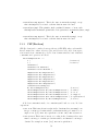
The following instructions guide you to install B-Prolog manually:
1. Download the file bp8_win.zip, and store it in C:\.
2. Extract the files by using winzip or jar in JSDK.
3. Run bp.exe in the BProlog directory to start B-Prolog.
4. Add the path C:\BProlog to the environment variable path. In this way
you can start B-Prolog from any working directory.
1.1.2
Linux
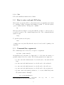
To install B-Prolog on a Linux machine, follow the following steps:
1. Download the file bp8_linux.tar.gz, and store it in your home directory.
2. Uncompress bp8_linux.tar.gz, and extract the files by typing
gunzip bp8_linux.tar.gz | tar xfv 3. Run bp in the BProlog directory to start B-Prolog.
4. Add the following line to the script file .cshrc, .bshrc, or .kshrc, depending
on the shell that you use:
alias
bp
’$HOME/BProlog/bp’
This enables you to start B-Prolog from any working directory.
1
1.1.3
Mac
Follow the installation instructions for Linux.
1.2
How to enter and quit B-Prolog
Like most Prolog systems, B-Prolog offers an interactive programming environment
for compiling, loading, debugging, and running programs. To enter the system,
open a command window,1 and type the command:
bp
After the system is started, it responds with the prompt |?-, and is ready to
accept Prolog queries. The command help shows some of the commands that the
system accepts:
help
To quit the system, use the query:
halt
or simply enter ^D (control-D) when the cursor is located at the beginning of an
empty line.
1.3
Command-line arguments
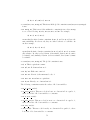
The command bp can be followed by a sequence of arguments:
bp {File |-Name Value}*
An argument can be the name of a binary file to be loaded into the system or a
parameter name followed by a value. The following parameters are supported:
• -s xxx: xxx is the initial amount of words allocated to the stack and the
heap.
• -b xxx: xxx is the initial amount of words allocated to the trail stack.
• -t xxx: xxx is the initial amount of words allocated to the table area.
• -p xxx: xxx is the initial amount of words allocated to the program area.
• -g Goal: Goal is the initial goal that is to be executed immediately after
the system is started. Example:
bp -g "writeln(hello)"
1
On
Windows,
either
select
Start->Run,
Start->Programs->accessories->command prompt.
2
and
type
cmd,
or
select
If the goal is made up of several subgoals, then it must be enclosed in a pair
of double quotation marks. Example:
bp -g "set_prolog_flag(singleton,off),cl(myFile),go"
The predicate $bp_top_level starts the B-Prolog interpreter. Users can
perform other operations before starting the interpreter. Example:
bp -g "consult(myFile),$bp_top_level"
1.4
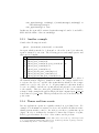
The command-line editor
The command-line editor resides at the top-level of the system, and accepts queries
from user. A query is a Prolog goal that ends with a new line. It is a tradition that
a period is used to terminate a query. In B-Prolog, since queries cannot expand
over more than one line, the terminating period can be omitted.
The command-line editor accepts the following editing commands:
^F Move the cursor one position forward.
^B Move the cursor one position backward.
^A Move the cursor to the beginning of the line.
^E Move the cursor to the end of the line.
^D Delete the character under the cursor.
^H Delete the character to the left of the cursor.
^K Delete the characters to the right of the cursor.
^U Delete the whole line.
^P Load the previous query in the buffer.
^N Load the next query in the buffer.
Note that, as mentioned above, the command ^D will halt the system if the line is
empty and the cursor is located at the beginning of the line.
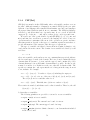
1.5
How to run programs
A program consists of a set of predicates. A predicate is made up of a (not
necessarily consecutive) sequence of clauses whose heads have the same predicate
symbol and the same arity. Each predicate is defined in one module that is stored
in a file, unless it is declared to be dynamic.
The name of a source file or a binary file is an atom. For example, a1, ’A1’, and
’124’ are correct file names. A file name can start with an environment variable
$V or %V%, which will be replaced by its value before the file is actually opened. The
file name separator ’/’ should be used. Since ’\’ is used as the escape character
in quoted strings and atoms, two consecutive backslashes constitute a separator,
as in ’c:\\work\\myfile.pl’.
3
Compiling and loading
A program first needs be compiled before it is loaded into the system for execution.
In order to compile a program in a file named fileName, type
compile(fileName).
If the file name has the extension pl, then the extension can be omitted. The
compiled byte-code will be stored in a new file with the same primary name and
the extension out. In order to have the byte-code stored in a designated file, use
compile(fileName,byteFileName).
For convenience, compile/1 accepts a list of file names.
The Prolog flag compiling instructs the compiler about the type of code to
generate. The default value of the flag is compactcode, and two other possible
values are debugcode and profilecode.
In order to load a compiled byte-code program, type
load(fileName).
In order to compile and load a program in one step, use
cl(fileName).
For convenience, both load/1 and cl/1 accept a list of file names.
Sometimes, users want to compile a program that is generated by another
program. Users can save the program into a file, and then use compile or cl to
compile the file. As file input and output take time, the following predicate is
provided to compile a program without saving it into a file:
compile_clauses(L).
where L must be a list of clauses to be compiled.
Consulting
Another way to run a program is to load it directly into the program area without compilation. This is called consulting. It is possible to trace the execution
of consulted programs, but it is not possible to trace the execution of compiled
programs. In order to consult a program in a file into the program area, type
consult(fileName)
or simply
[fileName].
As an extension, both consult/1 and []/1 accept a list of file names.
In order to see the consulted or dynamically asserted clauses in the program
area, use
listing
and in order to see the clauses that define a predicate Atom/Arity, use
listing(Atom/Arity)
4
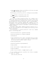
Running programs
After a program is loaded, users can query the program. For each query, the
system executes the program, and reports yes when the query succeeds or no
when the query fails. When a query that contains variables succeeds, the system
also reports the bindings for the variables. Users can ask the system to find the
next solution by typing ’;’ after a solution. Users can terminate the execution
by typing ^C.
Example:
?- member(X,[1,2,3]).
X=1;
X=2;
X=3;
no
The call abort stops the current execution and restores the system to the
top-level.
5
Chapter 2
Programs
This chapter describes the syntax of Prolog. Both programs and data are composed
from terms in Prolog.
2.1
Terms
A term is either a constant, a variable, or a compound term. There are two kinds
of constants: atoms and numbers.
Atoms
Atoms are strings of letters, digits, and underscore marks _ that begin with a
lower-case letter, or strings of any characters enclosed in single quotation marks.
Atoms cannot contain more than 1000 characters. The backslash character ’\’
is used as an escape character. This means that the atom ’a\’b’ contains three
characters, namely a, ’, and b.
Numbers
A number is either an integer or a floating-point number. A decimal integer is a
sequence of decimal digits with an optional sign preceding it.
An integer can be in the radix notation, with a base other than 10. In general,
an integer in the radix notation takes the form base’digits, where base is a decimal
integer, and digits is a sequence of digits. If the base is zero, then the notation
represents the code of the character that follows the single quotation mark. The
notation “0b” begins a binary integer; “0o” begins an octal integer; and “0x”
begins a decimal integer.
Examples:
• 2’100 : 4 in binary notation.
6
• 0b100 : 4 in binary notation.
• 8’73 : 59 in octal notation.
• 0o73 : 59 in octal notation.
• 16’f7: 247 in hexadecimal notation.
• 0xf7: 247 in hexadecimal notation.
• 0’a: the code of ’a’, which is 97.
• 0’\\: the code of ’\’, which is 92.
A floating-point number consists of an integer (optional), then a decimal point,
and then another integer, optionally followed by an exponent. For example, 23.2,
0.23, and 23.0e-10 are valid floating-point numbers.
Variables
Variables look like atoms, except that variable have names that begin with a capital
letter or an underscore mark. A single underscore mark denotes an anonymous
variable.
Compound terms
A compound term is a structure that takes the form f (t1 , . . . , tn ), where n is called
the arity, f is called the functor, or function symbol, and t1 , . . . , tn are terms. In BProlog, the arity must be greater than 0 and less than 32768. The terms enclosed
in the parentheses are called components of the compound term.
Lists are special structures whose functors are ’.’. The special atom ’[]’
denotes an empty list. The list [H|T] denotes the structure ’.’(H,T).
By default, a string is represented as a list of codes for the characters in the
string. For example, the string "abc" is the same as the list [97,98,99]. The
backslash character ’\’ is used as the escape character for strings. This means
that the string "a\"c" is the same as [97,34,98], where 34 is the code for the
double quotation mark. The representation of a string is dependent on the flag
double quotes (see Section 6.8).
Arrays and hashtables are also represented as structures. All of the built-ins for
structures can also be applied to arrays and hashtables. However, it is suggested
that only primitives on arrays and hashtables should be used to manipulate arrays
and hashtables.
2.2
Programs
A program is a sequence of logical statements, called Horn clauses. There are
three types of Horn clauses: facts, rules, and directives.
7
Facts
A fact is an atomic formula in the form p(t1 , t2 , . . . , tn ), where p is an n-ary
predicate symbol, and t1 , t2 , . . . , tn are terms which are called the arguments of
the atomic formula.
Rules
A rule takes the form
H :- B1,B2,...,Bn.
(n>0)
where H, B1, ..., Bn are atomic formulas. H is called the head, and the right
hand side of :- is called the body of the rule. A fact can be considered a special
kind of rule whose body is true.
A predicate is an ordered sequence of clauses whose heads have the same predicate symbol and the same arity.
Directives
A directive either gives a query that is to be executed when the program is loaded,
or tells the system some pragmatic information about the predicates in the program. A directive takes the form of
:- B1,B2,...,Bn.
where B1, ..., Bn are atomic formulas.
2.3
Control constructs
In Prolog, backtracking is employed to explore the search space for a query and
a program. Goals in the query are executed from left to right, and the clauses in
each predicate are tried sequentially from the top. A query may succeed, may fail,
or may be terminated due to exceptions. When a query succeeds, the variables
in the query may be bound to some terms. The call true always succeeds, and
the call fail always fails. There are several control constructs for controlling
backtracking, for specifying conjunction, negation, disjunction, and if-then-else,
and for finding all solutions. B-Prolog also provide loop constructs for describing
loops (see Chapter 4).
Cut
Prolog provides an operator, called cut, for controlling backtracking. A cut is
written as ! in programs. A cut in the body of a clause has the effect of removing
the choice points, or alternative clauses, of the goals to the left of the cut.
8
Example:
In the following program, the query p(X) only gives one solution: p(1). The cut
removes the choice points for p(X) and q(X), and thus, no further solution will be
returned when users force backtracking by typing ’;’. Without the cut, the query
p(X) would have three solutions.
p(X):-q(X),!.
p(3).
q(1).
q(2).
When a failure occurs, the execution will backtrack to the latest choice point,
i.e., the latest subgoal that has alternative clauses. There are two non-standard
built-ins, called savecp/1 and cutto/1, which can make the system backtrack to
a choice point deep in the search tree. The call savecp(Cp) binds Cp to the latest
choice point frame, where Cp must be a variable. The call cutto(Cp) discards all
of the choice points that are created after Cp. In other words, the call lets Cp be
the latest choice point. Note that Cp must be a reference to a choice point that is
set by savecp(Cp).
Conjunction, disjunction, negation, and if-then-else
The construct (P,Q) denotes conjunction. It succeeds if both P and Q succeed.
The constructs (not P) and \+ P denote negation. They succeed if and only if
P fails. Negation is not transparent to cuts. In other words, the cuts in a negation
are only effective within the negation. Cuts in a negation cannot remove choice
points that are created for the goals to the left of the negation.
The construct (P;Q) denotes disjunction. It succeeds if either P or Q succeeds.
Q is only executed after P fails. Disjunction is transparent to cuts. A cut in P or
in Q will remove not only the choice points that are created for the goals to the
left of the cut in P or in Q, but will also remove the choice points that are created
for the goals to the left of the disjunction.
The control construct (If->Then;Else) succeeds if (1) If and Then succeed,
or (2) If fails and Else succeeds. If is not transparent to cuts, but Then and
Else are transparent to cuts. The control construct (If->Then) is equivalent to
(If->Then;fail).
repeat/0
The predicate repeat, which is defined as follows, is a built-in predicate that is
often used to express iteration.
repeat.
repeat:-repeat.
9
For example, the query
repeat,write(a),fail
repeatedly outputs ’a’, until users type ^C to stop it.
call/1 and once/1
The call call(Goal) treats Goal as a subgoal. It is equivalent to Goal. The
call once(Goal) is equivalent to Goal, but can only succeed at most once. It is
implemented as follows:
once(Goal):-call(Goal),!.
call/2−n (not in ISO)
The call call(Goal,A1,...,An) creates a new goal by appending the arguments
A1, . . ., An to the end of the arguments of Goal. For example, call(Goal,A1,A2,A3)
is equivalent to the following:
Goal=..[F|Args],
append(Args,[A1,A2,A3],NewArgs),
NewCall=..[F|NewArgs],
call(NewCall)
When compiled, n can be any positive number that is less than 216 ; when interpreted, however, n cannot be larger than 10.
forall/2 (not in ISO)
The call forall(Generate,Test) succeeds if, for every solution of Generate, the
condition Test succeeds. This predicate is defined as follows:
forall(Generate, Test) :- \+ (call(Generate), \+ call(Test)).
For example, forall(member(X,[1,2,3]),p(X)).
call cleanup/2 (not in ISO)
The call call cleanup(Call,Cleanup) is equivalent to call(Call), except that
Cleanup is called when Call succeeds determinately (i.e., with no left choice point),
when Call fails, or when Call raises an exception.
time out/3 (not in ISO)
The call time out(Goal, Time, Result) is logically equivalent to once(Goal),
except that it imposes a time limit, in milliseconds, on the evaluation. If Goal is
not finished when Time expires, the evaluation will be aborted and Result will be
unified with the atom time out. If Goal succeeds within the time limit, Result
will be unified with the atom success.
10
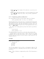
All solutions
• findall(Term,Goal,List): Succeeds if List is the list of instances of Term,
such that Goal succeeds. Example:
?-findall(X,member(X,[(1,a),(2,b),(3,c)]),Xs)
Xs=[(1,a),(2,b),(3,c)]
• bagof(Term,Goal,List): This is the same as findall(Term,Goal,List),
except for its treatment of free variables that occur in Goal but do not occur
in Term. It first picks the first tuple of values for the free variables, and then
uses this tuple to find the list of solutions List of Goal. It enumerates all
of the tuples for the free variables. Example:
?-bagof(Y,member((X,Y),[(1,a),(2,b),(3,c)]),Xs)
X=1
Y=[a];
X=2
Y=[b];
X=3
Y=[c];
no
• setof(Term,Goal,List): This is like bagof(Term,Goal,List), except that
the elements of List are sorted into alphabetical order.
Aggregates
• minof(Goal,Exp) : Find an instance of Goal, such that Exp is minimum,
where Exp must be an integer expression.
?-minof(member((X,Y),[(1,3),(3,2),(3,0)]),X+Y)
X=3
Y=0
• maxof(Goal,Exp): Find an instance of Goal, such that Exp is maximum,
where Exp must be an integer expression.
?-maxof(member((X,Y),[(1,3),(3,2),(3,0)]),X+Y)
X=3
Y=2
11
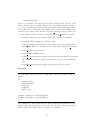
Chapter 3
Data Types and Built-ins
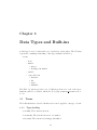
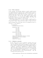
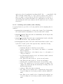
A data type is a set of values and a set of predicates on the values. The following
depicts the containing relationship of the types available in B-Prolog.
• term
– atom
– number
∗ integer
∗ floating-point number
– variable
– compound term
∗
∗
∗
∗
structure
list
array
hashtable
The B-Prolog system provides a set of built-in predicates for each of the types.
Built-ins cannot be redefined, unless the Prolog flag redefine builtin is set to
be on.
3.1
Terms
The built-ins that are described in this section can be applied to any type of term.
3.1.1
Type checking
• atom(X): The term X is an atom.
• atomic(X): The term X is an atom or a number.
• float(X): The term X is a floating-point number.
12
• real(X): This is the same as float(X).
• integer(X): The term X is an integer.
• number(X): The term X is a number.
• nonvar(X): The term X is not a variable.
• var(X): The term X is a free variable.
• compound(X): The term X is a compound term. This predicate is true if X is
either a structure or a list.
• ground(X): The term X is ground.
• callable(X): The term X is a callable term, i.e., an atom or a compound
term. Type errors will not occur in a meta-call, such as call(X) if X is
callable. Note that a callable term does not mean that the predicate is
defined.
3.1.2
Unification
• X = Y: The terms X and Y are unified.
• X \= Y: The terms X and Y are not unifiable.
• X?=Y: The terms X and Y are unifiable.
not(not(X=Y)).
3.1.3
This is logically equivalent to:
Term comparison and manipulation
• Term1 == Term2: The terms Term1 and Term2 are strictly identical.
• Term1 \== Term2: The terms Term1 and Term2 are not strictly identical.
• Term1 @< Term2: The term Term1 precedes the term Term2 in the standard
order.
• Term1 @=< Term2: The term Term1 either precedes, or is identical to, the
term Term2 in the standard order.
• Term1 @> Term2: The term Term1 follows the term Term2 in the standard
order.
• Term1 @>= Term2: The term Term1 either follows, or is identical to, the term
Term2 in the standard order.
• compare(Op,Term1,Term2): Op is the result of comparing the terms Term1
and Term2.
• copy term(Term,CopyOfTerm): CopyOfTerm is an independent copy of Term.
For an attributed variable, the copy does not carry any of the attributes.
13
• acyclic term(Term): This fails if Term is cyclic, and succeeds otherwise.
• number vars(Term,N0,N):
• numbervars(Term,N0,N): Number the variables in Term by using the integers starting from N0. N is the next integer that is available after the term is
numbered. Let N0, N1, ..., N-1 be the sequence of integers. The first variable
is bound to the term $var(N0), the second variable is bound to $var(N1),
and so on. Different variables receive different numberings. All occurrences
of the same variable receive the same numbering. (not in ISO).
• unnumber vars(Term1,Term2): Term2 is a copy of Term1, with all numbered
variables $var(N) being replaced by Prolog variables. Different numbered
variables are replaced by different Prolog variables.
Number the variables in Term by using the integers starting from N0. N is
the next integer that is available after the term is numbered. Let N0, N1,
..., N-1 be the sequence of integers. The first variable is bound to the term
$var(N0), the second variable is bound to $var(N1), and so on. Different
variables receive different numberings. All occurrences of the same variable
all receive the same numbering. (not in ISO).
• term variables(Term,Vars):
• vars set(Term,Vars): Vars is a list of variables that occur in Term.
• term variables(Term,Vars,Tail): This is the difference list version of
term variables/2. Tail is the tail of the incomplete list Vars.
• variant(Term1,Term2): This is true if Term1 is a variant of Term2. No
attributed variables can occur in Term1 or in Term2.
• subsumes term(Term1,Term2): This is true if Term1 subsumes Term2. No
attributed variables can occur in Term1 or in Term2.
• acyclic term(Term): This succeeds if Term is acyclic, and fails otherwise.
3.2
Numbers
An arithmetic expression is a term that is built from numbers, variables, and the
arithmetic functions. An expression must be ground when it is evaluated.
• Exp1 is Exp2: The term Exp2 must be a ground expression, and Exp1 must
either be a variable, or a ground expression. If Exp1 is a variable, then
the call binds the variable to the result of Exp2. If Exp1 is a non-variable
expression, then the call is equivalent to Exp1 =:= Exp2.
• X =:= Y: The expression X is numerically equal to Y.
14
• X =\= Y: The expression X is not numerically equal to Y.
• X < Y: The expression X is less than Y.
• X =< Y: The expression X is less than or equal to Y.
• X > Y: The expression X is greater than Y.
• X >= Y: The expression X is greater than or equal to Y.
The following functions are provided:
• X + Y: addition.
• X - Y: subtraction.
• X * Y: multiplication.
• X / Y: division.
• X // Y: integer division, the same as in C.
• X div Y: integer division, rounded down.
• X mod Y: modulo (X-integer(floor(X/Y))*Y).
• X rem Y: remainder (X-(X//Y)*Y).
• X /> Y : integer division (ceiling(X/Y)).
• X /< Y : integer division (floor(X/Y)).
• X ** Y : power.
• -X : sign reversal.
• X >> Y : bit shift right.
• X << Y : bit shift left.
• X /\ Y : bitwise and.
• X \/ Y : bitwise or.
•
\ X : bitwise complement.
• X xor Y: bit wise xor.
• abs(X) : absolute value.
• atan(X) : arctangent(the argument is in radians).
• atan2(X,Y) : principal value of the arctangent of Y / X.
15
• ceiling(X) : the smallest integer that is not smaller than X.
• cos(X) : cosine (the argument is in radians).
• exp(X) : natural antilogarithm, eX .
• integer(X) : convert X to an integer.
• float(X) : convert X to a float.
• float fractional part(X) : float fractional part.
• float integer part(X) : float integer part.
• floor(X) : the largest integer that is not greater than X.
• log(X) : natural logarithm, loge X.
• log(B,X) : logarithm in the base B, logB X.
• max(X,Y) : the maximum of X and Y (not in ISO).
• max(L) : the maximum of the list of elements L (not in ISO).
• min(X,Y) : the minimum of X and Y (not in ISO).
• min(L) : the minimum of the list of elements L (not in ISO).
• pi : the constant pi (not in ISO).
• random : a random number (not in ISO).
• random(Seed) : a random number that is generated by using Seed (not in
ISO).
• round(X) : the integer that is nearest to X.
• sign(X) : sign (-1 for negative, 0 for zero, and 1 for positive).
• sin(X) : sine (the argument is in radians).
• sqrt(X) : square root.
• sum(L) : the sum of the list of elements L (not in ISO).
• truncate(X) : the integer part of X.
16
3.3
Lists and structures
• Term =..
List: The functor and arguments of Term comprise the list List.
• append(L1,L2,L): This is true when L is the concatenation of L1 and L2.
(not in ISO).
• append(L1,L2,L3,L): This is true when L is the concatenation of L1, L2,
and L3. (not in ISO).
• arg(ArgNo,Term,Arg): The ArgNoth argument of the term Term is Arg.
• functor(Term,Name,Arity): The principal functor of the term Term has
the name Name and the arity Arity.
• length(List,Length): The length of list List is Length. (not in ISO).
• membchk(X,L): This is true when X is included in the list L. ’==/2’ is used
to test whether two terms are the same. (not in ISO).
• member(X,L): This is true when X is a member of the list L. It instantiates
X to different elements in L upon backtracking. (not in ISO).
• attach(X,L): Attach X to the end of the list L. (not in ISO).
• closetail(L): Close the tail of the incompelete list L. (not in ISO).
• reverse(L1,L2): This is true when L2 is the reverse of L1. (not in ISO).
• setarg(ArgNo,CompoundTerm,NewArg): This destructively replaces the ArgNoth
argument of CompoundTerm with NewArg. The update is undone when backtracking. (not in ISO).
• sort(List1,List2): List2 is a sorted copy of List1 in ascending order.
List2 does not contain duplicates. (not in ISO).
• sort(Order,List1,List2): List2 is a sorted copy of List1 in the specified
order, where Order is <,>,=<, or >=. Duplicates are not eliminated if the specified order is =< or >=. sort(List1,List2) is same as sort(<,List1,List2).
(not in ISO).
• keysort(List1,List2): List1 must be a list of pairs. Each pair must take
the form Key-Value. List2 is a copy of List1 that is sorted in ascending
order by the key. Duplicates are not removed. (not in ISO).
• nextto(X, Y, List): This is true if Y follows X in List. (not in ISO).
• delete(List1, Elem, List2): This is true when deleting all occurences of
Elem from List1 results in List2. (not in ISO).
• select(Elem, List, Rest): This is true when removing Elem from List1
results in List2. (not in ISO).
17
• nth0(Index, List, Elem): This is true when Elem is the Index’th element
of List. Counting starts at 0. (not in ISO).
• nth(Index, List, Elem): (not in ISO).
• nth1(Index, List, Elem): This is true when Elem is the Index’th element
of List. Counting starts at 1. (not in ISO).
• last(List, Elem): This is true if Last unifies with the last element of
List. (not in ISO).
• permutation(List1, List2): This is true when Xs is a permutation of Ys.
When given Xs, this can solve for Ys. When given Ys, this can solve for Xs.
This can also enumerate Xs and Ys together. (not in ISO).
• flatten(List1, List2): This is true when List2 is a non-nested version
of List1. (not in ISO).
• sumlist(List, Sum): Sum is the result of adding all of the numbers in List.
(not in ISO).
• numlist(Low, High, List): List is a list [Low, Low+1, ...
in ISO).
High]. (not
• and to list(Tuple,List): Let Tuple be (e1 , e2 , ..., en ). List is [e1 , e2 , ..., en ].
(not in ISO).
• list to and(List,Tuple): Let List be [e1 , e2 , ..., en ]. Tuple is (e1 , e2 , ..., en ).
List must be a complete list. (not in ISO).
3.4
Arrays and the array subscript notation (not in
ISO)
In B-Prolog, the maximum arity of a structure is 65535. This entails that a
structure can be used as a one-dimensional array, and a multi-dimensional array
can be represented as a structure of structures. In order to facilitate creating and
manipulating arrays, B-Prolog provides the following built-ins.
• new array(X,Dims): Bind X to a new array of the dimensions that are specified by Dims, which is a list of positive integers. An array of n elements is
represented as a structure with the functor ’[]’/n. All of the array elements
are initialized to be free variables. For example,
| ?- new_array(X,[2,3])
X = []([](_360,_364,_368),[](_370,_374,_378))
• a2 new(X,N1,N2): This is the same as new array(X,[N1,N2]).
18
• a3 new(X,N1,N2,N3): This is the same as new array(X,[N1,N2,N3]).
• is array(A): This succeeds if A is a structure whose functor is ’[]’/n.
The built-in predicate arg/3 can be used to access array elements, but it
requires a temporary variable to store the result, and also requires a chain of calls
to access an element of a multi-dimensional array. In order to facilitate the access
of array elements, B-Prolog supports the array subscript notation X[I1 ,...,In ],
where X is a structure, and each Ii is an integer expression. However, this common
notation for accessing arrays is not part of the standard Prolog syntax. In order
to accommodate this notation, the parser is modified to insert a token, ∧ , between
a variable token and [. So, the notation X[I1 ,...,In ] is just a shorthand for
X ∧ [I1 ,...,In ]. This notation is interpreted as an array access when it occurs
in an arithmetic expression, a constraint, or as an argument of a call to @=/2. In
any other context, it is treated as the term itself. The array subscript notation
can also be used to access elements of lists. For example, the nth/3 and nth0/3
predicates can be defined as follows:
nth(I,L,E) :- E @= L[I].
nth0(I,L,E) :- E @= L[I+1].
In arithmetic expressions and arithmetic constraints, the term X ∧ length indicates the size of the compound term X. Examples:
?-S=f(1,1), Size is S^length.
Size=2
?-L=[1,1], L^length=:=1+1.
yes
The term X ∧ length is also interpreted as the size of X when it occurs as one of
the arguments of a call to @=/2. Examples:
?-S=f(1,1), Size @= S^length.
Size=2
In any other context, the term X ∧ length is interpreted as is.
The operator @:= is provided for destructively updating an argument of a
structure or an element of a list. For example:
?-S=f(1,1), S[1] @:= 2.
S=f(2,1)
The update is undone upon backtracking.
The following built-ins on arrays have become obsolete, since they can be easily
implemented by using foreach and list comprehension (see Chapter 4).
• X^rows @= Rows: Rows is a list of rows in the array X. The dimension of X
must not be less than 2.
19
• X^columns @= Cols: Cols is a list of columns in the array X. The dimension
of X must not be less than 2.
• X^diagonal1 @= Diag: Diag is a list of elements in the left-up-diagonal
Xn1,...,X1n of array X. The dimension of X must be 2, and the number of
rows and the number of columns in X must be equal.
• X^diagonal2 @= Diag: Diag is a list of elements in the left-down-diagonal
X11,...,Xnn of array X. The dimension of X must be 2, and the number of
rows and the number of columns in X must be equal.
• a2 get(X,I,J,Xij): This is the same as X^[I,J] @= Xij. .
• a3 get(X,I,J,K,Xijk): This is the same as X^[I,J,K] @= Xijk. .
• array to list(X,List): The term List is a list of all of the elements in
array X. Suppose that X is an n-dimensional array, and that the sizes of the
dimensions are N1, N2, ..., and Nn. Then, List contains the elements with
indices from [1,...,1], [1,...,2], to [N1,N2,...,Nn].
3.5
Set manipulation (not in ISO)
• is set(Set): This is true if Set is a proper list without duplicates.
• eliminate duplicate(List, Set): This is true when Set has the same
elements as List, in the same order. Only the left-most copy of the duplicate
is retained.
• intersection(Set1, Set2, Set3): This is true if Set3 unifies with the
intersection of Set1 and Set2.
• union(Set1, Set2, Set3): This is true if Set3 unifies with the union of
Set1 and Set2.
• subset(SubSet, Set): This is true if all of the elements of SubSet also
belong to Set.
• subtract(Set, Delete, Result): Delete all of the elements from Set that
occur in the set Delete, and unify the result with Result.
3.6
Hashtables (not in ISO)
• new hashtable(T): Create a hashtable T with 7 bucket slots.
• new hashtable(T,N): Create a hashtable T with N bucket slots. N must be
a positive integer.
• is hashtable(T): This is true when T is a hashtable.
20
• hashtable get(T,Key,Value): Get the value Value that is stored under
the key Key from hashtable T. Fail if no such key exists.
• hashtable register(T,Key,Value): Get the value Value that is stored
under the key Key from hashtable T. Store the value in the table under Key,
if the key does not exist.
• hashtable size(T,Size): The number of bucket slots in hashtable T is
Size.
• hash code(Term,Code): The hash code of Term is Code.
• hashtable to list(T,List): List is the list of key and value pairs in
hashtable T.
• hashtable keys to list(T,List): List is the list of keys of the elements
in hashtable T.
• hashtable values to list(T,List): List is the list of values of the elements in hashtable T.
3.7
Character-string operations
• atom chars(Atom,Chars): Chars is the list of characters of Atom.
• atom codes(Atom,Codes): Codes is the list of numeric codes of the characters of Atom.
• atom concat(Atom1,Atom2,Atom3): The concatenation of Atom1 and Atom2
is equal to Atom3. Either Atom1 and Atom2 are atoms, or Atom3 is an atom.
• atom length(Atom,Length): The length, in characters, of Atom is Length.
• char code(Char,Code): The numeric code of the character Char is Code.
• number chars(Num,Chars): Chars is the list of digits (including ’.’) of the
number Num.
• number codes(Num,Codes): Codes is the list of numeric codes of the digits
of the number Num.
• sub atom(Atom,PreLen,Len,PostLen,Sub): The atom Atom is divided into
three parts, Pre, Sub, and Post. The three parts have the lengths PreLen,
Len, and PostLen, respectively.
• name(Const,CharList): The name of the atom or the number Const is the
string CharList. (not in ISO).
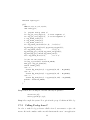
• parse atom(Atom,Term,Vars): Convert Atom to Term, where Vars is a list
of elements in the form (VarName=Var). It fails if Atom is not syntactically
correct. Examples:
21
| ?- parse_atom(’X is 1+1’,Term,Vars)
Vars = [X=_8c019c]
Term = _8c019c is 1+1?
| ?- parse_atom(’p(X,Y),q(Y,Z)’,Term,Vars)
Vars = [Z=_8c01d8,Y=_8c01d4,X=_8c01d0]
Term = p(_8c01d0,_8c01d4),q(_8c01d4,_8c01d8)?
| ?- parse_atom(’ a b c’,Term,Vars)
*** syntax error ***
a <<here>> b c
no
(not in ISO).
• parse atom(Atom,Term): This is equivalent to parse atom(Atom,Term, ).
(not in ISO).
• parse string(String,Term,Vars): This is similar to parse atom, except
that the first argument is a list of codes. Example:
| ?- name(’X is 1+1’,String),parse_string(String,Term,Vars)
Vars = [X=_8c0294]
Term = _8c0294 is 1+1
String = [88,32,105,115,32,49,43,49]?
(not in ISO).
• parse string(String,Term): This is equivalent to parse string(String,Term, ).
(not in ISO).
• term2atom(Term,Atom): Atom is an atom that encodes Term. Example:
| ?- term2atom(f(X,Y,X),S),writeq(S),nl.
’f(_9250158,_9250188,_9250158)’
S=f(_9250158,_9250188,_9250158)
(not in ISO).
• term2string(Term,String): This is equivalent to:
term2atom(Term,Atom),atom_codes(Atom,String)
(not in ISO).
• write string(String): Write the list of codes, String, as a readable string.
For example, write string([97,98,99]) outputs "abc". (not in ISO).
22
Chapter 4
Declarative Loops and List
Comprehensions (not in ISO)
Prolog relies on recursion to describe loops. This has basically remained the same
since Prolog’s inception 35 years ago. Many other languages provide powerful
loop constructs. For example, the foreach statement in C# and the enhanced
for statement in Java are very powerful for iterating over collections. Functional
languages provide higher-order functions and list comprehensions for creating collections, and for iterating over collections. The lack of powerful loop constructs has
arguably made Prolog less acceptable to beginners, and less productive to experienced programmers, because it is often tedious to define small auxiliary recursive
predicates for loops. The emergence of constraint programming constructs, such
as CLP(FD), has further revealed this weakness of Prolog as a host language.
B-Prolog provides a built-in, called foreach, and the list comprehension notation for writing repetition. The foreach built-in has a very simple syntax and semantics. For example, foreach(A in [a,b], I in 1..2, write((A,I))) outputs four tuples: (a,1), (a,2), (b,1), and (b,2). Syntactically, foreach is a
variable-length call whose last argument specifies a goal that should be executed
for each combination of values in a sequence of collections. A foreach call may also
give a list of variables that are local to each iteration, and a list of accumulators
that can be used to accumulate values from each iteration. With accumulators,
users can use foreach in order to describe recurrences for computing aggregates.
Recurrences have to be read procedurally, and thus do not fit well with Prolog.
For this reason, B-Prolog borrows list comprehensions from functional languages.
A list comprehension is a list whose first element has the functor ’:’/2. A list of
this form is interpreted as a list comprehension in calls to ’@=’/2, and in some
other contexts. For example, the query X@=[(A,I) : A in [a,b], I in 1..2]
binds X to the list [(a,1),(a,2),(b,1),(b,2)]. A list comprehension is treated
as a foreach call with an accumulator in the implementation.
23
4.1
The base foreach
The base form of foreach has the following form:
foreach(E1 in D1 , . . ., En in Dn , LocalV ars,Goal)
Ei is a pattern that is normally a variable, but can also be any term. Di a
collection. LocalV ars, which is optional, is a list of variables in Goal that are
local to each iteration. Goal is a callable term. All of the variables in the Ei ’s
are local variables. The foreach call means that, for each combination of values
E1 ∈ D1 , . . ., En ∈ Dn , the instance Goal is executed after the local variables are
renamed. The call fails if any of the instances fails. Any variable, including the
anonymous variable ’_’, that occurs in Goal, is shared by all iterations, unless the
variable is contained within an Ei or LocalV ars.
A collection takes one of the following forms:
• A list of terms.
• A list of numbers that is represented as an interval Begin..Step..End, which
denotes the list of numbers [B1 , B2 , . . . , Bk ],where B1 = Begin and Bi =
Bi−1 +Step for i = 2, ..., k. When Step is positive, Bk ≤ End and Bk +Step >
End. When Step is negative, Bk ≥ End and Bk + Step < End. When
Step = 1, the notation can be abbreviated as Begin..End. For example, the
interval 1..2..8 denotes the list [1,3,5,7].
• A term in the form (C1 , . . . , Cm ), where each Ci (i=1,...,m) is a collection of
the same number of elements. Let Ci be the list [ei1 , ..., eil ] (i = 1, ..., m).
The term (C1 , . . . , Cm ) denotes the list of tuples [(e11 , ..., em1 ), . . . , (e1l , ..., eml )].
For example, ([a,b,c],1..3) denotes the list of tuples [(a,1),(b,2),(c,3)].
Examples
?-foreach(I in [1,2,3],format("~d ",I)).
1 2 3
?-foreach(I in 1..3,format("~d ",I)).
1 2 3
?-foreach(I in 3..-1.. 1,format("~d ",I)).
3 2 1
?-foreach(F in 1.0..0.2..1.5,format("~1f ",F)).
1.0 1.2 1.4
|?-foreach(T in ([a,b],1..2),writeln(T))
a,1
b,2
24
|?-foreach((A,N) in ([a,b],1..2),writeln(A=N)
a=1
b=2
?-foreach(L in [[1,2],[3,4]], (foreach(I in L, write(I)),nl)).
12
34
?-functor(A,t,10),foreach(I in 1..10,arg(I,A,I)).
A = t(1,2,3,4,5,6,7,8,9,10)
?-foreach((A,I) in [(a,1),(b,2)],writeln(A=I)).
a=1
b=2
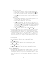
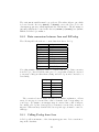
The power of foreach is more clearly revealed when it is used with arrays.
The following predicate creates an N×N array, initializes its elements to integers
from 1 to N×N, and then prints out the array.
go(N):new_array(A,[N,N]),
foreach(I in 1..N,J in 1..N,A[I,J] is (I-1)*N+J),
foreach(I in 1..N,
(foreach(J in 1..N,
[E],(E @= A[I,J], format("~4d ",[E]))),nl)).
In the last line, E is declared as a local variable. In B-Prolog, a term like A[I,J]
is interpreted as an array access in arithmetic built-ins, in calls to ’@=’/2, and in
constraints, but is interpreted as the term A^[I,J] in any other context. That is
why users can use A[I,J] is (I-1)*N+J to bind an array element, but cannot
use write(A[I,J]) to print an element.
As seen in the examples, foreach(T in ([a,b,c],1..3),writeln(T)) and
foreach((A,N) in ([a,b,c],1..3),writeln((A=N)), the base foreach can be
used to easily iterate over multiple collections simultaneously.
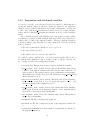
4.2
foreach with accumulators
The base foreach is not suitable for computing aggregates. B-Prolog extends it
to allow accumulators. The extended foreach takes the form:
foreach(E1 in D1 , . . ., En in Dn , LocalV ars,Accs,Goal)
or
foreach(E1 in D1 , . . ., En in Dn , Accs,LocalV ars,Goal)
25
where Accs is an accumulator or a list of accumulators. The ordering of LocalV ars
and Accs is not important, since the types are checked at runtime.
One form of an accumulator is ac(AC, Init), where AC is a variable and Init
is the initial value for the accumulator before the loop starts. In Goal, recurrences
can be used to specify how the value of the accumulator in the previous iteration,
denoted as AC^0, is related to the value of the accumulator in the current iteration,
denoted as AC^1. Let’s use Goal(ACi , ACi+1 ) to denote an instance of Goal in
which AC^0 is replaced with a new variable ACi , AC^1 is replaced with another
new variable ACi+1 , and all local variables are renamed. Assume that the loop
stops after n iterations. Then this foreach indicates the following sequence of
goals:
AC0 = Init,
Goal(AC0 , AC1 ),
Goal(AC1 , AC2 ),
. . .,
Goal(ACn−1 , ACn ),
AC = ACn
Examples
?-foreach(I in [1,2,3],ac(S,0),S^1 is S^0+I).
S = 6
?-foreach(I in [1,2,3],ac(R,[]),R^1=[I|R^0]).
R = [3,2,1]
?-foreach(A in [a,b], I in 1..2, ac(L,[]), L^1=[(A,I)|L^0]).
L = [(b,2),(b,1),(a,2),(a,1)]
?-foreach((A,I) in ([a,b],1..2), ac(L,[]), L^1=[(A,I)|L^0]).
L = [(b,2),(a,1)]
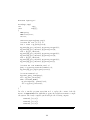
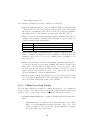
The following predicate takes a two-dimensional array, and returns its minimum
and maximum elements:
array_min_max(A,Min,Max):A11 is A[1,1],
foreach(I in 1..A^length,
J in 1..A[1]^length,
[ac(Min,A11),ac(Max,A11)],
((A[I,J]<Min^0->Min^1 is A[I,J];Min^1=Min^0),
(A[I,J]>Max^0->Max^1 is A[I,J];Max^1=Max^0))).
A two-dimensional array is represented as an array of one-dimensional arrays. The
notation A^length refers to the size of the first dimension.
26
Another form of an accumulator is ac1(AC, F in), where F in is the value that
ACn takes after the last iteration. A foreach call with this form of accumulator
indicates the following sequence of goals:
AC0 = F reeV ar,
Goal(AC0 , AC1 ),
Goal(AC1 , AC2 ),
. . .,
Goal(ACn−1 , ACn ),
ACn = F in,
AC = F reeV ar
The accumulator begins with a free variable, F reeV ar. After the iteration steps,
ACn takes the value F in, and the accumulator variable AC is bound to F reeV ar.
This form of an accumulator is useful for incrementally constructing a list by
instantiating the variable tail of the list.
Examples
?-foreach(I in [1,2,3], ac1(R,[]), R^0=[I|R^1]).
R = [1,2,3]
?-foreach(A in [a,b], ac1(L,Tail), L^0=[A|L^1]), Tail=[c,d].
L = [a,b,c,d]
?-foreach((A,I) in ([a,b],1..2), ac1(L,[]), L^0=[(A,I)|L^1]).
L = [(a,1),(b,2)]
4.3
List comprehensions
A list comprehension is a construct for building lists in a declarative way. List
comprehensions are very common in functional languages, such as Haskell, Ocaml,
and F#. We propose to introduce this construct into Prolog.
A list comprehension takes the form:
[T :
E1 in D1 , . . ., En in Dn , LocalV ars,Goal]
where the optional LocalV ars specifies a list of local variables, and the optional
Goal must be a callable term. The construct means that, for each combination
of values E1 ∈ D1 , . . ., En ∈ Dn , if the instance of Goal is true after the local
variables are renamed, then T is added into the list.
Note that, syntactically, the first element of a list comprehension, called a list
constructor, takes the special form of T:(E in D). A list of this form is interpreted
as a list comprehension in calls to ’@=’/2 and in constraints in B-Prolog.
A list comprehension is treated as a foreach call with an accumulator. For
example, the query L@=[(A,I) : A in [a,b], I in 1..2] is the same as
foreach(A in [a,b], I in 1..2, ac1(L,[]),L^0=[(A,I)|L^1]).
27
Examples
?- L @=[X : X in 1..5].
L = [1,2,3,4,5]
?- L @=[X : X in 5..-1..1].
L = [5,4,3,2,1]
?- L @= [F : F in 1.0..0.2..1.5]
L = [1.0,1.2,1.4]
?- L @= [1 : X in 1..5].
L = [1,1,1,1,1]
?- L @= [Y : X in 1..5].
L = [Y,Y,Y,Y,Y]
?- L @= [Y : X in 1..5,[Y]]. % Y is local
L = [_598,_5e8,_638,_688,_6d8]
?- L @= [Y : X in [1,2,3], [Y], Y is -X].
L = [-1,-2,-3]
?-L @=[(A,I): A in [a,b], I in 1..2].
L = [(a,1),(a,2),(b,1),(b,2)]
?-L @=[(A,I): (A,I) in ([a,b],1..2)].
L = [(a,1),(b,2)]
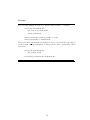
4.4
Cautions on the use
The built-in foreach and the list comprehension notation are powerful means for
describing repetition. When a program is compiled, calls to foreach are converted
into calls to internally-generated tail-recursive predicates, and list comprehensions
are converted into calls to foreach with accumulators. Therefore, loop constructs
incur almost no performance penalty when compared with recursion. Nevertheless,
in order to avoid unanticipated behavior, users must take the following cautions
in using them.
Firstly, iterators are matching-based. Iterators cannot change a collection,
unless the goal of the loop has that effect. For example,
?-foreach(f(a,X) in [c,f(a,b),f(Y,Z)],write(X)).
displays b. The elements c and f(Y,Z) are skipped because they do not match
the pattern f(a,X).
28
Secondly, variables are assumed to be global to all of the iterations, unless they
are declared local, or unless they occur in the patterns of the iterators. Sometimes,
one may use anonymous variables ’ ’ in looping goals, and wrongly believe that
they are local. The parser issues a warning when it encounters a variable that is
not declared local but occurs alone in a looping goal.
Thirdly, no meta-terms should be included in iterators or in list constructors!
For example,
?-D=1..5, foreach(X in D, write(X)).
is bad, since D is a meta-term. As another example,
?-C=(X : I in 1..5), L @=[C].
is bad since C is a meta-term. When meta-terms are included in iterators or in
list constructors, the compiler may generate code that has different behavior as
interpreted.
29
Chapter 5
Exception Handling
5.1
Exceptions
In addition to success and failure, a program may give an exception that is explicitly thrown by a call of throw/1, is raised by a built-in, or is caused by the user
typing ^C. An exception that is raised by a built-in is a one-argument structure,
where the functor shows the type of the exception, and the argument shows the
source of the exception.1
The following lists some of the exceptions:
• divide by zero(Goal): Goal divides a number by zero.
• file not found(Goal): Goal tries to open a file that does not exist.
• illegal arguments(Goal): Goal has an illegal argument.
• number expected(Goal): Goal evaluates an invalid expression.
• out of range(Goal): Goal tries to access an element of a structure or an
array by using an index that is out of range.
The exception that is caused by the typing of ^C is an atom named interrupt.
An exception that is not caught by a program will be handled by the system.
The system reports the type and the source of the exception, and aborts execution
of the query. For example, for the query a=:=1, the system will report:
***
error(type_error(evaluable,a/0),=:=/2)
where evaluable is the type, and =:=/2 is the source.
1
In version 6.9 and later, exceptions that are raised by ISO built-ins comply with the standard.
An exception is a term in the form error(Type,Source), where Type is an error type, and Source
is the source predicate of the error.
30
5.2
throw/1
A user’s program can throw exceptions. The call throw(E) raises an exception,
E, to be caught and handled by some ancestor catcher or handler. If there is no
catcher available in the chain of ancestor calls, the system will handle it.
5.3
catch/3
All exceptions, including those raised by built-ins and interruptions, can be caught
by catchers. A catcher is a call in the form:
catch(Goal,ExceptionPattern,Recovergoal)
which is equivalent to Goal, except when an exception is raised during the execution of Goal that unifies ExceptionPattern. When such an exception is
raised, all of the bindings that have been performed on variables in Goal will
be undone, and Recovergoal will be executed to handle the exception. Note
that ExceptionPattern is unified with a renamed copy of the exception before
Recovergoal is executed. Also note that only exceptions that are raised by a
descendant call of Goal can be caught.
Examples:
• q(X), which is defined in the following, is equivalent to p(X), except all
interruptions are ignored.
q(X):-catch(p(X),interrupt,q(X)).
• The query catch(p(X),undefined predicate( ),fail) fails p(X) if an undefined predicate is called during its execution.
• The query catch(q,C,write(hello q)), where q is defined in the following,
succeeds with the unifier C=c and the message hello q.
q :- r(c).
r(X) :- throw(X).
• The query catch(p(X),E,p(X)==E) for the following program fails, because
E is unified with a renamed copy of p(X), rather than p(X) itself.
p(X):-throw(p(X)).
31
Chapter 6
Directives and Prolog Flags
Directives inform the compiler or interpreter of some information about the predicates in a program1 .
6.1
Mode declaration
For Edinburgh style programs, users can provide the compiler with modes in order
to help it generate efficient code. The mode of a predicate p indicates how the
arguments of any call to p are instantiated just before the call is evaluated. The
mode of a predicate p which has n arguments is declared as
:-mode p(M1,...,Mn).
where Mi is c (or +), f (or -), nv, d (or ?), or a structured mode. The mode c
indicates a closed term that cannot be changed by the predicate; f indicates a free
variable; nv inidicates a non-variable term; and d indicates a don’t-know term.
The structured mode l(M1,M2) indicates a list whose head and tail have modes M1
and M2, respectively; the structured mode s(M1,..., Mn) indicates a compound
term whose arguments have modes M1, ..., and Mn, respectively.
Users must declare correct modes. Incorrect mode declarations can be a source
of vague bugs., e.g., causing interpreted and compiled programs to give different
results.
6.2
include/1
The directive
:-include(File).
1
The directives discontiguous/1 and char conversion/2 in ISO-Prolog are not currently
supported. A clause in the form :-Goal, where Goal is none of the directives described here,
specifies a query that is to be executed after the program is loaded or consulted. For example,
the clause :-op(Priority,Specifier,Atom) will invoke the built-in predicate op/3, and change
the atom Atom into an operator with properties as specified by Specifier and Priority.
32
will be replaced by the directives and clauses in File, which must be a valid Prolog
text file. The extension name can be omitted if it is pl.
6.3
Initialization
The directive
:-initialization(Goal).
is equivalent to:
:-Goal.
unless Goal is a directive. It specifies that as soon as the program is loaded or
consulted, the goal Goal is to be executed.
6.4
Dynamic declaration
A predicate is either static or dynamic. Static predicates cannot be updated during
execution. Dynamic predicates are stored in consulted form, and can be updated
during execution. Predicates are assumed to be static, unless they are explicitly
declared to be dynamic. In order to declare predicates to be dynamic, use the
following declaration:
:-dynamic Atom/Arity,...,Atom/Arity.
6.5
multifile/1
In order to inform the system that the definition of a predicate F/N can occur in
multiple files, use the following declaration:
:-multifile F/N.
Such a declaration must occur before any clause that defines the predicate F/N in
every file. Note that, if a predicate is declared multifile, it will be treated as
dynamic, and its definition is never initialized when a file is loaded.
6.6
Tabled predicate declaration
A tabled predicate is a predicate for which answers will be memorized in a table,
and for which variant calls of the predicate will be resolved by using the answers.
The declaration,
:-table P1/N1, ..., Pk/Nk.
declares that the predicates Pi/Ni (i=1,...,k) are tabled predicates.
33
6.7
Table mode declaration
The declaration,
:-table p(M1,...,Mn):C.
declares that up to C answers to p/n are selectively tabled based on the mode, where
Mi can be min, max, + (input), or - (output). Only input arguments participate
in variant testing, and only one argument can be minimized or maximized. An
optimized argument is not required to be numeric, and can be any term.
6.8
Prolog flags
A flag is an atom with an associated value. The following flags are currently
supported:
• compiling: Instruct the compiler about the type of code to generate. This
flag has three different values: compactcode (default), debugcode, and profilecode.
• debug: Turn the debugger on or off.
• double quotes: The possible values are chars, codes, and atom. The default value is codes. If the value is codes, then a string is represented as a
list of codes; if the value is chars, then a string is represented as a list of
characters; if the value is atom, then a string is represented as an atom.
• gc: Turn the garbage collector on or off (see Section 10.2 on Garbage collection).
• gc threshold: Set a new threshold constant (see Section 10.2 on Garbage
collection).
• macro expansion: The possible values are on and off. The default value is
on. If this flag is on, macros (predicates that are defined with single clauses)
in a program are expanded when they are compiled.
• max arity: The maximum arity of structures (65535).
• max integer: The maximum integer (268435455).
• min integer: The minimum integer (-268435456).
• redefine builtin: The flag value can be either on or off. If it is on, then
built-in predicates can be redefined; otherwise, they cannot. The default
value is off.
• singleton: This flag governs whether or not warning messages about singleton variables will be emitted. The value is either on or off, and the default
value is on.
34
• warning: This flag governs whether or not warning messages will be emitted
in general. The value is either on or off, and the default value is on.
• contiguous warning: This flag governs whether or not warning messages
will be emitted upon compilation or consultation of a program that contains
discontiguously defined predicates. The value is either on or off, and the
default value is on.
• stratified warning: This flag governs whether or not warning messages
will be emitted upon compilation of a tabled program that contains undefined
predicates. For a tabled program in a file, all of the predicates that are
defined outside the file must be stratified, i.e., they cannot form a negative
loop with any predicate that is defined in the file. The value is either on or
off, and the default value is on.
• unknown: The value is either fail, meaning that calls to undefined predicates
will be treated as failure, or error, meaning that an exception will be raised.
The default value for the flag is error.
Users can change the value of a flag to affect the behavior of the system, and
to access the current value of a flag.
• set prolog flag(Flag,Value): Set the value of Flag to be Value.
• current prolog flag(Flag,Value): Value is the current value of Flag.
35
Chapter 7
Debugging
7.1
Execution modes
There are two execution modes: usual mode and debugging mode. The query
trace
switches the execution mode to the debugging mode, and the query
notrace
switches the execution mode back to the usual mode. In debugging mode, it is
possible to trace the execution of asserted and consulted clauses. Compiled code
can also be traced if the code is generated when the Prolog flag compiling has
the value debugcode.
In order to trace part of the execution of a program, use spy to set spy points.
spy(Atom/Arity).
The spy points can be removed by
nospy
In order to remove only one spy point, use
nospy(Atom/Arity)
7.2
Debugging commands
In debugging mode, the system displays a message when a predicate is entered
(Call), exited (Exit), reentered (Redo), or has failed (Fail). After a predicate is
entered or reentered, the system waits for a command from the users. A command
is a single letter followed by a carriage-return, or may simply be a carriage-return.
The following commands are available:
• RET - This command causes the system to display a message at each step.
36
• c - creep, the same as a carriage-return RET.
• l - leap, causes the system to run in the usual mode until a spy-point is
reached.
• s - skip, causes the system to run in the usual mode until the predicate is
finished (Exit or Fail).
• r - repeat creep, causes the system to creep without asking for further commands from the users.
• a - abort, causes the system to abort execution.
• h or ? - help, causes the system to display available commands and their
meanings.
• t - backtrace, prints out the backtrace leading to the current call.
• t i - backtrace, prints out the backtrace from the call numbered i to the
current call.
• u - undoes what has been done to the current call, and redoes it.
• u i - undoes what has been done to the call numbered i, and redoes it.
• < - resets the print depth to 10.
• < d - resets the print depth to d.
37
Chapter 8
Input and Output
There are two groups of file manipulation predicates in B-Prolog. One group
includes all of the input/output predicates that are described in the ISO draft
for Prolog, and the other group is inherited from DEC-10 Prolog. The latter is
implemented by using the predicates in the former group.
8.1
Stream
A stream is a connection to a file. The terminal is treated as a special file. A
stream can be referenced by a stream identifier or its aliases. By default, the
streams user input and user output are already open, referring to the standard
input (keyboard) and the standard output (screen), respectively.
• open(FileName,Mode,Stream,Options):
• open(FileName,Mode,Stream): Opens a file for input or output, as indicated by I/O mode Mode and the list of stream-options Options. If it
succeeds in opening the file, it unifies Stream with the stream identifier of
the associated stream. If FileName is already opened, this predicate unifies
Stream with the stream identifier that is already associated with the opened
stream, but does not affect the contents of the file.
An I/O mode is one of the following atoms:
– read - Input. FileName must be the name of a file that already exists.
– write - Output. If the file that is identified by FileName already exists,
then the file is emptied; otherwise, a file with the name FileName is
created.
– append - Output. This is similar to write, except that the contents of
a file will not be lost if the file already exists.
The list of stream-options is optional. The list can either be empty, or it can
include1 :
1
The option reposition(true) in ISO-Prolog is not currently supported.
38
– type(text) or type(binary). The default is type(text). This option
does not have any effect on file manipulations.
– alias(Atom). Gives the stream the name Atom. A stream-alias can
appear anywhere that a stream can occur. A stream can be given
multiple names, but an atom cannot be used as the name of more than
one stream.
– eof action(Atom). Specifies what to do upon repeated attempts to
read past the end of the file. Atom can be2 :
∗ error - raises an error condition.
∗ eof code (the default) - makes each attempt return the same code
that the first attempt returned (-1 or end of file).
• close(Stream,Options):
• close(Stream): Closes a stream identified by Stream, which is a stream
identifier or a stream alias. The Options can include:
– force(false) - raises an error condition if an error occurs while closing
the stream.
– force(true) - succeeds in all cases.
• stream property(Stream,Property): This predicate is true if the stream
that is identified by the stream identifier or the stream alias Stream has a
stream property Property. Property may be one of the following3 :
– file name(Name) - the file name.
– mode(M) - input or output.
– alias(A) - A is the stream’s alias, if any.
– end of stream(E) - E is either at, past, or no, indicating whether
reading has just reached the end of file, has gone past the end of file, or
has not reached the end of file.
– eof action(A) - the action taken upon reading past the end of file.
– type(T) - T is the type of the file.
• current input(Stream): This predicate is true if the stream identifier or
the stream alias Stream identifies the current input stream.
• current output(Stream): This predicate is true if the stream identifier or
the stream alias Stream identifies the current output stream.
• set input(Stream): Sets the stream identified by Stream to be the current
input stream.
2
3
the option eof action(reset) in ISO-Prolog is not currently supported.
position(P) and reposition(B) in ISO-Prolog are not currently supported.
39
• set output(Stream): Sets the stream identified by Stream to be the current
output stream.
• flush output: Sends any output which is buffered for the current output
stream to that stream.
• flush output(Stream): Sends any output which is buffered for the stream
identified by Stream to the stream.
• at end of stream: This predicate is true if the current input stream has
reached the end of file, or is past the end of file.
• at end of stream(Stream): This predicate is true if the input stream Stream
has reached the end of file, or is past the end of file.
8.2
Character input/output
• get char(Stream,Char): Inputs a character (if Stream is a text stream) or
a byte (if Stream is a binary stream) from the stream Stream, and unifies it
with Char. After reaching the end of file, it unifies Char with end of file.
• get char(Char): This is the same as get char(Stream,Char), except that
the current input stream is used.
• peek char(Stream,Char): The current character in Stream is Char. The
position pointer of Stream remains the same after this operation.
• peek char(Char): This is the same as peek char(Stream,Char), except
that the current input stream is used.
• put char(Stream,Char): Outputs the character Char to the stream Stream.
• put char(Char): Outputs the character Char to the current output stream.
• nl(Stream): Outputs the new line character to the stream Stream.
• nl: Outputs the new line character to the current output stream.
• readLine(X): The call readLine(X) reads a line from the current input
stream as character codes. Normally, the last character code is the end-ofline code (i.e., 10). After the end of the stream has been reached, X will be
bound to []. (not in ISO).
• readFile(Name,Content): Reads a text file, and binds Content to the list
of character codes in the file. (not in ISO).
40
8.3
Character code input/output
• get code(Stream,Code): Inputs a byte from Stream, and unifies Code with
the byte. After reaching the end of file, it unifies Code with -1.
• get code(Code): This is the same as get code(Stream,Code), except that
the current input stream is used.
• peek code(Stream,Code): The current code in Stream is Code. The postion
pointer of Stream remains the same after this operation.
• peek code(Code): This is te same as peek code(Stream,Code), except that
the current input stream is used.
• put code(Stream,Code): Outputs a byte Code to the stream Stream.
• put code(Code): Outputs a byte Code to the current output stream.
8.4
Byte input/output
• get byte(Stream,Byte): Inputs a byte from Stream, and unifies Byte with
the byte. After reaching the end of file, it unifies Byte with -1.
• get byte(Byte): This is the same as get byte(Stream,Byte), except that
the current input stream is used.
• peek byte(Stream,Byte): The current byte in Stream is Byte. The postion
pointer of Stream remains the same after this operation.
• peek byte(Byte): This is the same as peek byte(Stream,Byte), except
that the current input stream is used.
• put byte(Stream,Byte): Outputs a byte Byte to the stream Stream.
• put byte(Byte): Outputs a byte Byte to the current output stream.
8.5
Term input/output
These predicates4 enable a Prolog term to be input from a stream, or to be output
to a stream. A term that is to be input must be followed by a period that is
followed by whitespace.
• read term(Stream,Term,Options): Inputs a term Term from the stream
Stream, using options Options. After reaching the end of file, it unifies
Term with end of file. The Options is a list of options that can include:
4
The predicates char conversion/2 and current char conversion/2 in ISO-Prolog are not
currently supported.
41
– variables(V list) - After reading a term, V list will be unified with
the list of variables that occur in the term.
– variable names(VN list) - After reading a term, VN list will be unified with a list of elements in the form of N = V, where V is a variable
occurring in the term, and N is the name of V.
– singletons(VS list) - After reading a term, VS list will be unified
with a list of elements in the form N = V, where V is a singleton variable
in Term, and N is its name.
• read term(Term,Options): This is the same as read term(Stream,Term,Options),
except that the current input stream is used.
• read(Stream,Term): This is equivalent to read term(Stream,Term),[]).
• read(Term): This is equivalent to read term(Term,[]).
• write term(Stream,Term,Options): Outputs a term Term into a stream
Stream, using the option list Options. The list of options Options can
include5 :
– quoted(Bool) - When Bool is true, each atom and functor is quoted,
such that the term can be read by read/1.
– ignore ops(Bool) - When Bool is true, each compound term is output
in functional notation, i.e., in the form of f(A1,...,An), where f is the
functor, and Ai (i=1,...,n) are arguments.
• write term(Term,Options): This is the same as write term(Stream,Term,Options),
except that the current output stream is used.
• write(Stream,Term): This is equivalent to write term(Stream,Term,[]).
• write(Term): This is equivalent to
current_output(Stream),write(Stream,Term).
• write canonical(Stream,Term): This is equivalent to
write_term(Stream,Term,[quoted(true),ignore_ops(true)]).
• write canonical(Term): This is equivalent to
current_output(Stream),write_canonical(Stream,Term).
• writeq(Stream,Term): This is equivalent to
write_term(Stream,Term,[quoted(true)]).
5
The option numbervars(Bool) in ISO-Prolog is not currently supported.
42
• writeq(Term): This is equivalent to
current_output(Stream),writeq(Stream,Term).
• portray clause(Clause):
• portray clause(Stream,Clause): After the variables in Clause are numbered, writes Clause with the body indented, the same as in listing.
• op(Priority,Specifier,Name): Makes atom Name an operator of type
Specifier and priority Priority6 . Specifier specifies the class (prefix,
infix or postfix) and the associativity, which can be:
– fx - prefix, non-associative.
– fy - prefix, right-associative.
– xfx - infix, non-associative.
– xfy - infix, right-associative.
– yfx - infix, left-associative.
– xf - postfix, non-associative.
– yf - postfix, left-associative.
The priority of an operator is an integer greater than 0 and less than 1201.
The lower the priority, the stronger the operator binds its operands.
• current op(Priority,Specifier,Operator): This predicate is true if Operator
is an operator with properties that are defined by a specifier Specifier and
precedence Priority.
8.6
Input/output of DEC-10 Prolog (not in ISO)
This section describes the built-in predicates for file manipulation that are inherited from DEC-10 Prolog. These predicates refer to streams by file names. The
atom user is a reference to both the standard input and standard output streams.
• see(FileName): Makes the file FileName the current input stream. It is
equivalent to
open(FileName,read,Stream),set_input(Stream).
• seeing(File): The current input stream is named FileName. It is equivalent to
current_input(Stream),stream_property(Stream,file_name(FileName)).
6
The predefined operator ’,’ cannot be altered.
43
• seen: Closes the current input stream. It is equivalent to
current_input(Stream),close(Stream).
• tell(FileName): Makes the file FileName the current output stream. It is
equivalent to
open(FileName,write,Stream),set_output(Stream).
• telling(FileName): The current output stream is named FileName. It is
equivalent to
current_output(Stream),
stream_property(Stream,file_name(FileName).
• told: Closes the current output stream. It is equivalent to
current_output(Stream),close(Stream).
• get(Code): Code is the next printable byte code in the current input stream.
• get0(Code): Code is the next byte code in the current input stream.
• put(Code): Outputs the character to the current output stream, whose code
is Code.
• tab(N): Outputs N spaces to the current output stream.
• exists(F): This predicate succeeds if the file F exists.
8.7
Formatted output of terms (not in ISO)
The predicate format(Format,L), which mimics the printf function in C, prints
the elements in the list L under the control of Format, which is a string of characters. There are two kinds of characters in Format: normal characters are output
verbatim, and control characters format the elements in L. Control characters all
start with ~. For example,
format("~thello~t world~t~a~t~4c~t~4d~t~7f",[atom,0’x,123,12.3])
gives the following output:
hello
world
atom
xxxx
123
12.300000
The control characters ~a, ~4c,~4d, and ~7f control the output of the atom atom,
the character 0’x, the integer 123, and the float 12.3, respectively. The control
characters ~t put the data into different columns.
44
• format(Format,L): Outputs the arguments in the list L under the control
of Format.
• format(Stream,Format,L): This is the same as format(Format,L), except
that it sends the output to Stream.
The following control characters are supported:
• ~~: Prints ~.
• ~N|: Specifies a new position for the next argument.
• ~N+: This is the same as ~N|.
• ~a: Prints the atom without quoting. An exception is raised if the argument
is not an atom.
• ~Nc: The argument must be a character code. Outputs the argument N
times. Outputs the argument once if N is missing.
• ~Nf,~Ne, ~Ng: The argument must be a number. The C function printf is
called to print the argument with the format "%.Nf", "%.Ne", and "%.Ng",
respectively. ".N" does not occur in the format for the C function if N is not
specified in the Prolog format.
• ~Nd: The argument must be a number. N specifies the width of the argument.
If the argument occupies more than N spaces, then enough spaces are filled
to the left of the number.
• ~Nr: The argument must be an integer. Prints the integer as a base N integer,
where 2 ≤ N ≤ 36. The letters ‘a-z’ denote digits larger than 9.
• ~NR: The argument must be an integer. Prints the integer as a base N integer,
where 2 ≤ N ≤ 36. The letters ‘A-Z’ denote digits larger than 9.
• ~Ns: The argument must be a list of character codes. Exactly N characters
will be printed. Spaces are filled to the right of the string if the length of the
string is less than N.
• ~k: Passes the argument to write canonical/1.
• ~p: Passes the argument to print/1.
• ~q: Passes the argument to writeq/1.
• ~w: Passes the argument to write/1.
• ~Nn: Prints N new lines.
• ~t: Moves the position to the next column. Each column is assumed to be
8 characters long.
• ~@: Interprets the next argument as a goal, and executes it.
45
Chapter 9
Dynamic Clauses and Global
Variables
This chapter describes predicates for manipulating dynamic clauses.
9.1
Predicates of ISO-Prolog
• asserta(Clause): Asserts Clause as the first clause in its predicate.
• assertz(Clause): Asserts Clause as the last clause in its predicate.
• assert(Clause): This is the same as assertz(Clause)
• retract(Clause): Removes a clause that unifies Clause from the predicate.
Upon backtracking, removes the next unifiable clause.
• retractall(Clause): Removes all clauses that unify Clause from the predicate.
• abolish(Functor/Arity): Completely removes the dynamic predicate that
is identified by Functor/Arity from the program area.
• clause(Head,Body): This predicate is true if Head and Body unify with the
head and the body of a dynamically asserted (or consulted) clause. The
body of a fact is true. Gives multiple solutions upon backtracking.
9.2
Predicates of DEC-10 Prolog (not in ISO)
• abolish: Removes all of the dynamic predicates from the program area.
• recorda(Key,Term,Ref): Makes the term Term the first record under the
key Key, with a unique identifier Ref.
• recorded(Key,Term,Ref): The term Term is currently recorded under the
key Key, with a unique identifier Ref.
46
• recordz(Key,Term,Ref): Makes the term Term the last record under the
key Key, with a unique identifier Ref.
• erase(Ref): Erases the record whose unique identifier is Ref.
9.3
Global variables (not in ISO)
A global variable has a name F/N and an associated value. A name cannot be used
as both a global variable name and a predicate name at the same time.
• global set(F,N,Value): Sets the value of the global variable F/N to Value.
After this call, the name F/N becomes a global variable. If the name F/N was
used as a predicate name, then all of the information about the predicate
will be erased.
• global set(F,Value): This is equivalent to global set(F,0,Value).
• global get(F,N,Value): The value that is associated with the global variable F/N is Value. If F/N is not a global variable, then the call fails.
• global get(F,Value): This is equivalent to global get(F,0,Value).
• is global(F,N): Tests whether F/N is a global variable.
• is global(F): This is equivalent to is global(F,0).
9.4
Properties
• predefined(F,N): The predicate F/N is a built-in. (not in ISO).
• predicate property(Head, Property): The predicate to which Head refers
has the property Property, which is dynamic, compiled, defined in c, or
interpreted. A predicate has the property static if it is not dynamic. A
predicate has the property built in if it is predefined.
• current predicate(Functor/Arity): This predicate is true if Functor/Arity
identifies a defined predicate, whether static or dynamic, in the program area.
Gives multiple solutions upon backtracking.
9.5
Global heap variables (not in ISO)
A global heap variable has a name (a non-variable term) and an associated value.
Unlike a normal global variable, a global heap variable is stored on the heap instead
of the code area, and updates on global heap variables are undone automatically
upon backtracking. A global heap variable is gone once execution backtracks over
the point where it was created.
47
• global heap set(Name,Value): Sets the value of the global heap variable
Name to Value. This action is undone upon backtracking.
• global heap get(Name,Value): The value that is associated with the global
heap variable Name is Value. If Name is not a global heap variable, then a
global heap variable with the name Name is created with the initial value
Value.
• is global heap(Name): Tests whether Name is a global heap variable.
48
Chapter 10
Memory Management and
Garbage Collection
In the ATOAM, there are five data areas: the program area, the heap, the control
stack, the trail stack, and the table area. The program area contains, besides
programs, a symbol table that stores information about the atoms, functions,
and predicate symbols in the programs. The heap stores terms that are created
during execution. The control stack stores activation frames that are associated
with predicate calls. The trail stack stores updates of those words that must be
unbound upon backtracking. The tail area is used to store tabled subgoals and
their answers.
10.1
Memory allocation
The shell file bp specifies the sizes (number of words) for the data areas. Initially,
the following values are given:
set
set
set
set
PAREA=2000000
STACK=2000000
TRAIL=1000000
TABLE=20000
PAREA is the size for the program area, STACK is the total size for the control stack
and the heap, TRAIL is the size for the trail stack, and TABLE is the size for the
table area. Users can freely update these values. Users can check the current
memory consumption by using statistics/0 or statistics/2.
Users can modify the shell script file to increase or decrease the amounts. Users
can also specify the amount of space that is allocated to a stack when starting the
system. For example,
bp -s 4000000
allocates 4M words, i.e., 16M bytes, to the control stack. Users can use the parameter -b to specify the amount that is allocated to the trail stack, -p to specify the
49
amount that is allocated to the program area, and -t to specify the amount that
is allocated to the table area. The stacks and data areas expand automatically.
10.2
Garbage collection
B-Prolog incorporates an incremental garbage collector for the control stack and
the heap. The garbage collector is active by default. Users can disable it by setting
the Prolog flag gc to off:
set_prolog_flag(gc,off)
The garbage collector is invoked automatically to reclaim the space taken by
garbage in the top-most segment when the top of the heap or the top of the
stack hits the current watermark. The watermarks are reset after each garbage
collection, and users have control over the values to which the watermarks are set
by changing the Prolog flag gc threshold. In general, the larger the threshold is,
the more frequently garbage collection is called. The default threshold is set 100.
Users can start the garbage collector by calling the following built-in predicate:
garbage_collect
and can check the number of garbage collections that have been performed since
the system was started by using statistics/0 or statistics/2.
50
Chapter 11
Matching Clauses
A matching clause is a form of a clause in which the determinacy and input/output
unifications are explicitly denoted. The compiler translates matching clauses into
matching trees, and generates indices for all of the input arguments. The compilation of matching clauses is much simpler than that of normal Prolog clauses,
because no complex program analysis or specialization is necessary, and because
the generated code tends to be faster and more compact.
A determinate matching clause takes the following form:
H, G
=> B
where H is an atomic formula, and G and B are two sequences of atomic formulas.
H is called the head, G is called the guard, and B is called the body of the clause.
Calls in G cannot bind variables in H, and all calls in G must be in-line tests. In
other words, the guard must be flat.
For a call C, matching is used instead of unification in order to select a matching
clause in its predicate. The matching clause H, G => B is applicable to C if C
matches H (i.e., C and H become identical after a substitution is applied to H)
and G succeeds. When applying the matching clause to C, the system rewrites
C determininately into B. In other words, when execution backtracks to C, no
alternative clauses will be tried.
A non-determinate matching clause takes the following form:
H, G
?=> B
It differs from the determinate matching clause H, G => B, in that the rewriting
from H into B is non-determinate. In other words, the alternative clause will be
tried upon backtracking.
The following types of predicates can occur in G:
• Type checking
– integer(X), real(X), float(X), number(X), var(X), nonvar(X), atom(X),
atomic(X): X must be a variable that has already occurred, either in
the head, or in some other call in the guard.
51
• Matching
– X=Y: One of the arguments must be a non-variable term, and the other
must be a variable that has already occurred. The non-variable term
serves as a pattern, and the variable refers to an object that is to be
matched against the pattern. This call succeeds when the pattern and
the object become identical once a substitution is applied to the pattern.
For instance, in a guard, the call f(X)=Y succeeds when Y is a structure
whose functor is f/1.
• Term inspection
– functor(T,F,N): T must be a variable that has already occurred. The
call succeeds if T’s functor is F/N. F can either be an atom or a variable.
If F is not a first-occurrence variable, then the call is equivalent to
functor(T,F1,N),F1==F. Similarly, N can either be an integer or a
variable. If N is not a first-occurrence variable, then the call is equivalent
to functor(T,F,N1),N1==N.
– arg(N,T,A): T must be a variable that has already occurred, and N must
be an integer that is in the range of 1 and the arity of T, inclusive. If
A is a first-occurrence variable, the call succeeds and binds A to the Nth
argument of T. If A is a variable that has already occurred, the call is
equivalent to arg(N,T,A1),A1==A. If A is a non-variable term, then the
call is equivalent to arg(N,T,A1),A1=A, where A is a pattern, and A1 is
an object that is to be matched against A.
– T1 == T2: T1 and T2 are identical terms.
– T1 \== T2: T1 and T2 are not identical terms.
• Arithmetic comparisons
– E1 =:= E2,E1 =\= E2, E1 > E2, E1 >= E2, E1 < E2, E1 =< E2: E1
and E2 must be ground expressions.
Example:
membchk(X,[X|_]) => true.
membchk(X,[_|Ys]) => membchk(X,Ys).
This predicate checks whether an element that is given as the first argument occurs in a list that is given as the second argument. The head of the first clause
membchk(X,[X| ]) matches any call whose first argument is identical to the first element of the list. For instance, the calls membchk(a,[a]) and membchk(X,[X,Y])
succeed, and the calls membchk(a,Xs), membchk(a,[X]), and membchk(X,[a])
fail.
52
Example:
append([],Ys,Zs) => Zs=Xs.
append([X|Xs],Ys,Zs) => Zs=[X|Zs1],append(Xs,Ys,Zs1).
This predicate concatenates the two lists that are given as the first two arguments,
and returns the concatenated list through the third argument. Note that all output
unifications that bind variables in heads must be moved to the right-hand sides
of clauses. In comparison with the counterpart in standard Prolog clauses, this
predicate cannot be used to split a list that is given as the third argument. In fact,
the call append(Xs,Ys,[a,b]) fails, since it matches neither of the clauses’ heads.
Matching clauses are determinate, and employ one-directional matching rather
than unification in the execution. The compiler takes advantage of these facts in
order to generate faster and more compact code for matching clauses. While the
compiler generates indexing code for Prolog clauses on at most one argument, it
generates indexing code on as many arguments as possible for matching clauses. A
program that is written by using matching clauses can be significantly faster than
its counterpart that is written by using standard clauses, if multi-level indexing is
effective.
When matching clauses are consulted into the program code area, they are
transformed into Prolog clauses that preserve the semantics of the original clauses.
For example, after being consulted, the membchk predicate becomes:
membchk(X,Ys):- $internal_match([Y|_],Ys),X==Y,!.
membchk(X,Ys):-$internal_match([_|Ys1],Ys),membchk(X,Ys1).
where the predicate $internal match(P,O) matches the object O against the pattern P.
53
Chapter 12
Action Rules and Events
The AR (Action Rules) language is designed to facilitate the specification of eventdriven functionality that is needed by applications (such as constraint propagators
and graphical user interfaces), where interactions of multiple entities are essential
[17]. An action rule specifies a pattern for agents, an action that the agents can
carry out, and an event pattern for events that can activate the agents. An agent
is a call or a subgoal that can be suspended, and that can later be activated by
events. Agents are a more general notion than freeze in Prolog-II and processes
in concurrent logic programming, in the sense that agents can be responsive to
various kinds of events, including user-defined events. This chapter describes the
syntax and the semantics of action rules. Later chapters will provide examples
of the use of action rules to program constraint propagators and interactive user
interfaces. A compiler which translates CHR (Constraint Handling Rules) into
AR is presented in [9].
12.1
Syntax
An action rule takes the following form:
Agent, Condition, {Event} => Action
where Agent is an atomic formula that represents a pattern for agents, Condition is a conjunction of in-line conditions on the agents, Event is a non-empty
disjunction of patterns for events that can activate the agents, and Action is a
sequence of subgoals which can be built-ins, calls of predicates defined in Prolog
clauses, matching clauses, or action rules. Condition and the following comma can
be omitted if the condition is empty. Action cannot be empty. The subgoal true
represents an empty action that always succeeds. An action rule degenerates into
a matching clause if Event, together with its enclosing braces, is missing.
A general event pattern takes the form of event(X,T), where X is a variable,
called a channel, and T is a variable that will reference the event object that is
transmitted to the agent from the event poster. If the event object is not used,
then the argument T can be omitted, and the pattern can be written as event(X).
54
The agent Agent will be attached to the channel X for each event event(X,T)
that is specified in the action rule. In general, an action rule may specify several
event patterns. However, co-existing patterns of event/2 must all have the same
variable as the second argument, so that the variable always references the event
object when the rule is triggered by an event of any of the patterns.
A channel expression, which takes one of the following forms, specifies agents
that are attached to channels:
• X: A channel variable indicates the agents that are attached to the channel.
• X1 /\X2 /\ . . . /\Xn : A conjunction of channel variables indicates the set of
agents that are attached to all of the channels.
• X1 \/X2 \/ . . . \/Xn : A disjunction of channel variables indicates the set of
agents that are attached to at least one of the channels.
The following primitives are provided for posting general-form events:
• post event(C,T): Posts a general-form event to the agents that are attached
to the channels that are specified by the channel expression C. The activated
agents are first connected to the chain of active agents, and are then executed
one at a time. Therefore, agents are activated in a breadth-first fasion.
• post event df(C,T): This is the same as post event(C,T), except agents
are activated in a depth-first fasion. The activated agents are added to the
active chain one at a time.
The event pattern ins(X) indicates that the agent will be activated when any
variable in X is instantiated. Note that X can be any term. If X is a ground term,
then the event pattern does not have any effect. Events of ins(X) are normally
posted by built-ins. Users can use the built-in post ins(X) in order to post ins
events for testing purposes.
• post ins(X): Posts an ins(X) event, where X must be a channel variable.1
A predicate consists of a sequence of action rules that define agents of the same
predicate symbol. In a program, predicates that are defined by action rules can
be intermingled with predicates that are defined by Prolog clauses.
12.2
Operational semantics
An action rule H,G,{E} => B is said to be applicable to an agent α, if α matches H,
and the guard G succeeds. For an agent, the system searches for an applicable rule
in its definition sequentially from the top. If no applicable rule is found, the agent
fails; if a matching clause is found, then the agent is rewritten to the body of the
clause, as described above; if an action rule is found, then the agent is attached
1
Note that, here, X is not allowed to be a disjunction or a conjunction of channel variables.
55
to the channels of E, and the agent is then suspended, waiting until an event of a
pattern in E is posted. When an event is posted, the conditions in the guard are
tested again. If they are satisfied, then the body B is executed. Actions cannot
succeed more than once. The system enforces this by converting B into once(B).
When B fails, the original agent fails as well. After B is executed, the agent does
not vanish; instead, it sleeps until the next event is posted.
Agents behave in an event-driven fashion. At the entry and exit points of
each predicate, the system checks whether an event has been posted. If so, the
current predicate is interrupted, and control is moved to the agents that the event
activates. After the agents finish their execution, the interrupted predicate will
resume. So, for the following query:
echo_agent(X), {event(X,Message)} => write(Message).
?-echo_agent(X),post_event(X,ping),write(pong)
the output message will be ping followed by pong. The execution of write(pong)
is interrupted after the event event(X,ping) is posted. The execution of agents
can be further interrupted by other postings of events.
There may be multiple events pending at an execution point (e.g., events posted
by non-interruptible built-ins). If this is the case, then a watching agent has to be
activated once for each of the events.
When an event is posted, all of the sleeping agents that are watching the event
in the system will be activated, after which the event is erased, ensuring that
agents that are generated later will not be responsive to this event. The activated
agents that are attached to a channel are added to the chain of active agents in the
first-generated-first-added order, unless the event was posted by using the built-in
post event df. Since there may exist multiple events on different channels at a
time, and since an agent can post events in its action, the ordering of agents is
normally unpredictable.
There is no primitive for explicitly killing agents. As described above, an agent
never disappears, as long as action rules are applied to it. An agent only vanishes
when a matching clause is applied to it. Consider the following example.
echo_agent(X,Flag), var(Flag), {event(X,Message)} =>
write(Message),Falg=1.
echo_agent(X,Flag) => true.
An echo agent that is defined here can only handle one event posting. After it
handles an event, it binds the variable Flag. Therefore, when a second event is
posted, the action rule is no longer applicable, and, hence, the matching clause
after it will be selected. Note that the matching clause is necessary here. Without
it, an agent would fail after a second event is posted.
One question arises here: what happens if there will never be another event
on X? In that case, the agent will stay forever. If users want to kill the agent
immediately after it is activated once, then users must define it as follows:
56
echo_agent(X,Flag), var(Flag), {event(X,Message),ins(Flag)} =>
write(Message),Falg=1.
echo_agent(X,Flag) => true.
In this way, the agent will be activated again after Flag is bound to 1, and will be
killed after the failure of the test var(Flag).
12.3
Another example
Consider the following action rule:
p(X,Y), {event(X,O),event(Y,O)} => write(O).
An agent, which is attached to both X and Y, echoes the event object when the
agent is activated by an event. The following gives several sample queries and
their expected outputs:
# Query
Output
1 p(X,Y),post_event(X,a)
a
2 p(X,Y),post_event(Y,b)
b
3 p(X,Y),post_event(X,a),post_event(Y,b) ab
4 p(X,Y),post_event(X\/Y,c)
c
5 p(X,Y),post_event(X/\Y,c)
c
6 p(X,Y),p(U,V),post_event(X\/U,c)
cc
7 p(X,Y),p(U,V),post_event(X/\U,c)
8 p(X,Y),p(U,V),X=U,post_event(X/\U,c)
cc
Query number 7 does not generate output, since no agent is attached to either of
the channels X and U. When two channels are unified, the younger variable is set
to reference the older one,2 and all of the agents that are attached to the younger
variable are copied to the older one. So, in query number 8, after X=U, X and U
become one variable, and the two agents p(X,Y) and p(U,V) become attached
to the variable. Therefore, after post_event(X/\U,c), both of the agents are
activated. In the examples, the queries will give the same outputs if post event df
is used instead of post event. This is generally not the case, if an action rule also
posts events.
12.4
Timers and time events
In some applications, agents are regularly activated at a predefined rate. For
example, a clock animator is activated every second, and the scheduler in a timesharing system switches control to the next process after a certain time quota
elapses. In order to facilitate the description of time-related behavior of agents,
B-Prolog provides timers. In order to create a timer, use the predicate
2
For two variables on the heap, the variable that resides closer to the top of the heap is said
to be younger than the variable that resides deeper on the heap. Because of garbage collection,
it is normally impossible to order variables by ages.
57
timer(T,Interval)
where T is a variable, and Interval is an integer that specifies the rate of the
timer. A timer runs as a separate thread. The call timer(T,Interval) binds T
to a Prolog term that represents the thread. A timer starts ticking immediately
after being created. It posts an event time(T) after every Interval milliseconds.
A timer stops posting events after the call timer stop(T). A stopped timer can
be started again. A timer is destroyed after the call timer kill(T) is executed.
• timer(T,Interval): T is a timer with the rate being set to Interval.
• timer(T): This is equivalent to timer(T,200).
• timer start(T): Starts the timer T. After a timer is created, it starts ticking
immediately. Therefore, it is unnecessary to start a timer with timer start(T).
• timer stop(T): Stops the timer.
• timer kill(T): Kills the timer.
• timer set interval(T,Interval): Sets the interval of the timer T to Interval.
The update is destructive, and the old value is not restored upon backtracking.
• timer get interval(T,Interval): Gets the interval of the timer T.
Example:
The following example shows two agents that behave in accordance with two
timers.
go:timer(T1,100),
timer(T2,1000),
ping(T1),
pong(T2),
repeat,fail.
ping(T),{time(T)} => write(ping),nl.
pong(T),{time(T)} => write(pong),nl.
Note that the two calls ’repeat,fail’ are needed after the two agents are created.
Without them, the query go would succeed before any time event is posted and,
thus, neither of the agents could get a chance to be activated.
58
12.5
Suspension and attributed variables
A suspension variable, or an attributed variable, is a variable to which suspended
agents and attribute values are attached. Agents are registered onto suspension
variables by action rules. Each attribute has a name, which must be ground, and
a value. The built-in put attr(Var,Attr,Value) is used to register attribute
values, and the built-in get attr(Var,Attr,Value) is used to retrieve attribute
values.
Due to attributed variables, the unification procedure must be revisited. When
a normal Prolog variable is unified with an attributed variable, the normal Prolog
variable will be bound to the attributed variable. When two attributed variables
Y and O are unified, supposing that Y is younger than O, the following operations
will be performed:
• All of the agents that are attached to Y are copied to O.
• An event, ins(Y), is posted.
• The variable Y is set to reference the variable O.
Note that, because no attributes are copied, the younder variable will lose all of
its attributes after unification. Also note that, because of garbage collection, the
age ordering of variables is normally unpredicatable.
• attvar(Term): This predicate is true if Term is an attributed variable.
• put attr(Var, Attr, Value): Sets the value for the attribute named Attr
to Value. If an attribute with the same name already exists on Var, the old
value is replaced. The setting is undone upon backtracking, as in setarg/3.
This primitive also attaches an agent to Var, which invokes attr unify hook/3
when ins(Var) is posted.
• put attr no hook(Var, Attr, Value): This is the same as put attr(Var,
Attr, Value), except that it does not attach any agent to Var to call
attr unify hook/3 when ins(Var) is posted.
• get attr(Var, Attr, Value): Retrieves the current value for the attribute
named Attr. If Var is not an attributed variable, or if no attribute named
Attr exists on Var, this predicate silently fails.
• del attr(Var, Attr): Deletes the attribute named Attr. This update is
undone upon backtracking.
• frozen(L): The list of all suspended agents is L.
• frozen(V,L): The list of suspended agents on the suspension variable V is
L.
• constraints number(X,N): N is the number of agents that are attached to
the suspension variable X.
59
Example:
The following example shows how to attach a finite-domain to a variable:
create_fd_variable(X,D):put_attr_no_hook(X,fd,D),
check_value(X,D).
check_value(X,D),var(X),{ins(X)} => true.
check_value(X,D) => member(X,D).
The agent check value(X,D) is activated in order to check whether the value is
in the domain when X is instantiated. This predicate can be equivalently defined
as follows:
create_fd_variable(X,D):put_attr(X,fd,D).
attr_unify_hook(X,fd,D):-member(X,D).
60
Chapter 13
Constraints
B-Prolog supports constraints over four different types of domains: finite-domains,
Boolean domains, trees, and finite sets. The symbol #= is used to represent equality, and #\= is used to represent inequality for all four types of domains. At
run-time, the system determines which solver it should call, based on the types
of the arguments. In addition to the four types of domains, B-Prolog provides a
declarative interface to linear programming (LP) and mixed programming (MIP)
packages, through which LP/MIP problems can be described in a CLP fashion.
Currently, the GLPK1 and CPLEX2 packages are supported.3 This chapter describes the four types of constraint domains, as well as the linear programming
interface. There are a number of books devoted to constraint solving and constraint programming (e.g., [5, 13, 7, 12]).
13.1
CLP(Tree)
• freeze(X,Goal): This is equivalent to once(Goal), except that the evaluation is delayed until X becomes a non-variable term. The predicate is defined
as follows:
freeze(X,Goal),var(X),{ins(X)} => true.
freeze(X,Goal) => call(Goal).
If X is a variable, the agent freeze(X,Goal) is delayed. When X is bound, an
event ins(X) is posted automatically, which will in turn activate the agent
freeze(X,Goal). If X is not a variable, then the second rule will rewrite
freeze(X,Goal) into call(Goal). Note that, since agents can never succeed
more than once, Goal in freeze(X,Goal) cannot return multiple solutions.
This is a big difference from the freeze predicate in Prolog-II.
1
www.gnu.org/software/glpk/glpk.html
www.cplex.com
3
The GLPK package is included by default, but the CPLEX interface is only available to
CPLEX licensees.
2
61
• dif(T1,T2): The two terms T1 and T2 are different. If T1 and T2 are not
arithmetic expressions, the constraint can be written as T1 #\= T2.
13.2
CLP(FD)
CLP(FD) is an extension of Prolog that supports built-ins for specifying domain
variables, constraints, and strategies for labeling variables. In general, a CLP(FD)
program is made of three parts: the first part, called variable generation, generates
variables and specifies their domains; the second part, called constraint generation,
posts constraints over the variables; and the final part, called labeling, instantiates
the variables by enumerating the values.
Consider the well-known SEND MORE MONEY puzzle. Given eight letters
S, E, N, D, M, O, R and Y, one is required to assign a digit between 1 and 9 to
each letter, such that different letters are assigned unique different digits and the
equation SEND + MORE = MONEY holds. The following program specifies the
problem.
sendmory(Vars):Vars=[S,E,N,D,M,O,R,Y], % variable generation
Vars :: 0..9,
alldifferent(Vars),
% constraint generation
S #\= 0,
M #\= 0,
1000*S+100*E+10*N+D
+ 1000*M+100*O+10*R+E
#= 10000*M+1000*O+100*N+10*E+Y,
labeling(Vars).
% labeling
The call alldifferent(Vars) ensures that variables in the list Vars take different
values, and labeling(Vars) instantiates the list of variables, Vars, in the given
order, from left to right.
13.2.1
Finite-domain variables
A finite domain is a set of ground terms that is given as a list. The special
notation Begin..Step..End denotes the set of integers {B1 , B2 , . . . , Bk }, where
B1 = Begin, Bi = Bi−1 + Step for i = 2, ..., k, Bk ≤ End, and Bk + Step > End.
When the increment Step is 1, the notation can be abbreviated as Begin..End.
For example, the notation 1..2..10 refers to the list [1,3,5,7,9], and 1..3 refers
to the list [1,2,3].
• Vars in D: The variables in Vars take on values from the finite domain D,
where Vars can be a single variable or a list of variables. For example, the call
X in 1..3 states that the domain of X is [1,2,3], the call X in 1..2..5
states that the domain is [1,3,5], and the call X in [a,b,c] states that
the domain is [a,b,c].
62
• Vars ::
D: This is the same as Vars in D.
• domain(Vars,L,U): This is the same as Vars in L..U.
• Vars notin D: Vars does not reside in D.
The following primitives are available for integer domain variables. As domain
variables are also suspension variables, primitives on suspension variables, such as
frozen/1, can also be applied to domain variables.
• fd var(V): V is a domain variable.
• fd new var(V): Creates a new domain variable V, whose domain is -268435455
.. 268435455.
• fd max(V,N): The maximum element in the domain of V is N. V must be an
integer domain variable or an integer.
• fd min(V,N): The minimum element in the domain of V is N. V must be an
integer domain variable or an integer.
• fd min max(V,Min,Max): The minimum and maximum elements in the domain of V are Min and Max, respectively. V must be an integer domain variable
or an integer.
• fd size(V,N): The size of the domain of V is N.
• fd dom(V,L): L is the list of elements in the domain of V.
• fd true(V,E): E is an element in the domain of V.
• fd set false(V,E): Excludes the element E from the domain of V. If this
operation results in a hole in the domain of V , then the domain changes from
an interval representation into a bit-vector representation, however big it is.
• fd next(V,E,NextE): NextE is the element that follows E in V’s domain.
• fd prev(V,E,PrevE): PrevE is the element that precedes E in V’s domain.
• fd include(V1,V2): This succeeds if V1’s domain includes V2’s domain as
a set.
• fd disjoint(V1,V2): This succeeds if V1’s domain and V2’s domain are
disjoint.
• fd degree(V,N): The number of variables that are connected with V in the
constraint network is N.
• fd vector min max(Min,Max): Specifies the range of bit vectors. Domain
variables, when being created, are usually represented internally by using
intervals. An interval turns to a bit vector when a hole occurs in the interval.
The default values for Min and Max are -3200 and 3200, respectively.
63
13.2.2
Table constraints
A table constraint, or an extensional constraint, over a tuple of variables specifies
a set of tuples that are allowed (called positive), or disallowed (called negative), for
the variables. A positive constraint takes the form X in R, and a negative constraint takes the form X notin R, where X is a tuple of variables (X1 , . . . , Xn ),
and R is a table that is defined as a list of tuples of integers, where each tuple takes the form (a1 , . . . , an ). In order to allow multiple constraints to share
a table, B-Prolog allows X to be a list of tuples of variables. The details of the
implementation of table constraints are described in [18].
The following example solves a toy crossword puzzle. A variable is used for
each cell, meaning that each slot corresponds to a tuple of variables. Each word
is represented as a tuple of integers, and each slot takes on a tuple from a table,
which is determined based on the length of the slot. Recall that the notation 0’c
denotes the code of the character c.
crossword(Vars):Vars=[X1,X2,X3,X4,X5,X6,X7],
Words2=[(0’I,0’N),
(0’I,0’F),
(0’A,0’S),
(0’G,0’O),
(0’T,0’O)],
Words3=[(0’F,0’U,0’N),
(0’T,0’A,0’D),
(0’N,0’A,0’G),
(0’S,0’A,0’G)],
[(X1,X2),(X1,X3),(X5,X7),(X6,X7)] in Words2,
[(X3,X4,X5),(X2,X4,X6)] in Words3,
labeling(Vars),
format("~s~n",[Vars]).
13.2.3
Arithmetic constraints
• E1 R E2: This is the basic form of an arithmetic constraint, where E1 and
E2 are two arithmetic expressions, and R is one of the following constraint
symbols: #=, #\=, #>=, #>, #=<, and #<. An arithmetic expression is made of
integers, variables, domain variables, and the following arithmetic functions:
+ (addition), - (subtraction), * (multiplication), / (division), // (integer
division), div (integer division), mod, ** (power), abs, min, max, and sum.
The ** operator has the highest priority, followed by *, /, //, and mod, then
followed by unary minus sign -, and finally followed by + and -. Let E, E1,
E2 be expressions, and let L be a list of expressions [E1,E2,...,En]. The
following are valid expressions, as well.
– if(Cond,ThenE,ElseE) - This is the same as Cond*ThenE+(1-Cond)*ElseE.
64
– min(L) - The minimum element of L, which can be given by a list
comprehension.
– max(L) - The maximum element of L, which can be given by a list
comprehension.
– min(E1,E2) - The minimum of E1 and E2.
– max(E1,E2) - The maximum of E1 and E2.
– sum(L) - The sum of the elements of L, which can be given by a list
comprehension.
• sum(Xs,R,E): This is equivalent to sum(X) R E, where Xs must be a list of
expressions. .
• scalar product(Coeffs, Xs, R, E): Let Coeffs be a list of integers [C1,...,Cn],
and let Xs be a list of expressions [E1,...,En]. This constraint is equivalent
to C1*E1+...+Cn*En R E.
13.2.4
Global constraints
• alldifferent(Vars):
• all different(Vars): The elements in Vars are mutually different, where
Vars is a list of terms.
• alldistinct(Vars):
• all distinct(Vars): This is equivalent to alldifferent(Vars), but it
uses a stronger consistency-checking algorithm in order to exclude inconsistent values from the domains of variables.
• post neqs(L): L is a list of inequality constraints of the form X #\= Y, where
X and Y are variables. This constraint is equivalent to the conjunction of the
inequality constraints in L, but it extracts all distinct constraints from
the inequality constraints.
• assignment(Xs,Ys): Let Xs=[X1,...,Xn], and let Ys=[Y1,...,Yn]. Then,
the following are true:
Xs in 1..n,
Ys in 1..n,
for each i,j in 1..n, Xi#=j #<=> Yj#=i
where #<=> is a Boolean constraint. The variables in Ys are called dual
variables.
• assignment0(Xs,Ys): Let Xs=[X0,...,Xn], and let Ys=[Y0,...,Yn]. Then,
the following are true:
65
Xs in 0..n,
Ys in 0..n,
for each i,j in 0..n, Xi#=j #<=> Yj#=i
The variables in Ys are called dual variables.
• fd element(I,L,V):
• element(I,L,V): This succeeds if the Ith element of L is V, where I must
be an integer or an integer domain variable, V must be a term, and L must
be a list of terms.
• fd atmost(N,L,V):
• atmost(N,L,V): This succeeds if there are at most N elements in L that are
equal to V, where N must be an integer or an integer domain variable, V must
be a term, and L must be a list of terms.
• fd atleast(N,L,V):
• atleast(N,L,V): This succeeds if there are at least N elements in L that
are equal to V, where N must be an integer or an integer domain variable, V
must be a term, and L must be a list of terms.
• fd exactly(N,L,V):
• exactly(N,L,V): This succeeds if there are exactly N elements in L that are
equal to V, where N must be an integer or an integer domain variable, V must
be a term, and L must be a list of terms.
• global cardinality(L,Vals): Let L be a list of integers or domain variables [X1 , . . ., Xd ], and let Vals be a list of pairs [K1 -V1 , . . ., Kn -Vn ],
where each key, Ki , is a unique integer, and each Vi is a domain variable or
an integer. This constraint is true if every element of L is equal to some key,
and if, for each pair Ki -Vi , exactly Vi elements of L are equal to Ki . This
constraint is a generalization of the fd exactly constraint.
• cumulative(Starts,Durations,Resources,Limit): This constraint is useful for describing and solving scheduling problems. The arguments Starts,
Durations, and Resources are lists of integer domain variables of the same
length, and Limit is an integer domain variable. Let Starts be [S1 , S2 ,
. . ., Sn ], let Durations be [D1 , D2 , . . ., Dn ], and let Resources be
[R1 , R2 , . . ., Rn ]. For each job i, Si represents the start time, Di represents the duration, and Ri represents the number of resources that is needed.
Limit is the number of resources that is available at any time.
• serialized(Starts,Durations): This constraint describes a set of nonoverlapping tasks, where Starts and Durations must be lists of integer domain variables of the same length. Let Os be a list of 1’s of the same length as
66
Starts. This constraint is equivalent to cumulative(Starts,Durations,Os,1).
• post disjunctive tasks(Disjs): Disjs is a list of terms, each in the form
disj tasks(S1 ,D1 ,S2 ,D2 ), where S1 and S2 are two integer domain variables, and D1 and D2 are two positive integers. This constraint is equivalent
to posting the disjunctive constraint S1 +D1 #=< S2 #\/ S2 +D2 #=< S1 for
each term disj tasks(S1 ,D1 ,S2 ,D2 ) in Disjs, but it may be more efficient, since it converts the disjunctive tasks into global constraints.
• diffn(L): This constraint ensures that no two rectangles in L overlap with
each other. A rectangle in an n-dimensional space is represented by a list
of 2 × n elements [X1 , X2 , . . ., Xn , S1 , S2 , . . ., Sn ], where Xi is the
starting coordinate of the edge in the ith dimension, and Si is the size of
the edge.
• count(Val,List,RelOp,N): Let Count be the number of elements in List
that are equal to Val. Then, the constraint is equivalent to Count RelOp N.
RelOp can be any arithmetic constraint symbol.
• circuit(L): Let L be a list of variables [X1 , X2 , . . . , Xn ], where each Xi
has the domain 1..n. A valuation X1 = v1 , X2 = v2 , . . ., Xn = vn satisfies the constraint if 1->v1 , 2->v2 , ..., n->vn forms a Hamilton cycle.
To be more specific, each variable has a different value, and no sub-cycles
can be formed. For example, for the constraint circuit([X1,X2,X3,X4]),
[3,4,2,1] is a solution, but [2,1,4,3] is not, because it contains sub-cycles.
• path from to(From,To,L): Let L be a list of domain variables [V1 , V2 ,
. . ., Vn ] representing a directed graph. This constraint ensures that there
is always a path from From to To. For each domain variable Vi , let vi be a
value in the domain of Vi . It is assumed that there is an arc from vertex i
to vertex vi in the directed graph, and that vi is in 1..n. It is also assumed
that From and To are two integers in 1..n.
• path from to(From,To,L,Lab): Let L be a list of terms
[node(LabV1 ,V1 ), . . ., node(LabVn ,Vn )]
where LabVi is a domain variable representing the label to be assigned to
node i, and Vi is a domain variable representing the set of neighboring vertices
that are directly reachable from node i. This constraint ensures that there
exists a path of vertices all labeled with Lab from From to To, and that all
of the vertices that are labeled with Lab are reachable from vertex From.
• paths from to(Connections,L): This constraint is a generalization of the
path from to(From,To,L,Lab) constraint for multiple paths, where Connections
gives a list of connections in the form [(Start1 ,End1 ,LabC1 ),. . .,(Startk ,Endk ,LabCk )],
67
and L gives a directed graph in the form [node(LabV1 ,V1 ), . . ., node(LabVn ,Vn )].
This constraint ensures that, for each connection (Starti ,Endi ,LabCi ),
there is a path of vertices that are all labeled with LabCi from Starti to
Endi in the directed graph, such that no two paths intersect at any vertex,
and such that all of the vertices that are labeled with LabCi can be reached
from Starti .
13.2.5
Labeling and variable/value ordering
Several predicates are provided for choosing variables, and for assigning values to
variables.
• indomain(V): V is instantiated to a value in the domain. Upon backtracking,
the domain variable is instantiated to the next value in the domain.
• indomain down(V): This is the same as indomain(V), but the largest value
in the domain is used first.
• indomain updown(V): This is the same as indomain(V), but the value that
is closest to the middle of the domain is used first.
• labeling(Options,Vars): Labels the variables Vars that are under control
by the list of search options, where Options may contain the following:
– Variable selection options
∗ backward: The list of variables is reversed first.
∗ constr: Variables are ordered first by the number of constraints
that are attached.
∗ degree: Variables are ordered first by degree, i.e., the number of
connected variables.
∗ ff: The first-fail principle is used: the leftmost variable with the
smallest domain is selected.
∗ ffc: This is the same as the two options: ff and constr.
∗ ffd: This is the same as the two options: ff and degree.
∗ forward: Chooses variables in the given order from left to right.
∗ inout: The variables are reordered in an inside-out fashion. For
example, the variable list [X1,X2,X3,X4,X5] is rearranged into the
list [X3,X2,X4,X1,X5].
∗ leftmost: This is the same as forward.
∗ max: First selects a variable whose domain has the largest upper
bound, breaking ties by selecting a variable with the smallest domain.
∗ min: First selects a variable whose domain has the smallest lower
bound, breaking ties by selecting a variable with the smallest domain.
68
– Value selection options
∗
∗
∗
∗
down: Values are assigned to variables by using indomain down.
updown: Values are assigned to variables by using indomain updown.
split: Bisects the variable’s domain, excluding the upper half first.
reverse split: Bisects the variable’s domain, excluding the lower
half first.
– Other options
∗ maximize(Exp): Maximizes the expression Exp. Exp must become
ground after all of the variables are labeled.
∗ minimize(Exp): Minimizes the expression Exp.
∗ time out(Time,Result): This option imposes a time limit for labeling the variables. With this option, the labeling(Options,Vars)
is equivalent to time out(labeling(Options1,Vars),Time,Result),
where Options1 is the same as Options, except that Options1 does
not have a time out option.
∗ time out(Time): This is the same as time out(Time, )
• deleteff(V,Vars,Rest): First chooses first a domain variable V from Vars
with the minimum domain. Rest is a list of domain variables without V.
• deleteffc(V,Vars,Rest): First chooses a variable that has the smallest
domain and the largest degree (i.e., the largest number of connected variables in the constraint network). Note that the degrees of variables are not
memorized; instead, they are computed each time that deleteffc is called.
• labeling(Vars):
• fd labeling(Vars): This is the same as labeling([],Vars).
• labeling ff(Vars):
• fd labeling ff(Vars): This is the same as labeling([ff],Vars).
• labeling ffc(Vars):
• fd labeling ffc(Vars): This is the same as labeling([ffc],Vars).
13.2.6
Optimization
• minof(Goal,Exp): This primitive finds a satisfiable instance of Goal, such
that Exp has the minimum value. Here, Goal is used as a generator (e.g.,
labeling(L)), and Exp is an expression. All satisfiable instances of Goal
must be ground, and, for every such instance, Exp must be an integer expression.
69
• minof(Goal,Exp,Report): This is the same as minof(Goal,Exp), except
that call(Report) is executed each time that an answer is found.
• maxof(Goal,Exp): This primitive finds a satisfiable instance of Goal, such
that Exp has the maximum optimal value. It is equivalent to fd minimize(Goal,-Exp).
• maxof(Goal,Exp,Report): This is the same as maxof(Goal,Exp), except
that call(Report) is executed each time that an answer is found.
13.3
CLP(Boolean)
CLP(Boolean) can be considered as a special case of CLP(FD), where each variable
has a domain of two values: 0 denotes false, and 1 denotes true. A Boolean expression is made from constants (0 or 1), Boolean domain variables, basic relational
constraints, and operators, as follows:
<BooleanExpression> ::=
0 |
/* false */
1 |
/* true */
<Variable> |
<Variable> in <Domain> |
<Variable> notin <Domain> |
<Expression> #= <Expression> |
<Expression> #\= <Expression> |
<Expression> #> <Expression> |
<Expression> #>= <Expression> |
<Expression> #< <Expression> |
<Expression> #=< <Expression> |
count(Val,List,RelOp,N) |
#\ <BooleanExpression> |
/* not */
<BooleanExpression> #/\ <BooleanExpression> | /* and */
<BooleanExpression> #\/ <BooleanExpression> | /* or */
<BooleanExpression> #=> <BooleanExpression> | /* imply */
<BooleanExpression> #<=> <BooleanExpression> | /* equivalent */
<BooleanExpression> #\ <BooleanExpression>
/* xor */
A Boolean constraint is made of a constraint symbol and one or two Boolean
expressions.
• Var in D: This is true if Var is a value in the domain D, where Var must be an
integer or an integer-domain variable, and D must an integer domain. For example, X in [3,5] #<=> B is equivalent to (X #= 3 #\/ X#= 5) #<=> B.
• Var notin D: This is true if Var is not a value in the domain D, where Var
must be an integer or an integer-domain variable, and D must be an integer
domain. For example, X notin [3,5] #<=> B is equivalent to
70
(X #\= 3 #/\ X#\= 5) #<=> B
• count(Val,List,RelOp,N): This is true iff the global constraint count(Val,List,RelOp,N)
is true.
• E1 RelOp E2: This is true if the arithmetic constraint is true, where RelOp
is one of the following: #=, #\=, #=<, #<, #>=, and #>. For example,
(X #= 3) #= (Y #= 5)
means that the finite-domain constraints (X #= 3) and (Y #= 5) have the
same satisfibility. In other words, they are either both true or both false. As
another example,
(X #= 3) #\= (Y #= 5)
means that the finite-domain constraints (X #= 3) and (Y #= 5) are mutually exclusive. In other words, if (X #= 3) is satisfied, then (Y #= 5) cannot
be satisfied, and, similarly, if (X #= 3) is not satisfied, then (Y #= 5) must
be satisfied.
• count(Val,List,RelOp,N): The global constraint is true.
• #\ E: This is equivalent to E#=0.
• E1 #/\ E2: Both E1 and E2 are 1.
• E1 #\/ E2: Either E1 or E2 is 1.
• E1 #=> E2: If E1 is 1, then E2 must be also 1.
• E1 #<=> E2: E1 and E2 are equivalent.
• E1 #\ E2: Exactly one of E1 and E2 is 1.
The following constraints restrict the values of Boolean variables.
• fd at least one(L):
• at least one(L): This succeeds if at least one element in L is equal to 1,
where L is a list of Boolean variables or constants.
• fd at most one(L):
• at most one(L): This succeeds if at most one element in L is equal to 1,
where L is a list of Boolean variables or constants.
• fd only one(L):
• only one(L): This succeeds if exactly one element in L is equal to 1, where
L is a list of Boolean variables or constants.
71
13.4
CLP(Set)
CLP(Set) is a member in the CLP family, where each variable can have a set as
its value. Although a number of languages are named CLP(Set), they are quite
different. Some languages allow intentional and infinite sets, and some languages
allows user-defined function symbols in set constraints. The CLP(Set) language
in B-Prolog only allows finite sets of ground terms. A set constant is either the
empty set {}, or {T1,T2,...,Tn}, where each Ti (i=1,2,...,n) is a ground term.
We reuse some of the operators in Prolog and CLP(FD) (e.g., /\, \/, \, #=, and
#\=), and introduce several new operators to the language in order to denote set
operations and set constraints. Since most of the operators are generic, and since
their interpretation depends on the types of constraint expressions, users have to
provide information for the system to infer the types of expressions.
The type of a variable can either be known from its domain declaration, or it
can be inferred from its context. The domain of a set variable is declared by a call
as follows:
V :: L..U
where V is a variable, and L and U are two set constants that respectively indicate
the lower and upper bounds of the domain. The lower bound contains all definite
elements that are known to be in V, and the upper bound contains all possible
elements that may be in V. All definite elements must be possible. In other words,
L must be a subset of U. If this is not the case, then the declaration fails. The
special set constant {I1..I2} represents the set of integers in the range from I1
to I2, inclusive. For example:
• V :: {}..{a,b,c} : V is subset of {a,b,c}, including the empty set.
• V :: {1}..{1..3} : V is one of the sets of {1},{1,2}, {1,3}, and {1,2,3}.
The set {2,3} is not a candidate value for V.
• V :: {1}..{2,3} : This fails, since {1} is not a subset of {2,3}.
The notation is extended, such that V can be a list of variables. Therefore, the call
[X,Y,Z] :: {}..{1..3}
declares three set variables.
The following primitives are provided to test and to access set variables:
• clpset var(V): V is a set variable.
• clpset low(V,Low): The current lower bound of V is Low.
• clpset up(V,Up): The current upper bound of V is Up.
• clpset added(E,V): E is a definite element, i.e., an element that is included
in the lower bound.
72
• clpset excluded(E,V): E has been forbidden for V. In other words, E has
been excluded from the upper bound of V.
The following two predicates are provided for converting between sets and lists:
• set to list(S,L) : Converts the set S into a list.
• list to set(L,S) : Converts the list L into a set.
A set expression is defined recursively as follows: (1) a constant set; (2) a
variable; (3) a composite expression in the form of S1 \/ S2, S1 /\ S2, S1 \ S2,
or \ S1, where S1 and S2 are set expressions. The operators \/ and /\ represent
union and intersection, respectively. The binary operator \ represents difference,
and the unary operator \ represents complement. The complement of a set \ S1
is equivalent to U \ S1, where U is the universal set. Since the universal set of a
constant is unknown, in the expression \ S1, S1 must be a variable whose universal
set has been declared.
The syntax for finite-domain constraint expressions is extended in order to
allow the expression #S, which denotes the cardinality of the set that is represented
by the set expression S.
Let S, S1, and S2 be set expressions, and let E be a term. A set constraint
takes one of the following forms:
• S1 #= S2: S1 and S2 are two equivalent sets (S1=S2).
• S1 #\= S2: S1 and S2 are two different sets (S16=S2).
• subset(S1,S2):
• clpset_subset(S1,S2): S1 is a subset of S2 (S1⊆S2). The proper subset
relation, S1 ⊂ S2, can be represented as S1 subset S2 and #S1 #< #S2,
where #< represents the less-than constraint on integers.
• clpset_disjoint(S1,S2):
• S1 #<> S2: S1 and S2 are disjoint (S1∩S2=∅).
• clpset_in(E,S):
• E #<- S: E is a member of S (E∈S). E must be ground.
• clpset_notin(E,S):
• E #<\- S: E is a not member of S (E∈S).
/
E must be ground.
Boolean constraint expressions are extended in order to allow set constraints.
For example, the constraint
(E #<- S1) #=> (E #<- S2)
73
says that, if E is a member of S1, then E must also be a member of S2.
Constraint propagation is used to maintain the consistency of set constraints,
like it is used for finite and Boolean constraints. However, constraint propagation alone is inadequate for finding solutions for many problems. The divideand-conquer or relaxation method must be used to find solutions to a system of
constraints. The call
• indomain(V):
finds a value for V, either by enumerating the values in V’s domain, or by splitting the domain. The instantiation of variables usually triggers related constraint
propagators.
13.5
Modeling with foreach and list comprehension
The loop constructs considerably enhance the modeling power of B-Prolog as a
CLP language. The following gives a program for the N-queens problem:
queens(N):length(Qs,N),
Qs :: 1..N,
foreach(I in 1..N-1, J in I+1..N,
(Qs[I] #\= Qs[J],
abs(Qs[I]-Qs[J]) #\= J-I)),
labeling([ff],Qs),
writeln(Qs).
The array notation on lists helps shorten the description. Without it, the foreach
loop in the program would have to be written as follows:
foreach(I in 1..N-1, J in I+1..N,[Qi,Qj],
(nth(Qs,I,Qi),
nth(Qs,J,Qj),
Qi #\= Qj,
abs(Qi-Qj) #\= J-I)),
where Qi and Qj are declared local to each iteration. The following gives a program
for the N-queens problem, which uses a Boolean variable for each square on the
board.
bool_queens(N):new_array(Qs,[N,N]),
Vars @= [Qs[I,J] : I in 1..N, J in
Vars :: 0..1,
foreach(I in 1..N,
% one queen
sum([Qs[I,J] : J in 1..N])
foreach(J in 1..N,
% one queen
74
1..N],
in each row
#= 1),
in each column
sum([Qs[I,J] : I
foreach(K in 1-N..N-1, %
sum([Qs[I,J] : I
foreach(K in 2..2*N,
sum([Qs[I,J] : I
labeling(Vars),
foreach(I in 1..N,[Row],
(Row @= [Qs[I,J]
in 1..N]) #= 1),
at most one queen in each diag
in 1..N, J in 1..N, I-J=:=K]) #=< 1),
in 1..N, J in 1..N, I+J=:=K]) #=< 1),
: J in 1..N], writeln(Row))).
75
Chapter 14
Programming Constraint
Propagators
AR is a powerful implementation language for programming constraint propagators [17]. This chapter shows how to program constraint propagators for various
constraints.
The following set of event patterns are provided for programming constraint
propagators:
• generated: When an agent is generated.
• ins(X): When any variable in X is instantiated.
• bound(X): When the lower or upper bound of any variable in X is updated. There is no distinction between lower bound changes and upper
bound changes.
• dom(X): When some inner element has been excluded from the domain of X.
• dom(X,E): When an inner element E has been excluded from the domain of
X.
• dom any(X): When some arbitrary element has been excluded from the domain of X.
• dom any(X,E): When an arbitrary element E has been excluded from the
domain of X.
Note that, when a variable is instantiated, no bound or dom event is posted.
Consider the following example:
76
p(X),{dom(X,E)} => write(dom(E)).
q(X),{dom any(X,E)} => write(dom any(E)).
r(X),{bound(X)} => write(bound).
go:-X ::
1..4, p(X), q(X), r(X), X #\= 2, X #\= 4, X #\= 1.
The query go gives the following outputs: dom(2), dom any(2), dom any(4), and
bound.1 The outputs dom(2) and dom any(2) are caused by X #\= 2, and the outputs dom any(4) and bound are caused by X #\= 4. After the constraint X #\= 1
is posted, X is instantiated to 3, which posts an ins(X) event, but does not post
a bound event or a dom event.
Also note that the dom any(X,E) event pattern should only be used on smallsized domains. If it is used on large domains, constraint propagators could be overflooded with a huge number of dom any events. For instance, for the propagator
q(X) that was defined in the previous example, the query
X :: 1..1002, q(X), X #>1000
posts 1000 dom any events. For this reason, in B-Prolog, propagators for handling
dom any(X,E) events are only generated after constraints are preprocessed, and
after the domains of the variables in the constraints become small.
Except for dom(X,E) and dom any(X,E), which have two arguments, none of
the events have extra information to be transmitted to their handlers. An action
rule can handle multiple single-parameter events. For example, for the following
rule,
p(X),{generated,ins(X),bound(X)} => q(X).
p(X) is activated when p(X) is generated, when X is instantiated, or when either
bound of X’s domain is updated.
The following two types of conditions can be used in the guards of rules:
• dvar(X): X is an integer domain variable.
• n vars gt(M,N): The number of variables in the last M arguments of the
agent is greater than N, where both M and N must be integer constants.
Note that the condition does not take the arguments whose variables are to
be counted. The system can always fetch that information from its parent
call. This built-in should only be used in guards of action rules or matching
clauses. The behavior is unpredictable if this built-in is used elsewhere.
1
In the implementation of AR in B-Prolog, when more than one agent is activated, the one
that was generated first is executed first. This explains why dom(2) occurs before dom any(2),
and also explains why dom any(4) occurs before bound.
77
14.1
A constraint interpreter
It is very easy to write a constraint interpreter by using action rules. The following
shows such an interpreter:
interp_constr(Constr), n_vars_gt(1,0),
{generated,ins(Constr),bound(Constr)}
=>
reduce_domains(Constr).
interp_constr(Constr) => test_constr(Constr).
If a constraint Constr contains at least one variable, the interpreter delays the constraint, and invokes the procedure reduce domains(Constr) in order to exclude
no-good values from the variables in Constr. The two kinds of events, namely
ins(Constr) and bound(Constr), ensure that the constraint will be reconsidered
whenever a bound of a variable in Constr is updated, or whenever a variable is
bound to any value.
14.2
Indexicals
Indexicals, which are adopted by many CLP(FD) compilers for compiling constraints, can be easily implemented by using action rules. Consider the indexical
X in min(Y)+min(Z)..max(Y)+max(Z).
which ensures that the constraint X #= Y+Z is interval-consistent on X. The indexical is activated whenever a bound of Y or Z is updated. The following shows the
implementation in action rules:
’V in V+V’(X,Y,Z),{generated,ins(Y),bound(Y),ins(Z),bound(Z)} =>
reduce_domain(X,Y,Z).
reduce_domain(X,Y,Z) =>
fd_min_max(Y,MinY,MaxY),
fd_min_max(Z,MinZ,MaxZ),
L is MinY+MinZ, U is MaxY+MaxZ,
X in L..U.
The action reduce domain(X,Y,Z) is executed whenever a variable is instantiated,
or whenever a variable’s bound is updated. The original indexical is equivalent to
the following call:
’V in V+V’(X,Y,Z)
Because of the existence of generated in the action rule, interval-consistency is
also enforced on X when the constraint is generated.
78
14.3
Reification
One well-used technique in finite-domain constraint programming is called reification, which uses a new Boolean variable, B, in order to indicate the satisfiability of
a constraint, C. C must be satisfied if and only if B is equal to 1. This relationship
is denoted as:
C #<=> (B #= 1)
It is possible to use Boolean constraints to represent the relationship, but it is
more efficient to implement specialized propagators to maintain the relationship.
As an example, consider the reification:
(X #= Y) #<=> (B #= 1)
where X and Y are domain variables, and B is a Boolean variable. The following
describes a propagator that maintains the relationship:
reification(X,Y,B),dvar(B),dvar(X),X\==Y,
{ins(X),ins(Y),ins(B)} => true.
reification(X,Y,B),dvar(B),dvar(Y),X\==Y,
{ins(Y),ins(B)} => true.
reification(X,Y,B),dvar(B),X==Y => B=1.
reification(X,Y,B),dvar(B) => B=0.
reification(X,Y,B) => (B==0 -> X #\= Y; X #= Y).
Curious readers might have noticed that ins(Y) is in the event sequence of the
first rule, but ins(X) is not specified in the second rule. The reason for this is
that X can never be a variable after the condition of the first rule fails and the
condition of the second rule succeeds.
14.4
Propagators for binary constraints
There are different levels of consistency for constraints. A unary constraint p(X) is
said to be domain-consistent if, for any element x in the domain of X, the constraint
p(x) is satisfied. The propagation rule that maintains domain-consistency is called
forward-checking. A constraint is said to be interval-consistent if, for any bound
of the domain of any variable, there are supporting elements in the domains of
the all of the other variables, such that the constraint is satisfied. Propagators for
maintaining interval consistency are activated whenever a bound of a variable is
updated, or whenever a variable is instantiated. A constraint is said to be arcconsistent if, for any element in the domain of any variable, there are supporting
elements in the domains of all of the other variables, such that the constraint is
satisfied. Propagators for maintaining domain consistency are triggered whenever
changes occur to the domain of a variable. This section considers how to implement
various propagators for the binary constraint A*X #= B*Y+C, where X and Y are
domain variables, A and B are positive integers, and C is an integer of any kind.
79
Forward-checking
The following shows a propagator that performs forward-checking for the binary
constraint.
’aX=bY+c’(A,X,B,Y,C) =>
’aX=bY+c_forward’(A,X,B,Y,C).
’aX=bY+c_forward’(A,X,B,Y,C),var(X),var(Y),{ins(X),ins(Y)} => true.
’aX=bY+c_forward’(A,X,B,Y,C),var(X) =>
T is B*Y+C, Ex is T//A, (A*Ex=:=T->X = Ex; true).
’aX=bY+c_forward’(A,X,B,Y,C) =>
T is A*X-C, Ey is T//B, (B*Ey=:=T->Y is Ey;true).
When both X and Y are variables, the propagator is suspended. When either
variable is instantiated, the propagator computes the value for the other variable.
Interval-consistency
The following propagator, which extends the forward-checking propagator, maintains interval-consistency for the constraint.
’aX=bY+c’(A,X,B,Y,C) =>
’aX=bY+c_forward’(A,X,B,Y,C),
’aX=bY+c_interval’(A,X,B,Y,C).
The call ’aX=bY+c interval’(A,X,B,Y,C) maintains interval-consistency for
the constraint.
’aX=bY+c_interval’(A,X,B,Y,C) =>
’aX in bY+c_interval’(A,X,B,Y,C), % reduce X when Y changes
MC is -C,
’aX in bY+c_interval’(B,Y,A,X,MC). % reduce Y when X changes
’aX in bY+c_interval’(A,X,B,Y,C),var(X),var(Y),{generated,bound(Y)} =>
’aX in bY+c_reduce_domain’(A,X,B,Y,C).
’aX in bY+c_interval’(A,X,B,Y,C) => true.
Note that the action ’aX in bY+c reduce domain’(A,X,B,Y,C) is only executed
when both variables are free. If either variable turns out to be instantiated, then
the forward-checking rule will take care of that situation.
’aX in bY+c_reduce_domain’(A,X,B,Y,C) =>
L is (B*min(Y)+C) /> A,
U is (B*max(Y)+C) /< A,
X in L..U.
80
The operation op1 /> op2 returns the lowest integer that is greater than or equal
to the quotient of op1 / op2, and the operation op1 /< op2 returns the greatest
integer that is less than or equal to the quotient. The arithmetic operations must
be sound, in order to ensure that no solution is lost. For example, the minimum
times any positive integer remains the minimum.
Arc-consistency
The following propagator, which extends the one shown above, maintains arcconsistency for the constraint.
’aX=bY+c’(A,X,B,Y,C) =>
’aX=bY+c_reduce_domain’(A,X,B,Y,C),
’aX=bY+c_forward’(A,X,B,Y,C),
’aX=bY+c_interval’(A,X,B,Y,C),
’aX=bY+c_arc’(A,X,B,Y,C).
’aX=bY+c_arc’(A,X,B,Y,C) =>
’aX in bY+c_arc’(A,X,B,Y,C), % reduce X when Y changes
MC is -C,
’aX in bY+c_arc’(B,Y,A,X,MC). % reduce Y when X changes
’aX in bY+c_arc’(A,X,B,Y,C),var(X),var(Y),{dom(Y,Ey)} =>
T is B*Ey+C,
Ex is T//A,
(A*Ex=:=T -> fd_set_false(X,Ex);true).
’aX in bY+c_arc’(A,X,B,Y,C) => true.
Whenever an element, Ey, is excluded from the domain of Y, the propagator ’aX in
bY+c arc’(A,X,B,Y,C) is activated. If both X and Y are variables, the propagator
will exclude Ex, which is the counterpart of Ey, from the domain of X. Again,
if either X or Y becomes an integer, the propagator does nothing. The forwardchecking rule will take care of that situation.
14.5
all different(L)
The constraint all different(L) holds if the variables in L are pair-wise different. One naive implementation method for this constraint is to generate binary
disequality constraints between all pairs of variables in L. This section provides an
implementation of the naive method which uses a linear number of propagators.
Stronger filtering algorithms have been proposed for the global constraint [14], and
the algorithm that has been adopted for all distinct in B-Prolog is presented
in [22].
The naive method, which splits all different into binary disequality constraints, has two problems: First, the space required to store the constraints is
81
quadratic in terms of the number of variables in L; Second, splitting the constraint
into small-granularity constraints may lose possible propagation opportunities.
In order to solve the space problem, B-Prolog defines all different(L) in the
following way:
all_different(L) => all_different(L,[]).
all_different([],Left) => true.
all_different([X|Right],Left) =>
outof(X,Left,Right),
all_different(Right,[X|Left]).
outof(X,Left,Right), var(X), {ins(X)} => true.
outof(X,Left,Right) =>
exclude_list(X,Left),exclude_list(X,Right).
For each variable X, let Left be the list of variables to the left of X, and let
Right be the list of variables to the right of X. The call outof(X,Left,Right)
holds if X appears in neither Left nor Right. Instead of generating disequality constraints between X and all of the variables in Left and Right, the call
outof(X,Left,Right) suspends until X is instantiated. After X becomes an integer, the calls exclude list(X,Left) and exclude list(X,Right) exclude X from
the domains of the variables in Left and Right, respectively.
There is a propagator outof(X,Left,Right) for each element X in the list,
which takes constant space. Therefore, all different(L) takes linear space in
terms of the size of L. Note that the two lists, Left and Right, are not merged
into one bigger list. Otherwise, the constraint would still take quadratic space.
82
Chapter 15
A Common Interface to SAT
and MP Solvers
B-Prolog provides a common interface to SAT and MP solvers. The interface
comprises primitives for creating decision variables, specifying constraints, and
invoking a solver, possibly with an objective function to be optimized. Users
can change the invoking call in order to change the solver that a program calls.
Therefore, the interface greatly facilitates experimentation with different solvers
and models. When used together with other features of B-Prolog, such as arrays
and loop constructs, the interface makes B-Prolog a powerful modeling language
for the SAT and MP solvers.
The implementation of the interface uses attributed variables in B-Prolog in
order to accumulate constraints. When a constraint is posted, it is added into the
global list of constraints. The constraints are only interpreted when a solverinvoking call is executed. If the solver is SAT, then all of the variables are
Booleanized, and all of the constraints are sent to the SAT solver after they are
compiled into CNF. If the solver is LP/MIP, all of the constraints are converted
to disequalities, and sent to the LP/MIP solver. An answer that is found by the
solver is returned to B-Prolog as a group of bindings of the decision variables.
The released package of B-Prolog does not include a SAT solver. Users need
to install a SAT solver separately, and must make the OS command satsolver
available to B-Prolog. B-Prolog dumps the generated CNF code into a file that is
named ’ tmp.cnf’ in the working directory, and uses the command
system(’satsolver __tmp.cnf > __tmp.res’,_)
in order to solve the CNF file. The solver’s result file, ’ tmp.res’, must only
contain solution literals.
15.1
Creating decision variables
A decision variable is a logic variable with a domain. The Boolean domain is
treated as a special integer domain where 1 denotes true, and 0 denotes false.
83
The CLP(FD) primitive X :: D can be used in order to declare integer-domain
variables for SAT solvers, and for integer programming solvers.
The primitive lp domain(Xs,L,U) is provided for declaring domain variables
for linear programming (LP) solvers. After the call, the domain of each of the
variables in Xs is restricted to the range L..U, where L (≥ 0) and U are either
integers or floats. If the domain of a variable is not declared, it is assumed to be
in the range of 0..∞.
The primitive lp integer(X) notifies the LP solver that the variable X is of
an integer type, and the primitive lp integers(Xs) forces the list of variables Xs
to be of an integer type. If the domain of an integer variable is not declared, then
it is assumed to be in the range of 0..268435455.
15.2
Constraints
There are three types of constraints: Boolean, arithmetic, and global. Note that
each of the new operators in the interface has a counterpart in CLP(FD). For example, the equality operator is $= in the interface, and its counterpart in CLP(FD)
is #=.
A basic Boolean expression is made from constants (0 and 1), Boolean variables,
and the following operators: $/\ (and), $\/ (or), $\ (not or xor), $<=> (equivalent),
and $=> (implication). The operator $\ is used for two different purposes: $\ X
indicates the negation of X, and X $\ Y is the exclusive or of X and Y (the same
as (X $/\ ($\ Y)) $\/ (Y $/\ ($\ X))).
An arithmetic constraint takes the form E1 R E2 , where E1 and E2 are two
arithmetic expressions, and R is one of the following constraint operators: $=
(equal), $\= (not equal), $>=, $>, $=<, and $<. An arithmetic expression is made
of numbers, domain variables, and the following arithmetic functions: + (sign or
addition), - (sign or subtraction), * (multiplication), div (integer division), mod
(remainder), abs, min, max, and sum.
In addition to the basic standard syntax for expressions, the following forms of
extended expressions are also acceptable. Let C be a Boolean expression, let E1
and E2 be expressions, and let L be a list of expressions [E1 ,E2 ,. . .,En ]. The
following are also valid expressions:
• if(C, E1 , E2 ): This is the same as C ∗ E1 + (1 − C) ∗ E2 .
• min(L): The minimum element of L, where L can be a list comprehension.
• max(L): The maximum element of L, where L can be a list comprehension.
• min(E1 , E2 ): The minimum of E1 and E2 .
• max(E1 , E2 ): The maximum of E1 and E2 .
• sum(L): The sum of the elements of L, where L can be a list comprehension.
84
An extended Boolean expression can also include arithmetic constraints as
operands. In particular, the constraint B $<=> (E1 $= E2) is called a reification
constraint, which uses a Boolean variable B to indicate the satisfiability of the
arithmetic constraint E1 $= E2.
The following two global constraints are currently supported:
• $alldifferent(L): Logically, the constraint $alldifferent(L) is equivalent to the conjunction of the pair-wise inequality constraints on the variables
in L.
• $element(I, L, V ): The Ith element of L is V .
15.3
Solver Invocation
A solver invocation call invokes a solver with a list of variables and an optional list
of options. For example, the option min(E) minimizes the expression E, and max(E)
maximizes E. When the solver succeeds in finding an answer, the call succeeds with
a valuation of the variables. When the solver fails to find any answer, the call fails.
The following primitives are provided:
• lp solve(Options, L): Invokes the LP/MIP solver, where Options is a list
of options, and L is a list of variables. The following options are allowed:
– min(Exp): minimizes Exp.
– max(Exp): maximizes Exp.
– dump: dumps the model in some format. The default format is the
CPLEX lp format.
– file(F ile): dumps the model into a file named F ile.
• ip solve(Options, L) Invokes the IP solver. This primitive is defined as
follows:
ip_solve(Options,L):lp_integers(L),
lp_solve(Options,L).
• sat solve(Options, L) Invokes the SAT solver, where Options can contain
the following:
– min(Exp): minimizes Exp.
– max(Exp): maximizes Exp.
– dump: dumps the CNF codes.
– file(F ile): dumps the CNF code into a file named F ile.
– cmp time(T ime): the compile time is T ime.
– nvars(N V ars): the number of variables in the CNF code is N V ars.
85
– ncls(N Cls): the number of clauses in the CNF code is N Cls.
• cp solve(Options, L) Invokes the CP solver, where the following extra options are allowed, in addition to the options that can used in labeling(Options, L):
–
–
–
–
–
–
min(Exp): minimizes Exp.
max(Exp): maximizes Exp.
dump: dumps the model in some format. The default format is CLP.
format(clp): dumps the model in CLP format.
format(sugar): dumps the model in Sugar’s CSP format.1 .
file(F ile): dumps the model into a file named F ile. If the file has the
extension sugar, the Sugar format is used; otherwise, if the file has the
extension pl, the CLP format is used.
A solver invocation call can only succeed once. Unlike the labeling predicates
in CLP(FD), execution can never backtrack to the call. Nevertheless, it is possible
to program backtracking to search for more answers. The following primitives are
provided to return all answers, where Bag is for returning all answers:
• cp solve all(L, Bag) Finds all answers, using the CP solver.
• ip solve all(L, Bag) Finds all answers, using the IP solver.
• sat solve all(L, Bag) Finds all answers, using the SAT solver.
The solver is repeatedly invoked, until it fails to return any new answer. After each
success, the answer is inserted into the database, and new constraints are added
in order to ensure that the next answer that is returned will be different from the
existing answers. In the end, all of the answers in the database are collected into
a list, and Bag is bound to the list.
15.4
Examples
15.4.1
A simple LP example
Here is a simple LP example:
go:Vars=[X1,X2,X3],
lp_domain(X1,0,40),
% 0 =< X1 =< 40
-X1+X2+X3 $=< 20,
% constraints
X1-3*X2+X3 $=< 30,
Profit=X1+2*X2+3*X3,
% objective function
lp_solve([max(Profit)],Vars), % call the LP solver
format("sol(~w,~f)~n",[Vars,Profit]).
Note that proper disequality constraints ($< or $>) cannot be used if a model
contains real variables.
1
http://bach.istc.kobe-u.ac.jp/sugar/sugar-v1-14-7/docs/syntax.html
86
15.4.2
Graph coloring
Given an undirected graph G = (V, E), where V is a set of vertices, and E is a
set of edges, and given a set of colors, the goal of the graph coloring problem is
to assign a color to each vertex in V , such that no two adjacent vertices share the
same color.
One model is to use one variable for each vertex, whose value is the color that is
assigned to the vertex. The following program encodes this model. The predicate
color(NV,NC) colors a graph with NV vertices and NC colors. It is assumed that
the vertices are numbered from 1 to NV, the colors are numbered from 1 to NC, and
the edges are given as a predicate named edge/2,
color(NV,NC):new_array(A,[NV]),
term_variables(A,Vars),
Vars :: 1..NC,
foreach(I in 1..NV-1, J in I+1..NV,
((edge(I,J);edge(J,I)) -> A[I] $\= A[J] ; true)
),
sat_solve(Vars),
writeln(Vars).
Another model is to use NC Boolean variables for each vertex, where each
variable corresponds to a color. The following program encodes this model. The
first foreach loop ensures that, for each vertex, only one of its Boolean variables
can take the value 1. The next foreach loop ensures that no two adjacent vertices
can have the same color. The formula
$\ A[I,K] $\/ $\ A[J,K]
ensures that the color K cannot be assigned to both vertex I and vertex J.
color(NV,NC):new_array(A,[NV,NC]),
term_variables(A,Vars),
Vars :: [0,1],
foreach(I in 1..NV,
sum([A[I,K] : K in 1..NC]) $= 1
),
foreach(I in 1..NV-1, J in I+1..NV,
((edge(I,J);edge(J,I)) ->
foreach(K in 1..NC, $\ A[I,K] $\/ $\ A[J,K]); true)
),
sat_solve(Vars),
writeln(A).
87
Chapter 16
Tabling
For years, there has been a need to extend Prolog in order to narrow the gap between the declarative and procedural readings of programs. Tabling is a technique
that can get rid of infinite loops for bounded-term-size programs. It can also eliminate redundant computations in the execution of Prolog programs [11, 15]. With
tabling, Prolog becomes more friendly to beginners and professional programmers
alike. Tabling can alleviate their burden by curing infinite loops and redundant
computations. Consider the following example:
reach(X,Y):-edge(X,Y).
reach(X,Y):-reach(X,Z),edge(Z,Y).
where the predicate edge defines a relation, and reach defines the transitive closure
of the relation. Without tabling, a query like reach(X,Y) would fall into an infinite
loop. Consider another example:
fib(0, 1).
fib(1, 1).
fib(N,F):-N>1,
N1 is N-1,
N2 is N-2,
fib(N1,F1),
fib(N2,F2),
F is F1+F2.
A query fib(N,X), where N is an integer, will not fall into an infinite loop. However,
it will spawn 2N calls, many of which are variants.
The main idea of tabling is to memorize the answers to some calls, which are
known as tabled calls, and to use the answers in order to resolve subsequent variant
calls. In B-Prolog, tabled predicates are explicitly declared by using declarations
in the following form:
:-table P1/N1,...,Pk/Nk
88
where each Pi (i=1,...,k) is a predicate symbol, and each Ni is an integer that
denotes the arity of Pi. In order to declare all the predicates in a Program as
tabled, add the following line to the beginning of the program:
:-table_all.
16.1
Table mode declarations
By default, all of the arguments of a tabled subgoal are used for variant checking.
Furthermore, by default, if a predicate is tabled, then all of its answers are tabled.
A table mode declaration allows the system to only use the input arguments for
variant checking, and allows the system to select the answers that it should table.
The declaration
:-table p(M1,...,Mn):C.
instructs the system about how it should table p/n, where C, which is called a
cardinality limit, is an integer that limits the number of answers to be tabled,
and Mi is a mode which can be min, max, + (input), or - (output). An argument
that has the mode min or the mode max is assumed to be output. For variant
checking, the system uses only input (+) arguments. If the cardinality limit C is 1,
the declaration can simply be written as
:-table p(M1,...,Mn).
Only one declaration can be given per predicate.
An argument with the mode min or max is called an optimized or aggregate
argument. In a tabled predicate, only one argument can be optimized, and the
built-in @</2 is used to select answers with minimum or maximum values.
16.1.1
Examples
Table modes are useful for the declarative description of dynamic programming
problems [6, 20]. The following program encodes the Dijkstra’s algorithm, which
is for finding the minimum-weight path between a pair of nodes.
:-table sp(+,+,-,min).
sp(X,Y,[(X,Y)],W) :edge(X,Y,W).
sp(X,Y,[(X,Z)|Path],W) :edge(X,Z,W1),
sp(Z,Y,Path,W2),
W is W1+W2.
89
The predicate edge(X,Y,W) defines a given weighted directed graph, where W is the
weight of the edge from node X to node Y. The predicate sp(X,Y,Path,W) states
that Path is a path from X to Y with the smallest weight W. Note that, whenever the
predicate sp/4 is called, the first two arguments are always instantiated. Therefore,
only one answer is tabled for each pair.
Note that, if table modes are not respected, or if there is no bound for an
optimized argument, a program may give unexpected answers. For example, if
the weights of some edges are negative, then there will be no lower bound for the
optimized argument; hence, the program will never stop.
Consider a variant of the problem, where the goal is to find a shortest path
among the paths that have the minimum weight for each pair of nodes. The
following gives a program:
:-table sp(+,+,-,min).
sp(X,Y,[(X,Y)],(W,1)) :edge(X,Y,W).
sp(X,Y,[(X,Z)|Path],(W,Len)) :edge(X,Z,W1),
sp(Z,Y,Path,(W2,Len1)),
Len is Len1+1,
W is W1+W2.
Since only one argument can be optimized, a compound term, (W,Len), is used
in order to denote the optimized value, where W is the weight of a path, and Len
is the length of the path. Note that the order is important. If the term would
be (Len,W), the program would find a shortest path, breaking ties by selecting a
path that has the minimum weight.
The cardinality limit of a tabled predicate can be dynamically changed by using
the built-in table cardinality limit.
• table cardinality limit(p/n,C): If C is a variable, it is bound to the
current cardinality limit for p/n. If C is a positive integer, the cardinality
limit for p/n is changed to C.
• table cardinality limit(p,n,C): This is the same as table cardinality limit(p/n,C),
except that the functor and the arity are given as two separate arguments.
16.2
Linear tabling and the strategies
B-Prolog employs a tabling mechanism, called linear tabling [21], which relies on
iterative computation, rather than suspension, in order to compute fixpoints. In
linear tabling, a cluster of inter-dependent subgoals, as represented by a top-most
looping subgoal, is iteratively evaluated until no subgoal in the cluster can produce
any new answers.
B-Prolog supports the lazy strategy, which only allows a cluster of subgoals
to return answers after the fixpoint has been reached. The lazy consumption
90
strategy is suited for finding all answers, due to the locality of the search. For
example, when the subgoal p(Y) is encountered in the goal “p(X),p(Y)”, the
subtree for p(X) must have been completely explored. For certain applications,
such as planning, it is unreasonable to find all of the answers, because either the set
is infinite, or only one answer is needed. For example, for the goal “p(X),!,q(X)”,
the lazy strategy produces all of the answers for p(X), even though only one is
needed; therefore, table modes should be used in order to let p(X) generate the
required number of answers.
16.3
Primitives on tables
A data area, called the table area, is used to store tabled calls and their answers.
The following predicate initializes the table area.
initialize_table
Tabled subgoals and answers are accumulated in the table area, until the table
area is explicitly initialized.
Tabled calls are stored in a hashtable, called the subgoal table, and for each
tabled call and its variants, a hashtable, called the answer table, is used to store
the answers for the call. The bucket size for the subgoal table is initialized to 9001.
In order to change or to access this size, use the following built-in predicate:
subgoal_table_size(SubgoalTableSize)
which sets the size when SubgoalTableSize is an integer, and gets the current
size when SubgoalTableSize is a variable.
The following two built-ins are provided for fetching answers from the table.
• table find one(Call): If the subgoal table contains a subgoal that is a
variant of Call and that has answers, Call is unified with the first answer.
This built-in fails if there is the table does not contain a variant subgoal, or
if no answer is available.
• table find all(Call,Answers): Answers is a list of answers of the subgoals that are subsumed by Call. For example, table find all( ,Answers)
fetches all of the answers in the table, since any subgoal is subsumed by the
anonymous variable.
16.4
Planning with Tabling
B-Prolog provides several built-in predicates for solving planning problems. Given
an initial state, a final state, and a set of possible actions, a planning problem is
to find a plan that transforms the initial state to the final state. In order to use a
planning built-in predicate to solve a planning problem, users have to provide the
following two global predicates:
91
• final(S): This predicate succeeds if S is a final state.
• action(S,N extS,Action,ActionCost): This predicate encodes the state
transition diagram of the planning problem. The state S can be transformed
into N extS by performing Action. The cost of Action is ActionCost. If the
plan’s length is the only interest, then ActionCost should be 1.
A state is normally a ground term. As states are tabled during search, It is
of paramount importance to find a good representation for states such that terms
among states can be as much shared as possible.
16.4.1
Depth-Bounded Search
Depth-bounded search amounts to exploring the search space, taking into account
the current available resource amount. A new state is explored only if the available
resource amount is non-negative. When depth-bounded search is used, the function
current resource() can be used to retrieve the current resource amount.
• bp plan(S,Limit,P lan,P lanCost): This predicate, if succeeds, binds P lan
to a plan that can transform state S to a final state. P lanCost is the cost
of P lan, which cannot exceed Limit, a given non-negative integer.
• bp plan(S,Limit,P lan): This predicate is the same as the above predicate
except that the plan’s cost is not returned.
• bp plan(S,P lan): This predicate is the same as the above predicate except
that the limit is assumed to be 268435455.
• bp best plan upward(S,Limit,P lan,P lanCost): This predicate, if succeeds, binds P lan to an optimal plan that can transform state S to a final
state. P lanCost is the cost of P lan, which cannot exceed Limit, a given
non-negative integer. The following algorithm is used to find an optimal
plan: First, call bp plan/4 to find a plan. Then, try to find a better plan by
imposing a stricter limit. This step is repeated until no better plan can be
found. Finally, return the last plan that was found.
• bp best plan upward(S,Limit,P lan): This predicate is the same as the
above predicate except that the plan’s cost is not returned.
• bp best plan upward(S,P lan): This predicate is the same as the above
predicate except that the limit is assumed to be 268435455.
• bp best plan downward(S,Limit,P lan,P lanCost): This predicate is the
same as bp best plan upward(S,Limit,P lan,P lanCost), but finds a best
plan by gradually relaxing the cost limit, starting with 0 cost.
• bp best plan downward(S,Limit,P lan): This predicate is the same as the
above predicate except that the plan’s cost is not returned.
92
• bp best plan downward(S,P lan): This predicate is the same as the above
predicate except that the limit is assumed to be 268435455.
• bp best plan(S,Limit,P lan,P lanCost): This predicate finds an optimal
plan by using the upward algorithm.
• bp best plan(S,Limit,P lan): This predicate is the same as the above
predicate except that the plan’s cost is not returned.
• bp best plan(S,P lan): This predicate is the same as the above predicate
except that the limit is assumed to be 268435455.
• bp current resource(Amount): This predicate binds Amont to the current available resource amount. This predicate must be called in the predicate final/1 or action/4, and the planner must be started by one of the
predicates that does resource-bounded search.
16.4.2
Depth-Unbounded Search
In contrast to depth-bounded search, depth-unbounded search does not take into
account the available resource amount. A new state can be explored even if no
resource is available for the exploration. The advantage of depth-unbounded search
is that failed states are never re-explored.
• bp plan unbounded(S,Limit,P lan,P lanCost): This predicate, if succeeds,
binds P lan to a plan that can transform state S to a final state. P lanCost is
the cost of P lan, which cannot exceed Limit, a given non-negative integer.
• bp plan unbounded(S,Limit,P lan): This predicate is the same as the
above predicate except that the plan’s cost is not returned.
• bp plan unbounded(S,P lan): This predicate is the same as the above predicate except that the limit is assumed to be 268435455.
• bp best plan unbounded(S,Limit,P lan,P lanCost): This predicate, if succeeds, binds P lan to an optimal plan that can transform state S to a final
state. P lanCost is the cost of P lan, which cannot exceed Limit, a given
non-negative integer.
• bp best plan unbounded(S,Limit,P lan): This predicate is the same as
the above predicate except that the plan’s cost is not returned.
• bp best plan unbounded(S,P lan): This predicate is the same as the above
predicate except that the limit is assumed to be 268435455.
16.4.3
Example
The program (in matching clauses) shown in Figure 16.1 solves the Farmer’s problem by using the planner module. The bp best plan(S0,Plan) searches for a
shortest plan.
93
go =>
S0=[s,s,s,s],
bp_best_plan(S0,Plan),
writeln(Plan).
final([n,n,n,n]) => true.
action([F,F,G,C],S1,Action,ActionCost)
Action=farmer_wolf,
ActionCost = 1,
opposite(F,F1),
S1=[F1,F1,G,C],
not unsafe(S1).
action([F,W,F,C],S1,Action,ActionCost)
Action=farmer_goat,
ActionCost = 1,
opposite(F,F1),
S1=[F1,W,F1,C],
not unsafe(S1).
action([F,W,G,F],S1,Action,ActionCost)
Action=farmer_cabbage,
ActionCost = 1,
opposite(F,F1),
S1=[F1,W,G,F1],
not unsafe(S1).
action([F,W,G,C],S1,Action,ActionCost)
Action=farmer_alone,
ActionCost = 1,
opposite(F,F1),
S1=[F1,W,G,C],
not unsafe(S1).
?=>
?=>
?=>
=>
opposite(n,Opp) => Opp=s.
opposite(s,Opp) => Opp=n.
unsafe([F,W,G,_C]),W==G,F\==W => true.
unsafe([F,_W,G,C]),G==C,F\==G => true.
Figure 16.1: A program for the Farmer’s problem using tabling.
94
Chapter 17
External Language Interface
with C
B-Prolog has a bi-directional interface with C, through which Prolog programs
can call functions written in C, and through which C programs can call Prolog. C
programs that use this interface must include the file "bprolog.h" in the directory
$BPDIR/Emulator.
The functions are renamed in Version 6.0, such that all function names start
with “bp ”. Old functions, except for build LIST and build STRUCTURE, are still
supported, but they are not documented here. Users are encouraged to use the
new functions.
17.1
Calling C from Prolog
17.1.1
Term representation
A term is represented by a word that contains a value and a tag. The tag distinguishes the type of the term. Floating-point numbers are represented as special
structures in the form of $float(I1,I2,I3), where I1, I2, and I3 are integers.
The value of a term is an address, unless the term is an integer. If the term
is an integer, the value represents the integer itself. The address points to a
location that depends on the type of the term. For a reference, the address points
to the referenced term. An unbound variable is represented by a self-referencing
pointer. For an atom, the address points to the record for the atom symbol in
the symbol table. For a structure, f (t1 , . . . , tn ), the address points to a block of
n + 1 consecutive words, where the first word points to the record for the functor
f/n in the symbol table, and the remaining n words store the components of the
structure. For a list, [H|T], the address points to a block of two consecutive words,
where the first word stores the car, H, and the second word stores the cdr, T.
95
17.1.2
Fetching arguments of Prolog calls
C functions that define a Prolog predicate should not take any argument. The
function bp get call arg(i,arity) is used in order to get the arguments in the
current Prolog call:
• TERM bp get call arg(int i, int arity): Fetch the ith argument, where
arity is the arity of the predicate, and i must be an integer between 1 and
arity. The validity of the arguments is not checked, and an invalid argument
may cause fatal errors.
17.1.3
Testing Prolog terms
The following functions are provided for testing Prolog terms. They return BP TRUE
when they succeed, and they return BP FALSE when they fail.
• int bp is atom(TERM t): Term t is an atom.
• int bp is integer(TERM t): Term t is an integer.
• int bp is float(TERM t): Term t is a floating-point number.
• int bp is nil(TERM t): Term t is a nil.
• int bp is list(TERM t): Term t is a list.
• int bp is structure(TERM t): Term t is a structure (but not a list).
• int bp is compound(TERM t): This predicate is true if bp is list(t) is
true, or if bp is structure(t) is true.
• int bp is unifiable(TERM t1, TERM t2): Terms t1 and t2 are unifiable.
This is equivalent to the Prolog call not(not(t1=t2)).
• int bp is identical(TERM t1, TERM t2): Terms t1 and t2 are identical.
This function is equivalent to the Prolog call t1==t2.
17.1.4
Converting Prolog terms into C
The following functions convert Prolog terms to C. If a Prolog term does not have
the expected type, then the global C variable exception is set. A C program that
uses these functions must check whether exception is set, in order to determine
whether data have correctly been converted. The converted data are only correct
when exception is NULL.
• int bp get integer(TERM t): Converts the Prolog integer t into C. bp is integer(t)
must be true; otherwise 0 is returned, and exception is set to integer expected.
96
• double bp get float(TERM t): Converts the Prolog float t into C. bp is float(t)
must be true; otherwise exception is set to number expected, and 0.0 is returned. This function must be declared before any use.
• (char *) bp get name(TERM t): Returns a pointer to the string that is the
name of term t. Either bp is atom(t) must be true, or bp is structure(t)
must be true; otherwise, exception is set to illegal arguments, and NULL
is returned. This function must be declared before any use.
• int bp get arity(TERM t): Returns the arity of term t. Either bp is atom(t)
must be true, or bp is structure(t) must be true; otherwise, 0 is returned,
and exception is set to illegal arguments.
17.1.5
Manipulating and writing Prolog terms
• int bp unify(TERM t1,TERM t2): Unifies two Prolog terms, t1 and t2.
The result is BP TRUE if the unification succeeds, and the result is BP FALSE
if the unification fails.
• TERM bp get arg(int i,TERM t): Returns the ith argument of term t.
The condition bp is compound(t) must be true, and i must be an integer
that is greater than 0, but is not greater than t’s arity; otherwise, exception
is set to illegal arguments, and the Prolog integer 0 is returned.
• TERM bp get car(TERM t): Returns the car of the list t. bp is list(t)
must be true; otherwise exception is set to list expected, and the Prolog
integer 0 is returned.
• TERM get cdr(TERM t): Returns the cdr of the list t. bp is list(t) must
be true; otherwise exception is set to list expected, and the Prolog integer
0 is returned.
• void bp write(TERM t): Sends term t to the current output stream.
17.1.6
Building Prolog terms
• TERM bp build var(): Returns a free Prolog variable.
• TERM bp build integer(int i): Returns a Prolog integer whose value is
i.
• TERM bp build float(double f): Returns a Prolog float whose value is f.
• TERM bp build atom(char *name): Returns a Prolog atom whose name is
name.
• TERM bp build nil(): Returns a Prolog empty list.
97
• TERM bp build list(): Returns a Prolog list whose car and cdr are free
variables.
• TERM bp build structure(char *name, int arity): Returns a Prolog structure whose functor is name, whose arity is arity, and whose arguments are
all free variables.
17.1.7
Registering predicates defined in C
The following function registers a predicate that is defined by a C function.
insert_cpred(char *name, int arity, int (*func)())
The first argument is the predicate name, the second argument is the arity, and the
third argument is the name of the function that defines the predicate. The function
that defines the predicate cannot take any argument. As described above, the
function bp get call arg(i,arity) is used to fetch arguments from the Prolog
call.
For example, the following registers a predicate whose name is "p" and whose
arity is 2.
extern int p();
insert_cpred("p", 2, p)
The C function’s name does not need to be the same as the predicate’s name.
Predicates that are defined in C should be registered after the Prolog engine
is initialized, and before any call is executed. One good place for registering
predicates is the Cboot() function in the file cpreds.c, which registers all of the
built-ins of B-Prolog.
Example:
Consider the Prolog predicate:
:-mode p(+,?).
p(a,f(1)).
p(b,[1]).
p(c,1.2).
where the first argument is given, and the second argument is unknown. The
following steps show how to define this predicate in C, and how to make it callable
from Prolog.
Step 1 . Write a C function to implement the predicate. The following shows a
sample:
98
#include "bprolog.h"
p(){
TERM a1,a2,a,b,c,f1,l1,f12;
char *name_ptr;
/*
prepare Prolog terms */
a1 = bp_get_call_arg(1,2); /* first argument */
a2 = bp_get_call_arg(2,2); /* second argument */
a = bp_build_atom("a");
b = bp_build_atom("b");
c = bp_build_atom("c");
f1 = bp_build_structure("f",1); /* f(1) */
bp_unify(bp_get_arg(1,f1),bp_build_integer(1));
l1 = bp_build_list();
/* [1] */
bp_unify(bp_get_car(l1),bp_build_integer(1));
bp_unify(bp_get_cdr(l1),bp_build_nil());
f12 = bp_build_float(1.2);
/* 1.2 */
/* code for the clauses */
if (!bp_is_atom(a1)) return BP_FALSE;
name_ptr = bp_get_name(a1);
switch (*name_ptr){
case ’a’:
return (bp_unify(a1,a) ? bp_unify(a2,f1) : BP_FALSE);
case ’b’:
return (bp_unify(a1,b) ? bp_unify(a2,l1) : BP_FALSE);
case ’c’:
return (bp_unify(a1,c) ? bp_unify(a2,f12) : BP_FALSE);
default: return BP_FALSE;
}
}
Step 2 Insert the following two lines into Cboot() in cpreds.c:
extern int p();
insert_cpred("p",2,p);
Step 3 Recompile the system. Now, p/2 is in the group of built-ins in B-Prolog.
17.2
Calling Prolog from C
In order to make Prolog predicates callable from C, users must to replace the
main.c file in the emulator with a new file that starts the users’ own application.
99
The following function must be executed before any call to Prolog predicates is
executed:
initialize_bprolog(int argc, char *argv[])
In addition, the environment variable BPDIR must correctly be set to the home
directory in which B-Prolog was installed. The function initialize bprolog()
allocates all of the stacks that are used in B-Prolog, initializes them, and loads the
bytecode file bp.out into the program area. BP ERROR is returned if the system
cannot be initialized.
A query can be a string or a Prolog term. A query can return a single solution,
or it can return multiple solutions.
• int bp call string(char *goal): This function executes the Prolog call,
as represented by the string goal. The return value is BP TRUE if the call
succeeds, BP FALSE if the call fails, and BP ERROR if an exception occurs.
Examples:
bp_call_string("load(myprog)")
bp_call_string("X is 1+1")
bp_call_string("p(X,Y),q(Y,Z)")
• bp call term(TERM goal): This function is similar to bp call string, except that it executes the Prolog call, as represented by the term goal. While
bp call string cannot return any bindings for variables, this function can
return results through the Prolog variables in goal. Example:
TERM call = bp_build_structure("p",2);
bp_call_term(call);
• bp mount query string(char *goal): Mounts goal as the next Prolog goal
to be executed.
• bp mount query string(TERM goal): Mounts goal as the next Prolog goal
to be executed.
• bp next solution(): Retrieves the next solution of the current goal. If no
goal is mounted before this function, then the exception illegal predicate
will be raised, and BP ERROR will be returned as the result. If no further
solution is available, the function returns BP FALSE. Otherwise, the next
solution is found.
Example:
This example program retrieves all of the solutions for the query member(X,[1,2,3]).
100
#include "bprolog.h"
main(argc,argv)
int
argc;
char
*argv[];
{
TERM query;
TERM list0,list;
int res;
initialize_bprolog(argc,argv);
/* build the list [1,2,3] */
list = list0 = bp_build_list();
bp_unify(bp_get_car(list),bp_build_integer(1));
bp_unify(bp_get_cdr(list),bp_build_list());
list = bp_get_cdr(list);
bp_unify(bp_get_car(list),bp_build_integer(2));
bp_unify(bp_get_cdr(list),bp_build_list());
list = bp_get_cdr(list);
bp_unify(bp_get_car(list),bp_build_integer(3));
bp_unify(bp_get_cdr(list),bp_build_nil());
/* build the call member(X,list) */
query = bp_build_structure("member",2);
bp_unify(bp_get_arg(2,query),list0);
/* invoke member/2 */
bp_mount_query_term(query);
res = bp_next_solution();
while (res==BP_TRUE){
bp_write(query); printf("\n");
res = bp_next_solution();
}
}
In order to run the program, users first need to replace the content of the file
main.c in $BPDIR/Emulator with this program, after which users must recompile
the system. The newly-compiled system will give the following outputs.
member(1,[1,2,3])
member(2,[1,2,3])
member(3,[1,2,3])
101
Chapter 18
External Language Interface
with Java
As the popularity of Java grows, it becomes more important to have an interface
that bridges between Prolog and Java. In one direction, Prolog applications can
have access to Java’s resources, such as the Abstract Window Toolkit(AWT) and
networking. In the other direction, Java programs can have access to Prolog’s
functionality, such as constraint solving. B-Prolog has a bi-directional interface
with Java, which is based on the JIPL package that was developed by Nobukuni
Kino.
An application that uses the Java interface usually works as follows: The Java
part invokes a Prolog predicate, and passes it a Java object, together with other
arguments; the Prolog predicate performs necessary computations, and invokes
the Java object’s methods, or directly manipulates the Java object’s fields. The
examples in the directory at $BPDIR/Examples/java interface show how to use
Java’s resources, including AWT and JDBC (MySQL), through the JIPL interface.
There should be no difficulty when using other Java resources, such as URLs,
Sockets, and Servlets, through the interface.
18.1
Installation
In order to use the Java interface, users must ensure that the environment variables
BPDIR, CLASSPATH, and PATH (Windows) or LD LIBRARY PATH (Solaris) are set
correctly. For a Windows PC, add the following settings to autoexec.bat:
set BPDIR=c:\BProlog
set PATH=%BPDIR%;%PATH%
set classpath=.;%BPDIR%\plc.jar
For a Solaris or a Linux machine, add the following settings to .cshrc.
set BPDIR=$HOME/BProlog
set LD_LIBRARY_PATH=$LD_LIBRARY_PATH:$BPDIR
set CLASSPATH=.:$BPDIR/plc.jar
102
The environment variables must be properly set. The archive file plc.jar, which
is located in the directory $BPDIR (or %BPDIR%), stores the bytecode for the
class bprolog.plc.Plc, which implements the Java interface. The file libbp.so
(bp.dll), which is also located in the directory $BPDIR (or %BPDIR%), is a dynamic
link file for B-Prolog’s emulator.
18.2
Data conversion between Java and B-Prolog
The following table shows how to convert data from Java to Prolog:
Java
Integer
Double
Long
BigInteger
Boolean
Character
String
Object array
Object
Prolog
integer
real
integer
integer
integer
string (list of codes)
string (list of integers)
list
$addr(I1,I2)
Note that primitive data types cannot be converted into Prolog. Data conversion
from Prolog to Java follows the same protocol, except that a string is converted
to an array of Integers rather than a String, and a Prolog atom is converted to a
Java String.
Prolog
integer
real
atom
string
list
structure
Java
Integer
Double
String
Object array
Object array
Object
The conversion between arrays and lists needs further explanation. A Java
array of some type is converted into a list of elements of the corresponding converted type. For instance, an Integer array is converted into a list of integers.
In contrast, a Prolog list of any type(s) of elements is converted into an array of
Objects. When an array element is used as a specific type, it must be casted to
that type.
18.3
Calling Prolog from Java
A Prolog call is an instance of the class bprolog.plc.Plc. It is convenient to
import the class first:
103
import bprolog.plc.Plc;
The class Plc contains the following constructor and methods:
• public Plc(String functor, Object args[]): This is a constructor that
constructs a Prolog call, where functor is the predicate name, and args is
the sequence of arguments of the call. If a call does not carry any argument,
then just give the second argument an empty array, new Object[] {}.
• public static void startPlc(String args[]): Initializes the B-Prolog
emulator, where args are parameter-value pairs that are given to B-Prolog.
Possible parameter-value pairs include:
"-b"
"-s"
"-p"
"-t"
TRAIL
STACK
PAREA
TABLE
words
words
words
words
that
that
that
that
are
are
are
are
allocated
allocated
allocated
allocated
to
to
to
to
the
the
the
the
trail stack
local and to the heap
program code area
table area
TRAIL, STACK, PAREA, and TABLE must all be strings of integers. After the
B-Prolog emulator is initialized, it will be waiting for calls from Java. Initialization only needs to be done once. Further calls to startPlc do not
have any effect.
• public static native boolean exec(String command): Executes a Prolog call, as represented by the string command. This method is static, and,
thus, can be executed without creating any Plc object. In order to call a
predicate in a file, say xxx.pl, it is first necessary to have the Prolog program loaded into the system. In order to do so, just execute the method
exec("load(xxx)") or exec("consult(xxx)").
• public boolean call(): Executes the Prolog call, as represented by the
Plc object that owns this method. The return value is true if the Prolog call
succeeds, and the return value is false if the call fails.
18.4
Calling Java from Prolog
The following built-ins are available for calling Java methods, or for setting the
fields of a Java object. The exception java exception(Goal) is raised if the Java
method or field does not exist, or if the Java method throws an exception.
• javaMethod(ClassOrInstance, Method, Return): Invokes a Java method,
where
– ClassOrInstance: is either an atom that represents a Java class’s
name, or a term $addr(I1,I2) that represents a Java object. Java
objects are passed to Prolog from Java. It is meaningless to construct
an object term by any other means.
104
– Method: is an atom or a structure in the form f(t1,...,tn), where f
is the method name, and t1,...,tn are arguments.
– Return: is a variable that the method will bind to the object that is
returned.
This method throws an exception, which is named java exception, if the
Java method is terminated by an exception.
• javaMethod(ClassOrInstance, Method): This is the same as javaMethod/3,
except that it does not require a return value.
• javaGetField(ClassOrInstance, Field, Value): Gets the value of Field
of ClassOrInstance, and binds it to Value. A field must be an atom.
• javaSetField(ClassOrInstance, Field, Value): Sets Field of ClassOrInstance
to be Value.
105
Chapter 19
Interface with Operating
Systems
19.1
Building standalone applications
A standalone application is a program that can be executed without the need to
start the B-Prolog interpreter first. Users do not have to use the external language
interface in order to build standalone applications. The default initial predicate
that the B-Prolog interpreter executes is called main/0. In version 6.9 and later,
an initial goal can be given as a command-line argument -g Goal. For example,
the following command
bp myprog.out -g ‘‘mymain(Output),writeln(Output)’’
loads the binary file myprog.out, and executes the goal
mymain(Output),writeln(Output)
instead of the default initial goal main.
Users can also build a Prolog program as a standalone application by redefining
the main/0 predicate. The following definition is recommended:
main:get_main_args(L),
call_your_program(L).
where get main args(L) fetches the command-line arguments as a list of atoms,
and call your program(L) starts the users’ program. If the program does not
need the command-line arguments, then the call get main args(L) can be omitted.
The second thing that users must do is to compile the program, and to let the
user-defined main/0 predicate overwrite the main/0 predicate that exists in the
system. Assume that the compiled program is named myprog.out. In order to
let the system execute main/0 in myprog.out instead of the main/0 that exists in
the system, users must either add myprog.out into the command-line in the shell
106
script bp (bp.bat for Windows), or must start the system with myprog.out as an
argument of the command-line, as in the following:
bp myprog.out
For example, assume that call your program(L) only prints out L. Then, the
command
bp myprog.out a b c
gives the following output:
[a,b,c]
19.2
Commands
• system(Command): Sends Command to the OS.
• system(Command,Status): Sends Command to the OS, and binds Status to
the status that is returned from the OS.
• getpid(Pid): The current process identifier is Pid.
• chdir(Atom):
• cd(Atom): Changes the current working directory to Atom.
• get cwd(Dir):
• getcwd(Dir): Binds Dir to the current working directory.
• date(Y,M,D): The current date is Y year, M month, and D day.
• date(Date): Assume that the current date is Y year, M month, and D day.
Then, Date is unified with the term date(Y,M,D).
• time(H,M,S): The current time is H hour, M minute, and S second.
• get environment(EVar,EValue):
• environ(EVar,EValue): The environment variable EVar has the value EValue.
• expand environment(Name,FullName): FullName is a copy of Name, except
that environment variables are replaced by their definitions.
• copy file(Name,NameCp): Copies a file.
• delete directory(Name): Deletes the directory named Name, if it exists.
• delete file(Name): Deletes a file.
107
• directory exists(Name): Determines whether a directory with the name
Name exists.
• directory files(Name,List): List is the list of all of the files in the directory named Name. The order of the files in List is undefined.
• file base name(Name,Base): Base is the base name of the file named Name.
• file directory name(Name,Dir): Dir is the directory that contains the file
named Name.
• file exists(Name): Determines whether a file with the name Name exists.
• file property(Name,Property): The file or directory with the name Name
has the property Property, where Property is one of the following:
– type(Value): Value is one of the following: regular, directory,
symbolic link, fifo, and socket.
– access time(Value): Value is the latest access time.
– modification time(Value): Value is the latest modification time.
– status change time(Value): Value is the time of the most recent file
status change.
– size(Value): Value is the size of the file in bytes.
– permission(Value): Value is one of the following: read, write, and
execute.
• file stat(Name,Property): This predicate calls the C function stat, and
unifies Property with a structure of the following form:
stat(St_dev,St_ino,St_mode,St_nlink,St_uid,St_gid,
St_rdev,St_size,St_atime,St_mtime,St_ctime)
Refer to the C language manual for the meanings of these arguments.
• make directory(Name): Creates a new directory named Name.
• rename file(OldName,NewName): Renames the file named OldName into
NewName.
• working directory(Name): This is the same as get cwd(Name).
108
Chapter 20
Profiling
20.1
Statistics
The predicates statistics/0 and statistics/2 are useful for obtaining statistics
of the system, such as how much space or time has been consumed, and how much
space is left.
• statistics: This predicate displays the number of bytes that are allocated
to each data area, and the number of bytes that are already in use. The
output looks like:
Stack+Heap:
12,000,000 bytes
Stack in use:
1,104 bytes
Heap in use:
816 bytes
Program:
In use:
8,000,000 bytes
1,088,080 bytes
Trail:
In use:
8,000,000 bytes
72 bytes
Table:
In use:
4,000,000 bytes
0 bytes
Number of GC calls:
0
Total GC time:
0 ms
Numbers of expansions: Stack+Heap(0), Program(0), Trail(0), Table(0)
Number of symbols:
FD backtracks:
5332
0
• statistics(Key,Value): The statistics concerning Key are Value. This
predicate gives multiple solutions upon backtracking. The following shows
the output that the system displays after receiving the query statistics(Key,Value).
109
| ?- statistics(Key,Value).
Key = runtime
Value = [633,633]?;
Key = program
Value = [483064,3516936]?;
Key = heap
Value = [364,3999604]?;
Key = control
Value = [32,3999604]?;
Key = trail
Value = [108,1999892]?;
Key = table
Value = [1324,1998676]?;
key = gc
Value = 0?;
Key = backtracks
V = 0 ?;
Key = gc_time
Value = 0
no
For all keys, the values are lists of two elements. For runtime, the first
element denotes the amount of time that has elapsed since the start of Prolog,
in milliseconds, and the second element denotes the amount of time that has
elapsed since the previous call to statistics/2 was executed. For the key
gc, the number indicates the number of times that the garbage collector has
been invoked. For the key backtracks, the number indicates the number of
backtracks done in the labeling of finite domain variables since B-Prolog was
started. For all other keys, the first element denotes the size of the memory
that is in use, and the second element denotes the size of the memory that
is still available in the corresponding data area.
• cputime(T): The current cpu time is T. It is implemented as follows:
cputime(T):-statistics(runtime,[T|_]).
110
• time(Goal): Calls Goal, and reports the CPU time that is consumed by the
execution. It is defined as follows:
time(Goal):cputime(Start),
call(Goal),
cputime(End),
T is (End-Start)/1000,
format(‘‘CPU time ~w seconds. ‘‘, [T]).
20.2
Profile programs
The source program profiler analyzes source Prolog programs, and reports the
following information about the programs:
• What predicates are defined?
• What predicates are used, but are not defined?
• What predicates are defined, but are not used?
• What kinds of built-ins are used?
In order to use the profiler, type
profile_src(F)
or
profile_src([F1,...,Fn])
where F and F1,...,Fn are the file names of the source programs.
20.3
Profile program executions
The execution profiler counts the number of times that each predicate is called
during execution. This profiler is helpful for identifying the portion of predicates
that are most frequently executed.
In order to gauge the execution of a program, follow the following steps:
1. Compile the program with gauging calls and predicates inserted. In order to
do so, either set the Prolog flag compiling to profilecode before compiling
?-set_prolog_flag(compiling,profilecode).
?-cl(filename).
or use profile consult(filename) to load the source code.
2. init profile. Initialize the counters.
3. Execute a goal.
4. profile. Report the results.
111
20.4
More statistics
Sometimes, users want to know how much memory space is consumed at the peak
time. In order to obtain this kind of information, users need to recompile the
emulator with the definition of the variable ToamProfile in toam.h. There is a
counter for each stack, and the emulator updates the counters each time that an
instruction is executed. In order to print the counters, use the predicate
print_counters
In order to initialize the counters, use the predicate
start_click
112
Chapter 21
Predefined Operators
op(1200,xfx,[=>,:-,-->]).
op(1200,fy,[delay]).
op(1200,fx,[?-,:-]).
op(1198,xfx,[::-]).
op(1150,xfy,[?]).
op(1150,fy,[table,public,mode,dynamic,determinate]).
op(1150,fx,[multifile,initialization,discontiguous]).
op(1105,xfy,[|,;]).
op(1050,xfy,[->]).
op(1000,xfy,[,]).
op(900,fy,[spy,not,nospy,\+]).
op(760,yfx,[#<=>]).
op(750,xfy,[#=>]).
op(740,yfx,[#\/]).
op(730,yfx,[#\]).
op(720,yfx,[#/\]).
op(710,fy,[#\]).
op(700,xfy,[::]).
op(700,xfx,[subset,notin,is,in,\==,\=,@>=,@>,@=<,@=,@<,@:=,?=,>=,>,
=\=,==,=<,=:=,=..,=,<=,<,:=,$>=,$=<,$=,#\=,#>=,#>,#=<,
#=,#<\-,#<>,#<-,#<,#:=,##]).
op(661,xfy,[.]).
op(600,xfy,[:]).
op(560,xfx,[..,to,downto]).
op(500,yfx,[\/,\,/\,-,+]).
op(400,yfx,[rem,mod,>>,<<,/>,/<,//,/,*]).
op(200,xfy,[^]).
op(200,xfx,[**]).
op(200,fy,[\,-,+]).
op(200,fx,[@,#]).
113
Chapter 22
Frequently Asked Questions
How can I get rid of the warnings on singleton variables?
In most cases, typos are singleton variables. The compiler reports singleton variables in order to help you detect typos. You can set the Prolog flag singleton to
off in order to get rid of the warnings.
set_prolog_flag(singleton,off)
A better way to get rid of the warnings is to rename singleton variables, such that
they all start with the underscore .
How can I deal with stack overflows?
Although the system automatically expands the stack before it overflows, there are
certain cases in which the stack does overflow (e.g., too many agents are activated
at a time). You can specify the amount of space that is allocated to a stack when
you start the system. For example,
bp -s 4000000
allocates 4 mega words, i.e., 16 megabytes, to the control stack. You can use the
parameter -b in order to specify the amount that is allocated to the trail stack,
-p in order to specify that amount that is allocated to the program area, and -t
in order to specify the amount that is allocated to the table area. See Section 10.1
for the details.
Is it possible to set break points in the debugger?
Yes. Break points are also called spy points. You can use spy(F/N) in order to
set a spy point, and nospy(F/N) in order to remove a spy point. You can control
the debugger, and can cause it to only display calls of spy points. See Chapter 7
for the details.
114
Is it possible to debug compiled code?
No. Debugging of compiled code is not supported. In order to trace the execution
of a program, you have to consult the program. Consulted programs are much
slower, and consume much more space than their compiled code. If your program
is big, you may have to split your program into several files, and then consult the
files that you want to debug.
I have a predicate that is defined in two different files. Why is
the definition in the first file still used, even after the second file is
loaded?
When a program in a file is compiled, calls of the predicates that are defined in the
same file are translated into jump instructions for the sake of efficiency. Therefore,
even if new definitions are loaded, the predicates in the first file will continue to
use the old definitions, unless the predicates themselves are also overwritten.
How can I build standalone applications?
You can use the external language interface with C or Java in order to make your
program standalone. You can also make your program standalone without using
the interface. You only need to redefine the main/0 predicate, which is the first
predicate that is executed by the B-Prolog interpreter. See Section 19.1 for the
details.
How can I disable the garbage collector?
Set the Prolog flag gc to off as follows: set prolog flag(gc,off).
Why do I get the error message when I compile a Java program
that imports bprolog.plc.Plc?
You have to make sure that the environment variable classpath is correctly set.
Add the following setting to autoexec.bat in Windows,
set classpath=.;%BPDIR%\plc.jar
and add the following line to .cshrc in Unix,
set classpath=.:$BPDIR\plc.jar
In this way, classpath will automatically be set every time that your computer
starts.
115
Can I pass a Prolog variable to a Java method, and let the Java
method instantiate the variable?
No. Prolog variables cannot be passed to a Java method. You should have the Java
method return a value, and have your Prolog program instantiate the variable. If
you want a Java method to return multiple values, you should let the Java method
store the values in the member variables of the enclosing object, and let Prolog
use javaGetField in order to get the values.
Is it possible for one language to know about exceptions that are
raised by a different language?
A call to a C function raises an exception, if the function returns BP ERROR. The
global C variable exception stores the type of the exception. The exception
can be caught by an ancestor catcher, just like any exceptions that are raised
by built-ins. The call java method throws java exception(Goal) if the Java
method is not defined, or if the Java method throws some exception. The exception
java exception(Goal) can also be caught by an ancestor catcher in Prolog.
The C function initialize bprolog returns BP ERROR if the B-Prolog system
cannot be initialized, e.g., the environment variable BPDIR is not set. The C
functions bp call string, bp call term, and bp next solution return BP ERROR
if any exception is raised by the Prolog program.
In the current version of JIPL, the methods Plc.exec and Plc.call return
boolean, and, thus, cannot tell whether or not an exception has occurred in the
Prolog execution. Your program must take the responsibility to inform Java about
any exceptions that are raised in Prolog. In order to do so, the Prolog program
should catch all exceptions, and should set the appropriate member variables of the
Java object that started the Prolog program. After Plc.exec or Plc.call returns,
the Java program can check the member variables to see whether exceptions have
occurred.
Is it possible to write CGI scripts in B-Prolog?
Because of the availability of the interfaces with C and Java, everything that can
be done in C, in C++, or in Java can be done in B-Prolog. Therefore, the answer
to the question is yes. However, B-Prolog does not provide special primitives for
retrieving forms and for sending HTML documents to browsers. The interface of
your CGI scripts with the browser must be written in C or in Java.
116
Chapter 23
Useful Links
23.1
CGLIB: http://www.probp.com/cglib/
CGLIB is a constraint-based high-level graphics library developed for B-Prolog. It
supports over twenty types of basic graphical objects, and provides a set of constraints, including non-overlap, grid, table, and tree constraints, which facilitates
the specification of the layouts of objects. The constraint solver of B-Prolog serves
as a general-purpose and efficient layout manager, which is significantly more flexible than the special-purpose layout managers that are used in Java. The library
adopts the action rules that are available in B-Prolog for creating agents, and for
programming interactions among agents or between agents and users. CGLIB is
only supported in the Windows version.1
23.2
CHR Compilers: http://www.probp.com/chr/
CHR (Constraint Handling Rules) is a popular high-level rule-based language. It
was originally designed for implementing constraint solvers, but it has found its
way into applications far beyond constraint solving. Two compilers for CHR run
on B-Prolog: the Leuven compiler and a compiler, called chr2ar, which translates
CHR into action rules. The former compiler has been around for some time, and
the latter compiler is a preliminary one. It has been shown that action rules can
serve as an efficient alternative intermediate language for compiling CHR.
23.3
JIPL: http://www.kprolog.com/jipl/index e.html
The JIPL package was designed and implemented by Nobukuni Kino, originally
for his K-Prolog system (kprolog.com). It has been ported to several other Prolog
systems, such as B-Prolog and SWI-Prolog. This bi-directional interface makes it
possible for Java applications to use Prolog features, such as search and constraint
solving, and for Prolog applications to use Java resources, such as networking,
1
In order to enable CGLIB, the system should be started by using the script bpp, rather than
bp.
117
GUI, and concurrent programming. The API of JIPL for B-Prolog is available at
http://www.probp.com/doc/index.html.
23.4
Logtalk: http://www.logtalk.org/
Logtalk is an extension of Prolog that supports object-oriented programming. It
runs on several Prolog systems. Recently, thanks to Paulo Moura’s effort, Logtalk
has been made to seamlessly run on B-Prolog. Logtalk can be used as a module
system on top of B-Prolog.
23.5
PRISM: http://sato-www.cs.titech.ac.jp/prism/
PRISM (PRogramming In Statistical Modeling) is a logic-based language that integrates logic programming, probabilistic reasoning, and EM learning. It allows
for the description of independent probabilistic choices and their consequences in
general logic programs. PRISM supports parameter learning. For a given set of
(possibly incomplete) observed data, PRISM can estimate the probability distributions that best explain the data. This power is suitable for applications that
include learning parameters of stochastic grammars, training stochastic models for
gene sequence analysis, game record analysis, user modeling, and obtaining probabilistic information for tuning systems performance. PRISM offers incomparable
flexibility when compared with specific statistical tools, such as Hidden Markov
Models (HMMs), Probabilistic Context Free Grammars (PCFGs), and discrete
Bayesian networks. Thanks to the good efficiency of the linear tabling system in
B-Prolog, and thanks to the EM learner adopted in PRISM, PRISM is comparable in performance to specific statistical tools on relatively large amounts of data.
PRISM is a product of the PRISM team that is led by Taisuke Sato at the Tokyo
Institute of Technology.
23.6
Constraint Solvers: http://www.probp.com/solvers/
The link provides solvers that were developed in B-Prolog, and that were submitted
to the annual CP solver competitions. The competition is an interesting platform
for various solvers to compete and to learn from each other. In the first two
competitions, B-Prolog was the only participating solver based on CLP(FD). In
the second competition held in 2006-2007, the B-Prolog solver was ranked top in
two categories.
23.7
XML: http://www.probp.com/publib/xml.html
The XML parser, a product from Binding Time Limited, is available here. The
main predicate is xml parse(XMLCodes,PlDocument), where one of the arguments is input, and the other argument is output. Two predicates are added
118
in order to facilitate the development of standalone applications: the predicate
xml2pl(XMLFile,PLFile) converts a document from XML format into Prolog
format, and the predicate pl2xmll(PLFile,XMLFile) converts a document from
Prolog format into XML format.
119
Bibliography
[1] Hassan Aı̈t-Kaci. Warren’s Abstract Machine: A Tutorial Reconstruction.
MIT Press, 1991.
[2] Ivan Bratko. Prolog for Artificial Intelligence. Addison-Wesley, 2000.
[3] W.F. Clocksin and C.S. Mellish. Programming in Prolog. Springer-Verlag,
1994.
[4] A. Colmerauer. Equations and inequations on finite and infinite trees. In
Proceedings of the International Conference on Fifth Generation Computer
Systems (FGCS-84), pages 85–99, Tokyo, Japan, 1984. ICOT.
[5] Rina Dechter. Constraint Processing. Morgan Kaufmann Publishers, 2003.
[6] Hai-Feng Guo and Gopal Gupta. Simplifying dynamic programming via
mode-directed tabling. Softw., Pract. Exper., 38(1):75–94, 2008.
[7] Kim Marriott and Peter J. Stuckey. Programming with Constraints: an Introduction. MIT Press, 1998.
[8] Richard A. O’Keefe. The Craft of Prolog. MIT Press, Cambridge, MA, USA,
1994.
[9] Tom Schrijvers, Neng-Fa Zhou, and Bart Demoen. Translating constraint
handling rules into action rules. In Proceedings of the Third Workshop on
Constraint Handling Rules, pages 141–155, 2006.
[10] L. Sterling and E. Shapiro. The Art of Prolog. The MIT Press, 1997.
[11] Hisao Tamaki and Taisuke Sato. OLD resolution with tabulation. In ICLP,
pages 84–98, 1986.
[12] E. Tsang. Foundations of Constraint Satisfaction. Academic Press, 1993.
[13] Pascal van Hentenryck. Constraint Satisfaction in Logic Programming. MIT
Press, 1989.
[14] W J van Hoeve. The alldifferent constraint: A survey. Technical report, 2001.
120
[15] D. S. Warren. Memoing for logic programs. Comm. of the ACM, Special
Section on Logic Programming, 35:93–111, 1992.
[16] Neng-Fa Zhou. Parameter passing and control stack management in Prolog
implementation revisited. ACM Transactions on Programming Languages and
Systems, 18(6):752–779, 1996.
[17] Neng-Fa Zhou. Programming finite-domain constraint propagators in action
rules. TPLP, 6(5):483–508, 2006.
[18] Neng-Fa Zhou. Encoding table constraints in CLP(FD) based on pair-wise
AC. In ICLP, pages 402–416, 2009.
[19] Neng-Fa Zhou. The language features and architecture of B-Prolog. TPLP,
Special Issue on Prolog Systems, 12(1-2):189–218, 2012.
[20] Neng-Fa Zhou, Yoshitaka Kameya, and Taisuke Sato. Mode-directed tabling
for dynamic programming, machine learning, and constraint solving. In ICTAI, pages 213–218, 2010.
[21] Neng-Fa Zhou, Taisuke Sato, and Yi-Dong Shen. Linear tabling strategies
and optimizations. TPLP, 8(1):81–109, 2008.
[22] Neng-Fa Zhou, Mark Wallace, and Peter J. Stuckey. The dom event and its
use in implementing constraint propagators. Technical report TR-2006013,
CUNY Compute Science, 2006.
121
Index
’,’/2, 9
’->’/2, 9
::/2, 63
;/2, 9
</2, 15
=../2, 17
=/2, 13
=</2, 15
==/2, 13
>/2, 15
>=/2, 15
?=/2, 13
[]/1, 4
#</2, 65
#=/2, 65
#=</2, 65
#>/2, 65
#>=/2, 65
a2 get/4, 20
a2 new/3, 18
a3 get/5, 20
a3 new/4, 19
abolish/0, 46
abolish/2, 46
abort/0, 5
abs, 16, 65
action/4, 92
acyclic term/1, 14
acyclic term/2, 13
all different/1, 65
all distinct/1, 65
alldifferent/1, 65
alldistinct/1, 65
and to list/2, 18
append/3, 17
append/4, 17
arg/3, 17
array to list/2, 20
assert/1, 46
asserta/1, 46
assertz/1, 46
assignment/2, 65
assignment0/2, 66
at end of stream/0, 40
at end of stream/1, 40
at least one/1, 71
at most one/1, 71
atan2, 16
atan, 16
atleast/2, 66
atmost/2, 66
atom/1, 12
atom chars/2, 21
atom codes/2, 21
atom concat/2, 21
atom length/2, 21
atomic/1, 12
attach/2, 17
attr unify hook/3, 59
attvar/1, 59
bagof/3, 11
bp best plan/2, 93
bp best plan/3, 93
bp best plan/4, 93
bp best plan downward/2, 93
bp best plan downward/3, 92
bp best plan downward/4, 92
bp best plan unbounded/2, 93
bp best plan unbounded/3, 93
bp best plan unbounded/4, 93
bp best plan upward/2, 92
bp best plan upward/3, 92
bp best plan upward/4, 92
bp build atom, 97
122
bp build float, 97
bp build integer, 97
bp build list, 98
bp build nil, 97
bp build structure, 98
bp build var, 97
bp call string, 100
bp call term, 100
bp current resource/, 93
bp get arg, 97
bp get arity, 97
bp get call arg, 96
bp get car, 97
bp get cdr, 97
bp get float, 97
bp get integer, 96
bp get name, 97
bp is atom, 96
bp is compound, 96
bp is float, 96
bp is identical, 96
bp is integer, 96
bp is list, 96
bp is nil, 96
bp is structure, 96
bp is unifiable, 96
bp plan/2, 92
bp plan/3, 92
bp plan/4, 92
bp plan unbounded/2, 93
bp plan unbounded/3, 93
bp plan unbounded/4, 93
bp unify, 97
bp write, 97
call/1, 10
call/2−n, 10
call cleanup/2, 10
callable/1, 13
catch/3, 31
cd/1, 107
ceiling, 16
char code/2, 21
chdir/1, 107
circuit/1, 67
cl/1, 4
clause/2, 46
close/1, 39
close/2, 39
closetail/1, 17
clpset added/2, 72
clpset disjoint/2, 73
clpset excluded/2, 73
clpset in/2, 73
clpset low/2, 72
clpset notin/2, 73
clpset subset/2, 73
clpset up/2, 72
clpset var/1, 72
compare/3, 13
compile/1, 4
compile clauses/1, 4
compound/1, 13
constraints number/2, 59
consult/1, 4
copy file/2, 107
copy term/2, 13
cos, 16
count/3, 67
cputime/1, 110
cumulative/4, 66
current input/1, 39
current op/3, 43
current output/1, 39
current predicate/1, 47
current prolog flag/2, 35
cutto/1, 9
date/1, 107
date/3, 107
del attr/2, 59
delete/3, 17
delete directory/1, 107
delete file/1, 107
deleteff/3, 69
deleteffc/3, 69
dif/2, 62
diffn/1, 67
directory exists/1, 108
directory files/2, 108
domain/3, 63
dvar/1, 77
123
dynamic/1, 33
element/3, 66
eliminate duplicate/2, 20
environ/2, 107
erase/1, 47
exactly/2, 66
exists/1, 44
expand environment/2, 107
exp, 16
fail/0, 8
fd atleast/2, 66
fd atmost/2, 66
fd degree/2, 63
fd disjoint/2, 63
fd dom/2, 63
fd exactly/2, 66
fd include/2, 63
fd labeling ff/1, 69
fd labeling ffc/1, 69
fd max/2, 63
fd min/2, 63
fd min max/3, 63
fd new var/1, 63
fd next/3, 63
fd prev/3, 63
fd set false/2, 63
fd size/2, 63
fd true/2, 63
fd var/1, 63
fd vector min max/2, 63
file base name/2, 108
file directory name/2, 108
file exists/1, 108
file property/2, 108
file stat/2, 108
final/1, 92
findall/3, 11
flatten/2, 18
float/1, 12
float fractional part, 16
float integer part, 16
float, 16
floor, 16
flush output/0, 40
flush output/1, 40
forall/2, 10
format/2, 45
format/3, 45
freeze/2, 61
frozen/1, 59
frozen/2, 59
functor/3, 17
get/1, 44
get0/1, 44
get attr/3, 59
get byte/1, 41
get byte/2, 41
get char/1, 40
get char/2, 40
get code/1, 41
get code/2, 41
get cwd/1, 107
get environment/2, 107
get main args/1, 106
getcwd/1, 107
getpid/1, 107
global cardinality/2, 66
global get/2, 47
global get/3, 47
global heap get/2, 48
global heap set/2, 48
global set/2, 47
global set/3, 47
ground/1, 13
halt/0, 2
hashtable get/3, 21
hashtable keys to list/2, 21
hashtable register/3, 21
hashtable size/2, 21
hashtable to list/2, 21
hashtable values to list/2, 21
help/0, 2
in/2, 62
include/1, 33
indomain/1, 68
indomain down/1, 68
indomain updown/1, 68
init profile/0, 111
initialize bprolog, 100
initialize table/1, 91
124
integer/1, 13
interrupt, 30
intersection/3, 20
is/2, 14
is global/1, 47
is global/2, 47
is global heap/1, 48
is hashtable/1, 20
is set/1, 20
javaGetField/3, 105
javaMethod/2, 105
javaMethod/3, 104
javaSetField/3, 105
java exception, 105
keysort/2, 17
labeling/1, 69
labeling/2, 68
labeling ff/1, 69
labeling ffc/1, 69
last/2, 18
length/2, 17
list to and/2, 18
list to set/2, 73
listing/0, 4
listing/1, 4
load/1, 4
log, 16
lp domain/3, 84
lp integer/1, 84
lp integers/1, 84
make directory/1, 108
maxof/2, 11, 70
maxof/3, 70
max, 16, 65
membchk/2, 17
member/2, 17
minof/2, 11, 69
minof/3, 70
min, 16, 65
mod, 65
multifile/1, 33
n vars gt/2, 77
name/2, 21
new array/2, 18
new hashtable/1, 20
new hashtable/2, 20
nextto/3, 17
nl/0, 40
nl/1, 40
nonvar/1, 13
nospy/0, 36
nospy/1, 36
not/1, 9
notin/2, 63
notrace/0, 36
nth/3, 18
nth0/3, 18
nth1/3, 18
number/1, 13
number chars/2, 21
number codes/2, 21
number vars/3, 14
numbervars/3, 14
numlist/3, 18
once/1, 10
only one/1, 71
op/3, 43
open/3, 38
open/4, 38
parse atom/2, 22
parse atom/3, 21
parse string/2, 22
parse string/3, 22
path from to/3, 67
path from to/4, 67
paths from to/1, 68
peek byte/1, 41
peek byte/2, 41
peek char/1, 40
peek char/2, 40
peek code/1, 41
peek code/2, 41
permutation/2, 18
pi, 16
portray clause/1, 43
portray clause/2, 43
post disjunctive tasks/1, 67
post event/2, 55
post event df/2, 55
post ins/1, 55
125
post neqs/1, 65
predicate property/2, 47
profile/0, 111
profile consult/1, 111
profile src/1, 111
put/1, 44
put attr/3, 59
put attr no hook/3, 59
put byte/1, 41
put byte/2, 41
put char/1, 40
put char/2, 40
put code/1, 41
put code/2, 41
random, 16
read/1, 42
read/2, 42
readFile/2, 40
readLine/1, 40
read term/2, 42
read term/3, 41
real/1, 13
recorda/3, 46
recorded/3, 46
recordz/3, 47
rename file/2, 108
repeat/0, 10
retract/1, 46
retractall/1, 46
reverse/2, 17
round, 16
savecp/1, 9
scalar product/4, 65
see/1, 43
seeing/1, 43
seen/0, 44
select/3, 17
serialized/2, 67
set input/1, 39
set output/1, 40
set prolog flag/2, 35
set to list/2, 73
setarg/3, 17
setof/3, 11
sign, 16
sin, 16
sort/2, 17
sort/3, 17
spy/1, 36
sqrt, 16
statistics/0, 109
statistics/2, 109
stream property/2, 39
sub atom/5, 21
subgoal table size/1, 91
subset/2, 20, 73
subsumes term/2, 14
subtract/3, 20
sum/3, 65
sumlist/3, 18
sum, 16, 65
system/1, 107
system/2, 107
tab/1, 44
table/1, 89
table all/0, 89
table cardinality limit/2, 90
table cardinality limit/3, 90
table find all/2, 91
table find one/1, 91
tell/1, 44
telling/1, 44
term2atom/2, 22
term2string/2, 22
term variables/2, 14
term variables/3, 14
throw/1, 31
time/1, 111
time/3, 107
time out/3, 10
time out, 69
timer/1, 58
timer/2, 58
timer get interval/2, 58
timer kill/1, 58
timer set interval/2, 58
timer start/1, 58
timer stop/1, 58
told/0, 44
trace/0, 36
126
true/0, 8
truncate, 16
union/3, 20
unnumber vars/2, 14
var/1, 13
variant/2, 14
vars set/2, 14
working directory/1, 108
write/1, 42
write/2, 42
write canonical/1, 42
write canonical/2, 42
write string/1, 22
write term/2, 42
write term/3, 42
writeq/1, 43
writeq/2, 42
:=/2+, 19
=/2+, 19, 20
#\=/2, 65
#, 73
#/\ / 2, 71
#<-/2, 73
#<=> /2 , 71
#<>/2, 73
#<\-/2, 73
#=/2, 73
#=> / 2, 71
#\ / 1, 71
#\ / 2, 71
#\/ / 2, 71
#\=/2, 73
**, 16, 65
*, 16, 65
-, 16, 65
/, 16, 65
//, 16, 65
/\, 16
<<, 16
=:=/2, 14
=\=/2, 15
>>, 16
¡/2+, 13
=¡/2+, 13
¿/2+, 13
¿=/2+, 13
\, 16
\/, 16
\=/2, 13
\==/2, 13
+, 16, 65
\+/1, 9
action rules, 54
aggregate argument, 89
aggregates, 11
arrays, 7
atoms, 6
attributed variables, 59
AWT, 102
backtracks, 110
boolean constraints, 70
bp, 2
cardinality, 89
command-line options, 50
compound terms, 7
conjunction, 9
constraints, 61
cut, 8
debugging, 36
directive, 32
disjunction, 9
div, 16
dynamic clauses, 46
dynamic declaration, 33
environment variables, 3, 107
escape character, 6
event handling, 54
events, 54
exceptions, 30
extensional constraints, 64
facts, 8
file names, 3
finite-domain constraints, 62
floating-point numbers, 7
garbage collection, 35, 50
127
gc, 50
global variables, 46
unification of attributed variables, 59
variables, 7
hashtables, 7
xor, 16
if-then-else, 9
initialization, 33
input, 38
integers, 7
interruption, 30
JDBC, 102
list, 7
matching clause, 51
mod, 16
mode, 32
mode declaration, 32
multifile, 33
MySQL, 102
negation, 9
numbers, 7
optimization predicates, 11
optimized argument, 89
output, 38
programs, 7
rows, 19
rules, 8
spy points, 36
standalone application, 106
stream, 38
strings, 7
structures, 7
suspension variables, 59
table cardinality, 89
table constraints, 64
table declaration, 33, 34, 89
table mode, 34
terms, 6
timers, 57
tree constraints, 62
128