Download TASCflow c STUDENT USER MANUAL

ME 566
Computational Fluid Dynamics for Fluids
Engineering Design
c STUDENT USER MANUAL
CFX - TASCflow
G.D. Stubley
Mechanical Engineering Department
University of Waterloo
c
Copyright 1998,1999,2001
by G.D. Stubley
Contents
c STUDENT USER MANUAL
1 CFX-TASCflow
1.1 Getting Started . . . . . . . . . . . . . . . . . . . .
1.1.1 Introduction to Windows 2000 . . . . . . .
1.1.2 Initialization . . . . . . . . . . . . . . . . .
1.1.3 Introduction to CFX-Build . . . . . . . . .
1.1.4 Introduction to CFX-TASCflow . . . . . . .
1.2 The Problem . . . . . . . . . . . . . . . . . . . . .
1.3 The Solution . . . . . . . . . . . . . . . . . . . . .
1.3.1 The Duct Bend Model . . . . . . . . . . . .
1.3.2 Grid Generation . . . . . . . . . . . . . . .
1.3.3 Pre-processing . . . . . . . . . . . . . . . .
1.3.4 Solver Operation . . . . . . . . . . . . . . .
1.3.5 Post-Processing . . . . . . . . . . . . . . . .
1.4 Commands for Duct Bend Example . . . . . . . .
1.4.1 CFX-Build . . . . . . . . . . . . . . . . . .
1.4.2 CFX-TASCflow . . . . . . . . . . . . . . . .
1.4.3 Clean Up . . . . . . . . . . . . . . . . . . .
iii
.
.
.
.
.
.
.
.
.
.
.
.
.
.
.
.
.
.
.
.
.
.
.
.
.
.
.
.
.
.
.
.
.
.
.
.
.
.
.
.
.
.
.
.
.
.
.
.
.
.
.
.
.
.
.
.
.
.
.
.
.
.
.
.
.
.
.
.
.
.
.
.
.
.
.
.
.
.
.
.
.
.
.
.
.
.
.
.
.
.
.
.
.
.
.
.
1
1
1
2
2
4
6
6
6
8
18
23
27
30
30
34
40
iv
September 3, 2002
CONTENTS
Chapter 1
c
CFX-TASCflow
STUDENT USER MANUAL
In these notes the basic elements of a CFD solution will be illustrated using
c
two professional software packages: CFX-Build Version
4.3 and CFXc
TASCflow Version
2.10. These notes can be viewed as an introductory
tutorial on the two software packages and as such are a mini user’s guide.
They are not meant to be or to replace a detailed user’s guide. For full information on these software packages refer to the on-line help documentation
provided with both software packages1 .
1.1
Getting Started
This working session has 2 purposes:
1. to introduce the Windows 2000 operating system, and
2. to introduce the look and feel of CFX-Build and CFX-TASCflow.
1.1.1
Introduction to Windows 2000
The CFD software is available on the workstations in the EERC LEVER lab
(E2-1302). The workstations in this lab use the Windows 2000 operating
system which is very similar to the Windows 95 operating system used on
the Waterloo Polaris system. You should be familiar with techniques to
create new folders (or directories), to delete files, to move through the folder
(directory) system with Windows Explorer, to open programs through the
Start menu on the Desktop toolbar, to move, resize, and close windows, and
to manage disk space usage with tools like WinZip.
1
It is likely that many of the features available in these software packages will not be
explored in introductory CFD courses.
1
c STUDENT USER MANUAL
CFX-TASCflow
2
1.1.2
Initialization
To have the system execute the CFD software properly you must configure
a software package, Exceed, which will manage the windowing system used
by the CFD software, do the following (for this first session only; next time
you log in these steps will not be necessary.):
• Make sure you have a default printer set. Open the Printers folder with
Start/Settings/Printers . If you do not have a default printer in
this folder click on the ΞAdd Printer icon to open the Wizard. Choose
Network Printer , Find a printer in the Directory to open the Find
Printers window. Set the In: POLARIS , click ΞFind Now , select the
Lever printer from the list of printers, and click ΞOK . Click ΞFinish
to close the Wizard and close the Printers folder.
• Open the program Start/Programs/Internet Tools/Exceed/Exceed
. This will take a few minutes while configuration files are downloaded
to your account. Once the configuration files are downloaded the Exceed window will be open on your desktop. Close this window.
• To maximize the screen area, you may wish to hide the Windows
taskbar when it is not in use. Start/Settings/Taskbar & Start
Menu will open a window in which you can set Auto hide on. Click
on ”Apply” and ”OK” to save this setting.
1.1.3
Introduction to CFX-Build
CFX-Build is the program you will use to generate meshes for the CFXTASCflow solver. In this section you will be introduced to the CFX-Build
user interface by generating and viewing a simple brick geometry. Perform
the following:
1. Create a new folder build intro on your N drive. Note that CFXBuild does not allow spaces in folder (directory) names.
2. Open the CFX-4.3 Launcher by
Start/Programs/Mechanical Engineering/CFX-4.3 .
3. Set your working directory by clicking on the ΞBrowse ... button.
This opens a folder selection window similar to that of other Windows
programs. Choose the build intro directory and click on the ΞOK
button to close the window. You should now see your selected working
directory displaced on the CFX-4.3 Launcher.
4. Click the CFX-Build tab on the Launcher. Wait until the wide window
along the top of the screen appears.
5. There are four main components to this window:
September 3, 2002
1.1 Getting Started
3
(a) The top menu bar (“File”, “Group”, ...) controls the global behaviour of CFX-Build. Most of them should be greyed out because there is nothing loaded. Choose “New” from the “File”
menu. Click in “New Database Name” and enter a name of your
choice. Click on “OK”. A dialog box entitled “New Model Preferences” will appear; click on “OK”.
This step should cause all items in the menu bar to be ungreyed.
(b) Below the menu bar are a set of diamond boxes (“Geometry”,
“Constraints”, ...) which outline the steps typically used in generating a mesh for a CFD analysis. For now we are only interested
in the geometry section, where the geometry bounding the region
of fluid flow is defined. Click on “Geometry”, which brings up a
form entitled “Geometry” to the right side of the screen.
(c) On the top right of the top menu window are a series of useful
icons, including: refresh graphics, reset graphics, interrupt the
current operation, and undo the last operation. The coloured
box (called the heartbeat) is green if input is possible, blue if an
interruptible operation is underway, and red if an uninterruptible
operation is underway.
(d) Below the diamond boxes is a tool bar featuring icons for other
common tasks. We will look at some of these later.
6. The goal of the geometry section of CFX-Build is to generate a volume
(called a solid by CFX-Build for historical reasons; the mesh generator
was originally developed for stress analysis in solids). Once the solid
is defined, it will be filled with a mesh and the fluid flow within that
volume will be determined. The geometry form has many options
which permit the generation of solids in various ways; Chapter 2 will
go into some of the options in more detail.
7. For now we will generate a simple brick solid. Choose “Solid” from
the “Object” menu and “XYZ” from the “Method” menu.
8. There are various ways that the dimensions of the solid can be set.
We want to do so simply by setting the brick dimensions. Click on the
arrow (“Vector”) in the window beside the “Geometry” dialog box.
Then set2 the brick dimensions in the “Vector Coordinates List” box;
change the <1 1 1> to <3 2 1>. Click on “Apply”. A view of the brick
from the +z-direction will appear.
9. The view of the object can be changed in several ways. On the tool
bar there are icons for 10 preset views (front view, rear view, isometric
views, etc.). Click on several of the choices and make sure the results
are as you expect.
2
You probably have to double-click in the dialog form box to be able to edit the values.
September 3, 2002
c STUDENT USER MANUAL
CFX-TASCflow
4
10. You can also use the mouse to rotate, translate, and scale (zoom) the
object. These choices are available on the left side of the tool bar.
Click on the translate button and move the brick around by holding
down the middle mouse button while moving the mouse. Try to get
a feel also for the rotate buttons; the “rotate XY” choice causes the
object to rotate in a way which follows the mouse, and the “rotate Z”
choice causes the object to rotate about an axis perpendicular to the
screen.
11. Sooner or later you will need to access the help pages. A general help
with an guided tour and glossary is available from the top menu bar.
A context-sensitive help is also available. Position the mouse pointer
in the geometry form and press <F1> to bring up the help page for
that form. (It may take a little while to load the viewer.)
12. A useful feature of CFX-Build when generating more complex geometries is the ability to show labels. To the right of the preset view
buttons is a button to show labels for the points and solids. Next to
the “Show Labels” button is another button to hide them.
13. That’s enough of CFX-Build for now: choose “Quit” from the “File”
menu. Close the CFX-4.3 Launcher window. To save disk space, delete
the folder build intro.
1.1.4
Introduction to CFX-TASCflow
CFX-TASCflow is the program which performs the CFD analysis. Unfortunately, it has a user interface which is somewhat different from CFX-Build.
To get a feel for its interface, we will look at a problem which has already
been solved: the flow through an elbow.
1. Make a directory called tascflow intro on your N: drive.
2. Use a web browser to visit the ME566 homepage: www.eng.uwaterloo.ca/~me566.
Click on the link to tascflow intro archive file. Save the downloaded file
in your directory. Use WinZip ( Start/Programs/Accessories/WinZip
7.0 ) to extract all the files from the archive into your directory. You
should now have a bcf, gci, grd, name.lun, and rso file.
3. To start CFX-TASCflow Launcher click on
Start/Programs/Mechanical Engineering/TASCflow
/CFX-TASCflow 02.10.00 ,
4. Set the working directory to N:\tascflow intro and then click the
ΞCFX-TASCflow button.
5. The configuration (mesh, flow attributes, and boundary condition information) for this problem is stored in various files in your directory,
September 3, 2002
1.1 Getting Started
5
and some are automatically read by CFX-TASCflow. (In later assignments you will go through the steps required to generate this information yourself.) However, the solution file must be read explicitly. From
the “File” menu, choose “Load Postprocess” and then “Full RSO”.
6. A wireframe model of the geometry through the middle of the elbow
appears. (Note that even though this problem is two-dimensional, it
was set up as three-dimensional, because CFX-TASCflow solves only
three-dimensional problems. But because it is two-dimensional, we
need only look at one plane in the z-direction.) The view can be
changed by holding down a mouse button while moving the mouse
around: holding down the left button rotates the object by following
the mouse, holding down the left button and the <ctrl> key simultaneously rotates the object about a vector perpendicular to the screen,
the middle button scales it, and the right button translates it. Try
to get a feel for these operations. You may centre the view or choose
a preset view by selecting “Viewport Options ...” from the “Viewer”
menu.
7. Now let’s look at some of the results of the solution (this is what
makes CFD colourful!). Choose “New” from the “Visualization Object
Manager” box. Choose “Vector Plot” as the object type and click
on “Ok”. Set the ”Region” to ”SYMMET T”. Change the “Type”
from “direct” to “surface” and click on “Apply”. A vector plot of
the velocity field should appear (note that the vectors are coloured
according to speed.)
8. Now let’s visualize the pressure field. Turn off the “Visibility” for
the vector plot and click on “New” to create another visualization
object. Choose “Fringe Plot” for the object type. (A fringe plot is
basically the same as a contour plot, but colours the areas between
contour lines.) In the “Fringe Interface” section, select the region to
be ”SYMMET T”, select the scalar to be “P” (pressure). Click on
“Apply”: a plot of the mesh having grid lines coloured according to
pressure will appear. A more colourful plot appears by turning off
“Lines” and turning on “Faces”. Does this pressure field make sense
to you?
9. On-line help is available through the index in the help menu. Contextsensitive help is also available. To access it, click the right mouse
button in the GUI panel to change the mouse pointer to a red question
mark. Then left-click on the widget you need help with. It may take a
little while to load the help viewer. The mouse pointer can be changed
back to normal by right-clicking again.
September 3, 2002
c STUDENT USER MANUAL
CFX-TASCflow
6
P
P
P
P NJV
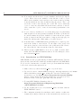
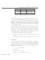
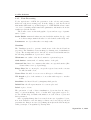
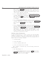
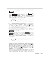
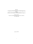
Figure 1.1: Geometry of short radius duct bend
10. A search facility is also available for the on-line help. On the Nexus system this is accessed at Start/Programs/Mechanical Engineering
/TASCflow/CFX-TASCflow Help Search . Try to find help sections that refer to Sutherland (a correlation for allowing variable viscosity in gases).
11. This should give a sense of the operation of the CFX-TASCflow postprocessor. Feel free to experiment with other object types and scalar
fields. When you have finished, choose “Quit” from the “File” menu.
12. Clean up by deleting the tascflow intro directory and closing CFXTASCflow Launcher window.
1.2
The Problem
To illustrate the use of the CFD software tools, consider the analysis problem
of estimating the pressure drop across the short radius duct bend shown in
Figure (1.1). The duct bend has a width of 1m and is made of galvanized
steel with an average surface roughness height of 0.10mm. Water flows
through the bend with a mass flow rate of ṁ = 225kgs−1 .
1.3
1.3.1
The Solution
The Duct Bend Model
The first phase in the CFD solution is a planning stage in which the complete
CFD model of the duct bend is specified. This specification includes:
September 3, 2002
1.3 The Solution
7
2
2
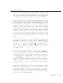
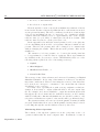
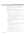
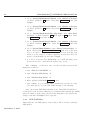
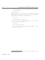
Figure 1.2: Geometry of the duct bend model
Physical Model Specification The steel walls of the bend and other duct
pieces are assumed to be rigid and joints in the duct work are assumed
to be smooth. The galvanized steel is assumed to have a uniform
surface roughness height. The width of the bend is sufficient that the
flow can be considered to be two dimensional.
Domain Geometry Specification To ensure that reasonable flow patterns are simulated in the bend it is necessary to add short entrance
and exit lengths of duct to simulate the actual flow through the bend
when it is situated in a duct. The domain geometry is shown in Figure (1.2).
The CFD simulation code is fully three dimensional, so even though
we are primarily interested in flow in the plane shown in Figure (1.2),
the geometry model must have a width into the page. A slice of width
0.10m will suffice.
Specification of Fluid Properties For this application the fluid is water
at STP which can be treated as a simple liquid with constant properties
( ρ = 1000kgm−3 , µ = 0.001N sm−2 ).
Specification of Flow Models For this analysis it is reasonable to assume the following flow features:
• steady incompressible flow,
• fully turbulent flow (the Reynolds number is approximately 225,000),
• the turbulent momentum stresses can be modelled with the standard k − ε model:
τij = µt
∂Ui
∂Uj
+
∂xi
∂xj
(1.1)
September 3, 2002
c STUDENT USER MANUAL
CFX-TASCflow
8
where the turbulent viscosity, µt , is proportional to the fluid density, the velocity scale of the turbulent eddies and the length scale
of the eddies. The velocity and length scales of the turbulent eddying motion are estimated from two field variables which are
calculated as part of the model: k, the turbulent kinetic energy,
and ε, the rate at which k is dissipated by molecular viscous
action.
Specification of the Boundary Conditions The boundary conditions that
we will use to model the interaction of the surroundings with the model
solution domain are:
• uniform velocity of 3ms−1 and uniform turbulence properties of
turbulence intensity of 3% and turbulence eddy length scales of
0.0075m (i.e. 10% of the duct height) across the inlet surface,
• uniform static pressure across the outlet surface,
• no-slip conditions along the duct walls and the standard wallfunction treatment to resolve log-law behaviour in the near wall
region where the flow is not fully turbulent, and
• symmetry conditions on the top and bottom surfaces (to ensure
that the simulated flow is two dimensional).
The above provides a mathematically complete description of the CFD
model. In the rest of this section, information on the use of the two software
tools that can implement this model and obtain a simulation of the flow
field in the model solution domain will be provided. The actual software
commands to use for this example problem are given in the last section of
these notes.
1.3.2
Grid Generation
Multi-Block Model: A computer model of the solution domain is created
and broken up into a set of finite elements. This model:
• is composed of multiple blocks ( regularly or irregularly shaped
boxes ),
• defines the region through which the fluid flows,
• may have interior blocks through which the fluid cannot flow,
• may have a complex shape (intake manifold - intake valve - cylinder geometry, passage between radial compressor blades, etc.),
and
• for historical reasons is often referred to as a solid body model.
September 3, 2002
1.3 The Solution
9
L
M
%
M
L
M
&
$
L
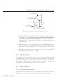
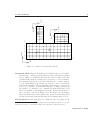
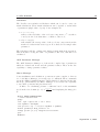
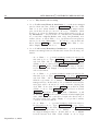
Figure 1.3: A three block structured mesh
Structured Mesh: Each block in the model is filled with a set of hexahedral elements or bricks ( possibly with non-orthogonal and non-parallel
faces ). This set of elements is known as the solid or volume mesh. The
elements in the mesh are arranged in a structured or ordered manner.
In a structured mesh, there are three independent coordinate indices,
(i, j, k), which uniquely specify the topological location of an element
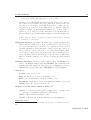
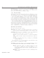
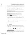
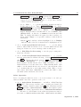
in the mesh ( similar to the way that three independent coordinate values, (x, y, z), specify a point in Cartesian space ). Figure (1.3) shows
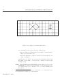
an example of a structured two dimensional mesh and Figure (1.4)
shows an example of an unstructured mesh3 . Each mesh is fitted to
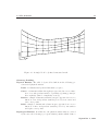
the body shape of its block, Figure (1.5). If it helps, you can imagine
that each mesh starts out as regular cube of rubber bricks and is then
stretched and twisted until it fits inside its irregularly shaped block.
Joining Blocks: In this introduction to CFD, the rules for joining blocks
3
Advanced techniques like grid embedding and grid attachment may allow some “unstructured” meshes to be used with a CFD solver designed for structured meshes.
September 3, 2002
10
c STUDENT USER MANUAL
CFX-TASCflow
Figure 1.4: A single block unstructured mesh
are very simple. At the join between two mesh blocks:
• the two surface faces that make the join must be identical in size,
shape, and orientation, and
• the mesh distribution on the two surface faces that make the join
must be identical.
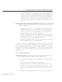
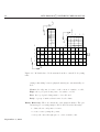
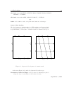
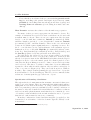
Applying these two rules to the geometry shown in Figure (1.3) means
that mesh block A must be broken up into 5 smaller blocks as shown
in Figure (1.6)4 .
Units: Both CFX-Build and CFX-TASCflow assume that you have used a
consistent set of units (i.e metric, British, or your own invention). To
keep things simple and to minimize errors, we will use metric units
throughout.
4
These rules can be relaxed by using the Constraints tools of CFX-Build and the
General Grid Interface (GGI) tools of CFX-TASCflow.
September 3, 2002
1.3 The Solution
11
M
L
Figure 1.5: A single block body-fitted structured mesh
Geometry Building
Physical Entities: The solid body model is built from the following parameterized physical entities:
Point: a 0 dimensional point in Cartesian xyz space,
Curve: a 1 dimensional line through space (specified as a vector function of one independent variable or parameter) joining points (either explicitly defined or implicitly created),
Surface: a simple 2 dimensional surface in space (specified as a vector
function of two independent variables) closed by four curves and
four corner points,
Solid: a simple 3 dimensional volume in space (specified as a vector
function of three independent variables) closed by six surfaces
and eight corner points
Topological Entities: In addition to the physical entities that are created
by the user, the following topological entities (entities which define a
September 3, 2002
c STUDENT USER MANUAL
CFX-TASCflow
12
L
M
M
%
L
M
&
$
$
$
$
L
Figure 1.6: Modified-three block structured mesh to match block joining
rules
joining relationship between physical entities) are automatically created:
Vertex: the endpoint of a curve or the corners of a surface or solid,
Edge: the topological closing curve of a surface or solid,
Face: the topological closing surface of a solid, and
Body: a group of surfaces that form a closed volume.
Entity Hierarchy: There is a hierarchy of the physical entities. The general strategy for creating simple solid blocks follows the hierarchy:
1. define the two endpoints of a curve,
2. create a curve joining the points,
3. sweep the curve through space to create a surface, and
September 3, 2002
$
1.3 The Solution
13
4. sweep the surface through space to create a solid.5
In this process, CFX-Build will automatically define new points for
the corners of every surface and solid, define new curves for the closing curves of each surface, and define new surfaces to make the closing surfaces of each solid. If an entity has been explicitly defined it
will have a unique cardinal identifier number (e.g. Point 2, Curve 3,
Surface 1, etc.). However, if the entity has been automatically defined it will have an identifier number assigned in the hierarchal form:
Solid . Surface . Curve . Point (i.e. Solid 2.5.3.2 is Point 2 of Curve
3 of Surface 5 of Solid 2.).
Congruent Model: If you stick to the simple types of physical entities and
simple strategy outlined above then you will form a congruent model
(i.e. a model which can be meshed). A congruent model is a model
in which all surfaces and solids share common edges and vertices at
their points of contact. Care has to be taken when forming multiblock solids to ensure that coincident points, curves, and surfaces are
treated as single entities. Following the recipe given above will ensure
that two separate entities do not end up occupying the same physical
space.
Geometry Grammar: In the geometry building phase, an Action is applied to an Object using a particular Method. The Geometry form
will automatically supply an appropriate list of Objects for a given
Action and an appropriate list of Methods for a given Object.
Actions: are:
Create: create a new object,
Edit: modify the properties of an existing object,
Show: provide information about an existing object,
Transform: create a new object by modifying an existing object, and
Delete: delete the object from the model.
Objects: are Point, Curve, Surface, Solid, plus
Coord: a coordinate system (point of origin, three coordinate axes,
and type: rectangular, cylindrical, or spherical),
Plane: a flat 2 dimensional surface, and
Vector: a directed line segment with direction and magnitude.
Methods: include
5
Note that there are short cuts. For example, you can create a box-shaped solid in one
step.
September 3, 2002
14
c STUDENT USER MANUAL
CFX-TASCflow
Create/Point/XYZ specify the Cartesian coordinates of a point,
Create/Curve/Point specify two, three or four points of a curve,
Create/Curve/Arc3Point an arc through the specified start, middle and end points,
Create/Curve/Revolve sweep specified point about specified axis
by a specified angle,
Create/Curve/XYZ a line with one point at the origin and the
other at the end of the specified vector,
Create/Surface/Extrude sweep a specified curve along a specified
vector,
Create/Surface/Revolve sweep a specified curve about a specified
axis through a specified angle,
Create/Surface/XYZ a plane with one corner on the origin and its
diagonally opposite corner at the end of the specified vector,
Create/Solid/Extrude sweep a specified surface along a specified
vector,
Create/Solid/Revolve sweep a specified surface about a specified
axis through a specified angle, and
Create/Solid/XYZ box with one corner on the origin and its diagonally opposite corner at the end of the specified vector.
Input: Many of these methods require you to enter a point, vector or axis
(i.e. a list of two points to set an axis). In some cases, these can be
picked off the graphics screen. In cases where the coordinate values
must be entered use the following conventions:
Point: [x y z] (the blanks between values can also be commas),
Vector: < x y z >, and
List: {Object1 Object2 . . .} (i.e. {[110][111]} specifies an axis in the
z direction through the point (1, 1) in the x − y plane.
Boundary and Object Identification
CFX-Build has the ability to assign “meaningful” names to two dimensional
surfaces and three dimensional volumes. These named surfaces and volumes
are known as Patches in CFX-Build. While this operation is not truly necessary, it is easy to use CFX-Build’s mouse picking capability to identify
surfaces that will later have boundary conditions attached to them and to
identify solid zones in the interior of the solution domain. CFX-TASCflow
will convert these patch names to region names when the CFX-Build geometry file is imported.
For historical reasons, CFX-Build has a very small number of patch
naming options:
September 3, 2002
1.3 The Solution
15
2D Patch: start with INLET, OUTLET, PRESS, SYMMET, WALL, CNDBDY,
BLKBDY, or USER2D,
3D Patch: start with SOLID, SOLCON, POROUS, or USER3D,
plus
Suffix: add a suffix to make each patch name distinctive and unique.
Surface Mesh Seeding
The development of optimal meshes for CFD analysis is still an art which
you can develop with practise. These notes are restricted to considering the
steps CFX-Build goes through to establish a mesh for a multi-block region.
,
-
Figure 1.7: Steps in the development of a surface mesh
As shown in Figure (1.7), mesh development follows the steps:
Placement of Nodes on Edges: nodes (corners of elements) are placed
along the edges of each surface in the solution domain,
September 3, 2002
c STUDENT USER MANUAL
CFX-TASCflow
16
Development of Surface Mesh: interpolation is used to create a surface
mesh of quadrilateral (Quad4) elements such that the element nodes
coincide with the specified edge nodes, and
Development of Volume Mesh: interpolation is used to create a volume
mesh of hexahedral (Hex8) elements such that the element faces coincide with the surface mesh quadrilateral elements.
'
$
%
&
'
'
'
)
$
%
&
)
$
*
(
(
&
*
&
D
E
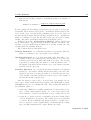
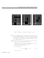
Figure 1.8: Mesh paths for multi-block surface
The CFX-Build meshing program, IsoMesh, uses mesh paths (a group of
topological parallel edges) to determine the placement of nodes on surface
edges. Figure (1.8) shows a two dimensional multi-block surface with the
mesh paths labelled A - G. Since the mesh is structured, each edge along
a mesh path must have the same number of elements (and nodes). The
placement of nodes along each edge of a mesh path is determined by the
following (in order of priority):
1. mesh seed (or user specified node placement),
2. carrying a mesh seed along the mesh path, or
September 3, 2002
1.3 The Solution
17
3. using the Global Edge Length to establish the number of elements of
uniform size,
Number of elements =
length of longest edge in path
Global Edge Length
For the example shown in Figure (1.8a) mesh seeds are placed on edges A1,
D4, and F2. These mesh seeds are used to establish the mesh seeding for the
A, D, and F edges, respectively.The remaining edges are seeded based on
the Global Edge Length. The Global Edge Length is used to establish the
number of elements on edges B1, C4 (the longest edge along the C path),
and E1. The surface mesh that results is shown in Figure (1.8b).
Meshing follows the Action/Object/Method syntax described in
the geometry phase. Typical actions are Create, Delete, and Show. The
relevant objects are Mesh Seed and Mesh. For creating a mesh, the only
relevant method is IsoMesh Surface.
The common mesh seeding methods are:
Uniform Mesh Seed: set a uniform placement by specifying either the
number of elements or the edge length of each element,
One-Way Bias Seed: set node placement with either increasing or decreasing element edge length (notice that the direction of each edge
is shown as an blue arrow when this method is active). The spacing
is specified by setting either the number of elements plus the ratio of
the lengths of the first and last element edges or the length of the first
and last element edges, and
Two-Way Bias Seed: set node placement with a symmetric non-uniform
spacing (i.e. decreasing to middle and then increasing to the end). The
spacing is specified by setting the number of elements plus the ratio
of the lengths of the first and middle element edges or the lengths of
the first and middle element edges.
After the surfaces of the solid body model have been meshed, the interior can be meshed with hexahedral elements. The CFX-Build program,
VOLMESH, is used to accomplish this task. After setting this task up in
the Analysis phase, i.e.:
• ensure that Reblock is on (This optimizes the block structure by trying to combine many small blocks into one or more larger grid blocks.
A fewer number of grid blocks will make post-processing easier.), and
• setting the geometry scale factors (usually left at their default values
of 1.0 if all inputs are in metric). The scaling factor in a particular
coordinate direction multiplies all distances in that coordinate direction on output (i.e. if the original distance is 100 mm and the scaling
factor is 0.001 m/mm then the output distance is 0.1 m),
September 3, 2002
c STUDENT USER MANUAL
CFX-TASCflow
18
CFX-Build will close and start the batch program VOLMESH executing.
When VOLMESH is completed, a geo file will be created. This file can be
imported into CFX-TASCflow for CFD processing.
1.3.3
Pre-processing
CFX-TASCflow runs with a Graphical User Interface (GUI) that provides a
thin-shell interface for a set of codes which carry out the CFD analysis. The
codes were all originally designed to operate from the UNIX command line,
to take text input (from ASCII files) and to provide output to the terminal
screen, output files, and a graphics window. While you will find the GUI
reasonably intuitive there will be less intuitive steps and nomenclature that
is leftover from the command line/text input design of the underlying codes.
The actual CFD analysis begins by using CFX-TASCflow to import the
geo file created for the solid body model in CFX-Build. The mesh and geometry information is translated to CFX-TASCflow’s native geometry database
and stored in the grd file. The next phases involve setting the relevant input
data to establish the flow conditions, boundary conditions, etc.
Flow Zones and Attributes
Two types of flow zones can be set up:
Fluid Zone: this default zone has fluid flowing through it. You must set
up the properties of the fluid and the fluid processes for this zone, and
Solid Zone: these zones can be established to create objects which block
off the fluid zone. Three types of objects can be created:
Inactive: a solid block with no fluid flow or conductive heat transfer,
CHT: a solid block with conductive heat transfer but no fluid flow,
and
Porous: porous mesh solid (screens, porous plug, etc.) with highly
constricted fluid flow,
For the Fluid Zone the following physical processes and sub-processes
will be relevant for a beginning user of CFD:
Fluid Flow: activates the solution of the momentum and mass conservation equations. The following sub-processes may be relevant:
Tracers: activates the solution of a transport equation for a passive scalar (i.e. simulates the advection and diffusion of a conserved scalar quantity which is useful for visualizing different flow
streams), and
Turbulent: activates the turbulence models for estimating the turbulent stresses,
September 3, 2002
1.3 The Solution
19
Notice that there are advanced sub-processes including particle tracking (for modelling solid particle and liquid droplet motion), compressible (for modelling transonic and supersonic flows of gases), and
rotating frame of reference (for modelling flow inside turbomachinery).
Heat Transfer: activates the solution of the thermal energy equation.
For many of these processes, appropriate models must be chosen. For
example, if turbulent flow is selected then a turbulence model and wall
treatment must be chosen. There are two two-equation models: the standard k − ε model with three variations: Default (recommended), RNG,
and Kato-Launder, and the k − ω model with three variations: Default
(recommended), SST , and Kato-Launder. There is also a second moment
closure model which requires significantly more computing resources. For
the k − ε models there are two wall treatments of the transition region to
laminar flow close to solid walls: High-Re (recommended) with two variations: Log. Law (Standard) (recommended) and Log. Law (Scalable), and
the Low-Re (requires a very fine grid in the near wall region).
For Solid Zones, also referred to as objects, it is necessary to specify the
mesh elements that are solid or blocked-off to fluid flow. If the zone has
already been given a name in the CFX-Build Patch phase then the Region
Manager6 is used to select the named patch. If a named patch does not
exist then the Region Manager is used to define a new nodal region that
can be selected. Care has to be taken to ensure that objects are sufficiently
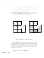
separated to allow valid flow field solutions. Objects cannot touch solely on
a line or a point, see Figure (1.9). They can touch along faces. While it
is valid to have a single element spanning the gap between two objects the
flow field will not be resolved in this gap. Therefore, it is recommended that
at least two elements span the gap between two objects.
Specification of Boundary Conditions
Throughout the flow domain mass and momentum conservation balances are
applied over each element. These are universal relationships which will not
distinguish one flow field from another. To a large extent a particular flow
field for a particular geometry is established by the boundary conditions on
the surfaces of the flow domain. It is crucial that these boundary conditions
reflect a reasonable physical situation and that they are consistent (i.e. a set
of boundary conditions which set the net inflow mass flow rate to be greater
than the net outflow mass flow rate is not consistent).
Boundary conditions are defined and then attached (or applied) to the
element faces on each surface of the flow domain. Typical boundary conditions include:
6
The Region Manager is described Section (1.3.5)
September 3, 2002
20
c STUDENT USER MANUAL
CFX-TASCflow
1RW5HFRPPHQGHG2EMHFWV
9DOLG2EMHFWV
,QYDOLG2EMHFWV
Figure 1.9: Valid, not recommended, and invalid objects
Wall: a solid wall through which no mass can flow. The wall can be stationary, translating (sliding), or rotating. If the flow field is turbulent
then the wall can be either smooth or rough. Depending upon which
of these options are chosen, suitable values must be input (i.e. the size
of the roughness elements, etc.),
Inflow: an inflow region is a surface over which mass enters the flow domain.
For each element face on an inflow region, either
• fluid speed and direction (either normal to the inflow face or in a
particular direction in Cartesian coordinates),
• mass flow rate and flow direction, or
• the total pressure 1
Ptotal ≡ P + ρV 2 = Ptotal spec
2
and flow direction
September 3, 2002
(1.2)
1.3 The Solution
21
must be specified. If the flow is turbulent that it is necessary to specify
the intensity of the turbulence I≡
Average of speed fluctuations
Mean speed
(1.3)
and one additional property of the turbulence: eddy viscosity ratio
(turbulent to molecular viscosity ration, µt /µ), or the length scale of
the turbulence (a representative average size of the turbulent eddies).
Typical turbulence length scales are 5% to 10% of the width of the
domain through which the mass flow occurs.
Outflow: an outflow region is a surface over which mass leaves the flow
domain. For each element face on an outflow region, either
• fluid velocity (speed and direction),
• mass flow rate, or
• static pressure
must be specified. A specified static pressure value can be set to a
specific face, applied as a constant over the outflow region, or treated
as the average over the outflow region. No information is required to
model the turbulence in the fluid flow at an outflow.
Opening: a region where fluid can enter or leave the flow domain. Pressure
and flow direction must be specified for an opening region. If the
opening region will have fluid entering/leaving close to normal to the
faces (i.e. a window opening) then the specified pressure value is the
total pressure on inflow faces and the static pressure on outflow faces
(a mixed type of pressure). If the opening region will have fluid flow
nearly tangent to the faces (i.e. the far field flow over an airfoil surface)
then the specified pressure is a constant static pressure over the faces.
For turbulent flows the turbulence intensity must also be set.
Symmetry: a region with no mass flow through the faces and with negligible shear stresses (and heat fluxes). This condition is often used
to simulate a two-dimensional flow field with a three-dimensional flow
solver and to minimize mesh size requirements by taking advantage of
natural symmetry planes in the flow domain.
Coalescence: a boundary condition that can be applied to faces of zero
area (a situation that occurs in structured meshes when the width of
the domain is pinched together).
Each boundary condition must be assigned to a set of surface element
faces. If all of the surface faces of the flow domain were named in the
grid generation phase, then it is relatively straightforward to attach the
appropriate set of surface element faces for a particular boundary condition
September 3, 2002
c STUDENT USER MANUAL
CFX-TASCflow
22
Inflow Sets
velocity
total pressure
Outflow Sets
static pressure
velocity
total pressure
static pressure
Solution Predicts
inflow static pressure
outflow pressure
inflow velocity
system mass flow
Table 1.1: Common boundary condition combinations
with the Region Manager. Since it is crucial that each surface element face
have a boundary condition attached to it, it is recommended that one of
the boundary conditions (usually a wall boundary condition) be set as the
default condition. If a face does not have a boundary condition explicitly
attached to it then the default condition will be attached to it. Using the
Display... command on the default condition will show the faces attached
to the default condition. This will often help identify faces which are missing
proper boundary conditions.
For the flow solver to successfully provide a simulated flow field, the
specified boundary conditions should be realizable (i.e. they should correspond to conditions in a laboratory setup). In particular, ensure that
the inflow and outflow boundary conditions are consistent and that they
take advantage of the known information. Table (1.1) lists several common
inflow/outflow condition combinations along with the global flow quantity
which is estimated as part of the solution for each combination.
The boundary condition specification steps ends with:
• a check to ensure that the boundary conditions are properly specified,
and
• then writing the complete boundary condition information to the bcf
file.
Initialization
The algebraic equation set that must be solved to find the velocity and pressure at each mesh point is composed of nonlinear equations. All strategies
for solving nonlinear equation sets involve iteration which requires an initial
guess for all solution variables. Therefore, for a turbulent flow, sufficient
information must be provided so that the following field values can be set
(initialized) at each mesh point:
• velocity vector (3 components),
• fluid pressure,
• turbulent kinetic energy, and
• dissipation rate of turbulent kinetic energy.
September 3, 2002
1.3 The Solution
23
Initial conditions are usually simple assumptions that are assumed to
apply uniformly (i.e. to be constant) over the complete flow domain. For
the velocity vector, it is possible to set uniform values of:
• the 3 velocity vector components (Uniform Cartesian), or
• fluid speed and grid direction (Uniform Grid Aligned).
In the latter case, the velocity vector is calculated for each mesh point by
assuming that the velocity vector is parallel to the specified grid line at the
mesh point, is in the direction of increasing grid index and has the specified
speed. Pressure is set to the specified value at each mesh point.
While it is possible to specify values of the turbulent kinetic energy, k,
and its dissipation rate, e, it is often difficult to intuitively establish appropriate guesses for these variables, especially the dissipation rate. However,
it is possible to establish initial values for k and e from estimates of the intensity of the turbulence and the length scale of the turbulence, as described
in the discussion on inflow boundary conditions.
The choice of initial conditions can significantly impact efficiency of the
iterative solution algorithm. The following guidelines will help ensure that
the initial conditions are reasonable:
• try to match the initial conditions to the dominant inflow boundary
conditions,
• usually a grid aligned initial velocity field will promote convergence to
the final solution fields,
• there is a Calculator 7 capability that can be used to make the initial
fields non-uniform (i.e. to vary over the flow domain).
The solution fields calculated by CFX-TASCflow are stored in the rso
file. The last step of setting the initial conditions will be to write the initial
fields out to the rso file.
1.3.4
Solver Operation
Setting Solver Parameters
The operation of the equation set solver in CFX-TASCflow is controlled by a
large set of parameters. Many of these parameters are given default values
and need not be changed by the beginning user. However, some features
should be explicitly set by the user for each run:
1. the timestep for the flow evolution,
2. the pressure offset,
7
Section (1.3.5)
September 3, 2002
c STUDENT USER MANUAL
CFX-TASCflow
24
3. the choice of discretization scheme, and
4. the selection of output fields.
Even though the focus is on steady flow simulations, transient evolution
is used in the iterative solution algorithm (in effect each iteration is treated
as a step forward in time). The choice of timestep for the flow evolution plays
a big role in establishing the rate of convergence. Good results are usually
obtained when the timestep is set to approximately 30% of the average
residence time (or cycle time) of a fluid parcel in the flow domain. This
residence time is referred to as the global time scale.
In incompressible flow fields the actual pressure level does not play any
role in establishing the flow field - it is pressure differences which are important. Therefore the pressure field can be changed by a constant value
without changing the results. This is known as the pressure offset and is
usually zero.
The variation of velocity, pressure, etc. between the mesh points has
to be approximated to form the discrete equations. These approximations
are classified as the discretization scheme. CFX-TASCflow uses one of the
following schemes ( listed in order of increasing accuracy ):
• Upwind ,
• Mass Weighted ,
• Modified Linear Profile , or
• Linear Profile Skew .
The accuracy of any of these schemes can be increased by turning on Physical
Advection Correction . In choosing a discretization, accuracy is obviously an
important consideration. However, increasing the accuracy of the discretization often slows convergence: sometimes to the extent that the solution
algorithm does not converge.
For many cases, especially those with a strong emphasis on fluid mechanics, it is necessary to output additional fields to the rso output data
file. For example, it is often worthwhile to output the turbulent stress fields
throughout the flow domain and the wall shear stresses on all boundary
walls. For fully three dimensional simulations, care should be taken to only
select those fields that are required or the rso file will be prohibitively large.
The parameters that you set are stored in the prm file. Parameters which
are given default values are not stored in the prm file, but they may be viewed
by scrolling through the out file which is created by the solver.
Monitoring Solver Operation
The solution of the algebraic equation set is the component of the code
operation which takes the most computer time. Fortunately, because it
September 3, 2002
1.3 The Solution
25
===========================================================================
TIME STEP = 1 SIMULATION TIME = 1.00E-01 CPU=9.53E+01
--------------------------------------------------------------------------| Equation | Rate | RMS Res | Max Res | Max Location | Linear Solution |
+----------+------+---------+---------+---------------+-------------------+
| TKE
| 0.00 | 3.6E-03 | 2.3E-02 | { 14, 19, 2} | 6.1 4.4E-03 OK |
| EPS
| 0.00 | 2.7E-02 | 2.0E-01 | { 14, 20, 1} | 5.7 7.6E-04 OK |
+----------+------+---------+---------+---------------+-------------------+
| U - Mom | 0.00 | 3.2E-04 | 2.8E-03 | { 13, 19, 2} |
2.4E-01 ok |
| V - Mom | 0.00 | 3.9E-04 | 8.6E-03 | { 13, 21, 2} |
3.4E-01 ok |
| W - Mom | 0.00 | 1.3E-06 | 6.7E-06 | { 1, 21, 3} |
3.6E+01 ok |
| P - Mass | 0.00 | 3.9E-03 | 5.9E-02 | { 14, 20, 2} | 9.1 1.5E-02 OK |
===========================================================================
Deleted existing backup RSO file: rso.bak
===========================================================================
TIME STEP = 2 SIMULATION TIME = 2.00E-01 CPU=9.79E+01
--------------------------------------------------------------------------| Equation | Rate | RMS Res | Max Res | Max Location | Linear Solution |
+----------+------+---------+---------+---------------+-------------------+
| TKE
| 2.47 | 9.0E-03 | 5.8E-02 | { 18, 25, 2} | 6.0 7.8E-04 OK |
| EPS
| 0.60 | 1.6E-02 | 1.1E-01 | { 13, 19, 1} | 5.8 6.4E-05 OK |
+----------+------+---------+---------+---------------+-------------------+
| U - Mom | 6.76 | 2.1E-03 | 1.2E-02 | { 12, 11, 2} |
3.0E-02 OK |
| V - Mom | 7.54 | 2.9E-03 | 1.8E-02 | { 12, 21, 2} |
2.7E-02 OK |
| W - Mom |60.81 | 7.6E-05 | 6.8E-04 | { 13, 22, 3} |
3.5E-01 ok |
| P - Mass | 0.36 | 1.4E-03 | 2.0E-02 | { 14, 12, 2} | 9.1 2.8E-02 OK |
===========================================================================
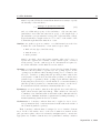
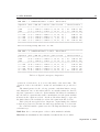
Table 1.2: Typical convergence diagnostics
operates in a batch mode, it does not take much of the user’s time. The
operation of the solver should be monitored and facilities are provided for
this.
The initial guesses for the velocity, pressure, turbulent kinetic energy,
and dissipation rate nodal values will not necessarily satisfy the discrete
algebraic equations for each node. If the initial nodal values are substituted
into the discrete equations there will be an imbalance in each equation which
is known as the equation residual . As the nodal values change to approach
the final solution, the residuals for each nodal equation should decrease.
Table (1.2) shows typical solver diagnostic output listing the residual
reduction properties for the first few time steps (iterations) of a solver run.
For each field variable equation set the following information is output
each time step:
RMS Res the root mean square of the nodal normalized residuals,
Max Res the maximum nodal normalized residual in the flow domain,
September 3, 2002
26
c STUDENT USER MANUAL
CFX-TASCflow
Max Location its location,
Rate the convergence rate
RMS res. current time step
RMS res. previous time step
which should typically be 0.95 or less, and,
Rate =
Linear Solver after each equation set is linearized, an estimate of the solution of the resulting linear equation set is obtained and statistics on
this solution is reported:
Work Units a measure of the effort required to obtain the solution
estimate,
Residual Reduction the amount that the linear solver has reduced
the RMS residual of the linear equation set, and
Status an indicator of the linear solver performance:
OK residual reduction criteria met,
ok residual reduction criteria not met but converging,
F solution diverging, solver terminated,
* residual increased dramatically, and
** residual overflowed.
Some of the above information is displayed graphically in the monitor window so that the solver execution can be monitored.
When execution is complete the final results are written to the rso file.
The original contents of the rso are written over, but a backup of the original
rso can be created. In addition, all of the information pertinent to the
operation of the solver is output to the out file, including:
• the CPU memory or storage requirements,
• the files used for input and output,
• an echo of the parameters explicitly set by the user,
• the complete list of parameters,
• grid, flow attribute, and boundary condition summaries,
• estimate of the global length, speed, and time scales based on the
initial fields,
• the convergence diagnostics,
• estimate of the global length, speed, and time scales based on the final
fields,
• the fluxes of all conserved quantities through the boundary surfaces
(these should balance to 0.01% of the maximum fluxes), and
• the computational time required to obtain the solution.
September 3, 2002
1.3 The Solution
1.3.5
27
Post-Processing
To the typical user of CFD, the generation of the velocity and pressure
fields is not the most exciting part. It is the ability to view the flow field
that makes CFD such a powerful design tool. CFX-TASCflow has a suite
of tools for obtaining useful visual and quantitative information from the
results stored in the rso file.
The PostProcessor works with graphic objects and two type of quantitative objects:
Scalar Fields: numerical values associated with the mesh nodes (i.e. each
node has a unique numerical value for each defined scalar field), and
Parameters: an object that takes on a single value.
Visualizer
The Visualizer is used to generate visual views of the flow field and its
properties. The Visualizer creates an image by drawing a set of visualization
objects. The viewing window is to the left of your screen and in this window
the following visualization objects can be drawn:
Wireframe: an outline of the flow domain for a given sub-region,
Grid Surface: an internal or boundary surface of the grid,
Contour Plot: lines of a constant scalar value on a specified surface (like
elevation lines on a topological map),
Fringe Plot: like a contour plot, except the regions between the contours
are filled in with colour,
Vector Plot: the field of vectors on a nodal region or 2D surface,
XY Graph: a plot of the variation of one scalar with respect to another
scalar,
Streakline: the lines followed by imaginary fluid parcels,
Relief Plot: the 3D representation of a contour plot, and
Label: a piece of text.
The generation of each of these visualization objects involves choosing a
range of options including: choice of scalar field, appropriate region, etc.
See the On-line help for further information on each of these objects and
their generation.
Once a graphical image has been created from a set of graphics objects,
it is often desirable to save the image so that it can be used in reports and
presentations. Images are saved by printing them (from the File menu) as
either postscript or encapsulated postscript files.
September 3, 2002
c STUDENT USER MANUAL
CFX-TASCflow
28
Region Manager
Many of the components of CFX-TASCflow, such as the specification of
boundary conditions, require that a region of the flow domain be selected.
The Region Manager is the tool that is used to specify regions:
Nodal: a portion of the flow domain mesh, or
Physical: a physical plane, line, or point in the flow domain.
The structured mesh coordinate indices (i, j, k) are used to specify nodal
regions in the flow domain. The general specification of a nodal region takes
the form:
[ib : ie, jb : je, kb : ke] : gridname
where the suffix b denotes beginning and e denotes end. The following short
forms are useful:
• for the main grid, the gridname need not be specified,
• if a range is not specified for an index direction, the complete range of
that index is assumed (i.e. [3,,] specifies the i = 3 mesh plane),
• if the beginning index is not specified, it is assumed to be 1 (i.e.
[3,:5,2:8] is the same as [3,1:5,2:8]), and
• a mesh plane in the main grid can be specified by its index and value
(i.e. i3 is the same as [3,,]:main).
While the Region Manager provides a GUI panel to fill in these ranges,
the resulting range will often be shown with this nomenclature and this
nomenclature must be used when writing macros.
Scalar Field Manager
The PostProcessor includes the Scalar Field Manager to:
• display and select from all of the scalar field nodal values calculated
and used by the solver, including grid locations x, y, and z, velocity
components u, v, and w, pressure, etc.,
• to define new scalar fields (i.e. to define normalized velocity components),
• to create copies of existing scalar fields, and
• to display the numerical values of the mesh node scalar field quantities.
The display of scalar field values can be either as:
C.V.: control volume solutions (i.e. the solutions of the discrete conservation equation set), or
Hybrid: c.v. values for interior nodes and boundary surface values for
control volumes adjacent to the boundary surfaces.
September 3, 2002
1.3 The Solution
29
Calculator
The PostProcessor includes a Calculator which can be used to carry out
math calculations. These math calculations can be applied to scalar fields
or parameters (single value objects). Some examples are:
• u=x∗x+2∗y
will set each nodal value of the u velocity component to x2 + 2y where
x and y are the local Cartesian coordinates of the node,
• ubar = avrg(u)
will calculate the average value of the u velocity component from the
mesh node values in the active region. Note that ubar is a single value
parameter.
The Calculator will also evaluate and display a single numerical expression.
This is useful for seeing the value of a parameter, like ubar, that has been
calculated.
ACL Parameter Manager
The ACL Parameter Manager tool shows the complete list of parameters
which are defined and in use and the parameter values. There is also the
capability to change parameter values.
Macro Manager
Some visualization and calculation operations are quite complex, so there is
a tool, the Macro Manager, for storing a set of commands. These commands
are in the AEA Command Language, ACL, which is documented in the Online help. Unfortunately, the Macro Manager does not have the capability
to save GUI operations and play them back.
A Macro for calculating pressure coefficients based on the maximum
(p−p
)
speed in the flow domain (i.e. Cp ≡ 1 V 2ref ) and displaying the fringe plot
is:
2
max
Define MACRO PCOEFFICIENT
-- Macro PCoefficient
purge
calc spd = sqrt( u*u + v*v + w*w )
calc spdmax = max(spd)
calc pcoeff = (p - 0.0)/(0.5 *spdmax * spdmax)
define parameter draw_filled = on
fringe pcoeff [*,*,2] range=local levels=11
plot
EndMacro
September 3, 2002
c STUDENT USER MANUAL
CFX-TASCflow
30
Writing PreProcessing before exiting CFX-TASCflow will save this macro
in the gci file. Other useful information like user-defined parameters, etc.
is also stored in the gci file.
1.4
Commands for Duct Bend Example
The following conventions will be used hereafter to indicate the various
commands that should be invoked:
Menu/Sub-Menu/Sub-sub-menu Item chosen from the menu hierarchy,
Radio Button Option activated by clicking on a radio button,
ΞIcon Command Option activated by clicking on the icon, and
Box Name value Enter value in the box.
To begin, set up a directory (you will want to make a new directory
every time you set up a new geometric model) and run CFX-Build to create
the mesh for this problem:
• Create a folder ductbend on your N: drive,
• Open the CFX-4.3 Launcher, Start/Programs/Mechanical Engineering/CFX4.3 ,
• set the working directory to ductbend and
• click on the ΞCFX-Build tab.
1.4.1
CFX-Build
The first step is to set up CFX-Build’s session files and some preferences:
• File / New...
will open a window called New Database, in this
window fill in the database name,
• New Database Name ductbend and click on ΞOK to close.
• After a short wait the window New Model Preferences will pop up.
Click on ΞOK to close8 .
8
In geometries with very small length scales, it is better to switch the Tolerance from
Based on Model to Default and then to set the Tolerance to a value significantly
smaller than the smallest length scale in the Global Preferences window opened by
choosing Preferences / Global ...
September 3, 2002
1.4 Commands for Duct Bend Example
31
Geometry Development
The commands given in the next paragraph will build the geometry for the
solid body model of the flow domain by:
• setting the point (0m, 0m, 0m) as the left end of the inlet,
• setting the point (0.075m, 0m, 0m) as the right end of the inlet,
• joining these two points to create a curve (line),
• extruding this line 0.10m in the y direction to create a rectangular
surface,
• sweeping the upper curve of this surface through 90◦ counterclockwise
about the axis x = 0.1m, y = 0.1m, to create a surface with an arc
shape,
• extruding the right curve of this surface 0.20m in the x direction to
create a second rectangular shape, and finally
• extruding all three surfaces 0.10m in the z direction to create three
solids which will define the solution domain.
On the row of radio button commands just below the menu bar at the
top of the screen turn Geometry on and then carry out the following
actions in the Geometry window:
• first though, go up to the tool bar and click ΞShow labels ,
• choose Create/Point/XYZ items in the Geometry window, check
that Auto Execute is off, fill in Point Coordinate List [0 0 0] , and
click Ξ-Apply- to make the first point (notice that a cyan (aqua blue)
coloured 1 appears),
• choose Create/Point/XYZ items in the Geometry window, check
that Auto Execute is off, fill in Point Coordinate List [0.075 0 0] ,
and click Ξ-Apply- to make the second point, (notice that two points
appear in the graphics window with cyan labels),
• choose Create/Curve/Point items in the Geometry window, check
that Auto Execute is off, fill in Starting Point List Point 1 ( click in
this box while it is empty, move the cursor into the graphics window,
place the cursor box over Point 1 on the screen and left click mouse),
fill in Ending Point List Point 2 , and click Ξ-Apply- to make the
line (notice that a yellow line with a yellow label 1 appears),
• choose Create/Surface/Extrude items in the Geometry window,
check that Auto Execute is off, fill in Translation Vector < 0 0.10 0 > ,
September 3, 2002
c STUDENT USER MANUAL
CFX-TASCflow
32
fill in Curve List Curve 1 (again use the mouse to pick the curve),
and click Ξ-Apply- to make the first surface ( notice that a green box
with a green label 1 appears on the screen and that the upper corners
of the box have aqua blue point labels),
• choose Create/Surface/Revolve items in the Geometry window,
check that Auto Execute is off, fill in Axis { [ 0.1 0.1 0] [0.1 0.1 1.0] } ,
fill in Total Angle -90 , fill in Curve List Surface 1.2 (notice that
1.2 is the 2 curve of the 1 surface), and click Ξ-Apply- to make the
second surface,
• choose Create/Surface/Extrude items in the Geometry window,
check that Auto Execute is off, fill in Translation Vector < 0.20 0 0 > ,
fill in Curve List Surface 2.2 , and click Ξ-Apply- to make the third
surface,
• choose Create/Solid/Extrude items in the Geometry window,
check that Auto Execute is off, fill in Translation Vector < 0 0 0.1 > ,
fill in Surface List Surface 1:3 (put cursor over Surface 1 and click
and then move to Surface 2 and Surface 3 holding the shift key down
while clicking to pick a list of surfaces) , and click Ξ-Apply- to make
the three solids (notice that a blue wireframe defines the edges of the
solids and the Solid labels are in blue).
Boundary Surface Identification
To make the implementation of boundary conditions easier when using CFXTASCflow, we will give names to the boundary surfaces of the solid body
model. In particular, the commands given in the next paragraph will need
make it easy to set boundary conditions:
• on the inlet surface,
• on the outlet surface,
• on the two symmetry planes, and
• on the outer and inner duct bend walls.
Turn Patches
Patches window :
on and then carry out the following actions in the
• turn Auto Execute off,
• choose Create/2D Patch , fill in Patch Name inlet , fill in Surface
Solid 1.3 (pick with the mouse by placing the cursor near the centroid
of the inlet surface), and click Ξ-Apply- ,
September 3, 2002
1.4 Commands for Duct Bend Example
33
• choose Create/2D Patch , fill in Patch Name outlet , fill in Surface
Solid 3.4 (notice that 3.4 is surface 4 of solid 3) , and click Ξ-Apply,
• choose Create/2D Patch , fill in Patch Name symmet1 , fill in
Surface Solid 1.6 2.6 3.6 (Use the shift key plus left click to pick a
list of surfaces with the mouse, check that the correct surfaces are
highlighted in brown. If you have wrong surface in your list you can
remove it by putting the cursor near its centroid and using the right
mouse click.) , and click Ξ-Apply- ,
• choose Create/2D Patch , fill in Patch Name symmet2 , fill in
Surface Surface 1:3 , and click Ξ-Apply- ,
• choose Create/2D Patch , fill in Patch Name wallout , fill in
Surface Solid 1.1 2.1 3.1 , and click Ξ-Apply- , and
• choose Create/2D Patch , fill in Patch Name wallin , fill in Surface
Solid 1.2 2.2 3.2 , and click Ξ-Apply- .
Surface Mesh Seeding
The commands listed in the next paragraph will develop the structured mesh
for the interior of the solid body model. These commands build the mesh
by:
• seeding a uniform mesh distribution with 10 elements along the inlet
axis, 8 elements along the bend axis, and 10 elements along the outlet
axis,
• seeding a non-uniform mesh distribution between the duct walls with
15 elements that are smaller near the walls,
• seeding two mesh elements between the two symmetry surfaces,
• calculating surface meshes on all of the surfaces, and
• calculating the volume mesh in the interior of the solid model.
Turn Mesh on and then carry out the following actions in the Mesh
window :
• turn Auto Execute off,
• choose Create/Mesh Seed/Uniform , turn Number of Elements
on, fill in Number= 10 , fill in Curve List Surface 9.2 , and click
Ξ-Apply- (notice the little yellow circles that appear),
September 3, 2002
c STUDENT USER MANUAL
CFX-TASCflow
34
• choose Create/Mesh Seed/Uniform , turn Number of Elements
on, fill in Number= 8 , fill in Curve List Surface 10.2 , and click
Ξ-Apply- ,
• choose Create/Mesh Seed/Uniform , turn Number of Elements
on, fill in Number= 10 , fill in Curve List Surface 11.2 , and click
Ξ-Apply- ,
• choose Create/Mesh Seed/Two Way Bias , turn Num Elems
and L2/L1 on, fill in Number= 15 , fill in L2/L1= 1.5 , fill in Curve
List Surface 4.3 , and click Ξ-Apply- ,
• choose Create/Mesh Seed/Uniform , turn Number of Elements
on, fill in Number= 2 , fill in Curve List Surface 9.1 , and click
Ξ-Apply- ,
• choose Create/Mesh/Surface , turn Ensure Structured Mesh on,
fill in Surface List Surface 1:3 Solid 1.1 ... (click in box and then
move box cursor to upper left of viewing screen, left click and drag
mouse to create a large box which completely encloses the solid body
model to pick all surfaces), and click Ξ-Apply- ,
• go to the tool bar and click ΞHide labels on to make the image clear
(rotate the model to check that the mesh looks correct).
Turn Analysis on and then carry out the following actions in the
Analysis on window :
• turn Reblock in VOLMESM on,
• turn Calculate Mesh Quality off,
• turn Visualise Mesh Quality off,
• fill in Solids for VOLMSH Solid 1:3 , and
• click ΞApply (a box warning that equivalencing tolerance is being
reset may appear. You can click ΞOK and ignore the warning).
After a short wait CFX-Build will shut down. Using Windows Explorer,
you should see a file in your working directory with the name build4.geo.99999
where the number at the end is generated automatically by the system and
changes each time VOLMSH creates a geo file.
1.4.2
CFX-TASCflow
This brings us to the CFD phases of the solution. There are three principal
CFD phases:
September 3, 2002
1.4 Commands for Duct Bend Example
35
Pre-processing: input information to get ready to calculate the velocity
and pressure fields,
Solver: execute the solver to calculate the field variables for the mesh, and
Post-processing: visualize and analyse the results.
• Start the CFX-TASCflow Launcher click on Start/Programs/Mechanical
Engineering/CFX-TACSflow/CFX-TASCflow 02.10.00 ,
• Set the working directory to N:\ductbend and then click the ΞCFXTASCflow button.
Pre-processing
After the CFX-TASCflow window opens up, the commands listed in the next
paragraph will accomplish the following steps:
• import the CFX-Build geo file and convert it to the grd file format,
• specify the region through which the fluid will flow, the physical models
(fluid flow, no heat transfer, turbulence, standard k-e model with wall
functions), and fluid properties ( water with ρ = 1000kgs−1 and µ =
0.001N sm−2 ),
• set up a rough wall boundary condition as the default condition,
• set up and attach the inlet boundary condition, the outlet boundary
condition, and the symmetry boundary conditions,
• check pre-processing,
• write the pre-processing information to the bcf file, and
• generate an initial guess for the flow fields ( a uniform speed of 3ms−1
with the velocity aligned with the grid lines that follow the duct axis,
uniform pressure of 0.0P a, uniform turbulence intensity of 3%, and
uniform turbulence eddy length scale that is 10% of the inlet length
scale)
To accomplish these steps execute the following commands:
• choose File/Import/CFX 4... which will open a window called
Import CFX 4. To select the filename turn 3 Dimensional Grid on,
select Browse... to open a file browsing window from which you can
select the geo file generated by CFX-Build. Highlight the geo filename
with a left click in the right frame and click ΞOk . The Filename
should contain the geo filename. Click ΞOk to import the file and
close the Import CFX 4 window.
September 3, 2002
36
c STUDENT USER MANUAL
CFX-TASCflow
• choose File/Load PreProcessing ,
• choose PreProcess/Zones & Attributes to open the Zone Manager
window. Make sure that 3D Region < default > is filled in, Fluid
Flow is on, and Heat Transfer is off. In the Fluid Subprocesses
pane check that all sub-processes are off except Turbulent which
should be on. Open the Turbulence Model Setup window by choosing Turbulence ... and check that k−ε Models and Default Model
are on and that High-Re Models with Log. Law (Standard) near
wall models are on. Click ΞOk to close. Open Material Properties
window by choosing Materials ... . We will use a custom fluid and
fill in Density 1000.0 and Viscosity 0.001 . Click ΞOk to close.
Click ΞApply to accept the above,
• choose PreProcess/Boundary Conditions to open the Boundary
Conditions Manager window. In this window issue the following commands:
– choose New ... to open New Boundary Condition window. In
this window choose Type: WALL , accept Name: 1 WALL
and click ΞOk . Choose Attachment General Default . With
Fluids on, choose Surface Type Rough and fill in Roughness
Height 0.0001 . With Turbulence on, notice that no information is required. Click ΞApply to accept this boundary condition
and its attachment,
– choose New ... to open New Boundary Condition window. In
this window choose Type: INFLOW , accept Name: 2 INFLOW
and click ΞOk . Choose Attachment Specified Region . To
fill in the region name, choose Select... which opens the Region
Manager window. In this window, choose INLET from the list (the
inlet plane will be shown in red on the wireframe display) and
click ΞOk . Notice that Region INLET is now filled in. With
Fluids on, choose Type Velocity , Vector Based on Normal
Normal and fill in Speed 3.0 . With Turbulence on, fill
in Intensity 0.03 and then select Fraction of Inlet Length Scale
with Med to specify a turbulence length scale that is 10% of
the inlet length scale. Click ΞApply to accept this boundary
condition and its attachment,
– choose New ... to open New Boundary Condition window.
In this window choose Type: OUTFLOW , accept Name:
3 OUTFLOW and click ΞOk . Choose Attachment Specified Region .
To fill in the region name, choose Select...
which opens
the Region Manager window. In this window, choose OUTLET
from the list and click ΞOk . With Fluids on, choose Type
September 3, 2002
1.4 Commands for Duct Bend Example
37
Pressure , Pressure Value 0.0 , Pressure Type Static and
fill in Applied As Constant . With Turbulence on, no information is needed. Click ΞApply to accept this boundary
condition and its attachment, and
– choose New ... to open New Boundary Condition window.
In this window choose Type: SYMMETRY , accept Name:
4 SYMMETRY and click ΞOk . Choose Attachment Specified Region .
To fill in the region name, choose Select... which opens the
Region Manager window. In this window, choose SYMMET1, turn
Multiple Select on, then choose SYMMET2 from the list and click
ΞOk . No further information is required for this boundary condition. Click ΞApply to accept this boundary condition and its
attachment,
– with the 1 Wall boundary condition highlighted, choose Display
. Only the walls of the flow domain should be highlighted in red,
• choose PreProcess/Check PreProcess ...
to open the Check
window. Click ΞOk and if there are no errors the Check window will
disappear. If there are errors a message window will appear,
• choose File/Write PreProcessing to save the preprocessing information in a bcf file,
• choose PreProcess/Initial Guess Generator ...
to open the
Initial Guess window. Fill the following: Velocity Uniform Grid Aligned ,
Axis J , Velocity Magnitude (signed) 3.0 , and Pressure 0.0 .
Then choose Turbulence ...
to open the Turbulence Initial
Guess Window. In this window select Med Intensity to get a 5%
initial turbulence level and then select Eddy Viscosity Ratio with
Med to set the initial effective viscous action of the turbulent eddies
to be 10 times that due to molecular activity. Click ΞOk to accept
these values. Check that Write RSO is on then click ΞOk to write
the initial solution fields into the rso file.
Solver Operation
Before executing the fluid flow solver code, it is necessary to set some parameters which control the operation of the code:
• choose Solve/Solver Parameters ... and fill in Fluid Time Step
0.04 (30% of the average residence time of a fluid parcel inside the
solution domain), Number of time steps 25 , and Maximum residual
1.0e-03 and turn Upwind Difference on in the discretization panel.
To add to the default output fields click on Additional Parameters
... and turn on I/O Control in the additional parameters window.
Now turn on Write mass flow scalar fields , Write surface area fields ,
September 3, 2002
c STUDENT USER MANUAL
CFX-TASCflow
38
Write BC information , Write turbulent Reynolds stresses , and Write
vorticity fields . Click ΞOk to return to the main parameter window.
Click ΞOk to save and close window,
• choose Solve/Solver Monitor ... and check that Serial , One
Computer , Normal , System , Single , and Batch are on,
before clicking ΞStart . After a few minutes execution should begin.
Diagnostics will scroll on the terminal output pane and the equation
residuals will be plotted as a function of timestep. After the first few
timesteps, the residuals should fall monotonically. Execution should
stop after 20 timesteps. Click ΞClose
Post-processing
The most interesting step is the analysis of the results. To illustrate this
step the commands listed in the next paragraph step through the following
tasks:
• load the results from the rso file for post-processing,
• create a vector plot on one of the symmetry boundary planes,
• save a postscript image of the plot,
• create a plot of the wall shear stress along the inner wall,
• look at a table of u velocity component values,
• create a fringe plot of the total (stagnation) pressure field, and
• create an ASCII file containing values of pressure and wall shear stress
along the inner wall.
To accomplish these tasks:
• choose File/Load PostProcessing/Full RSO ,
• in the Visualization Object Manager panel choose New... , choose
Object Type: Vector Plot , and click ΞOk ,
• in the Vector Interface panel choose Region SYMMET1 (you
can do this by following Select... ), choose Type Surface , and click
ΞApply . The vector plot should appear,
• choose File/Print ...
to open up a Print panel. In this panel
choose Format Postscript , fill in File Name vector.ps , and click
ΞPrint . The file vector.ps should be created and can be viewed with
the ghostview which is on the Waterloo Polaris workstations. This
file can be printed on the Lever lab printer. To create an image that
can be directly imported into a word processing document save the
image in encapsulated postscript format (eps).
September 3, 2002
1.4 Commands for Duct Bend Example
39
• in the Visualization Object Manager panel turn Visibility off (the
vector plot should disappear), select New... , choose Object Type:
XY Graph , and click ΞOk ,
• in the XY Graph Interface panel choose 1D Region: [16,1:29,2] and
Scalar: TAU WALL , and click ΞApply . To scale the graph choose
Viewer/Viewport Options... and turn Orthographic on and
select Ξ-Y orientation. Click ΞOk to close the Viewport Manager
window. Click ΞOk to view the scaled graph.
• choose File/Post Processing State/Save and accept the File
name viz.state to save all of the present format information for the
vector plot and the xy-graph. This facility will allow for the recreation
of images with new results for easy comparison between simulations.
• choose PostProcess/Scalar Field Manager... , select U from the
scalar field list, and choose Display... . With Region
blank use
the ΞStart and ΞMore buttons to scroll through the data to find
the U velocity component at the node [5,5,2]. Use ΞCancel to close
the Scalar Field Display and Manager panels,
• in the Visualization Object Manager panel turn Visibility off
(the graph should disappear), select New... , choose Object Type:
Fringe Plot , and click ΞOk ,
• in the Fringe Plot panel choose 2D Region: SYMMET1 and Scalar:
PTOTAL , turn Faces on and Lines off and click ΞApply . You
will need to reset the viewport orientation to Ξ+Z in the Viewport
Manger window ( Viewer/Veiwport Options ... ). The fringe plot
should appear,
• choose File/Post Processing State/Restore and accept the File
name viz.state to restore the original formatting that existed before
the fringe plot was created.
• choose Tools/Command Line to open the Command Line interface (an interface that allows keyboard entry of post-processing commands). In the interface window enter the command help rsf info.
Information on using rsf files to export data will be displayed. Hit
Enter key until you return to the command line prompt. Issuing the command write rsf rsf fields=’’i j k x y z tau wall
p’’ [16, 1 : 29, 2] will create an rsf containing the opening line:
$$$RSF 29 I J K X Y Z TAU WALL P
followed by a table of values giving the index numbers, locations, wall
shear stress and pressure, and wall shear for each node along the centreline of the inner wall. The contents of this file can be imported
September 3, 2002
c STUDENT USER MANUAL
CFX-TASCflow
40
into a conventional spreadsheet program and further post-processed
in that environment.
1.4.3
Clean Up
The last step is to remove unnecessary files created by CFX-Build and CFXTASCflow. This step is necessary to ensure that you do not exceed your disk
quota. At the end of each session delete all files except:
• *.db.jou9 ,
• name.lun, grd, gci, prm, bcf, and rso.
If you no longer need your results but would like to be able to replicate
them then you should delete all files except:
• *.db.jou,
• name.lun, gci, prm, and bcf.
After removing all unnecessary files, use the WinZip utility to compress
the contents of your directory.
9
This file can be used to recreate a mesh by choosing the CFX-Build command
File/Utilities/Rebuild...
September 3, 2002