Download Plotting rpart trees with prp

Plotting rpart trees with prp
Stephen Milborrow
February 4, 2015
Contents
1 Introduction
2
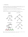
2 Overview
3
3 FAQ
6
4 Compatibility with plot.rpart and text.rpart
8
5 Customizing the node labels
9
6 Examples using the color arguments
14
7 Branch widths
20
8 Trimming a tree with the mouse
21
9 Using plotmo in conjunction with prp
22
10 The graph layout algorithm
25
A Appendix: mvpart mrt models
27
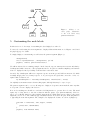
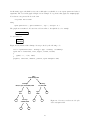
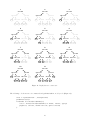
An Example
ozone
12
n=330 100%
temp < 68
temp >= 68
ozone
7.4
n=214 65%
ozone
20
n=116 35%
ibh >= 3574
ibt < 226
ibh < 3574
ibt >= 226
ozone
9.7
n=106 32%
dpg < −9.5
dpg >= −9.5
ozone
5.1
n=108 33%
ozone
6.5
n=35 11%
ozone
11
n=71 22%
1
ozone
16
n=55 17%
ozone
23
n=61 18%
1
Introduction
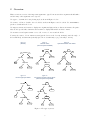
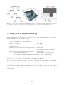
The prp function plots rpart trees [6, 7]. It automatically scales and adjusts the displayed tree for best fit.
It combines and extends the plot.rpart and text.rpart functions in the rpart package. Figure 1 below
shows some examples. The function is in the rpart.plot R package.
Note that rpart.plot is merely a front end to prp, with the most useful arguments of prp.
Section 2 of this document (the Overview) is the most important. The remaining sections may be skipped
or read in any order.
I assume you have already looked at the vignette included with the rpart package [7]:
An Introduction to Recursive Partitioning Using the RPART Routines by Therneau and Atkinson.
default prp
(type = 0)
type = 4, extra = 6
died
0.38
sex=mal
yes
no
sex=mal
fml
age>=9.5
died
0.19
survived
survived
0.73
age>=9.5
<9.5
sibsp>=2.5
died
died
0.17
survived
0.53
sibsp>=2.5
<2.5
died
survived
died
0.05
assorted arguments
survived
0.89
plot.rpart for comparison
sex=b
|
1
yes is sex = male?
no
age>=9.5
survived
1e+02/3e+02
2
is age >= 9.5?
sibsp>=2.5
died
7e+02/1e+02
5
is sibsp >= 2.5?
4
10
11
3
died
0.17 61%
died
0.05 2%
survived
0.89 2%
survived
0.73 36%
died
2e+01/1
survived
3/2e+01
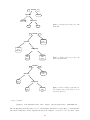
Figure 1: Some prp examples, with a plot.rpart graph for comparison. The data is the Titanic data with
survival as the response (sibsp is the number of siblings or spouses aboard).
2
2
Overview
This section is an overview of the important arguments to prp. For most users these arguments should suffice
and the many other arguments can be ignored.
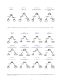
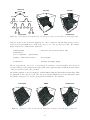
Use type to determine the basic plotting style, as shown in Figure 2 below.
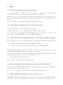
Use extra to add more details to the node labels, as shown in Figures 3 and 4 overleaf. Use under=TRUE to
put those details under the boxes.
Use digits, varlen, and faclen to display more significant digits and more characters in names. In particular, use the special values varlen=0 and faclen=0 to display full variable and factor names.
Use border.col and split.border.col to add or remove boxes around the labels.
You may also want to look at fallen.leaves (put the leaves at the bottom), branch (control the angle of
the branch lines), and uniform (vertically space the nodes uniformly or proportionally to the fit).
type = 0
(default)
type = 1
label all nodes
(like text.rpart all=TRUE)
sex=male
yes
age>=9.5
survived
survived
sibsp>=2.5
died
died
survived
survived
sibsp>=2.5
survived
survived
died
type = 3
left and right split labels
survived
type = 4
like type=3 but with interior labels
(like text.rpart fancy=TRUE)
died
sex=male
sex=male
female
female
survived
age>=9.5
died
survived
age>=9.5
<9.5
<9.5
died
died
sibsp>=2.5
survived
sibsp>=2.5
<2.5
died
no
died
age>=9.5
died
sibsp>=2.5
died
sex=male
yes
no
age>=9.5
died
died
no
died
sex=male
yes
type = 2
split labels below node labels
survived
<2.5
died
survived
Figure 2: The type argument.
3
died
survived
extra = 0
default
extra = 1
nbr of obs
extra = 100
percentage of obs
extra = 101
nbr and percentage
of obs
30
30
30
n=31
100%
n=31 100%
30
Girth<16
Girth<16
Girth<16
Girth>=16
23
56
Girth<16
Girth>=16
Girth>=16
Girth>=16
23
56
23
56
23
56
n=24
n=7
77%
23%
n=24 77%
n=7 23%
Figure 3: The extra argument with an anova model. Percentages are included by adding 100 to extra.
extra = 0
default
extra = 1
nbr of obs per class
extra = 2
class rate
extra = 3
misclass rate
died
809 500
died
809 / 1309
died
500 / 1309
died
sex=male
sex=male
female
died
survived
sex=male
female
died
682 161
survived
127 339
extra = 4
prob per class
(sum across a node is 1)
extra = 5
prob per class,
fitted class not displayed
died
.62 .38
.62 .38
survived
.27 .73
extra = 8
prob of fitted class
.81 .19
extra = 7
prob of 2nd class,
fitted class not displayed
sex=male
female
female
died
0.19
.27 .73
survived
0.73
extra = 100
percent of obs
0.19
died
0.38 100%
sex=male
sex=male
female
survived
.10 .26
died
64%
0.73
extra = 106
prob of 2nd class and
percent of obs
died
100%
female
died
.52 .12
survived
127 / 466
0.38
sex=male
sex=male
survived
0.73
female
died
161 / 843
died
0.38
died
.62 .38
female
died
0.81
extra = 6
prob of 2nd class
(useful for binary responses)
extra = 9
overall prob
(sum over all leaves is 1)
died
0.62
sex=male
survived
339 / 466
female
female
died
.81 .19
died
682 / 843
sex=male
sex=male
sex=male
female
survived
36%
female
died
0.19 64%
survived
0.73 36%
Figure 4: The extra argument with a class model. This figure also illustrates under=TRUE which puts the
extra data under the box.
4
The character size will be adjusted automatically unless cex is explicitly set. Use tweak to adjust the
automatically calculated size, often something like tweak=0.8 or tweak=1.2.
It helps to remember that the display has four constituents: the node labels, the split labels, the branch lines,
and the optional node numbers. Each of these constituents has a complete set of col etc. arguments. Thus
we have, for example, col (the color of the node label text), split.col (the split text), branch.col (the
branch lines), and nn.col (the optional node numbers).
Standard graphics parameters such as col can be passed in as ... arguments. So where the help page refers
to the col argument, what is meant is the col argument passed in as a ... argument, and if it is not passed
in, the value of par("col"). Such parameters typically affect only the node labels, not the split labels or
other constituents of the display.
2.1
Citing the package
If you use this package in a published document, please do the right thing and cite it [4]:
Stephen Milborrow. rpart.plot: Plot rpart Models. An Enhanced Version of plot.rpart., 2011. R Package.
@Manual{rpart.plotpackage,
author = {Stephen Milborrow},
title = {{rpart.plot: Plot rpart Models. An Enhanced Version of plot.rpart}},
year = {2011},
note = {R package},
url = {http://CRAN.R-project.org/package=rpart.plot }
}
5
3
3.1
FAQ
The text is too small. Can I make it bigger?
Use the tweak argument to make the text larger, e.g. tweak=1.2. This may cause overlapping labels.
However, there is a little elbow room because of the whitespace between the labels
Alternatively, you can reduce the whitespace around the text, allowing prp to (automatically) use a larger
type size. Do this by reducing the gap between boxes and the box space around the text (try gap=0 and/or
space=0).
Text size will often be too small with uniform=FALSE, arguably a bug in prp.
3.2
The graph is too cluttered. Can I reduce the clutter?
Use the tweak argument to make the text smaller, e.g. tweak=.8.
Or use an explicit value for cex, experimenting until the displayed graph looks right.
Also consider using compress=FALSE and ycompress=FALSE, so prp does not shift nodes around to make
space. Figure 22 on page 25 illustrates the effect of compress and ycompress.
3.3
I always use the same arguments to prp. Can I reduce the amount of typing?
There is a standard R recipe for this kind of thing. Create a wrapper function with the defaults you want:
p <- function(x, type=4, extra=100, under=TRUE, leaf.round=0, ...)
{
prp(x=x, type=type, extra=extra, under=under, leaf.round=leaf.round, ...)
}
Calling p(tree) will draw the tree using your defaults, which can be overridden when necessary. You can
pass any additional arguments to prp via your function’s ... argument.
The next step is to put the above code into your .Rprofile file so the function is always available. Locating
that file is the hardest part of the exercise. Under Windows 7, you can use
C:\Users\username\Documents\.Rprofile
Enter ?.Rprofile at the R prompt for the gnarly details.
3.4
How do I reproduce the graph on the cover page of this document?
The code for most of the graphs in this document can be found in the file inst/slowtests/user-manual-figs.R
included in the source release of rpart.plot.
Source code for the example plots on the webpage is in inst/slowtests/webpage-figs.R.
3.5
Please explain the warning Unrecognized rpart object
This warning is issued if your rpart object is not one of those recognized by prp, but prp is nevertheless
attempting to plot the tree. You typically see this warning if your tree was created by a package that is not
6
rpart although based on rpart.
Details: The prp node-labeling code recognizes the following values for the method field of a tree: "anova",
"class", "poisson", "exp", and "mrt" (Appendix A). If method is not one of those values, prp looks at
the object’s frame to deduce if it can treat the object as it were an "anova" or "class" rpart model. If so,
prp’s extra argument will work as described on prp’s help page. If not, prp calls the “text” function for the
object (see the rpart documentation).
Note for package writers: To allow prp to be easily extended to recognize your trees, (i) your object’s class
should be c("yourclass", "rpart") not plain "rpart", or (ii) your object’s method should be not be one
of the standard strings mentioned above and not "user".
7
4
Compatibility with plot.rpart and text.rpart
Here’s how to get prp to behave like plot.rpart:
• Instead of all=TRUE, use type=1 (type supersedes all and fancy, and provides more options).
• Instead of fancy=TRUE, use type=4.
• Instead of use.n=TRUE, use extra=1 (extra supersedes use.n and provides more options).
• Instead of pretty=0, use faclen=0 (faclen supersedes pretty).
• Instead of fwidth and fheight, use round and leaf.round to change the roundness of the node boxes,
and space and yspace to change the box space around the label. But those arguments are not really
equivalent. For square leaf-boxes use leaf.round=0.
• Instead of margin, use Margin (the name was changed to prevent partial matching with mar).
• Use border.col=0 to not draw boxes around the nodes.
• The post.rpart function may be approximated with:
postscript(file="tree.ps", horizontal=TRUE)
prp(tree, type=4, extra=1, clip.right.labs=FALSE, leaf.round=0)
dev.off()
• plot.rparts’s default value for uniform is FALSE; prp’s is TRUE (because with uniform=FALSE and
extra>0 the plot often requires too small a text size).
• plot.rparts’s default value for branch is 1;
ycompress that arguably looks better).
prp’s is 0.2 (because after applying compress and
• xpd=TRUE is often necessary with plot.rpart but is unneeded with prp. (See par’s help page for
information on xpd.)
Ideally prp’s arguments should be totally compatible with plot.rpart. I hope you will agree that the above
discrepancies are in some sense necessary, given the approach taken by prp.
4.1
An example: reproducing the plot produced by example(rpart)
The following code draws the first graph from example(rpart) and then draws a graph in the same style
with prp:
fit <- rpart(Kyphosis ~ Age + Number + Start, data=kyphosis) # from example(rpart)
par(mfrow=c(1,2), xpd=NA) # side by side comparison
plot(fit)
text(fit, use.n=TRUE)
prp(fit, extra=1, uniform=F, branch=1, yesno=F, border.col=0, xsep="/")
8
sex=mal
yes
age>=9.5
fraction
0.17
fraction
0.73
sibsp>=2.5
fraction
0.05
5
no
fraction
0.89
Figure 5: Adding a constant prefix “fraction”
to the node labels using
prefix="fraction".
Customizing the node labels
In this section we look at ways of customizing the data displayed at each node.
To start off, consider using the extra argument to display additional information. See Figures 3 and 4 and
the prp help page for details.
To simply display a constant string at each leaf use the prefix argument (Figure 5):
data(ptitanic)
tree <- rpart(survived~., data=ptitanic, cp=.02)
prp(tree, extra=7, prefix="fraction\n")
We will use this model as a running example. In the data the response survived is a factor and thus by
default rpart builds a class tree. The cp argument is used to keep the tree small for simplicity, and extra=7
is used to display the fitted probability of survival but not the fitted class.
An aside: By default rpart will treat a logical response as an integer and build an anova model, which
is usually inappropriate for a binary response. So if your response is logical, first convert it to a factor so
rpart builds a class model:
my.data$response <- factor(my.data$response, labels=c("No", "Yes"))
Or explicitly use method="class" when invoking rpart, although that may be easy to forget.
The prefix argument can be a vector, allowing us to display node-specific text in much the same way that
node-specific colors are displayed in Section 6.
If we need something more flexible we can define a labeling function to generate the node text. The usual
rpart way of doing that is to associate a function with the rpart object (functions$text). However,
prp does not call that function for the standard rpart methods. (This change was necessary for the extra
argument.) So here we look at a different approach which is in fact often easier. We pass our labeling function
to prp using the node.fun argument. The example below displays the deviance at each node (Figure 6):
node.fun1 <- function(x, labs, digits, varlen)
{
paste("dev", x$frame$dev)
}
prp(tree, node.fun=node.fun1)
9
sex=mal
yes
age>=9.5
no
dev 127
sibsp>=2.5
dev 136
dev 1
yes
Figure 6: Printing text at the nodes with
node.fun.
dev 3
sex=mal
no
survived
0.73
dev 127
age>=9.5
died
0.17
dev 136
sibsp>=2.5
died
0.05
dev 1
survived
0.89
dev 3
yes
sex=mal
Figure 7: Adding extra text to the node
labels with node.fun.
no
survived
0.73
age>=9.5
dev 127
died
0.17
sibsp>=2.5
dev 136
died
0.05
survived
0.89
dev 1
dev 3
Figure 8: Same as Figure 7, but with double newlines \n\n in the labels to move
text below the boxes.
or, more concisely:
prp(tree, node.fun=function(x, labs, digits, varlen) paste("dev", x$frame$dev))
The labeling function should return a vector of label strings, with labels corresponding to rows in x$frame.
The function must have all the arguments shown in the examples, even if it does not use them. Apart
10
from labs, these arguments are copies of those passed to prp. The labs argument is a vector of the labels
generated by prp in the usual manner. This argument is useful if we want to include those labels but add
text of our own. As an example, we modify the function above to include the text prp usually prints at the
node (Figure 7):
node.fun2 <- function(x, labs, digits, varlen)
{
paste(labs, "\ndev", x$frame$dev)
}
prp(tree, extra=6, node.fun=node.fun2)
Text after a double newline in the labels is drawn below the box. So to put the deviances below the box,
change \n to \n\n (Figure 8):
node.fun3 <- function(x, labs, digits, varlen)
{
paste(labs, "\n\ndev", x$frame$dev)
}
prp(tree, extra=6, node.fun=node.fun3)
We used a class model in the above examples, but the same approach can of course be used with other
rpart methods.
11
5.1
Customizing the split labels
In a similar manner, we can also generate custom split labels using prp’s split.fun argument.
Sometimes the standard split labels are very wide, especially when a variable has multiple factor levels.
Figure 9 is an example that wraps long split labels over multiple lines. The right plot was produced by the
following code. The maximum length of each line is 25 characters. Change the 25 to suit your purposes.
tree <- rpart(Price/1000 ~ Mileage + Type + Country, cu.summary)
split.fun <- function(x, labs, digits, varlen, faclen)
{
# replace commas with spaces (needed for strwrap)
labs <- gsub(",", " ", labs)
for(i in 1:length(labs)) {
# split labs[i] into multiple lines
labs[i] <- paste(strwrap(labs[i], width=25), collapse="\n")
}
labs
}
prp(tree, split.fun=split.fun)
yes
Type = Cmp,Sml,Spr,Van
no
Country = Frn,Kor,USA
Country = Brz,Frn,Jpn,J/U,Kor,Mxc,USA
yes
Country = Brz Frn Jpn
J/U Kor Mxc USA
28
22
Type = Mdm
Country = J/U,Mxc,USA 21
7.6
18
no
Country = Frn Kor USA
28
22
Type = Sml
Type = Cmp Sml Spr Van
Type = Mdm
Type = Sml
Country = J/U Mxc USA
7.6
21
18
15
15
12
12
Figure 9: Default
Long labels split with a split.fun
12
An alternative approach which is often easier, although not as flexible, is to use split.prefix and related
arguments. The bottom left graph of Figure 1 is an example. To regenerate that graph, use example(prp).
Note that we can generate labels of the form
"is pclass 2nd or 3rd?"
using
split.prefix="is ", split.suffix="?", eq=" ", facsep=" or ".
yes Type = Cmp,Sml,Spr,Van
Type:
no
no
yesa Cmp,Sml,Spr,Van
The graph can sometimes look better if we add
new line to the split
label, so for example
Country = Frn,Kor,USA
Type:
yes Type
yes Cmp,Sml,Spr,Van no
Country = Brz,Frn,Jpn,J/U,Kor,Mxc,USA
becomes narrower:
22
n=11
Country:
= Cmp,Sml,Spr,Van
no
Brz,Frn,Jpn,J/U,Kor,Mxc,USA
Country:
Frn,Kor,USA
Type:
yes Cmp,Sml,Spr,Van
28
n=12
Type:
Type:
22
28
Country:
Sml
Mdm
Country
= Frn,Kor,USA
Type = Mdm
n=11
n=12
Frn,Kor,USA
Country:
.
21
Brz,Frn,Jpn,J/U,Kor,Mxc,USA
Country = J/U,Mxc,USA
Country = Brz,Frn,Jpn,J/U,Kor,Mxc,USA
n=7
Country:
7.6 It was
21
Figure Type:
10 18
demonstrates
this technique.
produced by18the following
code:
7.6
Type:
22
28
J/U,Mxc,USA
n=21
n=18
n=7
n=21
n=18
22
28
Sml
Mdm
n=11
n=12
15
n=11
n=12
Type:
22
n=19 tree <- rpart(Price/1000 ~ Mileage + Type + Country, cu.summary)
12
15
12
Sml
Type
=
Mdm
Type
=
Sml
n=11
split.fun
<function(x,
labs,
digits,
varlen,
faclen)
Country:
6
18
21
n=29 n=19
n=29
{
1 J/U,Mxc,USA
n=18
n=7
Country:
Type = Sml
z,Frn,Jpn,J/U,Kor,Mxc,USA
21
n=7
Country
gsub("
= =",J/U,Mxc,USA
":\n", labs)
}
7.6
7.6
18 yesno=F, split.fun=split.fun)
prp(tree,
extra=100, under=T,
Type:
n=21
n=21
n=18
Cmp,Sml,Spr,Van
15
n=19
Country:
Country:
12
Brz,Frn,Jpn,J/U,Kor,Mxc,USA
Frn,Kor,USA
n=29
12
n=29
15
n=19
Type:
Sml
7.6
18%
22
Country:
J/U,Mxc,USA
12
15
25%
16%
18
21
6%
18
n=18
15
n=19
Type:
Cmp,Sml,Spr,Van
Country:
Brz,Frn,Jpn,J/U,Kor,Mxc,USA
Type:
Sml
7.6
12
n=29
Type:
Mdm
10%
15%
18%
Country:
J/U,Mxc,USA
Country:
Frn,Kor,USA
28
Type:
Mdm
9%
no
22
12
15
25%
16%
28
Type:
Mdm
9%
Country:
J/U,Mxc,USA
Country:
Frn,Kor,USA
10%
18
21
15%
6%
Figure 10: Inserting a newline into the split
labels with split.fun.
13
21
n=7
28
n=12
6
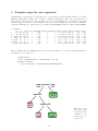
Examples using the color arguments
Arguments like col and lty are recycled and can be vectors, indexed on the row number in the tree’s frame.
Thus the call prp(tree, split.col = c("red", "blue")) would allocate red to the node in first row of
frame, blue to the second row, red to the third row, and so on. But that is not very useful, because splits
and leaves appear in “random” order in frame, as can be seen in the example below. Note the node numbers
along the left margin (we could plot those node numbers with nn=TRUE and their row indices with ni=TRUE):
> tree$frame
var
n
wt dev yval complexity ncompete nsurrogate yval2.1 yval2.2 yval2.3 yval2.4 yval2.5
1
sex 1309 1309 500
1
0.424
4
1
1.000 809.000 500.000
0.618
0.382
2
age 843 843 161
1
0.021
3
1
1.000 682.000 161.000
0.809
0.191
4 <leaf> 796 796 136
1
0.000
0
0
1.000 660.000 136.000
0.829
0.171
5
sibsp
47
47 22
2
0.021
3
2
2.000 22.000 25.000
0.468
0.532
10 <leaf>
20
20
1
1
0.020
0
0
1.000 19.000
1.000
0.950
0.050
11 <leaf>
27
27
3
2
0.020
0
0
2.000
3.000 24.000
0.111
0.889
3 <leaf> 466 466 127
2
0.015
0
0
2.000 127.000 339.000
0.273
0.727
Here’s something more useful (Figure 11). We use the fitted value at a node (the yval field in frame) to
determine the color of the node:
data(ptitanic)
tree <- rpart(survived~., data=ptitanic, cp=.02)
prp(tree, extra=6,
box.col=c("pink", "palegreen3")[tree$frame$yval])
sex=mal
yes
survived
0.73
age>=9.5
died
0.17
no
sibsp>=2.5
died
0.05
survived
0.89
14
Figure 11: Using
the fitted value
and the box.col
argument to determine the color
of the boxes.
Figure 12 is a similar example for a regression tree (based on code kindly supplied by Josh Browning):
heat.tree <- function(tree, low.is.green=FALSE, ...) { # dots args passed to prp
y <- tree$frame$yval
if(low.is.green)
y <- -y
max <- max(y)
min <- min(y)
cols <- rainbow(99, end=.36)[
ifelse(y > y[1], (y-y[1]) * (99-50) / (max-y[1]) + 50,
(y-min) * (50-1) / (y[1]-min) + 1)]
prp(tree, branch.col=cols, box.col=cols, ...)
}
data(ptitanic)
tree <- rpart(age ~ ., data=ptitanic)
heat.tree(tree, type=4, varlen=0, faclen=0, fallen.leaves=TRUE)
30
pclass = 2nd,3rd
1st
26
39
parch >= 0.5
parch >= 1.5
< 0.5
19
< 1.5
29
parch < 2.5
pclass = 3rd
>= 2.5
2nd
17
sibsp >= 1.5
< 1.5
20
survived = survived
died
17
sex = male
female
9.6
7.1
21
26
37
27
32
28
Figure 12: Using the fitted value to determine the color of regression nodes.
15
41
Figure 13: Using the color arguments
to indicate a nodes’s complexity.
Nodes with a complexity greater
than a certain value (0.021) are grayed
out in this example.
The following code creates a series of images — a movie — which shows how the tree is pruned on node
complexity. Figure 13 is one of the plots produced by this code.
complexities <- sort(unique(tree$frame$complexity)) # a vector of complexity values
for(complexity in complexities) {
cols <- ifelse(tree$frame$complexity >= complexity, 1, "gray")
dev.hold()
# hold screen output to prevent flashing
prp(tree, col=cols, branch.col=cols, split.col=cols)
dev.flush()
Sys.sleep(1) # pause for one second
}
16
1
2
3
sex = mal
sex = mal
sex = mal
age >= 9.5
die
pcl = 3rd
sib >= 2.5
sib >= 2.5
sur
die
die
sur
sib >= 2.5
die
sib >= 2.5
sur
die
6
pcl = 3rd
sib >= 2.5
die
sur
age >= 9.5
die
sur
pcl = 3rd
sib >= 2.5
die
sib >= 2.5
sur
die
sur
age >= 9.5
die
sur
sib >= 2.5
die
sur
die
8
9
sex = mal
sex = mal
sib >= 2.5
sur
die
sur
age >= 9.5
die
sur
pcl = 3rd
sib >= 2.5
die
sib >= 2.5
sur
die
10
11
sex = mal
sex = mal
pcl = 3rd
sib >= 2.5
sur
sib >= 2.5
die
sur
sur
age >= 9.5
die
sur
age >= 9.5
die
sib >= 2.5
die
sib >= 2.5
sur
die
sur
sur
sib >= 2.5
die
sur
sur
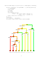
Figure 14: Depth first tree construction.
The following code shows a tree is constructed in depth-first fashion, node by node (Figure 14):
tree1 <- rpart(survived~., data=ptitanic)
par(mfrow=c(4,3))
for(iframe in 1:nrow(tree1$frame)) {
cols <- ifelse(1:nrow(tree1$frame) <= iframe, "black", "gray")
prp(tree1, col=cols, branch.col=cols, split.col=cols)
}
17
sur
pcl = 3rd
pcl = 3rd
sib >= 2.5
die
sur
sur
sib >= 2.5
7
pcl = 3rd
sur
pcl = 3rd
sex = mal
sib >= 2.5
die
die
die
sex = mal
age >= 9.5
die
sur
sur
5
sur
die
die
sib >= 2.5
pcl = 3rd
sex = mal
age >= 9.5
die
sur
sib >= 2.5
age >= 9.5
4
sib >= 2.5
die
die
pcl = 3rd
sex = mal
age >= 9.5
die
sur
age >= 9.5
sur
sur
1
sex = mal
2
3
age >= 9.5
survived
4
5
died
sibsp >= 2.5
10
11
died
survived
Figure 15: Node 11 and its
ancestors are highlighted.
The following code highlights a node and all its ancestors (Figure 15):
# return the given node and all its ancestors (a vector of node numbers)
path.to.root <- function(node)
{
if(node == 1)
# root?
node
else
# recurse, %/% 2 gives the parent of node
c(node, path.to.root(node %/% 2))
}
node <- 11
# 11 is our chosen node, arbitrary for this example
nodes <- as.numeric(row.names(tree$frame))
cols <- ifelse(nodes %in% path.to.root(node), "sienna", "gray")
prp(tree, nn=TRUE, col=cols, branch.col=cols, split.col=cols, nn.col=cols)
18
Here are some code fragments demonstrating additional techniques for manipulating rpart models. It is
worthwhile coming to grips with frame — look at print(tree$frame) and print.default(tree). Sometimes we with work with node numbers and sometimes it is necessary to work with row numbers in frame:
nodes <- as.numeric(row.names(tree$frame)) # node numbers in the order they appear in frame
node %/% 2
# parent of node
c(node * 2, node * 2 + 1)
# left and right child of node
inode <- match(node, nodes)
# row index of node in frame
is.leaf <- tree$frame$var == "<leaf>"
# logical vec, indexed on row in frame
nodes[is.leaf]
# the leaf node numbers
is.left <- nodes %% 2 == 0
# logical vec, indexed on row in frame
ifelse(is.left, nodes+1, nodes-1)
# siblings
get.children <- function(node)
if(is.leaf[match(node, nodes)]) {
node
} else
c(node,
get.children(2 * node),
get.children(2 * node + 1))
# node and all its children
# left child
# right child
19
7
Branch widths
It can be informative to have branch widths proportional to the number of observations. In the example on
the right side of Figure 16, the small number of observations at the bottom split is immediately obvious. We
can also estimate the relative number of males and females from the widths at the root split.
The right side of the figure was generated with:
prp(tree, branch.type=5, yesno=FALSE, faclen=0)
Note the branch.type argument. Other values of branch.type can be used to get widths proportional to
the node’s deviance, complexity, and so on. See the prp help page for details.
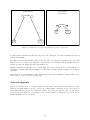
But be aware that the human eye is not good at estimating widths of branches at an angle. In Figure 17 the
left branch has the same width as the right branch, although one could be forgiven for thinking otherwise.
Width here should be measured horizontally, but the eye refuses to do that. The illusion is triggered by
the different slopes in this extreme example (whereas in a plotted tree the left and right branches at a split
usually have similar slopes and the illusion is irrelevant).
sex=male
sex=male
age>=9.5
died
61%
survived
36%
age>=9.5
sibsp>=2.5
died
2%
sibsp>=2.5
died
survived
2%
survived
died
survived
Figure 16: left The percentage of observations in a node.
right That information represented by the width of the branches.
Figure 17: Misleading branch widths. The two branches have the same width, measured horizontally.
20
8
Trimming a tree with the mouse
Set snip=TRUE to display a tree and interactively trim it with the mouse.
If you click on a split it will be marked as deleted. If you click on an already-deleted split it will be undeleted
(if its parent is not deleted). Information on the node is printed as you click.
When you have finished trimming, click on the QUIT button or right click, and prp will return the trimmed
tree (in the obj field). Example (Figure 18):
data(ptitanic)
tree <- rpart(survived~., data=ptitanic, cp=.012)
new.tree <- prp(tree, snip=TRUE)$obj # interactively trim the tree
prp(new.tree)
# display the new tree
You might like to prefix the above code with par(mfrow=c(1,2)) to display the original and trimmed trees
side by side.
Additionally, you can use the snip.fun argument to specify a function to be invoked after each mouse click.
The following example prints the trimmed tree’s performance after each click — using this technique you
can manually select a desired performance-complexity trade-off.
data(ptitanic)
tree <- rpart(survived ~ ., data=ptitanic)
my.snip.fun <- function(tree) { # tree is the trimmed tree
# should really use indep test data here
cat("fraction predicted correctly: ",
sum(predict(tree, type="class") == ptitanic$survived) /
length(ptitanic$survived),
"\n")
}
prp(tree, snip=TRUE, snip.fun=my.snip.fun)
Figure 18: Interactively trimming a
tree with snip=TRUE.
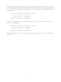
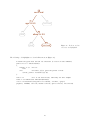
21
Figure 19: The same tree represented in three different ways. The middle and right graphs show the predicted
probability as a function of the predictors. The right graph is an aerial view of the middle graph.
9
Using plotmo in conjunction with prp
Another useful graphical technique is to plot the model’s response while changing the values of the predictors.
Figure 19 illustrates this on the kyphosis data:
tree <- rpart(Kyphosis~., data=kyphosis)
prp(tree, extra=7)
# left graph
library(plotmo)
plotmo(tree, type="prob", nresponse="present")
# middle graph
# type="prob" is passed to predict()
plotmo(tree, type="prob", nresponse="present", # right graph
type2="image", ngrid2=200,
# type2="image" for an image plot
col.response=ifelse(kyphosis$Kyphosis=="present", "red", "lightblue"))
The above code uses plotmo [3] to plot the regression surfaces. The figure actually shows just a subset of
the plots produced by the calls to plotmo, with some adjustments for printing.
Note how each “cliff” in the middle graph corresponds to a split in the tree. (The slight slope of the cliffs is
an artifact of the persp plot — the cliffs should be vertical.)
The type="prob" argument is passed internally in plotmo to predict.rpart, which returns a two column
response, and the nresponse="present" argument selects the second column. In other words, we are plotting
the predicted probability of kyphosis after surgery. We could instead plot the predicted class by using
type="class".
22
ozone level
yes
temp<68
ibh: temp
ibt: temp
no
12
ibh>=3574
ibt<226
7.4
20
5.1 dpg<−9.5
humidity<60
doy>=306
16
23
9.7
16
17
vis>=55
23
14
ibh
p
9
24
p
11
tem
11
ibt<159
tem
6.5
ibt
27
linear model
MARS
random forest
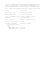
Figure 20: A tree built from the ozone data, and regression surfaces for the predictors at the upper splits.
Only two predictors were used in the kyphosis tree. More complex models with many predictors can be
viewed in a piecemeal fashion by looking at the action of one or two predictors at a time. For example,
Figure 20 shows a tree built from the ozone data:
# build a tree with the ozone1 data
prp(tree,
main="ozone level")
ozone level
yes
temp<68
plotmo(tree)
ibt
p
tem
p
tem
p
tem
library(earth)
data(ozone1)
tree <- rpart(O3~.,
data=ozone1)
ibt
ibt
# left graph
ibh: temp
no
ibt: temp
# middle and right graphs
12
ibh>=3574
ibt<226
The
model predicts the
ozone level, or air pollution, as a function of several variables: Also shown are
20 variables in the upper splits. (Once again, the figure actually shows just a subset
7.4
regression
surfaces for the
of the plots produced by the call to plotmo.)
5.1 dpg<−9.5
humidity<60
doy>=306
ibt
27
linear model
MARS
random forest
ibt
p
tem
p
tem
p
tem
ibt
p
23
14
ibh
tem
9
24
p
11
tem
9.7
23 by varying two variables while holding all others at their median values. Thus
The plotmo
graphs16are created
the graphs show only a thin slice of the data, but are nonetheless helpful. They are most informative when
6.5 ibt<159being
16dovis>=55
11 plotted
17
the variables
not have strong interactions with the other variables.
ibt
Figure 21: Surfaces for other models using the ozone data. Compare to the right graph of Figure 20.
23
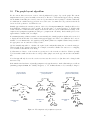
It is interesting to compare the rpart tree to other models (Figure 21). The linear model gives a flat surface. MARS [5] generates a surface by combining hinge functions (see http://en.wikipedia.org/wiki/
Multivariate_adaptive_regression_splines). The random forest [2] smooths out the surface by averaging lots of trees.
There are a large number of possible variable pairs (from the 9 predictors in the ozone data we can form
9 × 8/2 = 36 pairs). The options to plotmo in the code below select just the pair in the graphs. See the
plotmo help page for details. The code is:
a <- lm(O3~., data=ozone1)
plotmo(a, degree1=0, all2=TRUE, degree2=24)
# left graph, linear model
library(earth) # earth is an implementation of MARS (MARS is a trademarked term)
a <- earth(O3~., data=ozone1, degree=2)
plotmo(a, degree1=0, all2=TRUE, degree2=16)
# middle graph, MARS
library(randomForest)
a <- randomForest(O3~., data=ozone1)
plotmo(a, degree1=0, all2=TRUE, degree2=24)
24
# right graph, random forest
10
The graph layout algorithm
For the curious, this section is an overview of the algorithm used by prp to lay out the graph. The current
implementation is not perfect but suffices for most trees. The more-or-less standard approach for positioning
labels, simulated annealing, is not used because an objective function cannot (easily) be calculated efficiently.
A central issue is a chicken-and-egg problem: we need the cex to determine the best positions for the labels
but we need the positions to determine the cex.
Initially, prp calculates the tentative positions of the nodes. If compress=TRUE (the default), it slides nodes
horizontally into available space where possible. It uses the same code as plot.rpart to do all this, with
a little extension for fallen.leaves. Figure 22 shows the same tree plotted with different settings of the
compress and ycompress arguments (we will get to ycompress in a moment). In the middle plot see how
age>=16 has been shifted left, for example.
If cex=NULL (meaning calculate a suitable cex automatically, the default), prp then calculates the cex needed
to display the labels and their boxes with at least gap and ygap between the boxes. (Whether the boxes are
invisible or not is immaterial to the graph layout algorithm.) This is accomplished with a binary search for
the appropriate cex. A search is necessary because:
(a) It is virtually impossible to calculate the required scale analytically taking into account the many parameters such as adj, yshift, and space. For example, sometimes a smaller cex causes more overlapping
as boxes shift around with the scale change.
(b) Font sizes are discrete, so the font size we get may not be the font size we asked for. This is especially
a problem with a small cex where there is a large relative jump between the type size and the next smaller
size.
Note that prp will only decrease the cex; it never increases the cex above 1 (but that can be changed with
max.auto.cex).
If the initial cex is less than 0.7 (actually ycompress.cex), prp then tries to make additional space as follows
(assuming ycompress=TRUE, the default). If type=0, 1, or 2, it shifts alternate nodes vertically, looking for
compress=FALSE
ycompress=FALSE
compress=TRUE (default)
ycompress=FALSE
compress=TRUE (default)
ycompress=TRUE (default)
yes
yes
sex=mal
sex=mal
no
no
pclass=3rd
age>=9.5
yes
sex=mal
pclass=3rd
age>=9.5
no
sibsp>=2.5
age>=9.5
died
died
pclass=3rd
sibsp>=2.5
sibsp>=2.5
sibsp>=2.5
survived
survived
survived
died
parch>=3.5
died
parch>=3.5
died
died
survived
survived
survived
parch>=3.5
age>=28
died
age>=16
survived
age>=16
age>=16
died
survived
sibsp>=2.5
died
survived
died
died
sibsp>=2.5
age<22
died
age>=28
age>=28
died
died
calculated cex:
0.44
survived
calculated cex:
0.69
died
age<22
died
calculated cex:
0.82
age<22
died
survived
survived
died
Figure 22: The compress and ycompress arguments
25
xcompact=FALSE
ycompact=FALSE
yes
sex=male
default:
xcompact=TRUE
ycompact=TRUE
no
yes
died
0.19
died
0.19
sex=male
no
survived
0.73
survived
0.73
Figure 23: Small trees are compacted by default, as shown on the right.
the shift in shift.amounts that allows the biggest type size. If type=3 or 4 it tries alternating the leaves if
fallen.leaves=TRUE.
The shift is retained only if makes possible a type size gain of at least 10% (actually accept.cex). The
shifted tree is not as “tidy” as the original tree, but the larger text is usually worth the untidiness (but not
always). Compare the middle and right plots in Figure 22.
Finally, for small trees where there is too much white space, prp compacts the tree horizontally and/or
vertically by changing xlim and ylim (Figure 23). This can be disabled with the xcompact and ycompact
arguments.
Arguably the most serious limitation of the current implementation is its inability to display results on test
data (on the tree derived from the training data).
Acknowledgments
I have leaned heavily on the code in plot.rpart and text.rpart. Those functions were written by Terry
Therneau and Beth Atkinson, and were ported to R by Brian Ripley. The functions were descended from
Linda Clark and Daryl Pregibon’s S-Plus tree package. But please note that the prp code was written
independently and I must take responsibility for the excessive number of arguments, etc. I’d also like to
thank Beth Atkinson for her feedback.
26
A
Appendix: mvpart mrt models
Note: In December 2014 the mvpart package was removed from CRAN.
The extra argument of prp has a special meaning for mvpart mrt models [1], as shown in the figure below.
(Internally, mvpart sets the method field of the tree to "mrt", and prp recognizes that.) As always you can
print percentages by adding 100 to extra. The type and other arguments work in the usual way.
Example:
library(rpart.plot)
library(mvpart)
data(spider)
set.seed(10)
response <- data.matrix(spider[,1:3, drop=F])
tree <- mvpart(response~herbs+reft+moss+sand+twigs+water, data=spider,
method="mrt", xv="min")
prp(tree, type=1, extra=111, under=TRUE)
extra = 0
dev
extra = 1
dev, n
water < 5.5
165
twigs >= 8
8.3
103
extra = 2
dev, frac
water < 5.5
165
water < 5.5
165
water < 5.5
165
n=28
.36 1.18 1.54
.12 .38 .50
8.3
twigs >= 8
8.3
twigs >= 8
8.3
n=12
103
.00 .17 .33
103
.00 .33 .67
n=16
26
19
extra = 4
sqrt(dev)
13
twigs >= 8
26
19
n=8
n=8
26
19
.00 .75 .25
.21 .15 .65
extra = 6
sqrt(dev), frac
twigs >= 8
zora.spin
water < 5.5
13
n=28
.36 1.18 1.54
.12 .38 .50
2.9
twigs >= 8
2.9
twigs >= 8
2.9
n=12
10
.00 .17 .33
10
.00 .33 .67
twigs >= 8
10
.12 .39 .49
.62 1.94 2.44
5.1
4.4
n=8
n=8
extra = 9
predom species, n
5.1
4.4
5.1
4.4
.00 3.00 1.00
1.25 .88 3.88
.00 .75 .25
.21 .15 .65
extra = 10
predom species, frac
extra = 11
predom spec, frac / sum(frac)
water < 5.5
zora.spin
water < 5.5
zora.spin
water < 5.5
zora.spin
n=28
.36 1.18 1.54
.12 .38 .50
zora.spin
twigs >= 8
zora.spin
n=12
n=16
zora.spin
extra = 7
sqrt(dev), frac / sum(frac)
13
4.4
pard.lugu
19
1.25 .88 3.88
water < 5.5
water < 5.5
zora.spin
zora.spin
26
.00 3.00 1.00
n=16
extra = 8
predom species
103
.12 .39 .49
water < 5.5
13
10
5.1
twigs >= 8
.62 1.94 2.44
extra = 5
sqrt(dev), n
water < 5.5
2.9
extra = 3
dev, frac / sum(frac)
zora.spin
twigs >= 8
zora.spin
.00 .17 .33
zora.spin
.00 .33 .67
.62 1.94 2.44
pard.lugu
zora.spin
n=8
n=8
.12 .39 .49
pard.lugu
zora.spin
pard.lugu
.00 3.00 1.00
1.25 .88 3.88
.00 .75 .25
Figure 24: The extra argument with an mrt model.
27
twigs >= 8
zora.spin
zora.spin
.21 .15 .65
References
[1] Glenn De’ath. mvpart: Multivariate partitioning, 2014. R package. Cited on page 27.
[2] Andy Liaw, Mathew Weiner; Fortran original by Leo Breiman, and Adele Cutler. randomForest: Breiman
and Cutler’s random forests for regression and classification, 2014. R package. Cited on page 24.
[3] Stephen Milborrow. plotmo: Plot a Model’s Response while Varying the Values of the Predictors, 2011.
R package. Cited on page 22.
[4] Stephen Milborrow. rpart.plot: Plot rpart Models. An Enhanced Version of plot.rpart, 2011. R package.
Cited on page 5.
[5] Stephen Milborrow. Derived from mda:mars by Trevor Hastie and Rob Tibshirani. earth: Multivariate
Adaptive Regression Splines, 2009. R package. Cited on page 24.
[6] R Core Team. R: A Language and Environment for Statistical Computing. R Foundation for Statistical
Computing, 2014. Cited on page 2.
[7] Terry Therneau and Beth Atkinson. rpart: Recursive Partitioning and Regression Trees, 2014. R package.
Cited on page 2.
28