Download M86-E01007 GADDS User manual.book

BRUKER ADVANCED X-RAY SOLUTIONS
a
e
r
A
l
a
Gener
r
o
t
c
e
t
e
D
n
o
i
t
c
a
r
f
f
Di
)
S
D
D
A
G
(
m
e
t
s
Sy
.xx
1
.
4
n
o
i
s
Ver
USER MANUAL
M86-E01007
1/05
BRUKER ADVANCED X-RAY SOLUTIONS
General Area Detector
Diffraction System (GADDS)
User Manual
Version 4.1.xx
M86-E01007
1/05
This manual covers the GADDS software package. To order additional copies of this publication, request the part
number shown at the bottom of the page.
© 2005, 1999 Bruker AXS Inc. All world rights reserved. Printed in the U.S.A.
Notice
The information in this publication is provided for reference only. All information contained in this publication is
believed to be correct and complete. Bruker AXS Inc. shall not be liable for errors contained herein, nor for incidental or consequential damages in conjunction with the furnishing, performance, or use of this material. All product
specifications, as well as the information contained in this publication, are subject to change without notice.
This publication may contain or reference information and products protected by copyrights or patents and does
not convey any license under the patent rights of Bruker AXS Inc. nor the rights of others. Bruker AXS Inc. does not
assume any liabilities arising out of any infringements of patents or other rights of third parties. Bruker AXS Inc.
makes no warranty of any kind with regard to this material, including but not limited to the implied warranties of
merchantability and fitness for a particular purpose.
No part of this publication may be stored in a retrieval system, transmitted, or reproduced in any way, including but
not limited to photocopy, photography, magnetic, or other record without prior written permission of Bruker AXS
Inc.
Address comments to:
Technical Publications Department
Bruker AXS Inc.
5465 East Cheryl Parkway
Madison, Wisconsin 53711-5373
USA
All trademarks and registered trademarks are the sole property of their respective owners.
ii
Revision
Date
Changes
0
10/99
Original release.
1
1/05
Added Sections 11 and 12. Revised Sections 1, 2, 3, 5, 6, 7 and 10.
M86-E01007 1/05
GADDS User Manual
Table of Contents
Table of Contents
Notice . . . . . . . . . . . . . . . . . . . . . . . . . . . . . . . . . . . . . . . . . . . . . . . . . . . . . . . . . . . . . . . . . . . . . . . . ii
1. Introduction and Overview . . . . . . . . . . . . . . . . . . . . . . . . . . . . . . . . . . . . . . . . 1-1
1.1 Introduction . . . . . . . . . . . . . . . . . . . . . . . . . . . . . . . . . . . . . . . . . . . . . . . . . . . . . . . . . . . . . . . 1-1
1.2 Theory of X-ray Diffraction Using Area Detectors . . . . . . . . . . . . . . . . . . . . . . . . . . . . . . . . . . 1-4
1.2.1 X-ray Powder Diffraction . . . . . . . . . . . . . . . . . . . . . . . . . . . . . . . . . . . . . . . . . . . . . . . . . 1-4
1.2.2 Two-Dimensional X-ray Powder Diffraction (XRD2) . . . . . . . . . . . . . . . . . . . . . . . . . . . . 1-5
1.3 Geometry Conventions . . . . . . . . . . . . . . . . . . . . . . . . . . . . . . . . . . . . . . . . . . . . . . . . . . . . . . 1-8
1.3.1 Diffraction Cones and Conic Sections on 2D Detectors . . . . . . . . . . . . . . . . . . . . . . . . . 1-8
1.3.2 Diffraction Cones and Laboratory Axes . . . . . . . . . . . . . . . . . . . . . . . . . . . . . . . . . . . . . 1-9
1.3.3 Sample Orientation and Position in the Laboratory System . . . . . . . . . . . . . . . . . . . . . 1-10
1.3.4 Detector Position in the Laboratory System . . . . . . . . . . . . . . . . . . . . . . . . . . . . . . . . . 1-11
1.4 Diffraction Data Measured by an Area Detector . . . . . . . . . . . . . . . . . . . . . . . . . . . . . . . . . . 1-13
1.5 References . . . . . . . . . . . . . . . . . . . . . . . . . . . . . . . . . . . . . . . . . . . . . . . . . . . . . . . . . . . . . . 1-15
2. System Configuration . . . . . . . . . . . . . . . . . . . . . . . . . . . . . . . . . . . . . . . . . . . . 2-1
2.1 X-ray Generator . . . . . . . . . . . . . . . . . . . . . . . . . . . . . . . . . . . . . . . . . . . . . . . . . . . . . . . . . . . 2-3
2.1.1 Radiation Energy . . . . . . . . . . . . . . . . . . . . . . . . . . . . . . . . . . . . . . . . . . . . . . . . . . . . . . 2-3
2.1.2 X-ray Spectrum and Characteristic Lines . . . . . . . . . . . . . . . . . . . . . . . . . . . . . . . . . . . . 2-3
2.1.3 Focal Spot and Takeoff Angle . . . . . . . . . . . . . . . . . . . . . . . . . . . . . . . . . . . . . . . . . . . . . 2-4
2.1.4 Focal Spot Brightness and Profile . . . . . . . . . . . . . . . . . . . . . . . . . . . . . . . . . . . . . . . . . 2-5
2.1.5 Operation of the X-ray Generator . . . . . . . . . . . . . . . . . . . . . . . . . . . . . . . . . . . . . . . . . . 2-6
2.2 X-ray Optics . . . . . . . . . . . . . . . . . . . . . . . . . . . . . . . . . . . . . . . . . . . . . . . . . . . . . . . . . . . . . . 2-8
2.2.1 Monochromator . . . . . . . . . . . . . . . . . . . . . . . . . . . . . . . . . . . . . . . . . . . . . . . . . . . . . . . . 2-9
2.2.2 Pinhole Collimator . . . . . . . . . . . . . . . . . . . . . . . . . . . . . . . . . . . . . . . . . . . . . . . . . . . . . 2-10
2.2.3 Sample-to-Detector Distance and Angular Resolution . . . . . . . . . . . . . . . . . . . . . . . . . 2-13
2.2.4 Single and Cross-Coupled Göbel Mirrors . . . . . . . . . . . . . . . . . . . . . . . . . . . . . . . . . . . 2-22
M86-E01007 1/05
i
Table of Contents
GADDS User Manual
2.2.5 Monocapillary . . . . . . . . . . . . . . . . . . . . . . . . . . . . . . . . . . . . . . . . . . . . . . . . . . . . . . . .
2.3 Goniometer and Stages . . . . . . . . . . . . . . . . . . . . . . . . . . . . . . . . . . . . . . . . . . . . . . . . . . . .
2.4 Sample Alignment and Monitor Systems . . . . . . . . . . . . . . . . . . . . . . . . . . . . . . . . . . . . . . .
2.5 HI-STAR Area Detector . . . . . . . . . . . . . . . . . . . . . . . . . . . . . . . . . . . . . . . . . . . . . . . . . . . . .
2.6 Small Angle X-ray Scattering (SAXS) Attachment . . . . . . . . . . . . . . . . . . . . . . . . . . . . . . . .
2.7 Standard GADDS Systems . . . . . . . . . . . . . . . . . . . . . . . . . . . . . . . . . . . . . . . . . . . . . . . . . .
2.8 Standard GADDS Systems for Combinatorial Screening . . . . . . . . . . . . . . . . . . . . . . . . . . .
2.8.1 Reflection Mode Screening . . . . . . . . . . . . . . . . . . . . . . . . . . . . . . . . . . . . . . . . . . . . . .
2.8.2 Transmission Mode Screening . . . . . . . . . . . . . . . . . . . . . . . . . . . . . . . . . . . . . . . . . . .
2.8.3 Sample Stage and Screening Grid . . . . . . . . . . . . . . . . . . . . . . . . . . . . . . . . . . . . . . . .
2.8.4 Retractable Knife Edge . . . . . . . . . . . . . . . . . . . . . . . . . . . . . . . . . . . . . . . . . . . . . . . . .
2.8.5 Diffraction Mapping and Results Display . . . . . . . . . . . . . . . . . . . . . . . . . . . . . . . . . . .
2-25
2-27
2-31
2-34
2-36
2-37
2-45
2-46
2-48
2-52
2-54
2-59
3. Basic System Operation . . . . . . . . . . . . . . . . . . . . . . . . . . . . . . . . . . . . . . . . . . 3-1
3.1 Starting the System . . . . . . . . . . . . . . . . . . . . . . . . . . . . . . . . . . . . . . . . . . . . . . . . . . . . . . . . 3-2
3.2 Selecting Optics . . . . . . . . . . . . . . . . . . . . . . . . . . . . . . . . . . . . . . . . . . . . . . . . . . . . . . . . . . . 3-3
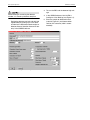
3.3 Choosing the Detector Position . . . . . . . . . . . . . . . . . . . . . . . . . . . . . . . . . . . . . . . . . . . . . . . . 3-3
3.4 Detector Aberration Analysis . . . . . . . . . . . . . . . . . . . . . . . . . . . . . . . . . . . . . . . . . . . . . . . . . 3-5
3.4.1 Flood-Field Correction . . . . . . . . . . . . . . . . . . . . . . . . . . . . . . . . . . . . . . . . . . . . . . . . . . 3-8
3.4.2 Spatial Correction . . . . . . . . . . . . . . . . . . . . . . . . . . . . . . . . . . . . . . . . . . . . . . . . . . . . . 3-10
3.5 System Calibration . . . . . . . . . . . . . . . . . . . . . . . . . . . . . . . . . . . . . . . . . . . . . . . . . . . . . . . . 3-14
3.6 Sample Positioning . . . . . . . . . . . . . . . . . . . . . . . . . . . . . . . . . . . . . . . . . . . . . . . . . . . . . . . . 3-18
3.6.1 XYZ Stage Sample Positioning . . . . . . . . . . . . . . . . . . . . . . . . . . . . . . . . . . . . . . . . . . . 3-18
3.6.2 Goniometer Head Sample Positioning . . . . . . . . . . . . . . . . . . . . . . . . . . . . . . . . . . . . . 3-19
3.6.3 Collision Limits for Your Sample . . . . . . . . . . . . . . . . . . . . . . . . . . . . . . . . . . . . . . . . . . 3-22
3.7 Data Collection . . . . . . . . . . . . . . . . . . . . . . . . . . . . . . . . . . . . . . . . . . . . . . . . . . . . . . . . . . . 3-23
3.7.1 Scan Method . . . . . . . . . . . . . . . . . . . . . . . . . . . . . . . . . . . . . . . . . . . . . . . . . . . . . . . . . 3-23
3.7.2 Add or Rotation Method . . . . . . . . . . . . . . . . . . . . . . . . . . . . . . . . . . . . . . . . . . . . . . . . 3-24
3.8 Basic Data Analysis and Preparation . . . . . . . . . . . . . . . . . . . . . . . . . . . . . . . . . . . . . . . . . . 3-25
4. Phase ID . . . . . . . . . . . . . . . . . . . . . . . . . . . . . . . . . . . . . . . . . . . . . . . . . . . . . . . 4-1
4.1 Overview . . . . . . . . . . . . . . . . . . . . . . . . . . . . . . . . . . . . . . . . . . . . . . . . . . . . . . . . . . . . . . . . . 4-1
4.2 Performing a phase ID analysis . . . . . . . . . . . . . . . . . . . . . . . . . . . . . . . . . . . . . . . . . . . . . . . 4-6
ii
M86-E01007 1/05
GADDS User Manual
Table of Contents
5. Texture . . . . . . . . . . . . . . . . . . . . . . . . . . . . . . . . . . . . . . . . . . . . . . . . . . . . . . . . 5-1
5.1 Overview . . . . . . . . . . . . . . . . . . . . . . . . . . . . . . . . . . . . . . . . . . . . . . . . . . . . . . . . . . . . . . . . . 5-1
5.2 General Data Collection Considerations for Texture Analysis . . . . . . . . . . . . . . . . . . . . . . . . 5-7
5.3 Preparation for the Texture Experiment . . . . . . . . . . . . . . . . . . . . . . . . . . . . . . . . . . . . . . . . . 5-9
5.4 Data Collection Considerations for ODF Analysis . . . . . . . . . . . . . . . . . . . . . . . . . . . . . . . . 5-10
5.5 Other Texture Representations . . . . . . . . . . . . . . . . . . . . . . . . . . . . . . . . . . . . . . . . . . . . . . 5-11
5.6 Using POLE_FIGURE/SCHEME to Plan Strategy and Coverage . . . . . . . . . . . . . . . . . . . . 5-11
5.7 Using POLE_FIGURE/PROCESS . . . . . . . . . . . . . . . . . . . . . . . . . . . . . . . . . . . . . . . . . . . . 5-13
5.8 Polymer Orientation . . . . . . . . . . . . . . . . . . . . . . . . . . . . . . . . . . . . . . . . . . . . . . . . . . . . . . . 5-17
5.9 Fiber Orientation . . . . . . . . . . . . . . . . . . . . . . . . . . . . . . . . . . . . . . . . . . . . . . . . . . . . . . . . . . 5-18
5.10 Sheet Orientation . . . . . . . . . . . . . . . . . . . . . . . . . . . . . . . . . . . . . . . . . . . . . . . . . . . . . . . . 5-20
5.11 Near Single Crystal Thin Film Orientation . . . . . . . . . . . . . . . . . . . . . . . . . . . . . . . . . . . . . . 5-21
5.12 Semiquantitative Analysis with CURSOR Commands . . . . . . . . . . . . . . . . . . . . . . . . . . . . 5-22
5.13 Preparation for ODF Analysis with popLA and ODF AT . . . . . . . . . . . . . . . . . . . . . . . . . . . 5-23
5.14 Hermans and White-Spruiell Orientation Indices . . . . . . . . . . . . . . . . . . . . . . . . . . . . . . . . 5-23
5.15 Fiber Texture Plots . . . . . . . . . . . . . . . . . . . . . . . . . . . . . . . . . . . . . . . . . . . . . . . . . . . . . . . 5-25
5.16 References . . . . . . . . . . . . . . . . . . . . . . . . . . . . . . . . . . . . . . . . . . . . . . . . . . . . . . . . . . . . . 5-29
6. Residual Stress . . . . . . . . . . . . . . . . . . . . . . . . . . . . . . . . . . . . . . . . . . . . . . . . . 6-1
6.1 Principle of Stress Measurement . . . . . . . . . . . . . . . . . . . . . . . . . . . . . . . . . . . . . . . . . . . . . . 6-1
6.1.1 Theory of Conventional Method . . . . . . . . . . . . . . . . . . . . . . . . . . . . . . . . . . . . . . . . . . . 6-1
6.1.2 Theory and Algorithm of 2D Method . . . . . . . . . . . . . . . . . . . . . . . . . . . . . . . . . . . . . . . . 6-3
6.1.3 Relationship Between Conventional Theory and 2D Theory . . . . . . . . . . . . . . . . . . . . . 6-7
6.1.4 Advantages of Using 2D Detectors . . . . . . . . . . . . . . . . . . . . . . . . . . . . . . . . . . . . . . . . . 6-9
6.1.5 Parameters . . . . . . . . . . . . . . . . . . . . . . . . . . . . . . . . . . . . . . . . . . . . . . . . . . . . . . . . . . 6-12
6.1.6 GADDS System Requirements . . . . . . . . . . . . . . . . . . . . . . . . . . . . . . . . . . . . . . . . . . . 6-15
6.1.7 Data Collection Strategy . . . . . . . . . . . . . . . . . . . . . . . . . . . . . . . . . . . . . . . . . . . . . . . . 6-16
6.1.8 Data Collection Procedures . . . . . . . . . . . . . . . . . . . . . . . . . . . . . . . . . . . . . . . . . . . . . 6-18
6.2 Stress Evaluation Using One-Dimensional Data (Conventional Method) . . . . . . . . . . . . . . . 6-19
6.3 Stress Evaluation Using Two-Dimensional Data (2D Method) . . . . . . . . . . . . . . . . . . . . . . . 6-22
6.4 Application Examples . . . . . . . . . . . . . . . . . . . . . . . . . . . . . . . . . . . . . . . . . . . . . . . . . . . . . . 6-28
6.4.1 Example 1. (Conventional Method) Residual Stress Measurement with GADDS
Microdiffraction System . . . . . . . . . . . . . . . . . . . . . . . . . . . . . . . . . . . . . . . . . . . . . . . . 6-28
M86-E01007 1/05
iii
Table of Contents
GADDS User Manual
6.4.2 Example 2. (2D Method) Comparison Between 2D Method and Conventional Method 6-31
6.4.3 Example 3. Stress Mapping with 2D Method . . . . . . . . . . . . . . . . . . . . . . . . . . . . . . . . 6-34
6.5 References . . . . . . . . . . . . . . . . . . . . . . . . . . . . . . . . . . . . . . . . . . . . . . . . . . . . . . . . . . . . . . 6-36
7. Crystal Size . . . . . . . . . . . . . . . . . . . . . . . . . . . . . . . . . . . . . . . . . . . . . . . . . . . . 7-1
7.1 Line Broadening Principles for Crystallite Size . . . . . . . . . . . . . . . . . . . . . . . . . . . . . . . . . . . .
7.2 Instrumental Broadening . . . . . . . . . . . . . . . . . . . . . . . . . . . . . . . . . . . . . . . . . . . . . . . . . . . . .
7.3 Microstrain Broadening . . . . . . . . . . . . . . . . . . . . . . . . . . . . . . . . . . . . . . . . . . . . . . . . . . . . . .
7.4 Data Collection for the Warren-Averbach and Scherrer Methods . . . . . . . . . . . . . . . . . . . . . .
7.5 References . . . . . . . . . . . . . . . . . . . . . . . . . . . . . . . . . . . . . . . . . . . . . . . . . . . . . . . . . . . . . . .
7-1
7-2
7-6
7-7
7-8
8. Percent Crystallinity . . . . . . . . . . . . . . . . . . . . . . . . . . . . . . . . . . . . . . . . . . . . . 8-1
8.1 Principle of Percent Crystallinity . . . . . . . . . . . . . . . . . . . . . . . . . . . . . . . . . . . . . . . . . . . . . . . 8-1
8.2 Data Evaluation for Two-Dimensional Data . . . . . . . . . . . . . . . . . . . . . . . . . . . . . . . . . . . . . . . 8-4
8.2.1 Methods Supporting Percent Crystallinity . . . . . . . . . . . . . . . . . . . . . . . . . . . . . . . . . . . . 8-4
8.2.2 Application Examples . . . . . . . . . . . . . . . . . . . . . . . . . . . . . . . . . . . . . . . . . . . . . . . . . . 8-10
8.3 References . . . . . . . . . . . . . . . . . . . . . . . . . . . . . . . . . . . . . . . . . . . . . . . . . . . . . . . . . . . . . . 8-16
9. Small-Angle X-ray Scattering . . . . . . . . . . . . . . . . . . . . . . . . . . . . . . . . . . . . . . 9-1
9.1 Principle of Small Angle Scattering . . . . . . . . . . . . . . . . . . . . . . . . . . . . . . . . . . . . . . . . . . . . . 9-1
9.1.1 General Equation and Parameters in SAXS . . . . . . . . . . . . . . . . . . . . . . . . . . . . . . . . . . 9-2
9.1.2 X-ray Beam Collimation . . . . . . . . . . . . . . . . . . . . . . . . . . . . . . . . . . . . . . . . . . . . . . . . . 9-3
9.2 Data Collection and Analysis . . . . . . . . . . . . . . . . . . . . . . . . . . . . . . . . . . . . . . . . . . . . . . . . . 9-5
9.2.1 SAXS Attachments Installation . . . . . . . . . . . . . . . . . . . . . . . . . . . . . . . . . . . . . . . . . . . . 9-5
9.2.2 SAXS System Adjustment and Calibration . . . . . . . . . . . . . . . . . . . . . . . . . . . . . . . . . . . 9-7
9.2.3 Data Collection . . . . . . . . . . . . . . . . . . . . . . . . . . . . . . . . . . . . . . . . . . . . . . . . . . . . . . . 9-11
9.3.14 Applications Examples . . . . . . . . . . . . . . . . . . . . . . . . . . . . . . . . . . . . . . . . . . . . . . . . . . . 9-15
9.3.14 References . . . . . . . . . . . . . . . . . . . . . . . . . . . . . . . . . . . . . . . . . . . . . . . . . . . . . . . . . . . . 9-16
10. Script Files . . . . . . . . . . . . . . . . . . . . . . . . . . . . . . . . . . . . . . . . . . . . . . . . . . . 10-1
10.1 SLAM Command Conventions . . . . . . . . . . . . . . . . . . . . . . . . . . . . . . . . . . . . . . . . . . . . . . 10-2
10.2 Executing Script Files . . . . . . . . . . . . . . . . . . . . . . . . . . . . . . . . . . . . . . . . . . . . . . . . . . . . . 10-5
iv
M86-E01007 1/05
GADDS User Manual
Table of Contents
10.3 Creating Script Files . . . . . . . . . . . . . . . . . . . . . . . . . . . . . . . . . . . . . . . . . . . . . . . . . . . . . . 10-7
10.4 Using Replaceable Parameters within Script Files . . . . . . . . . . . . . . . . . . . . . . . . . . . . . . 10-16
10.5 Adding Script Files to the Menu Bar as User Tasks . . . . . . . . . . . . . . . . . . . . . . . . . . . . . 10-21
10.6 Nesting Script Files . . . . . . . . . . . . . . . . . . . . . . . . . . . . . . . . . . . . . . . . . . . . . . . . . . . . . . 10-23
10.7 Flow Control Inside Script Files . . . . . . . . . . . . . . . . . . . . . . . . . . . . . . . . . . . . . . . . . . . . 10-25
11. Automation . . . . . . . . . . . . . . . . . . . . . . . . . . . . . . . . . . . . . . . . . . . . . . . . . . 11-1
11.1 Primitive Automation . . . . . . . . . . . . . . . . . . . . . . . . . . . . . . . . . . . . . . . . . . . . . . . . . . . . . .
11.2 Optimize Automation . . . . . . . . . . . . . . . . . . . . . . . . . . . . . . . . . . . . . . . . . . . . . . . . . . . . .
11.3 Sample Handling . . . . . . . . . . . . . . . . . . . . . . . . . . . . . . . . . . . . . . . . . . . . . . . . . . . . . . . .
11.4 Remote Control . . . . . . . . . . . . . . . . . . . . . . . . . . . . . . . . . . . . . . . . . . . . . . . . . . . . . . . . . .
11.5 Audit Trails . . . . . . . . . . . . . . . . . . . . . . . . . . . . . . . . . . . . . . . . . . . . . . . . . . . . . . . . . . . . .
11-2
11-4
11-6
11-7
11-8
12. Mapping . . . . . . . . . . . . . . . . . . . . . . . . . . . . . . . . . . . . . . . . . . . . . . . . . . . . . 12-1
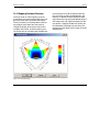
12.1 Procedure—Demo Data . . . . . . . . . . . . . . . . . . . . . . . . . . . . . . . . . . . . . . . . . . . . . . . . . . .
12.2 Procedure—Real Data . . . . . . . . . . . . . . . . . . . . . . . . . . . . . . . . . . . . . . . . . . . . . . . . . . . .
12.2.1 Frames to Process . . . . . . . . . . . . . . . . . . . . . . . . . . . . . . . . . . . . . . . . . . . . . . . . . . .
12.2.2 Processing Parameters . . . . . . . . . . . . . . . . . . . . . . . . . . . . . . . . . . . . . . . . . . . . . . .
12.3 Mapping Software Features . . . . . . . . . . . . . . . . . . . . . . . . . . . . . . . . . . . . . . . . . . . . . . . .
12-2
12-4
12-4
12-4
12-7
13. Nomenclature and Glossary . . . . . . . . . . . . . . . . . . . . . . . . . . . . . . . . . . . . 13-1
13.1 Nomenclature . . . . . . . . . . . . . . . . . . . . . . . . . . . . . . . . . . . . . . . . . . . . . . . . . . . . . . . . . . . 13-1
13.2 Glossary . . . . . . . . . . . . . . . . . . . . . . . . . . . . . . . . . . . . . . . . . . . . . . . . . . . . . . . . . . . . . . . 13-5
13.3 Glossary of Software Terms . . . . . . . . . . . . . . . . . . . . . . . . . . . . . . . . . . . . . . . . . . . . . . . 13-12
M86-E01007 1/05
v
Table of Contents
vi
GADDS User Manual
M86-E01007 1/05
GADDS User Manual
Introduction and Overview
1. Introduction and Overview
1.1 Introduction
GADDS (General Area Detector Diffraction System), introduced by Bruker AXS Inc., is the most
advanced X-ray diffraction system in the world.
The core of GADDS is the high-performance
two-dimensional (2D) detector—the Bruker AXS
HI-STAR area detector. The HI-STAR is the
most sensitive area detector, a true photon
counter with a large area. The speed of data collection with an area detector can be 104 times
faster than with a point detector and about 100
times faster than with a linear position-sensitive
detector. Most importantly, the data has a large
dynamic range and 2D diffraction information.
Compared to 1D diffraction profiles measured
with a conventional diffraction system, a 2D
image collected with GADDS contains far more
information for various applications. By introduction of the innovative two-dimensional X-ray diffraction (XRD2) theory, GADDS has opened a
new dimension in X-ray powder diffraction.
M86-E01007
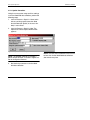
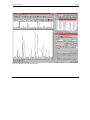
Phase identification (Phase ID) can be done by
integration over a selected range of two-theta
(2θ) and chi (χ). A direct link to the ICDD database, profile fitting with conventional peak
shapes and fundamental parameters, quantification of phases, and lattice parameter indexing
and refinement make powder diffraction analysis easy and fast. Due to the integration along
the Debye rings, the integrated data gives better
intensity and statistics for phase ID and quantitative analysis, especially for those samples
with texture, large grain size, or small quantity.
Texture measurement using an area detector is
extremely fast compared to the measurement
using a scintillation counter or a linear positionsensitive detector (PSD). The area detector collects texture data and background values simultaneously for multiple poles and multiple
directions. Due to the high measurement speed,
GADDS can measure pole figures at very fine
steps, allowing detection of very sharp textures.
1-1
Introduction and Overview
GADDS is the best tool for quantitative texture
analysis.
Stress measurement using the two-dimensional
area detector is based on a new 2D stress algorithm developed by Bruker AXS, which gives a
direct relationship between the stress tensor
and the diffraction cone distortion. Since the
whole or a part of the Debye ring is used for
stress calculation, GADDS can measure stress
with high sensitivity, high speed, and high accuracy. It is very suitable for samples with large
crystals and textures. Simultaneous measurement of stress and texture is also possible since
2D data consists of both stress and texture
information.
Percent crystallinity can be measured faster and
more accurately with the data analysis over the
2D frames, especially for samples with anisotropic distribution of crystalline orientation. The
amorphous region can be defined externally
within a user-defined region or the amorphous
region can be defined with the crystalline region
included when the crystalline region and the
amorphous region overlap. GADDS can also
calculate and display the Compton scattering so
the Compton effect can be excluded from the
amorphous result. The “rolling ball algorithm”
calculates the percent crystallinity by extracting
an amorphous background frame.
Small angle X-ray scattering (SAXS) data can
be collected at high speed. Anisotropic features
from specimens, such as polymers, fibrous
1-2
GADDS User Manual
materials, single crystals, and bio-materials, can
be analyzed and displayed in two dimensions.
De-smearing correction is not necessary due to
the collimated point X-ray beam. Since one
exposure takes all the SAXS information, it is
easy to scan over the sample to map the structure information from the small angle diffraction.
Microdiffraction data is collected with speed and
accuracy. X-ray diffraction from small sample
amount or small sample area has always been a
slow process due to limited beam intensity, difficulty in sample positioning, and slow point
detectors. In the GADDS microdiffraction system, we have solutions for all of these problems.
The cross-coupled Göbel mirrors and the MonoCapTM optics can deliver high intensity beams.
The laser-video sample alignment system can
accurately align the intended measurement spot
of a sample to the instrument center where the
X-ray beam hits. The motorized XYZ stage can
move the measurement spot to the instrument
center and map many sample spots automatically. The 2D detector captures the whole or a
large portion of the diffraction rings, so that
spotty, textured, or weak diffraction data can be
integrated over the selected diffraction rings.
Thin film samples with a mixture of single crystal, random polycrystalline layers and highly textured layers can be measured with all the
features appearing simultaneously in diffraction
frames. Stress and texture can be measured
quickly, or even simultaneously, with the new
stress and texture approach developed for
M86-E01007
GADDS User Manual
Introduction and Overview
XRD2. The texture can be displayed as a pole
figure or fiber plot. The weak and spotty diffraction pattern can be compensated by integration
over the 2D diffraction pattern.
M86-E01007
1-3
Introduction and Overview
GADDS User Manual
1.2 Theory of X-ray Diffraction
Using Area Detectors
1.2.1 X-ray Powder Diffraction
X-ray diffraction (XRD) is a technique used to
measure the atomic arrangement of materials.
When a monochromatic X-ray beam hits a sample, in addition to absorption and other phenomena, we observe X-ray scattering with the same
wavelength as the incident beam, called coherent X-ray scattering. The coherent scattering of
X-rays from a sample is not evenly distributed in
space but is a function of the electron distribution in the sample. The atomic arrangement in
materials can be ordered like a single crystal or
disordered like glass or liquid. As such, the
intensity and spatial distributions of the scattered X-rays form a specific diffraction pattern
which is the “fingerprint” of the sample.
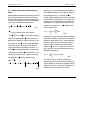
There are many theories and equations about
the relationship between the diffraction pattern
and the material structure. Bragg’s law is a simple way to describe the diffraction of X-rays by a
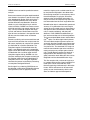
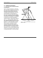
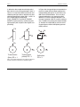
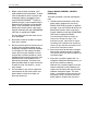
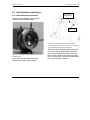
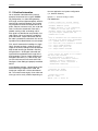
crystal. In Figure 1.1, the incident X-rays hit the
crystal planes in an angle θ, and the reflection
angle is also θ. The diffraction pattern is a delta
function when the Bragg condition is satisfied:
λ = 2d sinθ
where λ is the wavelength, d is the distance
between each adjacent crystal plane (d-spacing), and θ is the Bragg angle at which one
observes a diffraction peak.
1-4
Figure 1.1 - The incident X-rays and reflected X-rays make
an angle of θ symmetric to the normal of the crystal plane.
The diffraction peak is observed at the Bragg angle θ
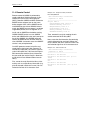
Figure 1.1 is an oversimplified model. For real
materials, the diffraction patterns vary from theoretical delta functions with discrete relationships between points to continuous distributions
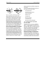
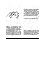
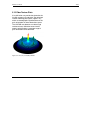
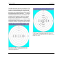
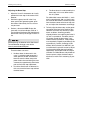
with spherical symmetry. Figure 1.2 shows the
diffraction from a single crystal and from a polycrystalline sample. The diffracted beams from a
single crystal point to discrete directions each
corresponding to a family of diffraction planes.
The diffraction pattern from a polycrystalline
(powder) sample forms a series of diffraction
cones if a large number of crystals oriented randomly in the space are covered by the incident
X-ray beam. Each diffraction cone corresponds
to the diffraction from the same family of crystalline planes in all of the participating grains. The
diffraction patterns from polycrystalline materials will be considered later in the discussion of
the theory and configuration of X-ray diffraction
using area detectors. The theory also applies to
any system with a two-dimensional detector.
M86-E01007
GADDS User Manual
Introduction and Overview
electrical conductivity, coefficient of expansion,
and so forth.
Analyses commonly performed on polycrystalline materials with X-rays include:
Phase identification
Quantitative phase analysis
Texture (orientation)
Figure 1.2 - The patterns of diffracted X-rays: (a) from a
single crystal and (b) from a polycrystalline sample
Polycrystalline materials consist of many crystalline domains, numbering from two to more
than a million in the incident beam. In singlephase polycrystalline materials, all of these
domains have the same crystal structure with
multiple orientations. Polycrystalline materials
could also be multiphase materials with more
than one kind of crystal blended together. Polycrystalline materials can also be bonded to different materials such as semiconductor thin
films on single crystal substrates. The crystalline
domains could be embedded in an amorphous
matrix or stressed from a forming operation.
Usually, the sample undergoing X-ray analysis
has a combination of these effects. Polycrystalline diffraction deals with this range of scattering
to determine the constituent phases in a material or the effect of processing conditions on the
crystallite structure and distribution. The myriad
properties that can be measured with X-rays are
related to material purity, strength, durability,
M86-E01007
Residual stress
Crystallite size
Percent crystallinity
Lattice dimensions
Structure refinement (Rietveld)
1.2.2 Two-Dimensional X-ray Powder
Diffraction (XRD2)
Two-dimensional X-ray diffraction (2DXRD or
XRD2) is a new technique in the field of X-ray
diffraction (XRD). XRD2 is not simply a diffractometer with a two-dimensional (2D) detector. In
addition to 2D detector technology, XRD2
involves 2D image processing and 2D diffraction
pattern manipulation and interpretation.
Because of the unique nature of the data collected with a 2D detector, a completely new
concept and new approach are necessary to
configure the XRD2 system and to understand
and analyze the 2D diffraction data. In addition,
the new theory should also be consistent with
1-5
Introduction and Overview
GADDS User Manual
the conventional theory so that the 2D data can
be used for conventional applications.
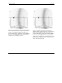
First, we compare conventional X-ray diffraction
(XRD) and two-dimensional X-ray diffraction
(XRD2). Figure 1.3 is a schematic of X-ray diffraction from a powder (polycrystalline) sample.
For simplicity, it shows only two diffraction
cones, one represents forward diffraction
(2θ<90°) and one backward diffraction (2θ>90°).
The diffraction measurement in the conventional
diffractometer is confined within a plane, here
referred to as the diffractometer plane. A point
detector makes a 2θ scan along a detection circle. If a one-dimensional position-sensitive
detector (PSD) is used in the diffractometer, it is
mounted along the detection circle (i.e., diffraction plane). Since the variation of the diffraction
pattern in the direction (Z) perpendicular to the
diffractometer plane is not considered in the
conventional diffractometer, the X-ray beam is
normally extended in the Z direction (line focus).
The actual diffraction pattern measured by a
conventional diffractometer is an average over a
range defined by beam size in the Z direction.
Since the diffraction data outside of the diffractometer plane is not detected, the material structure represented by the missing diffraction data
will either be ignored, or extra sample rotation
and time are needed to complete the measurement.
1-6
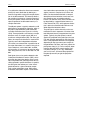
Figure 1.3 - Diffraction patterns in 3D space from a powder
sample and the diffractometer plane
With a two-dimensional detector, the diffraction
is no longer limited to the diffractometer plane.
Depending on the detector size, distance to the
sample and detector position, the whole or a
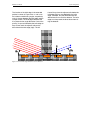
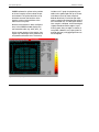
large portion of the diffraction rings can be measured simultaneously. Figure 1.4 shows the diffraction pattern on a two-dimensional detector
compared with the diffraction measurement
range of a scintillation detector and PSD. Since
the diffraction rings are measured, the variations
of diffraction intensity in all directions are equally
important, and the ideal shape of the X-ray
beam cross-section for XRD2 is a point (point
focus). In practice, the beam cross-section can
be either round or square in limited size.
M86-E01007
GADDS User Manual
Introduction and Overview
Figure 1.4 - Coverage comparison: point, line, and area
detectors
M86-E01007
1-7
Introduction and Overview
GADDS User Manual
1.3 Geometry Conventions
1.3.1 Diffraction Cones and Conic Sections
on 2D Detectors
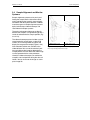
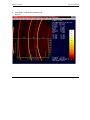
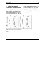
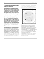
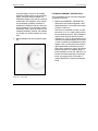
Figure 1.5 shows the geometry of a diffraction
cone. The incident X-ray beam always lies along
the rotation axis of the diffraction cone. The
whole apex angle of the cone is twice the 2θ
value given by the Bragg relation. The surface
of the 2D detector can be considered as a
plane, which intersects the diffraction cone to
form a conic section. D is the distance between
the sample and the detector, and α is the detector swing angle, also referred to as the detector
2θ angle. The conic section takes different
shapes for different α angles. When imaged onaxis (α = 0°), the conic sections appear as circles, producing the Debye rings familiar to most
diffractionists. When the detector is at off-axis
position (α ≠ 0°), the conic section may be an
ellipse, parabola, or hyperbola. For convenience, all kinds of conic sections will be
referred to as diffraction rings or Debye rings
alternatively hereafter in this manual. All diffraction rings collected in a single exposure will be
referred to as a frame. The area detector image
(frame) is normally stored as intensity values on
a 1024x1024-pixel grid or a 512x512-pixel grid.
1-8
Figure 1.5 - A diffraction cone and the conic section with a
2D detector plane
M86-E01007
GADDS User Manual
1.3.2 Diffraction Cones and Laboratory
Axes
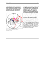
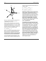
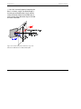
Figure 1.6 describes the geometric definition of
diffraction cones in the laboratory coordinates
system, XLYLZL.
Figure 1.6 - The geometric definition of diffraction rings in
laboratory axes
GADDS uses the same diffraction geometry
conventions as the conventional 3-circle goniometer, which is consistent with the Bruker AXS
P3 and P4 diffractometers. In these conventions, the direct X-ray beam propagates along
the XL axis, ZL is up, and YL makes up a righthanded rectangular coordinate system. The axis
XL is also the rotation axis of the cones. The
apex angles of the cones are determined by the
2θ values given by the Bragg equation. The
apex angels are twice the 2θ values for forward
reflection (2θ<90°) and twice the values of 180°2θ for backward reflection (2θ>90°). The γ angle
is the azimuthal angle from the origin at the 6
o’clock direction (-ZL direction) with a right-
M86-E01007
Introduction and Overview
handed rotation axis along the opposite direction of the incident beam (-XL direction). The γ
angle here is used to define the direction of the
diffracted beam on the cone. In the past, “χ” was
used to denote this angle, it was changed to γ to
avoid confusion with the goniometer angle χ.
The γ angle actually defines a half plane with the
XL axis as the edge, referred to as γ-plane hereafter. Intersections of any diffraction cones with
a γ-plane have the same γ value. The conventional diffractometer plane consists of two γplanes with one γ=90° plane in the negative YL
side and γ=270° plane in the positive YL side. γ
and 2θ angles form a kind of spherical coordinate system which covers all the directions from
the origin of sample (goniometer center). The γ2θ system is fixed in the laboratory systems
XLYLZL, which is independent of the sample orientation in the goniometer. This is a very important concept when we deal with the 2D
diffraction data.
As mentioned previously, the diffraction rings on
a 2D detector can be any one of the four conic
sections: circle, ellipse, parabola, or hyperbola.
The determination of the diffracted beam direction involves the conversion of pixel information
into the γ-2θ coordinates. In the GADDS system,
the γ and 2θ values for each pixel are given and
displayed on the frame. Users can observe all
the diffraction rings in terms of γ and 2θ coordinates with a conic cursor, disregarding the
actual shape of each diffraction ring.
1-9
Introduction and Overview
GADDS User Manual
1.3.3 Sample Orientation and Position in the
Laboratory System
In the GADDS geometric convention, we use
three rotation angles to describe the orientation
of a sample in the diffractometer. The three
angles are ω (omega), χg (goniometer chi) and φ
(phi). Since the χ symbol has been used for the
azimuthal angle on the diffraction cones in this
manual, we use χg to represent the χ rotation in
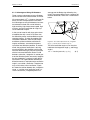
the 3- and 4-circle goniometer. Figure 1.7(a)
shows the relationship between rotation axes
(ω, χg, φ) and the laboratory system XLYLZL. ω
is defined as a right-handed rotation about ZL
axis. The ω axis is fixed on the laboratory coordinates. χg is a left-handed rotation about a horizontal axis. The χg axis makes an angle of ω
with XL axis in the XL-YL plane when ω≠0. The
χg axis lies on XL when ω is set at zero. φ is a
left-handed rotation. The φ axis overlaps with
the ZL axis when χg=0. The φ axis is away from
the ZL axis by χg rotation for any nonzero χg
angle.
1 - 10
Figure 1.7 - Sample rotation and translation in the laboratory
system. (a) Relationship between rotation axes and XLYLZL
coordinates; (b) Relationship among rotation axes (ω, χg, ψ,
φ) and translation axes XYZ
Figure 1.7(b) shows the relationship among all
rotation axes (ω, χg, ψ, φ) and translation axes
XYZ. ω is the base rotation, all other rotations
and translations are on top of this rotation. The
next rotation above ω is the χg rotation. ψ is also
a rotation above a horizontal axis. ψ and χg
have the same axis but different starting positions and rotation directions, and χg = 90°-ψ. In
order to make the GADDS geometry definition
consistent with other Bruker XRD systems, the
ψ angle will be used in the later version of
GADDS system. The next rotation above ω and
(ψ) is φ rotation. The sample translation coordinates XYZ are so defined that, when ω = χg = φ
=0, X is in the opposite direction of the incident
X-ray beam (X= -XL), Y is in the opposite direction of YL (Y= -YL), and Z overlaps with (Z= ZL).
In GADDS, it is very common to set the χg = 90°
(ψ= 0) for a reflection mode diffraction as is
M86-E01007
GADDS User Manual
shown in Figure 1.7(b). In this case, the relationship becomes X= -XL, Y= ZL, and Z= YL when ω
= ψ = φ =0. The φ rotation axis is always the
same as the Z-axis at any sample orientation.
In an aligned diffraction system, all three rotation axes and the primary X-ray beam cross at
the origin of XLYLZL coordinates. This cross
point is also known as goniometer center or
instrument center. The X-Y plane is normally the
sample surface and Z is the sample surface normal. In a preferred embodiment, XYZ translations are above all the rotations so that the
translations will not move any rotation axis away
from the goniometer center. Instead, the XYZ
translations bring a different part of the sample
into the goniometer center. Due to this nature, if
a sample is moved for the distances of x and y
away from the origin in the X-Y plane, the new
spot on the sample exposed to the X-ray beam
will be –x and –y away from the original spot.
In the past, GADDS documents and software
have used the symbol χ (or chi) for both diffraction cone and sample orientation. In this manual, we will adopt the two new symbols. γ
(gamma) represents the direction of diffracted
beam on the diffraction cone, and ψ. (psi) represents a sample rotation angle. Users may see
either the old or new symbol definition depending on the version of hardware or software, but
can normally distinguish the two parameters
from the definition if they are aware of the difference.
M86-E01007
Introduction and Overview
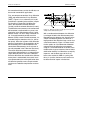
1.3.4 Detector Position in the Laboratory
System
As previously mentioned, the detector position
is defined by the sample-to-detector distance D
and the detector swing angle α. In the laboratory
coordinates XLYLZL, detectors at different positions are shown in Figure 1.8.
Figure 1.8 - Detector position in the laboratory system
XLYLZL: D is the sample-to-detector distance; α is the swing
angle of the detector
Three planes (1-3) represent the detection
planes of three 2D detectors. The detector distance D is defined as the perpendicular distance
from the goniometer center to the detection
plane. The swing angle α is a right-handed rotation angle above ZL axis. Detector 1 is exactly
centered on the positive side of XL axis, and its
swing angle is zero (on-axis). Detectors 2 and 3
are rotated away from XL axis with negative
swing angles (α2<0 and α3<0). The swing angle
is sometimes called detector two-theta in
1 - 11
Introduction and Overview
GADDS User Manual
GADDS documents and software. We will use
2θD to represent the detector swing angle hereafter in this manual. It is very important to distinguish between the Bragg angle 2θ and detector
angle 2θD. 2θ is the measured diffraction angle
on the data frame. At a given detector angle
2θD, a range of 2θ values can be measured. The
2θ value corresponding to the center pixel is
equal to 2θD. Users should be able to tell the difference between two parameters although the
same symbol may be used for both variables in
GADDS software or documents.
1 - 12
M86-E01007
GADDS User Manual
Introduction and Overview
1.4 Diffraction Data Measured by an
Area Detector
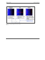
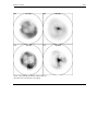
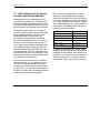
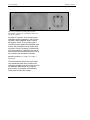
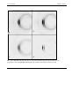
Without any analysis, an area detector frame
can provide a quick overview of the crystallinity,
composition, and orientation of a material. If the
observed Debye rings are smooth and continuous, the sample is polycrystalline and fine
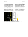
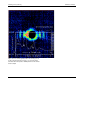
grained. If the rings are continuous but spotty,
the material is polycrystalline and large grained
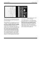
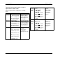
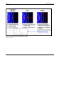
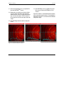
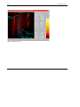
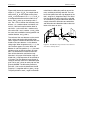
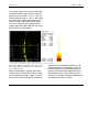
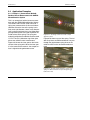
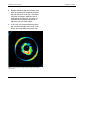
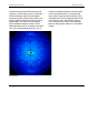
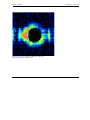
(Figure 1.11). Incomplete Debye rings indicate
orientation or texture (Figure 1.10). If only individual spots are observed, the material is single
crystal, which can be considered the extreme
case of crystallographic texture (Figure 1.9).
Often, you can visually determine the number of
phases when the phases have different degrees
of orientation (texture).
and both have fiber texture. The Al and TiN are highly
oriented polycrystalline materials, while the Si substrate is
single crystal. The stack is roughly 0.5 µm thick
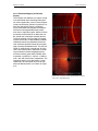
Figure 1.10 - Nylon 6 fiber with an inorganic filler. Two
distinct, orthogonal orientations are visible. The faint,
continuous rings are from the polycrystalline, inorganic filler
Al
T iN
Si
Si
Figure 1.9 - Al TiN film on Si Specimen was rotated in φ.
Note that the Al and TiN have the same (111) orientation,
M86-E01007
1 - 13
Introduction and Overview
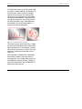
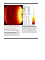
Figure 1.11 - Flexible TAB (Tape Automated Bonding)
material. The two phases are gold and copper. The smooth
and continuous rings are the fine-grained gold. The spotty
rings belong to large-grained copper. The small divisions on
the crosshair are 20 µm
When integrating an area detector frame in the
χ direction, a standard “powder pattern” (intensity versus 2θ diagram) is obtained. The added
benefit of the area detector is that the intensities
so obtained take preferred orientation into
account. This is a tremendous advantage when
performing phase analysis on oriented materials
such as clay minerals. Area detector frames
may also be processed to obtain texture information in the form of pole figures, fiber texture
plots, and orientation indices. The coverage of
the area detector frequently enables multiple
poles with backgrounds to be collected simultaneously, in a small fraction of the time it takes a
1 - 14
GADDS User Manual
conventional texture diffractometer with a scintillation detector to collect a single pole.
The HI-STAR detector is a gas-filled multiwire
proportional counter. It is a true photon counter,
which makes it extremely sensitive for weakly
diffracting materials. The extremely low background of the HI-STAR makes it ideal for applications requiring “long” measurement times
(tens of minutes to hours), such as small-angle
X-ray scattering and microdiffraction.
M86-E01007
GADDS User Manual
1.5 References
1.
B. D. Cullity, Elements of X-Ray Diffraction, 2nd
ed., Addison-Wesley, Reading, MA, 1978.
2.
R. Jenkins and R. L. Snyder, Introduction to XRay Powder Diffractometry, John Wiley, New
York, 1996.
3.
A. J. C. Wilson, International Tables for Crystallography, Kluwer Academic, Boston, 1995.
4.
Philip R. Rudolf and Brian G. Landes, Twodimensional X-ray Diffraction and Scattering of
Microcrystalline and Polymeric Materials, Spectroscopy, 9(6), pp 22-33, July/August 1994.
5.
J. Formica, “X-Ray Diffraction,” In Handbook of
Instrumental Techniques for Analytical Chemistry, edited by F. Settle (Prentice-Hall, New Jersey, 1997).
6.
N. F. M. Henry, H. Lipson, and W. A. Wooster,
The Interpretation of X-Ray Diffraction Photographs (St. Martin’s Press, New York, 1960).
7.
H. Lipson and H. Steeple, Interpretation of X-Ray
Powder Diffraction Patterns (St. Martin’s Press,
New York, 1970).
8.
S. N. Sulyanov, A. N. Popov and D. M. Kheiker,
Using a Two-Dimensional Detector for X-ray
Powder Diffractometry, J. Appl. Cryst. 27, pp
934-942, 1994.
9.
Hans J. Bunge and Helmut Klein, Determination
of Quantitative, High-Resolution Pole-Figures
with the Area Detector, Z. Metallkd. 87(6), pp
465-475, 1996.
M86-E01007
Introduction and Overview
10. Kingsley L. Smith and Richard B. Ortega, Use of
a Two-Dimensional, Position Sensitive Detector
for Collecting Pole Figures, Advances in X-ray
Analysis, Vol. 36, pp 641-647, Plenum, New
York, 1993.
11. Bob B. He and Kingsley L. Smith, Strain and
Stress Measurement with Two-Dimensional
Detector, Advances in X-ray Analysis, Vol. 41,
Proceedings of the 46th Annual Denver X-ray
Conference, Steamboat Springs, Colorado, USA,
1997.
12. Bob B. He and Kingsley L. Smith, Fundamental
Equation of Strain and Stress Measurement
Using 2D Detectors, Proceedings of 1998 SEM
Spring Conference on Experimental and Applied
Mechanics, Houston, Texas, USA, 1998.
13. Bob B. He, Uwe Preckwinkel and Kingsley L.
Smith, Advantages of Using 2D Detectors for
Residual Stress Measurements, Advances in Xray Analysis, Vol. 42, Proceedings of the 47th
Annual Denver X-ray Conference, Colorado
Springs, Colorado, USA, 1998.
14. Roger D. Durst et. al., The Use of CCD Detectors
for X-ray Diffraction, invited paper to: 1998 Denver X-ray Conference.
1 - 15
Introduction and Overview
1 - 16
GADDS User Manual
M86-E01007
GADDS User Manual
System Configuration
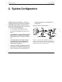
2. System Configuration
GADDS systems are available in a variety of
configurations to fulfill requirements of different
applications and samples. A system normally
consists of the following five major units (each of
which may have several options):
•
an X-ray generator to produce X-rays,
•
X-ray optics to condition the primary X-ray
beam,
•
a goniometer and sample stage to establish
and manipulate the geometric relationship
between primary beam, sample, and detector,
•
a sample alignment and monitor to assist
users in positioning the sample into the
instrument center and in monitoring the
sample state and position,
•
a detector (HI-STAR Area Detector System)
to intercept and record the scattering X-rays
from a sample and to save and display the
M86-E01007
diffraction pattern into a two-dimensional
image frame.
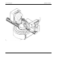
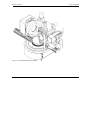
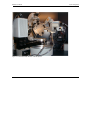
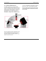
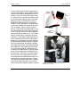
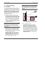
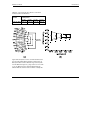
Figure 2.1 shows a typical system.
Figure 2.1 - Five major units in a GADDS system: X-ray
generator (sealed tube); X-ray optics (monochromator and
collimator); goniometer and sample stage; sample alignment
and monitor (laser-video); and area detector
2-1
System Configuration
GADDS User Manual
In addition to the five major units there are other
accessories, such as a low temperature stage, a
high temperature stage, a Helium (or vacuum)
beam path for SAXS, a beam stop, and alignment and calibration fixtures. The whole system
is controlled by a computer that uses GADDS
software.
D8 DISCOVER with GADDS (designed for
speed, precision, flexibility, versatility, and reliability) is the new generation of our GADDS
products. The following sections will introduce
the five major units, several standard systems,
and some accessories based on the D8 series.
Due to the large variety of customer needs and
the availability of new technologies and new
components that make for numerous system
combinations, this section introduces only the
most commonly used GADDS components.
Refer to other documents, the GADDS Administrator Manual, or consult our service personnel
for components not covered.
2-2
M86-E01007
GADDS User Manual
2.1 X-ray Generator
The X-ray generator produces X-rays with the
required radiation energy, focal spot, and intensity.
2.1.1 Radiation Energy
GADDS can use a variety of X-ray sources,
from a sealed tube generator to a rotating anode
generator (RAG) to synchrotron radiation (with
CCD detector). The sealed tube generator is the
most commonly used X-ray source in the
GADDS system.
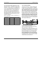
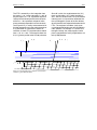
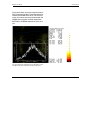
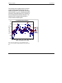
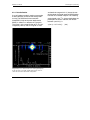
2.1.2 X-ray Spectrum and Characteristic
Lines
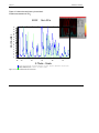
X-rays generated by sealed tubes or rotating
anode generator have an X-ray spectrum, which
presents intensity vs. wavelength (Figure 2.2).
System Configuration
(white) radiation and characteristic radiation lines Kα and Kβ
and (b) Kα line, a combination of two lines Kα1 and Kα2
The spectrum consists of continuous radiation
(also called white radiation, or Bremsstrahlung)
and a number of discrete characteristic lines.
For X-ray diffraction, the three most important
characteristic lines are Kα1 and Kα2 and Kβ. The
Kα1 and Kα2 lines are so close in their wavelengths that they are also called Kα doublet. The
Kα1 line is about twice the intensity of Kα2. If the
two Kα lines cannot be resolved, they are simply
referred to as Kα line. The wavelengths of characteristic lines are determined by the target
(anode) materials of the X-ray generator. Table
2.1 gives a list of common target materials and
their wavelengths. Table 2.2 lists typical applications for each target material.
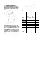
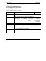
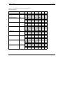
Table 2.1 – Wavelengths of characteristic lines of common
target elements
Target Energy Wavelength (Å =10-1 nm)
(Ka)
keV
Ka
Ag
22.11
0.560868 0.5594075 0.563789 0.497069
Ka1
Mo
17.44
0.710730 0.709300
0.713590 0.632288
Cu
8.04
1.541838 1.540562
1.544390 1.392218
Co
6.93
1.790260 1.788965
1.792850 1.62079
Fe
6.40
1.937355 1.936042
1.939980 1.75661
Cr
5.41
2.29100
2.293606 2.08487
2.28970
Ka2
Kb
Figure 2.2 - X-ray spectrum generated by a sealed X-ray
tube or rotating anode generator showing (a) continuous
M86-E01007
2-3
System Configuration
Table 2.2 – Selection of target material with respect to the
applications
Target
Typical Applications
Ag
Low absorption; single crystal, transmission
diffraction, (with CCD detector).
Mo
Low absorption; single crystal, transmission
diffraction, (with CCD detector).
Cu
Most powder diffraction, stress, texture, thin
films, polymer, SAXS, single crystal
Co
Used for ferrous alloys (steels) to reduce Fe
fluorescence, ideal for residual stress.
Fe
Used for ferrous alloys (steels) to reduce Fe
fluorescence, ideal for residual stress.
Cr
Ideal for materials with large unit cell, ideal for
residual stress with high resolution.
GADDS User Manual
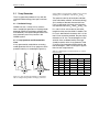
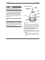
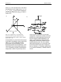
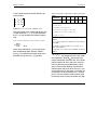
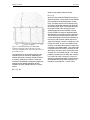
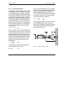
2.1.3 Focal Spot and Takeoff Angle
The focal spot (also called focal spot on target)
and takeoff angle are critical features in the production of X-rays by sealed tube and rotating
anode generators. Sealed tube and rotating
anode generators produce X-rays (Figure 2.3)
by bombarding the target sample with electrons
generated from the filament (cathode). The area
bombarded by electrons is called focal spot on
target, or simply focal spot, and the angle
between the primary X-ray beam and the anode
surface is called takeoff angle.
Figure 2.3 - Schematic of a sealed X-ray tube showing
filament (cathode), anode, focal spot on anode, takeoff
angle, projected line focus beam, and point focus beam
The size and shape of the focal spot is one of
the most important features for an X-ray generator. Sealed X-ray tubes normally have 2 to 4
beryllium windows through which X-rays may
exit. The focal spot is typically rectangular with a
2-4
M86-E01007
GADDS User Manual
System Configuration
length-to-width ratio of 10 to 1. The projection
along the length of the focal spot at a takeoff
angle from the anode surface is called spot
focus (or square focus, or point focus). The projection of the focal spot perpendicular to its
length is called line focus. Thus, line focus and
spot focus are separated by an angle of 90°
around the tube cylinder. The line focus is commonly used for the conventional diffractometer
with point detector or PSD. A standard GADDS
system uses the spot focus.
The takeoff angle can be set from 3° to 7° (6° for
most systems). Table 2.3 lists focal spot size,
line focus size, and spot focus size at a 6° takeoff angle for typical X-ray tubes used with
GADDS systems.
Table 2.3 – Focal spot size, line focus size, and spot focus
size of some typical X-ray tubes
Tube Type
Normal focus
Fine focus
Focal Spot
Line Focus
Size at Anode Size
(mm x mm)
(mm x mm)
Spot Focus
Size
(mm x mm)
1 x 10
1x1
0.4 x 8
Long fine focus 0.4 x 12
Micro focus
0.15 x 8
0.1 x 10
2.1.4 Focal Spot Brightness and Profile
Focal spot brightness, focal spot profile, and Xray optics (discussed in the next section) influence X-ray beam intensity. The focal spot
brightness is determined by the maximum target
loading, more specifically by power per unit
area. Table 2.4 gives the maximum target loading and brightness (power per unit area) for
some typical sealed tubes as well as some
rotating anode sources equipped with a Cu target.
Table 2.4 – Focal spot brightness for sealed tubes and
rotating anode sources with Cu target
Source
Focal Spot
Size
(mm x mm)
Maximum
Load (kW)
Maximum
Brightness
Normal focus
1 x 10
2.0
0.2
Fine focus
0.4 x 8
1.5
0.5
Long fine focus 0.4 x 12
2.2
0.5
Micro focus
0.15 x 8
0.8
0.7
Rotating
Anode
Generator
0.5 x 10
18.0
3.6
0.3 x 3
5.4
6.0
(kW/mm2)
0.04 x 8
0.4 x 0.8
0.04 x 12
0.4 x 1.2
0.2 x 2
3.0
7.5
0.15 x 0.8
0.1 x 1
1.2
12.0
0.015 x 8
As shown, the micro focus sealed tubes have
the brightest focal spot of all sealed tubes.
Rotating anode generators have very high brilliance compared with sealed tubes. The intensity over the focal spot is not evenly distributed.
M86-E01007
2-5
System Configuration
The focal spot profile is the intensity distribution
over the area of the beam cross section and is
eventually translated to the beam profile. The
beam profile is sometimes very important to the
diffraction result. The focal spot profile across
the beam from fine focus and long fine focus
sealed tube are typically saddled in the center
with the maximum near the edge. The intensity
at the center can be as low as 50% of the maximum. The focal spot profile for RAG is normally
more evenly distributed, like a flat-topped Gaussian distribution. The focal profile from a fine
focus or long fine focus sealed tube can satisfy
most GADDS applications. The micro focus
sealed tube and RAG may be necessary for
some applications.
GADDS User Manual
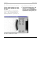
2.1.5 Operation of the X-ray Generator
Correct and careful operation of an X-ray generator is critical for satisfactory performance and
useful lifetime. All X-ray tubes have a maximum
power rating, which defines the highest power
input to the tube. A cathode current vs. anode
voltage chart (or table) is normally supplied for a
sealed tube. The tube’s filament current is also
provided by the tube vendors. D8 DISCOVER
with GADDS uses the K760 or K780 X-ray Generator (C79249-A3054-A3, -A4). The following
information is for the K760. The K780 is only
controlled by the software.
Detailed information for installation and operation is available in the vendor’s Operating
Instructions (C79000-B3476-C182-06). Refer to
the manufacturer’s manuals if your system has
a rotating anode generator (RAG). Generally,
you should adapt the following precautions
when operating an X-ray generator:
1. Before starting the generator.
1.1 Make sure the cooling water supply is
available and running properly (temperature, pressure, flow rate, clean water
and filter).
1.2 Make sure all the safety interlocks work
properly and are set correctly.
1.3 Set the key switch to position “I”. Position “II” is reserved for qualified service
personnel, so you should not operate
the generator on this setting.
2-6
M86-E01007
GADDS User Manual
System Configuration
3.2 When increasing the generator power
manually, always increase voltage first
and then current. When reducing the
generator power, always reduce the
current first and then voltage.
2. Start the generator.
2.1 Press the Heater key for approximately
2 seconds, and wait until the LED in the
Heater key lights continuously.
2.2 Then press the ON key. The X-RAYS
ON signal lamp and radiation warning
lamps light, the LED in the Heater key
goes off, the LED in the ON key lights.
And the display values read “kV=20
mA=5”. (See the Operating Instructions
if the generator responds differently).
3.3 When using a new X-ray tube or when
the generator has been shut down for
more then 12 hours, observe the following start-up procedures (Table 2.5),
unless suggested otherwise by the
manufacturer. An automatic start-up
routine can be selected for new tubes
(see Operating Instructions).
3. Adjust the voltage and current.
3.4 To increase the lifetime of X-ray tubes,
set the generator to standby mode
(20kV, 5mA for sealed tube) if the generator is not in use for extended time
(hours to days).
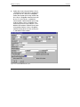
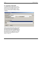
3.1 You can adjust the voltage and current
manually (for PLATFORM GADDS) or
through GADDS software (Collect >
Goniometer > Generator, or press the
Ctrl+Shft+G keys).
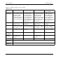
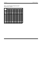
Table 2.5 – Start-up procedures for “cold generator” or
new tube
Pause in
Operation
(days)
M86-E01007
High Voltage/Duration
Total
time for
55 kV
20 kV
25 kV 30 kV 35 kV 40 kV 45 kV
50 kV
55 kV
0.5 to 3
30 s
30 s
30 s
30 s
30 s
1 min
2 min
3 to 30
30 s
30 s
2 min
2 min
5 min 5 min
> 30 or new
tube
30 s
30 s
2 min
2 min
5 min 10 min 15 min 15 min 50 min
30 s
6 min
10 min 10 min 35 min
2-7
System Configuration
GADDS User Manual
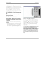
2.2 X-ray Optics
The function of X-ray optics is to condition the
primary X-ray beam into the required wavelength, beam focus size, beam profile, and
divergence. The X-ray optics components commonly used for GADDS systems (and discussed
in this section) are a monochromator, a pinhole
collimator, cross-coupled Göbel mirrors, and a
monocapillary.
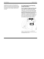
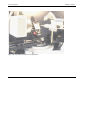
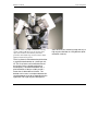
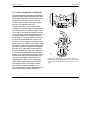
Figure 2.4 shows an X-ray tube, a monochromator, a collimator, and a beam stop in a standard
GADDS system. It also shows the instrument
center and the shadow of a fixed chi stage.
Using a point X-ray source with pinhole collimation enables you to examine small samples
(microdiffraction) or small regions on larger
samples (selected-area diffraction). This configuration enables you to measure crystallographic
phase, texture, and residual stress from precise
locations on irregularly shaped parts, including
curved surfaces.
2-8
Figure 2.4 - Typical X-ray optics in standard GADDS
includes X-ray tube, monochromator, collimator, and beam
stop. Also shown are the instrument center and the shadow
of a fixed chi stage
M86-E01007
GADDS User Manual
System Configuration
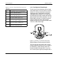
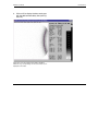
2.2.1 Monochromator
An important consideration for your system is
that you will want to have an appropriate monochromator for the characteristics of the source,
specimen, and instrument geometry. A crystal
monochromator is typically used with a sealed
tube or rotating anode generator to allow only a
selected characteristic line (Kα or Kα1 ) to pass
through the optics. While X-rays generated from
a sealed X-ray tube or rotating anode generator
consist of white radiation and other characteristic radiation lines, most X-ray diffraction applications need only the Kα (or Kα1) line. They need
only this line because the white radiation produces an unwanted high background in the diffraction pattern, and the other characteristic
lines produce extra and unwanted diffraction
peaks (rings) in the diffraction pattern.
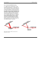
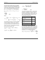
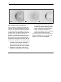
A crystal monochromator is illustrated in Figure
2.5. The single crystal has a d-spacing: d. The
wavelength of the X-rays diffracted by the crystal is given by the Bragg law, λ=2dsinθM. We
can set the monochromator crystal to a diffraction condition such that only the wavelength of
Kα1 satisfies the Bragg law. X-rays of other
wavelengths are filtered out by the monochromator. As shown, the X-rays must also be in the
correct direction to satisfy the diffraction condition. Thus, the reflected beam from a monochromator with a perfect crystal will be a parallel Xray beam.
M86-E01007
Figure 2.5 - Illustration of a crystal monochromator.
Monochromatic X-rays are obtained by diffraction from a
single crystal plate
In practice, the reflected beam from a monochromator is not strictly monochromatic due to
the mosaic of the crystal (measured by rocking
angle).
The crystal type in a monochromator must be
chosen based on the performance you require
in terms of intensity and resolution. Crystals
such as Si, Ge, and quartz have small rocking
angles, accompanied by high resolution and low
intensity, while graphite and LiF crystals have
high intensity and low resolution due to large
mosaic spreads. The monochromator crystal
shape also varies from flat to bent to cut-tocurve. A flat crystal is used for parallel beams
and a curved crystal is used for focus geometry.
The standard GADDS system uses the flat
graphite monochromator, which gives the strongest beam intensity. The monochromator is
designed to accept a limited angular range of Xrays about the takeoff angle. The monochroma-
2-9
System Configuration
GADDS User Manual
tor can be used for takeoff angles from 3° to 6°
(typically set to 6°). The graphite crystal cannot
resolve Kα1 and Kα2 lines, so it is aligned to the
Kα line. The monochromator is designed to use
various anode materials. Their 2θM angles are
listed in Table 2.6. You may need to input the
2θM value if you choose to process data with
polarization correction. See the service manual
(269-005502 for P4 monochromator) for monochromator alignment.
Table 2.6 – Bragg angles of graphite crystal (002) plane for
various target materials
Target Materials
Kα Wavelength Bragg angle 2θM
Ag
0.560868
9.58
Mo
0.710730
12.14
Cu
1.541838
26.53
Co
1.790260
30.90
Fe
1.937355
33.51
Cr
2.29100
39.87
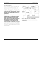
2.2.2 Pinhole Collimator
The pinhole collimator is normally used to control the beam size and divergence. In GADDS
systems, the pinhole collimator is normally used
with a monochromator or a set of cross-coupled
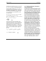
Göbel mirrors. Figure 2.6 shows the X-ray beam
path in a pinhole collimator achieved with two
pinholes apertures of the same diameter d separated by a distance h. F is the dimension of the
projection of focal spot or beam focus projection
from the monochromator or Göbel mirrors. The
distance between the focus and the second pinhole is H. The distance from the second pinhole
to the sample surface is g.
Figure 2.6 - Schematic of the beam path in a pinhole
collimator showing the parallel, divergent, and convergent
X-rays and beam spot on sample surface
The beam consists of three components: parallel, divergent, and convergent X-rays. The parallel part of the beam has a size of d all the way
from focus to sample. The anti-scattering pinhole is used to block the X-ray scattering from
the second pinhole. The size of the anti-scattering pinhole must be such that it allows no exposure to direct rays from the focus.
2 - 10
M86-E01007
GADDS User Manual
System Configuration
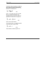
The maximum divergence angle β is given by
2d
β = ------h
(2-1)
The maximum angle of convergence α is given
by
d
α = ------------h+g
(2-2)
The maximum beam spot D on a flat sample
facing the X-ray source is given by
2g
D = d ⎛ 1 + ------- ⎞
⎝
h ⎠
(2-3)
As shown in the equation, the shorter the distance between the second pinhole and the sample (or the longer the distance between two
pinholes), the smaller the beam spot on the
sample. The effective beam focus size f is
determined by the pinhole distance h and the
distance between the X-ray source and the pinholes.
2H
f = d ⎛ -------- – 1⎞
⎝ h
⎠
(2-4)
the beam path. For example, when cross-coupled Göbel mirrors are used, the X-ray beam is
almost a parallel beam, and the divergence of
the beam is smaller than the value calculated
from equation (2-1). When the actual beam
focus on the source f′ is smaller than f, we have
the following equations to calculate the maximum divergence (β′), convergence (α′), and
beam spot size on sample (D′):
d + f′
β′ = ⎛ -------------⎞
⎝ H ⎠
(2-5)
f′
α′ = ------------H+g
(2-6)
D′ = ( β′ ( H + g ) – f ′ )
(2-7)
Table 2.7 lists the values of beam divergence,
convergence, and beam spot on sample for a
system with a 0.4 mm x 0.8 mm fine focus tube.
The graphite monochromator has a rocking
curve of 0.4° and cross-coupled Göbel mirrors
of 0.06°. The beam divergence and convergence angles should not be above these values.
If the actual X-ray source F is larger than the
effective focus size f, the difference between F
and f represents the wasted X-ray energy.
Sometimes, a micro-focus tube is required when
a small beam size is used. The actual beam
divergence is also determined by the monochromator and mirrors advancing the collimator in
M86-E01007
2 - 11
System Configuration
GADDS User Manual
Table 2.7 – X-ray beam divergence angle (β), convergence
angle (α), and beam spot size on sample (D) for a 0.4 mm
point focus tube with graphite monochromator or crosscoupled Göbel Mirrors
Collima- Graphite Monochromator
tor Size
α (°)
Göbel Mirrors
d (mm)
β (°)
D (mm) f (mm) β (°)
α (°)
0.05
0.041 0.017 0.07
0.15
0.041 0.017 0.07
0.10
0.082 0.034 0.14
0.30
0.060 0.034 0.13
0.20
0.164 0.067 0.29
0.60
0.060 0.060 0.23
0.30
0.246 0.101 0.42
0.80
0.060 0.060 0.33
0.50
0.266 0.148 0.64
0.80
0.060 0.060 0.53
0.80
0.327 0.148 0.97
0.80
0.060 0.060 0.83
D (mm)
The table also shows that the beam divergency
decreases continuously with decreasing pinhole
size for the combination of double pinhole collimator and monochromator. In some cases, the
application requires small beam size but not
necessarily the small divergence. We recommend that you remove the pinhole 1 from the
collimator tube to achieve higher beam intensity.
Table 2.8 gives the comparison between double
pinhole collimators and single pinhole collimators in terms of intensity gain (the approximate
ratio of single-to-double pinhole), beam divergency, and beam spot size on sample.
2 - 12
M86-E01007
GADDS User Manual
System Configuration
Table 2.8 – Comparison between single pinhole collimator
and double pinhole collimator in terms of intensity gain,
beam divergency angle (β), and beam spot size on sample
(D)
Collimator
size
Intensity
gain
Single
pinhole
Double
pinhole
d (mm)
Single/
double
b (×)
D (mm) b (×)
D (mm)
0.05
>20
0.174
0.14
0.041
0.07
0.10
16
0.184
0.20
0.082
0.14
0.20
4
0.205
0.31
0.164
0.29
0.30
2.4
0.225
0.42
0.225
0.42
0.50
1.2
0.266
0.64
0.266
0.64
0.80
1.0
0.327
0.97
0.327
0.97
The microdiffraction collimators are 50 µm and
100 µm in diameter. For quantitative analysis,
texture, or percent crystallinity measurements,
0.5 mm or 0.8 mm collimators are typically used.
In the case of quantitative analysis and texture
measurements, using too small a collimator can
actually be a detriment, causing poor statistical
grain sampling. In such cases, you can improve
statistics by oscillating the sample. Crystallite
size measurements are usually measured with a
0.2 mm collimator at 30 cm sample-to-detector
distance. The choice of collimator size is often a
trade-off between intensity and the ability to illuminate small regions or to resolve closely
spaced lines. The smaller the collimator, the
lower the photon flux that strikes the sample,
and the longer the count time to acquire statistically significant data.
M86-E01007
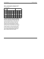
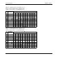
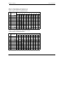
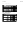
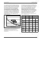
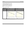
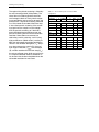
2.2.3 Sample-to-Detector Distance and
Angular Resolution
The divergence of the X-ray beam is a function
of collimator size, sample-to-detector distance,
ω and 2θ. The tables that follow can be used to
determine a suitable collimator size and sampleto-detector distance to resolve closely spaced
peaks. In all cases, the standard two-pinhole
collimators are assumed, which have a sampleto-front pinhole distance of 8 mm. Only the more
common combinations of collimator sizes and
sample-to-detector distances are tabulated.
These tables are for reflection mode. Transmission mode values for the apparent beam size
can be located by translating ω by 90°, ω - 90°.
2 - 13
System Configuration
GADDS User Manual
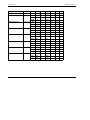
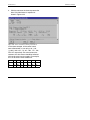
Table 2.9 – Beam divergence (2θ spread in [°]) as a function
of ω and 2θ with a 0.05 mm collimator, 30 cm sample-todetector distance, and 1024x1024 frames
ω
Apparent
Size [mm]
2θ
4°
10°
20°
40°
60°
80° 100° 120° 140° 160°
1°
3.21
— 0.01 0.02 0.04 0.06 0.07 0.07 0.06 0.04 0.02
2°
1.60
—
5°
0.64
10°
0.32
20°
30°
40°
50°
90°
0.06
— 0.01 0.02 0.03 0.03 0.03 0.03 0.02 0.01
—
— 0.01 0.01 0.01 0.01 0.01 0.01 0.01
—
— 0.01 0.01 0.01 0.01 0.01
—
0.16
—
—
—
—
—
—
—
0.11
—
—
—
—
—
—
—
0.09
—
—
—
—
—
—
0.07
—
—
—
—
—
—
—
—
—
—
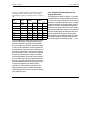
Table 2.10 – Beam divergence (2θ spread in [°]) as a
function of ω and 2θ with a 0.1 mm collimator, 30 cm
sample-to-detector distance, and 1024x1024 frames
ω
Apparent
Size [mm]
2θ
4°
10°
20°
40°
60°
80° 100° 120° 140° 160°
1°
6.42 0.01 0.02 0.04 0.09 0.12 0.13 0.13 0.12 0.09 0.05
2°
3.21
— 0.01 0.02 0.04 0.06 0.07 0.07 0.06 0.05 0.03
5°
1.28
— 0.01 0.02 0.02 0.03 0.03 0.02 0.02 0.01
10°
0.64
— 0.01 0.01 0.01 0.01 0.01 0.01 0.01
20°
0.33
—
— 0.01 0.01 0.01 0.01
—
30°
0.22
—
—
—
—
—
—
—
40°
0.17
—
—
—
—
—
—
50°
0.15
—
—
—
—
—
—
90°
0.11
—
—
—
—
2 - 14
M86-E01007
GADDS User Manual
System Configuration
Table 2.11 – Beam divergence (2θ spread in [°]) as a
function of ω and 2θ with a 0.2 mm collimator, 30 cm
sample-to-detector distance, and 1024x1024 frames
ω
Apparent
Size [mm]
1°
2θ
4°
10°
20°
40°
60°
80° 100° 120° 140° 160°
12.83 0.01 0.04 0.09 0.17 0.23 0.27 0.27 0.24 0.18 0.10
2°
6.42
— 0.02 0.04 0.08 0.12 0.13 0.13 0.12 0.09 0.05
5°
2.57
— 0.01 0.03 0.04 0.05 0.05 0.05 0.04 0.02
10°
1.29
— 0.01 0.02 0.03 0.03 0.03 0.02 0.01
20°
0.65
— 0.01 0.01 0.01 0.01 0.01 0.01
30°
0.45
—
40°
0.35
—
— 0.01 0.01 0.01 0.01
50°
0.29
—
—
90°
0.22
— 0.01 0.01 0.01 0.01 0.01
— 0.01 0.01 0.01
—
—
—
—
Table 2.12 – Beam divergence (2θ spread in [°]) as a
function of ω and 2θ with a 0.3 mm collimator, 30 cm
sample-to-detector distance, and 1024x1024 frames
ω
Apparent
Size [mm]
2θ
4°
10°
20°
40°
60°
80° 100° 120° 140° 160°
1°
19.25 0.02 0.06 0.13 0.26 0.35 0.40 0.40 0.36 0.27 0.15
2°
9.63 0.01 0.03 0.06 0.13 0.17 0.20 0.20 0.18 0.14 0.08
5°
3.85
0.01 0.02 0.05 0.07 0.08 0.08 0.07 0.06 0.03
10°
1.93
0.01 0.02 0.03 0.04 0.04 0.04 0.03 0.02
20°
0.98
0.01 0.01 0.02 0.02 0.02 0.02 0.01
30°
0.67
— 0.01 0.01 0.01 0.01 0.01 0.01
40°
0.52
— 0.01 0.01 0.01 0.01 0.01
50°
0.44
—
90°
0.34
M86-E01007
— 0.01 0.01 0.01 0.01
—
— 0.01 0.01
2 - 15
System Configuration
GADDS User Manual
Table 2.13 – Beam divergence (2θ spread in [°]) as a
function of ω and 2θ with a 0.5 mm collimator, 30 cm
sample-to-detector distance, and 1024x1024 frames
ω
Apparent
Size [mm]
2θ
4°
10°
20°
40°
60°
80° 100° 120° 140° 160°
1°
32.08 0.04 0.11 0.22 0.43 0.58 0.67 0.67 0.59 0.45 0.24
2°
16.04 0.01 0.05 0.11 0.21 0.29 0.33 0.34 0.30 0.23 0.13
5°
6.42
0.01 0.04 0.08 0.11 0.13 0.14 0.12 0.10 0.06
10°
3.22
0.01 0.03 0.05 0.06 0.07 0.06 0.05 0.03
20°
1.64
0.01 0.02 0.03 0.03 0.03 0.03 0.02
30°
1.12
— 0.01 0.02 0.02 0.02 0.02 0.02
40°
0.87
0.01 0.01 0.02 0.02 0.02 0.02
50°
0.73
— 0.01 0.01 0.01 0.02 0.01
90°
0.56
— 0.01 0.01 0.01
Table 2.14 – Beam divergence (2θ spread in [°]) as a
function of ω and 2θ with a 0.05 mm collimator, 15 cm
sample-to-detector distance, and 1024x1024 frames
ω
Apparent
Size [mm]
2θ
4°
10°
20°
40°
60°
80° 100° 120° 140° 160°
1°
3.21 0.01 0.02 0.04 0.08 0.11 0.13 0.13 0.11 0.09 0.05
2°
1.60
— 0.01 0.02 0.04 0.06 0.06 0.07 0.06 0.04 0.02
5°
0.64
— 0.01 0.02 0.02 0.03 0.03 0.02 0.02 0.01
10°
0.32
— 0.01 0.01 0.01 0.01 0.01 0.01 0.01
20°
0.16
—
— 0.01 0.01 0.01 0.01
—
30°
0.11
—
—
—
—
—
—
—
40°
0.09
—
—
—
—
—
—
50°
0.07
—
—
—
—
—
—
90°
0.06
—
—
—
—
2 - 16
M86-E01007
GADDS User Manual
System Configuration
Table 2.15 – Beam divergence (2θ spread in [°]) as a
function of ω and 2θ with a 0.1 mm collimator, 15 cm
sample-to-detector distance, and 1024x1024 frames
ω
Apparent
Size [mm]
2θ
4°
10°
20°
40°
60°
80° 100° 120° 140° 160°
1°
6.42 0.01 0.04 0.09 0.17 0.23 0.26 0.26 0.23 0.17 0.09
2°
3.21
— 0.02 0.04 0.08 0.11 0.13 0.13 0.12 0.09 0.05
5°
1.28
— 0.01 0.03 0.04 0.05 0.05 0.05 0.04 0.02
10°
0.64
— 0.01 0.02 0.02 0.03 0.02 0.02 0.01
20°
0.33
— 0.01 0.01 0.01 0.01 0.01 0.01
30°
0.22
—
40°
0.17
—
— 0.01 0.01 0.01 0.01
50°
0.15
—
—
90°
0.11
— 0.01 0.01 0.01 0.01 0.01
— 0.01 0.01 0.01
—
—
—
—
Table 2.16 – Beam divergence (2θ spread in [°]) as a
function of ω and 2θ with a 0.2 mm collimator, 15 cm
sample-to-detector distance, and 1024x1024 frames
ω
Apparent
Size [mm]
2θ
4°
10°
20°
40°
60°
80° 100° 120° 140° 160°
1°
12.83 0.03 0.08 0.17 0.33 0.45 0.52 0.52 0.46 0.34 0.19
2°
6.42 0.01 0.04 0.08 0.16 0.22 0.26 0.26 0.23 0.18 0.10
5°
2.57
0.01 0.03 0.06 0.09 0.10 0.10 0.10 0.07 0.04
10°
1.29
0.01 0.03 0.04 0.05 0.05 0.05 0.04 0.03
20°
0.65
0.01 0.02 0.02 0.03 0.03 0.02 0.02
30°
0.45
— 0.01 0.01 0.02 0.02 0.02 0.01
40°
0.35
— 0.01 0.01 0.01 0.01 0.01
50°
0.29
— 0.01 0.01 0.01 0.01 0.01
90°
0.22
M86-E01007
—
— 0.01 0.01
2 - 17
System Configuration
GADDS User Manual
Table 2.17 – Beam divergence (2θ spread in [°]) as a
function of ω and 2θ with a 0.3 mm collimator, 15 cm
sample-to-detector distance, and 1024x1024 frames
ω
Apparent
Size [mm]
2θ
4°
10°
20°
40°
60°
80° 100° 120° 140° 160°
1°
19.25 0.04 0.12 0.26 0.50 0.68 0.78 0.79 0.69 0.52 0.28
2°
9.63 0.01 0.05 0.12 0.24 0.33 0.39 0.39 0.35 0.26 0.15
5°
3.85
0.01 0.04 0.09 0.13 0.15 0.16 0.14 0.11 0.07
10°
1.93
0.01 0.04 0.06 0.07 0.08 0.07 0.06 0.04
20°
0.98
0.01 0.03 0.03 0.04 0.04 0.03 0.03
30°
0.67
— 0.01 0.02 0.03 0.03 0.03 0.02
40°
0.52
0.01 0.01 0.02 0.02 0.02 0.02
50°
0.44
— 0.01 0.01 0.02 0.02 0.02
90°
0.34
— 0.01 0.01 0.01
Table 2.18 – Beam divergence (2θ spread in [°]) as a
function of ω and 2θ with a 0.5 mm collimator, 15 cm
sample-to-detector distance, and 1024x1024 frames
ω
Apparent
Size [mm]
2θ
4°
10°
20°
40°
60°
80° 100° 120° 140° 160°
1°
32.08 0.07 0.21 0.43 0.83 1.13 1.29 1.30 1.15 0.86 0.47
2°
16.04 0.02 0.09 0.20 0.40 0.56 0.64 0.65 0.58 0.44 0.25
5°
6.42
0.02 0.07 0.15 0.22 0.25 0.26 0.24 0.19 0.11
10°
3.22
0.02 0.07 0.10 0.12 0.13 0.12 0.10 0.07
20°
1.64
0.02 0.04 0.06 0.07 0.07 0.06 0.04
30°
1.12
0.01 0.02 0.04 0.04 0.05 0.04 0.04
40°
0.87
0.01 0.02 0.03 0.04 0.04 0.03
50°
0.73
0.01 0.02 0.02 0.03 0.03 0.03
90°
0.56
— 0.01 0.02 0.02
2 - 18
M86-E01007
GADDS User Manual
System Configuration
Table 2.19 – Beam divergence (2θ spread in [°]) as a
function of ω and 2θ with a 0.8 mm collimator, 15 cm
sample-to-detector distance, and 1024x1024 frames
ω
Apparent
Size [mm]
2θ
4°
10°
20°
40°
60°
80° 100° 120° 140° 160°
1°
51.33 0.11 0.33 0.68 1.32 1.80 2.06 2.08 1.84 1.38 0.75
2°
25.67 0.04 0.15 0.32 0.65 0.89 1.03 1.04 0.93 0.70 0.39
5°
10.28
0.04 0.11 0.24 0.34 0.41 0.42 0.38 0.30 0.18
10°
5.16
0.04 0.11 0.16 0.20 0.21 0.20 0.16 0.11
20°
2.62
0.04 0.07 0.09 0.11 0.11 0.09 0.07
30°
1.79
0.01 0.04 0.06 0.07 0.07 0.07 0.06
40°
1.39
0.02 0.04 0.05 0.06 0.06 0.05
50°
1.17
0.01 0.02 0.04 0.05 0.05 0.05
90°
0.90
0.01 0.02 0.03 0.03
Table 2.20 – Beam divergence (2θ spread in [°]) as a
function of ω and 2θ with a 0.2 mm collimator, 6 cm sampleto-detector distance, and 1024x1024 frames
ω
Apparent
Size [mm]
2θ
4°
10°
20°
40°
60°
80° 100° 120° 140° 160°
1°
12.83 0.06 0.17 0.36 0.69 0.94 1.08 1.08 0.96 0.72 0.39
2°
6.42 0.02 0.08 0.17 0.34 0.47 0.54 0.54 0.48 0.37 0.21
5°
2.57
0.02 0.06 0.13 0.18 0.21 0.22 0.20 0.16 0.09
10°
1.29
0.02 0.06 0.08 0.10 0.11 0.10 0.08 0.06
20°
0.65
0.02 0.04 0.05 0.06 0.06 0.05 0.04
30°
0.45
0.01 0.02 0.03 0.04 0.04 0.04 0.03
40°
0.35
0.01 0.02 0.03 0.03 0.03 0.03
50°
0.29
— 0.01 0.02 0.02 0.03 0.02
90°
0.22
— 0.01 0.01 0.02
M86-E01007
2 - 19
System Configuration
GADDS User Manual
Table 2.21 – Beam divergence (2θ spread in [°]) as a
function of ω and 2θ with a 0.3 mm collimator, 6 cm sampleto-detector distance, and 1024x1024 frames
ω
Apparent
Size [mm]
2θ
4°
10°
20°
40°
60°
80° 100° 120° 140° 160°
1°
19.25 0.09 0.26 0.54 1.04 1.41 1.62 1.63 1.44 1.08 0.59
2°
9.63 0.03 0.11 0.25 0.51 0.70 0.81 0.82 0.73 0.55 0.31
5°
3.85
0.03 0.09 0.19 0.27 0.32 0.33 0.30 0.23 0.14
10°
1.93
0.03 0.08 0.13 0.16 0.17 0.16 0.13 0.08
20°
0.98
0.03 0.05 0.07 0.08 0.08 0.07 0.05
30°
0.67
0.01 0.03 0.04 0.05 0.06 0.05 0.04
40°
0.52
0.02 0.03 0.04 0.04 0.04 0.04
50°
0.44
0.01 0.02 0.03 0.04 0.04 0.04
90°
0.34
0.01 0.01 0.02 0.03
Table 2.22 – Beam divergence (2θ spread in [°]) as a
function of ω and 2θ with a 0.5 mm collimator, 6 cm sampleto-detector distance, and 1024x1024 frames
ω
Apparent
Size [mm]
2θ
4°
10°
20°
40°
60°
80° 100° 120° 140° 160°
1°
32.08 0.14 0.43 0.89 1.73 2.35 2.69 2.71 2.40 1.80 0.98
2°
16.04 0.05 0.19 0.42 0.84 1.16 1.34 1.36 1.21 0.92 0.51
5°
6.42
0.05 0.14 0.32 0.45 0.53 0.55 0.50 0.39 0.23
10°
3.22
0.05 0.14 0.21 0.26 0.28 0.26 0.21 0.14
20°
1.64
0.05 0.09 0.12 0.14 0.14 0.12 0.09
30°
1.12
0.02 0.05 0.07 0.09 0.10 0.09 0.07
40°
0.87
0.03 0.05 0.06 0.07 0.07 0.06
50°
0.73
0.01 0.03 0.05 0.06 0.06 0.06
90°
0.56
0.01 0.02 0.04 0.05
2 - 20
M86-E01007
GADDS User Manual
System Configuration
Table 2.23 – Beam divergence (2θ spread in [°]) as a
function of ω and 2θ with a 0.8 mm collimator, 6 cm sampleto-detector distance, and 1024x1024 frames
ω
Apparent
Size [mm]
2θ
4°
10°
20°
40°
60°
80° 100° 120° 140° 160°
1°
51.33 0.23 0.69 1.43 2.76 3.76 4.31 4.34 3.84 2.88 1.57
2°
25.67 0.08 0.31 0.68 1.35 1.86 2.15 2.17 1.94 1.47 0.82
5°
10.28
0.08 0.23 0.50 0.72 0.85 0.88 0.80 0.62 0.37
10°
5.16
0.08 0.22 0.34 0.41 0.44 0.41 0.34 0.22
20°
2.62
0.08 0.14 0.19 0.22 0.22 0.19 0.14
30°
1.79
0.03 0.08 0.12 0.14 0.15 0.14 0.12
40°
1.39
0.04 0.08 0.10 0.12 0.12 0.10
50°
1.17
0.02 0.05 0.08 0.09 0.10 0.09
90°
0.90
0.01 0.04 0.06 0.07
M86-E01007
2 - 21
System Configuration
2.2.4 Single and Cross-Coupled Göbel
Mirrors
Recent developments in X-ray optics include
graded multilayer X-ray mirrors, known as
Göbel mirrors. A cross-coupled arrangement of
these optics for the GADDS system provides a
highly parallel beam which is much more
intense than can be obtained with standard pinhole collimation and a graphite monochromator.
For applications such as microdiffraction, where
a small spot size is desired, Göbel mirrors can
offer greater intensity than conventional optics.
The low divergence of the beam incident on the
sample from Göbel mirrors also decreases the
width of crystalline peaks, improving the resolution of a GADDS system.
The Göbel mirror is a parabolic-shaped multilayer mirror. Multilayer mirrors reflect X-rays in
the same way as Bragg diffraction from crystals,
so multilayer mirrors can be used as a monochromator. In contrast to a conventional crystal
monochromator, Göbel mirrors are manufactured so that the d-spacing between the layers
varies in a controlled manner. The appropriate
gradient in the d-spacing depends on factors
which include wavelength, the location of the
mirror with respect to the source, and the application for which the mirror is designed.
GADDS User Manual
and highly parallel beam. With Bragg diffraction,
the radiation is monochromatized to Kα, while
Kβ and Bremsstrahlung are suppressed. The
single mirror can be used with either a point
focus or line focus tube. In Bruker UBC (universal beam concept) optics, a single mirror is coupled with a line focus tube. The combination
allows an easy switch between line focus geometry and point focus geometry without changing
the X-ray tube. When these optics are on a
GADDS system, a set of pinhole collimators and
pinhole slits convert the line focus beam into a
point focus beam. Figure 2.7(b) shows the
cross-coupled Göbel mirrors used for an X-ray
source with point focus, where a second Göbel
mirror turned 90° collimates the beam in the
direction perpendicular to the first mirror.
Figure 2.7(a) illustrates a single Göbel mirror.
The Göbel mirror is parabolically bent, which
causes a divergent beam striking the mirror at
different locations and angles to yield an intense
2 - 22
M86-E01007
GADDS User Manual
System Configuration
Figure 2.7 - (a) A single parabolically bent Göbel mirror
transforms the divergent primary beam from source into a
parallel beam. (b) In the cross-coupled Göbel mirrors, the
second Göbel mirror turned 90° collimates the beam in the
direction perpendicular to the first mirror.
M86-E01007
2 - 23
System Configuration
GADDS User Manual
For all applications requiring strong collimation
of the beam, Göbel mirrors provide considerable
intensity gains. Experimental results show that
the smaller the beam size, the stronger the
intensity gains from cross-coupled Göbel mirrors compared with a monochromator (Figure
2.8). Therefore, the cross-coupled Göbel mirrors
are especially suitable for microdiffraction and
small angle X-ray scattering. The specifications
of Göbel mirrors for various applications are
listed in Table 2.24.
The intensity break-even point for Göbel mirrors
versus standard pinhole collimation is about 0.3
to 0.4 mm. Thus, for applications such as texture or phase identification from a bulk powdered specimen, which ordinarily employ
collimators larger than 0.4 mm, there is no benefit to using Göbel mirrors. In fact, the low divergence of the resulting beam can cause poor
statistical grain sampling in such cases.
Table 2.24 – Specifications of the single Göbel mirror and
the cross-coupled Göbel mirrors.
Intensity Ratio (mirrors/monochromator)
100
10
Experiment
Simulation
1
0.0
0.1
0.2
0.3
0.4
0.5
0.6
0.7
0
Collimator Pinhole Size (mm)
Figure 2.8 - Comparison of X-ray intensity between crosscoupled Göbel mirrors and monochromator for various
collimator pinhole size. The solid line represents
experimental value, and the broken line is the computersimulated values.
2 - 24
0.8
Goniometer
D500X
D8
GADDS/SMART
Beam
parallel
parallel
parallel
Focus
line focus
line focus
point focus
Dimension
(mm)
40x20
40x20 or
60x20
40x20
60x20
d-spacing
Range (Å)
31–38
31–38
31–38
40–50
Radiation
Cu/Co/Cr
Cu/Co/Cr
Cu
Cu
Approximate
2θM(Cu)
2.5×
2.5×
2.5×
2.0×
Angle of
Acceptance
0.6×
0.6×
0.6×
1×
Beam
Divergence
0.05–
0.07×
0.05–
0.07×
0.05–
0.07×
0.05–
0.07×
Max. Beam
Size (mm)
>0.5
>0.5
>0.5
>0.5
Monochromatization
Kα
Kα
Kα
Kα
M86-E01007
GADDS User Manual
2.2.5 Monocapillary
The monocapillary is a cylindrical tube with a
smooth inner surface that may be used in place
of a pinhole collimator. The monocapillary is a
product of capillary X-ray optics, which is based
on the concept of total external reflection. That
is, X-rays can be reflected by a smooth surface
when the angle of incidence is smaller than the
critical angle θc. The critical angle is a function
of the wavelength and materials. The shorter the
wavelength, the lower the critical angle. When
X-rays are reflected by the inner surface of a
capillary at a grazing angle smaller than the critical angle of the capillary materials, X-rays are
reflected with little energy loss. The transmission efficiency depends upon the X-ray energy,
the capillary materials, reflection surface
smoothness, the capillary inner diameter, and
incident beam divergence. The Kβ radiation,
having higher energy than Kα, has less transmission efficiency. For typical capillary materials, the critical angle is about 0.2° for Cu-Kα
radiation.
M86-E01007
System Configuration
For GADDS systems, the monocapillary (trade
name MonoCapTM) is mounted inside a steel
tube. The tube is of the same design as the one
used for the pinhole collimator. Therefore, it is
easy to switch between pinhole collimator and
monocapillary. The monocapillary performs the
following main functions:
•
It collimates the beam spatially to a variety
of beam sizes for different applications. You
have a choice of monocapillary sizes from
1.0 mm down to 0.01 mm.
•
It collimates the beam divergency. The exit
beam divergency is controlled by the capillary dimensions (diameter and length) and
the critical angle of total reflection.
•
It can produce significant intensity gain on
the sample relative to pinhole collimators.
2 - 25
System Configuration
GADDS User Manual
Table 2.25 shows that 0.1 to 1.0 mm capillaries
give practically the same spot sizes on the sample as the corresponding double-pinhole collimators. The capillaries produce large intensity
gain relative to the corresponding double-pinhole collimators. In the case of small beam size,
a special combination of capillary and pinhole
may be favorable. A capillary of large diameter
captures more radiation near the source and
transports it with less intensity loss. The pinhole
with smaller diameter defines the final beam
size. The combination can obtain more uniformly distributed radiation energy on the sample.
Table 2.25 – Intensity gain (calculated and experimental)
and beam spot size including 90% energy on sample for
monocapillaries compared with double pinhole collimator
Capillary/
Pinhole
size: d
(mm)
Cu-Ka-radiation (8.0 keV)
Mo-Ka-radiation (17.4 keV)
Collimator
Gain
calc.
Gain
exp.
Spot
90%
Gain
calc.
Gain
exp.
Spot
90%
Spot 90%
0.10
110
66
0.18
39
40
0.14
0.10
0.30
15
10
0.34
5.6
5.9
0.31
0.31
0.50
7.4
6.0
0.50
2.6
3.0
0.49
0.50
1.00
3.4
4.2
0.89
1.2
1.5
0.97
0.98
2 - 26
M86-E01007
GADDS User Manual
2.3 Goniometer and Stages
The purpose of a goniometer and sample
stages is to establish and control the geometric
relationship between primary beam, sample,
and detector. All GADDS configurations are
based on a D8 (or PLATFORM for earlier versions) goniometer. The D8 goniometer is a highprecision, two-circle goniometer with independent stepper motors and optical encoders for θ
System Configuration
and 2θ circles. The selectable driving step size
can be as small as 0.0001°. The goniometer
reproducibility is ±0.0001°. The D8 goniometer
can be used in horizontal θ-2θ, vertical θ-2θ, and
vertical θ-θ geometry. Typical GADDS systems
are built on the D8 goniometers in horizontal θ2θ geometry (Figure 2.9). A vertical θ-θ configuration is also available.
Figure 2.9 - D8 goniometer and two tracks for X-ray tube
and optics and detector
M86-E01007
2 - 27
System Configuration
GADDS User Manual
The central opening in the θ ring provides the
maximum possible flexibility for different samples and sample stages. The offset track mount
mechanism allows the maximum θ, 2θ, and ω
ranges for different configurations. Two tracks
are typically mounted on the D8 goniometer,
one for the X-ray source and optics, and one for
the detector. The T-slot is available for mounting
the sample alignment system or other attachments.
A variety of sample stages are used in GADDS
systems. The sample stages are usually
mounted on the inner θ circle of the goniometer.
In θ-2θ mode, the sample rotation is defined as
ω rotation, so a sample stage directly mounted
on the goniometer inner circle is also called ωstage. The most commonly used sample stages
are fixed-chi, two-position, XYZ, and ¼-cradle
(Figure 2.10.).
2 - 28
M86-E01007
GADDS User Manual
System Configuration
(a) Fixed-chi stage
(b) 2-position chi stage
(c) XYZ stage
(d) ¼-circle Eulerian Cradle
Figure 2.10 - Four typical sample stages used in the
GADDS system
M86-E01007
2 - 29
System Configuration
GADDS User Manual
Table 2.26 lists the specifications and typical
applications for these stages.
Table 2.26 – Specifications and Applications of Sample
Stages
Stages
Specification
Application
Fixed-Chi
Motorized φ axis,
χg = 54.74° (ψ = 35.26°),
−∞ < φ < ∞ (usually used
with a goniometer head
with XYZ translation)
Phase ID with powder
sample in capillary.
Polymer applications.
Texture and stress for
small samples.
2-Position Motorized φ axis,
χg = 54.74° and 90° (ψ =
35.26° and 0°),
−∞ < φ < ∞ (usually used
with a goniometer head
with XYZ translation)
The same as fixed-chi
stage at cg = 54.74×.
cg = 90× is suitable for
reflection mode diffraction, stress (tensor),
and microdiffraction.
XYZ
Microdiffraction.
Phase ID.
Stress analysis.
X-Y mapping.
Multi-target screening.
2 - 30
Motorized X, Y and Z
axes,
Fixed χg = 90° (ψ = 0°),
Fixed φ = 0° (no φ rotation),
X, Y, and Z travels: ± 50
mm,
Max sample load: 10 kg,
Position accuracy: 12.5
µm,
Repeatability: 5 µm
Centric
¼-Circle
Eulerian
Cradle
Motorized ψ, φ, X, Y and
Z axes,
−11 < χg <= 98°,
(−8 < ψ < 101°),
−∞ < φ < ∞,
-40 mm < X < 40 mm,
-40 mm < Y < 40 mm,
-1 mm < Z < 2 mm
Max sample load: 1 kg,
Sphere of confusion:
< 50 µm
Microdiffraction.
Phase ID.
Stress analysis.
Texture analysis.
X-Y mapping.
High-resolution
diffraction.
Huber ¼Circle
Eulerian
Cradle
Motorized ψ, φ, X, Y and
Z axes,
-3 < χg <= 94°,
−∞ < φ < ∞,
-75 mm < X < 75 mm,
-75 mm < Y < 75 mm,
-1 mm < Z < 12 mm
Max sample load: 5 kg,
Sphere of confusion:
< 50 µm
Microdiffraction.
Phase ID.
Stress analysis.
Texture analysis.
X-Y mapping.
High-resolution
diffraction.
M86-E01007
GADDS User Manual
System Configuration
2.4 Sample Alignment and Monitor
Systems
Sample alignment systems assist you in positioning the sample into the instrument center
and in monitoring the sample’s state and position before and during data collection. GADDS
uses three types of sample alignment systems:
optical microscope, video microscope, and
laser/video microscope systems.
The optical microscope allows you to directly
observe the sample in a magnified image with a
crosshair to determine the sample position (Figure 2.11a).
The video microscope system includes a microscope head with manual zoom, a color CCD
camera, and a frame grabber to capture and
display the image of the sample (Figure 2.11b).
User-selectable reticles are available in the
video software. You can set the crosshair position and calibrate the image to determine the
sample position and size. Since the video image
can be captured with the safety enclosure
closed, the video microscope can monitor the
sample’s state and position during the data collection. You can also save the image as a computer image file.
M86-E01007
(a) Optical microscope
(b) Video microscope
Figure 2.11 - Sample alignment systems: (a) optical
microscope and (b) video microscope
2 - 31
System Configuration
GADDS User Manual
The laser-video sample alignment system is
based on a patent owned by Bruker AXS Inc.
The cross-point of the laser beam and the optical axis of the zoom video are pre-aligned to the
instrument center (Figure 2.12a). The laser
image spot falls on the center of the crosshair
when the sample surface is positioned at the
instrument center (Figure 2.12b). The 3D view
of the laser-video sample alignment system is
illustrated in Figure 2.12c.
(c)
Figure 2.12 - Laser video sample alignment system with (a)
principle of laser-video alignment system, (b) image of laser
spot and crosshair, and (c) illustration of the laser video
system
er
las
video
sample
right sample position:
laser spot at cross-hair of video image
represents the measured spot on sample
(a)
(b)
2 - 32
M86-E01007
GADDS User Manual
System Configuration
The specifications and applications of the three
sample alignment systems are listed in Table
2.27.
Table 2.27 – Specifications and Applications of Three
Sample Alignment Systems
System
Specification
Application
Optical
Microscope
Magnification: 40x.
Working distance: 73 mm.
Field of view: 6.1 mm.
Reticle: crosshair / 20mm division.
Sample alignment, suitable for capillary, single crystal and
small samples. System alignment.
Video
Microscope
Magnification:
30-114x (1/2ð CCD /13ð display),
45-171x (1/3ðCCD /13ð display).
Primary zoom magnification: 0.75-3x.
Working distance: 61 mm.
Field of view: 8-2 mm.
Color video camera (NTSC).
Picture element: 768H x 494V.
Horizontal resolution: > 480 TV lines.
Frame grabber and image software.
User selectable video reticles.
Sample alignment, suitable for capillary, single crystal and
small samples.
Monitor the sample during data collection.
Save the video image into files.
System alignment.
Laser/video
Microscope
Video features Magnification:
40-280x (1/2ð CCD /13ð display).
Computer controlled zoom lens: 1-7x.
Working distance: 78 mm.
Field of view: 6-0.9 mm.
Color video camera (NTSC).
Picture element: 768H x 494V.
Horizontal resolution: > 460 TV lines.
Frame grabber and image software.
User selectable video reticles.
Laser features
Beam size: < 20 mm.
Variable neutral density filter: manually
adjustable from 10% to 80% transmission.
Laser pointer for accurate sample positioning, suitable for
reflection samples.
Micro-sample and micro-area alignment.
Monitor the sample during data collection.
Save the video image into files.
System alignment.
M86-E01007
2 - 33
System Configuration
2.5 HI-STAR Area Detector
The HI-STAR Area Detector is a two-dimensional multiwire proportional counter (MWPC)
and is the core of a GADDS system (Figure
2.13).
GADDS User Manual
2.28 lists the specifications of the HI-STAR area
detector compared with a typical scintillation
detector and PSD. Table 2.29 lists the angular
resolution for various detector distances.
Table 2.28 – Specifications of HI-STAR area detector, some
properties are compared with typical PSD and scintillation
detector
Specifications
HI-STAR
PSD
Scintillation
Data format
2D image
1D profile
0-D point
Field of view
11.5 cm
diameter area
10-15 cm
linear
point
Pixel format
1024x1024
(512x512)
1x(1000~
2000)
1
Pixel size
105 µm (210 mm) ~100 µm
Point spread
function
200 µm
N/A
Quantum
80%
efficiency (8 keV)
80%
Sensitivity
1 photon / pixel
1 photon/
pixel
Figure 2.13 - HI-STAR Area Detector
Dynamic range
>106
>106
107
The area detector has a large imaging area
(11.5 cm diameter) for X-ray detection. It is sensitive to X-ray wavelengths corresponding to the
3-15keV energy range and is a true photoncounting device, with an absolute detection efficiency of 80 percent. It can collect a data frame
of 1024x1024 (or 512x512) pixels with the pixel
size of 105 µm (210 µm for 512x512 frames).
For most X-ray diffraction applications, the HISTAR system can be 104 times faster than a
scintillation counter and 100 times faster than a
linear position sensitive detector (PSD). Table
Overall count
rate
10 x 105 s-1
5 x 104 s-1
105 s-1
2 - 34
Local count rate/ 200 cps/pixel with
pixel
512x512 frame
70-90%
N/A
Noise rate
∼10-5 pixel-1 s-1
2-10 s-1
Energy range
3-15 keV
5-50 keV
Energy resolution ∆E/E
18%
18%
45%
M86-E01007
GADDS User Manual
System Configuration
The HI-STAR consists of an X-ray proportional
chamber with a precision, two-dimensional multiwire grid; an integral pre-amplifier; high-resolution, high-speed decoding electronics; and a
frame buffer computer for data collection, storage and detector control.
Table 2.29 – HI-STAR detector resolution.
Mode
Sample-to-Detector
Distance
Pixel Size
(Microns)
Resolution
1024x1024
30 cm
105
0.02°
1024x1024
15 cm
105
0.04°
1024x1024
6 cm
105
0.09°
512x512
30 cm
210
0.04°
512x512
15 cm
210
0.08°
512x512
6 cm
210
0.17°
Figure 2.14 illustrates the cross-section of the
proportional chamber.
Figure 2.14 - Cross-section and work principle of area
detector
M86-E01007
The chamber is filled with a Xe/methane gas
mixture pressurized to approximately 4 atmospheres. The window is 80% transparent to 8
keV radiation and permits pressurized operation. When an X-ray photon enters the detector,
it interacts with the Xenon near the front window, ionizing the gas and creating a cloud of
electrons. An electric field accelerates these
electrons from the near-window region through
a drift region. The detection grid consists of
plane of fine anode wires located between two
cathode planes of very fine-pitched wires. The
electron cloud passes through the first cathode
and is amplified by a factor of 2000 as it is collected at the anode wire surface.
Analog signal processing electronics, located
directly behind the detector, produce very low
noise signals, permitting high spatial resolution
(200 µm) to be achieved at low charge gains of
2000. The position decoding circuit (PDC) converts the analog signals from the detector into
digital values representing the X-Y position of
each X-ray photon. Data from the PDC transfers
to the frame buffer computer over a 32-bit wide
parallel data link, allowing the frame to be displayed in real time as a 512x512 or a
1024x1024 pixel frame (with 32-bit data for each
pixel) or to be stored in 8-, 16-, or 32-bit frames.
Because the detector is sealed, the xenon tube
remains stable for years and adjustments to its
circuitry are not usually necessary. Adjustment
of the detector bias is, however, required for use
2 - 35
System Configuration
with different X-ray sources. Two preset bias
settings are available, normally one for the given
X-ray source and one for the calibration source.
Two settings can be selected automatically or
manually.
GADDS User Manual
2.6 Small Angle X-ray Scattering
(SAXS) Attachment
The small angle X-ray scattering (SAXS) attachment is designed for GADDS users to perform
small angle X-ray scattering measurements
(Figure 2.15). The beam stop assembly shown
is mounted directly to the face of the HI-STAR
detector. You align the beam stop using a pair of
micrometers. The helium beam path can be
adjusted over a range of sample-to-detector distances. The vacuum beam path, designed for a
long sample-to-detector distance of 60 cm, is
also available to achieve higher resolution.
micrometer
beamstop
Figure 2.15 - Helium beam path for small angle X-ray
scattering measurement. The cross-section shows the beam
stop and adjustment micrometer
2 - 36
M86-E01007
GADDS User Manual
System Configuration
2.7 Standard GADDS Systems
A GADDS system can be built with the typical
components introduced in the previous sections
and many special components in various configurations for different applications. Due to the
modular design concept of the D8 DISCOVER,
GADDS systems have the compatibility and the
flexibility to switch quickly and easily between
different configurations and options. Based on
the majority of application requirements, we
have five standard GADDS systems in horizontal configuration: Standard Basic (Fixed-Chi)
System (Figure 2.16), Standard Microdiffraction
System (Figure 2.17), Standard Stress/Texture
System (Figure 2.18), Standard Huber Eulerian
¼-Cradle System (Figure 2.19), and Standard
Centric Eulerian ¼-Cradle System (Figure 2.20).
M86-E01007
2 - 37
System Configuration
GADDS User Manual
Figure 2.16 - Standard Basic (Fixed Chi) System
2 - 38
M86-E01007
GADDS User Manual
System Configuration
Figure 2.17 - Standard Microdiffraction System
M86-E01007
2 - 39
System Configuration
GADDS User Manual
Figure 2.18 - Standard Stress/Texture System
2 - 40
M86-E01007
GADDS User Manual
System Configuration
Figure 2.19 - Standard Huber Eulerian ¼-Cradle System
M86-E01007
2 - 41
System Configuration
GADDS User Manual
Figure 2.20 - Standard Centric Eulerian ¼-Cradle System
2 - 42
M86-E01007
GADDS User Manual
System Configuration
The specifications and application features of
the five standard systems are listed in Tables
2.30 and 2.31. A custom system can be built by
modifying one of the five standard systems.
Table 2.30 – Specifications and major components of the
five standard GADDS systems in horizontal configuration
Specifications
Basic (Fixed-Chi)
Microdiffraction
Stress/Texture
Eulerian 1/4-Cradle
(Large or Small)
Major Components:
(same for all five)
Horizontal D8 θ-2θ goniometer and microprocessor control unit; D8 radiation safety enclosure; Base
cabinet; Kristalloflex 760 X-ray generator; Outer circle track for detector; Stationary track for X-ray
tube and optics; 3DOF tube mount; HI-STAR area detector system and frame buffer computer;
Graphite monochromator and pinhole collimator support; GADDS software.
Major Components:
Fixed-chi stage and
goniometer head; optical microscope; 0.5 mm
pinhole collimator.
XYZ stage; Laser/video
sample alignment system; 0.05, 0.1, 0.3, and
0.5 mm pinhole collimators.
Two-position chi stage;
Laser/video sample
alignment system; 0.5
and 0.8 mm pinhole
collimators.
Huber or Centric Eulerian 1/4- cradle Laser/
video sample alignment system; 0.05,
0.1, 0.3, 0.5 and 0.8
mm pinhole collimators.
X-ray Target Material
Cu (optional Co, Cr)
Cu (optional Co, Cr)
Cr (optional Co, Cu)
Cu (optional Co, Cr)
Detector-to-Sample
Distance
6 cm to 30 cm
6 cm to 30 cm
6 cm to 30 cm
6 cm to 30 cm
Measuring Range (2θ)
65° at 6 cm detector distance; 18° at 30 cm detector distance
Resolution (2θ)
0.10° at 6 cm (1024x1024); 0.20° at 6 cm (512x512)
Max. Measurable 2θ
161° depending on the detector distance
Smallest Step Size
0.0001°
Reproducibility
±0.0001°
0.02° at 30 cm (1024x1024); 0.04° at 30 cm (512x512)
M86-E01007
2 - 43
System Configuration
GADDS User Manual
Table 2.31 – Application Features of the five standard
GADDS systems
Applications
Basic (Fixed-Chi)
Microdiffraction
Stress/Texture
Eulerian ¼-Cradle
(Large or Small)
Sample Type
and Handling
Powder in glass capillary
without preferred orientation; small or medium
samples (flat plate or
curved surface); films, foils
or fibers; mount in transmission or reflection mode
Small or large samples;
thin films; large wafer
plate; multiple samples;
accurate sample area
selection, alignment, and
video monitoring; automatic mapping grid for flat
samples; transmission or
reflection mode
Powder in glass capillary
without preferred orientation; small or medium
samples (flat plate or
curved surface); films, foils
or fibers; accurate sample
alignment and video monitoring; transmission or
reflection mode
Small or large samples;
thin films; large wafer
plate; multiple samples;
accurate sample area
selection, alignment, and
video monitoring; automatic mapping grid for flat
samples; transmission or
reflection mode
Phase ID
Yes, powder and small
sample preferred
Yes, especially for phase
ID mapping
Yes, powder and small
sample preferred
Yes, especially for phase
ID mapping
Texture
Pole-figure or fiber plot; ω
and/or φ scan for orientation coverage
Pole-figure or fiber plot; ω
scan only; mapping ability
Pole-figure or fiber plot; ω
and/or φ scan for orientation coverage
Pole-figure or fiber plot;
choice of ω, ψ and φ scan
for orientation coverage
Stress
Stress or stress tensor; ω Stress or stress mapping;
and φ scans for stress ten- ω scan only
sor
Stress or stress tensor; ω Stress or stress tensor; ω,
and φ scans for stress ten- ψ and φ scans for stress
sor
tensor
Percent
Crystallinity
Yes
Yes, mapping capability
Yes
Yes, mapping capability
MicroDiffraction
Yes, optional microdiffraction collimators are
required
Yes, mapping capability
Yes, optional microdiffraction collimators are
required
Yes, mapping capability
Thin Film
Yes
Yes, mapping capability
Yes
Yes, mapping capability
Small Angle
Scattering
Optional helium beam path or vacuum beam path is required; Göbel optics is preferred for high resolution
High
Temperature
Optional high temperature attachment is required
2 - 44
M86-E01007
GADDS User Manual
2.8 Standard GADDS Systems for
Combinatorial Screening
Combinatorial chemistry refers to techniques to
fabricate, test, and store the resulting data for a
material library containing tens, hundreds or
even thousands of different materials or compounds. Combinatorial investigations require
rapid screening techniques to test and evaluate
variations of composition, structure and property
within a material library. X-ray diffraction is one
of the most suitable screening techniques
because abundant information can be revealed
from the diffraction pattern, and X-ray diffraction
is fast and non-destructive.
The concept of combinatorial chemistry was
introduced about 30 years ago. Instead of the
traditional way of making and testing a few new
materials one at a time, the combinatorial technology allows scientists to fabricate, test, evaluate and store the resulting data for a material
library containing tens, hundreds or even thousands of different materials or compounds.
Combinatorial chemistry has become increasingly accepted by academia, government and
industry in the past few years. Excellent results
have been achieved in the discovery and synthesis of new phosphors, catalysts, zeolites and
new drugs. Combinatorial chemistry requires
rapid screening techniques to test and evaluate
the variation of composition, structure and property of the entire material library. X-ray diffraction is one of the most suitable rapid screening
M86-E01007
System Configuration
techniques because of the penetrating power of
the X-ray beam, it is nondestructive to samples,
data collection is rapid, and there is a lot of useful information about the materials contained in
the diffraction pattern. X-ray diffraction, especially two-dimensional X-ray diffraction, can be
used to measure the structural information of a
material library with high speed and high accuracy.
The D8 DISCOVER with GADDS for Combinatorial Chemistry is designed for the rapid
screening of combinatorial libraries. The system
design is based on two-dimensional X-ray diffraction (XRD2) theory. A two-dimensional multiwire area detector can collect a large area of a
diffraction pattern with high speed, high sensitivity, low noise, and in a real-time mode. A 2D diffraction pattern contains information about the
structure, quantitative phase contents, crystal
orientation and deformation. The laser/video
system ensures that each sample is aligned
accurately on the instrument center. The X-ray
beam is collimated to various sizes from 1000 to
50 µm. The vertical theta-theta geometry and
horizontally mounted XYZ stage allow one to
load the combinatorial library with ease, even for
loose powders or liquids. The GADDS software
helps to select and save a record of the screening area and steps. The diffraction results are
processed and mapped to the screening grid
based on the user-selected parameters.
2 - 45
System Configuration
2.8.1 Reflection Mode Screening
An XRD2 combinatorial screening system
mainly for reflection mode screening is shown in
Figure 2.21 (drawing) and Figure 2.22 (photo).
All components are mounted on a vertical θ-θ
goniometer. The X-ray tube and optics are
mounted on a dovetail track, referred to as the
GADDS User Manual
θ1 track. A 2D detector is mounted on a dovetail
track, the θ2 track. The XYZ stage is located
with X-Y in the horizontal surface and Z vertical.
A laser/video system is used to align and monitor the sample.
Figure 2.21 - Drawing of an XRD2 combinatorial screening
system; including a 2D detector, X-ray generator, X-ray
optics (monochromator and collimator), theta-theta
goniometer, XYZ sample stage, and a laser/video sample
alignment and monitoring system
2 - 46
M86-E01007
GADDS User Manual
Figure 2.22 - Photo of an XRD2 combinatorial screening
system; including a 2D detector, X-ray generator, X-ray
optics (monochromator and collimator), theta-theta
goniometer, XYZ sample stage, and a laser/video sample
alignment and monitoring system
System Configuration
short distance (65° measuring range at 6 cm) or
high angular resolution at a long distance (0.02°
resolution at 30 cm).
The X-ray beam is monochromatized with either
a graphite monochromator or a multi-layer mirror. The X-ray beam can be collimated to various sizes by using a pinhole collimator or
monocapillary. The multiwire detector has a
pixel resolution of 100 µm or 200 µm with a
frame size of 1024x1024 or 512x512. The
detector can be set at a sample-to-detector distance between 6 cm to 30 cm depending on the
application: For larger angular coverage at a
M86-E01007
2 - 47
System Configuration
GADDS User Manual
2.8.2 Transmission Mode Screening
In an XRD2 system, the diffracted X-rays are
measured simultaneously in a 2D range so no
slit or scanning step can be used to control the
instrument broadening. The beam-spread over
the sample surface can not be focused back to
the detector. Figure 2.23 shows geometry of 2D
diffraction in reflection mode (a) and transmission mode (b). Defocusing effect is observed
with low incident angle over a flat sample surface in reflection mode diffraction. In reflection
mode, the diffracted beam in low 2θ angle is
narrower than the diffracted beam in high 2θ
angle. In transmission mode with the incident
beam perpendicular to the sample surface, no
such defocusing effect is observed.
(a)
(b)
2
Figure 2.23 - Geometry of XRD : (a) reflection mode;
(b) transmission mode
2 - 48
M86-E01007
GADDS User Manual
System Configuration
If one looks at the cross-section on the diffractometer plane and forward diffraction (2θ<90°)
only, the defocusing effect with reflection mode
diffraction can be expressed as:
B
sin ( 2θ – ω )
---- = -----------------------------b
sin ω
(2-8)
where ω is the incident angle, b is the incident
beam size and B is diffracted beam size.
The defocusing with transmission mode with a
perpendicular incident beam can be given as:
t
B
---- = cos 2θ + ⎛ --- ⎞ sin 2θ
⎝b⎠
b
(2-9)
where t is the sample thickness.
If the sample thickness t is negligible compared
to the incident beam size b, we have:
B
---- = cos 2θ ≤ 1
b
(2-10)
There should be no defocusing effect at all.
M86-E01007
2 - 49
System Configuration
GADDS User Manual
Figure 2.24 is a comparison between reflection
mode and transmission mode diffraction with
data frames collected from corundum powder.
With 5° incident angle (a), the reflection pattern
shows severe peak broadening compared with
no defocusing in transmission mode pattern (b).
(a)
(b)
Figure 2.24 - Diffraction pattern from corundum:
(a) reflection mode diffraction 5° incident angle,
(b) transmission mode diffraction with perpendicular incident
beam
2 - 50
M86-E01007
GADDS User Manual
In many combinatorial screening applications,
such as polymorphism study in pharmaceutical
chemistry and catalysis development in the oil
industry, a typical 2θ measuring range is 2–60°.
It is necessary to run combinatorial XRD screening in transmission mode in order to avoid the
defocusing effect. A 2D diffraction system is
designed for XRD screening in transmission
mode for various applications, including screening of material libraries for combinatorial chemistry. As shown in Figure 2.25, the system is
built on a vertical two-circle goniometer. An offset-mounted XYZ translation stage yields space
for an X-ray source, optics, and X-ray detector,
while it provides translations in X, Y and Z directions for material library scanning and sample
alignment. A laser/video sample alignment system is mounted on the outer circle of the goniometer so it can be driven away after alignment.
An optional motorized beam stop has two positions: retracted position for loading, unloading
and aligning the sample; and extended position
during diffraction and scattering measurement.
In a transmission mode X-ray diffraction measurement, the incident beam is typically perpendicular to the sample so the irradiated area on
the specimen is limited to a size comparable to
the X-ray beam size, allowing the X-ray beam
concentrated to the intended measuring area. In
combinatorial screening applications, sample
cells are located close to each other. Therefore,
transmission mode diffraction can also avoid
cross-contamination between adjacent samples.
M86-E01007
System Configuration
Figure 2.25 - Transmission diffraction system for
combinatorial screening
2 - 51
System Configuration
GADDS User Manual
2.8.3 Sample Stage and Screening Grid
The XYZ stage has a travel range of 100 mm
(150 for transmission) x 100 (or 150) mm x 100
mm, and a maximum loading capacity of 10 kg
(5 kg for transmission) with a 12.5 µm position
accuracy and a 5 µm repeatability. The instrument center is defined by the cross-point of the
incident X-ray beam and the center line of the
detector. The system automatically and sequentially puts each cell in the material library into the
instrument center based on the predetermined
XYZ grid points. The system can also generate
an XYZ grid file by inputting the X-Y coordinates
of the starting point and end point, and the separation (step) between each grid point (see Figure 2.26).
2 - 52
M86-E01007
GADDS User Manual
System Configuration
Figure 2.26 - The grid points are determined by the starting
and ending points and steps
M86-E01007
2 - 53
System Configuration
GADDS User Manual
2.8.4 Retractable Knife Edge
A motorized retractable knife can be used for
reflection mode screening at low Bragg angle
range to improve the resolution, reduce the air
scattering and cross-contamination. The retractable knife edge is mounted on the stationary
base independent of the sample translation
stage so the knife edge stays at the same
aligned position while each cell of the combinatorial library moves into the X-ray diffraction
measurement position. The retractable knife
edge can be driven to two positions: retracted
position and extended position. In retracted
position, a laser-video alignment system aligns
each cell to the instrument center. In extended
position, the knife edge collimates the X-ray
beam for low angle diffraction. The motorized
retractable knife edge makes it possible to scan
over the whole combinatorial library with automatic sample alignment.
In the low angle diffraction measurement, the
incident X-ray beam is spread over the sample
surface into an area much larger than the size of
the original X-ray beam. In combinatorial
screening applications, sample cells are located
close to each other so the spread beam may
cause cross contamination in the collected diffraction data. Therefore it is necessary to use a
knife edge to limit the diffracted area.
Figure 2.27 shows the front view of the retractable knife edge in a 2D X-ray diffraction system.
2 - 54
M86-E01007
GADDS User Manual
System Configuration
Figure 2.27 - Front view of the retractable knife edge on a
2D X-ray diffraction system for combinatorial screening
M86-E01007
2 - 55
System Configuration
GADDS User Manual
Figure 2.28 shows the retractable knife edge.
The knife edge tilt angle is adjusted with the
adjusting knob to form a parallel gap between
the knife edge and the sample surface. The size
of the gap is adjusted through the micrometer.
Figure 2.28 - The retractable knife edge and the tilt and gap
adjustments
2 - 56
M86-E01007
GADDS User Manual
The function of the knife edge in the extended
position is shown in Figure 2.29. θ1 and θ2 are
the incident and diffracting angles, respectively,
and δ is the gap between the knife edge and the
sample surface. The knife edge collimates the
X-ray beam for low angle diffraction. Parts of the
primary X-rays are blocked by the knife edge so
they will not reach the adjacent cells on the
other side of the knife edge (right). The dif-
System Configuration
fracted X-rays from the adjacent cells before the
knife edge (left) are also blocked by the knife
edge. Therefore, only the diffraction from the
defined area S can reach the detector. The knife
edge can also prevent the direct beam from hitting the detector.
S
Figure 2.29 - The knife edge defines the area of diffraction
M86-E01007
2 - 57
System Configuration
GADDS User Manual
The relationship between the size of the diffracted area S and the incident angle θ1, diffracting angle θ2 and the gap δ is:
S = δ ( cot θ 1 + cot θ 2 )
(2-11)
for a given cell size or distance between the
center of adjacent cells.
The required knife edge gap δ is given as:
S
δ = --------------------------------cot θ 1 + cot θ 2
(2-12)
If a range of θ1 and θ2 angles are used for the
data collection, use the lowest possible angles
for this calculation.
Start
Stop if
last cell
2 - 58
Retract
knife-edge
Drive Z
down
Move XYZ stage to
locate the (next) cell
Collect
diffraction data
Align the cell to
instrument center
Extend
knife-edge
M86-E01007
GADDS User Manual
System Configuration
2.8.5 Diffraction Mapping and Results
Display
The multiwire area detector can capture a large
area of diffraction data containing information
for various applications such as: Phase ID (qualitative or quantitative); Percent Crystallinity; Particle Size and Shape; Texture; and Stress.
Figure 2.30 shows two examples of the diffraction frame and integrated diffraction profile,
each from a single library point. Almost all of the
parameters measured by X-ray diffraction can
be used for the screening of material libraries.
The data collection grid, including XYZ coordinates of all the cells, is determined by GADDS
software based on the coordinates of the two
cells at extreme positions (lower left and upper
right) and step size between cells. The data collection is automatically scanned over all of the
cells in the material library. Selection of screening parameters includes integrated intensity,
maximum intensity, peak width (FWHM), peak
2θ position, crystallinity (% internal, % external
and % full) and various stress components. The
screening results can be displayed in a colorcoded map, 3D surface plot, or pass/fail map
with user-defined criteria as is shown in Figure
2.31.
Figure 2.30 - 2D frames and integrated diffraction profiles,
each from a single library point
M86-E01007
2 - 59
System Configuration
GADDS User Manual
Figure 2.31 - The screening parameters are displayed in
color scale, 3D surface plot or pass/fail plot on the material
library map
2 - 60
M86-E01007
GADDS User Manual
Basic System Operation
3. Basic System Operation
This section covers the procedures used in
basic system operation of the D8 DISCOVER
with GADDS, including steps for turning on the
system, choosing the detector position, collecting detector correction files, calibrating the system, positioning the sample, and collecting data.
All functions used in this section are described
in detail in the GADDS Software Reference
Manual or in hardware manuals delivered for
hardware components of the diffractometer. It is
assumed that the system is installed and
aligned according to Bruker AXS standards.
M86-E01007
3-1
Basic System Operation
3.1 Starting the System
3.1.1 D8 Series I (K760 Generator)
1. Turn on the generator. (See the generator
manual for details on operation and diagnosis.)
GADDS User Manual
with the Phoenix/GGCS for this GADDS task. It
is often used for data evaluation while a new
measurement is running. See the Running
GADDS section of M86-Exx008 GADDS Software Reference Manual for further details.
3.1.2 D8 Series II (K780 Generator)
Increase high voltage and current in small steps
for maximum tube life.
2. Turn on the D8 controller (or GGCS for
PLATFORM systems) with the enclosure
Power button, and log on to your computer.
3. Turn on the PDC (HI-STAR controller).
4. Start the GADDS software.
5. Start the GADDS software. Wait for the program to establish a connection to the goniometer.
6. Go to Collect > Goniometer > Generator.
Ramp up the generator voltage and current
to your settings. Give the generator’s high
voltage a minute to stabilize.
1. Turn on the D8 controller with the green
enclosure Power button.
2. Turn on the generator high voltage by turning the switch clockwise. Wait until you hear
a click.
3. Turn on the PDC (HI-STAR controller).
4. Start the GADDS software.
5. Start the GADDS software. Wait for the program to establish a connection to the goniometer.
6. Go to Collect > Goniometer > Generator.
Ramp up the generator voltage and current
to your settings. Give the generator’s high
voltage a minute to stabilize.
NOTE: The argument provided in the Windows
NT shortcut command defines the hardware
configuration of the D8 DISCOVER with
GADDS (e.g. information about the installed
sample stage, the sample alignment tool, etc.).
The parameter “/nodiff” disables communication
3-2
M86-E01007
GADDS User Manual
3.2
Selecting Optics
The universal beam path concept (UBC) offers a
variety of X-ray optics. For specific applications
beam path, brilliance, monochromacy, divergence, and cross-section are optimized with collimators, single or cross-coupled Göbel Mirrors,
monochromators, Monocaps, slits, pinholes,
etc.
Exchanging these optics is very easy. Different
collimators are delivered with standard systems.
Replace the collimator in use as follows:
1. Open the collimator clamp.
2. Carefully remove the collimator tube and
mount the attached labyrinth to the new collimator.
Basic System Operation
3.3 Choosing the Detector Position
1. Ensure that the Detector Bias switch on the
PDC is turned off.
To avoid damaging the detector, always ensure
that the Detector Bias switch is turned off before
changing the sample-to-detector distance.
2. Move the detector to the sample-to-detector
distance you will use for your specific application, for optimum angular coverage and
resolution, per the following criteria:
•
3. Position the new collimator in the collimator
mount.
For the HI-STAR area detector, the angular
coverage varies linearly from about 70° at 6
cm to 18° at 30 cm.
•
4. Ensure that any monochromator or Göbel
Mirror exit is fully covered by the labyrinth
and that the collimator position is fixed by
both the setscrew and the spring-loaded
clamp of the collimator mount.
At the same time, the angular detector resolution (defined by: tan (angular detector resolution) = pixel dimension / sample-todetector distance) changes from .1–.02° in
2-theta for high-resolution mode.
•
In choosing the detector resolution and distance, see also the tables in Section 2.
NOTE: You can replace the pinholes within collimators with the Bruker AXS pinhole tool. First
remove the collimator tip and screw the pinhole
tool into the pinhole, and then use the pinhole
tool to pull the pinholes.
M86-E01007
To move the detector on the dovetail,
loosen the detector setscrews, grasp and
slide the detector at the dovetail mount (for
smoothest movement), then tighten the setscrews.
3-3
Basic System Operation
GADDS User Manual
3. Turn on the PDC and the detector high voltage.
Avoid touching or scratching the detector
window, as it contains poisonous beryllium.
Position the detector precisely and with high
reproducibility by putting a pin in the dovetail hole for the desired standard sample-todetector distance. Note the distance for later
entry in the GADDS software.
4. In the GADDS software, left-click Edit >
Configure > User Settings (see Figure 3.1).
5. Enter the sample-to-detector distance
(noted in Figure 3.1) and choose either
1024 or 512 framesize (1024 is recommended).
Figure 3.1 - Edit > Configure > User Settings window
3-4
M86-E01007
GADDS User Manual
Basic System Operation
3.4 Detector Aberration Analysis
Perform the corrections as follows:
Before routinely collecting data with the D8 DISCOVER with GADDS, you must perform a
detector analysis, which involves a flood-field
correction and a spatial correction. In performing these corrections, GADDS creates correction tables. The flood-field table is used to
correct for inhomogeneities in the wire of the
detector grids. The spatial table is used to compensate for parallax effects (caused by the finite
distance between detector grids and flatness of
the HI-STAR area detector. The parallax effects
disappear for long sample distances).
1. Mount the glassy iron foil (for Cu radiation)
or the Fe55 source (for other radiation) on
the sample stage, and ensure that the sample and detector surface are parallel. For
exact alignment, see Sample Positioning.
We recommend performing these steps every
six to eight weeks and whenever you change
the sample-to-detector distance. For high-resolution applications, you might have to perform
them more often. You should verify that the correct flood-field and spatial corrections are
loaded. If not loaded, see your Administrator
and refer to the GADDS Administrator Manual.
NOTE: If you perform this procedure at one distance, then another, and then return to a previous distance, you can avoid performing this
procedure again and instead automatically load
the correction files and settings for that previous
distance using the command Process > Flood >
Load and Process > Spatial > Load.
M86-E01007
Protective cap
(cover source
when not
in use)
To detector
Fe55 source must
face detector
Setscrew
(secures pin)
Setscrew
(secures shaft)
Goniometer
head
Figure 3.2 - Fe55 source mounting detail
2. Set the detector bias switch for the radiation
you will use, as follows. When using Cu
radiation as the standard radiation, set the
bias switch at the PDC to Auto and use the
command Collect > Detector > Fe Bias to
set the Fe settings. For other radiation, turn
the bias switch to Fe settings as marked on
3-5
Basic System Operation
GADDS User Manual
the PDC. Note that the lowest field on the
right is set to Fe Bias.
3. Left-click Collect > Goniometer > Drive. The
Goniometer/Drive options window will
appear (see Figure 3.3).
Figure 3.3 - Options for Collect Goniometer Drive window
3-6
M86-E01007
GADDS User Manual
Basic System Operation
4. Enter values in the first and second line to
drive the detector out of the primary beam.
Consult Table 3.1 for appropriate goniometer and generator settings for 2-theta and
omega.
Sample-to-detector Detector and Fe foil
distance
assembly rotation angle
Generator power for 0.5
and 0.8 mm collimator
6 cm
50°
40kV/5mA
10 cm
50°
40kV/10mA
15 cm
45°
40kV/10mA
20 cm
40°
40kV/15mA
25 cm
30°
40kV/20mA
30 cm
20°
40kV/20mA
>35 cm
15°
40kV/25mA
Table 3.1 – Recommended angle and generator power for
the amorphous Fe foil calibration
NOTE: For theta-theta systems, set theta1
(tube) to the angle in Table 3.1 and theta2
(detector) to zero.
M86-E01007
3-7
Basic System Operation
3.4.1 Flood-Field Correction
Begin the flood-field correction.
1. Left-click Process > Flood > Linear to disable any existing flood-field correction. The
main window will appear (see Figure 3.4).
GADDS User Manual
The correction filename and additional
related information display in the lower right
corner of the GADDS window. Note that the
field after FloodFld (in the main window) is
set to linear.
Figure 3.4 - Main window
3-8
M86-E01007
GADDS User Manual
Basic System Operation
2. Left-click Process > Flood > New. The
FLOOD/NEW Options window appears (see
(see Figure 3.5).
Figure 3.5 - FLOOD/NEW Options window
NOTE: The GADDS software will suggest a
default output filename in line 5. Do not change
the filename. The first four digits describe the
detector resolution as set in the configuration
table (accessed with Edit > Configure > Edit).
For the HI-STAR, the digits can be either 1024
or 0512. The fifth default digit is an underscore
(_). The last three digits stand for the sample-todetector distance in cm (e.g., 006 stands for the
sample-to-detector distance close to 6 cm).
Using the filename as is (without pathname), the
GADDS software will write the file to the frames
default directory, which enables the software to
automatically reload the file. If you want the file
written to a different directory, include that pathname before the filename.
M86-E01007
3. If using the glassy iron foil, check (enable)
the “Open & close shutter” checkbox. If
using the Fe 55 source, uncheck (disable) it.
4. Set the appropriate data fields to collect
long enough to reach 10000000 counts for
the total detector area.
5. Press the OK button to start data collection.
After the measurement is done, the FloodFld entry in the GADDS window displays the
new correction table (e.g., 0512_010._fl).
6. Mount the brass plate to the detector surface. Ensure that:
•
the two pins on the detector fit the two midsize holes of the plate;
•
the elongated midsize hole is oriented to the
negative 2-theta direction; and
•
the flat brass plate surface faces the detector window.
3-9
Basic System Operation
GADDS User Manual
3.4.2 Spatial Correction
Using the same system setup and bias settings
as for the flood-field data collection, perform the
following steps:
1. Left-click Process > Spatial > Linear to disable any existing spatial correction. Note
that the field after Spatial (in the main window) is set to linear.
2. Left-click Process > Spatial > New. The
Options for Process Spatial New window
appears.
Figure 3.6 - Options for Process Spatial New window
NOTE: The GADDS software will suggest a
default output filename, as shown in Figure 3.6.
Do not change the filename.
NOTE: The total counts collected at this time will
be less than for the flood-field data collection
due to the brass plate.
3. Set identical parameters as for the floodfield data collection.
3 - 10
M86-E01007
GADDS User Manual
Basic System Operation
4. Press OK to start data collection and collect
one frame. The spots in Figure 3.7 appear
on the screen during measurement and represent the rays of light transmitted through
the holes in the brass plate. During this
time, the software calculates centroid positions for each spot (ray), from which later
X,Y calculations will be made for analyzing
substances.
4.1.15
Figure 3.7 - Screen during measurement
M86-E01007
3 - 11
Basic System Operation
GADDS User Manual
GADDS software fits splines to the position
of all local intensity maxima above the preset threshold. The splines describe a map
function that moves the locations of the
intensity maxima to the positions of the
holes in the brass plate.
After the measurement is done, the Spatial
entry in the GADDS window displays the
new correction table (e.g., 0512_010._ix).
On the screen appears a blue overlay (see
Figure 3.8), indicating that the software has
analyzed the collected frame. The overlay
includes an X,Y graph for pinpointing centroids and a spotted grid with up to 19 rows
and columns (less for close sample-todetector distances). Each blue spot represents a centroid calculated from the spots of
the transmitted rays. The blue spots should
form a regular, complete, and balanced grid
(slightly bowed toward the edges. A grid
missing spots along an edge (as shown) is
acceptable. However, stray spots (within or
outside grid lines) and jagged grid lines are
not acceptable.
4.1.15
Figure 3.8 - Blue-spotted grid
3 - 12
M86-E01007
GADDS User Manual
Basic System Operation
NOTE: Though the X-ray spots still appear on
the screen’s background, they are of no concern
at this moment. The grid is a scaled-down representation of the X-ray spot pattern to provide
space for the X,Y graph.
5. Check that all spots are present (except for
those along an edge) and form the grid, and
that no stray spots or jagged lines exist. If
there are too few or too many spots, leftclick Process > Spatial > Reprocess and
enter the output filename. Then increase the
threshold if too many spots exist, or
decrease it if too few spots exist. Press OK.
A new grid appears.
NOTE: As a starting point when adjusting the
threshold, we recommend a threshold of 4.
NOTE: You might have to repeat the reprocessing (step 4) for threshold optimization.
M86-E01007
3 - 13
Basic System Operation
3.5 System Calibration
Two methods are available for reliable calibration of the sample-to-detector distance and
beam center. You can use either method. Use
manuals 269-023301 Detector Distance and
Beam Center Calibration for GADDS and 26902200 GADDS Application Test for instructions
on one method or use the following:
1. Mount corundum standard plate to the sample stage either as a flat sample (for reflec-
GADDS User Manual
tion measurements) or in a capillary (for
transmission measurements). (See Sample
Positioning for mounting details.)
2. Left-click Collect > Scan > SingleRun and
collect one or several frames at detector
swing angles within the 2-theta range you
need to calibrate. (See Data Collection for
details on performing this step.) If using a
corundum plate, XY sample oscillations
may improve the quality of the scan.
Figure 3.9 - Options for Collect Scan SingleRun window
3 - 14
M86-E01007
GADDS User Manual
Basic System Operation
NOTE: Get the best results by measuring at
detector angles where a diffraction line is
expected. At these detector angles, the parameters become independent.
3. Left-click Process > Calibrate. The following
window will display.
Figure 3.10 - Process > Calibrate
4. Set the window parameters as follows.
4.1 Ensure that the first line points to the file
“corundum.std”. This is an ASCII data
file that contains JCPDS powder diffraction file (PDF) information like d-spacings and relative intensities for the
corundum standard. For other standard
materials, you can create your own
*.std file.
M86-E01007
4.2 Check that the above start value for
sample-to-detector distance is close to
the value on the scale.
4.3 Ensure that the detector center is close
to 512 or 256, depending on whether
you use low or high resolution.
3 - 15
Basic System Operation
GADDS User Manual
Do not change the delta angle from 0.0. Doing
so would destroy the fixed factory calibration.
Blue rings will be overlaid on the frame’s diffraction pattern. The rings indicate the theoretical
position of the calculated standard pattern.
5. Adjust the sample-to-detector distance and
x and y beam center settings so the rings of
the calculated pattern coincide with those of
the measured one. To adjust the settings,
toggle between center mode (changing x
and y) and calibrate mode (changing the
distance) by pressing C and nudging the
rings with the arrow keys until you get the
results shown in Figure 3.11.
5.1 Use the y parameter to get symmetry
around the horizontal axis (i.e., the
deviations between the calculated and
measured pattern are identical for the
top and bottom of the detector).
5.2 Use the x parameter to locally adjust
the ring sections of measured and calculated rings in the detector center.
5.3 Use the distance parameter to get full
coincidence.
3 - 16
M86-E01007
GADDS User Manual
Basic System Operation
Figure 3.11 - Adjust the rings
6. If you are the Instrument Administrator,
press Enter to update the current configuration.
M86-E01007
3 - 17
Basic System Operation
3.6 Sample Positioning
3.6.1 XYZ Stage
The sample positioning procedure makes sure
that either the surface of a sample for reflection
measurements or the geometrical center of the
sample for transmissions mode is in the center
of the diffractometer. For this procedure, you
need either the video microscope or the laser
video alignment system.
1. Mount the sample to the sample stage.
Ensure that the major sample axes are parallel to the major axes of the sample mount
and to the major axes of the sample stage
(e.g., an orthorhombic sample is mounted
with its x-, y-, and z-axes parallel to the x-,
y-, and z-axes of the xyz-stage or of a standard goniometer head).
NOTE: Ensure that the beam stop is attached to
the collimator if you are going to measure in
transmission mode or at 2-theta and omega
angles below 2°.
2. Reflection mode—optical microscope:
Drive omega to 0° and adjust the sample
height until the focus line of the microscope
is in the microscope crosshair.
Reflection mode—laser video sample
alignment system: Drive 2-theta to 55°.
Use the video camera crosshair and laser
spot to align the sample in x and y.
3 - 18
GADDS User Manual
NOTE: The video camera has a zoom function
that is supported in manual mode. Adjust the
sample height until the laser spot appears in the
crosshair.
laser
video
sample
right sample position:
laser spot at cross-hair of video image
represents the measured spot on sample
Figure 3.12 - Adjust sample height
Transmission mode: Ensure that the
beam stop is attached to the collimator.
Drive omega to -30°. Adjust the sample
holder x- and y-coordinates so that the sample is centered in the crosshair. Ensure that
for the angles phi = 0, 90, 180, and 270 the
sample is centered in the crosshair. For flat
samples, do not drive phi. Align to the surface. Do not rotate.
M86-E01007
GADDS User Manual
Basic System Operation
3.6.2 Goniometer Head
For the Huber Centric cradle, do not drive
omega to -30° because the collision limit is -20°.
For flat/thin samples (e.g., polymer films, powder, etc.) on a quarter cradle with phi equal to
0°, drive omega to 0°. Mount the sample. In
manual mode, turn the camera and laser on.
Adjust the position of the sample with y and z.
Use x to bring the laser spot into the center of
the crosshair.
When using a capillary on a cradle, check the
rotation of the sample after performing the steps
above.
NOTE: Generally, in transmission mode the
plain normal to the optical axis containing the
geometrical sample center can be adjusted in
focus at omega = 55°. At omega = -30° the optical axis is parallel to the surface.
Figure 3.13 - Goniometer head showing X, Y, and Z
adjustments
Samples mounted on a goniometer head (see
Figure 3.13) can be used in either reflection or
transmission mode. Transmission samples must
be centered to the goniometer center, while
reflection samples must have the sample surface touching the goniometer center.
For transmission samples: The procedure for
mounting and aligning samples on the goniometer head is:
1. Mount the sample to the goniometer head
and then attach the assembly to the goniometer.
M86-E01007
3 - 19
Basic System Operation
2. Start GADDS online version (for your particular stage).
3. Collect > Goniometer > Optical command
and verify the base angles are correct.
Base Angles
Values
2-THETA
0° or –60°, or some out-of-the-way position,
so that microscope is easily accessed.
OMEGA
D8: variable, usually about -30°
(330°),PLATFORM: -30° (330°), Aztalan 90° (270°), P4: 0° or 330° (345° with LT).
PHI
D8: 0°, PLATFORM: 0°, Aztalan: 0°, P4:
30°.
CHI
D8, PLATFORM: 54.74° (or –54.74°), Aztalan: 45°, P4: 330°. Typically, one uses the
fixed chi value on systems with a chi axis.
4. Using the manual control box: Phoenix:
Press SHIFT, F1, 1, then ENTER. GGCS:
Depress button A, then press AXIS PRINT
button. The goniometer will drive to the first
optical alignment position, where the goniometer head’s X & Z axes are perpendicular
to the microscope’s view direction (if not,
your base angles are wrong).
5. View your sample through the microscope,
VIDEO program, or LCD monitor depending
on your system. We will refer to these as
“microscope” in the remainder of this procedure.
6. For the moment, assume that the microscope’s crosshairs are properly aligned.
You can rotate the crosshairs (physically on
microscope, software controlled on VIDEO,
3 - 20
GADDS User Manual
can’t on LCD) for easier viewing. Align
crosshairs simple axis with phi axis and the
division axis (with tick marks) perpendicular
to phi axis.
7. Using goniometer head tool, adjust Z (vertical) and X (left/right) until the sample is centered on the crosshairs.
8. While viewing the sample in the microscope, use the manual control box: Phoenix: Press ENTER. GGCS: Press AXIS
PRINT. Goniometer will drive phi by 180°.
The sample will move away from the
crosshairs, then return. It should stop centered on the cross hairs (yes jump to step
9). If not, then your crosshairs are misaligned, which is extremely common.
8.1 Using the goniometer head tool, move
the sample half way to the crosshairs
(use the tick marks). Repeat this step,
adjusting the sample position until the
start and end positions coincide. If the Z
crosshairs is misaligned, then the rotation center will be above or below the
crosshairs. Sometimes it is useful to
coarsely adjust the Y position (see
steps 9 & 10).
9. Using the manual control box:
9.1 Phoenix: Press 2, then ENTER.
9.2 GGCS: Press B, then AXIS PRINT.
Goniometer will drive phi by 90°.
M86-E01007
GADDS User Manual
Basic System Operation
10. Using goniometer head tool, adjust Y (left/
right) until sample is centered on the
crosshairs (or the true crosshairs center as
determined in step 8).
11. While viewing the sample in the microscope
perform, use the manual control box. [Phoenix: Press ENTER. GGCS: Press AXIS
PRINT.] Goniometer will drive phi by 180°.
The sample should remain centered in the
true crosshairs center.
12. Optional: Use the other two optical positions
(Phoenix: 3 & 4, GGCS: C & D) to double
check your sample centering.
Axis Button
Position
(4-Circle)
Position
(3-Circle)
1-2-theta, A-φ
Base Position
Base Position
2-omega, B-χ
+ 90 in φ
+ 90 in φ
3-phi, C-2-theta
+ 180 in χ
+ 180 in ω
4-chi, D-ω
+ 180 in chi + 90
in φ
+ 180 in ω + 90
in φ
3. Collect > Goniometer > Manual command.
4. Using the manual control box, drive omega,
phi, and/or chi until the microscope is viewing down the sample’s surface plane.
5. Using the goniometer head tool, adjust X, Y,
and or Z until the surface plane is center
along the crosshairs cursor.
6. If possible, drive 180° in omega and look
down the other direction.
7. Exit manual command by pressing ESC on
the frame buffer’s keyboard.
13. Exit optical command by pressing ESC on
the frame buffer’s keyboard.
For reflection samples: The procedure for
mounting and aligning samples on the goniometer head is (assumes no laser attachment):
1. Mount the sample to the goniometer head,
then attach assembly to the goniometer.
2. Start GADDS online version (for your particular stage).
M86-E01007
3 - 21
Basic System Operation
3.6.3 Collision Limits for Your Sample
A GADDS system has many moving components, such as the detector, X-ray source,
optics, and sample stages. Caution must be
taken to prevent collision between moving or
stationary components and samples. A collision
may cause component damage, sample damage or misalignment. In order to prevent collisions between components and samples,
GADDS systems have many hardware limit
switches and software controlled limits, depending on the configuration. Due to the complexity
of a GADDS system, and variety of sample size
and shape, those limit switches and software
limits can protect the system only if used with
caution. Some good practices for operating a
GADDS system are the following:
•
Be aware of the locations and set limits of
all the hardware limit switches. Consult
Bruker Service if you need this information.
•
If it is necessary to relocate the hardware
limit switches from the manufacturing settings for a particular application, mark the
original positions, make a note, and recover
the limit switch immediately after finishing
the application.
•
3 - 22
Check all software limit settings immediately
after starting the instrument and software, or
after changing components or a sample of
different size and shape.
GADDS User Manual
•
Manually drive each axis for the range to be
used in data collection before starting an
automatic data scan, especially for a new
sample or goniometer position.
•
Update the software limit settings based on
data collection strategy and sample size.
•
Find a “safe path” from one goniometer
position to another position—driving all axes
to the new positions randomly or simultaneously may cause a collision. The “safe
path” can typically be found by manually
driving all axes from the existing position to
the new position.
•
Add “safe path” positions in a .slm file for
automatic data collection.
•
Before starting an unattended long-term
data collection session, take a test run first
with the same data collection strategy, but
short collection time and coarse steps.
•
Before “homing” an axis, drive other axes to
clear space for the “home” position. Then
drive that axis to the vicinity of the home
position.
•
Remember all of the emergency software or
hardware measures to stop a run in case of
danger of collision.
M86-E01007
GADDS User Manual
3.7 Data Collection
This section describes the main procedure for
data collection and first data treatment.
NOTE: Ensure that the detector cannot be hit
with the primary beam by using a beam stop or
suitable goniometer angles.
Basic System Operation
NOTE: All data for these scans are saved, and
all of the corrections are applied, automatically.
Frames are named using the job name, run
number, and frame number with the file extension .gfrm. Frame series get the same job name
and run number.
Use one of the following methods to collect
data.
3.7.1 Scan Method
1. Left-click Collect > Scan and:
1.1 > SingleRun to collect one or more
frames while rotating one goniometer
axis in step, scan (continuous), or oscillation mode.
1.2 > MultiRun to run several SingleRuns.
1.3 > MultiTarget to perform one SingleRun
on many sample locations.
1.4 > CoupledScan to collect a raw spectrum in conventional Bragg-Brentano
geometry where 2-theta and omega are
coupled in a 2:1 ratio.
NOTE: Refer to M86-Exx008 GADDS Software
Reference Manual for details on these scan
options.
M86-E01007
3 - 23
Basic System Operation
GADDS User Manual
3.7.2 Add or Rotation Method
1. Left-click Collect > Add (to collect data at
fixed goniometer angles) or Collect > Scan
> Rotation (to collect one frame while rotating the phi-axis with constant rotation
speed). Refer to the GADDS Software Reference Manual for details on these scan
options.
2. Left-click Process > Spatial > Unwarp to
correct for spatial distortion. Enter the number of frames in the second line and the full
output file name in the third line.
Figure 3.14 - Options for Process Spatial Unwarp window
NOTE: The output file name can be identical to
the input file name. Many users add a “u” to the
original file name to mark it as unwarped. Also, if
you want to unwarp a series of frames, enter the
full name including extension of the first data file
in the first line.
3 - 24
M86-E01007
GADDS User Manual
Basic System Operation
3.8 Basic Data Analysis and
Preparation
3. Select an integration area in one of the following ways:
For an initial analysis of the 2D data, use the
special GADDS cursors from the Cursors menu.
(See M86-Exx008 GADDS Reference Manual
for details.)
•
If you know the integration range, enter start
and end values for 2-theta and chi in the
first four lines. Press OK and hit Enter. The
integration result will appear.
To determine peak position before an integration, use Conic Cursor (F9).
•
Press OK to exit the window. A blue frame
appears. One at a time, select numbers 1–4
and move the edges of the blue frame (with
the arrow keys or by dragging the mouse) to
define the start and end values of 2-theta
and chi.
To create and analyze a 1D diffraction pattern,
perform the following:
1. Left-click Peaks > Integrate > Chi to integrate the 2D diffraction data into an intensity-versus-2-theta plot (and to determine
peak position before an integration). The
Integrate window appears.
Figure 3.15 - Options for Peaks Integrate Chi window
2. Set the intensity normalization to 5-bin normalization.
M86-E01007
3 - 25
Basic System Operation
GADDS User Manual
Figure 3.16 - Define the values of 2-theta and chi
3 - 26
M86-E01007
GADDS User Manual
Basic System Operation
4. Press Enter. A typical plot is shown in Figure 3.17.
Figure 3.17 - 1D diffraction pattern
M86-E01007
3 - 27
Basic System Operation
GADDS User Manual
5. A pop-up window will appear prompting you
to save the integrated data. Enter the file
name, title, and set the file format to DIFFRACplus. You can append (add) integration results from several frames into one
DIFFRACplus file by checking the Append
checkbox.
Figure 3.18 - Integrate options window
3 - 28
M86-E01007
GADDS User Manual
Phase ID
4. Phase ID
4.1 Overview
GADDS is a very powerful tool for analyzing the
chemical composition of powder samples.
Because of its capability to collect the diffracted
intensity from a large angular range, the area
detector has strong advantages compared to a
conventional point detector system. The large
area of the GADDS detector allows for a large
2θ range to be analyzed without any movement
of the sample and detector. This results in a
huge speed advantage over conventional systems. (See the comparison between point, position-sensitive, and area detector in Figure 4.1).
M86-E01007
4-1
Phase ID
GADDS User Manual
Figure 4.1 - Comparison between a point, position-sensitive
and area detector
4-2
M86-E01007
GADDS User Manual
Phase ID
The GADDS software allows easy integration of
the 2D diffraction data into intensity versus 2θ
plots. This enables the collection of powder patterns even from large grained and textured samples without losing information. (See Figures
4.2a through 4.2c.)
(a)
(b)
(c)
Figure 4.2 - From a large grained and textured sample
M86-E01007
4-3
Phase ID
GADDS User Manual
The schematic intensity (I) versus 2θ plots show
the results of a point detector scan through a diffraction pattern, which is shown in the upper
right corner of each plot. The red arrow indicates the scanning direction of the point detector. Due to the non-isotropic sample structure—
large grains and texture—the intensity distribution along the Debye rings is inhomogeneous.
Consequently, the scans strongly differ as a
function of the scanning direction.
Figure 4.3 - Schematic intensity versus 2θ
The intensity versus 2θ plot shows the χ integration result of the two-dimensional intensity distribution collected with an area detector. The plot
clearly shows all lines of the sample. This is not
true for the schematic point detector scans in
Figure 4.1.
After integration, use DIFFRACplus Evaluation
Search Match software and import the integrated spectra. This package allows you to use
the ICDD/PDF database (formerly JCPDS) for
final phase identification. See the DIFFRACplus
EVA manual and Figure 4.4.
4-4
M86-E01007
GADDS User Manual
Phase ID
Figure 4.4 - Database search for unknown phases
M86-E01007
4-5
Phase ID
4.2 Performing a phase ID analysis
The following procedure contains the necessary
steps to perform a phase ID analysis:
1. Choose a wavelength that does not cause
fluorescence in the sample. If you have to
change X-ray tubes, see your GADDS
Administrator and refer to the GADDS
Administrator’s Manual.
2. Mount the sample. See also section 3.
3. Use high resolution (1024x1024) mode.
GADDS User Manual
focusing effects in reflection and minimum
absorption effects in transmission.
7. Choose a collimator with a diameter that
matches the sample dimensions.
8. Start the measurement and wait.
9. Load the first frame.
10. Left-click Peaks > Integrate > χ-integration
(see Figure 4.5) and select the region to be
integrated, the normalization mode 3 and an
appropriate step width (typically .05).
4. Move the detector to the appropriate detector distance. Make sure you can resolve all
lines at that distance. See also section 3 for
calibration.
•
Single frame Phase ID for quick, qualitative
results.
•
Multiframe Phase ID for better results
(especially reflection mode).
5. Make sure you measure the lowest diffraction line available from the sample. Note
that in reflection geometry the smallest
detectable reflection is at 2θ = ω. (beam
stop!)
Figure 4.5 - Peaks > Integrate > Chi Integration
6. Set up a SingleRun measurement to collect
at one or several detector and ω angles.
Make sure the 2θ coverage for the different
goniometer positions overlaps. Best resolution is obtained close to 2θ = 2ω because of
4-6
M86-E01007
GADDS User Manual
11. Save the integrated scan in a separate file.
Use the DIFFRACplus format.
12. Repeat the last step for each frame. Make
sure you keep step width and integration
mode constant. The 2θ ranges have to overlap in at least one point. The End value of
one range has to match one step of the next
range.
Phase ID
14. Use DIFFRACplus Eva to perform the database search. See the DIFFRACplus EVA
manual.
Figure 4.6 shows a measured diffraction pattern
from a textured sample surface. The integrated
diffraction spectrum is a function of the selected
integration range.
13. Use the Merge software tool to merge the
scans.
Figure 4.6 - Measured diffraction patterns
M86-E01007
4-7
Phase ID
GADDS User Manual
Figure 4.7 shows the result from a phase identification measurement on ZrO2.
ZrO2
9cm 50 s
15
14
Lin (Counts)
13
12
11
10
9
8
7
6
5
4
3
2
1
0
26
30
40
50
60
70
2-Theta - Scale
New Frame - File: DUP-zro2-9-2.raw - Type: 2Th alone - Start: 25.800 ° - End: 76.000 ° - Step: 0.010 ° - Step time: 50.0 s - Temp.: 25.0 °C (Roo
Operations: X Offset 0.125 | Import
37-1484 (*) - Baddeleyite, syn - ZrO2 - Y: 155.00 % - d x by: 0.998 - WL: 1.54056
Figure 4.7 - Phase identification measurement
4-8
M86-E01007
GADDS User Manual
Phase ID
XRD phase identification on very small samples
is called Microdiffraction. Due to its high speed
and sensitivity, the D8 DISCOVER with GADDS
is ideal for these usually extremely time-consuming applications. The system can measure
with beam diameters as small as 50 microns.
Figures 4.8a through 4.8c show typical applications for forensic work. The measurements were
performed on a 20 micron wire (4.8a), different
layers of a car paint (4.8b), and on very small
amount of different sands (4.8c).
NOTE: See sections 10.3 and 10.5 for examples
of creating a Phase ID script and adding it to the
menu bar.
(b)
(c)
(a)
Figure 4.8 - Typical applications for forensic work
M86-E01007
4-9
Phase ID
4 - 10
GADDS User Manual
M86-E01007
GADDS User Manual
Texture
5. Texture
5.1 Overview
A major part of condensed matter like minerals,
rocks, soils, ice (but also artificially-synthesized
phases like metals, ceramics, etc.) are found to
be polycrystalline [Bunge]. Classic examples of
materials that have been examined by texture
analysis are geologic samples, rolled metal
sheets and polymer fibers. New materials that
are examined include thin film layers on silicon
and superconductor thin films. The sample morphology is defined by properties like position,
crystallite size, grain boundaries, shape, and
orientation of the individual crystallites. Crystallographic texture, also known as crystallite orientation (distribution), is an important property
of materials. The meaning of orientation
becomes obvious when looking at macroscopic
properties that are anisotropic for single crystals. Misarranged crystallites can cause excessive “earing” in deep draw sheets, breakage in
fibers, poor bonding in composites, and high
M86-E01007
rejection rates for semiconductors. As more
materials are formulated at a molecular level,
texture must be specified and controlled to
ensure proper product performance. Texture
analysis is the key to understanding material
properties like:
•
Mechanical strength and elasticity
•
Electrical resistance and capacitance
•
Thermal conductivity
•
Magnetic and optical properties
•
Scattering of electromagnetic or mechanical
waves
An example for a specimen with only one orientation is a single crystal. Ideal polycrystalline
material has diffracting domains or crystallites
that are randomly distributed. Texture is
described with respect to a sample coordinate
system.
5-1
Texture
X-ray diffraction allows the direct measurement
of the (hkl)-axes’ distribution by looking at a
fixed 2θ-range while varying the sample orientation in the diffractometer. The intensity distribution could be visualized as “intensity mountains”
on the pole sphere, where each unit of the pole
sphere represents the diffracted intensity at a
sample orientation.
The 3D pole sphere is typically reduced to a 2D
pole figure by stereographic projection, which is
the primary representation used to describe
crystallite orientation (see Figure 5.1 & Cullity,
1978). These projections are relative to sample
directions such as sample normal (ND) and
machine or rolling direction (RD). For wires and
fibers, the sample axis direction is used for RD.
Typically, one to four independent reflections
(hkl-values) are measured for a quantification of
the major orientations in a material. Using all colinear reflections, such as 001, 002, and 004,
will not suffice. It is necessary to examine reflections along each axis, such as the 100, 110, and
002.
Pole figure data can be used to determine the
Orientation Distribution Function (ODF), which
quantifies the orientation density of the crystallites and provides the (volume) percent of crystallites oriented in specific directions. In general,
the ODF gives the volume part in the investigated volume for a given orientation respectively a given orientation range. While some
orientation distributions require a three-dimen-
5-2
GADDS User Manual
sional orientation representation (e.g., Eulerian
angles), texture in samples such as films and
fibers can often be described with a compact
description of the orientation since these samples are either one- or two-dimensional in
nature. The texture of many films and fibers can
be described by a representation known as a
Fiber Texture Plot (FTP), while polymer orientation is often characterized with Hermans and
White-Spruiell orientation indices.
The pole figure's relative intensity can be normalized such that it represents a fraction of the
total diffracted intensity integrated over the pole
sphere. Typically, the pole sphere is stereographically projected to the pole figure, but you
can also use polar projection for non-standard
uses. Three projection directions are supported,
depending on how you mount your sample on
the goniometer. For fibers and wires, project the
pole sphere along X (1). For flat samples, determine the direction of the sample normal (typically either along X (1) or 2 (3)). Additionally,
you can tilt, invert, and rotate the projection of
the pole sphere until you get the projection
required.
M86-E01007
GADDS User Manual
Texture
In a pole figure displayed with the GADDS software, the angle alpha α, is defined as the angle
between the normal to the reflecting plane of
interest (that is, the pole of interest) and a physical reference plane in the sample (for projection=3 the sample surface) (see Figure 5.1).
α = 90° –χ
sam ple
c rys tallite
pole
sp here
s outh po le
For example, in a cubic system, a (100) pole figure which has intensity at α = 90° implies that
the [100] direction is normal to the surface. A
(111) pole figure from this sample would have
intensity at α = 54.74°, which is the angle
between the [100] and [111] directions. The
angle beta (β) is the angle between the normal
to the reflecting plane of interest and a second
reference direction orthogonal to the first direction, usually a machine direction (MD), also
called rolling direction (RD) or fiber axes for
wires/fibers. Keep in mind that the reciprocal
and direct (real) space crystallographic directions are only coincident in cubic systems.
Other conventions will be noted here for reference. Metallurgists typically define α either identical to GADDS definition or as the angle from
sample normal to diffraction vector (which is α’ =
90° - α). Beta is defined starting at RD (which is
β ‘=β + 90°). Polymerists define χ (chi) (instead
of α) as either χ = α or χ = 90 – α. Phi is used
instead of Beta. As Bruker AXS uses φ and χ for
diffractometer angles, we will use α and β for
pole figures (for less confusion).
Figure 5.1 - Definition of the angles α and β and
stereographic projection
M86-E01007
5-3
Texture
GADDS User Manual
In Figure 5.2, the upper left quadrant shows
measured reflections of multiple discrete grains
in an inorganic thin film. The upper right plot
shows the 2θ values for each of the lines. The
lower right plot, a 2theta integration proves the
existence of texture in the thin film, and the
lower left shows the final pole figure for the film.
Notice again that several (hkl) lines are collected on the area detector simultaneously. As
long as corrections are made for sample
absorption and polarization, it is possible to collect data for several (hkl) lines and thus several
pole figures simultaneously, which greatly
reduces data collection time.
Figure 5.2 - Raw data to pole figure
5-4
M86-E01007
GADDS User Manual
Texture
Figure 5.3 shows a 3D-represented pole figure
of a highly oriented thin film. Two distinct orientations are observed (90° and 45°) with a weak
third orientation normal to the surface.
Figure 5.3 - Contours of oriented thin film
M86-E01007
5-5
Texture
GADDS User Manual
Figure 5.4 - Data processing
5-6
M86-E01007
GADDS User Manual
5.2 General Data Collection
Considerations for Texture Analysis
With the fixed χ stage (842-050600) and twoposition χ stage (842-050800), not all tilt angles,
α (the angle between the incident beam and the
sample normal) are accessible. With a fixed χ
stage, complete pole figures (to α = 80°) can
only be collected for pole 2θ < ~38°. With a two-
Texture
position χ stage, complete pole figures can only
be collected for pole 2θ < ~55°. The ¼-cradle
(810-300500) can reach all tilt angles by adjusting χ appropriately. The XYZ stage (842050700) lacks φ and χ motion, so only the central portion of the pole figure is observable. With
the XYZ stage, the maximum α = ±θ in reflection
mode only.
Figure 5.5 - Effect of sample oscillation on a large-grained
aluminum specimen. Data on the left is collected without
sample oscillation; data on the right is with sample
oscillation
M86-E01007
5-7
Texture
The choice of sample-to-detector distance for a
texture experiment depends on the resolution
required to separate adjacent diffraction lines
and the need to collect multiple poles simultaneously. For most metals and polymers, the distance is 6 cm.
To sample a larger number of crystallites, an
oscillator can be attached to the two-position χ
stage or ¼-cradle. A maximum of 12 mm of
stroke is attainable. Two types of oscillators
exist: 1) rotation below translation (Rot-Trans)
and 2) translation below rotation (Trans-Rot).
The Rot-Trans design can be used with the ¼cradle. Trans-Rot samples different grains as a
function of rotation. Rot-Trans samples the
same grains as a function of rotation.
GADDS User Manual
•
For reflection measurements, adjust the
machine direction (MD) of the sample to be
vertical when χ = 90°, then use GONIOMETER/UPDATE to set φ = 0° before starting
pole figure data collection. If this is not
done, the pole figure can be tilted during
data processing to orient the MD vertically
in the pole figure.
•
The collimator tip may be removed to allow
more sample clearance.
•
Using the manual control box, verify that the
SCHEME-recommended measuring parameters do not cause collisions with the current instrument configuration.
•
If the two-position χ stage is used, verify
that the appropriate χ angle is set both on
the stage and in the software. Use collect/
goniometer/fixedaxis to update χ. If pole figure data has been collected at any wrong,
fixed angle, the value may be corrected with
the FRMFIX utility. Use filename.* to process an entire series of frames.
•
When using an oscillator, make certain the
sample is securely fastened to its holder.
•
The Trans-Rot oscillator for the two-position
χ stage must be secured to the stage with
its support rails.
•
After repositioning χ on the two-position χ
stage, the sample height should be readjusted. After adjusting the sample height
with the threaded, knurled specimen mount
The following are other general considerations
for texture measurements:
•
For disk space considerations, the recommended frame size for complete pole figures is 512x512. For fiber texture plots,
1024x1024 frames can be used.
•
For pole figure data collection, a 0.5 mm
collimator is recommended. Smaller collimators are only necessary when collecting
selected-area (microtexture) data.
•
5-8
The recommended sample-to-detector distance for texture measurements is 6 cm.
Larger distances are only necessary to
resolve closely spaced lines.
M86-E01007
GADDS User Manual
for the oscillator, snug down the set screw
on that mount. Use GONIOMETER/
UPDATE whenever the specimen is physically rotated.
•
Verify that the ω angle is not so shallow that
closely spaced peaks are overlapped due to
broadening. If a ¼-cradle is used, it is recommended to vary χ rather than ω to minimize peak broadening.
Texture
5.3 Preparation for the Texture
Experiment
Consult the JCPDS-ICDD database, and examine the PDF card for the material. If the card is
not in the PDF file, then collect a standard powder diffraction scan rotating the sample in φ
while scanning in ω. Set χ = 54.74° to sample a
larger unique section of reciprocal space than
can be observed with χ = 90°. For alloys and
non-stoichiometric materials, PDF cards frequently do not exist, though there may be cards
for related materials. For thin films, always
determine the line positions because the layer of
interest may have infused material causing peak
shifts from the phase-pure material.
To determine optimal data collection parameters, it is recommended to collect several frames
with the sample in different orientations with
respect to the X-ray beam, if possible at different χ settings. In this way, for example, intense
single crystal substrate peaks may be avoided.
For highly textured materials, such as many
electronic thin films, it is important to scan ω
over a 5–15° range to observe the textured
reflections. In summary, confirm the phases
present, and get an overview of the orientation.
M86-E01007
5-9
Texture
5.4 Data Collection Considerations
for ODF Analysis
Pole figures collected for ODF analysis using
the popLA software must cover at least 70° α.
For other programs, the requirement may be as
high as 80° α. Consult the specific ODF software documentation for detailed requirements
before collecting pole figure data. For the material of interest, examine the Bravais lattice type
on the PDF card. If the reflections are indexed,
select the unique lines for the particular lattice.
For cubic, tetragonal, and hexagonal (or rhombohedral), two lines are needed. For monoclinic
and orthorhombic, three lines are required. The
trigonal case requires five pole figures due to an
overlap of the (hkl) and (khl) reflections. More
lines may be required for the higher symmetry
space groups if there is no sample symmetry.
For many sample symmetries, it is unnecessary
to collect pole figures covering 360° β since
symmetry can be used to expand the collected
data within the GADDS software using
POLE_FIGURE/SYMMETRIZE and also within
most ODF packages. For an unknown system,
collecting the full pole figure is advisable.
5 - 10
GADDS User Manual
The accuracy of an ODF series expansion
depends on the number of terms in the series
(typically 16). The quality of the coefficients in
the series depends on the number of unique
pole figures used in the analysis and on the
quality of the pole figure measurements. Additional considerations for large-grained materials
or complex orientations are the statistical significance of the grain sampling (related to sample
oscillation) and the possibility of unobserved
grains due to data collection conditions.
M86-E01007
GADDS User Manual
5.5 Other Texture Representations
In some cases, only a small section of the pole
figure is necessary to represent the necessary
sample orientation information. Other widely
used partial pole figure representations include
rocking curves and fiber texture plots. A rocking
curve (ω scan) is the simplest check for orientation. In single crystal work, it is a way to check
for crystal quality if only one orientation exists. If
more than one orientation exists, then two or
more crystals exist with different orientations for
that specific reciprocal lattice plane. In general,
rocking curves give a good relative comparison
of texture strength. The full width at half maximum (FWHM) of the fiber texture plot quantifies
the pole spread, with a larger FWHM indicating
a weaker (more random) texture. Two other
methods used to characterize orientation mostly
in the polymer field and are related to direction
cosines of intensity-weighted pole figures. The
functions are described by the Hermans and the
White-Spruiell orientation indices.
Texture
5.6 Using POLE_FIGURE/SCHEME
to Plan Strategy and Coverage
Sample shadowing is one of the difficulties that
can be overcome using POLE_FIGURE/
SCHEME. For a given set of data collection conditions, the simulated pole figure can have a
central hole in reflection mode or the poles
missing in transmission mode. To fill in this
missing polar data, which is caused by the α, β
angles not being in the diffracting condition or
the reflections not being on the detector face,
additional data must be collected, usually at a
second ω value. With a ¼-cradle when planning
coverage using POLE_FIGURE/SCHEME,
change χ first and ω second. At distances larger
than 6 cm, three or more ω values may be necessary. A typical second ω value is ½ * 2θ + X°
(with X = 5°). To fill in the center or north/south
poles of a pole figure, the value of X increases
as the χ value decreases. Adjust the value until
the simulated pole figure is complete. The central part of the pole figure in reflection mode is
always attainable at χ = 90° by setting ω = θ. If
rotation is available, a 180° scan in φ will give
the complete central portion of the pole figure to
a given β value.
The Projection Direction, PD, indicates the relationship of the sample normal to the X-ray
beam. PD = 1 is defined as the sample normal
being parallel to the x-ray beam when χ = 0°.
This is usually specified when examining polymer sheets in transmission or with fibers. PD = 3
M86-E01007
5 - 11
Texture
GADDS User Manual
is defined as the sample normal being coincident with the z-axis of the goniometer, which is
vertical. In cases where both transmission and
reflection pole figure data is collected, the data
should be processed as either PD = 1 or PD = 3.
If the sample requires remounting,
POLE_FIGURE/TILT and POLE_FIGURE/
ROTATE may be necessary to orient the pole
figure properly with respect to the original sample setting.
M
FA
N
M
TD
Io
Io
In Figure 5.6, the upper diagrams represent the
physical sample while the lower represent the
corresponding pole figures. FA is the fiber axis.
MD is the machine direction. This is usually a
processing direction (e.g. drawing or rolling
direction). TD is the transverse direction. N is
the normal direction. MD, TD, and N are orthogonal. The MD in the pole figure is determined by
φ0. Position the sample MD at φ0 for the resulting pole figure to have its MD pointing conventionally vertical.
FA
TD
M
M
N
N
Transmission
(fiber) PD = 1
Transmission
(sheet) PD = 1
TD
N
TD
Reflection
PD = 3
Figure 5.6 - Relationship between the significant directions
in texture specimens and their associated pole figure
5 - 12
M86-E01007
GADDS User Manual
Once a suitable set of data collection parameters is determined with POLE_FIGURE/
SCHEME, change the output filename from
$null to $scan to update the scan lines in the
MULTIRUN list. The data collection parameters
may be edited with COLLECT/SCAN/
EDITRUNS (e.g., reduce the default data collection time from 120 sec).
Texture
5.7 Using POLE_FIGURE/PROCESS
Once the pole figure frames are collected, the
following two processing steps are used to create a pole figure:
1. Apply Lorentz and polarization corrections,
if desired, using the appropriate CORRECTION command. The Lorentz correction
depends on the diffraction geometry and
sample properties. It differs for powders,
single crystals, and textured materials. For
details, see Blake (1933) and the International Tables (1967). Presently, no Lorentz
correction is implemented in GADDS. The
polarization correction depends on the incident beam optics (e.g. Kβ filter, monochromator, Göbel Mirrors). If fiber or plate
absorption corrections are desired, it is
faster to apply them as options of
POLE_FIGURE/PROCESS rather than
applying the CORRECTION command to
the entire series of frames.
2. Use POLE_FIGURE/PROCESS to integrate
the reflection of interest in each of the
frames. Typically, 72 frames are collected
(5° steps in φ), and all frames are processed
in sequence from *.001 through *.072,
unless a frame number is manually changed
to break the sequence.
M86-E01007
5 - 13
Texture
GADDS User Manual
For accurate ODF and percent random analysis,
background must be removed (see figure 5.4).
For unfamiliar systems, the integration should
be monitored to spot potential problems. For
example, if a substrate reflection occurs in a
background region, the integrated area will be
negative. A status line on the bottom of the
screen will indicate the number of pixels that
were negative and the magnitude of the largest.
The remedy is to select a background away
from the interfering intensity. The background
removal model in GADDS is linear. If the material has amorphous content, background should
not be removed near the amorphous region in
the frames, unless it is present under the crystalline line position.
The example in Figure 5.7 shows the effect of Xray absorption on pole figures. The more penetrating Mo radiation samples more grains in the
highly absorbing tungsten resulting in a
smoother pole figure than obtained with Cu.
While the texture is qualitatively similar for each
radiation, it is not necessarily the case that the
subsurface texture of the material is identical to
its surface texture, unless the sample has been
prepared according to ASTM standard E81-90
“Standard Test Method for Preparing Quantitative Pole Figures,” which applies only to metals.
The sample surface texture could be the result
of a machining operation, such as cross-sectioning or grinding.
5 - 14
M86-E01007
GADDS User Manual
Texture
Mo
W(110)
Mo
W(200)
Cu
W(110)
Cu
W(200)
Figure 5.7 - (110) and (200) pole figures from a tungsten (W)
cylinder collected with Mo and with Cu radiation. Data was
collected from the curved portion of the cylinder
M86-E01007
5 - 15
Texture
When merging multiple segments for a pole figure, absorption corrections must be applied. An
empirical and an analytical method of absorption correction exist. In the empirical method, a
reference pole figure is collected from a randomly oriented specimen of the same material
as the textured specimen. This method is valid
for infinitely thick samples in reflection or fibers
and films in transmission. The analytical method
is based on the absorption coefficient and the
sample thickness. The first method is implemented in many ODF programs, while the second is implemented in GADDS. Keep in mind
that the absorption coefficient of a material
depends on the wavelength of X-rays in use.
Also, the units of the absorption coefficient and
the thickness must be consistent (e.g., cm-1 and
cm). Typically, if the absorption is less than
10%, it can be ignored, except if extremely
accurate ODF results are desired.
If the density and chemical composition are
unknown, a method of selective integration and
intensity scaling can be used, as follows:
1. When collecting data for this method, break
the frame sequence by a least one frame
number (e.g. 001-072, 075-146). There
should be a separate sequence for each ω
value used during pole figure data collection
(as previously determined using
POLE_FIGURE/SCHEME).
GADDS User Manual
but different χ ranges. Set the χ ranges
based on the fall-off in the integrated intensity observed using PEAKS/INTEGRATE/
2θ. This intensity fall-off may be due to sample absorption or shadowing. There should
be a small (e.g., 0.1°) gap left between the
specified χ ranges. They should not overlap.
This is done to enable the different segments of the pole figure to be properly
scaled before merging.
3. Save the individual segments of the pole figure, then use FILE/LOAD to overlay each
adjoining segment. Zoom in on the region of
the gap in the data and examine the map of
pixel intensities. From those values, estimate an average intensity scale factor.
4. Reload the segment of the pole figure to be
scaled using the scale factor.
5. POLE_FIGURE/INTERPOLATE to fill in the
gap. The resulting pole figure may then be
smoothed using SMOOTH. The recommended option is SMOOTH/CONVOLVE 4.
6. Repeat this procedure for all pole figure
segments (typically 2 or 3).
7. Save the final pole figure.
2. POLE_FIGURE/PROCESS each series of
frames separately with the same 2θ range
5 - 16
M86-E01007
GADDS User Manual
5.8 Polymer Orientation
Data collection from polymers usually differs
from that of three-dimensional orientation in that
the orientations are usually one- or two-dimensional. Therefore, a complete pole figure is not
required to obtain orientation information. The
simplest orientation is that of a fiber. Usually,
the fiber axis is close to the chain orientation
direction in a fiber. This is described as the
meridional direction in a pole figure. The direction normal to the fiber axis is defined as the
equatorial direction. Fibers are usually rotationally symmetric. In other words, if a fiber were
mounted along the φ axis, the same diffraction
pattern would be observed regardless of the φ
rotation. For any given 2θ range, a single sample position is required to obtain orientation
information in the equatorial plane. The meridional reflections usually have a maximum intensity at the Bragg angle. This means that several
frames (i.e. a rocking curve) describe these
reflections. The rocking curve width is related to
the distribution of the orientations of the molecular chains about the physical axis. Note that in
this discussion a rocking curve is not necessarily an ω scan, but may also be a φ or χ scan,
depending on the orientation of the fiber. This
discussion applies to a single filament or a carefully prepared fiber bundle. Preparation of a multiple fiber bundle should be done so that all of
the fibers are oriented in the same direction and
under the same tension. Loose filaments are
undesirable. Keep in mind that the X-ray beam
M86-E01007
Texture
is only 0.5 mm or less in diameter, so every fiber
contributes to the diffraction pattern.
Polymer orientation measurements are performed in transmission. Remember to use the
beam stop. The collimator size should be
selected that is as near as possible to the diameter of the sample. This reduces parasitic air
scatter. The trade-off here is that for single filaments which are typically under 50 µm in diameter, data collection times may be prohibitively
long. The compromise is to use a larger collimator and subtract a background frame collected
under the same conditions in the absence of the
sample. The length of time the background
frame is collected can be less than that of the
sample frame, but long enough to ensure that
statistically reliable corrections can be made.
This frame is subtracted from the original frame
using FILE/LOAD with the /SCALE = -n qualifier
which scales the background frame to the time
of the data frame. If there is significant absorption in the polymer sample, the background
frame should be scaled so that the parasitic
scattering around the beam stop is reduced to
near zero. For 0.3 mm or larger collimators, the
6° beam stop should be used. Otherwise, use
the 4° beam stop.
5 - 17
Texture
5.9 Fiber Orientation
Figure 5.8 - Wire fiber holder attached to an SEM specimen
mount. The dashed line is a fiber
For orientation work, the fiber should be
mounted on a wire frame. These frames are
readily made from paper clips. The length of the
fiber should be no longer than 2 cm and the distance from the fiber to the back portion of the
frame should be no longer than 1.5 cm. The
goniometer head used for mounting fibers
should be of the eucentric type. This allows fine
adjustment of the physical fiber axis with respect
to the goniometer axis. The fiber frame can be
affixed with wax or clay to an aluminum SEM
specimen holder (available from electron
microscopy supply houses) which mounts in the
goniometer head. The wax should have good
adhesion properties at temperatures up to 40°C
and should not undergo elastic relaxation. The
physical fiber axis should be aligned vertically,
either using the two-position χ stage, or with an
adapter mount for the fixed χ stage. With this
arrangement, a meridional reflection up to 30°
can be observed with either the fixed or twoposition χ stages with the detector at 6 cm. For
the ¼-cradle, this restriction is removed by plac-
5 - 18
GADDS User Manual
ing χ = 0°. After setting the fiber axis vertical for
both the two-position and fixed χ stage, COLLECT/GONIOMETER/FIXED AXES should be
used to set χ = 0°. When this is done, processing the pole figure with PD = 1, the fiber axis will
be vertical on the pole figure diagram. If the fiber
is instead mounted at 54.74°, the χ value should
not be updated. If angles > 30° must be collected on the meridian, the sample must be
physically remounted so that the fiber axis is
horizontal. For those measurements, χ should
be updated to 90°.
M86-E01007
GADDS User Manual
Texture
For equatorial reflections, pole figure data is collected in a single frame and processed using the
POLE_FIGURE/PROCESS/FIBER option. The
resulting pole figure will show a rotationally symmetric data pattern. Figure 5.9 shows a data
frame and (200) pole figure from a bundle of
Kevlar 149 fibers.
Figure 5.9 - Data frame (left) and (200) pole figure (right)
from Kevlar 149 fibers
Meridional reflections are collected as follows:
1. With the physical fiber axis vertical, set φ =
0° with COLLECT/GONIOMETER/
UPDATE, and set χ = 90° with COLLECT/
GONIOMETER/FIXED AXES.
3. Set scan axis equal 3 (the φ axis).
4. Set step size for 2°.
5. Collect 16 frames.
6. Process the frames using POLE_FIGURE/
PROCESS without the /FIBER option.
2. In SCAN/SINGLE_RUN, set φ = 0°. If the
reflection occurs below 10° 2θ, set φ = -10°.
M86-E01007
5 - 19
Texture
5.10 Sheet Orientation
Polymer sheet data collection is similar to that
for reflection samples. The difference is that with
the detector at 6 cm, the complete Debye rings
are on the detector. This reduces the number of
required frames for pole figures by at least a factor of two. The preparation of the specimen is
very important. For polymer films that are rigid, it
is possible to hold them in place using a small
alligator clip mounted to a goniometer head. If
the film is not rigid, a piece is often trimmed to
mount in the same frame as the fiber.
GADDS User Manual
The polymer sheet should be aligned similar to
that of a fiber except that a machine direction
should be set along the φ axis. Once the sheet is
in place, so that the sheet normal is along the
microscope axis, update φ = 0° with COLLECT/
GONIOMETER/UPDATE. Use POLE_FIGURE/
SCHEME to plan the data collection strategy,
and use POLE_FIGURE/PROCESS to obtain
the pole figure. If the sheet is supported, make
sure the X-ray beam does not hit the frame during rotation, otherwise an intensity of zero will
be merged with a positive intensity collected at
another orientation.
The width of the sheet should be equal to the
sheet thickness, if possible; otherwise, the
reflections arising from planes parallel to the
surface will not be proportional in intensity to
those out of plane. The total transmitted intensity is a linear function of the sample thickness,
t, multiplied by an attenuation factor:
Itransmitted/I0 = t e-µt
where µ is the linear absorption coefficient of the
material. Differentiating this equation, the optimal thickness of the sheet to obtain the maximum transmitted intensity is found to equal the
inverse of the material’s linear absorption coefficient.
5 - 20
M86-E01007
GADDS User Manual
5.11 Near Single Crystal Thin Film
Orientation
Orientation and texture are usually synonymous
terms for the distribution of crystallites with
respect to a sample direction. For large single
crystals or single crystal wafers, orientation
refers to the tilt of the crystallographic axis with
respect to the sample surface. In some cases,
two or more angles are necessary to define the
orientation of the crystallographic axis to the
sample axes. These measurements are necessary in quartz oscillators and single crystal turbine blades. The determination of these values
is typically performed by Laue diffraction where
the complete X-ray spectrum from a tungsten Xray tube is used. Laue was the first X-ray diffraction technique used for characterization. It is fast
and is usually used in 100% industrial inspection
applications. Using characteristic radiation, several reflection centroids can be determined without a goniometer, and the orientation can be
determined based on a known unit cell. Usually
the sample must have a specific orientation
within set tolerances. The measured diffraction
pattern and orientation information obtained is
compared to theoretical values or standard patterns. Diffraction analysis software usually interacts with the production line in an accept or
reject mode.
M86-E01007
Texture
For single crystal thin films on single crystal substrates, an area detector can provide a view of
reciprocal space in a short period of time. Single-crystal analysis techniques can then be
used to determine orientation matrices for both
the film(s) and substrate. The resulting orientation matrices provide the information necessary
to determine the angle between any sample
direction and a crystallographic direction. This
type of an analysis is faster and more descriptive than pole figures for single crystal films on
single crystal substrates. In addition, if both the
orientation matrix of the film and the substrate
are determined, the relationship between the
two cells can also be determined. This type of
single crystal analysis is relatively advanced. A
simpler, though less powerful approach, is available using CURSOR commands.
5 - 21
Texture
5.12 Semiquantitative Analysis with
CURSOR Commands
CURSOR/CIRCLE is useful for examining pole
figures displayed in stereographic projection
because a circle represents a constant area on
a sphere. This is not the case if the pole figure is
displayed in polar projection. This cursor provides the total intensity, average intensity, peakto-background ratio (I/SigmaI) and centroids in
screen coordinates and stereographic angles. It
can be used to compare the intensity of a line at
specific orientations. For example, to determine
the intensity ratios of (111) to (200) for planes at
45° α in a drawing direction, set the cursor at
45° α, 0° β, and compare the total intensities
normalized by the (111) to (200) intensity ratio
from the PDF card to account for structure factor
differences. Another application would be to
examine an area of 10° solid angle at the center
of a pole figure and compare it to the same solid
angle at 54.74° α. This would give the ratio of
crystallites (e.g., 1:1, 2:1) in these two directions.
CURSOR/CIRCLE can also be used to determine the tilt and twist of single crystal films. Figure 5.10 shows the (111) pole figure from an
epitaxial thin film on a Si substrate. CURSOR/
CIRCLE can be used to determine the α and β
centroids for the film and substrate reflections.
The difference in the α centroids gives the tilt of
the film with respect to the substrate. The difference in the β centroids gives the twist of the film
with respect to the substrate. This analysis is
5 - 22
GADDS User Manual
valid only for cubic materials. For more general
crystal classes, use the orientation matrix
approach (using PEAKS/REFL_ARRAY), provided the films are near single crystal.
Figure 5.10 - (111) pole figure of an epitaxial thin film of
SixGey deposited on a single crystal Si substrate. The
larger, darker spots are from the substrate reflections
CURSOR/PIXEL gives the intensity at the intersection of the crosshairs and the values of α
and β. By definition, α = 0° at the outer edge and
α = 90° at the center of the pole figure. Conversely, χ = 0° at the center and χ = 90° at the
outer edge of the pole figure.
CURSOR/BOX, CURSOR/CONIC, and CURSOR/VECTOR are not particularly useful for
pole figure evaluation.
M86-E01007
GADDS User Manual
Texture
5.13 Preparation for ODF Analysis
with popLA and ODF AT
5.14 Hermans and White-Spruiell
Orientation Indices
Preferred Orientation Package–Los Alamos
(popLA) performs an ODF using vector methods. The orientation space is divided up into a
number of “cells” within which the ODF is
assigned a constant value. A simple initial value
of each cell is determined from the experimental
data. The resultant pole figures from such an
ODF are compared with the observed pole figures and adjustments are made to improve the
match. This process is repeated until no further
improvement is observed. Vector methods are
best suited to ODF’s which contain a few sharp
features.
Figure 5.11 shows the relationship between the
external (physical) coordinate system of the
sample and an internal (crystallographic) reference frame. The angles between the axes 1, 2
and 3 of the individual molecular units and the
main sample directions x, y and z are denoted
ϕ1x, ϕ2x, ϕ3x; ϕ1y, ϕ2y, ϕ3y; and ϕ1z, ϕ2z, ϕ3z. In
amorphous polymers there are no true crystallites, and one observes rotation around each of
the molecular axes. In polymers, discrete crystallites can be observed in which a crystallographic axis coincides with at least one of the
molecular axes. In addition, this crystallographic
axis is usually aligned with a physical axis. As in
other materials, the crystal symmetry can range
from cubic to triclinic, and the standard rules
concerning the position of rotation axes apply. In
any case, the following Pythagorean relation
must hold true:
The second line of the popLA file contains an
RM parameter which is the maximum pole figure
α. This must be edited to indicate the edge of
the pole figure data. The permutation parameter, IPER, must also be set according to whether
the GADDS pole figure data was collected in
transmission or reflection. In the transmission
cases described in Figure 5.6, the IPER parameter has the value (312). In the reflection case
described in Figure 5.6, the IPER parameter has
the value (213).
cos2 ϕ1x + cos2 ϕ1y + cos2 ϕ1z = 1.
No additional processing is required for GADDS
data exported with POLE_FIGURE/TEXTUREAT for use with ODF AT.
M86-E01007
5 - 23
Texture
GADDS User Manual
ment for uniaxial orientation to obtain biaxial orientation indices:
Z (M D )
1
fBz = 2 cos2 ϕ1z + cos2 ϕ1y - 1
ϕ1
2
fBy = 2 cos2 ϕ1y + cos2 ϕ1z - 1
ϕ1
Y (T D )
ϕ1
X (N )
3
Figure 5.11 - Relationship between the external (physical)
coordinate system of the sample and an internal
(crystallographic) reference frame
In fibers, uniaxial orientation is the most commonly observed symmetry. If the z-axis is taken
as the fiber axis, then cos2 ϕ1x = cos2 ϕ1y. Substitutions simplify the Pythagorean relation and
lead to the Hermans orientation index:
fH = ½ (3 cos2 ϕ1z - 1)
which is an analytical representation of orientation of unit cells in a specimen based on the
second moment of a specific unit cell axis (e.g.,
the fiber axis) with respect to a specific direction
in the specimen (e.g., the machine direction).
In films and sheets, biaxial orientation is more
common. White and Spruiell modified the treat-
5 - 24
Regardless of whether uniaxial or biaxial orientation is present, the orientation factors are usually displayed as diagrams which show the
relationship between the crystallite orientation
and the orientation of the sample. For the simultaneous calculation of Hermans and WhiteSpruiell indices, the pole figure can be submitted to POLE_FIGURE/ORIENT. A graphical
representation of the orientation indices known
as a Stein triangle is obtained using
POLE_FIGURE/STEIN.
This method may be used to determine the orientation not only in polymers, but also in other
fibrous or sheet-like materials. It has been used
on polypropylene sheets and talc, many different types of fibers, and on films comprised of
layers of different polymers. In a multilayer, the
orientation of each layer can be determined as
well as how each layer aligns itself with the layer
below it. This experiment is done using the ω
angle optimized to observe the specific layer,
similar to a glancing angle experiment. Another
application is the determination of the orientation of a mineral within a cut block. The machine
direction in this case is the direction that the
sample was cut and is not related to any
observed growth pattern.
M86-E01007
GADDS User Manual
Texture
5.15 Fiber Texture Plots
X-ray diffraction can provide the orientation of a
film with respect to its substrate. The technique
involves collecting pole figures (Figure 5.12),
which are stereographic representations of the
grain orientations in three-dimensional space.
The HI-STAR area detector can collect large
sections of many diffraction cones simultaneously, which enables a complete range of
grain orientations to be observed.
Figure 5.12 - Al (111) on Si (100) substrate
M86-E01007
5 - 25
Texture
GADDS User Manual
Texture strength can be quantified using Orientation Distribution Function (ODF) software. At
least three pole figures are required for ODF
analysis, which may lead to undesirably long
data collection times. In addition, many ODF
programs have difficulty handling sharply textured materials, which is the case with many
electronic thin films. Since most thin films have
symmetrical fiber or near fiber texture, in which
the orientation distribution possesses rational
symmetry about the substrate normal, the texture strength can be quantitatively represented
from a single pole figure as a Fiber Texture Plot
(FTP, Figure 5.13).
35000
Intensity
30000
25000
20000
Tilt Angle, α
15000
10000
5000
0
0
20
40
60
80
Figure 5.13 - Fiber texture plot of Al
5 - 26
M86-E01007
GADDS User Manual
Texture
The FTP is essentially a slice integration from
the center (α = 0°) to the outer edge (α = 90°) of
the pole figure. An α = 0° represents reciprocal
lattice planes oriented parallel to the substrate,
while an α = 90° represents reciprocal lattice
planes oriented perpendicular to the substrate
(see Figure 5.14). In reality, measurement of orientation perpendicular to the substrate requires
X-ray diffraction in transmission rather than
reflection, so most FTP representations extend
from α = 0° to α = 85°. The example shows the
Al (111) planes parallel to the Si (100) substrate.
αα
NpNp
NN
film
(hkl)
film(hkl)
Since Al is cubic, the angle between the (111)
plane and the other <111> family members is
70.5°, which is verified in the FTP by the second
intensity peak. It is important to remember that
the crystallographic system of the film dictates
where intensities are expected to be observed in
FTPs. The reciprocal and direct (real) space
crystallographic directions are only coincident in
cubic systems. For example, in Ti (which has a
hexagonal lattice), the (100) reciprocal lattice
plane is perpendicular to the [210] direction, not
to the [100] direction.
ττ
Np Np
NN
substrate(hkl)
substrate(hkl)
Film
Film
Substrate
Substrate
Figure 5.14 - Angle between the substrate normal and the
normal to a given diffraction plane
M86-E01007
5 - 27
Texture
The shape of the FTP curve provides a simple
qualitative picture of the fiber or near fiber texture. The area under the FTP can be integrated
to obtain a quantitative representation of the texture strength, from which pole spread and/or
pole tilt can be quantified. With appropriate
background correction of the measured raw
data, the linear background under the FTP can
be used to quantify the percent random distribution of the grains. Texture quantification is
reported as the volume fraction or half width,
ω90 and ω50, where ω represents the half angle
(in degrees) in which a specified fraction of the
intensity (90%, 50%) is contained. For example,
the half angle containing 50% of the (111) grain
orientations is ω50. From this definition, the
smaller the value for ω50, the narrower the (111)
grain distribution (the smaller the pole spread)
and the stronger the texture. For the FTP in Figure 5.13, the reported ω values representing the
pole spread and texture strength are ω90 = 3.2°
and ω50 = 0.8°, with 4% randomness.
GADDS User Manual
For example, if the pole is not completely symmetric about the perfect fiber normal, which can
occur if the pole is tilted or spread in one direction, the slice selected may misrepresent the
true texture. For this reason, it is often useful to
create FTPs from both one slice (of about 10°)
and from a full 360° pole figure integration. Otherwise, the more general ODF analysis is
required.
The value τ in Figure 5.14 represents the angle
between the substrate normal and the normal to
a given diffraction plane. It is sometimes called
the “off-cut” or “mismatch” angle. Its value is not
important for the determination of α, but is
required to determine the relationship between
the film and substrate orientations.
Because the FTP is essentially a slice of a complete pole figure, some of the information available in a complete set of pole figures is absent.
5 - 28
M86-E01007
GADDS User Manual
5.16 References
1.
L. E. Alexander, X-Ray Diffraction Methods in
Polymer Science (Krieger Publishing Company,
Malabar, Florida, 1985).
2.
C. F. Blake, “On the Factors Affecting the Reflection Intensities by the Several Methods of X-Ray
Analysis of Crystal Systems,” Rev. Mod. Phys.
5(3), 169-202 (1933).
3.
H.-J. Bunge, Texture Analysis in Materials Science (Butterworths, Boston, 1982).
4.
H.-J. Bunge, ed., Experimental Techniques of
Texture Analysis (DCM Informationsgesellschaft,
Germany, 1986).
5.
B. D. Cullity, Elements of X-ray Diffraction (Addison-Wesley, New York, 1978).
6.
C. R. Desper, and R. S. Stein, “Measurement of
Pole Figures and Orientation Functions for Polyethylene Films Prepared by Unidirectional and
Oriented Crystallization,” J. Appl. Phys. 37(11),
3990-4002 (1966).
7.
International Tables for X-ray Crystallography,
Vol. II (Kynoch Press, Birmingham, 1967).
8.
D. B. Knorr, H. Weiland, and J. A. Szpunar,
“Applying Texture Analysis to Materials Engineering Problems,” J. Materials 46(9), 32-36
(1994).
9.
D. B. Knorr, and J. A. Szpunar, “Applications of
Texture in Thin Films,” J. Materials 46(9) 42-47
(1994).
M86-E01007
Texture
10. M. Lorenz, and K. C. Holmes, “Computer Processing and Analysis of X-ray Fibre Diffraction
Data,” J. Appl. Cryst. 26, 82-91 (1993).
11. D. E. Sands, Vectors and Tensors in Crystallography (Addison-Wesley, New York, 1982).
12. J. L. White and J. E. Spruiell, “Specification of
Biaxial Orientation in Amorphous and Crystalline
Polymers,” Polym. Eng. Sci. 21(13), 859-868
(1981).
13. Z. W. Wilchinsky, “Recent Developments in the
Measurement of Orientation in Polymers by Xray Diffraction,” Adv. X-ray Anal. 6, 231-241
(1962).
14. H.J. Bunge, Cesling, Advances and Applications
of Quantitative Texture Analysis, Clausthal,
1989.
5 - 29
Texture
5 - 30
GADDS User Manual
M86-E01007
GADDS User Manual
Residual Stress
6. Residual Stress
The GADDS system has very strong residual
stress measurement capability. The two-dimensional (2D) detector and laser sample alignment
system give GADDS advantages over other
instruments in dealing with highly textured materials, large grain size, small sample area, weak
diffraction, stress mapping, and biaxial stress
tensor. This feature along with phase analysis,
texture, and other functions will make GADDS
more desirable to users in semiconductor, electronics, and auto industries.
GADDS can measure residual stress (strain)
using one of two approaches, conventional or
two dimensional. These are discussed in detail
in the following sections.
6.1 Principle of Stress
Measurement
6.1.1 Theory of Conventional Method
In the conventional approach, GADDS data on
each frame is reduced by integration to a onedimensional diffraction profile, so that the area
detector measures stress in the same way as a
linear position-sensitive detector (PSD). This
approach involves collecting data with GADDS
and evaluating stress using DIFFRACplus
STRESS software.
The fundamental equation used for conventional
stress measurement is given as [1]
ε φψ = ε 11 cos 2 φ sin 2 ψ + ε 12 sin 2φ sin 2 ψ + ε 22 sin 2 φ sin 2 ψ + ε 13 cos φ sin 2 ψ + ε 23 sin φ sin 2 ψ + ε 33 cos 2 ψ
(6-1)
M86-E01007
6-1
Residual Stress
GADDS User Manual
where εφψ is the measured strain in the orientation defined by φ and ψ angles and ε11, ε12, ε22,
ε13, ε23, and ε33 are strain tensor components
in the sample coordinates S1S2S3 as shown in
Figure 6.1(a).
Ω-axis
(a)
(b)
Figure 6.1 - Configurations for conventional stress
measurement method. (a) The relation between the
measured strain εφψ and the sample coordinates S1S2S3.
(b) Two kinds of ψ-tilt.
In the equation (6-1), one 2θ shift value (d-spacing change) is considered at each sample orientation (ψ, φ ). This is suitable to the stress
measurement with point detectors or onedimensional position-sensitive detectors. In the
conventional stress measurement method, the
ψ-tilt is achieved by two kinds of diffractometer
configurations, shown in Figure 6.1(b). One is
6-2
Ω-diffractometer (also called iso-inclination)
configuration, in which the ψ-rotation axis is perpendicular to the diffractometer plane that contains the incident and diffracted beams. The
other is ψ-diffractometer (or side-inclination)
configuration, in which the ψ-rotation axis is in
the diffractometer plane. The sin2ψ method
derived from equation (6-1) is most often used
to calculate residual stress on the sample surface in φ direction, σφ. The details are described
in [1,2] and the DIFFRACplus STRESS software
manual.
M86-E01007
GADDS User Manual
Residual Stress
6.1.2 Theory and Algorithm of 2D Method
The two-dimensional approach has been developed to evaluate stress from 2D diffraction data.
The principle of the 2D method is to use all the
data points on diffraction rings to calculate
stresses, getting better measurement results
with less data collection time [3-5].
The diffracted beams from a polycrystalline
sample form a series of cones corresponding to
each lattice plane, as is shown in Figure 6.2(a).
The incident X-ray beam lies along the rotation
axis of the cones. The apex angles of the cones
are determined by the 2θ values given by the
Bragg equation. The apex angels are twice the
2θ values for forward reflection (2θ<90°) and
twice the values of 180°-2θ for backward reflection (2θ>90°). The γ angle is the azimuthal angle
from origin at the 6 o’clock direction with rotation
axis on the incident X-ray beam in the opposite
direction. The γ angle defines each diffracted
beam on the diffraction cone. The γ angle here
is not to be confused with the sample rotation γ
angle in 4-circle goniometer convention. The diffraction cones from an unstressed polycrystalline sample are regular cones in which 2θ is
independent of γ and 2θ = 2θ0. Introducing a
stress into the sample distorts the diffraction
cone shape so that it is no longer a regular
cone. The 2θ becomes a function of γ, 2θ =
2θ(γ), this function is uniquely determined by the
stress tensor and the sample orientation.
M86-E01007
(a)
(b)
Figure 6.2 - (a) The diffraction cones from an unstressed
polycrystalline sample and the diffraction cone distortion due
to stresses. (b) Sample orientation in terms of ω, ψ and φ
angles
6-3
Residual Stress
Figure 6.2(b) shows the sample orientation
angles ω, ψ, and φ. S1S2S3 are sample coordinates with S1S2 on the sample surface plane
and S3 as surface normal. At ω = ψ = φ =0, S1 is
in the opposite direction of the incident X-ray
beam, and S2 points up and overlaps with ωaxis. The ω-axis is fixed on the laboratory coordinates. ψ is a rotation above a horizontal axis
and φ is a left-hand sample rotation about its
normal S3. ψ-axis varies with ω rotation and φ
axis varies with ω and ψ rotation. ψ and χg have
the same axis but different starting position and
rotation direction, and χg=90°-ψ.
The surface of the area detector can be considered a plane intersecting with the diffraction
cones. Figure 6.3 shows the diffraction data collected on the area detector. α is the detector
swing angle. When imaged on-axis (α = 0°), the
conic sections appear as circles. When the
detector is at off-axis position (α ≠ 0°), the conic
section may be an ellipse, parabola, or hyperbola. For convenience, all kinds of conic sections will be referred to as diffraction rings
hereafter in this paper. All diffraction rings collected with a single exposure will be referred to
as frames. The area detector image (frame) is
stored as intensity values on a 1024x1024 pixel
grid. The 2θ and γ values on each pixel are also
given by GADDS. The diffraction profile on a
particular γ line can be calculated from the 2D
image by a γ integration within a given χ range.
The peak position at each γ angle can be deter-
6-4
GADDS User Manual
mined from the diffraction profile by one of the
many available peak-fitting methods. The number of data points from one ring depends on the
total γ range and γ integration steps. The diffraction cone distortion due to stresses is recorded
as a function 2θ(γ). All the information about the
sample orientation, diffraction cone orientation,
and diffraction cone distortion leads to the resolution of the stress or strain:
Figure 6.3 - The diffraction rings collected on area detectors
at on-axis or off-axis positions
M86-E01007
GADDS User Manual
In the sample coordinate system S1S2S3, the
strain tensor is
ε 11
ε 21
ε 31
ε 12
ε 22
ε 32
ε 13
ε 23
ε33
Table 6.1 – Equations for Calculation of Strain Coefficients fij
Strain
Coefficients:
f11
f12
f22
f13
f23
f33
=
h12
2h1h
h22
2h1h
2h2h
h32
a = sin θ cos ω + sin χ cos θ sin ω
b = −cos γ cos θ
where ε12 = ε21, ε13 = ε31, and ε23 = ε32.
The strain tensor in the sample coordinates, the
sample orientation (ω, ψ, φ), and the diffraction
data (γ, 2θ) are related by the following expression.
f11ε11 + f12ε12 + f22ε22 + f13ε13 + f23ε23 + f33ε33 =
sin θ
ln -------------0sin θ
Residual Stress
(6-2)
where strain coefficients fij can be calculated
from simplified equations listed in Table 6.1.
In(sinθ0 / sinθ) determines the diffraction cone
distortion at the particular (γ, 2θ) position.
c = sin θ sin ω - sin γ cos θ cos ω
h1 = a cos φ - b cos ψ sin φ + c sin ψ sin φ
h2 = a sin φ + b cos ψ cos φ - c sin ψ cos φ
h3 = b sin ψ + c cos ψ
In GADDS, χg is used instead of ψ, so use ψ = 90° - χg in the
equation.
Use ω, ψ and φ angles in the equation even if the rotation is
not available.
For example: for fixed chi holder, use χg = 54.74° or ψ =
35.26° in the equation;
for XYZ stage, ψ or φ rotation are not available, use 0 in the
equation.
{ h 1, h 2 , h 3 }
are components of the unit vector
of the diffraction vector Hhkl expressed in the
sample coordinates. Equation (6-2) is the fundamental equation for strain and stress measurement by diffraction using 2D detectors, which
gives a direct relation between the diffraction
cone distortion and strain tensor. Since it is a linear equation with six unknowns, in principle, the
strain tensor can be solved with six (γ, 2θ) data
points. The least squares method can be used
to solve the strain or stress tensor with very high
M86-E01007
6-5
Residual Stress
GADDS User Manual
accuracy and low statistics error. For isotropic
materials, there are only two independent elastic constants, Young’s modulus E and Poisson’s
ratio ν or the macroscopic elastic constants ½
S2 = (1+ ν)/ Ε and S1 = -ν/ Ε. Then we have
Ρ11 σ11 + Ρ12 σ12 + Ρ13 σ13 + Ρ22 σ22 + Ρ23 σ23 +
Ρ33 σ33 =
sin θ
ln -------------0sin θ
(6-3)
where
1
⎛ ⎛ ----⎞ ( 〈 1 + v〉 f ij – v ) = ⎛ 1
--- S f ij + S 1⎞ ⎞ if i = j
⎝2 2
⎠⎟
⎜ ⎝ E⎠
P ij = ⎜
⎟
1⎞
⎛ --⎜
⎟ if i = j
- ( 〈 1 + v〉 f ij ) = 1
--- ( S 2 f ij )
⎝ E⎠
⎝
⎠
2
The anisotropy correction can also be included
in the X-ray elastic constants ½S2 (hkl) and
S1 (hkl) to replace the macroscopic elastic constants ½S2 and S1. The equations for calculating X-ray elastic constants are:
1
1
--- S 2 ( hkl ) = --- S 2 [ 1 + 3 ( 0.2 – Γ ( hkl )∆ ) ]
2
2
1
S 1 ( hkl ) = S 1 – --- S 2 [ 0.2 – Γ ( hkl ) ]∆
2
h2k2 + k2l2 + l2 h2
Γ ( hkl ) = -----------------------------------------------(h2 + k2 + l2 )2
5 ( A RX – 1 )
∆ = ---------------------------3 + 2A RX
(6-4)
The factor of anisotropy (ARX) is a measure for
the elastic anisotropy of a material. Values of
ARX for the most important cubic materials are
given in the following table, additional values
may be taken from literature.
Materials
ARX
Body-centered cubic (bcc) Febase materials
1.49
Face-centered cubic (fcc) Fe-base 1.72
materials
Face-centered cubic (fcc) Cu-base 1.09
materials
Ni-base materials (fcc)
1.52
Al-base materials (fcc)
1.65
The values of ARX have to be given by the user
in the calculation settings dialog. For most commonly measured biaxial stress, an approximate
2θ0 will introduce a pseudo hydrostatic stress
component, σph. The equation becomes:
1 – 2v
sin θ
p 11 σ 11 + p 12 σ 12 + p 22 σ 22 + ---------------- σ ph = In -------------0E
sin θ
(6-5)
6-6
M86-E01007
GADDS User Manual
Residual Stress
Considering the coefficient of σph as (1-2ν)/Ε,
6.1.3 Relationship Between Conventional
Theory and 2D Theory
squares method. When doing ω scan only, σ11
is equivalent to the conventional in iso-inclination mode, or when doing ψ (or χg) scan only,
In order to find the relationship between the conventional theory and the new 2D theory, we first
compare the configurations used for data collection in both cases. The conventional diffraction
profile is collected with a point detector scanning
in the diffractometer plane or a position-sensitive detector mounted in the diffractometer
plane. The 2D diffraction data consists of diffracted X-ray intensity distribution on the detector plane. The intensity distribution along any
line defined by a fixed γ (χ may be used alternatively) is a diffraction profile analogous to the
data collected with a conventional diffractometer. Figure 6.4 shows the relation between a 2D
detector and a conventional detector. The diffraction profiles at γ=90° and γ= -90(=270)° on
the 2D detector are equivalent to the diffraction
profiles collected in the conventional diffractometer plane. Therefore, you can use diffraction
profiles at γ=90° and γ= -90° on a 2D detector to
imitate a conventional diffractometer.
σ11, σ12, σ22, and σph can be solved by least
σ22 is equivalent to the conventional in side
inclination mode.
σ = 0
For biaxial stress with shear, where 13
σ = 0
and 23
we have Ρ11 σ11 + Ρ12 σ12 + Ρ22 σ22
+ Ρ13 σ13 + Ρ23 σ23 + Ρph σph =
sin θ
ln -------------0sin θ
(6-6)
The biaxial stress state corresponds to the
straight line of the d-sin2ψ plot. And the biaxial
stress with shear is the case when there is a
split between the data points in +ψ side and -ψ
side. The general normal stress (σφ) and shear
stress (τφ) at any arbitrary given φ angle are
given by
σ φ = σ 11
cos 2 φ + σ
12 sin 2φ + σ 22
τ φ = σ 13 cos φ + σ 23 sin φ
M86-E01007
sin 2 φ
(6-7)
In theory, it has been proved that the conventional fundamental equation is a special case of
the 2D fundamental equation. In the same way,
a conventional detector can be considered as a
limited part of a 2D detector. Depending on the
specific condition, you can choose either theory
for stress measurement when a 2D detector is
used. If the conventional theory is used, you
have to get a diffraction profile at γ=90° or
6-7
Residual Stress
GADDS User Manual
γ= -90°, this is normally done by integrating the
data in a limited γ range. The disadvantage is
that only part of the diffraction ring is used for
stress calculation. When the new 2D theory is
used, all parts of the diffraction ring can be used
for stress calculation.
Figure 6.4 - Relationship between diffraction ring on 2D
detectors and 1D detector on diffractometer plane
6-8
M86-E01007
GADDS User Manual
6.1.4 Advantages of Using 2D Detectors
There are many advantages of using 2D detectors for residual stress measurement, no matter
if the conventional “sin2 ψ “ theory or the new 2D
theory is used. The experiments have shown
that advantages to using 2D detectors for stress
measurement include, but are not limited to,
high sensitivity, high measurement speed, high
accuracy, and virtual oscillation for large crystals and textured samples.
In the case of materials with large grain size or
microdiffraction with a small X-ray beam size,
the diffraction profiles are distorted due to poor
counting statistics. To solve this problem with
conventional detectors, some kind of sample
oscillations, either translation oscillations or
angular oscillations, are used to bring more
crystallites into diffraction condition. In another
words, the purpose of oscillations is to bring
more crystallites in the condition such that the
normal of the diffracting crystal plane coincides
with the instrument diffraction vector. For 2D
detectors, when the γ-integration is used to generate the diffraction profile, we actually integrate
the data collected in a range of various diffraction vectors. The angle between two extreme
diffraction vectors is equivalent to the oscillation
angle in a so-called ψ-oscillation. Therefore, we
may call this effect “virtual oscillation.” Figure
6.5 shows the relation between the γ-integration
range, ∆γ, and the virtual oscillation angle, ∆ψ.
The 2θ value of the γ-integrated profile is an
M86-E01007
Residual Stress
average over the Debye ring defined by the γrange. The average effect is over a region of orientation distribution, rather than a volume distribution.
Figure 6.5 - The relationship between the γ-integration
range, ∆γ, and the virtual oscillation angle ∆ψ
The virtual oscillation angle ∆ψ can be calculated from the integration range ∆χ and Bragg
angle θ,
∆Ψ = 2arc sin [ cos θ sin ( ( ∆γ ) ⁄ 2 ) ]
(6-7)
6-9
Residual Stress
GADDS User Manual
For example, Figure 6.6 is a frame taken from a
stainless steel with large grain size. If we integrate from χ=80° to 100°, ∆χ=20°, θ ≈ 64°, the
virtual oscillation angle ∆ψ = 8.7°. In the conventional oscillation, mechanical movement may
results in some sample position error. Since
there is no actual physical movement of the
sample stage during data collection, the virtual
oscillation has no such problem.
Figure 6.6 - A diffraction frame taken from a stainless steel.
The virtual oscillation by γ-integration over ∆γ =20° gives a
smooth diffraction profile
When the 2D method is used for stress measurement, the virtual oscillation effect is further
enhanced due to the larger γ range. It is more
important that the smearing effect, caused by γ-
6 - 10
integration in the conventional method, can be
minimized by using the 2D method. In the conventional method, the γ-integrated profiles are
treated as if the data were collected within the
diffractometer plane (γ=90°). While in the 2D
method, the data points along the diffraction ring
are treated at their exact γ values.
M86-E01007
GADDS User Manual
The diffraction frames collected with a 2D detector contain both stress and texture information.
Two functions can be derived from the diffraction ring. One is the peak position as a function
of γ, 2θ = 2θ(γ), which is uniquely determined by
the stress tensor and the sample orientation.
Another is the integrated intensity as a function
of γ, I = I(γ), which is determined by the sample
texture. Figure 6.7 shows four frames collected
from samples with no texture, weak texture,
strong texture, and very strong texture. For the
case with very strong texture, the conventional
diffractometer using a scanning point detector or
PSD will miss the diffraction ring, so as not to be
Residual Stress
able to measure the diffraction peak. For mild
texture, the virtual oscillation can be used for the
stress calculation. For strong texture, the diffraction profiles integrated over a large ∆γ may not
accurately represent the angular position of
measurement. In this case, the new 2D method
should be used for stress calculation from the
diffraction profiles generated at various γ angles
with a relatively small ∆γ. Since the diffraction
data includes both stress and texture information, 2D detectors also make it possible to measure stress and texture simultaneously. This is
necessary for corrections on the elastic anisotropy caused by texture.
Figure 6.7 - Frames collected from samples with various degrees of texture, from random powder to very strong texture.
With the very strong textured sample, a conventional diffractometer may miss the diffraction ring
M86-E01007
6 - 11
Residual Stress
GADDS User Manual
6.1.5 Parameters
The parameters required for X-ray stress determination are crystal lattice parameter, d-spacing, Miller index, X-ray wavelength (target
material), non-stress two-theta 2θ0, Young’s
modulus E, Poisson’s ratio ν and anisotropic
factor ARX. Among these parameters, the most
important parameters are Young’s modulus E
and Poisson’s ratio ν. In principle, stress and
strain values can be determined from any measured diffraction rings in either transmission
mode or reflection mode using the 2D method
with given E and ν. In order to have a higher
angular resolution and enough sample rotation
range, diffraction rings with 2θ0 in the range of
110° to 160° are preferred. Table 6.2 lists the
parameters for most commonly used materials.
These parameters are supplied only for your
convenience. Since the parameters, especially
E and ν, are different with different material conditions, different experimental methods, or even
different theoretical assumptions, you are
encouraged to determine the parameters based
on your experience and sources.
6 - 12
M86-E01007
GADDS User Manual
Residual Stress
Table 6.2 – The parameters of commonly used materials for
stress measurement
Materials
a (/c)
<dhkl>
Parameter
Å
Å
Ferritic and martensitic
steel (bcc)
2.866
Austenitic Steel (fcc)
3.571
Aluminum (fcc)
Copper (fcc)
α-Brass (fcc)
β-Brass (bcc)
Chromium (bcc)
Nickel (fcc)
M86-E01007
4.049
3.615
3.680
2.945
2.884
3.529
(HKL)
Target
2θ0
1.170
211
Cr
156.0
1.013
220
Co
124.1
1.263
220
Cr
130.2
1.031
222
Co
120.5
0.798
420
Cu
149.8
1.221
311
Cr
139.5
0.929
331
Co
148.7
0.826
422
Cu
137.7
1.278
220
Cr
127.3
1.044
222
Co
118.1
0.829
331
Cu
136.7
1.301
220
Cr
123.4
0.920
400
Co
153.2
0.823
420
Cu
139.1
1.202
211
Cr
144.6
0.930
310
Co
146.4
0.850
222
Cu
130.1
1.177
211
Cr
153.0
1.020
220
Co
122.7
0.912
310
Cu
115.3
1.248
220
Cr
133.7
1.019
222
Co
122.9
0.810
331
Cu
145.0
E
n
ARX
210000
0.280
1.49
180000
0.3
1.72
70600
0.345
1.65
129800
0.343
1.09
100600
0.350
74000
0.290
279000
0.210
199500
0.312
degree MPa
1.52
6 - 13
Residual Stress
GADDS User Manual
Materials
a (/c)
<dhkl>
Parameter
Å
Å
Titanium (α-hcp)
2.951 /4.686 1.247
112
Cr
133.3
0.918
114
Co
154.6
Manganese (hcp)
Molybdenum (bcc)
Niobium (bcc)
Silver (fcc)
Gold (fcc)
Tungsten (bcc)
6 - 14
(HKL)
Target
2θ0
0.821
213
Cu
139.5
112
Cr
113.9
0.976
105
Co
133.1
0.899
213
Cu
118.0
1.285
211
Cr
126.0
0.995
310
Co
128.0
0.841
321
Cu
132.6
1.348
211
Cr
116.3
1.045
310
Co
117.7
0.884
321
Cu
121.2
1.231
311
Cr
136.9
0.938
331
Co
145.2
0.834
422
Cu
134.9
1.230
311
Cr
137.1
0.936
331
Co
145.8
0.833
422
Cu
135.4
1.292
211
Cr
124.9
0.914
222
Co
156.8
0.791
400
Cu
155.0
3.307
4.086
4.079
3.165
n
ARX
degree MPa
3.210 /5.210 1.366
3.147
E
120200
0.361
44700
0.291
324800
0.293
104900
0.397
82700
0.367
78000
0.440
411000
0.28
M86-E01007
GADDS User Manual
Residual Stress
6.1.6 GADDS System Requirements
The conventional method requires that the sample surface normally stay within the diffractometer plane during data collection scanning. A twoposition chi stage at ψ=0° (χg=90°) position, or
an XYZ stage or a ¼-cradle at ψ=0° (χg=90°)
position can satisfy this requirement. The new
2D stress method will work for any of the current
sample stages: fixed-chi, two-position chi, 1/4circle cradle, and XYZ stage. The laser sample
alignment system is highly recommended for
residual stress measurement. XYZ stage is necessary for stress mapping function. The 1/4-circle Eulerian Cradle or similar kind stages with all
rotations (ω, ψ, φ) and translation (X,Y,Z), can
dramatically increase GADDS stress tensor
capability.
One example is to measure residual stress of a
steel sample using the GADDS Microdiffraction
system with Cr-Kα radiation. The configuration
is shown in Figure 6.8. The XYZ stage can be
replaced by a two-position stage if stress tensor
measurement is desired. The detector position
can be set to an appropriate value depending on
the diffraction peak position. For most ferrous
alloys (steels), (211) peak at approximately 156°
2θ0 is used. The detector is set at D=15 cm and
highest swing angle (-143°). The ψ-tilt is
achieved by ω rotation. The relation between ω
and ψ-tilt is given by
ω = 180° - ψ - θ0
M86-E01007
For example, for most steel with bcc (bct) crystal
structure, 2θ0 ≅ 156°, the neutral ω position is
102°. If you want to set a stress data collection
from ψ = 45° to -45° with 15° steps, you would
have to set ω step scan from 57° to 147° with
15° steps.
Figure 6.8 - The stress measurement configuration of
GADDS Microdiffraction System
(6-9)
6 - 15
Residual Stress
6.1.7 Data Collection Strategy
X-ray diffraction measures stress by measuring
the d-spacing change caused by the stress. The
diffraction vector is in the normal direction of the
measured crystalline planes. It is not always
possible to have the diffraction vector on the
desired measurement direction. In the reflection
mode X-ray diffraction, it is easy to have the diffraction vector normal to the sample surface, but
impossible to have the vector on the surface
plane. The stress on the surface plane, or biaxial stress, is calculated by elasticity theory. The
final stress result can be considered as an
extrapolation from the measured values. So
that, in the conventional sin2ψ method, several
ψ-tilt angles are required, typically from -45° to
+45°. The same is true with an XRD2 system.
The diffraction vectors corresponding to the
data scan can be projected in a 2D plot in the
GADDS User Manual
same way as the pole density distribution in a
pole figure.
The GADDS software has a ‘2D Scheme’ function, which simulates the diffraction vectors distribution relative to the sample orientation S1
and S2. The data scan strategy can be simulated to estimate the outcome from the stress
calculation. Figure 6.9 shows the input parameters for 2D scheme. ‘Stress Peak’ is the approximate value of the stress-free 2θ, ‘2-theta’ is the
detector position, ‘Omega’, ‘Phi’ and ‘Chi’ are
the goniometer angles, ‘Distance’ is the sampleto-detector distance, ‘#frames’ is the total number of frames collected in the data scan, ‘Scan
axis’ can be set to ‘2-Omega’, ‘3-Phi’ and ‘4Chi’, and ‘Frame width’ is the scan step. The
parameters in Figure 6.9 are for a (211) peak of
steel sample using Cr radiation.
Figure 6.9 - The input menu of the 2D scheme function used
to plan the stress data collection strategy
6 - 16
M86-E01007
GADDS User Manual
Residual Stress
The 2D scheme plot from the parameters in Figure 6.9 is shown in Figure 6.10. The diffraction
vectors are clustered along the sample axis S1.
So that the data collected with the above setting
will yield the best stress result for σ11. If we collect the data with the same ω scan at φ=0°, 45°
and 90°, the 2D scheme in Figure 6.11 shows
that the data is good for biaxial stress tensor
including the components: σ11, σ12 and σ22. The
scheme function can be used for a more complicated data collection strategy to reduce the data
collection time and still achieve the best result.
Figure 6.11 - The 2D scheme plot simulated from the same
ω scan at φ=0°, 45° and 90°. The diffraction vectors are
distributed in S1, S2 and 45° directions. The data is good for
biaxial stress tensor
Figure 6.10 - The 2D scheme plot simulated from the
parameters in Figure 6.9. The diffraction vectors are
clustered along S1 direction
M86-E01007
6 - 17
Residual Stress
GADDS User Manual
6.1.8 Data Collection Procedures
(4) Unwarp frames
(1) Load sample
Unwarp the data frame before stress evaluation
if this step is not performed automatically.
Load the sample in a way that, when ω is in 90°
position, the incident beam hits the sample surface in the perpendicular direction. The sample
coordinates are so defined that when ω is set at
0° position, S1 is opposite to the incident beam
direction, S2 is on the ω rotation axis, and S3 is
the normal of the sample surface. If the laser/
video sample alignment system is available, the
sample surface Z position should be aligned by
bringing the laser spot to the center of the reticule (see Figure 6.22).
(5) LPA correction and absorption correction
(optional)
The LPA (Lorentz, polarization, air/faceplate
absorption) and sample absorption correction
can also be performed before stress evaluation.
It is, however, not necessary for most cases.
Experiments shows that the correction contributes less than 1% variation in the final stress
values.
(2) Check collision limit
Manually drive ω position of the sample stage to
the minimum and maximum ω angles for all the
samples on the stage to ensure no collision
between the sample stage and the detector, and
the laser/video microscope. All selected measurement positions should be tested if XYZ
stage is used for multiple sample or stress mapping. The φ and ψ rotations should also be
checked if the fixed-chi stage, the two-position
stage, or the ¼ circle stage is used for φ and ψ
scans during data collection.
(3) Data collection
Data collection functions, such as SingleRun,
MultiRun, and MultiTarget are all suitable for
stress data collection.
6 - 18
M86-E01007
GADDS User Manual
Residual Stress
6.2 Stress Evaluation Using
One-Dimensional Data
(Conventional Method)
For GADDS software version 3.323 or later, the
conventional stress function is added under the
Analyze menu. First, follow these steps to process the data in GADDS:
1. Load (or open) the first frame. For example,
if a set of 7 data frames “strsnom.000-006”
is used for stress evaluation, open the first
frame “strsnorm.000” (Figure 6.12). Input an
appropriate “High counts” value so the diffraction ring and background region are visible.
Figure 6.13 - Parameter input menu for Conventional Stress
Analysis
2theta start—lower 2θ of conic region, 2θ1;
2theta end—upper 2θ of conic region, 2θ2;
Chi start—lower χ (γ) of conic region, χ1 = 90 ∆χ;
Chi end—upper χ (γ) of conic region, χ2 = 90 +
∆χ;
Normalize intensity—3 for solid angle;
Figure 6.12 - Open file menu of GADDS
2. Select Analyze > Stress > Conventional to
activate the parameter menu for stress data
processing (Figure 6.13) and input the
parameters shown.
M86-E01007
Step size—2θ step size in the integrated profile
data, default 0.1, choose smaller value for
sharper peak;
Peak 2T—Input the estimated or pre-determined 2θ0, use 156 for most steels. This value
is used to calculate ψ tilt;
6 - 19
Residual Stress
GADDS User Manual
Title—‘$Title’ to use the frame title or input other
title;
∆χ=5 to 10 degrees, i.e. integrate over the χ
range of 85-95 or 80-100.
File name—The processed data will be saved in
DIFFRACplus format into this filename (*.raw) for
all ψ angles.
3. Click OK to start processing. You can redefine 2θ1, 2θ2, χ1, χ2 using the mouse for
each frame. After you have defined the integrated region, click the mouse on the region
to process the data (see Figure 6.14).
2θ1, 2θ2, χ1, χ2 defines the integrated region.
2θ1 and 2θ2 determine the background of the
profiles. χ1 and χ2 determine the integrated
region along the diffraction ring. Normally, use
Figure 6.14 - The χ-integration region on data frame
6 - 20
M86-E01007
GADDS User Manual
Residual Stress
After the above steps, GADDS saves the processed data in DIFFRACplus format (*.raw). For
the above example, the filename is “strsnorm.raw.”
The next step is to calculate stress using DIFFRACplus STRESS software. DIFFRACplus
STRESS can open the data saved in the last
step. For data format compatibility reasons, the
ψ-tilt of GADDS data is saved as the χ value for
DIFFRACplus STRESS. As such, DIFFRACplus
STRESS will process GADDS data as if it were
collected in side-inclination mode, although the
GADDS data was collected in iso-inclination
mode. This will not change the stress result as
long as the absorption and polarization corrections are not performed in DIFFRACplus
STRESS. These corrections can be made in
GADDS before data processing with DIFFRACplus STRESS. Verify that those correction functions are disabled when analyzing GADDS data
with DIFFRACplus STRESS. Refer to the DIFFRACplus STRESS manual for details.
M86-E01007
6 - 21
Residual Stress
6.3 Stress Evaluation Using
Two-Dimensional Data
(2D Method)
GADDS User Manual
2. Select Analyze > Stress > Biaxial 2D to activate a parameter input menu for stress data
processing (Figure 6.16). Input the following
parameters:
For GADDS software version 4.0 or above, the
new two-dimensional approach is added to the
Analyze menu. All data processes and stress
evaluations are performed within GADDS software, so the DIFFRACplus STRESS software is
not necessary. Follow these steps to process
and evaluate the stress data in GADDS:
1. Load (or open) the first frame. For example,
if a set of 7 data frames “strsnom.000-006”
is used for stress evaluation, open the first
frame “strsnorm.000” (Figure 6.15). Input an
appropriate “High counts” value so the diffraction ring and background region are visible.
Figure 6.16 - Parameter input menu for stress analysis using
2D method
2theta start—lower 2θ of conic region, 2θ1;
2theta end—upper 2θ of conic region, 2θ2;
Chi start—lower χ of conic region;
Chi end—upper χ of conic region;
Normalize intensity—3 for solid angle;
Figure 6.15 - Open file menu of GADDS
6 - 22
Step size—2θ step size in the integrated profile
data, default 0.1, choose smaller value for
sharper peak;
M86-E01007
GADDS User Manual
Residual Stress
# of Sub-regions (n)—Choose the number (3 to
64) of data points in the selected diffraction ring.
Peak 2T (or d)—Input the estimated or predetermined 2θ0 (d0), use 156 for most steels.
This value is also used as initial peak 2θ value in
profile fitting so: 2θ1 < 2θ0 < 2θ2;
Title—‘$Title’ to use the frame title or input other
title;
File name—The processed raw data will be
saved in this filename.
HKL—The diffraction plane index;
Young’s modulus, Poisson’s ratio and anisotropic factor ARX can be found in previous sections
or literature;
Lineshape—select one of the four peak-fitting
functions.
3. Click OK to display the selected data region.
You can redefine 2θ1, 2θ2, χ1, χ2 by using
the mouse or keyboard (see Figure 6.17).
M86-E01007
Figure 6.17 - Selected data region on frame
2θ1, 2θ2, χ1, χ2 define the selected diffraction
ring. 2θ1 and 2θ2 determine the background of
the profiles. χ1 and χ2 determine the angular
range of the diffraction ring. The χ-integration
range (∆χ) of each profile is determined by
∆χ=(χ2-χ1)/n.
It is very important to keep the parameters and
settings consistent through all the measurements. You should select a set of parameters
and settings for a particular material and use the
same parameter and settings for all the same
materials. It is deceptive to compare stress values calculated with different parameters or settings.
6 - 23
Residual Stress
GADDS User Manual
4. Click the mouse on the frame to process the
data. Calculated stress is reported as
shown in Figure 6.18.
Figure 6.18 - Stress result menu showing normal stress
In the above example, all the seven frames
were collected with ω scan only, φ=0°, ψ=0°
(χg=90°), and ω=57°, 72°, 87°, 102°, 117°, 132°,
and 147° respectively. For stress tensor measurement, the data frames should be collected
with two or more scanning angles. For example,
for a set of seven frames collected at
Frame
1
2
3
4
5
6
7
w=
57×
72×
87×
102×
117×
132×
147×
f=
0×
45×
90×
0×
45×
90×
0×
6 - 24
M86-E01007
GADDS User Manual
Residual Stress
Following the same steps, the stress result is
given as shown in Figure 6.19.
Figure 6.19 - Stress result menu showing biaxial stress
tensor
The quality of the stress measurement can be
evaluated by viewing the peak-fitting data points
(peak 2θ values) and a diffraction ring calculated from the stress result. Follow these steps:
1. After the stress value is calculated, open the
first frame in GADDS or move back to the
first frame by pressing the Ctrl+← keys a
few times.
M86-E01007
6 - 25
Residual Stress
GADDS User Manual
2. Select Analyze > Stress > View 2D to activate the data display menu (Figure 6.20).
Input the following parameters by following
the instructions at the bottom of the GADDS
window.
Figure 6.20 - Stress result display menu
6 - 26
M86-E01007
GADDS User Manual
Residual Stress
3. Click on OK to display the data one by one
with the defined movie delay time (see Figure 6.21).
Figure 6.21 - The stress data points and the simulated
diffraction ring corresponding to the measured stresses are
displayed on the frame
M86-E01007
6 - 27
Residual Stress
GADDS User Manual
6.4 Application Examples
6.4.1 Example 1. (Conventional Method)
Residual Stress Measurement with GADDS
Microdiffraction System
This is an example of residual stress measurement with the GADDS Microdiffraction System.
The residual stress on the inside surface of a
spring was measured with Cr tube and 0.3mm
collimator. Since the size of the spring is relatively small (coil diameter -10mm, wire diameter
1mm, and coil pitch 4mm) the Laser Video Sample Alignment System was used to position the
inside surface of the spring. The spring was
made of precipitation-hardenable stainless steel
17-7PH. The (211) diffraction ring of the alpha
phase was used for stress measurement.
Figure 6.22 shows the laser spot on the inside
surface of the spring wire. When the laser spot
is in the center of the crosshair, the sample surface is aligned to the goniometer center.
Figure 6.22 - The image from the laser video sample
alignment system
Figure 6.23 shows a part of the spring. The incident X-ray beam and diffracted beams can pass
through the gap between spring wires so the
residual stress can be measured nondestructively.
Figure 6.23 - The video image showing a section of the
spring. The diffracted beams can pass through the gap
between the wires
6 - 28
M86-E01007
GADDS User Manual
Residual Stress
Figure 6.24 shows one of the measured frames
with chi-integrated profile. The broken blue lines
indicate the shadow of the wires. For data evaluation, the frames were first processed with the
GADDS stress function and then imported to
DIFFRACplus STRESS software for stress analysis.
Figure 6.24 - A measured frame with chi-integrated profile.
The green broken line box defines the chi integration region.
The blue broken lines indicate the shadow of the wires
M86-E01007
6 - 29
Residual Stress
GADDS User Manual
The results are listed in Table 6.3. The ψ tilt is
achieved by iso-inclination (Ω scan). The residual stress values determined in scans of 7 and
19 steps agree very well. The 19 points measurement has a lower standard deviation, about
3.5%.
Table 6.3 – Residual stress measurement results of the
inside surface of a stainless-steel spring
Number of frames
7
19
ψ angles and steps
-45° to 45°, 15° steps
-45° to 45°, 5° steps
Data collection time
14 minutes
38 minutes
Measured stress
-864 (± 48) MPa
-875 (± 31) MPa
d vs. sin ψ plot
2
6 - 30
M86-E01007
GADDS User Manual
Residual Stress
6.4.2 Example 2. (2D Method) Comparison
Between 2D Method and Conventional
Method
The residual stresses in the end surface of a
carbon steel roller were measured by the conventional method and the new 2D method. The
roller is a cylinder, 1" long and 6/8" in diameter.
The stress data was taken from the center of the
roller end. The sample was loaded on the XYZ
stage of the GADDS microdiffraction system. A
total of 7 frames were taken with ω angles at 33,
48, 63, 78, 93, 108, 123° (corresponding to ψ
tilts of 69, 54, 39, 24, 9, 6 and -21° for a negative detector swing angle) with Cr-Kα radiation.
Figure 6.25 shows the frame collected at
ω=123°. The (211) ring covers the χ range from
60° to 120°. In order to have sufficient background for each profile, the χ range of 67.5° to
112.5° was used for stress analysis. First, the
frame data was integrated along the χ angle in
the interval of ∆χ=5°. A total of 9 diffraction profiles were obtained from the χ integration. The
diffraction profile at each χ value is an integration in the range from χ-½∆χ to χ+½∆χ. For
example, the profile at χ=70° is the χ-integration
from 67.5° to 72.5°. The peak position 2θ for
each χ angle was then obtained by fitting the
profile with Pearson VII function. A total of 63
data points in the form of 2θ(χ) can be obtained
from the 7 frames.
M86-E01007
6 - 31
Residual Stress
Figure 6.25 - The diffraction data collected with the HI-STAR
area detector. The frame is collected on a steel roller at
ω=123°. A total of 7 frames were collected at ω angles from
33° to 123°. A total of 9 profiles can be obtained from each
frame by χ integration over ∆χ intervals of 5°
The data points at χ=90° from 7 frames, a typical data set for an Ω-diffractometer, are used to
2
calculate stress with the conventional sin Ψ
method. For the 2D method, in order to compare
the statistical error between different numbers of
data points, the stress is calculated 3, 5, 7, and
9 data points on each frame. The results from
6 - 32
GADDS User Manual
the conventional method and the new 2D
method are summarized in Table 6.4 and compared in Figure 6.26. The measured residual
stress is compressive and the stress values
from different methods agree very well. With the
data taken from the same measurement (7
frames), the new method gives lower statistical
error and the error decreases with increasing
number of data points from the diffraction ring.
M86-E01007
GADDS User Manual
Residual Stress
Table 6.4 – The measured stress with the conventional
method and the new 2D method
Conventional
method
The new method with different numbers
of data points
3 points
-776 ±62 MPa -769 ±38
5 points
7 points
9 points
-775 ±33
-777 ±26
-769 ±23
+62
±62
±38
+38
+33
±33
+26
±26
±23
+23
Figure 6.26 - Comparison of the conventional method and
the new method with different numbers of data points. (a)
Data points taken from the diffraction ring, total of 9 points
from the diffraction ring in the χ range of 67.5° to 112.5° with
∆χ=5°; (b) Measured stress and standard deviation by
different methods and from various numbers of data points
M86-E01007
6 - 33
Residual Stress
GADDS User Manual
6.4.3 Example 3. Stress Mapping with 2D
Method
Residual stress mappings on friction stir welded
samples are measured on a GADDS with Huber
1/4-circle Eulerian cradle using the 2D method
[6]. The system with XYZ stage allows users to
select the mapping area and steps. The stress
results are processed and mapped to the grid
based on the user-selected stress component.
The stress is measured on the aluminum (311)
planes with Cr-Kα radiation. The X-ray beam
size is 0.8 mm in diameter. Each diffraction
frame is collected in 30 seconds and 5 frames
per stress data point at various ψ and φ angles.
Two specimens were made by friction stir welding with rotation speed of 580 rpm and welding
speed of 113 mm/min and 195 mm/min respectively. The specimens will be denoted as 113
and 195 thereafter. The stress mapping takes 1
mm stepwise scan for 0–40 mm from the center
line and 5 mm stepwise scan from 40 mm to the
edges.
Figure 6.27 - Specimen loaded on the XYZ stage of the
Eulerian cradle and the mapping spot is aligned with the
laser-video system
The specimen is loaded on the XYZ stage of the
Eulerian cradle (Figure 6.27) and each mapping
spot is aligned to the instrument center with the
laser-video alignment system.
6 - 34
M86-E01007
GADDS User Manual
Residual Stress
The residual stress mapping results on the top
surface with 40 mm from the center line are
shown in Figure 6.28. The stresses in the longitudinal direction (σ22) form a double-peak profile
symmetric to the weld center line. A similar profile was observed with neutron diffraction. The
relative small X-ray beam size may be the
cause of severe scattering data.
Longitudinal Normal Stress
150
Residual Stress (MPa)
100
50
113
195
0
113
195
-50
-100
-150
-40
-30
-20
-10
0
10
20
30
40
Distance from Weld Center Line (mm)
Figure 6.28 - Residual stresses in longitudinal direction
(σ22) on the top surface within 40 mm from the weld center
line
M86-E01007
6 - 35
Residual Stress
GADDS User Manual
6.5 References
1.
I. C. Noyan and J. B. Cohen, Residual Stress,
Springer-Verlag, New York, 1987.
2.
Jian Lu, Handbook of Measurement of Residual
Stress, The Fairmont Press, Lilburn, GA, 1996.
3.
Baoping B. He and Kingsley L. Smith, A New
Method for Residual Stress Measurement Using
An Area Detector, Proceedings of The Fifth International Conference on Residual Stresses
(ICRS-5), Linkoping, Sweden, 1997.
4.
Bob B. He, Uwe Preckwinkel and Kingsley L.
Smith, Advantages of Using 2D Detectors for
Residual Stress Measurement, Advances in Xray Analysis, Vol. 42, Proceedings of the 47th
Annual Denver X-ray Conference, Colorado
Springs, Colorado, USA, 1998.
5.
Bob B. He, Residual stress measurement with
two-dimensional diffraction (invited), The 20th
ASM Heat Treating Society Conference Proceedings, Vol.1, pp 408-417, St. Louis, Missouri,
2000.
6.
Bob B. He, et. al., Stress mapping using a twodimensional diffraction system, Proceedings of
2001 SEM Spring Conference on Experimental
and Applied Mechanics, Portland, Oregon, USA,
2001.
6 - 36
M86-E01007
GADDS User Manual
Crystal Size
7. Crystal Size
A crystallite is the smallest diffracting domain in
a material. Crystallite size, sometimes called
grain size, is not to be confused with particle
size. A particle may be comprised of many crystallites. Crystallite size can be correlated with
various thermal, mechanical, electrical, and
magnetic properties and with other effects such
as catalytic activity.
M86-E01007
7.1 Line Broadening Principles for
Crystallite Size
The traditional measure of crystallite size is
based on the Scherrer equation:
Cλ
t = ----------------B cos θ
where λ is the X-ray wavelength (Å), B is the full
width at half maximum (FWHM) of the peak
(radians) corrected for instrumental broadening,
θ is Bragg angle, C is a factor (typically from 0.9
to 1.0) depending on crystallite shape (see Klug
and Alexander, 1974), and t is the crystallite
size (Å). The FWHM values are those of unresolved Kα peaks, not those of resolved Kα1
peaks. This equation shows an inverse relationship between crystallite size and peak profile
width: the wider the peak, the smaller the crystallites.
7-1
Crystal Size
Not all peak broadening is due to crystallite size,
however. Both instrumental broadening and
microstrain can contribute to peak broadening
and influence peak profile shape.
7-2
GADDS User Manual
7.2 Instrumental Broadening
Determination of all peak broadening due to
instrumental parameters (e.g. collimator size,
detector resolution, beam divergence) is critical.
Only peak broadening due to crystallite size
should be considered in the crystallite size calculation. To correct for instrument broadening, a
standard such as NIST SRM 660 LaB6 (lanthanum hexaboride) should be measured. With this
standard, all broadening is due to instrumental
parameters, which include beam size, sampleto-detector distance, and air scatter. A suitable
standard should have no strain, particles larger
than 1 µm (no size broadening), a similar lattice
type as the material to be characterized, and
similar X-ray absorption properties. With a twodimensional detector, data from a standard and
an unknown must be collected at the same incident angle (ω angle), since the peak width varies as a function of this angle. Also, as a general
rule, the ω value should be selected as ½ the 2θ
value of the sample reflection to be characterized. For reflections below ~25° 2θ, the ω value
may be selected larger than ½ the 2θ value to
avoid unnecessarily large instrumental broadening caused by the large projected area of the Xray beam at low incident angles. If the material
is suspected to possess microstrain (e.g., the
specimen is a thin film), the Warren-Averbach or
Single Line methods should instead be used.
M86-E01007
GADDS User Manual
Crystal Size
while Cauchy profiles subtract linearly
B = U - S,
Figure 7.1 - NIST Standard Reference Material 660,
lanthanum hexaboride, LaB6. Profile fitting of the peak
shown gives a FWHM of 0.162° with a Gaussian profile and
0.133° with a Cauchy
The subtraction of the standard peak from the
unknown peak has two limits, depending on
whether the peaks have been fit with Gaussian
or Cauchy (Lorentzian) functions. These two
functions have different mathematical properties
concerning the addition properties of their
FWHMs. Gaussian profiles subtract in quadrature as
where B is the corrected FWHM for use in the
Scherrer equation, and U and S are the FWHMs
of the unknown and standard peaks, respectively. The above results can be derived using
the Fourier convolution theorem with the different function types. Bear in mind that other profile shape functions do not have the same
additive properties of their FWHMs. Usually
Cauchy profiles are used for two-dimensional
detector work, but the beam profile is Gaussian.
The smaller the crystallite size, the closer the
values obtained from the Scherrer equation for
the Cauchy and Gaussian profile shapes will
agree. For example, assume a sample has a diffraction line at 30° 2θ and a line width of 2.83°
and that a standard LaB6 pattern has been measured with a line width of 0.09°. This would yield
crystallite sizes of 29 Å with a Gaussian fit and
30 Å with a Cauchy fit. Now, assume the same
unknown has a line width of 0.26°. This would
produce crystallite sizes of 348 Å with a Gaussian fit and 545 Å with a Cauchy fit. Figure 7.2
shows the corrected full width at half maximum,
B, computed from the Scherrer equation as a
function of crystallite size, t, and 2θ value.
B2 = U2 - S2
M86-E01007
7-3
Crystal Size
GADDS User Manual
Table 7.1 – Size broadening [°] calculated from the Scherrer
equations for a given crystallite size, t [Å], and 2θ [°] value
with C = 0.9 and λ = 1.54184 Å
t [Å]
2θ [°]
5
10
15
20
30
40
50
60
70
80
20
3.98 3.99 4.01 4.04 4.12 4.23 4.39 4.59 4.85 5.19
30
2.65 2.66 2.67 2.69 2.74 2.82 2.92 3.06 3.24 3.46
40
1.99 2.00 2.00 2.02 2.06 2.12 2.19 2.30 2.43 2.59
50
1.59 1.60 1.60 1.61 1.65 1.69 1.75 1.84 1.94 2.08
100
0.80 0.80 0.80 0.81 0.82 0.85 0.88 0.92 0.97 1.04
200
0.40 0.40 0.40 0.40 0.41 0.42 0.44 0.46 0.49 0.52
300
0.27 0.27 0.27 0.27 0.27 0.28 0.29 0.31 0.32 0.35
400
0.20 0.20 0.20 0.20 0.21 0.21 0.22 0.23 0.24 0.26
500
0.16 0.16 0.16 0.16 0.16 0.17 0.18 0.18 0.19 0.21
1000
0.08 0.08 0.08 0.08 0.08 0.08 0.09 0.09 0.10 0.10
2000
0.04 0.04 0.04 0.04 0.04 0.04 0.04 0.05 0.05 0.05
4000
0.02 0.02 0.02 0.02 0.02 0.02 0.02 0.02 0.02 0.03
7-4
M86-E01007
GADDS User Manual
Figure 7.2 - u (111) peak from a semiconductor tab tape.
Profile fitting with a Cauchy function gives a peak location of
43.455° 2θ and a FWHM of 0.300°. Using LaB6 as an
instrumental broadening standard with a Cauchy FWHM of
0.133°, the corrected FWHM is 0.167°, and the Scherrer
equation gives a crystallite size of 512 Å
M86-E01007
Crystal Size
Figure 7.3 - Graphite-coated beads. Profile fitting the
graphite peak with a (split) Cauchy gives a peak location of
25.705° 2θ and a FWHM of 2.748°. Using LaB6 as an
instrumental broadening standard with a Cauchy FWHM of
0.133°, the corrected FWHM is 2.615°, and the Scherrer
equation gives a crystallite size of 32 Å. Note that to ensure
proper fitting of the graphite peak, the substrate peak was
also fit (with a Gaussian profile)
7-5
Crystal Size
7.3 Microstrain Broadening
Peak broadening due to microstrain can also be
determined. This technique usually involves
analysis of the peak profile shape, from which
contributions due to crystallite size and microstrain are separated. Microstrain in materials
increases the line width as a function of 2θ. The
deconvolution of the width from crystallite size
and lattice distortion is based on the WarrenAverbach method. This method involves the
measurement of the complete profile of multiple
orders of the same reflection (e.g., (100), (200),
(300)). In summary, the peak profiles of the
standard and unknown are deconvolved into
Fourier coefficients that are corrected for instrumental broadening. Plotting the Fourier coefficients as a function of the (hkl) values of the
measured reflections, a crystallite size distribution and a microstrain distribution are obtained,
which yield an average crystallite size and root
mean squared microstrain. The Single Line
method is based on the Warren-Averbach
method with additional assumptions (i.e. crystallite size broadening has a Cauchy profile, while
microstrain broadening has a Gaussian profile).
It can be used when only one diffraction peak is
available for analysis, provided that both crystallite size and microstrain effects are present in
the sample of interest. The Single Line method
also provides a crystallite size distribution, but
one of the assumptions is that the microstrain is
constant.
7-6
GADDS User Manual
DIFFRACplus Profile (an optional package) calculates crystallite size using an implementation
of the Scherrer equation. DIFFRACplus Crysize
(an optional package) implements the WarrenAverbach and Single Line methods. Refer to the
software manuals and online help files of those
packages for details. Since the derivations and
assumptions behind the Scherrer method and
the Warren-Averbach method differ (see Klug
and Alexander, 1974 for details), the average
crystallite size values obtained from each
method will not necessarily be comparable. For
many applications, precision (reproducibility) is
more important than absolute accuracy. These
methods (and variations thereof) are frequently
used for quality-control comparisons.
M86-E01007
GADDS User Manual
7.4 Data Collection for the WarrenAverbach and Scherrer Methods
Determination of all peak broadening due to
instrumental parameters (e.g., collimator size,
detector resolution, beam divergence) is critical.
Only peak broadening due to crystallite size can
be considered in the crystallite size calculation.
The detector distance of 30 cm is chosen to
maximize resolution and minimize peak FWHM
due to detector resolution. In this way, peak
broadening due to crystallite size is not
obscured by instrumental peak broadening.
Data was collected with both a 0.1 mm collimator and a 0.2 mm collimator with the same 2θ
and ω angles using LaB6. Data collection times
were adjusted to obtain comparable signal to
noise. No additional peak broadening of LaB6
was observed with a 0.2 mm collimator (above
that observed with the 0.1 mm collimator). It was
observed that the 0.3 mm collimator did contribute additional peak broadening.
In crystallite size measurements on randomly
oriented materials (e.g., fine powders), there is
no reason to rotate or oscillate the sample. If
sample characteristics warrant sample rotation
or oscillation (e.g., the sample has preferred orientation), then the standard should be collected
under identical measurement conditions.
M86-E01007
Crystal Size
NIST standard LaB6 (SRM 660) is used to
determine instrument broadening. With this
standard, all broadening is due to instrumental
parameters. With 99% of its particles larger than
1 µm, LaB6 contributes less than 0.01° FWHM
due to size broadening. This sample should be
measured on the GADDS system with the following instrument parameters:
Radiation
Cu
Sample-to-detector distance
30 cm
Collimator
0.2 mm
kV, Ma
40, 40
Data collection time
At least 1 hr
Sample rotation
As necessary
Sample oscillation
As necessary
As previously discussed, the ω and 2θ values
should be selected appropriately. Measurement
conditions for the standard and unknown must
be identical. If crystallite size measurements are
made in transmission, it is important to match
the thickness of the sample and the standard.
7-7
Crystal Size
GADDS User Manual
7.5 References
1.
G. Allegra and S. Brückner, “Crystallite-Size Distributions and Diffraction Line Profiles Near the
Peak Maximum,” Powder Diffr. 8(2), 102-106
(1993).
2.
R. Delhez, Th. H. de Keijser, and E. J. Mittemeijer, “Determination of Crystallite Size and Lattice Distortions through X-ray Diffraction
Analysis: Recipes, Methods and Comments,”
Fresenius Z. Anal. Chem. 312, 1-16 (1982).
3.
L. Dengfa and W. Yuming, “The ‘Hook Effect of
X-ray Diffraction Peak Broadening of Multilayer
Thin Films,” Powder Diffr. 2(3), 180-182 (1987).
4.
H. Ebel, “Crystallite Size Distributions from Intensities of Diffraction Spots,” Powder Diffr. 3(3),
168-171 (1988).
5.
H. P. Klug and L. E. Alexander, X-ray Diffraction
Procedures for Polycrystalline and Amorphous
Materials, 2nd ed. (John Wiley, New York, 1974).
6.
R. C. Reynolds, “Diffraction by Small and Disordered Crystals,” In Reviews in Mineralogy, Vol.
20, (Mineralogical Society of America, Washington, DC, 1989).
7-8
M86-E01007
GADDS User Manual
Percent Crystallinity
8. Percent Crystallinity
8.1 Principle of Percent Crystallinity
The crystallinity of a material influences many of
its characteristics, including mechanical
strength, opacity, and thermal properties. In
practice, crystallinity measurements are made
both for research and development and for quality control. X-ray scattering occurs from both the
crystalline and non-crystalline material illuminated with X-rays. The difference between the
two types of scattering is in the ordering of the
material. Materials, especially polymers, have
some amorphous contributions. The ability to
deconvolute the amorphous from the crystalline
scattering is the key to obtaining a reliable number that is consistent with other techniques such
as NMR and calorimetry.
M86-E01007
8-1
Percent Crystallinity
A
GADDS User Manual
B
C
Figure 8.1 - A) amorphous scattering, B) unoriented
polycrystalline scattering, C) oriented polycrystalline and
amorphous scattering
As shown in Figure 8.1, X-ray scattering from
amorphous material produces a “halo” of intensity which, when integrated, obtains a broad,
low-intensity “hump.” X-ray scattering from a
crystalline material produces well-defined spots
or rings, which integrate to sharp, higher-intensity peaks. Percent crystallinity, as obtained by
X-ray measurements, is defined as the ratio of
intensity from the crystalline peaks to the sum of
the crystalline and amorphous intensities:
percent crystallinity = Icrystalline / (Icrystalline +
Iamorphous).
The measured total intensity may have significant contributions other than crystalline and
amorphous scattering from the sample. Air scatter, specimen holder scatter (e.g., capillary
glass scatter), and Compton (or incoherent)
scatter must be taken into account.
8-2
M86-E01007
GADDS User Manual
A
Percent Crystallinity
B
Figure 8.2 - A) Nylon frame with air scatter, B) air scatter
frame, C) Nylon frame with air scatter subtracted
You can correct air scatter occurring after the
specimen and specimen holder scatter by measuring “blank” frames under identical conditions
as the sample (with the exception of the measurement time). You subtract these frames from
the data frames using FILE/LOAD with the /
SCALE = -n qualifier, which scales the background frame to the time of the data frame. Note
that the beam stop must not be repositioned
between the measurement of the blank and data
frames for measurements in transmission mode.
•
The beam stop will also cause considerable
scattering if it is not properly aligned (to
block the primary beam). A pair of screws is
present on the beam stop for this alignment.
•
Another air scatter effect arises from incident-beam scattering, which is a function of
M86-E01007
C
the sample geometry. The best approach is
to reduce this effect by putting the sample
as close to the incident beam as possible
and use a beam that is smaller than the
sample. This practice eliminates the
shadow on the detector, which is absorption
of the air scatter before the sample.
Compton (incoherent) scattering contributes to
the diffuse background in an X-ray diffraction
pattern in a way that can be modeled.
8-3
Percent Crystallinity
GADDS User Manual
8.2 Data Evaluation for
Two-Dimensional Data
Compton Method (PERCENT_CRYSTAL/
COMPTON)
8.2.1 Methods Supporting Percent
Crystallinity
Compton scattering can make a substantial contribution to the background intensity. If it is not
corrected for, the percent crystallinity value can
be artificially low, especially for polymeric materials. For further discussion, see Alexander
(1985). Compton scattering can be modeled
and removed in both the internal and external
methods. This correction is unnecessary if the
same material is examined and its density varies no more than ~20%.
Four methods that support percent crystallinity
calculation are available with GADDS. These
are Compton, Internal, External, and Full. External and internal methods employ user-specified
areas of frame data for a relative measurement
of percent crystallinity. Thus, the value obtained
is not absolute. The same is true of the
PERCENT_CRYSTAL/FULL method.
The Compton scattering table used by GADDS
is SAXI/GADDS32/COMPTON.TBL, which you
can view using a text editor such as NOTEPAD.
Examples of the empirical formula syntax follow:
•
AL+3 2 O 3 for aluminum oxide Al2O3. If O-2
were instead used, a warning would be
issued that no such entry exists in the scattering table.
•
C 12 H 22 O 2 N 2 for Nylon 66. For polymers, input the repeat unit.
Note that the default values in the table for C
and O are not for covalently bonded systems.
Two new entries should be made in this table
(see Table 3.4.4.2B in the International Tables,
Vol. III., 1968):
8-4
sinθ/λ
0.0
CV
0.000 1.203
2.914 3.826 4.238 4.486 4.686 4.871 5.044 5.462
OV
0.000 0.966
2.777 4.275 5.243 5.818 6.170 6.408 6.593 7.025
0.1
0.2
0.3
0.4
0.5
0.6
0.7
0.8
1.1
M86-E01007
GADDS User Manual
To correct for Compton scattering:
1. Compute the scattering function using
PERCENT_CRYSTAL/COMPTON.
Percent Crystallinity
Internal Method (PERCENT_CRYSTAL/
INTERNAL)
2. Specify the /COMPTON qualifier with
PERCENT_CRYSTAL/INTERNAL or
PERCENT_CRYSTAL/EXTERNAL. (Presently, PERCENT_CRYSTAL/FULL does not
allow for the Compton correction).
Figure 8.3 - γ-Nylon powder
You’ll want to use the internal method when you
see overlap of the crystalline and amorphous
regions (i.e., in frames containing a continuous
Debye ring) and only for materials with a single
crystalline peak or unresolvable peaks in the
crystalline region. While this method can be
used for oriented peaks, the external method is
better suited for such materials. For unoriented
materials, the start and end χ values for the
background must equal those of the peak. Otherwise, the region bounded by the difference in
the χ values is also considered amorphous.
M86-E01007
8-5
Percent Crystallinity
1. Before using the internal method, you’ll
need to determine the boundaries. To determine the boundaries of the crystalline and
amorphous regions, integrate the areas
using PEAKS or DIFFRACplus Profile (an
optional package), and use profile fitting to
deconvolve the crystalline and amorphous
peaks. If you use PEAKS, do not use the
default peak function (which is too sharp).
Instead, model the peak with PEAKS/SIMULATE with an appropriate FWHM.
The final fitting will show the extent (2θ limits) of both peaks.
2. Enter these values for the lower and upper
limits of this function.
3. Set the crystalline peak 2θ limits but not so
far out that the polynomial option for the
amorphous background would be modeled
as a straight line. One approach to determine if you’ve met this condition is to first
compute the crystallinity based on a linear
background, then compare the results computed under the same conditions with a
polynomial background. The linear background should provide an upper limit to the
crystallinity value. The extent in χ is arbitrarily chosen.
4. To be confident in your results, repeat the
measurements on the same system, and
obtain identical values of all angles (as
these are necessary).
8-6
GADDS User Manual
External Method (PERCENT_CRYSTAL/
EXTERNAL)
The external method is used for oriented polymers.
1. To determine the boundaries of the amorphous region, integrate this area using
PEAKS or DIFFRACplusProfile (an optional
package). If you use PEAKS, do not use the
default peak function, which is too sharp.
Instead, model the peak with PEAKS/SIMULATE with an appropriate FWHM.
The final fitting will show the extent (2θ
limits) of the amorphous region. The
amorphous region, rather than the region
containing both crystalline and amorphous
scatter, will give the best information on the
extent of the amorphous scatter.
2. Enter these values for the lower and upper
limits on the amorphous external function.
The same 2θ limits can also be used for the
crystalline region.
3. Examine the crystalline region with a 2θ
integration to determine the boundary in χ to
set for the crystalline scattering.
Note that the “crystalline region” must also
contain amorphous scatter. However, this
region must not overlap with the previously
selected “amorphous region.” The amorphous χ range does not have to match the
crystalline χ range. The area of the amorphous region is scaled to the area of the
M86-E01007
GADDS User Manual
crystalline region. There can be multiple,
oriented crystalline peaks in the crystalline
region, unlike the internal method. The
amorphous region must have no crystalline
scatter within its boundaries. If the sample
has unoriented crystallites, the external
method will include this scatter in the amorphous component. This will lead to a lower
crystallinity. If the amount of material that is
randomly oriented is constant, this method
is still valid as a relative measure of crystallinity.
4. Set the boundary for the crystalline scattering.
Percent Crystallinity
Full Method (PERCENT_CRYSTAL/FULL)
The full method is best to use when amorphous
scattering has texture.
1. Before using PERCENT_CRYSTAL/FULL,
collect data so that the background is well
determined (that is, so that the pixel-to-pixel
variation is within 3σ).
To ensure an acceptable variation, use the
box cursor (11 x 11 in 1024 mode) to examine the counting statistics. The background
and the mean must be within 0.4 counts,
and with I/σ(I) = 0±1 as you move the cursor
around the background regions of the frame
(i.e. non-crystalline, low amorphous content
regions). Also, use the pixel cursor with the
right mouse button to examine the actual
pixel values at higher 2θ values. You should
see little variation (≤3σ) between pixels. If
these conditions are not met, add to the collected frame. After collecting a satisfactory
frame, unwarp the frame and smooth it
using CONVOLVE=2. Save this processed
frame.
Figure 8.4 - γ-Nylon fiber
M86-E01007
8-7
Percent Crystallinity
GADDS User Manual
A
B
C
D
8.
Figure 8.5 - A) Nylon fiber frame with air scatter removed, B) smoothed Nylon fiber frame with air scatter removed,
C) amorphous scatter from PERCENT_CRYSTAL/FULL, D) crystalline scatter (difference frame of A and C)
8-8
M86-E01007
GADDS User Manual
2. Enter PERCENT_CRYSTAL/FULL, and
start with the defaults to see what part of the
crystalline pattern appears.
The radius and height parameters affect the
shape of the “sliding ellipsoid” used to characterize the non-crystalline scatter. The
smaller the radius parameter, the closer the
background surface follows the frame
image. The height parameter affects the
shape of the “sliding” ellipsoid. A height of
zero obtains a disk. A height equal to the
radius parameter produces a sphere.
Percent Crystallinity
The resulting frame from
PERCENT_CRYSTAL/FULL is an
unwarped amorphous scattering frame.
5. Save the final frame under a new name. To
obtain the crystalline scattering frame, use
FILE/LOAD with the original, smoothed
frame as the input file and the amorphous
scattering frame as the background file
using the argument /SCALE = -1.
3. Adjust the pattern as appropriate:
•
If the crystalline peaks are sharp, increase
the height parameter.
•
If no crystalline features appear on the
frame with the default values, decrease the
radius parameter until a crystalline pattern is
observed. Then, increase the radius until
the resultant pattern is free of the crystalline
scatter. The initial radius can be determined
with the vector cursor. Set the cursor normal
to a diffraction feature.
4. Record the length of the cursor (D-pixel)
from the statistics at the end of the screen.
Half the D-pixel value gives the radius
needed for the PERCENT_CRYSTAL/FULL
input screen.
M86-E01007
8-9
Percent Crystallinity
GADDS User Manual
8.2.2 Application Examples
Depth-Dependent Percent Crystallinity
The GADDS system has high spatial resolution
by virtue of its finely engineered point source
and optics of fine magnification. This magnification enables sample properties to be characterized as a function of depth. For example, skincore effects in polymer sheets can be studied in
transmission through thin sections. The most
convenient stage for such an operation is the
XYZ stage, though any stage can be used.
Figure 8.6 - Depth-dependent crystallinity measurements on
polypropylene-based material 200 µm apart
8 - 10
M86-E01007
GADDS User Manual
Percent Crystallinity of a Fiber
Fibers are the most challenging samples for
data collection (and, therefore, determination of
percent crystallinity). Usually, the fiber axis is
close to the chain orientation direction in a fiber.
This is described as the meridional direction.
The direction normal to the fiber axis is defined
as the equatorial direction. Fibers are usually
rotationally symmetric. In other words, if a fiber
were mounted vertically, the same diffraction
pattern would be observed regardless of the φ
setting. For any given 2θ range, a single sample
position is required to obtain orientation information in an equatorial plane. The meridional
reflections usually have a maximum intensity at
the Bragg angle. This means that for an arbitrary sample position with respect to the incident
beam, different percent crystallinities would be
determined based on the amount of the meridional reflection in the scan. To determine the
percent crystallinity, all reflections that are not
on the equator must be scanned. The scanning
of the sample introduces a pseudo-randomization of the pattern. The equatorial, amorphous,
and random components have one Lorentz correction, and the meridional reflections have
another. In order to weight these classes of
reflections appropriately:
1. Determine the angle of rotation about φ or ω
that includes the meridional reflections for
the same time as the equatorial reflections.
M86-E01007
Percent Crystallinity
(This is equivalent to having a powdered
specimen.)
2. Determine the breadth of the rocking curve
of the meridional reflections.
3. Set the scan range in COLLECT/SCAN to
start at -½ the reflection breadth from the
peak maximum, and set the scan width to
the reflection breadth. If multiple frames are
necessary to collect data out to 68° 2θ (with
Cu radiation), take great care when integrating χ in overlapping 2θ regions. Try to obtain
all of the meridional and equatorial reflections in one frame at low angles. Usually,
the meridional reflections on most fibers
become very weak above 30° 2θ.
In merging the integrations from the frames for
profile analysis with DIFFRACplusProfile, use
the following scheme:
1. Subtract a background scattering frame
from each frame using FILE/LOAD with the /
SCALE = -n qualifier which scales the background frame to the time of the data frame.
If the sample is broader than the beam, use
an attenuation factor. GADDS obtains the
scale factor from the absorption formula
It/I0 = e-µt
where µ is the linear absorption coefficient
of the material and t is its average thickness. For C, H compounds, the absorption
is usually less than 3%. Therefore, if the
8 - 11
Percent Crystallinity
background frame and the data frame were
collected for the same time, the scale factor
would be -0.97, instead of -1.00.
2. Integrate each frame, setting χ to a unique
part of reciprocal space, usually a quadrant.
3. If two or more frames are required in χ to
obtain all the scattering, check the χ limits
so the regions integrated over do not overlap.
4. Use the MERGE utility with the /S switch to
merge adjacent frames in 2θ and the same
range in χ.
5. Use the “Add./Subt.” feature in the (optional)
DIFFRACplusEVA toolbox to merge the
adjacent frames in χ and overlapping in 2θ.
Alternatively, use a profile fitting technique
to obtain the integrated area for both the
crystalline and amorphous peaks. Remember to subtract the intensity contribution
caused by Compton scattering before
obtaining the integrated area for the amorphous and crystalline peaks.
The following discussion applies to a single filament or a carefully prepared fiber bundle. Preparation of a multiple fiber bundle should be done
so that all of the fibers are oriented in the same
direction and under the same tension. Loose filaments are undesirable. Keep in mind that the
X-ray beam is only 0.5 mm or less in diameter,
so every fiber contributes to the diffraction pattern.
8 - 12
GADDS User Manual
1. Polymer percent crystallinity measurements are performed in transmission.
Remember to use the beam stop.
2. The collimator size should be selected that
is as near as possible to the diameter of the
sample. This reduces parasitic air scatter.
The trade-off here is that for single filaments, which are typically under 50 µm in
diameter, data collection times may be prohibitively long. As a compromise, use a
larger collimator and subtract a background
frame collected under the same conditions
in the absence of the sample.
3. Collect a background frame using a length
of time long enough to ensure that statistically reliable corrections can be made.
4. Subtract this frame from the original frame
using FILE/LOAD with the /SCALE = -n
qualifier which scales the background frame
to the time of the data frame. If you observe
significant absorption in the polymer sample, scale the background frame so that the
parasitic scattering around the beam stop is
reduced to near zero. For 0.3 mm or larger
collimators, use the 6° beam stop. Otherwise, use the 4° beam stop.
M86-E01007
GADDS User Manual
Percent Crystallinity
the ¼-cradle, this restriction is removed by
placing χ = 0°.
Figure 8.7 - Wire fiber holder attached to an SEM specimen
mount. The dashed line is a fiber
8. Use COLLECT/GONIOMETER/FIXED
AXES to set χ = 0°. If the fiber is instead
mounted at 54.74°, do not update the χ
value. If you must collect angles >30° on the
meridian, physically remount the sample so
that the fiber axis is horizontal. For those
measurements, update χ to 90°.
5. Tie a fiber (no longer than 2 cm) on a wire
frame such as a paper clip fashioned as
shown in Figure 8.7. The distance from the
fiber to the back portion of the frame should
be no longer than 1.5 cm.
6. Affix the fiber frame with wax or clay to an
aluminum SEM specimen holder (available
from electron microscopy supply houses).
Then mount the holder in the goniometer
head. The goniometer head used for mounting fibers should be of the eucentric type.
This allows fine adjustment of the physical
fiber axis with respect to the goniometer
axis.
The wax should have good adhesion properties at temperatures up to 40°C and
should not undergo elastic relaxation.
7. Align the physical fiber axis vertically, using
the two-position χ stage (or the fixed χ stage
with an adapter mount). With this arrangement, you can observe a meridional reflection up to 30° with the detector at 6 cm. For
M86-E01007
8 - 13
Percent Crystallinity
Percent Crystallinity of a Sheet
Polymer sheet data collection is similar to that
for reflection samples. The difference is that in
transmission with the detector at 6 cm, the complete Debye rings are on the detector. The preparation of the specimen is very important. To
mount polymer films that are rigid, you can clip
and hold them in place using a small alligator
clip and mount the clip to a goniometer head. If
the film is not rigid, you may be able to trim the
piece and mount it in the fiber (paper clip) frame.
GADDS User Manual
sheet is supported, make sure the X-ray beam
does not hit the frame during rotation. If hit, an
intensity of zero will be merged with a positive
intensity collected at another orientation.
The width of the sheet should be equal to the
sheet thickness, if possible. Otherwise, the
reflections arising from planes parallel to the
surface will not be proportional in intensity to
those out of plane. The total transmitted intensity is a linear function of the sample thickness
(t) multiplied by an attenuation factor:
Itransmitted/I0 = t e-µt
where µ is the linear absorption coefficient of the
material. Differentiating this equation, the optimal thickness of the sheet to obtain the maximum transmitted intensity is found to equal the
inverse of the material’s linear absorption coefficient.
You should align the polymer sheet similar to
that of a fiber, except that you should set a
machine direction along the φ axis. Once the
sheet is in place, so that the sheet normal is
along the microscope axis, update φ = 0° with
COLLECT/GONIOMETER/FIXED AXES. If the
8 - 14
M86-E01007
GADDS User Manual
Percent Crystallinity
Reflection Data Collection
Reflection mode data collection for percent crystallinity measurements is performed in a similar
manner as transmission work, except that only
45% of the diffraction sphere is available. This
low percentage is not a problem for powdered
samples, because the sample is rotated and ω
is scanned over 2° during data collection. The
low percentage does become a problem for
plate and needle samples, however. For these
samples, prepare or mount the sample such that
the unique axis or plate normal is not along a
rotation direction. This holds true for other samples with preferred orientation as well.
A check to see if most or all of the preferred orientation was eliminated is to overlay a PDF card
with the intensities corrected for “variable slits.”
These patterns are from randomly-oriented
specimens. If the measured intensities show the
same trend, then the data can be used for percent crystallinity determination.
M86-E01007
8 - 15
Percent Crystallinity
GADDS User Manual
8.3 References
1.
L. E. Alexander, X-Ray Diffraction Methods in
Polymer Science (Krieger Publishing Company,
Malabar, Florida, 1985).
2.
International Tables for X-ray Crystallography,
Vol. III (Kynoch Press, Birmingham, 1968).
3.
N. S. Murthy and H. Minor, “General procedure
for evaluating amorphous scattering and crystallinity from X-ray diffraction scans of semicrystalline polymers,” Polymer 31, 996-1002 (1990).
4.
N. S. Murthy, H. Minor, M. K. Akkapeddi, and B.
Van Buskirk, “Characterization of Polymer
Blends and Alloys by Constrained Profile-Analysis of X-Ray Diffraction Scans,” J. Appl. Polym.
Sci. 41, 2265-2272 (1990).
5.
K. B. Schwartz, J. Cheng, V. N. Reddy, M. Fone,
and H. P. Fisher, “Crystallinity and Unit Cell Variations in Linear High-Density Polyethylene,” Adv.
in X-Ray Anal. 38, 495-502 (1995).
8 - 16
M86-E01007
GADDS User Manual
Small-Angle X-ray Scattering
9. Small-Angle X-ray Scattering
9.1 Principle of Small-Angle
Scattering
The physical principle of small-angle X-ray scattering (SAXS) is the same as for wide-angle Xray scattering (WAXS). Both techniques
observe the coherent scattering from a sample
as a function of the electron distribution in the
sample. A simple difference between the two is
that WAXS has a diffraction 2θ angle range of
0.5° to 180°, while SAXS is in the range from 0°
up to roughly 2 or 3°. WAXS normally deals with
long range periodicity in all three dimensions
with the d-spacing range from a fraction of 1Å to
10Å (< 1 nm). The crystal structures of most
inorganic and organic materials fall into this category. The SAXS covers the size range
between 10Å and 1000Å (1–102 nm), depending on the collimation system, and not necessarily with long range order within each particle.
The size, shape, and distribution of the particles
are normally observed with SAXS.
M86-E01007
With the HI-STAR area detector, the SAXS data
can be collected at high speed. Anisotropic features from specimens, such as polymers,
fibrous materials, single crystals, and bio-materials, can be analyzed and displayed in twodimension. De-smearing correction is not necessary due to the collimated point X-ray beam.
Since one exposure takes all the SAXS information, you can easily scan over the sample to
map the structure information from the smallangle diffraction.
9-1
Small-Angle X-ray Scattering
GADDS User Manual
9.1.1 General Equation and Parameters in
SAXS
where I0 is a constant defined by the conditions
of the SAXS instrument. The intensity distribu-
SAXS pattern represents the scattering variation
due to the point-to-point variations in electron
density. The variation can be expressed by the
scattering amplitude of the X-ray illuminated volume V by the following transformation,
tion (SAXS pattern) as a function of q is
uniquely determined by the structure in terms of
its electron density distribution. In principle, the
structure can be uniquely determined from the
SAXS pattern. For instance, if the scattering is
A ( q ) = Ae ( q ) ∫ p ( r ) exp ( – iq ⋅ r ) d 3 r
spherically symmetric (i.e., I ( q ) depends only
on q), then we have
v
(9-1)
∞
q is the scattering vector with modulus
4π
q = q = ------ sin θ, A e ( q ) is the scattering ampliλ
tude of a single electron, r is the vector that
defines the position of a point relative to an arbitrary origin, and p ( r ) is the spatial distribution
of electron density. SAXS deals with the size
range well above the interatomic distance, so
that p ( r ) can be approximated as a continuous
variable of the position r in the specimen. The
actual measured intensity is given by the product amplitude A ( q ) and its complex conju3 2
I ( q ) = A ( q ) ⋅ A∗ ( q ) = I 0 p ( r ) exp ( iq ⋅ r ) d r
v
(9-2)
9-2
0
(9-3)
where p(r) is the so-called pair-distance distribution function (PDDF) which gives the number of
difference electron pairs with a mutual distance
between r and r+dr within the particle. We can
see that, like the electron spatial distribution
function p ( r ), p(r) is a function of the structure.
p(r) is given by the inverse transformation from
the scattering intensity
∞
∫
1
p ( r ) = --------2- I ( q )qr sin ( qr ) dq
2π
0
gate A∗ ( q ) .
∫
∫
sin qr
I ( q ) = 4 π p ( r ) -------------- dr
qr
(9-4)
The equation gives the direct relationship
between the measured scattering intensity I(q)
and the PDDF p(r). More basic equations for the
SAXS can found in a number of textbooks and
literature listed at the end of this section.
M86-E01007
GADDS User Manual
Small-Angle X-ray Scattering
9.1.2 X-ray Beam Collimation
The collimation system defines the size, shape,
and divergency of the X-ray beam. The collimation also determines the resolution of a SAXS
system. When GADDS is used for SAXS, either
the supplied pinhole collimators or custom made
collimators are used for the system, depending
on the required achievable resolution. Figure
9.1 shows the collimation of the SAXS system
with pinhole collimator, sample, beam stop, and
detector. The primary beam, consisting of parallel and divergent components, is blocked by the
beam stop. The maximum angular resolution
αmax is given as
α max = α 1 + α 2 (9-5)
where λ is the wavelength of the X-ray radiation.
R is so chosen, that for a lattice spacing smaller
than R, the angle between two consecutive
orders of Bragg-reflections is larger than αmax.
The actual achievable resolution is also limited
by the beam stop size (Bs), and the resolution
limit of beam stop (RBS) is given as
2L
R BS = λ ⋅ ------BS
(9-8)
The typical beam stop size is 4 mm in diameter
for the GADDS He-beam path and vacuum
beam path. The pinhole scattering is defined as
the scattering from the pinhole materials (second pinhole in Figure 9.1).
where α1 is the maximum angular divergence of
the incident beam, which is given in Table 2.7 of
section 2 denoted as β. And α2 is the maximum
angular deviation of the X rays recorded in the
detector, defined by the beam spot on the sample (D) and the resolution element of the detector (d). D is listed in the same table as above,
and the spatial resolution d =0.2 mm for HISTAR detector.
D+d
(9-6)
α 2 = -------------L
The resolution R, defined as the theoretically
largest Bragg spacing, is given as
R=λ/αmax
M86-E01007
Figure 9.1 - Pinhole collimation for SAXS
(9-7)
9-3
Small-Angle X-ray Scattering
The region of the pinhole scattering is limited by
the anti-scattering pinhole (third pinhole). The
size of the anti-scattering pinhole should be
small enough to block as much pinhole scattering as possible, but not so small as to ‘touch’ the
primary beam. The pinhole scattering, observed
as a halo around the shadow of the beam stop,
is also called parasitic scattering. If the scattering signal from the sample is much stronger
than the parasitic scattering, or if the halo is
evenly distributed around the beam stop, the
parasitic scattering will not limit the achievable
resolution. Some efforts are necessary to
reduce the parasitic scattering, such as using
high parallel beam (Göbel mirrors), smaller pinhole size and appropriate pinhole combination.
Table 9.1 lists the beam divergence (α1), the primary beam stop on the sample (D), the maximum angular resolution (αmax ), the resolution
(R), and the resolution limit of beam stop (Rbs)
for various collimator sizes (0.05 mm to 0.5 mm)
at a sample-to-detector distance of 300 mm. It
can be seen that the beam stop determines the
achievable resolution for most cases.
9-4
GADDS User Manual
Table 9.1 – The resolution power of various SAXS
configurations
Sample-Detector Distance:
Collimator
α1 (°)
L=300 mm
D (mm) αmax(°)
R (Å)
Rbs (Å)
Graphite Monochromator
0.05
0.04
0.071
0.09
951
231
0.10
0.08
0.143
0.15
599
231
0.20
0.16
0.286
0.26
344
231
0.30
0.23
0.418
0.34
257
231
0.50
0.27
0.639
0.43
207
231
Göbel Mirrors
0.05
0.04
0.071
0.09
951
231
0.10
0.06
0.131
0.12
716
231
0.20
0.06
0.231
0.14
620
231
0.30
0.06
0.331
0.16
546
231
0.50
0.06
0.531
0.20
442
231
M86-E01007
GADDS User Manual
Small-Angle X-ray Scattering
9.2 Data Collection and Analysis
9.2.1 SAXS Attachments Installation
M icrom eter
feedthrou ghs
Figure 9.2 shows the beam stop assembly
attached to the HI-STAR detector.
beam stop
Figure 9.3 - Helium beam path for small-angle X-ray
scattering measurement. The cross section shows the beam
stop and adjustment micrometer feedthroughs
Figure 9.2 - Small-angle scattering beam stop attached to
HI-STAR detector
Figure 9.3 shows the Helium beam path
attached on the beam stop assembly.
M86-E01007
The beam stop is attached through nylon wires
to two linear motion feedthroughs. The beam
stop can be positioned accurately to the X-ray
beam center. In order to reduce the air scattering, a He-beam path is normally attached to the
beam stop assembly as follows.
9-5
Small-Angle X-ray Scattering
1. Attach the beam stop to the detector first,
ensuring that the beam stop flange mounts
flush against the gasket on the detector
face.
2. Apply a small amount of vacuum grease to
the gasket surface before attaching the
Plexiglas cones. This ensures a gas-tight
seal.
3. If the gasket does not have precut holes
through which the alignment pins for the
fiducial plate extend, then remove the alignment pins. And use the threaded standoffs
to secure the beam stop assembly to the
detector.
4. Attach the Plexiglas cone to one of the
Plexiglas rings before inserting the ring in
the Plexiglas base. Grease the large O-ring,
then insert it in the groove on the Plexiglas
base.
5. Attach the Plexiglas assembly to the beam
stop using four long screws. The orientation
should be such that the gas inlet and outlet
tubes are vertical. The range of the sampleto-detector distance for use with the helium
beam path is approximately 15–30 cm.
GADDS User Manual
7. Attach the helium line to the top port. Use
the lowest pressure setting on the gas cylinder’s regulator. Failure to do so may cause
the front cone to be propelled into the collimator support.
8. Though not a critical parameter, increase
the helium’s flowrate slowly, watching for
bulging of the front Mylar window. Significant bulging indicates too high a pressure
(and too high a flowrate). Typical purge
rates are in the range of 100–500 cc/min.
Once the cone has been initially purged of
air (elapsed time typically 30–60 min), a
lower flowrate may be maintained. You may
experimentally determine the required
purge time (as a function of the specific flow
conditions) by collecting frames at intervals
and observing the decrease in background
scatter with time.
If the SAXS beam stop attachment is to be used
with our high-temperature attachment, we recommend operating the heater without its
shroud. Otherwise, the plastic shroud material
will contribute undesirable scatter.
6. Before attaching the helium line, you may
mount a user-supplied bubbler (a waterfilled, U-shaped glass tube) to the bottom
gas port with 1/16th inch rubber tubing. This
device helps regulate the gas pressure and
gives a visual indication of the flow rate.
9-6
M86-E01007
GADDS User Manual
9.2.2 SAXS System Adjustment and
Calibration
Selecting a Collimator
The most critical part of the operation is to find a
suitable pinhole collimator to reduce parasitic
scattering but not sacrifice too much of the
beam intensity. Ideally, you should use the
smallest available collimator, 50 µm or 100 µm.
The limiting factors are data collection time and
desired resolution. While the pinholes cannot be
repositioned within the standard collimator tube,
you may try different combinations of pinholes to
reduce parasitic scatter. The beam stop diameter (4 mm) and the available collimator sizes
limit the achievable resolution. This resolution is
200–250 Å (at the edge of the beam stop) for a
He-beam path (with the detector positioned at
30 cm), using 1024x1024 frames and copper
radiation.
Small-Angle X-ray Scattering
Performing a Flood-Field Correction
Initial flood-field and spatial corrections were
done before installation of the beam stop and
the beam path, and these corrections may be
adequate depending on your needs. For
instance, some users collect flood-field data
with the beam stop in place, while others contend that a linear flood-field is adequate with the
detector at 30 cm and beyond. The same holds
true for the spatial correction with the fiducial
plate. However, if the scattered image occupies
only the center part of the detector and you wish
it to cover more, you can use an alternate correction method to refine the flood-field and
obtain smoother images. You initiate that
method with the FLOOD/REPROCESS $1 $2
/XMIN / YMIN /MAG command (see the SAXS
Software Reference Manual, 269-0204xx, section 5.1.4). With this command, you can
increase the number of pixels per degree using
a selected area of the detector. This is an electronic interpolation technique, which produces
smoother images. For example, the command:
FLOOD/REPROCESS NORMAL._PJ
ZOOM._FL /XMIN=4096/YMIN=4096/
MAG=2
will use a quarter of the detector about the beam
center. The number of pixels will remain
1024x1024 starting from the origin XMIN, YMIN,
but each pixel is now 50 µm, instead of the
usual 100 µm. The maximum recommended
magnification is 4.
M86-E01007
9-7
Small-Angle X-ray Scattering
Adjusting the Beam Stop
1. Adjust the X and Y micrometers to visually
position the beam stop in the center of the
detector.
2. Position the glassy iron foil in the X-ray
beam path At low generator power, open
the shutter. Alternatively, the Fe55 source
may be used.
3. Perform a 30-second ADD. Display the
frame with a maximum display count of 1.
The position of the beam stop should be evident on the frame by the image of a dark circle.
Avoid exposing the detector to the direct beam.
To avoid detector damage, never let the
intensity exceed 200 CPS/pixel.
Three situations can occur:
9-8
1.
No direct beam is observed. In this
case, if a rotating anode generator is
used, open the shutter and allow the
beam to warm the beam stop at the
power level to be used during the measurement for approximately 30 minutes
prior to final beam stop adjustment.
2.
Part of the direct beam is observed. In
this case, move the beam stop to block
the direct beam.
GADDS User Manual
3.
The direct beam is not obscured by the
beam stop. In this case, follow correction in 2) above.
For 1024x1024 frames with MAG = 1, each
pixel is approximately 100 µm. Use the vector cursor to determine the number of pixels
from the beam center to the beam stop center, and adjust the micrometers accordingly.
4. To finely align the beam stop, set the generator power to the level to be used for data
collection and make any necessary adjustments as follows. Assuming perfectly
aligned pinholes, the scattering about the Xray axis is symmetrical. Therefore, remaining scatter around the beam stop, if any,
should also be symmetrical. If the pinholes
are not perfectly aligned (or positioned), the
asymmetrical, parasitic scattering will be
evident. With an Anton Paar HR-PHK, you
can eliminate this parasitic scatter by adjusting the guard pinhole whose micrometer
adjustments are located inside the sample
chamber. For Göbel Mirrors and pinhole collimator systems, adjust the beam stop to
eliminate as much of this scattering as possible.
M86-E01007
GADDS User Manual
Calibrating the Beam Center and Detector
Distance
1. For accurate determination of the beam
center and sample-to-detector distance, calibrate the beam center and detector distance using a calibration standard and
materials, such as silver behenate (Figure
9.4). At 30 cm, you can observe five orders
of silver behenate (00l) reflections. Standard files (*.std) for calibration are located in
either the SAXS$SYSDATA: directory or the
SAXI$SYSDATA directory. You can create
additional calibration files with a text editor,
such as NOTEPAD.
Small-Angle X-ray Scattering
2. Collect a calibration frame using silver
behenate powder sample as shown in Figure 9.4.
Figure 9.4 - Scattering pattern from silver behenate, a lowangle calibration material
M86-E01007
9-9
Small-Angle X-ray Scattering
GADDS User Manual
3. Readjust the beam stop to the center of the
beam by checking the shadow of the beam
stop with the conic cursor (F9). The above
calibration frame then redisplays with 4x
magnification in Figure 9.5. The conic cursor shows that the beam stop position is
higher than the true beam center.
4. In this case, you should readjust the beam
stop until the calibrated conic cursor is concentric with the shadow of the beam stop.
Figure 9.5 - The center of the beam stop is above the center
of conic circle
9 - 10
M86-E01007
GADDS User Manual
9.2.3 Data Collection
A rat-tail tendon sample is used as an example
of data collection and to test the SAXS performance. The SAXS result measured with
NanoSTAR (a high-end system dedicated to
SAXS) is shown as a reference in Figure 9.6.
The frame is in the magnification of 2x. The chiintegration profile (in the chi range of 75–105°
Small-Angle X-ray Scattering
and two-theta range of 0.2–2°) shows the second to above ninth order peaks of SAXS pattern
from the rat-tail tendon sample. The scattering
vector length q (nm-1) is also marked above the
profile plot. For Cu-Kα radiation, the relation
between q and 2θ(°) is
q (nm-1) = 0.71 x 2θ(°)
(9-9)
Figure 9.6 - The SAXS frame collected with NanoStar
magnified by 2x on rat-tail tendon. The chi-integrated profile
in the chi range of 75–105° and two-theta range of 0.2–2°
shows the second to above ninth order peaks
M86-E01007
9 - 11
Small-Angle X-ray Scattering
The data frame collected with He-beam path
(Figure 9.7) shows some parasitic scattering in
the left of the beam stop, but most regions
around the pinhole are free from parasitic scattering. Figure 9.8 shows the same frame in 8x
magnification. The conic cursor marked the
most achievable resolution, which is about
250Å, equivalent to 0.35° in two-theta and 0.25
(nm-1) in scattering vector length (q). This is
GADDS User Manual
maximum resolution with 30 cm He-beam path,
0.1 mm pinhole collimator, 4 mm beam stop,
and Cu tube. Figure 9.9 shows the data frame
magnified by 4x. The chi-integrated profile in the
chi range of 75–105° and two-theta range of
0.3–2° shows the third, sixth, and ninth order
peaks of SAXS pattern from the rat-tail tendon
sample.
Figure 9.7 - Data frame collected from rat-tail tendon with
He-beam path
9 - 12
M86-E01007
GADDS User Manual
Small-Angle X-ray Scattering
Figure 9.8 - Conic cursor shows the maximum resolution by
the beam stop edge at chi=90 is 248 Å
M86-E01007
9 - 13
Small-Angle X-ray Scattering
GADDS User Manual
Figure 9.9 - The chi-integrated profile in the chi range of 75°
to 105° and two-theta range of 0.3° to 2° shows the third,
sixth and ninth order peaks of SAXS pattern from the rat-tail
tendon sample
9 - 14
M86-E01007
GADDS User Manual
Small-Angle X-ray Scattering
9.3 Applications Examples
Types of information obtainable from smallangle X-ray scattering include:
•
Lamellar repeat distance (the distance from
the center of one bi-layer to the center of its
neighbor, which includes the thickness of
associated water layers).
•
Radius of gyration (the first moment of the
scattering center distribution function).
•
Large-scale structure (25 Å–5,000 Å with
pinhole optics) and long-range order (distances between similar structures).
•
For example, the pattern in Figure 9.10 can
yield the arrangement of a column structure,
its diameter, and the distances between columns.
Figure 9.10 - Small-angle scattering pattern of a polymer
sheet cross section showing a hexagonal columnar
structure
Types of samples for small-angle X-ray scattering include:
M86-E01007
•
Polymers/fibers
•
Wood products
•
Detergents/surfactants
•
Lipids/membranes.
•
Liquid crystals
•
Catalysts/ceramics
•
Glasses
9 - 15
Small-Angle X-ray Scattering
9.4 References
1.
2.
O. Glatter, Small-angle techniques, International
Tables for Crystallography, Volume C, edited by
A. J. C. Wilson, pp 89-112, (Kluwer Academic
Publishers, Dordrecht, The Netherlands, 1995).
L. E. Alexander, X-Ray Diffraction Methods in
Polymer Science (Krieger Publishing Company,
Malabar, Florida, 1985).
3.
F. J. Baltá-Calleja and C. G. Vonk, X-ray Scattering of Synthetic Polymers (Elsevier Science Publishing Company, New York, 1989).
4.
S. Fakirov, Z. Denchev, A. A. Apostolov, M.
Stamm, and C. Fakirov, “Morphological characterization during deformation of a poly(ether
ester) thermoplastic elastomer by small-angle Xray scattering,” Colloid Polym. Sci. 272, 13631372 (1994).
5.
P. Fratzl and A. Daxer, “Structural Transformation of Collagen Fibrils in Corneal Stoma During
Drying: An X-ray Scattering Study,” Biophys. J.
64, 1210-1214 (1993).
6.
P. Fratzl, F. Langmayr, and O. Paris, “Evaluation
of 3D Small-Angle Scattering from Non-Spherical
Particles in Single Crystals,” J. Appl. Cryst. 26,
820-826 (1993).
7.
O. Glatter and O. Kratky, eds. Small Angle X-ray
Scattering (Academic Press, New York, 1982).
8.
A. Guinier, G. Fournet, C. B. Walker, and K. L.
Yudowitch, Small-Angle Scattering of X-Rays
(John Wiley, New York, 1955).
9.
R. W. Hendricks, “The ORNL 10-Meter SmallAngle X-ray Scattering Camera. J. Appl. Cryst.
11, 15-30 (1978).
9 - 16
GADDS User Manual
10. T. C. Huang, H. Toraya, T. N. Blanton, and Y.
Wu, “X-ray Powder Diffraction Analysis of Silver
Behenate, a Possible Low-Angle Diffraction
Standard,” J. Appl. Cryst. 26, 180-184 (1993).
11. H. P. Klug and L. E. Alexander, X-ray Diffraction
Procedures for Polycrystalline and Amorphous
Materials, 1st ed. (John Wiley, New York, 1954).
12. O. Paris, P. Fratzl, F. Langmayr, G. Vogl, and H.
G. Haubold, “Internal Oxidation of Cu-Fe. I.
Small-Angle X-Ray Scattering Study of Oxide
Precipitation,” Acta Metall. Mater. 42, 2019-2026
(1994).
13. “Proceedings of the VIIth International Conference on Small-Angle Scattering, Leuwen,” J.
Appl. Cryst. 24, 413-877 (1991).
M86-E01007
GADDS User Manual
Script Files
10. Script Files
Scripts (sometimes called macros) are a very
powerful feature of the GADDS software. A
script is a series of GADDS commands that you
group together as a single command to accomplish a task automatically. That is, instead of
manually performing a series of time-consuming, repetitive actions in GADDS, you can create
and run a single script—in effect a custom command—that accomplishes the task for you.
Thus, it is convenient (and accurate) to think of
a script as a means for automating operation of
the diffractometer or frame processing from a
higher level.
Some typical uses of scripts are to:
•
Automate repetitive tasks (commands) via a
single command.
•
Process samples in “batch” mode (without
user intervention).
•
Simplify menu input by hiding unneeded
entries.
M86-E01007
•
Customize the menu-bar with “user-task”
commands.
•
Create demo loops for presentations.
Scripts are comprised of one or more script files,
which are simply ASCII files that contain a list of
commands, where each command is executed
in sequential order. That is, GADDS simply
starts at the beginning of the script file and proceeds one line at a time until it reaches the end,
at which point it stops. You can create script
files in two ways, using the auto-script recorder
or a text editor. The auto-script recorder can
help you get started creating scripts. After
you’ve assigned a script to a user-task, running
the script is as simple as clicking the menu item.
10 - 1
Script Files
Bruker AXS script files are sometimes called
SLAM files (for Scripting Lexical Analyzer and
Monitor). By convention, Bruker AXS script files
have the extension .slm. Wherever GADDS
asks for the name of a script file, the .slm extension is assumed unless you specifically give a
different extension.
For examples of script files, see the demo loop
script files located in the %GADDS$TEST:%
directory (default is “C:\saxi\gadds32”) or see
the examples later in this section.
GADDS User Manual
10.1 SLAM Command Conventions
Each command within a script is entered in the
SLAM command line syntax, which is similar to
the DOS command line syntax (and to DCL
under VMS). You use this syntax to enter commands in either a script file or on the command
line (at the GADDS> prompt). You do not use
any special words (for example, “begin” or
“end”) in the script. Branching, logical, and conditional statements (Flow Control) was not
allowed prior to release 4.0.14. Flow control is
discussed later in Section 10.7.
To understand a SLAM command, you must
become familiar with each component of a command. Either a space or a required slash delimits each component. For readability, we
recommend always using spaces to delimit
SLAM components.
Command verb:
Appearing first, the command verb (also
called “name”) identifies the command or
group of commands and has the form
<name>. You may abbreviate the verb, but
the verb must have enough characters to be
distinguished it from all other legal command verbs.
Subcommand:
Whenever the verb designates a group of
commands, it is immediately followed by a
subcommand, which must begin with a
slash character and has the form /<name>.
10 - 2
M86-E01007
GADDS User Manual
Commands will either always take a subcommand or never take a sub-command.
The combination of command and sub-command directly relates to an entire dialog box
in menu mode. A few commands are only
available in command mode and do not
have corresponding dialog boxes, such as
the comment and the execute-script commands. You may abbreviate the subcommand, but it must have enough characters
to be distinguished it from all other subcommands and qualifiers used for this verb.
Arguments:
The remaining components, parameters
and both types of qualifiers, are collectively
referred to as arguments. Each argument
consists of an argument name, an argument
value, or both. All argument names must
begin with the slash character and have the
form /<name>. All argument values consist
of either a text string or a number. Any argument value that contains slashes or embedded spaces must be enclosed within double
quotations (for example, /TITLE=”My title
has slashes and/or spaces”). Some arguments are required and if missing, the program will display that command's dialog box
and wait for user input. Missing nonrequired arguments are defaulted to either
the current default value or to “N” (for Yes/
No input arguments).
M86-E01007
Script Files
Parameters:
Parameters consists of only an argument
value and are recognized by the order in
which they appear in the argument list. In
the command syntax descriptions in this
manual, “$N” is used to refer to the Nth
parameter in the list (for example, $1 refers
to the first parameter, $2 refers to the second parameter). Up to ten parameters are
allowed in a command, the tenth being $0.
Most parameter arguments are required.
Qualifiers:
Valued qualifiers and non-valued qualifiers
are collectively referred to as qualifiers.
Because they are identified by name, qualifiers may occur in any order after the command name and may be intermixed with
parameters. Most qualifier arguments are
not required. You may abbreviate the qualifier's name, but it must have enough characters to be distinguished it from all other
subcommands and qualifiers used for this
verb.
Valued Qualifiers:
Valued-qualifiers have the syntax /
<name>=<value>, where <name> represents the name of the qualifier, and <value>
is a text string (<S>) or numeric value
(<N>). The value you specify for such a
qualifier is related directly to the value you
10 - 3
Script Files
specify for the corresponding input panel
item in menu mode.
Non-valued Qualifiers:
Non-valued qualifiers have the syntax /
<name>, and represents a corresponding
menu-mode input-panel item which takes Y
or N (for yes or no) as its value, which
includes all check box entries. If the qualifier
is present on the command line, the effect is
the same as if Y (yes or checked) was specified for the corresponding input-panel item;
if absent, the effect is an N (no or
unchecked) entry.
Some parameters and valued qualifiers may
use special variables as their value. These are:
@1 which refers to the current value of the 2θ
axis, @2 for ω, @3 for φ, @4 for χ, @5 for X,
@6 for Y, @7 for Z, and @8 for zoom. Release
4.0.14 added @9 for delta axis. Also, all parameter and valued qualifiers can take replaceable
parameters (%1 to %0) for their value or partial
value, as will be discussed later in section 10.3.
Release 4.0.14 adds both replaceable variables
(%A to %Z, see section 10.7) and new special
variables (@P for project name, @Q for folder,
@F for filename, @J for jobname, @R for frame
run, and @N for frame number) which refer to
the currently loaded frame. Release 4.1.13 adds
additional special variables (@A for anode “Cu”,
@C for total counts, @D for description [project
name], @S for seconds, @T for title [1st line],
@W for wavelength [Kavg]) which refer to the
10 - 4
GADDS User Manual
currently loaded frame. While special variables
cannot be used in flow control statements, all
variables and replaceable parameters may be
used in any SLAM command. In release 4.1.13,
all special variables can now be used in flow
control statements.
Each SLAM command consists of one or more
SLAM lines in the script file. SLAM lines are limited to 512 characters and SLAM commands are
limited to 1024 characters. You can continue a
long SLAM command on the next line by placing
an ampersand at the end of the line, for example:
DISPLAY /NEW SAXI$TEST:cor30u.001 &
/QUADRANT=0 /LO=0 /HI=100 &
/X=255 /Y=255 /MAG=1
Because one purpose of script files is to operate
the GADDS system in batch mode, you do not
wish to suspend the execution of a script whenever a warning condition exists. Thus within
script files, warnings are displayed for only a few
seconds before they time-out and default to
either OK or Yes. You may override the time-out
by entering OK, Yes, or No at any time. You can
also control the command mode time-out interval by using the Edit > Configure > User Settings (GADDS 4.x) or Edit > Configure > Edit
(GADDS 3.x) command.
Finally, do not confuse SLAM syntax with startup qualifier syntax. While startup qualifiers,
which are used when starting GADDS from icon
M86-E01007
GADDS User Manual
or command prompt window, allow either “:” or
“=” between qualifier name and value, SLAM
only recognizes the “=” convention. Also,
SAXI$SWCHAR can be used to override the
default switch character for startup qualifiers,
but has no effect on SLAM qualifiers.
Script Files
10.2 Executing Script Files
When the program is in command mode, you
can execute a script file by using the @ command, which instructs the program to start
accepting the SLAM commands within the script
file as if each command was typed, one at a
time, directly on the command line. You must
specify the name of the script file immediately
after the @ symbol. You may follow the filename
with the optional replaceable parameters, as will
be explained later in section 10.4.
The methods, for entering into command mode
and starting a script file, are as follows:
M86-E01007
•
If you are already working in GADDS, you
can execute the Special > Command Mode
command, which will change GADDS operation from menu mode to command mode.
The menu-bar becomes gray (disabled) and
the command prompt (GADDS>) appears at
the bottom of the window, where you enter
the @ script command.
•
You can start GADDS with the startup qualifier (/COMMAND) to immediately enter into
command mode when starting GADDS.
Then you enter the @ script command at
the command prompt (GADDS>).
•
You can start GADDS into command mode
and immediately start executing the script
by using the startup qualifier with the script
command attached (for example, GADDS /
COMMAND=@PhaseID).
10 - 5
Script Files
•
GADDS User Manual
You can setup and use the script as a user
task, as explained in section 10.5.
To interrupt a script while it is executing, press
the control key combination <CTRL/C> or
<CTRL/BREAK>. This will stop the script execution and exit from the script, returning the user to
the program's command line prompt.
To exit command mode and return to menumode, simply type “menumode” and Enter on
the command line by the GADDS> prompt. You
may wish to add this Menumode command as
the last command of the script, particularly for
scripts called as user tasks.
Several example scripts are provided in your
system. The scripts are stored in the
GADDS$TEST: directory and are used as part
of the demo loop. To execute this demo routine
on the frame buffer PC:
@GADDS$TEST:gadds
You can also start a script execution that uses
replaceable parameter (see section 10.4). For
example, to start a script that takes four replaceable parameters, the first is the filename, the
second is the sample title, the third is the sample name, and the fourth is the scan time would
look something like:
@PhaseID cor "My sample" Corundum 60.00
10 - 6
M86-E01007
GADDS User Manual
10.3 Creating Script Files
You can create and edit script files with any
ASCII text editor such as NotePad (under NT).
Word processors (Write, WordPad, Word or
WordPerfect) do not work for creating script
files! GADDS also contains an automatic script
generating function, which logs each interactively executed command as the equivalent
SLAM command into a script file (see the File >
ScriptFile command for more details). To create
your script file(s), you may either use the autoscript generating facility, an editor, or both. The
example below uses both.
Problem
Suppose you simply wish to identify the phases
of a sample, which is often called qualitative
phase identification. You need to collect several
frames so that the diffraction pattern will extend
from 5 to 110 degrees in 2θ. Next you need to
integrate the frame files into raw files. Finally,
you need to merge the raw pattern into a single
range for inputting into the search/match routine. Such mundane repetitiveness is ideally
suited to using script files. So let’s create a
script for this purpose.
Script Files
1. Decide which functions you wish to automate. By writing down the sequence of
commands, you are less likely to omit a crucial step or invert the required order of commands. In our case, we need to use:
•
Scan > SingleRun to collect all the frames,
one each at 20, 45, 70, and 95 degrees in
2θ.
•
Spatial > Unwarp to unwarp the frames prior
to integration. Under GADDS 4.0, this step
is automatically done during the scan command, but GADDS 3.X users must include
this step.
•
File > Load & Peaks > Integrate > Chi (for
each frame) to convert each frame into a
raw range.
•
The external MERGE utility to convert the
multi-range RAW file into a single-range
RAW file.
•
The external EVA program in batch mode to
perform the search/match operation.
2. Place your sample on the instrument or use
the corundum sample. Optically align the
sample. Because there is no automated
way of mounting and aligning your sample,
we will create the script procedure to begin
after the GADDS user manually did this
step.
3. Place GADDS menu’s into level 2 using the
Special > Level 2 command.
M86-E01007
10 - 7
Script Files
GADDS User Manual
4. Place GADDS into auto-script mode using
the File > ScriptFile command. Give a filename of “PhaseID” and an Append value of
N (unchecked). GADDS will automatically
add the .slm extension to the filename.
Figure 10.1 - Options for File Scriptfile
5. For GADDS 3.X users, skip to step 6. For
GADDS 4.0 users, each sample should
reside in a separate project. (Alternatively,
you may consider the project to be “qualitative phase identification” and thus all samples would belong to that project). Use the
Project > New command. Give a new values
for Project information and Directory information parameters. You may set Crystal
information parameters to “?”.
Figure 10.2 - Options for Project New
10 - 8
M86-E01007
GADDS User Manual
Script Files
6. Collect first frame using the Collect > Scan
> SingleRun command. Start at 20 degrees
in 2θ and scan in ω from 5 to 15 degrees.
Collect the second frame using another Collect > Scan > SingleRun command using 45
for 2θ, 17.5 (to 27.5) for ω, and 002 for
frame number. Collect the third frame using
another Collect > Scan > SingleRun command using 70 for 2θ, 30 (to 40) for ω, and
003 for frame number. Collect the last frame
using another Collect > Scan > SingleRun
command using 95 for 2θ, 42.5 (to 52.5) for
ω, and 004 for frame number.
Figure 10.3 - SCAN /SINGLERUN options
M86-E01007
10 - 9
Script Files
7. For GADDS 4.0 users, skip to step 8. For
GADDS 3.X users only, you will need to
unwarp the frames next. Use the Spatial >
Unwarp command, specifying the first filename, corund0.001 and the number of
frames as 4. We will assume GADDS 4.0
and skip this command.
8. Integrate each frame into a multi-range raw
file. This requires a File > Load and Peaks >
Integrate > Chi commands for each frame.
•
Use File > Load to load the first frame,
corund0.001.
•
Use Peaks > Integrate > Chi to integrate
from 5 to 35 degrees (-120 to -60 in chi).
Save as file corund and no append.
•
Use File > Load to load the second frame,
corund0.002.
•
Use Peaks > Integrate > Chi to integrate
from 30 to 60 degrees (-110 to -70 in chi).
•
Save as file corund and yes to append.
•
Use File > Load to load the third frame,
corund0.003.
GADDS User Manual
•
Use Peaks > Integrate > Chi to integrate
from 55 to 85 degrees (-105 to -75 in chi).
Save as file corund and yes to append.
•
Use File > Load to load the fourth frame,
corund0.004.
•
Use Peaks > Integrate > Chi to integrate
from 80 to 110 degrees (-105 to -75 in chi).
Save as file corund and yes to append.
9. Merge the multi-range raw file into a single
range. Use the Special > System command
to spawn the merge command.
10. Use the File > Script Enabled command to
toggle status, which will stop the auto-scripting feature. Then close the GADDS program.
Now we will edit the auto-created script file
using NotePad. We need to add comments and
to correct any mistakes and omissions.
11. Start NotePad and load the PhaseID.slm file
from the project's working directory. Make
sure “word-wrap” is off.
Figure 10.4 - Options for Special System
10 - 10
M86-E01007
GADDS User Manual
Script Files
12. Print the script file so you have a reference
to refer to. The file should look like:
PROJECT /NEW /CNAME=Corundum 0 /TITLE="Corundum Test Sample" &
/WORKDIR=D:\frames\Corundum0\ /FORMULA=? /MORPH=? /CCOL=? /DENSITY=? &
/DENSMETH=? /CLEAR /RESET
SCAN /SINGLERUN 1 /2THETA=20.0 /OMEGA=5.0 /PHI=0.0 /CHI=54.74 /AXIS=2 &
/WIDTH=10.0 /SCANTIME=1:00.00 /TITLE="Corundum Test Sample" &
/SAMPLE=Corundum /NUMSAMPLE=0 /NAME=corund /RUN=0 /FRAMENO=001 &
/DISPLAY=16 /REALTIME /CLEAR /MODE=Scan
SCAN /SINGLERUN 1 /2THETA=45.0 /OMEGA=17.5.0 /PHI=0.0 /CHI=54.74 /AXIS=2 &
/WIDTH=10.0 /SCANTIME=1:00.00 /TITLE="Corundum Test Sample" &
/SAMPLE=Corundum /NUMSAMPLE=0 /NAME=corund /RUN=0 /FRAMENO=002 &
/DISPLAY=16 /REALTIME /CLEAR /MODE=Scan
SCAN /SINGLERUN 1 /2THETA=70.0 /OMEGA=30.0 /PHI=0.0 /CHI=54.74 /AXIS=2 &
/WIDTH=10.0 /SCANTIME=1:00.00 /TITLE="Corundum Test Sample" &
/SAMPLE=Corundum /NUMSAMPLE=0 /NAME=corund /RUN=0 /FRAMENO=003 &
/DISPLAY=16 /REALTIME /CLEAR /MODE=Scan
SCAN /SINGLERUN 1 /2THETA=95.0 /OMEGA=42.5 /PHI=0.0 /CHI=54.74 /AXIS=2 &
/WIDTH=10.0 /SCANTIME=1:00.00 /TITLE="Corundum Test Sample" &
/SAMPLE=Corundum /NUMSAMPLE=0 /NAME=corund /RUN=0 /FRAMENO=004 &
/DISPLAY=16 /REALTIME /CLEAR /MODE=Scan
LOAD corund0.001 /DISPLAY=63 /SCALE=-n /OFFSET=0.0
INTEGRATE /CHI 5.000 35.000 -120.000 -60.000 /NORMAL=3. /STEPSIZE=0.1
INTEGRATE /WRITE $TITLE /FILENAME=corund /FORMAT=DIFFRACplus /SCALE=1.0
LOAD corund0.002 /DISPLAY=63 /SCALE=-n /OFFSET=0.0
INTEGRATE /CHI 30.000 60.000 -115.000 -75.000 /NORMAL=3. /STEPSIZE=0.1
INTEGRATE /WRITE $TITLE /FILENAME=corund /FORMAT=DIFFRACplus /APPEND &
/SCALE=1.0
LOAD corund0.003 /DISPLAY=63 /SCALE=-n /OFFSET=0.0
INTEGRATE /CHI 55.000 85.000 -115.000 -75.000 /NORMAL=3. /STEPSIZE=0.1
INTEGRATE /WRITE $TITLE /FILENAME=corund /FORMAT=DIFFRACplus /APPEND &
/SCALE=1.0
LOAD corund0.004 /DISPLAY=63 /SCALE=-n /OFFSET=0.0
INTEGRATE /CHI 80.000 110.000 -115.000 -75.000 /NORMAL=3. /STEPSIZE=0.1
INTEGRATE /WRITE $TITLE /FILENAME=corund /FORMAT=DIFFRACplus /APPEND &
/SCALE=1.0
SYSTEM GADDS$SYSTEM:merge
M86-E01007
10 - 11
Script Files
GADDS User Manual
13. Add comments to the script file. Comments
start with a exclamation, !, as the first character of a line. Use comments to identify the
script file’s purpose, history, parameters (if
any), and major steps.
! PhaseID.slm: Qualitative Phase Identification Script File: Version 1.0
! Created by: KLS 06Jan98 Last modified by: no one
! ---------------------------------------------------------------------! This script will collect 4 frames (at 20,45,70,95 deg), integrate, and
! merge results into a single range RAW file for input into EVA's search
! match routine.
!
! Step 1: define a new project (GADDS 4 users only)
... Place the PROJECT command here
!
! Step 2: collect the frames (and unwarp)
... Place all SCAN commands here
!
! Step 3: integrate each frame into a raw range
... Place all LOAD & INTEGRATE commands here
!
! Step 4: merge multi-range raw file into single range raw file
... Place the SYSTEM command here
!
! Step 5: spawn EVA and perform a search match operation
! n.y.i.: see your EVA manual on how to do this.
14. Check for omissions within the script file
and enter the appropriate syntax for any
missing commands. Only the last command
to spawn EVA is missing from our script. As
there are many version of EVA, I will leave
this command to the user to determine (see
your DIFFRACplus EVA manual).
10 - 12
M86-E01007
GADDS User Manual
Script Files
15. Check for errors or unwanted features in the
script file, such as expanded logical names
or non-echoed information.
For instance, in the PROJECT /NEW command, the working directory’s value was
expanded from the logical name of
$PROJECT. Change it back to read:
PROJECT /NEW /CNAME=Corundum 0 /TITLE="Corundum Test Sample" &
/WORKDIR=$PROJECT /FORMULA=? /MORPH=? /CCOL=? /DENSITY=? &
/DENSMETH=? /CLEAR /RESET
In the MERGE utility, the inputs were not
echoed to the script file. This is typical of
spawned utilities or programs. Refer to the
Merge section of the GADDS Software Reference Manual or the SLAM Appendix for
the complete command line syntax for the
MERGE utility. Then modify the line to read:
SYSTEM GADDS$SYSTEM:merge corund.raw corundMerged.raw
16. Now we could simplify the script file somewhat by deleting duplicate qualifiers from
subsequent re-issuance of the same command. For example, the second SCAN /
SINGLERUN command does not need to
contain the qualifiers: /PHI=0.0 /CHI=0.0 /
WIDTH=10.0 /SCANTIME=1:00.00 /RUN=0
/DISPLAY=16 /REALTIME /CLEAR. These
arguments are not required and can be
omitted. The program will, thus, default to
the settings used in the first SCAN /SINGLERUN command. However, we will leave
the script as is.
M86-E01007
17. Print the script file again.
10 - 13
Script Files
GADDS User Manual
18. Save the file and close NotePad.
The script should now look like:
! PhaseID.slm: Qualitative Phase Identification Script File: Version 1.0
! Created by: KLS 06Jan98 Last modified by: no one
! ---------------------------------------------------------------------! This script will collect 4 frames (at 20,45,70,95 deg), integrate, and
! merge results into a single range RAW file for input into EVA's search
! match routine.
!
! Step 1: define a new project (GADDS 4 users only)
PROJECT /NEW /CNAME=Corundum 0 /TITLE="Corundum Test Sample" &
/WORKDIR=$PROJECT /FORMULA=? /MORPH=? /CCOL=? /DENSITY=? &
/DENSMETH=? /CLEAR /RESET
!
! Step 2: collect the frames (and unwarp)
SCAN /SINGLERUN 1 /2THETA=20.0 /OMEGA=5.0 /PHI=0.0 /CHI=54.74 /AXIS=2 &
/WIDTH=10.0 /SCANTIME=1:00.00 /TITLE="Corundum Test Sample" &
/SAMPLE=Corundum /NUMSAMPLE=0 /NAME=corund /RUN=0 /FRAMENO=001 &
/DISPLAY=16 /REALTIME /CLEAR /MODE=Scan
SCAN /SINGLERUN 1 /2THETA=45.0 /OMEGA=17.5.0 /PHI=0.0 /CHI=54.74 /AXIS=2 &
/WIDTH=10.0 /SCANTIME=1:00.00 /TITLE="Corundum Test Sample" &
/SAMPLE=Corundum /NUMSAMPLE=0 /NAME=corund /RUN=0 /FRAMENO=002 &
/DISPLAY=16 /REALTIME /CLEAR /MODE=Scan
SCAN /SINGLERUN 1 /2THETA=70.0 /OMEGA=30.0 /PHI=0.0 /CHI=54.74 /AXIS=2 &
/WIDTH=10.0 /SCANTIME=1:00.00 /TITLE="Corundum Test Sample" &
/SAMPLE=Corundum /NUMSAMPLE=0 /NAME=corund /RUN=0 /FRAMENO=003 &
/DISPLAY=16 /REALTIME /CLEAR /MODE=Scan
SCAN /SINGLERUN 1 /2THETA=95.0 /OMEGA=42.5 /PHI=0.0 /CHI=54.74 /AXIS=2 &
/WIDTH=10.0 /SCANTIME=1:00.00 /TITLE="Corundum Test Sample" &
/SAMPLE=Corundum /NUMSAMPLE=0 /NAME=corund /RUN=0 /FRAMENO=004 &
/DISPLAY=16 /REALTIME /CLEAR /MODE=Scan
!
! Step 3: integrate each frame into a raw range
LOAD corund0.001 /DISPLAY=63 /SCALE=-n /OFFSET=0.0
INTEGRATE /CHI 5.000 35.000 -120.000 -60.000 /NORMAL=3. /STEPSIZE=0.1
INTEGRATE /WRITE $TITLE /FILENAME=corund /FORMAT=DIFFRACplus /SCALE=1.0
LOAD corund0.002 /DISPLAY=63 /SCALE=-n /OFFSET=0.0
10 - 14
M86-E01007
GADDS User Manual
Script Files
INTEGRATE /CHI 30.000 60.000 -115.000 -75.000 /NORMAL=3. /STEPSIZE=0.1
INTEGRATE /WRITE $TITLE /FILENAME=corund /FORMAT=DIFFRACplus /APPEND &
/SCALE=1.0
LOAD corund0.003 /DISPLAY=63 /SCALE=-n /OFFSET=0.0
INTEGRATE /CHI 55.000 85.000 -115.000 -75.000 /NORMAL=3. /STEPSIZE=0.1
INTEGRATE /WRITE $TITLE /FILENAME=corund /FORMAT=DIFFRACplus /APPEND &
/SCALE=1.0
LOAD corund0.004 /DISPLAY=63 /SCALE=-n /OFFSET=0.0
INTEGRATE /CHI 80.000 110.000 -115.000 -75.000 /NORMAL=3. /STEPSIZE=0.1
INTEGRATE /WRITE $TITLE /FILENAME=corund /FORMAT=DIFFRACplus /APPEND &
/SCALE=1.0
!
! Step 4: merge multi-range raw file into single range raw file
SYSTEM GADDS$SYSTEM:merge corund.raw corundMerged.raw
!
! Step 5: spawn EVA and perform a search match operation
! n.y.i.: see your EVA manual on how to do this.
M86-E01007
10 - 15
Script Files
10.4 Using Replaceable Parameters
within Script Files
A replaceable parameter is an “information”
placeholder that you add to a script file to permit
automatic replacement of a different value for
that parameter each time you run the script. For
instance, you may want to insert a replaceable
parameter for the script’s title, sample name, or
data files (common uses of replaceable parameters) so that the script many be used for more
than one sample.
Ten replaceable parameters are available (%1
through %0), with %1 representing the first
parameter, %2 representing the second parameter, and so forth. You pass the information (text
for the replaceable parameter) on the @ command used to invoke the script. SLAM will
replace all occurrences of %1 with the first text
string, %2 with the second text string, and so
forth.
Typically, one modifies an existing script to use
replaceable parameters. When inserting
replaceable parameters into a script file, keep
these rules in mind:
•
You must delimit replaceable parameters
with either spaces or single quotes within
the argument value.
•
If you wish to concatenate text and replaceable parameters into a single argument
value, then you must use single quotes (see
last two rules).
10 - 16
GADDS User Manual
•
You may use a replaceable parameter to
represent the entire argument value as in: /
TITLE=%1.
•
You may use a replaceable parameter to
represent part of the entire argument as in /
FILENAME=’%1’.001
•
You may use more than one replaceable
parameters in the argument value as in: /
FILENAME=’%1”%2’.’%3’
To execute a replaceable parameter script, you
would enter a command in the following format
at the command mode prompt:
@filename parm1 parm2 … parm0
where filename is the script file's filename (.slm
is assumed)
parm1 is the text for %1
parm2 is the text for %2
…
parm0 is the text for %0
For example, if one enters:
@PhaseID “Unknown sample XYZ” 1:00.00
SLAM replaces all occurrences of %1 with
“Unknown sample XYZ” and %2 with 1:00.00
within the file PhaseID.slm.
When using a script with replaceable parameters, keep these rules in mind:
M86-E01007
GADDS User Manual
•
You must specify parameters where one is
required. Unspecified parameters are
replaced by blanks, which typically will create problems executing the script file.
Script Files
Example
•
You must enclose inside double quotes any
parameter that contains slashes or embedded spaces.
Say you wish to identify the phases of numerous
samples. Rather than create a separate script
file for each sample, you can modify the script
you created in previous section (which identifies
the phases of the specific corundum sample) to
use replaceable parameters as follows:
•
You cannot use double quotes on any
parameter that is used to represent part of
an entire argument.
1. Create and test the script without replaceable parameters. You have already done
this in section 10.3.
If your script file command is:
2. Determine which parameters should be
replaceable. Any parameter that is unique to
the sample must be replaceable. For this
script use:
… /TITLE=’%1”%2’
And you invoke the script command:
@MyScript “This is my sample” XYZ
%1 for filenames.
The program will stop on the illegal command:
%2 for the sample title.
… /TITLE=“This is my sample”XYZ
(The second double quote is in an invalid
position).
%3 for sample name.
%4 for the scan time.
3. Using NotePad edit the script file to use the
replaceable parameters you have chosen.
For example, in line 13, you would replace /
SCANTIME=1:00.00 with /SCANTIME=%4
and /TITLE=“Corundum Test Sample” with /
TITLE=%2. Do not forget to add comments
to explain arguments.
4. Print the script file.
5. Save script.
M86-E01007
10 - 17
Script Files
GADDS User Manual
The final script should look like:
! PhaseID.slm: Qualitative Phase Identification Script File: Version 1.0
! Created by: KLS 06Jan98 Last modified by: no one
! ---------------------------------------------------------------------! This script will collect 4 frames (at 20,45,70,95 deg), integrate, and
! merge results into a single range RAW file for input into EVA's search
! match routine.
!
! %1 Filename, actually jobname part of filename.
! %2 Sample title, often in double quotes.
! %3 Sample number, often in double quotes.
! %4 Scan time, may be time string HH:MM::SS.S.
!
! Step 1: define a new project (GADDS 4 users only)
PROJECT /NEW /CNAME=Corundum 0 /TITLE=”Corundum Test Sample” &
/WORKDIR=$PROJECT /FORMULA=? /MORPH=? /CCOL=? /DENSITY=? &
/DENSMETH=? /CLEAR /RESET
!
! Step 2: collect the frames (and unwarp)
SCAN /SINGLERUN 1 /2THETA=20.0 /OMEGA=5.0 /PHI=0.0 /CHI=54.74 /AXIS=2 &
/WIDTH=10.0 /SCANTIME=%4 /TITLE=%2 &
/SAMPLE=%3 /NUMSAMPLE=0 /NAME=%1 /RUN=0 /FRAMENO=001 &
/DISPLAY=16 /REALTIME /CLEAR /MODE=Scan
SCAN /SINGLERUN 1 /2THETA=45.0 /OMEGA=17.5.0 /PHI=0.0 /CHI=54.74 /AXIS=2 &
/WIDTH=10.0 /SCANTIME=%4 /TITLE=%2 &
/SAMPLE=%3 /NUMSAMPLE=0 /NAME=%1 /RUN=0 /FRAMENO=002 &
/DISPLAY=16 /REALTIME /CLEAR /MODE=Scan
SCAN /SINGLERUN 1 /2THETA=70.0 /OMEGA=30.0 /PHI=0.0 /CHI=54.74 /AXIS=2 &
/WIDTH=10.0 /SCANTIME=%4 /TITLE=%2 &
/SAMPLE=%3 /NUMSAMPLE=0 /NAME=%1 /RUN=0 /FRAMENO=003 &
/DISPLAY=16 /REALTIME /CLEAR /MODE=Scan
SCAN /SINGLERUN 1 /2THETA=95.0 /OMEGA=42.5 /PHI=0.0 /CHI=54.74 /AXIS=2 &
/WIDTH=10.0 /SCANTIME=%4 /TITLE=%2 &
/SAMPLE=%3 /NUMSAMPLE=0 /NAME=%1 /RUN=0 /FRAMENO=004 &
/DISPLAY=16 /REALTIME /CLEAR /MODE=Scan
!
! Step 3: integrate each frame into a raw range
10 - 18
M86-E01007
GADDS User Manual
Script Files
LOAD '%1'0.001 /DISPLAY=63 /SCALE=-n /OFFSET=0.0
INTEGRATE /CHI 5.000 35.000 -120.000 -60.000 /NORMAL=3. /STEPSIZE=0.1
INTEGRATE /WRITE $TITLE /FILENAME=%1 /FORMAT=DIFFRACplus /SCALE=1.0
LOAD '%1'0.002 /DISPLAY=63 /SCALE=-n /OFFSET=0.0
INTEGRATE /CHI 30.000 60.000 -115.000 -75.000 /NORMAL=3. /STEPSIZE=0.1
INTEGRATE /WRITE $TITLE /FILENAME=%1 /FORMAT=DIFFRACplus /APPEND &
/SCALE=1.0
LOAD '%1'0.003 /DISPLAY=63 /SCALE=-n /OFFSET=0.0
INTEGRATE /CHI 55.000 85.000 -115.000 -75.000 /NORMAL=3. /STEPSIZE=0.1
INTEGRATE /WRITE $TITLE /FILENAME=%1 /FORMAT=DIFFRACplus /APPEND &
/SCALE=1.0
LOAD '%1'0.004 /DISPLAY=63 /SCALE=-n /OFFSET=0.0
INTEGRATE /CHI 80.000 110.000 -115.000 -75.000 /NORMAL=3. /STEPSIZE=0.1
INTEGRATE /WRITE $TITLE /FILENAME=%1 /FORMAT=DIFFRACplus /APPEND &
/SCALE=1.0
!
! Step 4: merge multi-range raw file into single range raw file
SYSTEM GADDS$SYSTEM:merge '%1'.raw '%1'Merged.raw
!
! Step 5: spawn EVA and perform a search match operation
! n.y.i.: see your EVA manual on how to do this.
6. Test the script file by placing GADDS into
command mode using Special > Command
Mode. Then type:
@PhaseID
corund
"Corundum Test Sample"
Corundum
1:00.00
Within the script file, PhaseID.slm, %1 is
replaced by corund, %2 is replaced by
“Corundum Test Sample”, %3 is replaced
by Corundum, and %4 is replaced by
1:00.00.
M86-E01007
10 - 19
Script Files
GADDS User Manual
You can now process numerous samples using
this script. For example, you could enter these
commands at the command line prompt
(GADDS>):
@PhaseID
SampleXYZ
@PhaseID
A1234
10 - 20
"Unknown geologic sample XYZ from stone quarry"
"Unknown whitish powder: Sample A1234"
A1234
XYZ
2:00.00
5:00.00
M86-E01007
GADDS User Manual
Script Files
10.5 Adding Script Files to the Menu
Bar as User Tasks
Scripts that are run frequently should be added
to the menu-bar as a user task, which permits
easy execution of the script file by a click of the
mouse. Up to 12 user tasks may be added to
the menu-bar by editing the GADDS$SYSDATA:usertask.ini file and then restarting
GADDS. You can create user tasks used by all
GADDS users or you can create different user
tasks for different GADDS users.
Example
You wish to add the PhaseID script (created in
the previous section) to the menu-bar so all your
users can easily access the script. The steps
are:
1. Using NotePad, open the file usertask.ini
which is located in the GADDS$SYSDATA:
directory (default is C:\saxi\gadds32)
2. Edit the file to add a new section for the
PhaseID script. See header of usertask.ini
for format.
[1]
menu="&Phase ID"
help="Collect, integrate, and merge data into 5 to 110 degree range"
slam="@D:\frames\PhaseID"
parm=0,"Basename","Enter the basename (jobname) for all filenames"
parm=0,"Title","Enter sample title"
parm=0,"Sample","Enter sample name"
parm=0,"Scan Time","Enter scan time in seconds or as time string"
M86-E01007
10 - 21
Script Files
GADDS User Manual
3. Save the file. The final usertask.ini file
should look like:
;
;
;
;
;
;
;
;
;
;
;
;
;
;
User Task Initialization File for GADDS-NT
Format:
[#]
Starts section for user task number #
menu="xxx"
; menubar text inside quotes
help="xxx"
; menubar help text inside quotes (optional)
slam="xxx"
; slam command inside quotes, without replaceable parms
parm=type,"xxx","xxx"
...
parm=type,"xxx","xxx"
; upto ten replaceable parameters with three values
;
type is currently unused, use 0
;
prompt text inside quotes
;
prompt help text inside quotes (optional)
[1]
menu="&Phase ID"
help="Collect, integrate, and merge data into 5 to 110 degree range"
slam="@D:\frames\PhaseID"
parm=0,"Basename","Enter the basename (jobname) for all filenames"
parm=0,"Title","Enter sample title"
parm=0,"Sample","Enter sample name"
parm=0,"Scan Time","Enter scan time in seconds or as time string"
4. Re-start GADDS.
10 - 22
M86-E01007
GADDS User Manual
Script Files
Example
10.6 Nesting Script Files
You wish to add the PhaseID script (created in
the previous section) to the menu-bar so only
yourself can easily access the script. The steps
are:
You may create and execute nested script files,
which are a script file within another script file.
Some typical uses of nesting script files are to:
•
1. Create a directory for GADDS customization files for your exclusive use.
C:\saxi\GADDSSmith.
Simplify the script file by replacing repeated
sections with a nested script file.
•
2. Copy, do not move, the GADDS customization files to the new directory. These files
are *.lut, *.std, and usertask.ini.
Simplify the script file by replacing similar
sections with a nested script file that uses
replaceable parameters.
•
Create a subroutine procedure that may be
called from several different script files.
•
Reorder replaceable parameters.
•
Modify (concatenate) passed replaceable
parameters and pass new replaceable
parameters to a nested script.
3. Use Start > Settings > Control Panel > System to add (or modify) the GADDS$SYSDATA: environment variable in user space
to point to the new directory.
4. Modify the GADDS$SYSDATA:usertask.ini
file as in the previous example.
M86-E01007
You start script files using the @ command. By
inserting an @ command within a script file, you
are calling a nested script file. The primary script
file is a first level script and it may call second
level nested script files. Script files may be
nested up to three levels deep. Re-entry into an
already opened script file is not allowed—that is
a sub-level script file cannot call an upper level
script file.
10 - 23
Script Files
GADDS User Manual
Example
For three different samples, you collected an
entire frame series of 72 frames and then
noticed that the configuration settings were
incorrectly set. The wavelength, distance, and
beam centers were erroneous. You need to correct the frame headers for each frame in the
frame series. This task is ideally suited to using
a 3 level nested script file.
The first script, UpdateSamples.slm, would look
like:
@UpdateFrames Corund0
@UpdateFrames Corund1
@UpdateFrames Corund2
The second script, UpdateFrames.slm, would
look like:
@UpdateHeader
@UpdateHeader
...
@UpdateHeader
'%1'.000
'%1'.001
The first script, UpdateSamples, calls the second script, UpdateFrames, with the replaceable
parameter, Corund0. The second script,
UpdateFrames, calls the third script, UpdateHeader, with the replaceable parameter,
Corund0.000. The third script, UpdateHeaders,
executes the commands:
LOAD Corund0.000 /USER_CONFIG
SAVE Corund0.000
Once the third script, UpdateHeaders, terminates, flow returns to the next line of the second
script, which calls the third script with the
replaceable parameter, Corund0.001. Flow continues, stepping through the entire frame series
of files: Corund0.000 to Corund0.071. Now the
second script, UpdateFrames, terminates and
flow returns to the next line of the first script,
which calls the second script, with the replaceable parameter, Corund1. And so on.
'%1'.071
The third script, UpdateHeader.slm, would look
like:
LOAD %1 /USE_CONFIG
SAVE %1
To execute, you would enter
@UpdateSamples
GADDS executes scripts one line at a time. If
the line is a nested script command, the entire
nested script file must be executed and completed before GADDS continues with the next
line of the original script file.
10 - 24
M86-E01007
GADDS User Manual
Script Files
10.7 Flow Control Inside Script Files
#INC %A:
GADDS executes script commands sequentially, from first to last. You can modify this
sequence by using blocks of executable commands and by transferring control to other commands. (Requires release 4.0.14). Note:
Program variables (such as @1, @F, etc.) are
not translated inside any flow control statement.
#INC[base] %A:
#LET %A = “string value”:
#ON ERROR THEN CONTINUE:
Define the value for a string variable. A
blank value is valid. Any value that contains
slashes or embedded spaces must be
enclosed within double quotations. When
nesting script files, the variable value is
inherited from the parent script for program.
New variable values are not propagated
back to the parent script or program.
#LET %C = A + B:
#INC16 %A:
#INC36 %A:
Increment a string variable using the specified base. Base must be between 2 and 36.
If missing, the base defaults to 10.
#ON ERROR THEN NEXT:
#ON ERROR THEN BREAK:
#ON ERROR THEN STOP:
#ON ERROR THEN EXIT:
Define how to handle error conditions. After
an error occurs, you may:
•
continue to process the next line in the
script file.
#LET %C = A * B:
•
next iteration of a #WHILE block.
#LET %C = A / B:
•
break out of a #WHILE block, then continue.
•
stop processing the current script.
•
exit all scripting.
#LET %C = A - B:
Define the value for a string variable using
simple math. Only a single operator, +, _, *,
or /, is allowed. A and B can be variables or
constants.
M86-E01007
When nesting script files, the “on error”
value is inherited from the parent script or
program. New “on error” value is not propagated back to the parent script or program.
Default is EXIT. Outside of a #WHILE block,
10 - 25
Script Files
BREAK is equivalent to STOP. Errors in any
flow control statement, always generate at
least a STOP (CONTINUE and BREAK are
treated as STOP).
#IF (conditional) THEN:
#ELSEIF (conditional) THEN: (optional)
Multiple #ELSEIF's are allowed.
#ELSE: (optional)
#ENDIF:
Define blocks of commands that are conditionally executed. When the conditional
expression evaluates to true, the block of
commands after the #IF statement is executed and all #ELSEIF and #ELSE command blocks are ignored. When conditional
is false, the next #ELSEIF statement is
treated as an #IF statement. When all conditionals are false, the block of commands
after the #ELSE statement is executed.
Nesting of multiple #IF statements is not
allowed.
GADDS User Manual
ated. When conditional is false, control continues after the #WEND statement. Thus the
#WHILE block of commands is repeatedly
executed until either the conditional
becomes false or an error occurs. In version
4.1.16, #NEXT forces a jump back to the
#WHILE statement.
Use #LET, #WHILE, and #INC statements
to emulate a “for” loop as in:
#LET %N = 1
#WHILE ('%N’ <= 12) DO
command block (executed 12 times)
#INC $N
#WEND
Use #NEXT to skip subsequent commands
inside a #WHILE block as in:
#LET %N = 1
#WHILE (‘%N’ <= 12) DO
#INC $N
#WHILE (conditional) DO:
command block (executed 12 times)
#NEXT:
#IF (clause) THEN
#WEND:
Define a block of commands to be executed, possibly repeatedly, whenever the
conditional evaluates to true. When #WEND
is reached, control returns to the #WHILE
statement and the conditional is re-evalu-
10 - 26
#NEXT
#ENDIF
more commands (may or may not get
executed)
#WEND
M86-E01007
GADDS User Manual
Script Files
(conditional):
Conditional expressions must be in the form
(TRUE), (FALSE), or (A operator B). A and
B are strings which may include replaceable
parameters and replaceable variables, but
not program variables. (Use single quotes
around replaceables). If both A and B are
integers, they are converted to integers
before performing the operation. Likewise if
both are reals (or one real, one integer),
they are converted to reals. The operator
must be either “==” or “=” for equal, “<>” or
“|=” for not equal, “>=” for greater than or
equal, “<=” for less than or equal, “>” for
greater than, or “<” for less than. Multiple
operators (A < B < C) are not allowed.
M86-E01007
10 - 27
Script Files
GADDS User Manual
Example (similar to example in 10.6)
Example
For 3 different samples, you collected an entire
frame series with various numbers of frames
and then noticed that the configuration settings
were incorrectly set. The wavelength, distance,
and beam centers were erroneous. You need to
correct the frame headers for each frame in the
frame series. This task is ideally suited to using
a 2 level nested script file and flow control.
For a sample, you wish to add with the scan
time dependant on the current 2T angle.
The first script, UpdateSamples.slm, would look
like:
The first script, MyAdd.slm, would look like:
#IF ('@1' < 0.0) THEN
#LET %T = 10:00.00
#ELSEIF ('@1' == 0.0) THEN
#LET %T = 1:00.00
#ELSEIF ('@1' > 0.0) THEN
#LET %T = 10:00.00
#END
ADD '%T'
#ON ERROR THEN CONTINUE
@UpdateFrames Corund_0_001
@UpdateFrames Corund_1_001
@UpdateFrames Corund_2_001
The second script, UpdateFrames.slm, would
look like:
! Exit this script file on any error
#ON ERROR THEN STOP
#LET %F = '%1'
! Loop until Display /Next gives error
#WHILE (TRUE) DO
LOAD '%F'.gfrm /USE_CONFIG
SAVE '%F'.gfrm
DISPLAY /NEXT
#INC %F
#WEND
To execute, you would enter
@UpdateSamples
10 - 28
M86-E01007
GADDS User Manual
Automation
11. Automation
Automation involves instrument operation with
minimal or no user interaction to perform sample
control, 24/7 operation, quality control, or an
audit trail.
Automation is best implemented in phases:
To minimize user interaction, you must first
determine how each sample is handled on the
instrument. What varies between samples and
what stays the same? For sample control, how
are multiple samples mounted on the instrument? For 24/7 operation, samples must be
removed and replaced with the next samples,
usually by robotics. Also, the information for the
new samples must be fed to the instrument.
Phase 3: Sample handling
Phase 1: Primitive automation
Phase 2: Optimize automation
Phase 4: Remote control
Phase 5: Audit trails
Phase 5: Audit trails
Quality control and audit trail are side effects of
automation. By automating procedures and
recording changes and steps (i.e., an audit trail),
you can achieve consistent results and prove
that you followed standard operating procedures
(SOP).
M86-E01007
11 - 1
Automation
11.1 Primitive Automation
Let us examine automation with a practical
example. Assume we have a typical GADDSCS configuration (i.e., theta-theta geometry,
XYZ stage, and laser alignment option), which is
ideal for high sample throughput. Our samples
are prepared in batches on sample libraries or
plates. Libraries can come in 24-, 48-, or 96-well
sizes. Our libraries are 96-well. Each well is
labeled, starting at A01 and ending at H12.
Each plate has identification and possibly a bar
code. When a library of samples is produced,
plate information, sample information and the
bar code is entered into a database. Our task is
to perform Phase Identification on each sample.
First, we will automate the handling of a single
library. Assume we have a guide on our XYZ
stage, so the library loading can be reproduced.
Map the well centers (for wells A01 and H12)
using the Scan > GridTargets command and
input the distance between each target in the
grid (increment). The run (target) numbers are
changed to the well id, (i.e., A01 to H12). Set
run chars to three and run base to 36 in Edit >
Configure > User Settings to properly record the
well id.
In the following example, a 96-well plate will be
measured using a coupled scan mode, two
frames per sample with a 2-theta deviation of
20º. The measurement angles, frame width and
scan type can be easily modified depending on
11 - 2
GADDS User Manual
the user application and system configuration
(i.e., detector distance).
Example 11.1 - Automatic handling of a library
File: 96wells.slm
!
!
!
!
!
!
!
!
!
!
!
!
!
!
!
!
Collect targets in a 96 well library
------------------------------------Assumes: GADDS-CS system
Assumes: distance = ?? cm, runbase=36,
runchar=3 (or this will fail!)
Assumes: Target list already defined by
the grid targets command with run
numbers A01 to H12
List of variables that are inserted into
the script file before every measurement
%1 = jobname (base of filename)
%2 = scan time (1:00) minutes or seconds
%3 = title ($FILE:filename)
%4 = sample name (plate id)
%5 = sample number (barcode)
! ------------------------------------! first collect all frames on all targets
#on error then continue
scan /multitargets 2 /theta1=10 &
/theta2=10 %1 /scantime=%2 /axis=C &
/width=20 /title=%3 /sample=%4 &
/numsample=%5 /clear /startrun=1 &
/endrun=9999 /mode=step
! ------------------------------------! Integrate all frames
#on error then continue
! Targets A01 to A12
#let %R = "A01"
#while ('%R' <= "A12") do
M86-E01007
GADDS User Manual
@gadds$scripts:96WellsSub %1 %R
#inc %R
#wend
! Targets B01 to B12
#let %R = "B01"
#while ('%R' <= "B12") do
@gadds$scripts:96WellsSub %1 %R
#inc %R
#wend
! Targets C01 to C12
#let %R = "C01"
#while ('%R' <= "C12") do
@gadds$scripts:96WellsSub %1 %R
#inc %R
#wend
! Targets D01 to D12
#let %R = "D01"
#while ('%R' <= "D12") do
@gadds$scripts:96WellsSub %1 %R
#inc %R
#wend
Automation
! Targets G01 to G12
#let %R = "G01"
#while ('%R' <= "G12") do
@gadds$scripts:96WellsSub %1 %R
#inc %R
#wend
! Targets H01 to H12
#let %R = "H01"
#while ('%R' <= "H12") do
@gadds$scripts:96WellsSub %1 %R
#inc %R
#wend
File: 96wellssub.slm
! Nested script file used by 96wells.slm
!
! %1 = jobname
! %2 = run (A01, A02, B01, etc)
! If frame doesn't exist, we exit
! processing this frame
#on error then stop
! Targets E01 to E12
#let %R = "E01"
#while ('%R' <= "E12") do
@gadds$scripts:96WellsSub %1 %R
#inc %R
#wend
! load and integrate 1st frame
display /new '%1'_'%2'_001.gfrm
INTEGRATE /CHI 10.600 31.500 -122.600 &
-58.800 /NORMAL=5 /STEPSIZE=0.050
INTEGRATE /WRITE $TITLE &
/FILENAME=$BASENAME &
/FORMAT=DIFFRACplus /SCALE=1.0
! Targets F01 to F12
#let %R = "F01"
#while ('%R' <= "F12") do
@gadds$scripts:96WellsSub %1 %R
#inc %R
#wend
! load and integrate 2nd frame
DISPLAY /NEXT
INTEGRATE /CHI 26.000 54.400 -109.200 &
-71.300 /NORMAL=5 /STEPSIZE=0.050
INTEGRATE /WRITE $TITLE &
M86-E01007
11 - 3
Automation
/FILENAME=$BASENAME &
/FORMAT=DIFFRACplus /SCALE=1.0 /APPEND
! Now merge the two ranges into a single
! range
system "c:\saxi\gaddsnew\merge /b
'%1'_'%2'.raw '%1'_'%2' merge.raw"
! Note: If the scan parameters are
! changed, the integration range (2theta
! start-end, Chi start-end) also needs to
! be changed to the correct values.
GADDS User Manual
11.2 Optimize Automation
In section 11.1 we automated our phase identification on a single library of wells. In this section
our goal is to handle many plates as quickly as
possible. To do this, we need to identify bottlenecks and minimize efforts.
Bottlenecks to this process are the manual loading of plates and sample information, data
acquisition (i.e., two frames on each sample)
and data processing. Data processing is faster
than data acquisition, so we can process the
last library while we’re collecting the next library.
Each well has different amounts of samples.
Some samples are amorphous and do not diffract. By identifying non-diffracting samples
early and then skipping those samples, we minimize effort. For diffracting samples, we identify
the minimum data acquisition time. The result is
the most time-efficient means of collecting data.
Let us say from experimentation with our samples, we’ve determined that frames below 1000
cps are too weakly diffracting for our purposes,
but frames with 250,000 total counts will process and produce acceptable results. We modify our previous script to perform a one second
“pre-“ scan at the low 2-theta detector position
and use frame header variables with flow control
to minimize effort. For data consistency, all
frames on the same well must have the same
acquisition time.
11 - 4
M86-E01007
GADDS User Manual
Example 11.2 - Pre-scan
File: 96WellsCollect.slm
!
!
!
!
!
!
!
!
!
!
!
!
!
!
Collect targets in a 96 well library
------------------------------------Assumes: GADDS-CST system (T2)
Assumes: distance = 25 cm, runbase=36,
runchar=3 (or this will fail!)
Assumes: Target list already defined
with run numbers A01 to H12
%1 = jobname (base of filename)
%2 = scan time (1:00) in minutes or
seconds (60)
%3 = title ($FILE:filename)
%4 = sample name (plate id)
%5 = sample number (barcode)
! ------------------------------------! first collect all frames on all targets
#on error then continue
! Targets A01 to H12
#let %N = "01"
#while ('%N' <= "96") do
! Drive to next target and quick screen
! (pre-scan) for diffraction statistics
scan /multitargets 1 /theta1=-2.5 &
/theta2=-2.5 %1 /scantime=1 /axis=2 &
/width=10 /title=%3 /sample=%4 &
/numsample=%5 /clear /startrun=%N &
/endrun=%N /mode=scan &
/oscillate=XY /amplitude=1
! Skip weak diffractor (25 cps is
! background?) Also prevents divide by
! zero.
M86-E01007
Automation
#IF (@C < 1000) THEN
echo "Skipping WELL -> diffraction is
too weak"
! Collect for 500,000 counts on first
! frame (low 2T frame)
#ELSE
! Calculate count time needed for
! 500,000 counts
#LET %T = 500000 / @C
! Collect 1st frame: 2T=0, Omega=-5 to
! +5 (for T2 systems)
scan /singlerun 1 /theta1=5.0 &
/theta2=-5.0 /axis=2 /width=-10 &
/scantime=%T /title=%3 /sample=%4 &
/numsample=%5 /name=%4 /run=@R &
/frameno=001 /display=15 /realtime &
/clear /mode=scan /oscillate=XY &
/amplitude=1
! Collect 2nd frame: 2T=20, OM=-5 to 5
scan /singlerun 1 /theta1=5.0 &
/theta2=15 /axis=2 /width=-10 &
/scantime=%T /title=%3 /sample=%4 &
/numsample=%5 /name=%4 /run=@R &
/frameno=002 /display=15 /realtime &
/clear /mode=scan /oscillate=XY &
/amplitude=1
! Collect 3rd frame: 2T=40, OM=-5 to 5
scan /singlerun 1 /theta1=5.0 &
/theta2=35 /axis=2 /width=-10 &
/scantime=%T /title=%3 /sample=%4 &
/numsample=%5 /name=%4 /run=@R &
/frameno=003 /display=15 /realtime &
/clear /mode=scan /oscillate=XY &
11 - 5
Automation
/amplitude=1
#ENDIF
! To next target in EditTargets list
#inc %N
#wend
The frame processing is extracted into a separate script file.
Example 11.3 - Frame processing
File: 96WellsProcess.slm
!
!
!
!
!
!
!
Process frames in a 96 well library
------------------------------------Assumes: Frames collected using
96WellsCollect.slm
Assumes: Used run numbers A01 to H12
GADDS User Manual
11.3 Sample Handling
In this section, we automate loading the library,
sample information entry, and the start of data
acquisition. Automating the loading and unloading of libraries involves robotics, which is
beyond the scope of this document. We will use
remote control of the GADDS program to send
the new library information, sample information,
and then start the data acquisition script. The
project information lines may store library information. The title information lines store individual well information. The amount of information
stored in frame headers is limited. Raw headers
are even more restrictive.
%1 = jobname (base of filename)
! ------------------------------------! Integrate all frames
#on error then continue
! Targets A01 to A12
#let %R = "A01"
#while ('%R' <= "A12") do
@gadds$scripts:96WellsSub %1 %R
#inc %R
#wend
etc. (as in Phase 1 Primitive Automation
example)
11 - 6
M86-E01007
GADDS User Manual
Automation
11.4 Remote Control
Example 11.4 - Script file of library information
Remote control of GADDS is performed by
sending individual SLAM commands via winsockets from your master control program
(MCP). Between GADDS and MCP resides the
SMARTservice software layer on the frame
buffer computer. MCP talks to SMARTservice
and SMARTservice talks to GADDS. Unfortunately, the SMARTservice program is no longer
supported by Bruker, but it is supplied “as is.”
File: LibraryABC.slm
Install and run SMARTservice before starting
GADDS. SMARTservice can start GADDS
online and GADDS off-line, but won’t connect to
the off-line GADDS. Only GADDS online will
connect to SMARTservice. Use the latest version of GADDS. Instrument status from SMARTservice is not yet implemented.
Our MCP generates several script files and
sends them to the frame buffer computer. To
send library information, we create a script file
called “LibraryABC.slm.” We’ll use the Project >
Edit command to send the library information,
but you could also use the Project > New command which will use different folders for each
library.
First, create the script file with the library information, such as sample library information (e.g.,
plate ID, barcode, technician's name). You are
limited to five lines of 72 characters each.
M86-E01007
! MCP created script: 05-Nov-2002
! Operator: K. Smith
!-------------------------------------Project /Edit &
/Title="Default well title 2" &
/Formula="Library title 1" &
/Morph="Library title 2" &
/CCOL="Library title 3" &
/Density="Library title 4" &
/Densmeth="Library title 5"
Then, execute this script by sending the winsocket command “M @LibraryABC.”
Next, create the title information file containing
sample information for each well. Without this
file, the default well title is used for all wells. You
are limited to eight lines of 72 characters each.
Example 11.5 - Title information file
! MCP created script: 05-Nov-2002
! Operator: K. Smith
!-------------------------------------A01:Title 1 for well A01
A01:Title 2 for well A01 (etc. up to 8
lines)
A02:Title 1 for well A02
etc.
H12:Title 1 for well H12
H12:Title 2 for well H12 (etc. up to 8
lines)
11 - 7
Automation
When GADDS moves to the next target (i.e.,
well), the sample information for that target gets
loaded using the $FILE feature of the Scan
command by passing "$FILE:filename" for the
title parameter.
GADDS User Manual
11.5 Audit Trails
GADDS produces audit trails for instrument configuration, alignment, and calibration changes.
Your MCP must create audit trails for sample
tracking.
Start data acquisition by sending the winsocket
command “M @96WellsCollect <jobname>
<scantime> <$FILE:filename> <platename>
<barcode>.” MCP monitors the GADDS log
stream. When the data acquisition finishes, start
data processing in a separate process by sending the commands “w c:\saxi\gaddsnew\gadds
/thetatheta /nodif /com=@96WellsProcess
<plateid>”. You do not have to wait for processing to terminate, just load and start the next
library.
11 - 8
M86-E01007
GADDS User Manual
Mapping
12. Mapping
Mapping involves the comparison of multiple
samples to each other using a predefined feature or characteristic of the data set. The most
common examples of these features include but
are not limited to peak area, peak 2θ and peak
FWHM. By defining one such criterion the
GADDS software is then able to extract that
information from each frame of a data set. In
order for the software to function correctly the
scans are required to be consecutive in run
number (as they would be in a grid targets
array). However, each sample spot measured
can be unique and not part of a grid with equal
spacing between targets.
M86-E01007
12 - 1
Mapping
GADDS User Manual
12.1 Procedure—Demo Data
The GADDS software (either offline or online
versions) must have loaded the project in which
the data frames are located (Project > Load).
Once you have the project loaded go to Analyze
> Mapping.
Figure 12.1 - Analyze > Mapping
Using the input information from above, you will
see a demonstration of how the mapping software works. Once started, the GADDSmap software automatically starts, importing in computer
generated data into a multiple spot array. What
you will see from the GADDSmap software is
shown in Figure 12.2.
12 - 2
M86-E01007
GADDS User Manual
Mapping
Figure 12.2 - GADDSmap
M86-E01007
12 - 3
Mapping
12.2 Procedure—Real Data
In the evaluation of actual data, however, you
will have to change the input parameters to fit
the specific functionality that you are looking for.
In the following description you will change the
mapping parameters to fit the FWHM of a
selected peak throughout a data set.
12.2.1Frames to Process
First frame = first frame of the data set you
want to analyze.
GADDS User Manual
12.2.2Processing Parameters
Map Parameter
Peak FWHM
Mapping Options
1. Type in Start and End values of both 2-theta
and Chi for the peak you want to get FWHM
information from or say OK.
2. Select them by choosing 1, 2, 3, or 4 and
moving the mouse.
To frame number = frame number of each
frame from the data set (typically 000).
To run number = run number of the last
frame from the data set (the software
defaults to the last run in the series).
NOTE: If the default run number is not true for
this series of frames, then the number of characters in Run # needs to be changed to the
appropriate value under Edit > Configure > User
Settings.
12 - 4
M86-E01007
GADDS User Manual
Mapping
3. Choose 5-Bin Normalized and an appropriate Step Size for the detector position.
Figure 12.3 - PEAKS /AUTO options
4. Hit OK within the PEAKS/AUTO options
window to perform the operation. If you
receive an error message, then there is
most likely no profile.pro calibration file to
profile fit the peak.
M86-E01007
12 - 5
Mapping
GADDS User Manual
5. To set up a Calibration file go to Special >
Command mode in the GADDS software.
5.1 Type PEAKS into the command line.
5.2 Hit enter and the following window will
appear.
Figure 12.4 - Peaks window
6. Select Profile and then select Add.
Figure 12.5 - Profile window
7. Select OK.
8. Change values using 1, 2, 3, and 4 while
moving the mouse. Values 1 and 2 correspond to the background region at low 2θ
while 3 and 4 represent the background
region at high 2θ.
9. Select Exit.
10. In the command line type MENU and hit
return (GADDS>MENU).
11. Repeat the procedure for mapping from the
beginning to achieve the mapping result.
12 - 6
M86-E01007
GADDS User Manual
12.3 Mapping Software Features
Once you have an active mapping array displayed there are several features within the program that allow you to customize the display.
The first of these is in the drop down menus of
the program itself. Select the view menu to
change the display of the map to see circular
samples, label values and even utilize a pass/
fail functionality for each data point. Double-click
Mapping
on the intensity scale to change the color display and scale, as well as the brightness and
contrast. In addition to these display changes,
right-click on the map and select 3D plot to get a
3D image of the map. Right-clicking on the 3D
map opens a separate window that allows you
to customize the 3D display to your liking. An
example from the demo data is shown in the following figures.
Figure 12.6 - Default Settings
M86-E01007
12 - 7
Mapping
GADDS User Manual
Figure 12.7 - Customized Settings
12 - 8
M86-E01007
GADDS User Manual
Nomenclature and Glossary
13. Nomenclature and Glossary
The nomenclature and glossary used in this
manual are frequently referred by textbooks and
literature and commonly accepted in the X-ray
diffraction field. To avoid confusing you with a
variety of different definitions of symbols and
technical terms, some of the symbols, technical
terms, and abbreviations used in this manual
are listed in the following sections. The symbols
and terms having no ambiguity may not be
included in the list.
M86-E01007
13.1 Nomenclature
α
The detector swing angle to define the
angle between detector center to the
laboratory axis XL, alternatively 2θD. (2Theta in GADDS software).
α
The maximum angle of convergence.
α
The takeoff angle-the angle between
exit beam and anode surface in the Xray tube.
α
The angle defining the pole direction of
a reflecting plane relative to a sample
plane. The stereographic projection of
this angle on the 2D pole figure is the
radial distance from the outer circle of
the pole figure. (Alpha in GADDS software).
αmax
The maximum angular resolution of a
SAXS system.
13 - 1
Nomenclature and Glossary
β
GADDS User Manual
2θ2
The higher 2θ boundary of (2θ- or χ-)
integration range. (2th end in GADDS
software).
2θD
The detector swing angle to define the
angle between detector center to the
laboratory axis XL, alternatively α. (2Theta in GADDS software)
2θM
=The Bragg angle of the monochromator crystal.
λ
The X-ray wavelength
appear as γ, ∆γ, γ1, and γ2, in some
future documents.
σij
The stress tensor with six components:
σ11, σ12, σ22, σ13, σ23, σ33.
∆ψ
Virtual oscillation angle for stress measurement using the 2D detector.
φ
∆χ
χ integration range.
εij
The strain tensor with six components:
ε11, ε12, ε22, ε13, ε23, ε33.
The left-handed sample rotation angle
about its surface normal or axis. The φ
axis is always perpendicular to χg (or ψ)
axis and the angle between the φ axis
and ω axis is χg.
θ
χ
The Bragg angle. The angle between
incident X-ray beam (or reflected beam)
and the reflecting crystal plane. Commonly denoted as 2θ. (2-Theta in
GADDS software)
2θ0
The unstressed Bragg angle, normally
used for stress measurement to represent 2θ value without stress.
The azimuthal angle about XL defining
the direction of the diffracted beams on
the diffraction cone. χ starts at 6 o’clock
direction with right handed rotation axis
in the opposite direction of XL.. It is also
called the diffraction cone χ angle to
distinguish from the instrument χg. (Chi
in GADDS software).
The lower 2θ boundary of (2θ- or χ-)
integration range. (2th begi in GADDS
software).
χ1
2θ1
The lower χ boundary of (2θ- or χ-) integration range. (chi begi in GADDS software).
The azimuthal angle between the pole
direction and a reference direction. The
stereographic projection of the angle on
the 2D pole figure is the angle from 3
o’clock position in the counterclockwise
direction. (Beta in GADDS software).
β
The maximum divergency angle of the
X-ray collimation.
γ
The angle symbol reserved to replace χ
in the future document except χg. The
nomenclature χ, ∆χ, χ1, and χ2 may
13 - 2
M86-E01007
GADDS User Manual
χ2
The higher χ boundary of (2θ- or χ-)
integration range. (chi end in GADDS
software).
χg
The sample rotation angle about a rotation axis within the XL-YL plane. When
ω=0, The χg is a left-handed rotation
with the axis on XL and sample surface
normal on ZL at χg =0. (The symbol χ
may be used to refer to this angle some
times.) (Chi in GADDS software).
ψ
ψ
ω
The sample rotation with the same rotation axis as χg except different starting
point. χg= 90° -ψ.
The tilt angle between the sample surface normal and the diffraction vector.
ψ-tilt is used for stress measurement in
the conventional diffractometer.
The right handed rotation of the sample
about ZL. When χg =90° and ω=0, the
sample surface normal is on YL. ω is
also the angle between XL and χg axis.
(Omega in GADDS software)
ARX
The anisotropic factor used in stress
calculation.
D
The detector distance from the instrument center, also called sample-todetector distance.
M86-E01007
Nomenclature and Glossary
d
The distance between two adjacent
crystal planes, also called d-spacing.
dhkl
The d-spacing of a specific crystalline
plane with index (hkl).
d
The pinhole diameter in the collimator.
d0
The unstressed d-spacing, normally
used for stress measurement to represent d value without stress.
fij
The strain coefficient used for strain
measurement with six components: f11,
f12, f22, f13, f23, f33.
pij
The stress coefficient used for stress
measurement with six components:
p11, p12, p22, p13, p23, p33.
q
The modulus of the scattering vector,
most frequently used in the small angle
scattering.
R
The resolution of a SAXS system
defined as the theoretically largest
resolvable Bragg spacing.
RBS
The resolution of limit of the beam stop
of a SAXS system.
S1
One of the macroscopic elastic constants used for stress measurement,
also expressed as S1(hkl) if the anisotropic correction for a specific crystalline plane is considered.
13 - 3
Nomenclature and Glossary
½S2
One of the macroscopic elastic constants used for stress measurement,
also expressed as ½S2(hkl) if the anisotropic correction for a specific crystalline plane is considered.
S1
One of the sample coordinates. It is in
the same direction as the sample translation axis X except the origin is fixed
on sample.
S2
One of the sample coordinates. It is in
the same direction as the sample translation axis Y except the origin is fixed
on sample.
S3
One of the sample coordinates. It is in
the same direction as the sample translation axis Z except the origin is fixed on
sample.
X
One of the sample translation coordinates with the origin on the instrument
center. X is in the opposite direction of
the incident X-ray beam when ω=φ=0. X
normally lies on the sample surface.
Y
One of the sample translation coordinates with the origin on the instrument
center. Y normally lies on the sample
surface angle and makes a 90° righthanded angle from X.
Z
One of the sample translation coordinates with the origin on the instrument
13 - 4
GADDS User Manual
center. Z is normally in the direction of
the sample surface normal.
XL
One of the laboratory coordinates. XL is
in the direction of the incident X-ray
beam.
YL
One of the laboratory coordinates. YL
lies in the diffractometer plane and
makes up a right handed rectangular
coordinate system with XL and ZL.
ZL
One of the laboratory coordinates. ZL is
up from the center of instrument and
perpendicular to the diffractometer
plane.
M86-E01007
GADDS User Manual
13.2 Glossary
2D Detector
Two-dimensional detectors, such as multiwire area detector, CCD detector, and
image plate.
2DXRD
Two-dimensional X-ray diffraction (system),
alternatively XRD2.
Absorption
As an X-ray beam passes through a sample, in addition to the scattered beam and
transmitted beam, its intensity is also
reduced by absorption. The extent of
absorption depends on the path length of
the beam through the sample, the nature of
the material, and the wavelength of the incident X-ray beam.
Anisotropic Factor
A factor that represents the different physical properties in different crystal direction. In
this manual, the anisotropic factor ARX is
used for stress calculation.
Anode (X-ray)
The electrode in an X-ray generator which
emits X-rays when bombarded by fast electrons. Also called target.
M86-E01007
Nomenclature and Glossary
Area Detector
A device for measuring 2D (two-dimensional) diffraction pattern at one time. It can
be a CCD detector, image plate or multiwire
detector. In this manual, it specifically refers
to the Hi-Star multiwire area detector.
Attenuation
The intensity reduction of an X-ray beam
after passing though a material or a device
(attenuator).
Backward Diffraction
The diffraction condition when 2θ > 90°.
Beam Center
The pixel position of the direct beam on a
2D detector sitting at on-axis position.
Beam Stop
A device used in a diffraction system to
block the direct beam from hitting the detector, commonly in transmission mode diffraction.
Body-Centered Cubic
A crystal structure found in some metals.
Within the cubic unit cell, atoms are located
at all corners and cell-center positions.
13 - 5
Nomenclature and Glossary
Bragg Law
An equation that defines the diffraction condition based on the relationship among the
X-ray incident angle to a crystal plane,
reflection angle from the crystal plane, crystalline plane d-spacing, and the X-ray wavelength.
Characteristic Line
X-rays of definite wavelengths, characteristic of a pure substance (generally a metal)
and produced when that substance is bombarded by fast electrons. The typical characteristic lines from an X-ray generator are
Kα (Kα1 and Kα2) and Kβ lines.
Collimator
A device for producing a parallel beam of
radiation.
Crystal
A solid having a regularly repeating threedimensional array of atoms, ions, or molecules.
Crystal Plane
The repeating two-dimensional atomic
arrangement within a crystal. Also called lattice plane.
Crystallinity
GADDS User Manual
achieved by molecular chain alignment. See
also percent crystallinity.
Detection Circle
The scanning circle of a point detector
within the diffractometer plane.
Detector Angle
The detector (swing) angle is a right-handed
rotation angle about the laboratory axis ZL.
When the center of the detector plane is
right on the axis XL, the detector angle is
zero. In the manual and software, this angle
is denoted by α, 2θD or 2-theta.
Detector Distance
The distance between the detection plane
and the instrument center (D), also called
sample-to-detector distance or crystal-todetector distance.
Detector Plane
The reference plane that the 2D diffraction
pattern is measured. A 2D detector is considered as such a plane in the diffraction
geometry.
Detector Position
Detector position consists of detector-tosample distance (D) and detector swing
angle (α or 2-theta).
For polymers, the state wherein a periodic
and repeating atomic arrangement is
13 - 6
M86-E01007
GADDS User Manual
Diffraction (X-ray)
Constructive interference of X-ray beams
that are scattered by atoms of crystals.
Diffraction Cone
The diffracted beams from a powder (polycrystalline) sample form a series of cones
corresponding to each lattice index. The
rotation axis of the cone lies on the incident
X-ray beam. Each cone shape is determined by the Bragg angle 2θ and the azimuthal angle χ.
Diffraction Pattern
The experimentally measured values of
intensities, diffraction angles (direction), and
order of diffraction for each diffracted beam
obtained when a sample is place in a narrow beam of X-rays or neutrons.
Diffraction Rings
The conic section of the detector plane on
the diffraction cones. Also called Debye
ring.
Diffractometer
An instrument for measuring diffraction
effects, specifically for measuring the directions and intensities of diffracted beams
from crystals.
M86-E01007
Nomenclature and Glossary
Diffractometer Plane
A plane defined by the laboratory axes XL
and YL. In the conventional diffractometer
with a point detector or linear PSD, the diffraction data is collected by scanning within
the plane. In a two-dimensional diffraction
system, the detector center moves within
this plane.
Divergence
The angle between two extreme rays in an
divergent (X-ray) beam.
Face-Centered Cubic
A crystal structure found in some metals.
Within the cubic unit cell, atoms are located
at all corners and face-centered positions.
Fiber
Any polymer, metal, or ceramic that has
been drawn into a long and thin filament.
Flood-Field Correction
A procedure to create a spatial mapping for
the multiwire detector from exposure to a
uniform, spherically radiating point source.
The flood-field correction does not alter the
number of photons counted and reported. It
simply applies a spatial “rubber-sheet”
stretching and shrinking of reported positions so that the frame collected from a uniform source appears uniform.
13 - 7
Nomenclature and Glossary
Focal Spot (On Target)
In a sealed tube or a rotating anode generator, the area on the anode bombarded by
electrons is called focal spot on target.
Depending on the size of filament, the focal
spot is categorized as normal focus, fine
focus, long fine focus, or micro focus.
Forward Diffraction
The diffraction condition when 2θ < 90°.
Four Circle (Geometry)
Sample can be rotated about three axes
(omega, phi, and chi) independently, and
detector can be rotated about a fourth
angle, two theta, concentric with omega.
GADDS
General Area Detector Diffraction System,
also refers to General Area Detector Diffraction Software.
Goniometer
An instrument for measuring and moving
angles.
Goniometer Head
A device for aligning a sample by means of
translation motion and, in some models,
moveable arcs.
13 - 8
GADDS User Manual
Integrated Intensity
The total intensity measured at a given
angular range, such as chi-integration,
2theta-integration, and area integration.
Laboratory Coordinates
The rectangular coordinate system in a diffraction system with three axes: XL, YL, and
ZL. XL is the direction of the incident X-ray
beam, XL-YL plane defines the diffractometer plane, and ZL defines the omega and
two-theta axes.
Lattice Plane
The repeating two-dimensional atomic
arrangement within a crystal. Also called
crystal plane.
Least-Squares Fitting (Method)
A statistical method of obtaining the best fit
of a large number of observations to a given
equation. This is done by minimizing the
sum of the squares of the deviations of the
experimentally observed values from their
respective calculated ones.
Line Focus
The projection of the focal spot perpendicular to the focal spot length with a takeoff
angle is line focus. The line focus is commonly used for conventional diffractometer
with point detector or PSD.
M86-E01007
GADDS User Manual
Line Geometry
The geometry, configuration or X-ray optics
for an X-ray diffraction system using line
focus X-ray beam, commonly associated
with a point detector or PSD.
Microdiffraction
Diffraction applications with small sample or
small (micro-) area on a sample. The X-ray
beam size used for microdiffraction is in the
range from a few hundred microns down to
microns or sub-microns.
Monocapillary
A glass tube used for collimating X-ray
beam by total external reflection.
Monochromatic
Consisting of radiation of a single wavelength or of a very small range of wavelengths.
Monochromator
A device used to select radiation of a single
wavelength by use of diffraction from an
appropriate crystal, such as a graphite crystal.
Parallel Beam
All rays of an X-ray beam travel in the same
direction within a limited cross-section size.
The cross-section size of the X-ray beam
does not change with distance.
M86-E01007
Nomenclature and Glossary
Parallel Optics
An X-ray optical device which delivers a
parallel X-ray beam, such as collimator and
Göbel mirror.
Parasitic Scattering
The scattering picked up by the detector
from the region around the direct beam
caused by pinhole scattering.
Percent Crystallinity
The ratio of integrated (X-ray diffraction)
intensity from the crystalline peaks to the
sum of the crystalline and amorphous intensity.
Point Detector
A detector used to measure the diffracted Xray intensity one specific angle at one time.
The data collected at one time is treated as
one point in the diffraction pattern. The typical point detectors are scintillation counters,
proportional counters, and semiconductor
detectors. It can also be called 0D (zerodimensional) detector.
Point Geometry
The geometry, configuration or X-ray optics
for an X-ray diffraction system using point
focus X-ray beam, commonly associated
with a 2D detector.
13 - 9
Nomenclature and Glossary
Pole Figure
The stereographic projection of pole density
space distribution of a polycrystalline sample.
Pole Image
Similar or identical to pole figure but not
necessarily a stereographic projection.
Pole Sphere
Spherical representation of pole density
space distribution.
Powder Diffraction
Diffraction by a crystalline powder (or a
polycrystalline sample). The diffraction pattern consists of lines or rings rather than
separate diffraction spots.
PSD
Position Sensitive Detector. Commonly 1D
linear PSD.
RAG
Rotating anode generator.
Reflection
Since diffraction by a crystal may be considered as reflection from a lattice plane, this
term is also used to denote a diffracted
beam.
13 - 10
GADDS User Manual
Reflection (Mode)
The diffraction condition that the diffracted
beam exits from the same surface that the
incident beam strikes on.
Sample Coordinates
A rectangular coordinates fixed on the sample (S1, S2 and S3). In a typical setup, S1
and S2 lie on the sample surface and S3 is
the normal of the sample surface.
Sample Orientation
Sample orientation is determined by the
three rotation angles (ω, χg and φ)
Sample Position
Sample position is determined by the three
rotation angles (ω, χg and φ) and the three
translation coordinates (X, Y and Z).
Sample Stage
A device in a diffractometer to hold sample(s) and maneuver the sample orientation
and translation. The typical sample stages
used in GADDS are fix-chi, 2-position chi,
XYZ stages and ¼-circle cradle.
Sample Translation
Sample translation is achieved by moving
sample along the three translation coordinates (X, Y and Z).
M86-E01007
GADDS User Manual
Small Angle X-ray Scattering (SAXS)
The study of matter by analysis of the diffraction of X-rays with diffraction angles
smaller than a few degrees-that is, less than
1 degree for copper radiation.
Spatial Correction
A procedure to build and maintain a position
table which corrects raw X, Y positions of
detector events. The spatial correction is
done by collecting a brass fiducial plate
image at a specific detector distance and
automatically computing and installing a
spatial correction for data subsequently collected at the same distance.
Spot Focus
The projection of the focal spot along the
focal spot length with a takeoff angle is spot
focus, also called square focus or point
focus. The spot focus is commonly used
with a 2D detector.
Synchrotron Radiation
Radiation emitted by very high-energy electrons, such as those in an electron storage
ring, when their path is bent by a magnetic
field. The radiation is characterized by a
continuous spectral distribution, a very high
intensity, a pulsed-time structure, and a high
degree of polarization.
M86-E01007
Nomenclature and Glossary
Takeoff Angle
The angle between the anode and the exit
X-ray beam in a sealed X-ray tube or RAG.
Target (X-ray)
The electrode in an X-ray generator which
emits X-rays when bombarded by fast electrons. Also called anode.
Transmission (mode)
The diffraction condition that occurs when
the incident beam strikes the sample in one
surface and the diffracted beam exits from
the opposite surface. The transmission
mode diffraction commonly applies to thin
plate samples.
White Radiation
Any radiation, such as sunlight, with a continuum of wavelengths. The term used here
denotes the X-ray radiation with such a continuum of wavelengths. It is also called
Bremsstrahlung.
X-rays
Electromagnetic radiation of wavelength
0.1-100A, produced by bombarding a target
(generally a metal such as copper or molybdenum) with fast electrons. The spectrum of
the emitted radiation has a maximum intensity at a few wavelengths characteristic of
the target material.
13 - 11
Nomenclature and Glossary
XRD2
Two-dimensional X-ray diffraction (system),
alternatively 2DXRD
GADDS User Manual
13.3 Glossary of Software Terms
Arguments
Within script files, arguments are parameters, valued qualifiers, or non-valued qualifiers.
ASCII
A file that consists of pure text characters,
no formatting codes.
Batch-mode
Non-interactive processing of data, typically
done using scripts.
Command
Within script files, a command consists of a
verb, sub-command, and arguments.
Command-mode
Program mode where commands are type
on the command prompt line.
Macro
See script.
Menu-Mode
Program mode where commands are
invoked from the menu bar and dialog
boxes.
Nesting
Calling one script file from within another
script file is called nesting.
13 - 12
M86-E01007
GADDS User Manual
Parameters
Within script files, parameters are arguments for the command. Typically, these
are required arguments.
Qualifier
Within script files, qualifiers are arguments
for the command. Typically, these are nonrequired arguments and can be either valued or non-valued qualifiers.
Replaceable Parameters
Within script files, the variables %1 to %0
are used as placeholders for text strings
passed on the @ command line.
Script
The ability to execute a series of commands
as a single task is called scripting.
SLAM
Scripting Lexical Analyzer Monitor, which is
the syntax for commands within script files.
Nomenclature and Glossary
pended until the spawned program terminates.
Subcommand
Within script files, the subcommand of the
major grouping of commands, such as DISPLAY /NEW.
Subroutine
See nesting.
User-task
A script added to the menu bar is called a
user-task.
Variables
Within script files, the variables @1 to @8
can be used to denote the current value of
the axes 2θ to zoom.
Verb
Within script files, the verb is the command
or major grouping of commands, such as
DISPLAY.
Spawn
Starting another program from within your
current program. Both programs are executing independently.
Spawn and Wait
Starting another program from within your
current program, but only the new program
is executing. The original program is sus-
M86-E01007
13 - 13
Nomenclature and Glossary
13 - 14
GADDS User Manual
M86-E01007