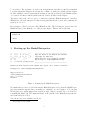
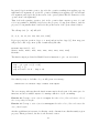
1
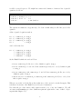
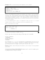
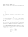
Getting Started With Haskell
Kees Doets and Jan van Eijck
First Chapter from ‘The Haskell Road to Logic, Math and Programming’
Preview
The purpose of the book of which this is the first chapter is to teach logic and mathematical
reasoning in practice, and to connect logical reasoning with computer programming.
It is convenient to choose a programming language for this that permits implementations to
remain as close as possible to the formal definitions. Such a language is the functional programming language Haskell [HT]. Haskell was named after the logician Haskell B. Curry. Curry,
together with Alonzo Church, laid the foundations of functional computation in the era Before
the Computer, around 1940. As a functional programming language, Haskell is a member of the
Lisp family. Others family members are Scheme, ML, Occam, Clean. Haskell98 is intended as
a standard for lazy functional programming. Lazy functional programming is a programming
style where arguments are evaluated only when the value is actually needed.
With Haskell, the step from formal definition to program is particularly easy. This presupposes,
of course, that you are at ease with formal definitions. Our reason for combining training in
reasoning with an introduction to functional programming is that your programming needs
will provide motivation for improving your reasoning skills. Haskell programs will be used as
illustrations for the theory throughout the book. We will always put computer programs and
pseudo-code of algorithms in frames (rectangular boxes).
The chapters of this book are written in so-called ‘literate programming’ style [Knu92]. Literate
programming is a programming style where the program and its documentation are generated
from the same source. The text of every chapter in this book can be viewed as the documentation
of the program code in that chapter. Literate programming makes it impossible for program
and documentation to get out of sync. Program documentation is an integrated part of literate
programming, in fact the bulk of a literate program is the program documentation. When writing
programs in literate style there is less temptation to write program code first while leaving the
documentation for later. Programming in literate style proceeds from the assumption that
the main challenge when programming is to make your program digestible for humans. For a
program to be useful, it should be easy for others to understand the code. It should also be easy
for you to understand your own code when you reread your stuff the next day or next week or
next month and try to figure out what you were up to when you wrote your program.
To save you the trouble of retyping, the code discussed in this book can be retrieved from the
1
book website.1 The program code is the text in typewriter font that you find in rectangular
boxes throughout the chapters. Boxes may also contain code that is not included in the chapter
modules, usually because it defines functions that are already predefined by the Haskell system,
or because it redefines a function that is already defined elsewhere in the chapter.
Typewriter font is also used for pieces of interaction with the Haskell interpreter, but these
illustrations of how the interpreter behaves when particular files are loaded and commands are
given are not boxed.
Every chapter of this book is a so-called Haskell module. The following two lines declare the
Haskell module for the Haskell code of the present chapter. This module is called GS.
module GS
where
1
Starting up the Haskell Interpreter
__
__
||
||
||___||
||---||
||
||
||
||
__ __ ____
___
|| || || || ||__
||__|| ||__|| __||
___||
Version: November 2002
_________________________________________
Hugs 98: Based on the Haskell 98 standard
Copyright (c) 1994-2002
World Wide Web: http://haskell.org/hugs
Report bugs to: [email protected]
_________________________________________
Haskell 98 mode: Restart with command line option -98 to enable extensions
Reading file "/usr/lib/hugs/lib/Prelude.hs":
Hugs session for:
/usr/lib/hugs/lib/Prelude.hs
Type :? for help
Prelude>
Figure 1: Starting up the Haskell interpreter.
We assume that you succeeded in retrieving the Haskell interpreter hugs from the Haskell homepage www.haskell.org and that you managed to install it on your computer. You can start
the interpreter by typing hugs at the system prompt. When you start hugs you should see
something like Figure (1). The string Prelude> on the last line is the Haskell prompt when no
user-defined files are loaded.
You can use hugs as a calculator as follows:
1
http://www.cwi.nl/~jve/HR
2
Prelude> 2^16
65536
Prelude>
The string Prelude> is the system prompt. 2^16 is what you type. After you hit the return
key (the key that is often labeled with Enter or ←-), the system answers 65536 and the prompt
Prelude> reappears.
Exercise 1 Try out a few calculations using * for multiplication, + for addition, - for subtraction, ^ for exponentiation, / for division. By playing with the system, find out what the
precedence order is among these operators.
Parentheses can be used to override the built-in operator precedences:
Prelude> (2 + 3)^4
625
To quit the Hugs interpreter, type :quit or :q at the system prompt.
2
Implementing a Prime Number Test
Suppose we want to implement a definition of prime number in a procedure that recognizes
prime numbers. A prime number is a natural number greater than 1 that has no proper divisors
other than 1 and itself. The natural numbers are 0, 1, 2, 3, 4, . . . The list of prime numbers starts
with 2, 3, 5, 7, 11, 13, . . . Except for 2, all of these are odd, of course.
Let n > 1 be a natural number. Then we use LD(n) for the least natural number greater than
1 that divides n. A number d divides n if there is a natural number a with a · d = n. In other
words, d divides n if there is a natural number a with nd = a, i.e., division of n by d leaves no
remainder. Note that LD(n) exists for every natural number n > 1, for the natural number
d = n is greater than 1 and divides n. Therefore, the set of divisors of n that are greater than
1 is non-empty. Thus, the set will have a least element.
The following proposition gives us all we need for implementing our prime number test:
Proposition 2
1. If n > 1 then LD(n) is a prime number.
2. If n > 1 and n is not a prime number, then (LD(n)) 2 ≤ n.
In the course of this book you will learn how to prove propositions like this.
Here is the proof of the first item. This is a proof by contradiction (see Chapter ??). Suppose,
for a contradiction that c = LD(n) is not a prime. Then there are natural numbers a and b with
3
c = a · b, and also 1 < a and a < c. But then a divides n, and contradiction with the fact that
c is the smallest natural number greater than 1 that divides n. Thus, LD(n) must be a prime
number.
For a proof of the second item, suppose that n > 1, n is not a prime and that p = LD(n). Then
there is a natural number a > 1 with n = p · a. Thus, a divides n. Since p is the smallest divisor
of n with p > 1, we have that p ≤ a, and therefore p 2 ≤ p · a = n, i.e., (LD(n))2 ≤ n.
The operator · in a·b is a so-called infix operator. The operator is written between its arguments.
If an operator is written before its arguments we call this prefix notation. The product of a and
b in prefix notation would look like this: · a b.
In writing functional programs, the standard is prefix notation. In an expression op a b, op
is the function, and a and b are the arguments. The convention is that function application
associates to the left, so the expression op a b is interpreted as (op a) b.
Using prefix notation, we define the operation divides that takes two integer expressions and
produces a truth value. The truth values true and false are rendered in Haskell as True and
False, respectively.
The integer expressions that the procedure needs to work with are called the arguments of the
procedure. The truth value that it produces is called the value of the procedure.
Obviously, m divides n if and only if the remainder of the process of dividing n by m equals 0.
The definition of divides can therefore be phrased in terms of a predefined procedure rem for
finding the remainder of a division process:
divides d n = rem n d == 0
The definition illustrates that Haskell uses = for ‘is defined as’ and == for identity. (The Haskell
symbol for non-identity is /=.)
A line of Haskell code of the form foo t = ... (or foo t1 t2 = ..., or foo t1 t2 t3= ...,
and so on) is called a Haskell equation. In such an equation, foo is called the function, and t
its argument.
Thus, in the Haskell equation divides d n = rem n d == 0, divides is the function, d is the
first argument, and n is the second argument.
Exercise 3 Put the definition of divides in a file prime.hs. Start the Haskell interpreter hugs
(Section 1). Now give the command :load prime or :l prime, followed by pressing Enter.
Note that l is the letter l, not the digit 1. (Next to :l, a very useful command after you have
edited a file of Haskell code is :reload or :r, for reloading the file.)
Prelude> :l prime
Main>
4
The string Main> is the Haskell prompt indicating that user-defined files are loaded. This is
a sign that the definition was added to the system. The newly defined operation can now be
executed, as follows:
Main> divides 5 7
False
Main>
The string Main> is the Haskell prompt, the rest of the first line is what you type. When you
press Enter the system answers with the second line, followed by the Haskell prompt. You can
then continue with:
Main> divides 5 30
True
It is clear from the proposition above that all we have to do to implement a primality test
is to give an implementation of the function LD. It is convenient to define LD in terms of a
second function LDF, for the least divisor starting from a given threshold k, with k ≤ n. Thus,
LDF(k)(n) is the least divisor of n that is ≥ k. Clearly, LD(n) = LDF(2)(n). Now we can
implement LD as follows:
ld n = ldf 2 n
This leaves the implementation ldf of LDF (details of the coding will be explained below):
ldf k n | divides k n = k
| k^2 > n
= n
| otherwise
= ldf (k+1) n
The definition employs the Haskell operation ^ for exponentiation, > for ‘greater than’, and +
for addition.
The definition of ldf makes use of equation guarding. The first line of the ldf definition handles
the case where the first argument divides the second argument. Every next line assumes that
the previous lines do not apply. The second line handles the case where the first argument does
not divide the second argument, and the square of the first argument is greater than the second
argument. The third line assumes that the first and second cases do not apply and handles all
other cases, i.e., the cases where k does not divide n and k 2 < n.
The definition employs the Haskell condition operator | . A Haskell equation of the form
foo t | condition = ...
5
is called a guarded equation. We might have written the definition of ldf as a list of guarded
equations, as follows:
ldf k n | divides k n = k
ldf k n | k^2 > n
= n
ldf k n
= ldf (k+1) n
The expression condition, of type Bool (i.e., Boolean or truth value), is called the guard of the
equation.
A list of guarded equations such as
foo
foo
foo
foo
t | condition_1 = body_1
t | condition_2 = body_2
t | condition_3 = body_3
t
= body_4
can be abbreviated as
foo t |
|
|
|
condition_1
condition_2
condition_3
otherwise
=
=
=
=
body_1
body_2
body_3
body_4
Such a Haskell definition is read as follows:
• in case condition_1 holds, foo t is by definition equal to body_1,
• in case condition_1 does not hold but condition_2 holds, foo t is by definition equal
to body_2,
• in case condition_1 and condition_2 do not hold but condition_3 holds, foo t is by
definition equal to body_3,
• and in case none of condition_1, condition_2 and condition_3 hold, foo t is by definition equal to body_4.
When we are at the end of the list we know that none of the cases above in the list apply. This
is indicated by means of the Haskell reserved keyword otherwise.
Note that the procedure ldf is called again from the body of its own definition. We will
encounter such recursive procedure definitions again and again in the course of this book (see
in particular Chapter ??).
6
Exercise 4 Suppose in the definition of ldf we replace the condition k^2 > n by k^2 >= n,
where >= expresses ‘greater than or equal’. Would that make any difference to the meaning of
the program? Why (not)?
Now we are ready for a definition of prime0, our first implementation of the test for being a
prime number.
prime0 n | n < 1
= error "not a positive integer"
| n == 1
= False
| otherwise = ld n == n
Haskell allows a call to the error operation in any definition. This is used to break off operation
and issue an appropriate message when the primality test is used for numbers below 1. Note
that error has a parameter of type String (indicated by the double quotes).
The definition employs the Haskell operation < for ‘less than’.
Intuitively, what the definition prime0 says is this:
1. the primality test should not be applied to numbers below 1,
2. if the test is applied to the number 1 it yields ‘false’,
3. if it is applied to an integer n greater than 1 it boils down to checking that LD(n) = n.
In view of the proposition we proved above, this is indeed a correct primality test.
Exercise 5 Add these definitions to the file prime.hs and try them out.
Remark. The use of variables in functional programming has much in common with the use
of variables in logic. The Haskell definition divides d n = rem n d == 0 is equivalent to
divides x y = rem y x == 0. This is because the variables denote arbitrary elements of the
type over which they range. They behave like universally quantified variables, and just as in
logic the definition does not depend on the variable names.
3
Haskell Type Declarations
Haskell has a concise way to indicate that divides consumes an integer, then another integer,
and produces a truth value (called Bool in Haskell). Integers and truth values are examples of
types. See Section ?? for more on the type Bool. Section 6 gives more information about types
in general. Arbitrary precision integers in Haskell have type Integer. The following line gives
a so-called type declaration for the divides function.
divides :: Integer -> Integer -> Bool
7
The type Integer -> Integer -> Bool should be read as Integer -> (Integer -> Bool).
A type of the form a -> b classifies a procedure that takes an argument of type a to produce
a result of type b. Thus, divides takes an argument of type Integer and produces a result of
type Integer -> Bool, i.e., a procedure that takes an argument of type Integer, and produces
a result of type Bool.
The full code for divides, including the type declaration, looks like this:
divides :: Integer -> Integer -> Bool
divides d n = rem n d == 0
If d is an expression of type Integer, then divides d is an expression of type Integer -> Bool.
The shorthand that we will use for “d is an expression of type Integer” is: d :: Integer.
Exercise 6 Can you gather from the definition of divides what the type declaration for rem
would look like?
Exercise 7 The hugs system has a command for checking the types of expressions. Can you
explain the following (please try it out; make sure that the file with the definition of divides is
loaded, together with the type declaration for divides):
Main> :t divides 5
divides 5 :: Integer -> Bool
Main> :t divides 5 7
divides 5 7 :: Bool
Main>
The expression divides 5 :: Integer -> Bool is called a type judgment. Type judgments in
Haskell have the form expression :: type.
In Haskell it is not strictly necessary to give explicit type declarations. For instance, the definition of divides works quite well without the type declaration, since the system can infer
the type from the definition. However, it is good programming practice to give explicit type
declarations even when this is not strictly necessary. These type declarations are an aid to
understanding, and they greatly improve the digestibility of functional programs for human
readers. A further advantage of the explicit type declarations is that they facilitate detection
of programming mistakes on the basis of type errors generated by the interpreter. You will find
that many programming errors already come to light when your program gets loaded. The fact
that your program is well typed does not entail that it is correct, of course, but many incorrect
programs do have typing mistakes.
The full code for ld, including the type declaration, looks like this:
8
ld :: Integer -> Integer
ld n = ldf 2 n
The full code for ldf, including the type declaration, looks like this:
ldf :: Integer -> Integer -> Integer
ldf k n | divides k n = k
| k^2 > n
= n
| otherwise
= ldf (k+1) n
The first line of the code states that the operation ldf takes two integers and produces an
integer.
The full code for prime0, including the type declaration, runs like this:
prime0 :: Integer ->
prime0 n | n < 1
| n == 1
| otherwise
Bool
= error "not a positive integer"
= False
= ld n == n
The first line of the code declares that the operation prime0 takes an integer and produces (or
returns, as programmers like to say) a Boolean (truth value).
In programming generally, it is useful to keep close track of the nature of the objects that are
being represented. This is because representations have to be stored in computer memory, and
one has to know how much space to allocate for this storage. Still, there is no need to always
specify the nature of each data-type explicitly. It turns out that much information about the
nature of an object can be inferred from how the object is handled in a particular program, or
in other words, from the operations that are performed on that object.
Take again the definition of divides. It is clear from the definition that an operation is defined
with two arguments, both of which are of a type for which rem is defined, and with a result of
type Bool (for rem n d == 0 is a statement that can turn out true or false). If we check the
type of the built-in procedure rem we get:
Prelude> :t rem
rem :: Integral a => a -> a -> a
In this particular case, the type judgment gives a type scheme rather than a type. It means: if
a is a type of class Integral, then rem is of type a -> a -> a. Here a is used as a variable
ranging over types.
9
In Haskell, Integral is the class (see Section ??) consisting of the two types for integer numbers,
Int and Integer. The difference between Int and Integer is that objects of type Int have
fixed precision, objects of type Integer have arbitrary precision.
The type of divides can now be inferred from the definition. This is what we get when we load
the definition of divides without the type declaration:
Main> :t divides
divides :: Integral a => a -> a -> Bool
4
Identifiers in Haskell
In Haskell, there are two kinds of identifiers:
• Variable identifiers are used to name functions. They have to start with a lower-case letter.
Examples are map, max, fct2list, fctToList, fct_to_list.
• Constructor identifiers are used to name types. They have to start with an upper-case
letter. Examples are True, False.
Functions are operations on data-structures, constructors are the building blocks of the data
structures themselves (trees, lists, Booleans, and so on).
Names of functions always start with lower-case letters, and may contain both upper- and
lower-case letters, but also digits, underscores and the prime symbol ’. The following reserved
keywords have special meanings and cannot be used to name functions.
case
if
let
class
import
module
data
in
newtype
default
infix
of
deriving
infixl
then
do
infixr
type
else
instance
where
The use of these keywords will be explained as we encounter them. at the beginning of a word
is treated as a lower-case character; all by itself is a reserved word for the wild card pattern
that matches anything (page ??).
5
Playing the Haskell Game
This section consists of a number of further examples and exercises to get you acquainted with
the programming language of this book. To save you the trouble of keying in the programs
below, you should retrieve the module GS.hs for the present chapter from the book website and
load it in hugs. This will give you a system prompt GS>, indicating that all the programs from
this chapter are loaded.
In the next example, we use Int for the type of fixed precision integers, and [Int] for lists of
fixed precision integers.
10
Example 8 Here is a function that gives the minimum of a list of integers:
mnmInt
mnmInt
mnmInt
mnmInt
:: [Int] -> Int
[] = error "empty list"
[x] = x
(x:xs) = min x (mnmInt xs)
This uses the predefined function min for the minimum of two integers. It also uses pattern
matching for lists . The list pattern [] matches only the empty list, the list pattern [x] matches
any singleton list, the list pattern (x:xs) matches any non-empty list. A further subtlety is that
pattern matching in Haskell is sensitive to order. If the pattern [x] is found before (x:xs) then
(x:xs) matches any non-empty list that is not a unit list. See Section ?? for more information
on list pattern matching.
It is common Haskell practice to refer to non-empty lists as x:xs, y:ys, and so on, as a useful
reminder of the facts that x is an element of a list of x’s and that xs is a list.
Here is a home-made version of min:
min’ :: Int -> Int -> Int
min’ x y | x <= y
= x
| otherwise = y
You will have guessed that <= is Haskell code for ≤.
Objects of type Int are fixed precision integers. Their range can be found with:
Prelude> primMinInt
-2147483648
Prelude> primMaxInt
2147483647
Since 2147483647 = 231 − 1, we can conclude that the hugs implementation uses four bytes (32
bits) to represent objects of this type. Integer is for arbitrary precision integers: the storage
space that gets allocated for Integer objects depends on the size of the object.
Exercise 9 Define a function that gives the maximum of a list of integers. Use the predefined
function max.
Conversion from Prefix to Infix in Haskell A function can be converted to an infix operator
by putting its name in back quotes, like this:
11
Prelude> max 4 5
5
Prelude> 4 ‘max‘ 5
5
Conversely, an infix operator is converted to prefix by putting the operator in round brackets
(p. 18).
Exercise 10 Define a function removeFst that removes the first occurrence of an integer m
from a list of integers. If m does not occur in the list, the list remains unchanged.
Example 11 We define a function that sorts a list of integers in order of increasing size, by
means of the following algorithm:
• an empty list is already sorted.
• if a list is non-empty, we put its minimum in front of the result of sorting the list that
results from removing its minimum.
This is implemented as follows:
srtInts :: [Int] -> [Int]
srtInts [] = []
srtInts xs = m : (srtInts (removeFst m xs)) where m = mnmInt xs
Here removeFst is the function you defined in Exercise 10. Note that the second clause is
invoked when the first one does not apply, i.e., when the argument of srtInts is not empty.
This ensures that mnmInt xs never gives rise to an error.
Note the use of a where construction for the local definition of an auxiliary function.
Remark. Haskell has two ways to locally define auxiliary functions, where and let constructions. The where construction is illustrated in Example 11. This can also expressed with let,
as follows:
srtInts’ :: [Int] -> [Int]
srtInts’ [] = []
srtInts’ xs = let
m = mnmInt xs
in m : (srtInts’ (removeFst m xs))
The let construction uses the reserved keywords let and in.
12
Example 12 Here is a function that calculates the average of a list of integers. The average of
n1 +···+nk
m and n is given by m+n
. In
2 , the average of a list of k integers n 1 , . . . , nk is given by
k
general, averages are fractions, so the result type of average should not be Int but the Haskell
data-type for floating point numbers, which is Float. There are predefined functions sum for the
sum of a list of integers, and length for the length of a list. The Haskell operation for division
/ expects arguments of type Float, so we need a conversion function for converting Ints into
Floats. This is done by fromInt. The function average can now be written as:
average :: [Int] -> Float
average [] = error "empty list"
average xs = fromInt (sum xs) / fromInt (length xs)
Again, it is instructive to write our own homemade versions of sum and length. Here they are:
sum’ :: [Int] -> Int
sum’ [] = 0
sum’ (x:xs) = x + sum’ xs
length’ :: [a] -> Int
length’ [] = 0
length’ (x:xs) = 1 + length’ xs
Note that the type declaration for length’ contains a variable a. This variable ranges over all
types, so [a] is the type of a list of objects of an arbitrary type a. We say that [a] is a type
scheme rather than a type. This way, we can use the same function length’ for computing the
length of a list of integers, the length of a list of characters, the length of a list of strings (lists
of characters), and so on.
The type [Char] is abbreviated as String. Examples of characters are ’a’, ’b’ (note the
single quotes) examples of strings are "Russell" and "Cantor" (note the double quotes). In
fact, "Russell" can be seen as an abbreviation of the list
[’R’,’u’,’s’,’s’,’e’,’l’,’l’].
Exercise 13 Write a function count for counting the number of occurrences of a character in
a string. In Haskell, a character is an object of type Char, and a string an object of type String,
so the type declaration should run: count :: Char -> String -> Int.
13
Exercise 14 A function for transforming strings into strings is of type String -> String.
Write a function blowup that converts a string a 1 a2 a3 · · · to a1 a2 a2 a3 a3 a3 · · · . blowup "bang!"
should yield "baannngggg!!!!!". (Hint: use ++ for string concatenation.)
Exercise 15 Write a function srtString that sorts a list of strings in alphabetical order. The
type declaration should run: srtString :: [String] -> [String].
Example 16 Suppose we want to check whether a string str1 is a prefix of a string str2. Then
the answer to the question prefix str1 str2 should be either yes (true) or no (false), i.e., the
type declaration for prefix should run: prefix :: String -> String -> Bool.
Prefixes of a string ys are defined as follows:
1. [] is a prefix of ys,
2. if xs is a prefix of ys, then x:xs is a prefix of x:ys,
3. nothing else is a prefix of ys.
Here is the code for prefix that implements this definition:
prefix
prefix
prefix
prefix
:: String -> String -> Bool
[] ys = True
(x:xs) [] = False
(x:xs) (y:ys) = (x==y) && prefix xs ys
The definition of prefix uses the Haskell operator && for conjunction.
Exercise 17 Write a function substring that checks whether str1 is a substring of str2. The
type declaration should run: substring :: String -> String -> Bool.
The substrings of an arbitrary string ys are given by:
1. if xs is a prefix of ys, xs is a substring of ys,
2. if ys equals y:ys’ and xs is a substring of ys’, xs is a substring of ys,
3. nothing else is a substring of ys.
6
Haskell Types
The basic Haskell types are:
• Int and Integer, to represent integers. Elements of Integer are unbounded. That’s why
we used this type in the implementation of the prime number test.
14
• Float and Double represent floating point numbers. The elements of Double have higher
precision.
• Bool is the type of Booleans.
• Char is the type of characters.
Note that the name of a type always starts with a capital letter.
To denote arbitrary types, Haskell allows the use of type variables. For these, a, b, . . . , are used.
New types can be formed in several ways:
• By list-formation: if a is a type, [a] is the type of lists over a. Examples: [Int] is the
type of lists of integers; [Char] is the type of lists of characters, or strings.
• By pair- or tuple-formation: if a and b are types, then (a,b) is the type of pairs with
an object of type a as their first component, and an object of type b as their second
component. Similarly, triples, quadruples, . . . , can be formed. If a, b and c are types,
then (a,b,c) is the type of triples with an object of type a as their first component,
an object of type b as their second component, and an object of type c as their third
component. And so on (p. ??).
• By function definition: a -> b is the type of a function that takes arguments of type a
and returns values of type b.
• By defining your own data-type from scratch, with a data type declaration. More about
this in due course.
Pairs will be further discussed in Section ??, lists and list operations in Section ??.
Operations are procedures for constructing objects of a certain types b from ingredients of a
type a. Now such a procedure can itself be given a type: the type of a transformer from a type
objects to b type objects. The type of such a procedure can be declared in Haskell as a -> b.
If a function takes two string arguments and returns a string then this can be viewed as a
two-stage process: the function takes a first string and returns a transformer from strings to
strings. It then follows that the type is String -> (String -> String), which can be written
as String -> String -> String, because of the Haskell convention that -> associates to the
right.
Exercise 18 Find expressions with the following types:
1. [String]
2. (Bool,String)
3. [(Bool,String)]
4. ([Bool],String)
15
5. Bool -> Bool
Test your answers by means of the Hugs command :t.
Exercise 19 Use the Hugs command :t to find the types of the following predefined functions:
1. head
2. last
3. init
4. fst
5. (++)
6. flip
7. flip (++)
Next, supply these functions with arguments of the expected types, and try to guess what these
functions do.
7
The Prime Factorization Algorithm
Let n be an arbitrary natural number > 1. A prime factorization of n is a list of prime numbers
p1 , . . . , pj with the property that p1 ·· · ··pj = n. We will show that a prime factorization of every
natural number n > 1 exists by producing one by means of the following method of splitting off
prime factors:
n
END
WHILE n 6= 1 DO BEGIN p := LD(n); n :=
p
Here := denotes assignment or the act of giving a variable a new value. As we have seen, LD(n)
exists for every n with n > 1. Moreover, we have seen that LD(n) is always prime. Finally, it is
clear that the procedure terminates, for every round through the loop will decrease the size of
n.
So the algorithm consists of splitting off primes until we have written n as n = p 1 · · · pj , with all
factors prime. To get some intuition about how the procedure works, let us see what it does for
an example case, say n = 84. The original assignment to n is called n 0 ; successive assignments
to n and p are called n1 , n2 , . . . and p1 , p2 , . . ..
n0
n1
n2
n3
n4
6= 1
6= 1
6= 1
6= 1
=1
p1
p2
p3
p4
=2
=2
=3
=7
n0
n1
n2
n3
n4
16
= 84
= 84/2 = 42
= 42/2 = 21
= 21/3 = 7
= 7/7 = 1
This gives 84 = 22 · 3 · 7, which is indeed a prime factorization of 84.
The following code gives an implementation in Haskell, collecting the prime factors that we find
in a list. The code uses the predefined Haskell function div for integer division.
factors :: Integer ->
factors n | n < 1
| n == 1
| otherwise
[Integer]
= error "argument not positive"
= []
= p : factors (div n p) where p = ld n
If you load the code for this chapter, you can try this out as follows:
GS> factors 84
[2,2,3,7]
GS> factors 557940830126698960967415390
[2,3,5,7,11,13,17,19,23,29,31,37,41,43,47,53,59,61,67,71]
8
Working with Lists: the map and filter Functions
Haskell allows some convenient abbreviations for lists: [4..20] denotes the list of integers from
4 through 20, [’a’..’z’] the list "abcdefghijklmnopqrstuvwxyz" of all lower case letters.
The call [5..] generates an infinite list of integers starting from 5. And so on.
If you use the Hugs command :t to find the type of the function map, you get the following:
Prelude> :t map
map :: (a -> b) -> [a] -> [b]
The function map takes a function and a list and returns a list containing the results of applying
the function to the individual list members.
If f is a function of type a -> b and xs is a list of type [a], then map f xs will return a list of
type [b]. E.g., map (^2) [1..9] will produce the list of squares
[1, 4, 9, 16, 25, 36, 49, 64, 81]
You should verify this by trying it out in Hugs. The use of (^2) for the operation of squaring
demonstrates a new feature of Haskell, the construction of sections.
Conversion from Infix to Prefix, Construction of Sections If op is an infix operator,
(op) is the prefix version of the operator. Thus, 2^10 can also be written as (^) 2 10. This is
a special case of the use of sections in Haskell.
17
In general, if op is an infix operator, (op x) is the operation resulting from applying op to its
right hand side argument, (x op) is the operation resulting from applying op to its left hand
side argument, and (op) is the prefix version of the operator (this is like the abstraction of the
operator from both arguments).
Thus (^2) is the squaring operation, (2^) is the operation that computes powers of 2, and
(^) is exponentiation. Similarly, (>3) denotes the property of being greater than 3, (3>) the
property of being smaller than 3, and (>) is the prefix version of the ‘greater than’ relation.
The call map (2^) [1..10] will yield
[2, 4, 8, 16, 32, 64, 128, 256, 512, 1024]
If p is a property (an operation of type a -> Bool) and xs is a list of type [a], then map p xs
will produce a list of type Bool (a list of truth values), like this:
Prelude> map (>3) [1..10]
[False, False, False, True, True, True, True, True, True, True]
Prelude>
The function map is predefined in Haskell, but it is instructive to give our own version:
map :: (a -> b) -> [a] -> [b]
map f [] = []
map f (x:xs) = (f x) : (map f xs)
Note that if you try to load this code, you will get an error message:
Definition of variable "map" clashes with import.
The error message indicates that the function name map is already part of the name space for
functions, and is not available anymore for naming a function of your own making.
Exercise 20 Use map to write a function lengths that takes a list of lists and returns a list of
the corresponding list lengths.
Exercise 21 Use map to write a function sumLengths that takes a list of lists and returns the
sum of their lengths.
Another useful function is filter, for filtering out the elements from a list that satisfy a given
property. This is predefined, but here is a home-made version:
18
filter :: (a -> Bool) -> [a] -> [a]
filter p [] = []
filter p (x:xs) | p x
= x : filter p xs
| otherwise = filter p xs
Here is an example of its use:
GS> filter (>3) [1..10]
[4,5,6,7,8,9,10]
Example 22 Here is a program primes0 that filters the prime numbers from the infinite list
[2..] of natural numbers:
primes0 :: [Integer]
primes0 = filter prime0 [2..]
This produces an infinite list of primes. (Why infinite? See Theorem ??.) The list can be
interrupted with ‘Control-C’.
Example 23 Given that we can produce a list of primes, it should be possible now to improve
our implementation of the function LD. The function ldf used in the definition of ld looks for
√
a prime divisor of n by checking k|n for all k with 2 ≤ k ≤ n. In fact, it is enough to check
√
p|n for the primes p with 2 ≤ p ≤ n. Here are functions ldp and ldpf that perform this more
efficient check:
ldp :: Integer -> Integer
ldp n = ldpf primes1 n
ldpf :: [Integer] -> Integer
ldpf (p:ps) n | rem n p == 0
| p^2 > n
| otherwise
-> Integer
= p
= n
= ldpf ps n
ldp makes a call to primes1, the list of prime numbers. This is a first illustration of a ‘lazy
list’. The list is called ‘lazy’ because we compute only the part of the list that we need for further
processing. To define primes1 we need a test for primality, but that test is itself defined in terms
of the function LD, which in turn refers to primes1. We seem to be running around in a circle.
19
This circle can be made non-vicious by avoiding the primality test for 2. If it is given that 2 is
prime, then we can use the primality of 2 in the LD check that 3 is prime, and so on, and we
are up and running.
primes1 :: [Integer]
primes1 = 2 : filter prime [3..]
prime :: Integer ->
prime n | n < 1
| n == 1
| otherwise
Bool
= error "not a positive integer"
= False
= ldp n == n
Replacing the definition of primes1 by filter prime [2..] creates vicious circularity, with
stack overflow as a result (try it out). By running the program primes1 against primes0 it is
easy to check that primes1 is much faster.
Exercise 24 What happens when you modify the defining equation of ldp as follows:
ldp :: Integer -> Integer
ldp = ldpf primes1
Can you explain?
9
Haskell Equations and Equational Reasoning
The Haskell equations f x y = ... used in the definition of a function f are genuine mathematical equations. They state that the left hand side and the right hand side of the equation
have the same value. This is very different from the use of = in imperative languages like C or
Java. In a C or Java program, the statement x = x*y does not mean that x and x ∗ y have the
same value, but rather it is a command to throw away the old value of x and put the value of
x ∗ y in its place. It is a so-called destructive assignment statement: the old value of a variable
is destroyed and replaced by a new one.
Reasoning about Haskell definitions is a lot easier than reasoning about programs that use
destructive assignment. In Haskell, standard reasoning about mathematical equations applies.
E.g., after the Haskell declarations x = 1 and y = 2, the Haskell declaration x = x + y will raise
an error "x" multiply defined. Because = in Haskell has the meaning “is by definition equal
to”, while redefinition is forbidden, reasoning about Haskell functions is standard equational
reasoning. Let’s try this out on a simple example.
20
a
b
f
f
= 3
= 4
:: Integer -> Integer -> Integer
x y = x^2 + y^2
To evaluate f a (f a b) by equational reasoning, we can proceed as follows:
f a (f a b) = f a (a2 + b2 )
= f 3 (32 + 42 )
= f 3 (9 + 16)
= f 3 25
= 32 + 252
= 9 + 625
= 634
The rewriting steps use standard mathematical laws and the Haskell definitions of a, b, f . And,
in fact, when running the program we get the same outcome:
GS> f a (f a b)
634
GS>
Remark. We already encountered definitions where the function that is being defined occurs
on the right hand side of an equation in the definition. Here is another example:
g :: Integer -> Integer
g 0
= 0
g (x+1) = 2 * (g x)
Not everything that is allowed by the Haskell syntax makes semantic sense, however. The
following definitions, although syntactically correct, do not properly define functions:
h1 :: Integer -> Integer
h1 0 = 0
h1 x = 2 * (h1 x)
h2 :: Integer -> Integer
h2 0 = 0
h2 x = h2 (x+1)
21
The problem is that for values other than 0 the definitions do not give recipes for computing a
value. This matter will be taken up in a later Chapter.
10
Further Reading
The standard Haskell operations are defined in the file Prelude.hs, which you should be able to
locate somewhere on any system that runs hugs. During startup of your hugs session, you will
see a line like this:
Reading file "/usr/lib/hugs/lib/Prelude.hs":
This indicates that (in this example) the Prelude.hs file is in directory /usr/lib/hugs/lib/.
In case Exercise 19 has made you curious, the definitions of these example functions can all be
found in Prelude.hs. If you want to quickly learn a lot about how to program in Haskell, you
should get into the habit of consulting this file regularly. The definitions of all the standard
operations are open source code, and are there for you to learn from. The Haskell Prelude may
be a bit difficult to read at first, but you will soon get used to the syntax and acquire a taste
for the style.
Various tutorials on Haskell and Hugs can be found on the Internet: see e.g. [HFP96] and
[JR+ ]. The definitive reference for the language is [Jon03]. A textbook on Haskell focusing on
multimedia applications is [Hud00]. Other excellent textbooks on functional programming with
Haskell are [Tho99] and, at a more advanced level, [Bir98]. A book on discrete mathematics that
also uses Haskell as a tool, and with a nice treatment of automated proof checking, is [HO00].
References
[Bir98]
R. Bird. Introduction to Functional Programming Using Haskell. Prentice Hall, 1998.
[HFP96] P. Hudak, J. Fasel, and J. Peterson. A gentle introduction to Haskell. Technical report,
Yale University, 1996. Available from the Haskell homepage: http://www.haskell.
org.
[HO00]
C. Hall and J. O’Donnell. Discrete Mathematics Using A Computer. Springer, 2000.
[HT]
The Haskell Team. The Haskell homepage. http://www.haskell.org.
[Hud00] P. Hudak. The Haskell School of Expression: Learning Functional Programming
Through Multimedia. Cambridge University Press, 2000.
[Jon03]
S. Peyton Jones, editor. Haskell 98 Language and Libraries; The Revised Report.
Cambridge University Press, 2003.
[JR+ ]
Mark P. Jones, Alastair Reid, et al. The Hugs98 user manual. http://www.haskell.
org/hugs/.
22
[Knu92] D.E. Knuth. Literate Programming. CSLI Lecture Notes, no. 27. CSLI, Stanford, 1992.
[Tho99] S. Thompson. Haskell: the craft of functional programming (second edition). Addison
Wesley, 1999.
23