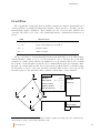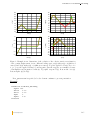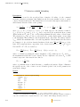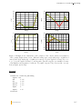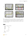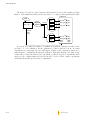
1
Material & Structure Analysis Suite Materials manual Version 8.6 Z-set 8.6 is distributed by Transvalor S.A. Centre des Matériaux B.P. 87 Ð 91003 EVRY Cedex France http://www.zset-software.com [email protected] Neither Transvalor, ARMINES nor ONERA assume responsibility for any errors appearing in this document. Information provided in this document is furnished for informational use only, is subject to change without notice, and should not be construed as a commitment by the distributors. Z-set, ZebFront, Z-mat, Z-cracks and Zebulon are trademarks of ARMINES, ONERA and Northwest Numerics and Modeling, Inc. c ARMINES and ONERA, 2015. Proprietary data. Unauthorized use, distribution, or duplication is prohibited. All rights reserved. Abaqus, the 3DS logo, SIMULIA, CATIA, and Unified FEA are trademarks or registered trademarks of Dassault Systèmes or its subsidiaries in the United States and/or other countries. ANSYS is a registered trademark of Ansys, Inc. Solaris is a registered trademark of Sun Microsystems. Silicon Graphics is a registered trademark of Silicon Graphics, Inc. Hewlett Packard is a registered trademark of Hewlett Packard Co. Windows, Windows XP, Windows 2000, and Windows NT are registered trademarks of Microsoft Corp. Contents Introduction What’s in this manual Conventions . . . . . . Introduction to Z-mat System Requirements Material Frameworks . . . . . . . . . . . . . . . . . . . . . . . . . . . . . . . . . . . . . . . . . . . . . . . . . . . . . . . . . . . . . . . . . . . . . . . . . . . . . . . . . . . . . . . . . . . . . . . . . . . . . . . . . . . . . . . . . . . . . . . . . . . . . . . . . . . . . . . . . . . . . 1.1 1.3 1.5 1.7 1.9 1.11 Z-mat General Commands Z-mat interfaces . . . . . . Interface files . . . . . . . . ***automatic time . ***behavior . . . . . ***debug . . . . . . ***external storage . ***material . . . . . ***parameter . . . . ***save energies . . ***skip cycle . . . . Zmaster interfaces . . . . . . . . . . . . . . . . . . . . . . . . . . . . . . . . . . . . . . . . . . . . . . . . . . . . . . . . . . . . . . . . . . . . . . . . . . . . . . . . . . . . . . . . . . . . . . . . . . . . . . . . . . . . . . . . . . . . . . . . . . . . . . . . . . . . . . . . . . . . . . . . . . . . . . . . . . . . . . . . . . . . . . . . . . . . . . . . . . . . . . . . . . . . . . . . . . . . . . . . . . . . . . . . . . . . . . . . . . . . . . . . . . . . . . . . . . . . . . . . . . . . . . . . . . . . . . . . . . . . . . . . . . . . . . . . . . . . . . . . . . . . . . . . . . . . . . . . . . . . . . 2.1 2.3 2.5 2.8 2.9 2.10 2.11 2.12 2.18 2.19 2.20 2.21 . . . . . . . . . 3.1 3.3 3.5 3.7 3.9 3.11 3.13 3.15 3.17 3.19 Z-mat ANSYS Zansys ANSYS interface . . . . . . . . . . . . . . . . . . . . . . . . . . . . . 4.1 4.3 Z-mat MSC-Marc Z-mat MSC-Marc interface . . . . . . . . . . . . . . . . . . . . . . . . . . . 5.1 5.3 Z-mat SAMCEF Z-mat SAMCEF interface . . . . . . . . . . . . . . . . . . . . . . . . . . . . 6.1 6.3 . . . . . . . . . . Z-mat ABAQUS Z-mat ABAQUS interface Current status . . . . . . Site definition . . . . . . . Interface files . . . . . . . Output variables . . . . . Extra files . . . . . . . . . User additions . . . . . . Example . . . . . . . . . . Post calculations . . . . . . . . . . . . . . . . . . . . . . . . . . . . . . . . . . . . . . . . . . . . . . . . . . . . . . . . . . . . . . . . . . . . . . . . . . . . . . . . . . . . . . . . . . . . . . . . . . . . . . . . . . . . . . . . . . . . . . . . . . . . . . . . . . . . . . . . . . . . . . . . . . . . . . . . . . . . . . . . . . . . . . . . . . . . . . . . . . . . . . . . . . . . . . . . . . . . . . . . . . . . . . . . . . . . . . . . . . . . . . . . . . . . . . . . . . . . . . . . . . . . . . . . Z-mat Cosmos Z-mat Cosmos/M interface . . . . . . . . . . . . . . . . . . . . . . . . . . . 7.1 7.3 Z-mat LS-Dyna Zlsdyna LS-Dyna interface . . . . . . . . . . . . . . . . . . . . . . . . . . . . 8.1 8.3 Behavior functionality Introduction to Behaviors Grad-Flux . . . . . . . . . Material variables . . . . . Material file . . . . . . . . BEHAVIOR . . . . . . . . . . . . . . . . . . . . . . . . . . . . . . . . . . . . . . . . . . . . . . . . . . . . . . . . . . . . . . . . . . . . . . . . . . . . . . . . . . . . . . . . . . . . . . . . . . . . . . . . . . . . . . . . . . . . . . . . . . . . . . . . . . . . . . . . . . . . . . . . . . . . 9.1 9.3 9.5 9.7 9.11 9.13 Material Models linear elastic . . . . . damage elasticity . . . hyper elastic . . . . . linear viscoelastic . . . viscoelastic spectral . hyperviscoelastic . . . gen evp . . . . . . . . reduced plastic . . . . porous plastic . . . . . mechanical step phase umat . . . . . . . . . . . . . . . . . . . . . . . . . . . . . . . . . . . . . . . . . . . . . . . . . . . . . . . . . . . . . . . . . . . . . . . . . . . . . . . . . . . . . . . . . . . . . . . . . . . . . . . . . . . . . . . . . . . . . . . . . . . . . . . . . . . . . . . . . . . . . . . . . . . . . . . . . . . . . . . . . . . . . . . . . . . . . . . . . . . . . . . . . . . . . . . . . . . . . . . . . . . . . . . . . . . . . . . . . . . . . . . . . . . . . . . . . . . . . . . . . . . . . . . . . . . . . . . . . . . . . . . . . . . . . . . . . . . . . . . . . . . . . . . . . . . . . . . . . . . . . . . . . . . . . . . . . . . . . . . . . . . . . . . . . . . . . . . . . . . . 10.1 10.3 10.4 10.5 10.6 10.9 10.12 10.13 10.16 10.18 10.24 10.25 Secondary Models aging . . . . . . . . aniso damage . . . becker needleman . cast iron . . . . . . bodner partom . . finite strain crystal matmod . . . . . . matmod z . . . . . memory . . . . . . non associated . . visco aniso damage . . . . . . . . . . . . . . . . . . . . . . . . . . . . . . . . . . . . . . . . . . . . . . . . . . . . . . . . . . . . . . . . . . . . . . . . . . . . . . . . . . . . . . . . . . . . . . . . . . . . . . . . . . . . . . . . . . . . . . . . . . . . . . . . . . . . . . . . . . . . . . . . . . . . . . . . . . . . . . . . . . . . . . . . . . . . . . . . . . . . . . . . . . . . . . . . . . . . . . . . . . . . . . . . . . . . . . . . . . . . . . . . . . . . . . . . . . . . . . . . . . . . . . . . . . . . . . . . . . . . . . . . . . . . . . . . . . . . . . . . . . . . . . . . . . . . . . . . . . . . . . . . . . . . . . . . . . . . . . . . . . . . . . . . . . . . . . . . . . . . . 11.1 11.3 11.5 11.7 11.9 11.11 11.13 11.15 11.17 11.19 11.20 11.22 Other Models coefficient diffusion . . needleman debonding crisfield debonding . . chaboche debonding . generalized debonding diffusion . . . . . . . . linear spring . . . . . . thermal . . . . . . . . . . . . . . . . . . . . . . . . . . . . . . . . . . . . . . . . . . . . . . . . . . . . . . . . . . . . . . . . . . . . . . . . . . . . . . . . . . . . . . . . . . . . . . . . . . . . . . . . . . . . . . . . . . . . . . . . . . . . . . . . . . . . . . . . . . . . . . . . . . . . . . . . . . . . . . . . . . . . . . . . . . . . . . . . . . . . . . . . . . . . . . . . . . . . . . . . . . . . . . . . . . . . . . . . . . . . . . . . . . . . . . . . . . . . . . . . . . . . . . . . 12.1 12.3 12.4 12.6 12.8 12.10 12.14 12.15 12.16 . . . . . . . . . . . variable friction . . . . . . . . . . . . . . . . . . . . . . . . . . . . . . . . . . Material Components ANISOTROPIC DAMAGE . . . . . . . . . ANISOTROPIC DAMAGE scalar . . . . . ANISOTROPIC DAMAGE elastic tensorial COEFFICIENT . . . . . . . . . . . . . . . . COEFFICIENT MATRIX . . . . . . . . . . CONDUCTIVITY . . . . . . . . . . . . . . CRITERION . . . . . . . . . . . . . . . . . CRITERION anisotropic . . . . . . . . . . . CRITERION bron . . . . . . . . . . . . . . CRITERION cast iron . . . . . . . . . . . . CRITERION hill . . . . . . . . . . . . . . . CRITERION karafillis boyce . . . . . . . . CRITERION linear drucker prager . . . . . CRITERION mises . . . . . . . . . . . . . . CRITERION modified nouailhas . . . . . . CRITERION nouailhas . . . . . . . . . . . CRITERION ratio . . . . . . . . . . . . . . CRITERION tensile mises . . . . . . . . . . CRITERION tresca . . . . . . . . . . . . . CRITERION unsym . . . . . . . . . . . . . CRITERION 2M1C . . . . . . . . . . . . . CRYSTAL KINEMATIC . . . . . . . . . . CRYSTAL ORIENTATION . . . . . . . . . DAMAGE . . . . . . . . . . . . . . . . . . . DIRECT KINEMATIC . . . . . . . . . . . DIRECT KINEMATIC asaro . . . . . . . . DIRECT KINEMATIC non symmetric . . . ELASTICITY . . . . . . . . . . . . . . . . . FLOW . . . . . . . . . . . . . . . . . . . . . FLOW function . . . . . . . . . . . . . . . . FLOW gsell . . . . . . . . . . . . . . . . . . FLOW hyperbolic . . . . . . . . . . . . . . FLOW modified visco . . . . . . . . . . . . FLOW sellars tegart . . . . . . . . . . . . . FLOW sum . . . . . . . . . . . . . . . . . . INTERACTION . . . . . . . . . . . . . . . ISOTROPIC . . . . . . . . . . . . . . . . . KINEMATIC . . . . . . . . . . . . . . . . . KINEMATIC aniso nonlinear . . . . . . . . LOCALIZATION . . . . . . . . . . . . . . . POROUS CRITERION . . . . . . . . . . . POROUS CRITERION cam clay . . . . . . POROUS CRITERION elliptic . . . . . . . POROUS CRITERION elliptic aniso . . . . . . . . . . . . . . . . . . . . . . . . . . . . . . . . . . . . . . . . . . . . . . . . . . . . . . . . . . . . . . . . . . . . . . . . . . . . . . . . . . . . . . . . . . . . . . . . . . . . . . . . . . . . . . . . . . . . . . . . . . . . . . . . . . . . . . . . . . . . . . . . . . . . . . . . . . . . . . . . . . . . . . . . . . . . . . . . . . . . . . . . . . . . . . . . . . . . . . . . . . . . . . . . . . . . . . . . . . . . . . . . . . . . . . . . . . . . . . . . . . . . . . . . . . . . . . . . . . . . . . . . . . . . . . . . . . . . . . . . . . . . . . . . . . . . . . . . . . . . . . . . . . . . . . . . . . . . . . . . . . . . . . . . . . . . . . . . . . . . . . . . . . . . . . . . . . . . . . . . . . . . . . . . . . . . . . . . . . . . . . . . . . . . . . . . . . . . . . . . . . . . . . . . . . . . . . . . . . . . . . . . . . . . . . . . . . . . . . . . . . . . . . . . . . . . . . . . . . . . . . . . . . . . . . . . . . . . . . . . . . . . . . . . . . . . . . . . . . . . . . . . . . . . . . . . . . . . . . . . . . . . . . . . . . . . . . . . . . . . . . . . . . . . . . . . . . . . . . . . . . . . . . . . . . . . . . . . . . . . . . . . . . . . . . . . . . . . . . . . . . . . . . . . . . . . . . . . . . . . . . . . . . . . . . . . . . . . . . . . . . . . . . . . . . . . . . . . . . . . . . . . . . . . . . . . . . . . . . . . . . . . . . . . . . . . . . . . . . . . . . . . . . . . . . . . . . . . . . . . . . . . . . . . . . . . . . . . . . . . . . . . . . . . . . . . . . . . . . . . . . . . . . . . . . . . . . . . . . . . . . . . . . . . . . . . . . . . 12.17 13.1 13.3 13.5 13.6 13.7 13.9 13.13 13.14 13.15 13.16 13.17 13.18 13.19 13.20 13.22 13.23 13.24 13.25 13.26 13.27 13.28 13.29 13.30 13.31 13.35 13.38 13.39 13.41 13.43 13.44 13.46 13.47 13.48 13.49 13.50 13.51 13.52 13.54 13.57 13.60 13.61 13.63 13.64 13.65 13.66 POROUS CRITERION fkm . . . . . . . . . POROUS CRITERION gurson . . . . . . . POROUS CRITERION rousselier . . . . . . POROUS CRITERION modified rousselier POROUS CRITERION zhang niemi . . . . POTENTIAL . . . . . . . . . . . . . . . . . POTENTIAL associated . . . . . . . . . . . POTENTIAL coupled recovery . . . . . . . POTENTIAL delobelle . . . . . . . . . . . POTENTIAL crystal . . . . . . . . . . . . . POTENTIAL gen evp . . . . . . . . . . . . POTENTIAL gen evp2 . . . . . . . . . . . POTENTIAL suvic . . . . . . . . . . . . . . POTENTIAL 2M1C . . . . . . . . . . . . . POTENTIAL z6 gen evp . . . . . . . . . . SINTERING STRAIN . . . . . . . . . . . . SLIP INTERACTION . . . . . . . . . . . . STRAIN NUCLEATION . . . . . . . . . . THERMAL STRAIN . . . . . . . . . . . . . . . . . . . . . . . . . . . . . . . . 13.68 13.69 13.70 13.71 13.72 13.73 13.74 13.76 13.77 13.80 13.83 13.86 13.87 13.89 13.90 13.91 13.92 13.93 13.94 . . . . . . . . . . 14.1 14.3 14.5 14.6 14.7 14.8 14.10 14.11 14.12 14.13 14.14 Model Simulation Model Simulation . . . . . . . . . . . . . . . . . . . . . . . . . . . . . . . . . ****simulate . . . . . . . . . . . . . . . . . . . . . . . . . . . . . . . . . . . ***test . . . . . . . . . . . . . . . . . . . . . . . . . . . . . . . . . . 15.1 15.3 15.4 15.6 Optimization Introduction . . . . . . . . . . . . ****optimize . . . . . . . . . . . ***compare . . . . . . . . ***compare t file file . . . ***compare i file file . . . ***compare i func file . . ***constraint . . . . . . . ***comparison constraint ***files . . . . . . . . . . ***function . . . . . . . . 16.1 16.3 16.5 16.10 16.12 16.14 16.15 16.16 16.17 16.18 16.20 Modifiers MODIFIER MODIFIER MODIFIER MODIFIER MODIFIER MODIFIER MODIFIER MODIFIER MODIFIER MODIFIER . . . . . . . . . lagrange polar lagrange rotate plane stress . . auto step . . . runge jacobian runge rollover . perturbation . explicit . . . . bifurcation . . . . . . . . . . . . . . . . . . . . . . . . . . . . . . . . . . . . . . . . . . . . . . . . . . . . . . . . . . . . . . . . . . . . . . . . . . . . . . . . . . . . . . . . . . . . . . . . . . . . . . . . . . . . . . . . . . . . . . . . . . . . . . . . . . . . . . . . . . . . . . . . . . . . . . . . . . . . . . . . . . . . . . . . . . . . . . . . . . . . . . . . . . . . . . . . . . . . . . . . . . . . . . . . . . . . . . . . . . . . . . . . . . . . . . . . . . . . . . . . . . . . . . . . . . . . . . . . . . . . . . . . . . . . . . . . . . . . . . . . . . . . . . . . . . . . . . . . . . . . . . . . . . . . . . . . . . . . . . . . . . . . . . . . . . . . . . . . . . . . . . . . . . . . . . . . . . . . . . . . . . . . . . . . . . . . . . . . . . . . . . . . . . . . . . . . . . . . . . . . . . . . . . . . . . . . . . . . . . . . . . . . . . . . . . . . . . . . . . . . . . . . . . . . . . . . . . . . . . . . . . . . . . . . . . . . . . . . . . . . . . . . . . . . . . . . . . . . . . . . . . . . . . . . . . . . . . . . . . . . . . . . . . . . . . . . . . . . . . . . . . . . . . . . . . . . . . . . . . . . . . . . . . . . . . . . . . . . . . . . . . . . . . . . . . . . . . . . . . . . . . . . . . . . . . . . . . . . . . . . . . . . . . . . . . . . . . . . . . . . . . . . . . . . . . . . . . . . . . . . . . . . . . . . . . . . . . . . . . . . . . . . . . . . . . . . . . . . . . . . . . . . . . . . . . . . . . . . . . . . . . . . . . . . . . . . . . . . . . . . . . . . . . . . . . . . . . . . . . . . . . . . . . . . . . . . . . . . . . . . . . . . . . . . . . . . . . . . . . . . . . . . . . . . . . . . . . . . . . . . . . . . . ***value . . . . . . . . . . . . ***shell . . . . . . . . . . . . ***zrun . . . . . . . . . . . . ****optimize nelder mead . . . . . . ****optimize levenberg marquardt . ****optimize evolution . . . . . . . . ****optimize augmented lagrangian ****optimize single . . . . . . . . . . . . . . . . . . . . . . . . . . . . . . . . . . . . . . . . . . . . . . . . . . . . . . . . . . . . . . . . . . . . . . . . . . . . . . . . . . . . . . . . . . . . . . . . . . . . . . . . . . . . . . . . . . . . . . . . . . . . . . . . . . . . . . . . . . . . . . . . . . . . . . . . . . . . . . . . . . . . . . . . . . . . . . . . . . . . . . . . . . 16.21 16.26 16.27 16.28 16.30 16.33 16.35 16.37 Reference Functions . . . . . . . . . . . . . . . . . . . . . . . . . . . . . . . . . . . . . Environment Variables . . . . . . . . . . . . . . . . . . . . . . . . . . . . . . 17.1 17.3 17.5 Bibliography 18.1 Index 19.1 Chapter 1 Introduction Z-set — Non-linear material & structure analysis suite 1.1 1.2 Z-set — Non-linear material & structure analysis suite What’s in this manual Description: This Z-mat user-commands handbook covers the command syntax and some of the details for the different files related to use of Z-mat. This includes the material behaviors, utilities and extra programs, and interfaces to the different FEA codes which Z-mat works with. For users who are interested only in the Z-mat interface to another FEA solver the primary source of information will be in the Examples/Training and this Z-mat User commands manual. There is supplementary information in the other books however, such as user development, and model theory. The Zmaster program has increasingly expanded its capabilities, and will continue to explore new interfaces with other software products, The Post computations section in the Z-set manual also has information on making batch post computations of imported results from various codes. Handbook Summary: The following list summarizes the documentation for all of Z-set. As part of our 8.2/8.3 developments, greatly expanding the software documentation is one of our primary goals. The list below is sorted in what we feel would be an appropriate sequence for the normal user, starting with installation and reviewing capabilities, to creating input files and eventually scripting and developing add-ons to the software. Release Notes/Zmaster The basic overview of the software, installation instructions, and documentation for the graphical user interface Zmaster on all platforms. The Zmaster manual also now covers all the base reference chapters such as environment variables, user parameters, function reference, command line programs, etc. Examples/Training This book is essentially the “getting started” documentation for the software. The book describes Z-mat, simulation, optimization, material models, and the FEA code use. The examples cover setup of complete models, and are meant to demonstrate the capabilities with relatively simple examples. Z-mat User commands This summarizes the command file formats and capabilities of the Z-mat interface, simulation, optimization and material files for all of Z-mat and Z-set. Z-set User commands This summarizes the command file formats for the FEA related capabilities including meshing, FEA solution, post processing, etc. Developer A guide to the user-extensible features of the software, including scripting, ZebFront material model development, making plugins, and the C++ programming API. Plugins A guide to add-on features available. Theory Theory manual covering formulations (under development). Z-set — Non-linear material & structure analysis suite 1.3 1.4 Z-set — Non-linear material & structure analysis suite Conventions This page summarizes the conventions used for the Z-set input files. An overview of the general command syntax (command hierarchies) is given in the beginning of the Examples/Training manual. • Running of Z-set modules generally requires that a “problem name” be given. Most input and output data files are based on this name with a variety of suffixes attached. Henceforth, problem will often be used to indicate the problem name given while running the commands. • The characters % and # indicate that the rest of the line is a comment. For example: ***load % external problem loading • There are no abbreviations allowed in the use of keywords. All keywords and command names must be written entirely. • The admissible characters for the names of user variables are: a-z, A-Z, ", +, -, *, ., =, /, , ), (, \, ~ • The text entry is always case-sensitive. • The use of braces [ ] in the syntax descriptions indicates an option with a default definition. • All parameter values used in the input files and described as “real” in the syntax descriptions must have a decimal point. All standard specifications of floating point values are accepted. Two examples of real values are: 3.0 4.2e-5 • The use of parenthesis () indicates data input of real values in vector form. An example is: (0.1 0.2 1.0). In most cases the size of such vectors must be compatible with the overall problem dimension. The symbol indicates a section where the calculation is sensitive to input data or format. Z-set — Non-linear material & structure analysis suite 1.5 1.6 Z-set — Non-linear material & structure analysis suite Introduction to Z-mat Starting with version 7.2 of Zebulon (approx 1997), the program has been modularized into components relating to finite element methods, and components for material simulation and optimization. These later programs are grouped into Z-mat which, while of course is natively implemented with all of Z-set, also includes interfaces to other codes. One of the more interesting aspects of this is to be able to use Z-set material behaviors as an “extension set” to codes which support user materials such as ABAQUS/Standard, ABAQUS/Explicit, ANSYS, LS-Dyna, MARC, and Cosmos/M. The Z-mat product is thus mainly a library of material behavior routines (constitutive equations) which can be interfaced with FEA software, and its supporting utilities. In contrast with other FEA software products however, Z-set and Z-mat are built on C++ with a strong object-oriented design, and many utility programming classes for advanced tensorial mathematics. Such advanced program design techniques have enabled the software to be enormously extensible, on many different levels of sophistication. In developing extensions to Z-mat, a user can make new behaviors using the many abstract “building bricks” to create a modular, flexible model based on fundamentals. For final use, we then let the different implemented “bricks” define the specifics. That is to say, the user always chooses the final model form (e.g specific evolution or state equations) in the input file, after development is finished. In that way, each model is really a “model class” or framework within which a user has a high degree of flexibility. One can also add to the “types” available for these building bricks. This not only lets one work on a smaller specific aspect, but allows extending the capabilities of every model using that particular “abstract” type. In this book, examples of the general behavior frameworks are the subject of the chapters Material Models (page 10.3) Secondary Models (page 11.3) and Other Models (page 12.3). The material “bricks” are described in the Material Components chapter beginning on page 13.3. In addition to the material behaviors, and the development kit, the Z-mat product also ships with a number of additional programs bundled. One such program is the ZebFront pre-processing language which greatly aids the development of user models. Others which are optionally included are the Simulation module and the Optimization module. These two combine to make a very powerful material coefficient identification tool1 . One can efficiently simulate and identify using the exact same model code as is used in the finite element code. This will virtually eliminate an extra testing/verification step, and ensures compatibility of behavior between the different stages of material modeling. The optimization works efficiently on multiple experimental/simulation data sets, and can even be used in conjunction with structural calculations. Finally with versions 8.3 and greater, Z-mat has been expanded to include more “method level” capabilities, such as pre and post processing of results, along with other analysis add ons such as cycle skipping and user elements. It is our hope that Z-mat will grow to be a large-scale CAE complimentary product for commercial and academic users. 1 although they are general purpose and can be used with subjects that have nothing to do with materials, or finite elements Z-set — Non-linear material & structure analysis suite 1.7 1.8 Z-set — Non-linear material & structure analysis suite System Requirements System Requirements Z-mat is an integral part of Z-set, and therefore is implemented on all the Z-set platforms 2 Floating licenses allow the user to employ model simulation and coefficient calibration on desktop systems, while the Z-mat interface can be used on different platform servers optimized for large FEA runs. Also, all file formats used by Z-set and Z-mat are platform independent, including the reading of externally created binary files such as the abaqus .fil or ansys .rst files. Specifics outlined below relate to the interfaces with the Z-mat available solvers. External interfaces are, at the time of this writing, available for ABAQUS 6.3-6.4, MARC, Ansys version 7.x, LS-Dyna 970, and COSMOS/M 2.7. Machine platforms for ABAQUS include Solaris (32 bit), IRIX (64 bit), HP-UX 11, HP-UX 11/Itanium, AIX 5, OSF1, Linux i86, Linux Itanium, and windows (NT4/2000/XP). The COSMOS interface is available on windows platforms only. Z-mat for Ansys is available on Windows, SunOS (64-bit), and IRIX64. Z-mat for MARC is available on 64 bit IRIX only at this time. Some of the platforms have limitations due to the methods of the different solvers. Information on these is described in the different Z-mat chapters. Normally we find the interface for ABAQUS the most robust, with Ansys next, then Cosmos followed by MARC. The library is compiled as a dynamic shared object which can be linked to other programs. The library is entirely programmed in C++, but only a system linker (ld) is required for basic use of the program. Again, some specifics relating to the different platforms are relevant. In particular for Ansys and Cosmos the user needs to compile a custom executable because we are not allowed to distribute a pre-linked Z-mat executable. To have user routines attached to the basic library (plug-ins), a C++ compiler is necessary. Which C++ to use is determined by the requirements of the interfacing code (e.g. ABAQUS), and one should seek information from that vendor for compatibility. For use with Z-set only a g++ version is available for all platforms. All Win32 platforms use Microsoft Visual C++. On SGI systems the development foundation package may be required on older systems. This package is supplied with all the MIPSpro compilers, or can be purchased separately. The package is required for the system libraries and linker which are not supplied with the standard system. The C++ compiler is required only for user additions to the package. Also, the software is currently compiled on IRIX 6.5, which will generate an undefined symbol error for earlier systems. A workaround is now available, so if you need that please contact your distributor. 2 The development of Z-mat interfaces requires of course operating copies of the mating code at our site for development and maintenance. It is frequently possible for additional platforms to be added per request (possibly with a supplemental charge). Please inquire to your vendor regarding any additional such desired ports. Z-set — Non-linear material & structure analysis suite 1.9 System Requirements 1.10 Z-set — Non-linear material & structure analysis suite Material Frameworks Material Frameworks One thing which needs mentioning right away with regards to the Z-mat documentation is that the material models are in general not documented with respect to the type of material, but rather the model framework. Each framework can be considered an assembly of different user-created “building blocks” which then finalize the full model definition. The commands for configuring Z-mat can be classified as follows: • Controls and context are commands which adjust the specific numerical run (Note: for Zebulon runs these controls are defined in the Z-set users manual, so this section does not apply). These are all ***-level commands in the Z-mat control file (filename depends on specific interface chosen). • Framework This part is determined basically by a selection of a ***behavior modeltype pair. All sub-commands after the behavior declaration will be context-sensitive. • Components Z-set — Non-linear material & structure analysis suite 1.11 Material Frameworks 1.12 Z-set — Non-linear material & structure analysis suite Chapter 2 Z-mat General Commands Z-set — Non-linear material & structure analysis suite 2.1 2.2 Z-set — Non-linear material & structure analysis suite Z-mat interface Z-mat interfaces The current version of Z-mat (Z-mat 8.3) supports the following interfaces. • Z-mat ABAQUS Both ABAQUS/Standard and ABAQUS/Explicit are supported. With ABAQUS there are perhaps the most comprehensive set of features due primarily to the very robust user capability within ABAQUS. In this regard, Z-mat is constantly looking for additional paths of interface, and with the 8.3 version we have added significant ODB input and output functions, and also UEL interfacing for all the Zebulon element formulations. • Z-mat ANSYS The Zansys interface has improved immensely in terms of stability and robustness due to the new ability for ANSYS to load shared libraries dynamically. • Z-mat MSC-Marc Marc fully supports Z-mat material models, and there is an interface for results files reading. • Z-mat SAMCEF SAMCEF is supported by the Transvalor group in France only. • Z-mat LS-DYNA The LS-DYNA fully supports the user materials numbers 41 and 42 currently. The remaining material numbers are left for the user to optionally select. The Z-mesh, Z-post, and Zmaster codes allow for inputting of the k file as well as the d3plot results files. There is currently no output to the LS-DYNA formats. • Cosmos/M Cosmos is no longer supported because of lacking customer demand. This port could potentially be re-activated upon request. Later in the manual these interfaces are discussed in detail. Z-set — Non-linear material & structure analysis suite 2.3 Z-mat interface 2.4 Z-set — Non-linear material & structure analysis suite Interface files Interface files The Z-mat interface file exists as a medium to configure the interface, translation, and provide extra convergence parameters for the local integration. This interface effectively duplicates the controls which exist in the Zebulon FEA input file. All the different Z-mat platforms (target FEA systems) use the same basic controls described in this chapter. Some certain commands may however have functionality specific to one or some of the codes due to limitations or special features available in the user interfaces. These differences will be noted in the description section for each command. Note that the interface file name itself is very dependent on the particular solver which is being interfaced to. For example, with ABAQUS materials are assigned character names, and that name will be the same ASCII filename to be opened by Z-mat. On other solvers such as ANSYS only a material number is given as an identifier, and in that case a convention of naming the file as: 100+material number+“.txt” (for example 105.txt for material id 5). Please double-check in the different chapters specific to each solver for further information. Syntax: The following commands are available in the Z-mat interface file. Reading of the commands will stop when a ***return command or the end of file is reached. ***automatic_time ***behavior ***debug ***external_storage ***material ***parameter ***save_energies ***skip_cycle ***state_var_engineering_shear ***state_var_no_change ***state_var_real_shear ***suppress_temperature ***symmetrize_tgmat ***verbose ***plane_stress_modifier ***zero_dt_for_first_dt These commands and their options are the subject of the rest of this chapter. Some of the commands are simply switches and thus do not have any sub-commands. These simple commands will be discussed in the following. ***state var no change This command indicates that the user does not require changing the Z-mat internal format of√shear variables to a real measure. Shear components output are √ multiplied by a factor 2 from the actual tensor component (t12 in the output is 2t12 ). Z-set — Non-linear material & structure analysis suite 2.5 Interface files ***state var engineering shear Transform shear variables to be output with an addi√ tional factor of 2. (e.g. γ12 = 212 ). This is now the default. √ ***state var real shear Divide the 2 term out of the shear components so the output is the real component of the tensor. ***suppress temperature Eliminate the setup for temperature as a parameter. This optimizes slightly the computations so constant coefficients may be assumed. ***symmetrize tgmat Make an extra step to symmetrize the material tangent returned from the Z-set behavior. ***verbose verbose message outputs. ***plane stress modifier This command may be used to de-activate the automatic detection of the plane stress condition and allows the use of an explicitly defined plane_stress modifier of the behavior instead. Note that automatic plane stress treatment is not implemented for all behaviors, and that in the case of anisothermal loadings convergence may be very slow, In those two cases the plane_stress modifier method should be preferred. ***zero dt for first dt use a zero ∆t for the pre-step test (with zero strain increment). This pre-step is used by ABAQUS to get the initial tangent modulus. Time-dependent materials may be non-linear if the time step is > 0 even with zero strain increment, because of stress relaxation under fixed displacement. The Z-mat material file: The Z-mat material file is the input which determines which constitutive model from the available models in Z-mat to use, and then specifies the particular coefficients accordingly. This file is the same as input for Zebulon, and for the Z-sim. The input format is the subject of chapters 4 and 5. Note: By default, the input file name for the material file is the same as the Z-mat interface file, so the behavior definition can follow the Z-mat interface commands. . . . continued 2.6 Z-set — Non-linear material & structure analysis suite Interface files Example: The following small material file is a simple example of Z-mat use (taken from the ABAQUS interface tests which puts together some of these concepts. Many more examples will of course be given in the different code-specific chapters and around the discussion of each subcommand. ***suppress_doing_first ***state_var_no_change ***suppress_temperature ***material *integration theta_method_a 1.0 1.e-10 1500 *initialize_variable epcum 0.43 X11 7.529e-03 X22 -1.065e-02 X33 3.118e-03 ***behavior gen_evp **elasticity isotropic young 2.1e5 poisson 0.3 **potential gen_evp ep *flow plasticity *criterion mises *isotropic nonlinear R0 200. Q 2000.0 b 0.26 *kinematic nonlinear X C 25500.0 D 81. ***return Z-set — Non-linear material & structure analysis suite 2.7 Interface files ***automatic time ***automatic time Description: This command is used to give parameters controlling the time stepping based on the convergence and gross change in material variables. Variables which control the time step may be taken from the FLUX or VINT data members. Note: This automatic time-stepping controls the global convergence stepping, which means that if there is a local divergence or violation of a limit variable, the current increment will be thrown away and the global solution time step reduced. One can use the auto_step beahvior modifier to control local-only automatic time stepping (see page 14.8). This command depends on the capabilities of the FEA solver used. ABAQUS allows the material to control the next time step to be used, while Cosmos and Ansys only allow the material to sub-cut the time step by 2. Syntax: The syntax for the automatic time stepping control is the following: ***automatic_time [ *security factor ] [ *divergence div ] *limit var1 val1 [ . . . varN valN ] where the following parameters are used: factor real value giving the maximum time increase factor for a well converged time step. The value must be greater than one. div dividing factor for a diverging increment. The global solution step will be re-run with a time step smaller than the rejected one by this factor. var1 a character name of a variable of the problem. This can be from the FLUX, or VINT variables. If the name is the base name of a tensorial or vector set of variables, the limit will be placed on all the components of that variable (e.g. if sig is given all the stress components will be used). val1 real value for the limit of the last-given variable name. Limit names/values must be given in pairs. Example: Here is a small typical use for viscoplasticity type problems. The time step will be limited both in the increment of viscoplastic strain (evcum to changes less than 0.1% and stress component changes to less that 15 MPa. All components of the stress tensor will be checked to be within the limits. ***automatic_time *limit evcum 1.e-3 sig 15. *divergence 2.0 *security 1.2 2.8 Z-set — Non-linear material & structure analysis suite Interface files ***behavior ***behavior Description: This command is more fully described in the chapter Material Models and Material Components. This command lets the user include in-line a material definition in the Z-mat interface file. If this command is not used, the material file will be sought using the *file or *standard sub-commands of ***material. Be aware of the following items when defining a Z-mat behavior. • Behavior definitions have the “external parameter” value temperature available always for coefficient definitions, thermal strains, and similar coefficient taking material objects. With ABAQUS, additional field variables can be defined using the field options. • One may use the Lagrangian modifiers described on page 14.5 to transform the behavior into finite strain when the conditions for calculating the deformation gradient in a UMAT have been met (see ABAQUS user manual 25.2.261 ). • For use with ABAQUS/Explicit one must add the material modifier explicit. 1 from version 5.6 handbook Z-set — Non-linear material & structure analysis suite 2.9 Interface files ***debug ***debug Description: This command indicates that debug output will be included during the run. This is primarily for user-defined functions and behavior models using the prn set of C++ functions. The command will also print out the active list of auto-load keywords so one may verify if a particular function is loaded with the Z-mat/ABAQUS link. Output from the debug statements will be in a file named OUT located in the given directory (full path). If no path is given, and the library is unable to determine the problem directory, the full path of the output file is /tmp/OUT. This path sometimes helps to get around the problem copying to a scratch directory by ABAQUS. Syntax: ***debug [ path ] [ *local_debug ele gp ] [ *flags flags ] [ *limit_debug_time st end ] where path is the path to use for storing the OUT debug file. *local debug localize the debug output to a given element number and a given Gauss point number. *flags Set flags for the internal int DeBuG. This is used control what gets printed. One can use the prn2 to make certain debug selections. See the developer manual for more information. *limit debug time Limit the time for debug output. Give the start and end time for debug output in the solution time scale. Example: The following example is taken from material input file e3danis located in test database directory Z − mat/umat v61. ***debug ***material *integration runge_kutta 1.e-3 1.e-3 2.10 Z-set — Non-linear material & structure analysis suite Interface files ***external storage ***external storage Description: This option is used to specify that the state variable storage is to be made in a separate file instead of using the FEA solver’s internal database. The command currently works with the ABAQUS and ANSYS interfaces. With this command, there is no limit to the number of state variables which can be used in a Z-mat model. In some cases we find that the codes efficiency can be improved as well by using external storage, because of the buffering and relief from some copying operations. Syntax: ***external_storage *buffer_size sz *file db-tmp-file *full_path db-tmp-file *vars list *buffer size The buffer size determines the file buffering given in number of integration points. This means that only every sz integration points will the storage be serialized to disk. *file Specifies the external file to be used for the storage. This file name is relative to the current working directory. *full path Specifies a fully qualifies filename for the external storage. Note that ABAQUS copies your input problem to a temporary directory, so do not use relative path names for this one. *vars Specifies the variables which will be made available for output. Zpreload can be used to determine the variable naming which is required here (the Zebulon type names, not sdv##. In the screen or log output the sdv-type naming will be printed, for example: done with material file reading... ** real state variables sdv(1) epcum sdv(2) epi22 Example: The following lines are an excerpt from a Z-mat material input file doghri st, which demonstrates the usage of the external storage keyword. The material file can be found in the test database in /Z − mat/umat v61. ***external_storage *file oo.store *vars epi22 epcum *buffer_size 5000 Z-set — Non-linear material & structure analysis suite 2.11 Interface files ***material ***material Description: This command marks the definition of the materials in a structure to be studied. The behavior of each material is defined in a file with special syntax (see the chapter Material Behavior). The purpose of this command is therefore to define the material file names, associate these files to different element sets, and specify other global applications on top of a material model such as rotation of material coordinates or give local integration methods. Syntax: ***material [ *file file ] [ *standard std-file ] [ *integration ] [ *rotation ] [ *initialize_variable ] The sub-commands for ***material pertain to the behavior defined in the current material file only. Note that the function of this command is somewhat different than the equivalently named command used in the Z-set .inp file. A last comment: Always Verify Your Materials. The behaviors supplied in the Z-mat library are compatible with the simulation program, so there is no excuse to not validate the material behavior with a given set of coefficients. 2.12 Z-set — Non-linear material & structure analysis suite Interface files ***material *integration *integration Description: This option determines the local integration method for a material behavior. Syntax: *integration method params The allowable methods are summarized in the table below: CODE runge kutta DESCRIPTION explicit Runge-Kutta integration with automatic time stepping based on integration error theta method a implicit generalized midpoint integration; this method normally supplies the best tangent matrix theta auto a automatic time stepping in the implicit θ-method runge kutta The Runge-Kutta method implements a second order explicit integration with automatic time stepping. Variables are normalized to allow varied variable magnitudes in “stiff” sets of equations. The method takes two real parameters. These are the convergence criteria followed by a minimum value for normalization. Standard RK error calculation for each integrated variable will be normalized by either the increment of the variable or this second parameter, whichever is greater. the resulting error is compared with the first parameter. The Runge-Kutta integration with the gen_evp material behavior provides a tangent matrix in models with a single inelastic deformation. This matrix is however not consistent with the integration scheme, and thus yields less than optimal global convergence. The explicit integration also performs poorly in heavily time-dependent problems such as viscoplasticity. However, some complex models are only implemented with this method. theta method a The θ-A method is the standard integration for the majority of material laws requiring integration. x(t + ∆t) − x(t) = ẋ (t + θ∆t) ∆t This method requires 3 parameters to describe the convergence. These are first the θ value (real) followed by the residual required for convergence (real) and the maximum number of local iterations in the integration (integer). The value for θ must be greater than zero and less than one. It is strongly advised to use theta values of 1 for time independent (plastic) materials, and 1/2 for time dependent (viscoplastic) problems. Time independent plasticity will normally show strong oscillations about the solution for values of θ less than 1. Reasonable values of convergence range from 10−6 to 10−10 . Values which are too large usually lead to poor global convergence. Too small values will not converge due to numerical roundoff (10−12 is about the limit). Convergence will rarely take more than 25 iterations, and should not take more than 50. If this is the case, there may be some Z-set — Non-linear material & structure analysis suite 2.13 Interface files ***material *integration error in the integration (make a bug report), or the material parameters are excessive (damage laws may provoke this). If the local iterations are greater than 50 it is probably better to reduce the global iterations or use automatic time stepping (global or local). The default integration is dependent on the material law used. Most behaviors modeling plastic or viscoplastic materials use a default of the θ-method with theta = 1.0 ,eta = 1.e-9 and max iteration = 200. Example: % plasticity or large deformation *integration theta_method_a 1.0 1.e-9 50 % difficult viscoplastic case *integration theta_method_a 0.5 1.e-6 100 % complex law *integration runge_kutta 1.e-3 1.e-3 2.14 Z-set — Non-linear material & structure analysis suite Interface files ***material *rotation *rotation Description: This material option is used to change a coordinate systems by rotation. It is used here to simplify specification of some materials (anisotropy, etc), but the syntax is general. Other applications using the rotation object include specification of grain orientations for polycrystals (see page 13.61). There are currently two methods for specifying a rotation. These are by vectors of the rotated coordinate axes in the global coordinate system, and by Euler angles (used for crystal orientation for example). The first case is displayed in the following figure: y’ y y x1 apply x’ apply x’ x1 x3 x x z’ y’ z For the material rotation of this section, the material gradient will be rotated (rotation is applied) before being integrated by the material behavior. For small deformation mechanics, this would be a rotation of the strain tensor. 0tot = RT tot R The material behavior then solves for the flux in terms of the new gradient, which is 0tot → σ 0 for the mechanical problem. Afterwards the flux is rotated to the global coordinates again: σ = Rσ 0 RT Rotation by giving Euler angles is similar. The significance of the three angles is given in the following figure: Z Z’ Z’ φ Y’ Y’ φ2 Y’ Y φ1 X X’ X’ X’ . . . continued Z-set — Non-linear material & structure analysis suite 2.15 Interface files ***material *rotation Syntax: For rotations specified using coordinate axes: *rotation [ x1 x∗ y ∗ [z ∗ ] ] [ x2 x∗ y ∗ [z ∗ ] ] [ x3 x∗ y ∗ [z ∗ ] ] The arguments x1, x2, x3 indicate the components of direction vectors for the transformed coordinate frame. Exactly one direction is required in 2D problems, and two directions are required in 3D. The order of definition is not important. The local coordinate system may be assembled with any of the geometrical axes. The input vectors will also be normalized by the program to automatically make unit vectors. Using the notation here that t1 is the first direction vector defined, and t2 is the second (for 3D problems), direction vectors of the coordinate system are defined as follows: The first vector is collinear to t1. The second vector is a vector in the plane defined by t1,t2 and is perpendicular to t1. The third direction will always be calculated using the vector product of the first two vectors. The t vectors will replaced by those given by you using the x1, x2, x3 choices. For rotations specified using Euler angles: *rotation 2.16 φ1 φ φ2 Z-set — Non-linear material & structure analysis suite Interface files ***material *initialize variable *initialize variable Description: This command is used to give initial values to the variables of a material. Currently, only constant (uniform) values are allowed. This command is used in the place of the initializing commands in ABAQUS. Syntax: The syntax for the automatic time stepping control is the following: ***initialize_variable var1 val1 ... varN valN The syntax is free format, except for the fact that variable name and initial values must be given in pairs. The definable parameters are: vari vari a character name of a variable of the problem. This can be from the FLUX, or VINT variables. Each component of a tensorial or vector variable must be initialized separately. real value for the limit of the last-given variable name. Example: This is an example for the problem 4022301 of ABAQUS. The input file is the following (this is for a custom behavior integrating the same Ziegler model as in ABAQUS: ***material *integration theta_method_a 1.0 1.e-7 1500 *initialize_variable epcum 0.43 X11 128.0 X22 -181.0 X33 53.0 ***behavior ziegler_test ... ***return Z-set — Non-linear material & structure analysis suite 2.17 Interface files ***parameter ***parameter Description: This command controls the translation of ABAQUS field variables to Z-mat external parameters which can be used in coefficient dependancies. Remember that the temperature parameter is always active in Z-mat. Syntax: ***parameter [ **ambient_temperature val ] [ **field_variable var-name location ] [ **initial_value val ] **ambient temperature sets the ambient temperature used as T0 . This is important for thermal strain calculations (see page 13.94). In the event that this command is not used, an additional state variable is added with fixed value of the temperature at the beginning of the problem (if there are dependancies on temperature in the behavior that is). It is probably desirable to use this command therefore if the initial temperature field is constant. **field variable add a new field variable to the problem, with index location in the list of fields defined within the ABAQUS problem. This index starts with 1. *initial value optional command with a similar meaning as **ambient temperature has for temperature. Example: The following example illustrates the use of parameter keyword. It is an excerpt of file ts1 located in test database in Z − mat/umat v61. ***parameter **ambient_temperature 125.0 **field_variable humidity 2 **initial_value 0.25 2.18 Z-set — Non-linear material & structure analysis suite Interface files ***save energies ***save energies Description: This command indicates stores the elastic energy for output. The command is a bit simplistic, but extracts from the material the variable eel and returns 1 sse = σ : el 2 if el does not exist in the material (not normally the case for standard materials, but possible) an error will occur, and the option should be removed. Z-set — Non-linear material & structure analysis suite 2.19 Interface files ***skip cycle ***skip cycle Description: The ***skip cycle command is used to give cyclic based extrapolation of the material state to allow skipped cycles for structures loaded with many cycles. Syntax: ***skip_cycle *check_with_component list-of-components *file sdv-file 2.20 Z-set — Non-linear material & structure analysis suite Zmaster interfaces Zmaster interfaces Description: Many of the different Z-mat platforms have integrated functionality for their mesh input and results files within the other Z-set products including the Zmaster GUI program. This software is what NW Numerics uses exclusively for validation and problem processing for all the different interfaces. Generally the Z-mat user could be interested in the following: • Opening results files for visualization and rendering. The following simple commands are examples: Zmaster -odb my_calculation.odb Zmaster my_calculation.fil Zmaster ansys_calc.rst • The 8.3.6 version includes the Simulation GUI interface for setting up and working with material simulation and fitting work. • Mesh files can be imported and saved to different formats with sets and other boundary condition data preserved. • Many of the Z-mat validation test cases use a post processing step to extract X-Y data in an automated manner. Zmaster can be used to plot general ASCII file data using the Plot button: Zmaster doghri.test More detail on the file format translators and use of Zmaster is given in the Release Notes / Zmaster handbook. Z-set — Non-linear material & structure analysis suite 2.21 Zmaster interfaces 2.22 Z-set — Non-linear material & structure analysis suite Chapter 3 Z-mat ABAQUS Z-set — Non-linear material & structure analysis suite 3.1 3.2 Z-set — Non-linear material & structure analysis suite Z-mat interface Z-mat ABAQUS interface Description: The commands described in this chapter are used to enable a Z-mat material model for use within ABAQUS1 . Syntax: Z-mat jobs are launched via the Zmat command line script only. % Zmat [ opts ] problem ←The command syntax for Zmat is given in more detail in the Release Notes & Zmaster handbook, including discussion of all the command line switches used to control the specifics of the Z-mat launch. The script will initially launch ABAQUS, and then be called again by the ABAQUS preprocessor in compile and link mode. By default the launch submits the job to the ABAQUS queue, and therefore the script exits rapidly (even though the job continues in the background). To see the status of the calculation, look at the problem.log file (e.g. tail -f myprob.log), or run with the -fg switch. ABAQUS Input: The definition of a material for the Z-mat behaviors always uses an external file to establish the model components and coefficients. Z-mat never uses the material parameters defined in the ABAQUS .inp file. This is because the Z-set coefficient definitions are much more flexible in their definitions, and are integral to the actual structuring of the material model to be used. Global dependencies are established using the temperature parameter, or other global field variables. Other commands are available in addition to the behavior definition which control the local integration method (implicit mid-point, Runge-Kutta explicit, etc), variable initializations, automatic time stepping parameters depending on the maximum allowable variable increments, and the local rotations. Linking summary: The Z-mat library is delivered as a dynamic shared object which can be linked to other programs. The library is entirely programmed in C++, but only a system linker (ld) is required for basic use of the program. The Zmat script prepares the proper link command in place of using the C++ or Fortran command lines. On Windows platforms no development software is necessary at all. To have user routines attached to the basic library, a C++ compiler will be necessary, as a second add-on shared library must be prepared2 . Since the standardization of C++, the compiler requirements are greatly reduced from what was previously the case. In most systems 1 The Z-mat interface is also known as Z-aba or ZeBaBa in some older circles. The Z-mat name is however the official product name and symbolizes an approach which is a step beyond classical single code UMAT solutions, and one which is tied to the extensive Z-set software. 2 actually there is no limit to the number of plugins which can be used. There is a specific naming convention for Z-mat plugins however. For unix systems the user-library should begin with libZmat and on windows the DLL should start with zmat. Z-set — Non-linear material & structure analysis suite 3.3 Z-mat interface Z-mat plugins can be made which whatever C++ compiler is convenient. Normally the user would be best advised to use the most modern version possible. The general compiler level requirements specified by ABAQUS, Inc will most likely not be absolutely necessary, though we validate that those compilers do in fact work so they can be used as a guideline. User plugins will always be compiled and linked before running ABAQUS, and the enduser will therefore not need any additional development tools in the same manner as running Z-mat without the plugins. 3.4 Z-set — Non-linear material & structure analysis suite Current status Since the initial releases, many improvements have been made for the ABAQUS interface of Z-mat. Some issues still remain however. Some of the additions with this version include: • Continuing streamlining and performance improvements. The distributed domain solvers in ABAQUS at versions 6.5 and above are well supported and are proven to give decent scalability with Z-mat. • Support for ABAQUS/Explicit is complete. • Improved automatic time stepping. • Improvements in the simulation/optimization tools, including support for finite strain problems. • Compatibility with the rest of Z-set, making one installation for sites with Z-set and Z-mat. • External disk storage for state variables. This allows models with thousands of state variables. • Finite strain has been improved, including now the addition of hyperelastic and Hyperviscoelastic models. • Direct reading of the .fil format is greatly improved. Abaqus ODB files can also be read and written by Zpost/Zmaster and Zebulon. This data file interface is without question the most robust of all the Z-mat interfaces. • All the Z-mat test cases use Z-post. • Support for all Abaqus 6.x versions. • Zebulon elements can be used as a UEL with output to an ODB file or other Zebulon supported output. This includes full state variable name and typing information. • Optional post processing step to translate all the Z-mat SDV# variable names to be the proper named and typed variable in a new ODB file. Z-set — Non-linear material & structure analysis suite 3.5 3.6 Z-set — Non-linear material & structure analysis suite Site definition Site definition There are a number of site definition files which must be configured to make the Z-mat program additions work with ABAQUS. These will most likely be configured by NW Numerics during the installation. The location of the abaqus executable to use is adjustable. There are two possibilities for defining the path. The first is to edit the file $Z7PATH/lib/Zmat/ABAQUS_ROOT and make an entry for the machine name (the name given via hostname) and the path to the ABAQUS installation directory. The second method is to define the environment variable ABAQUS_ROOT to point to the abaqus directory. When launching the script will automatically link the Z-mat library and all plugins with the libZmat (unix) or zmat (win32 DLL) prefixes found in the standard search path (see the Zmaster/release manual reference section on search paths). Unix configuration: The most important issue for the Z-mat programs to work is the definition of an environment variable Z7PATH to point to the root directory of the Z-mat distribution (see release notes). The next important thing is to source the $Z7PATH/lib/Z7_cshrc file to set up additional environment variables. These two definitions can be put in a users .cshrc file for the C-shell. The second most important environment variable is the Z7MACHINE variable. All the scripts which access binary executables use the Z7MACHINE variable to determine where and which binary to run. By default (if the variable is not set before sourcing the $Z7PATH/lib/Z7_cshrc file) the machine type will be set as setenv Z7MACHINE ‘uname‘. Sometimes this is not sufficient to distinguish an architecture, so the user may add additional machine types. Additional architectures may be defined for different machines in the $Z7PATH/lib/MACHINE_TYPES file. This file is also used to define different compilers to be used. The Release Notes/Zmaster manual has more information in the Configuration chapter. Windows configuration: Aside from specifying the ABAQUS_ROOT position, no special work is needed for running Zmat on windows platforms. Only a command line interface is available however. Z-set — Non-linear material & structure analysis suite 3.7 Site definition 3.8 Z-set — Non-linear material & structure analysis suite Interface files Interface files The fact that Z-mat is developed for use in Z-set (Zebulon FEA) natively, and that the interface with codes like ABAQUS is based on a Fortran subroutine implies that a certain amount of translation back and forth is required. Also, there are additional inputs required to control Z-mat outside of ABAQUS. The following figure outlines The interaction of different programs, and the use of input files. Z−sim Zebulon FEA FEA Code (e.g. ABAQUS) FEA code input (e.g. ABAQUS .inp file) UMAT FEA/Z−mat translation and control routine Z−mat input file Integration method Z−mat behavior integration Z−mat behavior file (model definition, coefficients) The ABAQUS .inp file: The use of an externally defined material behavior in ABAQUS requires a number of special entries to be made in the ABAQUS .inp file. Some of these entries are superfluous given the structure of the Z-mat library, but are nevertheless required to satisfy ABAQUS’s umat interface. The entries are: • *MATERIAL command to define the different materials of the problem. The name given to this command (using *NAME=) will be the name of an external file containing a Z-mat behavior definition (see previous section). • *DEPVAR command which establishes the storage per integration point for the material variables. This value must be greater or equal (best case) of the size determined by Z-mat for the behavior. There is no way except for user intervention to size this value, so the line must be included. If the value is too small for the behavior, an error message is printed in the .log file, and the calculation terminates. • *USER MATERIAL this defines that there is a user behavior. As as parameter to this command, one must give a CONSTANTS option, with at least one coefficient. This coefficient is not used in the Z-mat behavior however. Z-set — Non-linear material & structure analysis suite 3.9 Interface files ABAQUS commands for initializing the state variables, giving a material orientation, and material coefficients are not used with Z-mat. There are instead alternatives which may be defined in the separate Z-mat material file (see the commands starting at page 2.12). 3.10 Z-set — Non-linear material & structure analysis suite Output variables Output variables All the material variables should be available for output in ABAQUS calculations if the **external_storage option is not used. This should include the GRAD, FLUX, VINT and VAUX variables as shown with the Zpreload utility. The variables will all be stored as SDV variables. Caution There are some tricky spots which remain in the Z-mat output which may not be obvious to the new user. These are summarized below: • The √ shear components of symmetric tensional variables are natively stored with a factor of 2, which is removed by default at each exit of the z-mat routine. This operation takes up some CPU however, so it can be suppressed by using the ***state_var_shear_alter command. Also the default transformation for state variables is to change them to the real tensorial shear component. Engineering output is available by using the ***state_var_engineering_shear option. This is true for variables in the integrated vector and the auxiliary variables (VINT and VAUX variables). The GRAD and FLUX variables always have the factor removed however. • The integrated and auxiliary variables (VINT and VAUX) are stored sequentially in the vector prefixed sdv in ABAQUS. • For mechanical problems, the stress variable is named S and the strain E with all behavior as in ABAQUS standard. • Some extra variables such as the energy output variables are not yet calculated. Z-set — Non-linear material & structure analysis suite 3.11 Output variables 3.12 Z-set — Non-linear material & structure analysis suite Extra files Extra files The compilation and linking of UMAT routines (Z-mat included) are controlled by parameters in the abaqus_v6.env file (located in the Site directory of the ABAQUS distribution. Alterations must therefore exist in the active abaqus_v6.env file to link with the Z-mat library. An abaqus_v6.env to do this is supplied in the $Z7PATH/lib/Zmat/ directories. There is a default abaqus_v6.env file, and the option to have specific files for different machines (example files exist and it should be obvious how to manipulate these). The abaqus_v6.env file which is needed will be copied into the calculation directory in order to be the first read configuration file, and can thus be verified by looking at that file after an execution (possibly add comments to make the env file creation clearer). The user can add configuration options in their customized personal files also. The standard abaqus_v6.env file will not be used in this case, replacing that with the file named zebaba_v6.env (replaced only for Zmat jobs). The Zmat program will search first in a users home directory, followed by the local execution directory. The environment file shipped in the Z-mat for HP-UX is for example: link_sl="Zmat -link_v6 /usr/ccs/lbin/ld64 -b -ashared_archive +k +n +FPD +vnocompatwarnings +pd L +pi D +s -c%E +h%U -o %U %F %A %B %L -lpthread -lcps -lcl" compile_cpp="Zmat -compile_v6" compile_fortran="Zmat -compile_v6" In the standard Z-mat validation tests in the directory test/Z-mat/umat_v61 we have the custom file zebaba_v6.env with the following: ask_delete=OFF split_dat=ON For personal files one may wish to remove the ask_delete parameter. Z-set — Non-linear material & structure analysis suite 3.13 Extra files 3.14 Z-set — Non-linear material & structure analysis suite User additions User additions Extensions to Z-mat: User functions and classes may be added to the Z-mat library without limit. This is one of the advantages of working with Z-mat, as a site can create a library of user functionality in combination with Z-mat, and use it repeated without distributing the source files for each problem run. Also, the user classes will be automatically available to the simulation and optimization methods, creating a coherent extensible modeling environment. In order to make user-additions to Z-mat, a custom shared library must be compiled and installed into the proper location with the proper name. For running Z-mat with other ABAQUS, the shared library must be named libZmat*.so where * is replaced by a user designated character filename. On HP-UX systems the suffix is .sa and on AIX it is .a. Files fitting the above wildcard name will be automatically loaded using the system dlopen command (or equivalent). The search path is: • the current working directory. • the path pointed to by the environment variable ZEBU_PATH • the default binary location $Z7PATH/PUBLIC/lib-$Z7MACHINE More detail about the compiling process is given in the developer handbook, and there is always a pre-configured user-project in the installation directory $Z7PATH/User-project . ABAQUS user routines: The Z-mat package uses the ABAQUS UMAT function to interface with that FEA solver. This does not prevent one from programming extra user routines to run along with Z-mat. If the user routines are unrelated to the material (such as user loads or MPCs), an extra Fortran file can simply be appended to the Z-mat interface by using the Zmat option -uf. An example is provided in the +$Z7PATHtest/Z-mat/UMAT+ directory as problem 4020201. The execution is for example: Zmat -fg -uf mpc.f 4020201 which will link in the user routines in mpc.f. The user can override the default UMAT interface as well, by modifying the file +$Z7PATHlib/Zmat/mech-sd.c+ and using the -UF command switch. Z-set — Non-linear material & structure analysis suite 3.15 User additions 3.16 Z-set — Non-linear material & structure analysis suite Example Example This is an example material file which can be used with Z-mat. Note that all input is case sensitive! This example has the material definition in the file e3danis. The following lines are the material related entries for the ABAQUS .inp input file: *MATERIAL,NAME=e3danis *DEPVAR 20 *USER MATERIAL,CONSTANTS=1 0.0 *SOLID SECTION,MATERIAL=e3danis,ELSET=A1 Note that this syntax is very sensitive to positions, and connectivity. Commands are not case sensitive, but filenames may be. The command *DEPVAR allocates in ABAQUS storage for the material variables at each Gauss point. There is no way to dimension this quantity from the UMAT routine, so the user is obliged to enter the correct number corresponding to the material model used. Information concerning this quantity will be printed to the .log file generated by the ABAQUS output. ***material *integration runge_kutta 1.e-3 1.e-3 ***behavior gen_evp **thermal_strain isotropic alpha temperature 2.0e-06 -0.1 1.0e-06 1000.1 **elasticity isotropic young 200000. poisson 0.25 **potential gen_evp ev *criterion mises *flow norton n 4.0 K 500. *kinematic nonlinear % x1 C 10000.0 D 100.0 *isotropic constant R0 100.e+00 ***return For this material file, the output of the Zpreload program shows the material variables and their associated ABAQUS output variables. ============================================ Flux Name: Z-set — Non-linear material & structure analysis suite 3.17 Example sig11 sig31 sig22 sig33 sig12 sig23 Grad Name: eto11 eto22 eto31 eto33 eto12 eto23 var_int Name: eel11(sdv1) eel22(sdv2) eel33(sdv3) eel12(sdv4) eel23(sdv5) eel31(sdv6) evcum(sdv7) al111(sdv8) al122(sdv9) al133(sdv10) al112(sdv11) al123(sdv12) al131(sdv13) var_aux Name: evi11(sdv14) evi22(sdv15) evi33(sdv16) evi12(sdv17) evi23(sdv18) evi31(sdv19) ============================================ 3.18 Z-set — Non-linear material & structure analysis suite Post calculations Post calculations Description: With version 8.3 all the Z-set post computations can be used with ABAQUS results files, and are in fact used for each of the Z-mat validation examples. It is sufficient to use the ***data_source selection to choose an import format for the results files. The post processing environment contains a large number of very convenient curve extraction routines which can be used to automate analysis post processing. There are also a large number of both global and local post computations which can be applied for failure analysis etc. The post computations are now part of the Z-mat bundle. Example: An example from the Z-mat tests follows, generating an ASCII datafile with the stress strain behavior as computed at node 2345 of the structure. Note that some mesher operations can be included in the post computation as well to generate nsets for example which were not included in the abaqus model during the pre-processing stage. ****post_processing ***data_source fil **open doghri.fil ***global_post_processing **file node **output_number 1-999 **nset ALL_NODE **process curve doghri.test *precision 4 *node 2345 eto11 sig11 ****return Note: For Zansys the capability and input is quite the same thing, except that the file format should be ***data_source rst and the problems .rst file should be placed in the open input. Z-set — Non-linear material & structure analysis suite 3.19 Post calculations 3.20 Z-set — Non-linear material & structure analysis suite Chapter 4 Z-mat ANSYS Z-set — Non-linear material & structure analysis suite 4.1 4.2 Z-set — Non-linear material & structure analysis suite Zansys interface Zansys ANSYS interface Description: The Zansys functionality mirrors very much the same principals as in the Z-mat for ABAQUS port, and so we refer the user to that documentation as well. This section provides a getting started guide to Zansys. Syntax: % Zansys [ opts ] problem ←Getting started: Perform a standard installation of Z-set, including the binaries and shared files. The install location will henceforth be referred to as the Z7PATH. The launch procedures for Zansys will also need to be able to locate the ansys Note: In versions prior to 8.3.6 it was necessary to perform a user build and link process in order to generate a user executable of ansys. The newer versions interface with ANSYS via shared libraries, and henceforth the user needs to do nothing special for the interface to work. There are some test cases in the %Z7PATH%\test\Zansys\INP directory. The Z-mat material files are named 10#.txt where # is the material number selected in the test using ansys commands such as: TB,USER,4,0,0 TB,STATE,4,,40 MPCHG,4,1 which would set the Z-mat material for element group 1 to be read in the file 104.txt. Currently all the commands listed in the Z-mat handbook for the ABAQUS interface are supported with ANSYS as well, except the use of multiple field variables. Temperature is available as a parameter, and can be set using commands like: BFUNIF,TEMP,523.0 The name TEMP will be re-mapped to temperature in the Z-mat files. To try the test cases, do for example: z: cd %Z7PATH%\test\Zansys\INP Zansys plast3 which launches the ansys GUI from which the input file can be loaded: /INPUT,plast3,inp Elements and output Z-mat for ansys must be run using the 18x class elements. In order to get output for the state variables in the Z-mat material model, an additional command must be issued to get the variables stored to the output database, such as: Z-set — Non-linear material & structure analysis suite 4.3 Zansys interface OUTRES,SVAR,ALL, To plot the variable one can use the command: PLESOL,SVAR5,1 Note: With user materials in ANSYS the solver is by default set to not extrapolate integration point stresses to the nodal points. In fact ANSYS only does this extrapolation by default for linear materials, while most other codes assume that a least-squares fit extrapolation method should be done in all cases. In order to activate extrapolation the following lines can be used before the SOLVE command is issued: ERESX,YES With the Z-set RST file reader direct integration point visualization is supported, so unfortunately there is no refined solution for this issue. 4.4 Z-set — Non-linear material & structure analysis suite Chapter 5 Z-mat MSC-Marc Z-set — Non-linear material & structure analysis suite 5.1 5.2 Z-set — Non-linear material & structure analysis suite Zmarc interface Z-mat MSC-Marc interface Description: The command described in this chapter allows to use a Z-mat behavior within a MSC-Marc analysis. The interface with the Z-mat library is implemented by means of the uvscpl Marc user subroutine. The choice of uvscpl to build the interface, against other candidate subroutines available to implement user materials, has been motivated by its flexibility. Note however that Zmarc capabilities are by no means restricted to time-dependent creep behaviors. Syntax: % Zmarc -j problem [ run marc options ] ←- where problem.dat is the name of an MSC-Marc input data file. The Zmarc script is a simple copy of the standard run_marc script, where commands needed to link automatically the Z-mat package to build a custom marc executable have been added. Therefore, standard options of the run_marc procedure are also available with the Zmarc command. MSC-Marc Input: The definition of a material for the Z-mat behaviors always uses an external file to establish the model components and coefficients. Z-mat never uses the material parameters defined in the Marc .dat file. In the current implementation the definition of the Zmat behavior should be given in a file named problem.zebulon. Several additions to a standard Marc .dat file are necessary to activate the use of Zmat. Some of them cannot be accessed by means of the Mentat graphical interface and should be done directly in the .dat file. Those commands are listed hereafter: • Parameters section – The state vars command should be added to specify the number of material variables needed by the Zmat behavior. The Zpreload utility can be used to compute the number of variables required. In any case, Zmat outputs to the .log file the correspondence between the Marc user state variables and Zmat the behavior components. If not enough state variables are available for the behavior the analysis is stopped. Otherwise a warning is printed if more variables than necessary have been specified. state vars,20,20, – The creep procedure should be activated by means of the creep command, even if no creep effects are involved in the analysis. This is needed by Marc, because the uvscpl user subroutine can only be used within the creep algorithm. creep,0,0,1 • Model definition section Z-set — Non-linear material & structure analysis suite 5.3 Zmarc interface – The visco plas parameter of the isotropic or orthotropic command must be selected, to activate the use of material integration by means of the uvscpl user subroutine. Note that either isotropic or orthotropic materials can be selected indifferently, since values of the material coefficients given as arguments of these commands are ignored by Zmat, that reads the material definition in a separate problem.zebulon file. isotropic , 1,visco plas,isotropic,0,0,0,0,material1, 2.E+4,3.E-1,8.E-6,2.E-5,0.0,0.0,0.0,0.0, 1 to 1000 – To benefit from the consistent tangent matrix calculated by most Zmat behaviors, and accelerate the convergence of the global equilibrium iterations, the full newtonraphson algorithm should be selected by setting the 6th parameter of the control command to 1. control 1000,10,2,0,0,1,1,0,1,0, 0.001,0.,0.1E-8,0.,0.1,0.,0.1E-4,1.E-12, – Output of material variables to the Marc results file The post command allows to select which material variable should be stored in the results files. In this case the element codes that should be given as argument of the post command, is a negative integer value such as -varid, where varid is the number of the user variable required for output. post 14,16,17,0,0,19,20,0,1,0, 301 461 311 391 -30,,d1 -31,,d2 -32,,d3 The above command adds user variables 30, 31 and 32 to the .t16 result file. The corresponding values will then be accessed by the graphical post-processor of Mentat. Within Mentat the names given to those state variables will be respectively d1, d2 and d3, as defined by the post command. Note that this output capability makes use of the user subroutine plotv to interpret correctly the user element codes. An appropriate plotv code is provided in the Zmarc package. However, this means that the user cannot redefine this particular user subroutine for its own purpose. • History definition section 5.4 Z-set — Non-linear material & structure analysis suite Zmarc interface The use of the auto step procedure for adaptative load step control is strongly advised. Moreover, starting with Marc2003, auto load doens’t seem to handle anymore user material implemented with the uvscpl subroutine. Also, as described in the next section, the enhanced scheme of this procedure can be used to provide Marc some feedback about local integration results obtained in the Zmat library. This option should then be activated as well by setting the 9th parameter of the second data block to 1. auto step 0.02,0.4,,,0.0001,0.1,100,6,1, ,10,0,,,,,,,,,2, Automatic time-stepping and Zmat local integration: For complex material behaviors and/or large strain increments, non-convergence may occur during integration of the behavior equations by Zmat. Without a proper procedure, such local divergence will cause either premature convergence (especially in the case of anisothermal analysis under purely thermal loadings), or run-away newton iterations until the specified maximum number of recycles is reached and increment cutback eventually occurs. Unfortunately there is nothing available in uvscpl (as in other user material subroutines) to signal a local divergence back to Marc and force an immediate increment cutback. However, the enhanced scheme of the auto step command, that allows to specify user criteria to control the step-size, may be used to implement some kind of emergency procedure. The input data necessary to implement this mechanism from the .dat file is not trivial, and is described hereafter: • activate the enhanced scheme of the auto step procedure by setting to 1 the 9th parameter of the second data block, • choose to use user criteria as limits (versus targets) by setting to 0 the third parameter of the third data block, • add a criterion on a Zmat variable, that will cause increment cutback in case of its violation during local integration. To select a particular user state variable, a code such as 13x100 + state variable id should be used as first argument of the fourth data block. auto step 0.02,0.4,,,0.0001,0.1,100,6,1,0 ,10,0,,,1.2,,,,,,2, 1330,cmc 10.,0.01 In the above example, the user criterion used to monitor convergence is defined on user state variable number 30 (element code 1330). The criterion defines that this variable at any integration point of the element set named cmc, should not increase of a value of more than 10.0 (defined in the fifth data-block) over an increment. If the increase of the variable exceeds the limit value specified, the auto step procedure will discard the load increment, and the step size will be cut back accordingly. Z-set — Non-linear material & structure analysis suite 5.5 Zmarc interface More precisely, denoting by ∆t the current step size, ∆v the maximum variation of variable v found by local integration during the current increment cycle, and vmax the limit value specified, if ∆v > vmax a new icrement will be attempted with a lower step size calculated as: ∆t vmax ∆v . Additional commands may then be used in the Zmat problem.zebulon file, to control increment cut-back in case of local divergence. Those commands are the following ones: ***divergence_variable 30 20. The above command select variable 30 to monitor local convergence, and specify that in the event of divergence a ∆v value of 20. should be sent back to Marc (ie. two times the vmax limit value defined in the auto step command). Hence the effect will be to force a division by 2 of the global step size in the event of local divergence. When using this scheme, care must be taken to carefully select the vmax limit value. Typically the value should exceed likely variations for the variable selected, and the ***divergence_variable increment value set accordingly to produce an increment cut-back of the required size. Example: The following listing summarizes the options needed in a visco.dat Marc input file when using the Zmarc interface. title visco $ parameters section ... state var,19,19 creep,0,0,1 end $ model definition section ... isotropic , 1,visco plas,isotropic,0,0,0,0,material1, 20000.,0.3,8.E-6,2.E-5,0.0,0.0,0.0,0.0, all_element ... post 14,16,17,0,0,19,20,0,1,0, 301, 311, -7,,evcum ... control 100,10,2,0,0,1,1,0,1,0, 0.001,0.,0.1E-8,0.,0.1,0.,0.1E-4,1.E-12, 5.6 Z-set — Non-linear material & structure analysis suite Zmarc interface $ history definition section auto step 0.02,0.4,,,0.0001,0.1,100,6,1, ,10,0,,,,,,,,,2, 1308,all_element 10.,0.01 ... The Zmat behavior is defined in a separate visco.zebulon file included hereafter. The cooresponding model is a typical Chaboche viscoplasticity model. Note that the value of the young’s modulus will indeed be 150000. as defined in the Zmat file, and that the value of 20000. given after the isotropic command of the .dat file has no impact whatsoever on the results. ***material *integration theta_method_a 1. 1.e-9 100 ***divergence_variable 8 20. ***behavior gen_evp **elasticity young 150000. poisson 0.3 **potential gen_evp ev *criterion mises *flow norton n 7. K 1200. *kinematic nonlinear C 126000. D 380. *isotropic constant R0 10. ***return Using the Zpreload utility on the above material file would produce the following output: $ Zpreload visco.zebulon Reading behavior in file: visco.zebulon ============================================ Flux Name: sig11 sig22 sig33 sig12 sig23 sig31 Grad Name: eto11 eto22 eto31 Z-set — Non-linear material & structure analysis suite eto33 eto12 eto23 5.7 Zmarc interface var_int Name: eel11(sdv1) eel22(sdv2) eel33(sdv3) eel12(sdv4) eel23(sdv5) eel31(sdv6) evcum(sdv7) al111(sdv8) al122(sdv9) al133(sdv10) al112(sdv11) al123(sdv12) al131(sdv13) var_aux Name: evi11(sdv14) evi22(sdv15) evi33(sdv16) evi12(sdv17) evi23(sdv18) evi31(sdv19) ============================================ done with material file reading... Temperature not needed... ... This allows to select the number of state variables needed by the behavior (19 variables in the example) that should be given as argument of the state var command. State variable number 7 is the cumulated plastic strain (named evcum) for this particular Zmat behavior. This material variable will be stored in the Marc results file using the appropriate post elem var code (-7 in this case). This variable is also used to monitor local divergence (1308 code to define the user criterion used in the auto step procedure), and a corresponding ***divergence_variable is included in the Zmat file to control the increment cut-back in case of local divergence. Note that Marc always use the first state variable to store the temperature, such that the state variable id given by Zpreload must be incremented by one to select the proper material variable. Finally, note that this shift in the state variable id, is automatically taken into account for the post command (the shift is done in the plotv user subroutine included in the Zmarc release). 5.8 Z-set — Non-linear material & structure analysis suite Chapter 6 Z-mat SAMCEF Z-set — Non-linear material & structure analysis suite 6.1 6.2 Z-set — Non-linear material & structure analysis suite Zsamcef interface Z-mat SAMCEF interface Description: The command described in this chapter allows to use a Z-mat behavior within a SAMCEFMECANO analysis. The interface makes use of the OVMAXX user subroutine that allows to implement user-defined behavior within SAMCEF. Syntax: % Zsamcef problem ←where problem.dat is the name of a SAMCEF input data file. The Zsamcef script activates a non-standard MECANO executable with name: $Z7PATH/Zsamcef/mecano_zmat_$Z7MACHINE Please verify that this file is indeed included in your Zset distribution. A new user module (module "mecano_zmat" associated to module Id "zm") should be declared in the SAMCEF environment by means of the samrc.ini configuration file. The samrc.ini file in the user home directory is automatically updated by the Zsamcef script with the command required to declare this new user module: module*zm.me: mecano_zmat $Z7PATH/Zsamcef/mecano_zmat_$Z7MACHINE Note that a MECANO calculation with a Z-mat behavior can alternatively be launched by the following standard SAMCEF command, that chains the bacon mesher with the mecano_zmat user module: % samcef ba,zm problem n 1 ←MECANO Input: The main Z-mat modification needed in a standard MECANO input file concerns the .MAT command used to define material properties. Syntax is the following, where the BEHA parameter that usually allows to specify the name of a standard MECANO material behavior is replaced by a ROUTIN parameter followed by the name of the Zmat material file : .MAT NOM "MATERIAU" ROUTIN "zmat_fname" ! Elastic parameters definition is needed ! but values are not meaningful YT 10. NT 0.3 ! For anisothermal problems thermal expansion ! coef A should be set to 0. and defined ! in the Z-mat file by means of a **thermal_strain object A 0. where zmat_fname is the name of a Z-mat material file. Note that: Z-set — Non-linear material & structure analysis suite 6.3 Zsamcef interface • definition of some elastic properties (coefficients YT and NT) is required in the SAMCEF input file. However, values given for those coefficients have no incidence on the results, since the actual definition of the elasticity coefficients is given in the Z-mat material file • for anisothermal problems the value of the thermal expansion coefficient needed to calculate thermal strains should be given in the Z-mat file, and it is safer to set the A coefficient to zero in the SAMCEF input file. Z-mat interface file: Most of the commands are common to the various Z-mat interfaces and are described in the Z-mat interface file section (page 2.5). However, some commands are not supported by the SAMCEF interface, while others are specific to this port. Hence, the various commands allowed in the Zsamcef interface file are summarized hereafter. Only options that are indeed specific to SAMCEF will be described in detail. Syntax: [ ***debug ] [ *local_debug ip ] [ ***automatic_time ] [ *limit name1 vmax1 ] ... [ *limit namei vmaxi ] [ ***save_tensor tname ] [ ***save_scalar sname ] [ ***needs_temperature ] ***material [ *file fname ] [ *integration ... ] [ *rotation ... ] [ *initialize_variable ... ] [ *dim dim ] ***behavior ... ***return ***debug This command indicates that debug output will be generated during MECANO execution. Output will be stored in a file named ”fname.msg”, where ”fname” is the name of the Z-mat interface file. *local debug ip This subcommand restricts debug output to the integration point number ip given as argument. ip is an integration point counter managed internally by Zsamcef, incremented during the loop on the elements and resetted to zero at the beginning of each newton global iteration. Note that the OVMAXX SAMCEF user subroutine doesn’t provide any information on the element/integration point number that could allow a more meaningful selection mechanism. By default debug output will be generated for all integration 6.4 Z-set — Non-linear material & structure analysis suite Zsamcef interface point of the FE mesh, which will result in huge ouput files and may dramatically slow down the calculation. ***automatic time This command may be used in conjunction with the SAMCEF automatic time step procedure based upon material integration error. To enable this option the following parameters must be given as arguments of the .SUB command in the SAMCEF input file: .SUB ... VISC 1 ! activates material automatic time step PRCV 1. ! material allowable error. note that default value ! of 0.1 is not compatible with the Z-mat mechanism SREF 1. ! material ref norm (default value) ... *limit namei vmaxi This command indicates that, during a loading increment, the increase of the namei material variable should not be greater than a given value of vmaxi. Several *limit commands acting on different material variables may be added if necessary. The material error returned by Z-mat to SAMCEF will be calculated as follows: ERRLOC = max i ∆vi vmaxi where ∆vi is the increase of variable number i, and the max is taken over all material variables vi specified by a *limit command. This ERRLOC value will then be compared by SAMCEF to the PRCV parameter of the .SUB command in order to estimate the appropriate time step size. Note that PRCV should always be set to 1.0 in this particular context. ***save tensor tname ***save scalar sname Output of user-behavior material variables to the SAMCEF results files is restricted to one tensor and/or scalar only. Corresponding FAC codes are 1399 and 1499 that should be requested by an appropriate .SAI command in the SAMCEF input file: .SAI ... ARCHIVE ALL_ELEMENTS STYPE 1399 ! user scalar 1499 ! user tensor ... The ***save_tensor and ***save_scalar commands then allow to specify which Zmat variable will be saved in the results files. ***needs temperature Z-mat automatically detects that the temperature should be stored in the state variables when a material coefficient dependence on this parameter is defined in the behavior. However, if all material coefficients are constant, temperature is Z-set — Non-linear material & structure analysis suite 6.5 Zsamcef interface removed from the state vars management to cut down storage requirements. In this case the thermal strains calculated by the **thermal_strain object will always be zero. The ***needs_temperature command may then be used to force storage of the temperature and allow thermal strain calculation even if no coefficients are temperaturedependent. ***material As decribed in the Interface file section (page 2.12), this bloc of commands is used to set integration methods parameter (command *integration), define local axis for the calculation of material quantities (command *rotation), initialize material variables, etc... A different file may also be specified that will contain the actual behavior definition (***behavior commands) by using the *file command. This allows to separate the interface commands, that may be specific to the FEA code, and the material coefficients. Default is to look for the ***behavior definition in the interface file. *dimension dim Second order tensors passed in by SAMCEF as arguments of the user-material subroutine OVMAXX always have 6 components (storage of a 3D symmetric second order tensor in a vector), regardless of the problem dimension. Theorically, the particular kinematic hypothesis used in the calculation (3D, axisymetric, plane strain, plane stress ...), can be known at the level of the OVMAXX routine by means of the IHYP argument. Unfortunately, in the current SAMCEF version (SAMCEF v10.1), this argument is not correctly initialized during the loading phase of the Z-mat behavior. Therefore, by default, all Z-mat objects will be initialized with a 3D size. A *dimension 2 command may then be used to bypass this problem and cut-down material state variables storage requirements for 2D problems. Note also that for the same reason, it is currently necessary to add an explicit plane_stress modifier to the behavior, or a **plane_stress switch in the gen_evp assembly, in order to properly take into account the plane stress hypothesis. 6.6 Z-set — Non-linear material & structure analysis suite Chapter 7 Z-mat Cosmos Z-set — Non-linear material & structure analysis suite 7.1 7.2 Z-set — Non-linear material & structure analysis suite Zcosmos interface Z-mat Cosmos/M interface Description: Currently we are not providing any implicit interface for Z-mat with Cosmos. Users are encouraged to contact the distributor if they require a separate interface for Cosmos. Unfortunately demand for this port has been extremely limited. Like many of the older style interfaces, the user interface for Cosmos/M required compilation of a custom executable and therefore requires specifically the compiler and development environment recommended by SRAC. The build scripts are still supplied with Z-mat distributions, and it is very likely a user could modify that for current versions of Cosmos. The last supported Cosmos release was 2.8. Z-set — Non-linear material & structure analysis suite 7.3 Zcosmos interface 7.4 Z-set — Non-linear material & structure analysis suite Chapter 8 Z-mat LS-Dyna Z-set — Non-linear material & structure analysis suite 8.1 8.2 Z-set — Non-linear material & structure analysis suite Zlsdyna interface Zlsdyna LS-Dyna interface Description: The Zlsdyna port applies to the user material facility within the explicit dynamics code LSDyna. Implicit integration modes are not supported for this interface, so the port is strictly explicit and therefore somewhat different from the other codes. The user is referred to the LS-Dyna documentation sections under the *MAT chapter of the user commands manual for topic *MAT USER DEFINED MATERIAL MODELS, and also to information included in the Appendix A of the 970 user manual. Syntax: % Zlsdyna [ opts ] problem ←Compatibility: The Zlsdyna interface is tested at the time of writing with LS Dyna 970 which requires building a custom executable from the development kit. The interface has been tested with both single process and MPP versions of LS-Dyna. Unfortunately because of licensing restrictions NW Numerics is unable to re-distribute modified binaries of LS-Dyna, so the compilation obligation falls on the end user. In some cases NW Numerics has been able to assist in this compilation process, so please inquire with the distributor. This procedure imposes the following very strict requirements: • Precisely the same compiler as defined by LSTC must be available and used for the build process. • The development kit must be obtained from LSTC. There are different development kits for the single and MPI based distributed domain solver. • Check with NW Numerics on our testing level with the platform chosen. Because of the many different computer/distribution levels possible there is likely some configuration work to be done. Note: With LS Dyna 971 MPP versions there will be a more robust “plug-in” style interface will be implemented similar to ABAQUS and ANSYS. In that case the Zlsdyna installation and version tracking will become a negligible effort. All aspects of the user launch process will remain the same however. Getting started: Perform a standard installation of Z-set, including the binaries and shared files. The install location will henceforth be referred to as the Z7PATH. In the user-compiled case the LS-Dyna executable will be located in a common library directory. With the shared library method used with 971 it will be necessary to specify the location of the LS-Dyna executable via the Z7 DYNA ROOT environment variable. There are some test cases in the Zlsdyna/ directories in the validation test database. For LS-Dyna the Z-mat interface file name is standardized to be umat41 or umat42. Note that because of the need to have an automated testing environment with all the LS-Dyna validation cases in the same directory, the testing program copies a Z-mat interface file prob.zmat to Z-set — Non-linear material & structure analysis suite 8.3 Zlsdyna interface umat41 where prob is the basename of the prob.k input before running Zlsdyna. In fact this behavior is a convenienace option of the Zlsdyna command, with the -auto switch. One can equivalently set the environment variable Z7 DYNA AUTOCOPY to be equal to yes. Input file change: Like all the other Z-mat interfaces, there are some lines in the user’s input deck (the .k file) which must be changed to indicate that a user-material is being used, and to specify the amount of state variable storage. The following is an example: *MAT_USER_DEFINED_MATERIAL_MODELS $ mid ro mt 1 8.930 41 $ ivect ifail ithermal 0 0 0 $ p1 p2 1.3 0.433 lmc 2 nhv 40 iorth 0 ibulk 1 ig 2 The mt data entry specifies the user routine to use, and the nhv entry specifies the number of state variables required. Zmaster interface: The d3plot results files can be read via Zmaster directly as an alternate choice for post processing, though the standard LS-Dyna prepost is quite a nice environment and there may not be so much reason to do this. Because there is no default suffix an added switch -d3d is needed to indicate an LS Dyna file. When a numbered series of d3plot files is to be read only the 1st file (unnumbered) should be specified on the command line. Zmaster -d3d d3plot Either the Zmaster Mesh, Plot, or Results buttons can be used. Zpost interface: Probably more interesting than running in Zmaster for commercial users is the ability to do post processing or results file translations. The following is an example for extracting time displacement data at a node in a batch task (execute with Zrun -pp ): ****post_processing ***data_source d3plot **open d3plot ***global_post_processing **file node **output_number 1-999 **nset ALL_NODE **process curve control_energy.bar-impact.test *precision 3 *node 1333 U3 ****return 8.4 Z-set — Non-linear material & structure analysis suite Chapter 9 Behavior functionality Z-set — Non-linear material & structure analysis suite 9.1 9.2 Z-set — Non-linear material & structure analysis suite Introduction to Behaviors Introduction to Behaviors Material behaviors in Z-mat use by far the most dynamic and object oriented input of all the Z-set modules. This is because behaviors are a set of constitutive equations which get built from fundamental “building bricks” of sub-models. There is widespread re-use of all these “bricks” between different behavior models. It is therefore necessary to adjust our input syntax (or at least documentation of it) to allow for more flexibility. Classes: The most important concept for this chapter is the notion of a class of permissible options, of which the user will choose one or more objects from that class in the material definition. A class is an abstract notion of basic functionality, and will henceforth be denoted by the following convention: EXAMPLE CLASS indicating that an object of type EXAMPLE CLASS is permitted. In the handbook, one will find another section with heading EXAMPLE CLASS which describes the different types allowable for the class. An example is an ELASTICITY class which handles the calculation of stress from a strain, usually employing a 4th order tensor of various modulus coefficients. Because of this very general function, many behavior models allow for an ELASTICITY instance. In turn, the elasticity class has many possible types which one can select to fill in an elasticity object (isotropic, orthotropic, etc). **elasticity <ELASTICITY> The keyword **elasticity used here is in fact specific to the behavior model. While we frequently see the same keyword indicating classes between behaviors, this is not necessarily so. The function of each sub-command will be described in the discussion of the behavior model itself. What defines the syntax which follows this line is the ELASTICITY notation, indicating an elasticity matrix should be input. Again, the use should then go to the ELASTICITY section of the handbook, and investigate the possible models for this option. Many behavior models also include the possibility of multiple instances of certain keywords. These possibilities will be described in the section of the containing class (behavior is a “material piece” class, but there are many others which can contain sub-pieces themselves). The standard notation for multiple instances of a class is to include three dots following the data entry line: *kinematic <KINEMATIC> ... This means that the material at this location can take any number of *kinematic entries, in any order, and with no restriction on type. Example: An example file follows, which is of a simple elasto-viscoplastic model with non-linear isotropic hardening, and two kinematic hardening components. Note that the behavior has taken two objects, an elasticity matrix and a “potential” (dissipation potential with an inelastic deformation associated to it). The material behavior is gen_evp which stands for generalized Z-set — Non-linear material & structure analysis suite 9.3 Introduction to Behaviors elasto-viscoplastic (see page 10.13). The potential has in turn taken on a number of subobjects: criterion, flow, kinematics and an isotropic hardening. This behavior actually allows for more than one **potential instance, so very complex behaviors are possible. ***behavior gen_evp **elasticity isotropic young 260000. poisson 0.3 **potential associated ev *criterion mises *flow norton n 7.0 K 400. *kinematic linear C 15000.0 *kinematic nonlinear C 6000.0 D 100.0 *isotropic nonlinear R0 130.0 Q 20.0 b 500.0 ***return Another important thing to notice here is the coefficient C is entered after each *kinematic entry. These coefficients are distinct in the behavior because they belong strictly to the kinematic objects. This totally illuminates the possible conflicts inherent with hard-coding the model to have for example C1 and C2. 9.4 Z-set — Non-linear material & structure analysis suite Grad-Flux Grad-Flux The compatibility of material behaviors with the element is determined dynamically based on their gradient (or primal) and flux (dual) variables. These can also be thought of as the material input-output combination. These variables are also observable state variables and observable associated forces. Some of the primal-dual variable combinations in Z-mat are as follows1 : eto - sig DESCRIPTION small deformation –σ F - sig updated Lagrangian large-strain F–σ dT - q thermal analysis dC - J diffusion analysis CODE The process relative to element integration is shown schematically below. Non-linear finite element analysis consists of a loop over all elements in order to fabricate the global DOF residual vector (and possibly fabricate the stiffness if needed). In turn, there is a loop within the element over the integration points in order to numerically integrate the elements volume integrals. At each integration point, the new increment in primal variable is calculated using the increment of degrees of freedom, and their derivatives (this is where grad comes from), and this is passed to the material behavior with the current value of state variables. MAT_DATA Gradient Delta gradient grad delta_grad Internal variables IV Auxiliary variables AV External parameters EP BEHAVIOR integrate() Flux Tangent matrix 1 Z-mat used for other codes such as ABAQUS establish a similar relationship, where the UMAT interface adjusts itself according to the material primal-dual couple Z-set — Non-linear material & structure analysis suite 9.5 Grad-Flux 9.6 Z-set — Non-linear material & structure analysis suite Material variables Material variables As introduced in the previous section, material behaviors in Z-mat are dynamically “created” by the user through the assemblage of material sub-objects. The example given of a gen_evp behavior on page 9.4 was certainly structured this way. Of interest to the user is what variables are contained in the model, and what is available for output 2 . Principally all material objects (behaviors and their sub-component classes) have the possibility of the following variables: grad is the gradient or primal observable input variable. flux is the flux or dual output variable. Normally thermodynamically conjugate with the grad. var-int integrated state variables. These define the current state of the material, and are the subject of the integration method. Normally the more var-int variables, the higher the cost of local integration. var-aux auxiliary variables; normally used for output, or maintaining state information on a total basis (secondary to var-int). ext-param External parameters. These are imposed using ***parameter statements in Zebulon, or with field variables in other codes. coefs material coefficients. Can depend on any of the above! Note however that the integration method or implementation restrictions can limit such dependence. Each variable is assigned a name, but unlike other codes where the relationship between model options is hard-coded, the naming scheme is not known a priori. Much of the final naming is up to the user. The example on the next page demonstrates how the names are constructed. Variable attributes: When asking for specific output of the material variables, some additional attributes are available. These are summarized as follows: scal::fabs DESCRIPTION absolute value of scalar tens::mises von Mises equivalent of tensor tens::trace Trace of tensor tens::p1 Principal eigen values of tensor; also ::p2 and ::p3 vec::eq Equivalent of vector CODE 2 Because of the dynamic nature of the object construction, it is often difficult to strictly define the names of all the stored variables ahead of time. Users are thus strongly advised to observe the stored variables by using the -v command line switch or **verbose output option. Z-set — Non-linear material & structure analysis suite 9.7 Material variables An example of accessing these secondary variables in a Zebulon output statement follows: ***output **component sig::mises sig::p1 sig::p2 sig::p3 sig11 sig22 sig33 sig12 eto11 eto22 eto33 eto12 Example: Taking the gen_evp material file example given previously (page 9.4), and running it with verbose set (on by default in Z-mat for ABAQUS, or with a -v switch running in Zebulon or Z-sim) gives the following output: ============================================ Flux Name: sig11 sig22 sig33 sig12 Grad Name: eto11 eto22 eto33 eto12 var_int Name: eel11 eel22 eel33 eel12 evcum al111 al122 al133 al112 al211 al222 al233 al212 var_aux Name: evi11 evi22 evi33 evi12 Default Output: eto11 eto22 eto33 eto12 sig11 sig22 sig33 sig12 evcum evi11 evi22 evi33 evi12 ============================================ In fact what happens here is the behavior is put together by the different “bricks,” with each brick naming its own variables. Note that the potential line input was **potential associated ev and that the last key ev was used as a pre-fix for that potentials variables. Thus one has evcum for the plasticity (viscoplasticity in this case) multiplier, and evi## as components of the inelastic strain tensor. The variable construction in this model can be represented as shown below: <BEHAVIOR> (gen_evp) VI: VA: FL: GR: eel sig eto <POTENTIAL> VI: VA: FL: GR: <FLOW> evcum evi <ISOTROPIC> <KINEMATIC> al1 VI: Potential was named ev 9.8 <KINEMATIC> al2 VI: Z-set — Non-linear material & structure analysis suite Material variables Naming conventions: The dynamic nature of the material assembly notwithstanding, some conventions are given in the documentation and reflected in the default naming of variables. A small summary table of some common names follows. CODE eto DESCRIPTION total strain ETO “material strain” for finite strain. This is the integration of the corotational strain measure – not the logarithmic strain, etc. sig Cauchy stress eel elastic strain eth thermal strain evcum cumulated, monotonically increasing scalar measure of viscoplastic strain. Actually the integration of the viscoplastic multiplier. epcum cumulated plasticity equivalent of evcum. The naming difference is usually only symbolic. f porosity for porous materials. Z-set — Non-linear material & structure analysis suite 9.9 Material variables 9.10 Z-set — Non-linear material & structure analysis suite Material file Material file The material and global-scope coefficients to be used are defined in a separate file henceforth described as the material file. The material file is a standard ASCII text file of form similar to the main input file. Most instances where a material filename needs to be specified allows an optional integer value for the instance of behavior in that file, the default instance being the first. So, when a material file is opened, the program will search for the n-th occurrence of the keyword ***behavior, skipping all other data contained before. Frequently for example and verification problems, the material file is given in the same physical file as the referring input file for compactness and file management purposes3 . Regardless of how or where the material file is located, the material file is a separate entity from the other input commands, with an independent command hierarchy starting at the ***-level. The general structure of this file is the following: ***behavior BEHAVIOR [ modifiers ] **functions list of function declarations ... **behavior sub-procedures ... **coefficient coefficient name COEFFICIENT ... **save_coefficients coef-names **plane_stress ***return ***behavior begins the definition of a material law. The options which follow are of course specific to each material model. **coefficient indicates the definition of intrinsic coefficients which are not specific to material laws4 . These coefficients are applicable to all the material models. The allowable global coefficients are summarized below: masvol DESCRIPTION volumetric mass of the material capacity volumetric heat capacity(ρCp ) CODE 3 Note that we frequently find this the advisable approach for production runs as well, as it avoids confusion or possible version conflicts when numerous runs are to be made. 4 Older definitions with the ***coefficient command outside the ***behavior and ***return commands are no longer allowed. Z-set — Non-linear material & structure analysis suite 9.11 Material file Units should be coherent within the problem definition. For example, if using SI system, masvol is in kg · m−3 and capacity in J · m−3 · K −1 , but if using the (mm,MP a,s) unit system, masvol is in ton · mm−3 and capacity in J · mm−3 · K −1 . **plane stress indicates that a plane stress behavior is to be used (σ33 = 0). This is not available with all material behaviors. Zébulon plane stress must not use this option. **save coefficients list coefficient names which are to be saved as output variables. New var-aux variables are created, and therefore increase the total storage for each material integration point. This option is extremely useful when the variation of coefficients is important, such as in coupled problems. Example: Another example of material file input follows, showing some tabular coefficient input: ***behavior linear_elastic **elasticity isotropic young temperature humidity 200000.e0 100. 0. 100000.0 " 1. 100000.0 200. 0. 50000.0 " 1. poisson 0.3 **thermal_strain alpha temperature 1.e-6 0. 1.e-6 1000. ref_temperature 0.0 **coefficient masvol 7.e-9 ***return 9.12 Z-set — Non-linear material & structure analysis suite <BEHAVIOR> <BEHAVIOR> Description: This class of objects provides the basic building block for material models. Each object type tries to cover as broad a range of behavior as possible, using the idea of sub-model objects to increase the possible combinations. Syntax: ***behavior BEHAVIOR [modifier] **-level commands **coefficient coefficient list ***lagrange_modifier type We have broken the behavior models up into three classifications reflecting the following three chapters of this book. The first is for models which make up significant frameworks for treating broad ranges of characteristics, the details of which are fixed by selecting from a broad range of options and sub-components. The second group of models are “secondary models” in that they are coded in a specific fashion, usually as a prototype stage on their way to being incorporated into the general class materials. The third “Other” classification is for material models fitting a particular application which in general is not suitable for Z-mat interfaces with standard mechanical codes (e.g. debonding or spring behaviors specific to Zebulon). Finite Strain: The behaviors are normally defined using small strain assumptions. These models may be transformed to finite deformations / rotations using one of the behavior modifiers described on page 14.3. The hyper elastic behavior models are however formulated specially with total Lagrangian assumptions and must therefore be used with the appropriate total Lagrangian elements. Z-set — Non-linear material & structure analysis suite 9.13 <BEHAVIOR> 9.14 Z-set — Non-linear material & structure analysis suite Chapter 10 Material Models Z-set — Non-linear material & structure analysis suite 10.1 10.2 Z-set — Non-linear material & structure analysis suite ***behavior linear elastic ***behavior linear elastic Description: This behavior class provides classical linear elastic behavior with optional thermal deformation. The behavior understands two “blocks” from which it is defined. Syntax: ***behavior linear_elastic [ modifier ] **elasticity ELASTICTY [ **thermal_strain THERMAL STRAIN ] By default there is no thermal dilatation in the model. Example: Two examples of linear elastic behavior follow: ***behavior linear_elastic **elasticity isotropic young 200000. poisson 0.30 ***return ***behavior linear_elastic **thermal_strain anisotropic codila1 1.0e-06 codila2 2.0e-06 codila3 3.0e-06 **elasticity orthotropic y1111 350000. y2222 280000. y3333 280000. y1122 150000. y2233 120000. y3311 150000. y1212 180000. y2323 180000. y3131 180000. ***return Z-set — Non-linear material & structure analysis suite 10.3 ***behavior damage elastic ***behavior damage elasticity Description: This is a simple behavior for elastic energy based damage. It is duplicated by the gen_evp **damage option with type *elastic. This behavior is given as an example of a simple user model programmed without ZebFront. The source is available in the developer handbook. σ = (1 − D)Del : (to − zeth) 1 Ȳ = el : Del : el 2 h p p i D = α max Ȳ − Y0 Syntax: ***behavior damage_elasticity **elasticity <ELASTICITY> **Y0 COEFFICIENT **alpha COEFFICIENT Stored Variables: The grad variable is the gradient of temperature, and the flux is the heat flux. prefix size description default eto sig y max damage T-2 T-2 S S total (small deformation) strain Cauchy stress Ȳ damage D yes yes no yes Example: ***behavior damage_elasticity **elasticity isotropic young 200000. poisson 0.0 **Y0 20.0 **alpha 0.001 ***return 10.4 Z-set — Non-linear material & structure analysis suite ***behavior hyper elastic ***behavior hyper elastic Description: This behavior handles all (simply) hyperelastic material laws. For cases of hyper-viscoelastic or hyper-viscoplastic models please see those corresponding behaviors. Note that the syntax for hyperelasticity in Z-mat has changed significantly with the 8.3 release, and the (un-mixed) hyperelastic laws are now available for use with the different Z-mat interfaces. All the previous individual behaviors for each potential form have been deprecated, though a compatibility syntax is still provided. The hyperelastic potential is defined by a material component for this task, which is shared between the other laws employing such a potential. There are several main classes of hyperelastic “rules” which can be inserted in this behavior depending on their assumptions and integrated rules. The following type are allowed: • default HYPERELASTIC LAW objects. • isotropic HYPERELASTIC LAW objects which are somewhat more specific and where certain properties of the potential tangent can be made. • mixed hyperelastic models which are necessary for use with the Zebulon hyperelastic element, but cannot be used with Z-mat interfaces. These will be deprecated in the next version when the incompressible element is changed. Syntax: ***behavior hyper_elastic [ **thermal_strain <THERMAL_STRAIN> ] [ **hyperelasticity <HYPERELASTIC_LAW> ] [ **mixed_hyperelasticity <MIXED_HYPERELASTIC_LAW> ] [ **isotropic_hyperelasticity <ISOTROPIC_HYPERELASTIC_LAW> ] [ **model_coefficients ] ... Example: ***behavior hyper_elastic **hyperelasticity arruda_boyce **model_coefficients mu 0.893 lambda 9.0 d 0.1 ***return Z-set — Non-linear material & structure analysis suite 10.5 ***behavior linear viscoel ***behavior linear viscoelastic Description: This behavior defines a generalized linear viscoelastic Maxwell model. The model defines the stress, σ, to the strain by the following relation: Z t Z t σ(t) = 2G(t − τ )ė(τ ) dτ + 1 K(t − τ ) Trace ˙ dτ 0 0 with e the deviator of the strain tensor . The terms G and K are relaxation functions defined by Prony series: P α = G∞ − (G∞ − G0 )Ψ1 (τ ) Ψ1 (τ ) = i=n ωi exp(−τ /τi ) Pi=1 i=nβ = K∞ − (K∞ − K0 )Ψ2 (τ ) Ψ2 (τ ) = i=1 ωi exp(−τ /τi ) G(τ ) K(τ ) (1) G0 and G∞ are shear modulus coefficients K0 and K∞ are bulk modulus coefficients Remark: The sum of the coefficients ω for modulus terms must equal one. The implementation of the model is in differential form with the internal variables α and β. The state equations are written in the following form: σ= i=n Xα i=1 i=nβ Xi + X Yi + 2G∞ e + K∞ Trace 1 i=1 with Yi Xi = −2(G∞ − G0 )ωi (e − αi ) 1 ≤ i ≤ nα = −3(K∞ − K0 )ωi (Trace()/3 − βi )1 1 ≤ i ≤ nβ (2) The evolution equations for the internal variables are: β̇ α̇i = τ1i (e − αi ) 1 ≤ i ≤ nα = τ1i (Trace ∼/3 − βi ) 1 ≤ i ≤ nβ (3) It is necessary to define a single time the coefficients K0 , K∞ , G0 and G∞ using the key words **K0, **K_inf, **G0 and **G_inf respectively. One may then define an arbitrary number of the variables α and β using the key words omega and tau. omega is a constant coefficient. Syntax: The syntax for this behavior model is the following: 10.6 Z-set — Non-linear material & structure analysis suite ***behavior linear viscoel **K0 **K_inf **G0 **G_inf **shear **volumic COEFFICIENT COEFFICIENT COEFFICIENT COEFFICIENT ... ... Options **shear represent the shear mechanisms and are defined by the following form: **shear tau COEFFICIENT omega COEFFICIENT where the coefficient tau corresponds to the material constant τ and omega to ω as in equation 1. Similarly, the option *volumic represents the volumetric mechanisms using the same coefficient / material constant naming: **volumic tau COEFFICIENT omega COEFFICIENT Stored Variables: The internal variables stored for this model are the total strain (code etoxx), the tensorial variables α (code alpha#xx) and the βi variables (code beta#). ∼i prefix size description default eto sig alpha# beta# T-2 T-2 T-2 S total (small deformation) strain Cauchy stress α variable β variable yes yes no no The code names will replace the # symbol with the sequential number of that variable type as given by the order of declaration, and the xx symbols will be replaced with the tensorial components. The default saving of variables in the output files are only eto and sig. Specify other saved variables in the .inp file. Example: ***behavior linear_viscoelastic **K0 42261.904761 **K_inf 13500.0 **G0 29098.360655 **G_inf 0. **shear tau 0.4321660 omega 0.2324006 **shear tau 9.070154 Z-set — Non-linear material & structure analysis suite 10.7 ***behavior linear viscoel omega 0.1891879 **shear tau 27.61690 omega 0.2665674 **shear tau 102.8596 omega 0.3118441 **volumic tau 0.1000000E-01 omega 0.29800651 **volumic tau 0.3096638 omega 0.8500050E-01 **volumic tau 0.2696395 omega 0.4522469E-01 **volumic tau 6.517014 omega 0.5717688 ***return 10.8 Z-set — Non-linear material & structure analysis suite ***behavior viscoelastic s ***behavior viscoelastic spectral Description: This behavior defines a spectral viscoelastic model. The model defines the stress, σ, to the strain by the following differential equations system: σ = C0 (T ) : ( − a − th ) th = α(T − T0 ) ˙a = g(σ) i=n Xt Ẋi i=1 Ẋi = 1 −1 (µi (T ) ∗ g(σ)CR (T ) : σ − Xi ) τi C0 is the elastic matrix. Note that S0 used latter is defined by : S0 = C0−1 . g(σ) is the viscous non linear function τi and µi define the spectrum. Each mechanism Xi is associated with a relaxation time τi weighted by µi . The whole strain family (Xi ) describes a gaussian continuous spectrum. Note: For the moment, the thermal strains are not taken into account. Syntax: The material file structure for the viscoelastic spectral model consists of an elasticity object, the definition of spectrum, of the viscous effects tensor and of the assymptote. The syntax for this behavior model is the following: ***behavior viscoelastic_spectral [ modifier ] **elasticity <ELASTICITY> **spectrum ... **viscous_effects ... **reversible_asymptote ... Options **spectrum represent the spectrum which defined µi and τi (see next figure). µi = 1 i − nc 2 exp(−( ) ) no ∗ π n0 The spectrum is defined by the following form: Z-set — Non-linear material & structure analysis suite 10.9 ***behavior viscoelastic s µ n0 ln( τ ) **spectrum [*limit double] [*n1 double] [*n2 double] *nt interger *nc COEFFICIENT *n0 COEFFICIENT See the figure for the meaning of nt, nc and n0. n1 and n2 can be read in the material file (*n1 and *n2) or calculated such as µ(n1) > limit and µ(n2) < limit. Note: By default limit is equal to 1.e-4 and nt to 30. The option *viscous effects defined the viscous effects tensor CR . **viscous_effects *lrt COEFFICIENT *lrc COEFFICIENT CR is defined such as : for i equal 1 to 3 : CR (i, i) = lrt ∗ S0 (i, i) for i equal 4 to 6 : CR (i, i) = lrc ∗ S0 (i, i) and if i6=j for i and j equal 1 to 3 (isotropic condition): CR (i, j) = lrn ∗ S0 (i, j) with lrn = (lrt ∗ S0 (1, 1) − lrc ∗ S0 (2, 2))/S0 (1, 2). Finally the option *reversible asymptote is used to define the non linear funtion g(σ). 10.10 Z-set — Non-linear material & structure analysis suite ***behavior viscoelastic s **reversible_asymptote *beta COEFFICIENT/ *p COEFFICIENT/ p −1 g(σ) = 1 + beta( (σ : CR : σ))p Remark: beta=0 is equivalent to a classical linear assymptote. Note: Another definition of the asymptote (**plastic asymptote) is also implemented but not documented here because still under development. Stored Variables: The internal variables stored for this model are the total strain (code etoxx), the tensorial variables Xi (code kip#xx). prefix size description default eto sig eel ean kip# T-2 T-2 T-2 T-2 T-2 total (small deformation) strain Cauchy stress elastic strain anelastic strain Xi variable yes yes yes yes no The code names will replace the # symbol with a sequential number from 1. to nt. The default saving of variables in the output files are only those marked by yes in the previous table. Example: ***behavior viscoelastic_spectral **elasticity isotropic young 2800. poisson 0.3 **spectrum *n1 -30. *n2 30. *nt 50 *nc 7. *n0 3. **viscous_effects *lrt 0.6 *lrc 0.6 **reversible_asymptote *beta 1. *p 1. ***return Z-set — Non-linear material & structure analysis suite 10.11 ***behavior hyperviscoe ***behavior hyperviscoelastic Description: This behavior is a general Hyper-viscoelastic form with both shear and volumetric recovery components. The model is based on the discussions from Simo and Hughs [Simo98]. The model uses the same hyperelastic potential components as in the hyper_elastic behavior. Also any number of shear and volumetric terms can be added to the model. Syntax: ***behavior hyperviscoelastic [ **thermal_strain <THERMAL_STRAIN> ] [ **hyperelasticity <HYPERELASTIC_LAW> ] [ **hyperelasticity <ISOTROPIC_HYPERELASTIC_LAW> ] [ **model_coefficients ] ... possible **-level commands for hyper law Example: The following example comes from the validation tests. More examples can be found in test/Viscoelastic_test/INP ***behavior hyperviscoelastic **hyperelasticity logarithmic **elasticity isotropic young 2.8125 poisson 0.40625 **shear tau 1.0 omega 0.4 **shear tau 10.0 omega 0.4 **volumic tau 3. omega 0.5 ***return 10.12 Z-set — Non-linear material & structure analysis suite ***behavior gen evp ***behavior gen evp Description: This material model is a generalized implementation of elastic, elastic-plastic or viscoplastic, and multi potential constitutive equations. The model is constructed entirely using object “bricks.” For the moment, the model will be constructed using an elasticity object, a number of “potentials” and interactions between the potentials. Potentials represent inelastic dissipations which describe the evolution of independent inelastic deformation mechanisms. Hardening mechanisms are modeled with objects within the individual potentials (type of hardening depending on the type of potential) and are thus not yet specified. This behavior is essentially a manager of sub-model objects, and will be discussed in general terms about the permissible variables. The model’s internal variables are determined by the sub-objects which have been selected by the user. The general storage form includes variables which are “global” to the material laws, and therefore form relations with the imposed (observable) variables or apply to all the potentials. Each potential may additionally contain “parameter” variables which do not have associated forces, and “hardening” variables which do have associated forces. The distinction concerns the form of interaction which is possible. The total variables may therefore be envisioned as: [el . . .][p1 h1 ][p2 h2 ] . . . [pn hn ] where the first bracketed term represents the “global” model variables and each additional represents the potential mechanisms chosen. The first term is noted to assume a linear elastic small deformation law1 . Again, the pi and hi variables are defined by the chosen potentials. The model additionally stores auxiliary variables used as secondary output data. These variables take the following form: [. . .][1 . . .][2 . . .] . . . [n . . .] The first bracketed term is again for the “global” auxiliary variables and the following bracketed terms indicates each potential’s P variables. In the event of more than one potential, the first total inelastic strain, in = i will be stored in addition to each inelastic deformation component. If interactions are present, the hardening variable evolutions will take the form: ḣi = λ̇i mi (σ, vi , Hi ) − ω̇ i (Hi ) where λ̇i is the plasticity or viscoplasticity multiplier for the i-th potential, vi is the cumulated inelastic strain equivalent, and Hi are the associated forces for the potential i. Note that the evolution equations will normally only be written in terms of the associated force and thus one can immediately extend these models to include state coupling2 . State coupling is given through symmetric interaction matrices M: Hi = Mij hj 1 2 extensions which change the el variable will be given in the next release of ZéBuLoN exceptions are available Z-set — Non-linear material & structure analysis suite 10.13 ***behavior gen evp Syntax: The material file structure for the gen evp model consists of an elasticity object, an optional thermal strain object, an optional arbitrary number of potentials (without restriction on types), and a number of optional interaction objects: ***behavior gen_evp [ modifier ] **elasticity <ELASTICITY> [ **global_output [ **damage <DAMAGE> [ **localization <LOCALIZATION> [ **global_function <GLOBAL_FUNCTION> [ **thermal_strain <THERMAL_STRAIN> [ **conductivity <CONDUCTIVITY> [ **potential <POTENTIAL> [name] ... [ **interaction <INTERACTION> ] ... ] ] ] ] ] ] ] The compatibility of objects with the other objects, and with the integration method will be investigated during the running of the problem. Because of the dynamic nature of these models however, it is often difficult to make any verification as to the physical meaning of a particular model combination. It is therefore strongly advised to observe the material behavior on a single element. This allows experimentation of the integration method and selection of the output variables without performing costly full scale calculations. Multi-potential models are primarily used for cases of time independent plasticity in combination with viscoplastic deformation, or to assemble multiple crystalline deformation systems. By default, there is no thermal strain, no inelastic deformation or any interactions. The optional names (name) given after each potential type are used as a means to specify individual potentials (for interactions), and in construction of the output variable names. Normally, it is advised to use ep for a plastic potential’s name, and ev for a viscoplastic one. Unless the option **global output is given, the internal variables are stored in their local material frame instead of the global one. Stored Variables: The stored variables for this model are the following: prefix size description default eto sig eel ein enmi T-2 T-2 T-2 T-2 T-2 total (small deformation) strain Cauchy stress elastic strain total inelastic strain tensor potential named nm inelastic strain tensor yes yes no yes yes The variable ein is only stored in the event of multiple potentials. The separate inelastic strain tensors for each potential, and their hardening variable names will be given for each separate potential type. Because the behavior does not know any specifics of the potentials or the user supplied names, and the applications of the same potential object may differ according to the rest of the behavior options, the variable names are vaguely specified at this moment. Name 10.14 Z-set — Non-linear material & structure analysis suite ***behavior gen evp verifications are strongly advised with the -v command line switch or using the **verbose output option. Example: The first example is for a viscoplastic behavior with two kinematic hardening variables and a Von Mises criterion (see the following sections for the sub-model syntax): ***behavior gen_evp **elasticity isotropic young 200000. poisson 0.30 **potential gen_evp ev *criterion mises *flow norton n 7.0 K 400. *kinematic nonlinear C 15000.0 D 300.0 *kinematic nonlinear C 6000.0 D 100.0 *isotropic constant R0 130.0 ***return Different cases using this behavior are described more fully in the example handbook. This behavior is designed to work normally with all the integration methods, and gives the best tangent matrix possible for a given model. The use of specialized options may however limit the use to a certain integration, or otherwise. The user of this behavior is therefore advised to try the theta method method integration on a volume element, and adjust solution parameters according to the messages output if any3 . 3 This process will be automated for the best combination in later versions of the code Z-set — Non-linear material & structure analysis suite 10.15 ***behavior reduced plast ***behavior reduced plastic Description: The reduced plastic behavior is an alternate formulation of the gen_evp behavior which provides a much more efficient implicit integration. The behavior reduces the integration variables to a single tensor and a scalar per deformation potential. Because the integration must assume certain forms for the potentials and hardening variables, this behavior uses a sub-set of the gen_evp options. In particular, there is no possibility for state interactions, and the number of potentials implemented is reduced. Domain modifying options such as damage or localization is nor currently implemented in this framework either. Thermal deformations, variable coefficients, all the elasticity models, all the flow laws, and the majority of kinematic hardening models are implemented. There is no limitation on the number or mixing of kinematic models which are entered per potential, as long as they support the reduced integration. Note that certain laws break distinctly the reduced integration and are not implemented (i.e. Ziegler). There is currently a limitation that the isotropic hardening be a function of the cumulated multiplier. This means that the internal variable versions of isotropic model are not supported. Note that non-macro potential models such as the mono-crystals are not implemented. Syntax: ***behavior reduced_plastic [ modifier ] **elasticity <ELASTICITY> [ **thermal_strain <THERMAL_STRAIN> ] [ **potential <POTENTIAL> [name] ] ... Stored Variables: The stored variables for this model are the following: prefix size description default eto sig eel ein T-2 T-2 T-2 T-2 total (small deformation) strain Cauchy stress elastic strain total inelastic strain tensor yes yes no yes The variable ein is only stored in the event of multiple potentials. The separate inelastic strain tensors for each potential, and their hardening variable names will be given for each separate potential type. This behavior must be used with a θ-method of type A. Example: An example the input for which can be found in /test/Kinematic/M AT /.. is given below. ***behavior reduced_plastic **elasticity isotropic young 185000. poisson 0.3 **potential gen_evp ev 10.16 Z-set — Non-linear material & structure analysis suite ***behavior reduced plast *store_all *flow norton K .05 n 2.0 *kinematic nonlinear_with_crit C 600000. D 1000. omega 0.50 m1 1. m2 1. eta 1.e-12 *isotropic constant R0 400. ***return Z-set — Non-linear material & structure analysis suite 10.17 ***behavior porous plastic ***behavior porous plastic Description: This material model is used for damage and densification of porous materials for which the flow rule is associated4 . The model will be fabricated based on an assemblage of various objects to model the elasticity, criterion, flow, and various hardening (isotropic and kinematic) and nucleation options. The model supports multiple potentials, viscoplasticity, anisotropy, and combined isotropic and kinematic hardening. Many other features are also available for modifying the behavior including models for nucleation of porosity, fine tuning the numerical implementation, and studying the onset of bifurcation instabilities. Please note that the kinematic hardening for porous plasticity is fundamentally different from what is used for non-porous unified viscoplastic models such as in gen evp [BessXX]. The purpose of kinematic hardening is also not so much to simulate cyclic behavior, but rather to provide control of the yield surface curvature. Many porous plastic analysis problems involve finite strain. Please refer to the documentation for <MODIFIER> at page 14.5 for the specifics of different corotational finite strain methods. Note that frequently we use the no J option where the det(F) volumetric adjustment of the Cauchy stress is ignored. The reason to do this is because the volumetric change effects on the stress are essentially resolved by the porous potentials. A common theme in porous plasticity is that a matrix stress σ? is solved for based on the macroscopic nominal stress σ, current plastic strain p, and current porosity f . σ σ∗ The means of localizing to the effective matrix stress is therefore given by a potential function φ which must always be satisfied: φ(σ , f, σ? ) = 0 ∼ Since the matrix stress σ? is the “real material,” porous plasticity uses the measure σ? − R as the overstress condition with R being the current isotropic yield radius. The general porous viscoplastic material is therefore described by the following plastic multiplier: ṗ = v̇(σ? − R) with v̇ being any of the Z-mat flow laws given under <FLOW> (see page 13.44). The evolution of plastic strain is found via an equivalence of plastic work between the matrix stress/plastic 4 This behavior is programmed only for the θ-method. No plane stress is available. The coefficients can depend on porosity, notably of which is the f ∗ for the Gurson potential. 10.18 Z-set — Non-linear material & structure analysis suite ***behavior porous plastic strain and the macroscopic stress and strain (of the composite porous medium): (1 − f )σ? ṗ = ∼˙p : σ = (1 − f )λ̇ ∼ ∂σ? :σ ∼ ∂σ ∼ The evolution of porosity is given via conservation of mass given that the plastic strain has a volumetric part due to the pore growth or compaction: f˙ = (1 − f ) Trace ∼˙p In the case of multiple criterions Hp and Hf are used to specify interaction between potential so that: pie = X fi = X fti X Hpij (pj ) j Hfij (fgj + fnj ) j = j Hfij (fgj + fnj + fncl ) j . . . continued Z-set — Non-linear material & structure analysis suite 10.19 ***behavior porous plastic Syntax: The whole-behavior keyword summary is given below: ***behavior porous_plastic **thermal_strain **elasticity **porous_potential *porous_criterion *flow *isotropic_hardening *strain_nucleation *kinematic *shear_anisotropy **porous_potential **Hf **Hp **broken_behavior **adiabatic_heating **no_C_trick **save_D **save_L **bifurcation_D **bifurcation_L **perturbation **additional_var_aux [modifier] <THERMAL_STRAIN> <ELASTICITY> [name] <POROUS_CRITERION> <FLOW> <ISOTROPIC> <STRAIN_NUCLEATION> <POROUS_KINEMATIC> <CRITERION> ... <SMATRIX> <SMATRIX> <ELASTICITY> The following sub-options control the global behavior operation, while the rest of the specific model will be determined by the dynamic components chosen, most important of which is the porous potential. **additional var aux allows requesting that additional auxiliary variables be added to the model output. These can be chosen from triax, p1, p2, p3. These variables are closely coupled to the behavior so can be used for additional coefficient dependencies. **adiabatic heating includes adiabatic heating via plastic work, and temperature is included as a state variable named T. **broken behavior is used to enter an elasticity matrix to be used as the behavior after failure has been reached. The measure of “breaking” is determined by the models potentials (there could be different criteria for several potentials together). **Hf Coupling term for porosity given above. The matrix is read in as a series of real (floating point) values to fill the matrix. Note these are not general coefficients, but fixed values. The matrix is read Hf11 , Hf12 , . . . , Hf1N , Hf21 , . . . , HfN N with N the number of porous potentials. **Hp Interaction matrix for plastic strain influence between potentials. The matrix is read Hp11 , Hp12 , . . . , Hp1N , Hp21 , . . . , HpN N with N the number of porous potentials. 10.20 Z-set — Non-linear material & structure analysis suite ***behavior porous plastic **porous potential define a potential which is part of the model. This command is detailed separately on page 10.23. Any number of potentials (greater than or equal to 1) can be entered with repeated uses of this command. Stored Variables: The stored variables for this model are the following: prefix size description default eto sig eel broken seq p fg fn fncl f ft pe Xmic Xmac alpha X T-2 T-2 T-2 S S S S S S S S S T-2 T-2 T-2 T-2 Total (small deformation) strain Cauchy stress Elastic strain if broken effective flow stress σ ∗ equivalent plastic strain growth porosity nucleation porosity effective crack like nucleation porosity void volume fraction fg + fn total effective porosity fg + fn + fncl effective plastic strain microscopic back stress macroscopic back stress kinematic hardening internal variable sum of all macroscopic back stresses yes yes no yes yes yes yes yes yes yes yes yes no no no no Z-set — Non-linear material & structure analysis suite 10.21 ***behavior porous plastic Example: As discussed above, the porous plastic material behavior is a very broad code, and encompasses many options and features. The following is a simple “whole” example to give an indication of overall syntax. The user will please refer to the different applicable porous potentials for further examples and details. ***behavior porous_plastic lagrange_rotate_no_J **elasticity isotropic young 210000. poisson 0.3 **porous_potential *porous_criterion gurson fs = f q1 1.5 q2 1. *shear_anisotropy mises *isotropic_hardening constant R0 T 200. -50. 200. 0. 150. 100. 100. 500. *flow norton K .01 n 5. **adiabatic_heating .9 **coefficient capacity 3.6 ***return 10.22 Z-set — Non-linear material & structure analysis suite ***behavior porous plastic **porous potential **porous potential Description: *porous criterion *shear anisotropy *flow *isotropic *strain nucleation *kinematic Z-set — Non-linear material & structure analysis suite 10.23 ***behavior mechanical ste ***behavior mechanical step phase Description: This behavior is given to model materials which undergo a a phase change Syntax: ***behavior mechanical_step_phase **integer_steps **parameter phase_id **phase Oxide 0 *file step.mat 2 *rotation <rot definition> **phase Alu 1 *file Alu.mat **return Example: ***behavior mechanical_step_phase **integer_steps **parameter phase_id **phase Oxide 0 *file step.mat 2 *rotation <rot definition> **phase Alu 1 *file Alu.mat **return 10.24 % % % % % % specify integer step values to be used the parameter defining the step phases use this phase if phase_id = 0 (int value) This file, 2nd ***behavior instance a possible rotation defintion use mat defined in Alu.mat for phase_id = 1 Z-set — Non-linear material & structure analysis suite ***behavior umat ***behavior umat Description: This behavior is used to run a UMAT function within Z-set. It can be used to run Z-mat using the ABAQUS interface within Zebulon, or can be used to run a “real” Fortran UMAT within Z-set, which is perhaps very useful to be able to run the UMAT within the simulation module. Syntax: ***behavior umat **constants num-coef **finite_strain **skip_param **cmname mat-name **umat_file fname **depvar num-sdv **model_coef C## value Example: The following example shows a umat material definition, which is linked in fact to the Z-mat file on the right. By default (in the absence of a **umat file definition) the umat behavior uses a Z-mat one. ***behavior umat **cmname visc3_zmat.mat **depvar 2 **coefficient masvol 8.1e-9 ***return ***suppress_temperature ***material *file visc3_zmat.mat *integration theta_method_a 0.5 1.e-9 120 ***external_storage *file oo.store *vars evi22 evcum *buffer_size 3 ***behavior gen_evp **elasticity isotropic young 260000. poisson 0.3 **potential gen_evp ev *criterion mises *flow norton n 7.0 K 400. *kinematic nonlinear C 30000.0 D 500.0 *isotropic constant Z-set — Non-linear material & structure analysis suite x1 10.25 ***behavior umat R0 130.0 ***return 10.26 Z-set — Non-linear material & structure analysis suite Chapter 11 Secondary Models Z-set — Non-linear material & structure analysis suite 11.1 11.2 Z-set — Non-linear material & structure analysis suite ***behavior aging ***behavior aging Description: This behavior is a viscoplastic model intended for modeling the thermally activated aging behavior of aluminum for applications such as cast Al cylinder heads in TMF loading. The model includes classical combined nonlinear isotropic-kinematic hardening (only 2 kinematic terms are now allowed). The model is programmed for both Runge-Kutta and theta-method implicit integration, and for both general FEA and simulation modes. The model has a standard additive strain decomposition with elastic, viscoplastic and thermal strain parts. ˙ el = ˙ to − ˙ th − ˙ vp The stress is computed from linear elasticity depending on the elastic matrix component selected: σ = Del : el There is an integrated aging parameter ζ which will cause aging effects on the hardening. This parameter evolves from 0 (unaged) to 1 (fully aged) with a saturating nonlinear form. ζ∞ − ζ ζ̇ = τ and the coefficient τ is the time constant for saturation of the aging. We expect that the two coefficients ζ∞ and τ are functions of temperature to be able to handle overheating effects. The hardening parameters are computed with aging effects as follows: X1 = 23 C1 α1 X2 = (1 − ζ) 32 C2 α2 R = R0 + Q(1 − e−bλ ) + (1 − ζ)R0∗ The remainder of the model is classical viscoplasticity: f λ̇ ˙ vp α̇i = J(s − X1 − X2 ) − R n f = K = λ̇n h = λ̇ n − 3 Di 2 Ci X i n ∂f ∂σ i Note the aging effects are in the recall term for X2 . . . . continued Z-set — Non-linear material & structure analysis suite 11.3 ***behavior aging Syntax: The basic input syntax here is: ***behavior aging_theta [ **elasticity <ELASTICITY> ] [ **thermal_strain <THERMAL_STRAIN> ] **model_coef ... The following coefficients are available: K,n viscoplastic Norton law coefficients for λ̇ = hf /Kin C1,D1 nonlinear Armstrong-Frederick kinematic hardening. C1 is the kinematic modulus and D1 is the saturation rate. The saturation back stress is occurs at C1/D1. C2,D2 nonlinear kinematic coefficients which have the aging effects applied to them. R0, Q, b nonlinear isotropic hardening (or softening with Q < 0) having the same meaning as the nonlinear isotropic model. R0 star isotropic aging effect on the yield radius. Tau,a inf the two aging variable coefficients. alpha optional thermal strain expansion coefficient. Stored Variables: The following variables are stored with this model: prefix size description default eto sig eel evi eme evcum T-2 T-2 T-2 T-2 T-2 S yes yes yes yes yes yes age alpha(i) S T-2 total strain Cauchy stress elastic strain tensor viscoplastic strain tensor mechanical strain tensor cumulated viscoplastic strain magnitude aging variable kinematic back strain, i=1,2 yes yes Note: Early releases of this model misspell the model name as ageing Example: There is an example file in the test database directory ZebFront test/INP named aging*.inp These tests are normally deprecated compared to the equivalent but more general capability in the tests Simulator test/INP aging tmf*. 11.4 Z-set — Non-linear material & structure analysis suite ***behavior aniso damage ***behavior aniso damage Description: This model implements an anisotropic damage model for fibrous ceramic composites1 . The damage is described by a number of scalar and tensorial variables as input by the user. The effect of closure strains and non-symmetric tension-compression behavior is handled as well. The stress is calculated using the following definition of effective modulus: X Ceff : ( − c ) σ = C0 : − where C0 is the undamaged elasticity tensor, Ceff is the damage modification of the elasticity, and c is a user loadable closure strain. Each scalar and tensorial variable will contribute a term to the summation of Ceff . Syntax: ***behavior aniso_damage [modifier ] **C0 ELASTICITY [ **thermal_strain THERMAL STRAIN ] [ **damage ANISOTROPIC DAMAGE] [ **closure ] [ t1 ... t6 ] [ **scalar_interaction (full | identity) ] Stored Variables: prefix size description default eto sig d(i) D T-2 T-2 S T-2 strain tensor Cauchy stress scalar damage variables tensor damage variable yes yes yes yes Example: The following example shows the input format for a material with two scalar variables: ***behavior aniso_damage **closure 1.e-3 1.e-3 1.e-3 **c0 orthotropic c11 2.5662e11 c22 2.5662e11 c33 2.6887e11 c12 6.0439e10 c13 8.2435e10 c23 8.2435e10 c44 8.5e9 c55 8.5e9 c66 8.5e9 .5e-3 .5e-3 .5e-3 % 11 22 33 12 23 31 **damage scalar *eta 1.0 1 the model is coded in Aniso damage.z in the source dir zZfrontBehavior Z-set — Non-linear material & structure analysis suite 11.5 ***behavior aniso damage *n (1. 0. 0.) *K_coeffs 1. 0. 0. 0. 0. 0. 0.7 0.0 0.7 *g g1 Y0 1.69e4 Yc 1.6e5 delta_c 0.6 **damage scalar *n (0. 1. 0.) *K_coeffs 0. 1. 0. 0. 0. 0. 0.7 0.7 0.0 *g g1 delta_c 0.6 Y0 1.69e4 Yc 1.6e5 **damage scalar *n (0. 0. 1.) *K_coeffs 0. 0. 1. 0. 0. 0. 0.0 0.7 0.7 *g g1 delta_c 0.6 Y0 1.69e4 Yc 1.6e5 **damage elastic_tensorial *Q diagonal Q1 1.0 *Qd diagonal Qd1 1.0 *K_coeffs 1. 1. 1. 0.7 0.7 0.7 0.5 0.5 0.5 *g g1 delta_c 0.6 Y0 0.0 Yc 1.6e5 ***return 11.6 Z-set — Non-linear material & structure analysis suite ***behavior becker needleman ***behavior becker needleman Description: This model is a direct implementation of the viscoplastic porous damage model given by R. Becker and A. Needleman “Effect of Yield Surface Curvature on Necking and Failure in Porous Plastic Solids,” J. Appl. Mech. v53, 491-498 (1986). B0 B =σ−X φ q2 B : 1 3 B0 : B0 2 ∗ − 1 − q1 f ∗ + 2q1 f cosh = 2 2 σF 2σF =U:B n= ∂φ ∂σ Where f ∗ is a modification of the porosity f 2 so that if f < fc f ∗ = f and otherwise f ∗ = fc + ((1/q1 − fc )/(ff − fc )) ∗ (f − fc ) ∆λ = (1 − f )σF ∆p B:n ρ 0 g (p)(B : n)2 ∂φ (1 − b) + (1 − f )(1 − g(p)) (1 : n) [B : n]−1 1 − b + bg(p) (1 − f )σF ∂f = Rate equations ˙ el = ˙ to − λ̇n − ˙ th σF (1 − b)σo + bσo g(p) ṗ = o ḟ = λ̇(1 − f )(1 : n) α̇ = λ̇ρB 1/m Syntax: 2 In the porous plastic behavior f ∗ is calculated from f using the coefficient mechanism Z-set — Non-linear material & structure analysis suite 11.7 ***behavior becker needleman ***behavior becker_needleman modifier **elasticity <ELASTICITY> [ **thermal_strain <THERMAL_STRAIN> **model_coef coefs q1, q2, f_c, f_f, e_dot0, b, sig0, m, eps0, C Example: Here is an example using coefficients from the original paper. ***behavior becker_needleman **elasticity isotropic young 1865.67 poisson 0.3 **model_coef q1 2.38 q2 0.748 eps0 0.0125 e_dot0 1.e-3 % same as loading rate sig0 1.0 b 1.0 % 1==isotropic, 0==kinematic f_c 0.15 f_f 0.25 m 0.02 % 0.002 C 1. ***return 11.8 Z-set — Non-linear material & structure analysis suite ***behavior cast iron ***behavior cast iron Description: This behavior is a combined damage-viscoplasticity model to simulate the nonlinear and fatigue behavior of cast iron materials. It allows significant flexibility in terms of the combination of damage and plastic mechanisms, hardening models, and driving force for damage. There are quite a number of coefficients to manipulate however. A description of how to attack this problem is given in the Theory manual. This model uses a scalar damage variable which is the summation of a brittle mode based on maximum principal stress values, and a fatigue damage model like that described by [Lema85b]. The scalar damage value is however applied to an anisotropic closure treatment utilizing 2 separate closure/opening criteria. The use of a scalar variable is an approximation assuming close to cyclically proportional strain paths. The closure point is based on a strain criterion which shifts into compression as damage accumulates, and the opening criterion is a sole function of the principle stress being positive. Both terms are smoothed using an interpolation function with adjustable width. Note that the opening and closing combined with the general difficulties of damage based models can lead to convergence difficulties. The damage effects here are not really meant for predicting true failure, but rather are needed to predict the LCF hysteresis loops. Other methods of cast iron modeling are available using the cast_iron yield criterion and non-symmetric kinematic hardening model. Syntax: The basic input syntax here is: ***behavior cast_iron [ **thermal_strain <THERMAL_STRAIN> ] [ **elasticity <ELASTICITY> ] [ **isotropic <ISOTROPIC_HARDENING> ] **model_coef ... With the following coefficients available: K,n viscoplastic Norton law coefficients for λ̇ = hf /Kin Q1,D1 nonlinear Armstrong-Frederick kinematic hardening. Q1 is the saturation stress level and D1 is the saturation rate. Any number of these terms may be added, but both coefficients must be entered always, and the numbering is sequential from 1 to N. dmax,dmax b,dmax f damage limits preventing total failure. e 0, e, E Brittle mode damage. a, b, A, r Simple cumulated plastic strain fatigue mode damage. delta e, delta s Controls for the width of closure in strain dimensions (δe of 0.004 recommended as a start) and damage “opening” in stress dimensions (δs of 25 recommended). delta d Shift parameter for progressively compressive closure as damage increases. The closure point is δd × d coupled Set to 1.0 in order to have damage coupling to the kinematic hardening. Z-set — Non-linear material & structure analysis suite 11.9 ***behavior cast iron Stored Variables: prefix size description default eto sig eel eps me eps th evi evcum df db Dsum alpha(i) T-2 T-2 T-2 T-2 T-2 T-2 S S S S T-2 strain tensor Cauchy stress elastic strain mechanical strain thermal strain viscoplastic strain inelastic strain equivalent fatigue damage brittle damage total effective damage kinematic hardening variable yes yes yes yes yes yes yes yes yes yes yes Example: The following is a short example material file for gray iron. ***behavior cast_iron **elasticity isotropic young 130000. poisson 0.26 % yield **isotropic constant R0 150. **model_coef coupled 1.0 % viscoplastic K 400. n 4. % kinematic Q1 300.0 D1 80. % brittle damage e 1.0 % exponent e_0 2.0 % criterion E 1000. % approx critical stress % progressive closure delta_d 0.006 % shift in strain closure according to d delta_e 0.008 % width of strain transition ***return 11.10 Z-set — Non-linear material & structure analysis suite ***behavior bodner partom ***behavior bodner partom Description: This behavior is an implementation of the classical model due to Bodner and Partom. The model is viscoplastic and incorporates scalar and tensorial hardening variables. There is no initial yield radius thereby allowing inelastic deformation at very low stress levels over long periods of time. The state and evolution equations are the following: √ Z = Zi + Z0 + β : u u = σ/ σ : σ 2 n Z 2 Dp2 = D0 exp − 3J2 p S=U:σ λ2 = Dp2 /J2 ˙ vi = λ2 S p Wp = σ : ˙ vi = λ2 S : σ ˙ el Żi β̇ J2 = 21 S : S = ˙ to − ˙ vi = m1 (Z1 − Zi − Z0 )Wp = m2 (Z3 u − β)Wp (1) Syntax: ***behavior bodner_partom [ **thermal_strain <THERMAL_STRAIN> ] [ **elasticity <ELASTICITY> ] **model_coef Coefficient names are n, Z0, Z2, D0, Z1, Z3, m1, m2, A1, A2, r1, r2 Stored Variables: prefix size description default eto sig evi Zi beta p Ztot T-2 T-2 T-2 S T-2 S S total strain Cauchy stress inelastic strain tensor isotropic drag stress kinematic variable inelastic strain equivalent Sum of Z parts yes yes yes yes yes yes yes Z-set — Non-linear material & structure analysis suite 11.11 ***behavior bodner partom Example: The following is a simple example of the Bodner-partom material using room temperature coefs for HASTELLOY-X as given by Rowley and Thornton J. Eng. Mat. Tech. 118, 19-27 (1996). ***behavior bodner_partom **elasticity isotropic young 196.6e3 poisson 0.33 **model_coef n 1.0 Z0 1860. Z2 1860. D0 10000.0 Z1 2390. Z3 603. m1 0.139 m2 3.49 A1 1.0e-9 A2 1.0e-9 r1 1. r2 1. ***return 11.12 Z-set — Non-linear material & structure analysis suite ***behavior finite strain crystal ***behavior finite strain crystal Description: This behavior is a simple implementation of a finite strain formulation of a single crystal3 This behavior is included as an example of ZebFront programming, and the source can be found in the developers manual. This model only allows one crystal orientation to be input, and works for Runge-Kutta integration only. This model works with the assumption of multiplicative plasticity, where the deformation gradient F is broken into an elastic part Fe and a plastic part Fp . Fe = FF−1 p ; The elastic deformation gradient is separated into a rotation component and a stress component. Fe = Re Ue and the stress is calculated using the logarithmic strain measure from the elastic stretch. σ = Del : log(Fe ) There is a yield criterion for each slip system. fi = mi : σ − Cαi − R(gi ) which is used to calculate the evolution. X Ḟp = v̇(fi )mi Fp i γi is the integration of v̇(fi ). α̇i = γ̇i sign(mi : σ − Cαi ) − D ∗ αi ∗ γ̇i 3 Only Runge-Kutta integration is implemented. Z-set — Non-linear material & structure analysis suite 11.13 ***behavior finite strain crystal Syntax: ***behavior finite_strain_crystal **elasticity <ELASTICITY> **flow <FLOW> **isotropic <ISOTROPIC_HARDENING> **orientation <CRYSTAL_ORIENTATION> **model_coef C COEFFICIENT D COEFFICIENT Stored Variables: 11.14 prefix size description default F sig Fp gamma# alpha# crss# UT-2 T-2 UT-2 V V V deformation gradient total Cauchy stress plastic deformation gradient resolved shear strains back strains on slip system current resolved shear stress yes yes yes yes yes yes Z-set — Non-linear material & structure analysis suite ***behavior matmod ***behavior matmod Description: This model is an implementation of the MATMOD equations due to Miller [Mill76]. The model accounts for isotropic/kinematic hardening and presents a particular form of temperature dependence in the material coefficients. ( ˙ in = Bθ θ0 0 " sinh Af1 = exp J(σ − R) D i nh Q ln − 0.6kT m θ0 3/2 #)n 0.6Tm T 3 s−R 2 J(σ − R) o +1 = exp −Q/kT ) for T ≤ 0.6Tm for T ≥ 0.6Tm (2) Ṙ = H1 (˙ in − Bθ0 [sinh(A1 |R|)]n ) R |R| n Ḋ = H2 |˙ in | C2 + |R| − (A2 /A1 )D3 − H2 C2 Bθ0 sinh(A2 D3 ) Syntax: ***behavior matmod [ **thermal_strain <THERMAL_STRAIN> ] [ **elasticity <ELASTICITY> ] **model_coef Stored Variables: prefix size description default eto sig ein D R T-2 T-2 T-2 S T-2 total strain Cauchy stress inelastic strain tensor isotropic drag stress kinematic rest stress yes yes yes yes yes Example: The following is a simple example of the MATMOD material corresponding to the material in Miller’s original paper: % % As given by Mill76 (Tests matmod#) % ***behavior matmod Z-set — Non-linear material & structure analysis suite 11.15 ***behavior matmod **elasticity young temperature 1.93e5 23.0 1.55e5 538.0 poisson 0.3 ***model_coef A1 0.108 % MPa^-1 A2 2.27e-7 % MPa^-1 B 1.e15 % sec^-1 C2 0.69 % MPa H1 1930 % MPa H2 100 % n 5.8 % Q 91000.0 % cal/mol Tm 1800.0 % Degree K ***return 11.16 Z-set — Non-linear material & structure analysis suite ***behavior matmod z ***behavior matmod z Description: This model is an implementation of the MATMOD-Z equations due to Miller [Mill76]. The model accounts for isotropic/kinematic hardening and presents a particular form of temperature dependence in the material coefficients. Syntax: ***behavior matmod [ **thermal_strain <THERMAL_STRAIN> ] **model_coef Stored Variables: prefix size description default eto sig lam vp, lam ir R Fdef Fsol evp eir T-2 T-2 S total strain Cauchy stress plastic multipliers yes yes yes viscoplastic strain irradiation strain yes yes yes yes yes S S S T-2 T-2 Example: The following is a simple example of the MATMOD-Z material corresponding to the material in Miller’s original paper: % % Zircaloy model from Oldsberg, Miller and Lucas STP 681 (1978). % ***behavior matmod_z **model_coef E function 9.65e4 - (9.65e4-5.51e4)*(temperature-300.0)/700.0; poisson 0.3 F 0.5 G 0.25 H 0.75 A 500.0 A1 3240.0 A2 1.78e8 A4 8.89e-13 B 5.0e12 C1 0.143 C2 1.0e-10 Fsa -1.815e-7 Z-set — Non-linear material & structure analysis suite 11.17 ***behavior matmod z Fsb 4.99e-8 Fsm2 2.32e-7 Fsm3 3.25e-6 H1 0.0070 % dR H2 6.64e-4 % dFdef H3 2.0e-26 % dFdef irr k 1.9859 kp 91.0 kq 3.0 n 4.5 p 0.5 Qs 60000.0 Q4 8400.0 Tt 930.0 Z2 1.0e23 Z3 1.0e12 beta2 6.0 beta3 3.0 % phi = flux phi 0.0 11.18 Z-set — Non-linear material & structure analysis suite ***behavior memory ***behavior memory Description: This behavior is a ZebFront implementation of a strain range memory isotropic hardening model described by Lemaitre and Chaboche [Lema91]. The model has 2 non-linear kinematic hardening components (coefficients C1, D1, C2, and D2), and a Norton type flow law (coefficients K and n). Q = Q0 + (Qsat − Q0 ) exp(−2µq) R = R0 + bQr (3) n∗ = 12 (vi − z)/J(vi − z) η = n : n∗ q̇ = η λ̇ (4) ṙ = λ̇ [1 − (R − R0 )/Q] ż = 2(n∗ : vi )n∗ Syntax: ***behavior memory **elasticity <ELASTICITY> **model_coef coefs Example: ***behavior memory **elasticity isotropic young 260000. poisson 0.3 **model_coef n 7.0 K 100. C1 30000.0 D1 80. C2 100000. D2 1200. R0 150.0 b 150. Q0 400. Qsat -350. mu 100. ***return Z-set — Non-linear material & structure analysis suite 11.19 ***behavior non associated ***behavior non associated Description: The non_associated behavior is a ZebFront behavior used as an example for non-associated deformation with kinematic hardening variables, which can have deviatoric and spherical components4 . The source for this model can be found in the developer manual. The model uses elasticity, criterion, flow, and isotropic classes. An interesting use of this model is with a non-associated criterion such as linear_drucker_prager. There is however no such requirement, so the model could be used with von Mises as well. Any number of kinematic hardening variables are possible. For kinematic i, the back stress X is calculated as follows: Xi Xsi = Csi αsi Xdi = Cdi αdi = Xdi + δXsi (5) Noting that different back stress moduli are available for the two components. The evolution of back stress is also separated in two components: Dsi α̇si = λ̇ Tr(n) − Xs Csi i α̇di Ddi 0 = λ̇ n − Xdi Cdi Note here that n is the criterions normal and not ∂∂f σ. Syntax: The syntax is in standard ZebFront format, with a number of standard sub-classes. ***behavior non_associated **elasticity <ELASTICITY> **flow <FLOW> **isotropic <ISOTROPIC_HARDENING> **criterion <CRITERION> **model_coef Cd1 COEFFICIENT Cs1 COEFFICIENT Dd1 COEFFICIENT Ds1 COEFFICIENT .. 4 11.20 there is only a Runge-Kutta implementation in Z8.0 – this model will be implemented in gen evp in Z8.1 Z-set — Non-linear material & structure analysis suite ***behavior non associated Stored Variables: prefix size description default F sig Fp gamma# alpha# crss# UT-2 T-2 UT-2 V V V deformation gradient total Cauchy stress plastic deformation gradient resolved shear strains back strains on slip system current resolved shear stress yes yes yes yes yes yes Example: ***behavior drucker_prager **elasticity isotropic young 2.25 poisson 0.125 **isotropic constant R0 0.0011547 **flow norton K 1.e-6 n 2. **criterion linear_drucker_prager friction_angle 20.0 dilatation_angle 20.0 K .9 **model_coef Cd1 1.e-1 Dd1 0.0 Cs1 1.e-1 Ds1 0.0 ***return Z-set — Non-linear material & structure analysis suite 11.21 ***behavior visco aniso ***behavior visco aniso damage Description: This model implements a model of viscoplasticity with fully anisotropic coefficients and damage. The model accepts a number of mixed damage components based on scalar or tensorial variables, and any number of kinematic variables. The later must be chosen from a sub-set of the KINEMATIC objects described later in this chapter. The compatible models are indicated in the later section. Syntax: ***behavior visco_aniso_damage [modifier ] [ **thermal_strain THERMAL STRAIN **C0 ELASTICITY **H0 COEFFICIENT MATRIX **flow FLOW **isotropic ISOTROPIC **kinematic KINEMATIC ... [ **effective_stress ] [ **effective_operator ] [ **damage ANISOTROPIC DAMAGE ... [ **closure ] [ t11 t22 t33 t12 t23 t31 ] [ **scalar_interaction (full | identity) ] Stored Variables: prefix size description default eto sig delta(i) d Y evi evcum alpha(i) T-2 T-2 S T-2 T-2 T-2 S T-2 strain tensor Cauchy stress scalar damage variables tensor damage variable driving force for tensorial damage inelastic strain tensor inelastic strain equivalent kinematic hardening variable yes yes yes yes yes yes yes yes Example: ***behavior visco_aniso_damage **effective_stress **C0 orthotropic c11 154844.0 c22 154844.0 c33 203236.0 c12 54844.0 11.22 Z-set — Non-linear material & structure analysis suite ***behavior visco aniso c23 49357.0 c31 49357.0 c44 50000.0 % 0.5(b11-b12) c55 50000.0 c66 50000.0 **H0 orthotropic c11 0.5 c22 0.5 c33 0.15 c12 -0.3 c23 -0.1 c31 -0.1 c44 0.4 c55 0.35 c66 0.35 **flow norton n 12.0 K 250.0 **isotropic nonlinear R0 240.0 Q -70.0 b 180.0 **kinematic nonlinear X1 *C orthotropic c11 15000.00 c12 0.0 c23 0.0 c31 0.0 c22 15000.00 c33 50000.00 c44 7500.00 % 0.5(b11-b12) c55 7500.00 c66 7500.00 **kinematic nonlinear X2 *C orthotropic c11 30000.00 c12 0.0 c23 0.0 c31 0.0 c22 30000.00 c33 100000.00 c44 15000.00 % 0.5(b11-b12) c55 15000.00 c66 15000.00 *D diagonal 180.0 ***return Z-set — Non-linear material & structure analysis suite 11.23 ***behavior visco aniso 11.24 Z-set — Non-linear material & structure analysis suite Chapter 12 Other Models Z-set — Non-linear material & structure analysis suite 12.1 12.2 Z-set — Non-linear material & structure analysis suite ***behavior coefficient di ***behavior coefficient diffusion Description: Diffusion behavior which uses the COEFFICIENT to model variations in D with respect to the concentration. J~ = D(C)∇C Syntax: ***behavior coefficient_diffusion D COEFFICIENT Stored Variables: prefix size description default dC J C V V S gradient of concentration flux of concentration the concentration yes yes yes Example: ***behavior coefficient_diffusion D C 5.50339E-22 -1000. 5.50339E-22 0. 4.02370E-20 0.29 8.39143E-20 0.40 1.02221E-18 0.55 2.56706E-18 0.59 2.56706E-18 0.66 2.56706E-18 1000. ***return Z-set — Non-linear material & structure analysis suite 12.3 ***behavior needleman debonding ***behavior needleman debonding Description: This behavior1 is used for the special problem of interface debonding. See the command **create_interface_elements (and similar) in the Z-set user manual on how to insert cohesive elements in the mesh. The Needleman model2 is described through a scalar variable λ which characterizes the relative crack opening: s huN i 2 k~uT k 2 + , (1) λ= δN δT where hxi = x if x > 0 and hxi = 0 if x ≤ 0. With respect to the interface normal ~n, ~uN = (~u · ~n) ~n ≡ uN ~n and ~uT ≡ ~u − ~uN denote, respectively, the normal and shear opening displacements and δN and δT the corresponding maximum allowable values of their norms. The damage variable λmax , which is the maximum value of λ reached up until the current instant, increases from 0 (no damage) to 1 (for a broken element). The normal and shear components of the cohesive traction T~ , i.e. T~N = T~ · ~n ~n ≡ TN ~n and T~T = T~ − T~N , are defined by TN = uN 27 F (λmax ) , T~T = α ~uδTT F (λmax ) , F (λ) = σmax (1 − λ)2 , δN 4 (2) with α a constant representing the relative magnitude of kT~T k with respect to TN , and σmax the maximum stress allowable by the element. For the compressive case, where uN < 0, the normal component of the traction is modified to TN = αc uN F (0), δN (3) with αc a penalization factor. In the literature, αc usually is at least 10α. Figure 1 illustrates the typical response of the cohesive zone model under specific loads, for the parameters as given in the example. Syntax: ***behavior needleman_debonding sigmax σmax deltan δn deltat δt alpha α alphac αc [no_penetration] . . . continued 1 this behavior is Z-set specific, and therefore does not apply for Z-mat for other codes Needleman A., “A continuum model for void nucleation by inclusion debonding”, J. of Applied Mechanics, 54 (1987), pp. 525-531. 2 12.4 Z-set — Non-linear material & structure analysis suite ***behavior needleman debonding 16.0 125 14.0 100 12.0 75 50 T [MPa] u [µm] 10.0 8.0 6.0 4.0 25 0 -25 -50 2.0 -75 0.0 -100 -2.0 0.0 1.0 2.0 3.0 4.0 -125 0.0 5.0 1.0 2.0 time [s] 3.0 4.0 5.0 time [s] 1.0 125 100 0.8 75 50 λmax T [MPa] 0.6 0.4 25 0 -25 -50 0.2 -75 -100 0.0 0.0 1.0 2.0 3.0 4.0 time [s] 5.0 -125 -2.0 0.0 2.0 4.0 6.0 8.0 10.0 12.0 14.0 16.0 u [µm] Figure 1: Example in two dimensions of the evolution of the cohesive traction as a function of the opening displacement, for two different loading cases: uN (t) with uT (t) = 0 (thick red curves), and uT (t) with uN (t) = 0 (thin green curves). Top left: applied load u(t). Note: for 2 ≤ t ≤ 4 s, the applied loading becomes negative (but the response uN remains 0 because of an implicit non-penetration condition). Top right: response T (t). Bottom left: λmax (t). Bottom right: u(t) vs T (t). If no_penetration is specified, a broken element continues to prevent penetration. Example: ***behavior needleman_debonding sigmax 100. deltan 1.e-5 deltat 1.e-5 alpha 1. alphac 1.e3 ***return Z-set — Non-linear material & structure analysis suite 12.5 ***behavior crisfield debonding ***behavior crisfield debonding Description: This behavior3 is used for the special problem of interface debonding. See the command **create_interface_elements (and similar) in the Z-set user manual on how to insert cohesive elements in the mesh. The Crisfield model4 is described through a scalar variable λ, which characterizes the relative crack opening: r 2 2 u0T u0N 1 hκi huN i k~ uT k , κ= =1− , (4) + − 1, η = 1 − λ= u0N u0T η 1 + hκi δN δT where hxi = x if x > 0 and hxi = 0 if x ≤ 0. With respect to the interface normal ~n, ~uN = (~u · ~n) ~n ≡ uN ~n and ~uT ≡ ~u − u~N denote, respectively, the normal and shear opening displacements and δN and δT the corresponding maximum allowable values of their norms. The parameters u0N and u0T denote, respectively, the opening displacements corresponding to the maximum cohesive traction of the normal and shear components. The damage variable λmax , which is the maximum value of λ reached up until the current instant, increases from 0 and uδ0T have to be the (no damage) to 1 (for a broken element). In this model the ratios uδ0N N T same. The normal and shear components of the cohesive traction T~ , i.e. T~N = T~ · ~n ~n ≡ TN ~n and T~T = T~ − T~N , are defined by: TN = uN T F (λmax ), T~T = α u~u0T F (λmax ), F (λ) = σmax (1 − λ) , u0N (5) with α a constant representing the relative magnitude of kT~T k with respect to TN , and σmax the maximum stress allowable by the element. For the compressive case, where uN < 0, the normal component of the traction is modified to TN = αc uN F (0), u0N (6) with αc a penalization factor. In the literature, αc usually is at least 10α. Figure 5 illustrates the typical response of the cohesive zone model under specific loads, for the parameters as given in the example. Syntax: ***behavior crisfield_debonding sigmax σmax u0n U0N u0t U0T deltan δn deltat δt alpha α alphac αc . . . continued 3 this behavior is Z-set specific, and therefore does not apply for Z-mat for other codes Alfano G. and Crisfield M. A., ”Finite element interface models for the delamination analysis of laminated composites: mechanical and computational issues.”, Int. J. Numer. Meth. Engng. 50 (2001), 1701-1736. 4 12.6 Z-set — Non-linear material & structure analysis suite ***behavior crisfield debonding 16.0 125 14.0 100 12.0 75 50 T [MPa] u [µm] 10.0 8.0 6.0 4.0 25 0 -25 -50 2.0 -75 0.0 -100 -2.0 0.0 1.0 2.0 3.0 4.0 -125 0.0 5.0 1.0 2.0 time [s] 3.0 4.0 5.0 time [s] 1.0 125 100 0.8 75 50 λmax T [MPa] 0.6 0.4 25 0 -25 -50 0.2 -75 -100 0.0 0.0 1.0 2.0 3.0 4.0 time [s] 5.0 -125 -2.0 0.0 2.0 4.0 6.0 8.0 10.0 12.0 14.0 16.0 u [µm] Figure 2: Example in two dimensions of the evolution of the cohesive traction as a function of the opening displacement, for two different loading cases: uN (t) with uT (t) = 0 (thick red curves), and uT (t) with uN (t) = 0 (thin green curves). Top left: applied load u(t). Note: for 2 ≤ t ≤ 4 s, the applied loading becomes negative (but the response uN remains 0 because of an implicit non-penetration condition). Top right: response T (t). Bottom left: λmax (t). Bottom right: u(t) vs T (t). Example: ***behavior crisfield_debonding sigmax 100. u0n 1.e-6 u0t 1.e-6 deltan 1.e-5 deltat 1.e-5 alpha 1. alphac 1.e3 ***return Z-set — Non-linear material & structure analysis suite 12.7 ***behavior chaboche debonding ***behavior chaboche debonding Description: This behavior5 is used for the special problem of interface debonding. See the command **create_interface_elements (and similar) in the Z-set user manual on how to insert cohesive elements in the mesh. The Chaboche model6 is described through a scalar variable λ which characterizes the relative crack opening: s huN i 2 k~uT k 2 + , (7) λ= δN δT where hxi = x if x > 0 and hxi = 0 if x ≤ 0. With respect to the interface normal ~n, uN = (~u · ~n) ~n ≡ uN ~n and ~uT ≡ ~u − ~uN denote, respectively, the normal and shear opening displacements and δN and δT the corresponding maximum allowable values of their norms. The damage variable λmax , which is the maximum value of λ reached up until the current instant, increases from 0 (no damage) to 1 (for a broken element). The normal and shear ~ ~ ~ components of the cohesive traction T , i.e. TN = T · ~n ~n ≡ TN ~n and T~T = T~ − T~N , are defined by: TN = 1 27 uN F (λmax ) , T~T = α ~uδTT F (λmax ) , F (λ) = Kσmax λ n −1 (1 − λ) δN 4 (8) with α a constant representing the relative magnitude of kT~T k with respect to TN , σmax the maximum stress allowable by the element and K and n model parameters. When λ <1.e-8, the finite values of the cohesive traction and the consistent matrix are guaranteed by the parameters df_0 and dfdl_0. For the compressive case, where uN < 0, the normal component is modified to uN F (0), (9) TN = αc δN with αc a penalization factor. In the literature, αc usually is at least 10α. Figures 3 illustrates the typical response of the cohesive zone model under specific loads, with the parameters as given in the example. Syntax: ***behavior chaboche_debonding sigmax σmax deltan δn deltat δt alpha α alphac αc n n K K df_0 value dfdl_0 value . . . continued 5 this behavior is Z-set specific, and therefore does not apply for Z-mat for other codes Caliez M., ”Approche locale pour la simulation de l’écaillage des barrières thermiques EBPVD”, Ph.D. thesis, Ecole Nationale Supérieure des Mines de Paris, 2001 6 12.8 Z-set — Non-linear material & structure analysis suite ***behavior chaboche debonding 16.0 125 14.0 100 12.0 75 50 T [MPa] u [µm] 10.0 8.0 6.0 4.0 25 0 -25 -50 2.0 -75 0.0 -100 -2.0 0.0 1.0 2.0 3.0 4.0 -125 0.0 5.0 1.0 2.0 time [s] 3.0 4.0 5.0 time [s] 1.0 125 100 0.8 75 50 λmax T [MPa] 0.6 0.4 25 0 -25 -50 0.2 -75 -100 0.0 0.0 1.0 2.0 3.0 4.0 time [s] 5.0 -125 -2.0 0.0 2.0 4.0 6.0 8.0 10.0 12.0 14.0 16.0 u [µm] Figure 3: Example in two dimensions of the evolution of the cohesive traction as a function of the opening displacement, for two different loading cases: uN (t) with uT (t) = 0 (thick red curves), and uT (t) with uN (t) = 0 (thin green curves). Top left: applied load u(t). Note: for 2 ≤ t ≤ 4 s, the applied loading becomes negative (but the response uN remains 0 because of an implicit non-penetration condition). Top right: response T (t). Bottom left: λmax (t). Bottom right: u(t) vs T (t). Example: ***behavior chaboche_debonding sigmax 100. deltan 1.e-5 deltat 1.e-5 alpha 1. alphac 1.e3 n 22.6 K 0.18 df_0 44260000. dfdl_0 0. ***return Z-set — Non-linear material & structure analysis suite 12.9 ***behavior generalized debonding ***behavior generalized debonding Description: This behavior7 is used for the special problem of interface debonding. See the command **create_interface_elements (and similar) in the Z-set user manual on how to insert cohesive elements in the mesh. The Generalized model8 is based on the consideration of the characterization of interfacial properties and permits to use three different shapes for the cohesive law (bi-linear, tri-linear and trapezoidal). This model is described through a scalar variable λ, which characterizes the relative crack opening: ∗ ασ δ0 hδf − δi δ − ασ δ0 hδ − δ ∗ i hδ − δ ∗ i hδ − δ0 i + 1+ , (10) λ= 1− (δ − δ ∗ ) δ (δ ∗ − δ0 ) (δ − δ ∗ ) δ (δ ∗ − δf ) where hxi = x if x > 0 and hxi = 0 if x ≤ 0. The parameter δ is the relative displacement defined as q δ = huN i2 + k~uT k2 . (11) With respect to the interface normal ~n, ~uN = uN ~n and ~uT ≡ ~u − u~N denote, respectively, the normal and shear opening displacements. The parameters δ0 and δf are respectively the relative displacement associated with the interfacial strength τ0 and the one attained when the energy release rate is equal to the fracture toughness GC . It should be noted that the evolution of τ0 (resp. GC ), as a function of the mixed-mode ratio, is defined by the stress criterion (resp. the propagation law). Finally, the parameter δ ∗ is associated with the stress τ ∗ attained at the end of the first part of the damage process (Figure 4). These both parameters depend on the shape of the cohesive law which is defined using two shape parameters : ασ and αδ determined by ασ = ∗ τ∗ 0) . , αδ = (δδ −δ ( f −δ0 ) τ0 (12) Figure 4: Shape of the tri-linear model for a constant mixed-mode ratio in the (δ, T ) plane . The damage variable λmax , which is the maximum value of λ reached up until the current instant, increases from 0 (no damage) to 1 (for a broken element). The normal and shear 7 this behavior is Z-set specific, and therefore does not apply for Z-mat for other codes Vandellos T., Huchette C. and Carrere N., ”Proposition of a framework for the development of a cohesive zone model adapted to Carbon-Fiber Reinforced Plastic laminated composites.”, Comp. Struct. 105 (2013), 199-206. 8 12.10 Z-set — Non-linear material & structure analysis suite ***behavior generalized debonding components of the cohesive traction T~ , i.e. T~N = T~ · ~n ~n ≡ TN ~n and T~T = T~ − T~N , are defined by: TN = KuN (1 − λ) , T~T = K~uT (1 − λ) , (13) where K is the interfacial stiffness. For the compressive case, where uN < 0, the normal component of the traction is modified to TN = αc KuN , (14) with αc a penalization factor. Figure 5 illustrates the typical response of the cohesive zone model under specific loads, for the parameters as given in the example. Remarks: • the parameter αδ is not required with the bi-linear shape; • the parameter ασ has to be defined only with the tri-linear law; • two stress criteria (puissance and reinforcement) and three propagation laws (puissance, benzeggagh and vandellos) are available; • the option *turon is required for applying the modification proposed by Turon9 . . . . continued 9 Turon A., Camanho P.P., Costa J. and Renart J., ”Accurate simulation of delamination growth under mixed-mode loading using cohesive elements: Definition of interlaminar strengths and elastic stiffness.”, Comp. Struct. 92 (2010), 1857-1864. Z-set — Non-linear material & structure analysis suite 12.11 ***behavior generalized debonding Syntax: ***behavior generalized_cohesive_zone *strength Zt Zt Sc Sc *toughness G1c GIC G2c GIIC *stiffness K K alphac αc *propagation propagation law (puissance or benzeggagh or vandellos) n n *initiation stress criterion (puissance or reinforcement) *softening shape of the cohesive law (bi linear or tri linear or trapezoidal) alpha_delta αδ alpha_sigma ασ *turon (optional) Example: ***behavior generalized_cohesive_zone *strength Zt 100. Sc 100. *toughness G1c 0.0005 G2c 0.0005 *stiffness K 1.e8 alphac 1.e3 *propagation benzeggagh n 1.142 *initiation puissance *softening tri_linear alpha_delta 0.4 alpha_sigma 0.8 ***return . . . continued 12.12 Z-set — Non-linear material & structure analysis suite ***behavior generalized debonding Figure 5: Example in two dimensions of the evolution of the cohesive traction as a function of the opening displacement, for two different loading cases: uN (t) with uT (t) = 0 (thick red curves), and uT (t) with uN (t) = 0 (thin green curves). Top left: applied load u(t). Note: for 2 ≤ t ≤ 4 s, the applied loading becomes negative (but the response uN remains 0 because of an implicit non-penetration condition). Top right: response T (t). Bottom left: λmax (t). Bottom right: u(t) vs T (t). Z-set — Non-linear material & structure analysis suite 12.13 ***behavior diffusion ***behavior diffusion Description: Diffusion behavior is analogous to the stationary thermal behaviors. J~ = D∇C Syntax: ***behavior diffusion **inter_phase_diffusion val **phase D COEFFICIENT comp_max val comp_min val Stored Variables: prefix size description default dC J C phase Deff V V S S S gradient of concentration flux of concentration the concentration phase id (in input order) effective D at point yes yes yes yes yes Example: ***behavior diffusion **inter_phase_diffusion 8.e-10 **phase oxide D 1.e-7 comp_min 1200.0 **phase metal D 5.e-9 comp_max 400. ***return 12.14 Z-set — Non-linear material & structure analysis suite ***behavior linear spring ***behavior linear spring Description: This behavior class is used to specify linear response for spring or truss elements (element formulation linear_spring or spr). F = kU Where F is the spring tension, and U is the axial displacement of the spring. Note that k can vary with any external parameter, but not in relation to U . Syntax: ***behavior linear_spring k coef By default there is no thermal dilatation in the model. Example: A simple spring definition: ***behavior linear_spring k 1.e4 ***return Z-set — Non-linear material & structure analysis suite 12.15 ***behavior thermal ***behavior thermal Description: This is the basic thermal behavior. The conductivity is determined using a CONDUCTIVITY object. Transient thermal problems require that a coefficient capacity be defined as well (global behavior coefficient, see page 9.11). The behavior calculates the heat flux from the gradient in temperature: ~q = k∇T The enthalpy term is Z T dH = Cp (τ )dτ T0 where the integration will be carried out numerically if the heat capacity depends on the temperature. Syntax: ***behavior thermal **conductivity CONDUCTIVITY **coefficient capacity val Note that capacity and the coefficients in the conductivity object can be a variable coefficients (e.g. tables, functions, etc) of the temperature variable. This gives the model the possibility of including considerable non-linear effects. Stored Variables: The grad variable is the gradient of temperature, and the flux is the heat flux. prefix size dT V q V temperature S description default gradient of temperature heat flux the temperature at the Gauss point yes yes yes Example: Two examples of thermal behavior follow: ***behavior thermal **conductivity isotropic k 48.822 **coefficient capacity 4.8168e6 ***return ***behavior thermal **conductivity isotropic k temperature 0.1 0.0 0.6 500.0 ***return 12.16 Z-set — Non-linear material & structure analysis suite ***behavior variable friction ***behavior variable friction Description: This behavior10 is used to specify a variable friction in certain contact models (see the command ***contact **zone *variable_friction in the Z-set user manual). The behavior specifies a friction coefficient µ that may depend on the current total relative sliding us of the contact surfaces, and/or the cumulative relative sliding ucum . This is analogous to the role played by the current inelastic deformation and the cumulative plastic deformation in isotropic and kinematic hardening in conventional material models. The analogy is as follows: the total friction coefficient µ is written as µ = µ0 + µR (ucum ) + µX (ucum , us ), where µ0 plays the role analogous to the elastic limit, µR to the isotropic hardening and µX to the kinematic hardening. Syntax: ***behavior variable_friction *isotropic constant | linear | nonlinear fric1 µ0 [ fric3 Q ] [ b1 b1 ] [ betai βi ] [ *kinematic linear | nonlinear ] [ fric2 C ] [ b b ] [ betak βk ] Possible choices are: *isotropic constant takes one parameter µ0 . *isotropic linear takes two parameters µ0 and Q to give µR = Qucum . *isotropic nonlinear takes four parameters µ0 , Q, b1 and βi to give µR = Q 1. − exp[−(b1 ucum )βi ] . *kinematic linear takes one parameter C to give µX = C|us |. *kinematic nonlinear three parameters C, b and βk , to give µX takes |us | β k C 1. − exp[−(bucum ) ] umax . Here umax is... = Currently, the behavior parameters cannot depend on any external parameter (such as temperature). Also note that not all contact models support a variable friction coefficient. If so, it is indicated in the description of each contact model. Example: 10 this behavior is Z-set specific, and therefore does not apply for Z-mat for other codes Z-set — Non-linear material & structure analysis suite 12.17 ***behavior variable friction ***behavior variable_friction *kinematic nonlinear fric2 3. b 4.e-2 betak 1.8 *isotropic nonlinear fric1 0.18 fric3 3. b1 5.e-2 ***return 12.18 Z-set — Non-linear material & structure analysis suite Chapter 13 Material Components Z-set — Non-linear material & structure analysis suite 13.1 13.2 Z-set — Non-linear material & structure analysis suite <ANISOTROPIC DAMAGE> <ANISOTROPIC DAMAGE> Description: These behavior objects are specific to the elastic and viscoplastic anisotropic damage models. They allow different types of damage variable to be used easily, and in combination. All the coefficients and functions entered here are local to the each damage object, and must therefore be input for all applicable objects even if the coefficients have the same meaning. Syntax: **damage [ type ] [ *use_e_bar ] [ *dont_use_e_bar ] [ *eta <COEFFICIENT> ] % default 1.0 [ *K_coeffs V1 V2 V3 V4 V5 V6 V7 V8 ] [ *g <G_FUNCTION> ] where type may be from the following types: scalar DESCRIPTION scalar variables with fixed direction elastic tensorial tensorial variable rate tensorial tensorial variable CODE *use e bar Makes the calculation of Y or Y use the tensor in place of el . *dont use e bar default. use el to calculate Y or Y in place of . This option is currently the *K coeffs coefficients are entered to construct the tensor K use the compliance matrix (S = D−1 el ) and are as follows: S11 V1 S12 V4 S13 V5 S22 V2 S23 V6 S V 33 3 H0 = S44 V7 sym S55 V8 S66 V9 note that the tensors are stored as [S1 . . . S6 ] = [S11 S22 S33 S12 S23 S31 ] K = Del : H0 : Del The factors for V are entered in order after the *K_coeffs keyword is entered. See the behavior descriptions for examples. Z-set — Non-linear material & structure analysis suite 13.3 <ANISOTROPIC DAMAGE> *K matrix form for the K. This input is entered as an ELASTICITY object. Only one definition for the matrix K0i may be given with the K_coeffs or K. The coefficients correspond directly to the associate terms marked with a subscript i. 13.4 Z-set — Non-linear material & structure analysis suite <ANISOTROPIC DAMAGE> <ANISOTROPIC DAMAGE> scalar Description: Each scalar damage variable is defined using a “damage direction” input by the user, ~ni , and an effective fourth order “damage effects” tensor K0i . The modulus modification induced by a scalar damage variable i is the following: 0 Ceff i )Ni : K0i : Ni ) i = δi (Ki − ηi h(−¯ where δi is the scalar internal damage variable. The above uses the following terms to measure the degree of opening strain: ¯i Ni = (~ni ⊗ ~ni ) : ( − c ) = (~ni ⊗ ~ni ) ⊗ (~ni ⊗ ~ni ) (1) The material coefficient η is used to describe the influence of closing on the damage softening. **damage scalar std options [ *n <VECTOR> ] % orientation n the directions of the axes of damage for the isotropic variables entered as a vector. Example: Please see the examples in the anisotropic behaviors aniso_damage and visco_aniso_damage. Z-set — Non-linear material & structure analysis suite 13.5 <ANISOTROPIC DAMAGE> <ANISOTROPIC DAMAGE> elastic tensorial Description: This model using a 2nd order tensorial damage variable is calculated as follows: 0 Ceff j = Dj : Kj − 3 X ηj h(−¯ n )Pn : (Dj : K0j ) : Pn ) n=0 where the summation over n is over the three principal directions of the strain tensor, and Dj is a fourth order tensor constructed based on the second order damage variable dj . This will use the following calculations based on the principal strain eigenvectors p~n : ¯n = (~ pn ⊗ p~n ) : ( − c ) Pn = (~ pn ⊗ p~n ) ⊗ (~ pn ⊗ p~n ) (2) and the fourth order tensors Dj are constructed their tensorial variables as: Dj = (α − β)(1 ⊗ dj )s + 13.6 β 2 ((1⊗d)s + 1⊗d)s ) Z-set — Non-linear material & structure analysis suite <COEFFICIENT> <COEFFICIENT> Description: Coefficient objects are used to enter the values for material coefficients. Each behavior object may have any number of coefficients to parameterize the models for different materials. The coefficients are themselves behavior objects however, and therefore have a standard format for entry. Coefficients also provide the means to add external parameter or local material variable dependencies. Creating user-dependency on the internal variables may however significantly alter the material model, and invalidate integration methods. The only sure use for arbitrary dependencies on the integrated variables is with Runge-Kutta integration, and a time-dependent flow law. The tangent matrix may also be altered by these dependencies. Coefficients which are a function of the external parameters are however robustly implemented, and are valid for all integration methods. Syntax: Supposing that a material model coefficient C is required, a syntax similar to the following will be given: C COEFFICIENT where the term COEFFICIENT is to be replaced with a coefficient definition. The replacement syntax using the coefficient objects is given below: C [ type ] parameters equivalence DESCRIPTION coefficient which is the value of a variable = same as equivalence function coefficient which is a function of variables (see chapter Functions) equivalence coefficient which is the value of variables step wise step-wise tabular values default tabular description in terms of variables CODE Example: The first example is for a tabular coefficient. This example has an equivalent stress, sigeq, as a function of the cumulated flow, and the temperature. Note any number of variables may be given. If the parameter values are out of range from what is given in the table, and error will result. sigeq epcum temperature 400.0 0.0 20.0 350.0 " 120.0 290.0 " 200.0 Z-set — Non-linear material & structure analysis suite 13.7 <COEFFICIENT> 450.0 410.0 330.0 500.0 460.0 400.0 0.002 " " 0.01 " " 20.0 120.0. 200.0 20.0 120.0 200.0 The second example uses functions to describe the coefficient value. Function syntax is described more fully in the Functions chapter. Note parameter names must be on the same line as the function declaration. young function 230. + 1.e-2*temperature + temperature^2.0; The last example assumes a parameter is calculated in the material law called Bpa1v. This example will set the coefficient value to the value of that parameter at all times. *kinematic nonlinear A1 40.0 Bp = Bpa1v 13.8 Z-set — Non-linear material & structure analysis suite <COEFFICIENT MATRIX> <COEFFICIENT MATRIX> Description: This object is used to enter coefficients for a desired form of 4th order coefficient matrix. The use of these matrices is often as an elasticity matrix, so we sometimes refer to the object as ELASTICITY. Syntax: These objects take a list of coefficient declarations after the type keyword is given. There are no explicit restrictions on the types of coefficients or their dependencies. The different types (keywords) available are the following: diagonal DESCRIPTION 1 or dim coefficients isotropic 2 coefficients cubic 3 coefficients transverse 5 coefficients orthotropic 9 coefficients anisotropic 21 coefficients CODE The default type depends on its application. For elasticity objects this is isotropic. The anisotropic model represents the most general elasticity model. Coefficient names follow the same convention to describe components of the coefficient matrix. This sets the coefficient name for a component Cijkl to Cijkl. For example, a component y1212 is named y1212. When using elasticity objects, special care has to be taken with respect to the nomenclature of the components. When representing a tensor of elasticity in 6×6 form, the Voigt convention is assumed, but with one important difference: the order of storage is 11 → 1, 22 → 2, 33 → 3, 12 → 4, 23 → 5, 31 → 6 (Zebulon) instead of the usual 11 → 1, 22 → 2, 33 → 3, 23 → 4, 31 → 5, 12 → 6 (Voigt) For instance, a Voigt coefficient c66 becomes c44 or y1212 in Zmat/Zebulon. The matrix forms are given below: isotropic The isotropic model allows several methods of entering the coefficients for convenience. The primary method gives the Young’s modulus (E) and Poisson coefficient (ν) which correspond to the names young and poisson respectively. Dij = E νE + δij 1+ν (1 − 2ν)(1 + ν) An alternate definition defines the shear modulus (G or µ) and the bulk modulus (K or κ). These correspond to the coefficient names G or mu, and K or kappa. Z-set — Non-linear material & structure analysis suite 13.9 <COEFFICIENT MATRIX> transverse Transverse isotropy has two directions which are equivalent. There are two ways to specify transverse elasticity parameters. Elasticity modules Direction 1 is the longitudinal one and directions 2 and 3 are the two transverse ones. The elasticity is specified with 5 classical parameters : El, Et, nult, nutt and Glt. They define the Hooke relation such as : 1 −nult −nult ε11 0 0 0 σ El 11 Et Et −nutt 1 σ 0 0 0 ε22 22 Et Et 1 ε33 σ 0 0 0 33 Et = 1+nutt ε23 0 0 σ23 Et 1 ε13 sym 0 σ13 2Glt 1 ε12 σ12 2Glt An old parameter named glt (instead of Glt) is defined as : σ12 = glt ε12 whereas Glt is defined as : σ12 = 2 Glt ε12 This old parameter is still available for compatibility with old data sets. Matrix coefficients The program allows the user to specify which terms in the elastic matrix will be set equal, with a tag input after the transverse keyword. It is best to explain this syntax through an example: c11 c12 c13 0 0 0 c11 c13 0 0 0 0 0 0 c 33 D= 1 (c − c ) 0 0 11 12 2 sym c 0 55 c55 which is created by **elasticity transverse and the coefficients c11, c12, c13, c33 and c55 (or the corresponding y1111 etc.). For the moment it is only possible to work with c11 and c22 equal instead of, for instance, equal c22 and c33. The following relations are also given for reference in the case of c11 = c22 : c11 c12 c13 13.10 2 )E (1 − nνzx x AB 2 )E (νxy + nνzx x = AB νzx Ex = B = Z-set — Non-linear material & structure analysis suite <COEFFICIENT MATRIX> c33 c44 c55 cxy n (1 − νxy )Ez B = 21 (C11 − C12 ) = C66 = Gxy = Gxz Ex = 2(1 + νxy ) = Ex /Ez A = 1 + νxy = 2 B = 1 − νxy − 2nνzx cubic y1111 y1122 y1122 0 0 y 0 0 y 1111 1122 y 0 0 1111 D= y1212 0 sym y 1212 0 0 0 0 0 y1212 orthotropic 0 0 y1111 y1122 y3311 y2222 y2233 0 0 0 0 y 3333 D= y 0 1212 sym y2323 0 0 0 0 0 y3131 An alternative naming uses c11, c22, c33, c44, c55, c66, c12, c13, and c23 (or their symmetric counterparts). anisotropic y1111 y1122 y1133 y2222 y2233 y3333 D= sym y1112 y2212 y3312 y1212 y1123 y2223 y3323 y1223 y2323 y1131 y2231 y3331 y1231 y2331 y3131 Example: **elasticity isotropic young 200000. poisson 0.3 **elasticity cubic y1111 162321.0 y1122 78075.0 Z-set — Non-linear material & structure analysis suite 13.11 <COEFFICIENT MATRIX> y1212 110615.0 **elasticity young T 200000. 0. 200000. 1000. poisson 0.3 **elasticity transverse El 115000. Et 8500. Glt 4500. nult 0.32 nutt 0.40 13.12 Z-set — Non-linear material & structure analysis suite <CONDUCTIVITY> <CONDUCTIVITY> Description: Thermal conductivity is available in istropic and anisotropic forms. Conductivity acts much like the elasticity matrix does in mechanical problems, except the thermal behavior accounts for direct coefficient variations with respect to the temperature. ~q = k∇T Syntax: **conductivity type ... The following forms are available: isotropic k 0 0 k = 0 k 0 0 0 k where k is the only coefficient. anisotropic k1 0 0 k = 0 k2 0 0 0 k3 where the coefficients k1, k2, and k3 are to be entered. Z-set — Non-linear material & structure analysis suite 13.13 <CRITERION> <CRITERION> Description: The criterion object is used for specifying the calculation of an equivalent stress to be used in plasticity and viscoplasticity behavior models (for each potential in a gen_evp material). The criterion may also be used for determining the flow direction and in hardening evolution models depending on the application. Syntax: The syntax to specify a criterion object will consist of giving the keyword for a particular criterion desired, followed by a list of appropriate coefficients which are dependent on the model chosen. The possible criterion types are: mises DESCRIPTION classical von Mises criterion 2M1C criterion 2M1C (only for potential mises 2m1c) hill Hill criterion ratio classical criterion useful as viscoplastic overstress function karafillis boyce Karafillis Boyce criterion full hill Hill criterion tensile mises acts as von Mises criterion nouailhas macroscopic model developed by ONERA modified nouailhas modified nouailhas model linear drucker prager non-associated drucker-prager criterion anisotropic classical energy equivalent form due to von Mises cast iron criterion which provides asymmetric tension/compression bron modes anisotropic behavior in the criterion and flow direction unsym non-symmetric deviatoric / hydrostatic criterion tresca Tresca criterion CODE Some expressions which will be used are: r 3 1 J2 (σ̂) = ŝ : ŝ sij = σij − σii δij 2 3 where σ̂ is the effective stress which may be displaced by a kinematic back stress: X σ̂ = σ − X The true form of this stress will be determined by the potential. Stored Variables: Criterion objects are not allowed to have any variables. 13.14 Z-set — Non-linear material & structure analysis suite <CRITERION> <CRITERION> anisotropic Description: This criterion is the classical energy equivalent form due to von Mises. Here the effective stress is calculated based on the J2 stress invariant: q fcr = 32 (s − X) : M : (s − X) − R where s is the deviatoric component of stress. **<cmd> anisotropic matrix-type coefficients The input matrix-type indicates one of the COEFFICIENT MATRIX type keywords, and the coefficients will depend on the matrix chosen (e.g. diagonal, orthotropic, etc). Example: brief example using the anisotropic criterion is: *criterion anisotropic orthotropic c11 .44667 c22 .58 c33 .666 c44 0. c55 1.7 c66 0. c12 -.18 c23 -.4 c31 -.26667 The *criterion command indicates the application of the created criterion object in the higher-level, so can generally be different depending on the application. Z-set — Non-linear material & structure analysis suite 13.15 <CRITERION> <CRITERION> bron Description: The Bron criterion allows modeling of anisotropic behavior in the criterion and flow directions. The proposed yield function is defined by an equivalent stress: 1/a σ̄ = α(σ̄ 1 )a + (1 − α)(σ̄ 2 )a 1/bk σ̄ k = ψ k b1 b1 b1 1 1 ψ1 = S2 − S31 + S31 − S11 + S11 − S21 2 2 2 2 2 3b S12 b + S22 b + S32 b ψ 2 = b2 2 +2 k where Si=1−3 are the principal values of a modified stress deviator ∼sk defined as follows: k sk = L :σ ∼ ∼ ∼ k (c2 + ck3 )/3 −ck3 /3 −ck2 /3 0 0 0 −ck3 /3 (ck3 + ck1 )/3 −ck1 /3 0 0 0 k k k k −c2 /3 −c1 /3 (c1 + c2 )/3 0 0 0 k L = k ∼ 0 0 0 c 0 0 ∼ 4 k 0 0 0 0 c5 0 0 0 0 0 0 ck6 ∼ a, b1 , b2 and α are four material parameters that influence the shape of the yield surface but not its anisotropy which is only controlled by ck=1−2 i=1−6 . Thereby, the yield function has 16 parameters. To ensure convexity and derivability the following conditions are required: a ≥ 1 and bk ≥ 2. No restriction applies to the cki coefficients; in particular they can be negative. 1 = L2 and a = b1 = b2 corresponds to the yield function of The particular case where L ∼ ∼ ∼ ∼ Karafillis and Boyce (1993) and the case where α = 1 corresponds to the yield function of Barlat et al. (1991). Finally, when α = 1 and c1i = 1, it amounts to von Mises yield function if b1 = 2 or 4 and to Tresca yield function if b1 = 1 or + ∞. If cki = 1, the resulting yield function is isotropic as it only depends on the eigenvalues of σ . ∼ Example: **porous_potential *porous_criterion modified_rousselier ... *isotropic function ... *flow plasticity *shear_anisotropy bron a 2.2 alpha 0.60 b1 10.3 c11 0.58 c12 1.35 c13 1.14 c14 1.23 c15 1.35 c16 1.57 b2 13.1 c21 2.07 c22 0.20 c23 0.33 c24 0.85 c25 1.31 c26 0.59 13.16 Z-set — Non-linear material & structure analysis suite <CRITERION> <CRITERION> cast iron Description: This criterion provides assymetric tension/compression behavior which is suggested for cast iron modeling [Hjel94,Jose95]. In general this model would be used with behavior gen_evp potential gen_evp2 and includes one or more non_symmetric kinematic hardening terms (and possibly others as well). You can have either isotropic hardening scaling both the compressive and tensile behavior (with a given ratio relating them), or use isotropic hardening in only the tensile, or only the compressive with extra coefficients given for the non-hardening one. Probably the calling application requires that an R be given, so defining both Rt and Rc is not allowed. Rc = ratio R Rt = R if ratio is entered Rc = Rc Rt = R if Rc is entered Rc =R Rt = Rt if Rt is entered The different tension and compression yield values Rc and Rt are applied to two distinct different yield functions as follows. F1 F2 1/2 : s + Tr(σ)(Rc − Rt ) − (Rc Rt )1/2 1/2 = 32 s : s − Rc = 3 2s The transition from the tension P yield F1 to the compression yield F2 is determined if the trace of the effective stress σ − X is less than −Rc . See the section for the non_symmetric direct kinematic model on page 13.41 for a demonstration of the model’s effect. Syntax: The basic input syntax here is: *criterion cast_iron [ ratio value ] [ Rc value ] [ Rt value ] [ associated 0 | 1 ] Only one choice of ratio Rc or Rt may be given as discribed above. If the associated is set to 1, the F1 yield function will be used all the time. The default is associated behavior. Example: *criterion cast_iron ratio 3. associated 1 Z-set — Non-linear material & structure analysis suite 13.17 <CRITERION> <CRITERION> hill Description: The Hill criterion allows modeling of anisotropic behavior in the criterion and flow directions. fcr 3 = σ̂ : Mhill : σ̂ 2 1/2 −R where Mhill is a diagonal matrix of independent coefficients. These coefficients are named hill1 . . . hillN with N being 4 for two dimensional problems, and 6 for three dimensional. There is no problem giving the complete 6 coefficients in a 2D problem however. Example: **potential gen_evp ev *flow norton n 4.0 K 500. *criterion hill hill1 1. hill2 2. hill3 3. hill4 1.2 hill5 1.7 hill6 0.8 ... 13.18 Z-set — Non-linear material & structure analysis suite <CRITERION> <CRITERION> karafillis boyce Description: Also known as the K-B criterion, the karafillis-boyce criterion was developed in 1993 at MIT. This criterion is constructed by mixing two yield functions φ1 and φ2 . As shown in the equations below φ1 represents a yield locus located between the Von Mises yield locus and the Tresca yield locus and φ2 varies from von Mises to a theoretical upper bound as m changes from 2 to ∞. φ = (1 − c) φ1 + cφ2 = 2Y m where φ1 φ2 = |S1 − S2 |m + |S2 − S3 |m + |S3 − S1 |m 3m (|S1 |m + |S2 |m + |S3 |m ) = m 2 −1+1 and Si are the principal values of the isotropic plasticity equivalent(IPE) stress tensor as defined below, Y is the average yield stress in uniaxial tension, and L is a fourth order tensorial operator which introduces material anisotropy. S = L (σ − B) Syntax: The basic input sytax here is: *criterion karafillis_boyce coefficients c1, c2, c3 c4, c5, c6. Example: *criterion karafillis_boyce m 2.0 c 0.0 c1 1.0 c2 1.0 c3 1.0 c4 1.0 c5 1.0 c6 1.0 Z-set — Non-linear material & structure analysis suite 13.19 <CRITERION> <CRITERION> linear drucker prager Description: This criterion is a non-associated criterion (flow direction is not the same as the normal to the yield surface ∂∂f σ . It is commonly used for soils and plastics. β friction angle (general coef) ψ dilatation angle (general coef) K ratio of triaxial yield in tension to triaxial yield in compression. 0.778 ≤ K ≤ 1 S p q r3 = U : σ = σ + p1 = − 13 1 : σ 1/2 = 32 S : S = 92 S · S : S (3) t 1 1 r3 q 1+ − 1− = 2 K K q3 f = t − ptanβ − d = 1 − 31 tanβ σc d = 1 + 13 tanβ σt √ 3 d =d≡ τ (1 + K −1 ) 2 d g = t − ptanψ n = τ = shear yield (cohesion) (4) 1 ∂g c ∂σ c c 13.20 σc is the compressive yield σt is the tensile yield = 1 − 13 tanψ 1 c = 1 + 31 tanψ K 5 5 4 1/2 = + − 2 2K 2 K defined in compression yield defined in tension yield defined in pure shear (cohesion) Z-set — Non-linear material & structure analysis suite <CRITERION> (5) Note: Since this criterion is not associated, it should only be used with behaviors and criterion which accept a different criterion function from normal definition. Syntax: The criterion takes a few options and parameters. The following assumes that the criterion is selected with a **criterion command as in gen_evp behaviors. **criterion linear_drucker_prager friction_angle COEFFICIENT dilatation_angle COEFFICIENT K COEFFICIENT [ use_sigma_c ] [ use_sigma_t ] [ use_cohesion ] Example: **criterion linear_drucker_prager friction_angle 20.0 dilatation_angle 20.0 K .9 Z-set — Non-linear material & structure analysis suite 13.21 <CRITERION> <CRITERION> mises Description: This criterion is the classical energy equivalent form due to von Mises. Here the effective stress is calculated based on the J2 stress invariant: 0.5 3 σ̂ : σ̂ −R fcr = 2 n= 3 σ̂ 2 fcr Example: **potential gen_evp ev *flow plasticity *criterion mises *isotropic constant R0 300. 13.22 Z-set — Non-linear material & structure analysis suite <CRITERION> <CRITERION> modified nouailhas Description: This criterion modifies the nouailhas model above by basing the calculation of the I’s on the actual tensors σ − X in place of the deviator, and includes an extra term: fcr = 3 2 (I1 + 2a2 I2 + 2a4 I4 2 + 3a8 I8 3 4 − (a6 I6 ) 1/12 −R 2 2 2 I1 = S11 + S22 + S33 I2 = S11 S22 + S22 S33 + S33 S11 ; 2 2 2 I4 = S12 + S23 + S31 I6 = S12 ∗ S23 ∗ S31 4 4 4 I8 = S12 + S23 + S31 with S=σ−X This criterion is fully implemented, such that it will work with any normal gen_evp or reduced_plastic potential, with any otherwise valid integration. In 2D, the 23 and 31 terms are taken as zero. Z-set — Non-linear material & structure analysis suite 13.23 <CRITERION> <CRITERION> nouailhas Description: This criterion is a macroscopic model developed by ONERA for simulating anisotropic deformation of single crystals. The model does not accurately represent the individual slip system deformations, or their interactions, but could be useful for efficiently modeling the basic anisotropic behavior of a single crystal. The criterion is written: 1/12 3 3 0 0 2 0 0 4 + 3a8 I8 − (a6 I6 ) −R fcr = 2 (I1 + 2a4 I4 2 2 2 I1 = S11 + S22 + S33 I2 = S11 S22 + S22 S33 + S33 S11 ; 2 2 2 I4 = S12 + S23 + S31 4 4 4 I8 = S12 + S23 + S31 with S = σ 0 − X0 The criterion is associated: n= ∂f ∂I2 ∂f ∂I4 ∂f ∂I8 ∂f ∂I1 + + + ∂I1 ∂σ ∂I2 ∂σ ∂I4 ∂σ ∂I8 ∂σ This criterion is fully implemented, such that it will work with any normal gen_evp or reduced_plastic potential, with any otherwise valid integration. In 2D, the 23 and 31 terms are taken as zero. 13.24 Z-set — Non-linear material & structure analysis suite <CRITERION> <CRITERION> ratio Description: This is a classical type criterion which may be useful for some users seeking compatibility with other programs. Its usefulness is as a viscoplastic overstress function (i.e. when f > 0). fcr = J(σ̂) −L R Note that R is a radius measure passed in by the controlling behavior or potential object, and would normally be an isotropic hardening function. The effective stress σ̂ is likewise determined by the behavior and can include back stress influences, etc. Syntax: The model accepts a single optional coefficient for L (named L) in order to allow the user the option of having simply a ratio of f over R, which could be used to apply the isotropic hardening law as a viscosity hardening. The default value of L is 1, and the user should note that only values of 1 and 0 make sense. Example: The following example is from rate crit02.inp in test/Volume test/INP. ***behavior gen_evp **elasticity isotropic young 2.e9 poisson 0.4 **potential gen_evp ev *criterion ratio L 1.0 *flow norton A 1000. n 2. *isotropic by_point sigeq evcum 60.e6 0. 1.e8 2. 1.e8 200. ***return Z-set — Non-linear material & structure analysis suite 13.25 <CRITERION> <CRITERION> tensile mises Description: ThisP is a criterion which acts as a von Mises yield if the trace of the effective stress (e.g. σ − Xi ) is greater than zero. If it is less than zero, the criterion will never yield. 3 σ̂ : σ̂ fcr = 2 fcr = 0 0.5 −R T r(σ) ≥ 0 otherwise (6) 13.26 Z-set — Non-linear material & structure analysis suite <CRITERION> <CRITERION> tresca Description: The plasticity threshold in Tresca criterion is linked to the maximum shear stress and is given by: 1 max (|σi − σj |) 2 i6=j The complete equation of the criterion can be written as: f = max (|σi − σj |) − σs = 0 i6=j Z-set — Non-linear material & structure analysis suite 13.27 <CRITERION> <CRITERION> unsym Description: This criterion models the equivalent stress and deformation with deviatoric and hydrostatic terms. The criterion is written: fcr = (1 − a)σeq + a Tr(σ) − R This criterion accepts a single coefficient a which must be input on a separate line from the unsym token. This criterion is also non-associated where the flow normal is written: n= 3 σ0 − X 2 J2 (σ − X) with the X term being the summation of back stresses. Often this criterion is used in conjunction with the ziegler kinematic hardening options [Croi92], but this is not necessarily so. 13.28 Z-set — Non-linear material & structure analysis suite <CRITERION> <CRITERION> 2M1C Description: For this case, the criterion is calculated in two parts using the following form: q fcr = f12 + f22 − R fi = J2 (Ai σ − Xi ) The coefficients ga1 and ga2 exist in order to define the localization parameters Ai . Z-set — Non-linear material & structure analysis suite 13.29 <CRYSTAL KINEMATIC> <CRYSTAL KINEMATIC> Description: Because the crystal potential models takes into account the strains on the individual slip planes, kinematic hardening represents a linear measure of a slip offset distance Xi , or backstress, on the slip line. As described in the <POTENTIAL>Pcrystal section (see page 13.80), the yield criterion on each slip plane i is of the form |τi − j Xij | − ri , where τi is the resolved shear stress on slip plane i and ri is the sum of all isotropic hardenings on that slip plane. The internal variables αi , to which the backstresses are associated, are thus scalar and distinct from the tensorial kinematic hardening laws in the macroscopic potentials. They are related to the backstresses Xi through Xi = x0 + Cαi with x0 and C parameters having the dimensions of a stress. Trick: a large negative offset x0 might be used to model unidirectional slip, provided that the same positive offset is added to the corresponding isotropic hardening. These hardening laws will apply uniquely for the monocrystal potentials. Permissible crystalline kinematic types are with their additional parameters are 13.30 linear α̇i = γ̇ nonlinear α̇i = γ̇ − DXi |γ̇| /C nonlinear phi α̇i = γ̇φ(vi ) − D (Xi − Xbar) |γ̇| /C with φ(vi ) = (1 − phi) + phi e−delta vi Z-set — Non-linear material & structure analysis suite <CRYSTAL ORIENTATION> <CRYSTAL ORIENTATION> Description: This class is used to load in particular crystal slip systems into gen_evp crystal potentials (see page 13.80), or in seperate crystal behaviors. The crystal orientation will define the number of slip systems in the model, as well as the number of independent interaction parameters between these slip systems. The default orientations are as follows. For cubic crystals the (1 0 0)-axis is oriented horizontally to the right (along the zebulon x-axis), (0 1 0) vertically upwards (along the Zebulon y-axis) and (0 0 1) out of the paper towards the reader (along the Zebulon z-axis). For hexagonal crystals, the directions in the basal plane are depicted in the following figure (after [Tome and Kocks 1985]), and the c-axis coincides with the Z-set z-axis. β =[1210] y =[0110] α =[2110] x =[2110] γ =[1120] The crystal orientation will provide the localization tensors for the different slip systems i in a crystal: τi = m i : σ with τi the resolved shear stress on slip system i and σ the ’macroscopic’ stress tensor. For each slip system i in the particular crystal set, the second order Schmid tensor mi is defined as follows: i h mi = 12 ~ni ⊗ ~`i , with ~ni the normal of slip plane i, and ~`i the corresponding slip direction. Syntax: <creating-command> type [ *interaction h-coefs ] [ *c_over_a ] c-a value In absence of the *interaction command, only self-hardening is taken into account (i.e. h1=1. and the other coefficients are 0.). For some hexagonal crystals the ratio of the length of the c-axis to the length of the a-axis is needed. . . . continued Z-set — Non-linear material & structure analysis suite 13.31 <CRYSTAL ORIENTATION> The following crystal systems are available: cubic This orientation is for the 6 FCC cubic systems with up to 3 hardening coefficients. ( ( ( ( ( ( 0 0 1 1 0 0 0 0 0 0 1 1 1)[-1 1 1)[ 1 1 0)[ 0 1 0)[ 0-1 0)[-1 0 0)[ 1 0 0 0 1 1 1 1 ] ] ] ] ] ] octahedral This type of crystal is used for the 12 FCC octahedral slip systems, with up to 6 hardening coefficients. ( 1 1 1 )[-1 0 ( 1 1 1 )[ 0 -1 ( 1 1 1 )[-1 1 ( 1 -1 1 )[-1 0 ( 1 -1 1 )[ 0 1 ( 1 -1 1 )[ 1 1 (-1 1 1 )[ 0 -1 (-1 1 1 )[ 1 1 (-1 1 1 )[ 1 0 ( 1 1 -1 )[-1 1 ( 1 1 -1 )[ 1 0 ( 1 1 -1 )[ 0 1 1 1 0 1 1 0 1 0 1 0 1 1 ] ] ] ] ] ] ] ] ] ] ] ] basal 3 HCP basal slip systems with 2 hardening coefficients. ( 1 -2 1 ( 2 -1 -1 ( 1 1 -2 0 )[ 0 0 )[ 0 0 )[ 0 0 0 0 0 0 0 1 ] 1 ] 1 ] prismatic 3 HCP second-order prismatic systems with 2 hardening coefficients. ( 1 ( 0 (-1 0 -1 1 -1 1 0 0 )[ 1 -2 1 0 )[ 2 -1 -1 0 )[ 1 1 -2 0 ] 0 ] 0 ] pyramidal0 6 pyramidal systems - requires c over a to be entered. ( 1 0 -1 ( 0 1 -1 (-1 1 0 (-1 0 1 ( 0 -1 1 ( 1 -1 0 1 1 1 1 1 1 )[ )[ )[ )[ )[ )[ 1 2 1 1 2 1 -2 -1 1 -2 -1 1 1 -1 -2 1 -1 -2 0 0 0 0 0 0 ] ] ] ] ] ] . . . continued 13.32 Z-set — Non-linear material & structure analysis suite <CRYSTAL ORIENTATION> pyramidal1 12 additional pyramidal systems - requires c over a to be entered. ( 1 ( 1 ( 0 ( 0 (-1 (-1 (-1 (-1 ( 0 ( 0 ( 1 ( 1 0 0 1 1 1 1 0 0 -1 -1 -1 -1 -1 -1 -1 -1 0 0 1 1 1 1 0 0 1 1 1 1 1 1 1 1 1 1 1 1 )[ 2 )[ 1 )[ 1 )[-1 )[-1 )[-2 )[-2 )[-1 )[-1 )[ 1 )[ 1 )[ 2 -1 1 1 2 2 1 1 -1 -1 -2 -2 -1 -1 -2 -2 -1 -1 1 1 2 2 1 1 -1 -3 -3 -3 -3 -3 -3 -3 -3 -3 -3 -3 -3 ] ] ] ] ] ] ] ] ] ] ] ] ( 1 0 -1 ( 0 1 -1 (-1 1 0 (-1 0 1 ( 0 -1 1 ( 1 -1 0 1 1 1 1 1 1 )[ )[ )[ )[ )[ )[ -2 -1 1 -2 -1 1 1 -1 -2 1 -1 -2 0 0 0 0 0 0 ] ] ] ] ] ] pyramidalPi1 1 2 1 1 2 1 pyramidalPi2 (-1 2 -1 ( 2 -1 -1 ( 1 1 -2 ( 1 -2 1 (-2 1 1 (-1 -1 2 2 2 2 2 2 2 )[-1 2 -1 -3 ] )[ 2 -1 -1 -3 ] )[ 1 1 -2 -3 ] )[ 1 -2 1 -3 ] )[-2 1 1 -3 ] )[-1 -1 2 -3 ] twinning 6 twinning systems in hexagonal crystals - requires c over a to be entered. ( 1 0 -1 -1 )[ 1 0 -1 ( 0 1 -1 -1 )[ 0 1 -1 (-1 1 0 -1 )[-1 1 0 (-1 0 1 -1 )[-1 0 1 ( 0 -1 1 -1 )[ 0 -1 1 ( 1 -1 0 -1 )[ 1 -1 0 2 2 2 2 2 2 ] ] ] ] ] ] . . . continued Z-set — Non-linear material & structure analysis suite 13.33 <CRYSTAL ORIENTATION> bcc112 12 additional slip systems for bcc crystals. These also apply to Shockley partial dislocations in fcc crystals. ( 2 1 1 )[-1 1 1 ] ( 1 2 1 )[ 1 -1 1 ] ( 1 1 2 )[ 1 1 -1 ] (-2 1 1 )[ 1 1 1 ] ( 1 -2 1 )[ 1 1 1 ] ( 1 1 -2 )[ 1 1 1 ] ( 2 -1 1 )[ 1 1 -1 ] ( 1 2 -1 )[-1 1 1 ] (-1 1 2 )[ 1 -1 1 ] ( 2 1 -1 )[ 1 -1 1 ] (-1 2 1 )[ 1 1 -1 ] (-1 2 -1 )[-1 1 1 ] climb cfc 4 climb directions on octahedral planes: ( 1 1 1 ( 1 -1 1 (-1 1 1 ( 1 1 -1 )[ 1 1 1 )[ 1 -1 1 )[-1 1 1 )[ 1 1 -1 ] ] ] ] climb cubic 3 climb directions on cubic planes: ( 1 ( 0 ( 0 0 1 0 0 )[ 1 0 )[ 0 1 )[ 0 0 1 0 0 ] 0 ] 1 ] climb cubic1 The first of the cubic climb directions: ( 1 0 0 )[ 1 0 0 ] climb cubic2 The second of the cubic climb directions: ( 0 1 0 )[ 0 1 0 ] climb cubic3 The third of the cubic climb directions: ( 0 0 1 )[ 0 0 1 ] plane Enter in a single slip system. The first system in octahedral could be entered in as: **potential plane ( 1. 13.34 1. 1. ) (-1. 0. 1. ) Z-set — Non-linear material & structure analysis suite <DAMAGE> <DAMAGE> Description: This object class permits addition of damage mechanisms to a behavior assembly of type gen evp. These models are of the type “continuum damage mechanics” (CDM), and thus provide interaction through alteration of the elasticity modulus with damage and calculation of plasticity with the use of an effective stress. Damage models may be used in the gen_evp behavior with and without inelastic deformation potentials. The coupling with inelastic deformations and their hardening variables is discussed below. Syntax: The damage mechanisms are added through the use of a token **damage input after the **elasticity declaration. The general syntax is: [ [ [ [ **damage dama type *elastic ] *plastic ] *creep ] *coupling type ] There is a restriction currently that the *damage statement must come after the *elasticity statement in the behavior. The number of coefficients for each option depends of course on on the particular damage model selected. The currently implemented types are summarized below: DESCRIPTION elastic damage CODE *elastic *anisotropic elastic anisotropic elastic damage with scalar and tensorial variables *plastic plasticity damage which depends on the rate of inelastic deformation *creep time dependent damage fatigue cyclic damage *elastic The coefficients here are: B0 et alpha. The damage is calculated directly at a given time as: t+∆t Ymax 1 = el : Del : el 2 t = max(Ȳ , Ymax ) d = Ȳ 1/2 Z-set — Non-linear material & structure analysis suite 1/2 α (Ymax − Yo 0 ) Ymax > Yo Ymax ≤ Yo 13.35 <DAMAGE> *plastic This model integrates the damage as a function of the inelastic strain equivalent in the following manner: d˙ = ṗi (Y /S0)s0 For the i-th component of inelastic deformation. Note that ṗ is calculated as: 1/2 ṗi = 32 ˙ i : depsi *creep Classical viscoplastic damage using the Hayhurst stress function. The damage is calculated as: χ(σ) = αJ0 + βJ1 + (1 − α − β)J2 The rate of damage production will be calculated as: χ(σ) r ˙ d= (1 − d)−k A with J0 the maximum principle stress, J1 the trace of the stress tensor, and J2 the second invariant of the deviator ( 32 s : s)1/2 . Coupling with plasticity: Applying simply the damage mechanisms to a gen_evp plasticity model will only couple the stress calculation in the potentials and modify the elastic modulus. For the hardening mechanisms to be coupled to the damage rate, several additional changes must be made to the syntax. Addition of one or more plasticity potentials to a behavior with damage causes the following equations to be used for the inelastic strain rate: σ̃ = Del : el σ = (1 − d)σ̃ ˙ to = ˙ el + (1 − d)−1 λ̇n ḣ = λ̇m − ω̇ The default situation interfacing damage to the potential only involves use of the effective stress in the place of the actual (weakened) stress. This leads to the following set of evolution equations: f = f (σ̃, H, p) λ̇ = λ̇(f, p) ∂f ∂ σ̃ ∂f = = ∂σ ∂ σ̃ ∂σ ∂φ(σ̃, H, p) = ∂H n m from which it is noted that the hardening forces H are related to the internal (strain analogue) variables h by the same linear relationship: Hi = Mij hj 13.36 Z-set — Non-linear material & structure analysis suite <DAMAGE> Example: ***behavior gen_evp **elasticity isotropic young 260000. poisson 0.3 **damage isotropic *creep alpha 0.75 beta 0.0 A 3000. r 5.3 k 15. *coupling damage_hardening **potential gen_evp ev *var_coefs *flow alt_norton n 7.0 K 2070. K2 1600.0 K3 19.0 *kinematic nonlinear C inv_one_minus dv 15000.0 D 300.0 *kinematic nonlinear C inv_one_minus dv 6000.0 D 100.0 *isotropic constant R0 130. ***return Z-set — Non-linear material & structure analysis suite 13.37 <DIRECT KINEMATIC> <DIRECT KINEMATIC> Description: This object defines a class of kinematic hardening (tensorial back stresses) which can have a more general state variable form, and possibly nonlinear relationship between the integrated strains and the associated stresses. In the gen_evp behavior framework, these models must be used with the following potentials only: DESCRIPTION Generalized viscoplastic potential 13.86 CODE gen evp2 The kinematic models all support static recovery, and possibly have more than a 1-1 relation between the integrated variable size and the kinematic back stress size (forcibly the active tensor size for given problem dimension). Syntax: The syntax consists of specifying the type of kinematic object, supplying an optional name on the same line, and giving the appropriate coefficient definitions on the following lines. This is summarized below where the keyword specifying a DIRECT KINEMATIC object is assumed to be *kinematic: *kinematic type coefficients [name] Example: A duplication of the classical Armstrong Frederick kinematic class is implemented for verification and testing purposes (Normally using the nonlinear KINEMATIC type is the model to choose). An example use of that class is: *kinematic armstrong_frederick C 40000. D 500. 13.38 Z-set — Non-linear material & structure analysis suite <DIRECT KINEMATIC> <DIRECT KINEMATIC> asaro Description: This kinematic hardening model provides nonlinear modulus behavior forming a hysteresis loop with slight S shape. Normally this kinematic type would be combined with other linear and nonlinear hardenings to fine tune cyclic behavior. 1/2 :α C tanh(D αeq ) αi = D αeq αeq = Xi α̇i 3 2α = λ̇n Syntax: The basic input syntax here is: *kinematic asaro [ C coef-value [ D coef-value [ M coef-value [ m coef-value name ] ] ] ] . . . continued Z-set — Non-linear material & structure analysis suite 13.39 <DIRECT KINEMATIC> Example: The following example shows the use of this kinematic model in combination with a number of other kinematic hardenings, with the separate terms plotted below. ***behavior gen_evp **elasticity isotropic young 69000.00 poisson 0.3 **potential gen_evp2 ev *store_all *criterion mises *isotropic nonlinear R0 340.0 b 900.0 Q -210.0 *kinematic nonlinear 1_ C 187500. D 1250.0 *kinematic armstrong_frederick 2_ C 11250.0 D 150.0 *kinematic linear 3_ C 1000.0 *kinematic asaro 4_ C 56250.0 D 750.0 ***return asaro1_tm 500 400 "asaro1_tm.test" using 2:3 300 200 asaro1_tm 200 "<awk ’{print $4,$5+$6+$7+$8}’ asaro1_tm.test" using 1:2 "asaro1_tm.test" using 4:5 150 "asaro1_tm.test" using 4:6 "asaro1_tm.test" using 4:7 "asaro1_tm.test" using 4:8 100 50 100 0 0 -100 -50 -200 -100 -300 -150 -400 -500 -0.015 -0.01 -0.005 13.40 0 0.005 0.01 0.015 -200 -0.005 -0.004 -0.003 -0.002 -0.001 0 0.0010.0020.0030.0040.005 Z-set — Non-linear material & structure analysis suite <DIRECT KINEMATIC> <DIRECT KINEMATIC> non symmetric Description: This kinematic hardening model provides asymmetric behavior between tension and compression as recommended for cast iron materials [Hjel94,Jose95]. This model takes the tensile coefficients for computing Xi if the trace of the actual stress 1 : σ is greater than the I1_trans value. The evolution is therefore: 3 D∗ X if use alpha is set α̇i = λ̇ n − i 2 C∗ 3 D∗ ∗ Ẋi = C λ̇ n − Xi if use x is set 2 C∗ where the coefficients C ∗ and D∗ are either Ct ,Dt or Cc ,Dc depending on the above check on the stress. Note that in the use_x case the evolution is not the complete derivative where the terms involving the change in C ∗ with temperature are not taken into account. Syntax: The basic input syntax here is: *kinematic non_symmetric [ I1_trans coef-value ] [ Ct coef-value ] [ Cc coef-value ] [ Dc coef-value ] [ Dc coef-value ] [ M coef-value ] [ m coef-value ] [ use_x | use_alpha] Only one choice of use_x or use_alpha can be used (default is use_x). The default value of I1_trans is 0. The coefficients M and m are the standard Norton-like static recovery coefficients. . . . continued Z-set — Non-linear material & structure analysis suite 13.41 <DIRECT KINEMATIC> Example: The following example shows the use of this kinematic model in combination with the cast_iron yield criterion. ***behavior gen_evp **elasticity isotropic young 126000. poisson 0.265 **potential gen_evp2 ev *criterion cast_iron ratio 3. associated 1 *kinematic non_symmetric I1_trans 50. Ct 300000.0 Dt 5000.0 Cc 30000.0 Dc 500.0 *isotropic constant R0 100.0 ***return 200 x1 200 "cast_iron1_yield.test" using 1:2 100 "cast_iron1.test" using 2:3 100 0 0 -100 sig22 sig22 -100 -200 -200 -300 -300 -400 -400 -500 -600 -600 -500 -400 -300 -200 sig11 13.42 -100 0 100 200 -500 -0.005 -0.004 -0.003 -0.002 -0.001 0 0.001 0.002 0.003 0.004 0.005 eto22 Z-set — Non-linear material & structure analysis suite <ELASTICITY> <ELASTICITY> Description: An ELASTICITY behavior object is actually just an alias for COEFFICIENT MATRIX (see page 13.9). The class is frequently defined in the behavior descriptions however to further accentuate its task in the scheme of the constitutive relation. Virtually every location where this keyword is used, a hypoelastic relation is employed: σ = Del : el Noting however that the total internal strain el may be calculated in some manner which extends it from the normal limitations of hypoelasticity (e.g. the finite strain material transformations). The matrix Del is the elasticity matrix defined by the ELASTICITY class, and can take many forms, and vary according to any external parameter. Z-set — Non-linear material & structure analysis suite 13.43 <FLOW> <FLOW> Description: This object class defines the model for inelastic flow in plastic and viscoplastic models and potentials. Syntax: The syntax to specify a flow object will consist of giving the keyword for a particular flow desired, followed by a list of appropriate coefficients which are dependent on the model chosen. The flow type may be chosen among the following laws: CODE norton DESCRIPTION Norton power law hyperbolic hyperbolic sin function applied to power law of overstress strain hardening Norton type viscoplastic rate with hardening gsell viscoplastic model for some polymers modified visco viscoplastic rate using strain hardening or softnening sellars tegart Coupled with hardening to study variable strain rate function A function in terms of overstress and cumulated plastic strain abq strain hardening flow class available through ABAQUS norton exp exponential (saturating) Norton law double norton two term norton law flow sum summation of norton terms flow sum inv summation of inverse norton rates inv exp viscoplastic according to ˙ = A exp ((p − p0 )/ασ n ) interface control interface reaction flow plasticity time independent plasticity use global function uses a function defined elsewhere exponential crystal physically based exponential flow law esp. useful for crystal deformation The default type of flow is plasticity. norton This law corresponds to the classical Norton creep power law. The coefficients are chosen to normalize the stress term, and then apply the exponent: λ̇ =< f /K >n with f positive. The coefficients K and n must be non-zero. 13.44 Z-set — Non-linear material & structure analysis suite <FLOW> norton exp This flow provides a limit stress approximating creep at low stress levels and plasticity at high stresses: λ̇ =< f /K >n exp(α < f /K >n+1 ) which uses the coefficient names: K, n, and alpha. double norton This model is a two term variation of the Norton law in order to model changes in flow mechanisms over a wide stress range: λ̇ =< f /K >n1 + < f /K2 >n2 with the required coefficients K, n1, K2, n2. plasticity This flow type indicates time-independent plasticity (f = 0). The use of plasticity may limit integration to implicit only in the case of some complex models. There are no coefficients. inv exp This law provides an exponential dependence on the inverse of the effective over0 stress: λ̇ = A exp − p+p ασ n with the coefficients n, A alpha, and p0, where p0 is optional (default 0). interface control This flow rule is expressed: 1 k1 σ λ̇ = 2 d 1 + dσk2m with the coefficients k1, k2, m, d. d represents a grain size. flow sum inv This model is similar to the flow_sum rule, but sums the inverse of the different flow rules: #1/2 " X 1 λ̇ = λ̇i i where the λ̇i terms are given by the various sub-laws (different than sum_flow and flow_sum_inv). exponential crystal This law is a physically based flow law for crystalline slip which can be used with the crystal POTENTIAL models (actually it can be used anywhere viscoplasticity is allowed). " " n1 #n2 # f γ̇ = gamma0 exp −F0 RT 1 − K Note that the terms for this equation may be composed of function coefficient types in the event that a functional form is desired. For example: F0_RT function 6.8e4/(1.9868*temperature); strain hardening This flow law is a Norton type viscoplastic rate with a hardening effect. n f λ̇ = (v + v0 )m K The flow law accepts coefficients K, n, m, and v 0. Because when v = 0 there will be no flow rate in the absense of v0 (and therefore v will never become anything other than null), the coefficient should have a non-zero value (but possibly very small). Z-set — Non-linear material & structure analysis suite 13.45 <FLOW> <FLOW> function Description: This flow law is defined by a function which can be in terms of overstress f and cumulated plastic strain p. Syntax: The flow law will accept coefficients depending on the function. For example the above flow law will accept K,n, p as coefficients. Example: A function such as a norton law combined with cumulative plastic strain could be of interest: λ̇ = f K n (1 − ep ) This would result in the following syntax: *flow function K 120.0 n 5.0 p 10.e-3 13.46 Z-set — Non-linear material & structure analysis suite <FLOW> <FLOW> gsell Description: This is a viscoplastic model appropriate for some polymer materials. It includes some hardening behavior using the cumulated viscoplastic multiplier v. m1 f λ̇ = K (1 − e−wv ) ehvn Note that at v = 0 the term 1 − e−wv in the denominator will become zero, setting the denominator to zero (infinite initial strain rate). To alleviate this numerical difficulty, the term is modified to be 1 − e−w(v+e0 ) Example: A simple example of purely viscoplastic material follows. Because the yield radius R0 is zero, the material is always flowing. The use of elasticity in this case is also a pseudo-elasticity, attempting to model a purely viscous material in a displacement based FEA model. The higher the modulus, the more in approaches to − th . ***behavior gen_evp **elasticity isotropic young 100000. poisson 0.48 **potential gen_evp ev *isotropic constant R0 0.0 *flow gsell e0 1.e-5 K 40.0 w 65. h 0.75 n 1.75 m 0.08 ***return Z-set — Non-linear material & structure analysis suite 13.47 <FLOW> <FLOW> hyperbolic Description: For this law, the hyperbolic sin function is applied to the power law of overstress, and in turn taken to a second power. The flow is written: λ̇ = eps0 [sinh < f /K >n ]m with f positive. The coefficient K must be non-zero, and the coefficients n and m default to one. The flow law is fully implemented for Runge-Kutta or the standard theta method. It cannot presently be applied to the reduced integration. Because the sinh can “blow up” with large values of f /K a cutoff limit on that ratio is applied. This can be user-adjusted by entering a real value for cutoff in the law’s coefficient section. The default value is 10.0 which would result in an unrealistically high strain rate for this type of model. Syntax: The flow law accepts coefficients eps0, K, n, and m as outlined above. Example: A simple example follows: *flow hyperbolic K 22.3 m 1.44 eps0 .202e-8 cutoff 8. 13.48 Z-set — Non-linear material & structure analysis suite <FLOW> <FLOW> modified visco Description: This flow law is a Norton type viscoplastic rate, using a strain hardening or softening viscocity term. Let the following terms be defined: n f K = K0 + Q(1 − e−bv ) d1 = K With which the flow law is written: f λ̇ = d1 exp αd1 K Syntax: The flow law accepts coefficients K0, Q, b, n and alpha. Note: There is another version of this flow called norton_hardening which reduces to: n f λ̇ = K0 + Q(1 − e−bv ) Z-set — Non-linear material & structure analysis suite 13.49 <FLOW> <FLOW> sellars tegart Description: This is a flow rule given by C M Sellars and W J Tegart in 1969 as a proposed rate equation for hot forming conditions. The use of a hyperbolic sine function allows for increasing overstress at low strain rates, which is followed by essentially a saturation level of overstress. Another way of describing the model is viscous at low overstress levels followed by essentially rate independent behavior for high stresses. Normally this behavior would be combined with hardening (viscoplasticity) and not taken as a pure viscous creep law. The rule is given as: m f λ̇ = 0 sinh σ0 Note that the Z-mat formulation utilizes a ratio of the overstress by a normalizing flow stress σ0 . Once the overstress becomes of the order of the flow stress this law will make the transition to rate independence. Many uses of this equation include explicitly the activation energy term to scale the flow viscosity according to thermally activated mechanisms. In Z-mat the activation term should be entered in using the coefficient mechanism (either as tables or functions) for the value of de0. Syntax: The flow law accepts coefficients de0, m, sigma0 Example: An example input using the coefficient mechanism to add thermal activation is given below: *flow sellars_tegart de0 function 0.202e-2*exp(-401.0/(8.3144e-3*(temperature+273.0))); sigma0 120.0 m 1.44 13.50 Z-set — Non-linear material & structure analysis suite <FLOW> <FLOW> sum Description: P This law provides a summation of different flow rates λ̇ = i λ̇i where the λ̇i are the rates given by other flow objects (other than sum_flow or flow_sum_inv). Syntax: The syntax is the following: *flow flow_sum <FLOW> <FLOW> Similar kind of syntax applies to flow sum inv law also. Example: A simple example is given below which uses the Norton law as one of the flow rule. ***behavior gen_evp **elasticity isotropic young 260000. poisson 0.3 **potential gen_evp ev *criterion mises *flow flow_sum norton K 140.0 n 5.0 *isotropic constant R0 130.0 Z-set — Non-linear material & structure analysis suite 13.51 <INTERACTION> <INTERACTION> Description: This option allows addition of various variable interactions in the gen evp behavior object. Syntax: The syntax of the interaction types depends on the type of interaction. Generally there will be a specification of the type of interaction and two identifying tokens which define the variables which interact. This structure is summarized below: **interaction [ type ] item1 item2 ... where type may be from the following types: DESCRIPTION Crystalline isotropic hardening interaction. CODE iso default In the absence of type the default “state” interaction will be implemented as described by [Cont89]. This interaction calculates associated forces including terms of other internal variables. The coupling will be stated by using the (user supplied) name of a potential and the (user supplied) name of hardening mechanisms. **interaction P1::H P2::H <COEFFICIENT> iso This interaction will link the isotropic variables of one class of slip systems with another (latent strain coupling) between two mono-crystal potentials. The coupling is written: Ri = Roi + Qi n X (1 − e−bvj )hij j=1 syntax for this type of coupling takes the names of the two potentials, and a coefficient definition named h: **interaction iso name1 name2 h <COEFFICIENT> Note: for interactions between slip systems within one potential one should use the SLIP INTERACTION class (see page 13.92). Example: This is an example of the state-law default coupling to link two kinematic variables in a time-dependent viscoplastic potential and a time-independent plasticity potential. XX1 XX2 = 32 CX1 αX1 + 23 Cint αX2 = 32 CX2 αX2 + 23 Cint αX1 (7) The example material definition for this type of interaction is as follows: 13.52 Z-set — Non-linear material & structure analysis suite <INTERACTION> ***behavior gen_evp **elasticity isotropic young 170000.0 poisson 0.30 **potential gen_evp ev *flow norton n 1.0 K 20300. *kinematic nonlinear X1 C 2000.0 D 50.0 *isotropic constant R0 20.0 **potential gen_evp ep *kinematic nonlinear X2 C 25000.0 D 10.0 *isotropic constant R0 850.0 **interaction ev::X1 ep::X2 25000.0 ***return The names X1 and X2 were given in order to have readable names for the kinematic variables. In this syntax it is important to notice that a specification ev::X1 is different than ev::X1 because the kinematic names are localized within each potential. Z-set — Non-linear material & structure analysis suite 13.53 <ISOTROPIC> <ISOTROPIC> Description: This object class defines models of isotropic hardening for use in a variety of material behaviors and potentials. Isotropic hardening causes an isotropic expansion or contraction of the yield surface in tensorial stress space. The isotropic hardening may be a function of the simulated multiplier which is normally equal to the cumulated plastic strain equivalent p, or in terms of its own internal variable. The latter must be used for cases of static recovery. The initial value R0 for the yield radius is noted here to be the onset of plasticity, and not the engineering yield stress. It may thus be found to be significantly lower than expected. Syntax: The syntax to specify a isotropic hardening object will consist of giving the keyword for a particular law desired, followed by a list of appropriate coefficients which are dependent on the model chosen. The possible isotropic laws are the following: constant DESCRIPTION initial value only (perfect plasticity). linear (or iso linear) linear function of p. power law power law of p. by point hardening defined by a list of experimental points in an external datafile. iso table hardening defined by a table of points. linear pp linear hardening followed by perfect plasticity. nonlinear nonlinear, exponentially saturating function of p. nonlinear v1 nonlinear with an internal variable and coefs 1. nonlinear v2 nonlinear with an internal variable and coefs 2 (equivalent to nonlinear). nonlinear bsi nonlinear with kinematic interaction (for use with the mises 2m1c potential only). linear nonlinear combined linear and nonlinear saturating hardening. nonlinear sum multiple term nonlinear hardening. nonlinear double multiple term nonlinear hardening. This law is rigorously equal to nonlinear sum, but is retained for backwards compatibility. Although the name suggests that only two terms are allowed, more can be added. CODE nonlinear recovery function hardening according to a user-defined function of p. . . . continued 13.54 Z-set — Non-linear material & structure analysis suite <ISOTROPIC> Only the laws with an internal variable may have static recovery and be used in state interactions. Isotropic hardening is available with positive values of the Q or H parameters (depending on the model), while softening occurs with negative values of these coefficients. The saturation rate coefficients b are necessarily positive. All parameters may have the normal dependencies through the COEFFICIENT mechanism (see page 13.7). constant This gives the radius as a single coefficient R0. linear (or iso linear) Law with initial radius and a linear evolution depending on the cumulated inelastic strain p (i.e. R = R0 + Hp) and using the coefficients R0 and H. power law Gives a power-law evolution according to R = R0 + K (e0 + p)n with the coefficients R0, K, e0, n, and p the cumulated inelastic strain. Negative values for e0 are set to zero. The case n < 1 with e0 = 0 gives an infinite derivative at the onset of inelastic deformation and is therefore not allowed. Use a very small value for e0 instead. by point Gives the isotropic curve as input by a list of points (see the example). The first column should be sigeq and the second the cumulated plastic strain equivalent. iso table Gives the isotropic curve as input by a list of points directly in a table (see example). When the current value of p depasses the last value specified in the table, the isotropic hardening no longer changes, as if the isotropic hardening saturates. linear pp linear hardening with an initial radius R0 and slope H up to Ru (i.e. R = R0 + Hp for R < Ru), followed by perfect plasticy at R = Ru. nonlinear This law gives a nonlinear saturating evolution: R = R0 + Q 1 − e−bp where the saturation radius will be R0 + Q for large p. The law will reach 95% of the saturation value at p ≈ 3.0/b so that higher values of b give a more rapid saturation. linear nonlinear linear hardening with an initial radius R0 followed by a combined linear and nonlinear evolution with coefficients H, Q and b, according to R = R0 + Hp + Q 1 − e−bp . nonlinear sum or nonlinear double. This law allows fine tuning of the isotropic hardening by use of multiple-term evolution. For instance, two terms might be combined analogous to short and long term mechanisms. There is no upper limit for the number of terms N. The radius is calculated as: R = R0 + N X Qi 1 − e−bi p i with coefficients R0, Q1, Q2, ..., QN, and b1, b2, ..., bN. . . . continued Z-set — Non-linear material & structure analysis suite 13.55 <ISOTROPIC> nonlinear 1 miso = 1 − R − R0 Q Example: An example of a three-term nonlinear hardening with a very rapid initial hardening, a very slow hardening (third term) and an intermediate softening (negative Q2). Note: these are not necessarily reasonable values. *isotropic nonlinear_sum R0 50. Q1 30. b1 2000. Q2 -10. b2 20. Q3 40. b3 2. The next example shows the use of *isotropic by point. Between two data points, interpolation is linear. **potential gen_evp ep *criterion mises *flow plasticity *isotropic by_point sigeq epcum 130.0 0.0000 140.0 0.0001 145.0 0.0002 150.0 0.0004 160.0 0.0009 170.0 0.0017 180.0 0.0028 The following gives a point-by-point specification of an isotropic harding. Between two data points, interpolation is linear (as with all Z-set tables). For p > 0.1 it uses the values of 0.1 because that was the last specified. *isotropic table 0. temperature 220. 23.0 100. 200. 0.1 temperature 300. 23.0 120. 200. 13.56 % temp table for epcum = 0. % temp table for epcum = 0.1 Z-set — Non-linear material & structure analysis suite <KINEMATIC> <KINEMATIC> Description: This object defines the model of kinematic hardening (tensorial back stresses) applicable in behaviors or potential objects in the gen_evp behavior. The models generally store an additional tensorial internal variable, and therefore may support static recovery and state coupling without modification. The name of this internal variable will be determined normally by the object to which it belongs (a POTENTIAL for example). Kinematic hardening acts as a translation of the yield surface in stress space (often deviatoric). Syntax: The syntax consists of specifying the type of kinematic object, supplying an optional name on the same line, and giving the appropriate coefficient definitions on the following lines. This is summarized below where the keyword specifying a KINEMATIC object is assumed to be *kinematic: *kinematic type coefficients [nom] where the possible substitutions for type are: CODE linear DESCRIPTION linear hardening nonlinear nonlinear Armstrong-Fredrick hardening with static recovery nonlinear ai same as the nonlinear model but using more accurate asymptotic integration ziegler nonlinear hardening based on the Euclidean norm I2 nonlinear phi nonlinear with cumulative influence nonlinear evrad nonlinear with reduced ratcheting nonlinear with crit linear-nonlinear with criterion aniso nonlinear nonlinear model using coefficient matrices for the coefficients Kinematic models are all formulated in state variable form, where the stored (integrated) variable is analogous to a strain translation in tensorial strain space. The “back stress” component is then calculated using an appropriate modulus. Most of the kinematic models use the convention for calculating the back stress: 2 X = Cα 3 with X the back stress and α the internal variable. Material softening through kinematic variables is not thought to be physically reasonable, and so the modulus coefficients C should always be positive. Z-set — Non-linear material & structure analysis suite 13.57 <KINEMATIC> Evolution of the internal variable is written in the form: α̇i = λ̇mkin (σ, X, p, . . . ) − ω̇ kin (X) where m is the “hardening normal” and ω̇ kine a static recovery function. linear The linear kinematic hardening has its internal variable evolve with the inelastic strain: mkin = n The only coefficient for this model is the C modulus (units of stress). The slope in a uniaxial test will be equal to the C value. nonlinear The nonlinear model evolves much as the isotropic nonlinear model does (with a slight change in coefficient meaning). The evolution is the following: X mkin = n − 3D D2C Em J ( 2 X) ω kin = 32 J X M 2 (X ) (8) The coefficients are C and D for the strain evolution, and M and m for the static recovery term. In the absence of these latter two, there will be no static recovery calculation. The saturation of this model occurs at C/D in a uniaxial test at a rate determined by D. Increases in D yield faster saturating (more nonlinear) behavior. Static recovery is seen to follow a Norton type formulation in the back stress tensorial space. This kinematic model supports RK, TM, or Reduced TM integrations. nonlinear phi This model installs a kinematic variable with the following evolution: mkin = n − φ(λ) 3D X 2C where the function φ is: φ(λ) = φm + (1 − φm ) exp(−ωλ) where the material coefficients φm and ω are named phim and omega. Note that ω defines the rapidity of saturation in the non-linear coefficient, and φm is a factor between zero and one interpolating the D coefficient between initial and saturated values. This kinematic model works in RK, TM, or Reduced TM. nonlinear evrad This model limits the ratcheting effect in biaxial conditions by comparing the flow direction with the back stress. Evolution is calculated as follows: 3D mkin = n − η1 + 23 (1 − η)n ⊗ n X 2C The coefficients are defined such that uniaxial response is equivalent to the nonlinear model given equivalent coefficients. The coefficient names are C, D, and eta. This model works in RK, TM, or Reduced TM, but has no static recovery. 13.58 Z-set — Non-linear material & structure analysis suite <KINEMATIC> ziegler This model describes a back stress with hydrostatic and deviatoric components: mkin = ω kin = σ −X D I2 (σ −X) − C X D Em I2 (X) X M I2 (X) (9) which takes the coefficients C, D, M and m. In the absence of the latter two, there will be no static recovery. The Ziegler model may not be used with the reduced_plastic integration. nonlinear with crit 3D φ(X)X 2C DJ(X) − ω m1 1 φ(X) = 1−ω DJ(X)m2 mkin = n − Example: *kinematic nonlinear_evrad C 40000. D 500. eta 0.4 Z-set — Non-linear material & structure analysis suite 13.59 <KINEMATIC> <KINEMATIC> aniso nonlinear Description: This kinematic model implements anisotropic coefficients into a KINEMATIC behavior object. Note that this model does not include the 1.5 term in the modulus coefficients, so there are none in the evolution. The coefficients are to be entered into COEFFICIENT MATRIX objects (see page 13.9). mkin = n − DC−1 X m kX kQ ω kin = C−1 ξQ : X M (10) Any of the coefficients can of course be a function or table of the temperature, or other parameter. The equivalent term kXkQ above is calculated as follows: kXkQ = [X : Q : X]1/2 Syntax: [ [ [ [ **kinematic aniso_nonlinear C <COEFFICIENT_MATRIX> D <COEFFICIENT_MATRIX> xi <COEFFICIENT> ] Q <COEFFICIENT_MATRIX> ] m <COEFFICIENT> ] M <COEFFICIENT> ] [name] % defines recovery exists % overrides global % ditto Example: *kinematic aniso_nonlinear x1 C cubic C1111 20000.0 % 30000.0/1.5 C1122 0.0 C1212 20000.0 D cubic D1111 500. D1122 0.0 D1212 500. 13.60 Z-set — Non-linear material & structure analysis suite <LOCALIZATION> <LOCALIZATION> Description: This object selects a localization model to be applied to the different potentials of a gen evp type behavior. Syntax: Localization is indicated within a gen_evp behavior with an entry of the following type: **localization type From which the following localization types may be chosen: DESCRIPTION polycrystal (multi-grain) model CODE poly poly The polycrystal mode here is a generalized form of that described by Cailletaud and Pilvin [Cail92, Cail94, Pilv94]. Several potentials of type crystal will be assembled to form a slt/phase/ of the material, which in turn is grouped according to the orientations and volume fractions of material. The syntax for the model is: **localization poly *model_coefficients coefs [ [ [ *grains ] grain list ] *file file name ] Z-set — Non-linear material & structure analysis suite 13.61 <LOCALIZATION> Example: ***behavior gen_evp **elasticity isotropic young 200000. poisson 0.30 **localization poly *grains -149.676 15.61819 154.676 1. -149.676 15.61819 154.676 1. -150.646 33.86400 155.646 0.2 *model_coefficients C 50000. D 100. **potential octahedral *flow norton n 25. K 50. *isotropic nonlinear R0 100. Q 50.0 b 50.0 *kinematic linear C 2500. *interaction slip h1 1.0 h2 1.0 h3 1.0 h4 1.0 h5 1.0 h6 1.0 ***return 13.62 Z-set — Non-linear material & structure analysis suite <POROUS CRITERION> <POROUS CRITERION> Description: This behavior object is used to enter the citerion for a porous plastic material. The description of these models will use the following notation: σ DESCRIPTION stress tensor s deviatoric stress tensor J 2 the second invariant of deviatoric stress 12 s : s I 1 first invariant of stress Trace σ ∼ σ? current flow stress CODE Syntax: The syntax for a porous criterion requires that a type be given, followed by whatever coefficients are allowed for the particular model. As in all of Z-mat, these coefficients are entirely context sensitive. *porous_criterion type coefs The available list of porous plastic models are summarized below. CODE gurson DESCRIPTION model to capture progressive microrupture elliptic aniso generalization of the elliptic criterion for general anisotropy. elliptic criterion for densification of material elliptic fiber elliptic criterion for compaction of fibers in a powder matrix. fkm NIOT modified rousselier NIOT rousselier thermodynamic criterion through free energy cam clay criterion to study the porosity of clay zhang niemi NIOT The following pages discuss these models in details. Z-set — Non-linear material & structure analysis suite 13.63 <POROUS CRITERION> <POROUS CRITERION> cam clay Description: This criterion is developed to study the porous behavior of clay. In literature, many modified versions of cam-clay models have been developed recently to study the behavior of partially saturated soils. Zmat currently inlcudes the basic Cam-Clay model. 3J2 + (I1 /3 + pc )2 − σ?2 m2 with pc and m coefficients named pc and m. Syntax: *porous criterion cam clay coefficients ... Example: A simple example from a test case is given below *porous_criterion cam_clay pc ft 100. 0. 20. 1. m .5 13.64 Z-set — Non-linear material & structure analysis suite <POROUS CRITERION> <POROUS CRITERION> elliptic Description: The elliptic criterion is a simple ellipse in P-q plane, and allows a great deal of flexibility in adjusting the pressure sensitivity of plasticity. This model can be used for general densification of problems, such as powder compaction and foam plasticity. 3CJ2 + F I12 − σ?2 where C and F are the coefficients named C and F. Because the ratio between the deviatoric and pressure sensitivity is determined by the C and F coefficients, we can get great flexibility by making these coefficients depend on the porosity state variable f . A typical limiting case is that the material should behave in a fully deviatoric way at the fully dense condition (when f = 0 then C=1 and D=0), and similarly when the material is fully void there should only be pressure dependence( when f = 1 then C=0 and D=1). Syntax: *porous criterion elliptic coefficients ... Example: A simple example from a test case is given below *porous_criterion elliptic F f 0. 0. 5. 1. C f 1. 0. 11. 1. Z-set — Non-linear material & structure analysis suite 13.65 <POROUS CRITERION> <POROUS CRITERION> elliptic aniso Description: This porous potential allows for a very general anisotropic anisotropic porous plastic material. Anisotropic influence on the direct stress components for the (ordinarily) trace operator for the pressure term are replaced with a coefficient factored trace. Anisotropic effects in the shear term can be implemented with the generally available *shear anisotropy option in the porous plastic material behavior (which replaces the J2 term with an effective anisotropic measure of the shear criterion). The potential is therefore: 3C J˜22 + F I˜12 − σ?2 where C and F are the coefficients named C and F, and which can depend notably on the porosity variable f. As stated above the J˜2 will be as supplied by the shear anisotropy (default standard J2 measure), and the I˜ is calculated by: I˜1 = p σ11 + q σ22 + r σ33 and p q and r are coefficients (not depending on state variables). Syntax: The syntax follows the typical porous potential format with the 5 coefficients C, F, p, q, and r to be entered. Again, only C and F can depend on the porosity. *porous criterion elliptic coefficients ... . . . continued 13.66 Z-set — Non-linear material & structure analysis suite <POROUS CRITERION> Example: An example test is in Sam test/INP in the input files elliptica and ellaniso.inp ***behavior porous_plastic **elasticity orthotropic y1111 464. y2222 239. y3333 239. y1212 105. y2323 105. y3131 105. y1122 172. y2233 142. y3311 172. **porous_potential *porous_criterion elliptic_aniso C 1. F 1.839926000000000e-03 p 1. q 2.061266000000000e+01 r 2.330418000000000e+01 *shear_anisotropy hill hilla 4.172356995000000e-01 hillb 2.066054000000000e+00 hillc 1.992586000000000e+00 hilld 1. hillf 1. hille 1. *flow norton % pseudo rate independant K 0.001 n 10. % plasticity with these coefs *isotropic_hardening nonlinear_double R0 4.500000000000000e-01 Q1 3.729991000000000e-01 b1 3.276424000000000e+02 Q2 8.166423000000000e+03 b2 0.001 ***return Z-set — Non-linear material & structure analysis suite 13.67 <POROUS CRITERION> <POROUS CRITERION> fkm Description: This criterion is as developed by Fleck, Kuhn, and McMeeking [Flec92] for metal powder compaction. 6J2 + p 27J22 + 4I 2 6α with coefficients fm ax, offset and fs named fmax, offset and fs. Syntax: *porous criterion fkm coefficients ... Example: A simple example from a test case is given below *porous_criterion fkm fmax offset fs 13.68 Z-set — Non-linear material & structure analysis suite <POROUS CRITERION> <POROUS CRITERION> gurson Description: This criterion was proposed by Gurson and is no doubt a widely accepted model. The model was developed to capture the progressive microrupture through void nucleation and growth. Since then it has been modified in various forms for implementation in a variety of fields, ductile rupture of metals being the most applied one. The model defines the criterion as: 3J2 + 2f ? q1 ch σ?2 q2 I1 2σ? − (1 + q12 f ?2 ) where f? , q1 q2 are coefficients of the model. Names for these coefficients are fs, q1 and q2. The coefficients q1 and q2 have units of stress. Syntax: *porous criterion gurson coefficients ... prefix size description default eto sig T-2 T-2 total strain Cauchy stress yes yes Example: A simple example from a test case is given below *porous_criterion gurson q1 1.5 q2 1.0 fs = ft Z-set — Non-linear material & structure analysis suite 13.69 <POROUS CRITERION> <POROUS CRITERION> rousselier Description: The Rousselier model is a thermodynamics model formed by coupling the plasticity and damage through free energy. The criterion is defined as below: √ 3J2 + σ1 f D exp 1−f I1 3(1 − f )σ1 − σ? with the coefficients σ1 and D named sigma1 and D. Although the Rousselier model is very similar to the Gurson model, a major point of difference between the two is that in Rousselier model the damage grows under pure shear and the non zero shear deformation occurs under pure hydrostatic pressure due to the shape of the yield function. Syntax: *porous criterion rousselier coefficients ... Example: A simple example from a test case is given below *porous_criterion rousselier sigma1 200. D 0.85 13.70 Z-set — Non-linear material & structure analysis suite <POROUS CRITERION> <POROUS CRITERION> modified rousselier Description: √ 3J2 + σ1 f D exp 1−f q2 I1 3(1 − f )σ1 − σ? where q2 , D and sigma1 are coefficients named q2, D and sigma1. Syntax: *porous criterion modified rousselier coefficients ... Example: A simple example from a test case is given below *porous_criterion modified_rousselier sigma1 200. D 0.85 q2 Z-set — Non-linear material & structure analysis suite 13.71 <POROUS CRITERION> <POROUS CRITERION> zhang niemi Description: 2J2 + I3 1.5(1 − χ2 )Cf The coefficients for the criterion are λ0 , χc and fs named lambda0, chi c, fs. Syntax: *porous criterion zhang niemi coefficients ... Example: A simple example from a test case is given below *porous_criterion zhang_niemi lambda0 chi_c fs 13.72 Z-set — Non-linear material & structure analysis suite <POTENTIAL> <POTENTIAL> Description: The potential object classes define the dissipation potentials within a gen evp behavior assembly. Each potential given describes an inelastic strain mechanism, along with the hardening variables which affect its evolution. We can generally combine an arbitrary number and mix of the potentials in order to create complex behaviors. This combination is however not verified for physical compatibility so a particular assembly should be extensively studied under simple volume element loadings. Syntax: **potential potential type [name] The types and number of sub-options is dependent on the potential type and is thus left to be described with the potential types. The types available are summarized below: gen evp DESCRIPTION classical plasticity using un-coupled isotropic and kinematic hardening non associated need info delobelle special kinematic hardening evolution with multiple tensor variables gen evp2 modified gen evp with different hardening variables coupled recovery kinematic recovery which couples the back stresses associated completely associated version of classical plasticity z6 gen evp un-associated interactions compatible with Z6 mises 2m1c Complex interaction and criterion 2M1C memory gen evp with strain-range memory suvic SUVIC complex hardening evolutions CODE If the option name is given, the names of the inelastic deformation tensors will be constructed from the names given. By default the names will be generated automatically based on the type and number (by order of definition) of each potential. It is generally advised to use the names ev for the first viscoplastic potential and ep for the first plastic potential. Z-set — Non-linear material & structure analysis suite 13.73 <POTENTIAL> <POTENTIAL> associated Description: This potential takes the same form as the gen_evp potential described above, but alters the criterion to be associated with the hardening mechanisms input. The criterion form can be written: f = fcr (p, σ − ΣXi ) + Ωi (R) + ΣΩi (Xi ) where fcr is the criterion as calculated by the <CRITERION> object entered after *criterion. There are some additional restrictions with this potential type due to numerical or physical restrictions. The resulting behavior includes a nonlinear yield zone radius dependence on the R isotropic variable. A dependence also is introduced with the kinematic hardening variables on the isotropic radius. As the kinematic back stress is increased (through monotonic straining) the yield radius is decreased thereby increasing the Bauschinger type effect (reduced yield on reversal). Syntax: The syntax understood by this potential is summarized below: **potential associated [name] [ *flow <FLOW> [ *flow <RATE_VAR_FLOW> [ *criterion <CRITERION> [ *kinematic <KINEMATIC> [name] [ *kinematic <DIRECT_KINEMATIC> [ *isotropic <ISOTROPIC> [ *var_coefs [ *store_all ] ] ] ] [name] ] ] ] ] Example: The example given for the gen_evp potential may be run with this potential by only changing the potential name to associated. ***behavior gen_evp **elasticity isotropic young 260000. poisson 0.3 **potential associated *criterion mises *flow norton_k_variable n 7.0 *kinematic nonlinear A1 15000.0 Bp 30.0 *isotropic constant R0 130.0 *K non_linear_recovery 13.74 Z-set — Non-linear material & structure analysis suite <POTENTIAL> R0 200. A 0.0 Rp 1.0 *parameters A 7.8125e-3 N 1.0 vdot0 1.0e-11 sig0 1.0 m 1.0 B01 1.0 B02 1.0 ***return Z-set — Non-linear material & structure analysis suite 13.75 <POTENTIAL> <POTENTIAL> coupled recovery This potential provides a slight modification on the gen_evp potential in that it couples the back stress effect in recovery. The kinematic variables are the only ones affected in this coupling. The evolution for each kinematic variable j will use the following form: Ẋj = λ̇mj (σ, λ, Xj ) − ω̇ j (X) X= X Xi i 13.76 Z-set — Non-linear material & structure analysis suite <POTENTIAL> <POTENTIAL> delobelle Description: Delobelle’s potential implements a special form of kinematic hardening evolution using multiple tensorial variables1 . The implementation is based on the work described in [Delo96]. The class allows any CRITERION, FLOW, object to be used, and uses the ISOTROPIC object in a somewhat different manner than the gen_evp based potentials. There is a limitation on the ISOTROPIC objects which can be used, such that no additional integrated variables are added. The inelastic flow is controlled using a scalar CRITERION value for the “overstress:” f = f (σ − x) n= ∂f ∂σ where the function f is selected with the *criterion option below. The tensor x is the current back stress (not sum of back stresses as in other models). The scalar flow magnitude λ̇ is a function defined in terms of f using the *flow option as in other potential models. The inelastic strain rate tensor is also defined as in other models using the normality principle so ˙ in = λ̇ : n. The initial hardening slope for kinematic variables follows a flow normal which is modified from the inelastic strain by scalar hardening and a 4th order tensorial orientation matrix: m = 23 (R(λ) + Yθ )T1 : n The isotropic function R(λ) (λ is the cumulated equivalent inelastic strain) is chosen using the *isotropic option below. Note that only ISOTROPIC objects which have no integrated variables may be used (e.g. no recovery). The T1 matrix is entered using the *T1 command (required). The tensorial back stress evolves with the following three coupled state variables: α̇2 = λ̇ [m − T2 x2 ] x2 = p2 α2 α̇1 = λ̇ [m − T2 (x1 − x2 )] x1 = p1 α1 ∂g x=pα ∂x The last term is a static (time based) recovery mechanism in the x variable. It uses a separate recovery potential (CRITERION) object for g and a flow rate magnitude to find λ̇r . These are selected with the *g_function and *recovery_flow options for g and λ̇r respectively. In these evolutions, the matrix T2 is entered similarly to the T1 matrix, but using the *T2 command. An additional isotropic hardening component can be added to handle supplemental hardening in the case of non-radial loading. The variable is integrated using the following evolution: x ∂h( ẋ) Y˙θ = λ̇ [Yt inffθ − Yθ ] fθ = 1 − abs Yθ = btyθ g(x) ∂ ẋ α̇ = λ̇ [m − T2 (x − x1 )] − λ̇r (g)T1 : The potential function h is a CRITERION object which can be entered using the optional *h_function command. If it is not entered, the g function will be used. 1 explicit forms of this model are available in the ZebFront files Edf modif.z and Lma cwsr.z Z-set — Non-linear material & structure analysis suite 13.77 <POTENTIAL> Hardening variables will be stored in the following order: h = [α1 α2 α3 yθ ] while yθ is only included when the coefficient bt is given. Syntax: The syntax understood by this potential is summarized below: **potential delobelle [name] [ *flow <FLOW> [ *criterion <CRITERION> [ *isotropic <ISOTROPIC> [ *T1 [ *T2 [ *g_function [ *recovery_flow [ *model_coef p p1 p2 bt Yt_inf [ *h_function Output: Internal variables added by a ] ] ] ] ] ] ] ] ] delobelle potential instance are the prefix size description default pnvi pncum pn alpha2 pn alpha1 pn alpha yt T-2 S T-2 T-2 T-2 S inelastic strain tensor cumulated value of the λ̇ kinematic strain variable α2 kinematic strain variable α1 kinematic strain variable α non-radial hardening variable yes yes no no no no following: Note that the program does not normalize the value of n such that n : n = 1 which could affect the meaning of the behavior and the influence of the anisotropic coefficients. Compatibility/limitations: This potential is not valid for the reduced integration behavior. It also does not implement the copy mechanism required for use in the polycrystal. It may not be reasonable to make kinematic state variable coupling, but it should work (in the p coefficients). This model should be valid with the damage mechanics **damage or other similar gen_evp modifiers. Coefficients should not be allowed to vary with VINT or VAUX variables. The use of Yθ is not exceptionally tested. Example: ***behavior gen_evp **elasticity isotropic young 80000.0 poisson 0.32 **potential delobelle ev *flow hyperbolic 13.78 Z-set — Non-linear material & structure analysis suite <POTENTIAL> K 22.3 m 1.44 eps0 .202e-8 *isotropic constant R0 99.5 *criterion anisotropic orthotropic c11 .44667 c22 .58 c33 .666 c44 0. c55 1.7 c66 0. c12 -.18 c23 -.4 c31 -.26667 *T1 orthotropic c11 .1266667 c22 .338 c33 .666 c44 0. c55 .66 c66 0. c12 .101 c23 -.439 c31 -.2276667 *T2 orthotropic c11 .1021667 c22 .3235 c33 .6666666 c44 0. c55 1. c66 0. c12 .1205 c23 -.444 c31 -.2226667 *g_function anisotropic orthotropic c11 3.346000 c22 3.346 c33 .666 c44 0. c55 1.375 c66 0. c12 -3.012667 c23 -.333333 c31 -.3333333 *recovery_flow hyperbolic K 331.69 n 3.569 eps0 0.00000019831932773108 % .00354/11900.*2.0/3.0 *model_coef p 11900.0 p1 1656.0 p2 325.5 ***return Z-set — Non-linear material & structure analysis suite 13.79 <POTENTIAL> <POTENTIAL> crystal Description: The crystal potential type is rather a group of similar potential classes for modeling different monocrystalline slip systems. To construct a single crystal it is normally required to add several different potentials. For instance, a FCC crystal is often constructed with the octahedral and cubic planes modeled in two potentials. The model includes a localization step, where the stress is resolved into a scalar τi acting along the slip direction in the slip plane i (this is the resolved shear stress). The localization depends on the precise orientation of slip planes and slip directions, as described in the section <CRYSTAL ORIENTATION> on page 13.31. The yield criterion depends on a number of scalar kinematic back stress components Xij (see page 13.30), which oppose τi , and scalar isotropic variables Rik modeling the change in resolved shear stress length on plane i. Multiple kinematic components may be specified, but only one isotropic. The other contributions to the isotropic hardening come from latent hardening, i.e. from interactions with other slip systems of the current potential (see <SLIP INTERACTION> on page 13.92), and/or with slip systems of other crystal potentials (see <INTERACTION> on page 13.52). The variables are shown schematically below (for the specific case of only one kinematic back stress and all contributions to the isotropic radius contained in R). Resolved Shear Stress τ !"!" !"!" !"!" !"!" !"!" "" &!% &!% &!% &% !"!"!!"!"!!"!"!!"!"!!"!"!"" &!%&!% &!%&!% Viscoplastic &!% &% "!"!" "!"!" 2R"!"!" "!"!" "!"!" """ &!%&!%&!% &!%&!%&!% &!%&!%&!%&!% &%&%&%&% !""!!""!!""!!""!!""!.- "" .!- .!- &!%&!% .- &!%&!% .- &!%&!% .- &%&% "!"!"!"!"!"!"!"!"! 0"!"!"!('(' ,!+,!+,!+ "!"!"!.-.-.--!. ,+,+,+ *)*) """ .!-.!-.!--!. .!-.!-.!--!. &!% .-.!-.!--!. &!% .-.!-.!--!. &!% .-.-.--. &% $!##!$ $!##!$ $!##!$ (' $##$ .!-.!- X.!-.!- .!-.!- .!-.!- .!-.!- .-.$!#$!## $!#$!## $!#$!## $#$## .!-.!- .!-.!- .!-.!- .!-.!- .!-.!- .-.$!$!#$!# $!$!#$!# $!$!#$!# $$#$# .!-.!- .!-.!- .!-.!- .!-.!- System .!-.!-.!- .-.-.- elastic ! . ! . ! . ! . zone $!#$!# $!#$!# $!#$!# $#$# Viscoplastic Syntax: The syntax of each crystalline potential takes the following form: **potential <CRYSTAL_ORIENTATION> [ name ] [ *flow <FLOW> ] [ *kinematic <CRYSTAL_KINEMATIC> ] [ *isotropic <ISOTROPIC> ] [ *interaction <SLIP_INTERACTION> ] [ *rotate <ROTATION> ] [ *store_all ] . . . continued 13.80 Z-set — Non-linear material & structure analysis suite <POTENTIAL> P j P k • The criterion is always: |τi − xi | − ri with xi = j Xi and ri = k Ri , where the term k = 0 refers to the isotropic hardening of the current potential (specified with the *isotropic command), and the other terms k > 0 reflect the contributions due to SLIP INTERACTION (see page 13.92), or inter-potential INTERACTION (page 13.52). • If no *flow command is given, it is assumed to be plasticity (see page 13.44). • All the ISOTROPIC objects listed later in this manual (page 13.54) which do not have an integrated variable may be used for this model (i.e. no static recovery). If no *isotropic command is given, the code will assume *isotropic constant and a value for R0 should be given. Only one isotropic hardening object is allowed (but some of these objects contain multiple terms). • Multiple *kinematic objects may be given. • Due to the anisotropy of deformation for the single crystals, it is necessary to work in 3D geometries. • In the absence of SLIP INTERACTION (see page 13.92), h1=1. and all other values are zero (i.e. only self-hardening). • The axes with respect to which the slip systems are defined (and thus the slip systems themselves) can be rotated with a *rotation command (see page 2.15 for the correct syntax). • The *store all command stores all local associated force variables (such as the resolved shear stresses) as well as the internal hardening variables. Example: ***behavior gen_evp **elasticity cubic y1111 162321.0 y1122 78075.0 y1212 110615.0 **potential octahedral ev *flow norton K 100.0 n 10.0 *kinematic nonlinear_phi C 20995.0 D 1105.0 phi 0.0 delta 0.0 Xbar 23.8 *isotropic nonlinear R0 382.0 Q 7.93 b 2420.0 *interaction slip h1 1.0 h2 1.1 h3 1.3 h4 1.5 h5 1.7 h6 1.9 **potential cubic cu *flow norton K 100.0 n 10.0 *kinematic nonlinear_phi C 50000.0 D 1000.0 phi 0.0 delta 0.0 Xbar -6.0 *isotropic nonlinear R0 382.0 Z-set — Non-linear material & structure analysis suite 13.81 <POTENTIAL> Q -5.6 b 2429.0 *interaction slip h1 1.0 h2 1.2 h3 1.1 **interaction iso ev cu h 0.2 ***return 13.82 Z-set — Non-linear material & structure analysis suite <POTENTIAL> <POTENTIAL> gen evp Description: The potential object of type gen evp serves as the basic type for classical plasticity and viscoplasticity models with both isotropic variable and an arbitrary number of kinematic hardening variables (c.f. [Lema85]). The potential will accept a wide variety of criterion types, associated and non-associated, as well as a variety of flow rules (plastic and viscoplastic). The dissipation potential for this model is written generally: Ωi = fcr (p, σ − ΣXi ) + Ωr (R) + ΣΩαi (Xi ) If there are hardening variables, they will be stored in the following order: h = [α1 α2 . . . αn r] where the tensorial variables αi are the kinematic internal variables (analogue to an offset strain), and r is an internal variable modeling the isotropic expansion or contraction of the yield domain (analogue to an equivalent strain). Syntax: The syntax understood by this potential is summarized below: **potential gen_evp [name] [ *flow <FLOW> [ *criterion <CRITERION> [ *kinematic <KINEMATIC> [name] [ *isotropic <ISOTROPIC> [ *var_coefs [ *store_all ] ] ] ] ] ] The option *store_all is used to make all associated force variables to be stored as well as the internal hardening variables. This allows one to observe directly the effective back stresses or isotropic radius even in the case of coupling. Other statements may be made about this model: • The final form of the hardening will be determined by the options *kinematic and *isotropic which are given by the user. If there is incompatibility with one of the hardening mechanisms with this potential, an error message will be output as the invalid calculation is attempted. Static recovery is allowed in both the isotropic and kinematic variables. • The type of flow law, λ̇, and criterion, f , will be determined by the options *flow and *criterion. Default values for these options are plasticity (time independent flow) and mises respectively. • The flow direction is determined by the criterion chosen, which is not necessarily associated. • The names of the internal variables will be dependent on the choices given by the user. If no name is given for the potential, the potential name (henceforth referred to as pn will be “e#” with # being the sequential number of the potential in question (i.e. 1 Z-set — Non-linear material & structure analysis suite 13.83 <POTENTIAL> for the first potential, etc). In the absence of names for the kinematic variables (kn), default names will be of the form: “pna_#v” with # being the sequential number of the kinematic variable in the potential’s kinematic list. With these comments, the internal variables added by a gen evp potential instance are the following2 : prefix size description default pnvi pncum T-2 S yes yes kn T-2 inelastic strain tensor cumulated value of the multiplier λ̇ kinematic strain variable no Note that the cumulated value of the λ̇ multiplier is only sometimes equal to the equivalent cumulated inelastic strain (for Von Mises criterion for example, but not for Hill). The current version of the potential does not allow for calculation of the true equivalent for cases where R λ̇ 6= p. Example: An example viscoplastic model with Norton flow, Hill type criterion and kinematic hardening is given here as an example using the gen_evp potential. The dissipation potential (flow term only) and criterion may be written as: Ω 2 = [(σ − X) : M : (σ − X)]1/2 − R + 3D 2C X : X + (R − Ro ) /2Q 1/2 f = [(σ − X) : M : (σ − X)] − R (11) which leads to the evolution rules: ˙ vp ∂f 2 M:(σ −X) = λ̇ ∂∂Ω σ = λ̇ ∂ σ = λ̇ 3 σeq (12) with σeq = [(σ − X) : M : (σ − X)]1/2 . ***behavior gen_evp **elasticity isotropic young 260000.0 poisson 0.3 **potential gen_evp ev *flow norton n 7.0 K 400. *criterion hill hilla 1. hilld 1. hillb 2. hille 1. hillc 3. hillf 1. *kinematic nonlinear x1 2 13.84 This of course means in addition to those created by other potentials and the gen evp behavior itself. Z-set — Non-linear material & structure analysis suite <POTENTIAL> C 30000.0 m 1.0 D 500.0 M 20000.0 *isotropic constant R0 130.0 ***return Z-set — Non-linear material & structure analysis suite 13.85 <POTENTIAL> <POTENTIAL> gen evp2 Description: The gen_evp2 potential is a modified version of gen_evp with different assumptions of hardening and variables. The potential allows use of DIRECT KINEMATIC objects and RATE VAR FLOW laws which can both have arbitrary numbers of integrated variables, and the kinematic law does not limit the calculation of Xi as a linear modulus function of αi . Syntax: The syntax understood by this potential is summarized below: **potential gen_evp [name] [ *flow <FLOW> [ *flow <RATE_VAR_FLOW> [ *criterion <CRITERION> [ *kinematic <KINEMATIC> [name] [ *kinematic <DIRECT_KINEMATIC> [ *isotropic <ISOTROPIC> [ *var_coefs [ *store_all ] ] ] ] [name] ] ] ] ] Example: This potential is nominally the same as the original gen_evp potential, except for allowing the rate flow type and the direct kinematic types. ***behavior gen_evp **elasticity isotropic young 260000.0 poisson 0.3 **potential gen_evp2 ev *flow norton n 7.0 K 400. *criterion hill hilla 1. hilld 1. hillb 2. hille 1. hillc 3. hillf 1. *kinematic armstrong_frederick C 30000.0 m 1.0 D 500.0 M 20000.0 *isotropic constant R0 130.0 ***return 13.86 Z-set — Non-linear material & structure analysis suite <POTENTIAL> <POTENTIAL> suvic Description: This is the SUVIC model which applies well to ductile rock material such as sodium chloride materials over long term creep loading. There are isotropic and kinematic hardenings with static recovery, as well as evolution in the creep law and changing saturation values for the hardening variables. λ̇ = A f (σ − B) − R − R0 K + K0 ˙ v = λ̇n n= n ∂f ∂σ Bi J(Bi ) − Bi00 q α̇i = λ̇ n − 0 − Bi MB i R kRk − R00 p ṙ = λ̇ 1 − 0 − R MR K kKk − K 00 p k̇ = λ̇ 1 − 0 − K MK Bi R K K0 Mi = C(A1i /A2i )1/q Mr = C(A3 /A4 )1/p 1/u h Mk = C(A im 5 /A6 ) 0 ln(λ̇/v ) B0i = Bi0 0 h im R0 = R00 ln(λ̇/v0 ) h i = J(σ) ln(λ̇/v0 ) − B 0 − R0 (λ̇/A)−1/n = A1i αi = A3 r = A5 k Z-set — Non-linear material & structure analysis suite (13) 13.87 <POTENTIAL> Example: ***behavior gen_evp **elasticity isotropic young 18900. poisson 0.25 **potential salt ev *criterion mises *flow norton_k_variable n 4.0 *kinematic nonlinear % short range A1 6400.0 Bp equivalence Bpa0v *kinematic nonlinear % long range A1 40.0 Bp = Bpa1v *isotropic non_linear_recovery A 1800.0 R0 0.0 Rp = Rp *K non_linear_recovery R0 0.04 A 260.0 Rp = Kp *parameters A 6.00e-7 N 4.0 % must be duplicated! vdot0 1.e-13 sig0 4.63 R0 1.38 B01 0.83 B02 1.25 m 0.81 ***return 13.88 Z-set — Non-linear material & structure analysis suite <POTENTIAL> <POTENTIAL> 2M1C Description: The potential of type mises 2m1c exists for the particular case where there are two flow mechanisms which act under a single criterion. This model also allows interaction between the isotropic hardening variable and the kinematic back stresses. The model is particularly useful for accurate modeling of ratcheting phenomenon [Cail95]. 0.5 f = f12 + f22 Syntax: **potential 2M1C [name] *criterion mises_2m1c [ A1 <COEFFICIENT> ] [ A2 <COEFFICIENT> ] [ *flow <FLOW> [ *kinematic <KINEMATIC> [ *isotropic <ISOTROPIC> [ *coefficient [ C12 <COEFFICIENT> [ a <COEFFICIENT> [ beta <COEFFICIENT> ] [name] ] ] ] ] ] ] • The model requires giving mises 2m1c as a criterion type. This criterion will accept coefficients A1 and A2 (scalar) to simulate a localization process in each of the two mechanisms. In this case the stress equivalent terms in the criterion will be calculated as: fi = J(Ai s − Xij ) i = 1, 2 with j kinematic hardenings in each mechanism. • In the event that the isotropic hardening variable is coupled to the kinematic back stress (type nonlinear bsi), the radius will be calculated with kinematic interaction as: 1 R(α1 , α2 ) = Ro − kb(α1 + α2 ) : (α1 + α2 ) + Qr 3 A corresponding isotropic interaction is introduced into the kinematic hardening variable: 2 o Xi = [Cij + k(1 − br)]αj 3 i, j = 1, N where i are the mechanisms and j are the kinematic variables in each mechanism. • The coefficients a and b indicate that we desire the calculation of the coefficients C for the kinematic hardening and C12 (kinematic interaction) for special forms of the interaction matrix (e.g. zero determinant) Z-set — Non-linear material & structure analysis suite 13.89 <POTENTIAL> <POTENTIAL> z6 gen evp This potential gives hardening variable evolution in terms of the un-coupled internal state variables and not as a function of the associated forces. The criterion still includes the coupled terms, of course. This type of interaction was given in versions 6 and below. In the case of no interaction this potential is identical to the gen_evp potential. Example: 2 2 XX1 = CX1 αX1 + Cint αX2 3 3 2 2 XX2 = CX2 αX2 + Cint αX1 3 3 but the evolution of the internal variables has no coupling. The evolution equation for a nonlinear kinematic hardening variable is changed to: mkin = n − Dα 13.90 Z-set — Non-linear material & structure analysis suite <SINTERING STRAIN> <SINTERING STRAIN> Description: The mechanisms of sintering may be represented by a sintering strain s . Syntax: type [ anisotropic a1 COEFFICIENT a2 COEFFICIENT a3 COEFFICIENT ] model coefficient COEFFICIENT ... The replacements available for type are the following DESCRIPTION CODE non_linear f˙ = −A(f − f∞ )n coefficients : A, n, f∞ noms : A, n, f_inf The option anisotropic permits to enter a non-isotropic strain with the use of the three coefficients a1, a2 and a3. The strain is then defines as: ˙11 = a1 ˙s ˙22 = a2 ˙s ˙33 = a3 ˙s we must then have: a1 + a2 + a3 = 3 Z-set — Non-linear material & structure analysis suite 13.91 <SLIP INTERACTION> <SLIP INTERACTION> Description: The SLIP INTERACTION object is used to model the inter-system hardening of the isotropic variable for single crystal models. In the absence of this option, only self-hardening is taken into account (h1=1. and all other interaction parameters equal 0.). For each crystal potential, the maximum number of interaction parameters is given in the section on <CRYSTAL ORIENTATION> (page 13.31). As an example, the hardening matrix describing the inter-system hardening for octahedral slip systems is shown at the end of this section. Note: hardening between different crystal potentials (for instance between cubic and octahedral systems) can be taken into account through the INTERACTION object (see page 13.52). Syntax: The following models are implemented for slip interaction in single crystals. DESCRIPTION standard Zebulon form. CODE slip slip This is the “standard” Zebulon format for full slip interactions described by [Meri91]. The coupled radius Ri0 for system i is Ri0 = R0 + n X hik (Rk − R0 ) , k=1 where Rk is the radius of slip system k as calculated from the *isotropic variable option (e.g. R0 + Q(1 − e−bv )). Bd Ba Bc Db Dc Da Ab Ad Ac Cb Ca Cd 13.92 h1 h2 h2 h4 h5 h5 h5 h6 h3 h5 h3 h6 Bd h2 h1 h2 h5 h3 h6 h4 h5 h5 h5 h6 h3 Ba h2 h2 h1 h5 h6 h3 h5 h3 h6 h4 h5 h5 Bc h4 h5 h5 h1 h2 h2 h6 h5 h3 h6 h3 h5 Db h5 h3 h6 h2 h1 h2 h3 h5 h6 h5 h5 h4 Dc h5 h6 h3 h2 h2 h1 h5 h4 h5 h3 h6 h5 Da h5 h4 h5 h6 h3 h5 h1 h2 h2 h6 h5 h3 Ab h6 h5 h3 h5 h5 h4 h2 h1 h2 h3 h5 h6 Ad h3 h5 h6 h3 h6 h5 h2 h2 h1 h5 h4 h5 Ac h5 h5 h4 h6 h5 h3 h6 h3 h5 h1 h2 h2 Cb h3 h6 h5 h3 h5 h6 h5 h5 h4 h2 h1 h2 Ca h6 h3 h5 h5 h4 h5 h3 h6 h5 h2 h2 h1 Cd Bd Ba Bc Db Dc Da Ab Ad Ac Cb Ca Cd (111)[101] (111)[011] (111)[110] (111)[101] (111)[011] (111)[110] (111)[011] (111)[110] (111)[101] (111)[110] (111)[101] (111)[011] Z-set — Non-linear material & structure analysis suite <STRAIN NUCLEATION> <STRAIN NUCLEATION> Description: This option allows application of different methods from which the nucleation of porosity may occur. Syntax: The nucleation mechanisms are defined as follows: [ crack_like ] type [ yield COEFFICIENT ] [ porosity_yield COEFFICIENT ] model coefficient COEFFICIENT ... crack like keyword indicating that the mechanisms of porosity creation takes the form of cracking or “loss of material.” yield allows to define a value of plastic strain below which there is no nucleation. porosity yield nucleation. Defines a value for the trace of the stress tensor below which there is no The law of nucleation is given by: f˙n = A(. . . )λ̇ where λ̇ is the plastic multiplier. The form of the function A is variable according to the type of nucleation chosen. The table below summarizes the possible types of nucleation function: gaussian DESCRIPTION ˙ fn = Aλ̇ 2 fn 1 (p−n ) ˙ √ fn = 2πs exp − 2 λ̇ sn exponential f˙n = CODE constant n B 0 exp − p0 λ̇ The corresponding syntaxes are: constant A COEFFICIENT % A gaussian en COEFFICIENT fn COEFFICIENT sn COEFFICIENT exponential B COEFFICIENT e0 COEFFICIENT Z-set — Non-linear material & structure analysis suite % % % n fn σn % % B 0 13.93 <THERMAL STRAIN> <THERMAL STRAIN> Description: This object is used to define the calculation of a volumetric thermal strain. Syntax: The syntax for this object requires only input of the model coefficients (standard form). The types of thermal strain available are the following: isotropic DESCRIPTION Isotropic thermal dilatation anisotropic Anisotropic thermal dilatation CODE The default type is isotropic. The coefficients for the thermal strains are “secants.” That is to say that the thermal deformation th is given by the relation: th i = αi (T, . . . )(T − Tref ) where αi (T, . . . ) is the secant dilatation coefficient, T is the temperature, and Tref is a reference temperature (zero by default). NOTE : unexperienced users usually get confused about the exact signification of Tref . Let us consider, to clarify everything, the calculation of the incremental thermal strain at a given time t (it is assumed that the computation starts at t = 0 without thermal strain): ∆ε0→t th = α(T (t)) (T (t) − Tref ) − α(T (t = 0)) (T (t = 0) − Tref ) In the previous equation, the dilatation coefficient α(T ) is supposed to be measured using Tref as the reference temperature. Do not make any confusion between the initial time, which is the time at the beginning of the computation (usually t = 0), and the reference temperature: Tref is not related to any particular time; it is just the temperature used as ”reference“ by the people who did the experiment to measure α. To re-define the reference temperature, a coefficient ref_temperature3 must be input. The method of calculation is schematically shown below: ε ∆ε=α(Τ−Τ ref ) α Tref 3 13.94 temperature a standard coefficient Z-set — Non-linear material & structure analysis suite <THERMAL STRAIN> The coefficients required for the thermal deformation models are given below. All coefficient types and dependencies may be entered for the thermal dilatation coefficients. isotropic The isotropic model has only one coefficient for the dilatational secant which is named alpha. anisotropic The anisotropic thermal strain object calculates different thermal strains along each axis in the material coordinate frame. The dilatational coefficients names are alpha1, alpha2, and alpha3 to the three material axes. Example: **thermal_strain isotropic alpha temperature 10.e-6 25. 12.e-6 500. ref_temperature 100. Z-set — Non-linear material & structure analysis suite 13.95 <THERMAL STRAIN> 13.96 Z-set — Non-linear material & structure analysis suite Chapter 14 Modifiers Z-set — Non-linear material & structure analysis suite 14.1 14.2 Z-set — Non-linear material & structure analysis suite <MODIFIER> <MODIFIER> Description: This class is used as a “behavior” wrapper in order to modify the integration method or the formulation in some way. Primarily, these modifiers are used to transform the domain of application for the behavior by providing some translation of the primal-dual variable combination, such as is found for corotational large strain modifications. CODE lagrange polar DESCRIPTION corotational finite strain equivalent to a GreenNaghdi stress rate formulation (polar decomposition of the deformation gradient) lagrange rotate corotational modification for updated Lagrangian finite strain using an integrated rotation lagrange polar no J polar corotational formulation without a density correction lagrange rotate no J integrated corotational formulation without a density correction bifurcation bifurcation of mechanical solution analysis auto step activates automatic sub-stepping theta method a integration runge jacobian mixed integration method associating explicit (runge kutta) integration of behavior differential equations with a final Jacobian call (as in theta method a) for the computation of the consistent tangent matrix runge rollover replacement of the previous one, that switches to to mixed integration only when the initial theta method a integration fails plane stress external wrapper enforcing the plane-stress condition for material behaviors that don’t handle this case internally perturbation activates calculation of a tangent matrix obtained by perturbation of the loading strain increment tensor for implicit Global convergence may be inhibited by the addition of the finite-strain options, especially corotational frame ones. In this case, it is advised to use small increment steps or automatic time stepping options in the global calculation sequences. Large deformation methods: Large deformation formulations in Z-mat are available for the majority of material behaviors1 based on corotational transformation of the stress-strain problem into an “equivalent material referential.” Corotational formulations are implemented because they are applicable to 1 excepting behaviors with explicitly different treatment of finite strain Z-set — Non-linear material & structure analysis suite 14.3 <MODIFIER> material models with tensorial internal variables and anisotropic response without modifying the local evolution rules [Lade80]. Description of the models uses the following standard expressions: D = 1 2 (L L = ḞF−1 T +L ) Ω = 12 (L − LT ) (1) where F is the deformation gradient and L the rate of deformation. Both these tensors are non-symmetric. The stretch rate D and rotation rate Ω are symmetric and non-symmetric respectively. These methods require elements of the type updated lagrangian (specified with the option ***mesh in the .inp file). 14.4 Z-set — Non-linear material & structure analysis suite <MODIFIER> <MODIFIER> lagrange polar The lagrange polar modifier is a corotational formulation for finite strain leading to an equivalent Green-Naghdi stress rate in elastic problems [Gree65, Nagt82]. The stretch rate tensor is transformed into a local strain rate measure through the following expression: ė = RT DR where the rotation tensor R is found by the polar decomposition of the deformation gradient: F = RU with R being a pure rotation and U a pure stretch tensor. Using the transformed “material” strain rate e, the behavior may be evaluated as in small deformation. An conjugate stress results from the material behavior integration, S which is transformed to the global Cauchy stress as: σ = det−1 (F) R S RT Z-set — Non-linear material & structure analysis suite 14.5 <MODIFIER> <MODIFIER> lagrange rotate The lagrange rotate modifier is a corotational finite strain formulation based on an integrated rotation tensor [Lade80]. This method yields an equivalent stress-strain response to a Jaumann-rate formulation but allows tensorial internal variables and anisotropic relations to be used as was in the polar decomposition case [Lade80]. The principle of this method is to always evaluate the material within a local “material” referential. Passing from the global to material referential is made using a rotation tensor in the following relations: Q̇ = ΩQ ėtot = QT DQ Qo = 1 (local strain) σ = det−1 (F) Q S QT (2) This method requires additional storage at each Gauss point for the non-symmetric rotation tensor, and the local material strain. The name of strain used in the material law is therefore changed to ETO## in place of eto##. This strain is also observed to be a logarithmic strain. For the two methods, the nonlinear material tangent Dnl describing the ∂∆S/∂∆e relationship is modified for the additional large strain non-linearities as follows: D0nl = det−1 (F) ADnl AT Aijkl = Qik Qjl which relates ∂∆σ/∂∆tD. The polar decomposition method will of course use R in the place of Q in the above. One may note an improved convergence for conditions where the material behavior calculation of Dnl is best (i.e. implicit θ-method integration with θ = 1). The calculation of the stress is also noted to depend on the determinant of the total value of the deformation gradient (F from time t0 to the current time). Nonlinearity in this term (especially in trial solutions during iterations) may limit the convergence of the method. 14.6 Z-set — Non-linear material & structure analysis suite <MODIFIER> <MODIFIER> plane stress Description: The plane stress modifier allows any material behavior to be run in plane stress conditions without extra terms being added to the model. This is at the cost of extra local iterations but with the benefit that extremely complex cases can be treated effectively (e.g. multi-mats, runge-kutta models, multi-potential deformations, multiplicative finite strain, etc). Syntax: The following options are available after the **plane_stress_controls heading. *skip first The code attempts to predict the plane strain effect ahead of time, which in some cases can push the nonlinear computation in the wrong direction. Using this flag prevents that step. *eps default from theta method or 10−9 *iter default from theta method or 200. Example: The modifier order is important for this object to be used properly. Some typical examples follow: ***behavior gen_evp plane_stress ***behavior gen_evp plane_stress auto_step ***behavior gen_evp lagrange_rotate auto_step plane_stress Z-set — Non-linear material & structure analysis suite 14.7 <MODIFIER> <MODIFIER> auto step Description: The auto step modifier applies a “local” method of substepping for any material behavior, in an attempt to pass divergences and improve accuracy without cutting back the global time step. *divergence div [ num ] takes parameters div (real) for the division factor to make when a divergence occurs, and num (int) for the maximum number of successive divergences allowed (default 10). *security [ factor ] set the maximum amount the step can enlarge (e.g. 1.2). *min dtime takes a real value to set the minimum dtime before giving up and calling for a global divergence. *use last tangent use the last computed tangent matrix instead of averaging the sub-step tangents. *re solve re-solve the step initializing with the sub-step result increment, possibly leading to better global convergence. *forceit force sub-stepping, primarily for testing the process. *limit takes a list of integrated variable names (VINT) and maximum change values to ensure that any sub-step will not have any greater increment than this one. *full step jacobian use the resulting computed full-step variable increment to compute a new tangent matrix in place of the averaged sub-step tangents. Example: The following is a typical example. ***behavior gen_evp auto_step **elasticity isotropic young 170000.0 poisson 0.30 **plane_stress **potential gen_evp ev *flow norton n 6.0 K 800. *kinematic nonlinear X1 C 3000.0 D 50.0 *kinematic nonlinear X2 C 3000.0 D 50.0 *isotropic constant R0 10000. 14.8 Z-set — Non-linear material & structure analysis suite <MODIFIER> ***stepping_controls *divergence 2. 50 *min_dtime 1.e-8 *limit evcum 0.01 ***return Note: For finite strain applications this will only work in the order as in the following example: ***behavior gen_evp lagrange_rotate auto_step Z-set — Non-linear material & structure analysis suite 14.9 <MODIFIER> <MODIFIER> runge jacobian Description: This modifier activates a mixed explicit-implicit integration scheme performed in 2 steps. (i) integration of the set of material integrated variables Vi using an explicit runge-kutta method: Vit+∆t = runge kutta(t, ∆t, ∆, Vit ) with t the time at the beginning of the step, ∆t the time increment, and ∆∼ the strain increment loading. (ii) once known Vit+∆t calculated during step (i), perform a single implicit iteration to obtain an evaluation of the consistent tangent matrix ∂∆σ ∂∆ ∂∆σ = calc grad f (t, ∆t, ∆, Vit+∆t , ∆Vi ) ∂∆ where calc grad f () is the Jacobian calculation function called at each iteration of the implicit theta_method_a integration method. This scheme then combines the benefits of the 2 base local integration methods: • automatic sub-stepping with error control (runge_kutta) efficient for stiff set of differential equations, • good-quality consistent tangent matrix as provided usually by one-step implicit methods. and can be used when theta_method_a fails to converge, or in replacement of the previously described auto_step modifier. Syntax: ***material *integration runge_kutta ... ***behavior behavior name runge_jacobian [ ***controls *theta theta ] ***return where the optional command: *theta theta allows to specify the θ value used for the tangent-matrix calculation of step (ii). θ = 1 correspond to the fully implicit case (default), while θ = 0.5 may be used to trigger semi-implicit integration. Example: ***behavior gen_evp runge_jacobian ***behavior gen_evp runge_jacobian lagrange_rotate 14.10 Z-set — Non-linear material & structure analysis suite <MODIFIER> <MODIFIER> runge rollover Description: This definition is an alternative to runge_jacobian (see page 14.10), where the mixed scheme described previously is only attempted when a single-step theta_method_a implicit integration fails to converge. Syntax: ***material *integration theta_method_a ... ***behavior behavior name runge_rollover [ ***runge_rollover *runge eps norm iter nit min_dtime dtmin ] ***return where the optional command: *runge can be used to enter non-default values for the runge_kutta integration method parameters (see page 2.13). Default values are eps=norm=1.e-3, and no control on the maximum number of runge-kutta steps (nit=∞), or the minimum step size during sub-stepping (dtmin=1.e-19). Example: ***behavior gen_evp runge_rollover ***behavior gen_evp runge_rollover lagrange_rotate Z-set — Non-linear material & structure analysis suite 14.11 <MODIFIER> <MODIFIER> perturbation Description: ∂∆σ This modifier triggers the calculation of a tangent matrix obtained by perturbation ∂∆ of each component of the input strain increment tensor ∆ (or ∆F for finite-strain models). This particular scheme may be used for material behaviors that don’t implement a proper calculation of a full consistent tangent operator (runge-kutta only ZebFront models for example). In this case, global convergence of FE equilibrium iterations may be greatly improved. However, the increase of global time-step allowed by this option, is somewhat counter-balanced by an increase of local integration cost: for small-strain 3D formulations, one additional integration is needed for each perturbation of the 6 individual components of the symmetric ∆ tensor. Syntax: ***behavior behavior name perturbation [ ***perturbation_controls [ *perturb pert ] [ *symmetrize ] [ *one_sided | two_sided ] ] where the previous optional command are described hereafter: *perturb can be used to set the value of the perturbation parameter (default value is pert=1.e-9) *symmetrize this-command activates symmetrization of the tangent operator (default is no) *one sided *two sided those commands control the way the input strain tensor is perturbated to calculate each column of the tangent operator. In the two_sided mode (default), two integrations are needed to compute each column of the tangent (perturbation of each i component by a value of +/-pert), while the one_sided option only needs one (perturbation by a value of +pert in this case). Example: ***behavior norton perturbation ... ***return 14.12 Z-set — Non-linear material & structure analysis suite <MODIFIER> <MODIFIER> explicit Description: This behavior modifier is used with ABAQUS/Explicit to provide the total integrated corotational strain. One may equally use the lagrange_polar and lagrange_rotate modifiers, but these duplicate many calculations already done by ABAQUS before entry into VUMAT, and therefore are costly. Z-set — Non-linear material & structure analysis suite 14.13 <MODIFIER> <MODIFIER> bifurcation Description: This behavior is used to make bifurcation analysis. At each iteration, it find the solution of the following minimization problem : min ~n : C : ~ n ∼ ~ n∈R3 ∼ C is usually the consistent tangent operator (which means that the solution to the previous ∼ ∼ problem depends on the time discretization), but may also be the tangent one. The solution vanish to zero when localization occurs. It works with any mechanical behavior, and add the following auxiliary variables : theta phi det_min the first angle of ~n the second angle of ~n (available only in 3D) the minimum of the determinant. Note that the coefficient of the underlying real behavior may depend on these auxiliary variables. It is possible to specify ***bifurcation_controls **non_linear_bif to take into account non linear geometry which induces new terms in the minimization, coming from the Jaumann derivative. 14.14 Z-set — Non-linear material & structure analysis suite Chapter 15 Model Simulation Z-set — Non-linear material & structure analysis suite 15.1 15.2 Z-set — Non-linear material & structure analysis suite Model Simulation Model Simulation Description: As part of the Z-set package there is a model simulation mode, which can be applied to any differential model as supplied by the user, or used to simulate material behavior for a volume element based on one of the standard behaviors, or a ZebFront behavior (see the developers handbook for a description of the latter). To allow rapid prototyping of models, ZebFront modes are available in either a pure model definition, or (with small additions) to user behaviors defined in this manner. For mechanical material behaviors, some special functionality is provided. This includes generalized mixed-mode loading, and the visualization of yield surfaces. Note that curve output of a finite element calculation may be obtained using the **curve command (in Zebulon), and then fed into the simulator for loading to obtain more detailed output or yield surface visualization. Syntax: % Zrun -S problem ←More Information: For more information on simulations, please refer to the following manual sections, and example files. • Tests in the directory $Z7PATH/test/Simulator_test where there are many examples of input files exercising all the simulator options. • Examples handbook and corresponding example files. There is some information showing basic use (the Simulation chapter), and many more examples in the Material Behaviors chapter. In fact, most of the behavior outputs are generated with the simulation module. • Developer handbook to see how to make simulation compatible models including ZebFront. Z-set — Non-linear material & structure analysis suite 15.3 ****simulate ****simulate Description: This command marks the beginning of a simulator calculation definition. The Z-set program in simulation mode (-S switch) will search this command and interpret all the sub-commands until the next **** level command is reached. More than one simulation block may be included in the input file, which are accessed using the -N <num> command line option. Syntax: The simulation accepts the following syntax for the problem definition: ****simulate ***test test name ... ***model model definition ***solver solver-type name solver options ****return The definition of a ***test is used to specify particular tests to simulate. The tests will be run through in the order of their appearance, using the default output file prefix of test name. The test test name is required. In each test, different loading conditions, output, models, etc may be defined. See the following pages for these commands and their syntax. Options ***model and ***solver are available1 as a means to change the default model definition and the default solver method. It can be a great convenience to define these at the ***-level in simulations where there are many tests of the same material. The command syntax for ***model is the same as in the ***test section, as found on page 15.13 as is the command ***solver found on page 15.15. Note that this includes the *-level. Example: The following is an example of a complete simulation file with a single test definition. See the following pages for descriptions of the individual commands. ****simulate ***test funny % define a test name which defines the default output **load % start the loading section *segment 100 % 100 outputs per load segment below time sig11 eto22 sig33 eto12 sig23 sig31 0.0 0. 0. 0. 0. 0. 0. 1.0 0. 1.e-3 0. 0. 0. 0. 2.0 0. 1.e-3 0. .5e-3 0. 0. 3.0 0. 1.e-3 0. -.5e-3 0. 0. 4.0 0. -1.e-3 0. -.5e-3 0. 0. 5.0 0. -1.e-3 0. .5e-3 0. 0. **model % standard model definition with *file funny.mat % integration, file name, rotation *integration runge_kutta 1.e-3 % and other options 1 15.4 Introduced in 8.2 Z-set — Non-linear material & structure analysis suite ****simulate **yield_surface yield0.test *degrees 5. *eps 1.e-12 *component sig22 sig12 *time 5.0 **output time eto22 sig22 eto12 sig12 ****return Z-set — Non-linear material & structure analysis suite % make a yield surface output % the default ascii file for output % is funny.test (from above ***test def). 15.5 ****simulate ***test ***test Description: This command marks an individual test condition to simulate. Loadings, output, and model specification will be contained within this option. The output file name will be determined by the test name given after the command. Loadings and outputs may be repeated in the input sequence to create complex cases. The model definition must be compatible with the solver type chosen. Many simple simulation models are only compatible with the Runge-Kutta integration, with other FEAspecific material models with implicit integration only must be used with the iterative Newton solver. If the model is not compatible, a run-time error message will be issued. Syntax: The definition of a test case within the simulation will follow the syntax below: ***test test name **load **model type **output **solver type **time_ini **time_end **var_mat_ini **yield_surface **error_map **constant_parameter **simulation plugin Each of these commands takes at least some extra input. The different sub-commands are all described fully in the following sections. Use of at least one **load command is required, although multiple entries are possible. The model must be defined as well, either through the use of a defined default behavior using the ***model keyword before the test instance (see page 15.4. For the explicit solver (more accurate), this may be a simple ZebFront model of type SIMUL_MODEL or a finite element behavior properly modified for the simulation mode2 . The syntax for a FEM behavior does not take a behavior type after the **model command. The model name will be found in the material file after the command ***behavior. Specialty simulation models do require the type following **model in the test definition. . . . continuedExample: An example test definition for use with a finite element behavior was given in the previous section (page 15.4). A simulation model (1D simulation only) example follows: ****simulate ***test relax12 **time_ini -5.0 **load *file relax12.load 2 2 presently (July 1997) all the gen evp models are implemented as are some ZebFront FEM models; others are in development 15.6 Z-set — Non-linear material & structure analysis suite ****simulate ***test **model ddi *file relax12.mat *integration runge_kutta 2.e-3 2.e-3 **output time eto sig evcum epcum ****return Z-set — Non-linear material & structure analysis suite 15.7 ****simulate ***test **constant parameter **constant parameter Description: This option is used to set parameters that are used in the material behavior (temperature for instance). It replaces the ***parameter bloc in a standard computation, and, as its name suggests, only allows constant parameter values. Syntax: **constant_parameter param1 value1 [param2 value2 ...] Example: **constant_parameter temperature 200. depth 60. 15.8 Z-set — Non-linear material & structure analysis suite ****simulate ***test **error plot **error plot Description: This option is used to get error maps for integration algorithms Under non-proportional loading. Syntax: The error maps to output are defined in the following manner: **error_map output name *component comp1 comp2 *direction1 dir *direction2 dir *make_contour *number num *scale factor *time times *component *direction1 *direction2 *make contour *number *scale *time Example: **error_map shear_error.test *time 20. % after loading to the yield surface *scale 0.1 % ten percent strain *make_contour % look at with Zmaster shear_error Z-set — Non-linear material & structure analysis suite 15.9 ****simulate ***test **load **load Description: This command defines a segment of loading for the simulation. The load commands are executed in the order they appear, and there can be any number of loads for the problem. Blocks of loading defined seperately are usefull to change control, or apply cycles in between single segements of loading. The command looses some coherence in an attempt to give additional options, and due to the fundimental difference in the loading for fem behaviors and the generalized simulator models. Syntax: Simulation loading is given with the following syntax: **load [ cycle ] ncycle *rate var rate for dval *rate var rate stop_at break var dval dtime *segment rate [num ] *segment [num ] loading table *file filename num The cycle keyword indicates that the loading is to be repeated a given number of times. This may also be useful in the rate loading case for switching between rates (see example following). num The number of output points between each given loading segment in the loading table. ncycle The number of times the loading segment will be run in the event of the cycle keyword. loading table a tabular form which describes the loading for the simulation. The table should have time as the first column, followed by an appropriate list of imposed variables. For tensor loading with fem behaviors, the size of the behavior (dimension) will be determined from the number of components given. Thus giving 4 variables in small deformation will give 2D behavior, while 6 gives 3D. Note that some models like the crystal potentials require 3D and thus 6 componnets to be given. External parameters are imposed at this level as well, using the prefixed nameing param:var name. Note: initial values are required. *rate this option is used for rate loading in the generalized simulator only (i.e. not for fem behaviors). The command allows simple rate loading to be defined for a given duration (with the for keyword), or with breakpoints which are to be determined (with stop_at). *segment a segment of loading. The optional keyword rate indicates that values are in rate form. *file indicates that the loading table will be given in the external ASCII file with name given by filename. The syntax is exactly that desribed by loading table above. Note if you use FEM output from a **curve option the leading pound sign must be removed from the variable list. 15.10 Z-set — Non-linear material & structure analysis suite ****simulate ***test **load . . . continuedExample: An example with multiple load segments and cycles follows. Note that the second load segment uses a time variable offset by the ending of the first segment. ****simulate ***test biaxe **load *segment time sig11 sig22 sig33 sig12 0.0 0.0 0.0 0.0 0.0 1. 0. 100.0 0. 0.0 **load cycle 4 *segment time sig11 sig22 sig33 eto12 0.0 0.0 100.0 0.0 0.0 1.0 0.0 100.0 0.0 0.02 3.0 0.0 100.0 0.0 -0.02 4.0 0.0 100.0 0.0 0.0 **model *file biaxe.sim *integration runge_kutta 1.e-3 1.e-3 **output time eto22 sig22 eto12 sig12 evcum ****return The second example imposes an external parameter temperature which can be used in the behavior through variable coefficients or a parametric strain definition. ****simulate ***test genevp_variable_temp **load *segment time sig11 sig22 sig33 sig12 param:temperature 0.0 0.0 0.0 0.0 0.0 0.0 1.0 0.0 210.0 0. 0.0 0.0 2.0 0.0 210.0 0. 0.0 100.0 **model *file genevp_variable_temp.sim *integration runge_kutta 1.e-2 **output time eto22 epcum sig22 temperature R0 C sig::mises ****return . . . continuedAnother useful loading employes the rate form to convienantly give a pre-loading, followed by an anternating strain rate: ****simulate ***test rate_loading **load *segment 5 time sig11 eto22 sig33 sig12 0.0 0. 0. 0. 0. 1000. 0. 0.01 0. 0. **load cycle 8 *segment rate 5 time sig11 eto22 sig33 sig12 4. 0. 0.004 0. 0. Z-set — Non-linear material & structure analysis suite 15.11 ****simulate ***test **load 400. 0. 0.004 0. 0. **model *file rate_loading.sim *integration runge_kutta 5.e-2 **output time eto22 sig22 ****return 15.12 Z-set — Non-linear material & structure analysis suite ****simulate ***test **model **model Description: This command defines the model to be simulated in the current test. Syntax: One specifies the simulation one time per test using the following syntax: **model [ type ] *coefficients coef list (constant) *file name *integration INTEGRATION *initial_value var name value If the optional model name type is given after the **model command, the model will be of the generalized simulation type (not fem compatible). In this case, the model coefficients will be read below the *coefficients command, or in a file with the *coefficients command in it (terminated with *return). Otherwise the *file command must be used to specify the external file name with the fem compatible behavior (standard behavior file as described in the chapter “Material File”). *file gives the file name for a behavior type model. This can be one of the standard finite element behaviors, or a custom ZebFront behavior. Note that the filename may be the same as the input file name (including the suffix). The file will be scanned for the ***behavior keyword. We normally suggest putting the behavior definition at the end of the input file. *integration defines the integration method. This command is equivilent to that for a FEM material. Currently only the explicit integration (i.e. Runge-Kutta) methods are supported by the simulator. *rotation defines a material rotation which will be affected on the gradient/flux combination (for tensorial variables) before and after the loading steps. Note that the rotation defines the transition from global to material as in the finite element method. . . . continuedNote: In the event of rotation and tensorial integrated variables, the integrated variable values which get output are in the material coordiante system. This will change in the future sometime, so tests and examples which depend on that will change. Z-set — Non-linear material & structure analysis suite 15.13 ****simulate ***test **output **output Description: This option is used to create an ASCII file with the output values from the simulation. Output is in column format, with a heading of the variable names requested commented with the # character. Several output files may be specified, while the default file name is the problem name (without suffix) appeded with .test. Syntax: The yield surfaces to output are defined in the following manner: **output [ filename | variable list ] [ *file filename variable list ] [ *sido ] [ *precision digits ] [ *small epsilon ] [ *frequency options ] [ *limit_output_var function; ] variable list a list of variables to be output. The available variables consist of the var-int and var-aux variables listed when the program is run with the -v command line switch, and the imposed external parameters. *file used to specify an output filename. *sido output compatible with the sidolo program and graphical utilities. *precision gives the number of significant digits (3 by default) with which the variables are written. *small specifies a small value epsilon (1.0e-9 by default) below which the (absolute) output value is considered zero. Note: this command is not related to the global parameter Solver.SmallForTest, which plays a similar role for the test output of the finite element solver. *frequency similar to the ***output **frequency command of the finite element solver (see the Z-set user manual). *limit output var defines a function of one or more output variables (or of time) which inhibits output if its function value is smaller than 0.5. Example: **output example.test time sig11 sig22 evcum **output evcum damage **output *file strain.test time eto11 eto22 eto33 eto12 *file stress.test time sig11 sig22 sig33 sig12 15.14 Z-set — Non-linear material & structure analysis suite ****simulate ***test **solver **solver Description: This command defines the solution method for the simulation. The default solver is an explicit Runge-Kutta method. In some cases, the Runge-Kutta integration may not be available for a material model, or greater efficiency can be achieved with use of the implicit integration. However, use of an implicit solution allows the possibility of divergence. Which approach to use varies greatly with the problem at hand, and some experimentation and experience may be required to find the best choice. Many of the convergence control options below follow the same syntax as in the Zebulon FEA solver. In fact, the solution parallels very closely the RVE element, but gives improved efficiency and convenience with the other simulation options. The current solvers available are as follows3 . explicit DESCRIPTION default explicit solution newton iterative solution. CODE Explicit method: The solution of mixed loading in the explicit solver requires some additional equations for the model derivative function (the function returning rates for all state variables as a function of the current state). This discussion applies primarily to the mechanical solution procedure, while other simulation models would have a similar formulation requirement. Fundamentally, because the solver needs to support a mixed combination of stress and strain rates, we need to write the complete equation for the rate of change in stress: σ̇ = Del : [˙ to − ˙ in − ˙ th − . . .] + Ḋel : el (1) For rate dependant behaviors, ˙ in , ˙ th , and el are known, while for rate independent behaviors the inelastic strain rate is a function of the total strain rate, normally of the form: ˙ in = λ̇n = n : Del : ˙ to n : Del : n + H (2) This term, while not greatly complicating the solution, may not be handled in the simulation solution for a particular model4 . In that event a rate dependant flow law must be used, for example using a norton law with very small viscosity to approximate rate independence. The basic solution proceedure rearranges the mixed equations to first solve for the total strain rates, and then resubstituting them into the basic rate equation to find dsig. For example, a 2D solution could take the form: σ̇1 ? ? = Del : ˙tot2 − Del : [˙ in + ˙ th ] + Ḋel : el (3) ? ˙tot3 σ̇4 ? 3 versions before 8.2 do not allow the explicit keyword, it is activated by the absence of a **solver entry starting with 8.2 rate independent plasticity is handled by gen evp and some ZebFront demonstration models 4 Z-set — Non-linear material & structure analysis suite 15.15 ****simulate ***test **solver From which the following equation would be extracted: −1 Del1 1 Del1 4 σ̇1 1 ˙tot11 = = ˙tot12 Del4 1 Del4 4 σ̇1 2 (4) Syntax: The solver syntax accepts a number of options which determine the convergence and automatic time stepping controls (primarily applicable to the newton solver). syntax: **solver [ type ] *algorithm algo-type *automatic_time *divergence factor *iteration iter *iter_optimal opt-iter *max_dtime max-time *min_dtime min-time *ratio ratio *security sec *algorithm *automatic time *divergence *iteration *iter optimal *max dtime *min dtime *ratio *security 15.16 Z-set — Non-linear material & structure analysis suite ****simulate ***test **yield surface **yield surface Description: This option is used to create an ASCII file with the yield surface data at a load segment start or end time. Any number of yield surfaces may be given for a single test. The output files contain a list of the entire flux variable values for the surface taken in order, followed by the angle. Syntax: The yield surfaces to output are defined in the following manner: **yield_surface output file name *time time0 [ time1 time2 ... ] *criterion num *potential num *component comp1 comp2 *degrees degrees *angles angle0 [ angle1 angle2 ... ] *factor factor *eps eps *rate [ rate0 rate1 rate2 ... ] *find_offset *offset offset values *time A list of one or more real values time0 [ time1 time2 ... ] to define the time at which the yield surface is evaluated. The times can be any time from 0.0 onward. In the event that multiple times are given, the surface scans will be given in the same file seperated by two blank lines. *criterion This gives the criterion name which will be used for the surface. They are arbitrary values to match with zero or the rate if given. *potential A gen_evp behavior potential which will be used for the criterion. By default all potentials input will be used to establish the material criteria for flow. *component Two strain names for the two flux components which are scanned5 . An example would be to give sig11 sig12 for the components. *degrees The sweep angle which will be used for each step in the surface. Note that fineness of the surface depends on this, but also that the sweep center be in the center of the surface. Being close to the surface in one point increases the number of output points because it dominates the “point of view.” *angles Instead of using the sweep angle to define the steps, a list of angles (in degrees) angle0 angle1 angle2 ... can be specified. If both *degrees and *angles are specified, the *degrees command will be ignored. 5 unfortunately, gradient values cannot yet be used to scan for strain space yields surfaces, etc. Z-set — Non-linear material & structure analysis suite 15.17 ****simulate ***test **yield surface *factor A magnitude of the flux gradient which is considered large for the surface. Look in the output file for bad value lines (marked with a comment line). If there are bad values, increase the factor. The default value is 400. *eps A positive real value eps specifying the degree of convergence in the surface. The actual value depends on the strain rates as specified by the *rate command. • If neither *eps nor *rate commands are given, then the default value is 1.e-1. • If no *eps command is given, and the *rate command is given without specifying any strain rate, then the default value is 1.e-1. • If no *eps command is given while the *rate command is given with one or more strain rates, then the default value is 1.e-6 times the average of the specified strain rates. • On the other hand, if the *eps command is given, but the *rate command is not, then the actual value is eps. • If the *eps command is given while the *rate command is given without specifying any strain rate, then the actual value is 1.e-12 times eps. • Finally, if the *eps command is given, and if the *rate command specifies one or more strain rates, then the actual value is eps times the average of the strain rates. *rate Optional rate values for an equipotential surface. If more than one value is given, the surfaces will be placed in the same file with two blank lines between them. The default is zero. *find offset This command is used to find the surface when the current position is outside of it. A large rate value will be used to hopefully expand the surface such that the current position is inside, and an average of that surface will be used to estimate the center. An optional real value following the command sets this large rate factor, while the default is quite arbitrarily 1.0. *offset Allows setting the actual offset flux variable (the estimated difference between current position and yield center) in place of the automated method *find_offset (not recommended). Each component of the flux tensor should be specified. Example: **yield_surface yield_find_offset.test *degrees 5.0 *factor 1000.0 *find_offset *time 0.0 50. 200. 500. *time 1000. *rate 0.0 1.e-9 1.e-6 1.e-3 15.18 Z-set — Non-linear material & structure analysis suite Chapter 16 Optimization Z-set — Non-linear material & structure analysis suite 16.1 16.2 Z-set — Non-linear material & structure analysis suite Introduction Introduction Description: The version 8.0 of Z-set introduces a generalized optimization module which may be used to identify material coefficients, optimize geometry, etc. The optimizer will modify tokenized parameters in a different user specified ASCII files in order to minimize the combined error of a variety of tests. Each test will generally consist of one or more shell scripts or sub-processes used for “simulation” of the test, and a certain method of comparison with experimental, reference data, or optimal condition. No explicit assumption is made to the nature of simulation method so these simulations may be made using the Z-set programs internally, or by another means. The real strength of this method is one can obtain the best comprehensive approximation to many data sets, even if they are theoretically over-constrained. The optimizer problem and its solution are defined in an input text file, similar to that for the other main program types. The optimizer uses a template file for definition of the parameters to be modified. Basic Concepts and Notations: Optimization problems are formulated in Z-set in the standard form, N minimize F(x) = 1X wi (f (x, ti ) − y(ti ))2 2 i=1 = by changing such that N 1X 2 wi (fi (x) − yi )2 (1) i=1 x∈S gj (x) ≤ 0, j = 1, ng (2) F is the cost function (scalar), g is a vector of constraints, x are the parameters to be optimized, ti tags the experiment (experiment number, time, ...), and wi is the weight associated to experiment i. A variable x (set of parameters) such that gj (x) ≤ 0 , j = 1, ng represents a feasible point (vice versa infeasible). Z-set’s optimizers are primarily meant for parameter identification of material behaviors. Therefore, the default cost function F is the least-square distance between experiments and simulations, and constraints g are used to bound and/or to relate parameters with each other. Of course, other general type of optimization problems can be addressed. There are two main categories of optimization methods, local and global optimizers. Global optimizers seek x∗ such that F(x∗ ) < F(x), ∀x ∈ S Local optimizers look for x∗ such that F(x∗ ) < F(x), ∀x such that||x − x∗ || < Typically, local methods iterate from a set of variables x in the search space S to another based on information gathered in a neighborhood of x. Zeroth order optimizers use exclusively Z-set — Non-linear material & structure analysis suite 16.3 Introduction the value of F and g. First order methods additionally use gradF and gradg, second order methods hessianF and hessiang (or an approximation of grad and hessian). Global optimizers typically rely on pseudo-stochastic transitions in the search space in order to be able to escape local optima (we do not consider optimizers based on enumeration of all possible local optima). Practically, an important difference between global and local optimizers is that global optimizers are slower to converge, but offer greater guarantees on the quality of the solution produced. In many cases, convergence of global optimizers is so slow that a solution cannot be found in a reasonable time. Optimization methods can also be divided into methods that explicitly handle constraints (2) (SQP) and the others (Levenberg-Marquardt, Simplex, evolutionary algorithm). Penalizing f is a simple way of transforming a constrained optimization problem into an unconstrained optimization problem: minimize Fp = F(x) + ng X pi max(0., gi (x))α i=1 where p is a vector of (positive) penalty parameters. The exponent α is usually taken larger than 1 (typically 2) for gradient based optimization methods (in order to ensure differentiability). The tricky aspect of penalization is in choosing p. If p is to small, the solution to the optimization problem will not satisfy the constraints. On the contrary, if p is taken too large, convergence to the optimum might be difficult. Optimizers that explicitly handle constraints do not require that the user specifies p. Further details on optimization in mechanics can be found in [Gür92]. Four principal optimizers are available in Z-set: Levenberg-Marquardt, simplex, SQP, and an evolutionary algorithm. They span the different categories of optimizers mentioned earlier. A rapid description of their principle can be found in the relevant sections. Exceution proceedure: % Zrun -o problem ←- 16.4 Z-set — Non-linear material & structure analysis suite ****optimize ****optimize Description: This keyword marks the start of an optimization command sequence, which will be terminated by the next ****-level command. Syntax: The syntax is as follows: ****optimize type ***files ... ***values ... ***shell ... ***zrun ... ***compare ... [ ***enforce ... ] [ ***function ... ] [ ***convergence ... ] [ ***evaluate ... ] [ ***constraint ... ] [ ***linear_constraint ... ****return ] Different optimizer types are available by substituting keywords for type from the following: CODE nelder mead DESCRIPTION nelder-mead (aka simplex) method (slow but it gets there) levenberg marquardt Levenberg-Marquardt method. (the classic for identification) augmented lagrangian augmented lagrangian dual method for constrained optimization evolution evolutionary stochastic method, slow but escapes local minima Anatomy of an optimization: All the optimization methods rely on a centralized method of evaluating the error function, and modifying the simulation using the variables being optimized. Error functions will be computed using a weighted sum of reference-simulation comparisons specified using the ***compare commands. The variables of the optimization are specified in the ***values section, and must correspond to one or more entries in the “optimization” files listed in ***files. These optimization files are in fact templates for real files, which alter the simulation result of commands listed in ***shell or ***zrun entries. The optimizer thus constructs new input files for the simulations, with the current optimization variables inserted in the appropriate locations. Z-set — Non-linear material & structure analysis suite 16.5 ****optimize The figure below shows a basic diagram of the interaction between the optimizer and any number of sub-simulations which generate the data to be compared with experimental results. Comparisons opt.inp Test1 Zrun −o opt Optimize variables ***shell sim1 exp1 sim2 exp2 sim3 exp3 Test4 sim4 exp4 Test5 sim5a sim5b sim5c exp5a exp5b exp5c Test2 Test3 Function value (error) ***zrun In general (hopefully) the number of simulation-experiment comparisons will lead the problem to be over-constrained. Its the optimizers job then to find the best fit. If certain experiments are “important” the user will employ weights on the comparisons functions to make them more dominant in the function evaluation. Remember that the best, must robust results will be found with many diverse experiment conditions. Repeated experiments which merely provide a slight variation in response should be avoided, while complex experiments with many interacting effects should be emphasized. 16.6 Z-set — Non-linear material & structure analysis suite ****optimize Recommendations: Some comments follow which are purely the personal preferences of the author, but can probably help ahead of time with the management of typical real-life optimization projects. The fact of life is that optimization involves many trials of different models, simulations, and overall rapid iteration towards the solution – both by the code and by the user. Also it is relatively easy to find oneself in a situation where, when lightly “tweaking” some parameters, the last best solution gets lost. It is really important to maintain control of the changes in input files, models, coefficients, etc in order to safeguard against loosing valuable time. Some hints are therefore: • Use a hierarchical structure for different stages in the analysis, and keep the number of files in each directory very specific to one task. That is, if you want to modify the initial values dramatically, or continue from a previous solution, make a new directory, and copy the files before running. A typical directory structure could be: BasicIdentification/ exp_files/ .. trial1/ Makefile simulation.inp levenberg.inp simplex.inp trial2/ Makefile simulation.inp levenberg.inp simplex.inp continue2/ Makefile simulation.inp levenberg.inp and so on. • A Makefile can ease the work of cleaning out a lot of secondary files, but more importantly it is a very good way to clean those files without the risk of deleting important files by mistake. I (RF) always set up a makefile more or less as follows: all : clean : Zclean -a rm -f *.best Remember to use tabs for the target lines. to clean the directory one then issues make clean Z-set — Non-linear material & structure analysis suite 16.7 ****optimize • It’s helpful to have the experiment (reference) files is a centralized location, as shown above, but instead of using absolute path names use relative ones. In trial2 for example an experiment file can be accessed1 as ../exp_files/exp1.dat In this way the project can be moved without everything breaking. To start a whole new iteration then, one just copies the BasicIdentification directory elsewhere and the work starts. 1 16.8 this works in Win32 platforms the same Z-set — Non-linear material & structure analysis suite ****optimize Example: This example is from EXAMPLES-MAT/Identify-in738/STEP1. First is the template file for the material definition in738.tmpl: *coefficients young 149650.0000 n ?n K ?K n2 ?n2 K2 ?K2 C1 ?C1 D1 ?D1 R0 80.0 ***return ****optimize levenberg_marquardt ***convergence perturb 0.06 lambda0 5.0 iter 60 ***zrun Zrun -Q -S simulate ***files in738 ***values **auto_init_from_file levenberg.best K 700. min 600. max 5000. n 4.47 min 1.2 max 20. K2 500. min 200. max 5000. n2 35. min 3. max 75. C1 290. min 3.0 max 800. D1 600. min 5. max 5000. ***compare g_file_file tenx2.test 1 2 ../EXP/tenx2.exp g_file_file tenx3.test 1 2 ../EXP/tenx3.exp g_file_file tx6x2x6.test 1 2 ../EXP/tx6x2x6.exp g_file_file tx6x3x4.test 1 2 ../EXP/tx6x3x4.exp g_file_file cr410.test 1 2 ../EXP/cr410.exp g_file_file frlx3.test 1 2 ../EXP/frlx3.exp ****return Z-set — Non-linear material & structure analysis suite 1 1 1 1 1 1 4 4 4 4 3 4 16.9 ****optimize ***compare ***compare Description: The option ***compare constructs the function to be minimized. Four comparisons are possible. It is always possible to indicate a relative weight adding [weight vweight] where vweight is the relative weight. The function to the minimized by the optimizer is given by: F= X Fi i where Fi is the function constructed by a ***compare instruction. Example: In this example, x and y are function arguments, and a, b, c are optimization variables. ****optimize levenberg_marquardt ***function f1 ?a*x^2. + ?b*x + ***compare i_func_file f1 1 2 3 teri.dat ***values a 1. min -10. max 10. b 1. min -10. max 10. c 1. min -10. max 10. ***convergence ****return ?c + y; Note: It is recommanded to normalize the functions involved in the optimization (F and the constraints). Note: If one exclusively wishes to minimize a function f subjected to a constraint, one could proceed as follows : In the “master” file, optimize.inp ****optimize <OPTIMIZER> ***function f ?a * exp(-1. * ?b); ***constraint cos(a - b); ***compare i_func_file f 1 unreachable_goal.dat ***values a 1. min 0. max 10. a 2. min 2. max 5. ***convergence ... ****return 16.10 Z-set — Non-linear material & structure analysis suite ****optimize ***compare where the file unreachable goal.dat contains a lower bound on f, for example,“ 0.” here. The optimizer will minimize the distance between the lower bound in the reference file and f. Note that if the optimizer is Levenberg-Marquardt, the lower bound should be near the real minimum of the function, otherwise the Levenberg-Marquardt approximation might be poor and convergence impaired. Z-set — Non-linear material & structure analysis suite 16.11 ****optimize ***compare t file file ***compare t file file Description: This comparison is used to compare two files (names fname1 et fname2) with a time-weighted averaging. Files are “columns” files containing doubles. For each file, one considers a relation yi (t), i = 1, 2 interpolated from columns y1 and t1. To compare two files, one considers the instersection of columns t1 and t2. One defines t− = max min, min t+ = min max, max t∈t1 t∈t2 t∈t1 t∈t2 The function to be optimized is given by: Z t+ 1 (y2 (t) − y1 (t))2 dt Fi = 2(t+ − t− ) t− The optimization variables x should affect one of the two files fname1 or fname2. Note: Because of the time weighting of the error, the density of comparison points is not important for the comparison function (although more points will be more accurate). Also, if the time scale of a test changes this method can totally miss important features of the response. For example, if a hold-time loading profile of 10s-300s-10s is applied, the emphasis will be on the response during 300s. Any details of the 10s segments will essentially be lost. Syntax: t file file fname1 t1 y1 fname2 t2 y2 [weight vweight] 16.12 Z-set — Non-linear material & structure analysis suite ****optimize ***compare t file file **compare g file file **compare g file file Description: This comparison is a generalized-file-file method, based on point densities. The user therefore has to think about the distribution of comparison points (either in the simulation or reference files) in order to best control the quality of error estimation. Either file (ref or simulation) can have more points, and the points of the smaller will be interpolated between points of the larger file. This assumes that the larger file will have points who’s linear segment will more closely approximate the real curve. Files must contain continous “column” data of real (floating point format) values. Lines can be commented with % or #. The function to be optimized is given by: " #2 N 1 X ysk − ȳk Fi = N |ysrefk | k with ȳk being the interpolated value from the smaller file, and ysk the test value from the smaller file. ysrefk is the points value in the reference file (“experiment” file), which may be an interpolated point if that file was smaller. Syntax: g_file_file sim-file sx sy exp-file ex ey [weight vweight] sim-file is the simulation file, which the optimization variables x should be changing, expfile is the “reference” which is the goal (should not change during optimization). sx and sy are the x and y columns of the simulation file, and ex and ey are the x and y columns of the reference file. Note: One is advised to make sure that the x variables are continuously increasing, as a comparison of multi-valued functions or data curves are not allowed. In normal use, time makes a very useful x variable, although a control parameter such as strain could be used as well. The measure of error may differ quite significantly from the t_file_file output, so if it is desired to mix the two types of comparison, use of the weight values will be very useful. Z-set — Non-linear material & structure analysis suite 16.13 ****optimize ***compare i file file ***compare i file file Description: allows to compare two files (names fname1 et fname2). Files are “columns” files containing doubles. Column c1 of file fname1 is compared with column c2 of file fname2. Both files must have the same number of lines. The function to be optimized is given by: Fi = N 1 X (yc2,i − yc1,i )2 2N i=1 where N is the number of lines. The optimization variables x should affect one of the two files fname1 or fname2. Syntax: i file file fname1 c1 fname2 c2 [weight vweight] 16.14 Z-set — Non-linear material & structure analysis suite ****optimize ***compare i func file ***compare i func file Description: This comparison is similar to i_file_file except that a function will be evaluated for all the x values of the reference file, and the values will be compared directly. The function to be optimized is given by: Fi = N 1 X (f uname(t1,i . . . tn,i ) − yi )2 2N i=1 Syntax: The following syntax is used here: i func file funame ti,1 . . . ti,n y flname [weight vweight] funame is the name of a function defined under ***function, flname is the name of a “column” file. ti,1 . . . ti,n are the columns id’s representing the n arguments of flname (other than optimization variables that also can be arguments of the function). y is the column of flname representing the function values associated with the n–uplets (ti,1 . . . ti,n ). Z-set — Non-linear material & structure analysis suite 16.15 ****optimize ***constraint ***constraint Description: The ***constraint option allows to create constraints that relate the different variables. Constraints are functions that need to be less than or equal to 0. When this option is used, an OPTIMIZER need to be called that can handle constraints (for example, levenberg marquardt cannot do it). Syntax: The syntax is: ***constraint FUNCTION [ lambda0 ] where lambda0 is an optional value for the initial lagrange multiplier associated with the constraint. Example: ***constraint A - b; 0.01 In this case, the optimizer will change A and b such that A − b ≤ 0.. 16.16 Z-set — Non-linear material & structure analysis suite ****optimize ***comparison constraint ***comparison constraint Description: The ***comparison constraint option can be used to add constraints that force the solution near some critical points of the reference curves. Note that there may be no solution satisfying the constraint. In this case an appropriate value of the convergence parameter constraint_tol should be used to allow some constraint violation (see the ***convergence options of the corresponding optimization method). Syntax: The syntax is: ***comparison_constraint s file file xref fname1 t1 y1 fname2 t2 y2 [ lambda0 ] where xref is the value along the x coordinate for which a constraint is added to enforce y1(x)=y2(x), fname1, fname2 are the names of the two files used in the comparison, t1, t2 are the column numbers in files fname1 and fname2 that are used to define the x coordinates, y1, y2 are the column numbers in files fname1 and fname2 that are used to define the y(x) values, lambda0 is an optional value for the initial lagrange multiplier associated with the constraint. Example: ***comparison_constraint s_file_file 55. fat_al2.test 1 3 fat_al2.exp 1 3 0.0001 Z-set — Non-linear material & structure analysis suite 16.17 ****optimize ***files ***files Description: The ***files option is used to declare files where the optimization variables are to be replaced during the trial evaluations of the error function. The following diagram shows the function of the template files in order that the the optimizer can alter the execution data for simulations in a general way. Current Variables (R, Load, ...) Optimizer file.tmpl *R ?R *load ?Load algorithm Error test Compare ref Shell file *R *load 93.502 324.0129 Zrun The program detects variables to be optimized in the .tmpl suffixed versions of the files by searching for alphanumeric strings with the following format: ?[a-z,A-Z,0-9]* Thus, the ? indicates that the parameter is to be optimized, and the following token string is used to reference the variable in the solution. References are needed to give initial values, define constraints on the variables, etc. If the file exists with the name given with the ***files command, the initial values will be taken from that file. Otherwise, the ***value command must be used (see page 16.21). If a variable name is repeatedly found in several files/functions, they are treated to be the same and therefore only one optimization unknown is created. If the initial value file is given, it will be copied to a new file with the suffix .bak to save the values. Syntax: This command is generally a one-liner, where it only takes the file name bases for optimization files. ***file f1 . . . fn where f1. . . fn are filenames where variables are. The software searches these variables in “template” files named f1.tmpl . . . fn.tmpl. It then creates files f1. . . fn with the actual values of the variables. Example: The following statement declares that file file1 contains the data to be optimized. ***files file1 where file1.tmpl could for example be: ***behavior gen_evp **elasticity young 260000. **potential gen_evp ev *flow norton n 7.0 K ?Visco 16.18 poisson 0.3 Z-set — Non-linear material & structure analysis suite ****optimize ***files *isotropic constant R0 ?RRR ***return The lines ?Visco and ?RRR indicate that two variable values are to be substituted in their places during the optimization. Z-set — Non-linear material & structure analysis suite 16.19 ****optimize ***function ***function Description: The ***function is used to declare functions with variables to be optimized. The functions use a similar format for declaring places for optimization variables as in the ***files option. That is, parameters within the function syntax which are named ?[a-z,A-Z,0-9]* are taken to be variables for the optimization algorithm. Initial values and bounds are to be given for each function and file optimization variable using the ***value command (page 16.21). Syntax: The syntax is: ***function name FUNCTION where name is the name given to the function. If a variable name is repeatedly found in several files/functions, they are treated to be the same and therefore only one optimization unknown is created. Example: The horrible function from Ackley. ****optimize sqp ***function f1 -20. * exp(-0.2*sqrt(0.5*(?x1^2+?x2^2))) exp(0.5*(cos(4.*3.14159265358979*?x1)+ cos(4.*3.14159265358979*?x2)))+ 20.+2.71828182845905; ***compare i_func_file f1 1 goal_ackley ***values x1 -1.1 min -5. max 5. x2 -0.5 min -5. max 5. 16.20 Z-set — Non-linear material & structure analysis suite ****optimize ***value ***value Description: The ***value command is used to initialize the variables to be optimized. The initial value of the variables is used to normalize them. It is also possible to indicate min and max values for the variable. Some algorithms need these values (an error message will be given if they are missing). Variables can conveniantly be taken out of the optimization by using the fixed keyword in the variable initialization. All fixed variables will still be substituted in the tmpl files, but they remain at the given initial value throughout the optimization. Syntax: The syntax for variable initialization follows. The sub-commands will be described in the next pages of the manual. ***value [ **init_from_file fname ] [ **auto_init_from_file fname ] [ **format fmt ] vname1 [fixed ] vini1 [min vmin1] [max vmax1] [-log|+log] ... vnameN [fixed ] viniN [min vminN] [max vmaxN] [-log|+log] where vname the variable name, vini its initial value (also used for scaling) (double), vmin its min value and vmax its max value. Scaling is important, particularly when the variables that are handled are of widely differing magnitudes. Without scaling, matrices used by the optimization algorithms are typically ill-conditionned. Scaling is automatically performed in Z-set using vname/vini instead of vname. It is possible to have different initial and scaling values using the **init from file command. fixed fix the value to the initial, and remove the variable from the optimization problem. min set the minimum allowable value for the variable. max set the maximum allowable value for the variable. +log|-log treat variables as being log’s of the values to be substituted in the files (the .tmpl substitutions)2 . if +log is selected the variables ? entries in the .tmpl file will be substituted not with the variable, but instead ex . If the option -log is chosen the program will use −ex . Note that the order in which the values are given is not the order in which they are handled (thus printed) by the optimizers. For instance, when reading the results of the evolution optimizer, care should be taken not to misinterprete the order of the variables. THE REAL ORDER is given in the ”.msg” files, for instance. Example: 2 this is very useful for variables which span orders of magnitude. A classical example is a creep law of the form Aσ n where A much change orders of magnitude in response to small changes in n for similar values of σ. Sometimes a better approach is to re-formulate, for example with (σ/K)n Z-set — Non-linear material & structure analysis suite 16.21 ****optimize ***value ***values **auto_init_from_file levenberg.best C1 fixed 200. min 1.e-5 max 1.e6 f_trans fixed 1. min 0.3 max 1.1 m M f_crit 16.22 0.2 2.01 0.85 min min min 0.05 0.01 0.0 max 20. max 40. max 0.95 Z-set — Non-linear material & structure analysis suite ****optimize ***value **auto init from file **auto init from file Description: This option is used to conveniantly re-start an optimization from the last best values. Syntax: The syntax takes the name of an ascii file which has the format of the problem.best file. This file is written each time a trial of the function is less than the previous best value. **auto_init_from_file file Example: Supposing the following values entry is given: ***values **auto_init_from_file levenberg.best K 700. min 600. max n 4.47 min 1.2 max K2 500. min 200. max n2 35. min 3. max C1 290. min 3.0 max D1 600. min 5. max 5000. 20. 5000. 75. 800. 5000. An example of the levenberg.best file is: # best objective function : 6.050340e-01 # best values : n 6.101396e+00 K 1.314714e+03 n2 5.967421e+01 K2 5.244540e+02 C1 3.100267e+02 D1 6.302586e+02 Z-set — Non-linear material & structure analysis suite 16.23 ****optimize ***value **init from file **init from file Description: The option **init from file filename enables initiating the optimization from the point written in filename. This can be handy in some cases where one does not wish to change the .inp file. The initial values of the design variables are given as real numbers. The order is the order of the variables (cf. note above, this is the order of the .msg and .tra files). When this option is used, the syntax for the rest of the ***value is unchanged. The value that follows the variable name is no longer the starting value (since the starting value is read in filename) but it is used as scaling variable. Therefore, the option **init from file filename permits separated initial and reference values. 16.24 Z-set — Non-linear material & structure analysis suite ****optimize ***value **format **format Description: The option format controls the output format of the variables declared as ?x in the .tmpl files. It can be important to output lots of decimals to reduce numerical noise (for example in order to have accurate gradient calculation). Example: ***value A 10. min 1. **format %30.15e **init_from_file init b 2. min 1. max 50. c 9. Z-set — Non-linear material & structure analysis suite 16.25 ****optimize ***shell ***shell Description: The ***shell option allows to declare external (system) commands to be executed before the evaluation of the function to be optimized. These jobs are done using a posix system call. Use the ***zrun command if the job is a Z-set calculation (using Zrun), because it will not launch a whole new executable. Example: ***shell Zmat -fg test1 >& /dev/null abaqus post job=test1 input=test1.jnl >& /dev/null awk ’{print $3, $4/100.0}’ test1.test > result One can also make up a script with the shell commands, for a bit more flexibility: ***shell ./RUN # # From EXAMPLES-ZBB/Inverse-aba-thermal/Levenberg/RUN # #!/bin/sh Zmat -fg nt4xx28c PLT nt4xx28c 2>&1 > /dev/null cat nt4xx28c.test exit 0 16.26 Z-set — Non-linear material & structure analysis suite ****optimize ***zrun ***zrun Description: The ***zrun option runs a sub-process of Z-set to simulate some part of the model(s) as part of the optimzation comparison scheme. All zrun statements will be run after all the ***shell entries. Example: Note that for simulation, running with -Q suppresses the screen output of the simulation, so one can watch just the optimization progression. ***zrun Zrun -S -Q test1 Z-set — Non-linear material & structure analysis suite 16.27 ****optimize nelder mead ****optimize nelder mead Description: The nelder-mead or simplex method ([Neld65]) is an order 0 local optimizer. The method is numerically simple and robust, but slow for large scale problems. A flow chart of the method is given in the figure hereafter. The simplex method starts with a regular geometric figure called the simplex consisting of n + 1 vertices where n is the dimension of the design space. Then, vertices are moved according to their respective values f . There are 3 main steps during a sequential simplex search: the reflection (from the worst point to the best), the expansion (continuation of the displacement towards the best vertex, when reflection improved f ), and the contraction of all the vertices towards the simplex gravity center when reflection has failed. In the figure, xh, xl, xs and xm are the highest, lowest, second lowest point, and the gravity center, respectively. fh, fl, and fs are associated cost functions. Typically, a ≈ 1, b ≈ 2, et 0 < c < 1. This implementation integrates an optional automatic restarting procedure in an attempt to render the algorithm less sensitive to local minima. In this case, the new starting point is automatically evaluated based upon previous results. Optimization constraints are also supported, by means of a basic penalty technique. initialize the simplex determine xh, xs, and xm fh, fs, fl Reflection : xr = xm + a ( xm − xh) fh < fl n fr <= fs n fr < fh o replace xh by xr o o Expansion : xe = xm + b (xr − xm) o replace xh by xe convergence Contraction : xc = xm + c (xh − xm) fc > fh fe < fr n n n o replace xh by xr o replace all x’s replace xh by xc stop Syntax: The nelder-mead optimizer has a number of adjustable parameters which can be set in the ***convergence section. These are summarized below. tolerance Minimal relative difference between the highest and lowest vertex for convergence. This is exclusive with min. The algorithm stops when the last change in objective function is fractionally smaller than tolerance. It is the default stopping criterion with a value of 1.e-9. size optimum Minimal value of the objective function below which the search stops. This is exclusive with tolerance. It is not the default stopping criterion. Default value is 1.e-5. size degeneration Minimal relative value below which, simplex is considered as degenerate, ie. vertices are no more linearly independent. Default value is 1.e-6. 16.28 Z-set — Non-linear material & structure analysis suite ****optimize nelder mead length Initial perturbation magnitude as a factor times the initial value. It is the characteristic length scale. It is used to construct the initial simplex from one starting point. Default value is 1. It is a rather sensitive parameter, and one should play with it if the simplex does not start the search properly. iter Maximum function evaluations before terminating. Default value is 100 . max restart Maximum number of restarts. Default value is 0 (ie. no restart). reflection Value of the reflection parameter a (default value is 1.0) expansion Value of the expansion parameter b (default value is 2.0) contraction Value of the contraction parameter c (default value is 0.5). lag mult step Step size used to update the penalty parameters associated to the optimization constraint: if gi > 0. then λi + = step . gi . Default value is 0.01. constraint tol Constraint violation tolerance value, ie. constraints are verified when gi (x) < constraint tol, and the corresponding design point x retained as feasible. Default value is 0.001. Z-set — Non-linear material & structure analysis suite 16.29 ****optimize levenberg mar ****optimize levenberg marquardt Description: This optimizer ([Leve44], [Moré77]) is a robust first order method (uses gradients of the objective function) specially meant for least-square minimization. It does not explicitly handle constraints. The least-square norm of the distance between simulation and experience can be written, F = 1 (f (x) − y)T W (f (x) − y) , 2 (3) where f (x) is the (N × 1) vector of simulations, y is the (N × 1) vector of experiments, and W is the positive diagonal (N × N ) weight matrix. The first and second derivatives of F(x) are, gradF(x) = J T W (f (x) − y) hessianF(§) = J T W J + N X (4) Wii (fi (x) − yi )hessianfi (5) i=1 (6) where J is the (n × N ) matrix composed of [gradf1 . . . gradfN ] (here n is the number of optimization variables). The first fundamental idea in Levenberg-Marquardt is that the last terms of hessianF(§) can be neglected, hessianF(§) ≈ J T WJ . This is true in particular when the terms (fi (x) − yi ) are small in comparison to hessianfi , which stands when the simulation is near the experiments and the largest eigenvalue of hessianfi is not too large (if not true, another optimization method, sqp for example, should be used). Necessary conditions of optimality state that the gradient of the objective function should vanish at the optimum x∗ , gradF(x∗ ) = 0 . (7) Linearization of Equation (7) about the current point xk yields, gradF(xk ) + hessianF(§k )(§k+∞ − §k ) = 0 . (8) The second idea underlying Levenberg-Marquardt is to regularize the approximation of the Hessian of the objective function by adding positive terms on the diagonal, and use this in Equation (8). The regularized approximation to hessianF is then strictly positive definite and Equation (8) can always be solved. The fundamental equation used to update optimization variables is, (JkT W Jk + λk I)(xk+1 − xk ) = − JkT W (f (xk ) − y) . (9) where λk is a scalar positive parameter. The principle of Levenberg-Marquardt algorithm can also be derived from the linearized original optimization problem with a bound on the design variables. This yields an interpretation of λ as Lagrange multiplier associated to the move limit on the design variables. The value of λ can therefore be iteratively adjusted to guarantee that the linearization performed is still valid and that progress in terms of the objective function is made. The Levenberg-Marquardt algorithm proceeds as follows: 16.30 Z-set — Non-linear material & structure analysis suite ****optimize levenberg mar 1. k = 0 , λ = λ0 , xk = x0 . 2. Solve (9) for xk+1 . 3. If ||gradF(xk+1 )|| < gmin|| or F(xk+1 ) < f min, or number of F evaluations ¿ iter, or ||xk+1 − xk || ¡ stepmini, stop. 4. If F(xk+1 ) < F(xk ), λk+1 = λk /nu, k = k + 1, goto 2. 5. If F(xk+1 ) ≥ F(xk ), λk = λk ∗ nu, goto 2. Gradients are calculated by finite differences. Min and max bounds on the optimization variables are taken into account by projection into the feasible domain. Syntax: The following adjustable parameters are allowed in the ***convergence section. perturb Magnitude of the perturbation (in percent of the normalized design variables) used to calculate gradient through finite differences. Default value is 0.5 percent. lambda0 Initial value of the λ parameter which controls the algorithm. Smaller values when closer to the solution. lambda max Maximal value of lambda. Default is 1.e+07. iter Maximum number of function F evaluations before terminating. Default is 100. nu cutting/amplification factor of the lambda parameter on reduced or increased function value. It was originally suggested to have 10 for this parameter (default value). A factor of 4 may be more conservative. fmin minimum function value for convergence. Default is 0.0001. gmin minimum norm of the gradient of the objective function for convergence. Default is 1.e-8 . stepmini minimum step at each iteration. Default is 0.00001. There is a possible false stopping of the optimizer if lambda is taken very large and stepmini very small (because lambda acts as a move limit on the parameter change). Example: This following is a complete optimization input using this method: ****optimize levenberg_marquardt ***files plast.sim ***shell Zrun -S plast3 2>&1 > /dev/null ***values cl 1000. min 200. max 15000. cnl 140000. min 50000. max 200000. dnl 100. min 50. max 2000. r0 260. min 50. max 500. q 200. min 20. max 500. b 5. min 2. max 20. Z-set — Non-linear material & structure analysis suite 16.31 ****optimize levenberg mar ***convergence perturb 0.005 lambda0 5 lambda_max 1.e+08 iter 100 nu 5 fmin 0.00001 gmin 0.00001 ***compare t_file_file plast3.test 1 3 data_plast3 1 3 weight 1. ****return 16.32 Z-set — Non-linear material & structure analysis suite ****optimize evolution ****optimize evolution Description: This section describes indeed the options available for the evolution type optimizer engine is used. In that case, an evolutionary (or genetic) algorithm is used for the optimization. Evolution methods search the space of variables using random jumps. Even though such jumps are oriented so as to be more efficient than a completely random search, evolution still needs around 1000 calculations of the function to get near the optimum. The advantage of evolution is that it can escape local optima in the search space. A useful application of the evolution method is to generate a starting point for other optimization methods. This is because the evolution method is not sensitive to the convexity of the problem, which permits approaching optimization problems that are numerically illconditionned, that diverge, that have discontinuous functions,. . . . evolution is a steady state genetic algorithm that handles continuous variables. It can handle constraints using a penalization scheme (cf. introduction of the optimization in Zset, page 16.4). There is a rule of thumb when changing the parameters of evolution: some parameters will make the search more random, i.e. more robust but also less efficient, others will increase the speed of convergence, but the probability of getting trapped far from the global optimum simultaneously increases. The tradeoff is clear, and default parameters are supposed to represent a reasonable compromise between randomness and efficiency. Based on its experience, the user may decide to emphasize an aspect or another of evolution’s search. population size and prob muta should be increased to increase randomness. The following files are generated by a run of evolution: case.evo.log contains various data about the convergence of the run. case.evo.gnut is an executable file that will automatically plot (with gnuplot) the main results found in case.evo.log . case.evo.best contains the best solution found at the end of the run. case.evo.gid contains “good ideas”, that is to say good solutions, different from each other, classified in two groups, feasible solutions that satisfy the constraints, and infeasible solutions. Parameters: Parameters of evolution are given in the ***convergence section. They may be taken from the following: population size Sets the population size of the algorithm, i.e., the number of points that are processed by the algorithm. Default value is 50. prob Xover Sets the probability of crossover (a number between 0. and 1.). Default value is 0.8 . prob muta Sets the probability of mutation (a number between 0. and 1.). Default value is 0.2 . max nb analyse Sets max nb analyse. The search is stopped after max nb analyse calculations of the function. Default value is 700. Z-set — Non-linear material & structure analysis suite 16.33 ****optimize evolution max no progress Sets max no progress The search is stopped after max no progress calculations of the function without improvement. Default value is very large, making it inactive. no records Sets the number of outputs recorded in the file case.evo.log . This is the number of points that will be ploted then with the command case.evo.gnut . Default value is 30. no feas pts res , no ifeas pts res evolution also collects points that might not be the best overall, but might be the best of their kind. Those points are to be found at the end of the run in the file case.evo.gid . They are divided in 2 groups, the feasible and the infeasible points. no feas pts res sets the number of feasible points that are collected, and no ifeas pts res the number of infeasible points. The algorithm that collects those points make sure that they are different based on a distance metric that can be set with the command neighborhood dist. If two points are separated bby a distance smaller than neighborhood dist, they are considered as being close and only onepof will be kept in case.evo.gid . A default value of neighborhood dist is Pthem n 2 1/20 × (x i=0 i,max − xi, min) . lag mult v1 . . . vm , where m is the number of constraints. It enables to set the lagrange multipliers at the beginning of the runs. Lagrange multipliers apply to each constraint separately, and they are used here as penalties. If a constraint is difficult to satisfy, the corresponding lagrange multiplier should be increased. Lagrange multipliers are automatically changed by the optimizer, and they will eventually represent the real lagrange multipliers after convergence. Default values are 1. lag mult step sets the amount of change of the lagrange multipliers after each evaluation of the function. The lagrange multipliers are updated at each function evaluation according to , λk+1 = λki + lag_mult_step × gi i , i = 1, m λk+1 = max(λk+1 , 0.) i i where λki is the lagrange multiplier of the ith constraint at the kth iteration, and gi is the value of the ith constraint of the best solution known so far. The larger lag_mult_step, the quicker the lagrange multipliers will change. Default value is 0.1 . 16.34 Z-set — Non-linear material & structure analysis suite ****optimize augmented lagrangian ****optimize augmented lagrangian Description: This optimizer is a basic implementation of the classic augmented-lagrangian method for constrained optimization. For problems of the form: M in f (x) gi (x) ≤ 0 (i = 1, ..., m) x ∈ <n a dual method is used to find a saddle point of the augmented lagrangian function L̂(x, λ, r): n o ( M axλ ŵ(λ, r) = M axλ M inx L̂(x, λ, r) λ ∈ <m+ where L̂(x, λ, r) is defined by: L̂(x, λ, r) = f (x) + Pm i=1 λi gi (x) + r Pm 2 i=1 gi (x) with λi the lagrange multipliers, and r a penalty parameter that insure the differentiability of the dual function ŵ(λ, r) near the optimum λ∗ . The penalty parameter r must then be chosen large enough to improve convergence of the dual problem, but not too large because the lagrange function L̂(x, λ, r) can become ill-conditioned in this case. For each value of the lagrange multiplier λi the unconstrained problem M inx L̂(x, λ, r) is solved by a BFGS method. At each iteration of the BFGS method an economic line-search procedure based upon the Goldstein rule has been implemented. Syntax: The following adjustable parameters are allowed in the ***convergence section. iter Maximum number of function f evaluations before terminating. Default is 100. Note that this doesn’t include function evaluations associated with the line-search procedure. perturb Magnitude of the perturbation (in percent of the normalized design variables) used to calculate gradient through finite differences. Default value is 0.5 percent. r0 Value of the penalty parameter r. Default is 1.0. aug conv Convergence parameter for dual problem based upon the relative variation of design variables. Default value is 1.e-7. bfgs conv Convergence parameter for the inner unconstrained optimization problem based upon the relative variation of design variables. Default value is 1.e-7. oned conv Convergence parameter for the line search procedure. Default value is 1.e-7. gradient tol Additional convergence parameter for the inner unconstrained problem, based upon the gradient of the lagrangian function. Default value is 1.e-7. Z-set — Non-linear material & structure analysis suite 16.35 ****optimize augmented lagrangian constraint tol Constraint violation tolerance value, ie. constraints are verified when gi (x) < constraint tol, and the corresponding design point x retained as feasible. Default value is 0.001. 16.36 Z-set — Non-linear material & structure analysis suite ****optimize single ****optimize single Description: single is not an optimizer, but rather a convenience to test, or re-analyze, a set of optimization parameters. It performs one single calculation of the cost function going through the principal routines of the optimizer. It is particularly meant to be used in conjunction with the **init from file command to choose a particular initial point. There are no parameters in the convergence section, and the reading of this algorithm will pass by entries there without an error message. Example: The following is an example where the variables cl ... b are read in the ASCII file init. The values 1000 ... 5 are in fact used for scaling only. Only one simulation is performed, and the objective function is calculated. ****optimize single ***files plast.sim ***shell Zrun -S -Q plast3 2>&1 > /dev/null ***values **init_from_file init cl 1000. min 200. max 15000. cnl 140000. min 50000. max 200000. dnl 100. min 50. max 2000. r0 260. min 50. max 500. q 200. min 20. max 500. b 5. min 2. max 20. ***convergence delta 0.005 eps 1.e-08 iter 100 ***compare t_file_file plast3.test 1 3 data_plast3 1 3 weight 1. ****return Z-set — Non-linear material & structure analysis suite 16.37 ****optimize single 16.38 Z-set — Non-linear material & structure analysis suite Chapter 17 Reference Z-set — Non-linear material & structure analysis suite 17.1 17.2 Z-set — Non-linear material & structure analysis suite Functions Functions Description: The functions have been generalized in code versions greater than 7.1 to have a natural equation like form, and apply more widely throughout the program. In addition to coefficient definitions, the functions may now be used to define load waveforms, apply to the optimizer, etc. More applications will be added as well. The functions follow a C-like syntax, and may be defined in terms of pre-defined functions (sin, log, etc) and named parameters of the problem. What parameters are allowed and available depends on application. Syntax: Objects which are functions may now be entered using a C-like format. This must include a semi-colon at the end of the function definition to terminate the reading of the function. Many operators exist, which have the same meaning and order of selection as in C. Coefficients which are functions still require the keyword function to follow the coefficient name, but are otherwise generally given in terms of the relevant parameters. The following operators are defined in functions: := == >= <= + - * / ^ > < as are the following functions: triangle floor asinh acosh atanh asin acos atan cosh sinh tanh ceil sqrt neg abs sqr sin cos tan exp ln Hx H Pre-defined functions may take complex arguments of other expressions or functions. triangle floor function used to make a sawtooth waveform with period 1 of the parameter. largest integral value not greater than x. H Heaviside function. Equal to 1 for x > 0 and 0 otherwise. Hx Heaviside of its parameter times its parameter. Equal to x for x > 0 and 0 otherwise. Example: ***function load_tab sin(6.28319*time); ***elasticity young function 2.e6-100.*temperature -2.*temperature^2.; poisson 0.3 Z-set — Non-linear material & structure analysis suite 17.3 Functions 17.4 Z-set — Non-linear material & structure analysis suite Environment Variables Environment Variables The environment variables are used to personalize the Z-set program for individual users, and maintain a self-contained project structure. The function extends as well to manage multi-architecture sites, thereby allowing the transparent use of the program over a diverse network. The currently used environment variables are summarized as: Z7PATH DESCRIPTION path to the head Z-set’s directory structure Z7 MAX NB DOF number of DOFs above which disk storage is used Z7 TMP DIR path for the temporary files if needed Z7 LICENSE path to a license file $Z7PATH/lib/Zebulon.License CODE if not stored in Z7PATH variable which indicates the location of the Z-set distribution. This variable allows easy switching to different distributions. It also is a cause of much difficulty with users if not configured correctly. cd /usr/local/Z8-Sept-1999 setenv Z7PATH ‘pwd‘ source lib/Z7_cshrc Z7 MAX NB DOF This sets the maximum number of degrees of freedom before the global matrix is stored on disk. Because disk storage is not expensive, it is advisable to set this to a fairly low value (e.g. 5000). One can also use ***file management to control the parameter. Z7 TMP DIR directory where the temporary files are to be stored. Default is the problem directory. This can also be set with ***file management. Z7 LICENSE fully qualified path to a license file. Extremely useful when there are multiple versions, or for running Zebulon directly off a CD-ROM where one can’t put the license file in a read only lib dir. Example: In the C-shell, these variables are set using the setenv command. The variables may be directly in the user’s .cshrc file, or in a separate file. For the later case, one may add the line to the .cshrc file: if (-f ~/lib/Z7_vars) source ~/lib/Z7_vars Examples of variable settings are given below: Z-set — Non-linear material & structure analysis suite 17.5 Environment Variables % cat ~/lib/Z7_vars setenv Z7_TMP_DIR /home/disk/me/Z7 setenv Z7_MAX_NB_DOF 5000 setenv Z7_PRINTER_COLOR_A3 HPDESKJET 17.6 Z-set — Non-linear material & structure analysis suite Chapter 18 Bibliography Z-set — Non-linear material & structure analysis suite 18.1 18.2 Z-set — Non-linear material & structure analysis suite Bäck91 T.F. Bäck. “A survey of evolution strategies.” In R.K. Belew and L.B. Booker, editors, Proc. of the 4th International Conference on Genetic Algorithms, volume I, pages 2–9, USA, Morgan Kauffmann (1991). Bely00 T. Belytschko, W.K. Liu, B. Moran, Nonlinear Finite Elements for Continua and Structures, John Wiley & Sons (2000). Bone97 J. Bonet and R.D. Wood Nonlinear Continuum Mechanics for Finite Element Analysis Cambridge University Press Cambridge, United Kingdom (1997). Cont89 E. Contesti and G. Cailletaud, “Description of Creep-Plasticity Interaction with Non-Unified Constitutive Equations: Application to Austenitic Stainless Steel,” Nuclear Engineering Design 116, 265-280 (1989). Cail92 G. Cailletaud, “A Micromechanical Approach to Inelastic Behavior of Metals,” Int. J. Plasticity, 8, 55-73 (1992). Cail94 G. Cailletaud, P. Pilvin, “Utilisation de modèles polycristallins pour le calcul par éléments finis,” Revue européenne des éléments finis, 515-542, 1994 G. Cailletaud and K. Saı̈, ”Study of Plastic/Viscoplastic Models with various Inelastic Mechanisms,” Int. J. Plasticity, 10 (1995). Cail95 Croi92 D. Croizet, L. Méric, M. Boussuge G. Cailletaud, “General Formulation of a Plasticity / Viscoplasticity Algorithm in Finite Element,” Num. Meth. Eng ‘92. ed. C. Hirsch et al, Bruxelles, 741-747 (1992). Delo96 P. Delobelle, P. Robinet, P. Geyer, and P. Bouffioux, “A Model to Describe the Anisotropic Viscoplastic Behavior of Zircaloy-4 Tubes,” J. Nuclear Materials 238 135-162 (1996). Flec92 N. A. Fleck, L. T. Kuhn, and R. M. McMeeking, “Yielding of metal powder bonded by isolated contacts. J. Mech. Phys. Solids, 40, 11391162, (1992). Gree65 A.E. Green and P.M. Naghdi, “A General Theory of Elastic-Plastic Continuum,” Arch. Rat. Mech. Anal. 18, 251-281 (1965). Gür92 Z. Gürdal R.T. Haftka, “Elements of Structural Optimization” Kluwer Academic Publishers, (1992). Hjel94 H.E. Hjelm, “Yield Surface for Grey Cast Iron Under Biaxial Stress,” J. Eng. Mater. Tech 116 148-154 (1994). Jose95 B.L. Josetson, U. Stigh, and H.E. Hjelm, “A Nonlinear Kinematic Hardening Model for Elastoplastic Deformations in Grey Cast Iron,” J. Eng. Mater. Tech, 117 145-149 (1995). Lade80 P. Ladevèze, “Sur la Théorie de la Plasticité en Grandes Déformations,” ENS-Cachan-LMT Internal Report No. 9 (1980). Lema85 J. Lemaitre and J-L. Chaboche, Mechanics of Solid Materials, Cambridge University press (1985). Leve44 K. Levenberg. “A method for the solution of certain non-linear problems in least squares.” Quaterly of Applied Mathematics, 2, 164–168 (1944). Z-set — Non-linear material & structure analysis suite 18.3 18.4 Mill76 A. Miller, “An Inelastic Constutive Model for Monotonic, Cyclic, and Creep Deformation: Part I and II. J. Eng. Mater. Tech, 97-113 (1976). Moré77 J.J. Moré. “The levenberg-marquardt algorithm: Implementation and theory.” In G.A. Watson, editor, Numerical Analysis Proceedings, Lecture Notes in Mathematics, pages 105-116, Springer Verlag, Berlin, Germany (1977). Nagt82 J.C. Nagtegaal, “On the Implementation of Inelastic Constitutive Equations with Special Reference to Large Deformation Problems,” Comp. Meth. Applied Mech. Eng., 33, 469-484 (1982). Neld65 J.A. Nelder and R. Mead, A simplex method for function minimization. Computer Journal., 7, 308–313 (1965). Pilv94 P. Pilvin, “The Contribution of Micromechanical Approaches to the Modelling of Inelastic Behavior of Polycrystals,” Fourth International Conference on Biaxial/Multiaxial Fatigue, May 31-June 3, Paris, France (1994). Pilv96 P. Pilvin, Sidolo2.3, Manuel utilisateur, Centre des Matériaux, Ecole des Mines de Paris, France (1996). Simo98 J.C. Simo and T.J.R. Hughes, Computational Inelasticity SpringerVerlag, New York (1998). Schit91 K. Schittkowski, QLD : A FORTRAN Code for Quadratic Programming, User’s Guide, Mathematisches Institut, Universit ät Bayreuth, Germany, (1986). Zhou97 J.L. Zhou C. Lawrence and A.L. Tits, User’s Guide for CFSQP Version 2.5 Inst. for System Research TR-94-16r1, Univ. of Maryland, College Park, MD 20742, (1997). Z-set — Non-linear material & structure analysis suite Chapter 19 Index Z-set — Non-linear material & structure analysis suite 19.1 19.2 Z-set — Non-linear material & structure analysis suite Index ****optimize ***compare, 16.10 ***compare i file file, 16.14 ***compare i func file, 16.15 ***compare t file file, 16.12 **compare g file file, 16.13 ***comparison constraint, 16.17 ***constraint, 16.16 ***files, 16.18 ***function, 16.20 ***shell, 16.26 ***value, 16.21 **auto init from file, 16.23 **format, 16.25 **init from file, 16.24 ***zrun, 16.27 ****simulate ***test, 15.6 **constant parameter, 15.8 **error plot, 15.9 **load, 15.10 **model, 15.13 **output, 15.14 **solver, 15.15 **yield surface, 15.17 ***behavior porous plastic **porous potential, 10.23 ***behavior aging, 11.3 ***behavior aniso damage, 11.5 ***behavior becker needleman, 11.7 ***behavior bodner partom, 11.11 ***behavior cast iron, 11.9 ***behavior chaboche debonding, 12.8 ***behavior coefficient diffusion, 12.3 ***behavior crisfield debonding, 12.6 ***behavior damage elasticity, 10.4 ***behavior diffusion, 12.14 ***behavior finite strain crystal, 11.13 ***behavior ***behavior ***behavior ***behavior ***behavior ***behavior ***behavior ***behavior ***behavior ***behavior ***behavior ***behavior ***behavior ***behavior ***behavior ***behavior ***behavior ***behavior ***behavior ***behavior gen evp, 10.13 generalized debonding, 12.10 hyper elastic, 10.5 hyperviscoelastic, 10.12 linear elastic, 10.3 linear spring, 12.15 linear viscoelastic, 10.6 matmod, 11.15 matmod z, 11.17 mechanical step phase, 10.24 memory, 11.19 needleman debonding, 12.4 non associated, 11.20 porous plastic, 10.18 reduced plastic, 10.16 thermal, 12.16 umat, 10.25 variable friction, 12.17 visco aniso damage, 11.22 viscoelastic spectral, 10.9 abaqus v6.env, 3.13 algorithm, 15.16 angles, 15.17 anisotropic, 13.11, 13.95 anisotropic elasticity, 13.11 anisotropic thermal strain, 13.95 armstrong frederick, 13.38 asaro, 13.39 auto init from file, 16.23 auto step, 14.8 automatic time, 6.5, 15.16 behavior, 9.13 behavior:aging theta, 11.3 behavior:veil theta, 11.3 by point, 13.55 cast iron, 13.41 class, 9.3 19.3 compaction, 10.18 compare g file file, 16.13 component, 15.9, 15.17 constant, 13.55 constant parameter, 15.8 conventions, 1.5 creep, 13.36 criterion, 15.17 cubic, 13.11 cubic elasticity, 13.11 debonding, 12.4, 12.6, 12.8, 12.10 debug, 6.4 default, 13.52 degrees, 15.17 DEPVAR, 3.9, 3.17 dimension, 6.6 direction1, 15.9 direction2, 15.9 divergence, 2.8, 14.8, 15.16 dont use e bar, 13.3 double norton, 13.45 elastic, 13.35 ELASTICITY, 13.9 Elasticity modules, 13.10 eps, 14.7, 15.18 error plot, 15.9 exponential crystal, 13.45 factor, 15.18 file, 15.10, 15.13, 15.14 find offset, 15.18 flow sum inv, 13.45 forceit, 14.8 format, 16.25 frequency, 15.14 full step jacobian, 14.8 function, 17.3 Gurson, 10.18 init from file, 16.24 initialize variable, 2.17 integration, 2.13, 15.13 Interface files ***automatic time, 2.8 ***behavior, 2.9 ***debug, 2.10 19.4 ***external storage, 2.11 ***material, 2.12 ***parameter, 2.18 ***save energies, 2.19 ***skip cycle, 2.20 interface control, 13.45 inv exp, 13.45 iso, 13.52 iso table, 13.55 isotropic, 13.9, 13.95 isotropic elasticity, 13.9 isotropic thermal strain, 13.95 iter, 14.7 iter optimal, 15.16 iteration, 15.16 K, 13.4 K coeffs, 13.3 lagrange rotate, 14.3 limit, 2.8, 6.5, 14.8 limit output var, 15.14 linear, 13.55, 13.58 linear nonlinear, 13.55 linear pp, 13.55 load, 15.10 local debug, 6.4 make contour, 15.9 MATERIAL, 3.9 material, 6.6 matmod, 11.15 matmod z, 11.17 Matrix coefficients, 13.10 max dtime, 15.16 min dtime, 14.8, 15.16 model, 15.13 monocrystal, 13.80 needs temperature, 6.5 nonlinear, 13.55, 13.58 nonlinear 1, 13.56 nonlinear evrad, 13.58 nonlinear phi, 13.58 nonlinear sum, 13.55 nonlinear with crit, 13.59 normalization, 16.21 norton, 13.44 Z-set — Non-linear material & structure analysis suite norton exp, 13.45 nucleation, 13.93 number, 15.9 object, 9.3 offset, 15.18 one sided, 14.12 orthotropic, 13.11 orthotropic elasticity, 13.11 OUT, 2.10, 2.11 output, 15.14 output (simulation), 15.14 perturb, 14.12 perturbation, 14.12 plane stress, 14.7 plastic, 13.36 plasticity, 13.45, 13.73 porous potential, 10.23 potential, 15.17 power law, 13.55 precision, 15.14 rate, 15.10, 15.18 ratio, 15.16 re solve, 14.8 ref temperature, 13.94 reversible asymptote, 10.10 ROTATION, 2.15 rotation, 2.15, 15.13 runge, 14.11 runge jacobian, 14.10 runge kutta, 2.13 runge rollover, 14.11 spectrum, 10.9 storage, 3.17 strain hardening, 13.45 symmetrize, 14.12 theta, 14.10 theta method a, 2.13 time, 15.9, 15.17 transverse, 13.10 transverse elasticity, 13.10 two sided, 14.12 use e bar, 13.3 use last tangent, 14.8 USER MATERIAL, 3.9 variable friction, 12.17 variable environnement, 17.5 verbose, 2.6 viscous effects, 10.10 volumic, 10.7 yield surface, 15.17 Z-mat, 3.5 Z7 LICENSE, 17.5 Z7 MAX NB DOF, 17.5 Z7 TMP DIR, 17.5 Z7PATH, 17.5 zebaba v6.env, 3.13 ziegler, 13.59 salt, 13.87 save scalar, 6.5 save tensor, 6.5 scale, 15.9 security, 2.8, 14.8, 15.16 segment, 15.10 shear, 10.7 sido, 15.14 sintering, 13.91 skip first, 14.7 slip, 13.92 small, 15.14 solver, 15.15 Z-set — Non-linear material & structure analysis suite 19.5