Download MQ200 User Manual

MaxQData, LLC
Windows Desktop and Windows Mobile Software
END USER LICENSE AGREEMENT
NOTICE: THIS IS A LEGAL AGREEMENT BETWEEN YOU AND MAXQDATA, LLC. YOU MUST READ AND ACCEPT ALL OF
THE TERMS OF THIS END USER LICENSE AGREEMENT IN ORDER TO BE LICENSED TO USE THE ACCOMPANYING
SOFTWARE.
USAGE OF ANY COMPONENT OF THE ACCOMPANYING SOFTWARE, OR INSTALLATION OF THE
ACCOMPANYING SOFTWARE ON A COMPUTER, OR DOWNLOADING THE SOFTWARE INDICATES YOUR ACCEPTANCE OF
AND BINDS YOU TO ALL THE TERMS OF THIS AGREEMENT. READ THIS AGREEMENT CAREFULLY. IF YOU ARE NOT
WILLING TO ACCEPT THE TERMS OF THIS AGREEMENT, DO NOT DOWNLOAD OR INSTALL OR USE THE SOFTWARE.
This MaxQData, LLC ("MaxQData") End User License Agreement ("EULA") covers the accompanying software products and related
written materials and images, including but not limited to Chart, Flight, gCal, Setup, Codes, MQGPS-TraQr Manager, sensor drivers,
related .DLLs, and other related software and documentation (collectively, "Software"), designed to work with related MaxQData
hardware products or compatible products from third parties ("Hardware"). This End User License Agreement also covers upgrades,
patches, bug fixes, or documentation or utility software, related to said software product or written materials or images, that are
distributed without an accompanying EULA. You must agree to use any Hardware according to all terms and conditions in this EULA
in order be licensed to use the Software.
1. Intellectual Property
MaxQData owns intellectual property rights in the Software and Hardware, including but not limited to Copyright, Patent, Look and
Feel, Trade Dress, Trademark, and Trade Secret rights. These rights are protected by U.S. and international laws and treaties. You
agree not to violate these intellectual property rights. You agree not to copy the Software except as explicitly allowed herein. You
agree not to reverse engineer the Software or Hardware, including data file formats and APIs.
2. Terms and Fees
You are not licensed until you have accepted all the terms and conditions of this EULA and paid the appropriate license and/or
purchase fees for the Software and/or Hardware to MaxQData or its authorized distributor or reseller.
3. Installation
In the absence of a separate specific license agreement superseding this section, you are permitted to install the Software on an
unlimited number of computers, as long as you own, lease, or rent each computer. You may be required to purchase unlock or
registration codes for each separate installation. You are not permitted to install the Software on computers you do not own, lease, or
rent, except when you are acting as an agent of the owner and the owner is licensed under this EULA. You must remove the Software
before the computer on which it is installed passes from your control.
4. Use
You are permitted to use the Software and Hardware so long as your use of the Software and Hardware does not violate any laws,
including but not limited to traffic laws and noise ordinances. You are permitted to use the Software and Hardware only when
exercising due caution, when using appropriate safety equipment, and under circumstances that present no unusual or unexpected risk
to life, limb, or property.
5. Third Party Use
You agree that third-party use of any Software licensed to you shall be on a short-term basis (e.g. for a racing event; for a demonstration;
for instructional purposes; where the scope of use is limited in duration to a racing event or less and the Software returns to your
possession and control afterwards) and only when you are present and aware of that party's actions. Refer to section "Indemnification"
for other relevant terms and conditions.
6. Suggestions
You grant MaxQData a fully-paid-up, perpetual, unrestricted, transferrable, irrevocable license to any recommendations,
improvements, new product ideas, designs, copyrighted material, or patentable methods you transmit to MaxQData or post on any
forum or Wiki owned or managed by MaxQData, whether solicited or unsolicited, for use in its present or future products, services, or
business methods.
7. Data
You grant MaxQData a fully-paid-up, perpetual, unrestricted, transferrable, irrevocable license to any flight recordings, data files,
telemetry data, images, video, or debug logs (collectively "Data"), related to or deriving from your use of the Software or Hardware,
which you transmit to MaxQData, or post on any forum or Wiki owned or managed by MaxQData, whether solicited or unsolicited.
8. Indemnification
You agree to indemnify and hold harmless MaxQData for any claim against it regarding all: a) injuries or damages occurring during
your use of the Hardware and/or the Software, and b) injuries or damages occurring during third party use of Hardware owned by you
and/or Software licensed to you. You agree this indemnification shall hold under any circumstances and in any place including but not
limited to injuries or damages occurring while racing, while on public or private roads or property, while on a body of water or while
airborne, and even when such injuries or damages are claimed or proven to have resulted from correct, incorrect, unexpected,
distracting, or erroneous operation or inoperation of the Software or Hardware, and even when such injuries or damages were
foreseeable or not foreseeable by you or by MaxQData, and even when an agent of MaxQData was present at the time of the injuries or
damages, and even when an agent of MaxQData was in control of or co-driving the vehicle used at the time of the injuries or damages.
You agree to indemnify and hold harmless MaxQData for any claim against it by you or by third parties for intellectual property you
transmitted to MaxQData covered by section "Suggestions" or section "Data".
9. Disclaimer of Warranties
MaxQData provides the Software and Hardware AS IS AND WITH ALL FAULTS. MAXQDATA MAKES NO WARRANTIES,
EXPRESS OR IMPLIED OR STATUTORY, AS TO NONINFRINGEMENT OF THIRD PARTY RIGHTS, MERCHANTABILITY,
ACCURACY, SAFETY, LACK OF NEGLIGENCE, LACK OF WORKMANLIKE EFFORT, OR FITNESS FOR ANY PARTICULAR
PURPOSE. IN NO EVENT WILL MAXQDATA BE LIABLE TO YOU FOR ANY CONSEQUENTIAL, INCIDENTAL OR SPECIAL
DAMAGES, INCLUDING ANY LOST PROFITS OR LOST SAVINGS, TOWING CHARGES, RACING DAMAGES, EMISSIONSRELATED FAILURES OR VIOLATIONS, OR TRAFFIC TICKETS, EVEN IF A MAXQDATA REPRESENTATIVE HAS BEEN ADVISED
OF THE POSSIBILITY OF SUCH DAMAGES, OR THE POSSIBILITY OF SUCH DAMAGES WAS FORESEEABLE BY MAXQDATA,
OR FOR ANY CLAIM BY ANY THIRD PARTY. THE ENTIRE RISK AS TO THE QUALITY OF THE SOFTWARE, ITS
PERFORMANCE, SIDE EFFECTS, AND FORSEEN OR UNFORSEEN CONSEQUENCES OF USE, REMAINS WITH YOU. Some states
or jurisdictions do not allow the exclusion or limitation of incidental, consequential or special damages, or the exclusion of implied
warranties or limitations on how long an implied warranty may last, so the above limitations may not apply to you. To the extent
permissible, any implied warranties are limited to ninety (90) days.
10. Termination
Termination is automatic at the time you violate any of the provisions in this EULA. MaxQData may terminate this EULA at any time
with or without cause, and with or without refunding any license fees. You may terminate this EULA at any time, with or without
cause, by destroying all copies of the Software and notifying MaxQData. In the event of termination, you agree to destroy all copies of
the Software. The provisions of section "Intellectual Property", section "Suggestions", section "Data", section "Indemnification", section
"Disclaimer of Warranties", and section "Governing Law" shall survive termination.
11. Governing Law
This EULA is governed by the laws of the State of Washington.
12. Version, Supersession
This EULA is version 4, revised April 21, 2008, and supersedes all previous EULAs upon installation or download of any
accompanying Software.
2
MQ200™ User Manual
© Copyright 2008 MaxQData, LLC
3
4
MQ200 Quickstart Guide ................................................................................................................................. 9
MQ200 Datasheet ............................................................................................................................................ 16
Mounting .......................................................................................................................................................... 18
Pocket PC...................................................................................................................................................... 18
Laptop ........................................................................................................................................................... 19
Using Flight ...................................................................................................................................................... 20
Initial Configuration ................................................................................................................................... 20
Display Dashboard...................................................................................................................................... 22
Display Graphs ............................................................................................................................................ 23
Starting a Flight Recording – Automatic Flight Recording Trigger ...................................................... 26
Starting a Flight Recording – Screen Tap ................................................................................................. 26
Starting a Flight Recording – Other Methods .......................................................................................... 27
Changing the Default Filename Prefix ..................................................................................................... 27
Mulitple Driver Support ............................................................................................................................. 28
Preopened Flight Recording File ............................................................................................................... 29
The Preopened Flight Recording File and Pit Stops ............................................................................... 29
Timeslips ...................................................................................................................................................... 30
Launch Chart at End of Run ...................................................................................................................... 30
Display Report ............................................................................................................................................. 30
Course Walk Beacons.................................................................................................................................. 30
Using Chart ...................................................................................................................................................... 31
User Interface ............................................................................................................................................... 33
Viewing Data – Simple Corner Analysis .................................................................................................. 36
Data Smoothing ........................................................................................................................................... 38
Landscape Mode User Interface ................................................................................................................ 40
Using GPS Beacons ..................................................................................................................................... 40
Example – Placing Beacons ........................................................................................................................ 41
Adding Beacons ........................................................................................................................................... 43
Exporting Beacons ....................................................................................................................................... 45
Importing Beacons ...................................................................................................................................... 45
Viewing the List of Lap and Segment Times ........................................................................................... 46
Comparing Two Laps ................................................................................................................................. 47
Determining Time Lost/Gained ................................................................................................................. 50
Comparing Two Laps with Qview™ ........................................................................................................ 52
Zooming in on Qview™ ............................................................................................................................. 54
Comparing Lines ......................................................................................................................................... 55
Showing Lap and Segment Timing ........................................................................................................... 56
Plot by Time vs. Plot by Distance .............................................................................................................. 57
g-g Plot.......................................................................................................................................................... 57
5
Show Grid..................................................................................................................................................... 59
Align to Start of Run ................................................................................................................................... 59
Set zero time ................................................................................................................................................. 59
Play ................................................................................................................................................................ 59
Show Yaw Path, Show g Path .................................................................................................................... 59
Copy [t..tA] and Copy [t..tB] ...................................................................................................................... 60
Manual Beacon Editing in Chart ............................................................................................................... 60
Comparing Laps from Different Files ....................................................................................................... 60
Exporting Data ............................................................................................................................................. 61
Qview Report ............................................................................................................................................... 62
Course Walk Beacons and Cones .............................................................................................................. 65
Slide map B................................................................................................................................................... 65
Using Setup ...................................................................................................................................................... 67
Calibration and Sensors .............................................................................................................................. 67
Lap Time Beacons........................................................................................................................................ 69
Saving the Calibration ................................................................................................................................ 69
Serial Communications ............................................................................................................................... 69
MQ Module Configuration ........................................................................................................................ 70
Email and SMS Text Message Telemetry.................................................................................................. 71
Advanced Options ...................................................................................................................................... 72
Using the MQ200 for Road Racing ............................................................................................................... 73
Racing Type.................................................................................................................................................. 73
Pocket PC Mounting ................................................................................................................................... 73
Finding a Racing Buddy ............................................................................................................................. 73
Setting Beacons ............................................................................................................................................ 73
Showing Real-Time Lap and Segment Times .......................................................................................... 73
Showing Lap Time without using Beacons .............................................................................................. 76
Pocket PC Power Usage.............................................................................................................................. 76
Road Racing Data Analysis ........................................................................................................................ 77
Using the MQ200 for Autocrossing .............................................................................................................. 79
Racing Type.................................................................................................................................................. 79
Finding a Racing Buddy ............................................................................................................................. 79
Flight Recording Trigger ............................................................................................................................ 79
Flight Recording Trigger vs Manual Trigger ........................................................................................... 80
Placing Beacons ........................................................................................................................................... 80
Back-to-Back Runs ....................................................................................................................................... 80
Stopping after your Run ............................................................................................................................. 80
Pocket PC Power Usage.............................................................................................................................. 80
Real-time Segment Time Display .............................................................................................................. 81
Autocrossing Data Analysis ....................................................................................................................... 81
6
Using the MQ200 for Drag Racing ............................................................................................................... 82
Racing Type ................................................................................................................................................. 82
Log Options in Flight .................................................................................................................................. 82
GPS Beacons ................................................................................................................................................. 82
Recording Your Run ................................................................................................................................... 82
Timeslip Information .................................................................................................................................. 83
Accuracy ....................................................................................................................................................... 86
Telemetry .......................................................................................................................................................... 88
SMS Text Messaging of Lap and Segment Times .................................................................................... 88
Email of Flight Recording Files ................................................................................................................. 89
Generating a Google Earth Satellite Plot .................................................................................................... 91
Sensor Reference ............................................................................................................................................. 93
A00..A37 voltage.......................................................................................................................................... 93
Beacon lap counter ...................................................................................................................................... 93
Beacon lap time............................................................................................................................................ 93
Beacon segment time .................................................................................................................................. 94
Beacon timestamp ....................................................................................................................................... 94
Distance ........................................................................................................................................................ 94
ECT (Engine Coolant Temp) ...................................................................................................................... 94
Flight recording trigger .............................................................................................................................. 95
Fuel Consumed [Since Reset]..................................................................................................................... 96
Fuel Consumption Rate .............................................................................................................................. 96
Gear Ratio ..................................................................................................................................................... 96
Standard GPS values ................................................................................................................................... 96
GPS Beacon timestamp ............................................................................................................................... 97
GPS Distance ................................................................................................................................................ 98
GPS Time Since Last Here .......................................................................................................................... 99
GPS LongG ................................................................................................................................................... 99
GPS Jerk ........................................................................................................................................................ 99
GPS LatG .................................................................................................................................................... 100
GPS Power ratio......................................................................................................................................... 100
GPS Road power ....................................................................................................................................... 100
GPS Turn radius ........................................................................................................................................ 101
Injector pulse width .................................................................................................................................. 101
Internal LatG .............................................................................................................................................. 101
Internal LongG........................................................................................................................................... 102
Internal VertG ............................................................................................................................................ 102
MAP ............................................................................................................................................................ 102
MQTemp .................................................................................................................................................... 103
OBD2 values............................................................................................................................................... 103
7
OBD2 Generic PID..................................................................................................................................... 104
P0..P5 duty cycle ........................................................................................................................................ 104
P0..P5 period .............................................................................................................................................. 104
P0..P5 pulse count ..................................................................................................................................... 104
Pitch rate ..................................................................................................................................................... 104
PWM0 and PWM1 control ....................................................................................................................... 105
Road Power ................................................................................................................................................ 106
Roll rate....................................................................................................................................................... 106
RPM............................................................................................................................................................. 106
RPM (injector) ............................................................................................................................................ 107
RPM (pulse)................................................................................................................................................ 107
Speed ........................................................................................................................................................... 107
TPS............................................................................................................................................................... 108
TransSpeed ................................................................................................................................................. 108
Vbat ............................................................................................................................................................. 108
Yaw rate ...................................................................................................................................................... 109
I/O Port Pinouts ............................................................................................................................................. 110
Voltage and Current Limits ......................................................................................................................... 112
About MaxQData™ ...................................................................................................................................... 114
Revision 4
8
MQ200 Quickstart Guide
Thank you for purchasing a MaxQData™ MQ200™ system. If you have any problems getting started,
you can send email to [email protected] or call 800-589-7305.
This quickstart guide assumes you are using an MQ200 with a Pocket PC. If you are using a laptop in
the car to do the actual data collection, the steps are similar, but please refer to your laptop’s
documentation for instructions on setting up a Bluetooth Serial Port Profile connection to the MQ200,
as the exact steps can vary between different computers. If you are using an MQ200 with an RS-232
connection, the steps are the same except of course that you do not need to set up Bluetooth.
NOTE: The ‚X‛ in the upper right corner of the Pocket PC screen does not close an application. It
minimizes it. Always use File > Exit to truly exit from any MaxQData application.
IF YOU ORDERED YOUR MQ200 WITH A POCKET PC, YOU DO NOT NEED TO PAIR IT. ALL
SOFTWARE HAS BEEN LOADED AND CONFIGURED FOR YOU. TO OPERATE:
IF YOU PURCHASE THE MQ200 BY ITSELF, YOU WILL NEED TO PAIR IT WITH YOUR POCKET
PC OR LAPTOP AND SET UP THE SOFTWARE ACCORDING TO THE INSTRUCTIONS BELOW.
Mounting
MQ200 data acquisition unit: The MQ200 needs to be mounted flat and level for the internal
accelerometers to work properly. Try the floor or the trunk. Check the installation location with a
bubble level before attaching the unit with fasteners. The unit must also be mounted either
lengthwise/parallel to the centerline of the vehicle or widthwise/perpendicular to the centerline.
Mount the system in a dry, clean location where it is not exposed to heat, water, fluids, or excessive
dirt. The recommended attachment method for most applications is high-strength adhesive Velcro
strips.
Pocket PC: Mount the Pocket PC securely in a dry, clean location. You can mount the Pocket PC with
the Velcro, but be careful when dismounting the Pocket PC as excessive force can pull off the battery
cover.
Wiring
WARNING: Work carefully around airbag wiring. These wires are usually yellow. Never
make a connection to an airbag wire. Always stay clear of airbag deployment areas when
working on an airbag-equipped vehicle. DO NOT MOUNT ANYTHING IN FRONT OF
AN AIRBAG.
CAUTION: Do not tap sensors used in ABS, Stability Control, or other safety-critical
systems.
9
CAUTION: Make wiring connections only with power disconnected and the car turned
“off”. Check for short circuits before applying power. Protect wires from cuts and
abrasion.
Pocket PC: Connect the Bluetooth adapter (or RS-232 cable) to the connector on ‚Side 3‛ of the
MQ200. If you need to, you can use a DB9 M-F ‚straight-through‛ extension cable to provide
additional length. If you are using an RS-232 cable to connect a standard male PC-type serial port,
you need a M-F ‚straight-through‛ cable.
GPS only: Plug into the ‚GPS/OBD-II‛ port on ‚Side 1‛ of the MQ200. The GPS module is powered
directly from the port.
OBD-II with GPS: Your OBD-II module came with a Y-cable. Plug the ‚MQ200‛ end into the
‚GPS/OBD-II‛ port. Plug the GPS module into the ‚GPS‛ end. Plug the OBD-II module into the
‚OBD-II‛ end. Plug the OBD-II cable into the other end of the OBD-II module. Plug the OBD-II cable
into the OBD-II port on the car
Direct sensor inputs: You may wish to tap into the vehicle’s wiring harness to read sensors directly.
You will need to identify which wires to tap with the help of a service manual wiring diagram. You
can use ‚tap-in squeeze connectors‛ (e.g. Radio Shack 64-3053) to make the connection. Be sure to
protect the tap connection from moisture and corrosion by wrapping it with silicone tape or by using
a sealant. On cars with OBD-II systems, do not leave the MQ200 unpowered while the car is ‚on‛ if
you have tapped into existing sensor wiring, as this can trip fault codes.
+12V Power: If you are not using OBD-II, you connect power to the MQ200 through the ‚BAT+‛ and
‚BAT-‚ screw terminals.
Calibration
The internal 3-axis accelerometer (and angular rate sensors, if equipped) were tested at the factory
and the calibration constants stored in the file a factory calibration file. This file is emailed to you
from MaxQData and is named with the serial number of your MQ200. You must load this file for
proper operation of the internal sensors, as described later. Do not lose this file.
Step 1 - Partnering your Pocket PC with Windows 2000 or Windows XP
Before you can connect your Pocket PC to your laptop or desktop PC, you must first download and
install the ‚ActiveSync‛ application from Microsoft. You may also have ActiveSync on the CD-ROM
that came with your Pocket PC, but it is recommended to download the latest version from the
Microsoft website. You can find this quickly by going to www.microsoft.com and searching for
‚ActiveSync‛. Install ActiveSync, then follow the on-screen instructions for connecting to and setting
up a partnership with your Pocket PC. From then on, ActiveSync will run automatically when you
connect your Pocket PC.
10
You can transfer files by clicking the ‚Explore‛ button in the ActiveSync window. The initial file
explorer window shows the ‚\My Documents‛ folder on the Pocket PC, which is where you will find
all your data files unless you change the location later.
Step 1 - Partnering your Pocket PC with Windows Vista
Setting up a Pocket PC is automatic under Windows Vista. Do not install ActiveSync. Instead, you
need to use ‚Windows Mobile Device Center‛. First, be sure that your PC is connected to the Internet.
Then connect your Pocket PC to your PC using the USB cable that came with it. Windows Vista will
recognize the device and automatically download and install Windows Mobile Device Center from
Microsoft. Follow the on-screen instructions for setting up a partnership with your Pocket PC. From
then on, Windows Mobile Device Center will run automatically when you connect your Pocket PC.
You can also access it from the Control Panel.
You can transfer files by clicking ‚Browse the contents of your device‛ under ‚File Management‛.
The initial file explorer window shows the root folder ‚\‛ and may also show a Storage Card folder.
Double-click on ‚\‛, then double click on ‚\My Documents‛. This is the folder where you will find
all your data files unless you change the location later.
Step 2 - Software Download and Installation – Pocket PC
Download the latest software from the MaxQData website. You will need the file specifically for
Pocket PC. The name of the file will be similar to ‚MaxQData 28c PPC Software.exe‛. Transfer this
file to the \My Documents folder on your Pocket PC using ActiveSync or Windows Mobile Device
Center as explained above. Then on the Pocket PC, tap Start > Programs > File Explorer (it may also
be found on the Start menu). You should see the \My Documents folder; if not, navigate to that
folder. Locate the installation file and tap its name to install the MaxQData software. This will install
the Chart, Flight, and Setup applications, and optionally the Codes utility. Chart is for data analysis,
Flight is for collecting the data, and Setup is for setup and calibration. Codes is a simple OBD-II code
scanning utility. After installing the software, delete the install file from the Pocket PC.
In addition to the installation file, be sure to transfer the factory calibration file you got from
MaxQData to the Pocket PC. You will use it later.
Step 3 – Software Download and Installation – Laptop/Desktop
Again, download the latest software from the MaxQData website. You will need the file labeled as
‚PC Chart‛. The name of the file will be similar to ‚MaxQData 28c PC Chart.exe‛. Download the file
to your laptop and double-click on it to run it. This will install only the Chart software on your PC,
which is what you will need to do data analysis.
Step 4 – Bluetooth Pairing with a Windows Mobile 2003 Pocket PC
•
•
•
11
Power on the MQ200.
Tap the Bluetooth icon at the lower right of the Today screen and turn on Bluetooth.
Run the Bluetooth Manager from the Bluetooth icon.
•
•
•
•
•
•
•
•
•
Tap ‚New‛, and then ‚Explore a Bluetooth Device‛. The Pocket PC will search for new
Bluetooth devices. An icon should appear for ‚Aircable xxxxx‛ or similar. The number
‚xxxxx‛ identifies your module. Tap this icon.
Select ‚Serial Port‛ and ‚Next‛. A shortcut will be created.
Go back to the Today screen and select ‚Bluetooth Settings‛ from the Bluetooth icon.
Tap the ‚Services‛ tab.
Tap ‚Serial Port‛. Check ‚Enable service‛. Uncheck the other checkboxes.
Tap ‚Advanced‛ and make a note of the ‚Outbound COM Port‛.
Tap ‚OK‛ and ‚OK‛ again to get out of the Bluetooth Settings applet.
Run MaxQData Setup and go to Settings > Serial Port Settings. For ‚GPS Port‛, enter
‚COMx‛, where ‚x‛ is the number of the Outbound COM Port. Select ‚Is Bluetooth‛
under ‚GPS Port‛. Continue with the remaining setup as described below under
‚MQ200 Setup‛.
If you are ever asked for a passkey for the Aircable, it is either 1234 or the module ID
number.
Step 4 – Bluetooth Pairing with an HP iPAQ rx4200 Pocket PC and certain others
•
A few Pocket PCs based on Windows Mobile 2005 use the same pairing process as the
one above for Windows Mobile 2003 devices.
Step 4 – Bluetooth Pairing with most other Windows Mobile 2005 Pocket PCs – Dell Axim X51, etc.
•
•
•
•
•
•
•
•
•
•
•
Turn on the MQ200
Tap the Bluetooth icon at the lower right of the Today screen.
Check ‚Turn on Bluetooth‛. You can either check or uncheck ‚Make this device
discoverable‛
Go to the ‚Devices‛ tab and tap ‚New Partnership...‛. The Pocket PC will scan for
Bluetooth devices. An entry for ‚Aircable xxxxx‛ or similar will appear. The number
‚xxxxx‛ identifies your GPS module. Tap this entry and then ‚Next‛.
Enter the passkey for the Aircable and tap ‚Next‛. The passkey is either 1234 or the
module ID number.
Check the ‚Serial Port‛ box and tap ‚Finish‛.
Go to the ‚COM Ports‛ tab.
Tap ‚New Outgoing Port‛
Select your Socket BT GPS module and tap ‚Next‛.
Choose a COM port to use for the connection. ‚COM7‛ is recommended if available.
Uncheck ‚Secure Connection‛. Tap ‚Finish‛. Note: on a Pocket PC Phone Edition device,
your choice of COM port may interfere with the ‚Wireless Modem‛ function. If you find
that you are unable to use the PPCPE as a wireless data modem after pairing the MQ200,
delete the Outgoing Port and try a different COM port number.
Run MaxQData Setup and go to Settings > Serial Port Settings. For ‚GPS Port‛, enter
‚COMx‛, where ‚x‛ is the number of the Outbound COM Port. Select ‚Is Bluetooth‛
under ‚GPS Port‛.
Step 5 - Setup
12
After installing the software and pairing the MQ200 with your Pocket PC, run MaxQData Setup and
check the following settings.
Settings > Serial Port Settings:
•
•
•
•
•
•
•
•
•
‚MQ Port‛ must be the outgoing COM port that you set up earlier during pairing.
‚Is Bluetooth‛ under ‚MQ Port‛ should be checked.
‚MQ Baud Rate‛ should be 115200
‚Delay Bluetooth Init‛ should be checked.
‚GPS Port‛ must blank (no spaces or any other characters).
‚Is Bluetooth‛ under ‚GPS Port‛ should be unchecked.
‚GPS Baud Rate‛ should be ‚38400‛.
‚Enable $GPRGH‛ must be checked.
‚GPS Hz‛ should be ‚Default‛
Settings > MQ Module Configuration:
•
•
•
•
•
•
•
•
‚System type‛ must be ‚MQ200‛. Check ‚Pro‛ if you are using either an MQ200-PRO or
MQ200-MAX
For an MQ200-RT, check the following boxes: A0-A3, A12-A15, P0, and P5
For an MQ200-PRO, check the following boxes: A0-A3, A4-A7, A8-A11, A12-A15, P0, P1,
P2, P3, P4, and P5.
For an MQ200-MAX, check the following boxes: A0-A3, A4-A7, A8-A11, A12-A15, A16A19, A20-A23, A24-A27, A28-A31, P0, P1, P2, P3, P4, and P5.
If you have any of the optional internal roll, pitch, or yaw rate sensors, check ‚A32-A37‛.
Also check ‚Roll‛, ‚Pitch‛, and/or ‚Yaw‛ appropriately.
Check ‚GPS‛ if you are using a GPS module
Check ‚OBD2‛ if you are using an OBD-II module.
Check ‚PWM‛ if you intend to use the PWM outputs of the MQ200-MAX.
Settings > Advanced:
•
•
•
•
•
•
•
13
You do not need an unlock code for the MQ200. Simply leave this number ‚0‛.
‚Racing type‛ should be set to the kind of racing you expect to be doing most often.
‚Log type 1 records only‛ may be checked if you like. This will reduce the size of flight
recordings by removing certain data that may be redundant. This is only really
necessary for long recordings many hours in length.
‚Open before trigger‛ should be checked (but see later for details on how to use this
option when hot-swapping data cards during pit stops).
‚Max lap count‛ prepares each flight recording to hold enough beacons for the specified
number of laps. The default of 100 laps works for most users. Do not change this to an
unnecessarily high value, as this will make the flight recordings unnecessarily large.
If you are using OBD-II and you know your car’s OBD-II bus type, set ‚OBD2 Bus‛
accordingly. This will speed bus initialization. You can also choose ‚Autosense‛.
Otherwise, for systems without OBD-II, choose ‚None‛.
Leave the ISO init timeout unless you are directed otherwise by MaxQData.
•
•
•
Check ISO 14230 if your car has an ISO 14230 OBD-II bus (e.g. Subaru WRX STi)
MQ ticks/s must be 1000.
‚Debug mode‛ and ‚Log serial‛ should be unchecked unless directed otherwise by
MaxQData.
Next, use ‚File > Load Calibration Backup‛ to load the factory calibration file. Then expand ‚Sensors
Requiring Calibration‛ and ‚Internal LatG‛. You must set ‚Orientation‛ under ‚Internal LatG‛ to
match the orientation of the MQ200 as installed in the vehicle; see the on-screen tip or the sensor
reference at the end of this manual for more information.
Step 6 – Verify Operation
Turn on the MQ200. From within MaxQData Setup, choose ‚Settings > Get firmware version‛. You
may be prompted to select a Bluetooth device; if so, check the ‚Always use the selected device‛ box if
it appears, then tap the icon for the Aircable. After a short wait, you should be presented with a
message box that displays a firmware code which ends in the serial number for your MQ200. Exit
from MaxQData Setup. Do not use the ‚X‛ button, which only hides the application on a Pocket PC
instead of closing it. Use File > Exit instead. Make sure the GPS module has a good view of the sky.
Run MaxQData Flight. Go into Configure > Sensors, select ‚Standard‛, and click ‚OK‛. Make sure
the MQ200 is flat and level. Pick ‚Internal LatG‛ from one of the two drop-down selection boxes on
the main screen. Verify that it is reading very close to 0.00g. Check ‚Internal LongG‛ as well to
verify it is also very close to 0.00g. Pick ‚Satellite Count‛ from one of the two drop-down selection
boxes on the main screen and verify that the GPS module is picking up a satellite count greater than 3.
Step 8 – Trial Run
With the MQ200 turned on and the Pocket PC running Flight, do a test run. Be sure to reach a speed
above 20 MPH in order to trigger a flight recording. After your run, come to a stop, then run
MaxQData Chart and load the file you just created, which should be named ‚Run000‛. Tap Map >
Full GPS Map‛ if necessary to see your complete GPS trackmap. Your car is at the ‚+‛ sign. Tap one
of the fields which reads ‚Select...‛ and choose ‚GPS Vehicle speed‛. This will bring up a vehicle
speed data trace on the screen in the crosshair plot area. To move the data forward in time, tap and
drag the plot area to the left. As you move the data forward in time, you will see the ‚+‛ sign move
around the trackmap.
Step 9 – View Flight Recording on PC
Reconnect your Pocket PC to your PC. Using ActiveSync or Windows Mobile Device Center, open
the \My Documents folder on the Pocket PC. You should see the ‚Run000.mqd‛ flight recording file.
Drag and drop this file to your desktop, then double-click on it. MaxQData Chart will launch and
automatically load the file. Be sure to select the correct racing type under ‚File > Racing type...‛. You
may need to exit and restart Chart for this to take effect.
14
15
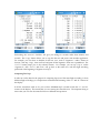
MQ200 Datasheet
General System capabilities

















Autocrossing: track mapping, segment timing, acceleration/ braking/ cornering/ MPH;
immediate review of data without leaving your car
Road racing: real-time lap time display, track mapping, lap and segment times calculated
from GPS position, lap count, ‚continuous‛ lap time measurement (Time since last here),
acceleration/ braking/ cornering/ MPH, etc.
Strip/Street: full ‚magazine test‛ performance calculations, including:
o Time to speed (e.g. 0-60, 5-60, 50-70, 0-100, ...)
o Time to distance (60’, 330’, 1/8 mile, 1000’, ¼ mile), speed at distance, deceleration
o Lateral acceleration
3-axis internal accelerometer
Analog and Pulse inputs for direct sensor connections
Optional OBD-II
Optional 5 Hz high performance GPS
Horsepower
Altitude
GPS UTC time (synchronized among all vehicles)
Automatic start and stop of flight recordings based on vehicle speed
Color graphic real-time display featuring four display modes: bar graph, strip chart, X vs. Y,
and numeric; touch-screen operation
Recording time limited only by available memory. 32 MB can hold more than 20 hours of
data.
Color graphic timeslip images, Excel spreadsheets, web page result summaries
Analysis software for both Pocket PC and PC, including data file overlays, lap/segment time
lists with min/max/average, manual and automatic beacon placement, GPS track map
full/zoom, export to Excel™ and text files, timeslip generation
Automatic emailing of data files; automatic text messaging of lap and segment times in real
time (requires Phone Edition device and a data plan from your wireless provider).
Automatic start and stop of flight recordings based on vehicle speed
MQ200-PRO system capabilities




6g, 3-axis accelerometer
12 analog and 6 pulse input channels
100 Hz sampling
Optional internal Roll, Pitch, and Yaw rate sensors
MQ200-MAX system capabilities



16
6g, 3-axis accelerometer
28 analog and 6 pulse input channels
2 relay or pulse-width modulated outputs



100 Hz sampling
Up to 500 Hz sampling on selected channels (recommended for shock velocity measurements)
Optional internal Roll, Pitch, and Yaw rate sensors
GPS Module Technical specifications




17
32 channel GPS receiver
1 second hot start, 39 seconds cold start
-158 dBm sensitivity
5 Hz sample rate
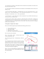
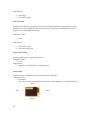
Mounting
The most important considerations for mounting are:
The MQ200 must be both flat and level when mounted in the vehicle so the accelerometers read
accurately.
It must be aligned with the centerline of the vehicle, though it does not have to be directly on the
centerline. Either the major or minor axis of the MQ200 must be parallel with the centerline of the
vehicle. Locating the MQ200 near the center of gravity is not critical. Eyeballing the centerline
alignment is generally OK.
Typical good mounting locations are in the passenger footwell, under the passenger’s seat,
behind the driver’s seat, in the trunk, or under the rear parcel shelf. As long as the MQ200 is flat
and level, pretty much anywhere will do.
Do not mount the MQ200 in the engine compartment, or where it will be exposed to intense heat,
or where it will be exposed to water spray.
The recommended mounting mechanism for most installations is high-strengthVelcroTM or a similar
product. Here are some of the more common scenarios:
Production car carpeting
This usually works very well if Velcro will stick to your carpet. Apply the ‚hook‛ side of the
Velcro to the box and discard the ‚loop‛ (fuzzy) side.
Race car floorpan
You'll want to find a flat and level smooth metal or plastic surface that isn't exposed to heat,
fluids, water, or excessive dirt. You can apply Velcro to hold it in place.
Hard mount
You can fabricate a strap that will hold it in place on a flat surface. Alternatively, you can drill
through the housing of the box and insert your own hardware. You need to take apart the
MQ200 enclosure to do this, and you need to clean out all the aluminum chips from any drilling
or cutting that you do. Send email to [email protected] for details.
Pocket PC
There are numerous mounting solutions available for mounting Pocket PCs in cars. Check with a
vendor such as www.mobileplanet.com or www.ram-mount.com to see if there is anything that suits
your needs.
At MaxQData, our favorite approach is to fasten the Pocket PC to the dashboard with Velcro™. A
few judiciously applied strips on the back of the device and on the dashboard are usually enough to
hold under hard driving. Be careful when removing the Pocket PC so as not to pop off the battery
door on the back of the Pocket PC.
18
If you have Flight set up to trigger a flight recording automatically, then you can put the Pocket PC in
a glove box, center console, or otherwise hidden out of sight. Be sure to flip the screen lock switch or
close the screen cover to prevent the screen from being touched while operating.
Protect your Pocket PC from water, heat sources, and dirt. Use a protective case where necessary.
Laptop
If you are using a laptop for data collection, it will require a secure mounting solution. For
temporary use, it is sometimes possible to use the seat belt of the passenger seat to hold the laptop.
Other applications may require the installation of a permanent hardmount. Keep in mind that the
hard drives in laptops may become damaged from excessive shock and vibration. Companies like
www.ram-mount.com provide vehicle mounting solutions for laptops.
19
Using Flight
Flight is the application that records your data, displays data in real time, and shows lap and segment
times. You can start Flight either before or after you turn on your MQ200. You can even assign it to a
button on the Pocket PC using ‚Start > Settings > Personal > Buttons‛.
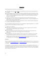
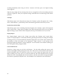
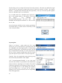
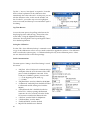
Initial Configuration
Turn on your MQ200 and run Flight. The first time you
do this, you will see:
20
Tap "Config" and a menu pops up:
Now tap "Sensors..." and you'll be presented with a list of
sensors that you can flight record. To begin with, tap the
‚Standard‛ button. This will enable the most commonlyused sensors. Later, you can add other sensors by clicking
on them. Flight will remember the sensors you pick and
will automatically select them each time you restart Flight.
The Standard sensor configuration does not enable lap
and segment timing. You first need to set up beacons
using the Chart application. See the ‚Working with
Beacons‛ section later in this manual for complete details.
The Standard sensor configuration enables automatic
flight recording based on vehicle speed. The default
configuration causes a flight recording to start when the
vehicle exceeds 20 MPH, then stop when the speed drops
below 15 MPH for more than 5 seconds. Flight stores 25
seconds of data (12.5 seconds at 10 Hz) from the time
before the vehicle hits 20 MPH to ensure that you do not
lose data from the launch.
21
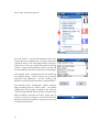
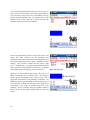
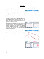
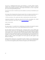
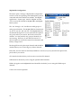
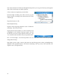
Display Dashboard
Tap "OK" and you will return to the main screen. This is
the default ‚Display Dashboard‛ mode, accessible with
Config > Display Dashboard. If the MQ200 is connected,
the number in the upper right corner (‚000020200‛ in this
case) will be counting up. If the MQ200 is not connected,
it will read ‚*time code+‛.
Also note the "\My Documents\Run" in the upper left
corner. This is telling you that any flight recordings you
log will go in the "\My Documents" folder on the Pocket
PC, and they will begin with the word "Run".
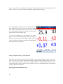
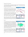
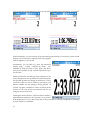
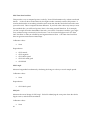
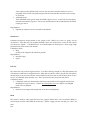
This image explains the elements of the dashboard display.
The larger numbers are the current values of MPH, LatG,
and LongG. The smaller numbers along the right side are
the maximum values of each over the past 10 seconds.
LatG and LongG are also plotted as red and blue traces in
the background. At the bottom of the screen are the
current satellite count, the average sample rate over the
past 10 seconds, and the altitude above sea level.
22
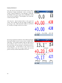
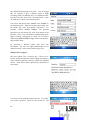
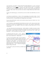
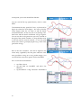
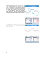
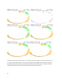
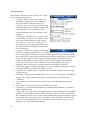
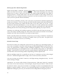
Display Graphs
You can also use the user-configurable ‚graphs‛ display
mode. Tap Config > Display Graphs. Initially, you will
see this screen:
To the right of ‚Flight recording trigger *0, 1+‛ there is a
small down-arrow. Tap one and a list of values will
appear:
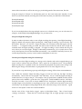
23
You can scroll through the list to select a value to view. In
this screen, we have chosen ‚GPS Vehicle speed MPH *0,
150+‛ for the top (red) value, and ‚GPS Satellite count *0,
20+‛ for the bottom (blue) value. It is useful to check ‚GPS
Satellite count‛ before each run to ensure that the GPS
module is tracking at least four satellites.
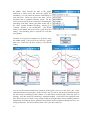
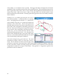
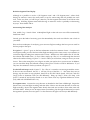
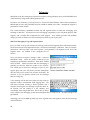
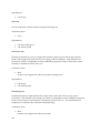
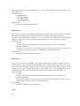
Here is an explanation of what you see on the screen. The
"Max" and "Min" numbers are the maximum and
minimum values seen in the last few seconds (either 10 or
20 seconds, depending on the Config > MinMax window
setting). The ‚Current‛ numbers are the values ‚right
now‛. ‚Elapsed time‛ is a number that basically tells you
if the connection to the MQ200 is operational. As long as
this number keeps counting up, you are connected.
There are two bar graphs in this image. The red one is
MPH, and the blue one is Satellite count. The length of
the bar graph corresponds to the current value, with a
range that corresponds to the numbers in brackets. For
MPH, the range is 0 to 150 MPH. In this example, the car
is not moving, so MPH is 0 and the red bar graph has a
zero length. The range on satellite count is 0 to 20
satellites. We are currently seeing 10 satellites, which is
half of 20, so the bar graph extends halfway across the
screen.
24
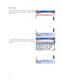
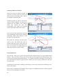
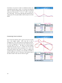
The Config > Display Graphs option actually gives you a total of eight configurable screens for
viewing data in real time. There are eight data views you can watch. There are two bar chart screens,
two strip chart screens, two X vs. Y screens, and two numeric summary screens. To cycle between
the screens, you use the left/right buttons on the front of your Pocket PC. You can also bring up the
soft keyboard (tap the little keyboard at the bottom) and use the left or right arrows. Here are
examples of the strip chart, X vs. Y, and Numeric Summary screens:
The two numeric text summary screens (Numeric A and Numeric B). summarize the min, current,
and max values from the other bar graph, strip chart, and X vs. Y graphic screens. Numeric A
summarizes the ‚A‛ screens and Numeric B summarizes the ‚B‛ screens. To see the numeric data
you want on the numeric summary screens, you need to set up the previous six screens appropriately.
25
Starting a Flight Recording – Automatic Flight Recording Trigger
You must trigger a flight recording in order to cause data to be saved to memory. You can cause a
flight recording to trigger automatically based on vehicle speed, which is the easiest method. Just
ensure that you have ‚Flight recording trigger‛ in the list of sensors you have configured to record.
It is automatically selected when you pick the ‚Standard‛ sensor configuration. This is the default
setting when the software is first installed. The ‚Flight recording trigger‛ works for road racing as
well as autocrossing a drag racing. In the default configuration, it will start recording when the
vehicle is above 20 MPH, and then it will stop when the vehicle speed drops below 15 MPH for more
than 5 seconds. This is a good all-purpose setting, because it filters out driving around the paddock
at slow speeds. It works for autocrossing and drag racing because it will still capture 25 seconds (12.5
seconds at 10 Hz) of data before the trigger speed is hit, allowing you to see your burnout and launch.
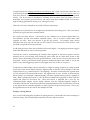
Starting a Flight Recording – Screen Tap
The next most common way to start a flight recording is to
use ‚Screen tap‛. Tap ‚Config‛, then tap on ‚Screen tap‛
to check it (we recommend leaving it unchecked when
using the automatic Flight recording trigger to help
prevent accidental triggering).
Now, to manually trigger a flight recording, tap anywhere
in the middle of the screen and this will come up:
The big ‚Start Flight Recording‛ button is what starts the
flight recording. The ‚Zero‛ button, which is rarely used,
26
resets certain values. ‚Freeze/Release‛ allows you to freeze the values on the screen and then release
them. ‚Cancel‛ gets you out of this screen without creating a flight recording.
Tap ‚Start Flight Recording‛ and you will be back at the
main display screen, only this time you will be recording
data. When recording data, the top line will be colored
red. In the upper left corner you will see the name of the
temporary file used to hold the data.
To stop the recording, tap the center of the screen
again. After a short delay (during which time Flight is
flushing its data buffers and closing the flight recording
file), you will hear a double beep and the red highlighting
of the top line text will go away.
Starting a Flight Recording – Other Methods
The ‚Log‛ menu also gives you two more methods to start and stop a flight recording. The ‚Log >
Start‛ and ‚Log > Stop‛ menu options start and stop a flight recording without using ‚Screen tap‛.
The ‚Log > Force recording‛ option causes a flight recording to start immediately as soon as you
launch Flight and it doesn’t stop until you exit Flight. We do not recommend using Force Recording
except in special circumstances.
Changing the Default Filename Prefix
27
The default filename begins with ‚Run‛. You can change
this, for example to give a different name to flight
recordings taken on different days or at different tracks.
In order to do this, chose ‚File > Set name prefix...‛ from
the main menu. Enter a new filename prefix.
You can use the special codes ‚MMDD‛ and ‚HHMM‛ in
the filename prefix. Flight will replace these codes with
the month, day, hour, and minute, respectively. For
example, ‚Detroit MMDD HHMM‛ will generate
filenames with the month, day, hour, and minute in the
filename. This is very convenient for determining which
flight recording corresponds to which run or session.
When using MMDD/HHMM, Flight will not use the threedigit numeric suffix.
By specifying a different folder other than ‚My
Documents‛, you can have Flight automatically save to
another location, such as a removable Storage Card.
Mulitple Driver Support
The menu option ‚File > Set driver list...‛ allows you to
further modify the filenames used for flight recordings in
order to better organize the data you collect from multiple
drivers. Enter driver names separated by semicolons as
shown here:
You must switch manually between drivers. To do this,
you use the ‚up/down‛ control on your Pocket PC. The
28
name of the current driver will be shown in grey in the background of the main screen, like this:
Using the example of ‚Detroit‛ for the filename prefix (i.e. the event name) and ‚Jack;Kay‛ for the
driver list, and with manually switching drivers between runs, then your data files will be named:
DetroitJack000.mqd
DetroitKay000.mqd
DetroitJack001.mqd
DetroitKay001.mqd
...
If you have multiple drivers driving multiple courses (as in a ProSolo event), you can also enter, for
example, ‚JackLeft;KayLeft;JackRight;KayRight‛ for your driver list.
Preopened Flight Recording File
In order to reduce the time it takes to start a flight recording after pressing ‚Start Flight Recording‛,
Flight by default will preopen a flight recording file. While Flight is running, if you look in the ‚My
Documents‛ directory, you will see a flight recording with a numeric name that begins with the
character ‘~’. If a flight recording is started, the data is stored in this file, and the file is closed and
renamed when the flight recording is stopped. If a flight recording is never started, this file goes
away when you exit from Flight. If Flight is abnormally terminated (e.g. by a system reset or some
error), this temporary file will not be deleted automatically. You can delete it manually; however, if it
contains important data, you may want to send it to MaxQData for recovery.
The Preopened Flight Recording File and Pit Stops
Some users save their flight recordings to a storage card so that the card can be swapped during a pit
stop in order to analyze data just collected. This is typical in an endurance event. The preopened
flight recording file is a problem in this case, because the preopened file resides on the storage card.
Removing the storage card while there is a preopened file on it can cause Flight to lock up.
If you need to swap cards during a pit stop (while Flight is running), follow these recommendations:
First, enable the automatic Flight Recording Trigger to both start and stop the flight recording
automatically. Ensure that the ‚Stop Speed‛ and ‚Off Delay‛ are set so that the flight recording is
closed before the car stops in the pit. For example, if the pit speed limit is 35MPH and the slowest
point on the track is 50MPH, a good choice for ‚Stop Speed‛ would be 40MPH, and for ‚Off Delay‛
would be 5 seconds. If you were to choose 30MPH for the ‚Stop Speed‛, then the flight recording
wouldn’t begin to close until the car is pulling into its pit. Since it takes several seconds to close (even
of Off Delay is 0), the flight recording might still be active when the storage card is removed. A good
choice for ‚Start Speed‛ in this case would be 45 MPH.
Second, turn off the ‚Open before trigger‛ option in MaxQData Setup. This is found under
‚Settings >Advanced...‛ When this box is unchecked, Flight will no longer preopen a new flight
29
recording immediately after closing an old one. Instead, it will only open a new flight recording
when triggered.
With this setup, Flight will stay running when the car is stopped but will not be recording data and
will have no open file. Then you can eject the Storage Card and insert a second Storage Card without
problems.
Timeslips
When Racing Type is set to Drag Race (in Setup), the ‚Timeslip‛ option will appear in the ‚Config‛
menu. When enabled, a ¼ mile timeslip will be automatically generated at the end of your run.
Launch Chart at End of Run
When Racing Type is set to something other than Drag Race, the ‚Timeslip‛ option will be replaced
with ‚Launch Chart‛. If this option is enabled, Chart will be launched at the end of your run and the
flight recording you just collected will be displayed, allowing for immediate access to your data.
Display Report
The ‚Display Report‛ option in the ‚Config‛ menu affects the ‚Timeslip‛ and ‚Launch Chart‛
options. If ‚Display Report‛ is unchecked, then after generating the timeslip or loading the last flight
recording in Chart, you will automatically returned to Flight after a few seconds. But if checked, then
the timeslip or Chart will remain in the foreground. Flight, however, is still running in the
background while the Timeslip or Chart is displayed. You can continue to record data assuming you
have the Flight Recording Trigger enabled.
Course Walk Beacons
Under the ‚Config‛ menu you will find ‚Add beacon‛. Use this while walking the course to add
beacons to the flight recording during the course walk. There are two main reasons for this feature: 1)
to mark individual cones on an autocross course so you can see orange cone marks when you load
flight recordings into Chart, and 2) to mark the finish line and other desirable beacon locations
around the course. Most MQ200 users will not be able to walk the course while carrying the MQ200.
This feature is primarily for MQGPS users. See the MQGPS User’s Manual for more information.
30
Using Chart
Chart is the app you use to review flight recordings that have been generated by Flight. Chart lets
you load several files at once and view them either
individually or two at a time, overlaid.
This section uses screenshots primarily from Chart
running on a Pocket PC. You can also run Chart on a
desktop or laptop PC. The functionality is the same, with
just a few minor differences in the user interface which
will be discussed later.
The data shown here is the file ‚Mitch000.mqd‛, which is
downloadable from the MaxQData website. You can
follow along with the examples by transferring it to your
Pocket PC or using it on your PC.
Run Chart. You do not need to have Flight running. You
will see this screen. To ensure consistency with this
example, you should tap ‚File > Racing type...‛ and make
sure that ‚Road race‛ is selected. If not, change it to
‚Road race‛, then ‚File > Exit‛ from Chart and restart to
make the change take effect.
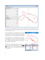
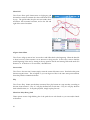
Now tap ‚File > Load...‛ and select the file
‚Mitch000.mqd‛. The trackmap will be displayed in the
plot area of the screen. In this view (‚Full GPS map‛),
North is always at the top of the screen.
31
On a PC, it will look like this:
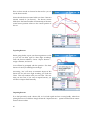
Tap the blue ‚Select...‛ field and you will see this:
32
Scroll down to ‚GPS Vehicle speed MPH *0, 150+‛, select it,
and tap ‚OK‛. Now you get this:
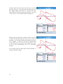
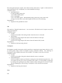
User Interface
This is a good time to describe the user interface. Here we have expanded the screenshot and
numbered the various areas of the screen you need to learn about:
33
In order to get the most out of the small screen on a Pocket PC, we made the display elements
respond to screen taps in order to access related functionality. You are encouraged to try these out to
learn how to access all of the features of the software.
The Pocket PC takes advantage of the ‚tap and hold‛ feature from the Pocket PC user interface. ‚Tap
and hold‛ means to hold the stylus down for a couple of seconds. A ring of colored dots will circle
around the tap point, and then something happens, either a menu pops up or a value underneath the
stylus changes. On a desktop or laptop PC, you would use a right button click to do the same thing.
‚(1)‛ As you just learned, tapping this field brings up a screen that allows you to select from a list of
sensor values to view. The current value is displayed here.
Tap and hold on this area to bring up a context menu as
shown in this screenshot. On a PC, you would right-click
to get the menu.
The top line of the menu indicates the sensor value that is
being displayed. The next line shows the range, in this
case 0 to 150 MPH. That means that the bottom of the plot
area is 0 MPH and the top is 150 MPH.
You can set two marker positions specifically for this data
trace using the Set Marker 0 and Set Marker 1 menu
options. This is used for calculating minimum, maximum,
and average values over a given time period, or for
calculating time deltas. You would do this by scrolling
through the data to the first time position (e.g. the entry to
a particular corner), setting marker 0, then scrolling to the
second time position (e.g. the exit of that corner) and
setting marker 1. Finally, when you bring up this context
menu after setting the two markers, you pull up this menu again to read the values. The maximum,
average, and minimum values for that sensor reading over the time between the two markers will be
in the ‚*max+‛, ‚*avg+‛, and ‚*min+‛ positions. The time between the two markers will be in the
‚*m1-m0+‛ position. ‚m0-tA‛ and ‚m1-tA‛ are used for calculating time deltas to the tA marker
which will be discussed later. ‚Jump to Marker‛ allows you to instantly shift the data to the specified
marker point.
‚(2)‛ This is the MPH data trace corresponding to the sensor value we enabled earlier. Note that it is
color coded to match the numeric value. In this example, you can see that the car is initially stopped,
and then after about 13 seconds the vehicle starts moving and the MPH trace rises.
‚(3)‛ This checkbox turns on and off the corresponding data trace. This is useful when you get so
many data traces on the screen that you can’t easily make them out. Turn off the ones you don’t need
to unclutter the screen.
34
‚(4)‛ This is the ‚A‛ file selector. It shows the name of the file loaded on the ‚A‛ side. You can load
many files, but you can only view two files at once. You select the files you want to view by tapping
on either the ‚A‛ or ‚B‛ file selectors. Notice how the values are color coded. ‚A‛ side files use
bluish colors, while ‚B‛ side files use reddish colors. In this case, we have the same file loaded on the
‚A‛ and ‚B‛ sides, which is what you need to do in order to compare different laps within the same
data file.
Tapping on this field brings up a screen that lets you choose which of the loaded files you want to
view.
‚(5)‛ This is the current file time ‚t‛ for the ‚A‛ file, corresponding to the vertical crosshair. To scroll
the data forward in time, you drag the plot area to the left of the screen with your stylus (or with
your mouse on a PC). To scroll backward, you drag the plot area to the right.
You can also scroll the data in specific time increments using the large arrow buttons ‚(8)‛ or the
small arrow buttons ‚(9)‛.
‚(6)‛ This checkbox, when unchecked, locks the data traces for the ‚A‛ file. They are frozen in time,
allowing you to scroll the ‚B‛ file independently with your stylus. This is useful for comparing laps.
The ‚B‛ file also has a lock checkbox so that you can hold it in place and move the ‚A‛ file
independently.
‚(7)‛ This is the time scale for the data traces. In this example, it is initially set to plus or minus
twenty seconds. That means that the right edge of the plot area is twenty seconds in the future, and
the left edge is twenty seconds in the past. The middle of the plot area is the ‚current‛ time,
designated ‚t‛, which corresponds to the numeric values.
To change the time scale, use the ‚+‛ and ‚-‚ buttons on
the left. This is how you zoom in or out on the data traces.
Here we have zoomed out to +- 1000 seconds:
To switch to plot-by-distance mode, you tap and hold (or
right click) on this field. In plot-by-distance mode, both
data files scroll the same distance, keeping them aligned
according to track position. You will then see (for
example) ‚+-500’‛ instead of ‚+-20s‛. This means the right
edge of the plot area is 500 feet ahead and the left edge is
500 feet behind. The ‚+‛ and ‚-‚ buttons also change the
distance scaling in this mode.
To switch back to plot-by-time mode, tap and hold again
on this field.
35
‚(8)‛ The large arrow buttons scroll the data forward or backward in increments of one-tenth of the
time scale (or the distance scale).
‚(9)‛ The small arrow buttons scroll the data in increments of one-hundredth of the time scale (or the
distance scale).
‚(10)‛ This is the time delta display. As described later, you can set a time marker for the ‚A‛ file
and the ‚B‛ file. The time delta between ‚t‛ (the current time) and either the ‚tA‛ or ‚tB‛ mark is
shown here. To switch from ‚t-tA‛ to ‚t-tB‛, tap on this field.
‚(11)‛ The big red ‚+‛ sign is where the car is at the current time. If you scroll the data forward, you
will see the car move around the track.
‚(12)‛ The grey box where it reads ‚*no beacon+‛ is called the ‚beacon counter field‛. It displays the
timestamp of the most recent beacon before the current car position, if any. Also, if you tap and hold
or right-click on this box, you will get the beacon context menu. Please read the section on setting up
beacons for more information.
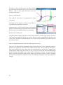
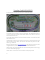
Viewing Data – Simple Corner Analysis
Here we will walk through the steps to determine the following values in Turn 1:




Top speed before the turn
Entry and exit speed
Elapsed time from entry to exit
Mid-corner average and peak lateral acceleration
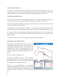
Turn 1 is shown in this screenshot.
Step 1: Tap the blue ‚Select...‛ field and select ‚GPS
Vehicle speed MPH [0, 150]‛.
Step 2: Tap the green ‚Select...‛ field and select ‚GPS LatG
[-2, 2+‛.
Step 3: Drag the plot area to the left to start the car moving
around the track. We don’t want to see the very first time
that the car enters Turn 1, because it is only just leaving
the pits and is not up to speed. So continue to advance the
data until the car goes all the way around the track and
comes back onto the front straightaway.
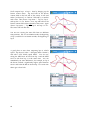
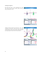
Step 4: Look at the blue MPH trace and find the peak
MPH. Drag the data traces so that the MPH peak is under
the vertical crosshair.
36
At this point, your screen should look like this:
You can read off the top speed directly, which is 120.2
MPH.
To determine the entry speed for Turn 1, we first need to
figure out where the corner begins. We will say that the
corner begins when the car turns in and the lateral
acceleration builds. In this case, the car is entering a lefthand turn and the lateral acceleration will go negative.
You can see this in the green trace just a few seconds to
the right of the vertical crosshair. So, drag the data traces
to the left until the vertical crosshair is over the point
where LatG starts to go steeply negative (e.g. where LatG
goes below -0.10 g).
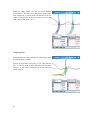
Here is the new screenshot. The data is aligned to the
corner entry, signified by the first point where the LatG
trace goes below -0.10 g (it is -0.14 g in this image). You
can read off the corner entry speed, which is 84.9 MPH.
Now we will set several markers:



37
tap Chart > Set tA
tap and hold on ‚84.9MPH‛ and select ‚Set
Marker 0‛
tap and hold on ‚-0.14g‛ and select ‚Set Marker 0‛
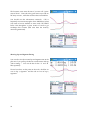
Next, we will scroll forward in the data until we find the
corner exit. We will define the corner exit as the point
where LatG comes back above -0.10 g. Here is the new
screenshot.
Note the vertical green line in the left half of the plot area.
This line is the ‚tA‛ mark which we placed at the corner
entry point. You can read the elapsed time through the
corner where it reads ‚t-tA‛, which is 7.097 seconds. You
can also read the corner exit speed, which is 88.6 MPH.
Now, tap and hold on ‚88.6MPH‛ and select ‚Set marker
1‛. Do the same for ‚-0.06g‛.
After setting marker 0 and marker 1 for a given sensor
value, you can get min/max/average information by doing
another tap-and-hold (or right click) on the value. For
example, if we tap-and-hold on the MPH value, we get
this display where we can read off these values. Through
Turn 1, our maximum speed was 89.1 MPH, our
minimum speed was 69.6 MPH, and our average speed
was 77.6 MPH.
Similarly, we find that our maximum LatG was -1.21g, our
minimum LatG was -0.06g, and our average LatG through
the turn was -0.76g.
Data Smoothing
All data is noisy. ‚Noise‛, meaning random transient fluctuations in the value of the data, makes
data analysis difficult and misleading. It would be wrong, for example, to conclude that your car has
amazing cornering potential if you see a 1.5g spike on a corner where it otherwise only averages 1.0g.
That spike is unlikely to be ‚real‛ – it might have resulted from hitting a berm, or from a GPS signal
glitch, or from something bumping the accelerometer, or for any number of other reasons.
38
By default, Chart smooths the data in the graphs
somewhat to reduce noise and make the graphs less
misleading. You can control the amount of smoothing on
each data trace. When you select a data trace, you are
presented with a parameter selection screen. On this
screen (as shown here), there is a slider for controlling the
smoothing of the data. Moving the slider all the way to
the ‚Raw‛ position disables smoothing. Moving it to
‚Smooth‛ smooths it out considerably. The default
setting, in the middle, has proven to be a good all-around
setting. The smoothing factor is separate for each data
trace plotted.
The data in the previous examples was all shown using
the middle setting. Take a look at how the LatG (green)
data trace varies from the Raw setting to the Smooth
setting:
Raw
Smooth
You can see the minute instantaneous variations all along the LatG trace in the ‚Raw‛ plot. These
small fluctuations are meaningless. In the ‚Smooth‛ plot, you can see that these fluctuations are gone,
but the excessive smoothing erased evidence of a mid-corner correction right where the arrow is
pointing. Still, this amount of smoothing is sometimes helpful. Notice that in the right half of the
plot, where LatG goes to about +1.0 g (corresponding to the right-hand Turn 2), smoothing makes it
immediately clear that the driver gradually increased his lateral acceleration through the turn, as if
feeling for the limit. This is less obvious in the ‚Raw‛ plot due to the noise.
39
Landscape Mode User Interface
Pocket PCs based on Windows Mobile 5.0
and later are able to rotate the screen into
either portrait or landscape mode. Here is
an example of landscape mode:
In landscape mode, in order for the numeric
values to still be readable, it is necessary to
maintain the font height of the numeric
values and squeeze the plot area.
Unfortunately, this makes the trackmap
much smaller and the data traces shorter.
You can turn off the bottom three lines (the
ones containing the numeric data values) by
unchecking ‚Chart > Show numerics‛. Then
the display will look like this:
This makes the trackmap and data traces
easier to view. The feature also works in
portrait mode and can be useful when the
track is tall North-South and skinny EastWest. This feature is not enabled (and is not
necessary) on the PC version of Chart.
Using GPS Beacons
GPS ‚beacons‛ allow you to get lap and segment times without having to set up trackside optical
beacons. They can also be set up to give you real-time lap and segment times while driving. They
are far more convenient than optical beacons. It is expensive and time consuming to set up three or
four optical beacons around a typical racetrack, whereas you can set up ten GPS beacons with just a
few screen taps.
(GPS Beacons are also used for marking cones during a course walk; see the section ‚Marking Cones‛
later in this chapter.)
The accuracy of GPS beacon lap timing is about as good as a handheld stopwatch, or better (typically
down to a few hundredths of a second).
40
You place beacons by starting with at least one full lap of data, which you load into Chart, then you
scroll through the data until the car is at the position on the track where you want a beacon, then you
mark that position with either the ‚Add beacon‛ or ‚Add beacon each lap‛ function, explained
shortly. You do not need to download a trackmap from anywhere, since you make your own
trackmaps. You can place up to ten beacons. The course can be open-ended or closed. You can use a
flight recording generated by driving or by walking the course.
There are a few rules of thumb for successful GPS beacon placement:
In general, try to place beacons on straightaways shortly before the braking zone. This is not always
practical, but it gives the most consistent results.
Do not place too many beacons. GPS beacons are not a reliable way to measure elapsed time over
short distances (use the time markers explained earlier). Also, it is hard to analyze data when
segments are short. Place your beacons to get the ‚big picture‛. For example, many courses
naturally break down into one fast and two slow sections, or two fast and two slow sections. That
should be your guide for beacon placement.
Avoid placing beacons where the track folds back on itself tightly. You might get erroneous triggers
if the track folds back too close to a beacon position.
GPS beacons work by remembering the Latitude and Longitude of the beacon position and the
direction the car was traveling, then finding the point where the car comes back closest to that
position and is still heading in the same general direction. If the car is too far away, the beacon will
be ignored. However, the software makes generous assumptions about track width, so you do not
have to worry about triggering a beacon if you happen to be way off line as you pass it.
Technical note: When adding a beacon manually to a flight recording, the beacon is actually marked
by the time of the current sample, therefore segment times for this file will be multiples of the base
sample frequency (e.g. 0.200 second for 5 Hz sampling). This does not mean that the segment times
are only accurate to the nearest 0.200 second. The segment time is exact. In effect, it means that the
beacon position you requested is adjusted slightly so that the segment time is precisely a multiple of
0.200. When exporting the beacon to a file, the beacon Latitude and Longitude are taken from this
sample and placed in the beacon file. When this beacon is imported into a new file, the
Latitude/Longitude samples will be slightly different from the Latitude/Longitude samples as
recorded for the first file. So the beacon times are interpolated based on the closest that the car comes
to the original beacon Latitude/Longitude, in order to preserve 0.001 second precision. This is why
the segment times for the new file are not multiples of 0.200.
Example – Placing Beacons
Now we will walk through the procedure for placing beacons. Take another look at the trackmap we
have been using. The track naturally breaks down into slow and fast sections:
41
We’ll place two beacons. Segment 1 will be the ‚slow‛ section of the course, and segment 2 will be
the ‚fast‛ section. We will show screenshots from the Pocket PC version of Chart, but you can do the
exact same process on a PC.
Start by moving back to the beginning of the run (use
‚Chart > Align to start of run‛). Bring up a GPS Vehicle
speed data trace. You see here that we are staring with
the car just about to come out of the paddock onto pit lane:
Just to emphasize, you do not place beacons by tapping on
the trackmap where you want the beacon to be placed.
This is imprecise. Instead, you must move the data until
the ‚+‛ symbol is at the location where you want a beacon,
then add a beacon at that point.
Drag the data forward in time (slide it to the left with your
stylus or mouse). Continue until the car is on its first hot
lap. This makes it easier to see braking points and place
beacons relative to them. The lap times on warmup laps
are unimportant.
42
In this example, you can see the driver is up to speed by
the time he comes around for his first full lap (notice that
the car in this screenshot is on the front straight, not pit
lane). We’re going to pick t = 146.000s as the location for
the first beacon, because it is shortly before the braking
zone going into Turn 1.
Adding Beacons
To place a beacon, you tap-and-hold (or right click) on the
field which reads ‚*no beacon+‛. Do it on the ‚A‛ side for
this example. You will see the beacon context menu pop
up as in this screenshot.
You have two options:
1.
2.
‚Add beacon‛ This places a single beacon at this
point. It does not change the ‚beacons per lap‛
count.
‚Add beacon each lap‛ This places beacons on
every successive lap starting at the current file
time (but not earlier). It also increments the
‚beacons per lap‛ count.
Typically, you would use ‚Add beacon each lap‛.
However, you might use ‚Add beacon‛ for specialized timing or if you are adding in a missing
beacon.
43
In this case, choose ‚Add beacon each lap‛. You will now
see several ‚X‛ symbols appear right around the point
where you added the beacon. These symbols are beacon
markers, one for each lap. They do not always lie exactly
on top of one another due to GPS drift, but they should be
close.
The first beacon you place determines the start of lap 1.
Note that your lap times will not correspond to official
timing if you do not put your first beacon at the
start/finish line. However, for analysis it is sometimes
better to choose your own beacon position rather than try
to align it with start/finish.
Now, scroll the data forward until the car is at the location
shown here. Although it is not on a straightaway, the
beacon location is good because speed is not changing
rapidly at this point and it is not a sharp turn. As before,
‚Add beacon each lap‛.
44
Here we have moved car forward on the track so you can
see the beacon marks.
Notice that the beacon counter fields now show ‚Beacon 2:
210.80s‛ instead of ‚*no beacon+‛. The beacon counter
fields show the beacon number and timestamp of the most
recent beacon position relative to the current position of
the car.
Exporting Beacons
Before going further, export your beacon positions to a file
so you can use them again in other flight recordings.
From the beacon submenu, choose ‚Export beacons...‛,
assign a filename, and save it.
You will then be prompted with the question: ‚Use these
beacons for newly-loaded flight recordings?‛
Answering ‚Yes‛ will cause an automatic import of this
beacon file for each new flight recording you load into
Chart. This will continue until you exit Chart. The next
time you run Chart, if you want to import beacons, you
will have to import them manually.
Importing Beacons
If we had previously saved a beacon file, or if we had copied one from a racing buddy, rather than
placing beacons we could have simply chosen the ‚Import beacons...‛ option from the beacon context
menu as shown earlier.
45
Please remember that the GPS beacons are ‚directional‛ in order to reduce false triggering. The
direction the car is traveling when it passes a beacon position is a factor in determining if a beacon
point has been crossed.
Viewing the List of Lap and Segment Times
On the beacon context menu you may have noticed the
‚Lap times...‛ option. In this example, the ‚Lap times...‛
option brings up the following screen.
The MQGPS system samples GPS Latitude and Longitude
in intervals of 0.200 s. But the actual lap timing accuracy
is better than that. Chart uses interpolation to estimate lap
times down to a typical accuracy of a few hundredths of a
second. This is about the same as or better than a
handheld stopwatch. Optical beacons will do even better.
By expanding the different areas of this tree view (tap the
‚+‛ signs), you can see other interesting information as
shown in the following screenshots. In some cases the
information is off the right edge of the screen and it is
necessary to scroll over to see it. For example, the ‚Sum of
fastest segments‛ figure, which indicates a theoretical
fastest lap time, scrolls off to the right. Also, the segment
times include ‚MPH at beacon‛ and ‚Max segment MPH‛ information.
46
Unchecking the ‚m:ss.sss‛ checkbox will give you timings in seconds rather than minutes and
seconds. The ‚Copy‛ button allows you to copy the data out and paste it into another application.
For example, you can select an element of this tree view, such as ‚Segment 1‛ under ‚Fastest to
slowest‛, then tap ‚Copy‛, then run Excel and paste all the Segment 1 times into a spreadsheet. The
‚Go To‛ button jumps you to the selected location. For example, you can tap ‚Lap 3‛ under
‚Segment 2‛, then ‚Go To‛ and Char t will go back to the main view with the flight recording
positioned at the beginning of Segment 2 on Lap 3.
Comparing Two Laps
In order to overlay data for the purpose of comparing laps (out of the same flight recording, or from
different flight recordings), it is important to understand the meaning of the ‚A‛ and ‚B‛ sections of
the display.
In all the screenshots used so far, you see that ‚Mitch000.mqd‛ is listed in both the ‚A‛ and ‚B‛
sections of the display. This means that you are viewing the same file twice. The important thing to
note is that you can view the same file from two different time positions.
47
We’ll compare lap 1 to lap 2. Start by bringing up the
beacon context menu. Tap and hold on the beacon
counter field on the left side of the screen; it will read
either ‚*no beacon+‛ or ‚Beacon‛ followed by a number
and a time. Then choose ‚Lap times...‛ Tap on ‚Lap 1‛
and tap the ‚Go To‛ button. Now, tap and hold on the
beacon counter field on the right side of the screen. Again
choose ‚Lap times...‛ Tap on ‚Lap 2‛ and tap ‚Go To‛.
The screen will look like this:
You are now viewing the same file from two different
time positions. File A is at 146.000 seconds, the beginning
of lap 1, and file B is at 254.656 seconds, the beginning of
lap 2.
A good place to start when comparing laps is vehicle
speed. Tap the red ‚Select...‛ field (just under ‚254.656‛)
and select ‚GPS Vehicle speed MPH‛. You are now
seeing the MPH trace in blue from lap 1 and the MPH
trace in red from lap 2 at the same time. You can
immediately see some differences; for example, on lap 2
the driver reached a significantly higher speed between
turns 1 and 2 than he did on the first lap. Let’s zoom into
that to get a closer look.
48
First, to unclutter the screen, turn off the track maps. Tap
‚Map‛ and then uncheck ‚Show GPS map B‛. You will
notice the trackmap is now displayed in aqua rather than
red. That is because you only turned off the trackmap for
the ‚B‛ file, which is colored red. The trackmap for the
‚A‛ file is still displayed. Showing two trackmaps is
useful when there might be significant differences
between the trackmaps of two different flight recordings.
Tap ‚Map‛ and then uncheck ‚Show GPS map A‛ to turn
off the ‚A‛ trackmap. You will be left with just the MPH
traces as shown here.
49
We’d like to see just how much of a difference there was
in speed between turns 1 and 2. To do this, first slide the
data over until the smaller peaks on the right are centered
in the plot. Then tap the ‚-‚ next to ‚+-20s‛ to zoom into
the +-10s range. You can see that the peak speed on lap 1
at this point was only 88.6 MPH, while on lap 2 it was 94.5
MPH.
Determining Time Lost/Gained
How much time did the driver gain in this short section
due to his higher speed? First, turn the A and B
trackmaps on. Now, move both cars to the apex of turn 1.
Do this by dragging the data traces back until the red car
is at the apex of turn 1. The blue car will be slightly
displaced from the red car. Uncheck the B file time
counter (the checkbox directly under the ‚B)‛, which will
freeze the location of the red car. Then, by tapping the
small left/right arrow buttons, move the blue car until it is
directly under the red car. Then put a check back in the B
file time counter so the red car can move again.
50
Scroll the data forward in time until the red car reaches
the entry of turn 2. You will notice in that the red car is
now slightly ahead of the blue car. Uncheck the B file
time counter to freeze the location of the red car. Now tap
‚Chart > Set tA‛ to set a time marker for the blue car.
Finally, using the small arrow buttons, advance the blue
car until it is directly under the red car (or as close as
possible). You can then read the time difference from the
‚t-tA‛ display. In this case, the red car gained 0.300
seconds in this short section due to the higher speed. This
is not an exact measurement, but it is a reasonable
estimate.
Put a check back in the B file time counter checkbox to
continue with this example.
51
Comparing Two Laps with Qview™
Qview™ is an innovative way to visualize the performance of a car as it drives around the track. It
combines lateral acceleration, longitudinal acceleration, and speed differences into a single graphic
that is easy to grasp.
QView™ requires the following values to be in the flight
recording:





GPS Latitude
GPS Longitude
GPS LatG
GPS LongG
GPS Track Made Good
Tap ‚Map > Zoom GPS map‛. Also tap ‚Map‛ and make
sure ‚Qview (tm) in Zoom is checked. Finally, tap ‚Map‛
and make sure ‚Overlay‛ is unchecked to be consistent
with this example.
Immediately, you can see where lap 2 was faster than lap
1. It is outlined in green. You can also see that the
upcoming turn (turn 2) was actually slower on lap 2 than
on lap 1, because it is outlined in orange.
Notice that we have switched to a view directly over the car, as if you are a helicopter flying and
turning with it. As you scroll forward in time, the track will pass underneath you. The top of the
display is the forward direction of the car.
52
As before, to move forward in time you either drag the
plot area to the left with the stylus, or you use the arrow
buttons. Here, we have gone backwards exactly five
seconds to show turn 1.
Qview™ works like this:
The width of each block is proportional to lateral
acceleration
The length (in the direction of travel) of each block is
proportional to longitudinal acceleration
The inside color is red for braking, blue for accelerating.
Intense red is hard braking, intense blue hard acceleration.
White means you are neither braking nor accelerating
Blocks are 0.2 seconds apart
The green outline indicates where the ‚B‛ file is faster than the ‚A‛ file, orange where it is slower.
This coloring only appears when the ‚A‛ and ‚B‛ files are synced to approximately the same point
on the track. The blocks on left-hand side for the ‚A‛ file are only outlined in grey because they are
the ‚reference‛ data.
There is a minimum block size even if LatG and LongG are near zero.
There are a few things that are immediately apparent from the Qview™ plot. Remember earlier we
pointed out a mid-course correction in turn 1 from the LatG trace. That is obvious in the Qview™
plot, in the middle of the corner where there is a small blue block. Second, just by looking at the
overall greater width of the plot for the ‚B‛ file, it is easy to see that the driver maintained high
lateral acceleration through the turn on lap 2, with no mid-corner correction. You can see that the
driver was faster on lap 2 from early in turn 1 all the way to the entry of turn 2. Finally, you can see
that the driver actually lost a little time on lap 2 in the braking zone before turn 1 (it is outlined in
orange).
53
Zooming in on Qview™
The time zoom factor (‚+-10s‛) determines how much
data will be plotted in Qview™ mode. Here is what you
see if you zoom in to ‚+-2s‛:
And here is what you see if you zoom out to ‚+-50s‛. This
is perhaps a bit too much. Chart tries to plot +-50 seconds
of track starting at the current position, which means that
the track plot goes off the screen and comes back on.
54
Under the ‚Map‛ menu, you will see several distance
zoom factors. The plots so far have been at 200 yards.
This means that, in zoom mode, the distance from the
center of the plot area to the top of the plot area is 200
yards. Here is 100 yards, +-10 s.
Comparing Lines
Zooming back out to 200 yards, here is what you get when
you check ‚Map > Overlay‛:
The ‚B‛ file is plotted on top of the ‚A‛ file. This obscures
the ‚A‛ file but tends to make differences in line more
obvious. In this case, it looks like the driver turned in
earlier on lap 2.
55
This becomes even more obvious if you turn off ‚Qview
(tm) in Zoom‛. Notice how the green trace stays wide on
the entry to turn 1, while the red trace takes an inside line.
You should use this information cautiously. GPS is
frequently not accurate enough to show differences in line.
You need to have 8 satellites or more with GPS HDOP
below 1.20 throughout a given section of track to get
trackmaps this accurate (and even then the accuracy
cannot be guaranteed).
Showing Lap and Segment Timing
You can also view the current lap and segment time in the
plot area if you pull up the beacon context menu and tap
‚Show timing...‛. You can do this for the ‚A‛ and ‚B‛
files separately.
We see here that, at this point on the track, the blue car
was on lap 1, segment 1 and the red car was on lap 2,
segment 1.
56
Plot by Time vs. Plot by Distance
In the previous examples, we were using the ‚Plot by Time‛ mode. This means that the data on the
screen was plotted where the horizontal axis was measured in time. ‚+-20s‛ means that the right
edge of the screen is 20 seconds into the future, and the
left edge is 20 seconds into the past.
The problem with Plot by Time mode is that, as you scroll
forward in time, the ‚A‛ and ‚B‛ data traces will get out
of sync as one car moves faster than the other, shown here.
To correct this, you would uncheck one of the file time
counter checkboxes, scroll the other file until it is
realigned, and then recheck the time counter checkbox.
Alternatively, you can use Plot by Distance mode. You
need to have ‚GPS Distance‛ recorded in your file for this
to work. To access this mode, tap and hold (or right click)
on the time zoom factor (‚+-20s‛). It will change to a
distance range, e.g. (‚+-500’‛). Now as you scroll the data,
both cars move the same distance down the track.
Plot by Time is more commonly used than Plot by
Distance. We feel that it’s easier to see where one car falls
behind or moves ahead. Having to resync the data traces
from time to time is a minor inconvenience. But occasionally Plot by Distance turns out to be useful.
g-g Plot
The ‚g-g‛ plot, otherwise (somewhat erroneously) known
as a ‚friction circle‛ plot, is a way to gauge the overall
performance of the car and driver. Here is the g-g plot for
the ‚Mitch000.mqd‛ file. You can access it from the ‚g-g‛
menu. Here we have turned on ‚g-g A‛ and selected the
‚1.5g‛ scale. In this mode, the top of the screen represents
1.5g acceleration, and the bottom of the screen represents
1.5g deceleration. The left edge of the screen is 1.5g left
turn, and the right edge is 1.5g right turn (actually, since
the plot area is a bit wider than it is tall, the left and right
edges are somewhat more than 1.5g).
You can see two major features with the g-g plot. The first
is the ‚point cloud‛ of small square symbols in roughly an
ellipse shape. These points represent the performance
envelope of the car as measured by actual on-track
acceleration, braking, and cornering. The idea is that the
fastest way around a racetrack is to always be on the edge
57
of this ellipse, or to transition across it quickly. The bigger this ellipse, the higher the all-around
capabilities of the car (and the more the driver has extracted from it). The second major feature is the
mess of green lines in the center. This is a trace of lateral and longitudinal acceleration based on the
current zoom factor, which in this case is +-200s, so the green lines cover the 200 seconds of data
before and after the current file time. The sharp peak in the upper-left corner is most likely caused by
noise in the data.
Zooming in to +-5 seconds gives this plot. You can see
from the red and blue ‚+‛ symbols that the car is entering
turn 1. The light green trace also has a ‚+‛ symbol on it,
which indicates where the car is inside the performance
envelope at the current time. See how the green trace
descends from the center of the plot to the bottom of the
point cloud. That corresponds to the braking zone before
turn one. Then see how the green trace goes back up and
over to the left. That corresponds to the entry into turn 1.
In this case, we can see that the driver did not reach
maximum braking going into turn 1. Also, the green trace
did not track around the edge of the point cloud going
into turn 1. That means that the driver did not do as good
a job of trail braking as perhaps he could have.
You need to interpret the g-g plot with care. The actual
performance envelope of the car varies from corner to
corner. The fact that the car did not reach the edge of the
envelope in a particular corner may be due to that corner being off-camber, for example. It may also
be due to the driver simply not having enough skill. Braking can be excellent in some areas and
compromised in others by a rough or slick surface. The g-g plot is a ‚big picture‛ guide to the
performance of the car and driver.
58
Show Grid
The ‚Chart > Show grid‛ feature turns on a light grey grid
that makes it easier to estimate the value of the data traces
by eye. The grid divides the plot area into tenths above
and below the horizontal crosshair, and to the left and
right of the vertical crosshair.
Align to Start of Run
The ‚Chart > Align to start of run‛ moves the A and B files back to the beginning. When the data file
is short, however, Chart assumes it is an autocross or drag race file. In this case, it tries to find the
actual beginning of the run by starting at the top speed in the file and moving backwards until GPS
Distance = 0. It also does a ‚Set zero time‛, described next.
Set zero time
The ‚Chart > Set zero time‛ feature simply resets the current file times to zero. Data before this point
becomes negative time. This is helpful so you can align two files to the same start point and then
have that point be t=0.000 for both files.
Play
The ‚Chart > Play‛ feature sets the data in motion, like a play button on a tape recorder, according to
the time factor selected. ‚Play 1x‛ will play the data back in real time. ‚Play 2x‛ will play the data
back in double time, etc. To stop the playback, simply tap the plot area.
Show Yaw Path, Show g Path
These options create a high-fidelity plot of the path the car took based on yaw rate and/or lateral
acceleration.
59
Copy [t..tA] and Copy [t..tB]
If you have set tA (or tB) time markers as described earlier, this function, found under ‚Chart‛, will
copy the three numeric data values currently selected across the [t..tA] (or [t..tB]) time range to the
Windows clipboard. You can then paste this data into another application, such as Excel.
Manual Beacon Editing in Chart
If you do not have GPS Latitude and Longitude information, if you need to add a missing beacon, or
if you wish to add or remove beacons at irregular locations, use the beacon context menu.
To add a beacon, position the flight recording at the point where you want a beacon and select ‚Add
beacon‛ from the Beacon Context Menu.
After adding all your beacons, select ‚Configure...‛ from the Beacon Context Menu and enter the
number of beacons per lap. If this number is not correct, your lap and segment times will be incorrect.
To remove a beacon, position the flight recording just past the beacon that you want to remove and
select ‚Delete beacon‛. This deletes the last beacon encountered before the current position in the
flight recording.
If you make a mistake, select ‚Undo last change‛ from the Beacon Context Menu.
Comparing Laps from Different Files
Everything just discussed applies when you want to
compare laps from different files. In this screenshot, we
did a ‚Chart > Align to start of run‛ to bring the ‚A‛ file
(‚Mitch000.mqd‛) back to the beginning of the session,
and then a ‚File > Load‛ to load ‚Mitch001.mqd‛. The
second file loaded is automatically placed into the ‚B‛
section.
There are a couple of things to notice:
The red ‚X‛ symbols are gone.
That is because
Mitch001.mqd does not have any beacons yet. Remember,
the trackmap for the ‚A‛ file is plotted in light blue and
the trackmap for ‚B‛ is plotted in dark red.
There are a few small differences in the trackmap
compared to Mitch000.mqd. There is a short tail coming
off of turn 1 because the flight recording ended when the
driver had a minor off at that point. For the same reason, there is no red trace coming back into the
pits.
60
The first thing to do is to import the beacon file saved previously. This time, tap and hold (or right
click) on the ‚B‛ side beacon counter field, where it reads ‚*no beacon+‛ in pink. Tap ‚Import
beacons...‛, and then select the beacon file saved previously. Now you can access lap and segment
times for ‚Mitch001.mqd‛ as you did before.
If you would rather have ‚Mitch001.mqd‛ displayed as
the ‚A‛ file, simply tap the ‚A‛ file selector. This screen
will
appear.
Tap
‚Mitch001
\My
Documents\Mitch001.mqd‛ and then ‚OK‛.
Now
Mitch001 will be displayed on both the ‚A‛ side as well as
the ‚B‛ side.
You can load up to 100 files at a time, memory permitting.
To unload a file (e.g. to make room for other files), use the
‚File > Unload‛ feature.
Exporting Data
There is an ‚Export...‛ option under the ‚File‛ menu
which gives you several options for generating files that
are compatible with other applications or for generating
reports of various types. To perform an export, you first
tap on the filename of the file you wish to export (this is
the list of files currently loaded), then select the export
type, then tap the ‚Export‛ button. The export types are:
Timeslip: This is for straight-line testing and drag racing
and is more fully described in a later chapter.
.CSV: ‚Comma-Separated-Variable‛ is one of the most
universal data formats for spreadsheet and mathematical
analysis software. Exporting to CSV creates a file with all
of the data organized as one column per sensor value, one
row per sample interval. If the resulting file would be
more than 65000 rows, it will give you the option of
splitting it into several successive files for compatibility
with some applications.
61
GPX: This is a standardized XML format for GPS information. It encodes Latitude, Longitude,
Altitude, Time, Course Made Good, Speed, Satellite Count, and HDOP into a .XML file. You can use
this file in various third party applications. A later chapter will describe how to create a Google Earth
plot of your data using the GPX Export feature.
Excel 5.0/95: This creates an .XLS file from your data suitable for use in Excel (or Excel Mobile on your
Pocket PC).
Power report: This is histogram data of the power output of the car as it drives around the course. It
is a specialized report and requires manipulation in Excel to generate usable horsepower plots.
.TXT: This is the same as .CSV, except the data values are separated by tabs rather than commas.
TrackVision: TrackVision™ is third party software that will overlay a data display onto a digital
video file collected from a video camera. Contact www.trackvision.net for details.
Qview: See next section.
Qview Report
This Export option is a powerful tool for summarizing your lap-by-lap and segment-by-segment
results, either within a given session or when comparing different sessions or drivers.
The Qview Report is shown on the following pages. A full Qview report is a series of HTML pages
that are viewed in a web browser. Each report page is generated lap-by-lap and segment-by-segment.
At the top of the report is a Qview plot of the trackmap for the given segment with lap and segment
times calculated. Next is a time-series graph of several important data values, including speed and
horsepower. Finally, individual Qview plots are generated comparing the given segment to the same
segment in every other lap. This is perhaps the most powerful feature, since it gives the driver, at a
glance, the ability to evaluate every segment of the course against any other segment to find
differences in technique.
During the Qview export process, you are asked for two files to compare. You can compare the same
file to itself, or you can compare two different files. In either case, all report pages are linked together
so you can browse through them quickly to find the track segments you are most interested in.
62
63
Gold means slower, green means faster – for example, the front straight is colored in gold for laps 1, 3,
4, 5, and 6, which means that the car went faster down the front straight on the reference lap (lap 2 in
this example) than any other lap. Notice that the outline color for lap 2 is white, which is a result of
comparing the reference lap to itself (white meaning no difference in speed).
64
Course Walk Beacons and Cones
In the chapter on Flight, the section ‚Course Walk Beacons‛ describes how to add beacons to a flight
recording while walking the course for the purpose of marking cone locations. This creates an MQD
flight recording file that contains GPS Beacons which are not used for timing, but rather for plotting
orange cone marks so you can see your driving line relative to the cones. You must use the special
‚File > Load cones‛ menu choice in order to load a ‚cone file‛. If you simply use ‚File > Load‛, your
cone file will load as a normal flight recording, and instead of seeing orange cone marks, you will
simply see a trackmap with a lot of beacon marks.
When you load the cone file properly, orange cone markers will be placed in the background of all
flight recordings you load with ‚File > Load‛. Please note that, due to errors inherent in the GPS
system, your cone marks may not line up perfectly with your trackmap. GPS drift throughout the
day can cause this to happen. The cone markers are more for orienting yourself to the layout of the
course and remembering key course features than they are for doing line analysis.
Slide map B
The ‚Map > Slide map B‛ feature allows you to slide the B map around with the stylus to adjust for
GPS drift when comparing files. The slide distance is not permanently recorded in the flight
recording.
65
66
Using Setup
Setup is used to configure a number of things, including:







Calibration values
GPS Lap Time beacons
Bluetooth and serial communications
The unlock code
MQ Module type and configuration
Email and Text message telemetry
Debug settings
Calibration and Sensors
As you know from the explanation in the Flight chapter, the ‚Sensors‛ are responsible for measuring
all the different values that can be recorded by the MaxQData system. For example, ‚GPS Altitude‛
is a ‚sensor‛ that measures the height above mean sea level. ‚GPS Altitude‛ computes its
measurement directly from GPS data with no input from the user. But some sensors, such as ‚GPS
Road power‛, require you to configure or ‚calibrate‛ them before they can produce the value you
want. In the case of ‚GPS Road power‛, you need to enter the mass of the car. ‚Flight recording
trigger‛ is another ‚sensor‛. It measures whether the car is going fast enough to warrant starting up
a new flight recording. There are several calibration points that go along with the ‚Flight recording
trigger‛: Start Speed, Stop Speed, Off Delay, and Max Record Time.
You can view a complete list of sensors using Setup. You can also edit the calibration points for those
sensors that have them. Here is a sequence of screenshots showing how to access the ‚Flight
recording trigger‛ calibration points.
Here is the initial MaxQData Setup screen.
67
Tap on the ‚+‛ next to ‚Sensors requiring calibration‛ to
expand the list.
Tap on the ‚+‛ next to ‚Flight recording trigger‛ to
expand its calibration point list.
68
Tap the ‚+‛ next to ‚Start Speed‛ to expand it. Note that
there is a brief explanation of the calibration value
immediately above the value itself. At this point, you can
edit the calibration value, in this case the number ‚20‛.
On a Pocket PC, you need to tap it once to highlight it,
wait two seconds, and then tap it a second time to open it
for editing.
Lap Time Beacons
You use the same process for pulling in the beacons for
displaying lap times while driving. Please refer to the
section titles ‚Using the MQ200 for Road Racing‛,
subsection ‚Showing Real-Time Lap and Segment Times‛,
for a detailed explanation.
Saving the Calibration
Use the ‚File > Save calibration backup‛ command to save
a copy of the calibration to a file in case you need to reinstall or upgrade the software. The calibration
itself is saved in the system registry. A calibration backup file only stores calibration points. It does
not save the unlock code or other Setup settings.
Serial Communications
The menu option ‚Settings > Serial Port Settings‛ reveals
this screen.








69
‚MQ Port‛ is the COM port for communicating to
an MQ200. Must be set to the name of the COM
port to which the MQ200 is connected. If the
COM port is COM10 or greater, you must add
\\.\ to the beginning of the name, e.g.
\\.\COM10.
‚MQ Baud Rate‛ must be 115200 for the MQ200.
‚Is Bluetooth‛ under MQ Port should be checked
if a Bluetooth module is being used with the
MQ200
‚Delay Bluetooth Init‛ should be checked on
Pocket PCs. It delays opening the Bluetooth
connection for a few seconds so that the Pocket
PC has time to initialize the Bluetooth stack.
‚GPS Port‛ must be blank for MQ200 use.
‚GPS Baud Rate‛ must be 38400.
‚Enable $GPRGH‛ must be checked
MQGPS Hz should be set to Default
MQ Module Configuration
The menu option ‚Settings > MQ Module Configuration‛
reveals a screen for specifying which MaxQData system is
connected and which features are enabled. For MQ200
applications, ‚System type‛ must be ‚MQ200‛ and the
‚Pro‛ box must be checked for MQ200-PRO and MQ200MAX systems.
The ‚A0‛ through ‚A37‛ checkboxes enable groups of
analog input channels. The MQ200-PRO has channels A0A3, A4-A7, A8-A11, and A12-A15. The MQ200-MAX has
all channels through A31. If your system has the optional
roll, pitch, and/or yaw sensors, then A32-A37 must be
checked. You may uncheck any group of channels you
are not using. However, do not uncheck A12-A15, as
these channels are used for the internal accelerometer and
battery voltage sensor.
P0 through P5 are the pulse input channels and should be
checked unless you are not using any of these channels.
Roll, Pitch, and Yaw must be checked (in addition to A32-A37) if your system has the optional roll,
pitch, and/or yaw sensors.
GPS must be checked unless you choose not to use the GPS channels.
OBD2 must be checked if you are using the optional OBD-II module.
PWM only applies to the MQ200-MAX and should be checked if you are using the PWM output
channels.
Camera is for future expansion.
70
Email and SMS Text Message Telemetry
If you are running the software on a Windows Mobile
Pocket PC Phone Edition or Smartphone, you can do basic
telemetry using the phone’s data capabilities.
You can email your data files while driving, and have
your lap and segment times sent via email, too. If your
email is handled by a Microsoft Exchange Server that
supports Always Up To Date technology, the delivery of
the email will be nearly instantaneous.
You can also use SMS to send lap and segment times.
Please read the chapter on Telemetry for more
information about these capabilities.
71
Advanced Options
The ‚Settings > Advanced‛ menu option reveals a screen
with several important options:
 ‚Unlock‛ is where you enter your unlock code.
The number in the grey box is the ‚challenge‛
code. The number in the white box is your
‚response‛ code. You must provide the challenge
code to MaxQData so that a unique response code
can be generated. If you do not have a valid
unlock code entered, you will be limited to 1 Hz
sampling.
 ‚Racing Type‛ should be set to the type of racing
you are doing. This adjusts a few internal values,
such as the threshold distance for GPS beacons.
Also, when set to ‚Autocross‛, it tells Chart to
assume that courses are open-ended and that the
start point should be calculated from acceleration,
not a beacon point.
 ‚Log type 1 records only‛ is specific to the MQ200.
It must be unchecked for MQGPS use. On the MQ200, checking this box does two things.
First, it makes flight recording files somewhat smaller. Second, it ensures that the samples
stored in the file have timestamps synchronized with the base sample rate you set in Flight.
If you leave this unchecked, you will get asynchronous samples in addition to the base
sample rate, depending on exactly when GPS and/or OBD-II samples arrive from their
sources. Most users won’t notice the difference, so we recommend leaving this box
unchecked. Users who require a constant sample interval should check this box.
 ‚Open before trigger‛ should be unchecked if you are storing flight recordings on a memory
card which will be hot-swapped while Flight is running.
 ‚Max lap count‛ should be set to a value above the maximum number of consecutive laps
you expect to run
 ‚OBD2 Bus‛ should be set to the OBD-II bus of the car if you are using the optional OBD-II
module. We strongly recommend setting this to the specific bus rather than using
‚Autosense‛.
 ‚ISO init timeout‛ should be 5 unless you are having trouble initializing an ISO 9141-2
interface.
 ‚ISO is 14230‛ must be checked if your vehicle bus is ISO 14230.
 ‚MQ ticks/s‛ is for backward compatibility with the MQ100/MQ125/MQ175. It should be
1000 for MQ200 systems.
 ‚Debug mode‛ and ‚Log serial‛ work together to generate special debug files while Flight is
running. If you encounter a problem with the software, you may be asked to check both of
these checkboxes and run a test in order to collect additional data about the problem. Be sure
to leave these boxes unchecked if you have no need to collect debug data. The debug files
can grow to become quite large, possibly affecting the operation of the Pocket PC, so you
should only use debug mode when necessary.
72
Using the MQ200 for Road Racing
Road racers should go through the Flight and Chart walkthroughs earlier in this manual. The
walkthroughs, which use road racing data as an example, show most of what a typical road racer
would do with an MQ200 system. Here are some specific tips and comments.
Racing Type
Be sure to set the ‚Racing Type‛ to ‚Road race‛ in MaxQData Setup (under ‚Settings > Advanced‛).
In this configuration, laps are assumed to be closed-ended, and the first lap begins at the first beacon
position. Certain other software settings, such as zoom factors and track widths, are automatically
set for typical road racing courses.
Pocket PC Mounting
If your race car still has the factory interior, then consider mounting your Pocket PC with Velcro™ on
your dashboard, or put it in your glove box or center console. Be sure that nothing will tap the screen
while driving, since this could erroneously stop a flight recording in progress. Some Pocket PCs (e.g.
Dell Axim X51) have a lock button on the side to lock out button presses and screen taps.
If your race car has been stripped of its interior, you can mount the Pocket PC to the floorpan or
center tunnel. Putting it in a small plastic box or Pelican™ case is a good idea.
Do not mount the Pocket PC where it will get hot. Watch for excessive exhaust heat, and don’t
mount it in continuous direct sunlight on a hot day. Some Pocket PCs will shut themselves off if they
get too hot. If the Pocket PC screen goes blank but comes on after you let it cool down for several
minutes and press the power button, then it got too hot. A white sheet of paper covering the Pocket
PC is often enough to keep it cool if sunlight is the problem.
Finding a Racing Buddy
It is extremely helpful to be able to share and compare data files. The ideal situation is to get a better
driver to drive your car and capture the data. But you can still lean a lot even if you are able to get
the data from a driver in a different car, so long as that car is in the same class as yours.
Setting Beacons
Road racers will typically use the data from their first session to set their beacons. If you have
beacons from a previous event on the same course, you can reuse them.
Showing Real-Time Lap and Segment Times
Flight can display real-time lap and segment times as you drive the course, provided you have
properly set up the GPS beacons. It is important to remember that you need to export the beacons
73
from Chart and then load them into MaxQData Setup before you can get real-time lap and segment
times. Here are the steps you need to perform.
Collect at least one complete lap worth of data.
Load the flight recording into chart and set up your
beacon locations according to the instructions in the Chart
walkthrough.
Export the beacons to a file.
Run MaxQData Setup.
Expand ‚Sensors requiring calibration‛, then ‚GPS Beacon
timestamp‛, then ‚BeaconCount‛.
Tap the BeaconCount number (‚0‛ in this screenshot) once
to highlight it, wait a moment, then tap it again. You will
be asked if you want to import beacons from a file. Tap
‚Yes‛ and then select the beacon file you exported earlier.
File > Exit from Flight. Your beacon positions are now locked and will be used until you again
change them in Setup.
Run Flight, go into Config > Sensors, and make sure the following sensor values are highlighted in
addition to the Standard sensors: GPS Beacon timestamp; GPS Lap count; GPS Lap time; GPS
Segment count; GPS segment time
74
You can use the normal displays to show the lap and/or segment timing information, for example:
In the first display, you are currently on lap 2 and the lap time from lap 1 was 2:33.017. In the second
display, you are currently in segment 2 and your segment
time for segment 1 was 1:07.790.
Alternatively, you can pull up a pure lap time/count
display using ‚Config > Display lap times‛. The
numbers are large and easy to read. Again, this shows
that you are currently on lap 2 and the lap time for lap 1
was 2:33.017.
Please note that the real time lap time calculation is the
sum of the previous one lap of beacons, which means that
the reported lap time may change at each beacon. This is
a feature so that you can see earlier in your lap (at each
beacon) whether you are gaining or losing ground. In
contrast, lap times calculated in Chart are based off the
location of the first beacon encountered and do not
change at successive beacons.
This display mode will show ‚GPS Time Since Last Here‛
(described next) instead of ‚GPS Lap time‛ if it is present.
If the display shows ‚N/A‛, then no lap time or lap count value is currently configured for recording
and you will have to add them.
75
Showing Lap Time without using Beacons
Flight can also display ‚continuous‛ lap time without setting up any GPS beacons. This function is
called ‚GPS Time since last here‛, abbreviated ‚TSLH‛. It has certain advantages over using GPS
beacons. First, of course, is that you can use this value without going through any of the steps for
setting up beacons. You just need to select ‚GPS Time since last here‛ in the ‚Config > Sensors‛ list.
Second, it gives you a continuous measure of lap time as you drive around the track. You can see
where you lose or gain time almost immediately.
TSLH works by maintaining a history of the exact time you passed each Latitude/Longitude point
around your trackmap. As you are driving, the TSLH software searches backwards in the data for
the most recent time that you passed the same point on the track where you are now. It then
calculates the time delta and displays it. Every two-tenths of a second it performs this calculation
again. In a sense, it is like having an infinite number of beacons around the track, and the lap time
(meaning the time since exactly one lap ago at the same point) is updating every step of the way.
Assuming you are driving with excellent consistency, the TSLH value will always be the same. As
soon as you make a mistake, though, the TSLH value will increase by the amount of the mistake.
Similarly, the TSLH value will decrease if you make an improvement.
TSLH is especially effective for endurance racing where you are trying to maintain a consistent lap
time target. You do not need to wait until you complete a lap to get a lap time. Just glance down
whenever it is convenient to see how you are doing.
Pocket PC Power Usage
The Pocket PC battery life will depend on the Pocket PC type, battery age, and backlight setting. If
you are not viewing data or lap times while driving, turn the backlight brightness down all the way
to the ‚off‛ position (Start > Settings > System > Backlight > Brightness). If you are viewing data or
lap times while driving, turn the brightness down to the minimum setting where it is still visible in
daylight. Some Pocket PCs also have a processor speed setting for improved battery life. You can
turn this down to the lowest setting without compromising software responsiveness.
With the backlight turned off, we typically see 4-6 hours of continuous use from a fully-charged
Pocket PC. With the backlight turned on ‚high‛, this can cut the run time by about half.
You can try leaving your Pocket PC turned on, with Flight running, throughout the day. You will
need to recharge it at night.
Alternatively, you can turn off the Pocket PC between sessions. With many Pocket PCs, especially
newer ones, it is not even necessary to exit from Flight. Just push the power button. When you turn
the Pocket PC back on, it may take 30 seconds or so for Flight to reconnect to the MQ200 and for the
MQ200 to reacquire satellites. However, if you find that Flight does not reliably reconnect to the
MQ200 after turning the power off, you will need to exit from Flight before turning the power off.
76
Some Pocket PCs have optional extended life batteries. If battery life is a concern, you can also use
car charger cigarette lighter adapters for both the Pocket PC and the MQ200. This would be required
for the longer endurance races.
Road Racing Data Analysis
The procedures for comparing two laps as described earlier in the Chart Walkthrough are the basis
for doing data analysis. Here are some suggestions for zeroing in quickly on the important data:
Start by setting up your GPS beacons and getting your lap and segment times.
Decide which area of the track you want to focus on, and then check the segment times for that area.
Start with comparing your best or second-best segments with your average segments. The worst
segments are likely to be the result of either traffic or big mistakes you already know how to avoid.
Whenever possible, get data from a better driver for comparison.
Align the ‚A‛ file to the start of your best segment. Align the ‚B‛ file to the start of an average
segment. Then use Qview™ mode to immediately see where you were faster or slower on your
average segment. Pay attention to the acceleration information from Qview™. For example, you
may find you braked earlier and not as hard in an area of the slower segment, or you didn’t maintain
the same LatG level through a turn.
Look carefully at your braking technique in the significant braking zones. A common issue with
many drivers is that they simply do not go as deep into the brakes as the car is capable. Your average
minivan can achieve 1.0 g braking, but we often see race cars only hitting 0.7-0.8g under braking. Of
course, track conditions and traffic need to be taken into account.
Look at your cornering technique. If you are ragged through turns or pinching them, two common
mistakes, this will be immediately evident in the Qview™ plot. Also, compare your technique to that
of a better driver, especially through transients. You will probably learn something.
Pick the most significant one or two things you need to do better and work on those in the next
session.
Most drivers, especially at the amateur level, will gain what they need to learn from these basic steps.
Drivers with excellent consistency will need to look at increasing levels of detail in order to gain
further improvements. At these more advanced levels, you will want to look closely at corner exit
speeds and braking points.
77
78
Using the MQ200 for Autocrossing
Autocrossers should go through the walkthroughs for Flight and Chart. Although they are based on
road racing examples, the walkthroughs are essential in order to learn the basics of capturing and
comparing data.
The MaxQData software has features specifically for Autocrossing.
comments about using the system.
Here are some tips and
Racing Type
Be sure to set the ‚Racing Type‛ to ‚Autocross‛ in MaxQData Setup (under ‚Settings > Advanced‛).
In this configuration, laps are assumed to be open-ended. The ‚lap‛ (or run) does not begin at the
first beacon position. Instead, Chart will find the beginning of the run by looking for the top speed in
the file and then working backwards to find the point where the car started moving. This means that
the segment time calculations will ignore any paddock driving, burnouts, or other motion before you
get to the start line. The ‚Lap‛ count will either be 0 (all times before the start of the run) or 1 (when
the car is making its run). Certain other software settings, such as zoom factors, are automatically set
for typical autocross courses. When calculating segment times, Chart assumes a narrower track than
with other racing types. When ‚Chart > Show timing‛ is enabled, Chart will show all of the segment
times in the plot area, rather than just the time of the current segment.
Finding a Racing Buddy
Even more so than road racers, our autocross customers tend to pair up in order to share data. You
can learn quite a bit from another driver, even if that driver is not necessarily faster than you are.
Whenever possible, get an instructor to ride along with you and help you review the data.
Flight Recording Trigger
The default ‚Start Speed‛ is 20 MPH, the default ‚Stop Speed‛ is 15 MPH, and the default ‚Off delay‛
is 5 seconds. That means that a flight recording will be created if the car reaches 20 MPH, and it will
be stopped once the car gets below 15 MPH for more than 5 seconds. This is fine for most autocross
courses. However, if you happen to be at a course which is very tight in the beginning, preventing
the car from exceeding 20 MPH until well into the course, then you will want to change the ‚Start
Speed‛ and ‚Stop Speed‛ values. Run MaxQData Setup, expand ‚Sensors requiring calibration‛,
expand ‚Flight recording trigger‛, and change the values as necessary.
Please note: the data that you capture does not begin at the 20 MPH point. That would mean that
you lose the data covering your launch and run up to 20 MPH. Flight is smarter than that. While
Flight is running, it fills a buffer with up to 25 seconds worth of data (12.5 seconds at 10 Hz). Once
the car crosses 20 MPH, the first thing Flight does is write this buffer to the flight recording file, and
then it continues with new data. You do not lose your launch, unless it takes a long time to get to 20
MPH.
79
Flight Recording Trigger vs Manual Trigger
The Flight Recording Trigger reduces the burden on the driver. Use it. It’s ‚fire and forget‛ to
ensure you get a flight recording on each run. The software comes preconfigured to use the Flight
Recording Trigger. All you need to do is make sure ‚Flight Recording Trigger‛ is one of the sensors
enabled under Flight > Config > Sensors.
Some drivers prefer to use a manual trigger mode to initiate a flight recording before they begin their
run. This allows them to visually verify that data is being collected before they start. The downside
of this technique is that, in the heat of battle, it is too easy to forget to do this.
Placing Beacons
Don’t place beacon at the start line. The start line is determined by where the car starts moving for
greater accuracy. The software determines where the run begins by reading through the recording to
find the top speed, then working backwards from that point to find where the car was last stopped.
Do not place too many beacons or the information will become hard to analyze. Two or three
beacons (creating three or four segments) generally are enough. Be sure to place a beacon at the
finish line. Do not place beacons too close to one another, and do not place beacons where the track
folds back on itself.
Back-to-Back Runs
In some autocross competitions, and especially in practice sessions, you may have the opportunity to
do back-to-back runs. We encourage you to take advantage of the automatic Flight Recording
Trigger. This will automatically create a new flight recording for each run without need to tap the
screen or do any other manual intervention.
Stopping after your Run
This applies to the automatic Flight Recording Trigger. If you do not stop shortly after your run, or at
least if you do not drop below the ‚Stop Speed‛ specified in the Flight Recording Trigger calibration,
then you will continue to collect data beyond the last beacon, which might include your complete trip
back to the paddock, or out to get lunch, or whatever. Then, when you bring up your data, the
trackmap plot will be huge and full of irrelevant driving. We recommend that you come to a stop for
a few seconds as soon as reasonably possible after the finish line or at least slow down to below the
‚Stop Speed‛.
Obviously, if you exceed the ‚Start Speed‛ on the way from the paddock to the start line, you will
start an unnecessary Flight recording.
Pocket PC Power Usage
See the comments in the Road Racing section. Autocrossers generally don’t have much to worry
about in terms of battery life during a 1-day event.
80
Real-time Segment Time Display
Although it is possible to use the ‚GPS Segment count‛ and ‚GPS Segment time‛ values while
driving an autocross course, they really aren’t set up for autocrossing and will probably not work
well. At the very least, you will not get a time for your first segment (since there is no beacon at the
start line). Watching segment times while driving an autocross course is probably too distracting
anyways. Don’t bother with it.
Autocrossing Data Analysis
First, enable ‚Log > Launch Chart‛ in MaxQData Flight so that each new run will be automatically
loaded into Chart.
Second, get in the habit of reviewing your data immediately after each run while the run is fresh in
your mind.
Here are three techniques for analyzing your autocross flight recordings that have proven useful to
the best people in the sport.
Use Qview™. Qview™ gives us the best information in the least amount of time. Compare each
new flight recording to one of the best earlier flight recordings on the same course, or (even better) to
a reference flight recording from someone who is faster. With the new file loaded as the ‚B‛ file and
the reference file loaded as the ‚A‛ file in Chart, simply tap ‚Play 1x‛ to scroll through the data and
observe the outline coloring of QView™. Green is where you went faster, orange is where you went
slower. This is often enough for you to figure out what you need to do on your next run. In addition,
you can watch the shape and internal coloring of the Qview™ blocks to look for differences. If you
only have five minutes to look at your data, use Qview™.
Use the full track map instead of Qview™. Use ‚Play 1x‛ to start the cars moving around the course.
If the two runs are identical, the red ‚+‛ will stay on top of the blue ‚+‛. But where they start to
diverge, tap the screen to stop playback, then look at the GPS Vehicle Speed, GPS LatG, and GPS
LongG traces to determine what you did differently. Bring up ‚Map > Zoom GPS map‛ with
Qview™ turned off and Overlay turned on to see if there were any significant differences in line
(only valid with GPS HDOP below 1.2).
Use segment times. You need to set up beacons as described in the Chart walkthrough. Import the
beacons into your first flight recording, and then allow Chart to use the same beacons for each new
flight recording. Review the segment times shortly after each run in order to learn what went well
and what didn’t. When you see an improvement (or mistake), play through the data until you reach
the segment in question, then use Qview™ or the data traces to figure out what you did differently.
81
Using the MQ200 for Drag Racing
You can use the MQ200 to generate highly accurate timeslip information as well as analyze your
driving technique. Be sure to read the general walkthroughs for Flight and Chart.
Racing Type
Be sure to set the ‚Racing Type‛ to ‚Drag race‛ in MaxQData Setup (under ‚Settings > Advanced‛).
Log Options in Flight
Enable ‚Log > Timeslip‛. Optionally, enable ‚Log > Display Report‛ if you want to see your results
immediately after your run.
Technically, you do not need to enable timeslips in Flight, since you can export to a Timeslip after
your run from within Chart. However, enabling timeslips in Flight makes the timeslip generation
automatic.
GPS Beacons
Do not set any GPS beacons for drag racing. The Timeslip data is calculated based on vehicle speed
and distance traveled, not beacons.
Recording Your Run
We recommend using the automatic Flight recording trigger so that you will get one new flight
recording per run without needing to interact with the Pocket PC. The default settings will work for
most drag racers. See the autocrossing section for additional comments.
If you do a running burnout (as opposed to using line locks or not performing a burnout), you may
exceed the Flight recording trigger ‚Start Speed‛ and create a flight recording of your burnout. This
may or may not be desirable. You can adjust the ‚Start Speed‛ if necessary in the flight recording
calibration in MaxQData Setup.
As mentioned earlier, your data does not begin when you exceed the ‚Start Speed‛. Your data
actually includes up to 25 seconds (12.5 seconds at 10 Hz) before the ‚Start Speed‛ threshold, so you
will not lose the beginning of your run.
Flight record at least the ‚GPS Vehicle speed‛ and ‚GPS Distance‛ sensors. You may also flight
record ‚GPS LongG‛.
Do a clean run that begins with a standing start and accelerates ‚continuously‛ until the end of the
run, then decelerate. You can also begin a run from a non-zero speed, but be sure to hold speed
steady for a few seconds before beginning your acceleration.
82
Timeslip Information
The software generates a standing start timeslip by looking for the highest speed in the file, then
looking backwards from that time to find the time when the vehicle was at a standstill. In a typical
drag race scenario, it is recommended that you start the flight recording when you enter the burnout
box, or even earlier. The movements of the car during the burnout and staging will not be counted in
the final timeslip calculation.
Technical note: when generating timeslips, if GPS Jerk and GPS LongG are present and there is a
rolling start, a standing start timeslip is calculated. The time to go from 0 to the rolling start speed is
estimated based on the acceleration of the vehicle immediately after the initial Jerk spike. The total 0to-whatever time is therefore the estimated 0-to-rolling start time plus the actual rolling start-towhatever time. This is good for measuring boat acceleration (since it is hard to get a boat completely
stopped on the water) and also car acceleration if there is some initial roll due to slope in the road at
the start line or GPS speed drift. For most accurate results, keep the rolling start speed low, e.g.
under 5-6 MPH for a boat, under 1-2 MPH for a car. (In a car, especially one with a clutch, the jerk
phase of a rolling launch will not resemble that of a standing launch if the car is already rolling so fast
that a drop-clutch engagement or sudden WOT produces little or no momentum transfer from the
rotating mass of the engine to the forward momentum of the car.)
For a data file named ‚Run000.mqd‛, the following files are created:
Run000-Timeslip.htm: web page with detailed performance information
Run000-TimeslipSummary.png: graphic timeslip image, suitable for emailing or posting to
newsgroups (standard .png file format, similar to .gif)
Run000-TimeslipTimeGraph.png: larger graph of speed and acceleration vs. time
Run000-Timeslip.txt: text file of results
Run000-Timeslip.xls: spreadsheet of results
Here are some samples of the data you will get from Timeslip generation.
83
Brem001-Timeslip
4/9/2005 13:04
Data acquisition by MaxQData, LLC
Minimum speed:
0.0 MPH
Maximum speed: 103.2 MPH
0510152025-
84
5
10
15
20
25
30
0.13
0.36
0.28
0.29
0.37
0.35
30- 35
35- 40
40- 45
45- 50
50- 55
55- 60
60- 65
65- 70
70- 75
75- 80
80- 85
85- 90
90- 95
95-100
60':
330':
1/8 mi:
1000':
1/4 mi:
Peak:
MPH
g
Time
0.000
0.250
0.500
0.750
1.000
1.250
1.500
1.750
2.000
2.250
2.500
2.750
3.000
85
0.39
0.75
0.51
0.52
0.76
0.79
0.68
0.77
1.22
0.88
0.95
1.04
1.52
1.30
sec
1.99
5.74
8.87
11.55
13.81
MPH
32.79
61.76
79.00
92.46
99.83
Launch
59.5
0.91
Run
103.2
0.91
g
+0.01
+0.19
+0.89
+0.56
+0.77
+0.91
+0.61
+0.63
+0.67
+0.61
+0.57
+0.27
+0.15
MPH
0.00
1.06
5.94
9.03
13.26
18.25
21.58
25.05
28.69
32.02
35.17
36.62
37.43
ft
0.0
0.4
2.6
5.9
10.8
17.5
25.4
34.5
45.1
56.8
69.8
83.2
96.9
HP
0.
0.
0.
0.
0.
0.
0.
0.
0.
0.
0.
0.
0.
3.250
3.500
3.750
4.000
4.250
4.500
4.750
5.000
5.250
5.500
5.750
6.000
6.250
6.500
6.750
7.000
7.250
7.500
7.750
8.000
8.250
8.500
8.750
9.000
9.250
9.500
9.750
10.000
10.250
10.500
10.750
11.000
11.250
11.500
11.750
12.000
12.250
12.500
12.750
13.000
13.250
13.500
13.750
14.000
14.250
14.500
14.750
15.000
+0.49
+0.45
+0.44
+0.47
+0.41
+0.42
+0.37
+0.13
+0.24
+0.30
+0.30
+0.34
+0.33
+0.33
+0.30
+0.31
+0.28
+0.29
+0.21
+0.03
+0.19
+0.23
+0.26
+0.26
+0.26
+0.25
+0.24
+0.25
+0.23
+0.24
+0.21
+0.23
+0.20
+0.22
+0.22
+0.21
+0.20
+0.08
+0.01
+0.13
+0.16
+0.19
+0.17
+0.20
+0.17
+0.18
+0.18
+0.17
40.09
42.56
44.97
47.53
49.80
52.11
54.13
54.85
56.18
57.81
59.49
61.35
63.17
64.98
66.66
68.33
69.89
71.48
72.63
72.81
73.84
75.08
76.49
77.92
79.34
80.74
82.05
83.39
84.65
85.97
87.10
88.36
89.48
90.71
91.92
93.08
94.17
94.59
94.67
95.35
96.25
97.30
98.24
99.33
100.28
101.27
102.25
103.16
111.6
127.2
143.7
161.2
179.4
198.6
218.4
238.5
259.2
280.4
302.2
324.7
347.9
371.8
396.2
421.3
446.9
473.1
499.8
526.5
553.6
581.1
609.2
637.8
666.9
696.5
726.6
757.3
788.3
819.8
851.8
884.2
917.1
950.3
984.1
1018.2
1052.8
1087.5
1122.2
1157.2
1192.5
1228.2
1264.2
1300.7
1337.5
1374.6
1412.2
1450.0
0.
0.
0.
0.
0.
0.
0.
0.
0.
0.
0.
0.
0.
0.
0.
0.
0.
0.
0.
0.
0.
0.
0.
0.
0.
0.
0.
0.
0.
0.
0.
0.
0.
0.
0.
0.
0.
0.
0.
0.
0.
0.
0.
0.
0.
0.
0.
0.
Accuracy
Statistical testing has shown the 60’, 330’, 1/8 mile, 1000’, and ¼ mile times to be generally within a
few hundredths of a second of the official track timing system. The measurement with the largest
error is typically the 60’ time. The MPH numbers at 1/8 and ¼ mile are slightly higher (e.g. 1%) than
what the track timing system will report. This is because the MQ200 reports the instantaneous MPH,
whereas the track timing system measures the average MPH over the preceding 66 feet. The timing
information is insensitive to any slope in the road, although of course any slope in the road will have
86
a real effect on the speed of the vehicle. Poor GPS reception, caused by trees or poor GPS module
placement, can reduce this accuracy. Errors inherent in the GPS satellite system can reduce accuracy
in rare conditions, for example if the GPS satellites are positioned poorly in the sky.
87
Telemetry
MaxQData is the first racing data acquisition company to bring telemetry down to the affordable end
of the market by using smart cellular phone devices.
In order to use Telemetry, you need to have a ‚Pocket PC Phone Edition‛ PDA based on Windows
Mobile 2003 or later, and preferably based on Windows Mobile 5.0 or later. Smartphone support is
planned for a future release.
Our current telemetry capabilities include lap and segment times via SMS text messaging, and
emailing of data files. You must have a text messaging component to your cell phone plan for SMS
support, and a cellular data component for email support. Your cellular provider will probably
charge you extra for them if you do not already have them as part of your plan.
SMS Text Messaging of Lap and Segment Times
First, you need to set up your beacons for GPS Lap Time and GPS Segment Time as described earlier.
These beacons need to be imported into the ‚GPS Beacon timestamp‛ calibration. Then you need to
ensure that ‚GPS Lap count‛ and ‚GPS Lap time‛, and optionally ‚GPS Segment count‛ and ‚GPS
Segment time‛, are enabled in the configured list of
sensors.
Next, you need to set up the ‚Settings > SMS...‛ option in
MaxQData Setup. Enter the phone number(s) of the
recipient(s), separated by semicolons. Then check ‚Enable
send via SMS‛. Please note that SMS text messaging is
generally not free for either the sender or the receiver.
You would pay for these text messages as part of your
regular plan with your cell phone provider (MaxQData
does not bill you nor receive any revenue from this). Be
cautions, as you can quickly overrun your text message
limit on a long race.
A text message will be sent every time your lap count (or
segment count) is incremented while logging data. The
time delay between crossing a beacon position and a
recipient receiving the text message is typically about 1520 seconds, but can extend to a few minutes, and
occasionally much longer than that. This is due to delays
in the cellular text messaging system that MaxQData has no control over. In-order receipt is not
guaranteed.
Assuming you have enabled lap time, lap count, segment time, and segment count, the text message
will look like this:
88
‚L 1 2:15.692 L 2 S 2 0:28.989‛
The message is necessarily cryptic due to the limited size of text messages and the desire to be able to
read the lap and segment times at a glance without having to open up the message.
Here’s how to decipher it:
‚L 1 2:15.692‛: The most recently completed lap was Lap 1. The lap time was 2:15.692.
‚L2 S 2 0:28.989‛: The most recently completed segment was Segment 2 on Lap 2. The segment time
was 0:28.989.
A sequence on a course with three beacons might look like this:
L 0 0:00.000 L 0 S 0 0:00.000
passes
the
L
0
0:00.000
L
0
0:00.000
L
1
1:20.933
L
1
1:20.933
L
1
1:20.933
L 2 1:19.483 L 2 S 3 0:28.989
[this is the initial message sent when the car
first
beacon]
L
1
S
1
0:16.094
L
1
S
2
0:35.435
L
1
S
3
0:29.404
L
2
S
1
0:15.650
L
2
S
2
0:34.844
If you are not recording all four lap time/lap count/segment time/segment count values, you will get
a somewhat different message, such as:
‚On L 3 Prv L 2:14.030‛
which means that the car is currently on Lap 2 and the lap time of the previous lap (lap 2) was
2:14.030.
Email of Flight Recording Files
The other form of telemetry currently supported is the ability to automatically email your flight
recording file when it is closed. This is handy if you have racing buddies with whom you are sharing
data (they will also need Pocket PC Phone Edition devices), or if you have a remote observer that is
going to analyze your data for you.
Although this is not exactly ‚real-time‛ telemetry, you can send periodic flight recordings if you use
the Flight Recording Trigger and set the ‚Max Record Time‛ calibration value to a value such as, for
example, 600, which would send a new flight recording every 10 minutes. During an endurance race,
this would allow a data analysis person to periodically check the data coming from the car and look
for problems.
There are a few prerequisites for using this feature:
Data plan for your phone
89
Email account already set up (contact your cellular provider or ISP for instructions) and capable of
sending email
The Flight recording trigger does not need to be enabled (the flight recording will email even on a
manual trigger), but it is recommended.
To set up email, go into MaxQData Setup and select the
‚Settings > Email...‛ option. First, you need to type the
name of the email account already set up on your phone
you will use for sending email. If this is a POP3 account,
type the name you assigned to it during setup (this is
usually either ‚POP3‛ or the email address). If you are
using an Exchange Server account (common for corporate
email accounts), use ‚ActiveSync‛ instead.
Next, type in the recipient email addreses, separated by
semicolons.
Finally, check the ‚Enable send via email‛ checkbox.
Each time a flight recording closes (either at the end of a
session or as a result of the Max Record Time for the
Flight Recording Trigger), an email message will be
created, the flight recording will be attached, and it will
be placed in the Outbox for the outgoing email account.
Assuming you have Windows Mobile 5.0 on your device, the email will be sent immediately (subject
to cellular reception). The attachment will arrive as a normal .mqd file. The delay time between
sending and receiving is a function of your cellular connectivity, file size, and server delays, but it can
be as little as a few seconds. Exchange users will want to enable ‚Direct Push‛ on both the sender
and receiver for best performance.
At the time of this writing, Windows Mobile 2003 devices are not recommended. Although the email
is constructed and placed in the Outbox, the attachment is Base64 encoded into the body of the
message and does not appear as an attachment, making it very awkward to extract. Also, there is no
operating system function to force the message to be sent. Instead, you have to set up your Inbox
application to do a periodic send/receive, which reduces battery life.
The maximum supported flight recording size for this feature is 2 megabytes, which is more than
enough for most applications. Please note that some cellular data plans charge per kilobyte. We
recommend using only an ‚all you can eat‛ data plan, otherwise you can quickly rack up some
expensive phone bills.
Note that, once emailed, a copy of the email including the attachment will be saved in your ‚Sent
mail‛ folder on the Pocket PC. Also, the original flight recording will still be saved in the usual
location. This is good redundancy, but it eats up more memory.
90
Generating a Google Earth Satellite Plot
In a few simple steps, you can plot your track data on a satellite image, like this:
In this graphic, the color of the line is a function of vehicle speed. With Google Earth software, you
can zoom in on the track and, given excellent satellite visibility and low HDOP, you can do line
analysis against the actual course.
You will need a laptop or desktop PC with an active Internet connection. You must also have Google
Earth installed on your PC.
Load the data file into Chart on your PC, and choose ‚File > Export‛. Select the file, choose the ‚GPX‛
option, and click the ‚Export‛ button. This will create a file with the same prefix but an ‚.XML‛
extension, e.g. ‚Run000.xml‛.
Bring up a web browser and go to www.gpsvisualizer.com . This is the service you will use to create
a Google Earth file from your data. MaxQData is not associated with GPSVisualizer.com
Select the ‚Make a map: Google Earth KML‛ link. Most of the default parameters on the next page
are correct. Make the following changes:
Click the ‚Browse...‛ button next to ‚File #1‛ and select the .xml file you just created.
91
Under ‚Track options‛, select ‚Colorize by: Speed‛.
Now click the ‚Create KML file‛ button. After a short delay, a new page will be displayed. There is
a link on this page to your Google Earth KML file (actually a .KMZ file). Right click on this link,
choose ‚Save target as...‛, and put the file somewhere convenient.
Finally, run Google Earth and load your .KMZ file. You can use Google Earth to pan across and
zoom in on your trackmap. If you zoom in close enough and if your satellite reception was good
enough, you should be able to see lap-to-lap variations in your racing line.
Please note that we have seen instances where the GPS Latitude/Longitude data does not exactly
match with the Google Earth satellite imagery, so the trackmap won’t line up with the satellite image.
Also, Google Earth does not have high-resolution imagery of all areas. Tracks in remote locations
will probably have fuzzy satellite images.
For off-road rallys, you can tilt the Google Earth map and see your trackmaps plotted against the
terrain.
92
Sensor Reference
Following is a description of the sensor drivers supported by the MQ200.
A00..A37 voltage
These are raw analog voltage inputs. The input voltage must be between 0 and 5 volts. The raw
resolution on channels A00-A15 is 10 bits, oversampled and averaged to 12 bits. The raw resolution
on channels A16-A31 is 12 bits. The raw resolution on channels A32-A37 is 10 bits, oversampled and
filtered to 12 bits. Channels that are not present (e.g. A16 on an MQ200-RT) will report undefined
values. Some channels are used internally:
• A12 is used to measure supply voltage
• A13 is the X accelerometer axis (minor axis of the MQ200)
• A14 is the Y accelerometer axis (major axis of the MQ200)
• A15 is the Z accelerometer axis (vertical axis of the MQ200)
• A32 is the raw roll rate input
• A33 is the temperature sensor for roll rate
• A34 is the raw pitch rate input
• A35 is the temperature sensor for pitch rate
• A36 is the raw yaw rate input
• A37 is the temperature sensor for yaw rate, which is the same as ‚MQTemp‛
Calibration values:
 None
Dependencies:
 These inputs do not depend on any other inputs. However, other sensors (such as MAP
sensors or throttle position sensors) may depend on these inputs.
Beacon lap counter
Counts the number of laps completed when a beacon system is attached. A beacon system must have
a compatible square wave output and be connected to one of the P0..P3 inputs.
Calibration values:
 None (depends on the calibration for ‚Beacon lap time‛)
Dependencies:
 Beacon lap time
Beacon lap time
Measures lap time when using an optical beacon system.
Calibration values:
 Channel
Channel number [0..3] of the pulse channel where the beacon is attached.
93

BeaconCount
Number of beacons around the track.
Dependencies:
 None
Beacon segment time
Reports the elapsed time over the last segment when using a beacon system.
Calibration values:
 None (depends on the calibration for ‚Beacon lap time‛)
Dependencies:
 Beacon lap time
Beacon timestamp
This value is the timestamp recorded when the car passes a beacon when a beacon system is attached.
One timestamp count is one millisecond.
Calibration values:
 None (depends on the calibration for ‚Beacon lap time‛)
Dependencies:
 Beacon lap time
Distance
Estimates distance traveled. Used for time-to-distance calculations and plotting by distance.
Calibration values:
 SpeedSignalSource
0: ‚Speed‛
1: ‚OBD2 Vehicle speed‛
2: ‚TransSpeed‛
3: GPS. When using certain GPS modules in conjunction with the ‚Enable $GPRGH‛ setting
in the MaxQData Setup serial port settings, Distance is calculated by Doppler shift. This is
generally the most accurate way to measure distance. If $GPRGH is not enabled, then
Distance is calculated from changes in Latitude and Longitude. This is the recommended
setting.
Dependencies:
 Depends on the specified base sensor.
ECT (Engine Coolant Temp)
94
Measures engine coolant temperature based on a standard thermistor-based sensor. You should
calibrate the sensor near its operating point. This is a very simple linear model which will be
increasingly inaccurate as the temperature gets far away from the calibration points.
Calibration values:
 Channel
Specifies the analog input channel used for the signal
 HighTempDegrees
The high temperature calibration point in degrees C
 HighTempVoltage
The voltage output from the sensor at HighTempDegrees
 LowTempDegrees
The low temperature calibration point in degrees C
 LowTempVoltage
The voltage output from the sensor at LowTempDegrees
Dependencies:
 None
Flight recording trigger
This ‚sensor‛ is used to start and stop the datalogging process in ‚Flight‛ automatically. Be sure to
select ‚Flight recording trigger‛ along with the other sensors being recorded in ‚Flight‛, otherwise it
will only respond to manual commands.
Calibration values:




Start Speed
When the vehicle speed exceeds this value, flight recording begins automatically.
Stop Speed
Once the flight recording has been started automatically, it continues until the vehicle speed
comes down below the Stop Speed and stays there for more than the time specified by Off
Delay. The Stop Speed must be less than the Start Speed.
Off Delay
This sets the delay before the flight recording is automatically turned off. The value is the
number of seconds for the delay. Typically, this value would be set to 2-4 seconds. With
such a delay, momentary brake lockup will not turn off a flight recording.
Max Record Time
For long sessions, it is sometimes desirable to break up the data file into chunks rather than
save one huge file. If Maximum Record Time is 0, the flight recording will be one big file.
Otherwise, the flight recording will be broken up into chunks N seconds long, where N is the
Maximum Record Time. Note that there will be a gap in the data between one data file and
the next, corresponding to the time it takes to close out the first file and open the second file.
This feature can be combined with Email Telemetry to send data files from a moving car.
Dependencies:
95

Depends on the ‚GPS Vehicle speed‛ sensor.
Fuel Consumed [Since Reset]
Total fuel consumed since the flight recording was started.
Calibration values:
 None
Dependencies:
 Uses Fuel Consumption Rate.
Fuel Consumption Rate
Estimates the fuel flow rate (in cc/min) based on injector pulse width.
Calibration values:
 MaxFlowRate
Set this to the flow rate of one injector at 100% duty cycle.
 InjectorCount
The number of injectors on the engine.
Dependencies:
 Uses the Channel setting for InjectorPulseWidth.
Gear Ratio
Estimates the gearbox ratio based on vehicle speed and RPM.
Calibration values:
 FinalDriveRatio
Set this to the final (differential) drive ratio, e.g. 4.100.
 RevsPerMile
Set this to the number of rolling revolutions per mile for the tire. This can usually be found
in the tire manufacturer’s specifications.
Dependencies:
 Depends on both the ‚RPM‛ sensor and the ‚Speed‛ sensor. Be sure to configure both of
these sensors to get information from the appropriate sources.
Standard GPS values
GPS Latitude
Latitude. 0 degrees is the Equator, +90 degrees is the North Pole, -90 degrees is the South Pole.
GPS Longitude
Longitude. 0 degrees is the Prime Meridian through Greenwich, England. Negative values are west,
positive are east of the Prime Meridian.
96
GPS Altitude
Height above mean sea level.
GPS Satellite count
Number of satellites used to compute the GPS position fix. Should be at least four. Eight or more
satellites gives the best results.
GPS Seconds past midnight UTC
Based on global GPS time. Not adjusted for local time zone. Watch this value for a quick check to see
if GPS is connected. Also a good way to check the exact time between different runs. If you have
data files collected from two separate cars that drove at the same time, you can align them according
to this value and you will see their exact locations on the course, relative to one another, throughout
the session.
GPS Track made good
0 degrees is due North, 90 degrees is due East, etc. Note that this is the direction the vehicle actually
traveled, not the direction it was pointing.
GPS Vehicle speed
The speed of the car in the direction of travel. This is calculated using a highly accurate Doppler shift
measurement from the GPS satellites instead of the change in Latitude/Longitude.
GPS HDOP
This value (‚Horizontal Dilution Of Precision‛) is a measure of the quality of the GPS fix. It is based
on the position of the satellites used to generate the fix. Good HDOP values are below 1.2. If Satellite
Count stays above 8 and HDOP stays above 1.2, the accuracy is typically good enough to do line
analysis. HDOP varies with the positions of the satellites position in the sky (which are constantly
changing), vehicle motion, and satellite visibility.
GPS Fix quality
This value is either 0, 1, or 2. 0 means no satellite fix, 1 means standard GPS fix, 2 means DGPS fix
(only when using a DGPS-enabled unit). Flight will disregard GPS data points where this value is 0.
GPS Beacon timestamp
You can use GPS to simulate trackside beacons. See the ‚Chart‛ walkthrough for more details. You
must first make a flight recording of a lap of the course, and then in Chart you must place beacons
where you want them around the track. Then you export the beacons, which saves the first lap of
beacon positions to a file. After that, go into the GPS Beacon Timestamp calibration and modify the
setting for BeaconCount. This will bring up a dialog that will ask you if you want to import the
beacons from a file. Answer ‚Yes‛ and then select the file you exported from Chart. This will
populate the beacon count and locations automatically. You will have to change the beacon settings
when you go to a new track, so save the beacon export files. Note: you do not need to use GPS
Beacon Timestamp in order to place beacons in Chart, but it does save you from having to add them
later, plus you get a lap time readout while driving the course.
97
Calibration values:



MaxDistanceToBeacon
This is the maximum allowable distance between the car and a beacon position, in meters (1
meter is approximately 1 yard), beyond which the beacon will not trigger. Adjust this value
for tracks that are extremely wide or narrow, or that fold back onto themselves tightly.
BeaconCount
The number of virtual GPS beacons in one lap. (maximum 10).
BeaconXXLatitude/BeaconXXLongitude
The latitude and longitude of the specified beacon.
Dependencies:


GPS Latitude
GPS Longitude.
GPS Distance
This is measures distance traveled based on GPS Vehicle Speed. GPS Vehicle Speed is used instead of
delta Latitude/Longitude because it is more accurate. This sensor value is important for many
features of the MaxQData software.
Calibration values:

GPSDistanceZero
If set to 1, then the GPS Distance calculation is automatically reset to zero when the vehicle
stops. This is required for some software features. Setting it to 0 is useful when calculating
total distance traveled including stops
Dependencies:


GPS Vehicle speed
GPS Longitude.
GPS Lap count, Lap time, Segment Count, and Segment time
If you have set up the GPS virtual beacons as described under ‚GPS Beacon timestamp‛, then you
can view these values while driving to see your lap and segment times in real time.
Calibration values:

None
Dependencies:

98
Depends on GPS Latitude and GPS Longitude
GPS Time Since Last Here
This provides a way to compute lap time ‚on the fly‛ from GPS information only, without a trackside
beacon. As the car drives around the track, the flight recorder constantly watches GPS position. It
searches backwards in its recording to find the most recent time that the vehicle has been at the same
spot on the track. Then it computes the time difference. If you look at this value every time you cross
the start/finish line, you will have lap time. But it’s a bit more powerful than that. If, for example,
you lose a couple seconds in the middle of the track, you will see ‚Time Since Last Here‛ grow right
away without having to wait until you hit a beacon. You do not need to flight record ‚GPS Time
Since Last Here‛ in order to calculate lap and segment times in Chart. ‚GPS Time Since Last Here‛
does not generate virtual beacon timestamps.
Calibration values:

None
Dependencies:





GPS Latitude
GPS Longitude
GPS Vehicle speed
GPS Track made good
GPS HDOP
GPS LongG
Measures longitudinal acceleration by calculating the change in velocity over each sample period.
Calibration values:

None
Dependencies:

GPS Vehicle speed
GPS Jerk
Measures the rate of change of GPS LongG. Useful for identifying the exact point where the vehicle
began to move, and also shift smoothness.
Calibration values:

99
None
Dependencies:

GPS LongG
GPS LatG
Lateral acceleration calculation based on speed and turning rate.
Calibration values:

None
Dependencies:


GPS Track made good
GPS Vehicle speed
GPS Power ratio
Estimates instantaneous power-to-weight ratio (actually weight-to-power ratio, lb/hp or kg/kw)
based on the weight of the vehicle, how fast it is going, and its acceleration. Note that this is net
horsepower, which is considerably less than crankshaft horsepower because of losses due to wind
resistance, transmission and tire losses, etc.
Calibration values:

Mass
Set this to the weight of the vehicle in pounds, including driver
Dependencies:


GPS LongG
GPS Vehicle speed
GPS Road power
Estimates horsepower output based on the weight of the vehicle, how fast it is going, and its
acceleration. Note that this is net horsepower, which is considerably less than crankshaft horsepower
because of losses due to wind resistance, transmission and tire losses, etc. You should therefore
compare power numbers only within the same speed range.
Calibration values:

100
Mass
Set this to the weight of the vehicle in pounds.
Dependencies:


GPS LongG
GPS Vehicle speed
GPS Turn radius
Estimates the radius of the imaginary circle the car is traveling around as it goes through a corner.
When the car is going straight or nearly so, this value gets very large and will flip from positive to
negative as you turn slightly left or right.
Calibration values:

None
Dependencies:


GPS Vehicle speed
GPS Track made good
Injector pulse width
Measures injector pulse width in milliseconds.
Calibration values:
 None
Dependencies:
 Depends on the calibration for ‚RPM (injector)‛
Internal LatG
Measures lateral acceleration from the internal lateral accelerometer.
Calibration values:
 Orientation
This value must be set according to the orientation of the MQ200 as it is installed in the car.
Side 0
Side
3
Side 1
Side 2
101
If side 0 is towards the front of the car, ‚Orientation‛ should be set to ‚0‛. If side 1 is towards the
front, ‚Orientation‛ should be set to ‚1‛, and so forth.
 Other calibration values are determined at the factory and stored in a file shipped with the
unit. Recalibration is not necessary. Contact [email protected] if you believe your
MQ200 needs to be recalibrated. Calibration values are shared with Internal LongG.
Dependencies:
 Based on A13 or A14, depending on orientation.
Internal LongG
Measures longitudinal acceleration from the internal accelerometer.
Calibration values:
 Internal LongG shares the same calibration values with Internal LatG.
Dependencies:
 Based on A13 or A14, depending on orientation.
Internal VertG
Measures vertical acceleration from the internal accelerometer.
Calibration values:
 Internal VertG shares the same calibration values with Internal LatG.
Dependencies:
 Based on A15
MAP
MAP stands for ‚Manifold Absolute Pressure‛. You can add a MAP sensor as long as it has a 0 to 5V
analog output. MAP is the best measurement of engine load. TPS (Throttle Position) tells you what
the driver is commanding out of the engine, but MAP essentially tells you how hard the engine is
actually working (meaning how much air is pumping through it).
Calibration values:
 Channel
Set this to the channel number of the analog input where the MAP sensor is hooked up.
 OneHundredkPaVoltage
Set this to the voltage representing ‚atmospheric‛ pressure. This is the pressure that the
MAP sensor sees at sea level when the engine is not running. This value can either be looked
up in the pressure sensor specifications or can be measured by looking at the raw analog
voltage input when the engine is off.
 ZerokPaVoltage
Set this to the voltage produced by the sensor in response to full vacuum. Normally, you
have to either look up this voltage from the sensor specification. You can get a fairly good
102
estimate of this voltage if you flight record the sensor analog voltage output, rev the engine
high, and then suddenly close the throttle.
Dependencies:
 Based on the underlying analog input, e.g. ‚A00‛
MQTemp
Measures the temperature inside the MQ200.
Calibration values:
 Calibration values are determined at the factory and stored in a file shipped with the unit.
Recalibration is not necessary. Contact [email protected] if you believe your MQ200
needs to be recalibrated.
Dependencies:
 Based on A37
OBD2 values
The MQ200 connects to the OBD-II bus in late-model vehicles in order to acquire data from built-in
sensors. It can communicate with ISO 9141-2 (most imports and many Chrysler vehicles), ISO 14230
(Subaru STi, Cadillac CTS, some other imports), VPW (mostly GM), and PWM (mostly Ford).
Consult Web references to verify which bus your vehicle has. CAN is supported as a special option;
contact MaxQData for details.
The sampling rate depends on the bus and is typically in the range of 5-10 samples per second. The
more OBD-II values you flight record, the slower the sample rate on each.
Here are the standard OBD-II parameters supported:
 Calculated Load Value
 Coolant Temperature
 IAT (Intake Air Temperature)
 Long Term Fuel Trim Bank 1 / Bank2
 MAF (Mass Air Flow)
 MAP (Manifold Absolute Pressure)
 O2 Trim Bank 1 Sensor 1 through Bank 2 Sensor 4
 O2 Voltage Bank 1 Sensor 1 through Bank 2 Sensor 4
 RPM
 Short Term Fuel Trim Bank 1 / Bank 2
 Spark Advance
 TPS (Throttle Position)
 Vehicle Speed
Calibration values:
 None
Dependencies:
 None
103
OBD2 Generic PID
Allows reading of manufacturer-specific PIDs. You must know the PID number. PID numbers above
0xFF are requested using SAE J2190 protocol.
Calibration values:
 PID
Set to the hexadecimal PID number.
 DataLength
Set to the number of data bytes used in the response.
Dependencies:
 None
P0..P5 duty cycle
The pulse inputs are capable of measuring the duty cycle of a square wave signal. The duty cycle is
the ratio of the ‚on‛ time of the signal to the ‚on+off‛ time of the signal.
Calibration values:
 Invert
Set this to ‚1‛ if you’d like to measure the ratio of ‚off‛ time to ‚on+off‛ time.
Dependencies:
 Based on the underlying pulse input, e.g. ‚P0‛
P0..P5 period
Measures the period (on time plus off time) of a square wave signal.
Calibration values:
 None
Dependencies:
 Other sensors may depend on these values
P0..P5 pulse count
Counts the number of pulses received on the input line during one sample period.
Calibration values:
 None
Dependencies:
 Other sensors may depend on these values
Pitch rate
104
This senses the rate of pitch in degrees/second. A car that is driving straight on a flat and smooth
road will measure a Roll Rate of 0 degrees/second. When the driver suddenly brakes, the pitch rate
will spike in one direction as the car noses down, then it will fall back down to zero. When the brake
is released or the car stops, it will briefly spike the other way as the nose of the car comes back up.
This can be used to tune sway bars and shocks.
Calibration values:
 Calibration values are determined at the factory and stored in a file shipped with the unit.
Recalibration is not necessary. Contact [email protected] if you believe your MQ200
needs to be recalibrated.
Dependencies:
 Based on A34 voltage with temperature correction from MQTemp.
PWM0 and PWM1 control
The MQ200-MAX has two ‚PWM‛ outputs (‚PWM‛ stands for ‚Pulse Width Modulation‛). The
PWM outputs stay off until activated. When activated, they produce a square wave output. The ‚on‛
time and ‚off‛ time of the square wave is calibratable. The conditions that determine when the PWM
outputs go active are also calibratable. There are many threshold values that can be set, such as RPM
and Speed. The PWM output is active only while all threshold values are exceeded.
In the event that the serial connection to the MQ200 is broken, or if the Pocket PC fails, the MQ200
will automatically turn off the PWM outputs after a short time.
The PWM output feature is not designed to control delivery of flammable or inflammable substances
(e.g. fuel or nitrous oxide) or to control critical components (e.g. electronic throttle). In any
application, consider the effects of a PWM output getting ‚stuck‛ either on or off before deciding
whether or not to use PWM control. While this failure mode is unlikely, the effects must be
understood to make sure there is no possibility of damage or injury.
The state of the PWM outputs is updated at the sample rate set in Flight.
The value recorded in the flight recording is based on the OnTime, OffTime, and Timeout calibration
values, plus the on/off state of the PWM output. When this value is above 1000000000, the PWM
output is active. When it is below 1000000000, the PWM output is inactive.
Calibration values:
 OffTime
Number of milliseconds per cycle that the output is ‚off‛ when the PWM output is active.
Set this to 0 to get an output that stays on continuously while active.
 OnTime
Number of milliseconds per cycle that the output is ‚on‛ when the PWM output is active.
 Timeout
Number of periods to cycle before shutting off if no update is received from the Pocket PC.
For most situations, the value of Timeout multiplied by the sum of OffTime plus OnTime
should be greater than the sample period. For example, if Flight is set to sample at 10Hz, the
sample period is 100 milliseconds. Then if OffTime is 5 milliseconds and OnTime is 10
milliseconds, the period of the PWM output square wave is 15 milliseconds. At a minimum,
Timeout should therefore be set to 7, since (7 * 15 milliseconds) = 105 milliseconds. This
keeps the PWM output active until the next update. To allow for software latencies, it is best
to increase Timeout by a factor of at least two or three over the minimum. The maximum
105

value can be used by default (255); however, the user must consider whether or not it is
acceptable to have such a long timeout period in the event that the connection to the Pocket
PC is broken.
A0Threshold, etc.
These threshold values govern when the PWM output is active. A value of 0 for a threshold
means that threshold is ignored. All non-zero thresholds must be exceeded before the PWM
output goes active.
Dependencies:
 Depends on whatever sensors are used for thresholds.
Road Power
Estimates horsepower output based on the weight of the vehicle, how fast it is going, and its
acceleration. Note that you will probably different values for ‚Road Power‛ based on the sources
you choose for ‚Speed‛. ‚GPS Road Power‛ is recommended over ‚Road power‛ when using a high
performance (4 Hz or faster) GPS module.
Calibration values:
 Mass
Set this to the weight of the vehicle in pounds.
Dependencies:
 Internal LongG
 Speed
Roll rate
This senses the rate of roll in degrees/second. A car that is driving straight on a flat and smooth road
will measure a Roll Rate of 0 degrees/second. When that car enters a corner, the roll rate will spike in
one direction as the car turns into the corner and the body leans, then it will fall back down to zero.
On exit, it will briefly spike the other way. This can be used to tune sway bars and shocks.
Calibration values:
 Calibration values are determined at the factory and stored in a file shipped with the unit.
Recalibration is not necessary. Contact [email protected] if you believe your MQ200
needs to be recalibrated.
Dependencies:
 Based on A32 voltage with temperature correction from MQTemp.
RPM
This sensor is used by other sensor drivers as the ‚generic‛ RPM value. You can measure RPM via
several means (see the other RPM sensor drivers). ‚RPM‛ simply uses the one that you ‚trust‛ the
most.
106
RPM is important because other sensors (such as ‚Gear ratio‛) depend on its value and do not use
other RPM sources.
Calibration values:
 RPMSignalSource
0: use ‚RPM (Pulse)‛
1: use ‚OBD2 RPM‛
2: use ‚RPM (injector)‛
Dependencies:
 Depends on the specified base sensor
RPM (injector)
This sensor is used to measure RPM by tapping into an injector drive line. This works for normal
saturated-circuit or peak-and-hold injector drives (not continuous flow or direct injection).
The injector drive line must be attached to ‚P4‛ or ‚P5‛ due to the nature of the electrical signal
coming off of the injector. Do not connect the injector directly to a one of the ‚P0‛..‛P3‛ inputs.
Calibration values:
 Channel
Set this to the pulse input channel that the pulse conditioner circuitry is connected to.
 RevolutionsPerPulse
Set this to the number of revolutions per pulse that your fuel injection system uses.
‚Sequential‛ systems are normally 2. ‚Double-fire‛ systems are normally 1.
Dependencies:
 Depends on the base pulse input channel.
RPM (pulse)
This sensor is used to measure RPM by using either a Hall effect or inductive crankshaft sensor or a
‚Clean Tach Out‛ output from an electronic ignition system. Make sure the signal output is a 0-5V or
0-12V pulse train (the trigger voltage is about 1V; do not exceed the battery supply voltage). Do not
connect a pulse input to the secondary side of the ignition coil. Contact MaxQData for pulse
conditioning advice if you need to make the connection to the primary side of the ignition coil.
Calibration values:
 Channel
Set this to the pulse input channel that the pulse conditioner circuitry is connected to.
 PulsesPerRevolution
Set this to the number of spark pulses per revolution sent by your ignition system. You can
enter a negative value to signify ‚revolutions per pulse‛.
Dependencies:
 Depends on the base pulse input channel.
Speed
107
This is the general-purpose ‚Speed‛ sensor that is used by other sensors. ‚Speed‛ can be based on an
actual speed sensor (e.g. ‚TransSpeed‛) or can be estimated from LongG.
Calibration values:
 SpeedSignalSource
0: LongG (standing starts only)
1: use ‚OBD2 Vehicle speed‛
2: use ‚TransSpeed‛
3: use ‚GPS Vehicle speed‛ < Recommended setting when using 5 Hz or faster GPS
4: LongG, but uses GPS to reset vehicle speed when the car is not accelerating
Dependencies:
 Depends on the specified base sensor.
TPS
TPS stands for ‚Throttle Position Sensor‛. You can connect a TPS that has a 0-5V output to any of the
analog input channels.
Calibration values:
 Channel
Set this to the number of the analog channel where the sensor is connected.
 WOTVoltage
Set this to the voltage output of the sensor when the throttle is wide open.
 ClosedThrottleVoltage
Set this to the voltage output of the sensor when the throttle is fully closed.
Dependencies:
 Depends on the base analog channel.
TransSpeed
The MQ200 is capable of measuring vehicle speed from a transmission speed sensor that has a 0-5V
(or 0-12V) pulse output, which is common on many production vehicles. The advantage of
TransSpeed is that it updates faster than GPS or OBD-II. It is subject to errors due to tire slip.
Calibration values:
 Channel
Set this to the number of the pulse channel where the sensor is connected.
 PulsesPerKilometer
Set this to number of pulses per kilometer coming from the transmission speed sensor. You
can usually look this up in a service manual for the vehicle. It is also possible to adjust this
by starting with a good guess (say 2548, a common value), driving the car at a known speed,
and then adjusting this value to bring ‚TransSpeed‛ in line with the known speed.
Dependencies:
 Depends on the base pulse channel.
Vbat
108
Measures the Vbat voltage (essentially the same as the supply voltage to the MQ200).
Calibration values:
 None
Dependencies:
 None
Yaw rate
This sensor is commonly used in OEM stability control systems to detect whether a car is
understeering or oversteering (or spinning). The output tells you how fast the car is rotating around
its vertical axis in degrees per second (clockwise is positive).
When a car is going dead straight, Yaw rate is zero. When a car is in a constant-radius turn at a
constant speed and steering neutrally, Yaw rate will be a constant non-zero value (on the order of 20
degrees per second for a typical corner on a road course, and 50 degrees per second or more on
hairpin autocross turns). If the car begins to understeer in that turn, Yaw rate will drop to a lower
level, and will drop farther depending on the severity of the understeer. If the car begins to oversteer
or spin in that turn, Yaw rate will suddenly increase.
Yaw rate is also used to compute path maps that are generally more accurate than path maps based
on LatG, and with more detail than GPS track maps.
Calibration values:
 Calibration values are determined at the factory and stored in a file shipped with the unit.
Recalibration is not necessary. Contact [email protected] if you believe your MQ200
needs to be recalibrated.
Dependencies:
 Based on A36 voltage with temperature correction from MQTemp.
109
I/O Port Pinouts
The I/O boards are normally mounted on the MQ200. You can relocate them elsewhere in the
vehicleif you use a standard DB-25 M-F extension cable. You can also create a custom wiring harness
based on the pinouts below. Please note that the MQ200 I/O ports are not compatible with the older
MQ125 / MQ175 Expansion Port pinout.
Standard I/O Port:
Pin #
Function
1
2
3
4
5
6
7
8
9
10
11
12
13
14
15
16
17
18
19
20
21
22
23
24
25
A00
A01
A02
A03
A04
A05
A06
A07
A08
A09
A10
A11
P0
P1
P2
P3
P4P
P4N
P5P
P5N
GND
+5V out
Vbat out
BAT+ in
BAT- in
Expansion I/O Port (MQ200-MAX only):
Pin #
Function
1
2
3
A16
A17
A18
110
4
5
6
7
8
9
10
11
12
13
14
15
16
17
18
19
20
21
22
23
24
25
A19
A20
A21
A22
A23
A24
A25
A26
A27
A28
A29
A30
A31
no connection
no connection
no connection
no connection
GND
+5V out
Vbat out
PWM0 output (open collector current sink)
PWM1 output (open collector current sink)
The pins are numbered on the connector. Look carefully into the connector for the number markings
at each end. The top row is numbered 1 through 13 and the bottom row is numbered 14 through 25.
The most common retail source for the DB-25 female connector you need to make your own wiring
harness that attaches to the expansion port is Radio Shack.
111
Voltage and Current Limits
The following voltage and current limits must be respected in order to avoid improper operation or
damage to the MQ200 and/or damage to the attached devices. In each case, make sure to get the
voltage polarity right when making connections.
BAT-/BAT+ power supply input: 10 to 15 volts DC. Power is normally supplied by an automotive
12V power connection. You can also use 8 AA batteries in series (lithium or NiMH recommended).
You can also use a 9.6V RC car battery. Contact [email protected] for information on operating at
lower voltages if you have a special application.
The continuous current draw from the battery is about 110 mA for the MQ200-PRO, plus about 40mA
for the optional Bluetooth adapter and about 70 mA for the GPS module. Additional current may be
drawn by sensors. It is usually not a problem to leave everything powered on continuously in
vehicles that have good batteries and are driven on a daily basis. However, if the vehicle is kept in
storage for a significant period, it is recommended that the power be disconnected from the MQ200 to
avoid discharging the battery.
Special note for OBD-II cars: It is not recommended that the car be driven with power disconnected
from the MaxQData system if there are direct connections to any OEM sensors on an OBD-II car.
When the power to the MQ200 is disconnected, there are tiny leakage paths through the MaxQData
input circuitry which may be detected by some cars as a sensor failure. This is normally not harmful,
but could set an erroneous trouble code.
A00-A31 inputs are limited to signals between 0 and +5 volts.
P0-P3 inputs are limited to signals between 0 and VBat. The trigger voltage for these pulse inputs is
approximately 1 volt. DO NOT connect P0-P3 inputs to either the primary or secondary side of an
ignition coil. Also, do not connect directly to injector drive lines as these can be subject to inductive
voltage spikes (you can, however, connect an injector drive line if you use a diode clamp or transient
suppression diode; contact [email protected] for details). Use the ‚Clean Tach Out‛ signal
available from the ECU on some cars instead.
P4P and P4N / P5P and P5N inputs: These inputs provide voltage conditioning that allows
attachment of coil primaries or injector drive lines for RPM and Injector Pulse Width measurements.
The ‚N‛ line should be connected to the negative side of the signal (usually ground) and ‚P‛ line
should be connected to the positive side.
PWM Outputs (MQ200-MAX only): These can be used to drive LEDs, shift lights, solenoids, or relays
as long as voltage and current limits are respected. PWM0 and PWM1 are ‚open collector‛ outputs.
They can each sink up to 200 mA and can drive lights and small inductive loads (e.g. relay coils). The
Expansion I/O module contains two relays, R0 and R1. Use a PWM output to drive the coil of a relay
by connecting the ‚cl‛ terminal to one of the PWM outputs. The relays are double-throw, so the ‚in‛
terminal is connected to the ‚nc‛ (normally closed) terminal when the relay coil is off, and the ‚no‛
(normally open) terminal when the coil is energized. The current limit for the relay contacts is 2A.
112
+5V Out: This is a regulated 5V supply used for powering sensors. Current limit is 250mA.
Vbat Out: This is a switched line to the BAT+ In terminal. When BAT+ In/BAT- In are connected at
the proper polarity, Vbat turns on. Current limit is 500 mA. You can track Vbat voltage using the
‚Vbat‛ sensor driver.
113
About MaxQData™
MaxQData is a leader in developing high value data acquisition solutions that bring advanced
technology to amateur and professional racers. MaxQData is proud to be a technology leader and an
early adopter of advanced technologies such as PDAs, GPS, OBD-II, solid state inertial sensors, and
cellular data services.
MaxQData™, the MaxQData logo, MQGPS™, MQGPS-5Hz™, MQGPS-HiDef™, MQGPS-TraQr™,
other MQnnn product names, and QView™ are trademarks of MaxQData, LLC.
Contact information:
MaxQData, LLC
2526 229TH PL NE
Sammamish, WA 98074
[email protected]
800-589-7305
425-562-3423
114