1
µ ARGUS version 4.0 User’s Manual Document: 2-D6 Project: CASC-project Date: November 2004 BPA no: 768-02-TMO Contributors: Statistics Netherlands P.O. Box 4000 2270 JM Voorburg The Netherlands email: [email protected] Anco Hundepool, Aad van de Wetering and Ramya Ramaswamy Luisa Franconi. Silvia Polettini and Alessandra Capobianchi (Risk models) Peter-Paul de Wolf (PRAM) Josep Domingo and Vicenc Torra (Numerical micro aggregation and rank swapping) Ruth Brand and Sarah Giessing (Sullivan Masking) Contents Preface ................................................................................................................................................ 5 1. Introduction ............................................................................................................................... 8 1.1 System Requirements................................................................................................................ 8 2. Producing safe microdata .......................................................................................................... 9 2.1 Safe and unsafe microdata ................................................................................................. 9 2.2 Statistical disclosure control measures............................................................................. 11 2.2.1 Global recoding ............................................................................................................ 11 2.2.2 Local suppression ......................................................................................................... 11 2.2.3 Top and bottom coding ................................................................................................ 11 2.2.4 The Post RAndomisation Method (PRAM) ................................................................. 12 2.2.5 Numerical Micro Aggregation ..................................................................................... 13 2.2.6 Numerical Rank Swapping............................................................................................... 15 2.2.7 Sullivan masking .............................................................................................................. 15 2.3 The Risk approach ........................................................................................................... 17 2.3.1 Indroduction ................................................................................................................. 17 2.3.2 Disclosure and disclosure scenario............................................................................... 18 2.3.3 Measures of risk ........................................................................................................... 19 2.3.3.1 Notation.................................................................................................................. 19 2.3.3.2 Definition of disclosure risk for files of independent records ................................ 19 2.3.3.3 Estimation of the individual risk ............................................................................ 20 2.3.3.4 Approximation of the individual risk ..................................................................... 21 2.3.3.5 Assessing the risk of the whole file: global risk..................................................... 23 2.3.4 Application of local suppression within the individual risk methodology................... 24 2.3.4.1 Threshold setting using the re-identification rate................................................... 24 2.3.5 Releasing files with a hierarchical structure................................................................. 25 2.3.5.1 The household risk ................................................................................................. 25 2.3.5.2 Household risk: threshold setting and identification of the unsafe records ........... 26 2.3.6 Some Comments on Risk Estimation ........................................................................... 27 2.4 A guided tour of µ-Argus for the application of the Individual Risk Methodology ........ 27 2.4.1 Specification of a household structure in the Menu Specify|Metadata ........................ 29 2.4.2 Menu Specify|Combinations ........................................................................................ 31 2.4.2.1 Output window....................................................................................................... 33 2.4.3 Menu Modify|Risk Specification: the Risk Chart window .......................................... 35 2.4.3.1 Risk histogram........................................................................................................ 35 2.4.3.2 Risk levels in the data before suppression.............................................................. 35 2.4.3.3 Setting the risk threshold to be used for local suppression .................................... 35 2.4.4 Menu Modify|Household Risk Specification: the Household Risk Chart window...... 39 2.4.4.1 Setting the household risk threshold and identifying unsafe records ..................... 39 2.4.4.2 Validity of the assumptions that define the scenario for estimating the household risk .......................................................................................................................... 40 2.4.5 Output: Make protected file window............................................................................ 40 2.5 Information loss ...................................................................................................................... 43 2.6 Sampling weights.................................................................................................................... 43 2.7 Household variables................................................................................................................ 43 2.8 Functional design of µ-ARGUS.............................................................................................. 45 3. A tour of µ-ARGUS ................................................................................................................ 46 3.1 Preparation ....................................................................................................................... 46 3.1.1 Specify tables set. ......................................................................................................... 49 3.2 The process of Disclosure Control................................................................................... 50 3.2.1 Global Recoding........................................................................................................... 53 3.2.2 PRAM specification ..................................................................................................... 54 3.2.3 Risk approach ............................................................................................................... 55 3.2.4 Numerical variables...................................................................................................... 56 µ-ARGUS (4.0) user’s manual -3- 3.2.5 Numerical Micro Aggregation ..................................................................................... 57 3.2.6 Numerical Rank Swapping........................................................................................... 58 3.2.7 Sullivan Masking.......................................................................................................... 59 3.3 Local suppression and making a safe microdata file........................................................ 62 4. Description of Menu Items...................................................................................................... 64 4.1 Main window ................................................................................................................... 64 4.2 The File Menu.................................................................................................................. 65 4.2.1 File|OpenMicrodata...................................................................................................... 65 4.2.2 File|Exit ........................................................................................................................ 65 4.3 The Specify menu ............................................................................................................ 65 4.3.1 Specify|MetaFile .......................................................................................................... 65 4.3.2 Specify|Combinations .................................................................................................. 70 4.4 Modify ............................................................................................................................. 70 4.4.1 Modify|Show Tables .................................................................................................... 70 4.4.2 Global Recode .............................................................................................................. 71 4.4.3 PRAM specification ..................................................................................................... 73 4.4.4 Individual risk specification ......................................................................................... 74 4.4.5 Modify numerical variables.......................................................................................... 75 4.4.6 Numerical Micro Aggregation ..................................................................................... 76 4.4.7 Numerical Rank Swapping........................................................................................... 77 4.4.8 Sullivan Masking.......................................................................................................... 78 4.5 Output .............................................................................................................................. 79 4.5.1 Output|Make Suppressed File....................................................................................... 79 4.5.2 Output|View Report ..................................................................................................... 81 4.6 Help.................................................................................................................................. 82 4.6.1 Help|Contents ............................................................................................................... 82 4.6.2 Help|About ................................................................................................................... 82 -4- µ-ARGUS (4.0) user’s manual Preface This is the users manual of version 4.0 of µ−ARGUS, a software package to assist in producing safe microdata. The package has been developed under Windows 2000 and runs under Windows versions from Windows 98. This is the final version of µ-ARGUS that has been produced in the fifth Framework CASC (Computational Aspects of Statistical Confidentiality) project. The purpose of the present manual is to give a potential user enough information so that he can understand the general principles on which µ−ARGUS is based, and also allow him to apply the package. So it contains both general background information and detailed program information. µ−ARGUS is one part of a twin, the other one named τ−ARGUS. τ−ARGUS is a tool to help produce safe tables. Although the twins look quite different, from the inside they have a lot in common. In a sense they are Siamese twins, since their bodies have various organs in common. Nevertheless, a description of τ−ARGUS cannot be found in the present manual, but in a separate one.1 About the name ARGUS Somewhat jokingly the name ARGUS can be interpreted as the acronym of ‘Anti-Re-identification General Utility System’2. As a matter of fact, the name ARGUS was inspired by a myth of the ancient Greeks. In this myth Zeus has a girl friend named Io. Hera, Zeus’ wife, did not approve of this relationship and turned Io into a cow. She let the monster Argus guard Io. Argus seemed to be particularly well qualified for this job, because it had a hundred eyes that could watch over Io. If it would fall asleep only two of its eyes were closed. That would leave plenty of eyes to watch Io. Zeus was eager to find a way to get Io back. He hired Hermes who could make Argus fall asleep by the enchanting music on his flute. When Hermes played his flute to Argus this indeed happened: all its eyes closed, one by one. When Hermes had succeeded in making Argus fall asleep, Argus was decapitated. Argus’ eyes were planted onto a bird’s tail - a type of bird that we now know under the name of peacock. That explains why a peacock has these eye-shaped marks on its tail. This also explains the picture on the cover of this manual. It is a copperplate engraving of Gerard de Lairesse (1641-1711) depicting the process where the eyes of Argus are being removed and placed on the peacock’s tail.3 Like the mythological Argus, the software is supposed to guard something, in this case data. This is where the similarity between the myth and the package is supposed to end, as we believe that the package is a winner and not a looser as the mythological Argus is. Contact Feedback from users will help improve future versions of µ−ARGUS and is therefore greatly appreciated. Suggestions for improvements can be sent to [email protected]. Acknowledgements µ−ARGUS has been developed as part of the CASC project that was partly sponsored by the EU under contract number IST-2000-25069. This support is highly appreciated. The CASC (Computational Aspects of Statistical Confidentiality) project is part of the Fifth Framework of the European Union. Anco Hundepool et al 2004, τ−ARGUS user manual Version 3.0, Department of Statistical Methods, Statistics Netherlands, Voorburg, The Netherlands. 2 This interpretation is due to Peter Kooiman, and dates back to around 1992 when the first prototype of ARGUS was built by Wil de Jong. 3 The original copy of this engraving is in the collection of ‘Het Leidsch Prentenkabinet’ in Leiden, The Netherlands. 1 µ-ARGUS (4.0) user’s manual -5- The main part of the µ−ARGUS software has been developed at Statistics Netherlands by Aad van de Wetering and Ramya Ramaswamy (who wrote the kernel) and Anco Hundepool (who wrote the interface). However this software would not have been possible without the contributions of several others, both partners in the CASC-project and outsiders. New developments included in this version are the risk-approach, coordinated by Luisa Franconi from Istat and the Post Randomisation (PRAM) method (PRAM), based on work by Peter Kooiman, Peter-Paul de Wolf at CBS and Ardo van den Hout at Utrecht University. Further developments include work on Numerical Micro Aggregation and Rank Swapping by Josep Domingo and Vicenc Torra, and on Sullivan Masking by Ruth Brand and Sarah Giessing. The CASC-project The CASC project is the initiative in the 5th framework to explore new possibilities of Statistical Disclosure Control and to extend further the existing methods and tools. A key issue in this project is an emphasis more on practical tools, and the research needed to develop them. For this purpose a new consortium has been brought together. It has taken over the results and products emerging from the SDC-project. The main software developments in CASC are µ-ARGUS, the software package for the disclosure control of microdata while τ-ARGUS handles tabular data. The CASC-project will involve both research and software development. As far as research is concerned the project will concentrate on those areas that can be expected to result in practical solutions, which can then be built into (future version of) the software. Therefore the CASC-project has been designed round this software twin ARGUS. This will make the outcome of the research readily available for application in the daily practice of the statistical institutes. CASC-partners At first sight the CASC-project team had become rather large. However there is a clear structure in the project, defining which partners are working together for which tasks. Sometimes groups working closely together have been split into independent partners only for administrative reasons. Institute -6- Short Country 1. Statistics Netherlands CBS NL 2. Istituto Nationale di Statistica ISTAT I 3. University of Plymouth UoP UK 4. Office for National Statistics ONS UK 5. University of Southampton SOTON UK 6. The Victoria University of Manchester UNIMAN UK 7. Statistisches Bundesamt StBA D 8. University La Laguna ULL ES 9. Institut d’Estadistica de Catalunya IDESCAT ES 10. Institut National de Estadística INE ES 11. TU Ilmenau TUIlm D 12. Institut d’Investigació en Intelligència Artificial-CSIC CIS ES µ-ARGUS (4.0) user’s manual 13. Universitat Rovira i Virgili URV ES 14. Universitat Politècnica de Catalunya UPC ES Although Statistics Netherlands is the main contractor, the management of this project is a joint responsibility of the steering committee. This steering committee constitutes of 5 partners, representing the 5 countries involved and also bearing a responsibility for a specific part of the CASCproject: CASC Steering Committee Institute Statistics Netherlands Country Netherlands Istituto Nationale di Statistica Office for National Statistics Statistisches Bundesamt Universitat Rovira i Virgili Italy UK Germany Spain Responsibility Overall manager Software development Testing Tabular data Microdata The CASC-microdata team Several partners of the CASC-team work together and contribute in various stages to the development of µ-ARGUS. These contributions are either the actual software development, the research underlying this software development or the testing of the software. UoP IStat StBA CBS URV CISC INE µ-ARGUS IDesCat Soton UniMan µ-ARGUS (4.0) user’s manual ONS -7- 1. Introduction The growing demands from researchers, policy makers and others for more and more detailed statistical information leads to a conflict. The statistical offices collect large amounts of data for statistical purposes. The respondents are only willing to provide a statistical office with the required information if they can be certain that their data will be used with the greatest care, and in particular will not jeopardise their privacy. So statistical use of the data by outside users should not lead to a compromise of confidentiality. However, making sure that microdata cannot be misused for disclosure purposes, requires, generally speaking, that they should be less detailed, or modified in another way that hampers the disclosure risk. This is in direct conflict with the wish of researchers to have as detailed data as possible. Much detail allows not only more detailed statistical questions to be answered, but also more flexibility: the user can lump together categories in a way that suits his purposes best. The field of statistical disclosure control in fact feeds on this trade-off: How should a microdata set be modified in such a way that another one is obtained with acceptable disclosure risk, and with minimum information loss? And how exactly can one define disclosure risk? And how should one quantify information loss? And once these problems have been solved - no matter how provisionary - the question is how all this wisdom can actually be applied in case of real microdata. If a certain degree of sophistication is reached the conclusion is inescapable: specialised software is needed to cope with this problem and µ−ARGUS is such software. In order to be able to use µ−ARGUS one should understand the ideas about disclosure risk, information loss, etc. on which it is based. Therefore the section 2 is devoted to giving the necessary background information. In later sections more detailed information about the working and use of µ−ARGUS can be found. 1.1 System Requirements In general terms, the user requires a reasonably powerful Windows PC (Windows 98 or later). The RAM available will influence the performance, as with all applications. After installation, 128Mb is a minimum requirement for running the program. Any libraries required (except those for Sullivan Masking) will be installed automatically on installation, provided, of course, that the installer has appropriate installation rights, e.g. administrator rights on a Win2000 PC. -8- µ-ARGUS (4.0) user’s manual 2. Producing safe microdata The purpose of the present chapter is to give the necessary background information for the use of µ−ARGUS. Producing safe micro data is not a trivial issue. It should first be explained when microdata are considered safe or unsafe. It should also be explained how unsafe data can be modified to become safe. 2.1 Safe and unsafe microdata µ−ARGUS is based on a view of safety/unsafety of microdata that is used at Statistics Netherlands. In fact the incentive to build a package like µ−ARGUS was to allow data protectors at Statistics Netherlands to apply the general rules for various types of microdata easily, and to relieve them from the chore and tedium that producing a safe file in practice can involve. Not only should it be easy to produce safe microdata, it should also be possible to generate a logfile that documents the modifications of a microdata file. When implementing µ−ARGUS it was the objective to produce a package that, on the one hand, is able to handle the specific rules that Statistics Netherlands applies to produce safe data, and on the other hand is more general. Nevertheless the generality has a bound. Despite unavoidable limitations, we believe that µ−ARGUS can justly be called a general-purpose package to help produce safe microdata. It is “general” within its philosophy, in the same sense as a Volkswagen Beetle is general in its capability of transporting a limited number of persons, but not 10 tons of bricks. So we can say that the development of µ−ARGUS was heavily inspired by the type of rules that Statistics Netherlands uses to protect its microdata, rather than the precise form of the rules. So in order to be able to understand the general ideas that µ−ARGUS uses, it is necessary that the reader has a good understanding of the type of rules that it is supposed to support. A brief discussion of these is given below. A more extensive treatment can be found in Willenborg and De Waal (1996).4 The aim of statistical disclosure control is to limit the risk that sensitive information of individual respondents can be disclosed from data that are released to third party users. In case of a microdata set, i.e. a set of records containing information on individual respondents, such a disclosure of sensitive information of an individual respondent can occur after this respondent has been re-identified. That is, after it has been deduced which record corresponds to this particular individual. So, the aim of disclosure control should help to hamper re-identification of individual respondents represented in data to be published. An important concept in the theory of re-identification is a key. A key is a combination of (potentially) identifying variables. An identifying variable, or an identifier, is one that may help an intruder reidentify an individual. Typically an identifying variable is one that describes a characteristic of a person that is observable, that is registered (identification numbers, etc.), or generally, that can be known to other persons. This, of course, is not very precise, and relies on one's personal judgement. But once a variable has been declared identifying, it is usually a fairly mechanical procedure to deal with it in µ−ARGUS. In order to develop a theory of re-identification one should have a disclosure scenario.5 Such a scenario is essentially a re-identification model, in which it is stated what sort of information an intruder is supposed to have, how he uses this information to re-identify individuals represented in a given microdata set, what sort of disclosures such a person is likely to make, and what motives he has for making such disclosures (he might want to know something about a particular individual, but his 4 Leon Willenborg and Ton de Waal (1996), Statistical Disclosure Control in Practice, Lecture Notes in Statistics Vol. 111, Springer-Verlag, New York. See in particular Section 4.2.9. 5 This concept is developed and used in Gerhard Paass and Udo Wauschkuhn, 1985, Datenzugang, Datenschutz und Anonymisierung, R. Oldenbourg Verlag, Munich. µ-ARGUS (4.0) user’s manual -9- motive could also be to embarrass the data collector/releaser). More formally, such a disclosure scenario may lead to a disclosure risk model, i.e. a statistical model that gives a probability that disclosures are being made by an intruder, with an assumed level of knowledge of the population and for a given data file. Such disclosure risk models can range from a fairly simple, intuitive model to a rather sophisticated one. Of the latter type are models that either yield estimations of the number of unsafe combinations, or give for each record in the file a probability that an intruder will disclose it. In a disclosure scenario, keys (as described above) are supposed to be used by an intruder to reidentify a respondent. Re-identification of a respondent can occur when this respondent is rare in the population with respect to a certain key value, i.e. a combination of values of identifying variables. Hence, rarity of respondents in the population with respect to certain key values should be avoided. When a respondent appears to be rare in the population with respect to a key value, then disclosure control measures should be taken to protect this respondent against re-identification. In practice, however, it is not a good disclosure control strategy to attempt to prevent only the occurrence of respondents in the data file who are rare in the population (with respect to a certain key). For this several reasons can be given. Firstly, there is a practical reason: rarity in the population, in contrast to rarity in the data file, is hard to establish. There is generally no way to determine with certainty whether a person who is rare in the data file (with respect to a certain key) is also rare in the population. Secondly, an intruder may use another key than the key(s) considered by the data protector. For instance, the data protector may consider only keys consisting of at most three variables while the intruder may use a key consisting of four variables. Therefore, it is better to avoid the occurrence of combinations of scores that are rare in the population instead of avoiding only population-uniques. To define what is meant by rare the data protector has to choose a threshold value Dk, for each key value k, where the index k indicates that the threshold value may depend on the key k under consideration. A combination of scores, i.e. a key value, that occurs not more than Dk times in the population is considered unsafe, a key value that occurs more than Dk times in the population is considered safe. The unsafe combinations must be protected, while the safe ones may be published. Re-identification of an individual can take place when several values of so-called identifying variables, such as ‘Place of residence’, ‘Sex’ and ‘Occupation’, are taken into consideration. The values of these identifying variables can be assumed to be known to relatives, friends, acquaintances and colleagues of a respondent. When several values of these identifying variables are combined a respondent may be re-identified. Consider for example the following record obtained from an unknown respondent: ‘Place of residence = Urk’, ‘Sex = Female’ and ‘Occupation = Statistician’. Urk is a small fishing-village in the Netherlands, in which it is unlikely that many statisticians live, let alone female statisticians. So, when we find a statistician in Urk, a female statistician moreover, in the microdata set, then she is probably the only one. When this is indeed the case, anybody who happens to know this rare female statistician in Urk is able to disclose sensitive information from her record if such information is contained in this record. There is a practical problem when applying the above rule that the occurrence (in the data file) of combinations of scores that are rare in the population should be avoided. Namely, it is usually not known how often a particular combination of scores occurs in the population. In many cases one only has the data file itself available to estimate the frequency of a combination of scores in the population. In practice one therefore uses the estimated frequency of a key value k to determine whether or not this key value is safe or not in the population. When the estimated frequency of a key value, i.e. a combination of scores, is at least equal to the threshold value Dk, then this combination is considered safe. When the estimated frequency of a key value is less than the threshold value Dk, then this combination is considered unsafe. An example of such a key is ‘Place of residence’, ’Sex’, ’Occupation’. -10- µ-ARGUS (4.0) user’s manual 2.2 Statistical disclosure control measures When a file is considered unsafe it has to be modified in order to produce a safe file. This modification can generally be done using so-called SDC techniques. Examples of such techniques are global recoding (grouping of categories), local suppression, PostRAndomisation Method (PRAM6), adding noise. The effect of applying such techniques to a microdata set is that its information content is decreased. Variables are specified in fewer, and less detailed categories; values in certain records are suppressed; or, values in certain records are replaced by other values. 2.2.1 Global recoding In case of global recoding several categories of a variable are collapsed into a single one. In the above example we can recode the variable ‘Occupation’, by combining the categories ‘Statistician’ and ‘Mathematician’ into a single category ‘Statistician or Mathematician’. When the number of female statisticians in Urk plus the number of female mathematicians in Urk is sufficiently high, then the combination ‘Place of residence = Urk’, ‘Sex = Female’ and ‘Occupation = Statistician or Mathematician’ is considered safe for release. Note that instead of recoding ‘Occupation’ one could also recode ‘Place of residence’ for instance. It is important to realise that global recoding is applied to the whole data set, not only to the unsafe part of the set. This is done to obtain a uniform categorisation of each variable. Suppose, for instance, that we recode the ‘Occupation’ in the above way. Suppose furthermore that both the combinations ‘Place of residence = Amsterdam’, ‘Sex = Female’ and ‘Occupation = Statistician’, and ‘Place of residence = Amsterdam’, ‘Sex = Female’ and ‘Occupation = Mathematician’ are considered safe. To obtain a uniform categorisation of ‘Occupation’ we would, however, not publish these combinations, but only the combination ‘Place of residence = Amsterdam’, ‘Sex = Female’ and ‘Occupation = Statistician or Mathematician’. 2.2.2 Local suppression When local suppression is applied one or more values in an unsafe combination are suppressed, i.e. replaced by a missing value. For instance, in the above example we can protect the unsafe combination ‘Place of residence = Urk’, ‘Sex = Female’ and ‘Occupation = Statistician’ by suppressing the value of ‘Occupation’, assuming that the number of females in Urk is sufficiently high. The resulting combination is then given by ‘Place of residence = Urk’, ‘Sex = Female’ and ‘Occupation = missing’. Note that instead of suppressing the value of ‘Occupation’ one could also suppress the value of another variable of the unsafe combination. For instance, when the number of female statisticians in the Netherlands is sufficiently high then one could suppress the value of ‘Place of residence’ instead of the value of ‘Occupation’ in the above example to protect the unsafe combination. A local suppression is only applied to a particular value. When, for instance, the value of ‘Occupation’ is suppressed in a particular record, then this does not imply that the value of ‘Occupation’ has to be suppressed in another record. The freedom that one has in selecting the values that are to be suppressed allows one to minimise the number of local suppressions. 2.2.3 Top and bottom coding 6 See P.-P. de Wolf, J.M. Gouweleeuw, P. Kooiman and L.C.R.J. Willenborg, Reflections on PRAM, Proceedings SDP98, Lisbon. µ-ARGUS (4.0) user’s manual -11- Global recoding is a technique that can be applied to general categorical variables, i.e. without any requirement of the type. In case of ordinal categorical variables one can apply a particular global recoding technique namely top coding (for the larger values) or bottom coding (for the smaller values). When, for instance, top coding is applied to an ordinal variable, the top categories are lumped together to form a new category. Bottom coding is similar, except that it applies to the smallest values instead of the largest. In both cases, the problem is to calculate “tight” threshold values. In case of top coding this means that the threshold value should be chosen in such a way that the top category is as small as possible under the condition that this category is large enough to guarantee safety. In other words the threshold value should be chosen as large as possible, under the safety constraint. In case of bottom coding this threshold value should be as small as possible, of course. The safety is checked in terms of the frequencies of the value combinations that have to be checked. Top and bottom coding can also be applied to continuous variables. What is important is that the values of such a variable can be linearly ordered. It is possible to calculate threshold values and lump all values larger than this value together (in case of top coding) or all smaller values (in case of bottom coding). Checking whether the top (or bottom) category is large enough is also feasible.7 2.2.4 The Post RAndomisation Method (PRAM) General introduction PRAM is a disclosure control technique that can be applied to categorical data. Basically, it is a form of deliberate misclassification, using a known probability mechanism. Applying PRAM means that for each record in a microdatafile, the score on one or more categorical variables is changed. This is done, independently of the other records, using a predetermined probability mechanism. Hence the original file is perturbed, so it will be difficult for an intruder to identify records (with certainty) as corresponding to certain individuals in the population. Since the probability mechanism that is used when applying PRAM is known, characteristics of the (latent) true data can still be estimated from the perturbed data file. Another technique that is closely related to PRAM is the technique called Randomised Response (RR), see e.g. Warner (1965). Whereas RR is applied before the data are obtained, PRAM is applied after the data have been obtained. Both methods use known probability mechanisms to change scores on categorical variables. RR is used when interviewers have to deal with highly sensitive questions, on which the respondent is not likely to report true values in a face-to-face interview setting. By embedding the question in a pure chance experiment, the true value of the respondent is never revealed to the interviewer. PRAM, the method In this section a short theoretical description of PRAM is given. For a detailed description of the method, see e.g., Gouweleeuw et al. (1998a and 1998b). For a discussion of several issues concerning the method and its consequences, see e.g., De Wolf (1998). Consider a categorical variable ξ in the original microdata file to which PRAM will be applied and denote the same categorical variable in the perturbed file by X. Moreover, assume that ξ (and hence X as well) has K categories, numbered 1, …, K. Define the transition probabilities involved in applying PRAM by pkl = P(X = l | ξ = k), i.e., the probability that an original score k will be changed into the score l. PRAM is then fully described by the K × K matrix with entries pkl with k, l = 1, …, K. Applying PRAM then means that, given the score k in the original file in record r, the score will be 7 For the other values this is generally not feasible because there are too many. One should first categorize the values and apply top or bottom coding to this new, ordinal variable. Note that in practice there is no difference between a continuous variable and an ordinal variable with many categories, since we are dealing with finite populations. -12- µ-ARGUS (4.0) user’s manual replaced by a score drawn from the probability distribution pk1, …, pkK. For each record in the original file, this procedure is performed independently of the other records. Note that pkk is the probability that the score k in the original file is left unchanged. Moreover, be aware of the fact that, since PRAM involves a chance experiment, different (perturbed) microdata files will be obtained when applying the same PRAM-matrix several times to a single original microdata file (each time starting with the unperturbed original microdata file). Since the transition probabilities are known, unbiased estimates of contingency tables are easily obtained. Other more elaborate techniques will be needed to correct for the PRAM-perturbation in more complex analyses as e.g., in loglinear models. References on PRAM Gouweleeuw, J.M., P. Kooiman, L.C.R.J. Willenborg and P.P. de Wolf (1998a), Post Randomisation for Statistical Disclosure Control: Theory and Implementation, Journal of Official Statistics, Vol. 14, 4, pp. 463 – 478. Gouweleeuw, J.M., P. Kooiman, L.C.R.J. Willenborg and P.P. de Wolf (1998b), The post randomisation method for protecting micropdata, Qüestiió, Quaderns d’Estadística i Investigació Operativa, Vol. 22, 1, pp. 145 – 156. Warner, S.L. (1965), Randomized Response; a survey technique for eliminating evasive answer bias, Journal of the American Statistical Association, Vol. 57, pp. 622 – 627. De Wolf, P.P., J.M. Gouweleeuw, P. Kooiman and L.C.R.J. Willenborg (1998), Reflections on PRAM, Proceedings of the conference “Statistical Data Protection”, March 25-27 1998, Lisbon, Portugal. This paper can also be found on the CASC-Website (http://neon.vb.cbs.nl/casc/ : Related Papers) 2.2.5 Numerical Micro Aggregation Microaggregation is a family of statistical disclosure control techniques for quantitative (numeric) microdata, which belong to the substitution/perturbation category. The rationale behind microaggregation is that confidentiality rules in use allow publication of microdata sets if records correspond to groups of k or more individuals, where no individual dominates (i.e. contributes too much to) the group and k is a threshold value. Strict application of such confidentiality rules leads to replacing individual values with values computed on small aggregates (microaggregates) prior to publication. This is the basic principle of microaggregation. To obtain microaggregates in a microdata set with n records, these are combined to form g groups of size at least k. For each variable, the average value over each group is computed and is used to replace each of the original averaged values. Groups are formed using a criterion of maximal similarity. Once the procedure has been completed, the resulting (modified) records can be published. Consider a microdata set with p continuous variables and n records (i.e. the result of observing p variables on n individuals). A particular record can be viewed as an instance of X'=(X1, ... , Xp) where the Xi are the variables. With these individuals, g groups are formed with ni individuals in the i-th group (ni ≥ k and n = ∑ g i =1 ni ). Denote by xij the j-th record in the i-th group; denote by xi the average record over the i-th group, and by x the average record over the whole set of n individuals. The optimal k-partition is defined to be the one that maximizes within-group homogeneity; the higher the within-group homogeneity, the lower the information loss, since microaggregation replaces values in a group by the group centroid. The sum of squares criterion is common to measure homogeneity in clustering. The within-groups sum of squares SSE is defined as g ni SSE = ∑∑ ( xij − xi )' ( xij − xi ). i =1 j =1 µ-ARGUS (4.0) user’s manual -13- The lower SSE, the higher the within-group homogeneity. The total sum of squares is g ni SST = ∑∑ ( xij − x)' ( xij − x). i =1 j =1 In terms of sums of squares, the optimal k-partition is the one that minimizes SSE. A measure L of information loss standardized between 0 and 1 can be obtained from L= SSE SST For a microdata set consisting of many variables, these can be microaggregated together or partitioned into several groups of variables. In the latter case, independent microaggregation for each group of variables is performed. Different results are obtained depending on whether and how variables are partitioned. Multivariate fixed-size microaggregation The method for multivariate fixed-size microaggregation implemented in µ-Argus tries to form homogeneous groups of records by taking into account the distances between records themselves and between records and the average of all records in the data set; this method will be called MDAV (multivariate microaggregation based on Maximum Distance to Average Vector). Given a group of variables, the MDAV algorithm is as follows: Algorithm MDAV 1. The average record x of all records in the data set is computed. The most distant record xr to the average record x is considered (using the squared Euclidean distance). 2. The most distant record xs from the record xr considered in the previous step is found. 3. Two groups are formed around xr and xs, respectively. One group contains xr and the k-1 records closest to xr. The other group contains xs and the k-1 records closest to xs. 4. If there are at least 3k records which do not belong to the two groups formed in Step 3, go to Step 1 taking as new data set the previous data set minus the groups formed in the previous instance of Step 3. 5. If there are between 3k-1 and 2k records which do not belong to the two groups formed in Step 3, compute: a) the average record x of the remaining records; b) the most distant record xr from x ; c) the group containing the k-1 records closest to xr and xr; d) the other group containing the rest of records. Exit the Algorithm. 6. If there are less than 2k records which do not belong to the groups formed in Step 3, form a new group with those records and exit the Algorithm. The above algorithm will be applied independently to each group of variables resulting from partitioning the set of variables in the data set. If each variable in the data set is processed independently from the other variables (i.e. microaggregation is performed on a variable by variable basis, which results in univariate microaggregation), a polynomial shortest-path algorithm exists to find the exact solution to optimal univariate microaggregation (Hansen and Mukherjee, 2002). Due to its high memory and computing requirements, this optimal algorithm is only recommended for small data sets. References on microaggregation J. Domingo-Ferrer and J. M. Mateo-Sanz (2002) “Practical data-oriented microaggregation for statistical disclosure control”, IEEE Transactions on Knowledge and Data Engineering, vol. 14, pp. 189-201. -14- µ-ARGUS (4.0) user’s manual J. Domingo-Ferrer and V. Torra (2001) “A quantitative comparison of disclosure control methods for microdata”, in Confidentiality, Disclosure and Data Access: Theory and Practical Applications for Statistical Agencies (eds. P. Doyle, J. Lane, J. Theeuwes and L. Zayatz), Amsterdam: NorthHolland, pp. 111-133. S. L. Hansen and S. Mukherjee (2002) “A polynomial algorithm for univariate optimal microaggregation”, IEEE Trans. on Knowledge and Data Engineering (to appear). 2.2.6 Numerical Rank Swapping Although originally described only for ordinal variables (Greenberg, 1987), this method can be used for any numerical variable (Moore, 1996). First, values of variable Vi are ranked in ascending order, then each ranked value of Vi is swapped with another ranked value randomly chosen within a restricted range (e.g. the rank of two swapped values cannot differ by more than p% of the total number of records). This algorithm is independently used on each variable in the original data set. Rank swapping has been identified as a particularly well-performing methods in terms of the tradeoff between disclosure risk and information loss (see the comparison Domingo-Ferrer and Torra (2001)). References on rank swapping J. Domingo-Ferrer and V. Torra (2001) “A quantitative comparison of disclosure control methods for microdata”, in Confidentiality, Disclosure and Data Access: Theory and Practical Applications for Statistical Agencies (eds. P. Doyle, J. Lane, J. Theeuwes and L. Zayatz), Amsterdam: NorthHolland, pp. 111-133. B. Greenberg (1987) “Rank swapping for ordinal data”, U. S. Bureau of the Census (unpublished manuscript). R. Moore (1996) “Controlled data swapping techniques for masking public use microdata sets”, U. S. Bureau of the Census (unpublished manuscript). 2.2.7 Sullivan masking Preface The method has been implemented and tested at the German Federal Statistical Office. The report (Brand, 2002) describes the method and presents results of these experiments. The report concludes that, although Sullivan’s masking performs very well in terms of information loss and disclosure risk, it is not easy to use. Users must be well informed, both, on the specific properties of the data set that is to be masked, and on the properties of Sullivan’s method, in order to be able to choose the parameters of the method properly. If the parameter choice is not adequate, or if the input data set has some ‘bad’ properties, the method may fail. Therefore, the report suggests that more convenient masking algorithms (such as microaggregation and rank swapping) might be better suited for a general purpose SDC package like Argus. The method has been integrated into the ARGUS package in spite of that, but we do recommend use of this methods only for experts on SDC, for purposes such as comparison with alternative SDC methods. To be able to set parameters properly, we recommend for those users to at least read the report mentioned above closely. Brief description of the method, and its parameters Basically, the algorithm proposed by Sullivan (1989), (Fuller 1993) combines transformations with adding noise. The transformations are chosen as to ensure that the univariate distributions are µ-ARGUS (4.0) user’s manual -15- preserved approximately. Additional procedures are used for correcting differences in correlations induced by transformations and mask. The transformations allow in particular for application to discrete variables. During the application of the algorithm a distance criterion is evaluated. This ensures that the distance between the masked variables and its "standard normal" counterpart is not one of the two smallest distances. The algorithm consists of six steps (Sullivan/Fuller 1989, Fuller 1993): 1. Calculate the empirical distribution function for every variable, 2. Smooth the empirical distribution function, 3. Convert the smoothed empirical distribution function into a uniform random variable and this into a standard normal random variable, 4. Add noise to the standard normal variable, 5. Back-transformation to values of the distribution function, 6. Back-transformation to the original scale. In the µ-ARGUS implementation of the method, the user is supposed to control the program by setting six parameters. In the following, we explain the six steps of the algorithm, referring to, and illustrating the use of these five parameters. Steps 1 and 2 provide transformations for continuous and discrete variables. For a continuous variable the empirical distribution is computed in step 1. In step 2, this distribution is transformed towards the so called smoothed empirical distribution (Sullivan (1989)). These are mapped into standard normal values. Correlations of the transformed variables are nearly identical to those of the original variables as long as the variables are jointly normal. Note, that the correlations of the transformed variables may differ substantially from the original ones, when the observed variables are not normally distributed. For details concerning the transformation of discrete variables see (Brand (2002)). It is important to note here, that the overall total number of categories of all the discrete variables minus the number of discrete variables must not exceed the number of continuous variables! In the fourth step of the algorithm, the transformed variables are masked by adding noise. The relative amount of noise can be chosen setting the value of the parameter “Relative amount of noise”. Subsequently, for any masked observation, a vector of Mahalanobis-distances between masked and original observations is calculated. The criterion chosen for sufficiency is that the distance between the original record and it’s masked counterpart is not one of the two smallest distances. Otherwise the mask will be repeated. For manipulating the noise, the program offers two subroutines: If the noise is “slightly” to small, that is, if the distance of the true pair is the second smallest but the distance exceeds a certain threshold value, to be given by the user as parameter “Minimum difference (normal data)”, the noise will be multiplied by a constant, specified by the user as parameter “Multiplier for noise ‘slightly too small’ ”. Otherwise the noise will be generated completely new. Noise generation will be repeated two times at most. Even after the second time, there may still be records where the distance criterion is not satisfied. Id-numbers of those records are listed in the log-file. It is recommended that the user inspects those records manually. In steps 5 and 6 of the algorithm, the masked values are transformed back to the original scale. The back transformations ensure that the univariate distributions are approximately preserved. Sample means and variances are similar to those of the original data. The correlations, however, differ, due to numerical differences and/or not jointly normally distributed original variables, or because of partial masks. In order to improve the situation, the program offers to adjust cross correlations between the variables and their masked counterparts to a robust average. The adjustment step is repeated until the observed cross correlations differ from the desired cross -16- µ-ARGUS (4.0) user’s manual correlations less than a user specified amount (set parameter “Similarity of masking for all variables”), or until a predetermined number of iterations is exceeded. A second iterative adjustment step is included to make the off diagonal elements of the correlation matrices nearly identical. In steps 5 and 6 of the algorithm masked values are transformed back to the original scale. This approximation can be repeated until a convergence criterion for the correlations (to be given by the user as parameter “Allowed difference correlation matrix”) is achieved, or a certain number of iterations is exceeded. Finally, for the method to work smoothly, the number of records on the input file (parameter “Max batch size”)should be below 1500. When the data input file, as supplied by the user, exceeds the maximum number of records given by this parameter, ARGUS will split the set into subsets, and will apply the method subsequently to each of the subset. Afterwards, ARGUS merges the output files into one. References on Sullivan’s Method Brand, R. (2002): Tests of the Applicability of Sullivan’s Algorithm to Synthetic Data and Real Business Data in Official Statistics, Deliverable 1.1-D1 of the EPROS Project CASC Fuller, W.A. (1993): Masking Procedures for Microdata Disclosure Limitation, Journal of Official Statistics 9, pp. 383 – 406. Sullivan, G.R. (1989): The Use of Added Error to Avoid Disclosure in Microdata Releases, unpublished PhD-Thesis, Iowa State University. Sullivan, G.R. and W.A. Fuller (1989): The Use of Measurement Error to Avoid Disclosure, Proceedings of the Section on Survey Research Methods 1989, American Statistical Association, pp. 802 -- 807. 2.3 The Risk approach 2.3.1 Indroduction When microdata files are released, it is possible that external users may attempt to breach confidentiality. For this reason it is necessary to apply some form of disclosure risk assessment and data protection. In social surveys, the observed variables are frequently categorical in nature, and often comprise public domain variables (such as sex, age, region of residence) that may allow identification. An intruder may use these variables that are referred to as key variables, to perform a disclosure. The definition of disclosure adopted in this framework uses the concept of re-identification disclosure (e.g. Chen and Keller-McNulty, 1998; Fienberg and Makov, 1998; Skinner and Holmes, 1998; Duncan and Lambert, 1986; Willenborg and de Waal, 2001): by disclosure it is meant a correct record reidentification operation that is achieved by an intruder when comparing a target individual in a sample with an available list of units that contains individual identifiers such as name and address. Reidentification occurs when the unit in the released file and a unit in the register that an intruder has access to belong to the same individual in the population. The underlying hypothesis is that the intruder will always try to match a record in the sample and a unit in the register using the key variables only. This document describes the individual risk methodology as introduced in an initial paper by Benedetti and Franconi (1998) and implemented in version 4.0 of µ-ARGUS. This approach defines a measure of disclosure risk per-record (namely, the individual risk) that can be used to protect selected records by local suppression. The individual risk of re-identification of unit i in the sample is defined as the probability of it being correctly re-identified, i.e. recognised as corresponding to a particular unit in the population. In social surveys, this risk of re-identification can be expressed through the concept of unique or rare combinations in the sample. A combination is a cell in the contingency table obtained by cross-tabulating the key variables. A key issue is to be able to distinguish between combinations µ-ARGUS (4.0) user’s manual -17- that are at risk, for example sample uniques corresponding to rare combinations in the population, and combinations that are not at risk, for example sample uniques corresponding to combinations that are common in the population. Benedetti and Franconi (1998) propose a framework for definition and estimation of the individual risk using the sampling weights, as the usual instrument that national statistical institutes adopt to allow for inference from the sample to the population Besides the one just mentioned, a number of proposals for defining and estimating a re-identification risk per record has been made in the last few years: Fienberg and Makov (1998), Skinner and Holmes (1998), Elamir and Skinner (2004) define, with different motivations, a log linear model for the estimation of the individual risk. Further discussion of the approach presented here is in Rinott (2003), Polettini (2003b), Franconi and Polettini (2004). A related approach is described in Carlson (2002), Elamir and Skinner (2004) and Polettini and Stander (2004). After the risk has been estimated, protection takes place. To this aim, a threshold in terms of risk, e.g. probability of re-identification (see Section 2.3.3.2) is selected; units exceeding such a threshold are defined at risk, and µ-Argus applies local suppression to those individuals only, so as to lower their probability of being re-identified. Note that this approach allows to release the sensitive variables unchanged, while suppressing some of the key variables for some records. The paper has two different components: a technical description of the individual risk methodology, and a guided tour through µ-Argus for the application of the individual risk methodology The first part is devoted to the methodology. Section 2.3.2 introduces the definition of disclosure and the disclosure scenario. Section 2.3.3 is devoted to measures of risk for independent records: after introducing the basic notation (Section 2.3.3.1), the individual risk is presented in Sections 2.3.3.2 (definition), 2.3.3.3 (estimation) and 2.3.3.4 (approximation). Section 2.3.3.5 introduces a new concept of global risk of the whole file, namely the re-identification rate, that can be helpful in selecting a threshold for the individual risk; this topic is dealt with in Section 2.3.4. Section 2.3.5 discusses the release of household data: the household risk is presented in Section 2.3.5.1, while Section 2.3.5.2 indicates how to set the threshold for household data. Finally, Section 2.3.6 contains a discussion of some theoretical issues in the individual risk methodology. The second part is devoted to application and guides the reader through the use of µ-Argus; in particular, Section 2.4 shows the main steps needed to produce a safe microdata file according to the individual risk methodology, that combines local suppression with the individual risk measure . 2.3.2 Disclosure and disclosure scenario As mentioned in the Introduction section, the definition of disclosure mimics the strategy of an intruder trying to establish a link between a unit in the sample s to be released and a unit in an available archive. Such an archive, or register, contains individual direct identifiers (name, ID number, phone number…) plus a set of variables called identifying or key variables (sex, age, marital status…). The intruder tries to match unit i in the sample with a unit i* in the register by comparing their scores on the key variables. A re-identification occurs when, based on this comparison, a unit i* in the register is selected as matching to i and this link is correct, e.g. i* is the labelling of unit i in the population. To define the disclosure scenario, the following assumptions are made. Most of them are conservative and contribute to the definition of a worst case scenario: 1. a sample s from a population P is to be released, and sampling design weights are available; 2. the archive available to the intruder covers the whole population P; consequently for each i∈s, the matching unit i* does always exist in P; 3. the archive available to the intruder contains the individual direct identifiers and a set of categorical key variables that are also present in the sample; -18- µ-ARGUS (4.0) user’s manual 4. the intruder tries to match a unit i in the sample with a unit i* in the population register by comparing the values of the key variables in the two files; 5. the intruder has no extra information other than that contained in the register; 6. a re-identification occurs when a link between a sample unit i and a population unit i* is established and i* is actually the individual of the population from which the sampled unit i was derived; e.g. the match has to be a correct match before an identification takes place. Moreover we add the following assumptions: 1. the intruder tries to match all the records in the sample with a record in the population register; 2. the key variables agree on correct matches, that is no errors, missing values or time-changes occur in recording the key variables in the two data archives. 2.3.3 Measures of risk In this section we briefly introduce the basic concepts underlying the individual risk methodology within µ-Argus. For a detailed description of the individual risk methodology we refer to Benedetti and Franconi (1998), Benedetti, Franconi and Capobianchi (2003), Franconi and Polettini (2004). The concepts of individual and global risk are introduced, and technical details are provided. 2.3.3.1 Notation Let the released file be a random sample s of size n selected from a finite population P consisting of N units. For a generic unit i in the population, we denote by 1/wi its probability to be included in the sample. Consider the contingency table built by cross-tabulating the key variables. A combination k is defined as the k-th cell in the contingency table. The set of combinations {1, …, k, …, K} defines a partition of both the population and the sample into cells. Observing the values of the key variables on individual i∈s will classify such individual into one cell. We denote by k(i) the index of the cell into which individual i∈s is classified based on the values of the key variables. Typically, we expect to find several sampled units within the same combination k. We focus the analysis on each of the k=1, …, K cells of this contingency table. Let fk and Fk denote, respectively, the number of records in the released file and the number of units in the population with the k-th combination of categories of the key variables; Fk is unknown for each k. Depending on the key variables, the total number K of combinations can be quite high; in the sample to be released, only a subset of such number will be observed and only this subset of combinations for whom fk>0, is of interest to the disclosure risk estimation problem. 2.3.3.2 Definition of disclosure risk for files of independent records According to the concept of re-identification disclosure mentioned , we define the individual risk of disclosure of unit i in the sample as its probability of re-identification. In symbols: ρi = Pr ( i correctly linked with i* | s, P ) . (1) Clearly the probability that i∈s is correctly linked with i*∈P is null if the intruder does not perform any link. Therefore we can condition on the event Li : “the intruder attempts a re-identification of unit i ∈ s” and write ρ i = Pr(i correctly linked with i* | s, P, Li ) Pr( Li ) , where Pr(Li) represents the probability that the intruder tries to establish a link between unit i∈s and some unit in P. The re-identification attempt is cast under the scenario described in Section 2.3.2. We adopt a pessimistic scenario by assuming that the intruder attempts to match all the records in the file µ-ARGUS (4.0) user’s manual -19- (Pr(Li)=1 for all i); moreover we assume that the key variables agree on matching pairs, e.g. these are recorded without error or missing values in either s or P and moreover no time changes occur in the values of the key variables. The latter hypothesis raises the probability of re-identification of record i. Therefore the risk ri that we get under this scenario is certainly not smaller than the risk ρi of formula (1): ρi ≤ ri = Pr ( i correctly linked with i* | s, P, worst case scenario ) (2) Therefore measuring the disclosure risk by ri in place of ρi is prudential, e.g. the actual risk is lower than the one we are estimating. We refer to ri in (2) as the (base) individual risk of re-identification; this is the measure available in µ-Argus. Recall that ri is an upper bound to the probability of reidentification of unit i in the sample. Details on estimation of ri are provided in the next section. 2.3.3.3 Estimation of the individual risk We take into account the base individual risk of formula (2), that is, the upper bound to the probability of re-identification of a unit in the sample under the worst case scenario described in Section 2.3.2. As we already discussed, the risk is cast in terms of the cells of the contingency table built by crosstabulating the key variables. Consequently all the records in the same cell have the same value of the risk; for this reason, for any record i in cell k we refer to rk instead of ri. Looking at the k-th combination of the key variables, k=1, …, K, the intruder finds in the sample fk individuals having such combination, out of Fk in the population. These individuals are exchangeable for re-identification, e.g. each of the Fk can be linked to any of the fk. If we were to know the population frequency of the k-th combination, Fk, we would define the probability of re-identification simply by 1/Fk. The agency that distributes the data may not have access to the population register, and may not know the population cell sizes Fk, therefore an inferential step is to be performed. We define the individual risk as the agency estimate of the upper bound to the intruder’s re-identification probability. In the proposal by Benedetti and Franconi (1998), the uncertainty on Fk is accounted for in a Bayesian fashion by introducing the distribution of the population frequencies given the sample frequencies. The individual risk of disclosure is then measured as the (posterior) mean of 1/Fk with respect to the distribution of Fk|fk: 1 1 ri = E | f k = ∑ Pr( Fk = h | f k ) . Fk h≥ fk h (3) To determine the probability mass function of Fk|fk, the following superpopulation approach is introduced (see Bethlehem et al., 1990; Rinott, 2003; Polettini, 2003b): π k ∼ [π k ] ∝ 1/ π k Fk | π k ∼ Poisson( N π k ) independently, k = 1, independently, Fk = 0,1, f k | Fk ∼ binomial( Fk , pk ) independently, ,K f k = 0,1, (4) , Fk . Under model (4), the posterior distribution of Fk|fk is negative binomial with success probability pk and number of successes fk. The law of Fk|fk is that of a negative binomial variable counting the number of trials before the j-th success, each with probability pk. Its probability mass function is: h − 1 j h− j Pr [ Fk = h | f k = j ] = pk (1 − pk ) , h ≥ j . j − 1 (5) In Benedetti and Franconi (1998) it is shown that under the negative binomial distribution (5) the risk (3) can be expressed as ∞ fk pk e − t rk = E ( F | f k ) = ∫ dt 1 − qk e −t 0 −1 k where qk = 1 – pk . -20- µ-ARGUS (4.0) user’s manual (6) In the original formulation, the transformation y = (1 − qk e − t ) −1 and the Binomial theorem were used in (6) to get p rk = k qk f k 1/ p k ∫ 1 ( ) f k pk fk − 2 p j +1− fk − 1 1 f k −1 ( y − 1) dy = ∑ (−1) j f k − 1 k + (−1) fk log( pk ) j y fk − j −1 qk j =0 (7) which is valid for fk>1. Alternatively, formula (6) can be expressed via the transformation y = exp(– t) as: 1 rk = pk ∫t fk f k −1 (1 − tqk )− f k dt ; (8) 0 further, (8) can be rewritten (Polettini, 2003a) in terms of the hypergeometric function as pk fk rk = 2 F1 ( f k , f k ; f k + 1; qk ) fk where 2 F1 ( a, b; c; z ) = (9) 1 Γ (c) −a t b −1 (1 − t c −b −1 )(1 − tz ) dt ∫ Γ (b) Γ (c − b) 0 is the integral representation (valid for ℜ ( c ) > ℜ ( b ) > 0 ) of the Gauss hypergeometric series (see Abramowitz and Stegun, 1965). An estimate of the individual risk of disclosure (3) can be obtained by estimating pk in (7) or (9). Given Fk, the maximum likelihood estimator of pk under the binomial model in (4) is pˆ k = fk . Fk Fk being not observable, Benedetti and Franconi (1998) propose to use pˆ k = fk ∑ i:k ( i ) = k where ∑ i:k ( i ) = k wi , (10) wi is an estimate of Fk based on the sampling design, possibly calibrated (Deville and Särndal, 1992). Generally speaking, use of formula (7) for the risk leads to numerically unstable estimates for values of pˆ k close to 0 or 1. Formula (9) does not suffer from this drawback. Using (10) in (9) we therefore end up with the following plug-in estimate of the individual risk: rˆk = pˆ k fk ˆ 2 F1 ( f k ; f k ; f k + 1;1- pk ) . fk (11) The negative binomial distribution is defined for 0 < pk < 1; in practice, the estimates pˆ k might attain the extremes of the unit interval. We never deal with pˆ k = 0 , as it corresponds to fk = 0; on the other hand, if pˆ k = 1 , 2 F1 ( f k ; f k ; f k + 1;1- pˆ k ) = 1 , so that the individual risk equals 1/fk. 2.3.3.4 Approximation of the individual risk For large values of the parameters fk, 1- pˆ k , numerical evaluation of the hypergeometric function can be computationally demanding. Polettini (2003b) has derived approximations that can be used even for moderate cell sizes. The approximations provided are based on the series representation of the hypergeometric function 2 F1 ( f k , f k ; f k + 1; qk ) . The former is divergent when fk <0, therefore µ-ARGUS (4.0) user’s manual -21- divergence is never of concern in practice. Absolute convergence of the series is guaranteed for fk > 1. This constraint does never apply as we are dealing with an approximation; moreover the analytic expression for the risk when fk = 1 is known and equals − log( pk ) pk . 1 − pk For fk =2 or 3 the analytic expressions of the risk are known as well: fk=2: rk = pk ( pk log pk + qk ) ; qk 2 fk=3: rk = pk qk (3qk − 2) − 2 pk 2 log pk . 3 2qk ( ) The approximations to be proposed use the contiguity property of the hypergeometric function 2 F1 ( f k , f k ; f k + 1; qk ) = (1 − qk )1− fk 2 F1 (1, 1; f k + 1; qk ) (see Abramowitz and Stegun, 1965), and the series expansion: Γ(c) ∞ Γ(a + n)Γ(b + n) z n ∑ Γ (c + n) n ! . 2 F1 ( a, b; c; z ) = Γ(a )Γ(b) n =0 The formulae above lead to expressions of the type rk = pk fk qk 2qk 2 6qk 3 1 + + + + O( f k −4 ) . f k + 1 ( f k + 1)( f k + 2 ) ( f k + 1)( f k + 2 )( f k + 3) (12) Approximations from below can be derived by truncating the series representation (12); the error depends on the remainder. Better accuracy may be achieved by introducing additional terms in the truncated series representation. In general, the approximation pk fk qk 2qk 2 + 1 + f k + 1 ( f k + 1)( f k + 2 ) (13) which has order O(fk-3), is accurate even for moderate cell sizes. Numerical assessment of the relative error (rk − rk′ ) / rk has shown that the fourth order representation p rk′ = k fk qk 2qk 2 + + 1 + f k + 1 ( f k + 1)( f k + 2 ) 7!qk 7 + ( f k + 1)( f k + 2 ) ( f k + 7) is satisfactory even for small cell sizes (see Fig. 1). Figure 1 also indicates that the truncated series approximation is not uniform in fk and pk and in general is more accurate for high values of fk and small values of qk . -22- µ-ARGUS (4.0) user’s manual (14) Figure 1. Relative errors of the approximation for different orders (a) fk = 4 and (b) fk = 50 Evaluation of the risk using the hypergeometric function requires specialised code and can prove computationally intensive for large values of the parameters; for these reasons and based on the previous findings, we suggest using formula (14) to evaluate the risk. Estimation of the risk can be performed by plug-in of the estimates pˆ k of formula (10) in the approximation (14). 2.3.3.5 Assessing the risk of the whole file: global risk The individual risk provides a measure of risk at the individual level. A global measure of disclosure risk for the whole file can be expressed in terms of the expected number of re-identifications in the file (see Lambert, 1993). In this section we introduce the expected number of re-identifications and the reidentification rate. Whereas the first is a measure of disclosure that depends on the number of records in the file, the re-identification rate is independent of n. Define a dichotomous random variable Φ, assuming value 1 if the re-identification is correct and 0 if the re-identification is not correct. In general for each unit in the sample one such variable Φi is defined, assuming value 1 with at most probability ri.. In the discussion we behave as if such probability was exactly ri. The random variables Φi are not i.i.d., but the risk is constant over the cells of the contingency table; therefore for combination k of the key variables we have fk i.i.d. random variables Φi assuming value 1 when the re-identification is correct, with constant probability rk . This probability can be exploited to derive the expected number of re-identifications per cell, which equals fk rk. In general, the overall expected number of re-identifications over the whole sample is ER= n K i =1 k =1 ∑ E ( Φi ) = ∑ f k rk . The previous measure can be used to define the re-identification rate ξ as 1 n ξ = ER = 1 K ∑ f k rk . n k =1 (15) ξ provides a measure of global risk, i.e. a measure of disclosure risk for the whole file, that does not depend on the sample size and can be used to assess the risk of the file or to compare different types of release. The percentage of expected re-identifications, i.e. the value ψ =100*ξ % provides an equivalent measure of global risk. µ-ARGUS (4.0) user’s manual -23- 2.3.4 Application of local suppression within the individual risk methodology µ-Argus contains a module that estimates the individual risk. As we have already seen, actually what is estimated is an upper bound for the probability of re-identification, thus leading to prudential evaluation of the risk. After the risk has been estimated, protection takes place. One option in protection is recoding the categories of selected variables (global recoding), the other is the application of local suppression. Local suppression consists of introducing missing values in some of the key variables of selected records; note that this choice allows to release the sensitive variables unchanged. In µ-Argus the user can combine the technique of local suppression with either of two different measures of risk, both at the combination level: one is the sample frequency of the combination (used by the CBS methodology), the other is the risk of the individuals in that combination. In either event, protection by local suppression is applied to unsafe cells or combinations, and the user must input a threshold to classify these as either safe or unsafe. When applying local suppression in combination with the individual risk, users must select a threshold in terms of risk, e.g. probability of reidentification (see Section 2.3.3.2). Local suppression is applied to the unsafe individuals, so as to lower their probability of being re-identified. In order to select the risk threshold, that represents a level of acceptable risk, i.e. a risk value under which an individual can be considered safe, we suggest that the user refers to the re-identification rate defined in the previous section. Indeed the reidentification rate has a very natural interpretation, and a fixed range, whereas the range of the individual risk varies substantially with the data, and it is usually not possible to define a threshold that is valid for all data releases. The user will therefore define a release safe when the expected rate of correct re-identifications is below a level he/she considers acceptable. As the re-identification rate is cast in terms of the individual risk (see formula (15)), a threshold on the re-identification rate can be transformed into a threshold on the individual risk: this is described in Section 2.3.4.1. Under this approach, individuals are at risk because their probability of re-identification contributes a large proportion of expected reidentifications in the file. Clearly, choice of the threshold affects the quality of the resulting “safe” file, and before saving the output file, the threshold can be changed. This will allow for assessment of the risk of the file, number of consequent suppressions and therefore quality of the “safe” file before data release. In order to reduce the number of suppressions, joint use of global recoding and local suppression is recommended. Recoding of selected variables will indeed lower the individual risks and therefore the re-identification rate of the file. The whole procedure of releasing a safe file indeed makes use of both global recoding and local suppression (see Section 2.4). The individual risk has here a twofold use: directly, it permits to identify unsafe records; indirectly, as ri measures the contribution of record i to the re-identification rate ξ (or its equivalent ψ), it permits to assess whether the whole file can be safely released. 2.3.4.1 Threshold setting using the re-identification rate In the previous section we remarked that a threshold for the individual risk can be determined by choosing the maximum tolerable re-identification rate in the sample. We next motivate this correspondence and show how this operation can be performed. Consider the re-identification rate (15): cell k contributes to ξ an amount rkfk of expected reidentifications. Since units belonging to the same cell k have the same individual risk, we can arrange cells in increasing order of risk rk. We use the brackets to denote the generic element in this ordering; therefore the k-th element in this ordering will be denoted by the subscript (k). Suppose that a threshold r* has been set on the individual risk. Unsafe cells are those for which rk ≥ r*. In the risk ordering of cells, we can find a cell index (K*) (which is relative to r*) that discriminates between safe and unsafe cells, i.e. K *such that r(K* ) < r * and r(K* +1) ≥ r * ; -24- µ-ARGUS (4.0) user’s manual (16) Formula (16) above puts r* and K* in one-to-one correspondence. Unsafe cells are indexed by (k) = K*+1, …, K, and local suppression ensures that after protection these cells will have risk below r*. For the unsafe cells therefore r(k) < r* after protection. Once protection is applied using threshold r*, the expected number of re-identifications in the released sample is then certainly smaller than K* ∑ ( k ) =1 f ( k ) r( k ) + r * K ∑ ( k ) = K* +1 f(k ) . In fact, the threshold r* can be picked from the discrete set of observed risk values, because choosing a threshold that is bracketed by two consecutive observed risk levels would not change the expected number of re-identifications. The previous formula allows setting r* so that the re-identification rate of the released file is bounded by a user-defined threshold value, i.e. ξ < ξ*. A sufficient condition for this is that * K 1 K * * ∑ f ( k ) r( k ) + r ∑ f ( k ) < ξ . * n ( k ) =1 ( k ) = K +1 (17) Instead of selecting a threshold on the individual risk, it is more natural for the user to define a threshold on the re-identification rate ξ. Reversing the approach pursued so far, formula (17) can be exploited to determine a cell index K* that keeps the re-identification rate ξ of the released file below τ. This in turn identifies a threshold on the individual risk: by relation (16), the corresponding individual risk threshold is r(K*+1). The search of such a K* is performed by a simple iterative algorithm. 2.3.5 Releasing files with a hierarchical structure A relevant characteristic of social microdata is its inherent hierarchical structure, which allows us to recognise groups of individuals in the file, the most typical case being the household. Very often in social surveys the same information is collected for each household member and all this is stored in a single record that refers to the household. When defining the re-identification risk, it is important to take into account this dependence among units: indeed re-identification of an individual in the group may affect the probability of disclosure of all its members. So far, implementation of a hierarchical risk has been performed only with reference to households. We will therefore refer to individual and household risk for files of independent units and of households, respectively. The individual risk methodology is currently the only approach that to some extent allows for a hierarchical structure in the data, which is in fact typical in many contexts. Under the hypothesis that the file has a hierarchical structure, it is possible to locate units within the household and, to a certain extent, also establish relationships between members of the same household. Allowing for dependence in estimating the risk enables us to attain a higher level of safety than when merely considering the case of independence. In the next section we introduce a measure that addresses this problem, in the effort to suit hierarchically structured, in particular household, microdata. 2.3.5.1 The household risk For the household risk we adopt the same framework that we referred to in defining the individual risk. In particular, we use the concept of re-identification disclosure and the scenario described in Section 2.3.2. However, as external registers that contain information on households are not commonly available, for files of households we make the additional assumption that the intruder attempts a confidentiality breach by re-identification of individuals in households. From the definition given in Section 2.3.3.2, it follows that the individual risk can be considered an estimate of a probability of re-identification. We define the household risk as the probability that at least one individual in the household is re-identified. By consequence, the household risk can be derived from the individual risks and knowledge of the household structure of the data. For a given household g of size |g|, whose members we label i1, …, i|g|, we define the household risk as µ-ARGUS (4.0) user’s manual -25- r h ( g ) = Pr (i1 ∪ i2 ∪ ... ∪ i| g | re-identified) . (18) Assuming independence of re-identification attempts within the same household, (18) can be expressed by Boole's formula using the individual risks ri1 ,… , ri|g| defined in (3): |g | rg h = ∑ ri j − ∑ ri j ril + j =1 i j < il ∑ i j < il <im ri j ril rim + … + (−1)| g |+1 ri1 ri2 … ri|g| By symmetry of the Boole’s formula, the ordering of units in the group is not relevant. In a hierarchical file therefore the measure of disclosure risk is the same for all the individuals in household g and equals rg h . Estimation of the household risk can be performed by plug-in of the estimates of the individual risks ri1 ,… , ri|g| along the lines described in Section 2.3.3. 2.3.5.2 Household risk: threshold setting and identification of the unsafe records Since all the individuals in a given household have the same household risk, the expected number of re-identified records in household g equals g rg h . We define the re-identification rate in a hierarchical file as ξh = 1 G | g | rg h , ∑ n g =1 where G is the total number of households in the file. The re-identification rate can now be used to * define a threshold rh on the household risk rh, much in the same way as in Section 2.3.4.1. Note that the household risk rg h of household g is computed by the individual risks of its household members. For a given household, it might happen that a household is unsafe ( rg h exceeds the threshold) because just one of its members, i, say, has a high value ri of the individual risk. In order to protect the households, our approach is therefore to protect individuals in households, first protecting those individuals who contribute most to the household risk. For this reason, inside unsafe households, we need to identify unsafe individuals. In other words, we need a way to transform a threshold on the household risk rh into a threshold on the individual risk r. To this aim, we notice that by formula (19) the household risk is bounded by the sum of the individual risks of the members of the household: |g| rg h ≤ ∑ ri j . j =1 h* Consider to apply a threshold r on the household risk. In order for household g to be classified safe * (i.e. rg h < rh ) it is sufficient that all of its components have individual risk less than * δg = rh /|g|. This is clearly a strongly prudential approach, as we check whether a bound on the household risk is below a given threshold. It is important to remark that the threshold δg just defined depends on the size of the household to which individual i belongs. This implies that for two individuals that are classified in the same combination k of key variables (and therefore have the same individual risk rk), but belong to different households with different sizes, it might happen that one is classified safe, while the other unsafe. In practice, denoting by g(i) the household to which record i belongs, the approach pursued so far * consists in turning a threshold rh on the household risk into a vector of thresholds on the individual risks ri; i = 1, …, n: -26- µ-ARGUS (4.0) user’s manual (19) * δ g = δ g (i ) = rh /|g( i )|. Individuals are finally set to unsafe whenever ri ≥ δ g ( i ) ; local suppression is then applied to those records, if requested. Suppression of these records ensures that after protection the household risk is below the threshold δg. 2.3.6 Some Comments on Risk Estimation The procedure relies on the assumption that the available data are a sample from a larger population. The sampling design is assumed to be known, as far as the sampling weights are concerned at least. If the sampling weights are not available, or if data represent the whole population, the strategy used to estimate the individual risk is not meaningful. Therefore we recommend using the individual risk methodology only for sample data, when sampling weights are available. Recall that the household risk rg h of household g only depends on the risks ri1 ,… , ri|g| of its components, and these are evaluated under the hypothesis of no hierarchical structure in the file. For household data it is therefore important to include in the key variables that are used to estimate the risks ri1 ,… , ri|g| also the available information on the household, such as the number of components or the household type. Note that when the household size is used as one of the key variables, a single threshold δg for each cell is defined, as all the individuals in the same cell have the same household size. Under this circumstance records in cell k are all safe or all unsafe (contrast with the remark of Section 2.3.5.2). Suppose one computes the risk using the household size as the only key variable in a household data file, and that such file contains households whose risk is above a fixed threshold. Since information on the number of components in the household cannot be removed from a file with household structure, these records cannot be safely released, and no suppression can make them safe. This permits to check for presence of very peculiar households (usually, the very large ones) that can be easily recognised in the population just by their size and whose main characteristic, namely their size, can be immediately computed from the file. In Di Consiglio et al. (2003) an experiment was conducted to assess the performance of the individual risk of disclosure. The aim was to investigate whether the individual risk is estimating the correct quantity, i.e. the real risk of an individual, and also whether the quality of this estimation is appropriate. A good agreement was noticed between the real risk and its estimates, although the precision of the estimator seems poor for rare combinations in the sample as compared to the more common ones. A minor precision is an intrinsic problem of small counts. Discriminating rare and common features in the population is, by far, the most difficult task especially when one can count on only one occurrence in the sample. For this reason further studies to improve the performance of the estimator used for the individual risk have been planned. Model (4) was questioned to provide a good fit to real data under some circumstances (e.g. Rinott, 2003). Our experiments seem to indicate that the model holds, at least with the data we use. Notice that the assumed model is compatible with a large number of relatively small cells in the population. These might occur with both small sized population and large number of combinations of key variables. 2.4 A guided tour of µ-Argus for the application of the Individual Risk Methodology A general guided tour of µ-ARGUS can be found in Chapter 3. The special character of the risk-model justifies a special introduction here. This Section describes application of the individual risk methodology within µ-Argus version 4.0. Basically, the method detailed in the previous sections defines a measure of re-identification risk per record that is estimated using the sampling design weights. We distinguish here two different types of application: the first concerns files of independent records, whereas the second concerns files with a household structure. The latter must have a special structure that we discuss in Section 2.4.1. A household structure is detected by the software through the presence of a household identifier variable, i.e. a counter that distinguishes different households. µ-ARGUS (4.0) user’s manual -27- This information has to be imputed in the metadata window (see Section 2.4.1). A household file usually also presents household variables, i.e. variables that take the same level for any member of the household. For files of independent records, µ-Argus computes the individual risk measure described in Section 2.3.3; for household data, µ-Argus automatically computes a household risk as described in Section 2.3.5. Once the proper risk measure has been estimated, local suppression is applied to the individuals whose risk exceeds a given threshold. This is to be set by the user (see Sections 2.3.4 and 2.3.5). Local suppression lowers the individual risk of the protected records, and therefore the global risk of the file, as measured by the re-identification rate. To reduce the number of suppressions, global recoding can also be applied. Global recoding affects all the records in the file, thereby reducing their risks; as a consequence, the re-identification rate or global risk of the file is decreased. We next discuss the steps needed to perform the protection of a data file under the individual risk model. Generally speaking, µ-Argus requires the following elements to be specified: • the data and its structure; • the key variables; • a risk table based on the observed combinations of the key variables, that contains the individual risks. As the individual risk is the same for all the individuals having the same combination of key variables, the risk table can be built on combinations; • a threshold that permits to classify records into safe/unsafe, respectively. Recall that the key variables are public domain variables, such as sex, age, region of residence, that may allow identification; we assume that these are available to the intruder when attempting a disclosure. -28- µ-ARGUS (4.0) user’s manual INPUT FILE Specify|Combination Risk Table (Risk Computation) Modify|Risk Specification Risk chart (Graphics) 1. Threshold setting Global recoding? Output|Make Suppressed File (µ-Argus protection) µ-Argus OUTPUT FILE+Report Confirm Results? SAFE FILE = µ-Argus OUTPUT FILE The next Sections discuss the main ingredients of the procedure, presented following the steps that a user of µ-Argus has to take in order to protect the data using the individual risk method together with local suppression and, possibly, global recoding. The graph shows the main lines along which the individual risk methodology proceeds. 2.4.1 Specification of a household structure in the Menu Specify|Metadata The procedure for importing files of independent records does not differ from what is described in Section 4 of the user manual of µ-Argus. The menu Specify|Metadata is indeed common to any µ-ARGUS (4.0) user’s manual -29- protection procedure applied by the software. For this reason we only discuss the case when the file to be protected has a household structure. First of all, the data file must be presented in the form of a file of individuals, in which an additional variable, namely the household identifier, contains the household structure of the data. For an example of one such file, see the scheme in Figure 2. A few lines of the SAMHH.ASC demonstration file (that can be found in the hhdata directory of the µ-Argus installation directory) are also shown in Figure 3 to see how the input file looks like. The household identifier (highlighted in both figures) is simply a counter that permits to identify the household and to distinguish different households. Figure 2. Structure of a household data file. hhident is the household identifier whereas region and hhtype represent the household variables “region of residence” and “household type”. Figure 3 Structure of the hhdata. Highlighted is the household identifier variable. -30- µ-ARGUS (4.0) user’s manual It is important to remark that the input file must be arranged into households, in the sense that it is necessary that at least the members of the same household are grouped together in the input file. A sufficient condition for that is to sort the file by the value of the household identifier variable. If this is not the case, the household risk that Argus computes will be unreliable. The information on the household identifier, which is crucial to make Argus aware that a household structure is present in the data, has to be entered in the Specify|Metadata window (setting for this variable the type HH identifier, see Figure 4). A household data file generally also presents household variables (variables that take the same level for all the members of the household, see Figure 2 and Section 2.7 of the manual); this information can be specified in the same window. The other steps do not differ from the usual data import procedure. Figure 4. Specifying the household identifier variable hhnum to let µ-Argus read the household structure of the file 2.4.2 Menu Specify|Combinations From the menu Specify|Combinations, users access a multi-purpose window (Select Combinations, see Figure 5) where the key variables can be selected. These represent the information that is assumed to be available to the intruder and therefore depend on the scenario. The software completes this step by building the contingency table obtained by cross-classifying the selected key variables; if the user requires to apply the individual risk methodology, µ-Argus additionally stores a so-called risk table, i.e. a contingency table in which a risk value is associated to each cell or combination. Note that µArgus allows specifying separate subgroups of key variables; in this circumstance, the software computes as many contingency tables as there are groups of key variables. When the traditional (Dutch) method is chosen, µ-Argus computes the unsafe combinations according to the concept of uniques or fingerprints as described e.g. in Willenborg and de Waal (1996; 2001). Under the individual risk approach, the unsafe records are those exceeding a given risk threshold; this can only be specified after the risk has been computed (see Section 2.4.3) From the left panel of the window, the key variables can be moved to the central box using the button 1 in Figure 5. Move further the selected set of key variables to the right panel, using the arrow button indicated by 2 and press the button Set table for risk model (3). An R appears in the right panel of the window (indicated by a circle in Figure 5), indicating that the individual risk methodology will be µ-ARGUS (4.0) user’s manual -31- applied. With this option µ-Argus is ready to build the above mentioned risk table. Recall that if the R option is not activated in the right panel, the traditional (Dutch) approach to identify unsafe records or combinations is pursued. Suppose a user wants to apply the individual risk methodology using a single set of say, 4 key variables, e.g. REGION*SEX*AGE*MARSTAT (182*2*60*4 classes, see Figure 5). When the Select Combinations procedure is completed, µ-Argus computes the sample and population frequencies of the combinations of all 4 key variables, and attach a risk value to each combination. Figure 5. Select combinations window Although this is not the recommended option, the software allows users to specify more than a single table, unless these overlap. Figure 6 below shows an instance of specifying two separate tables; recall that these must not have key variables in common. Suppose that a user has specified two nonoverlapping sets of two key variables, e.g. REGION*SEX plus AGE*MARSTAT; the combinations to be considered in the two risk tables pertain to two separate two-way contingency tables, consequently 4-fold combinations are not taken into account. The user must decide in advance whether his/her model for the intruder accounts for knowledge of the set of all four key variables, or if the hypothesis is made that the intruder knows either set of two key variables. This latter instance is also equivalent to protecting data against two alternative attacks. In this case the procedure is split, and the steps to be described next are doubled. Of course, specifying the set of all four key variables is conservative i.e. safer, as more information is assumed to be available to the intruder (this is the recommended approach). -32- µ-ARGUS (4.0) user’s manual Figure 6. Selection of two sets of key variables If overlapping risk tables are defined, i.e. if the user specifies two or more sets of key variables with at least one common variable, µ-Argus returns an alert message such as the one shown here. After that, either the introduction of an additional risk table is inhibited, or µ-Argus forces the user to remove the overlapping table(s). Recall also that when multiple risk tables are defined, the button Set table for risk model has to be used for every single table. To start the procedure that computes the risk table and close the Select Combinations window, press the button Calculate tables (indicated by number 4 in Figure 5) . The software runs the routine that computes the risks and shows an output window. 2.4.2.1 Output window Being common to any procedure run in µ-Argus, this window (see for instance Figure 7) is not directly connected with the risk methodology. Indeed it reports the number of unsafe combinations computed according to the traditional (Dutch) methodology which relies on the concept of uniques or fingerprints. Recall that in the traditional framework the number of unsafe records depends on the frequency threshold: a combination is unsafe if its frequency is below a given threshold value, that is imputed in the threshold box of the Select Combination window (see Figure 5, number 5). Note that the settings of the Select Combinations window would apparently allow to adopt both the traditional (Dutch) approach based on the frequency threshold and the individual risk approach. Indeed even when the individual risk methodology is adopted, the frequency threshold box (see Figure 5, number 5) is active. However in this case the software does not make use of the selected threshold value, as it has no role in risk computation: any value of the frequency threshold has the same effect on risk computation, although the standard output given by µ-Argus (shown in Figure 7) changes according to the frequency threshold. The output also differs according to whether one or more risk tables have been specified: in either case the left panel shows the number of unsafe records (defined according to the traditional methodology) for each dimension, e.g. level of cross-tabulation of the key variables. µ-ARGUS (4.0) user’s manual -33- As already explained, the default output does not return information specific to the risk model, nonetheless it can be useful for a generic assessment of the file. For instance, screening the left panel can suggest which variables may undergo recoding, whereas the right panel may help identifying the categories to be collapsed. In our example, when all four key variables are selected into one single risk table, the output contains the number of unsafe records for each dimension up to 4 (Figure 7). Figure 7. Output window for the individual risk methodology (4 key variables) When we define two separate risk tables, each having two key variables, a single output window (see Figure 8) shows both tables. Compare the output shown in Figure 7: although the key variables are the same in both windows, in Figure 8 combinations up to dimension 2 are shown. In the latter case the two tables are indeed considered separately. Clearly the highest dimension considered in the output window depends on the maximum level of cross-classification allowed in each of the risk tables defined by the user. Figure 8. Output window for the individual risk methodology (2 sets of 2 key variables) -34- µ-ARGUS (4.0) user’s manual 2.4.3 Menu Modify|Risk Specification: the Risk Chart window As already mentioned, the risk table stored in µ-Argus contains the individual risk for each combination of key variables. This table cannot be accessed, but several aspects of the risk structure of the data can be inspected on request, either by selecting the menu Modify|Risk Specification, or by icon on the toolbar. The Risk Chart window contains the available information on clicking the the risk structure of the file. If global recoding is applied to any of the key variables, the risk table is updated, and for assessing such protection procedure users must rely on a new inspection of the Risk Chart window. 2.4.3.1 Risk histogram First of all, the Risk Chart window (Figure 9) illustrates the histogram of the individual risks, presented on a logarithmic scale. Note that if more than a single risk table is specified, users are requested to choose the graph to be inspected first. The key variables used to compute the risk are specified on top of the graph. Finally, the option Cumulative chart transforms the histogram into a cumulative frequency graph. 2.4.3.2 Risk levels in the data before suppression The risk chart window also contains information that refers to the file before suppression is applied to the data. The left-hand panel (Maximum levels in the file) shows the maximum individual risk in the file (5) and its re-identification rate (6), expressed as 100*ξ %. The first of these quantities gives the highest individual risk that is attained in the original file, whereas the second represents the global risk of the file, i.e. the percentage (over the file size) of expected re-identifications in the file, would the file be released without suppressions. If global recoding is applied, this information is updated and the above mentioned values indicate the extent to which recoding affects the data. These values can therefore be used to assess whether the recoded file can be released without suppressions. 2.4.3.3 Setting the risk threshold to be used for local suppression Before describing the rest of the window, we remark that, under the individual risk methodology, local suppression is driven by the value of the individual risk. This means that a rule, which is based on the risk, is applied to identify the unsafe records, i.e. the ones that need to be protected by suppression. Here the unsafe records are defined as those records whose risk is above a given threshold. Specification of this latter parameter is left to the user, who can proceed either directly, by selecting a threshold value for the individual risk r, or indirectly by imposing either a threshold (i.e. a maximum tolerable level) on the re-identification rate 100*ξ, or a target number of unsafe records nu. In any circumstances, the left-hand panel, that contains information relative to the risks of the unprotected file, should be used as a benchmark in threshold setting. First of all, the user can select the individual risk threshold manually, by using the slider (1) below the graph (see Figure 9). The risk threshold box 2, the corresponding number of unsafe records 3 (i.e. the records whose risk is above the selected threshold) and finally the threshold on the reidentification rate (4) are automatically updated. A risk threshold can also be selected by using the tools in the threshold setting area of the risk chart window (central panel). If the user has already in mind a threshold on the individual risk, this value can be typed in directly in the Risk threshold box 2. Clearly this value should be smaller than the maximum risk in the file, which is shown in 5. As discussed in Section 2.3.4.1, the individual risk threshold can also be set through the re-identification rate; to this aim, the user must type a value in the re-identification rate threshold box 4. Clearly this value cannot exceed the re-identification rate shown in the left hand panel (6). In all cases, the Calc button relative to the current box updates the quantities in the other boxes (number of unsafe records and re-identification rate threshold/risk threshold, respectively). µ-ARGUS (4.0) user’s manual -35- Figure 9. Risk chart for the set of key variables Region, Sex, Age and Marital status For a given risk threshold r* specified by the user, µ-Argus computes the corresponding number of unsafe records as nu = Card{ i: ri ≥ r* }. However the estimated risks in fact form a discrete set of values; for this reason there is a whole set of threshold values compatible with the same number of unsafe records. Once typed a threshold r* and determined the corresponding nu, the user should compute the actual threshold level, e.g. the maximum estimated risk compatible with the given number nu of unsafe records. This is obtained by pressing the Calc button 3. Of course the user can also determine the thresholds 2 and 4 on the individual risk and the reidentification rate, respectively, that correspond to the desired number of unsafe records; this must be typed in 3. If necessary, the precision shown in the threshold boxes can be changed by selecting the appropriate number of digits in the right hand-side of the window (7). Pressing the button OK sets the individual risk threshold at the current level. Recall that when the suppressed file is built, this level will be used to identify the unsafe records, i.e. the records to be protected. Choice of the threshold depends on the assumed scenario and on the uses of the file, e.g. whether it is intended as a microdata file for research or as a public use file. A subjective judgement of the availability of the external archive can also affect the threshold level. Eventually, the assessment of the appropriate threshold level for the data at hand, relative to the assumed scenario, is left to the person who is responsible for the release. In our DEMODATA example, it could be considered safe to release a data file in which the expected number of re-identifications is certainly less than 5 expected re-identifications out of 4000 records. This corresponds to a threshold 100 ξ* %= 0.125 %. µ-Argus calculates a corresponding risk threshold r*= 0.00125, which means that in the released data the -36- µ-ARGUS (4.0) user’s manual 200 0 100 frequencies 300 400 maximum probability of re-identification will be less than 1 out of 800 records8. However, prior to protection, the records whose risk is above this threshold are 3968; these are marked by the software as unsafe and undergo local suppression: applying suppression with this threshold would lead to a file in which nearly all records have at least one missing value, which cannot be considered a satisfactory compromise between protection and information loss. 0.00074 0.00141 0.00279 0.00818 r 0.01442 * 0.0245 0.04069 estimated risk values Figure 10. Graph of the risks (on a logarithmic scale) estimated for the DEMODATA file (key variables: Region, Sex, Age and Marital status; the interval of threshold values returning the same number of unsafe records as r*. As the above example shows, care should be taken of the number of unsafe records induced by the selected risk threshold. An exceedingly high number of unsafe records implies a high number of suppressions, that is, a highly corrupted microdata file. To ensure quality of the released data, it is advisable to apply global recoding and/or bottom/top-coding first. For the same example as in Figure 9 above, we recoded Age and Region to 6 and 18 classes, respectively. To this aim, the recode files REGION.GRC and AGE.GRC accompanying the µ-Argus DEMODATA file were used. Recall that after any manipulations of the key variables, the Risk Chart window is automatically updated; the Risk chart shown in Figure 11 can be accessed via the icon, for instance. 8 In our example the actual risk values (i.e. the closest observed individual and global risk values that are below the nominal level) are 0.119 % for the re-identification rate threshold and 0.00119 for the individual risk threshold; higher protection is therefore achieved. To determine the actual levels, set the desired threshold, update the other values and use the calc button (3) of the number of unsafe records. In order to avoid that the number of unsafe records changes unexpectedly, merely as the effect of rounding, do not press the Calc button 2 again at this stage. Indeed in that case the software re-reads the value appearing in the risk box using the digits shown; this implies some rounding that might affect the number of unsafe records, that might change even if the risk threshold was not changed by the user. µ-ARGUS (4.0) user’s manual -37- Figure 11. Risk chart for the set of key variables Region, Sex, Age and Marital status after recoding is applied to variables Region and Age. Comparison of Figure 9 and Figure 11 illustrates the changes induced in the risk distribution by global recoding. Setting the same risk threshold as before, we notice that recoding has considerably lowered the number of unsafe records, that are now less than 400. Of course, the decrease in the number of unsafe records depends on how recoding is applied, i.e. on the number of collapsed categories and their frequencies. Compared to the previous example, records are now allocated to cells of a broader contingency table; consequently the sample cell frequencies are increased and the risk is lowered for most records, not only the unsafe ones. The global risk of the unprotected file has also sensibly decreased (0.125%, or 5 expected re-identifications in the file, instead of 1.956%, i.e. about 78 expected re-identifications in the raw data). In practice a combination of approaches is usually adopted, as the example has made clear: so far, Istat has been applying first global recoding; the re-identification rate of the file before suppression, the maximum risk level and the whole individual risk graph help the user in assessing whether the solely recoded file can be considered safe; current practice at Istat consists in first recoding the variables to the finest detail at which the estimates retain their planned precision. Some of the key variables – usually geographical variables and age- are also considered for further recoding. Numerical key variables may also be treated by top/bottom coding. If the risk properties of the file do not meet the required standard, local suppression, based on the individual risk of re-identification, is applied. Clearly the number of suppression induced by the threshold should always be inspected to decide whether other solutions (further recodings, suppression of variables from the file…) should be considered. Such a strategy aims at maintaining the quality of the file, while guaranteeing confidentiality. -38- µ-ARGUS (4.0) user’s manual 2.4.4 Menu Modify|Household Risk Specification: the Household Risk Chart window When a household identifier is detected in the metadata, and the risk methodology is chosen, the household risk described in Section 2.3.5 is automatically computed. The Modify menu (or the button) permits to access the household risk window. Its aspect is very similar to that of the Individual Risk Chart window. Figure 12. Household risk window for the HHDATA demonstration file Using the demonstration file SAMHH.ASC, we follow the usual procedure to create a risk table having the following key variables: province, MarStat, sex, age. The corresponding household risk chart window is shown in Figure 12. By this window the user can perform an assessment of the (household) risk of the data and identify the unsafe records as discussed in the next section. 2.4.4.1 Setting the household risk threshold and identifying unsafe records In a file having a household structure, the unsafe records are defined in two steps: first a threshold on the household risk is selected; in this way households are defined as safe or unsafe. However, depending on the values of the key variables, within the same household there will be high risk as well as low risk records. As the household risk is the composition of the individual risks of the members of the household, to decrease the household risk it will be most effective to protect the records whose individual risk is highest. Therefore the second step in the procedure is to define a rule that permits to identify, within the unsafe households, the records to be suppressed. These will be referred to as the unsafe (or at risk) records. By this rule, in fact only a subset of the records belonging to unsafe households will be classified as unsafe. As discussed in Section 2.3.5.2, our rule to detect the unsafe records relies on a condition that is sufficient to ensure that, after protection, a household is safe for a * given threshold rh on the household risk. Such condition is that all records in the household do not contribute more than (1/d)-th of the household risk, d being the household size. This in fact amounts to using different thresholds for different household sizes. To illustrate the procedure to identify unsafe records, we refer to the SAMHH data example. µ-ARGUS (4.0) user’s manual -39- * For illustration purposes only, we position the slider at a threshold rh =0.13431. This value identifies 71 unsafe households, three of whom are shown in Figure 13. Here for instance the first household has three members, of whom only the second has high individual risk. For a household * risk threshold rh =0.134310 as in the example, records of the first household are defined safe whenever their individual risk is below 0.04477; only the second record in the first household is therefore set to unsafe. Likewise, in the third household, the first two records are at risk for the given * threshold rh =0.134310. For households of size 1, like the third household in Figure 13, this procedure induces no difference between the household and the individual risk threshold. Figure 13. Data selected from the demonstration file samhh.dat. Each records is sided by the individual and household risk. The household risk is reported only for the first record in the household. * Once a household risk threshold rh is selected in the Household Risk Chart window, the number of unsafe households and records, respectively, is shown in the proper box. As explained in the previous example, the number of unsafe records is generally smaller than the total number of records belonging to unsafe households. 2.4.4.2 Validity of the assumptions that define the scenario for estimating the household risk The disclosure scenario defined in Section 2.3.5.1 for the release of files of households assumes that the intruder’s archive refers to individuals and does not contain information about the household structure. Depending on the information provided by the public archives, sometimes it might be more realistic to assume that the re-identification attempt also makes use of household variables such as the size of the household and/or the household type. In this circumstance we recommend to use these as additional key variables in computing the risk, so as to allow for the additional information concerning the household. If not directly available in the data, both variables can be computed from the file. If instead it is deemed more appropriate to define a scenario under which the intruder has access to an archive of households, each containing as many individual records as there are members in the household, then the definition of household risk is not fully appropriate. In this circumstance, including the household size and the household type in the key variables permits to approximate the appropriate household risk, i.e. allows for part of the dependence between records in the same household. 2.4.5 Output: Make protected file window Once the individual and/or global risk thresholds, and the corresponding number of unsafe records are deemed appropriate, the output file (safe file) can be produced. From the menu Output select Make protected file. The window Make protected file pops up (see Figure 14). This window looks the same for all the protection methods offered by µ-Argus. In the application of the individual risk methodology, the left panel shows the key variables only; as partial suppression only affects these variables. If this is reasonable, users can ask for no suppressions, otherwise a criterion to place missing codes in the data must be chosen. µ-Argus has two options, either entropy or suppression weights. With the latter option, users can adjust the suppression weights manually as it happens with the traditional (Dutch) technique. Introducing different weights can be useful to give different suppression penalties for different key variables: for instance, users can assign sex the maximum weight (100) so -40- µ-ARGUS (4.0) user’s manual as to discourage suppressing that variable, as long as it is possible. With both options, the suppression criterion used by µ-Argus is based on an optimisation algorithm. Missing codes are placed so as to minimise a measure of information loss (either entropy or suppression weight). In any case, the effect of suppression is to lower the individual risk of the protected records; after protection , this will be below the selected threshold r*. Figure 14. Make protected file window Pressing Make file will store the safe file. A report is produced, that details all the procedures that lead to the safe file. Besides information on the original and protected file, the report details the main aspects of the protection: a list of the key variables used in the model and the risk table, the list of recodings, when global recoding has been applied, detailed for each recoded variable, the maximum risk levels in the output file, i.e. the individual risk threshold, the global risk threshold, and, if applicable, the household risk threshold; finally, the marginal number of suppressions per variable needed to produce a data file that is safe for the given threshold levels. The report also contains a record description of the output We next show an excerpt from one such report for the example at hand (for the DEMODATA file, that does not carry a household structure). The final results can be assessed by inspection of the suppression overview in the report. If the number of suppressions per variable is not satisfactory, the user may want to recode selected variables; in this case, go to Modify|Global Recode and inspect the new Risk Chart, possibly selecting a new risk threshold. The process may be iterated until satisfactory results are produced. The risk threshold, if appropriate, can also be modified; in this case, go back to the Risk Chart. µ-ARGUS (4.0) user’s manual -41- References on the risk estimation Abramowitz, M. and Stegun, I. A. (1965). Handbook of Mathematical Functions, Dover, New York. Benedetti, R. and Franconi, L. (1998). Statistical and technological solutions for controlled data dissemination, Pre-proceedings of New Techniques and Technologies for Statistics, 1, 225-232. Benedetti, R. and Franconi, L. and Capobianchi, A. (2003). Individual Risk of Disclosure Using Sampling Design Information. Contributi Istat n.14-03. Bethlehem, J., Keller, W. and Pannekoek, J. (1990). Disclosure control of microdata, Journal of the American Statistical Association 85, 38-45. Carlson, M. (2002). Assessing microdata disclosure risk using the Poisson-inverse Gaussian distribution. Statistics in Transition 5, 901–925. Chen, G. and Keller-McNulty, S. (1998) Estimation of identification disclosure risk in microdata. Journal of Official Statistics 14, 79–95. Deville, J.C. and Särndal, C.E. (1992). Calibration estimators in survey sampling, Journal of the American Statistical Association 87, 367–382. Di Consiglio, L., Franconi, L. and Seri, G. (2003). Assessing individual risk of disclosure: an experiment, Proceedings of the Joint ECE/Eurostat Work Session on Statistical Data Confidentiality, Luxembourg. Duncan, G.T. and Lambert, D. (1986). Disclosure-limited data dissemination (with comments), Journal of the American Statistical Association 81: 10-27. Elamir, E. and Skinner, C. (2004). Modeling the re-identification risk per record in microdata. Technical report, Southampton Statistical Sciences Research Institute, University of Southampton, U.K. Fienberg, S.E. and Makov, U.E. (1998). Confidentiality, uniqueness and disclosure limitation for categorical data. Journal of Official Statistics, 14, 385-397. Franconi, L. and Polettini, S. (2004). Individual risk estimation in µ-Argus: a review. In: DomingoFerrer, J. (Ed.), Privacy in Statistical Databases. Lecture Notes in Computer Science. Springer, 262-272 Lambert, D. (1993). Measures of disclosure risk and harm. Journal of Official Statistics 9, 313–331. Polettini, S. (2003a). A note on the individual risk of disclosure. Contributi Istat n.14/2003 Polettini, S. (2003b). Some remarks on the individual risk methodology. In: Proceedings of the Joint ECE/Eurostat Work Session on Statistical Data Confidentiality. Luxembourg. Polettini, S. (2004). Revision of Deliverable 1.2-D3 “Guidelines for the protection of social micro-data using the individual risk methodology” by S. Polettini and G. Seri, available at http://neon.vb.cbs.nl/CASC Polettini, S. and Stander, J. (2004). A bayesian hierarchical model approach to risk estimation in statistical disclosure limitation. In: Domingo-Ferrer, J. (Ed.), Privacy in Statistical Databases. Lecture Notes in Computer Science. Springer, 247-261 Rinott, Y. (2003). On models for statistical disclosure risk estimation. In: Proceedings of the Joint ECE/Eurostat Work Session on Statistical Data Confidentiality. Luxembourg. Skinner, C.J. and Holmes, D.J., (1998). Estimating the re-identification risk per record in microdata. Journal of Official Statistics, 14, 4, 361-372. Willenborg, L. and de Waal, T. (1996). Statistical Disclosure Control in Practice. Lecture Notes in Statistics, 111, New-York: Springer Verlag. Willenborg, L. and de Waal, T. (2001). Elements of Statistical Disclosure Control, New York: Springer-Verlag. -42- µ-ARGUS (4.0) user’s manual 2.5 Information loss A measure for disclosure risk such as a thresholding rule or the more sophisticated individual risk approach can be used as a criterion to distinguish between safe and unsafe microdata. If unsafe microdata are going to be transformed into safe microdata it is necessary to have a measure of information loss at one’s disposal. This is used to limit the amount of “damage” done to the data when they are being modified. In practice, if the modifications are being carried out interactively by a data protector, this person is likely to use a crude and intuitive measure of information loss. However, if the modification is (partly) done automatically using µ−ARGUS it is necessary that the package uses some measure for the information loss. In case of applying local suppressions only, µ−ARGUS simply counts the number of local suppressions. The more suppressions the higher the information loss. In case of automatic global recoding µ−ARGUS uses an information loss measure that uses the following parameters: a valuation of the importance of an identifying variable (according to the data protector), as well as a valuation of each of the possible predefined codings for each identifying variable. Both global recoding and local suppression lead to a loss of information, because either less detailed information is provided or some information is not given at all. A balance between global recoding and local suppression has to be found in order to make the information loss due to SDC measures as low as possible. It is recommended to start by recoding some variables globally until the number of unsafe combinations that have to be protected by local suppression is sufficiently low. The remaining unsafe combinations can then be protected by suppressing some values. 2.6 Sampling weights So far we only discussed the most direct form of re-identification, namely that of an intruder recognising an individual. Sometimes a more indirect form of disclosure is possible. This is for instance the case if a microdata file contains certain explicit information that allows an intruder to deduce other information that a data releaser would not like to release. It is not so much the danger of a privacy threat that drives the prevention of this type of disclosure, but rather the prevention of an embarrassing situation for the data releaser. For it is somewhat embarrassing if information can be derived from the data that is not supposed to be available. An example of this is postsampling weights. Such weights are often included in a microdata file so as to correct for all sorts of defects in a sample due to selective response and over- or undersampling of certain subpopulations. However, knowledge of the procedure to calculate such weights, together with some population data (stratum frequencies) can be supposed to be generally known. With this information an intruder might in some cases be able to re-identify the stratum to which a respondent belongs. Knowing the stratum means in fact that certain attributes (that define the stratum) are known to an intruder. This could for example be a region. If it were the policy of the data releaser not to release any regional data in the file, this would be an embarrassment. This can be avoided in various ways. It is possible to draw a suitable subsample (records) from the microdata set, such that the weights for this new sample are not very different. It is also possible to add some noise to the weights, in order to hamper the stratum re-identification procedure. In µ−ARGUS it is possible to add noise to the weights. 2.7 Household variables Some identifiers necessarily yield the same scores for all members of the same household. Such variables are called household variables. Examples of such variables are “the size of the household” and “the occupation of the head of the household”. If a household variable determines the households in the population uniquely it is called a household key. Household variables in a microdata set containing records pertaining to different persons in a household, some of whom are represented in this file, may allow an intruder to group the records of persons belonging to the same household. This is an extra disclosure risk that threatens a microdata set containing such variables. The increased risk µ-ARGUS (4.0) user’s manual -43- follows from the fact that households might be more easily recognisable than individual persons. µ−ARGUS is able to deal with household variables. This means that if a value of a household variable in a record is suppressed, then the corresponding values are suppressed in the records referring to the other members of the same household. -44- µ-ARGUS (4.0) user’s manual 2.8 Functional design of µ-ARGUS Meta Data description Microdata SPECIFY TABLE SET GENERATE TABLES AND MARGINALS APPLY BASE INDIVIDUAL RISK MODEL IDENTIFY UNSAFE COMBINATIONS (Threshold method) GLOBAL RECODE PRAM SPECIFICATION PERTURBATE SAMPLING WEIGHTS TOP/BOTTOM CODING Sullivan's masking Num. Micro aggregation ROUNDING Num. Rank Swapping LOCAL SUPPRESSION GENERATE SAFE DATA Disclosure report µ-ARGUS (4.0) user’s manual Updated data description Safe Microdata -45- 3. A tour of µ-ARGUS This section will give the reader a brief introduction through the use of µ−ARGUS. Some Windows experience is assumed. In this section we will use a demo-dataset called DEMODATA, which has been supplied with the µ−ARGUS software. In section 4 a more systematic description of the different parts of µ−ARGUS will be given. Please note that all options in µ-ARGUS can be accessed via the drop-down menu, but also via the toolbar. In this tour we will use the drop-down menu. 3.1 Preparation When you double click the µ−ARGUS icon the program starts. To start the disclosure control with µ−ARGUS you need to have a microdata file and the metadata describing this microdata file. Three options are now available for microdata file format: • fixed format (as previously), • free format (with a defined separator), • free format with variable names in the first line (called FreeWithMeta format in µ−ARGUS). A format very convenient for e.g. SAS-users. Here we restrict our attention to fixed format input. The other formats are discussed in Section 4. In the methods presented in Section 3, the microdata file must be a fixed format ASCII file. If you click (File|Open microdata) you can specify the name of the microdata file. The program assumes the extension .asc, but you can use your own extension. Open micro data The metadata describing this ASCII file is stored in a separate file. For this file the program assumes the extension .rda (Record Description for Argus), but you can select another extension. If no metadata file is specified, the program has the facility to specify the metadata interactively via the menu option (Specify|Metadata). In this section, we will give a description of how the use of (Specify|Metadata) results in a display of the information in the metadata file for µ−ARGUS. When you enter or change the metadata interactively using µ−ARGUS the option (Specify|Metadata) will bring you to this screen: Specify metadata -46- µ-ARGUS (4.0) user’s manual In a first tour you should leave the fields as they are, but we will explain here the meaning of these fields. In the left pane of the ‘Specify metadata’ window the available variables of the dataset are shown. In the other fields the various attributes, relevant for the disclosure control process are shown. • The starting position in each record of the datafile will be familiar. • The Variable Type: o HH Identifier: The unique identifier of a household o HH Variable: A variable that by nature has the same value for each member of a household o Weight: The variable is a sampling weight o Categorical: A categorical variable can be used as a spanning variable in a table. For µARGUS this variable can be defined as identifying o Numerical: A numerical variable can be used for top/bottom coding and rounding • The identification level is an option to easily generate the set of tables to be inspected in the disclosure control process. The contents of these sets are based on certain rules used by Statistics Netherlands, but they could easily be used in other situations as well. This procedure is further explained in the next section o 0: an individual cannot be identified by this variable and it will not play a role in the disclosure control process. o 1: the variable is most identifying. o 2: the variable is more identifying. o 3: the variable is identifying. • The weight for local suppression. When at the end of a µ-ARGUS run the remaining unsafe combinations are suppressed by local suppression, one of the options is to use the user-supplied weights to select the variables that will be suppressed. These weights are specified here. • The codelists of the variables used to span the tables is always generated by µ-ARGUS itself. However the user can supply the name of a codelist file (see example below in the metadata file example). The labels in this codelist file are then used when displaying information on this variable. Besides the name of the codelist file it is possible to indicate whether truncation is a feasible way of recoding. This is the case when the codelist is hierarchical. µ-ARGUS (4.0) user’s manual -47- • One or two missing values can be specified per variable. Missing values play a specific role in the SDC-process, as missing values will be imputed when local suppression is applied. Note that the weight variable cannot have a missing value, but categorical variables need to have at least one missing value. The SDC-file stores the information in the format of a keyword (enclosed by ‘<’, ‘>’) followed by the relevant parameters. • • • • <RECODABLE> <CODELIST> <IDLEVEL> <TRUNCABLE> • • • <NUMERIC> <DECIMALS> <WEIGHT> • • <HOUSE_ID> <HOUSEHOLD> • <SUPPRESSWEIGHT> This variable may be recoded. Name of the codelist file. Identification level. The codelist is hierarchical and therefore removing one or more digits is a relevant way of recoding. The variable is numeric and rounding etc. is allowed. The number of decimal positions for a (numeric) variable. The variable contains the sample weights. Randomising (check) the weight is an option by specifying the amount of noise to add, as a percentage . This variable is a household identification. A household variable contains typically the same value for each member of a household. When the suppression of the value for one member is necessary, it will be done for each member. Priority weight for the selection of the suppression pattern; default value = 50. An example of a meta data file: REGION 1 4 9999 9998 <RECODABLE> <CODELIST> “Regio.cdl” <IDLEVEL> 1 <SUPPRESSWEIGHT> 50 SEX 5 1 9 <RECODABLE> <CODELIST> “Sex.cdl” <IDLEVEL> 2 <SUPPRESSWEIGHT> 50 AGE 6 2 99 <RECODABLE> <IDLEVEL> 3 <SUPPRESSWEIGHT> 50 <NUMERIC> ………. COMPCODE 31 3 999 <RECODABLE> <IDLEVEL> 3 <SUPPRESSWEIGHT> 50 <TRUNCABLE> ………… WEIGHT 44 6 <NUMERIC> <DECIMALS> 2 <WEIGHT> INCOME 50 8 99999999 -48- µ-ARGUS (4.0) user’s manual <NUMERIC> In case of as free-format data file the first line of the metadata file reads <SEPARATOR> "," In case of a free format file with the variable names on the first line of the datafile, the second line of the metadata file reads <NAMESINFRONT> An example of a codelist file of the Dutch provinces: 20,Groningen 21,Friesland 22,Drenthe 23,Overijssel 24,Flevoland 25,Gelderland 26,Utrecht 27,Noord-Holland 28,Zuid-Holland 29,Zeeland 30,Noord-Brabant 31,Limburg 3.1.1 Specify tables set. When the metadata is ready, the set of combinations to be inspected by µ−ARGUS can be specified. Either you specify the tables manually or you use one of the two rules to generate this set. If you select the tables manually you select the variables in the left pane and move them to the middle pane (with the ‘>’-button). If the table is ready and the appropriate threshold has been specified you add the table to the set of tables in the right pane with the ‘->’-button. Each table can have a different threshold. If you use the 'automatic specification of tables' , you will have two options, based on the rules used in Statistics Netherlands, 1: using the identification level and 2: all tables up to a given dimension. 1. In the first case the set of tables is constructed as follows: For each variable the parameter identification level must be specified. The selection of variables is restricted to those variables where the identification level is >0. Each variable with a level = 1 is combined with each variable of level ≤ 2 with each variable of level ≤3 etc. At Statistics Netherlands this rule is used to produce microdata files for researchers (MUC). For all tables the same threshold must be specified. 2. In the second case all tables up to a given dimension are used. The selection of variables is restricted to those variables where the identification level is >0. For each dimension a different threshold can be specified. At Statistics Netherlands this rule is used to produce public use files (PUF). When the set of tables is constructed using the generator, it is still possible to make adjustments. You can add additional ones or delete certain tables. If a large number of tables is being generated due to the specific parameters µ-ARGUS will ask whether it should proceed or not. Independent of the way in which the set of tables is constructed, the threshold for the tables must be specified - separate thresholds for each number of dimensions in the table (1d, 2d, etc). This threshold is the maximum value of a cell in a table, which is still considered unsafe. Above this threshold a cell is considered safe. In case of a sample survey this value is calculated at the level of the sample. To translate this at the level of the population the sample fraction should be taken into account by the user. µ-ARGUS (4.0) user’s manual -49- If the new risk model is used, you select a table for this model by pressing the button ‘set table for risk model’. A description of this model can be found in section 3.2.3. A restriction is that there cannot be an overlap between the tables used for the classical threshold method and the new risk-model. Mixing the basic model and the new risk approach makes no sense. Therefore the overlapping tables will be removed automatically. The window for the specification of the combinations When you are satisfied with the specified set of tables you press the button ‘Calculate tables’. This will be done in three phases. In the first phase µ−ARGUS will inspect the microdata file and construct lists of existing codes for the active variables. These lists are constructed independently from the specified codelists. This is done in order to prevent from problems arising when some existing codes might be missing in the codelists. When the codelists are available µ−ARGUS will in the second phase calculate the tables to be inspected. In the final third phase the marginals of the tables will be calculated. The progress is shown by the progress bar. After this you are ready to start the disclosure control process. 3.2 The process of Disclosure Control When all the preparations have been made the actual process of Disclosure Control can start. The two main actions that can be performed are Global Recoding and Local Suppression. Additionally you can modify numerical variables by ‘top/bottom coding‘, ‘rounding’, ‘numerical Micro Aggregation’, ‘numerical Rank Swapping’ and ‘Sullivan’s Masking’. The user can select and perform manually the Global Recodings (via Modify|Global Recode). The central µ-ARGUS window is the main window where for each variable the number of unsafe combinations is shown by dimension of the table. The left hand window displays the number of unsafe cells in one-dimensional tables involving the named -50- µ-ARGUS (4.0) user’s manual variable; then the same information is given for tables of greater dimension up to the highest dimension created by the user. For the selected variable in the left window, the number of unsafe combinations for each category of the selected variable is shown in the right hand window. The higher the number of unsafe combinations for a variable the more likely it is that the variable needs to be globally recoded in order to achieve a safe microdata file. The main menu for µ-ARGUS, showing the number of unsafe combinations per variable. The unsafe combinations are calculated by checking the threshold value in each combination. Please note that if e.g. a three-dimensional combination is checked also the one and two dimensional marginal combinations are checked. In this window also the scores of these marginal tables are shown. As the unsafe combinations are calculated for the tables specified, it is possible to inspect the number of unsafe cells per table via the menu option (Modify|Show tables). The following window is shown: µ-ARGUS (4.0) user’s manual -51- Number of unsafe cells per table -52- µ-ARGUS (4.0) user’s manual 3.2.1 Global Recoding Via the µ−ARGUS main window the user decides which variable will be recoded. Double click on the variable in the main window or choosing the menu option Modify|Global recode brings you to the global recode window. In this window the global recodings for each variable can be specified. Specifying and selecting global recodings 1. On the left you see a list of the variables. You can recode a variable by applying a recode scheme or by truncating a variable. Truncation is only possible if in the metadata description the variable has been designed as hierarchical. 2. If you apply a global recoding or truncate a variable, the colour of the variable will be changed into red and an ‘R’ or ‘T ‘ will be indicated in the first column of the list-window. 3. If no global recode file is available you can make one yourself or read an existing one. You can also edit the recoding. 4. In the edit-box ‘Codelist’ you can specify the name of the file containing the codelist (labels) for the recoded variable. 5. It is also possible to change the codes for the missing values. 6. If you apply a global recoding, µ-ARGUS will show the result of the recoding in the warningwindow. This can either be an error message showing on which line the error occurred, but also it can be a warning. For example some codes in the base code file have not been recoded. However this could be the purpose of the global recoding. µ-ARGUS (4.0) user’s manual -53- A recoding scheme Global recoding means that certain categories of a variable are collapsed into one new category. The syntax of the recode file is as follows: each line in the file corresponds to one new category. The code of the new category is placed before a colon (:). The old categories to be grouped into the new category are placed behind the colon. Single categories are separated by commas (,) and if a hyphen () is placed between two categories it refers to all subsequent categories between and including these two categories. If a hyphen is only placed before or after a category, this refers to all categories before or after and including this category respectively. Example: The line “7:-4,6,8-10,13-“ means that the categories 0, 1, 2, 3, 4, 6, 8, 9, 10, 13, 14, ... (if present) are recoded as 7. Between the two windows there are five buttons. 1. “Read” allows you to read a previously made recode file into the program. 2. “Apply” applies the recode in the file to the tables. This will add the corresponding cells. If the cell was unsafe the new cell might exceed the “Safe Limit” and become safe. 3. “Truncate”: Variables which are preceded by an asterisk in the left window can be truncated. This means that you are allowed to chop of digits from the end of the code for the categories. When you click on “Truncate” you can specify how many digits must be chopped. This number always applies to the original codes: if you want to truncate the same variable twice, each time one digit, you have to fill in “2” the second time. 4. “Undo” will undo any recodes, truncations and replaces performed on a variable. This brings the variable to its original state. 5. “Close” will close the dialog box and bring you back to the main window of µ-ARGUS and show the updated overview of the unsafe combinations per variable. 3.2.2 PRAM specification Post Randomisation is a technique where noise is deliberately added to categorical variables. See also section 2.2.4. Additionally the parameters of the added noise can be made available to the users of a dataset. They can then make better use of the datafile. At this stage you can specify the amount of noise added to the variable. Typically this is done by specifying the chance of changing a category into an other category. In the current implementation you specify the chance of not changing a certain category. The complement is the chance of changing the value into an other category. You can limit the spread of this by specifying the bandwidth. This implies that the chance of changing a category is limited to the nearest n categories. The individual chance per category can be changed by using the slider. Press the apply button to accept the settings. The ’Undo’-button will reset the specification. If a variable is PRAM-med, this is shown in the listbox by a P in the first column and an indication that the bandwidth has been used or not. -54- µ-ARGUS (4.0) user’s manual 3.2.3 Risk approach If for certain combinations the individual risk approach has been selected then you can specify the level of risk. All records with an individual risk above this level will be treated as unsafe. Local suppression will then be applied in the final stage of ARGUS. Of course it is possible to apply global recoding and re-inspect the risk chart. The level of risk acceptable for making a datafile available is of course dependent of the usage of a file, whether it goes to a research-institute or whether it is meant as a public use file. When the graph is shown, the slider can be used to adjust the risk-level. Also the number of unsafe records is constantly adjusted as well. If more than one risk-table had been specified, you are first asked to specify for which table you want to specify the risk-threshold. µ-ARGUS (4.0) user’s manual -55- Individual risk chart 3.2.4 Numerical variables For numerical variables you have the possibility of modifying them here. You can simply round the variable or apply top/bottom coding. Top/Bottom coding means that all values above/below a certain threshold are replace by a given value. For rounding the rounding base should be supplied. Additionally for the weight variable you could add noise. All these modifications will only take place when the safe datafile is generated. At this stage the information is only stored. -56- µ-ARGUS (4.0) user’s manual Modifying numerical variables 3.2.5 Numerical Micro Aggregation To obtain microaggregates in a microdata set with n records, these are combined to form g groups of size at least k. For each variable, the average value over each group is computed and is used to replace each of the original averaged values. Groups are formed using a criterion of maximal similarity. Further details of the technique are given in Section 2.2.5. The user can select the variable(s) required for numerical microaggregation as well as selecting the minimum number of records per group. The user can also specify that the optimal method should be used. However, the optimal method is not available for numerical micro-aggregation of a single variable. µ-ARGUS (4.0) user’s manual -57- Numerical Micro aggregation 3.2.6 Numerical Rank Swapping This technique, applied to variable Vi, involves first ranking values of Vi in ascending order, then each ranked value of Vi is swapped with another ranked value randomly chosen within a restricted range (e.g. the rank of two swapped values cannot differ by more than p% of the total number of records). This algorithm is independently used on each variable in the original data set. Only one parameter must be specified in order to use rank swapping: 'Rank swapping percentage': two values will not be swapped unless their rank difference is below this percentage of the total number of records. The value of this parameter must lie between 0 and 100. Values of p around 15 are recommended. Example If 'Rank swapping percentage' = 5, and there are 1000 rows, then a specific record will be swapped with records at a maximum rank distance of 50. -58- µ-ARGUS (4.0) user’s manual Numerical rank swapping 3.2.7 Sullivan Masking This facility is included in the software for use by those with expert knowledge of Sullivan masking. Further guidance on its use can be obtained from the CASC web site. A runtime version of GAUSS, which is required for the Sullivan Masking approach, can also be downloaded from the web site.. The window displaying the input required for calling Sullivan Masking is presented after a description of the program messages. How to read the program messages When the program has been started, a window displaying program messages appears on the screen, starting with lines such as: » run c:\gsrun36\programs\sul_anco.prg.gcg; constants realtive amount of noise 0.50000000 minimum difference for multiplying with constant 0.50000000 minimum difference for sufficient mask if initial mask is not sufficient 0.50000000 Maximum difference between cross correlations 0.10000000 Maximum difference between elements of correlation matrices 0.10000000 Partial mask: First column not to be masked 5.0000000 For the most part, these messages are also stored in a log-file. In the following, we illustrate typical messages of the log-file using an instance with two continuous, and one discrete variable, while occasionally referring to the messages displayed on the screen. Display of input parameters constants realtive amount of noise 0.50000000 minimum difference for multiplying with constant 0.50000000 minimum difference for sufficient mask if initial mask is not sufficient 0.50000000 Maximum difference between cross correlations 0.10000000 µ-ARGUS (4.0) user’s manual -59- Maximum difference between elements of correlation matrices 0.10000000 Partial mask: First column not to be masked -- Statistics for continuous variables: Mean and Standard Deviation for original and transformed variables, Correlations, Differences between original and transformed variables continouus variables descriptive statistics means and standarddeviations mean stdc 564240.00000000 252139.95175406 54438.44000000 25999.13278896 correlations transformed data 1.00000000 -0.03924644 -0.03924644 1.00000000 original data 1.00000000 -0.03730867 -0.03730867 1.00000000 difference in correlations 0.00000000 -0.00193777 -0.00193777 0.00000000 Statistics for discrete variables: • Mean and Standard Deviation for original and transformed variables, • Correlations, Differences between original and transformed variables binary variables deskriptive statistics means and standard deviations mean stdc 0.492 0.500 correlations transformed data 1.00000000 original data 1.00000000 Difference in correlations 2.2204460e-016 Record id-numbers for those records where the criterion for sufficiency of the masking is not satisfied. in 32.0 cases the internal distance criterion is not fulfilled case numbers 29.0 55.0 57.0 78.0 119. 121. 155. 162. 168. 178. 192. 216. 253. 265. 270. 273. 276. 293. 301. 343. 377. 380. 384. 386. 388. 394. 397. 429. 433. 453. 479. 494. Because the sufficiency criterion is not always satisfied in this instance, the masking is repeated for part of the data set, that is, the noise is “generated completely new” for 31 records..., in 31.0 cases errors will be generated completly new: 29.0 55.0 57.0 78.0 119. 121. 155. 162. 168. 178. 192. 216. 265. 270. 273. 276. 293. 301. 343. 377. 380. 384. 386. 388. 394. 397. 429. 433. 453. 479. 494. iteration of mask 2.0 ..., but still, the sufficiency criterion is not satisfied for 30 records,... in 30.0 cases the internal distance criterion is not fulfilled case numbers 55.0 57.0 78.0 119. 121. 155. 162. 168. 178. 192. 216. 265. 270. 273. 276. 293. 301. 343. 377. 380. 384. 386. 388. 394. 397. 429. 433. 453. 479. 494. ..., and the noise is “generated completely new”..., in 30.0 cases errors will be generated completly new: 55.0 57.0 78.0 119. 121. 155. 162. 168. 178. 192. 216. 265. 270. 273. 276. 293. 301. 343. 377. 380. 384. 386. 388. 394. 397. 429. 433. 453. 479. 494. iteration of mask 3.0 -60- µ-ARGUS (4.0) user’s manual .... Although this procedure has still left some records without sufficient protection according to the distance criterion, the algorithm stops here, because the number of iterations is limited to three. According to the internal distance criterion the cases listed above9 are not sufficiently masked 55.0 57.0 78.0 119. 121. 155. 162. 168. 178. 192. 216. 265. 270. 273. 276. 293. 301. 343. 377. 380. 384. 386. 388. 394. 397. 429. 433. 453. 479. 494. In this instance, no adjustment is required. no adjustment required If it were, it would be up to the user to decide: Adjusting cross-correlations? (yes = 1)?1 The program would then do some adjustment, writing messages on the screen such as Cross-correlations: target 0.77 Iteration 1.0 cross correlations 0.88 0.78 0.68 0.76 1.0 Iteration 2.0 cross correlations 0.78 0.77 0.73 0.77 1.0 correlations Original 1.0 0.64 0.37 0.22 0.077 0.64 1.0 0.61 0.12 0.13 0.37 0.61 1.0 0.063 0.046 0.22 0.12 0.063 1.0 0.0090 0.077 0.13 0.046 0.0090 1.0 Masked 1.0 0.57 0.31 0.13 0.090 0.57 1.0 0.42 0.070 0.16 0.31 0.42 1.0 0.022 0.060 0.13 0.070 0.022 1.0 -0.017 0.090 0.16 0.060 -0.017 1.0 Difference 2.2e-016 0.063 0.055 0.093 -0.014 0.063 1.1e-016 0.19 0.052 -0.032 0.055 0.19 0.00 0.041 -0.014 0.093 0.052 0.041 -2.2e-016 0.026 -0.014 -0.032 -0.014 0.026 0.00 ..., and thereafter ask the user to decide upon adjustment of the correlation matrix (see sec. 1, above): Adjusting correlations? (yes = 1)? 1 The adjustment steps produce log messages such as Variable 2.0 initial correlations 0.64 1.0 0.61 0.12 0.13 0.57 1.0 0.42 0.070 0.16 Maximum difference: 0.19 5.0 iterations comparison of correlations 0.64 1.0 0.61 0.12 0.13 0.55 1.0 0.52 0.10 0.11 Maximum difference: 0.093 The output is stored according to user request. The log-file concludes with warnings of records without sufficient protection: saving adjusted data?, yes = 2 saving datstern and binmask in 35.000 cases the internal distance criterion is not fulfilled case numbers 31.000 48.000 55.000 57.000 78.000 119.000 121.000 155.000 162.000 168.000 178.000 192.000 216.000 265.000 270.000 273.000 276.000 293.000 294.000 301.000 343.000 377.000 380.000 384.000 386.000 388.000 390.000 394.000 397.000 410.000 429.000 433.000 453.000 479.000 494.000 µ-ARGUS (4.0) user’s manual -61- Sullivan Masking 3.3 Local suppression and making a safe microdata file When the user is satisfied with the set of global recodings, it is time to solve the remaining unsafe combinations with local suppression. For this you select the option (Output|Make suppressed file). To protect the remaining unsafe combinations µ−ARGUS will suppress certain values (i.e. impute a missing value). If there is more than one unsafe combination in a record and the unsafe combinations have a variable in common, then µ−ARGUS will suppress the common variable. If not µ−ARGUS will have to choose one of the variables minimising the loss of information. This information loss can be either based on the entropy function or a user-specified priority function. The user-defined priority function can be used e.g. if a certain variable has been recoded already so much, or if a user thinks that for a certain variable the imputation of a missing value is very undesirable. Other options are the treatment of the household identifier: keep it as it is, change it into a simple sequence number or remove it. Also it is possible to change the order of the records in the output file. -62- µ-ARGUS (4.0) user’s manual Then you press “Make File”. The program then makes new microdata, the program will apply the global recodings, replacements and truncations as ordered, and protect the last unsafe cells by locally suppressing categories in single records or sometimes, in case of a household variable, in all records belonging to the same household. If there is a weight variable it will be randomised, if requested. If there is a household identifier then there is an option to keep this identifier in the datafile, or change the household identifier into a sequence number. Please bear in mind that this variable can be very sensitive. The suggested extension of the filename is ”.saf”. It also makes a new metafile, which is the same as for the original microdata. Specific meta-information for µ-ARGUS will be removed. For the new metafile the extension is “.rds”. When finished making the output file the program makes a report file. The format of this file is HTML. This will make it possible to view the report when ARGUS has been finished with a browser. The report file can be viewed with (Output|View report), but will also be shown automatically when ARGUS has made a safe file. This report will give a summary of the actions performed by µ-ARGUS. µ-ARGUS (4.0) user’s manual -63- 4. Description of Menu Items In this section we will give a description of the program by menu-item. The information in this section is the same as the information shown when the help-facility of µ−ARGUS is invoked. 4.1 Main window Overview of the menu-items: File Specify Modify Output Help Open microdata Metadata Show Table Collection Make suppressed file Contents Exit Combinations Global recode View report About PRAM specification Individual Risk specification Household Risk specification Qualitative MicroAggregation Modify numeric var Numerical Microagregation Numerical Rank Swapping Sullivan masking -64- µ-ARGUS (4.0) user’s manual 4.2 The File Menu 4.2.1 File|OpenMicrodata In this dialog box you can select the microdata file and the corresponding metafile. By default the microdata-file has extension .asc and the metafile .rda. you get an open file dialog box. In this box you can search for the files you When you click on want to use. You can choose other file-types when you click on the files of types listbox. When you have selected the microdata-file a suggestion for the metafile is given but only when this file exists. The data file can be fixed format, free format (with defined separator) or 'FreeWithMeta' format. Data files in the FreeWithMeta format (with variable names specified in the headings over the columns of data) can be generated from SAS. If this input format is used, a first version of the metadata file can be generated automatically by µ−ARGUS by pressing the Generate button (in the Specify metadata window) after the data have been read into the program. - Before you click OK you must have filled in the name of the microdata-file. - If you change your mind you can cancel the whole operation by clicking Cancel. 4.2.2 File|Exit Terminates the µ−ARGUS-session. 4.3 The Specify menu 4.3.1 Specify|MetaFile µ-ARGUS (4.0) user’s manual -65- In this dialog box all the attributes of the identifying variables can be specified. Attributes If under File|Open microdata an rda file has been specified, this dialog box shows the contents of this file. If no rda file has been specified the information can be specified in this dialog box after pushing the New button. As a default "new" is substituted. Apart from defining a new variable, an existing one can be modified or deleted. Fixed format data file The following attributes can be specified: name of the variable, its first position in the data file, its length and the number of decimal places. Furthermore the kind of variable can be specified: weight variable, household variable, household identifier, or none of these. A weight variable specifies the weight of the record, and is based on the (post)sampling design used. A household variable is one that yields the same score for individuals belonging to the same household. A household identifier uniquely identifies households represented in the file. -66- µ-ARGUS (4.0) user’s manual Free format data file The following attributes can be specified: name of the variable, the character used as a separator between different data items, the length of the variable, and the number of decimal places. Furthermore the kind of variable can be specified: weight variable, household variable, household identifier, or none of these. A weight variable specifies the weight of the record, and is based on the (post)sampling design used. A household variable is one that yields the same score for individuals belonging to the same household. A household identifier uniquely identifies households represented in the file. The ‘Up’ and ‘Down’ buttons can be used to change the order of the variables. Different from the fixed format record description the order of specification is necessarily the order in which the variables are stored in the free-format datafile. µ-ARGUS (4.0) user’s manual -67- FreeWithMeta format datafile The free format with meta format is a special variant of a free format data file. E,g, SAS users can easily generate this format. The difference with the normal free format datafile is that the first record contains the names of all the variables. The following attributes can be specified: name of the variable, the character used as a separator between different data items, the length of the variable, and the number of decimal places. Furthermore the kind of variable can be specified: weight variable, household variable, household identifier, or none of these. A weight variable specifies the weight of the record, and is based on the (post)sampling design used. A household variable is one that yields the same score for individuals belonging to the same household. A household identifier uniquely identifies households represented in the file. -68- µ-ARGUS (4.0) user’s manual If this input format is used, a first version of the metadata file can be generated automatically by µARGUS by pressing the Generate button (in the Specify metadata window) after the data have been read into the program. Options for ARGUS The identification level of the variable can also be specified. This level is used to let µ−ARGUS generate combinations of variables that should be checked. Identification level 0 means that the variable is not identifying, implying that it does not appear in any of the combinations to be checked. Identification level 1 is the highest level of identifiability, followed by levels 2, 3, etc. (Identification levels ≥ 4 leads to very large sets of combinations to be checked). If a variable is identifiable at level i, it is also identifiable at level i+1. In other words the identification levels (for i>0) are nested. Also the suppression priority (weight for local suppression) can be specified here already. It will play a role when the safe datafile is created at the end of a µ-ARGUS-run. Codelist The codelist of a variable should be known to µ−ARGUS before it can operate properly. There are two options for obtaining the codelist for each variable. In the first place they can be specified by the user, by listing them in a codelist filename. Or such a codelist (or rather the part that appears in the data) can be determined by µ−ARGUS by a run through the microdata. Hierarchical variables can be truncated, that is, some digits of the codes can be "chopped off" and then yield a meaningful code. In this way one can replace a ‘n+1’ digit code by a ‘n’ digit code, by chopping off the least significant (n+1th) digit. A variable can have two missing values. The first one is the one that is used by µ−ARGUS when it locally suppresses a value of this variable. The second missing value is only used by µ−ARGUS to know that this value should not be used as a regular, i.e. nonmissing, value. In many surveys two missing values are used for don't know and refusal. µ-ARGUS (4.0) user’s manual -69- 4.3.2 Specify|Combinations This dialog box can be used to specify the tables that should be checked. This option can be used in one of two ways. First of all a user can interactively select variables from the listbox that should span a table. Secondly it can be used to let µ−ARGUS generate the tables. The package can do that in one of two ways: • by generating all combinations of k variables. Only the variables with identification level >0 are used. K is to be specified by the user. For each dimension the threshold value should be specified. This option is the implementation of the Dutch approach for Public Use Files (PUF). • by using the identification levels of all variables, provided that they have been specified by the user. In this case µ−ARGUS generates all tables that can be obtained when variables from different levels of identification are chosen. In this case a single threshold should be specified. This option is the Dutch approach for Micro data files Under Contract. (MUC). There are undo options that allows one to remove variables from a table or to remove tables that have been selected at an earlier stage. Additionally there is the option of specifying that a table will be used for the new Individual risk approach. Because the traditional risk model and the new apprach cannot be applied to the same identifying variables, all overlapping combinations are removed,when a table is used for the individual risk model. 4.4 Modify 4.4.1 Modify|Show Tables In this window you can see which tables have been generated and how many unsafe cells each table has. -70- µ-ARGUS (4.0) user’s manual • On default only the tables with unsafe cells are shown. You can see all tables when you check Show all tables. • If you are only interested in one variable you could use the select variable box • The Close button closes the dialog box. 4.4.2 Global Recode Global recoding (in conjunction with local suppression) is the main option for protecting individual information in a data file. This dialog box offers two possibilities These are global recode and truncate. to reduce the number of unsafe cells. Short description • The left pane shows a list of all the variables that can be recoded. • If it is possible to truncate a variable the truncate button is active. • With Read you can open existing recode files. • If you click on the right edit box, you can easily change a recoding scheme • With Apply the recoding scheme will be applied to the selected variable. • With Truncate the truncation will be applied to the selected variable. • All recoding and truncations are applied on the original categories. When a recoding, truncation or replacement is applied, a R or T is placed in front of the variable, and the variable is shown in red. • With Undo you can undo a global recoding or truncation of the variable which has been selected. • The Close button closes the dialog box. Global Recode There are some rules on how you have to specify a recode scheme. All the codelists are treated as alphanumeric codes. This means that the codelist are not restricted to numbers only. However this implies that the codes '01' and ' 1' are considered different and also 'aaa' and 'AAA' are different. In a µ-ARGUS (4.0) user’s manual -71- recoding scheme you can specify separated by a hyphen (-). Special right value. This means every code new category 1 will contain all the larger than or equal to 150. individual codes separated by a comma (,) or ranges of codes attention should be paid when a range is given without a left or less or greater than the given code. In the first example below the codes less than or equal to 49 and code 4 will contain everything Example: For a variable with the categories 1 till 182 a possible recode is then: 1: - 49 2: 50 - 99 3: 100 - 149 4: 150 For a variable with the categories 01 till 10 a possible recode is: 1: 2: 3: 4: 01 , 02 03 , 04 05 - 07 08 , 09 , 10 Don't forget the colon (:) if you forget it the recode will not work. The recode 3: 05-07 is the same as 3: 05,06,07 you can choose what you like best. Truncate If you click Truncate this dialog box will pop up. You can specify how many digits you want to truncate. If you apply a truncation and you want to truncate another digit you have to fill in 2 digits in the popup dialog box. This is because the recodings are always applied to the original categories. Codelist A new codelist can be selected for the recoded variable. Note that similar to the codelists in the meta data file (.RDA), this codelist is only used for enhancing the information reported on a variable in the main-window of µ-ARGUS. Missing values When a new recoding scheme is selected also a new set of missing values can be specified. If these boxes are empty the original missing values will still be used. -72- µ-ARGUS (4.0) user’s manual Warning In the warning pane µ-ARGUS reports back on a recoding that has been applied. Sometimes these are only warnings, e.g. only a part of the codelist has been recoded. Sometimes a severe error has occurred, preventing µ-ARGUS from applying a recoding scheme. Typically the syntax of a recoding scheme has been violated. When the focus is moved to another variable, or when this window is closed, µ-ARGUS will ask you whether the recoding scheme must be saved. Note that also the changed missing codes and the name of the codelist are stored in this file. A typical extension is .GRC. Example of a .GRC-file 20:1-15 21:16-30 22:31-45 23:46-60 24:61-75 25:76-90 26:91-105 27:106-120 28:121-135 29:136-150 30:151-165 31:166-182 <MISSING> 97 98 <CODELIST> regiop.cdl 4.4.3 PRAM specification PRAM is a disclosure control technique that can be applied to categorical data. Basically, it is a form of deliberate misclassification, using a known probability mechanism. Applying PRAM means that for each record in a microdatafile, the score on one or more categorical variables is changed. See also section 2.2.4. At this stage you can specify the probability of changing the score of a category. First you select a variable to be PRAMmed. In the listbox in the middle you will see all the categories. The probability is the probability of not changing a score. You can set all probabilities to a certain percentage with the button ‘Set all codes to default’. Further it is possible to change individual scores using the slider. If a category will be changed, randomly another category will be selected. However if you want to restrict this, you can select a bandwidth. In that case the new category will be a neighbouring one. Pressing the ‘Apply’-button will store the information. The actual PRAMming will only be done when the new datafile is generated. It is still possible to apply global recoding and come back to re-specify your PRAM-probabilities. µ-ARGUS (4.0) user’s manual -73- 4.4.4 Individual risk specification A new risk model has been incorporated in µ-ARGUS. This method is based on the work by Luisa Franconi and her colleagues at Istat. A full description can be found in section 2.3 and 2.4. Here you can specify the threshold level for the risk-model. All records above the chosen risk-level are considered unsafe. When generating a safe file in the final stage of µ-ARGUS the combination of variables on which the risk model is based is considered unsafe and a missing value will be imputed. Use the slider to set a risk-level. You will see at the same time the number of records that will be considered unsafe, when you fix this risk level. When you have fixed a risk-level, you can still go back, select an other global recoding and inspect the risk-chart again. -74- µ-ARGUS (4.0) user’s manual 4.4.5 Modify numerical variables Several modifications to a numerical variable are possible. • Top/Bottom coding • Rounding • Add noise to the weight variable Top and bottom coding is a technique to protect the extreme values of a distribution. Typically it is applied to numerical variables. All values above respectively below a certain threshold value will be replaced by another value. In this stage of using µ−ARGUS only the instructions will be stored. The actual top/bottom coding will be done when the safe microdata file is written. In this window µ-ARGUS shows the real minimum and maximum of a variable. You can specify a value above/below which all values are replaced by a specified replacement value. µ-ARGUS is completely flexible what replacement you specify. The replacement value can also be alphanumeric. µ-ARGUS only prevents you from entering a top/bottom value above/below the extreme value. Rounding can be applied to a numerical variable. It will increase the protection of the datafile, however there are no real measures to calculate the increase in protection. Weight/Noise. As the weight variable might in some cases be identifying, it might e.g. disclose the municipality, adding noise can be a solution. At this stage you can specify the amount of noise to be added as a percentage. µ-ARGUS (4.0) user’s manual -75- 4.4.6 Numerical Micro Aggregation Numerical Micro Aggregation can be applied to numerical variables only. The user can specify whether the optimal method should be used or not. However, the optimal method is not available for numerical micro-aggregation of a single variable. The minimum number of records per group can also be specified To run the program click on the ‘Go’ button. The ‘Ready’ button will take the user back to the main menu. -76- µ-ARGUS (4.0) user’s manual 4.4.7 Numerical Rank Swapping The user choices here are to select the numerical variables required for rank swapping and choose the rank swapping percentage. If 5% is selected and there are 1000 rows, then a specific record will be swapped with records at a maximum rank distance of 50. The ‘Go’ Button performs the operation and the ‘Ready’ button takes the user back to the main menu. µ-ARGUS (4.0) user’s manual -77- 4.4.8 Sullivan Masking This facility is included in the software for use by those with expert knowledge of Sullivan masking. Further guidance on its use can be obtained from the CASC web site. A runtime version of GAUSS, which is required for the Sullivan Masking approach, can also be downloaded from the web site. The window displaying the input required for calling Sullivan Masking is presented here. A description of the program messages is provided in Section 0. Sullivan masking can only be applied to numerical variables.. The options for the user are • Relative amount of noise • Minimum difference • Multiplier for noise slightly too small • Similarity of masking for all variables • Allowed difference correlation matrices • Maximum batch size. Please note that there are restrictions on the selected variables. These restrictions are implied by the Sullivan-methodology. o The number of continuous variables should be at least 2 o The number of categories in the categorical variables should be less than the total number of variables involved in this Sullivan-run. The ‘Go’ Button performs the operation and the ‘Ready’ button takes the user back to the main menu. -78- µ-ARGUS (4.0) user’s manual 4.5 Output 4.5.1 Output|Make Suppressed File When finally all the data modifications have been specified, Global recoding, Risk specification, PRAM-parameters, Top/bottom coding, rounding, noise added to the weight variable, it is time to write a protected file. µ-ARGUS (4.0) user’s manual -79- When actually writing the safe file, the data manipulations are applied and the remaining unsafe combinations are protected by local suppression. I.e. certain values are replaced by the first missing value. Which variable(s) are selected is a small optimisation problem. If there is only one unsafe combination the variable with the lowest information loss is chosen. To calculate the information loss there are two options. Either you select the ‘use weights’ and you are free to assign an information loss (suppression weight) to each variable. The variable with the lowest information loss is then suppressed. The alternative option is to use an entropy function. The variable with the lowest value of the entropy function will then be suppressed. This entropy H(x) is defined as H ( x)= − 1 N ∑ f ( x) log x∈ X 2 f ( x) N where f(x) is the frequency of category x of variable X and N the total number of records. In the case of more than one unsafe combination in a record a set of variables must be suppressed. This set is chosen in such a way that all unsafe combinations are protected, but the total information loss is being minimised. Note that if a household variable need to be suppressed in a record it is suppressed in all records of the same household. If there is a household identifier, there are three possibilities • Do not change • Change the Household identifier into a simple sequence number • Remove the Household identifier completely from the datarecord. Finally there is an option to write the records in a random order. This could be done to prevent easy linking to other data files. Pressing the ‘make file’ button will start the writing process. First you will have the opportunity to specify the name of the output file. Automatically a report file will be written at the same time. The name of the reportfile is the same as the outputfile, but with the extension .HTML. This HTML-format allows you to inspect the report later with a browser. When the datafile is ready, however, µ-ARGUS will show the report directly. -80- µ-ARGUS (4.0) user’s manual In any case you will now have a ‘safe’file, safe according to the modifications that you have applied. 4.5.2 Output|View Report Views the report file which has been generated with Output|Make suppressed file µ-ARGUS (4.0) user’s manual -81- 4.6 Help 4.6.1 Help|Contents Shows the content page of the help file. This program has context-sensitive help. Whenever you press the F1, you will get some information referring to the stage of the program where you are. 4.6.2 Help|About Shows the about box. -82- µ-ARGUS (4.0) user’s manual


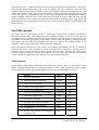
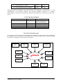


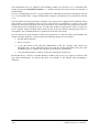
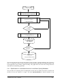
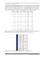

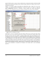
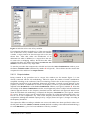
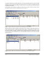
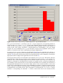
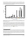
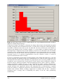
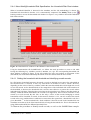
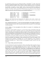
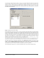

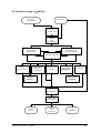
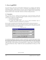
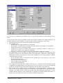


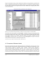
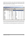

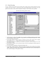

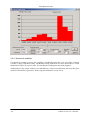

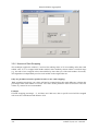
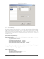
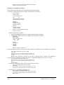
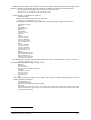
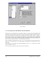
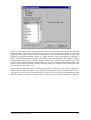
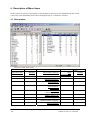
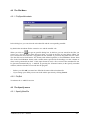
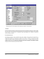
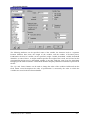
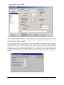
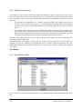


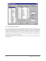
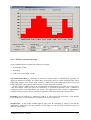


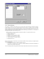
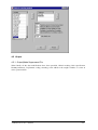
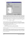
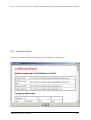
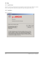


![Registry Manual []](http://vs1.manualzilla.com/store/data/005750489_1-c8586633e9f35db1a00a4874731a3151-150x150.png)