1
QuickSim II Advanced Training
Workbook
Software Version 8.5_1
Copyright
1991 - 1995 Mentor Graphics Corporation. All rights reserved.
Confidential. May be photocopied by licensed customers of
Mentor Graphics for internal business purposes only.
The software programs described in this document are confidential and proprietary products of Mentor
Graphics Corporation (Mentor Graphics) or its licensors. No part of this document may be photocopied,
reproduced or translated, or transferred, disclosed or otherwise provided to third parties, without the prior
written consent of Mentor Graphics.
The document is for informational and instructional purposes. Mentor Graphics reserves the right to make
changes in specifications and other information contained in this publication without prior notice, and the
reader should, in all cases, consult Mentor Graphics to determine whether any changes have been made.
The terms and conditions governing the sale and licensing of Mentor Graphics products are set forth in the
written contracts between Mentor Graphics and its customers. No representation or other affirmation of
fact contained in this publication shall be deemed to be a warranty or give rise to any liability of Mentor
Graphics whatsoever.
MENTOR GRAPHICS MAKES NO WARRANTY OF ANY KIND WITH REGARD TO THIS MATERIAL
INCLUDING, BUT NOT LIMITED TO, THE IMPLIED WARRANTIES OR MERCHANTABILITY AND
FITNESS FOR A PARTICULAR PURPOSE.
MENTOR GRAPHICS SHALL NOT BE LIABLE FOR ANY INCIDENTAL, INDIRECT, SPECIAL, OR
CONSEQUENTIAL DAMAGES WHATSOEVER (INCLUDING BUT NOT LIMITED TO LOST PROFITS)
ARISING OUT OF OR RELATED TO THIS PUBLICATION OR THE INFORMATION CONTAINED IN IT,
EVEN IF MENTOR GRAPHICS CORPORATION HAS BEEN ADVISED OF THE POSSIBILITY OF SUCH
DAMAGES.
RESTRICTED RIGHTS LEGEND Use, duplication, or disclosure by the Government is subject to
restrictions as set forth in the subdivision (c)(1)(ii) of the Rights in Technical Data and Computer Software
clause at DFARS 252.227-7013.
A complete list of trademark names appears in a separate “Trademark Information” document.
Mentor Graphics Corporation
8005 S.W. Boeckman Road, Wilsonville, Oregon 97070-7777.
This is an unpublished work of Mentor Graphics Corporation.
Table of Contents
TABLE OF CONTENTS
About This Training Workbook
Purpose of Course
Course Overview
Workbook Format
Lab Exercises
Timeline For Completion of the Course
Related Publications
Simulation Manuals
Modeling Manuals
Falcon Framework Manuals
Learning Programs
Module 1
Setting Up for QuickSim II
Module 1 Overview
Lessons
Design Hierarchy
Property Value Resolution
What Needs to Be Set Up?
Custom Design Configuration
Using Primitives for Performance
Using RAMs and ROMs
MTM Interface File Example
Timing Statistics
Editing a Component Interface
MGC Shell Environment Variables
Using Invocation Options
Changing Invocation Defaults
Lab Overview
Module 1 Lab Exercise
Procedure 1: Copying the Training Data
Procedure 2: Creating MTM Initialization File
Procedure 3: Checking for the Modelfile Property
QuickSim II Advanced Training Workbook, 8.5_1
November 1995
xi
xii
xiv
xvi
xviii
xx
xxii
xxiv
xxvi
xxvii
xxviii
1-1
1-2
1-3
1-4
1-6
1-8
1-10
1-12
1-14
1-16
1-18
1-20
1-22
1-24
1-26
1-28
1-30
1-30
1-32
1-34
iii
Table of Contents
TABLE OF CONTENTS [continued]
Procedure 3b (optional): Checking Using CIB
Procedure 4: Adding the Modelfile Property
Procedure 5: Verifying the ROM Models
Module 1 Summary
Module 2
Advanced Stimulus Techniques
2-1
Module 2 Overview
Lessons
Design Signal Initialization
The Initialization Process
The INIT Property
Developing Design Stimulus
Setting Up Force Types
Force Type Examples
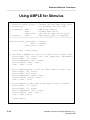
Using AMPLE for Stimulus
AMPLE Access to Waveform Data
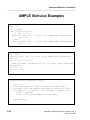
AMPLE Stimulus Examples
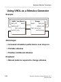
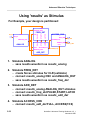
Using VHDL as a Stimulus Generator
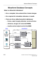
Waveform Database Concepts
Editing Waveforms
Merging Waveforms
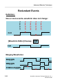
Redundant Events
Using 'results' as Stimulus
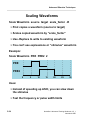
Scaling Waveforms
Dithering Waveforms
Inserting Waveform Ambiguity
Loading/Connecting Waveforms
Creating Stimulus Patterns
Gathering Toggle Statistics
Lab Overview
Module 2 Lab Exercise
Procedure 1: Using the Stimulus Pattern Generator
iv
1-35
1-38
1-40
1-43
2-2
2-3
2-4
2-6
2-8
2-10
2-12
2-14
2-16
2-18
2-20
2-22
2-24
2-26
2-28
2-30
2-32
2-34
2-36
2-38
2-40
2-42
2-44
2-46
2-47
2-48
QuickSim II Advanced Training Workbook, 8.5_1
November 1995
Table of Contents
TABLE OF CONTENTS [continued]
Procedure 2: Write an AMPLE Stimulus File
Module 2 Summary
Module 3
Debugging Timing and Unknowns
Module 3 Overview
Lessons
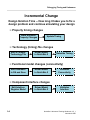
Factors in Design Debugging
Incremental Change
Board Simulation--Helpful Hints
Board Simulation with ASICs
Spikes
Technology File Spike Models
When Are Spikes Suppressed
When Do Spikes Produce X’s
When Spikes Pulses Transport
Technology File Spike Model Example
Inertial vs. Transport Delays
Hazards and Oscillations
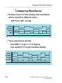
Comparing Waveforms
VHDL Debugger Process
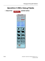
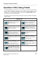
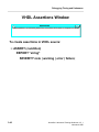
QuickSim II VHDL Debugger
QuickSim II VHDL Debug Palette
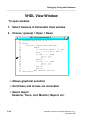
VHDL View Window
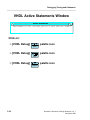
VHDL Active Statements Window
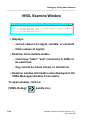
VHDL Examine Window
VHDL Assertions Window
VHDL-Related Windows
Lab Overview
Module 3 Lab Exercise
Procedure 1: Setting Up the VHDL Training Data
Procedure 2: Creating and Saving Valid Results
Procedure 3: Changing to the VHDL Design Model
QuickSim II Advanced Training Workbook, 8.5_1
November 1995
2-54
2-56
3-1
3-2
3-3
3-4
3-6
3-8
3-10
3-12
3-14
3-16
3-18
3-20
3-22
3-24
3-26
3-28
3-30
3-32
3-34
3-36
3-38
3-40
3-42
3-44
3-46
3-48
3-48
3-50
3-53
v
Table of Contents
TABLE OF CONTENTS [continued]
Procedure 4: Debugging VHDL With QuickSim II
Procedure 5: Modify and Verify the VHDL Source
Module 3 Summary
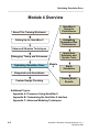
Module 4
Optimizing Simulation Runs
3-54
3-59
3-61
4-1
Module 4 Overview
Lessons
QuickSim II Optimization
Modeling for Performance
Hardware Considerations
Stimulus and Reporting
Limiting Display Updates
Estimating Accuracy
Estimating Performance (Run-time)
Estimating Memory Requirements
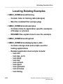
Locating Existing Examples
Running Application Systests
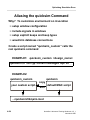
Aliasing the quicksim Command
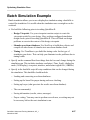
Batch Simulation Example
Lab Overview
Module 4 Lab Exercise
Procedure 1: Running the QuickSim II Systest
Procedure 2: Test Simulation Performance
Module 4 Summary
4-2
4-3
4-4
4-6
4-8
4-10
4-12
4-14
4-16
4-18
4-20
4-22
4-24
4-26
4-28
4-30
4-30
4-33
4-37
Module 5
Viewpoints and Annotations
5-1
Module 5 Overview
Lessons
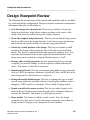
Design Viewpoint Review
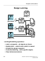
Design Latching
Back Annotation Benefits
5-2
5-3
5-4
5-6
5-8
vi
QuickSim II Advanced Training Workbook, 8.5_1
November 1995
Table of Contents
TABLE OF CONTENTS [continued]
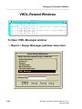
Back Annotations
Merging Back Annotations
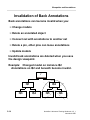
Invalidation of Back Annotations
ASCII Back Annotations
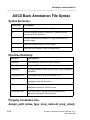
ASCII Back Annotation File Syntax
ASCII Back Annotation File Examples
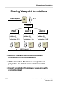
Sharing Viewpoint Annotations
Design Viewing and Analysis Support
Selection Examples
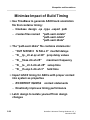
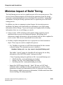
Minimize Impact of Build Timing
Lab Overview
Module 5 Lab Exercise
Procedure 1: Creating a DVE Script
Procedure 2: Managing Annotations
Procedure 3: Latching Design Objects
Procedure 4: Selection using System Properties
Procedure 5: Connect and Merge Annotations
Module 5 Summary
Module 6
Custom Design Checks
Module 6 Overview
Lessons
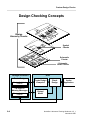
Design Checking Concepts
Custom Design Checking
Design Checking Applications
QuickCheck
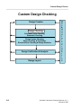
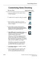
Customizing Name Checking
Name Checking Example
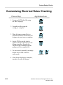
Customizing Electrical Rules Checking
Electrical Rules Checking Example
Netlisting Designs
EDIF Netlisting
QuickSim II Advanced Training Workbook, 8.5_1
November 1995
5-10
5-12
5-14
5-16
5-18
5-20
5-22
5-24
5-26
5-28
5-30
5-32
5-32
5-33
5-36
5-37
5-38
5-43
6-1
6-2
6-3
6-4
6-6
6-8
6-10
6-12
6-14
6-16
6-18
6-20
6-22
vii
Table of Contents
TABLE OF CONTENTS [continued]
DDP and DFI Netlisting
Hierarchical and Flat Netlisting
Lab Overview
Module 6 Lab Exercise
Procedure 1: Creating a Custom Naming Check
Procedure 2: Creating a Custom Electrical Rules Check
Module 6 Summary
Appendix A
Processes Using QuickSim II
6-24
6-26
6-28
6-30
6-30
6-33
6-36
A-1
Appendix A Lessons
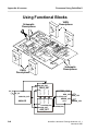
Principles of Top-Down Design
Using Functional Blocks
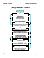
Design Process--ASIC
Design Process--Board
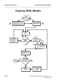
Creating VHDL Models
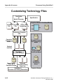
Customizing Technology Files
A-1
A-2
A-4
A-6
A-8
A-10
A-12
Appendix B
Customizing QuickSim II Interface
B-1
Appendix B Lessons
Customizing the Simulation Interface
Creating Custom Key Definitions
Creating Custom Strokes
Available QuickSim II Strokes
The Userware Environment
Loading Custom Userware Files
Customizing Startup Files
Lab Overview
Appendix B Lab Exercise
Procedure 1: Define Keys to Run Simulation
Procedure 2: Define Strokes to Scroll List Window
Procedure 3: Prompt for Working Directory
viii
B-1
B-2
B-4
B-6
B-8
B-10
B-12
B-14
B-16
B-18
B-18
B-21
B-23
QuickSim II Advanced Training Workbook, 8.5_1
November 1995
Table of Contents
TABLE OF CONTENTS [continued]
Procedure 4: Create a QuickSim II Startup File
Appendix C
Advanced Modeling Techniques
Appendix C Lessons
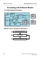
Simulating with Different Models
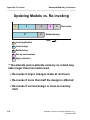
Updating Models vs. Re-invoking
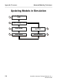
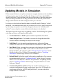
Updating Models in Simulation
Re-using Models (review)
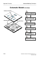
Schematic Models (review)
BRES Resistor Model
Advanced Modeling Process (AMP)
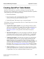
Creating QuickPart Table Models
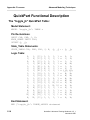
QuickPart Functional Description
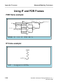
Using IF and FOR Frames
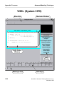
VHDL (System-1076)
Appendix C Summary
QuickSim II Advanced Training Workbook, 8.5_1
November 1995
B-26
C-1
C-1
C-2
C-4
C-6
C-8
C-10
C-12
C-14
C-16
C-18
C-20
C-22
C-24
ix
Table of Contents
TABLE OF CONTENTS [continued]
x
QuickSim II Advanced Training Workbook, 8.5_1
November 1995
About This Training Workbook
About This Training Workbook
Welcome to the QuickSim II Advanced Training Workbook. In this course you
will learn advanced QuickSim II concepts such as modeling details,
troubleshooting, VHDL simulation, and optimization. You will also learn to
create macros and AMPLEware to create stimulus and automate the setup process.
Note
This training workbook requires that you know how to use the
common user interface of the Falcon Framework. QuickSim II uses
this interface for the window, mouse, and keyboard environment. For
more information about Falcon Framework, refer to the Getting
Started with Falcon Framework.
You are also required to know how to use QuickSim II, Design
Architect, and Design Viewpoint Editor (DVE). Many of the concepts
presented in this course build upon the basic fundamentals used in
these applications.
If you are using this document online in INFORM, you will see occasional
highlighted text. On a black and white display, this text appears enclosed in a
rectangle, and on a color display using the default color map, the text is blue. The
highlighted text is a hypertext link to related materials in this and other
documents. If you click the Select mouse button on a hypertext link, the linked
location will be displayed.
i
For information about the documentation conventions used in this
manual, refer to Mentor Graphics Corporation Documentation
Conventions.
QuickSim II Advanced Training Workbook, 8.5_1
November 1995
xi
Purpose of Course
About This Training Workbook
Purpose of Course
• Make you more productive using QuickSim II
• Discuss the process that uses QuickSim II to
simulate functionality and timing of digital designs
• Show efficient methods of analysis & verification
• Let you choose efficient modeling strategy
• Generate stimulus in an efficient manner
• Use QuickSim II to debug VHDL models
• Perform “automated” simulation runs
• Troubleshoot design problems and understand
their causes
• Customize the QuickSim II user interface to
become more productive
This training workbook does not address the
following:
• Writing VHDL models, or other model structures
• Basic QuickSim II, Design Architect or DVE
concepts
xii
QuickSim II Advanced Training Workbook, 8.5_1
November 1995
About This Training Workbook
Purpose of Course
Purpose of Course
The main aim of this course is to contribute to make your work with QuickSim II
efficient and satisfactory.
This workbook takes up where the SimView and QuickSim II Training Workbook
leave off. Lessons and Lab Exercises build on concepts you have already learned
from the basic training. Therefore, many of the basic concepts will not be taught
in this workbook, but will be used to support more advanced concepts.
This workbook explains the main features of QuickSim II, shows efficient
methods of design analysis and verification, and discusses tools and data objects
connected to simulation process. This includes the following:
• Discuss the processes that use QuickSim II to simulate functionality and
timing of digital designs. This includes Top-down design, ASIC design, board
design, and MCM.
• Show efficient methods of design analysis and verification.
• Let you choose efficient modeling strategies.
• Generate stimulus in an efficient and effective manner. You will use the
Stimulus Generator, AMPLE stimulus files, and VHDL.
• Use QuickSim II to debug VHDL models. The viewing capabilities will be
presented.
• Perform “automated” simulation runs. Batch viewpoint creation and batch
simulation will be demonstrated.
• Troubleshoot design problems and understand their causes.
• Customize the QuickSim II user interface to become more productive.
This workbook does not address the following:
• Writing VHDL models, or other model structures
• Basic QuickSim II, Design Architect, or DVE concepts
QuickSim II Advanced Training Workbook, 8.5_1
November 1995
xiii
Purpose of Course
About This Training Workbook
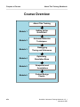
Course Overview
About This Training
xiv
Module 1
Setting Up for
QuickSim II
Module 2
Advanced Stimulus
Techniques
Module 3
Debugging
Timing and Unknowns
Module 4
Optimizing
Simulation Runs
Module 5
Viewpoints and
Annotations
Module 6
Custom Design
Checks
QuickSim II Advanced Training Workbook, 8.5_1
November 1995
About This Training Workbook
Purpose of Course
Course Overview
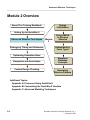
This workbook is divided into modules. In addition, this “About This Training
Workbook” section introduces this training workbook. Here is a brief description
of each module:
• About This Training Workbook. Describes how to use this workbook and
the accompanying software.
1. Setting Up for QuickSim II. This module discusses how to prepare your
design environment prior to invoking QuickSim II. The areas of setup are:
design viewpoint, back annotations, timing, stimulus, and QuickSim II
invocation.
2. Advanced Stimulus Techniques. This module contains information about
using VHDL as stimulus, merging waveforms and waveform databases, MISL
files, and advanced waveform editing techniques.
3. Debugging Timing and Unknowns. This module discusses advanced
modeling techniques (including AMS), using features of technology files,
creating Memory Table Models, VHDL simulation debug mode, and
TimeBase debug mode.
4. Optimizing Simulation Runs. This module presents design complexity and
timing trade-offs, Top-down design optimization, simulation throughput,
incorporating back annotations from ASIC and Board layout, and estimating
memory size and simulation run times.
5. Custom Design Checks. This module discusses the viewpoint and back
annotations creation/connection process. It discusses design latching. It also
talks about design object selection using DVAS system properties.
6. Viewpoints and Annotations. This module discusses the viewpoint and back
annotations creation/connection process. It discusses design latching. It also
talks about design object selection using DVAS system properties.
In addition, there are several appendixes that contain information on how to
customize the QuickSim II interface, an details about how QuickSim II is used in
other design processes, and the structure of the commonly used models.
QuickSim II Advanced Training Workbook, 8.5_1
November 1995
xv
Purpose of Course
About This Training Workbook
Workbook Format
• The lecture page layout:
The Mouse
Stroke/Drag
Select
Menu
The Three-Button Mouse
The three-button mouse is the most common
graphic input device. You interact with
an application by moving the mouse and
manipulating the mouse buttons. The mouse
actions affect what is displayed on the
screen and how the application operates.
Each button has a standard Mentor Graphics
name and predefined function.
Mouse Buttons
The three-button mouse has a left,
middle, and right button.
Mentor Graphics manuals refer to the
mouse buttons by the
following names:
The Select mouse button is the left button.
The Three-Button Mouse
The Stroke/Drag mouse button is the
center button.
Mouse Buttons
The Menu mouse button is the right button.
i
Title, Pictures
and Bulleted List
For more information on using the
mouse, refer to page 3-23.
Explanatory Text
and References
• Reference documentation is available online
(INFORM)
xvi
QuickSim II Advanced Training Workbook, 8.5_1
November 1995
About This Training Workbook
Purpose of Course
Workbook Format
As shown in the illustration, left- and right-facing pages of the module discussions
serve different purposes. The left page contains brief descriptions, figures, and
tables. The right page explains concepts, and contains document references.
Within this workbook you will find:
• Table of Contents: A listing of section titles, figures and tables.
• About This Training Workbook: Contains general workbook information
and explains how to use this student workbook.
• Modules: Each module has the following structure:
o Overview: Description of the module contents and a list of objectives for
using the material. The objectives describe what you should know or be
able to do after completing the material.
o Lesson: Narrative explanations of concepts and practice procedures. This
material uses the left- right- page concept.
o Lab Exercises: Complete materials to perform the hands-on lab session for
each module. Each lab session includes:
o Lab Procedures: Step-by-step lab instructions for a procedure.
o Module Summary: A text review of what was learned in this module.
• Appendixes: Additional supporting material that can optionally be added to
this training course.
QuickSim II Advanced Training Workbook, 8.5_1
November 1995
xvii
Purpose of Course
About This Training Workbook
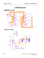
Lab Exercises
MEMORY circuit:
A(7:0)
AIN(9:0)
RAM1
74LS139A
ROM1
$MTM
A(7:0)
DATA_IN(15:0)
DATA_IN(15:0)
DATA_OUT(15:0)
DATA_OUT(15:0)
CLOCK
READ_EN
WRITE_EN
CHIP_EN
CLOCK
READ_EN
WRITE_EN
CHIP_EN
RAM2
DIN(15:0)
ROM2
$MTM
$MTM
A(7:0)
A(7:0)
DATA_IN(15:0)
DATA_IN(15:0)
DATA_OUT(15:0)
DATA_OUT(15:0)
CIN
$MTM
A(7:0)
CLOCK
READ_EN
WRITE_EN
CHIP_EN
CLOCK
READ_EN
WRITE_EN
CHIP_EN
R_W
MOUT(15:0)
add_det circuit:
D
_PRE
74LS74A
74LS04
Q
_CLR
CLK
FULL
_Q
74LS08
TEST
PARITY
R2
74259
_E Q0
_CLRQ1
Q2
A0 Q3
A1 Q4
A2 Q5
Q6
D
Q7
74LS161A
_CLR
_LOAD
ENT RCO
ENP
CLK
START
PULSE
A
B
C
D
74259
_E Q0
_CLRQ1
Q2
A0 Q3
A1 Q4
A2 Q5
Q6
D
Q7
ACCESS(15:0)
QA
QB
QC
QD
ANALOG_OUT
_CLR
R1
74LS04
74LS08
74LS04
74LS08
74LS04
LATCH
xviii
QuickSim II Advanced Training Workbook, 8.5_1
November 1995
About This Training Workbook
Purpose of Course
Lab Exercises
Many of the Lab Exercises in this training workbook are based on the MEMORY
circuit shown on the previous page. This circuit uses a Memory Table model for
the RAM and ROM components.
In addition, an add_det circuit is provided for troubleshooting and back annotation
Lab Exercises. This circuit uses several TTL devices and gen_lib components.
Lab Exercises are divided into numbered steps that are short groups of actions that
form an operation. Procedures may require several steps to complete. A step is
divided into three parts:
1. What you will do. A short description of what you should expect to complete
at the end of the step. The details of how to perform the actions are not given in
this part.
2. How you will do it. A detailed description of the things you must do to
complete the step. This includes caveats and helpful hints.
3. What is the result. Usually a picture or a brief explanation, showing the
outcome of this step. You use this information to verify that you have done the
step correctly. Remember that each step builds on the preceding step. If you
incorrectly perform a step, the subsequent steps may be impossible to complete
correctly.
QuickSim II Advanced Training Workbook, 8.5_1
November 1995
xix
Purpose of Course
About This Training Workbook
Timeline For Completion of the Course
9:00
Day 1 of 2
Day 2 of 2
Module 1:
Setting up for
QuickSim II
Module 4:
Optimizing Simulation Runs
9:30
xx
Module 5:
Viewpoints and Annotations
11:30
LUNCH
LUNCH
12:30
Module 2:
Advanced Stimulus
Techniques
(Continue)
Module 5:
Viewpoints and Annotations
2:00
Module 3:
Debugging Timing and
Unknowns
3:30
Module 6:
Custom Design Checks
5:00
Wrap-up
QuickSim II Advanced Training Workbook, 8.5_1
November 1995
About This Training Workbook
Purpose of Course
Timeline For Completion of the Course
The QuickSim II Advanced Training Workbook, delivered by a trained instructor,
takes 2 days. Use the table on the previous page to determine the timing and
delivery of each module.
If you are using this training workbook as a Personal Learning Program, you
should allow about 18 hours to complete the Lessons and Lab Exercises. It is not
necessary to complete all of the Lab Exercises in one sitting. But lab exercises
must be completed in the order presented in this workbook, since each exercise
builds on the previous one.
QuickSim II Advanced Training Workbook, 8.5_1
November 1995
xxi
Related Publications
About This Training Workbook
Related Publications
The following text and illustration lists the Mentor Graphics manuals that
document all of the features used by simulation applications. The manuals are
divided into the following categories:
• Simulation Manuals (page xxiv) -- document individual simulation
applications and closely-related functionality that is common among two or
more simulators, such as viewpoint creation and charting capability.
• Modeling Manuals (page xxvi) -- document the methodologies available to
create models for Mentor Graphics simulation applications.
• Framework Manuals (page xxvii) -- document features that are common to
all Mentor Graphics applications.
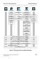
The Simulation Documentation Roadmap on page xxiii shows which manuals
document the various Mentor Graphics simulation products. To use this figure,
locate the icon for your application across the top row and then descend along the
shaded bar. This bar overlaps each document title box that contains information
about your application. For more information about manuals listed in the
Simulation Documentation Roadmap, refer to the following pages.
xxii
QuickSim II Advanced Training Workbook, 8.5_1
November 1995
About This Training Workbook
SimView
Related Publications
QuickSim II
Continuum
AccuSim II
Getting
Started with
QuickSim II
Continuum User’s
and
Reference Manual
Getting Started
with AccuSim II
QuickSim II
User’s Manual
AIK
Analog Simulators User’s Manual
Analog Simulators Reference Manual
Digital Simulators Reference Manual
QuickSim II
Training
Workbook
AccuParts
User’s Manual
System Modeling
Blocks User’s and
Reference Manual
Analog
Interface Kit
Programmer’s
Guide
AccuSim II Models
Reference Manual
HDL-A
Reference Manual
Analog Station
Training Workbook
HDL-A
Training Workbook
SimView Common Simulation User's Manual
SimView Common Simulation Reference Manual
Charting User's and Reference Manual
Design Viewing and Analysis Support Manual
Design Viewpoint Editor User's and Reference Manual
Digital Modeling Manuals
Falcon Framework Manuals
Figure 1. Simulation Documentation Roadmap
QuickSim II Advanced Training Workbook, 8.5_1
November 1995
xxiii
Related Publications
About This Training Workbook
Simulation Manuals
Analog Simulators Reference Manual contains information about the commands,
functions, userware, and related reference material specific to the Mentor
Graphics analog simulators.
Analog Simulators User's Manual describes how to use AccuSim and an
assembled Analog Interface Kit. This manual provides background information,
various simulation procedures, and a comprehensive list of related procedures.
Circuit PathFinder User's and Reference Manual contains conceptual
information; a brief, hands-on tutorial; procedures for compilation, analysis, and
model generation; and a description of commands and functions for the Circuit
PathFinder timing analyzer.
Design Viewing and Analysis Support Manual contains information about Design
Viewing and Analysis Support (DVAS). DVAS consists of functions and
commands that provide selection, viewing, highlighting, reporting, grouping,
syntax checking, naming, and window-manipulating capabilities.
Design Viewpoint Editor User's and Reference Manual contains information
about the Design Viewpoint Editor (DVE). DVE allows you to add, modify, and
manage back annotation data, as well as define and modify design configuration
rules for design viewpoints.
Digital Simulators Reference Manual contains information about the commands,
functions, userware, and related reference material specific to the QuickSim II,
QuickGrade II, and QuickFault II digital analysis applications.
Fault Analysis User's Manual contains overview information and fault analysis
operating procedures relating to the QuickGrade II and QuickFault II fault
analysis applications.
xxiv
QuickSim II Advanced Training Workbook, 8.5_1
November 1995
About This Training Workbook
Related Publications
QuickPath User's and Reference Manual contains information about the
QuickPath timing analyzer. It provides background information, a hands-on
tutorial intended for new users, and various procedures for validating the timing of
digital circuit designs.
QuickSim II User's Manual describes how to use the QuickSim II logic simulator.
This manual provides background information, various simulation procedures,
and a comprehensive list of related procedures.
SimView Common Simulation Reference Manual contains information about the
commands, functions, userware, and related reference material for the SimView
application. This material is also common to all Mentor Graphics digital and
analog analysis applications.
SimView Common Simulation User's Manual describes how to use the SimView
application. This manual provides background information, various simulation
procedures, and a comprehensive list of related procedures that are common to all
Mentor Graphics digital and analog analysis applications.
QuickSim II Advanced Training Workbook, 8.5_1
November 1995
xxv
Related Publications
About This Training Workbook
Modeling Manuals
Behavioral Language Model (BLM) Development Manual describes how to use
the files, commands, and data structures available with Mentor Graphics software
to write BLMs.
Memory Table Model Development Manual contains information that helps you
develop Memory Table Models, which specify the functionality of a memory
device's pins.
Properties Reference Manual contains comprehensive information about Mentor
Graphics design properties, which are used by many Mentor Graphics products,
including all simulation applications.
QuickPart Schematic Model Development Manual contains information that helps
you develop QuickPart Schematic models. These types of models are based on a
compiled schematic.
QuickPart Table Model Development Manual contains information that helps you
develop QuickPart Table models. These types of models are based on ASCII truth
tables.
System-1076 Design and Model Development Manual provides concepts,
procedures, and techniques for using VHDL within the System-1076
environment.
Technology File Development Manual explains the use of technology files to aid
in the modeling of electronic parts and components. This manual provides
detailed reference information about technology file statements, usage
information, and a tutorial.
xxvi
QuickSim II Advanced Training Workbook, 8.5_1
November 1995
About This Training Workbook
Related Publications
Falcon Framework Manuals
AMPLE User's Manual describes how to use the Mentor Graphics AMPLE
language. This manual contains flow-diagram descriptions and explanations of
important concepts, and shows how to write AMPLE functions.
BOLD Browser User's Manual explains basic BOLD Browser operations such as
searching for a phrase in the INFORM library, using the travel log, and following
hypertext links to view different documents. The BOLD Browser provides access
to reference help for most Mentor Graphics applications.
Common User Interface Manual describes how to use the user interface features
that are common to all Mentor Graphics products. This manual tells how to
manage and use windows, the popup command line, function keys, strokes,
menus, prompt bars, and dialog boxes.
Customizing the Common User Interface describes how to extend the Common
User Interface. This manual explains how to redefine keys and how to create your
own menus, windows, dialog boxes, messages, and palettes.
Design Manager User's Manual provides information about the concepts and use
of the Design Manager. This manual contains a basic overview of design
management and of the Design Manager, key concepts to help you use the Design
Manager, and many design management procedures.
Notepad User's and Reference Manual describes how to edit files and documents
in Notepad, a text editor. This manual provides examples, explanations, and an
alphabetical listing of AMPLE functions that are available for customizing
Notepad.
QuickSim II Advanced Training Workbook, 8.5_1
November 1995
xxvii
Related Publications
About This Training Workbook
Learning Programs
The following Getting Started workbooks provide conceptual information about
the product and lab exercises that you can follow to gain hands-on experience
with the product. Many of these workbooks contain prerequisite information to
this course.
Getting Started with AccuSim II is for analog design engineers who have not
previously used AccuSim. This training workbook provides basic instructions for
using AccuSim to simulate analog designs.
Getting Started with Design Architect is for new users of Design Architect who
have some knowledge about schematic drawing and electronic design, and are
familiar with the UNIX or Aegis environment. The training workbook provides
you with basic instructions on how to use Design Architect to create schematics
and symbols.
Getting Started with Falcon Framework is for new users of the Mentor Graphics
Falcon Framework. This workbook provides information about and practice using
the Common User Interface, Design Manager, INFORM, Notepad, and Decision
Support System applications.
Getting Started with QuickGrade II is for digital design engineers who have not
previously used QuickGrade II. This training workbook provides basic
instructions for using QuickGrade II to perform statistical fault analysis on digital
designs.
Getting Started with QuickPath is for digital design engineers who have not
previously used QuickPath. This training workbook provides basic instructions
for using QuickPath to perform a static timing analysis on digital designs.
Getting Started with QuickSim II is for digital design engineers who have not
previously used QuickSim II. This training workbook provides basic instructions
for using QuickSim II to simulate digital designs.
xxviii
QuickSim II Advanced Training Workbook, 8.5_1
November 1995
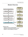
Setting Up for QuickSim II
Module 1
Setting Up for QuickSim II
Module 1 Overview
1-2
Lessons
Design Hierarchy
Property Value Resolution
What Needs to Be Set Up?
Custom Design Configuration
Using Primitives for Performance
Using RAMs and ROMs
MTM Interface File Example
Timing Statistics
Editing a Component Interface
MGC Shell Environment Variables
Using Invocation Options
Changing Invocation Defaults
Lab Overview
1-3
1-4
1-6
1-8
1-10
1-12
1-14
1-16
1-18
1-20
1-22
1-24
1-26
1-28
Module 1 Lab Exercise
Procedure 1: Copying the Training Data
Procedure 2: Creating MTM Initialization File
Procedure 3: Checking for the Modelfile Property
Procedure 3b (optional): Checking Using CIB
Procedure 4: Adding the Modelfile Property
Procedure 5: Verifying the ROM Models
1-30
1-30
1-32
1-34
1-35
1-38
1-40
Module 1 Summary
1-43
QuickSim II Advanced Training Workbook, 8.5_1
November 1995
1-1
Setting Up for QuickSim II
Module 1 Overview
About This Training Workbook
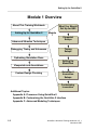
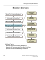
Setting Up for QuickSim II
Advanced Stimulus Techniques
Debugging Timing and Unknowns
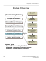
What You Should
Set Up for QSII
Module
1
Viewpoint
Setups
Timing
Setups
Optimizing Simulation Runs
Viewpoints and Annotations
Custom Design Checking
Setting Up
Modelfiles
QuickSim II
Invocation
Setups
Customizing
Invocation
Additional Topics:
Appendix A: Processes Using QuickSim II
Appendix B: Customizing the QuickSim II Interface
Appendix C: Advanced Modeling Techniques
1-2
QuickSim II Advanced Training Workbook, 8.5_1
November 1995
Setting Up for QuickSim II
Lessons
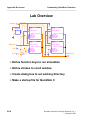
On completion of this module, you should:
• Know what you need to set up for a QuickSim II digital simulation.
• Understand the design hierarchy and how to describe objects within that
hierarchy.
• Be able to create a custom design configuration script that uses DVE to build a
custom design viewpoint.
• Be able to use the Component Interface Browser (CIB) to locate information
from the component interface, and to make changes to the interface.
• Be able to create an ASCII initialization file for a Memory Table model to
efficiently initialize all memory locations.
• Be able to properly attach the ASCII initialization file to a Memory Table
model using the modelfile property.
• Know the shell environment variables that are recognized by QuickSim II and
what actions are taken if a specific variable is not available.
• Be able to customize the invocation script for QuickSim II to preset any switch
configuration that is required for your site.
You should allow approximately 2 hours to complete the Lesson,
Lab Exercise, and Test Your Knowledge portions of this module.
Note
QuickSim II Advanced Training Workbook, 8.5_1
November 1995
1-3
Setting Up for QuickSim II
Design Hierarchy
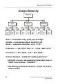
/:sheet1
I$1
I$2
cpu1
cpu2
I$2
I$10
AND
AND
I$4
INV
I$2
I$10
AND
AND
I$3
controller
I$4 I$1#1 I$1#2
INV
OR
OR
I$3
INV
Root -- invocation entry point, top of design
Handle -- local design object identifier: I$2
Name -- substitute identifier; cpu1 <-> I$1
Pathname -- / I$2 / I$10 / OUT or / cpu2 / AND / OUT
For Frame -- / I$3 / I$1#1 and / I$3 / I$1#2
Current Context -- similar to “working directory”
• Activate a source view window (schematic view or
VHDL view window) *PRIORITY*
• Set Naming Context command -- only if no source
view is active
1-4
QuickSim II Advanced Training Workbook, 8.5_1
November 1995
Setting Up for QuickSim II
Design Hierarchy
(review)
The pathnames for every instance, net, and pin are defined in relation to a
hierarchy of instances that comprise the design. The figure on the previous page
illustrates this hierarchy, or design tree:
• The top of the design (labeled “/”) is the design root. The design pathname to
the root is “/”.
• The root contains three instances, I$1, I$2, and I$3. The pathnames to each of
the instances are /cpu1, /cpu2, and /controller, respectively. You can use
handles and names interchangeably.
• /I$1 and /I$2 are different instances of the same “cpu” component. Therefore,
/I$1 and /I$2 point to the same copy of the sheet-based component, but have
different design pathnames.
• If a component is replicated in a FOR frame, the instances created are
identified by “#n”, where “n” is the replication number. The two OR gates
(FOR framed) have pathnames /I$3/I$1#1 and /I$3/I$1#2 instead of the
pathnames /I$3/I$1 and /I$3/I$2.
• You can designate signals (nets and pins) by writing the instance pathname and
appending the name of the net or pin as the “leaf”. The pathname for a pin
might be /I$1/I$4/OUT, while a net might be /I$1/controller/busa. If a net and
pin have the same name, you can differentiate them using handles. You can
also append an :<object_type> extension to the name. For example,
/I$1/I$4/OUT:pin and /I$1/I$4/OUT:net are unique design pathnames.
The “context of the design” refers to examining a design with respect to the design
viewpoint. The current context is similar to a “working directory” within an
operating system. Moving the current context lets you use shorter pathnames in
commands. The following set the current context:
• Active view window. The current context is the location of the active
schematic sheet view or VHDL view in the design hierarchy.
• Naming context. If no view window is active, the current context is the value
of the naming context. The naming context is set by the DVAS command, Set
Naming Context. Check its value with the Report Naming Context command.
QuickSim II Advanced Training Workbook, 8.5_1
November 1995
1-5
Setting Up for QuickSim II
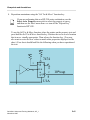
Property Value Resolution
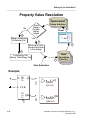
Symbol Model/
Comp. Interface
Does
Design
Contain
Higher
Levels
?
5
3
Sheet
Instance
CLR
No
Q
D
Design Viewpoint
Parameter List
PRE
Yes
CLK
4
2
Move up to next
hierarchical level
in the design
6
Technology File
Library Technology File
1
Back
Annotation
Priority 1
Start Evaluation
ENA
ENA
1-6
Q
OUT
QB
Q
0
0
(QRISE)
(QFALL)
0
0
(QBRISE)
(QBFALL)
CLK
CLR
IN
D
PRE
Example:
OUT
QB
QuickSim II Advanced Training Workbook, 8.5_1
November 1995
Setting Up for QuickSim II
Property Value Resolution
The figure shows the order of property value resolution within a design. These
values are called “parameters” because they are passed to the property from
another place in the design hierarchy. The search begins in the back annotation
objects, and is stopped as soon as the value is found. Property values are resolved
as follows:
1. The value of the property (parameter) is sought in the back annotation object.
If more than one back annotation object is connected to the design viewpoint,
the back annotation objects are searched in prioritized order; that is, the one
with the highest priority is searched first, and so on. The search is stopped at
the first occurrence of a property value, even if the same property has been
modified in multiple back annotation objects.
2. The object (instance, net, or pin) itself, and then the parent instance is
searched.
3. The symbol model (body property list) is searched next.
4. If the design has more levels of hierarchy, the search moves up a level and start
again at step #1. In step 2, only the parent instance is checked.
5. Search the design viewpoint parameter list for a value of the property.
6. Search the technology file (if registered to the beginning component) and then
the library data technology file (if registered to the beginning component) for
the property value. If the property value is not found or the technology files do
not exist, an error is issued. For additional information on using values in
technology files, refer to “Understanding the Scoping Rules” in the
Technology File Development Manual.
Each time a property value (parameter) is needed, evaluation occurs in this order.
Therefore, any changes made via back annotations cause the new property value
to be seen throughout the design.
i
For additional information on property resolution, refer to “Rules for
Resolving Property Value Variables” in the Design Architect User's
Manual.
QuickSim II Advanced Training Workbook, 8.5_1
November 1995
1-7
Setting Up for QuickSim II
What Needs to Be Set Up?
• Design Viewpoint:
Default viewpoint should not be used
Use vendor viewpoint or custom site viewpoint
Parameters--define the process and conditions
Primitives--determine depth of hierarchy
--remove large hierarchical blocks
o Latch versions in production environment
o Perform configured design checks in DVE
Back Annotation Objects:
o Create or assign modelfiles for RAMs and ROMs
o Annotate any generic timing
Timing Generation:
o TimeBase can generate timing info prior to
QuickSim II invocation
o Use TimeBase debug mode to troubleshoot
Stimulus Generation:
o Use SimView to generate/view stimulus
o Use VHDL test bench for conditional stimulus
Setup the shell environment (variables)
QuickSim II Invocation:
o Invoke on the correct design viewpoint
o Assign simulator resolution
o Set global mode switches on invocation--set local
modes in kernel after invoke
o
o
o
o
•
•
•
•
•
1-8
QuickSim II Advanced Training Workbook, 8.5_1
November 1995
Setting Up for QuickSim II
What Needs to Be Set Up?
There are many design setup considerations prior to invoking QuickSim II. Here
is a list of setups that you may need to perform prior to invocation:
• Design Viewpoint. Create a custom configuration, or use an ASIC vendor
viewpoint creation script. The default viewpoint is too limited for most
simulation runs. Set the value of unique parameters and primitives. Latch
design objects that may be changed while you are performing the simulation.
• Back Annotation Object. In one or more back annotation objects, you add or
change properties on your design. Models should all be defined in a back
annotation object, and should not be allowed to follow the default, which could
change during an update. Assign all modelfile paths in this same back
annotation object. Timing annotations should be kept in a separate back
annotation object, as they will change as the model evolves.
• Timing Generation. I some cases, time can be saved by generating timing
prior to invoking QuickSim II. TimeBase utilities allow you to debug timing
problems. You can also export timing information in back annotation ASCII
form and use it to annotate timing directly on the design.
• Stimulus Generation. Generate as much stimulus as possible in SimView
prior to entering QuickSim II. SimView supports waveform generation and
graphical editing. Create VHDL test benches to generate conditional stimulus
in your design. The test bench is added as a component in the design.
• Shell Environment. Make sure that the proper shell environment variables are
set. A list of the required and optional variables is on page.
• QuickSim II Invocation. Many of the invocation options can be changed
within QuickSim II after you invoke, but will incur a performance hit. The
simulator resolution, viewpoint, interface, and design root can't be changed
and must be set at invocation. It is a good practice to set all global conditions
and checks at invoke time, and only change local setups after invocation.
More information on these setup guidelines are contained on the next several
pages.
QuickSim II Advanced Training Workbook, 8.5_1
November 1995
1-9
Setting Up for QuickSim II
Custom Design Configuration
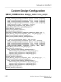
$MGC_HOME/bin/dve design_name < dve_script
// Setting up PCB design viewpoint
$add_visible_property(@instance, @nopin, @nonet, @nogroup,
$add_visible_property(@instance, @nopin, @nonet, @nogroup,
$add_visible_property(@noinstance, @pin, @nonet, @nogroup,
$add_visible_property(@noinstance, @nopin, @net, @nogroup,
$add_primitive("comp", @noexcept, @string);
$save_design_viewpoint("pcb_design_vpt");
$open_back_annotation("pcb_design_vpt");
$save_design_viewpoint();
$set_active_window("session");
$close_design_viewpoint();
$writeln("Created design viewpoint named pcb_design_vpt.");
$open_design_viewpoint(component_name, "sim_design_vpt", "",
$set_active_window("Design_Viewpoint");
$set_active_window("Design_Configuration");
//
Set up for(Quick)SIM, Fault, Path & Grade
$add_visible_property(@instance, @pin, @net, @nogroup,
$add_visible_property(@instance, @nopin, @nonet, @nogroup,
$add_visible_property(@noinstance, @pin, @nonet, @nogroup,
$add_visible_property(@noinstance, @nopin, @net, @nogroup,
$add_primitive("MODEL", @noexcept, @string, "INV", "BUF",
$open_back_annotation("sim_design_vpt");
$save_design_viewpoint();
$set_active_window("Design_Configuration");
$disconnect_back_annotation("sim_design_vpt");
$connect_back_annotation("pcb_design_vpt");
$connect_back_annotation("sim_design_vpt");
$save_design_viewpoint();
$close_design_viewpoint();
$open_design_viewpoint(component_name, "pcb_design_vpt", "",
$set_active_window("Design_Viewpoint");
$set_active_window("Design_Configuration");
$disconnect_back_annotation("pcb_design_vpt");
$connect_back_annotation("sim_design_vpt");
$connect_back_annotation("pcb_design_vpt");
$save_design_viewpoint();
$close_design_viewpoint();
1-10
QuickSim II Advanced Training Workbook, 8.5_1
November 1995
Setting Up for QuickSim II
Custom Design Configuration
It is rare that the default QuickSim II configuration will work for your design or
company requirements. You must create a custom design configuration using the
Design Viewpoint Editor (DVE). DVE can be used interactively from the user
interface or through a script of functions that runs DVE in batch mode.
You must use a custom design configuration when you need to set the level of
primitiveness other than the default, substitute property values, define parameters
for variables in the design, or need to set the visible properties. You typically
create a custom design configuration if you are using DFI, Netlist Module,
AutoLogic, or PCB products, because these applications either do not
automatically create a design viewpoint, or you need to change the default
settings.
A custom configuration is required to use Logic Modeling Corporation (LMC)
models or many ASIC designs. LMC and ASIC vendors usually provide a unique
configuration script to setup the initial custom design configuration. You may also
want to add to (modify) this design viewpoint to provide site-specific
configuration rules. A subsequent script can be run on an existing viewpoint to
add or change these rules.
The figure on the previous page shows a script that creates two viewpoints for a
single design (one for simulation and one for PCB layout). It also creates two back
annotation objects and cross connects them. The DVE command at the top of the
page shows how to direct the file contents to the input of the DVE command.
You can create a custom startup file that automatically runs when you invoke
DVE. This file is named dve_session.startup and can be located in the MGC tree
or your $HOME/mgc/startup directory, depending on its function. For these
startup file locations, see “Customizing Startup Files” on page B-14
i
For more information about design configuration, refer to “Design
Configuration” in the Design Viewpoint Editor User's and Reference
Manual. For more information, refer to “Editing in the Context of a
Design” in the Design Architect User's Manual.
QuickSim II Advanced Training Workbook, 8.5_1
November 1995
1-11
Setting Up for QuickSim II
Using Primitives for Performance
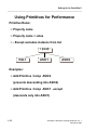
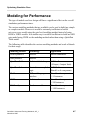
Primitive Rules:
• Property name
• Property name + value
• - Except excludes instance from list
/ (root)
PAL1
ASIC1
ASIC2
Examples:
• Add Primitive Comp ASIC2
(prevents descending into ASIC2)
• Add Primitive Comp ASIC1 -except
(descends only into ASIC1)
1-12
QuickSim II Advanced Training Workbook, 8.5_1
November 1995
Setting Up for QuickSim II
Using Primitives for Performance
Primitives allow you to specify the level at which the simulator stops looking for
simulation models. In addition, the invocation process does not build connectivity
or timing information below components specified as primitive. Primitives
definitions are added to the design viewpoint during the viewpoint creation
process, using the Design Viewpoint Editor. There are several modes in which
you can define primitives:
• Property only. In this mode, you specify the name of the property only, and
any instance containing that property is a primitive. For example, “Primitive
model” will make all instances containing the model property a primitive.
• Property + value. This allows you to specify a subset of property name/value
pairs as primitive. This is useful, for example, for specifying comp or inst
values to declare as primitive, so that you can remove functional blocks or
components from your simulation.
• Property + value -except. This mode allows you to declare all values of a
property name primitive except the value specified. For example, if you have
several functional blocks at the root (/) of your design, and you only want to
simulate one of them, you use the -except switch with the block identifier.
The following benefits can be gained by using primitives during simulation:
• Build time reduced. The timing and connectivity build process does not
include information contained below primitives. By breaking your simulation
apart into blocks and declaring non-essential blocks as primitive, you can save
invocation time.
• Simulation time reduced. Once a simulation run is initiated in QuickSim II,
the performance is much better because evaluations are not required with the
blocks that are declared primitive. Since a primitive model will not be
available for these blocks, the outputs use the state of Xz.
QuickSim II Advanced Training Workbook, 8.5_1
November 1995
1-13
Setting Up for QuickSim II
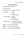
Using RAMs and ROMs
If any X's appear on the ROM address bus, the ROM
outputs all X's on the data bus.
Modelfile property value--pathname to ASCII file:
• Data and addresses must be hexadecimal or X
• Specify memory data using the form:
o address / data ; or
o low_address-high_address / data ;
• Any letter can be in upper or lower case
• Underspecifying--simulator fills in with zeros
16-bit example: FF = 00FF
Example 1: Initializing RAMs or ROMs to zero:
# 16-bit input-output
0-FFFF / 0 ; # Put zeros in all memory locations
0-ffff / f ; # Put 000F in all memory locations
Example 2: Using X in ROM or RAM modelfile:
# 16-bit input-output
00000 / 0 ;
# Put value of zero into location 0
FFXX / 1234 ; # Illegal addresses
FF00 / 1234 ; # Put value of 1234 into location FF00
FF00 / 11234 ; # Illegal data
FF00 / 12XX ; # Put value of 12XX into location FF00
1-14
QuickSim II Advanced Training Workbook, 8.5_1
November 1995
Setting Up for QuickSim II
Using RAMs and ROMs
The RAM and ROM models behave similarly, except that a ROM does not use
read and write pins. The ROM model operates like it has a read pin tied to a logic
1 and a write pin tied to logic 0. If any X's appear on the RAM or ROM address
bus, the device outputs all X's on the data bus.
When you use a ROM in a simulation, you must specify the ROM contents with
the Modelfile property. Although not required for a RAM (since you can write
RAM contents during the simulation), you can initialize RAM contents in a
similar manner. The Modelfile property gives the pathname to an ASCII file that
contains initialization data. The format of the ROM/RAM initialization file is as
follows:
• All data and addresses must be in hexadecimal, although X characters are
allowed in order to specify unknown data values. Note that a single X value
represents 4 bits of unknown value.
• Precede all comments with a pound sign (#).
• Specify the contents of a particular memory location using the form:
address / data ; or low_address-high_address / data ;
• Any letter can be in upper or lower case.
The previous page shows examples of ROM or RAM initialization files.
If you under-specify a data or address value, the simulator pads the value with
zeros. Thus, for a 16-bit ROM, a data value of FF becomes 00FF. While you can
legally over-specify data values with zeros or Xs, if over-specification causes a
binary 1 to occur in a non-valid part of the data (for example, the eighth bit of a 7bit data field) an error results. This is illustrated in the second example.
i
For more information on RAM and ROM models refer to the “Memory
Devices (RAM, ROM)” section of the Digital Simulators Reference
Manual.
QuickSim II Advanced Training Workbook, 8.5_1
November 1995
1-15
Setting Up for QuickSim II
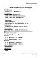
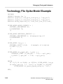
MTM Interface File Example
Model Statement:
Model sram : MEMORY =
Pin Declarations:
LOW_TRUE SELECT cs ;
LOW_TRUE WRITE_ENABLE we ;
LOW_TRUE OUT_ENABLE oe ;
ADDR adl ;
DATA INPUT din ;
DATA OUTPUT dout ENABLED_BY oe ;
Port Statement:
PORT (READ_WRITE, adl, din, dout)
Functional Table:
-_cs, we, adl:: MEM_ACTION,dout ;
##------------------------------||------------------------------## block unselected
1, ?, ?:: N,
0;
## read
0, 1, $VALID:: N, $MEM ;
0, 1, $UNKNOWN:: N, X ;
## write
0, 0, $VALID:: $WR,(din) ;
0, 0, $UNKNOWN:: $MX,X ;
Endport Statement:
ENDPORT;
End Statement:
END ;
1-16
QuickSim II Advanced Training Workbook, 8.5_1
November 1995
Setting Up for QuickSim II
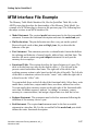
MTM Interface File Example
The Memory Table Model Interface file, like the QuickPart Table file, is the
ASCII source that describes the functionality of the Memory Table Model. An
example of a MTM interface is shown on the previous page. The following lists
the major sections in an MTM interface file:
• Model Statement. The required model statement must be the first executable
statement. It names the functional description and starts the model/end pair.
• Pin Declarations. The pin declaration area lists every pin on the symbol.
Reserved words, such as low_true and high_true, let you describe the
behavior of the pin.
• Port Statement. This statement provides a column/header format that defines
the ordering and behavior of control signals, address lines, and data lines. The
interface file must contain one port/endport statement for each port the
memory device employs.
• Functional Table. This section describes the logical behavior of a port. The
table is divided into two sides by the double colon (::). The left side is the
present control and address line states. The right side of the table is the
resulting memory action to take based on the left side of the table. The left side
of the table is sometimes referred to as the “cause” side, while the right side is
referred to as the “effect” side.
You can include these on the left side of the functional table: Select lines, write
enable lines, strobe lines, output enable lines, reset lines, address line or bus.
You can supply these memory actions on the right side of the functional table:
write data, invalidate memory, indicate “no change” to memory, output
memory to a current address, and assign a logical state to a data line or bus.
• Endport Statement. This statement must be the last statement following the
definition of the memory device's port.
• End Statement. The required end statement must be the last executable
statement in a interface file. It is the second half of the model/end pair which
defines the entire functional description.
QuickSim II Advanced Training Workbook, 8.5_1
November 1995
1-17
Setting Up for QuickSim II
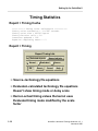
Timing Statistics
Report > Timing Cache
*********** Timing cache information ***********
Timing cache evaluation = 11.6667 seconds
Timing cache size = 483365 Bytes
Timing function calls = 20
Instances updated = 166
Equation complexity metric = 2
Report > Timing
Report Timing Info
On Selected objects
Kernel
OK
Named objects
Evaluated
Reset
Cancel
Source
Help
• Source--technology file equations
• Evaluated--calculated technology file equations
Doesn't show timing mode or delay scale
• Kernel--actual timing values the kernel uses
Evaluated timing mode modified by the scale
factor
1-18
QuickSim II Advanced Training Workbook, 8.5_1
November 1995
Setting Up for QuickSim II
Timing Statistics
When you invoke QuickSim II in one of the timing modes, TimeBase compiles
the timing information, if it does not already exist. You can also use TimeBase to
compile your timing prior to invoking QuickSim II. In either case, a timing cache
is prepared, which contains timing information and statistics about your design.
You can report information on the timing build process using the Report >
Timing Cache menu item. The information that is presented give you an idea of
the size of the cache, and the time required to build it. This information can be
useful in determining memory requirements and runtime performance. Here is a
typical report:
*********** Timing cache information ***********
Timing cache evaluation = 11.6667 seconds
Timing cache size = 483365 Bytes
Timing function calls = 20
Instances updated = 166
Equation complexity metric = 2
You can also select an instance in your design and report timing on it using the
Report > Timing menu item. A dialog box appears with three choices for the type
of timing information:
• Source. Displays the unevaluated source technology file information.
• Evaluated. Displays the calculated values from the timing equations in the
technology file. This does not take into account the timing mode (min, typ,
max) or the delay scale.
• Kernel. Displays the actual timing values the kernel uses during simulation.
This is the evaluated time for the specific timing mode, modified by the scale
factor.
The desired information is displayed in the Timing Info window.
When troubleshooting timing, report kernel information first, to determine what
pin or path caused the delay. Then view the source to determine the equations that
produced the delay. This is the effect to cause approach.
QuickSim II Advanced Training Workbook, 8.5_1
November 1995
1-19
Setting Up for QuickSim II
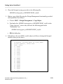
Editing a Component Interface
Invoking CIB in a shell:
$ cib <component_path>
Opening a component in edit mode:
CIB > open /idea/user/gen_lib/dff
Using CIB in edit mode to:
• Edit model labels
o add new label
o alter existing label
o delete label
• Unregister models from component interface
• Validate models
o Verify external net definitions in registered
model to pins
1-20
QuickSim II Advanced Training Workbook, 8.5_1
November 1995
Setting Up for QuickSim II
Editing a Component Interface
You can use the Component Interface Browser to edit the component interface,
making fixes as necessary to accommodate your design process. Such changes fall
into the following categories:
• Edit model labels. Add a new label, alter an existing label, or delete a label.
• Unregister models. Unregister a specific model from a component interface.
• Validate models. Verify external net definitions in the registered model to
pins.
For example, you examine a component interface with CIB and discover that one
of the models listed shows a status as:
Not valid for Interface
Not valid for Property
This can happen when you add a new model or model label to the interface
without verifying that existing models are correct. You can use the “Validate
Model” option at the CIB prompt to check if the existing models are valid.
QuickSim II Advanced Training Workbook, 8.5_1
November 1995
1-21
Setting Up for QuickSim II
MGC Shell Environment Variables
Variable Name
Action If Missing
Purpose
MGC_HOME
Sets MGC_HOME
to /idea & validates
8.x otherwise exits
Locates the
Mentor Graphics
software tree
MGC_WD
Uses current
working directory
Sets context for
filename paths
LM_LICENSE_FILE or
MGLS_LICENSE_FILE
/etc/cust/mgls/
mgc_licenses
Location of
license data file
MGC_LOCATION_MAP
$MGC_HOME/etc/
mgc_location_map
Variables are
mapped to real
locations
MGC_<library_name>
none
Path to MGC
parts libraries
LANG
$MGC_HOME/pkgs/ Specifies human
<appl>/userware/
language and
default
char set to use.
AMPLE_PATH
$MGC_HOME/pkgs/ Specifies unique
<appl>/userware/
application
LANG/scope.ample userware area
MGC_TMPDIR
$MGC_HOME/tmp
1-22
Locates
directory for
temp files
QuickSim II Advanced Training Workbook, 8.5_1
November 1995
Setting Up for QuickSim II
MGC Shell Environment Variables
QuickSim II, and other Mentor Graphics applications use shell environment
variables to determine certain operating environments. These shell variables must
be created prior to invoking the application.
On the previous page is a table of variables that are used by QuickSim II and other
related applications. These variables are further described below:
• MGC_HOME. This variable points to the top of the MGC tree. You should
always define this variable before invoking a Mentor Graphics application. If
MGC_HOME is not set, many applications will check for a valid (V8.X) /idea
tree (one that contains the /idea/bin/set_mgc_env command). If found,
MGC_HOME is set to /idea and the application invokes.
• MGC_WD. This is the working directory context as seen by the application. If
MGC_WD is not set, most application will set the application working
directory to the filesystem directory at invocation.
• LM_LICENSE_FILE. You set this variable to the location of the workstation
license file for Mentor Graphics software. If absent, invocation will examine
the file $MGC_HOME/etc/cust/mgls/mgc_licenses for your authorization.
• MGC_LOCATION_MAP. This points to a file containing soft pathnames
names and corresponding hard paths to MGC resources, such as design
libraries. If you do not provide this path, the application will look for this file at
$MGC_HOME/etc/mgc_location_map or
$MGC_HOME/shared/etc/mgc_location_map.
• AMPLE_PATH and LANG. These variables determine the userware that is
used with the application. AMPLE_PATH determines where the alternate
userware is located (the default is $MGC_HOME/pkgs/<appl>/userware). The
LANG variable specifies which directory within the “userware” directory has
the scope.ample files. A default link at this location is used if the LANG
variable is not specified.
i
For more information on the shell environment variables used with
Mentor Graphics applications, refer to Managing Mentor Graphics
Software.
QuickSim II Advanced Training Workbook, 8.5_1
November 1995
1-23
Setting Up for QuickSim II
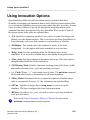
Using Invocation Options
Option Name
Option argument
component_name
design_viewpoint
-Help
-Usage
-I|-S
root_name
-NODisplay
-TIMing_mode
min|typ|max|lmin|ltyp|lmax|unit
-Delay_Scale
<number> (1.0)
-Time_Scale
<number> (0.1ns)
-CONStraint_Mode
off| state_only | message
-COntention_Check off | on
-SPike_Check
off | on
-Model_Messages
off | on
-BLM_Check
off | on
-TOggle_Check
off | on
-HAzard_Check
off | on
-DBG_BLM
1-24
-SPike_Model
suppress | x_immediate
-DELay_Mode
inertial | transport
-SETup
setup_name
-REStore
save_state_obj
-ABSfile
abstract_signal_file
QuickSim II Advanced Training Workbook, 8.5_1
November 1995
Setting Up for QuickSim II
Using Invocation Options
QuickSim II has defined several invocation options (switches) that allow
flexibility in bringing up a simulation from a shell. Shell invocation options allow
you to set up the simulation prior to invocation rather than after it invokes. In most
cases, it is more efficient to specify the appropriate setup information on the
command line rather than interactively after QuickSim II has invoked. Some of
the options shown in the table are explained here:
• -I|-S. Specifies a component interface (root_name) or symbol for design root.
Default: uses the default interface. This is used when invoking QuickSim II on
lower hierarchy with a root that contains several interfaces or symbols.
• -NODisplay. This switch causes the simulator to invoke in the shell
background. Use this option with batch simulation to save run time.
• -Delay_Scale. Provides modifying delay for all timing values in the
simulation. It can be used to estimate min or max timing from typical values.
• -Time_Scale. Sets the resolution of simulation time steps. This value can't be
changed within QuickSim II after invocation.
• -CONStraint_Mode. Disables constraint checking (setup, hold, fmax, width)
and enables checking (state_only) and reporting (messages).
• -<>_Check. Where “<>” is the unique type of check. The quicksim command
allows individual checks to be turned on or off upon invocation.
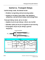
• -SPike_Model. Determines the way component outputs are handled when a
spike is encountered. See page 3-12 for information on spike handling.
• -SETup. Specifies a design object (setup_name) to use to set up the
simulator. The object configures the kernel upon invocation.
• -REStore. Specifies a save_state_obj used to restore a previous simulation
state upon invocation.
i
Refer to the Digital Simulators Reference Manual for more on the
quicksim command and invocation options.
QuickSim II Advanced Training Workbook, 8.5_1
November 1995
1-25
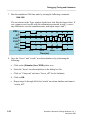
Setting Up for QuickSim II
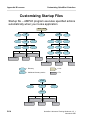
Changing Invocation Defaults
$MGC_HOME
pkgs
bin
quicksim
bin
quicksim
quicksim
## MAKE SURE THESE ARE ALL UNSET, TO ALLOW MINIMIZING THE
## NUMBER OF OPTIONS THAT ACTUALLY GET SENT TO THE
## INVOCATION LINE BELOW
timing_mode=''
delay_scale=''
time_scale=''
constraint_mode=''
contention_check=''
display_flag=''
spike_check=''
set_up=''
save_state=''
model_messages=''
blm_check=''
toggle_check=''
hazard_check=''
spike_model=''
delay_mode=''
abstract_sig_file=''
Never edit the original script--make a copy
1-26
QuickSim II Advanced Training Workbook, 8.5_1
November 1995
Setting Up for QuickSim II
Changing Invocation Defaults
Most Mentor Graphics applications use an invocation script that validates the
command arguments that you have entered. When you enter the
$MGC_HOME/bin/quicksim command in a shell, you are running this script for
QuickSim II. This path is actually a link to the
$MGC_HOME/pkgs/quicksim/bin/quicksim script.
The quicksim script verifies that necessary environment variables are set, the
design path is valid, and that command switches have valid arguments. If this
script finds a problem, it displays a message and exits. If it validates your
command, the arguments are passed to the binary file and invocation finishes.
If you want to create your own custom script, you can copy and modify the
$MGC_HOME/pkgs/quicksim/bin/quicksim script. DON'T MODIFY THE
ORIGINAL SCRIPT, but make a copy into another area and modify the copy. For
example, you could issue the command:
cp $MGC_HOME/pkgs/quicksim/bin/quicksim $HOME/quicksimx
This would create an editable file in your home account. Note that a different
name was given to this copy. This is so you can still issue the default quicksim
command, if needed, for system troubleshooting.
There is an area of the quicksim script that “pre-defines” command arguments, if
they are absent from the command line. This area begins at line 50 in the script.
The boxed figure on the previous pages shows this area. Note that no default
entries are provided here. But this is the area that you use to make your default
changes.
To set a new default value, enter the switch argument between the quote marks
following the appropriate switch name. If you are unsure of the arguments that
each switch can accept, refer to the help information that immediately follows this
area in the script. For example, you can make these changes: timing_mode “typ”
time_scale “1.0” spike_check “on” and when you invoke QuickSim II using this
script, you get typical timing, simulation resolution of 1 nsec, and spike checking
enabled.
QuickSim II Advanced Training Workbook, 8.5_1
November 1995
1-27
Setting Up for QuickSim II
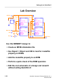
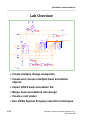
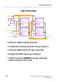
Lab Overview
AIN(9:0)
74LS139A
DIN(15:0)
CIN
A(7:0)
RAM1
A(7:0)
$MTM
ROM1
A(7:0)
$MTM
DATA_IN(15:0)
DATA_IN(15:0)
DATA_OUT(15:0)
CLOCK
READ_EN
WRITE_EN
CHIP_EN
DATA_OUT(15:0)
CLOCK
READ_EN
WRITE_EN
CHIP_EN
RAM2
A(7:0)
ROM2
A(7:0)
$MTM
$MTM
DATA_IN(15:0)
DATA_IN(15:0)
DATA_OUT(15:0)
CLOCK
READ_EN
WRITE_EN
CHIP_EN
DATA_OUT(15:0)
CLOCK
READ_EN
WRITE_EN
CHIP_EN
R_W
MOUT(15:0)
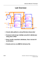
Use this MEMORY design to:
• Create an MTM initialization file
• Use Report > Object and CIB to look for modelfile
property on ROMs
• Add the modelfile property to an MTM
• Perform a quick check of the ROM operation
• Edit the root schematic of a design and reload it
without exiting QuickSim II
1-28
QuickSim II Advanced Training Workbook, 8.5_1
November 1995
Setting Up for QuickSim II
Lab Overview
In the lab exercise for this module, you will:
• Using the Notepad editor, create an ASCII Memory Table Model (MTM)
initialization file for each of the two ROMs in the MEMORY design, and save
the files directly beneath the MEMORY component.
• Use the Report > Object menu item within QuickSim II to determine if a
model property exists on the ROMs.
• Use the Component Interface Browser (CIB) to examine the interface for the
MEMORY component, and for the MTM (ram) component, to check for the
modelfile property.
• Add the modelfile property to both ROM1 and ROM2 with a value that points
to the ASCII initialization file. You will use the back annotation object in
QuickSim II to store this property addition.
• Perform a quick check to verify that the ROMs are operating properly. You
will create the stimulus and run interactively.
• Use design iteration techniques to repair a problem with the MEMORY circuit
using the Design Architect, without exiting QuickSim II.
• Reload the root schematic in QuickSim II and again perform a quick check to
verify the operation of the ROMs. The entire circuit will be fully exercised in
the Module 2 Lab Exercise.
QuickSim II Advanced Training Workbook, 8.5_1
November 1995
1-29
Setting Up for QuickSim II
Module 1 Lab Exercise
Note
If you are reading this workbook online, you might want to print
out the lab exercises to have them handy when you are at your
workstation.
Procedure 1: Copying the Training Data
In this procedure you will make a working copy of the training data for use with
subsequent lab exercises.
1. If the Design Manager is not invoked, invoke it now in a shell.
shell> $MGC_HOME/bin/dmgr
2. Set up a training directory in your account (or the location designated by your
instructor or system administrator) by doing the following steps:.
a. First check to see if your student training directory exists in your home
account ($HOME). Use the Design Manager to navigate to the location of
your training directory.
b. If it exists, go to Step 3. Otherwise, create the training directory using the
menu item: (Menu bar) > Add > Directory:
c. When the prompt bar appears, enter the path where you want this training
directory to be located (normally under your $HOME directory, or
optionally in the /tmp directory):
$HOME/training
Note that $HOME appears in the pathname. This represents the path to the
directory which houses your training directory. If you did not place your
training directory beneath $HOME, wherever you see “$HOME” you should
substitute your actual path for this name.
d. Click on the OK button.
1-30
QuickSim II Advanced Training Workbook, 8.5_1
November 1995
Setting Up for QuickSim II
3. Locate the qsim851nwp lab software for this training workbook. It should be
located in the following directory:
$MGC_HOME/shared/training
4. Make a copy of the qsim851nwp object in your local training directory, naming
it qsim_a using the following steps:
a. Select the qsim851nwp object in the Navigator window.
b. Choose the following Navigator popup menu:
(Navigator) > Edit > Copy
c.
Enter the pathname in the Destination field to where you want the copy to
be created, as follows:
$HOME/training/qsim_a
d. OK the prompt bar. The “Working....” message appears in the message
area. By specifying a target object that does not exist (qsim_a), the copy
will be made using that name instead of the original name (qsim851nwp).
QuickSim II Advanced Training Workbook, 8.5_1
November 1995
1-31
Setting Up for QuickSim II
Procedure 2: Creating MTM Initialization File
This lab procedure provides instructions and practice in creating an ASCII
Memory Table Model initialization file. In addition, you will add the modelfile
property to the ROM model instances, and point this property to the appropriate
ASCII initialization file.
1. Using default shell invocation, invoke QuickSim II on the MEMORY design.
This design is located in your $HOME/training/qsim_a directory.
2. Open a new Notepad session by choosing the following pulldown menu item:.
MGC > Notepad > New
A new (untitled) editing pad is opened within QuickSim II.
3. Using Notepad edit operations, create the following ASCII file text:
# ROM1 Initialization File
# Created: <current_date> by <your_name>
# 8-bit Address, 16-bit Data
0-FF / FFFF;
FX / 1234;
FF / FFXX;
10 / 0000;
11 / 1111;
12 / 2222;
13 / 3333;
14 / 4444;
15 / 5555;
16 / 6666;
17 / 7777;
18 / 8888;
19 / 9999;
1A / AAAA;
1B / BBBB;
1C / CCCC;
1D / DDDD;
1E / EEEE;
1F / FFFF
1-32
QuickSim II Advanced Training Workbook, 8.5_1
November 1995
Setting Up for QuickSim II
4. Close the Notepad, saving your edits to the following file:
$HOME/training/qsim_a/MEMORY/ROM1_initfile
5. Make a copy of this file using the Design Management functionality provided
with QuickSim II as follows:
a. Choose: MGC > Design Management > Copy Object
b. Find and select $HOME/training/qsim_n/MEMORY/ROM1_initfile in the
“Copy object in:” source side, and enter the following path in the
“Destination” box:
$HOME/training/qsim_a/MEMORY/ROM2_initfile
c. OK the dialog box.
6. Edit and save the new ROM2_initfile object as follows (closing the Notepad
window when you are done):
# ROM2 Initialization File
# Created: <current_date> by <your_name>
# 8-bit Address, 16-bit Data
0-FF / 0000;
0 / 0000;
1 / 1111;
2 / 2222;
3 / 3333;
4 / 4444;
5 / 5555;
6 / 6666;
7 / 7777;
8 / 8888;
9 / 9999;
A / AAAA;
B / BBBB;
C / CCCC;
D / DDDD;
E / EEEE;
F / FFFF;
G / GGGG
QuickSim II Advanced Training Workbook, 8.5_1
November 1995
1-33
Setting Up for QuickSim II
7. The Notepad edit process creates a “.bak” file when you save. Choose the
MGC > Design Management > Delete menu item to remove this object.
Procedure 3: Checking for the Modelfile Property
In most cases, the Modelfile property already exists on the MTM component, and
is set to null. In order to configure your MTM instance to the proper initialization
file, you annotate this property in QuickSim II. If the property does not exist, you
can still add the property as a back annotation in QuickSim II.
1. Using the Open Sheet palette icon, open the sheet for the MEMORY circuit in
QuickSim II.
2. Check the instance to see if the Modelfile property exists on ROM1 and ROM2
by performing the following:
a. Choose the Report > Objects menu item.
b. When the dialog box appears, make sure you get the 'long' amount of
information and OK it.
c. Check the properties entries for the existence and value of the Modelfile
property. Under the “Properties:” entry you can see that the Modelfile
property has not been added to ROM1 and ROM2.
d. Close the Objects report window
Note
1-34
You can also use Component Interface Browser to verify this
modelfile property. The next procedure (optional) describes how
to do this.
QuickSim II Advanced Training Workbook, 8.5_1
November 1995
Setting Up for QuickSim II
Procedure 3b (optional): Checking Using CIB
This procedure uses the Component Interface Browser (CIB) to determine if the
modelfile property is attached to the ROM and RAM instances. It also uses editing
capabilities of CIB to validate the “ram” component interface.
1. Locate the model for the ROM instance and invoke CIB on this component, as
follows:
a. First, you must determine where this component exists. Use the Report >
Objects information again to determine the component path.
Enter it here: _______________________________________________
b. Now, in a new shell, invoke CIB on this path using the shell invocation as
described in the lesson “Editing a Component Interface” on page 1-20.
2. View the interface for the ROM model.
This interface information is provided on the next page, and has been
rearranged slightly to fit on the page.
Is there a body property named “modelfile?”
QuickSim II Advanced Training Workbook, 8.5_1
November 1995
1-35
Setting Up for QuickSim II
ram::ram > view
COMPONENT ram
INTERFACE: ram
PINS: Compiled
Id #
Pin Name
-2
DATA_OUT(1
DEFAULT INTERFACE IS:
ram
User
Pin Name
Properties
DATA_OUT(1(pin, DATA_OUT(15:0))
(pintype, OUT)
(cap_pin, CASE (model) {(S:one_m :N:8:0.080000);(OTHERWISE :U
-1
DATA_IN(15 DATA_IN(15(pintype, IN)
(pin, DATA_IN(15:0))
(cap_pin, CASE (model) {(S:one_m :N:8:0.060000);(OTHERWISE :U
0
A(7:0)
A(7:0)
(pintype, IN)
(pin, A(7:0))
(cap_pin, CASE (model) {(S:one_m :N:8:0.080000);(OTHERWISE :U
1
WRITE_EN
WRITE_EN (pintype, IN)
(pin, WRITE_EN)
(cap_pin, CASE (model) {(S:one_m :N:8:0.170000);(OTHERWISE :U
2
READ_EN
READ_EN
(pintype, IN)
(pin, READ_EN)
(cap_pin, CASE (model) {(S:one_m :N:8:0.050000);(OTHERWISE :U
3
CHIP_EN
CHIP_EN
(pintype, IN)
(pin, CHIP_EN)
(cap_pin, CASE (model) {(S:one_m :N:8:0.250000);(OTHERWISE :U
4
CLOCK
CLOCK
(pin, CLOCK)
(pintype, IN)
BODY PROPERTIES:
(_qp_prim, CASE (model) {(S:two_m :S:4:TRUE);(S:one_m S:def_t
(model, $MTM)
INTERFACE MODEL ENTRIES:
Model Entry Type
Model Info
0
mgc_symbol
Path: .../lib/ram/ram
Labels: 'default_sym'
Status: Valid for interface;
NOT valid for property
1
Technology
Path: ...techfiles/one_m/bin/ram
Labels: 'one_m' 'def_tech'
Status: Valid for interface;
NOT valid for property
2
MTM
Path: .../bin/ram/ram.mtm
Labels: '$MTM''one_m''two_m'
Status: Valid for interface;
NOT valid for property
3
Library Technology Path: .../one_m/bin/library
Labels: 'def_tech''two_m' 'one_m'
Status: Valid for interface;
Valid for property
4
Technology
Path: ...techfiles/two_m/bin/ram
Labels: 'two_m'
Status: Valid for interface;
NOT valid for property
ram::ram >
1-36
QuickSim II Advanced Training Workbook, 8.5_1
November 1995
Setting Up for QuickSim II
3. Issue the help command at the CIB prompt as follows:
ram::ram >
help
This gives you a list of component interface editing commands. Notice that
one of the entries is “validate model”. Now examine the interface again. Notice
that all but one of the interface model entries show a status of:
Status: Valid for interface;
NOT valid for property
In the next step you will edit the interface to validate these entries.
4. Validate all of the model entries by entering the following:
ram::ram >
vm
CIB checks all interface paths to determine if they are valid. It also determines
if the property list in all interfaces match the interface objects. When the check
is successful, it updates a “NOT Valid” to a “Valid” entry. If unsuccessful, a
“NOT Valid” entry is entered.
5. View the interface again to determine the validation status.
Which interface model did not validate? _____________________________
6. Save the updated (validated) interface by entering the following:
ram::ram >
save
The changes are saved to the interface and the version is updated.
7. Close the interface and quit CIB.
There is still no modelfile property, so you must add it in the next procedure.
QuickSim II Advanced Training Workbook, 8.5_1
November 1995
1-37
Setting Up for QuickSim II
Procedure 4: Adding the Modelfile Property
You have verified that the modelfile property does not exist. In order to configure
your MTM instance to the proper initialization file, you will back annotate this
property in QuickSim II.
1. Open the schematic sheet for the MEMORY circuit in QuickSim II (if not
already opened).
2. Add the Modelfile property to ROM1 as follows:
a. Select the ROM1 instance.
b. Choose Edit > Property > Add
c. Enter the following in the dialog box:
New property name: modelfile
Property value: $HOME/training/qsim_a/MEMORY/ROM1_initfile
This will back annotate the model property on ROM1.
d. OK the dialog box.
The following Info Message is displayed:
Status returned while resetting modelfile inst '/ROM1'
Note: X values in address assumed to be zero
e. Examine your modelfile ROM1_initfile to see where this error occurred, but
do not fix it. In a later lab, you will test to see if the X value in address FX
was interpreted as zero (F0).
3. Check the ROM1 instance to verify that the modelfile property is correctly set
by choosing the Report > Objects menu item.
You should now see a modelfile entry under the “Properties:” heading.
4. Close all windows except the schematic view window.
1-38
QuickSim II Advanced Training Workbook, 8.5_1
November 1995
Setting Up for QuickSim II
5. Now add the Modelfile property to ROM2. Be sure to enter the value as the
path to ROM2_initfile.
Once the Modelfile property is added an additional Info Message is displayed
as follows:
Status returned while resetting modelfile for inst '/ROM2'.
Errors found while parsing Modelfile:
$HOME/training/qsim_a/MEMORY/ROM2_initfile
device has been initialized with X's
Line 21: Illegal character in data
Line 21: Illegal character in data
The ROM2_initfile didn't compile, and instead initialized with X values.
6. Fix the file using the Notepad editor and save to the same name.
7. Reload the new modelfile as follows.
Select the ROM2 instance and either choose File > Restore > Modelfile or
click on the Read Modelfile palette icon to reload the repaired ROM2_initfile
object. Verify that it now loads correctly (no error or warning messages).
8. Report on the ROM2 instance to verify that the modelfile property is correct,
using the following method:
Select the ROM2 instance and choose: Report > Objects
9. Close all windows except the schematic view window.
QuickSim II Advanced Training Workbook, 8.5_1
November 1995
1-39
Setting Up for QuickSim II
Procedure 5: Verifying the ROM Models
Before you perform a full-blown simulation, you should verify that the Modelfile
additions you made work correctly. In this procedure, you will perform a simple
simulation that reads data out of both ROM1 and ROM2.
1. Using Notepad in read-only mode, examine the table model source for this
device to determine its operating mode. This file is located using the path
$HOME/training/qsim_a/lib/ram/tables/src/ram/ram.src and is partially listed
below for your convenience:
MODEL sp_ram : MEMORY =
LOW_TRUE SELECT chip_en;
LOW_TRUE STROBE clock;
LOW_TRUE WRITE_ENABLE write_en;
LOW_TRUE OUT_ENABLE read_en;
ADDR a CLOCKED_BY clock;
DATA INPUT data_in CLOCKED_BY clock;
DATA OUTPUT data_out ENABLED_BY read_en;
Notice that this model requires active low signals on write_en and read_en.
Also, the address must be strobed by a negative-going clock signal (connected
to net CIN on the schematic).
If you examine the MEMORY circuit, you'll notice that the ROM1 and ROM2
write_en pins are tied to ground (low) and read_en are tied to a pullup device
(high). This is just the opposite of the requirements--not good!
2. Close the Notepad window.
1-40
QuickSim II Advanced Training Workbook, 8.5_1
November 1995
Setting Up for QuickSim II
3. Exercise the circuit to verify that it will not read ROM1 and ROM2 by setting
up stimulus as follows:
a. CIN: Clock Period 10; 1 at time 0; 0 at time 5
b. AIN: 0 at time 0; 101 at time 10; 102 at time 20; 1FF at time 30
c. Add the MOUT signal to the List window.
d. Initialize the circuit to the “1” state by choosing the Run > Initialize menu
item.
e. Run for 40 ns
Notice that the output net MOUT goes from the FFFFr states to the FFFF state,
and remains in that state even though valid addresses are being provided.
4. Use design incrementality techniques to fix the MEMORY problem as
described in the following steps:
a. Without exiting QuickSim II, invoke Design Architect in a new shell on the
MEMORY sheet.
b. Edit the nets that connect to ROM1 and ROM2 so that read_en is connected
to ground and write_en is connected to the pullup device.
c. Change the name R_W to W_R to accurately reflect the signal intent. When
the input signal is high (1) a write is performed; when it is low (0) a read is
performed.
d. Check and save the sheet.
e. Close Design Architect
f. In QuickSim II, reload the model for the design root by clicking on the
Reload Model > All icon in the Design Changes palette.
This operation takes a short period of time as it rebuilds connectivity. It also
invalidates simulation window information. The forces waveform database
remains intact.
QuickSim II Advanced Training Workbook, 8.5_1
November 1995
1-41
Setting Up for QuickSim II
5. Build the List and Trace windows, including all of the MEMORY input and
output signals.
6. Reset the simulation (state only, and don't save results).
7. Initialize the circuit to “1”.
8. Run the simulation (40 ns) again with the existing stimulus.
Now the MOUT bus outputs valid data that represents what you entered into
the modelfiles. In a later lab, you will use the QuickSim II pattern generator to
exercise all parts of the MEMORY design.
9. Now read location F0 in ROM1 as follows:
a. Force AIN to F0.
b. Run 10 nanoseconds.
c. Examine the MOUT results.
Remember that the Info Message told you that FX was interpreted as F0.
This means that the entry “FX / 1234" should put the data in ROM1 at F0.
Verify that this is the case.
10. Exit QuickSim II, saving the changes to your design (choose “Save Design
Viewpoint” only).
1-42
QuickSim II Advanced Training Workbook, 8.5_1
November 1995
Setting Up for QuickSim II
Module 1 Summary
Module 1 presented setup details considered more advanced than those presented
in the introductory training.
• Designs can be created hierarchical or flat. Hierarchical designs allow you to
nest components within other components. Design paths, similar to filesystem
paths, uniquely identify each object in your design. Names and “handles”
uniquely identify each object. The naming context allows you to abbreviate
naming in lower levels of hierarchy.
• Property values are resolved in an orderly manner. The rules for this order are:
back annotation, instance, symbol, higher levels of hierarchy, the design
viewpoint, and finally, the technology file. Models use different locations in
the scheme to satisfy property values.
• Memory Table models are an efficient way to model RAMs and ROMs. You
can provide an ASCII initialization file to provide a starting value for each
memory location. This file is identified by a modelfile property attached to
each instance of a memory device. Special initialization is required of RAM
inputs and outputs for proper operation of the device.
• The Component Interface Browser (CIB) allows you to examine and edit
component interfaces. The information contained in the interface is a pin list, a
property list, and a model table. The model table provides labels and paths to
functional and timing models used with each interface. CIB validates the paths
to these models.
• Shell environment variables allow you to point to the resources that
QuickSim II need to run. There are default locations for each of the resources
if a variable is not specified.
• Invocation Options. When you issue the quicksim command, a shell script is
called that properly sets up all of the parameters according to command
arguments you specified. You can copy this script and modify it to create your
own default invocation mode.
The next module, Module 2, describes advances stimulus techniques. You will
learn how to generate stimulus using AMPLE files, forcefiles, and the stimulus
generator. You will also merge waveforms and connect results as stimulus.
QuickSim II Advanced Training Workbook, 8.5_1
November 1995
1-43
Setting Up for QuickSim II
1-44
QuickSim II Advanced Training Workbook, 8.5_1
November 1995
Advanced Stimulus Techniques
Module 2
Advanced Stimulus Techniques
Module 2 Overview
2-2
Lessons
Design Signal Initialization
The Initialization Process
The INIT Property
Developing Design Stimulus
Setting Up Force Types
Force Type Examples
Using AMPLE for Stimulus
AMPLE Access to Waveform Data
AMPLE Stimulus Examples
Using VHDL as a Stimulus Generator
Waveform Database Concepts
Editing Waveforms
Merging Waveforms
Redundant Events
Using 'results' as Stimulus
Scaling Waveforms
Dithering Waveforms
Inserting Waveform Ambiguity
Loading/Connecting Waveforms
Creating Stimulus Patterns
Gathering Toggle Statistics
2-3
2-4
2-6
2-8
2-10
2-12
2-14
2-16
2-18
2-20
2-22
2-24
2-26
2-28
2-30
2-32
2-34
2-36
2-38
2-40
2-42
2-44
Module 2 Lab Exercise
2-47
Module 2 Summary
2-56
QuickSim II Advanced Training Workbook, 8.5_1
November 1995
2-1
Advanced Stimulus Techniques
Module 2 Overview
About This Training Workbook
Design
Initialization
Setting Up for QuickSim II
Advanced Stimulus Techniques
Debugging Timing and Unknowns
Module
2
Using AMPLE
to Develop
Stimulus
Understanding
Force Types
Optimizing Simulation Runs
Viewpoints and Annotations
Custom Design Checking
Waveform
Database
Concepts
Generating
Stimulus Patterns
Additional Topics:
Appendix A: Processes Using QuickSim II
Appendix B: Customizing the QuickSim II Interface
Appendix C: Advanced Modeling Techniques
2-2
QuickSim II Advanced Training Workbook, 8.5_1
November 1995
Advanced Stimulus Techniques
Lessons
On completion of this module, you should:
• Know how to initialize your design using both the INIT property and the two
methods of net initialization.
• Know how to create different force types and how to use the Setup Forces
command prior to connecting waveform databases.
• Be able to develop stimulus patterns using the Pattern Generator within the
QuickSim II Stimulus palette.
• Be able to develop clock, force, pattern stimulus using AMPLE constructs.
• Create independent stimulus waveform databases, and merge them so that they
are used on your design at different times in the simulation.
• Understand how redundant events are created, and know how to remove them.
• Be able to create duplicate waveform databases, applying the following
waveform manipulation techniques:
o Dither a waveform
o Scale a waveform
o Add waveform ambiguity
• Be able to take the results of a previous simulation run and connect it to your
design as stimulus for the current simulation. This is very useful for partitioned
simulation runs.
• Know how to gather toggle statistics from a simulation run.
You should allow approximately 2 hours to complete the Lesson,
Lab Exercise, and Test Your Knowledge portions of this module.
Note
QuickSim II Advanced Training Workbook, 8.5_1
November 1995
2-3
Advanced Stimulus Techniques
Design Signal Initialization
Why initialize?
• To define all signals before stimulus is applied
• To approximate power up state conditions
What are the initialize modes?
• Default-o applies state but does not stabilize circuit (an
IEEE1076 specified requirement)
o compatible with VHDL operation
• Classic-o applies state and runs until stable
o simulation time does not advance
o compatible with pre-V8 initialization
What initialization value to use?
• Default value Xr
• To set your own value:
o Global--use the init command
o Use the init property on nets and pins; only
active on invoke or reset of simulation
NOTE: Wrong mode (classic/default) or value will
change results!
2-4
QuickSim II Advanced Training Workbook, 8.5_1
November 1995
Advanced Stimulus Techniques
Design Signal Initialization
Before a simulation can begin, the simulator must know the state of each
component in the design. To find this out, the simulator performs an initialization
process when you invoke it. This initialization process assigns a state to each net
in the design. A circuit initialization will occur at the following times in your
simulation:
• QuickSim II Invocation. The simulator automatically performs a default
initialization at invocation. Although this initialization occurs automatically,
you can create custom initialization values.
• Initialize Command. The Initialize command allows you to initialize the
circuit any time during a simulation. You can supply a unique value to the nets
in your design by specifying this value with the command. Use the Initialize
command to initialize the circuit at any time.
• Reset State Command. Note that the simulator automatically initializes the
circuit when you reset it by issuing the Reset State command. This
initialization uses the “default” mode.
There are two forms of initialization: default initialization (or V8 type), which is
always performed when the simulator invokes, and classic initialization (pre-V8
type). The default initialization scheme is compatible with System-1076 models.
For compatibility with pre-V8 versions of the simulator, you can perform classic
initialization.
i
For additional information on the initialization process, refer to the
QuickSim II User's Manual. For information on the Initialize command,
refer the Digital Simulators Reference Manual.
QuickSim II Advanced Training Workbook, 8.5_1
November 1995
2-5
Advanced Stimulus Techniques
The Initialization Process
When does initialization occur?
• On invocation
• Resetting the simulation
• Issuing the Initialize command
There are two types of initialization:
Default Initialization
Classic Initialization
Set pins and nets to XR
or state_value
Set pins and nets to XR
or state_value
Set nets with init
property value
Set nets with init
property value
Evaluate each instance
once, schedule events
Evaluate each instance
until circuit is stable
NOTE: Default initialization can create pending
events at beginning of simulation.
• May cause spikes at time 0 when you add stimulus
and run
• Before applying stimulus, you should run (1000ns)
to stabilize circuit
2-6
QuickSim II Advanced Training Workbook, 8.5_1
November 1995
Advanced Stimulus Techniques
The Initialization Process
The simulator can initialize your design in one of two ways: default initialization
or classic initialization. Here is a description of the default initialization process.
1. The simulator sets the initial state of all pins and nets to the state_value
argument of the Initialize command. Note that this argument defaults to XR.
2. The simulator sets the state of all nets according to any associated Init
properties. The Init property values override values in the previous step.
3. The simulator evaluates all instances once by using the states set in steps 1 and
2 and then schedules output events according to any associated delays.
Note
Unevaluated transitions, called pending events, can exist at the end
of a default initialization. If you apply stimulus at time zero, spike
conditions can occur. To avoid spike conditions at time zero, you
should run the simulator before applying stimulus (for example,
“Run 1000"). This allows the simulator to process the pending
events before the stimulus is applied.
Here is a description of the classic initialization scheme (-Classic):
1. The simulator sets all nets according to associated Init properties.
2. It sets all other nets (without Init property) to XR or according to the
state_value argument of the Initialize command.
3. Using a delay of 0 for every transition, the simulator propagates the initialized
values through the circuit until it reaches a stable state (no zero-delay events
exist) or until the simulator reaches the iteration limit. The simulator does not
advance simulation time during classic initialization.
i
For information about events and how the simulator processes circuit
activity, refer to the section “How QuickSim II Processes Circuit
Activity” in the QuickSim II User's Manual. For information about the
Init property, refer to section “Init” in the Properties Reference Manual.
QuickSim II Advanced Training Workbook, 8.5_1
November 1995
2-7
Advanced Stimulus Techniques
The INIT Property
Create initial state on net or pin.
Init state_string
state_string = 1, 2, or 3 characters as follows:
• Logic state:
1 = High
0 = Low
X = Stable/Unknown
• Drive strength: S = Strong
R = Resistive
Z = High impedance
• Change enable: T = Simulator can change
F = Fixed for entire simulation
Example:
Init 0 (same as Init 0ST)
Example:
Init 1SF (used on VCC pins)
Example:
Init 0SF (used on GROUND pins)
2-8
QuickSim II Advanced Training Workbook, 8.5_1
November 1995
Advanced Stimulus Techniques
The INIT Property
The Init property specifies the initial state of a net or of an input, output, or I/O pin
on a primitive component. The term “State” includes the logic state, drive
strength, and whether the specified state can change during simulation. You can
also use the Init property to define a constant state, such as Vcc or Ground. If you
create a model you can specify initial pin states on the model by attaching an Init
property to its pins.
The Init property is attached to nets and pins of primitive components. Therefore,
conflicts can occur if multiple connections are made to a net or if multiple
Init/Drive properties exist. The following rules apply:
• If conflicting net Init property values are attached to different parts of an
electrically equivalent net, when you invoke QuickSim II on that design,
QuickSim II notifies you of the discrepancy and picks one of the values to use
as the Init property.
• If the simulator finds conflicting Init and Drive property values on a pin, the
simulator issues a warning message, and the Drive value predominates. Thus,
for QuickPart Tables, the Init property value on a pin should be consistent with
the output states specified in the QuickPart Table for that pin.
The Init property is also used by QuickFault II, QuickGrade II, QuickPath, and
Lsim. Lsim requires the Init property on global symbols only.
A text string consisting of one, two, or three characters, for example, “0ST”. The
significance of the character in each position of the text string is described below:
• Position 1: Logic state 1=High, 0=Low, X=Stable/unknown
• Position 2: Drive Strength S=Strong, R=Resistive, Z=High impedance
• Position 3: Value Change Enable/Disable
F Init state fixed for the entire simulation.
T The simulator can change the Init state.
Thus, the Init value “0ST” defines the initial state of the pin or net as logic low,
strong drive strength, and subject to change during simulation.
QuickSim II Advanced Training Workbook, 8.5_1
November 1995
2-9
Advanced Stimulus Techniques
Developing Design Stimulus
QuickSim II, supports several types of stimulus:
• AMPLE functions or force files
o more extendible and flexible
o similar to C programming language
• VHDL test bench
o can provide complex, cycle-based stimulus
o can also examine results
• Waveform editor--Waveform Databases
o simulation results are created in this form
o issued to simulation kernel much faster
o run-time stimulus in this form
• logfiles
o used by third party and ASIC vendors
o ASCII text (readable/editable) format
2-10
QuickSim II Advanced Training Workbook, 8.5_1
November 1995
Advanced Stimulus Techniques
Developing Design Stimulus
The digital simulator, QuickSim II, supports several forms of input stimulus. The
source of this stimulus is usually Advanced Multipurpose Language (AMPLE)
functions or force files. Optionally, you can use the waveform editor within
QuickSim II, the Waveform Database (WDB), the Mentor Interactive Stimulus
Language (MISL), VHDL test bench, or logfiles as input to the simulator. The
logfile is the method by which third party and ASIC vendors move stimulus into
the Mentor Graphics simulation environment, along with results into and out of
the environment.
In general, it is best to use AMPLE functions as the source for stimulus
generation. If you are accustomed to a cycle-based stimulus, you may prefer
MISL. But, in general, MISL is more difficult to understand and maintain than
equivalent AMPLE functions, while AMPLE is more extendible and flexible than
MISL. If you are familiar with the C programming language, you will find
learning AMPLE fairly straightforward, since the majority of the syntax is
identical.
After you have created the stimulus and run the simulation, the results of the
simulation can be saved in the form of a Waveform Database. On subsequent
invocation of the simulator, you can use the waveform databases to eliminate the
majority of the time needed to regenerate the stimulus. For additional information,
refer to the SimView Common Simulator User's Manual.
QuickSim II Advanced Training Workbook, 8.5_1
November 1995
2-11
Advanced Stimulus Techniques
Setting Up Force Types
Force signal state <time> <-type>
Force
D
1r
1000 -Wired
Types:
• -Charge
o State gets blown away when any other event is
scheduled on the net
• -Fixed
o Used to patch circuits--overrides any other
force or events being scheduled
o Can't override VCC or GND
• -Wired
o Acts like another driver on the net
• -Old
o Provided for V5.2 compatibility
o An instance drives overriding state on net
• (default)
o defined for each waveform when connected
o Retains “default” type for re-connections
o “default” type is set to -Charge at invocation
o Change “default” with Setup Force command
2-12
QuickSim II Advanced Training Workbook, 8.5_1
November 1995
Advanced Stimulus Techniques
Setting Up Force Types
Force stimulus is created by issuing the Force command or function with the
appropriate arguments. For example, you could issue the command:
Force D 1r 1000 -W (Force signal state <time> <-type>)
This command forces the net named “D” to the “1r” state at time 1000
(nanoseconds, unless otherwise defined) with a force type “Wired”. The time and
type are optional specifiers. If you omit the time, QuickSim II schedules the force
event at the current time. If you omit the force type, you get the “default” type.
This is important to understand as explained below.
Five different force types can be specified which represent four force
characteristics. Any can be removed with the Delete Forces command.
• -Charge. A charge force is in effect until:
o You apply a second force to the same net.
o An instance evaluation (event) drives an new state on the net.
• -Fixed. Fixes a signal to a state so an instance driver can't change the state. A
fixed force is in effect until:
o You apply a second force to the same signal.
• -Wired. Force is “Wire-OR'd” with instances as another net driver. A wired
force is in effect until:
o You apply a second force to the same signal.
• -Old. Compatible with pre-V5.2 force type. A charge force is in effect until:
o You apply a second force to the same net that overrides the old force.
o An instance evaluation drives an overriding state on the net.
• Default. The default type is used when no type is specified. All forces issued
with no type specified use the default that was valid at the time the waveform
was attached in the waveform database. All subsequent default forces issued
on that waveform use the attached default, even if a new default is defined.
When you invoke QuickSim II, the default type is -Charge. You can change
the default type using the Setup Force command, to affect any new waveform
connections.
QuickSim II Advanced Training Workbook, 8.5_1
November 1995
2-13
Advanced Stimulus Techniques
Force Type Examples
Example 1:
Force D 1
Force CLK 0 20 -Wired
Run 20
Setup Force FIXED
Force PRE 1 10
Force CLR 1 10 -Wired
Force D
0
Run 20
Setup Force CHARGE
Force D
1 10
Force D
1
-Fixed
Force CLK 1
Run 20
D
-C
-F
-F
CLK
-C
-W
PRE
-F
CLR
-W
20
-C
40
60
Example 2:
Setup Force OLD
Disconnect/Reconnect D
D
-O
-O
20
-F
40
-O
60
Why Setup Forces works on connection:
• QuickSim II uses -Charged as default
• QuickFault II uses -Wired as default
• Scheme allows both QS/QF to use same stimulus
2-14
QuickSim II Advanced Training Workbook, 8.5_1
November 1995
Advanced Stimulus Techniques
Force Type Examples
To help you understand how different force types behave in a simulation, here is
an example that creates stimulus on several signals:
EXAMPLE1: The previous page shows a forcefile that is executed in
QuickSim II. The type of force for each waveform is shown in the Trace window
at right side of the page. Here is a brief description of the type of force at each
point in time, as shown on the waveforms.
• D. Connected at time 0 as default (Charge). Forced at time 0 as default
(Charge). Forced at time 20 as default (Fixed). Forced at time 40 as -Fixed
(switch). Forced at time 50 as default (Charge).
• CLK. Connected at time 0 as default (Charge). Forced at time 20 as -Wired
(switch). Forced at time 40 as default (Charge, Setup Force)
• PRE. Connected at time 20 as default (Fixed, Setup Force). Forced at time 30
as default (Fixed).
• CLR. Connected at time 20 as default (Fixed, Setup Force). Forced at time 30
as -Wired (switch).
EXAMPLE2: You disconnect the “D” waveform and reconnect it at this time.
Because the new default is -Old, all of the default forces in the previous example
are now of type Old as shown in the single waveform for “D”. Because of this
feature, you can make wholesale changes to “default” stimulus on a waveform by
waveform basis.
The scheme of determining the default type of stimulus only on connection of the
waveform database allows the same stimulus to be used among all the analysis
applications. QuickSim II requires that most stimulus be of type Charged to
properly exercise a digital simulation (special requirements such as bi-directional
buses use Wired forces). QuickFault requires all stimulus to be of the Wired type.
With this scheme, the same stimulus can be connected as Charged in QuickSim II
and as Wired in QuickFault II.
QuickSim II Advanced Training Workbook, 8.5_1
November 1995
2-15
Advanced Stimulus Techniques
Using AMPLE for Stimulus
/////////////////////////////////////////////////////////////
// function write_cycle() : Creates 100 nsec mem write cycle
// Written by :
Joe Designer, Nov 28, 1993
// Arguments: addr RAM write address.
//
data Decimal data value.
//
start_time - Sim time to apply write cycle.
// Returns :
time Time write_cycle is complete.
/////////////////////////////////////////////////////////////
function write_cycle(addr : integer,
value : integer,
start_time : real)
{
local time = start_time;
// Set data & address to high-Z for 25ns; force control high.
$force("AS", "1", time, void, void, @absolute, @norepeat);
$force("RW", "1", time);
$force("address", "Xz", time);
$force("data", "Xz", time);
time = time + 25.0;
// Force address/value & hold for 50ns; assert control low.
$force("AS", "0", time);
$force("RW", "0", time);
$force("address", addr, time);
$force("data", value, time);
time = time + 50.0;
// force address & data high-Z; de-assert control signals.
$force("AS", "1", time);
$force("RW", "1", time);
$force("address", "Xz", time);
$force("data", "Xz", time);
time = time + 50.0;
return(time);
}
2-16
QuickSim II Advanced Training Workbook, 8.5_1
November 1995
Advanced Stimulus Techniques
Using AMPLE for Stimulus
AMPLE is the most common method for developing simulation stimulus. You can
write high level functions or dofiles to be executed in succession to drive the
simulation. AMPLE functions execute faster than dofiles, because the dofiles are
compiled every time they are executed, whereas, an AMPLE function is only
compiled when it is first loaded. Subsequent executions of the function do not
require compilation.
As an example of writing stimulus with AMPLE, let's consider a design for a
memory board that is driven by the control signals RW and AS, has a 16 bit
address, and a 16 bit data bus. You can write a function to do a write cycle as
shown in the figure on the previous page.
After this function is written it can be used to generate large amounts of stimulus
to the our memory board by using the looping constructs within AMPLE
(identical to C). The bus cycle can easily be modified without affecting the calling
AMPLE function, since it returns the time completed.
Note
For better performance of forcefile command scripts, the Force
command is executed significantly faster than the $force()
function. This is because the Force command is interpreted
directly in the simulation kernel while the $force() function
requires AMPLE syntax parsing. Therefore it is recommended to
use the Force command, instead of the $force() function, in scripts
that issue large amounts of stimulus.
QuickSim II Advanced Training Workbook, 8.5_1
November 1995
2-17
Advanced Stimulus Techniques
AMPLE Access to Waveform Data
$get_signal_value(name, time)
• Returns a value for “name” signal at “time”
• If name/time omitted, uses selected name/time
$get_signal_transitions(name, op, time1, time2)
• Returns array (AMPLE vector) of time/value pairs
for named waveform or expression.
• Get transitions between times--if null vector, no
transition occurred
• Get first transition forward to check Hold time
• Get first transition backward for Setup time
• Use for specialized waveform comparison
2-18
QuickSim II Advanced Training Workbook, 8.5_1
November 1995
Advanced Stimulus Techniques
AMPLE Access to Waveform Data
There are times when you want to access waveform data within an AMPLE
function or script. You could convert the waveform to logfile format and use text
searches to examine the data, but this is a cumbersome and after-the-fact
approach.
To help you access data in AMPLE during a simulation run, there are a couple of
functions that can access data for you. These functions are described below:
• $get_signal_value(name, time). This function accesses the state of a named
signal (name) at a given point (time) in the waveform. This function is useful if
you know the time that a check needs to be performed. You can assign the
value of this function to an AMPLE variable for further use.
• $get_signal_transitions(name, operation, time1, time2, count). This
function returns an AMPLE vector that is an array of time/value pairs for a
specific waveform. Several operation types allow you to locate specific
information relative to the time specified. Some operation examples are:
o @between. Returns the values between the time1 and time2 arguments.
Check between times to check stability--NULL if the signal didn't change.
o @next. Returns the values after to time1 limited by the count argument.
Use this to get forward transition to check Hold time.
o @previous. Returns the values prior to time1 limited by the count
argument. Use to get the first transition back in time (count = 1) to check
for Setup time.
i
For more information on the $get_signal_value() function or the
$get_signal_transitions() function, refer to the SimView Common
Simulation Reference Manual.
QuickSim II Advanced Training Workbook, 8.5_1
November 1995
2-19
Advanced Stimulus Techniques
AMPLE Stimulus Examples
// CREATE A FINITE CLOCK
val = 1;
i2 = 154000;
for (i=0;i<i2;i=i+50){
if (val == 1) {
$force("/CIN", "1", i, void, void, @absolute, @norepeat);
val = 0; }
else {
$force("/CIN", "0", i, void, void, @absolute, @norepeat);
val = 1; }}
// READ THE ROM1 AND ROM2 DATA
i2 = 100;
$force("/R_W", "0", i2, void, void, @absolute, @norepeat);
i3 = 0;
for (i=0;i<512;i=i+1){
$force("/AIN", $format("%x",i3), i2, void, void, @absolute,
@norepeat);
i3 = i3 + 1;
i2 = i2 + 100;
}
function write_lots(time : real)
{
local i;
// Write ram board 256 times starting at address zero,
// increment both the address and data on every bus cycle.
for(address = 0; address < 256; address = address +1){
value = address;
time = write_cycle(address,value,time);
}
return(time);
}
2-20
QuickSim II Advanced Training Workbook, 8.5_1
November 1995
Advanced Stimulus Techniques
AMPLE Stimulus Examples
The functions on the previous page are examples of how you can use AMPLE to
generate stimulus. Each mini-example demonstrates how to generate a single
signal. By putting many of these examples together, you can generate a complex
AMPLE stimulus file.
The “FINITE CLOCK” example shows you how to generate a clock with a
specific period and duty cycle, that runs for a finite length of time. Note that
variables are used to modify the parameters of the clock. This is useful if you
make this a function and pass the information from an external call.
The “ADDRESS GENERATE” example shows how to generate incrementing
address stimulus on a bus.
The “WRITE_LOTS” function generates 256 bus cycles in four lines of AMPLE
code. It defines the for loop in which the function write_cycle is called. The
function is defined so that you can make external calls to this script from the main
AMPLE script. Note that this function is passed a value for “time” which is a real
number.
After this function executes, you can save the forces waveform database and then
reload it on subsequent invocations of the simulator. This saves significant time in
getting ready to simulate the design. Loading stimulus for an entire ASIC or
circuit board can take many minutes to process the extremely complex stimulus,
while loading a WDB takes only seconds.
QuickSim II Advanced Training Workbook, 8.5_1
November 1995
2-21
Advanced Stimulus Techniques
Using VHDL as a Stimulus Generator
Example:
Design
VHDL_Test_Bench
RED_LED
RESET
RESET
GREEN_LED
TEST_DATA(15:0)
RED_LED
GREEN_LED
TEST_DATA(15:0)
OUTPUT(15:0)
OUTPUT(15:0)
Advantages:
• Increased simulation performance over stop-run
• Portable stimulus
• Flexible conditional stimulus
Drawback:
• Reload model is required to change stimulus
2-22
QuickSim II Advanced Training Workbook, 8.5_1
November 1995
Advanced Stimulus Techniques
Using VHDL as a Stimulus Generator
You can also create a VHDL model to exercise your design during simulation, and
to examine the results of the design outputs. This VHDL design is called a VHDL
test bench. VHDL test bench can input signals to the design, monitor outputs from
the design, and generate new input signals based on outputs. In this topic, you will
explore the stimulus generation part of the VHDL test bench.
There are several advantages to using VHDL to generate stimulus. The
advantages include:
• Increased simulation performance over the run-stop method of performing a
simulation.
• Portable stimulus. Because the stimulus generator is actually a model, you can
swap models easily, edit and recompile a model, or use the model in several
different designs.
• Efficient conditional stimulus (without lowering performance).
The one drawback is that you lose some of the simulator's incremental stimulus
features. You must perform a reload model on the VHDL test bench model to
change the stimulus for the design.
To use a VHDL stimulus model, you need to create a schematic that contains two
functional blocks: one for the complete design (or sub-module) and another for
the VHDL stimulus model, as shown in the figure on the previous page.
i
For additional information on VHDL test benches, refer to “Using VHDL
for Simulation Stimulus” in the Mentor Graphics Introduction to VHDL
manual.
QuickSim II Advanced Training Workbook, 8.5_1
November 1995
2-23
Advanced Stimulus Techniques
Waveform Database Concepts
What is a Waveform Database?
• It is a compiled, time-ordered file of state changes
• It is required for simulation stimulus or results
• There are three default waveform databases:
o forces--used to apply stimulus; receives forces
o stimulus--merges all connected WDBs
o results--kernel output sent to this WDB
Disk
QuickSim II
save
Waveform
database
objects
keeps
results
waveform
database
load/save
unload
forces
waveform
database
connect
Logfiles
load/save
unload
Forcefiles
2-24
User
waveform
databases
connect
stimulus
waveform
database
Kernel
QuickSim II Advanced Training Workbook, 8.5_1
November 1995
Advanced Stimulus Techniques
Waveform Database Concepts
The simulator interacts only with waveform databases, translating all other forms
of stimulus, such as Force commands (and force files), logfiles, and MISL files, to
the waveform database format before they are used. Waveform databases have the
following characteristics:
• They are a binary form of values that are associated with a signal. This is a
particularly fast form of stimulus, because the data is event-ordered.
• They can be merged. The lesson “Merging Waveforms” on page 2-28
discusses merging waveform databases.
• They can be viewed and edited. To view waveforms load into memory and
then add to the Trace, List, or Monitor windows. To edit a waveform, add it to
a Trace window and modify it with the waveform editor.
• They can be saved to disk. The resulting objects are versioned.
• They are the source for logfiles and forcefiles. You can translate any waveform
database loaded in memory, including the Results, or Forces waveform
database.
Some waveform databases serve special purposes, although you can create other
waveform databases. The special purpose waveform databases are as follows:
• Results waveform database. This unique database always holds the
simulation results that are displayed, defined as keeps, used in expressions, or
breakpoint evaluation.
• Stimulus waveform database. This unique database merges and supplies to
the kernel all the stimulus being applied. The Stimulus waveform database acts
like a funnel, merging and managing the waveforms from all connected
waveform databases, presenting a single stream of waveforms to the kernel.
• Forces waveform database. This unique database contains waveform data
that can be created or modified by the Force command. You can load any
waveform database from the disk into the Forces waveform database. By
default, the Forces database is connected to the kernel, although it can be
disconnected.
QuickSim II Advanced Training Workbook, 8.5_1
November 1995
2-25
Advanced Stimulus Techniques
Editing Waveforms
The Waveform Editor Palette:
Waveform Editor
2-26
SETUP
STIMULUS
WF EDITOR
DESIGN CHG
DBG GATES
DBG VHDL
ANALYZE
DBG HIER
RUN
RESET...
TRACE
LIST
DELETE
EDIT
UNSELECT
ALL
SELECT
COUNTS
EDIT
WAVEFORM
SETUP
WAVEFORM
EDITOR
TOGGLE
PULSE
NEAREST
DELTAS
ADD
CHANGE
MOVE
SHIFT
CUT
COPY
PASTE
DELETE
CLEANUP
UNDO
QuickSim II Advanced Training Workbook, 8.5_1
November 1995
Advanced Stimulus Techniques
Editing Waveforms
The Waveform Editor palette is displayed when the WF EDITOR button is
selected. This palette is the only graphical way to perform waveform edits
(menus, strokes, and function keys do not provide waveform editing choices).
The Waveform Editor functions perform their operations based on specific predefined setup conditions. These conditions include:
• waveform snap to grid
• waveform database from which to edit waveforms or to place new waveforms
• initial value (state) for new waveforms
To see the currently defined setup conditions, or to define new setup conditions,
choose the Setup Waveform Editor palette icon. Text instructions on the dialog
box that appears help you make the desired changes.
To edit a waveform, first include it in the Trace window. You can do this by
selecting a signal name and then choose the Edit Waveform palette icon. If this is
an existing waveform, it will be displayed in the active Trace window. If it is a
new waveform, it will be added to the 'forces' waveform database, and an empty
trace will be added to the Trace window. You are only allowed to edit stimulus
that is in the “forces” waveform database.
When you have traced a waveform, it is named using the following format:
waveform_database_name@@signal_name
If the Trace window is not active, only the top two icons (Edit Waveforms and
Setup Waveform Editor) will be available.
i
For more information about the function of each icon button in this
palette, refer to the Help > On Palettes pulldown menu.
QuickSim II Advanced Training Workbook, 8.5_1
November 1995
2-27
Advanced Stimulus Techniques
Merging Waveforms
Example A:-----------------------------------------------------------/IN
0
25
50
Connect
WDB1
Stimulus
WDB
/IN
0
25
/IN
0
Kernel
25
50
50 Connect
WDB1
Example B:-----------------------------------------------------------/IN
0
25
Forces
WDB
Connect
/IN
Stimulus
WDB
Kernel
0
25
/IN
0
25
Connect
WDB2
2-28
QuickSim II Advanced Training Workbook, 8.5_1
November 1995
Advanced Stimulus Techniques
Merging Waveforms
There are times you may want to merge two or more waveforms onto the same
signal as stimulus. This could be several independently boards that drive the same
bus. You can also apply two sets of stimulus that are offset by a specified time.
For example, each waveform database tests one microprocessor command and
you want to apply all of them in sequence. Merging waveforms allows you to
connect waveforms to perform these tasks.
All connected waveforms that have matching valid signal names are applied as a
single stimulus. If multiple waveforms are connected to the same object in a
design, you can combine the waveforms as a single stimulus by using the Merge
switch. However, keep in mind the following considerations:
• Stimulus combination occurs along the time axis.
• Stimulus events defined at the same time result in an undefined event at that
time, except that the Forces waveform database overrides all other stimulus.
As the top figure (Example A) shows, you can have a stimulus waveform named
/IN stored in a waveform database named WDB1 and another stimulus waveform
named /IN stored in a waveform database named WDB2. If both waveform
databases are connected as stimulus, the two waveforms named /IN will be
combined during simulation. If WDB1@@/IN has events defined at 8 and 16
nanoseconds and if WDB2@@/IN has events defined at times 24, 32, and 36
nanoseconds, the resultant stimulus /IN will look like StimulusWDB@@/IN from
zero to 50 nanoseconds.
However, if both WDB1@@/IN and WDB2@@/IN have events defined at the
exact same times, the resultant stimulus /IN may or may not change at the times
that the overlaps occur.
Now examine the bottom figure (Example B). If the Forces waveform database is
connected and contains a waveform with the name /IN, it is combined with the
other stimulus waveform of the same name during evaluation. Because any
waveform in the Forces waveform database takes precedence, the resultant
waveform takes on the values in Forces@@/IN where event overlaps occur. The
bottom figure shows how a waveform in the Forces waveform database takes
priority over the WFDB2@@/IN waveform connected to the same design object.
QuickSim II Advanced Training Workbook, 8.5_1
November 1995
2-29
Advanced Stimulus Techniques
Redundant Events
Definition:
One or more events--waveform does not change:
Force CLK 1
Force CLK 0
Force CLK 0
Force CLK 1
Force CLK 1
CLK
[Waveform Editor] Cleanup
CLEANUP
CLK
Merging Waveforms:
WA@@IN
WB@@IN
STIMULUS@@IN
2-30
QuickSim II Advanced Training Workbook, 8.5_1
November 1995
Advanced Stimulus Techniques
Redundant Events
When you issue one or more events at the same time on the same stimulus
waveform, and the signal does not change, you have created a redundant event on
that signal. These conditions occur when you force a signal to its current state, or
you toggle a waveform where a transition already exists.
A redundant event appears on the waveform in the Trace window as a red dot at
the time the redundant event occurs. A redundant event is shown in the List
window as a recorded entry, but with no change to the entry (black text).
For example, the top figure on the previous page shows the CLK waveform in the
forces waveform database. This waveform has been edited at the points shown in
the waveform. The redundant events produce a dot on the waveform.
The rules that determine the state of the signal after the redundant event may not
be predictable, based on the conflicting events. It is therefore wise to remove
redundant events, whenever possible. You can remove redundant events by using
the Cleanup Traces button in the Waveform Editor palette. This operation allows
you to enclose an area of a waveform within a box. All redundant events within
that area are removed from the waveform database.
Another way you can get redundant events is by merging two or more non-priority
(non-forces waveform database) waveform databases together. Since the stimulus
waveform database combines these signals, it can contain redundant events.
Cleanup Traces will not remove redundant events from the stimulus waveforms,
since the stimulus waveform database is not editable.
To fix redundant events shown on the stimulus waveforms, you must edit the
source waveforms that are merged to form the stimulus. First set up the waveform
editor to edit the appropriate waveform database. Then move any transition
(event) that corresponds to an event on another merged waveform. This withe
redundant event on the stimulus waveform.
i
For more information on removing redundant events, refer to “Deleting
Events From a Waveform” in the SimView Common Simulation Users
Manual.
QuickSim II Advanced Training Workbook, 8.5_1
November 1995
2-31
Advanced Stimulus Techniques
Using 'results' as Stimulus
For Example, your design is partitioned:
OSC
ANALOG_OUT
LATCH
OSC
RF_IN
START
RF_IN
PULSE
FREQ_DET
CLR
RED_LED
ACCESS(15:0)
FULL
LATCH
START
PULSE
ANALOG_OUT
ANALOG
ACCESS_CHK
ACCESS(15:0)
ANALOG_OUT
RED_LED
GREEN_LED
CLR
GREEN_LED
ACCESS(15:0)
ADD_DET
1. Simulate ANALOG
o save results waveform as results_analog
2. Simulate FREQ_DET
o create forces stimulus for CLR (estimate)
o connect results_analog OSC and ANALOG_OUT
o save results waveform as results_freq_det
3. Simulate ADD_DET
o connect results_analog ANALOG_OUT stimulus
o connect results_freq_det PULSE,START,LATCH
o save results waveform as results_add_det
4. Simulate ACCESS_CHK
o connect results_add_det FULL, ACCESS(15:0)
2-32
QuickSim II Advanced Training Workbook, 8.5_1
November 1995
Advanced Stimulus Techniques
Using 'results' as Stimulus
It is very useful, especially in the debugging phase, to simulate your design in
smaller blocks. This is made easier if you have used the functional block
approach. Each block represents a unit, (board, ASIC, assembly) that might be
tested separately from the system in manufacturing.
Since most functional blocks provide outputs that are used as inputs to other
blocks in the system, you can use the results information for the outputs of one
block as inputs to the next. The figure on the previous page shows a functional
block schematic that will show how this process works.
You can simulate the blocks in your design using a signal-flow approach starting
at a block that provides outputs to other blocks in your design, and simulating the
blocks in an ordered manner. You can also add stimulus that may not be present in
a previously generated results file and merge this forces stimulus together with the
results as stimulus.
Using the example on the previous page:
1. Invoke QuickSim II on the ANALOG block, providing manually generated
stimulus to the RF_IN input. During the simulation run, be sure to “keep”
signal results for the outputs OSC and ANALOG_OUT so they are recorded in
the results waveform database. Save the results waveform database to a file
(named results_analog) in a common design area.
2. Invoke QuickSim II on the FREQ_DET block. Create stimulus for the CLR
input which approximates the FULL output of the ADD_DET block, since this
waveform is not available yet. Merge (load and connect) OSC and
ANALOG_OUT waveforms from the results_analog waveform database.
Keep the PULSE, START, and LATCH results, and save results wdb to a file
(results_freq_det)
3. Simulate ADD_DET, merging (load/connect) ANALOG_OUT from
results_analog and PULSE, START, and LATCH from results_freq_det. Keep
and save (results_add_det) the FULL and ACCESS(15:0) waveform).
4. Simulate the ACCESS_CHK block, connecting the FULL and ACCESS(15:0).
You can also re-simulate the FREQ_DET block using the real FULL
waveform as stimulus for the CLR input.
QuickSim II Advanced Training Workbook, 8.5_1
November 1995
2-33
Advanced Stimulus Techniques
Scaling Waveforms
Scale Waveform source target scale_factor -R
• First copies a waveform (source to target)
• Scales copied waveform by “scale_factor”
• Use -Replace to write to existing waveform
• You can't use expressions or “stimulus” waveform
Example:
Scale Waveform PRE PRE2 2
PRE
PRE2
0
5
10
15
20
25
30
Uses:
• Instead of speeding up ASIC, you can slow down
the stimulus
• Test the frequency or pulse width limits
2-34
QuickSim II Advanced Training Workbook, 8.5_1
November 1995
Advanced Stimulus Techniques
Scaling Waveforms
The Scale Waveform command enlarges or compresses a waveform and places
the results in a new waveform. The command multiplies each time domain in the
waveform by the scale factor in order to determine the size of the new waveform.
The example enlarges the time axis of a waveform called PRE (located in the
Results waveform database) to twice its current size and to place the new
waveform in a waveform called PRE2 (located in the default waveform database)
as shown in the figure on the previous page, issue the following command:
SCale WAveform results@@/PRE PRE2 2
To re-execute the previous example such that the currently existing waveform
targeted is replaced with a similar version that is offset by 7 ns, issue the
following command:
SCale WAveform results@@/PRE PRE2 2 7 -Replace
The Scale Waveform command is useful when you want to adjust the frequency
of a waveform either higher or lower to adapt to different logic speeds. Since the
original waveform is unchanged, you can create a range of varying frequency
waveforms for testing purposes.
i
For additional information about the Scale Waveform command, refer to
the SimView Common Simulation Reference Manual.
QuickSim II Advanced Training Workbook, 8.5_1
November 1995
2-35
Advanced Stimulus Techniques
Dithering Waveforms
Dither Waveform source target neg <pos> <time>
• First copies a waveform (source to target)
• Adjusts each edge by random value between
<neg> and <pos> offset values
SOURCE
neg pos
neg pos
TARGET
• You must specify stop time <time> when using
repeating (infinite clock) waveforms
• You can't use expressions or “stimulus” waveform
Example:
Dither Waveform CLK CLKD 5 3 -Replace
CLK
0
10
20
30
40
50
60
CLKD
0
2-36
8.2
19
32.3 36
50
61.9
QuickSim II Advanced Training Workbook, 8.5_1
November 1995
Advanced Stimulus Techniques
Dithering Waveforms
There are times when a you want to insert timing variations on clock or data
signals to represent timing variation in the real design. QuickSim II provides a
function that allows you to randomly adjust the transition of a signal within
specified limits. This process is called “dithering” a waveform.
The Dither Waveform command copies a waveform and then randomly displaces
the transitions in the copied waveform. The randomly displaced transitions reside
within the displacement boundaries specified by the neg and pos arguments. The
top figure on the previous page shows the relationship of the displacement
boundaries to the signal transition, neg, and pos.
Note
If displacing a transition causes it to overlap a neighboring
transition, a warning is issued and the remainder of the waveform
is processed. The resulting target waveform may not be useful. To
avoid overlapping, you need to choose your neg and pos
displacement values carefully.
You cannot use expressions in this argument nor can you specify a
waveform in the Stimulus waveform database.
Note
To displace the transitions in a waveform called CLK (located in the waveform
database, Results) such that each transition is displaced no more than 5ns before
or 3ns after the source transition and that the new displaced waveform is placed in
an existing waveform called CLKD (located in the default waveform database),
issue the following command:
DIther WAveform results@@/CLK CLKD 5 3 -Replace
i
For additional information about the Dither Waveform command, refer to
the SimView Common Simulation Reference Manual.
QuickSim II Advanced Training Workbook, 8.5_1
November 1995
2-37
Advanced Stimulus Techniques
Inserting Waveform Ambiguity
Insert Waveform Ambiguity source target rise_neg
rise_pos> <fall_neg> <fall_pos> <time>
• First copies a waveform (source to target)
• Creates X (unknown) region at each transition
SOURCE
rise_neg
rise_pos
fall_neg
fall_pos
TARGET
• You must specify stop time <time> when using
repeating (infinite clock) waveforms
• You can't use expressions or “stimulus” waveform
Example:
Insert Waveform Ambiguity CLK CLKD 2 3 3 1 -R
CLK
0
10
0
8
20
30
40
50
60
CLKD
2-38
13
21
28
33
41
48
53
61
QuickSim II Advanced Training Workbook, 8.5_1
November 1995
Advanced Stimulus Techniques
Inserting Waveform Ambiguity
The Insert Waveform Ambiguity command transforms each rise and fall of a
source waveform to be an undefined (X) value region in a new waveform. The
duration of the undefined region is determined by the negative displacement
(neg_disp) and positive displacement (pos_disp) arguments.
The top figure on the previous page shows the relationship between a source
waveform and a resulting target waveform after applying the Insert Waveform
Ambiguity command. The command performs the transformation according to the
following rules:
• If a transition occurs from low to high or from low to X, create two more
transitions with the rise_neg_disp and rise_pos_disp deltas, respectively.
• If a transition occurs from high to low or from high to X, create two more
transitions with the fall_neg_disp and fall_pos_disp deltas, respectively.
If the deltas cause overlapping to the neighboring transition, the command does its
best to process the non-overlapping transition while reporting the overlapped
transition. In such case, the resulting waveform may or may not be useful.
The following example sets the waveform database default to forces, sets the user
time scale to nanoseconds, adds ambiguity at the rise and fall times of the
waveform CLK, and to replace the contents of the waveform CLKD with the
results:
SET DEfault Wdb forces
SET USer Scale 1e-9
INSert WAveform Ambiguity CLK CLKD 2 3 3 1 -Replace
The bottom figure on the previous page shows the waveform that results from the
preceding Insert Waveform Ambiguity command example.
i
For additional information about the Insert Waveform Ambiguity
command, refer to the SimView Common Simulation Reference Manual.
QuickSim II Advanced Training Workbook, 8.5_1
November 1995
2-39
Advanced Stimulus Techniques
Loading/Connecting Waveforms
File > Load > Waveform DB
Load Waveform DB
Viewpoint
Pathname
Navigator...
Load into the ’forces’ WDB
WDB name
Repeat (Used with logfiles only)
Should the WDB be connected now for use as stimulus? If not, the
WDB may be connected later with ’Connect WDB’ command
Connect Waveform DB immediately
OK
Reset
Cancel
Help
• “Load into the 'forces' WDB”
o Loads disk object into the forces waveform
database in memory
o Necessary if you plan to edit a waveform
• “Connect Waveform DB immediately”
o Connects waveforms for stimulus
o Otherwise, only loads into memory for viewing
2-40
QuickSim II Advanced Training Workbook, 8.5_1
November 1995
Advanced Stimulus Techniques
Loading/Connecting Waveforms
There are two important operations that you perform on a waveform database,
loading/unloading, and connecting/disconnecting. You must perform one or both
of these operations to use a waveform database.
• When you load a waveform database, it is copied from disk into program
memory. At this point, the waveform database is not connected to the
simulator, but can be edited or viewed.
• Waveform databases must be connected to the simulator to be used during a
simulation run. The connection can be either as forces, or as a separate
waveform database that is merged with forces.
You can perform this load operation by doing the following:
1. Select: File > Load > Waveform DB
• “Load into the 'forces' WDB” button loads the waveform database from
disk into the forces waveform database in program memory.
• “Connect Waveform DB immediately” button automatically connects the
waveforms as stimulus.
2. Use either of the following methods to identify the waveform database on disk
that you want to load:
• Type the pathname of the waveform database.
• Click on the Navigator button and use the Navigator dialog box to select the
waveform database.
3. Enter a waveform database name used while it is in program memory. If you
don't specify a program-memory name, the leaf name of the disk path is
automatically used. Click on the OK button.
QuickSim II Advanced Training Workbook, 8.5_1
November 1995
2-41
Advanced Stimulus Techniques
Creating Stimulus Patterns
Create special bus stimulus patterns
001 110
010 101
100 011
PATTERN
GENERATR
From the Stimulus palette:
Force Pattern Generator
Specify the type of pattern you want generated:
0000
0001
0010
0011
0100
0100
0011
0010
0001
0000
Incr/Decr Value
0001
0010
0100
1000
0001
Walking 1
1110
1101
1011
0111
1110
1010
0101
1010
0101
1010
Walking 0 Alternating 1-0
Signal to generate pattern for
Initial value
Incr
0
Decr
each pattern by
1
Radix of input values:
Hex
Start at time 0
Octal Binary Decimal Float Signed
Force type
Duration of each pattern
Default
Fixed
Total number of patterns
Wired
Duration of high-impedance regions
before and after each pattern:
Before
0
After
OK
2-42
0
Reset
Charge
Old
Clear old forces
Cancel
QuickSim II Advanced Training Workbook, 8.5_1
November 1995
Advanced Stimulus Techniques
Creating Stimulus Patterns
Sometimes the buses in your design do not require unique stimulus patterns, but
only random patterns, such as in automated test. QuickSim II provides a stimulus
pattern generator that can help you create stimulus when repetitive patterns are
needed.
You access the pattern generator from the Stimulus palette. Click on the
PATTERN GENERATOR palette button. The Force Pattern Generator dialog box
appears, which allows you to specify the type and timing values for the pattern.
The dialog box is shown on the previous page.
You can choose between four basic patterns:
• Incremented value. With this pattern you specify the “Initial Value” and click
on either the Incr or the Decr button, providing the amount to change and the
radix.
• Walking 1. The simulator shifts a 1 bit-wise through a field of zeros for each
new pattern.
• Walking 0. Similar to Walking 1, except 0 is shifted in a field of ones.
• Alternating 1-0. This pattern, sometimes referred to as the 5/2 pattern, forces
every other line to the opposite state at each event.
The “Initial Value” field and Incr/Decr buttons only appear when the Incr/Decr
Value button is chosen. You must supply a value for all entry fields shown, or else
you will not be allowed to OK the dialog box.
When you OK the dialog box, QuickSim II builds the stimulus in the forces
waveform database. You can examine or edit these waveforms using techniques
you learned in this module.
You can use the pattern generator to create stimulus on a single signal. The
“Incremented Value” and “Alternating 1-0” choices produce a clock-like pattern
with a period of twice the “between events” time. This pattern is finite, while a
true clock pattern is infinite.
QuickSim II Advanced Training Workbook, 8.5_1
November 1995
2-43
Advanced Stimulus Techniques
Gathering Toggle Statistics
Setup > Kernel >
Change >
Change Toggle Check
On Selected objects
Named objects
Object name
Toggle Check
Toggle check
Off
On
OK
Report > Toggle
Reset
Override
Cancel
Help
Report Toggle
On Selected objects
Named objects
Object name
Type
Either
Both
One
Zero
None
Any
Detail amount
Short
Long
OK
Reset
Cancel
Help
Toggle Summary
Toggle Status, since toggle checking was enabled:
Total number of nets traversed:’610’
Total nets toggled either to one or to zero:’601’
Total nets toggled both to one and to zero:’587’
Total nets toggled only to one and not to zero:’22’
Total nets toggled only to zero and not to one:’24’
Total nets which have not toggled to one or to zero:’9’
2-44
QuickSim II Advanced Training Workbook, 8.5_1
November 1995
Advanced Stimulus Techniques
Gathering Toggle Statistics
To measure how many times signals toggle between 1 and 0, you can use toggle
statistics. Toggle statistics are useful in estimating how effective your functional
verification stimulus will be for detecting manufacturing faults. Valid toggle
states are: 0S, 0R, 1S, and 1R. Therefore, a signal that transitions from 0S to 1Z or
from 0S to XS has not toggled. However, a signal that transitions from 0S to XS to
1R has toggled. You must perform two steps to view toggle statistics: 1) enable
gathering toggle data, 2) report toggle statistics.
• Gathering Toggle Statistics.
o Select the desired nets, buses, or hierarchical instances.
o (Menu bar) > Setup > Kernel > Change > Toggle Check displays the
Change Toggle Check dialog box, which is shown in the top figure. If you
choose the Named objects button, you must also complete the Object name
entry box. To apply toggle checking to the entire design, you can specify a
slash (“/”) in the Object name entry box.
o Activate your choices by clicking the OK button at the bottom of the dialog
box. Then run the simulation.
• Reporting Toggle Statistics. After the simulation run, you can create the
Toggle Summary or Toggle Report windows. The Toggle Summary window
contains a short (summary) account of toggle statistics. The Toggle Report
window contains a signal-by-signal account of the toggle statistics. The
following procedure describes how to generate toggle reports:
o Select the desired nets or buses.
o (Menu Bar) > Report > Toggle displays the Report Toggle dialog box.
o Select the appropriate Type button. Types are defined in “Reporting Toggle
Statistics” in the QuickSim II User's Manual.
o OK the dialog box.
For best performance, do not gather toggle statistics unless you need the data.
Then gather data only on desired specific objects, rather than the entire design.
QuickSim II Advanced Training Workbook, 8.5_1
November 1995
2-45
Advanced Stimulus Techniques
Lab Overview
AIN(9:0)
A(7:0)
74LS139A
DIN(15:0)
CIN
RAM1
A(7:0)
$MTM
ROM1
A(7:0)
$MTM
DATA_IN(15:0)
DATA_IN(15:0)
DATA_OUT(15:0)
CLOCK
READ_EN
WRITE_EN
CHIP_EN
DATA_OUT(15:0)
CLOCK
READ_EN
WRITE_EN
CHIP_EN
RAM2
A(7:0)
ROM2
A(7:0)
$MTM
$MTM
DATA_IN(15:0)
DATA_IN(15:0)
DATA_OUT(15:0)
CLOCK
READ_EN
WRITE_EN
CHIP_EN
DATA_OUT(15:0)
CLOCK
READ_EN
WRITE_EN
CHIP_EN
R_W
MOUT(15:0)
• Create data patterns using Stimulus Generator
• Connect and merge multiple waveform databases
using time offset
• Save results waveform database, then connect it
as stimulus
• Create and run an AMPLE stimulus file
2-46
QuickSim II Advanced Training Workbook, 8.5_1
November 1995
Advanced Stimulus Techniques
Lab Overview
In the lab exercise for this module, you will:
• Create an alternating 1-0 data pattern using the Stimulus Generator palette
icon.
• Create incrementing address pattern using the Stimulus Generator.
• Create and save multiple waveform databases for use in subsequent
simulations.
• Connect and merge multiple waveform databases as stimulus using waveform
offset to allow each waveform database to act at a different time.
• Save the results waveform database, and then connect it as stimulus.
• Create an AMPLE stimulus file that does the following:
o generates a finite clock signal
o produces an incrementing address pattern
o produces an alternating 1-0 data pattern
• Run the AMPLE script, and compare the results of the AMPLE generated
stimulus with the previous merged waveform database results.
Module 2 Lab Exercise
Note
If you are reading this workbook online, you might want to print
out the lab exercises to have them handy when you are at your
workstation.
QuickSim II Advanced Training Workbook, 8.5_1
November 1995
2-47
Advanced Stimulus Techniques
Procedure 1: Using the Stimulus Pattern Generator
This lab procedure uses the stimulus pattern generator to help you exercise the
MEMORY design. You will also learn how to test the circuit in stages, and to
merge the stimulus for the final test. Here is what you will do:
• Initialize the MEMORY design and stabilize signals. Save this stimulus to a
file.
• Read all of the ROM1 and ROM2 data and save stimulus to a file.
• Write RAM1 and RAM2 with pattern data and save this stimulus to a file.
• Read back RAM1 and RAM2 data and save stimulus.
• Merge all of the saved stimulus using offsets, reset the simulation, and
simulate the entire design.
Perform the following steps to accomplish the above objectives.
1. Invoke QuickSim II on your MEMORY design using default settings.
2. Setup the window environment as follows.
a. Open the root (/) sheet for the MEMORY design.
b. Create a List window with all input and output signals included.
c. Create a Trace window with all input and output signals included.
d. Create a Monitor window with all input and output signals included.
2-48
QuickSim II Advanced Training Workbook, 8.5_1
November 1995
Advanced Stimulus Techniques
3. Create the following initialization stimulus patterns:
a. Initialize the circuit to the “1” state using Run > Initialize.
b. Create a clock on CIN with these parameters:
Clock Period 100
To 1 at time 0
To 0 at time 50
c. Force W_R high (1).
d. Force AIN low (0).
e. Force DIN FFFF
4. Run the simulation for 100 ns.
5. Check the results (MOUT) to verify that your circuit is stabilized. You should
see the following events:
0.0
0.1
0.2
50.0
50.1
1
1
1
1
1
FFFF
FFFFz
XXXX
XXXX
FFFF
6. Unload the current forces waveform database to the viewpoint and name it
“mem_init”. Use the File > Unload > Waveform DB menu item.
This step clears out the forces waveform database. This is important, because
you will be adding new forces that will be saved in a separate waveform
database. Each of these waveform databases will be managed separately.
7. Reset the simulator state, but don't save anything.
8. Load the mem_init waveform database starting at time 0. Do not load as forces,
but name it “mem_init” and connect it immediately using defaults.
9. Initialize the circuit to the “1”
The MTM model used in this design must be initialized to valid internal states
(Xr is not valid) in order to initialize properly.
QuickSim II Advanced Training Workbook, 8.5_1
November 1995
2-49
Advanced Stimulus Techniques
10. Using the Pattern Generator from the Stimulus palette, generate an
incrementing pattern on the AIN signal as follows:
a. Choose: [Stimulus palette] Pattern Generator
b. Enter the following information in the dialog box:
“Incremented Value” button
Signal to generate pattern for AIN
Initial Value 0 Increment by 1
Start at time 100 with 100 between events
Total number of events 512
c. OK the dialog box.
Start time is set to 100 to allow the mem_init waveform database to initialize
the signals during this time. Using 100 between events synchronizes the
address changes to the clock (CIN) signal. Using 512 events allows all 256
locations in ROM1 and 256 locations in ROM2 to be read.
11. Run the simulation for 51300 nsec.
Examine the results in the List window to verify that the data read corresponds
to information from your ASCII initialization files:
0.0
0.1
0.2
50.0
50.1
. . .
1750.1
. . .
3250.0
3250.1
. . .
25700.2
. . .
27250.0
27250.1
. . .
51250.0
Time(ns)
2-50
1 FFFF 1 FFFF 000
1 FFFF 1 FFFFz 000
1 FFFF 1 XXXX 000
0 FFFF 1 XXXX 000
0 FFFF 1 FFFF 000
. . . . . . . . . . .
0 FFFF 1 0000 010
. . . . . . . . . . .
0 FFFF 1 EEEE 01F
0 FFFF 1 FFFF 01F
. . . . . . . . . . .
1 FFFF 1 0000 100
. . . . . . . . . . .
0 FFFF 1 EEEE 10F
0 FFFF 1 0000 10F
. . . . . . . . . . .
0 FFFF 1 0000 1FF
^/CIN
^/W_R
^/AIN(9:0)
^/DIN(15:0)
^/MOUT(15:0)
QuickSim II Advanced Training Workbook, 8.5_1
November 1995
Advanced Stimulus Techniques
12. Save (Unload) the “forces” waveform database to the viewpoint, giving it the
leafname rom_read.
13. Reset the simulation state.
14. Initialize the circuit to “1”.
15. Create the following stimulus patterns to write and read data patterns to
RAM1/RAM2 as follows:
a. Force the W_R signal high (1) at time 100 and low (0) at time 51300.
b. Using the Pattern Generator from the Stimulus palette, generate an
incrementing read pattern on the AIN signal using the following data:
“Incremented Value” button
Signal to generate pattern for AIN
Initial Value 1000000000 Increment by 1
Start at time 100 with 100 between events
Total number of events 512
c. Using the Pattern Generator from the Stimulus palette, generate an
incrementing write pattern on the AIN signal (other data is the same as
above):
Start at time 51300
d. Using the Pattern Generator, generate a pattern for the DIN signal as
follows:
“Alternating 1-0” button
Signal to generate pattern for: DIN
Start at time 100 with 100 between events
Total number of events 512
16. Run the simulation for 102500 ns.
Examine your data to determine if the RAMs were correctly written and read.
QuickSim II Advanced Training Workbook, 8.5_1
November 1995
2-51
Advanced Stimulus Techniques
17. Save (Unload) the “forces” waveform database to the viewpoint, giving it the
leafname ram_w_r.
You have now completed exercising the MEMORY design, but it would be
more convenient if you could perform all of the previous steps during a single
run. The next steps will show you how to merge all of the saved waveform
databases to provide stimulus for a single run.
18. Merge all of the waveform databases and run a simulation, as follows:
a. Reset the simulation state.
b. Initialize the circuit to “1”.
c. Load the rom_read waveform database with no offset.
d. Load the ram_w_r waveform with a 51300 offset.
e. Run the simulation for 154000 to verify that the MEMORY design
functions properly. Verify that the results are correct.
19. Write the List window to a file named memlist1 beneath the MEMORY
design.
20. Save the results waveform database to the viewpoint and name it mem_rw.
As you learned in the Lesson portion of this module, you can use a “results”
waveform database as stimulus for the current design or for adjacent circuit
blocks. You can connect all of the signals as stimulus, and only those signals
that are connected to inputs are used.
Since you cannot save the “stimulus” waveform database, the “results”
waveform database allows you to merge stimulus and save it to a common
waveform database.
2-52
QuickSim II Advanced Training Workbook, 8.5_1
November 1995
Advanced Stimulus Techniques
21. Test the saved stimulus waveform database as follows:
a. Reset and initialize (to “1”) the simulation again.
b. Unload all of the waveform databases connected as stimulus.
c. Load the mem_rw waveform database for stimulus.
You can either load it into the “forces” waveform database, or you can load
it as itself (mem_rw) and connect it immediately.
d. Run the simulation for 154000 ns.
e. Write the List window information to a file named memlist2 beneath the
MEMORY design.
22. Using a separate shell window, compare memlist1 and memlist2 to verify your
new mem_rw waveform database as follows:
SHELL> cmp memlist1 memlist2
23. Exit QuickSim II, without saving anything.
QuickSim II Advanced Training Workbook, 8.5_1
November 1995
2-53
Advanced Stimulus Techniques
Procedure 2: Write an AMPLE Stimulus File
As explained in the lesson material, AMPLE dofiles provide you power and
flexibility when you are generating stimulus. Looping constructs allow you to
generate a wide variety of stimulus patterns. When you “dofile” the AMPLE
script, the stimulus patterns are loaded into the forces waveform database, ready
to simulate.
In this procedure, you will create an AMPLE file that provides stimulus to fully
exercise the MEMORY circuit. This file should duplicate the stimulus you created
in the previous procedure with the pattern generator. Refer to page 2-20 for syntax
examples.
1. Invoke QuickSim II on the MEMORY circuit.
2. Open a new Notepad and create an AMPLE stimulus script as follows:
a. Create the header and comment fields to include:
Your Name:
Date:
Circuit Name: (MEMORY) or (full_path_to_MEMORY)
Description of Stimulus: (what does this script do)
b. Create the stimulus to initialize the design:
Initialize 1
Run 100
c. Create the waveform for a CIN signal that has the following characteristics:
Clock period of 100 nsec
Duty cycle of 50%
Runs for 1540 cycles (154000 nsec)
d. Create the stimulus to read the ROM1 and ROM2 data. For examples
showing how to generate address and data signals, refer to “AMPLE
Stimulus Examples” on page 2-20.
ROM1 addresses: 000-0FF hex
ROM2 addresses: 100-1FF hex
2-54
QuickSim II Advanced Training Workbook, 8.5_1
November 1995
Advanced Stimulus Techniques
e. Create the stimulus to write the RAM1 and RAM2 data.
RAM1 addresses: 200-2FF hex
RAM2 addresses: 300-3FF hex
Refer to “AMPLE Stimulus Examples” on page 2-20 for help in creating
this stimulus.
f. Create the stimulus to read the RAMs.
3. Save the AMPLE script to a file beneath MEMORY named stimulus.ample.
4. Reset the simulator.
5. Load the stimulus.ample file using the command line (dofile).
6. Examine the stimulus in the Trace window by selecting the signal names in the
schematic view window and using the Edit Waveform palette button.
7. Examine the stimulus in the List window by selecting the signal names in the
Trace window and copying them to the list window.
8. Run the simulation for 154000 ns.
9. Write the List window information to the file memlist3.
10. Compare memlist3 with memlist2 from the previous procedure to verify that
your new stimulus exercises the circuit the same way.
This completes Procedure 2.
QuickSim II Advanced Training Workbook, 8.5_1
November 1995
2-55
Advanced Stimulus Techniques
Module 2 Summary
This module, Advanced Stimulus Techniques, introduced more advanced
simulation topics.
• Checking can be performed at several levels in your design: sheets,
schematics, and configured design. QuickCheck allows you to customize both
name checking and electrical rules checking. These custom checks can be
integrated with the default checking performed in QuickSim II.
• Every net in your design is automatically initialized using 'default type'
initialization, to Xr upon invocation of QuickSim II. You use the initialize
command to change the initialization value, or the type (also 'classic'). The Init
property can be placed on a net to uniquely set the value for that net.
• Stimulus is loaded into a waveform database and connected to the kernel.
There are many ways to generate stimulus:
• AMPLE script. You can use force commands and function within a script to
generate stimulus. Repetitive looping and conditional statements give you
maximum control over the creation process. The script must be compiled
(or executed as a dofile) to generate the waveform database.
• VHDL test bench. VHDL models can be placed directly in the design and
can both generate (assert) and monitor signals. Stimulus from VHDL does
not need to be compiled into a waveform database, but is inserted directly
into the design.
• Stimulus generator. The stimulus palette provides a stimulus generator that
allows you to create data patterns. Intended for use with buses, these
patterns include incrementing, alternating 1-0, and sliding 1 or 0.
• Many waveform databases can be loaded and merged (with offsets) as
stimulus. You can also connect the results of a simulation as stimulus for
another simulation run. All waveforms can be edited using a graphical
waveform editor.
The next module, Module 3, presents techniques you can use to debug your
design. It discusses many of the simulation problems you will see.
2-56
QuickSim II Advanced Training Workbook, 8.5_1
November 1995
Debugging Timing and Unknowns
Module 3
Debugging Timing and Unknowns
Module 3 Overview
3-2
Lessons
Factors in Design Debugging
Incremental Change
Board Simulation--Helpful Hints
Board Simulation with ASICs
Spikes
Technology File Spike Models
When Are Spikes Suppressed
When Do Spikes Produce X’s
When Spikes Pulses Transport
Inertial vs. Transport Delays
Hazards and Oscillations
Comparing Waveforms
VHDL Debugger Process
QuickSim II VHDL Debugger
QuickSim II VHDL Debug Palette
VHDL View Window
VHDL Active Statements Window
VHDL Examine Window
VHDL Assertions Window
VHDL-Related Windows
Lab Overview
3-3
3-4
3-6
3-8
3-10
3-12
3-14
3-16
3-18
3-20
3-24
3-26
3-28
3-30
3-32
3-34
3-36
3-38
3-40
3-42
3-44
3-46
Module 3 Lab Exercise
3-48
Module 3 Summary
3-61
QuickSim II Advanced Training Workbook, 8.5_1
November 1995
3-1
Debugging Timing and Unknowns
Module 3 Overview
Incremental
Change
About This Training Workbook
Design
Checking
Setting Up for QuickSim II
Advanced Stimulus Techniques
Debugging
Boards/ASICs
Debugging Timing and Unknowns Module
3
Optimizing Simulation Runs
Custom Design
Configurations
Viewpoints and Annotations
Simulation
Violations
Custom Design Checking
Using Models
for Debug
Additional Topics:
Appendix A: Processes Using QuickSim II
Appendix B: Customizing the QuickSim II Interface
Appendix C: Advanced Modeling Techniques
3-2
QuickSim II Advanced Training Workbook, 8.5_1
November 1995
Debugging Timing and Unknowns
Lessons
On completion of this module, you should:
• Know how to make design changes in QuickSim II and in Design Architect.
You should also know the impact of the types of changes you make on the
method needed to reload these changes in the QuickSim II session.
• Know what types of design checking QuickSim II performs, by default, and
what custom checking you can perform.
• Understand the conditions that produce the following design problems, and
know how to determine the source of the problems:
o Spikes
o Hazards and Oscillations
o Unknowns (X) and contention conflicts
• Be able to step through the events and iterations in your simulation run, and to
use VHDL debugging methods.
You should allow approximately 2 hours to complete the Lesson,
Lab Exercise, and Test Your Knowledge portions of this module.
Note
QuickSim II Advanced Training Workbook, 8.5_1
November 1995
3-3
Debugging Timing and Unknowns
Factors in Design Debugging
Functionality
• Performed in unit delay mode (default)
• Checking turned off
Signal-state propagation
• Design initialization (mode, value)
• Signal propagation (node resolution)
• Backtracing unknown signals (X)
• Contention mode and checking
Timing considerations
• Timing mode (min, typ, max, delay_scale)
• Simulator resolution (defaults to 0.1ns)
• Timing values
o Pin delays (rise, fall, parameters)
o Net delays (delay, decay)
o Technology file timing estimation (tP, delay)
o Back annotated “real” timing
• Timing checks
o Iteration (oscillation) limits
o Hazard checking (zero delay feedback)
o Spike model and checking
Constraint checks (from technology files)
• Setup/Hold violations
• Maximum frequency (fMAX)
• Minimum pulse width (tW, width)
System testing
3-4
QuickSim II Advanced Training Workbook, 8.5_1
November 1995
Debugging Timing and Unknowns
Factors in Design Debugging
QuickSim II allows you to operate in many different modes, which can affect your
simulation performance, and even your results. When you debug a design, you can
simplify your task by dividing the process into manageable steps. The following
guidelines can help you efficiently debug your design.
1. Functionality First. Use unit delay timing with all checking turned off. This
operates the simulator in the fastest mode, and does not require timing to be
compiled prior to simulation. Simulate smaller parts of your design before
performing a design-wide simulation.
2. Signal-State Propagation. The following factors must be considered to ensure
that valid states are propagated in your design:
o Initialization - be sure that the mode (default or classic) is correct for the
models you are using, and that the value (default Xr) is correct.
o Propagation - Signal conflicts are resolved using node resolution table.
o Backtracing X - Some conflicts resolve to unknown (X). You must find the
source of the problem and fix it.
o Contention Mode - Determines how multiple net drivers resolve.
3. Timing. When functionality is correct, simulate with timing. The following
timing factors can affect the simulation results.
o Timing Mode - Min, Typ, or Max values can be specified, or Linear values
o Simulator Resolution - Determines how timing values are 'rounded'
o Timing Values/Equations - Are all parameters/variables satisfied
4. Timing Checks. Hazard, Oscillation and Spike checks.
5. Constraint Checks. The final timing checks verify that all timing is within the
constraints specified in the technology file.
o Setup/Hold violations - Is data being clocked properly
o Maximum frequency (fMAX)
o Minimum pulse width (tW, width)
6. System Tests. With all timing and checking enabled, perform a final system
test with a complete set of test vectors.
QuickSim II Advanced Training Workbook, 8.5_1
November 1995
3-5
Debugging Timing and Unknowns
Incremental Change
Design Iteration Time -- How long it takes you to fix a
design problem and continue simulating your design
• Property timing changes
Back Annotate
Property Changes
Update Timing
• Technology (timing) file changes
Edit & Compile
Technology File
Reload Model
in QuickSim II
Rebuilds Timing
• Functional model changes (connectivity)
Edit Schematic
in DA and Save
Reload Model
in QuickSim II
Validates
Connectivity
• Component interface changes
Edit Interface
Register Model
3-6
Reload Model
in QuickSim II
Validates
Interface
QuickSim II Advanced Training Workbook, 8.5_1
November 1995
Debugging Timing and Unknowns
Incremental Change
Design iteration time is defined as the time required to fix a design problem you
have discovered and return to the task at hand. If you are simulating and discover
a wiring error (as you did in the Lab Exercise for Module 2), you must fix the
error and return to the point in the simulation where you left off. Some changes
can be made directly in QuickSim II, while others are made in Design Architect or
DVE without exiting QuickSim II. The flow diagrams on the previous page show
the impact changes have on your simulation.
• Property Timing Changes. These changes can be made in QuickSim II using
the Change Property operation. The changes are saved in a back annotation
object instead of in the design database. The timing cache is immediately
updated when a property timing change is made.
• Technology File Changes. Technology files are timing models. When you
make a Technology file change, you must recompile the file using the TC
command. In order for QuickSim II to see the changes, you then must reload
the model(s) that have Technology file changes. The timing cache is updated
and windows that display timing results are invalidated.
• Functional Model Changes. When you must make changes to design
connectivity or provide different components (that also may contain internal
connectivity changes), you do not need to exit QuickSim II. Once you have
made the changes, you must reload all models that changed (including the
design root, if it changed).
• Component Interface Changes. Component Interface updates, which change
the version, can also be incorporated using incremental change. Adding new
models to a component will always increment the component interface version.
Depending on the magnitude of the changes, the time required to reload in
QuickSim II might be significant. Module 6 has guidelines on when it is better to
exit QuickSim II and re-invoke or to remain in the simulator and reload models.
i
For information about how design changes affect QuickSim II refer to
“Changing the Design in QuickSim II” in the QuickSim II User's
Manual.
QuickSim II Advanced Training Workbook, 8.5_1
November 1995
3-7
Debugging Timing and Unknowns
Board Simulation--Helpful Hints
• Design top down
• Use bus-functional microprocessor models to
quickly create test vectors in microprocessor
designs
• Use VHDL models to decrease instance count
• Use Reload Modelfile on PALs and ROMs
• Minimize virtual memory required to run certain
types of simulations
• Use soft pathnames in creating the design
• Use AMPLE for stimulus
• Avoid run-stop-run during simulation
• Keep only necessary driving pins and net results
to aid debugging
• Use unknown selection and backtracing-X
• Use simulation accuracy only when you need it
• Avoid setting unnecessary breakpoints and
expressions
• Use multiple List and Trace window capabilities
3-8
QuickSim II Advanced Training Workbook, 8.5_1
November 1995
Debugging Timing and Unknowns
Board Simulation--Helpful Hints
You can increase your productivity in the analysis of your design by using the
following helpful hints. These hints can help you decrease your invoke time,
increase simulation performance, and make it easy to move your design.
• Design top down. Use hierarchy. Remove portions of the design by “nulling
them out.” Simulate sub-blocks independently.
• Use bus-functional microprocessor models from LMC to quickly create
test vectors in microprocessor designs. These BLM models drive external
nets but do not contain internal microprocessor functions.
• Use behavioral models (VHDL) for functional blocks to decrease instance
count and improve simulation performance.
• Use Reload Modelfile or change the modelfile property on PALs and
ROMs to change their function or contents.
• Minimize the amount of virtual memory required by the workstation to
run certain types of simulations.
• Use soft pathnames in creating the design, its sub-blocks, and any
Modelfile properties. Use a pathname like $DESIGN2/pals/u74.jed.
• Use AMPLE for stimulus.
• Avoid run-stop-run during the simulation.
• Keep only the necessary information needed for debug. This may include
primary driving pins as well as net result.
• Use the unknown selection and backtracing features in QuickSim II to
quickly isolate undriven net and bus contention problems.
• Use simulation accuracy only when you need it.
• Avoid setting unnecessary breakpoints and expressions.
• Use the multiple list and trace window capabilities.
QuickSim II Advanced Training Workbook, 8.5_1
November 1995
3-9
Debugging Timing and Unknowns
Board Simulation with ASICs
1. Make sure ASIC model is latest version
2. Place parameter definitions on the ASIC
o on-board design viewpoint as parameters
o collisions resolved by adding them to instance
3. Export ASIC annotations to an ASCII file
o import for the board design viewpoint
4. Add ASIC properties to board design viewpoint
o make sure that primitive levels are compatible
3-10
QuickSim II Advanced Training Workbook, 8.5_1
November 1995
Debugging Timing and Unknowns
Board Simulation with ASICs
When setting up the simulation of a released ASIC design within the board, there
are several steps that need to occur, because you cannot include a design
viewpoint as a model:
1. If you currently have a symbol on your schematic sheet, make sure that the
latest version of the ASIC model is registered with that component; otherwise,
instantiate the new component released by ASIC design team in place of the
old instance.
2. Examine the released design viewpoint parameter list. Parameter definitions
must be placed on the ASIC instance as properties, or added to the board
design viewpoint as parameters for the board. Note that, if there are collisions
by defining these values higher up in the design, you must instead add them to
the instance.
3. If back annotations are used with the ASIC design, you must first export these
annotations to an ASCII back annotation file. Next, you import the ASCII back
annotation file into a new back annotation object for the board design
viewpoint. Note that, when back annotations are imported, they must be in the
context of the ASIC. This means you need to provide the design pathname for
the ASIC instance during the import.
4. Any visible properties that were in the ASIC design viewpoint that are needed,
but do not exist in the board design viewpoint, need to be added to the board
design viewpoint. Also, make sure that the primitive levels are compatible.
i
QuickSim II can run the simulation with ASICs at unit delay, while the
rest of the simulation (the PCB components) can be run with timing and
constraint checking on. This can increase simulation performance by an
order of magnitude.
QuickSim II Advanced Training Workbook, 8.5_1
November 1995
3-11
Debugging Timing and Unknowns
Spikes
Spike condition -- simulator schedules an event on a
pin that already has an event scheduled
Two model types:
Kernel spike control
Technology File spike control
• X-immediate model description
o Current value (1,0,X) != scheduled logic value
&& scheduled value != violating state value
Spike state is X, otherwise same as current
o Current strength (S,R,Z,I) != scheduled strength
&& scheduled strength != violating state
strength
Spike strength is I, otherwise same as current
o Simulator removes scheduled event
o Simulator schedules spike state with no delay
(next iteration)
o Simulator schedules new state with delay
• Suppress model description
o Simulator removes violating state
o Simulator adds new state to event queue
o This model is considered optimistic
3-12
QuickSim II Advanced Training Workbook, 8.5_1
November 1995
Debugging Timing and Unknowns
Spikes
A spike condition is a violation that occurs when the simulator tries to schedule an
event on a pin that already has an event scheduled. Spike models instruct the
simulator on how to handle spike conditions. Spike models look at three signal
values: the current driving state (cs) of the pin, the scheduled state (ss), and the
violating state (vs). The simulator uses two types of spike models:
• X-immediate model follows these rules:
a. If the logic value (1, 0, X) of 'cs' doesn't equal the logic value of the 'ss', and
the logic value of the 'ss' does not equal the logic value of the 'vs', the logic
value of the spike state is X. Otherwise, the logic value of the spike state is
the same as the 'cs'.
b. If the strength (S, R, Z, I) of the 'cs' is not equal to the strength of the 'ss',
and the strength of the 'ss' is not equal to the strength of the 'vs', the strength
of the spike state is I (indeterminate). Otherwise, the strength of the spike
state is the same as 'cs'.
c. The simulator removes the scheduled state from the event queue.
d. The simulator schedules the spike state with no delay.
e. The simulator schedules the new state with any delay that is associated.
The spike duration equals the scheduled time of the violating state minus the
current simulation time. This spike model is considered pessimistic because
new state has a negative effect on the resulting output.
• The suppress spike model follows these rules:
a. The simulator removes the violating state from the event queue.
b. The simulator schedules the new state according to the associated delay.
This spike model is considered optimistic because it assumes that the new
state does not have a negative effect on the resulting output.
You report spikes using the Change Spike Check command or the Setup >
Kernel > Change > Spike Check pulldown menu.
QuickSim II Advanced Training Workbook, 8.5_1
November 1995
3-13
Debugging Timing and Unknowns
Technology File Spike Models
•Customizes spike model for each component
•This model overrides the kernel spike model
•Model defines 3 width-dependent spike regions:
suppress region
0
X-pulse region
suppress_limit
transport region
x_limit
total path delay
time (after leading pulse edge)
Technology File Example:
SPIKE_MODEL MODEL_DEFAULT = {
SUPPRESS_PERCENTAGE 40;
X_PERCENTAGE 70;
};
SPIKE_MODEL low_pulse(pth_del, i_pin) = {
SUPPRESS_LIMIT (( pth_del * .133) + cp(i_pin);
X_LIMIT (( pth_del * .276) + cp(i_pin);
};
BEGIN
tP 11, 13, 19 on IN(AL) to OUT(AL)
SPIKE_MODEL low_pulse;
3-14
QuickSim II Advanced Training Workbook, 8.5_1
November 1995
Debugging Timing and Unknowns
Technology File Spike Models
The configurable spike model allows the modeler to specify three different
regions in the period between the arrival of the previously scheduled output event,
and the arrival of the conflicting event. The regions are “suppress”, “X-pulse” and
“transport”. They are specified using two parameters, a “SUPPRESS_LIMIT” and
an “X_LIMIT”, which divide the spike period as shown in the figure on the
previous page.
A signal pulse on a model’s output pin is handled as follows:
CONDITION
REGION
ACTION
pulse_width < suppress_limit
suppress region suppress pending action, schedule
new state if different from current
state
suppress_limit <= pulse_width < x_limit X-pulse region an “X” state is propagated to the
output until new state arrives
x_limit <= pulse_width < path delay
transport region the pulse is passed through model
to the output
Spike models are defined in the DECLARE region of the model’s Technology
File. Once declared, a SPIKE_MODEL may be explicitly associated with one or
more propagation delay statements (tP) in the body of the timing model. There is
no limit on how many spike models may be defined in a timing model, there may
be one for every delay path if necessary.
The syntax for defining a spike model in a Technology File is given below.
SPIKE_MODEL MODEL_DEFAULT | NETDELAY_DEFAULT | <model name>
( <optional arguments> ) = {
[<optional directives>]
SUPPRESS_LIMIT <time spec> | SUPPRESS_PERCENTAGE <percentage>
X_LIMIT <time spec> | X_PERCENTAGE <percentage>;
};
i
For Spike_model syntax, refer to “SPIKE_MODEL” in the Technology
File Development Manual.
QuickSim II Advanced Training Workbook, 8.5_1
November 1995
3-15
Debugging Timing and Unknowns
When Are Spikes Suppressed
“Suppress” Kernel Spike Model
Technology File Spike Model
suppress_limit = 4
x limit = 7
d1 = 13
IN
event 2
event 1
OUT
t1
t2
@t1: Event 1 scheduled for time t1+d1
@t2: Event 1 is cancelled
Event 2 is scheduled if result differs
3-16
QuickSim II Advanced Training Workbook, 8.5_1
November 1995
Debugging Timing and Unknowns
When Are Spikes Suppressed
The pulse width (t2-t1) is in the “suppress region” if it is less than the
SUPPRESS_LIMIT parameter. This represents the case where the pulse width of
the spike was narrow enough that the device output will not get the chance to
change to state1
The figure shows that event1 is scheduled with the normal I/O delay (d1). As soon
as the trailing edge of the pulse occurs in the suppress region, event1 is removed
from the event queue, the “suppressing” the short pulse.
QuickSim II Advanced Training Workbook, 8.5_1
November 1995
3-17
Debugging Timing and Unknowns
When Do Spikes Produce X’s
“X-Immediate” Kernel Spike Model
Pulse in X-pulse Region (Technology File)
suppress_limit = 4
x limit = 7
d1 = 13
IN
event1 changed
event 2 scheduled
event1
OUT
(no X-Immediate)
(TechFile only)
X-pulse state
OUT
(X-Immediate)
X-pulse state
t1
t2
@t1: Event 1 is scheduled for t1+d1
@t2: Transition occurs in X-pulse region
either Event 1 is changed to “X-pulse state”
or
Event 1 is cancelled, X-immediately
3-18
QuickSim II Advanced Training Workbook, 8.5_1
November 1995
Debugging Timing and Unknowns
When Do Spikes Produce X’s
The pulse width (t2-t1) is in the “x-pulse” region if it is greater than the
SUPPRESS_LIMIT and less than the X_LIMIT. This region represents the case
where the spike pulse is just wide enough that the device output may or may not
temporarily change to a different state due to event1. An X-pulse, that indicates
the uncertainty, is output.
The output of the device depends on the following two factors:
•X-Pulse State. The spike model determines an “X-pulse state”, given the
state transitions that cause the spike, which is scheduled on the device. For
the common case of a device which is not affected by strength of input
states, and whose outputs always have a drive strength of “S” (strong) the
X-pulse state will always be “Xs” since any event must be due to a logic
level change.
•X-Pulse Behavior. The behavior in this region differs depending on whether
X_IMMEDIATE is specified in the SPIKE_MODEL.
X_immediate not specified:
When a spike occurs, the X-pulse state is applied to the output at the pending
event (event1) time(t1+d1). This means that event1 time is maintained, but the
state is changed to the X-pulse state.
X_immediate is specified:
When an X-immediate spike occurs, the pending event (event1) is canceled, and
the output is immediately set to the X-pulse state:
QuickSim II Advanced Training Workbook, 8.5_1
November 1995
3-19
Debugging Timing and Unknowns
When Spikes Pulses Transport
No Kernel Equivalent: Spikes are either suppressed
or X-Immediate at output
Technology File: When pulse is between X_limit and
the I/O delay. Pulse is passed unaffected.
suppress_limit = 4
x limit = 7
d1 = 13
IN
OUT
t1
t2
event1
(t1+d1)
event2
(t2+d1)
@t1: Event1 is scheduled at t1+d1
@t2: Event2 is scheduled at t2+d2
3-20
QuickSim II Advanced Training Workbook, 8.5_1
November 1995
Debugging Timing and Unknowns
Spike Pulse in Transport Region
The pulse width (t2-t1) is in the “transport” region if it is greater than the
X_LIMIT parameter but still less than the total path delay. This represents the
case where the pulse width of the spike is wide enough that the output can reach
the intermediate state (state1 in our example) before going to the new state.
If the X_LIMIT is set to the propagation delay of the gate, this region is zero,
which means that no transport region exists. Pulses must be wider than the inputto-output delay before a pulse transports normally.
QuickSim II Advanced Training Workbook, 8.5_1
November 1995
3-21
Debugging Timing and Unknowns
Technology File Spike Model Example
DECLARE
DEFAULT
#define
#define
#define
derate_fac 1;
cp(pin_n) sim_$pin_eval(pin_n, “cap_pin”)
cn(pin_n) sim_$net_eval(pin_n, “cap_net”)
delay_eqn(coef_in, coef_out, pin_n)(((coef_
SPIKE_MODEL MODEL_DEFAULT = {
SUPPRESS_PERCENTAGE 40;
X_PERCENTAGE 70;
};
SPIKE_MODEL NETDELAY_DEFAULT = {
SUPPRESS_PERCENTAGE 0; #transporting all
X_PERCENTAGE 0;
};
SPIKE_MODEL low_p = {
SUPPRESS_LIMIT 2,4,6;
X_LIMIT 5,7,9;
};
# example of triplets
SPIKE_MODEL hi_p(pth_del, i_pin) = {
SUPPRESS_LIMIT (( pth_del * .133) + cp(i_pin);
X_LIMIT (( pth_del * .276) + cp(i_pin);
};
BEGIN
tP 11,13,19 on IN(AL) to OUT(AL) SPIKE_MODEL low_p;
tP delay_eqn(.8, 3.7, “out”) on IN(AH) to OUT(AH)
SPIKE_MODEL hi_p(sim_$path_delay(), “in”);
END;
3-22
QuickSim II Advanced Training Workbook, 8.5_1
November 1995
Debugging Timing and Unknowns
Technology File Spike Model Example
The example on the previous page show many of the syntax options that can be
used with the SPIKE_MODEL statement within a Technology File:
• SPIKE_MODEL MODEL_DEFAULT: This statement describes the spike
model for all delay statements that do not specify a specific spike model.
• SPIKE_MODEL NETDELAY_DEFAULT: This statement determines the
behavior
Note
Note that both of the previous default (MODEL_DEFAULT and
NETDELAY_DEFAULT) use SUPPRESS_PERCENTAGE and
X_PERCENTAGE values rather than absolute delay values. These
percentage values are a percentage of the propagation delay to the
output.
• SPIKE_MODEL low_p (or hi_p): These statements use specifically named
spike models (low_p, hi_p) that can be referenced by name in the delay
statements. The name is used in the delay (tP) statement to specify which spike
model statement defines the model for that delay.
• The delay statement. The SPIKE_MODEL “clause” is used in the delay
statements to specify which spike model definition applies to this delay. If no
SPIKE_MODEL is used in the delay statement, the MODEL_DEFAULT
spike model is used.
If no model default is defined, the Technology File spike model is not defined,
and the kernel spike model (suppress/x-immediate) is used.
QuickSim II Advanced Training Workbook, 8.5_1
November 1995
3-23
Debugging Timing and Unknowns
Inertial vs. Transport Delays
Inertial delay mode, the default mode:
• Enables recognizing and processing spikes
• Applies to all delay types (Rise, Fall, Netdelay
properties, and pin-to-pin delays (technology files)
Transport delay mode, set on invoke:
• Applies to pin-to-pin delays; others use inertial
• Disables spike pin-to-pin recognition & processing
• Propagates all pin-to-pin delays, ignores
frequency
QuickPart Buffer
IN
Gen_lib Buffer
TRANSPORT
2
2
INERTIAL
Trace
IN
TRANSPORT
INERTIAL
Spike at
3.0 nS
2.0
3-24
Spike at
8.0 nS
4.0
8.0
6.0
Time(ns)
10.0
12.0
14.0
QuickSim II Advanced Training Workbook, 8.5_1
November 1995
Debugging Timing and Unknowns
Inertial vs. Transport Delays
The simulation delay mode determines how QuickSim II schedules events within
the simulation. QuickSim II uses either inertial or transport delay mode, which
you choose at invocation.
Inertial delay mode, the default mode, exhibits the following behaviors:
• Enables the simulator to recognize and process spike conditions.
• Applies to all delay types (pin Rise and Fall properties, Netdelay property, and
pin-to-pin delays from technology files)
The transport delay mode, which you can request when you invoke QuickSim II,
behaves as follows:
• Applies only to pin-to-pin delays; all other delays use inertial delay mode
• Disables spike recognition and processing for all pin-to-pin delays
• Propagates all events through a device according to the pin-to-pin delay
specified, regardless of the frequency of events
In the circuit on the previous page, the QuickPart buffer uses transport delays with
a 2ns pin-to-pin delay. The Gen_lib buffer uses inertial delay Rise/Fall properties.
QuickSim II is using the suppress spike model in transport mode.
Note that QuickPart buffer passes all inputs to the output with a 2ns delay. This is
because transport delays disable spike recognition, and propagate all events. This
mode only applies to models with pin-to-pin delays.
The Gen_lib buffer, which is an inertial model, behaves the same in transport
mode as it does in the default inertial mode. A spike is detected at time 3ns and is
suppressed at the output (suppress mode). Only those pulses of 2ns or longer
appear at the output.
i
For additional information on this discussion, or on inertial and transport
delays, refer to the “Delay Modes” section of the QuickSim II User's
Manual.
QuickSim II Advanced Training Workbook, 8.5_1
November 1995
3-25
Debugging Timing and Unknowns
Hazards and Oscillations
Three step iteration process:
• Reads the event list, and processes mature events
• Evaluates the effects on circuit
• Schedules the resulting events
If resulting events have 0 delay:
• Schedules them in new event list (next iteration)
for the current slot
• Events are mature, so the simulator performs
another iteration for the current slot. Repeats.
Oscillation limit:
• Allowable number of new events for current slot
(iterations)
• Use the Set Iteration Limit command
o default is 1000
• Oscillation limit error
o clears current events for oscillation loop
o does not clear current state in Monitor window
o you must fix the oscillation, then issue stimulus
and run again
3-26
QuickSim II Advanced Training Workbook, 8.5_1
November 1995
Debugging Timing and Unknowns
Hazards and Oscillations
QuickSim II reads the event list, processes the mature events and evaluates their
logical effects on the circuit, and then schedules resulting events according to any
associated delays. This three-step process is an iteration.
If any of the resulting events have a delay of 0, the simulator schedules them in a
new event list in the current slot. Immediately, these events become mature,
requiring the simulator to perform another iteration for the current slot. The
simulator repeatedly performs iterations until there are no more events in the
current slot or an iteration limit is reached.
An oscillation limit occurs when required iterations exceed the maximum number
allowed for the simulation. When this condition occurs, an Oscillation message
warns you of the condition, the event queue is cleared for the current event slot,
and the simulation comes to a halt. The default iterations allowed before and
oscillation limit occurs is 1000, and is user settable with the Setup > Kernel >
Run Parameters pulldown menu. You can also use the Set Iteration Limit
command.
Most oscillation limit errors are caused by zero-delay gates with feedback. By
default, unit delay will not incur oscillation limits, since all gates are simulated
with a “unit” of delay. When timing mode is turned on, oscillations can occur.
Add delays to all gates to remove this problem.
i
You can limit iterations with the Set Iteration Limit command described
in the Digital Simulators Reference Manual.
QuickSim II Advanced Training Workbook, 8.5_1
November 1995
3-27
Debugging Timing and Unknowns
Comparing Waveforms
• Overlay traces in Trace window--two waveforms
will be overlaid in different colors
Add Trace QB -overlay
/I$1/Q
/I$1/QB
/I$1/Q
QB
• Trace expressions directly
o Use XOR (^) to get 1 / 0 / X display
o Use equality (==) to get true/false display
/I$1/Q
/I$1/QB
Q^QB
Q==QB
3-28
T F
F
F
F
F
T
F
F
QuickSim II Advanced Training Workbook, 8.5_1
November 1995
Debugging Timing and Unknowns
Comparing Waveforms
Comparing waveforms is a useful way to determine if your circuit is behaving
correctly. You can compare waveforms on-the-fly during the simulation and
perform actions based on the outcome of the comparison. You can also compare
waveform data during a post-simulation SimView session. Use the following
techniques to compare waveform data:
• Overlaying Traces. The Add Traces command has an overlay option. It
allows you to view one trace on top of another. The overlaid traces are always
placed on top of the last (bottom) trace in the active Trace window. Different
colors are used for each overlay. As a practical limit, no more than three traces
should be added as overlays. At this time, moving and copying overlaid traces
is not supported.
• Tracing Expressions. You can always trace or list expressions. This allows
you to examine combinations of waveforms.
The XOR (^) operator is useful to determine when two signals are the same or
different. For example SIG1 ^ SIG2 or EXPR1 ^ EXPR2 will be a 0 if the
signals are equal, 1 if the signals differ, and X if the either signal is unknown.
Note that only the value (1, 0, X) is used in this evaluation, while the strength
is ignored.
The equals (==) operator compares two signals or expressions. It is true (T) if
they are equal and false (F) when they differ. For example, Add Trace d==1S
will only be true when the “D” signal is a “one-strong”.
QuickSim II Advanced Training Workbook, 8.5_1
November 1995
3-29
Debugging Timing and Unknowns
VHDL Debugger Process
Start
System-1076
Design
Create
System-1076
source file
Instantiate
symbol on a
schematic sheet
Create
symbol with
properties
Compile
code
Correct
compile-time
errors
Yes
Compile-time
No
errors?
STOP
Correct
model errors
3-30
Yes
No Create Design
Viewpoint
Simulate the
schematic
design
Simulate the
compiled code
Optional:
Create/Modify
symbol
Create Yes
Custom
Viewpoint
?
Design
simulates
correctly
?
Yes
STOP
No
Debug
code
Correct model
or routing
errors
QuickSim II Advanced Training Workbook, 8.5_1
November 1995
Debugging Timing and Unknowns
VHDL Debugger Process
The following list describes the steps you take to create and verify a design that
includes System-1076 models. You can see where the process of debugging
System-1076 models fits in this overall design flow. The embolded areas in the
figure on the previous page represent the steps covered by this section. The dashed
lines show an alternate path through the design flow.
1. Create a symbol (by using the Symbol Editor from within the Design Architect
session) for your System-1076 design with appropriate properties, or create a
directory where the source code will be located.
2. If a System-1076 symbol was created in the prior step, instantiate it on a sheet
using the schematic editor, which is also invoked from within the Design
Architect session.
3. Enter the VHDL code in a plain text file with an editor such as the Notepad or
UNIX Vi editor, or create a source code object with the VHDL Editor.
4. Run the System-1076 compiler on the source code. The compiler checks the
source code for proper syntax and semantics, displays any errors encountered,
and (once you correct any errors) translates the source code into a simulatorcompatible database, called the object code. Errors encountered when running
the compiler are called compile-time errors. This level of code debugging is
not a part of the System-1076 Debugger tool.
5. If you wish, create a viewpoint for your design other than the default.
6. Test your System-1076 model (object code) by using the QuickSim II
simulator and the associated System-1076 Debugger, described in this section.
Errors encountered in a System-1076 model during this step are called runtime errors.
7. Refine the model to eliminate errors found in step 6 and recompile the source
code. Continue with steps 4 and 6 until the model performs as desired.
QuickSim II Advanced Training Workbook, 8.5_1
November 1995
3-31
Debugging Timing and Unknowns
QuickSim II VHDL Debugger
Features include:
• Integration into the simulator environment
• Multiple VHDL View windows to show concurrency
• Examine values of signals, variables, and
constants during simulation
• Modify signal and variable values during
simulation
• Single-step through the design
3-32
QuickSim II Advanced Training Workbook, 8.5_1
November 1995
Debugging Timing and Unknowns
QuickSim II VHDL Debugger
The System-1076 source code Debugger is an interactive tool that assists you in
analyzing and correcting VHDL source code from within the simulator.
The following list includes many of the System-1076 Debugger features:
• The Debugger is integrated into the simulator environment.
• You can open multiple VHDL View windows to show the concurrency in a
design.
• During the simulation, you can examine the values of signals, variables, and
constants.
• You can modify the values of signals and variables during simulation.
• You can single-step through the design.
• You can set one or more breakpoints.
QuickSim II Advanced Training Workbook, 8.5_1
November 1995
3-33
Debugging Timing and Unknowns
QuickSim II VHDL Debug Palette
• Select the
DBG VHDL
palette button
Debug VHDL
SETUP
STIMULUS
WF EDITOR
DESIGN CHG
DBG GATES
DBG VHDL
ANALYZE
DBG HIER
RUN
RESET...
TRACE
LIST
DELETE
EDIT
UNSELECT
ALL
SELECT
COUNTS
ADD
BREAK PT
RESUME
STEP
OVER
STEP
INTO
STEP
RETURN
STEP
ITERATION
STEP
EVENT
STEP
END
ACTIVATE
EXAMINE
GOTO
3-34
QuickSim II Advanced Training Workbook, 8.5_1
November 1995
Debugging Timing and Unknowns
QuickSim II VHDL Debug Palette
The Debug VHDL palette provides a convenient way to access the functions that
support VHDL debugging, in addition to some common simulator functions such
as Resume. To view the Debug VHDL palette select the Debug VHDL palette
button as shown on the previous page.
The following table contains a brief description of each icon found in the Debug
VHDL palette.
Debug VHDL
ADD
BREAK PT
STEP
OVER
STEP
RETURN
STEP
EVENT
ACTIVATE
GOTO
$add_breakpoint() Add a
breakpoint on the selected or
named statement(s).
RESUME
$step_over() Continues the
simulation, stepping over the
activated statement.
$step_return() Continues the
simulation, stepping over the
active statement(s) until
finding a return or wait stmnt.
$step_event() Continues the
simulation until the next event
occurs.
$activate_statement() When
two or more statements are
active, the statement you
selected becomes activated.
STEP
INTO
STEP
ITERATION
STEP
END
EXAMINE
$resume_simulation()
Continue a simulation that
might be stopped due to
encountering a breakpoint.
$step_into() Continues the
simulation, stepping into
(evaluating) activated stmnt.
$step_iteration() Continues
the simulation to the next
iteration.
$step_end() Steps the
simulation to the end of the
current timestep.
$examine_objects()
Displays current value of the
selected signals, variables, or
constants.
$goto_highlight(@forward,
@selected) View the area in
the VHDL View window that
contains selected statement.
QuickSim II Advanced Training Workbook, 8.5_1
November 1995
3-35
Debugging Timing and Unknowns
VHDL View Window
To open window:
1. Select Instance in Schematic View window
2. Choose: (popup) > Open > Down
/I$1 :/vhdl_source.vhdl_2
14 ARCHETECTURE behav OF dff IS
15
16 BEGIN
dff_beh: PROCESS(CLK,PRE,CLR)
17
BEGIN
18
19
IF CLK'LAST_VALUE = '0' AND
20
Q <= D; QB <= NOT D;
ELSE
21
IF PRE = '0' THEN
22
QB <= '0';
23
Q <= '1';
24
25
END IF;
26
IF CLR = '0' THEN
27
QB <= '1';
28
Q <= '0';
29
END IF;
30
END IF;
31
END PROCESS dff_beh;
32 END behhav;
• Allows graphical selection
• Scroll bars and arrows are removable
• Select object:
Examine, Trace, List, Monitor, Report, etc.
3-36
QuickSim II Advanced Training Workbook, 8.5_1
November 1995
Debugging Timing and Unknowns
VHDL View Window
The VHDL View windows display VHDL source code. The Open Down
command displays a VHDL View window on source code objects that contain the
architecture body. If the entity declaration was compiled separate from the
architecture body, one VHDL View window can be brought up to display the
architecture body and another window can be brought up to display the entity
declaration.
Active lines of code are highlighted in the VHDL View window as you step
through a simulation and debugging session. The example on the previous page
shows the assignment statement (Q <= '1') on line 24 is currently active and is
ready for evaluation. The window indicates the active line statement with an
arrow and by displaying the active statement is red (bold in the example). This
active statement is also reflected in the Active Statements window which is
discussed in the next lesson.
Using a VHDL View window you can examine the values of internal System1076 signals1, constants, and variables as you step through the design. You can
also set (modify) the values for variables when debugging code.
For sheet-based designs, it is possible to open multiple VHDL View windows
from one design sheet, one for each System-1076 instance selected. For structural
VHDL models you can bring up a VHDL View window on each instantiated
component. You must either move the windows around on the screen or pop
between them to make them all visible. The display and operation of the VHDL
View window is discussed further in the “Debugging Operating Procedures”
subsection in the System-1076 Design and Model Development Manual. Also
refer to the SimView Common Simulation User's Manual for information about
how to set up the simulator windows.
1
Internal signals are those that do not appear in a port clause declaration.
QuickSim II Advanced Training Workbook, 8.5_1
November 1995
3-37
Debugging Timing and Unknowns
VHDL Active Statements Window
Active Statements
VHDL/BREAK @ Line /I$1/dff_beh/24 @ time 900.0ns (STEP)
Click on:
• [VHDL Debug]
• [VHDL Debug]
• [VHDL Debug]
3-38
palette icon
STEP
EVENT
palette icon
STEP
INTO
palette icon
STEP
ITERATION
QuickSim II Advanced Training Workbook, 8.5_1
November 1995
Debugging Timing and Unknowns
VHDL Active Statements Window
The Active Statements window works in harmony with the VHDL View window
by displaying the currently active statements as the simulator encounters them. An
active statement is encountered as a result of using a VHDL Debugger function
such as Step Event, Step Into, or Step Iteration. If an Active Statements window
does not exist when an active statement is encountered, the simulator brings up an
Active Statements window.
The example on the previous page shows that the active statement is on line 24 of
the VHDL behavioral model dff_beh for instance I$1. As a result of the active
statement also being displayed in the VHDL View window and due to cross
highlighting, the source code line number of the active statement is highlighted in
the Active Statements window as you step through a simulation and debugging
session.
QuickSim II Advanced Training Workbook, 8.5_1
November 1995
3-39
Debugging Timing and Unknowns
VHDL Examine Window
/D
/Q
/D
/Q
=
=
=
=
1
0
1
1
@
@
@
@
time
time
time
time
800.0ns
800.0ns
800.0ns
800.0ns
Examine
iter 1
iter 1 (next value: 1 type: EVENT a
iter 2
iter 2
• Displays:
o current values of a signal, variable, or constant
o future values of signals
• Examine local variable states-o must have “label” “end” constructs in VHDL to
be examined
o they cannot be listed, traced, or monitored
• Examine window information also displayed in the
VHDL Messages window if one exists.
To open window, click on:
[VHDL Debug]
palette icon
EXAMINE
3-40
QuickSim II Advanced Training Workbook, 8.5_1
November 1995
Debugging Timing and Unknowns
VHDL Examine Window
The Examine window displays the current values of a signal, variable, or constant
and the future values of signals. If the specified object is an array type, either all
the values of the sub-elements are displayed or all the values up to the limit
specified by the Setup Array Size command are displayed. If the Examine window
does not exist when the function is executed, the simulator opens a window.
The default for a signal is its current value, its next scheduled value, and the time
it is scheduled to occur. The example on the previous page shows in the second
line that the current value of Q is 0 at time 800.0 ns iteration 1, the next scheduled
value is 1, and that the scheduled event is to occur at time 800.0 ns (iteration 2, not
shown). If the signal is a composite, the next scheduled value is the next
scheduled event that occurs on any of its sub-elements.
The Examine window is especially useful if you want to examine the state of local
variables because they cannot be listed, traced, or monitored.
In order for information to be placed in the examine window, it must be contained
in the “label” “end” constructs within VHDL. The figure on page 3-36 shows this
construct on lines 14 and 32.
The information displayed in the Examine window is also displayed in the VHDL
Messages window, if one exists.
i
For more information about the Examine window, refer to “Examining
VHDL Signals and Variables” in the System-1076 Design and Model
Development Manual.
QuickSim II Advanced Training Workbook, 8.5_1
November 1995
3-41
Debugging Timing and Unknowns
VHDL Assertions Window
Assertions
VHDL/NOTE: (/I$/dff_beh/31) @ time 875.0ns : Input D Setu
To create assertions in VHDL source:
• ASSERT (condition)
REPORT “string”
SEVERITY note | warning | error | failure;
3-42
QuickSim II Advanced Training Workbook, 8.5_1
November 1995
Debugging Timing and Unknowns
VHDL Assertions Window
The Assertions window displays the report issued from an assertion statement
within the VHDL source. The assertion statement checks a condition that you
specify to determine if it is true, and reports a message with a specified severity if
the condition is not true. For example, when the condition in the following assert
statement evaluates to a value of “false” during simulation, the report is sent to
the Assertions window with a severity of 'note':
ASSERT (sel = '1')
--When this assert condition is false
REPORT "Input d0 is selected"
--issue this report
SEVERITY note;
The following list shows the pre-defined severity levels from least to most severe.
• NOTE: use for general information messages.
• WARNING: use for a possible undesirable condition.
• ERROR: use for a task completed with the wrong results.
• FAILURE: use for a task that is not completed.
If an Assertions window does not exist when a report is issued, the simulator
brings up the Assertions window. Any subsequent report messages from an assert
statement will appear in the Assertions window.
There is also a concurrent assertion statement. Both assertion statements are
described further in the Mentor Graphics VHDL Reference Manual.
QuickSim II Advanced Training Workbook, 8.5_1
November 1995
3-43
Debugging Timing and Unknowns
VHDL-Related Windows
VHDL Messages
/D = 1 @ time 875.0ns iter 1
/Q = 1 @ time 875.0ns iter 1
VHDL/NOTE: (/I$/dff_beh/31) @ time 875.0ns : Input D Setup
/D = 1 @ time 900.0ns iter 1
/Q = 1 @ time 900.0ns iter 1 (next value: 1 type: EVENT at
/D = 1 @ time 900.0ns iter 2
/Q = 1 @ time 900.0ns iter 2
To Open VHDL Messages window:
• Report > Design Messages pulldown menu item
Open Design Messages
Design message categories (@ = combined):
Active Statements
Assertions
Examine
Info Messages
Model Messages
Simulation Messages
VHDL Messages
Window title
OK
3-44
Reset
Cancel
Help
QuickSim II Advanced Training Workbook, 8.5_1
November 1995
Debugging Timing and Unknowns
VHDL-Related Windows
As the previous topics have discussed, there are a number of windows within the
simulator that specifically relate to debugging System-1076 models. However,
QuickSim II (SimView) contains many other windows that are invaluable when
debugging VHDL models. This lesson discusses the last of the VHDL-specific
windows and lists some of the more commonly used non-VHDL-specific
windows.
The VHDL Messages window displays the combined contents from both the
Examine and Assertions windows. This window is invoked using either the
Report > Design Messages pulldown menu item or the Open Design Messages
command. Both of these invocations display the dialog box shown on the previous
page. Select the VHDL Messages category and click on OK to display the VHDL
Messages window. Notice that the Examine, Assertions, and Active Statements
windows can also be displayed using this method.
The non-VHDL-specific windows include the Schematic View, Breakpoint,
Objects report, Trace, List, and Monitor windows to name a few. These windows
display values for System-1076 qsim_state signals and variables in the same way
that values for other design signals are displayed. In addition, System-1076
abstract values can be displayed. For more information about the windows that are
available, refer to the SimView Common Simulation Reference Manual and the
Digital Simulators Reference Manual.
QuickSim II Advanced Training Workbook, 8.5_1
November 1995
3-45
Debugging Timing and Unknowns
Lab Overview
• Modify source file for existing VHDL model
• Compile VHDL model
• Create force-type stimulus for your VHDL model
• Change model type to use VHDL model
• Run simulation using VHDL model
• Compare results of schematic & VHDL simulation
• Use the VHDL debugging techniques
o Step Event
o Step Into
o Step End
• Edit ASCII VHDL source
• Recompile & run VHDL model again
• Compare results--were problems fixed?
3-46
QuickSim II Advanced Training Workbook, 8.5_1
November 1995
Debugging Timing and Unknowns
Lab Overview
In the lab exercise for this module, you will:
• Make a copy of your VHDL design data
• Modify the source file for an existing, but problematic VHDL model.
• Compile a VHDL model.
• Create force-type stimulus for your VHDL model.
• Change the model type so that the VHDL model is now being used.
• Compare the output waveform (results) of the schematic model to that of the
VHDL simulation run.
• Use the VHDL debugging techniques 'Step Event,' 'Step Into,' and
'Step End,' to determine where the problem(s) are occurring in your VHDL
model.
• Use the ASCII editor to fix the problems in the VHDL source code
• Recompile and run the simulation on the VHDL model again to determine if
the problems were fixed.
QuickSim II Advanced Training Workbook, 8.5_1
November 1995
3-47
Debugging Timing and Unknowns
Module 3 Lab Exercise
Note
If you are reading this workbook online, you might want to print
out the lab exercises to have them handy when you are at your
workstation.
Procedure 1: Setting Up the VHDL Training Data
In this procedure you will make a working copy of the training data, set up a
design, and create a VHDL source for use with subsequent VHDL debug lab
exercises. To do so, perform the following steps.
1. Invoke Design Architect in a shell.
2. Open a new VHDL source for the dff component that is contained in the
qsim_a directory you just copied by doing the following:
a. Click on the [session_palette] Open VHDL icon.
The Open VHDL dialog box is displayed.
b. Enter “vhdl_source” as the VHDL Source Name.
Do not use the navigator to select the VHDL source file--one does
not exist; you are creating it.
Note
c. Click “Yes” on the Inside Component?
d. Click on the Navigator button and select:
$HOME/training/qsim_a/LATCH/dff
e. OK the Navigator form and then OK the Open VHDL dialog box.
An empty VHDL Source window is now displayed.
3-48
QuickSim II Advanced Training Workbook, 8.5_1
November 1995
Debugging Timing and Unknowns
3. Import a VHDL source ASCII file for use in this lab by performing these steps:
a. Choose the File > Import... pulldown menu item.
An “Import from” navigator is displayed.
b. Use the Navigator to select the following ASCII source file:
$MGC_HOME/shared/training/da82nwp/com/my_dff.vhdl.src
c. OK the “Import from” navigator dialog box.
4. Modify the VHDL source you just imported by using the VHDL source editor
to change “my_dff” to “dff” in the following lines:
• Line 8; entity declaration
• Line 12; end of entity declaration
• Line 14; architecture declaration
5. Perform a “set options” to make sure that you are compiling for Sys-1076 and
not for QuickVHDL.
6. Compile the new VHDL source by choosing the Compile > Compile
pulldown menu item.
It generally takes a few seconds for the compiler to initialize and then compile
the source. If all goes well the Compilation Report window will return a
message similar to the following:
Compilation Completed: 0 errors, 0 warnings.
7. This completes the VHDL source setup procedures. You can now exit Design
Architect.
QuickSim II Advanced Training Workbook, 8.5_1
November 1995
3-49
Debugging Timing and Unknowns
Procedure 2: Creating and Saving Valid Results
In this procedure you will examine the properly functioning dff schematic model,
create a set of stimulus, run a simulation, and save the results, all using
QuickSim II. You will use the known good results that you save here to compare
against results in subsequent VHDL debug lab exercises.
1. Invoke QuickSim II on the LATCH using default invocation.
2. After QuickSim II invokes, maximize the QuickSim II session window.
3. Display the schematic sheet of LATCH and of the dff instance by performing
the following steps:
a. Click on the [Setup] Open Sheet palette icon.
b. Select the dff symbol.
c. Click on the [Design Change] Change Model palette icon to choose the
dff model to be displayed.
The “Change Model on instance” dialog box is displayed.
d. Select the “schematic” model and click on the OK button.
e. Select the dff symbol (large rectangle in the center of the Schematic sheet)
once again.
f. Choose the Open > Down popup menu item from the Schematic window.
A Schematic View window is displayed containing the dff schematic.
g. Activate the new Schematic View window and move it to the right so as to
expose both Schematic View windows: LATCH and dff.
3-50
QuickSim II Advanced Training Workbook, 8.5_1
November 1995
Debugging Timing and Unknowns
4. Trace all the I/O signals on the LATCH sheet.
5. Using Notepad, create an ASCII forcefile called
"$HOME/training/qsim_a/LATCH/forces_dofile" and edit it such that it
contains the following stimulus commands:
// SET USer Scale -type Time 1e-09
// SETup FOrce -Charge
SET CLock Period 100
FORCe /CLK 1
0.0 -Abs
FORCe /D
0
0.0 -Abs
FORCe /PRE 1 100.0 -Abs
FORCe /CLR 0 100.0 -Abs
FORCe /PRE 0 200.0 -Abs
FORCe /CLR 1 200.0 -Abs
FORCe /PRE 1 300.0 -Abs
FORCe /CLK 0 450.0 -Abs -Repeat
FORCe /CLK 1 500.0 -Abs -Repeat
FORCe /D
0 625.0 -Abs
FORCe /D
1 725.0 -Abs
FORCe /D
0 825.0 -Abs
FORCe /D
1 875.0 -Abs
6. Execute the stimulus forcefile you just created by entering the following
command:
DOFile $HOME/training/qsim_a/LATCH/forces_dofile
QuickSim II Advanced Training Workbook, 8.5_1
November 1995
3-51
Debugging Timing and Unknowns
7. Run the simulation 1000 time units by issuing the following command:
RUN 1000
The waveforms in the Trace window should now look like the figure below. If
not, compare your forcefile with the information presented in step 5, correct
any differences, reset the simulation state, and repeat steps 6 and 7.
/PRE
/D
/CLK
/CLR
/Q
/QB
0.0
200.0
400.0
600.0
800.0
Time (ns)
8. Save the “forces” and “results” waveform databases by performing the
following:
a. Click on the [Stimulus] Save WDB palette icon.
b. Select the 'forces' waveform database in the dialog box list.
c. Click on “Viewpoint” and enter “forces_dff” for the leafname.
d. Click on OK.
e. Repeat steps 8a through 8d for the 'results' waveform database and name it
“results_dff”.
3-52
QuickSim II Advanced Training Workbook, 8.5_1
November 1995
Debugging Timing and Unknowns
Procedure 3: Changing to the VHDL Design Model
This procedure tells you how to change the design model to the VHDL model
without leaving QuickSim II, run the simulation, and examine the results.
1. Change the design model in QuickSim II from the schematic model to the
VHDL behavior model by performing the following:
a. Select the dff instance symbol in the LATCH Schematic View window.
b. Click on the [Design Changes] Change Model palette icon.
c. Select the model entry that contains the string “behav”.
d. Click on OK.
The dff Schematic View window is closed, the VHDL Source View
window is opened, and the simulation state is reset to time 0 (the Trace
window contains no waveforms).
2. Load the expected results for Q and QB that you saved in the default
viewpoint, and add them to the Trace window by performing the following:
a. Click on the [Stimulus] Load WDB palette icon.
b. Click on the Viewpoint button if it is not already selected.
c. Select the “results_dff” waveform database that you saved earlier in this lab
and OK.
The 'results_dff' waveform report window is displayed.
d. Select the following two waveforms in the “results_dff” waveform report
window:
results_dff@@/Q
results_dff@@/QB
e. Click on the Trace palette button.
QuickSim II Advanced Training Workbook, 8.5_1
November 1995
3-53
Debugging Timing and Unknowns
The waveforms in the Trace window should now look like the figure below.
/PRE
/D
/CLK
/CLR
/Q
/QB
results_dff@@/Q
results_dff@@/QB
200.0
400.0
600.0
800.0
Time (ns)
3. Run the simulator 1000 time units.
You'll notice that /Q and /QB do not respond to /PRE and /CLR as they did
with the schematic model. Notice also that /Q and /QB are not the inverse of
one another, as they should be.
Procedure 4: Debugging VHDL With QuickSim II
This procedure illustrates one method that you can use to debug VHDL source.
This method exercises the VHDL debug features provided with QuickSim II.
1. Reset the simulation state.
Only the results_dff@@/Q and results_dff@@/QB waveforms remain in the
Trace window (as shown in the previous figure).
2. Click on the [Debug VHDL] Step Event palette icon to run the simulator to
the first scheduled event. (Recall that the stimulus waveforms forced events on
/CLK and /D at time 0.0, therefore, the first scheduled event is at time 0.0.)
The Active Statements report window is displayed and the active VHDL
process in the VHDL Source View window is displayed in red with a red arrow
pointing to the current line.
3-54
QuickSim II Advanced Training Workbook, 8.5_1
November 1995
Debugging Timing and Unknowns
3. Click on the [Debug VHDL] Step Into palette icon to move to the next active
statement for this event.
The red arrow moves to the next line to be executed (the line is displayed in red
also). You can evaluate the line of VHDL source and decide which of the
statements you think/expect to become active next.
4. Repeat step 3 until the red arrow disappears indicating that there are no more
statements to be evaluated for the current event.
5. Continue on through the next event by repeating steps 2, 3, and 4 while
noticing the following:
• Step Event runs the simulator to the next scheduled event which is on /PRE
and /CLR at time 100.0 ns.
• Step Into runs out of statements to evaluate before /Q and /QB are assigned
values (see /Q and /QB in the Monitor window and results_dff@@/Q and
results_dff@@/QB in the Trace window).
6. Step through the next event by, again, repeating steps 2, 3, and 4 while noticing
the following:
• Step Event runs the simulator to the next scheduled event which is on /PRE
and /CLR at time 200.0 ns.
• Again, step Into runs out of statements to evaluate before /Q and /QB are
assigned values (see /Q and /QB in the Monitor window and
results_dff@@/Q and results_dff@@/QB in the Trace window).
• Only the following two statements in the VHDL source are being activated
during the Step Into calls:
dff_beh: PROCESS(CLK,PRE,CLR) and
IF CLK'LAST_VALUE = '0' AND CLK = '1' AND PRE = '1' AND
CLR = '1' THEN
QuickSim II Advanced Training Workbook, 8.5_1
November 1995
3-55
Debugging Timing and Unknowns
None of the other 'IF' statements in the VHDL source are being evaluated.
Further examination of the VHDL source shows that the following are only
evaluated when the first IF statement is true:
IF PRE = '0' THEN
IF CLR = '0' THEN
and
The solution is to insert an ELSE statement after line 20 of the VHDL source.
But, before doing that, that there is another problem that causes /Q and /QB to
track one another rather than the inverse. The remaining steps continue the
debug process to locate that error.
7. Click on the [Debug VHDL] Step Event palette icon to run the simulator to
the next scheduled event which is on /PRE at time 300.0 ns.
At this time the /PRE signal is forced high to release the dff's preset state.
Because there are no changes expected in /Q or /QB the next step shows how
to avoid the repetitive Step Into process when not necessary.
8. Click on the [Debug VHDL] Step End palette icon to move to the end of the
time step. Using Step End allow you to skip all the repetitive Step Into steps.
The message area at the bottom of the Session window displays a message
indicating that the simulator has run to the end of the time step (300.1ns).
9. Step through the next event by repeating steps 7, and 8 while noticing the
following:
• Step Event runs the simulator to the next scheduled event which is on /CLK
at time 450.0 ns.
• Step End runs the simulator to the end of the time step (450.1ns). As with
the previous /PRE event, there are no changes expected in /Q or /QB due to
the /CLK event, so you avoid the repetitive Step Into process by issuing the
Step End.
3-56
QuickSim II Advanced Training Workbook, 8.5_1
November 1995
Debugging Timing and Unknowns
10. Click on the [Debug VHDL] Step Event palette icon to run the simulator to
the next scheduled event which is on /CLK at time 500.0 ns.
At this time the /CLK signal is forced high. This /CLK pulse is expected to
cause /Q and /QB to go low and high respectively. Therefore, the next step
reverts back to using the Step Into palette icon to see the details of the VHDL
source evaluation.
11. Step through the complete time step examining the source code statements and
the values assigned /Q and /QB by performing the following procedure:
a. Click on the [Debug VHDL] Step Into palette icon to move to the next
active statement for this event.
The red arrow moves to the following line for evaluation:
IF CLK'LAST_VALUE = '0' AND CLK = '1' AND PRE = '1' AND
CLR = '1' THEN
b. Click on the [Debug VHDL] Step Into palette icon again.
Because the IF statement is evaluated as true, other portions of the source
are now evaluated (displayed in red).
c. To better monitor the changes to /Q and /QB, do the following:
i. Select the /Q and /QB objects in one of the windows currently displayed.
ii. Click on the [Debug VHDL] Examine palette icon.
An Examine report window is displayed showing the current values of
/Q and /QB. (Notice that neither have been defined yet.)
d. Repeat step 11b to move to the next assignment statement and examine the
current values.
The Examine report window now shows that the next value to be assigned
/Q will be 0 due to an event at time 500 ns. (Notice however, that the
assignment has not yet been made.)
QuickSim II Advanced Training Workbook, 8.5_1
November 1995
3-57
Debugging Timing and Unknowns
e. Repeat step 11b to move to the next statement within the IF clause and
examine the current values.
The Examine report window now shows that the next value to be assigned
/QB will be 0 due to an event at time 500ns.
At this point you can see that /Q and /QB will be assigned the value (0).
Look closely at the two assignment statements that were just evaluated.
You should see that both Q and QB are assign the value of D:
Q <= D; QB <= D;
Because you know that /QB should be the inverse of /Q you can assume
that the assignment statement should be changed to the following:
Q <= D; QB <= NOT D;
But, before making the changes to the VHDL source file, finish going
through the current timestep to see where in the timestep the values of /Q
and /QB actually change.
f. Continue to repeat step 11b until there are no more VHDL statements to
evaluate in this iteration.
At the end of iteration 1, /Q and /QB have still not been assigned their new
values.
g. Click on the [Debug VHDL] Step Event palette icon to move to the next
event. In this case the next event is iteration 2 where /Q and /QB are
assigned the values that were scheduled in iteration 1. Notice that there are
no active statements indicated in red for iteration 2.
h. Verify that /Q and /QB were assigned their new values by clicking on the
[Debug VHDL] Examine palette icon.
12. This completes the debug portion of the lab. You have found both errors in the
VHDL source code: a missing ELSE statement and an incorrect QB
assignment statement. However, if you choose, now would be a good time to
exercise what you have learned by stepping through the VHDL source until
you reach time 1000.0 ns. If you choose to do so, try some of the other icons
available in the Debug VHDL palette.
3-58
QuickSim II Advanced Training Workbook, 8.5_1
November 1995
Debugging Timing and Unknowns
Procedure 5: Modify and Verify the VHDL Source
This, the last VHDL debug lab procedure, tells you how to modify the VHDL
source, recompile the modified source, reload the recompiled model into
QuickSim II, and finally how to verify that the modifications corrected the
problems.
1. Restore the Design Architect session (if it was iconized).
2. Activate the VHDL source window and modify the VHDL source as follows
by using the VHDL source editor:
• Insert the following line after line 20:
ELSE
• Change line 20 to read as follows:
Q <= D; QB <= NOT D;
3. Choose the Compile > Compile pulldown menu item to compile the new
VHDL source.
Verify that the Compilation Report returns the message:
Compilation Completed: 0 errors, 0 warnings.
4. This completes the VHDL source modifications. You can now exit Design
Architect.
5. Restore the QuickSim II session so you can test the VHDL source
modifications.
6. Reset the simulation state to 0.0.
7. Choose the File > Load > New Models > All pulldown menu item to load the
VHDL model you just modified.
A Question box is displayed asking whether you want to close the existing
VHDL View window. Click on Yes.
QuickSim II Advanced Training Workbook, 8.5_1
November 1995
3-59
Debugging Timing and Unknowns
When the load is complete a new VHDL View window is displayed containing
the new VHDL source you just compiled.
8. Run the simulation 1000 ns.
You can see in the Trace window that /Q and /QB now mirror the
results_dff@@/Q and results_dff@@/QB waveforms as expected.
This completes the VHDL Debug lab. To further exercise the VHDL debug
features, you may choose to repeat some of the steps in this lab using the new
VHDL source to see how the debugger steps through the corrected source.
3-60
QuickSim II Advanced Training Workbook, 8.5_1
November 1995
Debugging Timing and Unknowns
Module 3 Summary
This module, Debugging Timing and Unknowns, presents some of the problems
that occur in the simulation process, and gives you the steps to debug these
problems.
• Incremental change allows you to make many debug changes without exiting
QuickSim II. Property changes are stored in back annotation files, and edits
can be reloaded. The viewpoint determines the configuration of your design
and can 'latch' to specific versions, allowing design changes to occur without
affecting your simulation run.
• Spikes, hazards, and oscillations, are timing problems. A spike indicates that a
signal pulse is too short to be propagate through an instance. Hazards and
oscillations occur when zero-delay gates with feedback are used.
• Special debug models can be placed in your design. These models are placed
in IF or CASE frames so that they can be configured out of the circuit when
they are not needed.
• TimeBase has a powerful debug mode that you can use to analyze the design
timing data. You can examine evaluated timing on a model basis, or pre-build
timing for the entire design.
• QuickSim II provides a powerful VHDL debugger. It can be used to step
through and highlight the VHDL source code as the simulation runs. Several
VHDL windows are provided to present information about this debug process.
A VHDL debug palette makes it easy for you to access the debug commands
and windows.
In the next module, Module 4, you will learn the factors that contribute to
simulation performance, and how to determine the size of a simulation run. You
will also setup and perform a batch simulation, saving the results for review using
SimView.
QuickSim II Advanced Training Workbook, 8.5_1
November 1995
3-61
Debugging Timing and Unknowns
3-62
QuickSim II Advanced Training Workbook, 8.5_1
November 1995
Optimizing Simulation Runs
Module 4
Optimizing Simulation Runs
Module 4 Overview
4-2
Lessons
QuickSim II Optimization
Modeling for Performance
Hardware Considerations
Stimulus and Reporting
Limiting Display Updates
Estimating Accuracy
Estimating Performance (Run-time)
Estimating Memory Requirements
Locating Existing Examples
Running Application Systests
Aliasing the quicksim Command
Batch Simulation Example
Lab Overview
4-3
4-4
4-6
4-8
4-10
4-12
4-14
4-16
4-18
4-20
4-22
4-24
4-26
4-28
Module 4 Lab Exercise
Procedure 1: Running the QuickSim II Systest
Procedure 2: Test Simulation Performance
4-30
4-30
4-33
Module 4 Summary
4-37
QuickSim II Advanced Training Workbook, 8.5_1
November 1995
4-1
Optimizing Simulation Runs
Module 4 Overview
QuickSim II
Setup for
Performance
About This Training Workbook
Estimating
Simulation Run
Performance
Setting Up for QuickSim II
Advanced Stimulus Techniques
Application
Examples and
System Tests
Debugging Timing and Unknowns
Optimizing Simulation Runs
Module
4
Batch
Simulation
Viewpoints and Annotations
Custom Design Checking
Viewing Batch
Results
Additional Topics:
Appendix A: Processes Using QuickSim II
Appendix B: Customizing the QuickSim II Interface
Appendix C: Advanced Modeling Techniques
4-2
QuickSim II Advanced Training Workbook, 8.5_1
November 1995
Optimizing Simulation Runs
Lessons
On completion of this module, you should:
• Understand the factors that interplay in the QuickSim II environment to reduce
or increase simulation performance.
• Be able to use the MGC tree to locate existing design and application
examples.
• Understand the structure of the Mentor Graphics system test utilities within the
MGC tree. You should be able to run a system test on QuickSim II and other
support application to verify proper operation.
• Be able to perform a displayless simulation run.
• Be able to perform a batch stimulation run, using redirected input and saving
your results for later viewing.
• Know how to use SimView to examine your simulation results.
You should allow approximately 1.5 hours to complete the Lesson,
Lab Exercise, and Test Your Knowledge portions of this module.
Note
QuickSim II Advanced Training Workbook, 8.5_1
November 1995
4-3
Optimizing Simulation Runs
QuickSim II Optimization
Consider the following to improve performance:
• Appropriate modeling method
• Optimum Hardware
• SimView setup
• QuickSim II kernel setup
• Stimulus & reporting methods
• Displayless and batch mode simulation
4-4
QuickSim II Advanced Training Workbook, 8.5_1
November 1995
Optimizing Simulation Runs
QuickSim II Optimization
The optimization of your simulation is a balance between high or moderate
accuracy, interactive, modeling methods and volume of information output.
There are a number of ways in which you can optimize your simulations to
improve the performance of the simulation times. The next several pages will
discuss the trade-offs that you can make to your design and to the QuickSim II
simulation environment. These trade-offs are introduced in the following list:
• Modeling methods. Simulation models may not be totally under your control,
but the way you use model information (timing, constraints, changes) is. For a
discussion of modeling performance, see “Modeling for Performance” on
page 4-6.
• Hardware. Mentor Graphic application software is a network resource. As
such, you decide on which workstation your simulation is run. For workstation
and network performance issues, see “Hardware Considerations” on page 4-8.
• SimView setup. This 'environment' configures the interface input and output
information. Techniques on how to streamline the I/O environment are
described on page 4-9.
• QuickSim II kernel setup. The global timing mode, error checking, constraint
monitoring, and logging of warning messages is determined in the kernel
setup. You should always use minimum timing and checking when possible.
You can also incrementally customize checking in a small part of your design.
• Stimulus and Results. The method you use to apply stimulus during a
simulation can have a big effect on performance. The amount of information
you save (results) and the way it is stored will also change simulation
performance. For optimizing stimulus and reporting, see “Stimulus and
Reporting” on page 4-10.
• Displayless/Batch simulation. Many of your simulation activities don't
necessarily require direct interaction, or immediate viewing of results. For tips
on running displayless in QuickSim II, see “Batch Simulation Example” on
page 4-26.
QuickSim II Advanced Training Workbook, 8.5_1
November 1995
4-5
Optimizing Simulation Runs
Modeling for Performance
• Gate/Switch primitives
• QuickPart Table models
• QuickPart Schematic models
• BLM (Behavioral Language Modeling)
• VHDL (VHSIC Hardware Description Language)
• LM-Family of hardware modelers
4-6
QuickSim II Advanced Training Workbook, 8.5_1
November 1995
Optimizing Simulation Runs
Modeling for Performance
The type of models used in a design will have a significant effect on the overall
simulation performance times.
The various modeling methods that are available can be used to build any simple
or complex models. However it would be extremely inefficient to build a
microprocessor model using the gate level modeling method instead of using
BLM or VHDL models. In a similar way it would be inefficient to build an AND
gate model using VHDL as the modeling method rather than using a QuickPart
Table model.
The following table identifies the various modeling methods and a rule of thumb
for their usage:
Modeling Method
Technology
Application
Switch primitive
Built-in.
Switch simulation.
Gate primitive
Built-in.
QuickPart Table
Built-in table look-up
ASIC cells
(10 input, 4 output limit)
QuickPart Schematic Event driven compiled
logic
ASIC Soft macros
Board Level components
BLM
'C'/Pascal language
interface.
Board level components
> 10 instances
VHDL
Built-in solver
Board level components
> 200 instances
LM-Family
Hardware modeler
Board level components
> 1000 instances
QuickSim II Advanced Training Workbook, 8.5_1
November 1995
4-7
Optimizing Simulation Runs
Hardware Considerations
To optimize hardware for your simulation:
• Use highest performance platforms available
Compare platforms using MIPS rating
• RAM memory size -- entire design must fit
• Disc virtual memory (swap space) size
• Types and location of swap files
o fastest--dedicated swap partitions on internal
disk
o slowest--file system swaps on external disk
• Local storage of Application/Libraries/Designs
To check for local/remote design objects:
• Turn off net service or library access
• Use “check references” in Design Manager
• Repair all 'broken' references
4-8
QuickSim II Advanced Training Workbook, 8.5_1
November 1995
Optimizing Simulation Runs
Hardware Considerations
If you are simulating for maximum performance, dictates that the highest
performance platform available should be utilized whenever possible. The MIPS
measure of processor performance is a universal measure of how many
calculations can be performed in a given length of time.
The overall nature of event driven simulations requires that a design fits within
RAM for maximum simulation performance. When a design is unable to fit within
the available RAM, the simulation run time will increase dramatically due to disk
paging. In addition, RAM must be able to hold the simulation kernel, and any
frequently used data handling functions.
Another consideration to invocation and simulation performance is the access to
the design, library components, and application software. To avoid network
overhead, it is very much more efficient to store application software, libraries
and design data on the local disk whenever possible.
Here is a list of applications and design objects used by QuickSim II:
build_timing | chart | da_strrgy | pcv | pfgen | qpart | quicksim | reg_model |
schematic_sv | se | se_any | sim | simv | svdm | swf | syn_any | syn_techlib |
syn_techlib_any | sys_1076_base | tdm | tech_compiler | timebase | timing | tsv
If you install the quicksimII package locally, you will also get these packages
installed locally.
If it is not possible to have local copies of all libraries referenced by your design,
you can make local copies of only the component that are referenced by your
design. A good way to check for local references is to turn off access to global
libraries (turn off network service, or disable library links) and then check design
references using the Design Manager. This process will give you a list of broken
(non-valid) references which need to be changed to point to local objects.
QuickSim II Advanced Training Workbook, 8.5_1
November 1995
4-9
Optimizing Simulation Runs
Stimulus and Reporting
• Pre-compile force / log or MISL files into WDB
format
• Only keep required signals
• Setup a window for signals to keep
• Use the “nofull” option when setting up Keeps
• Limit the List, Trace, and Monitor windows used
4-10
QuickSim II Advanced Training Workbook, 8.5_1
November 1995
Optimizing Simulation Runs
Stimulus and Reporting
QuickSim II supports an efficient architecture known as a waveform database.
When stimulus is applied using either forces, log files or MISL file as the input
method, SimView will compile the stimulus into an appropriate waveform
database which is then used to drive the simulation kernel.
Once the waveform database has been created, it can be saved to disk as a
waveform database file. Future simulations can use this waveform database file
rather than recompiling the forcefile, logfile or MISL file input. The process of
loading and connecting a wdb is significantly faster than compiling force, log or
MISL statements.
Signals are “kept” whenever you trace, list, monitor or keep signals. You can
determine which signals will be kept by issuing the Report Keeps command.
If you must keep signals, follow these rules to improve performance:
• Use the Setup Keeps command to keep a limited number of signals. The more
signals 'kept', the slower the simulation performance.
• Specify only a window of data. Windowed keeps are kept in the simulation
kernel and need not be constantly communicated to the simulation front-end.
Therefore, performance is better using windowed keeps. When the simulation
run is complete, these results must be saved to the results waveform database
in order to be preserved.
• Keep with the “nofull” option. The full option keeps both net states and the
driving pin states for the nets. If the driving pin information is not needed
(usually required only in contention debugging), use the nofull option so that
driving pin information is not kept.
QuickSim II Advanced Training Workbook, 8.5_1
November 1995
4-11
Optimizing Simulation Runs
Limiting Display Updates
• The “- nodisplay” invocation option
• Freeze Gadgets and Unfreeze Gadgets command
• Freeze Window and Unfreeze Window command
• Set Update Rate command
• Editing gadget control information
4-12
QuickSim II Advanced Training Workbook, 8.5_1
November 1995
Optimizing Simulation Runs
Limiting Display Updates
When you are performing an interactive simulation, you may want to run
efficiently for longer periods of time. If you have a number of signals in the Trace,
List and Monitor windows, the time required to update these signals can be a
significant part of the simulation run. Here are some aids that can help you
perform these types of runs more efficiently.
• quicksim -nodisplay. Probably the most effective way to limit display
updates is not to display anything. This method does not allow graphical
interactions, but you can still issue commands on the shell command line.
• Freeze Gadgets. The $freeze_gadgets() function freezes all of the list columns
or traces. This is useful when you want to keep a window at a specific time
without updating.
• Freeze Window. The $freeze_window() function can be allows you to inhibit
all activity within a QuickSim II window. It allows you to perform numerous
window operations without a window update after each operation.
For example, you could freeze the schematic view window, and then run a
script that changed the rise and fall property on every component. No window
updates are made until the window is unfrozen ($unfreeze_window()), at
which time a complete update is made.
• Set Update Rate. When you invoke QuickSim II, the default update rate is at
the end of a simulation run. This maximizes performance. You can change this
rate for each window or each gadget (trace, or list column) in a window.
Note
Limit the of run-stop-run in your stimulus file as much as possible,
since each stop updates all windows. You can change a run-stop-run
force file to the single run type using the by saving the forces
waveform database after you 'do' this file the first time. Discard the
stimulus file, save the forces waveform database, and use with a
single run command.
• Edit Gadget control. Each of the display rows or columns is controlled by a
set of parameters. By selecting the gadget and clicking on the
[palette] Change button. A dialog box allows you to change this information.
QuickSim II Advanced Training Workbook, 8.5_1
November 1995
4-13
Optimizing Simulation Runs
Estimating Accuracy
Better
QuickPart Table
with Technology File
00 1
10 1
A
C
C
U
R
A
C
Y
Tp=5
Ts=10
BLM
qsim_allocate()
qsim_delay(1,15)
Primitive
Sheet-Based Schematic
Without Technology File
Worse
Delay = x
Fanout=3
TECHNOLOGY
FILE
Instance 1
Delay = (fanout*.25)
ON a TO b;
Delay = y
Fanout=1
Instance 2
4-14
QuickSim II Advanced Training Workbook, 8.5_1
November 1995
Optimizing Simulation Runs
Estimating Accuracy
Technology Files offer several features that help you accurately describe timing
and technology-dependent data for a digital model. These features include:
• A robust timing model and a complete set of timing delay and constraint
statements.
• The ability to specify timing as a function of technology, circuit
connections, and environmental factors
• Provisions for timing accuracy during both pre-layout and post-layout
design phases. Technology Files promote design accuracy during all phases of
the design cycle without requiring multiple libraries. To produce accurate
simulation, the Technology File must provide equations to resolve such things
as load and slope dependencies. But these values are only available after
design layout. During pre-layout, however, the Technology File provides an
efficient mechanism to specify estimated layout data and to perform estimated
or approximate timing analysis.
After pre-layout design analysis, the designer can use layout tools to determine
exact values for parasitics or physical layout effects, that are back annotated
into the design. The design is then re-simulated with even greater accuracy.
Note that in both cases, pre-layout and post-layout, the designer uses the same
Technology File. However, because the Technology File has more designcontext information to work with after back annotation, the resulting values are
more accurate. In this way, the component accuracy increases throughout the
entire design cycle.
• The ability to specify actions in response to constraint violations. You can
instruct the simulator to display messages that you define, following the
detection of a constraint violation. Simulators perform this task in response to
a special clause you append to Technology File constraint statements. These
messages let you report violations in the model (not just instance names). The
same clause can also instruct the simulator to set the states of functional model
signals to different states as a result of the violation.
QuickSim II Advanced Training Workbook, 8.5_1
November 1995
4-15
Optimizing Simulation Runs
Estimating Performance (Run-time)
Better
P
E
R
F
O
R
M
A
N
C
E
Primitive with
Technology File
QuickPart Table
with Technology File
Tp=5
Ts=10
Tp=5
Ts=10
00 1
10 1
Sheet-based Schematic
BLM
qsim_allocate()
qsim_delay(1,15)
Worse
• Gate Count--proportional to run time... up to
memory limit
• Memory Size--does design fit?
• Library and Design local--invoke time, reload time
• Workstation CPU speed--MIPS factor
• Simulation Resolution
• Kernel setups--timing mode, checking, reporting
• Keeps (results saved)--full, windowed
4-16
QuickSim II Advanced Training Workbook, 8.5_1
November 1995
Optimizing Simulation Runs
Estimating Performance (Run-time)
A simulation run is a series of stimulus-response evaluations performed on your
circuit. As the simulation progresses, the QuickSim II kernel must keep track of
stimulus (events), your design connectivity, timing information, and results. How
rapidly the kernel can process this information is determined by the following
factors:
• Gate count. Does the design fit in memory, or must sections of your design be
paged in and out of memory.
• Network Logistics. Is your design and library information located on the
workstation that is running the QuickSim II kernel. If not, and the design
doesn't fit in memory, network accesses are needed during the simulation build
process. These accesses require more time than accessing a local design.
• CPU speed. The simulation speed is proportional to the workstation speed. A
40 MIP machine will run a simulation about twice as fast as a 20 MIP machine.
Run your simulation on the fastest machine possible. Also, don't let other
processes bog down the simulation run.
• Simulation Resolution. The kernel stores events--the more event positions in
the event queue, the larger the event queue. Streamline your simulation by
specifying the resolution only to the accuracy you need in your design.
• Kernel setup. Timing mode, checking, and reporting all add tasks to your
simulation that the kernel must compute. Therefore, start simple. If you are
only testing functionality, don't turn on timing mode. Add kernel checking and
message reporting only when necessary.
• Keeps. Keeps are results that must be saved by the kernel.
o Full keeps save both net and pin information. Use the -full option only
when necessary (debugging contention problems).
o Windowed keeps (enabled with -window switch) save the information in
the kernel. This is very efficient. Be sure to write windowed keeps at the
end of a simulation, or information will be lost.
QuickSim II Advanced Training Workbook, 8.5_1
November 1995
4-17
Optimizing Simulation Runs
Estimating Memory Requirements
Better
QuickPart Table
with Technology File
Primitive with
Technology File
Tp=5
Ts=10
C
A
P
A
C
I
T
Y
00 1
10 1
Tp=5
Ts=10
BLM
qsim_allocate()
qsim_delay(1,15)
Sheet-based Schematic
Worse
• Gate Count / Instance count
o 1 meg of ram per 2000 instances (ASIC)
o “Your capacity may vary!”
• Timing Build Duration: gives you an idea of the
size or number of gates / instances
• Stimulus Vector file size (WDB): may not be
proportional to design size, but to results size
• Keep list / run-time: windowed keeps must be
stored in the kernel (memory)
4-18
QuickSim II Advanced Training Workbook, 8.5_1
November 1995
Optimizing Simulation Runs
Estimating Memory Requirements
Will your design fit in memory? This question is a very important one when it
comes to simulation performance. Once a design exceeds memory, or other
processes bump QuickSim II, a significant time hit is incurred due to paging to
disk. Here are some methods of determining if your design will remain in memory
during a simulation run.
• Use the general guideline that each 2000 instances in your design require
1 megabyte of RAM. This assumes that these instances are modeled using
Table models. The storage is required for the functional model, the timing
model, and the event queue. In addition, about 15 megabytes is required to
keep the simulation kernel in memory.
Note
Actual memory requirements for design loading may vary widely. For
example, a memory instance may require 1 megabyte for the
functional model and the modelfile data storage. The above guidelines
assume a typical ASIC design, with SSI building blocks.
• Don't run other jobs on the QuickSim II workstation while your design is
loading or during the simulation run. Other job also require memory space, and
may cause parts of the QuickSim II simulation to page to disk.
• Design timing is loaded into memory from a timing cache located beneath the
design viewpoint. If you are performing a timing simulation, you must load
timing into memory also. For most designs, timing models require as much
space as functional models. Use the guideline that each 2000 instances require
about 1 megabyte of RAM for timing.
• Stimulus vector sizes (waveform database size) is not so much an indicator of
design size as it is of results waveform database size. Large results waveform
databases and windowed keep caches consume memory also.
QuickSim II Advanced Training Workbook, 8.5_1
November 1995
4-19
Optimizing Simulation Runs
Locating Existing Examples
• $MGC_HOME/shared/training
o Contain links to training data (designs)
o Must be installed first (unique pkg)
• $MGC_HOME/shared/examples
o Contains links to application specific examples
of design or process
o README files explain how to use the example
• $MGC_HOME/shared/systest
• $MGC_HOME/shared/pkg/systest_data
o Contains design data and scripts used for
testing applications
o Related application test scripts include:
o test.cibr
o test.des_arch
o test.dmgr
o test.dve
o test.qcheck
o test.qpart
o test.quicksim
o test.simview
o test.timing
4-20
QuickSim II Advanced Training Workbook, 8.5_1
November 1995
Optimizing Simulation Runs
Locating Existing Examples
The MGC tree contains many example files and designs that can be used to
understand the concepts presented in this training material. This information is
located in directories beneath the $MGC_HOME/shared/pkgs/pkg_name
directory. These directories are named as follows:
• training -- This directory contains training data used with “Getting Started”
training material, and the PLP and workshop training courses. Training data is
not automatically installed when an application package is installed. Due to the
size requirements of some of this training data, the package must be installed
separately. For information about installing training data, use the Mentor
Graphics self-documented install program.
• examples -- This directory contains usage examples for procedural languages,
applications, and processes. Many of the examples show you how to set up the
user interface for applications. Other examples provide AMPLE use, or calls
from AMPLE to “c” programs. These examples are useful for users who
customize the user interface, or write macros to work with the applications.
• systest -- This directory includes a macro that invokes the package on
“systest_data” information and performs a diagnostic to determine if the
application is functioning properly. You can use these test scripts as a template
for writing your own scripts to use within the application, or to invoke the
application in “batch” mode.
• systest_data -- Many of the systest scripts require some type of design object
in order to run properly. These design objects are located in the systest_data
directory. The type of object you find depends on the application, but can
include schematic sheets, VHDL source code, INFORM library objects,
references, and configurations. You can copy any of this data and modify it for
your own use. You also use this data when performing the systest for any of
the MGC applications (see previous page).
QuickSim II Advanced Training Workbook, 8.5_1
November 1995
4-21
Optimizing Simulation Runs
Running Application Systests
$MGC_HOME
shared
systest
pkgs
quicksim.#
test.quicksim
systest
systest_data
test.quicksim
alu_state
• Contains test files to perform application tests
• test.quicksim does the following:
o
o
o
o
A minimum acceptance test
Installation verification
Version number verification
Authorization code verification
• You issue the following “batch” shell script:
$MGC_HOME/shared/systest/test.quicksim
4-22
QuickSim II Advanced Training Workbook, 8.5_1
November 1995
Optimizing Simulation Runs
Running Application Systests
Systests are application test utilities that are created by Mentor Graphics and
provided in the MGC tree along with the application. Mentor Graphics uses these
test as a quick install verification to insure that applications have been installed
properly. These systests are not run when the install occurs, but must be manually
run after installation of the software package.
The $MGC_HOME/shared/systest directory is a linking directory to the actual
systest scripts which reside under $MGC_HOME/shared/pkgs/pkg_name/systest.
These scripts are named “test.<pkg_name>” and exercise the corresponding
application. You should adhere to the following procedure when running a systest
for a Mentor Graphics application:
• Verify that you have read/write/delete rights to the $MGC_HOME/tmp
directory. Most of the test scripts use this directory to create or copy systest
data. This directory is also used to create and compare results, and to output an
error file upon failure.
• In a shell, set your working directory to the $MGC_HOME/shared/systest
directory. You should see many objects (links) named “test.<appl_name>”.
• Execute the appropriate script by issuing it on the command line. Most of these
scripts do not use arguments or switches.
• When the script completes, examine the bottom of the shell transcript. It will
indicate whether the test passed or failed. If the test passed, you will see a
message like:
PASS: Quicksim SYSTEST output correct.
------- Quicksim SYSTEST COMPLETE Tue Mar 30 14:03:41 1993 --------
• If the test fails, you can examine the transcript of the process to determine
where the error occurred. You will see the following messages:
FAIL: ERROR IN Quicksim SYSTEST OUTPUT!
Test miscompares are located in:
/idea/tmp/quicksim.log
Application transcript is located in: /idea/tmp/quicksim.out
QuickSim II Advanced Training Workbook, 8.5_1
November 1995
4-23
Optimizing Simulation Runs
Aliasing the quicksim Command
Why? To customize environment on invocation
• setup window configuration
• include signals in windows
• setup explicit keeps and keep types
• waveform database connections
Create a script named “quicksim_custom” calls the
real quicksim command
EXAMPLE1: quicksim_custom <design_name>
quicksim $1 -tim typ -consm messages -spc on
EXAMPLE2:
quicksim_custom
quicksim
copy
your custom script
edit
default MGC script
.../quicksim/lib/qsim.mod
4-24
QuickSim II Advanced Training Workbook, 8.5_1
November 1995
Optimizing Simulation Runs
Aliasing the quicksim Command
There are times when you want to modify the QuickSim II invocation defaults for
your site. For example, you always run in typical timing mode (the default is unit
delay) and have certain checks enabled. Of course, you can enter the proper
switch combinations each time you invoke QuickSim II, but there is an easier
way.
A command alias is application invocation script that is called first, or instead of,
the normal script. The normal script that is called when you invoke QuickSim II is
located at $MGC_HOME/pkgs/quicksim/bin/quicksim. This script performs all
the necessary pre-invocation checks and validates switches. The alias command
should perform the same checking.
Simple alias scripts call the main invocation script using the new switch settings.
This is shown in the first example on the previous page. The script named
quicksim_custom calls the normal quicksim command using custom switch
settings.
If you want a more complex invocation, or would like all switches fully
customizable, you may want to copy the complete MGC invocation script, and
modify it to meet your needs. The Lab Exercise for this module has you copy and
customize such a script.
Note
This script should not replace the default quicksim script. The MGC
default quicksim script must be in place to properly perform
application diagnostics. Also, don't placed your edited copy in the
MGC tree since the installation process may not properly preserve it.
The Design Manager allows you to customize a toolbox entry for QuickSim II that
changes the default invocation switch options. When you use this different
toolbox, QuickSim II is invoked with the new defaults. Refer to the “Tool
Invocation” in the Design Manager User's Manual for information on
customizing toolbox entries.
QuickSim II Advanced Training Workbook, 8.5_1
November 1995
4-25
Optimizing Simulation Runs
Batch Simulation Example
Pre-build the following:
• Design Viewpoint
• Stimulus (into waveform database format)
• Timing (build and check using TimeBase)
quicksim <design_name> -tim typ -nod
< $project_x/batch/batchfile
What does batchfile do?
• Loads and connects waveform databases
• Sets up kernel for mode and checking
• Sets up “keeps” list (what goes in results)
• Run command(s)
• Saving information (results, states, messages)
• Exit
4-26
QuickSim II Advanced Training Workbook, 8.5_1
November 1995
Optimizing Simulation Runs
Batch Simulation Example
Batch simulation allows you to run a displayless simulation using a batchfile to
control the simulation. It is useful when the simulation runs overnight or on the
weekend.
• Pre-build the following prior to invoking QuickSim II:
o Design Viewpoint. Use your viewpoint creation scripts to create the
viewpoint needed by your design. Also, perform configured simulation
design checks prior to invoking QuickSim II. This will flush out design
problems as seen in the context of the design viewpoint.
o Stimulus waveform databases. Use SimView to build these objects and
compile all other forms of stimulus into waveform database form.
o Timing. Use TimeBase to pre-build the timing cache for the type of
simulation you desire. This can help you eliminate invoke problems due to
timing builds.
• Specify on the command line those things that don't or can't change during the
simulation run. This includes simulator resolution (-Time_Scale), displayless
mode (-NODisplay), viewpoint, interface, and abstract signal file (-ABSfile).
• Specify in the batchfile script all setup conditions that can be changed during
the simulation. This batchfile should include:
o Loading and connecting waveform databases.
o Setting up the kernel for proper timing and error checking.
o Setting up keeps (what goes into the results waveform database)
o The run command(s)
o Saving information (results, states, messages)
o Proper exiting. You may want to perform several runs, so exiting may not
be necessary before the next simulation is run.
QuickSim II Advanced Training Workbook, 8.5_1
November 1995
4-27
Optimizing Simulation Runs
Lab Overview
In this lab exercise you will:
• Perform a QuickSim systest to verify QuickSim II
• Perform a DVE systest
• Examine systest_data and examples
Create a test design from the examples
• Estimate the time of a simulation run
Change setup and modeling conditions
4-28
QuickSim II Advanced Training Workbook, 8.5_1
November 1995
Optimizing Simulation Runs
Lab Overview
This lab exercise will demonstrate performance trade-offs in a QuickSim II
simulation. You will use an existing systest design to demonstrate these tradeoffs.
In the lab exercise for this module, you will:
• Perform a QuickSim systest to verify that QuickSim II and supporting
applications are properly installed and running.
• Perform a DVE systest to verify that this application is installed and working
properly.
• Examine systest_data and examples. You will look for specific examples of
design practice and userware creation. You will create a test design from the
examples.
• Estimate the time of a simulation run using the principles and formulas you
were given in the lesson material. You will also change many of the setup and
modeling conditions to determine their effect on performance.
• Create an ASCII back annotation object to hand-annotate your design. You
will import this information into a back annotation object. You will then
change one of the models in your design, to invalidate the back annotations.
Finally you will use the Design Architect to merge all non-protected back
annotations into the design.
QuickSim II Advanced Training Workbook, 8.5_1
November 1995
4-29
Optimizing Simulation Runs
Module 4 Lab Exercise
Note
If you are reading this workbook online, you might want to print
out the lab exercises to have them handy when you are at your
workstation.
Procedure 1: Running the QuickSim II Systest
This lab procedure will show you how to use the system test scripts in the MGC
tree to test QuickSim II and support utilities. The test scripts are accessed from a
linking directory at $MGC_HOME/shared/systest.
1. In a new shell, set your working directory (cd command) to
$MGC_HOME/shared/systest
2. Examine the contents of this directory, showing any linked text.
Note that these objects are really links to objects within the
$MGC_HOME/shared/pkgs directory. Each object is an executable script and
is usually accompanied by systest data.
3. Examine the $MGC_HOME/shared/pkgs/quicksim directory. You should see
the following objects:
systest
systest_data
4. Now examine the contents of the systest_data directory. You should see the
following objects:
alu_state
alu_state.mgc_component.attr
quicksim.ref
The alu_state is an MGC component used as the design for the test. The
quicksim.ref object is a file that contains valid results. The results of
subsequent tests are compared to this file.
4-30
QuickSim II Advanced Training Workbook, 8.5_1
November 1995
Optimizing Simulation Runs
5. Perform the QuickSim II system test in a shell as follows:
a. First, set your working directory to $MGC_HOME/shared/systest.
b. Then issue the following command:
SHELL> test.quicksim
As the test runs, the transcript informs you of its progress:
-------------- Quicksim SYSTEST --------------Copyright (c) 1992
Mentor Graphics Corporation
All Rights Reserved
The purpose of this SYSTEST is:
1. A minimum acceptance test
2. Installation verification
3. Version number verification
4. Authorization code verification
All test results are logged in "$MGC_HOME/tmp/quicksim.log"
Standard output of the Quicksim session is logged in
"$MGC_HOME/tmp/quicksim.out". These files are ASCII text
files, and can be examined with file editor of your choice.
Successful completion of this test requires it be executed
from systest directory "$MGC_HOME/shared/systest". You must
have R/W/Del permission for the "$MGC_HOME/tmp" directory.
BEGIN: Quicksim SYSTEST Wed May 26 13:51:09 1993
Copying the design to $MGC_HOME/tmp/alu_state
Ex: quicksim $MGC_HOME/tmp/alu_state/viewpoint -tim typ
Filtering output results...
Comparing transcript...
PASS: Quicksim SYSTEST output correct.
-- Quicksim SYSTEST COMPLETE
Note
Wed May 26 14:00:32 1993 --
If an error had occurred, instead of “PASS:” you would see:
FAIL: ERROR IN Quicksim SYSTEST OUTPUT!
Test miscompares loc: $MGC_HOME/tmp/quicksim.log
Appl transcript loc: $MGC_HOME/tmp/quicksim.out
QuickSim II Advanced Training Workbook, 8.5_1
November 1995
4-31
Optimizing Simulation Runs
6. Examine the test results.
Test results are placed in $MGC_HOME/tmp directory and are named:
quicksim.log
quicksim.out
(the shell transcript from "BEGIN" and std error)
(actual run results to be compared to quicksim.ref file)
Examine the ASCII quicksim.log and quicksim.out files.
How long did it take for the test to run? _________________________
What is the version of QuickSim II? ________________
7. Perform the DVE system test in the shell as follows.
a. Remember to first set your working directory to the
$MGC_HOME/shared/systest directory.
b. Then issue the following systest command:
test.dve
This script uses a tar'd version of the design that is untar'd prior to test, as
shown in the following transcript:
Tar: blocksize = 20
Invoking Design Viewpoint Editor
Wed May 26 16:00:43 1993
Wed May 26 16:01:50 1993
Comparing transcript...
PASS: Design Viewpoint Editor SYSTEST output correct.
----- Design Viewpoint Editor SYSTEST COMPLETE -----
4-32
QuickSim II Advanced Training Workbook, 8.5_1
November 1995
Optimizing Simulation Runs
Procedure 2: Test Simulation Performance
In this lab procedure you will use the alu_state design to test the performance of
QuickSim II using different setup and modeling criteria. You will enter the data in
the following chart that will help you understand performance trade-offs.
QuickSim II Performance Tests
Test #
1
2
3
4
5
Elapsed Time
1. Using the Design Manager, copy the alu_state design to $MGC_HOME/tmp.
Choose the option that does not modify references.
Source: $MGC_HOME/shared/pkgs/quicksim/systest_data/alu_state
Dest:
$MGC_HOME/tmp
2. Set your working directory to $MGC_HOME/tmp and invoke QuickSim II on
the design viewpoint named “viewpoint” as follows.
SHELL> quicksim
alu_state/viewpoint
3. Load waveform database ...alu_state/test_vectors as 'forces'.
4. Open the root sheet.
5. View all of the stimulus in the Trace window.
To do this, select all of the inputs and then click on the
[Waveform Editor] Edit Waveform palette icon.
6. Create the List window including all of the output signals.
7. Display the Transcript window in the vacant area above the List and schematic
view windows.
QuickSim II Advanced Training Workbook, 8.5_1
November 1995
4-33
Optimizing Simulation Runs
8. Create an AMPLE script that does the following:
• Starts a local runtime timer
• Runs for 65000 nanoseconds
• Saves the elapsed time in a variable named “finish”
When you have completed your function, it should look like the following:
{
local start = $real_time(); //start timer
run 65000;
local finish = $real_time(); //stop timer
$writeln("Time Elapsed: ",finish, " seconds"); //transcript
}
Be sure to save your script: ______________________________________
9. Perform Test# 1 as described in the following list:
a. Issue the following commands to perform the first simulation run.
$writeln("Test1: Default invocation with keep List window")
dof path_to_script
b. Now enter the runtime data in the table under Test# 1 (from your Transcript
window) next to “Elapsed Time”.
10. Perform Test# 2 as follows:
a. Reset the simulation without saving anything.
b. Enable “Typ” timing using the Setup > Kernel (Analysis) dialog box.
c. Issue the following commands to perform the simulation run.
$writeln("Test2: Typical timing with keep List window")
dof path_to_script
d. Enter the runtime in the table under Test# 2.
4-34
QuickSim II Advanced Training Workbook, 8.5_1
November 1995
Optimizing Simulation Runs
11. Perform Test# 3 with the following:
a. Reset the simulation without saving anything.
b. Enable all checking and messages using the Setup > Analysis dialog box.
Make sure that “Typ” timing mode is still enabled.
c. Issue the following commands:
$writeln("Test3: Full timing and constraint checking")
dof path_to_script
You should get a Simulation Messages window reporting spikes and
hazards. Close this window.
d. Enter the data in the table under Test# 3.
12. Perform Test# 4 with the following:
a. Reset the simulation without saving anything.
b. Select all of the signals in the List window and add them as windowed so
that these signals are not Kept. Use the Add > Keeps menu item. You must
“Setup Keeps” window for 65000 nanoseconds.
c. Close the List window.
d. Issue the following commands:
$writeln("Test4: Typical timing-full timing and constraint checking")
dof path_to_script
e. Enter the data in the table under Test# 4.
QuickSim II Advanced Training Workbook, 8.5_1
November 1995
4-35
Optimizing Simulation Runs
13. Perform Test# 5 with the following:
a. Exit QuickSim II without saving anything.
b. Invoke QuickSim II in the same shell as follows:
SHELL> quicksim
alu_state/viewpoint -nodisplay
When QuickSim II invokes, there will not be a prompt. You can still enter
commands in the shell entry box.
c. Load the waveform database into forces as follows:
$$load_wdb("$MGC_HOME/tmp/alu_state/test_vectors", "forces")
d. Issue the following commands:
$writeln("Test5: Typical timing-full timing and constraint checking")
dof path_to_script
e. Enter the data in the table under Test# 5
f. Exit QuickSim II as follows:
$$force_exit()
14. Now examine the data in the table and draw conclusions about the
performance hit that these simulation modes incur. Note that significant
performance was gained running in nodisplay mode. This is the mode that
batch simulation uses.
This completes the lab exercise.
4-36
QuickSim II Advanced Training Workbook, 8.5_1
November 1995
Optimizing Simulation Runs
Module 4 Summary
In this module, Optimizing Simulation Runs, you learned about the factors and
trade-offs that contribute to simulation performance. You also performed a batch
simulation, saving the results, and examining them with SimView.
• There are many setup and design considerations that affect simulation
performance. By knowing and choosing the proper balance for your design and
environment, you can optimize QuickSim II performance.
o The simulation workstation should be a high-performance (high MIPS)
machine with lots of RAM. The design should fit completely into memory
when loaded. All design data should be on the local disk.
o Stimulus should be pre-loaded into a waveform database and should not be
of the run-stop-run type. Use any method to create this stimulus. Keep only
the results that you need to see, since keeping results slows the simulation
run. Windowed keeps are much faster than non-windowed keeps, since they
are kept in the kernel (but must be saved at the end of the simulation run).
The full option also keeps driving pin information, and should only be used
during critical debug.
o You can estimate accuracy, run-time, and memory requirements based on
the size of your design, and the timing models used.
• The MGC tree contains design and userware examples in the shared/examples
directory. A systest directory allows you to test QuickSim II and supporting
application. The systest designs and scripts provide useful examples of batch
simulation with checking. You can cut and paste sections of these scripts to
help you build your own batch files.
• You perform batch simulations to save run-time (night or weekends), and you
can view your results using SimView. SimView provides all of the viewing
and waveform analysis portions of QuickSim II, but without creating any
results. In addition, SimView does not consume a QuickSim license.
The next module, Module 5, details Viewpoint considerations, back annotations,
and DVAS operations.
QuickSim II Advanced Training Workbook, 8.5_1
November 1995
4-37
Optimizing Simulation Runs
4-38
QuickSim II Advanced Training Workbook, 8.5_1
November 1995
Viewpoints and Annotations
Module 5
Viewpoints and Annotations
Module 5 Overview
5-2
Lessons
Design Viewpoint Review
Design Latching
Back Annotation Benefits
Back Annotations
Merging Back Annotations
Invalidation of Back Annotations
ASCII Back Annotations
ASCII Back Annotation File Syntax
ASCII Back Annotation File Examples
Sharing Viewpoint Annotations
Design Viewing and Analysis Support
Selection Examples
Minimize Impact of Build Timing
Lab Overview
5-3
5-4
5-6
5-8
5-10
5-12
5-14
5-16
5-18
5-20
5-22
5-24
5-26
5-28
5-30
Module 5 Lab Exercise
Procedure 1: Creating a DVE Script
Procedure 2: Managing Annotations
Procedure 3: Latching Design Objects
Procedure 4: Selection using System Properties
Procedure 5: Connect and Merge Annotations
5-32
5-32
5-33
5-36
5-37
5-38
Module 5 Summary
5-43
QuickSim II Advanced Training Workbook, 8.5_1
November 1995
5-1
Viewpoints and Annotations
Module 5 Overview
Viewpoint
Concepts
About This Training Workbook
Latching
the Version
Setting Up for QuickSim II
Advanced Stimulus Techniques
Writing Batch
Viewpoint Scripts
Debugging Timing and Unknowns
Back Annotation
Concepts
Optimizing Simulation Runs
Viewpoints and Annotations
Custom Design Checking
Module
5
Importing or
Exporting
Annotation Files
Multiple Back
Annotations
Additional Topics:
Appendix A: Processes Using QuickSim II
Appendix B: Customizing the QuickSim II Interface
Appendix C: Advanced Modeling Techniques
5-2
QuickSim II Advanced Training Workbook, 8.5_1
November 1995
Viewpoints and Annotations
Lessons
On completion of this module, you should:
• Know how to create a custom viewpoint creation script, and to create a script
the incrementally modify a design viewpoint.
• Be able to latch your design to the current version of components, and to
update the latch whenever the new versions are stable.
• Be able to create a back annotation ASCII file, and import the file into a back
annotation object.
• Be able to merge a back annotation object into your design, and know the
consequences of such a merge on reusable components.
• Use Design Viewing and Analysis Support (DVAS) selection techniques to
select using System Properties and wildcards.
You should allow approximately 1.5 hours to complete the Lesson,
Lab Exercise, and Test Your Knowledge portions of this module.
Note
QuickSim II Advanced Training Workbook, 8.5_1
November 1995
5-3
Viewpoints and Annotations
Design Viewpoint Review
Benefits through design configuration/viewpoints
• Lock the design at its current state
• Check the complete design hierarchy
• Selectively exclude portions of the design
• Change, add, delete properties--back annotation
• Simulate using mixed-models
• Change the model definition type--without reinvoking the simulator
• Update a model to the newest version
• Share models--called reusable models
• Design viewpoint saves disk space by only
referencing components used within the design
5-4
QuickSim II Advanced Training Workbook, 8.5_1
November 1995
Viewpoints and Annotations
Design Viewpoint Review
The following list presents many of the benefits and capabilities that are available
to you through design configuration. Design viewpoints contain the configuration
information, and give you the ability to:
• Lock the design at its current state. This lets you simulate or layout the
design in a fixed state, while others continue working on the source of the
design. This process is called latching the design viewpoint.
• Check the complete design hierarchy. This lets you run default design syntax
checks on all levels of the design hierarchy. It also lets you run custom name
and electrical rule checks (which you can write using QuickCheck).
• Selectively exclude portions of the design. This lets you simulate a small
portion of the design without taking the time to load the rest and calculate
timing. This feature is implemented through setting the primitive level. You
can create an annotation to the models (typically functional blocks) in the
design you want to exclude by setting the Model property to “null”.
• Change, add, or delete properties. In most applications that use a design
viewpoint, you can add, change, or delete properties without affecting the
source. This feature is called back annotation.
• Simulate mixed-levels. This lets you simulate using different types of models
(such as VHDL descriptions, schematics, QuickPart Tables, and BLMs) in the
same design, and is called mixed-level simulation.
• Change the model definition type. This lets you change the type of model
you are using within the simulator without re-invoking the simulator, such as
changing a VHDL model to a schematic. This is called changing models.
• Update a model to the newest version. This lets you make changes to the
model in Design Architect and reload the model in the simulator without reinvoking the simulator. This feature is called updating models.
• Share models. This feature is called reusable models. Also, the design
viewpoint saves disk space by only referencing components used within the
design, instead of copying every component to a new database.
QuickSim II Advanced Training Workbook, 8.5_1
November 1995
5-5
Viewpoints and Annotations
Design Latching
design_x
QuickSimII
dvpt
qsim.vpt
vers_1
vers_2
part
Accusim
dvpt
asim.vpt
vers_4
vers_6
vers_9
sheet
design_arch
Latching/Unlatching operations:
•
•
•
•
•
5-6
Latch a viewpoint -- all objects are frozen
Update latch -- unlatch and re-latch to newest
Unlatch the design viewpoint
Controlled latching -- latch specific objects
View references/versions
QuickSim II Advanced Training Workbook, 8.5_1
November 1995
Viewpoints and Annotations
Design Latching
When simulating a design, you can “freeze” (latch) the design in its current state
so that you can perform simulations over a span of time without being affected by
daily changes made by others on your design team. Also, you do not want to have
to wait until the design editing or layout is done before you can continue to work
on the design.
To accomplish this, you need to latch and then save the design viewpoint.
Latching prevents the currently referenced versions of objects from being deleted,
and specifies that only these versions should be used with the design viewpoint. It
also lets others continue with design capture or layout on other versions from
which to perform their tasks. Once a design viewpoint is latched, the design
(design viewpoint) does not use an updated version of a component until the
design viewpoint is specifically updated. Each time an application is invoked on
that design viewpoint, the application uses the latched version of the referenced
objects.
You can latch a design viewpoint using DVE or QuickSim II. The latching
capabilities let you:
• Latch (or freeze) a version of every object referenced by the design viewpoint.
These objects include components, models, component interfaces, VHDL
source, and back annotation objects.
• Update the entire design to use the latest component and back annotation
objects. This action unlatches the design and re-latches with the newest
versions.
• Unlatch the design viewpoint. This lets the design viewpoint use the newest
version of each object each time the design viewpoint is opened. Models must
be reloaded in order to view the latest version in the current analysis session.
• Control the latching or unlatching of a specific component or back annotation
object. This lets you specify when you want the design viewpoint to use the
updated version of the component or back annotation object.
• View references and version numbers of some or all of the objects used by the
design viewpoint.
QuickSim II Advanced Training Workbook, 8.5_1
November 1995
5-7
Viewpoints and Annotations
Back Annotation Benefits
Back annotation--adding or changing property value
• Estimating Timing Values.
Back-annotate net segment delay information
• Floor Planning.
Using derived geometrical information to improve
timing calculations
• Layout Timing.
Back-annotating capacitance data from layout
• Timing into Libraries.
Back-annotate cell schematics with the layoutextracted data
• Reference Designators.
Back-annotate reference designator properties
• Pin Numbers.
Actual pin numbers used at PCB layout
• Generic Properties.
Any property (power dissipation, temperature)
• Model Selection.
Configure design to use given set of models for
that particular design viewpoint
5-8
QuickSim II Advanced Training Workbook, 8.5_1
November 1995
Viewpoints and Annotations
Back Annotation Benefits
Back annotation is the method of adding or changing property value design
information. You can back-annotate properties in most applications that use a
design viewpoint. Some of the uses of back-annotated properties are:
• Estimating Timing Values. Provide the simulators with values of timing
properties that take into account the effects of circuit connectivity (loading). If
you are using Quad Design PCB applications, you can back-annotate net
segment delay information for extremely accurate board level simulations.
• Floor Planning. Improve the accuracy of estimated timing analysis of a highlevel layout or a floor plan of the major blocks of your design, by using the
derived geometrical information to improve timing calculations.
• Layout Timing. Account for interconnect capacitance by back-annotating the
parasitic capacitance data from layout before the timing values are calculated.
• Timing into Libraries. Timing analysis is often done on a cell, out of the
context of any design, before it is inserted into a library. Therefore, it is helpful
to back-annotate the schematics of each cell with the layout-extracted data,
such as net capacitances and actual transistor sizes.
• Reference Designators. Back-annotate reference designator properties and
values to make PCB part packaging information available for design analysis
or reports generated from the design viewpoint.
• Pin Numbers. Make the schematic reflect the actual pin numbers used at PCB
layout by assigning the pin numbers as back annotations.
• Generic Properties. Add additional information to the design through any
arbitrary property (such as power dissipation or temperature).
• Model Selection. Store annotations to model properties that can configure the
design to use a given set of models for that particular design viewpoint.
A back annotation object is a special database object that contains the back
annotation data. Back annotation objects are explained further in the following
topics.
QuickSim II Advanced Training Workbook, 8.5_1
November 1995
5-9
Viewpoints and Annotations
Back Annotations
Back annotations may be opened from Design
Viewpoint pop-up menu
• Back annotations are managed separately from
the design. They are connected and disconnected
• Priority of BAO’s is dependent on order of
connection - the last connected object has highest
priority
• ASCII BA’s may be imported and exported
• Can be shared between viewpoints
e.g. between PCB and simulation
• Recommended input currently through ASCII file
format
• Can also use DFI
5-10
QuickSim II Advanced Training Workbook, 8.5_1
November 1995
Viewpoints and Annotations
Back Annotations
If you are working with multiple back annotation objects, you need to be aware of
where property edits are being stored.
To help you maintain and organize your back annotations into specific groups of
changes, DVE provides many menu items, commands, and functions. These
capabilities include: connecting, disconnecting, importing, exporting, prioritizing,
and editing back annotation objects.
When you make a property change to your design through back annotation, the
application needs to know which back annotation object should receive the edit.
This back annotation object is called the “active” back annotation object. The
“active” back annotation object has the highest priority, 1, and it receives all
property edits until a new (different) back annotation object is specified. There are
four ways you can specify a back annotation object as “active”:
1. Supply a different back annotation name when executing a back annotation
menu item, command, or function.
2. Interactively select a specific back annotation object in the Design Viewpoint
window.
3. Make a specific Back Annotation window active and issue one of the property
modification commands.
4. If no back annotation object has been specified during this session, the back
annotation object with the priority of “1” (highest) is active.
To change the priority of back annotation objects, you need to disconnect and then
connect them in a particular order to set your new priority. To disconnect a back
annotation, issue the Design Viewpoint > Disconnect Back Annotation menu
item. To connect a back annotation, issue the Design Viewpoint > Connect Back
Annotation menu item. If you currently have a back annotation object connected
to your design and you connect an additional back annotation object, both remain
connected with the new back annotation object having the highest priority. All
back annotation objects remain connected until they are disconnected.
QuickSim II Advanced Training Workbook, 8.5_1
November 1995
5-11
Viewpoints and Annotations
Merging Back Annotations
• If a merge is performed, it is done directly into the
Design Sheet
• Merge replaces sheet property values with those
from all connected BA objects
• A successful property merge removes the
property from the back annotation objects
• NOTE:
Back annotations are not merged into protected
objects or properties
• CAUTION:
DO NOT use merge on instances of component
models that are reusable...all instances will
change
5-12
QuickSim II Advanced Training Workbook, 8.5_1
November 1995
Viewpoints and Annotations
Merging Back Annotations
You can merge back annotations into the design sheet when you are operating
Design Architect in the context of a Design Viewpoint. When a schematic sheet is
open with back annotation displayed and schematic edits “on”, you can merge all
back annotations shown on the current schematic sheet using the Merge
Annotation command.
The Merge Annotation command replaces the schematic sheet property values
with the back annotated property values from the connected back annotation
objects on the current viewed sheet.
After this command is executed, if you decide to save the sheet, the back
annotation objects will no longer contain the property values which were
successfully merged into the schematic sheet.
Property values may not be successfully merged, for example, if the property has
a protection switch value that does not allow changes to the schematic sheet value.
These values will remain in the back annotation color (red) rather than the merged
color (dark blue).
Note
!
Caution
If you intend to perform a merge, be sure to disconnect the back
annotations that you do not want merged. All back annotations that
are connected will be merged. Once merged, the operation cannot
be reversed.
If the schematic sheet is used in more than one place in your
design, when you merge back annotation to that one sheet, all
other components that use this sheet see the changes. So, do not
merge to reusable sheets any changes which are specific for just
one occurrence.
QuickSim II Advanced Training Workbook, 8.5_1
November 1995
5-13
Viewpoints and Annotations
Invalidation of Back Annotations
Back annotations can become invalid when you:
• Change models
• Delete an annotated object
• Connect net with annotations to another net
• Delete a pin, other pins can loose annotations
• Update models
Invalid back annotations are deleted when you save
the design viewpoint.
Example: Changed model on instance I$2
Annotations on I$2 and beneath become invalid.
/
I$1
I$3
5-14
I$2
I$4
I$5
I$6
QuickSim II Advanced Training Workbook, 8.5_1
November 1995
Viewpoints and Annotations
Invalidation of Back Annotations
Back annotations can become invalid when you either change models or update
models. All invalid back annotations are deleted when you save the design
viewpoint.
When you change models, all back annotations for a specific instance, and all of
the design hierarchy below that instance, are no longer valid. For example, if you
changed instance I$2 (as shown in the figure on the previous page) to another
schematic or a VHDL model, the annotations on this instance, and all those
hierarchically beneath it, would become invalid.
When you update a model, only those back annotations that were associated with
the deleted or changed instance, net, or pin become invalid. If you delete an
instance from a sheet, all back annotations attached to or below that instance
become invalid. If you connect one net to another net, the back annotations for
one of the two nets become invalid because there is now only one net. If you
delete a pin, the back annotations on the other pins can also become invalid, due to
the pin identifiers changing.
QuickSim II Advanced Training Workbook, 8.5_1
November 1995
5-15
Viewpoints and Annotations
ASCII Back Annotations
• Used for property changes from applications that
do not create “compiled” back annotations
• Can be “imported” into a back annotation object
• Back annotation object can be “exported” to
create ASCII back annotation file
Create an
ASCII file
(ASCII editor)
5-16
Import ASCII
back annotation
file in DVE
ASCII Back
Annotation
File
Export (Create)
ASCII BA file
Use DVE
Back
Annotation
Object
QuickSim II Advanced Training Workbook, 8.5_1
November 1995
Viewpoints and Annotations
ASCII Back Annotations
ASCII back-annotation files are the recommended method by which you and third
party vendors can annotate data into the design. ASCII back annotation files are
especially useful to add large number of back annotations, rather than entering
each back annotation interactively within an application.
Using the Notepad text editor, you can create ASCII back annotation files that can
be imported by DVE into back annotation objects. You can also create an ASCII
back annotation file from a back annotation object in DVE. Then you import the
file using the DVE to make a back annotation object usable in QuickSim II.
After creating an ASCII back annotation file, you must import it using DVE in
order to use it with the design viewpoint. Importing an ASCII file creates a BAO
and connects this object to the design viewpoint. After the import is complete, you
can open the BAO from DVE, and to use it in the target application, such as
simulating the design with the changes.
An ASCII BA file includes special instructions used during import, individual
back annotations, and comments. The back annotation file format will be shown
in the next topic.
If you want to edit manually a BAO with Notepad editor or any ASCII editor, you
have to make ASCII file of it. This is done in DVE by export command. “Export”
is done into a specified ASCII file. It has automatically the correct syntax.
i
For details about building and formatting ASCII back annotation files,
refer to “ASCII Back Annotation Files” in the Design Viewpoint Editor
User's and Reference Manual.
QuickSim II Advanced Training Workbook, 8.5_1
November 1995
5-17
Viewpoints and Annotations
ASCII Back Annotation File Syntax
Syntax Summary:
Character
Description
#
Defines a comment line. Followed by space.
#!
Defines attached word as a directive, followed by the
arguments of the directive.
\
Escapes character that follows it. Only valid inside of
quoted strings.
./
Specifies current context of the design.
../
Specifies next instance closer to design root.
Directive Summary:
Directive
Description
#!context
Sets naming context for relative names.
#!header
Required directive; specifies release version
#!property
Assigns property name and its owner type to property
identifier.
#!synonym_file
Pathname to ASCII cross-reference file.
#!synonym_inst
Name of property that contains back- annotated
synonym value for instances.
#!synonym_net
Provides name of property that contains backannotated synonym value for nets.
#!synonym_pin
Provides name of property that contains backannotated synonym value for pins.
Property annotation line:
design_path {value_type prop_name-id prop_value}
5-18
QuickSim II Advanced Training Workbook, 8.5_1
November 1995
Viewpoints and Annotations
ASCII Back Annotation File Syntax
A structured format is required in order to properly import ASCII back
annotations. Here are some of the syntax rules for this file:
• Comment. A line whose first two non-whitespace characters are a pound sign
(#) followed by a space (the space is required)
• Directive. Statement (similar to a command) whose first non-whitespace
characters are “#!”. Directives are used to set conditions in the ASCII file.
Back annotation directives are summarized in the table on the previous page.
The first non-comment line of the ASCII file must be the #!header directive.
• Property annotation lines. There are four fields in the property annotation
format. The curly brackets ({}) around the property name and value pair means
that the pair is repeatable.
design_path {value_type property_name-id property_value}
o design_path. A full pathname or the relative pathname using the current
naming context established by the #!context directive.
o value_type. Specifies the type of property value. Valid entries are N
(numeric), S (string), T (triplet), or E (expression) and are not case
sensitive.
o property_name-id. Specifies the name of the property. The #!property
directive can set the property name or a numeric identifier.
o property_value. A quoted string with no limit to its length.
You can combine all back annotations that are relative to the current context on
the same line as the #!content directive as shown in the following line of text:
#!context /cpu/io/U1
in1 S cap 10pf
QuickSim II Advanced Training Workbook, 8.5_1
November 1995
out N rise 12
out N fall 12
5-19
Viewpoints and Annotations
ASCII Back Annotation File Examples
#!header 1.0
# This file annotates the reference designators in the design
I$1 s REF U1
I$231 s REF U2
I$24 s REF U3
#!header 1.0
#!property LOAD_FACTOR PIN N 0
#!property TRACE_TYPE NET S 1
#!property temp instance E 2
#!property timing INSTANCE T 3
#!context /
# Next statement will annotate prop pair TRACE_TYPE/grid to
# the specified object. The id of "1" has been defined in a
# previous property directive statement to mean "TRACE_TYPE",
# and grid has been defined in that same directive to be of
# type STRING.
mux/ground 1 grid
core/vcc 1 wide
# Next statement annotates 'min,typ,max' TRIPLET prop value.
register_bank 3 "6 8 10"
# Next, set context to an instance, and annotate its pins
#!context mux/buffer
outa 0 2.334
outb 0 2.335
outc 0 2.334
outd 0 2.332
# next statement establishes /mux/ctrl has current context
#!context ../ctrl
# The next statements annotate several EXPRESSION property
# values. Like all values, any embedded blanks mean you need
# to enclose the value in quotes.
i$324 2 x+3
i$335 2 (x+3)
i$441 2 "x + 3"
i$442 3 "6 8 12"
# And here's a few than don't use the property ids
i$445 s position "upper left"
i$446 N size 12.34
5-20
QuickSim II Advanced Training Workbook, 8.5_1
November 1995
Viewpoints and Annotations
ASCII Back Annotation File Examples
The previous page show several examples that illustrate ways you can create
ASCII back annotation files. The following paragraphs give some helpful hints
that will aid you in creating your files.
The naming context lets you re-use a portion of the hierarchical pathname. The
#!context directive was kept simple in order to minimize the effort to switch the
naming context. This was done so that annotation of more than one pin on an
instance could most likely benefit from changing context to the instance that the
pins are on.
A property name can be either encoded as an integer ID or used directly. To
minimize the length of property names, you can use an identifier (ID) in place of
the property name and value_type. You should assign an identifier using the
#!property directive when a name is to be used multiple times in the file. You can
still use the property name in the file even though an identifier has been assigned
to it.
If you are importing large ASCII files, you can improve the performance by using
the -Clear option on the $import_back_annotation() function and by turning off
the maintenance of back annotations with the $maintain_back_annotation()
function.
i
For details about building and formatting ASCII back annotation files,
refer to “ASCII Back Annotation Files” in the Design Viewpoint Editor
User's and Reference Manual.
QuickSim II Advanced Training Workbook, 8.5_1
November 1995
5-21
Viewpoints and Annotations
Sharing Viewpoint Annotations
ASCII Import
VPT
BA
/ (root)
ASIC1
PAL1
Temperature = 90
Voltage = 3
Process = "A"
Technology = P1
ASIC2
Temperature = 100
Voltage = 5.5
Process = "B"
Technology = 1u
BA
Temperature = 70
Voltage = 5.5
Process = "W"
Technology = VGX
BA
BA
ASCII Export
• ASIC on a Board--need to include ASIC
information in board viewpoint
• Add parameters from lower viewpoints as
properties on instances in root schematic
• Import annotation from lower viewpoint with
correct context
5-22
QuickSim II Advanced Training Workbook, 8.5_1
November 1995
Viewpoints and Annotations
Sharing Viewpoint Annotations
During the design process, you may have functional blocks on a board that
represent components, such as ASICs and PALs, that were simulated separately
using their own viewpoint and back annotation data. These components usually
require different values for the same parameter. In addition, unique timing
information is contained in each back annotation object.
To manage this information at the board or system level, you must make sure that
this information is preserved in the new viewpoint for this system level. The
easiest way to accomplish this is to do the following:
• Add parameters as instance properties. Add the viewpoint parameter
information to the back annotation object as instance properties for each of the
lower level instances. For example, add a property named “Temperature” with
a value of “100” to ASIC1. Also add the other three parameters (Voltage,
Process, Technology) as properties. These changes are added to the back
annotation object for ASIC1.
• Export back annotations. When you export a back annotation object, it
converts it to ASCII formatted text. It can be edited, merged, and then
converted back into a back annotation object.
• Import back annotations to system. When you import ASCII back
annotation information, you can specify the context of that information. This
allows you to import several sets of back annotations at the system level and
still maintain the instance path that the annotations came from.
It is recommended that you maintain separate back annotation objects at the
system level, connecting all of them to the same viewpoint. Since the context
of each back annotation object is to a separate instance, none of the entries will
conflict.
QuickSim II Advanced Training Workbook, 8.5_1
November 1995
5-23
Viewpoints and Annotations
Design Viewing and Analysis Support
• Bound together with DVE and QuickSim II
• Provides:
o Sheet Viewing
o Synonyms
o Naming Context
o Selection
o by Property and by Name
o use UNIX expressions for selecting objects
o Database query and access functions
o Available in DVE, Quick* applications and PCB
5-24
QuickSim II Advanced Training Workbook, 8.5_1
November 1995
Viewpoints and Annotations
Design Viewing and Analysis Support
Design Viewing and Analysis Support (DVAS) is bound into the QuickSim II
process during invocation. It provides many selection, naming, and database
query functions that allow you to get the information required by your tasks.
DVAS is available in DVE, QuickSim II (and other Quick* applications), and in
PCB. You can perform the following tasks using DVAS utilities:
• Source Viewing. This allows you to view the root sheet of a design, the sheets
of lower level instances, and the VHDL source for a design or model. You can
select an object and view the schematic or VHDL source, or you can specify
the path to a source view, and view it in that context.
• Synonyms. When you use the Synonym command or add a Probe to your
design, DVAS manages the synonym that is created. You can use synonyms
interchangeably with the object name in a design. The properties INST, NET,
and PIN also provide synonym names for design objects.
• Naming Context. This is the current reference for all object paths. When you
first invoke QuickSim II, the root (/) is the naming context. When you view a
new source schematic or VHDL, the naming context is automatically changed
for you. You can also specify a naming context with the Set Naming Context
command, but remember that an active source view takes priority to this
command. DVAS uses the naming context to manage all object path naming
for you.
• Selection. You can use Select > By Property and Select > By Name to
perform local or global selection. This allows you to manipulate properties or
object groups. UNIX expressions and syntax can be used in this selection
process. Some examples are shown on the next few pages.
• Database access. System functions allow you to directly access EDDM design
data. You can use system properties (see examples on page 5-26) such as
$primitive, $driving_pin, $external, etc.
QuickSim II Advanced Training Workbook, 8.5_1
November 1995
5-25
Viewpoints and Annotations
Selection Examples
• Select all capacitors in board design
SELect BY Property REF C.* -reg -instance
• Select all instances at one level of hierarchy
SELect BY Name /i$1/.* -instance -reg
• Select all instances
SEL BY Prop $all -instance
SEL BY Prop $primitive -instance
• Select all components with given filesystem path
SEL BY Prop $defining_comp_name
user/design/block
• Other useful system properties
o $instance_pathname, $instance_name
o $external, $global_net
o $driving_pin, $driven_pin, $io_pin, $ixo_pin
5-26
QuickSim II Advanced Training Workbook, 8.5_1
November 1995
Viewpoints and Annotations
Selection Examples
Examples are usually the best way to show selection concepts using system
properties and wildcards. Here is a description of some examples.
To select all capacitors on a board, you could select all the REF properties that
begin with a “C” (since this is a common reference designator for capacitors). Ref
properties with values like C123, C007 and CXXX will be selected.
To select all instances at a level of hierarchy, you can use an instance path and
then wild card all of the objects within that instance. Be sure to use the -instance
switch to select only instances.
To select all instances within a design, use the $all system property modified by
the -instance switch. The syntax is shown in Example 3 on the previous page.
To select objects by their filesystem path, you can use the
$defining_component_name system property and provide a filesystem type path
to the object.
You can use the following system properties to allow you to select or unselect
design objects:
• $instance_pathname. Type I(nstance). True if path provided is to instance.
• $instance_name. Type I. True if name belongs to an instance.
• $external. Type N(et). True if net connects ports outside of design.
• $global_net. Type N. True if net connects to global property (VCC, GND)
• $driving_pin. Type P. True if pintype is OUT, IO, or IXO
• $driven_pin. Type P(in) true if pin is type IN, IO, or IXO.
• $io_pin, $ixo_pin. Type P(in), True if either io pin or if ixo pin.
QuickSim II Advanced Training Workbook, 8.5_1
November 1995
5-27
Viewpoints and Annotations
Minimize Impact of Build Timing
• Use TimeBase to generate ASCII back annotation
file that contains timing:
o timebase design -qs -type -export path
o creates files named
"path.ascii.mdata"
"path.ascii.ndata"
"path.ascii.tdata"
• The "path.ascii.tdata" file contains statements:
o "OUT N RISE 0 N FALL 0" rise/fall delays
o "N __tp._clr.al.qc.al 20" prop delay values
o "N __fmax.clk.ah 25"
maximum frequency
o "N __ts._clr.h.clk.ah 25" setup time
o "N __th.enp.h.clk.ah 3"
hold time
• Import ASCII timing for ASICs with proper context
into system as properties
o #!CONTEXT /I$28/I$2
context statements
o Drastically improves timing performance
• Latch design to isolate yourself from design
changes
5-28
QuickSim II Advanced Training Workbook, 8.5_1
November 1995
Viewpoints and Annotations
Minimize Impact of Build Timing
The build timing process can be a significant part of the invocation process. This
process locates timing properties from the design, parameters from the design
viewpoint, and timing equations from technology files to build the “timing.data”
information. Solving the timing equations can be a significant part of the build
timing process.
In addition, any time a component version changes, the invocation process
invalidates the timing cache and builds new information, even if the timing
information did not change. To prevent frequent and lengthy builds of timing
information, there are several things you can do:
• Latch versions. ASICs with large and complex timing equations require
significant time to process the timing information. By latching these
components, timing information is not recalculated until the latch is updated to
a new version. This can save considerable invocation time.
• Evaluate complex timing and then save as properties in a back annotation
object. These steps are used to complete this process:
o Use TimeBase to generate an ASCII back annotation file that contains
evaluated timing. The command you use is similar to:
timebase design_asic -qs -typ -export /user/jsmith/timing.ascii
This builds “typical” timing for QuickSim II and exports the net delay
information to an ASCII file named “timing.ascii.ndata”.
// Note: Exporting timing for quicksim to file: /user/jsmith/timing.ascii
// - Model info file: /user/jsmith/timing.ascii.mdata
// - Instance info file: /user/jsmith/timing.ascii.tdata
// - Net Delay info file: /user/jsmith/timing.ascii.ndata
o Import this ASCII timing from the “.ndata” file into an ASIC back
annotation object, making sure that you use the proper context. These
annotations become back annotated net DELAY properties on the design.
When timing is build from property information, it builds much faster than
from technology file timing equations.
QuickSim II Advanced Training Workbook, 8.5_1
November 1995
5-29
Viewpoints and Annotations
D
_PRE
Lab Overview
Q
4 9 15
5 10 15
_CLR
CLK
_Q
FULL
6 13 25
13 25 40
TEST
PARITY
R2
4 8 15
5 10 20
74LS161A
_CLR
_LOAD
ENT RCO
ENP
CLK
START
PULSE
A
B
C
D
74259
74259
_E Q0
_CLRQ1
Q2
A0 Q3
A1 Q4
A2 Q5
Q6
D
Q7
_E
Q0
_CLR Q1
Q2
A0 Q3
A1 Q4
A2 Q5
Q6
D
Q7
ACCESS(15:0)
QA
QB
QC
QD
ANALOG_OUT
R1
_CLR
4 9 15
5 10 15
4 8 15
5 10 20
4 9 15
5 10 15
4 8 15
5 10 20
4 9 15
5 10 15
LATCH
• Create multiple design viewpoints
• Create and connect multiple back annotation
objects
• Import ASCII back annotation file
• Merge back annotations into design
• Create a null model
• Use DVAS System Property selection techniques
5-30
QuickSim II Advanced Training Workbook, 8.5_1
November 1995
Viewpoints and Annotations
Lab Overview
In the lab exercise for this module, you will:
• Create multiple design viewpoints for the add_det design. One of the
viewpoints will use the default settings and one will be set up for PCB layout.
• Create multiple back annotations for the design. These back annotations will
be connected to several design viewpoints and will be prioritized using the
connect process.
• Import ASCII back annotation information from the PCB process into the
default design viewpoint.
• Merge back annotations to the root sheet.
• Use Design Viewing and Analysis Support (DVAS) selection commands and
System Properties to select groups of design objects.
• Null out a model in the design.
QuickSim II Advanced Training Workbook, 8.5_1
November 1995
5-31
Viewpoints and Annotations
Module 5 Lab Exercise
Note
If you are reading this workbook online, you might want to print out
the lab exercises to have them handy when you are at your
workstation.
Procedure 1: Creating a DVE Script
This lab procedure gives you a simple way to create custom DVE scripts.
1. Invoke DVE and setup your viewpoint as follows:
a. Invoke DVE on the add_det design. This will create the “default”
viewpoint for the add_det design. Close this viewpoint without saving it.
b. Create a new viewpoint named qsim_pcb_vpt that is setup for both
QuickSim II and PCB. Use the following menu items to build the
viewpoint:
Setup > (Quick)SIM, Fault, Path and Grade
Setup > PCB
c.
Show the Transcript window.
d. Copy the transcripted functions used to create this viewpoint to a file
(Notepad), beginning with the first function.
e. Remove comments and extra commands (such as the $show_transcript())
Note that this script renames both the viewpoint and the back annotation
object to “pcb_design_vpt” when it saves creates and saves them. These
commands are:
$add_back_annotation("pcb_design_vpt")
$save_design_viewpoint("pcb_design_vpt", @nolock)
f. Edit these commands, changing the name to “qsim_pcb_vpt”.
g. Save the script in your home directory named dve_custom_script.
5-32
QuickSim II Advanced Training Workbook, 8.5_1
November 1995
Viewpoints and Annotations
h. Exit DVE.
2. Invoke DVE, using the file path as redirected input to the application, as
follows:
dve add_det < $HOME/dve_custom_script
This script performs all of the DVE edits but remains in DVE so you can edit
and save the new viewpoint.
3. Save the viewpoint but do not exit DVE.
Procedure 2: Managing Annotations
This lab procedure uses the qsim_pcb_vpt that you created in the last procedure to
attach a back annotation object to the design.
1. Open the add_det sheet.
Choose: (Menu bar) > File > Open > Sheet
The schematic view window containing the add_det circuit appears in the
lower-right area of the session.
2. Add properties to the add_det design.
These properties are normally added to the design via a back annotation file
generated in PCB Package, but you will be doing it manually in this step, for
illustration purposes.
Select the dff symbol instance on the add_det sheet, and add the following
properties using the (schematic view) > Add > Property menu item.
(New Property Name)
(Property Value)
(Property Type)
comp
7474
string
(New Property Name)
(Property Value)
(Property Type)
ref
U6A
string
QuickSim II Advanced Training Workbook, 8.5_1
November 1995
5-33
Viewpoints and Annotations
3. Change the dff model to be the schematic model.
Choose: (Menu bar) > Edit > Change > Model
4. Save the viewpoint.
Choose: (Menu bar) > File > Save Design Viewpoint (> with same name)
A message appears that the Viewpoint “qsim_pcb_vpt” is saved as version 3,
which is reflected in the Design Viewpoint window title (path).
5. Open a new back annotation file named qsim_pcb_vpt as follows.
a. Use the (Design Viewpoint) > Open > Back Annotation menu item.
b. When the dialog box appears, examine the back annotation object name.
Note that the new properties that you added appear in this back annotation
object.
6. Open different level of hierarchy on the dff instance as follows.
a. Place your pointer on the dff instance and use the Open Down function key.
It doesn't work! Instead, you get the message: 'Instance “/I$245” is
primitive. No view is created.' This is because the “comp” property you just
added is primitive.
b. Select and delete the “comp <VOID>” entry from the PRIMITIVE list in
the Design Configuration window.
c. Now try the Open Down function key again on the dff symbol. The
schematic for the dff instance is successfully displayed.
d. Now open up using the Open Up function key.
Note the message 'Popping already existing “view / : sheet1”.'
e. Try viewing down and up again several times. Finish by removing the
“/I$245 sheet”.
5-34
QuickSim II Advanced Training Workbook, 8.5_1
November 1995
Viewpoints and Annotations
7. From Notepad, create a PCB ASCII file to import.
In a new Notepad window, enter the following ASCII text:
#!header 1.0
# This file annotates
I$245/D
N
pin_no
I$245/CLK N
pin_no
I$245/QB
N
pin_no
I$245/Q
N
pin_no
I$245/PRE N
pin_no
I$245/CLR N
pin_no
the 7474 pin numbers
3
6
2
1
4
5
8. Save this Notepad as ASCII file named pcb_ba in your home directory.
You can use the save option when you close the Notepad window.
9. Import pcb_ba (ASCII) as pcb_ba.
Choose: (Menu bar) > File > Back Annotation > Import
The Import Back Annotation dialog box appears. Use the navigator button to
locate and select the ASCII file you just created.
Make sure that you use the new name “pcb_ba” for the BA Name field, or you
will add annotations to the existing qsim_pcb_vpt back annotation object.
What is the priority of the two back annotation objects? 1. ______________
2. ______________
Also note that the annotations have been added as pin numbers to each of the
pins on the instance. All annotations are indicated in the default color (red).
10. Save the design viewpoint “qsim_pcb_vpt”.
Choose: (Menu bar) > File > Save Design Viewpoint
Version 4 is now the current version.
QuickSim II Advanced Training Workbook, 8.5_1
November 1995
5-35
Viewpoints and Annotations
Procedure 3: Latching Design Objects
1. Latch the add_det design as follows:
a. Choose the menu item (Menu Bar) > Edit > Latch Version > Latch
Version
b. In the “Latch Version” dialog box, verify that ALL is chosen.
The filter “$MGC.*” is used so that a latch is not added to any referenced
library component which are usually stable during the design process. If not
specified, latches would be placed on all library components, requiring
significant time.
c. OK this dialog box.
The “Latching viewpoint references...” appears as each referenced
component is examined and latched. A Done message indicates the process
is complete.
2. Unlatch the inv component as follows:
a. Choose the menu item (Menu Bar) > Edit > Latch Version > Unlatch
Version
b. In the “Unlatch Version” dialog box, choose the COMPONENT button.
Enter the path to the component you want to unlatch. This is not a design
hierarchy path but a file system path:
$HOME/training/qsim_a/lib/inv
c. OK this dialog box.
The latch for this component is released.
3. Unlatch the entire design as follows.
(Menu Bar) > Edit > Latch Version > Unlatch Version
Choose the “ALL” button and OK the dialog box.
5-36
QuickSim II Advanced Training Workbook, 8.5_1
November 1995
Viewpoints and Annotations
Procedure 4: Selection using System Properties
In this procedure, you will experiment with design object selection using system
properties and wild cards.
1. Select all of the external nets as follows:
a. First, make sure that everything is unselected (Unselect All)
b. Choose the popup menu item Select > By Property.
c. When the “Select by Property” dialog box appears, enter “$external” for the
Property Name field.
d. OK the dialog box. All external nets (those that enter or leave the top level
of hierarchy) are selected. This is a useful way to trace or list I/O nets.
2. Select primitive instances in the design hierarchy, as follows.
a. Unselect All
b. Issue the command: Sel by property $primitive
Note that nets and pins are also selected. These are considered primitive.
The dff component and the pullup component are not primitive and thus not
selected.
c. Unselect All
d. Issue the command: Sel by prop $primitive -instance
This should give the correct result (only primitive instances selected).
3. Select all instances in the hierarchical design that are non-primitive:
Command: Sel by prop $all -inst
: Unsel by prop $primitive
Which items are selected (Report Objects > Selected)? ______________
QuickSim II Advanced Training Workbook, 8.5_1
November 1995
5-37
Viewpoints and Annotations
4. Select the clock signal local to the dff instance.
Unselect All
Sel by name I$245/clk
Examine the sheet below the dff component. Note that the net “clk” on this
sheet is selected as well as the connect net on the root schematic.
5. Select any primitive instance that does not contain the ref property:
Unselect All
Sel by prop $primitive -instance
Unsel by prop REF
The simulator primitives NAND2 and INV should remain selected.
Procedure 5: Connect and Merge Annotations
1. Close the design viewpoint “qsim_pcb_vpt”.
Choose: (Menu bar) > File > Close Design Viewpoint
2. Open the “default” viewpoint by performing the following steps:
a. Using the method you used previously in this lab exercise, open the
viewpoint named “default” for the add_det design.
b. When it has opened you should see the setup for QuickSim II.
Note that no “default” back annotation object is attached. This is because
you haven't added any annotations yet. You will create this back annotation
object in step 3.
c. Open the sheet for this design.
Notice that the changes you made in the qsim_pcb_vpt do not show up
here. We'll fix that next.
5-38
QuickSim II Advanced Training Workbook, 8.5_1
November 1995
Viewpoints and Annotations
3. Add the “default” back annotation object as follows:
a. Select the dff instance (former 7474 component)
b. Open the Change > Model dialog box.
c. Select the $gen_qpt model.
d. Specify the “BA Name” as path/default. In other words, “default” should be
the leaf of the existing path, in place of “pcb_ba”.
e. OK the dialog box. The new “default” BA object is created as priority 1.
What is the current model for dff? Use Report > Object to determine this.
4. Connect both “pcb” back annotation objects to this default QuickSim II
viewpoint as follows:
Choose: (Menu bar) > File > Back Annotation > Connect
The most recent connection has the highest priority. If more than one back
annotation object changes the same property, the change in the highest priority
back annotation object will prevail.
A Connect Back Annotation dialog box appears allowing you to enter the path
to the back annotation object. Click on the Navigator button and use the
navigator to locate the “qsim_pcb_vpt” back annotation object. OK the
navigator and then OK the dialog box.
QuickSim II Advanced Training Workbook, 8.5_1
November 1995
5-39
Viewpoints and Annotations
Using this same procedure, connect the “pcb_ba” back annotation object to the
default viewpoint. At this point, all three back annotation object should be
shown connected in the Design Viewpoint window in the order shown:
Design Viewpoint: ...qsim_a/add_det/default_1
DESIGN CONFIGURATION
1 BACK ANNOTATION: pcb_ba
2 BACK ANNOTATION: qsim_pcb_vpt
3 BACK ANNOTATION: default
Note
At this point, any additional changes made to the design via the
Design Viewpoint Editor will be recorded in the “pcb_ba” back
annotation file, because it is currently the highest priority back
annotation file connected to the viewpoint. If you don't want your
new annotations going into “pcb_ba,” you should create and
connect a new (blank) back annotation object to the viewpoint you
are using. Then it will be the highest priority and will capture the
further changes you make to your design in either DVE or
QuickSim II.
5. Save the viewpoint.
6. Close DVE.
7. Using DA, open a design sheet on add_det using default viewpoint.
shell> $MGC_HOME/bin/da -design add_det default
When the sheet appears, check it for proper back annotations. You should see
all of the back annotations that you just connected in DVE.
5-40
QuickSim II Advanced Training Workbook, 8.5_1
November 1995
Viewpoints and Annotations
8. Reposition annotations using the “Sel Txt & Move” function key.
Note
If you are performing this on a HP-700 series workstation, use the
Select Area Property menu pick to select the property to move,
and then use the Move menu item -or- turn off the “Repeat Key”
function in HP VUE.
To use the Sel Txt & Move function, place the pointer on the property text and
press/hold the Sel Txt & Move function key. Position the text to a new location
that is move visually appropriate. Then release the function key. (You may
also want to resize the new values to match other properties displayed on the
sheet.) Your sheet should look like the following when you have repositioned
the text:
4
3
Q
CLK
CLR
6
D
PRE
7474
QB
5
QuickSim II Advanced Training Workbook, 8.5_1
November 1995
1
10
15
2
0
0
10*tcap
U1A
5-41
Viewpoints and Annotations
9. Merge all back annotations.
Choose: Miscellaneous > Merge Annotations (> All)
Merged properties change from red to the default colors of the owner for the
object. For example, “20.000000” turns orange to indicate it is attached to the
net. The comp property (7474) and the ref property (U1A) are now blue since
they are attached to the instance.
Lets say that you didn't want to merge all of the properties, but only some of
them. How would you selectively merge some back annotation properties that
are displayed in “red,” but not all of them?
_____________________________________________________________
_____________________________________________________________
10. Close Design Architect and save the design viewpoint.
Choose: (session window menu) > Close
Because you haven't saved the information yet, a question box appears asking
if you want to save the viewpoint changes. Answer “Yes” to save and exit
Design Architect.
5-42
QuickSim II Advanced Training Workbook, 8.5_1
November 1995
Viewpoints and Annotations
Module 5 Summary
This module, Viewpoints and Annotations, you learned about the following:
• The viewpoint determines the configuration of your design and can 'latch' to
specific versions, allowing design changes to occur without affecting your
simulation run.
• ASIC vendors provide you a DVE script that configures your design to
properly recognize their specific library information. When you netlist your
design, the viewpoint determines what is visible in the netlist.
• You can create your own site-specific or design-specific viewpoint scripts. It is
most useful to run these scripts from the shell as batch processing jobs.
• DVE is used to prioritize back annotation objects. This priority is determined
by the order in which back annotation objects are connected. The most recently
connected object has the highest priority.
• Back annotation objects are compiled property changes. You can “uncompile”
the information into ASCII format using the Export operation. You must
import formatted ASCII files into back annotation format before the
information can be used in QuickSim II.
In the next module, you will learn about modeling techniques that will help you
perform faster and more accurate simulation runs. You will also examine
TimeBase and the Component Interface Browser.
QuickSim II Advanced Training Workbook, 8.5_1
November 1995
5-43
Viewpoints and Annotations
5-44
QuickSim II Advanced Training Workbook, 8.5_1
November 1995
Custom Design Checks
Module 6
Custom Design Checks
Module 6 Overview
6-2
Lessons
Design Checking Concepts
Custom Design Checking
Design Checking Applications
QuickCheck
Customizing Name Checking
Name Checking Example
Customizing Electrical Rules Checking
Electrical Rules Checking Example
Netlisting Designs
EDIF Netlisting
DDP and DFI Netlisting
Hierarchical and Flat Netlisting
Lab Overview
6-3
6-4
6-6
6-8
6-10
6-12
6-14
6-16
6-18
6-20
6-22
6-24
6-26
6-28
Module 6 Lab Exercise
Procedure 1: Creating a Custom Naming Check
Procedure 2: Creating a Custom Electrical Rules Check
6-30
6-30
6-33
Module 6 Summary
6-36
QuickSim II Advanced Training Workbook, 8.5_1
November 1995
6-1
Custom Design Checks
Module 6 Overview
Design Check
Concepts
About This Training Workbook
Customizing
Design Checks
Setting Up for QuickSim II
Advanced Stimulus Techniques
QuickCheck
Debugging Timing and Unknowns
Name and
Electrical Rules
Checking
Optimizing Simulation Runs
Viewpoints and Annotations
Custom Design Checking
Module
6
Netlisting
Designs
EDIF, DDP, DFI
Additional Topics:
Appendix A: Processes Using QuickSim II
Appendix B: Customizing the QuickSim II Interface
Appendix C: Advanced Modeling Techniques
6-2
QuickSim II Advanced Training Workbook, 8.5_1
November 1995
Custom Design Checks
Lessons
On completion of this module, you should:
• Understand the default design checking methods including: sheet checking,
schematic checking, and default simulation checking.
• Know the types of custom design checking that you can perform.
• Know what tools to use to customize design checking.
• Be able to use the QuickCheck product to prepare custom design checking.
• Understand the process of netlisting a design.
• Be able to use Mentor Graphics netlist tools to create custom design netlists.
You should allow approximately 1.5 hours to complete the Lesson,
Lab Exercise, and Test Your Knowledge portions of this module.
Note
QuickSim II Advanced Training Workbook, 8.5_1
November 1995
6-3
Custom Design Checks
Design Checking Concepts
Design
Hierarchy Checks
Design Architect
Symbol
Checks
Schematic
Checks
Schematic
Sheet Checks
DVE
Create Design
Design Architect
Checks
Fix Error or
Warning Messages
Design Architect
Checks
6-4
Create Design
Viewpoint
Check
Design
Invoke
Application
Reload
Model
QuickSim II Advanced Training Workbook, 8.5_1
November 1995
Custom Design Checks
Design Checking Concepts
You can use DVE for interactive design hierarchy checking. Unlike symbol,
schematic sheet, or schematic checks in Design Architect, design hierarchy
checks examine the design at all levels (as shown on the previous page) with
respect to the current design configuration rules specified in the design viewpoint.
Design hierarchy checking is performed to verify the syntax of the evaluated
design to ensure that downstream applications can use the design. During design
hierarchy checks, you can also run name and electrical rule checks (written using
QuickCheck). You can also run the design hierarchy and QuickCheck checks
within QuickSim II which can save unnecessary invocation of DVE.
For a list of checks performed, refer to “Design Checking” in the Design Viewing
and Analysis Support Manual. For more information on Design Architect checks,
refer to “Design Error Checking” in the Design Architect User's Manual.
In the scenario presented in the bottom figure on the previous page, you have both
Design Architect and DVE open on the same design at the same time (Design
Architect on the component, DVE on the design viewpoint). You may want to use
this method on new designs, or on designs where you anticipate the possibility of
numerous errors. Using this technique can save time, by eliminating the need to
re-invoke applications.
You are not required to run DVE checks every time your design changes, but it
can be helpful for some changes.
Note
You should perform design hierarchy checks prior to releasing the
design to downstream applications, such as board layout or before
netlisting the design for submission to your ASIC vendor.
QuickSim II Advanced Training Workbook, 8.5_1
November 1995
6-5
Custom Design Checks
Custom Design Checking
Design Creation
Design Checking
Schematic Sheet Checking
Schematic Checking
Design Syntax Checking
Name Checking & Translation
Electrical Rule Checking & Design Statistics
Design Verification & Analysis
Design Layout
6-6
B
a
c
kA
n
n
o
t
a
t
e
P
r
o
p
e
r
t
i
e
s
QuickSim II Advanced Training Workbook, 8.5_1
November 1995
Custom Design Checks
Custom Design Checking
The following list shows the applications in which checking occurs and when a
design viewpoint must be created:
• Schematic-Based Checking. In Design Architect use the Check command.
This command performs schematic (all sheets within the schematic) or sheetlevel checks on instances, nets, and pins.
• Design Syntax Checking. You use the design checking capabilities available
within the analysis applications. This level of checking makes sure that
downstream applications can work with the design, and that the hierarchy of
the design is connected correctly and is complete.
• Name Checking and Translation. Mentor Graphics provides several options
for checking and translating object names:
o Name Checker (from the QuickCheck product) for checking pin, net, and
instance names against any naming restrictions the vendor may have. A
translation feature can translate these pin, net, and instance names to names
that are legal in the vendor's environment. Back annotations are generated
for names that are incorrect, and are then applied to your design before
netlisting. For Name Checker concepts, refer to “Name Checker Concepts”
in the QuickCheck User's and Reference Manual.
o EDIF Netlist Write (ENWrite) interface creates an EDIF netlist of your
design, while providing functions for name and legal character checking,
translation, and mapping.
o Design Architect Netlisters create netlists in Dracula, Lsim, VHDL,
Verilog, and Spice output formats, as well as providing functions for name
and legal character checking, translation, and mapping.
• Electrical Rules Checking and Statistics. You can use the Electrical Rules
Checker (from the QuickCheck product) for checking your design against a set
of technology-specific electrical design rules. It also provides design statistics,
such as gate count and I/O pad usage. You can run these checks from within
DVE or QuickSim II at the same time you are performing name and design
syntax checks.
QuickSim II Advanced Training Workbook, 8.5_1
November 1995
6-7
Custom Design Checks
Design Checking Applications
Applications that allow checking:
• Design Architect
o Schematic Sheet Checks--the Check command
o Schematic checking--Check -schematic
• Design Viewpoint Editor/QuickSim II/QuickCheck
o Design Syntax Checks--Check Design
command
o Name checking and translation
use Check Design command
checks design against naming restriction rules
can translate pin, net, and instance names
o Electrical rule checking and design statistics
use the DVE Check Design command
validate design against electrical design rules
6-8
QuickSim II Advanced Training Workbook, 8.5_1
November 1995
Custom Design Checks
Design Checking Applications
Mentor Graphics provides applications that let you to perform checking at both
the schematic and the design level. The following list describes these applications
that allow checking, and describes each type of checking.
• Design Architect.
o Schematic Sheet Checks. Issue the Check command in DA. This
command performs checks on instances, nets, and pins within the current
active sheet or schematic.
o Schematic checking. Issue the Check command with one of the schematic
switches. This command performs checks on instances, nets, and pins
within all the sheets for the schematic model.
i
Refer to “Error Checking in Design Architect” in the Design Architect
User's Manual.
• Design Viewpoint Editor/QuickSim II/QuickCheck.
o Design Syntax Checks. Use the DVE Check Design command after
creating a design viewpoint. Downstream applications, such as
QuickSim II, use this command during invocation on a design.
o Name checking and translation. Use the DVE Check Design command
after creating a design viewpoint. It checks pin, net, and instance properties
against naming restriction rules you specify in an ASCII rules file, and can
translate these pin, net, and instance names into legal names.
o Electrical rule checking and design statistics. Use the DVE Check
Design command after creating a design viewpoint. These checks validate a
design against a set of electrical design rules you specify in an ASCII rules
file using the Electrical Rule Checker language.
i
Refer to “Design Checking” in the Design Viewpoint Editor User's and
Reference Manual.
QuickSim II Advanced Training Workbook, 8.5_1
November 1995
6-9
Custom Design Checks
QuickCheck
A four-part customizable checking product
•
•
•
•
Name Checker compiler
Name Checker run-time
Electrical Rule Checker compiler
Electrical Rule Checker run-time
Used in DVE and analysis (QuickSim II)
Name Checker (NC)
• Checks instance, pin, and net property names
• Rule writers develop and compile rules so
• Rule runners used within DVE to check design
Electrical Rule Checker (ERC)
• Technology-specific electronic rule checking
• Statistics report generation
• List of ERC checks available:
o Technology checks
o Array-Dependent checks
o External I/O checks
o Pin and Net checks/global net shorts
o Fanout checks
o Clock Signal checks
o Wired Logic/Parallel Drive/Tri-state checks
o Estimate static power dissipation
o Improper use of cell combinations
o Statistical information
6-10
QuickSim II Advanced Training Workbook, 8.5_1
November 1995
Custom Design Checks
QuickCheck
QuickCheck is a customizable checking product consisting of four parts: Name
Checker compiler, Name Checker run-time, Electrical Rule Checker compiler,
and Electrical Rule Checker run-time. The compilers are stand-alone applications
which compile an ASCII rules file into a format that can be used from within
DVE. When you issue the DVE Check Design command and specify that you
want name checking and/or electrical rule checking, the run-time portions are
invoked to run the checks in the compiled rules files.
Name Checker (NC). This is an application that checks instance, pin, and net
properties to ensure that the design complies with naming requirements specific to
your particular design environment. Name Checker has two types of users: rule
writers and rule runners. Rule writers use the Name Checker language to write
rules that check properties. Rule writers also compile the rules so that the rules can
be used by rule runners within DVE to check their design.
Electrical Rule Checker (ERC). This provides technology-specific electronic
rule checking and statistics report generation. ERC has two types of users: rule
writers and rule runners. Rule writers use the ERC language to write rules that
check electrical characteristics of the design and provide statistics. Rule writers
also compile the rules so that the rules can be used by rule runners within DVE to
check the design. The following list gives you an idea of some of the ASIC rules
you can write using the ERC language:
•
•
•
•
•
•
•
•
•
•
•
Technology checks
Array-Dependent checks
External I/O checks
Pin and Net checks
Fanout checks
Clock Signal checks
Wired Logic/Parallel Drive/Tri-state checks
Estimate static power dissipation
Evaluate the improper use of cells when combined with other cells
Check global net shorts
Statistical information
QuickSim II Advanced Training Workbook, 8.5_1
November 1995
6-11
Custom Design Checks
Customizing Name Checking
Process Step
Application Icon
1. Create an ASCII rules file using the Name
Checker language.
Notepad
2. Compile the file using the config_nc compiler.
config_nc
3. Place the binary output file in a location
that can be accessed by all designers in your
team or company.
DesignMgr
4. Invoke DVE to run the checks against a
design with respect to the design viewpoint.
Execute the Check Design command with the
pathname to the compiled binary file.
DVE
5. If the DOBA option is specified, a back
annotation object is created and automatically
connected to the design viewpoint that
contains changes to the design.
DVE
Otherwise, an ASCII back annotation file is
created. Next, import the ASCII file into a
back annotation object using the DVE Import
Back Annotation command. The new property
values are now available to the design.
Optionally, you can create a synonym file
for importing ASCII back annotation files
generated with different property names.
6. After design checking is complete, simulate
or netlist the design.
7. If you are importing a back annotation file
that uses different property names, then
use the synonym file generated in step 5.
6-12
QuickSim II Advanced Training Workbook, 8.5_1
November 1995
Custom Design Checks
Customizing Name Checking
Name Checker has two types of users: rule writers and rule runners. The figure on
the previous page shows the steps each type of user performs in the process along
with the corresponding application's icon.
If you are a rule writer, you start (in Step 1) by specifying property checks and
translations in an ASCII rules file. Next, you compile it using the config_nc
compiler. Test the checks against a test design to verify that the names are
properly translated. Once verified, provide this compiled file to others in your
design team so that they can run it against their designs.
If you are a rule runner, you start (in Step 4) by running the Name Checker on a
design (while in DVE) using the compiled binary file supplied to you by your rule
writer. In step 5, DOBA means to “do automatic back annotation.” Any property
changes can be stored in a back annotation object which can either be used with
the design viewpoint or merged into the component through Design Architect.
After the design checks have been corrected, you are ready to netlist or simulate
the design.
The following list summarizes the mandatory and optional tasks you complete to
support Name Checker in your design process environment:
• Write the ASCII rules file which contains the name checking rules.
• Compile the rules file, using config_nc to check for syntax and semantic errors
and to compile the data.
You can optionally complete these tasks to further integrate Name Checker into
your environment:
• Create customized userware to control the use of Name Checker in DVE.
• Edit the ENWrite configuration file for synonyms and aliases.
• Provide custom encapsulation of the Name Checker within Design Manager.
QuickSim II Advanced Training Workbook, 8.5_1
November 1995
6-13
Custom Design Checks
Name Checking Example
#! Header 1.0 DOBA
#! Reserved "FOO" "BAR"
# Alias all instance INST properties
FOR_EACH INST WHERE PROPNAME == "Inst" DO
ALIAS "Inst_TID" "I" i:4 1
FOR_EACH NET WHERE (PROPNAME == "net") DO BEGIN
FIRSTCHAR ['A'-'Z' '_' ] replace [* with '_']
OTHERCHAR ['A'-'Z' '0'-'9' '_' '(' ')' ':' ]
DELETEREPLACE ['$' , * with '_']
SYNONYM "Net_tid"
END
FOR_EACH PIN DO BEGIN
IF(PROPNAME == "PIN") THEN BEGIN
FIRSTCHAR ['A'-'Z' '_'] REPLACE [* with '_']
OTHERCHAR ['A'-'Z' '0'-'9' '_' '(' ')' ':']
REPLACE[ * with '_']
MAXLENGTH 10 TRUNCATE
SYNONYM "Pin_tid"
END
IF PROPNAME == "pintype" THEN BEGIN
# Translate in place any property value that is not IN,
# OUT, IO
FIRSTCHAR ['I' 'O'] # Fatal error if first character
# does not = 'I' or 'O'
OTHERCHAR ['N' 'O' 'U' 'T'] delete # Delete all illegal
# non-first chars.
END
END
6-14
QuickSim II Advanced Training Workbook, 8.5_1
November 1995
Custom Design Checks
Name Checking Example
The figure on the previous page shows a name checker rules file. This file can be
created using any text editor, but must be compiled before it can be used by the
run-time check commands. The ASCII file name must include the “.mgc_nc”
suffix so that the Design Manager can recognize it as a special object. Example
names are ascii_rules.mgc_nc and cpu_name_rules.mgc_nc.
Once you complete your rules file for the Name Checker, you use the config_nc
compiler to check the file for errors and to compile it into a binary format. You
can invoke config_nc from the shell or the Design Manager. If your file has any
errors, config_nc does not produce the binary file.
You run the name checks against your design using the Miscellaneous > Check
Design menu item or the Check Design command in DVE. You can run these
checks with DVE open in either standard or batch mode. When you have DVE
open in standard mode, the user interface is visible and you can list the errors in
the Design Syntax Messages window. When you have DVE open in batch mode,
no user interface is displayed and the messages are listed to the transcript, or to a
file if the -File switch is specified.
Regardless of how DVE is run, you use the Check Design command or
$check_design() function to check the design. To perform name checks and have
the messages appear in the Design Syntax Messages window, enter:
CHEck DEsign -NC -NC_Bin_file "$CPU_PROJECT/nc_checks/nc_rules.bin"
To generate a synonym file that contains synonym and alias mapping, enter the
same command, but include the -Nc_syn_file switch and the pathname to the file:
CHEck DEsign -NC -NC_Bin_file "$CPU_PROJECT/nc_checks/nc_rules.bin"
-NC_Syn_file "$CPU_PROJECT/nc_checks/nc_syn"
i
For additional information on the Check Design command or
$check_design() function, refer to the $check_design() reference page in
the Design Viewpoint Editor User's and Reference Manual.
QuickSim II Advanced Training Workbook, 8.5_1
November 1995
6-15
Custom Design Checks
Customizing Electrical Rules Checking
Process Step
Application Icon
1. Create an ASCII rules file using
the ERC language.
Notepad
2. Compile the file using the
config_erc compiler.
config_erc
3. Place the binary output file in a
location that can be accessed by all
designers in your team or company.
4. Invoke DVE to run the checks
against a design with respect to the
design viewpoint. Execute the
Check Design command with the
pathname to the complied file.
5. Fix errors and (optionally) warnings.
Repeat steps 4 and 5 until no
errors occur.
DesignMgr
DVE
design_arch
DVE
6. After design checking is complete,
simulate or netlist the design.
6-16
QuickSim II Advanced Training Workbook, 8.5_1
November 1995
Custom Design Checks
Customizing Electrical Rules Checking
The Electrical Rule Checker (ERC) provides electronic rule checking and statistic
report generation that is technology-independent. ERC has two types of users: rule
writers and rule runners. The figure on the previous page shows the steps in the
writing-running process along with the corresponding application's icon.
If you are a rule writer, you start (in Step 1) by specifying electrical rule checks
and statistics in an ASCII rules file. You control the checks and statistics by
creating one or more rules files for each type of technology. Next, you compile the
rules files using the config_erc compiler. You then provide these compiled files to
others in your design team for their use.
If you are a rule runner, you start (in Step 4) by running ERC on a design (while in
DVE) using a compiled file supplied to you by the rule writer. Error, warning,
note and statistical messages are listed in the Design Syntax Messages window in
DVE and transcripted at the shell. Fix errors in Design Architect. When errors are
eliminated, you are ready to netlist or simulate the design.
You can execute multiple ERC files from DVE. You also have the option to run
DVE in batch mode, which outputs messages to the transcript.
The following list summarizes the tasks you need to complete to support ERC in
your design process environment:
1. Write the ASCII rules file which contains the ERC rules. You can write
multiple rules files, letting you switch ERC checks depending on the
conditions you specify. For example, you could have one rules file for statistic
checks and another for rules.
2. Compile the rules file(s) using config_erc to check for syntax and semantic
errors. You must compile multiple files one at a time.
You can optionally complete these tasks Checker into your environment:
• Create userware to control the use of Electrical Rule Checker in DVE.
• Provide custom encapsulation of ERC within Design Manager.
QuickSim II Advanced Training Workbook, 8.5_1
November 1995
6-17
Custom Design Checks
Electrical Rules Checking Example
#! Header 1.0
# Check for Shorted Outputs on a net
FOR_EACH NET(net1) DO BEGIN
IF (COUNT(count1) OF PIN(pin1)
WHERE PROPERTY(pin1,"pintype") == "OUT" > 1)
THEN
OUTPUT(WARNING,"Net $1 contains shorted output pins. $2\\
output pins were found on net.",net1,count1)
END
# Check for shorted outputs on an instance
FOR_EACH INST(inst1) DO BEGIN
IF (COUNT OF PIN(pin1)
WHERE PROPERTY(pin1,"pintype") == "OUT" > 1) THEN BEGIN
FOR_EACH PIN(pin2)
WHERE PROPERTY(pin2,"pintype")=="OUT"
DO BEGIN
FOR_EACH PIN(pin3) ON pin2.net
WHERE PROPERTY(pin3,"pintype") == "OUT" AND\\
pin3 <> pin2
DO BEGIN
IF (pin3.inst == inst1) THEN
OUTPUT(WARNING,"Pin $1 and pin $2 are\\
shorted on instance $3.",pin2,pin3,inst1)
END
END
END
END
6-18
QuickSim II Advanced Training Workbook, 8.5_1
November 1995
Custom Design Checks
Electrical Rules Checking Example
The figure on the previous page shows an example of an ERC rules file. This file
can be created within any text editor, but must be compiled before it is used. The
ASCII file name choose must contain the “.mgc_erc” suffix so that the Design
Manager can recognize it as a special object. Examples are ascii_rules.mgc_erc,
ascii_statistics.mgc_erc, and cpu_name_rules.mgc_erc.
Once you complete your rules file for ERC, you use the config_erc compiler to
check the file for errors and to compile it into a binary format. You can invoke
config_erc from the shell or Design Manager. If your rules file has any errors,
config_erc does not produce the binary file.
You run the electrical rule checks against your design using the Miscellaneous >
Check Design menu item or the Check Design command in DVE. You can run
these checks with DVE open in either standard or batch mode. When you have
DVE open in standard mode, the user interface is visible and you can list the
errors in the Design Syntax Messages window. When you have DVE open in
batch mode, no user interface is displayed and the messages are listed to the
transcript, or placed in a file by specifying the -File switch.
Regardless of how DVE is run, you use the Check Design command or
$check_design() function to check the design. To perform electrical rule checks
with all other defaults for the command and have the messages appear in the
Design Syntax Messages window, enter:
CHEck DEsign -ERC -ERC_Bin_file
["$CPU_PROJECT/erc_checks/config_data/erc_rules.bin"]
You can also specify multiple binary rules files to check the design by separating
each pathname by a comma.
i
For additional information on the Check Design command or
$check_design() function, refer to the $check_design() reference page in
the Design Viewpoint Editor User's and Reference Manual.
QuickSim II Advanced Training Workbook, 8.5_1
November 1995
6-19
Custom Design Checks
Netlisting Designs
• EDIF (Electronic Design Interface File)
o ENWrite
o ENRead
• Design Architect netlisters--DAnet
MGC
Design
DAnet Netlisters
V-Net
Verilog
Netlist
SpiceNet
LsimNet
Lsim
Netlist
( SpiceNet
DracNet
HspiceNet
"custom" )
Spice2G6
Netlist
Dracula
Netlist
HSPICE
Netlist
SPICE
Netlist
• Customized netlisters
o Procedural Interfaces
o Design File Interface (DFI)
o Design Dataport (DDP)
6-20
QuickSim II Advanced Training Workbook, 8.5_1
November 1995
Custom Design Checks
Netlisting Designs
A common mechanism for transferring EDA design information from one tool to
another is a netlist. A netlist lists each element in the design (such as instances,
nets, and pins), describes each one (through the inclusion of properties), and
specifies how the elements connect. A netlist can take many forms, but usually a
netlist is an ASCII file. Many design, simulation, and layout applications can read
and understand netlists, and many require netlists to be in a particular format.
A netlister is an application that accesses a design database, retrieves the
necessary information, and creates a netlist in a format specific to a downstream
application. Mentor Graphics provides a variety of netlisters:
• EDIF Netlist products. Read and write EDIF netlists
o ENWrite. Creates standard EDIF netlist file from Mentor Graphics database
format.
o ENRead. Converts a standard EDIF netlist file to Mentor Graphics type
database format.
The next topic discusses the EDIF processes and tools in more detail.
• Design Architect Netlisters. Create Verilog, SPICE, and Lsim netlists. The
figure on the previous page shows the capabilities of the Design Architect
netlisters (DAnet).
• Customized netlisters. If you need to create a custom netlister, Mentor
Graphics provides procedural interfaces, DFI, and Design Dataport (DDP).
Procedural interfaces are applications that provide programmatic (C or Pascal)
access to the design database. Uses of DDP include Design Architect sheet
checking, netlisting to non-Mentor Graphics applications, system-to-system
sheet conversion, and automatic symbol and schematic creation.
i
Refer to the Design Dataport User's and Reference Manual or the DFI
Users and Reference Manual for details.
QuickSim II Advanced Training Workbook, 8.5_1
November 1995
6-21
Custom Design Checks
EDIF Netlisting
The EDIF Process:
Mentor
Graphics
System
Mentor Graphics Designs
1
Design
Design
6
2
7
Config
File
EDIF Netlisting
3
ENRead
ENWrite
EDIF
Netlist
EDIF
Netlist
5
Config
File
4
Other EDA System
1.
2.
3.
4.
5.
6.
7.
6-22
Create design
Create configuration file
Write EDIF netlist
Convert from EDIF to other system
Convert from other system to EDIF
Create configuration file
Read EDIF file and create design
Data created
Information Used
QuickSim II Advanced Training Workbook, 8.5_1
November 1995
Custom Design Checks
EDIF Netlisting
EDIF, which stands for Electronic Design Interchange Format, is an industry
standard to facilitate formatting and exchanging electronic design data between
EDA (Electronic Design Automation) systems. It was approved as a standard by
the Electronic Industries Association (EIA) in 1987, and by the American
National Standards Institute (ANSI) in 1988. It accounts for all types of electronic
design information, including schematic design, symbolic and physical layout,
connectivity, and textual information, such as properties.
To support the EDIF standard, Mentor Graphics has created the EDIF Netlist
Read (ENRead) and EDIF Netlist Write (ENWrite) applications. These
applications allow you to both translate an EDIF file into a Mentor Graphics
design and create an EDIF netlist from a Mentor Graphics design.
The ENRead and ENWrite products are sold and authorized separately
from QuickSim II or Idea Station.
Note
To create an EDIF file for a Mentor Graphics design:
1. Creating a design using Design Architect or other MGC tool (step 1).
2. (optional) Create a configuration file of control commands (step 2). This file
may be supplied by the ASIC vendor who's libraries are used.
3. Next, you invoke ENWrite, specifying the design name and the configuration
file, and translate your design into an EDIF representation (step 3).
4. To convert the EDIF file to another system, you must use whatever application
that system supports for EDIF conversions (step 4).
To convert an EDIF file into Mentor Graphics data form, you would reverse the
process, using a different configuration file, and ENRead. This process is shown
as steps 5, 6, and 7 in the figure.
i
For information on the EDIF netlisting process, refer to the EDIF Netlist
User's and Reference Manual.
QuickSim II Advanced Training Workbook, 8.5_1
November 1995
6-23
Custom Design Checks
DDP and DFI Netlisting
DDP in the Mentor Graphics Environment:
C
Program
Design Dataport
Design
• Collection of C functions
• read/edit schematic sheets and symbols
• Uses:
o Design Architect sheet checking,
o system-to-system sheet conversion, and
o automatic symbol creation
DFI
Design
Architect
User Program
DVE
1
2
4
5
3
Component
Design
Viewpoint
DFI
6
• Uses design viewpoint to access visible objects
• C or Pascal programs call DFI procedures
6-24
QuickSim II Advanced Training Workbook, 8.5_1
November 1995
Custom Design Checks
DDP and DFI Netlisting
Two procedural interfaces are Design Dataport (DDP) and Design File Interface.
These interfaces both use C-like functions to access the Mentor Graphics design
database. Here is a brief description of each interface:
The DDP interface is a collection of C functions that lets you write a C program to
read and edit existing schematic sheets and symbols, as well as create new ones.
DDP “scans” the database for a specific type of object. The scan returns a
reference to the object, which can then be used to extract information. Uses of this
interface include Design Architect sheet checking, system-to-system sheet
conversion, and automatic symbol creation. Although it is possible to netlist with
DDP, you should use the DFI interface for netlisting programs. In the future, a
CFI-compliant netlisting interface will also be available.
Note
Design Dataport may require an optional license to run in certain
environments. If you are unable to run your DDP program, consult
your system administrator.
Design File Interface (DFI) is a set of procedures and functions that your C
program can call to interface with a design through a design viewpoint. DFI
allows netlist-type reading from, and back annotation writing to, the design
viewpoint.
The DFI Pascal interface is only available on Apollo/Domain OS
workstations, and is not recommended for any new programming.
Note
DFI accesses the design through the design viewpoint. You write a Pascal or C
program that calls functions and procedures of DFI to gain access to the design
data. The bottom figure gives a pictorial explanation of this process. When you
invoke your program, you specify the design viewpoint you wish DFI to open on
the design. Your program then accesses the design data, performing the tasks you
specified in your program.
i
For more information on DDP, refer to the Design Dataport User's and
Reference Manual. For information on DFI, refer to the DFI User's and
Reference Manual.
QuickSim II Advanced Training Workbook, 8.5_1
November 1995
6-25
Custom Design Checks
Hierarchical and Flat Netlisting
Hierarchical Design:
(I$1)
(I$3)
A
B
(I$2)
(I$4)
A
C
(I$5) (I$6)
D
E
(I$7) (I$8)
G
F
(I$9)
H
Flattened Design:
/I$3
/I$1/I$5 /I$1/I$6
D
B
E
/I$2/I$5 /I$2/I$6
D
6-26
E
/I$4/I$7 /I$4/I$8/I$9
F
H
QuickSim II Advanced Training Workbook, 8.5_1
November 1995
Custom Design Checks
Hierarchical and Flat Netlisting
Design connectivity can be listed in one of two ways: hierarchical or flat.
• Hierarchical netlisting describes the connectivity of the design at each level of
the design hierarchy, and then describes how that hierarchy is assembled. The
top figure on the previous page represents a hierarchical view of a design.
Hierarchical netlisting lists both hierarchical and primitive components.
• Flat netlisting describes the connectivity of the design as if it was all one giant
sheet, with no hierarchical components used at all. Flat netlisting looks through
the hierarchical components and shows only the primitives.
Flat netlisting lists out connectivity in a flattened design format, meaning that
each occurrence of a primitive instance in the entire design is described, while
hierarchical instances are not described at all. Notice (in the bottom figure) that
this flattened view of the design contains only primitive instances--hierarchical
components A, C, and G are no longer visible.
How do you know which type of netlisting to use? Examine the following criteria
to decide. Hierarchical netlisting:
• Is a more efficient way of representing the design.
• Preserves information about hierarchical components in the design.
• Has certain hierarchical nesting limitations.
Flat netlisting:
• Requires more time to examine the design in a flattened manner.
• Generates a much larger output EDIF file.
• Is free from some of the hierarchical netlisting limitations, but has some
capacity limitations.
You should use hierarchical netlisting whenever possible. However, if you intend
to read the EDIF file produced by ENWrite with a tool that only accepts flat
netlists, you should use flat netlisting.
QuickSim II Advanced Training Workbook, 8.5_1
November 1995
6-27
Custom Design Checks
Lab Overview
AIN(9:0)
74LS139A
DIN(15:0)
CIN
A(7:0)
RAM1
A(7:0)
$MTM
ROM1
A(7:0)
$MTM
DATA_IN(15:0)
DATA_IN(15:0)
DATA_OUT(15:0)
CLOCK
READ_EN
WRITE_EN
CHIP_EN
DATA_OUT(15:0)
CLOCK
READ_EN
WRITE_EN
CHIP_EN
RAM2
A(7:0)
ROM2
A(7:0)
$MTM
$MTM
DATA_IN(15:0)
DATA_IN(15:0)
DATA_OUT(15:0)
CLOCK
READ_EN
WRITE_EN
CHIP_EN
DATA_OUT(15:0)
CLOCK
READ_EN
WRITE_EN
CHIP_EN
R_W
MOUT(15:0)
• Create an ASCII naming check file
• Compile the naming check file using config_nc
• Create an ASCII electrical rules check file
• Compile the ERC file using config_erc
• In DVE, check the MEMORY design with both
custom naming and erc files
6-28
QuickSim II Advanced Training Workbook, 8.5_1
November 1995
Custom Design Checks
Lab Overview
In the lab exercise for this module, you will:
• Use Notepad to create an ASCII naming check file that names all nets and
checks for net names that are too long.
• Use the QuickCheck config_nc tool to compile the ASCII naming check
source file and create a binary run-time file.
• Use Notepad to create an ASCII electrical rules check file that determines for
pintype “OUT” if more than one driver is connected to a net.
• Use the QuickCheck config_erc tool to compile the ASCII electrical rules
check source file and create a binary run-time file.
• Invoke DVE, and use the design checking options to run your custom naming
and electrical rules checks.
• Fix any design problems uncovered by the custom checks, rerun the checks to
verify that the problems have been fixed.
QuickSim II Advanced Training Workbook, 8.5_1
November 1995
6-29
Custom Design Checks
Module 6 Lab Exercise
If you are reading this workbook online, you can print out the lab
exercises to have them handy when you are at your workstation.
Note
Procedure 1: Creating a Custom Naming Check
This lab procedure gives you a simple way to create custom name checking file
that can be used with DVE and QuickSim II.
1. Invoke the Design Manager in a shell.
2. Open a new Notepad edit session and enter the following:
#! Header 1.0 DOBA
#! Reserved "FOO" "BAR"
FOR_EACH INST WHERE PROPNAME == "Inst" DO
ALIAS "Inst_TID" "I" i:4 1
FOR_EACH NET WHERE (PROPNAME == "net") DO BEGIN
FIRSTCHAR ['A'-'Z' '_' ] replace [* with '_']
OTHERCHAR ['A'-'Z' '0'-'9' '_' '(' ')' ':' ]
DELETEREPLACE ['$' , * with '_']
SYNONYM "Net_tid"
END
FOR_EACH PIN DO BEGIN
IF (PROPNAME == "PIN") THEN BEGIN
FIRSTCHAR ['A'-'Z' '_'] REPLACE [* with '_']
OTHERCHAR ['A'-'Z' '0'-'9' '_' '(' ')' ':']
REPLACE[ * with '_']
MAXLENGTH 10 TRUNCATE
SYNONYM "Pin_tid"
END
IF (PROPNAME == "pintype") THEN BEGIN
# Translate in place any property value that is not IN,
# OUT, IO
FIRSTCHAR ['I' 'O'] # Fatal error
OTHERCHAR ['N' 'O' 'U' 'T'] delete # Delete all illegal
END
END
6-30
QuickSim II Advanced Training Workbook, 8.5_1
November 1995
Custom Design Checks
3. Save the file to the following path:
$HOME/training/qsim_a/MEMORY/name_rules.mgc_nc
4. Compile this file as follows:
a. Navigate beneath the MEMORY object, and select the name_rules object.
b. Choose: Open > config_nc from the popup menu.
c. When the dialog box appears, enter the path to the source file you just
created (path shown in step 3).
d. In the second entry field, enter the path to the new binary file as:
$HOME/training/qsim_a/MEMORY/name_rules.bin
e. OK the dialog box.
The config_nc tool compiles the source file and saves the binary file. A
window appears informing you if any errors occurred during the compile.
f. Close the config_nc window.
5. Check your design using this new file, as follows:
a. Invoke DVE on the MEMORY design using any method.
b. In DVE, choose: Miscellaneous > Check Design > Check Options
c. Enable “Simulation Checks?” (YES)
d. Enable the “Name Checks?” option.
e. Fill in the path to your compiled name_rules file, but leave the “NC
Synonym File” entry blank.
f. OK the dialog box.
The check algorithm checks the MEMORY design using the default rules, and
then runs your custom compiled name_rules file.
QuickSim II Advanced Training Workbook, 8.5_1
November 1995
6-31
Custom Design Checks
6. Examine the Syntax Message window.
This window reports numerous errors similar to the one shown:
Error: Duplicate property value of < DATA_OUT(1 > created during synonym
generation for property < PIN > on Pin < /RAM2/DATA_OUT(15) > and
</RAM2/DATA_OUT(15:0) >. Synonym property name is < PIN_TID >.
(from: Capture/Name_checking 06)
This error occurs because the truncated names have created identical net
names. Normally, you would change your name to fit the rule, but in this case,
we will change the rule.
7. Fix the cause of the error, as follows:
a. Using the Notepad editor, edit the file by changing the following line:
MAXLENGTH 10 TRUNCATE
to
MAXLENGTH 14 TRUNCATE
b. Save the file under the same source pathname.
c. Recompile the name_rules.mgc_nc file to:
$HOME/training/qsim_a/MEMORY/name_rules2.bin
d. In DVE, run the check again, with the new compiled file.
The check runs successfully this time, the Back Annotation is created and
added to the viewpoint, and the schematic view window is displayed.
8. Maximize and examine the schematic view window.
Note the back annotations that have been added to the nets and instances.
9. Do not close the DVE window or the Design Manager window. You will use
them in the next procedure.
6-32
QuickSim II Advanced Training Workbook, 8.5_1
November 1995
Custom Design Checks
Procedure 2: Creating a Custom Electrical Rules
Check
This lab procedure gives you a simple way to create custom electrical rules check
(ERC) file that can be used with DVE and QuickSim II.
1. Invoke Design Manager, if not already invoked.
2. Open a new Notepad edit session and enter the following (note--\\ means next
line should be on the current line):
#! Header 1.0
# Check for Shorted Outputs on a net
FOR_EACH NET(net1) DO BEGIN
IF (COUNT(count1) OF PIN(pin1)
WHERE PROPERTY(pin1,"pintype") == "OUT" > 1)
THEN
OUTPUT(WARNING,"Net $1 contains shorted output pins. $2\\
output pins were found on net.",net1,count1)
END
# Check for shorted outputs on an instance
FOR_EACH INST(inst1) DO BEGIN
IF (COUNT OF PIN(pin1)
WHERE PROPERTY(pin1,"pintype") == "OUT" > 1) THEN BEGIN
FOR_EACH PIN(pin2)
WHERE PROPERTY(pin2,"pintype")=="OUT"
DO BEGIN
FOR_EACH PIN(pin3) ON pin2.net
WHERE PROPERTY(pin3,"pintype") == "OUT" AND\\
pin3 <> pin2
DO BEGIN
IF (pin3.inst == inst1) THEN
OUTPUT(WARNING,"Pin $1 and pin $2 are\\
shorted on instance $3.",pin2,pin3,inst1)
END
END
END
END
QuickSim II Advanced Training Workbook, 8.5_1
November 1995
6-33
Custom Design Checks
3. Save the file to the following path:
$HOME/training/qsim_a/MEMORY/elec_rules.mgc_erc
4. Compile this file as follows:
a. Navigate beneath the MEMORY design object, and select the elec_rules
object.
b. Choose: Open > config_erc from the popup menu.
c. When the dialog box appears, enter the path to the directory as follows:
$HOME/training/qsim_a/MEMORY
d. Enter the prefix: erc_rules
e. OK the dialog box.
The config_erc tool compiles the naming check source file and creates:
config_data/erc_rules.bin
string_registry/default/erc_rules.xstring.tab
5. Check your design using this new file, as follows:
a. Invoke DVE on the MEMORY design using any method.
b. In DVE, choose: Miscellaneous > Check Design > Check options
c. Click on the “Electrical Rule Checks?” (Yes) button and fill in the path to
your compiled elec_rules.bin file as follows:
$HOME/training/qsim_a/MEMORY/config_data/erc_rules.bin
Notice that you can enter more than one ERC pathname at a time.
d. OK the dialog box.
The check algorithm checks the MEMORY design using your custom
electrical rules checks. The Design Syntax window appears with results.
6-34
QuickSim II Advanced Training Workbook, 8.5_1
November 1995
Custom Design Checks
6. Examine the Design Syntax messages window.
Notice that each of the 16 MOUT signals is being driven by four outputs. This
is because two RAMs and two ROMs output on these nets (the MOUT bus).
Since only one driver is enabled onto the bus at a time (the other 3 are hiimpedance Z) this condition is OK.
Also notice that several Error messages appeared. These are because several
component pins do not have the “pintype” property. Using naming selection
techniques, report on the objects specified to determine if the errors are valid.
7. Add (back annotate) the following pintype properties into the design:
I$7/IN
I$7/OUT
I$12/I$2/IN
I$12/I$2/OUT
pintype = IN
pintype = OUT
pintype = IN
pintype = OUT
8. Rerun the electrical rules check to verify that the errors have been fixed.
9. Exit DVE, saving the new annotations.
10. Exit the Design Manager.
This concludes the Lab Exercise for Module 6.
QuickSim II Advanced Training Workbook, 8.5_1
November 1995
6-35
Custom Design Checks
Module 6 Summary
This module, Custom Design Checks, you learned about the following:
• There are three types of checking that you can perform on your design:
o Sheet checks--Check the individual sheet to determine if design creation
rules were followed.
o Schematic checks--Checks all sheets contained within a schematic to
determine if design creation rules were followed in Design Architect.
Requires the -schematic option with the check command.
o Configured Simulation Checks--Uses the rules and definitions in the design
viewpoint along with the design structure.
• Design Architect allows you to check both schematics and sheets.
• DVE, QuickSim II and other downstream application allow you to perform
configured checks. A configured check uses viewpoint information. In
addition, custom checks can be performed in addition to the standard
configured checks, or instead of the standard checks.
o The QuickCheck utilities allow you to write and compile your own naming
and electrical rules checks. The following tools compile these files:
o config_nc. This tool compiles an ASCII naming check source file to a
binary run-time file.
o config_erc. This tool compiles the ASCII electrical rules check source file
to a binary run_time file, and a string registry of error messages.
This completes the QuickSim II Advanced Training. There is additional
information contained in the Appendixes that may be useful to you.
6-36
QuickSim II Advanced Training Workbook, 8.5_1
November 1995
Processes Using QuickSim II
Appendix A Lessons
Appendix A
Processes Using QuickSim II
Appendix A Lessons
Principles of Top-Down Design
Using Functional Blocks
Design Process--ASIC
Design Process--Board
Creating VHDL Models
Customizing Technology Files
QuickSim II Advanced Training Workbook, 8.5_1
November 1995
A-2
A-4
A-6
A-8
A-10
A-12
A-1
Appendix A Lessons
Processes Using QuickSim II
Principles of Top-Down Design
• Create a high level, functional model
o Technology independent
• Partition using functional blocks
• Use High-level Language Models
o VHDL (System-1076) or AutoLogic Blocks
• Simulate Functional Blocks
o Verify functionality
o models simulated directly in QuickSim II
• Synthesize for Technology -- Create gate-level
design from high-level language model
• Simulate Synthesized Design -- QuickSim II
o verify synthesized design functions
o estimate timing information
• Layout Design
o provides real timing and delay value
o timing saved in ASCII file or back annotations
• Simulate System Timing -- QuickSim II
o
o
o
o
A-2
merge back annotated timing
simulate to verify entire design
check all constraints
generate (save) test vectors
QuickSim II Advanced Training Workbook, 8.5_1
November 1995
Processes Using QuickSim II
Appendix A Lessons
Principles of Top-Down Design
The top-down design process involves specifying a design from the abstract to the
detailed using computer aided tools. This process involves several steps that may
be new to a simulation engineer who has only been involved in board-level or
chip-level simulation. Here are the steps involved in the top-down process:
• Functional Blocks. Model the design with functional blocks. These blocks
represent a rough partitioning of the design, usually by the type of
technology used to build the devices. This step is similar to sketching a
rough view of the system and its interconnections.
• High-level Language Models. Describe the functionality of the blocks
with some type of high level language, such as VHDL, or AutoLogic
Blocks.
• Simulate Functional Blocks. Verify the functionality of the design. VHDL
and other block models can be simulated directly in QuickSim II. Source
code debugging is essential to rapid refinement at this step.
• Synthesize for Technology. Create a gate-level design from the high-level
language model. Synthesis is performed with a technology focus for each
functional block.
• Simulate Synthesized Design. This step allows you to verify that the
synthesized design functions the same. Also, estimated timing information
is added so that timing effects can be considered.
• Layout Design. Whatever technology you use (board, ASIC, custom IC,
FPGA, etc.), the layout process provides real timing and delay values.
These values can be saved in an ASCII file or back annotation object.
• Simulate System Timing. Merge back annotated timing and simulate to
verify the entire design. Check all constraints. Generate (save) test vectors
for manufacturing test.
QuickSim II Advanced Training Workbook, 8.5_1
November 1995
A-3
Appendix A Lessons
Processes Using QuickSim II
Using Functional Blocks
VHDL
Descriptions
Schematic
Descriptions
Schematic
Descriptions
VHDL
Descriptions
OSC
ANALOG_OUT
FREQ_DET
OSC
RF_IN
RF_IN
CLR P
U
L
S
E
S
T
A
R
T
L
A
T
C
H
RED_LED
ACCESS(15:0)
ANALOG_OUT
ANALOG
ACCESS_CHK
P
U
L
S
E
FULL
S
T
A
R
T
L
A
T
C
H
RED_LED
GREEN_LED
GREEN_LED
CLR
ACCESS(15:0)
ACCESS(15:0)
ANALOG_OUT
ADD_DET
A-4
QuickSim II Advanced Training Workbook, 8.5_1
November 1995
Processes Using QuickSim II
Appendix A Lessons
Using Functional Blocks
When creating a hierarchical design, it is very useful to create functional blocks.
You can think of functional blocks as partitioning (or decomposing) a hardware
design and associated descriptions into smaller units.
The top figure on the previous page shows a flat-level design (no hierarchy)
partitioned into smaller units. The function of each hardware partition is described
with a hardware description language or schematic. The hardware language
descriptions are associated with the partitioned schematic sections.
To create true functional blocks, the individual blocks must be self-contained. A
self-contained block is independent, so changes are easily implemented and only
affect the individual block.
When creating a hierarchical design, you first create a schematic sheet or highlevel language description that has nothing but several functional blocks
connected. The bottom figure shows schematic blocks connected with nets.
Beneath a functional block in the design are descriptions of the block's
functionality. These descriptions can take many forms, for example: VHDL, PLA,
and Boolean descriptions. After you have created the functional blocks for your
design, you can then add lower-level descriptions to define each blocks
functionality.
Maintaining a hierarchical design provides you the ability to independently test
and simulate each block in the design. A hierarchical design lets you verify the
functionality of each portion of the design as you traverse the hierarchy of the
design. This gives you confidence in each module's correctness early in the design
process when changes to the design can be easily implemented. In addition, a
block developed as a VHDL model can simulate the function of the design at the
system level. This can be useful in detecting design flaws early in the design
process.
In summary, functional blocks let you divide the design into self-contained
portions in which the lower-level descriptions can be created and simulated by
different engineers, or that will be created by different layout technologies.
QuickSim II Advanced Training Workbook, 8.5_1
November 1995
A-5
Appendix A Lessons
Processes Using QuickSim II
Design Process--ASIC
Specifications
Design Creation
High-level Descriptions
Synthesis and Optimization
Schematic Capture
Design Checking
Schematic-Based Checking
Design Viewpoint Creation
Design Syntax Checking
Name Checking & Translation
Electrical Rules Checking & Statistics
Design Verification & Analysis
Tester Constrained Test Vector Generation
Unit Delay Simulation
Delay Estimation
Estimated or Actual Wirelength Delay Simulation
Timing Analysis
Dynamic Power Analysis
Test Vector Grading
Design Release for Board-Level Analysis
Release Design To Vendor
EDIF Netlist Generation
Test Vector Translation
Bonding Diagram Generation
Design Release
Vendor Verification & Layout
Modify Design With Vendor Revisions
Design Changes
Actual Delay Back Annotation
Bonding Diagram Back Annotation
ASIC to Board Level Testing
A-6
QuickSim II Advanced Training Workbook, 8.5_1
November 1995
Processes Using QuickSim II
Appendix A Lessons
Design Process--ASIC
The figure shows the typical ASIC design process and how design revisions can
occur. Boxes outlined in dashed lines indicate steps that you, the ASIC designer,
typically do not perform. The shaded test in the figure are areas where Mentor
Graphics does not currently provide a solution.
1. Create the design.
2. Check the design, making changes to fix errors.
3. Verify the functionality of the design by using test vectors (stimulus) and
perform other types of analysis. You may Repair, Check and Verify many
times. An early version of the ASIC may go to engineering test to verify the
operation of the ASIC in the board before it is sent to the vendor.
4. Release the design to the ASIC vendor. This can include the source design
itself, the netlist of the design, and the test vectors.
5. The vendor then:
o Uses verification tools on the design and performs the layout.
o Returns revisions back to you (designer) for design modifications. This
includes actual wire capacitance (pre-layout used estimated capacitance
values). It also includes actual pin-to-pin propagation delay.
6. Re-simulate the design with the more accurate timing values or physical
parameters (inter-connect capacitance) to verify proper operation of the
“post-layout” design. This can include re-simulating at the system or board
level with the ASIC again with more accurate post-layout timing.
7. Possibly modify the design with vendor revisions and repeat previous steps.
8. When the ASIC meets both your standards and the vendor's standards,
release the ASIC to the engineering team that is testing the printed circuit
board to verify the operation of the final ASIC in the board.
Most ASIC vendors perform only the “Vendor Verification and Layout” step in
this process, but may perform some of the other steps in the ASIC design process.
If this occurs, you will release your design to them at a different point in the
process, so they can complete the additional steps in the process.
QuickSim II Advanced Training Workbook, 8.5_1
November 1995
A-7
Appendix A Lessons
Processes Using QuickSim II
Design Process--Board
Specifications
Design Creation
High-level Descriptions
Synthesis and Optimization
Schematic Capture * Design Rule Setup
Design Checking
Schematic-Based Checking
Design Viewpoint Creation
Design Syntax Checking
Electrical Rules Checking & Statistics
Design Verification & Analysis
Tester Constrained Test Vector Generation
Unit Delay Simulation * Delay Estimation
Estimated or Actual Wirelength Delay Simulation
Timing Analysis * Test Vector Grading
Board-Level Analysis
Component Package Creation
PCB Creation * Geometry Creation
Part Number Creation * Design Library Setup
Logic Symbols Assigned to Packages
Package Config Setup * Symbol Assignment
Assignment Changes * Geometry Resolution
Back Annotation
Component Package Placement
Design Rule Changes * Placement
Placement Changes * Back Annotation
Thermal Analysis
Thermal Analysis of Board
Component Placement Changes
Trace Routing
Design Rule Changes * Routing * Changes
Testpoint Creation * Back Annotation
Manufacturing Data Generation
Photoplotter Data Creation * Drill Data
Mill Data Creation * Neutral File Creation
Fabrication and Assembly Drawings
Back Annotation * Bill of Materials
A-8
QuickSim II Advanced Training Workbook, 8.5_1
November 1995
Processes Using QuickSim II
Appendix A Lessons
Design Process--Board
The figure shows a typical PCB design process and design iterations.
1. Create the design.
2. Check the design, making changes to fix errors.
3. Verify design functionality by using test vectors and performing other types
of analysis. You may have to make changes to the design and proceed
through the “Design Checking” step, and possibly through the “Design
Verification and Analysis” step, several times until the design is complete.
4. Create geometries and assign part numbers.
5. Assign logic symbols to the physical components that are used in the layout
of the design on the board.
6. Place the components on the board.
7. Analyze the thermal characteristics of the placement of components on the
board with regard to the airflow across the board.
8. Route the traces between components on the board.
9. Generate manufacturing data used in the final stages of manufacturing to
create the PCB. This includes photoplotter data, fabrication and assembly
drawings, NC drill and mill data, bill of materials, and other reports.
PCB design engineers typically create, check, then verify and analyze the design.
They could also assign logic symbols to components. PCB layout designers
typically assign logic symbols to components, place components, perform thermal
analysis, route the design, and generate manufacturing data. They could also
create geometries and part numbers, but this is typically performed by a librarian.
The manufacturing data is passed to the production department so they can start
building the board. The potential parts list is passed on to production during the
initial pass through the process to verify the availability of the parts.
QuickSim II Advanced Training Workbook, 8.5_1
November 1995
A-9
Appendix A Lessons
Processes Using QuickSim II
Creating VHDL Models
Start
VHDL Design
1
Create symbol and
instantiate it on a
schematic sheet
Create VHDL
source file
2
Compile
code
3
Correct
compile-time
errors
Yes
Compiletime
errors?
Create
custom
No viewpoint
?
No
Yes
4
Create design
viewpoint
Simulate the
compiled code
Yes
STOP
Design
simulates
correctly?
5
No
Debug
code
A-10
Correct model
or routing
errors
QuickSim II Advanced Training Workbook, 8.5_1
November 1995
Processes Using QuickSim II
Appendix A Lessons
Creating VHDL Models
A VHDL model is registered with a component when it is compiled. The
component is specified when the VHDL source object is opened. If a component
name is not specified, a component is created at that location.
A Mentor Graphics VHDL description consists of a set of instructions and data
types. The process of creating and simulating a model covers a number of Mentor
Graphics applications. The figure on the previous page shows each of the designflow steps outlined in the following list.
1. Optionally, create a symbol for your design using the Symbol Editor from
within the Design Architect with the appropriate properties. For
information on creating symbols, refer to “Creating a Symbol” in the
Design Architect User's Manual.
2. Enter the VHDL instructions using the System-1076 language in the VHDL
Editor in Design Architect. For concepts and procedures related to creating
VHDL models, refer to “Creating and Compiling Source Code” in the
System-1076 Design and Model Development Manual.
3. Issue the System-1076 compiler command on the source code. The
compiler is a program that checks source code for proper syntax and
semantics, displays and highlights any errors encountered, then (once you
correct any errors) translates the source code into the common database.
4. You can create a custom design viewpoint for your design, rather than
using the design viewpoint automatically-generated during the invocation
of QuickSim II or the opening of a design sheet in Design Architect.
Custom viewpoints allow you to specify unique parameters, primitives,
visible properties, and back annotation objects.
5. Finally, test your VHDL model by using the source level debugger
available with QuickSim II. For information about simulation, refer to the
SimView Common Simulation User's Manual. Errors encountered in a
System-1076 model during this step are called run-time errors. For
information about debugging the model, refer to “Debugging System-1076
Models” in the System-1076 Design and Model Development Manual.
QuickSim II Advanced Training Workbook, 8.5_1
November 1995
A-11
Appendix A Lessons
Processes Using QuickSim II
Customizing Technology Files
Text Editor
or
Model Generator
Specification
Graphical Model Functional Model
Include Technology Library Data
File
Technology File
File
Technology Compiler
(TC)
Compiled
Technology
Model
Compiled Library
Data Technology
Model
Optional
List Files
TimeBase
(Equation Analysis)
Saved Timing
Cache for a
Complete Design
Optional
Evaluated Timing
Data Files
QuickSim II
(Function and Timing Interaction)
A-12
Graphical and
Functional Model
Compiled
Technology
Model
Complete Design
QuickSim II Advanced Training Workbook, 8.5_1
November 1995
Processes Using QuickSim II
Appendix A Lessons
Customizing Technology Files
To complete the overall view of the Technology File creation process, the figure
on the previous page shows the results of your steps through this process, and the
tools you use to produce these results. This picture shows:
• You start with a specification for the model's timing and technology.
• You then use the text editor of your choice to create the Technology File
and Library Data Technology File. Also, some companies develop tools to
generate Technology Files given input data. You can create an include file
with common statements also.
• You compile the Technology File, checking for errors, using the
Technology Compiler (TC). Using a switch in the TC command, you also
compile the Library Data Technology File.
These actions create a compiled version of your source files that the
analysis tools use. You can also have TC (through a switch) produce an
optional list file that shows information such as error locations, debugging
information, and documentation of the model.
• You can then use TimeBase to debug your Technology File and evaluate
the Technology File equations. You can use QuickSim II to evaluate the
timing that the Technology File provides. You can debug on a stand-alone
basis (a single model) or using a complete design. If you work with a
complete design, you can save the information that TimeBase creates in a
cache file that the analysis tools can use. You can also save evaluated
timing data.
i
This is a high-level view of the process results and tools. For the details
about the Technology File creation process, refer to “Creating
Technology Files” in the Technology File Development Manual.
QuickSim II Advanced Training Workbook, 8.5_1
November 1995
A-13
Appendix A Lessons
A-14
Processes Using QuickSim II
QuickSim II Advanced Training Workbook, 8.5_1
November 1995
Customizing QuickSim II Interface
Appendix B Lessons
Appendix B
Customizing QuickSim II Interface
Appendix B Lessons
Appendix B Lessons
Customizing the Simulation Interface
Creating Custom Key Definitions
Creating Custom Strokes
Available QuickSim II Strokes
The Userware Environment
Loading Custom Userware Files
Customizing Startup Files
Lab Overview
B-1
B-2
B-4
B-6
B-8
B-10
B-12
B-14
B-16
Appendix B Lab Exercise
Procedure 1: Define Keys to Run Simulation
Procedure 2: Define Strokes to Scroll List Window
Procedure 3: Prompt for Working Directory
Procedure 4: Create a QuickSim II Startup File
B-18
B-18
B-21
B-23
B-26
QuickSim II Advanced Training Workbook, 8.5_1
November 1995
B-1
Appendix B Lessons
Customizing QuickSim II Interface
Customizing the Simulation Interface
MGC_HOME
bin
etc
font_
registry
dev
net
install8
base
converters
bin
lib
= Directory
pkgs
lib
des_arch
registry
quicksim
dependencies
toolbox
customer_
support
Directory if
master tree
Link if user
tree
userware
examples
etc
user
tmp
...
string_registry
= Link
shared
include
lib
registry
pkgs
training
systest
• Changing the Defaults
o Shell invocation
o Design Manager invocation
• Custom key definitions
• Custom stroke definitions
• Developing custom userware
• Personal userware files
o Can be automatically loaded in QuickSim II
o Manually load at run-time
• Sharing personal userware with others
o Can be automatically loaded in QuickSim II
o Manually load at run-time
B-2
QuickSim II Advanced Training Workbook, 8.5_1
November 1995
Customizing QuickSim II Interface
Appendix B Lessons
Customizing the Simulation Interface
The MGC Tree contains Mentor Graphics application software and support
utilities/designs. The figure on the previous page shows the structure of the MGC
Tree. This tree structure has been developed to support customization without
interfering with the default operation of the software. In the next few pages, you
will learn how to create or modify objects within the MGC Tree to customize the
simulation user interface.
The ultimate purpose of using QuickSim II is not just to learn how to perform and
debug digital simulations accurately, but to perform them efficiently. The
QuickSim II and SimView user interfaces allow you to customize for performance
(and the way you like to work). Here are some of the productivity modifications
you can make to the QuickSim II user interface:
• Changing the defaults that are used at invocation. You can create your
own QuickSim II invocation script that runs as a shell command that uses
different defaults. Do not modify the existing quicksim shell command.
• Automatically preparing the QuickSim II environment. You can
accomplish this in two ways:
o Create a custom QuickSim II startup file that runs during invocation.
o Create a setup file that is run when you invoke QuickSim II using the
-Setup switch and setup_file with the quicksim command.
Any of the following can be defined within the custom startup or setup
files:
o Custom key definitions. You can define/redefine any non-
alphanumeric key, including the mouse keys, to perform custom tasks.
o Custom stroke definitions. You can issue graphical commands, called
strokes, that perform custom tasks.
o Personal and group userware. You can also load your own custom
userware files (or shared userware) automatically during invocation, or
manually at any time during the simulation.
QuickSim II Advanced Training Workbook, 8.5_1
November 1995
B-3
Appendix B Lessons
Customizing QuickSim II Interface
Creating Custom Key Definitions
To create a custom key definition:
1.
2.
3.
4.
Determine the key identifier
Create function with same name as key identifier
Create the body of the function
Compile or load the function
EXAMPLE 1--Customize the Activate (Enter) key:
function $key_name()
{
AMPLE statements
}
// identifier for a key
EXAMPLE 2--Define Help key to display quick help:
function $key_help(function_name : string)
{
$message($function_help(function_name)); // AMPLE
functions
}
EXAMPLE 3--Sets Again key to repeat last command:
function $key_again()
{
$key_command(); // gets a command line
$key_undo();
// brings up last command
$key_return(); // executes sequence
}
EXAMPLE 4--Define Select Mouse button to get time:
function $key_lmb()
{
$message($time());
}
B-4
QuickSim II Advanced Training Workbook, 8.5_1
November 1995
Customizing QuickSim II Interface
Appendix B Lessons
Creating Custom Key Definitions
You can create a key definition by writing an AMPLE function that has the same
name as the key identifier of the key you want to customize. The procedure for
creating a custom key definition follows:
1. Determine the key identifier for the key you want to customize. Refer to the
“Logical Key Names” section in Customizing the Common User Interface.
2. Create a function with the same name as the key identifier. Refer to
workstation-specific key identifier tables in Customizing the Common User
Interface.
3. Create the body of the function.
4. Compile or load the function. Refer to “Loading Userware into a Scope” in
Customizing the Common User Interface.
Example 1 on the previous page shows structure for defining a key. You can
include any valid AMPLE statements or functions in the function body.
Example 2 uses the $key_help() function to define the Help key to display a quick
help string for a function. The $function_help() function returns the quick help
string associated with the specified function, and the $message() function displays
the string in the message area.
Example 3 defines the Again to execute the last command. It pops up the
command line, uses Undo to bring back the text for the last command, then
executes the command line.
Like defining keys, you can define single and multiple mouse button
combinations. The Common User Interface also supports the notion of “doubleclicking” a mouse button, which doubles the number of available mouse button
definitions. A double click is rapid succession of two presses and releases. You
can use the $set_double_click_interval() to define the interval during which two
clicks are treated as a double click.
To define the downstroke of the left mouse button, create a function called
$key_lmb(). Example 4 causes a click of the left mouse button to display the
current time in the message area.
QuickSim II Advanced Training Workbook, 8.5_1
November 1995
B-5
Appendix B Lessons
Customizing QuickSim II Interface
Creating Custom Strokes
The Stroke Grid:
1
2
3
1
2
3
4
5
6
4
5
6
7
8
9
7
8
9
EXAMPLE 1:
function $stroke_753()
{
local pat = $get_pattern();
$set_pattern(pat + 1);
$message($strcat("Pattern number: ", pat));
}
EXAMPLE 2:
function $stroke_321456987()
{
$dofile($HOME/bin/my_quicksim_setup);
$message("my_quicksim_setup completed.")
}
B-6
QuickSim II Advanced Training Workbook, 8.5_1
November 1995
Customizing QuickSim II Interface
Appendix B Lessons
Creating Custom Strokes
A stroke is a method of executing a function by drawing a pattern on the screen
with the graphic input device (mouse). For example, you could define a U-shaped
stroke to undo the last action. You use the Stroke/Drag mouse key to issue strokes.
Strokes have the following characteristics:
• Stroke Name. A stroke name is a numerical sequence taken from its grid
path and preceded by “$stroke_”. As you draw a stroke, the system
identifies it according to the path the stroke traces on the numerical 3x3
grid. This grid is shown on the previous page. For example, $stroke_753()
is the name of a stroke that begins in the lower-left corner of the grid and
continues to the upper-right corner, as shown in the right figure.
• Stroke Function. You can create, issue, delete, and report strokes by using
the stroke functions provided by the Common User Interface. For more
information about these functions, refer to the “Function Dictionary”
section of the Common User Interface Reference Manual.
A stroke is identified by a $stroke_name() function, where name is a numerical
sequence that defines the stroke pattern. By defining a function named after a
stroke, you can issue one or more commands and functions when a stroke is
executed. The following procedure explains how to create a stroke that increments
the active window's foreground pattern by 1:
1. Enter the function declaration in a Userware Notepad. This is shown in
Example 1 on the previous page.
2. Compile the function by entering the following in the popup command line:
$compile_userware();
3. Issue the stroke by pressing and holding the Stroke/Drag mouse button and
moving the mouse along the 753 pattern shown in the figure on the previous
page, then releasing the Stroke/Drag mouse button.
i
For information about creating and using strokes, refer to “Customizing
Strokes” in the Customizing the Common User Interface.
QuickSim II Advanced Training Workbook, 8.5_1
November 1995
B-7
Appendix B Lessons
Customizing QuickSim II Interface
Available QuickSim II Strokes
Quick Help on Strokes
Common SimView Strokes
Activate Window
5
Unselect All
1478963
View Area
159
View Centered
Double Click MMB
Report Selected
1474123
View All
951
Pop Window
98741
Set Select Filter
32147
Zoom In (2)
357
Clear Select Filter
1236987
Zoom Out (2)
753
Delete
741236987
Open Selected
78963
Change
95123
Open Down Selected
258
Move
74159
Open Up
852
Copy
3214789
Open Sheet
36987
Select Window
1475963
Add Traces
96321
Add Lists
14789
Snap Trace Cursor
321456987
Schematic View Strokes
Select Area
74123
Open Down Nearest
258
Stroke Recognition Grid
1
2
3
4
5
6
Other
Strokes
7
8
9
Execute Last Menu
12369
More help on strokes
Ref Help
More Help on SimView Strokes
Print
Palette Strokes
Dialog Strokes
Execute prompt bar
456
Cancel prompt bar
654
Help on Strokes
123658
Report Strokes
Execute
456
Scroll Up
753
Close Window
456
Cancel
654
Scroll Down
357
Close Window
654
Stroke Recognition Grid
Strokes are drawn with the middle
1 2 3
mouse key. They are recognized by
fitting the stroke path onto a 3x3
grid creating a numerical sequence.
4 5 6
7
Print
B-8
Close
8
9
Ref Help
Close
QuickSim II Advanced Training Workbook, 8.5_1
November 1995
Customizing QuickSim II Interface
Appendix B Lessons
Available QuickSim II Strokes
There are a certain number of strokes that are available in QuickSim II. Many of
these strokes duplicate the functions and operations that are available using the
menus and palette. In many cases, these strokes take fewer steps to issue, and thus
less time. Therefore they are very useful for repetitive operations.
The figure on the previous page shows the strokes that are defined for you within
the QuickSim II application. This figure is available in a dialog box when you
access the Help > On strokes menu item. If you click on the “More help on
strokes” button, a second dialog box is presented with another 9 strokes and
information on how to issue strokes.
Strokes are context sensitive (only defined within a specific scope), and may not
be available in all windows. Title fields define this context. For example, the Open
Down Nearest stroke is only valid when the schematic view window is the active
window.
Note that many strokes are defined the same in all Idea Station applications. For
example, you will find the following definitions in Design Architect, Design
Viewpoint Editor, QuickSim II, and SimView:
Activate Window
Cancel
Cancel Prompt Bar
Change
Close Window
Copy
Delete
i
Execute
Execute Prompt Bar
Help on Strokes
Move
Report Selected
Select Window
Select Area
Set Select Filter
Unselect All
View All
View Area
View Centered
Zoom In
Zoom Out
For additional information about creating and using strokes, click on the
Ref Help button in one of the Quick Help on Strokes dialog boxes, or
refer to “Strokes” in the Getting Started with Falcon Framework.
QuickSim II Advanced Training Workbook, 8.5_1
November 1995
B-9
Appendix B Lessons
Customizing QuickSim II Interface
The Userware Environment
Two general methods of loading userware:
• Invocation-time loading
a. $MGC_HOME/pkgs/pkg_name/userware/LANG/
scope.ample
b. $MGC_HOME/shared/etc/cust/a_package_name
/userware/a_language
c. $MGC_HOME/etc/cust/a_package_name
/userware/a_language
d. Determined by AMPLE_PATH or defaults to:
$HOME)/mgc/userware/a_package_name
• User loading:
$load_userware() function
Optional environment variables:
• LANG -- language and set of characters that are
required by the user
• AMPLE_PATH -- Define alternate location where
the system looks for userware
B-10
QuickSim II Advanced Training Workbook, 8.5_1
November 1995
Customizing QuickSim II Interface
Appendix B Lessons
The Userware Environment
When you invoke a Mentor Graphics application, such as QuickSim II, there are
certain rules that determine how userware is loaded. There are two general
methods of loading userware, invocation-time and on demand:
• Invocation-time loading. Invocation loading rules determine the order and
location of userware that gets loaded. Mentor Graphics applications
automatically load userware in the following order:
a. Mentor Graphics supplied userware in the directories:
$MGC_HOME/pkgs/pkg_name/userware/LANG/scope.ample
b. Site-specific userware located in the directory:
$MGC_HOME/shared/etc/cust/pkg_name/userware/language
c. Workstation-specific userware located in the directory:
$MGC_HOME/etc/cust/pkg_name/userware/language
d. User-specific userware located in directories specified in the
AMPLE_PATH shell environment variable. If this environment
variable is not set, it defaults to: $HOME)/mgc/userware/pkg_name
• Demand loading. During a simulation, you can load custom userware
using the $load_userware() function. This is discussed in a later topic.
As noted above, environment variables can be defined to change where
QuickSim II looks for userware:
• LANG. The LANG environment variable provides applications with the
language and set of characters that are required by the user.
• AMPLE_PATH. The AMPLE_PATH environment variable allows you to
define alternate locations where the system looks for userware.
i
For information on userware organization and the LANG or the
AMPLE_PATH environment variables, refer to “Userware
Organization” in the AMPLE User's Manual.
QuickSim II Advanced Training Workbook, 8.5_1
November 1995
B-11
Appendix B Lessons
Customizing QuickSim II Interface
Loading Custom Userware Files
Scope -- environment (set of conditions)
Three ways to load custom userware:
• Direct command line
function say_hi() {$writeln(“Hi!”);
$writeln(“Good Day!”); };
// “Hi!”
// “Good Day!”
• $dofile() function
$dofile(“custom_pcb.ample”);
• $load_userware() function
$load_userware(“custom_bold.ample”,
“ol_document_area”);
B-12
QuickSim II Advanced Training Workbook, 8.5_1
November 1995
Customizing QuickSim II Interface
Appendix B Lessons
Loading Custom Userware Files
You control where (scope) functions and variables are loaded within an
application by when and where you load the userware. Remember that the active
window for Common User Interface applications determines the current scope.
The following lists methods you can use to load custom userware files.
• Direct command line. You can load userware into the current scope at the
popup command line by typing a series of statements, separated by
semicolons. For example, to load the function $say_hi(), you enter the
following in a popup command line:
function say_hi() {$writeln("Hi!") ;$writeln("Good Day!") ;};
Once loaded, if you type say_hi() the following output appears on $stdout:
//
//
"Hi!"
"Good Day!"
• $dofile() function. The $dofile() function compiles and loads the specified
userware into the currently active scope, and executes callables that are
outside function declarations. The $dofile() function requires the pathname
to the file and optionally permits you to specify arguments to the file.
To load the userware in the file custom_pcb.ample into the current scope,
for example, you type the following in a popup command line:
$dofile("custom_pcb.ample");
• $load_userware() function. This function compiles and loads the
specified userware into either the current scope or a specified scope. The
function requires the file pathname and permits you to specify the scope
into which the userware is to be loaded. In the following example, the
$load_userware() function call results in the file custom_bold.ample being
loaded into the ol_document_area scope:
$load_userware("custom_bold.ample", "ol_document_area");
i
For more information on the $dofile() and $load_userware() functions,
refer to the Common User Interface Reference Manual.
QuickSim II Advanced Training Workbook, 8.5_1
November 1995
B-13
Appendix B Lessons
Customizing QuickSim II Interface
Customizing Startup Files
Startup file -- AMPLE program executes specified actions
automatically when you invoke application
$MGC_HOME
...
etc
...
cust
...
...
startup
...
simview.startup
dve.startup
...
shared
...
...
etc
...
...
cust
...
...
startup
...
quicksim.startup
...
...
bold_bro.startup
dve.startup
...
quicksim.startup
...
= Directory
= Link
= Additional directory entries
= File
...
$HOME
...
mgc
...
startup
bold_bro.startup
dve.startup
B-14
quicksim.startup
...
...
QuickSim II Advanced Training Workbook, 8.5_1
November 1995
Customizing QuickSim II Interface
Appendix B Lessons
Customizing Startup Files
A startup file is an AMPLE program or list of commands and functions that
allows you to execute specified actions automatically when you invoke an
application. Startup files are like $dofile functions and are executed automatically
at the end of the invocation process. There are four locations for application
startup files, that applications execute in the following order:
1. Site-specific startup files. These files are customized to applications for
your workplace. For QuickSim II, the default path is:
$MGC_HOME/shared/etc/cust/startup/quicksim.startup
2. Node-specific startup files. These files are customized to invoke
applications for your type of workstation. See your system manager if you
need modifications to this file. The default QuickSim II path is:
$MGC_HOME/etc/cust/startup/quicksim.startup
3. User-specific startup files. These files are customized to suit your personal
working environment. They are associated with the $HOME environment
variable and are usually define by your login account. The default path is:
($HOME)/mgc/startup/quicksim.startup
4. Design-specific startup files. These files are customized to set up specific
design conditions. Each design viewpoint can use a different startup file.
The default path to this file is:
design_path/viewpoint_name/quicksim.startup
Note
i
Invoking QuickSim II will always execute these files, and will not
execute any other application.startup file. To disable a startup file,
you must remove or rename it.
Refer to Customizing the Common User Interface for a detailed
discussion of startup files. Application manuals also contain examples
QuickSim II Advanced Training Workbook, 8.5_1
November 1995
B-15
Appendix B Lessons
Customizing QuickSim II Interface
Lab Overview
AIN(9:0)
74LS139A
DIN(15:0)
CIN
A(7:0)
RAM1
A(7:0)
$MTM
ROM1
A(7:0)
$MTM
DATA_IN(15:0)
DATA_IN(15:0)
DATA_OUT(15:0)
CLOCK
READ_EN
WRITE_EN
CHIP_EN
DATA_OUT(15:0)
CLOCK
READ_EN
WRITE_EN
CHIP_EN
RAM2
A(7:0)
ROM2
A(7:0)
$MTM
$MTM
DATA_IN(15:0)
DATA_IN(15:0)
DATA_OUT(15:0)
CLOCK
READ_EN
WRITE_EN
CHIP_EN
DATA_OUT(15:0)
CLOCK
READ_EN
WRITE_EN
CHIP_EN
R_W
MOUT(15:0)
• Define function keys to run simulation
• Define strokes to scroll window
• Create dialog box to set working directory
• Make a startup file for QuickSim II
B-16
QuickSim II Advanced Training Workbook, 8.5_1
November 1995
Customizing QuickSim II Interface
Appendix B Lessons
Lab Overview
The figure on the previous page shows the MEMORY circuit. It is this design that
you use during this lab exercise. In the lab exercise for this module, you will:
• Create key definitions for the Alt-F1, Alt-F2, Alt-F3 and Alt-F4 function
keys to run the simulation for varying periods of time.
• Define several strokes to scroll the contents of the list window.
• Create a function that overlays the $set_working_directory() function. This
new function gives you the path to the current working directory, and
provides a larger text entry box.
• Make a QuickSim II startup file located in your $HOME/mgc directory that
automatically defines the function keys, strokes, and working directory
upon invoking QuickSim II.
QuickSim II Advanced Training Workbook, 8.5_1
November 1995
B-17
Appendix B Lab Exercise
Customizing QuickSim II Interface
Appendix B Lab Exercise
Note
If you are reading this workbook online, you might want to print
out the lab exercises to have them handy when you are at your
workstation.
Procedure 1: Define Keys to Run Simulation
In this procedure, you will define several function keys to issue the Run command
with increasing time values. You will end up with definitions as shown in the
following table:
Function Key
Physical Key Name
Command
Alt-F1
Run 10
Alt-F2
Run 50
Alt-F3
Run 100
Alt-F4
Run 1000
1. Set your working directory to $HOME/training/qsim_a.
2. Invoke QuickSim II on the MEMORY circuit using default invocation.
B-18
QuickSim II Advanced Training Workbook, 8.5_1
November 1995
Customizing QuickSim II Interface
Appendix B Lab Exercise
3. Find out what key names correspond to the function keys in the table by
performing the following steps:
a. Issue the following menu path:
Help > On Keys > Open Logical Key Name Mapping
This invokes the Bold Browser (you may need to OK the Question
Box) and takes you to a section of workstation-specific tables that map
logical key to physical key. Note that you do not find the function keys
in these tables. This is because there is no logical key defined for any of
the Alt-Function Keys, you must use the physical key name.
b. Use the Bold Browser to locate the “Programmable Keys” section in
Appendix A of the Common User Interface Manual.
Here you will find a list of physical key names. Locate the key map for
the function keys in the table above.
c. Now fill in the Physical Key Names field of the previous table with the
names you found. You will use these names in a later function.
4. Activate the QuickSim II session window.
By activating a window prior to defining userware, you are setting the
“scope” of the userware, that is, where the userware is defined. Defining
userware for the sessions allows it to function anywhere in the session.
5. Open a new userware ASCII file for edit:
MGC > Userware > Define
This menu choice understands that the file you create is executable
userware, and provides you with “Compiling” options from the window's
popup menu.
QuickSim II Advanced Training Workbook, 8.5_1
November 1995
B-19
Appendix B Lab Exercise
Customizing QuickSim II Interface
6. Create a key definition for the Alt-F1 key so that it runs the simulation for
10 nanoseconds, and makes an entry in the softkey area, as follows:
// This function defines Alt-F1 to run for 10ns
extern $key_label_f1a = "Run 10";
$update_softkey_labels();
function $key_f1a(), indirect
{
Run 10
};
7. Using the above function as a template, create key definitions for the AltF2, Alt-F3, and Alt-F4 keys as defined in the table on page B-18.
When you have finished, you should have four key definition function in
the ASCII file.
8. Compile and then save the ASCII file to the following location:
$HOME/training/qsim_a/MEMORY/keys_run.uw
i
Use the Compile menu item from the this edit window to load this
userware, and then use the File > Save As menu item.
9. Verify your new key definitions as follows:
a. Create the schematic view window.
b. Select one or more signals and create the Monitor window.
c. Press each of the newly defined function keys in sequence and watch
the simulation time increment in the Monitor window.
B-20
QuickSim II Advanced Training Workbook, 8.5_1
November 1995
Customizing QuickSim II Interface
Appendix B Lab Exercise
Procedure 2: Define Strokes to Scroll List Window
When you have a large number of signals in the List window, you need an easy
way to scroll to the hidden information. This lab shows you how to define several
strokes that can be used to scroll the List window (or any other window).
1. Using the Common User Interface Reference Manual accessed from the
BOLD Browser, find the functions that scroll information horizontally in a
window. List this information in the following table:
Operation
Function
Scroll right horizontally
Scroll left horizontally
There are several functions that perform a horizontal window scroll. Use
the one that suits your needs.
2. Using the QuickSim II help system, access help on strokes to determine
which strokes have already been defined.
Help > On Strokes
also [More help on strokes]
Convenient strokes for this operation are $stroke_456 and $stroke_654. But
these strokes are already being used for closing the window. You can
replace this definition with a new one (and close the windows using another
method).
3. First, open a List window (or activate the List window, if it already exists).
This step sets the “scope” of the following userware definition.
4. Open a new Userware ASCII edit pad:
MGC > Userware > Define
QuickSim II Advanced Training Workbook, 8.5_1
November 1995
B-21
Appendix B Lab Exercise
Customizing QuickSim II Interface
5. Enter the stroke function to scroll the List window left as follows:
function $stroke_654() //Scrolls List window left
{
$scroll_left_by_window()
}
6. Enter the stroke function to scroll the List window right.
7. Compile the stroke definition userware and save the ASCII file to the
following location:
$HOME/training/qsim_a/MEMORY/stroke_scroll.uw
8. Verify your new key definitions as follows:
a. Create the schematic view window (if one doesn't already exist).
b. Select all nets in the circuit using the Select > All > Nets menu item.
c. Create the List window (adding these signals). If the signals you added
are not enough to fill the List window, list the signals again so that
multiple entries are created.
d. Using the Stroke mouse button, issue the two strokes several times to
verify that the List window scrolls horizontally. Remember that the List
window must be active for this to work.
Will this stroke work in the Trace, Monitor, and schematic view
windows? Test your hypothesis.
Note
You can modify your stroke definition so that the window scrolls
the opposite direction for each stroke. This gives the appearance
that you are pushing the window contents.
9. Now load the stroke definitions to work in all windows.
i
B-22
Perform step 7 again, but this time make the session active. Verify that
the strokes scroll all windows now.
QuickSim II Advanced Training Workbook, 8.5_1
November 1995
Customizing QuickSim II Interface
Appendix B Lab Exercise
Procedure 3: Prompt for Working Directory
You must set the MGC_WD environment variable prior to entering QuickSim II
or your working directory will be set to the current directory upon invocation.
This AMPLE userware prompts you to set the working directory.
1. Verify that you have QuickSim II invoked locally on the MEMORY circuit
using default invocation options.
2. Set your working directory to your home directory as follows:
a. Choose the following menu item:
MGC > Location Map > Set Working Directory
When the prompt bar appears, note that it does not give you the path to
your current working directory.
b. Now enter the path to your home directory:
$HOME
c. OK the prompt bar. You have now set a new working directory.
It would be nice if this operation showed you where your current
working directory was defined. In addition, the small prompt bar is too
small to display such a path. In the next steps, you will create a function
that overlays this function with a new and improved one.
3. First, activate the Session window so that the scope is globally defined.
QuickSim II Advanced Training Workbook, 8.5_1
November 1995
B-23
Appendix B Lab Exercise
Customizing QuickSim II Interface
4. Create a new userware ASCII file for edit:
MGC > Userware > Define
A Notepad window appears named “Ample Userware for Kernel
(untitled)”.
5. Enter the following function that overwrites the current function, creating a
large entry area to allow you to set your working directory:
// This file overloads the $$set_working_directory() function so that the
// current working directory comes up in the menu bar.
fuction $set_working_directory(name :string {default =
$$get_working_dir
{
$$set_working_directory(name);
}
// This function creates a bigger popup form
function $set_working_directory_form(),INVISIBLE
{
local accept_button = $form_button(" OK ", "$execute()", @true);
local can_button = $form_button("Cancel", "$forget()");
local button_parts = $form_row(@false, accept_button, can_button);
local title = $form_column(@false, $form_label("Set Working Directory"));
local text_val = $form_string_entry_box_gadget ("New Directory");
local Text_gadget = $form_argument(0, $form_gadget_value(text_val),600);
$create_form("session_area",
@$set_working_directory,
@true,
,
$form_column(
@true,
title,
text_gadget,
button_parts
)
);
}
$set_working_directory();
B-24
QuickSim II Advanced Training Workbook, 8.5_1
November 1995
Customizing QuickSim II Interface
Appendix B Lab Exercise
6. Compile this userware file and save it to the following location:
$HOME/training/qsim_a/MEMORY/set_wd.uw
7. Verify your new function for setting the working directory:
MGC > Location Map > Set Working Directory
You should now see a large dialog box containing the path to the current
working directory. Enter a new path and OK the dialog box.
8. Now issue the menu item once again and verify that your new working
directory is the path listed in the dialog box.
QuickSim II Advanced Training Workbook, 8.5_1
November 1995
B-25
Appendix B Lab Exercise
Customizing QuickSim II Interface
Procedure 4: Create a QuickSim II Startup File
While you may need some userware only occasionally, other customization is
desired all the time. The userware that you just wrote can be placed in a startup
file so that it is executed every time you invoke QuickSim II.
1. Verify that you have QuickSim II invoked locally on the MEMORY circuit
using default invocation options.
2. Open a new Notepad for edit.
3. Append all of the userware files that you created in Procedures 1-3 into this
file. Use the following menu item:
File > Import
The order is not important, since all of the functions are self-contained. Be
sure to move the cursor to the location you want to append the file before
you issue the menu item.
4. Save the file to the following path:
$HOME/mgc/startup/quicksim.startup
5. Exit QuickSim II without saving results.
6. Invoke QuickSim II on MEMORY.
During the invocation, the default userware will be loaded. Then your
quicksim.startup file will be overloaded. The Set Working Directory dialog
box is displayed.
7. Verify that the key definitions, strokes, and set_working_directory
operation function as in the previous procedures.
B-26
QuickSim II Advanced Training Workbook, 8.5_1
November 1995
Advanced Modeling Techniques
Appendix C Lessons
Appendix C
Advanced Modeling Techniques
Appendix C Lessons
Appendix C Lessons
Simulating with Different Models
Updating Models vs. Re-invoking
Updating Models in Simulation
Re-using Models (review)
Schematic Models (review)
Advanced Modeling Process (AMP)
Creating QuickPart Table Models
QuickPart Functional Description
Using IF and FOR Frames
VHDL (System-1076)
C-1
C-2
C-4
C-6
C-8
C-10
C-14
C-16
C-18
C-20
C-22
Appendix C Summary
C-24
QuickSim II Advanced Training Workbook, 8.5_1
November 1995
C-1
Appendix C Lessons
Advanced Modeling Techniques
Simulating with Different Models
True Mixed-Model Simulation:
Gate
QuickPart
Table
Model
Vendor
Model
Hardware
Model
VHDL
Level
Model
Schematic
Model
Behavioral
Language
Model
Video
Interface
Chip
(ASIC)
Gate
Level
Model
Models can be changed in QuickSim II
C-2
1
Invoke Simulator or DVE
2
Change Model
3
Continue Simulation and Test
QuickSim II Advanced Training Workbook, 8.5_1
November 1995
Advanced Modeling Techniques
Appendix C Lessons
Simulating with Different Models
In many cases, you may want to use multiple models for a single portion of a
design to speed simulation, ease development, and increase timing accuracy.
This allows design functions modeled at different levels of abstraction to be
simulated and tested. The results of this testing can then be compared at each level
of abstraction to verify design implementation.
The Mentor Graphics QuickSim II digital simulator can simulate a design using
many different model types in the same design.
While you are in QuickSim II or DVE, you can change the type of functional
model for a particular instance. The top figure on the previous page shows
different simulation models for instances of the same component within a design.
For example, you have a system-level description that you modeled using VHDL.
You use this model to verify design functionality. Next, you create or synthesize a
schematic model for layout purposes and want to verify its behavior. Change the
Model property for the instance, then simulate the design. You can compare the
results to verify that the schematic and VHDL models are equivalent.
The bottom figure shows the major steps in changing a functional model. The
following list explains each step:
1. Invoke Simulator or DVE. You can switch models while in QuickSim II
or DVE. For procedures on invoking these applications, refer to “Invoking
QuickSim II” in the QuickSim II User's Manual, and “Invoking DVE” in
the Design Viewpoint Editor User's and Reference Manual.
2. Change Model. You can change which model is used by specifying a new
value for the Model Property. For concepts on changing models, refer to
“Changing Models” in the Design Viewpoint Editor User's and Reference
Manual. For procedures on changing models, refer to “Changing Model
Types” in the Design Viewpoint Editor User's and Reference Manual.
3. Continue Simulation and Test. Once the model is replaced, you can
continue simulating and testing your design at time zero. All stimulus for
your design still exist. In DVE, you can recheck the design with the new
model.
QuickSim II Advanced Training Workbook, 8.5_1
November 1995
C-3
Appendix C Lessons
Advanced Modeling Techniques
Updating Models vs. Re-invoking
1
2
2**
3
3
4
5
Re-invoke
Reload design
Time
1 Load application
2 Load design
3 Build timing
4 Set up environment
5 Apply stimulus
** De-allocate and re-allocate memory on reload may
take longer than invocation load.
• Re-invoke if major changes made at root level
• Re-invoke if more than half the design is affected
• Re-invoke if current design is close to memory
limit
C-4
QuickSim II Advanced Training Workbook, 8.5_1
November 1995
Advanced Modeling Techniques
Appendix C Lessons
Updating Models vs. Re-invoking
When getting the design ready to simulate with QuickSim II, the following
actions take time (as shown in the top figure on the previous page), and must be
taken into account when making the decision whether to reload models, or to reinvoke QuickSim II on the design:
1. Load application. The time it takes to load the application software.
2. Load design. The time it takes to load the design, plus initializing the
contents of any RAM or ROM components.
3. Build timing. The time it takes to build the timing for AMP models in the
design. This timing data is cached so that timing does not need to be re-built
on subsequent QuickSim II invocations (when the design has not changed).
If any part of the design changes, then the timing is re-built for all of the
affected circuitry. No timing is built if you are using the unit delay
simulation mode.
4. Set up Environment. The time it takes to define buses, synonyms,
breakpoints, waveform tests, and action points within QuickSim II. It also
includes setting up the following types of reports or windows for the
simulation: lists, traces, and keep signals.
5. Apply Stimulus. The time it takes to connect a waveform database to the
design or apply (by hand or AMPLE dofile) the forces and functions to
exercise the design.
In general, if a change is necessary at the root level of the design (the top-level
schematic), then it is faster to quit and re-invoke. In this situation, re-invoking the
application is faster because during a reload, memory must be de-allocated for the
old circuitry before the new circuitry is re-built in memory. If timing is on (not in
unit delay simulation), then timing is also re-built for the affected portion of the
design.
Another point to consider is that if more than half of the design is affected by the
reload, it may take longer to rebuild the circuit than it would to load the design
from scratch (re-invoke).
QuickSim II Advanced Training Workbook, 8.5_1
November 1995
C-5
Appendix C Lessons
Advanced Modeling Techniques
Updating Models in Simulation
C-6
1
Invoke Simulator or
DVE
2
Found Design Errors
3
Edit Model
4
Save Model
Continue Simulation
and Test
Reload Model
6
5
QuickSim II Advanced Training Workbook, 8.5_1
November 1995
Advanced Modeling Techniques
Appendix C Lessons
Updating Models in Simulation
If the amount of time to set up the environment or apply stimulus to the simulation
is long, you may save time by reloading the design, even if more than half the
design is affected. When reloading, you also save the time to load the application.
Also, the timing calculations are only performed for the affected portion of the
design, rather than for the entire design as when you re-invoke.
It is faster to reload selected models than to reload all models. During a “reload
model all,” the simulator must check the revision level of every object referenced
by the design viewpoint to see if it has changed, whereas, the “reload model
selected” causes only the version of the selected objects to be checked.
The figure shows the major steps in updating a model. The following list explains
each step and where each hypertext link points.
1. Invoke Simulator or DVE. Update models in QuickSim II or DVE.
2. Found Design Errors. You found an error in the design that should be
corrected before continuing the analysis of the design.
3. Edit Model. Leave the analysis application open, and invoke Design
Architect to correct the error if the model is a schematic or VHDL model.
4. Save Model. After you make the corrections, check and save the schematic
sheets or recompile the VHDL source code. You do not have to close
Design Architect. For concepts, refer to “Design Capture Concepts” in the
Design Architect User's Manual. For procedures, refer to “Operating
Procedures” in the Design Architect User's Manual.
5. Reload Model. Reload the model in the analysis application. For concepts
on updating models, refer to “Updating Models” in the Design Viewpoint
Editor User's and Reference Manual. For procedures on updating models,
refer to “Updating a Model” in the Design Viewpoint Editor User's and
Reference Manual.
6. Continue Simulation and Test. Once the model is replaced, you can
continue simulating and testing your design at time zero. All stimulus for
your design still exists. In DVE and QuickSim II, you can recheck the
design with the new model.
QuickSim II Advanced Training Workbook, 8.5_1
November 1995
C-7
Appendix C Lessons
Advanced Modeling Techniques
Re-using Models (review)
Referenced
component
Timing changes kept in back annotations
CAUTION:
• Do not merge back annotations
• When releasing design, BAO kept separately
C-8
QuickSim II Advanced Training Workbook, 8.5_1
November 1995
Advanced Modeling Techniques
Appendix C Lessons
Re-using Models (review)
In your design, you may have a component or functional block of your design that
can be used many times within the design. To save disk space, only one
description of this functionality needs to exist. All instances of this component in
the design reference this one copy of the component. For example, if you have
500 instances of the same component on a sheet in your design, you would
actually have only one component on disk, and 500 references to that component,
instead of 500 copies of that component. See the figure on the previous page.
Through back annotation, you can place location-specific delay timing
information, reference designators, and pin names on each instance of the
component or functional block. When using reusable models, you need to keep
your back annotation objects when you release or archive the design, because you
cannot merge these annotations onto the source schematic sheets.
Note
If you are using reusable models, do not merge back annotation
information onto the source sheet. If you do, you could lose your
instance-specific information. For more information on merging back
annotations, refer to “Merging Back Annotations to Schematic” in the
Design Architect User's Manual.
QuickSim II Advanced Training Workbook, 8.5_1
November 1995
C-9
Appendix C Lessons
Advanced Modeling Techniques
Schematic Models (review)
Instance of Symbol
1
Create a Component
Schematic Model
Schematic Sheet
2
Create a Schematic
3
Check the Schematic
4
Save the Schematic
5
Create a
Design Viewpoint
6
Simulate the Design
C-10
QuickSim II Advanced Training Workbook, 8.5_1
November 1995
Advanced Modeling Techniques
Appendix C Lessons
Schematic Models (review)
For large designs that are hard to organize on one sheet you may partition your
schematic into many different sheets, so that you can have multiple designers
editing different sheets of the same schematic at the same time. All of the
schematic sheets together comprise a schematic model, also called a schematic.
Signals between schematic sheets (of the same schematic model) are connected
together by offpage and onpage connectors.
The first figure on the previous page shows the relationship between schematic
sheets and schematic models. Schematic sheets cannot be simulated by
themselves; you can only simulate a schematic model as a whole.
Schematic Model Registration
Schematic models are not usable with QuickSim II or other downstream
applications until they are associated (registered) with a component. A schematic
model is registered when the schematic sheet(s) that comprise the model is saved.
For more information on opening and registering a schematic, refer to “Open a
Schematic Editor Window” and “Schematic Registration” in the Design Architect
User's Manual.
You can register your schematic with more than one component interface of the
component. To do this you need to understand the component structure, including
the concept of a component interface and how it works. The Component Interface
Browser (CIB) allows you to examine this component structure and interface.
Schematic Creation Process
Schematic models describe the functional aspects of the design. The flow diagram
on the previous page shows the major steps in creating schematic models.
QuickSim II Advanced Training Workbook, 8.5_1
November 1995
C-11
Appendix C Lessons
Advanced Modeling Techniques
BRES Resistor Model
Board Simulation Resistor model:
BRES
4
4
RESIST
• MODEL Property = BRES
• BRES_VALUE Property:
o RESIST - acts as “RES” resistor
“strong” signal changed to “resistive”
o SHORT - acts as connection between nets
signals are wire-or’d together
o OPEN - acts as open circuit
no signal connection is made
• RISE/FALL Properties - used to assign delay to
this component
C-12
QuickSim II Advanced Training Workbook, 8.5_1
November 1995
Advanced Modeling Techniques
Appendix C Lessons
BRES Resistor Model
A new bidirectional resistor model is available for the A.3 release. A resistor
component can be created by setting the MODEL property on the component
symbol to “BRES”. This model works with the full 12 state QuickSim state
abstraction. This new component will be a built-in primitive made available in
gen_lib. This model will benefit board simulation users.
The BRES_VALUE Property
A BRES model may be assigned one of three resistive value’s. A property
“BRES_VALUE” on the resistor instance will be provided to set the value. The
values that BRES_VALUE can take and the associated mode of operation is:
• RESIST - BRES will function as a regular resistor where signals propagate
through with the same logic value and strengths with the exception that
“Strong” strengths get transformed to “Resistive” strengths.
• SHORT -- Operate as a switch that is enabled at all times. This means that
the nets on either sides of the resistor will be “wire-or’d” together. Under
this situation the final net value will be determined by resolving the logic
values on either side of the resistor.
• OPEN -- Setting BRES_VALUE to OPEN indicates infinite resistance. An
infinite resistance resistor will function as an open circuit.
i
For more information on the BRES_VALUE property, refer to
“bres_value” in the Properties Reference Manual.
Modeling Timing
The designer will be able to provide resistor delays by pin RISE/FALL properties.
BRES will not support technology files. The BRES model will use the inertial
delay spike model mode set in QuickSim, either SUPRESS or X_IMMEDIATE.
QuickSim II Advanced Training Workbook, 8.5_1
November 1995
C-13
Appendix C Lessons
Advanced Modeling Techniques
Advanced Modeling Process (AMP)
What is Advanced Modeling Process?
• New modeling techniques
o QuickPart Table models (QPT)
o Memory Table models (MTM)
• Enhancements to existing modeling techniques
o Many QuickPart Schematic restrictions gone
o New Technology Files equations
• Enhancements to design tools
o QuickSim II supports Unit and Linear delays
o TimeBase creates/edits timing cache
• Enhanced modeling and design methodology
o Component interface allows shared elements
o Incremental design changes in QuickSim II
o Modular Technology File support
AMP benefits the design process through:
• Accuracy of models
• Improved simulator performance
• Improved simulator capacity
C-14
QuickSim II Advanced Training Workbook, 8.5_1
November 1995
Advanced Modeling Techniques
Appendix C Lessons
Advanced Modeling Process (AMP)
The Advanced Modeling Process (AMP) is a library development process that
was implemented to improve the performance of simulator models used in ASIC
designs. AMP training is available for ASIC vendors and Mentor Graphics
customers who want to optimize the simulation performance of their library
models. Here is a list of issues addressed by AMP:
• QuickPart Table models (QPTs) and Memory Table Models (MTMs) have
been developed as high performance modeling techniques.
• Many of the QuickPart Schematic restrictions, such as hierarchical models,
have been removed so these models are more flexible. Technology File
capabilities have been expanded.
• New timing modes (Unit, Lmin, Ltyp, Lmax) are available in QuickSim II.
An independent timing calculator/editor (TimeBase) is available. Parts
menus are user-definable.
• Shared parts elements; incrementally; modular Technology File support.
The changes that have been made to applications and models provide the
following benefits to simulation performance and accuracy:
• Timing equations (pre- & post-layout) allow performance/accuracy tradeoffs; signal handling (X, tri-state) can be defined; timing error handling.
• Instance count reduction. Table models replace multiple gate models to
reduce gate/instance count. Simulator instance/gate evaluations and event
scheduling is reduced.
• BLM replacements (QPTs & MTMs). Although BLMs can replace many
gates, they hinder simulation performance. QPTs and MTMs have replaced
most smaller BLMs.
QuickSim II Advanced Training Workbook, 8.5_1
November 1995
C-15
Appendix C Lessons
Advanced Modeling Techniques
Creating QuickPart Table Models
Modeling
Decisions and
Strategy
Create and
register graphical
description
Create
Model
Create and
register functional
description
Verify
Model
Create and
Need
Yes
register
technology
technology
description
file
Problems
Yes
?
No
Release to
Library
No
$QPT
in
A
C
out
B
in
C-16
QuickSim II Advanced Training Workbook, 8.5_1
November 1995
Advanced Modeling Techniques
Appendix C Lessons
Creating QuickPart Table Models
QuickPart Table models are created by combining a functional logic table
description with a technology file of timing and constraint information. QuickPart
Table models provide the following advantages:
• Increased performance.
• Increased capacity. The compiled QuickPart Table model uses far less
memory that equivalent gate and behavioral models.
• Truth table format. This format is easy to create and support.
As the figure on the previous page shows, there are 3 major steps you use to create
QuickPart Table models:
1. Graphical Description (Symbol). You use the Design Architect symbol
editor to create and register the symbol. The bottom figure on the previous
page shows a symbol for a simple NAND device. Refer to “Graphical
Description (Symbol)” in the QuickPart Table Model Development
Manual.
2. Functional Description. You create and compile an ASCII file. This piece
of the digital model is referred to as the “QuickPart table”. Compiling file
provides some error checking and also registers the resulting binary file.
3. Technology Description. The technology description is an optional piece
of the QuickPart Table model. In it you can supply technology-specific
timing information such as propagation delays and timing constraints.
Without a technology description, you are able to only apply pin delays that
you attach as Rise or Fall properties to individual pins on the graphical
description. The Technology File Development Manual describes in detail
the language and development process needed to create a Technology File.
4. Model Verification. Create a schematic that contains an instance of your
model and use QuickSim II to verify that your model works as required. It
is a good idea to save your verification scheme for others to use.
QuickSim II Advanced Training Workbook, 8.5_1
November 1995
C-17
Appendix C Lessons
Advanced Modeling Techniques
QuickPart Functional Description
The “toggle_jk” QuickPart Table:
Model Statement:
MODEL 'toggle_jk': TABLE =
Pin Declarations:
INPUT CLR, PRE, J, K;
EDGE_SENSE INPUT CLK;
OUTPUT Q, _Q;
State_Table Statements:
STATE_TABLE CLR, PRE, CLK, J, K,
Q, _Q ::
Q, _Q;
Logic Table:
0,
1,
0,
1,
1,
1,
1,
1,
1,
1,
1,
1,
1,
0,
X,
1,
!0,
X,
1,
0,
0,
1,
1,
1,
1,
1,
1,
1,
1,
1,
1,
X,
0,
1,
X,
!0,
[??],
[??],
[??],
[01],
[01],
[01],
[01],
[?0],
[?0],
[1?],
[1?],
[?0],
[1?],
[??],
[??],
[0X],
[??],
[??],
?,
?,
?,
0,
1,
0,
1,
?,
?,
?,
?,
?,
?,
?,
?,
?,
?,
?,
?, ?, ? :: 0, 1;
?, ?, ? :: 1, 0;
?, ?, ? :: 1, 1;
0, ?, ? :: N, N;
0, ?, ? :: 1, 0;
1, ?, ? :: 0, 1;
1, ?, ? ::(_Q),(Q);
?, 0, ? :: N, N;
?, ?, 0 :: N, N;
?, 0, ? :: N, N;
?, ?, 0 :: N, N;
?, !0, !0 :: X, X;
?, !0, !0 :: X, X;
?, ?, ? :: X, 1;
?, ?, ? :: 1, X;
?, ?, ? :: X, X;
?, ?, ? :: X, X;
?, ?, ? :: X, X;
End Statement:
END ['toggle_jk': TABLE];MODEL statement
C-18
QuickSim II Advanced Training Workbook, 8.5_1
November 1995
Advanced Modeling Techniques
Appendix C Lessons
QuickPart Functional Description
The ASCII source file for a functional description is organized in two main
sections that provide pin declarations and a state table. The following shows the
basic form of the file:
• Model Statement. The required model statement must be the first
executable statement in the description. This statement names the
functional description and provides the beginning of the model/end pair.
• Pin Declarations. The pin declaration area of the functional description
declares every pin that is a part of the symbol. You use statements such as
input and output in this section to declare pin characteristics.
• State_Table Statement. This statement starts the logical description of the
device. It provides a column/header format that defines the ordering and
behavior of “present” and “next” states during the operation of the device.
• Logic Table. This section describes the logical behavior of the device. It is
divided into two sides by the double colon (::). The left side is the “presentstate” side. The right side is the “next-state” side. It is these state variables
the simulators assign to the device during the model's evaluation.
The following list shows the types of state variables you can include on the
present state side of the state table:
o Input pins
o Bidirectional pins (current driven value)
o User-defined internal states
o Internal states of output pins
The following are the types of state variables you can include on the next
state side of the state table:
o Output pins
o Bidirectional pins (the next state value)
o User-defined internal states
• End Statement. The required end statement must be the last executable
statement in a QuickPart Table source file.
QuickSim II Advanced Training Workbook, 8.5_1
November 1995
C-19
Appendix C Lessons
Advanced Modeling Techniques
Using IF and FOR Frames
FOR frame example:
sa0,sa1
EN
sa0,sa1
sa0,sa1
0
0
(TPZH)
(TPHZ)
sa0,sa1
0
0
I0(I)
(TPZL)
sa0,sa1 (TPLZ)
sa0,sa1
0
0
(TPZH)
0
(TPZL)
0
sa0,sa1
0
0
sa0,sa1
sa0,sa1
(TRISE)
(TFALL)
sa0,sa1
sa0,sa1
sa0,sa1
sa0,sa1
sa0,sa1
0
0
OUT(I)
sa0,sa1
0
0
sa0,sa1
0
0
FOR I := 0 TO N-1
IF frame example:
OUT
IF
C-20
logic==TTL
QuickSim II Advanced Training Workbook, 8.5_1
November 1995
Advanced Modeling Techniques
Appendix C Lessons
Using IF and FOR Frames
Frames provide you with the ability to repeat or conditionally include a circuit in a
schematic sheet. The number of iterations, or the conditions determining inclusion
or selection are controlled by parameters assigned during design creation and
evaluation, and make use of the frame expression assigned as a value to the Frexp
property. The figure illustrates a typical FOR Frame.
FOR <clause>
Clause:
or
Clause:
variable_name := expression TO expression
variable_name := expression DOWNTO expression
The FOR frame expression specifies that the frame contents are to be repeated on
the sheet “n” times. The variable “n” can be a variable in a frame expression on an
outer frame. The value of “i” as it iterates through the values 0 to n-1 in the
following example can be used to evaluate the value within this frame.
Example:
FOR i := 0 TO n-1
DOWNTO works the same way as the TO example, except it decrements the start
index value by one. For example, FOR i := n-1 TO 0, would generate the “i”
values of n-1, n-2, to 0 in that order.
Do not use negative indices. If you use them, you can get unexpected
(and possibly unpleasant) results.
Note
IF <clause>
If the IF expression evaluates to FALSE (or zero) at design evaluation time, the
frame is not included in the design. Otherwise, the frame is included.
Frame expressions can involve property names that are valid for instance items. In
the following example, the contents of the IF frame are included on the sheet, if
the instance property “logic” is set to the property value “TTL”.
Example: IF logic == “TTL”
QuickSim II Advanced Training Workbook, 8.5_1
November 1995
C-21
Appendix C Lessons
Advanced Modeling Techniques
VHDL (System-1076)
Menu Bar
Maximize Window
Design Architect
MGC
1
2
3
4
5
6
7
8
9
10
File
Edit
Search
Templates
Compile
View
Options
Help
VHDL Editor - $QVLAB/aol_model
LIBRARY ieee; USE ieee.std_logic_1164_.ALL
There is no active symbol
ENTITY
aoi IS
PORT (A, B, C, D : IN std_ulogic
E : OUT std_ulogic );
END aoi;
vhdl_palette
Select Window...
Compile...
ARCHITECTURE behav3 OF aoi IS
SIGNAL O1, O2, O3: std_ulogic;
Set Compiler Options...
Expand Template...
Insert Template...
Next Template
Delete Template
Comment/Un-
VHDL Editor
Window
Indent Right
Indent Left
VHDL
Palette
F1
F2
Toggle Sel Unselect
F3
F4
Popup Me
F5
F6
Text Templ
S
C
A
F9
F7
F8
F10
F11
F12
Find Comp Toggle Tra Setup Ses Pulldown M Command Pop Windo
Read File Close Win
i
Message Area
C-22
Soft Keys
QuickSim II Advanced Training Workbook, 8.5_1
November 1995
Advanced Modeling Techniques
Appendix C Lessons
VHDL (System-1076)
VHDL is a high-level description language used to describe the electrical
characteristics of a design. It can be used to describe a functional block or
component. VHDL is often the first description created for a design, because it
can be used to determine if the concepts work at a high level.
VHDL models are written as an ASCII text file using the System-1076 language.
System-1076 is based on the IEEE Std 1076-1987, IEEE Standard VHDL
Language Reference Manual. You must compile these models before using them
with the Mentor Graphics digital analysis and synthesis applications.
A VHDL model, described in VHDL terms as a design entity, consists of two
main pieces: an entity declaration and an architecture body. The entity declaration
defines the interface between the design entity and the environment outside of the
design entity, much like a symbol model does.
The architecture body describes the relationships between the design entity inputs
and outputs in terms of a behavioral, a data flow, or a structural level description.
You can have multiple architecture bodies for a given entity declaration. You can
include both the entity declaration and one or more architecture bodies in the same
text file or in individual files. You have the ability to select which architecture
body is associated with a given instance of a given design entity.
The Mentor Graphics VHDL Editor within Design Architect lets you create and
edit VHDL text files by inserting and expanding VHDL language constructs. The
System-1076 compiler built into the VHDL Editor lets you compile System-1076
VHDL text without exiting Design Architect.
i
For more information on VHDL fundamentals, refer to the Mentor
Graphics Introduction to VHDL manual.
QuickSim II Advanced Training Workbook, 8.5_1
November 1995
C-23
Appendix C Summary
Advanced Modeling Techniques
Appendix C Summary
Appendix C presented modeling details considered more advanced than those
presented in the introductory training.
• Models are the backbone of a software simulation. Some models, such as
off-the-shelf component models, should not be modified, while other
models (VHDL system implementations, for example) are continually
edited. Reusable models are those that are instantiated more than once in
your design. Do not merge back annotations to reusable models.
• The most efficient simulation models are modeled by state tables.
Examples of these are QuickPart Table models and Memory Table models.
A Technology file provides the timing and constraint information for these
models. The ASIC Modeling Process (AMP) identifies how to create and
work with these model types.
• Memory Table models are an efficient way to model RAMs and ROMs.
You can provide an ASCII initialization file to provide a starting value for
each memory location. This file is identified by a modelfile property
attached to each instance of a memory device. Special initialization is
required of RAM inputs and outputs for proper operation of the device.
• The Component Interface Browser (CIB) allows you to examine and edit
component interfaces. The information contained in the interface is a pin
list, a property list, and a model table. The model table provides labels and
paths to functional and timing models used with each interface. CIB
validates the paths to these models.
• IF and FOR frames are created in Design Architect to provide conditional
or repetitive functionality. You can place a model in a FOR frame and use a
parameter to determine the number of repetitions of the model. IF frames
allow you to place models in a design that can be enabled or disabled under
certain conditions.
C-24
QuickSim II Advanced Training Workbook, 8.5_1
November 1995