1
User’s Manual for elegant
Program Version 25.1.0
Advanced Photon Source
Michael Borland
October 4, 2012
Note: another source of help for elegant is the on-line forum. Users are encouraged to join
and participate. At minimum, users should subscribe to the “Bugs” topic, since this is where bug
notifications are posted. Contrary to previous practise, we will no longer announce bugs via email.
A brief overview of elegant is also available, which introduces the capabilities at a high-level.
1
Highlights of What’s New in Version 25.1
Here is a summary of what’s changed since release 25.0:
1.1
Bug Fixes for Elements
• There was a bug in the ECOL element when the length was nonzero and the offset (DX or DY)
was nonzero. This was fixed.
• To avoid numerical problems, synchrotron radiation is now disabled automatically for KSEXT
elements shorter than 1 µm when performing beam moments calculations with radiation.
• In some cases, the matrix for the MATR element would not get loaded prior to tracking, resulting
in a crash. This was fixed.
• A bug was fixed in post-adjustment of synchrotron radiation losses in the CSRCSBEND element,
which made extremely small errors in the results This was reported by K. Amyx (Tech-X).
1.2
Bug Fixes for Commands
• Determination of the matrix for the MAPSOLENOID and TWMTA elements was broken in version
22. This was fixed.
1.3
New and Modified Elements
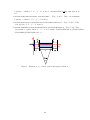
• Added the CORGPIPE element, which implements a beam dechirper using a corrugated pipe
wakefield, based on the theoretical treatment of K. Bane [38]. This was suggested by P.
Emma (LBNL).
• If not set by the users, the N_KICKS parameter of RFCA and RFCW will now be automatically
set in order to ensure a sufficient number of kicks, defined as 100 kicks per wavelength. This
may be excessive for high-energy beams.
1
• Automatic selection of the number of bins and bin size for the WAKE element was modified to
avoid warning messages.
• The EDRIFT element can now be subdivided using the usual element division commands.
• The CSRCSBEND element was improved to support the integrated Green’s function method for
steady-state wakes. This was done with the assistance of R. Ryne (LBNL).
• The NIBEND element now allows positioning of the fringe region relative to the reference plane.
The fringe region may be inside, outside, or centered on the reference plane. This was added
after discussions with N. Nakamura (KEK).
1.4
New and Modified Commands
• When determining momentum aperture (momentum\_aperture) the tunes near the aperture
boundary are now recorded.
1.5
Changes for Parallel Version Only
Changes to the parallel version are made by Y. Wang (ANL), unless otherwise noted.
• In the last version, we added the ability to change the randomization mode for different
processors. However, the default mode was not changed to one of the improved methods,
even though the documentation said it had been changed. The default mode has now been
changed mode 3 (see the documentation for global_settings).
• Updated to get the correct latest result from genetic optimization by using the right population group. Improved population log file for multiple restarts.
1.6
Changes to Related Programs and Files
• The scripts radiationEnvelope was added. It allows computing the envelope over harmonics of brightness and flux tuning curves, such as those obtained from sddsbrightness and
sddsfluxcurve.
• The program sddsfluxcurve now computes the flux in the central cone if computation of
the flux density is requested.
• The programs ibsEmittance and touschekLifetime now accept an argument giving the
vertical emittance.
1.7
Known Bugs, Problems, and Limitations
• Setting CHANGE_T=1 on RFCA and RFCW elements can give invalid results when tracking beams
with very large time spread compared to the bunch length.
• Twiss output contains entries for the higher-order dispersion, tune shifts with amplitude,
higher-order chromaticity, and tune spreads due to chromaticity and amplitude even when
these are not calculated, which is potentially misleading. The values are zero when the calculation is not requested.
2
• Computation of closed orbits and Twiss parameters will not always include the effects of
synchrotron radiation losses when these are imposed using SREFFECTS elements. See the
documentation for SREFFECTS for details.
• Computation of beam moments does not include synchrotron radiation effects from CWIGGLER,
WIGGLER, or UKICKMAP elements.
• The file created with the parameters field of run_setup does not contain any non-numerical
parameters of the lattice.
• When transmute_elements is used to turn a sextupole into a quadrupole, several problems are seen. Some of the quadrupole parameters are filled with garbage values. When
alter_elements or save_lattice are subsequently used, elegant crashes. These problems
were reported by V. Sajaev (ANL).
• Computation of radiation integrals does not include the effect of steering magnets.
• There is a bug related to using ILMATRIX that will result in a crash if one does not request
computation of the twiss parameters. If you encounter this problem, just add the following
statement after the run_setup command:
&twiss_output
matched = 1
&end
2
Credits
Contributors to elegant include M. Borland, W. Guo, R. Soliday, V. Sajaev, C. Wang, Y. Wang,
Y. Wu, and A. Xiao. Contributors to related programs include M. Borland, R. Dejus, L. Emery, A.
Petrenko, H. Shang, Y. Wang, A. Xiao, and B. Yang. R. Soliday is responsible for multi-platform
builds and distribution. Of course, we also appreciate the many suggestions, comments, and bug
reports from users.
3
Introduction
elegant stands for “ELEctron Generation ANd Tracking,” a somewhat out-of-date description
of a fully 6D accelerator program that now does much more than generate particle distributions
and track them. elegant, written entirely in the C programming language[1], uses a variant of
the MAD[2] input format to describe accelerators, which may be either transport lines, circular
machines, or a combination thereof. Program execution is driven by commands in a namelist
format.
This document describes the features available in elegant, listing the commands and their
arguments. The differences between elegant and MAD formats for describing accelerators are
listed. A series of examples of elegant input and output are given. Finally, appendices are
included describing the post-processing programs.
3
3.1
Program Philosophy
For all its complexity, elegant is not a stand-alone program. For example, most of the output is
not human-readable, and elegant itself has no graphics capabilities. These tasks are handled by a
suite of post-processing programs that serve both elegant and other physics programs. These programs, collectively known as the SDDS Toolkit[8, 9], provide sophisticated data analysis and display
capabilities. They also serve to prepare input for elegant, supporting multi-stage simulation.
Setting up for an elegant run thus involves more than creating input files for elegant per se.
A complicated run will typically involve creation of a post-processing command file that processes
elegant output and puts it in the most useful form, typically a series of graphs. Users thus have the
full power of the SDDS Toolkit, the resident command interpreter (e.g., the UNIX shell), and their
favorite scripting language (e.g., Tcl/Tk) at their disposal. The idea is that instead of continually
rewriting the physics code to, for example, make another type of graph or squeeze another item
into a crowded table, one should allow the user to tailor the output to his specific needs using a
set of generic post-processing programs. This approach has been quite successful, and is believed
particularly suited to the constantly changing needs of research.
Unlike many other programs, elegant allows one to make a single run simulating an arbitrary
number of randomizations or variations of an accelerator. By using the SDDS toolkit to postprocess
the data, the user’s postprocessing time and effort do not depend on how many random seeds or
situations are chosen. Hence, instead of doing a few simulations with a few seed numbers or values,
the user can simulate hundreds or even thousands of instances of one accelerator to get an accurate
representation of the statistics or dependence on parameters, with no more work invested than in
doing a few simulations.
In addition, complex simulations such as start-to-end jitter simulations[11] and top-up tracking[12]
can be performed involving hundreds or thousands of runs, with input created by scripts depending
on the SDDS toolkit. These simulations make use of concurrent computing on about 20 workstation
using the Distributed Queueing System[10]. Another example is the elegantRingAnalysis script,
which allows using many workstations for simulation of storage ring dynamic and momentum aperture, frequency maps, and so on. Clearly, use of automated postprocessing tools greatly increases
the scale and sophistication of simulations possible.
In passing, we note another “philosophical” point about elegant, namely, the goal of complete
backward compatibility. We consider it unacceptable if a new version of the program gives different
answers than an old version, unless the old version was wrong. Hence, there are sometimes lessthan-ideal default settings in elegant, incorrect spelling of parameters, etc., that are never fixed,
because doing so would break old input files. It helps to read the manual pages carefully for the
more complex features to ensure that the defaults are understood and appropriate.
3.2
Capabilities of elegant
elegant started as a tracking code, and it is still well-suited to this task. elegant tracks in
the 6-dimensional phase space (x, x′ , y, y′ , s, δ), where x (y) is the horizontal (vertical) transverse
coordinate, primed quantities are slopes, s is the total, equivalent distance traveled, and δ is the
fractional momentum deviation[3]. Note that these quantities are commonly referred to as (x, xp,
y, yp, s, dp) in the namelists, accelerator element parameters, and output files. (“dp” is admittedly
confusing—it is supposed to remind the user of ∆P/Po . Sometimes this quantity is referred to as
“delta.”)
Tracking may be performed using matrices (of selectable order), canonical kick elements, numerically integrated elements, or any combination thereof. For most elements, second-order matrices
4
are available; matrix concatenation can be done to any order up to third. Canonical kick elements are available for bending magnets, quadrupoles, sextupoles, and higher-order multipoles; all
of these elements also support optional classical synchrotron radiation losses. Among the numerically integrated elements available are extended-fringe-field bending magnets and traveling-wave
accelerators. A number of hybrid elements exist that have first-order transport with exact time
dependence, e.g., RF cavities. Some of the more unusual elements available are third-order alphamagnets[5, 4], time-dependent kicker magnets, voltage-ramped RF cavities, beam scrapers, and
beam-analysis “screens.”
Several elements support simulation of collective effects, such as short-range wakefields, resonator impedances, intra-beam scattering, coherent synchrotron radiation, and the longitudinal
space charge impedance.
A wide variety of output is available from tracking, including centroid and sigma-matrix output
along the accelerator, phase space output at arbitrary locations, turn-by-turn moments at arbitrary
locations, histograms of particle coordinates, coordinates of lost particles, and initial coordinates of
transmitted particles. In addition to tracking internally generated particle distributions, elegant
can track distributions stored in external files, which can either be generated by other programs
or by previous elegant runs. Because elegant uses SDDS format for reading in and writing out
particle coordinates, it is relatively easy to interface elegant to other programs using files that can
also be used with SDDS to do post-processing for the programs.
elegant allows the addition of random errors to virtually any parameter of any accelerator
element. One can correct the orbit (or trajectory), tunes, and chromaticity after adding errors,
then compute Twiss parameters, track, or perform a number of other operations. elegant makes
it easy to evaluate a large number of ensembles (“seeds”) in a single run. Alternatively, different
ensembles can be readily run of different CPUs and the SDDS output files combined.
In addition to randomly perturbing accelerator elements, elegant allows one to systematically
vary any number of elements in a multi-dimensional grid. As before, one can track or do other
computations for each point on the grid. This is a very useful feature for the simulation of experiments, e.g., emittance measurements involving beam-size measurements during variation of one or
more quadrupoles[6].
Like many accelerator codes, elegant does accelerator optimization. It will optimize a user
defined function of the transfer matrix elements (up to third-order), beta functions, tunes, chromaticities, radiation integrals, natural emittance, floor coordinates, beam moments, etc. It also has
the ability to optimize results of tracking using a user-supplied function of the beam parameters at
one or more locations. This permits solution of a wide variety of problems, from matching a kicker
bump in the presence of nonlinearities to optimizing dynamic aperture by adjusting sextupoles.
elegant provides several methods for determining accelerator aperture, whether dynamic or
physical. One may do straightforward tracking of an ensemble of particles that occupies at uniform
grid in (x, y) space. One may also invoke a search procedure that finds the aperture boundary. A
related feature is the ability to determine the frequency map for an accelerator, to help identify
aperture-limiting resonances.
In addition to using analytical expressions for the transport matrices, elegant supports computation of the first-order matrix and linear optics properties of a circular machine based on tracking.
A common application of this is to compute the tune and beta-function variation with momentum
offset by single-turn tracking of a series of particles. This is much more efficient than, for example,
tracking and performing FFTs (though elegant will do this also). This both tests analytical expressions for the chromaticity and allows computations using accelerator elements for which such
expressions do not exist (e.g., a numerically integrated bending magnet with extended fringe fields).
A common application of random error simulations is to set tolerances on magnet strength
5
and alignment relative to the correctability of the closed orbit. A more efficient way to do these
calculations is to use correct-orbit amplification factors[6]. elegant the computes amplification
factors and functions for corrected and uncorrected orbits and trajectories pertaining to any element
that produces an orbit or trajectory distortion. It simultaneously computes the amplification
functions for the steering magnets, in order to determine how strong the steering magnets will need
to be.
4
Digression on the Longitudinal Coordinate Definition
A word is in order about the definition of s, which we’ve described as the total, equivalent distance
traveled. First, by total distance we mean that s is not measured relative to the bunch center or
a fiducial particle. It is entirely a property of the individual particle and its path through the
accelerator.
To explain what we mean by equivalent distance, note that the relationship between s and
arrival time t at the observation point is, for each particle, s = βct, where βc is the instantaneous
velocity of the particle. Whenever a particle’s velocity changes, elegant recomputes s to ensure
that this relationship holds. s is thus the “equivalent” distance the particle would have traveled
at the present velocity to arrive at the observation point at the given time. This book-keeping is
required because elegant was originally a matrix-only code using s as the longitudinal coordinate.
Users should keep the meaning of s in mind when viewing statistics for s, for example, in the
sigma or watch point output files. A quantity like Ss is literally the rms spread in s. It is not
defined as σt /(hβic). A nonrelativistic beam with velocity spread will show no change in Ss in a
drift space, because the distance traveled is the same for all particles.
5
Fiducialization in elegant
In some tracking codes, there is a “fiducial particle” that is tracked along with the beam. This
particle follows the ideal trajectory or orbit, with the ideal momentum, and at the ideal phase.
There is no fiducial particle in elegant. Instead, fiducialization is typically based on statistical
properties of the bunch. This can be performed on a bunch-by-bunch basis, or for the first bunch
seen in a run. The latter method must be used if one wants to look at the effects of changing phase,
voltage, or magnets relative to some nominal configuration.
Internally, elegant fiducializes each element in the beamline. Fiducializing an element means
determining the reference momentum and arrival time (or phase) for that element. If the reference
momentum does not change along a beamline and no time-dependent elements are involved, then
fiducialization is irrelevant. All elements are fiducialized at the central momentum defined in
run_setup.
A number of commands have parameters for controlling fiducialization:
• The always_change_p0 parameter of run_setup causes elegant to re-establish the central
momentum after each element when fiducializing. This may be more convenient than setting
the CHANGE_P0 parameter on the elements themselves. However, it can have unexpected
consequences, such as changing the central momentum to match changes in beam momentum
due to synchrotron radiation.
• run_control has three parameters that affect fiducialization, which come into play when
multi-step runs are made. Typically, these are runs that involve variation of elements, addition
of errors, or loading of multiple sets of parameters.
6
– reset_rf_for_each_step — If nonzero, the rf phases are re-established for each beam
tracked. If this is 1 (the default), the time reference is discarded after each bunch is
tracked. This means that bunch-to-bunch phasing errors due to time-of-flight differences
would be lost.
– first_is_fiducial — The first bunch seen is taken to establish the fiducial phases
and momentum profile. If one is simulating, for example, successive beams in a fixed
accelerator, this should be set to 1. Otherwise, the momentum reference is discarded
after each bunch is tracked.
– restrict_fiducialization — If nonzero, then momentum profile fiducialization occurs only after elements that are known to possibily change the momentum. It would
not occur, for example, after a scraper that changes the average beam momentum by
removing a low-momentum tail.
• The bunched_beam command has a first_is_fiducial parameter that is convenient for use
with the first_is_fiducial mode established by run_control. If nonzero, this parameter
causes elegant to generate a first bunch with only one particle. This is very useful if one
wants to track with many particles but doesn’t want to waste time fidicializing with a manyparticle bunch.
Here are some examples that may be helpful.
• Scanning a phase error in a linac with a bunch compressor: The scan is performed using
the vary_element command. For this to work properly, it is necessary to fidcualize the
system with zero phase error. Hence, one must use the enumeration feature of vary_element
to provide an input file with the phase errors and the file must be sorted so that the row
with zero phase error is first. Further, one must set reset_rf_for_each_step = 0 and
first_is_fiducial = 1 in run_control, and CHANGE_P0=1 on all rf cavity elements. (See
the bunchComp/phaseSweep and bunchComp/dtSweep examples.)
• Scanning the voltage of a linac to simulate different operating energy choices at the compressor: In this case, one scans the linac voltage, but wants to fiducialize the system for each voltage. (It’s a change in design, not an error or perturbation.) One again uses vary_element,
but nothing special needs to be done about the order of the voltage values. One must
set reset_rf_for_each_step = 1 and first_is_fiducial = 0 in in run_control, and
CHANGE_P0=1 on all rf cavity elements. (See the bunchComp/energySweep example.)
• Simulation of phase and voltage jitter: In this case, one uses the error_elements command
to impart errors to the PHASE and VOLT parameters of rf cavity elements. However, the
first beam through the system must not see any errors. This is accomplished by setting
no_errors_for_first_step=1 in error_control. One can also (optionally) use a 1-particle
beam for fiducialization by setting first_is_fiducial=1 in bunched_beam. In addition, one
must set reset_rf_for_each_step = 0 and first_is_fiducial = 1 in run_control, and
CHANGE_P0=1 on all rf cavity elements. (See the bunchCompJitter/jitter example.)
6
Namelist Command Dictionary
The main input file for an elegant run consists of a series of namelists, which function as commands.
Most of the namelists direct elegant to set up to run in a certain way. A few are “action” commands
that begin the actual simulation. FORTRAN programmers should note that, unlike FORTRAN
7
namelists, these namelists need not come in a predefined order; elegant is able to detect which
namelist is next in the file and react appropriately.
6.1
Commandline Syntax
The commandline syntax for elegant is of the form
elegant {inputfile|-pipe=in} [-rpnDefns=filename]
-macro=tag1=value1[,tag2=value2...]
inputfile is the name of the command input file, which is a series of namelist commands directing
the calculations. Alternatively, one may give the -pipe=in option, allowing elegant to be fed a
stream of commands by another program or script. The -rpnDefns option allows providing the
name of the RPN definitions file as an alternative to defining the RPN_DEFNS environment variable.
The -macro option allows performing text substitutions in the command stream. Multiple -macro
options may be given. Usage is described in more detail below.
6.2
General Command Syntax
Each namelist has a number of variables associated with it, which are used to control details of the
run. These variables come in three data types: (1) long, for the C long integer type. (2) double,
for the C double-precision floating point type. (3) STRING, for a character string enclosed in double
quotation marks. All variables have default values, which are listed on the following pages. STRING
variables often have a default value listed as NULL, which means no data; this is quite different from
the value “”, which is a zero-length character string. long variables are often used as logical flags,
with a zero value indicating false and a non-zero value indicating true.
On the following pages the reader will find individual descriptions of each of the namelist
commands and their variables. Each description contains a sequence of the form
&<namelist-name>
<variable-type> <variable-name> = <default-value>;
.
.
.
&end
This summarizes the parameters of the namelist. Note, however, that the namelists are invoked in
the form
&<namelist-name>
[<variable-name> = <value> ,]
[<array-name>[<index>] = <value> [,<value> ...] ,]
.
.
.
&end
The square-brackets enclose an optional component. Not all namelists require variables to be given–
the defaults may be sufficient. However, if a variable name is given, it must have a value. Values
for STRING variables must be enclosed in double quotation marks. Values for double variables may
8
be in floating-point, exponential, or integer format (exponential format uses the ‘e’ character to
introduce the exponent).
Array variables take a list of values, with the first value being placed in the slot indicated by
the subscript. As in C, the first slot of the array has subscript 0, not 1. The namelist processor
does not check to ensure that one does not put elements into nonexistent slots beyond the end of
the array; doing so may cause the processor to hang up or crash.
Wildcards are allowed in a number of places in elegant and the SDDS Toolkit. The wildcard
format is very similar to that used in UNIX:
• * — stands for any number of characters, including none.
• ? — stands for any single character.
• [<list-of-characters>] — stands for any single character from the list. The list may
include ranges, such as a-z, which includes all characters between and including ‘a’ and ‘z’
in the ASCII character table.
The special characters *, ?, [, and ] are entered literally by preceeding the character by a backslash
(e.g., \*).
In many places where a filename is required in an elegant namelist, the user may supply a
so-called “incomplete” filename. An incomplete filename has the sequence “%s” imbedded in it, for
which is substituted the “rootname.” The rootname is by default the filename (less the extension)
of the lattice file. The most common use of this feature is to cause elegant to create names for
all output files that share a common filename but differ in their extensions. Post-processing can
be greatly simplified by adopting this naming convention, particularly if one consistently uses the
same extension for the same type of output. Recommended filename extensions are given in the
lists below.
When elegant reads a namelist command, one of its first actions is to print the namelist back
to the standard output. This printout includes all the variables in the namelist and their values.
Occasionally, the user may see a variable listed in the printout that is not in this manual. These are
often obsolete and are retained only for backward compatibility, or else associated with a feature
that is not fully supported. Use of such “undocumented features” is discouraged.
elegant supports substitution of fields in namelists using the commandline macro option. This
permits making runs with altered parameters without editing the input file. Macros inside the
input file have one of two forms: <tag> or \$tag. To perform substitution, use the syntax
elegant inputfile|-pipe=in -macro=tag1=value1[,tag2=value2...]
When using this feature, it is important to substitute the value of rootname (in run setup) so that
one can get a new set of output files (assuming use of the suggested “%s” field in all the output
file names). One may give the macro option any number of times, or combine all substitutions in
one option. The name of the input file is available using the macro INPUTFILENAME.
elegant also allows execution of commands in the shell as part of evaluation of a namelist field.
To invoke this, one encloses the commandline string in curly braces. E.g.,
betax = "{sdds2stream -parameter=betaxFinal data.twi}"
(Note that the quotes are also required.) In this example, betax is assigned the value of the
parameter betaxFinal from the file data.twi. Frequently, the commandline RPN calculator,
rpnl is also used in this way, for example
9
betax = "{rpnl 8 pi / 2 /}"
assigns the value 8/(2π) to betax. One possible pitfall with using rpnl in this fashion is interpretation of the multiplication symbol (*) as a file wildcard by the shell. For this reason, the alternate
multiplication operator mult is preferred, e.g.,
betax = "{rpnl 8 pi mult}"
rather than
betax = "{rpnl 8 pi *}"
We used the program rpnl in these examples because it is perhaps familiar. However, versions
17.4 and later allow direct evaluation of RPN expressions in commands whenever parentheses are
used to delimite a sequence. For example,
betax = "(8 2 / pi /)"
(Note that the quotes are also required.) The advantages of this method are speed (no subprocess is
needed), lack of intermediate interpretation by the shell, and persistence of the stack and variables.
So, for example, one might use
betax = "(8 2 / pi / sto betax0)"
betay = "(betax0)"
Another advantage is the ability to mix subcommands and rpn expressions, as in
betax = "({sdds2stream -parameter=betaxFinal data.twi} 2 /)"
would assign to betax half the value of the parameter betaxFinal from the file data.twi.
6.3
Setup and Action Commands
A subject of frequent confusion for elegant users is the distinction between setup and action commands. An “action” command causes elegant to immediately perform a specific computation or
set of computations. In contrast, a “setup” command tells elegant how to perform computations when it later encounters a “major” action command (one of analyze_map, find_aperture,
frequency_map, momentum_aperture, optimize, or track).
Several commands are switchable between action and setup modes. These include the coupled_
twiss_output, correction_matrix_output, twiss_output, find_aperture, matrix_output, and
sasefel commands. Except for find_aperture, all of the commands that can run in both modes
have the output_at_each_step parameter, which is used to switch between the modes. In the
case of find_aperture, the switch is accomplished using the optimization_mode parameter. Regardless of which parameter is present, unless the parameter is given a value of 1, the command
operates in action mode. Further, if the command is used in setup mode and no relevant action
command is present later in the file, then the requested will not be performed.
Typically one wants to use these switchable commands in setup mode whenever one is simulating
random errors, performing a parameter scan, or performing optimization. When in setup mode,
the indicated computations will be performed repeatedly, e.g., for each set of errors, for each step
in the parameter scan, or for use in each evaluation of the optimization penalty function.
10
6.4
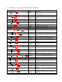
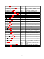
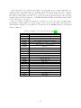
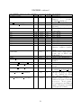
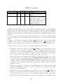
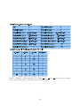
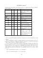
Table of elegant commands and their functions
Command name
alter elements6.5
amplification factors6.6
analyze map6.7
aperture data6.8
bunched beam6.9
change particle6.10
chromaticity6.11
closed orbit6.12
correct6.13
correction matrix output6.14
correct tunes6.15
coupled twiss output6.16
divide elements6.17
error element6.18
error control6.19
find aperture6.20
floor coordinates6.21
frequency map6.22
global settings6.23
insert sceffects6.24
insert sceffects6.25
linear chromatic tracking setup6.26
link control6.27
link elements6.28
load parameters6.29
matrix output6.30
modulate elements6.31
moments output6.32
momentum aperture6.33
Type
action
Description
Change an element parameter from the
command file.
action
Compute orbit amplification functions.
major
Determine first-order matrix from trackaction
ing.
setup
Define aperture using an SDDS file.
setup
Set up beam generation.
action
Change the type of particle. Default is
electron.
setup
Correct the chromaticity.
setup
Compute the closed orbit.
setup
Correct the orbit or trajectory.
action/setup Obtain orbit/trajectory correction matrix
in a file.
setup
Correct the tunes.
setup/action Compute and output coupled twiss parameters.
setup
Specify division of elements into pieces.
setup
Define errors for a set of elements.
setup
Set up and control error generation process.
setup/major Determine the transverse (e.g., dynamic)
action
aperture.
action
Compute and output floor coordinates.
major
Compute and output frequency map.
action
action
Change global settings.
action
Insert elements into the lattice at many
places.
action
Insert space charge kick elements.
setup
Set up for fast tracking with chromatic effects.
setup
Control linking of element parameters.
setup
Define link between parameters of two elements.
setup/action Load element parameters from SDDS file.
setup/action Output transfer matrix along beamline.
setup
Set up time-dependent modulation of elements.
setup/action Compute coupled beam moments, with
radiation option.
major
Determine s-dependent momentum aperaction
ture.
11
optimize6.34
major
action
setup
Execute an optimization.
Define a dependent parameter for optimization.
optimization setup6.37
setup
Perform initial optimization setup.
optimization term6.39
setup
Define a term of penalty function.
optimization variable6.40
setup
Define an optimization variable.
parallel optimization setup6.38
setup
Perform initial parallel optimization
setup.
print dictionary6.41
action
Print the element dictionary.
ramp elements6.42
setup
Set up turn-by-turn ramping of elements.
rf setup6.43
setup/action Set up RF cavity elements for storage
rings.
rpn expression6.45
action
Execute an expression in the rpn interpreter.
rpn load6.46
action
Load values from SDDS file into rpn interpreter.
run control6.47
setup
Set up simulation steps and passes.
run setup6.48
setup
Define global simulation parameters and
output files.
sasefel6.49
setup/action Evaluate SASE FEL gain etc.
save lattice6.50
action
Save new lattice file.
sdds beam6.51
setup
Define loading of particles from SDDS file.
semaphores6.52
setup
Define file semaphores for start/end of
run.
slice analysis6.53
setup
Perform slice analysis along beamline.
subprocess6.54
action
Execute a command in the shell.
steering element6.55
setup
Define element parameters as steering correctors.
transmute elements6.57
setup
Transmute elements from one type to another.
twiss analysis6.58
setup
Define subset of beamline for twiss parameter analysis.
twiss output6.59
setup/action Set up twiss parameter and related computation.
track6.60
major
Execute tracking of particles and other opaction
erations.
tune shift with amplitude6.61
setup
Compute tune shifts with amplitude.
vary element6.62
setup
Vary element parameters in loops.
Table 1: Table of elegant commands and their functions.
optimization covariable6.36
12
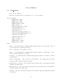
alter_elements
6.5
alter elements
• type: action command.
• function: modify the value of a parameter for one or more elements
&alter_elements
STRING name = NULL;
STRING item = NULL;
STRING type = NULL;
STRING exclude = NULL;
double value = 0;
STRING string_value = NULL;
long differential = 0;
long multiplicative = 0;
long verbose = 0;
long allow_missing_elements = 0;
long allow_missing_parameters = 0;
long start_occurence = 0;
long end_occurence = 0;
double s_start = -1;
double s_end = -1;
STRING before = NULL;
STRING after = NULL;
&end
• name — A possibly-wildcard-containing string giving the names of the elements to alter. If
not specified, then one must specify type.
• item — The name of the parameter to alter.
• type — A possibly-wildcard-containing string giving the names of element types to alter.
May be specified with name or by itself.
• exclude — A possibly-wildcard-containing string giving the names of elements to excluded
from alteration.
• value, string_value — The new value for the parameter. Use string_value only if the
parameter takes a character string as its value.
• differential — If nonzero, the new value is the predefined value of the parameter plus the
quantity given with value.
• multiplicative — If nonozero, the new given value is the predefined value of the parameter
times the quantity given with value.
• verbose — If nonzero, information is printed to the standard output describing what elements
are changed.
13
• allow_missing_elements — If nonzero, then it is not an error if an element matching name
does not exist. Normally, such an occurence is an error and terminates the program.
• allow_missing_parameters — If nonzero, then it is not an error if an element does not have
the parameter named with item. Normally, such an occurence is an error and terminates the
program.
• start_occurence, end_occurence — If nonzero, these give the starting and ending occurence
numbers of elements that will be altered. N.B.: if wildcards are used, occurence number
counting is for each set of identically-named elements separately, rather than for the sequence
of matched elements.
• s_start, s_end — If non-negative, these give the gaving and ending position limits for the
end-of-element locations of elements to be altered.
• after — The name of an element. If given, the alteration is applied only to elements that
follow the named element in the beamline.
• before — The name of an element. If given, the alteration is applied only to elements that
precede the named element in the beamline.
14
amplification_factors
6.6
amplification factors
• type: action command.
• function: compute corrected and uncorrected orbit amplification factors and functions.
&lification_factors
STRING output = NULL;
STRING uncorrected_orbit_function = NULL;
STRING corrected_orbit_function = NULL;
STRING kick_function = NULL;
STRING name = NULL;
STRING type = NULL;
STRING item = NULL;
STRING plane = NULL;
double change = 1e-3;
long number_to_do = -1;
double maximum_z = 0;
&end
• output — The (incomplete) name of a file for text output. Recommended value: “%s.af”.
• uncorrected_orbit_function — The (incomplete) name of a file for an SDDS-format output
of the uncorrected-orbit amplification function. Recommended value: “%s.uof”.
• corrected_orbit_function — The (incomplete) name of a file for an SDDS-format output
of the corrected-orbit amplification function. Recommended value: “%s.cof”.
• kick_function — The (incomplete) name of a file for an SDDS-format output of the kick
amplification function. Recommended value: “%s.kaf”.
• name — The optionally wildcarded name of the orbit-perturbing elements.
• type — The optional type name of the the orbit-perturbing elements.
• item — The parameter of the elements producing the orbit.
• plane — The plane (“h” or “v”) to examine.
• change — The parameter change to use in computing the amplification.
• number_to_do — The number of elements to perturb.
• maximum_z — The maximum z coordinate of the elements to perturb.
15
analyze_map
6.7
analyze map
• type: major action command.
• function: find the approximate first-order matrix and related quantities for an accelerator by
tracking.
&analyze_map
STRING output = NULL;
double delta_x = 1e-6;
double delta_xp = 1e-6;
double delta_y = 1e-6;
double delta_yp = 1e-6;
double delta_s = 1e-6;
double delta_dp = 1e-6;
long center_on_orbit = 0;
long verbosity = 0;
&end
• output — The (incomplete) name of a file for SDDS output.
– Recommended value: “%s.ana”.
– File contents: A series of dumps, each consisting of a single data point containing the
centroid offsets for a single turn, the single-turn R matrix, the matched Twiss parameters,
tunes, and dispersion functions.
• delta_X — The amount by which to change the quantity X in computing the derivatives that
give the matrix elements.
• center_on_orbit — A flag directing the expansion to be made about the closed orbit instead
of the design orbit.
• verbosity — The larger this value, the more output is printed during computations.
16
aperture_data
6.8
aperture data
• type: setup command.
• function: specify a file from which to take x and y aperture data vs s.
• note: this command is also available under the name aperture_input.
&aperture_data
STRING input = NULL;
long periodic = 1;
long persistent = 0;
long disable = 0;
&end
• input — Name of SDDS file supplying the aperture data. The following columns are all
required, in double or float type, with units of m (meters).
1. s — Distance along the central trajectory.
2. xHalfAperture — Half aperture in the horizontal.
3. yHalfAperture — Half aperture in the vertical.
4. xCenter — Center of the aperture in the horizontal.
5. yCenter — Center of the aperture in the vertical.
• periodic — If non-zero, the aperture is a periodic function of s, with period equal to the
range of the data.
• persistent — If non-zero, the aperture data persists across subsequent run_setup commands. By default, the aperture data is forgotten when a new run_setup command is seen.
• disable — If non-zero, the command is ignored.
17
bunched_beam
6.9
bunched beam
• type: setup command.
• function: set up for tracking of particle coordinates with various distributions.
&bunched_beam
STRING bunch = NULL;
long n_particles_per_bunch = 1;
double time_start = 0;
STRING matched_to_cell = NULL;
double emit_x = 0;
double emit_nx = 0;
double beta_x = 1.0;
double alpha_x = 0.0;
double eta_x
= 0.0;
double etap_x = 0.0;
double emit_y = 0;
double emit_ny = 0;
double beta_y = 1.0;
double alpha_y = 0.0;
double eta_y
= 0.0;
double etap_y = 0.0;
long use_twiss_command_values = 0;
double Po = 0.0;
double sigma_dp = 0.0;
double sigma_s = 0.0;
double dp_s_coupling = 0;
double emit_z = 0;
double beta_z = 0;
double alpha_z = 0;
double momentum_chirp = 0;
long one_random_bunch = 1;
long symmetrize = 0;
long halton_sequence[3] = {0, 0, 0};
long halton_radix[6] = {0, 0, 0, 0, 0, 0};
long optimized_halton = 0;
long randomize_order[3] = {0, 0, 0};
long limit_invariants = 0;
long limit_in_4d = 0;
long enforce_rms_values[3] = {0, 0, 0};
double distribution_cutoff[3] = {2, 2, 2};
STRING distribution_type[3] = {"gaussian","gaussian","gaussian"};
double centroid[6] = {0.0, 0.0, 0.0, 0.0, 0.0, 0.0};
long first_is_fiducial = 0;
long save_initial_coordinates = 1;
&end
18
• bunch — The (incomplete) name of an SDDS file to which the phase-space coordinates of the
bunches are to be written. Recommended value: “%s.bun”.
• n_particles_per_bunch — Number of particles in each bunch.
• time_start — The central value of the time coordinate for the bunch.
• matched_to_cell — The name of a beamline from which the Twiss parameters of the bunch
are to be computed.
• emit_X — RMS emittance for the X plane.
• emit_nX — RMS normalized emittance for the X plane. Ignored if emit_X is nonzero.
• beta_X, alpha_X, eta_X, etap_X — Twiss parameters for the X plane.
• use_twiss_command_values — If nonzero, then the values for β, α, η, and η ′ are taken from
the twiss_output command. It is an error if no twiss_output command has been given.
• Po — Central momentum of the bunch.
• sigma_dp, sigma_s — Fractional momentum spread, δ, and bunch length. Note that sigma_s
is actually the length in βz ∗ c ∗ t, so that for βz << 1 the length of the bunch in time will be
greater than one might expect.
• dp_s_coupling — Specifies the coupling between s and δ, defined as hsδi/(σs σδ ).
• emit_z, beta_z, alpha_z — Provide another way to specify the longitudinal phase space,
either separately from or in combination with sigma_dp, sigma_s, and dp_s_coupling.
Basically, which values elegant uses depends on what one sets to nonzero values. If one sets
emit z, then sigma dp, sigma s, and dp s coupling are ignored. If one doesn’t set emit z, then
elegant uses sigma dp and sigma s; it additionally uses alpha z if it is nonzero, otherwise it
α
uses dp s coupling. For reference, the relationship between them is C = √ΣΣ56Σ = − √1+α
.
2
55 66
Note that to impart a chirp that results in compression for R56 < 0 (e.g., a normal four-dipole
chicane), one must have αz < 0 or C > 0.
• momentum_chirp — Permits imparting an additional momentum chirp to the beam, in units
of 1/m. E.g., a value of 1 indicates that a 1mm long bunch has a linear variation in momentum
of 0.1% from end-to-end. A positive chirp is needed to provide compression of a bunch with
an ordinary R56 < 0 four-dipole chicane.
• one_random_bunch — If non-zero, then only one random particle distribution is generated.
Otherwise, a new distribution will be generated for every simulation step.
• enforce_rms_values[3] — Flags, one for each plane, indicating whether to force the distribution to have the specified RMS properties.
• distribution_cutoff[3] — Distribution cutoff parameters for each plane. For gaussian
distributions, this is the number of sigmas to use. For other distributions (except dynamic
aperture), this number simply multiplies the sizes. This is potentially confusing and hence it
is suggested that the distribution cutoff be set to 1 for nongaussian beams.
The exception is “dynamic-aperture” distribution type. In this case, the cutoff value is the
number of grid points in the dimension in question.
19
• distribution_type[3] — Distribution type for each plane. May be “gaussian”, “hard-edge”,
“uniform-ellipse”, “shell”, “dynamic-aperture”, “line”, “halo(gaussian)”.
For the transverse plane, the interpretation of the emittance is different for the different
beam
√
ǫ
∗
β
times
types. For gaussian beams, the emittances are rms values. For all other types,
p
the distribution cutoff defines the edge of the beam in position space, while ǫ ∗ (1 + α2 )/β
times the distribution cutoff defines the edge of the beam in slope space.
A hard-edge beam is a uniformly-filled parallelogram in phase space. A uniform-ellipse beam
is a uniformly-filled ellipse in phase space. A shell beam is a hollow ellipse in phase space. A
dynamic aperture beam has zero slope and uniform spacing in position coordinates. A line
beam is a line in phase space. A “halo(gaussian)” beam is the part of the gaussian distribution
beyond the distribution cutoff.
• limit_invariants — If non-zero, the distribution cutoffs are applied to the invariants, rather
than to the coordinates. This is useful for gaussian beams when the distribution cutoff is small.
• limit_in_4d — If non-zero, then the transverse distribution is taken to be a 4-d gaussian or
uniform distribution. One of these must be chosen using the distribution_type control. It
must be the same for x and y. This is useful, for example, if you want to make a cylindrically
symmetric beam.
• symmetrize — If non-zero, the distribution is symmetric under changes of sign in the coordinates. Automatically results in a zero centroid for all coordinates.
• halton_sequence[3] and halton_radix[6] and optimized_halton — This provides a “quietstart” feature by choosing Halton sequences in place of random number generation. There
are three new variables that control this feature. halton_sequence is an array of three flags
that permit turning on Halton sequence generation for the horizontal, vertical, or longitudinal
planes. For example, halton_sequence[0] = 3*1 will turn on Halton sequences for all three
planes, while halton_sequence[2] = 1, will turn it on for the longitudinal plane only.
halton_radix is an array of six integers that permit giving the radix for each sequence (i.e.,
x, x’, y, y’, t, p). Each radix must be a prime number. One should never use the same prime
for two sequences, unless one randomizes the order of the sequences relative to each other (see
the next item). If these are left at zero, then elegant chooses values that eliminate phase-space
banding to some extent. The user is cautioned to plot all coordinate combinations for the
initial phase space to ensure that no unacceptable banding is present.
A suggested way to use Halton sequences is to set halton_radix[0] = 2, 3, 2, 3, 2, 3
and to set randomize_order[0] = 2, 2, 2,. This avoids banding that may result from
choosing larger radix values.
optimized_halton uses the improved halton sequence [33]. (Algorithm 659, Collected Algorithm from ACM. Derandom Algorithm is added by Hongmei CHI (CS/FSU)). It avoids the
banding problem automatically and the halton_radix values are ignored.
• randomize_order[3] — Allows randomizing the order of assigned coordinates for the pairs
(x, x’), (y, y’), and (t,p). 0 means no randomization; 1 means randomize (x, x’, y, y’, t, p)
values independently, which destroys any x-x’, y-y’, and t-p correlations; 2 means randomize
(x, x’), (y, y’), and (t, p) in pair-wise fashion. This is used with Halton sequences to remove
banding. It is suggested that that the user employ sddsanalyzebeam to verify that the beam
properties when randomization is used.
20
• centroid[6] — Centroid offsets for each of the six coordinates.
• first_is_fiducial — Specifies that the first beam generated shall be a single particle beam,
which is suitable for fiducialization. See the section on “Fiducialization in elegant” for more
discussion.
• save_initial_coordinates — A flag that, if set, results in saving initial coordinates of
tracked particles in memory. This is the default behavior. If unset, the initial coordinates
are not saved, but are regenerated each time they are needed. This is more memory efficient
and is useful for tracking very large numbers of particles.
21
change_particle
6.10
change particle
• type: action command.
• function: change the particle type from the default value of “electron.”
• N.B.: this feature has had limited testing, mostly to verify that electron tracking is not
impacted by the implementation. Please use with caution and be alert for suspicious results.
&change_particle
STRING name = "electron";
double mass_ratio = 0;
double charge_ratio = 0;
&end
• name — The name of the particle to use. Possible values are electron, positron, proton,
muon, and custom.
• mass_ratio, charge_ratio — If the particle name is “custom,” these parameters specify the
mass and charge of the particle relative to the electron. E.g., for an anti-proton, one would
use a mass ratio of 1836.18 and a charge ratio of 1.
22
chromaticity
6.11
chromaticity
• type: setup command.
• function: set up for chromaticity correction.
&chromaticity
STRING sextupoles = NULL;
double dnux_dp = 0;
double dnuy_dp = 0;
double sextupole_tweek = 1e-3;
double correction_fraction = 0.9;
long n_iterations = 5;
double tolerance = 0;
STRING strength_log = NULL;
long change_defined_values = 0;
double strength_limit = 0;
long use_perturbed_matrix = 0;
&end
• sextupoles — List of names of elements to use to correct the chromaticities.
• dnux_dp, dnuy_dp — Desired chromaticity values.
• sextupole_tweek — Amount by which to tweak the sextupoles to compute derivatives of
chromaticities with respect to sextupole strength. [The word “tweak” is misspelled “tweek”
in the code.]
• correction_fraction — Fraction of the correction to apply at each iteration. In some cases,
correction is unstable at this number should be reduced.
• n_iterations — Number of iterations of the correction to perform.
• tolerance — Stop iterating when chromaticities are within this value of the desired values.
• strength_log — The (incomplete) name of an SDDS file to which the sextupole strengths
will be written. Recommended value: “%s.ssl”.
• change_defined_values — Changes the defined values of the sextupole strengths. This
means that when the lattice is saved (using save_lattice), the sextupoles will have the
corrected values. This would be used for correcting the chromaticity of a design lattice, for
example, but not for correcting chromaticity of a perturbed lattice.
• strength_limit — Limit on the absolute value of sextupole strength (K2 ). ‘
• use_perturbed_matrix — If nonzero, requests use of the perturbed correction matrix in
performing correction. For difficult lattices with large errors, this may be necessary to obtain
correction. In general, it is not necessary and only slows the simulation.
23
closed_orbit
6.12
closed orbit
• type: setup command.
• function: set up for computation of the closed orbit.
&closed_orbit
STRING output = NULL;
long output_monitors_only = 0;
long start_from_centroid = 1;
long start_from_dp_centroid = 1;
double closed_orbit_accuracy = 1e-12;
long closed_orbit_iterations = 10;
double iteration_fraction = 1;
long fixed_length = 0;
long start_from_recirc = 0;
long verbosity = 0;
&end
• output — The (incomplete) name of an SDDS file to which the closed orbits will be written.
Recommended value: “%s.clo”.
• output_monitors_only — If non-zero, indicates that the closed orbit output should include
only the data at the locations of the beam-position monitors.
• start_from_centroid — A flag indicating whether to force the computation to start from
the centroids of the beam distribution.
• start_from_dp_centroid — A flag indicating whether to force the computation to use
the momentum centroid of the beam for the closed orbit. This can allow computing the
closed orbit for an off-momentum beam, then starting the beam on that orbit using the
offset_by_orbit or center_on_orbit parameters of the track command. In contrast to
the start_from_centroid, this command doesn’t force the algorithm to start from the beam
transverse centroids.
• closed_orbit_accuracy — The desired accuracy of the closed orbit, in terms of the difference
between the start and end coordinates, in meters.
• closed_orbit_iterations — The number of iterations to take in finding the closed orbit.
• iteration_fraction — Fraction of computed change that is used each iteration. For lattices
that are very nonlinear or close to unstable, a number less than 1 can be helpful. Otherwise,
it only slows the simulation.
• fixed_length — A flag indicating whether to find a closed orbit with the same length as the
design orbit by changing the momentum offset.
• start_from_recirc — A flag indicating whether to compute the closed orbit from the recirculation (recirc) element in the beamline. In general, if one has a recirculation element,
one should give this flag.
24
• verbosity — A larger value results in more printouts during the computations.
25
correct
6.13
correct
• type: setup command.
• function: set up for correction of the trajectory or closed orbit.
&correct
STRING mode = "trajectory";
STRING method = "global";
STRING trajectory_output = NULL;
STRING corrector_output = NULL;
STRING statistics = NULL;
double corrector_tweek[2] = {1e-3, 1e-3};
double corrector_limit[2] = {0, 0};
double correction_fraction[2] = {1, 1};
double correction_accuracy[2] = {1e-6, 1e-6};
long remove_smallest_SVs[2] = {0, 0};
long keep_largest_SVs[2] = {0, 0};
double minimum_SV_ratio[2] = {0, 0};
long auto_limit_SVs[2] = {1, 1};
long threading_divisor[2] = {100, 100};
double bpm_noise[2] = {0, 0};
double bpm_noise_cutoff[2] = {1.0, 1.0};
STRING bpm_noise_distribution[2] = {"uniform", "uniform"};
long verbose = 1;
long fixed_length = 0;
long fixed_length_matrix = 0;
long n_xy_cycles = 1;
long minimum_cycles = 1;
long n_iterations = 1;
long prezero_correctors = 1;
long track_before_and_after = 0;
long start_from_centroid = 1;
long use_actual_beam = 0;
double closed_orbit_accuracy = 1e-12;
long closed_orbit_iterations = 10;
double closed_orbit_iteration_fraction = 1;
long use_perturbed_matrix = 0;
long disable = 0;
long use_response_from_computed_orbits = 0;
&end
In the case of array variables with dimension 2, the first entry is for the horizontal plane and
the second is for the vertical plane.
• mode — Either “trajectory” or “orbit”, indicating correction of a trajectory or a closed orbit.
26
• method — For trajectories, may be “one-to-one”, “one-to-best”, “one-to-next”, “thread”, or
“global”. “One-to-one” and “one-to-next” are the same: steering is performed by pairing one
corrector with the next downstream BPM. “One-to-best” attempts to find a BPM with a
large response to each corrector. “Thread” does corrector sweeps to work the beam through
a beamline with apertures; it is quite slow. “Global” simply uses the global response matrix;
it is the best choice if the trajectory is not lost on an aperture. For closed orbit, must be
“global”.
• trajectory_output — The (incomplete) name of an SDDS file to which the trajectories or
orbits will be written. Recommended value: “%s.traj” or “%s.orb”.
• corrector_output — The (incomplete) name of an SDDS file to which information about
the final corrector strengths will be written. Recommended value: “%s.cor”.
• statistics — The (incomplete) name of an SDDS file to which statistical information about
the trajectories (or orbits) and corrector strengths will be written. Recommended value:
“%s.scor”.
• corrector_tweek[2] — The amount by which to change the correctors in order to compute
correction coefficients for transport lines. [The word “tweak” is misspelled “tweek” in the
code.] The default value, 1 mrad, may be too large for systems with small apertures. If you
get an error message about “tracking failed for test particle,” try decreasing this value.
• corrector_limit[2] — The maximum strength allowed for a corrector.
• correction_fraction[2] — The fraction of the computed correction strength to actually
use for any one iteration.
• correction_accuracy[2] — The desired accuracy of the correction in terms of the RMS
BPM values.
• remove_smallest_SVs, keep_largest_SVs, minimum_SV_ratio, auto_limit_SVs — These
parameters control the elimination of singular vectors from the inverse response matrix, which
can help deal with degeneracy in the correctors and reduce corrector strength. By default,
the number of singular vectors is limited to the number of BPMs, which is a basic condition
for stability; this can be defeated by setting auto_limit_SVs to 0 for the desired planes.
Set remove_smallest_SVs to require removal of a given number of vectors with the smallest
singular values; this is ignored if auto_limit_SVs is also requested and would remove more
SVs. Set keep_largest_SVs to require keeping at most a given number of the largest SVs.
Set minimum_SV_ratio to require removal of any vectors with singular values less than a
given factor of the largest singular value.
• bpm_noise[2] — The BPM noise level.
• bpm_noise_cutoff[2] — Cutoff values for the random distributions of BPM noise.
• bpm_noise_distribution[2] — May be either “gaussian”, “uniform”, or “plus or minus”.
• verbose — If non-zero, information about the correction is printed during computations.
• fixed_length — Indicates that the closed orbit length should be kept the same as the design
orbit length by changing the momentum offset of the beam.
27
• fixed_length_matrix — Indicates that for fixed-length orbit correction, the fixed-length
matrix should be computed and used. This will improve convergence but isn’t always needed.
• n_xy_cycles — Number of times to alternate between correcting the x and y planes.
• minimum_cycles — The minimum number of x-y cycles to perform, even if the correction
does not improve.
• n_iterations — Number of iterations of the correction in each plane for each x/y cycle.
• prezero_correctors — Flag indicating whether to set the correctors to zero before starting.
• track_before_and_after — Flag indicating whether tracking should be done both before
and after correction.
• start_from_centroid — Flag indicating that correction should start from the beam centroid.
For orbit correction, only the beam momentum centroid is relevant.
• use_actual_beam — Flag indicating that correction should employ tracking of the beam
distribution rather than a single particle. This is valid for trajectory correction only.
• closed_orbit_accuracy — Accuracy of closed orbit computation.
• closed_orbit_iterations — Number of iterations of closed orbit computation.
• closed_orbit_iteration_fraction — Fraction of change in closed orbit to use at each
iteration.
• use_perturbed_matrix — If nonzero, specifies that prior to each correction elegant shall
recompute the response matrix. This is useful if the lattice is changing significantly between
corrections.
• disable — If nonzero, the command is ignored.
• use_response_from_computed_orbits — If nonzero, in-plane response matrices are computed using differences of closed orbits, which is slower but may be more accurate. For
cross-plane matrices, this is always the case.
28
correction_matrix_output
6.14
correction matrix output
• type: setup/action command.
• function: provide output of the orbit/trajectory correction matrix.
&correction_matrix_output
STRING response[4] = NULL, NULL;
STRING inverse[2] = NULL, NULL;
long KnL_units = 0;
long BnL_units = 0;
long output_at_each_step = 0;
long output_before_tune_correction = 0;
long fixed_length = 0;
long coupled = 0;
long use_response_from_computed_orbits = 0;
&end
• response — Array of (incomplete) filenames for SDDS output of the x and y response matrices, plus the cross-plane response matrices. Recommended values, in order: “%s.hrm”
(horizontal response to horizontal correctors), “%s.vrm” (vertical response to vertical correctors), “%s.vhrm” (vertical response to horizontal correctors), and “%s.hvrm” (horizontal
response to vertical correctors).
• inverse — Array of (incomplete) filenames for SDDS output of the x and y inverse response
matrices. Recommended values: “%s.hirm” and “%s.virm”.
• KnL_units — Flag that, if set, indicates use of “units” of m/K0L rather than m/rad. This
results in a sign change for the horizontal data.
• BnL_units — Flag that, if set, indicates use of “units” of m/(T*m) rather than m/rad. This
is useful for linac work in that the responses are automatically scaled with beam momentum.
• output_at_each_step — Flag that, if set, specifies output of the data at each simulation
step. By default, the data is output immediately for the defined lattice.
• output_before_tune_correction — Flag that, if set, specifies that when output_at_each_step
is set, that output shall occur prior to correcting the tunes.
• fixed_length — Flag that, if set, specifies output of the fixed-path-length matrix.
• coupled — If nonzero, the cross-plane response matrices are computed.
• use_response_from_computed_orbits — If nonzero, in-plane response matrices are computed using differences of closed orbits, which is slower but may be more accurate. For
cross-plane matrices, this is always the case.
29
correct_tunes
6.15
correct tunes
• type: setup command.
• function: set up for correction of the tunes.
&correct_tunes
STRING quadrupoles = NULL;
double tune_x = 0;
double tune_y = 0;
long n_iterations = 5;
double correction_fraction = 0.9;
double tolerance = 0;
long step_up_interval = 0;
double max_correction_fraction = 0.9;
double delta_correction_fraction = 0.1;
STRING strength_log = NULL;
long change_defined_values = 0;
long use_perturbed_matrix = 0;
&end
• quadrupoles — List of names of quadrupoles to be used. Only two may be given.
• tune_x, tune_y — Desired x and y tune values. If not given, the desired values are assumed
to be the unperturbed tunes.
• n_iterations — The number of iterations of the correction to perform.
• correction_fraction — The fraction of the correction to apply at each iteration.
• tolerance — When both tunes are within this value of the desired tunes, the iteration is
stopped.
• step_up_interval — Interval between increases in the correction fraction.
• max_correction_fraction — Maximum correction fraction to allow.
• delta_correction_fraction — Change in correction fraction after each step_up_interval
steps.
• strength_log — The (incomplete) name of a SDDS file to which the quadrupole strengths
will be written as correction proceeds. Recommended value: “%s.qst”.
• change_defined_values — Changes the defined values of the quadrupole strengths. This
means that when the lattice is saved (using save_lattice), the quadrupoles will have the
corrected values. This would be used for correcting the tunes of a design lattice, for example,
but not for correcting tunes of a perturbed lattice.
• use_perturbed_matrix — If nonzero, requests use of the perturbed correction matrix in
performing correction. For difficult lattices with large errors, this may be necessary to obtain
correction. In general, it is not necessary and only slows the simulation.
30
coupled_twiss_output
6.16
coupled twiss output
• type: setup/action command.
• function: set up or execute computation of coupled twiss parameters and beam sizes
&coupled_twiss_output
STRING filename = NULL;
long output_at_each_step = 0;
long emittances_from_twiss_command = 1;
double emit_x = 0;
double emittance_ratio = 0.01;
double sigma_dp = 0;
long calculate_3d_coupling = 1;
long verbosity = 0;
long concat_order = 2;
&end
• filename — The (incomplete) name of the SDDS file to which coupled twiss parameters and
beam sizes will be written. Suggested value: “%s.ctwi”.
• output_at_each_step — If nonzero, then this is a setup command and results in computations occurring for each simulation step (e.g., for each perturbed machine if errors are
included). If zero, then this is an action command and computations are done immediately
(e.g., for the unperturbed machine).
• emittances_from_twiss_command — If nonzero, then the values of the horizontal emittance and the momentum spread are taken from the uncoupled computation done with the
twiss_output command. In this case, the user must issue a twiss_output command prior
to the coupled_twiss_output. If zero, then the values of the horizontal emittance and
the momentum spread are taken from the parameters emit_x and sigma_dp, respectively.
\verb|emit_x|— Gives the horizontal emittance, if emittances_from_twiss_command=0.
• emittance_ratio — Gives the ratio of the x and y emittances. Used to determine the vertical
emittance from the horizontal emittance. Note that the computation is not self-consistent.
I.e., the user is free to enter any emittance ratio desired, whether it is consistent with the
machine optics or now.
• sigma_dp — Gives the momentum spread, if emittances_from_twiss_command=0.
This feature was added to elegant using code supplied by V. Sajaev, based on Ripkin’s method.
The code computes the coupled lattice functions, then uses the supplied emittance, emittance ratio,
and momentum spread to compute the beam sizes, bunch length (if rf is included), and beam tilt.
31
divide_elements
6.17
divide elements
• type: setup command.
• function: define how to subdivide certain beamline elements.
• notes:
– Any number of these commands may be given.
– Not effective unless given prior to run_setup.
– The element_divisions field in run_setup provides a simpler, but less flexible, method
of performing element division. At present, these element types may be divided: QUAD,
SBEN, RBEN, DRIF, SEXT.
– Only effective if given prior to the run_setup command.
• warnings:
– Using save_lattice and element divisions together will produce an incorrect lattice file.
– Element subdivision may produce unexpected results when used with load_parameters
or parameters saved via the parameter entry of the run_setup command. If you wish to
load parameters while doing element divisions or if you wish to load parameters from a
run that had element divisions in effect, you should not load length data for any elements
that are (or were) split. The name and item pattern features of load_parameters are
helpful in restricting what is loaded.
÷_elements
STRING name = NULL;
STRING type = NULL;
STRING exclude = NULL;
long divisions = 0;
double maximum_length = 0;
long clear = 0;
&end
• name — A possibly wildcard-containing string specifying the elements to which this specification applies.
• type — A possibly wildcard-containing string specifying the element types to which this
specification applies.
• exclude — A possibily wildcard-containing string specifying elements to be excluded from
the specification.
• divisions — The number of times to subdivide the specified elements.
maximum_length should be nonzero.
If zero, then
• maximum_length — The maximum length of a slice. This is usually preferrable to specifying
the number of divisions, particularly when the elements divided may be of different lengths.
If zero, then divisions should be nonzero.
• clear — If nonzero, all prior division specifications are deleted.
32
error_element
6.18
error element
• type: setup command.
• function: assert a random error defintion for the accelerator.
&error_element
STRING name = NULL;
STRING element_type = NULL;
STRING item = NULL;
STRING type = "gaussian";
double amplitude = 0.0;
double cutoff = 3.0;
long bind = 1;
long bind_number = 0;
longn bind_across_names = 0;
long post_correction = 0;
long fractional = 0;
long additive = 1;
long allow_missing_elements = 0;
STRING after = NULL;
STRING before = NULL;
&end
• name — The possibly wildcarded name of the elements for which errors are being specified.
• element_type — An optional, possibly wildcarded string giving the type of elements to which
the errors should be applied. E.g., element_type=*MON* would match all beam position
monitors. If this item is given, then name may be left blank.
• item — The parameter of the elements to which the error pertains.
• type — The type of random distribution to use. May be one of “uniform”, “gaussian”, or
“plus or minus”. A “plus or minus” error is equal in magnitude to the amplitude given, with
the sign randomly chosen.
• amplitude — The amplitude of the errors.
• cutoff — The cutoff for the gaussian random distribution in units of the amplitude. Ignored
for other distribution types.
• bind, bind_number, bind_across_names — These parameters control “binding” of errors
among elements, which means assigning the same error contribution to several elements.
This occurs if bind is nonzero, which it is by default! If bind is negative, then the sign of
the error will alternate between successive elements. bind_number can be used to limit the
number of elements bound together. In particular, if bind_number is positive, then a positive
value of bind indicates that bind_number successive elements having the same name will have
the same error value. Finally, by default, elegant only binds the errors of objects having
the same name, even if they are assigned errors by the same error_element command (i.e.,
33
through a wildcard name). If bind_across_names is nonzero, then binding is done even for
elements with different names.
• post_correction — A flag indicating whether the errors should be added after orbit, tune,
and chromaticity correction.
• fractional — A flag indicating whether the errors are fractional, in which case the amplitude
refers to the amplitude of the fractional error.
• additive — A flag indicating that the errors should be added to the prior value of the
parameter. If zero, then the errors replace the prior value of the parameter.
• allow_missing_elements — A flag indicating that execution may continue even if no matching elements are found.
• after — The name of an element. If given, the error is applied only to elements that follow
the named element in the beamline.
• before — The name of an element. If given, the error is applied only to elements that precede
the named element in the beamline.
34
error_control
6.19
error control
• type: setup command
• function: overall control of random errors.
&error_control
long clear_error_settings = 1;
long summarize_error_settings = 0;
long no_errors_for_first_step = 0;
STRING error_log = NULL;
double error_factor = 1;
&end
• clear_error_settings — Clear all previous error settings.
• summarize_error_settings — Summarize current error settings. If non-zero, then the command has no other function except showing a summary of the current error settings.
• no_errors_for_first_step — If non-zero, then there will be no errors for the first step.
This can be useful for fiducialization of phase and momentum profiles.
• error_log — The (incomplete) name of a SDDS file to which error values will be written.
Recommended value: “%s.erl”.
• error_factor — A value by which to multiply the error amplitudes in all error commands.
The proper use of this command can be confusing. A typical sequence will be as follows:
&error_control
clear_error_settings = 1,
error_log = %s.erl
&end
&error_element ... &end
&error_element ... &end
.
.
.
&error_element ... &end
&error_control
summarize_error_settings = 1
&end
35
find_aperture
6.20
find aperture
• type: setup/major action command.
• function: find the aperture in (x, y) space for an accelerator.
&find_aperture
STRING output = NULL;
STRING search_output = NULL;
STRING boundary = NULL;
STRING mode = "many-particle";
double xmin = -0.1;
double xmax = 0.1;
double ymin = 0.0;
double ymax = 0.1;
long nx = 21;
long ny = 11;
long n_splits = 0;
double split_fraction = 0.5;
double desired_resolution = 0.01;
long assume_nonincreasing = 0;
long verbosity = 0;
long offset_by_orbit = 0;
long n_lines = 11;
long optimization_mode = 0;
&end
• output — The (incomplete) name of an SDDS file to send output to. Recommended value:
“%s.aper”.
• mode — May be “many-particle”, “single-particle”, “one-line, “three-lines”, or “n-lines”.
Many-particle searching is much faster than single-particle, but does not allow interval splitting to search for the aperture boundary. Both “many-particle” and “single-particle” modes
involve searching from the outside inward, which improves speed but may result in including
islands.
The line modes avoid this by searching form the origin outward. Of these, the one-line and
three-line modes are special: one-line mode searches the line from the origin to (xmax , ymax ).
three-line mode searches this line, plus the lines from the origin to (xmax , 0) and (0, ymax ).
For n-line mode, the number of lines is set with the n_lines parameter. With n > 3, n lines
are explored from (0, 0) to (xmax ∗ sin(θ), ymax ∗ cos(θ)), where θ takes values from −pi/2 to
π/2. In these modes, the output file contains a parameter called “Area,” which gives the area
of the dynamic aperture.
Also still recognized are other modes, namely, “five-line”, “seven-line”, “nine-line”, and
“eleven-line”.
• search_output — The (incomplete) name of an SDDS file for output of detailed information
on each tracked particle (single-particle mode only). Recommended value: “%s.apso”.
36
• boundary — The (incomplete) name of an SDDS file for the boundary points of the aperture
search. Recommended value: “%s.bnd”. Valid for many- and single-particle modes.
• xmin, xmax, ymin, ymax — Region of the aperture search. The minimum values are relevant
only for many- and single-particle modes.
• nx — For many- and single-particle modes, the number of x values to take in initial search.
For line modes, this determines the initial x and y step sizes via ∆x = xmax /nx and ∆y =
ymax /nx .
• ny — For many- and single-particle modes, the number of y values to take in search. Ignored
for line modes.
• n_splits — If positive, the number of times to do interval splitting. Interval splitting refers
to searching between the original grid points in order to refine the results. This is done only
for single-particle and line modes.
• split_fraction — If interval splitting is done, how the interval is split.
• desired_resolution — If interval splitting is done, fraction of xmax-xmin to which to resolve
the aperture. Ignored for all but single-particle mode.
• assume_nonincreasing — If this variable is non-zero, the search assumes that the aperture
at y + sign(y) ∗ ∆y is no larger than that at y. This results in tracking of fewer particles but
may give a pessimistic result. Used only for single- and multi-particle modes.
• offset_by_orbit — A flag indicating whether to offset the transverse beam coordinates by
the closed orbit before tracking. The default value is zero for backward compatibility, but
the recommended value is 1.
• verbosity — A larger value results in more printouts during computations.
• n_lines — In “n-lines” mode, the number of lines to search.
• optimization_mode — If non-zero, then find_aperture is a setup command and can be
used with elegant’s internal optimizer. The quantity Area is defined, giving the area of the
dynamic aperture for use in the penalty function. This is available only for the line search
modes.
37
floor_coordinates
6.21
floor coordinates
• type: action command.
• function: compute floor coordinates for an accelerator.
&floor_coordinates
STRING filename = NULL;
double X0 = 0.0;
double Z0 = 0.0;
double theta0 = 0.0;
long include_vertices = 0;
long vertices_only = 0;
long magnet_centers = 0;
&end
• filename — The (incomplete) name of an SDDS file to send output to. Recommended value:
“%s.flr”.
• X0, Z0, theta0 — Initial X, Z, and angle coordinate of the beamline.
• include_vertices — Flag that, if set, specifies including in the output the coordinates of
the vertices of bending magnets.
• vertices_only — Flag that, if set, specifies that output will contain only the coordinates of
the vertices of bending magnets.
• magnet_centers — Flag that, if set, specifies that output will contain the coordinates of the
centers of all magnets. By default, the coordinates of the downstream end are given.
38
frequency_map
6.22
frequency map
• type: major action command.
• function: compute frequency map from tracking Note that the number of turns tracked is set
by the run_control command.
&frequency_map
STRING output = NULL;
double xmin = -0.1;
double xmax = 0.1;
double ymin = 1e-6;
double ymax = 0.1;
double delta_min = 0;
double delta_max = 0;
long nx = 21;
long ny = 21;
long ndelta = 1;
long verbosity = 1;
long include_changes = 0;
&end
• output — The (incomplete) name of an SDDS file to send output to. Recommended value:
“%s.fma”. For the parallel version, particles will be listed in essentially random order. If
needed, sddssort can be used to sort particles by initial coordinates.
• xmin, xmax — Limits of grid of initial x coordinates for tracking.
• ymin, ymax — Limits of grid of initial y coordinates for tracking. ymin should typically be a
small, positive value so that there is some betatron oscillation from which to get the tune.
• delta_min, delta_max — Limits of grid of initial δ coordinates for tracking. Not that particles
are not centered around the dispersive closed orbit. Hence, the tracking is appropriate to
simulation of dynamics from a touschek scattering event.
• nx — Number of values of x coordinate in the grid.
• ny — Number of values of y coordinate in the grid.
• ndelta — Number of values of δ coordinate in the grid.
• verbosity — If nonzero, prints possibly useful information while running.
• include_changes — If nonzero, then computes not only the tunes, but also the changes in
the tunes. This is expressed in terms of the diffusion, which is defined as
d = log ∆νx2 + ∆νy2
Use of this feature results in a doubling of the number of turns tracked.
39
(1)
global_settings
6.23
global settings
• type: action command.
• function: change global settings.
&global_settings
long inhibit_fsync = 0;
long echo_namelists = 1;
STRING log_file = NULL;
STRING error_log_file = NULL;
long mpi_randomization_mode = 1;
&end
• inhibit_fsync — By default, elegant forces file synchronization across a network file system
to ensure that users see up-to-date files as soon as possible. In cases where a great deal of
output is generated, this can degrade performance. Setting this parameter to 1 will turn off
synchronization until the end of the run.
• echo_namelists – By default, elegant echoes all namelist input to the terminal. If this
parameter is set to 0, this output will be inhibited.
• log_file — By default, elegant writes status information to the terminal. If a filename is
supplied for this parameter, the output will instead go to the file. On Linux and Unix, using
/dev/null will result in the output being discarded.
• error_log_file — By default, elegant writes error messages to the terminal. If a filename
is supplied for this parameter, the output will instead go to the file. On Linux and Unix,
using /dev/null will result in the output being discarded.
• mpi_randomization_mode — Controls how the random numbers are seeded on multiple processors
1 — This is the original default, which showed issues in some simulations. The seed on
the ith processor is s0 + 2 ∗ i.
2 — The seed on the ith processor is s0 + 2 ∗ i2 .
3 — This is the new default. The seed on the ith processor is s0 + i ∗ (i + 1).
4 — The seed on the ith processor is s0 + Ri , where Ri is the ith random integer returned
by the system rand() function.
40
insert_elements
6.24
insert elements
• type: action command.
• function: Insert elements into a beamline at specified locations. This is a convenient way to
add elements to a beamline without modifying the lattice file.
• notes: The modified beamline can be saved through save_lattice command. Be sure to use
“output seq = 1” option in that command.
&insert_elements
STRING name = NULL;
STRING type = NULL;
STRING exclude = NULL;
double s_start = -1;
double s_end = -1;
long skip = 1;
long disable = 0;
long add_at_end = 0;
STRING element_def = NULL;
long total_occurrences = 0;
long occurrence[100]={0};
&end
• name — Possibly wild-card containing string specifying the names of the elements after which
the new element is inserted. A list of comma- or space-separated names may be given.
• type — Possibly wild-card containing string specifying the type of the elements after which
the new element is inserted.
• exclude — Possibly wild-card containing string specifying the names of elements to be excluded from the specification.
• skip — New elements are inserted at every nth specified location.
• s_start, s_end — If positive, these give the starting and ending s locations for insertion of
new elements. Note that the s locations are not updated as elements are inserted, but only
after completion of all insertions covered by a single command.
• disable — If nonzero, the command is ignored.
• add_at_end — If nonzero, the element is also inserted to the end of the beamline.
• element_def — The definition of the new element should be just as it would be entered in
the lattice file.
• total_occurrences, occurrence — These parameters are used to insert the new elements
after specified occurrences of the element name. total_occurrences specifies how many new
elements to add, up to a maximum of 100, while the entries in the array occurrence specify
the occurrences after which to add the new elements. If total_occurrences is non-zero, then
skip must be set to zero and the name must be the exact name (no wild-card matching).
41
insert_sceffects
6.25
insert sceffects
• type: setup command.
• function: set up for transverse space charge calculation.
• This feature can not work with concatenation matrix tracking.
• N.B.: This feature is not designed for space charge calculations in guns or linacs.
It is only intended for simulating space charge in rings.
&insert_sceffects
STRING name = NULL;
STRING type = NULL;
STRING exclude = NULL;
long disable = 0;
long clear = 0;
STRING element_prefix = "MYSC";
long skip = 0;
long vertical = 0;
long horizontal = 0;
long nonlinear = 0;
long uniform_distribution = 0;
&end
• name — Possibily wild-card containing string specifying the name of the elements after which
to insert the space charge kick element.
• type — Possibily wild-card containing string specifying the type of the elements after which
to insert the space charge kick element.
• exclude — Possibily wild-card containing string specifying the name of elements to be excluded from the insertion of the space charge kick element.
• disable — If nonzero, the command is ignored.
• clear — If nonzero, all prior space charge insertions are deleted.
• element_prefix — Name under which the space charge kick will appear in the beamline.
• skip — If nonzero, the given number of insertion locations are skipped. If zero, only one
space charge kick is inserted at the end of beamline.
• vertical, horizontal, nonlinear — If non-zero, then space charge is included in the plane
in question.
• uniform_distribution — Used for bi-Gaussian distributed beam (coasting beam), i.e., beam
that is uniform in z but gaussian in x and y.
Note: Some users use matched_to_cell or use_twiss_command_values in the bunched_beam
command. Those options will erase SCMULT assignments along the beamline. In this case, user
has to re-calculate twiss using twiss_output just before tracking.
42
linear_chromatic_tracking_setup
6.26
linear chromatic tracking setup
• type: setup command.
• function: define chromatic variation of beta functions, tunes, etc. for using in fast linearchromatic tracking
&linear_chromatic_tracking_setup
double nux[4] = {-1, 0, 0, 0};
double betax[2] = {1.0, 0.0};
double alphax[2] = {0.0, 0.0};
double etax[2] = {0.0, 0.0};
double etapx[2] = {0.0, 0.0};
double nuy[4] = {-1, 0, 0, 0};
double betay[2] = {1.0, 0.0};
double alphay[2] = {0.0, 0.0};
double etay[2] = {0.0, 0.0};
double etapy[2] = {0.0, 0.0};
double alphac[2] = {0.0, 0.0};
&end
• nux — Provide the horizontal tune plus its first three chromatic derivatives, i.e., ∂νx /∂δ,
∂ 2 νx /∂δ2 , and ∂ 3 νx /∂δ3 .
• betax — Provide the horizontal beta function plus its chromatic derivative.
• alphax — Provide the horizontal alpha function plus its chromatic derivative.
• etax — Provide the first- and second-order horizontal dispersion: ηx = ηx [0] + ηx [1] δ.
• etapx — Provide the first- and second-order horizontal dispersion slope.
• alphac — Provide the first and second-order momentum compaction. N.B: if you are tracking
with an rf cavity, be sure that your lattice length equal to the actual circumference. See the
example below.
An example of a good lattice for use with this feature is the following:
! Actual length of the ring
d0: drift,l=30.6667
! Actual rf voltage and frequency
rf: rfca,l=0,volt=30e3,phase=180,freq="c_mks 30.6667 /"
w1: watch,filename="%s.w1",mode="centroid"
ring: line=(d0,rf,w1)
Any additional elements (e.g,. wakes or impedances) should follow d0. No other elements represented by a matrix should be present!
An alternative for using this command is to use ILMATRIX elements in the lattice definition.
This is more flexible, since one can include tune shifts with amplitude.
43
link_control
6.27
link control
• type: setup command.
• function: overall control of element parameter links.
&link_control
long clear_links = 1;
long summarize_links = 0;
long verbosity = 0;
&end
• clear_links — Clear all previously set links.
• summarize_links — Summarize all current set links.
• verbosity — A larger value results in more output during computations.
44
link_elements
6.28
link elements
• type: setup command.
• function: assert a link between parameters of accelerator elements.
&link_elements
STRING target = NULL;
STRING exclude = NULL;
STRING item = NULL;
STRING source = NULL;
STRING source_position = "before";
STRING mode = "dynamic";
STRING equation = NULL;
double minimium = -DBL_MAX;
double maximum = DBL_MAX;
&end
• target — The name of the elements to be modified by the link. May contain wild-cards.
• exclude — Wildcard sequence to match to element names. If a match is found, the element
is excluded from the link.
• item — The parameter that will be modified.
• source — The name of the elements to be linked to.
• source_position — May be one of “before”, “after”, “adjacent”, “nearest”, or “sameoccurrence”.
• mode — May be either “dynamic” or “static”. A dynamic link is asserted whenever the source
is changed (during correction, for example). A static link is asserted only when an error or
variation is imparted to the source, and at the end of correction.
• equation — An rpn equation for the new item value in terms of the item values for the source.
The prior value of the item is on the top of the stack. To refer to the source parameter values,
use the name of the parameters. To refer to the initial source parameter values, append “0”
to the parameter name. These names must appear in capital letters.
• minimum, maximum — Minimum and maximum values that will be assigned to the target
parameter.
45
load_parameters
6.29
load parameters
• type: setup command.
• function: load parameters for elements from an SDDS file.
&load_parameters
STRING filename = NULL;
STRING filename_list = NULL;
STRING include_name_pattern = NULL;
STRING exclude_name_pattern = NULL;
STRING include_item_pattern = NULL;
STRING exclude_item_pattern = NULL;
STRING include_type_pattern = NULL;
STRING exclude_type_pattern = NULL;
long change_defined_values = 0;
long clear_settings = 0;
long allow_missing_elements = 0;
long allow_missing_parameters = 0;
long allow_missing_files = 0;
long force_occurence_data = 0;
long verbose = 0;
long use_first = 0;
&end
• filename — Name (possibly containing the “%s” field) of SDDS file from which to take data.
The file must contain some of the following columns:
– ElementName — Required string column. The name of the element to change.
– ElementParameter — Required string column. The name of the parameter of the element
to change.
– ParameterValue — Optional double column. If given, gives value of the parameter
named in ElementParameter for element named in ElementName.
– ParameterValueString — Optional string column. If ParameterValue is not present, then
this column must be present. The string data will be scanned, if necessary, to obtain a
value for the parameter.
– ParameterMode — Optional string column. If given, for each row the value must be
one of “absolute”, “differential”, “ignore”, or “fractional”. The meaning of these modes
is as follows: absolute mode means the given value is used as the new value for the
parameter; differential mode means the given value is added to the existing value for the
parameter; ignore mode means the value is ignored; fractional mode means the existing
value is increased by the product of the given value and the existing value (i.e., the given
value is a fractional change).
Unless change_defined_values is set, successive pages of the file are used for successive steps
of the simulation. Several elegant commands generate output that may be used (on a subsequent run) with load_parameters; among these are the tune and chromaticity correction
commands and the run_setup command (parameters output).
46
• filename_list — A list of filenames, which may be given in place of filename. If used, each
file in the list is treated as if it was separately supplied with an individual load_parameters
command.
• include_name_pattern, exclude_name_pattern — Wildcard patterns to be used in selecting, respectively, which elements to include and which to exclude from loading.
• include_item_pattern, exclude_item_pattern — Wildcard patterns to be used in selecting, respectively, which items (i.e., which element parameters) to include and which to exclude
from loading.
• include_type_pattern, exclude_type_pattern — Wildcard patterns to be used in selecting, respectively, which element types (e.g., QUAD, DRIFT) to include and which to exclude
from loading.
• change_defined_values — Changes the defined values of the parameters. This means that
when the lattice is saved (using save_lattice), the parameters will have the altered values.
Also, if one wants to alter the values for all steps of the simulation, one must set this flag.
Note that the ElementOccurence data is normally ignored if change_defined_values is
nonzero. This is because there is only one definition of each element, even if it is used
multiple times. This behavior can be altered with the next control.
• force_occurence_data — If set, then occurence data is used even in change_defined_values
mode.
• use_first — It is possible that the input file will contain multiple lines for any given parameter. In this case, elegant will by default process all lines. For example, if the lines give
differential values, then all would be included. However, if the lines give absolute values, then
the last one will overwrite the previous values; this flag allows overriding the behavior in this
case to force elegant to use the first value. This can have speed advantages for cases where
there are many identical occurences of the same element.
• clear_settings — If set, clear all settings and files being used for loading parameters.
• allow_missing_elements — If set, allow elements in the file that are not in the lattice. In
this case, the nonapplicable data is simply ignored.
• allow_missing_parameters — If set, it is not an error if any element in the lattice lacks a
parameter that exists in the file.
• allow_missing_files — If set, it is not an error if any listed file is missing.
• verbose — If set, provide informational printouts about changes to parameters.
47
matrix_output
6.30
matrix output
• type: setup/action command.
• function: generate matrix output, or set up to do so later.
&matrix_output
STRING printout = NULL;
long printout_order = 1;
long full_matrix_only = 0;
STRING SDDS_output = NULL;
long SDDS_output_order = 1;
long individual_matrices = 0;
STRING SDDS_output_match = NULL;
long output_at_each_step = 0;
STRING start_from = NULL;
long start_from_occurrence = 1;
&end
• printout — The (incomplete) name of a file to which the matrix output will be printed (as
text). Recommended value: “%s.mpr”.
• printout_order — The order to which the matrix is printed.
• full_matrix_only — A flag indicating that only the matrix of the entire accelerator is to
be output.
• SDDS_output — The (incomplete) name of an SDDS file to which the matrix will be written.
Recommended value: “%s.mat”.
• SDDS_output_order — The order to which the matrix is output in SDDS format.
• individual_matrices — If non-zero, the matrices in the SDDS file are the individual ontrajectory matrices of the elements, rather than the concatenated matrix of the beamline.
• SDDS_output_match — A wildcard string which element names must match in order for data
to appear in the SDDS output file.
• output_at_each_step — A flag indicating whether matrix output is desired at every simulation step.
• start_from — The optional name of the accelerator element from which to begin concatenation and output.
• start_from_occurrence — If start_from is not NULL, the number of the occurrence of
the named element from which to start.
48
modulate_elements
6.31
modulate elements
• type: setup command.
• function: define parameters for time-dependent modulation of elements
• N.B.: this feature is somewhat experimental. Please use with caution and report any problems
on the forum.
&modulate_elements
STRING name = NULL;
STRING item = NULL;
STRING type = NULL;
STRING expression = NULL;
STRING filename = NULL;
STRING time_column = NULL;
STRING amplitude_column = NULL;
long refresh_matrix = 0;
long differential = 1;
long multiplicative = 0;
long start_occurence = 0;
long end_occurence = 0;
double s_start = -1;
double s_end = -1;
STRING before = NULL;
STRING after = NULL;
long verbose = 0;
&end
N.B.: This command will produce unpredictable results when used with error_element, alter_elements,
and load_parameters (except when change_defined_values=1). It should work properly with
link_elements in turn-by-turn mode when the source element is modulated, but not when the
target element is modulated.
• name — A possibly-wildcard-containing string giving the names of the elements to modulate.
If not specified, then one must specify type.
• item — The name of the parameter to modulate.
• type — A possibly-wildcard-containing string giving the names of element types to modulate.
May be specified with name or by itself.
• expression — RPN expression for the modulation amplitude A. The value of the time is on
top of the stack.
• filename — Name of SDDS file from which to read modulation data, if expression is not
used.
• time_column — Name of column in filename giving time data for the modulation table.
49
• amplitude_column — Name of column in filename giving amplitude data for the modulation. Together, time_column and amplitude_column define a function A(t).
• refresh_matrix — Frequently there is a matrix associated with an element even if tracking
through the element does not use the matrix. In this case, elegant doesn’t normally update
the matrix for the element as it modulates the element, since that may involve a significant
time penalty. If this parameter is set to a non-zero value, the matrix will be updated. For
elements that use a matrix for tracking, the matrix is always updated.
• differential, multiplicative — Determine how the amplitude function A(t) is used to
obtain the new value of the parameter. There are four cases
– differential=1, multiplicative=0: v(t) = v0 + A(t) (default).
– differential=0, multiplicative=0: v(t) = A(t).
– differential=1, multiplicative=1: v(t) = v0 + v0 A(t).
– differential=0, multiplicative=1: v(t) = v0 A(t).
• start_occurence, end_occurence — If nonzero, these give the starting and ending occurrence numbers of elements that will be modulated. N.B.: if wildcards are used, occurrence
number counting is for each set of identically-named elements separately, rather than for the
sequence of matched elements.
• s_start, s_end — If non-negative, these give the gaving and ending position limits for the
end-of-element locations of elements to be modulated.
• after — The name of an element. If given, the modulation is applied only to elements that
follow the named element in the beamline.
• before — The name of an element. If given, the modulation is applied only to elements that
precede the named element in the beamline.
• verbose — If nonzero, information is printed to the standard output as changes are made.
Use for debugging only, since otherwise it may slow the simulation.
50
moments_output
6.32
moments output
• type: action/setup command.
• function: compute periodic or non-periodic beam moments, optionally including radiation
&moments_output
STRING filename = NULL;
long output_at_each_step = 0;
long output_before_tune_correction = 0;
long final_values_only = 0;
long verbosity = 0;
long matched = 1;
long equilibrium = 1;
long radiation = 1;
long n_slices = 10;
double emit_x = 0;
double beta_x = 0;
double alpha_x = 0;
double eta_x = 0;
double etap_x = 0;
double emit_y = 0;
double beta_y = 0;
double alpha_y = 0;
double eta_y = 0;
double etap_y = 0;
double emit_z = 0;
double beta_z = 0;
double alpha_z = 0;
&end
• filename — The (incomplete) name of a file to which the moments results will be written.
Recommended value: “%s.mom”.
• output_at_each_step — A flag indicating, if set, that computations and/or output is desired
at each step of the simulation.
• output_before_tune_correction — A flag indicating, if set, that output is desired both
before and after tune correction.
• final_values_only — A flag indicating, if set, that only the final values of the Twiss parameters should be output, and not the parameters as a function of s.
• verbosity — Larger numbers result in an increasing amount of informational output to the
standard output stream.
• matched — A flag indicating, if set, that the periodic or matched moments should be found.
51
• equilibrium — A flag indicating, if set, that the equilibrium moments should be found.
If matched=1 and equilibrium=0, then the initial twiss parameters are computed from the
periodic solution for the beamline.
• radiation — A flag indicating, if set, that synchrotron radiation effects should be included.
• n_slices — The number of slices into which to cut individual dipoles, quadrupoles, and
sextuoples for computations. 10 has been found to work for all rings tested, but users are
advised to ensure it is sufficient for their cases.
• emit_x, beta_x, alpha_x, eta_x, etap_x, and related quantities for y and z — If matched=0,
then these specify the starting beam ellipses in all three planes.
This command performs several functions. In the most basic form, it propagates beam moments,
i.e., the 6x6 sigma matrix, from the beginning to the end of a transport line, including coupling
from rotated elements or offset sextupoles. This can be performed with or without synchrotron
radiation effects in dipoles, quadrupoles, and sextupoles. (NB: radiation effects are not yet included
for wigglers!) These computations include the evolution of the trajectory due to errors and (if
included) synchrotron radiation.
If desired, the command will instead compute the periodic beam moments. In this case, the user
must include an appropriate rf cavity in the lattice in order to get valid results. (By “appropriate
rf cavity” we mean that it must have the right voltage, frequency, and phase to support stored
beam.) It is also suggested that the user compute the closed orbit using closed_orbit so that the
computations are performed on the closed orbit.
The results of moments computation may be subjected to optimization using values at marker
elements. See the documentation for MARK for more details.
52
momentum_aperture
6.33
momentum aperture
• type: major action command.
• function: determine momentum aperture as a function of position in the lattice by tracking
&momentum_aperture
STRING output = NULL;
double x_initial = 0;
double y_initial = 0;
double delta_negative_start = 0.0;
double delta_positive_start = 0.0;
double delta_negative_limit = -0.10;
double delta_positive_limit = 0.10;
double delta_step_size = 0.01;
long steps_back = 1;
long splits = 2;
long split_step_divisor = 10;
long skip_elements = 0;
long process_elements = 2147483647;
double s_start = 0;
double s_end = DBL_MAX;
STRING include_name_pattern = NULL;
STRING include_type_pattern = NULL;
long fiducialize = 0;
long verbosity = 1;
long soft_failure = 0;
long output_mode = 0;
long forbid_resonance_crossing = 0;
&end
• output — The (incomplete) name of a file to which the momentum aperture results will be
written. Recommended value: “%s.mmap”.
• x_initial, y_initial — The initial x and y coordinate values for tracking. It is essential
that y_initial be nonzero if one wants to see losses due to vertical resonances.
• delta_negative_start, delta_positive_start — Starting values of scans in the negative
and positive directions.
• delta_negative_limit, delta_positive_limit — Limiting values of scans in the negative
and positive directions.
• delta_step_size — Initial size of steps in δ. This should be fairly large in order to save
time.
• steps_back — Number of steps to back up after a particle is lost, relative to the last surviving
δ, before continuing with a smaller step size. If this is set to zero, there is a risk of finding a
too-large momentum aperture (a stable island).
53
• splits — Number of times to split the step size in order to refine the location of the maximum
surviving momentum offsets. When a particle is lost, the algorithm steps back to a momentum
offset where a particle survived, subdivides the step size, and continues searching.
• split_step_divisor — Factor by which to subdivide the step size for each split.
• skip_elements — Number of elements to skip before starting to compute momentum apertures.
• process_elements — Number of elements for which to compute momentum aperture.
• s_start, s_end — Limiting s coordinates of the elements from which tracking will start. The
default values will exclude no elements.
• include_name_pattern — If given, tracking will start only at the entrance to elements that
match the given wildcard pattern.
• include_type_pattern — If given, tracking will start only at the entrance to elements whose
type matches the given wildcard pattern.
• fiducialize — If given, an initially on-energy particle is tracked before the momentum
aperture search begins, in order to fiducialize the reference momentum. This is useful if there
are synchrotron radiation losses or energy gain due to cavities in the system.
• verbosity — Larger values result in more detailed printouts as calculations proceed. Mostly
for debugging.
• soft_failure — Normally, if elegant fails to find the momentum aperture, it aborts. If
soft_failure is non-zero, it instead assigns a momentum aperture equal to the search limit.
• output_mode — Normally, elegant puts the values for positive and negative momentum
aperture in different columns. Each element thus has a single row of data in the output
file. If output_mode is nonzero, elegant instead puts the values for positive and negative
apertures in successive rows, with a reduced number of columns. This is mostly advantageous
for the parallel version, since it allows using twice as many simultaneous processors.
• forbid_resonance_crossing — Normally, elegant allows the momentum aperture search
to cross integer and half-integer resonances if no unstable particles are found. If this is
undesirable, this flag can be set to 1.
The idea for this command is from M. Belgroune et al., “Refined Tracking Procedure for the
SOLEIL Energy Acceptance Calculation,” Proceedings of PAC 2003, p 896, as implemented for
TRACYII. In particular, the energy aperture as a function of position around the ring is determined
by tracking. Starting at the beginning of the lattice and working downstream, particles are tracked
starting from the exit of each selected element. The betatron coordinates are initially zero (or very
small), while the momentum deviation is gradually increased until loss of the particle is observed.
This defines the momentum aperture at that location.
In elegant version 19.0 and later, the algorithm is as follows. For simplicity in wording, we’ll
assume the momentum deviations are positive values, although the method is applied separately
for negative values as well:
1. Start with δ = 0, i.e., zero momentum offset.
54
2. Track a particle to see if it gets lost. If so, proceed to step 4.
3. Increase δ by step size ∆δ and return to step 2.
4. If no splitting steps remain, proceed to the next step. Otherwise:
(a) Change δ to deltas − sb ∆δ., where δs is the largest δ for which the particle survived, and
sb is the steps_back parameter.
(b) Divide the step size by split_step_divisor to get a new step size ∆δ.
(c) Set δ = δ + ∆δ.
(d) Decrement the “splits remaining” counter by 1.
(e) Continue from step 2.
5. Stop. The momentum aperture is δs
This command can be used for both rings and transport lines. For rings it is most appropriate
to have an rf cavity (i.e., an RFCA element) in the lattice. One should also include radiation loss
using either of two methods:
1. SREFFECTS element, with QEXCITATION=0. To set up this element more easily, one can include
a twiss_output command with radiation_integrals=1.
2. Use CSBEND and KQUAD elements with SYNCH_RAD=1 and ISR=0.
When including radiation loss, one must be certain to set the phase of the rf cavity correctly. It is
also a good idea to track for several synchrotron oscillation periods.
55
optimize
6.34
optimize
• type: major action command.
• function: perform optimization.
• note: on UNIX systems, the user may press Control-C to force elegant to terminate optimization and proceed as if optimization had converged. (To genuinely terminate the run
during optimization press Control-C twice.) This is very useful if one wants to get a look at
the partially optimized result. If one uses parameter saving (run_setup) or save_lattice
one can make a new run that starts from the optimized result.
&optimize
long summarize_setup = 0;
&end
• summarize_setup — A flag indicating, if set, that a summary of the optimization parameters
should be printed.
56
optimization_constraint
6.35
optimization constraint
• type: setup command.
• function: define a constraint for optimization.
• N.B.: This command is disparaged. It is far better to put constraints into the optimization
equation (via the equation parameter of optimization_setup or via optimization_term).
The reason is that the hard constraints imposed by optimization_constraint may make it
more difficult for the optimizer to converge. See the discussion of the selt and segt macros
in the manual entry to optimization_setup.
&optimization_constraint
STRING quantity = NULL;
double lower = 0;
double upper = 0;
&end
• quantity — The quantity to be constrained, given as the name of a quantity from among
the optimization variables, optimization covariables, and the “final” parameters (see the entry for run_setup for the last of these). The optimization (co)variables are referred to as
<element-name>.<parameter-name>, in all capital letters. Other quantities, such as Twiss
parameters or anything else but what is listed just above, are not recognized. Expressions
involving multiple quantities are not supported.
• lower, upper — The lower and upper limits allowed for the expression.
57
optimization_covariable
6.36
optimization covariable
• type: setup command.
• function: define an element parameter to be varied as a function of optimization parameters.
• N.B.: It is not possible to optimize an element if the element name starts with one of the
following characters: 0, 1, 2, 3, 4, 5, 6, 7, 8, 9, ., +, or -. The reason is that elegant
will attempt to make an SDDS parameter name containing the element name, and these
characters are disallowed at the beginning of such a name.
&optimization_covariable
STRING name = NULL;
STRING item = NULL;
STRING equation = NULL;
long disable = 0;
&end
• name — The name of the element.
• item — The parameter of the element to be changed.
• equation — An rpn equation for the value of the parameter in terms of the values of any
parameters of any optimization variable. These latter appear in the equation in the form
<element-name>.<parameter-name>, in all capital letters. The original values of all variables
and covariable may be accessed via names like <element-name>.<parameter-name>0.
• disable — If nonzero, the covariable is ignored.
58
optimization_setup
6.37
optimization setup
• type: setup command.
• function: define overall optimization parameters and methods.
&optimization_setup
STRING equation = NULL;
STRING mode = "minimize";
STRING method = "simplex";
double tolerance = -0.01;
double target = 0;
long center_on_orbit = 0;
long center_momentum_also = 1;
long soft_failure = 1;
long n_passes = 2;
long n_evaluations = 500;
long n_restarts = 0;
long matrix_order = 1;
STRING log_file = NULL;
STRING term_log_file = NULL;
long output_sparsing_factor = 0;
long balance_terms = 0;
double restart_worst_term_factor = 1;
long restart_worst_terms = 1;
long verbose = 1;
long balance_terms = 0;
double simplex_divisor = 3;
double simplex_pass_range_factor = 1;
long include_simplex_1d_scans = 1;
long start_from_simplex_vertex1 = 0;
long restart_random_numbers = 0;
&end
• equation — An rpn equation for the optimization function, expressed in terms of any parameters of any optimization variables, the “final” parameters of the beam (as recorded in the
final output file available in the run_setup namelist), and selected quantities from Twiss
parameter, tune shift with amplitude, closed orbit, beam moments, driving terms, and other
computations. The optimization variables or covariables may appear in the equation in the
form <element-name>.<parameter-name>, all in capital letters. In addition, initial values of
variables and covariables are available in the form <element-name>.<parameter-name>0.
Data from MARK elements with FITPOINT=1 and from beam position monitors with CO FITPOINT=1
may be used via symbols of the form elementName#occurenceNum.parameterName. See the
documentation for the MARK, MONI, HMON, and VMON elements for detailed discussion and listing.
If response matrix calculation is requested, response matrix values are available in variables
with names PlaneR bpmName#occurence corrName#occurence.corrParam, where Plane is H
59
(horizontal) or V (vertical) and corrParam is the parameter of the corrector used for changing
the orbit (e.g., HKICK or VKICK for a KICKER element).
If cross-plane response matrix calculation is requested, response matrix values are available in
variables with names BpmPlaneCorrPlaneR bpmName#occurence corrName#occurence.corrParam,
where BpmPlane and CorrPlane are H (horizontal) or V (vertical) and corrParam is the parameter of the corrector used for changing the orbit (e.g., HKICK or VKICK for a KICKER
element).
Many quantities are made available for optimization if twiss_output command is given with
output_at_each_step=1:
– Final Twiss parameters, e.g., betax, alphax, etax. The names are the same as the
column names in the twiss output file.
– Statistics of Twiss parameters in the form <statistic>.<parameter-name>, where
<statistic> is min, max, ave, p99, p98, or p96. p99 is the 99th pencentile value, a
similarly for p98 and p96.
– Tunes and chromaticities via symbols nux, dnux/dp, (and corresponding symbols for y).
– First- and second-order momentum compaction factors via symbols alphac and alphac2.
– If radiation integral computation is requested, one may use ex0 and Sdelta0 for the
equilibrium emittance and momentum spread, plus J<plane> and tau<plane> for the
damping partition and damping time, where <plane> is x, y, or delta. One may also
use I1 through I5 for the individual radiation integrals.
– If compute_driving_terms=1, then the quantities h11001, h00111, h20001, h00201,
h10002, h21000, h30000, h10110, h10020, h10200, h22000, h11110, h00220, h31000,
h40000, h20110, h11200, h20020, h20200, h00310, h00400, dnux/dJx, dnux/dJy, and
dnuy/dJy may be used. Table 2 explains the meaning of the terms.
– The coupling integral and emittance ratio due to x-y coupling may be accessed using
the symbols couplingIntegral and emittanceRatio. See section 3.1.4.4 of [19].
– If higher-order chromaticity is requested, then one may use the symbols dnux/dp2,
dnux/dp3, dnuy/dp2, dnuy/dp3, etax2 , etax3, etay2 , etay3, nuxChromLower, nuxChromUpper,
nuyChromLower, and nuyChromUpper.
– If the tune_shift_with_amplitude command was also given and one may use the symbols dnux/dAx, dnux/dAy, dnuy/dAx, dnuy/dAy, dnux/dAx2, dnux/dAy2, dnux/dAxAy,
dnuy/dAx2, dnuy/dAy2, dnuy/dAxAy, nuxTswaLower, nuxTswaUpper, nuyTswaLower,
and nuyTswaUpper.
If the floor_coordinates command was given, one may use X, Z, and theta to refer to the
final values of the floor coordinates.
If the sasefel command was given, one may use variables of the form SASE.<property>,
where <property> is one of gainLength, saturationLength, saturationPower, or lightWavelength.
Finally, one may use any of the names from the “final” output file (see run_setup), e.g., Sx
(x beamsize) or eny (y normalized emittance). These refer to tracked properties of the beam.
The equation may be left blank, in which case the user must give one or more optimization_term
commands. These use the same symbols, of course.
There are several rpn functions that are useful in constructing a good optimization equation.
These are “soft-edge” greater-than, less-than, and not-equal functions, which have the names
segt, selt, and sene, respectively. The usage is as follows:
60
– V1 V2 T segt. Returns a nonzero value if and only if value V1 is greater than V2.
The returned value is ((V1 − V2 )/T )2 . Typically used to constraint a quantity from
above. E.g., to limit the maximum horizontal beta function to 10m with a tolerance of
T = 0.1m, one would use max.betax 10 .1 segt.
– V1 V2 T selt. Returns a nonzero value if and only if value V1 is less than value V2.
The returned value is ((V1 − V2 )/T )2 . Typically used to constrain a value from below.
E.g., to limit a beta function to greater than 3 m with a tolerance of 0.1 m, one would
use betax 3 .1 selt.
– V1 V2 T sene. Returns a nonzero value if and only if V1 and V2 differ by more than
tol. If V1 > V2 , returns ((V1 − (V2 + T ))/T )2 . If V2 > V1 , returns ((V2 − (V1 + T ))/T )2 .
• mode — May be either “minimize” or “maximize”.
• method — May be one of “simplex”, “grid”, “powell”, “randomwalk”, “randomsample”, or
“sample”. Recommended methods are “simplex” and “randomwalk”. The latter is very useful
when the lattice is unstable or nearly so.
• tolerance — The convergence criterion for the optimization, with a negative value indicating
a fractional criterion.
• target — The value which, if reached, results in immediate termination of the optimization,
whether it has converged or not.
• center_on_orbit — A flag indicating whether to center the beam transverse coordinates on
the closed orbit before tracking.
• center_momentum_also — A flag indicating whether to center the momentum coordinate
also.
• soft_failure — A flag indicating, if set, that failure of an optimization pass should not
result in termination of the optimization.
• n_evaluations — The number of allowed evaluations of the optimization function. If simplex
optimization is used, this is the number of allowed evaluations per pass.
• n_passes — The number of optimization passes made to achieve convergence (“simplex”
only). A pass ends (roughly) when the number of evaluations is completed or the function
doesn’t change within the tolerance. A new pass involves starting the optimization again using
step sizes determined from the range of the simplex and the factor simplex_pass_factor.
• n_restarts — The number of complete restarts of the optimization (simplex only). This is
an additional loop around the n_passes loop. The difference is that a restart involves using
the optimized result but the original step sizes. It is highly recommended that this feature
be used if convergence problems are seen.
• restart_worst_term_factor, restart_worst_terms — Often when there are convergence
problems, it is because a few terms are causing difficulty. Convergence can often be obtained
by increasing the weighting of these terms. If restart_worst_term_factor is positive, then
elegant will multiply the weight of the restart_worst_terms largest terms by this factor
at the beginning of a restart.
61
• matrix_order — Specifies the highest order of matrix elements that should be available for
fitting. Elements up to third order are available for the terminal point of the beamline, and
up to secod order for interior fit points. Names for first-, second-, and third-order elements
are of the form Rij, Tijk, and Uijkl.
• log_file — A file to which progress reports will be written as optimization proceeds. For
SDDS data, use the final output file from the run_setup namelist.
• term_log_file — This names a file to which the values of the optimization terms are written
at the completion of optimization, which can be convenient when large numbers of terms are
used. For example, by using sddssort one could find which terms are contributing most to
the penalty value.
• output_sparsing_factor — If set to a value larger than 0, results in sparsing of output to
the “final” file (see run_setup). This can make a significant difference in the optimization
speed.
• balance_terms — If nonzero, then all terms of the optimization expression have their weights
adjusted so they make equal contributions to the penalty function. This can help prevent
optimization of a single term at the expense of others. It is performed only for the initial
value of the optimization function.
• simplex_divisor — The factor by which simplex step sizes are changed as the optimization
algorithm searches for a valid initial simplex.
• simplex_pass_range_factor — When starting a new pass, the simplex optimizer takes the
range over the previous simplex of each variable times this factor as the starting step size for
that variable. This can be useful if the optimization brings the system close to an instability.
In such a case, the simplex routine may have trouble constructing an initial simplex if the
range of the variables is large. Setting this control to a value less than 1 may help.
• include_simplex_1d_scans — If nonzero, optimizer performs single-variable scans prior to
starting simplex optimization. This is usually a good idea, but in some cases it will cause
problems. For example, if your design is on the edge of being unstable, you may get some
many errors from the initial steps that the single-variable optimizer can’t continue. Disabling
the single-variable scans will sometimes solve this.
• start_from_simplex_vertex1 — If nonzero, optimizer uses the initial simplex vertex as the
starting point for each new 1d scan. Otherwise, it uses the result of the previous scan.
• restart_random_numbers — If nonzero, the random number generators used by elegant are
reset for each evaluation of the optimization function. This is valuable if one is optimizing
tracking results that involve random processes (e.g., ISR or scattering).
62
parallel_optimization_setup
6.38
parallel optimization setup
• type: setup command (for Pelegant only).
• function: define overall parallel optimization parameters and methods.
• N.B.: In addition to the optimization parameters used in the optimization setup command,
several new parameters are added for parallel optimization. User should replace optimization setup with parallel optimization setup and append necessary parameters.
¶llel_optimization_setup
STRING method = "simplex";
double random_factor = 1
long n_iterations = 10000;
long max_no_change = 10000;
long population_size = 100;
STRING population_log = NULL;
long print_all_individuals = 0;
long output_sparsing_factor = 1;
STRING crossover = "twopoint";
&end
• method — May be one of “genetic”, “hybridsimplex” or “swarm”. If the default “simplex”
method is chosen, all the processors will do the same optimization as the serial version if
there is only one particle for optimization tracking, or do optimization tracking in parallel if
the number of particles is larger than the number of CPUs. All algorithms can be used for
global optimization. “swarm” is recommended when there is sufficient computation resource
available, so it can reach the optimization target fast. “hybridsimplex” is recommended when
the initial point is close to the optimal result. “genetic” can be chosen for a global optimizer
with a random start point (0 should be avoided for any initial coordinate).
• random_factor — The factor to scale the step size for both parallel swarm and genetic
methods.
• n_restarts — For the parallel “hybridsimplex” method, this number should be set larger
than 1, so the the best result across all processors can be used for the next restart. The
parameter is not used for the swarm method.
• n_iterations — The maximal number of generations/iterations for the parallel genetic and
particle swarm optimization.
• population_size — The number of individuals to be generated for each generation/iteration
for the swarm and genetic method. For the hybridsimplex method, the number of individuals
is equal to the number of processors used.
• max_no_change — The maximal number of generations in which no change in the best evaluation is allowed before the genetic method stops (genetic method only).
63
• n_evaluations — This is not used as a stop condition in the genetic optimization. The
n iterations or max no change can be used instead. For the hybridsimplex method, this is
the number of allowed evaluations per restart.
• population_log — An SDDS file to which the best individual in a population can be written
after each iteration as optimization proceeds. Recommended value: “%s.pop”. For the parallel genetic method, user can choose to print out all the individuals (See print all individuals).
• print_all_individuals — If nonzero, all the strings in a population will be recorded in the
population log file. This is supported for the genetic method only.
• output_sparsing_factor — For genetic optimization, this is used to set the frequency of
printing strings in the log file with the number of generations as the interval.
• crossover — For genetic optimization, it allows the user to choose a crossover type from
“onepoint”, “twopoint” and “uniform”. “twopoint” is the default crossover type. If the
dimension is 2, it will be set to onepoint crossover.
Note:
• Genetic optimization in Pelegant terminates when at least one of the stopping rules specified
has been met. The two stopping rules are:
– generation limit (n iterations) exceeded
– no change in the best solution found in a given number of generations. The default
is to stop when the generation limit (10000 is the default value) is reached. While the
max no change is more favorite to use, as it will stop until the result can not be improved
after a certain number of iterations (10000 is the default value). The n iterations can be
set to a very large number to use this rule as the stop condition alone.
• step size control – The mutation step size in the genetic optimization is selected from a Gaussian distribution with mean 0 and standard deviation step size, where step size is provided by
user. All the dimensions will use the same standard deviation for an iteration. The step size
of the first dimension provided by user will be used as the original step size for all the dimensions. The step size will be reduced by the golden ratio (1.618) if the best value is unchanged
after every 3000 iterations. After every 3000 iterations since the last time the step size is
reduced, the step size will be increased by the golden ratio.
• As the genetic optimization implementation in Pelegant internally updates individuals with
a relative change of the current value for a variable, 0 should be avoided to use as an initial
value.
64
optimization_term
6.39
optimization term
• type: setup command.
• function: define optimization equation via individual terms
&optimization_term
STRING term = NULL;
double weight = 1.0;
STRING field_string = NULL;
long field_initial_value = 0;
long field_final_value = 0;
long field_interval = 1;
STRING input_file = NULL;
STRING input_column = NULL;
long verbose = 0;
&end
• term — An rpn expression giving one term to be optimized. If more than one optimization_term
command is given, then the terms are added. The advantage of using this command over
giving an equation via optimization_setup is that elegant will report the value of each
term as it performs the optimization (if a log_file is given to optimization_setup). This
permits determination of which terms are causing problems for the optimization.
Please see the entry for equation under optimization setup for details on designing optimization terms.
• weight — The weight to assign to this term. If zero, the term is ignored.
• field_string, field_initial_value, field_final_value, field_interval — These parameters are used to perform substitution of a series of values into the string given by term.
This can be used to make an identical constraint at a number of instances of the same marker.
For example, to constraint Cx to zero at instances 1, 3, 5, ..., 39, of marker M1, one could use
&optimization_term
term = "M1#@.Cx sqr",
field_string = @,
field_initial_value = 1, field_final_value = 39, field_interval = 2
&end
• input_file, input_column — If given, input_file is taken as the name of an SDDS file,
which is expected to have a string column named by input_column. Each row of the column
is taken as a separate optimization term.
• verbose — If nonzero, optimization terms are echoed to the terminal as they are created or
read from the input file.
65
optimization_variable
6.40
optimization variable
• type: setup command.
• function: defines a parameter of an element to be used in optimization.
• N.B.: It is not possible to optimize an element if the element name starts with one of the
following characters: 0, 1, 2, 3, 4, 5, 6, 7, 8, 9, ., +, or -. The reason is that elegant
will attempt to make an SDDS parameter name containing the element name, and these
characters are disallowed at the beginning of such a name.
&optimization_variable
STRING name = NULL;
STRING item = NULL;
double lower_limit = 0;
double upper_limit = 0;
double step_size = 1;
long disable = 0;
long force_inside = 0;
&end
• name — The name of the element.
• item — The parameter of the element to be varied.
• lower_limit, upper_limit — The lower and upper limits allowed for the parameter. If these
are equal, the range of the parameter is unlimited.
• step_size — The initial step size (“simplex” optimization ) or the grid size in this dimension
(“grid” or “sample” optimization).
• disable — If nonzero, the covariable is ignored.
• force_inside — If nonzero, the initial value is forced inside the allowed range defined by
the lower_limit and upper_limit parameters.
66
print_dictionary
6.41
print dictionary
• type: action command.
• function: print dictionary of supported accelerator elements.
&print_dictionary
STRING filename = NULL;
long SDDS_form = 0;
&end
• filename — The name of a file to which the dictionary will be written. By default, the
output is in LATEXformat.
• SDDS_form — If non-zero, then the output is in SDDS format.
67
ramp_elements
6.42
ramp elements
• type: setup command.
• function: define parameters for time-dependent ramping of elements
• N.B.: this feature is somewhat experimental. Please use with caution and report any problems
on the forum.
&modulate_elements
STRING name = NULL;
STRING item = NULL;
STRING type = NULL;
long start_pass = 0;
long end_pass = LONG_MAX;
double start_value = 0;
double end_value = 0;
long differential = 1;
long multiplicative = 0;
long start_occurence = 0;
long end_occurence = 0;
double exponent = 1;
double s_start = -1;
double s_end = -1;
STRING before = NULL;
STRING after = NULL;
long verbose = 0;
&end
N.B.: This command will produce unpredictable results when used with error_element, alter_elements,
modulate_elements, and load_parameters (except when change_defined_values=1). It should
work properly with link_elements in turn-by-turn mode when the source element is ramped, but
not when the target element is ramped.
• name — A possibly-wildcard-containing string giving the names of the elements to modulate.
If not specified, then one must specify type.
• item — The name of the parameter to modulate.
• type — A possibly-wildcard-containing string giving the names of element types to modulate.
May be specified with name or by itself.
• start_pass, end_pass — The starting and ending pass, istart and iend for the ramp. For
passes less than start_pass, the ramp value is start_value. For passes greater than
end_pass, the ramp value is end_value.
• start_value, end_value — The end-point values S (start) and E (end) of the ramp.
68
• exponent — The exponent p for the variation of values between the start and end of the
ramp. The ramp function R(i) is
R(i) = S + (E − S) ∗
i − istart
iend − istart
p
.
(2)
Note that i = 0 on the first pass.
• differential, multiplicative — Determine how the amplitude function A(t) is used to
obtain the new value of the parameter. There are four cases
– differential=1, multiplicative=0: v(t) = v0 + R(i) (default).
– differential=0, multiplicative=0: v(t) = R(i).
– differential=1, multiplicative=1: v(t) = v0 + v0 R(i).
– differential=0, multiplicative=1: v(t) = v0 R(i).
• start_occurence, end_occurence — If nonzero, these give the starting and ending occurrence numbers of elements that will be modulated. N.B.: if wildcards are used, occurrence
number counting is for each set of identically-named elements separately, rather than for the
sequence of matched elements.
• s_start, s_end — If non-negative, these give the gaving and ending position limits for the
end-of-element locations of elements to be modulated.
• after — The name of an element. If given, the modulation is applied only to elements that
follow the named element in the beamline.
• before — The name of an element. If given, the modulation is applied only to elements that
precede the named element in the beamline.
• verbose — If nonzero, information is printed to the standard output as changes are made.
Use for debugging only, since otherwise it may slow the simulation.
69
rf_setup
6.43
rf setup
• type: setup/action command.
• function: set up rf cavity frequency, phase, and voltage for a storage ring
&rf_setup
STRING name = NULL;
long start_occurence = -1;
long end_occurence = -1;
double s_start = -1;
double s_end = -1;
long set_for_each_step = 0;
double near_frequency = 0;
long harmonic = -1;
double bucket_half_height = 0;
double over_voltage = 0;
&end
This command must follow a twiss_output command that includes radiation integral computation, since the energy loss per turn is needed to set up the rf cavities. Note that the command
includes features to allow selecting a subset of the RFCA elements in the beamline. The selected
subset is assumed to include all of the cavities that will impart net energy to the beam.
• name — A possibly-wildcard-containing string giving the names of the elements to set. If not
given, all RFCA elements are selected.
• start_occurence, end_occurence — If nonzero, these give the starting and ending occurrence numbers of elements that will be set.
• s_start, s_end — If non-negative, these give the gaving and ending position limits for the
end-of-element locations of elements to be set.
• set_for_each_step — If nonzero, then the setup is repeated at each simulation step. In this
case, one must also give output_at_each_step=1 for twiss_output.
• near_frequency – If nonzero, then the rf frequency is chosen to be the closest harmonic to
the given frequency.
• harmonic — If nonzero, then the rf frequency is set to the given harmonic of the revolution
frequency.
• bucket_half_height — If nonzero, the voltage is computed so as to give the specified bucket
half height.
s
U0 q
∆p
=
F (q),
(3)
p bucket
παhE
where U0 is the energy loss per turn, α is the momentum compaction factor, h is the harmonic,
E is the beam energy,
q
1
q 2 − 1 − arcsin
,
(4)
F (q) = 2
q
70
and q is the overvoltage factor, related to the rf voltage by q = V /U0 . (See Wiedemann, Vol.
1, 8.2.2.)
• over_voltage — If nonzero, the voltage is set to the given factor relative to the energy loss
per turn.
71
replace_elements
6.44
replace elements
• type: action command.
• function: Replace old element with a newly defined element, or just remove it from beamline.
This is a convenient way to modify lattice in an elegant run.
• notes: The modified lattice can be saved through save_lattice command. Be sure to use
“output seq = 1” option in that command.
• warning: The element’s occurrence is re-calculated after each usage of this command. If you
need to repeat this command for SAME named element several times, you have to re-calculate
it occurrence every time. For example, you want to remove Q1 at occurrence position (1,3,5),
and use ‘replace elements” twice. If in the first command you use “occurence[0]=1,3”, then
in the second command you have to use “occurence[0]=3”, since after remove of (1,3) Q1s,
the 5th Q1 now becoming 3rd Q1.
&replace_elements
STRING name = NULL;
STRING type = NULL;
STRING exclude = NULL;
long skip = 1;
long disable = 0;
STRING element_def = NULL;
long total_occurrences = 0;
long occurrence[100]={0};
&end
• name — Possibly wild-card containing string specifying the name of the elements to be removed or replaced.
• type — Possibly wild-card containing string specifying the type of the elements to be removed
or replaced.
• exclude — Possibly wild-card containing string specifying the name of elements to be excluded from this command.
• skip — The element is removed or replaced at every nth specified location.
• disable — If nonzero, the command is ignored.
• element_def — If NULL, the specified elements are removed from the beamline. If not
NULL, the specified elements are replaced with the new element defined here. The definition
of the element should be just as it would be entered in the lattice file.
• total_occurrences, occurrence — These parameters are used to replace or delete specified
occurrences of the element name. total_occurrences specifies how many elements to replace
or delete up to a maximum of 100, while the entries in the array occurrence specify the
occurrences to replace or delete. If total_occurrences is non-zero, then skip must be set
to zero and the name must be the exact name (no wild-card matching).
72
rpn_expression
6.45
rpn expression
• type: action/setup command.
• function: pass an expression directly to the rpn submodule for execution.
&rpn_expression
STRING expression = NULL;
&end
• expression — An rpn expression. This expression is executed immediately and can be used,
for example, to read in rpn commands from a file or store values in rpn memories.
73
rpn_load
6.46
rpn load
• type: action/setup command.
• function: load data from SDDS file into RPN variables.
&rpn_load
STRING tag = NULL;
STRING filename = NULL;
STRING match_column = NULL;
STRING match_column_value = NULL;
long matching_row_number = -1;
STRING match_parameter = NULL;
STRING match_parameter_value = NULL;
long use_row = -1;
long use_page = -1;
long load_parameters = 0;
&end
This command is used to facilitate multi-stage optimization runs by allowing convenient loading
of data from SDDS files into RPN variables. For example, one may match the final Twiss parameters
of a lattice to the parameters stored in an SDDS file from a different run.
• tag — Option string that will be pre-pended to the names of all the numerical columns in the
file in order to create RPN variable names. E.g., if the input file was from the twiss_output
command and tag = tw1 was given, then RPN variables tw1.betax, tw1.alphax, etc. would
be used. N.B.: If the tag is blank, then nothing is appended to the names from the file. This
can be dangerous since the names may conflict with the names of other variables!
• filename — The (incomplete) name of the SDDS file from which to read data. By default,
data is taken from all columns from the last row of the last page of the file. This default
behavior can be altered using one or more of the following parameters:
– match_column — The name of a string column to use in selecting the row from which
data will be taken.
– match_column_value — The value that the column named by match_column must have
to be selected from the file. By default, the last row with a matching value is used.
– matching_row_number — If a nonnegative value is given, then the matching_row_numberth
matching row is selected (0 is the first row, 1 the second, etc). Otherwise, the last match
row is used. Ignored if match_column is not given.
– match_parameter — The name of a string parameter to use in selecting the page from
which data will be taken.
– match_parameter_value — The value that the parameter named by match_parameter
must have to be selected from the file. By default, the last page with a matching value
is used.
– use_row — If nonnegative, specifies the row number to use, starting at 0 for the first
row. Ignored if match_column is given.
74
– use_page — If nonnegative, specifies the page number to use, starting at 1 for the first
page. Takes precedence over \match_parameter if both are given.
– load_parameters — If nonzero, specifies loading the SDDS parameter data rather than
the column data.
75
run_control
6.47
run control
• type: setup command.
• function: set up the number of simulation steps and passes.
&run_control
long n_steps = 1;
double bunch_frequency = 0;
long n_indices = 0;
long n_passes = 1;
long reset_rf_for_each_step = 1;
long first_is_fiducial = 0;
long restrict_fiducialization = 0;
&end
• n_steps — The number of separate repetitions of the action implied by the next action
command. If random errors are defined, this is also the number of separate error ensembles.
• bunch_frequency — The frequency to use in calculating the time delay between repetitions.
• n_indices — The number of looping indices for which to expect definitions in subsequent
vary_element commands. If nonzero, then n_steps is ignored.
• n_passes — The number of passes to make through the beamline per repetition.
• reset_rf_for_each_step — If nonzero, the rf phases are established anew for each bunch
tracked. Should be zero to simulate phase and timing jitter.
• first_is_fiducial — If nonzero, the first bunch seen is taken to establish the reference
phases and momentum profile. If zero, each bunch is treated as a new fiducializing bunch.
• restrict_fiducialization — If nonzero, then momentum profile fiducialization occurs only
after elements that are intended change the momentum, such as rf cavities. If zero, then each
element is fiducialized to the average momentum of the beam.
76
run_setup
6.48
run setup
• type: setup command.
• function: set global parameters of the simulation and define primary input and output files.
&run_setup
STRING lattice = NULL;
STRING use_beamline = NULL;
STRING rootname = NULL;
STRING output = NULL;
STRING centroid = NULL;
STRING sigma = NULL;
STRING final = NULL;
STRING acceptance = NULL;
STRING losses = NULL;
STRING magnets = NULL;
STRING semaphore_file = NULL;
STRING parameters = NULL;
long combine_bunch_statistics = 0;
long wrap_around = 1;
long final_pass = 0;
long default_order = 2;
long concat_order = 0;
long print_statistics = 0;
long random_number_seed = 987654321;
long correction_iterations = 1;
double p_central = 0.0;
double p_central_mev = 0.0;
long always_change_p0 = 0;
STRING expand_for = NULL;
long tracking_updates = 1;
long echo_lattice = 0;
STRING search_path = NULL;
long element_divisions = 0;
long load_balancing_on = 0;
&end
• lattice — Name of the lattice definition file.
• echo_lattice — If nonzero, the lattice input is echoed to the standard output as the lattice
is parsed. This can help detect certain problems with the lattice that cause elegant to crash.
• use_beamline — Name of the beamline to use.
• rootname — Filename fragment used in forming complete names from incomplete filenames.
By default, the filename minus extension of the input file is used.
77
• output — The (incomplete) name of an SDDS file into which final phase-space coordinates
will be written. Recommended value: “%s.out”.
• centroid — The (incomplete) name of an SDDS file into which beam centroids as a function
of s will be written. Recommended value: “%s.cen”.
• sigma — The (incomplete) name of an SDDS file into which the beam sigma matrix as a
function of z will be written. Recommended value: “%s.sig”. N.B.: confusion sometimes
occurs about some of the quantities related to the s coordinate in this file. Please see Section
4 above.
• final — The (incomplete) name of an SDDS file into which final beam and transport parameters will be written. Recommended value: “%s.fin”. N.B.: confusion sometimes occurs
about some of the quantities related to the s coordinate in this file. Please see Section 4
above.
• acceptance — The (incomplete) name of an SDDS file into which the initial coordinates of
transmitted particles will be written. Recommended value: “%s.acc”.
• losses — The (incomplete) name of an SDDS file into which information on lost particles
will be written. Recommended value: “%s.lost”.
• magnets — The (incomplete) name of an SDDS file into which a magnet layout representation
will be written. Recommended value: “%s.mag”.
• semaphore_file — The (incomplete) name of file that will be created just before exit from
the program, but only if no errors occured. If the file exists, it is deleted. This file can be
used to record the fact that the run completed without error.
• parameters — The (incomplete) name of an SDDS file into which parameters of accelerator
elements are written. N.B.: this file does not contain any non-numerical parameters of the
lattice. Hence, it is not a complete description of the settings of the lattice.
• combine_bunch_statistics — A flag indicating whether to combine statistical information
for all simulation steps. If non-zero, then the sigma and centroid data will be combined
over all simulation steps.
• wrap_around — A flag indicating whether the s coordinate should wrap-around or increase
monotonically in multipass simulations. If zero, then the centroid and sigma data is computed
for each turn with the s coordinate increasing continuously.
• final_pass — A flag indicating whether the centroid and sigma output should be computed
only from the data from the final pass. By default, the statistics include data from all passes.
• default_order — The default order of transfer matrices used for elements having matrices.
• concat_order — If non-zero, the order of matrix concatenation used.
• print_statistics — A flag indicating whether to print information as each element is
tracked.
• random_number_seed — A seed for the random number generators. If zero, a seed will be
generated from the system clock.
78
• correction_iterations — Number of iterations of tune and chromaticity correction.
• p_central — Central momentum of the beamline, about which expansions are done. This is
βγ.
• p_central_mev — Central momentum of the beamline in MeV/c, about which expansions
are done. Ignored if p_central is nonzero.
• always_change_p0 — If nonzero, then elegant will match the reference momentum to the
beam momentum after each element. For example, in a beamline with radiation losses, one
might want to adjust downstream magnets to match the energy of the incoming beam.
• expand_for — Name of an SDDS file containing particle information, from which the central
momentum will be set. The file contents are the same as required for elegant input with the
sdds_beam namelist.
• tracking_updates — A flag indicating whether to print summary information about tracking.
• search_path — Specify a list of pathnames in which to look for input files, including lattice files, wakefield input, particle input, etc. This allows storing common input files in a
convenient location without having to put the location into every filename.
• element_divisions — Specify how many pieces to split elements into. Only certain elements
(basically, those with a matrix) are split. Results in creation of element_divisions new
elements having the same name as each split element.
• load_balancing_on — If non-zero, load-balancing is performed for parallel mode. This can
result in non-deterministic results if the load-balancing is different on two otherwise identical
runs. Load-balancing variations may occur in heterogeneous clusters, clusters with multiple
users, or for other reasons. In such situations, turning off load balancing can be useful if,
for example, one is performing parameter scans and wishes to eliminate spurious sources of
variation.
79
sasefel
6.49
sasefel
• type: setup/action command.
• function: set parameters for computation of SASE FEL gain and other properties.
&sasefel
STRING output = NULL;
STRING model = "Ming Xie";
double beta = 0;
double undulator_K = 3.1;
double undulator_period = 0.033;
double slice_fraction = 0.0;
long n_slices = 0;
&end
• output — The (incomplete) filename of an SDDS file to which output will be written.
• model — The name of the FEL model used. At present, only one model is supported; the
“Ming-Xie” model is based on the simple parametrization M. Xie[13].
• beta — The value of the beta function, in meters.
• undulator_K — The K parameter of the undulator.
• undulator_period — The undulator period, in meters.
• slice_fraction, n_slices — The fraction of beam beam contained by each analysis slice and
the number of such slices. By default, no slice analysis is done. Instead, the beam is analyzed
only as a whole. If slice_fraction*n_slices is less than 1, then the slice analysis is centered
on the median of the time distribution. E.g., if n_slices=1 and slice_fraction=0.1, then
the central 10% of the beam would be analyzed. More typically, one gives values such that
slice_fraction*n_slices is equal to 1, so that every part of the beam is analyzed. There
are separate values in the output file for each slice, plus the whole-beam and slice-averaged
results.
80
save_lattice
6.50
save lattice
• type: action command.
• function: save the current accelerator element and beamline definitions.
&save_lattice
STRING filename = NULL;
long output_seq = 0;
&end
• filename — The (incomplete) name of a file to which the element and beamline definitions
will be written. Recommended value: “%s.new”.
• output_seq — If non-zero, the lattice will be saved as a single beamline sequence. Elements
used for the beamline are re-arranged according to their type. Note: sub-beamline definitions
in the original lattice file will be destroyed from the output file. This feature is intended to
be used together with insert_elements and replace_elements.
81
sdds_beam
6.51
sdds beam
• type: setup command.
• function: set up for tracking and histogram analyzing of particle coordinates stored in an
SDDS file.
&sdds_beam
STRING input = NULL;
STRING iput_list = NULL;
STRING input_type = "elegant";
long n_particles_per_ring = 0;
STRING selection_parameter = NULL;
STRING selection_string = NULL;
long one_random_bunch = 0;
long reuse_bunch = 0;
long prebunched = 0;
long sample_interval = 1;
long n_tables_to_skip = 0;
long center_transversely = 0;
long center_arrival_time = 0;
double sample_fraction = 1;
double p_lower = 0.0;
double p_upper = 0.0;
long save_initial_coordinates = 1;
long reverse_t_sign = 0;
&end
• input — Name of an SDDS file containing coordinates of input particles.
• input_type — May be “elegant” or “spiffe”, indicating the name of the program that wrote
the input file. The expected data quantities for the different types are:
– elegant: (x, xp, y, yp, t, p), where x and y are in meters, xp = x′ and xp = y′ are dimensionless, t is in seconds, and p = βγ is the dimensionless momentum. If this file is to be
generated by the user, the expected units string in the column definitions should be “m”,
“s”, and “m$be$nc” for meters, seconds and the dimensionless momentum, respectively.
– spiffe: (r, z, pr, pz, pphi, t), where r and z are in meters, pr = βr γ, pz = βz γ, pφ = ωrγ/c,
and t is in seconds. If this file is to be generated by the user use the units strings described
above.
• n_particles_per_ring — For spiffe data, gives the number of particles to generate for
each ring of charge.
• selection_parameter — The name of a parameter in the SDDS file to be used for selection
of pages of data.
82
• selection_string — The value of the selection_parameter selection parameter required
for a page to be used. E.g., if one has a file from the shower program containing positrons,
electrons, and photons, one might want to select only the positrons.
• one_random_bunch — A flag indicating whether, for spiffe data, a new random distribution
should be calculated for each step of the simulation.
• reuse_bunch — A flag indicating whether to use the bunch again or not. If set, then the first
bunch in the file is used repeatedly for as many tracking steps as requested. Otherwise, each
bunch is used only once and the number of steps is limited to the number of bunches (e.g.,
the number of pages in the file when prebunched=0).
• prebunched — A flag indicating, if zero, that the entire file is one “bunch,” and otherwise
that each page in the file is a different bunch.
• sample_interval — If non-zero, only every sample_intervalth particle is used.
• n_tables_to_skip — Number of SDDS pages to skip at the beginning of the file.
• center_transversely — If non-zero, the transverse centroids of the distribution are made
to be zero.
• center_arrival_time — If non-zero, the mean arrival time of particles at the start of the
accelerator is set to zero.
• sample_fraction — If non-unity, the randomly selected fraction of the distribution to use.
• p_lower, p_upper — If different, the lower and upper limit on βγ of particles to use.
• save_initial_coordinates — A flag that, if set, results in saving initial coordinates of
tracked particles in memory. This is the default behavior. If unset, the initial coordinates are
not saved, but are reread from disk each time they are needed. This is more memory efficient
and is useful for tracking very large numbers of particles.
83
semaphores
6.52
semaphores
• type: setup command.
• function: set up names for semaphore files, which are used to mark the start and end of
program execution.
&semaphores
STRING started = ‘‘%s.started’’;
STRING done
= ‘‘%s.done’’;
STRING failed = ‘‘%s.failed’’;
&end
• started — Gives the (incomplete) filename of a file to create when a valid run setup command is given.
• done — Gives the (incomplete) filename of a file to create when the program exits without
error. If the file exists, it is deleted when a valid run setup command is given.
• failed — Gives the (incomplete) filename of a file to create when the program exits with an
error. If the file exists, it is deleted when a valid run setup command is given.
84
slice_analysis
6.53
slice analysis
• type: setup command.
• function: set parameters for slice analysis of the beam along a beamline. Also, results in
placing the final slice analysis (at the end of the beamline) in symbols for use in optimization
equations. The names of the symbols are the same as the names of the columns in the output
file.
&slice_analysis
STRING output = NULL;
long n_slices = 0;
double s_start = 0;
double s_end = 1e300;
long final_values_only = 0;
&end
• output — The (incomplete) filename of the output file. Recommended value is “%s.slan”.
• n_slices — Number of slices to use.
• s_start, s_end — Position in beamline at which to start and stop performing slice analysis.
• final_values_only — If nonzero, then slice quantities are computed only at the end of the
beamline.
85
subprocess
6.54
subprocess
• type: action command.
• function: execute a system command in a shell.
&subprocess
STRING command = NULL;
&end
• command — The text of the command to execute. The command may use the sequence “%s”
for substitution of the rootname as set by run_setup. A literal “%s” must be entered as
“%%s”.
86
steering_element
6.55
steering element
• type: setup command.
• function: setup for use of a given parameter of a given element as a steering corrector.
• N.B.: any use of this command disables the built-in definition of HKICK, VKICK, and
HVKICK elements as steering elements. For trajectory correction, this facility works without
any additional effort by the user. However, it will not work for orbit correction unless the
user also sets use_response_from_computed_orbits=1 in &correct.
&steering_element
STRING name = NULL;
STRING element_type = NULL;
STRING item = NULL;
STRING plane = "h";
double tweek = 1e-3;
double limit = 0;
&end
• name — Optional: the (possibly wild-carded) name of the element to add to the steering list.
If not given, then element_type must be given.
• element_type — Optional: the (possibly wild-carded) name of the element type to add to
the steering list. If not given, then name must be given.
• item — The parameter of the element to be varied.
• plane — May be either “h” or “v”, for horizontal or vertical correction.
• tweek — The amount by which to change the item to compute the steering strength.
• limit — The maximum allowed absolute value of the item.
87
touschek_scatter
6.56
touschek scatter
• type: setup/action command.
• function: Simulate Touschek scattering process at each TSCATTER element based on Monte
Carlo method. The local scattering rate is calculated by using Piwinski’s formula and from
the Monte Carlo simulation. Scattered particles can be tracked through the entire beamline
(one pass only), and beam loss information is recorded.
• notes:
– A momentum aperture file is required previous using this command. It should contain
momentum aperture at least at each TSCATTER element and can be obtained by running
momentum_aperture command.
– The simulation can be done for a Gaussian distributed beam or an arbitrary particle
distribution given by histogram file(s) (See MHISTOGRAM).
– When using histogram file as input, it should contain data at least at each TSCATTER
element. This can be done by inserting a MHISTOGRAM element following each TSCATTER
element. With lumped=1 option, a multi page SDDS file will be output automatically
or you can combine individual output file into a multi page SDDS file before using this
command.
– The input particle distribution can be given in 3 ways: 2D(x-x’)+2D(y-y’)+2D(dt-dp);
or 4D(x-x’-y-y’)+2D(dt-dp); or 6D(x-x’-y-y’-dt-dp); base on user’s choice. We recommend to use lower “order” histogram table if the original particle number which used to
generate these table is not large enough.
– The emit_*, emit_dp and sigma_s is always required for running the simulation (Used
for Piwinski’s rate). Use closed value when simulate a non-Gaussian distributed bunch.
&touschek_scatter
double charge = 0;
double frequency = 1;
double emit_x = 0;
double emit_nx = 0;
double emit_y = 0;
double emit_ny = 0;
double sigma_dp = 0;
double sigma_s = 0;
double distribution_cutoff[3] = {3, 3, 3};
double Momentum_Aperture_scale = 0.85;
STRING Momentum_Aperture = NULL;
STRING XDist = NULL;
STRING YDist = NULL;
STRING ZDist = NULL;
STRING TranDist = NULL;
STRING FullDist = NULL;
STRING bunch = NULL;
88
STRING loss = NULL;
STRING distribution = NULL;
STRING initial = NULL;
STRING output = NULL;
long nbins = 100;
long n_simulated = 5E6;
double ignored_portion = 0.01;
long i_start = 0;
long i_end = 1;
long do_track = 0;
long match_position_only = 0;
long overwrite_files = 1;
long verbosity = 0;
&end
• charge — Bunch charge in “C”. Can not be zero.
• frequency — Bunch repeating frequency.
• emit_x, emit_y — RMS emittance for the X, Y plane. Ignored if RMS normalized emittance
is nonzero.
• emit_nx, emit_ny — RMS normalized emittance for the X, Y plane.
• sigma_dp, sigma_s — Fractional momentum spread, δ, and bunch length.
• distribution_cutoff — The number of sigmas to use at each plane for Gaussian beam.
• Momentum_Aperture — Input filename contains estimated momentum aperture at each TSCATTER
element.
• Momentum_Aperture_scale — This value times the aperture value from Momentum_Aperture
file sets up the limitation δm of the simulation. Only particles have δ > δm will be kept. And
the scattering rate is calulated at this value.
• XDist, YDist, ZDist — Input filename of 2D histogram table of X, Y, and Z plane. X and
Y are ignored when TranDist or FullDist is present.
• TranDist — Input file name of the 4D histogram table of transverse plane. Has to be used
together with ZDist.
• FullDist — Input file name of the 6D histogram table. If present, all other tables are ignored.
• bunch — The (incomplete) name of an SDDS file to which the phase-space coordinates of
the simulated scattered particles are to be written. Recommended value: “%s-%03ld.bun”.
If “%03ld” or the equivalent is not provided then only the last simulated bunch is kept (One
bunch for one TSCATTER element).
• loss — The (incomplete) name of an SDDS file to which the original and final phase-space
coordinates of the lost simulated scattered particles are to be written. Recommended value:
“%s-%03ld.los”. Used together with do_track = 1.
89
• distribution — The (incomplete) name of an SDDS file to which the one dimension
histogram of simulated scattered particles are to be written. Recommended value: “%s%03ld.dis”
• initial — The (incomplete) name of an SDDS file to which the one dimension histogram of
simulated particles before scattering are to be written. Recommended value: “%s-%03ld.ini”
• output — The (incomplete) name of an SDDS file. The loss rate is summarized along the
beamline and the average loss rate (particles per second per meter) at each location (1 m
step) is written to this file. Recommended value: “%s-%03ld.out”
• nbins — Bin number used for the distribution and initial table.
• n_simulated — The total number of simulatted scattered particles with δ > δm . Small value
will cause unstable simulation rate.
• ignored_portion — The total scattering rate ignored from tracking. This will greatly increase the tracking speed. This number should be much less than the total loss rate. For
example, if the total loss rate is 50% of the total scattering rate, then ignor 5% (0.05) of the
scattering particles will cause some of 10% error. But the simulation is greatly speed up.
• i_start, i_end — The simulation will be done from the i_start to i_end TSCATTER element
along the beamline.
• do_track — If non-zero, then scattered particles will be tracked from the location they are
generated to the end of the beamline. The loss property can be analysised using output or
loss.
• match_position_only — If non-zero, then matching of the momentum aperture data to the
lattice is done using the position data only (s column), rather than the element names. Can
be helpful if errors appear about files ending prematurely or data not matching.
• overwrite_files — If non-zero, then output files will be overwritten. If set to zero, then
when output files are found, the corresponding computations are skipped. This can be used
to restart a Touschek scattering run, provided the output filenames are index (e.g., of the
form “%s-%03ld.los” rather than “%s.los”.)
90
transmute_elements
6.57
transmute elements
• type: setup command.
• function: Changes the type of selected elements, which may be used to turn off unneeded
diagnostics and speed up tracking when concatenation is being used.
• notes:
– Any number of these commands may be given.
– Not effective unless given prior to run_setup.
– The only property of the original element that is preserved is the length. For example,
transmuting a SBEN into a CSBEN will not have the expected result.
&transmute_elements
STRING name = NULL,
STRING type = NULL,
STRING exclude = NULL,
STRING new_type = "DRIF",
long disable = 0;
long clear = 0;
&end
• name — Possibily wild-card containing string specifying the elements to which the transmutation specification is to be applied.
• type — Possibily wild-card containing string specifying the element types to which the transmutation specification is to be applied.
• exclude — Possibily wild-card containing string specifying elements to be excluded from the
specified transmutation. Does not affect elements transmuted due to other specifications.
• new_type — Type into which specified elements will be transmuted.
• disable — If nonzero, the command is ignored.
• clear — If nonzero, all prior transmutation specifications are deleted.
91
twiss_analysis
6.58
twiss analysis
• type: setup command.
• function: analyze Twiss parameters within a user-defined region for purposes of optimization.
&twiss_analysis
STRING match_name = NULL;
STRING start_name = NULL;
STRING end_name = NULL;
double s_start = -1;
double s_end = -1;
STRING tag = NULL;
long verbosity = 0;
long clear = 0;
&end
• match_name — Optional wildcard string to match to element names for selection of elements
to inculde in the analysis.
• start_name — Name of the element at which to start analysis. If the element occurs more
than once, the first occurrence is used.
• end_name — Name of the element at which to end analysis. If the element occurs more than
once, the first occurrence is used.
• s_start — Position (in meters) at which to start analysis.
• s_end — Position (in meters) at which to end analysis.
• tag — Name prefix for quantities computed by the analysis. The quantity names will have
the form tag.statistic.quantity, where statistic is one of min, max, and ave, and quantity is one
of betax, betay, etax, etay, alphax, alphay, etaxp, and etayp. E.g., if tag is region1,
then one could use expressions like region1.max.betax in optimization.
• clear — If nonzero, all previously defined analysis regions are deleted.
92
twiss_output
6.59
twiss output
• type: action/setup command.
• function: compute and output uncoupled Twiss parameters, or set up to do so.
&twiss_output
STRING filename = NULL;
long matched = 1;
long output_at_each_step = 0;
long output_before_tune_correction = 0;
long final_values_only = 0;
long statistics = 0;
long radiation_integrals = 0;
long concat_order = 3;
long higher_order_chromaticity = 0;
long higher_order_chromaticity_points = 5;
double higher_order_chromaticity_range = 4e-4;
double chromatic_tune_spread_half_range = 0;
long quick_higher_order_chromaticity = 0;
double beta_x = 1;
double alpha_x = 0;
double eta_x = 0;
double etap_x = 0;
double beta_y = 1;
double alpha_y = 0;
double eta_y = 0;
double etap_y = 0;
STRING reference_file = NULL;
STRING reference_element = NULL;
long reference_element_occurrence = 0;
long reflect_reference_values = 0;
long cavities_are_drifts_if_matched = 1;
long compute_driving_terms = 0;
long leading_order_driving_terms_only = 0;
long local_dispersion = 1;
&end
• filename — The (incomplete) name of an SDDS file to which the Twiss parameters will be
written. Recommended value: “%s.twi”.
• matched — A flag indicating, if set, that the periodic or matched Twiss parameters should
be found.
• output_at_each_step — A flag indicating, if set, that output is desired at each step of the
simulation.
• output_before_tune_correction — A flag indicating, if set, that output is desired both
before and after tune correction.
93
• final_values_only — A flag indicating, if set, that only the final values of the Twiss parameters should be output, and not the parameters as a function of s.
• statistics — A flag indicating, if set, that minimum, maximum, and average values of
Twiss parameters should be computed and included in output.
• radiation_integrals — A flag indicating, if set, that radiation integrals should be computed
and included in output. N.B.: Radiation integral computation is not correct for systems with
vertical bending, nor does it take into account coupling. See the moments_output command
if you need such computations.
• beta_X, alpha_X, eta_X, etap_X — If matched is zero, the initial values for the X plane.
• concat_order — Order of matrix concatenation to use for determining matrix for computation of Twiss parameters. Using a lower order will result in inaccuracy for nonlinear lattices
with orbits and/or momentum errors. However, for on-momentum conditions with zero orbit,
it is much faster to use concat_order=1.
• higher_order_chromaticity — If nonzero, requests computation of the second- and thirdorder chromaticity. To obtain reliable values, the user should use concat_order=3 in this
namelist and the highest available order for all beamline elements. elegant computes the
higher-order chromaticity by finding the trace of off-momentum matrices obtained by concantenation of the matrix for higher_order_chromaticity_points values of δ over the
full range higher_order_chromaticity_range. If quick_higher_order_chromaticity is
nonzero, then a quicker concatenation method is used that gives the second-order chromaticity only.
• chromatic_tune_spread_half_range — Half range of δ for which the chromatic tune spread
is computed. The results are available in for optimization and in the twiss output file under
the names nuxChromUpper, nuxChromLower, and similarly for the y plane. This computation
uses the chromaticities.
• reference_file — If given, the name of a file from which twiss parameter data will be taken
to give the starting values. Ignored if matched is nonzero. The file should have the beta and
alpha functions with the same names as the file created by this command.
• reference_element — Element in reference_file at which to take the twiss parameter
values. If not given, the values at the last element in reference_file are used.
• reference_element_occurrence — Ignored if reference_element is not given. Otherwise,
the occurence number of reference_element to use. If 0, the last occurence is used.
′
are multiplied
• reflect_reference_values — If nonzero, reference values of αx,y and ηx,y
by -1. This permits matching backwards from the reference point.
• cavities_are_drifts_if_matched — By default, if matched=1, elegant treats rf cavities
as drift spaces, allowing the user to have a cavity in the ring definition without it affecting the
lattice functions. By setting cavities_are_drifts_if_matched=0, one can force elegant
to use the actual matrix for the rf cavity. The differences between the results are generally
small, but the default behavior disagrees with the results of moments_output. This feature
is not available for cavities that change the beam energy (CHANGE_P0=1 in element definition
or always_change_p0=1 on run_setup).
94
• compute_driving_terms — If nonzero, then resonance driving terms [29, 36, 37] and tune
shifts with amplitude are computed by summing over dipole, quadrupole, sextupole, and
octupole elements. For dipoles, only the effects of gradients and sextupole terms are included;
curvature effects are not present in the theory. In addition, these quantities may be optimized
by using those names in optimization terms (see list below).
• leading_order_driving_terms_only — If nonzero, only the leading order driving terms are
computed. I.e., terms involving double sums over sextupole and quadrupole strengths are not
computed. However, leading-order octupole terms are computed, even though they affect the
same terms as the second-order sextupole and quadrupole terms. This option is provided
because computing the higher-order terms is time-consuming and not always worthwhile.
• local_dispersion — Normally, elegant will ignore acceleration in computing the dispersion. That is, the dispersion would be the “local” dispersion ∂x
∂δ , where δ was the local
fractional momentum deviation. In a linac or other systems with rf elements, one might also
∂x
be interested in the “global” dispersion ∂δ
, where δ0 is the energy deviation at the beginning
0
of the system. In this case, set local_dispersion=0. Alternatively, one may look at the Ri6
elements of the matrix from matrix_output.
The output file from this command contains the following columns, giving values of quantities
at the exit of each element, unless otherwise noted.
• s — The arc length.
• ElementName — The name of the element.
• ElementType — The type name of the element.
• betax and betay — The horizontal and vertical beta functions.
dβ
.
• alphax and alphay — The horizontal and vertical alpha functions, where α = − 2ds
• psix and psiy — The horizontal and vertical betatron phase advance in radians.
• etax and etay — The horizontal and vertical dispersion functions.
• etaxp and etayp — The slopes of the horizontal and vertical dispersion functions.
• xAperture and yAperture — The horizontal and vertical apertures. If undefined, will have a
value of 10m. If the beam trajectory is non-zero, then the aperture will be changed (usually
reduced) accordingly. Hence, these are best understood as the effective apertures. They
are used in determining the horizontal and vertical acceptance parameters, Ax and Ay.
• pCentral0 — The central momentum (βγ) at the entrance to the element.
• dIn — Contribution to radiation integral In. Radiation integrals take account of horizontal
bending only.
The output file contains the following parameters. Note that chromatic quantities depend on the
order settings of the individual elements, the default order (in run_setup), and the concatenation
order given in the twiss_output command. These quantities pertain to the end of the lattice or
to the lattice as a whole.
• nux and nuy — The horizontal and vertical tunes.
95
• dnux/dp and dnuy/dp — The horizontal and vertical chromaticities, defined as dν/dδ.
• dnux/dp2 and dnuy/dp2 — The horizontal and vertical 2nd-order chromaticities, defined as
d2 ν/dδ2 . Will be zero if higher_order_chromaticity is zero.
• dnux/dp3 and dnuy/dp3 — The horizontal and vertical 3rd-order chromaticities, defined as
d3 ν/dδ3 . Will be zero if higher_order_chromaticity is zero.
• dbetax/dp and dbetay/dp — Chromatic derivatives of the horizontal and vertical beta functions, defined as dβ
dδ .
• etax2, etax3, etay2, etay3 — Higher order dispersion in the horizontal and vertical planes.
For example, for the horizontal plane, the closed orbit at the end of the lattice depends on δ
according to x = ηx δ + ηx2 δ2 + ηx3 δ3 . This differs from the chromaticity expansion, which is
given in terms of successive derivatives of ν(δ).
• dnux/dAx, dnux/dAy, dnuy/dAx, dnuy/dAy — Tune shifts with amplitude, where amplitude
is defined as Aq = (1 + αq )q 2 /βq , with q = x or q = y. These will be zero unless the
tune_shift_with_amplitude command is given.
• h11001, h00111, h20001, h00201, h10002, h21000, h30000, h10110, h10020, h10200, h22000,
h11110, h00220, h31000, h40000, h20110, h11200, h20020, h20200, h00310, h00400— Resonance driving terms[29]. These will be zero unless compute_driving_terms is nonzero. See
table 2 for an explanation of each term.
• dnux/dJx, dnux/dJy, and dnuy/dJy — Tune shifts with amplitude from Bengtsson’s theory
[29]. See documentation for tune_shift_with_amplitude for discussion and comparison
with dnux/dAx etc. These will be zero unless compute_driving_terms is nonzero.
• Ax and Ay — The horizontal and vertical acceptance. These will be zero if no apertures are
defined.
• alphac, alphac2 — First- and second-order momentum compaction. The path length is
s = so + αc Lδ + αc2 Lδ2 .
• couplingIntegral, couplingDelta, and emittanceRatio — These quantities are defined
in section 3.1.4.4 of [19]. The computations include tilted quadrupoles, vertical orbit in
sextupoles, vertical sextupole displacement, and solenoids. Note that the emittance ratio
does not include the effect of vertical dispersion.
• In — The nth radiation integral.
• taux, tauy, taudelta — Radiation damping times for x, y, and δ.
• Jx, Jy, Jdelta — Damping partition factors for x, y, and δ.
• ex0, enx0 — Horizontal equilibrium geometric and normalized emittances.
• Sdelta0 — Equilibrium fractional rms energy spread.
• U0 — Energy loss per turn.
96
N.B.: the higher-order dispersion and higher-order chromaticity are computed using the concatenated third-order matrix. However, elegant only has third-order matrices for three elements:
alpha magnets, quadrupoles, and sextupoles. This may be acceptable if any dipoles (for example)
have large bending radius. Users who are concerned about these effects should perform off-energy
tracking using canonical elements (i.e., CSBEND, KQUAD, KSEXT, and MULT), which include
energy dependence to all orders.
Also, note that by default all elements are computed to second order only. You must change
the default\_order parameter on run\_setup to 3 in order to use the third-order matrices for
alpha magnets, quadrupoles, and sextupoles. You may also use the ORDER parameter on individual
element definitions.
Table 2: Meaning of the various driving terms[29].
Term Name
h11001
h00111
h20001
h00201
h10002
h21000
h30000
h10110
h10020
h10200
h22000
h11110
h00220
h31000
h40000
h20110
h11200
h20020
h20200
h00310
h00400
Explanation
drives x chromaticity
drives y chromaticity
drives synchro-betatron resonances
drives momentum-dependence of beta functions
drives second order dispersion
drives νx
drives 3νx
drives νx
drives νx − 2νy
drives νx + 2νy
drives dνx /dJx
drives dνx /dJy
drives dνy /dJy
drives 2νx
drives 4νx
drives 2νx
drives 2νy
drives 2νx − 2νy
drives 2νx + 2νy
drives 2νy
drives 4νy
97
track
6.60
track
• type: major action command.
• function: track particles.
&track
long
long
long
long
long
long
long
long
&end
center_on_orbit = 0;
center_momentum_also = 1;
offset_by_orbit = 0;
offset_momentum_also = 1;
soft_failure = 1;
use_linear_chromatic_matrix = 0;
longitudinal_ring_only = 0;
stop_tracking_particle_limit = -1;
• center_on_orbit — A flag indicating whether to center the beam transverse coordinates on
the closed orbit before tracking.
• center_momentum_also — A flag indicating whether to center the momentum coordinate
also.
• offset_by_orbit — A flag indicating whether to offset the transverse beam coordinates by
the closed orbit before tracking. Similar to center_on_orbit, but the initial centroids of
the beam are preserved. The beam is simply displaced by the closed orbit rather than being
centered on it.
• offset_momentum_also — A flag indicating whether to also offset the beam momentum to the
momentum of the closed orbit. If the start_from_centroid or start_from_dp_centroid
parameters are used on the closed_orbit command, this flag should be set to 0; otherwise,
one will offset the beam central momentum by its own value.
• soft_failure — If there is an error during tracking (e.g., a failure of orbit correction),
continue to produce file output. This creates essentially empty slots in the files corresponding
to the failed steps.
• use_linear_chromatic_matrix — For each particle, a first-order matrix is computed for the
particular momentum offset of the particle using the linear chromaticity and linear dependence
of the beta functions on momentum.
• longitudinal_ring_only — Tracks longitudinal coordinates only for a ring.
• stop_tracking_particle_limit — If a non-negative is given, then elegant will stop tracking when the number of particles falls below the given value. It will be as if all the particles
were lost.
98
tune_shift_with_amplitude
6.61
tune shift with amplitude
• type: setup command.
• function: prepare for computation of tune shifts with amplitude.
• note: must be given prior to the twiss_output command.
• methods:
Method 1 : tune shifts with amplitude are computed via tracking a series of particles at different
amplitudes or by a matrix method. NAFF is used to determine the tunes from the
tracking data. It is the user’s responsbility to optimize the parameters to ensure that
results are reasonable.
Method 2 : tune shifts are computed using a concatenated multi-turn third-order matrix. This
appears to be reliable for many cases we’ve tested.
Method 3 : tune shifts can be computed quickly using Bengtsson’s formulae [29] by setting compute_driving_term
in twiss_output. For cases where all methods are valid, the results will differ by a factor
of 2 from the results obtained with this command. Also, the present command has more
general validity because it includes dipole curvature effects.
The quantities computed are
Aq = (1 +
αq )q 2 /βq ,
∂
m νp ,
∂An
x ∂Ay
where n ≥ 0 and m ≥ 0 are integers and p is x or y.
with q = x or q = y.
&tune_shift_with_amplitude
long turns = 2048;
double x0 = 1e-6;
double y0 = 1e-6;
double x1 = 3e-4;
double y1 = 3e-4;
long grid_size = 6;
long lines_only = 0;
long sparse_grid = 0;
long spread_only = 0;
double nux_roi_width = 0.02;
double nuy_roi_width = 0.02;
double scale_down_factor = 2;
double scale_up_factor = 1.05;
double scale_down_limit = 0.01;
double scale_up_limit = 1e-4;
long scaling_iterations = 10;
long use_concatenation = 0;
long verbose = 0;
long order = 2;
STRING tune_output = NULL;
&end
99
• turns — The number of turns to track. If zero, then the concatenated matrix is used instead
of tracking, and all other parameters of this command are irrelevant. The matrix method
doesn’t work well with all lattices. The order of the concatenated matrix is given by the
concat_order control in twiss_output.
• x0, y0 — The initial x and y amplitudes to use for determining the small-amplitude tunes.
• x1, y1 — The initial x and y amplitudes to user for determining the tune shifts. These values
should be small enough to ensure linearity in the tune shift.
• grid_size — Size of the grid of points in x and y.
• lines_only — If nonzero, then instead of a full set of grid_size2 particles, only two lines of
particles with x = 0 and/or y = 0 are tracked. In this case, no Aix ∗ Ajy terms are computed
(except for i = 0 or j = 0). However, in addition to being faster, the results may be more
reliable, e.g., ∂νx /∂Ay = ∂νy /∂Ax may be more closely satisfied.
• sparse_grid — If nonzero, then instead of a full set of grid_size2 particles, a sparse grid
of particles is tracked. Will save time at some expense in accuracy.
• spread_only — Compute the tune spread only and don’t bother with the tune shift coefficients. These tune spreads can be optimized and appear in the twiss output file under the
names nuxTswaLower, nuxTswaUpper, and similarly for the y plane. This is the recommended
way to reduce tune shift with amplitude, as the tune spread is more reliable than the coefficients of the expansion. (Particles that get lost are automatically ignored in both types of
computations.)
• nux_roi_width, nuy_roi_width — Widths of the region of interest for x and y tunes. As
the grid is filled in, elegant finds the tune for each tracked particle on the grid. Successive
tune values are looked for in the region of the given width around the previous tune value.
This prevents jumping from the main tune peak to another peak, which can happen when
the tune spectrum has many lines.
• scale_down_factor, scale_up_factor, scale_down_limit, scale_up_limit, scaling_iterations
— These control automatic scaling of the amplitudes. If elegant sees a tune shift larger than
scale_down_limit it will decrease x0 (or y0) by the factor scale_down_factor. If elegant
sees a tune shift smaller than scale_up_limit it will increase x0 (or y0) by the factor
scale_up_factor. Suggestion: if you find yourself playing with these values and the initial
amplitudes in order to get reliable TSWA coefficients, try just using the tune spread.
• verbose — If nonzero, information about the progress of the algorithm is printed to the
screen.
• use_concatenation — If nonzero, then tracks with the concatenated matrix instead of
element-by-element. The order of the concatenated matrix is given by the concat_order
control in twiss_output. The user should experiment with this option to see if the results
are reliable for a particular lattice.
100
vary_element
6.62
vary element
• type: setup command.
• function: define an index and/or tie a parameter of an element to it.
• N.B.: It is not possible to vary an element if the element name starts with one of the following
characters: 0, 1, 2, 3, 4, 5, 6, 7, 8, 9, ., +, or -. The reason is that elegant will attempt
to make an SDDS parameter name containing the element name, and these characters are
disallowed at the beginning of such a name.
&vary_element
long index_number = 0;
long index_limit = 0;
STRING name = NULL;
STRING item = NULL;
double initial = 0;
double final = 0;
long differential = 0;
long multiplicative = 0;
long geometric = 0;
STRING enumeration_file = NULL;
STRING enumeration_column = NULL;
&end
• index_number — A non-negative integer giving the number of the index.
• index_limit — A positive integer giving the number of values the index will take. Must be
given if this index_number has not been listed in a previous vary_element command, unless
enumeration_file is given.
• name — The name of an element.
• item — The parameter of the element to vary.
• initial, final — The initial and final values of the parameter.
• enumeration_file — Name of an SDDS file giving values for the item.
• enumeration_column — Column of the SDDS file giving the values.
• differential — If nonzero, the initial and final values are taken as offsets from the predefined
value of the parameter.
• multiplicative — If nonzero, the initial and final values are taken as multipliers to be
applied to the predefined value of the parameter in order to obtain the actual initial and final
values.
• geometric — If nonzero, then variation is geometric rather than arithmetic.
101
7
Specialized Tools for Use with elegant
A number of specialized programs are available that work with elegant. Most are SDDS-compliant,
so they will also work with any program that reads or writes appropriate SDDS data. The following is a brief description of each program. Full descriptions for most programs are available on
subsequent pages. Most programs will return a help message if the program name is given with no
arguments.
• astra2elegant — Converts ASCII particle output from ASTRA [30] to a binary SDDS file
suitable for use with elegant. This program is recommended over the astra2sdds program
on the ASTRA website, because the latter produces ASCII SDDS files that are quite slow to
read and does not perform the correct computations for low-energy beams.
• coreEmittance — Computes the slice emittance for the beam core (e.g., 80% of the beam).
(Program by X. Dong.)
• csrImpedance — Computes the shielded steady-state CSR impedance for a dipole magnet.
The output can be used immediately with elegant’s ZLONGIT element. (Program by Y.
Wang, H. Shang, and M. Borland.)
• doubleDist6 — Increases the number of particles in a particle input file by successively
doubling the number. Intended to be used to increase the number of particles produced
by a photoinjector simulation to improve stability of CSR and LSC simulations. See also
smoothDist6.
• elegant2astra — This program translates elegant phase space files into ASTRA [30] format.
• elegant2track — This program translates elegant phase space files into TRACK [32] format. The ASCII version of TRACK is assumed.
• elegant2genesis — This program performs slice analysis of particle output files, which are
suitable for use with the SDDS-compliant APS version of GENESIS[14]. This program is
part of the SDDS toolkit. See the SDDS toolkit manual for documentation. (Program by R.
Soliday and M. Borland.)
• haissinski — Computes the steady-state longitudinal distribution in an electron storage
ring. Requires as input a file containing the Twiss parameters around the ring, such as that
provided by the twiss_output command. (Program by L. Emery and M. Borland.)
• ibsEmittance — Computes local intra-beam scattering rates for both storage ring and linac.
Also computes the equlibrium transverse and longitudinal emittances of a beam in an electron
storage ring, resulting from the combination of quantum excitation, damping, and intra-beam
scattering. Requires as input a file containing the Twiss parameters, such as that provided
by the twiss_output command. (Program by L. Emery, M. Borland, and A. Xiao)
• impact2elegant — Tranlates IMPACT-T [31] output into elegant conventions.
• impact2sdds — Translates IMPACT-T output files into SDDS for easier postprocessing.
• madto — Translates an elegant-style lattice file (or a MAD file, with some restrictions)
into formats accepted by other programs, such as COSY, PARMELA, PATPET, PATRICIA, TRANSPORT, and XORBIT. Will also generate an SDDS file containing lattice data.
(Program by M. Borland.)
102
• sddsanalyzebeam — Analyzes a beam of macro-particles and produces an SDDS file containing beam moments, emittances, equivalent beta functions, etc. The beam file is of the
type written by elegant using the output field of the run setup command, or the WATCH
element. (Program by M. Borland.)
• sddsbrightness — Uses twiss parameter output or data from sddsanalyzebeam to compute
undulator brightness curves. (Program by H. Shang, R. Dejus, M. Borland, X. Jiao.)
• sddsemitproc — Analyzes quadrupole scan emittance measurement data. Accepts a file
containing the transport matrix for each point and measured beam sizes. The file may, for
example, be the file produced by the final field of the run setup command. The quadrupole
scan can be executed inside of elegant using vary elements. (Program by M. Borland.)
• sddsfindresonances — Uses output from frequency map analysis to find and identify resonance lines. (Program by H. Shang, M. Borland.)
• sddsfluxcurve — Uses twiss parameter output or data from sddsanalyzebeam to compute
undulator flux tuning curves. (Program by M. Borland, H. Shang, R. Dejus.)
• sddsmatchtwiss — Transforms a beam of macro-particles to match to given beta functions
and dispersion. The beam file is of the type written by elegant using the output field of the
run setup command, or the WATCH element. (Program by M. Borland.)
• sddsurgent — Uses algorithms from the programs US (by R. Dejus) and URGENT (by
R. Walker) for computation of undulator radiation properties, including power density and
intensity distributions. (Program by H. Shang, R. Dejus, M. Borland, X. Jiao.)
• sddsrandmult — Simulates the effect of random mechanical errors in a quadrupole or sextupole, generating multipole error data that can be used with elegant’s KQUAD and KSEXT
elements. (Program by M. Borland.)
• sddssampledist — This program allows creating particle distributions from user-designed
distribution functions. It is thus a more flexible alternative to bunched_beam. This program
is part of the SDDS toolkit. See the SDDS toolkit manual for documentation. (Program by
M. Borland and H. Shang.)
• smoothDist6s — Increases the number of particles in an input particle distribution. At
the same time, smooths the distribution and adds optional energy and density modulation.
Intended to be used to increase the number of particles produced by a photoinjector simulation
to improve stability of CSR and LSC simulations. Also useful in studying the growth rate for
energy and density modulations. See also doubleDist6.
• The script spiffe2elegant allows converting the output of the PIC code spiffe to the same
form as output by elegant. Note that elegant will read spiffe output directly. This script
just allows converting the data for use with related programs, such as sddsanalyzebeam.
• touschekLifetime — This program calculates Touschek lifetime using A. Piwinski’s formula.
Input files are generated from “twiss output” and “momentum aperture”. (Program by A.
Xiao.)
• track2sdds — Translates output files, including phase space files, from version 39 of TRACK
(with ASCII output [32]) into SDDS.
103
• track2mag — Uses TRACK output files to create a file similar to the magnets outupt file
from elegant. This gives a profile of the beamline that can be plotted with other data.
• The scripts makeSkewResponseCP and correctCoupling can be used to compute the crossplane response matrices for skew quadrupoles and to perform coupling correction using those
matrices.
• tt view3dGeometry — Uses freewrl viewer to display 3D geometry of a lattice.
104
astra2elegant
7.1
astra2elegant
• description: Converts ASCII particle output from ASTRA to a binary SDDS file suitable
for use with elegant. This program is recommended over the astra2sdds program on the
ASTRA website, because the latter produces ASCII SDDS files that are quite slow to read.
• synopsis:
astra2elegant [inputFile] [outputFile] [-centerReference]
[-pipe=[input][,output]]
• files:
– inputFile — ASCII particle output file from ASTRA.
– outputFile — SDDS file containing phase space data. May be used directly with
elegant.
• switches:
– -centerReference — Normally, astra2elegant offsets the arrival time of all particles
by the arrival time of the reference particle. This behavior can be suppressed by giving
the -centerReference option. In that case, the arrival time of the reference particle is
defined as 0.
– -pipe[=input][,output] — Standard SDDS toolkit pipe option.
• authors: M. Borland (ANL/APS).
105
coreEmittance
7.2
coreEmittance
• description: Computes the slice emittance for 80%, 85%, 90%, 95%, and 100% fractions of
the beam.
• synopsis:
coreEmittance -input inputFilename [-nSlices numberOfSlices] [-pngRoot
<string>] [-pngThickness <integer>(2)]
• files:
– The input file is a particle output file from elegant or a compatible program.
• switches
– -input — Specify the name of the input file.
– -nSlices — Optionally specify the number of longitudinal slices. The default is 100.
– -pngRoot — Optionally specify the file rootname for PNG graphics files. If omitted, no
PNG files are created.
– -pngThickness — Optionally change the thickness of lines for PNG graphics. The
default is 2.
• author: X. Dong.
106
csrImpedance
7.3
csrImpedance
• description: Computes the steady-state CSR impedance with shielding by parallel plates.
By default, the computed impedance is for a dipole magnet that bends the beam in a complete
circle.
• synopsis:
csrImpedance outputFile | -pipe[=out] -height=valueInMeters
-radius=valueInMeters -frequencyLimit=maximum=valueInHz[,minimum=valueInHz]
-n=integer [-filter=cutoff1,cutoff2] [-angle=radians]
• files:
– outputFile — SDDS file containing computed impedance. May be used directly with
elegant’s ZLONGIT element. as columns, along with analysis and conditions as parameters.
• switches:
– -height — The full height of the vacuum chamber, in meters.
– -radius — The radius of the bending magnet, in meters.
– -angle — The angle of the bending magnet, in radians. The default is 2π.
– frequencyLimit — Allows specifying the upper frequency limit (required), as well as
the lower frequency limit, for the computed impedance. elegant will not accept the
data if the lower limit is not 0. If the rms bunch length is σt , then it is suggested to
have the maximum frequency much greater than 1/(2πσt ).
– -n — Allows specifying the number of data points to be computed. The number of
points computed is 2n + 1, which is required by elegant. A reasonable value is n = 10
to n = 14.
– -filter — Allows specifying the starting and ending frequency for a simple low-pass
filter. The frequencies are given as fractions of the maximum frequency. The filter ramps
linearly from 1 to 0 between the two cutoff values. If, for example, the cutoff is 0.2, then
the highest frequency in the impedance corresponds to a wavelength of 10 bins (2/0.2)
in elegant.
• authors: Y. Wang, H. Shang, ANL/APS. Based on a simplified form[26] of Warnock’s [25]
formula.
107
doubleDist6
7.4
doubleDist6
• description: Increases the number of particles in a particle input file by successively doubling the number. Intended to be used to increase the number of particles produced by a
photoinjector simulation to improve stability of CSR and LSC simulations.
The algorithm is as follows:
– For each doubling, insert a new particle “near” every pair of existing particles in time.
The particle has a new t value, but the same (x, xp, y, yp, p) as one of the original
particles.
– Bin the beam according to t into a large number of bins. Randomize the assignment of
p values relative to other coordinates across particles in the same bin, while additionally
adding a small random value to each p value.
• synopsis:
doubleDist6 -input name -output name -doublings number -nt bins
• files:
– input — A particle distribution file, such as might be used with sdds_beam.
– output — A particle distribution file, such as might be used with sdds_beam.
• switches:
– -doublings n — The number of times to double the size of the distribution. The
number of particles in the output file is 2n times the number in the input file.
– -nt bins — The number of time bins to use for momentum randomization. This helps
to avoid having many particles with exactly same momentum.
• author: M. Borland, ANL/APS.
• see also: smoothDist6s
108
haissinski
7.5
haissinski
• description: haissinski solves the Haissinski equation for the bunch steady-state longitudinal distribution in the presence of various impedances.
• synopsis:
haissinski twissFile resultsFile
-wakeFunction=file,tColumn=name,wColumn=name |
-model=[L=Henry|Zn=Ohms],R=Ohm -charge=C | -particles=value |
-bunchCurrent=A -steps=numberOfChargeSteps -outputLastStepOnly
-RF=Voltage=V,harmonic=value | -length=s
-harmonicCavity=Voltage=V,factor=harmonicFactor -superPeriods=number
-energy=GeV -integrationParameters=deltaTime=s,points=number,startTime=s,
iterations=number,fraction=value,tolerance=value
• files:
– twissFile — Twiss output file from elegant, including radiation integral calculations.
– resultsFile — SDDS file containing computed bunch longitudinal distributions as
columns, along with analysis and conditions as parameters.
• switches:
– -wakeFunction=file,tColumn=name,wColumn=name — Optionally specifies the impedance
as a Greens function using values in an SDDS file. The time points must be equi-spaced.
– -model=[L=Henry|Zn=Ohms],R=Ohm — Optionally specifies the impedance as an inductor L or broad-band value Zn, along with a resistance R.
– -charge=C | -particles=value | -bunchCurrent=A — Various ways to specify the
charge in each bunch.
– -steps=numberOfChargeSteps — Number of values of bunch charge to compute up
to the value specified with on the just-described options. Using more values can help
convergence, as the result of each prior step is used as the starting point for the new
step.
– -outputLastStepOnly — Requests output for the last charge step (full charge) only.
– -RF=Voltage=V,harmonic=value | -length=s — Two ways to specify the nominal
bunch length.
– -harmonicCavity=Voltage=V,factor=harmonicFactor — Specifies a harmonic cavity
voltage and the ratio of the harmonic cavity frequency to the main frequency.
– -superPeriods=number — Number of superiods of the lattice specified in twissfile to
simulate. If one has an N cell ring but only gives 1 cell in the input, this value should
be N. If one gives the whole ring, this value should be 1.
– -energy=GeV — Beam energy. If not given, the value in the twissfile is used.
109
– -integrationParameters=deltaTime=s,points=number,startTime=s,
iterations=number,fraction=value,tolerance=value — Integration parameters,
which must be set. deltaTime is the time interval for wake function and charge density
evaluation. points is the number of time points, while startTime is the time (relative
to synchronous phase) at which the time region starts. These values must be set by the
user based on knowledge of the likely bunch length. For the others, we suggest 1000
iterations, a fraction of 0.01, and a tolerance of 10−4 .
• authors: L. Emery, M. Borland, ANL/APS.
110
ibsEmittance
7.6
ibsEmittance
• description: ibsEmittance computes growth rates and equilibrium emittances for electron
rings due to intrabeam scattering (IBS). It will also integrate the growth rates to show the time
evolution of the emittances. The IBS algorithm is based on the Bjorken and Mtingwa’s [15]
formula, and with an extension of including vertical dispersion. The program can also estimate
IBS growth rates for and transport line or linac beam, provided special attention paid to the
beam’s energy change (splitting RF cavities as needed).
• examples: This example computes the IBS equilibrium parameters and the contributions to
the growth rates (at equilibrium) vs position in the APS lattice.
ibsEmittance aps.twi aps.ibs -charge=5 -coupling=0.02
-rf=voltage=9,harmonic=1296
• synopsis:
ibsEmittance twissFile resultsFile -charge=nC|-particles=value
{-coupling=value|-emityInput=value} [-emitInput=value] [-deltaInput=value]
[-superperiods=value] [-isRing=1|0]
{-RF=Voltage=MV,harmonic=value|-length=mm} [-energy=MeV] [{-growthRatesOnly |
-integrate=turns=number[,stepSize=number]}] [-noWarning]
• files: twissFile is a twiss parameter file from the twiss_output command of elegant. You
must use the radiation_integrals flag in twiss_output.
• switches:
– -charge, -particles — Give the charge (in nanocoulombs) or the number of electrons.
– -coupling — Give the emittance coupling ratio, ǫy /ǫx .
– -emityInput — Give the vertical emittance in meters.
– -emitInput — Give the initial total emittance in meters. If not specified, the value
from the parameter ex0 in twissFile is used.
– -deltaInput — Give the initial rms fractional momentum spread. If not specified, the
value from the parameter Sdelta0 in twissFile is used.
– -superperiods=value — If given, the number of superperiods in the lattice. twissFile
is taken to pertain to a single sector.
– -isRing — Specify the calculation is done for stored beam (isRing=1, default) or transport line/linac beam (isRing=0). When isRing is set to 0, the energy scaling and integration calculation will be disabled.
– -RF=Voltage=MV,harmonic=value — Specify rf voltage and harmonic number.
– -length=mm — Specify the rms bunch length.
– -energy=MeV — Specify the beam energy. By default, this is taken from the pCentral
parameter in twissFile.
111
– -growthRatesOnly — If given, only the initial growth rates are computed. Equilibrium
emittance values are not computed. resultsFile will contain columns of initial growth rate
contributions from individual elements. Without this option, resultsFile would normally
contain columns of growth rate contributions at equilibrium.
– -integrate=turns=number[,stepSize=number] — If given, then resultsFile contains the result of integrating the differential equations for the emittances for the given
number of turns and not the contributions of individual elements of growth rates. The
step size is the number of turns for each integration step, and can be adjusted to get
faster results. The options -growthRatesOnly and -integrate are not compatible.
– -noWarning — Removes warning messages.
• author: A. Xiao, L. Emery, M. Borland, ANL/APS.
112
madto
7.7
madto
• description: madto translates an elegant-style (or a MAD file, with some restrictions)
into formats accepted by other programs, such as COSY, PARMELA, PATPET, PATRICIA,
TRANSPORT, and XORBIT. Will also generate an SDDS file containing lattice data.
• examples: The following command would translate the elegant lattice file lattice.lte into
a TRANSPORT lattice file with 10mm quadrupole aperture and 5mm sextupole aperture, at
an energy of 1.5 GeV.
madto lattice.lte lattice.trin -transport=10,5,1.5
• synopsis:
madto inputfile outputfile {-patricia | -patpet |
-transport[=quadAper(mm),sextAper(mm),p(GeV/c)] |
-parmela[=quadAper(mm),sextAper(mm),p(GeV/c)] | -sdds[=p(GeV/c)] |
-cosy=quadAper(mm),sextAper(mm),p(MeV/c) | -xorbit} [-angle tolerance=value]
[-flip k signs] [-magnets=filename] [-header=filename] [-ender=filename]
• files:
– inputfile — An elegant-style lattice file.
– outputfile — A file containing lattice data in the chosen format.
• switches:
– -cosy — Provide data for the program COSY INFINITY. This can take a little while
as the program must figure out the Enge coefficients that correspond to the FINT and
HGAP values for all the dipoles. The user should test the output carefully.
– -patricia — Provide data for the program PATRICIA.
– -patpet — Provide data for the program PATPET, a merging of the programs PATRICIA and PETROS.
– -transport[=quadAper(mm),sextAper(mm),p(GeV/c)] — Provide data for the
program TRANSPORT (original style). One may give apertures for the quadrupoles
and sextupoles, as well as the beam momentum in GeV/c.
– -parmela[=quadAper(mm),sextAper(mm),p(GeV/c)] — Provide data for the program PARMELA. One may give apertures for the quadrupoles and sextupoles, as well
as the beam momentum in GeV/c.
– -sdds[=p(GeV/c)] — Provide data in SDDS form. One may give the beam momentum
in GeV/c.
– -angle tolerance=value — PATPET and PATRICIA only allow sector and rectangular bends. This tolerance, in radians, determines how far from sector or rectangular a
bend definition may be and still get processed.
– -flip k signs — Changes the signs of all quadrupoles.
113
– -magnets=filename — Results in output of an additional SDDS file with the magnet
layout. This is the same file that would be generated by the magnets field of the
run setup command in elegant.
– -header=filename, -ender=filename — Allow specification of files to be prepended
and appended to the lattice output. For example, if additional commands are required
prior to the lattice definition to set up the run, they would be put in the header file. If
additional commands are needed after the lattice definition to initiate processing, they
would be put in the ender file.
• author: M. Borland, ANL/APS.
114
sddsanalyzebeam
7.8
sddsanalyzebeam
• description: sddsanalyzebeam analyzes a beam of macro-particles and produces an SDDS
file containing beam moments, emittances, equivalent beta functions, etc. The beam file is
of the type written by elegant using the output field of the run setup command, or the
WATCH element.
• examples:
sddsanalyzebeam run.out run.analysis
• synopsis:
sddsanalyzebeam [-pipe=[input][,output]] [inputfile] [outputfile]
[-nowarnings] [-correctedOnly] [-canonical]
• files:
– inputfile — An SDDS file containing the columns x, xp, y, yp, t, and p, giving the
six phase-space coordinates for a set of macroparticles. This file can be produced from
elegant, for example, using the output field of the run setup command, the bunch
field of the bunched beam command, or the WATCH element in coordinate mode.
– outputfile — An SDDS file containing columns giving moments, emittances, equivalent
Twiss parameters, and so on, for the macro-particles. Each row of this file corresponds
to a page of the input file. The names and meanings of the columns are identical to
what is used for elegant’s final output file from the run setup command. The file
from elegant, however, stores the results as parameters instead of columns; to convert
outputfile to that convention, use the SDDS toolkit program sddsexpand.
• switches:
– pipe — The standard SDDS Toolkit pipe option.
– nowarnings — Suppressses warning messages.
– correctedOnly — If given, only the “corrected” twiss parameters and emittances are
computed and output. The corrected twiss parameters have the dispersive component subtracted. Normally, these are computed but given names like betacx, ecx, etc.
whereas the uncorrected values are betax, ex, etc. The corrected parameters are the
correct ones to match a beamline to, since they have the dispersive and mono-energetic
terms properly separated. The uncorrected values are more relevant if the dispersion is
spurious (i.e., uncorrected or due to something like CSR that doesn’t admit of correction).
– -canonical — If given,
all computations are performed using canonical momenta qx =
p
px /p0 = x′ (1 + δ)/ 1 + x′2 + y ′2 etc.
• author: M. Borland, ANL/APS.
115
sddsbrightness
7.9
sddsbrightness
• description: sddsbrightness computes undulator brightness curves using Twiss parameter
data from elegant or sddsanalyzebeam. Several calculation methods are available.
• examples:
sddsbrightness run.twi run.bri -harmonics=3
-Krange=start=0.2,end=2.2,points=100
-current=0.1 -totalLength=2.4 -periodLength=0.027 -coupling=0.01
sddsanalyzebeam run.out -pipe=out -correctedOnly
| sddsbrightness -pipe=in run.bri -harmonics=3
-Krange=start=0.2,end=2.2,points=100
-current=0.1 -totalLength=2.4 -periodLength=0.027 -coupling=0.01
• synopsis:
sddsbrightness [-pipe=[input][,output]] [twissFile] [SDDSoutputfile]
-harmonics=integer -Krange=start=value,end=value,points=integer
-current=Amps -totalLength=meters -periodLength=meters
[-emittanceRatio=value | -coupling=value] [-noSpectralBroadening]
[-method=string,device=string,neks=value]]
• files:
– twissFile — A Twiss output file from elegant, with radiation integral calculations included, or an output from sddsanalyzebeam. In the latter case, the -correctedOnly
option should be used.
– SDDSoutputFile — Contains the brightness data in column form. For each requested
harmonic i, there are columns photonEnergyi, wavelengthi, and Brightnessi.
• switches:
– pipe — The standard SDDS Toolkit pipe option.
– harmonics — The number of harmonics to compute.
– Krange=start=value,end=value,points=integer — The range of the K parameter
for the undulator and the number of points to compute on that range.
– -current=Amps — The current in amperes. If one gives the average current, one gets
the average brightness.
– -totalLength=meters — The total length of the undulator, in meters.
– -periodLength=meters — The period length of the undulator, in meters.
– -emittanceRatio=value | -coupling=value — In the case of a twiss output file from
elegant, which does not contain the vertical emittance, one must supply one of these
options. If -emittanceRatio=R is given, ǫy = ǫ0 ∗ R and ǫx = ǫ0 . If -coupling=k is
given, ǫx = ǫ0 /(1 + k) and ǫy = k ∗ ǫx . ǫ0 is the equilibrium emittance from the twiss
output of elegant.
In the case of twiss output from sddsanalyzebeam, both emittances are present and
these options are ignored.
116
– -method=string,device=string,neks=value] — Choose which method to use for
brightness calculations. Options are
∗ borland — M. Borland’s approximation method. Fast, but not as reliable as others.
∗ dejus — R. Dejus’ non-zero emittance, infinite-N+convolution method. This is the
default.
∗ walkerinfinite — R. Walker’s method. Dejus’ method is derived from this method.
∗ walkerfinite — R. Walker’s method using finite N without convolution. This is
quite slow.
The device qualifier may be planar or helical. neks is used to change the number of
points used for finding the peak of the distribution.
• authors: M. Borland, H. Shang, R. Dejus (ANL).
117
sddsemitproc
7.10
sddsemitproc
• description:
sddsemitproc analyzes quadrupole scan emittance measurement data. It accepts a file
containing the transport matrix for each data point and measured beam sizes. Because
sddsemitproc uses the matrix rather than a thin-lens model, it can analyze data from arbitrarily complex scans, involving, for example, multiple thick-lens quadrupoles.
The matrix data can be prepared using elegant. For example, the vary element command
can be used to vary one or more quadrupoles. In addition, the beam size data may be prepared
using elegant, to allow simulation of emittance measurements.
sddsemitproc will perform error analysis using a Monte Carlo technique. A user-specified
number of random error sets are generated and added to all measurements. Analysis is
performed for each error set. Statistics over all the error sets provide most likely values and
error bars.
The beam parameters computed by sddsemitproc pertain to the beginning of whatever
system is simulated in elegant.
• examples:
elegant quadScan.ele sddscollapse quadScan.fin -pipe=out
| sddsxref -pipe=in quadScan.data -take=SigmaX,SigmaY
| sddsemitproc -pipe=in emitResults.sdds
• synopsis:
sddsemitproc [inputfile] [outputfile] [-pipe=[input][,output]]
[-sigmaData=xName,yName] [-errorData=xName,yName |
-errorLevel=valueInm,[{gaussian,nSigmas | uniform}]] [-nErrorSets=number]
[-seed=integer] [-limitMode=resolution | zero[,reject]
[-deviationLimit=xLevelm,yLevelm] [-resolution=xResolutionm,yResolutionm]
[-verbosity=level]
• files:
– inputfile — An SDDS file containing one or more pages with columns named Rij, where ij
is 11, 12, 33, and 34. These give elements of the horizontal and vertical transport matrices
from the beginning of a system to the observation point. The sigma matrix inferred will
be that for the beginning of the system. Typically, one starts with the final file from
the run setup command in elegant, and collapses it using sddscollapse. Each page
of inputfile corresponds to a different emittance measurement.
In addition to this data, inputfile must also contain columns giving the rms beam sizes
in x and y. The user supplies the names of the columns using the -sigmaData option;
otherwise, they default to Sx and Sy. These columns may be from elegant (e.g., Sx and
Sy), if one wants to simulate an emittance measurement. Note that the theory behind the
emittance measurement is strictly correct only for true RMS beamsize measurements.
Use of FWHM or some other measure will give unreliable results.
118
– outputfile — A file containing one page for each page of inputfile. The parameters of
outputfile give the measured geometric rms emittance, sigma matrix, and Twiss parameters of the beam in the horizontal and vertical planes. If error sets were requested (using
-nErrorSets), then there are also parameters giving the error bars (“sigma’s”) of the
measured values.
• switches:
– -sigmaData=xName,yName — Supplies the names of the columns in inputfile from which
the x and y rms beam sizes are to be taken. Default values are Sx and Sy, which are the
data provided by elegant.
– -errorLevel=valueInm,[gaussian,nSigmas | uniform] — Supplies the standard deviation of random errors to be added to the measured beam sizes for Monte Carlo error
analysis.
– -errorData=xName,yName — May be used to supply the names of columns in the input
file that contain the error level for each measurement. This is an option instead of using
-errorLevel, which allows varying the measurement error for each point.
– -nErrorSets=number — The number of sets of random errors to generate and add to
the measurements. Each error set is used to perturb the original measurement data.
The results are analyzed separately for each error set, then combined to give means and
error bars.
– -seed=integer — Seed for the random number generator. Recommend a large, positive,
odd integer less than 23 1. If no seed is given or if the given seed is negative, then a seed
is generated from the system clock.
– -resolution=xResolutionm,yResolutionm — The resolution of the beam size measurements, in meters. These values are subtracted in quadrature from the measured
beam sizes to obtain the true beam sizes.
– -limitMode=resolution | zero[,reject] — If measured or perturbed beam sizes are
less than the resolution or less than zero, then errors will result. One can use this option
to limit minimum beam size values or reject points. In general, if one has to do this the
measurement is probably bad.
– -deviationLimit=xLevelm,yLevelm — Specifies the maximum deviation, in meters,
from the fit that data points may have and still be included. An initial fit is performed
for each randomized set or the raw data, as appropriate. Outliers are then removed and
the fit is repeated.
– -verbosity=level — Higher values of level result in more informational printouts as
the program runs.
• author: M. Borland, ANL/APS.
119
sddsfindresonances
7.11
sddsfindresonances
• description: sddsfindresonances scans frequency map analysis data and identifies resonances.
• examples:
sddsfindresonances run.fma run.res -multipoles=dipole,quad,sext,oct
-type=skew sddsfindresonances run.fma run.res -multipoles=sext,oct
-type=skew,norm
• synopsis:
sddsfindresonances [-pipe=[input][,output]] [inputFile] [outputfile]
-multipoles=[all=integer]|[dipole,][quadrupole,][sextupole,][octupole,]
[-type=[normal,][skew]] [-variables=firstColumn,secondColumn]
• files:
– inputFile — By default, frequency map analysis output file from elegant’s frequency map
command or equivalent, containing at minimum the columns x, y, nux, and nuy. Each
page of the file is treated separately.
– outputFile — Contains the identified resonance lines, one resonance line per page. The
file contains the columns x, y, nux, and nuy, along with parameters that identify the
resonance.
• switches:
– pipe — The standard SDDS Toolkit pipe option.
– multipoles=[all=integer]|[dipole,][quadrupole,][sextupole,][octupole,] —
Choose what order of resonances to search for by naming the type of magnet that
nominally drives it, or by giving the maximum order to search (all option).
– -type=[normal,][skew] — Specify normal- or skew-driven resonances. Default is both.
– -variables=firstColumn,secondColumn — Use to change the default names for the
coordinate variables.
• authors: H. Shang, M. Borland. (ANL).
120
sddsfluxcurve
7.12
sddsfluxcurve
• description: sddsfluxcurve computes undulator fluxcurve curves using Twiss parameter
data from elegant or sddsanalyzebeam. Several calculation methods are available.
• examples:
sddsfluxcurve run.twi run.bri -harmonics=3
-electronBeam=current=0.1,coupling=0.01
-undulator=period=0.033,numberOfPeriods=70,kmin=0.01,kmax=2.7,points=100
-pinhole=distance=30,xsize=0.0025,ysize=0.001
• synopsis:
sddsfluxcurve [-pipe=[input][,output]] [twissFile] [SDDSoutputfile]
[-harmonics=integer] [-method=methodName[,neks=integer]]
[-mode=pinhole|density|total]
-undulator=period=meters,numberOfPeriods=integer,kmin=value,kmax=value[,points=number]
[-electronBeam=current=amps,[,coupling=value | emittanceRatio=value]]
[-pinhole=distance=meters,xsize=meters,ysize=meters
[,xnumber=integer][,ynumber=integer][,xposition=meters][,yposition=meters]]
[-nowarnings]
• files:
– twissFile — A Twiss output file from elegant, with radiation integral calculations included, or an output from sddsanalyzebeam. In the latter case, the -correctedOnly
option should be used.
– SDDSoutputFile — Contains the flux data in column form. For each requested harmonic i, there are columns photonEnergyi and wavelengthi, plus a column for the flux
(TotalFluxi, PinholeFluxi, or FluxDensityi).
• switches:
– pipe — The standard SDDS Toolkit pipe option.
– harmonics — The number of harmonics to compute.
– -method=string,neks=value] — Choose which method to use for calculations. Options
are
∗ dejus — R. Dejus’ non-zero emittance, infinite-N+convolution method. This is the
default.
∗ walkerinfinite — R. Walker’s method. Dejus’ method is derived from this method.
neks is used to change the number of points used for finding the peak of the distribution.
• mode=pinhole|density|total — Specify whether to compute the flux through a pinhole,
the flux density, or the total flux.
121
• -undulator=period=meters,numberOfPeriods=integer,kmin=value,kmax=value[,points=number]
— Specify undulator parameters. points is the number of K values to use on the interval
[Kmin , Kmax ].
• electronBeam=current=amps,[,coupling=value | emittanceRatio=value] — Specify parameters of the electron beam. The current defaults to 0.1 A. Either the coupling or emittance
ratio must be given, unless the input file contains the parameter ey0 or the column ey.
• -pinhole=distance=meters,xsize=meters,ysize=meters[,xnumber=integer]
[,ynumber=integer][,xposition=meters][,yposition=meters] — Specify the parameters of the pinhole. Required for -mode=pinhole. By default xnumber=20, ynumber=20,
xposition=0, and yposition=0.
• authors: M. Borland, H. Shang, R. Dejus (ANL).
122
sddsmatchtwiss
7.13
sddsmatchtwiss
• description: sddsmatchtwiss transforms a beam of macro-particles to match to given beta
functions and dispersion. This can be useful in taking macro-particle data from one simulation
and using it in another. For example, a beam file from PARMELA could be given the
right beta functions for use with a specific lattice in an elegant run, saving the trouble of
rematching to join the two simulations. Similarly, a beam from elegant could be matched
into an FEL simulation.
• examples:
sddsmatchtwiss elegantBeam.out FELBeam.in -xPlane=beta=1.0,alpha=-0.2
-yPlane=beta=0.5,alpha=0.2
• synopsis:
sddsmatchtwiss [-pipe=[input][,output]] inputfile outputfile
[-saveMatrices=filename] [-loadMatrices=filename]
[-xPlane=[beta=meters,alpha=value][,etaValue=meters][,etaSlope=value]]
[-yPlane=[beta=meters,alpha=value][,etaValue=meters][,etaSlope=value]]
[-zPlane=[deltaStDev=value][,tStDev=value]
[,correlation=seconds|alpha=value][,chirp=seconds][,betaGamma=value]]
[-nowarnings]
• files:
inputfile is an SDDS file containing one or more pages of data giving the phase-space coordinates of macro particles. The macro particle data is stored in columns named x, xp, y, yp,
and p. The units are those used by elegant for the output file from run setup, the bunch file
from bunched beam, and the coordinate-mode output from the WATCH element. The data from
these columns is used together with the commandline arguments to produce new values for
these columns; the new values are delivered to outputfile. Other columns may be present
in inputfile; if so, they are passed to outputfile unchanged.
• switches:
– -xPlane=[beta=meters,alpha=value][,etaValue=meters][,etaSlope=value] — Specifies the desired parameters for the beam in the horizontal plane. beta and alpha give
β and α = − 12 ∂β
∂s ; they must both be given or both be omitted. etaValue and etaSlope
give the dispersion, η, and its slope, ∂η
∂s .
– -yPlane=[beta=meters,alpha=value][,etaValue=meters][,etaSlope=value] — Same
as -xPlane, except for the vertical plane.
– -zPlane=[deltaStDev=value][,tStDev=value]
[,{correlation=seconds|alpha=value}][,chirp=
p
p
— deltaStDev is σδ = h (δ − hδi)2 , tStDev is σt = h (t − hti)2 , and correlation
is
σ = h(δ − hδi)((t − hti)i, in terms of which the longitudinal emittance is ǫ =
q t,δ
2 . alpha is −σ /ǫ. The chirp, if requested, is added after generation of
σt2 ∗ σδ2 − σt,δ
t,δ
the beam according to the other parameters. If betaGamma is given, the beam is “accelerated” to the given average value of βγ in a idealized sense, preserving
the momentum
p
spread and transforming the transverse coordinates by the factor hβγi0 /(βγ)desired .
123
– -saveMatrices=filename — Requests saving the transformation matrices to a file.
– -loadMatrices=filename — Requests loading the transformation matrices from a file.
– -nowarnings — Suppresses warning messages.
• authors: M. Borland, H. Shang, ANL/APS.
124
sddsrandmult
7.14
sddsrandmult
• description: sddsrandmult computes the multipole errors in a quadrupole or sextupole due
to various construction errors. The program is based on the analysis of Halbach[16], with
which I’ll assume the reader is familiar. Instead of separately evaluating the effect of certain
types of mechanical errors, it allows one to simulate several types of errors in order to get
statistical distributions for the multipole perturbations.
• examples:
sddsrandmult quadpert.in
• synopsis:
sddsrandmult inputFile
• usage:
inputFile is a text file containing a series of namelist commands specifying the parameters of
a quadrupole or sextupole, the type and amplitude of the errors to include, and the filenames
for output. Each namelist command results in a complete computation and generation of
output files.
The namelist command is perturbations. It has the following fields:
– type — A string value, either “quadrupole” (default) or “sextupole”.
– name — An optional string value giving the name of the element. This is used in
preparing data for elegant.
– SDDS output — An required string value giving the name of an SDDS file to which data
for each seed will be written. This file can be used to compute statistics or perform
histograms.
– elegant output — An optional string value giving the name of a text file to which
elegant commands and element definitions will be written. Note that this file is a
mixture of commands and element definitions. As such, the user must manually edit the
file and place the appropriate parts in the lattice file and the command file.
– kmult output — An optional string value giving the name of an SDDS file to which
data will be written in the format accepted by the RANDOM MULTIPOLES feature of the
KQUAD and KSEXT elements. This is the recommended data to use with elegant.
– effective length — The effective length of the magnet, in meters.
– bore radius — The bore radius of the magnet, in meters.
– dx pole — The rms error, in meters, to be imparted to the horizontal position of each
pole.
– dy pole — The rms error, in meters, to be imparted to the vertical position of each
pole.
– dradius — The rms error, in meters, in the bore radius.
125
– dx split — The rms error, in meters, to be imparted to the horizontal distance between
the left and right sides of the magnet.
– dy split — The rms error, in meters, to be imparted to the vertical distance between
the top and bottom halves of the magnet.
– dphi halves — The rms error, in radians, to be imparted to the relative rotation of the
top and bottom halves of the magnet.
– n cases — The number of cases to simulate (default is 1000).
– n harm — The number of harmonics to simulate. The default is 0, which results in
computing all the harmonics for which Halbach indicates his treatment applies.
– random number seed — The initial seed for the random number generator. Should be
a large integer.
• author: M. Borland, ANL/APS.
126
sddsurgent
7.15
sddsurgent
• description: sddsurgent uses algorithms from the program US (by R. Dejus) and URGENT
(by R. Walker) for computation of undulator radiation properties, including power density
and intensity distributions.
• examples: Take particle data from a tracking run and compute the power density using a 1
mm by 1 mm pinhole for a 72-period, 3.3-cm-period undulator set for a 5 keV first harmonic.
sddsanalyzebeam run.out -pipe=out -correctedOnly
| sddsurgent -pipe=in power.sdds -electronbeam=current=0.025
-calc=method=dejus,mode=powerDensity -us
-pinhole=dist=30,xsize=1,ysize=1,xnum=100,ynum=100
-undulator=period=0.033,number=72,energy=5e3
• synopsis:
sddsurgent inputFile outputFile
[-calculation=mode=modeString,method=methodString,harmonics=integer]
[-undulator=period=meters,numberOfPeriods=integer,
kx=value,ky=value,phase=value,energy=eV]
[-electronBeam=current=Amp,energy=GeV,spread=fraction,
xsigma=mm,ysigma=mm,xprime=mrad,yprime=mrad,nsigma=number]
[-pinhole=distance=m,xposition=value,yposition=value,
xsize=value,ysize=value,xnumber=integer,ynumber=integer]
[-alpha=steps=integer,delta=value] [-omega=steps=integer,delta=value]
[-nphi=integer] [-us] [-photonEnergy=maximum=eV,minimum=eV,points=number]
[-nowarnings] [-coupling=value | -emittanceRatio=value]
• files:
– inputFile — A Twiss output file from elegant, with radiation integral calculations
included, or an output from sddsanalyzebeam. In the latter case, the -correctedOnly
option should be used with sddsanalyzebeam.
– outputFile — Contains the output data, which varies depending on the calculation mode.
Use sddsquery to view the file contents.
• switches:
– pipe — The standard SDDS Toolkit pipe option.
– -calculation=mode=modeString,method=methodString,harmonics=integer — Choose
which calculation to perform and what method to us, as well as the number of undulator
harmonics to compute. Values for modeString are
∗ 1 | fluxDistribution: Angular/spatial flux density distribution.
∗ 2 | fluxSpectrum: Angular/spatial flux density spectrum
∗ 3 | brightness | brilliance: On-axis brilliance spectrum
127
∗ 4 | pinholeSpectrum: Flux spectrum through a pinhole
∗ 5 | integratedSpectrum: Flux spectrum integrated over all angles
∗ 6 | powerDensity: Power density and integrated power
Values for methodString are
∗
∗
∗
∗
∗
1: Non-zero emittance; finite-N.
2: Non-zero emittance; infinite-N.
3 | WalkerFinite: Zero emittance; finite-N.
4 | Dejus: Non-zero emittance; infinite-N + convolution (Dejus, with -us only).
14 | WalkerInfinite: Non-zero emittance; infinite-N + convolution (Walker, with
-tt us only).
– -emittanceRatio=value | -coupling=value — In the case of a twiss output file from
elegant, which does not contain the vertical emittance, one must supply one of these
options. If -emittanceRatio=R is given, ǫy = ǫ0 ∗ R and ǫx = ǫ0 . If -coupling=k is
given, ǫx = ǫ0 /(1 + k) and ǫy = k ∗ ǫx . ǫ0 is the equilibrium emittance from the twiss
output of elegant.
In the case of twiss output from sddsanalyzebeam, both emittances are present and
these options are ignored.
– undulator=period=meters,numberOfPeriods=integer,
kx=value,ky=value,phase=value,energy=eV] — Specify undulator parameters. If energy (of first-harmonic photons) is given, kx=0 and ky is computed, corresponding to a
horizontally deflecting undulator. phase specifies the phase difference in degrees for a
canted undulator.
– -electronBeam=current=Amps,energy=GeV,spread=fraction,
xsigma=mm,ysigma=mm,xprime=mrad,yprime=mrad,nsigma=number specifies electron beam
parameters. Only the current is needed, as other data will be drawn from the input file.
∗
∗
∗
∗
∗
∗
∗
∗
current — electron beam current in A. (default is 0.1A).
energy — electron energy in Gev. (default is 7.0Gev).
spread — electron energy spread.
xsigma — horizontal RMS beam size (mm)
ysigma — vertical RMS beam size (mm)
xprime — horizontal RMS divergence (mrad)
yprime — vertical RMS divergence (mrad)
nsigma — no. of standard deviations of electron beam dimensions (size and divergence) to be included.
– -pinhole=distance=m,xposition=value,yposition=value,
xsize=value,ysize=value,xnumber=integer,ynumber=integer — Specifies pinhole
parameters. Pinhole parameters are not needed for computing on-axis brilliance (i.e.,
mode=3).
∗
∗
∗
∗
∗
distance — distance from the source (m) (distance=0.0 gives angular flux).
xposition — X-coordinate for center of pinhole (mm) or (mrad for distance=0)
yposition — Y-coordinate for center of pinhole (mm) or (mrad for distance=0)
xsize — X-size of pinhole (full width) (mm) or (mrad for distance=0)
ysize — y-size of pinhole (full width) (mm) or (mrad for distance=0)
128
∗ xnumber — Number of subdivisions of pinhole in X (max 500)
∗ ynumber — Number of subdivisions of pinhole in Y (max 500)
– nphi=number — Specifies number of steps in phi between 0 and π/2. Must be less than
100. used in (calculation mode=1,2,3,4,5 calculation method=1,2).
– alpha=steps=integer,delta=value — Specifies the number of steps in angle alpha
(gamma*theta) (¡100). Delta specifies range of angles in alpha2 to be used, in units of
the angular equivalent to 1/N. Used in (mode=1, method=1) and method=3.
– omegasteps=integer,delta=value — Specifies the number of steps in photon energy
for the natural lineshape (¡5000). delta specifies range of photon energies to be included
in the natural lineshape in units (energy of fundamental/N). The default value covers
the range ±2/N of the natural lineshape. Used in mode=2,3,4,5 method=1.
– photonEnergy=maximum=eV,minimum=eV,points=number — Specifies the maximum and
minimum photon energy in eV, and the number of energy points to be computed.
• authors: H. Shang, R. Dejus, M. Borland, X. Jiao (ANL).
129
smoothDist6
7.16
smoothDist6
• description: Increases the number of particles in a particle input file by sampling a simplified
distribution based the input file. Intended to be used to increase the number of particles
produced by a photoinjector simulation to improve stability of CSR and LSC simulations.
Can also add energy and density modulations for performing gain studies.
The algorithm is as follows:
1. Fit a 12th -order polynomial to p as a function of t. Evaluate the polynomial at 10,000
equispaced points to generate a lookup table for the momentum variation with time.
2. Compute the standard deviation of the momentum psd for blocks of 2,000 successive
particles. Fit this data with a 12th -order polynomial and evaluate it a 10,000 equispaced
points to generate a lookup table for psd as a function of t.
3. Create a histogram of t and smooth it with a low-pass filter having a cutoff at 0.1
THz. This may resulting in ringing at the ends of the histogram, which is clipped off by
masking with the original histogram.
4. Optionally modulate the histogram H(t) with a sinusoid, by multiplying the histogram
by (1 + dm ) cos 2πct/λm , where dm is the modulation depth and λm is the modulation
wavelength. For non-zero dm , this will result in a longitudinal-density-modulated distribution when the histogram is used as a probability distribution and sampled to create
time coordinates.
5. Sample the time histogram N times using a “quiet start” Halton sequence with radix 2,
where N is the number of desired particles. The sampling operationRis performed by
first
R∞
t
H(t′ )dt′ .
H(t′ )dt′ / −∞
numerically computing the cumulative distribution function C(t) = −∞
Inverting this to obtain t(C), we generate each sample from H(t) by evaluating t(U ),
where U is a quantity on the interval [0, 1] generated from the Halton sequence.
6. Create samples for other coordinates by quiet-sampling of gaussian distributions:
(a) Scaled transverse coordinates x̂, x̂′ , ŷ, and yˆ′ using Halton radices 3, 5, 7, and 11,
respectively. For convenience in scaling (step 9), these are defined such that the
standard deviation of each coordinate is 10−4 and all coordinates are uncorrelated.
(b) Scaled fractional momentum deviation δ1 using Halton radix 13, with unit standard
deviation.
7. Interpolate the look-up tables to determine the mean pmean and standard deviation psd
of the momentum at each particle’s time coordinate. Use these to compute the individual
particle momenta using p = pmean + δ1 psd .
8. Compute the projected transverse rms emittances and Twiss parameters for the original
beam.
9. Transform the scaled transverse phase-space coordinates to give the desired projected
Twiss parameters in the x and y planes. The x and y planes are assumed to be uncorrelated.
• synopsis:
smoothDist6 -input name -output name -factor number -rippleAmplitude %
-rippleWavelength microns -smoothPasses num(500) -energyMod % -betaSlices n
130
• files:
– input — A particle distribution file, such as might be used with sdds_beam.
– output — A particle distribution file, such as might be used with sdds_beam.
• switches:
– -factor number — Factor by which to multiply the number of particles.
– -rippleAmplitude value — Density ripple amplitude, in percent.
– -energyMod value — Energy modulation amplitude, in percent. The wavelength is
fixed at 1 µm.
– -rippleWavelength value — Density ripple and energy modulation wavelength, in
microns.
– -betaSlices n — Number of longitudinal slices to use for analysis of twiss parameters. The twiss parameters of the beam will vary step-wise from slice to slice. This
discontinuous variation may cause problems (e.g., unstable behavior).
– -smoothPases num — Presently ignored.
• author: M. Borland, ANL/APS.
• see also: doubleDist6
131
touschekLifetime
7.17
touschekLifetime
• description: touschekLifetime computes Touschek lifetime using A. Piwinski’s formula
[23, 24].
• examples:
touschekLifetime aps.life -twiss=aps.twi -aper=aps.aper -part=2e10
-coupling=0.01 -length=6
• synopsis:
touschekLifetime outputFile -twiss=twissFile -aperture=momentumApertureFile
-charge=nC|-particles=value {-coupling=value|-emityInput=value}
-RF=Voltage=MV,harmonic=value[,limit] | -length=mm
[-emitInput=valueInMeters] [-deltaInput=value] [-verbosity=value]
[-ignoreMismatch] [-deltaLimit=valueInPercent]
• files: outputFile — Contains resulting Touschek lifetime.
• switches:
– -twiss — A twiss parameter file from elegant. You must use the radiation_integrals
flag in twiss_output.
– -aperture — A momentum aperture file from elegant. This file can contain a subset
of elements of twissFile (for example: only Quadrupole elements). However, the Twiss
and momentum aperture files must cover the same beamline. Having one file for a part
of beamline (e.g., a few sectors) and one for the entire ring will yield incorrect results.
– -charge, -particles — Give the charge (in nanocoulombs) or the number of electrons.
– -coupling — Give the emittance coupling ratio, ǫy /ǫx . This is used to compute the
horizontal and vertical emittance from the natural emittance.
– -emityInput — Give the vertical emittance in meters.
– -RF=Voltage=MV,harmonic=value[,limit] — Specify rf voltage and harmonic number.
The limit qualifier, if given means that the momentum acceptance is limited by the
bucket half-height. N.B.: If the data files cover only a portion of the ring, using this
option will give incorrect results!
– -length=mm — Specify the rms bunch length. This is an alternative to giving rf parameters.
– -emitInput — Give the initial total emittance in meters. If not specified, the value
from the parameter ex0 in twissFile is used.
– -deltaInput — Give the initial rms fractional momentum spread. If not specified, the
value from the parameter Sdelta0 in twissFile is used.
– -verbosity — If nonzero, program execution information is printed to the standard
output.
132
– -ignoreMismatch — If given, then mismatch of element names between the twiss and
momentum aperture files is ignored. May be useful if there are zero-length elements.
– -deltaLimit — Give the maximum value for the momentum aperture, in percent. If not
specified, the values in the momentum aperture input file are used, possibly altered by the
use of the -RF option with the limit qualifier. If both -deltaLimit and -RF=limit...
are given, the smaller is enforced.
• author: A. Xiao, ANL/APS.
133
view3dGeometry
7.18
view3dGeometry
• description: Allows viewing the 3D geometry of a beamline using the freewrl viewer.
• examples: To generate 3d data and view:
view3dGeometry -rootname aps -showNames ‘‘*QUAD* *BEN*’’ -showCoordinates
‘‘*MON*’’
To view again:
freewrl aps.x3d
• synopsis:
view3dGeometry -rootname string -showNames listOfElementTypes
-showCoordinates listOfElementTypes
• input files:
– rootname.flr — Contains floor coordinate output from elegant (floor_coodinates
command).
– rootname.param — Contains parameter output from elegant (run_setup command).
• output files: rootname.x3d — Input data to freewrl.
• switches:
– -rootname — Gives the rootname of the run, used to identify the input and output files.
– -showNames — Gives list of element types, with optional wildcards, for which the element
name will be shown in the viewer. Default: “*SBEN*”.
– -showCoordinates — Gives list of element types, with optional wildcards, for which
the local coordinate system will be shown in the viewer. Default: “MARK* WATCH*”.
• author: A. Petrenko, BINP.
134
8
Accelerator and Element Description
As mentioned in the introduction, elegant uses a variant of the MAD input format for describing
accelerators. With some exceptions, the accelerator description for one program can be read by
the other with no modification. Among the differences:
• elegant does not support the use of MAD-style equations to compute the value of a quantity.
The link_elements namelist command can be used for this purpose, and is actually more
flexible than the method used by MAD. Also, rpn-style equations may be given in doublequotes; these are evaluated once only when the lattice is parsed.
• elegant does not support substitution of parameters in beamline definitions.
• elegant contains many elements that MAD does not have, such as kick elements, wake fields,
and numerically integrated elements.
• The length of an input line is not limited to 80 characters in elegant, as it is in MAD.
However, for compatibility, any lattice created by elegant will conform to this limit.
• The maximum length of the name of an element or beamline is 100 characters.
elegant’s lattice parser translates all input into upper case, except where the input is protected
by double quotes. However, various commands (such as vary element or link elements) that
accept element names as input do not perform any translation. Hence, when referring to element
names in commands, the user must enter the names in upper case unless they are protected by
double quotes in the lattice file.
When the lattice file is very complex, it is sometimes convenient to separate it into several files.
These can then be imported into a main lattice file using the #INCLUDE directive, as in
#INCLUDE: part1.lte
#INCLUDE: part2.lte
The rules for naming elements and beamlines are as follows:
• The name should start with an alphabetic character (i.e., a-z A-Z).
• The name may contain any of the following characters in addition to alphabetic characters
and numbers: ~ @ $ % ^ & - _ + = { } [ ] \ | / ? < > . : |\verb
• The name should not contain any of the following: # * ! ‘‘ ’ ‘
• The name should not contain spaces, tabs, or non-printing characters.
If using unusual characters in a name, it is a good idea to enclose the name in double quotes. This
is required if : is in the name.
elegant’s print_dictionary command allows the user to obtain a list of names and short
descriptions of all accelerator elements recognized by the program, along with the names, units,
types, and default values of all parameters of each element. The present output of this command
is listed in the next section. The reader is referred to the MAD manual[2] for details on sign
conventions for angles, focusing strength, and so forth.
Comments may be embedded in the lattice file by starting a line with an exclamation point
(“!”). Rpn expressions may be embedded separately from an element definition by starting a line
with a percent sign (“%”). For example
135
! Define pi
% 1 atan 4 * sto Pi
% Pi 40 / sto myAngle
! Define a rectangular bend for a ring with 80 equal bends
B1: SBEN,L=1.0,ANGLE=’’myAngle’’,E1=’’myAngle 2 /’’,E2=’’myAngle 2 /’’
(Note that pi is already defined in the standard defns.rpn file.)
136
9
Element Dictionary
137
ALPH
9.1
ALPH
An alpha magnet implemented as a matrix, up to 3rd order. PART is used to split the magnet into
halves. XS<n> and DP<n> allow momentum filtration at the midpoint.
Parallel capable? : yes
Parameter Name Units Type
Default Description
XMAX
M
double 0.0
size of alpha
XS1
M
double 0.0
inner scraper position relative
to XMAX
XS2
M
double 0.0
outer scraper position relative
to XMAX
DP1
double -1
inner scraper fractional momentum deviation
DP2
double 1
outer scraper fractional momentum deviation
XPUCK
M
double -1
position of scraper puck
WIDTHPUCK
M
double 0.0
size of scraper puck
DX
M
double 0.0
misalignment
DY
M
double 0.0
misalignment
DZ
M
double 0.0
misalignment
TILT
double 0.0
rotation about incoming longitudinal axis
PART
long
0
0=full, 1=first half, 2=second
half
ORDER
long
0
matrix order [1,3]
GROUP
string NULL
Optionally used to assign an
element to a group, with a
user-defined name.
Group
names will appear in the parameter output file in the column ElementGroup
This element provides a matrix-based implementation of an alpha magnet [5]. Matrices up to
third order are available [4].
The parameter XMAX determines the size of the alpha, which is related to the gradient g in the
magnet and the central momentum βγ by
s
xmax [m] = 0.07504986
βγ
.
g[T /m]
(5)
The path length of the central particle is 2.554xmax .
Because an alpha magnet has large dispersion at the midplane, it is often used for momentum
filtration in addition to bunch compression. The dispersion at the center is given by the simple
relation
1
(6)
R16 = − xmax .
2
138
To use an alpha magnet for momentum filtration in elegant, one must split the alpha magnet into
two pieces. One may then either use the scraper features of the ALPH element or other elements
such as SCRAPER or RCOL.
To split an alpha magnet, one uses the PART parameter. E.g.,
! First half, with momentum filter between -5% and +2.5%
AL1: ALPH,XMAX=0.11,PART=1,DP1=-0.05,DP2=0.025
! Second half
AL2: ALPH,XMAX=0.11,PART=2
AL: LINE=(AL1,AL2)
As just illustrated, the parameters DP1 and DP2 may be used to filter the momentum by providing fractional momentum deviation limits. These are implemented in a physical fashion by
computing the corresopnding horizontal position deviations and imposing these as limits on the
particle coordinates. One may also do this directly using the XS1 and XS2 parameters, which
specify maximum acceptable deviations from the nominal horizontal position. XS1 is the allowed
deviation on the low-energy side while XS2 is the allowed deviation on the high-energy side.
139
BMAPXY
9.2
BMAPXY
A map of Bx and By vs x and y.
Parallel capable? : yes
Parameter Name Units
Type
L
M
double
STRENGTH
N U LL double
Default
0.0
0.0
ACCURACY
METHOD
N U LL
N U LL
double
STRING
0.0
NULL
FILENAME
N U LL
STRING
NULL
FX
N U LL
STRING
NULL
FY
N U LL
STRING
NULL
string
NULL
GROUP
Description
length
factor by which to multiply
field
integration accuracy
integration method (rungekutta,
bulirsch-stoer,
modified-midpoint, two-pass
modified-midpoint, leap-frog,
non-adaptive runge-kutta
name of file containing
columns (x, y, Fx, Fy) giving
normalized field (Fx, Fy) vs
(x, y)
rpn expression for Fx in terms
of x and y
rpn expression for Fy in terms
of x and y
Optionally used to assign an
element to a group, with a
user-defined name.
Group
names will appear in the parameter output file in the column ElementGroup
This element simulates transport through a transverse magnetic field specified as a field map.
It does this by simply integrating the Lorentz force equation in cartesian coordinates. It does not
incorporate changes in the design trajectory resulting from the fields. I.e., if you input a dipole
field, it is interpreted as a steering element.
The field map file is an SDDS file with the following columns:
• x, y — Transverse coordinates in meters (units should be “m”).
• Fx, Fy — Normalized field values (no units). The field is multiplied by the value of the
STRENGTH parameter to convert it to a local bending radius. For example, if Fx=y and
Fy=x, then STRENGTH is the K1 quadrupole parameter.
• Bx, By — Field values in Tesla (units should be “T”). The field is still multiplied by the
value of the STRENGTH parameter, which is dimensionless. Note: the default value of
STRENGTH is 0, so if you don’t set it to something, you’ll get no effect!
140
The field map file must contain a rectangular grid of points, equispaced (separately) in x and
y. There should be no missing values in the grid (this is not checked by elegant). In addition, the
x values must vary fastest as the values are accessed in row order. To ensure that this is the case,
use the following command on the field file:
sddssort fieldFile -column=y,incr -column=x,incr
141
BUMPER
9.3
BUMPER
A time-dependent uniform-field rectangular kicker magnet with no fringe effects. The waveform is
in SDDS format, with time in seconds and amplitude normalized to 1.
Parallel capable? : yes
Parameter Name
Units Type
Default Description
L
M
double
0.0
length
ANGLE
RAD double
0.0
kick angle
TILT
RAD double
0.0
rotation about longitudinal
axis
DX
M
double
0.0
misalignment
DY
M
double
0.0
misalignment
DZ
M
double
0.0
misalignment
B2
1/M 2 double
0.0
Sextupole
term:
By=Bo*(1+b2*x2̂)
TIME OFFSET
S
double
0.0
time offset of waveform
PERIODIC
long
0
is waveform periodic?
PHASE REFERENCE
long
0
phase
reference
number
(to link with other timedependent elements)
FIRE ON PASS
long
0
pass number to fire on
N KICKS
long
0
Number of kicks to use for simulation. 0 uses an exact result
but ignores b2.
WAVEFORM
STRING NULL
<filename>=<x>+<y> form
specification of input file giving kick factor vs time
GROUP
string
NULL
Optionally used to assign an
element to a group, with a
user-defined name.
Group
names will appear in the parameter output file in the column ElementGroup
This element simulates a time-dependent kicker magnet as a rectangular dipole with no fringe
field effects. To use this element, you must supply an SDDS file giving the time-dependent waveform. The element is called BUMPER to because HKICK, VKICK, KICKER are used for steering magnets.
The arrival time of the beam is taken to define the reference time, t = 0. Hence, if the waveform
file has the maximum amplitude at t = 0, the beam will get kicked at the peak of the waveform.
If the waveform peaks at t = tpeak , then setting TIME_OFFSET equal to −tpeak will ensure that the
beam is kicked at the peak amplitude.
By default, the kicker fires on the first beam passage. However, if FIRE_ON_PASS is used, then
the kicker is treated like a drift space until the specified pass.
If PHASE_REFERENCE is non-zero, then the initial timing is taken from the first time-dependent
142
element that has the same PHASE_REFERENCE value. This would allow, for example, simulating
several kickers firing at the same time. Delays relative to this reference time can then be given with
positive adjustments to TIME_OFFSET.
The input file need not have equispaced points in time. However, the time values should increase
monotonically.
This element simulates a dipole kicker only. For multipole kickers, see the MBUMPER element.
Explanation of <filename>=<x>+<y> format: Several elements in elegant make use
of data from external files to provide input waveforms. The external files are SDDS files, which
may have many columns. In order to provide a convenient way to specify both the filename and
the columns to use, we frequently employ <filename>=<x>+<y> format for the parameter value.
For example, if the parameter value is waveform.sdds=t+A, then it means that columns t and A
will be taken from file waveform.sdds. The first column is always the independent variable (e.g.,
time, position, or frequency), while the second column is the dependent quantity.
143
CENTER
9.4
CENTER
An element that centers the beam transversely on the ideal trajectory.
Parallel capable? : yes
Parameter Name Units Type Default Description
X
long
1
center x coordinates?
XP
long
1
center x’ coordinates?
Y
long
1
center y coordinates?
YP
long
1
center y’ coordinates?
S
long
0
center s coordinates?
DELTA
long
0
center delta coordinates?
T
long
0
center t coordinates?
ONCE ONLY
long
0
compute centering offsets for
first beam only, apply to all?
ON PASS
long
-1
If nonnegative, do centering on
the nth pass only.
GROUP
string NULL
Optionally used to assign an
element to a group, with a
user-defined name.
Group
names will appear in the parameter output file in the column ElementGroup
144
CEPL
9.5
CEPL
A numerically-integrated
Parallel capable? : yes
Parameter Name
L
RAMP TIME
TIME OFFSET
VOLTAGE
linearly-ramped electric field deflector.
Units
M
S
S
V
Type
double
double
double
double
Default
0.0
1e-09
0.0
0.0
GAP
STATIC VOLTAGE
TILT
M
V
RAD
double
double
double
0.01
0.0
0.0
ACCURACY
X MAX
Y MAX
DX
DY
PHASE REFERENCE
M
M
M
M
double
double
double
double
double
long
0.0001
0.0
0.0
0.0
0.0
0
N STEPS
long
100
METHOD
STRING
runge-kutta
FIDUCIAL
STRING
t,median
GROUP
string
NULL
145
Description
length
time to ramp to full strenth
offset of ramp-start time
maximum voltage between
plates due to ramp
gap between plates
static component of voltage
rotation about longitudinal
axis
integration accuracy
x half-aperture
y half-aperture
misalignment
misalignment
phase
reference
number
(to link with other timedependent elements)
number of steps (for nonadaptive integration)
integration method (rungekutta, bulirsch-stoer, nonadaptive runge-kutta, modified midpoint)
{t|p},{median|min|max|ave|first|light}
(e.g., ”t,median”)
Optionally used to assign an
element to a group, with a
user-defined name.
Group
names will appear in the parameter output file in the column ElementGroup
CHARGE
9.6
CHARGE
An element to establish the total charge of a beam. Active on first pass only. If given, overrides all
charge specifications on other elements.
Parallel capable? : yes
Parameter Name Units Type
Default Description
TOTAL
C
double 0.0
total charge in beam
PER PARTICLE C
double 0.0
charge per macroparticle
GROUP
string NULL
Optionally used to assign an
element to a group, with a
user-defined name.
Group
names will appear in the parameter output file in the column ElementGroup
146
CLEAN
9.7
CLEAN
Cleans the beam by removing outlier particles.
Parallel capable? : yes
Parameter Name Units Type
Default
MODE
STRING stdeviation
XLIMIT
XPLIMIT
YLIMIT
YPLIMIT
TLIMIT
DELTALIMIT
GROUP
double
double
double
double
double
double
string
0.0
0.0
0.0
0.0
0.0
0.0
NULL
147
Description
stdeviation, absdeviation, or
absvalue
Limit for x
Limit for x’
Limit for y
Limit for y’
Limit for t
Limit for (p-p0)/p0
Optionally used to assign an
element to a group, with a
user-defined name.
Group
names will appear in the parameter output file in the column ElementGroup
CORGPIPE
9.8
CORGPIPE
A corrugated round pipe, commonly used as a dechirper in linacs.
Parallel capable? : yes
Parameter Name
Units Type
Default Description
L
M
double 0.0
length
RADIUS
M
double 0.0
pipe radius
PERIOD
M
double 0.0
period of corrugations (<< radius recommended)
GAP
M
double 0.0
gap in corrugations (< period
required)
DEPTH
M
double 0.0
depth of corrugations (<< radius, > period recommended)
DT
S
double 0.0
maximum time duration of
wake (0 for autoscale)
TMAX
S
double 0.0
maximum time duration of
wake (0 for autoscale)
N BINS
long
0
number of bins for charge histogram (0 for autoscale)
INTERPOLATE
long
0
interpolate wake?
SMOOTHING
long
0
Use Savitzky-Golay filter to
smooth current histogram?
SG HALFWIDTH
long
4
Savitzky-Golay filter halfwidth for smoothing
SG ORDER
long
1
Savitzky-Golay filter order for
smoothing
CHANGE P0
long
0
change central momentum?
ALLOW LONG BEAM
long
0
allow beam longer than wake
data?
RAMP PASSES
long
0
Number of passes over which
to linearly ramp up the wake
to full strength.
GROUP
string NULL
Optionally used to assign an
element to a group, with a
user-defined name.
Group
names will appear in the parameter output file in the column ElementGroup
This element implements the longitudinal wake for a corrugated pipe using a model by K. Bane
[38]. The method used is identical to that for the WAKE element. The only difference is that instead
of providing a file to specify the wake, one specifies the parameters of Bane’s model, as described
above.
Setting the N BINS and TMAX paramaters to 0 is recommended. This results in auto-scaling of
148
the number of bins and the time spacing of the wake to ensure sufficient length to cover the beam
and a sufficiently fine time step to resolve the oscillations in the wake.
As with WAKE, the default degree of smoothing (SG HALFWIDTH=4) may be excessive. It is
suggested that users vary this parameter to verify that results are reliable if smoothing is employed
(SMOOTHING=1).
149
CSBEND
9.9
CSBEND
A canonical kick sector dipole
Parallel capable? : yes
Parameter Name
Units
L
M
ANGLE
RAD
K1
1/M 2
K2
1/M 3
K3
1/M 4
K4
1/M 5
K5
1/M 6
K6
1/M 7
K7
1/M 8
K8
1/M 9
E1
RAD
E2
RAD
TILT
RAD
magnet.
Type
double
double
double
double
double
double
double
double
double
double
double
double
double
Default
0.0
0.0
0.0
0.0
0.0
0.0
0.0
0.0
0.0
0.0
0.0
0.0
0.0
double
double
double
double
double
double
double
double
double
0.0
0.0
0.0
0.5
0.0
0.0
0.0
0.0
0.0
N KICKS
NONLINEAR
long
long
4
1
SYNCH RAD
long
0
EDGE1 EFFECTS
EDGE2 EFFECTS
EDGE ORDER
long
long
long
1
1
1
H1
H2
HGAP
FINT
DX
DY
DZ
FSE
ETILT
1/M
1/M
M
M
M
M
RAD
Description
arc length
bend angle
geometric quadrupole strength
geometric sextupole strength
geometric octupole strength
geometric decapole strength
geometric 12-pole strength
geometric 14-pole strength
geometric 16-pole strength
geometric 18-pole strength
entrance edge angle
exit edge angle
rotation about incoming longitudinal axis
entrance pole-face curvature
exit pole-face curvature
half-gap between poles
edge-field integral
misalignment
misalignment
misalignment
fractional strength error
error rotation about incoming
longitudinal axis
number of kicks
include nonlinear field components?
include classical synchrotron
radiation?
include entrance edge effects?
include exit edge effects?
order to which to include edge
effects
150
CSBEND continued
A canonical kick sector dipole magnet.
Parameter Name
Units Type
FRINGE
long
Default
0
INTEGRATION ORDER
EDGE1 KICK LIMIT
long
double
4
-1
EDGE2 KICK LIMIT
double
-1
KICK LIMIT SCALING
long
0
USE BN
EXPANSION ORDER
long
long
0
0
B1
1/M
double
0.0
B2
B3
B4
B5
B6
B7
B8
ISR
1/M 2
1/M 3
1/M 4
1/M 5
1/M 6
1/M 7
1/M 8
double
double
double
double
double
double
double
long
0.0
0.0
0.0
0.0
0.0
0.0
0.0
0
ISR1PART
long
1
SQRT ORDER
long
0
USE RAD DIST
long
0
ADD OPENING ANGLE
long
1
151
Description
Include fringe effects (1=linear, 2=higher order)
integration order (2 or 4)
maximum kick entrance edge
can deliver
maximum kick exit edge can
deliver
scale maximum edge kick with
FSE?
use b<n> instead of K<n>?
Order of field expansion.
(0=auto)
K1 = b1/rho, where rho is
bend radius
K2 = b2/rho
K3 = b3/rho
K4 = b4/rho
K5 = b5/rho
K6 = b6/rho
K7 = b7/rho
K8 = b8/rho
include
incoherent
synchrotron radiation (scattering)?
Include ISR for single-particle
beam only if ISR=1 and
ISR1PART=1
Order of expansion of squareroot in Hamiltonian. 0 means
no expansion.
If
nonzero,
overrides
and
ISR,
SYNCH RAD
causing simulation of radiation from distributions,
optionally including opening
angle.
If nonzero, radiation opening angle effects are add if
USE RAD DIST is nonzero.
CSBEND continued
A canonical kick sector dipole magnet.
Parameter Name Units Type Default
GROUP
string NULL
Description
Optionally used to assign an
element to a group, with a
user-defined name.
Group
names will appear in the parameter output file in the column ElementGroup
This element provides a symplectic bending magnet with the exact Hamiltonian. For example,
it retains all orders in the momentum offset and curvature. The field expansion is available to
fourth order.
One pitfall of symplectic integration is the possibility of orbit and path-length errors for the
reference orbit if too few kicks are used. This may be an issue for rings. Hence, one must verify that
a sufficient number of kicks are being used by looking at the trajectory closure and length of an
on-axis particle by tracking. Using INTEGRATION ORDER=4 is recommended to reduce the number
of required kicks.
Normally, one specifies the higher-order components of the field with the K1, K2, K3, and K4
P
n ρo n
x ). By setting
parameters. The field expansion in the midplane is By (x) = Bo ∗ (1 + 4n=1 Kn!
the USE bN flag to a nonzero value, one may instead specify the b1 through b4 parameters, which
P
are defined by the expansion By (x) = Bo ∗ (1 + 4n=1 bn!n xn ). This is convenient if one is varying
the dipole radius but wants to work in terms of constant field quality.
Setting NONLINEAR=0 turns off all the terms above K 1 (or b 1) and also turns off effects due to
curvature that would normally result in a gradient producing terms of higher order.
Edge effects are included using a first- or second-order matrix. The order is controlled using
the EDGE ORDER parameter, which has a default value of 1. N.B.: if you choose the second-order
matrix, it is not symplectic.
Incoherent synchrotron radiation, when requested with ISR=1, normally uses gaussian distributions for the excitation of the electrons. Setting USE RAD DIST=1 invokes a more sophisticated
algorithm that uses correct statistics for the photon energy and number distributions. In addition,
if USE RAD DIST=1 one may also set ADD OPENING ANGLE=1, which includes the photon angular
distribution when computing the effect on the emitting electron.
Some confusion may exist about the edge angles, particularly the signs. For a sector magnet,
we have of course E1=E2=0. For a symmetric rectangular magnet, E1=E2=ANGLE/2. If ANGLE is
negative, then so are E1 and E2. To understand this, imagine a rectangular magnet with positive
ANGLE. If the magnet is flipped over, then ANGLE becomes negative, as does the bending radius ρ.
Hence, to keep the focal length of the edge 1/f = − tan Ei /ρ constant, we must also change the
sign of Ei .
When adding errors, care should be taken to choose the right parameters. The FSE and ETILT
parameters are used for assigning errors to the strength and alignment relative to the ideal values
given by ANGLE and TILT. One can also assign errors to ANGLE and TILT, but this has a different
meaning: in this case, one is assigning errors to the survey itself. The reference beam path changes,
so there is no orbit/trajectory error. The most common thing is to assign errors to FSE and ETILT.
Note that when adding errors to FSE, the error is assumed to come from the power supply, which
152
means that multipole strengths also change.
Special note about splitting dipoles: when dipoles are long, it is common to want to split them
into several pieces, to get a better look at the interior optics. When doing this, care must be
exercised not to change the optics. elegant has some special features that are designed to reduce
or manage potential problems. At issue is the need to turn off edge effects between the portions of
the same dipole.
First, one can simply use the divide_elements command to set up the splitting. Using this
command, elegant takes care of everything.
Second, one can use a series of dipoles with the same name. In this case, elegant automatically
turns off interior edge effects. This is true when the dipole elements directly follow one another or
are separated by a MARK element.
Third, one can use a series of dipoles with different names. In this case, you must also use the
EDGE1_EFFECTS and EDGE2_EFFECTS parameters to turn off interior edge effects.
153
CSRCSBEND
9.10
CSRCSBEND
Like CSBEND, but incorporates a simulation of
Parallel capable? : yes
Parameter Name
Units Type
Default
L
M
double 0.0
ANGLE
RAD double 0.0
K1
1/M 2 double 0.0
K2
1/M 3 double 0.0
K3
1/M 4 double 0.0
K4
1/M 5 double 0.0
K5
1/M 6 double 0.0
K6
1/M 7 double 0.0
K7
1/M 8 double 0.0
K8
1/M 9 double 0.0
E1
RAD double 0.0
E2
RAD double 0.0
TILT
RAD double 0.0
H1
H2
HGAP
FINT
DX
DY
DZ
FSE
ETILT
1/M
1/M
M
double
double
double
double
double
double
double
double
double
0.0
0.0
0.0
0.5
0.0
0.0
0.0
0.0
0.0
N KICKS
NONLINEAR
long
long
4
1
LINEARIZE
long
0
SYNCH RAD
long
0
EDGE1 EFFECTS
long
1
M
M
M
RAD
Coherent Synchrotron radiation.
Description
arc length
bend angle
geometric quadrupole strength
geometric sextupole strength
geometric octupole strength
geometric decapole strength
geometric 12-pole strength
geometric 14-pole strength
geometric 16-pole strength
geometric 18-pole strength
entrance edge angle
exit edge angle
rotation about incoming longitudinal axis
entrance pole-face curvature
exit pole-face curvature
half-gap between poles
edge-field integral
misalignment
misalignment
misalignment
fractional strength error
error rotation about incoming
longitudinal axis
number of kicks
include nonlinear field components?
use linear matrix instead of
symplectic integrator?
include classical synchrotron
radiation?
include entrance edge effects?
154
CSRCSBEND continued
Like CSBEND, but incorporates a simulation of Coherent Synchrotron radiation.
Parameter Name
Units Type
Default Description
EDGE2 EFFECTS
long
1
include exit edge effects?
EDGE ORDER
long
1
order to which to include edge
effects
INTEGRATION ORDER
long
4
integration order (2 or 4)
BINS
long
0
number of bins for CSR wake
BIN ONCE
long
0
bin only at the start of the
dipole?
BIN RANGE FACTOR
double
1.2
Factor by which to increase
the range of histogram compared to total bunch length.
Large value eliminates binning
problems in CSRDRIFTs.
SG HALFWIDTH
long
0
Savitzky-Golay filter halfwidth for smoothing current
histogram. If less than 1, no
SG smoothing is performed.
SG ORDER
long
1
Savitzky-Golay filter order for
smoothing current histogram
SGDERIV HALFWIDTH
long
0
Savitzky-Golay filter halfwidth for taking derivative of
current histogram. Defaults
(if
to
SG HALFWIDTH
positive) or else 1.
SGDERIV ORDER
long
1
Savitzky-Golay filter order for
taking derivative of current
histogram
TRAPAZOID INTEGRATION
long
1
Select
whether
to
use
trapazoid-rule
integration
(default) or a simple sum.
OUTPUT FILE
STRING NULL
output file for CSR wakes
OUTPUT INTERVAL
long
1
interval (in kicks) of output to
OUTPUT FILE
OUTPUT LAST WAKE ONLY
long
0
output final wake only?
STEADY STATE
long
0
use steady-state wake equations?
155
CSRCSBEND continued
Like CSBEND, but incorporates a simulation of Coherent Synchrotron radiation.
Parameter Name
Units Type
Default Description
IGF
long
0
use
integrated
Greens
function
(requires
STEADY STATE=1)?
USE BN
long
0
use b<n> instead of K<n>?
EXPANSION ORDER
long
0
Order of field expansion.
(0=auto)
B1
1/M
double
0.0
K1 = b1/rho, where rho is
bend radius
2
B2
1/M
double
0.0
K2 = B2/rho
B3
1/M 3 double
0.0
K3 = B3/rho
4
B4
1/M
double
0.0
K4 = B4/rho
B5
1/M 5 double
0.0
K5 = B5/rho
6
B6
1/M
double
0.0
K6 = B6/rho
B7
1/M 7 double
0.0
K7 = B7/rho
8
B8
1/M
double
0.0
K8 = B8/rho
ISR
long
0
include
incoherent
synchrotron radiation (scattering)?
ISR1PART
long
1
Include ISR for single-particle
beam only if ISR=1 and
ISR1PART=1
CSR
long
1
enable CSR computations?
BLOCK CSR
long
0
block CSR from entering CSRDRIFT?
DERBENEV CRITERION MODE
STRING disable disable, evaluate, or enforce
PARTICLE OUTPUT FILE
STRING NULL
name of file for phase-space
output
PARTICLE OUTPUT INTERVAL
long
0
interval (in kicks) of output to
PARTICLE OUTPUT FILE
SLICE ANALYSIS INTERVAL
long
0
interval (in kicks) of output
to slice analysis file (from
slice analysis command)
LOW FREQUENCY CUTOFF0
double
-1
Highest spatial frequency at
which low-frequency cutoff filter is zero. If not positive,
no low-frequency cutoff filter is
applied. Frequency is in units
of Nyquist (0.5/binsize).
156
CSRCSBEND continued
Like CSBEND, but incorporates a simulation of Coherent Synchrotron radiation.
Parameter Name
Units Type
Default Description
LOW FREQUENCY CUTOFF1
double
-1
Lowest
spatial
frequency
at
which
low-frequency
cutoff filter is 1.
If
not
given,
defaults
to
LOW FREQUENCY CUTOFF1.
HIGH FREQUENCY CUTOFF0
double
-1
Spatial frequency at which
smoothing
(high-frequency
cutoff) filter begins. If not
positive, no frequency filter
smoothing is done.
Frequency is in units of Nyquist
(0.5/binsize).
HIGH FREQUENCY CUTOFF1
double
-1
Spatial frequency at which
smoothing
(high-frequency
cutoff) filter is 0.
If
not
given,
defaults
to
HIGH FREQUENCY CUTOFF0.
CLIP NEGATIVE BINS
long
1
If non-zero, then any bins with
negative counts after the filters
are applied have the counts set
to zero.
WAKE FILTER FILE
STRING NULL
Name of file supplying wakefield filtering data.
WFF FREQ COLUMN
STRING NULL
Name of column supplying frequency values for wakefield filtering data.
WFF REAL COLUMN
STRING NULL
Name of column supplying
real values for wakefield filtering data.
WFF IMAG COLUMN
STRING NULL
Name of column supplying
imaginary values for wakefield
filtering data.
GROUP
string
NULL
Optionally used to assign an
element to a group, with a
user-defined name.
Group
names will appear in the parameter output file in the column ElementGroup
For a discussion of the method behind this element, see M. Borland, “Simple method for particle
tracking with coherent synchrotron radiation,” Phys. Rev. ST Accel. Beams 4, 070701 (2001) and
G. Stupakov and P. Emma, SLAC LCLS-TN-01-12 (2001).
157
Recommendations for using this element. The default values for this element are not
the best ones to use. They are retained only for consistency through upgrades. In using this
element, it is recommended to have 50 to 100 k particle in the simulation. Setting BINS=600
and SG HALFWIDTH=1 is also recommended to allow resolution of fine structure in the beam and
to avoid excessive smoothing. It is strongly suggested that the user vary these parameters and
view the histogram output to verify that the longitudinal distribution is well represented by the
histograms (use OUTPUT FILE to obtain the histograms). For LCLS simulations, we find that the
above parameters give essentially the same results as obtained with 500 k particles and up to 3000
bins.
In order to verify that the 1D approximation is valid, the user should also set DERBENEV CRITERION MODE
= ‘‘evaluate’’ and view the data in OUTPUT FILE. Generally, the criterion should be much less
than 1. See equation 11 of [20].
In order respects, this element is just like the CSBEND element, which provides a symplectic
bending magnet that is accurate to all orders in momentum offset. The field expansion is available
to fourth order.
One pitfall of symplectic integration is the possibility of orbit and path-length errors for the
reference orbit if too few kicks are used. This may be an issue for rings. Hence, one must verify that
a sufficient number of kicks are being used by looking at the trajectory closure and length of an
on-axis particle by tracking. Using INTEGRATION ORDER=4 is recommended to reduce the number
of required kicks.
Normally, one specifies the higher-order components of the field with the K1, K2, K3, and K4
P
n ρo n
x ). By setting
parameters. The field expansion in the midplane is By (x) = Bo ∗ (1 + 4n=1 Kn!
the USE bN flag to a nonzero value, one may instead specify the b1 through b4 parameters, which
P
are defined by the expansion By (x) = Bo ∗ (1 + 4n=1 bn!n xn ). This is convenient if one is varying
the dipole radius but wants to work in terms of constant field quality.
Setting NONLINEAR=0 turns off all the terms above K 1 (or b 1) and also turns off effects due to
curvature that would normally result in a gradient producing terms of higher order.
Edge effects are included using a first- or second-order matrix. The order is controlled using
the EDGE ORDER parameter, which has a default value of 1. N.B.: if you choose the second-order
matrix, it is not symplectic.
Some confusion may exist about the edge angles, particularly the signs. For a sector magnet,
we have of course E1=E2=0. For a symmetric rectangular magnet, E1=E2=ANGLE/2. If ANGLE is
negative, then so are E1 and E2. To understand this, imagine a rectangular magnet with positive
ANGLE. If the magnet is flipped over, then ANGLE becomes negative, as does the bending radius ρ.
Hence, to keep the focal length of the edge 1/f = − tan Ei /ρ constant, we must also change the
sign of Ei .
When adding errors, care should be taken to choose the right parameters. The FSE and ETILT
parameters are used for assigning errors to the strength and alignment relative to the ideal values
given by ANGLE and TILT. One can also assign errors to ANGLE and TILT, but this has a different
meaning: in this case, one is assigning errors to the survey itself. The reference beam path changes,
so there is no orbit/trajectory error. The most common thing is to assign errors to FSE and ETILT.
Note that when adding errors to FSE, the error is assumed to come from the power supply, which
means that multipole strengths also change.
Special note about splitting dipoles: when dipoles are long, it is common to want to split them
into several pieces, to get a better look at the interior optics. When doing this, care must be
exercised not to change the optics. elegant has some special features that are designed to reduce
or manage potential problems. At issue is the need to turn off edge effects between the portions of
the same dipole.
158
First, one can simply use the divide_elements command to set up the splitting. Using this
command, elegant takes care of everything.
Second, one can use a series of dipoles with the same name. In this case, elegant automatically
turns off interior edge effects. This is true when the dipole elements directly follow one another or
are separated by a MARK element.
Third, one can use a series of dipoles with different names. In this case, you must also use the
EDGE1_EFFECTS and EDGE2_EFFECTS parameters to turn off interior edge effects.
N.B.: For versions 19.X and ealier splitting dipoles is not generally recommended for CSRCSBEND
because the coherent synchrotron radiation computations start over at the beginning of each piece.
This is only acceptable when using STEADY_STATE=1. This was changed in version 20.X.
159
CSRDRIFT
9.11
CSRDRIFT
A follow-on element for CSRCSBEND
Parallel capable? : yes
Parameter Name
L
ATTENUATION LENGTH
that applies the CSR wake over a drift.
Units
M
M
Type
double
double
Default
0.0
0.0
DZ
N KICKS
SPREAD
USE OVERTAKING LENGTH
double
long
long
long
0.0
1
0
0
OL MULTIPLIER
double
1
USE SALDIN54
long
0
SALDIN54POINTS
long
1000
CSR
SALDIN54NORM MODE
SPREAD MODE
WAVELENGTH MODE
BUNCHLENGTH MODE
long
STRING
STRING
STRING
STRING
1
peak
full
sigmaz
68-percentile
SALDIN54 OUTPUT
STRING
NULL
USE STUPAKOV
long
0
STUPAKOV OUTPUT
STRING
NULL
STUPAKOV OUTPUT INTERVAL
long
1
SLICE ANALYSIS INTERVAL
long
0
160
Description
length
exponential
attenuation
length for wake
interval between kicks
number of kicks (if DZ is zero)
use spreading function?
use overtaking length for ATTENUATION LENGTH?
factor by which to multiply the
overtaking length to get the
attenuation length
Use Saldin et al eq. 54 (NIM
A 398 (1997) 373-394 for decay
vs z?
Number of values of position
inside bunch to average for
Saldin eq 54.
do CSR calcuations
peak or first
full, simple, or radiation-only
sigmaz or peak-to-peak
rms, 68-percentile, or 90percentile
Filename for output of CSR
intensity vs. z as computed using Saldin eq 54.
Use treatment from G. Stupakov’s note of 9/12/2001?
Filename for output of CSR
wake vs. s as computed using
Stupakov’s equations.
Interval (in kicks) between
output of Stupakov wakes.
interval (in kicks) of output
to slice analysis file (from
slice analysis command)
CSRDRIFT continued
A follow-on element for CSRCSBEND that applies the CSR wake over a drift.
Parameter Name Units Type Default Description
LINEARIZE
long
0
use linear optics for drift
pieces?
GROUP
string NULL
Optionally used to assign an
element to a group, with a
user-defined name.
Group
names will appear in the parameter output file in the column ElementGroup
This element has a number of models for simulation of CSR in drift spaces following CSRCSBEND elements. Note that all models allow support splitting the drift into multiple CSRDRIFT
elements. One can also have intervening elements like quadrupoles, as often happens in chicanes.
The CSR effects inside such intervening elements are applied in the CSRDRIFT downstream of the
element.
For a discussion of some of the methods behind this element, see M. Borland, “Simple method
for particle tracking with coherent synchrotron radiation,” Phys. Rev. ST Accel. Beams 4, 070701
(2001).
N.B.: by default, this element uses 1 CSR kick (N KICKS=1) at the center of the drift. This
is usually not a good choice. I usually use the DZ parameter instead of N KICKS, and set it to
something like 0.01 (meters). The user should vary this parameter to assess how small it needs to
be.
The models are as following, in order of decreasing sophistication and accuracy:
• G. Stupakov’s extension of Saldin et al. Set USE STUPAKOV=1. The most advanced model
at present is based on a private communication from G. Stupakov (SLAC), which extends
equation 87 of the one-dimensional treatment of Saldin et al. (NIM A 398 (1997) 373-394) to
include the post-dipole region. This model includes not only the attenuation of the CSR as
one proceeds along the drift, but also the change in the shape of the “wake.”
This model has the most sophisticated treatment for intervening elements of any of the
models. For example, if you have a sequence CSRCSBEND-CSRDRIFT-CSRDRIFT and compare
it with the sequence CSRCSBEND-CSRDRIFT-DRIFT -CSRDRIFT, keeping the total drift length
constant, you’ll find no change in the CSR-induced energy modulation. The model backpropagates to the beginning of the intervening element and performs the CSR computations
starting from there.
This is the slowest model to run. It uses the same binning and smoothing parameters as the
upstream CSRCSBEND. If run time is a problem, compare it to the other models and use
only if you get different answers.
• M. Borland’s model based on Saldin et al. equations 53 and 54. Set USE SALDIN54=1.
This model computes the fall-off of the CSR wake from the work of Saldin and coworkers, as
described in the reference above. It does not compute the change in the shape of the wake.
The fall-off is computed approximately as well, based on the fall-off for a rectangular current
161
distribution. The length of this rectangular bunch is taken to be twice the bunch length
computed according to the BUNCHLENGTH MODE parameter (see below). If your bunch
is nearly rectangular, then you probably want BUNCHLENGTH MODE of “90-percentile”.
• Exponential attenuation of a CSR wake with unchanging shape. There are two options here.
First, you can provide the attenuation length yourself, using the ATTENUATION LENGTH
parameter. Second, you can set USE OVERTAKING LENGTH=1 and let elegant compute
the overtaking length for use as the attenuation length. In addition, you can multiply this
result by a factor if you wish, using the OL MULTIPLIER parameter.
• Beam-spreading model. This model is not recommended. It is based on the seemingly plausible idea that CSR spreads out just like any synchrotron radiation, thus decreasing the
intensity. The model doesn’t reproduce experiments.
The “Saldin 54” and “overtaking-length” models rely on computation of the bunch length, which
is controlled with the BUNCHLENGTH MODE parameter. Nominally, one should use the true
RMS, but when the beam has temporal spikes, it isn’t always clear that this is the best choice. The
choices are “rms”, “68-percentile”, and “90-percentile”. The last two imply using half the length
determined from the given percentile in place of the rms bunch length. I usually use 68-percentile,
which is the default.
162
CWIGGLER
9.12
CWIGGLER
Tracks through a wiggler using canonical integration routines of Y. Wu (Duke University).
Parallel capable? : yes
Parameter Name
Units Type
Default Description
L
M
double
0.0
Total length
B MAX
double
0.0
Maximum on-axis magnetic
field.
BX MAX
double
0.0
Maximum on-axis magnetic
field. Ignored if B MAX is
nonzero.
BY MAX
double
0.0
Maximum on-axis magnetic
field. Ignored if B MAX is
nonzero.
DX
double
0.0
Misaligment.
DY
double
0.0
Misaligment.
DZ
double
0.0
Misaligment.
TILT
double
0.0
Rotation about beam axis.
PERIODS
long
0
Number of wiggler periods.
STEPS PER PERIOD
long
10
Integration steps per period.
INTEGRATION ORDER
long
4
Integration order (2 or 4).
BY FILE
STRING NULL
Name of SDDS file with By
harmonic data.
BX FILE
STRING NULL
Name of SDDS file with Bx
harmonic data.
BY SPLIT POLE
long
0
Use ”split-pole” expansion for
By?
BX SPLIT POLE
long
0
Use ”split-pole” expansion for
Bx?
SYNCH RAD
long
0
Include classical synchrotron
radiation?
ISR
long
0
Include
incoherent
synchrotron radiation (scattering)?
ISR1PART
long
1
Include ISR for single-particle
beam only if ISR=1 and
ISR1PART=1
SINUSOIDAL
long
0
Ideal
sinusoidal
wiggler?
If non-zero, BX FILE and
BY FILE are not used.
VERTICAL
long
0
If SINUSOIDAL is non-zero,
then setting this to non-zero
gives a vertical wiggler. Default is horizontal.
163
CWIGGLER continued
Tracks through a wiggler using canonical integration routines of Y. Wu (Duke University).
Parameter Name
Units Type
Default Description
HELICAL
long
0
Ideal helical wiggler?
If
non-zero and SINUSOIDAL is
also non-zero, BX FILE and
BY FILE are not used.
FORCE MATCHED
long
1
Force matched dispersion for
first harmonics? If non-zero,
start and end of magnetic field
will be inset from the ends of
the device if phase is not 0 or
π.
FIELD OUTPUT
STRING NULL
Name of file to which field
samples will be written. Slow,
so use only for debugging.
VERBOSITY
long
0
A higher value requires more
detailed printouts related to
computations.
GROUP
string
NULL
Optionally used to assign an
element to a group, with a
user-defined name.
Group
names will appear in the parameter output file in the column ElementGroup
N.B.: at present this element is not included in computations of beam moments (moments_output
command).
This element simulates a wiggler or undulator using a modified version of Ying Wu’s canonical
integration code for wigglers. To use the element, one must supply an SDDS file giving harmonic
analysis of the wiggler field. The field expansion used by the code for a horizontally-deflecting
wiggler is (Y. Wu, Duke University, private communication).
By = − |B0 |
X
Cmn cos(kxl x) cosh(kym y) cos(kzn z + θzn ),
(7)
m,n
where |B0 | is the peak value of the on-axis magnetic field, the Cmn give the relative amplitudes of
2 = k 2 + k 2 , and θ
the harmonics, the wavenumbers statisfy kym
zn is the phase.
zn
xl
The file must contain the following columns:
• The harmonic amplitude, Cmn , in column Cmn.
• The phase, in radians, in column Phase. The phase of the first harmonic should be 0 or π in
order to have matched dispersion.
• The three wave numbers, normalized to kw = 2π/λw , where λw is the wiggler period. These
are given in columns KxOverKw, KyOverKw, and KzOverKw.
164
In Version 17.3 and later, for matrix computations elegant uses a first-order matrix derived
from particle tracking when it encounterse a CWIGGLER. Tests show that this gives good agreement in the tunes from tracking and Twiss parameter calculations. For radiation integrals, an
P
idealized sinusoidal wiggler model is used with bending radius equal to Bρ/(B0 Cmn ) for each
plane. Energy loss, energy spread, and horizontal emittance should be estimated accurately.
elegant allows specifying field expansions for on-axis By and Bx components, so one can model
a helical wiggler. However, in this case one set of components should have θzn = 0 or θzn = π,
while the other should have θzn = ±π/2. Using Wu’s code, the latter set will not have matched
dispersion. Our modified version solves this by delaying the beginning of the field components in
question by λ/4 and ending the field prematurely by 3λ/4. This causes all the fields to start and
end at the crest, which ensures matched dispersion. The downside is that the (typically) vertical
wiggler component is missing a full period of field. One can turn off this behavior by setting
FORCE_MATCHED=0.
Additional field expansions
Y. Wu’s code included field expansions for a vertically-deflecting wiggler as well as the horizontallydeflecting wiggler given above. In both cases, these expansions are suitable for a wiggler with two
poles that are above/below or left/right of the beam axis. They are not always suitable for devices
with more complex pole geometries.
Another geometry that is important is a “split pole” wiggler, in which each pole is made from two
pieces. Such configurations are seen, for example, in devices used to produce variable polarization.
In such cases, the expansion given above may not be appropriate. Here, we summarize the form of
the various expansions that elegant supports. For brevity, we show the form of a single harmonic
component.
Horizontal wiggler, normal poles, produces By only on-axis. Specified by setting BY SPLIT POLE=0,
and giving BY FILE or SINUSOIDAL=1 with VERTICAL=0.
kx cos(kz z + φ) sin(kx x) sinh(ky y)
ky
= − |B0 | cos(kx x) cos(kz z + φ) cosh(ky y)
Bx = |B0 |
(8)
By
(9)
where ky2 = kx2 + kz2 .
Horizontal wiggler, split poles, produces By only on-axis. Specified by setting BY SPLIT POLE=1,
and giving BY FILE or SINUSOIDAL=1 with VERTICAL=0.
kx cos(kz z + φ) sin(ky y) sinh(kx x)
ky
= − |B0 | cos(ky y) cos(kz z + φ) cosh(kx x)
Bx = − |B0 |
(10)
By
(11)
where kx2 = ky2 + kz2 .
Vertical wiggler, normal poles, produces Bx only on-axis. Specified by setting BX SPLIT POLE=0,
and giving BX FILE or SINUSOIDAL=1 with either VERTICAL=1 or HELICAL=1.
Bx = |B0 | cos(ky y) cos(kz z + φ) cosh(kx x)
ky cos(kz z + φ) sin(ky y) sinh(kx x)
By = − |B0 |
kx
where kx2 = ky2 + kz2 .
165
(12)
(13)
Vertical wiggler, split poles, produces Bx only on-axis. Specified by setting BX SPLIT POLE=1,
and giving BX FILE or SINUSOIDAL=1 with either VERTICAL=1 or HELICAL=1.
Bx = |B0 | cos(kx x) cos(kz z + φ) cosh(ky y)
ky cos(kz z + φ) sin(kx x) sinh(ky y)
By = |B0 |
kx
where ky2 = kx2 + kz2 .
166
(14)
(15)
DRIF
9.13
DRIF
A drift space implemented
Parallel capable? : yes
Parameter Name Units
L
M
ORDER
GROUP
as a matrix, up to 2nd order
Type
double
long
string
Default
0.0
0
NULL
Description
length
matrix order
Optionally used to assign an
element to a group, with a
user-defined name.
Group
names will appear in the parameter output file in the column ElementGroup
167
DSCATTER
9.14
DSCATTER
A scattering element to add random changes to particle coordinates according to a user-supplied
distribution function
Parallel capable? : yes
Parameter Name
Units Type
Default Description
PLANE
STRING NULL
Plane to scatter: xp, yp, dp
(dp is deltaP/P)
FILENAME
STRING NULL
Name of SDDS file containing
distribution function.
VALUENAME
STRING NULL
Name of column containing
the independent variable for
the distribution function data.
CDFNAME
STRING NULL
Name of column containing
the cumulative distribution
function data.
PDFNAME
STRING NULL
Name of column containing
the probability distribution
function data.
ONCEPERPARTICLE
long
0
If nonzero, each particle can
only get scattered once by this
element.
FACTOR
double
1
Factor by which to multiply
the independent variable values.
PROBABILITY
double
1
Probability that any particle
will be selected for scattering.
GROUPID
long
-1
Group ID number (nonnegative integer) for linking onceper-particle behavior of multiple elements.
RANDOMSIGN
long
0
If non-zero, then the scatter is
given a random sign. Useful if
distribution data is one-sided.
LIMITPERPASS
long
-1
Maximum number of particles
that will be scattered on each
pass.
LIMITTOTAL
long
-1
Maximum number of particles
that will be scatter for each
step.
168
DSCATTER continued
A scattering element to add random changes
distribution function
Parameter Name Units Type Default
STARTONPASS
long
0
ENDONPASS
long
-1
GROUP
string
NULL
to particle coordinates according to a user-supplied
Description
Pass number to start on.
Pass number to end on (inclusive). Ignored if negative.
Optionally used to assign an
element to a group, with a
user-defined name.
Group
names will appear in the parameter output file in the column ElementGroup
169
ECOL
9.15
ECOL
An elliptical collimator.
Parallel capable? : yes
Parameter Name Units
L
M
X MAX
M
Y MAX
M
DX
M
DY
M
OPEN SIDE
Type
double
double
double
double
double
STRING
Default
0.0
0.0
0.0
0.0
0.0
NULL
EXPONENT
long
2
YEXPONENT
long
0
GROUP
string
NULL
Description
length
half-axis in x
half-axis in y
misalignment
misalignment
which side, if any, is open (+x,
-x, +y, -y)
Exponent for boundary equation. 2 is ellipse.
y exponent for boundary equation. 2 is ellipse. If 0, defaults
to EXPONENT
Optionally used to assign an
element to a group, with a
user-defined name.
Group
names will appear in the parameter output file in the column ElementGroup
170
EDRIFT
9.16
EDRIFT
Tracks through a drift with
Parallel capable? : yes
Parameter Name Units
L
M
GROUP
no approximations (Exact DRIFT).
Type
double
string
Default
0.0
NULL
Description
length
Optionally used to assign an
element to a group, with a
user-defined name.
Group
names will appear in the parameter output file in the column ElementGroup
171
ELSE
9.17
ELSE
Not implemented.
Parallel capable? : yes
Parameter Name Units
GROUP
Type
string
Default
NULL
Description
Optionally used to assign an
element to a group, with a
user-defined name.
Group
names will appear in the parameter output file in the column ElementGroup
172
EMATRIX
9.18
EMATRIX
Explicit matrix input with data in the element definition, rather than in a file.
Parallel capable? : yes
Parameter Name Units Type
Default Description
L
M
double 0.0
Length (used only for position
computation)
ANGLE
RAD double 0.0
Angle (used only for position
computation)
DX
M
double 0.0
misalignment
DY
M
double 0.0
misalignment
DZ
M
double 0.0
misalignment
TILT
RAD double 0.0
Tilt angle
YAW
RAD double 0.0
Yaw angle
PITCH
RAD double 0.0
Pitch angle
ORDER
long
0
C1
M
double 0.0
C2
double 0.0
C3
M
double 0.0
C4
double 0.0
C5
M
double 0.0
C6
double 0.0
Change in momentum offset
DELTAP
double 0.0
Change in central momentum
(beta*gamma)
R11
double 0.0
R12
M
double 0.0
R13
double 0.0
R14
M
double 0.0
R15
double 0.0
R16
M
double 0.0
R21
1/M
double 0.0
R22
double 0.0
R23
1/M
double 0.0
R24
double 0.0
R25
1/M
double 0.0
R26
double 0.0
R31
double 0.0
R32
M
double 0.0
R33
double 0.0
R34
M
double 0.0
R35
double 0.0
173
EMATRIX continued
Explicit matrix input with
Parameter Name Units
R36
M
R41
1/M
R42
R43
1/M
R44
R45
1/M
R46
R51
R52
M
R53
R54
M
R55
R56
M
R61
1/M
R62
R63
1/M
R64
R65
1/M
R66
T111
1/M
T121
T122
M
T131
1/M
T132
T133
1/M
T141
T142
M
T143
T144
M
T151
1/M
T152
T153
1/M
T154
T155
1/M
T161
T162
M
data in the element definition, rather than in a file.
Type
Default Description
double 0.0
double 0.0
double 0.0
double 0.0
double 0.0
double 0.0
double 0.0
double 0.0
double 0.0
double 0.0
double 0.0
double 0.0
double 0.0
double 0.0
double 0.0
double 0.0
double 0.0
double 0.0
double 0.0
double 0.0
double 0.0
double 0.0
double 0.0
double 0.0
double 0.0
double 0.0
double 0.0
double 0.0
double 0.0
double 0.0
double 0.0
double 0.0
double 0.0
double 0.0
double 0.0
double 0.0
174
EMATRIX continued
Explicit matrix input with
Parameter Name Units
T163
T164
M
T165
T166
M
T211
1/M 2
T221
1/M
T222
T231
1/M 2
T232
1/M
T233
1/M 2
T241
1/M
T242
T243
1/M
T244
T251
1/M 2
T252
1/M
T253
1/M 2
T254
1/M
T255
1/M 2
T261
1/M
T262
T263
1/M
T264
1
T265
1/M
T266
T311
1/M
T321
T322
M
T331
1/M
T332
T333
1/M
T341
T342
M
T343
T344
M
T351
1/M
data in the element definition, rather than in a file.
Type
Default Description
double 0.0
double 0.0
double 0.0
double 0.0
double 0.0
double 0.0
double 0.0
double 0.0
double 0.0
double 0.0
double 0.0
double 0.0
double 0.0
double 0.0
double 0.0
double 0.0
double 0.0
double 0.0
double 0.0
double 0.0
double 0.0
double 0.0
double 0.0
double 0.0
double 0.0
double 0.0
double 0.0
double 0.0
double 0.0
double 0.0
double 0.0
double 0.0
double 0.0
double 0.0
double 0.0
double 0.0
175
EMATRIX continued
Explicit matrix input with
Parameter Name Units
T352
T353
1/M
T354
T355
1/M
T361
T362
M
T363
T364
M
T365
T366
M
T411
1/M 2
T421
1/M
T422
T431
1/M 2
T432
1/M
T433
1/M 2
T441
1/M
T442
T443
1/M
T444
T451
1/M 2
T452
1/M
T453
1/M 2
T454
1/M
T455
1/M 2
T461
1/M
T462
T463
1/M
T464
1
T465
1/M
T466
T511
1/M
T521
T522
M
T531
1/M
T532
data in the element definition, rather than in a file.
Type
Default Description
double 0.0
double 0.0
double 0.0
double 0.0
double 0.0
double 0.0
double 0.0
double 0.0
double 0.0
double 0.0
double 0.0
double 0.0
double 0.0
double 0.0
double 0.0
double 0.0
double 0.0
double 0.0
double 0.0
double 0.0
double 0.0
double 0.0
double 0.0
double 0.0
double 0.0
double 0.0
double 0.0
double 0.0
double 0.0
double 0.0
double 0.0
double 0.0
double 0.0
double 0.0
double 0.0
double 0.0
176
EMATRIX continued
Explicit matrix input with
Parameter Name Units
T533
1/M
T541
T542
M
T543
T544
M
T551
1/M
T552
T553
1/M
T554
T555
1/M
T561
T562
M
T563
T564
M
T565
T566
M
T611
1/M 2
T621
1/M
T622
T631
1/M 2
T632
1/M
T633
1/M 2
T641
1/M
T642
T643
1/M
T644
T651
1/M 2
T652
1/M
T653
1/M 2
T654
1/M
T655
1/M 2
T661
1/M
T662
T663
1/M
T664
1
T665
1/M
data in the element definition, rather than in a file.
Type
Default Description
double 0.0
double 0.0
double 0.0
double 0.0
double 0.0
double 0.0
double 0.0
double 0.0
double 0.0
double 0.0
double 0.0
double 0.0
double 0.0
double 0.0
double 0.0
double 0.0
double 0.0
double 0.0
double 0.0
double 0.0
double 0.0
double 0.0
double 0.0
double 0.0
double 0.0
double 0.0
double 0.0
double 0.0
double 0.0
double 0.0
double 0.0
double 0.0
double 0.0
double 0.0
double 0.0
double 0.0
177
EMATRIX continued
Explicit matrix input with
Parameter Name Units
T666
GROUP
data in the element definition, rather than in a file.
Type
Default Description
double 0.0
string NULL
Optionally used to assign an
element to a group, with a
user-defined name.
Group
names will appear in the parameter output file in the column ElementGroup
178
EMITTANCE
9.19
EMITTANCE
Applies a linear transformation to the beam to force the emittance to given values.
Parallel capable? : yes
Parameter Name Units Type
Default Description
EMITX
M
double -1
horizontal emittance
EMITY
M
double -1
vertical emittance
EMITNX
M
double -1
horizontal normalized emittance
EMITNY
M
double -1
vertical normalized emittance
GROUP
string NULL
Optionally used to assign an
element to a group, with a
user-defined name.
Group
names will appear in the parameter output file in the column ElementGroup
This element allows changing the emittance of a beam during tracking. It is intended to be
used to modify the emittance “slightly” to agree with, for example, experimental measurements.
The LCLS provides an example application: we track a beam from a photo-injector simulation
through a laser/undulator beam heater and then through the entire linac. The beam emittance
and twiss parameters are measured at a diagnostic downstream of the laser heater. We can insert
an EMITTANCE element and a TWISS element at the location of the diagnostic to force the beam
properties to the exact values that are measured. This compensates for imperfect modeling of the
photo-injector while allowing us to conveniently model the system between the photo-injector and
the point at which the emittance is measured.
179
ENERGY
9.20
ENERGY
An element that matches the central momentum to the
momentum or energy to a specified value.
Parallel capable? : yes
Parameter Name
Units Type
Default
CENTRAL ENERGY
M C 2 double 0.0
CENTRAL MOMENTUM M C
double 0.0
MATCH BEAMLINE
long
0
MATCH PARTICLES
long
0
GROUP
string
NULL
180
beam momentum, or changes the central
Description
desired central gamma
desired central beta*gamma
if nonzero, beamline reference
momentum is set to beam average momentum
if nonzero, beam average momentum is set to beamline reference momentum
Optionally used to assign an
element to a group, with a
user-defined name.
Group
names will appear in the parameter output file in the column ElementGroup
FLOOR
9.21
FLOOR
Sets floor coordinates
Parallel capable? : yes
Parameter Name Units
X
Y
Z
THETA
PHI
PSI
GROUP
Type
double
double
double
double
double
double
string
Default
0.0
0.0
0.0
0.0
0.0
0.0
NULL
Description
X coordinate
Y coordinate
Z coordinate
theta value
phi value
psi value
Optionally used to assign an
element to a group, with a
user-defined name.
Group
names will appear in the parameter output file in the column ElementGroup
181
FMULT
9.22
FMULT
Multipole kick element with coefficient
Parallel capable? : yes
Parameter Name Units Type
L
M
double
TILT
RAD double
DX
DY
DZ
FSE
N KICKS
SYNCH RAD
M
M
M
input from an SDDS file.
Default
0.0
0.0
double
double
double
double
long
long
0.0
0.0
0.0
0.0
1
0
FILENAME
STRING
NULL
SQRT ORDER
long
0
GROUP
string
NULL
Description
length
rotation about longitudinal
axis
misalignment
misalignment
misalignment
fractional strength error
number of kicks
include classical synchrotron
radiation?
name of file containing multipole data
Order of expansion of squareroot in Hamiltonian. 0 means
no expansion.
Optionally used to assign an
element to a group, with a
user-defined name.
Group
names will appear in the parameter output file in the column ElementGroup
This element simulates a multipole element using a 4th-order sympletic integration. Specification
of the multipole strength is through an SDDS file. The file is expected to contain a single page of
data with the following elements:
1. An integer column named order giving the order of the multipole. The order is defined as
(Npoles − 2)/2, so a quadrupole has order 1, a sextupole has order 2, and so on.
2. A floating point column named KnL giving the integrated strength of the multipole, Kn L,
where n is the order. The units are 1/mn .
3. A floating point column named JnL giving the integrated strength of the skew multipole, Jn L,
where n is the order. The units are 1/mn .
The MULT element is also available, which allows the same functionality without an external
file.
182
FRFMODE
9.23
FRFMODE
One or more beam-driven TM monopole modes of an
Parallel capable? : yes
Parameter Name
Units Type
Default
FILENAME
STRING NULL
BIN SIZE
S
double
0.0
N BINS
long
20
RIGID UNTIL PASS
long
0
USE SYMM DATA
long
0
FACTOR
double
1
double
0.0
OUTPUT FILE
STRING
NULL
FLUSH INTERVAL
long
1
RAMP PASSES
long
0
GROUP
string
NULL
CUTOFF
HZ
RF cavity, with data from a file.
Description
input file
bin size for current histogram
(use 0 for autosize)
number of bins for current histogram
don’t affect the beam until this
pass
use ”Symm” columns from
URMEL output file?
factor by which to multiply
shunt impedances
If >0, cutoff frequency. Modes
above this frequency are ignored.
Output file for voltage in each
mode.
Interval in passes at which to
flush output data.
Number of passes over which
to linearly ramp up the
impedance to full strength.
Optionally used to assign an
element to a group, with a
user-defined name.
Group
names will appear in the parameter output file in the column ElementGroup
This element is similar to RFMODE, but it allows faster simulation of more than one mode. Also,
the mode data is specified in an SDDS file. This file can be generated using the APS version of
URMEL, or by hand. It must have the following columns and units:
1. Frequency — The frequency of the mode in Hz. Floating point.
2. Q — The quality factor. Floating point.
3. ShuntImpedance or ShuntImpedanceSymm — The shunt impedance in Ohms, defined as
V 2 /(2 ∗ P ). Floating point. By default, ShuntImpedance is used. However, if the parameter
USE_SYMM_DATA is non-zero, then ShuntImpedanceSymm is used. The latter is the full-cavity
shunt impedance that URMEL computes by assuming that the input cavity used is one half
of a symmetric cavity.
183
The file may also have the following column:
1. beta — Normalized load impedance (dimensionless). Floating point. If not given, the β = 0
is assumed for all modes.
In many simulations, a transient effect may occur when using this element because, in the
context of the simulation, the impedance is switched on instantaneously. This can give a false
indication of the threshold for instability. The RAMP PASSES parameter should be used to prevent
this by slowly ramping the impedance to full strength. This idea is from M. Blaskiewicz (BNL).
184
FTABLE
9.24
FTABLE
Tracks through a magnetic field which is expressed by a SDDS table.
Parallel capable? : yes
Parameter Name Units Type
Default Description
L
M
double
0.0
The effective field length measured along a straight line.
ANGLE
RAD double
0.0
The designed bending angle
L1
M
double
0.0
The left fringe field length.
L2
M
double
0.0
The right fringe field length.
L1+L+L2=Total z span in the
input field table.
E1
RAD double
0.0
The designed entrance edge
angle
E2
RAD double
0.0
The designed exit edge angle
TILT
RAD double
0.0
rotation about incoming longitudinal axis
DX
M
double
0.0
misalignment
DY
M
double
0.0
misalignment
DZ
M
double
0.0
misalignment
INPUT FILE
STRING NULL
Name of SDDS file which contains field data.
N KICKS
long
1
Number of kicks into which to
split the element.
VERBOSE
long
0
Used for debugging code. Not
applicable to Pelegant
GROUP
string
NULL
Optionally used to assign an
element to a group, with a
user-defined name.
Group
names will appear in the parameter output file in the column ElementGroup
This element is used for tracking through an arbitrary magnetic field when its values are known
at regularly spaced grid points and it is hard to find a suitable model to describe it. The input
magnet parameter and coordinate system definition are illustrated in Fig:1. The field data is saved
in a 3 pages (Bx , By , Bz ) 3D histogram SDDS table (see MHISTOGRAM for detail). An example is
shown in Fig:2. This SDDS file must have one column Frequency to store the field data in Tesla,
and following parameters:
• ND — Type “long”; Value “3”.
• Variable00Name, Variable01Name,Variable02Name — Type “string”; Value “x”, “y”, “z”.
• Variable00Min, Variable01Min, Variable02Min — Type “double”; Value: the minimum
185
boundary coordinates of “x”, “y”, “z” in meter. Variable02Min (z min) must start from
zero.
• Variable00Max,Variable01Max, Variable02Max — Type “double”; Value: the maximum
boundary coordinates of “x”, “y”, “z” in meter.
• Variable00Interval, Variable01Interval,Variable02Interval — Type “double”; Value
of the grid size of “x”, “y”, “z” in meter.
• Variable00Dimension,Variable01Dimension, Variable02Dimension — Type “long”; Value
of total number of grid points in “x”, “y”, “z”. For example: Variable00Dimension =(Variable00MaxVariable00Min)/Variable00Interval + 1.
Figure 1: Illustration of coordinate system and magnet definition.
186
Figure 2: Example of SDDS input file. The column x index, y index, z index is not the necessary
part, it’s shown here just for clarifying how the data is arranged
187
FTRFMODE
9.25
FTRFMODE
One or more beam-driven TM dipole modes of an RF cavity, with data from a file.
Parallel capable? : yes
Parameter Name
Units Type
Default Description
FILENAME
STRING NULL
input file
BIN SIZE
S
double
0.0
bin size for current histogram
(use 0 for autosize)
N BINS
long
20
number of bins for current histogram
RIGID UNTIL PASS
long
0
don’t affect the beam until this
pass
USE SYMM DATA
long
0
use ”Symm” columns from
URMEL output file?
DX
M
double
0.0
misalignment
DY
M
double
0.0
misalignment
XFACTOR
double
1
factor by which to multiply
shunt impedances
YFACTOR
double
1
factor by which to multiply
shunt impedances
CUTOFF
HZ
double
0.0
If >0, cutoff frequency. Modes
above this frequency are ignored.
OUTPUT FILE
STRING NULL
Output file for voltage in each
mode.
FLUSH INTERVAL
long
1
Interval in passes at which to
flush output data.
RAMP PASSES
long
0
Number of passes over which
to linearly ramp up the
impedance to full strength.
GROUP
string
NULL
Optionally used to assign an
element to a group, with a
user-defined name.
Group
names will appear in the parameter output file in the column ElementGroup
This element is similar to TRFMODE, but it allows faster simulation of more than one mode. Also,
the mode data is specified in an SDDS file. This file can be generated using the APS version of
URMEL, or by hand. It must have the following columns and units:
1. Frequency — The frequency of the mode in Hz. Floating point.
2. Q — The quality factor. Floating point.
188
3. ShuntImpedance or ShuntImpedanceSymm — The shunt impedance in Ohms/m, defined as
V 2 /(2∗P )/x or V 2 /(2∗P )/y. Floating point. By default, ShuntImpedance is used. However,
if the parameter USE_SYMM_DATA is non-zero, then ShuntImpedanceSymm is used. The latter
is the full-cavity shunt impedance that URMEL computes by assuming that the input cavity
used is one half of a symmetric cavity.
The file may also have the following columns:
1. beta — Normalized load impedance (dimensionless). Floating point. If not given, the β = 0
is assumed for all modes.
2. xMode — If given, then only modes for which the value is nonzero will produce an x-plane
kick. Integer. If not given, all modes affect the x plane.
3. yMode — If given, then only modes for which the value is nonzero will produce an y-plane
kick. Integer. If not given, all modes affect the y plane.
N.B.: Unlike TRFMODE, FTRFMODE does not include the longitudinal field that, strictly speaking,
must also be excited. Generally this is a very small effect. It will be added in a future version.
In many simulations, a transient effect may occur when using this element because, in the
context of the simulation, the impedance is switched on instantaneously. This can give a false
indication of the threshold for instability. The RAMP PASSES parameter should be used to prevent
this by slowly ramping the impedance to full strength. This idea is from M. Blaskiewicz (BNL).
189
GFWIGGLER
9.26
GFWIGGLER
Tracks through a wiggler using generate function method of J. Bahrdt and G. Wuestefeld (BESSY,
Berlin, Germany).
Parallel capable? : yes
Parameter Name Units Type
Default Description
L
M
double
0.0
Total length
B MAX
T
double
0.0
Maximum on-axis magnetic
field at gap=GAP0 and
equal longitudinal phases of
PHASE 1,2,3,4
SHIM SCALE
double
1
Scaling factor of shim correction field.
DX
M
double
0.0
Misaligment.
DY
M
double
0.0
Misaligment.
DZ
M
double
0.0
Misaligment.
TILT
RAD double
0.0
Rotation about beam axis.
PERIODS
long
0
Total number of wiggler periods. Include end poles
STEP
long
1
Number of normal periods to
track for each step
ORDER
long
0
Order=3 including the 3rd order terms. Otherwise using
2nd order formula.
END POLE
long
1
The ending poles are treated
as 2 half periods at each sides
of the wiggler with reducing
field strength, such as 0.25, 0.75, ..., 0.75, -0.25. Periods
has to > 2
SHIM ON
long
0
Include shim correction
INPUT FILE
STRING NULL
Name of SDDS file with By
harmonic data given at GAP0
and equal longitudinal phases.
SHIM INPUT
STRING NULL
Name of SDDS file with shim
field integral harmonic data
given at GAP0.
SYNCH RAD
long
0
Include classical synchrotron
radiation?
ISR
long
0
Include
incoherent
synchrotron radiation (scattering)?
190
GFWIGGLER continued
Tracks through a wiggler using generate function method of J. Bahrdt and G. Wuestefeld (BESSY,
Berlin, Germany).
Parameter Name Units Type
Default Description
ISR1PART
long
1
Include ISR for single-particle
beam only if ISR=1 and
ISR1PART=1
X0
M
double 0.0
Offset of magnet row center in
meter.
GAP0
M
double 0.0
Nominal magnetic gap.
D GAP
M
double 0.0
Delta gap: actual gap - nominal gap
PHASE 1
RAD double 0.0
Longitudinal phase of the first
row (top right)
PHASE 2
RAD double 0.0
Longitudinal phase of the second row (top left)
PHASE 3
RAD double 0.0
Longitudinal phase of the
third row (bottom left)
PHASE 4
RAD double 0.0
Longitudinal phase of the
fourth row (bottom right)
VERBOSITY
long
0
A higher value requires more
detailed printouts related to
computations.
GROUP
string NULL
Optionally used to assign an
element to a group, with a
user-defined name.
Group
names will appear in the parameter output file in the column ElementGroup
N.B.: at present this element is not included in computations of beam moments (moments_output
command).
This element simulates a wiggler or undulator using the generate function method given by J.
Bahrdt and G. Wüstefeld (“Symplectic tracking and compensation of dynamic field integrals in
complex undulator structures,” PRSTAB 14, 040703, 2011.).
To use the element, one must supply an SDDS file giving harmonic analysis of the wiggler field.
The field expansion used by the code is for a wiggler working at the nominal gap and provide pure
horizontal deflecting to the on-axis beam. See CWIGGLER, horizontal wiggler with normal poles, for
detail explaination of the field expansion and format of the input file. Besides the required columns
of Cmn, KxOverKw, KyOverKw, and KzOverKw by the CWIGGLER elements, two more input columns
are needed:
• The longitudinal harmonic number, n, in column zHarm.
• The horizontal harmonic number of l, in column xHarm.
191
If a file include all required columns from CWIGGLER and GFWIGGLER then user can use either of the
both methods for simulating a horizontal planar wiggler.
An universal wiggler field, which be used for generating an arbitrary polarization, can be derived
by given different longitudinal phase parameters: PHASE 1,2,3,4. The photon energy can be varied
by a non-zero D GAP value.
192
HISTOGRAM
9.27
HISTOGRAM
Request for histograms of particle coordinates to be output to SDDS file.
Parallel capable? : yes
Parameter Name
Units Type
Default Description
FILENAME
STRING
filename for histogram output,
possibly incomplete (see below)
INTERVAL
long
1
interval in passes between output
START PASS
long
0
starting pass for output
BINS
long
50
number of bins
FIXED BIN SIZE
long
0
if nonzero, bin size is fixed after the first histogram is made
X DATA
long
1
histogram x and x’ ?
Y DATA
long
1
histogram y and y’ ?
LONGIT DATA
long
1
histogram t and p?
BIN SIZE FACTOR
double
1
multiply computed bin size by
this factor before histogramming
NORMALIZE
long
1
normalize histogram with bin
size and number of particles?
DISABLE
long
0
If nonzero, no output will be
generated.
GROUP
string
NULL
Optionally used to assign an
element to a group, with a
user-defined name.
Group
names will appear in the parameter output file in the column ElementGroup
The output filename may be an incomplete filename. In the case of the HISTOGRAM point
element, this means it may contain one instance of the string format specification “%s” and one
occurence of an integer format specification (e.g., “%ld”). elegant will replace the format with
the rootname (see run_setup) and the latter with the element’s occurrence number. For example,
suppose you had a repetitive lattice defined as follows:
H1: HISTOGRAM,FILENAME=’’%s-%03ld.h1’’
Q1: QUAD,L=0.1,K1=1
D: DRIFT,L=1
Q2: QUAD,L=0.1,K1=-1
CELL: LINE=(H1,Q1,D,2*Q2,D,Q1)
BL: LINE=(100*CELL)
The element H1 appears 100 times. Each instance will result in a new file being produced. Successive
193
instances have names like “rootname-001.h1”, “rootname-002.h1”, “rootname-003.h1”, and so on
up to “rootname-100.h1”. (If instead of “%03ld” you used “%ld”, the names would be “rootname1.h1”, “rootname-2.h1”, etc. up to “rootname-100.h1”. This is generally not as convenient as the
names don’t sort into occurrence order.)
The files can easily be plotted together, as in
% sddsplot -column=dt,dtFrequency *-???.h1 -separate
They may also be combined into a single file, as in
% sddscombine *-???.h1 all.h1
In passing, note that if H1 was defined as
H1: HISTOGRAM,FILENAME=’’%s.h1’’
or
H1: HISTOGRAM,FILENAME=’’output.h1’’
only a single file would be produced, containing output from the last instance only.
194
HKICK
9.28
HKICK
A horizontal steering dipole
Parallel capable? : yes
Parameter Name
Units
L
M
KICK
RAD
TILT
RAD
implemented as a matrix, up to 2nd order.
Type
double
double
double
Default
0.0
0.0
0.0
double
0.0
CALIBRATION
EDGE EFFECTS
ORDER
STEERING
SYNCH RAD
double
long
long
long
long
1
0
0
1
0
ISR
long
0
LERAD
double
0.0
GROUP
string
NULL
B2
1/M 2
Description
length
kick strength
rotation about longitudinal
axis
normalized sextupole strength
(kick = KICK*(1+B2*x2̂)
when y=0)
strength multiplier
include edge effects?
matrix order
use for steering?
include classical synchrotron
radiation?
include
incoherent
synchrotron radiation (scattering)?
if L=0, use this length for radiation computations
Optionally used to assign an
element to a group, with a
user-defined name.
Group
names will appear in the parameter output file in the column ElementGroup
195
HMON
9.29
HMON
A horizontal position monitor, accepting a rpn equation for the readout as a function of the actual
position (x).
Parallel capable? : yes
Parameter Name Units Type
Default Description
L
M
double
0.0
length
DX
M
double
0.0
misalignment
DY
M
double
0.0
misalignment
WEIGHT
double
1
weight in correction
TILT
double
0.0
rotation about longitudinal
axis
CALIBRATION
double
1
calibration factor for readout
ORDER
long
0
matrix order
READOUT
STRING NULL
rpn expression for readout (actual position supplied in variable x)
CO FITPOINT
long
0
If nonzero, then closed orbit value is placed in variable
<name>#<occurence>.xco
GROUP
string
NULL
Optionally used to assign an
element to a group, with a
user-defined name.
Group
names will appear in the parameter output file in the column ElementGroup
196
IBSCATTER
9.30
IBSCATTER
A simulation of intra-beam scattering.
Parallel capable? : no
Parameter Name
Units
FACTOR
Type
double
Default
1
double
0.0
DO X
DO Y
DO Z
NSLICE
long
long
long
long
1
1
1
1
SMOOTH
long
1
FORCE MATCHED TWISS
long
0
ISRING
INTERVAL
long
long
1
1
FILENAME
GROUP
STRING
string
NULL
NULL
CHARGE
C
Description
factor by which to multiply
growth rates before using
beam charge (or use CHARGE
element)
do x-plane scattering?
do y-plane scattering?
do z-plane scattering?
The number of slices per
bunch
Use smooth method instead of
random numbers?
Force computations to be done
with twiss parameters of the
beamline, not the beam.
Is it storage ring?
Interval in passes at which to
update output file.
Output filename.
Optionally used to assign an
element to a group, with a
user-defined name.
Group
names will appear in the parameter output file in the column ElementGroup
This element is used for simulating intra-beam scattering (IBS) effect. The IBS algorithm is
based on the Bjorken and Mtingwa’s [15] formula, and with an extension of including vertical
dispersion. It can be used for both storage ring and Linac.
To initialize IBS calculation, one or more IBSCATTER elements must be inserted into the
beamline. elegant calculates the integrated IBS growth rates between IBSCATTERs (or from
beginning of the beamline to the first IBSCATTER), then scatter particles at each IBSCATTER
element. Beam’s parameters are updated for use in downstream elements.
This method requires that IBSCATTER can not be installed at the beginning of beamline. The
number of other elements between IBSCATTERs or from the beginning of beamline to the first
IBSCATTER has to be 2 or more. For storage ring, an IBSCATTER must be installed at the end
of beamline.
Because the IBS growth rates are energy dependent, special caution is needed for calculations
with accelerating beam. The user needs to split their accelerating cavity into several pieces, so that
γ has no large changes between elements.
197
The user can examine the calculation through an optional SDDS output file - filename. The
file has a multiple page structure. Each slice at pass i at each IBSCATTER element occupies one
page. Each page contains integrated IBS growth rates between IBSCATTERs (or from beginning
of the beamline to first IBSCATTER) as parameters, and local rates for elements in between as
tabular data.
198
ILMATRIX
9.31
ILMATRIX
An Individualized Linear Matrix for each particle for fast symplectic tracking with chromatic and
amplitude-dependent effects
Parallel capable? : yes
Parameter Name Units Type
Default Description
L
M
double 0.0
Length (used for position and
time-of-flight computation)
NUX
double 0.0
Horizontal tune
NUY
double 0.0
Vertical tune
NUX1M
double 0.0
First chromatic derivative of
the horizontal tune
NUY1M
double 0.0
First chromatic derivative of
the vertical tune
NUX2M
double 0.0
Second chromatic derivative of
the horizontal tune
NUY2M
double 0.0
Second chromatic derivative of
the vertical tune
NUX3M
double 0.0
Third chromatic derivative of
the horizontal tune
NUY3M
double 0.0
Third chromatic derivative of
the vertical tune
NUX1AX
double 0.0
First amplitude derivative of
the horizontal tune wrt Ax
NUY1AX
double 0.0
First amplitude derivative of
the vertical tune wrt Ax
NUX1AY
double 0.0
First amplitude derivative of
the horizontal tune wrt Ay
NUY1AY
double 0.0
First amplitude derivative of
the vertical tune wrt Ay
BETAX
M
double 0.0
On-momentum
horizontal
beta function
BETAY
M
double 0.0
On-momentum vertical beta
function
BETAX1M
M
double 0.0
First chromatic derivative of
horizontal beta function
BETAY1M
M
double 0.0
First chromatic derivative of
vertical beta function
ALPHAX
double 0.0
On-momentum horizontal alpha function
199
ILMATRIX continued
An Individualized Linear Matrix for each particle for fast symplectic tracking with chromatic and
amplitude-dependent effects
Parameter Name
Units Type
Default Description
ALPHAY
double 0.0
On-momentum vertical alpha
function
ALPHAX1M
double 0.0
First chromatic derivative of
horizontal alpha function
ALPHAY1M
double 0.0
First chromatic derivative of
vertical alpha function
ETAX
M
double 0.0
On-momentum horizontal eta
function
ETAPX
M
double 0.0
On-momentum horizontal eta’
function
ETAY
M
double 0.0
On-momentum vertical eta
function
ETAPY
M
double 0.0
On-momentum vertical eta’
function
ETAX1
M
double 0.0
First chromatic derivative of
horizontal eta function
ETAPX1
M
double 0.0
First chromatic derivative of
horizontal eta’ function
ETAY1
M
double 0.0
First chromatic derivative of
vertical eta function
ETAPY1
M
double 0.0
First chromatic derivative of
vertical eta’ function
ALPHAC
double 0.0
First-order momentum compaction factor
ALPHAC2
double 0.0
Second-order momentum compaction factor
TILT
RAD double 0.0
Rotation angle about the longitudinal axis.
CROSS RESONANCE
long
0
If zero, then particles that
cross an integer or half-integer
resonance are considered lost.
GROUP
string NULL
Optionally used to assign an
element to a group, with a
user-defined name.
Group
names will appear in the parameter output file in the column ElementGroup
This element allows fast, symplectic tracking of transport through a periodic cell with chromatic
and amplitude-dependent tunes, beta functions, and dispersion. This is done by computing a
linear matrix for every particle. The linear matrix is composed from Twiss parameters, tunes,
200
dispersion, etc., supplied by the user. The user can also supply selected chromatic and amplitude
derivatives of these quantities, which are used to compute the individual particle’s beta functions,
tune, dispersion, etc., which in turn allows computing the individual particle’s linear matrix.
Using this element is very similar to using linear chromatic matrix tracking via the setup_linear_chromatic_tr
command. The advantage is that using LMATRIX, one can split a ring into segments and place, for
example, impedance elements between the segments.
This element was inspired by requests from Y. Chae (APS).
N.B.: There is a bug related to using ILMATRIX that will result in a crash if one does not
request computation of the twiss parameters. If you encounter this problem, just add the following
statement after the run_setup command:
&twiss_output
matched = 1
&end
201
KICKER
9.32
KICKER
A combined horizontal-vertical steering magnet
time-dependent kickers, see BUMPER.
Parallel capable? : yes
Parameter Name
Units Type
Default
L
M
double 0.0
HKICK
RAD double 0.0
VKICK
RAD double 0.0
TILT
RAD double 0.0
B2
1/M 2
double
0.0
HCALIBRATION
VCALIBRATION
EDGE EFFECTS
ORDER
STEERING
SYNCH RAD
double
double
long
long
long
long
1
1
0
0
1
0
ISR
long
0
LERAD
double
0.0
GROUP
string
NULL
implemented as a matrix, up to 2nd order. For
Description
length
x kick angle
y kick angle
rotation about longitudinal
axis
normalized
sextupole
strength
(e.g.,
kick
=
KICK*(1+B2*x2̂))
factor applied to obtain x kick
factor applied to obtain y kick
include edge effects?
matrix order
use for steering?
include classical synchrotron
radiation?
include
incoherent
synchrotron radiation (scattering)?
if L=0, use this length for radiation computations
Optionally used to assign an
element to a group, with a
user-defined name.
Group
names will appear in the parameter output file in the column ElementGroup
202
KOCT
9.33
KOCT
A canonical kick octupole.
Parallel capable? : yes
Parameter Name
L
K3
TILT
Units
M
1/M 4
RAD
Type
double
double
double
Default
0.0
0.0
0.0
BORE
B
M
T
double
double
0.0
0.0
DX
DY
DZ
FSE
N KICKS
SYNCH RAD
M
M
M
double
double
double
double
long
long
0.0
0.0
0.0
0.0
4
0
SYSTEMATIC MULTIPOLES
STRING
NULL
RANDOM MULTIPOLES
STRING
NULL
INTEGRATION ORDER
SQRT ORDER
long
long
4
0
ISR
long
0
ISR1PART
long
1
GROUP
string
NULL
203
Description
length
geometric strength
rotation about longitudinal
axis
bore radius
field at pole tip (used if bore
nonzero)
misalignment
misalignment
misalignment
fractional strength error
number of kicks
include classical synchrotron
radiation?
input file for systematic multipoles
input file for random multipoles
integration order (2 or 4)
Order of expansion of squareroot in Hamiltonian. 0 means
no expansion.
include
incoherent
synchrotron radiation (scattering)?
Include ISR for single-particle
beam only if ISR=1 and
ISR1PART=1
Optionally used to assign an
element to a group, with a
user-defined name.
Group
names will appear in the parameter output file in the column ElementGroup
KPOLY
9.34
KPOLY
A thin kick element with polynomial dependence on the coordinates in one plane.
Parallel capable? : yes
Parameter Name Units
Type
Default Description
−ORDER
COEFFICIENT M
double
0.0
coefficient of polynomial
TILT
RAD
double
0.0
rotation about longitudinal
axis
DX
M
double
0.0
misalignment
DY
M
double
0.0
misalignment
DZ
M
double
0.0
misalignment
FACTOR
double
1
additional factor to apply
ORDER
long
0
order of polynomial
PLANE
STRING x
plane to kick (x, y)
GROUP
string
NULL
Optionally used to assign an
element to a group, with a
user-defined name.
Group
names will appear in the parameter output file in the column ElementGroup
204
KQUAD
9.35
KQUAD
A canonical kick quadrupole, which differs from the MULT element with ORDER=1 in that it can
be used for tune correction.
Parallel capable? : yes
Parameter Name
Units Type
Default Description
L
M
double
0.0
length
2
K1
1/M
double
0.0
geometric strength
TILT
RAD double
0.0
rotation about longitudinal
axis
BORE
M
double
0.0
bore radius
B
T
double
0.0
pole tip field (used if bore
nonzero)
DX
M
double
0.0
misalignment
DY
M
double
0.0
misalignment
DZ
M
double
0.0
misalignment
FSE
double
0.0
fractional strength error
HKICK
RAD double
0.0
horizontal correction kick
VKICK
RAD double
0.0
vertical correction kick
HCALIBRATION
double
1
calibration factor for horizontal correction kick
VCALIBRATION
double
1
calibration factor for vertical
correction kick
HSTEERING
long
0
use for horizontal correction?
VSTEERING
long
0
use for vertical correction?
N KICKS
long
4
number of kicks
SYNCH RAD
long
0
include classical synchrotron
radiation?
SYSTEMATIC MULTIPOLES
STRING NULL
input file for systematic multipoles
RANDOM MULTIPOLES
STRING NULL
input file for random multipoles
STEERING MULTIPOLES
STRING NULL
input file for multipole content
of steering kicks
INTEGRATION ORDER
long
4
integration order (2 or 4)
SQRT ORDER
long
0
Order of expansion of squareroot in Hamiltonian. 0 means
no expansion.
ISR
long
0
include
incoherent
synchrotron radiation (scattering)?
205
KQUAD continued
A canonical kick quadrupole, which differs from the MULT element with ORDER=1 in that it can
be used for tune correction.
Parameter Name
Units Type
Default Description
ISR1PART
long
1
Include ISR for single-particle
beam only if ISR=1 and
ISR1PART=1
EDGE1 EFFECTS
long
0
include entrance edge effects?
EDGE2 EFFECTS
long
0
include exit edge effects?
I0P
M
double 0.0
i0+ fringe integral
2
I1P
M
double 0.0
i1+ fringe integral
I2P
M3
double 0.0
i2+ fringe integral
4
I3P
M
double 0.0
i3+ fringe integral
LAMBDA2P
M3
double 0.0
lambda2+ fringe integral
I0M
M
double 0.0
i0- fringe integral
I1M
M2
double 0.0
i1- fringe integral
3
I2M
M
double 0.0
i2- fringe integral
I3M
M4
double 0.0
i3- fringe integral
3
LAMBDA2M
M
double 0.0
lambda2- fringe integral
RADIAL
long
0
If non-zero, converts the
quadrupole into a radiallyfocusing lens
GROUP
string NULL
Optionally used to assign an
element to a group, with a
user-defined name.
Group
names will appear in the parameter output file in the column ElementGroup
This element simulates a quadrupole using a kick method based on symplectic integration.
The user specifies the number of kicks and the order of the integration. For computation of twiss
parameters and response matrices, this element is treated like a standard thick-lens quadrupole;
i.e., the number of kicks and the integration order become irrelevant.
Specification of systematic and random multipole errors is supported through the SYSTEMATIC_MULTIPOLES
and RANDOM_MULTIPOLES fields. These fields give the names of SDDS files that supply the multipole
data. The files are expected to contain a single page of data with the following elements:
1. Floating point parameter referenceRadius giving the reference radius for the multipole data.
2. An integer column named order giving the order of the multipole. The order is defined as
(Npoles − 2)/2, so a quadrupole has order 1, a sextupole has order 2, and so on.
3. Floating point columns an and bn giving the values for the normal and skew multipole
strengths, respectively. These are defined
as a fraction of the main field strength measured
Kn r n /n!
at the reference radius, R: an = Km rm /m! , where m = 1 is the order of the main field and n
is the order of the error multipole. A similar relationship holds for the skew multipoles. For
random multipoles, the values are interpreted as rms values for the distribution.
206
Specification of systematic higher multipoles due to steering fields is supported through the
STEERING_MULTIPOLES field. This field gives the name of an SDDS file that supplies the multipole
data. The file is expected to contain a single page of data with the following elements:
1. Floating point parameter referenceRadius giving the reference radius for the multipole data.
2. An integer column named order giving the order of the multipole. The order is defined as
(Npoles − 2)/2. The order must be an even number because of the quadrupole symmetry.
3. Floating point column an giving the values for the normal multipole strengths, which are
driven by the horizontal steering field. an is specifies the multipole strength
as a fraction of
n
the steering field strength measured at the reference radius, R: an = KKmnrrm/n!
/m! , where m = 0
is the order of the steering field and n is the order of the error multipole. The bn values are
deduced from the an values, specifically, bn = an ∗ (−1)n/2 .
The dominant systematic multipole term in the steering field is a sextupole. Note that elegant
presently does not include such sextupole contributions in the computation of the chromaticity via
the twiss output command. However, these chromatic effects will be seen in tracking.
Apertures specified via an upstream MAXAMP element or an aperture_input command will be
imposed inside this element, with the following rules/limitations:
• If apertures from both sources are present, the smallest is used.
• The apertures are assumed to be rectangular, even if the ELLIPTICAL qualifier is set for
MAXAMP.
Fringe field effects are based on publications of D. Zhuo et al. [34] and J. Irwin et al. [35], as well
as unpublished work of C. X. Wang (ANL). The fringe field is characterized by 10 integrals given
in equations 19, 20, and 21 of [34]. However, the values input into elegant should be normalized
by K1 or K12 , as appropriate.
For the exit-side fringe field, let s1 be the center of the magnet, s0 be the location of the
nominal end of the magnet (for a hard-edge model), and let s2 be a point well outside the magnet.
Using K1,he (s) to represent the hard edge model and K1 (s) the actual field profile, we define the
normalized difference as k̃(s) = (K1 (s) − K1,he (s))/K1 (s1 ). (Thus, k̃(s) = K̃(s)/K0 , using the
notation of Zhou et al.)
The integrals to be input to elegant are defined as
i−
0
i−
1 =
i−
2 =
i−
3 =
λ−
2 =
Z
s0
s1
ds
Z
s0
s
Z
Z
s0
s1
s0
s
Z 1s0
s1
=
Z
s0
i+
0
k̃(s)ds
s1
=
i+
1 =
k̃(s)(s − s0 )ds
k̃(s)(s − s0 )2 ds
i+
2 =
k̃(s)(s − s0 )3 ds
i+
3 =
λ+
2 =
ds′k̃(s)k̃(s′)(s′ − s)
Z
s2
k̃(s)ds
(16)
k̃(s)(s − s0 )ds
(17)
k̃(s)(s − s0 )2 ds
(18)
k̃(s)(s − s0 )3 ds
(19)
s0
s2
Z
s0
s2
Z
s
Z 0s2
s
Z 0s2
s0
ds
Z
s
s2
ds′k̃(s)k̃(s′)(s′ − s)
(20)
+
Normally, the effects are dominated by i−
1 and i1 .
The EDGE1_EFFECTS and EDGE2_EFFECTS parameters can be used to turn fringe field effects on
and off, but also to control the order of the implementation. If the value is 1, linear fringe effects
are included. If the value is 2, leading-order (cubic) nonlinear effects are included. If the value is
3 or higher, higher order effects are included.
207
KQUSE
9.36
KQUSE
A canonical kick element combining quadrupole and sextupole fields.
Parallel capable? : yes
Parameter Name
Units Type
Default Description
L
M
double 0.0
length
K1
1/M 2 double 0.0
geometric quadrupole strength
3
K2
1/M
double 0.0
geometric sextupole strength
TILT
RAD double 0.0
rotation about longitudinal
axis
DX
M
double 0.0
misalignment
DY
M
double 0.0
misalignment
DZ
M
double 0.0
misalignment
FSE1
M
double 0.0
fractional strength error for
K1
FSE2
M
double 0.0
fractional strength error for
K2
N KICKS
long
4
number of kicks
SYNCH RAD
long
0
include classical synchrotron
radiation?
INTEGRATION ORDER
long
4
integration order (2 or 4)
ISR
long
0
include
incoherent
synchrotron radiation (scattering)?
ISR1PART
long
1
Include ISR for single-particle
beam only if ISR=1 and
ISR1PART=1
MATRIX TRACKING
long
0
For testing only.
GROUP
string NULL
Optionally used to assign an
element to a group, with a
user-defined name.
Group
names will appear in the parameter output file in the column ElementGroup
208
KSBEND
9.37
KSBEND
A kick bending magnet which is NOT canonical, but is better than a 2nd order matrix implementation. Recommend using CSBEND instead.
Parallel capable? : yes
Parameter Name
Units Type
Default
Description
L
M
double
0.0
arc length
ANGLE
RAD double
0.0
bend angle
K1
1/M 2 double
0.0
geometric quadrupole strength
3
K2
1/M
double
0.0
geometric sextupole strength
K3
1/M 4 double
0.0
geometric octupole strength
5
K4
1/M
double
0.0
geometric decapole strength
E1
RAD double
0.0
entrance edge angle
E2
RAD double
0.0
exit edge angle
TILT
RAD double
0.0
rotation about incoming longitudinal axis
H1
1/M
double
0.0
entrance pole-face curvature
H2
1/M
double
0.0
exit pole-face curvature
HGAP
M
double
0.0
half-gap between poles
FINT
double
0.5
edge-field integral
DX
M
double
0.0
misalignment
DY
M
double
0.0
misalignment
DZ
M
double
0.0
misalignment
FSE
double
0.0
fractional strength error
ETILT
RAD double
0.0
error rotation about incoming
longitudinal axis
N KICKS
long
4
number of kicks
NONLINEAR
long
1
include nonlinear field components?
SYNCH RAD
long
0
include classical synchrotron
radiation?
EDGE1 EFFECTS
long
1
include entrance edge effects?
EDGE2 EFFECTS
long
1
include exit edge effects?
EDGE ORDER
long
1
edge matrix order
PARAXIAL
long
0
use paraxial approximation?
TRANSPORT
long
0
use (incorrect) TRANSPORT
equations for T436 of edge?
METHOD
STRING modified-midpoint integration method (modifiedmidpoint, leap-frog
209
KSBEND continued
A kick bending magnet which is NOT canonical, but is better than a 2nd order matrix implementation. Recommend using CSBEND instead.
Parameter Name Units Type Default Description
GROUP
string NULL
Optionally used to assign an
element to a group, with a
user-defined name.
Group
names will appear in the parameter output file in the column ElementGroup
210
KSEXT
9.38
KSEXT
A canonical kick sextupole, which differs
be used for chromaticity correction.
Parallel capable? : yes
Parameter Name
Units
L
M
K2
1/M 3
TILT
RAD
from the MULT element with ORDER=2 in that it can
Type
double
double
double
Default
0.0
0.0
0.0
BORE
B
M
T
double
double
0.0
0.0
DX
DY
DZ
FSE
N KICKS
SYNCH RAD
M
M
M
double
double
double
double
long
long
0.0
0.0
0.0
0.0
4
0
SYSTEMATIC MULTIPOLES
STRING
NULL
RANDOM MULTIPOLES
STRING
NULL
INTEGRATION ORDER
SQRT ORDER
long
long
4
0
ISR
long
0
ISR1PART
long
1
GROUP
string
NULL
Description
length
geometric strength
rotation about longitudinal
axis
bore radius
field at pole tip (used if bore
nonzero)
misalignment
misalignment
misalignment
fractional strength error
number of kicks
include classical synchrotron
radiation?
input file for systematic multipoles
input file for random multipoles
integration order (2 or 4)
Order of expansion of squareroot in Hamiltonian. 0 means
no expansion.
include
incoherent
synchrotron radiation (scattering)?
Include ISR for single-particle
beam only if ISR=1 and
ISR1PART=1
Optionally used to assign an
element to a group, with a
user-defined name.
Group
names will appear in the parameter output file in the column ElementGroup
This element simulates a sextupole using a kick method based on symplectic integration. The
user specifies the number of kicks and the order of the integration. For computation of twiss
parameters, chromaticities, and response matrices, this element is treated like a standard thick211
lens sextuupole; i.e., the number of kicks and the integration order become irrelevant.
Specification of systematic and random multipole errors is supported through the SYSTEMATIC_MULTIPOLES
and RANDOM_MULTIPOLES fields. These fields give the names of SDDS files that supply the multipole
data. The files are expected to contain a single page of data with the following elements:
1. Floating point parameter referenceRadius giving the reference radius for the multipole data.
2. An integer column named order giving the order of the multipole. The order is defined as
(Npoles − 2)/2, so a quadrupole has order 1, a sextupole has order 2, and so on.
3. Floating point columns an and bn giving the values for the normal and skew multipole
strengths, respectively. These are defined
as a fraction of the main field strength measured
n
,
at the reference radius, R: an = KKmnrrm/n!
/m! where m = 2 is the order of the main field and n
is the order of the error multipole. A similar relationship holds for the skew multipoles. For
random multipoles, the values are interpreted as rms values for the distribution.
Apertures specified via an upstream MAXAMP element or an aperture_input command will be
imposed inside this element, with the following rules/limitations:
• If apertures from both sources are present, the smallest is used.
• The apertures are assumed to be rectangular, even if the ELLIPTICAL qualifier is set for
MAXAMP.
212
LMIRROR
9.39
LMIRROR
A mirror for light optics
Parallel capable? : yes
Parameter Name Units
RX
M
RY
M
THETA
RAD
Type
double
double
double
Default
0.0
0.0
0.0
DX
DY
DZ
TILT
M
M
M
RAD
double
double
double
double
0.0
0.0
0.0
0.0
YAW
RAD
double
0.0
PITCH
RAD
double
0.0
string
NULL
GROUP
Description
radius in horizontal plane
radius in vertical plane
angle of incidence (in horizontal plane)
misalignment
misalignment
misalignment
misalignment rotation about
longitudinal axis
misalignment rotation about
vertical axis
misalignment rotation about
transverse horizontal axis
Optionally used to assign an
element to a group, with a
user-defined name.
Group
names will appear in the parameter output file in the column ElementGroup
213
LSCDRIFT
9.40
LSCDRIFT
Longitudinal space charge impedance
Parallel capable? : yes
Parameter Name
Units
L
M
LEFFECTIVE
M
BINS
Type
double
double
long
Default
0.0
0.0
0
SMOOTHING
long
0
SG HALFWIDTH
long
1
SG ORDER
long
1
INTERPOLATE
LOW FREQUENCY CUTOFF0
long
double
1
-1
LOW FREQUENCY CUTOFF1
double
-1
HIGH FREQUENCY CUTOFF0
double
-1
HIGH FREQUENCY CUTOFF1
double
-1
214
Description
length
effective length (used if L=0)
number of bins for current histogram
Use Savitzky-Golay filter to
smooth current histogram?
Savitzky-Golay filter halfwidth for smoothing current
histogram
Savitzky-Golay filter order for
smoothing current histogram
Interpolate wake?
Highest spatial frequency at
which low-frequency cutoff filter is zero. If not positive,
no low-frequency cutoff filter is
applied. Frequency is in units
of Nyquist (0.5/binsize).
Lowest
spatial
frequency
at
which
low-frequency
cutoff filter is 1.
If
not
given,
defaults
to
LOW FREQUENCY CUTOFF1.
Spatial frequency at which
smoothing filter begins.
If
not positive, no frequency filter smoothing is done. Frequency is in units of Nyquist
(0.5/binsize).
Spatial frequency at which
smoothing filter is 0.
If
not
given,
defaults
to
HIGH FREQUENCY CUTOFF0.
LSCDRIFT continued
Longitudinal space charge impedance
Parameter Name
Units Type
RADIUS FACTOR
double
Default
1.7
LSC
long
1
GROUP
string
NULL
Description
LSC
radius
is
(Sx+Sy)/2*RADIUS FACTOR
Include longitudinal spacecharge impedance? If zero,
acts like ordinary drift.
Optionally used to assign an
element to a group, with a
user-defined name.
Group
names will appear in the parameter output file in the column ElementGroup
This element simulates longitudinal space charge in a drift space using the method described
in [22]. This is based on the longitudinal space charge impedance per unit length
Zlsc (k) =
iZ0
krb
krb
K1
1−
πkrb2
γ
γ
(21)
If L is 0 and LEFFECTIVE is not, then the element provides a LSC kick with impedance given by
Zlsc Lef f ective . This can be used to insert an LSC kick that integrates the longitudinal space charge
effect of a section of a lattice. This should be used only for cases where there is very little relative
longitudinal motion of particles.
215
LSRMDLTR
9.41
LSRMDLTR
A non-symplectic numerically integrated planar undulator including optional
beam for laser modulation of the electron beam.
Parallel capable? : yes
Parameter Name
Units
Type
Default
L
M
double
0.0
BU
T
double
0.0
PERIODS
long
0
METHOD
N U LL STRING non-adaptive runge-kutta
FIELD EXPANSION
N U LL
STRING
leading terms
ACCURACY
N U LL
double
0.0
N STEPS
long
0
POLE FACTOR1
double
0.1557150345504
POLE FACTOR2
double
0.380687012288581
POLE FACTOR3
double
0.802829337348179
LASER WAVELENGTH
M
double
0.0
LASER PEAK POWER
LASER W0
W
M
double
double
0.0
1
LASER PHASE
LASER X0
RAD
M
double
double
0.0
0.0
LASER Y0
M
double
0.0
216
co-propagating laser
Description
length
Undulator peak field
Number of undulator periods.
integration method (rungekutta,
bulirsch-stoer,
modified-midpoint, two-pass
modified-midpoint, leap-frog,
non-adaptive runge-kutta)
ideal, exact, or ”leading
terms”
Integration accuracy for adaptive integration. (Not recommended)
Number of integration steps
for non-adaptive integration.
Strength factor for the first
and last pole.
Strength factor for the second
and second-to-last pole.
Strength factor for the third
and third-to-last pole.
Laser wavelength. If zero, the
wavelength is calculated from
the resonance condition.
laser peak power
laser spot
√ size at waist, w0 =
√
2σx = 2σy
laser phase
laser horizontal offset at center
of wiggler
laser vertical offset at center of
wiggler
LSRMDLTR continued
A non-symplectic numerically integrated planar undulator including optional co-propagating laser
beam for laser modulation of the electron beam.
Parameter Name Units
Type
Default Description
LASER Z0
M
double
0.0
offset of waist position from
center of wiggler
LASER TILT
RAD
double
0.0
laser tilt
LASER M
long
0
laser horizontal mode number
(<5)
LASER N
long
0
laser vertical mode number
(<5)
SYNCH RAD
long
0
Include classical synchrotron
radiation?
ISR
long
0
Include quantum excitation?
TIME PROFILE N U LL STRING NULL
<filename>=<x>+<y> form
specification of input file giving time-dependent modulation of the laser electric and
magnetic fields.
TIME OFFSET
S
double
0.0
Time offset of the laser profile.
GROUP
string
NULL
Optionally used to assign an
element to a group, with a
user-defined name.
Group
names will appear in the parameter output file in the column ElementGroup
This element simulates a planar undulator, together with an optional co-propagating laser beam
that can be used as a beam heater or modulator. The simulation is done by numerical integration
of the Lorentz equation. It is not symplectic, and hence this element is not recommended for
long-term tracking simulation of undulators in storage rings.
The fields in the undulator can be expressed in one of three ways. The FIELD EXPANSION
parameter is used to control which method is used.
• The exact field, given by (see section 3.1.5 of the Handbook of Accelerator Physics and Engineering)
Bx = 0,
(22)
By = B0 cosh ku y cos ku z,
(23)
Bz = B0 sinh ku y cos ku z,
(24)
and
where ku = 2π/λu and λu is the undulator period. This is the most precise method, but also
the slowest.
• The field expanded to leading order in y:
1
By = B0 (1 + (ku y)2 ) cos ku z,
2
217
(25)
and
Bz = B0 ku y cos ku z.
(26)
In most cases, this gives results that are very close to the exact fields, at a savings of 10% in
computation time. This is the default mode.
• The “ideal” field:
By = B0 cos ku z,
(27)
Bz = B0 ku y cos ku z.
(28)
This is about 10% faster than the leading-order mode, but less precise. Also, it does not
include vertical focusing, so it is not generally recommended.
The expressions for the laser field used by this element are from A. Chao’s article “Laser Acceleration — Focussed Laser,” available on-line at
http://www.slac.stanford.edu/∼achao/LaserAccelerationFocussed.pdf . The implementation covers laser modes TEMij, where 0 ≤ i ≤ 4 and 0 ≤ j ≤ 4.
By default, if the laser wavelength is not given, it is computed from the resonance condition:
λu
1
λl = 2 1 + K 2 ,
2γ
2
(29)
where γ is the relativistic factor for the beam and K is the undulator parameter.
The adaptive integrator doesn’t work well for this element, probably due to sudden changes in
field derivatives in the first and last three poles (a result of the implementation of the undulator
terminations). Hence, the default integrator is non-adaptive Runge-Kutta. The integration accuracy is controlled via the N STEPS parameter. N STEPS should be about 100 times the number
of undulator periods.
The three pole factors are defined so that the trajectory is centered about x = 0 and x′ = 0
with zero dispersion. This wouldn’t be true with the standard two-pole termination, which might
cause problems overlapping the laser with the electron beam.
The laser time profile can be specified using the TIME_PROFILE parameter to specify the name
of an SDDS file containing the profile. If given, the electric and magnetic fields of the laser are
multiplied by the profile P (t). Hence, the laser intensity is multiplied by P 2 (t). By default t = 0 in
the profile is lined up with hti in the electron bunch. This can be changed with the TIME_OFFSET
parameter. A positive value of TIME_OFFSET moves the laser profile forward in time (toward the
head of the bunch).
Explanation of <filename>=<x>+<y> format: Several elements in elegant make use
of data from external files to provide input waveforms. The external files are SDDS files, which
may have many columns. In order to provide a convenient way to specify both the filename and
the columns to use, we frequently employ <filename>=<x>+<y> format for the parameter value.
For example, if the parameter value is waveform.sdds=t+A, then it means that columns t and A
will be taken from file waveform.sdds. The first column is always the independent variable (e.g.,
time, position, or frequency), while the second column is the dependent quantity.
218
LTHINLENS
9.42
LTHINLENS
A thin lens for light optics
Parallel capable? : yes
Parameter Name Units
FX
M
FY
M
DX
M
DY
M
DZ
M
TILT
RAD
Type
double
double
double
double
double
double
Default
0.0
0.0
0.0
0.0
0.0
0.0
YAW
RAD
double
0.0
PITCH
RAD
double
0.0
string
NULL
GROUP
Description
focal length in horizontal plane
focal length in vertical plane
misalignment
misalignment
misalignment
misalignment rotation about
longitudinal axis
misalignment rotation about
vertical axis
misalignment rotation about
transverse horizontal axis
Optionally used to assign an
element to a group, with a
user-defined name.
Group
names will appear in the parameter output file in the column ElementGroup
219
MAGNIFY
9.43
MAGNIFY
An element that allows multiplication of phase-space coordinates of all particles by constants.
Parallel capable? : yes
Parameter Name Units Type
Default Description
MX
double 1
factor for x coordinates
MXP
double 1
factor for x’ coordinates
MY
double 1
factor for y coordinates
MYP
double 1
factor for y’ coordinates
MS
double 1
factor for s coordinates
MDP
double 1
factor
for
(ppCentral)/pCentral
GROUP
string NULL
Optionally used to assign an
element to a group, with a
user-defined name.
Group
names will appear in the parameter output file in the column ElementGroup
220
MALIGN
9.44
MALIGN
A misalignment of the beam, implemented as a
Parallel capable? : yes
Parameter Name
Units Type
DXP
double
DYP
double
DX
M
double
DY
M
double
DZ
M
double
DT
S
double
DP
double
DE
double
ON PASS
long
FORCE MODIFY MATRIX
long
GROUP
string
zero-order matrix.
Default
0.0
0.0
0.0
0.0
0.0
0.0
0.0
0.0
-1
0
NULL
Description
delta x’
delta y’
delta x
delta y
delta z
delta t
delta p/pCentral
delta gamma/gammaCentral
pass on which to apply
modify the matrix even if
on pass>=0
Optionally used to assign an
element to a group, with a
user-defined name.
Group
names will appear in the parameter output file in the column ElementGroup
The default value of the PASS parameter (-1) means that the misalignment is imposed on the
beam every pass. This is appropriate for static misalignments. When using the MALIGN element
to kick the beam for beam dynamics studies in rings, PASS>=0 is required. If PASS=0, closed orbit
computation and correction will include the effect of the kick; however, matrix-based computations
by default will not (set FORCE_MODIFY_MATRIX=1 to change this). If PASS>0, then closed orbit
computation and correction do not include the kick, which is probably what is desired in beam
dynamics studies in rings.
221
MAPSOLENOID
9.45
MAPSOLENOID
A numerically-integrated solenoid specified as a map of (Bz, Br) vs (z, r).
Parallel capable? : yes
Parameter Name Units Type
Default
Description
L
M
double
0.0
length
DX
M
double
0.0
misalignment
DY
M
double
0.0
misalignment
ETILT
RAD double
0.0
misalignment
EYAW
RAD double
0.0
misalignment
EPITCH
RAD double
0.0
misalignment
N STEPS
long
100
number of steps (for nonadaptive integration)
INPUTFILE
STRING NULL
SDDS file containing (Br, Bz)
vs (r, z). Each page should
have values for a fixed r.
RCOLUMN
STRING NULL
column containing r values
ZCOLUMN
STRING NULL
column containing z values
BRCOLUMN
STRING NULL
column containing Br values
BZCOLUMN
STRING NULL
column containing Bz values
FACTOR
double
0.0001
factor by which to multiply
fields in file
BXUNIFORM
double
0.0
uniform horizontal field to superimpose on solenoid field
BYUNIFORM
double
0.0
uniform vertical field to superimpose on solenoid field
LUNIFORM
double
0.0
length of uniform field superimposed on solenoid field
ACCURACY
double
0.0001
integration accuracy
METHOD
STRING runge-kutta integration method (rungekutta, bulirsch-stoer, nonadaptive runge-kutta, modified midpoint)
GROUP
string
NULL
Optionally used to assign an
element to a group, with a
user-defined name.
Group
names will appear in the parameter output file in the column ElementGroup
222
MARK
9.46
MARK
A marker, equivalent to a zero-length drift space.
Parallel capable? : yes
Parameter Name Units Type
Default Description
DX
M
double 0.0
non-functional misalignment
(e.g., for girder)
DY
M
double 0.0
non-functional misalignment
(e.g., for girder)
FITPOINT
long
0
Supply local values of Twiss
parameters, moments, floor
coordinates, matrices, etc. for
optimization?
GROUP
string NULL
Optionally used to assign an
element to a group, with a
user-defined name.
Group
names will appear in the parameter output file in the column ElementGroup
If FITPOINT=0, this element results only in generation of additional output rows in the various
files that contain output vs s. For example, Twiss parameters, closed orbits, and matrices vs s will
all contain a row for each occurrence of each marker element.
If FITPOINT=1, the element has additional functionality in the context of optimizations. In
particular, for occurrence N of the defined element Element, a series of symbols are created of the
form Element#N.quantity, where quantity has the following values:
• The quantity pCentral will be available, giving the reference value of βγ at the marker
location.
• The quantities Cx, Cxp, Cy, Cyp, Cs, and Cdelta will be available, giving coordinate centroid
values from tracking to the marker location.
• The quantities
Sx, Sxp, Sy, Syp, Ss, and Sdelta will be available, giving coordinate rms
p
values h(xi − hxi i)2 i at the marker location from tracking.
• The quantity Particles will be available, giving the number of particles tracked to the marker
location.
• The quantities sij will be available, giving h(xi − hxi i)(xj − hxj i)i at the marker location,
where 1 ≤ i ≤ 6 and i < j ≤ 6.
• The quantities betaxBeam, alphaxBeam, betayBeam, and alphayBeam, which are the twiss
parameters computed from the beam moments obtained by tracking, will be available.
• The quantities Rij will be available, for 1 ≤ i ≤ 6 and 1 ≤ j ≤ 6, giving the accumulated
first-order transport matrix to the marker location.
223
• If the default matrix order (as set in run setup) is 2 or greater, the quantities Tijk will be
available, for 1 ≤ i ≤ 6, 1 ≤ j ≤ 6, and 1 ≤ k ≤ j, giving the accumulated second-order
transport matrix to the marker location.
• If Twiss parameter calculations are being performed (via twiss output with output at each step=1),
then the quantities alphax, betax, nux, etax, etapx, and etaxp, along with similarly-named
quantities for the vertical plane, will be available, giving twiss parameter values at the marker
location. Note that etapx and etaxp are the same, being alternate names for ηx′ . If radiation
integrals are requested, the values of the radiation integrals are available in the quantities I1,
I2, etc.
• If coupled Twiss parameter calculations are being performed (via coupled twiss output
with output at each step=1), then the quantities betax1, betax2, betay1, betay2, cetax,
cetay, and tilt will be available. (These are the two beta functions for x and y, the coupled
dispersion values for x and y, and the beam tilt).
• If moments calculations are being performed (via moments output with output at each step=1),
then the quantities sijm, 1 ≤ i ≤ j ≤ 6, giving the 21 unique elements of the sigma matrix.
The quantities cim, 1 ≤ i ≤ 6, are also created, giving the 6 centroids from the moments
computation. The m on the end of the symbols is to distinguish them from the moments
computed from tracking.
• If closed orbit calculations are being performed (via correct or closed orbit), then the
quantities xco, yco, xpco, and ypco will be available, giving the x and y closed orbits and
their slopes, respectively, at the marker location.
• If floor coordinate calculations are begin performed (via floor coordinates), then the quantities X, Y, Z, theta, phi, psi, and s will be available. These are, respectively, the three
position coordinates, the three angle coordinates, and the total arc length at the marker
location.
The misalignment controls for this element are non-functional, in the sense that they do not
affect the beam. However, when combined with external scripts and the GROUP parameter, one can
use this feature to implement girder misalignments using pairs of markers to indicate the ends of
the girders. A future version of elegant will implement this internally.
224
MATR
9.47
MATR
Explicit matrix input from
Parallel capable? : yes
Parameter Name Units
L
M
FILENAME
ORDER
GROUP
a text file, in the format written by the print matrix command.
Type
double
STRING
long
string
Default
0.0
1
NULL
Description
length
input file
matrix order
Optionally used to assign an
element to a group, with a
user-defined name.
Group
names will appear in the parameter output file in the column ElementGroup
The input file for this element uses a simple text format. It is identical to the output in the
printout file generated by the tt matrix output command. For example, for a 1st-order matrix,
the file would have the following appearance:
description: C1 C2 C3 C4 C5 C6
R1: R11 R12 R13 R14 R15 R16
R2: R21 R22 R23 R24 R25 R26
R3: R31 R32 R33 R34 R35 R36
R4: R41 R42 R43 R44 R45 R46
R5: R51 R52 R53 R54 R55 R56
R6: R61 R62 R63 R64 R65 R66
Items in normal type must be entered exactly as shown, whereas those in italics must be provided
by the user. The colons are important! For this particular example, one would set ORDER=1 in the
MATR definition. In general, the Ci are zero, except for C5, which is usually equal to the length of
the element (which must be specified with the L parameter in the MATR definition).
225
MATTER
9.48
MATTER
A Coulomb-scattering and
Parallel capable? : yes
Parameter Name
L
XO
ELASTIC
energy-absorbing element simulating material in the beam path.
Units
M
M
Type
double
double
long
Default
0.0
0.0
0
ENERGY STRAGGLE
long
0
Z
A
RHO
PLIMIT
long
double
double
double
0
0.0
0.0
0.05
string
NULL
AM U
KG/M 3
GROUP
Description
length
radiation length
elastic scattering?
If zero,
then particles will lose energy
due to material.
Use simple-minded energy
straggling model? Ignored for
ELASTIC scattering.
Atomic number
Atomic mass
Density
Probability cutoff for each
slice
Optionally used to assign an
element to a group, with a
user-defined name.
Group
names will appear in the parameter output file in the column ElementGroup
This element is based on section 3.3.1 of the Handbook of Accelerator Physics and Engineering, specifically, the subsections Single Coulomb scattering of spin- 12 particles, Multiple
Coulomb scattering through small angles, and Radiation length. There are two aspects to
this element: scattering and energy loss.
Scattering. The multiple Coulomb scattering formula is used whenever the thickness of the
material is greater than 0.001Xo , where Xo is the radiation length. (Note that this is inaccurate for
materials thicker than 100Xo .) For this regime, the user need only specify the material thickness
(L) and the radiation length (XO).
For materials thinner than 0.001Xo , the user must specify additional parameters, namely, the
atomic number (Z), atomic mass (A), and mass density (RHO) of the material. Note that the
density is given in units of kg/m3 . (Multiply by 103 to convert g/cm3 to kg/m3 .) In addition, the
simulation parameter PLIMIT may be modified.
To understand this parameter, one must understand how elegant simulates the thin materials.
3
1 π nL
,
First, it computes the expected number of scattering events per particle, E = σT nL = KK2 +K
∗π 2
2
2
e 2
where n is the number density of the material, L is the thickness of the material, K1 = ( 2Zr
) , and
β2 γ
2
2
Z3
K2 = α(βγ)
2 , with re the classical electron radius and α the fine structure constant. The material
is then broken into N slices, where N = E/Plimit . For each slice, each simulation particle has a
probability E/N of scattering. If scattering occurs, the location within the slice is computed using
226
a uniform distribution over the slice thickness.
For each scatter that occurs, the scattering angle, θ is computed using the q
cumulative probability
K2 (π 2 −θo2 )
)K2 π 2
distribution F (θ > θo ) = π2 (K2 +θ2 ) . This can be solved for θo , giving θo = (1−F
K2 +F π 2 . For each
o
scatter, F is chosen from a uniform random distribution on [0, 1].
Energy loss. Energy loss simulation is very simple. The energy loss per unit distance traveled,
x, is dE
dx = −E/Xo . Hence, in traveling through a material of thickness L, the energy of each particle
is transformed from E to Ee−L/Xo .
Energy straggling. This refers to variation in the energy lost by particles. The model used
by elegant is very, very crude. It assumes that the standard deviation of the energy loss is equal
to half the mean energy loss. This is an overestimate, we think, and is provided to give an upper
bound on the effects of energy straggling until a real model can be developed. Note one obvious
problem with this: if you split a MATTER element of length L into two pieces of length L/2, the
total energy loss will not not change, but the induced energy spread will be about 30% lower, due
to addition in quadrature.
227
MAXAMP
9.49
MAXAMP
A collimating element that sets the maximum transmitted particle amplitudes for all following
elements, until the next MAXAMP.
Parallel capable? : yes
Parameter Name Units Type
Default Description
X MAX
M
double
0.0
x half-aperture
Y MAX
M
double
0.0
y half-aperture
ELLIPTICAL
long
0
is aperture elliptical?
EXPONENT
long
2
exponent for boundary equation in elliptical mode. 2 is a
true ellipse.
YEXPONENT
long
0
y exponent for boundary equation in elliptical mode. If zero,
defaults to EXPONENT.
OPEN SIDE
STRING NULL
which side, if any, is open (+x,
-x, +y, -y)
GROUP
string
NULL
Optionally used to assign an
element to a group, with a
user-defined name.
Group
names will appear in the parameter output file in the column ElementGroup
This element sets the aperture for itself and all subsequent elements. The settings are in force
until another MAXAMP element is seen.
This can introduce unexpected behavior when beamlines are reflected. For example, consider
the beamline
...
L1:
L2:
MA1:
MA2:
BL1:
BL:
LINE=( ... )
LINE=( ... )
MAXAMP,X_MAX=0.01,Y_MAX=0.005
MAXAMP,X_MAX=0.01,Y_MAX=0.002
LINE=(MA1,L1,MA2,L2)
LINE=(BL1,-BL1)
This is equivalent to
BL:
LINE=(MA1,L1,MA2,L2,-L2,MA2,-L1,MA1)
Note that the aperture MA1 is the aperture for all of the first instance of beamline L1, but that MA2
is the aperture for the second instance, -L1. This is probably not what was intended. To prevent
this, it is recommended to always use MAXAMP elements in pairs:
BL1: LINE=(MA2,MA1,L1,MA1,MA2,L2)
BL: LINE=(BL1,-BL1)
228
which is equivalent to
BL:
LINE=(MA2,MA1,L1,MA1,MA2,L2,-L2,MA2,MA1,-L1,MA1,MA2)
Now, both instances of L1 have the aperture defined by MA1 and both instances of L2 have the
aperture defined by MA2.
229
MBUMPER
9.50
MBUMPER
A time-dependent multipole kicker magnet. The waveform is in SDDS format, with time in seconds
and amplitude normalized to 1.
Parallel capable? : yes
Parameter Name
Units Type
Default Description
L
M
double
0.0
length
STRENGTH
double
0.0
geometric
strength
in
1/môrder
TILT
RAD double
0.0
rotation about longitudinal
axis
DX
M
double
0.0
misalignment
DY
M
double
0.0
misalignment
DZ
M
double
0.0
misalignment
TIME OFFSET
S
double
0.0
time offset of waveform
ORDER
long
0
multipole order, where 1 is
quadrupole, 2 is sextupole,
etc.
PERIODIC
long
0
is waveform periodic?
PHASE REFERENCE
long
0
phase
reference
number
(to link with other timedependent elements)
FIRE ON PASS
long
0
pass number to fire on
N KICKS
long
0
Number of kicks to use for simulation.
WAVEFORM
STRING NULL
<filename>=<x>+<y> form
specification of input file giving kick factor vs time
GROUP
string
NULL
Optionally used to assign an
element to a group, with a
user-defined name.
Group
names will appear in the parameter output file in the column ElementGroup
This element simulates a time-dependent multipole kicker magnet. To use this element, you
must supply an SDDS file giving the time-dependent waveform. The element is called MBUMPER to
because HKICK, VKICK, KICKER are used for steering magnets.
The arrival time of the beam is taken to define the reference time, t = 0. Hence, if the waveform
file has the maximum amplitude at t = 0, the beam will get kicked at the peak of the waveform.
If the waveform peaks at t = tpeak , then setting TIME_OFFSET equal to −tpeak will ensure that the
beam is kicked at the peak amplitude.
By default, the kicker fires on the first beam passage. However, if FIRE_ON_PASS is used, then
the kicker is treated like a drift space until the specified pass.
230
If PHASE_REFERENCE is non-zero, then the initial timing is taken from the first time-dependent
element that has the same PHASE_REFERENCE value. This would allow, for example, simulating
several kickers firing at the same time. Delays relative to this reference time can then be given with
positive adjustments to TIME_OFFSET.
The input file need not have equispaced points in time. However, the time values should increase
monotonically.
This element simulates a quadrupole or higher order kicker only. For dipole kickers, see the
BUMPER element.
Explanation of <filename>=<x>+<y> format: Several elements in elegant make use
of data from external files to provide input waveforms. The external files are SDDS files, which
may have many columns. In order to provide a convenient way to specify both the filename and
the columns to use, we frequently employ <filename>=<x>+<y> format for the parameter value.
For example, if the parameter value is waveform.sdds=t+A, then it means that columns t and A
will be taken from file waveform.sdds. The first column is always the independent variable (e.g.,
time, position, or frequency), while the second column is the dependent quantity.
231
MHISTOGRAM
9.51
MHISTOGRAM
Request for multiple dimensions (1, 2, 4 or 6) histogram output of particle coordinates.
Parallel capable? : no
Parameter Name Units Type
Default Description
FILE1D
STRING NULL
filename for 1d histogram output, possibly incomplete (see
below)
FILE2DH
STRING NULL
filename for 2d x-x’ histogram
output, possibly incomplete
(see below)
FILE2DV
STRING NULL
filename for 2d y-y’ histogram
output, possibly incomplete
(see below)
FILE2DL
STRING NULL
filename for 2d dt-deltaP histogram output, possibly incomplete (see below)
FILE4D
STRING NULL
filename for 4d x-x’-y-y’ histogram output, possibly incomplete (see below)
FILE6D
STRING NULL
filename for 6d x-x’-y-y’-dtdeltaP histogram output, possibly incomplete (see below)
INPUT BINS
STRING NULL
Name of SDDS file contains input bin number.
INTERVAL
long
1
interval in passes between output.
START PASS
long
0
starting pass for output
NORMALIZE
long
1
normalize histogram with
number of particles?
DISABLE
long
0
If nonzero, no output will be
generated.
LUMPED
long
0
If nonzero, then results at elements with same name will be
output to a single multipage
SDDS file.
GROUP
string
NULL
Optionally used to assign an
element to a group, with a
user-defined name.
Group
names will appear in the parameter output file in the column ElementGroup
This element is used to generate multiple dimension (1, 2, 4, or 6) histogram output of particle
232
coordinates.
The calculation is set up through output filename: FILE1D, FILE2DH, FILE2DV, FILE2DL, FILE4D,
FILE6D. They may be an incomplete filename (see HISTOGRAM for detail). If LUMPED set to non zero,
then results are directed to a multi page SDDS file with each page contains data of same elements
MHISTOGRAM but at difference occurrence instead of multiple SDDS files. In this case the “%ld” in
filename is ignored.
The bin number used to do histogram analysis is given through a SDDS file from INPUT_BINS.
It contains 4 columns: Bins_1D, Bins_2D, Bins_4D, Bins_6D; and 6 rows (x, x’, y, y’, dt, delta).
A non-zero value in Bins_1D is a switch for doing histogram analysis in corresponding dimension,
and the maximum value in Bins_1D is used as bin number to do the analysis.
The normalization is different from HISTOGRAM as we alwayse treat bin-size = 1.
The output file uses the general format designed for a n-dimensional histogram data. It must
contains a column named “Frequency” (Type: “double”), and following parameters:
• ND — Type: long; Value: “n”.
• Variable??Name — Type: “string”. “??” counts from “0” to “ND-1” in double digits format,
same for all following parameters.
• Variable??Min — Type: “double”. Minimum value of “??” variable.
• Variable??Max — Type: “double”. Maximum value of “??” variable.
• Variable??Interval — Type: “double”. Bin size of “??” variable.
• Variable??Dimension — Type: “long”. Total number of bins of “??” variable. Variable??Dimension = (Variable??Max - Variable??Min)/Variable??Interval+1.
The data is arranged as it has a “ND” index counter [iN D−1 |...|i1 ], where iN D−1 takes value from
“0” to “Variable[%02d ND-1]Dimension”.
233
MODRF
9.52
MODRF
A first-order matrix RF cavity with exact phase dependence, plus optional amplitude and phase
modulation.
Parallel capable? : yes
Parameter Name
Units Type
Default
Description
L
M
double
0.0
length
VOLT
V
double
0.0
nominal voltage
PHASE
DEG double
0.0
nominal phase
FREQ
Hz
double
500000000 nominal frequency
Q
double
0.0
cavity Q
PHASE REFERENCE
long
0
phase
reference
number
(to link with other timedependent elements)
AMMAG
double
0.0
magnitude of amplitude modulation
AMPHASE
DEG double
0.0
phase of amplitude modulation
AMFREQ
Hz
double
0.0
frequency of amplitude modulation
AMDECAY
1/s
double
0.0
exponetial decay rate of amplitude modulation
PMMAG
DEG double
0.0
magnitude of phase modulation
PMPHASE
DEG double
0.0
phase of phase modulation
PMFREQ
Hz
double
0.0
frequency of phase modulation
PMDECAY
1/s
double
0.0
exponetial decay rate of phase
modulation
FIDUCIAL
STRING NULL
mode for determining fiducial arrival time (light, tmean,
first, pmaximum)
GROUP
string
NULL
Optionally used to assign an
element to a group, with a
user-defined name.
Group
names will appear in the parameter output file in the column ElementGroup
234
MONI
9.53
MONI
A two-plane position monitor, accepting two rpn
actual positions (x and y).
Parallel capable? : yes
Parameter Name
Units Type
Default
L
M
double
0.0
DX
M
double
0.0
DY
M
double
0.0
WEIGHT
double
1
TILT
double
0.0
XCALIBRATION
YCALIBRATION
ORDER
XREADOUT
double
double
long
STRING
1
1
0
NULL
YREADOUT
STRING
NULL
CO FITPOINT
long
0
GROUP
string
NULL
equations for the readouts as a function of the
235
Description
length
misalignment
misalignment
weight in correction
rotation about longitudinal
axis
calibration factor for x readout
calibration factor for y readout
matrix order
rpn expression for x readout
(actual position supplied in
variables x, y
rpn expression for y readout
(actual position supplied in
variables x, y
If nonzero, then closed orbit
values are placed in variables
<name>#<occurence>.xco
and
<name>#<occurence>.yco
Optionally used to assign an
element to a group, with a
user-defined name.
Group
names will appear in the parameter output file in the column ElementGroup
MRFDF
9.54
MRFDF
Zero-length Multipole RF DeFlector from dipole to decapole
Parallel capable? : yes
Parameter Name
Units Type
Default
Description
FACTOR
double 1
A factor to multiple all components with.
TILT
RAD double 0.0
rotation about longitudinal
axis
A1
V /m
double 0.0
Vertically-deflecting dipole
A2
V /m2 double 0.0
Skew quadrupole
A3
V /m3 double 0.0
Skew sextupole
4
A4
V /m
double 0.0
Skew octupole
A5
V /m5 double 0.0
Skew decapole
B1
V /m
double 0.0
Horizontally-deflecting dipole
B2
V /m2 double 0.0
Normal quadrupole
3
B3
V /m
double 0.0
Normal sextupole
B4
V /m4 double 0.0
Normal octupole
5
B5
V /m
double 0.0
Normal decapole
FREQUENCY1
HZ
double 2856000000 Dipole frequency
FREQUENCY2
HZ
double 2856000000 Quadrupole frequency
FREQUENCY3
HZ
double 2856000000 Sextupole frequency
FREQUENCY4
HZ
double 2856000000 Octupole frequency
FREQUENCY5
HZ
double 2856000000 Decapole frequency
PHASE1
HZ
double 0.0
Dipole phase
PHASE2
HZ
double 0.0
Quadrupole phase
PHASE3
HZ
double 0.0
Sextupole phase
PHASE4
HZ
double 0.0
Octupole phase
PHASE5
HZ
double 0.0
Decapole phase
PHASE REFERENCE
long
0
phase
reference
number
(to link with other timedependent elements)
GROUP
string NULL
Optionally used to assign an
element to a group, with a
user-defined name.
Group
names will appear in the parameter output file in the column ElementGroup
236
MULT
9.55
MULT
A canonical kick multipole.
Parallel capable? : yes
Parameter Name Units
L
M
KNL
M −ORDER
TILT
RAD
Type
double
double
double
Default
0.0
0.0
0.0
BORE
BTIPL
M
TM
double
double
0.0
0.0
DX
DY
DZ
FACTOR
M
M
M
double
double
double
double
0.0
0.0
0.0
1
ORDER
N KICKS
SYNCH RAD
long
long
long
1
4
0
GROUP
string
NULL
Description
length
integrated geometric strength
rotation about longitudinal
axis
bore radius
integrated field at pole tip,
used if BORE nonzero
misalignment
misalignment
misalignment
factor by which to multiply
strength
multipole order
number of kicks
include classical synchrotron
radiation?
Optionally used to assign an
element to a group, with a
user-defined name.
Group
names will appear in the parameter output file in the column ElementGroup
This element simulates a multipole element using 4th-order sympletic integration. A single
multipole order, n, is given. The multipole strength is specified by giving
Kn L =
∂ n By
∂xn
x=y=0
L
,
Bρ
(30)
where Bρ is the beam rigidity. A quadrupole is n = 1, a sextupole is n = 2, and so on.
The relationship between the pole tip field and Kn L is
Kn L =
n!Btip L
,
r n (Bρ)
where r is the bore radius.
237
(31)
NIBEND
9.56
NIBEND
A numerically-integrated dipole magnet with
Parallel capable? : yes
Parameter Name
Units Type
L
M
double
ANGLE
RAD double
E1
RAD double
E2
RAD double
TILT
double
DX
DY
DZ
FINT
HGAP
FP1
FP2
FP3
FP4
FSE
ETILT
M
M
M
various extended-fringe-field models.
Default
0.0
0.0
0.0
0.0
0.0
double
double
double
double
double
double
double
double
double
double
double
0.0
0.0
0.0
0.5
0.0
10
0.0
0.0
0.0
0.0
0.0
ACCURACY
double
0.0001
MODEL
STRING
linear
METHOD
STRING
runge-kutta
SYNCH RAD
long
0
ADJUST BOUNDARY
long
1
M
M
M
M
M
RAD
238
Description
arc length
bending angle
entrance edge angle
exit edge angle
rotation about incoming longitudinal axis
misalignment
misalignment
misalignment
edge-field integral
half-gap between poles
fringe parameter (tanh model)
not used
not used
not used
fractional strength error
error rotation about incoming
longitudinal axis
integration accuracy (for nonadaptive integration, used as
the step-size)
fringe model (hard-edge, linear, cubic-spline, tanh, quintic, enge1, enge3, enge5)
integration method (rungekutta,
bulirsch-stoer,
modified-midpoint, two-pass
modified-midpoint, leap-frog,
non-adaptive runge-kutta)
include classical synchrotron
radiation?
adjust fringe boundary position to make symmetric trajectory? (Not done if ADJUST FIELD is nonzero.)
NIBEND continued
A numerically-integrated dipole magnet with various extended-fringe-field models.
Parameter Name
Units Type Default Description
ADJUST FIELD
long
0
adjust central field strength to
make symmetric trajectory?
FUDGE PATH LENGTH
long
1
fudge central path length to
force it to equal the nominal
length L?
FRINGE POSITION
long
0
0=fringe centered on reference plane, -1=fringe inside,
1=fringe outside.
GROUP
string NULL
Optionally used to assign an
element to a group, with a
user-defined name.
Group
names will appear in the parameter output file in the column ElementGroup
For the NIBEND element, there are various fringe field models available. In the following descriptions, lf is the
extend of the fringe field, which starts at z = 0 for convenience in the expressions.
1R
Also, K = g − ∞∞ Fy (z)(1 − Fy (z))dz is K. Brown’s fringe field integral (commonly called FINT),
~ 0 , B0 being the value of the magnetic field well inside
where g is the full magnet gap and F~ = B/B
the magnet.
• Linear fringe field:
Fy = zFa
(32)
Fz
= yFa
(33)
Fa = 1/(6Kg)
(34)
For this model, the user specifies FINT and HGAP only.
• Cubic-spline fringe field:
Fy = Fa z 2 + Fb z 3 + y 2 (−Fa − 3Fb z)
2
Fz = (2Fa z + 3Fb z )y
Fa =
3/lf2
(36)
(37)
Fb = −2/lf3
lf
(35)
(38)
= 70Kg/9
(39)
For this model, the user specifies FINT and HGAP only.
• Tanh-like fringe field:
Fy =
1
1
(1 + tanh Fa z) + (yFa sechFa z)2 tanh Fa z +
2
2
239
(40)
Fa
1
(yFa sechFa z)4 sechFa z(11 sinh Fa z − sinh 3Fa z)
24
1
1
=
yFa sech2 Fa z + (yFa sechFa z)3 sechFa z(2 − cosh 2Fa z)) +
2
6
1
(yFa sechFa z)5 sechFa z(33 − 26 cosh 2Fa z + cosh4Fz z)
120
= 1/(2Kg)
(44)
lf
= P1 /Fa
(45)
Fz
(41)
(42)
(43)
For this model, the user specifies FINT and HGAP, along with the parameter FP1, which is the
quantity P1 in the last equation. It determines the length of the fringe field that is integrated.
• Quintic-spline fringe field, to third order in y:
Fy = (Fa z 3 + Fb z 4 + Fc z 5 ) + y 2 z(3Fa + 6Fb z + 10Fc z 2 )
2
3
4
3
(46)
2
Fz = y(3Fa z + 4Fb z + 5Fc z ) + y (−Fa − 4Fb z − 10Fc z )
(47)
Fa =
10/lf3
(48)
Fb =
−15/lf4
6/lf5
(49)
(50)
= 231Kg/25
(51)
Fc =
lf
For this model, the user specifies FINT and HGAP only.
• Enge model with 3 coefficients:
F0 =
1
1+
2
ea1 +a2 z/D+a3 (z/D)
1
1
(2)
(4)
Fy = F0 − y 2 F0 + y 4 F0
2
24
1
1 5 (5)
(1)
(3)
Fz = yF0 − y 3 F0 +
y F0
6
120
(n)
where F0
=
(52)
(53)
(54)
∂ n F0
∂z n .
The user may choose “enge1”, “enge3”, or “enge5”, where the number indicates the order of
the expansion of Fz with respect to y.
The need only specify FINT and HGAP. The Enge parameters are then automatically determined to give the correct linear focusing.
However, if user gives non-zero value for FP2, then FINT and HGAP are ignored. FP2, FP3, and
FP4 and taken as the Enge coefficients a1 , a2 , and a3 , respectively.
240
NISEPT
9.57
NISEPT
A numerically-integrated dipole magnet with a Cartesian gradient.
Parallel capable? : yes
Parameter Name Units Type
Default
Description
L
M
double
0.0
arc length
ANGLE
RAD double
0.0
bend angle
E1
RAD double
0.0
entrance edge angle
B1
1/M
double
0.0
normalized
gradient
(K1=B1*L/ANGLE)
Q1REF
M
double
0.0
distance from septum at which
bending radius is L/ANGLE
FLEN
M
double
0.0
fringe field length
ACCURACY
double
0.0001
integration accuracy
METHOD
STRING runge-kutta integration method (rungekutta,
bulirsch-stoer,
modified-midpoint, two-pass
modified-midpoint, leap-frog,
non-adaptive runge-kutta
MODEL
STRING linear
fringe model (hard-edge, linear, cubic-spline, tanh, quintic
GROUP
string
NULL
Optionally used to assign an
element to a group, with a
user-defined name.
Group
names will appear in the parameter output file in the column ElementGroup
241
OCTU
9.58
OCTU
An octupole implemented as a third-order matrix
Parallel capable? : yes
Parameter Name Units Type
Default Description
L
M
double 0.0
length
K3
1/M 3 double 0.0
geometric strength
TILT
RAD double 0.0
rotation about longitudinal
axis
DX
M
double 0.0
misalignment
DY
M
double 0.0
misalignment
DZ
M
double 0.0
misalignment
FSE
double 0.0
fractional strength error
ORDER
long
0
matrix order
GROUP
string NULL
Optionally used to assign an
element to a group, with a
user-defined name.
Group
names will appear in the parameter output file in the column ElementGroup
242
PEPPOT
9.59
PEPPOT
A pepper-pot plate.
Parallel capable? : yes
Parameter Name Units
L
M
RADII
M
TRANSMISSION
TILT
RAD
THETA RMS
N HOLES
GROUP
RAD
Type
double
double
double
double
Default
0.0
0.0
0.0
0.0
double
long
string
0.0
0
NULL
Description
length
hole radius
transmission of material
rotation about longitudinal
axis
rms scattering from material
number of holes
Optionally used to assign an
element to a group, with a
user-defined name.
Group
names will appear in the parameter output file in the column ElementGroup
243
PFILTER
9.60
PFILTER
An element for energy and momentum filtration.
Parallel capable? : yes
Parameter Name
Units Type
Default
DELTALIMIT
double -1
LOWERFRACTION
double
0.0
UPPERFRACTION
double
0.0
FIXPLIMITS
long
0
BEAMCENTERED
long
0
BINS
GROUP
long
string
1024
NULL
244
Description
maximum fractional momentum deviation
fraction of lowest-momentum
particles to remove
fraction of highest-momentum
particles to remove
fix the limits in p from LOWERFRACTION and UPPERFRACTION applied to first
beam
if
nonzero,
center
for
DELTALIMIT is average
beam momentum
number of bins
Optionally used to assign an
element to a group, with a
user-defined name.
Group
names will appear in the parameter output file in the column ElementGroup
QUAD
9.61
QUAD
A quadrupole implemented as
Parallel capable? : yes
Parameter Name
Units
L
M
K1
1/M 2
TILT
RAD
a matrix, up to 3rd order.
Type
double
double
double
Default
0.0
0.0
0.0
double
double
double
double
double
double
double
0.0
0.0
0.0
0.0
0.0
0.0
1
VCALIBRATION
double
1
HSTEERING
VSTEERING
ORDER
EDGE1 EFFECTS
EDGE2 EFFECTS
FRINGE TYPE
long
long
long
long
long
STRING
0
0
0
1
1
fixed-strength
FFRINGE
double
0.0
double
double
double
double
double
double
double
double
double
0.0
0.0
0.0
0.0
0.0
0.0
0.0
0.0
0.0
DX
DY
DZ
FSE
HKICK
VKICK
HCALIBRATION
I0P
I1P
I2P
I3P
LAMBDA2P
I0M
I1M
I2M
I3M
M
M
M
RAD
RAD
M
M2
M3
M4
M3
M
M2
M3
M4
245
Description
length
geometric strength
rotation about longitudinal
axis
misalignment
misalignment
misalignment
fractional strength error
horizontal correction kick
vertical correction kick
calibration factor for horizontal correction kick
calibration factor for vertical
correction kick
use for horizontal steering?
use for vertical steering?
matrix order
include entrance edge effects?
include exit edge effects?
type of fringe: ”inset”, ”fixedstrength”, or ”integrals”
For non-integrals mode, fraction of length occupied by linear fringe region
i0+ fringe integral
i1+ fringe integral
i2+ fringe integral
i3+ fringe integral
lambda2+ fringe integral
i0- fringe integral
i1- fringe integral
i2- fringe integral
i3- fringe integral
QUAD continued
A quadrupole implemented
Parameter Name Units
LAMBDA2M
M3
RADIAL
GROUP
as a matrix, up to
Type
Default
double 0.0
long
0
string
NULL
3rd order.
Description
lambda2- fringe integral
If non-zero, converts the
quadrupole into a radiallyfocusing lens
Optionally used to assign an
element to a group, with a
user-defined name.
Group
names will appear in the parameter output file in the column ElementGroup
This element simulates a quadrupole using a matrix of first, second, or third order.
By default, the element has hard edges and constant field within the defined length, L. However,
this element supports two different methods of implementing fringe fields. Which method is used
is determined by the FRINGE_TYPE parameter.
The first method is based on a third-order matrix formalism and the assumption of linear
fringe fields. To invoke this method, one specifies “inset” or “fixed-strength” for the FRINGE_TYPE
parameter and then provides a non-zero value for FFRINGE. If FFRINGE is zero (the default), then
the magnet is hard-edged regardless of the setting of FRINGE_TYPE. If FFRINGE is positive, then
the magnet has linear fringe fields of length FFRINGE*L/2 at each end. That is, the total length of
fringe field from both ends combined is FFRINGE*L.
Depending on the value of FRINGE TYPE, the fringe fields are modeled as contained within the
length L (“inset” type) or extending symmetrically outside the length L (“fixed-strength” type).
For “inset” type fringe fields, the length of the “hard core” part of the quadrupole is L*(1-FFRINGE).
For “fixed-strength” type fringe fields, the length of the hard core is L*(1-FFRINGE/2). In the latter case, the fringe gradient reaches 50% of the hard core value at the nominal boundaries of the
magnet. This means that the integrated strength of the magnet does not change as the FFRINGE
parameter is varied. This is not the case with “inset” type fringe fields.
A more recent implementation of fringe field effects is based on integrals and is invoked by
setting FRINGE_TYPE to “integrals”. However, this method provides a first-order matrix only. This
is based on publications of D. Zhuo et al. [34] and J. Irwin et al. [35], as well as unpublished work
of C. X. Wang (ANL). The fringe field is characterized by 10 integrals given in equations 19, 20,
and 21 of [34]. However, the values input into elegant should be normalized by K1 or K12 , as
appropriate.
For the exit-side fringe field, let s1 be the center of the magnet, s0 be the location of the
nominal end of the magnet (for a hard-edge model), and let s2 be a point well outside the magnet.
Using K1,he (s) to represent the hard edge model and K1 (s) the actual field profile, we define the
normalized difference as k̃(s) = (K1 (s) − K1,he (s))/K1 (s1 ). (Thus, k̃(s) = K̃(s)/K0 , using the
notation of Zhou et al.)
The integrals to be input to elegant are defined as
i−
0 =
Z
s0
i+
0 =
k̃(s)ds
s1
246
Z
s2
s0
k̃(s)ds
(55)
i−
1 =
i−
2 =
i−
3 =
λ−
2 =
Z
s0
s1
ds
Z
s0
s
Z
Z
s0
s1
s0
i+
1 =
k̃(s)(s − s0 )ds
k̃(s)(s − s0 )2 ds
i+
2 =
k̃(s)(s − s0 )3 ds
i+
3 =
ds′k̃(s)k̃(s′)(s′ − s)
λ+
2 =
s
Z 1s0
s1
+
Normally, the effects are dominated by i−
1 and i1 .
247
Z
s2
s0
s2
Z
s
Z 0s2
s
Z 0s2
s0
k̃(s)(s − s0 )ds
(56)
k̃(s)(s − s0 )2 ds
(57)
k̃(s)(s − s0 )3 ds
(58)
ds
Z
s
s2
ds′k̃(s)k̃(s′)(s′ − s)
(59)
QUFRINGE
9.62
QUFRINGE
An element consisting of a linearly increasing or decreasing quadrupole field.
Parallel capable? : yes
Parameter Name Units Type
Default Description
L
M
double 0.0
length
K1
1/M 2 double 0.0
peak geometric strength
TILT
RAD double 0.0
rotation about longitudinal
axis
DX
M
double 0.0
misalignment
DY
M
double 0.0
misalignment
DZ
M
double 0.0
misalignment
FSE
double 0.0
fractional strength error
DIRECTION
long
0
1=entrance, -1=exit
ORDER
long
0
matrix order
GROUP
string NULL
Optionally used to assign an
element to a group, with a
user-defined name.
Group
names will appear in the parameter output file in the column ElementGroup
248
RAMPP
9.63
RAMPP
A momentum-ramping element that changes the central momentum according to an SDDS- format
file of the momentum factor vs time in seconds.
Parallel capable? : yes
Parameter Name Units Type
Default Description
WAVEFORM
STRING NULL
<filename>=<x>+<y> form
specification of input file giving momentum factor vs time
GROUP
string
NULL
Optionally used to assign an
element to a group, with a
user-defined name.
Group
names will appear in the parameter output file in the column ElementGroup
Explanation of <filename>=<x>+<y> format: Several elements in elegant make use
of data from external files to provide input waveforms. The external files are SDDS files, which
may have many columns. In order to provide a convenient way to specify both the filename and
the columns to use, we frequently employ <filename>=<x>+<y> format for the parameter value.
For example, if the parameter value is waveform.sdds=t+A, then it means that columns t and A
will be taken from file waveform.sdds. The first column is always the independent variable (e.g.,
time, position, or frequency), while the second column is the dependent quantity.
249
RAMPRF
9.64
RAMPRF
A voltage-, phase-, and/or frequency-ramped
Parallel capable? : yes
Parameter Name
Units Type
L
M
double
VOLT
V
double
PHASE
DEG double
FREQ
Hz
double
PHASE REFERENCE
long
RF cavity, implemented like RFCA.
Default
0.0
0.0
0.0
500000000
0
VOLT WAVEFORM
STRING
NULL
PHASE WAVEFORM
STRING
NULL
FREQ WAVEFORM
STRING
NULL
FIDUCIAL
STRING
NULL
GROUP
string
NULL
Description
length
nominal voltage
nominal phase
nominal frequency
phase
reference
number
(to link with other timedependent elements)
<filename>=<x>+<y> form
specification of input file giving voltage waveform factor vs
time
<filename>=<x>+<y> form
specification of input file giving phase offset vs time (requires FREQ WAVEFORM)
<filename>=<x>+<y>
form specification of input file giving frequency
factor vs time (requires
PHASE WAVEFORM)
mode for determining fiducial arrival time (light, tmean,
first, pmaximum)
Optionally used to assign an
element to a group, with a
user-defined name.
Group
names will appear in the parameter output file in the column ElementGroup
Explanation of <filename>=<x>+<y> format: Several elements in elegant make use
of data from external files to provide input waveforms. The external files are SDDS files, which
may have many columns. In order to provide a convenient way to specify both the filename and
the columns to use, we frequently employ <filename>=<x>+<y> format for the parameter value.
For example, if the parameter value is waveform.sdds=t+A, then it means that columns t and A
will be taken from file waveform.sdds. The first column is always the independent variable (e.g.,
time, position, or frequency), while the second column is the dependent quantity.
250
RBEN
9.65
RBEN
A rectangular dipole, implemented as a
Parallel capable? : yes
Parameter Name
Units Type
L
M
double
ANGLE
RAD double
K1
1/M 2 double
E1
RAD double
E2
RAD double
TILT
RAD double
K2
H1
H2
HGAP
FINT
DX
DY
DZ
FSE
ETILT
1/M 3
1/M
1/M
M
SBEND with edge angles, up to 2nd order.
Default
0.0
0.0
0.0
0.0
0.0
0.0
double
double
double
double
double
double
double
double
double
double
0.0
0.0
0.0
0.0
0.5
0.0
0.0
0.0
0.0
0.0
EDGE1 EFFECTS
EDGE2 EFFECTS
ORDER
EDGE ORDER
TRANSPORT
long
long
long
long
long
1
1
0
0
0
USE BN
long
0
M
M
M
RAD
B1
1/M
double
0.0
B2
GROUP
1/M 2
double
string
0.0
NULL
Description
magnet (straight) length
bend angle
geometric focusing strength
entrance edge angle
exit edge angle
rotation about incoming longitudinal axis
geometric sextupole strength
entrance pole-face curvature
exit pole-face curvature
half-gap between poles
edge-field integral
misaligment of entrance
misalignment of entrance
misalignment of entrance
fractional strength error
error rotation about incoming
longitudinal axis
include entrance edge effects?
include exit edge effects?
matrix order
edge matrix order
use (incorrect) TRANSPORT
equations for T436 of edge?
use B1 and B2 instead of K1
and K2 values?
K1 = B1/rho, where rho is
bend radius
K2 = B2/rho
Optionally used to assign an
element to a group, with a
user-defined name.
Group
names will appear in the parameter output file in the column ElementGroup
When adding errors, care should be taken to choose the right parameters. The FSE and ETILT
parameters are used for assigning errors to the strength and alignment relative to the ideal values
given by ANGLE and TILT. One can also assign errors to ANGLE and TILT, but this has a different
251
meaning: in this case, one is assigning errors to the survey itself. The reference beam path changes,
so there is no orbit/trajectory error. The most common thing is to assign errors to FSE and ETILT.
Note that when adding errors to FSE, the error is assumed to come from the power supply, which
means that multipole strengths also change.
Special note about splitting dipoles: when dipoles are long, it is common to want to split them
into several pieces, to get a better look at the interior optics. When doing this, care must be
exercised not to change the optics. elegant has some special features that are designed to reduce
or manage potential problems. At issue is the need to turn off edge effects between the portions of
the same dipole.
First, one can simply use the divide_elements command to set up the splitting. Using this
command, elegant takes care of everything.
Second, one can use a series of dipoles with the same name. In this case, elegant automatically
turns off interior edge effects. This is true when the dipole elements directly follow one another or
are separated by a MARK element.
Third, one can use a series of dipoles with different names. In this case, you must also use the
EDGE1_EFFECTS and EDGE2_EFFECTS parameters to turn off interior edge effects.
252
RCOL
9.66
RCOL
A rectangular collimator.
Parallel capable? : yes
Parameter Name Units
L
M
X MAX
M
Y MAX
M
DX
M
DY
M
OPEN SIDE
Type
double
double
double
double
double
STRING
Default
0.0
0.0
0.0
0.0
0.0
NULL
INVERT
long
0
GROUP
string
NULL
Description
length
half-width in x
half-width in y
misalignment
misalignment
which side, if any, is open (+x,
-x, +y, -y)
If non-zero, particles inside the
aperture are lost while those
outside are transmitted.
Optionally used to assign an
element to a group, with a
user-defined name.
Group
names will appear in the parameter output file in the column ElementGroup
253
RECIRC
9.67
RECIRC
An element that defines the point
Parallel capable? : yes
Parameter Name
Units
I RECIRC ELEMENT
GROUP
to which particles recirculate in multi-pass tracking
Type
long
string
Default
0
NULL
254
Description
Optionally used to assign an
element to a group, with a
user-defined name.
Group
names will appear in the parameter output file in the column ElementGroup
REFLECT
9.68
REFLECT
Reflects the beam back on
Parallel capable? : yes
Parameter Name Units
DUMMY
GROUP
itself, which is useful for multiple beamline matching.
Type
long
string
Default
0
NULL
Description
Optionally used to assign an
element to a group, with a
user-defined name.
Group
names will appear in the parameter output file in the column ElementGroup
255
REMCOR
9.69
REMCOR
An element to remove correlations from the tracked beam to simulate certain types of correction.
Parallel capable? : no
Parameter Name Units Type Default Description
X
long
1
remove correlations in x?
XP
long
1
remove correlations in x’ ?
Y
long
1
remove correlations in y?
YP
long
1
remove correlations in y’ ?
WITH
long
6
coordinate
to
remove
correlations
with
(1,2,3,4,5,6)=(x,x’,y,y’,s,dP/Po)
ONCE ONLY
long
0
compute correction only for
first beam, apply to all?
GROUP
string NULL
Optionally used to assign an
element to a group, with a
user-defined name.
Group
names will appear in the parameter output file in the column ElementGroup
256
RFCA
9.70
RFCA
A first-order matrix RF cavity with exact phase dependence.
Parallel capable? : yes
257
Parameter Name
L
VOLT
PHASE
FREQ
Q
Type
double
double
double
double
double
Default
0.0
0.0
0.0
500000000
0.0
PHASE REFERENCE
long
0
CHANGE P0
long
0
CHANGE T
long
0
FIDUCIAL
STRING
NULL
END1 FOCUS
END2 FOCUS
BODY FOCUS MODEL
long
long
STRING
0
0
NULL
N KICKS
long
0
double
double
double
0.0
0.0
-1
LINEARIZE
LOCK PHASE
long
long
0
0
GROUP
string
NULL
DX
DY
T REFERENCE
Units
M
V
DEG
Hz
M
M
S
Description
length
peak voltage
phase
frequency
cavity Q (for cavity that
charges up to given voltage
from 0)
phase
reference
number
(to link with other timedependent elements)
does cavity change central momentum?
set to 1 for long runs to avoid
rounding error in phase
mode for determining fiducial arrival time (light, tmean,
first, pmaximum)
include focusing at entrance?
include focusing at exit?
None (default) or SRS (simplified Rosenzweig/Serafini for
standing wave)
Number of kicks to use for kick
method. Set to zero for matrix
method.
misalignment
misalignment
arrival time of reference particle
Linearize phase dependence?
Lock phase to given value regardless of bunch centroid motion?
Optionally used to assign an
element to a group, with a
user-defined name.
Group
names will appear in the parameter output file in the column ElementGroup
The phase convention is as follows, assuming a positive rf voltage: PHASE=90 is the crest for
acceleration. PHASE=180 is the stable phase for a storage ring above transition without energy
losses.
The body-focusing model is based on Rosenzweig and Serafini, Phys. Rev. E 49 (2), 1599. As
258
suggested by N. Towne (NSLS), I simplified this to assume a pure pi-mode standing wave.
The CHANGE_T parameter may be needed for reasons that stem from elegant’s internal use of
the total time-of-flight as the longitudinal coordinate. If the accelerator is very long or a large
number of turns are being tracked, rounding error may affect the simulation, introducing spurious
phase jumps. By setting CHANGE_T=1, you can force elegant to modify the time coordinates of
the particles to subtract off N Trf , where Ttf is the rf period and N = ⌊t/Ttf + 0.5⌋. If you are
tracking a ring with rf at some harmonic h of the revolution frequency, this will result in the time
coordinates being relative to the ideal revolution period, Trf ∗ h. If you have multiple rf cavities in
a ring, you need only use this feature on one of them. Also, you can use CHANGE_T=1 if you simply
prefer to have the offset time coordinates in output files and analysis.
N.B.: Do not use CHANGE_T=1 if you have rf cavities that are not at harmonics of one another
or if you have other time-dependent elements that are not resonant.
259
RFCW
9.71
RFCW
A combination of RFCA, WAKE, TRWAKE, and LSCDRIFT.
Parallel capable? : yes
Parameter Name
Units Type
Default
Description
L
M
double
0.0
length
CELL LENGTH
M
double
0.0
cell length (used to scale
wakes, which are assumed to
be given for a cell)
VOLT
V
double
0.0
voltage
PHASE
DEG double
0.0
phase
FREQ
Hz
double
500000000 frequency
Q
double
0.0
cavity Q (for cavity that
charges up to voltage from 0)
PHASE REFERENCE
long
0
phase
reference
number
(to link with other timedependent elements)
CHANGE P0
long
0
does element change central
momentum?
CHANGE T
long
0
see RFCA documentation
FIDUCIAL
STRING NULL
mode for determining fiducial arrival time (light, tmean,
first, pmaximum)
END1 FOCUS
long
0
include focusing at entrance?
END2 FOCUS
long
0
include focusing at exit?
BODY FOCUS MODEL
STRING NULL
None (default) or SRS (simplified Rosenzweig/Serafini for
standing wave)
N KICKS
long
0
Number of kicks to use for kick
method. Set to zero for matrix
method.
ZWAKE
long
1
If zero, longitudinal wake is
turned off.
TRWAKE
long
1
If zero, transverse wakes are
turned off.
WAKEFILE
STRING NULL
name of file containing Green
functions
ZWAKEFILE
STRING NULL
if WAKEFILE=NULL, optional name of file containing
longitudinal Green function
260
RFCW continued
A combination of RFCA, WAKE, TRWAKE, and LSCDRIFT.
Parameter Name
Units Type
Default
TRWAKEFILE
STRING NULL
TCOLUMN
WXCOLUMN
STRING
STRING
NULL
NULL
WYCOLUMN
STRING
NULL
WZCOLUMN
STRING
NULL
N BINS
long
0
INTERPOLATE
SMOOTHING
long
long
0
0
SG HALFWIDTH
long
4
SG ORDER
long
1
double
double
long
long
0.0
0.0
0
0
LSC BINS
long
1025
LSC INTERPOLATE
long
1
LSC LOW FREQUENCY CUTOFF0
double
-1
LSC LOW FREQUENCY CUTOFF1
double
-1
DX
DY
LINEARIZE
LSC
M
M
261
Description
if WAKEFILE=NULL, optional name of file containing
transverse Green functions
column containing time data
column containing x Green
function
column containing y Green
function
column containing longitudinal Green function
number of bins for current histogram
interpolate wake?
Use Savitzky-Golay filter to
smooth current histogram?
Savitzky-Golay filter halfwidth for smoothing
Savitzky-Golay filter order for
smoothing
misalignment
misalignment
Linearize phase dependence?
Include longitudinal spacecharge impedance?
Number of bins for LSC calculations
Interpolate computed LSC
wake?
Highest spatial frequency at
which low-frequency cutoff filter is zero. If not positive,
no low-frequency cutoff filter is
applied. Frequency is in units
of Nyquist (0.5/binsize).
Lowest
spatial
frequency
at
which
low-frequency
cutoff filter is 1.
If
not
given,
defaults
to
LOW FREQUENCY CUTOFF1.
RFCW continued
A combination of RFCA, WAKE, TRWAKE, and LSCDRIFT.
Parameter Name
Units Type
Default
LSC HIGH FREQUENCY CUTOFF0
double -1
LSC HIGH FREQUENCY CUTOFF1
double
-1
LSC RADIUS FACTOR
double
1.7
WAKES AT END
long
0
GROUP
string
NULL
Description
Spatial frequency at which
smoothing filter begins for
LSC. If not positive, no frequency filter smoothing is
done. Frequency is in units of
Nyquist (0.5/binsize).
Spatial frequency at which
smoothing filter is 0 for
LSC. If not given, defaults to
HIGH FREQUENCY CUTOFF0.
LSC
radius
is
(Sx+Sy)/2*RADIUS FACTOR
Do wake kicks at end of segment (for backward compatibility)?
Optionally used to assign an
element to a group, with a
user-defined name.
Group
names will appear in the parameter output file in the column ElementGroup
This element is a combination of the RFCA, WAKE, and TRWAKE elements. As such, it provides
combined simulation of an rf cavity with longitudinal and transverse wakes, as well as longitudinal
space charge.
For the wakes, the input files and their interpretation are identical to WAKE and TRWAKE, except
that the transverse and longitudinal wakes are interpreted as the wakes for a single cell of length
given by the CELL LENGTH parameter.
Users should read the entries for WAKE, TRWAKE, and RFCA for more details on this element.
This element simulates longitudinal space charge using the method described in [22]. This is
based on the longitudinal space charge impedance per unit length
krb
krb
iZ0
K1
1−
Zlsc (k) =
2
πkrb
γ
γ
262
(60)
RFDF
9.72
RFDF
A simple traveling or standing
Parallel capable? : yes
Parameter Name
L
PHASE
TILT
wave deflecting RF cavity.
Units
M
DEG
RAD
Type
double
double
double
Default
0.0
0.0
0.0
HZ
V
double
double
double
double
long
long
2856000000
0.0
0.0
0.0
0
0
STANDING WAVE
long
0
VOLTAGE WAVEFORM
STRING
NULL
VOLTAGE PERIODIC
long
0
ALIGN WAVEFORMS
long
0
VOLTAGE NOISE
double
0.0
FREQUENCY
VOLTAGE
FSE
TIME OFFSET
N KICKS
PHASE REFERENCE
S
PHASE NOISE
GROUP VOLTAGE NOISE
DEG
double
double
0.0
0.0
GROUP PHASE NOISE
DEG
double
0.0
VOLTAGE NOISE GROUP
long
0
PHASE NOISE GROUP
long
0
263
Description
length
phase
rotation about longitudinal
axis
frequency
voltage
Fractional Strength Error
time offset (adds to phase)
number of kicks (0=autoscale)
phase
reference
number
(to link with other timedependent elements)
If nonzero, then cavity is
standing wave.
<filename>=<x>+<y> form
specification of input file giving voltage waveform factor vs
time
If non-zero, voltage waveform
is periodic with period given
by time span.
If non-zero, waveforms’ t=0 is
aligned with first bunch arrival
time.
Rms fractional noise level for
voltage.
Rms noise level for phase.
Rms fractional noise level for
voltage linked to group.
Rms noise level for phase
linked to group.
Group number for voltage
noise.
Group number for phase noise.
RFDF continued
A simple traveling or standing wave deflecting RF cavity.
Parameter Name
Units Type
Default
START PASS
long
-1
END PASS
long
-1
DRIFT MATRIX
long
0
double
double
double
long
0.0
0.0
0.0
0
string
NULL
DX
DY
DZ
MAGNETIC DEFLECTION
M
M
M
GROUP
Description
If non-negative, pass on which
to start modeling cavity.
If non-negative, pass on which
to end modeling cavity.
If non-zero, calculations involving matrices assume this
element is a drift space.
misalignment
misalignment
misalignment
If non-zero, deflection is assumed to be performed by
a magnetic field, rather than
electric field (default).
Optionally used to assign an
element to a group, with a
user-defined name.
Group
names will appear in the parameter output file in the column ElementGroup
This cavity provides a transverse deflection that is constant as a function of transverse coordinates. It is probably the best model for a real cavity, because real cavities contain a mixture of
TM- and TE-like modes that result in a uniform deflection.
For simplicity of use, the deflection is specified as a voltage, even though it originates in a
magnetic field. The magnetic field is
B = B0 ŷ cos ωt
(61)
The corresponding electric field is obtained from Faraday’s law (MKS units)
~
∇×E
y
=−
~
∂B
.
∂y
(62)
Assuming Ex = Ey = 0, we have
Ez = B0 ωx sin ωt.
(63)
The change in momenta (in units of mc) in passing through a slice of length ∆L is
qB0 ∆L
cos ωt
mc
= 0
qB0 ωx∆L
sin ωt
=
mc2
∆px =
(64)
∆py
(65)
∆pz
264
(66)
If we want to think in terms of a deflecting voltage, we can re-write this as
qV
cos ωt
mc2
= 0
qV
kx sin ωt,
=
mc2
∆px =
(67)
∆py
(68)
∆pz
(69)
where k = ω/c.
Explanation of <filename>=<x>+<y> format: Several elements in elegant make use
of data from external files to provide input waveforms. The external files are SDDS files, which
may have many columns. In order to provide a convenient way to specify both the filename and
the columns to use, we frequently employ <filename>=<x>+<y> format for the parameter value.
For example, if the parameter value is waveform.sdds=t+A, then it means that columns t and A
will be taken from file waveform.sdds. The first column is always the independent variable (e.g.,
time, position, or frequency), while the second column is the dependent quantity.
265
RFMODE
9.73
RFMODE
A simulation of a beam-driven TM monopole mode of an
Parallel capable? : yes
Parameter Name
Units Type
Default
RA
Ohm double
0.0
RS
Ohm double
0.0
Q
double
0.0
FREQ
Hz
double
0.0
CHARGE
C
double
0.0
INITIAL V
INITIAL PHASE
INITIAL T
V
RAD
S
double
double
double
0.0
0.0
0.0
S
double
double
0.0
0.0
N BINS
long
20
PRELOAD
long
0
PRELOAD FACTOR
double
1
RIGID UNTIL PASS
long
0
DETUNED UNTIL PASS
long
0
SAMPLE INTERVAL
long
1
RECORD
SINGLE PASS
STRING
long
NULL
0
PASS INTERVAL
long
1
FREQ WAVEFORM
STRING
NULL
BETA
BIN SIZE
266
RF cavity.
Description
shunt impedance
shunt impedance (Ra=2*Rs)
cavity Q
frequency
beam charge (or use CHARGE
element)
initial voltage
initial phase
time at which INITIAL V and
INITIAL PHASE held
normalized load impedance
bin size for current histogram
(use 0 for autosize)
number of bins for current histogram
preload cavity with steadystate field
multiply preloaded field by
this value
don’t affect the beam until this
pass
cavity is completely detuned
until this pass
passes between output to
RECORD file
output file for cavity fields
if nonzero, don’t accumulate
field from pass to pass
interval in passes at which to
apply PASS INTERVAL times
the field (may increase speed)
<filename>=<x>+<y> form
specification of input file
giving frequency/f0 vs time,
where f0 is the frequency given
with the FREQ parameter
RFMODE continued
A simulation of a beam-driven TM monopole mode of an RF cavity.
Parameter Name Units Type
Default Description
Q WAVEFORM
STRING NULL
<filename>=<x>+<y> form
specification of input file giving qualityFactor/Q0 vs time,
where Q0 is the quality factor
given the the Q parameter.
RAMP PASSES
long
0
Number of passes over which
to linearly ramp up the
impedance to full strength.
BINLESS
long
0
If nonzero, use algorithm
that doesn’t requiring binning.
Best for few particles, widely
spaced.
GROUP
string
NULL
Optionally used to assign an
element to a group, with a
user-defined name.
Group
names will appear in the parameter output file in the column ElementGroup
Explanation of <filename>=<x>+<y> format: Several elements in elegant make use
of data from external files to provide input waveforms. The external files are SDDS files, which
may have many columns. In order to provide a convenient way to specify both the filename and
the columns to use, we frequently employ <filename>=<x>+<y> format for the parameter value.
For example, if the parameter value is waveform.sdds=t+A, then it means that columns t and A
will be taken from file waveform.sdds. The first column is always the independent variable (e.g.,
time, position, or frequency), while the second column is the dependent quantity.
267
RFTM110
9.74
RFTM110
Tracks through a TM110-mode (deflecting) rf cavity with all magnetic and electric field components.
NOT RECOMMENDED—See below.
Parallel capable? : yes
268
Parameter Name
PHASE
TILT
Units
DEG
RAD
Type
double
double
Default
0.0
0.0
FREQUENCY
VOLTAGE
PHASE REFERENCE
HZ
V
double
double
long
2856000000
0.0
0
VOLTAGE WAVEFORM
STRING
NULL
VOLTAGE PERIODIC
long
0
ALIGN WAVEFORMS
long
0
VOLTAGE NOISE
double
0.0
PHASE NOISE
GROUP VOLTAGE NOISE
DEG
double
double
0.0
0.0
GROUP PHASE NOISE
DEG
double
0.0
VOLTAGE NOISE GROUP
long
0
PHASE NOISE GROUP
START PASS
long
long
0
-1
END PASS
long
-1
GROUP
string
NULL
Description
phase
rotation about longitudinal
axis
frequency
peak deflecting voltage
phase
reference
number
(to link with other timedependent elements)
<filename>=<x>+<y> form
specification of input file giving voltage waveform factor vs
time
If non-zero, voltage waveform
is periodic with period given
by time span.
If non-zero, waveforms’ t=0 is
aligned with first bunch arrival
time.
Rms fractional noise level for
voltage.
Rms noise level for phase.
Rms fractional noise level for
voltage linked to group.
Rms noise level for phase
linked to group.
Group number for voltage
noise.
Group number for phase noise.
If non-negative, pass on which
to start modeling cavity.
If non-negative, pass on which
to end modeling cavity.
Optionally used to assign an
element to a group, with a
user-defined name.
Group
names will appear in the parameter output file in the column ElementGroup
NB: Although this element is correct insofar as it uses the fields for a pure TM110 mode, it is
recommended that the RFDF element be used instead. In a real deflecting cavity with entrance and
exit tubes, the deflecting mode is a hybrid TE/TM mode, in which the deflection has no dependence
on the radial coordinate.
To derive the field expansion, we start with some results from Jackson[17], section 8.7. The
269
longitudinal electric field for a TM mode is just
Ez = −2iE0 Ψ(ρ, φ) cos
pπz −iωt
e
,
d
(70)
where p is an integer, d is the length of the cavity, and we use cylindrical coordinates (ρ, φ, z). The
factor of −2i represents a choice of sign and phase convention. We are interested in the TM110
mode, so we set p = 0. In this case, we have
Ex = Ey = 0
(71)
and (using CGS units)
~ = −2iE0 iǫω ẑ × ∇Ψe−iωt .
H
ck2
For a cylindrical cavity, the function Ψ for the m = 1 aximuthal mode is
Ψ(ρ, φ) = J1 (kρ) cos φ,
(72)
(73)
where k = x11 /R, x11 is the first zero of J1 (x), and R is the cavity radius. We don’t need to know
the cavity radius, since k = ω/c, where ω is the resonant frequency. By choosing cos φ for the
aximuthal dependence, we’ll get a magnetic field primarily in the vertical direction.
In MKS units, the magnetic field is
~ = 2E0 e−iωt ρ̂ J1 (kρ) sin φ + φ̂ cos φ ∂J1 (kρ) .
B
kc
ρ
∂ρ
(74)
Using mathematica, we expanded these expressions to sixth order in k ∗ ρ. Here, we present
only the expressions to second order. Taking the real parts only, we now have
Ez ≈ E0 kρ cos φ sin ωt
cBρ ≈ E0 1 −
cBφ ≈ E0
k2 ρ2
8
!
3k2 ρ2
1−
8
(75)
sin φ cos ωt
!
cos φ cos ωt
(76)
(77)
~ can be computed easily
The Cartesian components of B
cBx = cBρ cos φ − cBφ sin φ
E0 2 2
ρ k cos φ sin φ cos ωt
=
4
cBy = cBρ sin φ + cBφ cos φ
= E0 1 −
(78)
(79)
(80)
!
k2 ρ2 (2 cos2 φ + 1)
cos ωt
8
(81)
~ × B,
~ giving
The Lorentz force on an electron is F = −eEz ẑ − ecβ
Fx /e = βz cBy
(82)
Fy /e = −βz cBx
(83)
Fz /e = −Ez − βx cBy + βy cBx
270
(84)
We see that for ρ → 0, we have Ez = 0, Bx = 0, and
cBy = E0 cos ωt.
(85)
Hence, for ωt = 0 and E0 > 0 we have Fx > 0. This explains our choice of sign and phase
convention above. Indeed, owing to the factor of 2, we have a peak deflection of eE0 L/E, where L
is the cavity length and E the beam energy. Thus, if V = E0 L is specified in volts, and the beam
energy expressed in electron volts, the deflection is simply the ratio of the two. As a result, we’ve
chosen to parametrize the deflection strength simply by referring to the “deflecting voltage,” V .
Explanation of <filename>=<x>+<y> format: Several elements in elegant make use
of data from external files to provide input waveforms. The external files are SDDS files, which
may have many columns. In order to provide a convenient way to specify both the filename and
the columns to use, we frequently employ <filename>=<x>+<y> format for the parameter value.
For example, if the parameter value is waveform.sdds=t+A, then it means that columns t and A
will be taken from file waveform.sdds. The first column is always the independent variable (e.g.,
time, position, or frequency), while the second column is the dependent quantity.
271
RFTMEZ0
9.75
RFTMEZ0
A TM-mode RF cavity specified by
Parallel capable? : yes
Parameter Name
Units
L
M
FREQUENCY
HZ
PHASE
RAD
EZ PEAK
V
the on-axis Ez field.
Type
double
double
double
double
Default
0.0
2856000000
0.0
0.0
TIME OFFSET
PHASE REFERENCE
S
double
long
0.0
0
DX
DY
DZ
ETILT
EYAW
EPITCH
N STEPS
M
M
M
RAD
RAD
RAD
double
double
double
double
double
double
long
0.0
0.0
0.0
0.0
0.0
0.0
100
RADIAL ORDER
long
1
CHANGE P0
long
0
INPUTFILE
ZCOLUMN
EZCOLUMN
SOLENOID FILE
STRING
STRING
STRING
STRING
NULL
NULL
NULL
NULL
SOLENOID ZCOLUMN
STRING
NULL
SOLENOID RCOLUMN
STRING
NULL
272
Description
length
frequency
phase
Peak on-axis longitudinal electric field
time offset (adds to phase)
phase reference number (to
link to other time-dependent
elements)
misalignment
misalignment
misalignment
misalignment
misalignment
misalignment
number of steps (for nonadaptive integration)
highest order in off-axis expansion
does element change central
momentum?
file containing Ez vs z at r=0
column containing z values
column containing Ez values
file containing map of Bz and
Br vs z and r. Each page contains values for a single r.
column containing z values for
solenoid map.
column containing r values for
solenoid map. If omitted, data
is assumed to be for r=0 and
an on-axis expansion is performed.
RFTMEZ0 continued
A TM-mode RF cavity specified by the on-axis Ez field.
Parameter Name
Units Type
Default
SOLENOID BZCOLUMN
STRING NULL
SOLENOID BRCOLUMN
STRING
NULL
SOLENOID FACTOR
double
1
double
double
double
double
double
double
double
double
double
STRING
0.0
0.0
0.0
0.0
0.0
0.0
0.0
0.0
0.0001
runge-kutta
FIDUCIAL
STRING
t,median
FIELD TEST FILE
STRING
NULL
GROUP
string
NULL
SOLENOID DX
SOLENOID DY
SOLENOID DZ
SOLENOID ETILT
SOLENOID EYAW
SOLENOID EPITCH
BX STRAY
BY STRAY
ACCURACY
METHOD
M
M
M
RAD
RAD
RAD
273
Description
column containing Bz values
for solenoid map.
column containing Br values
for solenoid map. If omitted,
data is assumed to be for r=0
and an on-axis expansion is
performed.
factor by which to multiply
solenoid fields.
misalignment
misalignment
misalignment
misalignment
misalignment
misalignment
Uniform stray horizontal field
Uniform stray vertical field
integration accuracy
integration method (rungekutta, bulirsch-stoer, nonadaptive runge-kutta, modified midpoint)
{t|p},{median|min|max|ave|first|light}
(e.g., ”t,median”)
filename for output of test
fields (r=0)
Optionally used to assign an
element to a group, with a
user-defined name.
Group
names will appear in the parameter output file in the column ElementGroup
RIMULT
9.76
RIMULT
Multiplies radiation integrals by a given factor. Use to compute emittance for collection of various
types of cells.
Parallel capable? : yes
Parameter Name Units Type
Default Description
FACTOR
double 1
factor
GROUP
string NULL
Optionally used to assign an
element to a group, with a
user-defined name.
Group
names will appear in the parameter output file in the column ElementGroup
274
RMDF
9.77
RMDF
A linearly-ramped electric field deflector, using an
ENERGY PARTICLES.
Parallel capable? : no
Parameter Name
Units Type
Default
L
M
double 0.0
TILT
RAD double 0.0
RAMP TIME
VOLTAGE
GAP
TIME OFFSET
N SECTIONS
PHASE REFERENCE
S
V
M
S
double
double
double
double
long
long
1e-09
0.0
0.01
0.0
10
0
DX
DY
GROUP
M
M
double
double
string
0.0
0.0
NULL
275
approximate analytical solution FOR LOW
Description
length
rotation about longitudinal
axis
length of ramp
full voltage
gap between plates
time offset of ramp start
number of sections
phase
reference
number
(to link with other timedependent elements)
misalignment
misalignment
Optionally used to assign an
element to a group, with a
user-defined name.
Group
names will appear in the parameter output file in the column ElementGroup
ROTATE
9.78
ROTATE
An element that rotates the beam about the longitudinal axis.
Parallel capable? : yes
Parameter Name Units Type
Default Description
TILT
RAD double 0.0
rotation about longitudinal
axis
GROUP
string NULL
Optionally used to assign an
element to a group, with a
user-defined name.
Group
names will appear in the parameter output file in the column ElementGroup
The sign convention for the TILT parameter is confusing on this element. In particular, a positive
TILT rotates the beam counter-clockwise about the longitudinal axis. This is the opposite sense to
rotations of elements, where a positive TILT rotates the element clockwise about the longitudinal
axis.
Hence, if one wanted to rotate a series of elements by 0.1 rad, one could do the following:
ROT1: ROTATE,TILT=0.1
ROT2: ROTATE,TILT=-0.1
BL: line=(ROT1,...,ROT2)
The TILT value for ROT1 is the same (including the sign) as the individual TILT values one would
give to all the elements represented by ....
276
SAMPLE
9.79
SAMPLE
An element that reduces the number of particles in the beam by interval-based or random sampling.
Parallel capable? : yes
Parameter Name Units Type
Default Description
FRACTION
double 1
fraction to keep
INTERVAL
long
1
interval between sampled particles
GROUP
string NULL
Optionally used to assign an
element to a group, with a
user-defined name.
Group
names will appear in the parameter output file in the column ElementGroup
277
SBEN
9.80
SBEN
A sector dipole implemented as a matrix, up to 2nd order.
Parallel capable? : yes
Parameter Name
Units Type
Default Description
L
M
double 0.0
arc length
ANGLE
RAD double 0.0
bend angle
2
K1
1/M
double 0.0
geometric focusing strength
E1
RAD double 0.0
entrance edge angle
E2
RAD double 0.0
exit edge angle
TILT
RAD double 0.0
rotation about incoming longitudinal axis
K2
1/M 3 double 0.0
geometric sextupole strength
H1
1/M
double 0.0
entrance pole-face curvature
H2
1/M
double 0.0
exit pole-face curvature
HGAP
M
double 0.0
half-gap between poles
FINT
double 0.5
edge-field integral
DX
M
double 0.0
misaligment of entrance
DY
M
double 0.0
misalignment of entrance
DZ
M
double 0.0
misalignment of entrance
FSE
double 0.0
fractional strength error
ETILT
RAD double 0.0
error rotation about incoming
longitudinal axis
EDGE1 EFFECTS
long
1
include entrance edge effects?
EDGE2 EFFECTS
long
1
include exit edge effects?
ORDER
long
0
matrix order
EDGE ORDER
long
0
edge matrix order
TRANSPORT
long
0
use (incorrect) TRANSPORT
equations for T436 of edge?
USE BN
long
0
use B1 and B2 instead of K1
and K2 values?
B1
1/M
double 0.0
K1 = B1/rho, where rho is
bend radius
2
B2
1/M
double 0.0
K2 = B2/rho
GROUP
string NULL
Optionally used to assign an
element to a group, with a
user-defined name.
Group
names will appear in the parameter output file in the column ElementGroup
Some confusion may exist about the edge angles, particularly the signs. For a sector magnet,
we have of course E1=E2=0. For a symmetric rectangular magnet, E1=E2=ANGLE/2. If ANGLE is
negative, then so are E1 and E2. To understand this, imagine a rectangular magnet with positive
278
ANGLE. If the magnet is flipped over, then ANGLE becomes negative, as does the bending radius ρ.
Hence, to keep the focal length of the edge 1/f = − tan Ei /ρ constant, we must also change the
sign of Ei .
When adding errors, care should be taken to choose the right parameters. The FSE and ETILT
parameters are used for assigning errors to the strength and alignment relative to the ideal values
given by ANGLE and TILT. One can also assign errors to ANGLE and TILT, but this has a different
meaning: in this case, one is assigning errors to the survey itself. The reference beam path changes,
so there is no orbit/trajectory error. The most common thing is to assign errors to FSE and ETILT.
Note that when adding errors to FSE, the error is assumed to come from the power supply, which
means that multipole strengths also change.
Special note about splitting dipoles: when dipoles are long, it is common to want to split them
into several pieces, to get a better look at the interior optics. When doing this, care must be
exercised not to change the optics. elegant has some special features that are designed to reduce
or manage potential problems. At issue is the need to turn off edge effects between the portions of
the same dipole.
First, one can simply use the divide_elements command to set up the splitting. Using this
command, elegant takes care of everything.
Second, one can use a series of dipoles with the same name. In this case, elegant automatically
turns off interior edge effects. This is true when the dipole elements directly follow one another or
are separated by a MARK element.
Third, one can use a series of dipoles with different names. In this case, you must also use the
EDGE1_EFFECTS and EDGE2_EFFECTS parameters to turn off interior edge effects.
279
SCATTER
9.81
SCATTER
A scattering element to add gaussian random
Parallel capable? : yes
Parameter Name Units Type
Default
X
M
double 0.0
XP
M
double 0.0
Y
M
double 0.0
YP
M
double 0.0
DP
M
double 0.0
PROBABILITY
double
1
GROUP
string
NULL
numbers to particle coordinates.
Description
rms scattering level for x
rms scattering level for x’
rms scattering level for y
rms scattering level for y’
rms scattering level for (ppCentral)/pCentral
Probability that any particle
will be selected for scattering.
Optionally used to assign an
element to a group, with a
user-defined name.
Group
names will appear in the parameter output file in the column ElementGroup
280
SCMULT
9.82
SCMULT
Tracks through a zero length multipole to simulate space charge effects
Parallel capable? : yes
Parameter Name Units Type Default Description
GROUP
string NULL
Optionally used to assign an
element to a group, with a
user-defined name.
Group
names will appear in the parameter output file in the column ElementGroup
This element simulates transverse space charge (SC) kick using K.Y. Ng’s formula ( K.Y. Ng,
FNAL, private communication). N.B.: This element is not designed for space charge
calculations in guns or linacs. It is only intended for simulating space charge in rings.
The linear SC force is given by:
2
2
2
2
∆x′ =
Ksc Le−z /(2σz )
x
√
σx (σx + σy )
2πσz
∆y ′ =
y
Ksc Le−z /(2σz )
√
σ
(σ
2πσz
y x + σy )
(86)
re
where Ksc = 2N
γ 3 β 2 , L is the integrating length, σx,y,z are rms beam size.
The non-linear SC force is given by:
∆x′ =
∆y ′ =
Ksc
2
2
Le−z /(2σz )
2σz
q
σx2
Ksc Le−z
2σz
q
−
σy2
2 /(2σ 2 )
z
σx2
−
σy2
−
−
x + iy
−e
Im w q
2(σx2 − σy2 )
x + iy
−e
Re w q
2
2
2(σx − σy )
y2
x2
2 − 2σ 2
2σx
y
y2
x2
2 − 2σ 2
2σx
y
where w(z) is the complex error function
−z 2
w(z) = e
2i
1 + √
π
Zz
0
ζ2
e dζ
σ
x σxy + iy σσxy
x σxy + iy σσxy
w q
2(σx2 − σy2 )
σ
w q
2
2
2(σx − σy )
(87)
(88)
Equation 87 appear to diverge when σx = σy . In fact, this is not true, because the expressions
inside the square brackets will provide zero too at σx = σy to cancel the poles outside. In our code,
we calculate this equation at 1.01σx and 0.99σx , and average the total effects.
To invoke the calculation, one must use set up command “insert sceffects” proceed “run setup”
and “Twiss output” command proceed “track”.
281
SCRAPER
9.83
SCRAPER
A collimating element that sticks into the beam
are from +x, +y, -x, and -y, respectively.
Parallel capable? : yes
Parameter Name
Units
Type
L
M
double
XO
M
double
ELASTIC
long
ENERGY STRAGGLE
from one side only. The directions 0, 1, 2, and 3
Default
0.0
0.0
0
long
0
long
double
double
double
0
0.0
0.0
0.05
double
double
double
STRING
0.0
0.0
0.0
NULL
DIRECTION
long
-1
GROUP
string
NULL
Z
A
RHO
PLIMIT
POSITION
DX
DY
INSERT FROM
AM U
KG/M 3
M
M
M
282
Description
length
radiation length
elastic scattering?
If zero,
then particles will lose energy
due to material.
Use simple-minded energy
straggling model? Ignored for
ELASTIC scattering.
Atomic number
Atomic mass
Density
Probability cutoff for each
slice
position of edge
misalignment
misalignment
direction from which inserted
(+x, -x, +y, -y)
obsolete, use insert from instead
Optionally used to assign an
element to a group, with a
user-defined name.
Group
names will appear in the parameter output file in the column ElementGroup
SCRIPT
9.84
SCRIPT
An element that allows transforming the beam using an external script.
Parallel capable? : yes
Parameter Name
Units Type
Default Description
L
M
double
0.0
Length to be used for matrixbased operations such as twiss
parameter computation.
COMMAND
STRING NULL
SDDS-compliant command to
apply to the beam. Use the sequence %i to represent the input filename and %o to represent the output filename.
USE CSH
long
1
Use C-shell for execution (may
be slower)?
VERBOSITY
long
0
Set the verbosity level.
START PASS
long
-1
Start script action on this
pass. Before that, behaves like
a drift space.
ON PASS
long
-1
Perform script action only on
this pass. Other than that, behaveslike a drift space.
DIRECTORY
STRING NULL
Directory in which to place input and output files. If blank,
the present working directory
is used.
ROOTNAME
STRING NULL
Rootname for use in naming
input and output files. %s may
be used to represent the run
rootname.
INPUT EXTENSION
STRING in
Extension for the script input
file.
OUTPUT EXTENSION
STRING out
Extension for the script output
file.
KEEP FILES
long
0
If nonzero, then script input and output files are not
deleted after use. By default,
they are deleted.
DRIFT MATRIX
long
0
If nonzero, then for matrix
calculations the element is
treated as a drift space.
283
SCRIPT continued
An element that allows transforming the beam using an external script.
Parameter Name
Units Type
Default Description
USE PARTICLE ID
long
1
If nonzero, then the output file
should use the original particle
ID.
NO NEW PARTICLES
long
1
If nonzero, then no new particles will be added in the script
output file.
NP0
double 0.0
User-defined numerical parameter for command substitution for sequence %np0
NP1
double 0.0
User-defined numerical parameter for command substitution for sequence %np1
NP2
double 0.0
User-defined numerical parameter for command substitution for sequence %np2
NP3
double 0.0
User-defined numerical parameter for command substitution for sequence %np3
NP4
double 0.0
User-defined numerical parameter for command substitution for sequence %np4
NP5
double 0.0
User-defined numerical parameter for command substitution for sequence %np5
NP6
double 0.0
User-defined numerical parameter for command substitution for sequence %np6
NP7
double 0.0
User-defined numerical parameter for command substitution for sequence %np7
NP8
double 0.0
User-defined numerical parameter for command substitution for sequence %np8
NP9
double 0.0
User-defined numerical parameter for command substitution for sequence %np9
284
SCRIPT continued
An element that allows transforming the beam using an external script.
Parameter Name Units Type
Default Description
SP0
STRING NULL
User-defined string parameter
for command substitution for
sequence %sp0
SP1
STRING NULL
User-defined string parameter
for command substitution for
sequence %sp1
SP2
STRING NULL
User-defined string parameter
for command substitution for
sequence %sp2
SP3
STRING NULL
User-defined string parameter
for command substitution for
sequence %sp3
SP4
STRING NULL
User-defined string parameter
for command substitution for
sequence %sp4
SP5
STRING NULL
User-defined string parameter
for command substitution for
sequence %sp5
SP6
STRING NULL
User-defined string parameter
for command substitution for
sequence %sp6
SP7
STRING NULL
User-defined string parameter
for command substitution for
sequence %sp7
SP8
STRING NULL
User-defined string parameter
for command substitution for
sequence %sp8
SP9
STRING NULL
User-defined string parameter
for command substitution for
sequence %sp9
GROUP
string
NULL
Optionally used to assign an
element to a group, with a
user-defined name.
Group
names will appear in the parameter output file in the column ElementGroup
This element allows expanding elegant by using external scripts (or programs) as elements in
a beamline. Here are requirements for the script:
• It must be executable from the commandline.
• It must read the initial particle distribution from an SDDS file. This file will have the usual
285
columns that an elegant phase-space output file has, along with the parameter Charge giving
the beam charge in Coulombs. The file will contain a single data page.
• It must write the final particle distribution to an SDDS file. This file should have all of the
columns and parameters that appear in the initial distribution file. Additional columns and
parameters will be ignored, as will all pages but the first.
The SCRIPT element works best if the script accepts commandline arguments. In this case, the
COMMAND parameter is used to provide a template for creating a command to run the script. The
COMMAND string may contain the following substitutable fields:
1. %i — Will be replaced by the name of the input file to the script. (elegant writes the initial
particle distribution to this file.)
2. %o — Will be replaced by the name of the output file from the script. (elegant expects the
script to write the final particle distribution to this file.)
3. %np0, %np1, ..., %np9 — Will be replaced by the value of Numerical Parameter 0, 1, ..., 9.
This can be used to pass to the script values that are parameters of the element definition.
For example, if one wanted to vary parameters or add errors to the parameter, one would use
this facility.
4. %sp0, %sp1, ..., %sp9 — Will be replaced by the value of String Parameter 0, 1, ..., 9. This
can be used to pass to the script values that are parameters of the element definition.
Here’s an example of a SCRIPT COMMAND:
myScript -input %i -output %o -accuracy %np0 -type %sp0
In this example, the script myScript takes four commandline arguments, giving the names of the
input and output files, an accuracy requirement, and a type specifier. By default, elegant will
choose unique, temporary filenames to use in communicating with the script. The actual command
when executed might be something like
myScript -input tmp391929.1 -output tmp391929.2 -accuracy 1.5e-6 -type scraper
where for this example I’ve assumed NP0=1.5e-6 and SP0=’’scraper’’.
If you have a program (e.g., a FORTRAN program) that does not accept commandline arguments, you can easily wrap it in a Tcl/Tk simple script to handle this. Alternatively, you can
force elegant to use specified files for communicating with the script. This is done using the
ROOTNAME, INPUT EXTENSION, and OUTPUT EXTENSION parameters. So if your program was crass
and it expected its input (output) in files crass.in (crass.out), then you’d use
S1: script,command=’’crass’’,rootname=’’crass’’,input_extension=’’in’’,&
output_extension=’’out’’
For purposes of computing concatenated transport matrices, Twiss parameters, response matrices, etc., elegant will perform initial tracking through the SCRIPT element using an ensemble of 25
particles. If this is not desirable, then set the parameter DRIFT_MATRIX to a non-zero value. This
will force elegant to treat the element as a drift space for any calculations that involve transport
matrices. Examples of where one might want to use this feature would be a SCRIPT that involves
randomization (e.g., scattering), particle loss, or particle creation.
286
SEXT
9.85
SEXT
A sextupole implemented as a matrix, up to 3rd order
Parallel capable? : yes
Parameter Name Units Type
Default Description
L
M
double 0.0
length
K2
1/M 3 double 0.0
geometric strength
TILT
RAD double 0.0
rotation about longitudinal
axis
DX
M
double 0.0
misalignment
DY
M
double 0.0
misalignment
DZ
M
double 0.0
misalignment
FSE
double 0.0
fractional strength error
FFRINGE
double 0.0
Length occupied by linear
fringe regions as fraction hardedge length L.
ORDER
long
0
matrix order
GROUP
string NULL
Optionally used to assign an
element to a group, with a
user-defined name.
Group
names will appear in the parameter output file in the column ElementGroup
287
SOLE
9.86
SOLE
A solenoid implemented as a matrix, up
Parallel capable? : yes
Parameter Name Units
Type
L
M
double
KS
RAD/M double
to 2nd order.
Default
0.0
0.0
B
T
double
0.0
DX
DY
DZ
ORDER
GROUP
M
M
M
double
double
double
long
string
0.0
0.0
0.0
0
NULL
288
Description
length
geometric
strength,
Bs/(B*Rho)
field strength (used if KS is
zero)
misalignment
misalignment
misalignment
matrix order
Optionally used to assign an
element to a group, with a
user-defined name.
Group
names will appear in the parameter output file in the column ElementGroup
SREFFECTS
9.87
SREFFECTS
Lumped simulation of synchrotron radiation effects
Parallel capable? : yes
Parameter Name
Units Type
Default
JX
double 1
JY
double 1
JDELTA
double 2
EXREF
m
double
0.0
EYREF
m
double
0.0
SDELTAREF
double
0.0
DDELTAREF
double
0.0
double
0.0
COUPLING
FRACTION
double
double
0.0
1
DAMPING
long
1
QEXCITATION
LOSSES
CUTOFF
long
long
double
1
1
100
INCLUDE OFFSETS
long
1
GROUP
string
NULL
PREF
me c
(damping and quantum excitation) for rings.
Description
x damping partition number
y damping partition number
momentum damping partition
number
reference equilibrium x emittance
reference equilibrium y emittance
reference equilibrium fractional momentum spread
reference fractional momentum change per turn due to SR
(negative value)
reference
momentum
(to
which other reference values
pertain)
x-y coupling
fraction of implied SR effect to
simulate with each instance
include damping, less rf effects?
include quantum excitation?
include average losses?
cutoff (in sigmas) for gaussian
random numbers
include orbit offsets in tracking (see below)?
Optionally used to assign an
element to a group, with a
user-defined name.
Group
names will appear in the parameter output file in the column ElementGroup
This element is intended for storage ring modeling only and provides a fast alternative to
element-by-element modeling of synchrotron radiation. It should be used with care because the
results will not necessarily be self-consistent. This is particularly an issue when there is dispersion
at the location of the SREFFECTS element.
There are several types of storage ring simulation in which one may want to use this element:
289
• Simulation of instabilities or other dynamics where radiation damping or quantum excitation
is important.
• Simulation of dynamics with an rf cavity when the synchronous phase is significantly different
from 180 degrees, so that average radiation losses must be included.
• Computation of dynamic and momentum aperture in the presence of radiation damping.
The major parameters (JX, JY, EXREF, SDELTAREF, DDELTAREF, and PREF) can be supplied explicitly by the user, or filled in by elegant if the twiss_output command is given with radiation_integrals=1.
In explicit initialization, the user supplies the quantities EXREF, EYREF, SDELTAREF, DDELTAREF,
and PREF. These are, respectively, the reference values for the x-plane emittance, y-plane emittance,
fractional momentum spread, energy loss per turn, and momentum. The first four values pertain
to the reference momentum. JX, JY, and JDELTA may also be given, although the defaults work for
typical lattices.
In automatic initialization, the user turns on the radiation integral feature in twiss output,
causing elegant to automatically compute the above quantities. This will occur only if PREF=0.
The COUPLING parameter can be used to change the partitioning of quantum excitation between
the horizontal and vertical planes. Because the radiation integrals computation in twiss_output
pertains to the horizontal plane only, the user must supply either EYREF or COUPLING if non-zero
vertical emittance is desired.
The user may elect to turn off some aspects of the synchrotron radiation model. These should
be changed from the default values with care!
• DAMPING — Default is 1. If set to 0, then no radiation damping effects will be included. More
precisely, it is equivalent to setting JX=JY=JDELTA=1. Damping still occurs at any rf cavities
(since elegant works in trace space).
• QEXCITATION — Default is 1. If set to 0, then no quantum excitation effects are included,
which is to say that all particles will experience the same perturbation.
• LOSSES — Default is 1. If set to 0, no average energy losses are included.
There are a number of caveats that must be observed when using this element.
1. If there is dispersion at the location of the SREFFECTS element, the closed orbit will change
because of the average momentum change, but it will disagree with tracking results. The
reason is that in tracking SREFFECTS must displace the beam to the new equilibrium orbit,
because otherwise there will be additional betatron motion excited and the wrong equilibrium
emittance will be obtained. (Since the SREFFECTS element is already adding the betatron
motion excitation for the entire ring, elegant is forced to offset each particle by ∆δ~
η to
suppress any additional excitation.)
This issue can be resolved by placing the SREFFECTS element next to the rf cavity and setting
INCLUDE_OFFSETS=0. Since the average momentum change is zero from the two elements, no
additional betatron motion will be generated. Optionally, one can also use many SREFFECTS
elements at equivalent locations in the lattice, which will decrease the magnitude of the effect.
2. When used for dynamic aperture and momentum aperture determination, one should set
QEXCITATION=0. Putting the rf cavity (if any) right next to the SREFFECTS element is a good
idea to avoid spurious excitation of betatron motion.
290
3. Nothing prevents including this element in a lattice when doing frequency map analysis,
although it probably doesn’t make any sense. Only the average energy loss per turn will be
included. Again, putting an rf cavity right after SREFFECTS is a good idea.
4. In versions 19.0 and later, elegant includes the effect of SREFFECTS on the closed orbit.
This presents a dilemna when automatic initialization is used, because in order to perform
automatic initialization, elegant has to compute the optics functions. However, it must
determine the closed orbit to compute the optics functions. The solution to this is for
the user to pre-compute the twiss parameters and radiation integrals using twiss_output
with output_at_each_step=0. The user is free to subsequently give twiss_output with
output_at_each_step=1 to obtain the results on the closed orbit.
5. Computation of Twiss parameters does not fully include the effects of synchrotron radiation
losses when these are imposed using SREFFECTS elements. If PREF=0 (automatic initialization),
these effects are completely missing. If PREF is non-zero, then elegant will use the DDELTAREF
parameter to compute the energy offset from the element, and thus its effect on the beam
trajectory.
291
STRAY
9.88
STRAY
A stray field element with local and
the initial beamline direction.
Parallel capable? : yes
Parameter Name Units Type
L
M
double
LBX
T
double
LBY
T
double
GBX
T
double
GBY
T
double
GBZ
T
double
ORDER
long
GROUP
string
global components. Global components are defined relative to
Default
0.0
0.0
0.0
0.0
0.0
0.0
0
NULL
Description
length
local Bx
local By
global Bx
global By
global Bz
matrix order
Optionally used to assign an
element to a group, with a
user-defined name.
Group
names will appear in the parameter output file in the column ElementGroup
This element simulates stray fields. These fields are considered perturbations, in that they
change the trajectory (or orbit), but not the floor coordinates. Local stray fields (LBX and LBY) are
referenced to the local coordinate system. Global stray fields (GBX, GBY, GBZ) are referenced to the
global coordinate system, which coincides with the local coordinate system only at the start of the
beamline (unless there is no bending, in which case the two systems are identical).
292
TFBDRIVER
9.89
TFBDRIVER
Driver for a transverse feedback loop
Parallel capable? : no
Parameter Name Units Type
ID
STRING
STRENGTH
double
KICK LIMIT
RAD double
DELAY
long
OUTPUT FILE
STRING
A0
A1
A2
A3
A4
A5
A6
A7
A8
A9
A10
A11
A12
A13
A14
GROUP
double
double
double
double
double
double
double
double
double
double
double
double
double
double
double
string
Default
NULL
0.0
0.0
0
NULL
1
0.0
0.0
0.0
0.0
0.0
0.0
0.0
0.0
0.0
0.0
0.0
0.0
0.0
0.0
NULL
Description
System identifier
Strength factor
Limit on applied kick
Delay (in turns)
File for logging filter output
and driver output
Filter coefficient
Filter coefficient
Filter coefficient
Filter coefficient
Filter coefficient
Filter coefficient
Filter coefficient
Filter coefficient
Filter coefficient
Filter coefficient
Filter coefficient
Filter coefficient
Filter coefficient
Filter coefficient
Filter coefficient
Optionally used to assign an
element to a group, with a
user-defined name.
Group
names will appear in the parameter output file in the column ElementGroup
This element is used together with the TFBPICKUP element to simulate a digital transverse
feedback system. Each TFBDRIVER element must have a unique identification string assigned to it
using the ID parameter. The same identifier must be used on a TFBPICKUP element. This is the
pickup from which the driver gets its signal. Each pickup may feed more than one driver, but a
driver can use only one pickup.
A 15-term FIR filter can be defined using the A0 through A14 parameters. The output of the
P
filter is simply 14
i=0 ai Pi , where Pi is the pickup filter output from i turns ago. The output of the
filter is optionally delayed by the number of turns given by the DELAY parameter.
To some extent, the DELAY is redundant. For example, the filter a0 = 0, a1 = 1 with a delay of
0 is equivalent to a0 = 1, a1 = 0 with a delay of 1. However, for long delays or delays combined
with many-term filters, the DELAY feature must be used.
293
The output of the filter is multiplied by the STRENGTH parameter to get the kick to apply to the
beam. The KICK LIMIT parameter provides a very basic way to simulate saturation of the kicker
output.
See Section 7.2.14 of Handbook of Accelerator Physics and Engineering (Chao and Tigner, eds.)
for a discussion of feedback systems.
294
TFBPICKUP
9.90
TFBPICKUP
Pickup for a transverse feedback loop
Parallel capable? : no
Parameter Name Units Type
ID
STRING
PLANE
STRING
RMS NOISE
M
double
A0
A1
A2
A3
A4
A5
A6
A7
A8
A9
A10
A11
A12
A13
A14
GROUP
double
double
double
double
double
double
double
double
double
double
double
double
double
double
double
string
Default
NULL
x
0.0
0.0
0.0
0.0
0.0
0.0
0.0
0.0
0.0
0.0
0.0
0.0
0.0
0.0
0.0
0.0
NULL
Description
System identifier
”x” or ”y”
RMS noise to add to position
readings.
Filter coefficient
Filter coefficient
Filter coefficient
Filter coefficient
Filter coefficient
Filter coefficient
Filter coefficient
Filter coefficient
Filter coefficient
Filter coefficient
Filter coefficient
Filter coefficient
Filter coefficient
Filter coefficient
Filter coefficient
Optionally used to assign an
element to a group, with a
user-defined name.
Group
names will appear in the parameter output file in the column ElementGroup
This element is used together with the TFBDRIVER element to simulate a digital transverse
feedback system. Each TFBPICKUP element must have a unique identification string assigned to it
using the ID parameter. This is used to identify which drivers get signals from the pickup.
A 15-term FIR filter can be defined using the A0 through A14 parameters. The input to the
filter is the turn-by-turn beam centroid at the pickup location. The output of the filter is simply
P14
P14
i=0 ai must be zero. Otherwise,
i=0 ai Ci , where Ci is the position from i turns ago. Note that
the system will attempt to correct the DC orbit. The output of the filter is the input to the driver
element(s).
See Section 7.2.14 of Handbook of Accelerator Physics and Engineering (Chao and Tigner, eds.)
for a discussion of feedback systems.
295
TMCF
9.91
TMCF
A numerically-integrated
Parallel capable? : yes
Parameter Name
L
FREQUENCY
PHASE
TIME OFFSET
RADIAL OFFSET
TILT
accelerating TM RF cavity with spatially-constant fields.
Units
M
HZ
S
S
M
RAD
Type
double
double
double
double
double
double
Default
0.0
2856000000
0.0
0.0
1
0.0
V
T
V
double
double
double
double
double
double
double
double
long
0.0
0.0
0.0
0.0001
0.0
0.0
0.0
0.0
0
N STEPS
long
100
METHOD
STRING
runge-kutta
FIDUCIAL
STRING
t,median
GROUP
string
NULL
ER
BPHI
EZ
ACCURACY
X MAX
Y MAX
DX
DY
PHASE REFERENCE
M
M
M
M
296
Description
length
frequency
phase
time offset (adds to phase)
not recommended
rotation about longitudinal
axis
radial electric field
azimuthal magnetic field
longitudinal electric field
integration accuracy
x half-aperture
y half-aperture
misalignment
misalignment
phase
reference
number
(to link with other timedependent elements)
number of steps (for nonadaptive integration)
integration method (rungekutta, bulirsch-stoer, nonadaptive runge-kutta, modified midpoint)
{t|p},{median|min|max|ave|first|light}
(e.g., ”t,median”)
Optionally used to assign an
element to a group, with a
user-defined name.
Group
names will appear in the parameter output file in the column ElementGroup
TRCOUNT
9.92
TRCOUNT
An element that defines the
Parallel capable? : no
Parameter Name Units
DUMMY
GROUP
point from which transmission calculations are made.
Type
long
string
Default
0
NULL
Description
Optionally used to assign an
element to a group, with a
user-defined name.
Group
names will appear in the parameter output file in the column ElementGroup
297
TRFMODE
9.93
TRFMODE
A simulation of a beam-driven TM dipole mode of an RF cavity.
Parallel capable? : yes
298
Parameter Name
RA
RS
Q
FREQ
CHARGE
Hz
C
Type
double
double
double
double
double
Default
0.0
0.0
0.0
0.0
0.0
S
double
double
0.0
0.0
N BINS
long
20
PLANE
SAMPLE INTERVAL
STRING
long
both
1
PER PARTICLE OUTPUT
long
0
RECORD
SINGLE PASS
STRING
long
NULL
0
RIGID UNTIL PASS
long
0
double
double
double
0.0
0.0
1
YFACTOR
double
1
RAMP PASSES
long
0
BINLESS
long
0
GROUP
string
NULL
BETA
BIN SIZE
DX
DY
XFACTOR
Units
Ohm/m
Ohm/m
M
M
299
Description
shunt impedance
shunt impedance (Ra=2*Rs)
cavity Q
frequency
beam charge (or use CHARGE
element)
normalized load impedance
bin size for current histogram
(use 0 for autosize)
number of bins for current histogram
x, y, or both
passes between output to
RECORD file
If non-zero, then in BINLESS
mode, provides per-particle
output of RECORD data.
output file for cavity data
if nonzero, don’t accumulate
field from pass to pass
don’t affect the beam until this
pass
misalignment
misalignment
factor by which to multiply
shunt impedances
factor by which to multiply
shunt impedances
Number of passes over which
to linearly ramp up the
impedance to full strength.
If nonzero, use algorithm
that doesn’t requiring binning.
Best for few particles, widely
spaced.
Optionally used to assign an
element to a group, with a
user-defined name.
Group
names will appear in the parameter output file in the column ElementGroup
TRWAKE
9.94
TRWAKE
Transverse wake specified as a function of time lag behind the particle.
Parallel capable? : yes
Parameter Name
Units Type
Default Description
INPUTFILE
STRING NULL
name of file giving Green functions
TCOLUMN
STRING NULL
column in INPUTFILE containing time data
WXCOLUMN
STRING NULL
column in INPUTFILE containing x Green function
WYCOLUMN
STRING NULL
column in INPUTFILE containing y Green function
CHARGE
C
double
0.0
beam charge (or use CHARGE
element)
FACTOR
double
1
factor by which to multiply
both wakes
XFACTOR
double
1
factor by which to multiply x
wake
YFACTOR
double
1
factor by which to multiply y
wake
N BINS
long
128
number of bins for current histogram
INTERPOLATE
long
0
interpolate wake?
SMOOTHING
long
0
Use Savitzky-Golay filter to
smooth current histogram?
SG HALFWIDTH
long
4
Savitzky-Golay filter halfwidth for smoothing
SG ORDER
long
1
Savitzky-Golay filter order for
smoothing
DX
M
double
0.0
misalignment
DY
M
double
0.0
misalignment
TILT
RAD double
0.0
rotation about longitudinal
axis
X DRIVE EXPONENT
long
1
Exponent applied to x coordinates of drive particles
Y DRIVE EXPONENT
long
1
Exponent applied to y coordinates of drive particles
X PROBE EXPONENT
long
0
Exponent applied to x coordinates of probe particles
Y PROBE EXPONENT
long
0
Exponent applied to y coordinates of probe particles
300
TRWAKE continued
Transverse wake specified as a function of time lag behind the particle.
Parameter Name Units Type Default Description
RAMP PASSES
long
0
Number of passes over which
to linearly ramp up the wake
to full strength.
GROUP
string NULL
Optionally used to assign an
element to a group, with a
user-defined name.
Group
names will appear in the parameter output file in the column ElementGroup
The input file for this element gives the transverse-wake Green functions, Wx (t) and Wy (t),
versus time behind the particle. The units of the wakes are V/C/m, so this element simulates the
integrated wake of some structure (e.g., a cell or series of cells). If you have, for example, the wake
for a cell and you need the wake for N cells, then you may use the FACTOR parameter to make the
appropriate multiplication. The values of the time coordinate should begin at 0 and be equi-spaced.
A positive value of time represents the distance behind the exciting particle. Time values must be
equally spaced.
The sign convention for Wq (q being x or y) is as follows: a particle with q > 0 will impart a
positive kick (∆q ′ > 0) to a trailing particle following t seconds behind if Wq (t) > 0. A physical
wake function should be zero at t = 0 and also be initially positive as t increases from 0.
Use of the CHARGE parameter on the TRWAKE element is disparaged. It is preferred to use the
CHARGE element as part of your beamline to define the charge.
Setting the N BINS paramater to 0 is recommended. This results in auto-scaling of the number
of bins to accomodate the beam. The bin size is fixed by the spacing of the time points in the wake.
The default degree of smoothing (SG HALFWIDTH=4) may be excessive. It is suggested that users
vary this parameter to verify that results are reliable if smoothing is employed (SMOOTHING=1).
The XFACTOR and YFACTOR parameters can be used to adjust the strength of the wakes if the
location at which you place the TRWAKE element has different beta functions than the location at
which the object that causes the wake actually resides.
The XPOWER and YPOWER parameters can be used to change the dependence of the wake on the
x and y coordinates, respectively, of the particles. Normally, XPOWER=1 and YPOWER=1. This is an
ordinary dipole wake in a (supposedly) symmetric chamber.
If you have an asymmetric chamber, then you will have a transverse wake kick even if the beam
is centered. (Of course, you’ll need a 3-D wake code like GdfidL or MAFIA to compute this wake.)
This part of the transverse wake is described with XPOWER=0 and YPOWER=0. It will result in an
orbit distortion, but conceivably could have other effects, such as emittance dilution. If XPOWER=0
or YPOWER=0, the units for the x or y wake (respectively) must be V /C. A negative value of the
wake corresponds to a kick toward negative x (or y).
301
TUBEND
9.95
TUBEND
A special rectangular bend element for
Parallel capable? : yes
Parameter Name
Units Type
L
M
double
ANGLE
RAD double
FSE
double
OFFSET
double
top-up backtracking.
Default
0.0
0.0
0.0
0.0
MAGNET WIDTH
double
0.0
MAGNET ANGLE
double
0.0
GROUP
string
NULL
Description
arc length
bend angle
fractional strength error
horizontal offset of magnet
center from arc center
horizontal width of the magnet
pole
angle that the magnet was designed for
Optionally used to assign an
element to a group, with a
user-defined name.
Group
names will appear in the parameter output file in the column ElementGroup
302
TWISS
9.96
TWISS
Sets Twiss parameter values.
Parallel capable? : yes
Parameter Name
Units
BETAX
M
ALPHAX
ETAX
M
ETAXP
BETAY
M
ALPHAY
ETAY
M
ETAYP
FROM BEAM
Type
double
double
double
double
double
double
double
double
long
Default
1
0.0
0.0
0.0
1
0.0
0.0
0.0
0
FROM 0VALUES
long
0
COMPUTE ONCE
long
0
APPLY ONCE
long
1
VERBOSE
long
0
DISABLE
BETAX0
long
double
0
1
double
0.0
double
0.0
M
ALPHAX0
ETAX0
M
Description
horizontal beta function
horizontal alpha function
horizontal eta function
slope of horizontal eta function
vertical beta function
vertical alpha function
vertical eta function
slope of vertical eta function
compute transformation from
tracked beam properties instead of Twiss parameters?
if non-zero, transformation is
from the ”0” values provided
in the element definition
compute transformation only
for first beam or lattice functions?
apply correction only on first
pass through for each beam?
if non-zero, print extra information about transformations
if non-zero, element is ignored
initial horizontal beta function
(if FROM 0VALUES nonzero)
initial horizontal alpha function (if FROM 0VALUES
nonzero)
initial horizontal eta function
(if FROM 0VALUES nonzero)
303
TWISS continued
Sets Twiss parameter values.
Parameter Name Units Type
ETAXP0
double
BETAY0
M
Default
0.0
double
1
double
0.0
double
0.0
ETAYP0
double
0.0
GROUP
string
NULL
ALPHAY0
ETAY0
M
Description
initial slope of horizontal eta
function (if FROM 0VALUES
nonzero)
initial vertical beta function (if
FROM 0VALUES nonzero)
initial vertical alpha function
(if FROM 0VALUES nonzero)
initial vertical eta function (if
FROM 0VALUES nonzero)
initial slope of vertical eta
function (if FROM 0VALUES
nonzero)
Optionally used to assign an
element to a group, with a
user-defined name.
Group
names will appear in the parameter output file in the column ElementGroup
This elements allows transformation of the twiss parameters of a beam with a first-order matrix.
The matrix is computed in various ways based on initial and final twiss parameters. Depending on
how you set it up, the final twiss parameters for your beam may not be the twiss parameters you
specify.
The twiss parameter values BETAX, BETAY, etc. specified in the element definition specify the
target values of the transformation. To completely specify the transformation, one must know the
initial values as well.
Lattice-Function-Based Transformation
If FROM_BEAM is zero, which is the default, then the initial values are taken from the incoming
lattice functions computed by twiss_output. This provides a way to transform the lattice functions
between two parts of a transport line without designing intervening optics. A beam that is matched
at the beginning of the transport line will remain matched. A beam that is mismatched at the
beginning of the transport line will not be matched after the TWISS element.
By default, each time the twiss parameters are recomputed, the transformation is updated to
maintain the desired lattice functions at the exit of the TWISS element. Setting COMPUTE_ONCE to
a non-zero value specifies that elegant should compute the transformation matrix only once, i.e.,
for the first set of computed lattice functions.
By default, the transformation is applied to the beam only the first time it passes the element.
Setting APPLY_ONCE to a zero will result in application of the transformation at each pass.
Beam-Ellipse-Based Transformation
If FROM_BEAM is non-zero, the the initial values for the transformation are computed from a beam.
This provides a way to transform the beam ellipse to the desired twiss parameters irrespective of
the lattice. The results from twiss_output will not necessarily be matched downstream of this
304
element. Only if the beam ellipse and lattice ellipse are the same will this occur.
By default, each time a new beam is generated, the transformation will be updated to maintain
the desired beam ellipse at the exit of the TWISS element. Setting COMPUTE_ONCE to a non-zero
value specifies that elegant should compute the transformation matrix only once, i.e., for the first
beam it sees.
By default, the transformation is applied to the beam only the first time it passes the element.
Setting APPLY_ONCE to a zero will result in application of the transformation at each pass. This
would make sense, for example, if the TWISS element was filling in for a section of a ring. It wouldn’t
make sense if the TWISS element was being used to match the beam from a transport line to a ring.
305
TWLA
9.97
TWLA
A numerically-integrated
Parallel capable? : yes
Parameter Name
L
FREQUENCY
PHASE
TIME OFFSET
EZ
B SOLENOID
ACCURACY
X MAX
Y MAX
DX
DY
BETA WAVE
ALPHA
PHASE REFERENCE
first-space-harmonic traveling-wave linear accelerator.
Units
M
HZ
RAD
S
V /M
T
Type
double
double
double
double
double
double
double
double
double
double
double
double
double
long
Default
0.0
2856000000
0.0
0.0
0.0
0.0
0.0001
0.0
0.0
0.0
0.0
1
0.0
0
N STEPS
long
100
FOCUSSING
METHOD
long
STRING
1
runge-kutta
FIDUCIAL
STRING
t,median
CHANGE P0
long
0
GROUP
string
NULL
M
M
M
M
1/M
306
Description
length
frequency
phase
time offset (adds to phase)
electric field
solenoid field
integration accuracy
x half-aperture
y half-aperture
misalignment
misalignment
(phase velocity)/c
field attenuation factor
phase
reference
number
(to link with other timedependent elements)
number of steps (for nonadaptive integration)
include focusing effects?
integration method (rungekutta, bulirsch-stoer, nonadaptive runge-kutta, modified midpoint)
{t|p},{median|min|max|ave|first|light}
(e.g., ”t,median”)
does element change central
momentum?
Optionally used to assign an
element to a group, with a
user-defined name.
Group
names will appear in the parameter output file in the column ElementGroup
TWMTA
9.98
TWMTA
A numerically-integrated
Parallel capable? : yes
Parameter Name
L
FREQUENCY
PHASE
EZ
ACCURACY
X MAX
Y MAX
DX
DY
KX
BETA WAVE
BSOL
ALPHA
PHASE REFERENCE
traveling-wave muffin-tin accelerator.
Units
M
HZ
RAD
V /M
Type
double
double
double
double
double
double
double
double
double
double
double
double
double
long
Default
0.0
2856000000
0.0
0.0
0.0001
0.0
0.0
0.0
0.0
0.0
1
0.0
0.0
0
N STEPS
METHOD
long
STRING
100
runge-kutta
FIDUCIAL
STRING
t,median
GROUP
string
NULL
M
M
M
M
1/M
1/M
307
Description
length
frequency
phase
electric field
integration accuracy
x half-aperture
y half-aperture
misalignment
misalignment
horizontal wave number
(phase velocity)/c
solenoid field
field attenuation factor
phase
reference
number
(to link with other timedependent elements)
number of kicks
integration method (rungekutta, bulirsch-stoer, nonadaptive runge-kutta, modified midpoint)
{t|p},{median|min|max|ave|first|light}
(e.g., ”t,median”)
Optionally used to assign an
element to a group, with a
user-defined name.
Group
names will appear in the parameter output file in the column ElementGroup
TWPL
9.99
TWPL
A numerically-integrated
Parallel capable? : yes
Parameter Name
L
RAMP TIME
TIME OFFSET
VOLTAGE
traveling-wave stripline deflector.
Units
M
S
S
V
Type
double
double
double
double
Default
0.0
1e-09
0.0
0.0
GAP
STATIC VOLTAGE
TILT
M
V
RAD
double
double
double
0.01
0.0
0.0
ACCURACY
X MAX
Y MAX
DX
DY
PHASE REFERENCE
M
M
M
M
double
double
double
double
double
long
0.0001
0.0
0.0
0.0
0.0
0
N STEPS
long
100
METHOD
STRING
runge-kutta
FIDUCIAL
STRING
t,median
GROUP
string
NULL
308
Description
length
time to ramp to full strenth
offset of ramp-start time
maximum voltage between
plates due to ramp
gap between plates
static component of voltage
rotation about longitudinal
axis
integration accuracy
x half-aperture
y half-aperture
misalignment
misalignment
phase
reference
number
(to link with other timedependent elements)
number of steps (for nonadaptive integration)
integration method (rungekutta, bulirsch-stoer, nonadaptive runge-kutta, modified midpoint)
{t|p},{median|min|max|ave|first|light}
(e.g., ”t,median”)
Optionally used to assign an
element to a group, with a
user-defined name.
Group
names will appear in the parameter output file in the column ElementGroup
UKICKMAP
9.100
UKICKMAP
An undulator kick map (e.g., using data from RADIA).
Parallel capable? : yes
Parameter Name Units Type
Default Description
L
M
double
0.0
length
TILT
RAD double
0.0
rotation about longitudinal
axis
DX
M
double
0.0
misalignment
DY
M
double
0.0
misalignment
DZ
M
double
0.0
misalignment
FIELD FACTOR
double
1
Factor by which to multiply
the magnetic fields.
XY FACTOR
double
1
Factor by which to multiply
the x and y values in the input file.
INPUT FILE
STRING NULL
Name of SDDS file with undulator kickmap data.
N KICKS
long
1
Number of kicks into which to
split the element.
PERIODS
long
0
Number of periods (for radiation integral computations
only).
KREF
double
0.0
Reference value
of undulator
parameter.
K=KREF*FIELD FACTOR
is used for radiation integral
calculations only assuming
period=L/PERIODS.
SYNCH RAD
long
0
include classical synchrotron
radiation?
ISR
long
0
include
incoherent
synchrotron radiation (scattering)?
GROUP
string
NULL
Optionally used to assign an
element to a group, with a
user-defined name.
Group
names will appear in the parameter output file in the column ElementGroup
This element provides simulation of undulators using kick maps [27]. A script (km2sdds) is
provided with the elegant distribution to translate RADIA [28] output into SDDS for use by
elegant.
309
The input file has the following columns:
• x — Horizontal position in meters.
• y — Vertical position in meters.
• xpFactor — Horizontal kick factor Cx in T 2 m2 . This factor is defined by equation (5a) in
[27]. In particular, ∆x′ = Cx /H 2 , where H is the beam rigidity in T 2 m2 .
• ypFactor — Vertical kick factor Cy in T 2 m2 . This factor is defined by equation (5b) in [27].
In particular, ∆y ′ = Cy /H 2 , where H is the beam rigidity in T 2 m2 .
The values of x and y must be laid out on a grid of equispaced points. It is assumed that the data
is ordered such that x varies fastest. This can be accomplished with the command
% sddssort -column=y,increasing -column=x,increasing input1.sdds input2.sdds
where input1.sdds is the original (unordered) file and input2.sdds is the new file, which would
be used with UKICKMAP.
The data file is assumed to result from integration through a full device. If instead
√ one integrates
through just a single period of a full device, one must multiply FIELD_FACTOR by Nu , where Nu
is the number of periods in the full device. It also makes a certain amount of sense to set N_KICKS
equal to Nu .
elegant performs radiation integral computations for UKICKMAP and can also include radiation
effects in tracking. This feature has limitations, namely, that the radiation integral computations
assume the device is horizontally deflecting. However, in tracking, no such assumption is made.
N.B.: at present this element is not presently included in beam moments computations via the
moments_output command.
This element was requested by W. Guo (BNL), who also assisted with the implementation and
debugging.
310
VKICK
9.101
VKICK
A vertical steering dipole implemented as a matrix, up to 2nd order.
Parallel capable? : yes
Parameter Name
Units Type
Default Description
L
M
double 0.0
length
KICK
RAD double 0.0
kick strength
TILT
RAD double 0.0
rotation about longitudinal
axis
2
B2
1/M
double 0.0
normalized sextupole strength
(kick = KICK*(1+B2*y2̂))
CALIBRATION
double 1
strength multiplier
EDGE EFFECTS
long
0
include edge effects?
ORDER
long
0
matrix order
STEERING
long
1
use for steering?
SYNCH RAD
long
0
include classical synchrotron
radiation?
ISR
long
0
include
incoherent
synchrotron radiation (scattering)?
LERAD
double 0.0
if L=0, use this length for radiation computations
GROUP
string NULL
Optionally used to assign an
element to a group, with a
user-defined name.
Group
names will appear in the parameter output file in the column ElementGroup
311
VMON
9.102
VMON
A vertical position
position (y).
Parallel capable? :
Parameter Name
L
DX
DY
WEIGHT
TILT
monitor, accepting a rpn equation for the readout as a function of the actual
yes
Units
M
M
M
Type
double
double
double
double
double
Default
0.0
0.0
0.0
1
0.0
CALIBRATION
ORDER
READOUT
double
long
STRING
1
0
NULL
CO FITPOINT
long
0
GROUP
string
NULL
Description
length
misalignment
misalignment
weight in correction
rotation about longitudinal
axis
calibration factor for readout
matrix order
rpn expression for readout (actual position supplied in variable y)
If nonzero, then closed orbit value is placed in variable
<name>#<occurence>.yco
Optionally used to assign an
element to a group, with a
user-defined name.
Group
names will appear in the parameter output file in the column ElementGroup
312
WAKE
9.103
WAKE
Longitudinal wake specified as a function of time lag behind the particle.
Parallel capable? : yes
Parameter Name
Units Type
Default Description
INPUTFILE
STRING NULL
name of file giving Green function
TCOLUMN
STRING NULL
column in INPUTFILE containing time data
WCOLUMN
STRING NULL
column in INPUTFILE containing Green function
CHARGE
C
double
0.0
beam charge (or use CHARGE
element)
FACTOR
C
double
1
factor to multiply wake by
N BINS
long
128
number of bins for current histogram
INTERPOLATE
long
0
interpolate wake?
SMOOTHING
long
0
Use Savitzky-Golay filter to
smooth current histogram?
SG HALFWIDTH
long
4
Savitzky-Golay filter halfwidth for smoothing
SG ORDER
long
1
Savitzky-Golay filter order for
smoothing
CHANGE P0
long
0
change central momentum?
ALLOW LONG BEAM
long
0
allow beam longer than wake
data?
RAMP PASSES
long
0
Number of passes over which
to linearly ramp up the wake
to full strength.
GROUP
string
NULL
Optionally used to assign an
element to a group, with a
user-defined name.
Group
names will appear in the parameter output file in the column ElementGroup
The input file for this element gives the longitudinal Green function, W (t) versus time behind
the particle. The units of the wake are V/C, so this element simulates the integrated wake of
some structure (e.g., a cell or series of cells). If you have, for example, the wake for a cell and
you need the wake for N cells, then you may use the FACTOR parameter to make the appropriate
multiplication. The values of the time coordinate should begin at 0 and be equi-spaced. A positive
value of time represents the distance behind the exciting particle.
A positive value of W (t) results in energy loss. A physical wake function should be positive at
t = 0.
313
Use of the CHARGE parameter on the WAKE element is disparaged. It is preferred to use the
CHARGE element as part of your beamline to define the charge.
Setting the N BINS paramater to 0 is recommended. This results in auto-scaling of the number
of bins to accomodate the beam. The bin size is fixed by the spacing of the time points in the wake.
The default degree of smoothing (SG HALFWIDTH=4) may be excessive. It is suggested that users
vary this parameter to verify that results are reliable if smoothing is employed (SMOOTHING=1).
The algorithm for the wake element is as follows:
1. Compute the arrival time of each particle at the wake element. This is necessary because
elegant uses the longitudinal coordinate s = βct.
2. Find the mean, minimum, and maximum arrival times (tmean , tmin , and tmax , respectively).
If tmax − tmin is greater than the duration of the wakefield data, then elegant either exits
(default) or issues a warning (if ALLOW_LONG_BEAM is nonzero). In the latter case, that part
of the beam that is furthest from tmean is ignored for computation of the wake.
3. If the user has specified a fixed number of bins (not recommended), then elegant centers
those bins on tmean . Otherwise, the binning range encompasses tmin − ∆t to tmax + ∆t, where
∆t is the spacing of data in the wake file.
4. Create the arrival time histogram. If any particles are outside the histogram range, issue a
warning.
5. If SMOOTHING is nonzero, smooth the arrival time histogram.
6. Convolve the arrival time histogram with the wake function.
7. Multiply the resultant wake by the charge and any user-defined factor.
8. Apply the energy changes for each particle. This is done in such a way that the transverse
momentum are conserved.
9. If CHANGE_P0 is nonzero, change the reference momentum of the beamline to match the
average momentum of the beam.
314
WATCH
9.104
WATCH
A beam property/motion monitor–allowed modes are centroid, parameter, coordinate, and fft.
Parallel capable? : yes
315
Parameter Name
FRACTION
Units
Type
double
Default
1
INTERVAL
long
1
START PASS
END PASS
long
long
0
-1
FILENAME
STRING
LABEL
MODE
STRING
STRING
coordinates
X DATA
long
1
Y DATA
long
1
LONGIT DATA
long
1
EXCLUDE SLOPES
long
0
FLUSH INTERVAL
long
100
DISABLE
long
0
USE DISCONNECT
long
0
INDEX OFFSET
long
0
GROUP
string
NULL
Description
fraction of particles to dump
(coordinate mode)
interval for data output (in
turns)
pass on which to start
pass on which to end (inclusive). Ignored if negative.
output filename, possibly incomplete (see below)
output label
coordinate, parameter, centroid, or fft. For fft mode, you
may add a space and a qualifer
giving the window type: hanning (default), parzen, welch,
or uniform.
include x data in coordinate
mode?
include y data in coordinate
mode?
include longitudinal data in
coordinate mode?
exclude slopes in coordinate
mode?
file flushing interval (parameter or centroid mode)
If nonzero, no output will be
generated.
If nonzero, files are disconnected between each write operation. May be useful for parallel operation. Ignored otherwise.
Offset for file indices for sequential file naming.
Optionally used to assign an
element to a group, with a
user-defined name.
Group
names will appear in the parameter output file in the column ElementGroup
The output filename may be an incomplete filename. In the case of the WATCH point element,
this means it may contain one instance of the string format specification “%s” and one occurence
of an integer format specification (e.g., “%ld”). elegant will replace the format with the rootname
316
(see run_setup) and the latter with the element’s occurrence number. For example, suppose you
had a repetitive lattice defined as follows:
W1: WATCH,FILENAME=’’%s-%03ld.w1’’
Q1: QUAD,L=0.1,K1=1
D: DRIFT,L=1
Q2: QUAD,L=0.1,K1=-1
CELL: LINE=(W1,Q1,D,2*Q2,D,Q1)
BL: LINE=(100*CELL)
The element W1 appears 100 times. Each instance will result in a new file being produced. Successive
instances have names like “rootname-001.w1”, “rootname-002.w1”, “rootname-003.w1”, and so on
up to “rootname-100.w1”. (If instead of “%03ld” you used “%ld”, the names would be “rootname1.w1”, “rootname-2.w1”, etc. up to “rootname-100.w1”. This is generally not as convenient as the
names don’t sort into occurrence order.)
The files can easily be plotted together, as in
% sddsplot -column=t,p *-???.w1 -graph=dot -separate
They may also be combined into a single file, as in
% sddscombine *-???.w1 all.w1
In passing, note that if W1 was defined as
W1: WATCH,FILENAME=’’%s.w1’’
or
W1: WATCH,FILENAME=’’output.w1’’
only a single file would be produced, containing output from the last instance only.
N.B.: confusion sometimes occurs about some of the quantities related to the s coordinate in
this file when in parameter mode. Please see Section 4 above.
317
WIGGLER
9.105
WIGGLER
A wiggler or undulator for
Parallel capable? : yes
Parameter Name Units
L
M
RADIUS
M
damping or excitation of the beam.
Type
double
double
Default
0.0
0.0
double
0.0
double
0.0
DX
DY
DZ
TILT
POLES
FOCUSING
double
double
double
double
long
long
0.0
0.0
0.0
0.0
0
1
GROUP
string
NULL
K
B
T
Description
length
Peak bending radius. Ignored
if K or B is non-negative.
Dimensionless strength parameter.
Peak vertical magnetic field.
Ignored if K is non-negative
Misaligment.
Misaligment.
Misaligment.
Rotation about beam axis.
Number of wiggler poles
If 0, turn off vertical focusing
(this is unphysical!)
Optionally used to assign an
element to a group, with a
user-defined name.
Group
names will appear in the parameter output file in the column ElementGroup
This element simulates a wiggler or undulator. There are two aspects to the simulation: the
effect on radiation integrals and the vertical focusing. Both are included as of release 15.2 of elegant.
N.B.: at present this element is not included in computations of beam moments (moments_output
command).
If the number of poles should be an odd integer, we include half-strength end poles to match
the dispersion, but only for the radiation integral calculation. For the focusing, we assume all the
poles are full strength (i.e., a pure sinusoidal variation). If the number of poles is an even integer,
no special end poles are required, but we make the unphysical assumption that the field at the
entrance (exit) of the device jumps instantaneously from 0 (full field) to full field (0).
The radiation integrals were computed analytically using Mathematica, including the variation
of the horizontal beta function and dispersion. For an odd number of poles, half-strength endpoles are assumed in order to match the dispersion of the wiggler. For an even number of poles,
half-length end poles are assumed (i.e., we start and end in the middle of a pole), for the same
reason.
The vertical focusing is implemented as a distributed quadrupole-like term (affecting ony the
vertical, unlike a true quadrupole). The strength of the quadrupole is (see Wiedemann, Particle
318
Accelerator Physics II, section 2.3.2)
K1 =
1
,
2ρ2
(89)
where ρ is the bending radius at the center of a pole. The undulator is focusing in the vertical
plane.
The wiggler field strength may be specified either as a peak bending radius ρ (RADIUS parameter) or using the dimensionless strength parameter K (K parameter). These are related by
K=
γλu
,
2πρ
where γ is the relativistic factor for the beam and λu is the period length.
319
(90)
ZLONGIT
9.106
ZLONGIT
A simulation of a single-pass broad-band or functionally specified longitudinal impedance.
Parallel capable? : yes
Parameter Name
Units Type
Default
Description
CHARGE
C
double
0.0
beam charge (or use CHARGE
element)
BROAD BAND
long
0
broad-band impedance?
RA
Ohm double
0.0
shunt impedance
RS
Ohm double
0.0
shunt impedance (Ra=2*Rs)
Q
double
0.0
cavity Q
FREQ
Hz
double
0.0
frequency
(BROAD BAND=1)
ZREAL
STRING NULL
<filename>=<x>+<y> form
specification of input file giving real part of impedance vs f
(BROAD BAND=0)
ZIMAG
STRING NULL
<filename>=<x>+<y>
form specification of input file giving imaginary
part of impedance vs f
(BROAD BAND=0)
BIN SIZE
S
double
0.0
bin size for current histogram
(use 0 for autosize)
N BINS
long
128
number of bins for current histogram
MAX N BINS
long
0
Maximum number of bins for
current histogram
WAKES
STRING NULL
filename for output of wake
WAKE INTERVAL
long
1
interval in passes at which to
output wake
WAKE START
long
0
pass at which to start to output wake
WAKE END
long
2147483647 pass at which to stop to output
wake
AREA WEIGHT
long
0
use area-weighting in assigning
charge to histogram?
INTERPOLATE
long
0
interpolate wake?
SMOOTHING
long
0
Use Savitzky-Golay filter to
smooth current histogram?
SG ORDER
long
1
Savitzky-Golay filter order for
smoothing
SG HALFWIDTH
long
4
Savitzky-Golay
filter
halfwidth for smoothing
320
ZLONGIT continued
A simulation of a single-pass broad-band or functionally specified longitudinal impedance.
Parameter Name
Units Type
Default Description
REVERSE TIME ORDER
long
0
Reverse time-order of particles
for wake computation?
FACTOR
double 1
Factor by which to multiply
impedance.
START ON PASS
long
0
The pass on which the
impedance effects start.
RAMP PASSES
long
0
Number of passes over which
to linearly ramp up the
impedance to full strength.
HIGH FREQUENCY CUTOFF0
double -1
Frequency at which smoothing
filter begins. If not positive,
no frequency filter smoothing
is done. Frequency is in units
of Nyquist (0.5/binsize).
HIGH FREQUENCY CUTOFF1
double -1
Frequency
at
which
smoothing filter is 0.
If
not
given,
defaults
to
HIGH FREQUENCY CUTOFF0.
GROUP
string NULL
Optionally used to assign an
element to a group, with a
user-defined name.
Group
names will appear in the parameter output file in the column ElementGroup
This element allows simulation of a longitudinal impedance using a “broad-band” resonator or
an impedance function specified in a file. The impedance is defined as the Fourier transform of the
wake function
Z
+∞
Z(ω) =
e−iωt W (t)dt
(91)
−∞
√
where i = −1, W (t) = 0f ort < 0, and W (t) has units of V /C.
For a resonator impedance, the functional form is
Z(ω) =
Rs
1 + iQ( ωωr −
ωr ,
ω )
(92)
where Rs is the shunt impedance in Ohms, Q is the quality factor, and ωr is the resonant frequency.
When providing an impedance in a file, the user must be careful to conform to these conventions.
Other notes:
1. The frequency data required from the input file is not ω, but rather f = ω/(2π).
2. The default smoothing setting (SG HALFWIDTH=4), may apply too much smoothing. It is
recommended that the user vary this parameter if smoothing is employed.
321
Explanation of <filename>=<x>+<y> format: Several elements in elegant make use
of data from external files to provide input waveforms. The external files are SDDS files, which
may have many columns. In order to provide a convenient way to specify both the filename and
the columns to use, we frequently employ <filename>=<x>+<y> format for the parameter value.
For example, if the parameter value is waveform.sdds=t+A, then it means that columns t and A
will be taken from file waveform.sdds. The first column is always the independent variable (e.g.,
time, position, or frequency), while the second column is the dependent quantity.
322
ZTRANSVERSE
9.107
ZTRANSVERSE
A simulation of a single-pass broad-band or functionally-specified transverse dipole impedance.
Parallel capable? : yes
Parameter Name
Units Type
Default Description
CHARGE
C
double
0.0
beam charge (or use CHARGE
element)
BROAD BAND
long
0
broad-band impedance?
RS
Ohm double
0.0
shunt impedance (Ra=2*Rs)
Q
double
0.0
cavity Q
FREQ
Hz
double
0.0
frequency
(BROAD BAND=1)
INPUTFILE
STRING NULL
name of file giving impedance
(BROAD BAND=0)
FREQCOLUMN
STRING NULL
column in INPUTFILE containing frequency
ZXREAL
STRING NULL
column in INPUTFILE containing real impedance for x
plane
ZXIMAG
STRING NULL
column in INPUTFILE containing imaginary impedance
for x plane
ZYREAL
STRING NULL
column in INPUTFILE containing real impedance for y
plane
ZYIMAG
STRING NULL
column in INPUTFILE containing imaginary impedance
for y plane
BIN SIZE
S
double
0.0
bin size for current histogram
(use 0 for autosize)
INTERPOLATE
long
0
interpolate wake?
N BINS
long
128
number of bins for current histogram
MAX N BINS
long
0
Maximum number of bins for
current histogram
SMOOTHING
long
0
Use Savitzky-Golay filter to
smooth current histogram?
SG ORDER
long
1
Savitzky-Golay filter order for
smoothing
SG HALFWIDTH
long
4
Savitzky-Golay
filter
halfwidth for smoothing
DX
M
double
0.0
misalignment
323
ZTRANSVERSE continued
A simulation of a single-pass broad-band or
Parameter Name
Units
DY
M
FACTOR
XFACTOR
YFACTOR
WAKES
WAKE INTERVAL
WAKE START
WAKE END
START ON PASS
RAMP PASSES
HIGH FREQUENCY CUTOFF0
HIGH FREQUENCY CUTOFF1
X DRIVE EXPONENT
Y DRIVE EXPONENT
X PROBE EXPONENT
Y PROBE EXPONENT
functionally-specified transverse dipole impedance.
Type
Default
Description
double
0.0
misalignment
double
1
Factor by which to multiply x
and y impedances.
double
1
Factor by which to multiply x
impedance.
double
1
Factor by which to multiply y
impedance.
STRING NULL
filename for output of wake
long
1
interval in passes at which to
output wake
long
0
pass at which to start to output wake
long
2147483647 pass at which to stop to output
wake
long
0
The pass on which the
impedance effects start.
long
0
Number of passes over which
to linearly ramp up the
impedance to full strength.
double
-1
Frequency at which smoothing
filter begins. If not positive,
no frequency filter smoothing
is done. Frequency is in units
of Nyquist (0.5/binsize).
double
-1
Frequency
at
which
smoothing filter is 0.
If
not
given,
defaults
to
HIGH FREQUENCY CUTOFF0.
long
1
Exponent applied to x coordinates of drive particles
long
1
Exponent applied to y coordinates of drive particles
long
0
Exponent applied to x coordinates of probe particles
long
0
Exponent applied to y coordinates of probe particles
324
ZTRANSVERSE continued
A simulation of a single-pass broad-band or functionally-specified transverse dipole impedance.
Parameter Name Units Type Default Description
GROUP
string NULL
Optionally used to assign an
element to a group, with a
user-defined name.
Group
names will appear in the parameter output file in the column ElementGroup
This element allows simulation of a transverse impedance using a “broad-band” resonator or
an impedance function specified in a file. The impedance is defined as the Fourier transform of the
wake function
Z
+∞
Z(ω) =
e−iωt W (t)dt
(93)
−∞
√
where i = −1, W (t) = 0f ort < 0, and W (t) has units of V /C/m. Note that there is no factor of i
in front of the integral. Thus, in elegant the transverse impedance is simply the Fourier transform
of the wake. This makes it easy to convert data from a program like ABCI into the wake formalism
using sddsfft.
For a resonator impedance, the functional form is
Z(ω) =
Rs
−iωr
ω 1 + iQ( ωωr −
ωr ,
ω )
(94)
where Rs is the shunt impedance in Ohms/m, Q is the quality factor, and ωr is the resonant
frequency.
When providing an impedance in a file, the user must be careful to conform to these conventions.
Other notes:
1. The frequency data required from the input file is not ω, but rather f = ω/(2π).
2. The default smoothing setting (SG HALFWIDTH=4), may apply too much smoothing. It is
recommended that the user vary this parameter if smoothing is employed.
325
10
Examples
Example runs and post-processing files are available in a separate tar file. The examples are
intended to demonstrate program capabilities with minimal work on the user’s part. However, they
don’t pretend to cover all the capabilities.
Each demo is (typically) invoked using a command (usually a C-shell script) that can both run
elegant and post-process the output. The post-processing is often handled by a lower-level script
that is called from the demo script. These lower-level scripts are good models for the creation of
customized scripts for user applications.
The examples are organized into a number of directories and subdirectories. In each area, the
user will find a “Notebook” file (a simple ASCII file) that describes the example and how to run it.
Many examples for storage ring simulations reside in the PAR subdirectory. The PAR (Particle
Accumulator Ring) is a small storage ring in the APS injector that is good for quick examples
because of its size.
Here’s a helpful tip in searching the examples on UNIX/LINUX systems: suppose one wants
to find an example of the frequency_map command. One can search all the elegant command files
very quickly with this command:
find . -name ’*.ele’ | xargs fgrep frequency_map
Similarly, to find all examples that use CSBEND elements, one could use
find . -name ’*.lte’ | xargs fgrep -i csbend
326
11
The rpn Calculator
The program rpn is a Reverse Polish Notation programmable scientific calculator written in C. It
is incorporated as a subprogram into elegant, and a number of the SDDS programs. It also exists
as a command-line program, rpnl, which executes its command-line arguments as rpn operations
and prints the result before exiting. Use of rpn in any of these modes is extremely straightforward.
Use of the program in its stand-alone form is the best way to gain familiarity with it. Once one has
entered rpn, entering “help” will produce a list of the available operators with brief summaries of
their function. Also, the rpn definitions file rpn.defns, distributed with elegant, gives examples
of most rpn operation types.
Like all RPN calculators, rpn uses stacks. In particular, it has a numeric stack, a logical stack,
and a string stack. Items are pushed onto the numeric stack whenever a number-token is entered, or
whenever an operation concludes that has a number as its result; items are popped from this stack
by operations that require numeric arguments. Items are pushed onto the logical stack whenever
a logical expression is evaluated; they are popped from this stack by use of logical operations
that require logical arguments (e.g., logical ANDing), or by conditional branch instructions. Items
enclosed in double quotes are pushed onto the string stack; items are popped from this stack by
use of operations that require string arguments (e.g., formatted printing).
rpn supports user-defined memories and functions. To create a user-defined memory, one simply
stores a value into the name, as in “1 sto unity”; the memory is created automatically when rpn
detects that it does not already exist. To create a user-defined function, enter the “udf” command;
rpn will prompt for the function name and the text that forms the function body. To invoke a
UDF, simply type the name.
A file containing rpn commands can be executed by pushing the filename onto the string stack
and invoking the “@” operator. rpn supports more general file I/O through the use of functions
that mimic the standard C I/O routines. Files are identified by integer unit numbers, with units 0
and 1 being permanently assigned to the terminal input and terminal output, respectively.
327
References
[1] B. W. Kernighan and D. M. Ritchie, The C Programming Language, Prentice-Hall, Englewood
Cliffs, N.J., second edition, 1988.
[2] H. Grote, F. C. Iselin, “The MAD Program–Version 8.1,” CERN/SL/90-13(AP), June 1991.
[3] K. L. Brown, R. V. Servranckx, “First- and Second-Order Charged Particle Optics,” SLACPUB-3381, July 1984.
[4] M. Borland, “A High-Brightness Thermionic Microwave Electron Gun,” SLAC-Report-402,
February 1991, Stanford University Ph.D. Thesis.
[5] H. A. Enge, “Achromatic Mirror for Ion Beams,” Rev. Sci. Inst., 34(4), 1963.
[6] M. Borland, private communication.
[7] W. H. Press, et al, Numerical Recipes in C, Cambridge University Press, Cambridge, 1988.
[8] M. Borland, “A Self-Describing File Protocol for Simulation Integration and Shared Postprocessors,” Proc. 1995 PAC, May 1-5, 1995, Dallas, Texas, pp. 2184-2186 (1996).
[9] M. Borland, “A Universal Postprocessing Toolkit for Accelerator Simulation and Data Analysis,” Proc. 1998 ICAP Conference, Sept. 14-18, 1998, Monterey, California, to be published.
[10] T. P. Green, “Research Toward a Heterogeneous Networked Computer Cluster: The Distributed Queuing System Version 3.0,” SCRI Technical Publication, 1994.
[11] M. Borland et al, “Start-to-End Jitter Simulation of the LCLS,” Proceedings of the 2001
Particle Accelerator Conference, Chicago, 2001.
[12] M. Borland and L. Emery, “Tracking Studies of Top-Up Safety for the Advanced Photon
Source,”, Proceedings of the 1999 Particle Accelerator Conference, New York, 1999, pg 23192321.
[13] M. Xie, “Free Electron Laser Driven by SLAC LINAC”.
[14] S. Reiche, NIM A 429 (1999) 242.
[15] J.D. Bjorken, S.K. Mtingwa, “Intrabeam Scattering,” Part. Acc. Vol. 13, 1983, 115-143.
[16] K. Halbach, “First Order Perturbation Effects in Iron-Dominated Two-Dimensional Symmetrial Multipoles”, NIM 74-1, 1969, 147-164.
[17] J. D. Jackson, Clasical Electrodynamics, second edition.
[18] G. Ripken, DESY Report No. R1-70/04, 1970 (unpublished).
[19] Handbook of Accelerator Physics and Engineering, A. Chao and M. Tigner eds., 1998.
[20] Ya. S. Derbenev, J. Rossbach, E. L. Saldin, V. D. Shiltsev, “Microbunch Radiative Tail-Head
Interaction,” September 1995, TESLA-FEL 95-05.
[21] A. Xiao et al., “Direct Space-Charge Calculation in elegant and its Application to the ILC
Damping Ring,” Proc. PAC2007, 3456-3458.
328
[22] Z. Huang et al., Phys. Rev. ST Accel. Beams 7 074401 (2004).
[23] A. Piwinski, “ The Touschek effect in strong focusing storage rings,” DESY-98-179, Nov 1998.
[24] A. Xiao et al., “Touschek Effect Calculation and its Application to a Transport Line,” Proc.
PAC07, 3453-3455 (2007).
[25] W. Warnock, “Shielded Coherent Synchrotron Radiation and Its Effect on Very Short
Bunches,” SLAC-PUB-5375, 1990.
[26] T. Agoh and K. Yokoya, “Calculation of coherent synchrotron radiation using mesh,” Phys.
Rev. ST Accel. Beams 7, 054403 (2004).
[27] P. Elleaume, “A New Approach to Electron Beam Dynamics in Undulators and Wigglers,”
Proc. EPAC 1992, 661-663.
[28] http://www.esrf.eu/Accelerators/Groups/InsertionDevices/Software/Radia
[29] J. Bengtsson, ”The Sextupole Scheme for the Swiss Light Source (SLS): An Analytic Approach,” SLS Note 9/97, March 7, 1997. (Corrections to several typos were supplied by W.
Guo, NSLS.)
[30] K. Flöttmann, Astra User Manual, http://www.desy.de/ mpyflo/Astra dokumentation/
[31] J. Qiang et al., J. Comp. Phys. 163, 434 (2000).
[32] V. N. Aseev et al., Proc. PAC05, 2053-2055 (2005); ASCII version 39 from B. Mustapha.
[33] H. Chi et al., Mathematics and Computers in Simulation 70 (2005) 9-21.
[34] D. Zhou et al., “Explicit maps for the fringe field of a quadrupole,” Proc. IPAC10, to be
published.
[35] J. Irwin et al., “Explicit soft fringe maps of a quadrupole,” Proc. PAC95.
[36] C. X. Wang, “Second-order driving terms due to sextupoles and chromatic effects of
quadrupoles”, AOP-TN-2009-020.
[37] J. Bengtsson and J. Irwin, “Analytical Calculations of Smear and Tune Shift,” SSC-232, Feb.
1990.
[38] K. Bane, “Corrugated Pipe as a Beam Dechirper,” SLAC-PUB-14925, April 2012.
329