Download Programming from the Ground Up

Programming from the Ground Up
Jonathan Bartlett
Programming from the Ground Up
by Jonathan Bartlett
Copyright © 2002 by Jonathan Bartlett
Permission is granted to copy, distribute and/or modify this document under the terms of the GNU Free Documentation License, Version 1.1 or
any later version published by the Free Software Foundation; with no Invariant Sections, with no Front-Cover Texts, and with no Back-Cover
Texts. A copy of the license is included in Appendix D.
Table of Contents
1. Introduction............................................................................................................................................1
Welcome to Programming..................................................................................................................1
Your Tools ..........................................................................................................................................1
2. Computer Memory Organization ........................................................................................................5
Post-Office Boxes...............................................................................................................................5
Some Terms........................................................................................................................................5
Interpretting Memory .........................................................................................................................6
Data Accessing Methods....................................................................................................................7
3. Your First Programs..............................................................................................................................9
Entering in the Program .....................................................................................................................9
Outline of an Assembly Language Program ....................................................................................11
A Program that Does Something .....................................................................................................13
Projects.............................................................................................................................................19
4. All About Functions.............................................................................................................................21
Dealing with Complexity .................................................................................................................21
How Functions Work .......................................................................................................................21
Assembly-Language Functions using the C Calling Convention ....................................................23
A Function Example ........................................................................................................................25
Recursive Functions .........................................................................................................................29
Projects.............................................................................................................................................34
5. Dealing with Files.................................................................................................................................35
The UNIX File Concept ...................................................................................................................35
Buffers and .bss .............................................................................................................................35
Standard and Special Files ...............................................................................................................36
Using Files in a Program..................................................................................................................37
Reading Simple Records ..................................................................................................................43
6. Developing Robust Programs .............................................................................................................45
Where Does the Time Go? ...............................................................................................................45
Some Tips for Developing Robust Programs...................................................................................45
Testing ....................................................................................................................................45
Handling Errors Effectively....................................................................................................46
Making Our Program More Robust .................................................................................................46
7. Sharing Functions with Code Libraries ............................................................................................55
Using a Shared Library ....................................................................................................................55
How Shared Libraries Work.............................................................................................................57
Finding Information about Libraries................................................................................................57
Building a Shared Library................................................................................................................61
Advanced Dynamic Linking Techniques .........................................................................................62
8. Intermediate Memory Topics .............................................................................................................63
How a Computer Views Memory.....................................................................................................63
The Instruction Pointer.....................................................................................................................64
The Memory Layout of a Linux Program ........................................................................................64
Every Memory Address is a Lie.......................................................................................................66
iii
Getting More Memory .....................................................................................................................67
A Simple Memory Manager ............................................................................................................67
Variables and Constants..........................................................................................................73
The allocate_init function ..............................................................................................74
The allocate function .........................................................................................................75
The deallocate function .....................................................................................................77
Performance Issues and Other Problems................................................................................78
9. Counting Like a Computer .................................................................................................................81
Counting...........................................................................................................................................81
Counting Like a Human .........................................................................................................81
Counting Like a Computer .....................................................................................................81
Conversions Between Binary and Decimal ............................................................................82
Truth, Falsehood, and Binary Numbers ...........................................................................................84
The Program Status Register............................................................................................................89
Other Numbering Systems ...............................................................................................................89
Floating-point Numbers..........................................................................................................89
Negative Numbers ..................................................................................................................90
Octal and Hexadecimal Numbers.....................................................................................................90
Example Programs ...........................................................................................................................91
10. High-Level Languages.......................................................................................................................93
Compiled and Interpretted Languages .............................................................................................93
Your First C Program .......................................................................................................................93
Perl ...................................................................................................................................................95
Python ..............................................................................................................................................96
11. Optimization.......................................................................................................................................97
When to Optimize ............................................................................................................................97
Where to Optimize ...........................................................................................................................97
Local Optimizations .........................................................................................................................98
Global Optimization.......................................................................................................................100
Projects...........................................................................................................................................101
12. Moving On from Here .....................................................................................................................103
Logical Data Organization .............................................................................................................103
Physical Data Organization............................................................................................................103
Program Architecture .....................................................................................................................104
Project Management ......................................................................................................................104
System Administration and Networking........................................................................................104
Security ..........................................................................................................................................105
A. GUI Programming ............................................................................................................................107
Introduction to GUI Programming.................................................................................................107
The GNOME Libraries ..................................................................................................................107
A Simple GNOME Program in Several Languages.......................................................................107
GUI Builders ..................................................................................................................................117
iv
B. Important System Calls ....................................................................................................................119
C. Table of ASCII Codes .......................................................................................................................121
D. GNU Free Documentation License..................................................................................................123
0. PREAMBLE ..............................................................................................................................123
1. APPLICABILITY AND DEFINITIONS ..................................................................................123
2. VERBATIM COPYING.............................................................................................................124
3. COPYING IN QUANTITY .......................................................................................................124
4. MODIFICATIONS.....................................................................................................................125
5. COMBINING DOCUMENTS...................................................................................................126
6. COLLECTIONS OF DOCUMENTS ........................................................................................126
7. AGGREGATION WITH INDEPENDENT WORKS................................................................126
8. TRANSLATION ........................................................................................................................127
9. TERMINATION.........................................................................................................................127
10. FUTURE REVISIONS OF THIS LICENSE...........................................................................127
Addendum ......................................................................................................................................127
Index........................................................................................................................................................129
v
vi
Chapter 1. Introduction
Welcome to Programming
* Mention layout of book and instructions for reading it.
* Somewhere in this book I need to include some more intel commands, like loop and rep.
I love programming. I enjoy the challenge, not only to make a working program, but to do so with style.
Programming is like poetry. It conveys a message, not only to the computer, but to those who modify and
use your program. With a program, you build your own world with your own rules. You create your
world according to your conception of both the problem and the solution. Masterful programmers create
worlds with programs that are clear and succinct, much like a poem or essay. One of the greatest
programmers, Donald Knuth, describes programming not as telling a computer how to do something, but
telling a person how they would instruct a computer to do something. The point is that programs are
meant to be read by people, not just computers. Your programs will be modified and updated by others
long after you move on to other projects. Thus, programming is not as much about communicating to a
computer as it is communicating to those who come after you. A programmer is a problem-solver, a poet,
and an instructor all at once. Your goal is to solve the problem at hand, doing so with balance and taste,
and teach your solution to future programmers. I hope that this book can teach at least some of the poetry
and magic that makes computing exciting.
Most introductory books on programming frustrate me to no end. At the end of them you can still ask
"how does the computer really work?" and not have a good answer. They tend to pass over topics that are
difficult, even though they are important. I will take you through the difficult issues, because that is the
only way to move on to masterful programming. My goal is to take you from knowing nothing about
programming to understanding how to think, write, and learn like a programmer. You won’t know
everything, but you will have a background for how everything fits together. At the end of this book, you
should be able to
•
Understand how a program works and interacts with other programs
•
Read other people’s programs and learn how they work
•
Learn new programming languages quickly
•
Learn advanced concepts in computer science quickly
I will not teach you everything. Computer science is a massive field, especially when you combine the
theory with the practice of computer programming. However, I will attempt to get you started on the
foundations so you can easily go wherever you want afterwards.
* Somewhere in here, I need to include the chicken and egg problems for newcomers to computer science. Also may need to include
Knuth’s reasons for using assembly language.
Your Tools
Hands-on learning is the best kind. Therefore we will be giving all of the examples using the GNU/Linux
operating system with the GCC tool set. If you are not familiar with GNU/Linux and the GCC tool set,
1
Chapter 1. Introduction
they will be described shortly.
* FIXME - also need a link to introductory information on Linux, and using the command line/pico
What I intend to show you is more about programming in general than using a specific tool set, but
standardizing on one makes the task much easier. All of these programs have been tested using RedHat
Linux 6.2 and 7.0. All of these are freely available and downloadable, which is the reason that they are
the ones used in this book. However, all skills learned in this book should be easily transferable to any
other system.
If you do not have access to a GNU/Linux machine, you can get an account at http://www.freeshell.org/
for just a $36 lifetime fee (the account is actually free, but permission to use the GCC tool set costs $36).
This only requires that you already have an Internet connection and a telnet program. If you use
Windows, you already have a telnet client - just click on start, then run, then type in telnet.
However, it is usually better to download Tera Term from
http://hp.vector.co.jp/authors/VA002416/teraterm.html because Windows’ telnet has some weird
problems. There are a lot of options for the Macintosh, too. NiftyTelnet is my favorite. If you don’t know
how to use a telnet account, FreeShell.org has some information about getting started.
So what is GNU/Linux? GNU/Linux is an operating system modeled after UNIX. The GNU part comes
from the GNU Project (http://www.gnu.org/)1, which includes most of the programs you will run,
including the GCC tool set that we will use to program with. The GCC tool set contains all of the
programs necessary to create programs in various computer languages.
Linux is the name of the kernel. The kernel is the core part of an operating system that keeps track of
everything. The kernel is both an fence and a gate. As a gate, it allows programs to access hardware in a
uniform way. Without the kernel, you would have to write programs to deal with every device model ever
made. The kernel handles all device-specific interactions so you don’t have to. It also handles file access
and interaction between processes. For example, when you type, your typing goes through several
programs before it hits your editor. The kernel controls the flow of information between programs. The
kernel is a program’s gate to the world around it. When you move your mouse, the kernel notices that,
and notifies the Windowing system. If you save a file, the program asks the kernel to do so. If you are
using a word processor and you do spell checking, the kernel controls the interaction between the word
processor and the spell checker. As a fence, the kernel prevents programs from accidentally overwriting
each other’s data and from accessing files and devices that they don’t have permission to.
In our case, the kernel is Linux. Now, the kernel all by itself won’t do anything. You can’t even boot up a
computer with just a kernel. Think of the kernel as the water pipes for a house. Without the pipes, the
faucets won’t work, but the pipes are pretty useless if there are no faucets. Together, the user applications
(from the GNU project and other places) and the kernel (Linux) make up the entire operating system,
GNU/Linux.
For the most part, this book will be using the computer’s low-level assembly language. There are
essentially three kinds of languages:
Machine Language
This is what the computer actually sees and deals with. Every command the computer sees is given
as a number or sequence of numbers.
1.
2
The GNU Project is a project by the Free Software Foundation to produce a complete, free operating system.
Chapter 1. Introduction
Assembly Language
This is the same as machine language, except the command numbers have been replaced by letter
sequences which are easier to memorize. Other small things are done to make it easier as well.
High-Level Language
High-level languages are there to make programming easier. Assembly language requires you to
work with the machine itself. High-level languages allow you to describe the program in a more
natural language. A single command in a high-level language usually is equivalent to several
commands in an assembly language.
In this book we will start with assembly language, and progress to a high-level language. That way, you
will see how the machine actually works first, and then we can make things easier later.
3
Chapter 1. Introduction
4
Chapter 2. Computer Memory Organization
Before you start programming, you must have a general understanding of how computer memory works.
This is the key to learning how the computer operates.
Post-Office Boxes
To understand how the computer views memory, imagine your local post office. They usually have a
room filled with PO Boxes. These boxes are similar to computer memory in that each are numbered
sequences of fixed-size storage locations. For example, if you have 256 megabytes of computer memory,
that means that your computer contains roughly 256 million fixed-size storage locations. Or, to use our
analogy, 256 million PO Boxes. Each location has a number, and each location has the same, fixed-length
size. The difference between a PO Box and computer memory is that you can store all different kinds of
things in a PO Box, but you can only store a single number in a computer memory storage location.
Some Terms
Computer memory is a numbered sequence of fixed-size storage locations. The number attached to each
storage location is called it’s address. The size of a single storage location is called a byte. On Intel-based
computers, a byte is a number between 0 and 256.
You may be wondering how computers can display and use text, graphics, and even large numbers when
all they can do is store numbers between 0 and 255. First of all, the hardware has special interpretations
of each number. When displaying to the screen, the computer uses ASCII code tables to translate the
numbers you are sending it into letters to display on the screen, with each number translating to exactly
one letter or numeral (in ASCII, to print the numeral 1, that is represented by a separate number in
ASCII)
* FIXME - need to find what this is
. In addition, you as the programmer get to make the numbers mean anything you want them to as well.
For example, if I am running a store, I would use a number to represent each item I was selling. Each
number would be linked to a series of other numbers which would be the ASCII codes for what I wanted
to display when the items were scanned in. I would have more numbers for the price, how many I have in
inventory, and so on.
So what about if we need numbers larger than 255? We can simply use a combination of bytes to
represent larger numbers. Two bytes can be used to represent any number between 0 and 65536. Four
bytes can be used to represent any number between 0 and 4294967295. Now, it is quite difficult to write
programs to stick bytes together to increase the size of your numbers, and requires a bit of math. Luckily,
the computer will do it for us for numbers up to 4 bytes long. In fact, that is what we will work with by
default.
In addition to the regular memory that the computer has, it also has special-purpose storage locations
called registers. Registers are what the computer uses for computation. Think of a register as a place on
your desk - it holds things you are currently working on. You may have lots of information tucked away
in folders and drawers, but the stuff you are working on right now is on the desk. Registers keep the
contents of numbers that you are currently manipulating.
5
Chapter 2. Computer Memory Organization
On the computers we are using, registers are each four bytes long. The size of a typical register is called
a computer’s word size. In our case, we have four-byte words. This means that it is most natural on these
computers to do computations four bytes at a time. This gives us roughly 4 billion values.
Addresses are also four bytes (1 word) long, and therefore also fit into a register. Intel-based computers
can access up to 4294967296 bytes, if enough memory is installed. Notice that this means that we can
store addresses the same way we store any other number. In fact, the computer can’t tell the difference
between a value that is an address, a value that is a number, a value that is an ASCII code, or a value that
you have decided to use for another purpose. A number becomes an ASCII code when you attempt to
display it. A number becomes an address when you try to look up the byte it points to. Addresses which
are stored in memory are also called pointers, because instead of having a regular value in them, they
point you to a different location in memory.
Computer instructions are also stored in memory. In fact, they are stored exactly the same way that other
data is stored. The way that the computer knows which memory locations to run as a program is by
keeping a pointer to the next instruction to execute.
Interpretting Memory
Computers are very exact. Because they are exact, you have to be equally exact. A computer has no idea
what your program is supposed to do. Therefore, it will only do exactly what you tell it to do. If you
accidentally print out a regular number instead of an ASCII code, the computer will let you - and you
will wind up with jibberish on your screen. If you tell the computer to start executing instructions at a
location containing other data, who knows how the computer will interpret that - but it will certainly try.
The point is, the computer will do exactly what you tell it, no matter how little sense it makes. Therefore,
as a programmer, you need to know exactly how you have your data arranged in memory. Remember,
computers can only store numbers, so letters, pictures, music, web pages, documents, and anything else
are just long sequences of numbers in the computer, which particular programs know how to interpret.
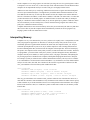
For example, say that you wanted to store customer information in memory. One way to do so would be
to set a maximum size for the customer’s name and address - say 50 characters for each, which would be
50 bytes for each. Then, after that, have a number for the customer’s age and their customer id. In this
case, you would have a block of memory that would look like this:
Start of Record:
Customer’s name (50 bytes) - start of record
Customer’s address (50 bytes) - start of record + 50 bytes
Customer’s age (1 word - 4 bytes) - start of record + 100 bytes
Customer’s id number (1 word - 4 bytes) - start of record + 104 bytes
This way, given the address of a customer record, you know where the rest of the data lies. However, it
does limit the customer’s name and address to only 50 characters each. What if we didn’t want to specify
a limit? Another way to do this would be to have in our record pointers to this information. For example,
instead of the customer’s name, we would have a pointer to their name. In this case, the memory would
look like this:
Start of Record:
Customer’s name pointer (1 word) - start of record
Customer’s address pointer (1 word) - start of record + 4
Customer’s age (1 word) - start of record + 8
6
Chapter 2. Computer Memory Organization
Customer’s id number (1 word) - start of record + 12
The actual name and address would be stored elsewhere in memory. This way, it is easy to tell where
each part of the data is from the start of the record, without explicitly limitting the size of the name and
address.
Data Accessing Methods
Processors have a number of different ways of accessing data, known as addressing modes. The simplest
mode is immediate mode, in which the data to access is embedded in the instruction itself. For example,
if we want to initialize a register to 0, instead of giving the computer an address to read the 0 from, we
would specify immediate mode, and give it the number 0.
In the direct addressing mode, the instruction contains the address to load the data from. For example, I
could say, please load this register with the data at address 2002. The computer would go directly to byte
number 2002, and copy the contents into our register.
In the indexed addressing mode, the instruction contains an address to load the data from, and also
specifies an index register to offset that address. For example, we could specify address 2002 and an
index register. If the index register contains the number 4, the actual address the data is loaded from
would be 2006. This way, if you have a set of numbers starting at location 2002, you can cycle between
each of them using an index register. On Intel machines, you can also specify a multiplier for the index.
Remember that you can access memory a byte at a time or a word at a time (4 bytes). If you are
accessing an entire word, your index will need to be multiplied by 4 to get the exact location of the fourth
element from your address. For example, if you wanted to access the fourth byte from location 2002, you
would load your index register with 3 (remember, we start counting at 0) and set the multiplier to 1 since
you are going a byte at a time. This would get you location 2005. However, if you wanted to access the
fourth word from location 2002, you would load your index register with 3 and set the multiplier to 4.
This would load from location 2014 - the fourth word.
In the indirect addressing mode, the instruction contains a register that contains a pointer to where the
data should be loaded from. For example, if we used indirect addressing mode and specified the %eax
register, and the %eax register contained the value 4, whatever value was at memory location 4 would be
used. In direct addressing, we would just load the value 4, but in indirect addressing, we use 4 as the
address to use to find the data we want.
Finally, there is the base-pointer addressing mode. This is similar to indirect addressing, but you also
include a number called the offset to add to the registers value before using it for lookup. In the Section
called Interpretting Memory we discussed having a structure in memory holding customer information.
Let’s say we wanted to access the customer’s age, which was the eighth byte of the data, and we had the
address of the start of the structure in a register. We could use base-pointer addressing and specify the
register as the base pointer, and 8 as our offset. This is a lot like indexed addressing, with the difference
that the offset is constant and the pointer is held in a register.
There are other forms of addressing, but these are the most important ones.
7
Chapter 2. Computer Memory Organization
8
Chapter 3. Your First Programs
In this chapter you will learn the process for writing and building Linux assembly-language programs. In
addition, you will learn the structure of assembly-language programs, and a few assembly-language
commands.
These programs may overwhelm you at first. However, go through them with diligence, read them and
their explanations as many times as necessary, and you will have a solid foundation of knowledge to
build on. Please tinker around with the programs as much as you can. Even if your tinkering does not
work, every failure will help you learn.
Entering in the Program
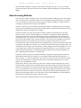
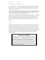
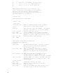
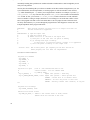
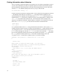
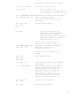
Okay, this first program is simple. In fact, it’s not going to do anything but exit! It’s short, but it shows
some basics about assembly language and Linux programming. You need to enter the program in an
editor exactly as written, with the filename exit.s. The program follows. Don’t worry about not
understanding it. This section only deals with typing it in and running it. The next section will describe
how it works.
#PURPOSE:
#
#
Simple program that exits and returns a
status code back to the Linux kernel
#INPUT:
#
none
#OUTPUT:
#
#
#
#
#
#
returns a status code.
by typing
This can be viewed
echo $?
after running the program
#VARIABLES:
#
%eax holds the system call number
#
(this is always the case)
#
#
%ebx holds the return status
#
.section .data
.section .text
.globl _start
_start:
movl $1, %eax
movl $0, %ebx
# this is the linux kernel command
# number (system call) for exiting
# a program
# this is the status number we will
9
Chapter 3. Your First Programs
#
#
#
#
int $0x80
return to the operating system.
Change this around and it will
return different things to
echo $?
# this wakes up the kernel to run
# the exit command
What you have typed in is called the source code. Source code is the human-readable form of a program.
In order to transform it into a program that a computer can run, we need to assemble and link it.
The first step is to assemble it. Assembling is the process that transforms what you typed into
instructions for the machine. The machine itself only reads sets of numbers, but humans prefer words.
An assembly language is a more human-readable form of the instructions a computer understands.
Assembling transforms the human-readable file into a machine-readable one. To assembly the program
type in the command
as exit.s -o exit.o
as is the command which runs the assembler, exit.s is the source file, and -o exit.o tells the
assemble to put it’s output in the file exit.o. exit.o is an object file. An object file is code that is in the
machine’s language, but has not been completely put together. In most large programs, you will have
several source files, and you will convert each one into an object file. The linker is the program that is
responsible for putting the object files together and adding information to it so that the kernel knows how
to load and run it. In our case, we only have one object file, so the linker is only adding the information
to enable it to run. To link the file, enter the command
ld exit.o -o exit
ld is the command to run the linker, exit.o is the object file we want to link, and -o exit instructs the
linker to output the new program into a file called exit. If any of these commands reported errors, you
have either mistyped your program or the command. After correcting the program, you have to re-run all
the commands. You must always re-assemble and re-link programs after you modify the source file for
the changes to occur in the program. You can run exit by typing in the command
./exit
The ./ is used to tell the computer that the program isn’t in one of the normal program directories, but is
the current directory instead1. You’ll notice when you type this command, the only thing that happens is
that you’ll go to the next line. That’s because this program does nothing but exit. However, immediately
after you run the program, if you type in
echo $?
It will say 0. What is happening is that every program when it exits gives Linux a result status code,
which tells it if everything went all right. If everything was okay, it returns 0. UNIX programs return
other numbers to indicate failure or other errors or warnings. The programmer determines what each
number means. Other numbers don’t have to indicate an error, but that is the typical behavior. You can
1.
10
. refers to the current directory in Linux and UNIX systems.
Chapter 3. Your First Programs
always view this code by typing in echo $?. In the following section we will look at what each part of the
code does.
Outline of an Assembly Language Program
Take a look at the program we just entered. At the beginning there are lots of lines that begin with hashes
(#). These are comments. Comments are not translated by the assembler. They are used only for the
programmer to talk to anyone who looks at the code in the future. Most programs you write will
generally be modified by others. Get into the habit of writing comments in your code that will help them
understand both why the program exists and how it works. Always include in your comments
•
The purpose of the code
•
An overview of the processing involved
•
Anything strange your program does and why it does it2
After the comments, the next line says
.section .data
Anything starting with a period isn’t directly translated into a machine instruction. Instead, it’s an
instruction to the assembler itself. The .section command breaks your program up into sections. This
command starts the data section, where you list any memory storage you will need for data. Our program
doesn’t use any, so we don’t need the section. It’s just here for completeness. Almost every program you
write will have data.
Right after this you have
.section .text
which starts the text section. The text section of a program is where the program instructions live.
The next instruction is
.globl _start
This instructs the assembler that _start is important to remember. _start is a symbol, which means
that it is going to be replaced by something else either during assembly or linking. Symbols are generally
used to mark locations of programs or data, so you can refer to them by name instead of by their location
number. Imagine if you had to refer to every memory location by it’s address. Every time you had to
insert a piece of data or code you would have to change all the addresses in your program! Symbols are
used so that the assembler and linker can take care of keeping track of addresses, and you can
concentrate on writing your program. .globl means that the assembler shouldn’t discard this symbol
after assembly, because the linker will need it. _start is a special symbol that always needs to be
2. You’ll find that many programs end up doing things strange ways. Usually there is a reason for that, but, unfortunately,
programmers never document such things in their comments. So, future programmers either have to learn the reason the hard way
by modifying the code and watching it break, or just leaving it alone whether it is still needed or not. You should always document
any strange behavior your program performs. Unfortunately, figuring out what is strange and what is straightforward comes mostly
with experience.
11
Chapter 3. Your First Programs
marked with .globl because it marks the location of the start of the program. Without marking this
location, when the computer loads your program it won’t know where to start.
The next line
_start:
defines the value of the _start label.
* FIXME - define a label. Maybe, a label is a symbol denoting it’s own place in the assembled file?
Previously, we just told the assembler that this symbol was special, and should be passed on to the linker.
Here, we have the definition of start. In assembly, if you have a symbol followed by a colon, it marks the
address of the next instruction or data item. From then on, any time you use that symbol, the assembler
or linker will replace it with the address it is referring to.
Now we get into actual commands. The first such instruction is
movl $1, %eax
When the program runs, this instruction transfers the number 1 into the %eax register. On IA32
machines, there are several general-purpose registers:
• %eax
• %ebx
• %ecx
• %edx
In addition to these general-purpose registers, there are also several special-purpose registers, including
• %edi
• %ebp
• %esp
• %eip
We’ll discuss these later, just be aware that they exist.3
So, the movl instruction moves the number 1 into %eax. The dollar-sign in front of the one indicates that
we want to use immediate mode addressing (see ). Without the dollar-sign it would do direct addressing,
loading whatever number is at address 1. We want the actual number 1 loaded in, so we have to use
immediate mode.
This instruction is preparing for when we call the Linux kernel. The number 1 is the number of the exit
system call.
* FIXME - do I need to describe system calls more?
When you make a system call, which we will do shortly, the system call number has to be loaded into
%eax and the other values needed for the call are stored in other registers. The exit system call also
3. You may be wondering, why do all of these registers begin with the letter e? The reason is that a long time ago, the registers
were only half the length they are now. When Intel doubled the size of the registers, they kept the old names to refer to the first half
of the register, and added an e to refer to the extended versions of the register. Usually you will only use the extended versions.
12
Chapter 3. Your First Programs
requires a status code be loaded in %ebx when it is called so it can return it to the system (this is what is
retrieved when you type echo $?. So, we load %ebx with 0 by typing
movl $0, %ebx
a
Now, loading registers with these numbers doesn’t do anything itself. This is simply how Linux expects
things to be set up when you make a system call. During normal programming, you can use registers to
hold any value that you are currently working with. However, when you make a system call, you have to
have the registers set up as the system call expects. You can find out how each system call expects to be
set up at .
The next instruction is the "magic" one. It looks like this:
int $0x80
The int stands for interrupt. The 0x80 is the interrupt number to use.4 An interrupt interrupts the
normal program flow, and transfers control from our program to Linux 5. You can think of it as like
signaling Batman(or Larry-Boy6, if you prefer). You need something done, you send the signal, and then
he comes to the rescue. You don’t care how he does his work - it’s more or less magic - and when he’s
done you’re back in control. In this case, all we’re doing is asking Linux to terminate the program, in
which case we won’t be back in control.
* FIXME - I added some info on syscalls earlier, what do I need to trim out?
How are we asking this? Simple - Linux has a number of features called system calls. These are referred
to by placing the number of the function you wish to use in %eax, and storing other information you
want to pass in other registers. Then, we invoke the system call by issuing int $0x80. Each system call
has a list of registers it uses. System call #1 is the exit system call, and it takes one parameter in %ebx,
which is the exit status of the program. 7
Now that you’ve assembled, linked, run, and examined the program, you should make some basic edits.
Do things like change the number that is loaded into %ebx, and watch it come out at the end with echo
$?. Don’t forget to assemble and link it again before running it. Add some comments. The worse thing
that would happen is that the program won’t assemble or link, or will freeze your screen. And that’s all
part of learning!
A Program that Does Something
* Need to introduce the idea of flow-control. Assembly language only has really basic flow-control statements, but need to talk
about it for a background for the other languages chapter.
4. You may be wondering why it’s 0x80 instead of just 80. The reason is that the number is written in hexadecimal. In hexadecimal, a single digit can hold 16 values instead of the normal 10. This is done by utilizing the letters a through f in addition to the
regular digits. a represents 10, b represents 11, and so on. 0x10 represents the number 16, and so on. This will be discussed more
in depth later, but just be aware that numbers starting with 0x are in hexadecimal. Tacking on an H at the end is also sometimes
used, but we won’t do that here. * FIXME - change to an XREF to the numbers chapter?
5. Actually, the interrupt transfers control to whoever set up an interrupt handler for the interrupt number. In the case of Linux,
all of them are set to be handled by the Linux kernel.
6. If you don’t watch Veggie Tales, you should.
7. The exit status is usually 0 if everything went well, otherwise, its a program-specific code. After running a command, you can
check it’s exit status by typing in echo $?.
13
Chapter 3. Your First Programs
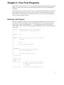
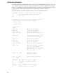
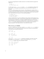
Don’t let the title of this section confuse you. We still aren’t doing anything useful. But we will be doing
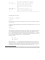
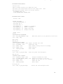
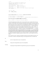
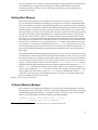
more than simply exiting here. Enter the following program as maximum.s
#PURPOSE:
#
#
This program finds the maximum number of a
set of data items.
#VARIABLES: The registers have the following uses:
#
# %edi - Holds the index of the data item being examined
# %ebx - Largest data item found
# %eax - Current data item
#
# The following memory locations are used:
#
# data_items - contains the item data. A 0 is used
#
to terminate the data
#
.section .data
data_items:
#These are the data items
.long 3,67,34,222,45,75,54,34,44,33,22,11,66,0
.section .text
.globl _start
_start:
movl $0, %edi
# move 0 into the index register
movl data_items(,%edi,4), %eax # load the first byte of data
movl %eax, %ebx
# since this is the first item, %eax is
# the biggest
start_loop:
cmpl $0, %eax
je loop_exit
incl %edi
movl data_items(,%edi,4),
cmpl %ebx, %eax
jle start_loop
movl %eax, %ebx
jmp start_loop
# start loop
# check to see if we’ve hit the end
# load next value
%eax
# compare values
# jump to loop beginning if the new
# one isn’t bigger
# move the value as the largest
# jump to loop beginning
loop_exit:
# %ebx is the return value, and it already has the number
movl $1, %eax
#1 is the exit() syscall
int $0x80
Now, assemble and link it with the commands
14
Chapter 3. Your First Programs
as maximum.s -o maximum.o
ld maximum.o -o maximum
Now run it, and check it’s status
./maximum
echo $?
You’ll notice it returns the value 222. Let’s take a look at the program and what it does. If you look in the
comments, you’ll see that the program finds the maximum of a set of numbers (aren’t comments
wonderful!). You may notice, however, that we actually have something in the data section. These lines
are the data section:
data_items:
#These are the data items
.long 3,67,34,222,45,75,54,34,44,33,22,11,66,0
So, lets look at this. data_items is a label that refers to the location that follows it. Then, there is a
directive that starts with .long. That causes the assembler to reserve memory for the list of numbers that
follow it. data_items refers to the location of the first one. There are several different types of memory
locations other than .long that can be reserved. They are as follows:
.byte
Bytes take up one storage location for each number. They are limited to numbers between 0 and
255.
.int
Ints (which differ from the int instruction) take up two storage locations for each number. These
are limitted to numbers between 0 and 65535.8
.long
Longs take up four storage locations. This is the same amount of space the registers use, which is
why they are used in this program. They can hold numbers between 0 and 4294967295.
.ascii
The .ascii directive is to enter in characters into memory. Characters each take up one storage
location (they are converted into bytes internally). So, if you gave the directive .ascii "Hello
there\0", you would reserve 12 storage locations (bytes). The first byte contains the numeric code
for H, the second byte contains the numeric code for e, and so forth. The last character is
represented by \0, and it is the terminating character (it will never display, it just tells other parts of
the program that that’s the end of the characters). All of the letters are in quotes.
There are more, but these are the important ones for now. So the assembler reserves 14 .longs, one right
after another. So, since each long takes up 4 bytes, that means that the whole list takes up 56 bytes. Also,
8. Note that no numbers in assembly language (or any other computer language I’ve seen) have commas embedded in them. So,
always write numbers like 65535, and never like 65,535.
15
Chapter 3. Your First Programs
remember that data_items will contain the location number of the first item in the list. 9 These are the
numbers we will be searching through to find the maximum. Note that the last one is a zero. I decided to
use a zero to tell my program that we’ve hit the end of the list. I could have done this other ways. I could
have had the size of the list hard-coded into the program. Also, I could have put the length of the list as
the first item, or in a separate location. I also could have made a symbol which marked the last location
of the list items. No matter how I do it, I must have some method of determining the end of the list. The
computer knows nothing - it can only do what its told. It’s not going to stop processing unless I give it
some sort of signal. Otherwise it would continue processing past the end of the list into the data that
follows it, and even to locations where we haven’t put any data. Also, notice that we don’t have a
.globl declaration for data_items. This is because we only refer to these locations within the
program. No other file or program needs to know where they are located. This is in contrast to the
_start symbol, which Linux needs to know where it is so that it knows where to begin the program’s
execution. It’s not an error to write .globl data_items, it’s just not necessary. Anyway, play around
with this line and add your own numbers. Even though they are .long, the program will produce strange
results if any number is greater than 255, because that’s the largest allowed exit status. Also notice that if
you move the 0 to earlier in the list, the rest get ignored. Remember that any time you change the source
file, you have to re-assemble and re-link your program. Do this now and see the results.
All right, we’ve played with the data a little bit. Now let’s look at the code. In the comments you will
notice that we’ve marked some variables that we plan to use. A variable is a storage location used for a
specific purpose. We have a variable for the current maximum number found, one for which number of
the list we are currently examining (called the index), and one holding the current number being
examined. In this case, we have few enough variables that we can hold them all in registers. In larger
programs, you have to put them in memory, and then move them to registers when you are ready to use
them. Anyway, we are using %ebx as the location of the largest item we’ve found. %edi is used as the
index to the current data item we’re looking at. Now, let’s talk about what an index is. When we read the
information from data_items, we will start with the first one (data item number 0), then go to the
second one (data item number 1), then the third (data item number 2), and so on. The data item number is
the index of data_items. You’ll notice that the first instruction we give to the computer is
movl $0, %edi
Since we are using %edi as our index, and we want to start looking at the first item, we load %edi with
0. Now, the next instruction is tricky, but crucial to what we’re doing. It says
movl data_items(,%edi,4), %eax
Now to understand this line, you need to keep several things in mind:
9.
•
data_items is the location number of the start of our number list.
•
Each number is stored across 4 storage locations (because we declared it using .long)
•
%edi is holding 0 at this point
Although it is possible to compute by hand what this location will be, it is easiest to just have the assembler remember that
data_items refers to it, and have the assembler fill in the blanks when it runs. Also, just so you’ll know, the location number of
the first item isn’t 0, it’s much higher. We’ll look into that further in the next chapter. Anyway, since we have the data_items
symbol, it doesn’t matter because the assembler will put in the correct value for us.
16
Chapter 3. Your First Programs
So, basically what this line does is say, "start at the beginning of data_items, and take the first item
number (because %edi is 0), and remember that each number takes up four storage locations." Then it
stores that number in %eax. So, the number 3 is now in %eax. If %edi was set to 1, the number 67 would
be in %eax, and if it was set to 2, the number 34 would be in %eax, and so forth. Very strange things
would happen if we used a number other than 4 as the size of our storage locations. 10 The way you write
this is very awkward, but if you know what each piece does, it’s not too difficult.
Let’s look at the next line.
movl %eax, %ebx
We have the first item to look at stored in %eax. Since it is the first item, we know it’s the biggest one
we’ve looked at. We store it in %ebx, since that’s where we are keeping the largest number found. Also,
even though movl stands for move, it actually copies the value, so %eax and %ebx both contain the
starting value.11
Now we move into a loop. A loop is a segment of your program that might run more than once. We have
marked the starting location of the loop in the symbol start_loop. The reason we are doing a loop is
because we don’t know how many data items we have to process, but the procedure will be the same no
matter how many there are. So, before looking at the code, let’s think about what our loop will have to
do.12 It will have to:
•
check to see if the current value being looked at is zero. If so, that means we are at the end of our data
and should exit the loop.
•
We have to load the next value of our list
•
We have to see if the next value is bigger than our current biggest value.
•
If it is, we have to copy it to the location we are holding the largest value in
•
Now we need to go back to the beginning of the loop
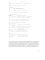
Okay, so now lets go to the code. We have the beginning of the loop marked with start_loop. That is
so we know where to go back to at the end of our loop. Then we have the instructions
cmpl $0, %eax
je end_loop
The cmpl instruction compares the two values. Here, we are comparing the number 0 to the number
stored in %eax. This compare instruction also affects a register not mentioned here, the %eflags. This is
also known as the status register, and has many uses which we will discuss later. Just be aware that the
result of the comparison is stored in the status register. The next line says to jump to the end_loop
location if the values that were just compared are equal (it uses the status register to find this
information). There are several jump statements we have to choose from:
10. 4 isn’t really the size of the storage locations, although looking at it that way works for our purposes now. It’s actually
what’s called a multiplier. basically, the way it works is that you start at the location specified by data_items, then you add
%edi*4 storage locations, and retrieve the number there. Usually, you use the size of the numbers as your multiplier, but in some
circumstances you’ll want to do other things.
11. Also, the l in movl stands for move long since we are moving a value that takes up four storage locations.
12. Keep in mind that upon entering the loop, we have already loaded the first data item and stored it as the maximum
17
Chapter 3. Your First Programs
je
Jump if the values were equal
jg
Jump if the second value was greater than the first value13
jge
Jump if the second value was greater than or equal to the first value
jl
Jump if the second value was less than the first value
jle
Jump if the second value was less than or equal to the first value
jmp
Jump no matter what. This does not need to be preceeded by a comparison. 14
In this case, we are jumping if %eax holds the value of zero. If so we are done, and we go to
loop_exit.15
If the last loaded element was not zero, we go on to the next instructions, which are
incl %edi
movl data_items(,%edi,4), %eax
If you remember from our previous discussion, %edi contains the index to our list of values in
data_items (if you don’t remember you should go back and read that section). incl increments the
value of %edi by one. Then the movl is just like the one before, except it’s getting the next item, since
we incremented %edi. Now, %eax has the next value to be tested. So, let’s test it!
cmpl %ebx, %eax
jle start_loop
So, here we compare our current value, stored in %eax to our biggest value so far, stored in %ebx. If the
current value is less or equal to our biggest value so far, we don’t care about it, so we just jump back to
the beginning of the loop. Otherwise, we need to record that value as the largest one, so we have the
instructions
movl %eax, %ebx
jmp start_loop
13. notice that the comparison is to see if the second value is greater than the first. I would have thought it the other way around.
You will find a lot of things like this when learning programming. It occurs because different things make sense to different people.
Anyway, you’ll just have to memorize such things and go on.
14. Actually, the others don’t either. You just have to know which instructions alter the status register and how they modify it.
We’ll get to that later.
15. The names of these symbols can be anything you want them to be, as long as they only contain letters and the underscore
character(_). The only one that is forced is _start, and possibly others that you declare with .globl. However, if its a symbol
you define and only you use, feel free to call it anything you want that is adequately descriptive (remember that others will have to
modify your code later)..
18
Chapter 3. Your First Programs
which moves the current value into %ebx and starts the loop over again.
Okay, so the loop executes until it reaches a 0, when it jumps to loop_exit. This part of the program
calls the Linux kernel to exit. If you remember from the last program, when you call the kernel
(remember it’s like signaling Batman), you store the system call number in %eax (1 for the exit call), and
store the other values in the other registers. The exit call requires that we put our exit status in %ebx. We
already have the exit status there since we are using %ebx as our largest number, so all we have to do is
load %eax with the number one and call the kernel to exit. Like this:
movl $1, %eax
int 0x80
Okay, that was a lot of work and explanation, especially for such a small program. But hey, you’re
learning a lot! Now, read through the whole program again, paying special attention to the comments.
Make sure that you understand what is going on at each line. If you don’t understand a line, go back
through this section and figure out what the line means. You might also grab a piece of paper, and go
through the program step-by-step, recording every change to every register, so you can see more clearly
what is going on. As an exercise, you should modify the program so that it finds the smallest value, and
uses the number 255 to end the program (otherwise it would always find 0 as the smallest value). Enjoy!
If you can do all that, you deserve a to have a coffee break.
Projects
•
Modify the first program to return the value 3.
•
Modify the first program to leave off the int instruction line. Assemble, link, and execute the new
program. What error message do you get. Why do you think this might be?
•
Modify the maximum program to find the minimum instead.
•
Modify the maximum program to use an ending address rather than the number 0 to know when to stop.
•
Modify the maximum program to use a length count rather than the number 0 to know when to stop.
•
Which approach would you use (the number 0, and ending address, or a length count) if you knew that
the list was sorted? Why?
19
Chapter 3. Your First Programs
20
Chapter 4. All About Functions
* I also need to talk about true functions versus subprograms/subroutines/procedures and stateless behavior
Dealing with Complexity
In Chapter 3, the programs we wrote only consisted of one section of code. However, if we wrote real
programs like that, it would be impossible to maintain them. It would be really difficult to get multiple
people working on the project, as any change in one part might adversely affect another part that another
developer is working on.
To assist programmers in working together in groups, it is necessary to break programs apart into
separate pieces, which communicate with each other through well-defined interfaces. This way, each
piece can be developed and tested independently of the others, making it easier for multiple
programmers to work on the project.
Programmers use functions to break their programs into pieces which can be independently developed
and tested. Functions are units of code that do a defined piece of work on specified types of data. For
example, in a word processor programmer, I may have a function called handle_typed_character
which is activated whenever a user types in a key. The data the function uses would probably be the
keypress itself and the document the user currently has open. The function would then modify the
document according to the keypress it was told about.
The data items a function is given to process are called it’s parameters. In the word processing example,
the key which was pressed and the document would be considered parameters to the
handle_typed_characters function. Much care goes into determining what parameters a function
takes, because if it is called from many places within a project, it is difficult to change if necessary.
A typical program is composed of thousands of functions, each with a small, well-defined task to
perform. However, ultimately there are things that you cannot write functions for which must be
provided by the system. Those are called primitive functions - they are the basics which everything else
is built off of. For example, imagine a program that draws a graphical user interface. There has to be a
function to create the menus. That function probably calls other functions to write text, to write icons, to
paint the background, calculate where the mouse pointer is, etc. However, ultimately, they will reach a
set of primitives provided by the operating system to do basic line or point drawing. Programming can
either be viewed as breaking a large program down into smaller pieces until you get to the primitive
functions, or building functions on top of primitives until you get the large picture in focus.
How Functions Work
Functions are composed of several different pieces:
function name
A function’s name is a symbol that represents the address where the function’s code starts. In
assembly language, the symbol is defined by typing the the function’s name followed by a colon
immediately before the function’s code. This is just like labels you have used for jumping.
21
Chapter 4. All About Functions
function parameters
A function’s parameters are the data items that are explicitly given to the function for processing.
For example, in mathematics, there is a sine function. If you were to ask a computer to find the sine
of 2, sine would be the function’s name, and 2 would be the parameter. Some functions have many
parameters, others have none. Function parameters can also be used to hold data that the function
wants to send back to the program.
local variables
Local variables are data storage that a function uses while processing that is thrown away it returns.
It’s kind of like a scratch pad of paper. You get a new piece of paper every time the function is
activated, and you have to throw it away when you are finished processing. Local variables of a
function are not accessible to any other function within a program.
static variables
Static variables are data storage that a function uses while processing that is not thrown away
afterwards, but is reused for every time the function’s code is activated. This data is not accessible
to any other part of the program. Static variables should not be used unless absolutely necessary, as
they can cause problems later on.
global variables
Global variables are data storage that a function uses for processing which are managed outside the
function. For example, a simple text editor may put the entire contents of the file it is working on in
a global variable so it doesn’t have to be passed to every function that operates on it. 1 Configuration
values are also often stored in global variables.
return address
The return address is an "invisible" parameter in that it isn’t directly used during the function, but
instead is used to find where the processor should start executing after the function is finished. This
is needed because functions can be called to do processing from many different parts of your
program, and the function needs to be able to get back to wherever it was called from. In most
languages, this parameter is passed automatically when the function is called.
return value
The return value is the main method of transferring data back to the main program. Most languages
only allow a single return value for a function, although some allow multiple.
These pieces are present in most programming languages. How you specify each piece is different in
each one, however.
The way that the variables are stored and the parameters and return values are transferred by the
computer varies from language to language as well. This variance is known as a language’s calling
convention, because it describes how functions expect to get and receive data when they are called. 2
1. This is generally considered bad practice. Imagine if a program is written this way, and in the next version they decided to
allow a single instance of the program edit multiple files. Each function would then have to be modified so that the file that was
being manipulated would be passed as a parameter. If you had simply passed it as a parameter to begin with, most of your functions
could have survived your upgrade unchanged.
2. A convention is a way of doing things that is standardized, but not forcibly so. For example, it is a convention for people
to shake hands when they meet. If I refuse to shake hands with you, you may think I don’t like you. Following conventions is
22
Chapter 4. All About Functions
Assembly language can use any calling convention it wants to. You can even make one up yourself.
However, if you want to interoperate with functions written in other languages, you have to obey their
calling conventions. We will use the calling convention of the C programming language because it is the
most widely used for our examples, and then show you some other possibilities.
Assembly-Language Functions using the C Calling Convention
You cannot write assembly-language functions without understanding how the computer’s stack works.
Each computer program that runs uses a region of memory called the stack to enable functions to work
properly. Think of a stack as a pile of papers on your desk which can be added to indefinitely. You
generally keep the things that you are working on toward the top, and you take things off as you are
finished working with them.
Your computer has a stack, too. The computer’s stack lives at the very top addresses of memory. You can
push values onto the top of the stack through an instruction called pushl, which pushes either a register
or value onto the top of the stack. Well, we say it’s the top, but the "top" of the stack is actually the
bottom of the stack’s memory. Although this is confusing, the reason for it is that when we think of a
stack of anything - dishes, papers, etc. - we think of adding and removing to the top of it. However, in
memory the stack starts at the top of memory and grows downward due to other architectural
considerations. Therefore, when we refer to the "top of the stack" remember it’s at the bottom of the
stack’s memory. When we are referring to the top or bottom of memory, we will specifically say so. You
can also pop values off the top using an instruction called popl.
When we push a value onto the stack, the top of the stack moves to accomodate the addition value. We
can actually continually push values onto the stack and it will keep growing further and further down in
memory until we hit our code or data. So how do we know where the current "top" of the stack is? The
stack register, %esp, always contains a pointer to the current top of the stack, wherever it is.
Every time we push something onto the stack with pushl, %esp gets subtracted by 4 so that it points to
the new top of the stack (remember, each word is four bytes long, and the stack grows downward). If we
want to remove something from the stack, we simply use the popl instruction, which adds 4 to %esp and
puts the previous top value in whatever register you specified. pushl and popl each take one operand the register to push onto the stack for pushl, or receive the data that is popped off the stack for popl.
If we simply want to access the value on the top of the stack, we can simply use the %esp register. For
example, the following code moves whatever is at the top of the stack into %eax:
movl (%esp), %eax
If we were to just do
movl %esp, %eax
%eax would just hold the pointer to the top of the stack rather than the value at the top. Putting %esp in
parenthesis causes the computer to go to indirect addressing mode , and therefore we get the value
pointed to by %esp. If we want to access the value right below the top of the stack, we can simply do
movl 4(%esp), %eax
important because it makes it easier for others to understand what you are doing.
23
Chapter 4. All About Functions
This uses the base pointer addressing mode which simply adds 4 to %esp before looking up the value
being pointed to.
* Does this need an xref to dataaccessingmethods?
In the C language calling convention, the stack is the key element for implementing a function’s local
variables, parameters, and return address.
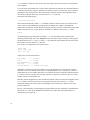
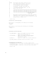
Before executing a function, a program pushes all of the parameters for the function onto the stack in the
reverse order that they are documented. Then the program issues a call instruction indicating which
function it wishes to start. The call instruction does two things. First it pushes the address of the next
instruction, which is the return address, onto the stack. Then it modifies the instruction pointer to point to
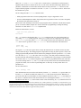
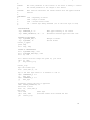
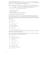
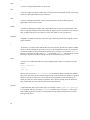
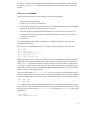
the start of the function. So, at the time the function starts, the stack looks like this:
Parameter #N
...
Parameter 2
Parameter 1
Return Address <--- (%esp)
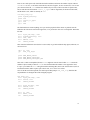
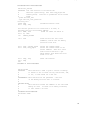
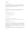
Now the function itself has some work to do. The first thing it does is save the current base pointer
register, %ebp, by doing pushl %ebp. The base pointer is a special register used for accessing function
parameters and local variables. Next, it copies the stack pointer to %ebp by doing movl %esp, %ebp.
This allows you to be able to access the function parameters as fixed indexes from the base pointer. You
may think that you can use the stack pointer for this. However, during your program you may do other
things with the stack such as pushing arguments to other functions. Copying the stack pointer into the
base pointer at the beginning of a function allows you to always know where in the stack your parameters
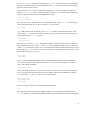
are (and as we will see, local variables too). So, at this point, the stack looks like this:
Parameter #N
...
Parameter 2
Parameter 1
Return Address
Old %ebp
<--- N*4+4(%ebp)
<--<--<--<---
12(%ebp)
8(%ebp)
4(%ebp)
(%esp) and (%ebp)
This also shows how to access each parameter the function has.
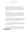
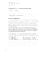
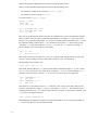
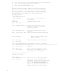
Next, the function reserves space on the stack for any local variables it needs. This is done by simply
moving the stack pointer out of the way. Let’s say that we are going to need 2 words of memory to run a
function. We can simply move the stack pointer down 2 words to reserve the space. This is done like this:
subl $8, %esp
This subtracts 8 from %esp (remember, a word is four bytes long).3 So now, we have 2 words for local
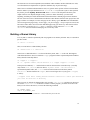
storage. Our stack now looks like this:
Parameter #N
...
Parameter 2
Parameter 1
<--- N*4+4(%ebp)
<--- 12(%ebp)
<--- 8(%ebp)
3. Just a reminder - the dollar sign in front of the eight indicates immediate mode addressing, meaning that we load the number
8 into %esp rather than the value at address 8.
24
Chapter 4. All About Functions
Return Address
<--Old %ebp
<--Local Variable 1 <--Local Variable 2 <---
4(%ebp)
(%ebp)
-4(%ebp)
-8(%ebp) and (%esp)
So we can now access all of the data we need for this function by using base pointer addressing using
different offsets from %ebp %ebp was made specifically for this purpose, which is why it is called the
base pointer. You can use other registers for base pointer addressing, but the x86 architecture makes
using the %ebp register a lot faster.
Global variables and static variables are accessed just like we have been accessing memory in previous
chapters. The only difference between the global and static variables is that static variables are only used
by the function, while global variables are used by many functions. Assembly language treats them
exactly the same, although most other languages distinguish them.
When a function is done executing, it does two things. First, it stores it’s return value in %eax. Second, it
returns control back to wherever it was called from. Returning control is done using the ret instruction,
which pops whatever value is at the top of the stack, and sets the instruction pointer to that value.
However, in our program right now, the top of the stack isn’t pointing to the return address. Therefore,
we have to restore the stack pointer to what it was. So to terminate the program, you have to do the
following:
movl %ebp, %esp
popl %ebp
ret
This restores the %ebp register and moves the stack pointer back to pointing at the return address. At this
point, you should consider all local variables to be disposed of. The reason is that after you move the
stack pointer, future stack operations will overwrite everything you put there. Therefore, you should
never save the address of a local variable past the life of the function it was created in, or else it will be
overwritten on future pushes. Control is now handed back to the calling program or function, which can
then examine %eax for the return value. The calling program also needs to pop off all of the parameters it
pushed onto the stack in order to get the stack pointer back where it was (you can also simply add
4*number of paramters to %esp using the addl instruction, if you don’t need the values of the
parameters anymore).
Destruction of Registers
When you call a function, you should assume that everything currently in your
registers will be wiped out. The only register that is guaranteed to be left with the
value it started with is %ebp. %eax is guaranteed to be overwritten, and the others
likely are. If there are registers you want to save before calling a function, you need
to save them by pushing them on the stack before pushing the function’s
paramters. You can then pop them back off in reverse order after popping off the
parameters. Even if you know a function does not overwrite a register you should
save it, because future versions of that function may. Other calling conventions
may be different. For example, other calling conventions may place the burden on
the function to save any registers it uses.
25
Chapter 4. All About Functions
A Function Example
Let’s take a look at how a function call works in a real program. The function we are going to write is the
power function. We will give the power function two parameters - the number and the power we want to
raise it to. For example, if we gave it the paramters 2 and 3, it would raise 2 to the power of 3, or 2*2*2,
giving 8. In order to make this program simple, we will only allow numbers 1 and greater.
The following is the code for the complete program. As usual, an explanation follows:
#PURPOSE:
#
#
#
Program to illustrate how functions work
This program will compute the value of
2^3 + 5^2
#Everything in the main program is stored in registers,
#so the data section doesn’t have anything.
.section .data
.section .text
.globl _start
_start:
pushl $3
pushl $2
call power
addl $8, %esp
second argument
first argument
the function
the stack pointer back
pushl %eax
#save the first answer before
#calling the next function
pushl
pushl
call
addl
$2
$5
power
$8, %esp
#push
#push
#call
#move
popl
%ebx
#The second answer is already
#in %eax. We saved the
#first answer onto the stack,
#so now we can just pop it
#out into %ebx
addl
%eax, %ebx
#add them together
#result in %ebx
movl
int
$1, %eax
$0x80
#exit (%ebx is returned)
#PURPOSE:
#
#
#
#INPUT:
#
26
#push
#push
#call
#move
second argument
first argument
the function
the stack pointer back
This function is used to compute
the value of a number raised to
a power.
First argument - the base number
Second argument - the power to
Chapter 4. All About Functions
#
raise it to
#
#OUTPUT:
Will give the result as a return value
#
#NOTES:
The power must be 1 or greater
#
#VARIABLES:
#
%ebx - holds the base number
#
%ecx - holds the power
#
#
-4(%ebp) - holds the current result
#
#
%eax is used for temporary storage
#
.type power, @function
power:
pushl %ebp
#save old base pointer
movl %esp, %ebp
#make stack pointer the base pointer
subl $4, %esp
#get room for our local storage
movl
movl
8(%ebp), %ebx #put first argument in %eax
12(%ebp), %ecx #put second argument in %ecx
movl
%ebx, -4(%ebp) #store current result
power_loop_start:
cmpl $1, %ecx
#if the power is 1, we are done
je
end_power
movl -4(%ebp), %eax #move the current result into %eax
imul %ebx, %eax
#multiply the current result by
#the base number
movl %eax, -4(%ebp) #store the current result
decl
jmp
%ecx
#decrease the power
power_loop_start #run for the next power
end_power:
movl -4(%ebp), %eax
movl %ebp, %esp
popl %ebp
ret
#return value goes in %eax
#restore the stack pointer
#restore the base pointer
Type in the program, assemble it, and run it. Try calling power for different values, but remember that the
result has to be less than 256 when it is passed back to the operating system. Also try subtracting the
results of the two computations. Try adding a third call to the power function, and add it’s result back in.
The main program code is pretty simple. You push the arguments onto the stack, call the function, and
then move the stack pointer back. The result is stored in %eax. Note that between the two calls to power,
we save the first value onto the stack. This is because the only register that is guaranteed to be saved is
27
Chapter 4. All About Functions
%ebp. Therefore we push the value onto the stack, and pop the value back off after the second function
call is complete.
Let’s look at how the function itself is written. Notice that before the function, there is documentation as
to what the function does, what it’s arguments are, and what it gives as a return value. This is useful for
programmers who use this function. This is the function’s interface. This let’s the programmer know
what values are needed on the stack, and what will be in %eax at the end.
We then have the following line:
.type power,@function
This tells the linker that the symbol power should be treated as a function. This isn’t useful now, but it
will be when you start building larger programs that run multiple files. Chapter 7 has additional
information on what this is used for. Because this program is only in one file, it would work just the same
with this left out. However, it is good practice. After that, we define the value of the power label:
power:
As mentioned previously, this defines the symbol power to be the address where the instructions
following the label begin. This is how call power works. It transfers control to this spot of the program.
The difference between call and jmp is that call also pushes the return address onto the stack so that
the function can return, while the jmp does not.
Next, we have our instructions to set up our function:
pushl %ebp
movl %esp, %ebp
subl $4, %esp
At this point, our stack looks like this:
Base Number
Power
Return Address
Old %ebp
Current result
<--<--<--<--<---
12(%ebp)
8(%ebp)
4(%ebp)
(%ebp)
-4(%ebp) and (%esp)
Although we could use a register for temporary storage, this program uses a local variable in order to
show how to set it up. Often times there just aren’t enough registers to store everything, so you have to
offload them into a local variable. Other times, your function will need to call another function and send
it a pointer to some of your data. You can’t have a pointer to a register, so you have to store it in a local
variable in order to send a pointer to it.
Basically, what the program does is start with the base number, and store it both as the multiplier (stored
in %ebx) and the current value (stored in -4(%ebp)). It also has the power stored in %ecx It then
continually multiplies the current value by the multiplier, decreases the power, and leaves the loop if
power gets down to 1.
By now, you should be able to go through the program without help. The only things you should need to
know is that imul does integer multiplication and stores the result in the second operand, and decl
decreases the given register by 1.
28
Chapter 4. All About Functions
* Need to have defined operand a long time before now. Need to differentiate operands and parameters by the fact that operands are
for instructions and parameters are for functions. Also need to have a list of important definitions at the end of each chapter or
something.
A good project to try now is to extend the program so it will return the value of a number if the power is
0 (hint, the anything raised to the zero power is 1). Keep trying. If it doesn’t work at first, try going
through your program by hand with a scrap of paper, keeping track of where %ebp and %esp are
pointing, what is on the stack, and the values in each register.
Recursive Functions
* This next part was just cut out from the previous section. I decided it was too much without a formal introduction to functions.
Anyway, it needs to be molded to fit this chapter.
The next program will stretch your brains even more. The program will compute the factorial of a
number. A factorial is the product of a number and all the numbers between it and one. For example, the
factorial of 7 is 7*6*5*4*3*2*1, and the factorial of 4 is 4*3*2*1. Now, one thing you might notice is
that the factorial of a number is the same as the product of a number and the factorial just below it. For
example, the factorial of 4 is 4 times the factorial of 3. The factorial of 3 is 3 times the factorial of 2. 2 is
2 times the factorial of 1. The factorial of 1 is 1. This type of definition is called a recursive definition.
That means, the definition of the factorial function includes the factorial funtion. However, since all
functions need to end, a recursive definition must include a base case. The base case is the point where
recursion will stop. Without a base case, the function would go on forever. In the case of the factorial, it
is the number 1. When we hit the number 1, we don’t run the factorial again, we just say that the factorial
of 1 is 1. So, let’s run through what we want the code to look like for our factorial function: 4
1. Examine the number
2. Is the number 1?
3. If so, the answer is one
4. Otherwise, the answer is the number times the factorial of the number minus one
This presents a problem. Previously, we named our storage locations in memory where we held the
values we were working on (data_items in the first example). This program, however, will call itself
before it is finished. Therefore, if we store our data in a register or fixed location in memory, it will be
overwritten when we call the function from itself. When the second function returns, all of our data will
be overwritten with the data from the call that just returned. To get around this, we use a section of
memory called the stack. The stack is like a stack of dishes. You put one dish at a time on top, and then
you take the dishes off in the reverse order (the last dish you put on the stack becomes the first dish you
take off). In your computer, there is a stack of data, that you can put stuff on the top and take stuff off the
top. The way this helps us with functions, is that whenever we call a function, we can put the stuff we’re
working with on the stack, call the function, and then afterwards take it back off. We just have to be sure
that we take off everything we put on, or the functions that calls us will be confused, because then they
won’t know where on the stack their stuff is. We would be leaving our dishes on top instead of cleaning
up after ourselves. Confused yet? Let’s take a look at some real code to see how this works.
#PURPOSE - Given a number, this program computes the
4.
This is a function, not a program, because it is called more than once (specifically, its called from itself) * FIXME - needs more
explanation
29
Chapter 4. All About Functions
#
#
#
#
factorial. For example, the factorial of
3 is 3 * 2 * 1, or 6. The factorial of
4 is 4 * 3 * 2 * 1, or 24, and so on.
#This program shows how to call a function. You
#call a function by first pushing all the arguments,
#then you call the function, and the resulting
#value is in %eax. The program can also change the
#passed parameters if it wants to.
.section .data
#This program has no global data
.section .text
.globl _start
.globl factorial
_start:
pushl $4
call
popl
movl
factorial
%ebx
%eax, %ebx
movl
int
$1, %eax
$0x80
#this is unneeded unless we want to share
#this function among other programs
#The factorial takes one argument - the number
#we want a factorial of. So, it gets pushed
#run the factorial function
#always remember to pop anything you pushed
#factorial returns the answer in %eax, but we
#want it in %ebx to send it as our exit status
#call the kernel’s exit function
#This is the actual function definition
.type factorial,@function
factorial:
pushl %ebp
#standard function stuff - we have to restore
#ebp to its prior state before returning,
#so we have to push it
movl %esp, %ebp
#This is because we don’t want to modify
#the stack pointer, so we use %ebp instead.
#This is also because %ebp is more flexible
movl
8(%ebp), %eax #This moves the first argument into %eax
#4(%ebp) holds the return address, and
#8(%ebp) holds the address of the first parameter
cmpl $1, %eax
#If the number is 1, that is our base case, and
#we simply return (1 is already in %eax as the
#return value)
je end_factorial
decl %eax
#otherwise, decrease the value
pushl %eax
#push it for our next call to factorial
call factorial
#call factorial
popl %ebx
#this is the number we called factorial with
#we have to pop it off, but we also need
30
Chapter 4. All About Functions
incl
imul
%ebx
%ebx, %eax
end_factorial:
movl %ebp, %esp
popl %ebp
ret
#it to find the number we were called with
#(which is one more than what we pushed)
#multiply that by the result of the last
#call to factorial (stored in %eax)
#the answer is stored in %eax, which is
#good since that’s where return values
#go.
#standard function return stuff - we
#have to restore %ebp and %esp to where
#they were before the function started
#return to the function (this pops the return value, too)
and assemble, link, and run it with
as factorial.s -o factorial.o
ld factorial.o -o factorial
./factorial
echo $?
which should give you the value 24. 24 is the factorial of 4, you can test it out yourself with a calculator 4 * 3 * 2 * 1 = 24.
I’m guessing you didn’t understand the whole code listing. Let’s go through it a line at a time to see what
is happening.
_start:
pushl $4
call factorial
Okay, this program is intended to compute the factorial of the number 4. The way functions work, is that
you are supposed to put the parameters of the function on the top of the stack right before you call it. 5
The pushl instruction puts the given value at the top of the stack. The next instruction, call, is a lot like
the jmp instruction. The difference is that call will put the address of the next instruction on top of the
stack first, so the factorial function knows where to go when its finished.
Next we have the lines
popl
movl
movl
int
%ebx
%eax, %ebx
$1, %eax
$0x80
This takes place after factorial has finished and computed the factorial of 4 for us. Now we have to
clean up the stack. The popl instruction removes the top item from the stack, and places it in the given
register. Since the factorial function isn’t changing any of our parameters, we don’t have a use for it, but
you should always clean up the stack after messing with it. The next instruction moves %eax to %ebx.
5. A function’s parameters are the data that you want the function to work with. In this case, the factorial function takes 1
parameter, the number you want the factorial of. For any function you call, though, you have to get the parameters in the right
order, or else the program will be operating on the wrong numbers. In this case, we have only one parameter, so it’s not a problem.
31
Chapter 4. All About Functions
What’s in %eax? It is factorial’s return value. A return value is a value that isn’t in the function’s
arguments that needs to be returned. In our case, it is the value of the factorial function. With 4 as our
parameter, 24 should be our return value. Return values are always stored in %eax. 6 However, Linux
requires that the program’s exit status be stored int %ebx, not %eax, so we have to move it. Then we do
the standard exit syscall.
The nice thing about the factorial function is that
•
Other programmers don’t have to know anything about it except it’s arguments to use it
•
It can be called multiple times and it always knows how to get back to where it was since call pushes
the location of the instruction to return to
These are the main advantages of functions. Larger programs also use functions to break down complex
pieces of code into smaller, simpler ones. In fact, almost all of programming is writing and calling
functions. Let’s look at how factorial is implemented.
Before the function starts, we have
.type factorial,@function
factorial:
The .type directive tells the linker that factorial is a function. This isn’t really needed unless we
were using factorial in other programs. Anyway, we’ve put it here for completeness. The line that
says factorial: gives the symbol factorial the storage location of the next instruction. That’s how
call knew where to go when we said call factorial. The first instructions of the function are
pushl %ebp
movl %esp, %ebp
The register %ebp is the only register that is saved by the function itself. A function can use any other
register without saving it. The calling program is responsible for saving any other registers it needs. The
calling program should push them onto the stack before pushing the function’s parameters. %ebp is then
set to the value of %esp. %esp is the value of the stack pointer. The stack pointer contains the memory
location of the last item pushed onto the stack. %esp is modified with every push, pop, or call instruction.
We need the value of %esp to find our arguments, since they were just pushed onto the stack. Therefore,
we save the starting value of %esp into %ebp in order to always know where the stack started when the
program was called, even if we have to push things later on. That way we always know where our
parameters are.
The next instruction is
movl
8(%ebp), %eax
This odd instruction moves the value at the memory location %ebp + 8 into the %eax register. What’s in
location %ebp + 8? Well, let’s think back. What is in %ebp? The current stack position. What have we
put on the stack? We’ve put the number we want to find the factorial of (with pushl $4), the address of
the where we wanted to return to after the function was over (this happens with the call factorial),
and then the old value of %ebp. Each of these values is four locations big. So, %ebp holds the location of
6. Different operating systems and platforms have different ways of calling functions. You actually can call functions any way
you want, as long as you aren’t calling functions written by other people or in other languages. However, it’s best to stick with the
standard, because it makes your code more readable, and if you ever need to mix languages, you are ready. The ways functions are
called is known as the ABI, which stands for Application Binary Interface.
32
Chapter 4. All About Functions
the old %ebp, %ebp + 4 will be the return address, and %ebp + 8 will be the number we want to find the
factorial of. So, this line moves the function parameter into %eax. This will be 4 the first time through,
then 3 the next time, then 2, then 1.
Next, we check to see if we’ve hit our base case (a parameter of 1). If so, we jump to the instruction
labeled end_factorial, where it will be returned (it’s already in %eax, which we mentioned earlier is
where you put return values). That is accomplished by the lines
cmpl $1, %eax
je end_factorial
If it’s not our base case, what did we say we would do? We would call the factorial function again
with our parameter minus one. So, first we decrease %eax by one with
decl %eax
decl stands for decrement. It subtracts 1 from %eax. incl stands for increment, and it adds 1. After
decrementing %eax, we push it onto the stack, since it’s going to be the parameter of the next function
call. And then we call factorial again!
pushl %eax
call factorial
Okay, now we’ve called factorial. One thing to remember is that after a function call, we can never
know what the registers are (except %esp and %ebp). So even though we had the value we were called
with in %eax, it’s not there any more. So, we can either pull it off the stack from the same place we got it
the first time (at 8(%ebp)) or, since we have to pop the value we called the function with anyway, we can
just increment that by one. So, we do
popl %ebx
incl %ebx
Now, we want to multiply that number with the result of the factorial function. If you remember our
previous discussion, the result of functions are left in %eax. So, we need to multiply %ebx with %eax.
This is done with the command
imul %ebx, %eax
This also stores the result in %eax, which is exactly where we want the return value for the function to
be! Now we just need to leave the function. If you remember, at the start of the function, we pushed
%ebp, and moved %esp into %ebp. Now we reverse the operation:
end_factorial:
movl %ebp, %esp
popl %ebp
Now we’re already to return, so we issue the following command
ret
This pops the top value off of the stack, and then jumps to it. If you remember our discussion about
call, we said that call first pushed the address of the next instruction onto the stack before it jumped to
33
Chapter 4. All About Functions
the beginning of the function. So, here we pop it back off so we can return there. The function is done,
and we have our answer!
Like our previous program, you should look over the program again, and make sure you know what
everything does, looking back through the section for the explanation of anything you don’t understand.
Then, take a piece of paper, and go through the program step-by-step, keeping track of what the values of
the registers are at each step, and what values are on the stack. Doing this should deepen your
understanding of what is going on.
Projects
34
•
Find an application on the computer you use regularly. Try to locate a specific feature, and practice
breaking that feature out into functions. Define the function interfaces between that feature and the rest
of the program.
•
The factorial function can be written non-recursively. Do so.
•
The call instruction pushes the location of the next instruction onto the stack, and then jumps to the
subroutine. Rewrite the code in this chapter to not use the call function, but to do these explicitly.
After doing so, try to write it without using ret either.
•
Come up with your own calling convention. Rewrite the programs in this chapter using it. An example
of a different calling convention would be to pass paramters in registers rather than the stack, to pass
them in a different order, to return values in other registers or memory locations. Whatever you pick,
be consistent and apply it throughout the whole program.
Chapter 5. Dealing with Files
A lot of computer programming deals with files. After all, when we reboot our computers, the only thing
that remains from previous sessions are what has been put on disk. Data which is stored in files is called
persistent data, because it persists between sessions.
The UNIX File Concept
Each operating system has it’s own way of dealing with files. However, the UNIX method, which is used
on Linux, is the simplest and most universal. UNIX files, no matter what program created them, can all
be accessed as a stream of bytes. When you access a file, you start by opening it by name. The operating
system then gives you a number, called a file descriptor, which you use to refer to the file until you are
through with it. You can then read and write to the file using its file descriptor. When you are done
reading and writing, you then close the file, which then makes the file descriptor useless.
In our programs we will use the following system calls to deal with files:
1. Tell Linux the name of the file to open, and what you want to do with it (read, write, both read and
write, create it if it doesn’t exist, etc.). This is handled with the open system call, which takes a
filename, a number representing your read/write intentions, and a permission set as its parameters.
Having the number 5 in %eax when you signal the interrupt will indicate the open system call to
Linux. The storage location of the first character of the filename should be stored in %ebx. The
read/write intentions, represented as a number, should be stored in %ecx. For now, use 0 for files you
want to read from, and 03101 for files you want to write to. This will be explained in more detail in
the Section called Truth, Falsehood, and Binary Numbers in Chapter 9. Finally, the permission set
should be stored as a number in %edx. If you are unfamiliar with UNIX permissions, just use 0666
for the permissions.
2. Linux will then return to you a file descriptor in %eax, which is a number that you use to refer to
this file throughout your program.
3. Next you will operate on the file doing reads and/or writes, each time giving Linux the file
descriptor you want to use. read is system call 3, and to call it you need to have the file descriptor in
%ebx, the address of a buffer for storing the data that is read, and the size of the buffer. Buffers will
be explained below. read will return with either the number of characters read from the file, or an
error code. Error codes can be distinguished because they are always negative numbers. write is
system call 4, and it requires the same parameters as the read system call, except that the buffer
should already be filled with the data to write out. The write system call will give back the number
of bytes written in %eax or an error code. same
4. When you are through with them, you then tell Linux to close your file. Afterwards, your file
descriptor is no longer valid. This is done using close, system call 6. The only parameter to close
is the file descriptor, which is placed in %ebx.
35
Chapter 5. Dealing with Files
Buffers and .bss
In the previous section we mentioned buffers without explaining what they were. A buffer is a
continuous block of bytes used for bulk data transfer. When you request to read a file, the operating
system needs to have a place to store the data it reads. That place is called a buffer. Usually, buffers are
only used temporarily, while the data is transformed to another form. For example, let’s say that you
want to read in a single line of text from a file. However, you do not know how long that line is.
Therefore, you will simply read a large number of bytes from the file into a buffer, look for the
end-of-line character, copy that to another location, and start looking for the next line.
Another thing to note is that buffers are a fixed size, set by the programmer. So, if you want to read in
data 500 bytes at a time, you send the read system call the address of a 500-byte unused location, and
send it the number 500 so it knows how big it is. You can make it smaller or bigger, depending on your
application needs.
To create a buffer, you need to either reserve static or dynamic storage. Static storage is what we have
talked about so far, storage locations declared using .long or .byte directives. Dynamic storage will be
discussed in the chapter on memory. Now, there are problems with declaring buffers using .byte. First,
it is tedious to type. You would have to type 500 numbers after the .byte declaration, and they wouldn’t
be used for anything but to take up space. Second, it uses up space in the executable. In the examples
we’ve used so far, it doesn’t use up too much, but that can change in larger programs. In order to get
around this if you want 500 bytes you have to type in 500 numbers and it wastes 500 bytes in the
executable. There is a solution to both of these. So far, we have discussed two program sections, the
.text and the .data sections. There is another section called .bss. This section is like the data section,
except that it doesn’t take up space in the executable. This section can reserve storage, but it can’t
initialize it. In the .data section, you could reserve storage and set it to an initial value. In the .bss
section, you can’t set an initial value. This is useful for buffers because we don’t need to initialize them
anyway, we just need to reserve storage. In order to do this, we do the following commands:
.section .bss
.lcomm my_buffer, 500
This will create a symbol, my_buffer, that refers to a 500-byte storage location that we can use as a
buffer. We can then do the following, assuming we have opened a file for reading and have placed the file
descriptor in %ebx:
movl
movl
movl
int
$my_buffer, %ecx
500, %edx
3, %eax
$0x80
which will read up to 500 bytes into our buffer. In this example, I placed a dollar sign in front of
my_buffer. The reason for this is that without the dollar sign, my_buffer is treated as a memory
location. Instead of moving the address of my_buffer into %ecx, without the dollar sign it would move
the first word of the data contained there into %ecx. The dollar sign makes the assembler treat
my_buffer as a number, so the address itself, rather than what is stored there, gets moved to %ecx.
36
Chapter 5. Dealing with Files
Standard and Special Files
You might think that programs start without any files open by default. This is not true. Linux programs
always have at least three open file descriptors when they begin. They are:
STDIN
This is the standard input. It is a read-only file, and usually represents your keyboard. 1 This is
always file descriptory 0.
STDOUT
This is the standard output. It is a write-only file, and usually represents your screen display. This
is always file descriptor 1.
STDERR
This is your standard error. It is a write-only file, and usually represents your screen display. Most
regular processing output goes to STDOUT, but any error messages that come up in the process go to
STDERR. This way, if you want to, you can split them up into separate places. This is always file
descriptor 2.
Any of these "files" can be redirected from or to a real file, rather than a screen or a keyboard. This is
outside the scope of this book, but any good book on the UNIX command-line will describe it in detail.
Notice that many of the files you write to aren’t files at all. UNIX-based operating systems treat all
input/output systems as files. Network connections are treated as files, your serial port is treated like a
file, your audio devices are treated as files, even your hard drive can be read and written to like a file.
Communication between processes is usually done through files called pipes. Some of these files have
different methods of opening and creating them than regular files, but they can all be read from and
written to using the standard read and write system calls.
Using Files in a Program
We are going to write a simple program to illustrate these concepts. The program will take two files, and
read from one, convert all of its lower-case letters to upper-case, and write to the other file. Before we do
so, let’s think about what we need to do to get the job done:
•
Have a function that takes a block of memory and converts it to upper-case. This function would need
an address of a block of memory and its size as parameters.
•
Have a section of code that repeatedly reads in to a buffer, calls our conversion function on the buffer,
and then writes the buffer back out to the other file.
•
Begin the program by opening the necessary files.
Notice that I’ve specified things in reverse order that they will be done. That’s a useful trick in writing
complex programs - first decide the meat of what is being done. In this case, it’s converting blocks of
characters to upper-case. Then, you think about what all needs to happen to get that done. In this case,
you have to open files, and continually read and write blocks to disk. One of the keys of programming is
1.
In Linux, almost everything is a "file". Your keyboard input is considered a file, and so is your screen display.
37
Chapter 5. Dealing with Files
continually breaking down problems into smaller and smaller chunks until it’s small enough that you can
easily solve the problem.
You may have been thinking that you will never remember all of these numbers being thrown at you - the
system call numbers, the interrupt number, etc. In this program we will also introduce a new directive,
.equ which should help out. .equ allows you to assign names to numbers. For example, if you did .equ
LINUX_SYSCALL, 0x80, any time after that you wrote LINUX_SYSCALL, the assembler would substitue
0x80 for that. So now, you can write int $LINUX_SYSCALL, which is much easier to read, and much
easier to remember. Coding is complex, but there are a lot of things we can do like this to make it easier.
Here is the program. Note that we have more labels than we use for jumps, but some of them are there
for clarity and consistency. Try to trace through the program and see what happens in various cases. An
in-depth explanation of the program will follow.
#PURPOSE:
#
#
#PROCESSING:
#
#
#
#
#
#
This program converts an input file to an output file with all
letters converted to uppercase.
1) Open the input file
2) Open the output file
4) While we’re not at the end of the input file
a) read part of the file into our piece of memory
b) go through each byte of memory
if the byte is a lower-case letter, convert it to uppercase
c) write the piece of memory to the output file
.section .data
#we actually don’t put anything in the data section in
#this program, but it’s here for completeness
#######CONSTANTS########
#system call numbers
.equ OPEN, 5
.equ WRITE, 4
.equ READ, 3
.equ CLOSE, 6
.equ EXIT, 1
#options for open
(look at /usr/include/asm/fcntl.h for
#
various values. You can combine them
#
by adding them)
.equ O_RDONLY, 0
#Open file options - read-only
.equ O_CREAT_WRONLY_TRUNC, 03101 #Open file options - these options are:
#CREAT - create file if it doesn’t exist
#WRONLY - we will only write to this file
#TRUNC - destroy current file contents, if any exist
#system call interrupt
.equ LINUX_SYSCALL, 0x80
#end-of-file result status
.equ END_OF_FILE, 0 #This is the return value of read() which
#means we’ve hit the end of the file
38
Chapter 5. Dealing with Files
#######BUFFERS#########
.section .bss
#This is where the data is loaded into from
#the data file and written from into the output file.
#should never exceed 16,000 for various reasons.
.equ BUFFER_SIZE, 500
.lcomm BUFFER_DATA, BUFFER_SIZE
This
#######PROGRAM CODE###
.section .text
#STACK POSITIONS
.equ ST_SIZE_RESERVE, 8
.equ ST_FD_IN, 0
.equ ST_FD_OUT, 4
.equ ST_ARGC, 8
#Number of arguments
.equ ST_ARGV_0, 12
#Name of program
.equ ST_ARGV_1, 16
#Input file name
.equ ST_ARGV_2, 20
#Output file name
.globl _start
_start:
###INITIALIZE PROGRAM###
subl $ST_SIZE_RESERVE, %esp
movl %esp, %ebp
#Allocate space for our pointers on the stack
open_files:
open_fd_in:
###OPEN INPUT FILE###
movl ST_ARGV_1(%ebp), %ebx
movl $O_RDONLY, %ecx
movl $0666, %edx
movl $OPEN, %eax
int
$LINUX_SYSCALL
#input filename into %ebx
#read-only flag
#this doesn’t really matter for reading
#open syscall
#call Linux
store_fd_in:
movl %eax, ST_FD_IN(%ebp)
#save the given file descriptor
open_fd_out:
###OPEN OUTPUT FILE###
movl ST_ARGV_2(%ebp), %ebx
movl $O_CREAT_WRONLY_TRUNC, %ecx
movl $0666, %edx
movl $OPEN, %eax
int
$LINUX_SYSCALL
store_fd_out:
movl %eax, ST_FD_OUT(%ebp)
#output filename into %ebx
#flags for writing to the file
#mode for new file (if it’s created)
#open the file
#call Linux
#store the file descriptor here
39
Chapter 5. Dealing with Files
###BEGIN MAIN LOOP###
read_loop_begin:
###READ IN A BLOCK FROM THE INPUT FILE###
movl ST_FD_IN(%ebp), %ebx
#get the input file descriptor
movl $BUFFER_DATA, %ecx
#the location to read into
movl $BUFFER_SIZE, %edx
#the size of the buffer
movl $READ, %eax
int
$LINUX_SYSCALL
#Size of buffer read is
#returned in %eax
###EXIT IF WE’VE REACHED THE END###
cmpl $END_OF_FILE, %eax
#check for end of file marker
jle
end_loop
#if found, go to the end
continue_read_loop:
###CONVERT THE BLOCK TO UPPER CASE###
pushl $BUFFER_DATA
#location of the buffer
pushl %eax
#size of the buffer
call convert_to_upper
popl %eax
popl %ebx
###WRITE THE BLOCK OUT TO THE OUTPUT FILE###
movl ST_FD_OUT(%ebp), %ebx
#file to use
movl $BUFFER_DATA, %ecx
#location of the buffer
movl %eax, %edx
#size of the buffer
movl $WRITE, %eax
int
$LINUX_SYSCALL
###CONTINUE THE LOOP###
jmp
read_loop_begin
end_loop:
###CLOSE THE FILES###
#NOTE - we don’t need to do error checking on these, because
#
error conditions don’t signify anything special here
movl ST_FD_OUT(%ebp), %ebx
movl $CLOSE, %eax
int
$LINUX_SYSCALL
movl
movl
int
ST_FD_IN(%ebp), %ebx
$CLOSE, %eax
$LINUX_SYSCALL
###EXIT###
movl $0, %ebx
movl $EXIT, %eax
int
$LINUX_SYSCALL
#####FUNCTION convert_to_upper
#
#PURPOSE:
This function actually does the conversion to upper case for a block
40
Chapter 5. Dealing with Files
#
#INPUT:
#
#
#OUTPUT:
#
#
#VARIABLES:
#
#
#
#
#
The first parameter is the location of the block of memory to convert
The second parameter is the length of that buffer
This function overwrites the current buffer with the upper-casified
version.
%eax - beginning of buffer
%ebx - length of buffer
%edi - current buffer offset
%cl - current byte being examined (%cl is the first byte of %ecx)
###CONSTANTS##
.equ LOWERCASE_A, ’a’
.equ LOWERCASE_Z, ’z’
.equ UPPER_CONVERSION, ’A’ - ’a’
###STACK POSITIONS###
.equ ST_BUFFER_LEN, 8
.equ ST_BUFFER, 12
convert_to_upper:
pushl %ebp
movl %esp, %ebp
#The lower boundary of our search
#The upper boundary of our search
#Conversion between upper and lower case
#Length of buffer
#actual buffer
###SET UP VARIABLES###
movl ST_BUFFER(%ebp), %eax
movl ST_BUFFER_LEN(%ebp), %ebx
movl $0, %edi
#if a buffer with zero length was given us, just leave
cmpl $0, %ebx
je
end_convert_loop
convert_loop:
#get the current byte
movb (%eax,%edi,1), %cl
#go to the next byte unless it is between ’a’ and ’z’
cmpb $LOWERCASE_A, %cl
jl
next_byte
cmpb $LOWERCASE_Z, %cl
jg
next_byte
#otherwise convert the byte to uppercase
addb $UPPER_CONVERSION, %cl
#and store it back
movb %cl, (%eax,%edi,1)
next_byte:
incl %edi
#next byte
cmpl %edi, %ebx
#continue unless we’ve reached the end
jne
convert_loop
41
Chapter 5. Dealing with Files
end_convert_loop:
#no return value, just leave
movl %ebp, %esp
popl %ebp
ret
Type in this program as toupper.s, and then enter in the following commands:
as toupper.s -o toupper.o
ld toupper.o -o toupper
This builds a program called toupper, which converts all of the lowercase characters in a file to
uppercase. For example, to convert the file toupper.s to uppercase, type in the command
./toupper toupper.s toupper.uppercase
and you will find in the file toupper.uppercase an uppercase version of your original file.
Let’s examine how the program works.
The first section of the program is marked CONSTANTS. In programming, a constant is a value that is
assigned when a program assembles or compiles, and is never changed. I make a habit of placing all of
my constants together at the beginning of the program. It’s only necessary to declare them before you use
them, but putting them all at the beginning makes them easy to find, and making them all upper-case
makes it obvious in your program which values are constants and where to find them. In assembly
language, we declare constants with the .equ directive as mentioned before. Here, we simply give
names to all of the standard numbers we’ve used so far, like system call numbers, the syscall interrupt
number, and file open options.
The next section is marked BUFFERS. We only use one buffer in this program, which we call
BUFFER_DATA. We also define a constant, BUFFER_SIZE, which holds the size of the buffer. If we
always refer to this constant rather than typing out the number 500 whenever we need to use the size of
the buffer, if it later changes, we only need to modify this value, rather than having to go through the
entire program and changing all of the values individually.
Instead of going on the the _startup section of the program, go to the end where we define the
convert_to_upper function. This is the part that actually does the conversion. Starting out, we have a set
of constants we are using. The reason these are put here rather than at the top is that they only deal with
this one function. We have:
.equ
.equ
.equ
LOWERCASE_A, ’a’
LOWERCASE_Z, ’z’
UPPER_CONVERSION, ’A’ - ’a’
#The lower boundary of our search
#The upper boundary of our search
#Conversion between upper and lower case
The first two simply define the letters that are the boundaries of what we are searching for. Remember
that in the computer, letters are represented as numbers. Therefore, we can use LOWERCASE_A in
comparisons, additions, subtractions, or anything else we can use numbers in. Also, notice we define the
constant UPPER_CONVERSION. Since letters are represented as numbers, we can subtract them.
Subtracting an upper-case letter from the same lower-case letter gives us how much we need to add to a
42
Chapter 5. Dealing with Files
lower-case letter to make it upper case. If that doesn’t make sense, look at the ASCII 2 code tables in the
appendix , and do the math yourself.
After this, we have some constants labelled STACK POSITIONS. Remember that function parameters
* FIXME - do I ever define parameters?
are pushed onto the stack before function calls. These constants, prefixed with ST for clarity, define
where in the stack we should expect to find each piece of data. The return address is at position 4, the
length of the buffer is at position 8, and the address of the buffer is at position 12. This way, when I use
these stack addresses in the program, it’s easier to see what is happening.
Next comes the label
* FIXME - do I define label anywhere?
convert_to_upper. This is the entry point of the function. The first two lines are our standard function
lines to save the stack pointer. The next two lines
movl
movl
ST_BUFFER(%ebp), %eax
ST_BUFFER_LEN(%ebp), %ebx
move the function parameters into the appropriate registers for use. Then, we load zero into %edi. What
we are going to do is iterate through each byte of the buffer by loading from the location %eax + %edi,
incrementing %edi, and repeating until %edi is equal to the buffer length in %ebx. The lines
cmpl
je
$0, %ebx
end_convert_loop
is just a sanity check to make sure that noone gave us a buffer of zero size. If they did, we just clean up
and leave. Guarding against potential user and programming errors is an important task of a programmer,
and is what makes usable, reliable software.
Now we start our loop
* FIXME - is loop defined anywhere? What about other flow-control functions?
. First, it moves a byte into %cl. The code for this is
movb
(%eax,%edi,1), %cl
This says to start at %eax and go %edi locations forward, with each location being 1 byte big. Take the
value found there, and put it in %cl. Then, it checks to see if that value is in the range of lower-case a to
lower-case z. To check the range, it simply checks to see if the letter is smaller than a. If it is, it can’t be a
lower-case letter. Likewise, if it is larger than z, it can’t be a lower-case letter. So, in each of these cases,
it simply moves on. If it is in the proper range, it then adds the uppercase conversion, and stores it back.
Either way, it then goes to the next value by incrementing %cl;. Next it checks to see if we are at the end
of the buffer. If we are not at the end, we jump back to the beginning of the loop (the convert_loop
label). If we are at the end, it simply carries on to the end of the function. Because we are just modifying
the buffer, we don’t need to return anything to the calling program - the changes are already in the buffer.
The label end_convert_loop is not needed, but it’s there so it’s easy to see where the parts of the
program are.
Now we know how the conversion process works. Now we need to figure out how to get the data in and
out of the files.
2.
ASCII is the numbering scheme which encodes letters and digits as numbers
43
Chapter 5. Dealing with Files
Reading Simple Records
44
Chapter 6. Developing Robust Programs
This chapter deals with developing programs that are robust. Robust programs are able to handle error
conditions with grace and ease. They are programs that do not crash no matter what the user does.
Building robust programs is essential to the practice of programming. Writing robust programs takes
discipline and work - it is usually finding every possible problem that can occur, and coming up with an
action plan for your program to take.
* Make sure somewhere I cover the fact that the sooner bugs are found, the easier it is to fix them
Where Does the Time Go?
Programmers schedule poorly. In almost every programming project, programmers will take two, four, or
even eight times as long to develop a program or function than they originally estimated. There are many
reasons for this problem, including:
•
Programmers not scheduling time for meetings
•
Programmers underestimating feedback times for projects
•
Programmers not understanding the full scope of what they are producing
•
Programmers trying to estimate a schedule on a totally different kind of project than they are used to,
thus unable to schedule accurately
•
Programmers underestimating the amount of time it takes to get a program fully robust
The last item is the one we are interested in here. It takes a lot of time and effort to develop robust
programs. More so than people usually guess, including experienced programmers. Programmers get so
focused on simply solving the problem at hand that they fail to look at the possible side issues.
In the toupper program, we do not have any course of action if the file the user selects does not exist.
The program will go ahead and try to work anyway. It doesn’t report any error message so the user won’t
even know that they typed in the name wrong. Let’s say that the destination file is on a network drive,
and the network temporarily fails. The operating system is returning a status code to us in %eax, but we
aren’t checking it. Therefore, if a failure occurs, the user is totally unaware. This program is definitely
not robust. As you can see, even in a simply program there are a lot of things that can go wrong.
In a large program, it gets much more problematic. There are usually many more possible error
conditions than possible successful conditions. Therefore, you should always expect to spend the
majority of your time making your program robust. If it takes two weeks to develop a program, it will
likely take at least two more to make it robust.
Some Tips for Developing Robust Programs
Testing
Testing is one of the most essential things a programmer does. If you haven’t tested something, you
should assume it doesn’t work. However, testing isn’t just about making sure your program works, it’s
45
Chapter 6. Developing Robust Programs
about making sure your program doesn’t break. For example, if I have a program that is only supposed to
deal with positive numbers, you need to test what happens if the user enters a negative number. Or a
letter. Or the number zero. You must test what happens if they put spaces before their numbers, spaces
after their numbers, and so on and so forth.
Not only should you test your programs, you need to have others test it as well. You should enlist other
programmers and users of your program to help you test your program. If something is a problem for
your users, even if it seems okay to you, it needs to be fixed. If the user doesn’t know how to use your
program correctly, that should be treated as a bug that needs to be fixed.
When testing numeric data, there are several cases you always need to test:
•
The number 0
•
The number 1
•
A number within the expected range
•
A number outside the expected range
•
The first number in the expected range
•
The last number in the expected range
•
The first number below the expected range
•
The first number above the expected range
For example, if I have a program that is supposed to accept values between 5 and 200, I should test 0, 1,
4, 5, 153, 200, 201, and 255 at a minimum (153 and 255 were randomly chosen inside and outside the
range, respectively). The same goes for any lists of data you have. You need to test that your program
behaves as expected for lists of 0 items, 1 item, and so on.
There will be some internal functions that you assume get good data because you have checked for errors
before this point. However, while in development most languages have a facility to easily check
assumptions about data correctness, like the C languages assert macro. These are abundantly useful.
They make sure that your code cleans and error-checks data appropriately before handing it off to
internal functions.
You should test your programs at several levels. For example, not only should you test your program as a
whole, you need to test the individual pieces. As you develop your program, you should test individual
functions by providing it with data you create to make sure it responds appropriately. You can develop a
fake main program called a driver (not to be confused with hardware drivers) that simply loads your
function, supplies it with data, and checks the results. This is especially useful if you are working on
pieces of an unfinished program, since you can’t test all of the pieces together. If the code you are testing
calls functions that haven’t been written yet, you can write a small function called a stub which simply
returns the values that function needs to proceed.
Handling Errors Effectively
* Remember to include user testing, numbered errors, recovery points, automatic recovery, well-written error messages (including
possible recovery steps - Windows 95 example). Also include a link to Joel on Software’s 12 steps.
46
Chapter 6. Developing Robust Programs
Making Our Program More Robust
* This section has not been written. The part that’s here is just a more robust version of the program in the previous chapter. It will
eventually go bye-bye.
This means that these values won’t change while the program is running, but they may be useful to
change in the long run. For example, the first constant is the buffer size. This is the number of bytes the
program reads in from the file at a time. As you run the program, you may find that larger or smaller
values may improve the performance, and so this is an easy place to try to tweak performance. Next,
there are error messages, which may need to be changed for clarity. Basically, any easily-changed value
should be in the front of your program so that it is easy for others and yourself to do minor tweaks to the
program without having to get into the depths of the code. The buffer size constant is fairly
self-explanatory. However, the error messages are a little wierd. Let’s look at the first one
.equ ERR_WRONG_NR_ARGS, 1
ERR_WRONG_NR_ARGS_MSG:
.ascii "ERROR: Wrong number of arguments\n"
ERR_WRONG_NR_ARGS_MSG_END:
.equ ERR_WRONG_NR_ARGS_MSG_LEN, ERR_WRONG_NR_ARGS_MSG_END - ERR_WRONG_NR_ARGS_MSG
The error being described occurs when the user types in the program name with the wrong number of
arguments. If you remember, you can either type it in with two arguments (the input and output file) or
none (reading and writing to STDIN and STDOUT). If you only type in one argument, or type in more than
three, you get this error message (the code for printing this is later on). Anyway, the first definition,
ERR_WRONG_NR_ARGS is the error number that we will return for this error (so you can retrieve it with
echo $?. The next symbol, ERR_WRONG_NR_ARGS_MSG is the location of the first byte of the message.
Then, we have the actual text of the message, followed by \n which means to jump to the next line when
printed. The next symbol is ERR_WRONG_NR_ARGS_END, which points at the byte just past the end of the
message. This isn’t used for anything, except computing the length of the message. The final definition is
ERR_WRONG_NR_ARGS_MSG_LEN, which is the length of the message. It is computed by subtracting the
beginning location from the end. This is used when we print the message, so we know how long to print
the message. Remember, the computer just stores each byte of data in the next location, so it can’t tell
where the message ends, unless we give it a length. Anyway, we define 5 such error conditions. Note that
the error numbers are application-specific. Each program you write will have different error codes and
different errors.
You can skip the rest of the constants in the data section. Next, in the text section, we define some stack
positions. These are the offsets from the stack for various items. ST_ARGC, ST_ARGV_0, ST_ARGV_1,
and ST_ARGV_2 are in the stack at the beginning of the program. ST_ARGC refers to the number of
arguments that were typed in to run the program. For example, if you typed in ./toupper, The value in
ST_ARGC(%ebp) would be 1, for the actual command name. If you typed in ./toupper toupper.s
toupper.uppercase, ST_ARGC(%ebp) would be 3, because you typed in three distinct words on the
command line. Anyway, ST_ARGV_0(%ebp) contains the address of the first byte of the first argument,
which is the name of the command that was run. ST_ARGV_1(%ebp) contains the address of the first
byte of the second argument, if there is one. These strings are null-terminated, which means that we
don’t need to know their length, because the last character isn’t a character, but is instead the null
character (typed as \0). These stack positions are set up for you by Linux, and are present when the
program is run, starting at offset 0. We have it defined here as starting with 12 because the first thing we
do is subtract 12 from the current stack position to make room for our own variables.
47
Chapter 6. Developing Robust Programs
The first thing the program does is initialize itself. Almost any program you write will begin by getting
things organized and in their right places. So, the first thing this program does is this subl
movl
call
$ST_SIZE_RESERVE, %esp
%esp, %ebp
allocate_init
Which reserves stack space for locate variables, copies the stack pointer to %ebp, and then initializes the
memory manager (with the call allocate_init). Now, allocate_init is not defined anywhere in this
file. So, when you run as toupper.s -o toupper.o it doesn’t know what location to put there. Instead it
marks it as unresolved. Later, when it is linked (ld toupper.o alloc.o -o toupper), it finds the symbol in
alloc.o, and uses the definition found there. If you run the linking command, and it can’t find the
definitions of all your symbols, it will refuse to link, and complain about unresolved references.
Occasionally, this is because you mistyped something, like said call allocat_init instead of call
allocate_init. In this case it would complain that allocate_init was an unresolved reference.
Anyway, the linking command puts all of the information of the two files together, and comes up with
one program at the end.
Now, if you remember, the program can either use two files or STDIN and STDOUT. So, the next lines of
the program look at ST_ARGC to see which one you wanted.
cmpl
je
cmpl
je
pushl
pushl
pushl
call
$1, ST_ARGC(%ebp)
use_standard_files
$3, ST_ARGC(%ebp)
open_files
$ERR_WRONG_NR_ARGS
$ERR_WRONG_NR_ARGS_MSG
$ERR_WRONG_NR_ARGS_LEN
error_exit
Now, ST_ARGC includes the number of all arguments, including the command itself. So, if it is set to 1,
you use STDIN and STDOUT, so the code jumps to that section of code. If there are three arguments, that
means that the input and output files have been specified, and it jumps to the code to handle that.
Otherwise, it falls through. In this case, the only valid values are 1 and 3, so falling through means that
there is an error - the user entered the wrong number of arguments. So, you push the error number, the
error message beginning, and the error message length, and call the error_exit function. This is a little
misleading, because unlike most functions, error_exit does not return. It calls Linux’s exit system
call, so it never returns.
Before we go on, let’s just take a look at the code labels. From here to the end of the program, we have
the following labels:
1. use_standard_files
2. open_files
3. open_fd_in
4. store_fd_in
5. open_fd_out
6. store_fd_out
7. allocate_buffer
48
Chapter 6. Developing Robust Programs
8. store_new_buffer
9. read_loop_begin
10. continue_read_loop
11. end_loop
use_standard_files is used for setting up STDIN and STDOUT, and open_files up until
allocate_buffer are used to open up the given files and set them up for processing. Any time
something unexpected occurs, we have a special error number and message, and we call error_exit.
After setting up the files, the two portions of the routine come back together at allocate_buffer
where we grab memory for processing, go to store_new_buffer where we save the beginning of the
buffer, go to read_loop_begin where we start reading and writing the files, and use
continue_read_loop and end_loop to control the loop’s execution.
Remember that opened files are represented as simple numbers in Linux. Also, remember that STDIN is
0, and STDOUT is 1. These files are already opened and ready for use when the program starts. So, all we
need to do is store them where the program can find them later. So, the code for use_standard_files
looks like this:
movl
movl
jmp
$STDIN, ST_FD_IN(%ebp)
$STDOUT, ST_FD_OUT(%ebp)
allocate_buffer
Very simple. However, if you have to open the files yourself, you have quite a few more steps. Let’s look
at some of the code for open_files:
movl
movl
movl
movl
int
ST_ARGV_1(%ebp), %ebx
$O_RDONLY, %ecx
$0666, %edx
$OPEN, %eax
$LINUX_SYSCALL
This code opens the input file. What it does is take a null-terminated string in %ebx, a set of options in
%ecx, a file mode in %edx, and calls the open Linux system call. We won’t go into a detailed discussion
of modes and options here, just that in this case we are opening this file read-only, which means that
write operations won’t be allowed. Now, after we open the file, we need to make sure that it worked.
Linux generally returns positive numbers or 0 on success, and negative numbers on failure. So, we have
cmpl
jge
pushl
pushl
pushl
call
$0, %eax
store_fd_in
$ERR_OPEN_INPUT
$ERR_OPEN_INPUT_MSG
$ERR_OPEN_INPUT_MSG_LEN
error_exit
So, if %eax is not negative, it goes to the next section of code, otherwise it does an error exit. The next
section of code is store_fd_in. The open system call returns the file descriptor in %eax. Now we need
to store it for later use. So, we do
movl
%eax, ST_FD_IN(%ebp)
49
Chapter 6. Developing Robust Programs
Now, this is the same place where we store STDIN in use_standard_files. This way, other code
sections don’t have to know whether we are using real files or STDIN and STDOUT. They just look on the
stack at ST_FD_IN(%ebp) and use whatever file descriptor is there.
Now, we won’t go over the code for open_fd_out and store_fd_out since it’s just the same as
open_fd_in and store_fd_in. The only difference is the options we use on the open system call. In
open_fd_in, we loaded %ecx with $O_RDONLY. Since we are writing to this file, we use
$O_CREAT_WRONLY_TRUNC instead. This set of options say to
•
Create the file if it doesn’t exist
•
Open it for writing only
•
Delete the file before writing if there was any data there
So, this file descriptor will be used as the output file.
The next thing we do is allocate a buffer to use for reading, writing, and processing. The size of the
buffer isn’t very important. We’ve set it to 500 bytes, but really any size will do. Since disk access is
slow, it’s best to read a chunk at a time, but the optimal chunk size depends on a lot of factors. To allocate
the buffer, we do
pushl $BUFF_SIZE
call allocate
popl %ebx
cmpl $0, %eax
jne
store_new_buffer
pushl $ERR_NO_MEM
pushl $ERR_NO_MEM_MSG
pushl $ERR_NO_MEM_MSG_LEN
call error_exit
store_new_buffer:
movl %eax, ST_BUFF_PTR(%ebp)
So, this code calls allocate from our last program, and, if there are no errors, it stores the location on the
stack. If there are, it dies with the memory error.
Now we have the input file, the output file, and a buffer. We’re all set! Now we just run a loop to read,
convert, and write the files. The code to read looks like this:
read_loop_begin:
movl ST_FD_IN(%ebp), %ebx
movl ST_BUFF_PTR(%ebp), %ecx
movl $BUFF_SIZE, %edx
movl $READ, %eax
int
$LINUX_SYSCALL
50
cmpl
je
jg
$END_OF_FILE, %eax
end_loop
continue_read_loop
pushl
pushl
pushl
call
$ERR_READ_INPUT
$ERR_READ_INPUT_MSG
$ERR_READ_INPUT_MSG_LEN
error_exit
Chapter 6. Developing Robust Programs
First we do a read system call, which fills the buffer with data, and stores the number of bytes read into
%eax. If %eax is zero, we are at the end of the file, and if it’s negative, an error occured. So, if we are not
yet at the end of the file, %eax will have the number of bytes read (it will be less than or equal to 500),
and we will then call the function convert_to_upper with two arguments, the location of the buffer,
and the buffer’s size, which is currently in %eax
continue_read_loop:
pushl ST_BUFF_PTR(%ebp)
pushl %eax
call convert_to_upper
popl %eax
popl %ebx
The function doesn’t return anything, so we just need to pop back off the values we pushed. Now the
buffer has all of its letters converted to uppercase, so we just need to write it to our output file. That looks
like this:
movl
movl
movl
movl
int
ST_FD_OUT(%ebp), %ebx
ST_BUFF_PTR(%ebp), %ecx
%eax, %edx
$WRITE, %eax
$LINUX_SYSCALL
This writes the buffer back out to disk. If it’s successful, we go back and do the loop again, otherwise, we
do an error exit.
cmpl
jge
$0, %eax
read_loop_begin
pushl $ERR_WRITE_OUTPUT
pushl $ERR_WRITE_OUTPUT_MSG
pushl $ERR_WRITE_OUTPUT_MSG_LEN
This code is a little oversimplified, because write might not write the entire buffer. write returns the
number of bytes actually written in %eax, so if it’s different than the number it was supposed to write,
it’s up to you to make the write call again with the remaining data, until it’s all written. However, this is
an unusual situation, and it requires quite a bit of code, so we won’t cover it here.
Once we hit the end of the input file, the read loop will then jump to end_read_loop, which has the
responsibilities of closing the files and exiting the program
end_read_loop:
movl ST_FD_OUT(%ebp), %ebx
movl $CLOSE, %eax
int
$LINUX_SYSCALL
movl
movl
int
ST_FD_IN(%ebp), %ebx
$CLOSE, %eax
$LINUX_SYSCALL
movl
movl
int
$0, %ebx
$EXIT, %eax
$LINUX_SYSCALL
51
Chapter 6. Developing Robust Programs
And now the program is finished and has returned a 0 to the operating system.
Okay, so we have the basic program down, but there’s still two missing pieces:
•
The function to actually do the conversion, convert_to_upper
•
The function to do error writing, error_exit
Let’s take a look at convert_to_upper:
convert_to_upper:
pushl %ebp
movl %esp, %ebp
movl
movl
movl
ST_BUFFER(%ebp), %eax
ST_BUFFER_LEN, %ebx
$0, %edi
This code sets up the function. The first two lines are standard. Then, we move our parameters from the
stack to registers so they are easier to deal with. In this function, we will use %eax to store the buffer
location, %ebx to store the buffer length, %edi to store our current position in the buffer, and %cl to store
the current byte being examined. Now, %cl is a wierd beast. It is a part of %ecx that is one byte long
(remember %ecx is four bytes long). So, if we use %cl, we can’t use %ecx without overwriting %cl.
The next thing we do is to check the size of the buffer
cmpl
je
$0, %ebx
end_convert_loop
This checks to make sure the buffer isn’t 0 size. If so, we don’t bother with the loop, we just go to the
end, since we have nothing to convert. If the buffer actually has a size, we run the loop.
The first thing we do is load the byte.
movb
(%eax, %edi, 1), %cl
This means, take the address in %eax (the start of the buffer), and add the offset in %edi. The 1 means
use %edi as-is. It can also be 2 or 4, which means to multiply %edi by 2 or 4 before adding it to %eax.
Now that we have the letter we want in %cl, we can see if we need to convert it to uppercase.
cmpb
jl
cmpb
jg
$LOWERCASE_A, %cl
next_byte
$LOWERCASE_Z, %cl
next_byte
This checks to see if the letter we have in %cl is between a and z. If not, we just skip it and go to the
next byte. Notice that we’re using movb and cmpb rather than movl and cmpl. This is because we are
operating on the byte-level. cmpl works on longs, which are four bytes. So, if the letter is between a and
z, we convert it to uppercase like this
addb
$UPPER_CONVERSION, %cl
Remember that everything in the computer is represented by numbers, so we can just add a number to
%cl to convert it. Now, we put it back into the buffer.
52
Chapter 6. Developing Robust Programs
movb
%cl, (%eax, %edi, 1)
Now, whether we converted or not, we move to the next byte
incl
cmpl
jne
%edi
%edi, %ebx
convert_loop
This increments the current position, checks to see if it is equal to the length, and if not it continues back
to the beginning. If so we’re done and can leave.
movl
popl
ret
%ebp, %esp
%ebp
And the function ends.
The error_exit function is very simple. It simply writes the error to STDERR and leaves. First, it
removes the return address from the stack.
error_exit:
popl %eax
Then, it pops the error message length and the message address from the stack, and uses it to do a write
to STDERR
popl
popl
movl
movl
int
%edx
%ecx
$STDERR, %ebx
$WRITE, %eax
$LINUX_SYSCALL
We don’t check for errors, because there’s nothing we could do about them. Now, we pop the exit status
from the stack, and exit.
popl
movl
int
%ebx
$EXIT, %eax
$LINUX_SYSCALL
And that’s the end of the function.
Now, that was quite a program. You’re probably still trying to understand it. That’s okay. You’re
probably wondering how you would come up with that yourself. That’s okay, too. It took me a while to
do it myself, and I’m writing this book. However, there are several lessons I want you to take away from
this program:
•
In a normal program, more code is spent handling exceptions and errors than doing the processing
•
Even for simple things, the computer has a lot of instructions to execute
•
Most projects will involve several files, each one for holding groups of related functionality
Soon, we will learn a new programming language that will be both easier to write and easier to read, and
the programs will be much, much shorter. However, it is important to have an understanding of how these
things work under the hood before we simplify it.
53
Chapter 6. Developing Robust Programs
54
Chapter 7. Sharing Functions with Code
Libraries
* Somewhere in here we need to say why we need to put .type label,@function before function labels
By now you should realize that the computer has to do a lot of work even for simple tasks. Because of
that, you have to do a lot of work to write the code for a computer to even do simple tasks. In addition,
programming tasks are usually not very simple. Therefore, we neeed a way to make this process easier
on ourselves. There are several ways to do this, including:
•
Write code in a high-level language instead of assembly language
•
Have lots of pre-written code that you can cut and paste into your own programs
•
Have a set of functions on the system that are shared among any program that wishes to use it
All three of these are usually used in any given project. The first option will be explored further in
Chapter 10. The second option is useful but it suffers from some drawbacks, including:
•
Every program has to have the same code in it, thus wasting a lot of space
•
If a bug is found in any of the copied code, it has to be fixed in every application program
Therefore, the second option is usually used sparingly. The third option, however, is used quite
frequently. The third option includes having a central repository of shared code. Then, instead of each
program wasting space storing the same copies of functions, they can simply point to the shared file
which contains the function they need. If a bug is found in one of these functions, it only has to be fixed
within the shared file, and all applications which use it are automatically updated. The main drawback
with this approach is that it creates some dependency problems, including:
•
If multiple applications are all using the shared file, how do we know when it is safe to delete the file?
For example, if 3 applications are sharing a file of functions and 2 of them are deleted, how does the
system know that there still exists an application that uses that code?
•
Some programs accidentally rely on bugs within shared functions. Therefore, if upgrading the shared
program fixes a bug that a program depended on, it could cause that application to cease functioning.
These problems are what led to what was known as "DLL hell" in windows. However, it is generally
assumed that the advantages outweigh the disadvantages.
In programming, these shared code files are referred to as shared libraries, shared objects, dynamic-link
libraries, DLLs, or .so files. We will refer to them as shared libraries.
Using a Shared Library
The program we will examine here is simple - it writes the characters hello world to the screen and
exits. The regular program, helloworld-nolib.s, looks like this:
#PURPOSE:
#
#
This program writes the message "hello world" and
exits
55
Chapter 7. Sharing Functions with Code Libraries
.section .data
helloworld:
.ascii "hello world\n"
helloworld_end:
.equ helloworld_len, helloworld_end - helloworld
.equ
.equ
.equ
.equ
STDOUT, 1
EXIT, 1
WRITE, 4
LINUX_SYSCALL, 0x80
.section .text
.globl _start
_start:
movl $STDOUT, %ebx
movl $helloworld, %ecx
movl $helloworld_len, %edx
movl $WRITE, %eax
int
$LINUX_SYSCALL
movl
movl
int
$0, %ebx
$EXIT, %eax
$LINUX_SYSCALL
That’s not too long. However, take a look at how short helloworld-lib is which uses a library:
#PURPOSE:
#
#
This program writes the message "hello world" and
exits
.section .data
helloworld:
.ascii "hello world\n\0"
.section .text
.globl _start
_start:
pushl $helloworld
call printf
pushl $0
call exit
Pretty short, huh? Now, the first program, you can build normally, by doing
as helloworld-nolib.s -o helloworld-nolib.o
56
Chapter 7. Sharing Functions with Code Libraries
ld helloworld-nolib.o -o helloworld-nolib
However, in order to build the second program, you have to do
as helloworld-lib.s -o helloworld-lib.o
ld -dynamic-linker /lib/ld-linux.so.2 -o helloworld-lib helloworld-lib.o -lc
-dynamic-linker /lib/ld-linux.so.2 allows our program to be linked to libraries, and the -lc
says to link to the c library, named libc.so on UNIX systems. This library contains many functions.
The two we are using are printf, which prints strings, and exit, which exits the program.
How Shared Libraries Work
In our first programs, all of the code was contained within the source file. Such programs are called
statically-linked executables, because they contained all of the necessary functionality for the program
that wasn’t handled by the kernel. In the toupper program, we used both our main program file and the
file containing our memory allocation routines. In this case, we still combined all of the code together
using the linker, so it was still statically-linked. However, in the helloworld-lib program, we started
using shared libraries. When you use shared libraries, your program is then dynamically-linked, which
means that not all of the code needed to run the program is actually contained within the program file
itself. When we put the -lc on the command to link the helloworld program, it told the linker to use
the c library to look up any symbols that weren’t already defined in helloworld.o. However, it doesn’t
actually add any code to our program, it just notes in the program where to look. When the helloworld
program begins, the file /lib/ld-linux.so.2 is loaded first. This is the dynamic linker. This looks at
our helloworld program and sees that it needs the c library to run. So, it searches for a file called
libc.so, looks in it for all the needed symbols (printf and exit in this case), and then loads the
library into the program’s virtual memory. It then replaces all instances of printf in the program with
the actual location of printf in the library. It’s a lot of work for just using shared code, but it’s usually
worth it.
Run the following command:
ldd ./helloworld-nolib
It should report back not a dynamic executable. This is just like we said - helloworld-nolib is
a statically-linked executable. However, try this:
ldd ./helloworld-lib
It will report back something like
libc.so.6 => /lib/libc.so.6 (0x4001d000)
/lib/ld-linux.so.2 => /lib/ld-linux.so.2 (0x400000000)
Note that the numbers in parenthesis may be different. This means that the program helloworld is
linked to libc.so.6 (the .6 is the version number), which is found at /lib/libc.so.6, and
/lib/ld-linux.so.2 is found at /lib/ld-linux.so.2.
57
Chapter 7. Sharing Functions with Code Libraries
Finding Information about Libraries
Okay, so now that you know about libraries, the question is, how do you find out what libraries you have
on your system and what they do? Well, let’s skip that question for a minute and ask another question:
How do programmers describe functions to each other in their documentation? Let’s take a look at the
function printf. It’s definition (usually referred to as a prototype) looks like this:
int printf(char *string, ...);
In Linux, functions are described in a language called C. In fact, almost all Linux programs are written in
C. This definition means that there is a function printf. The things inside the parenthesis are the
functions parameters or arguments. The first argument here is char *string. This means there is an
argument named string (the name isn’t important, except to use for talking about it), which has a type
char *. char means that it wants a character. The * after it means that it doesn’t actually want a
character as an argument, but instead it wants the address of a character or set of characters. If you look
back at our helloworld program, you will notice that the function call looked like this:
pushl $hello
call printf
So, we pushed the address of the hello string, rather than the actual characters. The way that printf
found the end of the string was because we ended it with a null character (\0). Many functions work that
way, although not all. The int before the function definition means that the function will return an int
in %eax when it’s through. Now, after the char *string, we have a series of periods, .... This means
that it can take additional arguments after the string. Most functions don’t do this. printf will look into
the string parameter, and everywhere it sees %s, it will look for another string to insert, and
everywhere it sees a %d it will look for a number to insert. Let’s look at an example.
#PURPOSE:
#
This program is to demonstrate how to call printf
.section .data
#This string is called the format string. It’s the first
#parameter, and printf uses it to find out how many parameters
#it was given, and what kind they are.
firststring:
.ascii "Hello! %s is a %s who loves the number %d\n\0"
name:
.ascii "Jonathan\0"
personstring:
.ascii "person\0"
#This could also have been an .equ, but we decided to give it
#a real memory location just for kicks
numberloved:
.long 3
.equ EXIT, 1
.equ LINUX_SYSCALL, 0x80
.section .text
.globl _start
58
Chapter 7. Sharing Functions with Code Libraries
_start:
#note that the parameters are passed in the
#reverse order that they are listed in the
#function’s prototype.
pushl numberloved
#This is the %d
pushl $personstring #This is the second %s
pushl $name
#This is the first %s
pushl $firststring
#This is the format string in the prototype
call printf
movl
movl
int
$0, %ebx
$EXIT, %eax
$LINUX_SYSCALL
Type it in with the filename printf-example.s, and then do the commands
as printf-example.s -o printf-example.o
ld printf-example.o -o printf-example -lc -dynamic-linker /lib/ld-linux.so.2
Then run the program with ./printf-example, and it should say
Hello! Jonathan is a person who loves the number 3
It doesn’t do anything useful, but that’s okay, it’s just an example. Now, if you look at the code, you’ll
see that we actually push the format string last, even though it’s the first argument. You always push the
arguments in reverse order. The reason is that the known arguments will then be in a known position, and
the extra arguments will just be further back. If we pushed the known arguments first, you wouldn’t be
able to tell where they were on the stack. You may be wondering how the printf function knows how
many arguments there are. Well, it searches through your string, and counts how many %ds and %ss it
finds, and then grabs that number of arguments from the stack. If the argument matches a %d, it treats it
as a number, and if it matches a %s, it treats it as a pointer to a null-terminated string. printf has many
more features than this, but these are the most-used ones. So, as you can see, printf can make output a
lot easier, but it also has a lot of overhead, because it has to count the number of characters in the string,
look through it for all of the control characters it needs to replace, pull them off the stack, convert them
to a suitable representation (numbers have to be converted to strings, etc), and stick them all together
appropriately. Personally, I’m glad they put that in a library, because it’s way too much for me to write
myself.
We’ve seen how to use the C prototypes to call library functions. To use them effectively, however, you
need to know several more of the possible data types for reading functions. Here are the main ones:
int
An int is an integer number (4 bytes on x86 platforms)
long
A long is also an integer number (4 bytes on an x86 platform)
long long
A long long is an integer number that’s larger than a long (8 bytes on an x86 platform)
59
Chapter 7. Sharing Functions with Code Libraries
short
A short is an integer number that’s two bytes long
char
A char is a single-byte integer number. This is mostly used for storing character data, since strings
usually are represented with one byte per character.
float
A float is a floating-point number (4 bytes on an x86 platform). Note that floats represent
approximate values, not exact values.
double
A double is a floating-point number that is larger than a float (8 bytes on an x86 platform). Like
floats, it only represent approximate values. Now, the biggest registers available are only four bytes
long, so doubles take quite a bit of trickery to work with, which we won’t go into here.
unsigned
unsigned is a modifier used for any of the above types which keeps them from being able to hold
negative numbers.
*
An asterisk (*) is used to denote that the data isn’t an actual value, but instead is a pointer (address
value) to a location holding the given value (4 bytes on an x86 platform). So, let’s say in address 6
you have the number 20 stored. If the prototype said to pass an integer, you would do pushl $20.
However, if the prototype said to pass a int *, you would do pushl $6. This can also be used for
indicating a sequence of locations, starting with the one pointed to by the given value.
struct
A struct is a set of data items that have been put together under a name. For example you could
declare:
struct teststruct {
int a;
char *b;
};
and any time you ran into struct teststruct you would know that it is actually two variables
right next to each other, the first being an integer, and the second a pointer to a character or group of
characters. You almost always never see structs passed as arguments to functions. Instead, you
usually see pointers to structs passed as arguments. This is because passing structs to functions is
fairly complicated, since they can take up so many storage locations.
typedefs
typedefs basically allow you to rename types. For example, I can do typedef int myowntype;
in a C program, and any type I typed myowntype, it would be just as if I typed int. This can get
kind of annoying, because you have to look up what all of the typedefs and structs in a function
prototype really mean.
60
Chapter 7. Sharing Functions with Code Libraries
The listed sizes are for intel-compatible (x86) machines. Other machines will have different sizes. Also,
even when shorter-sized parameters are passed to functions, they are passed as longs.
That’s how to read function documentation. Now, let’s get back to the question of how to find out about
libraries. Most of your system libraries are in /usr/lib or /lib. If you want to just see what symbols
they define, just run objdump -R FILENAME where FILENAME is the full path to the library. The
output of that isn’t too helpful, though. Usually, you have to know what library you want at the
beginning, and then just read the documentation. Most libraries have manual pages for their functions.
The web is the best source of documentation for libraries. Most libraries from the GNU project have info
pages on them. For example, to see the info page for the C library, type in info libc at the command line.
You can navigate info pages using n for next page, p for previous page, u for up to top-level section, and
hit return to follow links. You can scroll an individual page using your arrow keys. Note that in order to
use any library you need to use malloc and free from the C library instead of allocate and
deallocate. You can read their manual page to see how they work!
Building a Shared Library
Let’s say that we wanted to dynamically link our programs to our memory allocator. First, we assemble it
just like normal
as alloc.s -o alloc.o
Then, we must link it as a shared library, like this:
ld -shared alloc.o -o liballoc.so
Notice how we added the letters lib in front of the library name, and a .so to the end. This happens
with all shared libraries. Now, let’s build our toupper program so that it is dynamically linked with this
library instead of statically linked:
as toupper.s -o toupper.o
ld -L . -dynamic-linker /lib/ld-linux.so.2 -o toupper toupper.o -l alloc
In the previous command, -L . told the linker to look for libraries in the current directory 1 (it usually
only searches /lib, /usr/lib, and a few others). -dynamic-linker /lib/ld-linux.so.2
specified the dynamic linker, and -l alloc said to search for functions in the library named
liballoc.so. We have built the file toupper, but we can no longer run it. If you type in ./toupper,
it will say
./toupper: error while loading shared libraries: liballoc.so: cannot open shared object file: No such file or directory
This is because, by default, the dynamic linker only searches /lib, /usr/lib, and whatever directories
are listed in /etc/ld.so.conf for libraries. In order to run the program, you either need to move the
library to one of these directories, or execute the following command
LD_LIBRARY_PATH=.
export LD_LIBRARY_PATH
1.
Remember . means current directory in Linux and .. means the directory above this one.
61
Chapter 7. Sharing Functions with Code Libraries
If that gives you an error, do instead
setenv LD_LIBRARY_PATH .
Now, you can run toupper normally by typing ./toupper. Setting LD_LIBRARY_PATH tells the linker to
add whatever paths you give it to the library search path.
Advanced Dynamic Linking Techniques
One advantage of dynamic linking is that, since the code doesn’t look for it’s functions until it’s running,
you can change those functions out manually.
62
Chapter 8. Intermediate Memory Topics
Okay, so the last chapter was quite a doozy. This may seem overwhelming at first, but if you can stick it
out you will have the background you need to being a successful programmer.
How a Computer Views Memory
A computer looks at memory as a long sequence of numbered storage locations. A sequence of millions
of numbered storage locations. Everything is stored in these locations. Your programs are store there,
your data is stored there, everything. Each storage location looks like every other one. The locations
holding your program are just like the ones holding your data. In fact, the computer has no idea which
are which. So, we’ve seen how numbers are stored - each value takes up four storage locations. How are
the instructions stored? Each instruction is a different length. Most instructions take up one or two
storage locations for the instruction itself, and then storage locations for the instruction’s arguments. For
example,
movl data_items(,%edi,4), %ebx
takes up 7
* FIXME - NEED TO FIX - already covered
storage locations. The first two hold the instruction, the third one tells which registers to use, and the next
four hold the storage location of data_items. In memory, these look just like all the other numbers, and
the instructions themselves can be moved into and out of registers just like numbers, because that’s what
they are. Now, let’s define a few terms:
Address
An address is the number of a storage location. For example, the first storage location on a
computer has an address of 0, the second has an address of 1, and so on. 1 Every piece of data on the
computer not in a register has an address. Normally, we don’t ever type the exact address of
something, but we use symbols instead (like using data_items in our second program).
Pointer
A pointer is a register or memory storage location whose value is an address. In our second
example, %ebp was a pointer to the current stack position. Programming uses a lot of pointers,
which we will see eventually.
Byte
This is the size of a storage location. On Intel computers, a byte can hold numbers between 0 and
255
Word
This is the size of a normal register. On Intel computers, a word is four storage locations(bytes)
long.
1.
You actually never use addresses this low, but it works for discussion.
63
Chapter 8. Intermediate Memory Topics
We have been using terms like storage location instead of their proper terms, like byte. This was so you
could have a better grasp on what was being done. From here on, we will be using the above terms
instead, so be sure you know what they mean.
The Instruction Pointer
Previously we have concentrated on general registers and how they work. The only special register we’ve
dealt with is the status register, and we really didn’t say much about it. The next special register we will
deal with is the instruction pointer, or %eip. We mentioned earlier that the computer sees every byte on
the computer in the same way. If we have a number that is an entire word, the computer doesn’t know
what address that word starts or ends at. The computer doesn’t know the difference between instructions
and data, either. Any value in memory could be instructions, data, or the middle of an instruction or piece
of data. So how does the computer know what to execute? The answer is the instruction pointer. The
instruction pointer always has the value of the next instruction. When the computer is ready to execute an
instruction, it looks at the instruction pointer to see where to go next. It then increments the instruction
pointer to point to the next instruction. After it finishes executing the current instruction, it looks a the
instruction pointer again. That’s all well and good, but what about jumps (the jmp family of
instructions)? At the end of those instructions, the computer does _not_ look at the next instruction, it
goes to an instruction in a totally different place. How does this work? Because
jmp somewhere
is exactly the same as
movl $somewhere, %eip
Where somewhere is a symbol referring to a program section. Now, you can’t actually do this, because
you are not allowed to refer directly to %eip, but if you could this would be how. Also note that we put a
dollar sign in front of somewhere. How do we know when to put a dollar sign and when not to? The
dollar sign says to treat somewhere as a value. If the dollar sign weren’t there, it would move the value
in the somewhere’s address into %eip, which is not what we want. In our previous programs, we often
will load registers like this:
movl
$0, %ebx
If we accidentally left out the dollar sign, instead of putting the number zero in %ebx, we would be
putting whatever was at address zero on our computer into %ebx.
The Memory Layout of a Linux Program
Okay, this whole section is completely stolen. Call the police, I’m plagiarizing. This whole section was
basically copied from Konstantin Boldyshev’s document, Startup state of a Linux/i386 ELF binary,
available at http://linuxassembly.org/startup.html. Blame him for any mistakes (just kidding). This
information only applies to Linux running on IA-32 architectures (Intel machines). Other operating
systems and other system architectures probably work differently.
When you program is loaded into memory, each .section is loaded into its own spot. The actual code
(the .text section) is loaded at the address 0x08048000. The .data section is loaded immediately after
64
Chapter 8. Intermediate Memory Topics
that, followed by a section we haven’t talked about, called the .bss section. The .bss section has all of
the memory locations that we reserve that we don’t put values in until run-time. In the .data section, we
put actual values into the storage spaces we reserved (with the .long directive). This information is
embedded in the program file, and loaded when the program starts. The .bss section is not initialized
until after the program is run. Therefore, the data doesn’t have to be stored in the program file itself, it
just notes that it needs a certain number of storage spaces. Anyway, we’ll talk more about that later.
The last storage location that can be addressed is location 0xbfffffff. The .text, .data, and .bss
sections all start at 0x08048000 and grow larger. The next sections start at the end and grow back
downward.2 First, at the very end of memory, there are two words that just contain zeroes. After that
comes the name of the program. Each letter takes up one byte, and it is ended by the NULL character
(the \0 we talked about earlier).3 After the program name comes the program environment values. These
are not important to us now. Then come the program arguments. These are the values that the user typed
in on the command line to run this program. In the case of the "maximum" program, there would only be
one value, ./maximum. Other programs take more arguments. When we run as, for example, we give it
several arguments - as, maximum.s, -o, and maximum.o. After these, we have the stack. This is where
all of our data goes when we do pushes, pops and calls. Since the stack is at the top of the memory, it
grows down. %esp always holds the current address of where the next value will be put on the stack. It
then gets decreased whenever there is a push, and increased whenever there is a pop. So,
pushl %eax
is equivalent to
movl %eax, (%esp)
subl $4, %esp
subl does subtraction. Since %eax is four bytes big, we have to subtract 4 from %esp. In the same way
popl %eax
is the same as
movl (%esp), %eax
addl $4, %esp
Now, notice on the movl, we had %esp in parenthesis. That’s because we wanted the value that %esp
pointed to, not the actual address. If we just did
movl %esp, %eax
%eax would just have the pointer to the end of the stack.
So, the stack grows downward, while the .bss section grows upward. This middle part is called the
break, and you are not allowed to access it until you tell the kernel that you want to. If you try, you will
get an error (segmentation fault). The same will happen if you try to access data before the beginning of
2. You may be thinking, "what if they grow toward each other and overlap?" Although this is possible, it is extremely unlikely,
because the amount of space in-between is huge.
3. The NULL character is actually the number 0, not to be confused with the character 0, whose numeric value is not zero. Every
possible letter, symbol, or number you can type with your keyboard has a number associated with it. These numbers are called
"ASCII codes". We’ll deal more with these later.
65
Chapter 8. Intermediate Memory Topics
your program, 0x08048000. In general, it’s best not to access any location unless you have reserved
storage for it in the stack, data, or bss sections.
Every Memory Address is a Lie
So, why does the computer not allow you to access memory in the break area? To answer this question,
we will have to delve into the depths of how your computer really handles memory. Be warned, reading
this section is like taking the blue pill4.
You may have wondered, since every program gets loaded into the same place in memory, don’t they step
on each other, or overwrite each other? It would seem so. However, as a program writer, you only access
virtual memory. Physical memory refers to the actual RAM chips inside your computer and what they
contain. It’s usually between 16 and 512 Megabytes. If we talk about a physical memory address, we are
talking about where exactly on these chips a piece of memory is located. So, what’s virtual memory?
Virtual memory is the way your program thinks about memory. Before loading your program, Linux
finds empty physical memory, and then tells the processor to pretend that this memory is actually at the
address 0x0804800. Confused yet? Let me explain further.
Each program gets its own sandbox to play in. Every program running on your computer thinks that it
was loaded at memory address 0x0804800, and that it’s stack starts at 0xbffffff. When Linux loads a
program, it finds a section of memory, and then tells the processor to use that section of memory as the
address 0x0804800 for this program. The address that a program believes it uses is called the virtual
address, while the actual address on the chips that it refers to is called the physical address. The process
of assigning virtual addresses to physical addresses is called mapping. Earlier we talked about the break
in memory between the bss and the stack, but we didn’t talk about why it was there. The reason is that
this segment of virtual memory addresses hasn’t been mapped onto physical memory addresses. The
mapping process takes up considerable time and space, so if every possible virtual address of every
possible program were mapped, you probably couldn’t even run one program. So, the break is the area
that contains unmapped memory.
Virtual memory can be mapped to more than just physical memory; it can be mapped to disk as well.
Swap files, swap partitions, and paging files all refer to the same basic idea - extending memory mapping
to disk. For example, let’s say you only have 16 Megabytes of physical memory. Let’s also say that 8
Megabytes are being used by Linux and some basic applications, and you want to run a program that
requires 20 Megabytes of memory. Can you? The answer is yes, if you have set up a swap file or
partition. What happens is that after all of your remaining 8 Megabytes of physical memory have been
mapped into virtual memory, Linux starts mapping parts of your disk into memory. So, if you access a
"memory" location in your program, that location may not actually be in memory at all, but on disk.
When you access the memory, Linux notices that the memory is on disk, and moves that portion of the
disk back into physical memory, and moves another part of physical memory back onto the disk. So, not
only can Linux have a virtual address map to a different physical address, it can also move those
mappings around as needed.
Memory is separated out into groups called pages. When running Linux on Intel systems, a page is four
thousand ninety six bytes of memory. All of the memory mappings are done a page at a time. What this
means to you is that whenever you are programming, try to keep most memory accesses within the same
basic range of memory, so you will only need a page or two of memory. Otherwise, Linux will have to
keep moving pages on and off of disk to keep up with you. Disk access is slow, so this can really slow
4.
66
as in the movie, The Matrix
Chapter 8. Intermediate Memory Topics
down your program. Also, if you have a lot of programs that are all moving around too fast into memory,
your machine can get so bogged down moving pages on and off of disk that the system becomes
unusable. Programmers call this swap death. It’s usually recoverable if you start terminating your
programs, but it’s a pain.
Getting More Memory
We know that Linux maps all of our virtual memory into real memory or swap. If you try to access a
piece of virtual memory that hasn’t been mapped yet, it triggers an error known as a segmentation fault,
which will terminate your program. The program break point, if you remember, is the last valid address
you can use. Now, this is all great if you know beforehand how much storage you will need. You can just
add all the memory you need to your data section, and it will all be there. But let’s say you don’t know
how much memory you will need. For example, with a text editor, you don’t know how long the person’s
file will be. You could try to find a maximum file size, and just tell the user that they can’t go beyond
that, but that’s a waste if the file is small. So, Linux has a facility to move the break point. If you need
more memory, you can just tell Linux where you want the new break point to be, and Linux will map all
the memory you need, and then move the break point. The way we tell Linux to move the break point is
the same way we told Linux to exit our program. We load %eax with the system call number, 45 in this
case, and load %ebx with the new breakpoint. Then you call int $0x80 to signal Linux to do its work.
Linux will do its thing, and then return either 0 if there is no memory left or the new break point in %eax.
The new break point might actually be larger than what you asked for, because Linux rounds up to the
nearest page.
The problem with this method is keeping track of the memory. Let’s say I need to move the break to have
room to load a file, and then need to move a break again to load another file. Later, let’s say you get rid of
the first file. You now have a giant gap in memory that’s mapped, but you aren’t using. If you continue to
move the break for each file you load, you can easily run out of memory. So, what you need is a memory
manager. A memory manager consists of two basic functions - allocate and deallocate. A memory
manager usually also has an initialization function. Not that the function names might not be allocate
and deallocate, but that the functionality will be the same. Whenever you need a certain amount of
memory, you can simply tell allocate how much you need, and it will give you back an address to the
memory. When you’re done with it, you tell deallocate that you are through with it. Then allocate
will be able to reuse the memory. This minimizes the number of "holes" in your memory, making sure
that you are making the best use of it you can.
* FIXME - what about talking about handles?
A Simple Memory Manager
Here I will show you a simple memory manager. It is extremely slow at allocating memory, especially
after having been called several times5. However, it shows the principles quite well, and as we learn more
sophisticated programming techniques, we will improve upon it. As usual, I will give you the program
first for you to look through. Afterwards will follow an in-depth explanation.
#PURPOSE: Program to manage memory usage - allocates
#
and deallocates memory as requested
5.
I use the word "slow", but it will not be noticeably slow for any example used in this book.
67
Chapter 8. Intermediate Memory Topics
#
#NOTES:
#
#
#
#
#
#
#
#
#
#
#
#
#
#
#
#
The programs using these routines will ask
for a certain size of memory. We actually
use more than that size, but we put it
at the beginning, before the pointer
we hand back. We add a size field and
an AVAILABLE/UNAVAILABLE marker. So, the
memory looks like this
#########################################################
#Available Marker#Size of memory#Actual memory locations#
#########################################################
^--Returned pointer
points here
The pointer we return only points to the actual locations
requested to make it easier for the calling program. It
also allows us to change our structure without the calling
program having to change at all.
.section .data
#######GLOBAL VARIABLES########
#This points to the beginning of the memory we are managing
heap_begin:
.long 0
#This points to one location past the memory we are managing
current_break:
.long 0
###########CONSTANTS###########
.equ UNAVAILABLE, 0
.equ AVAILABLE, 1
.equ BRK, 45
#This is the number we will use to mark
#space that has been given out
#This is the number we will use to mark
#space that has been returned, and is
#available for giving
#system call number for the break system call
.equ LINUX_SYSCALL, 0x80 #make system calls easier to read
######STRUCTURE INFORMATION####
.equ HEADER_SIZE, 8 #size of space for memory segment header
.equ HDR_AVAIL_OFFSET, 0 #Location of the "available" flag in the header
.equ HDR_SIZE_OFFSET, 4 #Location of the size field in the header
.section .text
68
Chapter 8. Intermediate Memory Topics
##########FUNCTIONS############
##allocate_init##
#PURPOSE: call this function to initialize the
#
functions (specifically, this sets heap_begin and
#
current_break). This has no parameters and no return
#
value.
.globl allocate_init
.type allocate_init,@function
allocate_init:
pushl %ebp
#standard function stuff
movl %esp, %ebp
#If the brk system call is called with 0 in %ebx, it
#returns the last valid usable address
movl $BRK, %eax
#find out where the break is
movl $0, %ebx
int
$LINUX_SYSCALL
incl
%eax
#%eax now has the last valid
#address, and we want the memory
#location after that
movl
movl
%eax, current_break
%eax, heap_begin
#store the current break
#store the current break as our
#first address. This will cause
#the allocate function to get
#more memory from Linux the first
#time it is run
movl %ebp, %esp
popl %ebp
ret
#####END OF FUNCTION#######
#exit the function
##allocate##
#PURPOSE:
This function is used to grab a section of memory.
#
It checks to see if there are any free blocks, and,
#
if not, it asks Linux for a new one.
#
#PARAMETERS: This function has one parameter - the size
#
of the memory block we want to allocate
#
#RETURN VALUE:
#
This function returns the address of the allocated
#
memory in %eax. If there is no memory available,
#
it will return 0 in %eax
#
######PROCESSING########
#Variables used:
#
69
Chapter 8. Intermediate Memory Topics
#
%ecx - hold the size of the requested memory (first/only parameter)
#
%eax - current memory segment being examined
#
%ebx - current break position
#
%edx - size of current memory segment
#
#We scan through each memory segment starting with heap_begin.
#We look at the size of each one, and if it has been allocated.
#If it’s big enough for the requested size, and its available,
#it grabs that one. If it does not find a segment large enough,
#it asks Linux for more memory. In that case, it moves
#current_break up
.globl allocate
.type allocate,@function
.equ ST_MEM_SIZE, 8
#stack position of the memory size
#to allocate
allocate:
pushl %ebp
#standard function stuff
movl %esp, %ebp
movl
ST_MEM_SIZE(%ebp), %ecx #%ecx will hold the size we are
#looking for (which is the first
#and only parameter)
movl
heap_begin, %eax
movl
current_break, %ebx
#%eax will hold the current search
#location
#%ebx will hold the current break point
alloc_loop_begin:
#here we iterate through each
#memory segment
cmpl
je
%ebx, %eax
move_break
#need more memory if these are equal
movl
cmpl
je
HDR_SIZE_OFFSET(%eax), %edx #grab the size of this memory
$UNAVAILABLE, HDR_AVAIL_OFFSET(%eax) #If the space is unavailable, go to the
next_location
#next one
cmpl
jle
%edx, %ecx
allocate_here
#If the space is available, compare
#the size to the needed size. If its
#big enough, go to allocate_here
#may want to add code here to
#combine allocations
next_location:
addl $HEADER_SIZE, %eax
addl %edx, %eax
70
#The total size of the memory segment
#is the sum of the size requested
#(currently stored in %edx), plus another
#8 storage locations for the header
#(4 for the AVAILABLE/UNAVAILABLE flag,
#and 4 for the size of the segment). So,
#adding %edx and $8 to %eax will get
Chapter 8. Intermediate Memory Topics
#the address of the next memory segment
jmp
alloc_loop_begin
allocate_here:
#go look at the next location
#if we’ve made it here,
#that means that the segment header
#of the segment to allocate is in %eax
movl
addl
$UNAVAILABLE, HDR_AVAIL_OFFSET(%eax) #mark space as unavailable
$HEADER_SIZE, %eax
#move %eax past the header to
#the usable memory (since that’s what
#we return)
movl
popl
ret
%ebp, %esp
%ebp
move_break:
addl
addl
$HEADER_SIZE, %ebx
%ecx, %ebx
#return from the function
#if we’ve made it here, that
#means that we have exhausted all
#memory that we can address,
#we need to ask for more. %ebx holds
#the current endpoint of the data,
#and %ecx holds its size
#now we need to increase %ebx to
#where we _want_ memory to end, so we
#add space for the headers structure
#add space to the break for
#the data requested
#now its time to ask Linux for more
#memory
pushl %eax
pushl %ecx
pushl %ebx
#save needed registers
movl
$BRK, %eax
int
$LINUX_SYSCALL
#reset the break (%ebx has the requested
#break point)
#under normal conditions, this should
#return the new break in %eax, which
#will be either 0 if it fails, or
#it will be equal to or larger than
#we asked for. We don’t care
#in this program where it actually
#sets the break, so as long as %eax
#isn’t 0, we don’t care what it is
cmpl
je
$0, %eax
error
#check for error conditions
popl
%ebx
#restore saved registers
71
Chapter 8. Intermediate Memory Topics
popl
popl
%ecx
%eax
movl
$UNAVAILABLE, HDR_AVAIL_OFFSET(%eax) #set this memory as
#unavailable, since we’re about to
#give it away
%ecx, HDR_SIZE_OFFSET(%eax) #set the size of the memory
$HEADER_SIZE, %eax
#move %eax to the actual start of
#usable memory. %eax now holds the
#return value
movl
addl
movl
%ebx, current_break
#save the new break
movl
popl
ret
%ebp, %esp
%ebp
#return the function
error:
movl $0, %eax
#on error, we just return a zero
movl %ebp, %esp
popl %ebp
ret
########END OF FUNCTION########
##deallocate##
#PURPOSE:
The purpose of this function is to give back
#
a segment of memory to the pool after we’re done
#
using it.
#
#PARAMETERS: The only parameter is the address of the memory
#
we want to return to the memory pool.
#
#RETURN VALUE:
#
There is no return value
#
#PROCESSING:
#
If you remember, we actually hand the program the
#
start of the memory that they can use, which is
#
8 storage locations after the actual start of the
#
memory segment. All we have to do is go back
#
8 locations and mark that memory as available,
#
so that the allocate function knows it can use it.
.globl deallocate
.type deallocate,@function
.equ ST_MEMORY_SEG, 4
#stack position of the memory segment to free
deallocate:
#since the function is so simple, we
#don’t need any of the fancy function
#stuff.
movl
72
ST_MEMORY_SEG(%esp), %eax #get the address of the memory to free
#(normally this is 8(%ebp), but since
Chapter 8. Intermediate Memory Topics
#we didn’t push %ebp or move %esp to
#%ebp, we can just do 4(%esp)
subl
$HEADER_SIZE, %eax
#get the pointer to the real beginning
#of the memory
movl
$AVAILABLE, HDR_AVAIL_OFFSET(%eax)
#mark it as available
ret
#return
########END OF FUNCTION##########
The first thing to notice is that there is no _start symbol. The reason is that this is just a section of a
program. A memory manager by itself is not a full program - it doesn’t do anything. It has to be linked
with another program to work. Will will see that happen later. So, you can assemble it, but you can’t link
it. So, type in the program as alloc.s, and then assemble it with
as alloc.s -o alloc.o
Okay, now let’s look at the code.
Variables and Constants
At the beginning of the program, we have two locations set up heap_begin:
.long 0
current_break:
.long 0
The section of memory being managed is commonly referred to as the heap. Now, when we assemble the
program, we have no idea where the beginning of the heap is, nor where the current break point is.
Therefore, we reserve space for them, but just fill them with a 0 for the time being. You’ll notice that the
comments call them global variables. A set of terms commonly used are global and local variables. A
local variable is a variable that is allocated on the stack when a procedure is run. A global variable is
declared as above, and is allocated when the program begins. So, global variables last for the length of
the program, while local variables only last for the run of the procedure. It is good programming practice
to use as few global variables as possible, but there are some cases where its unavoidable. We will look
more at local variables later.
Next we have a section called constants. A constant is a symbol that we use to represent a number. For
example, here we have
.equ UNAVAILABLE, 0
.equ AVAILABLE, 1
This means that anywhere we use the symbol UNAVAILABLE, to make it just like we’re using the
number 0, and any time we use the symbol AVAILABLE, to make it just like we’re using the number 1.
73
Chapter 8. Intermediate Memory Topics
This makes the program much more readable. We also have several others that make the program more
readable, like
.equ BRK, 45
.equ LINUX_SYSCALL, 0x80
It is much easier to read int $LINUX_SYSCALL than int $0x80, even though their meanings are the
same. In general, you should replace any hardcoded value in your code that has a meaning with .equ
statements.
Next we have structure definitions. The memory that we will be handing out has a definite structure - it
has four bytes for the allocated flag, four bytes for the size, and the rest for the actual memory. The eight
bytes at the beginning are known as the header. They contain descriptive information about the data, but
aren’t actually a part of the data. Anyway, we have the following definitions:
.equ HEADER_SIZE, 8
.equ HDR_AVAIL_OFFSET, 0
.equ HDR_SIZE_OFFSET, 4
So, this says that the header is 8 bytes, the available flag is offset 0 positions from the beginning (it’s the
first thing), and the size field is offset 4 positions from the beginning (right after the available flag). Since
all of our structures are defined here, if we needed to rearrange for some reason, all we have to do is
change the numbers here. If we needed to add another field, we would just define it here, and change the
HEADER_SIZE. So, putting definitions like this at the top of the program is useful, especially for
long-term maintenance. Just remember that these are only valid for the current file.
The allocate_init function
Okay, this is a simple function. All it does is set up the heap_begin and current_break variables we
discussed earlier. So, if you remember the discussion earlier, the current break can be found using the
break system call. So, the function looks like this:
pushl %ebp
movl %esp, %ebp
movl
movl
int
$BRK, %eax
$0, %ebx
$LINUX_SYSCALL
incl
%eax
Anyway, after int $LINUX_SYSCALL, %eax holds the last valid address. We actually want the first
invalid address, so we just increment %eax. Then we move that value to the heap_begin and
current_break locations. Then we leave the function. Like this:
movl
movl
movl
popl
74
%eax, current_break
%eax, heap_begin
%ebp, %esp
%ebp
Chapter 8. Intermediate Memory Topics
So, why do we want to put an invalid address as the beginning of our heap? Because we don’t control
any memory yet. Our allocate function will notice this, and reset the break so that we actually have
memory.
The allocate function
This is the doozy function. Let’s start by looking at an outline of the function:
1. Start at the beginning of the heap
2. Check to see if we’re at the end of the heap
3. If we are at the end of the heap, grab the memory we need from the kernel, mark it as "unavailable"
and return it. If the kernel won’t give us any more, return a 0.
4. If the current memory segment is marked "unavailable", go to the next one, and go back to #2
5. If the current memory segment is large enough to hold the requested amount of space, mark it as
"unavailable" and return it.
6. Go back to #2
Now, look through the code with this in mind. Be sure to read the comments so you’ll know which
register holds which value.
Now that you’ve looked through the code, let’s examine it one line at a time. We start off like this:
pushl
movl
movl
movl
movl
%ebp
%esp, %ebp
ST_MEM_SIZE(%ebp), %ecx
heap_begin, %eax
current_break, %ebx
This section initializes all of our registers. The first two lines are standard function stuff. The next move
pulls the size of the memory to allocate off of the stack. This is our function parameter. Notice that we
used ST_MEM_SIZE instead of the number 8. This is to make our code more readable. I used the prefix
ST because it is a stack offset. You don’t have to do this, I do this just so I know which symbols refer to
stack offsets. After that, I move the beginning heap address and the end of the heap (current break) into
registers. I am now ready to do processing.
The next section is marked alloca_loop_begin. A loop is a section of code repeated many times in a
row until certain conditions occur. In this case we are going to loop until we either find an open memory
segment or determine that we need more memory. Our first statements check for needing more memory.
cmpl %ebx, %eax
je
move_break
%eax holds the current memory segment being examined, and %ebx holds the location past the current
break. Therefore, if this condition occurs, we need more memory to allocate this space. Notice, too, that
this is the case for the first call after allocate_init. So, let’s skip down to move_break and see what
happens there.
move_break:
addl $HEADER_SIZE, %ebx
75
Chapter 8. Intermediate Memory Topics
addl
pushl
pushl
pushl
movl
int
%ecx, %ebx
%eax
%ecx
%ebx
$BRK, %eax
$LINUX_SYSCALL
So, when we reach this point in the code, %ebx holds where we want the next segment of memory to be.
The size should be the size requested plus the size of our headers. So, we add those numbers to %ebx,
and that’s where we want the program break to be. We then push all the registers we want to save on the
stack, and call the break system call. After that we check for errors
cmpl
je
$0, %eax
error
Afterwards we pop the registers back off the stack, mark the memory as unavailable, record the size of
the memory, and make sure %eax points to the start of usable memory (after the headers).
popl
popl
popl
movl
movl
addl
%ebx
%ecx
%eax
$UNAVAILABLE, HDR_AVAIL_OFFSET(%eax)
%ecx, HDR_SIZE_OFFSET(%eax)
$HEADER_SIZE, %eax
Then we store the new program break and return
movl
movl
popl
ret
%ebx, current_break
%ebp, %esp
%ebp
The error code just returns 0 in %eax, so we won’t discuss it.
So let’s look at the rest of the loop. What happens if the current memory being looked at isn’t past the
end? Well, let’s look.
movl HDR_SIZE_OFFSET(%eax), %edx
cmpl $UNAVAILABLE, HDR_AVAIL_OFFSET(%eax)
je
next_location
First, we grab the size of the memory segment and put it in %edx. Then, we look at the available flag to
see if it is set to UNAVAILABLE. If so, that means that memory is in use, so we’ll have to skip over it. So,
if the available flag is set to UNAVAILABLE, you go to the code labeled next_location. If the available
flag is set to AVAILABLE, then we keep on going. This is known as falling through, because we didn’t
test for this condition and jump to another location - this is the default. We didn’t have to jump here, it’s
just the next instruction.
So, let’s say that the space was available, and so we fall through. Then we check to see if this space is big
enough to hold the requested amount of memory. The size of this segment is being held in %edx, so we
do
cmpl
76
%edx, %ecx
Chapter 8. Intermediate Memory Topics
jle
allocate_here
So, if the requested size is less than or equal to the current segment size, we can use this block. It doesn’t
matter if the current segment is larger than requested, because the extra space will just be unused. So,
let’s jump down to allocate_here and see what happens there movl
addl
movl
popl
ret
$UNAVAILABLE, HDR_AVAIL_OFFSET(%eax)
$HEADER_SIZE, %eax
%ebp, %esp
%ebp
So, we mark the memory as being unavailable, move %eax past the header, and use it as the return value
for the function.
Okay, so let’s say the segment wasn’t big enough. What then? Well, we fall through again, to the code
labeled next_location. This section of code is used both for falling through and for jumping to any
time that we figure out that the current memory segment won’t work for allocating memory. All it does is
advance %eax to the next possible memory segment, and go back to the beginning of the loop.
Remember that %edx is holding the size of the memory segment, and HEADER_SIZE is the symbol for
the size of the memory segment’s header. So we have
addl
addl
jmp
$HEADER_SIZE, %eax
%edx, %eax
alloc_loop_begin
And the function runs another loop. Now, whenever you have a loop, you must make sure that it will
always end. In our case, we have the following possibilities:
•
We will reach the end of the heap
•
We will find a memory segment that’s available and large enough
•
We will go to the next location
The first two items are conditions that will cause the loop to end. The third one will keep it going. This
loop will always end. Even if we never find an open segment, we will eventually reach the end of the
heap. Whenever you write a loop, you must always make sure it ends, or else the computer will waste all
of its time there, and you’ll have to terminate your program. This is called an infinite loop, because it
could go on forever without stopping.
The deallocate function
The deallocate function is much easier than the allocate one. That’s because it doesn’t have to do any
searching at all. It can just mark the current memory segment as AVAILABLE, and allocate will find it
next time it is run. So we have
movl
subl
movl
ret
ST_MEMORY_SEG(%esp), %eax
$HEADER_SIZE, %eax
$AVAILABLE, HDR_AVAIL_OFFSET(%eax)
77
Chapter 8. Intermediate Memory Topics
In this function, we don’t have to save %ebp or %esp since we’re not changing them, nor do we have to
restore them at the end. All we’re doing is reading the address of the memory segment from the stack,
backing up to the beginning of the header, and marking the segment as available. This function has no
return value, so we don’t care what we leave in %eax.
Performance Issues and Other Problems
Okay, so we have our nice little memory manager. It’s a very simplistic one. Most memory managers are
much more complex. Ours was simple so you could see the basics of what a memory manager has to deal
with. Now, our memory manager does work, it just doesn’t do so optimally. Before you read the next
paragraph, try to think about what the problems with it might be.
Okay, the biggest problem here is speed. Now, if there are only a few allocations made, then speed won’t
be a big issue. But think about what happens if you make a thousand allocations. On allocation number
1000, you have to search through 999 memory segments to find that you have to request more memory.
As you can see, that’s getting pretty slow. In addition, remember that Linux can keep pages of memory
on disk instead of in memory. So, since you have to go through every piece of memory, that means that
Linux has to load every part of memory from disk to check to see if its available. You can see how this
could get really, really slow.6 This method is said to run in linear time, which means that every element
you have to manage makes your program take longer. A program that runs in constant time takes the
same amount of time no matter how many elements you are managing. Take the deallocate function,
for instance. It only runs 4 instructions, no matter how many elements we are managing, or where they
are in memory. In fact, although our allocate function is one of the slowest of all memory managers,
the deallocate function is one of the fastest. Later, we will see how to improve allocate
considerably, without slowing down deallocate too much.
Another performance problem is the number of times we’re calling the break system call. System calls
take a long time. They aren’t like functions, because the processor has to switch modes. Your program
isn’t allowed to map itself memory, but the Linux kernel is. So, the processor has to switch into kernel
mode, then it maps the memory, and then switches back to user mode. This is also called a context
switch. This takes a long time because although your program looks at its virtual memory, Linux looks at
the physical memory. Therefore, the processor has to forget all of its page mappings. All of this takes a
lot of time. So, you should avoid calling the kernel unless you really need to. The problem that we have
is that we aren’t recording where Linux actually sets the break. In our previous discussion, we mentioned
that Linux might actually set the break past where we requested it. If we wanted to save time, we should
record that location in move_break, and the next time we ask for memory, look to see if the break is
already where we need it. Along the same lines, it might be wise to always ask for a lot more memory
than we really need, in order to reduce the number of times we have to call the break system call. We just
have to remember that Linux has to map everything, even if we don’t use it, so we don’t want to waste
too many resources. You will find that most things in programming are about balances. Do we want it to
go faster or use less memory? Do we want an exact answer in a few hours, or an approximate one in a
few minutes? Do we need allocate or deallocate to be faster? For example, let’s say that our
program has three times as many allocations as deallocations, and then at the end it deallocates
everything it hasn’t used. In that case, we need allocate to be as fast as possible, because it’s used
three times as often. Decisions like this characterize programming.
6. This is why adding more memory to your computer makes it run faster. The more memory your computer has, the less it puts
on disk, so it doesn’t have to always be interrupting your programs to retreive pages off the disk.
78
Chapter 8. Intermediate Memory Topics
Another problem we have is that if we are looking for a 5-byte segment of memory, and the first open
one we come to is 1000 bytes, we will simply mark the whole thing as allocated and return it. This leaves
995 bytes of unused, but allocated, memory. It would be nice in such situations to break it apart so the
other 995 bytes can be used later. It would also be nice to combine consecutive free spaces when looking
for large allocations.
A potentially bigger problem that we have is that we assume that we are the only program that can set the
break. In many programs, there is more than one memory manager. Also, there are other reasons to map
memory that we will see in a later chapter. Both of these things will break using this memory manager,
because it assumes that it has all of free memory. Trace through the program and see what kind of
problems you might run into if another function moved the break between allocates and used the
memory? allocate would have no idea, and just write over it. That would suck.
Finally, we have a problem that we have unrestricted access to global variables, namely heap_begin
and current_break. Now, heap_begin isn’t a problem because it is set once and then only read.
However, current_break changes quite often. Later, we will see cases where you might be in
allocate when you need to call allocate again because of an external event. If the two allocates
are both trying to modify current_break, it could be disasterous. If you are totally confused by this,
that’s okay. I’m just warning you about later chapters. Just be aware that you should avoid using global
variables as much as possible. In this book, we will use them a decent amount because the generally give
shorter, simpler programs - which is good for a book, but not so good for real life.
79
Chapter 8. Intermediate Memory Topics
80
Chapter 9. Counting Like a Computer
* I need to make sure I include explanation of stuff like open flags here, and that I reference this chapter in the sections that use
open flags
Counting
Counting Like a Human
In many ways, computers count just like humans. So, before we start learning how computers count, let’s
take a deeper look at how we count.
How many fingers do you have? No, it’s not a trick question. Humans (normally) have ten fingers. Why
is that significant? Look at our numbering system. At what point does a one-digit number become a
two-digit number? That’s right, at ten. Humans count and do math using a base ten numbering system.
Base ten means that we group everything in tens. Let’s say we’re counting sheep. 1, 2, 3, 4, 5, 6, 7, 8, 9,
10. Why did we all of a sudden now have two digits, and re-use the 1? That’s because we’re grouping our
numbers by ten, and we have 1 group of ten sheep. Okay, let’s go to the next number 11. That means we
have 1 group of ten sheep, and 1 sheep left ungrouped. So we continue - 12, 13, 14, 15, 16, 17, 18, 19,
20. Now we have 2 groups of ten. 21 - 2 groups of ten, and 1 sheep ungrouped. 22 - 2 groups of ten, and
2 sheep ungrouped. So, let’s say we keep counting, and get to 97, 98, 99, and 100. Look, it happened
again! What happens at 100? We now have ten groups of ten. At 101 we have ten groups of ten, and 1
ungrouped sheep. So we can look at any number like this. If we counted 60879 sheep, that would mean
that we had 6 groups of ten groups of ten groups of ten groups of ten, 0 groups of ten groups of ten
groups of ten, 8 groups of ten groups of ten, 7 groups of ten, and 9 sheep left ungrouped.
So, is there anything significant about grouping things by ten? No! It’s just that grouping by ten is how
we’ve always done it, because we have ten fingers. We could have grouped at nine or at eleven, in which
case we would have had to make up a new symbol. The only difference between the different groupings
of numbers, is that we have to re-learn our multiplication, addition, subtraction, and division tables. The
rules haven’t changed, just the way we represent them. Also, some of our tricks that we learned don’t
always apply, either. For example, let’s say we grouped by nine instead of ten. Moving the decimal point
one digit to the right no longer multiplies by ten, it now multiplies by nine. In base nine, 500 is only nine
times as large as 50.
Counting Like a Computer
The question is, how many fingers does the computer have to count with? The computer only has two
fingers. So that means all of the groups are groups of two. So, let’s count in binary - 0 (zero), 1 (one), 10
(two - one group of two), 11 (three - one group of two and one left over), 100 (four - two groups of two),
101 (five - two groups of two and one left over), 110 (six - two groups of two and one group of two), and
so on. In base two, moving the decimal one digit to the right multiplies by two, and moving it to the left
divides by two. Base two is also referred to as binary.
The nice thing about base two is that the basic math tables are very short. In base ten, the multiplication
tables are ten columns wide, and ten columns tall. In base two, it is very simple:
81
Chapter 9. Counting Like a Computer
Table of binary addition
+ | 0 | 1
--+-----+----0 | 0 | 0
--+-----+----1 | 1 | 10
Table of binary multiplication
* | 0 | 1
--+-----+----0 | 0 | 0
--+-----+----1 | 0 | 1
So, let’s add the numbers 10010101 with 1100101:
10010101
+
1100101
----------11111010
Now, let’s multiply them:
10010101
*
1100101
----------10010101
00000000
10010101
00000000
00000000
10010101
10010101
--------------11101011001001
Conversions Between Binary and Decimal
Let’s learn how to convert numbers from binary (base two) to decimal (base ten). This is actually a rather
simple process. If you remember, each digit stands for some grouping of two. So, we just need to add up
what each digit represents, and we will have a decimal number. Take the binary number 10010101. To
find out what it is in decimal, we take it apart like this:
1
82
0
0
1
0
1
0
1
Chapter 9. Counting Like a Computer
|
|
|
|
|
|
|
|
|
|
|
|
|
|
|
Individual units (2^0)
|
|
|
|
|
|
0 groups of 2 (2^1)
|
|
|
|
|
1 group of 4 (2^2)
|
|
|
|
0 groups of 8 (2^3)
|
|
|
1 group of 16 (2^4)
|
|
0 groups of 32 (2^5)
|
0 groups of 64 (2^6)
1 group of 128 (2^7)
and then we add all of the pieces together, like this:
1*128 + 0*64 + 0*32 + 1*16 + 0*8 + 1*4 + 0*2 + 1*1 =
128 + 16 + 4 + 1 =
149
So 10010101 in binary is 149 in decimal. Let’s look at 1100101. It can be written as
1*64 + 1*32 + 0 * 16 + 0*8 + 1*4 + 0*2 + 1*1 =
64 + 32 + 4 + 1 =
101
So we see that 1100101 in binary is 101 in decimal. Let’s look at one more number, 11101011001001.
You can convert it to decimal by doing
1*8192 + 1*4096 + 1*2048 + 0*1024 + 1*512 + 0*256 + 1*128 + 1*64 + 0*32 +
0*16 + 1*8 + 0*4 + 0*2 + 1*1 =
8192 + 4096 + 2048 + 512 + 128 + 64 + 8 + 1 =
15049
Now, if you’ve been paying attention, you have noticed that the numbers we just converted are the same
ones we used to multiply with earlier. So, let’s check our results: 101 * 149 = 15049. It worked!
Now let’s look at going from decimal back to binary. In order to do the conversion, you have to divide the
number into groups of two. So, let’s say you had the number 17. If you divide it by two, you get 8 with 1
left over. So that means there are 8 groups of two, and 1 ungrouped. That means that the rightmost digit
will be 1. Now, we have the rigtmost digit figured out, and 8 groups of 2 left over. Now, let’s see how
many groups of two groups of two we have, by dividing 8 by 2. We get 4, with nothing left over. That
means that all groups two can be further divided into more groups of two. So, we have 0 groups of only
two. So the next digit to the left is 0. So, we divide 4 by 2 and get two, with 0 left over, so the next digit
is 0. Then, we divide 2 by 2 and get 1, with 0 left over. So the next digit is 0. Finally, we divide 1 by 2
and get 0 with 1 left over, so the next digit to the left is 1. Now, there’s nothing left, so we’re done. So,
the number we wound up with is 10001.
Previously, we converted to binary 11101011001001 to decimal 15049. Let’s do the reverse to make sure
that we did it right:
15049 / 2 = 7524
7524 / 2 = 3762
3762 / 2 = 1881
1881 / 2 = 940
940 / 2 = 470
470 / 2 = 235
Remaining
Remaining
Remaining
Remaining
Remaining
Remaining
1
0
0
1
0
0
83
Chapter 9. Counting Like a Computer
235 / 2 = 117
117 / 2 = 58
58 / 2 = 29
29 / 2 = 14
14 / 2 = 7
7 / 2 = 3
3 / 2 = 1
1 / 2 = 0
Remaining
Remaining
Remaining
Remaining
Remaining
Remaining
Remaining
Remaining
1
1
0
1
0
1
1
1
Then, we put the remaining numbers back together, and we have the original number! Remember the
first division remainder goes to the far right, so from the bottom up you have 11101011001001.
Each digit in a binary number is called a bit, which stands for binary digit. Computers divide up their
memory into storage locations called bytes. Each storage location on an IA32 computer (and most
others) is 8 bits long. Earlier we said that a byte can hold any number between 0 and 255. The reason for
this is that the largest number you can fit into 8 bits is 255. You can see this for yourself if you convert
binary 11111111 into decimal:
11111111 =
(1 * 2^7) + (1 * 2^6) + (1 * 2^5) + (1 * 2^4) + (1 * 2^3) + (1 * 2^2) + (1 * 2^1) + (1 * 2^0
128 + 64 + 32 + 16 + 8 + 4 + 2 + 1 =
255
The largest number that you can hold in 16 bits is 65535. The largest number you can hold in 32 bits is
4294967295 (4 billion). The largest number you can hold in 64 bits is 18,446,744,073,709,551,615. The
largest number you can hold in 128 bits is 340,282,366,920,938,463,463,374,607,431,768,211,456.
Anyway, you see the picture. For IA32, most of the time you will deal with 4-byte numbers (32 bits),
because that’s the size of the registers.
Truth, Falsehood, and Binary Numbers
Now we’ve seen that the computer stores everything as sequences of 1’s and 0’s. Let’s look at some other
uses of this. What if, instead of looking at a sequence of bits as a number, we instead looked at it as a set
of switches. For example, let’s say there are four switches that control lighting in the house. We have a
switch for outside lights, a switch for the hallway lights, a switch for the living room lights, and a switch
for the bedroom lights. We could make a little table showing which of these were on and off, like so:
Outside
On
Hallway
Off
Living Room
On
Bedroom
On
It’s obvious from looking at this that all of the lights are on except the hallway ones. Now, instead of
using the words "On" and "Off", let’s use the numbers 1 and 0. 1 will represent on, and 0 will represent
off. So, we could represent the same information as
Outside
1
Hallway
0
Living Room
1
Bedroom
1
Now, instead of having labels on the light switches, let’s say we just memorized which position went
with which switch. Then, the same information could be represented as
84
Chapter 9. Counting Like a Computer
1
0
1
1
or as
1011
This is just one of many ways you can use the computers storage locations to represent more than just
numbers. The computers memory just sees numbers, but programmers can use these numbers to
represent anything their imaginations can come up with.
Not only can you do regular arithmetic with binary numbers, they also have a few operations of their
own. The standard binary operations are
•
AND
•
OR
•
NOT
•
XOR
Before we look at examples, I’ll describe them for you. AND takes two bits and returns one bit. AND
will return a 1 only if both bits are 1, and a 0 otherwise. For example, 1 AND 1 is 1, but 1 AND 0 is 0, 0
AND 1 is 0, and 0 AND 0 is 0. OR takes two bits and returns one bit. It will return 1 if either of the
original bits is 1. For example, 1 OR 1 is 1, 1 OR 0 is one, 0 OR 1 is 1, but 0 OR 0 is 0. NOT only takes
one bit, and returns it’s opposite NOT 1 is 0 and NOT 0 is 1. Finally, XOR is like OR, except it returns 0
if both bits are 1. Computers can do these operations on whole registers at a time. For example, if a
register has 10100010101010010101101100101010 and another one has
10001000010101010101010101111010, you can run any of these operations on the whole registers. For
example, if we were to AND them, the computer will run from the first bit to the 32nd and run the AND
operation on that bit in both registers. In this case:
10100010101010010101101100101010 AND
10001000010101010101010101111010
-------------------------------10000000000000010101000100101010
You’ll see that the resulting set of bits only has a one where both numbers had a one, and in every other
position it has a zero. Let’s look at what an OR looks like:
10100010101010010101101100101010 OR
10001000010101010101010101111010
-------------------------------10101010111111010101111101111010
In this case, the resulting number has a 1 where either number has a 1 in the given position. Let’s look at
the NOT operation:
NOT 10100010101010010101101100101010
-----------------------------------01011101010101101010010011010101
This just reverses each digit. Finally, we have XOR, which is like an OR, except if both digits are 1, it
returns 0.
85
Chapter 9. Counting Like a Computer
10100010101010010101101100101010 XOR
10001000010101010101010101111010
-------------------------------00101010111111000000111001010000
This is the same two numbers used in the OR operation, so you can compare how they work. Also, if you
XOR a number with itself, you get 0, like this:
10100010101010010101101100101010 XOR
10100010101010010101101100101010
-------------------------------00000000000000000000000000000000
These operations are useful for two reasons:
•
The computer can do them extremely fast
•
You can use them to compare many truth values at the same time
You may not have known that different instructions execute at different speeds. It’s true, they do. And
these operations are pretty much the fastest. For example, you saw that XORing a number with itself
produces 0. Well, the XOR operation is faster than the loading operation, so many programmers use it to
load a register with zero. For example, the code
movl
$0, %eax
is often replaced by
xorl
%eax, %eax
We’ll discuss speed more in the optimization chapter, but I want you to see how programmers often do
tricky things, especially with these binary operators, to make things fast. Now let’s look at how we can
use these operators to manipulate true/false values. Earlier we discussed how binary numbers can be used
to represent any number of things. Let’s use binary numbers to represent what things my Dad and I like.
First, let’s look at the things I like:
Food: yes
Heavy Metal Music: yes
Wearing Dressy Clothes: no
Football: yes
Now, let’s look at what my Dad likes:
Food: yes
Heavy Metal Music: no
Wearing Dressy Clothes: yes
Football: yes
Now, let’s use a 1 to say yes we like something, and a 0 to say no we don’t. Now we have:
Me
Food: 1
86
Chapter 9. Counting Like a Computer
Heavy Metal Music: 1
Wearing Dressy Clothes: 0
Football: 1
Dad
Food: 1
Heavy Metal Music: 0
Wearing Dressy Clothes: 1
Football: 1
Now, if we just memorize which position each of these are in, we have
Me
1101
Dad
1011
Now, let’s see we want to get a list of things both my Dad and I like. You would use the AND operation.
So
1101 AND
1011
-------1001
Which translates to
Things we both like
Food: yes
Heavy Metal Music: no
Wearing Dressy Clothes: no
Football: yes
Remember, the computer has no idea what the ones and zeroes represent. That’s your job. Obviously,
later down the road you would examine each bit and tell the user what it’s for. If you asked a computer
what two people agreed on and it answered 1001, it wouldn’t be very useful. Anyway, let’s say we want
to know the things that we disagree on. For that we would use XOR, because it will return 1 only if one
or the other is 1, but not both. So
1101 XOR
1011
-------0110
And I’ll let you translate that back out. So you see how these work.
The previous operations: AND, OR, NOT, and XOR are called boolean operator because they were first
studied by a guy with the last name of Bool. So, if someone mentiones boolean operators or boolean
algebra, you now know what they are talking about. Anyway, there are also two binary operators that
aren’t boolean, shift and rotate. Shifts and rotates each do what their name implies, and can do so to the
right or the left. A left shift moves each digit of a binary number one space to the left, puts a zero in the
87
Chapter 9. Counting Like a Computer
ones spot, and chops off the furthest digit to the left. A left rotate does the same thing, but takes the
furthest digit to the left and puts it in the ones spot. For example,
Shift left 10010111 = 00101110
Rotate left 10010111 = 00101111
Notice that if you rotate a number for every digit it has, you wind up with the same number. However, if
you shift a number for every digit you have, you wind up with 0. So, what are these shifts useful for?
Well, if you have binary numbers representing things, you use shifts to peek at each individual value.
Let’s say, for instance, that we had my Dad’s likes stored in a register (32 bits). It would look like this:
00000000000000000000000000001011
Now, as we said previously, this doesn’t work as program output. So, in order to do output, we would
need to do shifting and masking. Masking is the process of eliminating everything you don’t want. In this
case, for every value we are looking for, we will shift the number so that value is in the ones place, and
then mask that digit so that it is all we see. For example, let’s say we wanted to print out whether my Dad
likes dressy clothes or not. That data is the second value from the right. So, we have to shift the number
right 1 digit so it looks like this:
00000000000000000000000000000101
and then, we just want to look at that digit, so we mask it by ANDing it with
00000000000000000000000000000001.
00000000000000000000000000000101 AND
00000000000000000000000000000001
----------------------------------00000000000000000000000000000001
This will make the value of the register 1 if my Dad likes dressy clothes, and 0 if he doesn’t. Then we
can do a comparison to 1 and print the results. The code would look like this:
;;NOTE - assume that the register %ebx holds my Dad’s preferences
movl
%ebx, %eax ;;This copies the information into %eax so
;;we don’t lose the original data
sall
$1, %eax
andl
$0b00000000000000000000000000000001, %eax ;;This does the masking
cmpl
$0b00000000000000000000000000000001, %eax ;;Check to see if the result is 1 or 0
je
yes_he_likes_dressy_clothes
jmp
no_he_doesnt_like_dressy_clothes
;;This is the shift operator. It stands for
;;Shift Arithmatic Left Long. This first
;;number is the number of positions to shift,
;;and the second is the register to shift
And then we would have two labels which printed something about whether or not he likes dressy
clothes and then exits. The 0b notation means that what follows is a binary number. In this case it wasn’t
88
Chapter 9. Counting Like a Computer
needed, because 1 is the same in any numbering system. We also didn’t need the 31 zeroes, but I put
them in to make a point that the number you are using is 32 bits.
* Include a discussion of file-open flags here
The Program Status Register
We’ve seen how bits on a register can be used to give the answers of yes/no and true/false statements. On
your computer, there is a register called the program status register. This register holds a lot of
information about what happens in a computation. For example, have you ever wondered what would
happen if you added two numbers and the result was larger than would fit in a register? The program
status register has a flag called the overflow flag. You can test it to see if the last computation overflowed
the register. There are flags for a number of different statuses. In fact, when you do a compare (cmpl)
instruction, the result is stored in this register. The jump instructions (jge, jne, etc) use these results to
tell whether or not they should jump. jmp, the unconditional jump, doesn’t care what is in the status
register, since it is unconditional.
Let’s say you needed to store a number larger than 32 bits. So, let’s say the number is 2 registers wide, or
64 bits. How could you handle this? If you wanted to add two 64 bit numbers, you would add the least
significant registers first. Then, if you detected an overflow, you could add 1 to the most significant
register before adding them. In fact, this is probably the way you learned to do decimal addition. If the
result in one column is more than 9, you simply carried the number to the next most significant column.
If you added 65 and 37, first you add 7 and 4 to get 12. You keep the 2 in the right column, and carry the
one to the next column. There you add 6, 3, and the 1 you carried. This results in 10. So, you keep the
zero in that column and carry the one to the next most significant column, which is empty, so you just put
the one there. As you can see, most computer operations are exactly like their human counterparts,
except you have to describe them in excruciating detail.
The program status register has many more useful flags, but they aren’t important for what we’re doing
here. If you are interested, feel free to read more about it.
Other Numbering Systems
What we have studied so far only applies to positive integers. However, real-world numbers are not
always positive integers. Negative numbers and numbers with decimals are also used. The explanations
are not in-depth, because the concept is more important than the implementation. If you wish to know
implementation details, you can read further information on the subject.
Floating-point Numbers
So far, the only numbers we’ve dealt with are integers - numbers with no decimal point. Computers have
a general problem with numbers with decimal points, because computers can only store fixed-size, finite
values. Decimal numbers can be any length, including infinite length (think of a repeating decimal, like
the result of 1 / 3). The way a computer handles this is by storing decimals at a fixed precision. A
computer stores decimal numbers in two parts - the exponent and the mantissa. So, all numbers are
stored as X.XXXXX * 10^XXXX. The number 1 is stored as 1.00000 * 10^0. So, the mantissa is only so
long, and the exponent is only so long. This leads to some interesting problems. For example, when a
computer stores and integer, if you add 1 to it, the resulting number is one larger. This does not
89
Chapter 9. Counting Like a Computer
necessarily happen with floating point numbers. If the number is sufficiently big, like 5.234 * 10^5000,
adding 1 to it might not even register in the mantissa (remember, both parts are only so long). This
affects several things, especially order of operations. Let’s say that I add 1 to 5.234 * 10^5000 a few
billion or trillion times. Guess what, the number won’t change at all. However, if I add one to itself a few
trillion or billion times, and then add it to the original number, it might make a dent. Note that I haven’t
actually computed this, nor do I know the details of the representation. I’m just trying to let you in on
how this works in the computer so it doesn’t surprise you later on. You should note that it takes most
computers a lot longer to do floating-point arithmetic than it does integer arithmetic. So, for programs
that really need speed, integers are mostly used.
Negative Numbers
There has been much thought as to how to represent negative numbers in a computer. One thought might
be to use the first digit of a number as the sign, so 00000000000000000000000000000001 would
represent the number 1, and 10000000000000000000000000000001 would represent -1. This has a
problem with the number 0, however. In this system, you could have both a negative and a positive 0.
This leads to a lot of questions, like "should negative zero be equal to positive zero?", "What should the
sign of zero be in various circumstances?". In addition to questions that arose out of using a single sign
bit, there was also a problem of implementation. Adding a negative and a positive number would require
totally different circuitry than adding two positive numbers. Anyway, these problems were overcome by
using a representation called two’s complement representation. To get the negative representation of a
number in two’s complement form, you must perform the following steps:
1. Perform a NOT operation on the number
2. Add one to the resulting number
So, to get the negative of 00000000000000000000000000000001, you would first do a NOT
operation, which gives 11111111111111111111111111111110, and then add one, giving
11111111111111111111111111111111. To get negative two, first take
00000000000000000000000000000010. The NOT of that number is
11111111111111111111111111111101. Adding one gives
11111111111111111111111111111110. With this representation, you can add numbers just as if they
were positive, and come out with the right answers. For example, if you add one plus negative one in
binary, you will notice that all of the numbers flip to zero. The only thing you have to remember is to
ignore any number carried to far to the left (past the 32nd digit), and your answers should be fine. This
method still makes it easy to tell which numbers are negative and positive, because negative numbers
will always have a 1 in the leftmost position.
Octal and Hexadecimal Numbers
The numbering systems discussed so far have been decimal and binary. However, two others are used
common in computing - octal and hexadecimal. In fact, they are probably written more often than binary.
Octal is a representation that only uses the numbers 0-7. So, 10 is actual the number 8 in octal (one group
of eight). 121 is 81 (one group of 64 (8^2), two groups of 8, and one left over). What makes octal nice is
that every 3 binary digits make one octal digit (there is no such grouping of binary digits into decimal).
90
Chapter 9. Counting Like a Computer
So 0 is 000, 1 is 001, 2 is 010, 3 is 011, 4 is 100, 5 is 101, 6 is 110, and 7 is 111. Permissions in Linux are
done using octal. This is because Linux permissions are based on the ability to read, write and execute.
The first digit is the read permission, the second bit is the write permission, and the third bit is the execut
permission. So, 0 (000) gives no permissions, 6 (110) gives read and write permission, and 5 (101) gives
read, write, and execute permissions. These numbers are then used for the four different types of
permissions. The number 0644 means no permissions for the first type, read and write for the second
type, and read-only for the third and fourth type. The first type is for "elevated" permissions, which we
won’t discuss here. The second permission type is for the owner of the file. The third permission set is
for the group owner of the file. The last permission set is for everyone else. So, 0751 means that the
owner of the file can read, write, and execute the file, the group members can read and execute the file,
and everyone else can only execute the file. There are no elevated permissions on the file.
Anyway, as you can see, octal is used to group bits (binary digits) into threes. The way you write octal
numbers in assembly is by prefixing them with a zero. For example 010 means 10 in octal, which is 8 in
decimal, while if you just write 10 that means 10 in decimal. So, be careful not to put any leading zeroes
in front of decimal numbers, or they will be interepreted as octal numbers!
Hexadecimal numbers (also called just "hex") use the numbers 1-15 for each digit. however, since 10-15
don’t have their own numbers, hexadecimal uses the letters a through f to represent them. For example,
the letter a represents 10, the letter b represents 11, and so on. 10 in hexadecimal is 16 in decimal. In
octal, each digit represented three bits. In hexadecimal, each digit represents four bits. Every two digits is
a full byte, and eight digits is a 32-bit register. So you see, it is considerably easier to write a hexadecimal
number than it is to write a binary number. The most important number to remember in hexadecimal is f,
which means that all bits are set. So, if I want to set all of the bits of a register to 1, I can just do
movl
$0xFFFFFFFF, %eax
Which is considerably easier and less error-prone than writing
movl
$0b11111111111111111111111111111111, %eax
Note also that hexadecimal numbers are prefixed with 0x. So, when we do
int
$0x80
We are calling interrupt number 128 (8 groups of 16), or interrupt number
0b00000000000000000000000010000000.
Hexadecimal and octal numbers take some getting used to, but they are heavily used in computer
programming. It might be worthwhile to make up some numbers in hex and try to convert them back and
forth to binary, decimal, and octal.
Example Programs
I’ve thrown quite a bit at you this chapter. I apologize, but for modern programming it’s quite important
to learn how these things work. Donald Knuth actually envisioned a processor that didn’t force the
programmer to know any particular numbering system, but his dream was never practically realized.
Anyway, the rest of the chapter will simply be example programs illustrating what we’ve learned so far.
91
Chapter 9. Counting Like a Computer
92
Chapter 10. High-Level Languages
* Need to show how advanced flow-control works in other languages.
In this chapter we will begin to look at our first "real-world" programming language. Assembly language
is the language used at the machine’s level, but most people (including me) find coding in assembly
language too cumbersome for normal use. Many computer languages have been invented to make the
programming task easier. Knowing a wide variety of languages is useful for many reasons, including
•
Different languages are good for different types of projects
•
Different companies have different standard languages, so knowing more languages makes your skills
more marketable
•
The more languages you know, the easier it is to pick up new ones
•
Different languages are based on different concepts, which will help you to learn different and better
ways of doing things
As a programmer, you will often have to pick up new languages. Professional programmers can usually
pick up a new language with about a weeks worth of study and practice. Languages are simply tools, and
learning to use a new tool should not be something a programmer flinches at. This chapter will introduce
you to a few of the languages available to you. I encourage you to explore as many languages as you are
interested in.
Compiled and Interpretted Languages
C is a compiled language. When you wrote in assembly language, each instruction you wrote was
translated into exactly one machine instruction for processing. With compilers, an instruction can
translate into one or hundreds of machine instructions. In fact, depending on how advanced your
compiler is, it might even restructure parts of your code to make it faster. In assembly language, what
you write is what you get.
There are also languages that are interpretted languages. These languages require that the user run a
program called an interpretter (also called a run-time environment) that in turn runs the given program.
These are usually slower than compiled programs, since the translator has to read and interpret the code
as it goes along. However, in well-made translators, this time can be fairly negligible. There is also a
class of hybrid languages which partially compile a program before execution into byte-codes, which are
only machine readable. This is done because translator can read the byte-codes much faster than it can
read the regular language.
There are many reasons to choose one or the other. Compiled programs are nice, because you don’t have
to already have a translator installed in the user’s machine. You have to have a compiler for the language,
but the users of your program don’t. In a translated language, you have to be sure that the user has a
translator for your program, and that the computer knows which translator runs your program. Also,
translated languages tend to be more flexible, while compiled languages are more rigid. However, each
language is different, and the more languages you know the better programmer you will be. Knowing the
concepts of different languages will help you in all programming, because you can match the
programming language to the problem better, and you have a larger set of tools to work with. Even if
certain features aren’t directly supported in the language you are using, often they can be simulated.
However, if you don’t have a broad experience with languages, you won’t know of all the possibilities.
93
Chapter 10. High-Level Languages
Your First C Program
As you may have noticed, I enjoy presenting you with a program first, and then explaining how it works.
So, here is your first program, which prints "Hello world" to the screen and exits. Type it in, and give it
the name Hello-World.c
#include <stdio.h>
/* PURPOSE:
/*
/*
This program is mean to show a basic C program. */
All it does is print "Hello World!" to the
*/
screen and exit.
*/
/* Main Program */
int main(int argc, char **argv)
{
puts("Hello World!\n"); /* Print our string to standard output */
return 0;
/* Exit with status 0 */
}
As you can see, it’s a pretty simple program. To compile it, run the command
gcc -o HelloWorld Hello-World.c
To run the program, do
./HelloWorld
Let’s look at how this program was put together.
Comments in C are started with /* and ended with */. Comments can span multiple lines, but many
people prefer to start and end comments on the same line so they don’t get confused.
#include <stdio.h> is the first part of the program. This is a preprocessor directive. C compiling is
split into two stages - the preprocessor and the main compiler. This directive tells the preprocessor to
look for the file stdio.h and paste it into your program. The preprocessor is responsible for putting
together the text of the program. This includes sticking different files together, running macros on your
program text, etc. After the text is put together, the preprocessor is done and the main compiler goes to
work. Now, everything in stdio.h is now in your program just as if you typed it there yourself. The
angle brackets around the filename tell the compiler to look in it’s standard paths for the file
(/usr/include and /usr/local/include, usually). If it was in quotes, like #include "stdio.h"
it would look in the current directory for the file. Anyway, stdio.h contains the declarations for the
standard input and output functions and variables. These declarations tell the compiler what functions are
available for input and output. The next few lines are simply comments about the program.
Then there is the line int main(int argc, char **argv). This is the start of a function. C
Functions are declared with their name, arguments and return type. This declaration says that the
functions name is main, it returns an int (integer - 4 bytes long on the x86 platform), and has two
arguments - an int called argc and a char ** called argv. You don’t have to worry about where the
arguments are positioned on the stack - the C compiler takes care of that for you. You also don’t have to
worry about loading values into and out of registers because the compiler takes care of that, too. The
main function is a special function in the C language - it is the start or all C programs (much like _start
94
Chapter 10. High-Level Languages
in our assembly-language programs). It always takes two parameters. The first parameter is the number
of arguments given to this command, and the second parameter is a list of the arguments that were given.
The next line is a function call. In assembly language, you had to push the arguments of a function onto
the stack, and then call the function. C takes care of this complexity for you. You simply have to call the
function with the parameters in parenthesis. In this case, we call the function puts, with a single
parameter. This parameter is the character string we want to print. We just have to type in the string in
quotations, and the compiler takes care of defining storage, and moving the pointers to that storage onto
the stack before calling the function. As you can see, it’s a lot less work.
Finally our function returns the number 0. In assembly language, we stored our return value in %eax, but
in C we just use the return command and it takes care of that for us. The return value of the main
function is what is used as the exit code for the program.
As you can see, using compilers and interpretters makes life much easier. It also allows our programs to
run on multiple platforms more easily. In assembly language, your program is tied to both the operating
system and the hardware platform, while in compiled and interpretted languages the same code can
usually run on multiple operating systems and hardware platforms. For example, this program can be
built and executed on x86 hardware running Linux, Windows, UNIX, or most other operating systems. In
addition, it can also run on Macintosh hardware running a number of operating systems.
Perl
Perl is an interpretted language, existing mostly on Linux and UNIX-based platforms. It actually runs on
almost all platforms, but you find it most often on Linux and UNIX-based ones. Anyway, here is the Perl
version of the program, which should be typed into a file named Hello-World.pl:
#!/usr/bin/perl
print("Hello world!\n");
Since Perl is interpretted, you don’t need to compile or link it. Just run in with the following command:
perl Hello-World.pl
As you can see, the Perl version is even shorter than the C version. With Perl you don’t have to declare
any functions or program entry points. You can just start typing commands and the interpretter will run
them as it comes to them. In fact this program only has two linesw of code, one of which is optional.
The first, optional line is used for UNIX machines to tell which interpretter to use to run the program.
The #! tells the computer that this is an interpretted program, and the /usr/bin/perl tells the
computer to use the program /usr/bin/perl to interpret the program. However, since we ran the
program by typing in perl Hello-World.pl, we had already specified that we were using the perl
interpretter.
The next line calls a Perl builtin function, print. This has one parameter, the string to print. The program
doesn’t have an explicit return statement - it knows to return simply because it runs off the end of the file.
It also knows to return 0 because there were no errors while it ran. You can see that interpretted
languages are often focused on letting you get working code as quickly as possible, without having to do
a lot of program setup.
95
Chapter 10. High-Level Languages
One thing about Perl that isn’t so evident from this example is that Perl treats strings as a single value. In
assembly language, we had to program according to the computer’s memory architecture, which meant
that strings had to be treated as a sequence of multiple values, with a pointer to the first letter. Perl
pretends that strings can be stored directly as values, and thus hides the complication of manipulating
them for you. In fact, one of Perl’s main strengths is it’s ability and speed at manipulating text. However,
that is outside the scope of this book.
Python
The python version of the program looks almost exactly like the Perl one. However, Python is really a
very different language than Perl, even if it doesn’t seem so from this trivial example. Type the program
into a file named Hello-World.py. The program follows:
#!/usr/bin/python
print "Hello World";
You should be able to tell what the different lines of the program do.
96
Chapter 11. Optimization
Optimization is the process of making your application run more effectively. You can optimize for many
things - speed, memory space usage, disk space usage, etc. - however, this chapter focuses on speed
optimization.
When to Optimize
It is better to not optimize than to optimize too soon. When you optimize, your code generally becomes
less clear, because it becomes more complex. Readers of your code will have more trouble discovering
why you did what you did which will increase the cost of maintenance of your project. Even knowing
how and why your program runs the way it does, optimized code is harder to debug and extend. It slows
the development process down considerably, both because of the time it takes to optimize the code, and
the time it takes to modify your optimized code.
Compounding this problem is that you don’t even know where the speed issues in your program will be.
Even experienced programmers have trouble predicting which parts of the program will need
optimization, so you will probably end up wasting your time optimizing the wrong parts. the Section
called Where to Optimize will discuss how to find the parts of your program that need optimization.
While you develop your program, you need to have the following priorities:
•
Everything is documented
•
Everything works as documented
•
The code is written in an easily modifiable form
Documentation is essential, especially when working in groups. The proper functioning of the program
is essential. See Chapter 6 for why it is best to fix problems before adding new features or optimizations.
You’ll notice application speed was not anywhere on that list. Optimization is not necessary during early
development for the following reasons:
•
Minor speed problems can be usually solved through hardware, which is often much cheaper than
your time
•
Your application will change dramatically as you revise it, therefore wasting most of your efforts to
optimize it1
•
Speed problems are usually localized in a few places in your code - finding these is difficult before you
have most of the program in place.
Therefore, the time to optimize is toward the end of development, when you have determined that you
actually have performance problems.
* Include my story about optimize the Wolfram Web Store?
1. Many new projects often have a first code base which is completely rewritten as developers learn more about the problem they
are trying to solve. Any optimization done on the first codebase is completely wasted.
97
Chapter 11. Optimization
Where to Optimize
Once you have determined that you have a performance issue you need to determine where in the code
the problems occur. You can do this by running a profiler. A profiler is a program that will let you run
your program, and it will tell you how much time is spent in each function, and how many times they are
run. A discussion of using profilers is outside the scope of this text. The functions that are called the most
or have the most time spent in them are the ones that should be optimized.
In order to optimize functions, you need to understand in what ways they are being called and used. The
more you know about how and when a function is called, the better position you will be in to optimize it
appropriately.
There are two main categories of optimization - local optimizations and global optimizations. Local
optimizations consist of optimizations that are either hardware specific - such as the fastest way to
perform a given computation - or program-specific - such as making a specific piece of code perform the
best for the most often-occuring case. Global optimization consist of optimizations which are structural.
For example, if you were trying to find the best way for three people in different cities to meet in St.
Louis, a local optimization would be finding a better road to get there, while a global optimization would
be to decide to teleconference instead of meeting in person. Global optimization often involves
restructuring code to avoid performance problems, rather than trying to find the best way through them.
Local Optimizations
The following are some well-known methods of optimizing pieces of code. When using high level
languages, some of these may be done automatically by your compiler’s optimizer.
Precomputing Calculations
Sometimes a function has a limitted number of possible inputs and outputs. In fact, it may be so
few that you can actually precompute all of the possible answers beforehand, and simply look up
the answer when the function is called. This takes up some space since you have to store all of the
answers, but for small sets of data this works out really well, especially if the computation normally
takes a long time. This only works with true, stateless functions that use simple data.
Remembering Calculation Results
This is similar to the previous method, but instead of computing results beforehand, the result of
each calculation requested is stored. This way when the function starts, if the result has been
computed before it will simply return the previous answer, otherwise it will do the full computation
and store the result for later lookup. This has the advantage of requiring less storage space because
you aren’t precomputing all results. This is sometimes termed caching or memoizing. This only
works with true, stateless functions that use simple data.
Locality of Reference
Locality of reference is a term for where in memory the data items you are accessing are. With
virtual memory, you may access pages of memory which are stored on disk. In such a case, the
operating system has to load that memory page from disk, and unload others to disk. Let’s say, for
instance, that the operating system will allow you to have 20k of memory in physical memory and
forces the rest of it to be on disk, and your application uses 60k of memory. Let’s say your program
has to do 5 operations on each piece of data. If it does one operation on every piece of data, and then
98
Chapter 11. Optimization
goes through and does the next operation on each piece of data, eventually every page of data will
be loaded and unloaded from the disk 5 times. Instead, if you did all 5 operations on a given data
item, you only have to load each page from disk once. When you bundle as many operations on data
that is physically close to each other in memory, then you are taking advantage of locality of
reference. In addition, processors usually store some data on-chip in a cache. If you keep all of your
operations within a small area of physical memory, you can bypass even main memory and only use
the chips ultra-fast cache memory. This is all done for you - all you have to do is to try to operate on
small sections of memory at a time, rather than bouncing all over the place in memory.
Register Usage
Registers are the fastest memory locations on the computer. When you access memory, the
processor has to wait while it is loaded from the memory bus. However, registers are located on the
processor itself, so access is extremely fast. Therefore making wise usage of registers is extremely
important. If you have few enough data items you are working with, try to store them all in
registers. In high level languages, you do not always have this option - the compiler decides what
goes in registers and what doesn’t.
Inline Functions
Functions are great from the point of view of program management - they make it easy to break up
your program into independent, understandable, and reuseable parts. However, function calls do
involve the overhead of pushing arguments onto the stack and doing the jump (remember locality of
reference - your code may be on disk instead of in memory)s. It’s also impossible for compilers to
do optimizations across function-call boundaries. However, some languages support inline
functions. These functions look, smell, taste, and act like real functions, except the compiler has the
option to simply plug the code in exactly where it was called. This makes the program faster, but it
also increases the size of the code. There are also many functions, like recursive functions, which
cannot be inlined because they call themselves either directly or indirectly.
Optimized Instructions
Often times there are multiple assembly language instructions which accomplish the same purpose.
A skilled assembly language programmer knows which instructions are the fastest. However, this
can change from processor to processor. For more information on this topic, you need to see the
user’s manual that is provided for the specific chip you are using. An example of this that is true on
most processors is loading a 0 into a register. On most processors, doing a movl $0, %eax is not the
quickest way. The quickest way is to exclusive-or the register with itself, xorl %eax, %eax. This is
because it only has to access the register, and doesn’t have to transfer any data. For users of
high-level languages, the compiler handles this kind of optimizations for you. For
assembly-language programmers, you need to know your processor well.
Addressing Modes
Different addressing modes work at different speeds. The fastest are the immediate and register
addressing modes. Direct is the next fastest, indirect is next, and base-pointer and indexed indirect
are the slowest. Try to use the faster addressing modes, when possible. One interesting consequence
of this is that when you have a structured piece of memory that you are accessing using base-pointer
addressing, the first element can be accessed the quickest. Since it’s offset is 0, you can access it
using indirect addressing instead of base-pointer addressing, which makes it faster.
99
Chapter 11. Optimization
Data Alignment
Some processors can access data on word-aligned memory boundaries (i.e. - addresses divisible by
the word size) faster than non-aligned data. So, when setting up structures in memory, it is best to
keep it word-aligned. Some processors, in fact, cannot access non-aligned data in some modes.
These are just a smattering of examples of the kinds of local optimizations possible. However, remember
that the maintainability and readability of code is much more important except under extreme
circumstances.
Global Optimization
One of the goals of global optimizations is to put your code in a form where it is easy to do local
optimiztions. For example, if you have a large procedure that performs several slow, complex
calculations, you might see if you can break parts of that procedure into their own functions where the
values can be precomputed or memoized.
Stateless behavior is the easiest type of behavior to optimize in a computer. The more stateless parts of
your program you have, the more opportunities you have to optimize. In one program I wrote, the
computer had to find all of the associated parts for specific inventory items. This required about 12
database calls, and took about 20 seconds. However, the goal of this program was to be interactive, and a
20-second wait does not qualify as that. However, I knew that these inventory configurations do not
change. Therefore, I converted the database calls into their own functions, which were stateless. I was
then able to memoize the functions. At the beginning of each day, the function results were cleared in
case anyone had changed them, and several inventory items were automatically preloaded. From then on
during the day, the first time someone accessed an inventory item, it would take the 20 seconds it did
beforehand, but afterwards it would take less than a second, because the database results had been
memoized.
Global optimization usually often involves achieving the following properties in your functions:
Parallelization
Parallelization means that your algorithm can effectively be split among multiple processes. For
example, pregnancy is not very parallelizable because no matter how many women you have, it still
takes nine months. However, building a car is parallelizable because you can have one worker
working on the engine while another one is working on the interior. Usually, applications have a
limit to how parallelizable they are. The more parallelizable your application is, the better it can
take advantage of multiprocessor and clustered computers.
Statelessness
Stateless functions and programs are those that rely entirely on the data explicitly passed to them
for functioning. For example, mathematical functions are stateless. The multiplication function will
always produce the same output given the same inputs. However, sending in an order form to a
company is not stateless. If they run out of supplies, they will not be able to fulfill your order. If they
increase the price of the item you are purchasing, they will reject your order as well. Therefore, the
output that results from you submitting your order changes based on their state of affairs. Most
things are not entirely stateless, but they can be within limits. In my inventory program example, the
function wasn’t entirely stateless, but it was within the confines of a single day. Therefore, I
optimized it as if it were a stateless function, but made allowances for changes at night. Two great
100
Chapter 11. Optimization
benefits resulting from statelessness is that most stateless functions are also parallelizable, and
stateless functions can often benefit from memoization.
Global optimization takes quite a bit of practice to know what works and what doesn’t. Deciding how to
tackle optimization problems in code involves looking at all the issues, and knowing that fixing some
issues may cause others.
Projects
•
Go back through each program in this book and try to make optimizations according to the procedures
outlined in this chapter
•
Pick a program from the previous exercize and try to calculate the performance impact on your code
under specific inputs.2
•
Think of a program that you find particularly slow, and try to imagine the reasons for the slowness. Try
to think of ways that these could be improved. If the program you are thinking of is an open-source
project, go and evaluate both your guessed reasons and your proposed solution based on the code itself.
2. Since these programs are usually short enough not to have performance problems, looping through the program thousands of
times will exaggerate the time it takes to run enough to make calculations.
101
Chapter 11. Optimization
102
Chapter 12. Moving On from Here
Congratulations on getting this far. You should now have a basis for understanding the issues involved in
many areas of programming. Even if you never use assembly language again, you have gained a valuable
perspective and mental framework for understanding the rest of computer science.
As you learn more, continue trying to build it upon the foundation you have already laid. When you learn
new languages and APIs, remember that they all eventually go down to the assembly language level. It’s
nothing that you couldn’t do yourself if you had the time. Everything is within a reaching distance.
That said, you still have much to learn which is not covered by this book. This chapter describes what
you need to learn, and where to find that information. In fact, programming is only one part of what
programmers do. Programmers generally need to be knowledgeable in the following areas:
•
Logical Data Organization
•
Physical Data Organization
•
Program Architecture
•
Project Management
•
System Administration and Networking
•
Security
Logical Data Organization
Programs operate on data. They are used to process data, produce new data, and be used for data entry.
Therefore, knowing about data organization is extremely important. Logical data organization is mostly
learning how to define the relationships between data. Note that logical organization is simply how data
are related to each other logically, not how it is actually stored within a computer. Learning about
relational databases is probably the best way to gain skill in this area. 1 Books that will help you in this
area are:
•
Physical Data Organization
Physical data organization consists of methods of storing data on a computer for retrieval and update.
This field is mostly referred to as data structures. This book only really talks about two data structures the array and the linked list. However, there are many other data structures available to you as a
programmer. Having a background in assembly language will help you understand data structure design
much better.
1.
Please note that learning SQL is not all there is to know about databases and logical data organization.
103
Chapter 12. Moving On from Here
The following books are great ones for learning about data structures:
•
The Art of Computer Programming by Donald Knuth (3 volume set - volume 1 is the most important)
•
Data Structures in C++ using the Standard Template Library by
* FIXME - Who is this by?
Program Architecture
Program architecture, or how to design and write programs effectively, is not tought in this book. This
book teaches the concepts of how programming works, but not how to go about designing and writing a
large-scale program. The best books on this subject are:
•
Structure and Interpretation of Computer Programs by
* FIXME - who is this by?
In addition to these books, one of the best ways to learn good program design techniques is to read
well-architected programs. The Free Software and Open Source communities contain a number of
programs which can show you great programming practices on both large and small scales.
Project Management
A lot of programming is project management - learning to gather requirements, calculate return on
investment, estimate schedules, talk to people about requirements, status reports, etc. Contrary to popular
thought, successful programmers almost always have excellent communication skills, especially with
nontechnical people. Being able to communicate technical problems and options to nontechnical people
is an essential skill. Being able to listen to nontechnical people and translating their needs into technical
requirements is also an essential skill. Programming without effective communication is a hobby, not a
profession. Being able to run a project successfully can often be more important than the technical skills,
especially when outsourcing is an option.
Books on project management include:
•
The Mythical Man-Month by
* FIXME - who is this by?
System Administration and Networking
In small companies, the programmer and the system administrator are often the same person. However,
even when the tasks are separate, the programmer needs to have some understanding of system
administration concepts. Otherwise you are likely to create headaches for the system administrator who
has to install and administer your program on a daily basis. System administration varies quite a bit from
104
Chapter 12. Moving On from Here
organization to organization, but there are still books you can read to get a good grasp on the subject,
including:
•
* FIXME - what books go here?
Security
Security is a fundamental concept to computer programmers, especially when writing web applications,
server software, or any software that could be used as a component of such systems. In fact, because
most software interacts with the network and outside systems in some way, all programmers should have
a thorough understanding of the principles involved in developing secure applications.
Books with
105
Chapter 12. Moving On from Here
106
Appendix A. GUI Programming
Introduction to GUI Programming
The purpose of this appendix is not to teach you how to do Graphical User Interfaces. It is simply meant
to show how writing graphical applications is the same as writing other applications, just using an
additional library to handle the graphical parts. As a programmer you need to get used to learning new
libraries. Most of your time will be spent passing data from one library to another.
The GNOME Libraries
The GNOME projects is one of several projects to provide a complete desktop to Linux users. The
GNOME project includes a panel to hold application launchers and mini-applications called applets,
several standard applications to do things such as file management, session management, and
configuration, and an API for creating applications which fit in with the way the rest of the system works.
One thing to notice about the GNOME libraries is that they constantly create and give you pointers to
large data structures, but you never need to know how they are laid out in memory. All manipulation of
the GUI data structures are done entirely through function calls. This is a characteristic of good library
design. Libraries change from version to version, and so does the data that each data structure holds. If
you had to access and manipulate that data yourself, then when the library is updated you would have to
modify your programs to work with the new library, or at least recompile them. When you access the data
through functions, the functions take care of knowing where in the structure each piece of data is. The
pointers you receive from the library are opaque - you don’t need to know specifically what the structure
they are pointing to looks like, you only need to know the functions that will properly manipulate it.
When designing libraries, even for use within only one program, this is a good practice to keep in mind.
This chapter will not go into details about how GNOME works. If you would like to know more, visit the
GNOME developer web site at http://developer.gnome.org/. This site contains tutorials, mailing lists,
API documentation, and everything else you need to start programming in the GNOME environment.
A Simple GNOME Program in Several Languages
This program will simply show a Window that has a button to quit the application. When that button is
clicked it will ask you if you are sure, and if you click yes it will close the application. To run this
program, type in the following as gnome-example.s:
#PURPOSE:
#
#
#
#INPUT:
#
#
#OUTPUT:
#
#PROCESS:
This program is meant to be an example
of what GUI programs look like written
with the GNOME libraries
The user can only click on the "Quit"
button or close the window
The application will close
If the user clicks on the "Quit" button,
107
Appendix A. GUI Programming
#
#
#
#
#
the program will display a dialog asking
if they are sure. If they click Yes, it
will close the application. Otherwise
it will continue running
.section .data
###GNOME definitions - These were found in the GNOME
#
header files for the C language
#
and converted into their assembly
#
equivalents
#GNOME Button Names
GNOME_STOCK_BUTTON_YES:
.ascii "Button_Yes\0"
GNOME_STOCK_BUTTON_NO:
.ascii "Button_No\0"
#Gnome MessageBox Types
GNOME_MESSAGE_BOX_QUESTION:
.ascii "question\0"
#Standard definition of NULL
.equ NULL, 0
#GNOME signal definitions
signal_destroy:
.ascii "destroy\0"
signal_delete_event:
.ascii "delete_event\0"
signal_clicked:
.ascii "clicked\0"
###Application-specific definitions
#Application information
app_id:
.ascii "gnome-example\0"
app_version:
.ascii "1.000\0"
app_title:
.ascii "Gnome Example Program\0"
#Text for Buttons and windows
button_quit_text:
.ascii "I Want to Quit the GNOME Example Program\0"
quit_question:
.ascii "Are you sure you want to quit?\0"
.section .bss
108
Appendix A. GUI Programming
#Variables to save the created widgets in
.equ WORD_SIZE, 4
.lcomm appPtr, WORD_SIZE
.lcomm btnQuit, WORD_SIZE
.section .text
.globl main
.type main,@function
main:
pushl %ebp
movl %esp, %ebp
#Initialize GNOME libraries
pushl 12(%ebp)
#argv
pushl 8(%ebp)
#argc
pushl $app_version
pushl $app_id
call gnome_init
addl $16, %esp
#recover the stack
#Create new application window
pushl $app_title
#Window title
pushl $app_id
#Application ID
call gnome_app_new
addl $8, %esp
#recover the stack
movl %eax, appPtr #save the window pointer
#Create new button
pushl $button_quit_text #button text
call gtk_button_new_with_label
addl $4, %esp
#recover the stack
movl %eax, btnQuit
#save the button pointer
#Make
pushl
pushl
call
addl
the button show up inside the application window
btnQuit
appPtr
gnome_app_set_contents
$8, %esp
#Makes the button show up (only after it’s window
#shows up, though)
pushl btnQuit
call gtk_widget_show
addl $4, %esp
#Makes the application window show up
pushl appPtr
call gtk_widget_show
addl $4, %esp
#Have GNOME call our delete_handler function
#whenever a "delete" event occurs
109
Appendix A. GUI Programming
pushl $NULL
#extra data to pass to our
#function (we don’t use any)
pushl $delete_handler #function address to call
pushl $signal_delete_event #name of the signal
pushl appPtr
#widget to listen for events on
call gtk_signal_connect
addl $16, %esp
#recover stack
#Have GNOME call our destroy_handler function
#whenever a "destroy" event occurs
pushl $NULL
#extra data to pass to our
#function (we don’t use any)
pushl $destroy_handler #function address to call
pushl $signal_destroy #name of the signal
pushl appPtr
#widget to listen for events on
call gtk_signal_connect
addl $16, %esp
#recover stack
#Have GNOME call our click_handler function
#whenever a "click" event occurs. Note that
#the previous signals were listening on the
#application window, while this one is only
#listening on the button
pushl $NULL
pushl $click_handler
pushl $signal_clicked
pushl btnQuit
call gtk_signal_connect
addl $16, %esp
#Transfer control to GNOME. Everything that
#happens from here out is in reaction to user
#events, which call signal handlers. This main
#function just sets up the main window and connects
#signal handlers, and the signal handlers take
#care of the rest
call gtk_main
#After the program is finished, leave
movl $0, %eax
leave
ret
#A "destroy" event happens when the widget is being
#removed. In this case, when the application window
#is being removed, we simply want the event loop to
#quit
destroy_handler:
pushl %ebp
movl %esp, %ebp
#This causes gtk to exit it’s event loop
#as soon as it can.
110
Appendix A. GUI Programming
call
gtk_main_quit
movl $0, %eax
leave
ret
#A "delete" event happens when the application window
#gets clicked in the "x" that you normally use to
#close a window
delete_handler:
movl $1, %eax
ret
#A "click" event happens when the widget gets clicked
click_handler:
pushl %ebp
movl %esp, %ebp
#Create the "Are you sure" dialog
pushl $NULL
pushl $GNOME_STOCK_BUTTON_NO
pushl $GNOME_STOCK_BUTTON_YES
pushl $GNOME_MESSAGE_BOX_QUESTION
pushl $quit_question
call gnome_message_box_new
addl $16, %esp
#End of
#Button
#Button
#Dialog
#Dialog
buttons
1
0
type
mesasge
#recover stack
#%eax now holds the pointer to the dialog window
#Setting Modal to 1 prevents any other user
#interaction while the dialog is being shown
pushl $1
pushl %eax
call gtk_window_set_modal
popl %eax
addl $4, %esp
#Now we show the dialog
pushl %eax
call gtk_widget_show
popl %eax
#This sets up all the necessary signal handlers
#in order to just show the dialog, close it when
#one of the buttons is clicked, and return the
#number of the button that the user clicked on.
#The button number is based on the order the buttons
#were pushed on in the gnome_message_box_new function
pushl %eax
call gnome_dialog_run_and_close
addl $4, %esp
#Button 0 is the Yes button.
If this is the
111
Appendix A. GUI Programming
#button they clicked on, tell GNOME to quit
#it’s event loop. Otherwise, do nothing
cmpl $0, %eax
jne
click_handler_end
call
gtk_main_quit
click_handler_end:
leave
ret
To build this application, execute the following commands:
as gnome-example.s -o gnome-example.o
gcc gnome-example.o ‘gnome-config --libs gnomeui‘ -o gnome-example
Then type in ./gnome-example to run it.
This program, like most GUI programs, makes heavy use of passing pointers to functions as parameters.
In this program you create widgets with the GNOME functions and then you set up functions to be called
when certain events happen. These functions are called callback functions. All of the event processing is
handled by the function gtk_main, so you don’t have to worry about how the events are being
processed. All you have to do is have callbacks set up to wait for them.
Here is a short description of all of the GNOME functions that were used in this program:
gnome-init
Takes the command-line arguments, argument count, application id, and application version and
initializes the GNOME libraries.
gnome_app_new
Creates a new application window, and returns a pointer to it. Takes the application id and the
window title as arguments.
gtk_button_new_with_label
Creates a new button and returns a pointer to it. Takes one argument - the text that is in the button.
gnome_app_set_contents
This takes a pointer to the gnome application window and whatever widget you want (a button in
this case) and makes the widget be the contents of the application window
gtk_widget_show
This must be called on every widget created (application window, buttons, text entry boxes, etc) in
order for them to be visible. However, in order for a given widget to be visible, all of it’s parents
must be visible as well.
gtk_signal_connect
This is the function that connects widgets and their signal handling callback functions. This
function takes the widget pointer, the name of the signal, the callback function, and an extra data
112
Appendix A. GUI Programming
pointer. After this function is called, any time the given event is triggered, the callback will be
called with the widget that produced the signal and the extra data pointer. In this application, we
don’t use the extra data pointer, so we just set it to NULL, which is 0.
gtk_main
This function causes GNOME to enter into it’s main loop. To make application programming
easier, GNOME handles the main loop of the program for us. GNOME will check for events and
call the appropriate callback functions when they occur. This function will continue to process
events until gtk_main_quit is called by a signal handler.
gtk_main_quit
This function causes GNOME to exit it’s main loop at the earliest opportunity.
gnome_message_box_new
This function creates a dialog window containing a question and response buttons. It takes as
parameters the message to display, the type of message it is (warning, question, etc), and a list of
buttons to display. The final parameter should be NULL to indicate that there are no more buttons to
display.
gtk_window_set_modal
This function makes the given window a modal window. In GUI programming, a modal window is
one that prevents event processing in other windows until that window is closed. This is often used
with Dialog windows.
gnome_dialog_run_and_close
This function takes a dialog pointer (the pointer returned by gnome_message_box_new can be
used here) and will set up all of the appropriate signal handlers so that it will run until a button is
pressed. At that time it will close the dialog and return to you which button was pressed. The button
number refers to the order in which the buttons were set up in gnome_message_box_new.
The following is the same program written in the C language. Type it in as gnome-example-c.c:
/* PURPOSE: This program is meant to be an example
of what GUI programs look like written
with the GNOME libraries
*/
#include <gnome.h>
/* Program definitions */
#define MY_APP_TITLE "Gnome Example Program"
#define MY_APP_ID "gnome-example"
#define MY_APP_VERSION "1.000"
#define MY_BUTTON_TEXT "I Want to Quit the GNOME Example Program"
#define MY_QUIT_QUESTION "Are you sure you want to quit?"
/* Must declare functions before they are used */
int destroy_handler(gpointer window, GdkEventAny *e, gpointer data);
113
Appendix A. GUI Programming
int delete_handler(gpointer window, GdkEventAny *e, gpointer data);
int click_handler(gpointer window, GdkEventAny *e, gpointer data);
int main(int argc, char **argv)
{
gpointer appPtr; /* application window */
gpointer btnQuit; /* quit button */
/* Initialize GNOME libraries */
gnome_init(MY_APP_ID, MY_APP_VERSION, argc, argv);
/* Create new application window */
appPtr = gnome_app_new(MY_APP_ID, MY_APP_TITLE);
/* Create new button */
btnQuit = gtk_button_new_with_label(MY_BUTTON_TEXT);
/* Make the button show up inside the application window */
gnome_app_set_contents(appPtr, btnQuit);
/* Makes the button show up */
gtk_widget_show(btnQuit);
/* Makes the application window show up */
gtk_widget_show(appPtr);
/* Connect the signal handlers */
gtk_signal_connect(appPtr, "delete_event", GTK_SIGNAL_FUNC(delete_handler), NULL);
gtk_signal_connect(appPtr, "destroy", GTK_SIGNAL_FUNC(destroy_handler), NULL);
gtk_signal_connect(btnQuit, "clicked", GTK_SIGNAL_FUNC(click_handler), NULL);
/* Transfer control to GNOME */
gtk_main();
return 0;
}
/* Function to receive the "destroy" signal */
int destroy_handler(gpointer window, GdkEventAny *e, gpointer data)
{
/* Leave GNOME event loop */
gtk_main_quit();
return 0;
}
/* Function to receive the "delete_event" signal */
int delete_handler(gpointer window, GdkEventAny *e, gpointer data)
{
return 0;
}
/* Function to receive the "clicked" signal */
114
Appendix A. GUI Programming
int click_handler(gpointer window, GdkEventAny *e, gpointer data)
{
gpointer msgbox;
int buttonClicked;
/* Create the "Are you sure" dialog */
msgbox = gnome_message_box_new(
MY_QUIT_QUESTION,
GNOME_MESSAGE_BOX_QUESTION,
GNOME_STOCK_BUTTON_YES,
GNOME_STOCK_BUTTON_NO,
NULL);
gtk_window_set_modal(msgbox, 1);
gtk_widget_show(msgbox);
/* Run dialog box */
buttonClicked = gnome_dialog_run_and_close(msgbox);
/* Button 0 is the Yes button. If this is the
button they clicked on, tell GNOME to quit
it’s event loop. Otherwise, do nothing */
if(buttonClicked == 0)
{
gtk_main_quit();
}
return 0;
}
To compile it, type
gcc gnome-example-c.c ‘gnome-config --cflags --libs gnomeui‘ -o gnome-examplec
Run it by typing ./gnome-example-c.
Finally, we have a version in Python. Type it in as gnome-example.py:
#PURPOSE:
#
#
#
This program is meant to be an example
of what GUI programs look like written
with the GNOME libraries
#Import GNOME libraries
import gtk
import gnome.ui
####DEFINE CALLBACK FUNCTIONS FIRST####
#In Python, functions have to be defined before they are used,
#so we have to define our callback functions first.
115
Appendix A. GUI Programming
def destroy_handler(event):
gtk.mainquit()
return 0
def delete_handler(window, event):
return 0
def click_handler(event):
#Create the "Are you sure" dialog
msgbox = gnome.ui.GnomeMessageBox(
"Are you sure you want to quit?",
gnome.ui.MESSAGE_BOX_QUESTION,
gnome.ui.STOCK_BUTTON_YES,
gnome.ui.STOCK_BUTTON_NO)
msgbox.set_modal(1)
msgbox.show()
result = msgbox.run_and_close()
#Button 0 is the Yes button. If this is the
#button they clicked on, tell GNOME to quit
#it’s event loop. Otherwise, do nothing
if (result == 0):
gtk.mainquit()
return 0
####MAIN PROGRAM####
#Create new application window
myapp = gnome.ui.GnomeApp("gnome-example", "Gnome Example Program")
#Create new button
mybutton = gtk.GtkButton("I Want to Quit the GNOME Example program")
myapp.set_contents(mybutton)
#Makes the button show up
mybutton.show()
#Makes the application window show up
myapp.show()
#Connect signal handlers
myapp.connect("delete_event", delete_handler)
myapp.connect("destroy", destroy_handler)
mybutton.connect("clicked", click_handler)
#Transfer control to GNOME
gtk.mainloop()
To run it type python gnome-example.py.
116
Appendix A. GUI Programming
GUI Builders
In the previous example, you have created the user-interface for the application by calling the create
functions for each widget and placing it where you wanted it. However, this can be quite burdensome for
more complex applications. Many programming environments, including GNOME, have programs
called GUI builders that can be used to automatically create your GUI for you. You just have to write the
code for the signal handlers and for initializing your program. The main GUI builder for GNOME
applications is called GLADE. GLADE ships with most Linux distributions.
There are GUI builders for most programming environments. Borland has a range of tools that will build
GUIs quickly and easily on Linux and Win32 systems. The KDE environment has a tool called QT
Designer which helps you automatically develop the GUI for their system.
There is a broad range of choices for developing graphical applications, but hopefully this appendix gave
you a taste of what is out there.
117
Appendix A. GUI Programming
118
Appendix B. Important System Calls
119
Appendix B. Important System Calls
120
Appendix C. Table of ASCII Codes
121
Appendix C. Table of ASCII Codes
122
Appendix D. GNU Free Documentation License
0. PREAMBLE
The purpose of this License is to make a manual, textbook, or other written document “free” in the sense
of freedom: to assure everyone the effective freedom to copy and redistribute it, with or without
modifying it, either commercially or noncommercially. Secondarily, this License preserves for the author
and publisher a way to get credit for their work, while not being considered responsible for modifications
made by others.
This License is a kind of “copyleft”, which means that derivative works of the document must
themselves be free in the same sense. It complements the GNU General Public License, which is a
copyleft license designed for free software.
We have designed this License in order to use it for manuals for free software, because free software
needs free documentation: a free program should come with manuals providing the same freedoms that
the software does. But this License is not limited to software manuals; it can be used for any textual
work, regardless of subject matter or whether it is published as a printed book. We recommend this
License principally for works whose purpose is instruction or reference.
1. APPLICABILITY AND DEFINITIONS
This License applies to any manual or other work that contains a notice placed by the copyright holder
saying it can be distributed under the terms of this License. The “Document”, below, refers to any such
manual or work. Any member of the public is a licensee, and is addressed as “you”.
A “Modified Version” of the Document means any work containing the Document or a portion of it,
either copied verbatim, or with modifications and/or translated into another language.
A “Secondary Section” is a named appendix or a front-matter section of the Document that deals
exclusively with the relationship of the publishers or authors of the Document to the Document’s overall
subject (or to related matters) and contains nothing that could fall directly within that overall subject.
(For example, if the Document is in part a textbook of mathematics, a Secondary Section may not
explain any mathematics.) The relationship could be a matter of historical connection with the subject or
with related matters, or of legal, commercial, philosophical, ethical or political position regarding them.
The “Invariant Sections” are certain Secondary Sections whose titles are designated, as being those of
Invariant Sections, in the notice that says that the Document is released under this License.
The “Cover Texts” are certain short passages of text that are listed, as Front-Cover Texts or Back-Cover
Texts, in the notice that says that the Document is released under this License.
A “Transparent” copy of the Document means a machine-readable copy, represented in a format whose
specification is available to the general public, whose contents can be viewed and edited directly and
straightforwardly with generic text editors or (for images composed of pixels) generic paint programs or
(for drawings) some widely available drawing editor, and that is suitable for input to text formatters or
for automatic translation to a variety of formats suitable for input to text formatters. A copy made in an
otherwise Transparent file format whose markup has been designed to thwart or discourage subsequent
modification by readers is not Transparent. A copy that is not “Transparent” is called “Opaque”.
123
Appendix D. GNU Free Documentation License
Examples of suitable formats for Transparent copies include plain ASCII without markup, Texinfo input
format, LaTeX input format, SGML or XML using a publicly available DTD, and standard-conforming
simple HTML designed for human modification. Opaque formats include PostScript, PDF, proprietary
formats that can be read and edited only by proprietary word processors, SGML or XML for which the
DTD and/or processing tools are not generally available, and the machine-generated HTML produced by
some word processors for output purposes only.
The “Title Page” means, for a printed book, the title page itself, plus such following pages as are needed
to hold, legibly, the material this License requires to appear in the title page. For works in formats which
do not have any title page as such, “Title Page” means the text near the most prominent appearance of the
work’s title, preceding the beginning of the body of the text.
2. VERBATIM COPYING
You may copy and distribute the Document in any medium, either commercially or noncommercially,
provided that this License, the copyright notices, and the license notice saying this License applies to the
Document are reproduced in all copies, and that you add no other conditions whatsoever to those of this
License. You may not use technical measures to obstruct or control the reading or further copying of the
copies you make or distribute. However, you may accept compensation in exchange for copies. If you
distribute a large enough number of copies you must also follow the conditions in section 3.
You may also lend copies, under the same conditions stated above, and you may publicly display copies.
3. COPYING IN QUANTITY
If you publish printed copies of the Document numbering more than 100, and the Document’s license
notice requires Cover Texts, you must enclose the copies in covers that carry, clearly and legibly, all
these Cover Texts: Front-Cover Texts on the front cover, and Back-Cover Texts on the back cover. Both
covers must also clearly and legibly identify you as the publisher of these copies. The front cover must
present the full title with all words of the title equally prominent and visible. You may add other material
on the covers in addition. Copying with changes limited to the covers, as long as they preserve the title of
the Document and satisfy these conditions, can be treated as verbatim copying in other respects.
If the required texts for either cover are too voluminous to fit legibly, you should put the first ones listed
(as many as fit reasonably) on the actual cover, and continue the rest onto adjacent pages.
If you publish or distribute Opaque copies of the Document numbering more than 100, you must either
include a machine-readable Transparent copy along with each Opaque copy, or state in or with each
Opaque copy a publicly-accessible computer-network location containing a complete Transparent copy
of the Document, free of added material, which the general network-using public has access to download
anonymously at no charge using public-standard network protocols. If you use the latter option, you must
take reasonably prudent steps, when you begin distribution of Opaque copies in quantity, to ensure that
this Transparent copy will remain thus accessible at the stated location until at least one year after the last
time you distribute an Opaque copy (directly or through your agents or retailers) of that edition to the
public.
It is requested, but not required, that you contact the authors of the Document well before redistributing
any large number of copies, to give them a chance to provide you with an updated version of the
Document.
124
Appendix D. GNU Free Documentation License
4. MODIFICATIONS
You may copy and distribute a Modified Version of the Document under the conditions of sections 2 and
3 above, provided that you release the Modified Version under precisely this License, with the Modified
Version filling the role of the Document, thus licensing distribution and modification of the Modified
Version to whoever possesses a copy of it. In addition, you must do these things in the Modified Version:
• A. Use in the Title Page (and on the covers, if any) a title distinct from that of the Document, and
from those of previous versions (which should, if there were any, be listed in the History section of the
Document). You may use the same title as a previous version if the original publisher of that version
gives permission.
• B. List on the Title Page, as authors, one or more persons or entities responsible for authorship of the
modifications in the Modified Version, together with at least five of the principal authors of the
Document (all of its principal authors, if it has less than five).
• C. State on the Title Page the name of the publisher of the Modified Version, as the publisher.
• D. Preserve all the copyright notices of the Document.
• E. Add an appropriate copyright notice for your modifications adjacent to the other copyright notices.
• F. Include, immediately after the copyright notices, a license notice giving the public permission to
use the Modified Version under the terms of this License, in the form shown in the Addendum below.
• G. Preserve in that license notice the full lists of Invariant Sections and required Cover Texts given in
the Document’s license notice.
• H. Include an unaltered copy of this License.
• I. Preserve the section entitled “History”, and its title, and add to it an item stating at least the title,
year, new authors, and publisher of the Modified Version as given on the Title Page. If there is no
section entitled “History” in the Document, create one stating the title, year, authors, and publisher of
the Document as given on its Title Page, then add an item describing the Modified Version as stated in
the previous sentence.
• J. Preserve the network location, if any, given in the Document for public access to a Transparent
copy of the Document, and likewise the network locations given in the Document for previous
versions it was based on. These may be placed in the “History” section. You may omit a network
location for a work that was published at least four years before the Document itself, or if the original
publisher of the version it refers to gives permission.
• K. In any section entitled “Acknowledgements” or “Dedications”, preserve the section’s title, and
preserve in the section all the substance and tone of each of the contributor acknowledgements and/or
dedications given therein.
• L. Preserve all the Invariant Sections of the Document, unaltered in their text and in their titles.
Section numbers or the equivalent are not considered part of the section titles.
• M. Delete any section entitled “Endorsements”. Such a section may not be included in the Modified
Version.
• N. Do not retitle any existing section as “Endorsements” or to conflict in title with any Invariant
Section.
If the Modified Version includes new front-matter sections or appendices that qualify as Secondary
Sections and contain no material copied from the Document, you may at your option designate some or
125
Appendix D. GNU Free Documentation License
all of these sections as invariant. To do this, add their titles to the list of Invariant Sections in the
Modified Version’s license notice. These titles must be distinct from any other section titles.
You may add a section entitled “Endorsements”, provided it contains nothing but endorsements of your
Modified Version by various parties--for example, statements of peer review or that the text has been
approved by an organization as the authoritative definition of a standard.
You may add a passage of up to five words as a Front-Cover Text, and a passage of up to 25 words as a
Back-Cover Text, to the end of the list of Cover Texts in the Modified Version. Only one passage of
Front-Cover Text and one of Back-Cover Text may be added by (or through arrangements made by) any
one entity. If the Document already includes a cover text for the same cover, previously added by you or
by arrangement made by the same entity you are acting on behalf of, you may not add another; but you
may replace the old one, on explicit permission from the previous publisher that added the old one.
The author(s) and publisher(s) of the Document do not by this License give permission to use their
names for publicity for or to assert or imply endorsement of any Modified Version .
5. COMBINING DOCUMENTS
You may combine the Document with other documents released under this License, under the terms
defined in section 4 above for modified versions, provided that you include in the combination all of the
Invariant Sections of all of the original documents, unmodified, and list them all as Invariant Sections of
your combined work in its license notice.
The combined work need only contain one copy of this License, and multiple identical Invariant Sections
may be replaced with a single copy. If there are multiple Invariant Sections with the same name but
different contents, make the title of each such section unique by adding at the end of it, in parentheses,
the name of the original author or publisher of that section if known, or else a unique number. Make the
same adjustment to the section titles in the list of Invariant Sections in the license notice of the combined
work.
In the combination, you must combine any sections entitled “History” in the various original documents,
forming one section entitled “History”; likewise combine any sections entitled “Acknowledgements”,
and any sections entitled “Dedications”. You must delete all sections entitled “Endorsements.”
6. COLLECTIONS OF DOCUMENTS
You may make a collection consisting of the Document and other documents released under this License,
and replace the individual copies of this License in the various documents with a single copy that is
included in the collection, provided that you follow the rules of this License for verbatim copying of each
of the documents in all other respects.
You may extract a single document from such a collection, and dispbibute it individually under this
License, provided you insert a copy of this License into the extracted document, and follow this License
in all other respects regarding verbatim copying of that document.
126
Appendix D. GNU Free Documentation License
7. AGGREGATION WITH INDEPENDENT WORKS
A compilation of the Document or its derivatives with other separate and independent documents or
works, in or on a volume of a storage or distribution medium, does not as a whole count as a Modified
Version of the Document, provided no compilation copyright is claimed for the compilation. Such a
compilation is called an “aggregate”, and this License does not apply to the other self-contained works
thus compiled with the Document , on account of their being thus compiled, if they are not themselves
derivative works of the Document. If the Cover Text requirement of section 3 is applicable to these
copies of the Document, then if the Document is less than one quarter of the entire aggregate, the
Document’s Cover Texts may be placed on covers that surround only the Document within the aggregate.
Otherwise they must appear on covers around the whole aggregate.
8. TRANSLATION
Translation is considered a kind of modification, so you may distribute translations of the Document
under the terms of section 4. Replacing Invariant Sections with translations requires special permission
from their copyright holders, but you may include translations of some or all Invariant Sections in
addition to the original versions of these Invariant Sections. You may include a translation of this License
provided that you also include the original English version of this License. In case of a disagreement
between the translation and the original English version of this License, the original English version will
prevail.
9. TERMINATION
You may not copy, modify, sublicense, or distribute the Document except as expressly provided for under
this License. Any other attempt to copy, modify, sublicense or distribute the Document is void, and will
automatically terminate your rights under this License. However, parties who have received copies, or
rights, from you under this License will not have their licenses terminated so long as such parties remain
in full compliance.
10. FUTURE REVISIONS OF THIS LICENSE
The Free Software Foundation (http://www.gnu.org/fsf/fsf.html) may publish new, revised versions of
the GNU Free Documentation License from time to time. Such new versions will be similar in spirit to
the present version, but may differ in detail to address new problems or concerns. See
http://www.gnu.org/copyleft/ (http://www.gnu.org/copyleft).
Each version of the License is given a distinguishing version number. If the Document specifies that a
particular numbered version of this License “or any later version” applies to it, you have the option of
following the terms and conditions either of that specified version or of any later version that has been
published (not as a draft) by the Free Software Foundation. If the Document does not specify a version
number of this License, you may choose any version ever published (not as a draft) by the Free Software
Foundation.
127
Appendix D. GNU Free Documentation License
Addendum
To use this License in a document you have written, include a copy of the License in the document and
put the following copyright and license notices just after the title page:
Copyright © YEAR YOUR NAME.
Permission is granted to copy, distribute and/or modify this document under the terms of the GNU Free
Documentation License, Version 1.1 or any later version published by the Free Software Foundation; with the
Invariant Sections being LIST THEIR TITLES, with the Front-Cover Texts being LIST, and with the
Back-Cover Texts being LIST. A copy of the license is included in the section entitled “GNU Free
Documentation License”.
If you have no Invariant Sections, write “with no Invariant Sections” instead of saying which ones are
invariant. If you have no Front-Cover Texts, write “no Front-Cover Texts” instead of “Front-Cover Texts
being LIST”; likewise for Back-Cover Texts.
If your document contains nontrivial examples of program code, we recommend releasing these
examples in parallel under your choice of free software license, such as the GNU General Public
License (http://www.gnu.org/copyleft/gpl.html), to permit their use in free software.
128
Index
Addressing Modes
Base Pointer Addressing, 24
Indirect Addressing, 23
Base Pointer Register, 24
Calling Conventions, 22
Instruction Pointer, 24
Local Variables, 24
Parameters, 22
Profiling, 98
programming, 1
Registers
%ebp, 24
%eip, 24
%esp, 23
Return address, 22
Return value, 22
Stack Register, 23
Symbol, 21
Variables
Global variables, 22
Local variables, 22
Static variables, 22
129